Feedback Systems: An Introduction for Scientists and Engineers Karl Johan ˚ Astr¨om Department of Automatic Control Lund Institute of Technology Richard M. Murray Control and Dynamical Systems California Institute of Technology DRAFT v2.4a (16 September 2006) 2006 Karl Johan ˚ Astr¨om and Richard Murray All rights reserved. This manuscript is for review purposes only and may not be reproduced, in whole or in part, without written consent from the authors.

Am06 complete 16-sep06
Aug 15, 2015
Welcome message from author
This document is posted to help you gain knowledge. Please leave a comment to let me know what you think about it! Share it to your friends and learn new things together.
Transcript
Feedback Systems:
An Introduction for Scientists and Engineers
Karl Johan AstromDepartment of Automatic Control
Lund Institute of Technology
Richard M. MurrayControl and Dynamical SystemsCalifornia Institute of Technology
DRAFT v2.4a (16 September 2006)© 2006 Karl Johan Astrom and Richard MurrayAll rights reserved.
This manuscript is for review purposes only and may not be reproduced, in wholeor in part, without written consent from the authors.

Contents
Preface vii
Notation xi
1 Introduction 1
1.1 What is Feedback? . . . . . . . . . . . . . . . . . . . . . . . . 11.2 What is Control? . . . . . . . . . . . . . . . . . . . . . . . . . 41.3 Feedback Examples . . . . . . . . . . . . . . . . . . . . . . . . 61.4 Feedback Properties . . . . . . . . . . . . . . . . . . . . . . . 191.5 Simple Forms of Feedback . . . . . . . . . . . . . . . . . . . . 251.6 Control Tools . . . . . . . . . . . . . . . . . . . . . . . . . . . 281.7 Further Reading . . . . . . . . . . . . . . . . . . . . . . . . . 311.8 Exercises . . . . . . . . . . . . . . . . . . . . . . . . . . . . . 32
2 System Modeling 33
2.1 Modeling Concepts . . . . . . . . . . . . . . . . . . . . . . . . 332.2 State Space Models . . . . . . . . . . . . . . . . . . . . . . . . 422.3 Schematic Diagrams . . . . . . . . . . . . . . . . . . . . . . . 552.4 Examples . . . . . . . . . . . . . . . . . . . . . . . . . . . . . 602.5 Further Reading . . . . . . . . . . . . . . . . . . . . . . . . . 742.6 Exercises . . . . . . . . . . . . . . . . . . . . . . . . . . . . . 74
3 Examples 77
3.1 Cruise Control . . . . . . . . . . . . . . . . . . . . . . . . . . 773.2 Bicycle Dynamics . . . . . . . . . . . . . . . . . . . . . . . . . 833.3 Operational Amplifier . . . . . . . . . . . . . . . . . . . . . . 853.4 Web Server Control . . . . . . . . . . . . . . . . . . . . . . . 893.5 Atomic Force Microscope . . . . . . . . . . . . . . . . . . . . 953.6 Drug Administration . . . . . . . . . . . . . . . . . . . . . . . 993.7 Population Dynamics . . . . . . . . . . . . . . . . . . . . . . . 102
iii
iv CONTENTS
3.8 Exercises . . . . . . . . . . . . . . . . . . . . . . . . . . . . . 107
4 Dynamic Behavior 111
4.1 Solving Differential Equations . . . . . . . . . . . . . . . . . . 111
4.2 Qualitative Analysis . . . . . . . . . . . . . . . . . . . . . . . 117
4.3 Stability . . . . . . . . . . . . . . . . . . . . . . . . . . . . . . 122
4.4 Parametric and Non-Local Behavior . . . . . . . . . . . . . . 136
4.5 Further Reading . . . . . . . . . . . . . . . . . . . . . . . . . 141
4.6 Exercises . . . . . . . . . . . . . . . . . . . . . . . . . . . . . 141
5 Linear Systems 143
5.1 Basic Definitions . . . . . . . . . . . . . . . . . . . . . . . . . 143
5.2 The Convolution Equation . . . . . . . . . . . . . . . . . . . . 149
5.3 Stability and Performance . . . . . . . . . . . . . . . . . . . . 161
5.4 Second Order Systems . . . . . . . . . . . . . . . . . . . . . . 172
5.5 Linearization . . . . . . . . . . . . . . . . . . . . . . . . . . . 176
5.6 Further Reading . . . . . . . . . . . . . . . . . . . . . . . . . 183
5.7 Exercises . . . . . . . . . . . . . . . . . . . . . . . . . . . . . 184
6 State Feedback 187
6.1 Reachability . . . . . . . . . . . . . . . . . . . . . . . . . . . . 187
6.2 Stabilization by State Feedback . . . . . . . . . . . . . . . . . 196
6.3 State Feedback Design Issues . . . . . . . . . . . . . . . . . . 205
6.4 Integral Action . . . . . . . . . . . . . . . . . . . . . . . . . . 209
6.5 Linear Quadratic Regulators . . . . . . . . . . . . . . . . . . 212
6.6 Further Reading . . . . . . . . . . . . . . . . . . . . . . . . . 213
6.7 Exercises . . . . . . . . . . . . . . . . . . . . . . . . . . . . . 213
7 Output Feedback 215
7.1 Observability . . . . . . . . . . . . . . . . . . . . . . . . . . . 215
7.2 State Estimation . . . . . . . . . . . . . . . . . . . . . . . . . 221
7.3 Control using Estimated State . . . . . . . . . . . . . . . . . 226
7.4 Kalman Filtering . . . . . . . . . . . . . . . . . . . . . . . . . 229
7.5 State Space Control Systems . . . . . . . . . . . . . . . . . . 232
7.6 Further Reading . . . . . . . . . . . . . . . . . . . . . . . . . 239
7.7 Exercises . . . . . . . . . . . . . . . . . . . . . . . . . . . . . 239
8 Transfer Functions 241
8.1 Frequency Domain Analysis . . . . . . . . . . . . . . . . . . . 241
8.2 Derivation of the Transfer Function . . . . . . . . . . . . . . . 243
CONTENTS v
8.3 Block Diagrams and Transfer Functions . . . . . . . . . . . . 252
8.4 The Bode Plot . . . . . . . . . . . . . . . . . . . . . . . . . . 259
8.5 Transfer Functions from Experiments . . . . . . . . . . . . . . 265
8.6 Laplace Transforms . . . . . . . . . . . . . . . . . . . . . . . . 268
8.7 Further Reading . . . . . . . . . . . . . . . . . . . . . . . . . 271
8.8 Exercises . . . . . . . . . . . . . . . . . . . . . . . . . . . . . 272
9 Loop Analysis 277
9.1 The Loop Transfer Function . . . . . . . . . . . . . . . . . . . 277
9.2 The Nyquist Criterion . . . . . . . . . . . . . . . . . . . . . . 279
9.3 Stability Margins . . . . . . . . . . . . . . . . . . . . . . . . . 288
9.4 Bode’s Relations . . . . . . . . . . . . . . . . . . . . . . . . . 292
9.5 The Notion of Gain . . . . . . . . . . . . . . . . . . . . . . . . 296
9.6 Further Reading . . . . . . . . . . . . . . . . . . . . . . . . . 299
9.7 Exercises . . . . . . . . . . . . . . . . . . . . . . . . . . . . . 299
10 PID Control 301
10.1 The Controller . . . . . . . . . . . . . . . . . . . . . . . . . . 302
10.2 Tuning . . . . . . . . . . . . . . . . . . . . . . . . . . . . . . . 306
10.3 Modeling and Control Design . . . . . . . . . . . . . . . . . . 309
10.4 Integrator Windup . . . . . . . . . . . . . . . . . . . . . . . . 313
10.5 Implementation . . . . . . . . . . . . . . . . . . . . . . . . . . 315
10.6 Further Reading . . . . . . . . . . . . . . . . . . . . . . . . . 320
10.7 Exercises . . . . . . . . . . . . . . . . . . . . . . . . . . . . . 321
11 Loop Shaping 323
11.1 A Basic Feedback Loop . . . . . . . . . . . . . . . . . . . . . 323
11.2 Performance Specifications . . . . . . . . . . . . . . . . . . . . 328
11.3 Feedback Design via Loop Shaping . . . . . . . . . . . . . . . 334
11.4 Fundamental Limitations . . . . . . . . . . . . . . . . . . . . 340
11.5 Design Example . . . . . . . . . . . . . . . . . . . . . . . . . 345
11.6 Further Reading . . . . . . . . . . . . . . . . . . . . . . . . . 345
11.7 Exercises . . . . . . . . . . . . . . . . . . . . . . . . . . . . . 346
12 Robust Performance 347
12.1 Modeling Uncertainty . . . . . . . . . . . . . . . . . . . . . . 347
12.2 Stability in the Presence of Uncertainty . . . . . . . . . . . . 352
12.3 Performance in the Presence of Uncertainty . . . . . . . . . . 359
12.4 Limits on the Sensitivities . . . . . . . . . . . . . . . . . . . . 362
12.5 Robust Pole Placement . . . . . . . . . . . . . . . . . . . . . 366

vi CONTENTS
12.6 Design for Robust Performance . . . . . . . . . . . . . . . . . 37112.7 Further Reading . . . . . . . . . . . . . . . . . . . . . . . . . 37612.8 Exercises . . . . . . . . . . . . . . . . . . . . . . . . . . . . . 377
Bibliography 379
Index 387
Preface
This book provides an introduction to the basic principles and tools fordesign and analysis of feedback systems. It is intended to serve a diverseaudience of scientists and engineers who are interested in understandingand utilizing feedback in physical, biological, information, and economicsystems. To this end, we have chosen to keep the mathematical prerequi-sites to a minimum while being careful not to sacrifice rigor in the process.Advanced sections, marked by the “dangerous bend” symbol shown to the right, contain material that is of a more advanced nature and can be skippedon first reading.
This book was originally developed for use in an experimental course atCaltech involving students from a wide variety of disciplines. The courseconsisted of undergraduates at the junior and senior level in traditional en-gineering disciplines, as well as first and second year graduate students inengineering and science. This included graduate students in biology, com-puter science and economics, requiring a broad approach that emphasizedbasic principles and did not focus on applications in any one given area.
A web site has been prepared as a companion to this text:
http://www.cds.caltech.edu/∼murray/amwiki
The web site contains a database of frequently asked questions, supplementalexamples and exercises, and lecture materials for a course based on this text.It also contains the source code for many examples in the book, as well aslibraries to implement the techniques described in the text. Most of thecode was originally written using MATLAB M-files, but was also testedwith LabVIEW MathScript to ensure compatibility with both packages.Most files can also be run using other scripting languages such as Octave,SciLab and SysQuake. [Author’s note: the web site is under constructionas of this writing and some features described in the text may not yet beavailable.]
vii
viii PREFACE
Because of its intended audience, this book is organized in a slightlyunusual fashion compared to many other books on feedback and control. Inparticular, we introduce a number of concepts in the text that are normallyreserved for second year courses on control (and hence often not availableto students who are not control systems majors). This has been done atthe expense of certain “traditional” topics, which we felt that the astutestudent could learn on their own (and are often explored through the exer-cises). Examples of topics that we have included are nonlinear dynamics,Lyapunov stability, reachability and observability, and fundamental limitsof performance and robustness. Topics that we have de-emphasized includeroot locus techniques, lead/lag compensation (although this is essentiallycovered in Chapters 10 and 11), and detailed rules for generating Bode andNyquist plots by hand.
The first half of the book focuses almost exclusively on so-called “state-space” control systems. We begin in Chapter 2 with a description of mod-eling of physical, biological and information systems using ordinary differ-ential equations and difference equations. Chapter 3 presents a number ofexamples in some detail, primarily as a reference for problems that will beused throughout the text. Following this, Chapter 4 looks at the dynamicbehavior of models, including definitions of stability and more complicatednonlinear behavior. We provide advanced sections in this chapter on Lya-punov stability, because we find that it is useful in a broad array of applica-tions (and frequently a topic that is not introduced until much later in one’sstudies).
The remaining three chapters of the first half of the book focus on linearsystems, beginning with a description of input/output behavior in Chap-ter 5. In Chapter 6, we formally introduce feedback systems by demon-strating how state space control laws can be designed. This is followedin Chapter 7 by material on output feedback and estimators. Chapters 6and 7 introduce the key concepts of reachability and observability, whichgive tremendous insight into the choice of actuators and sensors, whetherfor engineered or natural systems.
The second half of the book presents material that is often considered tobe from the field of “classical control.” This includes the transfer function,introduced in Chapter 8, which is a fundamental tool for understandingfeedback systems. Using transfer functions, one can begin to analyze thestability of feedback systems using loop analysis, which allows us to reasonabout the closed loop behavior (stability) of a system from its open loopcharacteristics. This is the subject of Chapter 9, which revolves around theNyquist stability criterion.

PREFACE ix
In Chapters 10 and 11, we again look at the design problem, focusing firston proportional-integral-derivative (PID) controllers and then on the moregeneral process of loop shaping. PID control is by far the most commondesign technique in control systems and a useful tool for any student. Thechapter on loop shaping introduces many of the ideas of modern controltheory, including the sensitivity function. In Chapter 12, we pull togetherthe results from the second half of the book to analyze the fundamentaltradeoffs between robustness and performance. This is also a key chapterillustrating the power of the techniques that have been developed.
The book is designed for use in a 10–15 week course in feedback systemsthat can serve to introduce many of the key concepts that are needed ina variety of disciplines. For a 10 week course, Chapters 1–6 and 8–11 caneach be covered in a week’s time, with some dropping of topics from thefinal chapters. A more leisurely course, spread out over 14–15 weeks, couldcover the entire book, with two weeks on modeling (Chapters 2 and 3)—particularly for students without much background in ordinary differentialequations—and two weeks on robust performance (Chapter 12).
In choosing the set of topics and ordering for the main text, we neces-sarily left out some tools which will cause many control systems experts toraise their eyebrows (or choose another textbook). Overall, we believe thatthe early focus on state space systems, including the concepts of reachabilityand observability, are of such importance to justify trimming other topics tomake room for them. We also included some relatively advanced material onfundamental tradeoffs and limitations of performance, feeling that these pro-vided such insight into the principles of feedback that they could not be leftfor later. Throughout the text, we have attempted to maintain a balancedset of examples that touch many disciplines, relying on the companion website for more discipline specific examples and exercises. Additional notescovering some of the “missing” topics are available on the web.
One additional choice that we felt was very important was the decisionnot to rely on the use of Laplace transforms in the book. While this is byfar the most common approach to teaching feedback systems in engineering,many students in the natural and information sciences may lack the neces-sary mathematical background. Since Laplace transforms are not requiredin any essential way, we have only made a few remarks to tie things togetherfor students with that background. Of course, we make tremendous use oftransfer functions, which we introduce through the notion of response toexponential inputs, an approach we feel is much more accessible to a broadarray of scientists and engineers.
x PREFACE
Acknowledgments
The authors would like to thank the many people who helped during thepreparation of this book. The idea for writing this book came in part from areport on future directions in control [Mur03] to which Stephen Boyd, RogerBrockett, John Doyle and Gunter Stein were major contributers. KristiMorgenson and Hideo Mabuchi helped teach early versions of the course atCaltech on which much of the text is based and Steve Waydo served as thehead TA for the course taught at Caltech in 2003–04 and provide numerouscomments and corrections. [Author’s note: additional acknowledgments tobe added.] Finally, we would like to thank Caltech, Lund University andthe University of California at Santa Barbara for providing many resources,stimulating colleagues and students, and a pleasant working environmentthat greatly aided in the writing of this book.
Karl Johan Astrom Richard M. MurrayLund, Sweden Pasadena, California
Notation
Throughout the text we make use of some fairly standard mathematicalnotation that may not be familiar to all readers. We collect some of thatnotation here, for easy reference.
term := expr When we are defining a term or a symbol, we will use thenotation := to indicated that the term is being defined. A variant is=:, which is use when the term being defined is on the right hand sideof the equation.
x, x, . . . , x(n) We use the shorthand x to represent the time derivative of x,x for the second derivative with respect to time and x(n) for the nthderivative. Thus
x =dx
dtx =
d2x
dt2=
d
dt
dx
dtx(n) =
dn−1x
dtn−1
R The set of real numbers.
Rn The set of vectors of n real numbers.
Rm×n The set of m× n real-valued matrices.
C The set of complex numbers.
arg The “argument” of a complex number z = a + jb is the angle formedby the vector z in the complex plane; arg z = arctan(b/a).
∠ The angle of a complex number (in degrees); ∠z = arg z · 180/π.
‖ · ‖ The norm of a quantity. For a vector x ∈ Rn, ‖x‖ =
√xTx, also called
the 2-norm and sometimes written ‖x‖2. Other norms include the∞-norm ‖ · ‖∞ and the 1-norm ‖ · ‖1.
xi

xii NOTATION
Chapter 1
Introduction
Feedback is a central feature of life. The process of feedback governs howwe grow, respond to stress and challenge, and regulate factors such as bodytemperature, blood pressure, and cholesterol level. The mechanisms operateat every level, from the interaction of proteins in cells to the interaction oforganisms in complex ecologies.
Mahlon B. Hoagland and B. Dodson, The Way Life Works, 1995 [HD95].
In this chapter we provide an introduction to the basic concept of feedbackand the related engineering discipline of control. We focus on both historicaland current examples, with the intention of providing the context for currenttools in feedback and control. Much of the material in this chapter is adoptedfrom [Mur03] and the authors gratefully acknowledge the contributions ofRoger Brockett and Gunter Stein for portions of this chapter.
1.1 What is Feedback?
The term feedback is used to refer to a situation in which two (or more)dynamical systems are connected together such that each system influencesthe other and their dynamics are thus strongly coupled. By dynamicalsystem, we refer to a system whose behavior changes over time, often inresponse to external stimulation or forcing. Simple causal reasoning abouta feedback system is difficult because the first system influences the secondand the second system influences the first, leading to a circular argument.This makes reasoning based on cause and effect tricky and it is necessary toanalyze the system as a whole. A consequence of this is that the behaviorof feedback systems is often counterintuitive and it is therefore necessary toresort to formal methods to understand them.
1
2 CHAPTER 1. INTRODUCTION
(b) Open loop
(a) Closed loop
System 1 System 2
System 2System 1
Figure 1.1: Open and closed loop systems.
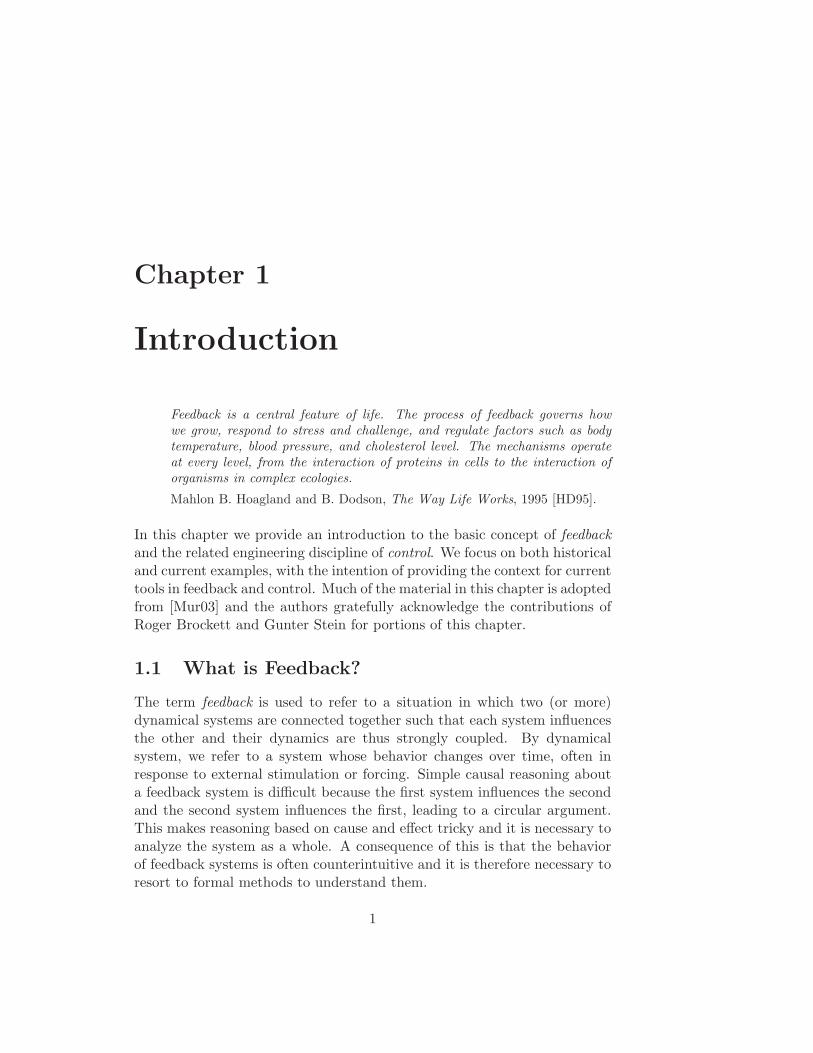
Figure 1.1 illustrates in block diagram form the idea of feedback. Weoften use the terms open loop and closed loop when referring to such systems.A system is said to be a closed loop system if the systems are interconnectedin a cycle, as shown in Figure 1.1a. If we break the interconnection, we referto the configuration as an open loop system, as shown in Figure 1.1b.
As the quote at the beginning of this chapter illustrates, a major sourceof examples for feedback systems is from biology. Biological systems makeuse of feedback in an extraordinary number of ways, on scales ranging frommolecules to microbes to organisms to ecosystems. One example is theregulation of glucose in the bloodstream, through the production of insulinand glucagon by the pancreas. The body attempts to maintain a constantconcentration of glucose, which is used by the body’s cells to produce energy.When glucose levels rise (after eating a meal, for example), the hormoneinsulin is released and causes the body to store excess glucose in the liver.When glucose levels are low, the pancreas secretes the hormone glucagon,which has the opposite effect. The interplay between insulin and glucagonsecretions throughout the day help to keep the blood-glucose concentrationconstant, at about 90 mg per 100 ml of blood.
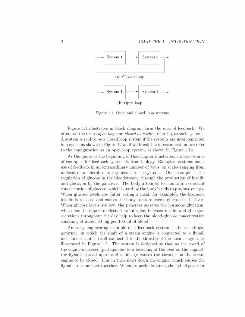
An early engineering example of a feedback system is the centrifugalgovernor, in which the shaft of a steam engine is connected to a flyballmechanism that is itself connected to the throttle of the steam engine, asillustrated in Figure 1.2. The system is designed so that as the speed ofthe engine increases (perhaps due to a lessening of the load on the engine),the flyballs spread apart and a linkage causes the throttle on the steamengine to be closed. This in turn slows down the engine, which causes theflyballs to come back together. When properly designed, the flyball governor
1.1. WHAT IS FEEDBACK? 3
(a) (b)
Figure 1.2: The centrifugal governor (a), developed in the 1780s, was an enablerof the successful Watt steam engine (b), which fueled the industrial revolution.Figures courtesy Richard Adamek (copyright 1999) and Cambridge University.
maintains a constant speed of the engine, roughly independent of the loadingconditions.
Feedback has many interesting properties that can be exploited in de-signing systems. As in the case of glucose regulation or the flyball governor,feedback can make a system very resilient towards external influences. Itcan also be used to create linear behavior out of nonlinear components, acommon approach in electronics. More generally, feedback allows a systemto be very insensitive both to external disturbances and to variations in itsindividual elements.
Feedback has potential disadvantages as well. If applied incorrectly, itcan create dynamic instabilities in a system, causing oscillations or evenrunaway behavior. Another drawback, especially in engineering systems, isthat feedback can introduce unwanted sensor noise into the system, requiringcareful filtering of signals. It is for these reasons that a substantial portionof the study of feedback systems is devoted to developing an understandingof dynamics and mastery of techniques in dynamical systems.
Feedback systems are ubiquitous in both natural and engineered sys-tems. Control systems maintain the environment, lighting, and power in ourbuildings and factories, they regulate the operation of our cars, consumerelectronics and manufacturing processes, they enable our transportation and
4 CHAPTER 1. INTRODUCTION
communications systems, and they are critical elements in our military andspace systems. For the most part, they are hidden from view, buried withinthe code of embedded microprocessors, executing their functions accuratelyand reliably. Feedback has also made it possible to increase dramatically theprecision of instruments such as atomic force microscopes and telescopes.
In nature, homeostasis in biological systems maintains thermal, chemical,and biological conditions through feedback. At the other end of the sizescale, global climate dynamics depend on the feedback interactions betweenthe atmosphere, oceans, land, and the sun. Ecologies are filled with examplesof feedback, resulting in complex interactions between animal and plantlife. Even the dynamics of economies are based on the feedback betweenindividuals and corporations through markets and the exchange of goodsand services.
1.2 What is Control?
The term “control” has many meanings and often varies between communi-ties. In this book, we define control to be the use of algorithms and feedbackin engineered systems. Thus, control includes such examples as feedbackloops in electronic amplifiers, set point controllers in chemical and materi-als processing, “fly-by-wire” systems on aircraft, and even router protocolsthat control traffic flow on the Internet. Emerging applications include highconfidence software systems, autonomous vehicles and robots, real-time re-source management systems, and biologically engineered systems. At itscore, control is an information science, and includes the use of informationin both analog and digital representations.
A modern controller senses the operation of a system, compares thatagainst the desired behavior, computes corrective actions based on a modelof the system’s response to external inputs, and actuates the system toeffect the desired change. This basic feedback loop of sensing, computation,and actuation is the central concept in control. The key issues in designingcontrol logic are ensuring that the dynamics of the closed loop system arestable (bounded disturbances give bounded errors) and that they have thedesired behavior (good disturbance rejection, fast responsiveness to changesin operating point, etc). These properties are established using a variety ofmodeling and analysis techniques that capture the essential physics of thesystem and permit the exploration of possible behaviors in the presence ofuncertainty, noise and component failures.
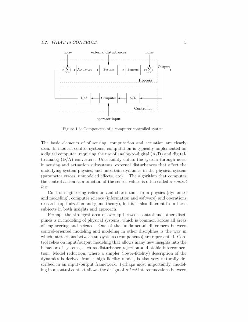
A typical example of a modern control system is shown in Figure 1.3.
1.2. WHAT IS CONTROL? 5
Σ System Sensors
D/A Computer A/D
operator input
noiseexternal disturbancesnoise
Output
Controller
Process
ΣActuators
Figure 1.3: Components of a computer controlled system.
The basic elements of of sensing, computation and actuation are clearlyseen. In modern control systems, computation is typically implemented ona digital computer, requiring the use of analog-to-digital (A/D) and digital-to-analog (D/A) converters. Uncertainty enters the system through noisein sensing and actuation subsystems, external disturbances that affect theunderlying system physics, and uncertain dynamics in the physical system(parameter errors, unmodeled effects, etc). The algorithm that computesthe control action as a function of the sensor values is often called a controllaw.
Control engineering relies on and shares tools from physics (dynamicsand modeling), computer science (information and software) and operationsresearch (optimization and game theory), but it is also different from thesesubjects in both insights and approach.
Perhaps the strongest area of overlap between control and other disci-plines is in modeling of physical systems, which is common across all areasof engineering and science. One of the fundamental differences betweencontrol-oriented modeling and modeling in other disciplines is the way inwhich interactions between subsystems (components) are represented. Con-trol relies on input/output modeling that allows many new insights into thebehavior of systems, such as disturbance rejection and stable interconnec-tion. Model reduction, where a simpler (lower-fidelity) description of thedynamics is derived from a high fidelity model, is also very naturally de-scribed in an input/output framework. Perhaps most importantly, model-ing in a control context allows the design of robust interconnections between
6 CHAPTER 1. INTRODUCTION
(a) (b)
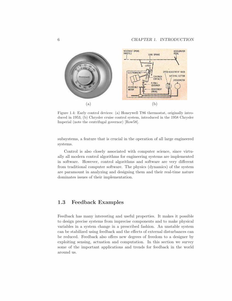
Figure 1.4: Early control devices: (a) Honeywell T86 thermostat, originally intro-duced in 1953, (b) Chrysler cruise control system, introduced in the 1958 ChryslerImperial (note the centrifugal governor) [Row58].
subsystems, a feature that is crucial in the operation of all large engineeredsystems.
Control is also closely associated with computer science, since virtu-ally all modern control algorithms for engineering systems are implementedin software. However, control algorithms and software are very differentfrom traditional computer software. The physics (dynamics) of the systemare paramount in analyzing and designing them and their real-time naturedominates issues of their implementation.
1.3 Feedback Examples
Feedback has many interesting and useful properties. It makes it possibleto design precise systems from imprecise components and to make physicalvariables in a system change in a prescribed fashion. An unstable systemcan be stabilized using feedback and the effects of external disturbances canbe reduced. Feedback also offers new degrees of freedom to a designer byexploiting sensing, actuation and computation. In this section we surveysome of the important applications and trends for feedback in the worldaround us.
1.3. FEEDBACK EXAMPLES 7
Early Technological Examples
The proliferation of control in engineered systems has occurred primarilyin the latter half of the 20th century. There are some familiar exceptions,such as the centrifugal governor described earlier and the thermostat (Fig-ure 1.4a), designed at the turn of the century to regulate temperature ofbuildings.
The thermostat, in particular, is often cited as a simple example of feed-back control that everyone can understand. Namely, the device measuresthe temperature in a building, compares that temperature to a desired setpoint, and uses the “feedback error” between these two to operate the heat-ing plant, e.g. to turn heating on when the temperature is too low and toturn if off when the temperature is too high. This explanation captures theessence of feedback, but it is a bit too simple even for a basic device such asthe thermostat. Actually, because lags and delays exist in the heating plantand sensor, a good thermostat does a bit of anticipation, turning the heateroff before the error actually changes sign. This avoids excessive temperatureswings and cycling of the heating plant.
This modification illustrates that, even in simple cases, good controlsystem design is not entirely trivial. It must take into account the dynamicbehavior of the object being controlled in order to do a good job. The morecomplex the dynamic behavior, the more elaborate the modifications. Infact, the development of a thorough theoretical understanding of the re-lationship between dynamic behavior and good controllers constitutes themost significant intellectual accomplishment of the control community, andthe codification of this understanding into powerful computer aided engi-neering design tools makes all modern control systems possible.
There are many other control system examples that have developed overthe years with progressively increasing levels of sophistication and impact.An early system with broad public exposure was the “cruise control” optionintroduced on automobiles in 1958 (see Figure 1.4b). With cruise control,ordinary people experienced the dynamic behavior of closed loop feedbacksystems in action—the slowdown error as the system climbs a grade, thegradual reduction of that error due to integral action in the controller, thesmall (but unavoidable) overshoot at the top of the climb, etc. More im-portantly, by experiencing these systems operating reliably and robustly,the public learned to trust and accept feedback systems, permitting theirincreasing proliferation all around us. Later control systems on automobileshave had more concrete impact, such as emission controls and fuel meteringsystems that have achieved major reductions of pollutants and increases in
8 CHAPTER 1. INTRODUCTION
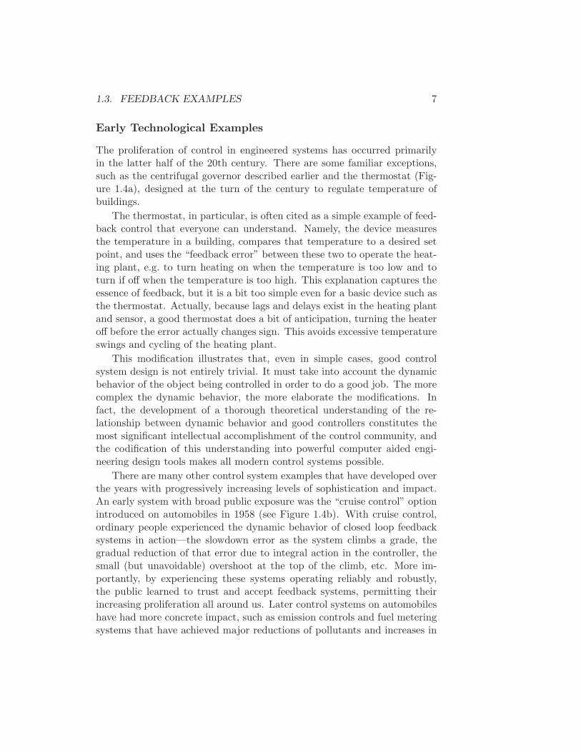
Figure 1.5: The F-18 aircraft, one of the first production military fighters to use “fly-by-wire” technology, and the X-45 (UCAV) unmanned aerial vehicle. Photographscourtesy of NASA Dryden Flight Research Center.
fuel economy.
In the industrial world, control systems have been a key enabling tech-nology for everything from factory automation (starting with numericallycontrolled machine tools), to process control in oil refineries and chemicalplants, to integrated circuit manufacturing, to power generation and distri-bution. Early use of regulators for manufacturing systems has evolved tothe use of hundreds or even thousands of computer controlled subsystemsin major industrial plants.
Aerospace and Transportation
Aerospace and transportation systems encompass a collection of criticallyimportant application areas where control is a central technology. Theseapplication areas represent a significant part of the modern world’s overalltechnological capability. They are also a major part of its economic strength,and they contribute greatly to the well being of its people.
In aerospace, control has been a key technological capability tracing backto the very beginning of the 20th century. Indeed, the Wright brothers arecorrectly famous not simply for demonstrating powered flight but controlledpowered flight. Their early Wright Flyer incorporated moving control sur-faces (vertical fins and canards) and warpable wings that allowed the pilot toregulate the aircraft’s flight. In fact, the aircraft itself was not stable, so con-tinuous pilot corrections were mandatory. This early example of controlledflight is followed by a fascinating success story of continuous improvementsin flight control technology, culminating in the very high performance, highly
1.3. FEEDBACK EXAMPLES 9
reliable automatic flight control systems we see on modern commercial andmilitary aircraft today.
Similar success stories for control technology occurred in many otherapplication areas. Early World War II bombsights and fire control servosystems have evolved into today’s highly accurate radar-guided guns andprecision-guided weapons. Early failure-prone space missions have evolvedinto routine launch operations, manned landings on the moon, permanentlymanned space stations, robotic vehicles roving Mars, orbiting vehicles at theouter planets, and a host of commercial and military satellites serving var-ious surveillance, communication, navigation, and earth observation needs.Cars have advanced from manually tuned mechanical/pneumatic technol-ogy to computer-controlled operation of all major functions, including fuelinjection, emission control, cruise control, braking, and cabin comfort.
Current research in aerospace and transportation systems is investigat-ing the application of feedback to higher levels of decision making, includinglogical regulation of operating modes, vehicle configurations, payload con-figurations, and health status. These have historically been performed byhuman operators, but today that boundary is moving, and control systemsare increasingly taking on these functions. Another dramatic trend on thehorizon is the use of large collections of distributed entities with local com-putation, global communication connections, very little regularity imposedby the laws of physics, and no possibility of imposing centralized controlactions. Examples of this trend include the national airspace managementproblem, automated highway and traffic management, and the commandand control for future battlefields.
Information and Networks
The rapid growth of communication networks provides several major op-portunities and challenges for control. Although there is overlap, we candivide these roughly into two main areas: control of networks and controlover networks.
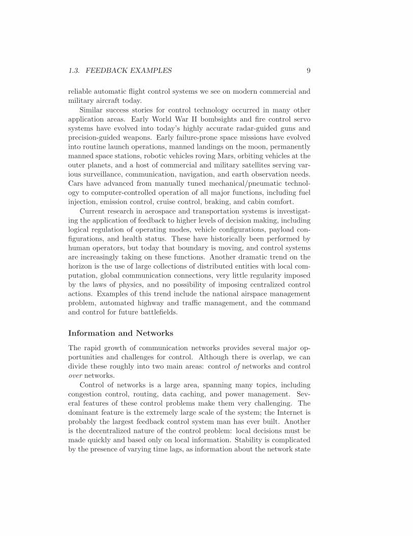
Control of networks is a large area, spanning many topics, includingcongestion control, routing, data caching, and power management. Sev-eral features of these control problems make them very challenging. Thedominant feature is the extremely large scale of the system; the Internet isprobably the largest feedback control system man has ever built. Anotheris the decentralized nature of the control problem: local decisions must bemade quickly and based only on local information. Stability is complicatedby the presence of varying time lags, as information about the network state
10 CHAPTER 1. INTRODUCTION
Figure 1.6: UUNET network backbone for North America. Figure courtesy ofWorldCom.
can only be observed or relayed to controllers after a delay, and the effect of alocal control action can be felt throughout the network only after substantialdelay. Uncertainty and variation in the network, through network topology,transmission channel characteristics, traffic demand, available resources, andthe like, may change constantly and unpredictably. Other complicating is-sues are the diverse traffic characteristics—in terms of arrival statistics atboth the packet and flow time scales—and the different requirements forquality of service that the network must support.
Resources that must be managed in this environment include computing,storage and transmission capacities at end hosts and routers. Performance ofsuch systems is judged in many ways: throughput, delay, loss rates, fairness,reliability, as well as the speed and quality with which the network adaptsto changing traffic patterns, changing resource availability, and changingnetwork congestion. The robustness and performance of the global Internetis a testament to the use of feedback to meet the needs of society in the faceof these many uncertainties.
While the advances in information technology to date have led to a globalInternet that allows users to exchange information, it is clear that the nextphase will involve much more interaction with the physical environment andthe increased use of control over networks. Networks of sensor and actua-tor nodes with computational capabilities, connected wirelessly or by wires,
1.3. FEEDBACK EXAMPLES 11
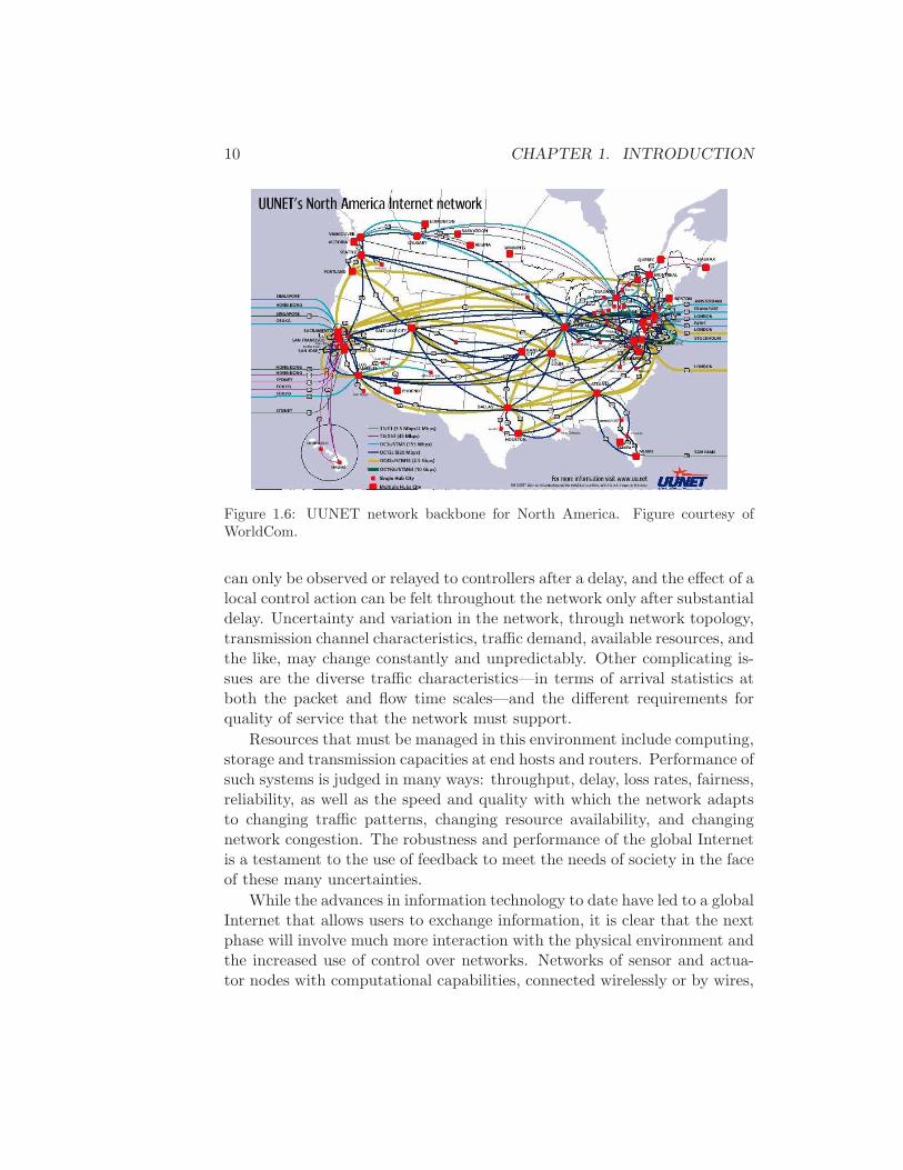
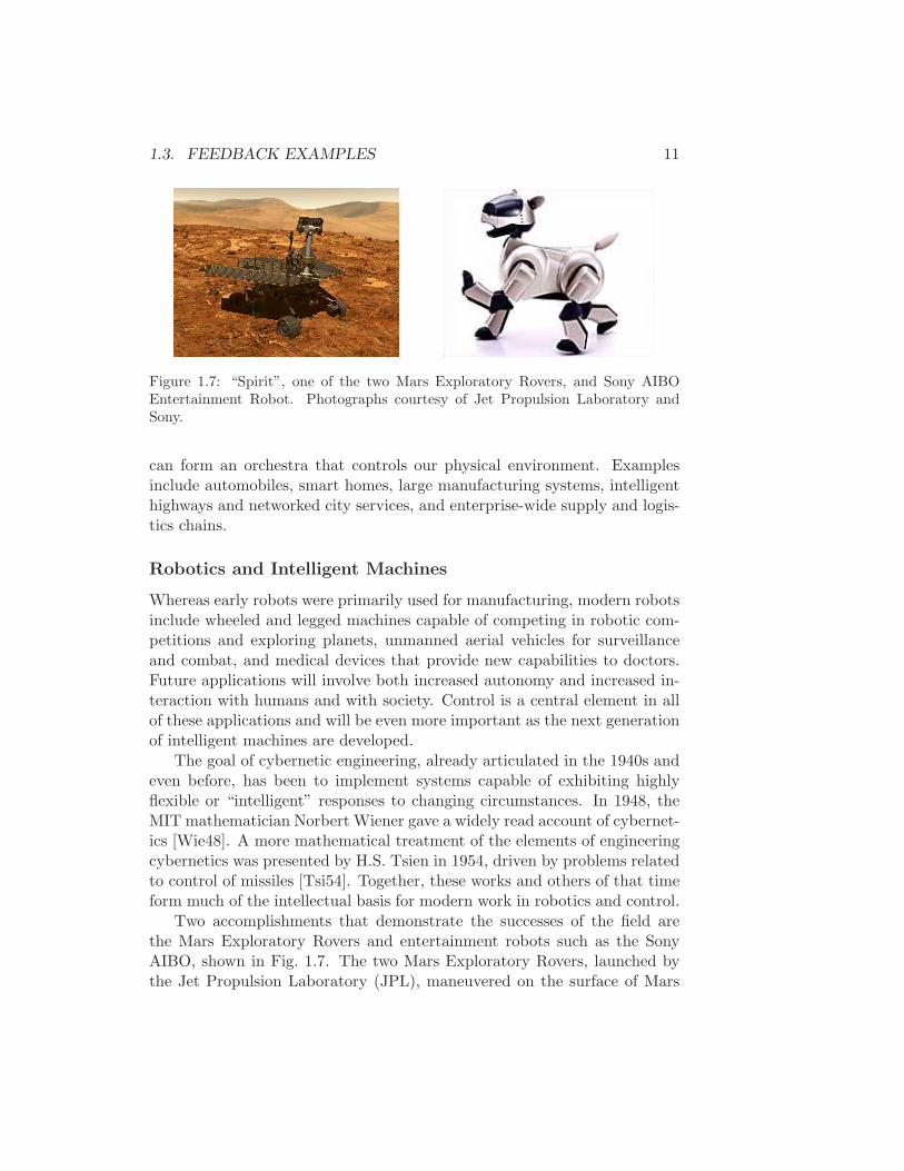
Figure 1.7: “Spirit”, one of the two Mars Exploratory Rovers, and Sony AIBOEntertainment Robot. Photographs courtesy of Jet Propulsion Laboratory andSony.
can form an orchestra that controls our physical environment. Examplesinclude automobiles, smart homes, large manufacturing systems, intelligenthighways and networked city services, and enterprise-wide supply and logis-tics chains.
Robotics and Intelligent Machines
Whereas early robots were primarily used for manufacturing, modern robotsinclude wheeled and legged machines capable of competing in robotic com-petitions and exploring planets, unmanned aerial vehicles for surveillanceand combat, and medical devices that provide new capabilities to doctors.Future applications will involve both increased autonomy and increased in-teraction with humans and with society. Control is a central element in allof these applications and will be even more important as the next generationof intelligent machines are developed.
The goal of cybernetic engineering, already articulated in the 1940s andeven before, has been to implement systems capable of exhibiting highlyflexible or “intelligent” responses to changing circumstances. In 1948, theMIT mathematician Norbert Wiener gave a widely read account of cybernet-ics [Wie48]. A more mathematical treatment of the elements of engineeringcybernetics was presented by H.S. Tsien in 1954, driven by problems relatedto control of missiles [Tsi54]. Together, these works and others of that timeform much of the intellectual basis for modern work in robotics and control.
Two accomplishments that demonstrate the successes of the field arethe Mars Exploratory Rovers and entertainment robots such as the SonyAIBO, shown in Fig. 1.7. The two Mars Exploratory Rovers, launched bythe Jet Propulsion Laboratory (JPL), maneuvered on the surface of Mars
12 CHAPTER 1. INTRODUCTION
for over two years starting in January 2004 and sent back pictures andmeasurements of their environment. The Sony AIBO robot debuted in Juneof 1999 and was the first “entertainment” robot to be mass marketed bya major international corporation. It was particularly noteworthy becauseof its use of AI technologies that allowed it to act in response to externalstimulation and its own judgment. This “higher level” of feedback is keyelement of robotics, where issues such as task-based control and learning areprevalent.
Despite the enormous progress in robotics over the last half century, thefield is very much in its infancy. Today’s robots still exhibit extremely simplebehaviors compared with humans, and their ability to locomote, interpretcomplex sensory inputs, perform higher level reasoning, and cooperate to-gether in teams is limited. Indeed, much of Wiener’s vision for robotics andintelligent machines remains unrealized. While advances are needed in manyfields to achieve this vision—including advances in sensing, actuation, andenergy storage—the opportunity to combine the advances of the AI commu-nity in planning, adaptation, and learning with the techniques in the controlcommunity for modeling, analysis, and design of feedback systems presentsa renewed path for progress.
Materials and Processing
The chemical industry is responsible for the remarkable progress in develop-ing new materials that are key to our modern society. Process manufacturingoperations require a continual infusion of advanced information and processcontrol technologies in order for the chemical industry to maintain its globalability to deliver products that best serve the customer reliably and at thelowest cost. In addition, several new technology areas are being exploredthat will require new approaches to control to be successful. These rangefrom nanotechnology in areas such as electronics, chemistry, and biomateri-als to thin film processing and design of integrated microsystems to supplychain management and enterprise resource allocation. The payoffs for newadvances in these areas are substantial, and the use of control is critical tofuture progress in sectors from semiconductors to pharmaceuticals to bulkmaterials.
There are several common features within materials and processing thatpervade many of the applications. Modeling plays a crucial role, and there isa clear need for better solution methods for multidisciplinary systems com-bining chemistry, fluid mechanics, thermal sciences, and other disciplinesat a variety of temporal and spatial scales. Better numerical methods for
1.3. FEEDBACK EXAMPLES 13
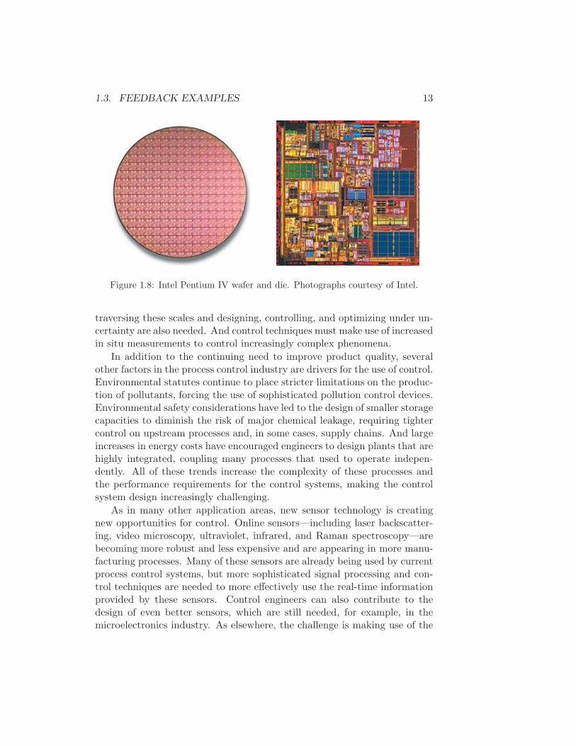
Figure 1.8: Intel Pentium IV wafer and die. Photographs courtesy of Intel.
traversing these scales and designing, controlling, and optimizing under un-certainty are also needed. And control techniques must make use of increasedin situ measurements to control increasingly complex phenomena.
In addition to the continuing need to improve product quality, severalother factors in the process control industry are drivers for the use of control.Environmental statutes continue to place stricter limitations on the produc-tion of pollutants, forcing the use of sophisticated pollution control devices.Environmental safety considerations have led to the design of smaller storagecapacities to diminish the risk of major chemical leakage, requiring tightercontrol on upstream processes and, in some cases, supply chains. And largeincreases in energy costs have encouraged engineers to design plants that arehighly integrated, coupling many processes that used to operate indepen-dently. All of these trends increase the complexity of these processes andthe performance requirements for the control systems, making the controlsystem design increasingly challenging.
As in many other application areas, new sensor technology is creatingnew opportunities for control. Online sensors—including laser backscatter-ing, video microscopy, ultraviolet, infrared, and Raman spectroscopy—arebecoming more robust and less expensive and are appearing in more manu-facturing processes. Many of these sensors are already being used by currentprocess control systems, but more sophisticated signal processing and con-trol techniques are needed to more effectively use the real-time informationprovided by these sensors. Control engineers can also contribute to thedesign of even better sensors, which are still needed, for example, in themicroelectronics industry. As elsewhere, the challenge is making use of the
14 CHAPTER 1. INTRODUCTION
large amounts of data provided by these new sensors in an effective manner.In addition, a control-oriented approach to modeling the essential physicsof the underlying processes is required to understand fundamental limits onobservability of the internal state through sensor data.
Instrumentation
Feedback has had a major impact on instrumentation. Consider for examplean accelerometer, where early instruments consisted of a mass suspended ona spring with a deflection sensor. The precision of such an instrument de-pends critically on accurate calibration of spring and the sensor. There isalso a design compromise because a weak spring gives high sensitivity butalso low bandwidth. An accelerometer based on feedback uses instead avoice coil to keep the mass at a given position and the acceleration is pro-portional to the current through the voice coil. In such an instrument theprecision depends entirely on the calibration of the voice coil and does notdepend on the sensor, which is only used as the feedback signal. The sen-sitivity bandwidth compromise is also avoided. This way of using feedbackwas applied to practically all engineering fields and it resulted in instrumentswith drastically improved performance. The development of inertial naviga-tion where position is determined from gyroscopes and accelerometers whichpermits accurate guidance and control of vehicles is a spectacular example.
There are many other interesting and useful applications of feedback inscientific instruments. The development of the mass spectrometer is an earlyexample. In a paper from 1935 by Nier it is observed that the deflectionof the ions depend on both the magnetic and the electric fields. Instead ofkeeping both fields constant, Nier let the magnetic field fluctuate and theelectric field was controlled to keep the ratio of the fields constant. Thefeedback was implemented using vacuum tube amplifiers. The scheme wascrucial for the development of mass spectroscopy.
Another example is the work by the Dutch Engineer van der Meer. Heinvented a clever way to use feedback to maintain a high density and goodquality of the beam of a particle accelerator. The idea is to sense particledisplacement at one point in the accelerator and apply a correcting signalat another point. The scheme, called stochastic cooling, was awarded theNobel Prize in Physics in 1984. The method was essential for the successfulexperiments in CERN when the existence of the particles W and Z was firstdemonstrated.
The 1986 Nobel Prize in Physics—awarded to Binnig and Rohrer fortheir design of the scanning tunneling microscope—is another example of
1.3. FEEDBACK EXAMPLES 15
clever use of feedback. The key idea is to move a narrow tip on a cantileverbeam across the surface and to register the forces on the tip. The deflectionof the tip was measured using tunneling which gave an extreme accuracy sothat individual atoms could be registered.
A severe problem in astronomy is that turbulence in the atmosphereblurs images in telescopes because of variations in diffraction of light in theatmosphere. The blur is of the order of an arc-second in a good telescope.One way to eliminate the blur is to move the telescope outside the Earthsatmosphere as is done with the Hubble telescope. Another way is to usefeedback to eliminate the effects of the variations in a telescope on the Earthwhich is the idea of “adaptive optics.” The reference signal is a bright staror an artificial laser beam projected into the atmosphere. The actuator is adeformable mirror which can have hundreds or thousands of elements. Theerror signal is formed by analyzing the shape of the distorted wave formfrom the reference. This signal is sent to the controller which adjusts thedeformable mirror. The light from the observed star is compensated becauseit is also reflected in the deformable mirror before it is sent to the detector.The wave lengths used for observation and control are often different. Sincediffraction in the atmosphere changes quite rapidly the response time of thecontrol system must be of the order of milliseconds.
Feedback in Nature
Many cutting edge problems in the natural sciences involve understandingaggregate behavior in complex large-scale systems. This behavior “emerges”from the interaction of a multitude of simpler systems, with intricate pat-terns of information flow. Representative examples can be found in fieldsranging from embryology to seismology. Researchers who specialize in thestudy of specific complex systems often develop an intuitive emphasis onanalyzing the role of feedback (or interconnection) in facilitating and sta-bilizing aggregate behavior, and it is often noted that one can only havehope of deep understanding if it is somehow possible for theories of collec-tive phenomenology to be robust to inevitable uncertainties in the modelingof fine-scale dynamics and interconnection.
While sophisticated theories have been developed by domain expertsfor the analysis of various complex systems, the development of rigorousmethodology that can discover and exploit common features and essentialmathematical structure is just beginning to emerge. Advances in science andtechnology are creating new understanding of the underlying dynamics andthe importance of feedback in a wide variety of natural and technological
16 CHAPTER 1. INTRODUCTION
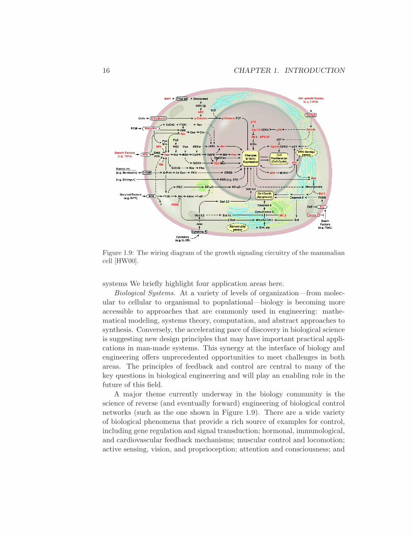
Figure 1.9: The wiring diagram of the growth signaling circuitry of the mammaliancell [HW00].
systems We briefly highlight four application areas here.
Biological Systems. At a variety of levels of organization—from molec-ular to cellular to organismal to populational—biology is becoming moreaccessible to approaches that are commonly used in engineering: mathe-matical modeling, systems theory, computation, and abstract approaches tosynthesis. Conversely, the accelerating pace of discovery in biological scienceis suggesting new design principles that may have important practical appli-cations in man-made systems. This synergy at the interface of biology andengineering offers unprecedented opportunities to meet challenges in bothareas. The principles of feedback and control are central to many of thekey questions in biological engineering and will play an enabling role in thefuture of this field.
A major theme currently underway in the biology community is thescience of reverse (and eventually forward) engineering of biological controlnetworks (such as the one shown in Figure 1.9). There are a wide varietyof biological phenomena that provide a rich source of examples for control,including gene regulation and signal transduction; hormonal, immunological,and cardiovascular feedback mechanisms; muscular control and locomotion;active sensing, vision, and proprioception; attention and consciousness; and
1.3. FEEDBACK EXAMPLES 17
population dynamics and epidemics. Each of these (and many more) provideopportunities to figure out what works, how it works, and what we can doto affect it.
Ecosystems. In contrast to individual cells and organisms, emergentproperties of aggregations and ecosystems inherently reflect selection mech-anisms which act on multiple levels, and primarily on scales well below thatof the system as a whole. Because ecosystems are complex, multiscale dy-namical systems, they provide a broad range of new challenges for modelingand analysis of feedback systems. Recent experience in applying tools fromcontrol and dynamical systems to bacterial networks suggests that much ofthe complexity of these networks is due to the presence of multiple layers offeedback loops that provide robust functionality to the individual cell. Yetin other instances, events at the cell level benefit the colony at the expenseof the individual. Systems level analysis can be applied to ecosystems withthe goal of understanding the robustness of such systems and the extentto which decisions and events affecting individual species contribute to therobustness and/or fragility of the ecosystem as a whole.
Quantum Systems. While organisms and ecosystems have little to dowith quantum mechanics in any traditional scientific sense, complexity androbustness issues very similar to those described above can be identified inthe modern study of quantum systems. In large part, this sympathy arisesfrom a trend towards wanting to control quantum dynamics and to harnessit for the creation of new technological devices. At the same time, physicistsare progressing from the study of elementary quantum systems to the studyof large aggregates of quantum components, and it has been recognized thatdynamical complexity in quantum systems increases exponentially fasterwith system size than it does in systems describable by classical (macro-scopic) physics. Factors such as these are prompting the physics communityto search broadly for new tools for understanding robust interconnectionand emergent phenomena.
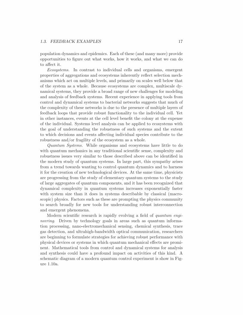
Modern scientific research is rapidly evolving a field of quantum engi-neering. Driven by technology goals in areas such as quantum informa-tion processing, nano-electromechanical sensing, chemical synthesis, tracegas detection, and ultrahigh-bandwidth optical communication, researchersare beginning to formulate strategies for achieving robust performance withphysical devices or systems in which quantum mechanical effects are promi-nent. Mathematical tools from control and dynamical systems for analysisand synthesis could have a profound impact on activities of this kind. Aschematic diagram of a modern quantum control experiment is show in Fig-ure 1.10a.
18 CHAPTER 1. INTRODUCTION
(a) (b)
Figure 1.10: Examples of feedback systems in nature: (a) quantum control systemand (b) global carbon cycle.
Environmental Science. It is now indisputable that human activitieshave altered the environment on a global scale. Problems of enormouscomplexity challenge researchers in this area and first among these is tounderstand the feedback systems that operate on the global scale. One ofthe challenges in developing such an understanding is the multiscale natureof the problem, with detailed understanding of the dynamics of microscalephenomena such as microbiological organisms being a necessary componentof understanding global phenomena, such as the carbon cycle illustratedFigure 1.10b.
Other Areas
The previous sections have described some of the major application areasfor control. However, there are many more areas where ideas from controlare being applied or could be applied. Some of these include: economicsand finance, including problems such as pricing and hedging options; energysystems, including load distribution and power management for the elec-trical grid; and manufacturing systems, including supply chains, resourcemanagement and scheduling, and factory automation.
1.4. FEEDBACK PROPERTIES 19
Compute
Actuate
Throttle
Sense
Speed
0 5 10 1520
25
30
35
time (sec)
spee
d (m
/s)
m = 1000 kg
m = 2000 kg
m = 3000 kg
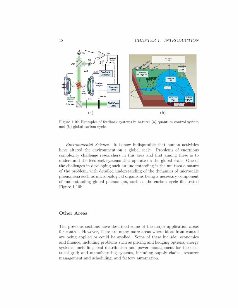
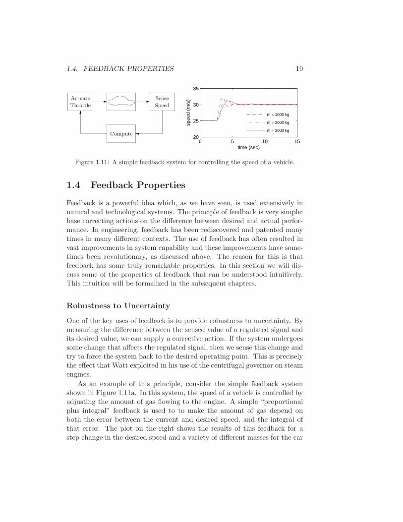
Figure 1.11: A simple feedback system for controlling the speed of a vehicle.
1.4 Feedback Properties
Feedback is a powerful idea which, as we have seen, is used extensively innatural and technological systems. The principle of feedback is very simple:base correcting actions on the difference between desired and actual perfor-mance. In engineering, feedback has been rediscovered and patented manytimes in many different contexts. The use of feedback has often resulted invast improvements in system capability and these improvements have some-times been revolutionary, as discussed above. The reason for this is thatfeedback has some truly remarkable properties. In this section we will dis-cuss some of the properties of feedback that can be understood intuitively.This intuition will be formalized in the subsequent chapters.
Robustness to Uncertainty
One of the key uses of feedback is to provide robustness to uncertainty. Bymeasuring the difference between the sensed value of a regulated signal andits desired value, we can supply a corrective action. If the system undergoessome change that affects the regulated signal, then we sense this change andtry to force the system back to the desired operating point. This is preciselythe effect that Watt exploited in his use of the centrifugal governor on steamengines.
As an example of this principle, consider the simple feedback systemshown in Figure 1.11a. In this system, the speed of a vehicle is controlled byadjusting the amount of gas flowing to the engine. A simple “proportionalplus integral” feedback is used to to make the amount of gas depend onboth the error between the current and desired speed, and the integral ofthat error. The plot on the right shows the results of this feedback for astep change in the desired speed and a variety of different masses for the car
20 CHAPTER 1. INTRODUCTION
(which might result from having a different number of passengers or towinga trailer). Notice that independent of the mass (which varies by a factorof 3), the steady state speed of the vehicle always approaches the desiredspeed and achieves that speed within approximately 5 seconds. Thus theperformance of the system is robust with respect to this uncertainty.
Another early example of the use of feedback to provide robustness wasthe negative feedback amplifier. When telephone communications were de-veloped, amplifiers were used to compensate for signal attenuation in longlines. The vacuum tube was a component that could be used to build ampli-fiers. Distortion caused by the nonlinear characteristics of the tube amplifiertogether with amplifier drift were obstacles that prevented development ofline amplifiers for a long time. A major breakthrough was invention of thefeedback amplifier in 1927 by Harold S. Black, an electrical engineer at theBell Telephone Laboratories. Black used negative feedback which reducesthe gain but makes the amplifier very insensitive to variations in tube char-acteristics. This invention made it possible to build stable amplifiers withlinear characteristics despite nonlinearities of the vacuum tube amplifier.
Design of Dynamics
Another use of feedback is to change the dynamics of a system. Throughfeedback, we can alter the behavior of a system to meet the needs of anapplication: systems that are unstable can be stabilized, systems that aresluggish can be made responsive, and systems that have drifting operatingpoints can be held constant. Control theory provides a rich collection oftechniques to analyze the stability and dynamic response of complex systemsand to place bounds on the behavior of such systems by analyzing the gainsof linear and nonlinear operators that describe their components.
An example of the use of control in the design of dynamics comes fromthe area of flight control. The following quote, from a lecture by WilburWright to the Western Society of Engineers in 1901 [McF53], illustrates therole of control in the development of the airplane:
“Men already know how to construct wings or airplanes, whichwhen driven through the air at sufficient speed, will not onlysustain the weight of the wings themselves, but also that of theengine, and of the engineer as well. Men also know how to buildengines and screws of sufficient lightness and power to drive theseplanes at sustaining speed ... Inability to balance and steer stillconfronts students of the flying problem. ... When this one
1.4. FEEDBACK PROPERTIES 21
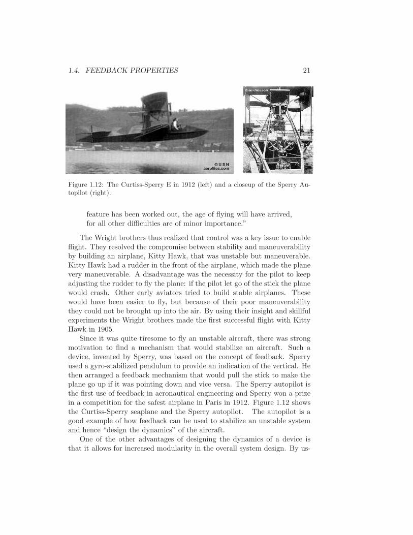
Figure 1.12: The Curtiss-Sperry E in 1912 (left) and a closeup of the Sperry Au-topilot (right).
feature has been worked out, the age of flying will have arrived,for all other difficulties are of minor importance.”
The Wright brothers thus realized that control was a key issue to enableflight. They resolved the compromise between stability and maneuverabilityby building an airplane, Kitty Hawk, that was unstable but maneuverable.Kitty Hawk had a rudder in the front of the airplane, which made the planevery maneuverable. A disadvantage was the necessity for the pilot to keepadjusting the rudder to fly the plane: if the pilot let go of the stick the planewould crash. Other early aviators tried to build stable airplanes. Thesewould have been easier to fly, but because of their poor maneuverabilitythey could not be brought up into the air. By using their insight and skillfulexperiments the Wright brothers made the first successful flight with KittyHawk in 1905.
Since it was quite tiresome to fly an unstable aircraft, there was strongmotivation to find a mechanism that would stabilize an aircraft. Such adevice, invented by Sperry, was based on the concept of feedback. Sperryused a gyro-stabilized pendulum to provide an indication of the vertical. Hethen arranged a feedback mechanism that would pull the stick to make theplane go up if it was pointing down and vice versa. The Sperry autopilot isthe first use of feedback in aeronautical engineering and Sperry won a prizein a competition for the safest airplane in Paris in 1912. Figure 1.12 showsthe Curtiss-Sperry seaplane and the Sperry autopilot. The autopilot is agood example of how feedback can be used to stabilize an unstable systemand hence “design the dynamics” of the aircraft.
One of the other advantages of designing the dynamics of a device isthat it allows for increased modularity in the overall system design. By us-
22 CHAPTER 1. INTRODUCTION
Supervisory Control
Actuation
Vehicle
FollowerPath
StateEstimator
PlannerPath
SensorsTerrain
MapElevation
MapCost
FindingRoad
Vehicle
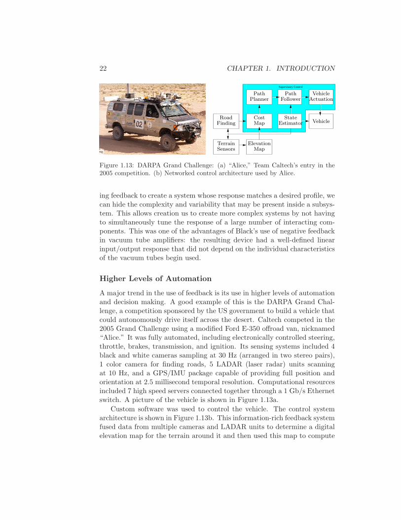
Figure 1.13: DARPA Grand Challenge: (a) “Alice,” Team Caltech’s entry in the2005 competition. (b) Networked control architecture used by Alice.
ing feedback to create a system whose response matches a desired profile, wecan hide the complexity and variability that may be present inside a subsys-tem. This allows creation us to create more complex systems by not havingto simultaneously tune the response of a large number of interacting com-ponents. This was one of the advantages of Black’s use of negative feedbackin vacuum tube amplifiers: the resulting device had a well-defined linearinput/output response that did not depend on the individual characteristicsof the vacuum tubes begin used.
Higher Levels of Automation
A major trend in the use of feedback is its use in higher levels of automationand decision making. A good example of this is the DARPA Grand Chal-lenge, a competition sponsored by the US government to build a vehicle thatcould autonomously drive itself across the desert. Caltech competed in the2005 Grand Challenge using a modified Ford E-350 offroad van, nicknamed“Alice.” It was fully automated, including electronically controlled steering,throttle, brakes, transmission, and ignition. Its sensing systems included 4black and white cameras sampling at 30 Hz (arranged in two stereo pairs),1 color camera for finding roads, 5 LADAR (laser radar) units scanningat 10 Hz, and a GPS/IMU package capable of providing full position andorientation at 2.5 millisecond temporal resolution. Computational resourcesincluded 7 high speed servers connected together through a 1 Gb/s Ethernetswitch. A picture of the vehicle is shown in Figure 1.13a.
Custom software was used to control the vehicle. The control systemarchitecture is shown in Figure 1.13b. This information-rich feedback systemfused data from multiple cameras and LADAR units to determine a digitalelevation map for the terrain around it and then used this map to compute
1.4. FEEDBACK PROPERTIES 23
a speed map that estimated the speed at which the vehicle could drive inthe environment. The map was modified to include additional informationwhere roads were identified (through vision-based algorithms) and where nodata was present (due to hills or temporary sensor outages). This speed mapwas then used by an optimization-based planner to determine the path thatwould allow the vehicle to make the most progress in a fixed period of time.The commands from the planner were sent to a trajectory tracking algorithmthat compared the desired vehicle position to its estimated position (fromGPS/IMU data) and issued appropriate commands to the steering, throttleand brake actuators. Finally, a supervisor control module performed higherlevel tasks, including implementing strategies for making continued forwardprogress if one of the hardware or software components failed temporarily(either due to external or internal conditions).
The software and hardware infrastructure that was developed enabledthe vehicle to traverse long distances at substantial speeds. In testing, Alicedrove itself over 500 kilometers in the Mojave Desert of California, with theability to follow dirt roads and trails (if present) and avoid obstacles alongthe path. Speeds of over 50 km/hr were obtained in fully autonomous mode.Substantial tuning of the algorithms was done during desert testing, in partdue to the lack of systems-level design tools for systems of this level of com-plexity. Other competitors in the race (including Stanford, which one thecompetition) used algorithms for adaptive control and learning, increasingthe capabilities of their systems in unknown environments. Together, thecompetitors in the grand challenge demonstrated some of the capabilitiesfor the next generation of control systems and highlighted many researchdirections in control at higher levels of decision making.
Drawbacks of Feedback
While feedback has many advantages, it also has some drawbacks. Chiefamong these is the possibility for instability if the system is not designedproperly. We are all familiar with the effects of “positive feedback” whenthe amplification on a microphone is turned up too high in a room. This isan example of a feedback instability, something that we obviously want toavoid. This is tricky because of the uncertainty that feedback was introducedto compensate for: not only must we design the system to be stable withthe nominal system we are designing for, but it must remain stable underall possible perturbations of the dynamics.
In addition to the potential for instability, feedback inherently couplesdifferent parts of a system. One common problem that feedback inherently
24 CHAPTER 1. INTRODUCTION
injects measurement noise into the system. In engineering systems, measure-ments must be carefully filtered so that the actuation and process dynamicsdo not respond to it, while at the same time insuring that the measurementsignal from the sensor is properly coupled into the closed loop dynamics (sothat the proper levels of performance are achieved).
Another potential drawback of control is the complexity of embeddinga control system into a product. While the cost of sensing, computation,and (to a lesser extent) actuation has decreased dramatically in the pastfew decades, the fact remains that control systems are often very compli-cated and hence one must carefully balance the costs and benefits. An earlyengineering example of this is the use of microprocessor-based feedback sys-tems in automobiles. The use of microprocessors in automotive applicationsbegan in the early 1970s and was driven by increasingly strict emissionsstandards, which could only be met through electronic controls. Early sys-tems were expensive and failed more often than desired, leading to frequentcustomer dissatisfaction. It was only through aggressive improvements intechnology that the performance, reliability and cost of these systems al-lowed them to be used in a transparent fashion. Even today, the complexityof these systems is such that it is difficult for an individual car owner tofix problems. There have also been spectacular failures due to unexpectedinteractions.
Feedforward
When using feedback that there must be an error before corrective actionsare taken. Feedback is thus reactive. In some circumstances it is possible tomeasure a disturbance before it enters the system and this information canbe used to take corrective action before the disturbance has influenced thesystem. The effect of the disturbance is thus reduced by measuring it andgenerating a control signal that counteracts it. This way of controlling asystem is called feedforward. Feedforward is particularly useful to shape theresponse to command signals because command signals are always available.Since feedforward attempts to match two signals, it requires good processmodels otherwise the corrections may have the wrong size or it may be badlytimed.
The ideas of feedback and feedforward are very general and appear inmany different fields. In economics, feedback and feedforward are analogousto a market-based economy versus a planned economy. In business a purefeedforward strategy corresponds to running a company based on extensivestrategic planning while a feedback strategy corresponds to a pure reactive
1.5. SIMPLE FORMS OF FEEDBACK 25
approach. The experience in control indicates that it is often advantageousto combine feedback and feedforward. Feedforward is particularly usefulwhen disturbances can be measured or predicted. A typical example is inchemical process control where disturbances in one process may be due toprocesses upstream. The correct balance of the approaches requires insightand understanding of their properties.
Positive Feedback
In most of this text, we will consider the role of negative feedback, in whichwe attempt to regulate the system by reacting to disturbances in a way thatdecreases the effect of those disturbances. In some systems, particularlybiological systems, positive feedback can play an important role. In a systemwith positive feedback, the increase in some variable or signal leads to asituation in which that quantify is further through its dynamics. This hasa destabilizing effect and is usually accompanied by a saturation that limitsthe growth of the quantity. Although often considered undesirable, thisbehavior is used in biological (and engineering) systems to obtain a veryfast response to a condition or signal.
1.5 Simple Forms of Feedback
The idea of feedback to make corrective actions based on the difference be-tween the desired and the actual value can be implemented in many differentways. The benefits of feedback can be obtained by very simple feedback lawssuch as on-off control, proportional control and PID control. In this sectionwe provide a brief preview of some of the topics that will be studied moreformally in the remainder of the text.
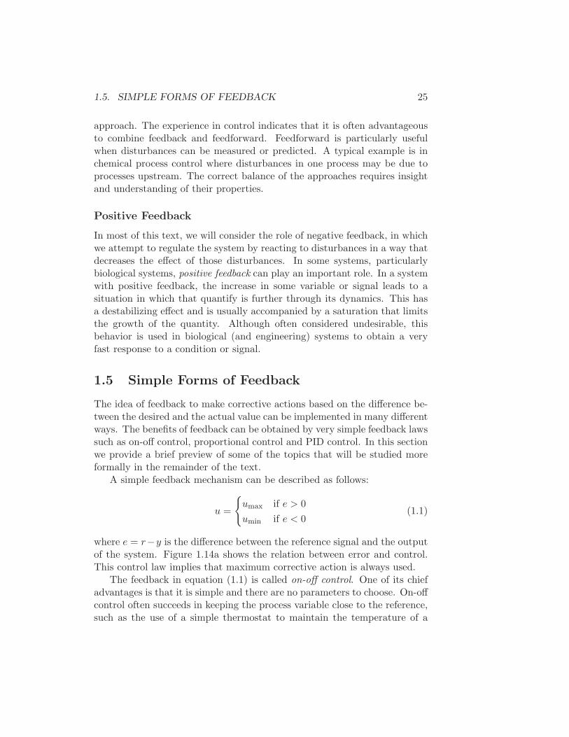
A simple feedback mechanism can be described as follows:
u =
umax if e > 0
umin if e < 0(1.1)
where e = r−y is the difference between the reference signal and the outputof the system. Figure 1.14a shows the relation between error and control.This control law implies that maximum corrective action is always used.
The feedback in equation (1.1) is called on-off control. One of its chiefadvantages is that it is simple and there are no parameters to choose. On-offcontrol often succeeds in keeping the process variable close to the reference,such as the use of a simple thermostat to maintain the temperature of a
26 CHAPTER 1. INTRODUCTION
(c)
e
u
e
u
e
u
(a) (b)
Figure 1.14: Controller characteristics for ideal on-off control (a), and modificationswith dead zone (b) and hysteresis (c).
room. It typically results in a system where the controlled variables oscillate,which is often acceptable if the oscillation is sufficiently small.
Notice that in equation (1.1) the control variable is not defined when theerror is zero. It is common to have some modifications either by introducinghysteresis or a dead zone (see Figure 1.14b and 1.14c).
The reason why on-off control often gives rise to oscillations is that thesystem over reacts since a small change in the error will make the actuatedvariable change over the full range. This effect is avoided in proportionalcontrol, where the characteristic of the controller is proportional to the con-trol error for small errors. This can be achieved by making the control signalproportional to the error, which gives the control law
u =
umax if e > emax
ke if emin ≤ e ≤ emax
umin if e < emin,
(1.2)
where where k is the controller gain, emin = umin/k, and emax = umax/k.The interval (emin, emax) is called the proportional band because the behaviorof the controller is linear when the error is in this interval:
u = k(r − y) = ke if emin ≤ e ≤ emax. (1.3)
While a vast improvement over on-off control, proportional control hasthe drawback that the process variable often deviates from its referencevalue. In particular, if some level of control signal is required for the systemto maintain a desired value, then we must have e 6= 0 in order to generatethe requisite input.
This can be avoided by making the control action proportional to the
1.5. SIMPLE FORMS OF FEEDBACK 27
integral of the error:
u(t) = ki
t∫
0
e(τ)dτ. (1.4)
This control form is called integral control and ki is the integral gain. It canbe shown through simple arguments that a controller with integral actionwill have zero “steady state” error (Exercise 5). The catch is that there maynot always be a steady state because the system may be oscillating. Thisproperty has been rediscovered many times and is one of the properties thathave strongly contributed to the wide applicability of integral controllers.
An additional refinement is to provide the controller with an anticipativeability by using a prediction of the error. A simple prediction is given bythe linear extrapolation
e(t+ Td) ≈ e(t) + Tdde(t)
dt,
which predicts the error Td time units ahead. Combining proportional, in-tegral and derivative control we obtain a controller that can be expressedmathematically as follows:
u(t) = ke(t) + ki
∫ t
0e(τ) dτ + kd
de(t)
dt
= k
(
e(t) +1
Ti
∫ t
0e(τ) dτ + Td
de(t)
dt
) (1.5)
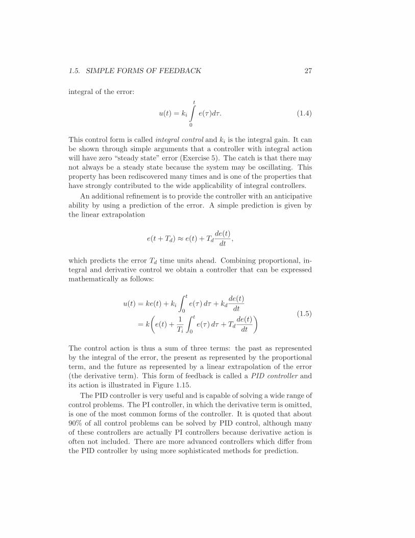
The control action is thus a sum of three terms: the past as representedby the integral of the error, the present as represented by the proportionalterm, and the future as represented by a linear extrapolation of the error(the derivative term). This form of feedback is called a PID controller andits action is illustrated in Figure 1.15.
The PID controller is very useful and is capable of solving a wide range ofcontrol problems. The PI controller, in which the derivative term is omitted,is one of the most common forms of the controller. It is quoted that about90% of all control problems can be solved by PID control, although manyof these controllers are actually PI controllers because derivative action isoften not included. There are more advanced controllers which differ fromthe PID controller by using more sophisticated methods for prediction.
28 CHAPTER 1. INTRODUCTION
Present
FuturePast
t t+ Td
Error
Time
Figure 1.15: A PID controller takes control action based on past, present and futurecontrol errors.
1.6 Control Tools
The development of a control system consists of the tasks modeling, analysis,simulation, architectural design, design of control algorithms, implementa-tion, commissioning and operation. Because of the wide use of feedback ina variety of applications, there has been substantial mathematical develop-ment in the field of control theory. In many cases the results have also beenpackaged in software tools that simplifies the design process. We brieflydescribe some of the tools and concepts here.
Modeling
Models play an essential role in analysis and design of feedback systems.Several sophisticated tools have been developed to build models that aresuited for control.
Models can often be obtained from first principles and there are severalmodeling tools in special domains such as electric circuits and multibody sys-tems. Since control applications cover such a wide range of domains it is alsodesirable to have modeling tools that cut across traditional discipline bound-aries. Such modeling tools are now emerging, with the models obtained bycutting a system into subsystems and writing equations for balance of mass,energy and momentum, and constitutive equations that describe materialproperties for each subsystem. Object oriented programming can be usedvery effectively to organize the work and extensive symbolic computationcan be used to simplify the equations. Models and components can then beorganized in libraries for efficient reuse. Modelica [Til01] is an example of amodeling tool of this type.
1.6. CONTROL TOOLS 29
Modeling from input/output data or system identification is another ap-proach to modeling that has been developed in control. Direct measurementof the response to step input is commonly used in the process industry totune proportional-integral (PI) controllers. More accurate models can beobtained by measuring the response to sinusoidal signals, which is partic-ularly useful for systems with fast response time. Control theory has alsodeveloped new techniques for modeling dynamics and disturbances, includ-ing input/output representations of systems (how disturbances propagatethrough the system) and data-driven system identification techniques. Theuse of “forced response” experiments to build models of systems is well devel-oped in the control field and these tools find application in many disciplines,independent of the use of feedback.
Finally, one of the hallmarks of modern control engineering is the devel-opment of model reduction techniques that allow a hierarchy of models tobe constructed at different levels of fidelity. This was originally motivatedby the need to produce low complexity controllers that could be imple-mented with limited computation. The theory is well developed for linearsystems and is now used to produce models of varying levels of complexitywith bounds on the input/output errors corresponding to different approx-imations. Model reduction for general classes of nonlinear systems is animportant unsolved problem.
The impact of modeling on engineering and control over the past 50 yearshas been profound. Today, entire products are designed using only models,with the first prototype being a fully working system. Doing this requiresan enormous amount of infrastructure in simulation tools, detailed physicalmodels, and experience in using models. Moving forward, this infrastructurebecomes even more important as suppliers of components compete and selltheir products based on detailed models of their systems which implementthe specifications of their products sometimes before the system has evenbeen built.
Analysis
Control theory has developed an extensive collection of theory and soft-ware tools for analysis of feedback systems. These tools include stabilityanalysis for both linear and nonlinear systems, performance measures forinput/output systems, and evaluation of robustness. For robustness analy-sis, the tools are particularly sophisticated in the case of linear dynamicalsystems, where it is possible to analyze the stability and performance ofthe system in the presence of external disturbances, parametric uncertainty
30 CHAPTER 1. INTRODUCTION
(e.g., unknown values of parameters such as mass or reaction rates), and un-modeled dynamics. In the case of unmodeled dynamics, one can even reasonabout the performance of a system without knowing the precise behavior ofevery subsystem, a very powerful concept.
In almost all cases, the theory used for analysis of feedback systems isimplemented in software tools that can be used in computer aided design en-vironments. Two very common environments for this analysis are MATLABand Mathematica. In both cases, toolboxes are available that implement thecommon calculations described in this text (and many more) and these havebecome indispensable aides for modern design. More sophisticated tools, ca-pable of constructing and analyzing very complex hierarchical models, arealso available for more discipline-specific environments.
An important point to remember about systems analysis is that it relieson models to describe the behavior of the system. In the simplest case,these models are simulated to provide information about how the system willrespond to a given set of initial conditions, disturbances, and environment.But modern computational tools can do much more than just simulate thesystem, and can provide very sophisticated analyses that answer questionsabout the parametric behavior of systems, tradeoffs between different designfactors, and even provide certificates (proofs) of performance. These toolsare very well developed for linear systems, but recent advances in nonlinearanalysis are quickly extending these results to larger and larger classes ofsystems.
Synthesis
In addition to tools for analysis of feedback systems, theory and softwarehas also been developed for synthesizing feedback systems. As an example,consider the control system depicted in Figure 1.3 on page 5. Given models ofthe process to be controlled, it is today possible to automatically synthesize acontrol algorithm that satisfies a given performance specification. A typicalapproach to doing this would involve first obtaining a nonlinear model forthe process that captured the key behavior that one was interested in. Thismodel would then be “linearized” around a desired operating point (this isdescribed in Chapter 5) and a performance condition specified (usually asa function that one wishes to minimize). Given the linear model and thecontrol specification, a feedback law can be computed that is the optimallaw for the given specification.
Modern implementation environments continue by allowing this controlalgorithm to be “autocoded”, so that programming code implementing the

1.7. FURTHER READING 31
control logic is automatically generated. This has the advantage that thecode generator can be carefully verified so that the resulting algorithm iscorrect (as opposed to hand coding the algorithm, which can lead to er-rors in translation). This autocoded control logic is then downloaded to adedicated computing platform with the proper interfaces to the hardwareand implemented. In addition to simple feedback algorithms, most moderncontrol environments allow complex decision-making logic to be constructedvia block diagrams and this is also automatically compiled and downloadedto a computer that is connected to the hardware.
This mechanism for generating control algorithms directly from speci-fications has vastly improved the productivity of control engineers and isnow standard practice in many application areas. It also provides a clearframework in which new advances, such as real-time, optimization-basedcontrol, can be transitioned to applications quickly and efficiently throughthe generation of standard toolboxes.
1.7 Further Reading
The material in this section draws heavily from the report of the Panelon Future Directions on Control, Dynamics, and Systems [Mur03]. Severalrecent papers and reports highlighted successes of control [NS99] and newvistas in control [Bro00, Kum01]. A fascinating examination of some ofthe early history of control in the United States has been written by Min-dell [Min02]. Additional historical overviews of the field have been preparedby Bennett [Ben86a, Ben86b] and Mayr[May70], which go back as far as the1800s. A popular book that describes many control concepts across a widerange of disciplines is “Out of Control” by Kelly [Kel94].
There are many textbooks available that describe control systems in thecontext of specific disciplines. For engineers, the textbooks by Franklin,Powell and Emami-Naeni [FPEN05], Dorf and Bishop [DB04], Kuo andGolnaraghi [KG02], and Seborg, Edgar and Mellichamp [SEM03] are widelyused. A number of books look at the role of dynamics and feedback in biolog-ical systems, including Milhorn [Mil66] (now out of print), Murray [Mur04]and Ellner and Guckenheimer [EG05]. There is not yet a textbook targetedspecifically at the physics community, although a recent tutorial article byBechhoefer [Bec05] covers many specific topics of interest to that community.
32 CHAPTER 1. INTRODUCTION
1.8 Exercises
1. Identify 5 feedback systems that you encounter in your everyday envi-ronment. For each system, identify the sensing mechanism, actuationmechanism, and control law. Describe the uncertainty that the feed-back system provides robustness with respect to and/or the dynamicsthat are changed through the use of feedback.
2. Perform the following experiment and explain your results: Holdingyour head still, move your right or left hand back and forth in frontof your face, following it with your eyes. Record how quickly you canmove your hand before you begin to lose track of your hand. Nowhold your hand still and move your head back and forth, once againrecording how quickly you can move before loosing track.
3. Balance yourself on one foot with your eyes closed for 15 seconds.Using Figure 1.3 as a guide, describe the control system responsiblefor keeping you from falling down. Note that the “controller” willdiffer from the diagram (unless you are an android reading this in thefar future).
4. Download the MATLAB code used to produce Figure 1.11 from thecompanion web site. Using trial and error, change the parameters ofthe control law so that the overshoot in the speed is not more than 1m/s for a vehicle with mass m = 1000kg.
5. We say that an system with a constant input reaches “steady state” ifthe output of the system approaches a constant value as time increases.Show that a controller with integral action, such as those given inequations (1.4) and (1.5), gives zero error if the closed loop systemreaches steady state.
Chapter 2
System Modeling
... I asked Fermi whether he was not impressed by the agreement betweenour calculated numbers and his measured numbers. He replied, “How manyarbitrary parameters did you use for your calculations?” I thought for amoment about our cut-off procedures and said, “Four.” He said, “I remembermy friend Johnny von Neumann used to say, with four parameters I can fitan elephant, and with five I can make him wiggle his trunk.”
Freeman Dyson on describing the predictions of his model for meson-protonscattering to Enrico Fermi in 1953 [Dys04].
A model is a precise representation of a system’s dynamics used to answerquestions via analysis and simulation. The model we choose depends on thequestions we wish to answer, and so there may be multiple models for a singlephysical system, with different levels of fidelity depending on the phenomenaof interest. In this chapter we provide an introduction to the concept ofmodeling, and provide some basic material on two specific methods that arecommonly used in feedback and control systems: differential equations anddifference equations.
2.1 Modeling Concepts
A model is a mathematical representation of a physical, biological or in-formation system. Models allow us to reason about a system and makepredictions about how a system will behave. In this text, we will mainlybe interested in models of dynamical systems describing the input/outputbehavior of systems and often in so-called “state space” form.
Roughly speaking, a dynamical system is one in which the effects ofactions do not occur immediately. For example, the velocity of a car does not
33
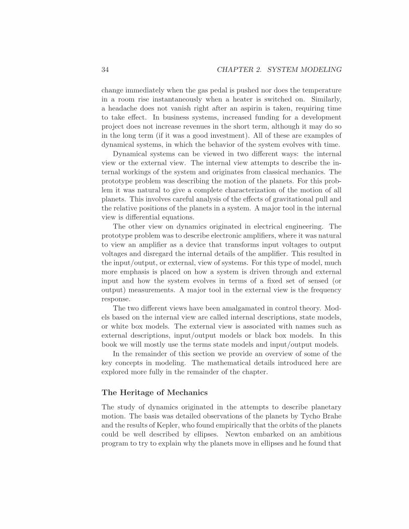
34 CHAPTER 2. SYSTEM MODELING
change immediately when the gas pedal is pushed nor does the temperaturein a room rise instantaneously when a heater is switched on. Similarly,a headache does not vanish right after an aspirin is taken, requiring timeto take effect. In business systems, increased funding for a developmentproject does not increase revenues in the short term, although it may do soin the long term (if it was a good investment). All of these are examples ofdynamical systems, in which the behavior of the system evolves with time.
Dynamical systems can be viewed in two different ways: the internalview or the external view. The internal view attempts to describe the in-ternal workings of the system and originates from classical mechanics. Theprototype problem was describing the motion of the planets. For this prob-lem it was natural to give a complete characterization of the motion of allplanets. This involves careful analysis of the effects of gravitational pull andthe relative positions of the planets in a system. A major tool in the internalview is differential equations.
The other view on dynamics originated in electrical engineering. Theprototype problem was to describe electronic amplifiers, where it was naturalto view an amplifier as a device that transforms input voltages to outputvoltages and disregard the internal details of the amplifier. This resulted inthe input/output, or external, view of systems. For this type of model, muchmore emphasis is placed on how a system is driven through and externalinput and how the system evolves in terms of a fixed set of sensed (oroutput) measurements. A major tool in the external view is the frequencyresponse.
The two different views have been amalgamated in control theory. Mod-els based on the internal view are called internal descriptions, state models,or white box models. The external view is associated with names such asexternal descriptions, input/output models or black box models. In thisbook we will mostly use the terms state models and input/output models.
In the remainder of this section we provide an overview of some of thekey concepts in modeling. The mathematical details introduced here areexplored more fully in the remainder of the chapter.
The Heritage of Mechanics
The study of dynamics originated in the attempts to describe planetarymotion. The basis was detailed observations of the planets by Tycho Braheand the results of Kepler, who found empirically that the orbits of the planetscould be well described by ellipses. Newton embarked on an ambitiousprogram to try to explain why the planets move in ellipses and he found that
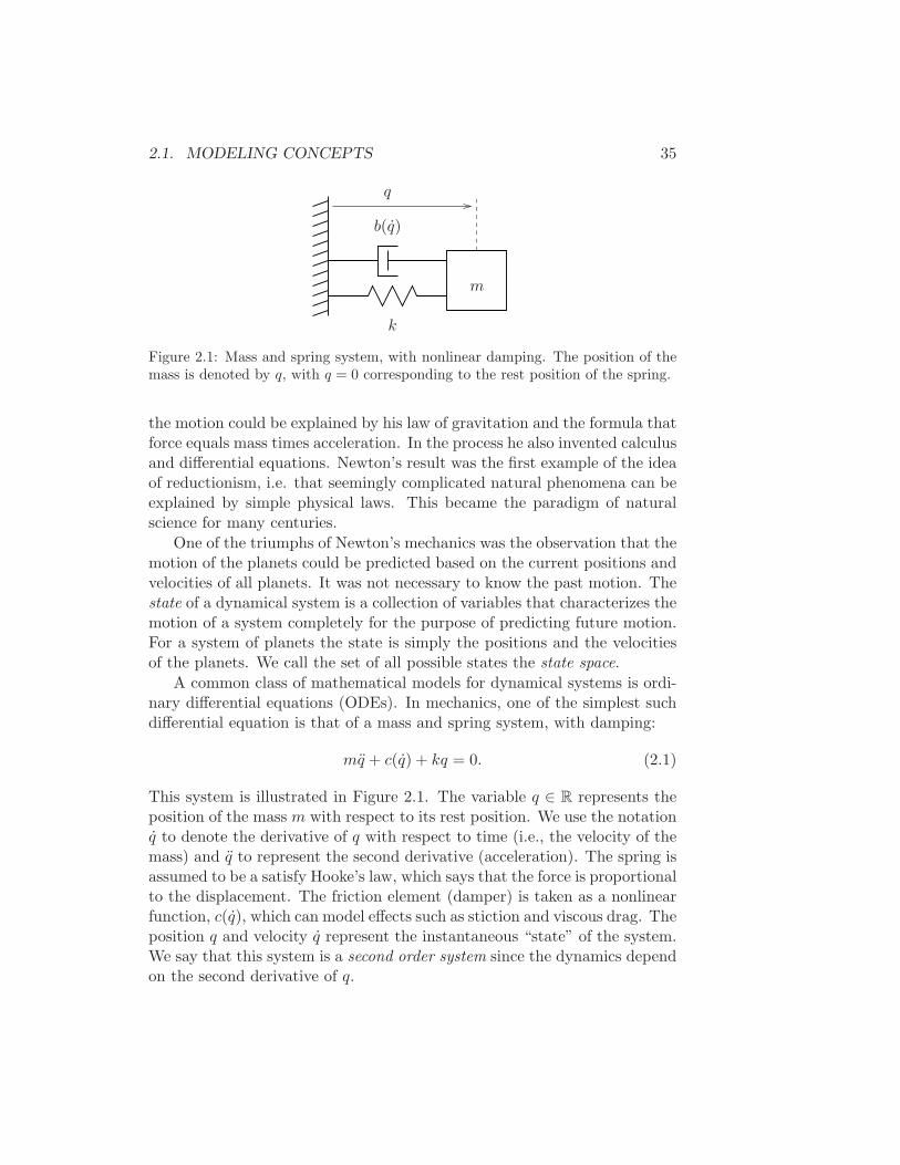
2.1. MODELING CONCEPTS 35
m
k
b(q)
q
Figure 2.1: Mass and spring system, with nonlinear damping. The position of themass is denoted by q, with q = 0 corresponding to the rest position of the spring.
the motion could be explained by his law of gravitation and the formula thatforce equals mass times acceleration. In the process he also invented calculusand differential equations. Newton’s result was the first example of the ideaof reductionism, i.e. that seemingly complicated natural phenomena can beexplained by simple physical laws. This became the paradigm of naturalscience for many centuries.
One of the triumphs of Newton’s mechanics was the observation that themotion of the planets could be predicted based on the current positions andvelocities of all planets. It was not necessary to know the past motion. Thestate of a dynamical system is a collection of variables that characterizes themotion of a system completely for the purpose of predicting future motion.For a system of planets the state is simply the positions and the velocitiesof the planets. We call the set of all possible states the state space.
A common class of mathematical models for dynamical systems is ordi-nary differential equations (ODEs). In mechanics, one of the simplest suchdifferential equation is that of a mass and spring system, with damping:
mq + c(q) + kq = 0. (2.1)
This system is illustrated in Figure 2.1. The variable q ∈ R represents theposition of the mass m with respect to its rest position. We use the notationq to denote the derivative of q with respect to time (i.e., the velocity of themass) and q to represent the second derivative (acceleration). The spring isassumed to be a satisfy Hooke’s law, which says that the force is proportionalto the displacement. The friction element (damper) is taken as a nonlinearfunction, c(q), which can model effects such as stiction and viscous drag. Theposition q and velocity q represent the instantaneous “state” of the system.We say that this system is a second order system since the dynamics dependon the second derivative of q.
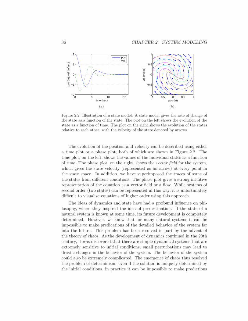
36 CHAPTER 2. SYSTEM MODELING
0 5 10 15−2
−1
0
1
2
time (sec)
pos
(m),
vel
(m
/sec
)
posvel
(a)
−1 −0.5 0 0.5 1−1
−0.5
0
0.5
1
pos (m)
vel (
m/s
ec)
(b)
Figure 2.2: Illustration of a state model. A state model gives the rate of change ofthe state as a function of the state. The plot on the left shows the evolution of thestate as a function of time. The plot on the right shows the evolution of the statesrelative to each other, with the velocity of the state denoted by arrows.
The evolution of the position and velocity can be described using eithera time plot or a phase plot, both of which are shown in Figure 2.2. Thetime plot, on the left, shows the values of the individual states as a functionof time. The phase plot, on the right, shows the vector field for the system,which gives the state velocity (represented as an arrow) at every point inthe state space. In addition, we have superimposed the traces of some ofthe states from different conditions. The phase plot gives a strong intuitiverepresentation of the equation as a vector field or a flow. While systems ofsecond order (two states) can be represented in this way, it is unfortunatelydifficult to visualize equations of higher order using this approach.
The ideas of dynamics and state have had a profound influence on phi-losophy, where they inspired the idea of predestination. If the state of anatural system is known at some time, its future development is completelydetermined. However, we know that for many natural systems it can beimpossible to make predications of the detailed behavior of the system farinto the future. This problem has been resolved in part by the advent ofthe theory of chaos. As the development of dynamics continued in the 20thcentury, it was discovered that there are simple dynamical systems that areextremely sensitive to initial conditions; small perturbations may lead todrastic changes in the behavior of the system. The behavior of the systemcould also be extremely complicated. The emergence of chaos thus resolvedthe problem of determinism: even if the solution is uniquely determined bythe initial conditions, in practice it can be impossible to make predictions
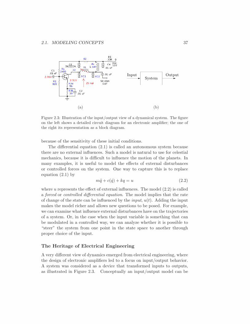
2.1. MODELING CONCEPTS 37
Input OutputSystem
(a) (b)
Figure 2.3: Illustration of the input/output view of a dynamical system. The figureon the left shows a detailed circuit diagram for an electronic amplifier; the one ofthe right its representation as a block diagram.
because of the sensitivity of these initial conditions.
The differential equation (2.1) is called an autonomous system becausethere are no external influences. Such a model is natural to use for celestialmechanics, because it is difficult to influence the motion of the planets. Inmany examples, it is useful to model the effects of external disturbancesor controlled forces on the system. One way to capture this is to replaceequation (2.1) by
mq + c(q) + kq = u (2.2)
where u represents the effect of external influences. The model (2.2) is calleda forced or controlled differential equation. The model implies that the rateof change of the state can be influenced by the input, u(t). Adding the inputmakes the model richer and allows new questions to be posed. For example,we can examine what influence external disturbances have on the trajectoriesof a system. Or, in the case when the input variable is something that canbe modulated in a controlled way, we can analyze whether it is possible to“steer” the system from one point in the state space to another throughproper choice of the input.
The Heritage of Electrical Engineering
A very different view of dynamics emerged from electrical engineering, wherethe design of electronic amplifiers led to a focus on input/output behavior.A system was considered as a device that transformed inputs to outputs,as illustrated in Figure 2.3. Conceptually an input/output model can be
38 CHAPTER 2. SYSTEM MODELING
viewed as a giant table of inputs and outputs. Given an input signal u(t),the model should produce the resulting output y(t).
The input/output framework is used in many engineering systems sinceit allows us to decompose a problem into individual components, connectedthrough their inputs and outputs. Thus, we can take a complicated systemsuch as a radio or a television and break it down into manageable pieces,such as the receiver, demodulator, amplifier and speakers. Each of thesepieces has a set of inputs and outputs and, through proper design, thesecomponents can be interconnected to form the entire system.
The input/output view is particularly useful for the special class of linear,time-invariant systems. This term will be defined more carefully later inthis chapter, but roughly speaking a system is linear if the superposition(addition) of two inputs yields an output which is the sum of the outputsthat would correspond to individual inputs being applied separately. Asystem is time-invariant if the output response for a given input does notdepend on when that input is applied. (Chapter 5 provides a much moredetailed analysis of linear systems.)
Many electrical engineering systems can be modeled by linear, time-invariant systems and hence a large number of tools have been developedto analyze them. One such tool is the step response, which describes therelationship between an input that changes from zero to a constant valueabruptly (a “step” input) and the corresponding output. As we shall see inthe latter part of the text, the step response is extremely useful in character-izing the performance of a dynamical system and it is often used to specifythe desired dynamics. A sample step response is shown in Figure 2.4a.
Another possibility to describe a linear, time-invariant system is to rep-resent the system by its response to sinusoidal input signals. This is calledthe frequency response and a rich powerful theory with many concepts andstrong, useful results has emerged. The results are based on the theory ofcomplex variables and Laplace transforms. The basic idea behind the fre-quency response is that we can completely characterize the behavior of asystem by its steady state response to sinusoidal inputs. Roughly speaking,this is done by decomposing any arbitrary signal into a linear combinationof sinusoids (e.g., by using the Fourier transform) and then using linearity tocompute the output by combining the response to the individual frequencies.A sample frequency response is shown in Figure 2.4b.
The input/output view lends itself naturally to experimental determi-nation of system dynamics, where a system is characterized by recordingits response to a particular input, e.g. a step or a sweep across a range offrequencies.

2.1. MODELING CONCEPTS 39
0 10 20 300
0.5
1
1.5
2
2.5
3
3.5
time (sec)
Inpu
t (da
shed
), o
utpu
t (so
lid)
output
input
(a)
10−1
100
101
102
10−4
10−2
100
Gai
n
10−1
100
101
102
−270
−180
−90
0
Pha
se (
deg)
Frequency (rad/sec)
(b)
Figure 2.4: Input/output response of a linear system. The step response (a) showsthe output of the system due to an input that changes from 0 to 1 at time t = 5s. The frequency response (b) shows the amplitude gain and phase change due toa sinusoidal input at different frequencies.
The Control View
When control theory emerged as a discipline in the 1940s, the approach todynamics was strongly influenced by the electrical engineering (input/output)view. A second wave of developments in control, starting in the late 1950s,was inspired by mechanics, where the state space perspective was used. Inaddition, there was a shift over this period from autonomous systems (withno inputs) to those where inputs to the process were available to modify thedynamics of the process. The emergence of space flight is a typical example,where precise control of the orbit is essential.
The models from mechanics were thus modified to include external con-trol forces and sensors, and more general forms of equations were considered.In control, the model given by equation (2.2) was replaced by
dx
dt= f(x, u)
y = h(x, u),(2.3)
where x is a vector of “state” variables, u is a vector of control signals, andy a vector of measurements. As before, x represents the derivative of x withrespect to time, now considered as a vector, and f and h are mappings oftheir arguments to vectors of the appropriate dimension.
This viewpoint has added to the richness of the classical problems andled to many new concepts. For example it is natural to ask if possiblestates x can be reached with the proper choice of u (reachability) and if
40 CHAPTER 2. SYSTEM MODELING
the measurement y contains enough information to reconstruct the state(observability) (these topics will be addressed in greater detail in Chapters 6and 7).
A final development in building the control point of view was the emer-gence of disturbance and model uncertainty as critical elements in the theory.The simple way of modeling disturbances as deterministic signals like stepsand sinusoids has the drawback that such signals can be predicted precisely.A much more realistic approach is to model disturbances like random signals.This viewpoint gives a natural connection between prediction and control.The dual views of input/output representations and state space representa-tions are particularly useful when modeling uncertainty, since state modelsare very convenient to describe a nominal model but uncertainties are eas-ier to describe using input/output models (often via a frequency responsedescription). Uncertainty will be a constant theme throughout the text andwill be studied in particular detail in Chapter 12.
An interesting experience in design of control system is that feedbacksystems can often be analyzed and designed based on comparatively simplemodels. The reason for this is the inherent robustness of feedback systems.However, other uses of models may require more complexity and more accu-racy. One example is feedforward control strategies, where one uses a modelto pre-compute the inputs that will cause the system to respond in a certainway. Another area is in system validation, where one wishes to verify thatthe detailed response of the system performs as it was designed. Because ofthese different uses of models, it is therefore common to use a hierarchy ofmodels having different complexity and fidelity.
Multi-Domain Modeling
Modeling is an essential element of many disciplines, but traditions andmethods from individual disciplines in can be very different from each other,as illustrated by the previous discussion of mechanical and electrical engi-neering. A difficulty in systems engineering is that it is frequently necessaryto deal with heterogeneous systems from many different domains, includingchemical, electrical, mechanical and information systems.
To deal with such multi-domain systems, we start by cutting a systeminto smaller subsystems. Each subsystem is modeled either by balance equa-tions for mass, energy, and momentum or by appropriate descriptions of theinformation processing in the subsystem. The behavior at the interfaces iscaptured by describing how the variables of the subsystem behave when thesubsystems are interconnected. These interfaces often act by constraining
2.1. MODELING CONCEPTS 41
variables within the individual subsystems to be equal (such as mass, energyor momentum fluxes). The complete model is then obtained by combiningthe descriptions of the subsystems and the interfaces.
Using this methodology it is possible to build up libraries of subsystemsthat correspond to physical, chemical and informational components. Theprocedure mimics the engineering approach where systems are built fromsubsystems that are themselves built from smaller components. As experi-ence is gained, the components and their interfaces can be standardized andcollected in model libraries. In practice, it takes several iterations to obtaina good library that can be reused for many applications.
State models or ordinary differential equations are not suitable for com-ponent based modeling of this form because states may disappear whencomponents are connected. This implies that the internal description of acomponent may change when it is connected to other components. As an il-lustration we consider two capacitors in an electrical circuit. Each capacitorhas a state corresponding to the voltage across the capacitors, but one of thestates will disappear if the capacitors are connected in parallel. A similarsituation happens with two rotating inertias, each of which are individuallymodeled using the the angle of rotation and the angular velocity. Two stateswill disappear when the inertias are joined by a rigid shaft.
This difficulty can be avoided by replacing differential equations by dif-ferential algebraic equations, which have the form
F (z, z) = 0
where z ∈ Rn. A simple special case is
x = f(x, y), g(x, y) = 0 (2.4)
where z = (x, y) and F = (x−f(x, y), g(x, y)). The key property is that thederivative z is not given explicitly and there may be pure algebraic relationsbetween the components of the vector z.
A differential equation is an imperative description: if it tells how tocalculate x from x. The differential algebraic equation is a declarative de-scription: it gives a relation between z and z, without explicitly describinghow to compute z. The model (2.4) captures the examples of the parallelcapacitors and the linked rotating inertias. For example, when two capaci-tors are connected we simply include the algebraic equation expressing thatthe voltages across the capacitors are the same.
A practical difficulty with component-based declarative descriptions is athat the model may contain many auxiliary variables. This was a severe lim-itation for hand calculations, but fortunately there are methods for symbolic
42 CHAPTER 2. SYSTEM MODELING
calculation that can be used to eliminate the auxiliary variables. Symboliccalculations can also be used to transform and simplify the models.
Modelica is a language that has been developed to support componentbased modeling. Differential algebraic equations are used as the basic de-scription, object-oriented programming is used to structure the models.Modelica is used to model the dynamics of technical systems in domainssuch as, mechanical, electrical, thermal, hydraulic, thermo-fluid, and con-trol subsystems. Modelica is intended to serve as a standard format so thatmodels arising in different domains can be exchanged between tools andusers. A large set of free and commercial Modelica component librariesare available and are utilized by a growing number of people in indus-try, research and academia. For further information about Modelica, seehttp://www.modelica.org.
2.2 State Space Models
In this section we introduce the two primary forms of models that we usein this text: differential equations and difference equations. Both of thesemake use of the notions of state, inputs, outputs and dynamics to describethe behavior of a system.
Ordinary Differential Equations
The state of a system is a collection of variables that summarize the past ofa system for the purpose of prediction the future. For an engineering systemthe state is composed of the variables required to account for storage of mass,momentum and energy. A key issue in modeling is to decide how accuratelythis storage has to be represented. The state variables are gathered in avector, x ∈ R
n, called the state vector. The control variables are representedby another vector u ∈ R
p and the measured signal by the vector y ∈ Rq. A
system can then be represented by the differential equation
dx
dt= f(x, u)
y = h(x, u),(2.5)
where f : Rn × R
p → Rn and h : R
n × Rp → R
q are smooth mappings. Wecall a model of this form a state space model.
The dimension of the state vector is called the order of the system.The system is called time-invariant because the functions f and g do not
2.2. STATE SPACE MODELS 43
depend explicitly on time t. It is possible to have more general time-varyingsystems where the functions do depend on time. The model thus consistsof two functions: the function f gives the velocity of the state vector as afunction of state x and control u, and the function g gives the measuredvalues as functions of state x and control u.
A system is called linear if the functions f and g are linear in x and u.A linear state space system can thus be represented by
dx
dt= Ax+Bu
y = Cx+Du,
where A, B, C and D are constant matrices. Such a system is said to be lin-ear and time-invariant, or LTI for short. The matrix A is called the dynamicsmatrix, the matrix B is called the control matrix, the matrix C is called thesensor matrix and the matrix D is called the direct term. Frequently sys-tems will not have a direct term, indicating that the control signal does notinfluence the output directly.
A different form of linear differential equations, generalizing the secondorder dynamics from mechanics, is an equation of the form
dnq
dtn+ a1
dn−1q
dtn−1+ · · · + anq = u, (2.6)
where t is the independent (time) variable, q(t) is the dependent (output)variable, and u(t) is the input. This system is said to be an nth order system.This system can be converted into state space form by defining
x =
x1
x2...xn
=
dn−1q/dtn−1
...dq/dtq
and the state space equations become
d
dt
x1
x2...
xn−1
xn
=
−a1x1 − · · · − anxn
x1
x2...
xn−1
+
10...0
y = xn.
44 CHAPTER 2. SYSTEM MODELING
With the appropriate definition of A, B, C and D, this equation is in linearstate space form.
An even more general system is obtained by letting the output be alinear combination of the states of the system, i.e.
y = b1x1 + b2x2 + · · · + bnxn + du
This system can be modeled in state space as
d
dt
x1
x2...
xn−1
xn
=
−a1 −a2 . . . −an
1 0 0 . . . 00 1 0 . . . 0...
. . .
0 1 0
x+
10...00
u
y =
b1 b2 . . . bn
x+ du.
This particular form of a linear state space system is called reachable canon-ical form and will be studied in more detail in later chapters.
Example 2.1 (Balance systems). An example of a class of systems thatcan be modeled using ordinary differential equations is the class of “balancesystems.” A balance system is a mechanical system in which the center ofmass is balanced above a pivot point. Some common examples of balancesystems are shown in Figure 2.5. The Segway human transportation system(Figure 2.5a) uses a motorized platform to stabilize a person standing ontop of it. When the rider leans forward, the vehicle propels itself along theground, but maintains its upright position. Another example is a rocket(Figure 2.5b), in which a gimbaled nozzle at the bottom of the rocket isused to stabilize the body of the rocket above it. Other examples of bal-ance systems include humans or other animals standing upright or a personbalancing a stick on their hand.
Figure 2.5c shows a simplified diagram for a balance system. To modelthis system, we choose state variables that represent the position and veloc-ity of the base of the system, p and p, and the angle and angular rate of thestructure above the base, θ and θ. We let F represent the force applied atthe base of the system, assumed to be in the horizontal direction (alignedwith p), and choose the position and angle of the system as outputs. Withthis set of definitions, the dynamics of the system can be computed usingNewtonian mechanics and has the form
(M +m) −ml cos θ−ml cos θ (J +ml2)
p
θ
+
cp+ml sin θ θ2
mgl sin θ + γθ
=
F0
, (2.7)
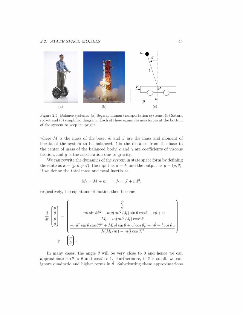
2.2. STATE SPACE MODELS 45
(a) (b)
l
MF
p
θm
(c)
Figure 2.5: Balance systems: (a) Segway human transportation systems, (b) Saturnrocket and (c) simplified diagram. Each of these examples uses forces at the bottomof the system to keep it upright.
where M is the mass of the base, m and J are the mass and moment ofinertia of the system to be balanced, l is the distance from the base tothe center of mass of the balanced body, c and γ are coefficients of viscousfriction, and g is the acceleration due to gravity.
We can rewrite the dynamics of the system in state space form by definingthe state as x = (p, θ, p, θ), the input as u = F and the output as y = (p, θ).If we define the total mass and total inertia as
Mt = M +m Jt = J +ml2,
respectively, the equations of motion then become
d
dt
pθp
θ
=
p
θ
−ml sin θθ2 +mg(ml2/Jt) sin θ cos θ − cp+ u
Mt −m(ml2/Jt) cos2 θ
−ml2 sin θ cos θθ2 +Mtgl sin θ + cl cos θp+ γθ + l cos θu
Jt(Mt/m) −m(l cos θ)2
y =
pθ
.
In many cases, the angle θ will be very close to 0 and hence we canapproximate sin θ ≈ θ and cos θ ≈ 1. Furthermore, if θ is small, we canignore quadratic and higher terms in θ. Substituting these approximations
46 CHAPTER 2. SYSTEM MODELING
into our equations, we see that we are left with a linear state space equation
d
dt
pθp
θ
=
0 0 1 00 0 0 1
0 m2l2gµ
−cJt
µ 0
0 Mtmglµ
clmµ
γmµ
pθp
θ
+
00
Jt
µ
lmµ
u
y =
1 0 0 00 1 0 0
x,
where µ = MtJt −m2l2g. ∇Example 2.2 (Inverted pendulum). A variation of this example is one inwhich the location of the base, p, does not need to be controlled. This hap-pens, for example, if we are only interested in stabilizing a rocket’s uprightorientation, without worrying about the location of base of the rocket. Thedynamics of this simplified system is given by
d
dt
θ
θ
=
θmgl
Jtsin θ − γ
Jtθ + l
Jtcos θ u
y =
1 0
x,
(2.8)
where γ is the coefficient of rotational friction, Jt = J + ml2 and u is theforce applied at the base. This system is referred to as an inverted pendulum.
∇
Difference Equations
In some circumstances, it is more natural to describe the evolution of asystem at discrete instants of time rather than continuously in time. Ifwe refer to each of these times by an integer k = 0, 1, 2, . . . , then we canask how the state of the system changes for each k. Just as in the case ofdifferential equations, we shall define the state to be those sets of variablesthat summarize the past of the system for the purpose of predicting itsfuture. Systems described in this manner are referred to as discrete timesystems.
The evolution of a discrete time system can written in the form
xk+1 = f(xk, uk)
yk = h(xk, uk)(2.9)
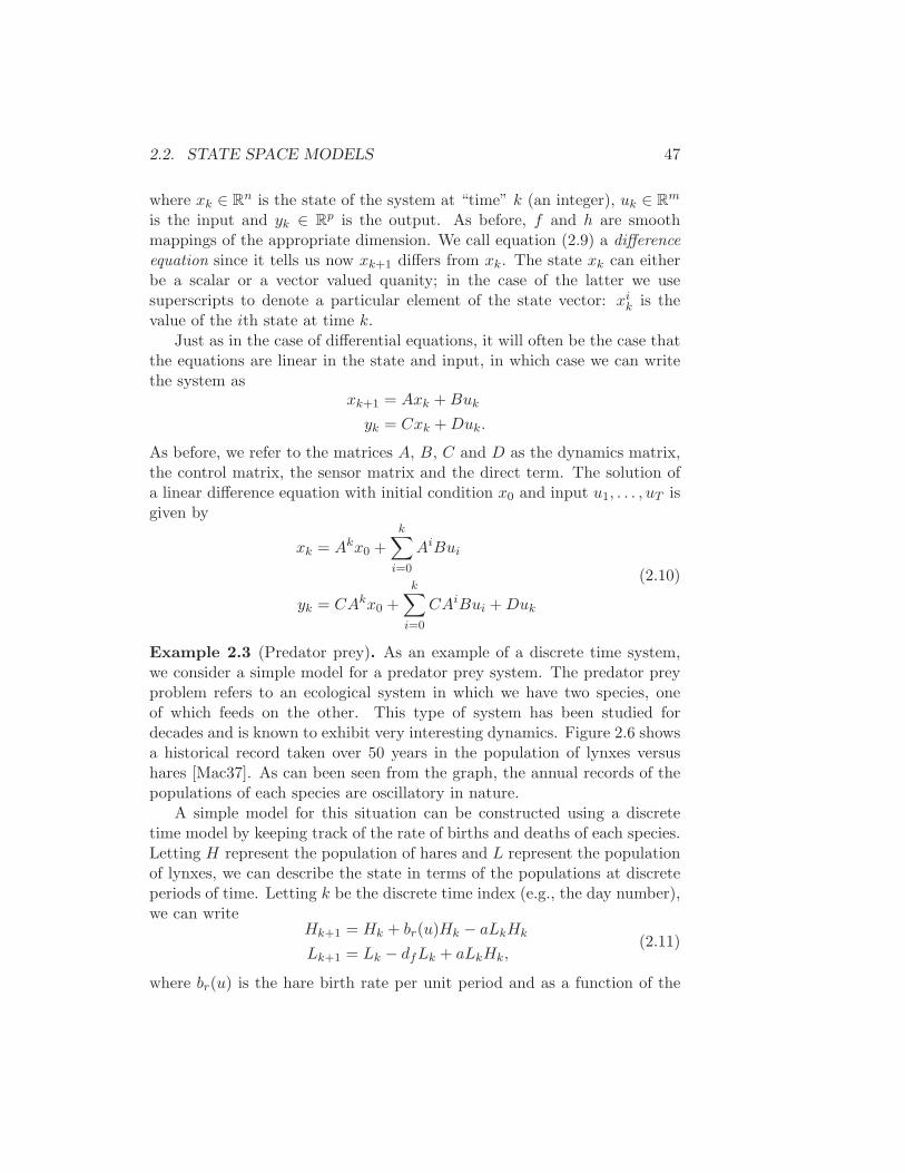
2.2. STATE SPACE MODELS 47
where xk ∈ Rn is the state of the system at “time” k (an integer), uk ∈ R
m
is the input and yk ∈ Rp is the output. As before, f and h are smooth
mappings of the appropriate dimension. We call equation (2.9) a differenceequation since it tells us now xk+1 differs from xk. The state xk can eitherbe a scalar or a vector valued quanity; in the case of the latter we usesuperscripts to denote a particular element of the state vector: xi
k is thevalue of the ith state at time k.
Just as in the case of differential equations, it will often be the case thatthe equations are linear in the state and input, in which case we can writethe system as
xk+1 = Axk +Buk
yk = Cxk +Duk.
As before, we refer to the matrices A, B, C and D as the dynamics matrix,the control matrix, the sensor matrix and the direct term. The solution ofa linear difference equation with initial condition x0 and input u1, . . . , uT isgiven by
xk = Akx0 +k∑
i=0
AiBui
yk = CAkx0 +k∑
i=0
CAiBui +Duk
(2.10)
Example 2.3 (Predator prey). As an example of a discrete time system,we consider a simple model for a predator prey system. The predator preyproblem refers to an ecological system in which we have two species, oneof which feeds on the other. This type of system has been studied fordecades and is known to exhibit very interesting dynamics. Figure 2.6 showsa historical record taken over 50 years in the population of lynxes versushares [Mac37]. As can been seen from the graph, the annual records of thepopulations of each species are oscillatory in nature.
A simple model for this situation can be constructed using a discretetime model by keeping track of the rate of births and deaths of each species.Letting H represent the population of hares and L represent the populationof lynxes, we can describe the state in terms of the populations at discreteperiods of time. Letting k be the discrete time index (e.g., the day number),we can write
Hk+1 = Hk + br(u)Hk − aLkHk
Lk+1 = Lk − dfLk + aLkHk,(2.11)
where br(u) is the hare birth rate per unit period and as a function of the
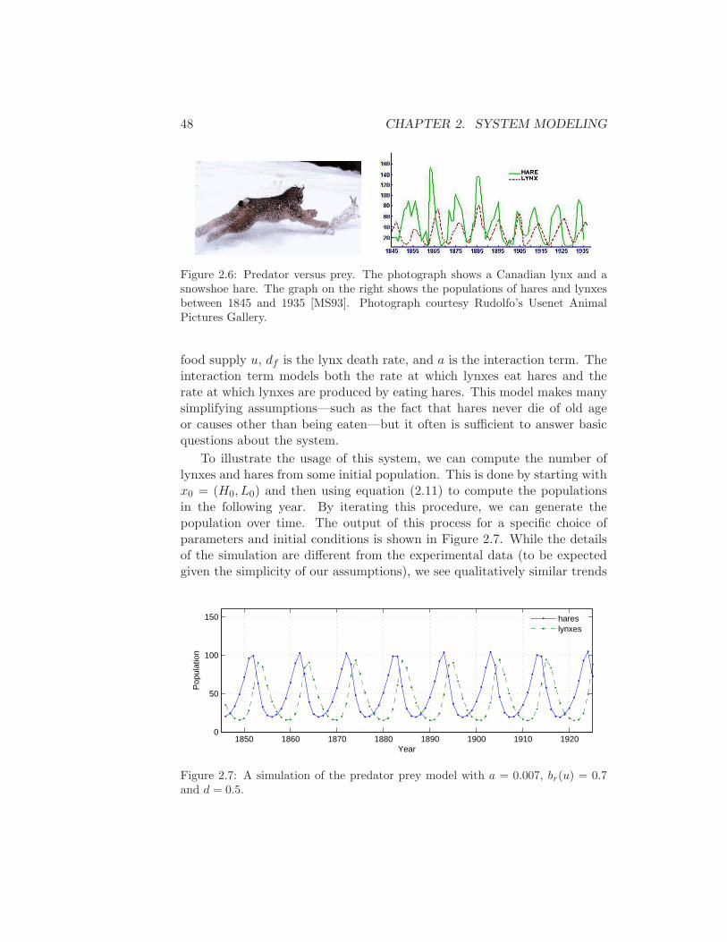
48 CHAPTER 2. SYSTEM MODELING
Figure 2.6: Predator versus prey. The photograph shows a Canadian lynx and asnowshoe hare. The graph on the right shows the populations of hares and lynxesbetween 1845 and 1935 [MS93]. Photograph courtesy Rudolfo’s Usenet AnimalPictures Gallery.
food supply u, df is the lynx death rate, and a is the interaction term. Theinteraction term models both the rate at which lynxes eat hares and therate at which lynxes are produced by eating hares. This model makes manysimplifying assumptions—such as the fact that hares never die of old ageor causes other than being eaten—but it often is sufficient to answer basicquestions about the system.
To illustrate the usage of this system, we can compute the number oflynxes and hares from some initial population. This is done by starting withx0 = (H0, L0) and then using equation (2.11) to compute the populationsin the following year. By iterating this procedure, we can generate thepopulation over time. The output of this process for a specific choice ofparameters and initial conditions is shown in Figure 2.7. While the detailsof the simulation are different from the experimental data (to be expectedgiven the simplicity of our assumptions), we see qualitatively similar trends
1850 1860 1870 1880 1890 1900 1910 19200
50
100
150
Year
Pop
ulat
ion
hareslynxes
Figure 2.7: A simulation of the predator prey model with a = 0.007, br(u) = 0.7and d = 0.5.
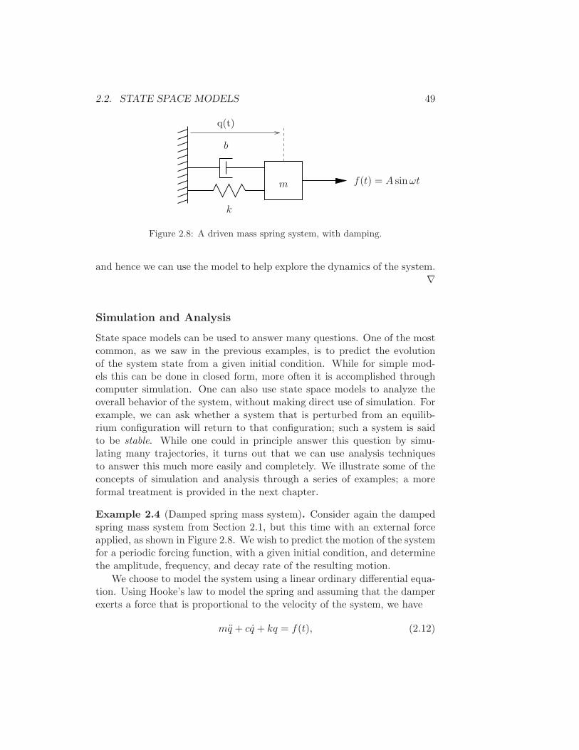
2.2. STATE SPACE MODELS 49
m
k
b
f(t) = A sinωt
q(t)
Figure 2.8: A driven mass spring system, with damping.
and hence we can use the model to help explore the dynamics of the system.∇
Simulation and Analysis
State space models can be used to answer many questions. One of the mostcommon, as we saw in the previous examples, is to predict the evolutionof the system state from a given initial condition. While for simple mod-els this can be done in closed form, more often it is accomplished throughcomputer simulation. One can also use state space models to analyze theoverall behavior of the system, without making direct use of simulation. Forexample, we can ask whether a system that is perturbed from an equilib-rium configuration will return to that configuration; such a system is saidto be stable. While one could in principle answer this question by simu-lating many trajectories, it turns out that we can use analysis techniquesto answer this much more easily and completely. We illustrate some of theconcepts of simulation and analysis through a series of examples; a moreformal treatment is provided in the next chapter.
Example 2.4 (Damped spring mass system). Consider again the dampedspring mass system from Section 2.1, but this time with an external forceapplied, as shown in Figure 2.8. We wish to predict the motion of the systemfor a periodic forcing function, with a given initial condition, and determinethe amplitude, frequency, and decay rate of the resulting motion.
We choose to model the system using a linear ordinary differential equa-tion. Using Hooke’s law to model the spring and assuming that the damperexerts a force that is proportional to the velocity of the system, we have
mq + cq + kq = f(t), (2.12)
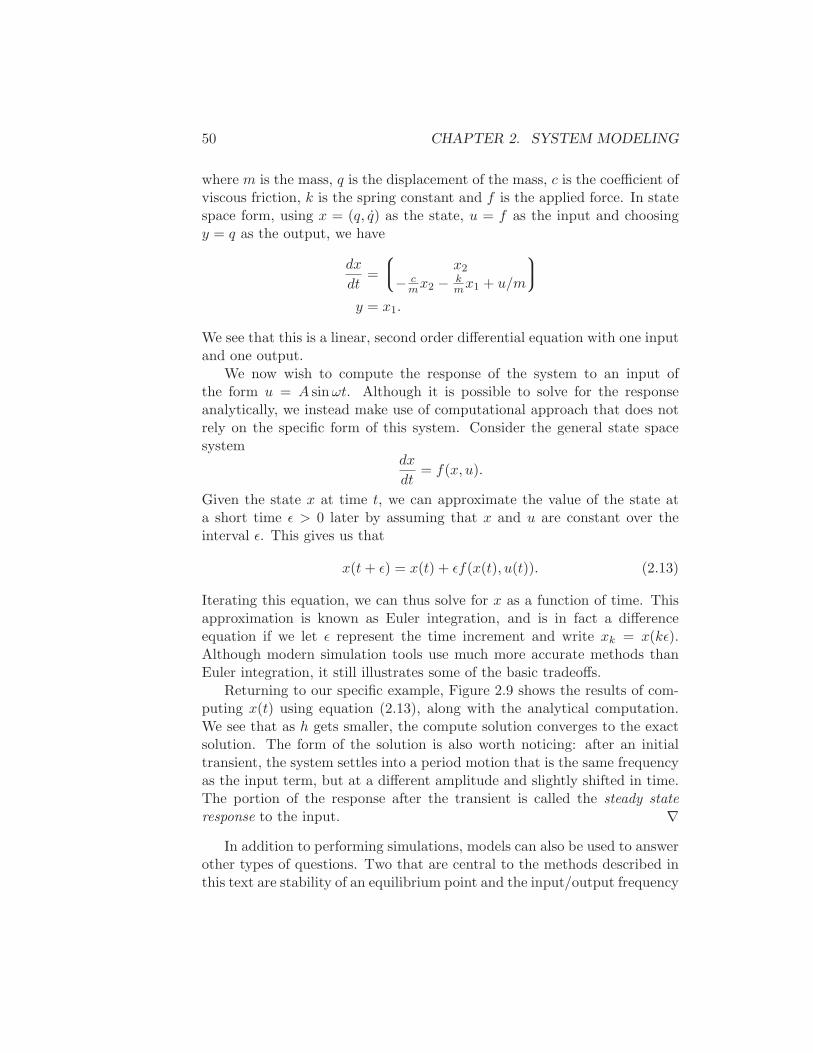
50 CHAPTER 2. SYSTEM MODELING
where m is the mass, q is the displacement of the mass, c is the coefficient ofviscous friction, k is the spring constant and f is the applied force. In statespace form, using x = (q, q) as the state, u = f as the input and choosingy = q as the output, we have
dx
dt=
x2
− cmx2 − k
mx1 + u/m
y = x1.
We see that this is a linear, second order differential equation with one inputand one output.
We now wish to compute the response of the system to an input ofthe form u = A sinωt. Although it is possible to solve for the responseanalytically, we instead make use of computational approach that does notrely on the specific form of this system. Consider the general state spacesystem
dx
dt= f(x, u).
Given the state x at time t, we can approximate the value of the state ata short time ǫ > 0 later by assuming that x and u are constant over theinterval ǫ. This gives us that
x(t+ ǫ) = x(t) + ǫf(x(t), u(t)). (2.13)
Iterating this equation, we can thus solve for x as a function of time. Thisapproximation is known as Euler integration, and is in fact a differenceequation if we let ǫ represent the time increment and write xk = x(kǫ).Although modern simulation tools use much more accurate methods thanEuler integration, it still illustrates some of the basic tradeoffs.
Returning to our specific example, Figure 2.9 shows the results of com-puting x(t) using equation (2.13), along with the analytical computation.We see that as h gets smaller, the compute solution converges to the exactsolution. The form of the solution is also worth noticing: after an initialtransient, the system settles into a period motion that is the same frequencyas the input term, but at a different amplitude and slightly shifted in time.The portion of the response after the transient is called the steady stateresponse to the input. ∇
In addition to performing simulations, models can also be used to answerother types of questions. Two that are central to the methods described inthis text are stability of an equilibrium point and the input/output frequency
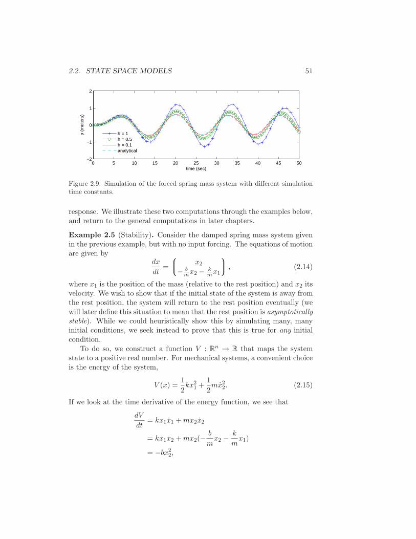
2.2. STATE SPACE MODELS 51
0 5 10 15 20 25 30 35 40 45 50−2
−1
0
1
2
time (sec)
p (m
eter
s)
h = 1h = 0.5h = 0.1analytical
Figure 2.9: Simulation of the forced spring mass system with different simulationtime constants.
response. We illustrate these two computations through the examples below,and return to the general computations in later chapters.
Example 2.5 (Stability). Consider the damped spring mass system givenin the previous example, but with no input forcing. The equations of motionare given by
dx
dt=
x2
− bmx2 − k
mx1
, (2.14)
where x1 is the position of the mass (relative to the rest position) and x2 itsvelocity. We wish to show that if the initial state of the system is away fromthe rest position, the system will return to the rest position eventually (wewill later define this situation to mean that the rest position is asymptoticallystable). While we could heuristically show this by simulating many, manyinitial conditions, we seek instead to prove that this is true for any initialcondition.
To do so, we construct a function V : Rn → R that maps the system
state to a positive real number. For mechanical systems, a convenient choiceis the energy of the system,
V (x) =1
2kx2
1 +1
2mx2
2. (2.15)
If we look at the time derivative of the energy function, we see that
dV
dt= kx1x1 +mx2x2
= kx1x2 +mx2(−b
mx2 −
k
mx1)
= −bx22,
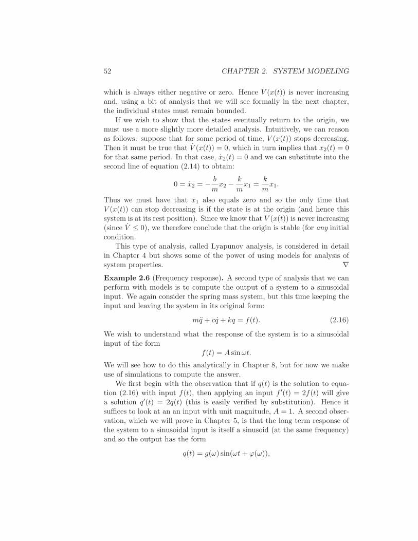
52 CHAPTER 2. SYSTEM MODELING
which is always either negative or zero. Hence V (x(t)) is never increasingand, using a bit of analysis that we will see formally in the next chapter,the individual states must remain bounded.
If we wish to show that the states eventually return to the origin, wemust use a more slightly more detailed analysis. Intuitively, we can reasonas follows: suppose that for some period of time, V (x(t)) stops decreasing.Then it must be true that V (x(t)) = 0, which in turn implies that x2(t) = 0for that same period. In that case, x2(t) = 0 and we can substitute into thesecond line of equation (2.14) to obtain:
0 = x2 = − b
mx2 −
k
mx1 =
k
mx1.
Thus we must have that x1 also equals zero and so the only time thatV (x(t)) can stop decreasing is if the state is at the origin (and hence thissystem is at its rest position). Since we know that V (x(t)) is never increasing(since V ≤ 0), we therefore conclude that the origin is stable (for any initialcondition.
This type of analysis, called Lyapunov analysis, is considered in detailin Chapter 4 but shows some of the power of using models for analysis ofsystem properties. ∇Example 2.6 (Frequency response). A second type of analysis that we canperform with models is to compute the output of a system to a sinusoidalinput. We again consider the spring mass system, but this time keeping theinput and leaving the system in its original form:
mq + cq + kq = f(t). (2.16)
We wish to understand what the response of the system is to a sinusoidalinput of the form
f(t) = A sinωt.
We will see how to do this analytically in Chapter 8, but for now we makeuse of simulations to compute the answer.
We first begin with the observation that if q(t) is the solution to equa-tion (2.16) with input f(t), then applying an input f ′(t) = 2f(t) will givea solution q′(t) = 2q(t) (this is easily verified by substitution). Hence itsuffices to look at an an input with unit magnitude, A = 1. A second obser-vation, which we will prove in Chapter 5, is that the long term response ofthe system to a sinusoidal input is itself a sinusoid (at the same frequency)and so the output has the form
q(t) = g(ω) sin(ωt+ ϕ(ω)),
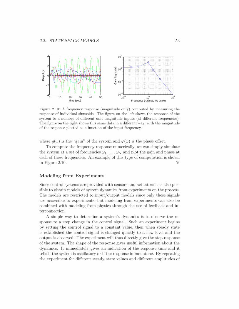
2.2. STATE SPACE MODELS 53
0 10 20 30 40 50−4
−2
0
2
4
time (sec)
Out
put,
y
10−1
100
101
10−2
10−1
100
101
Frequency (rad/sec, log scale)
Gai
n (lo
g sc
ale)
Figure 2.10: A frequency response (magnitude only) computed by measuring theresponse of individual sinusoids. The figure on the left shows the response of thesystem to a number of different unit magnitude inputs (at different frequencies).The figure on the right shows this same data in a different way, with the magnitudeof the response plotted as a function of the input frequency.
where g(ω) is the “gain” of the system and ϕ(ω) is the phase offset.
To compute the frequency response numerically, we can simply simulatethe system at a set of frequencies ω1, . . . , ωN and plot the gain and phase ateach of these frequencies. An example of this type of computation is shownin Figure 2.10. ∇
Modeling from Experiments
Since control systems are provided with sensors and actuators it is also pos-sible to obtain models of system dynamics from experiments on the process.The models are restricted to input/output models since only these signalsare accessible to experiments, but modeling from experiments can also becombined with modeling from physics through the use of feedback and in-terconnection.
A simple way to determine a system’s dynamics is to observe the re-sponse to a step change in the control signal. Such an experiment beginsby setting the control signal to a constant value, then when steady stateis established the control signal is changed quickly to a new level and theoutput is observed. The experiment will thus directly give the step responseof the system. The shape of the response gives useful information about thedynamics. It immediately gives an indication of the response time and ittells if the system is oscillatory or if the response in monotone. By repeatingthe experiment for different steady state values and different amplitudes of
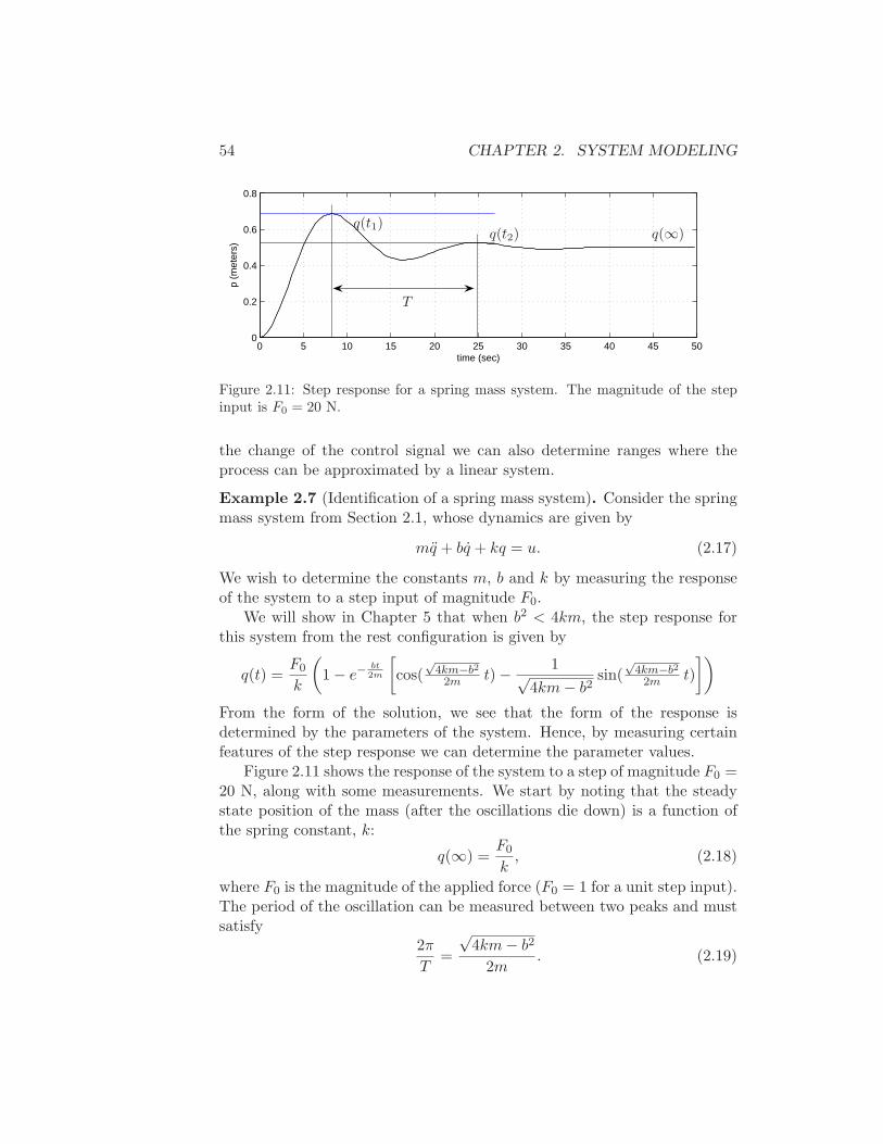
54 CHAPTER 2. SYSTEM MODELING
0 5 10 15 20 25 30 35 40 45 500
0.2
0.4
0.6
0.8
time (sec)
p (m
eter
s)q(t1)
q(t2) q(∞)
T
Figure 2.11: Step response for a spring mass system. The magnitude of the stepinput is F0 = 20 N.
the change of the control signal we can also determine ranges where theprocess can be approximated by a linear system.
Example 2.7 (Identification of a spring mass system). Consider the springmass system from Section 2.1, whose dynamics are given by
mq + bq + kq = u. (2.17)
We wish to determine the constants m, b and k by measuring the responseof the system to a step input of magnitude F0.
We will show in Chapter 5 that when b2 < 4km, the step response forthis system from the rest configuration is given by
q(t) =F0
k
(
1 − e−bt2m
[
cos(√
4km−b2
2m t) − 1√4km− b2
sin(√
4km−b2
2m t)
])
From the form of the solution, we see that the form of the response isdetermined by the parameters of the system. Hence, by measuring certainfeatures of the step response we can determine the parameter values.
Figure 2.11 shows the response of the system to a step of magnitude F0 =20 N, along with some measurements. We start by noting that the steadystate position of the mass (after the oscillations die down) is a function ofthe spring constant, k:
q(∞) =F0
k, (2.18)
where F0 is the magnitude of the applied force (F0 = 1 for a unit step input).The period of the oscillation can be measured between two peaks and mustsatisfy
2π
T=
√4km− b2
2m. (2.19)
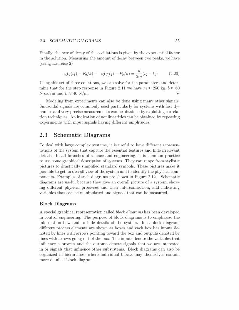
2.3. SCHEMATIC DIAGRAMS 55
Finally, the rate of decay of the oscillations is given by the exponential factorin the solution. Measuring the amount of decay between two peaks, we have(using Exercise 2)
log(q(t1) − F0/k) − log(q(t2) − F0/k) =b
2m(t2 − t1) (2.20)
Using this set of three equations, we can solve for the parameters and deter-mine that for the step response in Figure 2.11 we have m ≈ 250 kg, b ≈ 60N-sec/m and k ≈ 40 N/m. ∇
Modeling from experiments can also be done using many other signals.Sinusoidal signals are commonly used particularly for systems with fast dy-namics and very precise measurements can be obtained by exploiting correla-tion techniques. An indication of nonlinearities can be obtained by repeatingexperiments with input signals having different amplitudes.
2.3 Schematic Diagrams
To deal with large complex systems, it is useful to have different represen-tations of the system that capture the essential features and hide irrelevantdetails. In all branches of science and engineering, it is common practiceto use some graphical description of systems. They can range from stylisticpictures to drastically simplified standard symbols. These pictures make itpossible to get an overall view of the system and to identify the physical com-ponents. Examples of such diagrams are shown in Figure 2.12. Schematicdiagrams are useful because they give an overall picture of a system, show-ing different physical processes and their interconnection, and indicatingvariables that can be manipulated and signals that can be measured.
Block Diagrams
A special graphical representation called block diagrams has been developedin control engineering. The purpose of block diagrams is to emphasize theinformation flow and to hide details of the system. In a block diagram,different process elements are shown as boxes and each box has inputs de-noted by lines with arrows pointing toward the box and outputs denoted bylines with arrows going out of the box. The inputs denote the variables thatinfluence a process and the outputs denote signals that we are interestedin or signals that influence other subsystems. Block diagrams can also beorganized in hierarchies, where individual blocks may themselves containmore detailed block diagrams.

56 CHAPTER 2. SYSTEM MODELING
(a) (b)
(c) (d)
Figure 2.12: Examples of schematic descriptions: (a) schematic picture of an microgas turbine using Modelica, (b) neuronal network for respiratory control, (c) processand instrumentation diagram and (d) Petri net description of a communicationprotocol.
Figure 2.13 shows some of the notation that we use for block diagrams.Signals are represented as lines, with arrows to indicate inputs and outputs.The first diagram is the representation for a summation of two signals. Aninput/output response is represent as a rectangle with the system name (ormathematical description) in the block. Two special cases are a proportionalgain, which scales the input by a multiplicative factor, and an integrator,which outputs the integral of the input signal.
Figure 2.14 illustrates the use of a block diagram, in this case for mod-eling the flight response of a fly. The flight dynamics of an insect are
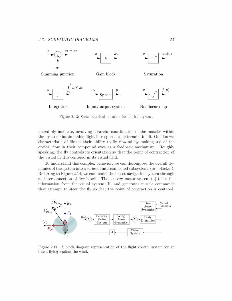
2.3. SCHEMATIC DIAGRAMS 57
Nonlinear map
u
∫ t
0
u(t) dt
System
u y
Input/output system
Gain block
kuu
k
u2
u1 + u2u1
Σ
Summing junction
Integrator
∫
Saturation
sat(u)u
f(u)u
Figure 2.13: Some standard notation for block diagrams.
incredibly intricate, involving a careful coordination of the muscles withinthe fly to maintain stable flight in response to external stimuli. One knowncharacteristic of flies is their ability to fly upwind by making use of theoptical flow in their compound eyes as a feedback mechanism. Roughlyspeaking, the fly controls its orientation so that the point of contraction ofthe visual field is centered in its visual field.
To understand this complex behavior, we can decompose the overall dy-namics of the system into a series of interconnected subsystems (or “blocks”).Referring to Figure 2.14, we can model the insect navigation system throughan interconnection of five blocks. The sensory motor system (a) takes theinformation from the visual system (b) and generates muscle commandsthat attempt to steer the fly so that the point of contraction is centered.
Ref
DragAero-
Wing
dynamicsAero- Dynamics
Body
WindVelocity
SystemVision
MotorSystem
Sensory
-1
Σ Σ
dynamics
Figure 2.14: A block diagram representation of the flight control system for aninsect flying against the wind.
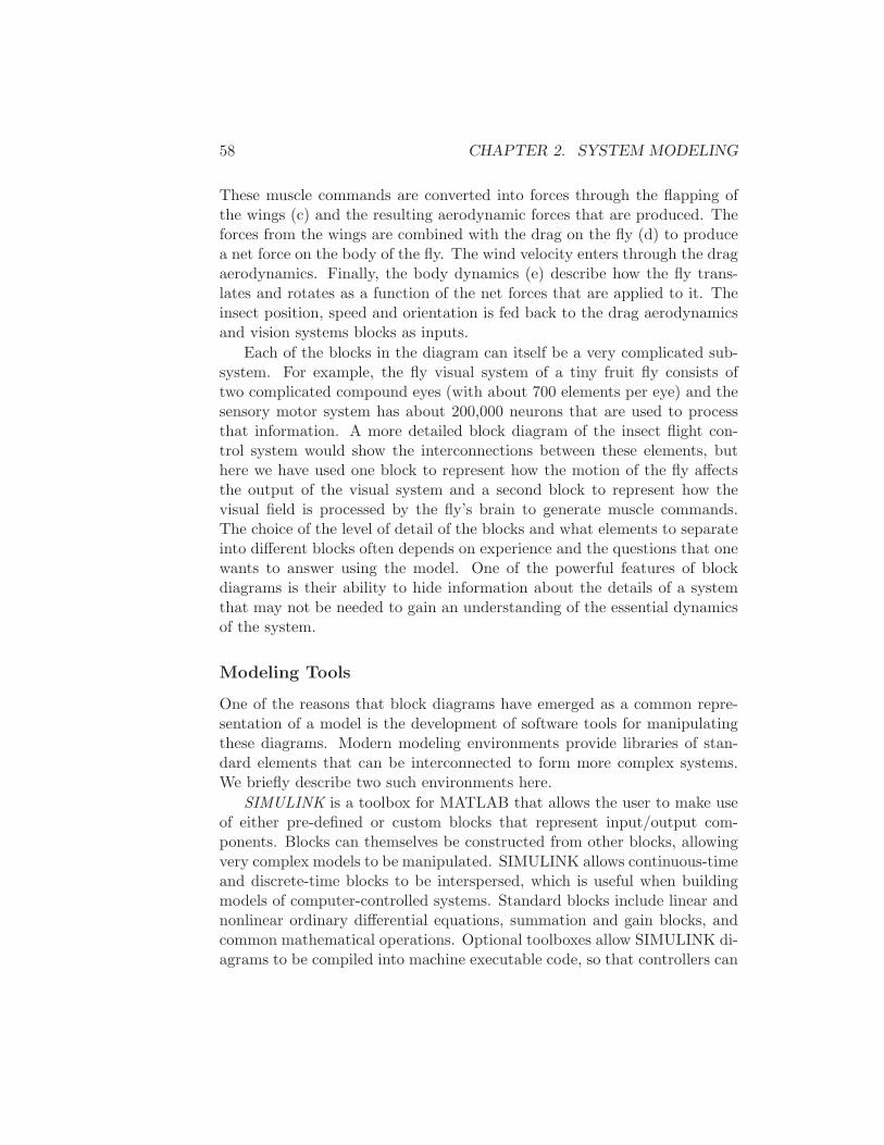
58 CHAPTER 2. SYSTEM MODELING
These muscle commands are converted into forces through the flapping ofthe wings (c) and the resulting aerodynamic forces that are produced. Theforces from the wings are combined with the drag on the fly (d) to producea net force on the body of the fly. The wind velocity enters through the dragaerodynamics. Finally, the body dynamics (e) describe how the fly trans-lates and rotates as a function of the net forces that are applied to it. Theinsect position, speed and orientation is fed back to the drag aerodynamicsand vision systems blocks as inputs.
Each of the blocks in the diagram can itself be a very complicated sub-system. For example, the fly visual system of a tiny fruit fly consists oftwo complicated compound eyes (with about 700 elements per eye) and thesensory motor system has about 200,000 neurons that are used to processthat information. A more detailed block diagram of the insect flight con-trol system would show the interconnections between these elements, buthere we have used one block to represent how the motion of the fly affectsthe output of the visual system and a second block to represent how thevisual field is processed by the fly’s brain to generate muscle commands.The choice of the level of detail of the blocks and what elements to separateinto different blocks often depends on experience and the questions that onewants to answer using the model. One of the powerful features of blockdiagrams is their ability to hide information about the details of a systemthat may not be needed to gain an understanding of the essential dynamicsof the system.
Modeling Tools
One of the reasons that block diagrams have emerged as a common repre-sentation of a model is the development of software tools for manipulatingthese diagrams. Modern modeling environments provide libraries of stan-dard elements that can be interconnected to form more complex systems.We briefly describe two such environments here.
SIMULINK is a toolbox for MATLAB that allows the user to make useof either pre-defined or custom blocks that represent input/output com-ponents. Blocks can themselves be constructed from other blocks, allowingvery complex models to be manipulated. SIMULINK allows continuous-timeand discrete-time blocks to be interspersed, which is useful when buildingmodels of computer-controlled systems. Standard blocks include linear andnonlinear ordinary differential equations, summation and gain blocks, andcommon mathematical operations. Optional toolboxes allow SIMULINK di-agrams to be compiled into machine executable code, so that controllers can
2.3. SCHEMATIC DIAGRAMS 59
Figure 2.15: An example of a SIMULINK block diagram, corresponding to thebody dynamics block of Figure 2.14.
be simulated in SIMULINK and then transferred to a hardware platform forimplementation on a physical system. An example of a SIMULINK blockdiagram is shown in Figure 2.15. This diagram represents the insect bodydynamics block of the larger block diagram in Figure 2.14.
LabVIEW is a graphical programming language developed by NationalInstruments that can be executed directly on a wide range of computer plat-forms and embedded targets. The Simulation Module is an add-on numericalsimulation package that includes continuous and discrete-time blocks, non-linear blocks, and various mathematical operations. All LabVIEW functionsand toolkits can be used with the Simulation Module, allowing for both of-fline simulation and real-time control implementation of complex models.LabVIEW also has a scripting language, MathScript, and toolboxes whichcan be used run many of the examples in this book.
Models for large systems are often built by combining models of differentsubsystems. Block diagram modeling has severe drawbacks in this context,as discussed in Section 2.1. There is software for modeling and simulationtailored to specific domains that overcome these difficulties. Typical exam-ples are SPICE for electrical circuits, Adams for multi-body mechanical sys-tems, AUTOSIM for cars and SBML (Systems Biology Markup Language)for biological systems. Modelica that was discussed in Section 2.1 coversseveral domains. Dymola from Dynasim is an environment for modelingand simulation of complex systems based on Modelica.
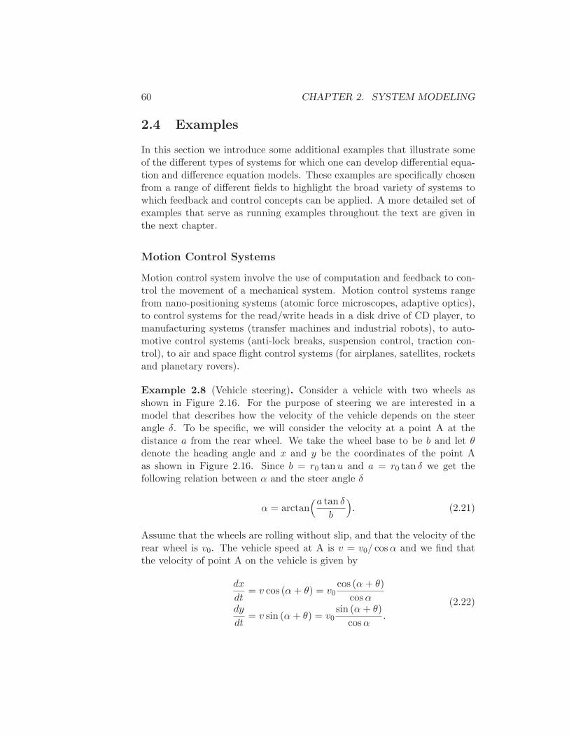
60 CHAPTER 2. SYSTEM MODELING
2.4 Examples
In this section we introduce some additional examples that illustrate someof the different types of systems for which one can develop differential equa-tion and difference equation models. These examples are specifically chosenfrom a range of different fields to highlight the broad variety of systems towhich feedback and control concepts can be applied. A more detailed set ofexamples that serve as running examples throughout the text are given inthe next chapter.
Motion Control Systems
Motion control system involve the use of computation and feedback to con-trol the movement of a mechanical system. Motion control systems rangefrom nano-positioning systems (atomic force microscopes, adaptive optics),to control systems for the read/write heads in a disk drive of CD player, tomanufacturing systems (transfer machines and industrial robots), to auto-motive control systems (anti-lock breaks, suspension control, traction con-trol), to air and space flight control systems (for airplanes, satellites, rocketsand planetary rovers).
Example 2.8 (Vehicle steering). Consider a vehicle with two wheels asshown in Figure 2.16. For the purpose of steering we are interested in amodel that describes how the velocity of the vehicle depends on the steerangle δ. To be specific, we will consider the velocity at a point A at thedistance a from the rear wheel. We take the wheel base to be b and let θdenote the heading angle and x and y be the coordinates of the point Aas shown in Figure 2.16. Since b = r0 tanu and a = r0 tan δ we get thefollowing relation between α and the steer angle δ
α = arctan(a tan δ
b
)
. (2.21)
Assume that the wheels are rolling without slip, and that the velocity of therear wheel is v0. The vehicle speed at A is v = v0/ cosα and we find thatthe velocity of point A on the vehicle is given by
dx
dt= v cos (α+ θ) = v0
cos (α+ θ)
cosαdy
dt= v sin (α+ θ) = v0
sin (α+ θ)
cosα.
(2.22)
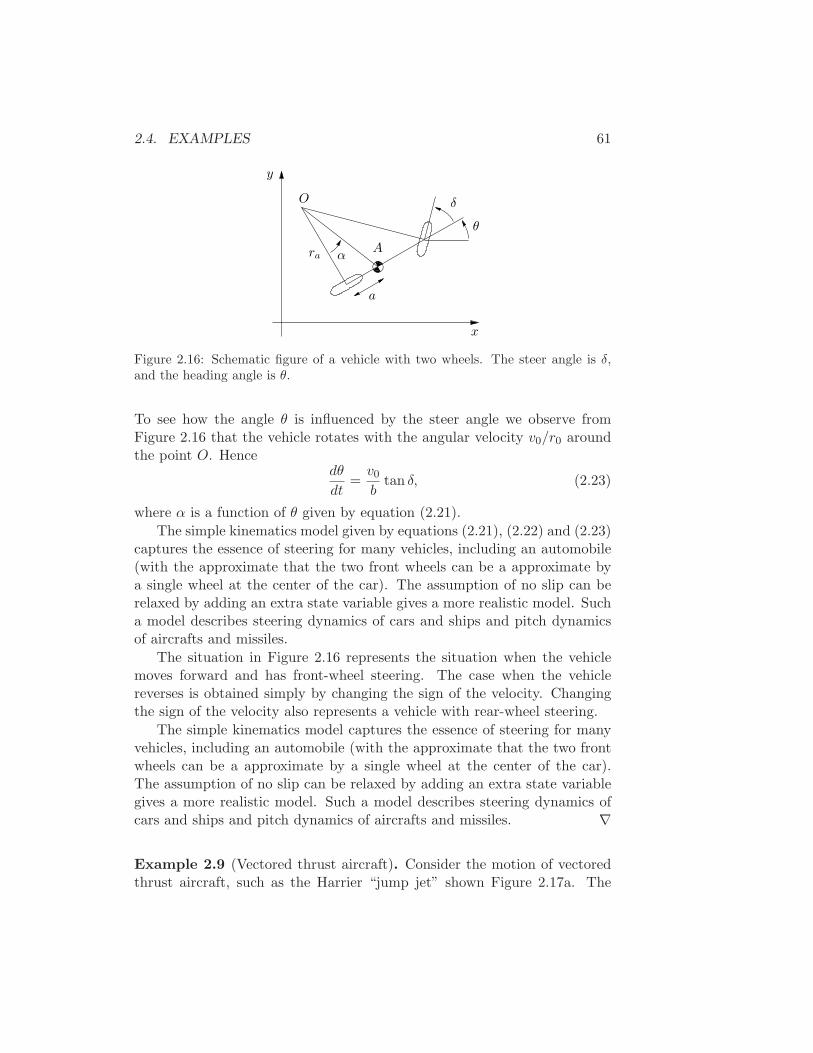
2.4. EXAMPLES 61
a
O
θ
δ
Ara α
x
y
Figure 2.16: Schematic figure of a vehicle with two wheels. The steer angle is δ,and the heading angle is θ.
To see how the angle θ is influenced by the steer angle we observe fromFigure 2.16 that the vehicle rotates with the angular velocity v0/r0 aroundthe point O. Hence
dθ
dt=v0b
tan δ, (2.23)
where α is a function of θ given by equation (2.21).
The simple kinematics model given by equations (2.21), (2.22) and (2.23)captures the essence of steering for many vehicles, including an automobile(with the approximate that the two front wheels can be a approximate bya single wheel at the center of the car). The assumption of no slip can berelaxed by adding an extra state variable gives a more realistic model. Sucha model describes steering dynamics of cars and ships and pitch dynamicsof aircrafts and missiles.
The situation in Figure 2.16 represents the situation when the vehiclemoves forward and has front-wheel steering. The case when the vehiclereverses is obtained simply by changing the sign of the velocity. Changingthe sign of the velocity also represents a vehicle with rear-wheel steering.
The simple kinematics model captures the essence of steering for manyvehicles, including an automobile (with the approximate that the two frontwheels can be a approximate by a single wheel at the center of the car).The assumption of no slip can be relaxed by adding an extra state variablegives a more realistic model. Such a model describes steering dynamics ofcars and ships and pitch dynamics of aircrafts and missiles. ∇
Example 2.9 (Vectored thrust aircraft). Consider the motion of vectoredthrust aircraft, such as the Harrier “jump jet” shown Figure 2.17a. The
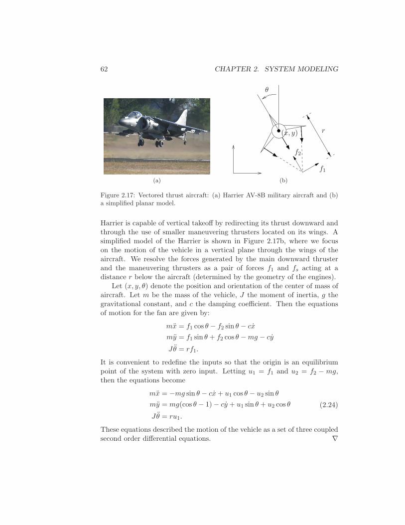
62 CHAPTER 2. SYSTEM MODELING
(a)
θ
f2
(x, y)
f1
r
(b)
Figure 2.17: Vectored thrust aircraft: (a) Harrier AV-8B military aircraft and (b)a simplified planar model.
Harrier is capable of vertical takeoff by redirecting its thrust downward andthrough the use of smaller maneuvering thrusters located on its wings. Asimplified model of the Harrier is shown in Figure 2.17b, where we focuson the motion of the vehicle in a vertical plane through the wings of theaircraft. We resolve the forces generated by the main downward thrusterand the maneuvering thrusters as a pair of forces f1 and fs acting at adistance r below the aircraft (determined by the geometry of the engines).
Let (x, y, θ) denote the position and orientation of the center of mass ofaircraft. Let m be the mass of the vehicle, J the moment of inertia, g thegravitational constant, and c the damping coefficient. Then the equationsof motion for the fan are given by:
mx = f1 cos θ − f2 sin θ − cx
my = f1 sin θ + f2 cos θ −mg − cy
Jθ = rf1.
It is convenient to redefine the inputs so that the origin is an equilibriumpoint of the system with zero input. Letting u1 = f1 and u2 = f2 − mg,then the equations become
mx = −mg sin θ − cx+ u1 cos θ − u2 sin θ
my = mg(cos θ − 1) − cy + u1 sin θ + u2 cos θ
Jθ = ru1.
(2.24)
These equations described the motion of the vehicle as a set of three coupledsecond order differential equations. ∇
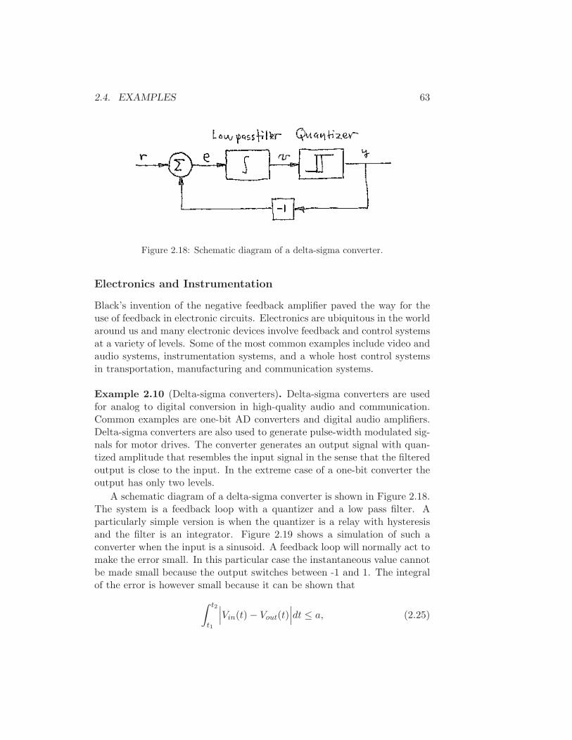
2.4. EXAMPLES 63
Figure 2.18: Schematic diagram of a delta-sigma converter.
Electronics and Instrumentation
Black’s invention of the negative feedback amplifier paved the way for theuse of feedback in electronic circuits. Electronics are ubiquitous in the worldaround us and many electronic devices involve feedback and control systemsat a variety of levels. Some of the most common examples include video andaudio systems, instrumentation systems, and a whole host control systemsin transportation, manufacturing and communication systems.
Example 2.10 (Delta-sigma converters). Delta-sigma converters are usedfor analog to digital conversion in high-quality audio and communication.Common examples are one-bit AD converters and digital audio amplifiers.Delta-sigma converters are also used to generate pulse-width modulated sig-nals for motor drives. The converter generates an output signal with quan-tized amplitude that resembles the input signal in the sense that the filteredoutput is close to the input. In the extreme case of a one-bit converter theoutput has only two levels.
A schematic diagram of a delta-sigma converter is shown in Figure 2.18.The system is a feedback loop with a quantizer and a low pass filter. Aparticularly simple version is when the quantizer is a relay with hysteresisand the filter is an integrator. Figure 2.19 shows a simulation of such aconverter when the input is a sinusoid. A feedback loop will normally act tomake the error small. In this particular case the instantaneous value cannotbe made small because the output switches between -1 and 1. The integralof the error is however small because it can be shown that
∫ t2
t1
∣∣∣Vin(t) − Vout(t)
∣∣∣dt ≤ a, (2.25)
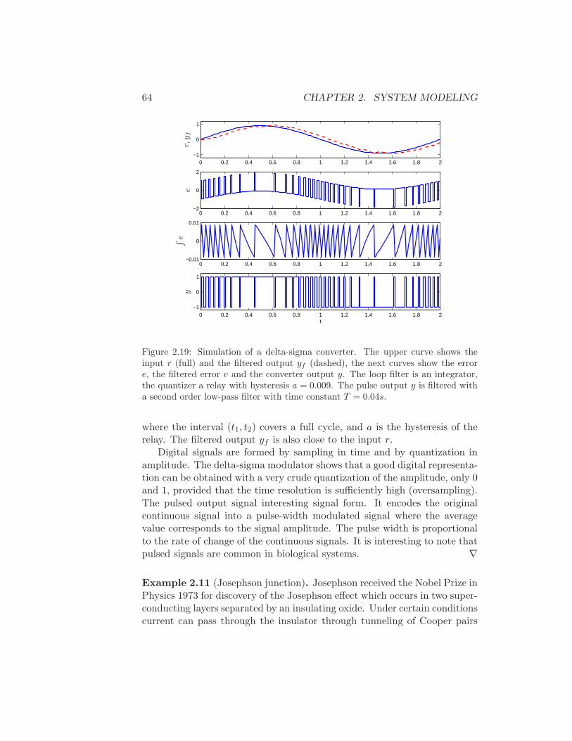
64 CHAPTER 2. SYSTEM MODELING
0 0.2 0.4 0.6 0.8 1 1.2 1.4 1.6 1.8 2−1
0
1
0 0.2 0.4 0.6 0.8 1 1.2 1.4 1.6 1.8 2−2
0
2
0 0.2 0.4 0.6 0.8 1 1.2 1.4 1.6 1.8 2−0.01
0
0.01
0 0.2 0.4 0.6 0.8 1 1.2 1.4 1.6 1.8 2−1
0
1
t
r,y
fe
R
ey
Figure 2.19: Simulation of a delta-sigma converter. The upper curve shows theinput r (full) and the filtered output yf (dashed), the next curves show the errore, the filtered error v and the converter output y. The loop filter is an integrator,the quantizer a relay with hysteresis a = 0.009. The pulse output y is filtered witha second order low-pass filter with time constant T = 0.04s.
where the interval (t1, t2) covers a full cycle, and a is the hysteresis of therelay. The filtered output yf is also close to the input r.
Digital signals are formed by sampling in time and by quantization inamplitude. The delta-sigma modulator shows that a good digital representa-tion can be obtained with a very crude quantization of the amplitude, only 0and 1, provided that the time resolution is sufficiently high (oversampling).The pulsed output signal interesting signal form. It encodes the originalcontinuous signal into a pulse-width modulated signal where the averagevalue corresponds to the signal amplitude. The pulse width is proportionalto the rate of change of the continuous signals. It is interesting to note thatpulsed signals are common in biological systems. ∇
Example 2.11 (Josephson junction). Josephson received the Nobel Prize inPhysics 1973 for discovery of the Josephson effect which occurs in two super-conducting layers separated by an insulating oxide. Under certain conditionscurrent can pass through the insulator through tunneling of Cooper pairs
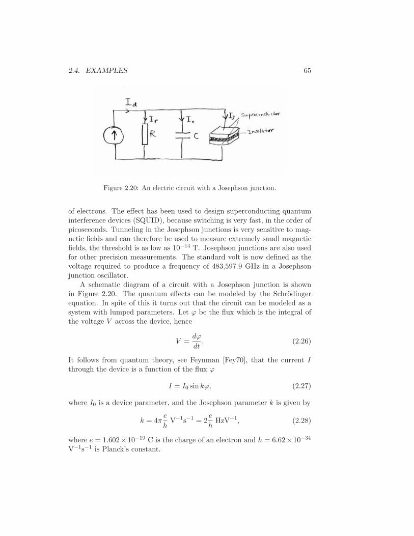
2.4. EXAMPLES 65
Figure 2.20: An electric circuit with a Josephson junction.
of electrons. The effect has been used to design superconducting quantuminterference devices (SQUID), because switching is very fast, in the order ofpicoseconds. Tunneling in the Josephson junctions is very sensitive to mag-netic fields and can therefore be used to measure extremely small magneticfields, the threshold is as low as 10−14 T. Josephson junctions are also usedfor other precision measurements. The standard volt is now defined as thevoltage required to produce a frequency of 483,597.9 GHz in a Josephsonjunction oscillator.
A schematic diagram of a circuit with a Josephson junction is shownin Figure 2.20. The quantum effects can be modeled by the Schrodingerequation. In spite of this it turns out that the circuit can be modeled as asystem with lumped parameters. Let ϕ be the flux which is the integral ofthe voltage V across the device, hence
V =dϕ
dt. (2.26)
It follows from quantum theory, see Feynman [Fey70], that the current Ithrough the device is a function of the flux ϕ
I = I0 sin kϕ, (2.27)
where I0 is a device parameter, and the Josephson parameter k is given by
k = 4πe
hV−1s−1 = 2
e
hHzV−1, (2.28)
where e = 1.602× 10⁻¹⁹ C is the charge of an electron and h = 6.62× 10⁻³⁴
V−1s−1 is Planck’s constant.
66 CHAPTER 2. SYSTEM MODELING
The circuit in Figure 2.20 has two storage elements the capacitor andthe Josephson junction. We choose the states as the voltage V across thecapacitor and the flux ϕ of the Josephson junction. Let IR, IC and IJ bethe currents through the resistor, the capacitor and the Josephson junction.We have
IR =V
R, IC = C
dV
dt, IJ = I0 sin kϕ,
and a current balance gives
IR + IC + IJ = Id,
which can be rewritten as
CdV
dt= Id −
V
R− I0 sin kϕ.
Combining this equation with equation (2.26) gives the following state equa-tion for the circuit
dϕ
dt= V
CdV
d= −I0 sin kϕ− V
R+ Id.
(2.29)
Notice that apart from parameter values equation (2.29) is identical to theequation for the inverted pendulum given in equation (2.8). ∇
Information Systems
Information systems can range from communication systems for transmit-ting data from one location to another, to software systems that manipulatedata or manage enterprise-wide resources, to economies and financial mar-kets, that use prices to reflect current and future value. Feedback is presentin all of these systems, although it is often not directly visible.
Example 2.12 (Congestion control). The Internet was created to obtaina large, highly decentralized, efficient, and expandable communication sys-tem. The system consists of a large number of interconnected gateways. Amessage is split into several packets that are transmitted over different pathsin the network. The packages are joined to recover the message at the re-ceiver. A message is sent back to the sender when a packet is received. Theoperation of the system is governed by a simple but powerful decentralizedcontrol structure which evolved over time.
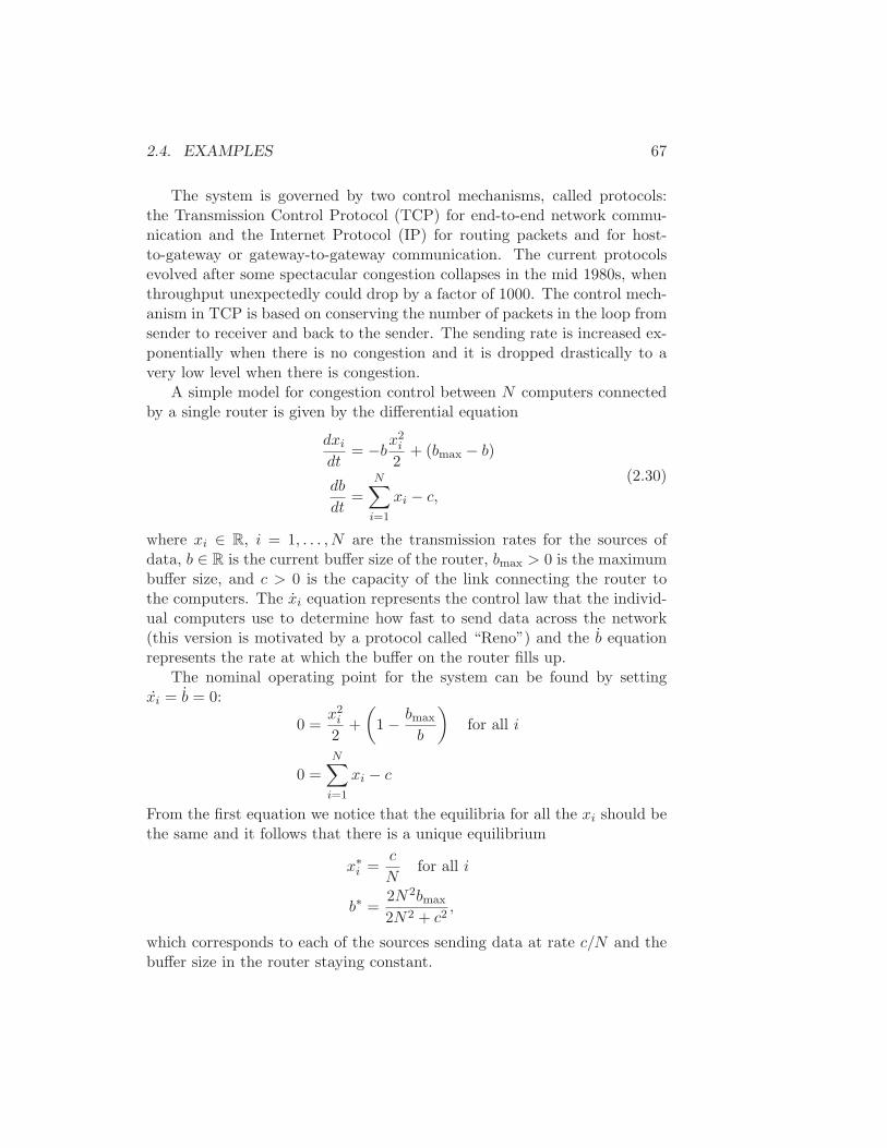
2.4. EXAMPLES 67
The system is governed by two control mechanisms, called protocols:the Transmission Control Protocol (TCP) for end-to-end network commu-nication and the Internet Protocol (IP) for routing packets and for host-to-gateway or gateway-to-gateway communication. The current protocolsevolved after some spectacular congestion collapses in the mid 1980s, whenthroughput unexpectedly could drop by a factor of 1000. The control mech-anism in TCP is based on conserving the number of packets in the loop fromsender to receiver and back to the sender. The sending rate is increased ex-ponentially when there is no congestion and it is dropped drastically to avery low level when there is congestion.
A simple model for congestion control between N computers connectedby a single router is given by the differential equation
dxi
dt= −bx
2i
2+ (bmax − b)
db
dt=
N∑
i=1
xi − c,
(2.30)
where xi ∈ R, i = 1, . . . , N are the transmission rates for the sources ofdata, b ∈ R is the current buffer size of the router, bmax > 0 is the maximumbuffer size, and c > 0 is the capacity of the link connecting the router tothe computers. The xi equation represents the control law that the individ-ual computers use to determine how fast to send data across the network(this version is motivated by a protocol called “Reno”) and the b equationrepresents the rate at which the buffer on the router fills up.
The nominal operating point for the system can be found by settingxi = b = 0:
0 =x2
i
2+
(
1 − bmax
b
)
for all i
0 =N∑
i=1
xi − c
From the first equation we notice that the equilibria for all the xi should bethe same and it follows that there is a unique equilibrium
x∗i =c
Nfor all i
b∗ =2N2bmax
2N2 + c2,
which corresponds to each of the sources sending data at rate c/N and thebuffer size in the router staying constant.
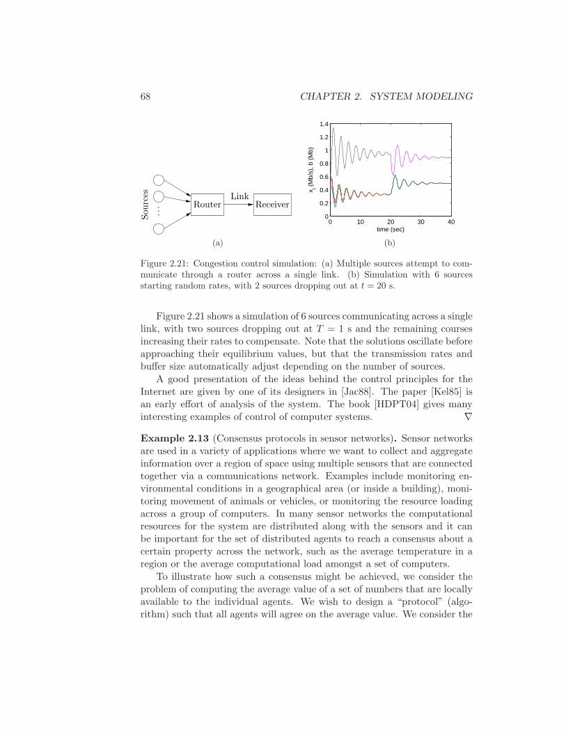
68 CHAPTER 2. SYSTEM MODELING
...Router Receiver
Link
Sou
rces
(a)
0 10 20 30 400
0.2
0.4
0.6
0.8
1
1.2
1.4
time (sec)
x i (M
b/s)
, b (
Mb)
(b)
Figure 2.21: Congestion control simulation: (a) Multiple sources attempt to com-municate through a router across a single link. (b) Simulation with 6 sourcesstarting random rates, with 2 sources dropping out at t = 20 s.
Figure 2.21 shows a simulation of 6 sources communicating across a singlelink, with two sources dropping out at T = 1 s and the remaining coursesincreasing their rates to compensate. Note that the solutions oscillate beforeapproaching their equilibrium values, but that the transmission rates andbuffer size automatically adjust depending on the number of sources.
A good presentation of the ideas behind the control principles for theInternet are given by one of its designers in [Jac88]. The paper [Kel85] isan early effort of analysis of the system. The book [HDPT04] gives manyinteresting examples of control of computer systems. ∇
Example 2.13 (Consensus protocols in sensor networks). Sensor networksare used in a variety of applications where we want to collect and aggregateinformation over a region of space using multiple sensors that are connectedtogether via a communications network. Examples include monitoring en-vironmental conditions in a geographical area (or inside a building), moni-toring movement of animals or vehicles, or monitoring the resource loadingacross a group of computers. In many sensor networks the computationalresources for the system are distributed along with the sensors and it canbe important for the set of distributed agents to reach a consensus about acertain property across the network, such as the average temperature in aregion or the average computational load amongst a set of computers.
To illustrate how such a consensus might be achieved, we consider theproblem of computing the average value of a set of numbers that are locallyavailable to the individual agents. We wish to design a “protocol” (algo-rithm) such that all agents will agree on the average value. We consider the

2.4. EXAMPLES 69
3
4
1
5 2
(a)
0 20 40 600
10
20
30
40
50
Iteration
x i(b)
Figure 2.22: Consensus protocols for sensor networks: (a) a simple sensor networkwith five notes; (b) simulation demonstrating convergence of the network to theaverage value of the initial conditions.
case in which all agents cannot necessarily communicate with each otherdirectly, although we will assume that the communications network is con-nected (meaning that no agents are completely isolated from the group).Figure 2.22a shows a simple situation of this type.
We model the connectivity of the sensor network using a graph, withnodes corresponding to the sensors and edges corresponding to the existenceof a direct communications link between two nodes. For any such graph, wecan build an adjacency matrix, where each row and column of the matrixcorresponds to a node and a 1 in the respective row and column indicatesthat the two nodes are connected. For the network shown in Figure 2.22a,the corresponding adjacency matrix is
A =
0 1 0 0 01 0 1 1 10 1 0 1 00 1 1 0 00 1 0 0 0
.
We also use the notation Ni to represent the set of neighbors of a node i.For example, N2 = 1, 3, 4, 5 and N3 = 2, 4.
To solve the consensus problem, we let xi be the state of the ith sensor,corresponding to that sensor’s estimate of the average value that we aretrying to compute. We initialize the state to the value of the quantitymeasured by the individual sensor. Our consensus protocol can now be
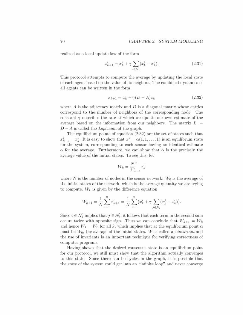
70 CHAPTER 2. SYSTEM MODELING
realized as a local update law of the form
xik+1 = xi
k + γ∑
i∈Ni
(xjk − xi
k). (2.31)
This protocol attempts to compute the average by updating the local stateof each agent based on the value of its neigbors. The combined dynamics ofall agents can be written in the form
xk+1 = xk − γ(D −A)xk (2.32)
where A is the adjacency matrix and D is a diagonal matrix whose entriescorrespond to the number of neighbors of the corresponding node. Theconstant γ describes the rate at which we update our own estimate of theaverage based on the information from our neighbors. The matrix L :=D −A is called the Laplacian of the graph.
The equilibrium points of equation (2.32) are the set of states such thatx∗k+1 = x∗k. It is easy to show that x∗ = α(1, 1, . . . , 1) is an equilibrum statefor the system, corresponding to each sensor having an identical estimateα for the average. Furthermore, we can show that α is the precisely theaverage value of the initial states. To see this, let
Wk =N∑
n
i=1
xik
where N is the number of nodes in the sensor network. W0 is the average ofthe initial states of the network, which is the average quantity we are tryingto compute. Wk is given by the difference equation
Wk+1 =1
N
n∑
i=1
xik+1 =
1
N
n∑
i=1
(xi
k + γ∑
j∈Ni
(xjk − xi
k)).
Since i ∈ Nj implies that j ∈ Ni, it follows that each term in the second sumoccurs twice with opposite sign. Thus we can conclude that Wk+1 = Wk
and hence Wk = W0 for all k, which implies that at the equilibrium point αmust be W0, the average of the initial states. W is called an invariant andthe use of invariants is an important technique for verifying correctness ofcomputer programs.
Having shown that the desired consensus state is an equilibrium pointfor our protocol, we still must show that the algorithm actually convergesto this state. Since there can be cycles in the graph, it is possible thatthe state of the system could get into an “infinite loop” and never converge

2.4. EXAMPLES 71
to the desired consensus state. A formal analysis requires tools that willbe introduced later in the text, but it can be shown that for any givengraph, we can always find a γ such that the states of the individual agentsconverge to the average. A simulation demonstrating this property is shownin Figure 2.22b.
Although we have focused here on consensus to the average value of aset of measurements, other consensus states can be achieved through choiceof appropriate feedback laws. Examples include finding the maximum orminimum value in a network, counting the number of nodes in a network, andcomputing higher order statistical moments of a distributed quantity. ∇
Biological Systems
Biological systems are filled with feedback loops and provide perhaps therichest source of feedback and control examples. The basic problem ofhomeostasis, in which a quantity such as temperature or blood sugar levelis regulated to a fixed value, is but one of the many types of complex feed-back interactions that can occur in molecular machines, cells, organisms andecosystems.
Example 2.14 (Transcriptional regulation). Transcription is the processby which mRNA is generated from a segment of DNA. The promoter regionof a gene allows transcription to be controlled by the presence of otherproteins, which bind to the promoter region and either repress or activateRNA polymerase (RNAP), the enzyme that produces mRNA from DNA.The mRNA is then translated into a protein according to its nucleotidesequence.
A simple model of the transcriptional regulation process is the use ofa Hill function [dJ02, Mur04]. Consider the regulation of a protein A withconcentration given by pA and corresponding mRNA concentration mA. LetB be a second protein with concentration pB that represses the productionof protein A through transcriptional regulation. The resulting dynamics ofpA and mA can be written as
dmA
dt= −τmA +
α
1 + pnB
+ α0
dpA
dt= β(mA − pA),
(2.33)
where α+ α0 is the basal transcription rate, τ represents the rate of degre-dation of mRNDA, α and n are parameters that describe how B represses
72 CHAPTER 2. SYSTEM MODELING
Figure 2.23: The repressilator genetic regulatory network: (a) a schematic diagramof the repressilator, showing the layout of the genes in the plasmid that holds thecircuit as well as the circuit diagram (center); (b) simulation of a simple model ofthe repressilator.
A and β represents both the rate of production of the protein from its cor-responding mRNA and also the rate of degradation of A. The parameterα0 describes the “leakiness” of the promotor and n is called the Hill coef-ficient and relates to the cooperativity of the promotor. For simplicity wewill assume that τ = 1, which corresponds to choosing units of time thatcorrespond to the mRNA decay rate.
A similar model can be used when a protein activates the production ofanother protein, rather than repressing it. In this case, the equations havethe form
dmA
dt= −τmA +
αpnB
1 + pnB
+ α0
dpA
dt= β(mA − pA),
(2.34)
where the variables are the same as described. Note that in the case of theactivator, if pB is zero then the production rate is α0 (versus α + α0 forthe repressor). As pB gets large, the second term in the expression for mA
approaches 1 and the transcription rate becomes α + α0 (versus α0 for therepressor). Thus we see that the activator and repressor act in oppositefashion from each other.
As an example of how these models can be used, we consider the model ofa “repressilator”, originally due to Elowitz and Leibler [EL00]. The repressi-lator is a synthetic circuit in which three proteins each repressor another in acycle. This is shown schematically in Figure 2.23a, where the three proteinsare tetR, λ cI and LacI. The basic idea of the repressilator is that if tetR
2.4. EXAMPLES 73
is present then it represses the production of λ cI. If λ cI is represent, thenLacI is produced (at the basal transcription rate), which in turn repressesTetR. Once TetR is repressed then λ cI is no longer repressed and so on.If the dynamics of the circuit are designed properly, the resulting proteinconcentrations will oscillate.
We can model this system using three copies of equation (2.33), with Aand B replaced by the appropriate combination of TetR, cI and LacI. Thestate of the system is then given by x = (mTetR, pTetR,mcI, pcI,mLacI, pLacI).Figure 2.23b shows the traces of the three protein concentrations for pa-rameters α0 = 0, α = 50, β = 0.2 and n = 2 and initial conditionsx(0) = 0.2, 0.1, 0.1, 0.4, 0.3, 0.5) (from [EG05]). ∇
Example 2.15 (Hodgkin-Huxley equations1). The dynamics of the mem-brane potential in a cell is a fundamental mechanism in discussing signalingin cells. The Hodgkin-Huxley equations provide a simple model for studyingpropagation waves in networks of neurons. The model for a single neuronhas the form
CdV
dt= −INa − IK − Ileak + Iinput
where V is the membrane potential, C the capacitance, INa and IK thecurrent caused by transport of sodium and potassium across the cell mem-brane, Ileak is a leakage current ant Iinput is the external stimulation of thecell. Each current obeys Ohms law, i.e.
I = g(V − E)
where g is the conductance and E the equilibrium voltage. The equilibriumvoltage is given by Nernst’s law
E =RT
xFlog(Cout/Cin)
where R is Boltzmann’s constant, T the absolute temperature, F Faraday’sconstant, Cout and Cin the ion concentrations outside and inside the cell.At 20 we have RT/F = 20 mV.
The Hodgkin-Huxley model was originally developed as a means to pre-dict the quantitative behavior of the squid giant axon [HH52]. Hodgkin andHuxley shared the 1963 Nobel Prize in Physiology (along with J. C. Eccles)for analysis of the electrical and chemical events in nerve cell discharge. ∇
1H. R. Wilson, Spikes, Decisions and Actions—Dynamical Foundations of Neuro-
science. Oxford University Press.
74 CHAPTER 2. SYSTEM MODELING
2.5 Further Reading
Modeling is ubiquitous in engineering and science and has a long historyin applied mathematics. For example, the Fourier series was introduced inconnection with modeling of heat conduction in solids. Models of dynamicshave been developed in many different fields, including mechanics [Gol53],heat conduction [CJ59], fluids![BS60], vehicles [Abk69, Bla91, Ell94], cir-cuit theory [Gui63], acoustics [Ber54] and micromechanical systems [Sen01].Control theory requires modeling from many different domains and mosttexts control theory contain several chapters on modeling using ordinarydifferential equations and difference equations (see, for example, [FPEN05]).
A classic book on modeling of physical systems, especially mechanical,electrical and thermo-fluid systems, is Cannon’s Dynamics of Physical Sys-tems [Can03]. Two of the authors’ favorite books on modeling of biologicalsystems are Mathematical Biology by J. D. Murray [Mur04] and Spikes, De-cision and Actions: The Dynamical Foundations of Neuroscience by H. R.Wilson [Wil99]. For readers interested in learning more about object ori-ented modeling and Modelica, the edited volume by Tiller [Til01] providesan excellent introduction.
2.6 Exercises
1. Use the equations of motion for a balance system to derive a dynamicmodel for the inverted pendulum described in Example 2.2 and verifythat for small θ they are approximated by equation (2.8).
2. (Second order system identification) Verify that equation (2.20) inExample 2.7 is correct and use this formula and the others in theexample to compute the parameters corresponding to the step responsein Figure 2.11.
3. (Least squares system identification) Consider a nonlinear differentialequation that can be written in the form
dx
dt=
M∑
i=1
αifi(x)
where fi(x) are known nonlinear functions and αi are unknown, butconstant, parameters. Suppose that we have measurements (or esti-mates) of the state x at time instants t1, t2, . . . , tN , with N > M .

2.6. EXERCISES 75
Show that the parameters αi can be determined by finding the leastsquares solution to a linear equation of the form
Hα = b
where α ∈ RM is the vector of all parameters and H ∈ R
N×M andb ∈ R
N are appropriately defined.
4. Consider the following discrete time system
zk+1 = Azk +Buk
yk = Czk
where
z =
z1
z2
A =
a11 a12
0 a22
B =
01
C =
1 0
In this problem, we will explore some of the properties of this discretetime system as a function of the parameters, the initial conditions,and the inputs.
(a) Assume that the off diagonal element a12 = 0 and that there isno input, u = 0. Write a closed form expression for the output ofthe system from a nonzero initial condition z0 = (z1
0 , z20) and give
conditions on a11 and a22 under which the output gets smaller ask gets larger.
(b) Now assume that a12 6= 0 and write a closed form expressionfor the response of the system from a nonzero initial conditions.Given a condition on the elements of A under which the outputgets smaller as k gets larger.
(c) Write a MATLAB program to plot the output of the system inresponse to a unit step input, u[k] = 1, k ≥ 0. Plot the responseof your system with z0 = 0 and A given by
A =
0.5 10 0.25
5. Consider the delta-sigma converter in Example 2.10. Propose a wayto obtain an estimate of the instantaneous value of the reference signaland its derivative from the pulsed output.

76 CHAPTER 2. SYSTEM MODELING
6. Consider the linear ordinary differential equation (2.6). Show that bychoosing a state space representation with x1 = y, the dynamics canbe written as
A =
0 1 0
0. . .
. . . 00 · · · 0 1
−an −an−1 −a1
B =
00...1
C =
1 . . . 0 0
This canonical form is called chain of integrators form.
Chapter 3
Examples
... Don’t apply any model until you understand the simplifying assumptionson which it is based, and you can test their validity. Catch phrase: use onlyas directed. Don’t limit yourself to a single model: More than one model maybe useful for understanding different aspects of the same phenomenon. Catchphrase: legalize polygamy.”
Saul Golomb in his 1970 paper “Mathematical Models—Uses and Limita-tions” [Gol70].
In this chapter we present a collection of examples spanning many differ-ent fields of science and engineering. These examples will be used throughoutthe text and in exercises to illustrate different concepts. First time read-ers may wish to focus only on a few examples with which they have themost prior experience or insight to understand the concepts of state, input,output, and dynamics in a familiar setting.
3.1 Cruise Control
The cruise control system of a car is one of the most common control systemsencountered in everyday life. The system attempts to keep the speed of thecar constant in spite of disturbances caused by changes in the slope of a roadand variations in the wind and road surface. The controller compensates forthese unknowns by measuring the speed of the car and adjusting the throttleappropriately.
To model the complete system we start with the block diagram in Fig-ure 3.1. Let v be the speed of the car and vr the desired (reference) speed.The controller, which typically is of the proportional-integral (PI) type de-scribed briefly in Chapter 1, receives the signals v and vr and generates a
77
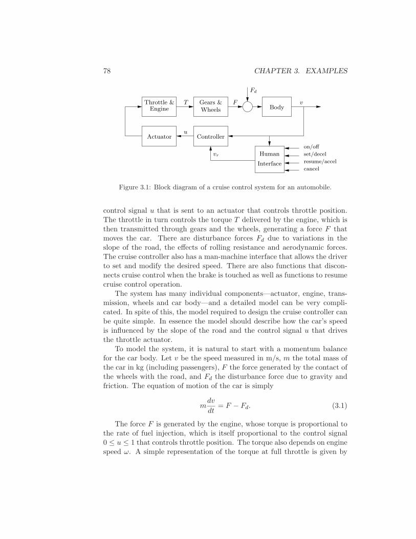
78 CHAPTER 3. EXAMPLES
Gears &
Actuator
vr
Controller
BodyThrottle &
Engine
Fd
v
cancel
resume/accel
set/decel
on/off
Human
Interface
T F
u
Wheels
Figure 3.1: Block diagram of a cruise control system for an automobile.
control signal u that is sent to an actuator that controls throttle position.The throttle in turn controls the torque T delivered by the engine, which isthen transmitted through gears and the wheels, generating a force F thatmoves the car. There are disturbance forces Fd due to variations in theslope of the road, the effects of rolling resistance and aerodynamic forces.The cruise controller also has a man-machine interface that allows the driverto set and modify the desired speed. There are also functions that discon-nects cruise control when the brake is touched as well as functions to resumecruise control operation.
The system has many individual components—actuator, engine, trans-mission, wheels and car body—and a detailed model can be very compli-cated. In spite of this, the model required to design the cruise controller canbe quite simple. In essence the model should describe how the car’s speedis influenced by the slope of the road and the control signal u that drivesthe throttle actuator.
To model the system, it is natural to start with a momentum balancefor the car body. Let v be the speed measured in m/s, m the total mass ofthe car in kg (including passengers), F the force generated by the contact ofthe wheels with the road, and Fd the disturbance force due to gravity andfriction. The equation of motion of the car is simply
mdv
dt= F − Fd. (3.1)
The force F is generated by the engine, whose torque is proportional tothe rate of fuel injection, which is itself proportional to the control signal0 ≤ u ≤ 1 that controls throttle position. The torque also depends on enginespeed ω. A simple representation of the torque at full throttle is given by
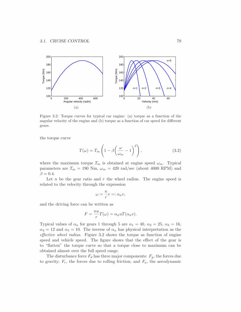
3.1. CRUISE CONTROL 79
0 200 400 600100
120
140
160
180
200
Angular velocity (rad/s)
Tor
que
(Nm
)
(a)
0 20 40 60100
120
140
160
180
200
n=1 n=2 n=3 n=4
n=5
Velocity (m/s)
Tor
que
(Nm
)
(b)
Figure 3.2: Torque curves for typical car engine: (a) torque as a function of theangular velocity of the engine and (b) torque as a function of car speed for differentgears.
the torque curve
T (ω) = Tm
(
1 − β
(ω
ωm− 1
)2)
, (3.2)
where the maximum torque Tm is obtained at engine speed ωm. Typicalparameters are Tm = 190 Nm, ωm = 420 rad/sec (about 4000 RPM) andβ = 0.4.
Let n be the gear ratio and r the wheel radius. The engine speed isrelated to the velocity through the expression
ω =n
rv =: αnv,
and the driving force can be written as
F =nu
rT (ω) = αnuT (αnv).
Typical values of αn for gears 1 through 5 are α1 = 40, α2 = 25, α3 = 16,α4 = 12 and α5 = 10. The inverse of αn has physical interpretation as theeffective wheel radius. Figure 3.2 shows the torque as function of enginespeed and vehicle speed. The figure shows that the effect of the gear isto “flatten” the torque curve so that a torque close to maximum can beobtained almost over the full speed range.
The disturbance force Fd has three major components: Fg, the forces dueto gravity; Fr, the forces due to rolling friction; and Fa, the aerodynamic
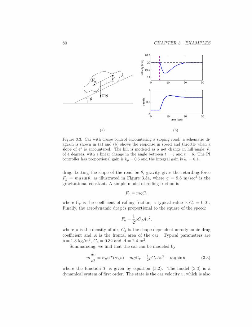
80 CHAPTER 3. EXAMPLES
Fg
mg
F
θ
0 10 20 30
19
19.5
20
20.5
velo
city
(m
/s)
0 10 20 300
0.5
1
time (sec)
thro
ttle
(a) (b)
Figure 3.3: Car with cruise control encountering a sloping road: a schematic di-agram is shown in (a) and (b) shows the response in speed and throttle when aslope of 4 is encountered. The hill is modeled as a net change in hill angle, θ,of 4 degrees, with a linear change in the angle between t = 5 and t = 6. The PIcontroller has proportional gain is kp = 0.5 and the integral gain is ki = 0.1.
drag, Letting the slope of the road be θ, gravity gives the retarding forceFg = mg sin θ, as illustrated in Figure 3.3a, where g = 9.8 m/sec2 is thegravitational constant. A simple model of rolling friction is
Fr = mgCr
where Cr is the coefficient of rolling friction; a typical value is Cr = 0.01.Finally, the aerodynamic drag is proportional to the square of the speed:
Fa =1
2ρCdAv
2,
where ρ is the density of air, Cd is the shape-dependent aerodynamic dragcoefficient and A is the frontal area of the car. Typical parameters areρ = 1.3 kg/m3, Cd = 0.32 and A = 2.4 m2.
Summarizing, we find that the car can be modeled by
mdv
dt= αnuT (αnv) −mgCr − 1
2ρCvAv2 −mg sin θ, (3.3)
where the function T is given by equation (3.2). The model (3.3) is adynamical system of first order. The state is the car velocity v, which is also
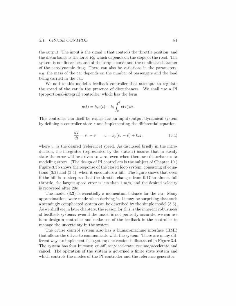
3.1. CRUISE CONTROL 81
the output. The input is the signal u that controls the throttle position, andthe disturbance is the force Fd, which depends on the slope of the road. Thesystem is nonlinear because of the torque curve and the nonlinear characterof the aerodynamic drag. There can also be variations in the parameters,e.g. the mass of the car depends on the number of passengers and the loadbeing carried in the car.
We add to this model a feedback controller that attempts to regulatethe speed of the car in the presence of disturbances. We shall use a PI(proportional-integral) controller, which has the form
u(t) = kpe(t) + ki
∫ t
0e(τ) dτ.
This controller can itself be realized as an input/output dynamical systemby defining a controller state z and implementing the differential equation
dz
dt= vr − v u = kp(vr − v) + kiz, (3.4)
where vr is the desired (reference) speed. As discussed briefly in the intro-duction, the integrator (represented by the state z) insures that in steadystate the error will be driven to zero, even when there are disturbances ormodeling errors. (The design of PI controllers is the subject of Chapter 10.)Figure 3.3b shows the response of the closed loop system, consisting of equa-tions (3.3) and (3.4), when it encounters a hill. The figure shows that evenif the hill is so steep so that the throttle changes from 0.17 to almost fullthrottle, the largest speed error is less than 1 m/s, and the desired velocityis recovered after 20s.
The model (3.3) is essentially a momentum balance for the car. Manyapproximations were made when deriving it. It may be surprising that sucha seemingly complicated system can be described by the simple model (3.3).As we shall see in later chapters, the reason for this is the inherent robustnessof feedback systems: even if the model is not perfectly accurate, we can useit to design a controller and make use of the feedback in the controller tomanage the uncertainty in the system.
The cruise control system also has a human-machine interface (HMI)that allows the driver to communicate with the system. There are many dif-ferent ways to implement this system; one version is illustrated in Figure 3.4.The system has four buttons: on-off, set/decelerate, resume/accelerate andcancel. The operation of the system is governed a finite state system andwhich controls the modes of the PI controller and the reference generator.
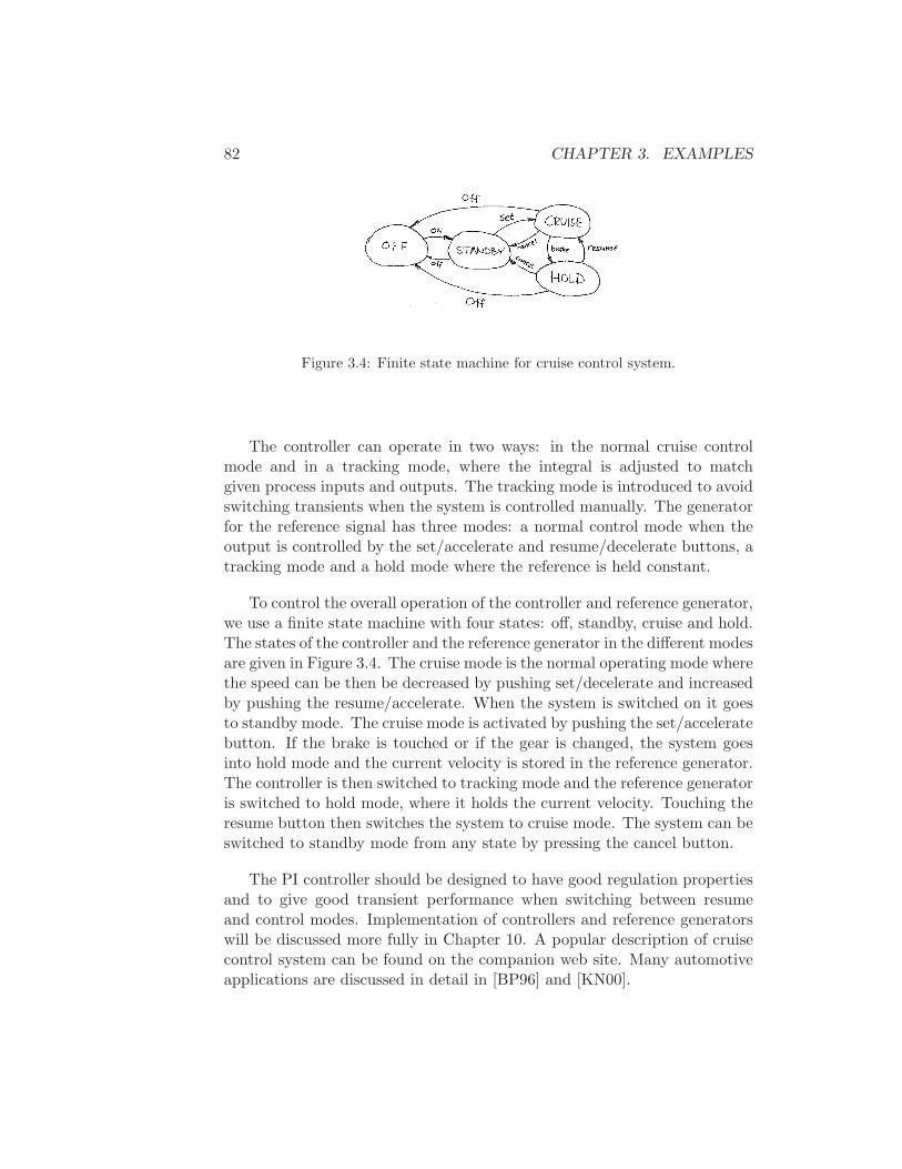
82 CHAPTER 3. EXAMPLES
Figure 3.4: Finite state machine for cruise control system.
The controller can operate in two ways: in the normal cruise controlmode and in a tracking mode, where the integral is adjusted to matchgiven process inputs and outputs. The tracking mode is introduced to avoidswitching transients when the system is controlled manually. The generatorfor the reference signal has three modes: a normal control mode when theoutput is controlled by the set/accelerate and resume/decelerate buttons, atracking mode and a hold mode where the reference is held constant.
To control the overall operation of the controller and reference generator,we use a finite state machine with four states: off, standby, cruise and hold.The states of the controller and the reference generator in the different modesare given in Figure 3.4. The cruise mode is the normal operating mode wherethe speed can be then be decreased by pushing set/decelerate and increasedby pushing the resume/accelerate. When the system is switched on it goesto standby mode. The cruise mode is activated by pushing the set/acceleratebutton. If the brake is touched or if the gear is changed, the system goesinto hold mode and the current velocity is stored in the reference generator.The controller is then switched to tracking mode and the reference generatoris switched to hold mode, where it holds the current velocity. Touching theresume button then switches the system to cruise mode. The system can beswitched to standby mode from any state by pressing the cancel button.
The PI controller should be designed to have good regulation propertiesand to give good transient performance when switching between resumeand control modes. Implementation of controllers and reference generatorswill be discussed more fully in Chapter 10. A popular description of cruisecontrol system can be found on the companion web site. Many automotiveapplications are discussed in detail in [BP96] and [KN00].
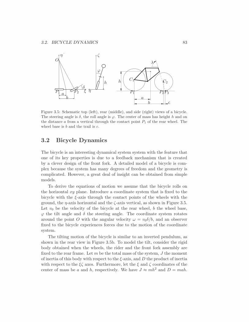
3.2. BICYCLE DYNAMICS 83
ξ
η
η
ζ
ab
hδ
ϕ
P1 P2
O
ab
h
c
C1 C2
P1 P2P3
λ
Figure 3.5: Schematic top (left), rear (middle), and side (right) views of a bicycle.The steering angle is δ, the roll angle is ϕ. The center of mass has height h and onthe distance a from a vertical through the contact point P1 of the rear wheel. Thewheel base is b and the trail is c.
3.2 Bicycle Dynamics
The bicycle is an interesting dynamical system system with the feature thatone of its key properties is due to a feedback mechanism that is createdby a clever design of the front fork. A detailed model of a bicycle is com-plex because the system has many degrees of freedom and the geometry iscomplicated. However, a great deal of insight can be obtained from simplemodels.
To derive the equations of motion we assume that the bicycle rolls onthe horizontal xy plane. Introduce a coordinate system that is fixed to thebicycle with the ξ-axis through the contact points of the wheels with theground, the η-axis horizontal and the ζ-axis vertical, as shown in Figure 3.5.Let v0 be the velocity of the bicycle at the rear wheel, b the wheel base,ϕ the tilt angle and δ the steering angle. The coordinate system rotatesaround the point O with the angular velocity ω = v0δ/b, and an observerfixed to the bicycle experiences forces due to the motion of the coordinatesystem.
The tilting motion of the bicycle is similar to an inverted pendulum, asshown in the rear view in Figure 3.5b. To model the tilt, consider the rigidbody obtained when the wheels, the rider and the front fork assembly arefixed to the rear frame. Letm be the total mass of the system, J the momentof inertia of this body with respect to the ξ-axis, andD the product of inertiawith respect to the ξζ axes. Furthermore, let the ξ and ζ coordinates of thecenter of mass be a and h, respectively. We have J ≈ mh2 and D = mah.
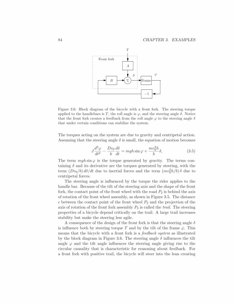
84 CHAPTER 3. EXAMPLES
ϕδ
A
T
Front fork
FrameB
−1
Σ
Figure 3.6: Block diagram of the bicycle with a front fork. The steering torqueapplied to the handlebars is T , the roll angle is ϕ, and the steering angle δ. Noticethat the front fork creates a feedback from the roll angle ϕ to the steering angle δthat under certain conditions can stabilize the system.
The torques acting on the system are due to gravity and centripetal action.Assuming that the steering angle δ is small, the equation of motion becomes
Jd2ϕ
dt2− Dv0
b
dδ
dt= mgh sinϕ+
mv20h
bδ, (3.5)
The term mgh sinϕ is the torque generated by gravity. The terms con-taining δ and its derivative are the torques generated by steering, with theterm (Dv0/b) dδ/dt due to inertial forces and the term (mv2
0h/b) δ due tocentripetal forces.
The steering angle is influenced by the torque the rider applies to thehandle bar. Because of the tilt of the steering axis and the shape of the frontfork, the contact point of the front wheel with the road P2 is behind the axisof rotation of the front wheel assembly, as shown in Figure 3.5. The distancec between the contact point of the front wheel P2 and the projection of theaxis of rotation of the front fork assembly P3 is called the trail. The steeringproperties of a bicycle depend critically on the trail. A large trail increasesstability but make the steering less agile.
A consequence of the design of the front fork is that the steering angle δis influence both by steering torque T and by the tilt of the frame ϕ. Thismeans that the bicycle with a front fork is a feedback system as illustratedby the block diagram in Figure 3.6. The steering angle δ influences the tiltangle ϕ and the tilt angle influences the steering angle giving rise to thecircular causality that is characteristic for reasoning about feedback. Fora front fork with positive trail, the bicycle will steer into the lean creating
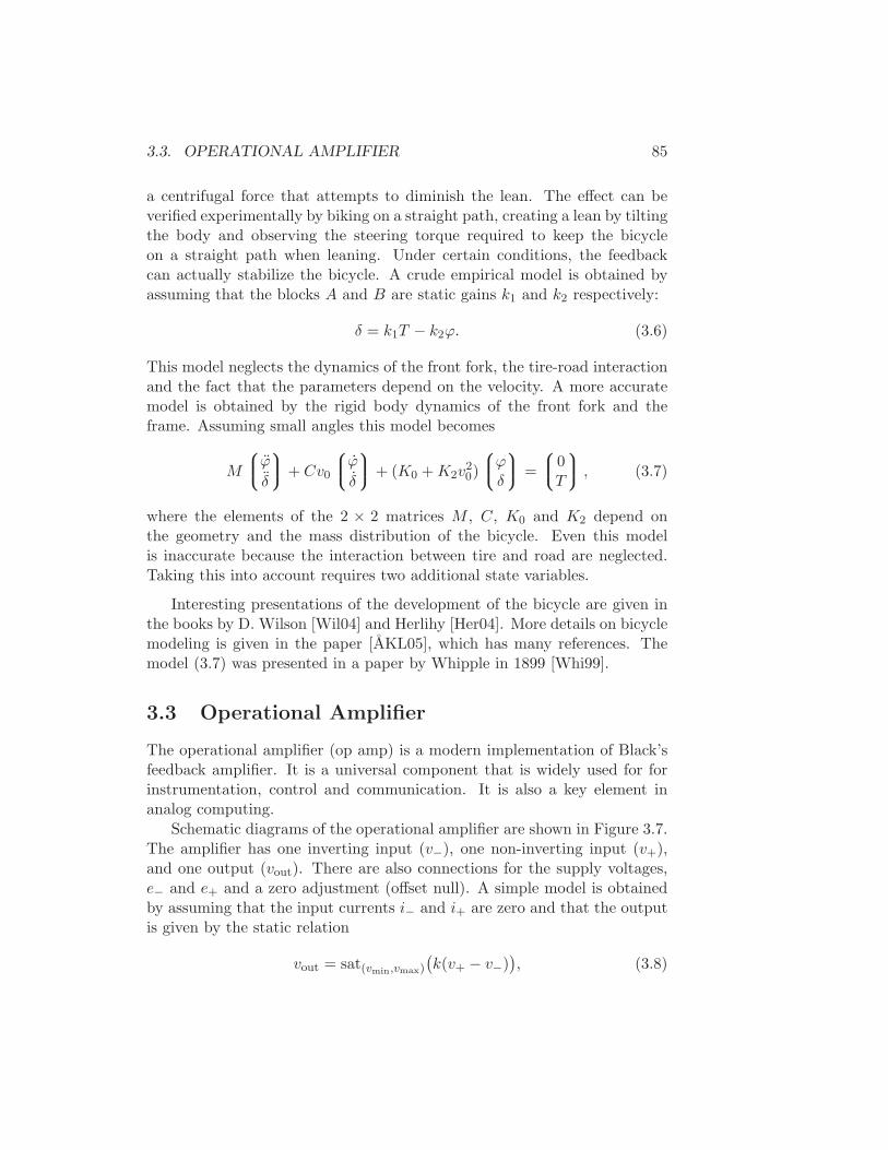
3.3. OPERATIONAL AMPLIFIER 85
a centrifugal force that attempts to diminish the lean. The effect can beverified experimentally by biking on a straight path, creating a lean by tiltingthe body and observing the steering torque required to keep the bicycleon a straight path when leaning. Under certain conditions, the feedbackcan actually stabilize the bicycle. A crude empirical model is obtained byassuming that the blocks A and B are static gains k1 and k2 respectively:
δ = k1T − k2ϕ. (3.6)
This model neglects the dynamics of the front fork, the tire-road interactionand the fact that the parameters depend on the velocity. A more accuratemodel is obtained by the rigid body dynamics of the front fork and theframe. Assuming small angles this model becomes
M
ϕ
δ
+ Cv0
ϕ
δ
+ (K0 +K2v20)
ϕδ
=
0T
, (3.7)
where the elements of the 2 × 2 matrices M , C, K0 and K2 depend onthe geometry and the mass distribution of the bicycle. Even this modelis inaccurate because the interaction between tire and road are neglected.Taking this into account requires two additional state variables.
Interesting presentations of the development of the bicycle are given inthe books by D. Wilson [Wil04] and Herlihy [Her04]. More details on bicyclemodeling is given in the paper [AKL05], which has many references. Themodel (3.7) was presented in a paper by Whipple in 1899 [Whi99].
3.3 Operational Amplifier
The operational amplifier (op amp) is a modern implementation of Black’sfeedback amplifier. It is a universal component that is widely used for forinstrumentation, control and communication. It is also a key element inanalog computing.
Schematic diagrams of the operational amplifier are shown in Figure 3.7.The amplifier has one inverting input (v−), one non-inverting input (v+),and one output (vout). There are also connections for the supply voltages,e− and e+ and a zero adjustment (offset null). A simple model is obtainedby assuming that the input currents i− and i+ are zero and that the outputis given by the static relation
vout = sat(vmin,vmax)
(k(v+ − v−)
), (3.8)
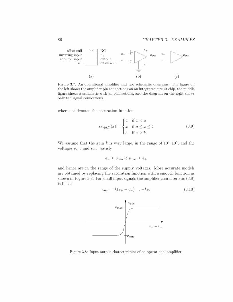
86 CHAPTER 3. EXAMPLES
(b)
v−
v+
e−
e+i+
i−
vout
NCv+
outputoffset null
offset nullinverting inputnon-inv. input
v−v+
v− vout
(c)(a)
Figure 3.7: An operational amplifier and two schematic diagrams. The figure onthe left shows the amplifier pin connections on an integrated circuit chip, the middlefigure shows a schematic with all connections, and the diagram on the right showsonly the signal connections.
where sat denotes the saturation function
sat(a,b)(x) =
a if x < a
x if a ≤ x ≤ b
b if x > b.
(3.9)
We assume that the gain k is very large, in the range of 106–108, and thevoltages vmin and vmax satisfy
e− ≤ vmin < vmax ≤ e+
and hence are in the range of the supply voltages. More accurate modelsare obtained by replacing the saturation function with a smooth function asshown in Figure 3.8. For small input signals the amplifier characteristic (3.8)is linear
vout = k(v+ − v−) =: −kv. (3.10)
vmin
vout
v+ − v−
vmax
Figure 3.8: Input-output characteristics of an operational amplifier.
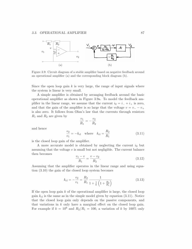
3.3. OPERATIONAL AMPLIFIER 87
v −+
v1
v2
R1 R2
i0
(a) (b)
Figure 3.9: Circuit diagram of a stable amplifier based on negative feedback aroundan operational amplifier (a) and the corresponding block diagram (b).
Since the open loop gain k is very large, the range of input signals wherethe system is linear is very small.
A simple amplifier is obtained by arranging feedback around the basicoperational amplifier as shown in Figure 3.9a. To model the feedback am-plifier in the linear range, we assume that the current i0 = i− + i+ is zero,and that the gain of the amplifier is so large that the voltage v = v− − v+is also zero. It follows from Ohm’s law that the currents through resistorsR1 and R2 are given by
v1R1
= − v2R2
and hencev2v1
= −kcl where kcl =R2
R1(3.11)
is the closed loop gain of the amplifier.A more accurate model is obtained by neglecting the current i0 but
assuming that the voltage v is small but not negligible. The current balancethen becomes
v1 − v
R1=v − v2R2
. (3.12)
Assuming that the amplifier operates in the linear range and using equa-tion (3.10) the gain of the closed loop system becomes
kcl = −v2v1
=R2
R1
1
1 + 1k
(
1 + R2
R1
) (3.13)
If the open loop gain k of the operational amplifier is large, the closed loopgain kcl is the same as in the simple model given by equation (3.11). Noticethat the closed loop gain only depends on the passive components, andthat variations in k only have a marginal effect on the closed loop gain.For example if k = 106 and R2/R1 = 100, a variation of k by 100% only
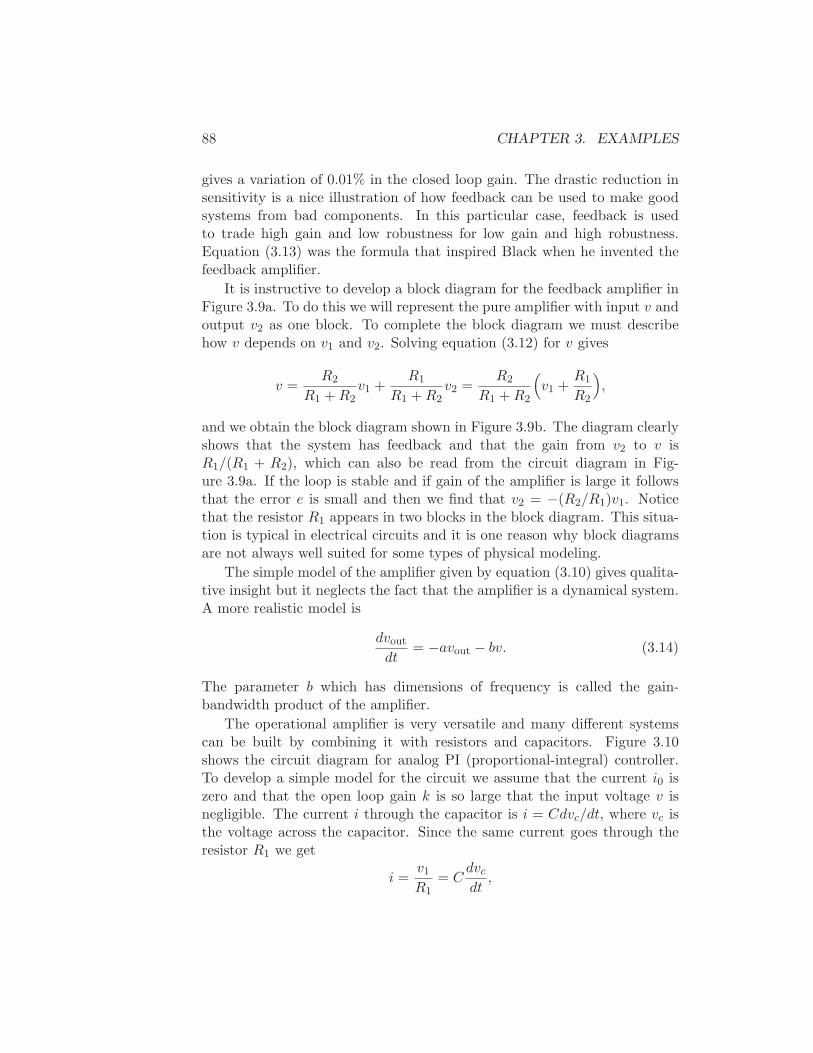
88 CHAPTER 3. EXAMPLES
gives a variation of 0.01% in the closed loop gain. The drastic reduction insensitivity is a nice illustration of how feedback can be used to make goodsystems from bad components. In this particular case, feedback is usedto trade high gain and low robustness for low gain and high robustness.Equation (3.13) was the formula that inspired Black when he invented thefeedback amplifier.
It is instructive to develop a block diagram for the feedback amplifier inFigure 3.9a. To do this we will represent the pure amplifier with input v andoutput v2 as one block. To complete the block diagram we must describehow v depends on v1 and v2. Solving equation (3.12) for v gives
v =R2
R1 +R2v1 +
R1
R1 +R2v2 =
R2
R1 +R2
(
v1 +R1
R2
)
,
and we obtain the block diagram shown in Figure 3.9b. The diagram clearlyshows that the system has feedback and that the gain from v2 to v isR1/(R1 + R2), which can also be read from the circuit diagram in Fig-ure 3.9a. If the loop is stable and if gain of the amplifier is large it followsthat the error e is small and then we find that v2 = −(R2/R1)v1. Noticethat the resistor R1 appears in two blocks in the block diagram. This situa-tion is typical in electrical circuits and it is one reason why block diagramsare not always well suited for some types of physical modeling.
The simple model of the amplifier given by equation (3.10) gives qualita-tive insight but it neglects the fact that the amplifier is a dynamical system.A more realistic model is
dvout
dt= −avout − bv. (3.14)
The parameter b which has dimensions of frequency is called the gain-bandwidth product of the amplifier.
The operational amplifier is very versatile and many different systemscan be built by combining it with resistors and capacitors. Figure 3.10shows the circuit diagram for analog PI (proportional-integral) controller.To develop a simple model for the circuit we assume that the current i0 iszero and that the open loop gain k is so large that the input voltage v isnegligible. The current i through the capacitor is i = Cdvc/dt, where vc isthe voltage across the capacitor. Since the same current goes through theresistor R1 we get
i =v1R1
= Cdvc
dt,
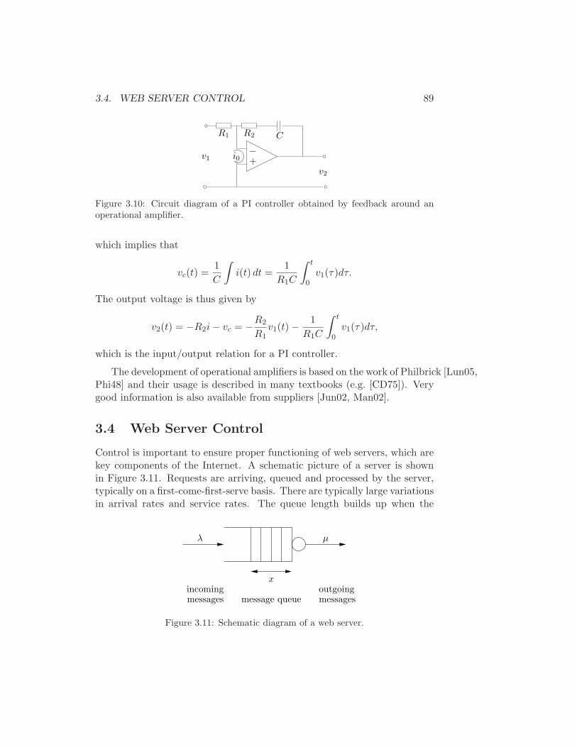
3.4. WEB SERVER CONTROL 89
i0−+
v1
R1 R2
v2
C
Figure 3.10: Circuit diagram of a PI controller obtained by feedback around anoperational amplifier.
which implies that
vc(t) =1
C
∫
i(t) dt =1
R1C
∫ t
0v1(τ)dτ.
The output voltage is thus given by
v2(t) = −R2i− vc = −R2
R1v1(t) −
1
R1C
∫ t
0v1(τ)dτ,
which is the input/output relation for a PI controller.
The development of operational amplifiers is based on the work of Philbrick [Lun05,Phi48] and their usage is described in many textbooks (e.g. [CD75]). Verygood information is also available from suppliers [Jun02, Man02].
3.4 Web Server Control
Control is important to ensure proper functioning of web servers, which arekey components of the Internet. A schematic picture of a server is shownin Figure 3.11. Requests are arriving, queued and processed by the server,typically on a first-come-first-serve basis. There are typically large variationsin arrival rates and service rates. The queue length builds up when the
messages
x
µλ
message queuemessagesincoming outgoing
Figure 3.11: Schematic diagram of a web server.
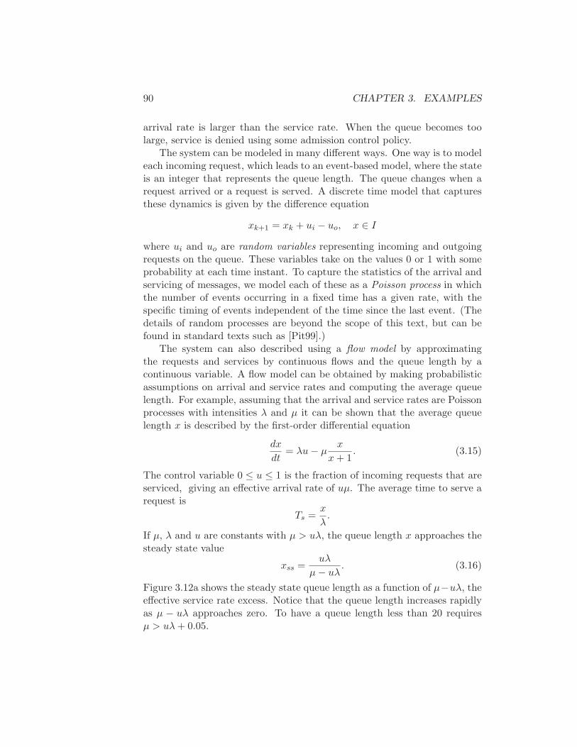
90 CHAPTER 3. EXAMPLES
arrival rate is larger than the service rate. When the queue becomes toolarge, service is denied using some admission control policy.
The system can be modeled in many different ways. One way is to modeleach incoming request, which leads to an event-based model, where the stateis an integer that represents the queue length. The queue changes when arequest arrived or a request is served. A discrete time model that capturesthese dynamics is given by the difference equation
xk+1 = xk + ui − uo, x ∈ I
where ui and uo are random variables representing incoming and outgoingrequests on the queue. These variables take on the values 0 or 1 with someprobability at each time instant. To capture the statistics of the arrival andservicing of messages, we model each of these as a Poisson process in whichthe number of events occurring in a fixed time has a given rate, with thespecific timing of events independent of the time since the last event. (Thedetails of random processes are beyond the scope of this text, but can befound in standard texts such as [Pit99].)
The system can also described using a flow model by approximatingthe requests and services by continuous flows and the queue length by acontinuous variable. A flow model can be obtained by making probabilisticassumptions on arrival and service rates and computing the average queuelength. For example, assuming that the arrival and service rates are Poissonprocesses with intensities λ and µ it can be shown that the average queuelength x is described by the first-order differential equation
dx
dt= λu− µ
x
x+ 1. (3.15)
The control variable 0 ≤ u ≤ 1 is the fraction of incoming requests that areserviced, giving an effective arrival rate of uµ. The average time to serve arequest is
Ts =x
λ.
If µ, λ and u are constants with µ > uλ, the queue length x approaches thesteady state value
xss =uλ
µ− uλ. (3.16)
Figure 3.12a shows the steady state queue length as a function of µ−uλ, theeffective service rate excess. Notice that the queue length increases rapidlyas µ − uλ approaches zero. To have a queue length less than 20 requiresµ > uλ+ 0.05.
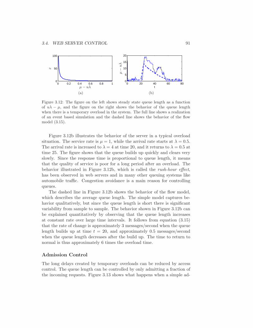
3.4. WEB SERVER CONTROL 91
0 0.2 0.4 0.6 0.8 10
50
100
µ − uλ
x
(a)
0 20 40 60 800
5
10
15
20
t
µ−
uλ
(b)
Figure 3.12: The figure on the left shows steady state queue length as a functionof uλ − µ, and the figure on the right shows the behavior of the queue lengthwhen there is a temporary overload in the system. The full line shows a realizationof an event based simulation and the dashed line shows the behavior of the flowmodel (3.15).
Figure 3.12b illustrates the behavior of the server in a typical overloadsituation. The service rate is µ = 1, while the arrival rate starts at λ = 0.5.The arrival rate is increased to λ = 4 at time 20, and it returns to λ = 0.5 attime 25. The figure shows that the queue builds up quickly and clears veryslowly. Since the response time is proportional to queue length, it meansthat the quality of service is poor for a long period after an overload. Thebehavior illustrated in Figure 3.12b, which is called the rush-hour effect,has been observed in web servers and in many other queuing systems likeautomobile traffic. Congestion avoidance is a main reason for controllingqueues.
The dashed line in Figure 3.12b shows the behavior of the flow model,which describes the average queue length. The simple model captures be-havior qualitatively, but since the queue length is short there is significantvariability from sample to sample. The behavior shown in Figure 3.12b canbe explained quantitatively by observing that the queue length increasesat constant rate over large time intervals. It follows from equation (3.15)that the rate of change is approximately 3 messages/second when the queuelength builds up at time t = 20, and approximately 0.5 messages/secondwhen the queue length decreases after the build up. The time to return tonormal is thus approximately 6 times the overload time.
Admission Control
The long delays created by temporary overloads can be reduced by accesscontrol. The queue length can be controlled by only admitting a fraction ofthe incoming requests. Figure 3.13 shows what happens when a simple ad-

92 CHAPTER 3. EXAMPLES
0 20 40 60 800
0.5
1
1.5
2
0 20 40 60 800
0.5
1
xu
t
(a) r = 2
0 20 40 60 800
2
4
6
0 20 40 60 800
0.5
1
xu
t
(b) r = 5
Figure 3.13: Behavior of queue length for a server with admission control whenthere is a temporary overload in the system. The figure on the left has r = 2 andthe right figure has r = 5, with k = 1 in both cases. Compare with a simulation ofthe uncontrolled system in Figure 3.12b.
mission control strategy is introduced. The feedback used in the simulationis a simple proportional control with saturation described by
u = sat(0,1)(k(r − x)), (3.17)
where sat(a,b) is defined in equation (3.9) and r is the desired (reference)queue length. The feedback gain is k = 1, and the saturation ensures thatthe control variable is in the interval 0 ≤ u ≤ 1. Comparing Figures 3.12band 3.13, we see that simple access control works very well in comparisonwith the uncontrolled server. The control law ensures that the access isrestricted when overload occurs.
The maximum queue length is determined by the reference value r. Alow value of r gives a short queue length and the service delay is short,as is clearly seen in Figure 3.13a. A number of customers are, however,denied service. The simulation also indicates that the control problem isnot too difficult and that a simple control strategy works quite well. Itallows all requests arrived to be serviced if the arrival rate is slow and itrestricts admission when the system is overloaded. Admission control isactivated when the queue length approaches the value r. Since service timeis proportional to queue length, r is a measure of service time.
Notice that the web server control problem we have discussed is not aconventional regulation problem where we wish to keep a constant queue
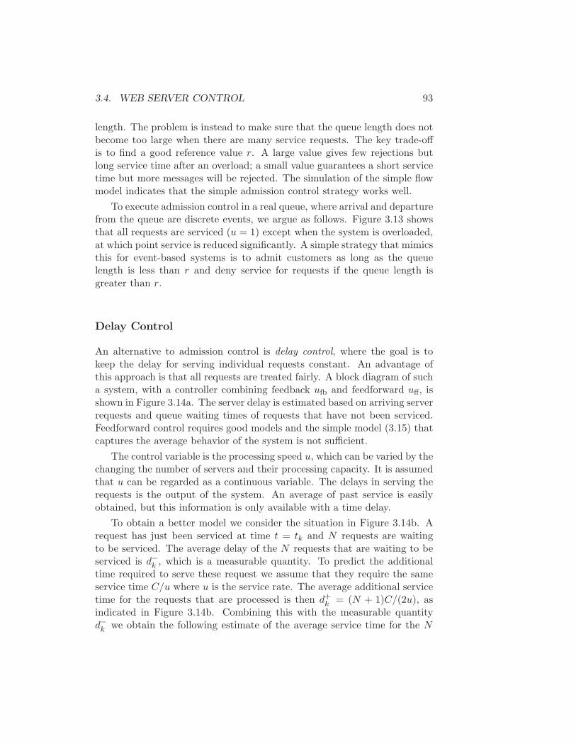
3.4. WEB SERVER CONTROL 93
length. The problem is instead to make sure that the queue length does notbecome too large when there are many service requests. The key trade-offis to find a good reference value r. A large value gives few rejections butlong service time after an overload; a small value guarantees a short servicetime but more messages will be rejected. The simulation of the simple flowmodel indicates that the simple admission control strategy works well.
To execute admission control in a real queue, where arrival and departurefrom the queue are discrete events, we argue as follows. Figure 3.13 showsthat all requests are serviced (u = 1) except when the system is overloaded,at which point service is reduced significantly. A simple strategy that mimicsthis for event-based systems is to admit customers as long as the queuelength is less than r and deny service for requests if the queue length isgreater than r.
Delay Control
An alternative to admission control is delay control, where the goal is tokeep the delay for serving individual requests constant. An advantage ofthis approach is that all requests are treated fairly. A block diagram of sucha system, with a controller combining feedback ufb and feedforward uff, isshown in Figure 3.14a. The server delay is estimated based on arriving serverrequests and queue waiting times of requests that have not been serviced.Feedforward control requires good models and the simple model (3.15) thatcaptures the average behavior of the system is not sufficient.
The control variable is the processing speed u, which can be varied by thechanging the number of servers and their processing capacity. It is assumedthat u can be regarded as a continuous variable. The delays in serving therequests is the output of the system. An average of past service is easilyobtained, but this information is only available with a time delay.
To obtain a better model we consider the situation in Figure 3.14b. Arequest has just been serviced at time t = tk and N requests are waitingto be serviced. The average delay of the N requests that are waiting to beserviced is d−k , which is a measurable quantity. To predict the additionaltime required to serve these request we assume that they require the sameservice time C/u where u is the service rate. The average additional servicetime for the requests that are processed is then d+
k = (N + 1)C/(2u), asindicated in Figure 3.14b. Combining this with the measurable quantityd−k we obtain the following estimate of the average service time for the N
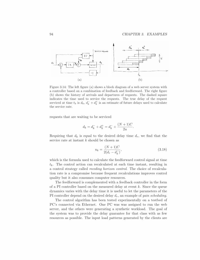
94 CHAPTER 3. EXAMPLES
(a) (b)
Figure 3.14: The left figure (a) shows a block diagram of a web server system witha controller based on a combination of feedback and feedforward. The right figure(b) shows the history of arrivals and departures of requests. The dashed squareindicates the time used to service the requests. The true delay of the requestserviced at time tk is dk, d−k + d+
k is an estimate of future delays used to calculatethe service rate.
requests that are waiting to be serviced
dk = d−k + d+k = d−k +
(N + 1)C
2u.
Requiring that dk is equal to the desired delay time dr, we find that theservice rate at instant k should be chosen as
uk =(N + 1)C
2(dr − d−k ), (3.18)
which is the formula used to calculate the feedforward control signal at timetk. The control action can recalculated at each time instant, resulting ina control strategy called receding horizon control. The choice of recalcula-tion rate is a compromise because frequent recalculations improves controlquality but it also consumes computer resources.
The feedforward is complemented with a feedback controller in the formof a PI controller based on the measured delay at event k. Since the queuedynamics varies with the delay time it is useful to let the parameters of thePI controller depend on the desired delay dr, an example of gain scheduling.
The control algorithm has been tested experimentally on a testbed ofPC’s connected via Ethernet. One PC was was assigned to run the webserver, and the others were generating a synthetic workload. The goal ofthe system was to provide the delay guarantee for that class with as fewresources as possible. The input load patterns generated by the clients are

3.5. ATOMIC FORCE MICROSCOPE 95
Figure 3.15: Arrival rate (top) and average service delay (bottom) for an experimentwith web server control (from [HLA04]).
shown in Figure 3.15. The desired delay for the class was set to dr = 4s in allexperiments. The figure shows that the control algorithm keeps the servicetime reasonably constant and that the PI controller reduces the variationsin delay compared with a pure feedforward controller.
This example illustrates that simple models can give good insight andthat nonlinear control strategies are useful. The example also illustratesthat continuous time models can be useful for phenomena that are basicallydiscrete. There are also converse examples. Therefore it is a good idea tokeep an open mind and master both discrete and continuous time modeling.
The book by Hellerstein et al. [HDPT04] gives many examples of use offeedback in computer systems. The example on delay control is based onthe work of Henriksson [HLA04, Hen06].
3.5 Atomic Force Microscope
The 1986 Nobel Prize in Physics was shared by Gerd Binnig and HeinrichRohrer for their design of the scanning tunneling microscope (SCM). Theidea of an SCM is to bring an atomically sharp tip so close to a conductingsurface that tunneling occurs. An image is obtained by traversing the tipand measuring the tunneling current as a function of tip position. Theimage reflects the electron structure of the upper atom-layers of the sample.

96 CHAPTER 3. EXAMPLES
(a) (b)
Figure 3.16: Schematic diagram of an atomic force microscope and a sample AFMimage of DNA.
This invention has stimulated development of a family of instruments thatpermit visualization of surface structure at the nanometer scale, includingthe atomic force microscope (AFM). These instruments are now standardtools for exploring nanoscale structures.
In the atomic force microscope, a sample is probed by a tip on a cantileverwhich is controlled to exert a constant force on the sample. The controlsystem is essential because it has a direct influence on picture quality andscanning rate. Since the dynamic behavior of the system changes with theproperties of the sample, it is necessary to tune the feedback loop, which iscurrently done manually by adjusting parameters of a PI controller. Thereare interesting possibilities to make the systems easier to use by introducingautomatic tuning and adaptation.
A schematic picture of an atomic force microscope is shown in Fig-ure 3.16a. A micro-cantilever with a tip having a radius of the order of10 nm is placed close to the sample. The tip can be moved vertically andhorizontally using a piezoelectric scanner. Atomic forces bend the cantileverand the cantilever tilt is measured by sensing the deflection of the beam us-ing a photo diode. The signal from the photo diode is amplified and sentto a controller that drives the amplifier for the vertical deflection of thecantilever. By controlling the piezo scanner so that the deflection of thecantilever is constant, the signal driving the vertical deflection of the scan-ner is a measure of the atomic forces between the cantilever tip and theatoms of the sample. An image of the surface is obtained by scanning thecantilever along the sample. The resolution makes it possible to see thestructure of the sample on the atomic scale, as illustrated in Figure 3.16b,
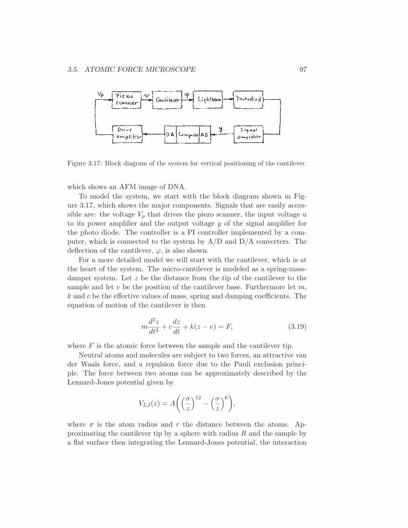
3.5. ATOMIC FORCE MICROSCOPE 97
Figure 3.17: Block diagram of the system for vertical positioning of the cantilever.
which shows an AFM image of DNA.
To model the system, we start with the block diagram shown in Fig-ure 3.17, which shows the major components. Signals that are easily acces-sible are: the voltage Vp that drives the piezo scanner, the input voltage uto its power amplifier and the output voltage y of the signal amplifier forthe photo diode. The controller is a PI controller implemented by a com-puter, which is connected to the system by A/D and D/A converters. Thedeflection of the cantilever, ϕ, is also shown.
For a more detailed model we will start with the cantilever, which is atthe heart of the system. The micro-cantilever is modeled as a spring-mass-damper system. Let z be the distance from the tip of the cantilever to thesample and let v be the position of the cantilever base. Furthermore let m,k and c be the effective values of mass, spring and damping coefficients. Theequation of motion of the cantilever is then
md2z
dt2+ c
dz
dt+ k(z − v) = F, (3.19)
where F is the atomic force between the sample and the cantilever tip.
Neutral atoms and molecules are subject to two forces, an attractive vander Waals force, and a repulsion force due to the Pauli exclusion princi-ple. The force between two atoms can be approximately described by theLennard-Jones potential given by
VLJ(z) = A
((σ
z
)12−(σ
z
)6)
,
where σ is the atom radius and r the distance between the atoms. Ap-proximating the cantilever tip by a sphere with radius R and the sample bya flat surface then integrating the Lennard-Jones potential, the interaction
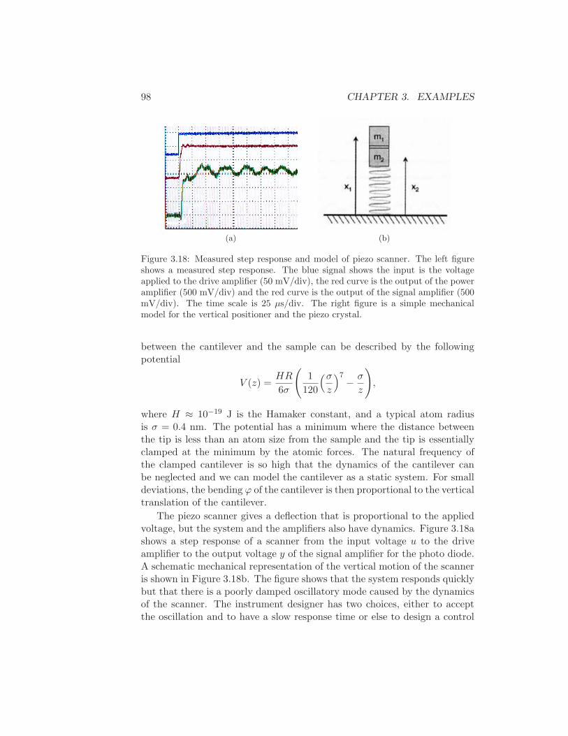
98 CHAPTER 3. EXAMPLES
(a) (b)
Figure 3.18: Measured step response and model of piezo scanner. The left figureshows a measured step response. The blue signal shows the input is the voltageapplied to the drive amplifier (50 mV/div), the red curve is the output of the poweramplifier (500 mV/div) and the red curve is the output of the signal amplifier (500mV/div). The time scale is 25 µs/div. The right figure is a simple mechanicalmodel for the vertical positioner and the piezo crystal.
between the cantilever and the sample can be described by the followingpotential
V (z) =HR
6σ
(
1
120
(σ
z
)7− σ
z
)
,
where H ≈ 10−19 J is the Hamaker constant, and a typical atom radiusis σ = 0.4 nm. The potential has a minimum where the distance betweenthe tip is less than an atom size from the sample and the tip is essentiallyclamped at the minimum by the atomic forces. The natural frequency ofthe clamped cantilever is so high that the dynamics of the cantilever canbe neglected and we can model the cantilever as a static system. For smalldeviations, the bending ϕ of the cantilever is then proportional to the verticaltranslation of the cantilever.
The piezo scanner gives a deflection that is proportional to the appliedvoltage, but the system and the amplifiers also have dynamics. Figure 3.18ashows a step response of a scanner from the input voltage u to the driveamplifier to the output voltage y of the signal amplifier for the photo diode.A schematic mechanical representation of the vertical motion of the scanneris shown in Figure 3.18b. The figure shows that the system responds quicklybut that there is a poorly damped oscillatory mode caused by the dynamicsof the scanner. The instrument designer has two choices, either to acceptthe oscillation and to have a slow response time or else to design a control
3.6. DRUG ADMINISTRATION 99
system that can damp the oscillations which gives a faster response and afaster imaging. Damping the oscillations is a significant challenge becausethere are many oscillatory modes and they can change depending on how theinstrument is used. An instrument designer also has the choice to redesignthe mechanics so that the resonances occur at higher frequencies.
The book by Sarid [Sar91] gives a broad coverage of atomic force micro-scopes. The interaction of atoms close to surfaces is fundamental to solidstate physics. A good source is Kittel [Kit95] where the Lennard-Jones po-tential is discussed. Modeling and control of atomic force microscopes arediscussed by Schitter [Sch01].
3.6 Drug Administration
The phrase “take two pills three times a day” is a recommendation that weare all familiar with. Behind this recommendation is a solution of an openloop control problem. The key issue is to make sure that the concentrationof a medicine in a part of our bodies will be sufficiently high to be effectivebut not so high that it will cause undesirable side effects. The control actionis quantized, take two pills, and sampled, every 8 hours. The prescriptionscan be based on very simple models in terms of empirical tables where thedosage is based on the age and weight of the patient. A more sophisticatedadministration of medicine is used to keep concentration of insulin and glu-cose at a right level. In this case the substances are controlled by continuousmeasurement and injection, and the control schemes are often model based.
Drug administration is clearly a control problem. To do it properly itis necessary to understand how a drug spreads in the body after it is ad-ministered. This topic, called pharmacokinetics, is now its own disciplineand the models used are called compartment models. They go back to 1920when Widmark modeled propagation of alcohol in the body [WT24]. Phar-macokinetics describes how drugs are distributed in different organs of thebody. Compartment models are now important for screening of all drugsused by humans. The schematic diagram in Figure 3.19 illustrates the ideaof a compartment model. Compartment models are also used in many otherfields such as environmental science.
One-Compartment Model
The simplest dynamic model is obtained by assuming that the body behaveslike a single compartment: that the drug is spread evenly in the body after
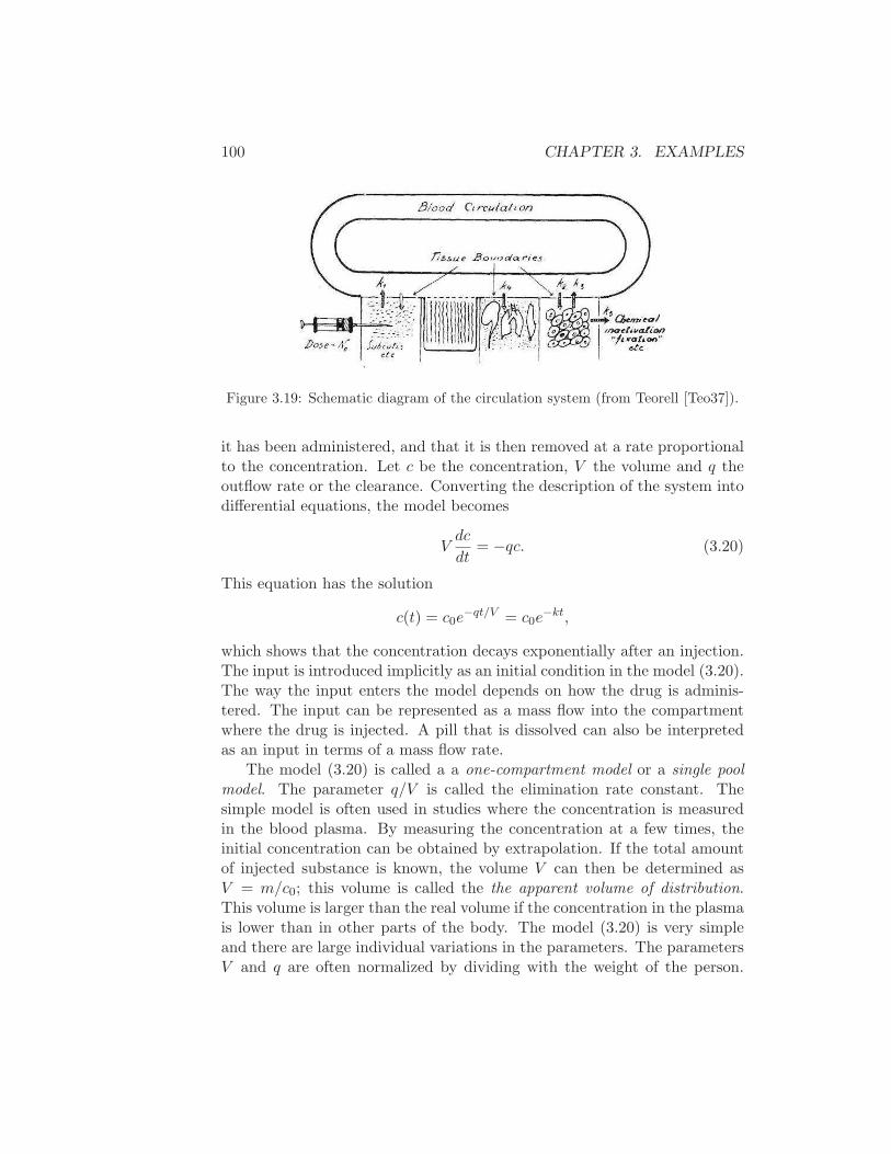
100 CHAPTER 3. EXAMPLES
Figure 3.19: Schematic diagram of the circulation system (from Teorell [Teo37]).
it has been administered, and that it is then removed at a rate proportionalto the concentration. Let c be the concentration, V the volume and q theoutflow rate or the clearance. Converting the description of the system intodifferential equations, the model becomes
Vdc
dt= −qc. (3.20)
This equation has the solution
c(t) = c0e−qt/V = c0e
−kt,
which shows that the concentration decays exponentially after an injection.The input is introduced implicitly as an initial condition in the model (3.20).The way the input enters the model depends on how the drug is adminis-tered. The input can be represented as a mass flow into the compartmentwhere the drug is injected. A pill that is dissolved can also be interpretedas an input in terms of a mass flow rate.
The model (3.20) is called a a one-compartment model or a single poolmodel. The parameter q/V is called the elimination rate constant. Thesimple model is often used in studies where the concentration is measuredin the blood plasma. By measuring the concentration at a few times, theinitial concentration can be obtained by extrapolation. If the total amountof injected substance is known, the volume V can then be determined asV = m/c0; this volume is called the the apparent volume of distribution.This volume is larger than the real volume if the concentration in the plasmais lower than in other parts of the body. The model (3.20) is very simpleand there are large individual variations in the parameters. The parametersV and q are often normalized by dividing with the weight of the person.
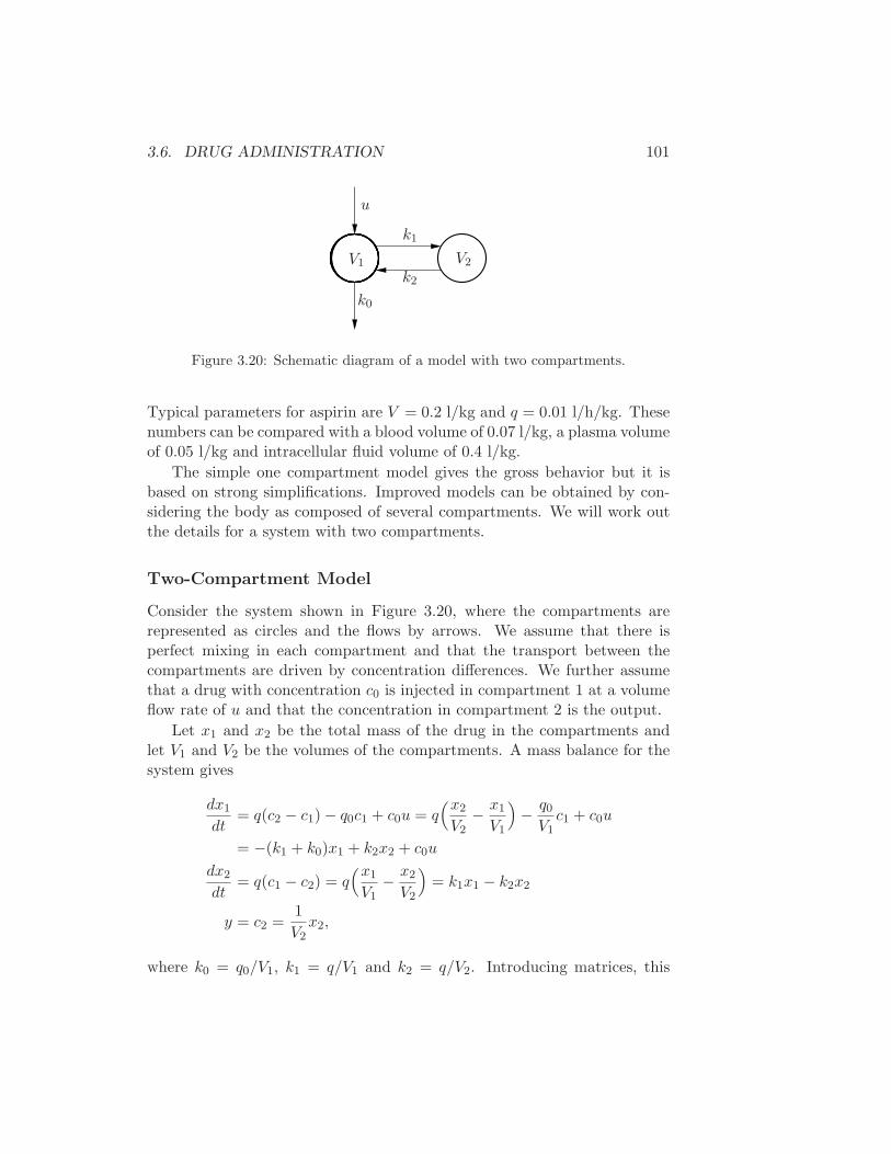
3.6. DRUG ADMINISTRATION 101
V1 V2
u
k1
k2
k0
Figure 3.20: Schematic diagram of a model with two compartments.
Typical parameters for aspirin are V = 0.2 l/kg and q = 0.01 l/h/kg. Thesenumbers can be compared with a blood volume of 0.07 l/kg, a plasma volumeof 0.05 l/kg and intracellular fluid volume of 0.4 l/kg.
The simple one compartment model gives the gross behavior but it isbased on strong simplifications. Improved models can be obtained by con-sidering the body as composed of several compartments. We will work outthe details for a system with two compartments.
Two-Compartment Model
Consider the system shown in Figure 3.20, where the compartments arerepresented as circles and the flows by arrows. We assume that there isperfect mixing in each compartment and that the transport between thecompartments are driven by concentration differences. We further assumethat a drug with concentration c0 is injected in compartment 1 at a volumeflow rate of u and that the concentration in compartment 2 is the output.
Let x1 and x2 be the total mass of the drug in the compartments andlet V1 and V2 be the volumes of the compartments. A mass balance for thesystem gives
dx1
dt= q(c2 − c1) − q0c1 + c0u = q
(x2
V2− x1
V1
)
− q0V1c1 + c0u
= −(k1 + k0)x1 + k2x2 + c0u
dx2
dt= q(c1 − c2) = q
(x1
V1− x2
V2
)
= k1x1 − k2x2
y = c2 =1
V2x2,
where k0 = q0/V1, k1 = q/V1 and k2 = q/V2. Introducing matrices, this
102 CHAPTER 3. EXAMPLES
model can be written as
dx
dt=
−k0 − k1 k2
k1 −k2
x+
c00
u
y =
0 1/V2
x.
(3.21)
In this model we have used the total mass of the drug in each compartmentas state variables. If we instead choose to use the concentrations as statevariables, the model becomes
dc
dt=
−k0 − k1 k1
k2 −k2
c+
b00
u
y =
0 1
x,
(3.22)
where b0 = c0/V1. Mass is called an extensive variable and concentration iscalled an intensive variable.
The papers by Widmark and Tandberg [WT24] and Teorell [Teo37] areclassics. Pharmacokinetics is now an established discipline with many text-books [Dos68, Jac72, GP82]. Because of its medical importance pharmacoki-netics is now an essential component of drug development. Compartmentmodels are also used in other branches of medicine and in ecology. Theproblem of determining rate coefficients from experimental data is discussedin [BA70] and [God83].
3.7 Population Dynamics
Population growth is a complex dynamic process that involves the interac-tion of one or more species with their environment and the larger ecosystem.The dynamics of population groups are interesting and important in manydifferent areas of social and environmental policy. There are examples wherenew species have been introduced in new habitats, sometimes with disas-trous results. There are also been attempts to control population growthboth through incentives and through legislation. In this section we describesome of the models that can be used to understand how populations evolvewith time and as a function of their environment.
Simple Growth Model
Let x the the population of a species at time t. A simple model is to assumethat the birth and death rates are proportional to the total population. This
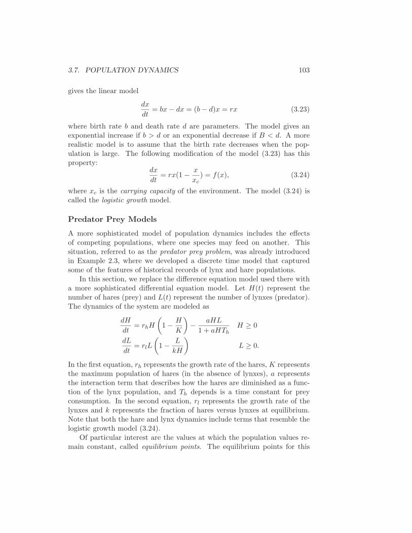
3.7. POPULATION DYNAMICS 103
gives the linear model
dx
dt= bx− dx = (b− d)x = rx (3.23)
where birth rate b and death rate d are parameters. The model gives anexponential increase if b > d or an exponential decrease if B < d. A morerealistic model is to assume that the birth rate decreases when the pop-ulation is large. The following modification of the model (3.23) has thisproperty:
dx
dt= rx(1 − x
xc) = f(x), (3.24)
where xc is the carrying capacity of the environment. The model (3.24) iscalled the logistic growth model.
Predator Prey Models
A more sophisticated model of population dynamics includes the effectsof competing populations, where one species may feed on another. Thissituation, referred to as the predator prey problem, was already introducedin Example 2.3, where we developed a discrete time model that capturedsome of the features of historical records of lynx and hare populations.
In this section, we replace the difference equation model used there witha more sophisticated differential equation model. Let H(t) represent thenumber of hares (prey) and L(t) represent the number of lynxes (predator).The dynamics of the system are modeled as
dH
dt= rhH
(
1 − H
K
)
− aHL
1 + aHThH ≥ 0
dL
dt= rlL
(
1 − L
kH
)
L ≥ 0.
In the first equation, rh represents the growth rate of the hares, K representsthe maximum population of hares (in the absence of lynxes), a representsthe interaction term that describes how the hares are diminished as a func-tion of the lynx population, and Th depends is a time constant for preyconsumption. In the second equation, rl represents the growth rate of thelynxes and k represents the fraction of hares versus lynxes at equilibrium.Note that both the hare and lynx dynamics include terms that resemble thelogistic growth model (3.24).
Of particular interest are the values at which the population values re-main constant, called equilibrium points. The equilibrium points for this
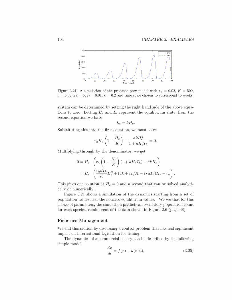
104 CHAPTER 3. EXAMPLES
0 10 20 30 40 50 60 70 80 900
50
100
150
200
250
Time (years)
Pop
ulat
ion
HareLynx
Figure 3.21: A simulation of the predator prey model with rh = 0.02, K = 500,a = 0.03, Th = 5, rl = 0.01, k = 0.2 and time scale chosen to correspond to weeks.
system can be determined by setting the right hand side of the above equa-tions to zero. Letting He and Le represent the equilibrium state, from thesecond equation we have
Le = kHe.
Substituting this into the first equation, we must solve
rhHe
(
1 − He
K
)
− akH2e
1 + aHeTh= 0.
Multiplying through by the denominator, we get
0 = He · (rh(1 − He
K
)
(1 + aHeTh) − akHe
)
= He · (rhaTh
KH2
e + (ak + rh/K − rhaTh)He − rh
)
.
This gives one solution at He = 0 and a second that can be solved analyti-cally or numerically.
Figure 3.21 shows a simulation of the dynamics starting from a set ofpopulation values near the nonzero equilibrium values. We see that for thischoice of parameters, the simulation predicts an oscillatory population countfor each species, reminiscent of the data shown in Figure 2.6 (page 48).
Fisheries Management
We end this section by discussing a control problem that has had significantimpact on international legislation for fishing.
The dynamics of a commercial fishery can be described by the followingsimple model
dx
dt= f(x) − h(x, u), (3.25)
3.7. POPULATION DYNAMICS 105
where x be the total biomass, f(x) the growth rate and h(x, u) the harvestingrate. The logistic function (3.24) is a simple model for the growth rate andthe harvesting can be modeled by
h(x, u) = axu, (3.26)
where the control variable u is the harvesting effort, and a is a constant.The rate of revenue is
g(x, u) = bh(x, u) − cu, (3.27)
where b and c are constants representing the price of fish and the cost offishing. Using equations (3.26) and (3.27) we find that the rate of revenueis
g(x, u) = (abx− c)u.
In a situation where there are many fishermen and no concern for the envi-ronment, it is economic to fish as long as abx > c and there will then be anequilibrium where the biomass is
x∞ =c
ab, (3.28)
which is the equilibrium with unrestricted fishing.Assume that the population is initially at equilibrium at x(0) = xc. The
revenue rate with unrestricted fishing is then (abxc − c)u, which can be verylarge. The fishing effort then naturally increases until the equilibrium (3.28),where the revenue rate is zero.
We can contrast unrestricted fishing with the situation for a single fish-ery. A typical case is when a country has all fishing rights in a large area.In such a case it is natural to maximize the rate of sustainable revenue.This can be accomplished by adding the constraint that the biomass x inequation (3.25) is constant, which implies that
f(x) = h(x, u).
Solving this equation for u gives
u = ud(x) =f(x)
ax.
Inserting the value of u into equation (3.27) gives the following rate of rev-enue
g(x) = bh(x, ud) − cud(x) =(
b− c
ax
)
f(x)
= rx(
b− c
ax
)(
1 − x
xc
)
=r
xc
(
−abx2 + (c+ abxc)x− cxc
)
.(3.29)
106 CHAPTER 3. EXAMPLES
0 5 10 15 20 25 30 35 40 45 500
50
100
0 5 10 15 20 25 30 35 40 45 500
2
4
0 5 10 15 20 25 30 35 40 45 500
10
20
30
xu
g
t
Figure 3.22: Simulation of a fishery. The curves show total biomass x, harvestingrate u and revenue rate g as a function of time t. The fishery is modeled byequations (3.25), (3.26), (3.27) with parameters xc = 100, a = 0.1, b = 1 and c = 1.Initially fishing is unrestricted at rate u = 3, at time t = 15 fishing is changed toharvesting at a sustainable rate, accomplished by a PI controller with parametersk = 0.5 and ki = 0.5.
The rate of revenue has a maximum
r0 =r(c− abxc)
2
4abxc, (3.30)
forx0 =
xc
2+
c
2ab. (3.31)
Figure 3.22 shows a simulation of a fishery. The system is initially in equi-librium with x = 100. Fishing begins with constant harvesting rate u = 3at time t = 0. The initial revenue rate is large, but it drops rapidly as thepopulation decreases. At time t = 12 the revenue rate is practically zero.The fishing policy is changed to a sustainable strategy at time t = 15. Thisis accomplished by using a PI controller where the reference is the optimalsustainable population size x0 = 55, given by equation (3.31). The feedbackstops harvesting for a period but the biomass increases rapidly. At timet = 28 the harvesting rate increases rapidly and a sustainable steady stateis reached in a short time.
Volume I of the two volume set by J. Murray [Mur04] give a broadcoverage of population dynamics. Maintaining a sustainable fish population
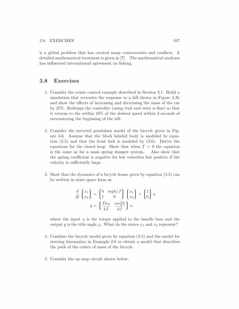
3.8. EXERCISES 107
is a global problem that has created many controversies and conflicts. Adetailed mathematical treatment is given in [?]. The mathematical analyseshas influenced international agreement on fishing.
3.8 Exercises
1. Consider the cruise control example described in Section 3.1. Build asimulation that recreates the response to a hill shown in Figure 3.3band show the effects of increasing and decreasing the mass of the carby 25%. Redesign the controller (using trail and error is fine) so thatit returns to the within 10% of the desired speed within 3 seconds ofencountering the beginning of the hill.
2. Consider the inverted pendulum model of the bicycle given in Fig-ure 3.6. Assume that the block labeled body is modeled by equa-tion (3.5) and that the front fork is modeled by (3.6). Derive theequations for the closed loop. Show that when T = 0 the equationis the same as for a mass spring damper system. Also show thatthe spring coefficient is negative for low velocities but positive if thevelocity is sufficiently large.
3. Show that the dynamics of a bicycle frame given by equation (3.5) canbe written in state space form as
d
dt
x1
x2
=
0 mgh/J1 0
x1
x2
+
10
u
y =
Dv0bJ
mv20h
bJ
x,
where the input u is the torque applied to the handle bars and theoutput y is the title angle ϕ. What do the states x1 and x2 represent?
4. Combine the bicycle model given by equation (3.5) and the model forsteering kinematics in Example 2.8 to obtain a model that describesthe path of the center of mass of the bicycle.
5. Consider the op amp circuit shown below:
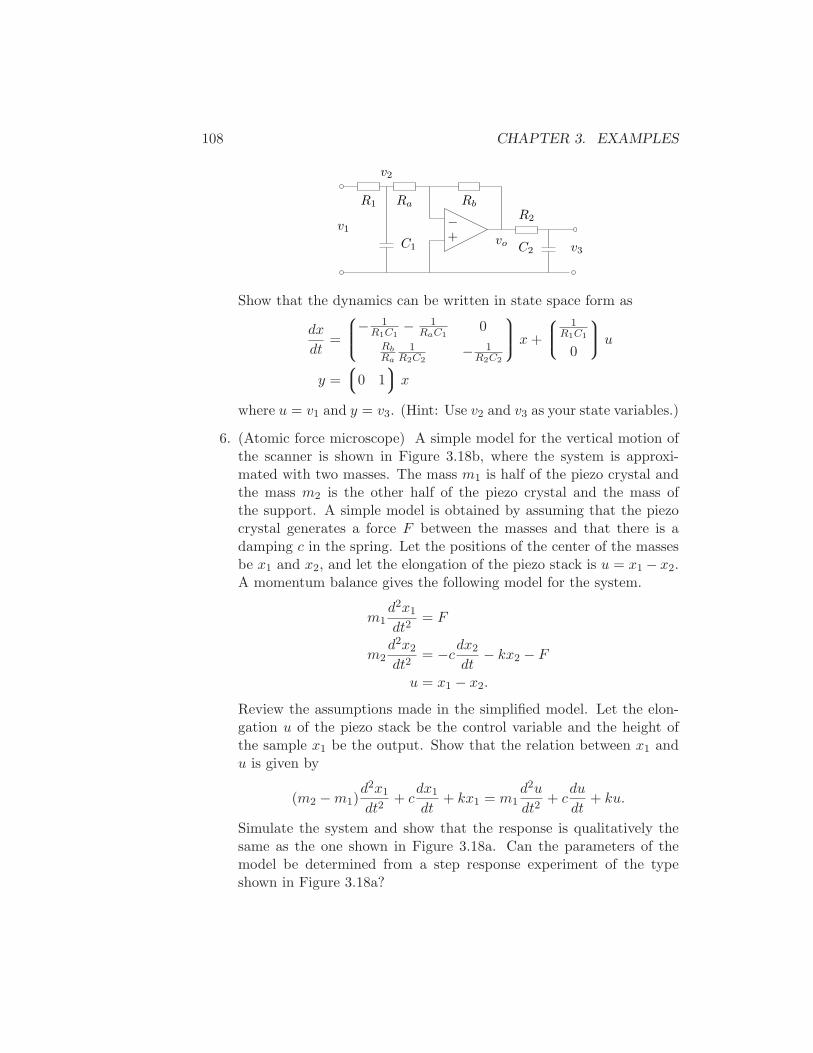
108 CHAPTER 3. EXAMPLES
v2
−+
Rb
v1
v3
R1 Ra
R2
C2C1
vo
Show that the dynamics can be written in state space form as
dx
dt=
− 1R1C1
− 1RaC1
0
Rb
Ra
1R2C2
− 1R2C2
x+
1R1C1
0
u
y =
0 1
x
where u = v1 and y = v3. (Hint: Use v2 and v3 as your state variables.)
6. (Atomic force microscope) A simple model for the vertical motion ofthe scanner is shown in Figure 3.18b, where the system is approxi-mated with two masses. The mass m1 is half of the piezo crystal andthe mass m2 is the other half of the piezo crystal and the mass ofthe support. A simple model is obtained by assuming that the piezocrystal generates a force F between the masses and that there is adamping c in the spring. Let the positions of the center of the massesbe x1 and x2, and let the elongation of the piezo stack is u = x1 − x2.A momentum balance gives the following model for the system.
m1d2x1
dt2= F
m2d2x2
dt2= −cdx2
dt− kx2 − F
u = x1 − x2.
Review the assumptions made in the simplified model. Let the elon-gation u of the piezo stack be the control variable and the height ofthe sample x1 be the output. Show that the relation between x1 andu is given by
(m2 −m1)d2x1
dt2+ c
dx1
dt+ kx1 = m1
d2u
dt2+ c
du
dt+ ku.
Simulate the system and show that the response is qualitatively thesame as the one shown in Figure 3.18a. Can the parameters of themodel be determined from a step response experiment of the typeshown in Figure 3.18a?
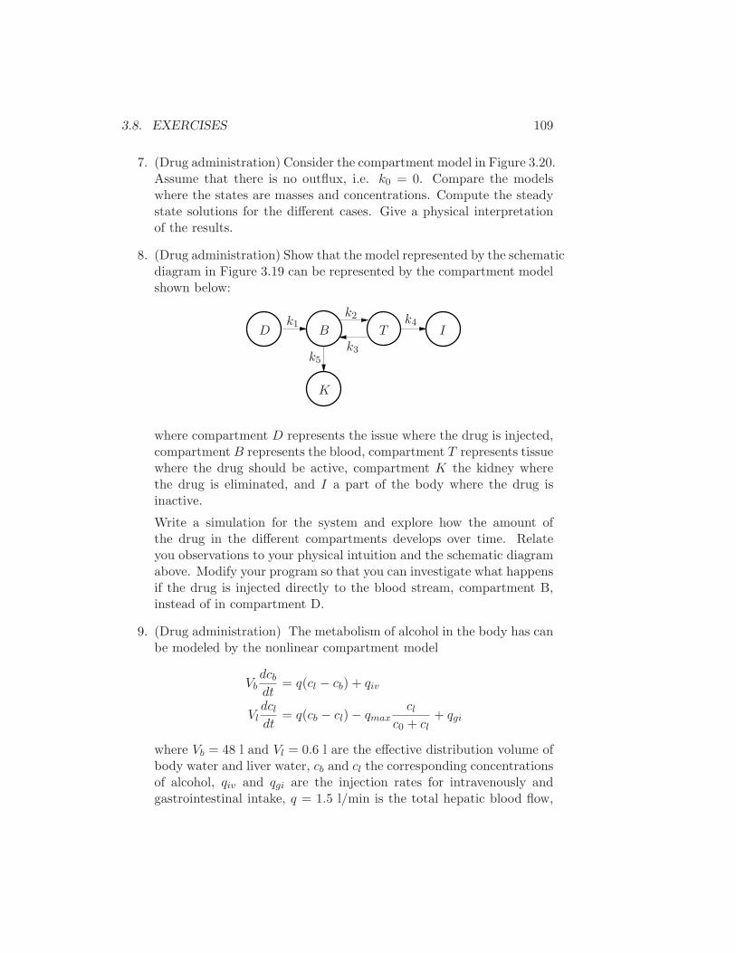
3.8. EXERCISES 109
7. (Drug administration) Consider the compartment model in Figure 3.20.Assume that there is no outflux, i.e. k0 = 0. Compare the modelswhere the states are masses and concentrations. Compute the steadystate solutions for the different cases. Give a physical interpretationof the results.
8. (Drug administration) Show that the model represented by the schematicdiagram in Figure 3.19 can be represented by the compartment modelshown below:
D B T I
K
k1k2
k3
k4
k5
where compartment D represents the issue where the drug is injected,compartment B represents the blood, compartment T represents tissuewhere the drug should be active, compartment K the kidney wherethe drug is eliminated, and I a part of the body where the drug isinactive.
Write a simulation for the system and explore how the amount ofthe drug in the different compartments develops over time. Relateyou observations to your physical intuition and the schematic diagramabove. Modify your program so that you can investigate what happensif the drug is injected directly to the blood stream, compartment B,instead of in compartment D.
9. (Drug administration) The metabolism of alcohol in the body has canbe modeled by the nonlinear compartment model
Vbdcbdt
= q(cl − cb) + qiv
Vldcldt
= q(cb − cl) − qmaxcl
c0 + cl+ qgi
where Vb = 48 l and Vl = 0.6 l are the effective distribution volume ofbody water and liver water, cb and cl the corresponding concentrationsof alcohol, qiv and qgi are the injection rates for intravenously andgastrointestinal intake, q = 1.5 l/min is the total hepatic blood flow,
110 CHAPTER 3. EXAMPLES
qmax = 2.75 mmol/min and km = 0.1 mmol. Simulate the system andcompute the concentration in the blood for oral and intravenous dosesof 12 g and 40 g of alcohol.
10. (Population dynamics) Consider the model for logistic growth givenby equation (3.24). Show that the maximum growth rate occurs whenthe size of the population is half of the steady state value.
11. (Population dynamics) Verify the curves in Figure 3.21 by creating aprogram that integrates the differential equations.
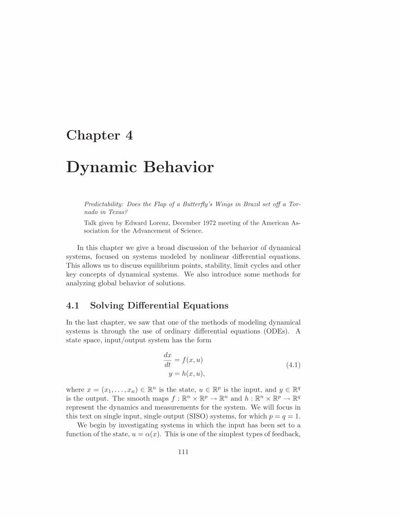
Chapter 4
Dynamic Behavior
Predictability: Does the Flap of a Butterfly’s Wings in Brazil set off a Tor-nado in Texas?
Talk given by Edward Lorenz, December 1972 meeting of the American As-sociation for the Advancement of Science.
In this chapter we give a broad discussion of the behavior of dynamicalsystems, focused on systems modeled by nonlinear differential equations.This allows us to discuss equilibrium points, stability, limit cycles and otherkey concepts of dynamical systems. We also introduce some methods foranalyzing global behavior of solutions.
4.1 Solving Differential Equations
In the last chapter, we saw that one of the methods of modeling dynamicalsystems is through the use of ordinary differential equations (ODEs). Astate space, input/output system has the form
dx
dt= f(x, u)
y = h(x, u),(4.1)
where x = (x1, . . . , xn) ∈ Rn is the state, u ∈ R
p is the input, and y ∈ Rq
is the output. The smooth maps f : Rn × R
p → Rn and h : R
n × Rp → R
q
represent the dynamics and measurements for the system. We will focus inthis text on single input, single output (SISO) systems, for which p = q = 1.
We begin by investigating systems in which the input has been set to afunction of the state, u = α(x). This is one of the simplest types of feedback,
111
112 CHAPTER 4. DYNAMIC BEHAVIOR
in which the system regulates its own behavior. The differential equationsin this case become
dx
dt= f(x, α(x)) = F (x). (4.2)
In order to understand the dynamic behavior of this system, we need toanalyze the features of the solutions of equation (4.2). While in some simplesituations we can write down the solutions in analytical form, more often wemust rely on computational approaches. We begin by describing the classof solutions for this problem.
Initial Value Problems
We say that x(t) is a solution of the differential equation (4.2) on the timeinterval t0 ∈ R to tf ∈ R if
dx(t)
dt= F (x(t)) for all t0 ≤ t ≤ tf .
A given differential equation may have many solutions. We will most oftenbe interested in the initial value problem, where x(t) is prescribed at a giventime t0 ∈ R and we wish to find a solution valid for all future time, t > t0.
We say that x(t) is a solution of the differential equation (4.2) with initialvalue x0 ∈ R
n at t0 ∈ R if
x(t0) = x0 anddx(t)
dt= F (x(t)) for all t0 ≤ t ≤ tf .
For most differential equations we will encounter, there is a unique solutionthat is defined for t0 ≤ t ≤ tf . The solution may defined for all time t ≥ t0,in which case we take tf = ∞. Because we will primarily be interested insolutions of the initial value problem for ODEs, we will often refer to thissimply as the solution of an ODE.
We will usually assume that t0 is equal to 0. In the case when F is inde-pendent of time (as in equation (4.2)), we can do so without loss of generalityby choosing a new independent (time) variable, τ = t− t0 (Exercise 2).
Example 4.1 (Damped oscillator). Consider a damped, linear oscillator,introduced in Example 2.4. The equations of motion for the system are
mq + cq + kq = 0,
where q is the displacement of the oscillator from its rest position. Weassume that c2 < 4km, corresponding to a lightly damped system (the
4.1. SOLVING DIFFERENTIAL EQUATIONS 113
0 2 4 6 8 10 12 14 16 18 20−1
−0.5
0
0.5
1
time (sec)
x 1, x2
x1
x2
Figure 4.1: Response of the damped oscillator to the initial condition x0 = (1, 0).
reason for this particular choice will become clear later). We can rewritethis in state space form by setting x1 = q and x2 = q, giving
x1 = x2
x2 = − k
mx1 −
c
mx2.
In vector form, the right hand side can be written as
F (x) =
x2
− kmx1 − c
mx2
.
The solution to the initial value problem can be written in a number ofdifferent ways and will be explored in more detail in Chapter 5. Here wesimply assert that the solution can be written as
x1(t) = e−ct2m
(
x10 cosωdt+(cx10 + 2mx20
2mωd
)
sinωdt
)
x2(t) = e−ct2m
(
x20 cosωdt−(2kx10 + cx20
2mωd
)
sinωdt
)
,
where x0 = (x10, x20) is the initial condition and ωd =√
4km− c2/2m. Thissolution can be verified by substituting it into the differential equation. Wesee that the solution is explicitly dependent on the initial condition and itcan be shown that this solution is unique. A plot of the initial conditionresponse is shown in Figure 4.1. We note that this form of the solution onlyholds for c2 − 4km < 0, corresponding to an “underdamped” oscillator. ∇
114 CHAPTER 4. DYNAMIC BEHAVIOR
Numerical Solutions
One of the benefits of the computer revolution that is that it is very easyto obtain a numerical solution of a differential equation when the initialcondition is given. A nice consequence of this is as soon as we have a modelin the form of equation (4.2), it is straightforward to generate the behaviorof x for different initial conditions, as we saw briefly in the previous chapter.
Modern computing environments such as LabVIEW, MATLAB and Math-ematica allow simulation of differential equations as a basic operation. Forexample, these packages provides several tools for representing, simulating,and analyzing ordinary differential equations of the form in equation (4.2).To define an ODE in MATLAB or LabVIEW, we define a function repre-senting the right hand side of equation (4.2):
function xdot = system(t, x)
xdot(1) = F1(x);
xdot(2) = F2(x);
...
Each expression Fi(x) takes a (column) vector x and returns the ith el-ement of the differential equation. The second argument to the functionsystem, t, represents the current time and allows for the possibility of time-varying differential equations, in which the right hand side of the ODE inequation (4.2) depends explicitly on time.
ODEs defined in this fashion can be simulated by using the ode45 com-mand:
ode45(’file’, [0,T], [x10, x20, ..., xn0])
The first argument is the name of the function defining the ODE, the secondargument gives the time interval over which the simulation should be per-formed and the final argument gives the vector of initial conditions. Similarcapabilities exist in other packages such as Octave and Scilab.
Example 4.2 (Balance system). Consider the balance system given in Ex-ample 2.1 and reproduced in Figure 4.2a. Suppose that a coworker hasdesigned a control law that will hold the position of the system steady inthe upright position at p = 0. The form of the control law is
F = −Kx,
where x = (p, θ, p, θ) ∈ R4 is the state of the system, F is the input, and
K = (k1, k2, k3, k4) is the vector of “gains” for the control law.
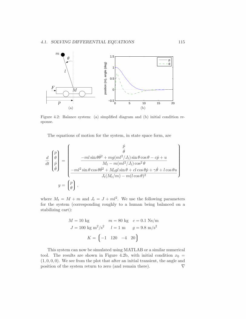
4.1. SOLVING DIFFERENTIAL EQUATIONS 115
l
MF
p
θm
(a)
0 5 10 15 20−0.5
0
0.5
1
1.5
posi
tion
(m),
ang
le (
deg)
pθ
(b)
Figure 4.2: Balance system: (a) simplified diagram and (b) initial condition re-sponse.
The equations of motion for the system, in state space form, are
d
dt
pθp
θ
=
p
θ
−ml sin θθ2 +mg(ml2/Jt) sin θ cos θ − cp+ u
Mt −m(ml2/Jt) cos2 θ
−ml2 sin θ cos θθ2 +Mtgl sin θ + cl cos θp+ γθ + l cos θu
Jt(Mt/m) −m(l cos θ)2
y =
pθ
,
where Mt = M + m and Jt = J + ml2. We use the following parametersfor the system (corresponding roughly to a human being balanced on astabilizing cart):
M = 10 kg m = 80 kg c = 0.1 Ns/m
J = 100 kg m2/s2 l = 1 m g = 9.8 m/s2
K =
−1 120 −4 20
This system can now be simulated using MATLAB or a similar numericaltool. The results are shown in Figure 4.2b, with initial condition x0 =(1, 0, 0, 0). We see from the plot that after an initial transient, the angle andposition of the system return to zero (and remain there). ∇
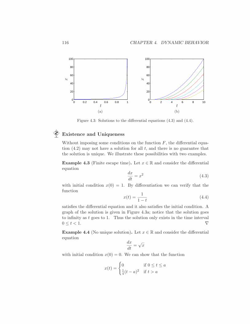
116 CHAPTER 4. DYNAMIC BEHAVIOR
0 0.2 0.4 0.6 0.8 10
20
40
60
80
100
t
x
(a)
0 2 4 6 8 100
20
40
60
80
100
t
x
(b)
Figure 4.3: Solutions to the differential equations (4.3) and (4.4).
Existence and Uniqueness
Without imposing some conditions on the function F , the differential equa-tion (4.2) may not have a solution for all t, and there is no guarantee thatthe solution is unique. We illustrate these possibilities with two examples.
Example 4.3 (Finite escape time). Let x ∈ R and consider the differentialequation
dx
dt= x2 (4.3)
with initial condition x(0) = 1. By differentiation we can verify that thefunction
x(t) =1
1 − t(4.4)
satisfies the differential equation and it also satisfies the initial condition. Agraph of the solution is given in Figure 4.3a; notice that the solution goesto infinity as t goes to 1. Thus the solution only exists in the time interval0 ≤ t < 1. ∇
Example 4.4 (No unique solution). Let x ∈ R and consider the differentialequation
dx
dt=
√x
with initial condition x(0) = 0. We can show that the function
x(t) =
0 if 0 ≤ t ≤ a14(t− a)2 if t > a
4.2. QUALITATIVE ANALYSIS 117
satisfies the differential equation for all values of the parameter a ≥ 0. Tosee this, we differentiate x(t) to obtain
dx
dt=
0 if 0 ≤ t ≤ a12(t− a) if t > a
and hence x =√x for all t ≥ 0 with x(0) = 0. A graph of some of the
possible solutions is given in Figure 4.3b. Notice that in this case there aremany solutions to the differential equation. ∇
These simple examples show that there may be difficulties even withsimple differential equations. Existence and uniqueness can be guaranteedby requiring that the function F has the property that for some fixed c ∈ R
‖F (x) − F (y)‖ < c‖x− y‖ for all x, y,
which is called Lipschitz continuity. A sufficient condition for a function tobe Lipschitz is that the Jacobian, ∂F/∂x, is uniformly bounded for all x.The difficulty in Example 4.3 is that the derivative ∂F/∂x becomes largefor large x and the difficulty in Example 4.4 is that the derivative ∂F/∂x isinfinite at the origin.
4.2 Qualitative Analysis
The qualitative behavior of nonlinear systems is important for understandingsome of the key concepts of stability in nonlinear dynamics. We will focus onan important class of systems known as planar dynamical systems. Thesesystems have two state variables x ∈ R
2, allowing their solutions to beplotted in the (x1, x2) plane. The basic concepts that we describe holdmore generally and can be used to understand dynamical behavior in higherdimensions.
Phase Portraits
A convenient way to understand the behavior of dynamical systems withstate x ∈ R
2 is to plot the phase portrait of the system, briefly introducedin Chapter 2. We start by introducing the concept of a vector field. For asystem of ordinary differential equations
dx
dt= F (x),
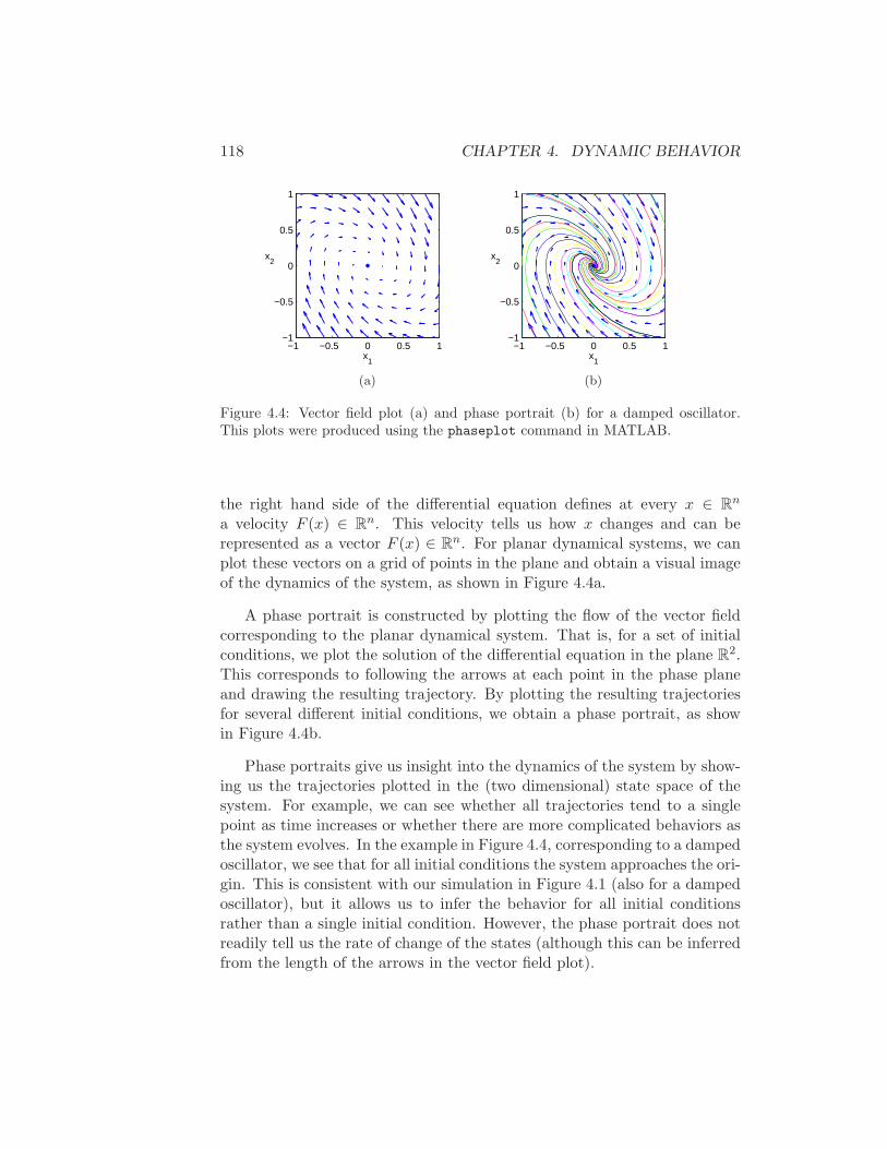
118 CHAPTER 4. DYNAMIC BEHAVIOR
−1 −0.5 0 0.5 1−1
−0.5
0
0.5
1
x1
x2
(a)
−1 −0.5 0 0.5 1−1
−0.5
0
0.5
1
x1
x2
(b)
Figure 4.4: Vector field plot (a) and phase portrait (b) for a damped oscillator.This plots were produced using the phaseplot command in MATLAB.
the right hand side of the differential equation defines at every x ∈ Rn
a velocity F (x) ∈ Rn. This velocity tells us how x changes and can be
represented as a vector F (x) ∈ Rn. For planar dynamical systems, we can
plot these vectors on a grid of points in the plane and obtain a visual imageof the dynamics of the system, as shown in Figure 4.4a.
A phase portrait is constructed by plotting the flow of the vector fieldcorresponding to the planar dynamical system. That is, for a set of initialconditions, we plot the solution of the differential equation in the plane R
2.This corresponds to following the arrows at each point in the phase planeand drawing the resulting trajectory. By plotting the resulting trajectoriesfor several different initial conditions, we obtain a phase portrait, as showin Figure 4.4b.
Phase portraits give us insight into the dynamics of the system by show-ing us the trajectories plotted in the (two dimensional) state space of thesystem. For example, we can see whether all trajectories tend to a singlepoint as time increases or whether there are more complicated behaviors asthe system evolves. In the example in Figure 4.4, corresponding to a dampedoscillator, we see that for all initial conditions the system approaches the ori-gin. This is consistent with our simulation in Figure 4.1 (also for a dampedoscillator), but it allows us to infer the behavior for all initial conditionsrather than a single initial condition. However, the phase portrait does notreadily tell us the rate of change of the states (although this can be inferredfrom the length of the arrows in the vector field plot).
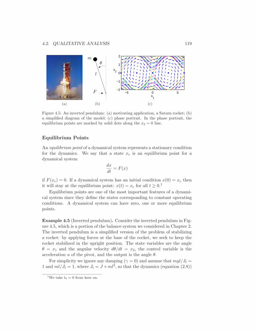
4.2. QUALITATIVE ANALYSIS 119
(a)
F
θm
l
(b)
−5 0 5−2
−1
0
1
2
x1
x2
(c)
Figure 4.5: An inverted pendulum: (a) motivating application, a Saturn rocket; (b)a simplified diagram of the model; (c) phase portrait. In the phase portrait, theequilibrium points are marked by solid dots along the x2 = 0 line.
Equilibrium Points
An equilibrium point of a dynamical system represents a stationary conditionfor the dynamics. We say that a state xe is an equilibrium point for adynamical system
dx
dt= F (x)
if F (xe) = 0. If a dynamical system has an initial condition x(0) = xe thenit will stay at the equilibrium point: x(t) = xe for all t ≥ 0.1
Equilibrium points are one of the most important features of a dynami-cal system since they define the states corresponding to constant operatingconditions. A dynamical system can have zero, one or more equilibriumpoints.
Example 4.5 (Inverted pendulum). Consider the inverted pendulum in Fig-ure 4.5, which is a portion of the balance system we considered in Chapter 2.The inverted pendulum is a simplified version of the problem of stabilizinga rocket: by applying forces at the base of the rocket, we seek to keep therocket stabilized in the upright position. The state variables are the angleθ = x1 and the angular velocity dθ/dt = x2, the control variable is theacceleration u of the pivot, and the output is the angle θ.
For simplicity we ignore any damping (γ = 0) and assume that mgl/Jt =1 and ml/Jt = 1, where Jt = J+ml2, so that the dynamics (equation (2.8))
1We take t0 = 0 from here on.
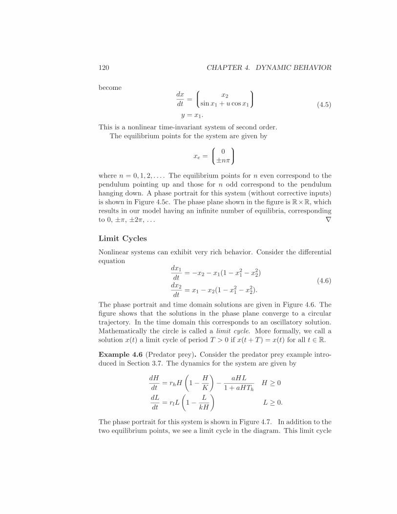
120 CHAPTER 4. DYNAMIC BEHAVIOR
becomedx
dt=
x2
sinx1 + u cosx1
y = x1.
(4.5)
This is a nonlinear time-invariant system of second order.The equilibrium points for the system are given by
xe =
0
±nπ
where n = 0, 1, 2, . . . . The equilibrium points for n even correspond to thependulum pointing up and those for n odd correspond to the pendulumhanging down. A phase portrait for this system (without corrective inputs)is shown in Figure 4.5c. The phase plane shown in the figure is R×R, whichresults in our model having an infinite number of equilibria, correspondingto 0, ±π, ±2π, . . . ∇
Limit Cycles
Nonlinear systems can exhibit very rich behavior. Consider the differentialequation
dx1
dt= −x2 − x1(1 − x2
1 − x22)
dx2
dt= x1 − x2(1 − x2
1 − x22).
(4.6)
The phase portrait and time domain solutions are given in Figure 4.6. Thefigure shows that the solutions in the phase plane converge to a circulartrajectory. In the time domain this corresponds to an oscillatory solution.Mathematically the circle is called a limit cycle. More formally, we call asolution x(t) a limit cycle of period T > 0 if x(t+ T ) = x(t) for all t ∈ R.
Example 4.6 (Predator prey). Consider the predator prey example intro-duced in Section 3.7. The dynamics for the system are given by
dH
dt= rhH
(
1 − H
K
)
− aHL
1 + aHThH ≥ 0
dL
dt= rlL
(
1 − L
kH
)
L ≥ 0.
The phase portrait for this system is shown in Figure 4.7. In addition to thetwo equilibrium points, we see a limit cycle in the diagram. This limit cycle
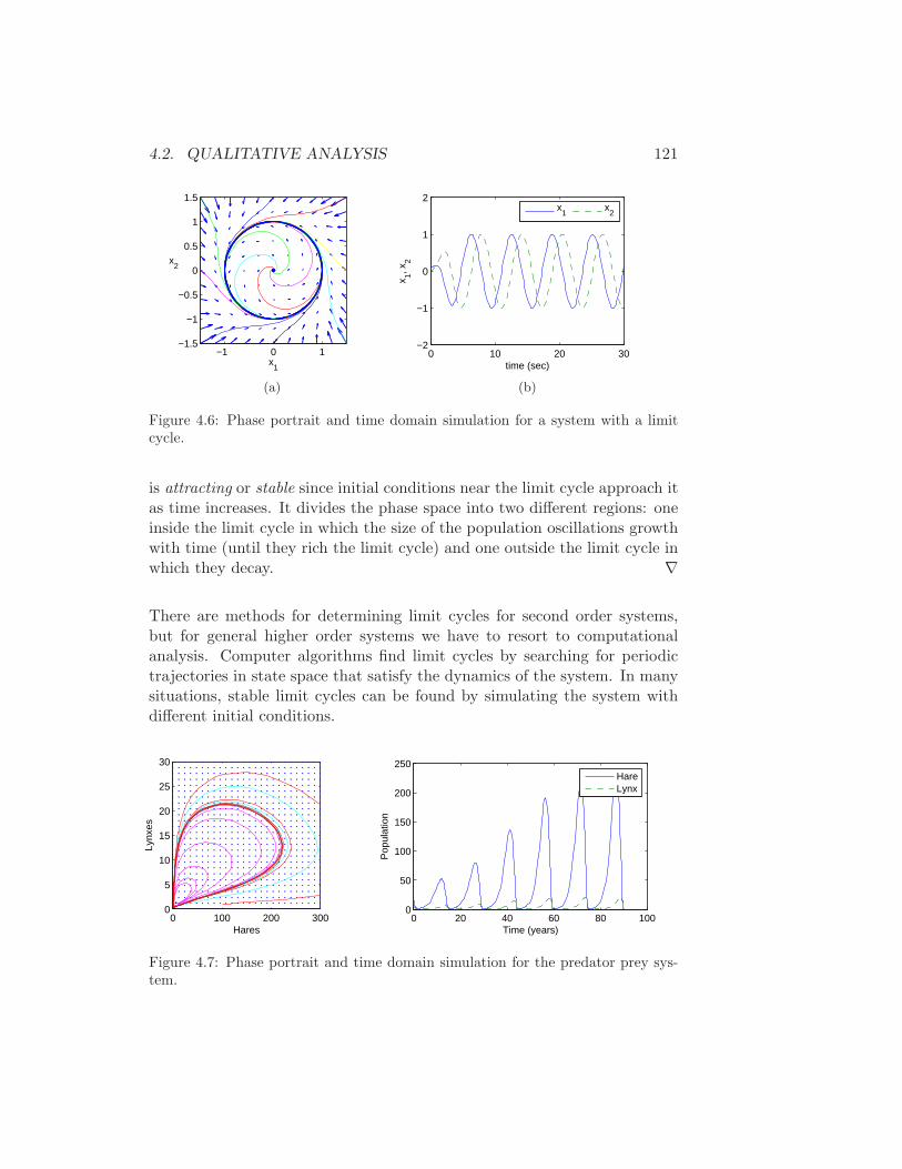
4.2. QUALITATIVE ANALYSIS 121
−1 0 1−1.5
−1
−0.5
0
0.5
1
1.5
x1
x2
(a)
0 10 20 30−2
−1
0
1
2
time (sec)
x 1, x2
x1
x2
(b)
Figure 4.6: Phase portrait and time domain simulation for a system with a limitcycle.
is attracting or stable since initial conditions near the limit cycle approach itas time increases. It divides the phase space into two different regions: oneinside the limit cycle in which the size of the population oscillations growthwith time (until they rich the limit cycle) and one outside the limit cycle inwhich they decay. ∇
There are methods for determining limit cycles for second order systems,but for general higher order systems we have to resort to computationalanalysis. Computer algorithms find limit cycles by searching for periodictrajectories in state space that satisfy the dynamics of the system. In manysituations, stable limit cycles can be found by simulating the system withdifferent initial conditions.
0 100 200 3000
5
10
15
20
25
30
Hares
Lynx
es
0 20 40 60 80 1000
50
100
150
200
250
Time (years)
Pop
ulat
ion
HareLynx
Figure 4.7: Phase portrait and time domain simulation for the predator prey sys-tem.
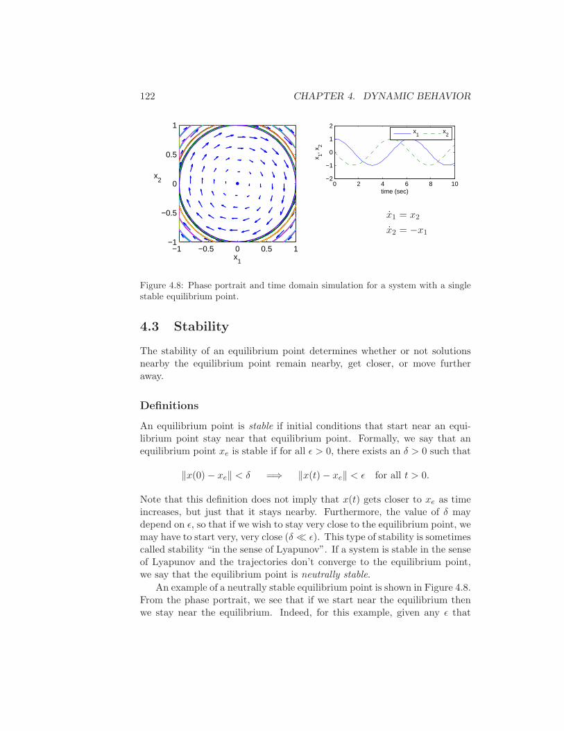
122 CHAPTER 4. DYNAMIC BEHAVIOR
−1 −0.5 0 0.5 1−1
−0.5
0
0.5
1
x1
x2
0 2 4 6 8 10−2
−1
0
1
2
time (sec)
x 1, x2
x1
x2
x1 = x2
x2 = −x1
Figure 4.8: Phase portrait and time domain simulation for a system with a singlestable equilibrium point.
4.3 Stability
The stability of an equilibrium point determines whether or not solutionsnearby the equilibrium point remain nearby, get closer, or move furtheraway.
Definitions
An equilibrium point is stable if initial conditions that start near an equi-librium point stay near that equilibrium point. Formally, we say that anequilibrium point xe is stable if for all ǫ > 0, there exists an δ > 0 such that
‖x(0) − xe‖ < δ =⇒ ‖x(t) − xe‖ < ǫ for all t > 0.
Note that this definition does not imply that x(t) gets closer to xe as timeincreases, but just that it stays nearby. Furthermore, the value of δ maydepend on ǫ, so that if we wish to stay very close to the equilibrium point, wemay have to start very, very close (δ ≪ ǫ). This type of stability is sometimescalled stability “in the sense of Lyapunov”. If a system is stable in the senseof Lyapunov and the trajectories don’t converge to the equilibrium point,we say that the equilibrium point is neutrally stable.
An example of a neutrally stable equilibrium point is shown in Figure 4.8.From the phase portrait, we see that if we start near the equilibrium thenwe stay near the equilibrium. Indeed, for this example, given any ǫ that
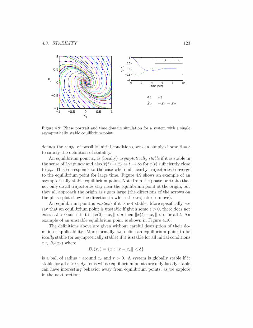
4.3. STABILITY 123
−1 −0.5 0 0.5 1−1
−0.5
0
0.5
1
x1
x2
0 2 4 6 8 10−1
−0.5
0
0.5
1
time (sec)
x 1, x2
x1
x2
x1 = x2
x2 = −x1 − x2
Figure 4.9: Phase portrait and time domain simulation for a system with a singleasymptotically stable equilibrium point.
defines the range of possible initial conditions, we can simply choose δ = ǫto satisfy the definition of stability.
An equilibrium point xe is (locally) asymptotically stable if it is stable inthe sense of Lyapunov and also x(t) → xe as t→ ∞ for x(t) sufficiently closeto xe. This corresponds to the case where all nearby trajectories convergeto the equilibrium point for large time. Figure 4.9 shows an example of anasymptotically stable equilibrium point. Note from the phase portraits thatnot only do all trajectories stay near the equilibrium point at the origin, butthey all approach the origin as t gets large (the directions of the arrows onthe phase plot show the direction in which the trajectories move).
An equilibrium point is unstable if it is not stable. More specifically, wesay that an equilibrium point is unstable if given some ǫ > 0, there does notexist a δ > 0 such that if ‖x(0) − xe‖ < δ then ‖x(t) − xe‖ < ǫ for all t. Anexample of an unstable equilibrium point is shown in Figure 4.10.
The definitions above are given without careful description of their do-main of applicability. More formally, we define an equilibrium point to belocally stable (or asymptotically stable) if it is stable for all initial conditionsx ∈ Br(xe) where
Br(xe) = x : ‖x− xe‖ < δ
is a ball of radius r around xe and r > 0. A system is globally stable if itstable for all r > 0. Systems whose equilibrium points are only locally stablecan have interesting behavior away from equilibrium points, as we explorein the next section.
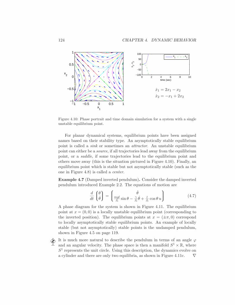
124 CHAPTER 4. DYNAMIC BEHAVIOR
−1 −0.5 0 0.5 1−1
−0.5
0
0.5
1
x1
x2
0 2 4 6 8 10−100
−50
0
50
100
time (sec)
x 1, x2
x1
x2
x1 = 2x1 − x2
x2 = −x1 + 2x2
Figure 4.10: Phase portrait and time domain simulation for a system with a singleunstable equilibrium point.
For planar dynamical systems, equilibrium points have been assignednames based on their stability type. An asymptotically stable equilibriumpoint is called a sink or sometimes an attractor. An unstable equilibriumpoint can either be a source, if all trajectories lead away from the equilibriumpoint, or a saddle, if some trajectories lead to the equilibrium point andothers move away (this is the situation pictured in Figure 4.10). Finally, anequilibrium point which is stable but not asymptotically stable (such as theone in Figure 4.8) is called a center.
Example 4.7 (Damped inverted pendulum). Consider the damped invertedpendulum introduced Example 2.2. The equations of motion are
d
dt
θ
θ
=
θmglJt
sin θ − γJtθ + l
Jtcos θ u
(4.7)
A phase diagram for the system is shown in Figure 4.11. The equilibriumpoint at x = (0, 0) is a locally unstable equilibrium point (corresponding tothe inverted position). The equilibrium points at x = (±π, 0) correspondto locally asymptotically stable equilibrium points. An example of locallystable (but not asymptotically) stable points is the undamped pendulum,shown in Figure 4.5 on page 119.
It is much more natural to describe the pendulum in terms of an angle ϕand an angular velocity. The phase space is then a manifold S1 × R, whereS1 represents the unit circle. Using this description, the dynamics evolve ona cylinder and there are only two equilibria, as shown in Figure 4.11c. ∇
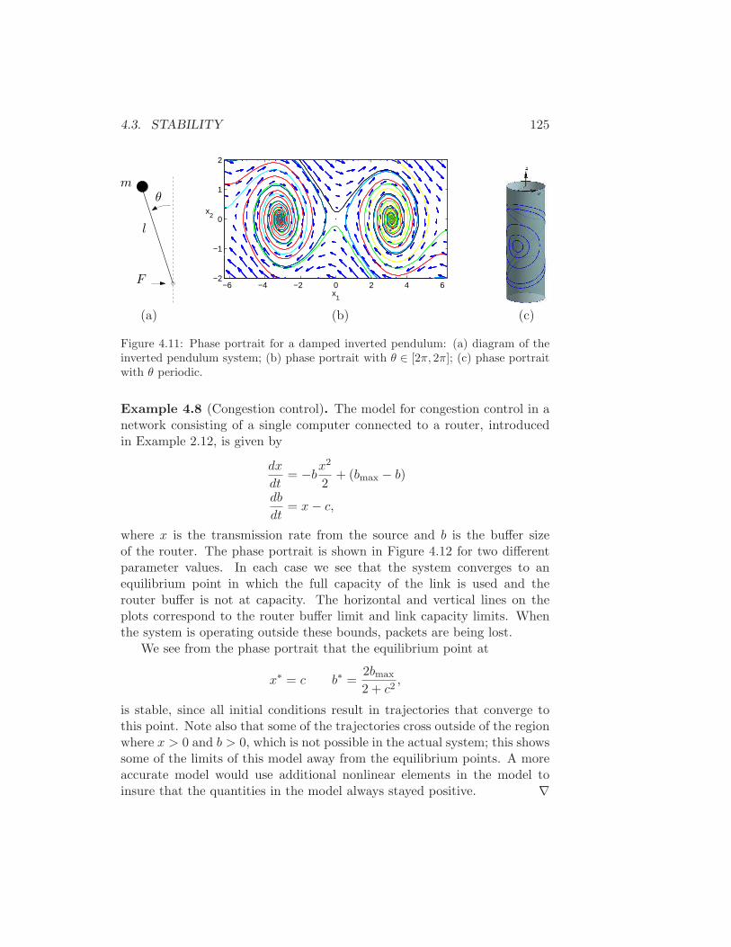
4.3. STABILITY 125
F
θm
l
−6 −4 −2 0 2 4 6−2
−1
0
1
2
x1
x2
(a) (b) (c)
Figure 4.11: Phase portrait for a damped inverted pendulum: (a) diagram of theinverted pendulum system; (b) phase portrait with θ ∈ [2π, 2π]; (c) phase portraitwith θ periodic.
Example 4.8 (Congestion control). The model for congestion control in anetwork consisting of a single computer connected to a router, introducedin Example 2.12, is given by
dx
dt= −bx
2
2+ (bmax − b)
db
dt= x− c,
where x is the transmission rate from the source and b is the buffer sizeof the router. The phase portrait is shown in Figure 4.12 for two differentparameter values. In each case we see that the system converges to anequilibrium point in which the full capacity of the link is used and therouter buffer is not at capacity. The horizontal and vertical lines on theplots correspond to the router buffer limit and link capacity limits. Whenthe system is operating outside these bounds, packets are being lost.
We see from the phase portrait that the equilibrium point at
x∗ = c b∗ =2bmax
2 + c2,
is stable, since all initial conditions result in trajectories that converge tothis point. Note also that some of the trajectories cross outside of the regionwhere x > 0 and b > 0, which is not possible in the actual system; this showssome of the limits of this model away from the equilibrium points. A moreaccurate model would use additional nonlinear elements in the model toinsure that the quantities in the model always stayed positive. ∇
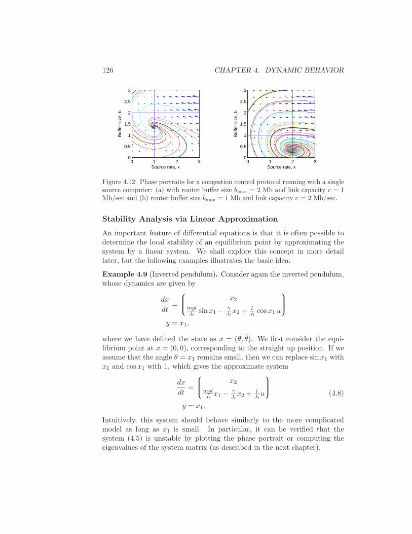
126 CHAPTER 4. DYNAMIC BEHAVIOR
0 1 2 30
0.5
1
1.5
2
2.5
3
Source rate, x
Buf
fer
size
, b
0 1 2 30
0.5
1
1.5
2
2.5
3
Source rate, x
Buf
fer
size
, b
Figure 4.12: Phase portraits for a congestion control protocol running with a singlesource computer: (a) with router buffer size bmax = 2 Mb and link capacity c = 1Mb/sec and (b) router buffer size bmax = 1 Mb and link capacity c = 2 Mb/sec.
Stability Analysis via Linear Approximation
An important feature of differential equations is that it is often possible todetermine the local stability of an equilibrium point by approximating thesystem by a linear system. We shall explore this concept in more detaillater, but the following examples illustrates the basic idea.
Example 4.9 (Inverted pendulum). Consider again the inverted pendulum,whose dynamics are given by
dx
dt=
x2
mglJt
sinx1 − γJtx2 + l
Jtcosx1 u
y = x1,
where we have defined the state as x = (θ, θ). We first consider the equi-librium point at x = (0, 0), corresponding to the straight up position. If weassume that the angle θ = x1 remains small, then we can replace sinx1 withx1 and cosx1 with 1, which gives the approximate system
dx
dt=
x2
mglJtx1 − γ
Jtx2 + l
Jtu
y = x1.
(4.8)
Intuitively, this system should behave similarly to the more complicatedmodel as long as x1 is small. In particular, it can be verified that thesystem (4.5) is unstable by plotting the phase portrait or computing theeigenvalues of the system matrix (as described in the next chapter).
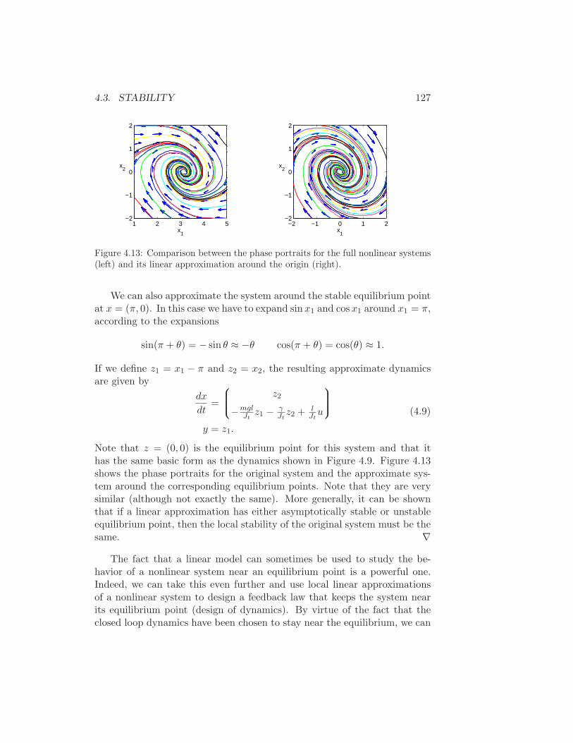
4.3. STABILITY 127
1 2 3 4 5−2
−1
0
1
2
x1
x2
−2 −1 0 1 2−2
−1
0
1
2
x1
x2
Figure 4.13: Comparison between the phase portraits for the full nonlinear systems(left) and its linear approximation around the origin (right).
We can also approximate the system around the stable equilibrium pointat x = (π, 0). In this case we have to expand sinx1 and cosx1 around x1 = π,according to the expansions
sin(π + θ) = − sin θ ≈ −θ cos(π + θ) = cos(θ) ≈ 1.
If we define z1 = x1 − π and z2 = x2, the resulting approximate dynamicsare given by
dx
dt=
z2
−mglJtz1 − γ
Jtz2 + l
Jtu
y = z1.
(4.9)
Note that z = (0, 0) is the equilibrium point for this system and that ithas the same basic form as the dynamics shown in Figure 4.9. Figure 4.13shows the phase portraits for the original system and the approximate sys-tem around the corresponding equilibrium points. Note that they are verysimilar (although not exactly the same). More generally, it can be shownthat if a linear approximation has either asymptotically stable or unstableequilibrium point, then the local stability of the original system must be thesame. ∇
The fact that a linear model can sometimes be used to study the be-havior of a nonlinear system near an equilibrium point is a powerful one.Indeed, we can take this even further and use local linear approximationsof a nonlinear system to design a feedback law that keeps the system nearits equilibrium point (design of dynamics). By virtue of the fact that theclosed loop dynamics have been chosen to stay near the equilibrium, we can
128 CHAPTER 4. DYNAMIC BEHAVIOR
even use the linear approximation to design the feedback that ensures thiscondition is true!
Lyapunov Functions
A powerful tool for determining stability is the use of Lyapunov functions.A Lyapunov function V : R
n → R is an energy-like function that can beused to determine stability of a system. Roughly speaking, if we can find anon-negative function that always decreases along trajectories of the system,we can conclude that the minimum of the function is a stable equilibriumpoint (locally).
To describe this more formally, we start with a few definitions. We saythat a continuous function V (x) is positive definite if V (x) > 0 for all x 6= 0and V (0) = 0. We will often write this as V (x) ≻ 0. Similarly, a functionis negative definite if V (x) < 0 for all x 6= 0 and V (0) = 0. We say thata function V (x) is positive semidefinite if V (x) can be zero at points otherthan x = 0 but otherwise V (x) is strictly positive. We write this as V (x) 0and define negative semi-definite functions analogously.
To illustrate the difference between a positive definite function and apositive semi-definite function, suppose that x ∈ R
2 and let
V1(x) = x21 V2(x) = x2
1 + x22.
Both V1 and V2 are always non-negative. However, it is possible for V1 tobe zero even if x 6= 0. Specifically, if we set x = (0, c) where c ∈ R is anynon-zero number, then V1(x) = 0. On the other hand, V2(x) = 0 if and onlyif x = (0, 0). Thus V1(x) 0 and V2(x) ≻ 0.
We can now characterize the stability of a system
dx
dt= F (x) x ∈ R
n.
Theorem 4.1. Let V (x) be a non-negative function on Rn and let V rep-
resent the time derivative of V along trajectories of the system dynamics:
dV (x)
dt=∂V
∂x
dx
dt=∂V
∂xF (x).
Let Br = Br(0) be a ball of radius r around the origin. If there exists r > 0such that V 0 for all x ∈ Br, then x = 0 is locally stable in the sense ofLyapunov. If V ≺ 0 in Br, then x = 0 is locally asymptotically stable.
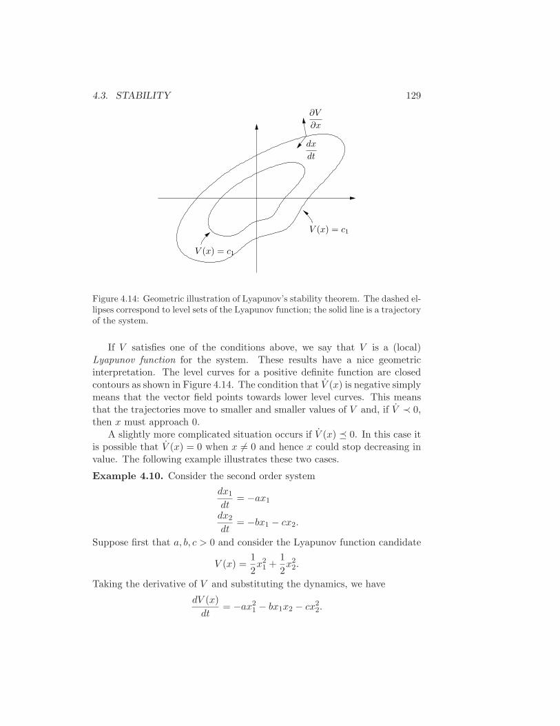
4.3. STABILITY 129
V (x) = c1
dx
dt
∂V
∂x
V (x) = c1
Figure 4.14: Geometric illustration of Lyapunov’s stability theorem. The dashed el-lipses correspond to level sets of the Lyapunov function; the solid line is a trajectoryof the system.
If V satisfies one of the conditions above, we say that V is a (local)Lyapunov function for the system. These results have a nice geometricinterpretation. The level curves for a positive definite function are closedcontours as shown in Figure 4.14. The condition that V (x) is negative simplymeans that the vector field points towards lower level curves. This meansthat the trajectories move to smaller and smaller values of V and, if V ≺ 0,then x must approach 0.
A slightly more complicated situation occurs if V (x) 0. In this case itis possible that V (x) = 0 when x 6= 0 and hence x could stop decreasing invalue. The following example illustrates these two cases.
Example 4.10. Consider the second order system
dx1
dt= −ax1
dx2
dt= −bx1 − cx2.
Suppose first that a, b, c > 0 and consider the Lyapunov function candidate
V (x) =1
2x2
1 +1
2x2
2.
Taking the derivative of V and substituting the dynamics, we have
dV (x)
dt= −ax2
1 − bx1x2 − cx22.
130 CHAPTER 4. DYNAMIC BEHAVIOR
To check whether this is negative definite, we complete the square by writing
dV
dt= −a(x1 +
b
ax2)
2 − (c− b2
a)x2
2.
Clearly V ≺ 0 if a > 0 and (c− b2
a ) > 0.Suppose now that a, b, c > 0 and c = b2/a. Then the derivative of the
Lyapunov function becomes
dV
dt= −a(x1 +
b
ax2)
2 ≤ 0.
This function is not negative definite since if x1 = − bax2 then V = 0 but
x 6= 0. Hence we cannot include asymptotic stability, but we can say thesystem is stable (in the sense of Lyapunov).
The fact that V is not negative definite does not mean that this systemis not asymptotically stable. As we shall see in Chapter 5, we can checkstability of a linear system by looking at the eigenvalues of the dynamicsmatrix for the model
dx
dt=
−a 0−b −c
x.
By inspection (since the system is lower triangular), the eigenvalues areλ1 = −a < 0 and λ2 = −c < 0, and hence the system can be shown to beasymptotically stable.
To demonstrate asymptotic stability using Lyapunov functions, we musttry a different Lyapunov function candidate. Suppose we try
V (x) =1
2x2
1 +1
2(x2 −
b
c− ax1)
2.
It is easy to show that V (x) ≻ 0 since V (x) ≥ 0 for all x and V (x) = 0implies that x1 = 0 and x2 − b
c−ax1 = x2 = 0. We now check the timederivative of V :
dV (x)
dt= x1x1 + (x2 −
b
c− ax1)(x2 −
b
c− ax1)
= −ax21 + (x2 −
b
c− ax1)(−bx1 − cx2 +
b
c− ax1)
= −ax21 − c(x2 −
b
c− ax1)
2.
We see that V ≺ 0 as long as c 6= a and hence we can show stability exceptfor this case (explored in more detail in the exercises). ∇
4.3. STABILITY 131
As this example illustrates, Lyapunov functions are not unique and hencewe can use many different methods to find one. It turns out that Lyapunovfunctions can always be found for any stable system (under certain condi-tions) and hence one knows that if a system is stable, a Lyapunov functionexists (and vice versa). Recent results using “sum of squares” methods haveprovided systematic approaches for finding Lyapunov systems [PPP02]. Sumof squares techniques can be applied to a broad variety of systems, includingsystems whose dynamics are described by polynomial equations as well as“hybrid” systems, which can have different models for different regions ofstate space.
Lyapunov Functions for Linear Systems
For a linear dynamical system of the form
x = Ax
it is possible to construct Lyapunov functions in a systematic manner. Todo so, we consider quadratic functions of the form
V (x) = xTPx
where P ∈ Rn×x is a symmetric matrix (P = P T ). The condition that
V ≻ 0 is equivalent to the condition that P is a positive definite matrix:
xTPx > 0 for all x 6= 0,
which we write as P > 0. It can be shown that if P is symmetric andpositive definite then all of its eigenvalues are real and positive.
Given a candidate Lyapunov function, we can now compute its derivativealong flows of the system:
dV
dt=∂V
∂x
dx
dt= xT (ATP + PA)x.
The requirement that V ≺ 0 (for asymptotic stability) becomes a conditionthat the matrix Q = ATP + PA be negative definite:
xTQx < 0 for all x 6= 0.
Thus, to find a Lyapunov function for a linear system it is sufficient to choosea Q < 0 and solve the Lyapunov equation:
ATP + PA = Q.
This is a linear equation in the entries of P and hence it can be solved usinglinear algebra. The following examples illustrate its use.
132 CHAPTER 4. DYNAMIC BEHAVIOR
Example 4.11. Consider the linear system from Example 4.10, for whichwe have
A =
−a 0−b −c
P =
p11 p12
p21 p22
.
We choose Q = −I ∈ R2×2 and the corresponding Lyapunov equation is
−a −b0 −c
p11 p12
p21 p22
+
p11 p12
p21 p22
−a 0−b −c
=
1 00 1
and solving for the elements of P yields
P =
b2+ac+c2
2a2c+2ac2−b
2c(a+c)
−b2c(a+c)
12
or
V (x) =b2 + ac+ c2
2a2c+ 2ac2x2
1 −b
c(a+ c)x1x2 +
1
2x2
2.
It is easy to verify that P > 0 (check its eigenvalues) and by constructionP = −I < 0. Hence the system is asymptotically stable. ∇
This same technique can also be used for searching for Lyapunov func-tions for nonlinear systems. If we write
dx
dt= f(x) =: Ax+ f(x),
where f(x) contains terms that are second order and higher in the elementsof x, then we can find a Lyapunov function for the linear portion of thesystem and check to see if this is a Lyapunov function for the full nonlinearsystem. The following example illustrates the approach.
Example 4.12 (Congestion control). Consider the congestion control prob-lem described in Example 4.8, where we used phase portraits to demonstratestability of the equilibrium points under different parameter values. We nowwish to consider the general set of equations (from Example 2.12):
dxi
dt= −bx
2i
2+ (bmax − b)
db
dt=
N∑
i=1
xi − c,
4.3. STABILITY 133
The equilibrium points are given by
x∗i =c
Nfor all i b∗ =
2N2bmax
2N2 + c2,
To check for stability, we search for an appropriate Lyapunov function.For notational simplicity, we choose N = 3. It will also be convenient torewrite the dynamics about the equilibrium point by choosing variables
z =
z1z2x3
=
x1 − x∗1x2 − x∗2b− b∗
.
The dynamics written in terms of z become
d
dt
z1z2x3
=
− b∗(z1+c)z1
N2 −(
1 + (2c+Nz1)2
2N2
)
− b∗(z2+c)z2
2 −(
1 + (2c+Nz2)2
2N2
)
z1 + z2
=: F (z)
and z = 0 is an equilibrium point for the transformed system.We now write F (z) as a linear portion plus higher order terms:
F (z) =
− b∗cN z1 − c2+2N2
2N2 z3
− b∗cN z2 − c2+2N2
2N2 z3
z1 + z2
+
− b∗
2 z21
z1(2c+Nz1)z3
2N
− b∗
2 z22
z2(2c+Nz2)z3
2N
z1 + z2
=
− b∗cN 0 − c2+2N2
2N2
0 − b∗cN − c2+2N2
2N2
1 1 0
z1z2z3
+
− b∗
2 z21
z1(2c+Nz1)z3
2N
− b∗
2 z22
z2(2c+Nz2)z3
2N
z1 + z2
.
To find a candidate Lyapunov function, we solve the equation
ATP + PA = Q
where A is the linear portion of F and Q < 0. Choosing Q = −I ∈ R3×3,
we obtain
P =
c2N+3N3
2b∗c3+4b∗cN2N3
2b∗c3+4b∗cN2N2
2c2+4N2
N3
2b∗c3+4b∗cN2c2N+3N3
2b∗c3+4b∗cN2N2
2c2+4N2
N2
2c2+4N2N2
2c2+4N2c2N+4N3
4b∗cN + b∗cN2c2+4N2 .
134 CHAPTER 4. DYNAMIC BEHAVIOR
We now check to see if this is a Lyapunov function for the original system:
V =∂V
∂x
dx
dt= (zTAT + F T (z))Pz + zTP (Az + F (z))
= zT (ATP + PA)z + F T (z)Pz + zTPF (z).
Note that all terms in F are quadratic or higher order in z and hence itfollows that F T (z)Pz and zTPF (z) consist of terms that are at least thirdorder in z. It follows that if z is sufficiently close to zero then the cubicand higher order terms will be smaller than the quadratic terms. Hence,sufficiently close to z = 0, V ≺ 0. ∇
This technique for proving local stability of a nonlinear system by lookingat the linearization about an equilibrium point is a general one that we shallreturn to in Chapter 5.
Krasovskii-Lasalle Invariance Principle
For general nonlinear systems, especially those in symbolic form, it canbe difficult to find a function V ≻ 0 whose derivative is strictly negativedefinition (V ≺ 0). The Krasovskii-Lasalle theorem enables us to concludeasymptotic stability of an equilibrium point under less restrictive conditions,namely in the case that V 0, which is often much easier to construct.However, it applies only to time-invariant or periodic systems.
We will deal with the time-invariant case and begin by introducing a fewmore definitions. We denote the solution trajectories of the time-invariantsystem
dx
dt= F (x) (4.10)
as x(t;x0, t0), which is the solution of equation (4.10) at time t startingfrom x0 at t0. We write x( · ;x0, t0) for the set of all points lying along thetrajectory.
Definition 4.1 (ω limit set). The ω limit set of a trajectory x( · ;x0, t0)is the set of all points z ∈ R
n such that there exists a strictly increasingsequence of times tn such that
s(tn;x0, t0) → z
as n→ ∞.
4.3. STABILITY 135
Definition 4.2 (Invariant set). The set M ⊂ Rn is said to be an invariant
set if for all y ∈M and t0 ≥ 0, we have
x(t; y, t0) ∈M for all t ≥ t0.
It may be proved that the ω limit set of every trajectory is closed andinvariant. We may now state the Krasovskii-Lasalle principle.
Theorem 4.2 (Krasovskii-Lasalle principle). Let V : Rn → R be a locally
positive definite function such that on the compact set Ωr = x ∈ Rn :
V (x) ≤ r we have V (x) ≤ 0. Define
S = x ∈ Ωr : V (x) = 0.
As t→ ∞, the trajectory tends to the largest invariant set inside S; i.e., itsω limit set is contained inside the largest invariant set in S. In particular,if S contains no invariant sets other than x = 0, then 0 is asymptoticallystable.
A global version of the preceding theorem may also be stated. An appli-cation of the Krasovskii-Lasalle principle is given in the following example.
Example 4.13 (Damped spring mass system). Consider a damped springmass system with dynamics
mq + cq + kq = 0.
A natural candidate for a Lyapunov function is the total energy of thesystem, given by
V =1
2mq2 +
1
2kq2.
The derivative of this function along trajectories of the system is
V = mqq + kqq = −cq.
This function is only negative semi-definite and hence we cannot concludeasymptotic stability using Theorem 4.1. However, note that V = 0 impliesthat q = 0. If we define
S = (q, q) : q = 0then we can compute the largest invariant set inside S. For this set, wemust have q(t) = 0 for all t and hence q(t) = 0 as well.
Using the dynamics of the system, we see that if q(t) = 0 and q(t) = 0then q(t) = 0 as well. hence the largest invariant set inside S is (q, q) = 0
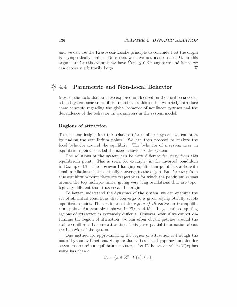
136 CHAPTER 4. DYNAMIC BEHAVIOR
and we can use the Krasovskii-Lasalle principle to conclude that the originis asymptotically stable. Note that we have not made use of Ωr in thisargument; for this example we have V (x) ≤ 0 for any state and hence wecan choose r arbitrarily large. ∇
4.4 Parametric and Non-Local Behavior
Most of the tools that we have explored are focused on the local behavior ofa fixed system near an equilibrium point. In this section we briefly introducesome concepts regarding the global behavior of nonlinear systems and thedependence of the behavior on parameters in the system model.
Regions of attraction
To get some insight into the behavior of a nonlinear system we can startby finding the equilibrium points. We can then proceed to analyze thelocal behavior around the equilibria. The behavior of a system near anequilibrium point is called the local behavior of the system.
The solutions of the system can be very different far away from thisequilibrium point. This is seen, for example, in the inverted pendulumin Example 4.7. The downward hanging equilibrium point is stable, withsmall oscillations that eventually converge to the origin. But far away fromthis equilibrium point there are trajectories for which the pendulum swingsaround the top multiple times, giving very long oscillations that are topo-logically different than those near the origin.
To better understand the dynamics of the system, we can examine theset of all initial conditions that converge to a given asymptotically stableequilibrium point. This set is called the region of attraction for the equilib-rium point. An example is shown in Figure 4.15. In general, computingregions of attraction is extremely difficult. However, even if we cannot de-termine the region of attraction, we can often obtain patches around thestable equilibria that are attracting. This gives partial information aboutthe behavior of the system.
One method for approximating the region of attraction is through theuse of Lyapunov functions. Suppose that V is a local Lyapunov function fora system around an equilibrium point x0. Let Γr be set on which V (x) hasvalue less than c,
Γr = x ∈ Rn : V (x) ≤ r,
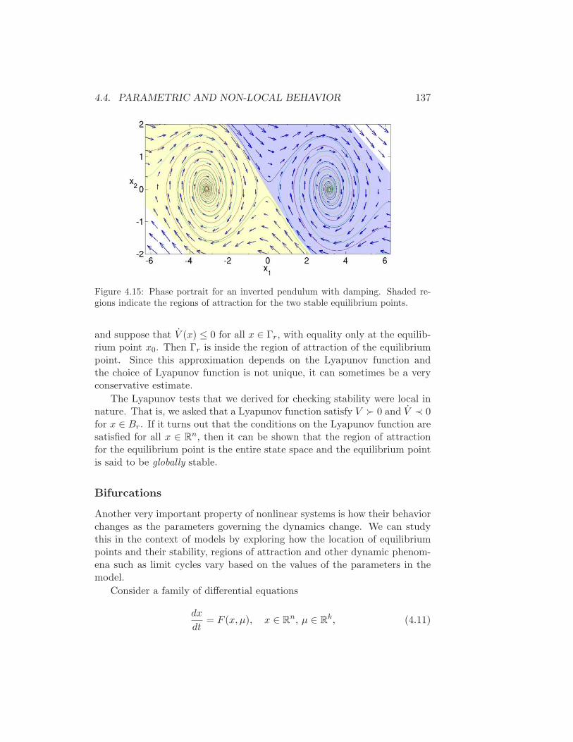
4.4. PARAMETRIC AND NON-LOCAL BEHAVIOR 137
Figure 4.15: Phase portrait for an inverted pendulum with damping. Shaded re-gions indicate the regions of attraction for the two stable equilibrium points.
and suppose that V (x) ≤ 0 for all x ∈ Γr, with equality only at the equilib-rium point x0. Then Γr is inside the region of attraction of the equilibriumpoint. Since this approximation depends on the Lyapunov function andthe choice of Lyapunov function is not unique, it can sometimes be a veryconservative estimate.
The Lyapunov tests that we derived for checking stability were local innature. That is, we asked that a Lyapunov function satisfy V ≻ 0 and V ≺ 0for x ∈ Br. If it turns out that the conditions on the Lyapunov function aresatisfied for all x ∈ R
n, then it can be shown that the region of attractionfor the equilibrium point is the entire state space and the equilibrium pointis said to be globally stable.
Bifurcations
Another very important property of nonlinear systems is how their behaviorchanges as the parameters governing the dynamics change. We can studythis in the context of models by exploring how the location of equilibriumpoints and their stability, regions of attraction and other dynamic phenom-ena such as limit cycles vary based on the values of the parameters in themodel.
Consider a family of differential equations
dx
dt= F (x, µ), x ∈ R
n, µ ∈ Rk, (4.11)
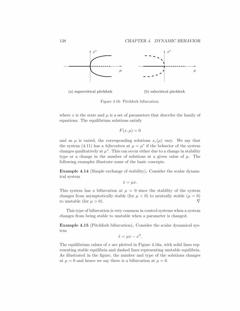
138 CHAPTER 4. DYNAMIC BEHAVIOR
(b) subcritical pitchfork
µ
x∗
µ
x∗
(a) supercritical pitchfork
Figure 4.16: Pitchfork bifurcation.
where x is the state and µ is a set of parameters that describe the family ofequations. The equilibrium solutions satisfy
F (x, µ) = 0
and as µ is varied, the corresponding solutions xe(µ) vary. We say thatthe system (4.11) has a bifurcation at µ = µ∗ if the behavior of the systemchanges qualitatively at µ∗. This can occur either due to a change in stabilitytype or a change in the number of solutions at a given value of µ. Thefollowing examples illustrate some of the basic concepts.
Example 4.14 (Simple exchange of stability). Consider the scalar dynam-ical system
x = µx.
This system has a bifurcation at µ = 0 since the stability of the systemchanges from asymptotically stable (for µ < 0) to neutrally stable (µ = 0)to unstable (for µ > 0). ∇
This type of bifurcation is very common in control systems when a systemchanges from being stable to unstable when a parameter is changed.
Example 4.15 (Pitchfork bifurcation). Consider the scalar dynamical sys-tem
x = µx− x3.
The equilibrium values of x are plotted in Figure 4.16a, with solid lines rep-resenting stable equilibria and dashed lines representing unstable equilibria.As illustrated in the figure, the number and type of the solutions changesat µ = 0 and hence we say there is a bifurcation at µ = 0.
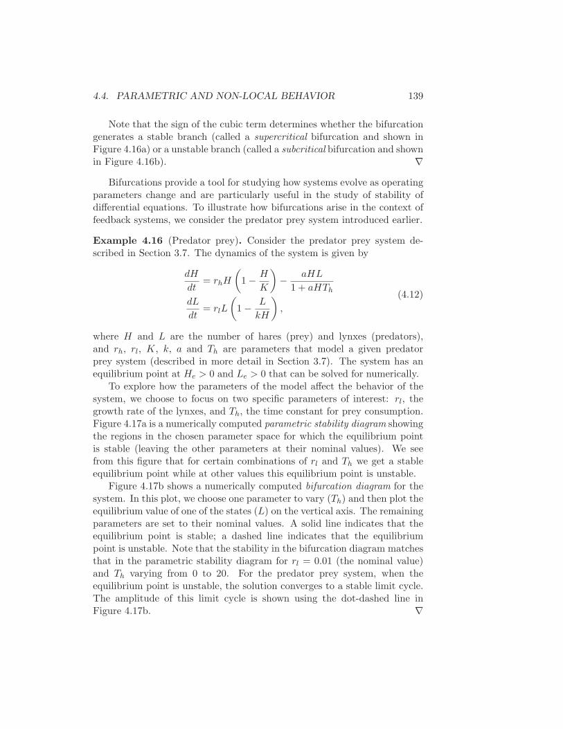
4.4. PARAMETRIC AND NON-LOCAL BEHAVIOR 139
Note that the sign of the cubic term determines whether the bifurcationgenerates a stable branch (called a supercritical bifurcation and shown inFigure 4.16a) or a unstable branch (called a subcritical bifurcation and shownin Figure 4.16b). ∇
Bifurcations provide a tool for studying how systems evolve as operatingparameters change and are particularly useful in the study of stability ofdifferential equations. To illustrate how bifurcations arise in the context offeedback systems, we consider the predator prey system introduced earlier.
Example 4.16 (Predator prey). Consider the predator prey system de-scribed in Section 3.7. The dynamics of the system is given by
dH
dt= rhH
(
1 − H
K
)
− aHL
1 + aHTh
dL
dt= rlL
(
1 − L
kH
)
,
(4.12)
where H and L are the number of hares (prey) and lynxes (predators),and rh, rl, K, k, a and Th are parameters that model a given predatorprey system (described in more detail in Section 3.7). The system has anequilibrium point at He > 0 and Le > 0 that can be solved for numerically.
To explore how the parameters of the model affect the behavior of thesystem, we choose to focus on two specific parameters of interest: rl, thegrowth rate of the lynxes, and Th, the time constant for prey consumption.Figure 4.17a is a numerically computed parametric stability diagram showingthe regions in the chosen parameter space for which the equilibrium pointis stable (leaving the other parameters at their nominal values). We seefrom this figure that for certain combinations of rl and Th we get a stableequilibrium point while at other values this equilibrium point is unstable.
Figure 4.17b shows a numerically computed bifurcation diagram for thesystem. In this plot, we choose one parameter to vary (Th) and then plot theequilibrium value of one of the states (L) on the vertical axis. The remainingparameters are set to their nominal values. A solid line indicates that theequilibrium point is stable; a dashed line indicates that the equilibriumpoint is unstable. Note that the stability in the bifurcation diagram matchesthat in the parametric stability diagram for rl = 0.01 (the nominal value)and Th varying from 0 to 20. For the predator prey system, when theequilibrium point is unstable, the solution converges to a stable limit cycle.The amplitude of this limit cycle is shown using the dot-dashed line inFigure 4.17b. ∇
140 CHAPTER 4. DYNAMIC BEHAVIOR
0 5 10 15 200
0.005
0.01
0.015
0.02
Th
r l
unstable
stable stable
(a)
0 5 10 15 200
100
200
300
400
Th
L
(b)
Figure 4.17: Bifurcation analysis of the predator prey system: (a) parametric stabil-ity diagram showing the regions in parameter space for which the system is stable;(b) bifurcation diagram showing the location and stability of the equilibrium pointas a function of Th. The dotted lines indicate the upper and lower bounds for thelimit cycle at that parameter value (computed via simulation). The nominal valuesof the parameters in the model are rh = 0.02, K = 500, a = 0.03, Th = 5, rl = 0.01and k = 0.2.
Parametric stability diagrams and bifurcation diagrams can provide valu-able insights into the dynamics of a nonlinear system. It is usually neces-sary to careful choose the parameters that one plots, including combiningthe natural parameters of the system to eliminate extra parameters whenpossible.
Control of bifurcations via feedback
Now consider a family of control systems
x = F (x, u, µ), x ∈ Rn, u ∈ R
m, µ ∈ Rk, (4.13)
where u is the input to the system. We have seen in the previous sectionsthat we can sometimes alter the stability of the system by choice of anappropriate feedback control, u = α(x). We now investigate how the controlcan be used to change the bifurcation characteristics of the system. As inthe previous section, we rely on examples to illustrate the key points. Amore detailed description of the use of feedback to control bifurcations canbe found in the work of Abed and co-workers [LA96].
A simple case of bifurcation control is when the system can be stabilizednear the bifurcation point through the use of feedback. In this case, we
4.5. FURTHER READING 141
can completely eliminate the bifurcation through feedback, as the followingsimple example shows.
Example 4.17 (Stabilization of the pitchfork bifurcation). Consider thesubcritical pitchfork example from the previous section, with a simple addi-tive control:
x = µx+ x3 + u.
Choosing the control law u = −kx, we can stabilize the system at thenominal bifurcation point µ = 0 since µ − k < 0 at this point. Of course,this only shifts the bifurcation point and so k must be chosen larger thanthe maximum value of µ that can be achieved.
Alternatively, we could choose the control law u = −kx3 with k > 1.This changes the sign of the cubic term and changes the pitchfork from asubcritical bifurcation to a supercritical bifurcation. The stability of the x =0 equilibrium point is not changed, but the system operating point movesslowly away from zero after the bifurcation rather than growing withoutbound. ∇
4.5 Further Reading
The field of dynamical systems has a rich literature that characterizes thepossible features of dynamical systems and describes how parametric changesin the dynamics can lead to topological changes in behavior. A very read-able introduction to dynamical systems is given by Strogatz [Sto94]. Moretechnical treatments include Guckenheimer and Holmes [GH83] and Wig-gins [Wig90]. For students with a strong interest in mechanics, the text byMarsden and Ratiu [MR94] provides a very elegant approach using toolsfrom differential geometry. Finally, very nice treatments of dynamical sys-tems methods in biology are given by Wilson [Wil99] and Ellner and Guck-enheimer [EG05].
There is a large literature on Lyapunov stability theory. We highlyrecommend the very comprehensive treatment by Khalil [Kha92].
4.6 Exercises
1. Consider the cruise control system described in Section 3.1. Plot thephase portrait for the combined vehicle dynamics and PI compensatorwith k = 1 and ki = 0.5.
142 CHAPTER 4. DYNAMIC BEHAVIOR
2. Show that if we have a solution of the differential equation (4.1) givenby x(t) with initial condition x(t0) = x0, then x(τ) = x(t− t0)− x0 isa solution of the differential equation
dx
dτ= F (x)
with initial condition x(0) = 0.
3. We say that an equilibrium point x∗ = 0 is an exponentially stableequilibrium point of (4.2) if there exist constants m,α > 0 and ǫ > 0such that
‖x(t)‖ ≤ me−α(t−t0)‖x(t0)‖ (4.14)
for all ‖x(t0)‖ ≤ ǫ and t ≥ t0. Prove that an equilibrium point isexponentially stable if and only if there exists an ǫ > 0 and a functionV (x, t) that satisfies
α1‖x‖2 ≤ V (x, t) ≤ α2‖x‖2
dV
dt
∣∣∣∣x=f(x,t)
≤ −α3‖x‖2
‖∂V∂x
(x, t)‖ ≤ α4‖x‖
for some positive constants α1, α2, α3, α4, and ‖x‖ ≤ ǫ.
4. Consider the asymptotically stable system
dx
dt=
−λ 0b −λ
x,
where λ > 0. Find a Lyapunov function for the system that provesasymptotic stability.
Chapter 5
Linear Systems
Few physical elements display truly linear characteristics. For example therelation between force on a spring and displacement of the spring is alwaysnonlinear to some degree. The relation between current through a resistor andvoltage drop across it also deviates from a straight-line relation. However, ifin each case the relation is ?reasonably? linear, then it will be found that thesystem behavior will be very close to that obtained by assuming an ideal, linearphysical element, and the analytical simplification is so enormous that wemake linear assumptions wherever we can possibly to so in good conscience.
R. Cannon, Dynamics of Physical Systems, 1967 [Can03].
In Chapters 2–4 we considered the construction and analysis of differen-tial equation models for physical systems. We placed very few restrictionson these systems other than basic requirements of smoothness and well-posedness. In this chapter we specialize our results to the case of linear,time-invariant, input/output systems. This important class of systems isone for which a wealth of analysis and synthesis tools are available, andhence it has found great utility in a wide variety of applications.
5.1 Basic Definitions
We have seen several examples of linear differential equations in the ex-amples of the previous chapters. These include the spring mass system(damped oscillator) and the operational amplifier in the presence of small(non-saturating) input signals. More generally, many physical systems canbe modeled very accurately by linear differential equations. Electrical cir-cuits are one example of a broad class of systems for which linear models canbe used effectively. Linear models are also broadly applicable in mechani-
143
144 CHAPTER 5. LINEAR SYSTEMS
cal engineering, for example as models of small deviations from equilibria insolid and fluid mechanics. Signal processing systems, including digital filtersof the sort used in CD and MP3 players, are another source of good exam-ples, although often these are best modeled in discrete time (as described inmore detail in the exercises).
In many cases, we create systems with linear input/output responsethrough the use of feedback. Indeed, it was the desire for linear behav-ior that led Harold S. Black, who invited the negative feedback amplifier,to the principle of feedback as a mechanism for generating amplification.Almost all modern single processing systems, whether analog or digital, usefeedback to produce linear or near-linear input/output characteristics. Forthese systems, it is often useful to represent the input/output characteristicsas linear, ignoring the internal details required to get that linear response.
For other systems, nonlinearities cannot be ignored if one cares aboutthe global behavior of the system. The predator prey problem is one exam-ple of this; to capture the oscillatory behavior of the coupled populationswe must include the nonlinear coupling terms. However, if we care aboutwhat happens near an equilibrium point, it often suffices to approximatethe nonlinear dynamics by their local linearization, as we already exploredbriefly in Section 4.3. The linearization is essentially an approximation ofthe nonlinear dynamics around the desired operating point.
Linearity
We now proceed to define linearity of input/output systems more formally.Consider a state space system of the form
dx
dt= f(x, u)
y = h(x, u),(5.1)
where x ∈ Rn, u ∈ R
p and y ∈ Rq. As in the previous chapters, we will
usually restrict ourselves to the single input, single output case by takingp = q = 1. We also assume that all functions are smooth and that for areasonable class of inputs (e.g., piecewise continuous functions of time) thatthe solutions of equation (5.1) exist for all time.
It will be convenient to assume that the origin x = 0, u = 0 is anequilibrium point for this system (x = 0) and that h(0, 0) = 0. Indeed, wecan do so without loss of generality. To see this, suppose that (xe, ue) 6= (0, 0)is an equilibrium point of the system with output ye = h(xe, ue) 6= 0. Then
5.1. BASIC DEFINITIONS 145
we can define a new set of states, inputs, and outputs
x = x− xe u = u− ue y = y − ye
and rewrite the equations of motion in terms of these variables:
d
dtx = f(x+ xe, u+ ue) =: f(x, u)
y = h(x+ xe, u+ ue) − ye =: h(x, u).
In the new set of variables, we have that the origin is an equilibrium pointwith output 0, and hence we can carry our analysis out in this set of vari-ables. Once we have obtained our answers in this new set of variables, wesimply have to remember to “translate” them back to the original coordi-nates (through a simple set of additions).
Returning to the original equations (5.1), now assuming without loss ofgenerality that the origin is the equilibrium point of interest, we write theoutput y(t) corresponding to initial condition x(0) = x0 and input u(t) asy(t;x0, u). Using this notation, a system is said to be a linear input/outputsystem if the following conditions are satisfied:
(i) y(t;αx1 + βx2, 0) = αy(t;x1, 0) + βy(t;x2, 0)
(ii) y(t;αx0, δu) = αy(t;x0, 0) + δy(t; 0, u)
(iii) y(t; 0, δu1 + γu2) = δy(t; 0, u1) + γy(t; 0, u2).
Thus, we define a system to be linear if the outputs are jointly linear in theinitial condition response and the forced response. Property (ii) is the usualdecomposition of a system response into the homogeneous response (u = 0)and the particular response (x0 = 0). Property (iii) is the formal definitionof the the principle of superposition illustrated in Figure 5.1.
Example 5.1 (Scalar system). Consider the first order differential equation
dx
dt= ax+ u
y = x
with x(0) = x0. Let u1 = A sinω1t and u2 = B cosω2t. The homogeneoussolution the ODE is
xh(t) = eatx0
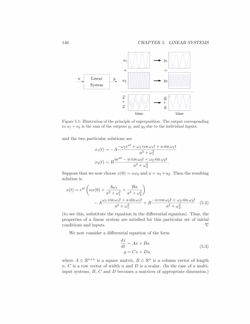
146 CHAPTER 5. LINEAR SYSTEMS
time
u yLinear
Systemy2
u1
+
u2
u1
+u
2
y 1+y 2
+
y1
time
Figure 5.1: Illustration of the principle of superposition. The output correspondingto u1 + u2 is the sum of the outputs y1 and y2 due to the individual inputs.
and the two particular solutions are
x1(t) = −A−ω1eat + ω1 cosω1t+ a sinω1t
a2 + ω21
x2(t) = Baeat − a cosω2t+ ω2 sinω2t
a2 + ω22
.
Suppose that we now choose x(0) = αx0 and u = u1+u2. Then the resultingsolution is
x(t) = eat
(
αx(0) +Aω1
a2 + ω21
+Ba
a2 + ω22
)
−Aω1 cosω1t+ a sinω1t
a2 + ω21
+B−a cosω2t+ ω2 sinω2t
a2 + ω22
(5.2)
(to see this, substitute the equation in the differential equation). Thus, theproperties of a linear system are satisfied for this particular set of initialconditions and inputs. ∇
We now consider a differential equation of the form
dx
dt= Ax+Bu
y = Cx+Du,(5.3)
where A ∈ Rn×n is a square matrix, B ∈ R
n is a column vector of lengthn, C is a row vector of width n and D is a scalar. (In the case of a multi-input systems, B, C and D becomes a matrices of appropriate dimension.)
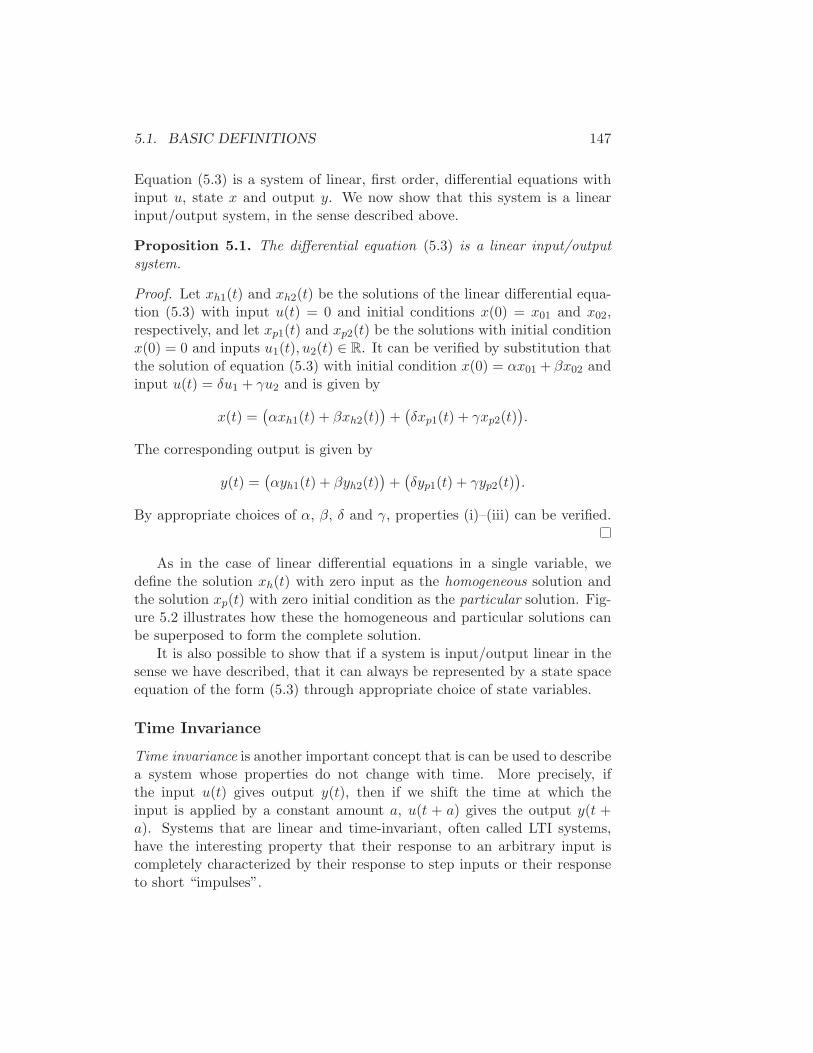
5.1. BASIC DEFINITIONS 147
Equation (5.3) is a system of linear, first order, differential equations withinput u, state x and output y. We now show that this system is a linearinput/output system, in the sense described above.
Proposition 5.1. The differential equation (5.3) is a linear input/outputsystem.
Proof. Let xh1(t) and xh2(t) be the solutions of the linear differential equa-tion (5.3) with input u(t) = 0 and initial conditions x(0) = x01 and x02,respectively, and let xp1(t) and xp2(t) be the solutions with initial conditionx(0) = 0 and inputs u1(t), u2(t) ∈ R. It can be verified by substitution thatthe solution of equation (5.3) with initial condition x(0) = αx01 + βx02 andinput u(t) = δu1 + γu2 and is given by
x(t) =(αxh1(t) + βxh2(t)
)+(δxp1(t) + γxp2(t)
).
The corresponding output is given by
y(t) =(αyh1(t) + βyh2(t)
)+(δyp1(t) + γyp2(t)
).
By appropriate choices of α, β, δ and γ, properties (i)–(iii) can be verified.
As in the case of linear differential equations in a single variable, wedefine the solution xh(t) with zero input as the homogeneous solution andthe solution xp(t) with zero initial condition as the particular solution. Fig-ure 5.2 illustrates how these the homogeneous and particular solutions canbe superposed to form the complete solution.
It is also possible to show that if a system is input/output linear in thesense we have described, that it can always be represented by a state spaceequation of the form (5.3) through appropriate choice of state variables.
Time Invariance
Time invariance is another important concept that is can be used to describea system whose properties do not change with time. More precisely, ifthe input u(t) gives output y(t), then if we shift the time at which theinput is applied by a constant amount a, u(t + a) gives the output y(t +a). Systems that are linear and time-invariant, often called LTI systems,have the interesting property that their response to an arbitrary input iscompletely characterized by their response to step inputs or their responseto short “impulses”.
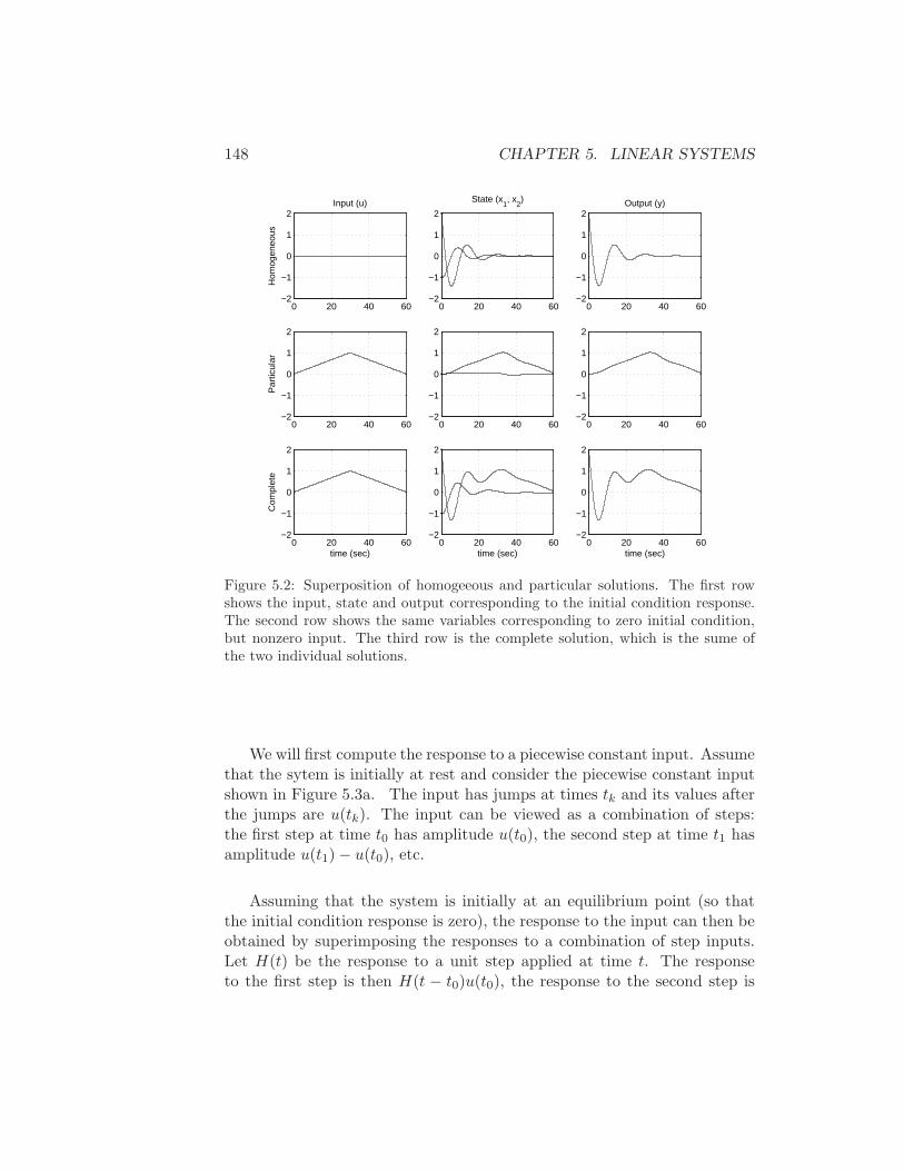
148 CHAPTER 5. LINEAR SYSTEMS
0 20 40 60−2
−1
0
1
2
Hom
ogen
eous
Input (u)
0 20 40 60−2
−1
0
1
2
State (x1, x
2)
0 20 40 60−2
−1
0
1
2Output (y)
0 20 40 60−2
−1
0
1
2
Par
ticul
ar
0 20 40 60−2
−1
0
1
2
0 20 40 60−2
−1
0
1
2
0 20 40 60−2
−1
0
1
2
Com
plet
e
time (sec)0 20 40 60
−2
−1
0
1
2
time (sec)0 20 40 60
−2
−1
0
1
2
time (sec)
Figure 5.2: Superposition of homogeeous and particular solutions. The first rowshows the input, state and output corresponding to the initial condition response.The second row shows the same variables corresponding to zero initial condition,but nonzero input. The third row is the complete solution, which is the sume ofthe two individual solutions.
We will first compute the response to a piecewise constant input. Assumethat the sytem is initially at rest and consider the piecewise constant inputshown in Figure 5.3a. The input has jumps at times tk and its values afterthe jumps are u(tk). The input can be viewed as a combination of steps:the first step at time t0 has amplitude u(t0), the second step at time t1 hasamplitude u(t1) − u(t0), etc.
Assuming that the system is initially at an equilibrium point (so thatthe initial condition response is zero), the response to the input can then beobtained by superimposing the responses to a combination of step inputs.Let H(t) be the response to a unit step applied at time t. The responseto the first step is then H(t − t0)u(t0), the response to the second step is
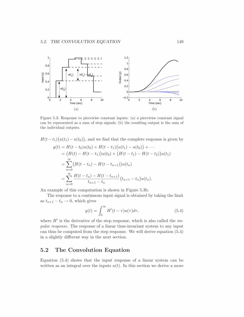
5.2. THE CONVOLUTION EQUATION 149
0 2 4 6 8 100
0.2
0.4
0.6
0.8
1
Time (sec)
Inpu
t (u)
u(t0)
u(t1) u(t
1) − u(t
0)
(a)
0 2 4 6 8 10−0.2
0
0.2
0.4
0.6
0.8
1
1.2
Time (sec)
Out
put (
y)
(b)
Figure 5.3: Response to piecewise constant inputs: (a) a piecewise constant signalcan be represented as a sum of step signals; (b) the resulting output is the sum ofthe individual outputs.
H(t− t1)(u(t1)−u(t0)
), and we find that the complete response is given by
y(t) = H(t− t0)u(t0) +H(t− t1)(u(t1) − u(t0)
)+ · · ·
=(H(t) −H(t− t1)
)u(t0) +
(H(t− t1) −H(t− t2)
)u(t1)
=∞∑
n=0
(H(t− tn) −H(t− tn+1)
)u(tn)
=∞∑
n=0
H(t− tn) −H(t− tn+1)
tn+1 − tn
(tn+1 − tn
)u(tn).
An example of this computation is shown in Figure 5.3b.The response to a continuous input signal is obtained by taking the limit
as tn+1 − tn → 0, which gives
y(t) =
∫ ∞
0H ′(t− τ)u(τ)dτ, (5.4)
where H ′ is the derivative of the step response, which is also called the im-pulse response. The response of a linear time-invariant system to any inputcan thus be computed from the step response. We will derive equation (5.4)in a slightly different way in the next section.
5.2 The Convolution Equation
Equation (5.4) shows that the input response of a linear system can bewritten as an integral over the inputs u(t). In this section we derive a more
150 CHAPTER 5. LINEAR SYSTEMS
general version of this formula, which shows how to compute the output ofa linear system based on its state space representation.
The Matrix Exponential
Although we have shown that the solution of a linear set of differential equa-tions defines a linear input/output system, we have not fully computed thesolution of the system. We begin by considering the homogeneous responsecorresponding to the system
dx
dt= Ax. (5.5)
For the scalar differential equation
x = ax x ∈ R, a ∈ R
the solution is given by the exponential
x(t) = eatx(0).
We wish to generalize this to the vector case, where A becomes a matrix.
We define the matrix exponential as the infinite series
eX = I +X +1
2X2 +
1
3!X3 + · · · =
∞∑
k=0
1
k!Xk, (5.6)
where X ∈ Rn×n is a square matrix and I is the n× n identity matrix. We
make use of the notation
X0 = I X2 = XX Xn = Xn−1X,
which defines what we mean by the “power” of a matrix. Equation (5.6) iseasy to remember since it is just the Taylor series for the scalar exponential,applied to the matrix X. It can be shown that the series in equation (5.6)converges for any matrix X ∈ R
n×n in the same way that the normal expo-nential is defined for any scalar a ∈ R.
Replacing X in equation (5.6) by At where t ∈ R we find that
eAt = I +At+1
2A2t2 +
1
3!A3t3 + · · · =
∞∑
k=0
1
k!Aktk,
5.2. THE CONVOLUTION EQUATION 151
and differentiating this expression with respect to t gives
d
dteAt = A+At+
1
2A3t2 + · · · = A
∞∑
k=0
1
k!Aktk = AeAt. (5.7)
Multiplying by x(0) from the right we find that x(t) = eAtx(0) is the solutionto the differential equation (5.5) with initial condition x(0). We summarizethis important result as a theorem.
Theorem 5.2. The solution to the homogeneous system of differential equa-tion (5.5) is given by
x(t) = eAtx(0).
Notice that the form of the solution is exactly the same as for scalarequations.
The form of the solution immediately allows us to see that the solutionis linear in the initial condition. In particular, if xh1 is the solution toequation (5.5) with initial condition x(0) = x01 and xh2 with initial conditionx02, then the solution with initial condition x(0) = αx01 + βx02 is given by
x(t) = eAt(αx01 + βx02
)=(αeAtx01 + βeAtx02) = αxh1(t) + βxh2(t).
Similarly, we see that the corresponding output is given by
y(t) = Cx(t) = αyh1(t) + βyh2(t),
where yh1 and yh2 are the outputs corresponding to xh1 and xh2.
We illustrate computation of the matrix exponential by three examples.
Example 5.2 (Double integrator). A very simple linear system that is usefulfor understanding basic concepts is the second order system given by
q = u
y = q.
This system system is called a double integrator because the input u isintegrated twice to determine the output y.
In state space form, we write x = (q, q) and
dx
dt=
0 10 0
x+
01
u.
152 CHAPTER 5. LINEAR SYSTEMS
The dynamics matrix of a double integrator is
A =
0 10 0
and we find by direct calculation that A2 = 0 and hence
eAt =
1 t0 1
.
Thus the homogeneous solution (u = 0) for the double integrator is givenby
x(t) =
x1(0) + tx2(0)
x2(0)
y(t) = x1(0) + tx2(0).
∇
Example 5.3 (Undamped oscillator). A simple model for an oscillator, suchas the spring mass system with zero damping, is
mq + kq = u.
Putting the system into state space form, the dynamics matrix for thissystem is
A =
0 1
− km 0
We have
eAt =
cosω0t
1ω0
sinω0t
−ω0 sinω0t cosω0t
ω0 =
√
k
m,
and the solution is then given by
x(t) = eAtx(0) =
cosω0t
1ω0
sinω0t
−ω0 sinω0t cosω0t
x1(0)x2(0)
.
This solution can be verified by differentiation:
d
dtx(t) =
−ω0 sinω0t cosω0t−ω2
0 cosω0t −ω0 sinω0t
x1(0)x2(0)
.
=
0 1
−ω20 0
cosω0t
1ω0
sinω0t
−ω0 sinω0t cosω0t
x1(0)x2(0)
= Ax(t).
5.2. THE CONVOLUTION EQUATION 153
If the damping c is nonzero, the solution is more complicated, but the matrixexponential can be shown to be
eAt = e−ct2m
eωdt + e−ωdt
2+eωdt − e−ωdt
2√c2 − 4km
eωdt − e−ωdt
√c2 − 4km
−keωdt − ke−ωdt
√c2 − 4km
eωdt + e−ωdt
2− ceωdt − ce−ωdt
2√c2 − 4km
,
where ωd =√c2 − 4km/2m. Note that ωd can either be real or complex,
but in the case it is complex the combinations of terms will always yield apositive value for the entry in the matrix exponential. ∇
Example 5.4 (Diagonal system). Consider a diagonal matrix
A =
λ1 0λ2
. . .
0 λn
The kth power of At is also diagonal,
(At)k =
λk1t
k 0λk
2tk
. . .
0 λknt
k
and it follows from the series expansion that the matrix exponential is givenby
eAt =
eλ1t 0eλ2t
. . .
0 eλnt
.
∇
Eigenvalues and Modes
The initial condition response of a linear system can be written in terms of amatrix exponential involving the dynamics matrix A. The properties of thematrix A therefore determine the resulting behavior of the system. Given a
154 CHAPTER 5. LINEAR SYSTEMS
matrix A ∈ Rn×n, recall that λ is an eigenvalue of A with eigenvector v if λ
and v satisfyAv = λv.
In general λ and v may be complex valued, although if A is real-valued thenfor any eigenvalue λ, its complex conjugate λ∗ will also be an eigenvalue(with v∗ as the corresponding eigenvector).
Suppose first that λ and v are a real-valued eigenvalue/eigenvector pairfor A. If we look at the solution of the differential equation for x(0) = v, itfollows from the definition of the matrix exponential that
eAtv =(I +At+
1
2A2t2 + · · ·
)v = (v + λtv +
λ2t2
2v + · · ·
)v = eλtv.
The solution thus lies in the subspace spanned by the eigenvector. Theeigenvalue λ describes how the solution varies in time and is often called amode of the system. If we look at the individual elements of the vectors xand v, it follows that
xi(t)
xj(t)=vi
vk,
and hence the ratios of the components of the state x are constants. Theeigenvector thus gives the “shape” of the solution and is also called a modeshape of the system.
Figure 5.4 illustrates the modes for a second order system. Notice thatthe state variables have the same sign for the slow mode λ = −0.08 anddifferent signs for the fast mode λ = −0.62.
The situation is a little more complicated when the eigenvalues of A arecomplex. Since A has real elements, the eigenvalues and the eigenvectorsare complex conjugates
λ = σ ± jω and v = u± jw,
which implies that
u =v + v∗
2w =
v − v∗
2j.
Making use of the matrix exponential, we have
eAtv == eλt(u+ jw) = eσt((u cosωt− w sinωt) + j(u sinωt+ w cosωt)
),
which implies
eAtu =1
2
(
eAtv + eAtv∗)
= ueσt cosωt− weσt sinωt
eAtw =1
2j
(
eAtv − eAtv∗)
= ueσt sinωt+ weσt cosωt.
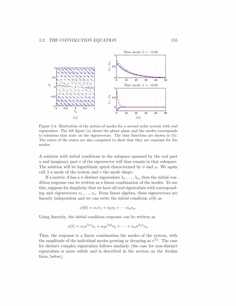
5.2. THE CONVOLUTION EQUATION 155
−1 −0.5 0 0.5 1−1
−0.5
0
0.5
1
x1
x2
(a)
0 10 20 30 40 500
0.5
1
0 10 20 30 40 50
0
0.5
1
x1,x
2x
1,x
2
Slow mode λ = −0.08
Fast mode λ = −0.62
(b)
Figure 5.4: Illustration of the notion of modes for a second order system with realeigenvalues. The left figure (a) shows the phase plane and the modes correspondsto solutions that start on the eigenvectors. The time functions are shown in (b).The ratios of the states are also computed to show that they are constant for themodes.
A solution with initial conditions in the subspace spanned by the real partu and imaginary part v of the eigenvector will thus remain in that subspace.The solution will be logarithmic spiral characterized by σ and ω. We againcall λ a mode of the system and v the mode shape.
If a matrix A has a n distinct eigenvalues λ1, . . . , λn, then the initial con-dition response can be written as a linear combination of the modes. To seethis, suppose for simplicity that we have all real eigenvalues with correspond-ing unit eigenvectors v1, . . . , vn. From linear algebra, these eigenvectors arelinearly independent and we can write the initial condition x(0) as
x(0) = α1v1 + α2v2 + · · ·αnvn.
Using linearity, the initial condition response can be written as
x(t) = α1eλ1tv1 + α2e
λ2tv2 + · · · + αneλntvn.
Thus, the response is a linear combination the modes of the system, withthe amplitude of the individual modes growing or decaying as eλit. The casefor distinct complex eigenvalues follows similarly (the case for non-distincteigenvalues is more subtle and is described in the section on the Jordanform, below).
156 CHAPTER 5. LINEAR SYSTEMS
Linear Input/Output Response
We now return to the general input/output case in equation (5.3), repeatedhere:
dx
dt= Ax+Bu
y = Cx+Du.(5.8)
Using the matrix exponential, the solution to equation (5.8) can be writtenas follows.
Theorem 5.3. The solution to the linear differential equation (5.8) is givenby
x(t) = eAtx(0) +
∫ t
0eA(t−τ)Bu(τ)dτ. (5.9)
Proof. To prove this, we differentiate both sides and use the property (5.7)of the matrix exponential. This gives
dx
dt= AeAtx(0) +
∫ t
0AeA(t−τ)Bu(τ)dτ +Bu(t) = Ax+Bu,
which proves the result. Notice that the calculation is essentially the sameas for proving the result for a first order equation.
It follows from equations (5.8) and (5.9) that the input/output relationfor a linear system is given by
y(t) = CeAtx(0) +
∫ t
0CeA(t−τ)Bu(τ)dτ +Du(t). (5.10)
It is easy to see from this equation that the output is jointly linear in boththe initial conditions and the state: this follows from the linearity of ma-trix/vector multiplication and integration.
Equation (5.10) is called the convolution equation and it represents thegeneral form of the solution of a system of coupled linear differential equa-tions. We see immediately that the dynamics of the system, as characterizedby the matrix A, play a critical role in both the stability and performanceof the system. Indeed, the matrix exponential describes both what hap-pens when we perturb the initial condition and how the system responds toinputs.
Another interpretation of the convolution equation can be given using the
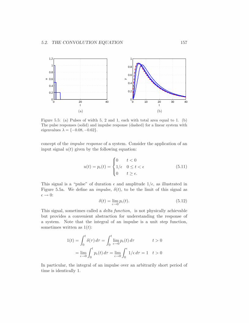
5.2. THE CONVOLUTION EQUATION 157
0 20 400
0.2
0.4
0.6
0.8
1
1.2
u
t
(a)
0 10 20 30 400
0.2
0.4
0.6
0.8
1
y
t
(b)
Figure 5.5: (a) Pulses of width 5, 2 and 1, each with total area equal to 1. (b)The pulse responses (solid) and impulse response (dashed) for a linear system witheigenvalues λ = −0.08,−0.62.
concept of the impulse response of a system. Consider the application of aninput signal u(t) given by the following equation:
u(t) = pǫ(t) =
0 t < 0
1/ǫ 0 ≤ t < ǫ
0 t ≥ ǫ.
(5.11)
This signal is a “pulse” of duration ǫ and amplitude 1/ǫ, as illustrated inFigure 5.5a. We define an impulse, δ(t), to be the limit of this signal asǫ→ 0:
δ(t) = limǫ→0
pǫ(t). (5.12)
This signal, sometimes called a delta function, is not physically achievablebut provides a convenient abstraction for understanding the response ofa system. Note that the integral of an impulse is a unit step function,sometimes written as 1(t):
1(t) =
∫ t
0δ(τ) dτ =
∫ t
0limǫ→0
pǫ(t) dτ t > 0
= limǫ→0
∫ t
0pǫ(t) dτ = lim
ǫ→0
∫ ǫ
01/ǫ dτ = 1 t > 0
In particular, the integral of an impulse over an arbitrarily short period oftime is identically 1.
158 CHAPTER 5. LINEAR SYSTEMS
We define the impulse response of a system, h(t), to be the output cor-responding to an impulse as its input:
h(t) =
∫ t
0CeA(t−τ)Bδ(τ) dτ = CeAtB, (5.13)
where the second equality follows from the fact that δ(t) is zero everywhereexcept the origin and its integral is identically one. We can now writethe convolution equation in terms of the initial condition response and theconvolution of the impulse response and the input signal,
y(t) = CeAtx(0) +
∫ t
0h(t− τ)u(τ) dτ. (5.14)
One interpretation of this equation, explored in Exercise 6, is that the re-sponse of the linear system is the superposition of the response to an infiniteset of shifted impulses whose magnitude is given by the input, u(t). Notethat the second term in this equation is identical to equation (5.4) and it canbe shown that the impulse response is formally equivalent to the derivativeof the step response.
The use of pulses as an approximation of the impulse response provides amechanism for identifying the dynamics of a system from data. Figure 5.5bshows the pulse responses of a system for different pulse widths. Notice thatthe pulse responses approaches the impulse response as the pulse width goesto zero. As a general rule, if the fastest eigenvalue of a stable system hasreal part −λmax, then a pulse of length ǫ will provide a good estimate ofthe impulse response if ǫλmax < 1. Note that for Figure 5.5, a pulse widthof ǫ = 1 s gives ǫλmax = 0.62 and the pulse response is very close to theimpulse response.
Coordinate Changes
The components of the input vector u and the output vector y are uniquephysical signals, but the state variables depend on the coordinate systemchosen to represent the state. The choice of coordinates affects the valuesof the matrices A, B and C that are used in the model. (The direct term Dis not affecting since it maps inputs to outputs.) We now investigate someof the consequences of changing coordinate systems.
Introduce new coordinates z by the transformation z = Tx, where T isan invertible matrix. It follows from equation (5.3) that
dz
dt= T (Ax+Bu) = TAT−1z + TBu = Az + Bu
y = Cx+DU = CT−1z +Du = Cz +Du.
5.2. THE CONVOLUTION EQUATION 159
The transformed system has the same form as equation (5.3) but the ma-trices A, B and C are different:
A = TAT−1, B = TB, C = CT−1, D = D. (5.15)
As we shall see in several places later in the text, there are often specialchoices of coordinate systems that allow us to see a particular propertyof the system, hence coordinate transformations can be used to gain newinsight into the dynamics.
We can also compare the solution of the system in transformed coordi-nates to that in the original state coordinates. We make use of an importantproperty of the exponential map,
eTST−1
= TeST−1,
which can be verified by substitution in the definition of the exponentialmap. Using this property, it is easy to show that
x(t) = T−1z(t) = T−1eAtTx(0) + T−1
∫ t
0eA(t−τ)Bu(τ) dτ.
From this form of the equation, we see that if it is possible to transformA into a form A for which the matrix exponential is easy to compute, wecan use that computation to solve the general convolution equation for theuntransformed state x by simple matrix multiplications. This technique isillustrated in the next section.
Example 5.5 (Modal form). Suppose that A has n real, distinct eigenval-ues, λ1, . . . , λn. It follows from matrix linear algebra that the correspondingeigenvectors v1, . . . vn are linearly independent and form a basis for R
n. Sup-pose that we transform coordinates according to the rule
x = Mz M =
v1 v2 · · · vn
.
Setting T = M−1, it is easy to show that
A = TAT−1 = M−1AM =
λ1 0λ2
. . .
0 λn
.
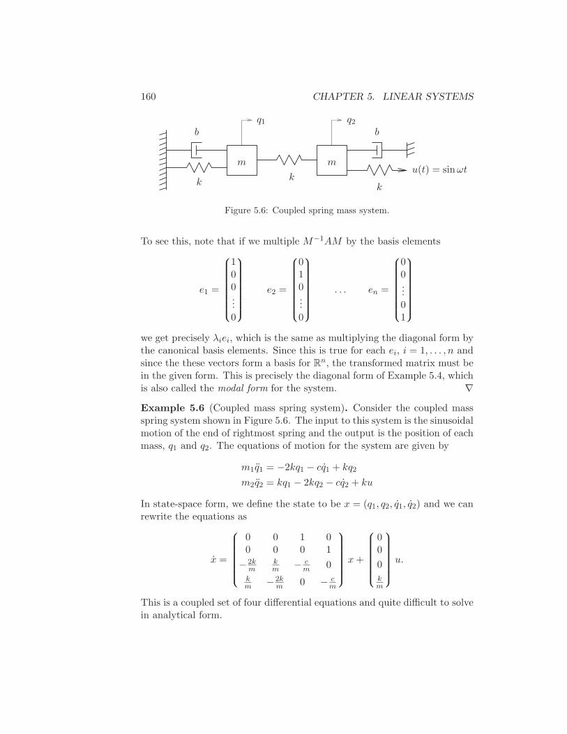
160 CHAPTER 5. LINEAR SYSTEMS
b
u(t) = sinωtm m
kk
bq1 q2
k
Figure 5.6: Coupled spring mass system.
To see this, note that if we multiple M−1AM by the basis elements
e1 =
100...0
e2 =
010...0
. . . en =
00...01
we get precisely λiei, which is the same as multiplying the diagonal form bythe canonical basis elements. Since this is true for each ei, i = 1, . . . , n andsince the these vectors form a basis for R
n, the transformed matrix must bein the given form. This is precisely the diagonal form of Example 5.4, whichis also called the modal form for the system. ∇
Example 5.6 (Coupled mass spring system). Consider the coupled massspring system shown in Figure 5.6. The input to this system is the sinusoidalmotion of the end of rightmost spring and the output is the position of eachmass, q1 and q2. The equations of motion for the system are given by
m1q1 = −2kq1 − cq1 + kq2
m2q2 = kq1 − 2kq2 − cq2 + ku
In state-space form, we define the state to be x = (q1, q2, q1, q2) and we canrewrite the equations as
x =
0 0 1 00 0 0 1
−2km
km − c
m 0
km −2k
m 0 − cm
x+
00
0
km
u.
This is a coupled set of four differential equations and quite difficult to solvein analytical form.
5.3. STABILITY AND PERFORMANCE 161
We now define a transformation z = Tx that puts this system into asimpler form. Let z1 = 1
2(q1 + q2), z2 = z1, z3 = 12(q1 − q2) and z4 = z3, so
that
z = Tx =1
2
1 1 0 00 0 1 11 −1 0 00 0 1 −1
x.
Using the coordinate transformations described above (or simple substitu-tion of variables, which is equivalent), we can write the system in the zcoordinates as
z =
0 1 0 0
− km − c
m 0 00 0 0 1
0 0 −3km − c
m
x+
0k
2m0
− k2m
u.
Note that the resulting matrix equations are are block diagonal and hencedecoupled. We can thus solve for the solutions by computing the two sets ofsecond order system represented by the states (z1, z2) and (z3, z4). Indeed,the functional form of each set of equations is identical to that of a singlespring mass system (Section 2.1).
Once we have solved the two sets of independent second order equations,we can recover the dynamics in the original coordinates by inverting the statetransformation and writing x = T−1z. We can also determine the stabilityof the system by looking at the stability of the independent second ordersystems (Exercise 1). ∇
5.3 Stability and Performance
The special form of a linear system and its solution through the convolutionequation allow us to analytically solve for the stability of equilibrium pointsand input/output performance properties.
Stability of Linear Systems
For a linear system, the stability of the equilibrium point at the origin canbe determined by looking at the eigenvalues of the stability matrix A:
λ(A) = s ∈ C : det(sI −A) = 0.
We use the notation λi for the ith eigenvalue of A, so that λi ∈ λ(A).
162 CHAPTER 5. LINEAR SYSTEMS
The easiest class of linear systems to analyze are those whose systemmatrices are in diagonal form. In this case, the dynamics have the form
dx
dt=
λ1 0λ2
. . .
0 λn
x+
β1
β2...βn
u
y =
γ1 γ2 · · · γn
x+Du.
Using Example 5.4, it is easy to show that the state trajectories for thissystem are independent of each other, so that we can write the solution interms of n individual systems
xi = λixi + βiu.
Each of these scalar solutions is of the form
xi(t) = eλitx(0) +
∫ t
0eλ(t−τ)u(t) dt.
If we consider the stability of the system when u = 0, we see that theequilibrium point xe = 0 is stable if λi ≤ 0 and asymptotically stable ifλi < 0.
Very few systems are diagonal, but some systems can be transformedinto diagonal form via coordinate transformations. One such class of sys-tems is those for which the dynamics matrix has distinct (non-repeating)eigenvalues, as outlined in Example 5.5. In this case it is possible to finda matrix T such that the matrix TAT−1 and the transformed system is indiagonal form, with the diagonal elements equal to the the eigenvalues of theoriginal matrix A. We can reason about the stability of the original systemby noting that x(t) = T−1z(t) and so if the transformed system is stable (orasymptotically stable) then the original system has the same type stability.
For more complicated systems, we make use of the following theorem,proved in the next section:
Theorem 5.4. The system
x = Ax
is asymptotically stable if and only if all eigenvalues of A all have strictlynegative real part and is unstable if any eigenvalue of A has strictly positivereal part.
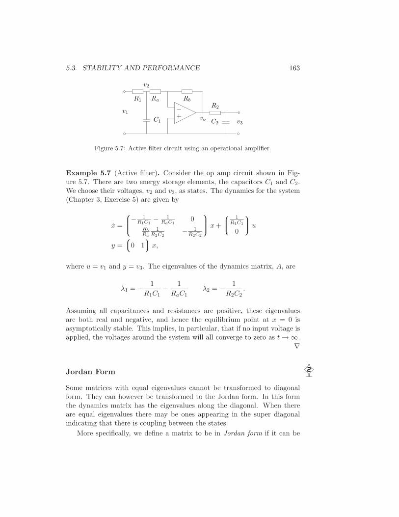
5.3. STABILITY AND PERFORMANCE 163
v2
−+
Rb
v1
v3
R1 Ra
R2
C2C1
vo
Figure 5.7: Active filter circuit using an operational amplifier.
Example 5.7 (Active filter). Consider the op amp circuit shown in Fig-ure 5.7. There are two energy storage elements, the capacitors C1 and C2.We choose their voltages, v2 and v3, as states. The dynamics for the system(Chapter 3, Exercise 5) are given by
x =
− 1R1C1
− 1RaC1
0
Rb
Ra
1R2C2
− 1R2C2
x+
1R1C1
0
u
y =
0 1
x,
where u = v1 and y = v3. The eigenvalues of the dynamics matrix, A, are
λ1 = − 1
R1C1− 1
RaC1λ2 = − 1
R2C2.
Assuming all capacitances and resistances are positive, these eigenvaluesare both real and negative, and hence the equilibrium point at x = 0 isasymptotically stable. This implies, in particular, that if no input voltage isapplied, the voltages around the system will all converge to zero as t→ ∞.
∇
Jordan Form
Some matrices with equal eigenvalues cannot be transformed to diagonalform. They can however be transformed to the Jordan form. In this formthe dynamics matrix has the eigenvalues along the diagonal. When thereare equal eigenvalues there may be ones appearing in the super diagonalindicating that there is coupling between the states.
More specifically, we define a matrix to be in Jordan form if it can be
164 CHAPTER 5. LINEAR SYSTEMS
written as
J =
J1 0 . . . 00 J2 0
0 . . .. . . 0
0 . . . Jk
where Ji =
λi 1 0 . . . 00 λi 1 0...
. . .. . .
...0 . . . 0 λi 10 . . . 0 0 λi
.
(5.16)Each matrix Ji is called a Jordan block and λi for that block corresponds toan eigenvalue of J .
Theorem 5.5 (Jordan decomposition). Any matrix A ∈ Rn×n can be trans-
formed into Jordan form with the eigenvalues of A determining λi in theJordan form.
Proof. See any standard text on linear algebra, such as Strang [Str88].
Converting a matrix into Jordan form can be very complicated, althoughMATLAB can do this conversion for numerical matrices using the Jordan
function. The structure of the resulting Jordan form is particularly inter-esting since there is no requirement that the individual λi’s be unique, andhence for a given eigenvalue we can have one or more Jordan blocks of dif-ferent size. We say that a Jordan block Ji is trivial if Ji is a scalar (1 × 1block).
Once a matrix is in Jordan form, the exponential of the matrix can becomputed in terms of the Jordan blocks:
eJ =
eJ1 0 . . . 00 eJ2 0
0 . . .. . . 0
0 . . . eJk .
(5.17)
This follows from the block diagonal form of J . The exponentials of theJordan blocks can in turn be written as
eJit =
eλit t eλit t2
2! eλit . . . tn−1
(n−1)! eλit
0 eλit t eλit . . . tn−2
(n−2)! eλit
eλit. . .. . . t eλit
0 eλit
(5.18)
5.3. STABILITY AND PERFORMANCE 165
When there are multiple eigenvalues, the invariant subspaces represent-ing the modes correspond to the Jordan blocks of the matrix A . Note that λmay be complex, in which case the transformation T that converts a matrixinto Jordan form will also be complex. When λ has a non-zero imaginarycomponent, the solutions will have oscillatory components since
eσ+jωt = eσt(cosωt+ j sinωt).
We can now use these results to prove Theorem 5.4.
Proof of Theorem 5.4. Let T ∈ Cn×n be an invertible matrix that trans-
forms A into Jordan form, J = TAT−1. Using coordinates z = Tx, we canwrite the solution z(t) as
z(t) = eJtz(0).
Since any solution x(t) can be written in terms of a solution z(t) with z(0) =Tx(0), it follows that it is sufficient to prove the theorem in the transformedcoordinates.
The solution z(t) can be written as a combination of the elements ofthe matrix exponential and from equation (5.18) these elements all decayto zero for arbitrary z(0) if and only if Reλi < 0. Furthermore, if any λi
has positive real part, then there exists an initial condition z(0) such thatthe corresponding solution increases without bound. Since we can scale thisinitial condition to be arbitrarily small, it follows that the equilibrium pointis unstable if any eigenvalue has positive real part.
The existence of a canonical form allows us to prove many properties oflinear systems by changing to a set of coordinates in which the A matrix isin Jordan form. We illustrate this in the following proposition, which followsalong the same lines as the proof of Theorem 5.4.
Proposition 5.6. Suppose that the system
x = Ax
has no eigenvalues with strictly positive real part and one or more eigenval-ues with zero real part. Then the system is stable if and only if the Jordanblocks corresponding to each eigenvalue with zero real part are scalar (1× 1)blocks.
Proof. Exercise 3.
166 CHAPTER 5. LINEAR SYSTEMS
Input/Output Response
So far, this chapter has focused on the stability characteristics of a system.While stability is often a desirably feature, stability alone may not be suf-ficient in many applications. We will want to create feedback systems thatquickly react to changes and give high performance in measurable ways.
We return now to the case of an input/output state space system
dx
dt= Ax+Bu
y = Cx+Du,(5.19)
where x ∈ Rn is the state and u, y ∈ R are the input and output. The
general form of the solution to equation (5.19) is given by the convolutionequation:
y(t) = CeAtx(0) +
∫ t
0CeA(t−τ)Bu(τ)dτ +Du(t).
We see from the form of this equation that the solution consists of an initialcondition response and an input response.
The input response, corresponding to the second term in the equationabove, itself consists of two components—the transient response and steadystate response. The transient response occurs in the first period of time afterthe input is applied and reflects the mismatch between the initial conditionand the steady state solution. The steady state response is the portion ofthe output response that reflects the long term behavior of the system underthe given inputs. For inputs that are periodic, the steady state response willoften also be periodic. An example of the transient and steady state responseis shown in Figure 5.8.
Step Response
A particularly common form of input is a step input, which represents anabrupt change in input from one value to another. A unit step is defined as
u = 1(t) =
0 t = 0
1 t > 0.
The step response of the system (5.3) is defined as the output y(t) startingfrom zero initial condition (or the appropriate equilibrium point) and givena step input. We note that the step input is discontinuous and hence is not
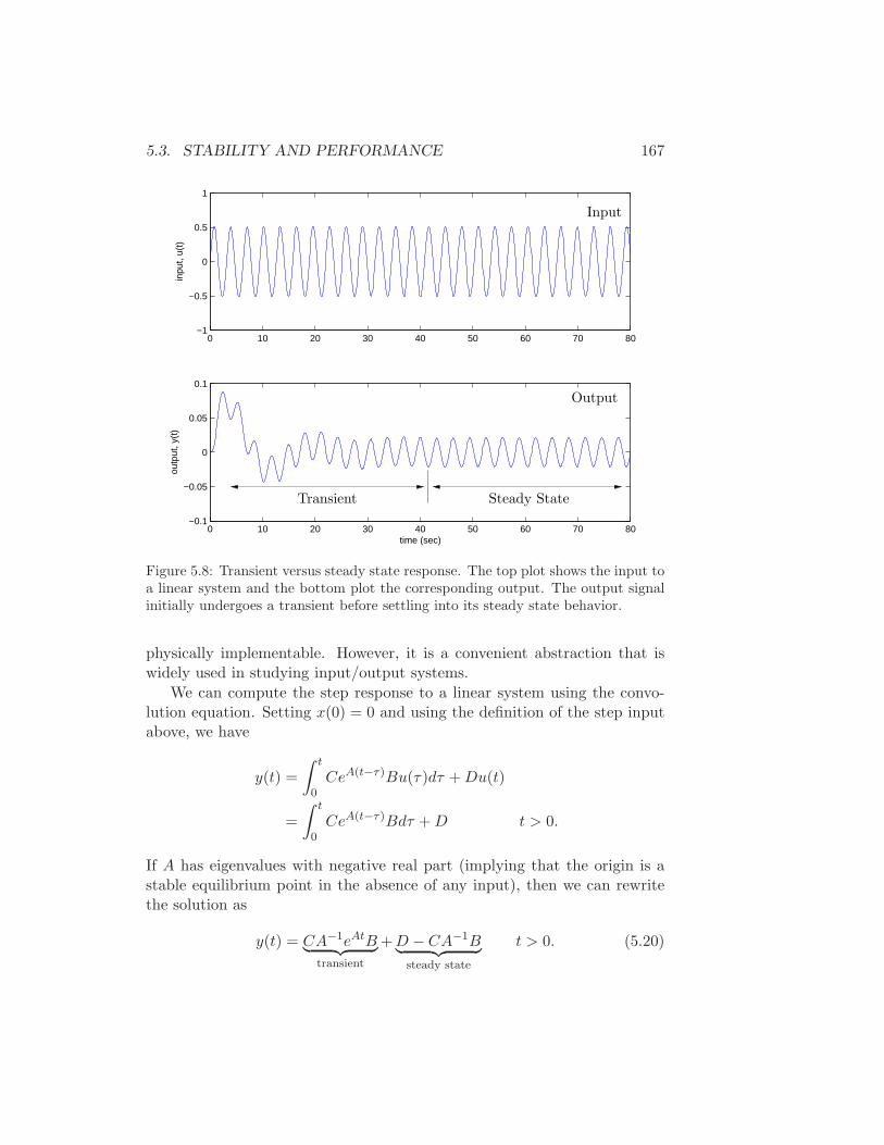
5.3. STABILITY AND PERFORMANCE 167
0 10 20 30 40 50 60 70 80−1
−0.5
0
0.5
1
inpu
t, u(
t)
0 10 20 30 40 50 60 70 80−0.1
−0.05
0
0.05
0.1
time (sec)
outp
ut, y
(t)
Input
Output
Steady StateTransient
Figure 5.8: Transient versus steady state response. The top plot shows the input toa linear system and the bottom plot the corresponding output. The output signalinitially undergoes a transient before settling into its steady state behavior.
physically implementable. However, it is a convenient abstraction that iswidely used in studying input/output systems.
We can compute the step response to a linear system using the convo-lution equation. Setting x(0) = 0 and using the definition of the step inputabove, we have
y(t) =
∫ t
0CeA(t−τ)Bu(τ)dτ +Du(t)
=
∫ t
0CeA(t−τ)Bdτ +D t > 0.
If A has eigenvalues with negative real part (implying that the origin is astable equilibrium point in the absence of any input), then we can rewritethe solution as
y(t) = CA−1eAtB︸ ︷︷ ︸
transient
+D − CA−1B︸ ︷︷ ︸
steady state
t > 0. (5.20)
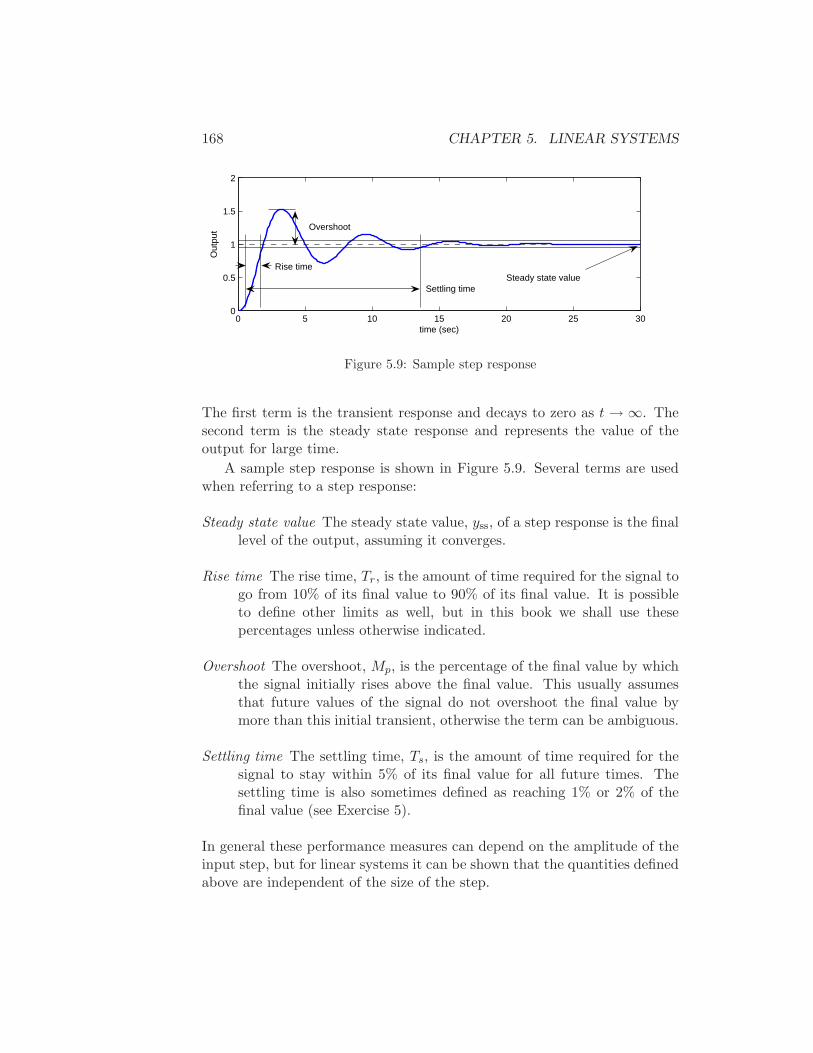
168 CHAPTER 5. LINEAR SYSTEMS
0 5 10 15 20 25 300
0.5
1
1.5
2
time (sec)
Out
put
Rise time
Settling time
Overshoot
Steady state value
Figure 5.9: Sample step response
The first term is the transient response and decays to zero as t → ∞. Thesecond term is the steady state response and represents the value of theoutput for large time.
A sample step response is shown in Figure 5.9. Several terms are usedwhen referring to a step response:
Steady state value The steady state value, yss, of a step response is the finallevel of the output, assuming it converges.
Rise time The rise time, Tr, is the amount of time required for the signal togo from 10% of its final value to 90% of its final value. It is possibleto define other limits as well, but in this book we shall use thesepercentages unless otherwise indicated.
Overshoot The overshoot, Mp, is the percentage of the final value by whichthe signal initially rises above the final value. This usually assumesthat future values of the signal do not overshoot the final value bymore than this initial transient, otherwise the term can be ambiguous.
Settling time The settling time, Ts, is the amount of time required for thesignal to stay within 5% of its final value for all future times. Thesettling time is also sometimes defined as reaching 1% or 2% of thefinal value (see Exercise 5).
In general these performance measures can depend on the amplitude of theinput step, but for linear systems it can be shown that the quantities definedabove are independent of the size of the step.
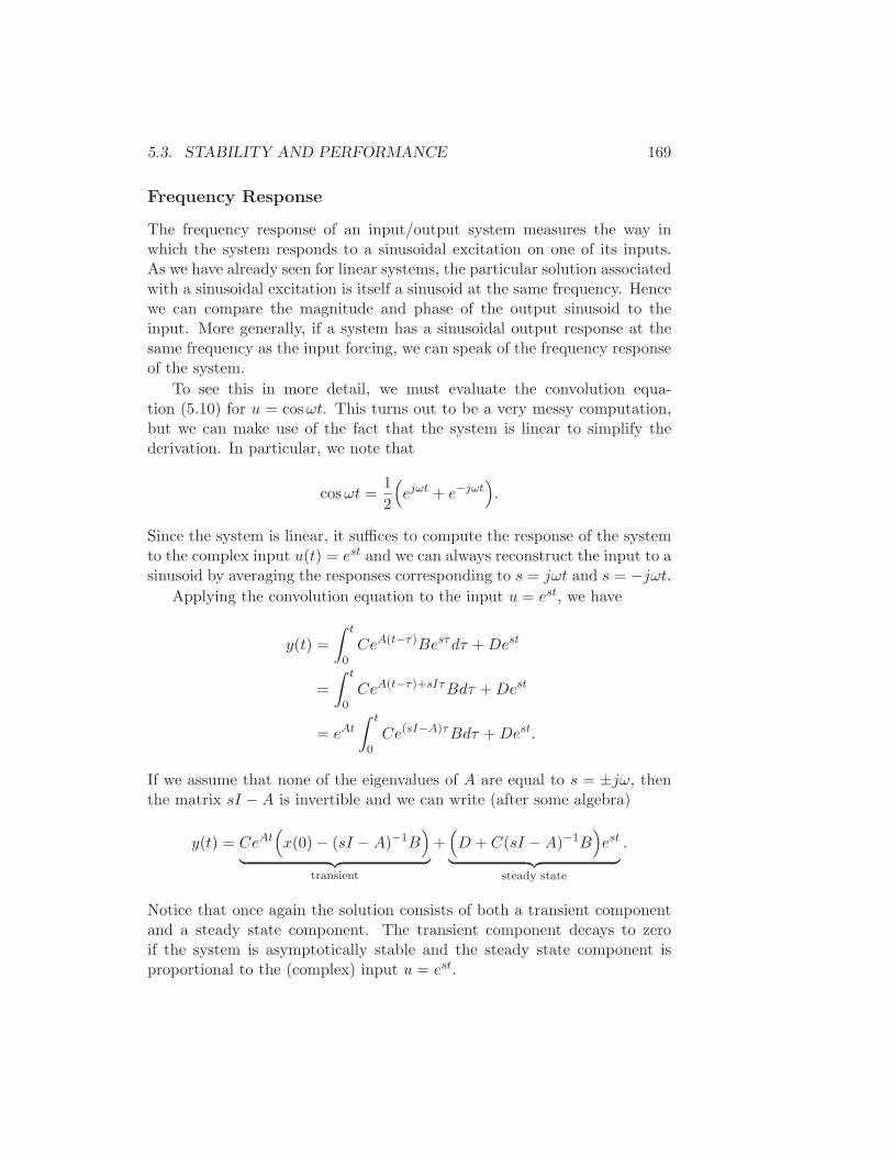
5.3. STABILITY AND PERFORMANCE 169
Frequency Response
The frequency response of an input/output system measures the way inwhich the system responds to a sinusoidal excitation on one of its inputs.As we have already seen for linear systems, the particular solution associatedwith a sinusoidal excitation is itself a sinusoid at the same frequency. Hencewe can compare the magnitude and phase of the output sinusoid to theinput. More generally, if a system has a sinusoidal output response at thesame frequency as the input forcing, we can speak of the frequency responseof the system.
To see this in more detail, we must evaluate the convolution equa-tion (5.10) for u = cosωt. This turns out to be a very messy computation,but we can make use of the fact that the system is linear to simplify thederivation. In particular, we note that
cosωt =1
2
(
ejωt + e−jωt)
.
Since the system is linear, it suffices to compute the response of the systemto the complex input u(t) = est and we can always reconstruct the input to asinusoid by averaging the responses corresponding to s = jωt and s = −jωt.
Applying the convolution equation to the input u = est, we have
y(t) =
∫ t
0CeA(t−τ)Besτdτ +Dest
=
∫ t
0CeA(t−τ)+sIτBdτ +Dest
= eAt
∫ t
0Ce(sI−A)τBdτ +Dest.
If we assume that none of the eigenvalues of A are equal to s = ±jω, thenthe matrix sI −A is invertible and we can write (after some algebra)
y(t) = CeAt(
x(0) − (sI −A)−1B)
︸ ︷︷ ︸
transient
+(
D + C(sI −A)−1B)
est
︸ ︷︷ ︸
steady state
.
Notice that once again the solution consists of both a transient componentand a steady state component. The transient component decays to zeroif the system is asymptotically stable and the steady state component isproportional to the (complex) input u = est.
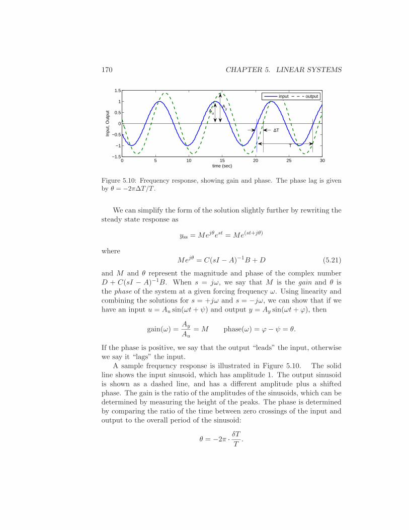
170 CHAPTER 5. LINEAR SYSTEMS
0 5 10 15 20 25 30−1.5
−1
−0.5
0
0.5
1
1.5
time (sec)
Inpu
t, O
utpu
t
Au
Ay
∆T
T
input output
Figure 5.10: Frequency response, showing gain and phase. The phase lag is givenby θ = −2π∆T/T .
We can simplify the form of the solution slightly further by rewriting thesteady state response as
yss = Mejθest = Me(st+jθ)
whereMejθ = C(sI −A)−1B +D (5.21)
and M and θ represent the magnitude and phase of the complex numberD + C(sI − A)−1B. When s = jω, we say that M is the gain and θ isthe phase of the system at a given forcing frequency ω. Using linearity andcombining the solutions for s = +jω and s = −jω, we can show that if wehave an input u = Au sin(ωt+ ψ) and output y = Ay sin(ωt+ ϕ), then
gain(ω) =Ay
Au= M phase(ω) = ϕ− ψ = θ.
If the phase is positive, we say that the output “leads” the input, otherwisewe say it “lags” the input.
A sample frequency response is illustrated in Figure 5.10. The solidline shows the input sinusoid, which has amplitude 1. The output sinusoidis shown as a dashed line, and has a different amplitude plus a shiftedphase. The gain is the ratio of the amplitudes of the sinusoids, which can bedetermined by measuring the height of the peaks. The phase is determinedby comparing the ratio of the time between zero crossings of the input andoutput to the overall period of the sinusoid:
θ = −2π · δTT.
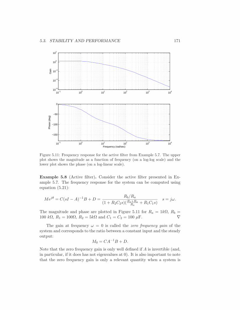
5.3. STABILITY AND PERFORMANCE 171
10−1
100
101
102
103
104
10−6
10−4
10−2
100
102
Gai
n
10−1
100
101
102
103
104
−150
−100
−50
0
Pha
se (
deg)
Frequency (rad/sec)
Figure 5.11: Frequency response for the active filter from Example 5.7. The upperplot shows the magnitude as a function of frequency (on a log-log scale) and thelower plot shows the phase (on a log-linear scale).
Example 5.8 (Active filter). Consider the active filter presented in Ex-ample 5.7. The frequency response for the system can be computed usingequation (5.21):
Mejθ = C(sI −A)−1B +D =Rb/Ra
(1 +R2C2s)(R1+Ra
Ra+R1C1s)
s = jω.
The magnitude and phase are plotted in Figure 5.11 for Ra = 1kΩ, Rb =100 kΩ, R1 = 100Ω, R2 = 5kΩ and C1 = C2 = 100 µF. ∇
The gain at frequency ω = 0 is called the zero frequency gain of thesystem and corresponds to the ratio between a constant input and the steadyoutput:
M0 = CA−1B +D.
Note that the zero frequency gain is only well defined if A is invertible (and,in particular, if it does has not eigenvalues at 0). It is also important to notethat the zero frequency gain is only a relevant quantity when a system is
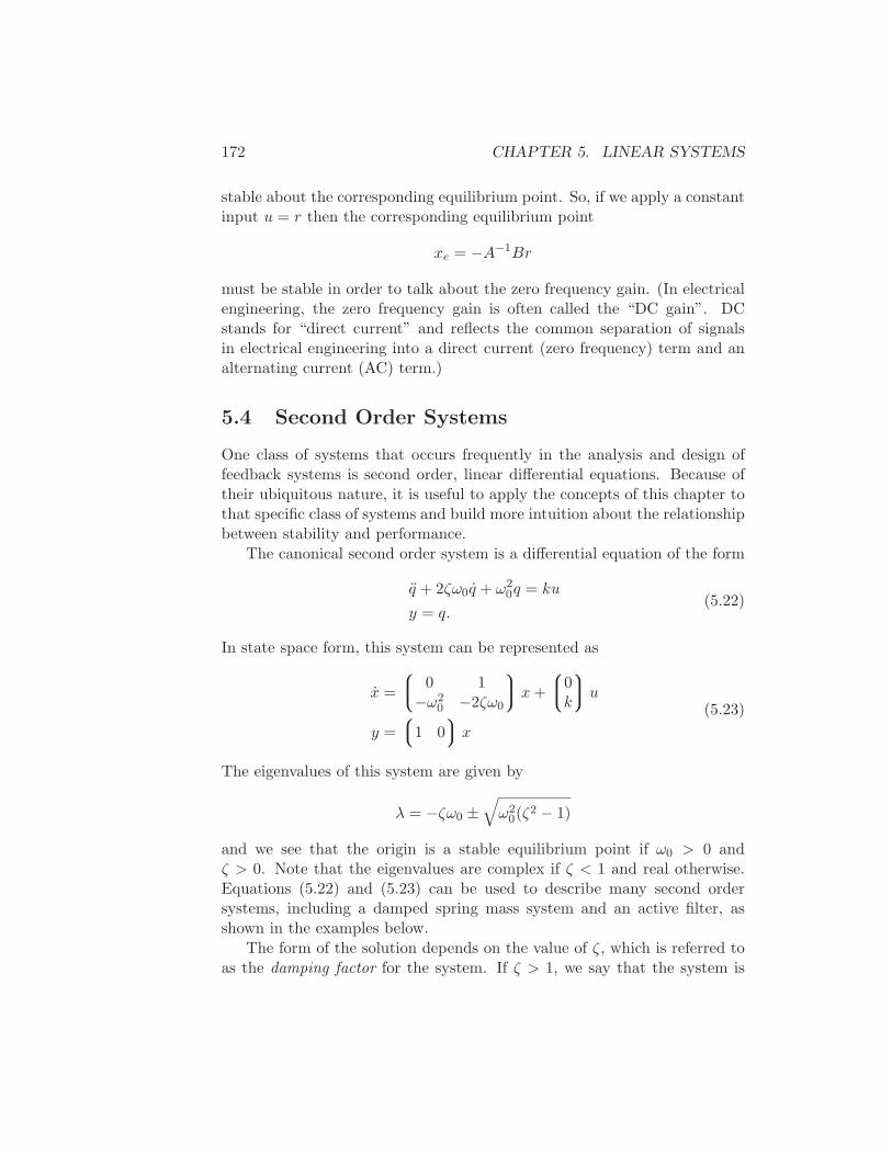
172 CHAPTER 5. LINEAR SYSTEMS
stable about the corresponding equilibrium point. So, if we apply a constantinput u = r then the corresponding equilibrium point
xe = −A−1Br
must be stable in order to talk about the zero frequency gain. (In electricalengineering, the zero frequency gain is often called the “DC gain”. DCstands for “direct current” and reflects the common separation of signalsin electrical engineering into a direct current (zero frequency) term and analternating current (AC) term.)
5.4 Second Order Systems
One class of systems that occurs frequently in the analysis and design offeedback systems is second order, linear differential equations. Because oftheir ubiquitous nature, it is useful to apply the concepts of this chapter tothat specific class of systems and build more intuition about the relationshipbetween stability and performance.
The canonical second order system is a differential equation of the form
q + 2ζω0q + ω20q = ku
y = q.(5.22)
In state space form, this system can be represented as
x =
0 1
−ω20 −2ζω0
x+
0k
u
y =
1 0
x
(5.23)
The eigenvalues of this system are given by
λ = −ζω0 ±√
ω20(ζ
2 − 1)
and we see that the origin is a stable equilibrium point if ω0 > 0 andζ > 0. Note that the eigenvalues are complex if ζ < 1 and real otherwise.Equations (5.22) and (5.23) can be used to describe many second ordersystems, including a damped spring mass system and an active filter, asshown in the examples below.
The form of the solution depends on the value of ζ, which is referred toas the damping factor for the system. If ζ > 1, we say that the system is
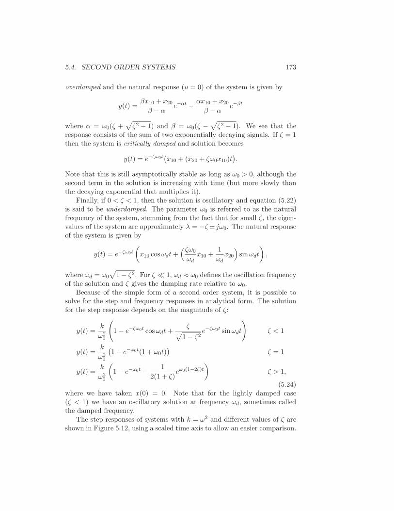
5.4. SECOND ORDER SYSTEMS 173
overdamped and the natural response (u = 0) of the system is given by
y(t) =βx10 + x20
β − αe−αt − αx10 + x20
β − αe−βt
where α = ω0(ζ +√
ζ2 − 1) and β = ω0(ζ −√
ζ2 − 1). We see that theresponse consists of the sum of two exponentially decaying signals. If ζ = 1then the system is critically damped and solution becomes
y(t) = e−ζω0t(x10 + (x20 + ζω0x10)t
).
Note that this is still asymptotically stable as long as ω0 > 0, although thesecond term in the solution is increasing with time (but more slowly thanthe decaying exponential that multiplies it).
Finally, if 0 < ζ < 1, then the solution is oscillatory and equation (5.22)is said to be underdamped. The parameter ω0 is referred to as the naturalfrequency of the system, stemming from the fact that for small ζ, the eigen-values of the system are approximately λ = −ζ± jω0. The natural responseof the system is given by
y(t) = e−ζω0t
(
x10 cosωdt+(ζω0
ωdx10 +
1
ωdx20
)
sinωdt
)
,
where ωd = ω0
√
1 − ζ2. For ζ ≪ 1, ωd ≈ ω0 defines the oscillation frequencyof the solution and ζ gives the damping rate relative to ω0.
Because of the simple form of a second order system, it is possible tosolve for the step and frequency responses in analytical form. The solutionfor the step response depends on the magnitude of ζ:
y(t) =k
ω20
(
1 − e−ζω0t cosωdt+ζ
√
1 − ζ2e−ζω0t sinωdt
)
ζ < 1
y(t) =k
ω20
(1 − e−ω0t(1 + ω0t)
)ζ = 1
y(t) =k
ω20
(
1 − e−ω0t − 1
2(1 + ζ)eω0(1−2ζ)t
)
ζ > 1,
(5.24)where we have taken x(0) = 0. Note that for the lightly damped case(ζ < 1) we have an oscillatory solution at frequency ωd, sometimes calledthe damped frequency.
The step responses of systems with k = ω2 and different values of ζ areshown in Figure 5.12, using a scaled time axis to allow an easier comparison.
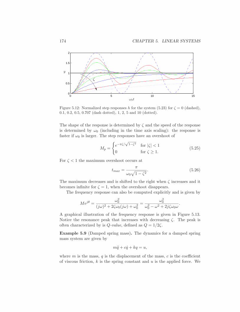
174 CHAPTER 5. LINEAR SYSTEMS
0 5 10 150
0.5
1
1.5
2
ω0t
y
ζ
Figure 5.12: Normalized step responses h for the system (5.23) for ζ = 0 (dashed),0.1, 0.2, 0.5, 0.707 (dash dotted), 1, 2, 5 and 10 (dotted).
The shape of the response is determined by ζ and the speed of the responseis determined by ω0 (including in the time axis scaling): the response isfaster if ω0 is larger. The step responses have an overshoot of
Mp =
e−πζ/√
1−ζ2for |ζ| < 1
0 for ζ ≥ 1.(5.25)
For ζ < 1 the maximum overshoot occurs at
tmax =π
ω0
√
1 − ζ2. (5.26)
The maximum decreases and is shifted to the right when ζ increases and itbecomes infinite for ζ = 1, when the overshoot disappears.
The frequency response can also be computed explicitly and is given by
Mejθ =ω2
0
(jω)2 + 2ζω0(jω) + ω20
=ω2
0
ω20 − ω2 + 2jζω0ω
.
A graphical illustration of the frequency response is given in Figure 5.13.Notice the resonance peak that increases with decreasing ζ. The peak isoften characterized by is Q-value, defined as Q = 1/2ζ.
Example 5.9 (Damped spring mass). The dynamics for a damped springmass system are given by
mq + cq + kq = u,
where m is the mass, q is the displacement of the mass, c is the coefficientof viscous friction, k is the spring constant and u is the applied force. We
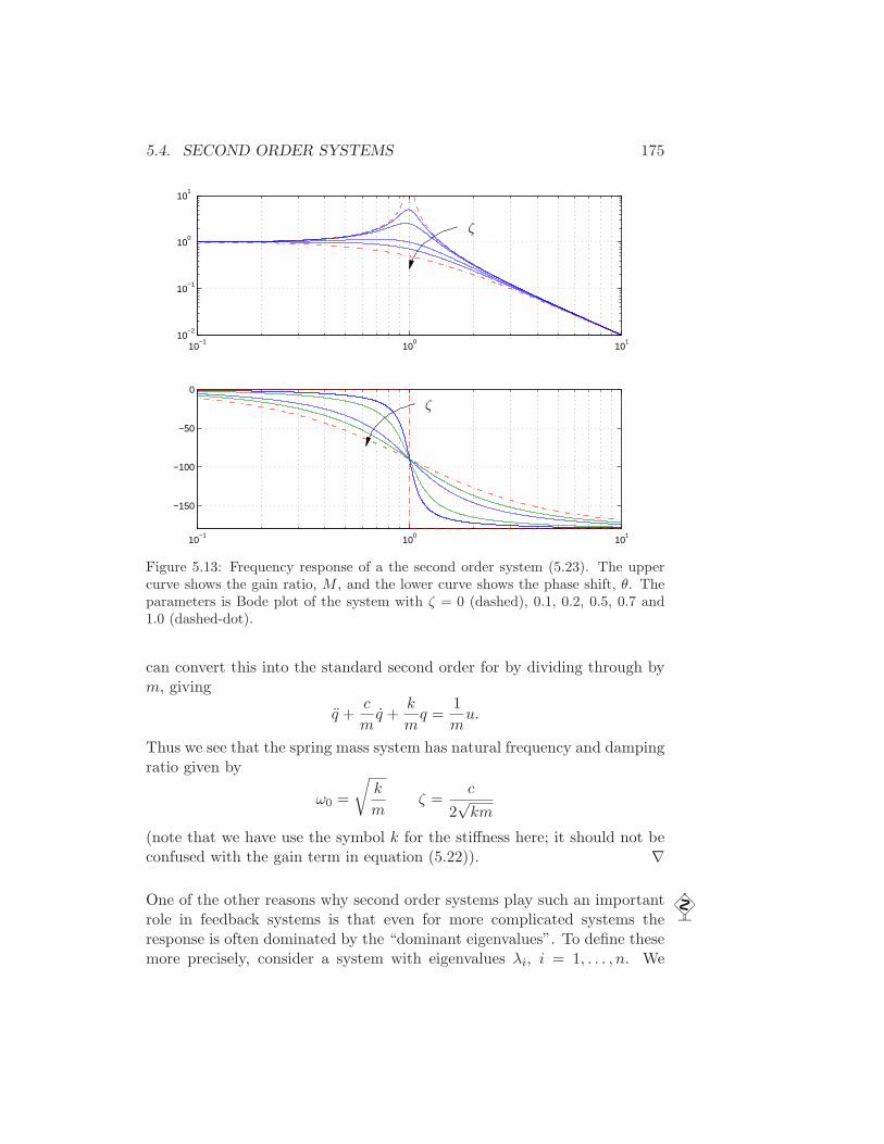
5.4. SECOND ORDER SYSTEMS 175
10−1
100
101
10−2
10−1
100
101
10−1
100
101
−150
−100
−50
0
ζ
ζ
Figure 5.13: Frequency response of a the second order system (5.23). The uppercurve shows the gain ratio, M , and the lower curve shows the phase shift, θ. Theparameters is Bode plot of the system with ζ = 0 (dashed), 0.1, 0.2, 0.5, 0.7 and1.0 (dashed-dot).
can convert this into the standard second order for by dividing through bym, giving
q +c
mq +
k
mq =
1
mu.
Thus we see that the spring mass system has natural frequency and dampingratio given by
ω0 =
√
k
mζ =
c
2√km
(note that we have use the symbol k for the stiffness here; it should not beconfused with the gain term in equation (5.22)). ∇
One of the other reasons why second order systems play such an important role in feedback systems is that even for more complicated systems theresponse is often dominated by the “dominant eigenvalues”. To define thesemore precisely, consider a system with eigenvalues λi, i = 1, . . . , n. We
176 CHAPTER 5. LINEAR SYSTEMS
define the damping factor for a complex eigenvalue λ to be
ζ =−Reλ
|λ|
We say that a complex conjugate pair of eigenvalues λ, λ∗ is a dominantpair if it has the lowest damping factor compared with all other eigenvaluesof the system.
Assuming that a system is stable, the dominant pair of eigenvalues tendsto be the most important element of the response. To see this, assume thatwe have a system in Jordan form with a simple Jordan block correspondingto the dominant pair of eigenvalues:
z =
λλ∗
J2
. . .
Jk
z +Bu
y = Cz.
(Note that the state z may be complex due to the Jordan transformation.)The response of the system will be a linear combination of the responsesfrom each of the individual Jordan subsystems. As we see from Figure 5.12,for ζ < 1 the subsystem with the slowest response is precisely the one withthe smallest damping factor. Hence when we add the responses from eachof the individual subsystems, it is the dominant pair of eigenvalues that willbe dominant factor after the initial transients due to the other terms in thesolution. While this simple analysis does not always hold (for example, ifsome non-dominant terms have large coefficients due to the particular formof the system), it is often the case that the dominant eigenvalues dominatethe (step) response of the system. The following example illustrates theconcept.
5.5 Linearization
As described in the beginning of the chapter, a common source of linearsystem models is through the approximation of a nonlinear system by a linearone. These approximations are aimed at studying the local behavior of asystem, where the nonlinear effects are expected to be small. In this sectionwe discuss how to locally approximate a system by its linearization and what
5.5. LINEARIZATION 177
can be said about the approximation in terms of stability. We begin withan illustration of the basic concept using the speed control example fromChapter 2.
Example 5.10 (Cruise control). The dynamics for the cruise control systemare derived in Section 3.1 and have the form
mdv
dt= αnuT (αnv) −mgCr − 1
2ρCvAv2 −mg sin θ, (5.27)
where the first term on the right hand side of the equation is the force gen-erated by the engine and the remaining three terms are the rolling friction,aerodynamic drag and gravitational disturbance force. There is an equilib-rium (ve, ue) when the force applied by the engine balances the disturbanceforces.
To explore the behavior of the system near the equilibrium we will lin-earize the system. A Taylor series expansion of equation (5.27) around theequilibrium gives
d(v − ve)
dt= a(v − ve) − bg(θ − θe) + b(u− ue) (5.28)
where
a =ueα
2nT
′(αnve) − ρCvAve
mbg = g cos θe b =
αnT (αnve)
m(5.29)
and terms of second and higher order have been neglected. For a car infourth gear with ve = 25 m/s, θe = 0 and the numerical values for the carfrom Section 3.1, the equilibrium value for the throttle is ue = 0.1687 andthe model becomes
d(v − ve)
dt= −0.0101(v − ve) + 1.3203(u− ue) − 9.8(θ − θe) (5.30)
This linear model describes how small perturbations in the velocity aboutthe nominal speed evolve in time.
Figure 5.14, which shows a simulation of a cruise controller with linearand nonlinear models, indicates that the differences between the linear andnonlinear models is not visible in the graph. ∇
Linear Approximation
To proceed more formally, consider a single input, single output nonlinearsystem
dx
dt= f(x, u) x ∈ R
n, u ∈ R
y = h(x, u) y ∈ R
(5.31)
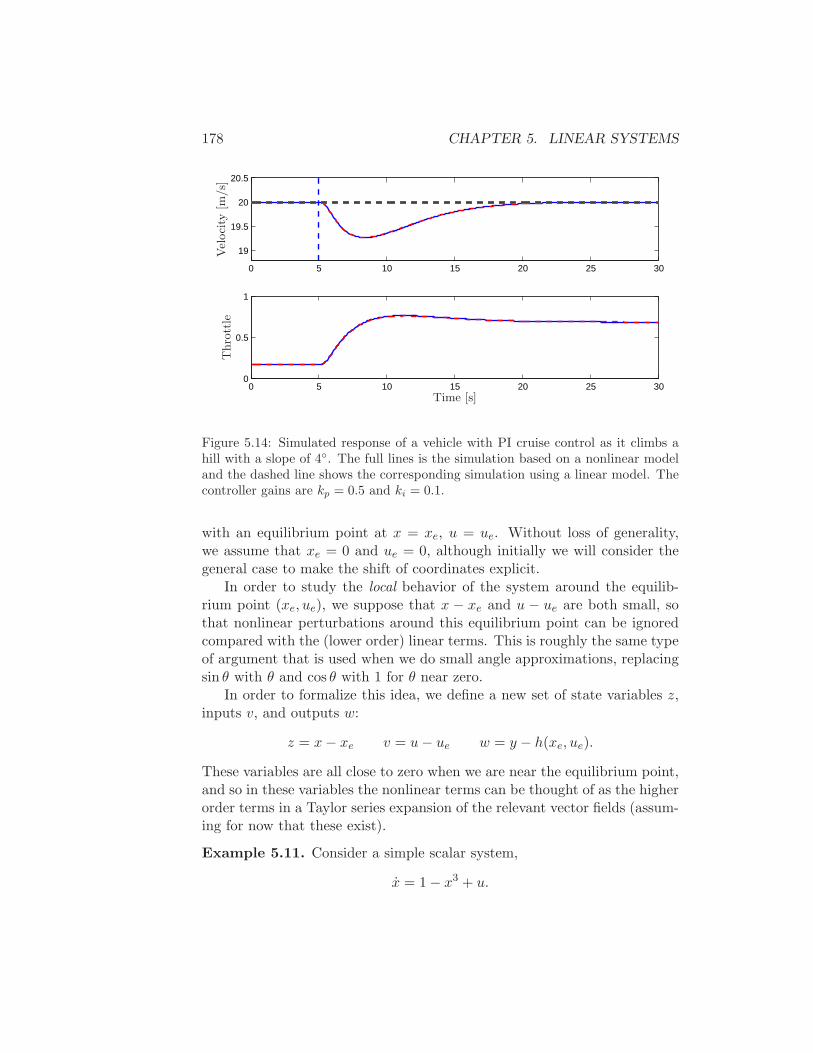
178 CHAPTER 5. LINEAR SYSTEMS
0 5 10 15 20 25 30
19
19.5
20
20.5
0 5 10 15 20 25 300
0.5
1
Thro
ttle
Vel
oci
ty[m
/s]
Time [s]
Figure 5.14: Simulated response of a vehicle with PI cruise control as it climbs ahill with a slope of 4. The full lines is the simulation based on a nonlinear modeland the dashed line shows the corresponding simulation using a linear model. Thecontroller gains are kp = 0.5 and ki = 0.1.
with an equilibrium point at x = xe, u = ue. Without loss of generality,we assume that xe = 0 and ue = 0, although initially we will consider thegeneral case to make the shift of coordinates explicit.
In order to study the local behavior of the system around the equilib-rium point (xe, ue), we suppose that x − xe and u − ue are both small, sothat nonlinear perturbations around this equilibrium point can be ignoredcompared with the (lower order) linear terms. This is roughly the same typeof argument that is used when we do small angle approximations, replacingsin θ with θ and cos θ with 1 for θ near zero.
In order to formalize this idea, we define a new set of state variables z,inputs v, and outputs w:
z = x− xe v = u− ue w = y − h(xe, ue).
These variables are all close to zero when we are near the equilibrium point,and so in these variables the nonlinear terms can be thought of as the higherorder terms in a Taylor series expansion of the relevant vector fields (assum-ing for now that these exist).
Example 5.11. Consider a simple scalar system,
x = 1 − x3 + u.
5.5. LINEARIZATION 179
The point (xe, ue) = (1, 0) is an equilibrium point for this system and wecan thus set
z = x− 1 v = u.
We can now compute the equations in these new coordinates as
z =d
dt(x− 1) = x
= 1 − x3 + u = 1 − (z + 1)3 + v
= 1 − z3 − 3z2 − 3z − 1 + v = −3z − 3z2 − z3 + v.
If we now assume that x stays very close to the equilibrium point, thenz = x− xe is small and z ≪ z2 ≪ z3. We can thus approximate our systemby a new system
z = −3z + v.
This set of equations should give behavior that is close to that of the originalsystem as long as z remains small. ∇
More formally, we define the Jacobian linearization of the nonlinear sys-tem (5.31) as
z = Az +Bv
w = Cz +Dv,(5.32)
where
A =∂f(x, u)
∂x
∣∣∣∣(xe,ue)
B =∂f(x, u)
∂u
∣∣∣∣(xe,ue)
C =∂h(x, u)
∂x
∣∣∣∣(xe,ue)
D =∂h(x, u)
∂u
∣∣∣∣(xe,ue)
(5.33)
The system (5.32) approximates the original system (5.31) when we are nearthe equilibrium point that the system was linearized about.
It is important to note that we can only define the linearization of a sys-tem about an equilibrium point. To see this, consider a polynomial system
x = a0 + a1x+ a2x2 + a3x
3 + u,
where a1 6= 0. There are a family of equilibrium points for this system givenby (xe, ue) = (xe,−a0−a1xe−a2x
2e −a3x
3e) and we can linearize around any
of these. Suppose that we try to linearize around the origin of the system,x = 0, u = 0. If we drop the higher order terms in x, then we get
x = a0 + a1x+ u,
180 CHAPTER 5. LINEAR SYSTEMS
which is not the Jacobian linearization if a0 6= 0. The constant term mustbe kept and this is not present in (5.32). Furthermore, even if we kept theconstant term in the approximate model, the system would quickly moveaway from this point (since it is “driven” by the constant term a0) andhence the approximation could soon fail to hold.
Software for modeling and simulation frequently has facilities for per-forming linearization symbolically or numerically. The MATLAB commandtrim finds the equilibrium and linmod extracts linear state-space modelsfrom a SIMULINK system around an operating point.
Example 5.12 (Vehicle steering). Consider the vehicle steering system in-troduced in Section 2.8. The nonlinear equations of motion for the systemare given by equations (2.21)–(2.23) and can be written as
d
dt
xyθ
=
v0cos (α+θ)
cos α
v0sin (α+θ)
cos α
v0
b tan δ
,
where x, y and θ are the position and orientation of the center of mass ofthe vehicle, v0 is the velocity of the rear wheel, δ is the angle of the frontwheel and α is the anglular devitation of the center of mass from the rearwheel along the instantaneous circle of curvature determined by the frontwheel:
α(δ) = arctan(a tan δ
b
)
.
We are interested in the motion of the vehicle about a straight line path(θ = θ0) with fixed velocity v0 6= 0. To find the relevant equilibrium point,we first set θ = 0 and we see that we must have δ = 0, corresponding to thesteering wheel being straight. This also yields α = 0. Looking at the firsttwo equations in the dynamics, we see that the motion in the xy directionis by definition not at equilibrium since x2 + y2 = v2
0 6= 0. Therefore wecannot formally linearize the full model.
Suppose instead that we are concerned with the lateral deviation of thevehicle from a straight line. For simplicity, we let θ0 = 0, which correspondsto driving along the x axis. We can then focus on the equations of motionin the y and θ directions, for which we have
d
dt
yθ
=
v0sin (α+θ)
cos α
v0
b tan δ
.
5.5. LINEARIZATION 181
Abusing notation, we write x = (y, θ) and u = δ so that
f(x, u) =
v0sin(α(u)+x2)
cos α(u)v0
b tanu,
where the equilibrium point of interest is now given by x = (0, 0) and u = 0.To compute the linearization the model around the equilibrium point,
we make use of the formulas (5.33). A straightforward calculation yields
A =∂f(x, u)
∂x
∣∣∣∣x=0u=0
=
0 v00 0
δ B =∂f(x, u)
∂u
∣∣∣∣x=0u=0
=
v0ab
v0
b
and the linearized systemz = Az +Bv (5.34)
thus provides an approximation to the original nonlinear dynamics.A model can often be simplified further by introducing normalized di-
mension free variables. For this system, we can normalize lengths by thewheel base b and introduce a new time variable τ = v0t/b. The time unit isthus the time is takes for the vehicle to travel one wheel base. We similarlynormalize the lateral position and write w1 = y/b, w2 = θ. The model (5.34)then becomes
dw
dτ=
w2 + αv
v
=
0 10 0
w +
α1
v
y =
1 0
w
(5.35)
The normalized linear model for vehicle steering with non-slipping wheels isthus a linear system with only one parameter α = a/b. ∇
Feedback Linearization
Another type of linearization is the use of feedback to convert the dynamicsof a nonlinear system into a linear one. We illustrate the basic idea with anexample.
Example 5.13 (Cruise control). Consider again the cruise control systemfrom Example 5.10, whose dynamics is given in equation (5.27). If we chooseu as a feedback law of the form
u =1
αnT (αnv)
(
u′ +mgCr +1
2ρCvAv
2
)
(5.36)
182 CHAPTER 5. LINEAR SYSTEMS
then the resulting dynamics become
mdv
dt= u′ + d (5.37)
where d = mg sin θ is the disturbance force due the slope of the road. Ifwe now define a feedback law for u′ (such as a PID controller), we can useequation (5.36) to compute the final input that should be commanded.
Equation (5.37) is a linear differential equation. We have essentially“inverted out” the nonlinearity through the use of the feedback law (5.36).This requires that we have an accurate measurement of the vehicle velocityv as well as an accurate model of the torque characteristics of the engine,gear ratios, drag and friction characteristics and mass of the car. While sucha model is not generally available (remembering that the parameter valuescan change), if we design a good feedback law for u′, then we can achieverobustness to these uncertainties. ∇
More generally, we say that a system of the form
dx
dt= f(x, u)
y = h(x)
is feedback linearizable if we can find a control law u = α(x, v) such thatthe resulting closed loop system is input/output linear with input v andoutput u. To fully characterize such systems is beyond the scope of thistext, but we note that in addition to changes in the input, we must alsoallow for (nonlinear) changes in the states that are used to describe thesystem, keeping only the input and output variables fixed. More detailsof this process can be found in the the textbooks by Isidori [Isi89] andKhalil [Kha92].
One case the comes up relatively frequently, and is hence worth specialmention, is the set of mechanical systems of the form
M(q)q + C(q, q)q +N(q, q) = B(q)u.
Here q ∈ Rn is the configuration of the mechanical system, M(q) ∈ R
n×n
is the configuration-dependent inertia matrix, C(q, q)q ∈ Rn represents the
Coriolis forces, N(q, q) ∈ Rn are additional nonlinear forces (such as stiffness
and friction) and B(q) ∈ Rn×p is the input matrix. If p = n then we have
the same number of inputs and configuration variables and if we further
5.6. FURTHER READING 183
have that B(q) is an invertible matrix for all configurations q, then we canchoose
u = B−1(q) (M(q)v − C(q, q)q −N(q, q)) . (5.38)
The resulting dynamics become
M(q)q = M(q)v =⇒ q = v,
which is a linear system. We can now use the tools of linear systems theoryto analyze and design control laws for the linearized system, rememberingto apply equation (5.38) to obtain the actual input that will be applied tothe system.
This type of control is common in robotics, where it goes by the nameof computed torque, and aircraft flight control, where it is called dynamicinversion.
Local Stability of Nonlinear Systems
Having constructed a linearized model around an equilibrium point, we cannow ask to what extent this model predicts the behavior of the originalnonlinear system. The following theorem gives a partial answer for the caseof stability.
Theorem 5.7. Consider the system (5.31) and let A ∈ Rn×n be defined as
in equations (5.32) and (5.33). If the real part of the eigenvalues of A arestrictly less than zero, then xe is a locally asymptotically stable equilibriumpoint of (5.31).
This theorem shows that global asymptotic stability of the linearizationimplies local asymptotic stability of the original nonlinear system. The esti-mates provided by the proof of the theorem can be used to give a (conserva-tive) bound on the domain of attraction of the origin. Systematic techniquesfor estimating the bounds on the regions of attraction of equilibrium pointsof nonlinear systems is an important area of research and involves searchingfor the “best” Lyapunov functions.
The proof of this theorem is the beyond the scope of this text, but canbe found in [Kha92].
5.6 Further Reading
The idea to characterize dynamics by considering the responses to step in-puts is due to Heaviside. The unit step is therefore also called the Heaviside
184 CHAPTER 5. LINEAR SYSTEMS
step function. The majority of the material in this chapter is very classicaland can be found in most books on dynamics and control theory, includ-ing early works on control such as James, Nichols and Phillips [JNP47], andmore recent textbooks such as Franklin, Powell and Emami-Naeni [FPEN05]and Ogata [Oga01]. The material on feedback linearization is typically pre-sented in books on nonlinear control theory, such as Khalil [Kha92]. Tracermethods are described in [She62].
5.7 Exercises
1. Compute the full solution to the couple spring mass system in Ex-ample 5.6 by transforming the solution for the block diagonal systemback into the original set of coordinates. Show that the system isasymptotically stable if m, b and k are all greater than zero.
2. Using the computation for the matrix exponential, show that equa-tion (5.18) holds for the case of a 3×3 Jordan block. (Hint: decomposethe matrix into the form S +N where S is a diagonal matrix.)
3. Prove Proposition 5.6.
4. Show that the step response for an asymptotically stable linear systemis given by equation (5.20).
5. Consider a first order system of the form
x = −τx+ u
y = x.
We say that the parameter τ is the time constant for the system sincethe zero input system approaches the origin as eτt. For a first ordersystem of this form, show that the rise time of the system is approxi-mately 2τ , a 5% settling time corresponds to approximately 3τ and a2% settling time corresponds to approximately 4τ .
6. Show that a signal u(t) can be decomposed in terms of the impulsefunction δ(t) as
u(t) =
∫ t
0δ(t− τ)u(τ) dτ
and use this decomposition plus the principle of superposition to showthat the response of a linear system to an input u(t) (assuming zero
5.7. EXERCISES 185
initial condition) can be written as
y(t) =
∫ t
0h(t− τ)u(τ) dτ,
where h(t) is the impulse response of the system.
7. Consider a linear discrete time system of the form
xk+1 = Axk +Buk
yk = Cxk +Duk.
(a) Show that the general form of the output of a discrete time linearsystem is given by the discrete time convolution equation:
yk = CAkx0 +k∑
i=0
CAiBui +Duk
(b) Show that a discrete time linear system is asymptotically stable ifand only if all eigenvalues of A have magnitude strictly less than1.
(c) Let uk = A sin(ωk) represent an oscillatory input with frequencyω < π (to avoid “aliasing”). Show that the steady state compo-nent of the response has gain M and phase θ where
Mejθ = C(jωI −A)−1B +D.
(d) Show that if we have a nonlinear discrete time system
xk = f(xk, uk) xk ∈ Rn, u ∈ R
yk = h(xk, u)k) y ∈ R
then we can linearize the system around an equilibrium point(xe, ue) by defining the matrices A, B, C and D as in equa-tion (5.33).
8. Consider the consensus protocol introduced in Example 2.13. Showthat if the connectivity graph of the sensor network is connected, thenwe can find a gain γ such that the agent states converge to the averagevalue of the measure quantity.

186 CHAPTER 5. LINEAR SYSTEMS
Chapter 6
State Feedback
Intuitively, the state may be regarded as a kind of information storage ormemory or accumulation of past causes. We must, of course, demand thatthe set of internal states Σ be sufficiently rich to carry all information aboutthe past history of Σ to predict the effect of the past upon the future. We donot insist, however, that the state is the least such information although thisis often a convenient assumption.
R. E. Kalman, P. L. Falb and M. A. Arbib, 1969 [KFA69].
This chapter describes how feedback of a system’s state can be usedshape the local behavior of a system. The concept of reachability is intro-duced and used to investigate how to “design” the dynamics of a systemthrough assignment of its eigenvalues. In particular, it will be shown thatunder certain conditions it is possible to assign the system eigenvalues toarbitrary values by appropriate feedback of the system state.
6.1 Reachability
One of the fundamental properties of a control system is what set of points inthe state space can be reached through the choice of a control input. It turnsout that the property of “reachability” is also fundamental in understandingthe extent to which feedback can be used to design the dynamics of a system.
Definition
We begin by disregarding the output measurements of the system and fo-cusing on the evolution of the state, given by
dx
dt= Ax+Bu, (6.1)
187
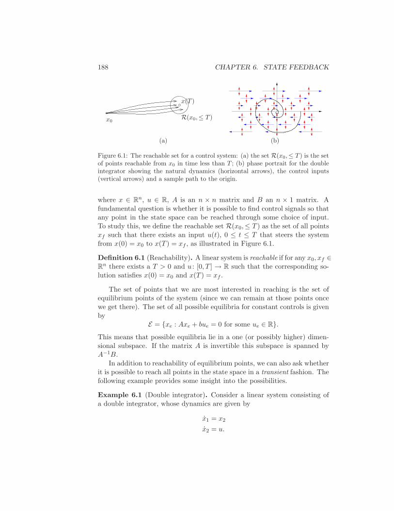
188 CHAPTER 6. STATE FEEDBACK
x0
x(T )
R(x0,≤ T )
(a) (b)
Figure 6.1: The reachable set for a control system: (a) the set R(x0,≤ T ) is the setof points reachable from x0 in time less than T ; (b) phase portrait for the doubleintegrator showing the natural dynamics (horizontal arrows), the control inputs(vertical arrows) and a sample path to the origin.
where x ∈ Rn, u ∈ R, A is an n × n matrix and B an n × 1 matrix. A
fundamental question is whether it is possible to find control signals so thatany point in the state space can be reached through some choice of input.To study this, we define the reachable set R(x0,≤ T ) as the set of all pointsxf such that there exists an input u(t), 0 ≤ t ≤ T that steers the systemfrom x(0) = x0 to x(T ) = xf , as illustrated in Figure 6.1.
Definition 6.1 (Reachability). A linear system is reachable if for any x0, xf ∈R
n there exists a T > 0 and u : [0, T ] → R such that the corresponding so-lution satisfies x(0) = x0 and x(T ) = xf .
The set of points that we are most interested in reaching is the set ofequilibrium points of the system (since we can remain at those points oncewe get there). The set of all possible equilibria for constant controls is givenby
E = xe : Axe + bue = 0 for some ue ∈ R.This means that possible equilibria lie in a one (or possibly higher) dimen-sional subspace. If the matrix A is invertible this subspace is spanned byA−1B.
In addition to reachability of equilibrium points, we can also ask whetherit is possible to reach all points in the state space in a transient fashion. Thefollowing example provides some insight into the possibilities.
Example 6.1 (Double integrator). Consider a linear system consisting ofa double integrator, whose dynamics are given by
x1 = x2
x2 = u.
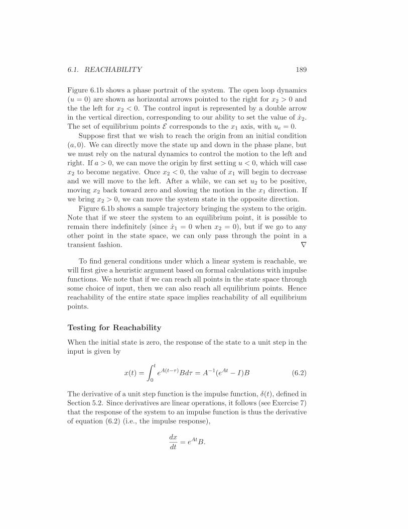
6.1. REACHABILITY 189
Figure 6.1b shows a phase portrait of the system. The open loop dynamics(u = 0) are shown as horizontal arrows pointed to the right for x2 > 0 andthe the left for x2 < 0. The control input is represented by a double arrowin the vertical direction, corresponding to our ability to set the value of x2.The set of equilibrium points E corresponds to the x1 axis, with ue = 0.
Suppose first that we wish to reach the origin from an initial condition(a, 0). We can directly move the state up and down in the phase plane, butwe must rely on the natural dynamics to control the motion to the left andright. If a > 0, we can move the origin by first setting u < 0, which will casex2 to become negative. Once x2 < 0, the value of x1 will begin to decreaseand we will move to the left. After a while, we can set u2 to be positive,moving x2 back toward zero and slowing the motion in the x1 direction. Ifwe bring x2 > 0, we can move the system state in the opposite direction.
Figure 6.1b shows a sample trajectory bringing the system to the origin.Note that if we steer the system to an equilibrium point, it is possible toremain there indefinitely (since x1 = 0 when x2 = 0), but if we go to anyother point in the state space, we can only pass through the point in atransient fashion. ∇
To find general conditions under which a linear system is reachable, wewill first give a heuristic argument based on formal calculations with impulsefunctions. We note that if we can reach all points in the state space throughsome choice of input, then we can also reach all equilibrium points. Hencereachability of the entire state space implies reachability of all equilibriumpoints.
Testing for Reachability
When the initial state is zero, the response of the state to a unit step in theinput is given by
x(t) =
∫ t
0eA(t−τ)Bdτ = A−1(eAt − I)B (6.2)
The derivative of a unit step function is the impulse function, δ(t), defined inSection 5.2. Since derivatives are linear operations, it follows (see Exercise 7)that the response of the system to an impulse function is thus the derivativeof equation (6.2) (i.e., the impulse response),
dx
dt= eAtB.
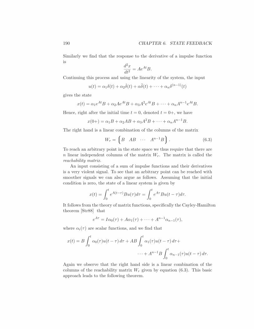
190 CHAPTER 6. STATE FEEDBACK
Similarly we find that the response to the derivative of a impulse functionis
d2x
dt2= AeAtB.
Continuing this process and using the linearity of the system, the input
u(t) = α1δ(t) + α2δ(t) + αδ(t) + · · · + αnδ(n−1)(t)
gives the state
x(t) = α1eAtB + α2Ae
AtB + α3A2eAtB + · · · + αnA
n−1eAtB.
Hence, right after the initial time t = 0, denoted t = 0+, we have
x(0+) = α1B + α2AB + α3A2B + · · · + αnA
n−1B.
The right hand is a linear combination of the columns of the matrix
Wr =
B AB · · · An−1B
. (6.3)
To reach an arbitrary point in the state space we thus require that there aren linear independent columns of the matrix Wr. The matrix is called thereachability matrix.
An input consisting of a sum of impulse functions and their derivativesis a very violent signal. To see that an arbitrary point can be reached withsmoother signals we can also argue as follows. Assuming that the initialcondition is zero, the state of a linear system is given by
x(t) =
∫ t
0eA(t−τ)Bu(τ)dτ =
∫ t
0eAτBu(t− τ)dτ.
It follows from the theory of matrix functions, specifically the Cayley-Hamiltontheorem [Str88] that
eAτ = Iα0(τ) +Aα1(τ) + · · · +An−1αn−1(τ),
where αi(τ) are scalar functions, and we find that
x(t) = B
∫ t
0α0(τ)u(t− τ) dτ +AB
∫ t
0α1(τ)u(t− τ) dτ+
· · · +An−1B
∫ t
0αn−1(τ)u(t− τ) dτ.
Again we observe that the right hand side is a linear combination of thecolumns of the reachability matrix Wr given by equation (6.3). This basicapproach leads to the following theorem.
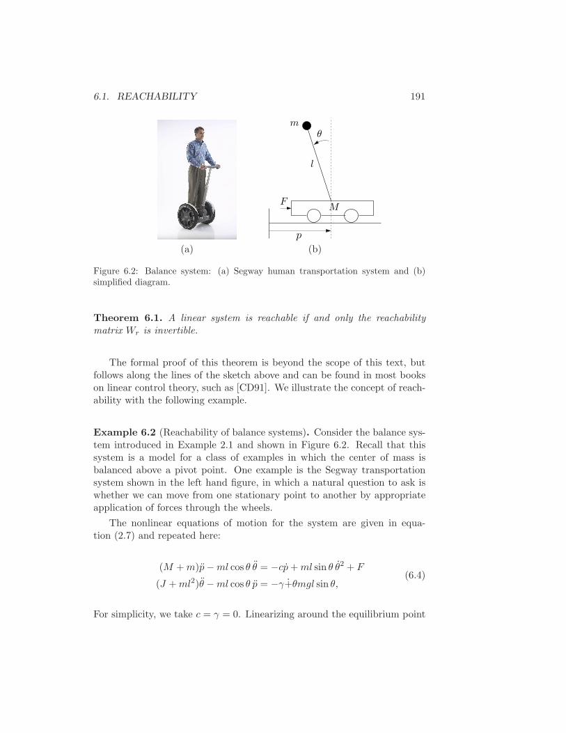
6.1. REACHABILITY 191
l
MF
p
θm
(a) (b)
Figure 6.2: Balance system: (a) Segway human transportation system and (b)simplified diagram.
Theorem 6.1. A linear system is reachable if and only the reachabilitymatrix Wr is invertible.
The formal proof of this theorem is beyond the scope of this text, butfollows along the lines of the sketch above and can be found in most bookson linear control theory, such as [CD91]. We illustrate the concept of reach-ability with the following example.
Example 6.2 (Reachability of balance systems). Consider the balance sys-tem introduced in Example 2.1 and shown in Figure 6.2. Recall that thissystem is a model for a class of examples in which the center of mass isbalanced above a pivot point. One example is the Segway transportationsystem shown in the left hand figure, in which a natural question to ask iswhether we can move from one stationary point to another by appropriateapplication of forces through the wheels.
The nonlinear equations of motion for the system are given in equa-tion (2.7) and repeated here:
(M +m)p−ml cos θ θ = −cp+ml sin θ θ2 + F
(J +ml2)θ −ml cos θ p = −γ+θmgl sin θ,(6.4)
For simplicity, we take c = γ = 0. Linearizing around the equilibrium point
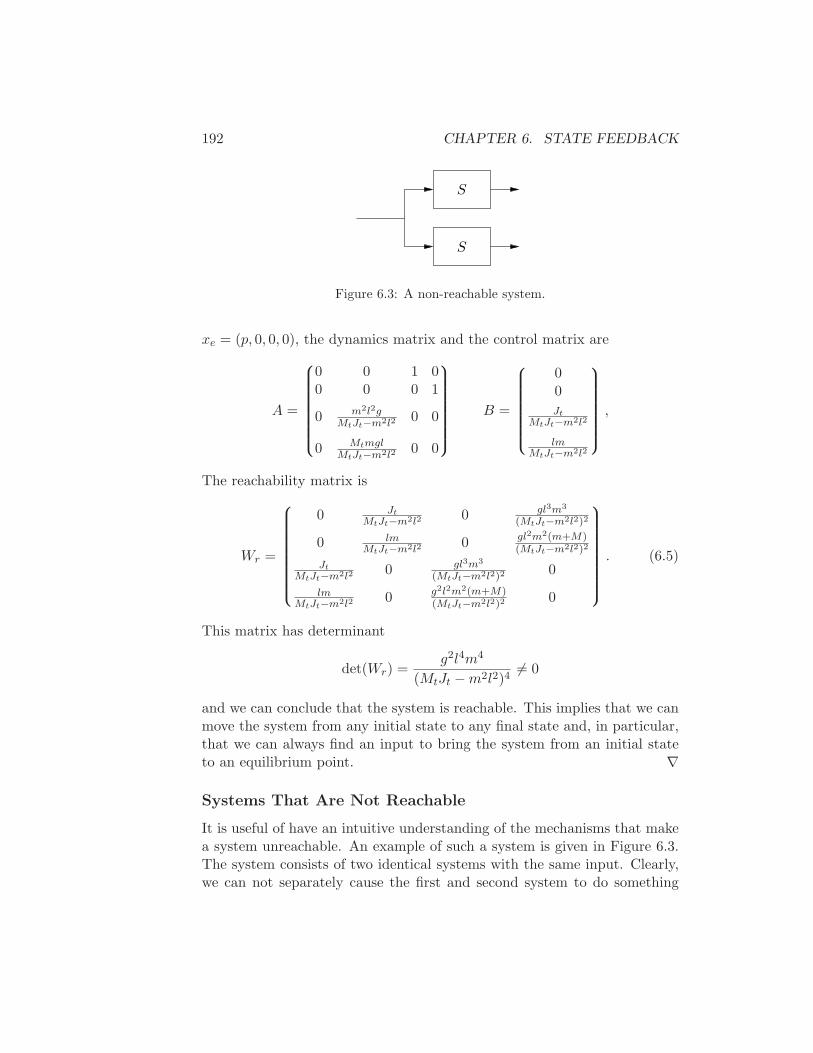
192 CHAPTER 6. STATE FEEDBACK
S
S
Figure 6.3: A non-reachable system.
xe = (p, 0, 0, 0), the dynamics matrix and the control matrix are
A =
0 0 1 00 0 0 1
0 m2l2gMtJt−m2l2
0 0
0 MtmglMtJt−m2l2
0 0
B =
00
Jt
MtJt−m2l2
lmMtJt−m2l2
,
The reachability matrix is
Wr =
0 Jt
MtJt−m2l20 gl3m3
(MtJt−m2l2)2
0 lmMtJt−m2l2
0 gl2m2(m+M)(MtJt−m2l2)2
Jt
MtJt−m2l20 gl3m3
(MtJt−m2l2)20
lmMtJt−m2l2
0 g2l2m2(m+M)(MtJt−m2l2)2
0
. (6.5)
This matrix has determinant
det(Wr) =g2l4m4
(MtJt −m2l2)46= 0
and we can conclude that the system is reachable. This implies that we canmove the system from any initial state to any final state and, in particular,that we can always find an input to bring the system from an initial stateto an equilibrium point. ∇
Systems That Are Not Reachable
It is useful of have an intuitive understanding of the mechanisms that makea system unreachable. An example of such a system is given in Figure 6.3.The system consists of two identical systems with the same input. Clearly,we can not separately cause the first and second system to do something
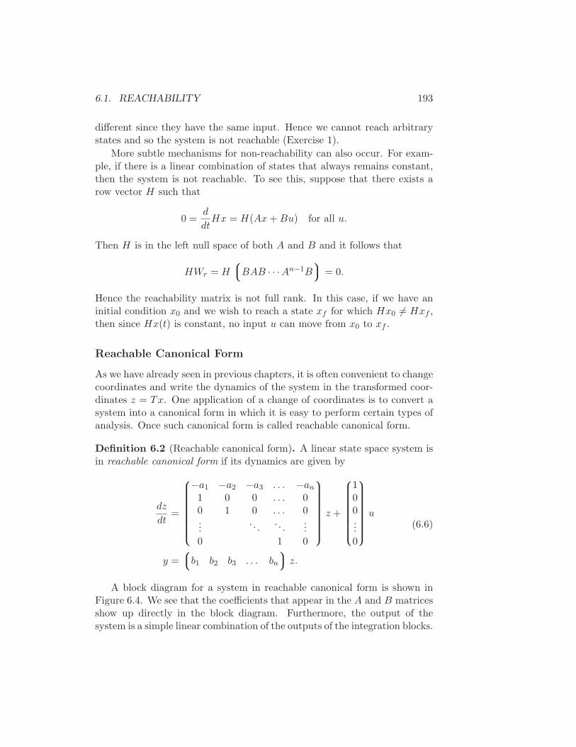
6.1. REACHABILITY 193
different since they have the same input. Hence we cannot reach arbitrarystates and so the system is not reachable (Exercise 1).
More subtle mechanisms for non-reachability can also occur. For exam-ple, if there is a linear combination of states that always remains constant,then the system is not reachable. To see this, suppose that there exists arow vector H such that
0 =d
dtHx = H(Ax+Bu) for all u.
Then H is in the left null space of both A and B and it follows that
HWr = H
BAB · · ·An−1B
= 0.
Hence the reachability matrix is not full rank. In this case, if we have aninitial condition x0 and we wish to reach a state xf for which Hx0 6= Hxf ,then since Hx(t) is constant, no input u can move from x0 to xf .
Reachable Canonical Form
As we have already seen in previous chapters, it is often convenient to changecoordinates and write the dynamics of the system in the transformed coor-dinates z = Tx. One application of a change of coordinates is to convert asystem into a canonical form in which it is easy to perform certain types ofanalysis. Once such canonical form is called reachable canonical form.
Definition 6.2 (Reachable canonical form). A linear state space system isin reachable canonical form if its dynamics are given by
dz
dt=
−a1 −a2 −a3 . . . −an
1 0 0 . . . 00 1 0 . . . 0...
. . .. . .
...0 1 0
z +
100...0
u
y =
b1 b2 b3 . . . bn
z.
(6.6)
A block diagram for a system in reachable canonical form is shown inFigure 6.4. We see that the coefficients that appear in the A and B matricesshow up directly in the block diagram. Furthermore, the output of thesystem is a simple linear combination of the outputs of the integration blocks.
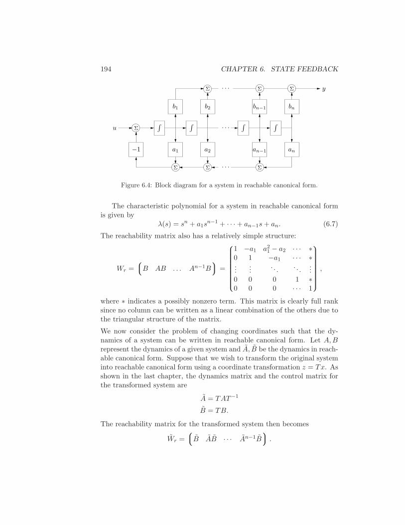
194 CHAPTER 6. STATE FEEDBACK
Σ
∫
a1
Σ
Σ
b1
−1
∫u
Σ
a2
Σ
. . .
. . .
. . .
b2
∫
Σ
Σ
an−1 an
bnbn−1
∫
y
Figure 6.4: Block diagram for a system in reachable canonical form.
The characteristic polynomial for a system in reachable canonical formis given by
λ(s) = sn + a1sn−1 + · · · + an−1s+ an. (6.7)
The reachability matrix also has a relatively simple structure:
Wr =
B AB . . . An−1B
=
1 −a1 a21 − a2 · · · ∗
0 1 −a1 · · · ∗...
.... . .
. . ....
0 0 0 1 ∗0 0 0 · · · 1
,
where ∗ indicates a possibly nonzero term. This matrix is clearly full ranksince no column can be written as a linear combination of the others due tothe triangular structure of the matrix.
We now consider the problem of changing coordinates such that the dy-namics of a system can be written in reachable canonical form. Let A,Brepresent the dynamics of a given system and A, B be the dynamics in reach-able canonical form. Suppose that we wish to transform the original systeminto reachable canonical form using a coordinate transformation z = Tx. Asshown in the last chapter, the dynamics matrix and the control matrix forthe transformed system are
A = TAT−1
B = TB.
The reachability matrix for the transformed system then becomes
Wr =
B AB · · · An−1B
.
6.1. REACHABILITY 195
Transforming each element individually, we have
AB = TAT−1TB = TAB
A2B = (TAT−1)2TB = TAT−1TAT−1TB = TA2B
...
AnB = TAnB.
and hence the reachability matrix for the transformed system is
Wr = T
B AB · · · An−1B
= TWr. (6.8)
Since Wr is invertible, we can thus solve for the transformation T that takesthe system into reachable canonical form:
T = WrW−1r .
The following example illustrates the approach.
Example 6.3. Consider a simple two dimensional system of the form
x =
α ω−ω α
x+
01
u.
We wish to find the transformation that converts the system into reachablecanonical form:
A =
−a1 −a2
1 0
B =
10
.
The coefficients a1 and a2 can be determined by looking at the characteristicequation for the original system:
λ(s) = det(sI −A) = s2 − 2αs+ (α2 + ω2) =⇒a1 = −2α
a2 = α2 + ω2.
The reachability matrix for each system is
Wr =
0 ω1 α
Wr =
1 −a1
0 1
.
The transformation T becomes
T = WrW−1r
−a1+αω 1
1ω 0
=
αω 1
1ω 0
196 CHAPTER 6. STATE FEEDBACK
and hence the coordinates
z1z2
= Tx =
αωx1 + x2
x2
put the system in reachable canonical form. ∇
We summarize the results of this section in the following theorem.
Theorem 6.2. Let (A,B) be the dynamics and control matrices for a reach-able system. Then there exists a transformation z = Tx such that in thetransformed coordinates the dynamics and control matrices are in reachablecanonical form (6.6) and the characteristic polynomial for A is given by
det(sI −A) = sn + a1sn−1 + · · · + an−1s+ an.
One important implication of this theorem is that for any reachablesystem, we can always assume without loss of generality that the coordinatesare chosen such that the system is in reachable canonical form. This isparticularly useful for proofs, as we shall see later in this chapter.
6.2 Stabilization by State Feedback
The state of a dynamical system is a collection of variables that permitsprediction of the future development of a system. We now explore the ideaof designing the dynamics a system through feedback of the state. Wewill assume that the system to be controlled is described by a linear statemodel and has a single input (for simplicity). The feedback control will bedeveloped step by step using one single idea: the positioning of closed loopeigenvalues in desired locations.
Figure 6.5 shows a diagram of a typical control system using state feed-back. The full system consists of the process dynamics, which we take tobe linear, the controller elements, K and kr, the reference input, r, andprocesses disturbances, d. The goal of the feedback controller is to regulatethe output of the system, y, such that it tracks the reference input in thepresence of disturbances and also uncertainty in the process dynamics.
An important element of the control design is the performance specifi-cation. The simplest performance specification is that of stability: in theabsence of any disturbances, we would like the equilibrium point of thesystem to be asymptotically stable. More sophisticated performance speci-fications typically involve giving desired properties of the step or frequency
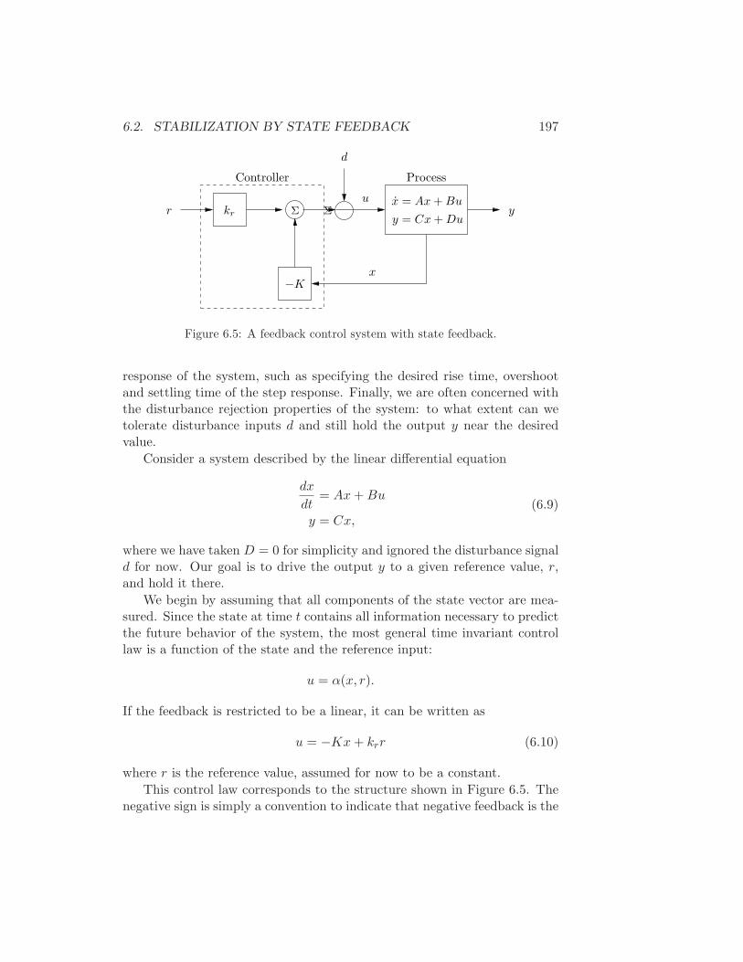
6.2. STABILIZATION BY STATE FEEDBACK 197
Process
y
x
uΣ
x = Ax+Bu
y = Cx+Du
d
Σ
−K
krr
Controller
Figure 6.5: A feedback control system with state feedback.
response of the system, such as specifying the desired rise time, overshootand settling time of the step response. Finally, we are often concerned withthe disturbance rejection properties of the system: to what extent can wetolerate disturbance inputs d and still hold the output y near the desiredvalue.
Consider a system described by the linear differential equation
dx
dt= Ax+Bu
y = Cx,(6.9)
where we have taken D = 0 for simplicity and ignored the disturbance signald for now. Our goal is to drive the output y to a given reference value, r,and hold it there.
We begin by assuming that all components of the state vector are mea-sured. Since the state at time t contains all information necessary to predictthe future behavior of the system, the most general time invariant controllaw is a function of the state and the reference input:
u = α(x, r).
If the feedback is restricted to be a linear, it can be written as
u = −Kx+ krr (6.10)
where r is the reference value, assumed for now to be a constant.
This control law corresponds to the structure shown in Figure 6.5. Thenegative sign is simply a convention to indicate that negative feedback is the
198 CHAPTER 6. STATE FEEDBACK
normal situation. The closed loop system obtained when the feedback (6.9)is applied to the system (6.10) is given by
dx
dt= (A−BK)x+Bkrr (6.11)
We attempt to determine the feedback gain K so that the closed loop systemhas the characteristic polynomial
p(s) = sn + p1sn−1 + · · · + pn−1s+ pn (6.12)
This control problem is called the eigenvalue assignment problem or “poleplacement” problem (we will define “poles” more formally in a later chapter).
Note that the kr does not affect the stability of the system (which isdetermined by the eigenvalues of A−BK), but does affect the steady statesolution. In particular, the equilibrium point and steady state output forthe closed loop system are given by
xe = −(A−BK)−1Bkrr ye = Cxe,
hence kr should be chosen such that ye = r (the desired output value). Sincekr is a scalar, we can easily solve to show
kr = −1/(C(A−BK)−1B
). (6.13)
Notice that kr is exactly the inverse of the zero frequency gain of the closedloop system.
Using the gains K and kr, we are thus able to design the dynamics of theclosed loop system to satisfy our goal. To illustrate how to such construct astate feedback control law, we begin with a few examples that provide somebasic intuition and insights.
Examples
Example 6.4 (Vehicle steering). In Example 5.12 we derived a normal-ized linear model for vehicle steering. The dynamics describing the lateraldeviation where given by
A =
0 10 0
B =
α1
C =
1 0
D = 0.

6.2. STABILIZATION BY STATE FEEDBACK 199
The reachability matrix for the system is thus
Wr =
B AB
=
α 11 0
.
The system is reachable since detWr = −1 6= 0.We now want to design a controller that stabilizes the dynamics and
tracks a given reference value r of the lateral position of the vehicle. To dothis we introduce the feedback
u = −Kx+ krr = −k1x1 − k2x2 + krr,
and the closed loop system becomes
dx
dt= (A−BK)x+Bkrr =
−αk1 1 − αk2
−k1 −k2
x+
αkr
kr
r
y = Cx+Du =
1 0
x.
(6.14)
The closed loop system has the characteristic polynomial
det (sI −A+BK) = det
s+ αk1 αk2 − 1k1 s+ k2
= s2 + (αk1 + k2)s+ k1.
Suppose that we would like to use feedback to design the dynamics of thesystem to have a characteristic polynomial
p(s) = s2 + 2ζcωcs+ ω2c .
Comparing this with the characteristic polynomial of the closed loop systemwe see that the feedback gains should be chosen as
k1 = ω2c , k2 = 2ζcωc − αω2
c .
To have x1 = r in the steady state it must be required that the parameterkr equal to k1 = ω2
c . The control law can thus be written as
u = k1(r − x1) − k2x2 = ω2c (r − x1) − (2ζcωc − αω2
c )x2.
∇
The example of the vehicle steering system illustrates how state feedbackcan be used to set the eigenvalues of the closed loop system to arbitraryvalues. The next example demonstrates that this is not always possible.
200 CHAPTER 6. STATE FEEDBACK
Example 6.5 (An unreachable system). Consider the system
dx
dt=
0 10 0
x+
10
u
y =
1 0
x
with the control lawu = −k1x1 − k2x2 + krr.
The closed loop system is
dx
dt=
−k1 1 − k2
0 0
x+
kr
0
r.
This system has the characteristic polynomial
det
s+ k1 −1 + k2
0 s
= s2 + k1s = s(s+ k1),
which has zeros at s = 0 and s = −k1. Since one closed loop eigenvalue isalways equal to s = 0, independently of our choice of gains, it is not possibleto obtain an arbitrary characteristic polynomial.
A visual inspection of the equations of motion shows that this systemalso has the property that it is not reachable. In particular, since x2 = 0,we can never steer x2 between one value and another. Computation of thereachability matrix Wr verifies that the system is not reachable. ∇
The reachable canonical form has the property that the parameters ofthe system are the coefficients of the characteristic equation. It is thereforenatural to consider systems on this form when solving the eigenvalue assign-ment problem. In the next example we investigate the case when the systemis in reachable canonical form.
Example 6.6 (System in reachable canonical form). Consider a system inreachable canonical form, i.e,
dz
dt= Az + Bu =
−a1 −a2 −a3 . . . −an
1 0 0 . . . 00 1 0 . . . 0...
. . .. . .
...0 1 0
z +
10...00
u
y = Cz =
b1 b2 · · · bn
z.
(6.15)
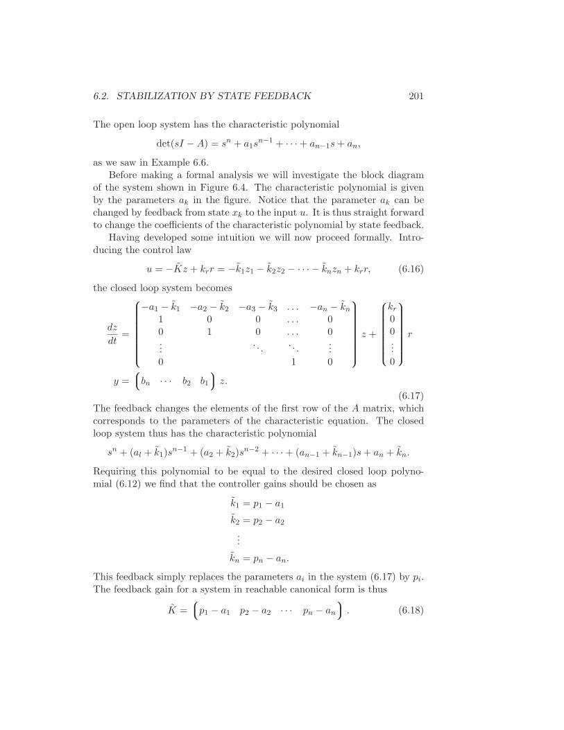
6.2. STABILIZATION BY STATE FEEDBACK 201
The open loop system has the characteristic polynomial
det(sI −A) = sn + a1sn−1 + · · · + an−1s+ an,
as we saw in Example 6.6.Before making a formal analysis we will investigate the block diagram
of the system shown in Figure 6.4. The characteristic polynomial is givenby the parameters ak in the figure. Notice that the parameter ak can bechanged by feedback from state xk to the input u. It is thus straight forwardto change the coefficients of the characteristic polynomial by state feedback.
Having developed some intuition we will now proceed formally. Intro-ducing the control law
u = −Kz + krr = −k1z1 − k2z2 − · · · − knzn + krr, (6.16)
the closed loop system becomes
dz
dt=
−a1 − k1 −a2 − k2 −a3 − k3 . . . −an − kn
1 0 0 . . . 00 1 0 . . . 0...
. . .. . .
...0 1 0
z +
kr
00...0
r
y =
bn · · · b2 b1
z.
(6.17)The feedback changes the elements of the first row of the A matrix, whichcorresponds to the parameters of the characteristic equation. The closedloop system thus has the characteristic polynomial
sn + (al + k1)sn−1 + (a2 + k2)s
n−2 + · · · + (an−1 + kn−1)s+ an + kn.
Requiring this polynomial to be equal to the desired closed loop polyno-mial (6.12) we find that the controller gains should be chosen as
k1 = p1 − a1
k2 = p2 − a2
...
kn = pn − an.
This feedback simply replaces the parameters ai in the system (6.17) by pi.The feedback gain for a system in reachable canonical form is thus
K =
p1 − a1 p2 − a2 · · · pn − an
. (6.18)
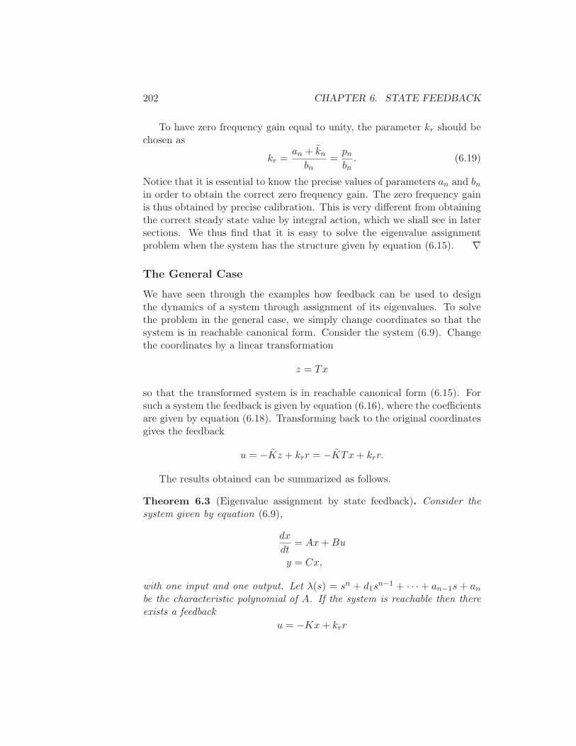
202 CHAPTER 6. STATE FEEDBACK
To have zero frequency gain equal to unity, the parameter kr should bechosen as
kr =an + kn
bn=pn
bn. (6.19)
Notice that it is essential to know the precise values of parameters an and bnin order to obtain the correct zero frequency gain. The zero frequency gainis thus obtained by precise calibration. This is very different from obtainingthe correct steady state value by integral action, which we shall see in latersections. We thus find that it is easy to solve the eigenvalue assignmentproblem when the system has the structure given by equation (6.15). ∇
The General Case
We have seen through the examples how feedback can be used to designthe dynamics of a system through assignment of its eigenvalues. To solvethe problem in the general case, we simply change coordinates so that thesystem is in reachable canonical form. Consider the system (6.9). Changethe coordinates by a linear transformation
z = Tx
so that the transformed system is in reachable canonical form (6.15). Forsuch a system the feedback is given by equation (6.16), where the coefficientsare given by equation (6.18). Transforming back to the original coordinatesgives the feedback
u = −Kz + krr = −KTx+ krr.
The results obtained can be summarized as follows.
Theorem 6.3 (Eigenvalue assignment by state feedback). Consider thesystem given by equation (6.9),
dx
dt= Ax+Bu
y = Cx,
with one input and one output. Let λ(s) = sn + d1sn−1 + · · · + an−1s + an
be the characteristic polynomial of A. If the system is reachable then thereexists a feedback
u = −Kx+ krr
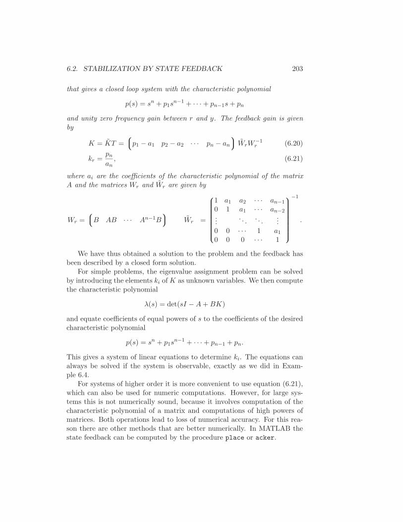
6.2. STABILIZATION BY STATE FEEDBACK 203
that gives a closed loop system with the characteristic polynomial
p(s) = sn + p1sn−1 + · · · + pn−1s+ pn
and unity zero frequency gain between r and y. The feedback gain is givenby
K = KT =
p1 − a1 p2 − a2 · · · pn − an
WrW−1r (6.20)
kr =pn
an, (6.21)
where ai are the coefficients of the characteristic polynomial of the matrixA and the matrices Wr and Wr are given by
Wr =
B AB · · · An−1B
Wr =
1 a1 a2 · · · an−1
0 1 a1 · · · an−2...
. . .. . .
...0 0 · · · 1 a1
0 0 0 · · · 1
−1
.
We have thus obtained a solution to the problem and the feedback hasbeen described by a closed form solution.
For simple problems, the eigenvalue assignment problem can be solvedby introducing the elements ki of K as unknown variables. We then computethe characteristic polynomial
λ(s) = det(sI −A+BK)
and equate coefficients of equal powers of s to the coefficients of the desiredcharacteristic polynomial
p(s) = sn + p1sn−1 + · · · + pn−1 + pn.
This gives a system of linear equations to determine ki. The equations canalways be solved if the system is observable, exactly as we did in Exam-ple 6.4.
For systems of higher order it is more convenient to use equation (6.21),which can also be used for numeric computations. However, for large sys-tems this is not numerically sound, because it involves computation of thecharacteristic polynomial of a matrix and computations of high powers ofmatrices. Both operations lead to loss of numerical accuracy. For this rea-son there are other methods that are better numerically. In MATLAB thestate feedback can be computed by the procedure place or acker.
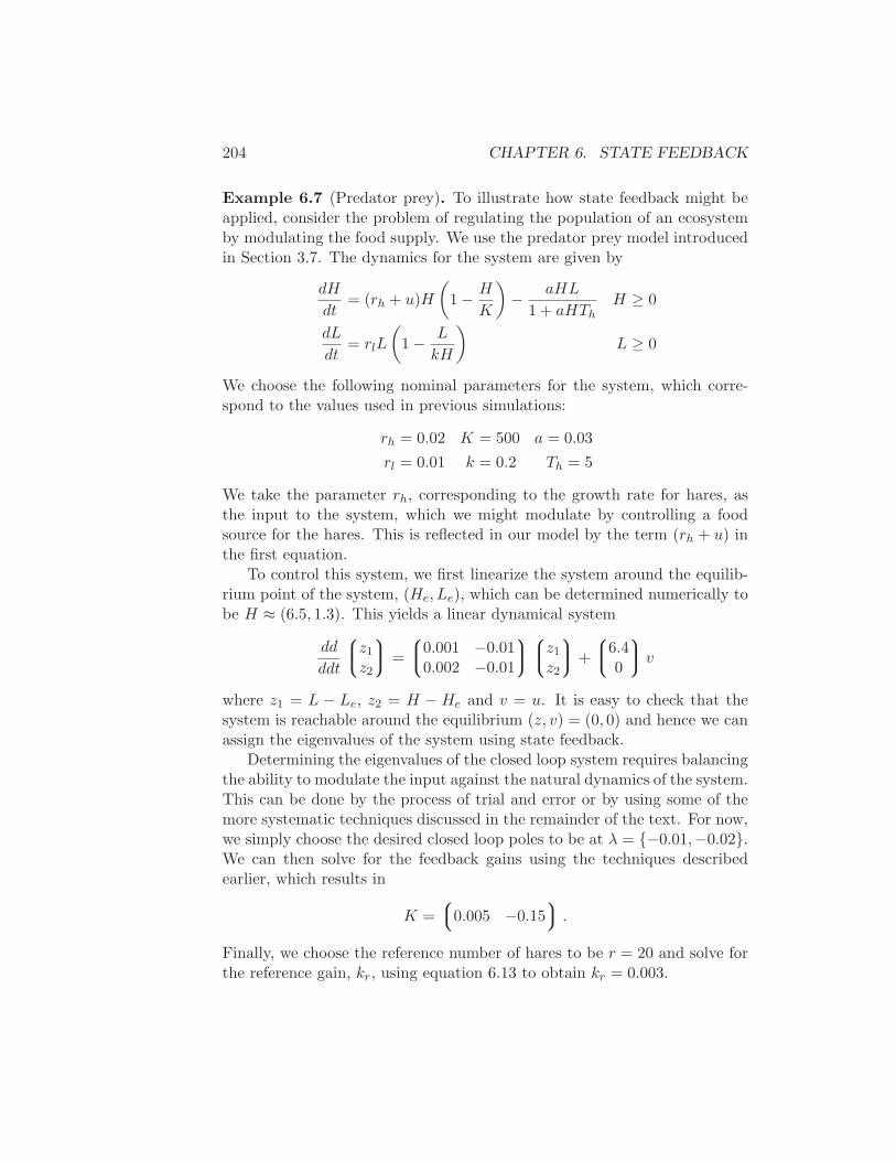
204 CHAPTER 6. STATE FEEDBACK
Example 6.7 (Predator prey). To illustrate how state feedback might beapplied, consider the problem of regulating the population of an ecosystemby modulating the food supply. We use the predator prey model introducedin Section 3.7. The dynamics for the system are given by
dH
dt= (rh + u)H
(
1 − H
K
)
− aHL
1 + aHThH ≥ 0
dL
dt= rlL
(
1 − L
kH
)
L ≥ 0
We choose the following nominal parameters for the system, which corre-spond to the values used in previous simulations:
rh = 0.02 K = 500 a = 0.03
rl = 0.01 k = 0.2 Th = 5
We take the parameter rh, corresponding to the growth rate for hares, asthe input to the system, which we might modulate by controlling a foodsource for the hares. This is reflected in our model by the term (rh + u) inthe first equation.
To control this system, we first linearize the system around the equilib-rium point of the system, (He, Le), which can be determined numerically tobe H ≈ (6.5, 1.3). This yields a linear dynamical system
dd
ddt
z1z2
=
0.001 −0.010.002 −0.01
z1z2
+
6.40
v
where z1 = L − Le, z2 = H − He and v = u. It is easy to check that thesystem is reachable around the equilibrium (z, v) = (0, 0) and hence we canassign the eigenvalues of the system using state feedback.
Determining the eigenvalues of the closed loop system requires balancingthe ability to modulate the input against the natural dynamics of the system.This can be done by the process of trial and error or by using some of themore systematic techniques discussed in the remainder of the text. For now,we simply choose the desired closed loop poles to be at λ = −0.01,−0.02.We can then solve for the feedback gains using the techniques describedearlier, which results in
K =
0.005 −0.15
.
Finally, we choose the reference number of hares to be r = 20 and solve forthe reference gain, kr, using equation 6.13 to obtain kr = 0.003.
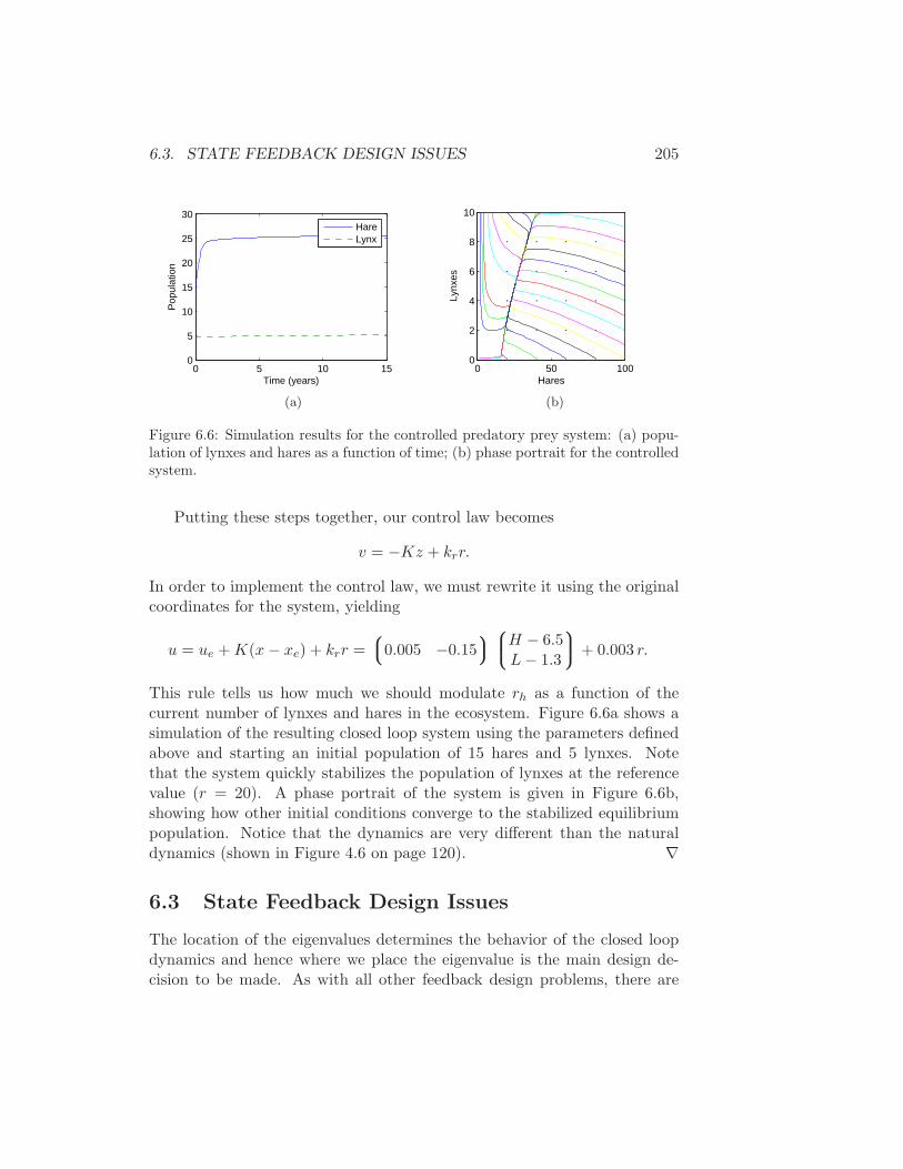
6.3. STATE FEEDBACK DESIGN ISSUES 205
0 5 10 150
5
10
15
20
25
30
Time (years)
Pop
ulat
ion
HareLynx
(a)
0 50 1000
2
4
6
8
10
Hares
Lynx
es
(b)
Figure 6.6: Simulation results for the controlled predatory prey system: (a) popu-lation of lynxes and hares as a function of time; (b) phase portrait for the controlledsystem.
Putting these steps together, our control law becomes
v = −Kz + krr.
In order to implement the control law, we must rewrite it using the originalcoordinates for the system, yielding
u = ue +K(x− xe) + krr =
0.005 −0.15
H − 6.5L− 1.3
+ 0.003 r.
This rule tells us how much we should modulate rh as a function of thecurrent number of lynxes and hares in the ecosystem. Figure 6.6a shows asimulation of the resulting closed loop system using the parameters definedabove and starting an initial population of 15 hares and 5 lynxes. Notethat the system quickly stabilizes the population of lynxes at the referencevalue (r = 20). A phase portrait of the system is given in Figure 6.6b,showing how other initial conditions converge to the stabilized equilibriumpopulation. Notice that the dynamics are very different than the naturaldynamics (shown in Figure 4.6 on page 120). ∇
6.3 State Feedback Design Issues
The location of the eigenvalues determines the behavior of the closed loopdynamics and hence where we place the eigenvalue is the main design de-cision to be made. As with all other feedback design problems, there are
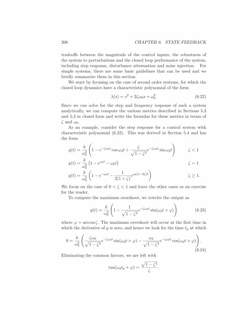
206 CHAPTER 6. STATE FEEDBACK
tradeoffs between the magnitude of the control inputs, the robustness ofthe system to perturbations and the closed loop performance of the system,including step response, disturbance attenuation and noise injection. Forsimple systems, there are some basic guidelines that can be used and webriefly summarize them in this section.
We start by focusing on the case of second order systems, for which theclosed loop dynamics have a characteristic polynomial of the form
λ(s) = s2 + 2ζω0s+ ω20. (6.22)
Since we can solve for the step and frequency response of such a systemanalytically, we can compute the various metrics described in Sections 5.3and 5.3 in closed form and write the formulas for these metrics in terms ofζ and ω0.
As an example, consider the step response for a control system withcharacteristic polynomial (6.22). This was derived in Section 5.4 and hasthe form
y(t) =k
ω20
(
1 − e−ζω0t cosωdt+ζ
√
1 − ζ2e−ζω0t sinωdt
)
ζ < 1
y(t) =k
ω20
(1 − eω0t − ω0t
)ζ = 1
y(t) =k
ω20
(
1 − e−ω0t − 1
2(1 + ζ)eω0(1−2ζ)t
)
ζ ≥ 1.
We focus on the case of 0 < ζ < 1 and leave the other cases as an exercisefor the reader.
To compute the maximum overshoot, we rewrite the output as
y(t) =k
ω20
(
1 − 1√
1 − ζ2e−ζω0t sin(ωdt+ ϕ)
)
(6.23)
where ϕ = arccos ζ. The maximum overshoot will occur at the first time inwhich the derivative of y is zero, and hence we look for the time tp at which
0 =k
ω20
(
ζω0√
1 − ζ2e−ζω0t sin(ωdt+ ϕ) − ωd
√
1 − ζ2e−ζω0t cos(ωdt+ ϕ)
)
.
(6.24)Eliminating the common factors, we are left with
tan(ωdtp + ϕ) =
√
1 − ζ2
ζ.

6.3. STATE FEEDBACK DESIGN ISSUES 207
Table 6.1: Properties of the response to reference values of a second order systemfor |ζ‖ < 1. The parameter ϕ = arccos ζ.
Property Value ζ = 0.5 ζ = 1/√
2 ζ = 1
Steady state error 1/ω20 1/ω2
0 1/ω20 1/ω2
0
Rise time Tr = 1/ω0 · eϕ/ tan ϕ 1.8/ω0 2.2/ω0 2.7/ω0
Overshoot Mp = e−πζ/√
1−ζ216% 4% 0%
Settling time (2%) Ts ≈ 4/ζω0 8/ω0 5.7/ω0 4/ω0
Since ϕ = arccos ζ, it follows that we must have ωdtp = π (for the firstnon-trivial extremum) and hence tp = π/ωd. Substituting this back intoequation (6.23), subtracting off the steady state value and normalizing, wehave
Mp = e−πζ/√
1−ζ2
.
Similar computations can be done for the other characteristics of a stepresponse. Table 6.1 summarizes the calculations.
One way to visualize the effect of the closed loop eigenvalues on thedynamics is to use the eigenvalue plot in Figure 6.7. This charge showsrepresentative step and frequency responses as a function of the locationof the eigenvalues. The diagonal lines in the left half plane represent thedamping ratio ζ =
√2 ≈ 0.707, a common value for many designs.
One important consideration that is missing from the analysis so far isthe amount of control authority required to obtain the desired dynamics.
Example 6.8 (Drug administration). To illustrate the usage of these formu-las, consider the two compartment model for drug administration, describedin Section 3.6. The dynamics of the system is
dc
dt=
−k0 − k1 k1
k2 −k2
c+
b00
u
y =
0 1
x,
where c1 and c2 are the concentrations of the drug in each compartment,ki, i = 0, . . . , 2 and b are parameters of the system, u is the flow rate ofthe drug into compartment 1 and y is the concentration of the drug in
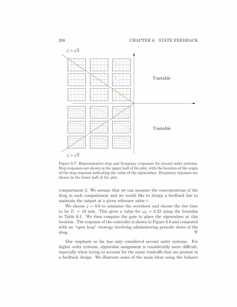
208 CHAPTER 6. STATE FEEDBACK
Unstable
Unstable
ζ =√
2
ζ =√
2
Figure 6.7: Representative step and frequency responses for second order systems.Step responses are shown in the upper half of the plot, with the location of the originof the step response indicating the value of the eigenvalues. Frequency reponses areshown in the lower half of the plot.
compartment 2. We assume that we can measure the concentrations of thedrug in each compartment and we would like to design a feedback law tomaintain the output at a given reference value r.
We choose ζ = 0.9 to minimize the overshoot and choose the rise timeto be Tr = 10 min. This gives a value for ω0 = 0.22 using the formulasin Table 6.1. We then compute the gain to place the eigenvalues at thislocation. The response of the controller is shown in Figure 6.8 and comparedwith an “open loop” strategy involving administering periodic doses of thedrug. ∇
Our emphasis so far has only considered second order systems. Forhigher order systems, eigenvalue assignment is considerably more difficult,especially when trying to account for the many tradeoffs that are present ina feedback design. We illustrate some of the main ideas using the balance
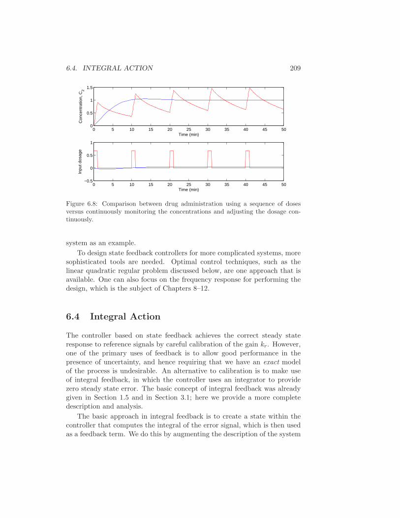
6.4. INTEGRAL ACTION 209
0 5 10 15 20 25 30 35 40 45 500
0.5
1
1.5
Time (min)
Con
cent
ratio
n, C
2
0 5 10 15 20 25 30 35 40 45 50−0.5
0
0.5
1
Time (min)
Inpu
t dos
age
Figure 6.8: Comparison between drug administration using a sequence of dosesversus continuously monitoring the concentrations and adjusting the dosage con-tinuously.
system as an example.
To design state feedback controllers for more complicated systems, moresophisticated tools are needed. Optimal control techniques, such as thelinear quadratic regular problem discussed below, are one approach that isavailable. One can also focus on the frequency response for performing thedesign, which is the subject of Chapters 8–12.
6.4 Integral Action
The controller based on state feedback achieves the correct steady stateresponse to reference signals by careful calibration of the gain kr. However,one of the primary uses of feedback is to allow good performance in thepresence of uncertainty, and hence requiring that we have an exact modelof the process is undesirable. An alternative to calibration is to make useof integral feedback, in which the controller uses an integrator to providezero steady state error. The basic concept of integral feedback was alreadygiven in Section 1.5 and in Section 3.1; here we provide a more completedescription and analysis.
The basic approach in integral feedback is to create a state within thecontroller that computes the integral of the error signal, which is then usedas a feedback term. We do this by augmenting the description of the system
210 CHAPTER 6. STATE FEEDBACK
with a new state z:
d
dt
xz
=
Ax+Buy − r
=
Ax+BuCx− r
The state z is seen to be the integral of the error between the desired out-put, r, and the actual output, y. Note that if we find a compensator thatstabilizes the system then necessarily we will have z = 0 in steady state andhence y = r in steady state.
Given the augmented system, we design a state space controller in theusual fashion, with a control law of the form
u = −Kx− kiz + krr
where K is the usual state feedback term, ki is the integral term and kr isused to set the nominal input for the desired steady state. The resultingequilibrium point for the system is given as
xe = −(A−BK)−1B(krr − kize)
Note that the value of ze is not specified, but rather will automatically settleto the value that makes z = y − r = 0, which implies that at equilibriumthe output will equal the reference value. This holds independently of thespecific values of A, B and K, as long as the system is stable (which can bedone through appropriate choice of K and ki).
The final compensator is given by
u = −Kx− kiz + krr
z = y − r,
where we have now included the dynamics of the integrator as part of thespecification of the controller. This type of compensator is known as adynamic compensator since it has its own internal dynamics. The followingexample illustrates the basic approach.
Example 6.9 (Cruise control). Consider the speed control example intro-duced in Section 3.1 and considered further in Example 5.10.
The linearized dynamics of the process around an equilibrium point ve,ue are given by
˙v = av − bggθ + bu
y = v = v + ve,
6.4. INTEGRAL ACTION 211
where v = v − ve, u = u− ue, m is the mass of the car and θ is the angle ofthe road. The constant a depends on the throttle characteristic and is givenin Example 5.10.
If we augment the system with an integrator, the process dynamics be-come
˙v = av − gθ + bu
z = r − y = (r − ve) − v,
or, in state space form,
d
dt
vz
=
a 0−1 0
vz
+
b0
u+
−g0
θ +
0
r − ve
.
Note that when the system is at equilibrium we have that z = 0 whichimplies that the vehicle speed, v = ve + v, should be equal to the desiredreference speed, r. Our controller will be of the form
z = r − y
u = −kpv − kiz + krr
and the gains kp, ki and kr will be chosen to stabilize the system and providethe correct input for the reference speed.
Assume that we wish to design the closed loop system to have charac-teristic polynomial
λ(s) = s2 + a1s+ a2.
Setting the disturbance θ = 0, the characteristic polynomial of the closedloop system is given by
det(sI − (A−BK)
)= s2 + (bK − a)s− bki
and hence we set
K =a1 + a
bki = −a2
b.
The resulting controller stabilizes the system and hence brings z = y − r tozero, resulting in perfect tracking. Notice that even if we have a small errorin the values of the parameters defining the system, as long as the closedloop poles are still stable then the tracking error will approach zero. Thusthe exact calibration required in our previous approach (using kr) is notrequired. Indeed, we can even choose kr = 0 and let the feedback controllerdo all of the work (Exercise 5).
Integral feedback can also be used to compensate for constant distur-bances. Suppose that we choose θ 6= 0, corresponding to climbing a (lin-earized) hill. The stability of the system is not affected by this external
212 CHAPTER 6. STATE FEEDBACK
disturbance and so we once again see that the car’s velocity converges tothe reference speed.
This ability to handle constant disturbances is a general property ofcontrollers with integral feedback and is explored in more detail in Exercise 6.
∇
6.5 Linear Quadratic Regulators
In addition to selecting the closed loop eigenvalue locations to accomplish acertain objective, another way that the gains for a state feedback controllercan be chosen is by attempting to optimize a cost function.
The infinite horizon, linear quadratic regulator (LQR) problem is oneof the most common optimal control problems. Given a multi-input linearsystem
x = Ax+Bu x ∈ Rn, u ∈ R
m,
we attempt to minimize the quadratic cost function
J =
∫ ∞
0
(xTQxx+ uTQuu
)dt
where Qx ≥ 0 and Qu > 0 are symmetric, positive (semi-) definite matricesof the appropriate dimension. This cost function represents a tradeoff be-tween the distance of the state from the origin and the cost of the controlinput. By choosing the matrices Qx and Qu, described in more detail below,we can balance the rate of convergence of the solutions with the cost of thecontrol.
The solution to the LQR problem is given by a linear control law of theform
u = −Q−1u BTPx
where P ∈ Rn×n is a positive definite, symmetric matrix that satisfies the
equationPA+ATP − PBQ−1
u BTP +Qx = 0. (6.25)
Equation (6.25) is called the algebraic Riccati equation and can be solvednumerically (for example, using the lqr command in MATLAB).
One of the key questions in LQR design is how to choose the weights Qx
and Qu. In order to guarantee that a solution exists, we must have Qx ≥ 0and Qu > 0. In addition, there are certain “observability” conditions on Qx
that limit its choice. We assume here Qx > 0 to insure that solutions to thealgebraic Riccati equation always exists.
6.6. FURTHER READING 213
To choose specific values for the cost function weights Qx and Qu, wemust use our knowledge of the system we are trying to control. A particu-larly simple choice of weights is to use diagonal weights
Qx =
q1 0 · · ·. . .
0 · · · qn
Qu = ρ
r1 0 · · ·. . .
· · · 0 rn
.
For this choice of Qx and Qu, the individual diagonal elements describe howmuch each state and input (squared) should contribute to the overall cost.Hence, we can take states that should remain very small and attach higherweight values to them. Similarly, we can penalize an input versus the statesand other inputs through choice of the corresponding input weight.
6.6 Further Reading
The importance of state models and state feedback was discussed in theseminal paper by Kalman [Kal60] where the state feedback gain was obtainedby solving an optimization problem that minimized a quadratic loss function.The notions of reachability and observability (next chapter) are also due toKalman [Kal61b];see also [Gil63, KHN63]. We note that in most textbooksthe term “controllability” is used instead of “reachability”, but we preferthe latter term because it is more descriptive of the fundamental propertyof being able to reach arbitrary states.
Most undergraduate textbooks on control will contain material on statespace systems, including, for example, Franklin, Powell and Emami-Naeini [FPEN05]and Ogata [Oga01]. Friedland’s textbook [Fri04] covers the material in theprevious, current and next chapter in considerable detail, including the topicof optimal control.
6.7 Exercises
1. Consider the system shown in Figure 6.3. Write the dynamics of thetwo systems as
dx
dt= Ax+Bu
dz
dt= Az +Bu.
214 CHAPTER 6. STATE FEEDBACK
Observe that if x and z have the same initial condition, they willalways have the same state, regardless of the input that is applied.Show that this violates the definition of reachability and further showthat the reachability matrix Wr is not full rank.
2. Show that the characteristic polynomial for a system in reachablecanonical form is given by equation (6.7).
3. Consider a system on reachable canonical form. Show that the inverseof the reachability matrix is given by
W−1r =
1 a1 a2 · · · an
0 1 a1 · · · an−1...0 0 0 · · · 1
(6.26)
4. Extend the argument in Section 6.1 to show that if a system is reach-able from an initial state of zero, it is reachable from a non-zero initialstate.
5. Build a simulation for the speed controller designed in Example 6.9and show that with kr = 0, the system still achieves zero steady stateerror.
6. Show that integral feedback can be used to compensate for a constantdisturbance by giving zero steady state error even when d 6= 0.
7. Show that if y(t) is the output of a linear system corresponding toinput u(t), then the output corresponding to an input u(t) is given byy(t). (Hint: use the definition of the derivative: y(t) = limǫ→0
(y(t +
ǫ) − y(t))/ǫ.)
Chapter 7
Output Feedback
There are none.
Abstract for “Gauranteed Margins for LQG Regulators”, John Doyle, 1978 [Doy78].
In the last chapter we considered the use of state feedback to modifythe dynamics of a system through feedback. In many applications, it is notpractical to measure all of the states directly and we can measure only asmall number of outputs (corresponding to the sensors that are available).In this chapter we show how to use output feedback to modify the dynamicsof the system, through the use of observers (also called “state estimators”).We introduce the concept of observability and show that if a system isobservable, it is possible to recover the state from measurements of theinputs and outputs to the system.
7.1 Observability
In Section 6.2 of the previous chapter it was shown that it is possible tofind a feedback that gives desired closed loop eigenvalues provided that thesystem is reachable and that all states are measured. For many situations,it is highly unrealistic to assume that all states are measured. In this sectionwe will investigate how the state can be estimated by using a mathematicalmodel and a few measurements. It will be shown that the computation ofthe states can be done by a dynamical system called an observer.
Consider a system described by
dx
dt= Ax+Bu
y = Cx+Du,(7.1)
215
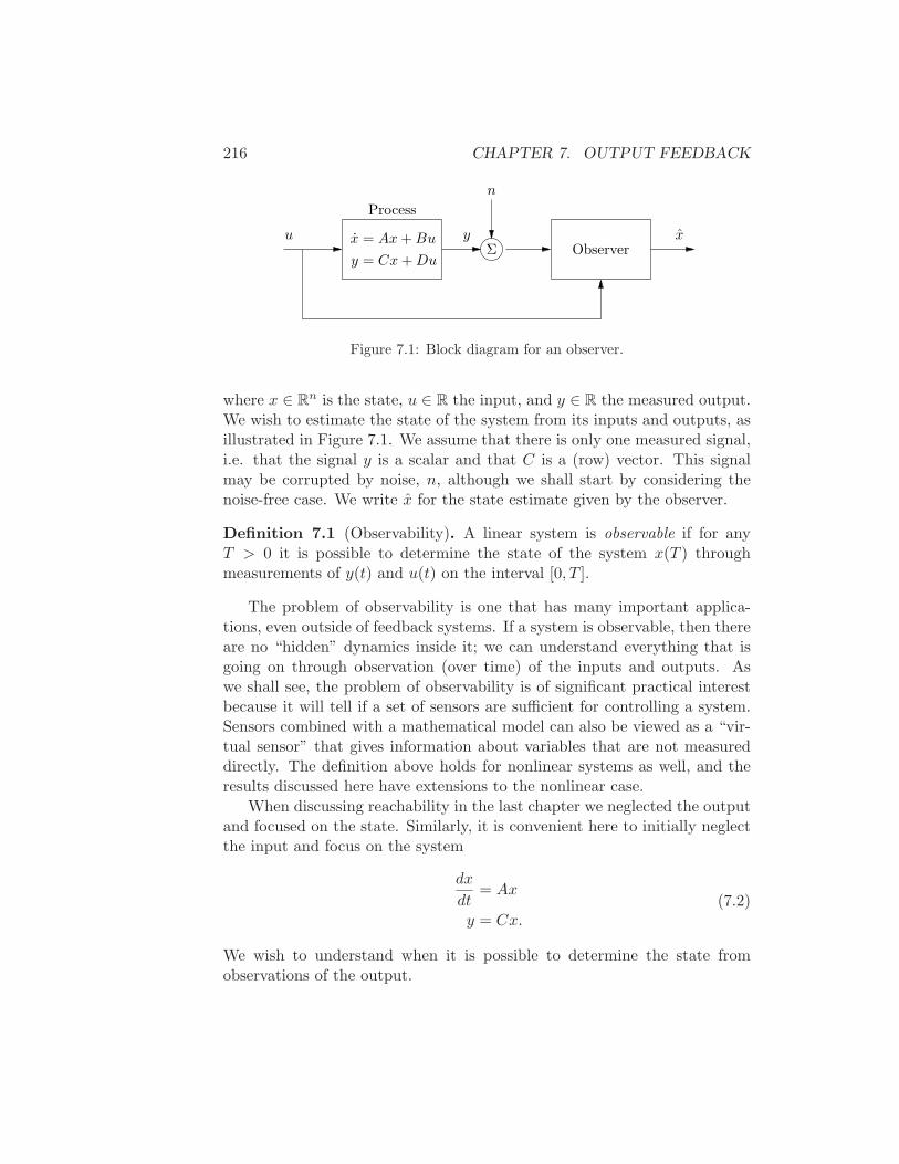
216 CHAPTER 7. OUTPUT FEEDBACK
Σ
Process
n
xyObserver
x = Ax+Bu
y = Cx+Du
u
Figure 7.1: Block diagram for an observer.
where x ∈ Rn is the state, u ∈ R the input, and y ∈ R the measured output.
We wish to estimate the state of the system from its inputs and outputs, asillustrated in Figure 7.1. We assume that there is only one measured signal,i.e. that the signal y is a scalar and that C is a (row) vector. This signalmay be corrupted by noise, n, although we shall start by considering thenoise-free case. We write x for the state estimate given by the observer.
Definition 7.1 (Observability). A linear system is observable if for anyT > 0 it is possible to determine the state of the system x(T ) throughmeasurements of y(t) and u(t) on the interval [0, T ].
The problem of observability is one that has many important applica-tions, even outside of feedback systems. If a system is observable, then thereare no “hidden” dynamics inside it; we can understand everything that isgoing on through observation (over time) of the inputs and outputs. Aswe shall see, the problem of observability is of significant practical interestbecause it will tell if a set of sensors are sufficient for controlling a system.Sensors combined with a mathematical model can also be viewed as a “vir-tual sensor” that gives information about variables that are not measureddirectly. The definition above holds for nonlinear systems as well, and theresults discussed here have extensions to the nonlinear case.
When discussing reachability in the last chapter we neglected the outputand focused on the state. Similarly, it is convenient here to initially neglectthe input and focus on the system
dx
dt= Ax
y = Cx.(7.2)
We wish to understand when it is possible to determine the state fromobservations of the output.
7.1. OBSERVABILITY 217
The output itself gives the projection of the state on vectors that arerows of the matrix C. The observability problem can immediately be solvedif the matrix C is invertible. If the matrix is not invertible we can takederivatives of the output to obtain
dy
dt= C
dx
dt= CAx.
From the derivative of the output we thus get the projection of the state onvectors which are rows of the matrix CA. Proceeding in this way we get
y
y
y...
y(n−1)
=
CCACA2
...CAn−1
x. (7.3)
We thus find that the state can be determined if the matrix
Wo =
CCACA2
...CAn−1
(7.4)
has n independent rows. It turns out that we need not consider any deriva-tives higher than n− 1 (this is an application of the Cayley-Hamilton theo-rem [Str88]).
The calculation can easily be extended to systems with inputs. The stateis then given by a linear combination of inputs and outputs and their higherderivatives. We leave this as an exercise for the reader.
In practice, differentiation can give very large errors when there is mea-surement noise and therefore the method sketched above is not particularlypractical. We will address this issue in more detail in the next section, butfor now we have the following basic result:
Theorem 7.1. A linear system of the form (7.1) is observable if and onlyif the observability matrix Wo is full rank.
Proof. The sufficiency of the observability rank condition follows from the analysis above. To prove necessity, suppose that the system is observable
218 CHAPTER 7. OUTPUT FEEDBACK
butWo is not full rank. Let v ∈ Rn, v 6= 0 be a vector in the null space ofWo,
so that Wov = 0. If we let x(0) = v be the initial condition for the systemand choose u = 0, then the output is given by y(t) = CeAtv. Since eAt canbe written as a power series in A and since An and higher powers can berewritten in terms of lower powers of A (by the Cayley-Hamilton theorem),it follows that the output will be identically zero (the reader should fill inthe missing steps if this is not clear). However, if both the input and outputof the system are 0, then a valid estimate of the state is x = 0 for all time,which is clearly incorrect since x(0) = v 6= 0. Hence by contradiction wemust have that Wo is full rank if the system is observable.
Example 7.1 (Bicycle dynamics). To demonstrate the concept of observ-ability, we consider the bicycle system, introduced in Section 3.2. Considerthe linearized model for the dynamics in equation (3.5), which has the form
Jd2ϕ
dt2− Dv0
b
dδ
dt= mghϕ+
mv20h
bδ,
where ϕ is the tilt of the bicycle and δ is the steering angle. Taking the torqueon the handle bars as an input and the lateral deviation as the output, wecan write the dynamics in state space form as (Exercise 3.3)
d
dt
x1
x2
=
0 mgh/J1 0
x1
x2
+
10
u
y =
Dv0bJ
mv20h
bJ
x.
The observability of this system determines whether it is possible to deter-mine the entire system state (tilt angle and tilt rate) from observations ofthe input (steering angle) and output (vehicle position).
The observability matrix is
W0 =
Dv0bJ
mv20h
bJ
mv20h
bJ
mgh
J· Dv0
bJ
and its determinant is
detWo =
(Dv0bJ
)2 mgh
J−(mv2
0h
bJ
)2
.
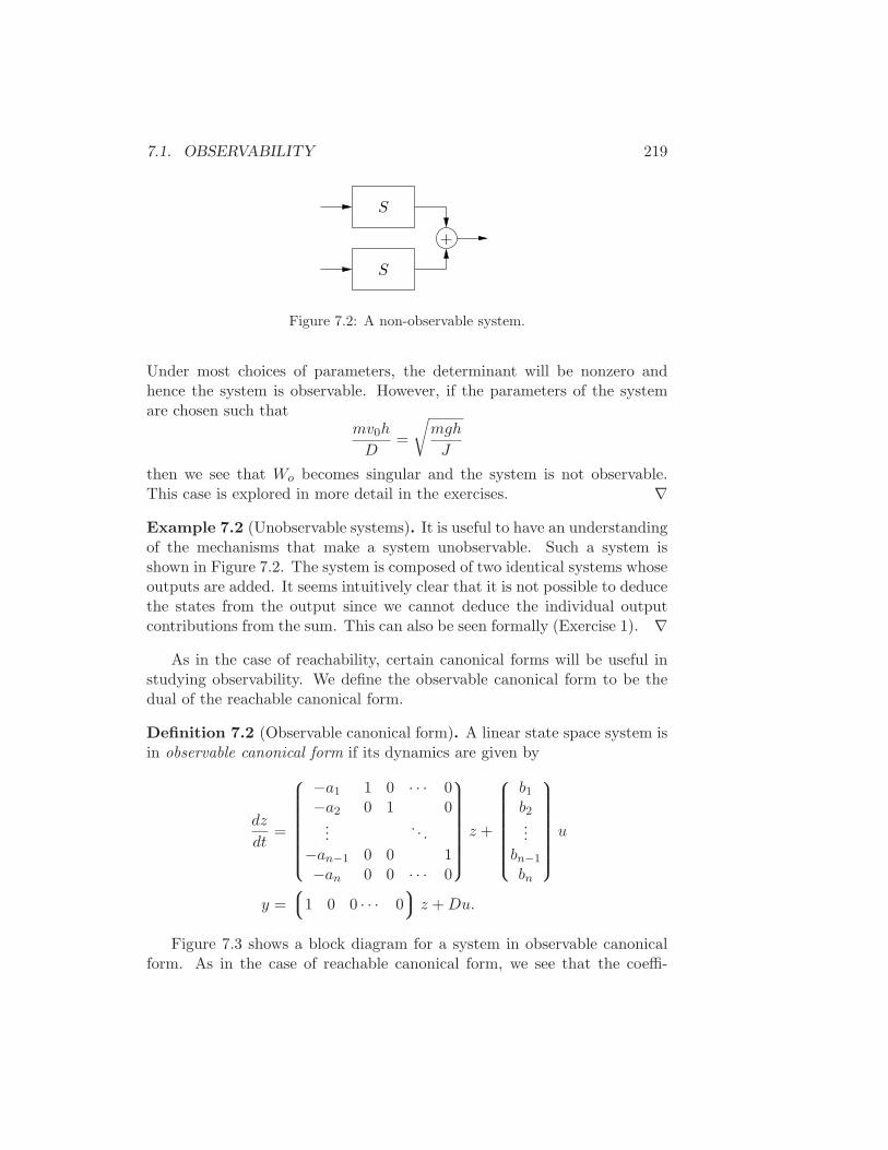
7.1. OBSERVABILITY 219
+
S
S
Figure 7.2: A non-observable system.
Under most choices of parameters, the determinant will be nonzero andhence the system is observable. However, if the parameters of the systemare chosen such that
mv0h
D=
√
mgh
J
then we see that Wo becomes singular and the system is not observable.This case is explored in more detail in the exercises. ∇
Example 7.2 (Unobservable systems). It is useful to have an understandingof the mechanisms that make a system unobservable. Such a system isshown in Figure 7.2. The system is composed of two identical systems whoseoutputs are added. It seems intuitively clear that it is not possible to deducethe states from the output since we cannot deduce the individual outputcontributions from the sum. This can also be seen formally (Exercise 1). ∇
As in the case of reachability, certain canonical forms will be useful instudying observability. We define the observable canonical form to be thedual of the reachable canonical form.
Definition 7.2 (Observable canonical form). A linear state space system isin observable canonical form if its dynamics are given by
dz
dt=
−a1 1 0 · · · 0−a2 0 1 0
.... . .
−an−1 0 0 1−an 0 0 · · · 0
z +
b1b2...
bn−1
bn
u
y =
1 0 0 · · · 0
z +Du.
Figure 7.3 shows a block diagram for a system in observable canonicalform. As in the case of reachable canonical form, we see that the coeffi-
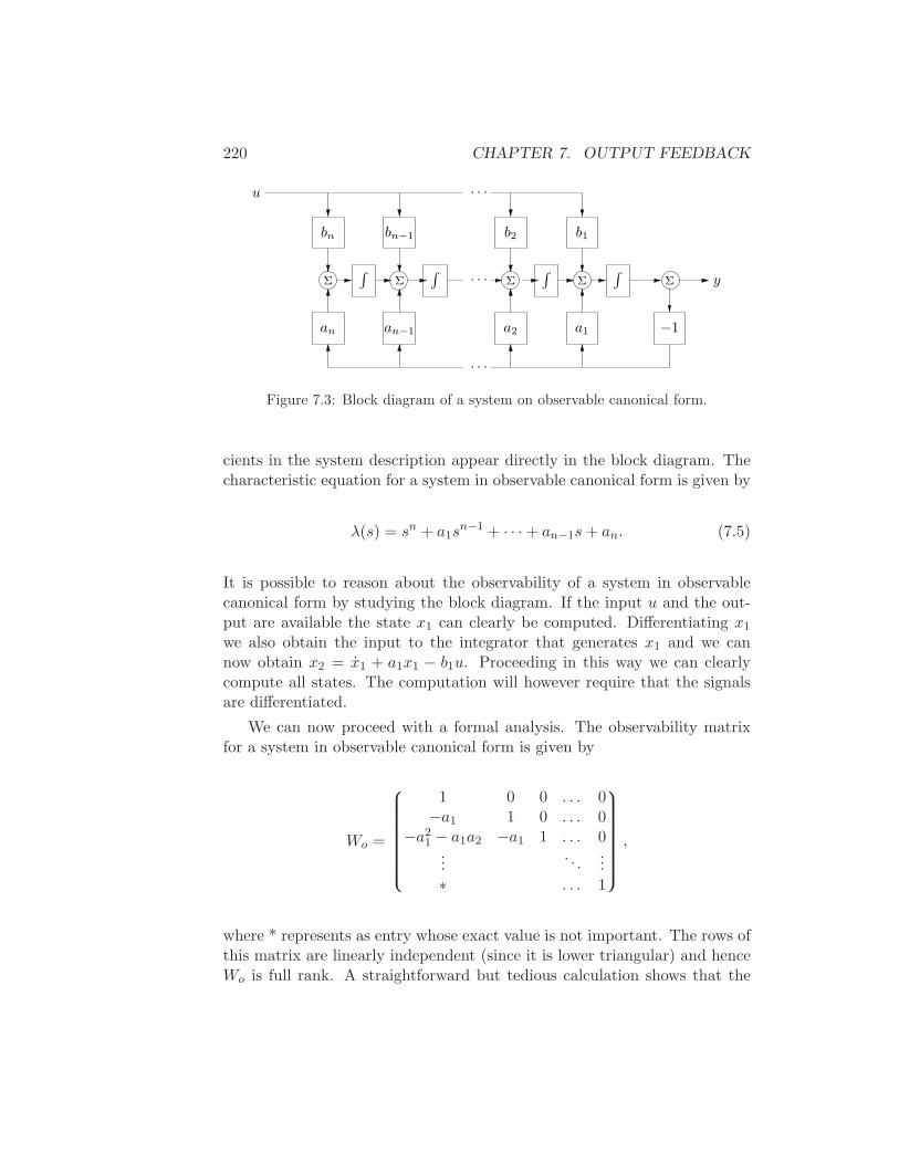
220 CHAPTER 7. OUTPUT FEEDBACK
Σ
an
u
∫
bn
. . .
. . .
an−1
∫
bn−1
Σ Σ
. . .
a2
∫
b2
−1
y
a1
∫
b1
ΣΣ
Figure 7.3: Block diagram of a system on observable canonical form.
cients in the system description appear directly in the block diagram. Thecharacteristic equation for a system in observable canonical form is given by
λ(s) = sn + a1sn−1 + · · · + an−1s+ an. (7.5)
It is possible to reason about the observability of a system in observablecanonical form by studying the block diagram. If the input u and the out-put are available the state x1 can clearly be computed. Differentiating x1
we also obtain the input to the integrator that generates x1 and we cannow obtain x2 = x1 + a1x1 − b1u. Proceeding in this way we can clearlycompute all states. The computation will however require that the signalsare differentiated.
We can now proceed with a formal analysis. The observability matrixfor a system in observable canonical form is given by
Wo =
1 0 0 . . . 0−a1 1 0 . . . 0
−a21 − a1a2 −a1 1 . . . 0
.... . .
...∗ . . . 1
,
where * represents as entry whose exact value is not important. The rows ofthis matrix are linearly independent (since it is lower triangular) and henceWo is full rank. A straightforward but tedious calculation shows that the
7.2. STATE ESTIMATION 221
inverse of the observability matrix has a simple form, given by
W−1o =
1 0 0 · · · 0a1 1 0 · · · 0a2 a1 1 · · · 0...
. . .
an−1 an−2 an−3 · · · 1
.
As in the case of reachability, it turns out that if a system is observablethen there always exists a transformation T that converts the system intoreachable canonical form (Exercise 3). This is very useful for proofs, sinceit lets us assume that a system is in reachable canonical form without anyloss of generality.
7.2 State Estimation
Having defined the concept of observability, we now return to the questionof how to construct an observer for a system. We will look for observersthat can be represented as a linear dynamical system that takes the inputsand outputs of the system we are observing and produces an estimate ofthe system’s state. That is, we wish to construct a dynamical system of theform
dx
dt= Fx+Gu+Hy,
where u and y are the input and output of the original system and x ∈ Rn
is an estimate of the state with the property that x(t) → x(t) as t→ ∞.
The Basic Observer
For a system governed by equation (7.1), we can attempt to determine thestate simply by simulating the equations with the correct input. An estimateof the state is then given by
dx
dt= Ax+Bu. (7.6)
To find the properties of this estimate, introduce the estimation error
x = x− x.
It follows from equations (7.1) and (7.6) that
dx
dt= Ax.
222 CHAPTER 7. OUTPUT FEEDBACK
If matrix A has all its eigenvalues in the left half plane, the error x will thusgo to zero and hence equation (7.6) is a dynamical system whose outputconverges to the state of the system (7.1).
The observer given by equation (7.6) uses only the process input u; themeasured signal does not appear in the equation. We must also requirethat the system is stable and essentially our estimator converges becausethe state of both the observer and the estimator are going zero. This is notvery useful in a control design context since we want to have our estimateconverge quickly to a nonzero state, so that we can make use of it in ourcontroller. We will therefore attempt to modify the observer so that theoutput is used and its convergence properties can be designed to be fastrelative to the system’s dynamics. This version will also work for unstablesystems.
Consider the observer
dx
dt= Ax+Bu+ L(y − Cx). (7.7)
This can be considered as a generalization of equation (7.6). Feedback fromthe measured output is provided by adding the term L(y − Cx), which isproportional to the difference between the observed output and the outputthat is predicted by the observer. To investigate the observer (7.7), formthe error x = x− x. It follows from equations (7.1) and (7.7) that
dx
dt= (A− LC)x.
If the matrix L can be chosen in such a way that the matrix A − LC haseigenvalues with negative real parts, the error x will go to zero. The con-vergence rate is determined by an appropriate selection of the eigenvalues.
The problem of determining the matrix L such that A − LC has pre-scribed eigenvalues is very similar to the eigenvalue assignment problem thatwas solved in the previous chapter. In fact, since the eigenvalues of the ma-trix and its transpose are the same, it is equivalent to search for LT suchthat AT −CTLT has the desired eigenvalues. This is precisely the eigenvalueassignment problem that we solved in the previous chapter, with A = AT ,B = CT and K = LT . Thus, using the results of Theorem 6.3, we can havethe following theorem on observer design:
Theorem 7.2 (Observer design by eigenvalue assignment). Consider thesystem given by
dx
dt= Ax+Bu
y = Cx(7.8)
7.2. STATE ESTIMATION 223
with one input and one output. Let λ(s) = sn + a1sn−1 + · · · + an−1s + an
be the characteristic polynomial for A. If the system is observable then thedynamical system
dx
dt= Ax+Bu+ L(y − Cx) (7.9)
is an observer for the system, with L chosen as
L = W−1o Wo
p1 − a1
p2 − a2...
pn − an
, (7.10)
and the matrices Wo and Wo given by
Wo =
CCA...
CAn−1
Wo =
1 0 0 · · · 0a1 1 0 · · · 0a2 a1 1 · · · 0...
an−1 an−2 an−3 · · · 1
−1
.
The resulting observer error x = x− x is governed by a differential equationhaving the characteristic polynomial
p(s) = sn + p1sn−1 + · · · + pn.
The dynamical system (7.9) is called an observer for (the states of) thesystem (7.8) because it will generate an approximation of the states of thesystem from its inputs and outputs. This particular form of an observeris a much more useful form than the one given by pure differentiation inequation (7.3).
Interpretation of the Observer
The observer is a dynamical system whose inputs are the process input uand process output y. The rate of change of the estimate is composed of twoterms. One term, Ax+Bu, is the rate of change computed from the modelwith x substituted for x. The other term, L(y − y), is proportional to thedifference e = y − y between measured output y and its estimate y = Cx.The estimator gain L is a matrix that tells how the error e is weighted anddistributed among the states. The observer thus combines measurements
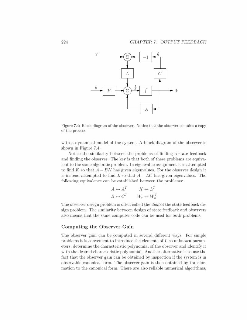
224 CHAPTER 7. OUTPUT FEEDBACK
x˙xu
yy
B Σ
Σ
∫
A
C
−1
L
Figure 7.4: Block diagram of the observer. Notice that the observer contains a copyof the process.
with a dynamical model of the system. A block diagram of the observer isshown in Figure 7.4.
Notice the similarity between the problems of finding a state feedbackand finding the observer. The key is that both of these problems are equiva-lent to the same algebraic problem. In eigenvalue assignment it is attemptedto find K so that A−BK has given eigenvalues. For the observer design itis instead attempted to find L so that A − LC has given eigenvalues. Thefollowing equivalence can be established between the problems:
A↔ AT
B ↔ CT
K ↔ LT
Wr ↔W To
The observer design problem is often called the dual of the state feedback de-sign problem. The similarity between design of state feedback and observersalso means that the same computer code can be used for both problems.
Computing the Observer Gain
The observer gain can be computed in several different ways. For simpleproblems it is convenient to introduce the elements of L as unknown param-eters, determine the characteristic polynomial of the observer and identify itwith the desired characteristic polynomial. Another alternative is to use thefact that the observer gain can be obtained by inspection if the system is inobservable canonical form. The observer gain is then obtained by transfor-mation to the canonical form. There are also reliable numerical algorithms,
7.2. STATE ESTIMATION 225
which are identical to the algorithms for computing the state feedback. Theprocedures are illustrated by example.
Example 7.3 (Vehicle steering). Consider the normalized, linear model forvehicle steering in Example 5.12. The dynamics relating steering angle u tolateral path deviation y is given by the state space model
dx
dt=
0 10 0
x+
α1
u
y =
1 0
x.
(7.11)
Recall that the state x1 represents the lateral path deviation and that x2
represents turning rate. We will now derive an observer that uses the systemmodel to determine turning rate from the measured path deviation.
The observability matrix is
Wo =
1 00 1
,
i.e., the identity matrix. The system is thus observable and the eigenvalueassignment problem can be solved. We have
A− LC =
−l1 1−l2 0
,
which has the characteristic polynomial
det (sI −A+ LC) = det
s+ l1 −1l2 s
= s2 + l1s+ l2.
Assuming that it is desired to have an observer with the characteristic poly-nomial
s2 + p1s+ p2 = s2 + 2ζoωos+ ω2o ,
the observer gains should be chosen as
l1 = p1 = 2ζoωo
l2 = p2 = ω2o .
The observer is then
dx
dt= Ax+Bu+ L(y = Cx) =
0 10 0
x+
01
u+
l1l2
(y − x1).
∇
226 CHAPTER 7. OUTPUT FEEDBACK
For larger systems, the place or acker commands can be used in MAT-LAB. Note that these functions are the same as the ones used for eigenvalueassignment with state feedback; for estimator design, one simply uses thetranspose of the dynamics matrix and the output matrix.
7.3 Control using Estimated State
In this section we will consider the same system as in the previous sections,i.e., the state space system described by
dx
dt= Ax+Bu
y = Cx.(7.12)
We wish to design a feedback controller for the system where only the outputis measured. As before, we will be assume that u and y are scalars. We alsoassume that the system is reachable and observable. In Chapter 6 we founda feedback of the form
u = Kx+ krr
for the case that all states could be measured and in Section 7.2 we havedeveloped an observer that can generate estimates of the state x basedon inputs and outputs. In this section we will combine the ideas of thesesections to find a feedback that gives desired closed loop eigenvalues forsystems where only outputs are available for feedback.
If all states are not measurable, it seems reasonable to try the feedback
u = −Kx+ krr (7.13)
where x is the output of an observer of the state, i.e.
dx
dt= Ax+Bu+ L(y − Cx). (7.14)
Since the system (7.12) and the observer (7.14) both are of state dimen-sion n, the closed loop system has state dimension 2n. The states of thecombined system are x and x. The evolution of the states is described byequations (7.12), (7.13) and (7.14). To analyze the closed loop system, thestate variable x is replaced by
x = x− x. (7.15)
7.3. CONTROL USING ESTIMATED STATE 227
Subtraction of equation (7.14) from equation (7.12) gives
dx
dt= Ax−Ax− L(y − Cx) = Ax− LCx = (A− LC)x.
Returning to the process dynamics, introducing u from equation (7.13)into equation (7.12) and using equation (7.15) to eliminate x gives
dx
dt= Ax+Bu = Ax−BKx+Bkrr = Ax−BK(x− x) +Bkrr
= (A−BK)x+BKx+Bkrr.
The closed loop system is thus governed by
d
dt
xx
=
A−BK BK
0 A− LC
xx
+
Bkr
0
r. (7.16)
Notice that the state x, representing the observer error, is not affected bythe command signal r. This is desirable since we do not want the referencesignal to generate observer errors.
Since the dynamics matrix is block diagonal, we find that the character-istic polynomial of the closed loop system is
λ(s) = det (sI −A+BK) det (sI −A+ LC).
This polynomial is a product of two terms: the characteristic polynomial ofthe closed loop system obtained with state feedback and the characteristicpolynomial of the observer error. The feedback (7.13) that was motivatedheuristically thus provides a very neat solution to the eigenvalue assignmentproblem. The result is summarized as follows.
Theorem 7.3 (Eigenvalue assignment by output feedback). Consider thesystem
dx
dt= Ax+Bu
y = Cx.
The controller described by
u = −Kx+ krr
dx
dt= Ax+Bu+ L(y − Cx)
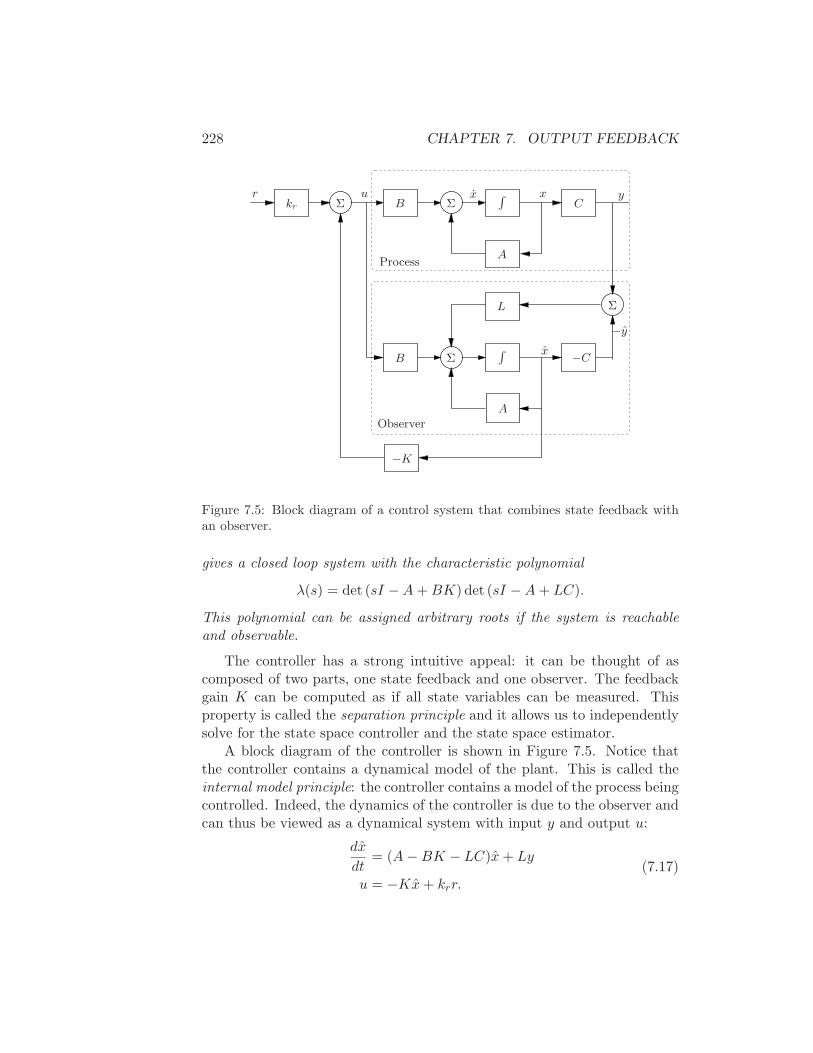
228 CHAPTER 7. OUTPUT FEEDBACK
r u yxx
x
−y
B
B
Σ
Σ
Σ
Σ
R
R
A
A
C
−C
L
−K
kr
Process
Observer
Figure 7.5: Block diagram of a control system that combines state feedback withan observer.
gives a closed loop system with the characteristic polynomial
λ(s) = det (sI −A+BK) det (sI −A+ LC).
This polynomial can be assigned arbitrary roots if the system is reachableand observable.
The controller has a strong intuitive appeal: it can be thought of ascomposed of two parts, one state feedback and one observer. The feedbackgain K can be computed as if all state variables can be measured. Thisproperty is called the separation principle and it allows us to independentlysolve for the state space controller and the state space estimator.
A block diagram of the controller is shown in Figure 7.5. Notice thatthe controller contains a dynamical model of the plant. This is called theinternal model principle: the controller contains a model of the process beingcontrolled. Indeed, the dynamics of the controller is due to the observer andcan thus be viewed as a dynamical system with input y and output u:
dx
dt= (A−BK − LC)x+ Ly
u = −Kx+ krr.(7.17)
7.4. KALMAN FILTERING 229
Example 7.4 (Vehicle steering). Consider again the normalized, linearmodel for vehicle steering in Example 5.12. The dynamics relating steeringangle u to lateral path deviation y is given by the state space model (7.11).Combining the state feedback derived in Example 6.4 with the observerdetermined in Example 7.3 we find that the controller is given by
dx
dt= Ax+Bu+ L(y − Cx) =
0 10 0
x+
01
u+
l1l2
(y − x1)
u = −Kx+ krr = k1(r − x1) − k2x2
The controller is thus a dynamical system of second order. Elimination ofthe variable u gives
dx
dt= (A−BK − LC)x+ Ly +Bkrr
=
−l1 − αk1 1 − αk2
−k1 − l2 −k2
x+
l1l2
y +
α1
k1r
u = −Kx+ krr = −
k1 k2
x+ k1r.
The controller is a dynamical system of second order, with two inputs y andr and one output u. ∇
7.4 Kalman Filtering
One of the principal uses of observers in practice is to estimate the state ofa system in the presence of noisy measurements. We have not yet treatednoise in our analysis and a full treatment of stochastic dynamical systems isbeyond the scope of this text. In this section, we present a brief introductionto the use of stochastic systems analysis for constructing observers. We workprimarily in discrete time to avoid some of the complications associatedwith continuous time random processes and to keep the mathematical pre-requisites to a minimum. This section assumes basic knowledge of randomvariables and stochastic processes.
Consider a discrete time, linear system with dynamics
xk+1 = Axk +Buk + Fvk
yk = Cxk + wk,(7.18)
230 CHAPTER 7. OUTPUT FEEDBACK
where vk and wk are Gaussian, white noise processes satisfying
Evk = 0 Ewk = 0
EvkvTj =
0 k 6= j
Rv k = jEwkw
Tj =
0 k 6= j
Rw k = j
EvkwTj = 0.
(7.19)
We assume that the initial condition is also modeled as a Gaussian randomvariable with
Ex0 = x0 Ex0xT0 = P0. (7.20)
We wish to find an estimate xk that minimizes the mean square errorE(xk − xk)(xk − xk)
T given the measurements y(δ) : 0 ≤ τ ≤ t. Weconsider an observer in the same basic form as derived previously:
xk+1 = Axk +Buk + Lk(yk − Cxk). (7.21)
The following theorem summarizes the main result.
Theorem 7.4. Consider a random process xk with dynamics (7.18) andnoise processes and initial conditions described by equations (7.19) and (7.20).The observer gain L that minimizes the mean square error is given by
Lk = ATPkCT (Rw + CPkC
T )−1,
wherePk+1 = (A− LC)Pk(A− LC)T +Rv + LRwL
T
P0 = EX(0)XT (0).(7.22)
Before we prove this result, we reflect on its form and function. First,note that the Kalman filter has the form of a recursive filter: given Pk =EEkE
Tk at time k, can compute how the estimate and covariance change.
Thus we do not need to keep track of old values of the output. Furthermore,the Kalman filter gives the estimate xk and the covariance PE,k, so we cansee how reliable the estimate is. It can also be shown that the Kalman filterextracts the maximum possible information about output data. If we formthe residual between the measured output and the estimated output,
ek = yk − Cxk,
we can can show that for the Kalman filter the correlation matrix is
Re(j, k) = Wδjk.
7.4. KALMAN FILTERING 231
In other words, the error is a white noise process, so there is no remainingdynamic information content in the error.
In the special case when the noise is stationary (Q, R constant) and ifPk converges, then the observer gain is constant:
K = ATPCT (Rw + CPCT ),
where
P = APAT +Rv −APCT(Rw + CPCT
)−1CPAT .
We see that the optimal gain depends on both the process noise and themeasurement noise, but in a nontrivial way. Like the use of LQR to choosestate feedback gains, the Kalman filter permits a systematic derivation ofthe observer gains given a description of the noise processes. The solutionfor the constant gain case is solved by the dlqe command in MATLAB.
Proof (of theorem). We wish to minimize the mean square of the error,E(xk − xk)(xk − xk)
T . We will define this quantity as Pk and then showthat it satisfies the recursion given in equation (7.22). By definition,
Pk+1 = Exk+1xTk+1
= (A− LC)Pk(A− LC)T +Rv + LRwLT
= APkAT −APkC
TLT − LCAT + L(Rw + CPkCT )LT
Letting Rǫ = (Rw + CPkCT ), we have
Pk+1 = APkAT −APkC
TLT − LCAT + LRǫLT
= APkAT +
(L−APkC
TR−1ǫ
)Rǫ
(L−APKC
TR−1ǫ
)T
−APkCTR−1
ǫ CP Tk A
T +Rw.
In order to minimize this expression, we choose L = APkCTR−1
ǫ and thetheorem is proven.
The Kalman filter can also be applied to continuous time stochastic pro-cesses. The mathematical derivation of this result requires more sophisti-cated tools, but the final form of the estimator is relatively straightforward.
Consider a continuous stochastic system
x = Ax+Bu+ Fv Ev(s)vT (t) = Q(t)δ(t− s)
y = Cx+ w Ew(s)wT (t) = R(t)δ(t− s)
232 CHAPTER 7. OUTPUT FEEDBACK
Assume that the disturbance v and noise w are zero-mean and Gaussian(but not necessarily stationary):
pdf(v) =1
n√
2π√
detQe−
1
2vT Q−1v
pdf(w) = . . . (using R)
We wish to find the estimate x(t) that minimizes the mean square errorE(x(t) − x(t))(x(t) − x(t))T given y(τ) : 0 ≤ τ ≤ t.Theorem 7.5 (Kalman-Bucy, 1961). The optimal estimator has the formof a linear observer
˙x = Ax+Bu+ L(y − Cx)
where L(t) = P (t)CTR−1 and P (t) = E(x(t) − x(t))(x(t) − x(t))T andsatisfies
P = AP + PAT − PCTR−1(t)CP + FQ(t)F T
P (0) = Ex(0)xT (0)
7.5 State Space Control Systems
In this section we consider a collection of additional topics on the designand analysis of control systems using state space tools.
Computer Implementation
The controllers obtained so far have been described by ordinary differentialequations. They can be implemented directly using analog components,whether electronic circuits, hydraulic valves or other physical devices. Sincein modern engineering applications most controllers are implemented usingcomputers we will briefly discuss how this can be done.
A computer controlled system typically operates periodically: every cy-cle, signals from the sensors are sampled and converted to digital form bythe A/D converter, the control signal is computed, and the resulting outputis converted to analog form for the actuators (as shown in Figure 1.3 onpage 5). To illustrate the main principles of how to implement feedback inthis environment, we consider the controller described by equations (7.13)and (7.14), i.e.,
u = −Kx+ krr
dx
dt= Ax+Bu+K(y − Cx).
7.5. STATE SPACE CONTROL SYSTEMS 233
The first equation consists only of additions and multiplications and canthus be implemented directly on a computer. The second equation hasto be approximated. A simple way is to approximate the derivative by adifference
dx
dt≈ x(tk+1) − x(tk)
h= Ax(tk) +Bu(tk) +K(y(tk) − Cx(tk))
where tk are the sampling instants and h = tk+1− tk is the sampling period.Rewriting the equation to isolate x(tk+1), we get
x(tk+1) = x(tk) + h(Ax(tk) +Bu(tk) +K(y(tk) − Cx(tk))
). (7.23)
The calculation of the estimated state at time tk+1 only requires additionand multiplication and can easily be done by a computer. A section ofpseudo code for the program that performs this calculation is
% Control algorithm - main loop
r = adin(ch1) % read setpoint from ch1
y = adin(ch2) % get process output from ch2
u = C*xhat + Kr*r % compute control variable
daout(ch1, u) % set analog output on ch1
xhat = xhat + h*(A*x+B*u+L*(y-C*x)) % update state estimate
The program runs periodically at a fixed rate h. Notice that the numberof computations between reading the analog input and setting the analogoutput has been minimized. The state is updated after the analog outputhas been set. The program has an array of states, xhat, that represents thestate estimate. The choice of sampling period requires some care.
There are several practical issues that also must be dealt with. For ex-ample it is necessary to filter a signal before it is sampled so that the filteredsignal has little frequency content above fs/2 where fs is the sampling fre-quency. If controllers with integral action are used, it is also necessary toprovide protection so that the integral does not become too large when theactuator saturates. This issue, called integrator windup, is studied in moredetail in Chapter 10. Care must also be taken so that parameter changesdo not cause disturbances.
A General Controller Structure
We now consider a general control structure that pulls together the variousresults the the previous and current chapters. This structure is one thatappears in may places in control theory and is the heart of most moderncontrol systems.

234 CHAPTER 7. OUTPUT FEEDBACK
TrajectoryGenerator
r
u
-x
xd
ProcessΣ ΣState
Feedback
Observer
ufb
ud
y
Figure 7.6: Block diagram of a controller based on a structure with two degreesof freedom. The controller consists of a command signal generator, state feedbackand an observer.
We begin by generalizing the way we handle the reference input. Sofar reference signals have been introduced simply by adding them to thestate feedback through a gain kr. A more sophisticated way of doing thisis shown by the block diagram in Figure 7.6, where the controller consistsof three parts: an observer that computes estimates of the states based ona model and measured process inputs and outputs, a state feedback anda trajectory generator that generates the desired behavior of all states xd
and a feedforward signal ud. The signal ud is such that it generates thedesired behavior of the states when applied to the system, under the idealconditions of no disturbances and no modeling errors. The controller is saidto have two degrees of freedom because the response to command signalsand disturbances are decoupled. Disturbance responses are governed by theobserver and the state feedback and the response to command signals isgoverned by the trajectory generator (feedfoward).
We start with the full nonlinear dynamics of the process
x = f(x, u)
y = h(x, u).(7.24)
Assume that the trajectory generator is able to generate a desired trajectory(xd, ud) that satisfies the dynamics (7.24) and satisfies r = h(xd, ud). Todesign the controller, we construct the error system. We will assume forsimplicity that f(x, u) = f(x) + g(x)u (i.e., the system is nonlinear in thestate, but linear in the input; this is often the case in applications). Let
7.5. STATE SPACE CONTROL SYSTEMS 235
e = x− xd, v = u− ud and compute the dynamics for the error:
e = x− xd = f(x) + g(x)u− f(xd) + g(xd)ud
= f(e+ xd) − f(xd) + g(e+ xd)(v + ud) − g(xd)ud
= F (e, v, xd(t), ud(t))
In general, this system is time varying.For trajectory tracking, we can assume that e is small (if our controller
is doing a good job) and so we can linearize around e = 0:
e ≈ A(t)e+B(t)v
where
A(t) =∂F
∂e
∣∣∣∣(xd(t),ud(t))
B(t) =∂F
∂v
∣∣∣∣(xd(t),ud(t)
.
It is often the case that A(t) and B(t) depend only on xd, in which case itis convenient to write A(t) = A(xd) and B(t) = B(xd).
Assume now that xd and ud are either constant or slowly varying (withrespect to the performance criterion). This allows us to consider just the(constant) linear system given by (A(xd), B(xd)). If we design a state feed-back controller K(xd) for each xd, then we can regulate the system usingthe feedback
v = K(xd)e.
Substituting back the definitions of e and v, our controller becomes
u = K(xd)(x− xd) + ud
This form of controller is called a gain scheduled linear controller with feed-forward ud.
Finally, we consider the observer. We can use the full nonlinear dynamicsfor the prediction portion of the observer and the linearized system for thecorrection term:
˙x = f(x, u) + L(x)(y − h(x, u))
where L(x) is the observer gain obtained by linearizing the system aroundthe currently estimate state. This form of the observer is known as anextended Kalman filter and has proven to be a very effective means of esti-mating the state of a nonlinear system.
To get some insight into the overall behavior of the system, we considerwhat happens when the command signal is changed. To fix the ideas let usassume that the system is in equilibrium with the observer state x equal to
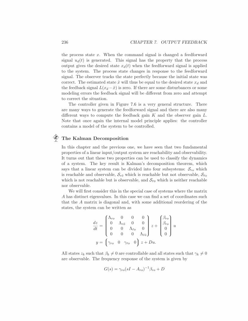
236 CHAPTER 7. OUTPUT FEEDBACK
the process state x. When the command signal is changed a feedforwardsignal ud(t) is generated. This signal has the property that the processoutput gives the desired state xd(t) when the feedforward signal is appliedto the system. The process state changes in response to the feedforwardsignal. The observer tracks the state perfectly because the initial state wascorrect. The estimated state x will thus be equal to the desired state xd andthe feedback signal L(xd− x) is zero. If there are some disturbances or somemodeling errors the feedback signal will be different from zero and attemptto correct the situation.
The controller given in Figure 7.6 is a very general structure. Thereare many ways to generate the feedforward signal and there are also manydifferent ways to compute the feedback gain K and the observer gain L.Note that once again the internal model principle applies: the controllercontains a model of the system to be controlled.
The Kalman Decomposition
In this chapter and the previous one, we have seen that two fundamentalproperties of a linear input/output system are reachability and observability.It turns out that these two properties can be used to classify the dynamicsof a system. The key result is Kalman’s decomposition theorem, whichsays that a linear system can be divided into four subsystems: Sro whichis reachable and observable, Sro which is reachable but not observable, Sro
which is not reachable but is observable, and Sro which is neither reachablenor observable.
We will first consider this in the special case of systems where the matrixA has distinct eigenvalues. In this case we can find a set of coordinates suchthat the A matrix is diagonal and, with some additional reordering of thestates, the system can be written as
dz
dt=
Λro 0 0 00 Λro 0 00 0 Λro 00 0 0 Λro
z +
βro
βro
00
u
y =
γro 0 γro 0
z +Du.
All states zk such that βk 6= 0 are controllable and all states such that γk 6= 0are observable. The frequency response of the system is given by
G(s) = γro(sI −Aro)−1βro +D
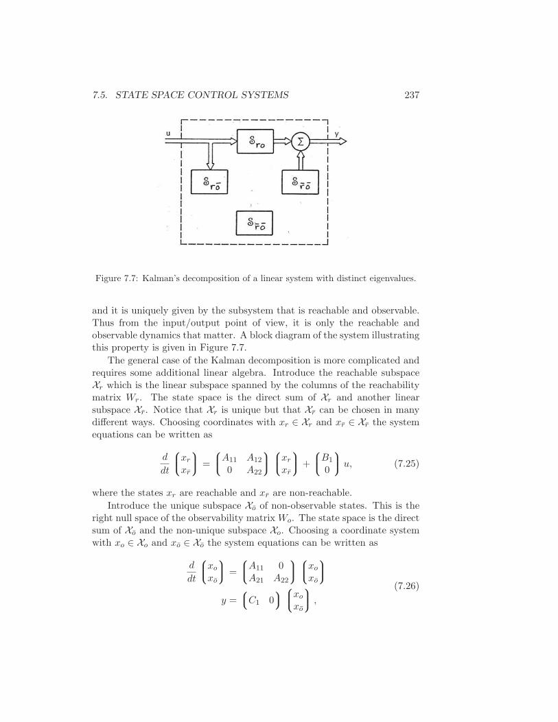
7.5. STATE SPACE CONTROL SYSTEMS 237
Figure 7.7: Kalman’s decomposition of a linear system with distinct eigenvalues.
and it is uniquely given by the subsystem that is reachable and observable.Thus from the input/output point of view, it is only the reachable andobservable dynamics that matter. A block diagram of the system illustratingthis property is given in Figure 7.7.
The general case of the Kalman decomposition is more complicated andrequires some additional linear algebra. Introduce the reachable subspaceXr which is the linear subspace spanned by the columns of the reachabilitymatrix Wr. The state space is the direct sum of Xr and another linearsubspace Xr. Notice that Xr is unique but that Xr can be chosen in manydifferent ways. Choosing coordinates with xr ∈ Xr and xr ∈ Xr the systemequations can be written as
d
dt
xr
xr
=
A11 A12
0 A22
xr
xr
+
B1
0
u, (7.25)
where the states xr are reachable and xr are non-reachable.
Introduce the unique subspace Xo of non-observable states. This is theright null space of the observability matrix Wo. The state space is the directsum of Xo and the non-unique subspace Xo. Choosing a coordinate systemwith xo ∈ Xo and xo ∈ Xo the system equations can be written as
d
dt
xo
xo
=
A11 0A21 A22
xo
xo
y =
C1 0
xo
xo
,
(7.26)
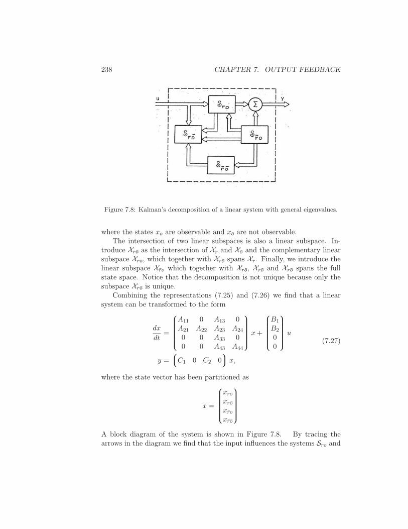
238 CHAPTER 7. OUTPUT FEEDBACK
Figure 7.8: Kalman’s decomposition of a linear system with general eigenvalues.
where the states xo are observable and xo are not observable.The intersection of two linear subspaces is also a linear subspace. In-
troduce Xro as the intersection of Xr and Xo and the complementary linearsubspace Xro, which together with Xro spans Xr. Finally, we introduce thelinear subspace Xro which together with Xro, Xro and Xro spans the fullstate space. Notice that the decomposition is not unique because only thesubspace Xro is unique.
Combining the representations (7.25) and (7.26) we find that a linearsystem can be transformed to the form
dx
dt=
A11 0 A13 0A21 A22 A23 A24
0 0 A33 00 0 A43 A44
x+
B1
B2
00
u
y =
C1 0 C2 0
x,
(7.27)
where the state vector has been partitioned as
x =
xro
xro
xro
xro
A block diagram of the system is shown in Figure 7.8. By tracing thearrows in the diagram we find that the input influences the systems Sro and

7.6. FURTHER READING 239
Sro and that the output is influenced by Sro and Sro. The system Sro isneither connected to the input nor the output. The frequency response ofthe system is thus
G(s) = C1(sI −A11)−1B1, (7.28)
which is the dynamics of the reachable and observable subsystem Sro.
7.6 Further Reading
The notion of observability is due to Kalman [Kal61b] and, combined withthe dual notion of reachability, it was a major stepping stone toward estab-lishing state space control theory beginning in the 1960s. For linear systemsthe output is a projection of the state and it may seem unnecessary to esti-mate the full state since a projection is already available. Luenberger [Lue71]constructed an reduced order observer that only reconstructs the state thatis not measured directly.
The main result of this chapter is the general controller structure in Fig-ure 7.6. This controller structure emerged as a result of solving optimizationproblems. The observer first appeared as the Kalman filter which was alsothe solution to an optimization problem [Kal61a, KB61]. It was then shownthat the solution to an optimization with output feedback could be obtainedby combining a state feedback with a Kalman filter [JT61, GF71]. Laterit was found that the controller with the same structure also emerged assolutions of other simpler deterministic control problems like the ones dis-cussed in this chapter [?, ?]. Much later it was shown that solutions torobust control problems also had a similar structure but with different waysof computing observer and state feedback gains [DGKF89]. The material isnow an essential part of the tools in control.
A more detailed presentation of stochastic control theory is given in [Ast70].
7.7 Exercises
1. Show that the system depicted in Figure 7.2 is not observable.
2. Consider a system under a coordinate transformation z = Tx, whereT ∈ R
n×n is an invertible matrix. Show that the observability ma-trix for the transformed system is given by Wo = WoT
−1 and henceobservability is independent of the choice of coordinates.

240 CHAPTER 7. OUTPUT FEEDBACK
3. Show that if a system is observable, then there exists a change ofcoordinates z = Tx that puts the transformed system into reachablecanonical form.
Chapter 8
Transfer Functions
The typical regulator system can frequently be described, in essentials, bydifferential equations of no more than perhaps the second, third or fourthorder. . . . In contrast, the order of the set of differential equations describingthe typical negative feedback amplifier used in telephony is likely to be verymuch greater. As a matter of idle curiosity, I once counted to find out whatthe order of the set of equations in an amplifier I had just designed wouldhave been, if I had worked with the differential equations directly. It turnedout to be 55.
Henrik Bode, 1960 [Bod60].
This chapter introduces the concept of the transfer function, which is acompact description of the input/output relation for a linear system. Com-bining transfer functions with block diagrams gives a powerful method fordealing with complex linear systems. The relationship between transferfunctions and other system descriptions of dynamics is also discussed.
8.1 Frequency Domain Analysis
Figure 8.1 shows a block diagram for a typical control system, consisting of aprocess to be controlled and a (dynamic) compensator, connected in a feed-back loop. We saw in the previous two chapters how to analyze and designsuch systems using state space descriptions of the blocks. As was mentionedin Chapter 2, an alternative approach is to focus on the input/output char-acteristics of the system. Since it is the inputs and outputs that are used toconnect the systems, one could expect that this point of view would allowan understanding of the overall behavior of the system. Transfer functionsare the main tool in implementing this point of view for linear systems.
241
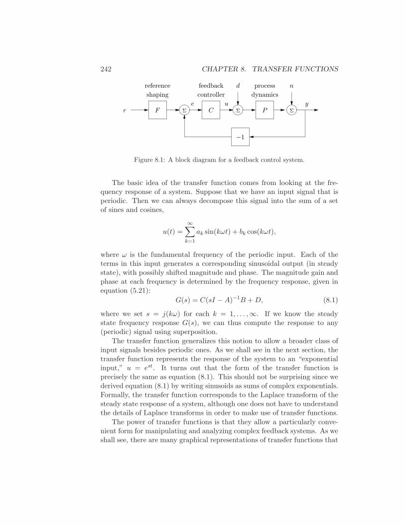
242 CHAPTER 8. TRANSFER FUNCTIONS
−1
r ΣF Pyu
d n
Ce
reference feedback process
shaping controller dynamics
Σ Σ
Figure 8.1: A block diagram for a feedback control system.
The basic idea of the transfer function comes from looking at the fre-quency response of a system. Suppose that we have an input signal that isperiodic. Then we can always decompose this signal into the sum of a setof sines and cosines,
u(t) =∞∑
k=1
ak sin(kωt) + bk cos(kωt),
where ω is the fundamental frequency of the periodic input. Each of theterms in this input generates a corresponding sinusoidal output (in steadystate), with possibly shifted magnitude and phase. The magnitude gain andphase at each frequency is determined by the frequency response, given inequation (5.21):
G(s) = C(sI −A)−1B +D, (8.1)
where we set s = j(kω) for each k = 1, . . . ,∞. If we know the steadystate frequency response G(s), we can thus compute the response to any(periodic) signal using superposition.
The transfer function generalizes this notion to allow a broader class ofinput signals besides periodic ones. As we shall see in the next section, thetransfer function represents the response of the system to an “exponentialinput,” u = est. It turns out that the form of the transfer function isprecisely the same as equation (8.1). This should not be surprising since wederived equation (8.1) by writing sinusoids as sums of complex exponentials.Formally, the transfer function corresponds to the Laplace transform of thesteady state response of a system, although one does not have to understandthe details of Laplace transforms in order to make use of transfer functions.
The power of transfer functions is that they allow a particularly conve-nient form for manipulating and analyzing complex feedback systems. As weshall see, there are many graphical representations of transfer functions that
8.2. DERIVATION OF THE TRANSFER FUNCTION 243
capture interesting properties of dynamics. Transfer functions also make itpossible to express the changes in a system because of modeling error, whichis essential when discussing sensitivity to process variations of the sort dis-cussed in Chapter 12. In particular, using transfer functions it is possibleto analyze what happens when dynamic models are approximated by staticmodels or when high order models are approximated by low order models.One consequence is that we can introduce concepts that express the degreeof stability of a system.
The main limitation of transfer functions is that they can only be usedfor linear systems. While many of the concepts for state space modelingand analysis extend to nonlinear systems, there is no such analog for trans-fer functions and there are only limited extensions of many of the ideasto nonlinear systems. Hence for the remainder of the text we shall limitourselves to linear models. However, it should be pointed out that despitethis limitation, transfer functions still remain a valuable tool for designingcontrollers for nonlinear systems, chiefly through constructing their linearapproximations around an equilibrium point of interest.
8.2 Derivation of the Transfer Function
As we have seen in previous chapters, the input/output dynamics of a linearsystem has two components: the initial condition response and the forcedresponse. In addition, we can speak of the transient properties of the systemand its steady state response to an input. The transfer function focuses onthe steady state response due to a given input, and provides a mappingbetween inputs and their corresponding outputs. In this section, we willderive the transfer function in terms of the “exponential response” of alinear system.
Transmission of Exponential Signals
To formally compute the transfer function of a system, we will make use ofa special type of signal, called an exponential signal, of the form est wheres = σ+jω is a complex number. Exponential signals play an important rolein linear systems. They appear in the solution of differential equations and inthe impulse response of linear systems, and many signals can be representedas exponentials or sums of exponentials. For example, a constant signal issimply eαt with α = 0. Damped sine and cosine signals can be representedby
e(σ+jω)t = eσtejωt = eσt(cosωt+ i sinωt),
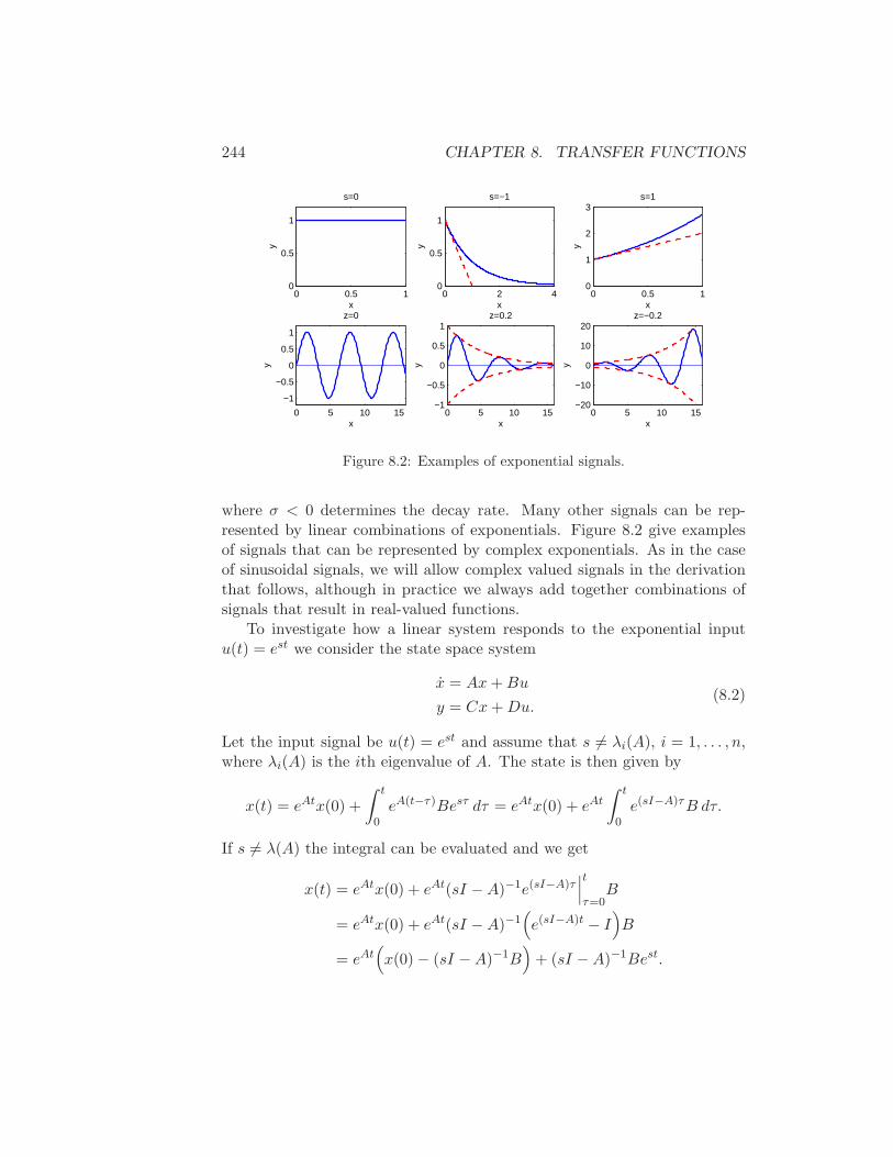
244 CHAPTER 8. TRANSFER FUNCTIONS
0 0.5 10
0.5
1
x
y
s=0
0 2 40
0.5
1
x
y
s=−1
0 0.5 10
1
2
3
x
y
s=1
0 5 10 15
−1
−0.5
0
0.5
1
x
y
z=0
0 5 10 15−1
−0.5
0
0.5
1
xy
z=0.2
0 5 10 15−20
−10
0
10
20
x
y
z=−0.2
Figure 8.2: Examples of exponential signals.
where σ < 0 determines the decay rate. Many other signals can be rep-resented by linear combinations of exponentials. Figure 8.2 give examplesof signals that can be represented by complex exponentials. As in the caseof sinusoidal signals, we will allow complex valued signals in the derivationthat follows, although in practice we always add together combinations ofsignals that result in real-valued functions.
To investigate how a linear system responds to the exponential inputu(t) = est we consider the state space system
x = Ax+Bu
y = Cx+Du.(8.2)
Let the input signal be u(t) = est and assume that s 6= λi(A), i = 1, . . . , n,where λi(A) is the ith eigenvalue of A. The state is then given by
x(t) = eAtx(0) +
∫ t
0eA(t−τ)Besτ dτ = eAtx(0) + eAt
∫ t
0e(sI−A)τB dτ.
If s 6= λ(A) the integral can be evaluated and we get
x(t) = eAtx(0) + eAt(sI −A)−1e(sI−A)τ∣∣∣
t
τ=0B
= eAtx(0) + eAt(sI −A)−1(
e(sI−A)t − I)
B
= eAt(
x(0) − (sI −A)−1B)
+ (sI −A)−1Best.
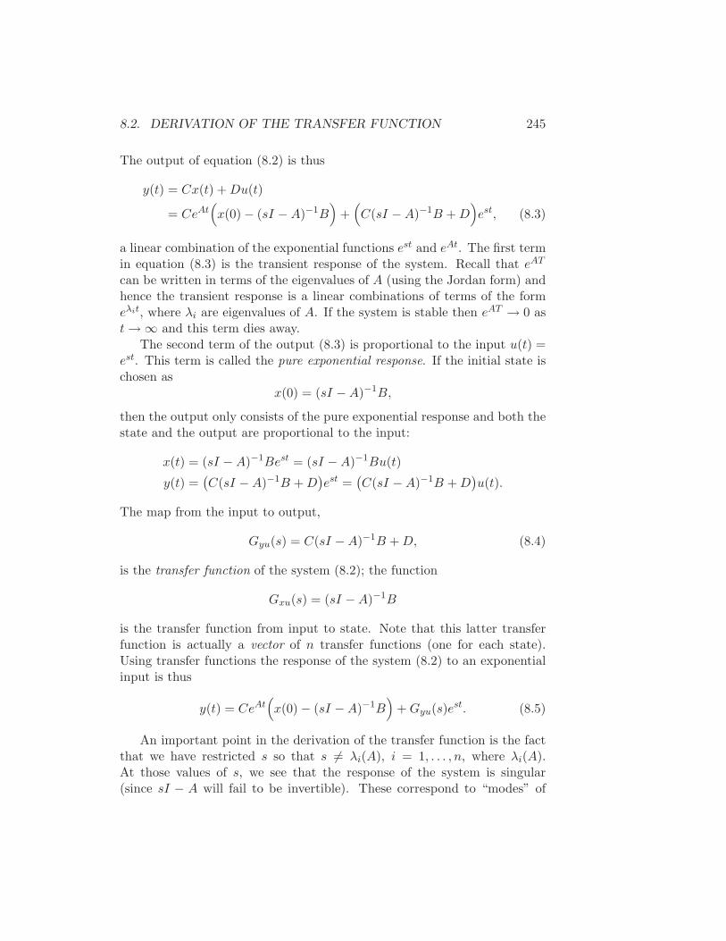
8.2. DERIVATION OF THE TRANSFER FUNCTION 245
The output of equation (8.2) is thus
y(t) = Cx(t) +Du(t)
= CeAt(
x(0) − (sI −A)−1B)
+(
C(sI −A)−1B +D)
est, (8.3)
a linear combination of the exponential functions est and eAt. The first termin equation (8.3) is the transient response of the system. Recall that eAT
can be written in terms of the eigenvalues of A (using the Jordan form) andhence the transient response is a linear combinations of terms of the formeλit, where λi are eigenvalues of A. If the system is stable then eAT → 0 ast→ ∞ and this term dies away.
The second term of the output (8.3) is proportional to the input u(t) =est. This term is called the pure exponential response. If the initial state ischosen as
x(0) = (sI −A)−1B,
then the output only consists of the pure exponential response and both thestate and the output are proportional to the input:
x(t) = (sI −A)−1Best = (sI −A)−1Bu(t)
y(t) =(C(sI −A)−1B +D
)est =
(C(sI −A)−1B +D
)u(t).
The map from the input to output,
Gyu(s) = C(sI −A)−1B +D, (8.4)
is the transfer function of the system (8.2); the function
Gxu(s) = (sI −A)−1B
is the transfer function from input to state. Note that this latter transferfunction is actually a vector of n transfer functions (one for each state).Using transfer functions the response of the system (8.2) to an exponentialinput is thus
y(t) = CeAt(
x(0) − (sI −A)−1B)
+Gyu(s)est. (8.5)
An important point in the derivation of the transfer function is the factthat we have restricted s so that s 6= λi(A), i = 1, . . . , n, where λi(A).At those values of s, we see that the response of the system is singular(since sI − A will fail to be invertible). These correspond to “modes” of
246 CHAPTER 8. TRANSFER FUNCTIONS
the system and are particularly problematic when Re s ≥ 0, since this canresult in bounded inputs creating unbounded outputs. This situation canonly happen when the system has eigenvalues with either positive or zeroreal part, and hence it relates to the stability of the system. In particular,if a linear system is asymptotically stable, then bounded inputs will alwaysproduce bounded outputs.
Coordinate Changes
The matrices A, B and C in equation (8.2) depend on the choice of coor-dinate system for the states. Since the transfer function relates input tooutputs, it should be invariant to coordinate changes in the state space. Toshow this, consider the model (8.2) and introduce new coordinates z by thetransformation z = Tx, where T is a nonsingular matrix. The system isthen described by
z = T (Ax+Bu) = TAT−1z + TBu = Az + Bu
y = Cx+DU = CT−1z +Du = Cz +Du
This system has the same form as equation (8.2) but the matrices A, B andC are different:
A = TAT−1 B = TB C = CT−1 D = D. (8.6)
Computing the transfer function of the transformed model we get
G(s) = C(sI − A)−1B +D
= CT−1T (sI −A)−1T−1TB +D
= CT−1(sI − TAT−1)−1TB +D
= C(T−1(sI − TAT−1)T
)−1B +D
= C(sI −A)−1B +D = G(s),
which is identical to the transfer function (8.4) computed from the systemdescription (8.2). The transfer function is thus invariant to changes of thecoordinates in the state space.
Another property of the transfer function is that it corresponds to the por-tion of the state space dynamics that are both reachable and observable. Inparticular, if we make use of the Kalman decomposition (Section 7.5), thenthe transfer function only depends on the dynamics on the reachable andobservable subspace, Sro (Exercise 2).
8.2. DERIVATION OF THE TRANSFER FUNCTION 247
Transfer Functions for Linear Differential Equations
Consider a linear input/output system described by the differential equation
dny
dtn+ a1
dn−1y
dtn−1+ · · · + any = b0
dmu
dtm+ b1
dm−1u
dtm−1+ · · · + bmu, (8.7)
where u is the input and y is the output. This type of description arises inmany applications, as described briefly in Section 2.2. Note that here wehave generalized our previous system description to allow both the inputand its derivatives to appear.
To determine the transfer function of the system (8.7), let the input beu(t) = est. Since the system is linear, there is an output of the systemthat is also an exponential function y(t) = y0e
st. Inserting the signals inequation (8.7) we find
(sn + a1sn−1 + · · · + an)y0e
st = (b0sm + b1s
m−1 · · · + bm)e−st
and the response of the system can be completely described by two polyno-mials
a(s) = sn + a1sn−1 + · · · + an−1s+ an
b(s) = b0sm + b1s
m−1 + · · · + bm−1s+ bm.(8.8)
The polynomial a(s) is the characteristic polynomial of the ordinarydifferential equation. If a(s) 6= 0 it follows that
y(t) = y0est =
b(s)
a(s)est = G(s)u(t). (8.9)
The transfer function of the system (8.7) is thus the rational function
G(s) =b(s)
a(s), (8.10)
where the polynomials a(s) and b(s) are given by equation (8.8). Notice thatthe transfer function for the system (8.7) can be obtained by inspection,since the coefficients of a(s) and b(s) are precisely the coefficients of thederivatives of u and y.
Equations (8.7)–(8.10) can be used to compute the transfer functions ofmany simple ODEs. The following table gives some of the more commonforms:
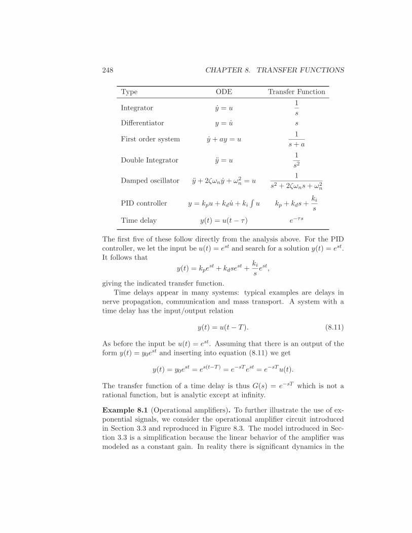
248 CHAPTER 8. TRANSFER FUNCTIONS
Type ODE Transfer Function
Integrator y = u1
s
Differentiator y = u s
First order system y + ay = u1
s+ a
Double Integrator y = u1
s2
Damped oscillator y + 2ζωny + ω2n = u
1
s2 + 2ζωns+ ω2n
PID controller y = kpu+ kdu+ ki
∫u kp + kds+
ki
s
Time delay y(t) = u(t− τ) e−τs
The first five of these follow directly from the analysis above. For the PIDcontroller, we let the input be u(t) = est and search for a solution y(t) = est.It follows that
y(t) = kpest + kdse
st +ki
sest,
giving the indicated transfer function.Time delays appear in many systems: typical examples are delays in
nerve propagation, communication and mass transport. A system with atime delay has the input/output relation
y(t) = u(t− T ). (8.11)
As before the input be u(t) = est. Assuming that there is an output of theform y(t) = y0e
st and inserting into equation (8.11) we get
y(t) = y0est = es(t−T ) = e−sT est = e−sTu(t).
The transfer function of a time delay is thus G(s) = e−sT which is not arational function, but is analytic except at infinity.
Example 8.1 (Operational amplifiers). To further illustrate the use of ex-ponential signals, we consider the operational amplifier circuit introducedin Section 3.3 and reproduced in Figure 8.3. The model introduced in Sec-tion 3.3 is a simplification because the linear behavior of the amplifier wasmodeled as a constant gain. In reality there is significant dynamics in the
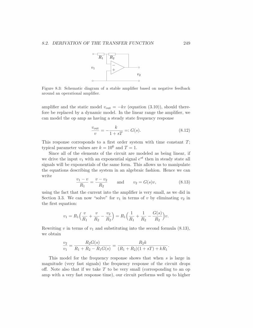
8.2. DERIVATION OF THE TRANSFER FUNCTION 249
R2
−+
v1
v2
R1
Figure 8.3: Schematic diagram of a stable amplifier based on negative feedbackaround an operational amplifier.
amplifier and the static model vout = −kv (equation (3.10)), should there-fore be replaced by a dynamic model. In the linear range the amplifier, wecan model the op amp as having a steady state frequency response
vout
v= − k
1 + sT=: G(s). (8.12)
This response corresponds to a first order system with time constant T ;typical parameter values are k = 106 and T = 1.
Since all of the elements of the circuit are modeled as being linear, ifwe drive the input v1 with an exponential signal est then in steady state allsignals will be exponentials of the same form. This allows us to manipulatethe equations describing the system in an algebraic fashion. Hence we canwrite
v1 − v
R1=v − v2R2
and v2 = G(s)v, (8.13)
using the fact that the current into the amplifier is very small, as we did inSection 3.3. We can now “solve” for v1 in terms of v by eliminating v2 inthe first equation:
v1 = R1
( v
R1+
v
R2− v2R2
)
= R1
( 1
R1+
1
R2− G(s)
R2
)
v.
Rewriting v in terms of v1 and substituting into the second formula (8.13),we obtain
v2v1
=R2G(s)
R1 +R2 −R1G(s)=
R2k
(R1 +R2)(1 + sT ) + kR1.
This model for the frequency response shows that when s is large inmagnitude (very fast signals) the frequency response of the circuit dropsoff. Note also that if we take T to be very small (corresponding to an opamp with a very fast response time), our circuit performs well up to higher
250 CHAPTER 8. TRANSFER FUNCTIONS
frequencies. In the limit that T = 0, we recover the responds that we derivedin Section 3.3.
Note that in solving this example, we bypassed explicitly writing thesignals as v = v0e
st and instead worked directly with v, assuming it was anexponential. This shortcut is very handy in solving problems of this sort.
∇
Although we have focused thus far on ordinary differential equations, trans-fer functions can also be used for other types of linear systems. We illustratethis via an example of a transfer function for a partial differential equation.
Example 8.2 (Transfer function for heat propagation). Consider the onedimensional heat propagation in a semi-infinite metal rod. Assume that theinput is the temperature at one end and that the output is the temperatureat a point on the rod. Let θ be the temperature at time t and position x.With proper choice of length scales and units, heat propagation is describedby the partial differential equation
∂θ
∂t=∂2θ
∂2x, (8.14)
and the point of interest can be assumed to have x = 1. The boundarycondition for the partial differential equation is
θ(0, t) = u(t).
To determine the transfer function we choose the input as u(t) = est. As-sume that there is a solution to the partial differential equation of the formθ(x, t) = ψ(x)est, and insert this into equation (8.14) to obtain
sψ(x) =d2ψ
dx2,
with boundary condition ψ(0) = est. This ordinary differential equation(with independent variable x) has the solution
ψ(x) = Aex√
s +Be−x√
s.
Matching the boundary conditions gives A = 0 and B = est, so the solutionis
y(t) = θ(1, t) = ψ(1)est = e−√
sest = e−√
su(t).
The system thus has the transfer function G(s) = e−√
s. As in the case of atime delay, the transfer function is not a simple ratio of polynomials, but itis an analytic function. ∇
8.2. DERIVATION OF THE TRANSFER FUNCTION 251
Transfer Function Properties
The transfer function has many useful physical interpretations and the fea-tures of a transfer function are often associated with important system prop-erties.
The zero frequency gain of a system is given by the magnitude of thetransfer function at s = 0. It represents the ratio of the steady state valueof the output with respect to a step input (which can be represented asu = est with s = 0). For a state space system, we computed the zerofrequency gain in equation (5.20):
G(0) = D − CA−1B.
For a system written as a linear ODE, as in equation (8.7), if we assumethat the input and output of the system are constants y0 and u0, then wefind that any0 = bmu0. Hence the zero frequency gain gain is
G(0) =y0
u0=bman. (8.15)
Next consider a linear system with the rational transfer function
G(s) =b(s)
a(s).
The roots of the polynomial a(s) are called poles of the system and theroots of b(s) are called the zeros of the system. If p is a pole it followsthat y(t) = ept is a solution of equation (8.7) with u = 0 (the homogeneoussolution). The function ept is called a mode of the system. The unforcedmotion of the system after an arbitrary excitation is a weighted sum ofthe modes. Since the pure exponential output corresponding to the inputu(t) = est with a(s) 6= 0 is G(s)est it follows that the pure exponentialoutput is zero if b(s) = 0. Zeros of the transfer function thus block thetransmission of the corresponding exponential signals.
For a state space system with transfer functionG(s) = C(sI−A)−1B+D,the poles of the transfer function are the eigenvalues of the matrix A in thestate space model. One easy way to see this is to notice that the value ofG(s) is unbounded when s is an eigenvalue of a system since this is preciselythe set of points where the characteristic polynomial λ(s) = det(sI−A) = 0(and hence sI − A is non-invertible). It follows that the poles of a statespace system depend only on the matrix A, which represents the intrinsicdynamics of the system.
252 CHAPTER 8. TRANSFER FUNCTIONS
To find the zeros of a state space system, we observe that the zeros arecomplex numbers s such that the input u(t) = est gives zero output. Insert-ing the pure exponential response x(t) = x0e
st and y(t) = 0 in equation (8.2)gives
sestx0 = Ax0est +Bu0e
st
0 = Cestx0 +Destu0,
which can be written as
sI −A BC D
x0
u0
= 0.
This equation has a solution with nonzero x0, u0 only if the matrix on theleft does not have full rank. The zeros are thus the values s such that
det
sI −A BC D
= 0. (8.16)
Since the zeros depend on A, B, C and D, they therefore depend on howthe inputs and outputs are coupled to the states. Notice in particular that ifthe matrix B has full rank then the matrix has n linearly independent rowsfor all values of s. Similarly there are n linearly independent columns if thematrix C has full rank. This implies that systems where the matrices B orC are of full rank do not have zeros. In particular it means that a system hasno zeros if it is fully actuated (each state can be controlled independently)or if the full state is measured.
A convenient way to view the poles and zeros of a transfer functionis through a pole zero diagram, as shown in Figure 8.4. In this diagram,each pole is marked with a cross and each zero with a circle. If there aremultiple poles or zeros at a fixed location, these are often indicated withoverlapping crosses or circles (or other annotations). Poles in the left halfplane correspond to stable models of the system and poles in the right halfplane correspond to unstable modes. Notice that the gain must also be givento have a complete description of the transfer function.
8.3 Block Diagrams and Transfer Functions
The combination of block diagrams and transfer functions is a powerful wayto represent control systems. Transfer functions relating different signals inthe system can be derived by purely algebraic manipulations of the transfer
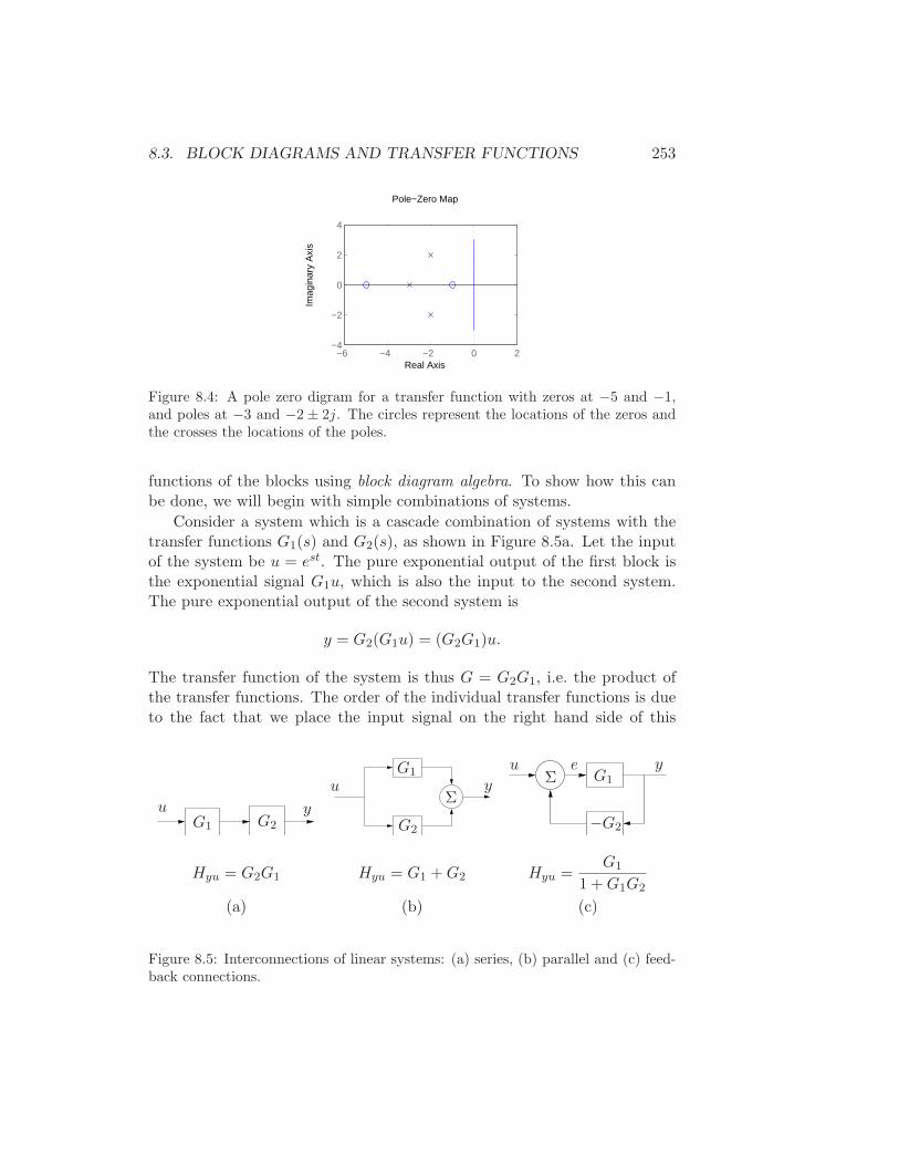
8.3. BLOCK DIAGRAMS AND TRANSFER FUNCTIONS 253
−6 −4 −2 0 2−4
−2
0
2
4
Pole−Zero Map
Real Axis
Imag
inar
y A
xis
Figure 8.4: A pole zero digram for a transfer function with zeros at −5 and −1,and poles at −3 and −2 ± 2j. The circles represent the locations of the zeros andthe crosses the locations of the poles.
functions of the blocks using block diagram algebra. To show how this canbe done, we will begin with simple combinations of systems.
Consider a system which is a cascade combination of systems with thetransfer functions G1(s) and G2(s), as shown in Figure 8.5a. Let the inputof the system be u = est. The pure exponential output of the first block isthe exponential signal G1u, which is also the input to the second system.The pure exponential output of the second system is
y = G2(G1u) = (G2G1)u.
The transfer function of the system is thus G = G2G1, i.e. the product ofthe transfer functions. The order of the individual transfer functions is dueto the fact that we place the input signal on the right hand side of this
u yG1 G2
u y
G2
G1
Σ
u yeG1
−G2
Σ
Hyu = G2G1 Hyu = G1 +G2 Hyu =G1
1 +G1G2
(a) (b) (c)
Figure 8.5: Interconnections of linear systems: (a) series, (b) parallel and (c) feed-back connections.
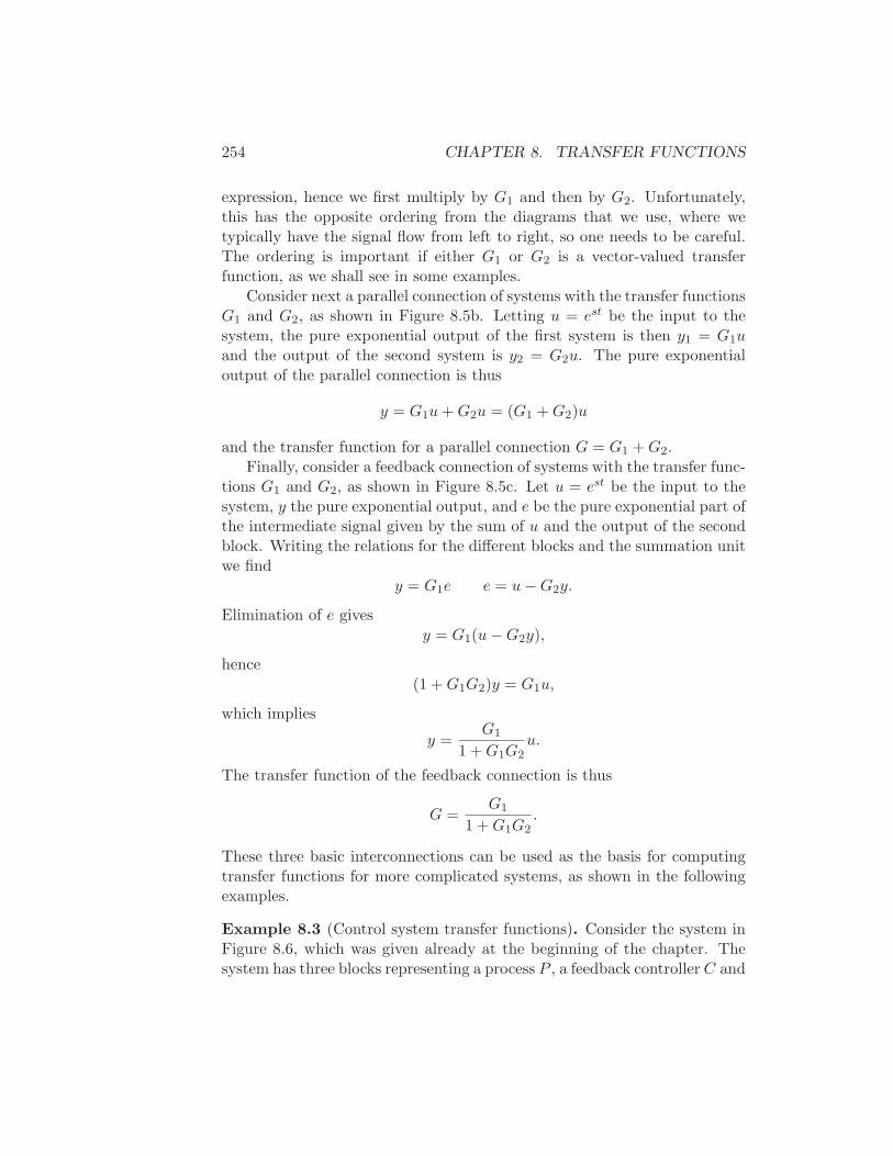
254 CHAPTER 8. TRANSFER FUNCTIONS
expression, hence we first multiply by G1 and then by G2. Unfortunately,this has the opposite ordering from the diagrams that we use, where wetypically have the signal flow from left to right, so one needs to be careful.The ordering is important if either G1 or G2 is a vector-valued transferfunction, as we shall see in some examples.
Consider next a parallel connection of systems with the transfer functionsG1 and G2, as shown in Figure 8.5b. Letting u = est be the input to thesystem, the pure exponential output of the first system is then y1 = G1uand the output of the second system is y2 = G2u. The pure exponentialoutput of the parallel connection is thus
y = G1u+G2u = (G1 +G2)u
and the transfer function for a parallel connection G = G1 +G2.Finally, consider a feedback connection of systems with the transfer func-
tions G1 and G2, as shown in Figure 8.5c. Let u = est be the input to thesystem, y the pure exponential output, and e be the pure exponential part ofthe intermediate signal given by the sum of u and the output of the secondblock. Writing the relations for the different blocks and the summation unitwe find
y = G1e e = u−G2y.
Elimination of e givesy = G1(u−G2y),
hence(1 +G1G2)y = G1u,
which implies
y =G1
1 +G1G2u.
The transfer function of the feedback connection is thus
G =G1
1 +G1G2.
These three basic interconnections can be used as the basis for computingtransfer functions for more complicated systems, as shown in the followingexamples.
Example 8.3 (Control system transfer functions). Consider the system inFigure 8.6, which was given already at the beginning of the chapter. Thesystem has three blocks representing a process P , a feedback controller C and
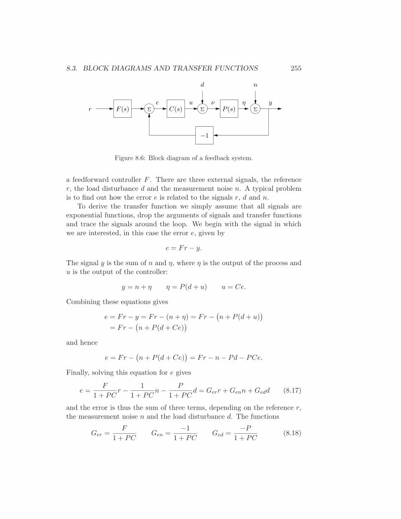
8.3. BLOCK DIAGRAMS AND TRANSFER FUNCTIONS 255
νr ΣF (s) P (s)
yu
d n
C(s)e
Σ Σ
−1
η
Figure 8.6: Block diagram of a feedback system.
a feedforward controller F . There are three external signals, the referencer, the load disturbance d and the measurement noise n. A typical problemis to find out how the error e is related to the signals r, d and n.
To derive the transfer function we simply assume that all signals areexponential functions, drop the arguments of signals and transfer functionsand trace the signals around the loop. We begin with the signal in whichwe are interested, in this case the error e, given by
e = Fr − y.
The signal y is the sum of n and η, where η is the output of the process andu is the output of the controller:
y = n+ η η = P (d+ u) u = Ce.
Combining these equations gives
e = Fr − y = Fr − (n+ η) = Fr −(n+ P (d+ u)
)
= Fr −(n+ P (d+ Ce)
)
and hence
e = Fr −(n+ P (d+ Ce)
)= Fr − n− Pd− PCe.
Finally, solving this equation for e gives
e =F
1 + PCr − 1
1 + PCn− P
1 + PCd = Gerr +Genn+Gedd (8.17)
and the error is thus the sum of three terms, depending on the reference r,the measurement noise n and the load disturbance d. The functions
Ger =F
1 + PCGen =
−1
1 + PCGed =
−P1 + PC
(8.18)
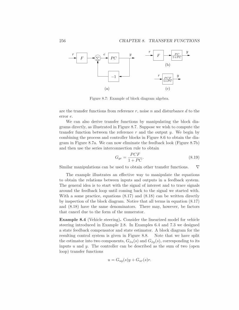
256 CHAPTER 8. TRANSFER FUNCTIONS
e
PCF1+PC
yr
Fr
PC1+PC
y
(a)
(b)
(c)
P
F PCr
−1
y
Figure 8.7: Example of block diagram algebra.
are the transfer functions from reference r, noise n and disturbance d to theerror e.
We can also derive transfer functions by manipulating the block dia-grams directly, as illustrated in Figure 8.7. Suppose we wish to compute thetransfer function between the reference r and the output y. We begin bycombining the process and controller blocks in Figure 8.6 to obtain the dia-gram in Figure 8.7a. We can now eliminate the feedback look (Figure 8.7b)and then use the series interconnection rule to obtain
Gyr =PCF
1 + PC. (8.19)
Similar manipulations can be used to obtain other transfer functions. ∇The example illustrates an effective way to manipulate the equations
to obtain the relations between inputs and outputs in a feedback system.The general idea is to start with the signal of interest and to trace signalsaround the feedback loop until coming back to the signal we started with.With a some practice, equations (8.17) and (8.18) can be written directlyby inspection of the block diagram. Notice that all terms in equation (8.17)and (8.18) have the same denominators. There may, however, be factorsthat cancel due to the form of the numerator.
Example 8.4 (Vehicle steering). Consider the linearized model for vehiclesteering introduced in Example 2.8. In Examples 6.4 and 7.3 we designeda state feedback compensator and state estimator. A block diagram for theresulting control system is given in Figure 8.8. Note that we have splitthe estimator into two components, Gxu(s) and Gxy(s), corresponding to itsinputs u and y. The controller can be described as the sum of two (openloop) transfer functions
u = Guy(s)y +Gur(s)r.
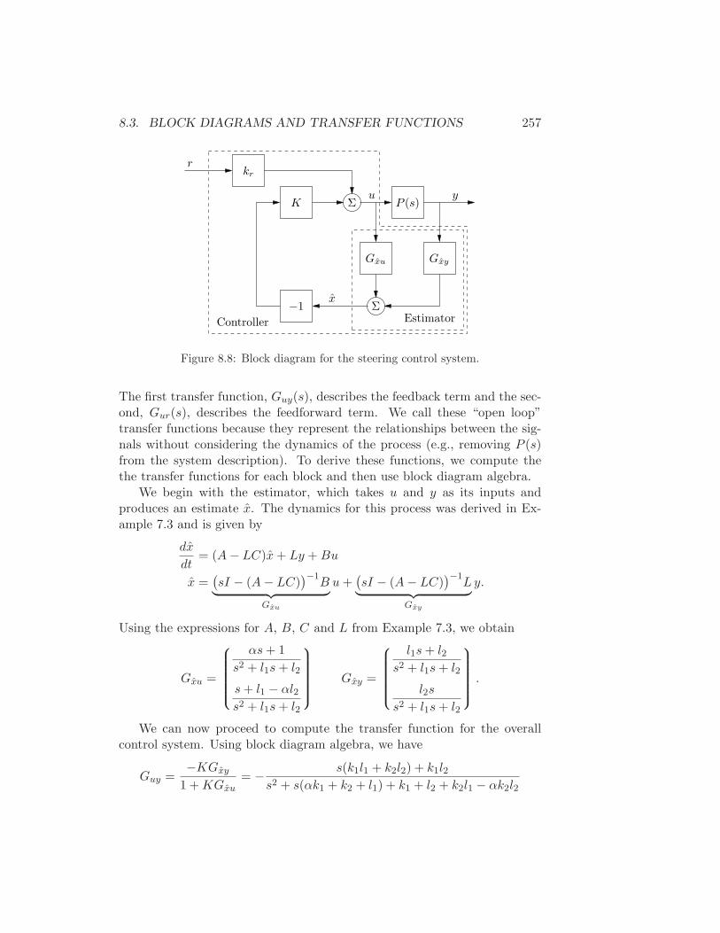
8.3. BLOCK DIAGRAMS AND TRANSFER FUNCTIONS 257
Controller
K P (s)
Gxu Gxy
−1
uΣ
ΣEstimator
x
y
rkr
Figure 8.8: Block diagram for the steering control system.
The first transfer function, Guy(s), describes the feedback term and the sec-ond, Gur(s), describes the feedforward term. We call these “open loop”transfer functions because they represent the relationships between the sig-nals without considering the dynamics of the process (e.g., removing P (s)from the system description). To derive these functions, we compute thethe transfer functions for each block and then use block diagram algebra.
We begin with the estimator, which takes u and y as its inputs andproduces an estimate x. The dynamics for this process was derived in Ex-ample 7.3 and is given by
dx
dt= (A− LC)x+ Ly +Bu
x =(sI − (A− LC)
)−1B
︸ ︷︷ ︸
Gxu
u+(sI − (A− LC)
)−1L
︸ ︷︷ ︸
Gxy
y.
Using the expressions for A, B, C and L from Example 7.3, we obtain
Gxu =
αs+ 1
s2 + l1s+ l2
s+ l1 − αl2s2 + l1s+ l2
Gxy =
l1s+ l2s2 + l1s+ l2
l2s
s2 + l1s+ l2
.
We can now proceed to compute the transfer function for the overallcontrol system. Using block diagram algebra, we have
Guy =−KGxy
1 +KGxu= − s(k1l1 + k2l2) + k1l2
s2 + s(αk1 + k2 + l1) + k1 + l2 + k2l1 − αk2l2
258 CHAPTER 8. TRANSFER FUNCTIONS
and
Gur =kr
1 +KGxu= k1
s2 + l1s+ l2s2 + s(αk1 + k2 + l1) + k1 + l2 + k2l1 − αk2l2
.
Finally, we compute the full closed loop dynamics. We begin by de-riving the transfer function for the process, P (s). We can compute thisdirectly from the state space description of the dynamics, which was givenin Example 6.4. Using that description, we have
P = Gyu = C(sI −A)−1B +D =
1 0
s −10 s
−1α1
=αs+ 1
s2.
The transfer function for the full closed loop system between the input rand the output y is then given by
Gyr =krP (s)
1 − P (s)Gyu(s)=
k1(αs+ 1)
s2 + (k1α+ k2)s+ k1.
Note that the observer gains do not appear in this equation. This is becausewe are considering steady state analysis and, in steady state, the estimatedstate exactly tracks the state of the system if we assume perfect models. Wewill return to this example in Chapter 12 to study the robustness of thisparticular approach. ∇
The combination of block diagrams and transfer functions is a powerfultool because it is possible both to obtain an overview of a system and finddetails of the behavior of the system.
Pole/Zero Cancellations
Because transfer functions are often polynomials in s, it can sometimeshappen that the numerator and denominator have a common factor, whichcan be canceled. Sometimes these cancellations are simply algebraic sim-plifications, but in other situations these cancellations can mask potentialfragilities in the model. In particular, if a pole/zero cancellation occurs dueto terms in separate blocks that just happen to coincide, the cancellationmay not occur if one of the systems is slightly perturbed. In some situationsthis can result in severe differences between the expected behavior and theactual behavior, as illustrated in this section.
To illustrate when we can have pole/zero cancellations, consider theblock diagram shown in Figure 8.6 with F = 1 (no feedforward compensa-tion) and C and P given by
C =nc(s)
dc(s)P =
np(s)
dp(s).
8.4. THE BODE PLOT 259
The transfer function from r to e is then given by
Ger =1
1 + PC=
dc(s)dp(s)
dc(s)dp(s) + nc(s)np(s).
If there are common factors in the numerator and denominator polynomials,then these terms can be factored out and eliminated from both the numera-tor and denominator. For example, if the controller has a zero at s = a andthe process has a pole at s = a, then we will have
Ger =(s+ a)d′c(s)dp(s)
(s+ a)dc(s)d′p(s) + (s+ a)n′c(s)np(s)=
d′c(s)dp(s)
dc(s)d′p(s) + n′c(s)np(s),
where n′c(s) and d′p(s) represent the relevant polynomials with the term s+afactored out.
Suppose instead that we compute the transfer function from d to e, whichrepresents the effect of a disturbance on the error between the reference andthe output. This transfer function is given by
Ged =d′c(s)np(s)
(s+ a)dc(s)d′p(s) + (s+ a)n′c(s)np(s).
Notice that if a < 0 then the pole is in the right half plane and the transferfunction Ged is unstable. Hence, even though the transfer function from r toe appears to be OK (assuming a perfect pole/zero cancellation), the trans-fer function from d to e can exhibit unbounded behavior. This unwantedbehavior is typical of an unstable pole/zero cancellation.
It turns out that the cancellation of a pole with a zero can also be under-stood in terms of the state space representation of the systems. Reachabilityor observability is lost when there are cancellations of poles and zeros (Ex-ercise 11). A consequence is that the transfer function only represents thedynamics in the reachable and observable subspace of a system (see Sec-tion 7.5).
8.4 The Bode Plot
The frequency response of a linear system can be computed from its transferfunction by setting s = jω, corresponding to a complex exponential
u(t) = ejωt = cos(ωt) + j sin(ωt).
The resulting output has the form
y(t) = Mejωt+ϕ = M cos(ωt+ ϕ) + jM sin(ωt+ ϕ)
260 CHAPTER 8. TRANSFER FUNCTIONS
where M and ϕ are the gain and phase of G:
M = |G(jω)| ϕ = ∠G(jω) = arctanImG(jω)
ReG(jω).
The phase of G is also called the argument of G, a term that comes fromthe theory of complex variables.
It follows from linearity that the response to a single sinusoid (sin orcos) is amplified by M and phase shifted by ϕ. Note that ϕ ∈ [0, 2π), so thearctangent must be taken respecting the signs of the numerator and denom-inator. It will often be convenient to represent the phase in degrees ratherthan radians. We will use the notation ∠G(jω) for the phase in degreesand argG(jω) for the phase in radians. In addition, while we always takeargG(jω) to be in the range [0, 2π), we will take ∠G(jω) to be continuous,so that it can take on values outside of the range of 0 to 360.
The frequency response G(jω) can thus be represented by two curves:the gain curve and the phase curve. The gain curve gives gain |G(jω)|as a function of frequency ω and the phase curve gives phase ∠G(jω) asa function of frequency ω. One particularly useful way of drawing thesecurves is to use a log/log scale for the magnitude plot and a log/linear scalefor the phase plot. This type of plot is called a Bode plot and is shown inFigure 8.9.
Part of the popularity of Bode plots is that they are easy to sketch andto interpret. Consider a transfer function which is a ratio of polynomialterms G(s) = (b1(s)b2(s))/(a1(s)a2(s)). We have
log |G(s)| = log |b1(s)| + log |b2(s)| − log |a1(s)| − log |a2(s)|
and hence we can compute the gain curve by simply adding and subtractinggains corresponding to terms in the numerator and denominator. Similarly
∠G(s) = ∠b1(s) + ∠b2(s) − ∠a1(s) − ∠a2(s)
and so the phase curve can be determined in an analogous fashion. Since apolynomial is a product of terms of the type
k, s, s+ a, s2 + 2ζas+ a2,
it suffices to be able to sketch Bode diagrams for these terms. The Bodeplot of a complex system is then obtained by adding the gains and phasesof the terms.
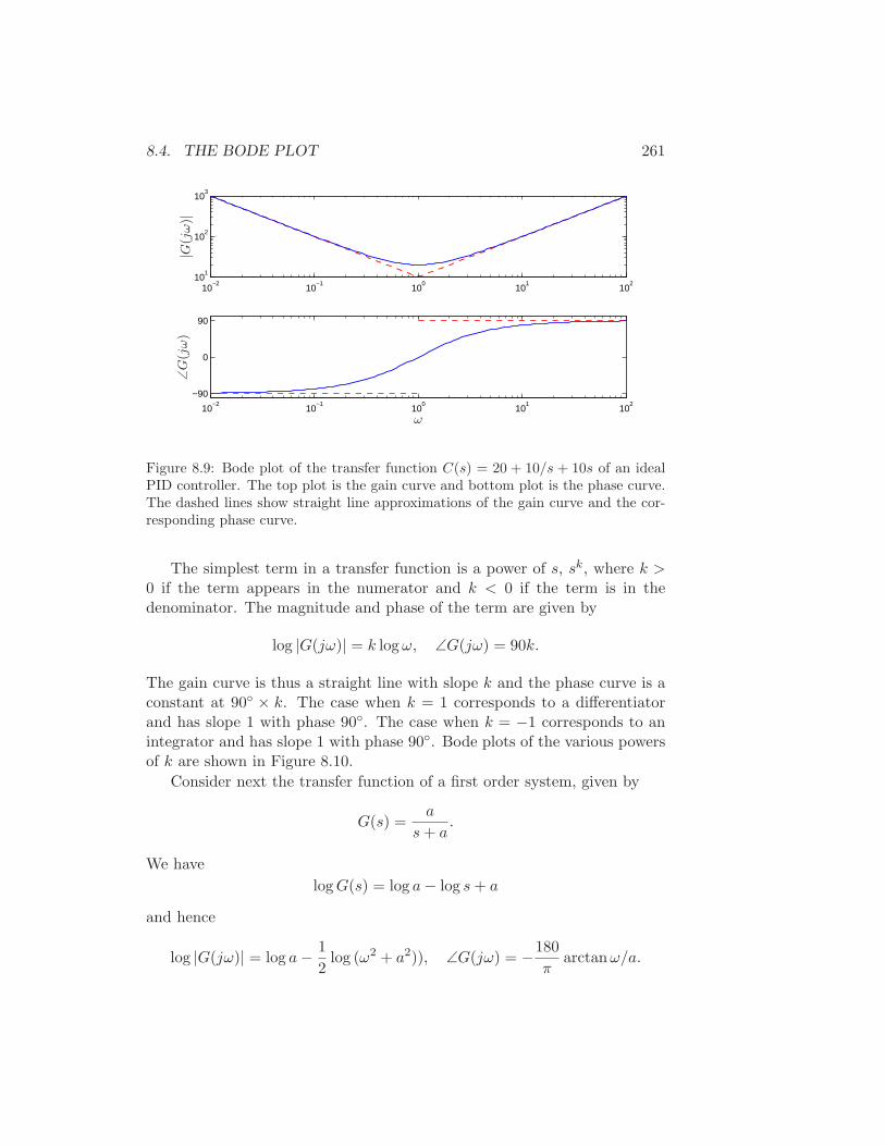
8.4. THE BODE PLOT 261
10−2
10−1
100
101
102
101
102
103
10−2
10−1
100
101
102
−90
0
90
ω
|G(j
ω)|
∠G
(jω)
Figure 8.9: Bode plot of the transfer function C(s) = 20 + 10/s + 10s of an idealPID controller. The top plot is the gain curve and bottom plot is the phase curve.The dashed lines show straight line approximations of the gain curve and the cor-responding phase curve.
The simplest term in a transfer function is a power of s, sk, where k >0 if the term appears in the numerator and k < 0 if the term is in thedenominator. The magnitude and phase of the term are given by
log |G(jω)| = k logω, ∠G(jω) = 90k.
The gain curve is thus a straight line with slope k and the phase curve is aconstant at 90 × k. The case when k = 1 corresponds to a differentiatorand has slope 1 with phase 90. The case when k = −1 corresponds to anintegrator and has slope 1 with phase 90. Bode plots of the various powersof k are shown in Figure 8.10.
Consider next the transfer function of a first order system, given by
G(s) =a
s+ a.
We have
logG(s) = log a− log s+ a
and hence
log |G(jω)| = log a− 1
2log (ω2 + a2)), ∠G(jω) = −180
πarctanω/a.
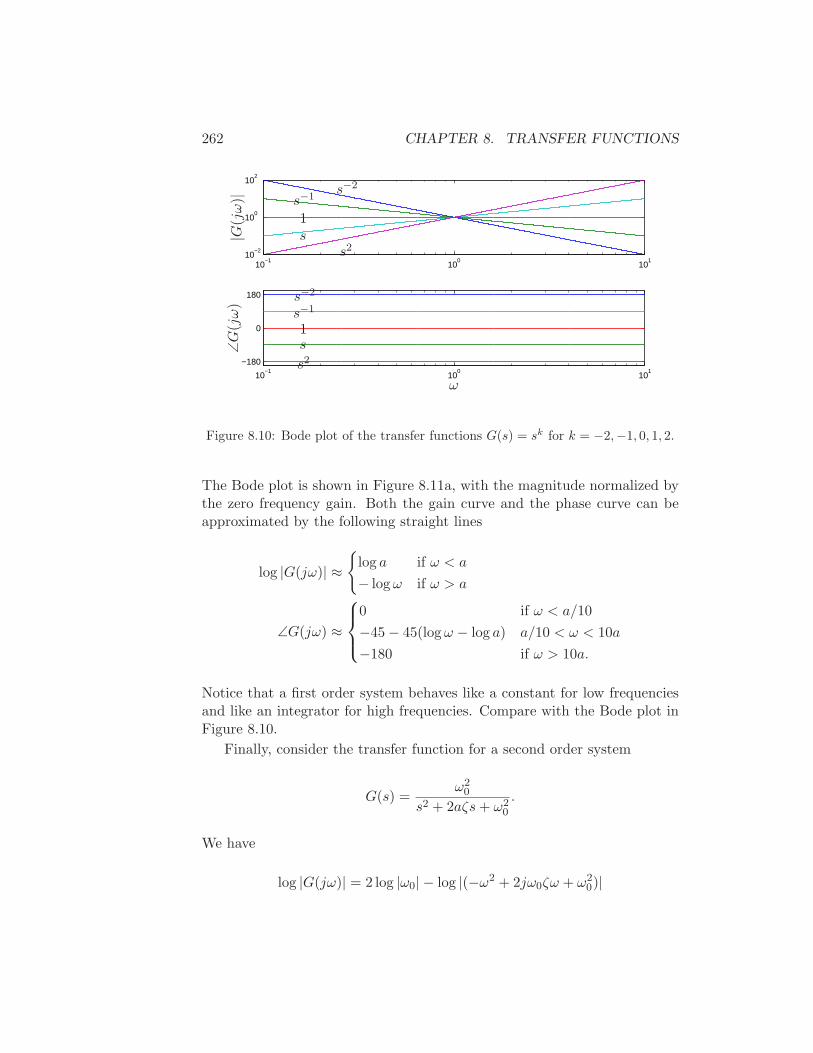
262 CHAPTER 8. TRANSFER FUNCTIONS
10−1
100
101
10−2
100
102
10−1
100
101
−180
0
180
ω
|G(jω)|
∠G
(jω)
s2
s2
s
s
1
1
s−1
s−1
s−2
s−2
Figure 8.10: Bode plot of the transfer functions G(s) = sk for k = −2,−1, 0, 1, 2.
The Bode plot is shown in Figure 8.11a, with the magnitude normalized bythe zero frequency gain. Both the gain curve and the phase curve can beapproximated by the following straight lines
log |G(jω)| ≈
log a if ω < a
− logω if ω > a
∠G(jω) ≈
0 if ω < a/10
−45 − 45(logω − log a) a/10 < ω < 10a
−180 if ω > 10a.
Notice that a first order system behaves like a constant for low frequenciesand like an integrator for high frequencies. Compare with the Bode plot inFigure 8.10.
Finally, consider the transfer function for a second order system
G(s) =ω2
0
s2 + 2aζs+ ω20
.
We have
log |G(jω)| = 2 log |ω0| − log |(−ω2 + 2jω0ζω + ω20)|
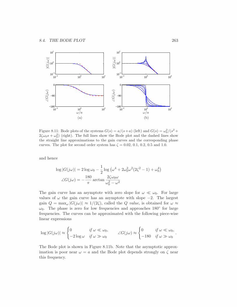
8.4. THE BODE PLOT 263
10−2
100
102
10−1
100
101
10−2
100
102
−180
−90
0
ω/a
|G(j
ω)|
∠G
(jω)
10−2
100
102
10−2
100
102
10−2
100
102
−180
−90
0
ω/a|G
(jω)|
∠G
(jω)
(a) (b)
Figure 8.11: Bode plots of the systems G(s) = a/(s+a) (left) and G(s) = ω20/(s
2 +2ζω0s + ω2
0) (right). The full lines show the Bode plot and the dashed lines showthe straight line approximations to the gain curves and the corresponding phasecurves. The plot for second order system has ζ = 0.02, 0.1, 0.2, 0.5 and 1.0.
and hence
log |G(jω)| = 2 logω0 −1
2log(ω4 + 2ω2
0ω2(2ζ2 − 1) + ω4
0
)
∠G(jω) = −180
πarctan
2ζω0ω
ω20 − ω2
The gain curve has an asymptote with zero slope for ω ≪ ω0. For largevalues of ω the gain curve has an asymptote with slope −2. The largestgain Q = maxω |G(jω)| ≈ 1/(2ζ), called the Q value, is obtained for ω ≈ω0. The phase is zero for low frequencies and approaches 180 for largefrequencies. The curves can be approximated with the following piece-wiselinear expressions
log |G(jω)| ≈
0 if ω ≪ ω0,
−2 logω if ω ≫ ω0
∠G(jω) ≈
0 if ω ≪ ω0,
−180 if ω ≫ ω0
.
The Bode plot is shown in Figure 8.11b. Note that the asymptotic approx-imation is poor near ω = a and the Bode plot depends strongly on ζ nearthis frequency.
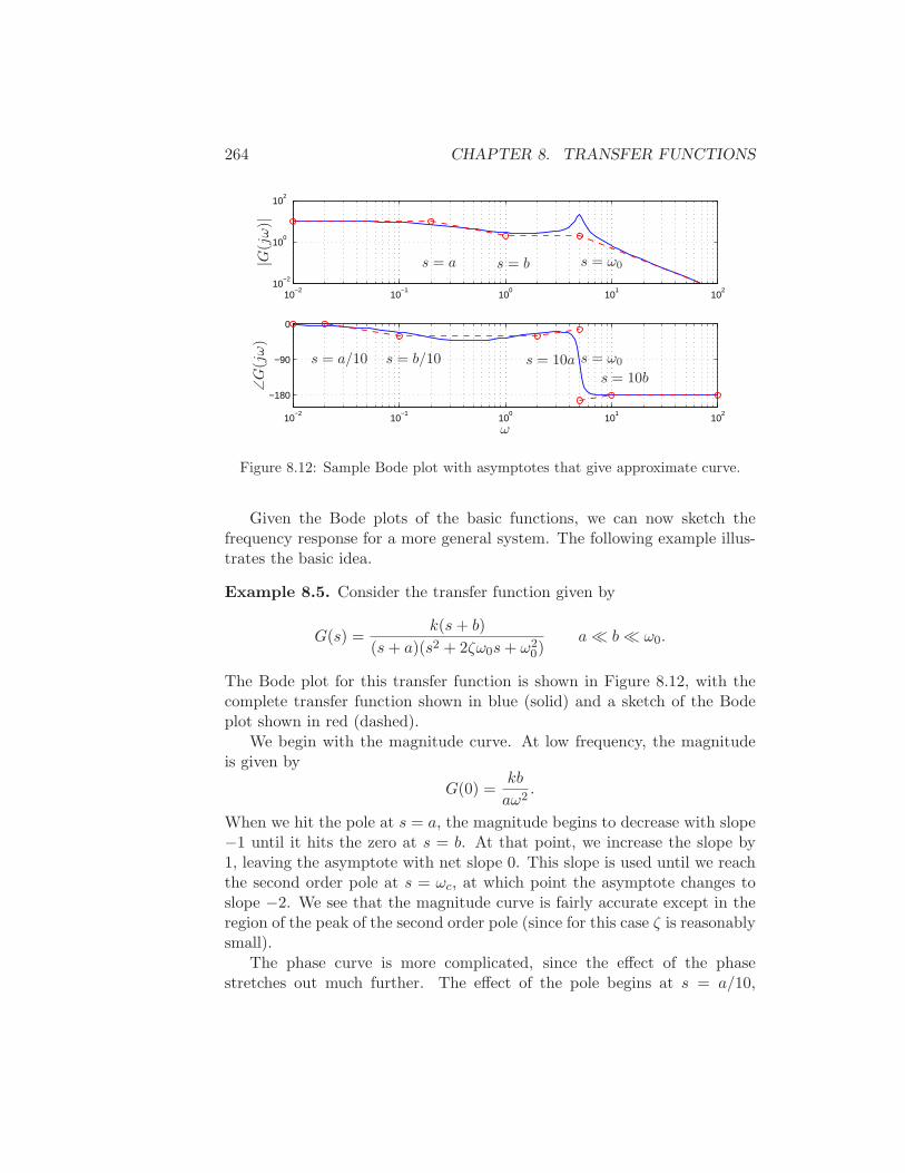
264 CHAPTER 8. TRANSFER FUNCTIONS
10−2
10−1
100
101
102
10−2
100
102
10−2
10−1
100
101
102
−180
−90
0
|G(jω)|
∠G
(jω)
ω
s = a s = b
s = ω0
s = ω0
s = a/10 s = b/10 s = 10as = 10b
Figure 8.12: Sample Bode plot with asymptotes that give approximate curve.
Given the Bode plots of the basic functions, we can now sketch thefrequency response for a more general system. The following example illus-trates the basic idea.
Example 8.5. Consider the transfer function given by
G(s) =k(s+ b)
(s+ a)(s2 + 2ζω0s+ ω20)
a≪ b≪ ω0.
The Bode plot for this transfer function is shown in Figure 8.12, with thecomplete transfer function shown in blue (solid) and a sketch of the Bodeplot shown in red (dashed).
We begin with the magnitude curve. At low frequency, the magnitudeis given by
G(0) =kb
aω2.
When we hit the pole at s = a, the magnitude begins to decrease with slope−1 until it hits the zero at s = b. At that point, we increase the slope by1, leaving the asymptote with net slope 0. This slope is used until we reachthe second order pole at s = ωc, at which point the asymptote changes toslope −2. We see that the magnitude curve is fairly accurate except in theregion of the peak of the second order pole (since for this case ζ is reasonablysmall).
The phase curve is more complicated, since the effect of the phasestretches out much further. The effect of the pole begins at s = a/10,
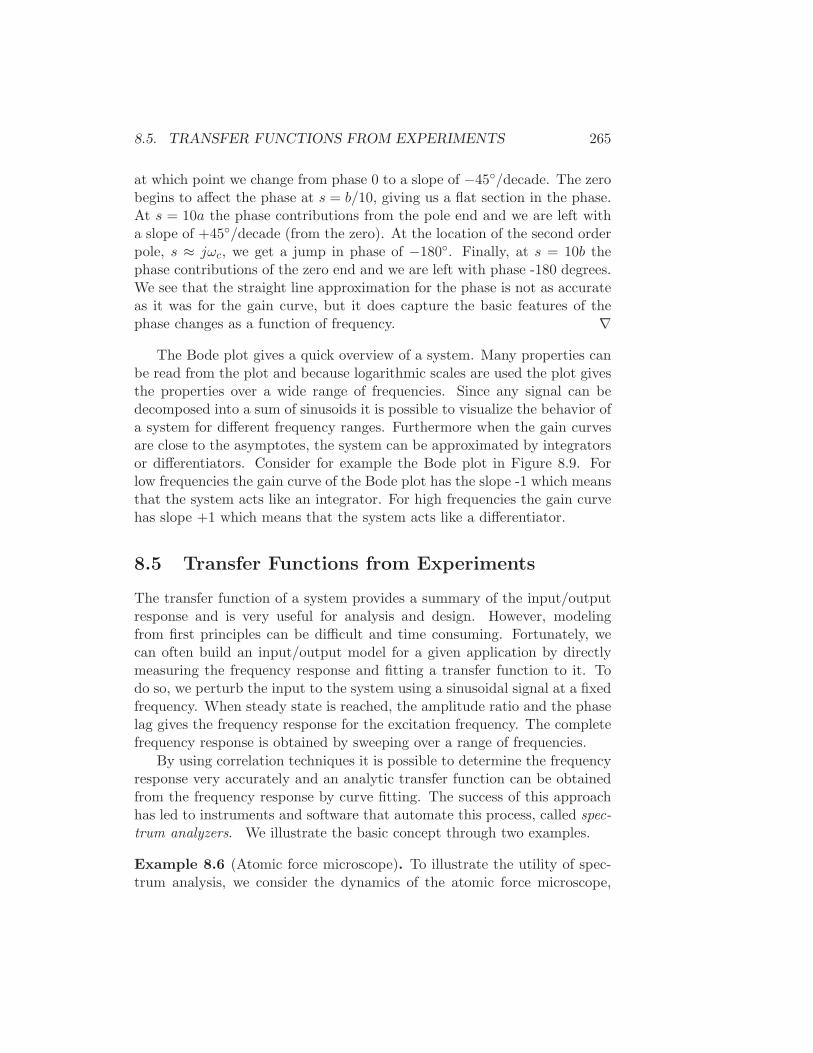
8.5. TRANSFER FUNCTIONS FROM EXPERIMENTS 265
at which point we change from phase 0 to a slope of −45/decade. The zerobegins to affect the phase at s = b/10, giving us a flat section in the phase.At s = 10a the phase contributions from the pole end and we are left witha slope of +45/decade (from the zero). At the location of the second orderpole, s ≈ jωc, we get a jump in phase of −180. Finally, at s = 10b thephase contributions of the zero end and we are left with phase -180 degrees.We see that the straight line approximation for the phase is not as accurateas it was for the gain curve, but it does capture the basic features of thephase changes as a function of frequency. ∇
The Bode plot gives a quick overview of a system. Many properties canbe read from the plot and because logarithmic scales are used the plot givesthe properties over a wide range of frequencies. Since any signal can bedecomposed into a sum of sinusoids it is possible to visualize the behavior ofa system for different frequency ranges. Furthermore when the gain curvesare close to the asymptotes, the system can be approximated by integratorsor differentiators. Consider for example the Bode plot in Figure 8.9. Forlow frequencies the gain curve of the Bode plot has the slope -1 which meansthat the system acts like an integrator. For high frequencies the gain curvehas slope +1 which means that the system acts like a differentiator.
8.5 Transfer Functions from Experiments
The transfer function of a system provides a summary of the input/outputresponse and is very useful for analysis and design. However, modelingfrom first principles can be difficult and time consuming. Fortunately, wecan often build an input/output model for a given application by directlymeasuring the frequency response and fitting a transfer function to it. Todo so, we perturb the input to the system using a sinusoidal signal at a fixedfrequency. When steady state is reached, the amplitude ratio and the phaselag gives the frequency response for the excitation frequency. The completefrequency response is obtained by sweeping over a range of frequencies.
By using correlation techniques it is possible to determine the frequencyresponse very accurately and an analytic transfer function can be obtainedfrom the frequency response by curve fitting. The success of this approachhas led to instruments and software that automate this process, called spec-trum analyzers. We illustrate the basic concept through two examples.
Example 8.6 (Atomic force microscope). To illustrate the utility of spec-trum analysis, we consider the dynamics of the atomic force microscope,
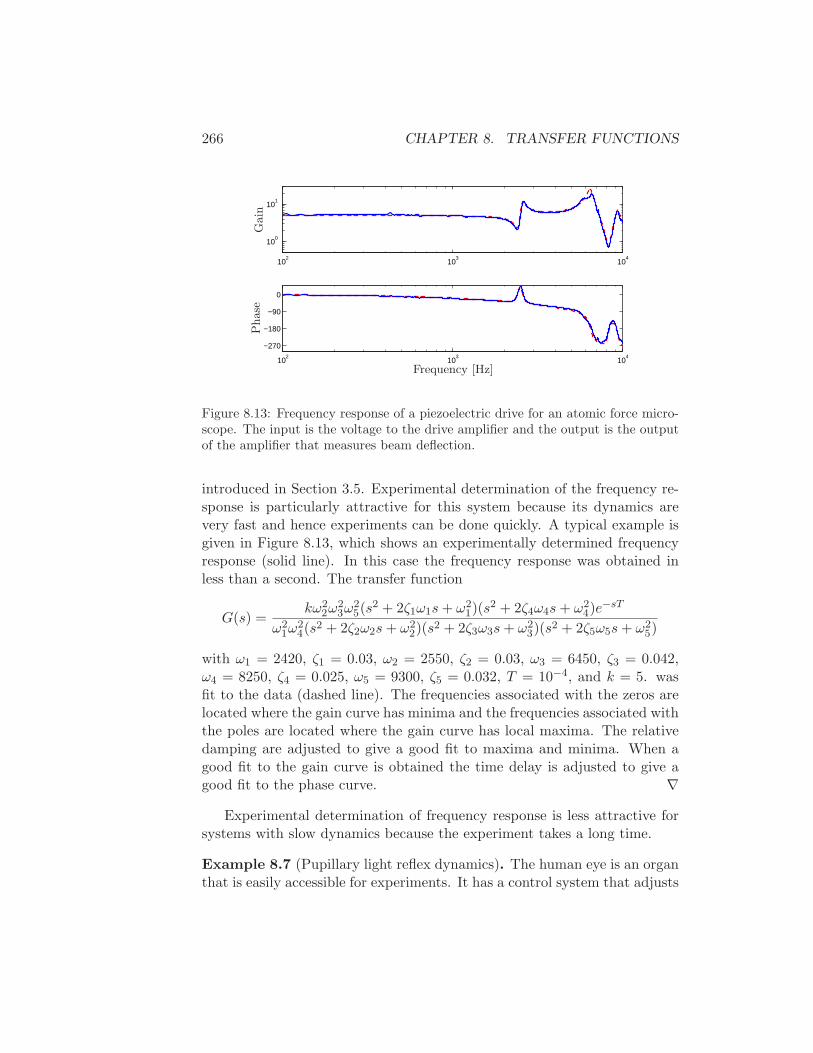
266 CHAPTER 8. TRANSFER FUNCTIONS
102
103
104
100
101
102
103
104
−270
−180
−90
0
Gain
Phase
Frequency [Hz]
Figure 8.13: Frequency response of a piezoelectric drive for an atomic force micro-scope. The input is the voltage to the drive amplifier and the output is the outputof the amplifier that measures beam deflection.
introduced in Section 3.5. Experimental determination of the frequency re-sponse is particularly attractive for this system because its dynamics arevery fast and hence experiments can be done quickly. A typical example isgiven in Figure 8.13, which shows an experimentally determined frequencyresponse (solid line). In this case the frequency response was obtained inless than a second. The transfer function
G(s) =kω2
2ω23ω
25(s
2 + 2ζ1ω1s+ ω21)(s
2 + 2ζ4ω4s+ ω24)e
−sT
ω21ω
24(s
2 + 2ζ2ω2s+ ω22)(s
2 + 2ζ3ω3s+ ω23)(s
2 + 2ζ5ω5s+ ω25)
with ω1 = 2420, ζ1 = 0.03, ω2 = 2550, ζ2 = 0.03, ω3 = 6450, ζ3 = 0.042,ω4 = 8250, ζ4 = 0.025, ω5 = 9300, ζ5 = 0.032, T = 10−4, and k = 5. wasfit to the data (dashed line). The frequencies associated with the zeros arelocated where the gain curve has minima and the frequencies associated withthe poles are located where the gain curve has local maxima. The relativedamping are adjusted to give a good fit to maxima and minima. When agood fit to the gain curve is obtained the time delay is adjusted to give agood fit to the phase curve. ∇
Experimental determination of frequency response is less attractive forsystems with slow dynamics because the experiment takes a long time.
Example 8.7 (Pupillary light reflex dynamics). The human eye is an organthat is easily accessible for experiments. It has a control system that adjusts
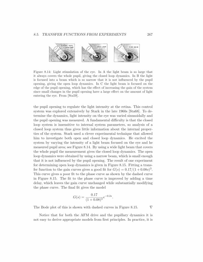
8.5. TRANSFER FUNCTIONS FROM EXPERIMENTS 267
Figure 8.14: Light stimulation of the eye. In A the light beam is so large thatit always covers the whole pupil, giving the closed loop dynamics. In B the lightis focused into a beam which is so narrow that it is not influenced by the pupilopening, giving the open loop dynamics. In C the light beam is focused on theedge of the pupil opening, which has the effect of increasing the gain of the systemsince small changes in the pupil opening have a large effect on the amount of lightentering the eye. From [Sta59].
the pupil opening to regulate the light intensity at the retina. This controlsystem was explored extensively by Stark in the late 1960s [Sta68]. To de-termine the dynamics, light intensity on the eye was varied sinusoidally andthe pupil opening was measured. A fundamental difficulty is that the closedloop system is insensitive to internal system parameters, so analysis of aclosed loop system thus gives little information about the internal proper-ties of the system. Stark used a clever experimental technique that allowedhim to investigate both open and closed loop dynamics. He excited thesystem by varying the intensity of a light beam focused on the eye and hemeasured pupil area; see Figure 8.14. By using a wide light beam that coversthe whole pupil the measurement gives the closed loop dynamics. The openloop dynamics were obtained by using a narrow beam, which is small enoughthat it is not influenced by the pupil opening. The result of one experimentfor determining open loop dynamics is given in Figure 8.15. Fitting a trans-fer function to the gain curves gives a good fit for G(s) = 0.17/(1 + 0.08s)3.This curve gives a poor fit to the phase curve as shown by the dashed curvein Figure 8.15. The fit to the phase curve is improved by adding a timedelay, which leaves the gain curve unchanged while substantially modifyingthe phase curve. The final fit gives the model
G(s) =0.17
(1 + 0.08)3e−0.2s.
The Bode plot of this is shown with dashed curves in Figure 8.15. ∇
Notice that for both the AFM drive and the pupillary dynamics it isnot easy to derive appropriate models from first principles. In practice, it is
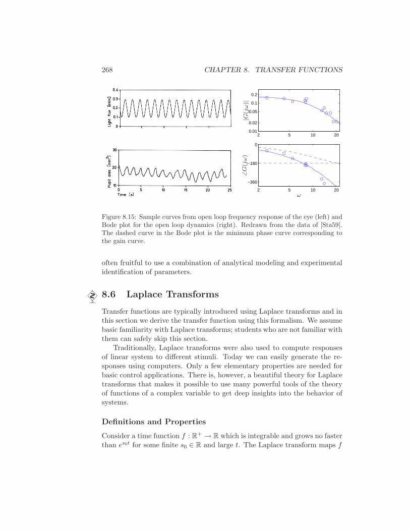
268 CHAPTER 8. TRANSFER FUNCTIONS
2 5 10 200.01
0.02
0.05
0.1
0.2
2 5 10 20
−360
−180
0
ω
|G(j
ω)|
∠G
(jω)
Figure 8.15: Sample curves from open loop frequency response of the eye (left) andBode plot for the open loop dynamics (right). Redrawn from the data of [Sta59].The dashed curve in the Bode plot is the minimum phase curve corresponding tothe gain curve.
often fruitful to use a combination of analytical modeling and experimentalidentification of parameters.
8.6 Laplace Transforms
Transfer functions are typically introduced using Laplace transforms and inthis section we derive the transfer function using this formalism. We assumebasic familiarity with Laplace transforms; students who are not familiar withthem can safely skip this section.
Traditionally, Laplace transforms were also used to compute responsesof linear system to different stimuli. Today we can easily generate the re-sponses using computers. Only a few elementary properties are needed forbasic control applications. There is, however, a beautiful theory for Laplacetransforms that makes it possible to use many powerful tools of the theoryof functions of a complex variable to get deep insights into the behavior ofsystems.
Definitions and Properties
Consider a time function f : R+ → R which is integrable and grows no faster
than es0t for some finite s0 ∈ R and large t. The Laplace transform maps f
8.6. LAPLACE TRANSFORMS 269
to a function F = Lf : C → C of a complex variable. It is defined by
F (s) =
∫ ∞
0e−stf(t) dt, Re s > s0. (8.20)
The transform has some properties that makes it very well suited to dealwith linear systems.
First we observe that the transform is linear because
L(af + bg) =
∫ ∞
0e−st(af(t) + bg(t)) dt
= a
∫ ∞
0e−stf(t) dt+ b
∫ ∞
0e−stg(t) dt = aLf + bLg.
(8.21)
Next we will calculate the Laplace transform of the derivative of a function.We have
Ldfdt
=
∫ ∞
0e−stf ′(t) dt = e−stf(t)
∣∣∣
∞
0+ s
∫ ∞
0e−stf(t) dt = −f(0) + sLf,
where the second equality is obtained by integration by parts. We thusobtain the following important formula for the transform of a derivative
Ldfdt
= sLf − f(0) = sF (s) − f(0). (8.22)
This formula is particularly simple if the initial conditions are zero becauseit follows that differentiation of a function corresponds to multiplication ofthe transform with s.
Since differentiation corresponds to multiplication with s we can expectthat integration corresponds to division by s. This is true, as can be seenby calculating the Laplace transform of an integral. We have
L∫ t
0f(τ) dτ =
∫ ∞
0
(
e−st
∫ t
0f(τ) dτ
)
dt
= −e−st
s
∫ t
0e−sτf(τ) dτ
∣∣∣
∞
0+
∫ ∞
0
e−sτ
sf(τ) dτ =
1
s
∫ ∞
0e−sτf(τ) dτ,
hence
L∫ t
0f(τ) dτ =
1
sLf =
1
sF (s). (8.23)
Integration of a time function thus corresponds to dividing the Laplace trans-form by s.
270 CHAPTER 8. TRANSFER FUNCTIONS
The Laplace Transform of a Convolution
Consider a linear time-invariant system with zero initial state. The relationbetween the input u and the output y is given by the convolution integral
y(t) =
∫ ∞
0h(t− τ)u(τ) dτ,
where h(t) is the impulse response for the system. We will now consider theLaplace transform of such an expression. We have
Y (s) =
∫ ∞
0e−sty(t) dt =
∫ ∞
0e−st
∫ ∞
0h(t− τ)u(τ) dτ dt
=
∫ ∞
0
∫ t
0e−s(t−τ)e−sτh(t− τ)u(τ) dτ dt
=
∫ ∞
0e−sτu(τ) dτ
∫ ∞
0e−sth(t) dt = H(s)U(s)
The result can be written as Y (s) = H(s)U(s) where H, U and Y are theLaplace transforms of h, u and y. The system theoretic interpretation isthat the Laplace transform of the output of a linear system is a productof two terms, the Laplace transform of the input U(s) and the Laplacetransform of the impulse response of the system H(s). A mathematicalinterpretation is that the Laplace transform of a convolution is the productof the transforms of the functions that are convolved. The fact that theformula Y (s) = H(s)U(s) is much simpler than a convolution is one reasonwhy Laplace transforms have become popular in control.
The Transfer Function
The properties (8.21) and (8.22) makes the Laplace transform ideally suitedfor dealing with linear differential equations. The relations are particularlysimple if all initial conditions are zero.
Consider for example a linear state space system described by
x = Ax+Bu
y = Cx+Du.
Taking Laplace transforms under the assumption that all initial values arezero gives
sX(s) = AX(s) +BU(s)
Y (s) = CX(s) +DU(s).
8.7. FURTHER READING 271
Elimination of X(s) gives
Y (s) =(
C(sI −A)−1B +D)
U(s). (8.24)
The transfer function is thus G(s) = C(sI − A)−1B + D (compare withequation (8.4)).
The formula (8.24) has a strong intuitive interpretation because it tellsthat the Laplace transform of the output is the product of the transferfunction of the system and the transform of the input. In the transformdomain the action of a linear system on the input is simply a multiplicationwith the transfer function. The transfer function is a natural generalizationof the concept of gain of a system.
8.7 Further Reading
Heaviside, who introduced the idea to characterize dynamics by the responseto a unit step function, also introduced a formal operator calculus for an-alyzing linear systems. This was a significant advance because it gavethe possibility to analyze linear systems algebraically. Unfortunately it wasdifficult to formalize Heaviside’s calculus properly. This was not done untilthe the mathematician Laurent Schwartz developed the distribution the-ory in the late 1940s. Schwartz was given the Fields Medal in 1950. Theidea of characterizing a linear system by its steady state response to sinu-soids was introduced by Fourier in his investigation of heat conduction insolids [Fou07]. Much later it was used by Steinmetz when he introduced thejω method to develop a theory for alternating currents.
The concept of transfer functions was an important part of classical con-trol theory; see [JNP47]. It was introduced via the Laplace transform byGardner Barnes [GB42], who also used it to calculate response of linearsystems. The Laplace transform was very important in the early phase ofcontrol because it made it possible to find transients via tables. The Laplacetransform is of less importance today when responses to linear systems caneasily be generated using computers. For a mathematically inclined audi-ence it is still a very convenient to introduce the transfer function via theLaplace transform, which is an important part of applied mathematics. Foran audience with less background in mathematics it may be preferable tointroduce the transfer function via the particular solution generated by theinput est as was done in Section 8.2.
There are many excellent books on the use of Laplace transforms andtransfer functions for modeling and analysis of linear input/output systems.
272 CHAPTER 8. TRANSFER FUNCTIONS
Traditional texts on control, such as [FPEN05] and [DB04], are representa-tive examples.
8.8 Exercises
1. Let G(s) be the transfer function for a linear system. Show that if weapply an input u(t) = A sin(ωt) then the steady state output is givenby y(t) = |G(jω)|A sin(ωt+ argG(jω)).
2. Show that the transfer function of a system only depends on the dy-namics in the reachable and observable subspace of the Kalman de-composition.
3. The linearized model of the pendulum in the upright position is char-acterized by the matrices
A =
0 11 0
, B =
01
, C =
1 0
, D = 0.
Determine the transfer function of the system.
4. Compute the frequency response of a PI controller using an op ampwith frequency response given by equation (8.12).
5. Consider the speed control system given in Example 6.9. Computethe transfer function between the throttle position u, angle of theroad θ and the speed of the vehicle v assuming a nominal speed ve
with corresponding throttle position ue.
6. Consider the differential equation
dny
dtn+ a1
dn−1y
dtn−1+ a2
dn−2y
dtn−2+ · · · + any = 0
Let λ be a root of the polynomial
sn + a1sn−1 + · · · + an = 0.
Show that the differential equation has the solution y(t) = eλt.
7. Consider the system
dny
dtn+ a1
dn−1y
dtn−1+ · · · + any = b1
dn−1u
dtn−1+ b2
dn−2u
dtn−2+ · · · + bnu,
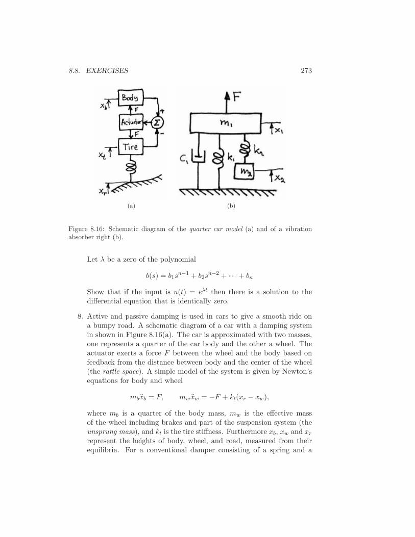
8.8. EXERCISES 273
(a) (b)
Figure 8.16: Schematic diagram of the quarter car model (a) and of a vibrationabsorber right (b).
Let λ be a zero of the polynomial
b(s) = b1sn−1 + b2s
n−2 + · · · + bn
Show that if the input is u(t) = eλt then there is a solution to thedifferential equation that is identically zero.
8. Active and passive damping is used in cars to give a smooth ride ona bumpy road. A schematic diagram of a car with a damping systemin shown in Figure 8.16(a). The car is approximated with two masses,one represents a quarter of the car body and the other a wheel. Theactuator exerts a force F between the wheel and the body based onfeedback from the distance between body and the center of the wheel(the rattle space). A simple model of the system is given by Newton’sequations for body and wheel
mbxb = F, mwxw = −F + kt(xr − xw),
where mb is a quarter of the body mass, mw is the effective massof the wheel including brakes and part of the suspension system (theunsprung mass), and kt is the tire stiffness. Furthermore xb, xw and xr
represent the heights of body, wheel, and road, measured from theirequilibria. For a conventional damper consisting of a spring and a
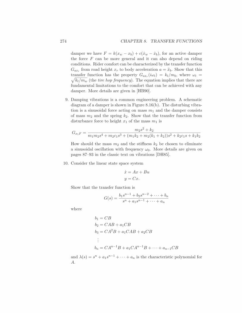
274 CHAPTER 8. TRANSFER FUNCTIONS
damper we have F = k(xw − xb) + c(xw − xb), for an active damperthe force F can be more general and it can also depend on ridingconditions. Rider comfort can be characterized by the transfer functionGaxr from road height xr to body acceleration a = xb. Show that thistransfer function has the property Gaxr(iωt) = kt/mb, where ωt =√
kt/mw (the tire hop frequency). The equation implies that there arefundamental limitations to the comfort that can be achieved with anydamper. More details are given in [HB90].
9. Damping vibrations is a common engineering problem. A schematicdiagram of a damper is shown in Figure 8.16(b). The disturbing vibra-tion is a sinusoidal force acting on mass m1 and the damper consistsof mass m2 and the spring k2. Show that the transfer function fromdisturbance force to height x1 of the mass m1 is
Gx1F =m2s
2 + k2
m1m2s4 +m2c1s3 + (m1k2 +m2(k1 + k2))s2 + k2c1s+ k1k2
How should the mass m2 and the stiffness k2 be chosen to eliminatea sinusoidal oscillation with frequency ω0. More details are given onpages 87–93 in the classic text on vibrations [DH85].
10. Consider the linear state space system
x = Ax+Bu
y = Cx.
Show that the transfer function is
G(s) =b1s
n−1 + b2sn−2 + · · · + bn
sn + a1sn−1 + · · · + an
where
b1 = CB
b2 = CAB + a1CB
b3 = CA2B + a1CAB + a2CB
...
bn = CAn−1B + a1CAn−1B + · · · + an−1CB
and λ(s) = sn + a1sn−1 + · · · + an is the characteristic polynomial for
A.
8.8. EXERCISES 275
11. Consider a closed loop system of the form of Figure 8.6 with F = 1 andP and C having a common pole. Show that if each system is writtenin state space form, the resulting closed loop system is not reachableand not observable.
12. The Physicist Angstrom, who is associated with the length unit A,used frequency response to determine thermal diffusivity of metals [Ang61].Heat propagation in a metal rod is described by the partial differentialequation
∂T
∂t= a
∂2T
∂x2− µT, (8.25)
where a = λρC is the thermal diffusivity, and the last term represents
thermal loss to the environment. Show that the transfer function re-lating temperatures at points with the distance ℓ is
G(s) = e−ℓ√
(s+µ)/a, (8.26)
and the frequency response is given by
log |G(iω)| = −ℓ
√
µ+√
ω2 + µ2
2a
argG(iω) = −ℓ
√
−µ+√
ω2 + µ2
2a.
Also derive the following equation
log |G(iω)| argG(iω) =ℓ2ω
2a.
This remarkably simple formula shows that diffusivity can be deter-mined from the value of the transfer function at one frequency. It wasthe key in Angstrom’s method for determining thermal diffusivity. No-tice that the parameter µ which represents the thermal losses does notappear in the formula.

276 CHAPTER 8. TRANSFER FUNCTIONS
Chapter 9
Loop Analysis
Regeneration or feed-back is of considerable importance in many applicationsof vacuum tubes. The most obvious example is that of vacuum tube oscil-lators, where the feed-back is carried beyond the singing point. Another ap-plication is the 21-circuit test of balance, in which the current due to theunbalance between two impedances is fed back, the gain being increased untilsinging occurs. Still other applications are cases where portions of the outputcurrent of amplifiers are fed back to the input either unintentionally or by de-sign. For the purpose of investigating the stability of such devices they maybe looked on as amplifiers whose output is connected to the input through atransducer. This paper deals with the theory of stability of such systems.
Abstract for “Regeneration Theory”, Harry Nyquist, 1932 [Nyq32].
In this chapter we study how how stability and robustness of closed loopsystems can be determined by investigating how signals propagate aroundthe feedback loop. The Nyquist stability theorem is a key result that pro-vides a way to analyze stability and introduce measures of degrees of stabil-ity.
9.1 The Loop Transfer Function
The basic idea of loop analysis is to trace how a sinusoidal signal propagatesin the feedback loop and explore the resulting stability by investigating ifthe signal grows or decays around the loop. This is easy to do because thetransmission of sinusoidal signals through a (linear) dynamical system ischaracterized by the frequency response of the system. The key result is theNyquist stability theorem, which provides a great deal of insight regardingthe stability of a system. Unlike proving stability with Lyapunov functions,
277
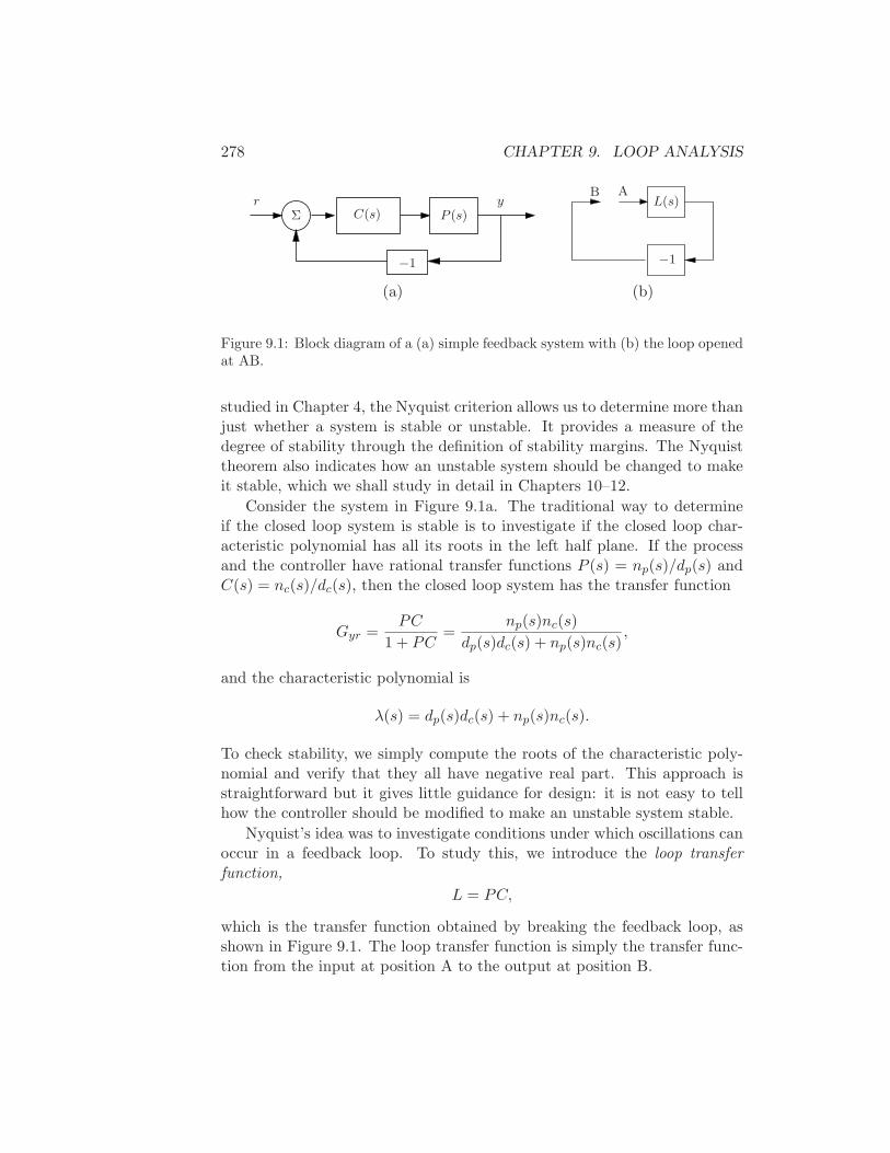
278 CHAPTER 9. LOOP ANALYSIS
C(s) P (s)Σr y
−1
AB
−1
L(s)
(a) (b)
Figure 9.1: Block diagram of a (a) simple feedback system with (b) the loop openedat AB.
studied in Chapter 4, the Nyquist criterion allows us to determine more thanjust whether a system is stable or unstable. It provides a measure of thedegree of stability through the definition of stability margins. The Nyquisttheorem also indicates how an unstable system should be changed to makeit stable, which we shall study in detail in Chapters 10–12.
Consider the system in Figure 9.1a. The traditional way to determineif the closed loop system is stable is to investigate if the closed loop char-acteristic polynomial has all its roots in the left half plane. If the processand the controller have rational transfer functions P (s) = np(s)/dp(s) andC(s) = nc(s)/dc(s), then the closed loop system has the transfer function
Gyr =PC
1 + PC=
np(s)nc(s)
dp(s)dc(s) + np(s)nc(s),
and the characteristic polynomial is
λ(s) = dp(s)dc(s) + np(s)nc(s).
To check stability, we simply compute the roots of the characteristic poly-nomial and verify that they all have negative real part. This approach isstraightforward but it gives little guidance for design: it is not easy to tellhow the controller should be modified to make an unstable system stable.
Nyquist’s idea was to investigate conditions under which oscillations canoccur in a feedback loop. To study this, we introduce the loop transferfunction,
L = PC,
which is the transfer function obtained by breaking the feedback loop, asshown in Figure 9.1. The loop transfer function is simply the transfer func-tion from the input at position A to the output at position B.
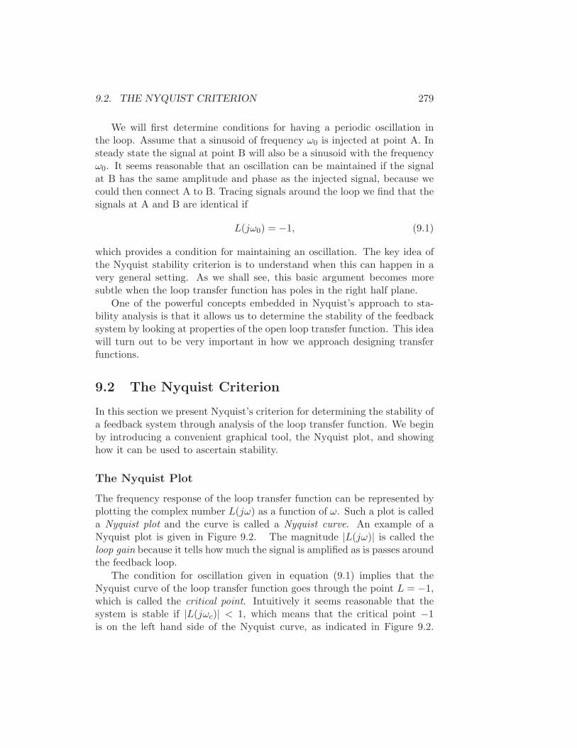
9.2. THE NYQUIST CRITERION 279
We will first determine conditions for having a periodic oscillation inthe loop. Assume that a sinusoid of frequency ω0 is injected at point A. Insteady state the signal at point B will also be a sinusoid with the frequencyω0. It seems reasonable that an oscillation can be maintained if the signalat B has the same amplitude and phase as the injected signal, because wecould then connect A to B. Tracing signals around the loop we find that thesignals at A and B are identical if
L(jω0) = −1, (9.1)
which provides a condition for maintaining an oscillation. The key idea ofthe Nyquist stability criterion is to understand when this can happen in avery general setting. As we shall see, this basic argument becomes moresubtle when the loop transfer function has poles in the right half plane.
One of the powerful concepts embedded in Nyquist’s approach to sta-bility analysis is that it allows us to determine the stability of the feedbacksystem by looking at properties of the open loop transfer function. This ideawill turn out to be very important in how we approach designing transferfunctions.
9.2 The Nyquist Criterion
In this section we present Nyquist’s criterion for determining the stability ofa feedback system through analysis of the loop transfer function. We beginby introducing a convenient graphical tool, the Nyquist plot, and showinghow it can be used to ascertain stability.
The Nyquist Plot
The frequency response of the loop transfer function can be represented byplotting the complex number L(jω) as a function of ω. Such a plot is calleda Nyquist plot and the curve is called a Nyquist curve. An example of aNyquist plot is given in Figure 9.2. The magnitude |L(jω)| is called theloop gain because it tells how much the signal is amplified as is passes aroundthe feedback loop.
The condition for oscillation given in equation (9.1) implies that theNyquist curve of the loop transfer function goes through the point L = −1,which is called the critical point. Intuitively it seems reasonable that thesystem is stable if |L(jωc)| < 1, which means that the critical point −1is on the left hand side of the Nyquist curve, as indicated in Figure 9.2.
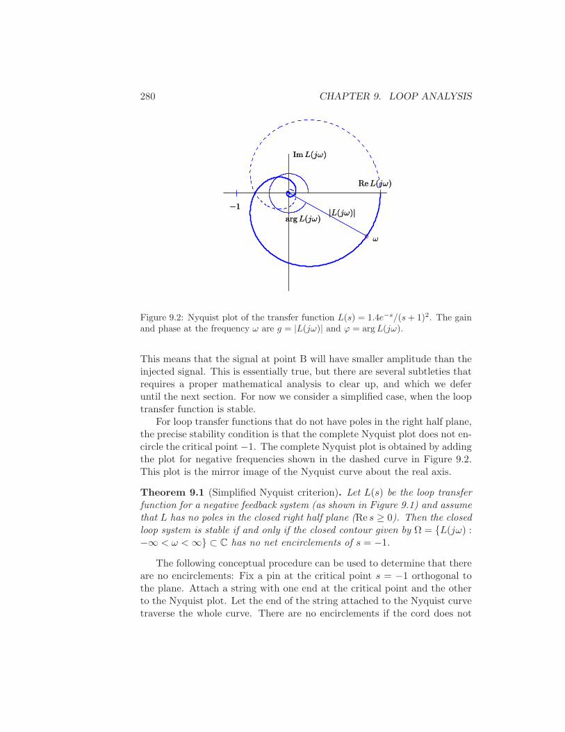
280 CHAPTER 9. LOOP ANALYSIS
Re L(jω)Re L(jω)Re L(jω)
Im L(jω)Im L(jω)Im L(jω)
ωωω
arg L(jω)arg L(jω)arg L(jω)|L(jω)||L(jω)||L(jω)|
−1−1−1
Figure 9.2: Nyquist plot of the transfer function L(s) = 1.4e−s/(s+ 1)2. The gainand phase at the frequency ω are g = |L(jω)| and ϕ = argL(jω).
This means that the signal at point B will have smaller amplitude than theinjected signal. This is essentially true, but there are several subtleties thatrequires a proper mathematical analysis to clear up, and which we deferuntil the next section. For now we consider a simplified case, when the looptransfer function is stable.
For loop transfer functions that do not have poles in the right half plane,the precise stability condition is that the complete Nyquist plot does not en-circle the critical point −1. The complete Nyquist plot is obtained by addingthe plot for negative frequencies shown in the dashed curve in Figure 9.2.This plot is the mirror image of the Nyquist curve about the real axis.
Theorem 9.1 (Simplified Nyquist criterion). Let L(s) be the loop transferfunction for a negative feedback system (as shown in Figure 9.1) and assumethat L has no poles in the closed right half plane (Re s ≥ 0). Then the closedloop system is stable if and only if the closed contour given by Ω = L(jω) :−∞ < ω <∞ ⊂ C has no net encirclements of s = −1.
The following conceptual procedure can be used to determine that thereare no encirclements: Fix a pin at the critical point s = −1 orthogonal tothe plane. Attach a string with one end at the critical point and the otherto the Nyquist plot. Let the end of the string attached to the Nyquist curvetraverse the whole curve. There are no encirclements if the cord does not
9.2. THE NYQUIST CRITERION 281
wind up on the pin when the curve is encircled.
Example 9.1 (Cruise control). Consider the speed control system intro-duced in Section 3.1 and analyzed using state space techniques in Exam-ple 6.9. In this example, we study the stability of the system using theNyquist criterion.
The linearized dynamics around the equilibrium speed ve and throttleposition ue are given by
˙v = av − gθ + bu
y = v = v + ve,
where v = v − ve, u = u− ue, m is the mass of the car and θ is the angle ofthe road. The constant a < 0 depends on the throttle characteristic and isgiven in Example 5.10.
The transfer function from throttle to speed is given by
P (s) = Gyu(s) =b
s− α.
We consider a controller that is a modified version of the proportional-integral (PI) controller given previously. Assume that the transfer functionof the controller is
C(s) = Gue(s) = kp +ki
s+ β=kps+ ki + kpβ
s+ β
giving a loop transfer function of
L(s) = bkps+ ki + kpβ
(s+ a)(s+ β).
The Nyquist plot for the system, using a = 0.0101, b = 1.3203, kp = 0.5,ki = 0.1 and β = 0.1, is shown in Figure 9.3. We see from the Nyquist plotthat the closed loop system is stable, since there are no net encirclements ofthe -1 point. ∇
One nice property of the Nyquist stability criterion is that it can be applied to infinite dimensional systems, as is illustrated by the following example.
Example 9.2 (Heat conduction). Consider a temperature control systemwhere the heat conduction process has the transfer function
P (s) = e−√
s
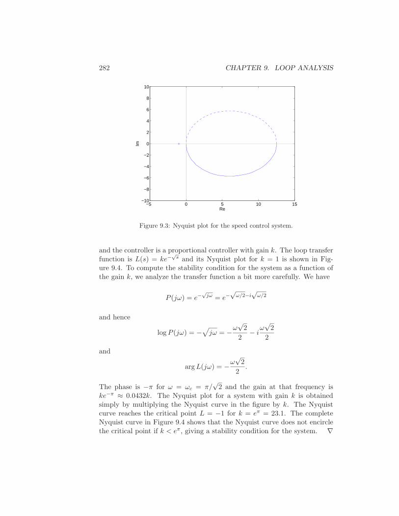
282 CHAPTER 9. LOOP ANALYSIS
−5 0 5 10 15−10
−8
−6
−4
−2
0
2
4
6
8
10
Re
Im
Figure 9.3: Nyquist plot for the speed control system.
and the controller is a proportional controller with gain k. The loop transferfunction is L(s) = ke−
√s and its Nyquist plot for k = 1 is shown in Fig-
ure 9.4. To compute the stability condition for the system as a function ofthe gain k, we analyze the transfer function a bit more carefully. We have
P (jω) = e−√
jω = e−√
ω/2−i√
ω/2
and hence
logP (jω) = −√
jω = −ω√
2
2− i
ω√
2
2
and
argL(jω) = −ω√
2
2.
The phase is −π for ω = ωc = π/√
2 and the gain at that frequency iske−π ≈ 0.0432k. The Nyquist plot for a system with gain k is obtainedsimply by multiplying the Nyquist curve in the figure by k. The Nyquistcurve reaches the critical point L = −1 for k = eπ = 23.1. The completeNyquist curve in Figure 9.4 shows that the Nyquist curve does not encirclethe critical point if k < eπ, giving a stability condition for the system. ∇
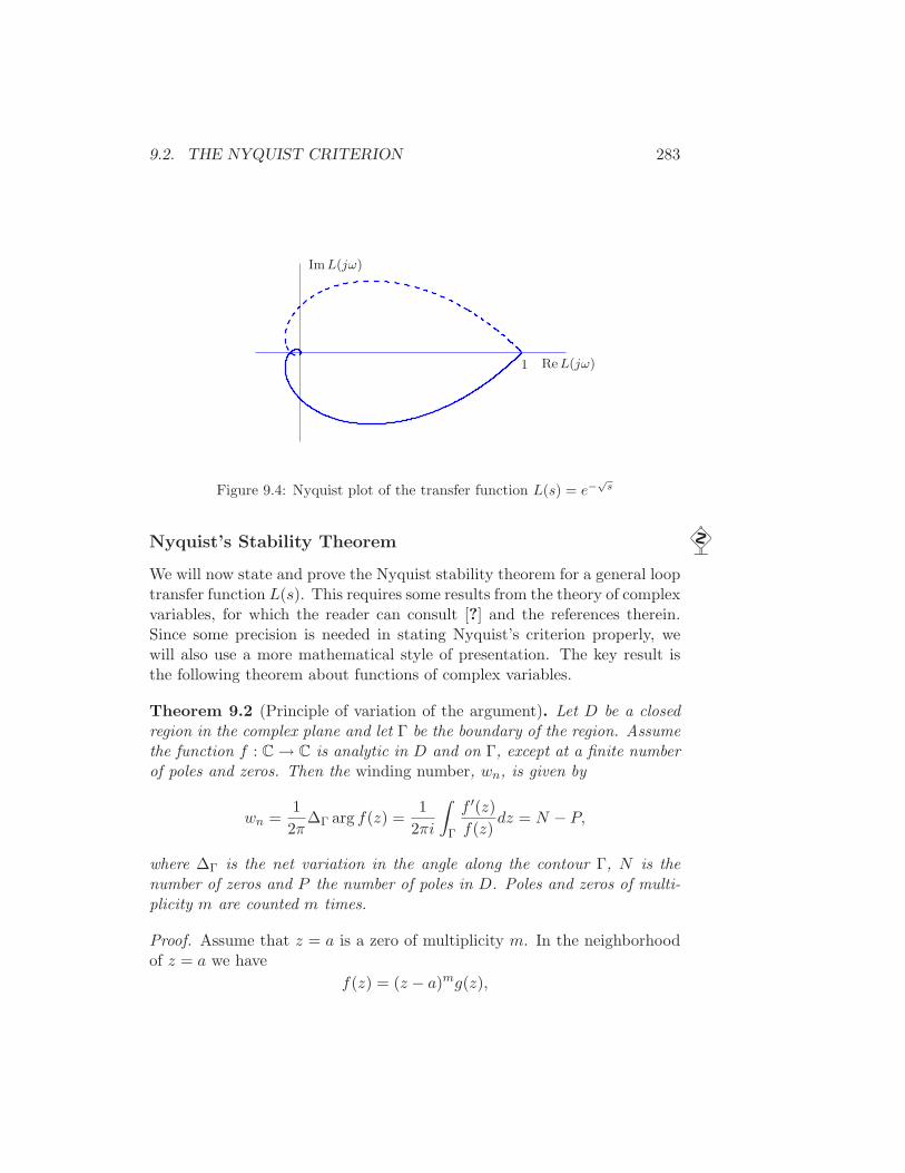
9.2. THE NYQUIST CRITERION 283
Re L(jω)
Im L(jω)
1
Figure 9.4: Nyquist plot of the transfer function L(s) = e−√
s
Nyquist’s Stability Theorem
We will now state and prove the Nyquist stability theorem for a general looptransfer function L(s). This requires some results from the theory of complexvariables, for which the reader can consult [?] and the references therein.Since some precision is needed in stating Nyquist’s criterion properly, wewill also use a more mathematical style of presentation. The key result isthe following theorem about functions of complex variables.
Theorem 9.2 (Principle of variation of the argument). Let D be a closedregion in the complex plane and let Γ be the boundary of the region. Assumethe function f : C → C is analytic in D and on Γ, except at a finite numberof poles and zeros. Then the winding number, wn, is given by
wn =1
2π∆Γ arg f(z) =
1
2πi
∫
Γ
f ′(z)f(z)
dz = N − P,
where ∆Γ is the net variation in the angle along the contour Γ, N is thenumber of zeros and P the number of poles in D. Poles and zeros of multi-plicity m are counted m times.
Proof. Assume that z = a is a zero of multiplicity m. In the neighborhoodof z = a we have
f(z) = (z − a)mg(z),
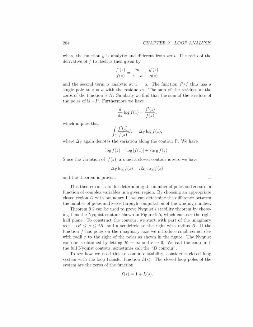
284 CHAPTER 9. LOOP ANALYSIS
where the function g is analytic and different from zero. The ratio of thederivative of f to itself is then given by
f ′(z)f(z)
=m
z − a+g′(z)g(z)
and the second term is analytic at z = a. The function f ′/f thus has asingle pole at z = a with the residue m. The sum of the residues at thezeros of the function is N . Similarly we find that the sum of the residues ofthe poles of is −P . Furthermore we have
d
dzlog f(z) =
f ′(z)f(z)
,
which implies that∫
Γ
f ′(z)f(z)
dz = ∆Γ log f(z),
where ∆Γ again denotes the variation along the contour Γ. We have
log f(z) = log |f(z)| + i arg f(z).
Since the variation of |f(z)| around a closed contour is zero we have
∆Γ log f(z) = i∆Γ arg f(z)
and the theorem is proven.
This theorem is useful for determining the number of poles and zeros of afunction of complex variables in a given region. By choosing an appropriateclosed region D with boundary Γ, we can determine the difference betweenthe number of poles and zeros through computation of the winding number.
Theorem 9.2 can be used to prove Nyquist’s stability theorem by choos-ing Γ as the Nyquist contour shown in Figure 9.5, which encloses the righthalf plane. To construct the contour, we start with part of the imaginaryaxis −iR ≤ s ≤ iR, and a semicircle to the right with radius R. If thefunction f has poles on the imaginary axis we introduce small semicircleswith radii r to the right of the poles as shown in the figure. The Nyquistcontour is obtained by letting R → ∞ and r → 0. We call the contour Γthe full Nyquist contour, sometimes call the “D contour”.
To see how we used this to compute stability, consider a closed loopsystem with the loop transfer function L(s). The closed loop poles of thesystem are the zeros of the function
f(s) = 1 + L(s).
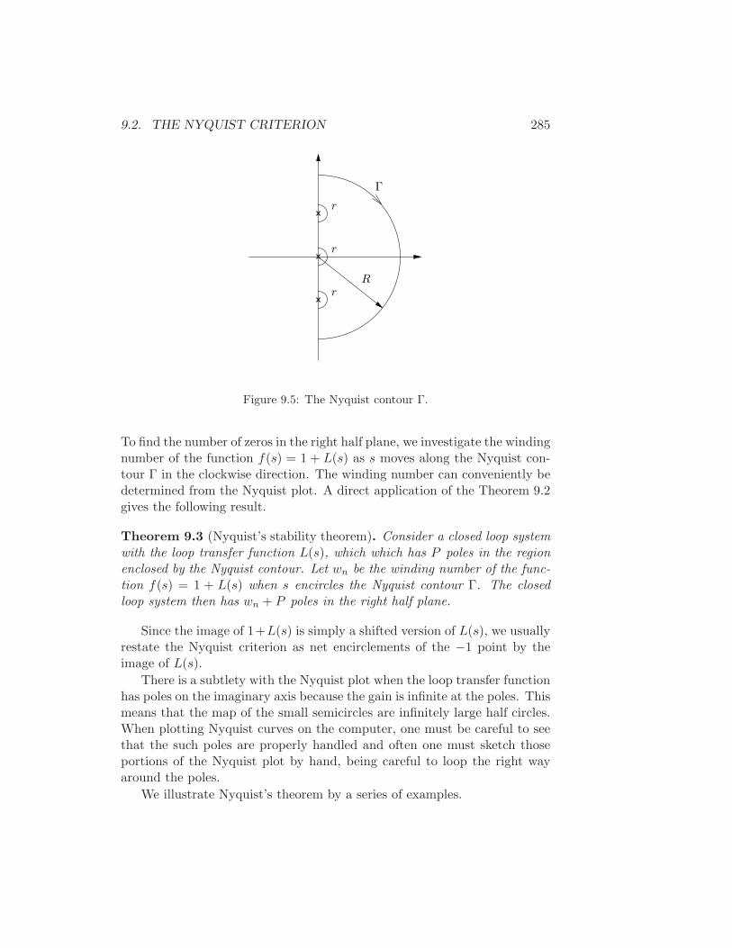
9.2. THE NYQUIST CRITERION 285
R
Γ
r
r
r
Figure 9.5: The Nyquist contour Γ.
To find the number of zeros in the right half plane, we investigate the windingnumber of the function f(s) = 1 + L(s) as s moves along the Nyquist con-tour Γ in the clockwise direction. The winding number can conveniently bedetermined from the Nyquist plot. A direct application of the Theorem 9.2gives the following result.
Theorem 9.3 (Nyquist’s stability theorem). Consider a closed loop systemwith the loop transfer function L(s), which which has P poles in the regionenclosed by the Nyquist contour. Let wn be the winding number of the func-tion f(s) = 1 + L(s) when s encircles the Nyquist contour Γ. The closedloop system then has wn + P poles in the right half plane.
Since the image of 1+L(s) is simply a shifted version of L(s), we usuallyrestate the Nyquist criterion as net encirclements of the −1 point by theimage of L(s).
There is a subtlety with the Nyquist plot when the loop transfer functionhas poles on the imaginary axis because the gain is infinite at the poles. Thismeans that the map of the small semicircles are infinitely large half circles.When plotting Nyquist curves on the computer, one must be careful to seethat the such poles are properly handled and often one must sketch thoseportions of the Nyquist plot by hand, being careful to loop the right wayaround the poles.
We illustrate Nyquist’s theorem by a series of examples.
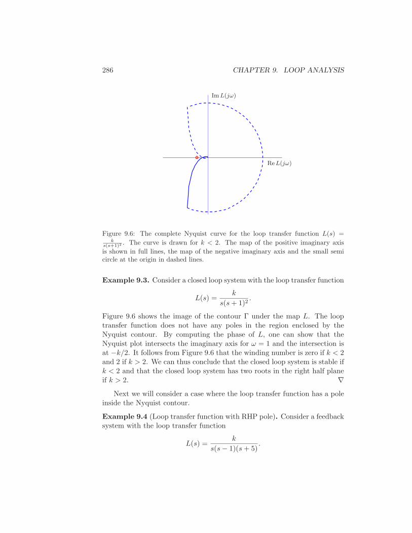
286 CHAPTER 9. LOOP ANALYSIS
Re L(jω)
Im L(jω)
Figure 9.6: The complete Nyquist curve for the loop transfer function L(s) =k
s(s+1)2 . The curve is drawn for k < 2. The map of the positive imaginary axis
is shown in full lines, the map of the negative imaginary axis and the small semicircle at the origin in dashed lines.
Example 9.3. Consider a closed loop system with the loop transfer function
L(s) =k
s(s+ 1)2.
Figure 9.6 shows the image of the contour Γ under the map L. The looptransfer function does not have any poles in the region enclosed by theNyquist contour. By computing the phase of L, one can show that theNyquist plot intersects the imaginary axis for ω = 1 and the intersection isat −k/2. It follows from Figure 9.6 that the winding number is zero if k < 2and 2 if k > 2. We can thus conclude that the closed loop system is stable ifk < 2 and that the closed loop system has two roots in the right half planeif k > 2. ∇
Next we will consider a case where the loop transfer function has a poleinside the Nyquist contour.
Example 9.4 (Loop transfer function with RHP pole). Consider a feedbacksystem with the loop transfer function
L(s) =k
s(s− 1)(s+ 5).
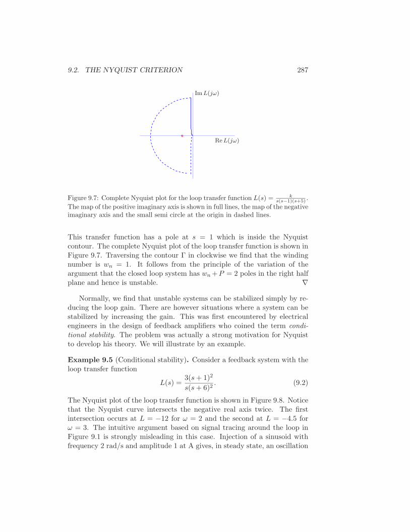
9.2. THE NYQUIST CRITERION 287
Re L(jω)
Im L(jω)
Figure 9.7: Complete Nyquist plot for the loop transfer function L(s) = ks(s−1)(s+5) .
The map of the positive imaginary axis is shown in full lines, the map of the negativeimaginary axis and the small semi circle at the origin in dashed lines.
This transfer function has a pole at s = 1 which is inside the Nyquistcontour. The complete Nyquist plot of the loop transfer function is shown inFigure 9.7. Traversing the contour Γ in clockwise we find that the windingnumber is wn = 1. It follows from the principle of the variation of theargument that the closed loop system has wn +P = 2 poles in the right halfplane and hence is unstable. ∇
Normally, we find that unstable systems can be stabilized simply by re-ducing the loop gain. There are however situations where a system can bestabilized by increasing the gain. This was first encountered by electricalengineers in the design of feedback amplifiers who coined the term condi-tional stability. The problem was actually a strong motivation for Nyquistto develop his theory. We will illustrate by an example.
Example 9.5 (Conditional stability). Consider a feedback system with theloop transfer function
L(s) =3(s+ 1)2
s(s+ 6)2. (9.2)
The Nyquist plot of the loop transfer function is shown in Figure 9.8. Noticethat the Nyquist curve intersects the negative real axis twice. The firstintersection occurs at L = −12 for ω = 2 and the second at L = −4.5 forω = 3. The intuitive argument based on signal tracing around the loop inFigure 9.1 is strongly misleading in this case. Injection of a sinusoid withfrequency 2 rad/s and amplitude 1 at A gives, in steady state, an oscillation
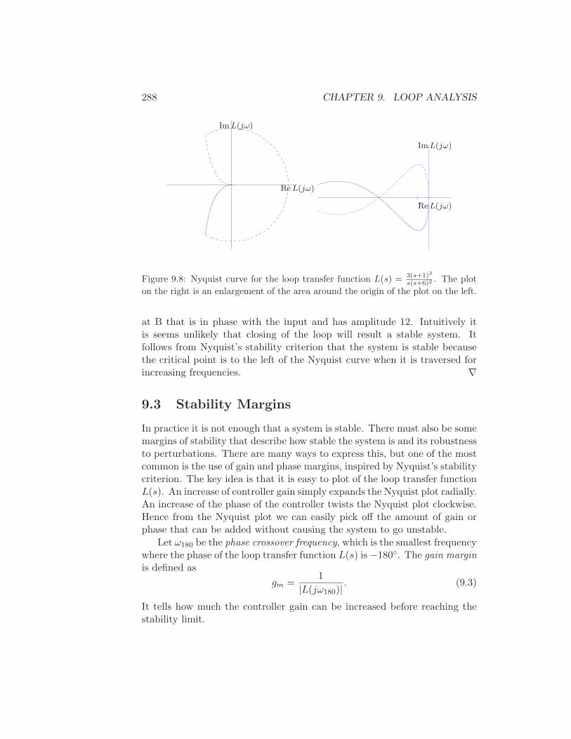
288 CHAPTER 9. LOOP ANALYSIS
Re L(jω)
Im L(jω)
−1
Re L(jω)
Im L(jω)
Figure 9.8: Nyquist curve for the loop transfer function L(s) = 3(s+1)2
s(s+6)2 . The plot
on the right is an enlargement of the area around the origin of the plot on the left.
at B that is in phase with the input and has amplitude 12. Intuitively itis seems unlikely that closing of the loop will result a stable system. Itfollows from Nyquist’s stability criterion that the system is stable becausethe critical point is to the left of the Nyquist curve when it is traversed forincreasing frequencies. ∇
9.3 Stability Margins
In practice it is not enough that a system is stable. There must also be somemargins of stability that describe how stable the system is and its robustnessto perturbations. There are many ways to express this, but one of the mostcommon is the use of gain and phase margins, inspired by Nyquist’s stabilitycriterion. The key idea is that it is easy to plot of the loop transfer functionL(s). An increase of controller gain simply expands the Nyquist plot radially.An increase of the phase of the controller twists the Nyquist plot clockwise.Hence from the Nyquist plot we can easily pick off the amount of gain orphase that can be added without causing the system to go unstable.
Let ω180 be the phase crossover frequency, which is the smallest frequencywhere the phase of the loop transfer function L(s) is −180. The gain marginis defined as
gm =1
|L(jω180)|. (9.3)
It tells how much the controller gain can be increased before reaching thestability limit.
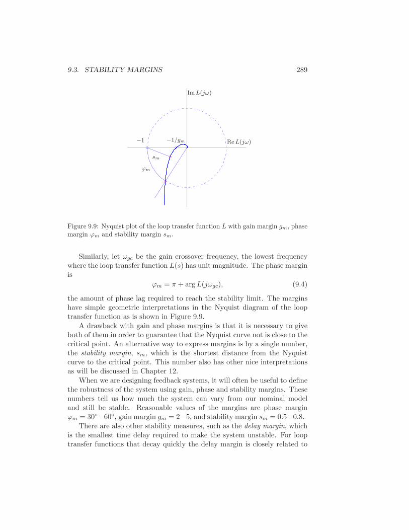
9.3. STABILITY MARGINS 289
Re L(jω)
Im L(jω)
−1
ϕm
sm
−1/gm
Figure 9.9: Nyquist plot of the loop transfer function L with gain margin gm, phasemargin ϕm and stability margin sm.
Similarly, let ωgc be the gain crossover frequency, the lowest frequencywhere the loop transfer function L(s) has unit magnitude. The phase marginis
ϕm = π + argL(jωgc), (9.4)
the amount of phase lag required to reach the stability limit. The marginshave simple geometric interpretations in the Nyquist diagram of the looptransfer function as is shown in Figure 9.9.
A drawback with gain and phase margins is that it is necessary to giveboth of them in order to guarantee that the Nyquist curve not is close to thecritical point. An alternative way to express margins is by a single number,the stability margin, sm, which is the shortest distance from the Nyquistcurve to the critical point. This number also has other nice interpretationsas will be discussed in Chapter 12.
When we are designing feedback systems, it will often be useful to definethe robustness of the system using gain, phase and stability margins. Thesenumbers tell us how much the system can vary from our nominal modeland still be stable. Reasonable values of the margins are phase marginϕm = 30−60, gain margin gm = 2−5, and stability margin sm = 0.5−0.8.
There are also other stability measures, such as the delay margin, whichis the smallest time delay required to make the system unstable. For looptransfer functions that decay quickly the delay margin is closely related to
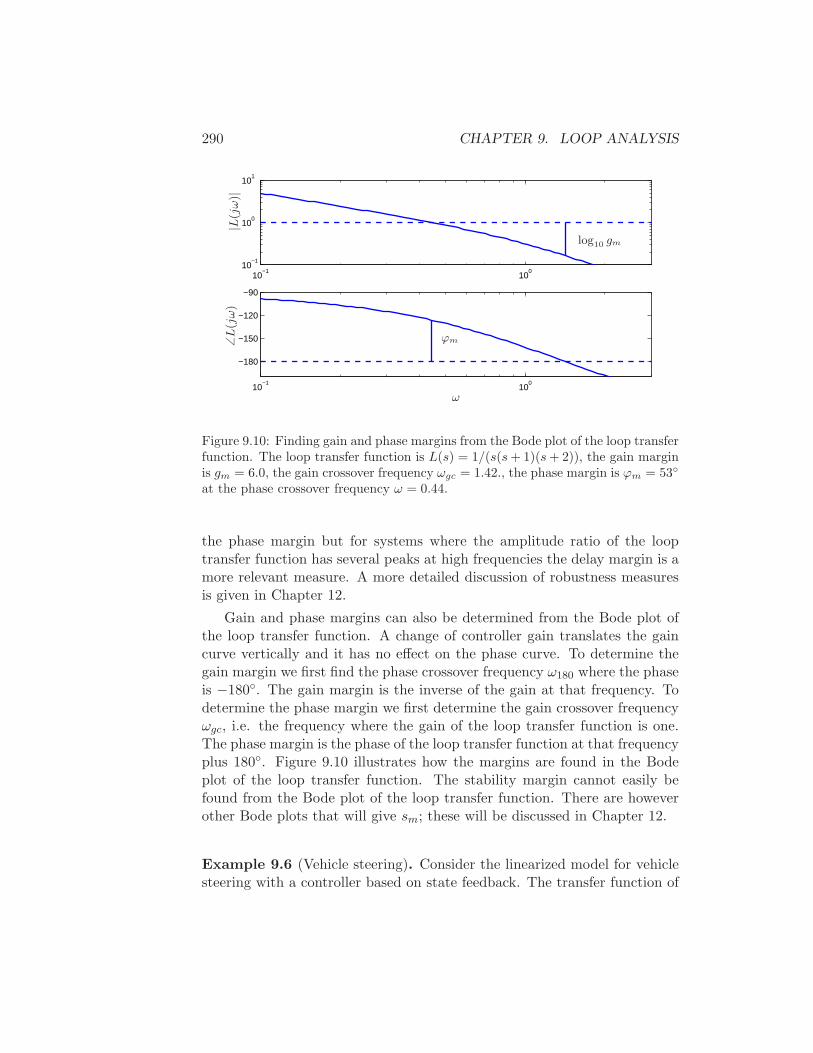
290 CHAPTER 9. LOOP ANALYSIS
10−1
100
10−1
100
101
10−1
100
−180
−150
−120
−90
|L(j
ω)|
∠L
(jω)
ω
log10 gm
ϕm
Figure 9.10: Finding gain and phase margins from the Bode plot of the loop transferfunction. The loop transfer function is L(s) = 1/(s(s+ 1)(s+ 2)), the gain marginis gm = 6.0, the gain crossover frequency ωgc = 1.42., the phase margin is ϕm = 53
at the phase crossover frequency ω = 0.44.
the phase margin but for systems where the amplitude ratio of the looptransfer function has several peaks at high frequencies the delay margin is amore relevant measure. A more detailed discussion of robustness measuresis given in Chapter 12.
Gain and phase margins can also be determined from the Bode plot ofthe loop transfer function. A change of controller gain translates the gaincurve vertically and it has no effect on the phase curve. To determine thegain margin we first find the phase crossover frequency ω180 where the phaseis −180. The gain margin is the inverse of the gain at that frequency. Todetermine the phase margin we first determine the gain crossover frequencyωgc, i.e. the frequency where the gain of the loop transfer function is one.The phase margin is the phase of the loop transfer function at that frequencyplus 180. Figure 9.10 illustrates how the margins are found in the Bodeplot of the loop transfer function. The stability margin cannot easily befound from the Bode plot of the loop transfer function. There are howeverother Bode plots that will give sm; these will be discussed in Chapter 12.
Example 9.6 (Vehicle steering). Consider the linearized model for vehiclesteering with a controller based on state feedback. The transfer function of
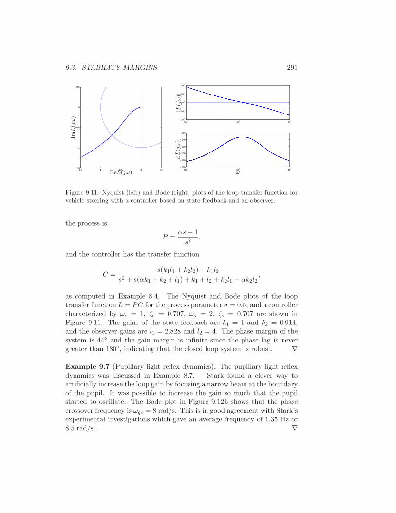
9.3. STABILITY MARGINS 291
−1.5 −1 −0.5 0 0.5−1.5
−1
−0.5
0
0.5
ReL(jω)
ImL
(jω)
10−1
100
101
10−2
10−1
100
101
102
10−1
100
101
−180
−170
−160
−150
−140
−130
|L(j
ω)|
∠L
(jω)
ω
Figure 9.11: Nyquist (left) and Bode (right) plots of the loop transfer function forvehicle steering with a controller based on state feedback and an observer.
the process is
P =αs+ 1
s2.
and the controller has the transfer function
C =s(k1l1 + k2l2) + k1l2
s2 + s(αk1 + k2 + l1) + k1 + l2 + k2l1 − αk2l2,
as computed in Example 8.4. The Nyquist and Bode plots of the looptransfer function L = PC for the process parameter a = 0.5, and a controllercharacterized by ωc = 1, ζc = 0.707, ωo = 2, ζo = 0.707 are shown inFigure 9.11. The gains of the state feedback are k1 = 1 and k2 = 0.914,and the observer gains are l1 = 2.828 and l2 = 4. The phase margin of thesystem is 44 and the gain margin is infinite since the phase lag is nevergreater than 180, indicating that the closed loop system is robust. ∇
Example 9.7 (Pupillary light reflex dynamics). The pupillary light reflexdynamics was discussed in Example 8.7. Stark found a clever way toartificially increase the loop gain by focusing a narrow beam at the boundaryof the pupil. It was possible to increase the gain so much that the pupilstarted to oscillate. The Bode plot in Figure 9.12b shows that the phasecrossover frequency is ωgc = 8 rad/s. This is in good agreement with Stark’sexperimental investigations which gave an average frequency of 1.35 Hz or8.5 rad/s. ∇
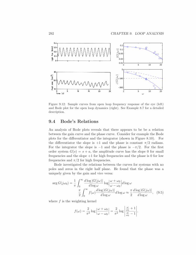
292 CHAPTER 9. LOOP ANALYSIS
2 5 10 200.01
0.02
0.05
0.1
0.2
2 5 10 20
−360
−180
0
ω
|G(j
ω)|
∠G
(jω)
Figure 9.12: Sample curves from open loop frequency response of the eye (left)and Bode plot for the open loop dynamics (right). See Example 8.7 for a detaileddescription.
9.4 Bode’s Relations
An analysis of Bode plots reveals that there appears to be be a relationbetween the gain curve and the phase curve. Consider for example the Bodeplots for the differentiator and the integrator (shown in Figure 8.10). Forthe differentiator the slope is +1 and the phase is constant π/2 radians.For the integrator the slope is −1 and the phase is −π/2. For the firstorder system G(s) = s + a, the amplitude curve has the slope 0 for smallfrequencies and the slope +1 for high frequencies and the phase is 0 for lowfrequencies and π/2 for high frequencies.
Bode investigated the relations between the curves for systems with nopoles and zeros in the right half plane. He found that the phase was auniquely given by the gain and vice versa:
argG(jω0) =1
π
∫ ∞
0
d log |G(jω)|d logω
log∣∣∣ω + ω0
ω − ω0
∣∣∣d logω
π
2
∫ ∞
0f(ω)
d log |G(jω)|d logω
d logω ≈ π
2
d log |G(jω)|d logω
, (9.5)
where f is the weighting kernel
f(ω) =2
π2log∣∣∣ω + ω0
ω − ω0
∣∣∣ =
2
π2log
∣∣∣∣∣
ωω0
+ 1ωω0
− 1
∣∣∣∣∣.
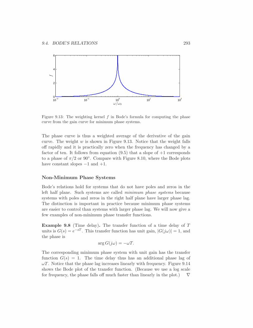
9.4. BODE’S RELATIONS 293
10−2
10−1
100
101
102
0
2
4
6
f
ω/ω0
Figure 9.13: The weighting kernel f in Bode’s formula for computing the phasecurve from the gain curve for minimum phase systems.
The phase curve is thus a weighted average of the derivative of the gaincurve. The weight w is shown in Figure 9.13. Notice that the weight fallsoff rapidly and it is practically zero when the frequency has changed by afactor of ten. It follows from equation (9.5) that a slope of +1 correspondsto a phase of π/2 or 90. Compare with Figure 8.10, where the Bode plotshave constant slopes −1 and +1.
Non-Minimum Phase Systems
Bode’s relations hold for systems that do not have poles and zeros in theleft half plane. Such systems are called minimum phase systems becausesystems with poles and zeros in the right half plane have larger phase lag.The distinction is important in practice because minimum phase systemsare easier to control than systems with larger phase lag. We will now give afew examples of non-minimum phase transfer functions.
Example 9.8 (Time delay). The transfer function of a time delay of Tunits is G(s) = e−sT . This transfer function has unit gain, |G(jω)| = 1, andthe phase is
argG(jω) = −ωT.
The corresponding minimum phase system with unit gain has the transferfunction G(s) = 1. The time delay thus has an additional phase lag ofωT . Notice that the phase lag increases linearly with frequency. Figure 9.14shows the Bode plot of the transfer function. (Because we use a log scalefor frequency, the phase falls off much faster than linearly in the plot.) ∇
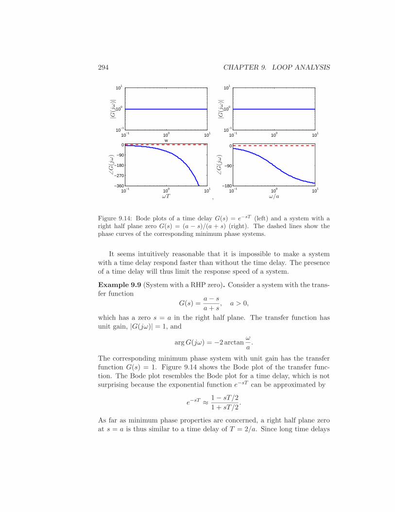
294 CHAPTER 9. LOOP ANALYSIS
10−1
100
101
10−1
100
101
w
10−1
100
101
−360
−270
−180
−90
0
ωT
|G(j
ω)|
∠G
(jω)
,
10−1
100
101
10−1
100
101
10−1
100
101
−180
−90
0
ω/a
|G(j
ω)|
∠G
(jω)
Figure 9.14: Bode plots of a time delay G(s) = e−sT (left) and a system with aright half plane zero G(s) = (a − s)/(a + s) (right). The dashed lines show thephase curves of the corresponding minimum phase systems.
It seems intuitively reasonable that it is impossible to make a systemwith a time delay respond faster than without the time delay. The presenceof a time delay will thus limit the response speed of a system.
Example 9.9 (System with a RHP zero). Consider a system with the trans-fer function
G(s) =a− s
a+ s, a > 0,
which has a zero s = a in the right half plane. The transfer function hasunit gain, |G(jω)| = 1, and
argG(jω) = −2 arctanω
a.
The corresponding minimum phase system with unit gain has the transferfunction G(s) = 1. Figure 9.14 shows the Bode plot of the transfer func-tion. The Bode plot resembles the Bode plot for a time delay, which is notsurprising because the exponential function e−sT can be approximated by
e−sT ≈ 1 − sT/2
1 + sT/2.
As far as minimum phase properties are concerned, a right half plane zeroat s = a is thus similar to a time delay of T = 2/a. Since long time delays
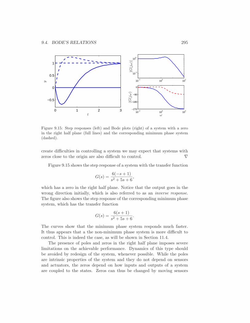
9.4. BODE’S RELATIONS 295
0 1 2 3
−0.5
0
0.5
1
y
t
10−2
100
102
10−1
100
10−2
100
102
−270
−180
−90
0
ω
|G(j
ω)|
〈G(j
ω)
Figure 9.15: Step responses (left) and Bode plots (right) of a system with a zeroin the right half plane (full lines) and the corresponding minimum phase system(dashed).
create difficulties in controlling a system we may expect that systems withzeros close to the origin are also difficult to control. ∇
Figure 9.15 shows the step response of a system with the transfer function
G(s) =6(−s+ 1)
s2 + 5s+ 6,
which has a zero in the right half plane. Notice that the output goes in thewrong direction initially, which is also referred to as an inverse response.The figure also shows the step response of the corresponding minimum phasesystem, which has the transfer function
G(s) =6(s+ 1)
s2 + 5s+ 6.
The curves show that the minimum phase system responds much faster.It thus appears that a the non-minimum phase system is more difficult tocontrol. This is indeed the case, as will be shown in Section 11.4.
The presence of poles and zeros in the right half plane imposes severelimitations on the achievable performance. Dynamics of this type shouldbe avoided by redesign of the system, whenever possible. While the polesare intrinsic properties of the system and they do not depend on sensorsand actuators, the zeros depend on how inputs and outputs of a systemare coupled to the states. Zeros can thus be changed by moving sensors
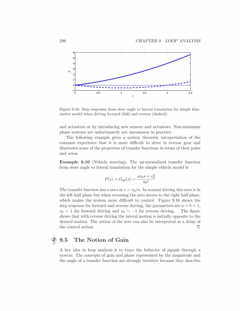
296 CHAPTER 9. LOOP ANALYSIS
0 0.5 1 1.5 2 2.5−1
0
1
2
3
4
5
6
t
y
Figure 9.16: Step responses from steer angle to lateral translation for simple kine-matics model when driving forward (full) and reverse (dashed).
and actuators or by introducing new sensors and actuators. Non-minimumphase systems are unfortunately not uncommon in practice.
The following example gives a system theoretic interpretation of thecommon experience that it is more difficult to drive in reverse gear andillustrates some of the properties of transfer functions in terms of their polesand zeros.
Example 9.10 (Vehicle steering). The un-normalized transfer functionfrom steer angle to lateral translation for the simple vehicle model is
P (s) = Gyδ(s) =av0s+ v2
0
bs2
The transfer function has a zero at s = v0/a. In normal driving this zero is inthe left half plane but when reversing the zero moves to the right half plane,which makes the system more difficult to control. Figure 9.16 shows thestep response for forward and reverse driving, the parameters are a = b = 1,v0 = 1 for forward driving and v0 = −1 for reverse driving. The figureshows that with reverse driving the lateral motion is initially opposite to thedesired motion. The action of the zero can also be interpreted as a delay ofthe control action. ∇
9.5 The Notion of Gain
A key idea in loop analysis it to trace the behavior of signals through asystem. The concepts of gain and phase represented by the magnitude andthe angle of a transfer function are strongly intuitive because they describe
9.5. THE NOTION OF GAIN 297
how sinusoidal signals are transmitted. We will now show that the notion ofgain can be defined in a much more general way. Something has to be givenup to do this and it turns out that it is difficult to define gain for transmissionof general signal but that it is easy to define the maximum gain. For thispurpose we first define appropriate classes of input and output signals, u ∈ Uand u ∈ Y, where U and Y are spaces where a notion of magnitude is defined.The gain of a system is defined as
γ = supu∈U
‖y‖‖u‖ , (9.6)
where sup is the supremum, defined as the smallest number that is largerthan its argument. The reason for using supremum is that the maximummay not be defined for u ∈ U . A correct treatment requires considerablecare and space so will will only give a few examples.
Example 9.11 (Linear systems with square integrable inputs). Let theinput space U be square integrable functions, and consider a stable linearsystem with transfer function G(s). The norm of a signal is given by
‖u‖2 =
√∫ ∞
0u2(τ) dτ
where the subscript 2 refers to the fact that U is the set of square integrablefunctions. Using the same norm for Y, the gain of the system can be shownto be
γ = supω
|G(jω)| := ‖G‖∞. (9.7)
∇
Example 9.12 (Static nonlinear system). Consider a nonlinear static sys-tem with scalar inputs and outputs described by y = f(u). The gain ob-tained γ is a number such that −γu ≤ |f(u)| ≤ γu. The gain thus defines asector that encloses the function. ∇
Example 9.13 (Multivariable static system). Consider a static multivari-able system y = Au, where A is a matrix, whose elements are complexnumbers. The matrix does not have to be square. Let the and inputs andoutputs be vectors whose elements are complex numbers and use the Eu-clidean norm
‖u‖ =√
Σ|ui|2.
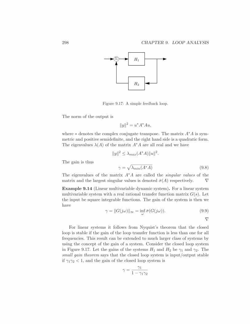
298 CHAPTER 9. LOOP ANALYSIS
Σ H1
H2
Figure 9.17: A simple feedback loop.
The norm of the output is
‖y‖2 = u∗A∗Au,
where ∗ denotes the complex conjugate transpose. The matrix A∗A is sym-metric and positive semidefinite, and the right hand side is a quadratic form.The eigenvalues λ(A) of the matrix A∗A are all real and we have
‖y‖2 ≤ λmax(A∗A)‖u‖2.
The gain is thusγ =
√
λmin(A∗A) (9.8)
The eigenvalues of the matrix A∗A are called the singular values of thematrix and the largest singular values is denoted σ(A) respectively. ∇Example 9.14 (Linear multivariable dynamic system). For a linear systemmultivariable system with a real rational transfer function matrix G(s). Letthe input be square integrable functions. The gain of the system is then wehave
γ = ‖G(jω)‖∞ = infωσ(G(jω)). (9.9)
∇For linear systems it follows from Nyquist’s theorem that the closed
loop is stable if the gain of the loop transfer function is less than one for allfrequencies. This result can be extended to much larger class of systems byusing the concept of the gain of a system. Consider the closed loop systemin Figure 9.17. Let the gains of the systems H1 and H2 be γ1 and γ2. Thesmall gain theorem says that the closed loop system is input/output stableif γ1γ2 < 1, and the gain of the closed loop system is
γ =γ1
1 − γ1γ2
9.6. FURTHER READING 299
Notice that if systems H1 and H2 are linear it follows from the Nyquiststability theorem that the closed loop is stable, because if γ1γ2 < 1 theNyquist curve is always inside the unit circle. The small gain theorem isthus an extension of the Nyquist stability theorem.
It also follows from the Nyquist stability theorem that a closed loopsystem is stable if the phase of the loop transfer function is between −π andπ. This result can also be extended to nonlinear systems as well. It is calledthe passivity theorem and is closely related to the small gain theorem.
Additional applications of the small gain theorem and its application torobust stability are given in Chapter 12.
9.6 Further Reading
Nyquist’s original paper giving his now famous stability criterion was pub-lished in the Bell Systems Technical Journal in 1932 [Nyq32].
9.7 Exercises
1. Use the Nyquist theorem to analyze the stability of the speed con-trol system in Example 9.1, but using the original PI controller fromExample 6.9.
2. Discrete time Nyquist
3. Example systems:

300 CHAPTER 9. LOOP ANALYSIS
Chapter 10
PID Control
Based on a survey of over eleven thousand controllers in the refining, chemi-cals and pulp and paper industries, 97% of regulatory controllers utilize PIDfeedback.
Desborough Honeywell, 2000, see [DM02].
PID control is by far the most common way of using feedback in naturaland man-made systems. PID controllers are commonly used in industryand a large factory may have thousands of them, in instruments and lab-oratory equipment. In engineering applications the controllers appear inmany different forms: as a stand alone controller, as part of hierarchical,distributed control systems, or built into embedded components. Most con-trollers do not use derivative action. In this chapter we discuss the basicideas of PID control and the methods for choosing the parameters of thecontrollers. Many aspects of control can be understood based on linearanalysis. However, there is one nonlinear effect, that has to be considered inmost control systems namely that actuators saturate. In combinations withcontrollers having integral actions saturations give rise to an effect calledintegral windup. This phenomenon that occurs in practically all controlsystems will be discussed in depth for PID controllers. Methods to avoidwindup will also be presented. Finally we will also discuss implementationof PID controllers, similar methods can be used to implement many othercontrollers.
301
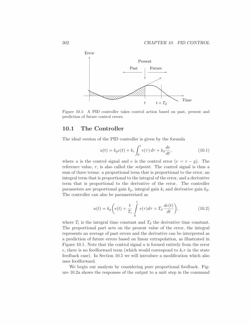
302 CHAPTER 10. PID CONTROL
Present
FuturePast
t t+ Td
Error
Time
Figure 10.1: A PID controller takes control action based on past, present andprediction of future control errors.
10.1 The Controller
The ideal version of the PID controller is given by the formula
u(t) = kpe(t) + ki
∫ t
0e(τ) dτ + kd
de
dt, (10.1)
where u is the control signal and e is the control error (e = r − y). Thereference value, r, is also called the setpoint. The control signal is thus asum of three terms: a proportional term that is proportional to the error, anintegral term that is proportional to the integral of the error, and a derivativeterm that is proportional to the derivative of the error. The controllerparameters are proportional gain kp, integral gain ki and derivative gain kd.The controller can also be parameterized as
u(t) = kp
(
e(t) +1
Ti
t∫
0
e(τ)dτ + Tdde(t)
dt
)
, (10.2)
where Ti is the integral time constant and Td the derivative time constant.The proportional part acts on the present value of the error, the integralrepresents an average of past errors and the derivative can be interpreted asa prediction of future errors based on linear extrapolation, as illustrated inFigure 10.1. Note that the control signal u is formed entirely from the errore, there is no feedforward term (which would correspond to krr in the statefeedback case). In Section 10.5 we will introduce a modification which alsouses feedforward.
We begin our analysis by considering pure proportional feedback. Fig-ure 10.2a shows the responses of the output to a unit step in the command
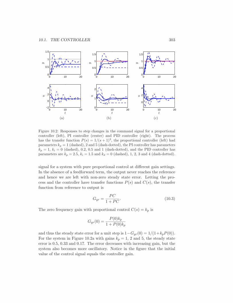
10.1. THE CONTROLLER 303
0 10 200
0.5
1
1.5
0 10 20−2
0
2
4
t
yu
0 10 200
0.5
1
1.5
0 10 200
1
2
t
yu
0 10 200
0.5
1
1.5
0 10 20
0
2
4
t
yu
(a) (b) (c)
Figure 10.2: Responses to step changes in the command signal for a proportionalcontroller (left), PI controller (center) and PID controller (right). The processhas the transfer function P (s) = 1/(s + 1)3, the proportional controller (left) hadparameters kp = 1 (dashed), 2 and 5 (dash-dotted), the PI controller has parameterskp = 1, ki = 0 (dashed), 0.2, 0.5 and 1 (dash-dotted), and the PID controller hasparameters are kp = 2.5, ki = 1.5 and kd = 0 (dashed), 1, 2, 3 and 4 (dash-dotted).
signal for a system with pure proportional control at different gain settings.In the absence of a feedforward term, the output never reaches the referenceand hence we are left with non-zero steady state error. Letting the pro-cess and the controller have transfer functions P (s) and C(s), the transferfunction from reference to output is
Gyr =PC
1 + PC. (10.3)
The zero frequency gain with proportional control C(s) = kp is
Gyr(0) =P (0)kp
1 + P (0)kp
and thus the steady state error for a unit step is 1−Gyr(0) = 1/(1+kpP (0)).For the system in Figure 10.2a with gains kp = 1, 2 and 5, the steady stateerror is 0.5, 0.33 and 0.17. The error decreases with increasing gain, but thesystem also becomes more oscillatory. Notice in the figure that the initialvalue of the control signal equals the controller gain.
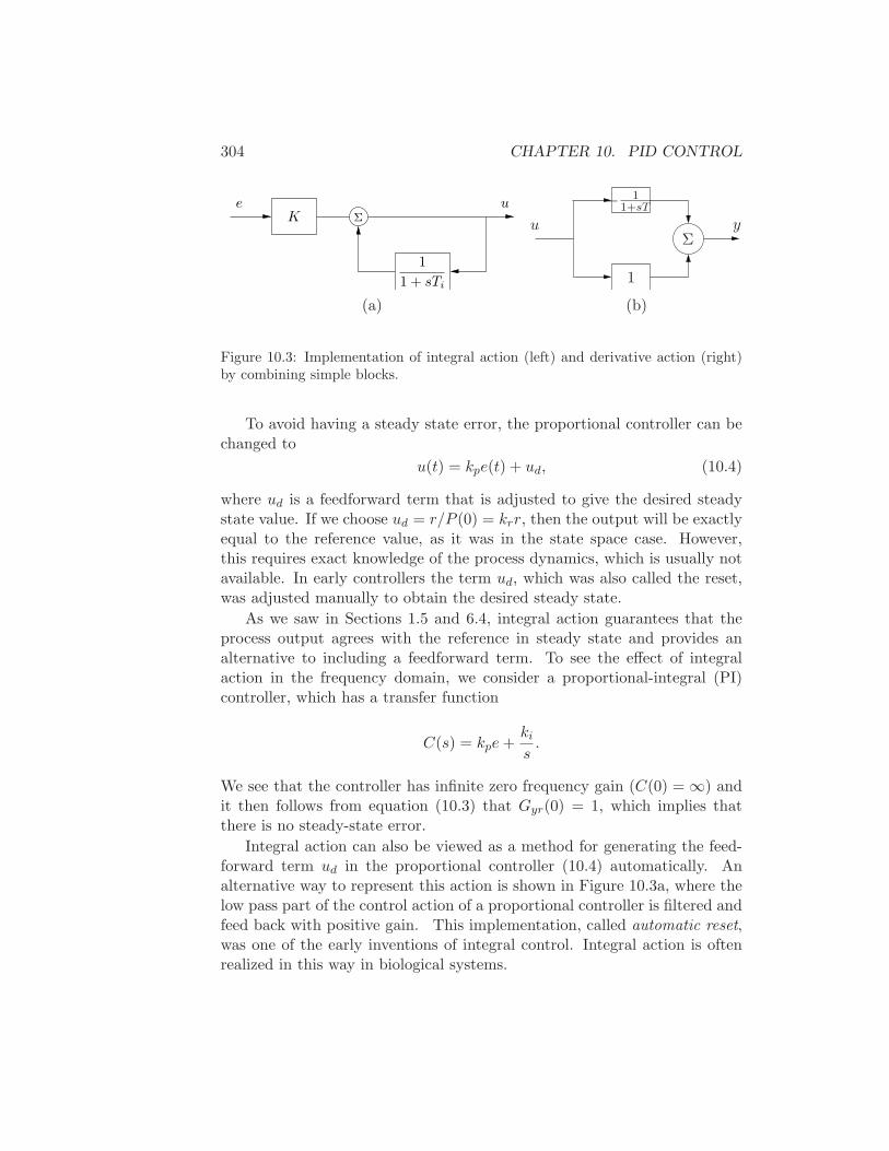
304 CHAPTER 10. PID CONTROL
ΣKe u
1
1 + sTi
u y
1
− 11+sT
Σ
(a) (b)
Figure 10.3: Implementation of integral action (left) and derivative action (right)by combining simple blocks.
To avoid having a steady state error, the proportional controller can bechanged to
u(t) = kpe(t) + ud, (10.4)
where ud is a feedforward term that is adjusted to give the desired steadystate value. If we choose ud = r/P (0) = krr, then the output will be exactlyequal to the reference value, as it was in the state space case. However,this requires exact knowledge of the process dynamics, which is usually notavailable. In early controllers the term ud, which was also called the reset,was adjusted manually to obtain the desired steady state.
As we saw in Sections 1.5 and 6.4, integral action guarantees that theprocess output agrees with the reference in steady state and provides analternative to including a feedforward term. To see the effect of integralaction in the frequency domain, we consider a proportional-integral (PI)controller, which has a transfer function
C(s) = kpe+ki
s.
We see that the controller has infinite zero frequency gain (C(0) = ∞) andit then follows from equation (10.3) that Gyr(0) = 1, which implies thatthere is no steady-state error.
Integral action can also be viewed as a method for generating the feed-forward term ud in the proportional controller (10.4) automatically. Analternative way to represent this action is shown in Figure 10.3a, where thelow pass part of the control action of a proportional controller is filtered andfeed back with positive gain. This implementation, called automatic reset,was one of the early inventions of integral control. Integral action is oftenrealized in this way in biological systems.
10.1. THE CONTROLLER 305
The transfer function of the system in Figure 10.3 is obtained by looptracing: assuming exponential signals, we have
u = kpe+1
1 + sTu,
and solving for u gives
u = kp1 + sT
sTe = kp +
kp
sT,
which is the transfer function for a PI controller.The properties of integral action are illustrated in Figure 10.2b. The
proportional gain is constant, kp = 1, and the integral gains are ki = 0, 0.2,0.5 and 1. The case ki = 0 corresponds to pure proportional control, with asteady state error of 50%. The steady state error is removed when integralgain action is used. The response creeps slowly towards the reference forsmall values of ki, but faster for larger integral gains, but the system alsobecomes more oscillatory.
We now return to the general PID controller and consider the use ofthe derivative term, kd. Recall that the original motivation for derivativefeedback was to provide predictive action. The input-output relation of acontroller with proportional and derivative action is
u = kpe+ kdde
dt= k
(e+ Td
de
dt
),
where Td = kd/kp is the derivative time constant. The action of a controllerwith proportional and derivative action can be interpreted as if the controlis made proportional to the predicted process output, where the predictionis made by extrapolating the error Td time units into the future using thetangent to the error curve (see Figure 10.1).
Derivative action can also be implemented by taking the difference be-tween the signal and its low-pass filtered version as shown in Figure 10.3a.The transfer function for the system is
C(s) =(
1 − 1
1 + sT
)
=sT
1 + sTU(s).
The system thus has the transfer function G(s) = sT/(1 + sT ), which ap-proximates a derivative for low frequencies. Notice that this implementationgives filtering automatically.
Figure 10.2c illustrates the behavior of a system with a PID controller:the system is oscillatory when no derivative action is used and it becomes
306 CHAPTER 10. PID CONTROL
more damped as derivative gain is increased. A comparison of the systemswith P, PI and PID control in Figure 10.2 shows that the steady-state erroris removed by introducing integral action and that the response speed canbe improved by introducing derivative action.
10.2 Tuning
Users of control systems are frequently faced with the task of adjustingthe controller parameters to obtain a desired behavior. There are manydifferent ways to do this. One way to do this is to go through the steps ofmodeling and control design. Since the PID controller has so few parametersa number of special empirical methods have also been developed. A simpleidea is to connect a controller, increase the gain until the the system startsto oscillate, and then reduce the gains by an appropriate factor. Anotheris to measure some features of the open loop response and to determinecontroller parameters based on these features. We will present the Ziegler-Nichols methods which are the most celebrated tuning rules.
Ziegler-Nichols’ Tuning
Ziegler and Nichols develped two techniques for controller tuning in the1940s. The idea was to tune the controller based on the following idea: Makea simple experiment, extract some features of process dynamics from theexperimental data, and determine controller parameters from the features.
One method is based on direct adjustment of the controller parameters.A controller is connected to the process, integral and derivative gain areset to zero and the proportional gain is increased until the system startsto oscillate. The critical value of the proportional gain kc is observed to-gether with the period of oscillation Tc. The controller parameters are thengiven by Table 10.1. The values in the table were obtained based on manysimulations and experiments on processes that are normally encountered inprocess industry. There are many variations of the method which are widelyused in industry.
Another method proposed by Ziegler and Nichols is based on determi-nation of the open loop step response of the process, as shown Figure 10.4a.The step response is measured by applying a step input to the process andrecording the response. The response is scaled to correspond to a unit stepinput and characterized by parameters a and Tdel, which are the interceptsof the steepest tangent of the step response with the coordinate axes. Theparameter Tdel is an approximation of the time delay of the system and
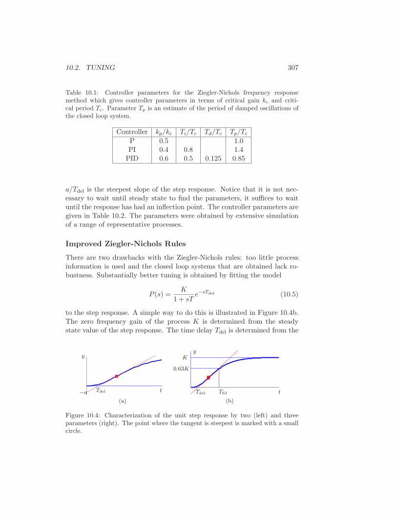
10.2. TUNING 307
Table 10.1: Controller parameters for the Ziegler-Nichols frequency responsemethod which gives controller parameters in terms of critical gain kc and criti-cal period Tc. Parameter Tp is an estimate of the period of damped oscillations ofthe closed loop system.
Controller kp/kc Ti/Tc Td/Tc Tp/Tc
P 0.5 1.0PI 0.4 0.8 1.4
PID 0.6 0.5 0.125 0.85
a/Tdel is the steepest slope of the step response. Notice that it is not nec-essary to wait until steady state to find the parameters, it suffices to waituntil the response has had an inflection point. The controller parameters aregiven in Table 10.2. The parameters were obtained by extensive simulationof a range of representative processes.
Improved Ziegler-Nichols Rules
There are two drawbacks with the Ziegler-Nichols rules: too little processinformation is used and the closed loop systems that are obtained lack ro-bustness. Substantially better tuning is obtained by fitting the model
P (s) =K
1 + sTe−sTdel (10.5)
to the step response. A simple way to do this is illustrated in Figure 10.4b.The zero frequency gain of the process K is determined from the steadystate value of the step response. The time delay Tdel is determined from the
tTdel
y
−a
(a)
tTdel
yK
0.63K
T63
(b)
Figure 10.4: Characterization of the unit step response by two (left) and threeparameters (right). The point where the tangent is steepest is marked with a smallcircle.
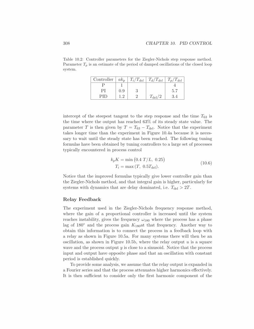
308 CHAPTER 10. PID CONTROL
Table 10.2: Controller parameters for the Ziegler-Nichols step response method.Parameter Tp is an estimate of the period of damped oscillations of the closed loopsystem.
Controller akp Ti/Tdel Td/Tdel Tp/Tdel
P 1 4PI 0.9 3 5.7
PID 1.2 2 Tdel/2 3.4
intercept of the steepest tangent to the step response and the time T63 isthe time where the output has reached 63% of its steady state value. Theparameter T is then given by T = T63 − Tdel. Notice that the experimenttakes longer time than the experiment in Figure 10.4a because it is neces-sary to wait until the steady state has been reached. The following tuningformulas have been obtained by tuning controllers to a large set of processestypically encountered in process control
kpK = min(0.4 T/L, 0.25
)
Ti = max (T, 0.5Tdel).(10.6)
Notice that the improved formulas typically give lower controller gain thanthe Ziegler-Nichols method, and that integral gain is higher, particularly forsystems with dynamics that are delay dominated, i.e. Tdel > 2T .
Relay Feedback
The experiment used in the Ziegler-Nichols frequency response method,where the gain of a proportional controller is increased until the systemreaches instability, gives the frequency ω180 where the process has a phaselag of 180 and the process gain K180at that frequency. Another way toobtain this information is to connect the process in a feedback loop witha relay as shown in Figure 10.5a. For many systems there will then be anoscillation, as shown in Figure 10.5b, where the relay output u is a squarewave and the process output y is close to a sinusoid. Notice that the processinput and output have opposite phase and that an oscillation with constantperiod is established quickly.
To provide some analysis, we assume that the relay output is expanded ina Fourier series and that the process attenuates higher harmonics effectively.It is then sufficient to consider only the first harmonic component of the
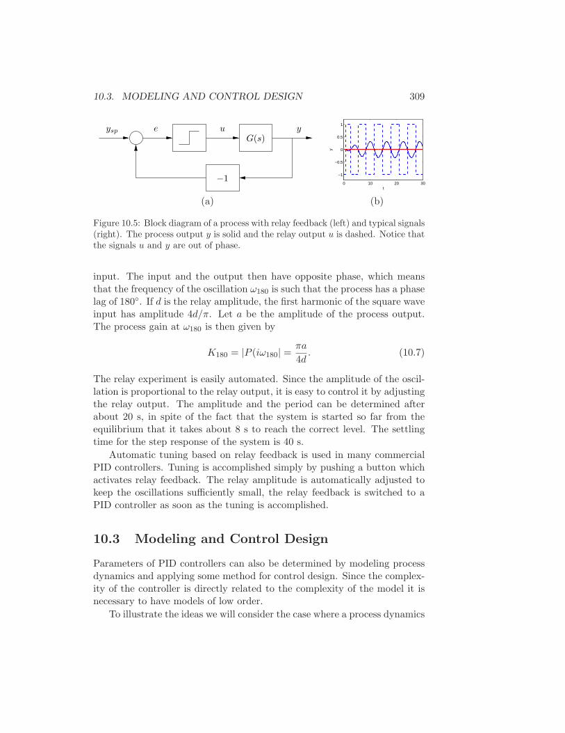
10.3. MODELING AND CONTROL DESIGN 309
G(s)yueysp
−10 10 20 30
−1
−0.5
0
0.5
1
y
t
(a) (b)
Figure 10.5: Block diagram of a process with relay feedback (left) and typical signals(right). The process output y is solid and the relay output u is dashed. Notice thatthe signals u and y are out of phase.
input. The input and the output then have opposite phase, which meansthat the frequency of the oscillation ω180 is such that the process has a phaselag of 180. If d is the relay amplitude, the first harmonic of the square waveinput has amplitude 4d/π. Let a be the amplitude of the process output.The process gain at ω180 is then given by
K180 = |P (iω180| =πa
4d. (10.7)
The relay experiment is easily automated. Since the amplitude of the oscil-lation is proportional to the relay output, it is easy to control it by adjustingthe relay output. The amplitude and the period can be determined afterabout 20 s, in spite of the fact that the system is started so far from theequilibrium that it takes about 8 s to reach the correct level. The settlingtime for the step response of the system is 40 s.
Automatic tuning based on relay feedback is used in many commercialPID controllers. Tuning is accomplished simply by pushing a button whichactivates relay feedback. The relay amplitude is automatically adjusted tokeep the oscillations sufficiently small, the relay feedback is switched to aPID controller as soon as the tuning is accomplished.
10.3 Modeling and Control Design
Parameters of PID controllers can also be determined by modeling processdynamics and applying some method for control design. Since the complex-ity of the controller is directly related to the complexity of the model it isnecessary to have models of low order.
To illustrate the ideas we will consider the case where a process dynamics
310 CHAPTER 10. PID CONTROL
is approximated by a first order transfer function
P (s) =b
s+ a.
The approximation is reasonable for systems where storage of mass, momen-tum and energy can be captured by one state variable. Typical examplesare the velocity of a car on the road, control of the velocity of a rotatingsystem, electric systems where energy is essentially stored in one compo-nent, incompressible fluid flow in a pipe, level control of a tank, pressurecontrol in a gas tank and temperature in a body with uniform temperaturedistribution.
A PI controller has the transfer function
C(s) = kp +ki
s,
and the transfer function of the closed loop system from reference to outputis
Gyr =PC
1 + PC=
b(kps+ ki)
s2 + (a+ bkp)s+ bki.
The closed loop system has the characteristic polynomial
s2 + (a+ bkp)s+ bki.
Assuming that the desired characteristic polynomial is
s2 + 2ζω0s+ ω20, (10.8)
we find that the controller parameters are given by
kp =2ζω0 − a
b=
2ζω0T − 1
K
ki =ω2
0
b=ω2
0T
K.
(10.9)
The parameter ω0 determines the response speed and ζ determines thedamping. Notice that controller gain becomes negative if ζω0 < 0.5, whichgives a closed loop system with bad properties, as will be discussed in Sec-tion 12.5.
The same approach can be used to find the parameters of a PID controllerfor a process with dynamics of second order (Exercise 1).

10.3. MODELING AND CONTROL DESIGN 311
Example 10.1 (Cruise control design). Consider the problem of maintain-ing the speed of a car as it goes up a hill. In Example 5.14we found thatthere was very little difference between the linear and nonlinear models wheninvestigating PI control provided that the throttle does not reach the satu-ration limits. We will now use a linear model to design a controller and toinvestigate the effects of design parameters. A simple linear model of a carwas given in Example 5.10:
d(v − ve)
dt= a(v − ve) + b(u− ue) − gθ, (10.10)
where v is the velocity of the car, u is the input from the engine and θis the slope of the hill. The parameters were a = −0.101, b = 1.3203,g = 9.8, ve = 20, and ue = 0.1616. This model will be used to find suitableparameters of a vehicle speed controller. To investigate the behavior of theclosed loop system we start with the linearized process model (10.10) andwe assume that the cruise controller is PI controller is described by
u = kp(ve − v) + ki
∫ t
0(ve − v(τ))dτ. (10.11)
To compute the error dynamics, introduce the error e = ve − v, differentiateequations (10.10) and (10.11), and eliminate u. The error is then given bythe differential equation
d2e
dt2+ (−a+ bkp)
de
dt+ bkie = 9.8
dθ
dt. (10.12)
We notice that the steady state error is zero if θ and e are constant, whichis no surprise since the controller has integral action.
To understand the effects of the controller parameters K and ki we cancompare equation (10.12) with the standard second order system
q + 2ζω0q + ω20q = ku.
This gives
kp =a+ 2ζω0
bki =
ω20
b
where ζ denotes relative damping and ω0 is the undamped natural frequency.The parameter ω0 gives response speed and ζ determines the shape of theresponse. Since it is desirable that a cruise control system should respond tochanges smoothly without oscillations we choose ζ = 1, which correspondsto critical damping.
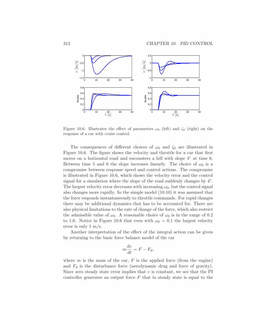
312 CHAPTER 10. PID CONTROL
0 10 20 30 40−1.5
−1
−0.5
0
0 10 20 30 400
0.2
0.4
0.6
0.8
thro
ttle
t [s]
v[m
/s]
0 10 20 30 40−1
−0.5
0
0.5
0 10 20 30 400
0.2
0.4
0.6
0.8
thro
ttle
t [s]
v[m
/s]
Figure 10.6: Illustrates the effect of parameters ω0 (left) and ζ0 (right) on theresponse of a car with cruise control.
The consequences of different choices of ω0 and ζ0 are illustrated inFigure 10.6. The figure shows the velocity and throttle for a car that firstmoves on a horizontal road and encounters a hill with slope 4 at time 6.Between time 5 and 6 the slope increases linearly. The choice of ω0 is acompromise between response speed and control actions. The compromiseis illustrated in Figure 10.6, which shows the velocity error and the controlsignal for a simulation where the slope of the road suddenly changes by 4.The largest velocity error decreases with increasing ω0, but the control signalalso changes more rapidly. In the simple model (10.10) it was assumed thatthe force responds instantaneously to throttle commands. For rapid changesthere may be additional dynamics that has to be accounted for. There arealso physical limitations to the rate of change of the force, which also restrictthe admissible value of ω0. A reasonable choice of ω0 is in the range of 0.2to 1.0. Notice in Figure 10.6 that even with ω0 = 0.1 the largest velocityerror is only 1 m/s.
Another interpretation of the effect of the integral action can be givenby returning to the basic force balance model of the car
mdv
dt= F − Fd,
where m is the mass of the car, F is the applied force (from the engine)and Fd is the disturbance force (aerodynamic drag and force of gravity).Since zero steady state error implies that v is constant, we see that the PIcontroller generates an output force F that in steady state is equal to the
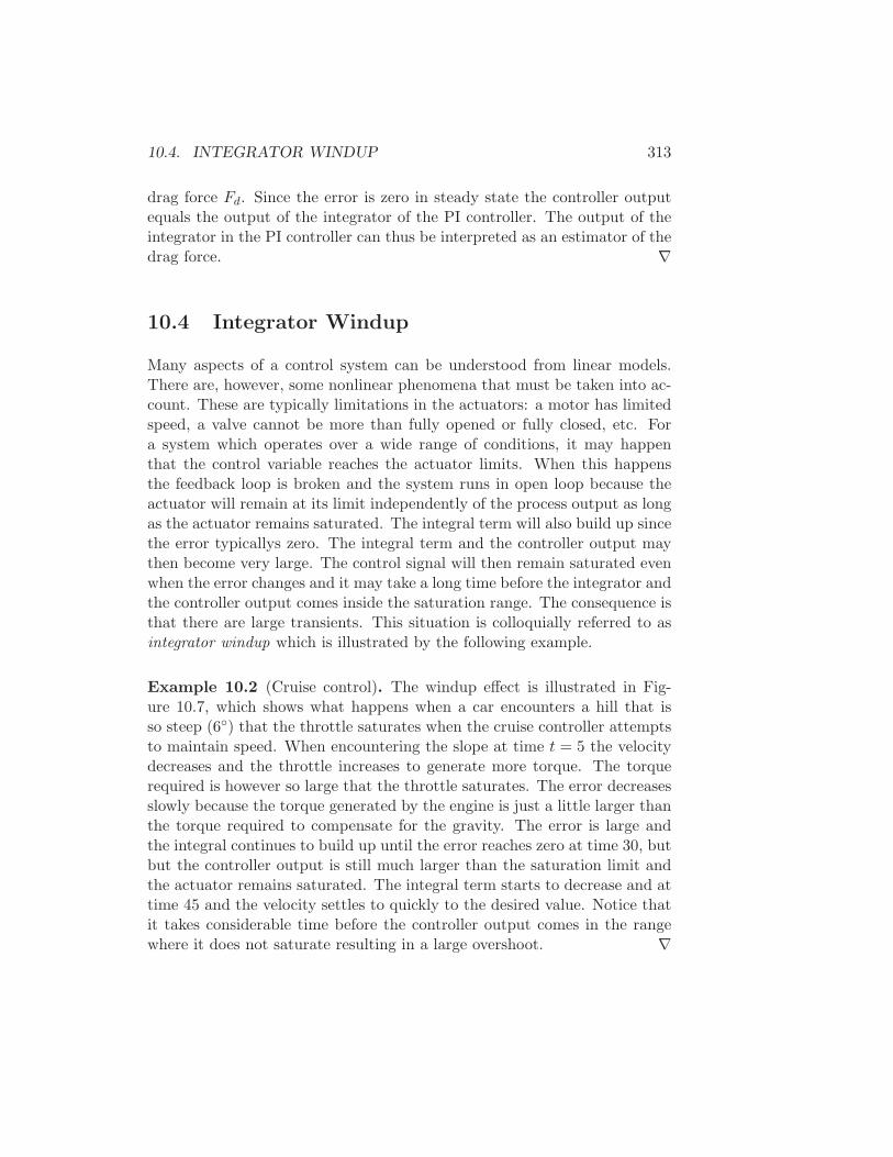
10.4. INTEGRATOR WINDUP 313
drag force Fd. Since the error is zero in steady state the controller outputequals the output of the integrator of the PI controller. The output of theintegrator in the PI controller can thus be interpreted as an estimator of thedrag force. ∇
10.4 Integrator Windup
Many aspects of a control system can be understood from linear models.There are, however, some nonlinear phenomena that must be taken into ac-count. These are typically limitations in the actuators: a motor has limitedspeed, a valve cannot be more than fully opened or fully closed, etc. Fora system which operates over a wide range of conditions, it may happenthat the control variable reaches the actuator limits. When this happensthe feedback loop is broken and the system runs in open loop because theactuator will remain at its limit independently of the process output as longas the actuator remains saturated. The integral term will also build up sincethe error typicallys zero. The integral term and the controller output maythen become very large. The control signal will then remain saturated evenwhen the error changes and it may take a long time before the integrator andthe controller output comes inside the saturation range. The consequence isthat there are large transients. This situation is colloquially referred to asintegrator windup which is illustrated by the following example.
Example 10.2 (Cruise control). The windup effect is illustrated in Fig-ure 10.7, which shows what happens when a car encounters a hill that isso steep (6) that the throttle saturates when the cruise controller attemptsto maintain speed. When encountering the slope at time t = 5 the velocitydecreases and the throttle increases to generate more torque. The torquerequired is however so large that the throttle saturates. The error decreasesslowly because the torque generated by the engine is just a little larger thanthe torque required to compensate for the gravity. The error is large andthe integral continues to build up until the error reaches zero at time 30, butbut the controller output is still much larger than the saturation limit andthe actuator remains saturated. The integral term starts to decrease and attime 45 and the velocity settles to quickly to the desired value. Notice thatit takes considerable time before the controller output comes in the rangewhere it does not saturate resulting in a large overshoot. ∇
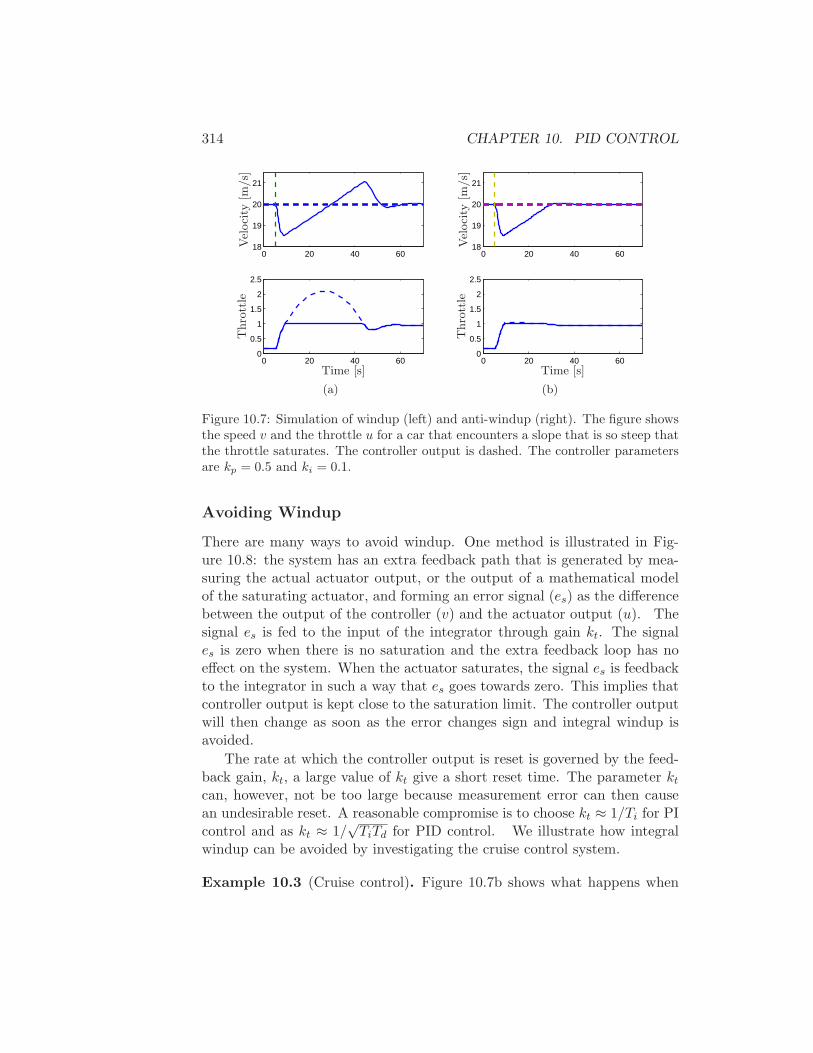
314 CHAPTER 10. PID CONTROL
0 20 40 6018
19
20
21
0 20 40 600
0.5
1
1.5
2
2.5
Vel
oci
ty[m
/s]
Thro
ttle
Time [s]
(a)
0 20 40 6018
19
20
21
0 20 40 600
0.5
1
1.5
2
2.5
Vel
oci
ty[m
/s]
Thro
ttle
Time [s]
(b)
Figure 10.7: Simulation of windup (left) and anti-windup (right). The figure showsthe speed v and the throttle u for a car that encounters a slope that is so steep thatthe throttle saturates. The controller output is dashed. The controller parametersare kp = 0.5 and ki = 0.1.
Avoiding Windup
There are many ways to avoid windup. One method is illustrated in Fig-ure 10.8: the system has an extra feedback path that is generated by mea-suring the actual actuator output, or the output of a mathematical modelof the saturating actuator, and forming an error signal (es) as the differencebetween the output of the controller (v) and the actuator output (u). Thesignal es is fed to the input of the integrator through gain kt. The signales is zero when there is no saturation and the extra feedback loop has noeffect on the system. When the actuator saturates, the signal es is feedbackto the integrator in such a way that es goes towards zero. This implies thatcontroller output is kept close to the saturation limit. The controller outputwill then change as soon as the error changes sign and integral windup isavoided.
The rate at which the controller output is reset is governed by the feed-back gain, kt, a large value of kt give a short reset time. The parameter kt
can, however, not be too large because measurement error can then causean undesirable reset. A reasonable compromise is to choose kt ≈ 1/Ti for PIcontrol and as kt ≈ 1/
√TiTd for PID control. We illustrate how integral
windup can be avoided by investigating the cruise control system.
Example 10.3 (Cruise control). Figure 10.7b shows what happens when
10.5. IMPLEMENTATION 315
− +Σ
Σ
Σ
Actuator
model Actuator
−y
e = ysp − y
ki
kd
1
s
kt
es
k
v u
Figure 10.8: PID controller with anti-windup.
a controller with anti-windup is applied to the system simulated in Fig-ure 10.7a. Because of the feedback from the actuator model the output ofthe integrator is quickly reset to a value such that the controller output isat the saturation limit. The behavior is drastically different from that inFigure 10.7a and the large overshoot is avoided. The tracking gain kt = 2in the simulation. ∇
10.5 Implementation
There are many practical issues that have to be considered when implement-ing PID controllers. They have been developed over time based on practicalexperiences. In this section we consider some of the most common. Similarconsiderations also apply to other types of controllers.
Filtering the Derivative
A drawback with derivative action is that an ideal derivative has very highgain for high frequency signals. This means that high frequency measure-ment noise will generate large variations of the control signal. The effect ofmeasurement noise be reduced by replacing the term kds by
Da = − kds
1 + sTf. (10.13)
This can be interpreted as an ideal derivative that is filtered using a first-order system with the time constant Tf . For small s the transfer function is
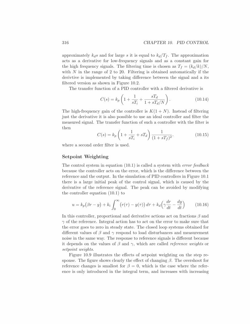
316 CHAPTER 10. PID CONTROL
approximately kds and for large s it is equal to kd/Tf . The approximationacts as a derivative for low-frequency signals and as a constant gain forthe high frequency signals. The filtering time is chosen as Tf = (kd/k)/N ,with N in the range of 2 to 20. Filtering is obtained automatically if thederivtive is implemented by taking difference between the signal and a itsfiltered version as shown in Figure 10.2.
The transfer function of a PID controller with a filtered derivative is
C(s) = kp
(
1 +1
sTi+
sTd
1 + sTd/N
)
. (10.14)
The high-frequency gain of the controller is K(1 + N). Instead of filteringjust the derivative it is also possible to use an ideal controller and filter themeasured signal. The transfer function of such a controller with the filter isthen
C(s) = kp
(
1 +1
sTi+ sTd
)1
(1 + sTf )2. (10.15)
where a second order filter is used.
Setpoint Weighting
The control system in equation (10.1) is called a system with error feedbackbecause the controller acts on the error, which is the difference between thereference and the output. In the simulation of PID controllers in Figure 10.1there is a large initial peak of the control signal, which is caused by thederivative of the reference signal. The peak can be avoided by modifyingthe controller equation (10.1) to
u = kp
(βr − y
)+ ki
∫ ∞
0
(r(τ) − y(τ)
)dτ + kd
(
γdr
dt− dy
dt
)
(10.16)
In this controller, proportional and derivative actions act on fractions β andγ of the reference. Integral action has to act on the error to make sure thatthe error goes to zero in steady state. The closed loop systems obtained fordifferent values of β and γ respond to load disturbances and measurementnoise in the same way. The response to reference signals is different becauseit depends on the values of β and γ, which are called reference weights orsetpoint weights.
Figure 10.9 illustrates the effects of setpoint weighting on the step re-sponse. The figure shows clearly the effect of changing β. The overshoot forreference changes is smallest for β = 0, which is the case where the refer-ence is only introduced in the integral term, and increases with increasing
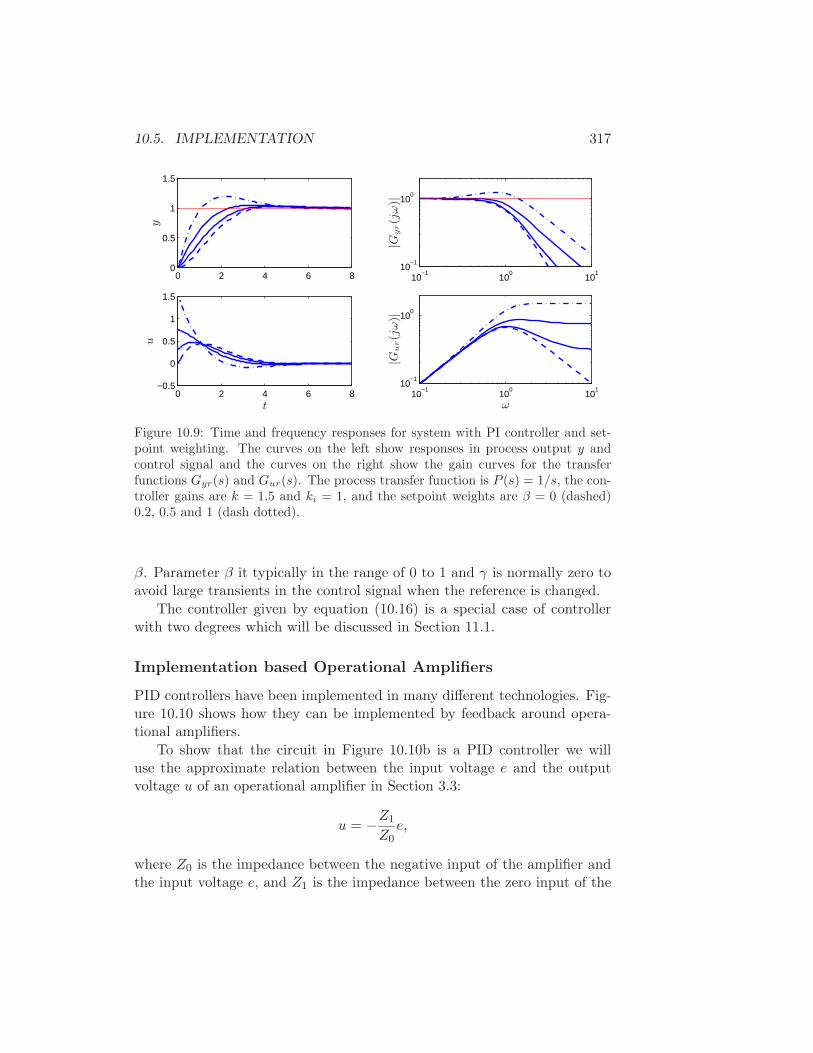
10.5. IMPLEMENTATION 317
0 2 4 6 80
0.5
1
1.5
0 2 4 6 8−0.5
0
0.5
1
1.5
uy
t
10−1
100
101
10−1
100
10−1
100
101
10−1
100
ω|G
yr(j
ω)|
|Gu
r(j
ω)|
Figure 10.9: Time and frequency responses for system with PI controller and set-point weighting. The curves on the left show responses in process output y andcontrol signal and the curves on the right show the gain curves for the transferfunctions Gyr(s) and Gur(s). The process transfer function is P (s) = 1/s, the con-troller gains are k = 1.5 and ki = 1, and the setpoint weights are β = 0 (dashed)0.2, 0.5 and 1 (dash dotted).
β. Parameter β it typically in the range of 0 to 1 and γ is normally zero toavoid large transients in the control signal when the reference is changed.
The controller given by equation (10.16) is a special case of controllerwith two degrees which will be discussed in Section 11.1.
Implementation based Operational Amplifiers
PID controllers have been implemented in many different technologies. Fig-ure 10.10 shows how they can be implemented by feedback around opera-tional amplifiers.
To show that the circuit in Figure 10.10b is a PID controller we willuse the approximate relation between the input voltage e and the outputvoltage u of an operational amplifier in Section 3.3:
u = −Z1
Z0e,
where Z0 is the impedance between the negative input of the amplifier andthe input voltage e, and Z1 is the impedance between the zero input of the

318 CHAPTER 10. PID CONTROL
R0 R1 C1
e
u
R0 R1
C0
C1
e
u
(a) (b)
Figure 10.10: Schematic diagram of an electronic PI (left) and PID controllers(right) based on feedback around an operational amplifier.
amplifier and the output voltage u. The impedances are given by
Z0 =R0
1 +R0C0pZ1 = R1 +
1
C1p,
and we find the following relation between the input voltage e and the outputvoltage u:
u = −Z1
Z0e = −R1
R0
(1 +R0C0p)(1 +R1C1p)
R1C1pe.
This is the input-output relation for a PID controller on the form (10.2)with parameters
kp =R1
R0Ti = R1C1 Td = R0C0.
The corresponding results for a PI controller is obtained by setting C0 = 0.
Computer Implementation
In this section we briefly describe how a PID controller may be implementedusing a computer. The computer typically operates periodically, with sig-nals from the sensors sampled and converted to digital form by the A/Dconverter, the control signal computed and then converted to analog formfor the actuators. The sequence of operation is as follows:
1. Wait for clock interrupt
2. Read input from sensor
3. Compute control signal
4. Send output to the actuator
5. Update controller variables
10.5. IMPLEMENTATION 319
6. Repeat
Notice that an output is sent to the actuators as soon as it is available. Thetime delay is minimized by making the calculations in Step 3 as short aspossible and performing all updates after the output is commanded.
As an illustration we consider the PID controller in Figure 10.8, whichhas a filtered derivative, setpoint weighting and protection against integralwindup. The controller is a continuous time dynamical system. To imple-ment it using a computer, the continuous time system has to be approxi-mated by a discrete time system.
The signal v is the sum of the proportional, integral and derivative terms
v(t) = P (t) + I(t) +D(t) (10.17)
and the controller output is u(t) = sat(v(t)) where sat is the saturationfunction that models the actuator. The proportional term is
P = kp(βysp − y).
This term is implemented simply by replacing the continuous variables withtheir sampled versions. Hence
P (tk) = kp (βyr(tk) − y(tk)) , (10.18)
where tk denotes the sampling instants, i.e., the times when the computerreads its input. The integral term is
I(t) = ki
t∫
0
e(s)ds+1
Tt
(sat(v) − v)
)
and approximating the integral by a sum gives
I(tk+1) = I(tk) + kih e(tk) +h
Tt
(sat(v) − v)
). (10.19)
The derivative term D is given by the differential equation
TfdD
dt+D = −kdy.
Approximating this equation with a backward difference we find
TfD(tk) −D(tk−1)
h+D(tk) = −kd
y(tk) − y(tk−1)
h,
320 CHAPTER 10. PID CONTROL
which can be rewritten as
D(tk) =Tf
Tf + hD(tk−1) −
kd
Tf + h(y(tk) − y(tk−1)) . (10.20)
The advantage of using a backward difference is that the parameter Tf/(Tf +h) is nonnegative and less than one for all h > 0, which guarantees that thedifference equation is stable.
Reorganizing equations (10.17)–(10.20), the PID controller can be de-scribed by the following pseudo code:
% Precompute controller coefficients
bi=ki*h
ad=Tf/(Tf+h)
bd=kd/(Tf+h)
br=h/Tt
% Control algorithm - main loop
while (running)
r=adin(ch1) % read setpoint from ch1
y=adin(ch2) % read process variable from ch2
P=kp*(b*r-y) % compute proportional part
D=ad*D-bd*(y-yold) % update derivative part
v=P+I+D % compute temporary output
u=sat(v,ulow,uhigh) % simulate actuator saturation
daout(ch1) % set analog output ch1
I=I+bi*(r-y)+br*(u-v) % update integral
yold=y % update old process output
sleep(h) % wait until next update interval
Precomputation of the coefficients bi, ad, bd and br saves computer timein the main loop. These calculations have to be done only when controllerparameters are changed. The main loop is executed once every samplingperiod. The program has three states: yold, I, and D. One state variablecan be eliminated at the cost of a less readable code. Notice that the codeincludes computing the derivative of the process output, proportional actionon a portion of the error (b 6= 1), and modeling of the actuator saturationin the integral computation to give protection against windup.
10.6 Further Reading
The history of PID control is a very rich one and stretches back to thebeginning of the foundation of control theory. A very readable treatment is
10.7. EXERCISES 321
given by Mindel [Min02]. A comprehensive presentation of PID control isgiven in [AH95].
10.7 Exercises
1. Consider a second order process with transfer function
P (s) =b
s2 + a1s+ a2.
Find the gains for a PID controller that gives the closed loop systema characteristic polynomial of the form
s2 + 2ζω0s+ ω20.
2. (Vehicle steering) Design a proportion-integral controller for the vehi-cle steering system that gives closed loop characteristic equation
s3 + 2ω0s2 + 2ω0s+ ω3
0.

322 CHAPTER 10. PID CONTROL
Chapter 11
Loop Shaping
Quotation
Authors, citation.
In this chapter we continue to explore the use of frequency domain tech-niques for design of feedback systems. We begin with a more thoroughdescription of the performance specifications for control systems, and thenintroduce the concept of “loop shaping” as a mechanism for designing con-trollers in the frequency domain. We also introduce some fundamental lim-itations to performance for systems with right half plane poles and zeros.
11.1 A Basic Feedback Loop
In the previous chapter, we considered the use of PID feedback as a mecha-nism for designing a feedback controller for a given process. In this chapterwe will expand our approach to include a richer repertoire of tools for shap-ing the frequency response of the closed loop system.
One of the key ideas in this chapter is that we can design the behaviorof the closed loop system by studying the open loop transfer function. Thissame approach was used in studying stability using the Nyquist criterion:we plotted the Nyquist plot for the open loop transfer function to determinethe stability of the closed loop system. From a design perspective, the useof loop analysis tools is very powerful: since the loop transfer function isL = PC, if we can specify the desired performance in terms of propertiesof L, we can directly see the impact of changes in the controller C. This ismuch easier, for example, than trying to reason directly about the response
323
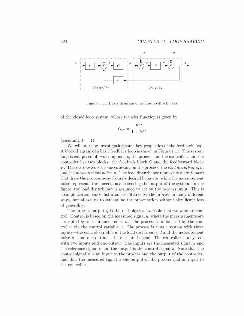
324 CHAPTER 11. LOOP SHAPING
F C P
−1
Σ Σ Σr e u ν
d
η
n
y
Controller Process
Figure 11.1: Block diagram of a basic feedback loop.
of the closed loop system, whose transfer function is given by
Gyr =PC
1 + PC
(assuming F = 1).
We will start by investigating some key properties of the feedback loop.A block diagram of a basic feedback loop is shown in Figure 11.1. The systemloop is composed of two components, the process and the controller, and thecontroller has two blocks: the feedback block C and the feedforward blockF . There are two disturbances acting on the process, the load disturbance, d,and the measurement noise, n. The load disturbance represents disturbancesthat drive the process away from its desired behavior, while the measurementnoise represents the uncertainty in sensing the output of the system. In thefigure, the load disturbance is assumed to act on the process input. This isa simplification, since disturbances often enter the process in many differentways, but allows us to streamline the presentation without significant lossof generality.
The process output η is the real physical variable that we want to con-trol. Control is based on the measured signal y, where the measurements arecorrupted by measurement noise n. The process is influenced by the con-troller via the control variable u. The process is thus a system with threeinputs—the control variable u, the load disturbance d and the measurementnoise n—and one output—the measured signal. The controller is a systemwith two inputs and one output. The inputs are the measured signal y andthe reference signal r and the output is the control signal u. Note that thecontrol signal u is an input to the process and the output of the controller,and that the measured signal is the output of the process and an input tothe controller.
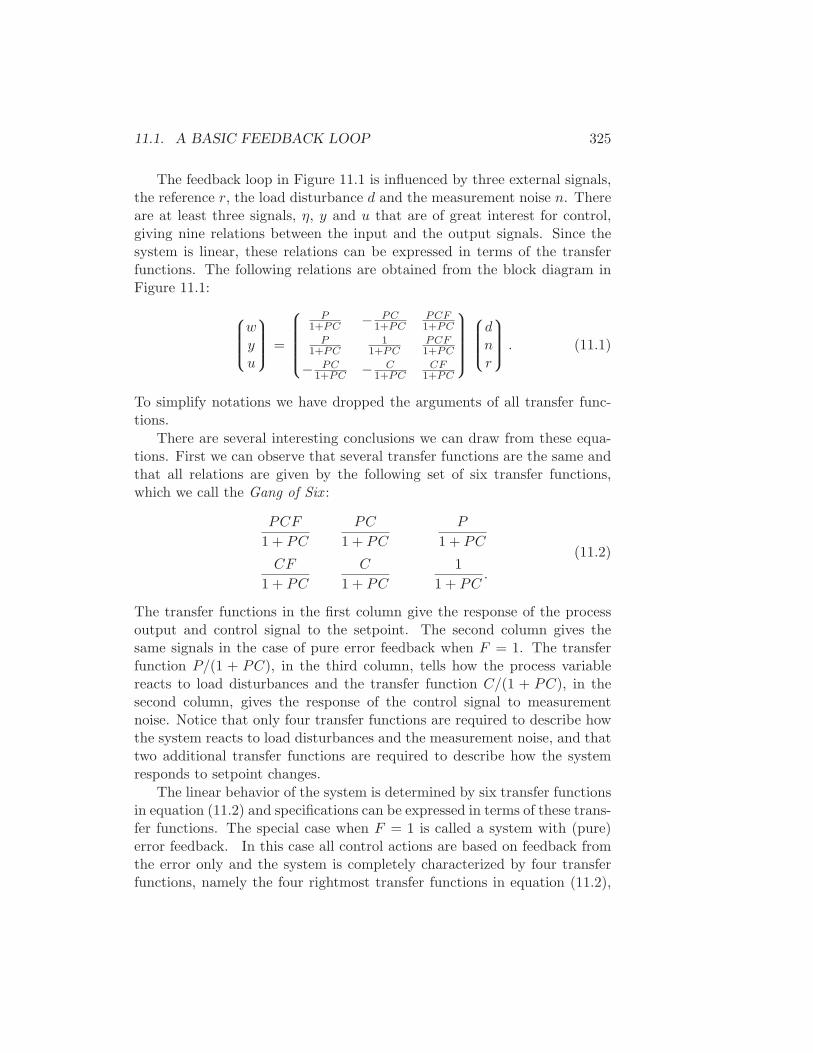
11.1. A BASIC FEEDBACK LOOP 325
The feedback loop in Figure 11.1 is influenced by three external signals,the reference r, the load disturbance d and the measurement noise n. Thereare at least three signals, η, y and u that are of great interest for control,giving nine relations between the input and the output signals. Since thesystem is linear, these relations can be expressed in terms of the transferfunctions. The following relations are obtained from the block diagram inFigure 11.1:
wyu
=
P1+PC − PC
1+PCPCF1+PC
P1+PC
11+PC
PCF1+PC
− PC1+PC − C
1+PCCF
1+PC
dnr
. (11.1)
To simplify notations we have dropped the arguments of all transfer func-tions.
There are several interesting conclusions we can draw from these equa-tions. First we can observe that several transfer functions are the same andthat all relations are given by the following set of six transfer functions,which we call the Gang of Six :
PCF
1 + PC
PC
1 + PC
P
1 + PC
CF
1 + PC
C
1 + PC
1
1 + PC.
(11.2)
The transfer functions in the first column give the response of the processoutput and control signal to the setpoint. The second column gives thesame signals in the case of pure error feedback when F = 1. The transferfunction P/(1 + PC), in the third column, tells how the process variablereacts to load disturbances and the transfer function C/(1 + PC), in thesecond column, gives the response of the control signal to measurementnoise. Notice that only four transfer functions are required to describe howthe system reacts to load disturbances and the measurement noise, and thattwo additional transfer functions are required to describe how the systemresponds to setpoint changes.
The linear behavior of the system is determined by six transfer functionsin equation (11.2) and specifications can be expressed in terms of these trans-fer functions. The special case when F = 1 is called a system with (pure)error feedback. In this case all control actions are based on feedback fromthe error only and the system is completely characterized by four transferfunctions, namely the four rightmost transfer functions in equation (11.2),
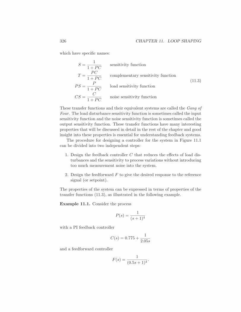
326 CHAPTER 11. LOOP SHAPING
which have specific names:
S =1
1 + PCsensitivity function
T =PC
1 + PCcomplementary sensitivity function
PS =P
1 + PCload sensitivity function
CS =C
1 + PCnoise sensitivity function
(11.3)
These transfer functions and their equivalent systems are called the Gang ofFour. The load disturbance sensitivity function is sometimes called the inputsensitivity function and the noise sensitivity function is sometimes called theoutput sensitivity function. These transfer functions have many interestingproperties that will be discussed in detail in the rest of the chapter and goodinsight into these properties is essential for understanding feedback systems.
The procedure for designing a controller for the system in Figure 11.1can be divided into two independent steps:
1. Design the feedback controller C that reduces the effects of load dis-turbances and the sensitivity to process variations without introducingtoo much measurement noise into the system.
2. Design the feedforward F to give the desired response to the referencesignal (or setpoint).
The properties of the system can be expressed in terms of properties of thetransfer functions (11.3), as illustrated in the following example.
Example 11.1. Consider the process
P (s) =1
(s+ 1)4
with a PI feedback controller
C(s) = 0.775 +1
2.05s
and a feedforward controller
F (s) =1
(0.5s+ 1)4.
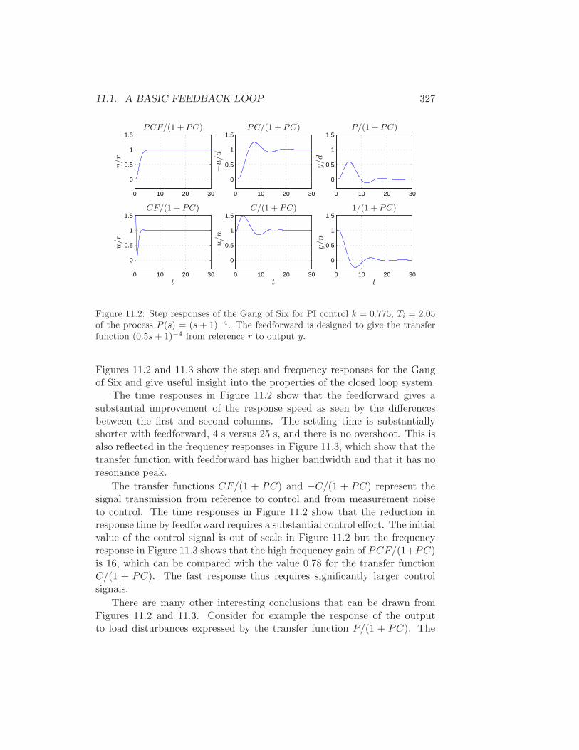
11.1. A BASIC FEEDBACK LOOP 327
0 10 20 30
0
0.5
1
1.5
0 10 20 30
0
0.5
1
1.5
0 10 20 30
0
0.5
1
1.5
0 10 20 30
0
0.5
1
1.5
0 10 20 30
0
0.5
1
1.5
0 10 20 30
0
0.5
1
1.5
PCF/(1 + PC) PC/(1 + PC)
C/(1 + PC)
P/(1 + PC)
CF/(1 + PC) 1/(1 + PC)
η/r
−u/d
y/d
u/r
−u/n
y/n
ttt
Figure 11.2: Step responses of the Gang of Six for PI control k = 0.775, Ti = 2.05of the process P (s) = (s + 1)−4. The feedforward is designed to give the transferfunction (0.5s+ 1)−4 from reference r to output y.
Figures 11.2 and 11.3 show the step and frequency responses for the Gangof Six and give useful insight into the properties of the closed loop system.
The time responses in Figure 11.2 show that the feedforward gives asubstantial improvement of the response speed as seen by the differencesbetween the first and second columns. The settling time is substantiallyshorter with feedforward, 4 s versus 25 s, and there is no overshoot. This isalso reflected in the frequency responses in Figure 11.3, which show that thetransfer function with feedforward has higher bandwidth and that it has noresonance peak.
The transfer functions CF/(1 + PC) and −C/(1 + PC) represent thesignal transmission from reference to control and from measurement noiseto control. The time responses in Figure 11.2 show that the reduction inresponse time by feedforward requires a substantial control effort. The initialvalue of the control signal is out of scale in Figure 11.2 but the frequencyresponse in Figure 11.3 shows that the high frequency gain of PCF/(1+PC)is 16, which can be compared with the value 0.78 for the transfer functionC/(1 + PC). The fast response thus requires significantly larger controlsignals.
There are many other interesting conclusions that can be drawn fromFigures 11.2 and 11.3. Consider for example the response of the outputto load disturbances expressed by the transfer function P/(1 + PC). The
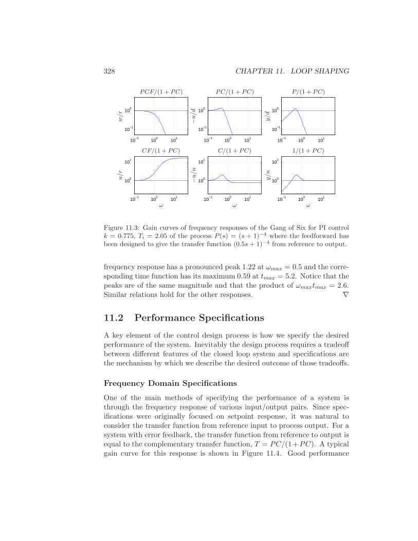
328 CHAPTER 11. LOOP SHAPING
10−1
100
101
10−1
100
10−1
100
101
10−1
100
10−1
100
101
10−1
100
10−1
100
101
100
101
10−1
100
101
100
101
10−1
100
101
100
101
PCF/(1 + PC) PC/(1 + PC)
C/(1 + PC)
P/(1 + PC)
CF/(1 + PC) 1/(1 + PC)
w/r
−u/d
y/d
u/r
−u/n
y/n
ωωω
Figure 11.3: Gain curves of frequency responses of the Gang of Six for PI controlk = 0.775, Ti = 2.05 of the process P (s) = (s + 1)−4 where the feedforward hasbeen designed to give the transfer function (0.5s+ 1)−4 from reference to output.
frequency response has a pronounced peak 1.22 at ωmax = 0.5 and the corre-sponding time function has its maximum 0.59 at tmax = 5.2. Notice that thepeaks are of the same magnitude and that the product of ωmaxtmax = 2.6.Similar relations hold for the other responses. ∇
11.2 Performance Specifications
A key element of the control design process is how we specify the desiredperformance of the system. Inevitably the design process requires a tradeoffbetween different features of the closed loop system and specifications arethe mechanism by which we describe the desired outcome of those tradeoffs.
Frequency Domain Specifications
One of the main methods of specifying the performance of a system isthrough the frequency response of various input/output pairs. Since spec-ifications were originally focused on setpoint response, it was natural toconsider the transfer function from reference input to process output. For asystem with error feedback, the transfer function from reference to output isequal to the complementary transfer function, T = PC/(1+PC). A typicalgain curve for this response is shown in Figure 11.4. Good performance
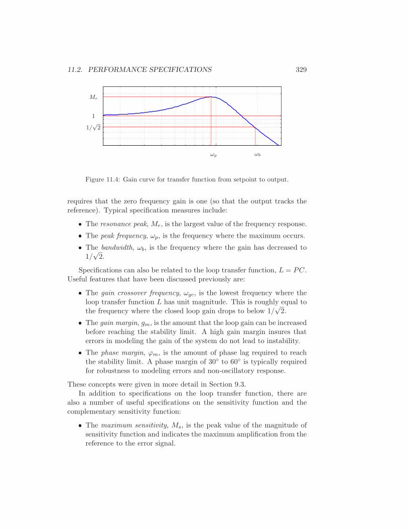
11.2. PERFORMANCE SPECIFICATIONS 329
ωp ωb
Mr
1
1/√
2
Figure 11.4: Gain curve for transfer function from setpoint to output.
requires that the zero frequency gain is one (so that the output tracks thereference). Typical specification measures include: The resonance peak, Mr, is the largest value of the frequency response. The peak frequency, ωp, is the frequency where the maximum occurs. The bandwidth, ωb, is the frequency where the gain has decreased to
1/√
2.
Specifications can also be related to the loop transfer function, L = PC.Useful features that have been discussed previously are: The gain crossover frequency, ωgc, is the lowest frequency where the
loop transfer function L has unit magnitude. This is roughly equal tothe frequency where the closed loop gain drops to below 1/
√2. The gain margin, gm, is the amount that the loop gain can be increased
before reaching the stability limit. A high gain margin insures thaterrors in modeling the gain of the system do not lead to instability. The phase margin, ϕm, is the amount of phase lag required to reachthe stability limit. A phase margin of 30 to 60 is typically requiredfor robustness to modeling errors and non-oscillatory response.
These concepts were given in more detail in Section 9.3.In addition to specifications on the loop transfer function, there are
also a number of useful specifications on the sensitivity function and thecomplementary sensitivity function: The maximum sensitivity, Ms, is the peak value of the magnitude of
sensitivity function and indicates the maximum amplification from thereference to the error signal.
330 CHAPTER 11. LOOP SHAPING The maximum sensitivity frequency, ωms, is the frequency where thesensitivity function has its maximum. The sensitivity crossover frequency, ωsc, is the frequency where thesensitivity function becomes greater than 1 for the first time. Dis-turbances are attenuated below this frequency and can be amplifiedabove this frequency. The maximum complementary sensitivity, Mt, is the peak value of themagnitude of the complementary sensitivity function. It provides themaximum amplification from the reference signal to the output signal. The maximum complementary sensitivity frequency, ωmt, is the fre-quency where the complementary sensitivity function has its maxi-mum.
As we will see in the rest of the chapter, these various measures can be usedto gain insights into the performance of the closed loop system and are oftenused to specify the desired performance for a control design.
Although we have defined different specifications for the loop transferfunction L, the sensitivity function S and the complementary sensitivityfunction T , these transfer functions are all related through a set of algebraicrelationships:
S =1
1 + LT =
L
1 + LS + T = 1.
These relationships can limit the ability to independently satisfy specifica-tions for the quantities listed above and may require tradeoffs, as we shallsee.
Relations between Time and Frequency Domain Features
In Section 5.3 we described some of the typical parameters that describedthe step response of a system. These included the rise time, steady stateerror, and overshoot. For many applications, it is natural to provide thesetime domain specifications and we can relate these to the eigenvalues of theclosed loop system, which are equivalent to the poles of the transfer functionT = PC/(1 + PC).
There are approximate relations between specifications in the time andfrequency domain. Let G(s) be the transfer function from reference to out-put. In the time domain the response speed can be characterized by the risetime Tr and the settling time Ts. In the frequency domain the response time
11.2. PERFORMANCE SPECIFICATIONS 331
can be characterized by the closed loop bandwidth ωb, the gain crossoverfrequency ωgc, the sensitivity frequency ωms. The product of bandwidth andrise time is approximately constant Trωb ≈ 2, so decreasing the rise timecorresponds to increasing the closed loop bandwidth.
The overshoot of the step response Mp is related to the resonant peak Mr
of the frequency response in the sense that a larger peak normally impliesa larger overshoot. Unfortunately there is no simple relation because theovershoot also depends on how quickly the frequency response decays. ForMr < 1.2 the overshoot Mp in the step response is often close to Mr − 1.For larger values of Mr the overshoot is typically less than Mr − 1. Theserelations do not hold for all systems: there are systems with Mr = 1 thathave a positive overshoot. These systems have transfer functions that decayrapidly around the bandwidth. To avoid overshoot in systems with errorfeedback it is advisable to require that the maximum of the complementarysensitivity function is small, say Mt = 1.1 − 1.2.
Response to Load Disturbances
The sensitivity function in equation (11.3) shows how feedback influencesdisturbances. Disturbances with frequencies that are lower than the sen-sitivity crossover frequency ωsc are attenuated by feedback and those withω > ωsc are amplified by feedback. The largest amplification is the maxi-mum sensitivity Ms.
Consider the system in Figure 11.1. The transfer function from loaddisturbance d to process output w is
Gwd =P
1 + PC= PS =
T
C. (11.4)
Since load disturbances typically have low frequencies, it is natural that thecriterion emphasizes the behavior of the transfer function at low frequen-cies. Filtering of the measurement signal has only marginal effect on theattenuation of load disturbances because the filter typically only attenuateshigh frequencies. For a system with P (0) 6= 0 and a controller with integralaction, the controller gain goes to infinity for small frequencies and we havethe following approximation for small s:
Gwd =T
C≈ 1
C≈ s
ki. (11.5)
Figure 11.5 gives the gain curve for a typical case and shows that the ap-proximation is very good for low frequencies.
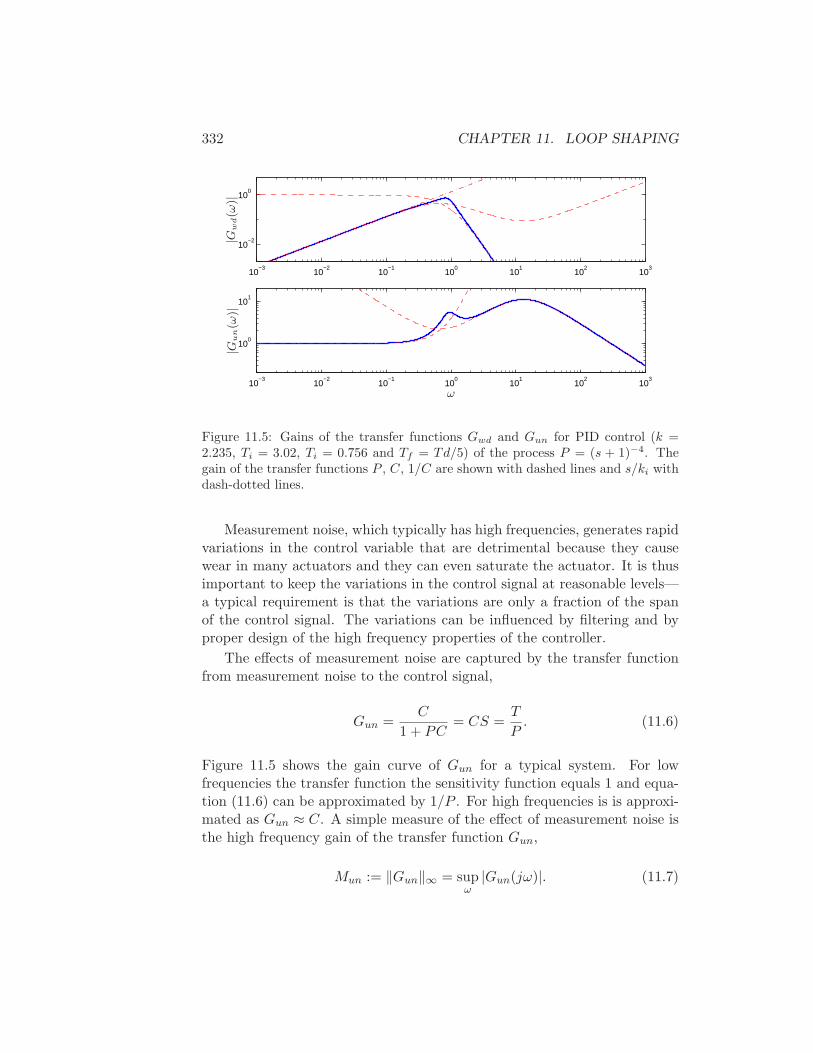
332 CHAPTER 11. LOOP SHAPING
10−3
10−2
10−1
100
101
102
103
10−2
100
10−3
10−2
10−1
100
101
102
103
100
101
ω
|Gw
d(ω
)||G
un(ω
)|
Figure 11.5: Gains of the transfer functions Gwd and Gun for PID control (k =2.235, Ti = 3.02, Ti = 0.756 and Tf = Td/5) of the process P = (s + 1)−4. Thegain of the transfer functions P , C, 1/C are shown with dashed lines and s/ki withdash-dotted lines.
Measurement noise, which typically has high frequencies, generates rapidvariations in the control variable that are detrimental because they causewear in many actuators and they can even saturate the actuator. It is thusimportant to keep the variations in the control signal at reasonable levels—a typical requirement is that the variations are only a fraction of the spanof the control signal. The variations can be influenced by filtering and byproper design of the high frequency properties of the controller.
The effects of measurement noise are captured by the transfer functionfrom measurement noise to the control signal,
Gun =C
1 + PC= CS =
T
P. (11.6)
Figure 11.5 shows the gain curve of Gun for a typical system. For lowfrequencies the transfer function the sensitivity function equals 1 and equa-tion (11.6) can be approximated by 1/P . For high frequencies is is approxi-mated as Gun ≈ C. A simple measure of the effect of measurement noise isthe high frequency gain of the transfer function Gun,
Mun := ‖Gun‖∞ = supω
|Gun(jω)|. (11.7)
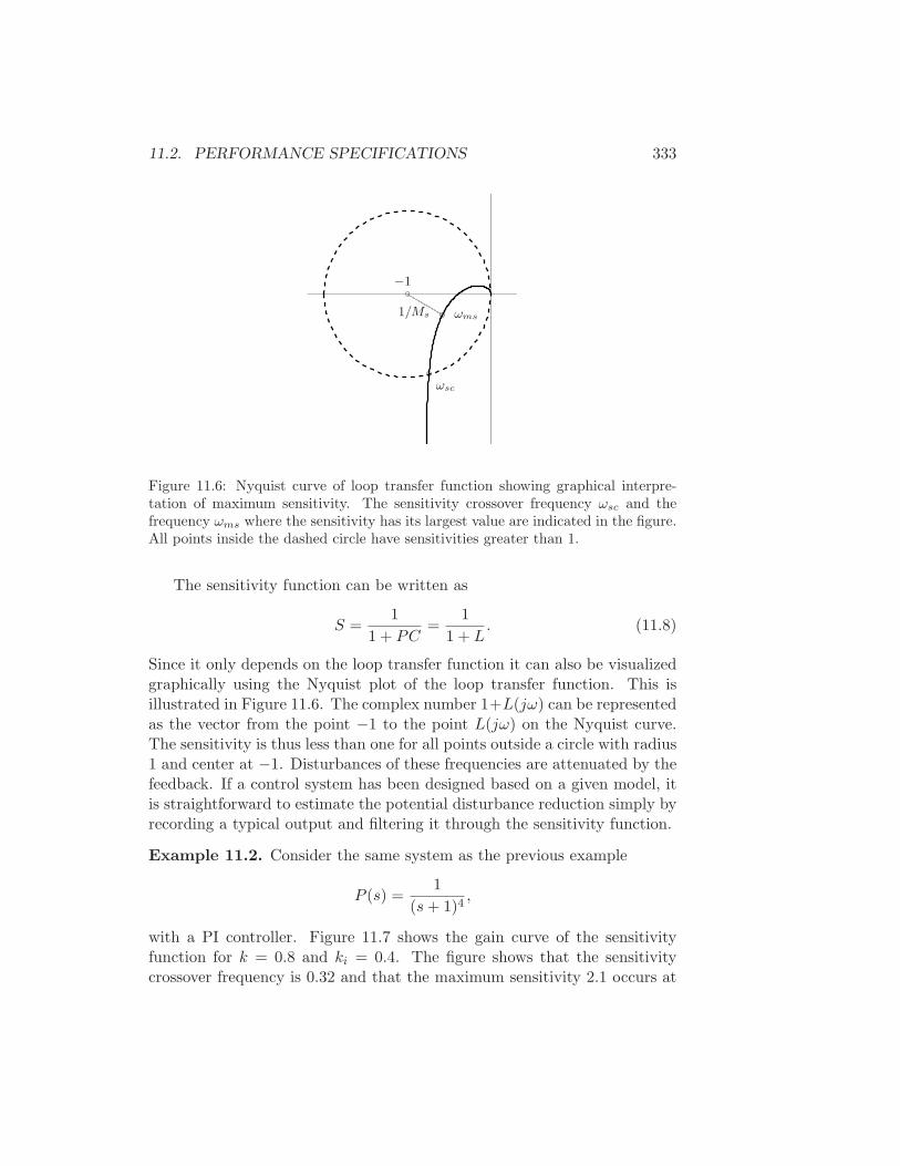
11.2. PERFORMANCE SPECIFICATIONS 333
1/Ms ωms
ωsc
−1
Figure 11.6: Nyquist curve of loop transfer function showing graphical interpre-tation of maximum sensitivity. The sensitivity crossover frequency ωsc and thefrequency ωms where the sensitivity has its largest value are indicated in the figure.All points inside the dashed circle have sensitivities greater than 1.
The sensitivity function can be written as
S =1
1 + PC=
1
1 + L. (11.8)
Since it only depends on the loop transfer function it can also be visualizedgraphically using the Nyquist plot of the loop transfer function. This isillustrated in Figure 11.6. The complex number 1+L(jω) can be representedas the vector from the point −1 to the point L(jω) on the Nyquist curve.The sensitivity is thus less than one for all points outside a circle with radius1 and center at −1. Disturbances of these frequencies are attenuated by thefeedback. If a control system has been designed based on a given model, itis straightforward to estimate the potential disturbance reduction simply byrecording a typical output and filtering it through the sensitivity function.
Example 11.2. Consider the same system as the previous example
P (s) =1
(s+ 1)4,
with a PI controller. Figure 11.7 shows the gain curve of the sensitivityfunction for k = 0.8 and ki = 0.4. The figure shows that the sensitivitycrossover frequency is 0.32 and that the maximum sensitivity 2.1 occurs at

334 CHAPTER 11. LOOP SHAPING
10−2
10−1
100
101
10−2
10−1
100
101
ω
|S(jω)|
Figure 11.7: Gain curve of the sensitivity function for PI control (k = 0.8, ki = 0.4)of process with the transfer function P (s) = (s + 1)−4. The sensitivity crossoverfrequency is indicated by + and the maximum sensitivity by o.
ωms = 0.56. Feedback will thus reduce disturbances with frequencies lessthan 0.32 rad/s, but it will amplify disturbances with higher frequencies.The largest amplification is 2.1. ∇
11.3 Feedback Design via Loop Shaping
One advantage the the Nyquist stability theorem is that it is based on theloop transfer function, which is related to the controller transfer functionthrough L = PC. It is thus easy to see how the controller influences theloop transfer function. To make an unstable system stable we simply haveto bend the Nyquist curve away from the critical point.
This simple idea is the basis of several different design methods, collec-tively called loop shaping. The methods are based on the idea of choosing acompensator that gives a loop transfer function with a desired shape. Onepossibility is to start with the loop transfer function of the process and mod-ify it by changing the gain and adding poles and zeros to the controller untilthe desired shape is obtained.
Design Considerations
We will first discuss suitable forms of a loop transfer function that givegood performance and good stability margins. Good robustness requiresgood gain and phase margins. This imposes requirements on the loop trans-fer function around the crossover frequencies ωpc and ωgc. The gain of Lat low frequencies must be large in order to have good tracking of com-mand signals and good rejection of low frequency disturbances. This can be
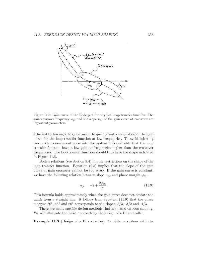
11.3. FEEDBACK DESIGN VIA LOOP SHAPING 335
Figure 11.8: Gain curve of the Bode plot for a typical loop transfer function. Thegain crossover frequency ωgc and the slope ngc of the gain curve at crossover areimportant parameters.
achieved by having a large crossover frequency and a steep slope of the gaincurve for the loop transfer function at low frequencies. To avoid injectingtoo much measurement noise into the system it is desirable that the looptransfer function have a low gain at frequencies higher than the crossoverfrequencies. The loop transfer function should thus have the shape indicatedin Figure 11.8.
Bode’s relations (see Section 9.4) impose restrictions on the shape of theloop transfer function. Equation (9.5) implies that the slope of the gaincurve at gain crossover cannot be too steep. If the gain curve is constant,we have the following relation between slope ngc and phase margin ϕm:
ngc = −2 +2ϕm
π. (11.9)
This formula holds approximately when the gain curve does not deviate toomuch from a straight line. It follows from equation (11.9) that the phasemargins 30, 45 and 60 corresponds to the slopes -5/3, -3/2 and -4/3.
There are many specific design methods that are based on loop shaping.We will illustrate the basic approach by the design of a PI controller.
Example 11.3 (Design of a PI controller). Consider a system with the
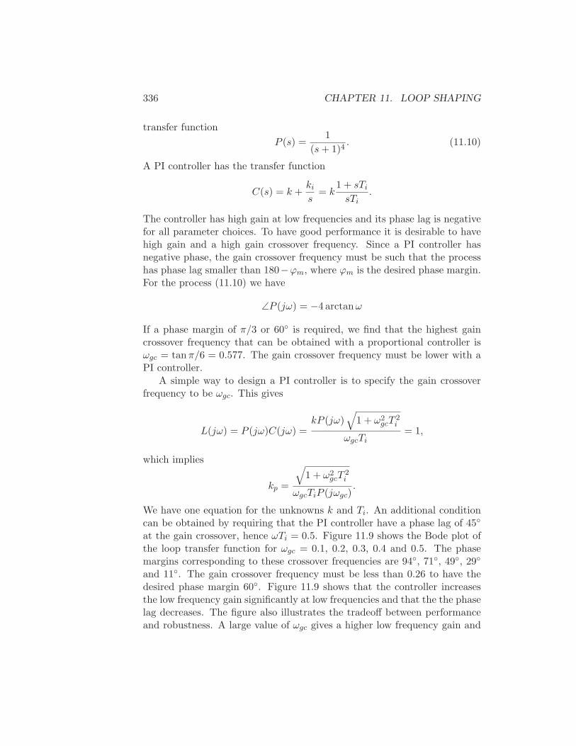
336 CHAPTER 11. LOOP SHAPING
transfer function
P (s) =1
(s+ 1)4. (11.10)
A PI controller has the transfer function
C(s) = k +ki
s= k
1 + sTi
sTi.
The controller has high gain at low frequencies and its phase lag is negativefor all parameter choices. To have good performance it is desirable to havehigh gain and a high gain crossover frequency. Since a PI controller hasnegative phase, the gain crossover frequency must be such that the processhas phase lag smaller than 180−ϕm, where ϕm is the desired phase margin.For the process (11.10) we have
∠P (jω) = −4 arctanω
If a phase margin of π/3 or 60 is required, we find that the highest gaincrossover frequency that can be obtained with a proportional controller isωgc = tanπ/6 = 0.577. The gain crossover frequency must be lower with aPI controller.
A simple way to design a PI controller is to specify the gain crossoverfrequency to be ωgc. This gives
L(jω) = P (jω)C(jω) =kP (jω)
√
1 + ω2gcT
2i
ωgcTi= 1,
which implies
kp =
√
1 + ω2gcT
2i
ωgcTiP (jωgc).
We have one equation for the unknowns k and Ti. An additional conditioncan be obtained by requiring that the PI controller have a phase lag of 45
at the gain crossover, hence ωTi = 0.5. Figure 11.9 shows the Bode plot ofthe loop transfer function for ωgc = 0.1, 0.2, 0.3, 0.4 and 0.5. The phasemargins corresponding to these crossover frequencies are 94, 71, 49, 29
and 11. The gain crossover frequency must be less than 0.26 to have thedesired phase margin 60. Figure 11.9 shows that the controller increasesthe low frequency gain significantly at low frequencies and that the the phaselag decreases. The figure also illustrates the tradeoff between performanceand robustness. A large value of ωgc gives a higher low frequency gain and
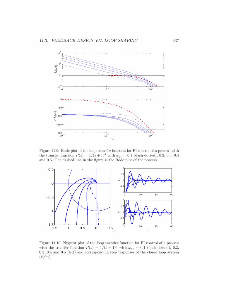
11.3. FEEDBACK DESIGN VIA LOOP SHAPING 337
10−2
10−1
100
10−1
100
101
102
10−2
10−1
100
−200
−150
−100
−50
0
|L(ω
)|∠
L(ω
)
ω
Figure 11.9: Bode plot of the loop transfer function for PI control of a process withthe transfer function P (s) = 1/(s+ 1)4 with ωgc = 0.1 (dash-dotted), 0.2, 0.3, 0.4and 0.5. The dashed line in the figure is the Bode plot of the process.
−1.5 −1 −0.5 0 0.5−1.5
−1
−0.5
0
0.5
,
0 20 40 600
0.5
1
1.5
2
y
0 20 40 600
0.5
1
1.5
2
t
u
Figure 11.10: Nyquist plot of the loop transfer function for PI control of a processwith the transfer function P (s) = 1/(s + 1)4 with ωgc = 0.1 (dash-dotted), 0.2,0.3, 0.4 and 0.5 (left) and corresponding step responses of the closed loop system(right).
338 CHAPTER 11. LOOP SHAPING
a lower phase margin. Figure 11.10 shows the Nyquist plots of the looptransfer functions and the step responses of the closed loop system. Theresponses to command signals show that the designs with large ωgc are toooscillatory. A reasonable compromise between robustness and performanceis to choose ωgc in the range 0.2 to 0.3. For ωgc = 0.25, the controllerparameters are k = 0.50 and Ti = 2.0. Notice that the Nyquist plot of theloop transfer function is bent towards the left for low frequencies. This isan indication that integral action is too weak. Notice in Figure 11.10 thatthe corresponding step responses are also very sluggish. ∇
Lead Compensation
A common problem in design of feedback systems is that the phase lag ofthe system at the desired crossover frequency is not high enough to alloweither proportional or integral feedback to be used effectively. Instead, onemay have a situation where you need to add phase lead to the system, sothat the crossover frequency can be increased.
A standard way to accomplish this is to use a lead compensator, whichhas the form
C(s) = ks+ a
s+ ba < b. (11.11)
The transfer function corresponding to this controller is shown in Figure 11.11.A key feature of the lead compensator is that it adds phase lead in the fre-quency range between the pole/zero pair (and extending approximately 10Xin frequency in each direction). By appropriately choosing the location ofthis phase lead, we can provide additional phase margin at the gain crossoverfrequency.
Because the phase of a transfer function is related to the slope of themagnitude, increasing the phase requires increasing the gain of the looptransfer function over the frequency range in which the lead compensationis applied. Hence we can also think of the lead compensator as changing theslope of the transfer function and thus shaping the loop transfer function inthe crossover region (although it can be applied elsewhere as well).
Example 11.4 (Pitch control for a ducted fan). Consider the control of thepitch (angle) of a vertically oriented ducted fan, as shown in Figure 11.12.We model the system with a second order transfer function of the form
P =r
Js2 + ds+mgl,
with the parameters given in Table 11.1. We take as our performance
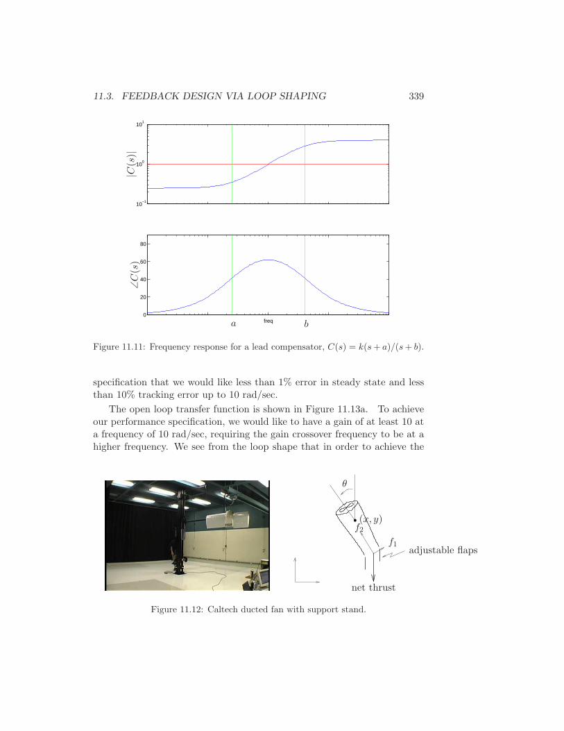
11.3. FEEDBACK DESIGN VIA LOOP SHAPING 339
10−1
100
101
0
20
40
60
80
freq
|C(s
)|∠C
(s)
a b
Figure 11.11: Frequency response for a lead compensator, C(s) = k(s+ a)/(s+ b).
specification that we would like less than 1% error in steady state and lessthan 10% tracking error up to 10 rad/sec.
The open loop transfer function is shown in Figure 11.13a. To achieveour performance specification, we would like to have a gain of at least 10 ata frequency of 10 rad/sec, requiring the gain crossover frequency to be at ahigher frequency. We see from the loop shape that in order to achieve the
adjustable flaps
net thrust
(x, y)
θ
f2
f1
Figure 11.12: Caltech ducted fan with support stand.
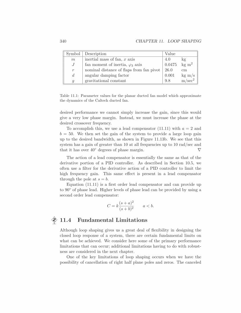
340 CHAPTER 11. LOOP SHAPING
Symbol Description Value
m inertial mass of fan, x axis 4.0 kgJ fan moment of inertia, ϕ3 axis 0.0475 kg m2
r nominal distance of flaps from fan pivot 26.0 cmd angular damping factor 0.001 kg m/sg gravitational constant 9.8 m/sec2
Table 11.1: Parameter values for the planar ducted fan model which approximatethe dynamics of the Caltech ducted fan.
desired performance we cannot simply increase the gain, since this wouldgive a very low phase margin. Instead, we must increase the phase at thedesired crossover frequency.
To accomplish this, we use a lead compensator (11.11) with a = 2 andb = 50. We then set the gain of the system to provide a large loop gainup to the desired bandwidth, as shown in Figure 11.13b. We see that thissystem has a gain of greater than 10 at all frequencies up to 10 rad/sec andthat it has over 40 degrees of phase margin. ∇
The action of a lead compensator is essentially the same as that of thederivative portion of a PID controller. As described in Section 10.5, weoften use a filter for the derivative action of a PID controller to limit thehigh frequency gain. This same effect is present in a lead compensatorthrough the pole at s = b.
Equation (11.11) is a first order lead compensator and can provide upto 90 of phase lead. Higher levels of phase lead can be provided by using asecond order lead compensator:
C = k(s+ a)2
(s+ b)2a < b.
11.4 Fundamental Limitations
Although loop shaping gives us a great deal of flexibility in designing theclosed loop response of a system, there are certain fundamental limits onwhat can be achieved. We consider here some of the primary performancelimitations that can occur; additional limitations having to do with robust-ness are considered in the next chapter.
One of the key limitations of loop shaping occurs when we have thepossibility of cancellation of right half plane poles and zeros. The canceled
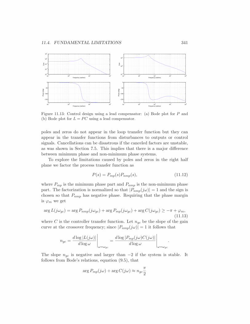
11.4. FUNDAMENTAL LIMITATIONS 341
10−1
100
101
102
10−3
10−2
10−1
100
101
Gai
n
Frequency (rad/sec)
10−1
100
101
102
−150
−100
−50
0
Pha
se (
deg)
Frequency (rad/sec)
10−1
100
101
102
103
10−2
100
102
Gai
n
Frequency (rad/sec)
10−1
100
101
102
103
−150
−100
−50
0
Pha
se (
deg)
Frequency (rad/sec)
Figure 11.13: Control design using a lead compensator: (a) Bode plot for P and(b) Bode plot for L = PC using a lead compensator.
poles and zeros do not appear in the loop transfer function but they canappear in the transfer functions from disturbances to outputs or controlsignals. Cancellations can be disastrous if the canceled factors are unstable,as was shown in Section 7.5. This implies that there is a major differencebetween minimum phase and non-minimum phase systems.
To explore the limitations caused by poles and zeros in the right halfplane we factor the process transfer function as
P (s) = Pmp(s)Pnmp(s), (11.12)
where Pmp is the minimum phase part and Pnmp is the non-minimum phasepart. The factorization is normalized so that |Pnmp(jω)| = 1 and the sign ischosen so that Pnmp has negative phase. Requiring that the phase marginis ϕm we get
argL(jωgc) = argPnmp(jωgc) + argPmp(jωgc) + argC(jωgc) ≥ −π + ϕm,(11.13)
where C is the controller transfer function. Let ngc be the slope of the gaincurve at the crossover frequency; since |Pnmp(jω)| = 1 it follows that
ngc =d log |L(jω)|d logω
∣∣∣∣∣ω=ωgc
=d log |Pmp(jω)C(jω)|
d logω
∣∣∣∣∣ω=ωgc
.
The slope ngc is negative and larger than −2 if the system is stable. Itfollows from Bode’s relations, equation (9.5), that
argPmp(jω) + argC(jω) ≈ ngcπ
2
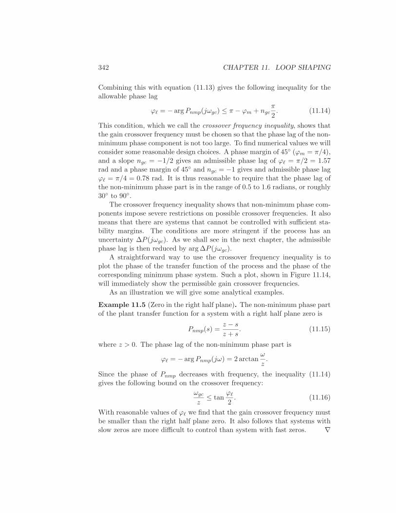
342 CHAPTER 11. LOOP SHAPING
Combining this with equation (11.13) gives the following inequality for theallowable phase lag
ϕℓ = − argPnmp(jωgc) ≤ π − ϕm + ngcπ
2. (11.14)
This condition, which we call the crossover frequency inequality, shows thatthe gain crossover frequency must be chosen so that the phase lag of the non-minimum phase component is not too large. To find numerical values we willconsider some reasonable design choices. A phase margin of 45 (ϕm = π/4),and a slope ngc = −1/2 gives an admissible phase lag of ϕℓ = π/2 = 1.57rad and a phase margin of 45 and ngc = −1 gives and admissible phase lagϕℓ = π/4 = 0.78 rad. It is thus reasonable to require that the phase lag ofthe non-minimum phase part is in the range of 0.5 to 1.6 radians, or roughly30 to 90.
The crossover frequency inequality shows that non-minimum phase com-ponents impose severe restrictions on possible crossover frequencies. It alsomeans that there are systems that cannot be controlled with sufficient sta-bility margins. The conditions are more stringent if the process has anuncertainty ∆P (jωgc). As we shall see in the next chapter, the admissiblephase lag is then reduced by arg ∆P (jωgc).
A straightforward way to use the crossover frequency inequality is toplot the phase of the transfer function of the process and the phase of thecorresponding minimum phase system. Such a plot, shown in Figure 11.14,will immediately show the permissible gain crossover frequencies.
As an illustration we will give some analytical examples.
Example 11.5 (Zero in the right half plane). The non-minimum phase partof the plant transfer function for a system with a right half plane zero is
Pnmp(s) =z − s
z + s. (11.15)
where z > 0. The phase lag of the non-minimum phase part is
ϕℓ = − argPnmp(jω) = 2 arctanω
z.
Since the phase of Pnmp decreases with frequency, the inequality (11.14)gives the following bound on the crossover frequency:
ωgc
z≤ tan
ϕℓ
2. (11.16)
With reasonable values of ϕℓ we find that the gain crossover frequency mustbe smaller than the right half plane zero. It also follows that systems withslow zeros are more difficult to control than system with fast zeros. ∇
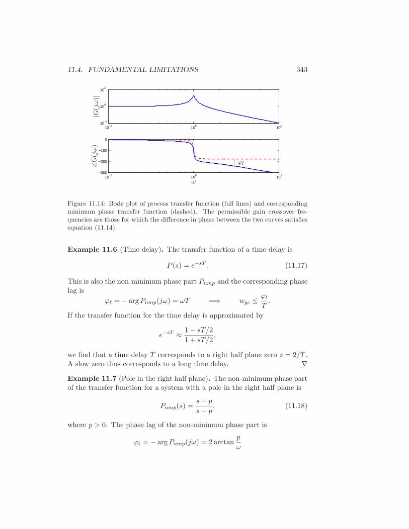
11.4. FUNDAMENTAL LIMITATIONS 343
10−1
100
101
10−2
100
102
10−1
100
101
−300
−200
−100
0
|G(jω)|
ω
∠G
(jω)
ϕl
Figure 11.14: Bode plot of process transfer function (full lines) and correspondingminimum phase transfer function (dashed). The permissible gain crossover fre-quencies are those for which the difference in phase between the two curves satisfiesequation (11.14).
Example 11.6 (Time delay). The transfer function of a time delay is
P (s) = e−sT . (11.17)
This is also the non-minimum phase part Pnmp and the corresponding phaselag is
ϕℓ = − argPnmp(jω) = ωT =⇒ wgc ≤ϕl
T.
If the transfer function for the time delay is approximated by
e−sT ≈ 1 − sT/2
1 + sT/2,
we find that a time delay T corresponds to a right half plane zero z = 2/T .A slow zero thus corresponds to a long time delay. ∇
Example 11.7 (Pole in the right half plane). The non-minimum phase partof the transfer function for a system with a pole in the right half plane is
Pnmp(s) =s+ p
s− p, (11.18)
where p > 0. The phase lag of the non-minimum phase part is
ϕℓ = − argPnmp(jω) = 2 arctanp
ω

344 CHAPTER 11. LOOP SHAPING
Table 11.2: Achievable phase margin for for ϕm = π/4 and ngc = −1/2 and differentpole-zero ratios p/z.
p/z 0.45 0.24 0.20 0.17 0.12 0.10 0.05
z/p 2.24 4.11 5.00 5.83 8.68 10 20
ϕm 0 30 38.6 45 60 64.8 84.6
and the crossover frequency inequality becomes
ωgc >p
tan(ϕℓ/2).
With reasonable values of ϕℓ we find that the gain crossover frequency shouldbe larger than the unstable pole. ∇
Example 11.8 (Pole and a zero in the right half plane). The non-minimumphase part of the transfer function for a system with both poles and zerosin the right half plane is
Pnmp(s) =(z − s)(s+ p)
(z + s)(s− p). (11.19)
The phase lag of this transfer function is
ϕℓ = − argPnmp(jω) = 2 arctanω
z+ 2 arctan
p
ω= 2 arctan
ωgc/z + p/ωgc
1 − p/z.
The mininum value of the right hand side is given by
minωgc
(
2 arctanωgc/z + p/ωgc
1 − p/z
)
= 2 arctan2√
p/z
1 − p/z= 4 arctan
√p
z,
which is achieved at ω =√pz. The crossover frequency inequality (11.14)
becomes
ϕℓ = − argPnmp(jω) ≤ 4 arctan
√p
z,
orp
z≤ tan
ϕℓ
4.
The design choices ϕm = π/4 and ngc = −1/2 gives p < 0.17z. Table 11.2shows the admissible pole-zero ratios for different phase margins. The
11.5. DESIGN EXAMPLE 345
phase-margin that can be achieved for a given ratio p/z is
ϕm < π + ngcπ
2− 4 arctan
√p
z. (11.20)
A pair of poles and zeros in the right half plane thus imposes severe con-straints on the gain crossover frequency. The best gain crossover frequencyis the geometric mean of the unstable pole and zero. A robust controllerdoes not exist unless the pole/zero ratio is sufficiently small. ∇
Avoiding Difficulties with RHP Poles and Zeros
As the examples above show, right half plane poles and zeros significantlylimit the achievable performance of a system, hence one would like to avoidthese whenever possible. The poles of a system depend on the intrinsicdynamics of the system and are given by the eigenvalues of the dynamicsmatrix A of a linear system. Sensors and actuators have no effect on thepoles. The only way to change poles is to redesign the system. Noticethat this does not imply that unstable systems should be avoided. Unstablesystem may actually have advantages; one example is high performancesupersonic aircraft.
The zeros of a system depend on the how sensors and actuators arecoupled to the states. The zeros depend on all the matrices A, B, C and Din a linear system. The zeros can thus be influenced by moving sensors andactuators or by adding sensors and actuators. Notice that a fully actuatedsystem B = I does not have any zeros.
11.5 Design Example
In this section we carry out a detailed design example that illustrates themain techniques in this chapter.
11.6 Further Reading
A more complete description of the material in this chapter is available inthe text by Doyle, Frances and Tannenbaum [DFT92] (out of print, butavailable online).

346 CHAPTER 11. LOOP SHAPING
11.7 Exercises
1. Regenerate the controller for the system in Example 11.4 and use thefrequency responses for the Gang of Four to show that the performancespecification is met.
Chapter 12
Robust Performance
However, by building an amplifier whose gain is deliberately made, say 40decibels higher than necessary (10000 fold excess on energy basis), and thenfeeding the output back on the input in such a way as to throw away thatexcess gain, it has been found that extraordinary improvements in constancyof amplification and freedom from non-linearity.
Harold S. Black, “Stabilized Feedback Amplifiers”, 1934 [Bla34].
The above quote illustrates that one the key uses of feedback is to pro-vide robustness to uncertainty. It is one of the most useful properties offeedback and is what makes it possible to design feedback systems basedon strongly simplified models. This chapter focuses on the analysis of ro-bustness of feedback systems. We consider the stability and performance ofsystems who process dynamics are uncertain and derive fundamental limitsfor robust stability and performance. To do this we develop ways to modeluncertainty, both in the form of parameter variations and in the form ofneglected dynamics. We also discuss how to design controllers to achieverobust performance. One limitation of the tools we present here is that theyare usually restricted to linear systems, although some nonlinear extensionshave been developed.
12.1 Modeling Uncertainty
One form of uncertainty in dynamical systems is that the parameters de-scribing the system are unknown, which is called parametric uncertainty. Atypical example is the variation of the mass of a car, which changes withthe number of passengers and the weight of the baggage. When linearizinga nonlinear system, the parameters of the linearized model also depend on
347
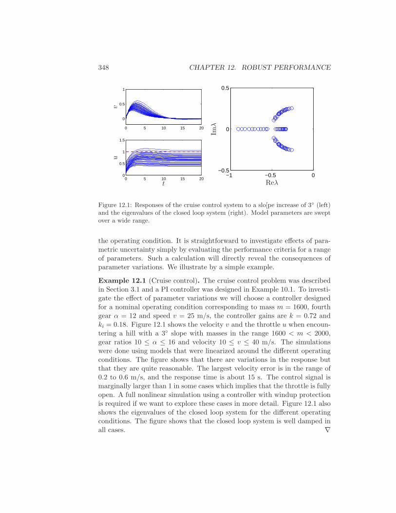
348 CHAPTER 12. ROBUST PERFORMANCE
0 5 10 15 20
0
0.5
1
0 5 10 15 200
0.5
1
1.5
t
uv
−1 −0.5 0−0.5
0
0.5
Reλ
Imλ
Figure 12.1: Responses of the cruise control system to a slo[pe increase of 3 (left)and the eigenvalues of the closed loop system (right). Model parameters are sweptover a wide range.
the operating condition. It is straightforward to investigate effects of para-metric uncertainty simply by evaluating the performance criteria for a rangeof parameters. Such a calculation will directly reveal the consequences ofparameter variations. We illustrate by a simple example.
Example 12.1 (Cruise control). The cruise control problem was describedin Section 3.1 and a PI controller was designed in Example 10.1. To investi-gate the effect of parameter variations we will choose a controller designedfor a nominal operating condition corresponding to mass m = 1600, fourthgear α = 12 and speed v = 25 m/s, the controller gains are k = 0.72 andki = 0.18. Figure 12.1 shows the velocity v and the throttle u when encoun-tering a hill with a 3 slope with masses in the range 1600 < m < 2000,gear ratios 10 ≤ α ≤ 16 and velocity 10 ≤ v ≤ 40 m/s. The simulationswere done using models that were linearized around the different operatingconditions. The figure shows that there are variations in the response butthat they are quite reasonable. The largest velocity error is in the range of0.2 to 0.6 m/s, and the response time is about 15 s. The control signal ismarginally larger than 1 in some cases which implies that the throttle is fullyopen. A full nonlinear simulation using a controller with windup protectionis required if we want to explore these cases in more detail. Figure 12.1 alsoshows the eigenvalues of the closed loop system for the different operatingconditions. The figure shows that the closed loop system is well damped inall cases. ∇
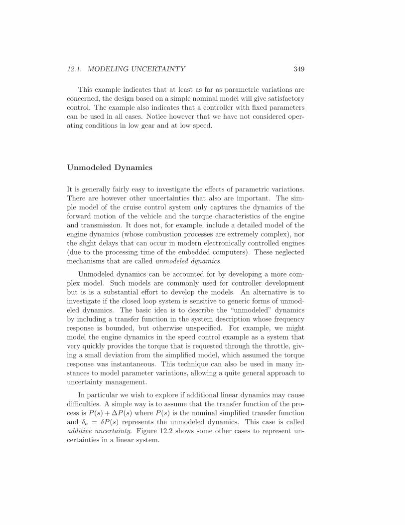
12.1. MODELING UNCERTAINTY 349
This example indicates that at least as far as parametric variations areconcerned, the design based on a simple nominal model will give satisfactorycontrol. The example also indicates that a controller with fixed parameterscan be used in all cases. Notice however that we have not considered oper-ating conditions in low gear and at low speed.
Unmodeled Dynamics
It is generally fairly easy to investigate the effects of parametric variations.There are however other uncertainties that also are important. The sim-ple model of the cruise control system only captures the dynamics of theforward motion of the vehicle and the torque characteristics of the engineand transmission. It does not, for example, include a detailed model of theengine dynamics (whose combustion processes are extremely complex), northe slight delays that can occur in modern electronically controlled engines(due to the processing time of the embedded computers). These neglectedmechanisms that are called unmodeled dynamics.
Unmodeled dynamics can be accounted for by developing a more com-plex model. Such models are commonly used for controller developmentbut is is a substantial effort to develop the models. An alternative is toinvestigate if the closed loop system is sensitive to generic forms of unmod-eled dynamics. The basic idea is to describe the “unmodeled” dynamicsby including a transfer function in the system description whose frequencyresponse is bounded, but otherwise unspecified. For example, we mightmodel the engine dynamics in the speed control example as a system thatvery quickly provides the torque that is requested through the throttle, giv-ing a small deviation from the simplified model, which assumed the torqueresponse was instantaneous. This technique can also be used in many in-stances to model parameter variations, allowing a quite general approach touncertainty management.
In particular we wish to explore if additional linear dynamics may causedifficulties. A simple way is to assume that the transfer function of the pro-cess is P (s) + ∆P (s) where P (s) is the nominal simplified transfer functionand δa = δP (s) represents the unmodeled dynamics. This case is calledadditive uncertainty. Figure 12.2 shows some other cases to represent un-certainties in a linear system.
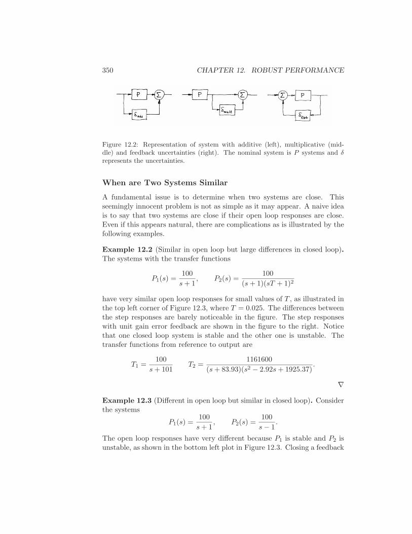
350 CHAPTER 12. ROBUST PERFORMANCE
Figure 12.2: Representation of system with additive (left), multiplicative (mid-dle) and feedback uncertainties (right). The nominal system is P systems and δrepresents the uncertainties.
When are Two Systems Similar
A fundamental issue is to determine when two systems are close. Thisseemingly innocent problem is not as simple as it may appear. A naive ideais to say that two systems are close if their open loop responses are close.Even if this appears natural, there are complications as is illustrated by thefollowing examples.
Example 12.2 (Similar in open loop but large differences in closed loop).The systems with the transfer functions
P1(s) =100
s+ 1, P2(s) =
100
(s+ 1)(sT + 1)2
have very similar open loop responses for small values of T , as illustrated inthe top left corner of Figure 12.3, where T = 0.025. The differences betweenthe step responses are barely noticeable in the figure. The step responseswith unit gain error feedback are shown in the figure to the right. Noticethat one closed loop system is stable and the other one is unstable. Thetransfer functions from reference to output are
T1 =100
s+ 101T2 =
1161600
(s+ 83.93)(s2 − 2.92s+ 1925.37).
∇
Example 12.3 (Different in open loop but similar in closed loop). Considerthe systems
P1(s) =100
s+ 1, P2(s) =
100
s− 1.
The open loop responses have very different because P1 is stable and P2 isunstable, as shown in the bottom left plot in Figure 12.3. Closing a feedback
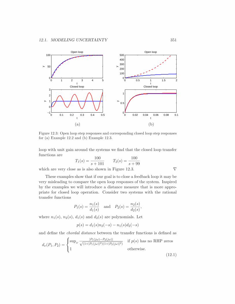
12.1. MODELING UNCERTAINTY 351
0 1 2 3 4 50
50
100Open loop
t
y
0 0.1 0.2 0.3 0.4 0.5−1
0
1
2
3Closed loop
t
y
0 0.5 1 1.5 20
100
200
300
400
500Open loop
t
y0 0.02 0.04 0.06 0.08 0.1
0
0.5
1
Closed loop
ty
(a) (b)
Figure 12.3: Open loop step responses and corresponding closed loop step responsesfor (a) Example 12.2 and (b) Example 12.3.
loop with unit gain around the systems we find that the closed loop transferfunctions are
T1(s) =100
s+ 101T2(s) =
100
s+ 99
which are very close as is also shown in Figure 12.3. ∇These examples show that if our goal is to close a feedback loop it may be
very misleading to compare the open loop responses of the system. Inspiredby the examples we will introduce a distance measure that is more appro-priate for closed loop operation. Consider two systems with the rationaltransfer functions
P1(s) =n1(s)
d1(s)and P2(s) =
n2(s)
d2(s),
where n1(s), n2(s), d1(s) and d2(s) are polynomials. Let
p(s) = d1(s)n2(−s) − n1(s)d2(−s)and define the chordal distance between the transfer functions is defined as
dν(P1, P2) =
supω|P1(jω)−P2(jω)|√
(1+|P1(jω)|2)(1+|P2(jω)|2)if p(s) has no RHP zeros
1 otherwise.
(12.1)
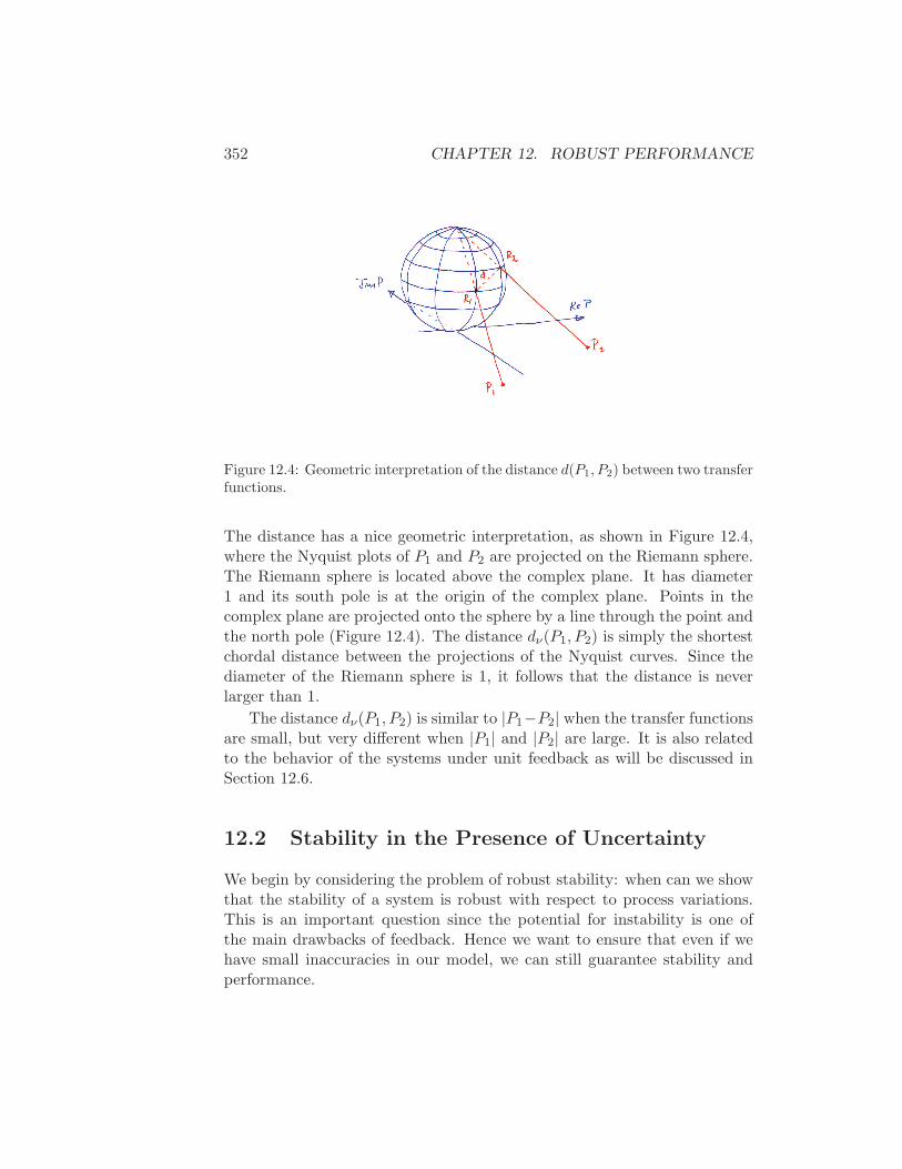
352 CHAPTER 12. ROBUST PERFORMANCE
Figure 12.4: Geometric interpretation of the distance d(P1, P2) between two transferfunctions.
The distance has a nice geometric interpretation, as shown in Figure 12.4,where the Nyquist plots of P1 and P2 are projected on the Riemann sphere.The Riemann sphere is located above the complex plane. It has diameter1 and its south pole is at the origin of the complex plane. Points in thecomplex plane are projected onto the sphere by a line through the point andthe north pole (Figure 12.4). The distance dν(P1, P2) is simply the shortestchordal distance between the projections of the Nyquist curves. Since thediameter of the Riemann sphere is 1, it follows that the distance is neverlarger than 1.
The distance dν(P1, P2) is similar to |P1−P2| when the transfer functionsare small, but very different when |P1| and |P2| are large. It is also relatedto the behavior of the systems under unit feedback as will be discussed inSection 12.6.
12.2 Stability in the Presence of Uncertainty
We begin by considering the problem of robust stability: when can we showthat the stability of a system is robust with respect to process variations.This is an important question since the potential for instability is one ofthe main drawbacks of feedback. Hence we want to ensure that even if wehave small inaccuracies in our model, we can still guarantee stability andperformance.
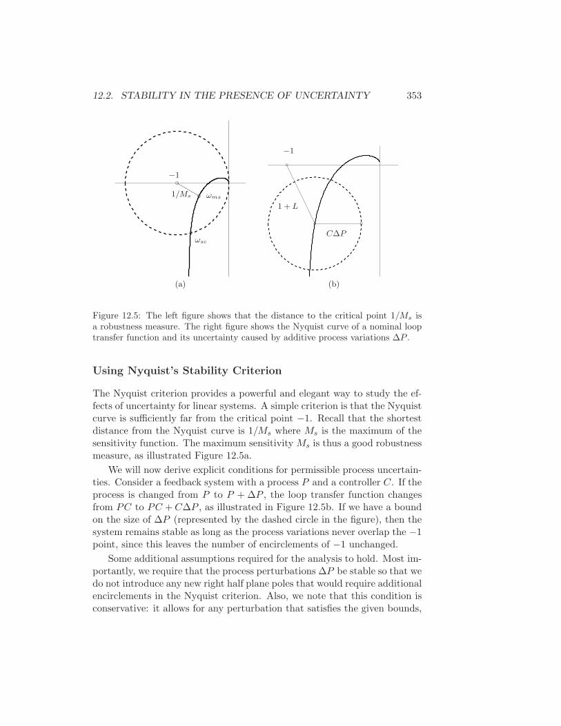
12.2. STABILITY IN THE PRESENCE OF UNCERTAINTY 353
1/Ms ωms
ωsc
−1
−1
1 + L
C∆P
(a) (b)
Figure 12.5: The left figure shows that the distance to the critical point 1/Ms isa robustness measure. The right figure shows the Nyquist curve of a nominal looptransfer function and its uncertainty caused by additive process variations ∆P .
Using Nyquist’s Stability Criterion
The Nyquist criterion provides a powerful and elegant way to study the ef-fects of uncertainty for linear systems. A simple criterion is that the Nyquistcurve is sufficiently far from the critical point −1. Recall that the shortestdistance from the Nyquist curve is 1/Ms where Ms is the maximum of thesensitivity function. The maximum sensitivity Ms is thus a good robustnessmeasure, as illustrated Figure 12.5a.
We will now derive explicit conditions for permissible process uncertain-ties. Consider a feedback system with a process P and a controller C. If theprocess is changed from P to P + ∆P , the loop transfer function changesfrom PC to PC +C∆P , as illustrated in Figure 12.5b. If we have a boundon the size of ∆P (represented by the dashed circle in the figure), then thesystem remains stable as long as the process variations never overlap the −1point, since this leaves the number of encirclements of −1 unchanged.
Some additional assumptions required for the analysis to hold. Most im-portantly, we require that the process perturbations ∆P be stable so that wedo not introduce any new right half plane poles that would require additionalencirclements in the Nyquist criterion. Also, we note that this condition isconservative: it allows for any perturbation that satisfies the given bounds,
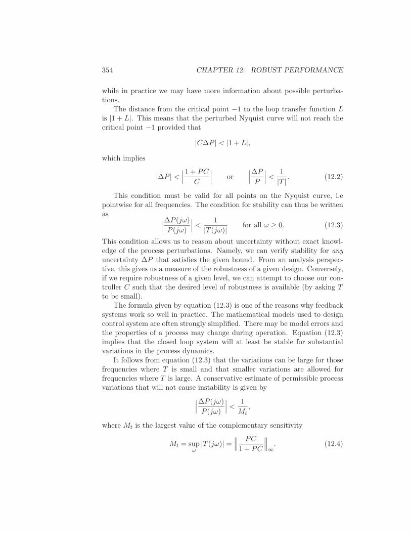
354 CHAPTER 12. ROBUST PERFORMANCE
while in practice we may have more information about possible perturba-tions.
The distance from the critical point −1 to the loop transfer function Lis |1 + L|. This means that the perturbed Nyquist curve will not reach thecritical point −1 provided that
|C∆P | < |1 + L|,
which implies
|∆P | <∣∣∣1 + PC
C
∣∣∣ or
∣∣∣∆P
P
∣∣∣ <
1
|T | . (12.2)
This condition must be valid for all points on the Nyquist curve, i.epointwise for all frequencies. The condition for stability can thus be writtenas
∣∣∣∆P (jω)
P (jω)
∣∣∣ <
1
|T (jω)| for all ω ≥ 0. (12.3)
This condition allows us to reason about uncertainty without exact knowl-edge of the process perturbations. Namely, we can verify stability for anyuncertainty ∆P that satisfies the given bound. From an analysis perspec-tive, this gives us a measure of the robustness of a given design. Conversely,if we require robustness of a given level, we can attempt to choose our con-troller C such that the desired level of robustness is available (by asking Tto be small).
The formula given by equation (12.3) is one of the reasons why feedbacksystems work so well in practice. The mathematical models used to designcontrol system are often strongly simplified. There may be model errors andthe properties of a process may change during operation. Equation (12.3)implies that the closed loop system will at least be stable for substantialvariations in the process dynamics.
It follows from equation (12.3) that the variations can be large for thosefrequencies where T is small and that smaller variations are allowed forfrequencies where T is large. A conservative estimate of permissible processvariations that will not cause instability is given by
∣∣∣∆P (jω)
P (jω)
∣∣∣ <
1
Mt,
where Mt is the largest value of the complementary sensitivity
Mt = supω
|T (jω)| =∥∥∥
PC
1 + PC
∥∥∥∞. (12.4)
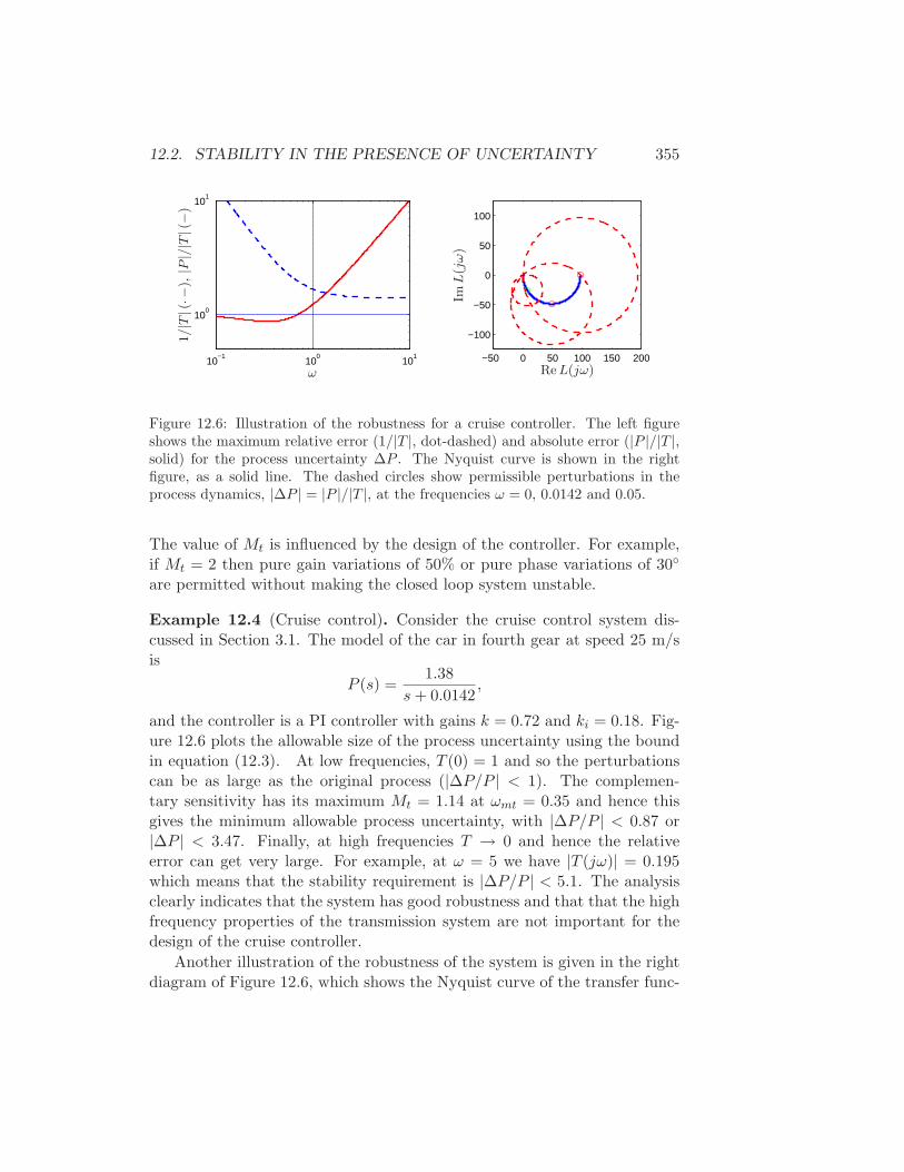
12.2. STABILITY IN THE PRESENCE OF UNCERTAINTY 355
10−1
100
101
100
101
−50 0 50 100 150 200
−100
−50
0
50
100
Re L(jω)
ImL
(jω)
ω
1/|T
|(
·−),|P|/|T|(−)
Figure 12.6: Illustration of the robustness for a cruise controller. The left figureshows the maximum relative error (1/|T |, dot-dashed) and absolute error (|P |/|T |,solid) for the process uncertainty ∆P . The Nyquist curve is shown in the rightfigure, as a solid line. The dashed circles show permissible perturbations in theprocess dynamics, |∆P | = |P |/|T |, at the frequencies ω = 0, 0.0142 and 0.05.
The value of Mt is influenced by the design of the controller. For example,if Mt = 2 then pure gain variations of 50% or pure phase variations of 30
are permitted without making the closed loop system unstable.
Example 12.4 (Cruise control). Consider the cruise control system dis-cussed in Section 3.1. The model of the car in fourth gear at speed 25 m/sis
P (s) =1.38
s+ 0.0142,
and the controller is a PI controller with gains k = 0.72 and ki = 0.18. Fig-ure 12.6 plots the allowable size of the process uncertainty using the boundin equation (12.3). At low frequencies, T (0) = 1 and so the perturbationscan be as large as the original process (|∆P/P | < 1). The complemen-tary sensitivity has its maximum Mt = 1.14 at ωmt = 0.35 and hence thisgives the minimum allowable process uncertainty, with |∆P/P | < 0.87 or|∆P | < 3.47. Finally, at high frequencies T → 0 and hence the relativeerror can get very large. For example, at ω = 5 we have |T (jω)| = 0.195which means that the stability requirement is |∆P/P | < 5.1. The analysisclearly indicates that the system has good robustness and that that the highfrequency properties of the transmission system are not important for thedesign of the cruise controller.
Another illustration of the robustness of the system is given in the rightdiagram of Figure 12.6, which shows the Nyquist curve of the transfer func-
356 CHAPTER 12. ROBUST PERFORMANCE
Figure 12.7: Illustration of robustness to process perturbations.
tion of the process and the uncertainty bounds ∆P = |P |/|T | for a fewfrequencies. Note that the controller can tolerate very large amounts ofuncertainty and still maintain stability of the closed loop. ∇
The situation illustrated in the previous example is typical for manyprocesses: moderately small uncertainties are only required around the gaincrossover frequencies, but large uncertainties can be permitted at higherand lower frequencies. A consequence of this is that a simple model thatdescribes the process dynamics well around the crossover frequency is oftensufficient for design. Systems with many resonance peaks are an exceptionto this rule because the process transfer function for such systems may havelarge gains also for higher frequencies.
Notice that the results we have given can be very conservative. Refer-ring to Figure 12.5, the critical perturbations, which were the basis for ouranalysis, are in the direction towards the critical point. It is possible to havemuch larger perturbations in the opposite direction.
The Small Gain Theorem
The robustness result given by equation (12.3) can be given another inter-pretation by using the small gain theorem, introduced in Section 9.5. Itis convenient to choose a particular form of the small gain theorem wherethe gain of a system is defined in terms of the maximum amplitude of thefrequency response. We first define the gain of a system as the H∞ norm ofits transfer function H(s):
‖H‖∞ = supω
|H(jω)|.
The small gain theorem can now be written as follows.
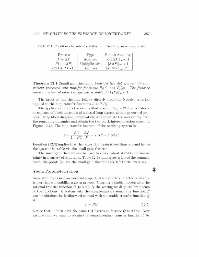
12.2. STABILITY IN THE PRESENCE OF UNCERTAINTY 357
Table 12.1: Conditions for robust stability for different types of uncertainty
Process Type Robust Stability
P + ∆P Additive |CS∆P‖∞ < 1P (1 + ∆P ) Multiplicative ‖S∆P‖∞ < 1
P/(1 + ∆P ·P ) Feedback ‖PS∆P‖∞ < 1
Theorem 12.1 (Small gain theorem). Consider two stable, linear time in-variant processes with transfer functions P1(s) and P2(s). The feedbackinterconnection of these two systems is stable if ‖P1P2‖∞ < 1.
The proof of this theorem follows directly from the Nyquist criterionapplied to the loop transfer functions L = P1P2.
The application of this theorem is illustrated in Figure 12.7, which showsa sequence of block diagrams of a closed loop system with a perturbed pro-cess. Using block diagram manipulation, we can isolate the uncertainty fromthe remaining dynamics and obtain the two block interconnection shown inFigure 12.7c. The loop transfer function of the resulting system is
L =PC
1 + PC
∆P
P= T∆P = CS∆P.
Equation (12.3) implies that the largest loop gain is less than one and hencethe systems is stable via the small gain theorem.
The small gain theorem can be used to check robust stability for uncer-tainty in a variety of situations. Table 12.1 summarizes a few of the commoncases; the proofs (all via the small gain theorem) are left to the exercises.
Youla Parameterization
Since stability is such an essential property it is useful to characterize all con-troller that will stabilize a given process. Consider a stable process with therational transfer function P , to simplify the writing we drop the argumentsof the functions. A system with the complementary sensitivity function Tcan be obtained by feedforward control with the stable transfer function Qif
T = PQ (12.5)
Notice that T must have the same RHP zeros as P since Q is stable. Nowassume that we want to obtain the complementary transfer function T by
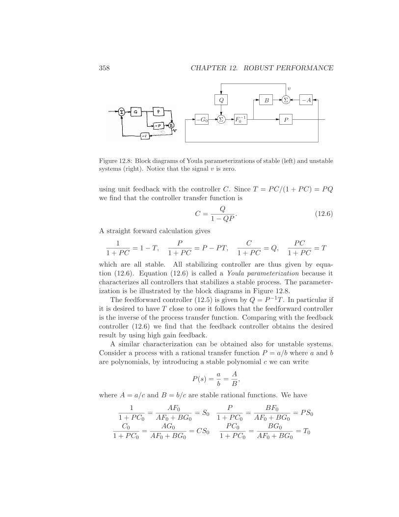
358 CHAPTER 12. ROBUST PERFORMANCE
−AB
P
Q
−G0 F−10Σ
Σ
v
Figure 12.8: Block diagrams of Youla parameterizations of stable (left) and unstablesystems (right). Notice that the signal v is zero.
using unit feedback with the controller C. Since T = PC/(1 + PC) = PQwe find that the controller transfer function is
C =Q
1 −QP. (12.6)
A straight forward calculation gives
1
1 + PC= 1 − T,
P
1 + PC= P − PT,
C
1 + PC= Q,
PC
1 + PC= T
which are all stable. All stabilizing controller are thus given by equa-tion (12.6). Equation (12.6) is called a Youla parameterization because itcharacterizes all controllers that stabilizes a stable process. The parameter-ization is be illustrated by the block diagrams in Figure 12.8.
The feedforward controller (12.5) is given by Q = P−1T . In particular ifit is desired to have T close to one it follows that the feedforward controlleris the inverse of the process transfer function. Comparing with the feedbackcontroller (12.6) we find that the feedback controller obtains the desiredresult by using high gain feedback.
A similar characterization can be obtained also for unstable systems.Consider a process with a rational transfer function P = a/b where a and bare polynomials, by introducing a stable polynomial c we can write
P (s) =a
b=A
B,
where A = a/c and B = b/c are stable rational functions. We have
1
1 + PC0=
AF0
AF0 +BG0= S0
P
1 + PC0=
BF0
AF0 +BG0= PS0
C0
1 + PC0=
AG0
AF0 +BG0= CS0
PC0
1 + PC0=
BG0
AF0 +BG0= T0
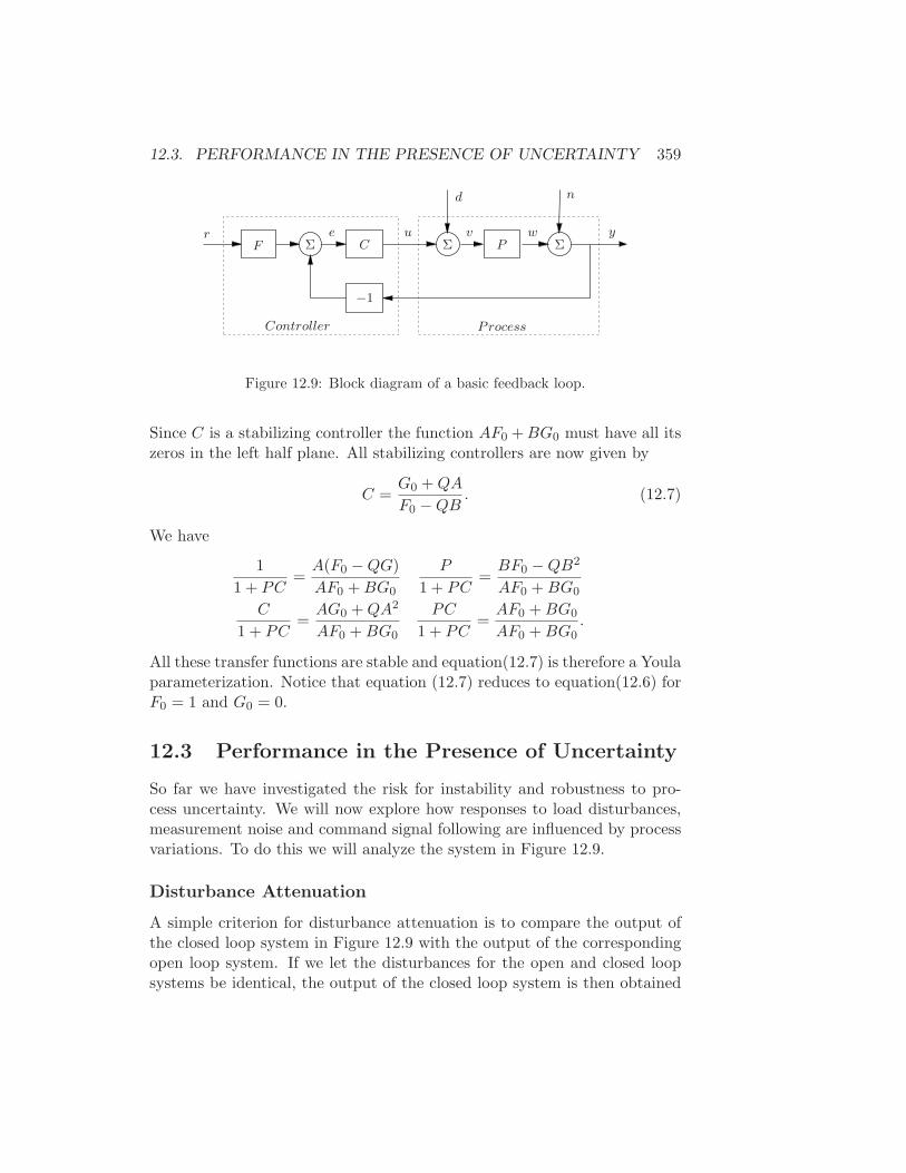
12.3. PERFORMANCE IN THE PRESENCE OF UNCERTAINTY 359
F C P
−1
Σ Σ Σr e u v
d
w
n
y
Controller Process
Figure 12.9: Block diagram of a basic feedback loop.
Since C is a stabilizing controller the function AF0 +BG0 must have all itszeros in the left half plane. All stabilizing controllers are now given by
C =G0 +QA
F0 −QB. (12.7)
We have
1
1 + PC=A(F0 −QG)
AF0 +BG0
P
1 + PC=BF0 −QB2
AF0 +BG0
C
1 + PC=AG0 +QA2
AF0 +BG0
PC
1 + PC=AF0 +BG0
AF0 +BG0.
All these transfer functions are stable and equation(12.7) is therefore a Youlaparameterization. Notice that equation (12.7) reduces to equation(12.6) forF0 = 1 and G0 = 0.
12.3 Performance in the Presence of Uncertainty
So far we have investigated the risk for instability and robustness to pro-cess uncertainty. We will now explore how responses to load disturbances,measurement noise and command signal following are influenced by processvariations. To do this we will analyze the system in Figure 12.9.
Disturbance Attenuation
A simple criterion for disturbance attenuation is to compare the output ofthe closed loop system in Figure 12.9 with the output of the correspondingopen loop system. If we let the disturbances for the open and closed loopsystems be identical, the output of the closed loop system is then obtained
360 CHAPTER 12. ROBUST PERFORMANCE
simply by passing the open loop output through a system with the transferfunction S. The sensitivity function thus tells how the variations in theoutput are influenced by feedback. Disturbances with frequencies such that|S(jω)| < 1 are attenuated but disturbances with frequencies such that|S(jω)| > 1 are amplified by feedback. The maximum sensitivity Ms andthe sensitivity crossover frequency ωsc are simple performance measures.
The sensitivity function S gives a gross characterization of the effect offeedback on disturbances. A more detailed characterization is given by thetransfer function from load disturbances to process output:
Gyd =P
1 + PC= PS. (12.8)
Load disturbances typically have low frequencies and it is therefore impor-tant that the transfer function is small for low frequencies. For processeswith constant low frequency gain and a controller with integral action wehave Gyd ≈ s/ki. Integral gain ki is thus a simple measure of attenuation ofload disturbances.
To find how the transfer function Gyd is influenced by small variationsin the process transfer function we differentiate equation (12.8) which gives
dGyd
Gyd= S
dP
P. (12.9)
The response to load disturbances is thus insensitive to process variationsfor frequencies where |S(jω)| is small, i.e. for those frequencies where loaddisturbances are important.
A drawback with feedback is that the controller feeds measurement noiseinto the system. In addition to the load disturbance rejection, it thus is alsoimportant that the control actions generated by measurement noise are nottoo large. It follows from Figure 12.9 that the transfer function Gun frommeasurement noise to controller output is given by
Gun = − C
1 + PC= −T
P(12.10)
Since measurement noise typically has high frequencies it is important thatthe transfer function Gun is not too large for high frequencies. The looptransfer function PC is typically small for high frequencies, which impliesthat Gun ≈ C for large s. To avoid injecting too much measurement noise itis therefore important that C(s) is small for large s. This property is calledhigh frequency roll-off. Filtering of the measured signal in a PID controlleris done to reduce injection of measurement noise, see Section 10.5.
12.3. PERFORMANCE IN THE PRESENCE OF UNCERTAINTY 361
To find how the transfer function Gun is influenced by small variationsin the process transfer function we differentiate equation (12.10) which gives
dGun
Gun= T
dP
P. (12.11)
Measurement noise typically has high frequencies. Since the complementarysensitivity function also is small for high frequencies we find that processuncertainty has little influence on the transfer function Gun for frequencieswhere measurement are important.
Command Signal Following
The transfer function from reference to output is given by
Gyr =PCF
1 + PC= T, (12.12)
which is the complementary sensitivity function. To see how variations in Paffect the performance of the system, we differentiate equation (12.12) withrespect to the process transfer function:
dGyr
dP=
CF
1 + PC− PCFC
(1 + PC)2=
CF
(1 + PC)2= S
Gyr
P.
and it follows thatdGyr
Gyr= S
dP
P. (12.13)
The relative error in the closed loop transfer function thus equals the productof the sensitivity function and the relative error in the process. In particular,it follows from equation (12.13) that the relative error in the closed looptransfer function is small when the sensitivity is small. This is one of thevery useful properties of feedback.
When analyzing robust stability we were able to deal with large distur-bances. In this section we have limited the analysis to small (differential)perturbations. There are some additional assumptions required for the anal-ysis to hold. Most importantly, we require that the process perturbationsdP be stable so that we do not introduce any new right half plane polesthat would require additional encirclements in the Nyquist criterion. Also,we note that this condition is conservative: it allows for any perturbationthat satisfies the given bounds, while in practice we have more informationabout possible perturbations.
362 CHAPTER 12. ROBUST PERFORMANCE
12.4 Limits on the Sensitivities
The sensitivity function S and the complementary sensitivity function Ttell us a great deal about the feedback loop. Disturbance rejection andsensitivity to process uncertainties are low for frequencies where S is smalland tracking performance is good when T is close to 1. In this sectionwe explore some of the limitations on robust performance by looking atalgebraic and integral constraints on the functions.
Since
S =1
1 + PCand T =
PC
1 + PC
it follows that the sensitivity functions are related through
S + T = 1. (12.14)
A useful design goal is to make S close to zero and T close to one, a designgoal that is compatible with equation (12.14). The loop transfer function Lis typically large for small values of s and it goes to zero as s goes to infinity.This means that S is typically small for small s and close to 1 for large s.The complementary sensitivity function is close to 1 for small s and it goesto 0 as s goes to infinity.
Bode’s Integral Formula
A basic problem is to investigate if S can be made small over a large fre-quency range. We will start by investigating an example.
Example 12.5 (System that admits small sensitivities). Consider a closedloop system consisting of a first order process and a proportional controller.Let the loop transfer function
L = PC =k
s+ 1
where parameter k is the controller gain. The sensitivity function is
S =s+ 1
s+ 1 + k
and we have
|S(jω)| =
√
1 + ω2
1 + 2k + k2 + ω2
This implies that |S(jω)| < 1 for all finite frequencies and that the sensitivitycan be made arbitrary small for any finite frequency by making k sufficientlylarge. ∇
12.4. LIMITS ON THE SENSITIVITIES 363
The system in Example 12.5 is unfortunately an exception. The keyfeature of the system is that the Nyquist curve of the process is completelycontained in the right half plane. Such systems are called positive real. Forthese systems the Nyquist curve never enters the region shown in Figure 11.6where the sensitivity is greater than one.
For typical control systems there are unfortunately severe constraintson the sensitivity function. The following theorem, due to Bode, providesfundamental insights into the limits of performance under feedback.
Theorem 12.2 (Bode’s integral formula). Let S(s) be the sensitivity func-tion for a feedback system and assume that it goes to zero faster than 1/sfor large s. If the loop transfer has poles pk in the right half plane then thesensitivity function satisfies the following integral:
∫ ∞
0log |S(jω)| dω =
∫ ∞
0log
1
|1 + L(jω)| dω = π∑
Re pk. (12.15)
Equation (12.15) implies that there are fundamental limitations to whatcan be achieved by control and that control design can be viewed as aredistribution of disturbance attenuation over different frequencies. Thisequation shows that if the sensitivity function is made smaller for somefrequencies it must increase at other frequencies. This means that if dis-turbance attenuation is improved in one frequency range it will be worse inother. This is called the waterbed effect. It also follows that systems withpoles in the right half plane have larger sensitivity.
For a loop transfer function without poles in the right half plane equa-tion (12.15) reduces to
∫ ∞
0log |S(jω)|dω = 0.
This formula can be given a nice geometric interpretation as shown in Fig-ure 12.10, which shows log |S(jω)| as a function of ω. The area over thehorizontal axis must be equal to the area under the axis when frequency isplotted on a linear scale.
There is an analogous result for the complementary sensitivity functionwhich tells that ∫ ∞
0log |T
( 1
jω
)| dω = π
∑ 1
zi,
where the summation is over all right half plane zeros. Notice that smallright half plane zeros are worse than large ones and that large right halfplane poles are worse than small ones.
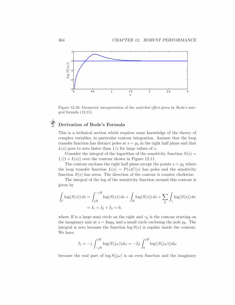
364 CHAPTER 12. ROBUST PERFORMANCE
0 0.5 1 1.5 2 2.5 3−3
−2
−1
0
1
ω
log|S
(jω)|
Figure 12.10: Geometric interpretation of the waterbed effect given by Bode’s inte-gral formula (12.15).
Derivation of Bode’s Formula
This is a technical section which requires some knowledge of the theory ofcomplex variables, in particular contour integration. Assume that the looptransfer function has distinct poles at s = pk in the right half plane and thatL(s) goes to zero faster than 1/s for large values of s.
Consider the integral of the logarithm of the sensitivity function S(s) =1/(1 + L(s)) over the contour shown in Figure 12.11.
The contour encloses the right half plane except the points s = pk wherethe loop transfer function L(s) = P (s)C(s) has poles and the sensitivityfunction S(s) has zeros. The direction of the contour is counter clockwise.
The integral of the log of the sensitivity function around this contour isgiven by
∫
Γlog(S(s)) ds =
∫ −jR
jRlog(S(s)) ds+
∫
Rlog(S(s)) ds+
∑
k
∫
γlog(S(s)) ds
= I1 + I2 + I3 = 0,
where R is a large semi circle on the right and γk is the contour starting onthe imaginary axis at s = Impk and a small circle enclosing the pole pk. Theintegral is zero because the function logS(s) is regular inside the contour.We have
I1 = −j∫ jR
−jRlog(S(jω))dω = −2j
∫ jR
0log(|S(jω)|)dω
because the real part of logS(jω) is an even function and the imaginary
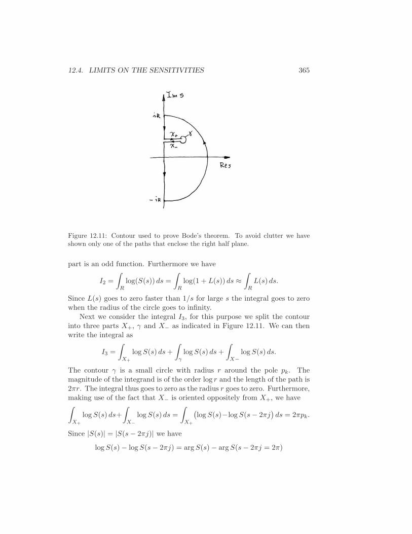
12.4. LIMITS ON THE SENSITIVITIES 365
Figure 12.11: Contour used to prove Bode’s theorem. To avoid clutter we haveshown only one of the paths that enclose the right half plane.
part is an odd function. Furthermore we have
I2 =
∫
Rlog(S(s)) ds =
∫
Rlog(1 + L(s)) ds ≈
∫
RL(s) ds.
Since L(s) goes to zero faster than 1/s for large s the integral goes to zerowhen the radius of the circle goes to infinity.
Next we consider the integral I3, for this purpose we split the contourinto three parts X+, γ and X− as indicated in Figure 12.11. We can thenwrite the integral as
I3 =
∫
X+
logS(s) ds+
∫
γlogS(s) ds+
∫
X−logS(s) ds.
The contour γ is a small circle with radius r around the pole pk. Themagnitude of the integrand is of the order log r and the length of the path is2πr. The integral thus goes to zero as the radius r goes to zero. Furthermore,making use of the fact that X− is oriented oppositely from X+, we have∫
X+
logS(s) ds+
∫
X−
logS(s) ds =
∫
X+
(logS(s)−logS(s− 2πj
)ds = 2πpk.
Since |S(s)| = |S(s− 2πj)| we have
logS(s) − logS(s− 2πj) = argS(s) − argS(s− 2πj = 2π)
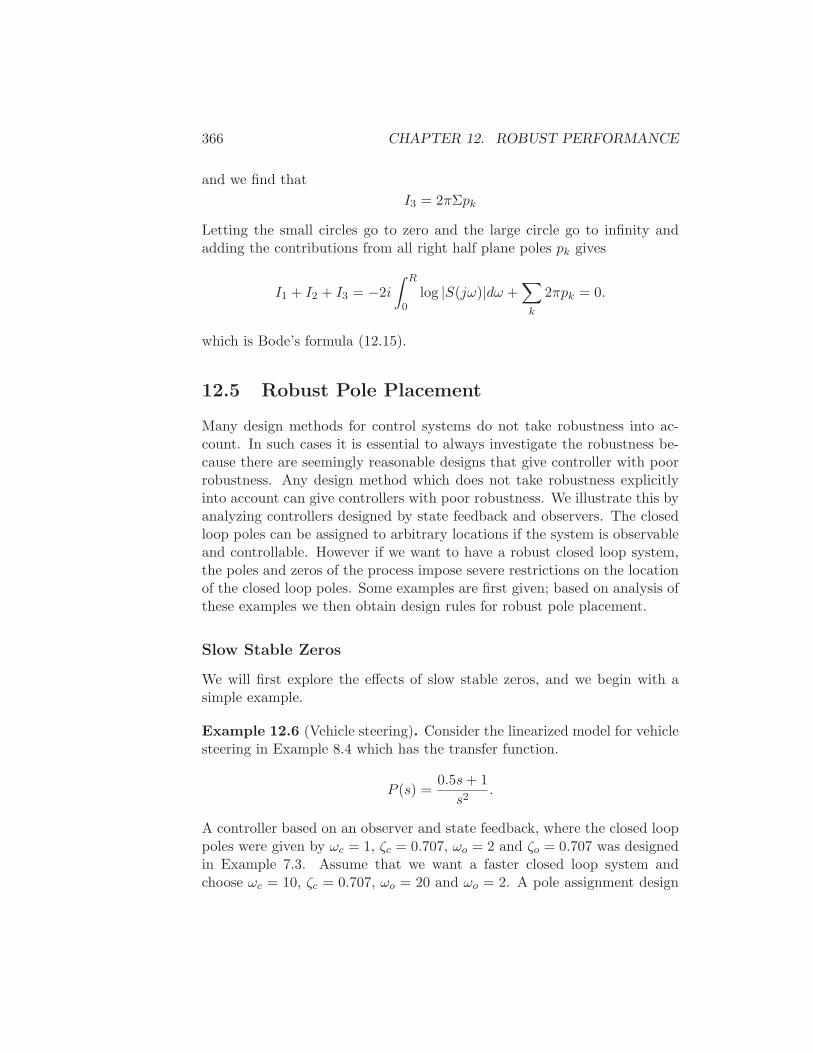
366 CHAPTER 12. ROBUST PERFORMANCE
and we find that
I3 = 2πΣpk
Letting the small circles go to zero and the large circle go to infinity andadding the contributions from all right half plane poles pk gives
I1 + I2 + I3 = −2i
∫ R
0log |S(jω)|dω +
∑
k
2πpk = 0.
which is Bode’s formula (12.15).
12.5 Robust Pole Placement
Many design methods for control systems do not take robustness into ac-count. In such cases it is essential to always investigate the robustness be-cause there are seemingly reasonable designs that give controller with poorrobustness. Any design method which does not take robustness explicitlyinto account can give controllers with poor robustness. We illustrate this byanalyzing controllers designed by state feedback and observers. The closedloop poles can be assigned to arbitrary locations if the system is observableand controllable. However if we want to have a robust closed loop system,the poles and zeros of the process impose severe restrictions on the locationof the closed loop poles. Some examples are first given; based on analysis ofthese examples we then obtain design rules for robust pole placement.
Slow Stable Zeros
We will first explore the effects of slow stable zeros, and we begin with asimple example.
Example 12.6 (Vehicle steering). Consider the linearized model for vehiclesteering in Example 8.4 which has the transfer function.
P (s) =0.5s+ 1
s2.
A controller based on an observer and state feedback, where the closed looppoles were given by ωc = 1, ζc = 0.707, ωo = 2 and ζo = 0.707 was designedin Example 7.3. Assume that we want a faster closed loop system andchoose ωc = 10, ζc = 0.707, ωo = 20 and ωo = 2. A pole assignment design
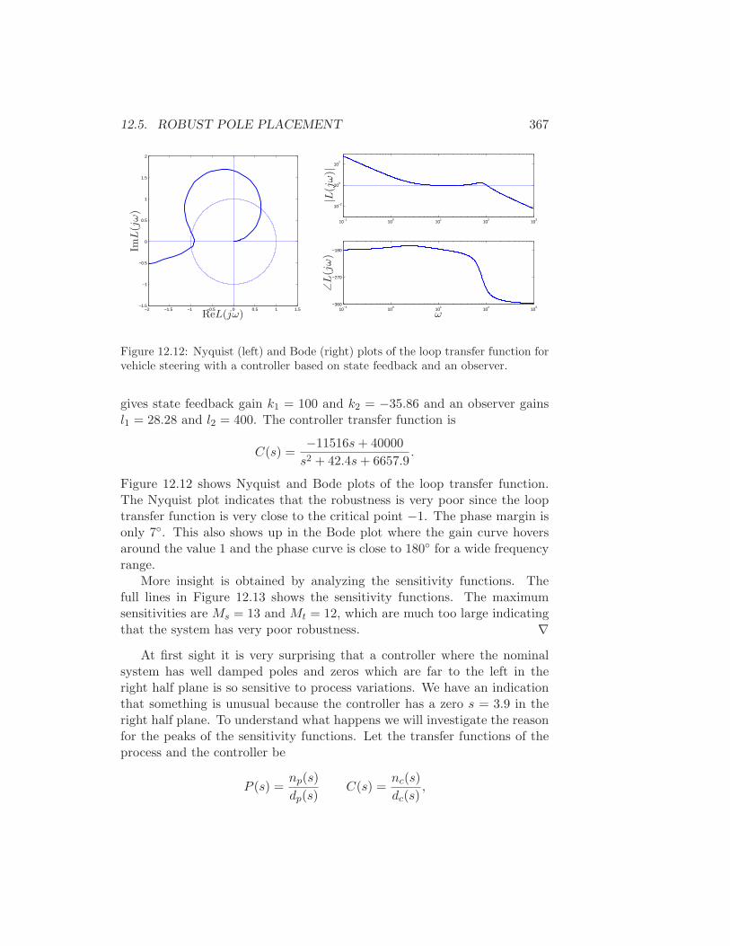
12.5. ROBUST POLE PLACEMENT 367
−2 −1.5 −1 −0.5 0 0.5 1 1.5−1.5
−1
−0.5
0
0.5
1
1.5
2
ReL(jω)
ImL
(jω)
10−1
100
101
102
103
10−2
100
102
10−1
100
101
102
103
−360
−270
−180
|L(j
ω)|
∠L
(jω)
ω
Figure 12.12: Nyquist (left) and Bode (right) plots of the loop transfer function forvehicle steering with a controller based on state feedback and an observer.
gives state feedback gain k1 = 100 and k2 = −35.86 and an observer gainsl1 = 28.28 and l2 = 400. The controller transfer function is
C(s) =−11516s+ 40000
s2 + 42.4s+ 6657.9.
Figure 12.12 shows Nyquist and Bode plots of the loop transfer function.The Nyquist plot indicates that the robustness is very poor since the looptransfer function is very close to the critical point −1. The phase margin isonly 7. This also shows up in the Bode plot where the gain curve hoversaround the value 1 and the phase curve is close to 180 for a wide frequencyrange.
More insight is obtained by analyzing the sensitivity functions. Thefull lines in Figure 12.13 shows the sensitivity functions. The maximumsensitivities are Ms = 13 and Mt = 12, which are much too large indicatingthat the system has very poor robustness. ∇
At first sight it is very surprising that a controller where the nominalsystem has well damped poles and zeros which are far to the left in theright half plane is so sensitive to process variations. We have an indicationthat something is unusual because the controller has a zero s = 3.9 in theright half plane. To understand what happens we will investigate the reasonfor the peaks of the sensitivity functions. Let the transfer functions of theprocess and the controller be
P (s) =np(s)
dp(s)C(s) =
nc(s)
dc(s),
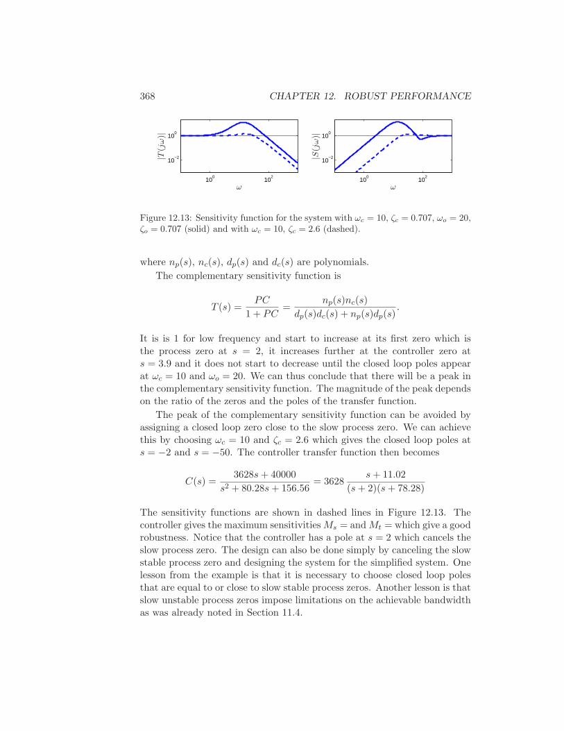
368 CHAPTER 12. ROBUST PERFORMANCE
100
102
10−2
100
100
102
10−2
100
|S(j
ω)|
|T(j
ω)|
ωω
Figure 12.13: Sensitivity function for the system with ωc = 10, ζc = 0.707, ωo = 20,ζo = 0.707 (solid) and with ωc = 10, ζc = 2.6 (dashed).
where np(s), nc(s), dp(s) and dc(s) are polynomials.
The complementary sensitivity function is
T (s) =PC
1 + PC=
np(s)nc(s)
dp(s)dc(s) + np(s)dp(s).
It is is 1 for low frequency and start to increase at its first zero which isthe process zero at s = 2, it increases further at the controller zero ats = 3.9 and it does not start to decrease until the closed loop poles appearat ωc = 10 and ωo = 20. We can thus conclude that there will be a peak inthe complementary sensitivity function. The magnitude of the peak dependson the ratio of the zeros and the poles of the transfer function.
The peak of the complementary sensitivity function can be avoided byassigning a closed loop zero close to the slow process zero. We can achievethis by choosing ωc = 10 and ζc = 2.6 which gives the closed loop poles ats = −2 and s = −50. The controller transfer function then becomes
C(s) =3628s+ 40000
s2 + 80.28s+ 156.56= 3628
s+ 11.02
(s+ 2)(s+ 78.28)
The sensitivity functions are shown in dashed lines in Figure 12.13. Thecontroller gives the maximum sensitivitiesMs = andMt = which give a goodrobustness. Notice that the controller has a pole at s = 2 which cancels theslow process zero. The design can also be done simply by canceling the slowstable process zero and designing the system for the simplified system. Onelesson from the example is that it is necessary to choose closed loop polesthat are equal to or close to slow stable process zeros. Another lesson is thatslow unstable process zeros impose limitations on the achievable bandwidthas was already noted in Section 11.4.
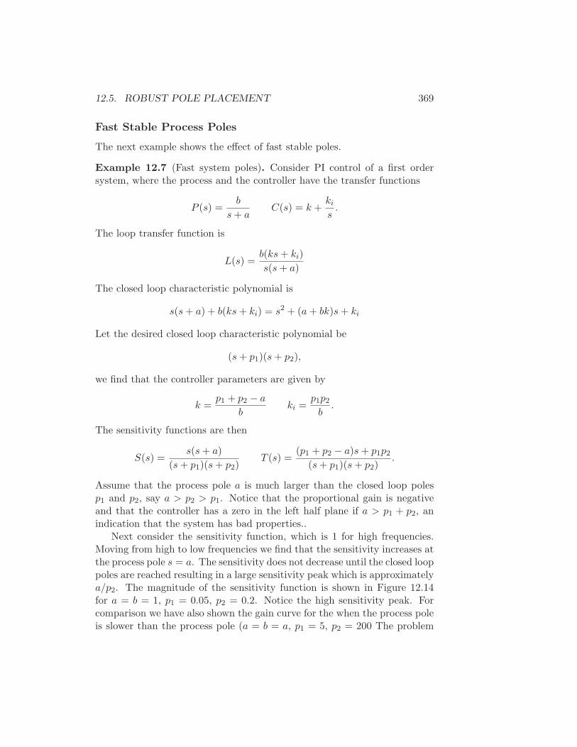
12.5. ROBUST POLE PLACEMENT 369
Fast Stable Process Poles
The next example shows the effect of fast stable poles.
Example 12.7 (Fast system poles). Consider PI control of a first ordersystem, where the process and the controller have the transfer functions
P (s) =b
s+ aC(s) = k +
ki
s.
The loop transfer function is
L(s) =b(ks+ ki)
s(s+ a)
The closed loop characteristic polynomial is
s(s+ a) + b(ks+ ki) = s2 + (a+ bk)s+ ki
Let the desired closed loop characteristic polynomial be
(s+ p1)(s+ p2),
we find that the controller parameters are given by
k =p1 + p2 − a
bki =
p1p2
b.
The sensitivity functions are then
S(s) =s(s+ a)
(s+ p1)(s+ p2)T (s) =
(p1 + p2 − a)s+ p1p2
(s+ p1)(s+ p2).
Assume that the process pole a is much larger than the closed loop polesp1 and p2, say a > p2 > p1. Notice that the proportional gain is negativeand that the controller has a zero in the left half plane if a > p1 + p2, anindication that the system has bad properties..
Next consider the sensitivity function, which is 1 for high frequencies.Moving from high to low frequencies we find that the sensitivity increases atthe process pole s = a. The sensitivity does not decrease until the closed looppoles are reached resulting in a large sensitivity peak which is approximatelya/p2. The magnitude of the sensitivity function is shown in Figure 12.14for a = b = 1, p1 = 0.05, p2 = 0.2. Notice the high sensitivity peak. Forcomparison we have also shown the gain curve for the when the process poleis slower than the process pole (a = b = a, p1 = 5, p2 = 200 The problem
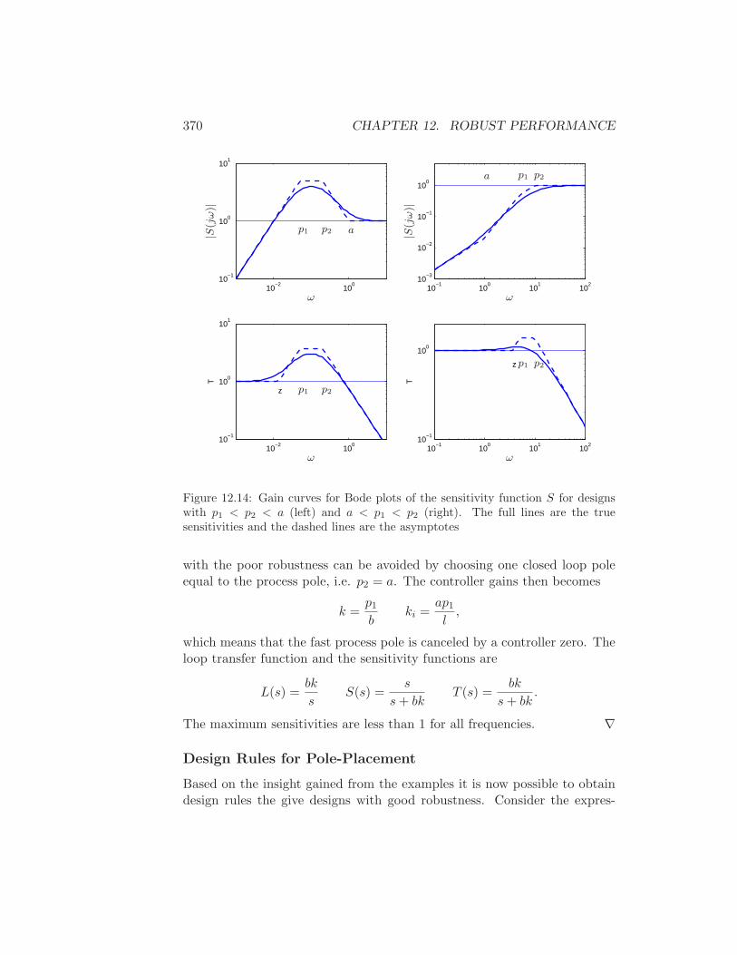
370 CHAPTER 12. ROBUST PERFORMANCE
10−2
100
10−1
100
101
10−2
100
10−1
100
101
z
T
10−1
100
101
102
10−3
10−2
10−1
100
10−1
100
101
102
10−1
100
z
T
ω
ω
ω
ω
|S(j
ω)|
|S(j
ω)|
a
a
p1
p1
p1
p1
p2
p2
p2
p2
Figure 12.14: Gain curves for Bode plots of the sensitivity function S for designswith p1 < p2 < a (left) and a < p1 < p2 (right). The full lines are the truesensitivities and the dashed lines are the asymptotes
with the poor robustness can be avoided by choosing one closed loop poleequal to the process pole, i.e. p2 = a. The controller gains then becomes
k =p1
bki =
ap1
l,
which means that the fast process pole is canceled by a controller zero. Theloop transfer function and the sensitivity functions are
L(s) =bk
sS(s) =
s
s+ bkT (s) =
bk
s+ bk.
The maximum sensitivities are less than 1 for all frequencies. ∇
Design Rules for Pole-Placement
Based on the insight gained from the examples it is now possible to obtaindesign rules the give designs with good robustness. Consider the expres-
12.6. DESIGN FOR ROBUST PERFORMANCE 371
sion (12.5) for the complementary sensitivity function. Let wgc be the de-sired gain crossover frequency. Assume that the process has zeros whichare slower than ωgc. The complementary sensitivity function is one for lowfrequencies and it increases for frequencies close to the process zeros unlessthere is a closed loop pole in the neighborhood. To avoid large values ofthe complementary sensitivity function we find that the closed loop systemshould have poles close to or equal to the slow stable zeros. This meansthat slow stable zeros should be canceled by controller poles. Since unsta-ble zeros cannot be canceled slow stable zeros the presence of slow unstablezeros means that achievable gain crossover frequency must be smaller thanthe slowest unstable process zero, (see Section 11.3).
Now consider process poles that are faster than the desired gain crossoverfrequency. Consider the expression (12.5) for the sensitivity function. Thesensitivity function is 1 for high frequencies. Moving from high to low fre-quencies the sensitivity function increases at the fast process poles. Largepeaks can be obtained unless there are closed loop poles close to the fastprocess poles. To avoid large peaks in the sensitivity the closed loop systemshould be have poles close that matches the fast process poles. This meansthat the controller should cancel the fast process poles by controller zeros.Since unstable modes cannot be canceled, the presence of a fast unstablepole implies that the gain crossover frequency must be sufficiently large,(see Section 11.3).
To summarize, we obtain the following simple design rule: slow stableprocess zeros should be matched slow closed loop poles and fast stable pro-cess poles should be matched by fast process poles. Slow unstable processzeros and fast unstable process poles impose severe limitations.
12.6 Design for Robust Performance
Control design is a rich problem where many factors have to be taken intoaccount. Typical requirements are that load disturbances should be attenu-ated, the controller should only inject a moderate amount of measurementnoise, the output should follow variations in the command signal well andthe closed loop system should be insensitive to process variations. For thesystem in Figure 12.9 these requirements can be captured by specificationson the sensitivity functions S and T and the transfer functions Gyd, Gun,Gyr and Gur. Notice that it is necessary to consider at least six transfer func-tions, as discussed Section 11.1. The requirements are mutually conflictingand it is necessary to make trade-offs. Attenuation of load disturbances will
372 CHAPTER 12. ROBUST PERFORMANCE
be improved if the bandwidth is increased but so will the noise injection.
It is highly desirable to have design methods that can guarantee ro-bust performance. Such design methods did not appear until the late 1980.There are many issues to consider in control design. It is interesting thatmany design methods result in controllers having the same structure as thecontroller based on state feedback and an observer.
Linear Quadratic Control LQG
One way to make the trade-off between attenuation of load disturbances andinjection of measurement noise is to design a controller which minimizes theloss function
J =1
T
∫ T
0(y2(t) + ρu2(t))dt,
where ρ is a weighting parameters as discussed in Section 6.5. This lossfunction gives a compromise between load disturbance attenuation and dis-turbance injection because it balances control actions against deviations inthe output. If all state variables are measured, the controller is a statefeedback
u = K(xm − x).
The controller has the same form as the controller obtained by pole assign-ment in Section 6.2. The controller gain is, however, obtained by solvingthe optimization problem. It has been shown that this controller is veryrobust. It has a phase margin of at least 60 and an infinite gain margin.The controller is called a linear quadratic control or LQ control because theprocess model is linear and the criterion is quadratic.
When all state variables are not measured, the state can be reconstructedusing an observer as discussed in Section 7.3. It is also possible to introduceprocess disturbances and measurement noise explicitly in the model and toreconstruct the states using a Kalman filter. The Kalman filter has thesame structure as the observer designed by pole assignment in Section 7.3,but the observer gains L are now obtained by solving an optimization prob-lem. The control law obtained by combining linear quadratic control witha Kalman filter is called linear quadratic Gaussian control or LQG Control.The Kalman filter is optimal when the models for load disturbances andmeasurement noise are Gaussian.
It is interesting that the solution to the optimization problem leads toa controller having the structure of a state feedback and an observer. Thestate-feedback gains depend on the parameter ρ and the filter gains depend
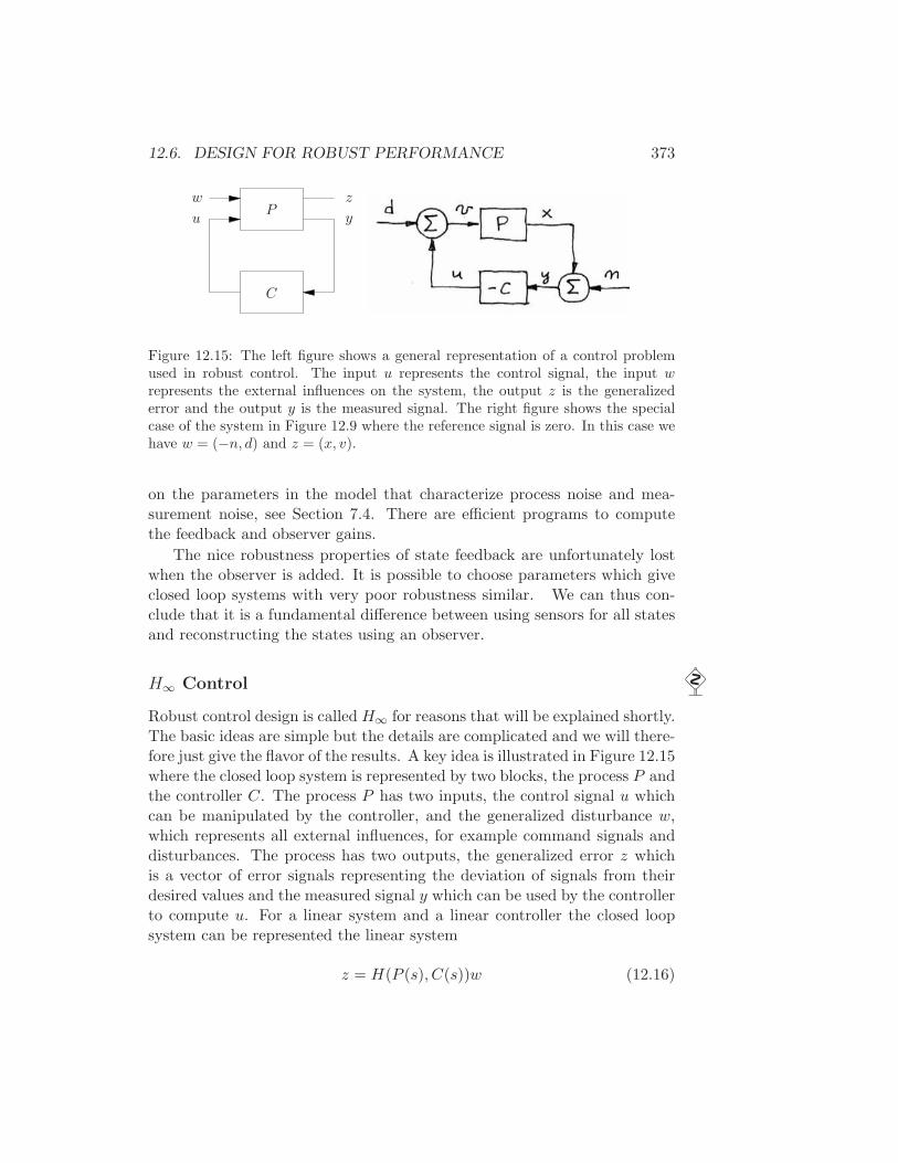
12.6. DESIGN FOR ROBUST PERFORMANCE 373
C
Pyu
zw
Figure 12.15: The left figure shows a general representation of a control problemused in robust control. The input u represents the control signal, the input wrepresents the external influences on the system, the output z is the generalizederror and the output y is the measured signal. The right figure shows the specialcase of the system in Figure 12.9 where the reference signal is zero. In this case wehave w = (−n, d) and z = (x, v).
on the parameters in the model that characterize process noise and mea-surement noise, see Section 7.4. There are efficient programs to computethe feedback and observer gains.
The nice robustness properties of state feedback are unfortunately lostwhen the observer is added. It is possible to choose parameters which giveclosed loop systems with very poor robustness similar. We can thus con-clude that it is a fundamental difference between using sensors for all statesand reconstructing the states using an observer.
H∞ Control
Robust control design is called H∞ for reasons that will be explained shortly.The basic ideas are simple but the details are complicated and we will there-fore just give the flavor of the results. A key idea is illustrated in Figure 12.15where the closed loop system is represented by two blocks, the process P andthe controller C. The process P has two inputs, the control signal u whichcan be manipulated by the controller, and the generalized disturbance w,which represents all external influences, for example command signals anddisturbances. The process has two outputs, the generalized error z whichis a vector of error signals representing the deviation of signals from theirdesired values and the measured signal y which can be used by the controllerto compute u. For a linear system and a linear controller the closed loopsystem can be represented the linear system
z = H(P (s), C(s))w (12.16)
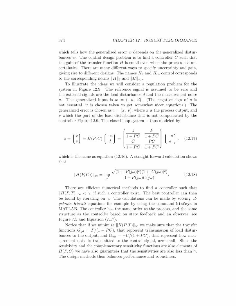
374 CHAPTER 12. ROBUST PERFORMANCE
which tells how the generalized error w depends on the generalized distur-bances w. The control design problem is to find a controller C such thatthe gain of the transfer function H is small even when the process has un-certainties. There are many different ways to specify uncertainty and gain,giving rise to different designs. The names H2 and H∞ control correspondsto the corresponding norms ‖H‖2 and ‖H‖∞.
To illustrate the ideas we will consider a regulation problem for thesystem in Figure 12.9. The reference signal is assumed to be zero andthe external signals are the load disturbance d and the measurement noisen. The generalized input is w = (−n, d). (The negative sign of n isnot essential, it is chosen taken to get somewhat nicer equations.) Thegeneralized error is chosen as z = (x, v), where x is the process output, andv which the part of the load disturbance that is not compensated by thecontroller Figure 12.9. The closed loop system is thus modeled by
z =
xv
= H(P,C)
−nd
=
1
1 + PC
P
1 + PCC
1 + PC
PC
1 + PC
−nd
, (12.17)
which is the same as equation (12.16). A straight forward calculation showsthat
‖H(P,C))‖∞ = supω
√
(1 + |P (jω)|2)(1 + |C(jω)|2)|1 + P (jω)C(jω)| . (12.18)
There are efficient numerical methods to find a controller such that‖H(P, T )‖∞ < γ, if such a controller exist. The best controller can thenbe found by iterating on γ. The calculations can be made by solving al-gebraic Riccati equations for example by using the command hinfsyn inMATLAB. The controller has the same order as the process, and the samestructure as the controller based on state feedback and an observer, seeFigure 7.5 and Equation (7.17).
Notice that if we minimize ‖H(P, T )‖∞ we make sure that the transferfunctions Gyd = P/(1 + PC), that represent transmission of load distur-bances to the output, and Gun = −C/(1 + PC), that represent how mea-surement noise is transmitted to the control signal, are small. Since thesensitivity and the complementary sensitivity functions are also elements ofH(P,C) we have also guarantees that the sensitivities are also less than γ.The design methods thus balances performance and robustness.
12.6. DESIGN FOR ROBUST PERFORMANCE 375
Figure 12.16: Block diagrams of a system with disturbance weighting.
Disturbance Weighting
Minimizing the gain ‖H(P,C)‖∞ means that gains of all individual signaltransmissions from disturbances to outputs are less that γ for all frequen-cies of the input signals. The assumption that the disturbances are equallyimportant and that all frequencies are also equally important is not veryrealistic, recall that load disturbances typically have low frequencies andmeasurement noise is typically dominated by high frequencies. It is straightforward to modify the problem so that disturbances of different frequenciesare given different emphasis, by introducing a weighting filter on the loaddisturbance as shown in Figure 12.15. For example low frequency load dis-turbances will be enhanced by choosing Wd as a low pass filter because theactual load disturbance is Wdd. By using block diagram manipulation asshown in Figure 12.16 we find that the system with frequency weighting isequivalent to the system with no frequency weighting in Figure 12.16 andthe signals are related through
zw =
xv
1
1 + PwCw
Pw
1 + PwCw
Cw
1 + P + wCw
PwCw
1 + PwCw
−nd
= H(Pw, Cw)ww
(12.19)where Pw = PWd and Cw = W−1
d C. The problem of finding a controller Cw
which minimizes the gain of H(Pw, Cw) is thus equivalent to the problemwithout disturbance weighting, having obtained Cw the controller for theoriginal system is then C = WdC. Notice that if we introduce the frequencyweighting Wd = k/s we will automatically get a controller with integralaction.
376 CHAPTER 12. ROBUST PERFORMANCE
Robustness
There are strong robustness results associated with the H∞ controller. Wecan understand this intuitively by comparing Equations (12.1) and (12.18).We can then conclude that
‖H(P,C)‖∞ =1
d(P,−1/C)(12.20)
The inverse of ‖H(P,C)‖∞ is thus equal to chordal distance between P and1/C. If we find a controller C with ‖H(P,C)‖∞ < γ this controller willthen stabilize any process P∗ such that d(P, P∗) < γ.
Limits of Robust Design
There is a limit to what can be achieved by robust design. In spite of the niceproperties of feedback there are situations where the process variations areso large that it is not possible to find a linear controller which gives a robustsystem with good performance. It is then necessary to use other controllers.In some cases it is possible to measure a variable that is well correlatedwith the process variations. Controllers for different parameters values canthen be designed and the corresponding controller can be chosen based onthe measured signal. This type of controller is called gain scheduling. Thecruise controller is a typical example where the measured signal could begear position and velocity. Gain scheduling is the common solution for highperformance aircraft where scheduling is done based on Mach number anddynamic pressure. When using gain scheduling it is important to make surethat switches between the controllers do not create undesirable transients.
If it is not possible to measure variables related to the parameters, it ispossible to use automatic tuning and adaptive control. In automatic tuningprocess dynamics is measured by perturbing the system and a controlleris then designed automatically. Automatic tuning requires that parametersremain constant, it has been widely applied for PID control, it is a reasonableguess that, in the future, many controllers will have features for automatictuning. If parameters are changing it is possible to use adaptive methodswhere where process dynamics is measured on-line.
12.7 Further Reading
Robustness was a central issue in classical control, see [Bod45]. It wasdeemphasized in the euphoria of the development of design methods based
12.8. EXERCISES 377
on optimization. The strong robustness of LQ control based on state feed-back shown by Anderson and Moore [?] contributed to the optimism. Thepoor robustness of output feedback based on LQG was pointed out by Rosen-brock [RM71], Horowitz [Hor75] and Doyle [Doy78] resulted in a renewedinterest in robustness. A major step forward was the development of designmethods where robustness was explicitly taken into account. Seminal workby Zames [Zam81] was a major step forward. Robust control was origi-nally developed using powerful results from the theory of complex variableswhich unfortunately gave controllers of very high order. A major breakthrough was given by Doyle, Glover, Khargonekar, and Francis [DGKF89]who showed that the solution could be obtained using Riccati equations andthat a controller of low order could be found. This paper led to an exten-sive treatment of the so-called H∞ control [Fra87, MG90, DFT92, GL95,ZDG96, SP96, Vin01]. A major advantage of the theory is that it combinesmuch of the intuition from servomechanism theory with sound numericalalgorithms based on numerical linear algebra and optimization. The resultshave been extended to nonlinear systems by treating the design problem asa game where the disturbances are generated by an adversary as describedin [BB91]. Auto-tuning and adaptive control are treated in [AW95] andautomatic tuning is dealt with in depth in [AH05].
12.8 Exercises
1. Show that an additive disturbance δadd, show that it can create RHPzeros, but not RHP poles, and that a feedback disturbance δfbk cancreate RHP poles but not RHP zeros. Also give constructive examples.
2. Compute the distance between the systems
P1(s) =k
s+ 1, andP2(s) =
k
s− 11.
for k = 1, 2 and 5.
3. The distance measure is closely related to closed loop systems withunit feedback. Show how the measure can be modified to applied toan arbitrary feedback.
4. Consider the Nyquist curve in Figure 12.12. Explain why part of thecurve is approximately a circle. Derive a formula for the center andthe radius and compare with the actual Nyquist curve.
378 CHAPTER 12. ROBUST PERFORMANCE
5. Consider the transfer functions in examples 12.2 and 12.3. Computethe distance measure δ(P1, P1) in both cases. Repeat the calculationswhen the controller is C = 0.1.
6. (Ideal Delay Compensator) Consider a process whose dynamics is apure time delay, the transfer function is P (s) = e−s. The ideal delaycompensator is a controller with the transfer function C(s) = 1/(1 −e−s). Show that the sensitivity functions are T (s) = e−s and S(s) =1− e−s and that the closed loop system will be unstable for arbitrarysmall changes in the delay.
7. Let P and C be matrices whose entries are complex numbers, showthat the singular values of the matrix
H(P,C) =
1
1 + PC
P
1 + PCC
1 + PC
PC
1 + PC
are σ1 = 0 and σ2 = supω
√
(1 + |P (jω)|2)(1 + |C(jω)|2)|1 + P (jω)C(jω)
.
8. Show that
supw
|1 + P (jω)C(jω)|√
(1 + |P (jω)|2)(1 + |C(jω)|2)= d(P,−1/C)

Bibliography
[Abk69] M. A. Abkowitz. Stability and Motion Control of Ocean Vehicles. MITPress, Cambridge, MA, 1969.
[AH95] K. J. Astrom and T. Hagglund. PID Controllers; Theory, Design andTuning. Instrument Society of American, 1995.
[AH05] Karl Johan Astrom and Tore Hagglund. Advanced PID Control. ISA- The Instrumentation, Systems, and Automation Society, ResearchTriangle Park, NC 27709, 2005.
[AKL05] K. J. Astrom, R. E. Klein, and A. Lennartsson. Bicycle dynamics andcontrol. IEEE Control Systems Magazine, 25(4):26–47, 2005.
[Ang61] A. I. Angstrom. Neue Methode, das varmeleitungsvermogen der Korperzu bestimmen. Ann. der Physik und Chemie, 114:513–530, 1861.
[Ast70] K. J. Astrom. Introduction to Stochastic Control Theory. AcademicPress, 1970. Republished by Dover Publications, 2006.
[AW95] K. J. Astrom and B. Wittenmark. Adaptive Control. Addison-Wesley,Reading, Massachusetts, second edition, 1995.
[BA70] R. Bellman and K. J. Astrom. On structural identifiability. Mathemat-ical Biosciences, 7:329–339, 1970.
[BB91] T. Basar and P. Bernhard. H∞-Optimal control and related minimaxdesign problems - A Dynamic game approach. Birkhauser, Boston, 1991.
[Bec05] J. Bechhoefer. Feedback for physicists: A tutorial essay on control.Reviews of Modern Physics, 77:783–836, 2005.
[Ben86a] S. Bennett. A History of Control Engineering: 1800–1930. Peter Pere-grinus, 1986.
[Ben86b] S. Bennett. A History of Control Engineering: 1930–1955. Peter Pere-grinus, 1986.
[Ber54] L. L. Beranek. Acoustics. McGraw-Hill, New York, NY, 1954.
[BK64] R. E. Bellman and R. Kalaba. Selected Papers on Mathematical Trendsin Control Theory. Dover, New York, NY, 1964.
379
380 BIBLIOGRAPHY
[Bla34] H. S. Black. Stabilized feedback amplifiers. Bell System Technical Jour-nal, 13:1–2, 1934.
[Bla91] J. H. Blakelock. Automatic Control of Aircraft and Missiles. Addison-Wesley, Cambridge, MA, second edition, 1991.
[Bod45] H. W. Bode. Network Analaysis and Feedback Amplifier Design. VanNostrand, 1945.
[Bod60] H. W. Bode. Feedback—The History of an Idea. In Symposium on Ac-tive Networks and Feedback Systems. Polytechnic Institute of Brooklyn,1960. in [BK64].
[BP96] M. B. Barron and W. F. Powers. The role of electronic controls for futureautomotive mechatronic systems. IEEE Transactions on Mechatronics,1(1):80–89, 1996.
[Bro00] R. W. Brockett. New issues in the mathematics of control. In B. En-gquist and W. Schmid, editors, Mathematics Unlimited—2001 and Be-yond, pages 189–220. Springer Verlag, 2000.
[BS60] J. F. andG. Reethof Blackburn and J.L. Shearer. Fluid Power Control.MIT Press, Cambridge, MA, 1960.
[Can03] R. H. Cannon. Dynamics of Physical Systems. Dover, originally pub-lished by mc-graw hill 1967 edition, 2003.
[CD75] R. F. Coughlin and F. F. Driscoll. Operational Amplifiers and LinearIntegrated Circuits. 6th Edition. Prentice Hall, Englewood Cliffs, NJ,1975.
[CD91] F. M. Callier and C. A. Desoer. Linear System Theory. Springer-Verlag,1991.
[CJ59] H. S. Carslaw and J. C. Jaeger. Conduction of Heat in Solids. CarendonPress, Oxford, second edition, 1959.
[DB04] R. C. Dorf and R. H. Bishop. Modern Control Systems. Prentice Hall,tenth edition, 2004.
[DFT92] J. C. Doyle, B. A. Francis, and A. R. Tannenbaum. Feedback ControlTheory. Macmillan Publishing Company, 1992.
[DGKF89] J. C. Doyle, K. Glover, P. P. Khargonekar, and B. A. Francis. State-space solutions to standard H2 and H∞ control problems. IEEE Trans-actions on Automatic Control, 34(8):831–847, 1989.
[DH85] J.P. Den Hartog. Mechanical Vibrations. Dover, New York, 1985.Reprint of fourth edition from 1956, first edition published in 1934.
[dJ02] H. de Jong. Modeling and simulation of genetic regulatory systems: Aliterature review. Journal of Computational Biology, 9:67–103, 2002.
BIBLIOGRAPHY 381
[DM02] L. Desbourough and R. Miller. Increasing customer value of indus-trial control performance monitoring - Honeywell’s experience. In SixthInternational Conference on Chemical Process Control. AIChE Sympo-sium Series Number 326 (Volume 98), 2002.
[Dos68] F.H. Dost. Grundlagen der Pharmakokinetik. Thieme Verlag, Stuttgart,1968.
[Doy78] J. C. Doyle. Guaranteed margins for lqg regulators. IEEE Transactionson Automatic Control, 23(4):756–757, 1978.
[Dys04] F. Dyson. A meeting with enrico fermi. Nature, 247(6972):297, 2004.
[EG05] S. P. Ellner and J. Guckenheimer. Dynamic Models in Biology. Prince-ton University Press, 2005.
[EL00] M. B. Elowitz and S. Leibler. A synthetic oscillatory network of tran-scriptional regulators. Nature, 403(6767):335–338, 2000.
[Ell94] J. R. Ellis. Vehicle Handling Dynamics. Mechanical Engineering Pub-lications, London, 1994.
[Fey70] R. P. Feynmann. Lectures on Physics. Addison Wesley, New York, NY,1970.
[Fou07] J. B. J. Fourier. On the Propagation of Heat in Solid Bodies. 1807.
[FPEN05] G. F. Franklin, J. D. Powell, and A. Emami-Naeini. Feedback Controlof Dynamic Systems. Addison Wesley Longman, fifth edition, 2005.
[Fra87] B. A. Francis. A Course in H∞ Control. Springer-Verlag, Berlin, 1987.
[Fri04] B. Friedland. Control System Design: An Introduction to State SpaceMethods. Dover, 2004.
[GB42] M. A. Gardner and J. L. Barnes. Transients in Linear Systems. JohnWiley, New York, 1942.
[GF71] L. Gunkel and G. F. Franklin. A general solution for linear sampleddata systems. IEEE Transactions on Automatic Control, AC-16:767–775, 1971.
[GH83] J. Guckenheimer and P. Holmes. Nonlinear Oscillations, DynamicalSystems, and Bifurcations of Vector Fields. Springer Verlag, 1983.
[Gil63] E. Gilbert. Controllability and observability in multivariable controlsystems. SIAM J. Control, 1(1):128–151, 1963.
[GL95] Michael Green and D. J. N. Limebeer. Linear Robust Control. PrenticeHall, Englewood Cliffs, N.J., 1995.
[God83] K. Godfrey. Compartment models and their application. AcademicPress, New York, NY, 1983.
382 BIBLIOGRAPHY
[Gol53] H. Goldstein. Classical Mechanics. Addison-Wesley, Cambridge, MA,1953.
[Gol70] S. W. Golomb. Mathematical models—uses and limitations. Simulation,4(14):197–198, 1970.
[GP82] M. Giobaldi and D. Perrier. Pharmacokinetics, Second Edition. MarcelDekker, New York, 1982.
[Gui63] E. A. Guillemin. Theory of Linear Physical Systems. MIT Press, Cam-bridge, MA, 1963.
[HB90] J. K. Hedrick and T. Batsuen. Invariant properties of automobile sus-pensions. In Proc. Institution of Mechanical Engineers, volume 204,pages 21–27, London, UK., 1990.
[HD95] M. B. Hoagland and B. Dodson. The Way Life Works. Times Books,1995.
[HDPT04] J. L. Hellerstein, Y. Diao, S. Parekh, and D. M. Tilbury. FeedbackControl of Computing Systems. John Wiley, New York, 2004.
[Hen06] Dan Henriksson. Resource-Constrained Embedded Control and Com-puting Systems. PhD thesis, Department of Automatic Control, LundInstitute of Technology, Sweden, January 2006.
[Her04] David V. Herlihy. Bicycle - The History. Yale University Press, Yale,NH, 2004.
[HH52] A. L. Hodgkin and A. F. Huxley. A quantitative description of mem-brane current and its application to conduction and excitation in nerve.Journal of Physiology, 117(500–544), 1952.
[HLA04] D. Henriksson, Y. Lu, and T. Abdelzaher. Improved prediction forweb server delay control. In 16th Euromicro Conference on Real-TimeSystems, Catania, Sicily, Italia, 2004.
[Hor75] I. M. Horowitz. Superiority of transfer function over state-varible meth-ods in linear, time-invariant feedback system design. IEEE Transactionson Automatic Control, AC-20(1):84–97, 1975.
[HW00] D. Hanahan and R. A. Weinberg. The hallmarks of cancer. Cell, 100:57–70, 2000.
[Isi89] A. Isidori. Nonlinear Control Systems. Springer-Verlag, 2nd edition,1989.
[Jac72] J. A. Jacquez. Compartment analysis in biology and medicine. Elsevier,Amsterdam, 1972.
[Jac88] V. Jacobson. Congestion avoidance and control. In Proc. SIGCOMM’88, pages 314–329, 1988.
BIBLIOGRAPHY 383
[JNP47] H. James, N. Nichols, and R. Philips. Theory of Servomechanisms.McGraw-Hill, 1947.
[JT61] P. D. Joseph and J. T. Tou. On linear control theory. Transactions ofAIEE, 80(18), 1961.
[Jun02] W. G. (editor) Jung, editor. Op Amp Applications. Analog Devices,Norwood, MA, 2002.
[Kal60] R. E. Kalman. Contributions to the theory of optimal control. Boletinde la Sociedad Matematica Mexicana, 5:102–119, 1960.
[Kal61a] R. E. Kalman. New methods and results in linear prediction and filter-ing theory. Technical Report 61-1, RIAS, February 1961. 135 pp.
[Kal61b] R. E. Kalman. On the general theory of control systems. In Proceedingsfirst IFAC Congress on Automatic Control, Moscow, 1960, volume 1,pages 481–492, London, 1961. Butterworths.
[KB61] R. E. Kalman and R. S. Bucy. New results in linear filtering and predic-tion theory. Trans ASME (J. Basic Engineering), 83 D:95–108, 1961.
[Kel85] F. P. Kelley. Stochastic models of computer communication. J. RoyalStatistical Society, B47(3):379–395, 1985.
[Kel94] K. Kelly. Out of Control. Addison-Wesley, 1994. Available at http:
//www.kk.org/outofcontrol.
[KFA69] R. E. Kalman, P. L. Falb, and M. A. Arbib. Topics in MathematicalSystem Theory. McGraw-Hill, 1969.
[KG02] B. C. Kuo and F. Golnaraghi. Automatic Control Systems. Wiley,eighth edition, 2002.
[Kha92] H. K. Khalil. Nonlinear Systems. Macmillan Publishing Company, 1992.
[KHN63] R. E. Kalman, Y. Ho, and K. S. Narendra. Controllability of Linear Dy-namical Systems, volume 1 of Contributions to Differential Equations.John Wiley & Sons, Inc., New York, 1963.
[Kit95] C. Kittel. Introduction to Solid State Physics. John Wiley, New York,1995.
[KN00] U. Kiencke and L. Nielsen. Automotive Control Systems : For Engine,Driveline, and Vehicle. Springer, Berlin, 2000.
[Kum01] P. R. Kumar. New technological vistas for systems and control: Theexample of wireless networks. Control Systems Magazine, 21(1):24–37,2001.
[LA96] D. C. Liaw and E. H. Abed. Control of compressor stall inception: Abifurcation-theoretic approach. Automatica, 32(1):109–115, 1996.
384 BIBLIOGRAPHY
[Lue71] D. G. Luenberger. An introduction to observers. IEEE Transactionson Automatic Control, 5(10):213–214, 1971.
[Lun05] K. H. Lundberg. History of analog computing. IEEE Control SystemsMagazine, 25(3):22–28, 2005.
[Mac37] D. A. MacLulich. Fluctuations in the numbers of the varying hare (Le-pus americanus). University of Toronto Press, 1937.
[Man02] R. Mancini. Op Amps for Everyone. Texas Instruments, Houston. TX,2002.
[May70] O. Mayr. The Origins of Feedback Control. MIT Press, 1970.
[McF53] M. W. McFarland, editor. The Papers of Wilbur and Orville Wright.McGraw Hill, 1953.
[MG90] D. C. MacFarlane and K. Glover. Robust controller design using nor-malized coprime factor plant descriptions. Springer, New York, 1990.
[Mil66] H. T. Milhorn. The Application of Control Theory to PhysiologicalSystems. Saunders, 1966.
[Min02] D. A. Mindel. Between Human and Machine: Feedback, Control, andComputing Before Cybernetics. Johns Hopkins University Press, 2002.
[MR94] J. E. Marsden and T. S. Ratiu. Introduction to Mechanics and Symme-try. Springer Verlag, 1994.
[MS93] L. Moore and D. Smith. Predator-prey models, 1993. http://www.
math.duke.edu/education/ccp.
[Mur03] R. M. Murray, editor. Control in an Information Rich World: Reportof the Panel on Future Direcitons in Control, Dynamics and Systems.SIAM, 2003. Available at http://www.cds.caltech.edu/∼murray/
cdspanel.
[Mur04] J. D. Murray. Mathematical Biology, volume I and II. Springer, thirdedition, 2004.
[NS99] H. Nijmeijer and J. M. Schumacher. Four decades of mathematicalsystem theory. In J. W. Polderman and H. L. Trentelman, editors,The Mathematics of Systems and Control: From Intelligent Control toBehavioral Systems, pages 73–83. Univ. of Groningen, 1999.
[Nyq32] H. Nyquist. Regeneration theory. Bell System Technical Journal,11:126–147, 1932.
[Oga01] K. Ogata. Modern Control Engineering. Prentice-Hall, fourth editionedition, 2001.
[Phi48] G. A. Philbrick. Designing industrial controllers by analog. Electronics,21(6):108–111, 1948.
BIBLIOGRAPHY 385
[Pit99] J. Pitman. Probability. Springer, 1999.
[PPP02] S. Prajna, A. Papachristodoulou, and P. A. Parrilo. SOSTOOLS: Sumof squares optimization toolbox for MATLAB, 2002. Available fromhttp://www.cds.caltech.edu/sostools.
[RM71] H. H. Rosenbrock and P. D. Moran. Good, bad or optimal? IEEETransactions on Automatic Control, AC-16(6):552–554, 1971.
[Row58] F. Rowsone Jr. What it’s like to drive an auto-pilot car. PopularScience Monthly, April 1958. Available at http://www.imperialclub.com/ImFormativeArticles/1958AutoPilot.
[Sar91] D Sarid. Atomic Force Microscopy. Oxford University Press, Oxford,1991.
[Sch01] G. Schitter. High performance feedback for fast scanning atomic forcemicroscopes. Review of Scientific Instruments, 72(8):3320–3327, 2001.
[SEM03] D. E. Seborg, T. F. Edgar, and D. A. Mellichamp. Process Dynamicsand Control. Wiley, 2003.
[Sen01] S. D. Senturia. Microsystem Design. Kluwer, Boston, MA, 2001.
[She62] C. W. Sheppard. Basic Principles of the Tracer Method. John Wiley &Sons, Inc., New York,, 1962.
[SP96] S Skogestad and I. Postlethwaite. Multivariable feedback control: anal-ysis and design. Wiley, Chichester, UK, 1996.
[Sta59] L. Stark. Oscillations and noise in the human pupil servomechanism.Proceedings of the Institute of Radio Engineers, IRE-47:1925–1939,1959.
[Sta68] L. Stark. Neurological Control Systems - Studies in Bioengineering.Plenum Press, New York, N. Y., 1968.
[Sto94] S. H. Storgatz. Nonlinear Dynamics and Chaos, with Applications toPhysics, Biology, Chemistry, and Engineering. Addison-Wesley, 1994.
[Str88] G. Strang. Linear Algebra and its Applications. Harcourt Brace Jo-vanovich, San Diego, third edition, 1988.
[Teo37] T. Teorell. Kinetics of distribution of substances administered to thebody i and ii. Archives Internationales de Pharmacodynamie et de Ther-apie, 57:205–240, 1937.
[Til01] M. Tiller, editor. Introduction to Physical Modeling with Modelica.Springer, 20001.
[Tsi54] H. S. Tsien. Engineering Cybernetics. McGraw-Hill, 1954.
[Vin01] G. Vinnicombe. Uncertainty and Feedback: H∞ loop-shaping and theν-gap metric. Imperial College Press, London, 2001.
386 BIBLIOGRAPHY
[Whi99] F. J. W. Whipple. The stability of the motion of a bicycle. QuarterlyJournal of Pure and Applied Math., 30:312–348, 1899.
[Wie48] N. Wiener. Cybernetics: Or Control and Communication in the Animaland the Machine. John Wiley, 1948.
[Wig90] S. Wiggins. Introduction to Applied Nonlinear Dynamical Systems andChaos. Springer-Verlag, 1990.
[Wil99] H. R. Wilson. Spikes, Decisions, and Actions: The Dynamical Founda-tions of Neuroscience. Oxford University Press, 1999.
[Wil04] D. G. Wilson. Bicycling Science. MIT Press, Cambridge, MA, 2004.Third edition, with contributions by Jim Papadopoulos.
[WT24] E. P. M. Widmark and J. Tandberg. Uber die bedinungen fr die akku-mulation indifferenter narkotika. Biochemische Zeitung, 148:358–389,1924.
[Zam81] G. Zames. Feedback and optimal sensitivity: Model reference transfor-mations, multiplicative seminorms, and approximative inverse. IEEETransactions on Automatic Control, AC-26(2):301–320, 1981.
[ZDG96] J. C. Zhou, J. C. Doyle, and K. Glover. Robust and optimal control.Prentice Hall, New Jersey, 1996.
Index
A/D converters, see analog-to-digital con-verters
active filter, 163, 171actuation, 4, 5Adams (modeling tool), 59adaptive control, 376, 377adaptive optics, 15additive uncertainty, 349adjacency matrix, 69aerospace systems, 8airspace management, 9analog-to-digital converters, 5, 63, 318
zz, see also delta-sigma convertersanti-windup, 314argument, 260asymptotic stability, 123atomic force microscope, 95–99, 265attractor, 124autocoding, 30automatic reset, 304automatic tuning, 376, 377automobiles, 7, 24, 60, 82, 91
zz, see also cruise control, vehicle steer-ing
autonomous system, 37zz, see also time-invariant systems
autonomous vehicles, 22–23autopilot, 21AUTOSIM (modeling tool), 59
balance system, 44, 114reachability, 191
Bell Labs, 20, 299Bennett, S., 31bicycle dynamics, 83–85, 218bifurcation, 138bifurcation control, 140bifurcation diagram, 139biological engineering, 4
biological systems, 1repressilator, 72–73zz, see also drug administration, pop-
ulation dynamicsblack box models, 34Black, H. S., 20, 22, 63, 85, 88, 144, 347block diagrams, 55Bode plot, 259, 260Bode’s integral formula, 363Bode’s relations, 292Brockett, R. W., x, 1
calibration, 202carrying capacity, 103center, 124centrifugal governor, 2, 6chain of integrators, 76chemical industry, 12chordal distance, 351circular reasoning, 84closed loop, 2, 4, 7, 182, 278
versus open loop, 2, 279, 299, 323command and control, 9compartment models, 99complementary sensitivity function, 326, 361complexity
of control systems, 24component failures, robustness to, 4computation, 5computed torque, 183computer numerically controlled (CNC) ma-
chining, 8computer science
relationship to control, 6conditional stability, 287congestion control, 9, 66, 125, 132consensus, 68consumer electronics, 3control, 4–6
387

388 INDEX
as enabling technology, 8early examples, 7modeling, 39–40of bifurcations, 140successes of, 31synthesis, 30system, 4
control error, 25control law, 5, 25, 197control matrix, 43, 47controlled differential equation, 37convolution equation, 156critical point, 279critically damped, 173crossover frequency inequality, 342cruise control, 6, 7, 77–82, 141, 177, 181,
210, 281, 311, 313, 314, 348, 355cybernetics, 11
D/A converters, see digital-to-analog con-verters
damped oscillator, 112damping factor, 172DARPA Grand Challenge, 22DC gain, see zero frequency gaindeclarative description, 41delay control, 93delay margin, 289delta function, see impulsedelta-sigma converters, 63derivative action, 305derivative gain, 302derivative time constant, 302design of dynamics, 20diagonal system, 153difference equations, 46–49differential algebraic equations, 41differential equations, 35, 111–117
finite escape time, 116non-unique solutions, 116solution, 112, 151
digital-to-analog converters, 5direct term, 43, 47discrete time systems, 46disturbance rejection, 4, 6disturbances, 5, 29, 40Dodson, B., 1double integrator, 151, 188Doyle, J. C., x, 215, 345, 377
drug administration, 99–102, 207drugadministration
zz, see also compartment modelsdual, 219duality, 224ducted fan
pitch control, 338dynamic compensator, 210dynamic inversion, 183dynamical system, 33dynamics, 4, 7dynamics matrix, 43, 47, 130, 153
economic systems, 18, 24ecosystems, 4, 17eigenvalue assignment, 202, 222, 227eigenvalues, 131, 161electrical engineering, 37–38electronic amplifiers, 4, 34emissions control, 7energy systems, 18entertainment robots, 11environmental science, 4, 13, 18equilibrium point, 103, 119
stability, 122error feedback, 316, 325exponential signals, 243exponential stability, 142extended Kalman filter, 235external descriptions, 34external disturbances, 5
feedback, 1–4, 7, 20as technology enabler, 3drawbacks, 23in biological systems, 1, 2, 16–17
zz, see also biological systemsin ecological systems, 17in engineered systems, see controlin financial systems, 4in nature, 15–18loop, 4positive, see positive feedbackversus control, 4
feedback linearizable, 182feedback loop, 4feedforward, 24financial systems, 18finite escape time, 116

INDEX 389
first order system, 309flight control, 20, see also vectored thrust
aircraftflow, 36flow model, 90flyball governor, see centrifugal governorforced response, 29frequency response, 38, 52fully actuated, 252fundamental limitations, 363
gain, 170, 296–299zero frequency, see zero frequency gainzz, see also loop gain
gain crossover frequency, 289, 329gain margin, 288, 289, 329gain scheduling, 94, 235, 376Gang of Four, 326Gang of Six, 325gene regulation, 16global climate, see environmental scienceglucose regulation, 2, 99
Harrier AV-8B aircraft, 61heat propagation, 74, 250, 275, 281Heaviside, 183high frequency roll off, 360higher levels of decision making, 9, 22Hoagland, M. B., 1Hodgkin-Huxley equations, 73homeostasis, see biological systemshomogeneous solution, 147, 251Honeywell, 6
identification, see system identificationimperative description, 41impulse, 157impulse response, 149, 157, 158information science, 4information systems, 9input, 37input sensitivity function, 326input/output models, 5, 28, 34instability, 23instrumentation, 14insulin, see glucose regulationintegral action, 7, 202, 304integral control, 27integral gain, 302, 360
integral time constant, 302integral windup, 301integrator windup, 233, 313, 315intelligent machines, see roboticsinterconnection, 5internal descriptions, 34internal model principle, 228, 236Internet, 4, 9Internet Protocol (IP), 66intial value problem, 112invariant (programming), 70invariant set, 135inverse response, 295inverted pendulum, 46, 119
damped, 124linear approximation, 126
Jacobian linearization, 179Jordan decomposition, 164Jordan form, 163
trivial block, 164Josephson Junction, 64josephson junction, 64
Kalman decomposition, 272Kalman, R. E., 187Kelly, K., 31Krasovskii-Lasalle principle, 134–136
LabVIEW, vii, 59, 114Laplace transform, 268–271Laplace transforms, ixLaplacian matrix, 70Lasalle’s invariance principle, see Krasovskii-
Lasalle principlelead compensator, 338limit cycle, 120linear input/output system, 145linear quadratic control, 372linear system, 43linear systems, 38linearization, 176–183Lipschitz continuity, 117load disturbance, 324load sensitivity function, 326logistic growth model, 103loop gain, 279loop shaping, 334loop transfer function, 278

390 INDEX
LQ control, 372LTI systems, 147Lyapunov equation, 131Lyapunov function, 128, 129Lyapunov stability theorem, 128
manufacturing, 8manufacturing systems, 18Mars Exploratory Rovers, 11materials science, 12Mathematica, 30, 114MATLAB, vii, 30, 32, 58, 114, 115, 118, 164,
180, 203, 212, 226, 231, 374matrix exponential, 150–153maximum complementary sensitivity, 330maximum sensitivity, 329Mayr, O., 31measurement noise, 324measures, 29mechanical systems, 182mechanics, 34–37microsystems, 12Mindell, D., 31minimum phase, 293modal form, 159, 160mode, 154, 155, 251mode shape, 154mode: Jordan form, 165model, 33model reduction, 5, 29model uncertainty, 355Modelica, 42, 59modeling, 5, 12, 28modeling from experiments, 53
nanotechnology, 12negative definite, 128, 131negative feedback, 20networks, 9neuroscience, 73neutrally stable, 122noise, 229noise sensitivity function, 326non-minimum phase, 293non-unique solutions, 116normalization, 181Nyquist criterion, 280, 285Nyquist curve, 279Nyquist plot, 279
observability, 40, 216rank condition, 217
Observable Canonical Form, 219observable canonical form, 219observers, 215Octave, 114ODEs, see differential equationsω limit set, 134on-off control, 25open loop, 2, 189operational amplifier, 85–89, 248operational amplifier (op amp), 85order, 42order of a system, 43ordinary differential equation: controlled,
37ordinary differential equations, see differen-
tial equations, 42–46output sensitivity function, 326overdamped, 173overshoot, 168overshoot: error feedback, 331
parametric stability diagram, 139parametric uncertainty, 347particular solution, 147passivity theorem, 299pharmacokinetics, see drug administrationphase, 170
minimum vs. nonminimum, 293phase crossover frequency, 288phase margin, 289, 329phase portrait, 117physics
relationship to control, 5PI control, 27PI control, first order systems, 309PID control, 27PID controller, 340pitchfork bifurcation, 138, 141pole, 251
right half plane, 343, 344pole zero diagram, 252pollution, 7population dynamics, 102–107positive definite, 128, 131positive feedback, 25positive real, 363positive semidefinite, 128
INDEX 391
predator prey system, 47, 103, 120, 139, 204prediction, ability of controllers, 27principle of the variation of the argument,
283process control, 8, 12, 25, 29proportional control, 26
zz, see also PID controlproportional gain, 302proportional, integral, derivative control, see
PID controlprotocols, 4public awareness, 7pupil response, 266, 291pure error feedback, 325pure exponential response, 245
Q-value, 174, 263quantum systems, 17quarter car model, 273
random variable, 90reachability, 39, 188
rank condition, 190reachability matrix, 190reachable canonical form, 193, 196, 200real-time systems, 6receding horizon control, 94reference weighting, 316reference weights, 316region of attraction, 136regulation, 1relay feedback, 308reliability, 7repressilator, 72–73reset, 304resource management, 18Riccati equation, 212, 374rise time, 168robotics, 4, 11–12robustness, 19–20, 29rush-hour effect, 91
saddle, 124saturation function, 86SBML (Systems Biology Markup Language),
59Scilab, 114second order system, 35second order systems, 172
sensing, 4, 5sensitivity crossover frequency, 330sensitivity function, 326sensitivity function:disturbance attenuation,
360sensor matrix, 43, 47sensors, 13separation principle, 228setpoint, 302, 316setpoint weights, 316settling time, 168Sigma-delta converters, see delta-sigma con-
verterssimple models, 356simulation, 49SIMULINK, 58, 59, 180sink, 124small gain theorem, 298–299, 356–357Sony AIBO, 11source, 124spectrum analyzer, 265Sperry autopilot, 21SPICE (modeling tool), 59spring mass system, 49, 135, 160, 174
system identification, 54stability, 4, 5, 20, 29, 51, 122–136
exponential, 142linear system, 162local versus global, 123, 136, 137, 183
stability by linearization, 183stability margin, 289stability margins, 288stable, 49state, 35, 42state estimators, see oservers215state models, 34state space, 35, 42–55state space model, 42state vector, 42steady state
value, 168steady state gain, see zero frequency gainsteady state response, 50steam engine, 3Stein, G., x, 1step input, 166step response, 38, 149, 158, 166subcritical bifurcation, 138supercritical bifurcation, 138
392 INDEX
superposition, 145supply chains, 18supremum (sup), 297system identification, 28system: time-invariant, 43
temperature control, 1, 7thermostat, 6, 7time constant, 184time delay, 7, 9, 293, 343time invariance, 147time-invariant system, 42time-invariant systems, 38traffic management, 9trail, 84transcriptional regulation, 71transfer function, 241, 245, 247transfer function: differentiator, 247transfer function: integrator, 247transient, 188Transmission Control Protocol (TCP), 66transportation systems, 8Tsien, H. S., 11two degrees of freedom, 234
uncertainty, 5, 19–20, 40, 347–352component or parameter variation, 5unmodeled dynamics, 5, 349
undamped oscillator, 152underdamped, 113, 173unit step, 166unmodeled dynamics, 30, 349unobservable systems, 219unreachable system, 200unstable, 123unstable pole/zero cancellation, 259
vector field, 36vectored thrust aircraft, 61vehicle steering, 60, 180, 198, 225, 229, 256,
290, 296lack of robustness, 366
vertical takeoff and landing, see vectoredthrust aircraft
vibration absorber, 274
waterbed effect, 363, 364Watt governor, see centrifugal governorweb server admission control, 89–95
web site, viiwhite box, 34Wiener, N., 11winding number, 283windup, see integrator windupWright brothers, 20
Youla parameterization, 357, 358
zero, 251right half plane, 344
zero frequency gain, 171, 198, 202, 251, 303,307, 329
zeros, signal blocking property, 251Ziegler-Nichols methods, 306
Related Documents


![[ IT 융합차세대금융]sep06)1.pdf · 차세대금융시스템성공전략 [ IT 융합차세대금융] ... Cross-System Incompatibility Core System Replacement Data Access Standardizing](https://static.cupdf.com/doc/110x72/5e59daea8436f040f85bf8e2/-it-oeeoeeoe-sep061pdf-eoeeoeoeoeee-.jpg)
