ROBERT SEDGEWICK | KEVIN WAYNE FOURTH EDITION Algorithms http://algs4.cs.princeton.edu Algorithms R OBERT S EDGEWICK | K EVIN WAYNE G EOMETRIC A PPLICATIONS OF BST S ‣ 1d range search ‣ line segment intersection ‣ kd trees ‣ interval search trees ‣ rectangle intersection

Welcome message from author
This document is posted to help you gain knowledge. Please leave a comment to let me know what you think about it! Share it to your friends and learn new things together.
Transcript

ROBERT SEDGEWICK | KEVIN WAYNE
F O U R T H E D I T I O N
Algorithms
http://algs4.cs.princeton.edu
Algorithms ROBERT SEDGEWICK | KEVIN WAYNE
GEOMETRIC APPLICATIONS OF BSTS
‣ 1d range search
‣ line segment intersection
‣ kd trees
‣ interval search trees
‣ rectangle intersection
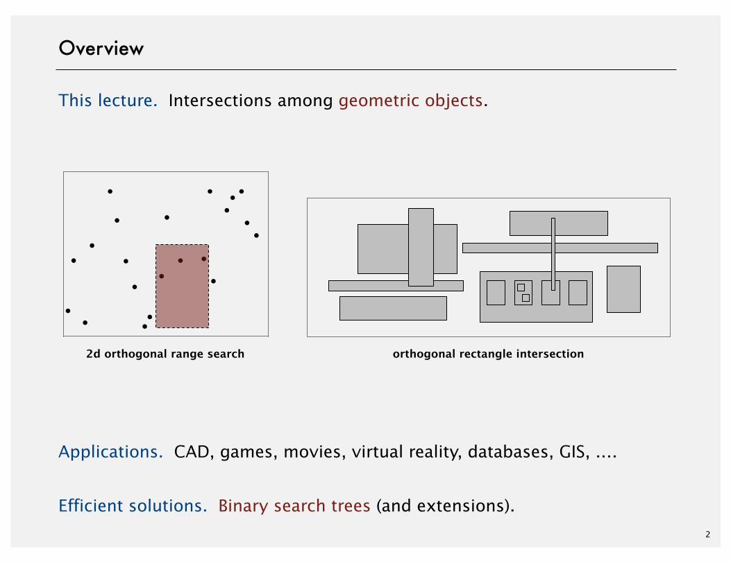
This lecture. Intersections among geometric objects.
Applications. CAD, games, movies, virtual reality, databases, GIS, .…
Efficient solutions. Binary search trees (and extensions).2
Overview
2d orthogonal range search orthogonal rectangle intersection

http://algs4.cs.princeton.edu
ROBERT SEDGEWICK | KEVIN WAYNE
Algorithms
‣ 1d range search
‣ line segment intersection
‣ kd trees
‣ interval search trees
‣ rectangle intersection
GEOMETRIC APPLICATIONS OF BSTS

4
1d range search
Extension of ordered symbol table.
・Insert key-value pair.
・Search for key k.
・Delete key k.
・Range search: find all keys between k1 and k2.
・Range count: number of keys between k1 and k2.
Application. Database queries.
Geometric interpretation.
・Keys are point on a line.
・Find/count points in a given 1d interval.
insert B B
insert D B D
insert A A B D
insert I A B D I
insert H A B D H I
insert F A B D F H I
insert P A B D F H I P
count G to K 2
search G to K H I

5
1d range search: elementary implementations
Unordered list. Fast insert, slow range search.
Ordered array. Slow insert, binary search for k1 and k2 to do range search.
data structure insert range count range search
unordered list 1 N N
ordered array N log N R + log N
goal log N log N R + log N
order of growth of running time for 1d range search
N = number of keysR = number of keys that match
6
1d range count: BST implementation
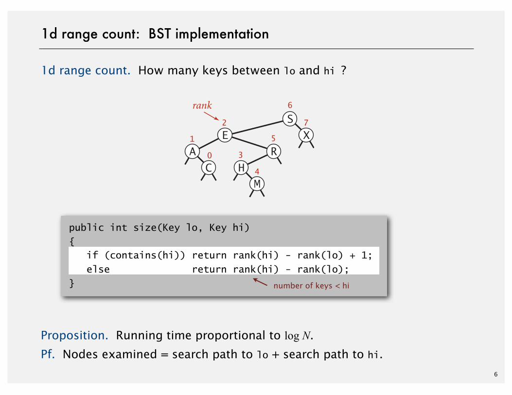
1d range count. How many keys between lo and hi ?
Proposition. Running time proportional to log N.
Pf. Nodes examined = search path to lo + search path to hi.
public int size(Key lo, Key hi) { if (contains(hi)) return rank(hi) - rank(lo) + 1; else return rank(hi) - rank(lo); } number of keys < hi
AC
E
HM
R
SX1
2
6
7
4
0
5
3
rank
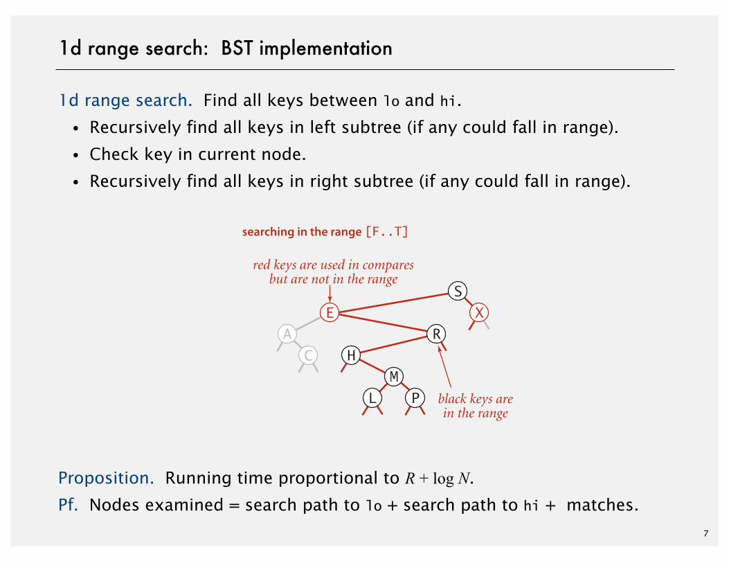
1d range search. Find all keys between lo and hi.
・Recursively find all keys in left subtree (if any could fall in range).
・Check key in current node.
・Recursively find all keys in right subtree (if any could fall in range).
Proposition. Running time proportional to R + log N.
Pf. Nodes examined = search path to lo + search path to hi + matches.7
1d range search: BST implementation
black keys arein the range
red keys are used in comparesbut are not in the range
AC
E
H
LM
P
R
SX
searching in the range [F..T]
Range search in a BST

http://algs4.cs.princeton.edu
ROBERT SEDGEWICK | KEVIN WAYNE
Algorithms
‣ 1d range search
‣ line segment intersection
‣ kd trees
‣ interval search trees
‣ rectangle intersection
GEOMETRIC APPLICATIONS OF BSTS
9
Orthogonal line segment intersection
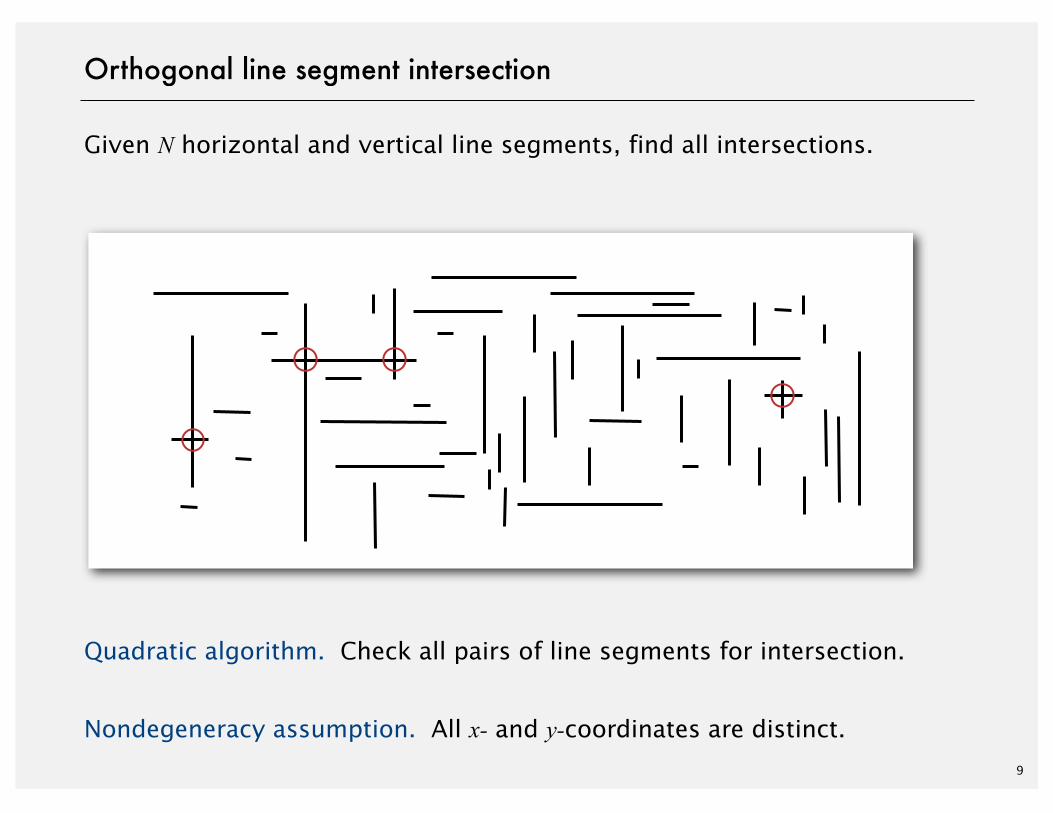
Given N horizontal and vertical line segments, find all intersections.
Quadratic algorithm. Check all pairs of line segments for intersection.
Nondegeneracy assumption. All x- and y-coordinates are distinct.
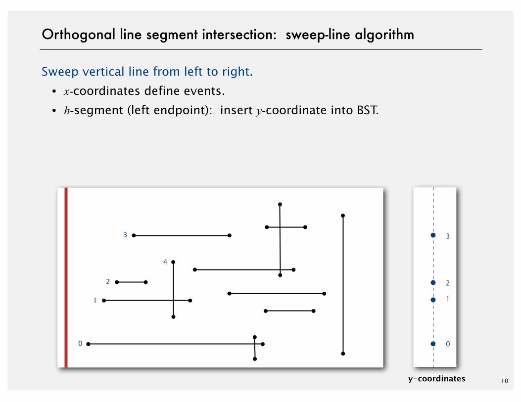
Sweep vertical line from left to right.
・x-coordinates define events.
・h-segment (left endpoint): insert y-coordinate into BST.
10
Orthogonal line segment intersection: sweep-line algorithm
y-coordinates
0
1
2
3
0
1
3
2
4

Sweep vertical line from left to right.
・x-coordinates define events.
・h-segment (left endpoint): insert y-coordinate into BST.
・h-segment (right endpoint): remove y-coordinate from BST.
11
Orthogonal line segment intersection: sweep-line algorithm
y-coordinates
0
1
2
3
4
0
1
3
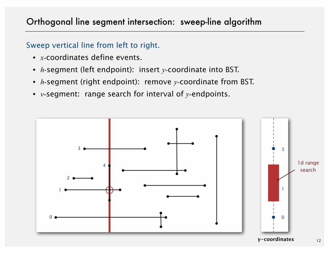
Sweep vertical line from left to right.
・x-coordinates define events.
・h-segment (left endpoint): insert y-coordinate into BST.
・h-segment (right endpoint): remove y-coordinate from BST.
・v-segment: range search for interval of y-endpoints.
12
Orthogonal line segment intersection: sweep-line algorithm
1d rangesearch
y-coordinates
0
1
2
3
4
0
1
3
13
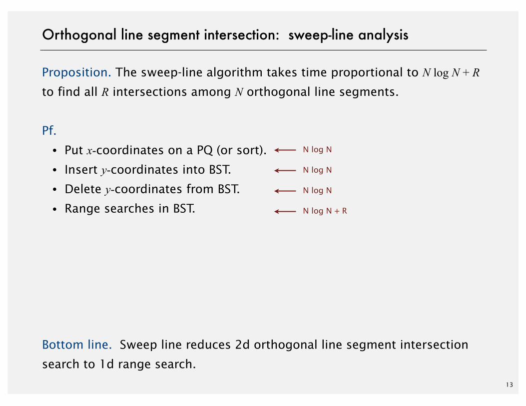
Orthogonal line segment intersection: sweep-line analysis
Proposition. The sweep-line algorithm takes time proportional to N log N + R
to find all R intersections among N orthogonal line segments.
Pf.
・Put x-coordinates on a PQ (or sort).
・Insert y-coordinates into BST.
・Delete y-coordinates from BST.
・Range searches in BST.
Bottom line. Sweep line reduces 2d orthogonal line segment intersection
search to 1d range search.
N log N
N log N
N log N
N log N + R
http://algs4.cs.princeton.edu
ROBERT SEDGEWICK | KEVIN WAYNE
Algorithms
‣ 1d range search
‣ line segment intersection
‣ kd trees
‣ interval search trees
‣ rectangle intersection
GEOMETRIC APPLICATIONS OF BSTS
15
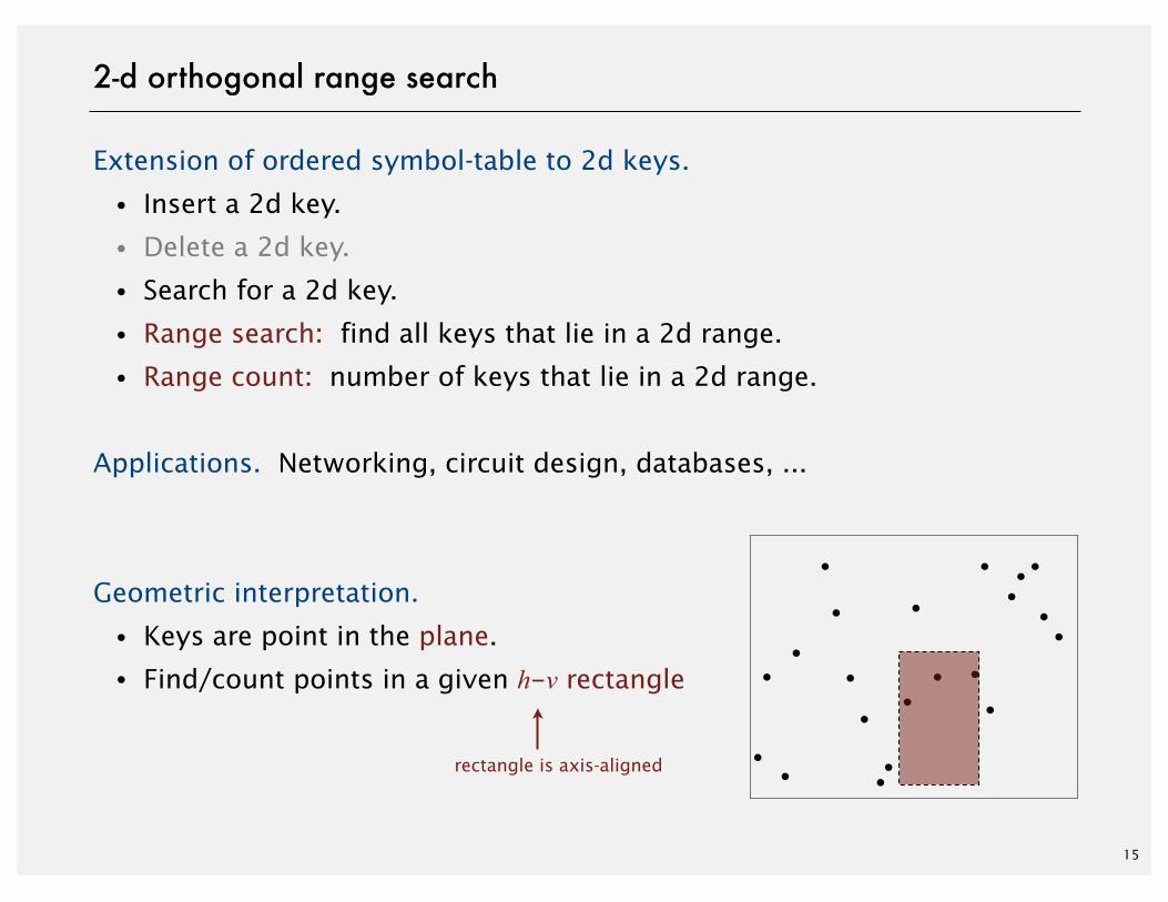
2-d orthogonal range search
Extension of ordered symbol-table to 2d keys.
・Insert a 2d key.
・Delete a 2d key.
・Search for a 2d key.
・Range search: find all keys that lie in a 2d range.
・Range count: number of keys that lie in a 2d range.
Applications. Networking, circuit design, databases, ...
Geometric interpretation.
・Keys are point in the plane.
・Find/count points in a given h-v rectangle
rectangle is axis-aligned

16
2d orthogonal range search: grid implementation
Grid implementation.
・Divide space into M-by-M grid of squares.
・Create list of points contained in each square.
・Use 2d array to directly index relevant square.
・Insert: add (x, y) to list for corresponding square.
・Range search: examine only squares that intersect 2d range query.
LB
RT
17
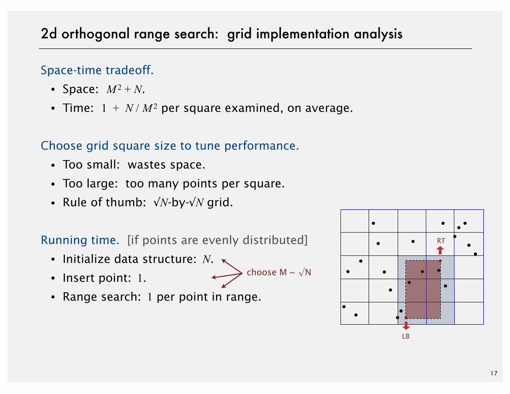
2d orthogonal range search: grid implementation analysis
Space-time tradeoff.
・Space: M 2 + N.
・Time: 1 + N / M 2 per square examined, on average.
Choose grid square size to tune performance.
・Too small: wastes space.
・Too large: too many points per square.
・Rule of thumb: √N-by-√N grid.
Running time. [if points are evenly distributed]
・Initialize data structure: N.
・Insert point: 1.
・Range search: 1 per point in range.
LB
RT
choose M ~ √N

Grid implementation. Fast, simple solution for evenly-distributed points.
Problem. Clustering a well-known phenomenon in geometric data.
・Lists are too long, even though average length is short.
・Need data structure that adapts gracefully to data.
18
Clustering

Grid implementation. Fast, simple solution for evenly-distributed points.
Problem. Clustering a well-known phenomenon in geometric data.
Ex. USA map data.
19
Clustering
half the squares are empty half the points arein 10% of the squares
13,000 points, 1000 grid squares

Use a tree to represent a recursive subdivision of 2d space.
Grid. Divide space uniformly into squares.
2d tree. Recursively divide space into two halfplanes.
Quadtree. Recursively divide space into four quadrants.
BSP tree. Recursively divide space into two regions.
20
Space-partitioning trees
Grid 2d tree BSP treeQuadtree

Applications.
・Ray tracing.
・2d range search.
・Flight simulators.
・N-body simulation.
・Collision detection.
・Astronomical databases.
・Nearest neighbor search.
・Adaptive mesh generation.
・Accelerate rendering in Doom.
・Hidden surface removal and shadow casting.
21
Space-partitioning trees: applications
Grid 2d tree BSP treeQuadtree

Recursively partition plane into two halfplanes.
22
2d tree construction
1
2
3
4
6
7
8
9
10
5
1
2
87
10 9
3
4 6
5

Data structure. BST, but alternate using x- and y-coordinates as key.
・Search gives rectangle containing point.
・Insert further subdivides the plane.
23
2d tree implementation
even levels
p
points
left of ppoints
right of p
p
q
points
below q
points
above q
odd levels
q
1
2
87
10 9
3
4 6
5
1 2
3
4
6
7
8
9
10
5

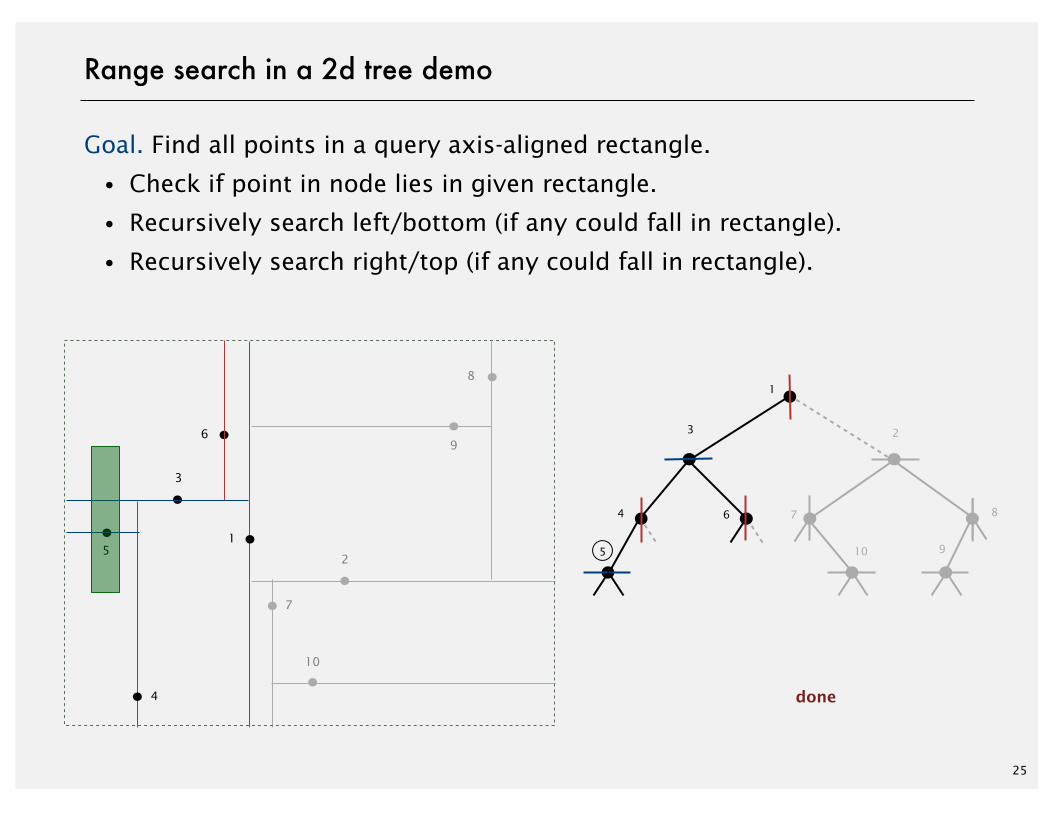
Goal. Find all points in a query axis-aligned rectangle.
・Check if point in node lies in given rectangle.
・Recursively search left/bottom (if any could fall in rectangle).
・Recursively search right/top (if any could fall in rectangle).
24
Range search in a 2d tree demo
1
2
3
4
6
7
8
9
10
5
1
2
87
10 9
3
4 6
5
Goal. Find all points in a query axis-aligned rectangle.
・Check if point in node lies in given rectangle.
・Recursively search left/bottom (if any could fall in rectangle).
・Recursively search right/top (if any could fall in rectangle).
25
Range search in a 2d tree demo
2
3
7
8
9
10
2
87
10 9
3
1
1
4
4
5 5
6
6
done
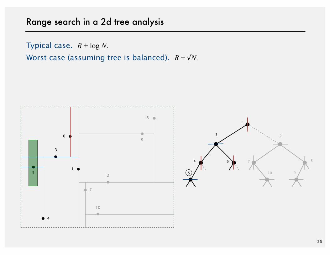
Typical case. R + log N.Worst case (assuming tree is balanced). R + √N.
26
Range search in a 2d tree analysis
2
3
7
8
9
10
2
87
10 9
3
1
1
4
4
5 5
6
6
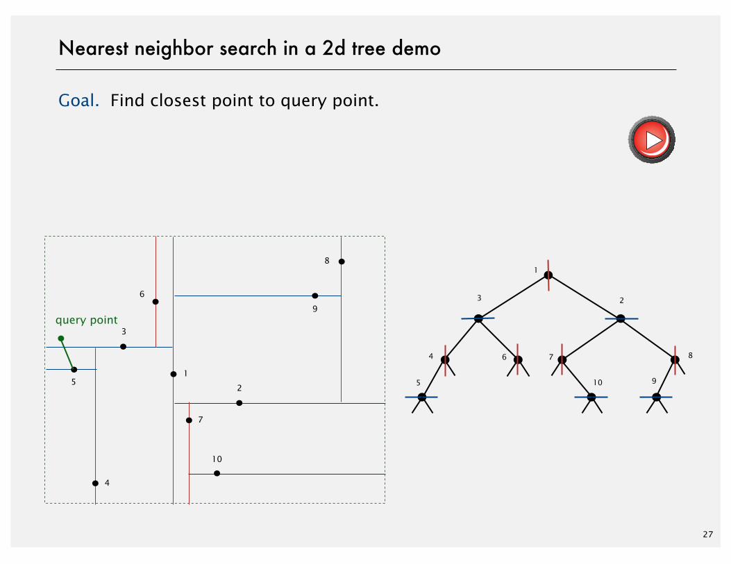
Goal. Find closest point to query point.
27
Nearest neighbor search in a 2d tree demo
2
3
4
7
8
9
10
5
1
2
87
10 9
3
4 6
5
query point
1
6
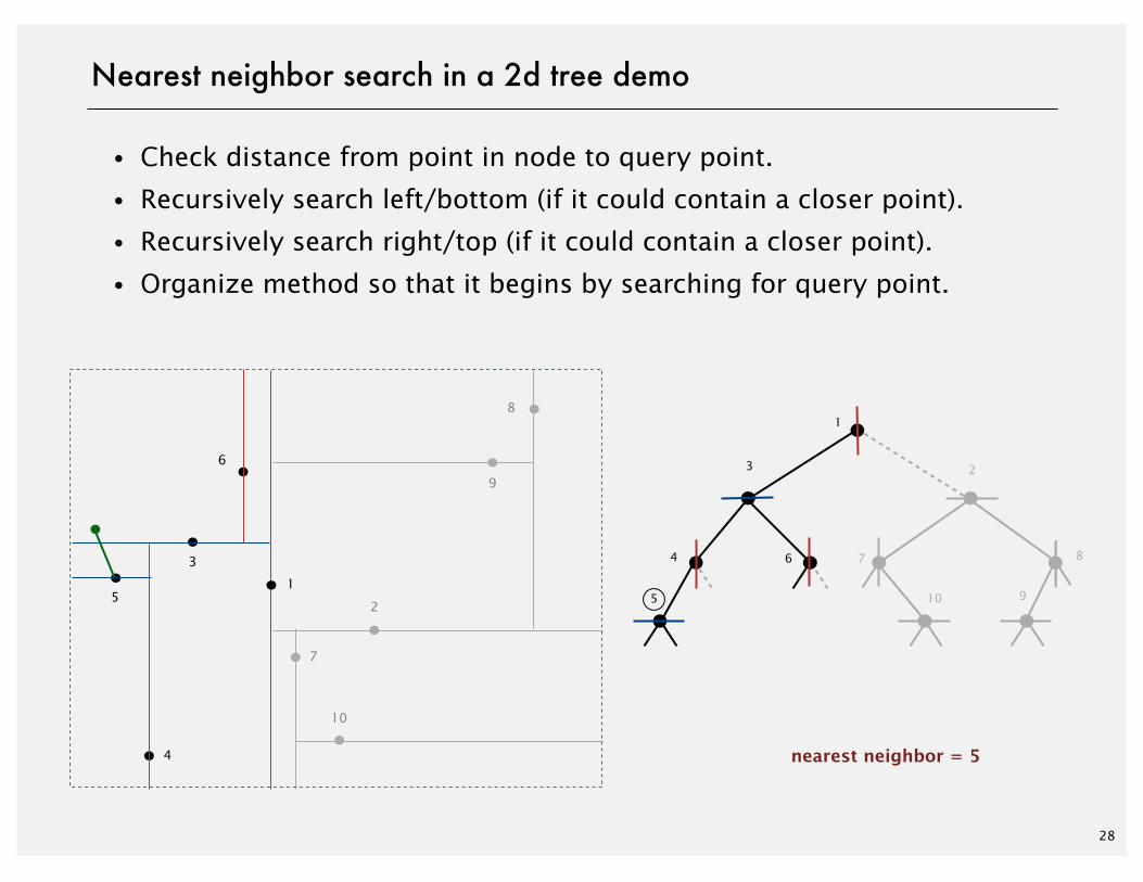
・Check distance from point in node to query point.
・Recursively search left/bottom (if it could contain a closer point).
・Recursively search right/top (if it could contain a closer point).
・Organize method so that it begins by searching for query point.
28
Nearest neighbor search in a 2d tree demo
2
4
7
8
9
10
5
2
87
10 9
3
4 6
5
1
1
3
6
nearest neighbor = 5

29
Nearest neighbor search in a 2d tree analysis
Typical case. log N. Worst case (even if tree is balanced). N.
30
2
4
7
8
9
10
5
2
87
10 9
3
4 6
5
1
1
3
6
nearest neighbor = 5

30
Flocking birds
Q. What "natural algorithm" do starlings, migrating geese, starlings,
cranes, bait balls of fish, and flashing fireflies use to flock?
http://www.youtube.com/watch?v=XH-groCeKbE

31
Flocking boids [Craig Reynolds, 1986]
Boids. Three simple rules lead to complex emergent flocking behavior:
・Collision avoidance: point away from k nearest boids.
・Flock centering: point towards the center of mass of k nearest boids.
・Velocity matching: update velocity to the average of k nearest boids.
32
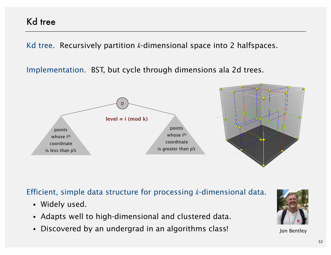
Kd tree
Kd tree. Recursively partition k-dimensional space into 2 halfspaces.
Implementation. BST, but cycle through dimensions ala 2d trees.
Efficient, simple data structure for processing k-dimensional data.
・Widely used.
・Adapts well to high-dimensional and clustered data.
・Discovered by an undergrad in an algorithms class!
level ≡ i (mod k)
points
whose ith
coordinate
is less than p’s
points
whose ith
coordinate
is greater than p’s
p
Jon Bentley

Goal. Simulate the motion of N particles, mutually affected by gravity.
Brute force. For each pair of particles, compute force:
Running time. Time per step is N 2.
33
N-body simulation
F =G m1 m2
r2
http://www.youtube.com/watch?v=ua7YlN4eL_w

34
Appel's algorithm for N-body simulation
Key idea. Suppose particle is far, far away from cluster of particles.
・Treat cluster of particles as a single aggregate particle.
・Compute force between particle and center of mass of aggregate.

35
Appel's algorithm for N-body simulation
・Build 3d-tree with N particles as nodes.
・Store center-of-mass of subtree in each node.
・To compute total force acting on a particle, traverse tree, but stop
as soon as distance from particle to subdivision is sufficiently large.
Impact. Running time per step is N log N ⇒ enables new research.
SIAM J. ScI. STAT. COMPUT.Vol. 6, No. 1, January 1985
1985 Society for Industrial and Applied MathematicsO08
AN EFFICIENT PROGRAM FOR MANY-BODY SIMULATION*ANDREW W. APPEL
Abstract. The simulation of N particles interacting in a gravitational force field is useful in astrophysics,but such simulations become costly for large N. Representing the universe as a tree structure with theparticles at the leaves and internal nodes labeled with the centers of mass of their descendants allows severalsimultaneous attacks on the computation time required by the problem. These approaches range fromalgorithmic changes (replacing an O(N’) algorithm with an algorithm whose time-complexity is believedto be O(N log N)) to data structure modifications, code-tuning, and hardware modifications. The changesreduced the running time of a large problem (N 10,000) by a factor of four hundred. This paper describesboth the particular program and the methodology underlying such speedups.
1. Introduction. Isaac Newton calculated the behavior of two particles interactingthrough the force of gravity, but he was unable to solve the equations for three particles.In this he was not alone [7, p. 634], and systems of three or more particles can besolved only numerically. Iterative methods are usually used, computing at each discretetime interval the force on each particle, and then computing the new velocities andpositions for each particle.
A naive implementation of an iterative many-body simulator is computationallyvery expensive for large numbers of particles, where "expensive" means days of Cray-1time or a year of VAX time. This paper describes the development of an efficientprogram in which several aspects of the computation were made faster. The initialstep was the use of a new algorithm with lower asymptotic time complexity; the useof a better algorithm is often the way to achieve the greatest gains in speed [2].
Since every particle attracts each of the others by the force of gravity, there areO(N2) interactions to compute for every iteration. Furthermore, for the same reasonsthat the closed form integral diverges for small distances (since the force is proportionalto the inverse square of the distance between two bodies), the discrete time intervalmust be made extremely small in the case that two particles pass very close to eachother. These are the two problems on which the algorithmic attack concentrated. Bythe use of an appropriate data structure, each iteration can be done in time believedto be O(N log N), and the time intervals may be made much larger, thus reducingthe number of iterations required. The algorithm is applicable to N-body problems inany force field with no dipole moments; it is particularly useful when there is a severenonuniformity in the particle distribution or when a large dynamic range is required(that is, when several distance scales in the simulation are of interest).
The use of an algorithm with a better asymptotic time complexity yielded asignificant improvement in running time. Four additional attacks on the problem werealso undertaken, each of which yielded at least a factor of two improvement in speed.These attacks ranged from insights into the physics down to hand-coding a routine inassembly language. By finding savings at many design levels, the execution time of alarge simulation was reduced from (an estimated) 8,000 hours to 20 (actual) hours.The program was used to investigate open problems in cosmology, giving evidence tosupport a model of the universe with random initial mass distribution and high massdensity.
* Received by the editors March 24, 1983, and in revised form October 1, 1983.r Computer Science Department, Carnegie-Mellon University, Pittsburgh, Pennsylvania 15213. Thisresearch was supported by a National Science Foundation Graduate Student Fellowship and by the officeof Naval Research under grant N00014-76-C-0370.
85

http://algs4.cs.princeton.edu
ROBERT SEDGEWICK | KEVIN WAYNE
Algorithms
‣ 1d range search
‣ line segment intersection
‣ kd trees
‣ interval search trees
‣ rectangle intersection
GEOMETRIC APPLICATIONS OF BSTS

37
1d interval search. Data structure to hold set of (overlapping) intervals.
・Insert an interval ( lo, hi ).
・Search for an interval ( lo, hi ).
・Delete an interval ( lo, hi ).
・Interval intersection query: given an interval ( lo, hi ), find all intervals
(or one interval) in data structure that intersects ( lo, hi ).
Q. Which intervals intersect ( 9, 16 ) ?A. ( 7, 10 ) and ( 15, 18 ).
1d interval search
(7, 10)
(5, 8)
(4, 8) (15, 18)
(17, 19)
(21, 24)

38
Nondegeneracy assumption. No two intervals have the same left endpoint.
1d interval search API
public class IntervalST<Key extends Comparable<Key>, Value> public class IntervalST<Key extends Comparable<Key>, Value> public class IntervalST<Key extends Comparable<Key>, Value>
IntervalST() create interval search tree
void put(Key lo, Key hi, Value val) put interval-value pair into ST
Value get(Key lo, Key hi) value paired with given interval
void delete(Key lo, Key hi) delete the given interval
Iterable<Value> intersects(Key lo, Key hi)all intervals that intersect
the given interval

Create BST, where each node stores an interval ( lo, hi ).
・Use left endpoint as BST key.
・Store max endpoint in subtree rooted at node.
39
Interval search trees
binary search tree(left endpoint is key)
(17, 19)
(5, 8) (21, 24)
(4, 8) (15, 18)
(7, 10)
24
18
8 18
10
24
max endpoint insubtree rooted at node

To insert an interval ( lo, hi ) :
・Insert into BST, using lo as the key.
・Update max in each node on search path.
40
Interval search tree demo
(17, 19)
(5, 8) (21, 24)
(4, 8) (15, 18)
(7, 10)
insert interval (16, 22)
24
18
8 18
10
24

41
Interval search tree demo
To search for any one interval that intersects query interval ( lo, hi ) :
・If interval in node intersects query interval, return it.
・Else if left subtree is null, go right.
・Else if max endpoint in left subtree is less than lo, go right.
・Else go left.
interval intersectionsearch for (21, 23)
(17, 19)
(5, 8) (21, 24)
(4, 8) (15, 18)
(7, 10)
24
22
8 22
10
24
22 (21, 23)
compare (21, 23) to (16, 22) (intersection!)
(16, 22)

42
Search for an intersecting interval implementation
To search for any one interval that intersects query interval ( lo, hi ) :
・If interval in node intersects query interval, return it.
・Else if left subtree is null, go right.
・Else if max endpoint in left subtree is less than lo, go right.
・Else go left.
Node x = root;
while (x != null)
{
if (x.interval.intersects(lo, hi)) return x.interval;
else if (x.left == null) x = x.right;
else if (x.left.max < lo) x = x.right;
else x = x.left;
}
return null;
43
Search for an intersecting interval analysis
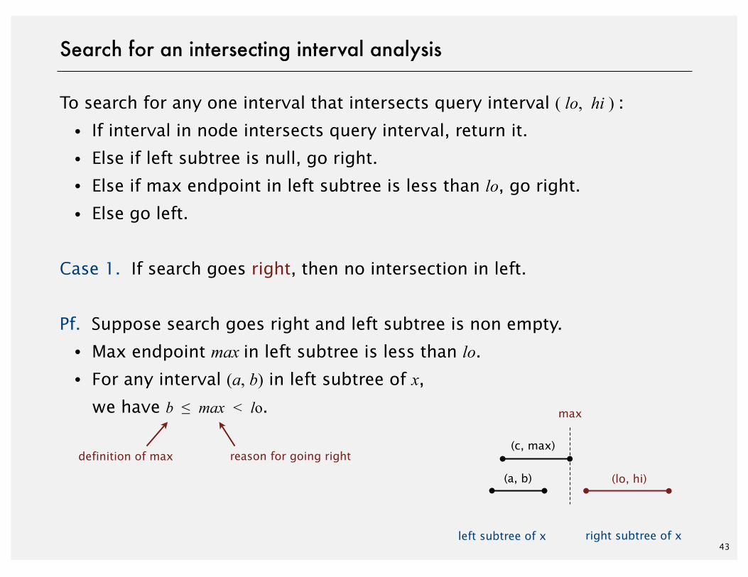
To search for any one interval that intersects query interval ( lo, hi ) :
・If interval in node intersects query interval, return it.
・Else if left subtree is null, go right.
・Else if max endpoint in left subtree is less than lo, go right.
・Else go left.
Case 1. If search goes right, then no intersection in left.
Pf. Suppose search goes right and left subtree is non empty.
・Max endpoint max in left subtree is less than lo.
・For any interval (a, b) in left subtree of x,we have b ≤ max < lo.
definition of max reason for going right
(a, b)
left subtree of x
(lo, hi)
max
right subtree of x
(c, max)

44
Search for an intersecting interval analysis
To search for any one interval that intersects query interval ( lo, hi ) :
・If interval in node intersects query interval, return it.
・Else if left subtree is null, go right.
・Else if max endpoint in left subtree is less than lo, go right.
・Else go left.
Case 2. If search goes left, then there is either an intersection in left
subtree or no intersections in either.
Pf. Suppose no intersection in left.
・Since went left, we have lo ≤ max.
・Then for any interval (a, b) in right subtree of x, hi < c ≤ a ⇒ no intersection in right.
no intersectionsin left subtree
intervals sortedby left endpoint
(a, b)
left subtree of x right subtree of x
(c, max)
(lo, hi)
max

45
Interval search tree: analysis
Implementation. Use a red-black BST to guarantee performance.
easy to maintain auxiliary informationusing log N extra work per op
operation bruteinterval
search treebest
in theory
insert interval 1 log N log N
find interval N log N log N
delete interval N log N log N
find any one intervalthat intersects (lo, hi)
N log N log N
find all intervalsthat intersects (lo, hi)
N R log N R + log N
order of growth of running time for N intervals

http://algs4.cs.princeton.edu
ROBERT SEDGEWICK | KEVIN WAYNE
Algorithms
‣ 1d range search
‣ line segment intersection
‣ kd trees
‣ interval search trees
‣ rectangle intersection
GEOMETRIC APPLICATIONS OF BSTS
47
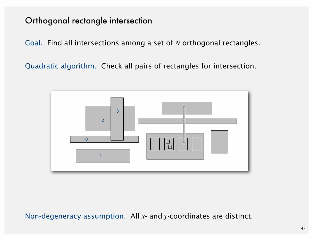
Orthogonal rectangle intersection
Goal. Find all intersections among a set of N orthogonal rectangles.
Quadratic algorithm. Check all pairs of rectangles for intersection.
Non-degeneracy assumption. All x- and y-coordinates are distinct.
0
1
2
3

48
Microprocessors and geometry
Early 1970s. microprocessor design became a geometric problem.
・Very Large Scale Integration (VLSI).
・Computer-Aided Design (CAD).
Design-rule checking.
・Certain wires cannot intersect.
・Certain spacing needed between different types of wires.
・Debugging = orthogonal rectangle intersection search.

49
Algorithms and Moore's law
"Moore’s law." Processing power doubles every 18 months.
・197x: check N rectangles.
・197(x+1.5): check 2 N rectangles on a 2x-faster computer.
Bootstrapping. We get to use the faster computer for bigger circuits.
But bootstrapping is not enough if using a quadratic algorithm:
・197x: takes M days.
・197(x+1.5): takes (4 M) / 2 = 2 M days. (!)
Bottom line. Linearithmic algorithm is necessary to sustain Moore’s Law.
2x-fastercomputer
quadraticalgorithm
Gordon Moore

Sweep vertical line from left to right.
・x-coordinates of left and right endpoints define events.
・Maintain set of rectangles that intersect the sweep line in an interval
search tree (using y-intervals of rectangle).
・Left endpoint: interval search for y-interval of rectangle; insert y-interval.
・Right endpoint: remove y-interval.
50
Orthogonal rectangle intersection: sweep-line algorithm
y-coordinates
0
1
2
3
0
1
23

51
Orthogonal rectangle intersection: sweep-line analysis
Proposition. Sweep line algorithm takes time proportional to N log N + R log Nto find R intersections among a set of N rectangles.
Pf.
・Put x-coordinates on a PQ (or sort).
・Insert y-intervals into ST.
・Delete y-intervals from ST.
・Interval searches for y-intervals.
Bottom line. Sweep line reduces 2d orthogonal rectangle intersection
search to 1d interval search.
N log N
N log N
N log N
N log N + R log N

Geometric applications of BSTs
52
problem example solution
1d range search BST
2d orthogonal linesegment intersection
sweep line reduces to1d range search
kd range search kd tree
1d interval search interval search tree
2d orthogonalrectangle intersection
sweep line reduces to1d interval search
Related Documents


![Multidimensional Range Search in Dynamically Balanced Trees · Multidimensional Range Search in Dynamically Balanced Trees H. Tropf, H. Herzog, ... dimensional space. In [1] a survey](https://static.cupdf.com/doc/110x72/5f06c6597e708231d419ab7a/multidimensional-range-search-in-dynamically-balanced-trees-multidimensional-range.jpg)