Lower Bounds for Orthogonal Range Searching: I. The ...chazelle/pubs/LBOrthoRangeSearchReporting.pdfd-range q, orthogonal range searching is the problem of computing the sum c pEPnq

Lower Bounds for Orthogonal Range Searching: I. The Reporting Case

BERNARD CHAZELLE

Princeton University, Princeton, New Jersey

Abstract. We establish lower bounds on the complexity of orthogonal range reporting in the static case. Given a collection of n points in d-space and a box [a,, b,] x . x [ad, bd], report every point whose ith coordinate lies in [a,, biJ, for each i = 1, . . . , d. The collection of points is fixed once and for all and can be preprocessed. The box, on the other hand, constitutes a query that must be answered on- line. It is shown that on a pointer machine a query time of O(k + polylog(n)), where k is the number of points to be reported, can only be achieved at the expense of fl(n(logn/loglogn)d-‘) storage. Interestingly, these bounds are optimal in the pointer machine model, but they can be improved (ever so slightly) on a random access machine. In a companion paper, we address the related problem of adding up weights assigned to the points in the query box.

Categories and Subject Descriptors: F.2.2 [Analysis of Algorithms and Problem Complexity]: Nonnu- merical Algorithms and Problems--sorting and searching; E. 1 [Data]: Data Structures

General Terms: Algorithms, Theory

1. Introduction

Orthogonal range searching [l-5, 8-10, 12- 141 is a direct generalization of list searching. Let P = (p,, . . . , pnj be a set of rz points in d-space; assume that each point is given by its coordinates in a fixed Cartesian system of reference. Given a queryq= [a,, b,] X ++. X [ad, bd], report all the points in P n q. To motivate this problem, the classical scenario is to regard the points of P as the employees of a certain company. The coordinates of the points are important attributes of the employees, such as seniority, age, salary, traveling assignments, legal status, etc. Crucial to the well functioning of the company is the ability to provide fast answers to questions of the form: “Which senior-level employees are less than x years of age, make more than y dollars a year, have been abroad in the last z months, have never taken the Fifth Amendment, etc.?”

For obvious reasons, this is called orthogonal range searching in report-mode, or more simply, orthogonal range reporting. To put this problem in perspective, let

A preliminary version of this work has appeared in Proceedings of the 27th Annual IEEE Symposium on Foundations of Computer Science. IEEE, New York, 1986, pp. 87-96. Part of this research was done while B. Chazelle was a visiting professor at Ecole Not-male Superieure, Paris, France. The research for this paper was partially supported by the National Science Foundation (NSF) under grant CCR 87-009 17. Author’s address: Department of Computer Science, Princeton University, Princeton, N.J. 08544. Permission to copy without fee all or part of this material is granted provided that the copies are not made or distributed for direct commercial advantage, the ACM copyright notice and the title of the publication and its date appear, and notice is given that copying is by permission of the Association for Computing Machinery. To copy otherwise, or to republish, requires a fee and/or specific permission. 0 1990 ACM 0004-541 l/90/0400-0200 $01.50

Journal of the Association for Computing Machinery, Vol. 37, No. 2, April 1990. pp. 200-212.

Orthogonal Range Searching: I. Reporting 201

us define a d-range as the Cartesian product of d closed intervals over the real line. Orthogonal range reporting refers to the task of reporting all the points of P fl q, given an arbitrary query d-range q. Evaluating the size of P n q is called orthogonal range counting. Both problems can be put under the same umbrella by associating a weight w(p) to each point p E P. Weights are chosen in a suitable algebraic structure (9 , +), such as a group or a semigroup. Given a query d-range q, orthogonal range searching is the problem of computing the sum c pEPnq w(p). The group (z, +) can be used for range counting, while the semigroup (2’, U) is suitable for the reporting version of the problem. The generality of range searching has other benefits. For example, given n points in 3-space, computing the highest point over a query rectangular region can be regarded as a two- dimensional range-searching problem.

From a complexity viewpoint, range reporting must be studied separately because, as opposed to, say, range counting, the query time is a function not only of the input size n, but also of the output size. The most efficient data structures to date capitalize on the fact that if many points are to be reported, the query time will be high, anyway, so the search component of the query-answering process does not need to be all that efftcient; this is the idea offiltering search [3], which is behind many algorithms for multidimensional searching. To introduce our main result, let us consider the case d = 2. As was shown in [3], there exists a data structure of size O(n log n/log log n)’ that guarantees a query time of O(k + log n), where k is the number of points to be reported. The algorithm operates on a pointer machine [ 111, which means that no address calculations are required. The factor log n/loglog n might look a little odd, especially in light of the fact that it can be removed in many variants of the problem. Indeed, there exist data structures of size O(n) and query time O(k +logn) if (i) the query rectangle is grounded, meaning that it is required to be in contact with a fixed line [9], or (ii) its aspect- ratio is fixed [5], or (iii) the query is a grounded trapezoid [6]. Again, in all cases, those linear-size solutions work on a pointer machine. Adding to the suspicion that the factor log n/log log n can be removed (or at least lowered) on a pointer machine is the fact that it can on a random access machine (RAM). If address calculations are allowed, then the storage requirement can be reduced to O(nlog’n), for any fixed t > 0 [4].

Putting these questions to rest, we prove the rather surprising result that if a query time of O(k + logn) is desired then the storage must be O(nlogn/loglogn). More generally, we show that in d dimensions, a query time of O(k + log’n), for any constant c, can only be achieved at the expense of R(n(logn/loglogn)‘-‘) storage, which is optimal. This comes in sharp contrast with the random access machine model, in which a query time of O(k + logd-‘n) can be achieved with only O(n(logn)“2+‘) storage [4]. These results show that orthogonal range reporting is inherently more difficult on a pointer machine than on a RAM. This is a rare separation result that sheds light on two of the most common models of sequential computation.

The lower-bound proof is based entirely on control-flow considerations and relies on syntactic, rather than semantic, properties of pointer machine-based data structures. We believe that the underlying idea can be used for many other problems. As a starter, we recall a few basic facts about pointer machines and prove a result of general interest concerning the complexity of navigating through a

’ All logarithms in this paper are taken to the base 2, unless specified otherwise.

202 BERNARD CHAZELLE

pointer-based data structure (Section 2). In two dimensions, the desired lower bound can be established by constructive means (Section 3). Things become a little more complicated in higher dimensions, so we turn to probabilistic arguments to prove the existence of “hard” inputs (Section 4). The issue of matching upper bounds is addressed in Section 5. We close with concluding remarks in Section 6.

2. The Complexity of Navigation on a Pointer Machine We assume that the reader is familiar with the notion of a pointer machine, as defined in [ 1 I]. As long as we are only concerned with lower bounds, we have the freedom to increase the power of our machine at will. This is a good idea aimed at eliminating unessential particulars that might get in the way of a simple proof. The memory of a pointer machine is an unbounded collection of registers. Each register is a record with a fixed number of data and pointer fields. In this way, the memory can be modeled as a directed graph with bounded outdegree. At the cost of increasing the storage requirement by a constant multiplicative factor, we can always reduce the outdegree of each node of the graph to 0, 1, or 2 (why?).

Let P= (p,, . . . , p,,) be a set of IZ points in Ed. A data structure for orthogonal range reporting is a digraph G = (V, E) with a source u. Each node u is assigned an integer, label(u), between 0 and n. If i = label(u) is not 0, the node u is associated with point pi. Note that many nodes can be labeled the same way. Given a query q, the answering algorithm begins a traversal of G at the source u. We place only two restrictions on the algorithm. To begin with, no node (other than the source) can be visited if a node pointing to it has not already been visited. Furthermore, completion cannot occur until each label i (pi E q) has been encountered at least once. During its execution, the algorithm is allowed to modify data and address fields as it visits them. It can also add new nodes to G by requesting them from a pool of free nodes with blank fields, the freelist. Let N(U) denote the set 1 w ] (u, w) E E ). For our purposes, the algorithm executes a program made up of the following instructions. Initially, W = (g):

(i) Pick any u E Wand add N(u) to W. (ii) Request a new node u from the freelist and add it to IV. Initialize N(u) to 0.

(iii) Pick any u, w E Wand, if l N(u)] < 2, add (u, w) to E (and u or w to I’, if necessary).

(iv) Pick any u, w E Wand remove the edge (u, w) from E if it exists.

Let W(q) denote the set W at termination. Correctness is ensured by the requirement

(i 1 pi E q) !Z (label(u) I U E W).

This means that the query-answering algorithm must reach at least one rep- resentative node for every point to be reported. The query time is measured as I Wq)l.

Let us make a few comments about this framework. Our first remark is that the model is more powerful than the standard pointer machine. (Once again, recall that this is a good thing in the context of lower bounds.) The “pick any” feature cannot be implemented in constant time on a real computer. After a while, W can grow to be very big, and “pick any” offers the full power of nondeterminism. The


fact that we add all of N(u) into IV, as opposed to any particular node is inconsequential, considering that 1 N(u) 1 5 2. The labeling scheme has a natural interpretation. Nodes labeled 0 are used internally by the data structure. The other nodes are used both internally but also as means of output. Suppose that pi E q. Then, the model requires the algorithm to reach at least one node labeled i. This assumption might seem unnecessarily exclusive: After all, why can’t we simply require that i be computed rather than discovered? Certainly, the output should give us direct access to the points of P rl q. However, the mere knowledge of their indices does not fulfill this requirement on a pointer machine. This is perhaps where the difference between a RAM and a pointer machine shines in its true light. If pi lies in q, what we want is either pi itself or a pointer to pi, but not just the integer i. In the model described above, we can store pi inside each record labeled i. If the coordinates of pi are huge or are defined implicitly, then we might want to keep P in a table and add a pointer from each record labeled i to the entry of the table where pi is stored. This model describes all the pointer machine data structures proposed in the literature for solving range-searching problems.

Let a and b be two positive reals. We say that the data structure G = (I’, E) for P is (a, b)-effective if, for any query d-range q, we have 1 W(q) 1 5 a( I P II q I + logbn). This means that the query time is linear in the output size, aside from a polylogarithmic overhead. To establish our lower bound, intuitively, we want to argue that nodes labeled after the points of P rl q cannot be too much spread out in the graph; otherwise, it would be impossible to get to them in linear time. Our goal is to produce a large set of queries, no two of which share too many points of P. In this way, we are able to argue that the graph has many subsets of nodes with the following properties: (i) each subset is fairly compact (vertices are close to each other), and (ii) no two subsets share too many edges. This will imply that the graph has many edges. Now, by virtue of the bounded outdegree condition, this means that the graph has many vertices, and therefore the need for storage is large. Let s= (41, --., q5.3 be a set of queries and let CY be a positive real. We say that S is cY-favorable if, for each i, j (i Z j),

(i) 1 P fl qi I 2 1og”n. (ii) 1 P n qi n qj I 5 1.

The following result is the key to the lower-bound proof. It asserts that the storage requirement is at least proportional to the size of any b-favorable set of queries. The lemma suggests the remainder of the proof: finding large favorable sets of queries. Interestingly, the investigation of favorable sets is purely geometric, and does not involve the model of computation at all.

LEMMA 2.1. Let a and b be two positive reals. If the data structure G is (a, b)- eflective and the set of queries S is b-favorable, then I VI > I S I (logbn)/2’6”+4, for n large enough.

PROOF. We define the distance p(u, w) between two nodes u and w of G as the number of edges on the shortest directed path from u to w. If there is no such path, p(u, w) = +a~. The distance p(u, w) has serious deficiencies: It is not symmetric and it is not always finite. We correct for these flaws by introducing the new distance d(u, w) = min( p(z, u) + p(z, w) I z E V]. Note that because of the source g the new distance is always finite. Given a query q we define orbit(q) as the set

204

of pairs (u, w) E Vz such that

(i) lUbel(U) E (i 1 pi E q}, (ii) I&el(+V) E {i 1 pi E q),

(iii) label(u) < lubel( w), (iv) d(v, w) < 8~.

BERNARD CHAZELLE

Note that the pair (u, w) need not be an edge of G. The various conditions express the fact that (i)-(ii) both u and w can be used for the output, (iii) the pair is neither trivial nor repeated, (iv) u and w are within a constant distance of each other.

Given a query q, consider the graph G before the algorithm begins. There exists at least one path from the source c to every node of W(q). This implies the existence of a directed tree T rooted at the source, whose node-set is W(q) (the reader will forgive us for leaving these facts as exercises). The tree T is called directed because all its edges are oriented in the same direction (pointing away from the root). Let uI, u2, . . . , urn be the sequence of nodes of the tree T corresponding to a first-order traversal. For each index in (i 1 Pi E q ), mark exactly one node uj such that lubeI = i. Let ~1, ~2, . . . , w/ be the subsequence of marked Q’S. Note that m = 1 W(q) I and E’ = I P n q I. Next, we define a distance 6(u, w) over the tree Tin exactly the same way we defined d(u, w) over G. If u and w belong to T, it is clear that

d(u, w) 5 6(u, w) < +m. (1)

The distance 6 trivially satisfies the triangular inequality. Therefore

C a(Wi, Wi+l) 5 C &(Ui, vi+,). (2) I sic/ lzsi-an

The distance 6(Ui, ui+l) measures the number of edges on the path(s) from z to Ui and u. I+1, where z is the nearest common ancestor of ui and Ui+ I in T. Because of the first-order labeling, the sum C lai<m 6(ui, ui+ ,) counts each edge of T at most twice. Therefore,

C &(Ui, Ui+l) 5 2(l w(q)I - 1). (3) I5iCrn

Since G is (a, b)-effective, we have ( W(q) I I a( I P n q I + logbn). Assume now that I P n q I L logbn. We derive

I Wq)l 5 2alPf7 41. (4)

Combining (l)-(4), we find

C d(wi, Wi+l)c4QIpn 41, Isi</

andhence, I(ild(wi,wi+l)Z8U}I < IPnq(/2.Since!= IPnq(,wefindthat

I(iId(wi, W;+I)<QII > 2 lpnqi _ 1 - (5)

LetS={q,,..., qs] be a b-favorable set of queries. Relation (5) holds for each qi. Moreover, because no two points of P can belong to two distinct queries, the pairs ( wi, Wi+, ) are all distinct. Since I P n q I goes to infinity with n,

U orbit = C I orbit( > i lSllogbn, I5iSS Isis.7

(6)


for n large enough. Because of the bounded outdegree condition ( 1 N(u) 1 5 2, for each u E V), we have

Il(u, w) E V214u, w) < 8011 5 1 ((z, u, w) E V3 Ip(z, u) < 8a and p(z, w) < 8a) I I I V/12’6a+2.

From (6) it follows that 1 VI > 1 S 1 (logbn)/2’6”+4, which completes the proof. 0

Lemma 2.1 suggests an obvious line of attack for proving lower bounds on the size of the data structure. Since V is already a lower bound, it suffices to exhibit a large b-favorable set of queries. In the two-dimensional case (Section 3), we are able to define the points and queries by constructive means. In higher dimensions (Section 4), we can still define the queries explicitly, but we must rely on probabilistic arguments to produce a hard set of points.

3. Orthogonal Range Reporting in the Planar Case

Although this section is superseded by the next one, we include it because it gives us a glimpse of what “hard” inputs look like. We define the points first; then we specify the queries and show that they form a b-favorable set. Let m = L210gbpl and X = L(logp)/( 1 + bloglogp)l, where p is an integer large enough so that m, X > 4. We define n as rn’.’ Each query will contain exactly m points. The definition of the queries will be recursive, which explains why the choice of n as a power of m is particularly appropriate. For p large enough, it is easy to show that m 2 logbn and

Xr L

log n 1 + bloglogn I ’

For any integer i (0 5 i < n) let pm(i) be the integer obtained by writing i in base m over X bits and reversing the digits. If i = ml m2 . - . mA, we have p*(i) = mA .-- m2m,. We now define the set of points P as ((p,(i), i)l 0 5 i < n). This definition generalizes the bit-reversal permutation. Figure 1 illustrates the case n = 33. Keep in mind that the point-set is two-dimensional: Edges have been drawn to exhibit the structure of the point system.

We are now ready to define the queries. Going back to Figure 1, we notice that the cube has three principal 3-point sequences: (a, b, c), (a, d, e), and (a, f; g). Each sequence can be enclosed tightly by a query rectangle. Since we have 9 translates of each sequence, we obtain a total of 27 queries. In general, we have Am’-’ queries. To see this, think of a tree T that encodes the x-coordinates of P in base m. Each internal node of T has m children, labeled 0, 1, . . . , m - 1 from left to right. The tree has depth X. The root of T is associated with P as a whole. A node u with ancestors labeled ml, m2, . . . , m,, from the root down, maps to the subset of points whose x-coordinates have the prefix m1m2 . - - m, in base m. For each internal node u, sort its associated set of points by y-coordinates and break it up into groups of size m: Each group can be enclosed by a query rectangle that does not contain any other point. Since a node with r ancestors has n/m’ associated

’ Restricting n to be a power of m should not be viewed as a weakness of the argument. For one thing, the proof can be generalized to any n. Also, if we are concerned with lower bounds, we should be (reasonably) happy as long as we have an infinite number of input sizes for which the lower bound holds. But there is a third, more compelling reason: the results of the next section will supersede the results of this one, so why bother?


26 -

25 -

24 -

23 -

22 -

21-

20 -

19 -

18 -

17 -

16 -

15 -

14 -

13 -

12 -

I1 -

10 -

9-

8-

7-

6-

5-

4-

3-

2-

I-

O- b

I I I I I I I I I I I I I I I I I I I I I I I I I I I 0 1 2 3 4 5 6 7 8 9 10 I1 12 13 14 15 16 17 18 19 20 21 22 23 24 25 26

FIGURE 1

points, this will give us a total of

C Olr<X

(# nodes at depth r) x c = $

queries. It is immediate to check that, for n large enough, the set of queries is b-favorable. From Lemma 2.1 and the fact that m = O(logbn), we conclude that a query time of 0( ] P n q ] + polylog(n)) can be achieved only at a cost of O(n log n/log log n) storage. It follows from [3] that this lower bound is tight on a pointer machine.

THEOREM 3.1. Given n points in E2 there exists a data structure of size O(n lognlloglogn) that allows us to answer any orthogonal range reporting query in time O(k + logn), where k is the number of points to be reported. The algorithm is optimal on a pointer machine.


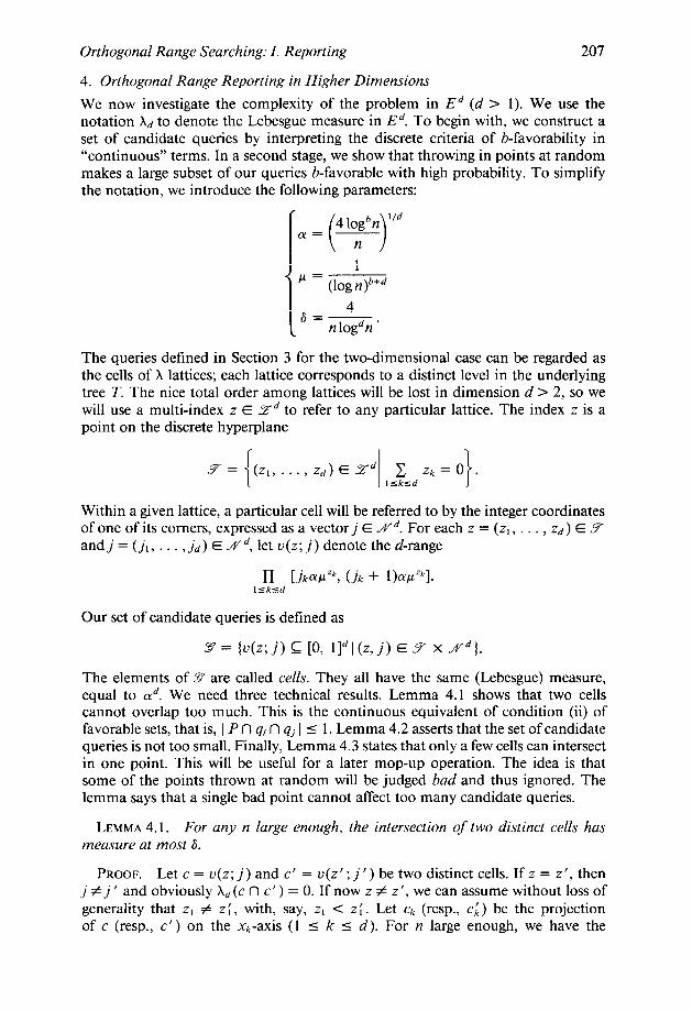
4. Orthogonal Range Reporting in Higher Dimensions

We now investigate the complexity of the problem in Ed (d > 1). We use the notation Ad to denote the Lebesgue measure in Ed. To begin with, we construct a set of candidate queries by interpreting the discrete criteria of b-favorability in “continuous” terms. In a second stage, we show that throwing in points at random makes a large subset of our queries b-favorable with high probability. To simplify the notation, we introduce the following parameters:

I 410gbn ‘Id (y= ~ ( ) n

1 ’ = (logn)b+d

4 a=- n logdn *

The queries defined in Section 3 for the two-dimensional case can be regarded as the cells of X lattices; each lattice corresponds to a distinct level in the underlying tree T. The nice total order among lattices will be lost in dimension d > 2, so we will use a multi-index z E .Zd to refer to any particular lattice. The index z is a point on the discrete hyperplane

y= (z,, . . ..zd)E% d/,&,zk=o}* Within a given lattice, a particular cell will be referred to by the integer coordinates of one of its corners, expressed as a vectorj E Nd. For each z = (zl, . . . , zd) E 7 and j = (jr, . . . , jd) E A’“‘, let u(z; j) denote the d-range

Our set of candidate queries is defined as

F = (u(z; j) C [0, lIdI (z, j) E 7 x Nd).

The elements of .Y are called cells. They all have the same (Lebesgue) measure, equal to ad. We need three technical results. Lemma 4.1 shows that two cells cannot overlap too much. This is the continuous equivalent of condition (ii) of favorable sets, that is, 1 P I-I qi rl qj ] 5 1. Lemma 4.2 asserts that the set of candidate queries is not too small. Finally, Lemma 4.3 states that only a few cells can intersect in one point. This will be useful for a later mop-up operation. The idea is that some of the points thrown at random will be judged bad and thus ignored. The lemma says that a single bad point cannot affect too many candidate queries.

LEMMA 4.1. For any n large enough, the intersection of two distinct cells has measure at most 6.

PROOF. Let c = U(Z; j) and c’ = u(z’ ; j’ ) be two distinct cells. If z = z’, then j # j ’ and obviously Ad (c rl c’ ) = 0. If now z # z’, we can assume without loss of generality that zI # z;, with, say, zI < z;. Let ck (resp., CL) be the projection of c (resp., c’) on the &-axis (1 I k 5 d). For yt large enough, we have the


following derivations

therefore, hd(c rl c’) I pad. 0

LEMMA 4.2. For any n large enough, we have

’ .I71 ’ (b + d)4d(loglogn)d-’ ’

PROOF. We easily check that CXP’~ 5 $, for any zk E X such that

1 zk Z b+d (7)

This shows that, for any z = (zr, . . . , zd) E 7 such that each zk satisfies (7), the number of cells of the form u(z;j) is at least

The right-hand side of (7) is negative for n large enough. This gives us the following lower bound on the number of z E Y whose coordinates zk’s satisfy (7):

log n dloglogn

- e-z!!! - ;)J + 1)d-l > (,,(, :Odg;;oglogn)d-l. loglogn

This implies that the number of cells in 5 exceeds

n(logn)d-b-’ 22d+‘dd-1(b + d)d-l(loglogn)d-l ’

from which the lemma follows. 0

LEMMA 4.3. For any n large enough, no point can lie in the interior of more than (d log n/log log n)d-’ cells of z?.

PROOF. Supposethatu(z;j)C[O, l]‘,forsomez=(z,,...,zd)EXdandjE Nd. Then, for n large enough, zk exceeds -3 log n/log log n (1 5 k I d ). The lemma follows from the fact that since z E 7 we have zk < (d - 1)/2 log n/log log n. 0

The first criterion of b-favorability concerns the fact that a query should contain at least logbn points of P. We strengthen this requirement a little to shield us against the later removal of bad points. We say that a cell is heavy if its interior contains more than 210gbn points of P. As usual, P denotes the set of n input points. A random set of points in a compact set K is a shorthand for a set of points whose elements have been chosen randomly and independently from the uniform distri- bution in K.

LEMMA 4.4. Let P be a random set of n points in [0, lld. If n is large enough, then with probability greater than 1 - 2/lo$n, more than half the cells of g are heavy.


PROOF. Let c be an arbitrary cell of ZY and let x be the number of points of P in the interior of c. We also define P as the probability that c is heavy (i.e., Pr(x > 210gbn)). The mean and variance of x are, respectively, n&(c) and nXd(c)( 1 - Ad(c)). Using Chebyshev’s inequality [7], we derive

nAd(c)(l - Ad(c)) ’ - T 5 (nXd(c) - 210gbn)2 ’

and hence ?r > 1 - l/logbn. Let II be the probability that more than half the cells of 5 are heavy. Since the expected number of heavy cells is equal to 7r ] .V 1, a straightforward Markov-type argument gives us

( ) 1 - & 1g1-c aIF1 5 $1 - rI)l~I + ILIZ],

which completes the proof. 0

To satisfy the second favorability criterion, we make sure that no two points are too close to each other. The underlying metric is not the Euclidean metric. We define the range-distance between two points (xl, . . . , xd) and ( yI , . . . , yd ) in Ed to be the measure of the smallest d-range containing them, that is, HI =,&d I & - yk I. We say that a point p E P is stranded if its range-distance to any point of P\(p) exceeds 6. Finally, we say that P is p-difuse (0 I p 5 1) if it contains at least pn stranded points.

LEMMA 4.5. Let p = 1 - I/&$. For any n large enough, a random set of n points in [0, lid is p-diffuse with probability greater than 1 - 2d+3/ sn.

PROOF. Let L(d, y) denote the Lebesgue measure of {(x,, . . . , &) E [0, lid I nlSkSd & I y), with 0 < y < 1. We have the recurrence relation L(0, y) = 0 and, for d 2 1,

L(d,y)=y+l’L(d- $)dx.

Let M(d, y) = L(d, y) - L(d - 1, y), for d 2 1. We derive the simpler recurrence: M(1, y)= yand

M(d,y)=l’M(d- l,f)dx,

for d > 1. This gives

M(d,y)=y~livM(d- l,;)dx,

hence,

MC4 v) = ~"y~--f+2x, x ..'i x xd-, dXd-, ... dx,.

It is elementary to evaluate this integral directly. This leads to


assuming that O! = 1. Since l/6 goes to infinity with n, we have, for y1 large enough,

L(d >

@ < (-1)“‘d~ (d - I)!

(In a)d-l < 26(log n)d-’ ;

hence,

8 L(d, S) < -

nlogn *

Consider the locus of points in [0, lld whose range-distance to a given point of [0, lld is at most 6. Let V be the largest measure of such a set. It is immediate that

V 5 2%(d, 8). (9)

Let Y be the expected number of stranded points in P and let ir be the probability that P is p-diffuse. Obviously,

v I (1 - 7r)pvl + 7ry1. (10)

The probability that a given point of P is stranded exceeds 1 - nI’/; therefore, v > n( 1 - n I’). Combining this inequality with (8)-( 10) completes the proof. 0

Lemmas 4.4 and 4.5 imply that with probability 1 - o( 1) a random pick P of n points is p-diffuse and makes more than half the cells of 5 heavy. Move outside of [0, lid every point of P that is not stranded, and let T be the cells of B whose interiors contain at least logbn points after the moving.

LEMMA 4.6. For n large enough, we have

n(logn)d-b-’ ” ’ ’ (b + d)5d(logfogn)d-’ .

PROOF. Mark each heavy cell of ZY that, prior to the moving, has at least half of its interior points stranded. Since P is p-diffuse, Lemma 4.3 shows that the number of heavy cells left unmarked cannot exceed dd-‘,(logn)d-b-3’2/(loglogrz)d-‘, for n large enough. Because more than half the cells are heavy, the proof follows from Lemma 4.2. Cl

The cells of I’ satisfy the first criterion of b-favorability. Lemma 4.1 justifies the notion of a stranded point. No two cells of I can contain the same pair of points of P (after the moving). We derive that I forms a b-favorable set of queries. The lower bound is now within reach. From Lemmas 2.1 and 4.6, we conclude that a query time of @output size + polylog(n)) can only be achieved at the expense of O(n(logn/loglog n)d-‘) storage. Although the set of input points is not random (because of the moving), it is not difficult to see how to modify the proof so that the lower bound holds for a random set P. This means that the lower bound is not confined to some pathological configuration of points, but applies to almost any point system. Another remark concerns the fact that orthogonal range reporting is defined over the reals (points of Ed). It is easy to see, however, that the proof technique discriminates among point sets only by means of coordinate compari- sons. This easily implies that hard inputs can be defined with integer coordinates over O(log n) bits.

5. Upper Bounds

Assume that our pointer machine has only O(n(logn/loglogn)d-‘) storage. How fast can we solve orthogonal range reporting in d-space? We already know


the answer in the case where d = 2 (Theorem 3.1). In [lo, pp. 471, Mehlhorn gives a general method for answering orthogonal range queries in time O(k + (2”/n~)~-‘log~n), where k is the number of points to be reported, using a data structure of size O(n(logn)d-‘/md-‘). The quantity m is a slack parameter that we can adjust at will. The assignment m = Itloglogn/(d - l)l, for any fixed c > 0, guarantees that the space requirement stays within the desired bounds. The query time is O(k + logd+‘n).

As it turns out, Mehlhorn’s data structure was designed to support dynamic operations, and it can be slimmed down a little if it is to be used in a static environment. For the sake of completeness, we briefly sketch how this works. We assume that the reader is familiar with the notion of a range tree [ 11. We briefly recall the definition. Let ql , . . . , q,, be a set of n points in the plane. We can always relabel the points so that ql , . . . , q,, appear in order of nondecreasing x-coordinates (breaking ties arbitrarily). Let T be a binary tree whose leaves are associated bijectively with ql, . . . , q,,, from left to right. For each node u of the tree we define the node-set N(u) as the set of points associated with the leaves descending from u. The root has (q,, . . . , qnJ as node-set, while each leaf has a singleton. There is more to the story of range trees, but this is enough for our purposes.

Returning now to orthogonal range reporting, we build a range tree with respect to the set ( p,, p2, . . . , pn) along the first dimension. For each node u of the tree, let N*(u) denote the set of (d - I)-dimensional points obtained by depriving each point of N(u) of its first coordinate. Next, for each node u of the tree whose depth is a multiple of the slack parameter m, attach a pointer to a data structure defined recursively with respect to N*(u). Note that the dimension of the sets decreases by 1 with each recursive call. When the dimension is 2, instead of pushing the recursion further, we simply attach a pointer to the two-dimensional data structure of Theorem 3.1.

From d = 2 on, each increment of 1 in dimension increases the search component of the query time by a factor of 0(2”(logn)/m). Similarly, the storage is multiplied by a factor of O((logn)/m). The same assignment of the slack parameter gives us a data structure of the desired size, O(n(logn/loglogn)d-‘). Its query time is in O(k + logd-‘+‘n).

THEOREM 5.1. Consider a data structure for orthogonal range reporting on n points in Ed that operates on a pointer machine, and let c be an arbitrary constant. If the data structure provides a query time of O(k + log’n), where k is the number of points to be reported, then its size must be O(n(logn/loglogn)d-‘). The lower boundistightforanycr l,t!d=2,andanycrd- 1 +c(foranyt>O),if d> 2.

6. Conclusions and Open Problems

Theorem 5.1 says that, for the query time claimed, no data structure can be asymptotically smaller than stated. It does not say, however, that the query time is optimal. To reduce the upper bound in dimension greater than 2 is an interesting open problem. Another limitation of our proof technique is to require the query time to be linear in the output size. If instead of O(k + log’n), we allow a more general function such as O(f(k, n) + log’n), what can we say? If f(n, k) is small, say, O(kloglogn), the same technique will lead to a nontrivial lower bound. If f(k, n) = klogn, however, the technique breaks down completely. It is easy to see why. Store the points in the nodes of a perfectly balanced binary tree. Every point of the output is at most logn nodes away from the root; therefore, Q(n) is the only


lower bound on the storage requirement we can expect to derive. What goes wrong here is that our model of computation charges only for the number of memory cells visited, and not for the time spent figuring out which cells to visit. This is good in the sense that lower bounds have very broad applicability. On the other hand, more cost factors may sometimes be needed in order to obtain nontrivial lower bounds. This is certainly the case if we are interested in query times of the form O(klogn + log’n).

Editor’s Note: Part II of Dr. Chazelle’s paper will appear in the July issue of J. ACM.

ACKNOWLEDGMENTS. I wish to thank Robert E. Tarjan for valuable comments on a draft of this paper. I am also grateful to the referees for several useful suggestions.

REFERENCES

1. BENTLEY, J. L. Decomposable searching problems. If: Proc. Lett. 8 (1979), 244-25 1. 2. BENTLEY, J. L. Multidimensional divide and conquer. Commtm. ACM 23,4 (1980), 214-229. 3. CHAZELLE, B. Filtering search: A new approach to query-answering. SIAM J. Comput. 15, 3

(1986), 703-724. 4. CHAZELLE, B. A functional approach to data structures and its use in multidimensional searching.

SIAM J. Comput. I7, 3 (1988), 427-462. 5. CHAZELLE, B., AND EDELSBRUNNER, H. Linear space data structures for two types of range search,

Discrete Comput. Geom. 2 (1987), 113- 126. 6. CHAZELLE, B., AND GUIBAS, L. J. Fractional cascading: II. Applications. Algorithmica I (1986),

163-191. 7. FELLER, W. An Introduction to Probability Theory arid Its Applications, vol. 1, 3rd ed. Wiley,

New York, 1968. 8. LUEKER, G. S. A data structure for orthogonal range queries. In Proceedings of the 19th Annual

IEEE Symposium on Foundations of Computer Science. IEEE, New York, 1978, pp. 28-34. 9. MCCREIGHT, E. M. Priority search trees. SIAM J. Comput. 14, 2 (1985), 257-276.

10. MEHLHORN, K. Data Structures and Algorithms. 3: Multidimensional Searching and Computational Geometry. Springer-Verlag, Berlin, 1984.

11. TARJAN, R. E. A class of algorithms which require nonlinear time to maintain disjoint sets. J. Comput. System Sci. 18 (1979), 110-127.

12. WILLARD, D. E. Predicate-oriented database search algorithms. Rep. TR-20-78. PhD dissertation, Aiken Computational Lab., Harvard Univ., Cambridge, Mass., 1978.

13. WILLARD, D. E. New data structures for orthogonal range queries. SIAM J. Comput. 14, 1 (1985), 232-253.

14. WILLARD, D. E., AND LUEKER, G. S. Adding range restriction capability to dynamic data structures. J. ACM 32, 3 (1985) 597-617.

RECEIVED AUGUST 1986; REVISED JUNE 1988; ACCEPTED JUNE 1989

Journal of the Association for Computing Machinery, Vol. 37, No. 2, April 1990.

Lower Bounds for Orthogonal Range Searching: I. The ...chazelle/pubs/LBOrthoRangeSearchReporting.pdfd-range q, orthogonal range searching is the problem of computing the sum c pEPnq

Documents