Algorithms for the Split Variational Inequality Problemmath.haifa.ac.il/yair/SVIP-arXiv-280711.pdfAlgorithms for the Split Variational Inequality Problem Yair Censor1, Aviv Gibali

Algorithms for the Split VariationalInequality Problem

Yair Censor1, Aviv Gibali2 and Simeon Reich2

1Department of Mathematics, University of Haifa,Mt. Carmel, 31905 Haifa, Israel

2Department of Mathematics,The Technion - Israel Institute of Technology

Technion City, 32000 Haifa, Israel

March 26, 2011. Revised: June 23, 2011.This version contains some further corrections discovered at

the galley proof-reading stage.

Abstract

We propose a prototypical Split Inverse Problem (SIP) and a newvariational problem, called the Split Variational Inequality Problem(SVIP), which is a SIP. It entails �nding a solution of one inverse prob-lem (e.g., a Variational Inequality Problem (VIP)), the image of whichunder a given bounded linear transformation is a solution of anotherinverse problem such as a VIP. We construct iterative algorithms thatsolve such problems, under reasonable conditions, in Hilbert space andthen discuss special cases, some of which are new even in Euclideanspace.

Keywords Constrained Variational Inequality Problem - Hilbertspace - Inverse strongly monotone operator - Iterative method - Metricprojection - Monotone operator - Product space - Split Inverse Prob-lem - Split Variational Inequality Problem - Variational InequalityProblem

1

1 Introduction

In this paper we introduce a new problem, which we call the Split VariationalInequality Problem (SVIP). The connection of SVIP to inverse problems andmany relevant references to earlier work are presented in Section 2. LetH1 and H2 be two real Hilbert spaces: Given operators f : H1 ! H1 andg : H2 ! H2; a bounded linear operator A : H1 ! H2, and nonempty, closedand convex subsets C � H1 and Q � H2; the SVIP is formulated as follows:

�nd a point x� 2 C such that hf(x�); x� x�i � 0 for all x 2 C (1.1)

and such that

the point y� = Ax� 2 Q and solves hg(y�); y � y�i � 0 for all y 2 Q: (1.2)

When looked at separately, (1.1) is the classical Variational InequalityProblem (VIP) and we denote its solution set by SOL(C; f). The SVIPconstitutes a pair of VIPs, which have to be solved so that the image y� =Ax�; under a given bounded linear operator A; of the solution x� of the VIPin H1, is a solution of another VIP in another space H2.SVIP is quite general and should enable split minimization between two

spaces so that the image of a solution point of one minimization problem,under a given bounded linear operator, is a solution point of another mini-mization problem. Another special case of the SVIP is the Split FeasibilityProblem (SFP) which had already been studied and used in practice as amodel in intensity-modulated radiation therapy (IMRT) treatment planning;see [11, 15].We consider two approaches to the solution of the SVIP. The �rst ap-

proach is to look at the product space H1 � H2 and transform the SVIP(1.1)�(1.2) into an equivalent Constrained VIP (CVIP) in the product space.We study this CVIP and devise an iterative algorithm for its solution, whichbecomes applicable to the original SVIP via the equivalence between theproblems. Our new iterative algorithm for the CVIP, thus for the SVIP, isinspired by an extension of the extragradient method of Korpelevich [30]. Inthe second approach we present a method that does not require the trans-lation to a product space. This algorithm is inspired by the work of Censorand Segal [20] and Mouda� [34].Our paper is organized as follows. The connection of SVIP to inverse

problems and many relevant references to earlier work are presented in Sec-tion 2. In Section 3 we present some preliminaries. In Section 4 the algorithm

2

for the constrained VIP is presented. In Section 5 we analyze the SVIP andpresent its equivalence with the CVIP in the product space. In Section 6we �rst present our method for solving the SVIP, which does not rely onany product space formulation, and then prove convergence. In Section 7we present some applications of the SVIP. It turns out that in addition tohelping us solve the SVIP, the CVIP uni�es and improves several existingproblems and methods where a VIP has to be solved with some additionalconstraints. Further relations of our results to previously published work arediscussed in detail after Theorems 4.5 and 6.3.

2 The split variational inequality problem asa methodology for inverse problems

Following the case which has already been studied and used in practice as amodel in intensity-modulated radiation therapy (IMRT) treatment planning;see [11, 15], a prototypical Split Inverse Problem (SIP) concerns a model inwhich there are two spaces X and Y and there is given a bounded linearoperator A : X ! Y: Additionally, there are two inverse problems involved,one inverse problem denoted IP1 formulated in the space X and anotherinverse problem IP2 formulated in the space Y: The Split Inverse Problem(SIP) is the following:

�nd a point x� 2 X that solves IP1 (2.1)

such that

the point y� = Ax� 2 Y solves IP2. (2.2)

Many models of inverse problems can be cast in this framework by choos-ing di¤erent inverse problems for IP1 and IP2. The Split Convex FeasibilityProblem (SCFP) �rst published in Numerical Algorithms [14] is the �rstinstance of a SIP in which the two problems IP1 and IP2 are CFPs each.This was used for solving an inverse problem in radiation therapy treatmentplanning in [15]. More work on the SCFP can be found in [6, 15, 27, 34,38, 40, 43, 44, 46, 48, 49]. Two candidates for IP1 and IP2 that come tomind are the mathematical models of the Convex Feasibility Problem (CFP)and the problem of constrained optimization. In particular, the CFP for-malism is in itself at the core of the modeling of many inverse problems in

3

various areas of mathematics and the physical sciences; see, e.g., [10] and ref-erences therein for an early example. Over the past four decades, the CFPhas been used to model signi�cant real-world inverse problems in sensor net-works, in radiation therapy treatment planning, in resolution enhancement,in wavelet-based denoising, in antenna design, in computerized tomography,in materials science, in watermarking, in data compression, in demosaicking,in magnetic resonance imaging, in holography, in color imaging, in opticsand neural networks, in graph matching and in adaptive �ltering, see [12] forexact references to all the above. More work on the CFP can be found in[5, 7, 13].It is therefore natural to investigate if other inversion models for IP1 and

IP2, besides CFP, can be embedded in the SIP methodology. For example,CFP in the space X and constrained optimization in the space Y ? In thispaper we make a step in this direction by formulating a SIP with VariationalInequality Problems (VIP) in each of the two spaces of the SIP. Since, asis well-known, both CFP and constrained optimization are special cases ofVIP, our newly-proposed SVIP covers the earlier SCFP and allows for newSIP situations. Such new situations are described in Section 7 below.

3 Preliminaries

Let H be a real Hilbert space with inner product h�; �i and norm k � k; andlet D be a nonempty, closed and convex subset of H. We write xk * x toindicate that the sequence

�xk1k=0

converges weakly to x; and xk ! x toindicate that the sequence

�xk1k=0

converges strongly to x: For every pointx 2 H; there exists a unique nearest point in D, denoted by PD(x). Thispoint satis�es

kx� PD (x)k � kx� yk for all y 2 D: (3.1)

The mapping PD is called the metric projection of H onto D. We know thatPD is a nonexpansive operator of H onto D, i.e.,

kPD (x)� PD (y)k � kx� yk for all x; y 2 H: (3.2)

The metric projection PD is characterized by the fact that PD (x) 2 D and

hx� PD (x) ; PD (x)� yi � 0 for all x 2 H; y 2 D; (3.3)

4

and has the property

kx� yk2 � kx� PD (x)k2 + ky � PD (x)k2 for all x 2 H; y 2 D: (3.4)

It is known that in a Hilbert space H,

k�x+ (1� �)yk2 = �kxk2 + (1� �)kyk2 � �(1� �)kx� yk2 (3.5)

for all x; y 2 H and � 2 [0; 1]:The following lemma was proved in [42, Lemma 3.2].

Lemma 3.1 Let H be a Hilbert space and let D be a nonempty, closed andconvex subset of H: If the sequence

�xk1k=0

� H is Fejér-monotone withrespect to D; i.e., for every u 2 D;

kxk+1 � uk � kxk � uk for all k � 0; (3.6)

then�PD�xk�1

k=0converges strongly to some z 2 D:

The next lemma is also known (see, e.g., [35, Lemma 3.1]).

Lemma 3.2 Let H be a Hilbert space, f�kg1k=0 be a real sequence satisfying0 < a � �k � b < 1 for all k � 0; and let

�vk1k=0

and�wk1k=0

be twosequences in H such that for some � � 0,

lim supk!1

kvkk � �; and lim supk!1

kwkk � �: (3.7)

Iflimk!1

k�kvk + (1� �k)wkk = �; (3.8)

thenlimk!1

kvk � wkk = 0: (3.9)

De�nition 3.3 Let H be a Hilbert space, D a closed and convex subset ofH; and let M : D ! H be an operator. Then M is said to be demiclosedat y 2 H if for any sequence

�xk1k=0

in D such that xk * x 2 D andM(xk)! y; we have M(x) = y:

Our next lemma is the well-known Demiclosedness Principle [4].

5

Lemma 3.4 Let H be a Hilbert space, D a closed and convex subset of H;and N : D ! H a nonexpansive operator. Then I � N (I is the identityoperator on H) is demiclosed at y 2 H:

For instance, the orthogonal projection P onto a closed and convex set isa demiclosed operator everywhere because I � P is nonexpansive [28, page17].The next property is known as the Opial condition [36, Lemma 1]. It

characterizes the weak limit of a weakly convergent sequence in Hilbert space.

Condition 3.5 (Opial) For any sequence�xk1k=0

in H that convergesweakly to x,

lim infk!1

kxk � xk < lim infk!1

kxk � yk for all y 6= x: (3.10)

De�nition 3.6 Let h : H ! H be an operator and let D � H:(i) h is called inverse strongly monotone (ISM) with constant � on

D � H if

hh(x)� h(y); x� yi � �kh(x)� h(y)k2 for all x; y 2 D: (3.11)

(ii) h is called monotone on D � H if

hh(x)� h(y); x� yi � 0 for all x; y 2 D: (3.12)

De�nition 3.7 An operator h : H ! H is called Lipschitz continuouson D � H with constant � > 0 if

kh(x)� h(y)k � �kx� yk for all x; y 2 D: (3.13)

De�nition 3.8 Let S : H � 2H be a point-to-set operator de�ned on areal Hilbert space H. S is called a maximal monotone operator if S ismonotone, i.e.,

hu� v; x� yi � 0; for all u 2 S(x) and for all v 2 S(y); (3.14)

and the graph G(S) of S;

G(S) := f(x; u) 2 H �H j u 2 S(x)g ; (3.15)

is not properly contained in the graph of any other monotone operator.

6

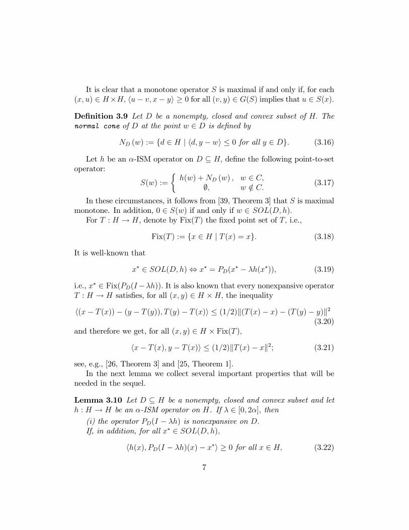
It is clear that a monotone operator S is maximal if and only if, for each(x; u) 2 H�H; hu� v; x� yi � 0 for all (v; y) 2 G(S) implies that u 2 S(x):

De�nition 3.9 Let D be a nonempty, closed and convex subset of H: Thenormal cone of D at the point w 2 D is de�ned by

ND (w) := fd 2 H j hd; y � wi � 0 for all y 2 Dg: (3.16)

Let h be an �-ISM operator on D � H; de�ne the following point-to-setoperator:

S(w) :=

�h(w) +ND (w) ; w 2 C;

;; w =2 C: (3.17)

In these circumstances, it follows from [39, Theorem 3] that S is maximalmonotone. In addition, 0 2 S(w) if and only if w 2 SOL(D; h):For T : H ! H, denote by Fix(T ) the �xed point set of T; i.e.,

Fix(T ) := fx 2 H j T (x) = xg: (3.18)

It is well-known that

x� 2 SOL(D; h), x� = PD(x� � �h(x�)); (3.19)

i.e., x� 2 Fix(PD(I��h)): It is also known that every nonexpansive operatorT : H ! H satis�es, for all (x; y) 2 H �H; the inequality

h(x� T (x))� (y � T (y)); T (y)� T (x)i � (1=2)k(T (x)� x)� (T (y)� y)k2(3.20)

and therefore we get, for all (x; y) 2 H � Fix(T );

hx� T (x); y � T (x)i � (1=2)kT (x)� xk2; (3.21)

see, e.g., [26, Theorem 3] and [25, Theorem 1].In the next lemma we collect several important properties that will be

needed in the sequel.

Lemma 3.10 Let D � H be a nonempty, closed and convex subset and leth : H ! H be an �-ISM operator on H. If � 2 [0; 2�]; then(i) the operator PD(I � �h) is nonexpansive on D:If, in addition, for all x� 2 SOL(D; h);

hh(x); PD(I � �h)(x)� x�i � 0 for all x 2 H; (3.22)

7

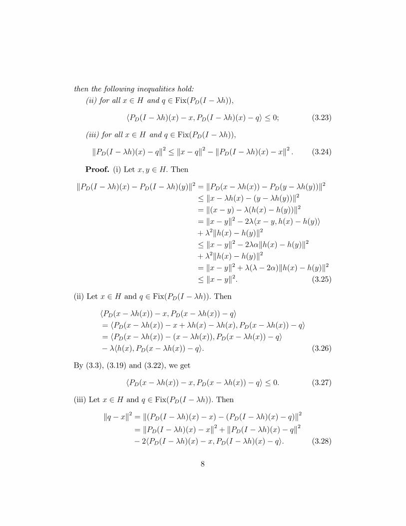
then the following inequalities hold:

(ii) for all x 2 H and q 2 Fix(PD(I � �h));

hPD(I � �h)(x)� x; PD(I � �h)(x)� qi � 0; (3.23)

(iii) for all x 2 H and q 2 Fix(PD(I � �h));

kPD(I � �h)(x)� qk2 � kx� qk2 � kPD(I � �h)(x)� xk2 : (3.24)

Proof. (i) Let x; y 2 H: Then

kPD(I � �h)(x)� PD(I � �h)(y)k2 = kPD(x� �h(x))� PD(y � �h(y))k2

� kx� �h(x)� (y � �h(y))k2

= k(x� y)� �(h(x)� h(y))k2

= kx� yk2 � 2�hx� y; h(x)� h(y)i+ �2kh(x)� h(y)k2

� kx� yk2 � 2��kh(x)� h(y)k2

+ �2kh(x)� h(y)k2

= kx� yk2 + �(�� 2�)kh(x)� h(y)k2

� kx� yk2: (3.25)

(ii) Let x 2 H and q 2 Fix(PD(I � �h)): Then

hPD(x� �h(x))� x; PD(x� �h(x))� qi= hPD(x� �h(x))� x+ �h(x)� �h(x); PD(x� �h(x))� qi= hPD(x� �h(x))� (x� �h(x)); PD(x� �h(x))� qi� �hh(x); PD(x� �h(x))� qi: (3.26)

By (3.3), (3.19) and (3.22), we get

hPD(x� �h(x))� x; PD(x� �h(x))� qi � 0: (3.27)

(iii) Let x 2 H and q 2 Fix(PD(I � �h)): Then

kq � xk2 = k(PD(I � �h)(x)� x)� (PD(I � �h)(x)� q)k2

= kPD(I � �h)(x)� xk2 + kPD(I � �h)(x)� qk2

� 2hPD(I � �h)(x)� x; PD(I � �h)(x)� qi: (3.28)

8

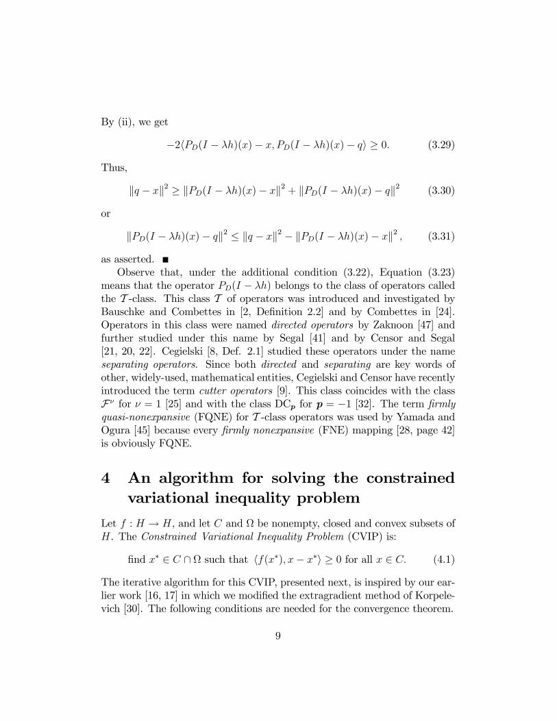
By (ii), we get

�2hPD(I � �h)(x)� x; PD(I � �h)(x)� qi � 0: (3.29)

Thus,

kq � xk2 � kPD(I � �h)(x)� xk2 + kPD(I � �h)(x)� qk2 (3.30)

or

kPD(I � �h)(x)� qk2 � kq � xk2 � kPD(I � �h)(x)� xk2 ; (3.31)

as asserted.Observe that, under the additional condition (3.22), Equation (3.23)

means that the operator PD(I � �h) belongs to the class of operators calledthe T -class. This class T of operators was introduced and investigated byBauschke and Combettes in [2, De�nition 2.2] and by Combettes in [24].Operators in this class were named directed operators by Zaknoon [47] andfurther studied under this name by Segal [41] and by Censor and Segal[21, 20, 22]. Cegielski [8, Def. 2.1] studied these operators under the nameseparating operators. Since both directed and separating are key words ofother, widely-used, mathematical entities, Cegielski and Censor have recentlyintroduced the term cutter operators [9]. This class coincides with the classF� for � = 1 [25] and with the class DCp for p = �1 [32]. The term �rmlyquasi-nonexpansive (FQNE) for T -class operators was used by Yamada andOgura [45] because every �rmly nonexpansive (FNE) mapping [28, page 42]is obviously FQNE.

4 An algorithm for solving the constrainedvariational inequality problem

Let f : H ! H, and let C and be nonempty, closed and convex subsets ofH. The Constrained Variational Inequality Problem (CVIP) is:

�nd x� 2 C \ such that hf(x�); x� x�i � 0 for all x 2 C: (4.1)

The iterative algorithm for this CVIP, presented next, is inspired by our ear-lier work [16, 17] in which we modi�ed the extragradient method of Korpele-vich [30]. The following conditions are needed for the convergence theorem.

9

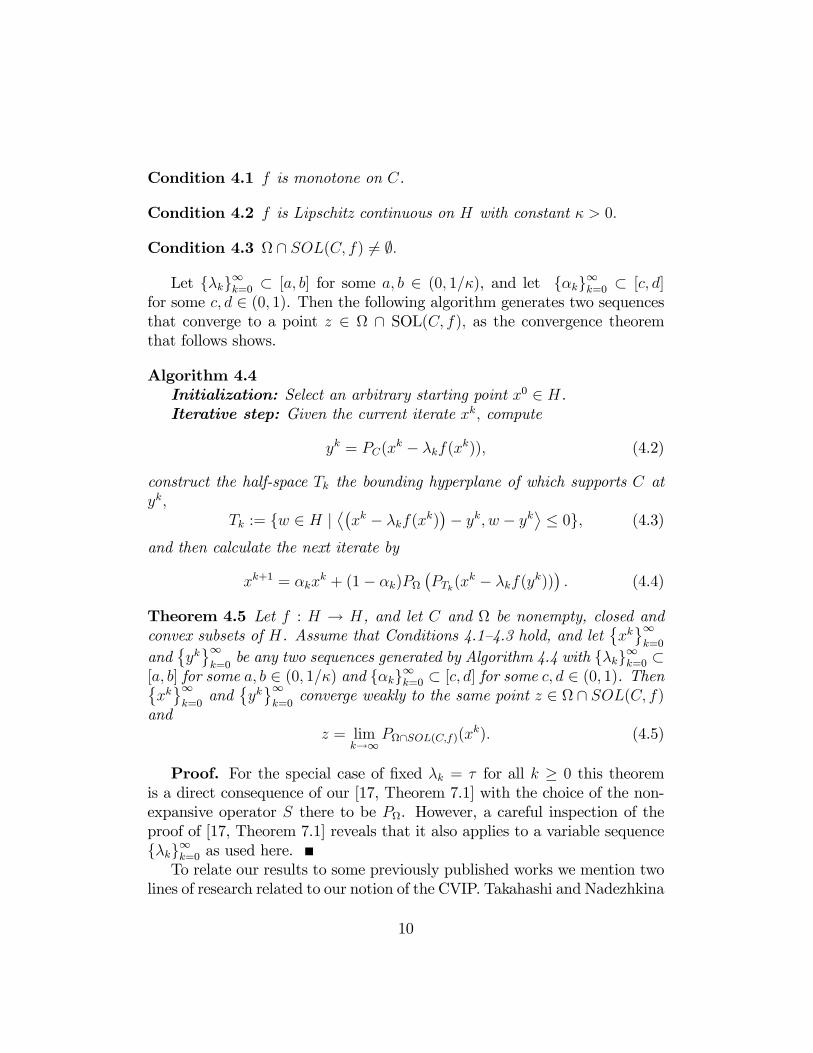
Condition 4.1 f is monotone on C.

Condition 4.2 f is Lipschitz continuous on H with constant � > 0:

Condition 4.3 \ SOL(C; f) 6= ;:

Let f�kg1k=0 � [a; b] for some a; b 2 (0; 1=�), and let f�kg1k=0 � [c; d]for some c; d 2 (0; 1). Then the following algorithm generates two sequencesthat converge to a point z 2 \ SOL(C; f); as the convergence theoremthat follows shows.

Algorithm 4.4Initialization: Select an arbitrary starting point x0 2 H.Iterative step: Given the current iterate xk; compute

yk = PC(xk � �kf(xk)); (4.2)

construct the half-space Tk the bounding hyperplane of which supports C atyk;

Tk := fw 2 H j�xk � �kf(xk)

�� yk; w � yk

�� 0g; (4.3)

and then calculate the next iterate by

xk+1 = �kxk + (1� �k)P

�PTk(x

k � �kf(yk))�: (4.4)

Theorem 4.5 Let f : H ! H, and let C and be nonempty, closed andconvex subsets of H. Assume that Conditions 4.1�4.3 hold, and let

�xk1k=0

and�yk1k=0

be any two sequences generated by Algorithm 4.4 with f�kg1k=0 �[a; b] for some a; b 2 (0; 1=�) and f�kg1k=0 � [c; d] for some c; d 2 (0; 1). Then�xk1k=0

and�yk1k=0

converge weakly to the same point z 2 \ SOL(C; f)and

z = limk!1

P\SOL(C;f)(xk): (4.5)

Proof. For the special case of �xed �k = � for all k � 0 this theoremis a direct consequence of our [17, Theorem 7.1] with the choice of the non-expansive operator S there to be P. However, a careful inspection of theproof of [17, Theorem 7.1] reveals that it also applies to a variable sequencef�kg1k=0 as used here.To relate our results to some previously published works we mention two

lines of research related to our notion of the CVIP. Takahashi and Nadezhkina

10

[35] proposed an algorithm for �nding a point x� 2 Fix(N)\SOL(C; f); whereN : C ! C is a nonexpansive operator. The iterative step of their algorithmis as follows. Given the current iterate xk; compute

yk = PC(xk � �kf(xk)) (4.6)

and thenxk+1 = �kx

k + (1� �k)N�PC(x

k � �kf(yk))�: (4.7)

The restriction PjC of our P in (4.4) is, of course, nonexpansive, and so itis a special case of N in [35]. But a signi�cant advantage of our Algorithm4.4 lies in the fact that we compute PTk onto a half-space in (4.4) whereasthe authors of [35] need to project onto the convex set C: Various wayshave been proposed in the literature to cope with the inherent di¢ culty ofcalculating projections (onto closed convex sets) that do not have a closed-form expression; see, e.g., He, Yang and Duan [29], or [18].Bertsekas and Tsitsiklis [3, Page 288] consider the following problem in

Euclidean space: given f : Rn ! Rn, polyhedral sets C1 � Rn and C2 � Rm;and an m� n matrix A, �nd a point x� 2 C1 such that Ax� 2 C2 and

hf(x�); x� x�i � 0 for all x 2 C1 \ fy j Ay 2 C2g: (4.8)

Denoting = A�1(C2), we see that this problem becomes similar to,but not identical with a CVIP. While the authors of [3] seek a solution inSOL(C1\; f); we aim in our CVIP at \SOL(C; f): They propose to solvetheir problem by the method of multipliers, which is a di¤erent approachthan ours, and they need to assume that either C1 is bounded or AtA isinvertible, where At is the transpose of A:

5 The split variational inequality problem asa constrained variational inequality prob-lem in a product space

Our �rst approach to the solution of the SVIP (1.1)�(1.2) is to look at theproduct spaceH = H1�H2 and introduce in it the product setD := C�Qand the set

V := fx = (x; y) 2H j Ax = yg: (5.1)

11

We adopt the notational convention that objects in the product space arerepresented in boldface type. We transform the SVIP (1.1)�(1.2) into thefollowing equivalent CVIP in the product space:

Find a point x� 2D \ V ; such that hh(x�);x� x�i � 0for all x = (x; y) 2D; (5.2)

where h :H !H is de�ned by

h(x; y) = (f(x); g(y)): (5.3)

A simple adaptation of the decomposition lemma [3, Proposition 5.7, page275] shows that problems (1.1)�(1.2) and (5.2) are equivalent, and, therefore,we can apply Algorithm 4.4 to the solution of (5.2).

Lemma 5.1 A point x� = (x�; y�) solves (5.2) if and only if x� and y� solve(1.1)�(1.2).

Proof. If (x�; y�) solves (1.1)�(1.2), then it is clear that (x�; y�) solves(5.2). To prove the other direction, suppose that (x�; y�) solves (5.2). Since(5.2) holds for all (x; y) 2D, we may take (x�; y) 2D and deduce that

hg(Ax�); y � Ax�i � 0 for all y 2 Q: (5.4)

Using a similar argument with (x; y�) 2D; we get

hf(x�); x� x�i � 0 for all x 2 C; (5.5)

which means that (x�; y�) solves (1.1)�(1.2).Using this equivalence, we can now employ Algorithm 4.4 in order to solve

the SVIP. The following conditions are needed for the convergence theorem.

Condition 5.2 f is monotone on C and g is monotone on Q.

Condition 5.3 f is Lipschitz continuous on H1 with constant �1 > 0 and gis Lipschitz continuous on H2 with constant �2 > 0:

Condition 5.4 V \ SOL(D;h) 6= ;:

12

Let f�kg1k=0 � [a; b] for some a; b 2 (0; 1=�), where � = minf�1; �2g,and let f�kg1k=0 � [c; d] for some c; d 2 (0; 1). Then the following algorithmgenerates two sequences that converge to a point z 2 V \ SOL(D;h); asthe convergence theorem given below shows.

Algorithm 5.5Initialization: Select an arbitrary starting point x0 2H.Iterative step: Given the current iterate xk; compute

yk = PD(xk � �kh(xk)); (5.6)

construct the half-space T k the bounding hyperplane of which supports D atyk;

T k := fw 2H j�xk � �kh(xk)

�� yk;w � yk

�� 0g; (5.7)

and then calculate

xk+1 = �kxk + (1� �k)P V

�P T k(x

k � �kh(yk))�: (5.8)

Our convergence theorem for Algorithm 5.5 follows from Theorem 4.5.

Theorem 5.6 Consider f : H1 ! H1 and g : H2 ! H2; a bounded linearoperator A : H1 ! H2, and nonempty, closed and convex subsets C � H1 andQ � H2. Assume that Conditions 5.2�5.4 hold, and let

�xk1k=0

and�yk1k=0

be any two sequences generated by Algorithm 5.5 with f�kg1k=0 � [a; b] forsome a; b 2 (0; 1=�), where � = minf�1; �2g, and let f�kg1k=0 � [c; d] forsome c; d 2 (0; 1). Then

�xk1k=0

and�yk1k=0

converge weakly to the samepoint z 2 V \ SOL(D;h) and

z = limk!1

P V \SOL(D;h)(xk): (5.9)

The value of the product space approach, described above, depends on theability to �translate�Algorithm 5.5 back to the original spaces H1 and H2:Observe that due to [37, Lemma 1.1] for x=(x; y) 2 D; we have PD(x) =(PC(x); PQ(y)) and a similar formula holds for P T k : The potential di¢ cultylies in P V of (5.8). In the �nite-dimensional case, since V is a subspace,the projection onto it is easily computable by using an orthogonal basis. Forexample, if U is a k-dimensional subspace of Rn with the basis fu1; u2; :::; ukg,then for x 2 Rn; we have

PU(x) =

kXi=1

hx; uiikuik2

ui: (5.10)

13

6 Solving the split variational inequality prob-lem without a product space

In this section we present a method for solving the SVIP, which does notneed a product space formulation as in the previous section. Recalling thatSOL(C; f) and SOL(Q; g) are the solution sets of (1.1) and (1.2), respec-tively, we see that the solution set of the SVIP is

� := �(C;Q; f; g; A) := fz 2 SOL(C; f) j Az 2 SOL(Q; g)g : (6.1)

Using the abbreviations T := PQ(I � �g) and U := PC(I � �f); we proposethe following algorithm.

Algorithm 6.1Initialization: Let � > 0 and select an arbitrary starting point x0 2 H1.Iterative step: Given the current iterate xk; compute

xk+1 = U(xk + A�(T � I)(Axk)); (6.2)

where 2 (0; 1=L), L is the spectral radius of the operator A�A, and A� isthe adjoint of A.

The following lemma, which asserts Fejér-monotonicity, is crucial for theconvergence theorem.

Lemma 6.2 Let H1 and H2 be real Hilbert spaces and let A : H1 ! H2 bea bounded linear operator. Let f : H1 ! H1 and g : H2 ! H2 be �1-ISMand �2-ISM operators on H1 and H2; respectively, and set � := minf�1; �2g.Assume that � 6= ; and that 2 (0; 1=L). Consider the operators U =PC(I � �f) and T = PQ(I � �g) with � 2 [0; 2�]. Then any sequence�xk1k=0; generated by Algorithm 6.1, is Fejér-monotone with respect to the

solution set �.

Proof. Let z 2 �: Then z 2 SOL(C; f) and, therefore, by (3.19) andLemma 3.10(i), we get xk+1 � z 2 = U �xk + A�(T � I)(Axk)�� z 2

= U �xk + A�(T � I)(Axk)�� U(z) 2

� xk + A�(T � I)(Axk)� z 2

= xk � z 2 + 2 A�(T � I)(Axk) 2

+ 2 xk � z; A�(T � I)(Axk)

�: (6.3)

14

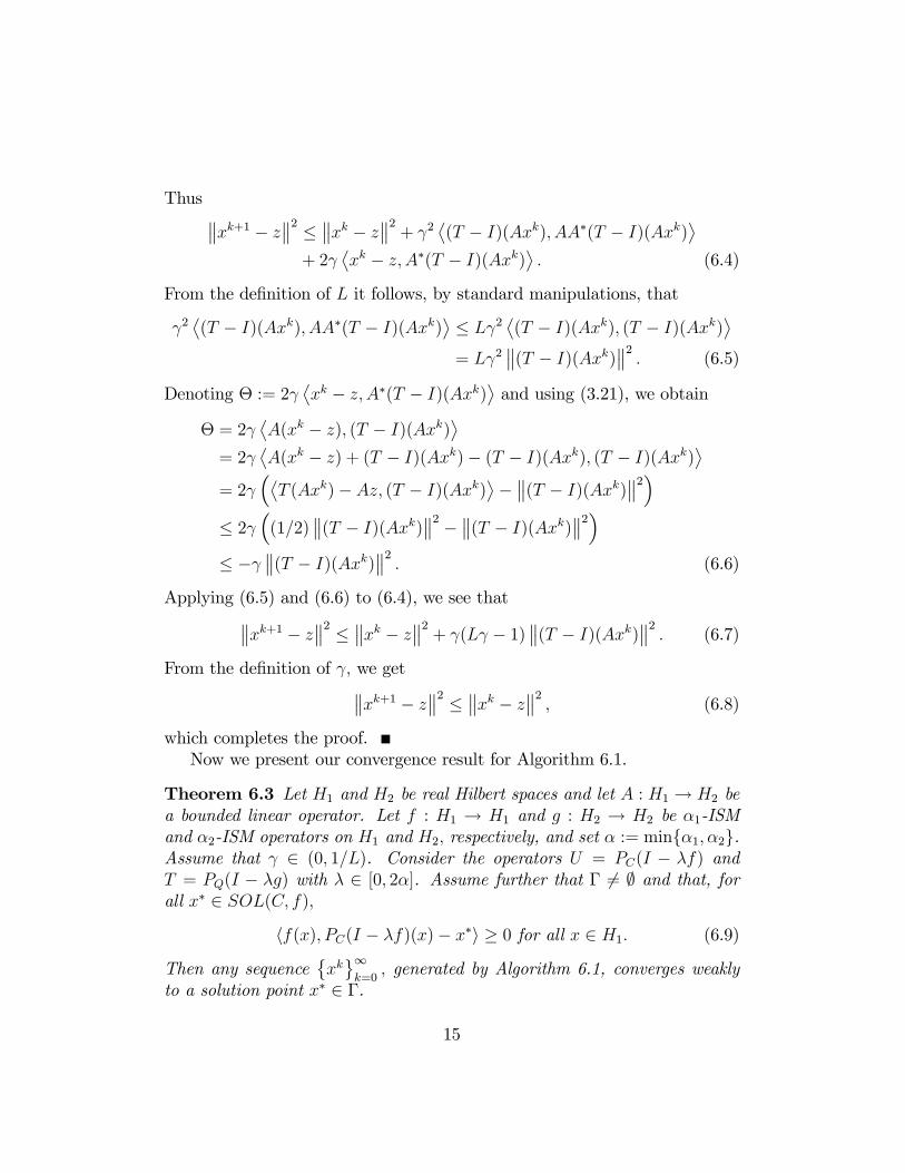
Thus xk+1 � z 2 � xk � z 2 + 2 (T � I)(Axk); AA�(T � I)(Axk)�+ 2

xk � z; A�(T � I)(Axk)

�: (6.4)

From the de�nition of L it follows, by standard manipulations, that

2(T � I)(Axk); AA�(T � I)(Axk)

�� L 2

(T � I)(Axk); (T � I)(Axk)

�= L 2

(T � I)(Axk) 2 : (6.5)

Denoting � := 2 xk � z; A�(T � I)(Axk)

�and using (3.21), we obtain

� = 2 A(xk � z); (T � I)(Axk)

�= 2

A(xk � z) + (T � I)(Axk)� (T � I)(Axk); (T � I)(Axk)

�= 2

�T (Axk)� Az; (T � I)(Axk)

�� (T � I)(Axk) 2�

� 2 �(1=2)

(T � I)(Axk) 2 � (T � I)(Axk) 2�� �

(T � I)(Axk) 2 : (6.6)

Applying (6.5) and (6.6) to (6.4), we see that xk+1 � z 2 � xk � z 2 + (L � 1) (T � I)(Axk) 2 : (6.7)

From the de�nition of ; we get xk+1 � z 2 � xk � z 2 ; (6.8)

which completes the proof.Now we present our convergence result for Algorithm 6.1.

Theorem 6.3 Let H1 and H2 be real Hilbert spaces and let A : H1 ! H2 bea bounded linear operator. Let f : H1 ! H1 and g : H2 ! H2 be �1-ISMand �2-ISM operators on H1 and H2; respectively, and set � := minf�1; �2g.Assume that 2 (0; 1=L). Consider the operators U = PC(I � �f) andT = PQ(I � �g) with � 2 [0; 2�]. Assume further that � 6= ; and that, forall x� 2 SOL(C; f);

hf(x); PC(I � �f)(x)� x�i � 0 for all x 2 H1: (6.9)

Then any sequence�xk1k=0; generated by Algorithm 6.1, converges weakly

to a solution point x� 2 �.

15

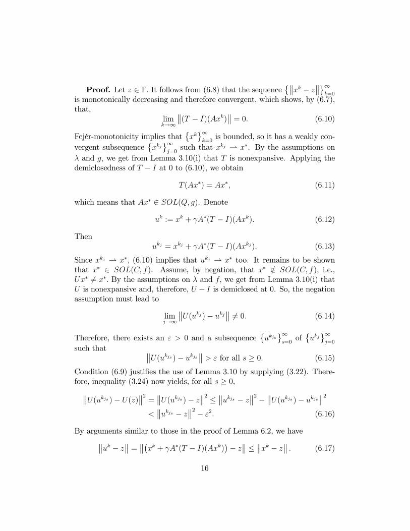
Proof. Let z 2 �: It follows from (6.8) that the sequence� xk � z 1

k=0is monotonically decreasing and therefore convergent, which shows, by (6.7),that,

limk!1

(T � I)(Axk) = 0: (6.10)

Fejér-monotonicity implies that�xk1k=0

is bounded, so it has a weakly con-vergent subsequence

�xkj1j=0

such that xkj * x�. By the assumptions on� and g; we get from Lemma 3.10(i) that T is nonexpansive. Applying thedemiclosedness of T � I at 0 to (6.10), we obtain

T (Ax�) = Ax�; (6.11)

which means that Ax� 2 SOL(Q; g). Denote

uk := xk + A�(T � I)(Axk). (6.12)

Thenukj = xkj + A�(T � I)(Axkj): (6.13)

Since xkj * x�; (6.10) implies that ukj * x� too. It remains to be shownthat x� 2 SOL(C; f). Assume, by negation, that x� =2 SOL(C; f); i.e.,Ux� 6= x�: By the assumptions on � and f; we get from Lemma 3.10(i) thatU is nonexpansive and, therefore, U � I is demiclosed at 0. So, the negationassumption must lead to

limj!1

U(ukj)� ukj 6= 0: (6.14)

Therefore, there exists an " > 0 and a subsequence�ukjs

1s=0

of�ukj1j=0

such that U(ukjs )� ukjs > " for all s � 0: (6.15)

Condition (6.9) justi�es the use of Lemma 3.10 by supplying (3.22). There-fore, inequality (3.24) now yields, for all s � 0; U(ukjs )� U(z) 2 = U(ukjs )� z 2 � ukjs � z 2 � U(ukjs )� ukjs 2

< ukjs � z 2 � "2: (6.16)

By arguments similar to those in the proof of Lemma 6.2, we have uk � z = �xk + A�(T � I)(Axk)�� z � xk � z : (6.17)

16

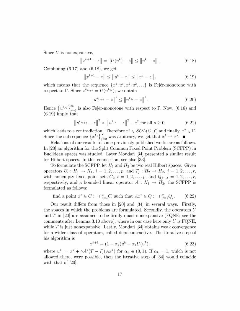
Since U is nonexpansive, xk+1 � z = U(uk)� z � uk � z : (6.18)

Combining (6.17) and (6.18), we get xk+1 � z � uk � z � xk � z ; (6.19)

which means that the sequence fx1; u1; x2; u2; : : :g is Fejér-monotone withrespect to �: Since xkjs+1 = U(ukjs ), we obtain ukjs+1 � z 2 � ukjs � z 2 : (6.20)

Hence�ukjs

1s=0

is also Fejér-monotone with respect to �: Now, (6.16) and(6.19) imply that ukjs+1 � z 2 < ukjs � z 2 � "2 for all s � 0; (6.21)

which leads to a contradiction. Therefore x� 2 SOL(C; f) and �nally, x� 2 �.Since the subsequence

�xkj1j=0

was arbitrary, we get that xk * x�:

Relations of our results to some previously published works are as follows.In [20] an algorithm for the Split Common Fixed Point Problem (SCFPP) inEuclidean spaces was studied. Later Mouda� [34] presented a similar resultfor Hilbert spaces. In this connection, see also [33].To formulate the SCFPP, letH1 andH2 be two real Hilbert spaces. Given

operators Ui : H1 ! H1, i = 1; 2; : : : ; p; and Tj : H2 ! H2; j = 1; 2; : : : ; r;with nonempty �xed point sets Ci; i = 1; 2; : : : ; p; and Qj; j = 1; 2; : : : ; r;respectively, and a bounded linear operator A : H1 ! H2, the SCFPP isformulated as follows:

�nd a point x� 2 C := \pi=1Ci such that Ax� 2 Q := \rj=1Qj: (6.22)

Our result di¤ers from those in [20] and [34] in several ways. Firstly,the spaces in which the problems are formulated. Secondly, the operators Uand T in [20] are assumed to be �rmly quasi-nonexpansive (FQNE; see thecomments after Lemma 3.10 above), where in our case here only U is FQNE,while T is just nonexpansive. Lastly, Mouda� [34] obtains weak convergencefor a wider class of operators, called demicontractive. The iterative step ofhis algorithm is

xk+1 = (1� �k)uk + �kU(uk); (6.23)

where uk := xk + A�(T � I)(Axk) for �k 2 (0; 1): If �k = 1; which is notallowed there, were possible, then the iterative step of [34] would coincidewith that of [20].

17

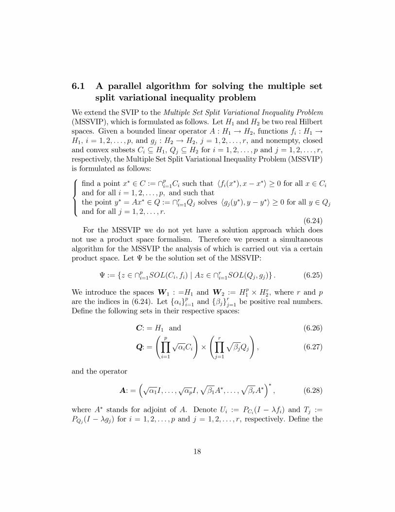
6.1 A parallel algorithm for solving the multiple setsplit variational inequality problem

We extend the SVIP to the Multiple Set Split Variational Inequality Problem(MSSVIP), which is formulated as follows. LetH1 andH2 be two real Hilbertspaces. Given a bounded linear operator A : H1 ! H2, functions fi : H1 !H1; i = 1; 2; : : : ; p; and gj : H2 ! H2; j = 1; 2; : : : ; r, and nonempty, closedand convex subsets Ci � H1; Qj � H2 for i = 1; 2; : : : ; p and j = 1; 2; : : : ; r,respectively, the Multiple Set Split Variational Inequality Problem (MSSVIP)is formulated as follows:8>><>>:�nd a point x� 2 C := \pi=1Ci such that hfi(x�); x� x�i � 0 for all x 2 Ciand for all i = 1; 2; : : : ; p; and such thatthe point y� = Ax� 2 Q := \ri=1Qj solves hgj(y�); y � y�i � 0 for all y 2 Qjand for all j = 1; 2; : : : ; r:

(6.24)For the MSSVIP we do not yet have a solution approach which does

not use a product space formalism. Therefore we present a simultaneousalgorithm for the MSSVIP the analysis of which is carried out via a certainproduct space. Let be the solution set of the MSSVIP:

:= fz 2 \pi=1SOL(Ci; fi) j Az 2 \ri=1SOL(Qj; gj)g : (6.25)

We introduce the spaces W 1 : =H1 and W 2 := Hp1 � Hr

2 ; where r and pare the indices in (6.24). Let f�igpi=1 and f�jg

rj=1 be positive real numbers.

De�ne the following sets in their respective spaces:

C: = H1 and (6.26)

Q: =

pYi=1

p�iCi

!�

rYj=1

p�jQj

!; (6.27)

and the operator

A: =�p�1I; : : : ;

p�pI;

p�1A

�; : : : ;p�rA

���; (6.28)

where A� stands for adjoint of A. Denote Ui := PCi(I � �fi) and Tj :=PQj(I � �gj) for i = 1; 2; : : : ; p and j = 1; 2; : : : ; r, respectively: De�ne the

18

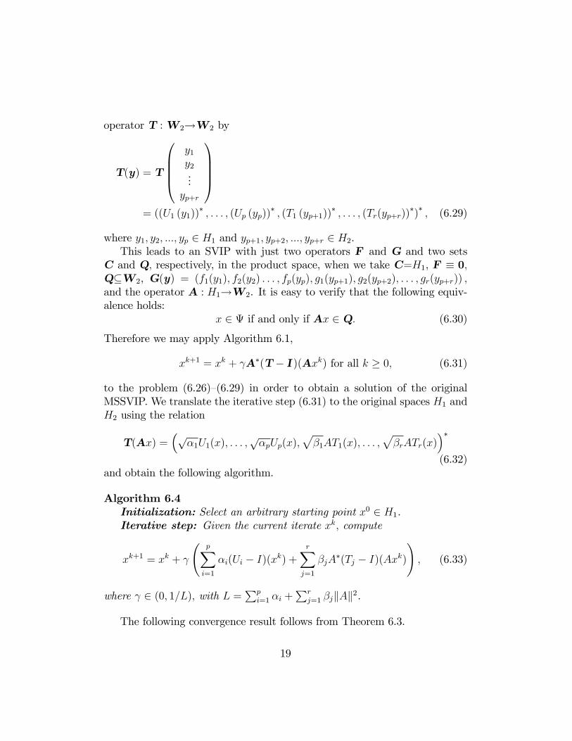
operator T :W 2!W 2 by

T (y) = T

[email protected]+r

1CCCA= ((U1 (y1))

� ; : : : ; (Up (yp))� ; (T1 (yp+1))

� ; : : : ; (Tr(yp+r))�)�; (6.29)

where y1; y2; :::; yp 2 H1 and yp+1; yp+2; :::; yp+r 2 H2.This leads to an SVIP with just two operators F and G and two sets

C and Q; respectively, in the product space, when we take C=H1, F � 0;Q�W 2, G(y) = (f1(y1); f2(y2) : : : ; fp(yp); g1(yp+1); g2(yp+2); : : : ; gr(yp+r)) ;and the operator A : H1!W 2. It is easy to verify that the following equiv-alence holds:

x 2 if and only if Ax 2 Q: (6.30)

Therefore we may apply Algorithm 6.1,

xk+1 = xk + A�(T � I)(Axk) for all k � 0; (6.31)

to the problem (6.26)�(6.29) in order to obtain a solution of the originalMSSVIP. We translate the iterative step (6.31) to the original spaces H1 andH2 using the relation

T (Ax) =�p�1U1(x); : : : ;

p�pUp(x);

p�1AT1(x); : : : ;

p�rATr(x)

��(6.32)

and obtain the following algorithm.

Algorithm 6.4Initialization: Select an arbitrary starting point x0 2 H1.Iterative step: Given the current iterate xk; compute

xk+1 = xk +

pXi=1

�i(Ui � I)(xk) +rXj=1

�jA�(Tj � I)(Axk)

!; (6.33)

where 2 (0; 1=L); with L =Pp

i=1 �i +Pr

j=1 �jkAk2.

The following convergence result follows from Theorem 6.3.

19

Theorem 6.5 Let H1 and H2 be two real Hilbert spaces and let A : H1 !H2 be a bounded linear operator. Let fi : H1 ! H1; i = 1; 2; : : : ; p; andgj : H2 ! H2; j = 1; 2; : : : ; r, be �-ISM operators on nonempty, closed andconvex subsets Ci � H1; Qj � H2 for i = 1; 2; : : : ; p; and j = 1; 2; : : : ; r,respectively. Assume that 2 (0; 1=L) and 6= ;. Set Ui := PCi(I � �fi)and Tj := PQj(I � �gj) for i = 1; 2; : : : ; p and j = 1; 2; : : : ; r, respectively,with � 2 [0; 2�]. If, in addition, for each i = 1; 2; : : : ; p and j = 1; 2; : : : ; rwe have

hfi(x); PCi(I � �fi)(x)� x�i � 0 for all x 2 H1 (6.34)

for all x� 2 SOL(Ci; fi) and

hgj(x); PQj(I � �gj)(x)� x�i � 0 for all x 2 H2; (6.35)

for all x� 2 SOL(Ci; fi), then any sequence�xk1k=0

; generated by Algorithm6.1, converges weakly to a solution point x� 2 .

Proof. Apply Theorem 6.3 to the two-operator SVIP in the productspace setting with U = I : H1 ! H1, FixU = C; T = T : W ! W ; andFixT = Q.

Remark 6.6 Observe that conditions (6.34) and (6.35) imposed on Ui andTj for i = 1; 2; : : : ; p and j = 1; 2; : : : ; r, respectively, in Theorem 6.5,which are necessary for our treatment of the problem in a product space,ensure that these operators are �rmly quasi-nonexpansive (FQNE). There-fore, the SVIP under these conditions may be considered a Split CommonFixed Point Problem (SCFPP), �rst introduced in [20], with C; Q; A andT :W 2 !W 2 as above, and the identity operator I : C ! C. Therefore,we could also apply [20, Algorithm 4.1]. If, however, we drop these condi-tions, then the operators are nonexpansive, by Lemma 3.10(i), and the resultof [34] would apply.

7 Applications

The following problems are special cases of the SVIP. They are listed herebecause their analysis can bene�t from our algorithms for the SVIP andbecause known algorithms for their solution may be generalized in the futureto cover the more general SVIP. The list includes known problems such as theSplit Feasibility Problem (SFP) and the Convex Feasibility Problem (CFP).

20

In addition, we introduce two new �split�problems that have, to the best ofour knowledge, never been studied before. These are the Common Solutionsto Variational Inequalities Problem (CSVIP) and the Split Zeros Problem(SZP).

7.1 The split feasibility and convex feasibility prob-lems

The Split Feasibility Problem (SFP) in Euclidean space is formulated asfollows:

�nd a point x� such that x� 2 C � Rn and Ax� 2 Q � Rm; (7.1)

where C � Rn; Q � Rm are nonempty, closed and convex sets, and A : Rn !Rm is given. Originally introduced in Censor and Elfving [14], it was laterused in the area of intensity-modulated radiation therapy (IMRT) treatmentplanning; see [15, 11]. Obviously, it is formally a special case of the SVIPobtained from (1.1)�(1.2) by setting f � g � 0: The Convex FeasibilityProblem (CFP) in a Euclidean space is:

�nd a point x� such that x� 2 \mi=1Ci 6= ;; (7.2)

where Ci; i = 1; 2; : : : ;m; are nonempty, closed and convex sets in Rn: This,in its turn, becomes a special case of the SFP by taking in (7.1) n = m; A = IQ = Rn and C = \mi=1Ci: Many algorithms for solving the CFP have beendeveloped; see, e.g., [1, 23]. Byrne [5] established an algorithm for solvingthe SFP, called the CQ-Algorithm, with the following iterative step:

xk+1 = PC�xk + At(PQ � I)Axk

�; (7.3)

which does not require calculation of the inverse of the operator A; as in [14],but needs only its transpose At. A recent excellent paper on the multiple-setsSFP which contains many references that re�ect the state-of-the-art in thisarea is [31].It is of interest to note that looking at the SFP from the point of view of

the SVIP enables us to �nd the minimum-norm solution of the SFP, i.e., asolution of the form

x� = argminfkxk j x solves the SFP (7.1)g: (7.4)

This is done, and easily veri�ed, by solving (1.1)�(1.2) with f = I and g � 0:

21

7.2 The common solutions to variational inequalitiesproblem

The Common Solutions to Variational Inequalities Problem (CSVIP), newlyintroduced here, is de�ned in Euclidean space as follows. Let ffigmi=1 be afamily of functions from Rn into itself and let fCigmi=1 be nonempty, closedand convex subsets of Rn with \mi=1Ci 6= ;. The CSVIP is formulated asfollows:

�nd a point x� 2 \mi=1Ci such that hfi(x�); x� x�i � 0for all x 2 Ci, i = 1; 2; : : : ;m: (7.5)

This problem can be transformed into a CVIP in an appropriate productspace (di¤erent from the one in Section 5). Let Rmn be the product spaceand de�ne F : Rmn ! Rmn by

F�(x1; x2; : : : ; xm)

�= (f1(x

1); : : : ; fm(xm)); (7.6)

where xi 2 Rn for all i = 1; 2; : : : ;m: Let the diagonal set in Rmn be

� := fx 2 Rmn j x=(a; a; : : : ; a); a 2 Rng (7.7)

and de�ne the product setC := �mi=1Ci: (7.8)

The CSVIP in Rn is equivalent to the following CVIP in Rmn:

�nd a point x� 2 C \� such that hF (x�);x� x�i � 0for all x = (x1; x2; : : : ; xm) 2 C: (7.9)

So, this problem can be solved by using Algorithm 4.4 with = �: A newalgorithm speci�cally designed for the CSVIP appears in [19].

7.3 The split minimization and the split zeros prob-lems

From optimality conditions for convex optimization (see, e.g., Bertsekas andTsitsiklis [3, Proposition 3.1, page 210]) it is well-known that if F : Rn ! Rn

is a continuously di¤erentiable convex function on a closed and convex subsetX � Rn; then x� 2 X minimizes F over X if and only if

hrF (x�); x� x�i � 0 for all x 2 X; (7.10)

22

where rF is the gradient of F . Since (7.10) is a VIP, we make the followingobservation. If F : Rn ! Rn and G : Rm ! Rm are continuously di¤eren-tiable convex functions on closed and convex subsets C � Rn and Q � Rm;respectively, and if in the SVIP we take f = rF and g = rG; then weobtain the following Split Minimization Problem (SMP):

�nd a point x� 2 C such that x� = argminff(x) j x 2 Cg (7.11)

and such that

the point y� = Ax� 2 Q and solves y� = argminfg(y) j y 2 Qg: (7.12)

The Split Zeros Problem (SZP), newly introduced here, is de�ned as fol-lows. Let H1 and H2 be two Hilbert spaces. Given operators B1 : H1 ! H1and B2 : H2 ! H2; and a bounded linear operator A : H1 ! H2, the SZP isformulated as follows:

�nd a point x� 2 H1 such that B1(x�) = 0 and B2(Ax�) = 0: (7.13)

This problem is a special case of the SVIP if A is a surjective operator. Tosee this, take in (1.1)�(1.2) C = H1, Q = H2; f = B1 and g = B2; and choosex := x��B1(x�) 2 H1 in (1.1) and x 2 H1 such that Ax := Ax��B2(Ax�) 2H2 in (1.2).The next lemma shows when the only solution of an SVIP is a solution of

an SZP. It extends a similar result concerning the relationship between the(un-split) zero �nding problem and the VIP.

Lemma 7.1 Let H1 and H2 be real Hilbert spaces, and C � H1 and Q � H2nonempty, closed and convex subsets. Let B1 : H1 ! H1 and B2 : H2 ! H2be �-ISM operators and let A : H1 ! H2 be a bounded linear operator.Assume that C \ fx 2 H1 j B1(x) = 0g 6= ; and that Q \ fy 2 H2 j B2(y) =0g 6= ;, and denote

� := �(C;Q;B1; B2; A) := fz 2 SOL(C;B1) j Az 2 SOL(Q;B2)g : (7.14)

Then, for any x� 2 C with Ax� 2 Q; x� solves (7.13) if and only if x� 2 �.

Proof. First assume that x� 2 C with Ax� 2 Q and that x� solves(7.13). Then it is clear that x� 2 �: In the other direction, assume thatx� 2 C with Ax� 2 Q and that x� 2 �: Applying (3.4) with C as D there,

23

(I��B1) (x�) 2 H1; for any � 2 (0; 2�], as x there, and q1 2 C\Fix(I��B1);with the same �; as y there, we get

kq1 � PC(I � �B1) (x�)k2 + k(I � �B1) (x�)� PC(I � �B1) (x�)k2

� k(I � �B1) (x�)� q1k2 ; (7.15)

and, similarly, applying (3.4) again, we obtain

kq2 � PQ(I � �B2) (Ax�)k2 + k(I � �B2) (Ax�)� PQ(I � �B2) (Ax�)k2

� k(I � �B2) (Ax�)� q2k2 : (7.16)

Using the characterization of (3.19), we get

kq1 � x�k2 + k(I � �B1) (x�)� x�k2 � k(I � �B1) (x�)� q1k2 (7.17)

and

kq2 � Ax�k2 + k(I � �B2) (Ax�)� x�k2 � k(I � �B2) (Ax�)� q2k2 : (7.18)

It can be seen from the proof of Lemma 3.10(i) that the operators I��B1and I ��B2 are nonexpansive for every � 2 [0; 2�], so with q1 2 C \Fix(I ��B1) and q2 2 Q \ Fix(I � �B2);

k(I � �B1) (x�)� q1k2 � kx� � q1k2 (7.19)

andk(I � �B2) (Ax�)� q2k2 � kAx� � q2k2 : (7.20)

Combining the above inequalities, we obtain

kq1 � x�k2 + k(I � �B1) (x�)� x�k2 � kx� � q1k2 (7.21)

and

kq2 � Ax�k2 + k(I � �B2) (Ax�)� x�k2 � kAx� � q2k2 : (7.22)

Hence, k(I � �B1) (x�)� x�k2 = 0 and k(I � �B2) (Ax�)� Ax�k2 = 0: Since� > 0; we get that B1(x�) = 0 and B2(Ax�) = 0, as claimed

Acknowledgments. This work was partially supported by a UnitedStates-Israel Binational Science Foundation (BSF) Grant number 200912, byUS Department of Army award number W81XWH-10-1-0170, by Israel Sci-ence Foundation (ISF) Grant number 647/07, by the Fund for the Promotionof Research at the Technion and by the Technion President�s Research Fund.

24

References

[1] H. H. Bauschke and J. M. Borwein, On projection algorithms for solvingconvex feasibility problems, SIAM Review 38 (1996), 367�426.

[2] H. H. Bauschke and P. L. Combettes, A weak-to-strong convergenceprinciple for Fejér-monotone methods in Hilbert spaces, Mathematics ofOperations Research 26 (2001), 248�264.

[3] D. P. Bertsekas and J. N. Tsitsiklis, Parallel and Distributed Computa-tion: Numerical Methods, Prentice-Hall International, Englwood Cli¤s,NJ, USA, 1989.

[4] F. E. Browder, Fixed point theorems for noncompact mappings inHilbert space, Proceedings of the National Academy of Sciences USA53 (1965), 1272�1276.

[5] C. L. Byrne, Iterative projection onto convex sets using multiple Breg-man distances, Inverse Problems 15 (1999), 1295�1313.

[6] C. Byrne, Iterative oblique projection onto convex sets and the splitfeasibility problem, Inverse Problems 18 (2002), 441�453.

[7] C. Byrne, A uni�ed treatment of some iterative algorithms in signalprocessing and image reconstruction, Inverse Problems 20 (2004), 103�120.

[8] A. Cegielski, Generalized relaxations of nonexpansive operators and con-vex feasibility problems, Contemporary Mathematics 513 (2010), 111�123.

[9] A. Cegielski and Y. Censor, Opial-type theorems and the common �xedpoint problem, in: H. Bauschke, R. Burachik, P. Combettes, V. Elser, R.Luke and H. Wolkowicz (Editors), Fixed-Point Algorithms for InverseProblems in Science and Engineering, Springer-Verlag, New York, NY,USA, 2011, pp. 155�183.

[10] Y. Censor, M. D. Altschuler and W. D. Powlis, On the use of Cimmino�ssimultaneous projections method for computing a solution of the inverseproblem in radiation therapy treatment planning, Inverse Problems 4(1988), 607�623.

25

[11] Y. Censor, T. Bortfeld, B. Martin and A. Tro�mov, A uni�ed approachfor inversion problems in intensity-modulated radiation therapy, Physicsin Medicine and Biology 51 (2006), 2353�2365.

[12] Y. Censor, W. Chen, P. L. Combettes, R. Davidi and G. T. Herman, Onthe e¤ectiveness of projection methods for convex feasibility problemswith linear inequality constraints, Computational Optimization and Ap-plications, accepted for publication, DOI: 10.1007/s10589-011-9401-7,Online First http://arxiv.org/abs/0912.4367.

[13] Y. Censor, R. Davidi and G. T. Herman, Perturbation resilience andsuperiorization of iterative algorithms, Inverse Problems 26 (2010),065008 (pp. 17).

[14] Y. Censor and T. Elfving , A multiprojection algorithm using Bregmanprojections in product space, Numerical Algorithms 8 (1994), 221�239.

[15] Y. Censor, T. Elfving, N. Kopf and T. Bortfeld, The multiple-sets splitfeasibility problem and its applications for inverse problems, InverseProblems 21 (2005), 2071�2084.

[16] Y. Censor, A. Gibali and S. Reich, Extensions of Korpelevich�s extragra-dient method for solving the variational inequality problem in Euclideanspace, Optimization, accepted for publication.

[17] Y. Censor, A. Gibali and S. Reich, The subgradient extragradientmethod for solving the variational inequality problem in Hilbert space,Journal of Optimization Theory and Applications 148 (2011), 318�335.

[18] Y. Censor, A. Gibali and S. Reich, Strong convergence of subgradientextragradient methods for the variational inequality problem in Hilbertspace, Optimization Methods and Software, accepted for publication.

[19] Y. Censor, A. Gibali, S. Reich and S. Sabach, Common solutions tovariational inequalities, Technical Report, April 5, 2011. Revised: July18, 2011.

[20] Y. Censor and A. Segal, The split common �xed point problem fordirected operators, Journal of Convex Analysis 16 (2009), 587�600.

26

[21] Y. Censor and A. Segal, On the string averaging method for sparsecommon �xed point problems, International Transactions in OperationalResearch 16 (2009), 481�494.

[22] Y. Censor and A. Segal, On string-averaging for sparse problems and onthe split common �xed point problem, Contemporary Mathematics 513(2010), 125�142.

[23] Y. Censor and S. A. Zenios, Parallel Optimization: Theory, Algorithms,and Applications, Oxford University Press, New York, NY, USA, 1997.

[24] P. L. Combettes, Quasi-Fejérian analysis of some optimization algo-rithms, in: D. Butnariu, Y. Censor and S. Reich (Editors), InherentlyParallel Algorithms in Feasibility and Optimization and Their Applica-tions, Elsevier Science Publishers, Amsterdam, The Netherlands, 2001,pp. 115�152.

[25] G. Crombez, A geometrical look at iterative methods for operatorswith �xed points, Numerical Functional Analysis and Optimization 26(2005), 157�175.

[26] G. Crombez, A hierarchical presentation of operators with �xed pointson Hilbert spaces, Numerical Functional Analysis and Optimization 27(2006), 259�277.

[27] Y. Dang and Y. Gao, The strong convergence of a KM�CQ-like algo-rithm for a split feasibility problem, Inverse Problems 27 (2011), 015007.

[28] K. Goebel and S. Reich, Uniform Convexity, Hyperbolic Geometry, andNonexpansive Mappings, Marcel Dekker, New York and Basel, 1984.

[29] S. He, C. Yang and P. Duan, Realization of the hybrid method forMann iteration, Applied Mathematics and Computation 217 (2010),4239�4247.

[30] G. M. Korpelevich, The extragradient method for �nding saddle pointsand other problems, Ekonomika i Matematicheskie Metody 12 (1976),747�756.

[31] G. López, V. Martín-Márquez and H.-K. Xu, Iterative algorithms forthe multiple-sets split feasibility problem, in: Y. Censor, M. Jiang and

27

G. Wang (Editors), Biomedical Mathematics: Promising Directions inImaging, Therapy Planning and Inverse Problems, Medical Physics Pub-lishing, Madison, WI, USA, 2010, pp. 243�279.

[32] S. M¼aruster and C. Popirlan, On the Mann-type iteration and the convexfeasibility problem, Journal of Computational and Applied Mathematics212 (2008), 390�396.

[33] E. Masad and S. Reich, A note on the multiple-set split convex feasibilityproblem in Hilbert space, Journal of Nonlinear and Convex Analysis 8(2007), 367�371.

[34] A. Mouda�, The split common �xed-point problem for demicontractivemappings, Inverse Problems 26 (2010), 1�6.

[35] N. Nadezhkina and W. Takahashi, Weak convergence theorem by anextragradient method for nonexpansive mappings and monotone map-pings, Journal of Optimization Theory and Applications 128 (2006),191�201.

[36] Z. Opial, Weak convergence of the sequence of successive approximationsfor nonexpansive mappings, Bulletin of the American Mathematical So-ciety 73 (1967), 591�597.

[37] G. Pierra, Decomposition through formalization in a product space,Mathematical Programming 28 (1984), 96�115.

[38] B. Qu and N. Xiu, A note on the CQ algorithm for the split feasibilityproblem, Inverse Problems 21 (2005), 1655�1666.

[39] R. T. Rockafellar, On the maximality of sums of nonlinear monotone op-erators, Transactions of the American Mathematical Society 149 (1970),75�88.

[40] F. Schöpfer, T. Schuster and A. K. Louis, An iterative regularizationmethod for the solution of the split feasibility problem in Banach spaces,Inverse Problems 24 (2008), 055008.

[41] A. Segal, Directed Operators for Common Fixed Point Problems andConvex Programming Problems, Ph.D. Thesis, University of Haifa, Sep-tember 2008.

28

[42] W. Takahashi and M. Toyoda, Weak convergence theorems for non-expansive mappings and monotone mappings, Journal of OptimizationTheory and Applications 118 (2003), 417�428.

[43] H. K. Xu, A variable Krasnosel�skii�Mann algorithm and the multiple-set split feasibility problem, Inverse Problems 22 (2006), 2021�2034.

[44] H. K. Xu, Iterative methods for the split feasibility problem in in�nite-dimensional Hilbert spaces, Inverse Problems 26 (2010), 105018.

[45] I. Yamada and N. Ogura, Adaptive projected subgradient method forasymptotic minimization of sequence of nonnegative convex functions,Numerical Functional Analysis and Optimization 25 (2005), 593�617.

[46] Q. Yang, The relaxed CQ algorithm solving the split feasibility problem,Inverse Problems 20 (2004), 1261�1266.

[47] M. Zaknoon, Algorithmic Developments for the Convex Feasibility Prob-lem, Ph.D. Thesis, University of Haifa, April 2003.

[48] W. Zhang, D. Han and Z. Li, A self-adaptive projection method forsolving the multiple-sets split feasibility problem, Inverse Problems 25(2009), 115001.

[49] J. Zhao and Q. Yang, Several solution methods for the split feasibilityproblem, Inverse Problems 21 (2005), 1791�1800.

29