Algorithms for the Split Variational Inequality Problem · Algorithms for the Split Variational Inequality Problem ... [email protected] ... demiclosed operator everywhere because

Numer Algor (2012) 59:301–323DOI 10.1007/s11075-011-9490-5

ORIGINAL PAPER

Algorithms for the Split VariationalInequality Problem

Yair Censor · Aviv Gibali · Simeon Reich

Received: 26 March 2011 / Accepted: 6 July 2011 /Published online: 5 August 2011© Springer Science+Business Media, LLC 2011

Abstract We propose a prototypical Split Inverse Problem (SIP) and a newvariational problem, called the Split Variational Inequality Problem (SVIP),which is a SIP. It entails finding a solution of one inverse problem (e.g., aVariational Inequality Problem (VIP)), the image of which under a givenbounded linear transformation is a solution of another inverse problem suchas a VIP. We construct iterative algorithms that solve such problems, underreasonable conditions, in Hilbert space and then discuss special cases, some ofwhich are new even in Euclidean space.

Keywords Constrained variational inequality problem · Hilbert space ·Inverse strongly monotone operator · Iterative method · Metric projection ·Monotone operator · Product space · Split inverse problem ·Split variational inequality problem · Variational inequality problem

1 Introduction

In this paper we introduce a new problem, which we call the Split VariationalInequality Problem (SVIP). The connection of SVIP to inverse problemsand many relevant references to earlier work are presented in Section 2.

Y. Censor (B)Department of Mathematics, University of Haifa,Mt. Carmel, 31905, Haifa, Israele-mail: [email protected]

A. Gibali · S. ReichDepartment of Mathematics, The Technion - Israel Institute of Technology,Technion City, 32000, Haifa, Israel

302 Numer Algor (2012) 59:301–323

Let H1 and H2 be two real Hilbert spaces. Given operators f : H1 → H1and g : H2 → H2, a bounded linear operator A : H1 → H2, and nonempty,closed and convex subsets C ⊆ H1 and Q ⊆ H2, the SVIP is formulated asfollows:

find a point x∗ ∈ C such that 〈 f (x∗), x − x∗〉 ≥ 0 for all x ∈ C (1.1)

and such that

the point y∗ = Ax∗ ∈ Q and solves 〈g(y∗), y − y∗〉 ≥ 0 for all y ∈ Q. (1.2)

When looked at separately, (1.1) is the classical Variational Inequality Prob-lem (VIP) and we denote its solution set by SOL(C, f ). The SVIP constitutesa pair of VIPs, which have to be solved so that the image y∗ = Ax∗, undera given bounded linear operator A, of the solution x∗ of the VIP in H1, is asolution of another VIP in another space H2.

SVIP is quite general and should enable split minimization between twospaces so that the image of a solution point of one minimization problem,under a given bounded linear operator, is a solution point of another min-imization problem. Another special case of the SVIP is the Split FeasibilityProblem (SFP) which had already been studied and used in practice as amodel in intensity-modulated radiation therapy (IMRT) treatment planning;see [11, 15].

We consider two approaches to the solution of the SVIP. The first approachis to look at the product space H1 × H2 and transform the SVIP (1.1) and (1.2)into an equivalent Constrained VIP (CVIP) in the product space. We studythis CVIP and devise an iterative algorithm for its solution, which becomesapplicable to the original SVIP via the equivalence between the problems.Our new iterative algorithm for the CVIP, thus for the SVIP, is inspired byan extension of the extragradient method of Korpelevich [30]. In the secondapproach we present a method that does not require the translation to aproduct space. This algorithm is inspired by the work of Censor and Segal [20]and Moudafi [34].

Our paper is organized as follows. The connection of SVIP to inverse prob-lems and many relevant references to earlier work are presented in Section 2.In Section 3 we present some preliminaries. In Section 4 the algorithm forthe constrained VIP is presented. In Section 5 we analyze the SVIP andpresent its equivalence with the CVIP in the product space. In Section 6we first present our method for solving the SVIP, which does not rely onany product space formulation, and then prove convergence. In Section 7 wepresent some applications of the SVIP. It turns out that in addition to helpingus solve the SVIP, the CVIP unifies and improves several existing problemsand methods where a VIP has to be solved with some additional constraints.Further relations of our results to previously published work are discussed indetail after Theorems 4.5 and 6.3.

Numer Algor (2012) 59:301–323 303

2 The Split Variational Inequality Problem as a methodologyfor inverse problems

Following the case which has already been studied and used in practice as amodel in intensity-modulated radiation therapy (IMRT) treatment planning;see [11, 15], a prototypical Split Inverse Problem (SIP) concerns a model inwhich there are two spaces X and Y and there is given a bounded linearoperator A : X → Y. Additionally, there are two inverse problems involved,one inverse problem denoted IP1 formulated in the space X and anotherinverse problem IP2 formulated in the space Y. The Split Inverse Problem(SIP) is the following:

find a point x∗ ∈ X that solves IP1 (2.1)

such that

the point y∗ = Ax∗ ∈ Y solves IP2. (2.2)

Many models of inverse problems can be cast in this framework by choosingdifferent inverse problems for IP1 and IP2. The Split Convex Feasibility Prob-lem (SCFP) first published in Numerical Algorithms [14] is the first instanceof a SIP in which the two problems IP1 and IP2 are CFPs each. This was usedfor solving an inverse problem in radiation therapy treatment planning in [15].More work on the SCFP can be found in [6, 15, 27, 34, 38, 40, 43, 44, 46, 48, 49].Two candidates for IP1 and IP2 that come to mind are the mathematical modelsof the Convex Feasibility Problem (CFP) and the problem of constrainedoptimization. In particular, the CFP formalism is in itself at the core of themodeling of many inverse problems in various areas of mathematics and thephysical sciences; see, e.g., [10] and references therein for an early example.Over the past four decades, the CFP has been used to model significant real-world inverse problems in sensor networks, in radiation therapy treatmentplanning, in resolution enhancement, in wavelet-based denoising, in antennadesign, in computerized tomography, in materials science, in watermarking,in data compression, in demosaicking, in magnetic resonance imaging, inholography, in color imaging, in optics and neural networks, in graph matchingand in adaptive filtering, see [12] for exact references to all the above. Morework on the CFP can be found in [5, 7, 13].

It is therefore natural to investigate if other inversion models for IP1 and IP2,besides CFP, can be embedded in the SIP methodology. For example, CFP inthe space X and constrained optimization in the space Y? In this paper wemake a step in this direction by formulating a SIP with Variational InequalityProblems (VIP) in each of the two spaces of the SIP. Since, as is well-known,both CFP and constrained optimization are special cases of VIP, our newly-proposed SVIP covers the earlier SCFP and allows for new SIP situations. Suchnew situations are described in Section 7 below.

304 Numer Algor (2012) 59:301–323

3 Preliminaries

Let H be a real Hilbert space with inner product 〈·, ·〉 and norm ‖ · ‖, and letD be a nonempty, closed and convex subset of H. We write xk ⇀ x to indicatethat the sequence

{xk

}∞k=0 converges weakly to x, and xk → x to indicate that

the sequence{

xk}∞

k=0 converges strongly to x. For every point x ∈ H, thereexists a unique nearest point in D, denoted by PD(x). This point satisfies

‖x − PD (x)‖ ≤ ‖x − y‖ for all y ∈ D. (3.1)

The mapping PD is called the metric projection of H onto D. We know thatPD is a nonexpansive operator of H onto D, i.e.,

‖PD (x) − PD (y)‖ ≤ ‖x − y‖ for all x, y ∈ H. (3.2)

The metric projection PD is characterized by the fact that PD (x) ∈ D and

〈x − PD (x) , PD (x) − y〉 ≥ 0 for all x ∈ H, y ∈ D, (3.3)

and has the property

‖x − y‖2 ≥ ‖x − PD (x)‖2 + ‖y − PD (x)‖2 for all x ∈ H, y ∈ D. (3.4)

It is known that in a Hilbert space H,

‖λx + (1 − λ)y‖2 = λ‖x‖2 + (1 − λ)‖y‖2 − λ(1 − λ)‖x − y‖2 (3.5)

for all x, y ∈ H and λ ∈ [0, 1].The following lemma was proved in [42, Lemma 3.2].

Lemma 3.1 Let H be a Hilbert space and let D be a nonempty, closed andconvex subset of H. If the sequence

{xk

}∞k=0 ⊂ H is Fejér-monotone with

respect to D, i.e., for every u ∈ D,∥∥xk+1 − u

∥∥ ≤ ∥∥xk − u∥∥ for all k ≥ 0, (3.6)

then{

PD(xk

)}∞k=0 converges strongly to some z ∈ D.

The next lemma is also known (see, e.g., [35, Lemma 3.1]).

Lemma 3.2 Let H be a Hilbert space, {αk}∞k=0 be a real sequence satisfying 0 <

a ≤ αk ≤ b < 1 for all k ≥ 0, and let{vk

}∞k=0 and

{wk

}∞k=0 be two sequences in

H such that for some σ ≥ 0,

lim supk→∞

∥∥vk∥∥ ≤ σ, and lim sup

k→∞

∥∥wk∥∥ ≤ σ. (3.7)

If

limk→∞

∥∥αkvk + (1 − αk)w

k∥∥ = σ, (3.8)

then

limk→∞

∥∥vk − wk∥∥ = 0. (3.9)

Numer Algor (2012) 59:301–323 305

Definition 3.3 Let H be a Hilbert space, D a closed and convex subset of H,

and let M : D → H be an operator. Then M is said to be demiclosed aty ∈ H if for any sequence

{xk

}∞k=0 in D such that xk ⇀ x ∈ D and M(xk) → y,

we have M(x) = y.

Our next lemma is the well-known Demiclosedness Principle [4].

Lemma 3.4 Let H be a Hilbert space, D a closed and convex subset of H, andN : D → H a nonexpansive operator. Then I − N (I is the identity operator onH) is demiclosed at y ∈ H.

For instance, the orthogonal projection P onto a closed and convex set is ademiclosed operator everywhere because I − P is nonexpansive [28, p. 17].

The next property is known as the Opial condition [36, Lemma 1]. Itcharacterizes the weak limit of a weakly convergent sequence in Hilbert space.

Condition 3.5 (Opial) For any sequence{

xk}∞

k=0 in H that converges weaklyto x,

lim infk→∞

∥∥xk − x∥∥ < lim inf

k→∞∥∥xk − y

∥∥ for all y = x. (3.10)

Definition 3.6 Let h : H → H be an operator and let D ⊆ H.

(i) h is called inverse strongly monotone (ISM) with constant α onD ⊆ H if

〈h(x) − h(y), x − y〉 ≥ α‖h(x) − h(y)‖2 for all x, y ∈ D. (3.11)

(ii) h is called monotone on D ⊆ H if

〈h(x) − h(y), x − y〉 ≥ 0 for all x, y ∈ D. (3.12)

Definition 3.7 An operator h : H → H is called Lipschitz continuouson D ⊆ H with constant κ > 0 if

‖h(x) − h(y)‖ ≤ κ‖x − y‖ for all x, y ∈ D. (3.13)

Definition 3.8 Let S : H ⇒ 2H be a point-to-set operator defined on a realHilbert space H. S is called a maximal monotone operator if S ismonotone, i.e.,

〈u − v, x − y〉 ≥ 0, for all u ∈ S(x) and for all v ∈ S(y), (3.14)

and the graph G(S) of S,

G(S) := {(x, u) ∈ H × H | u ∈ S(x)} , (3.15)

is not properly contained in the graph of any other monotone operator.

306 Numer Algor (2012) 59:301–323

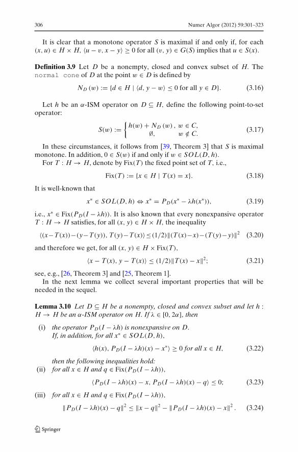
It is clear that a monotone operator S is maximal if and only if, for each(x, u) ∈ H × H, 〈u − v, x − y〉 ≥ 0 for all (v, y) ∈ G(S) implies that u ∈ S(x).

Definition 3.9 Let D be a nonempty, closed and convex subset of H. Thenormal cone of D at the point w ∈ D is defined by

ND (w) := {d ∈ H | 〈d, y − w〉 ≤ 0 for all y ∈ D}. (3.16)

Let h be an α-ISM operator on D ⊆ H, define the following point-to-setoperator:

S(w) :={

h(w) + ND (w) , w ∈ C,

∅, w /∈ C.(3.17)

In these circumstances, it follows from [39, Theorem 3] that S is maximalmonotone. In addition, 0 ∈ S(w) if and only if w ∈ SOL(D, h).

For T : H → H, denote by Fix(T) the fixed point set of T, i.e.,

Fix(T) := {x ∈ H | T(x) = x}. (3.18)

It is well-known that

x∗ ∈ SOL(D, h) ⇔ x∗ = PD(x∗ − λh(x∗)), (3.19)

i.e., x∗ ∈ Fix(PD(I − λh)). It is also known that every nonexpansive operatorT : H → H satisfies, for all (x, y) ∈ H × H, the inequality

〈(x−T(x))−(y−T(y)), T(y)−T(x)〉≤(1/2)‖(T(x)−x)−(T(y)−y)‖2 (3.20)

and therefore we get, for all (x, y) ∈ H × Fix(T),

〈x − T(x), y − T(x)〉 ≤ (1/2)‖T(x) − x‖2; (3.21)

see, e.g., [26, Theorem 3] and [25, Theorem 1].In the next lemma we collect several important properties that will be

needed in the sequel.

Lemma 3.10 Let D ⊆ H be a nonempty, closed and convex subset and let h :H → H be an α-ISM operator on H. If λ ∈ [0, 2α], then

(i) the operator PD(I − λh) is nonexpansive on D.

If, in addition, for all x∗ ∈ SOL(D, h),

〈h(x), PD(I − λh)(x) − x∗〉 ≥ 0 for all x ∈ H, (3.22)

then the following inequalities hold:(ii) for all x ∈ H and q ∈ Fix(PD(I − λh)),

〈PD(I − λh)(x) − x, PD(I − λh)(x) − q〉 ≤ 0; (3.23)

(iii) for all x ∈ H and q ∈ Fix(PD(I − λh)),

‖PD(I − λh)(x) − q‖2 ≤ ‖x − q‖2 − ‖PD(I − λh)(x) − x‖2 . (3.24)

Numer Algor (2012) 59:301–323 307

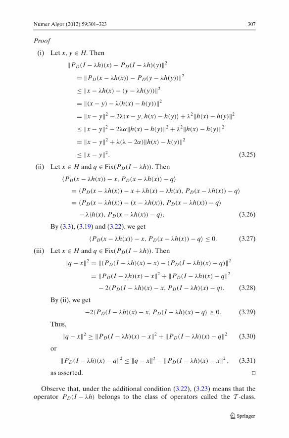
Proof

(i) Let x, y ∈ H. Then

‖PD(I − λh)(x) − PD(I − λh)(y)‖2

= ‖PD(x − λh(x)) − PD(y − λh(y))‖2

≤ ‖x − λh(x) − (y − λh(y))‖2

= ‖(x − y) − λ(h(x) − h(y))‖2

= ‖x − y‖2 − 2λ〈x − y, h(x) − h(y)〉 + λ2‖h(x) − h(y)‖2

≤ ‖x − y‖2 − 2λα‖h(x) − h(y)‖2 + λ2‖h(x) − h(y)‖2

= ‖x − y‖2 + λ(λ − 2α)‖h(x) − h(y)‖2

≤ ‖x − y‖2. (3.25)

(ii) Let x ∈ H and q ∈ Fix(PD(I − λh)). Then

〈PD(x − λh(x)) − x, PD(x − λh(x)) − q〉= 〈PD(x − λh(x)) − x + λh(x) − λh(x), PD(x − λh(x)) − q〉= 〈PD(x − λh(x)) − (x − λh(x)), PD(x − λh(x)) − q〉

− λ〈h(x), PD(x − λh(x)) − q〉. (3.26)

By (3.3), (3.19) and (3.22), we get

〈PD(x − λh(x)) − x, PD(x − λh(x)) − q〉 ≤ 0. (3.27)

(iii) Let x ∈ H and q ∈ Fix(PD(I − λh)). Then

‖q − x‖2 = ‖(PD(I − λh)(x) − x) − (PD(I − λh)(x) − q)‖2

= ‖PD(I − λh)(x) − x‖2 + ‖PD(I − λh)(x) − q‖2

− 2〈PD(I − λh)(x) − x, PD(I − λh)(x) − q〉. (3.28)

By (ii), we get

−2〈PD(I − λh)(x) − x, PD(I − λh)(x) − q〉 ≥ 0. (3.29)

Thus,

‖q − x‖2 ≥ ‖PD(I − λh)(x) − x‖2 + ‖PD(I − λh)(x) − q‖2 (3.30)

or

‖PD(I − λh)(x) − q‖2 ≤ ‖q − x‖2 − ‖PD(I − λh)(x) − x‖2 , (3.31)

as asserted. ��

Observe that, under the additional condition (3.22), (3.23) means that theoperator PD(I − λh) belongs to the class of operators called the T -class.

308 Numer Algor (2012) 59:301–323

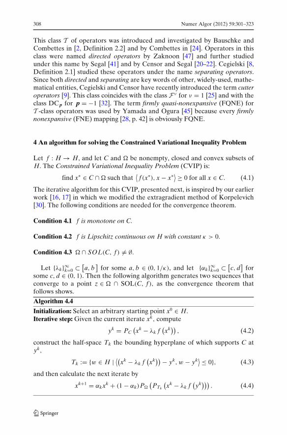
This class T of operators was introduced and investigated by Bauschke andCombettes in [2, Definition 2.2] and by Combettes in [24]. Operators in thisclass were named directed operators by Zaknoon [47] and further studiedunder this name by Segal [41] and by Censor and Segal [20–22]. Cegielski [8,Definition 2.1] studied these operators under the name separating operators.Since both directed and separating are key words of other, widely-used, mathe-matical entities, Cegielski and Censor have recently introduced the term cutteroperators [9]. This class coincides with the class F ν for ν = 1 [25] and with theclass DC p for p = −1 [32]. The term firmly quasi-nonexpansive (FQNE) forT -class operators was used by Yamada and Ogura [45] because every firmlynonexpansive (FNE) mapping [28, p. 42] is obviously FQNE.

4 An algorithm for solving the Constrained Variational Inequality Problem

Let f : H → H, and let C and � be nonempty, closed and convex subsets ofH. The Constrained Variational Inequality Problem (CVIP) is:

find x∗ ∈ C ∩ � such that⟨f (x∗), x − x∗⟩ ≥ 0 for all x ∈ C. (4.1)

The iterative algorithm for this CVIP, presented next, is inspired by our earlierwork [16, 17] in which we modified the extragradient method of Korpelevich[30]. The following conditions are needed for the convergence theorem.

Condition 4.1 f is monotone on C.

Condition 4.2 f is Lipschitz continuous on H with constant κ > 0.

Condition 4.3 � ∩ SOL(C, f ) = ∅.

Let {λk}∞k=0 ⊂ [a, b

]for some a, b ∈ (0, 1/κ), and let {αk}∞k=0 ⊂ [

c, d]

forsome c, d ∈ (0, 1). Then the following algorithm generates two sequences thatconverge to a point z ∈ � ∩ SOL(C, f ), as the convergence theorem thatfollows shows.

Algorithm 4.4

Initialization: Select an arbitrary starting point x0 ∈ H.Iterative step: Given the current iterate xk, compute

yk = PC(xk − λk f

(xk)) , (4.2)

construct the half-space Tk the bounding hyperplane of which supports C atyk,

Tk := {w ∈ H | ⟨(xk − λk f

(xk)) − yk, w − yk⟩ ≤ 0}, (4.3)

and then calculate the next iterate by

xk+1 = αkxk + (1 − αk)P�

(PTk

(xk − λk f

(yk))) . (4.4)

Numer Algor (2012) 59:301–323 309

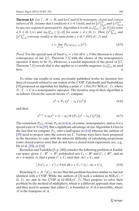
Theorem 4.5 Let f : H → H, and let C and � be nonempty, closed and convexsubsets of H. Assume that Conditions 4.1–4.3 hold, and let

{xk

}∞k=0 and

{yk

}∞k=0

be any two sequences generated by Algorithm 4.4 with {λk}∞k=0 ⊂ [a, b

]for some

a, b ∈ (0, 1/κ) and {αk}∞k=0 ⊂ [c, d

]for some c, d ∈ (0, 1). Then

{xk

}∞k=0 and

{yk

}∞k=0 converge weakly to the same point z ∈ � ∩ SOL(C, f ) and

z = limk→∞

P�∩SOL(C, f )(xk) . (4.5)

Proof For the special case of fixed λk = τ for all k ≥ 0 this theorem is a directconsequence of our [17, Theorem 7.1] with the choice of the nonexpansiveoperator S there to be P�. However, a careful inspection of the proof of [17,Theorem 7.1] reveals that it also applies to a variable sequence {λk}∞k=0 as usedhere. ��

To relate our results to some previously published works we mention twolines of research related to our notion of the CVIP. Takahashi and Nadezhkina[35] proposed an algorithm for finding a point x∗ ∈ Fix(N)∩SOL(C, f ), whereN : C → C is a nonexpansive operator. The iterative step of their algorithm isas follows. Given the current iterate xk, compute

yk = PC(xk − λk f

(xk)) (4.6)

and then

xk+1 = αkxk + (1 − αk)N(PC

(xk − λk f

(yk))) . (4.7)

The restriction P�|C of our P� in (4.4) is, of course, nonexpansive, and so it is aspecial case of N in [35]. But a significant advantage of our Algorithm 4.4 lies inthe fact that we compute PTk onto a half-space in (4.4) whereas the authors of[35] need to project onto the convex set C. Various ways have been proposedin the literature to cope with the inherent difficulty of calculating projections(onto closed convex sets) that do not have a closed-form expression; see, e.g.,He et al. [29], or [18].

Bertsekas and Tsitsiklis [3, p. 288] consider the following problem in Euclid-ean space: given f : Rn → Rn, polyhedral sets C1 ⊂ Rn and C2 ⊂ Rm, and anm × n matrix A, find a point x∗ ∈ C1 such that Ax∗ ∈ C2 and

⟨f (x∗), x − x∗⟩ ≥ 0 for all x ∈ C1 ∩ {y | Ay ∈ C2}. (4.8)

Denoting � = A−1(C2), we see that this problem becomes similar to, but notidentical with a CVIP. While the authors of [3] seek a solution in SOL(C1 ∩�, f ), we aim in our CVIP at �∩SOL(C, f ). They propose to solve theirproblem by the method of multipliers, which is a different approach than ours,and they need to assume that either C1 is bounded or At A is invertible, whereAt is the transpose of A.

310 Numer Algor (2012) 59:301–323

5 The Split Variational Inequality Problem as a Constrained VariationalInequality Problem in a product space

Our first approach to the solution of the SVIP (1.1) and (1.2) is to look at theproduct space H = H1 × H2 and introduce in it the product set D := C × Qand the set

V := {x = (x, y) ∈ H | Ax = y}. (5.1)

We adopt the notational convention that objects in the product space arerepresented in boldface type. We transform the SVIP (1.1) and (1.2) into thefollowing equivalent CVIP in the product space:

Find a point x∗ ∈ D ∩ V, such that⟨h(x∗), x − x∗⟩ ≥ 0

for all x = (x, y) ∈ D, (5.2)

where h : H → H is defined by

h(x, y) = ( f (x), g(y)). (5.3)

A simple adaptation of the decomposition lemma [3, Proposition 5.7, p. 275]shows that problems (1.1), (1.2) and (5.2) are equivalent, and, therefore, wecan apply Algorithm 4.4 to the solution of (5.2).

Lemma 5.1 A point x∗ = (x∗, y∗) solves (5.2) if and only if x∗ and y∗ solve (1.1)and (1.2).

Proof If (x∗, y∗) solves (1.1) and (1.2), then it is clear that (x∗, y∗) solves (5.2).To prove the other direction, suppose that (x∗, y∗) solves (5.2). Since (5.2)holds for all (x, y) ∈ D, we may take (x∗, y) ∈ D and deduce that

⟨g(Ax∗), y − Ax∗⟩ ≥ 0 for all y ∈ Q. (5.4)

Using a similar argument with (x, y∗) ∈ D, we get⟨f (x∗), x − x∗⟩ ≥ 0 for all x ∈ C, (5.5)

which means that (x∗, y∗) solves (1.1) and (1.2). ��

Using this equivalence, we can now employ Algorithm 4.4 in order to solvethe SVIP. The following conditions are needed for the convergence theorem.

Condition 5.2 f is monotone on C and g is monotone on Q.

Condition 5.3 f is Lipschitz continuous on H1 with constant κ1 > 0 and g isLipschitz continuous on H2 with constant κ2 > 0.

Numer Algor (2012) 59:301–323 311

Condition 5.4 V ∩ SOL(D, h) = ∅.

Let {λk}∞k=0 ⊂ [a, b

]for some a, b ∈ (0, 1/κ), where κ = min{κ1, κ2}, and let

{αk}∞k=0 ⊂ [c, d

]for some c, d ∈ (0, 1). Then the following algorithm generates

two sequences that converge to a point z ∈ V ∩ SOL(D, h), as the conver-gence theorem given below shows.

Algorithm 5.5

Initialization: Select an arbitrary starting point x0 ∈ H.Iterative step: Given the current iterate xk, compute

yk = P D(xk − λkh

(xk)) , (5.6)

construct the half-space Tk the bounding hyperplane of which supports Dat yk,

Tk := {w ∈ H | ⟨(xk − λkh

(xk)) − yk, w − yk⟩ ≤ 0}, (5.7)

and then calculate

xk+1 = αkxk + (1 − αk)PV(PTk

(xk − λkh

(yk))) . (5.8)

Our convergence theorem for Algorithm 5.5 follows from Theorem 4.5.

Theorem 5.6 Consider f : H1 → H1 and g : H2 → H2, a bounded linear operatorA : H1 → H2, and nonempty, closed and convex subsets C⊆ H1 and Q⊆ H2.Assume that Conditions 5.2–5.4 hold, and let

{xk

}∞k=0 and

{yk

}∞k=0 be any

two sequences generated by Algorithm 5.5 with {λk}∞k=0 ⊂ [a, b

]for some

a, b ∈ (0, 1/κ), where κ = min{κ1, κ2}, and let {αk}∞k=0 ⊂ [c, d

]for some c, d ∈

(0, 1). Then{xk

}∞k=0 and

{yk

}∞k=0 converge weakly to the same point z ∈ V ∩

SOL(D, h) and

z = limk→∞

PV∩SOL(D,h)

(xk) . (5.9)

The value of the product space approach, described above, depends on theability to “translate” Algorithm 5.5 back to the original spaces H1 and H2.

Observe that due to [37, Lemma 1.1] for x=(x, y) ∈ D, we have P D(x) =(PC(x), PQ(y)) and a similar formula holds for PTk . The potential difficultylies in PV of (5.8). In the finite-dimensional case, since V is a subspace,the projection onto it is easily computable by using an orthogonal basis. Forexample, if U is a k-dimensional subspace of Rn with the basis {u1, u2, ..., uk},then for x ∈ Rn, we have

PU (x) =k∑

i=1

〈x, ui〉‖ui‖2 ui. (5.10)

312 Numer Algor (2012) 59:301–323

6 Solving the Split Variational Inequality Problem without a product space

In this section we present a method for solving the SVIP, which does notneed a product space formulation as in the previous section. Recalling thatSOL(C, f ) and SOL(Q, g) are the solution sets of (1.1) and (1.2), respectively,we see that the solution set of the SVIP is

:= (C, Q, f, g, A) := {z ∈ SOL(C, f ) | Az ∈ SOL(Q, g)} . (6.1)

Using the abbreviations T := PQ(I − λg) and U := PC(I − λ f ), we proposethe following algorithm.

Algorithm 6.1

Initialization: Let λ > 0 and select an arbitrary starting point x0 ∈ H1.Iterative step: Given the current iterate xk, compute

xk+1 = U(xk + γ A∗(T − I)

(Axk)) , (6.2)

where γ ∈ (0, 1/L), L is the spectral radius of the operator A∗ A, and A∗ is theadjoint of A.

The following lemma, which asserts Fejér-monotonicity, is crucial for theconvergence theorem.

Lemma 6.2 Let H1 and H2 be real Hilbert spaces and let A : H1 → H2 be abounded linear operator. Let f : H1 → H1 and g : H2 → H2 be α1-ISM andα2-ISM operators on H1 and H2, respectively, and set α := min{α1, α2}. Assumethat = ∅ and that γ ∈ (0, 1/L). Consider the operators U = PC(I − λ f ) andT = PQ(I − λg) with λ ∈ [0, 2α]. Then any sequence

{xk

}∞k=0 , generated by

Algorithm 6.1, is Fejér-monotone with respect to the solution set .

Proof Let z ∈ . Then z ∈ SOL(C, f ) and, therefore, by (3.19) and Lemma3.10(i), we get

∥∥xk+1 − z∥∥2 = ∥∥U

(xk + γ A∗(T − I)

(Axk)) − z

∥∥2

= ∥∥U(xk + γ A∗(T − I)

(Axk)) − U(z)

∥∥2

≤ ∥∥xk + γ A∗(T − I)(

Axk) − z∥∥2

= ∥∥xk − z∥∥2 + γ 2

∥∥A∗(T − I)(

Axk)∥∥2

+ 2γ⟨xk − z, A∗(T − I)

(Axk)⟩ . (6.3)

Thus∥∥xk+1 − z

∥∥2 ≤ ∥∥xk − z∥∥2 + γ 2 ⟨

(T − I)(

Axk) , AA∗(T − I)(

Axk)⟩

+ 2γ⟨xk − z, A∗(T − I)

(Axk)⟩ . (6.4)

Numer Algor (2012) 59:301–323 313

From the definition of L it follows, by standard manipulations, that

γ 2 ⟨(T − I)

(Axk) , AA∗(T − I)

(Axk)⟩ ≤ Lγ 2 ⟨

(T − I)(

Axk) , (T − I)(

Axk)⟩

= Lγ 2∥∥(T − I)

(Axk)∥∥2

. (6.5)

Denoting � := 2γ⟨xk − z, A∗(T − I)(Axk)

⟩and using (3.21), we obtain

� = 2γ⟨A

(xk − z

), (T − I)

(Axk)⟩

= 2γ⟨A

(xk − z

) + (T − I)(

Axk) − (T − I)(

Axk) , (T − I)(

Axk)⟩

= 2γ(⟨

T(

Axk) − Az, (T − I)(

Axk)⟩ − ∥∥(T − I)(

Axk)∥∥2)

≤ 2γ((1/2)

∥∥(T − I)(

Axk)∥∥2 − ∥∥(T − I)(

Axk)∥∥2)

≤ −γ∥∥(T − I)

(Axk)∥∥2

. (6.6)

Applying (6.5) and (6.6) to (6.4), we see that∥∥xk+1 − z

∥∥2 ≤ ∥∥xk − z∥∥2 + γ (Lγ − 1)

∥∥(T − I)(

Axk)∥∥2. (6.7)

From the definition of γ, we get∥∥xk+1 − z

∥∥2 ≤ ∥∥xk − z∥∥2

, (6.8)

which completes the proof. ��

Now we present our convergence result for Algorithm 6.1.

Theorem 6.3 Let H1 and H2 be real Hilbert spaces and let A : H1 → H2 be abounded linear operator. Let f : H1 → H1 and g : H2 → H2 be α1-ISM andα2-ISM operators on H1 and H2, respectively, and set α := min{α1, α2}. Assumethat γ ∈ (0, 1/L). Consider the operators U = PC(I − λ f ) and T = PQ(I − λg)

with λ ∈ [0, 2α]. Assume further that = ∅ and that, for all x∗ ∈ SOL(C, f ),

〈 f (x), PC(I − λ f )(x) − x∗〉 ≥ 0 for all x ∈ H1. (6.9)

Then any sequence{

xk}∞

k=0 , generated by Algorithm 6.1, converges weakly to asolution point x∗ ∈ .

Proof Let z ∈ . It follows from (6.8) that the sequence{∥∥xk − z

∥∥}∞k=0 is

monotonically decreasing and therefore convergent, which shows, by (6.7),that,

limk→∞

∥∥(T − I)(

Axk)∥∥ = 0. (6.10)

Fejér-monotonicity implies that{

xk}∞

k=0 is bounded, so it has a weakly con-vergent subsequence

{xk j

}∞j=0 such that xk j ⇀ x∗. By the assumptions on λ

314 Numer Algor (2012) 59:301–323

and g, we get from Lemma 3.10(i) that T is nonexpansive. Applying thedemiclosedness of T − I at 0 to (6.10), we obtain

T(Ax∗) = Ax∗, (6.11)

which means that Ax∗ ∈ SOL(Q, g). Denote

uk := xk + γ A∗(T − I)(

Axk) . (6.12)

Then

uk j = xk j + γ A∗(T − I)(

Axk j). (6.13)

Since xk j ⇀ x∗, (6.10) implies that uk j ⇀ x∗ too. It remains to be shown thatx∗ ∈ SOL(C, f ). Assume, by negation, that x∗ /∈ SOL(C, f ), i.e., Ux∗ = x∗.By the assumptions on λ and f, we get from Lemma 3.10(i) that U is nonex-pansive and, therefore, U − I is demiclosed at 0. So, the negation assumptionmust lead to

limj→∞

∥∥U(uk j

) − uk j∥∥ = 0. (6.14)

Therefore, there exists an ε > 0 and a subsequence{uk js

}∞s=0 of

{uk j

}∞j=0 such

that∥∥U

(uk js

) − uk js∥∥ > ε for all s ≥ 0. (6.15)

Condition (6.9) justifies the use of Lemma 3.10 by supplying (3.22). Therefore,inequality (3.24) now yields, for all s ≥ 0,

∥∥U(uk js

) − U(z)∥∥2 = ∥∥U

(uk js

) − z∥∥2 ≤ ∥∥uk js − z

∥∥2 − ∥∥U(uk js

) − uk js∥∥2

<∥∥uk js − z

∥∥2 − ε2. (6.16)

By arguments similar to those in the proof of Lemma 6.2, we have∥∥uk − z

∥∥ = ∥∥(xk + γ A∗(T − I)

(Axk)) − z

∥∥ ≤ ∥∥xk − z∥∥ . (6.17)

Since U is nonexpansive,∥∥xk+1 − z

∥∥ = ∥∥U(uk) − z

∥∥ ≤ ∥∥uk − z∥∥ . (6.18)

Combining (6.17) and (6.18), we get∥∥xk+1 − z

∥∥ ≤ ∥∥uk − z∥∥ ≤ ∥∥xk − z

∥∥ , (6.19)

which means that the sequence {x1, u1, x2, u2, . . .} is Fejér-monotone withrespect to . Since xk js+1 = U(uk js ), we obtain

∥∥∥uk js+1 − z∥∥∥

2 ≤ ∥∥uk js − z∥∥2

. (6.20)

Numer Algor (2012) 59:301–323 315

Hence{uk js

}∞s=0 is also Fejér-monotone with respect to . Now, (6.16) and

(6.19) imply that

∥∥∥uk js+1 − z∥∥∥

2<

∥∥uk js − z∥∥2 − ε2 for all s ≥ 0, (6.21)

which leads to a contradiction. Therefore x∗ ∈ SOL(C, f ) and finally, x∗ ∈ .Since the subsequence

{xk j

}∞j=0 was arbitrary, we get that xk ⇀ x∗. ��

Relations of our results to some previously published works are as follows.In [20] an algorithm for the Split Common Fixed Point Problem (SCFPP) inEuclidean spaces was studied. Later Moudafi [34] presented a similar result forHilbert spaces. In this connection, see also [33].

To formulate the SCFPP, let H1 and H2 be two real Hilbert spaces. Givenoperators Ui : H1 → H1, i = 1, 2, . . . , p, and T j : H2 → H2, j = 1, 2, . . . , r,with nonempty fixed point sets Ci, i = 1, 2, . . . , p, and Q j, j = 1, 2, . . . , r,respectively, and a bounded linear operator A : H1 → H2, the SCFPP isformulated as follows:

find a point x∗ ∈ C := ∩pi=1Ci such that Ax∗ ∈ Q := ∩r

j=1 Q j. (6.22)

Our result differs from those in [20] and [34] in several ways. Firstly, thespaces in which the problems are formulated. Secondly, the operators U and Tin [20] are assumed to be firmly quasi-nonexpansive (FQNE; see the commentsafter Lemma 3.10 above), where in our case here only U is FQNE, whileT is just nonexpansive. Lastly, Moudafi [34] obtains weak convergence fora wider class of operators, called demicontractive. The iterative step of hisalgorithm is

xk+1 = (1 − αk)uk + αkU(uk), (6.23)

where uk := xk + γ A∗(T − I)(Axk) for αk ∈ (0, 1). If αk = 1, which is notallowed there, were possible, then the iterative step of [34] would coincidewith that of [20].

6.1 A parallel algorithm for solving the Multiple Set Split VariationalInequality Problem

We extend the SVIP to the Multiple Set Split Variational Inequality Problem(MSSVIP), which is formulated as follows. Let H1 and H2 be two real Hilbertspaces. Given a bounded linear operator A : H1 → H2, functions fi : H1 →H1, i = 1, 2, . . . , p, and g j : H2 → H2, j = 1, 2, . . . , r, and nonempty, closedand convex subsets Ci ⊆ H1, Q j ⊆ H2 for i = 1, 2, . . . , p and j = 1, 2, . . . , r,

316 Numer Algor (2012) 59:301–323

respectively, the Multiple Set Split Variational Inequality Problem (MSSVIP)is formulated as follows:⎧⎪⎪⎪⎨

⎪⎪⎪⎩

find a point x∗ ∈ C := ∩pi=1Ci such that 〈 fi(x∗), x − x∗〉 ≥ 0 for all x ∈ Ci

and for all i = 1, 2, . . . , p, and such that

the point y∗ = Ax∗ ∈ Q := ∩ri=1 Q j solves

⟨g j(y∗), y − y∗⟩ ≥ 0 for all y ∈ Q j

and for all j = 1, 2, . . . , r.(6.24)

For the MSSVIP we do not yet have a solution approach which does not usea product space formalism. Therefore we present a simultaneous algorithm forthe MSSVIP the analysis of which is carried out via a certain product space.Let � be the solution set of the MSSVIP:

� := {z ∈ ∩p

i=1SOL(Ci, fi) | Az ∈ ∩ri=1SOL(Q j, g j)

}. (6.25)

We introduce the spaces W 1 : =H1 and W 2 := H p1 × Hr

2, where r and p arethe indices in (6.24). Let {αi}p

i=1 and{β j

}rj=1 be positive real numbers. Define

the following sets in their respective spaces:

C: = H1 and (6.26)

Q: =( p∏

i=1

√αiCi

)

×⎛

⎝r∏

j=1

√β jQ j

⎞

⎠ , (6.27)

and the operator

A: =(√

α1 I, . . . ,√

αp I,√

β1 A∗, . . . ,√

βr A∗)∗

, (6.28)

where A∗ stands for adjoint of A. Denote Ui := PCi(I − λ fi) and T j :=PQ j(I − λg j) for i = 1, 2, . . . , p and j = 1, 2, . . . , r, respectively. Define theoperator T : W 2→W 2 by

T(y) = T

⎛

⎜⎜⎜⎝

y1y2...

yp+r

⎞

⎟⎟⎟⎠

= ((U1 (y1))

∗ , . . . ,(U p

(yp

))∗,(T1

(yp+1

))∗, . . . ,

(Tr(yp+r)

)∗)∗, (6.29)

where y1, y2, ..., yp ∈ H1 and yp+1, yp+2, ..., yp+r ∈ H2.This leads to an SVIP with just two operators F and G and two sets C and

Q, respectively, in the product space, when we take C=H1, F ≡ 0, Q⊆W 2,G(y) = (

f1(y1), f2(y2) . . . , fp(yp), g1(yp+1), g2(yp+2), . . . , gr(yp+r)), and the

operator A : H1→W 2. It is easy to verify that the following equivalenceholds:

x ∈ � if and only if Ax ∈ Q. (6.30)

Numer Algor (2012) 59:301–323 317

Therefore we may apply Algorithm 6.1 ,

xk+1 = xk + γ A∗(T − I)(Axk) for all k ≥ 0, (6.31)

to the problem (6.26)–(6.29) in order to obtain a solution of the originalMSSVIP. We translate the iterative step (6.31) to the original spaces H1 andH2 using the relation

T(Ax) =(√

α1U1(x), . . . ,√

αpU p(x),√

β1 AT1(x), . . . ,√

βr ATr(x))∗

(6.32)

and obtain the following algorithm.

Algorithm 6.4

Initialization: Select an arbitrary starting point x0 ∈ H1.Iterative step: Given the current iterate xk, compute

xk+1 = xk + γ

⎛

⎝p∑

i=1

αi(Ui − I)(xk) +

r∑

j=1

β j A∗(T j − I)(

Axk)⎞

⎠ , (6.33)

where γ ∈ (0, 1/L), with L = ∑pi=1 αi + ∑r

j=1 β j‖A‖2.

The following convergence result follows from Theorem 6.3.

Theorem 6.5 Let H1 and H2 be two real Hilbert spaces and let A : H1 → H2be a bounded linear operator. Let fi : H1 → H1, i = 1, 2, . . . , p, and g j : H2 →H2, j = 1, 2, . . . , r, be α-ISM operators on nonempty, closed and convex subsetsCi ⊆ H1, Q j ⊆ H2 for i = 1, 2, . . . , p, and j = 1, 2, . . . , r, respectively. Assumethat γ ∈ (0, 1/L) and � = ∅. Set Ui := PCi(I − λ fi) and T j := PQ j(I − λg j) fori = 1, 2, . . . , p and j = 1, 2, . . . , r, respectively, with λ ∈ [0, 2α]. If, in addition,for each i = 1, 2, . . . , p and j = 1, 2, . . . , r we have

〈 fi(x), PCi(I − λ fi)(x) − x∗〉 ≥ 0 for all x ∈ H1 (6.34)

for all x∗ ∈ SOL(Ci, fi) and

〈g j(x), PQ j(I − λg j)(x) − x∗〉 ≥ 0 for all x ∈ H2, (6.35)

for all x∗ ∈ SOL(Ci, fi), then any sequence{

xk}∞

k=0 , generated by Algorithm 6.1,converges weakly to a solution point x∗ ∈ �.

Proof Apply Theorem 6.3 to the two-operator SVIP in the product spacesetting with U = I : H1 → H1, Fix U = C, T = T : W → W , and Fix T = Q.

��

Remark 6.6 Observe that conditions (6.34) and (6.35) imposed on Ui and T j

for i = 1, 2, . . . , p and j = 1, 2, . . . , r, respectively, in Theorem 6.5, which arenecessary for our treatment of the problem in a product space, ensure thatthese operators are firmly quasi-nonexpansive (FQNE). Therefore, the SVIP

318 Numer Algor (2012) 59:301–323

under these conditions may be considered a Split Common Fixed PointProblem (SCFPP), first introduced in [20], with C, Q, A and T : W 2 → W 2as above, and the identity operator I : C → C. Therefore, we could also apply[20, Algorithm 4.1]. If, however, we drop these conditions, then the operatorsare nonexpansive, by Lemma 3.10(i), and the result of [34] would apply.

7 Applications

The following problems are special cases of the SVIP. They are listed herebecause their analysis can benefit from our algorithms for the SVIP andbecause known algorithms for their solution may be generalized in the futureto cover the more general SVIP. The list includes known problems such as theSplit Feasibility Problem (SFP) and the Convex Feasibility Problem (CFP). Inaddition, we introduce two new “split” problems that have, to the best of ourknowledge, never been studied before. These are the Common Solutions toVariational Inequalities Problem (CSVIP) and the Split Zeros Problem (SZP).

7.1 The Split Feasibility and Convex Feasibility Problems

The Split Feasibility Problem (SFP) in Euclidean space is formulated asfollows:

find a point x∗ such that x∗ ∈ C ⊆ Rn and Ax∗ ∈ Q ⊆ Rm, (7.1)

where C ⊆ Rn, Q ⊆ Rm are nonempty, closed and convex sets, and A : Rn →Rm is given. Originally introduced in Censor and Elfving [14], it was laterused in the area of intensity-modulated radiation therapy (IMRT) treatmentplanning; see [11, 15]. Obviously, it is formally a special case of the SVIPobtained from (1.1) and (1.2) by setting f ≡ g ≡ 0. The Convex FeasibilityProblem (CFP) in a Euclidean space is:

find a point x∗ such that x∗ ∈ ∩mi=1Ci = ∅, (7.2)

where Ci, i = 1, 2, . . . , m, are nonempty, closed and convex sets in Rn. This,in its turn, becomes a special case of the SFP by taking in (7.1) n = m, A =I, Q = Rn and C = ∩m

i=1Ci. Many algorithms for solving the CFP have beendeveloped; see, e.g., [1, 23]. Byrne [5] established an algorithm for solving theSFP, called the CQ-Algorithm, with the following iterative step:

xk+1 = PC(xk + γ At(PQ − I)Axk) , (7.3)

which does not require calculation of the inverse of the operator A, as in [14],but needs only its transpose At. A recent excellent paper on the multiple-setsSFP which contains many references that reflect the state-of-the-art in this areais [31].

Numer Algor (2012) 59:301–323 319

It is of interest to note that looking at the SFP from the point of view of theSVIP enables us to find the minimum-norm solution of the SFP, i.e., a solutionof the form

x∗ = argmin{‖x‖ | x solves the SFP (7.1)}. (7.4)

This is done, and easily verified, by solving (1.1) and (1.2) with f = I and g ≡ 0.

7.2 The Common Solutions to Variational Inequalities Problem

The Common Solutions to Variational Inequalities Problem (CSVIP), newlyintroduced here, is defined in Euclidean space as follows. Let { fi}m

i=1 be a familyof functions from Rn into itself and let {Ci}m

i=1 be nonempty, closed and convexsubsets of Rn with ∩m

i=1Ci = ∅. The CSVIP is formulated as follows:

find a point x∗ ∈ ∩mi=1Ci such that

⟨fi(x∗), x − x∗⟩ ≥ 0

for all x ∈ Ci, i = 1, 2, . . . , m. (7.5)

This problem can be transformed into a CVIP in an appropriate product space(different from the one in Section 5). Let Rmn be the product space and defineF : Rmn → Rmn by

F((

x1, x2, . . . , xm)) = (f1

(x1) , . . . , fm

(xm))

, (7.6)

where xi ∈ Rn for all i = 1, 2, . . . , m. Let the diagonal set in Rmn be

� := {x ∈ Rmn | x=(a, a, . . . , a), a ∈ Rn} (7.7)

and define the product set

C := �mi=1Ci. (7.8)

The CSVIP in Rn is equivalent to the following CVIP in Rmn:

find a point x∗ ∈ C ∩ � such that⟨F(x∗), x − x∗⟩ ≥ 0

for all x = (x1, x2, . . . , xm) ∈ C. (7.9)

So, this problem can be solved by using Algorithm 4.4 with � = �. A newalgorithm specifically designed for the CSVIP appears in [19].

7.3 The Split Minimization and the Split Zeros Problems

From optimality conditions for convex optimization (see, e.g., Bertsekas andTsitsiklis [3, Proposition 3.1, p. 210]) it is well-known that if F : Rn → Rn isa continuously differentiable convex function on a closed and convex subsetX ⊆ Rn, then x∗ ∈ X minimizes F over X if and only if

〈∇F(x∗), x − x∗〉 ≥ 0 for all x ∈ X, (7.10)

320 Numer Algor (2012) 59:301–323

where ∇F is the gradient of F. Since (7.10) is a VIP, we make the following ob-servation. If F : Rn → Rn and G : Rm → Rm are continuously differentiableconvex functions on closed and convex subsets C ⊆ Rn and Q ⊆ Rm, respec-tively, and if in the SVIP we take f = ∇F and g = ∇G, then we obtain thefollowing Split Minimization Problem (SMP):

find a point x∗ ∈ C such that x∗ = argmin{ f (x) | x ∈ C} (7.11)

and such that

the point y∗ = Ax∗ ∈ Q and solves y∗ = argmin{g(y) | y ∈ Q}. (7.12)

The Split Zeros Problem (SZP), newly introduced here, is defined as follows.Let H1 and H2 be two Hilbert spaces. Given operators B1 : H1 → H1 and B2 :H2 → H2, and a bounded linear operator A : H1 → H2, the SZP is formulatedas follows:

find a point x∗ ∈ H1 such that B1(x∗) = 0 and B2(Ax∗) = 0. (7.13)

This problem is a special case of the SVIP if A is a surjective operator. To seethis, take in (1.1) and (1.2) C = H1, Q = H2, f = B1 and g = B2, and choosex := x∗ − B1(x∗) ∈ H1 in (1.1) and x ∈ H1 such that Ax := Ax∗ − B2(Ax∗) ∈H2 in (1.2).

The next lemma shows when the only solution of an SVIP is a solution ofan SZP. It extends a similar result concerning the relationship between the(un-split) zero finding problem and the VIP.

Lemma 7.1 Let H1 and H2 be real Hilbert spaces, and C ⊆ H1 and Q ⊆ H2nonempty, closed and convex subsets. Let B1 : H1 → H1 and B2 : H2 → H2 beα-ISM operators and let A : H1 → H2 be a bounded linear operator. Assumethat C ∩ {x ∈ H1 | B1(x) = 0} = ∅ and that Q ∩ {y ∈ H2 | B2(y) = 0} = ∅, anddenote

:= (C, Q, B1, B2, A) := {z ∈ SOL(C, B1) | Az ∈ SOL(Q, B2)} . (7.14)

Then, for any x∗ ∈ C with Ax∗ ∈ Q, x∗ solves (7.13) if and only if x∗ ∈ .

Proof First assume that x∗ ∈ C with Ax∗ ∈ Q and that x∗ solves (7.13). Thenit is clear that x∗ ∈ . In the other direction, assume that x∗ ∈ C with Ax∗ ∈ Qand that x∗ ∈ . Applying (3.4) with C as D there, (I − λB1) (x∗) ∈ H1, for anyλ ∈ (0, 2α], as x there, and q1 ∈ C ∩ Fix(I − λB1), with the same λ, as y there,we get

∥∥q1 − PC(I − λB1)(x∗)∥∥2 + ∥∥(I − λB1)

(x∗) − PC(I − λB1)

(x∗)∥∥2

≤ ∥∥(I − λB1)(x∗) − q1

∥∥2, (7.15)

Numer Algor (2012) 59:301–323 321

and, similarly, applying (3.4) again, we obtain∥∥q2 − PQ(I − λB2)

(Ax∗)∥∥2 + ∥∥(I − λB2)

(Ax∗) − PQ(I − λB2)

(Ax∗)∥∥2

≤ ∥∥(I − λB2)(

Ax∗) − q2∥∥2

. (7.16)

Using the characterization of (3.19), we get∥∥q1 − x∗∥∥2 + ∥∥(I − λB1)

(x∗) − x∗∥∥2 ≤ ∥∥(I − λB1)

(x∗) − q1

∥∥2 (7.17)

and∥∥q2 − Ax∗∥∥2 + ∥∥(I − λB2)

(Ax∗) − x∗∥∥2 ≤ ∥∥(I − λB2)

(Ax∗) − q2

∥∥2. (7.18)

It can be seen from the proof of Lemma 3.10(i) that the operators I − λB1and I − λB2 are nonexpansive for every λ ∈ [0, 2α], so with q1 ∈ C ∩ Fix(I −λB1) and q2 ∈ Q ∩ Fix(I − λB2),

∥∥(I − λB1)(x∗) − q1

∥∥2 ≤ ∥∥x∗ − q1∥∥2 (7.19)

and∥∥(I − λB2)

(Ax∗) − q2

∥∥2 ≤ ∥∥Ax∗ − q2∥∥2

. (7.20)

Combining the above inequalities, we obtain∥∥q1 − x∗∥∥2 + ∥∥(I − λB1)

(x∗) − x∗∥∥2 ≤ ∥∥x∗ − q1

∥∥2 (7.21)

and∥∥q2 − Ax∗∥∥2 + ∥∥(I − λB2)

(Ax∗) − x∗∥∥2 ≤ ∥∥Ax∗ − q2

∥∥2. (7.22)

Hence, ‖(I − λB1) (x∗) − x∗‖2 = 0 and ‖(I − λB2) (Ax∗) − Ax∗‖2 = 0. Sinceλ > 0, we get that B1(x∗) = 0 and B2(Ax∗) = 0, as claimed. ��

Acknowledgements This work was partially supported by a United States-Israel BinationalScience Foundation (BSF) Grant number 200912, by US Department of Army award numberW81XWH-10-1-0170, by Israel Science Foundation (ISF) Grant number 647/07, by the Fund forthe Promotion of Research at the Technion and by the Technion President’s Research Fund.

References

1. Bauschke, H.H., Borwein, J.M.: On projection algorithms for solving convex feasibility prob-lems. SIAM Rev. 38, 367–426 (1996)

2. Bauschke, H.H., Combettes, P.L.: A weak-to-strong convergence principle for Fejér-monotone methods in Hilbert spaces. Math. Oper. Res. 26, 248–264 (2001)

3. Bertsekas, D.P., Tsitsiklis, J.N.: Parallel and Distributed Computation: Numerical Methods.Prentice-Hall, Englwood Cliffs (1989)

4. Browder, F.E.: Fixed point theorems for noncompact mappings in Hilbert space. Proc. Natl.Acad. Sci. USA 53, 1272–1276 (1965)

5. Byrne, C.L.: Iterative projection onto convex sets using multiple Bregman distances. InverseProbl. 15, 1295–1313 (1999)

322 Numer Algor (2012) 59:301–323

6. Byrne, C.: Iterative oblique projection onto convex sets and the split feasibility problem.Inverse Probl. 18, 441–453 (2002)

7. Byrne, C.: A unified treatment of some iterative algorithms in signal processing and imagereconstruction. Inverse Probl. 20 103–120 (2004)

8. Cegielski, A.: Generalized relaxations of nonexpansive operators and convex feasibility prob-lems. Contemp. Math. 513, 111–123 (2010)

9. Cegielski, A., Censor, Y.: Opial-type theorems and the common fixed point problem. In:Bauschke, H., Burachik, R., Combettes, P., Elser, V., Luke, R., Wolkowicz, H. (eds.) Fixed-Point Algorithms for Inverse Problems in Science and Engineering, pp. 155–183. Springer,New York (2011)

10. Censor, Y., Altschule, M.D., Powlis, W.D.: On the use of Cimmino’s simultaneous projectionsmethod for computing a solution of the inverse problem in radiation therapy treatment plan-ning. Inverse Probl. 4, 607–623 (1988)

11. Censor, Y., Bortfeld, T., Martin, B., Trofimov, A.: A unified approach for inversion problemsin intensity-modulated radiation therapy. Phys. Med. Biol. 51, 2353–2365 (2006)

12. Censor, Y., Chen, W., Combettes, P.L., Davidi, R., Herman, G.T.: On the effectivenessof projection methods for convex feasibility problems with linear inequality constraints.Comput. Optim. Appl. (2011, accepted for publication). doi:10.1007/s10589-011-9401-7.http://arxiv.org/abs/0912.4367

13. Censor, Y., Davidi, R., Herman, G.T.: Perturbation resilience and superiorization of iterativealgorithms. Inverse Probl. 26 065008 (17 pp.) (2010)

14. Censor, Y., Elfving, T.: A multiprojection algorithm using Bregman projections in productspace. Numer. Algorithms 8, 221–239 (1994)

15. Censor, Y., Elfving, T., Kopf, N., Bortfeld, T.: The multiple-sets split feasibility problem andits applications for inverse problems. Inverse Probl. 21, 2071–2084 (2005)

16. Censor, Y., Gibali, A., Reich, S.: Extensions of Korpelevich’s extragradient method for solv-ing the variational inequality problem in Euclidean space. Optimization (2011, accepted forpublication)

17. Censor, Y., Gibali, A., Reich, S.: The subgradient extragradient method for solving the varia-tional inequality problem in Hilbert space. J. Optim. Theory Appl. 148, 318–335 (2011)

18. Censor, Y., Gibali, A., Reich, S.: Strong convergence of subgradient extragradient methods forthe variational inequality problem in Hilbert space. Optim. Methods Softw. (2011, accepted forpublication)

19. Censor, Y., Gibali, A., Reich, S., Sabach, S.: Common solutions to variational inequalities.Technical Report, 5 April 2011. Revised: July 18, 2011

20. Censor, Y., Segal, A.: The split common fixed point problem for directed operators. J. ConvexAnal. 16, 587–600 (2009)

21. Censor, Y., Segal, A.: On the string averaging method for sparse common fixed point prob-lems. Int. Trans. Oper. Res. 16, 481–494 (2009)

22. Censor, Y., Segal, A.: On string-averaging for sparse problems and on the split common fixedpoint problem. Contemp. Math. 513, 125–142 (2010)

23. Censor, Y., Zenios, S. A.: Parallel Optimization: Theory, Algorithms, and Applications.Oxford University Press, New York (1997)

24. Combettes, P.L.: Quasi-Fejérian analysis of some optimization algorithms. In: Butnariu, D.,Censor, Y., Reich, S. (eds.) Inherently Parallel Algorithms in Feasibility and Optimizationand Their Applications, pp. 115–152. Elsevier, Amsterdam (2001)

25. Crombez, G.: A geometrical look at iterative methods for operators with fixed points. Numer.Funct. Anal. Optim. 26, 157–175 (2005)

26. Crombez, G.: A hierarchical presentation of operators with fixed points on Hilbert spaces.Numer. Funct. Anal. Optim. 27, 259–277 (2006)

27. Dang, Y., Gao, Y.: The strong convergence of a KM–CQ-like algorithm for a split feasibilityproblem. Inverse Probl. 27, 015007 (2011)

28. Goebel, K., Reich, S.: Uniform Convexity, Hyperbolic Geometry, and Nonexpansive Map-pings. Marcel Dekker, New York (1984)

29. He, S., Yang, C., Duan, P.: Realization of the hybrid method for Mann iteration. Appl. Math.Comput. 217, 4239–4247 (2010)

Numer Algor (2012) 59:301–323 323

30. Korpelevich, G.M.: The extragradient method for finding saddle points and other problems.Ekon. Mat. Metody 12, 747–756 (1976)

31. López, G., Martín-Márquez, V., Xu, H.K.: Iterative algorithms for the multiple-sets split feasi-bility problem. In: Censor, Y., Jiang, M., Wang, G. (eds.) Biomedical Mathematics: PromisingDirections in Imaging, Therapy Planning and Inverse Problems, pp. 243–279. Medical PhysicsPublishing, Madison (2010)

32. Maruster, S., Popirlan, C.: On the Mann-type iteration and the convex feasibility problem. J.Comput. Appl. Math. 212, 390–396 (2008)

33. Masad, E., Reich, S.: A note on the multiple-set split convex feasibility problem in Hilbertspace. J. Nonlinear Convex Anal. 8, 367–371 (2007)

34. Moudafi, A.: The split common fixed-point problem for demicontractive mappings. InverseProbl. 26, 1–6 (2010)

35. Nadezhkina, N., Takahashi, W.: Weak convergence theorem by an extragradient method fornonexpansive mappings and monotone mappings. J. Optim. Theory Appl. 128, 191–201 (2006)

36. Opial, Z.: Weak convergence of the sequence of successive approximations for nonexpansivemappings. Bull. Am. Math. Soc. 73, 591–597 (1967)

37. Pierra, G.: Decomposition through formalization in a product space. Math. Program. 28, 96–115 (1984)

38. Qu, B., Xiu, N.: A note on the CQ algorithm for the split feasibility problem. Inverse Probl.21, 1655–1666 (2005)

39. Rockafellar, R.T.: On the maximality of sums of nonlinear monotone operators. Trans. Am.Math. Soc. 149, 75–88 (1970)

40. Schöpfer, F., Schuster, T., Louis, A.K.: An iterative regularization method for the solution ofthe split feasibility problem in Banach spaces. Inverse Probl. 24, 055008 (2008)

41. Segal, A.: Directed operators for common fixed point problems and convex programmingproblems. Ph.D. Thesis, University of Haifa (2008)

42. Takahashi, W., Toyoda, M.: Weak convergence theorems for nonexpansive mappings andmonotone mappings. J. Optim. Theory Appl. 118, 417–428 (2003)

43. Xu, H.K.: A variable Krasnosel’skii–Mann algorithm and the multiple-set split feasibilityproblem. Inverse Probl. 22, 2021–2034 (2006)

44. Xu, H.K.: Iterative methods for the split feasibility problem in infinite-dimensional Hilbertspaces. Inverse Probl. 26, 105018 (2010)

45. Yamada, I., Ogura, N.: Adaptive projected subgradient method for asymptotic minimizationof sequence of nonnegative convex functions. Numer. Funct. Anal. Optim. 25, 593–617 (2005)

46. Yang, Q.: The relaxed CQ algorithm solving the split feasibility problem. Inverse Probl. 20,1261–1266 (2004)

47. Zaknoon, M.: Algorithmic developments for the convex feasibility problem. Ph.D. Thesis,University of Haifa (2003)

48. Zhang, W., Han, D., Li, Z.: A self-adaptive projection method for solving the multiple-setssplit feasibility problem. Inverse Probl. 25, 115001 (2009)

49. Zhao, J., Yang, Q.: Several solution methods for the split feasibility problem. Inverse Probl.21, 1791–1800 (2005)