Algorithms for Combinatorial Coalition Formation and Payoff Division in an Electronic Marketplace

Algorithms for Combinatorial Coalition Formation and Payo�

Division in an Electronic Marketplace1

Cuihong Li

Graduate School of Industrial Administration

Carnegie Mellon University

5000 Forbes Avenue

Pittsburgh, PA 15213

[email protected]

Katia Sycara

The Robotics Institute

Carnegie Mellon University

5000 Forbes Avenue

Pittsburgh, PA 15213

[email protected]

November 16, 2001

1This work has been partially supported by DARPA contract F30602-98-2-0138 and by MURI

contract N00014-96-122. The authors thank Professor R. Ravi and Alan Andrew Scheller-Wolf for

their helpful advice about this work.

Abstract

In an electronic marketplace coalition formation allows buyers to enjoy a price discount for

each item while combinatorial auction enables buyers to place bids for a bundle of items that

are complementary. Coalition formation and combinatorial auction both help to improve

the e�ciency of a market and have received much attention from economists and computer

scientists. But neither in laboratories nor in practice has there been literature on the sit-

uations where both coalition formation and combinatorial auctions exist. In this paper we

consider an e-market where each buyer places a bid on a combination of items with a reserva-

tion cost, and sellers o�er price discounts for each item based on volumes. We call coalition

formation under this condition a Combinatorial Coalition Formation (CCF) problem since

coalition formation is motivated by price discounts on single items while multiple items are

complementary for buyers. By arti�cially dividing the reservation cost of each buyer appro-

priately among the items we can construct optimal coalitions with respect to each item. We

then try to make these coalitions satisfy the complementarity of the items, and thus induce

the optimal solution. Based on this idea we present polynomial-time algorithms to �nd a

semi-optimal solution of CCF and a payo� division scheme that is in the core of the coalition

when linear price functions are applied, and in the pseudo-core when general price functions

are applied. Simulation results show that the algorithms obtain solutions in a satisfactory

ratio to the optimal value.

1 Introduction

Coalition formation and combinatorial auctions have received much attention from both

economists and computer scientists. By o�ering price discounts suppliers drive customers to

buy in wholesale lots while by forming coalitions customers take advantage of the price

discount without purchasing more than their real demand [18]. Auction is an e�cient

mechanism to allocate resources when a real market in which each resource is equipped

with a price does not exist. We say goods g and h are complementary to buyer b if

ub(fg; hg)> ub(fgg)+ ub(fhg), where ub(G) is the utility of the set of goods G to b [31]. For

example, a customer may want to buy both a cellular phone and a battery but does not need

only a cellular phone without a battery or a battery without a cellular phone. In combina-

torial auctions bidders can express the complementarity of items explicitly by placing bids

on combinations of items [25]. In the example above, the customer can place a bid including

both the cellular phone and the battery with a reservation cost, which is equal to the utility

of both of them to the customer.

It is common in real markets that price discounts and complementarity among items exist

simultaneously. In this condition coalition formation and combinatorial auctions are both

needed to improve the e�ciency of the markets. Suppose in the example above there are

two buyers b1 and b2. They both need a cellular phone g1 and a battery g2. A customer

needs to pay $500 to buy one unit of g1 or $405 for each to buy two units. Also one needs

to pay $50 to buy one unit of g2 or $40 for each to buy two units. The utility of both

of g1 and g2 for each buyer is $450, while either g1 or g2 values zero for both b1 and b2.

Suppose only the mechanism of coalition formation is considered. b1 and b2 need to split the

value of fg1; g2g and bid for g1 and g2 separately. Assume pb1(fg1g) = $405, pb2(fg1g) = $400,

pb1(fg2g) = $45, pb2(fg2g) = $50, where pb(G) is the bidding price of buyer b for a set of goods

G. The result of the bidding is that b1 and b2 both only get g2, which has no use for them,

although they enjoy the price discount of g2 by coalition. On the other side suppose only the

mechanism of combinatorial auctions is considered. Let pb1(fg1; g2g) = pb2(fg1; g2g) = $450,

which are the highest bidding prices they can endure. In this case neither b1 nor b2 can win

their bids without coalition. But when both of the mechanisms are applied, then both b1 and

b2 can win their bids and furthermore have $10 pro�t together.

Although economists have provided much insight into the stability analysis of coalitions

[2, 4] and mechanism design of combinatorial auctions [40, 41, 25], both the determination

1

of optimal coalition structure and stable payo� division in coalition formation problems, and

winner determination in combinatorial auction problems are computationally intractable.

There is some research discussing the computational problems by computer scientists in each

of these two �elds (for example, [12, 13, 15, 19, 14] in coalition formation, and [31, 33, 26,

28, 29, 30, 32, 34] in winner determination in combinatorial auctions), but there is limited

work to date on considering both behaviors simultaneously.

In this paper we consider an electronic market in which both coalition formation and combi-

natorial auction exist. There are many sellers and buyers with some items traded from sellers

to buyers in the market. Each buyer may want a bundle of items that complement each other

and have a reservation cost, the highest cost he can pay for his request. Suppose a one-round

sealed auction mechanism (the buyers submit sealed bids and the allocation and payment are

determined at one round of bidding) is applied in the market and each buyer unstrategically

places a bid including all the items he desires with his reservation cost. Assume a fractional

part of the bid has value zero for the buyer and will not be accepted1. Each seller has a price

schedule for each item he provides and o�ers price discounts in each transaction based on the

quantity of the item that is sold. The larger the quantity, the lower the price. By forming

coalitions buyers can enlarge the quantity in each transaction and take advantage of price

discounts. We call such a coalition formation problem Combinatorial Coalition Formation

(CCF) since the coalition formation is motivated by price discounts of single items while

multiple items are complementary for buyers. Since buyers are self-interested a stable payo�

division mechanism for each coalition is needed so that no coalition members have incentive

to leave the coalitions. In this paper we consider the problem of combinatorial coalition

formation and payo� division in such an electronic market. The objective is to �nd a sub-

set of the buyers who have the maximum coalition value among all the possible coalitions

and distribute the payo� among the coalition members such that the division is in the core

(we say a payo� division of a coalition is in the core if the payo� assigned to any subset of

the coalition is no less than the pro�t that the subset can make by themselves. A coalition

with the payo� division in the core is stable since no members have incentives to leave the

coalition.).

In [1] an e�cient algorithm of coalition formation and payo� division has been given for the

case when each buyer wants an XOR listing of multiple items within a category (for instance,

1Otherwise the buyer needs to place multiple bids, one for each set of items that has positive value for him.

This more general case is discussed at the end of the paper.

2

a buyer wants to buy either a camera A for 300 or lower, or a camera B for 400 or lower). It

gives an algorithm to form an optimal coalition for each item and a mechanism to distribute

the payo� for one coalition in the core. A suboptimal coalition con�guration is constructed by

choosing in each round a coalition with the maximal value among all the optimal coalitions,

which are formed one for each item by the buyers who have not been picked into the coalition

con�guration. Based on the approach with respect to one item in that paper, our solution

to CCF is as follows. Suppose each buyer has a virtual reservation cost for each item he

desires. The sum of the virtual reservation costs of a buyer is equal to his real reservation

cost for his whole request. Based on the virtual reservation costs the optimal coalition of

each item (called subcoalition) can be constructed and the surplus is shared in a way stable

in the core. We prove that when the optimal subcoalitions are compatible (satisfying the

complementarity of the items for each buyer), the coalition induced from the subcoalitions

is optimal and the payo� division by summing up the sharing in the subcoalitions for each

buyer is in the core of the optimal coalition. A virtual reservation cost transfer scheme

is proposed to reach compatible optimal subcoalitions when they exist. Evolution of the

optimal subcoalitions in the transfer procedure is analyzed. Based on the analysis we give

two polynomial-time approximation algorithms for coalition formation in the two situations

where linear price functions and general price functions are applied. The payo� division

obtained is in the core with linear price functions and in the pseudo-core with general price

functions. Simulation results show that the approximation algorithms reach a solution with

good ratio to the optimal value.

The paper is organized as follows. Section 2 formulates the problem mathematically. In

Section 3 the approach is introduced and analyzed. The algorithm for optimal subcoalition

formation, the basic transfer scheme, the approximation algorithms of coalition formation in

the conditions of linear and general price functions are presented correspondingly in Section

4, 5, 6 and 7. Section 8 gives the experimental results and Section 9 presents some conclusion.

2 Problem Formulation

An electronic market is composed of buyers, sellers and items.

Let G = fg1; g2; : : : ; gKg indexed by k, B = fb1; b2; : : : ; bNg indexed by n, and E =

fe1; e2; : : : ; eLg indexed by l denote the collection of items, buyers and sellers respectively.

Each buyer bn places a bid, bidn = fQn; rng, where Qn = fq1n; : : : ; qKn g is the quantity of

3

each item that bn requests, and rn is the reservation cost, the highest cost that bn can pay

for his request Qn. Denote by Gn = fgk 2 Gjqkn > 0g the set of items that bn requests, and

by Bk = fbn 2 Bjqkn > 0g the set of buyers that request gk. Each seller has a price schedule

pl;k(�) : Z+ ! R+ for each item gk he provides. The function pl;k(m) is a decreasing step

function of m, which represents the unit price of gk when m units of gk are sold together.

If we assume the sellers have no capacity constraint then we can obtain an integrated price

schedule pk(m) : Z+ ! R+ for each item which is the minimum unit price of gk when m

units are sold together among all those price functions pl;k(m) o�ered by the sellers.

A coalition C is a subset of the buyers with a coalition value which is the di�erence

between the sum of the reservation cost of the coalition members and the minimum cost

needed to satisfy the requests of all the members:

v(C) =Xbn2C

(rn �KXk=1

qkn � pk(qkC))

where

qkC =Xbn2C

qkn

A payo� division XC of a coalition C is a vector fxC(b) : b 2 Cg with the sum of the

elements equal to the value of C:

Xb2C

xC(b) = v(C)

The core of a coalition C is the collection of all payo� divisions of C such that each element

XC satis�es, for any C0 � C,

vC0 � xC(C0)

where xC(C0) =

Pb2C0 xC(b). With a payo� division in the core any subset of the coalition

members can get at least as much by joining the coalition as the value of the coalition formed

by themselves.

If the payo� division XC is in the core of the coalition C, we say C is stable in the core.

The objective of the problem is to �nd a set of exclusive coalitions such that the sum of the

coalition values is maximized, and to distribute the payo� for each coalition such that they

4

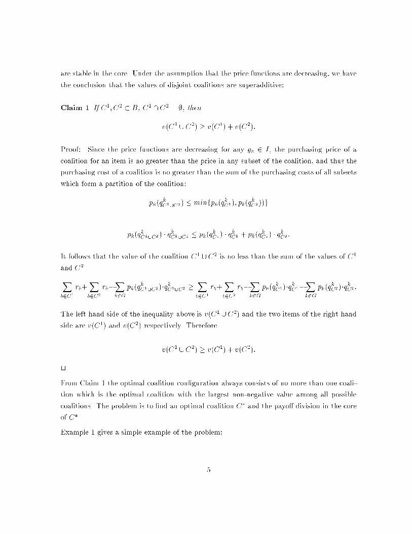
are stable in the core. Under the assumption that the price functions are decreasing, we have

the conclusion that the values of disjoint coalitions are superadditive:

Claim 1 If C1; C2 � B, C1 \ C2 = ;, then

v(C1[ C2) � v(C1) + v(C2):

Proof: Since the price functions are decreasing for any gk 2 I , the purchasing price of a

coalition for an item is no greater than the price in any subset of the coalition, and thus the

purchasing cost of a coalition is no greater than the sum of the purchasing costs of all subsets

which form a partition of the coalition:

pk(qkC1[C2) � minfpk(q

kC1); pk(q

kC2))g

pk(qkC1[C2) � q

kC1[C2 � pk(q

kC1) � q

kC1 + pk(q

kC2) � q

kC2 :

It follows that the value of the coalition C1 [ C2 is no less than the sum of the values of C1

and C2.

Xb2C1

rb+Xb2C2

rb�Xk2G

pk(qkC1[C2)�q

kC1[C2 �

Xb2C1

rb+Xb2C2

rb�Xk2G

pk(qkC1)�q

kC1�

Xk2G

pk(qkC2)�q

kC2 :

The left hand side of the inequality above is v(C1 [ C2) and the two items of the right hand

side are v(C1) and v(C2) respectively. Therefore

v(C1[ C2) � v(C1) + v(C2):

2

From Claim 1 the optimal coalition con�guration always consists of no more than one coali-

tion which is the optimal coalition with the largest non-negative value among all possible

coalitions. The problem is to �nd an optimal coalition C� and the payo� division in the core

of C�.

Example 1 gives a simple example of the problem:

5

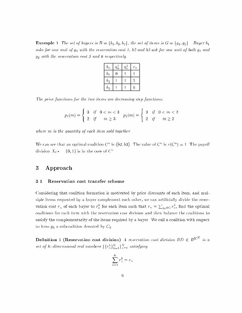
Example 1 The set of buyers is B = fb1; b2; b3g, the set of items is G = fg1; g2g. Buyer b1

asks for one unit of g2 with the reservation cost 1, b2 and b3 ask for one unit of both g1 and

g2 with the reservation cost 5 and 6 respectively.

bn q1n q2n rn

b1 0 1 1

b2 1 1 5

b3 1 1 6

The price functions for the two items are decreasing step functions:

p1(m) =

8<:

3 if 0 < m < 3

2 if m � 3p2(m) =

8<:

3 if 0 < m < 2

2 if m � 2

where m is the quantity of each item sold together.

We can see that an optimal coalition C� is fb2; b3g. The value of C� is v(C�) = 1. The payo�

division XC� = f0; 1g is in the core of C�.

3 Approach

3.1 Reservation cost transfer scheme

Considering that coalition formation is motivated by price discounts of each item, and mul-

tiple items requested by a buyer complement each other, we can arti�cially divide the reser-

vation cost rn of each buyer to rkn for each item such that rn =P

gk2Grkn, �nd the optimal

coalitions for each item with the reservation cost division and then balance the coalitions to

satisfy the complementarity of the items required by a buyer. We call a coalition with respect

to item gk a subcoalition denoted by Ck.

De�nition 1 (Reservation cost division) A reservation cost division RD 2 RKNis a

set of K-dimensional real numbers ffrkngKk=1g

Nn=1 satisfying

KXk=1

rkn = rn

6

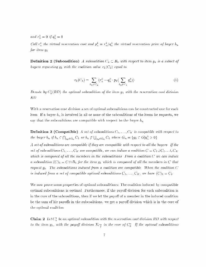
and rkn = 0 if qkn = 0.

Call rkn the virtual reservation cost and pkn = rkn=qkn the virtual reservation price of buyer bn

for item gk.

De�nition 2 (Subcoalition) A subcoalition Ck � Bk with respect to item gk is a subset of

buyers requesting gk with the coalition value vk(Ck) equal to

vk(Ck) =X

bn2Ck

(rkn � qkn � pk(X

bn2Ck

qkn)) (1)

Denote by C�k(RD) the optimal subcoalition of the item gk with the reservation cost division

RD.

With a reservation cost division a set of optimal subcoalitions can be constructed one for each

item. If a buyer bn is involved in all or none of the subcoalitions of the items he requests, we

say that the subcoalitions are compatible with respect to the buyer bn.

De�nition 3 (Compatible) A set of subcoalitions C1; : : : ; CK is compatible with respect to

the buyer bn if bn 2Tgk2Gn

Ck or bn 62Sgk2Gn

Ck where Gn = fgk 2 Gjqkn > 0g.

A set of subcoalitions are compatible if they are compatible with respect to all the buyers. If the

set of subcoalitions C1; : : : ; CK are compatible, we can induce a coalition C = C1[C2 : : :[CK

which is composed of all the members in the subcoalitions. From a coalition C we can induce

a subcoalition (C)k = C \Bk for the item gk which is composed of all the members in C that

request gk. The subcoalitions induced from a coalition are compatible. When the coalition C

is induced from a set of compatible optimal subcoalitions C1; : : : ; CK, we have (C)k = Ck.

We now prove some properties of optimal subcoalitions: The coalition induced by compatible

optimal subcoalitions is optimal. Furthermore, if the payo� division for each subcoalition is

in the core of the subcoalitions, then if we let the payo� of a member in the induced coalition

be the sum of his payo�s in the subcoalitions, we get a payo� division which is in the core of

the optimal coalition.

Claim 2 Let C�k be an optimal subcoalition with the reservation cost division RD with respect

to the item gk, with the payo� division XC�

kin the core of C�

k. If the optimal subcoalitions

7

of all the items, C�k, k = 1; : : : ; K, are compatible then C� =

SKk=1 C

�k is an optimal coalition

and XC� = fxC�(bn)jbn 2 C�; xC�(bn) =P

k:bn2C�

k(RD) xC�

k(bn)g is in the core of C�.

Proof: For any coalition C � B

v(C) =Xbn2C

[rn �KXk=1

qkn � pk(qkC)]:

SincePK

k=1 rkn = rn,

v(C) =KXk=1

Xbn2C

[rkn � qkn � pk(qkC)]:

The items to be summed up at the outer round in the equation above are the value of the

subcoalitions induced from C,

vk((C)k) =Xbn2C

[rkn � qkn � pk(qkC)]:

It follows that

v(C) =KXk=1

vk((C)k) (2)

(i) Prove C� is an optimal coalition:

Suppose C 6= C� and v(C) > v(C�), from Equation 2 we have

KXk=1

vk((C)k) >KXk=1

vk((C�)k):

There exists some k such that vk((C)k) > vk((C�)k). But (C

�)k = C�k . This contradicts

that C�k is an optimal subcoalition with respect to gk.

(ii) Prove XC� is in the core of C�:

For any C � C�, the payo� of C according to XC� is equal to the sum of the payo� of

the subcoalitions (C)k induced from C according to the payo� division of the optimal

subcoalitions XC�

k,

8

xC�(C) =KXk=1

xC�

k((C)k):

Since the subcoalitions C�k , k = 1; : : : ; K, are stable in the core,

vk((C)k) � xC�

k((C)k):

It follows from Equation 2 that

v(C) � xC�(C):

2

Balancing the subcoalitions to make them compatible can be realized by transferring payo�s

between the subcoalitions. For one buyer who is involved in the optimal subcoalitions of some

of the items he desires but not in the others, if his contribution to the former subcoalitions

covers the loss of the later ones caused by his joining, the buyer can be accepted by all the

subcoalitions by having the former subcoalitions transfer some payo� to the later ones to

compensate for their loss, else he is rejected by all the subcoalitions since he causes more

loss to some subcoalitions than bene�t to the others. The contribution of a buyer to a

subcoalition, however, is decided by his virtual reservation cost for the item.(We can see

from Equation 1 that the value of a subcoalition Ck is an increasing function of the virtual

reservation cost of the members for the item gk). The more the virtual reservation cost,

the more the contribution and the higher the coalition payo�. Therefore this leads to the

transfer of virtual reservation costs of buyers among items. For one buyer that is involved

in some of the optimal subcoalitions he desires but not the others, we can make the optimal

subcoalitions compatible with respect to him by transferring some virtual reservation cost of

the buyer from the items with optimal subcoalitions involving him, to those he desires but

with the optimal subcoalitions not involving him. If the transfers end up with a reservation

cost division such that all the optimal subcoalitions are compatible, then the coalition induced

by the subcoalitions is optimal.

Example 2 Take the electronic market described in Example 1 for an example. Suppose the

initial reservation cost division RD0 is:

9

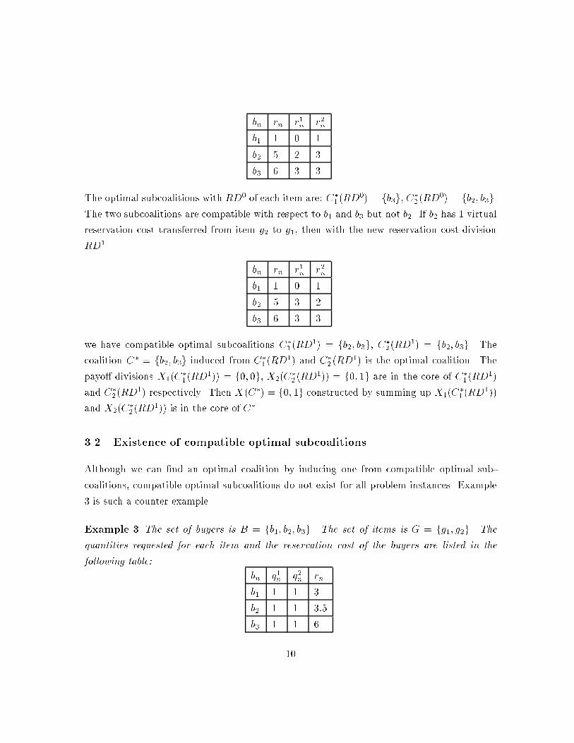
bn rn r1n r2n

b1 1 0 1

b2 5 2 3

b3 6 3 3

The optimal subcoalitions with RD0 of each item are: C�1(RD

0) = fb3g, C�2(RD

0) = fb2; b3g.

The two subcoalitions are compatible with respect to b1 and b3 but not b2. If b2 has 1 virtual

reservation cost transferred from item g2 to g1, then with the new reservation cost division

RD1

bn rn r1n r2n

b1 1 0 1

b2 5 3 2

b3 6 3 3

we have compatible optimal subcoalitions C�1(RD

1) = fb2; b3g, C�2(RD

1) = fb2; b3g. The

coalition C� = fb2; b3g induced from C�1(RD

1) and C�2(RD

1) is the optimal coalition. The

payo� divisions X1(C�1(RD

1)) = f0; 0g, X2(C�2(RD

1)) = f0; 1g are in the core of C�1(RD

1)

and C�2(RD

1) respectively. Then X(C�) = f0; 1g constructed by summing up X1(C�1(RD

1))

and X2(C�2(RD

1)) is in the core of C�.

3.2 Existence of compatible optimal subcoalitions

Although we can �nd an optimal coalition by inducing one from compatible optimal sub-

coalitions, compatible optimal subcoalitions do not exist for all problem instances. Example

3 is such a counter example.

Example 3 The set of buyers is B = fb1; b2; b3g. The set of items is G = fg1; g2g. The

quantities requested for each item and the reservation cost of the buyers are listed in the

following table:

bn q1n q2n rn

b1 1 1 3

b2 1 1 3:5

b3 1 1 6

10

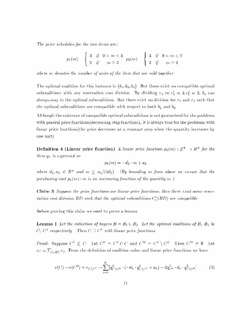
The price schedules for the two items are:

p1(m) =

8<:

3 if 0 < m < 3

2 if m � 3p2(m) =

8<:

3 if 0 < m < 2

2 if m � 2

where m denotes the number of units of the item that are sold together.

The optimal coalition for this instance is fb1; b2; b3g. But there exist no compatible optimal

subcoalitions with any reservation cost division. By dividing r3 to r13 = 3,r23 = 3, b3 can

always stay in the optimal subcoalitions. But there exist no division for r1 and r2 such that

the optimal subcoalitions are compatible with respect to both b1 and b2.

Although the existence of compatible optimal subcoalitions is not guaranteed for the problems

with general price functions(decreasing step functions), it is always true for the problems with

linear price functions(the price decreases at a constant step when the quantity increases by

one unit).

De�nition 4 (Linear price function) A linear price function pk(m) : Z+ ! R+ for the

item gk is expressed as

pk(m) = �dk �m+ ak

where dk; ak 2 R+ and m � ak=(2dk). (By bounding m from above we ensure that the

purchasing cost pk(m) �m is an increasing function of the quantity m.)

Claim 3 Suppose the price functions are linear price functions, then there exist some reser-

vation cost division RD such that the optimal subcoalitions C�k(RD) are compatible.

Before proving this claim we need to prove a lemma.

Lemma 1 Let the collection of buyers B = B1 [B2. Let the optimal coalitions of B, B1 be

C, C1 respectively . Then C � C1 with linear price functions.

Proof: Suppose C1 6� C. Let C0 = C1 \ C and C00 = C1 n C0. Then C

00 6= ;. Let

rC =P

bn2Crn. From the de�nition of coalition value and linear price functions we have

v(C)� v(C0) = rCnC0 �

KXk=1

[qkCnC0 � (�dk � qkCnC0 + ak)� 2qkC0 � dk � q

kCnC0 ] (3)

11

and

v(C [ C00)� v(C1) = rCnC0 �

KXk=1

[qkCnC0 � (�dk � qkCnC0 + ak)� 2qkC1 � dk � q

kCnC0 ] (4)

Since qkC1 � qk

C0 and the strict inequality holds for at least one gi 2 G, by comparing Equation

3 and 4 we have

v(C [ C00)� v(C1) > v(C)� v(C0):

v(C [ C00)� v(C1) > v(C)� v(C1):

v(C [ C00) > v(C):

This contradicts the optimality of C.2

Corollary 1 With linear price functions the optimal coalition contains all the optimal coali-

tions of subsets of the buyers .

Following Lemma 1 we have the proof of Claim 3.

Proof: By induction with the number of buyers N :

When N = 1 it holds straightforwardly.

Suppose the statement stands for N � n.

When N = n + 1: Let the optimal coalition of B0 = fb1; b2; : : : ; bng be C0. Let B0 =

(B0 n C0) [ fbn+1g. Let the optimal coalition of B = B0 [ fbn+1g be C. From Lemma 1 we

have C � C0. Then

C n C0 = argmaxT�(BnC0)v(C0[ T )

= argmaxT�(BnC0)fv(C0[ T )� v(C0)g

= argmaxT�(BnC0)frT �

KXk=1

[qkT (�dk � qkT + ak � dk � 2q

kC0)]g

12

Therefore C n C0 is an optimal coalition of B n C0 with the price functions p0

k(m) = �dk �

m+ ak � dk � 2qkC0 , k = 1; : : : ; K. This is a linear price function and from the assumption of

inductions there exists some reservation cost division for all the buyers bi 2 B nC0 such that

(C n C0)k is an optimal subcoalition among all the subsets of (B n C0) \Bk with respect to

each item gk with the linear price function p0

k(m). With this reservation cost division frki g,

k = 1; : : : ; K, bi 2 B n C0,

(C nC0)k = argmaxT�(BnC0)\BkfrkT � qkT (�dk � q

kT + ak � dk � 2q

kC0)g

= argmaxT�(Bkn(C0)k)

fvk((T [ C0)k)� vk((C

0)k)g

= argmaxT�(Bkn(C0)k)

vk((T )k [ (C0)k) (5)

From Lemma 1 the optimal subcoalition Ck of Bk with respect to item gk includes (C0)k for

every k. Equation 5 means that (C)k = (C n C0)k [ (C0)k is an optimal subcoalition with

respect to gk if (C0)k is an optimal subcoalition of the buyers in (C0)k with respect to gk.

Let the reservation cost division of C0 to be that with which (C0)k is optimal with respect

to the item gk among all the subsets of (C0)k for every k.(From the assumption of inductions

such a reservation cost division exists.) Then (C)k is an optimal subcoalition of the item gk

with the reservation cost division stated above and (C)k, k = 1; : : : ; K are compatible. 2

Although the existence of compatible optimal subcoalitions is not guaranteed for the systems

with general price functions, the approach of virtual reservation cost transfer still helps to

give a solution for the problem with general price functions, as shown in Section 7.

Based on the approach we need to answer the following questions:

� How to e�ciently form an optimal subcoalition and distribute the payo� in the core

� How to transfer the virtual reservation cost among items to make the optimal subcoali-

tions compatible if they exist

� How to reduce the computational complexity and construct an approximation algorithm

in polynomial time for the system with linear price functions

� How to construct an approximation algorithm in polynomial time for the system with

general price functions based on the virtual reservation cost transfer approach

13

These problems are solved in Section 4, 5, 6 and 7 respectively. The notations with a "0" are

used to denote the terms with the reservation cost division after a transfer.

4 Optimal subcoalition formation and payo� division

Optimal subcoalition formation is a basic component of the reservation cost transfer scheme.

In [1] an e�cient and accurate algorithm for subcoalition formation and stable payo� division

is given for the situation where each buyer asks for one unit of the items. With some

modi�cations the algorithm can be extended to the situation with multiple units.

4.1 Algorithm for optimal subcoalition formation

Claim 4 Suppose bi and bj ask for the same quantity of gk with virtual reservation cost rki

and rkj respectively, rki > rkj . Let the optimal subcoalition of gk be C�k. If bj 2 C�

k, then

bi 2 C�k .

Proof: If bi 62 C�k , construct a subcoalition C

0

k by replacing bj with bi in C�k . This does not

change the discount price of the item with the subcoalition since bi and bj ask for the same

quantity of gk. But rki > rkj , hence vk(C�k) < vk(C

0

k) and this contradicts the optimality of

C�k .2

From Claim 4 to form an optimal subcoalition for the item gk, we can �rst sort the buyers

with the same bid quantity for gk by their virtual reservation cost in a descending order.

The candidates for the optimal subcoalition can be constructed by extracting from each

list buyers from the pre�x of the list. The subcoalition with the largest value among these

candidate subcoalitions is the optimal subcoalition. The algorithm is stated in Algorithm 1.

The complexity of the algorithm is analyzed in Claim 5.

Algorithm 1 (Optimal subcoalition formation)

Step 1: Calculate the virtual reservation price of each buyer for the item

pkn = rkn=qkn

14

Step 2: Order the buyers with the same bid quantity for the item by their virtual reservation

prices descendantly, and form M lists qu1; : : : ; quM where M is the number of bid quantities

for the item.

Step 3: Construct all possible collections formed by the buyers from pre�xes of the lists and

calculate their values with respect to the item. The collection with the largest value is the

optimal subcoalition. 2

Claim 5 The complexity of Algorithm 1 is O(NM) where M is the number of di�erent

bidding quantities for the item2, N is the number of buyers requesting the item.

Proof: The number of coalitions to be considered isQMm=1(Km + 1) where Km is the length

of qum, the number of buyers who desire m units of the item. Since Km � N ,

MYm=1

(Km + 1) � (N + 1)M

The algorithm has complexity O(NM).2

4.2 Payo� division of a subcoalition

Claim 6 gives a strategy to divide the payo� of the optimal subcoalition such that the payo�

division is in the core of the subcoalition. Claim 7 gives the computational complexity of the

strategy.

Claim 6 Let costk(Ck) denote the purchase cost to satisfy the requests of the members in

Ck, i.e. costk(Ck) = qkCk� pk(q

kCk). The payo� division Xk(Ck) of the subcoalition Ck is in

the core of Ck with

xik =

8<:

(pki � hCk) � qki (bi 2 Ck)

0 (bi 62 Ck)

where hCkand Ck satisfy

2Based on the goods traded in electronic markets to personal buyers, for instance, books, electrics, parts

and accessories, we can reasonably assume M be a small number.

15

costk(Ck) = (X

bi2Ck

qki ) � hCk+

X

bi2CknCk

pki � qki

Ck = fbi 2 CkjhCk� pki g

Proof: The conclusion follows from Proposition 1 in [1] by regarding a buyer bn asking for qkn

units of gk with the reservation cost rkn as qkn buyers each one asking for 1 unit of gk with the

same reservation price rkn=qkn.2

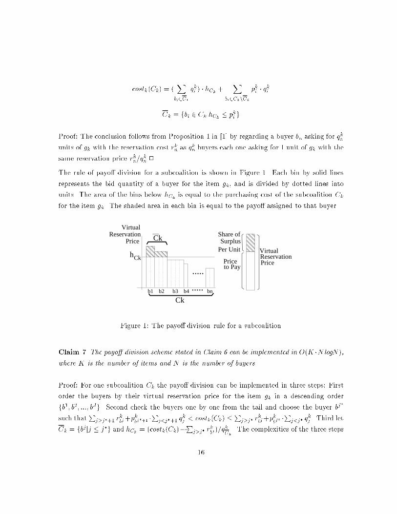
The rule of payo� division for a subcoalition is shown in Figure 1. Each bin by solid lines

represents the bid quantity of a buyer for the item gk, and is divided by dotted lines into

units. The area of the bins below hCkis equal to the purchasing cost of the subcoalition Ck

for the item gk. The shaded area in each bin is equal to the payo� assigned to that buyer.

h

Ck

CkPer Unit

Share ofSurplus

Price

VirtualReservationPrice

to Pay

Ck

VirtualReservation

Price

bn

��������

��������

.....

.....b1 b2 b3 b4

������������

������

������

Figure 1: The payo� division rule for a subcoalition

Claim 7 The payo� division scheme stated in Claim 6 can be implemented in O(K �N logN),

where K is the number of items and N is the number of buyers.

Proof: For one subcoalition Ck the payo� division can be implemented in three steps: First

order the buyers by their virtual reservation price for the item gk in a descending order

fb1; b2; :::; bJg. Second check the buyers one by one from the tail and choose the buyer bj�

such thatP

j�j�+1 rkbj+pk

bj�+1 �Pj<j�+1 q

kj < costk(Ck) �

Pj�j� r

kbj+pk

bj� �P

j<j� qkj . Third let

Ck = fbjjj � j�g and hCk= (costk(Ck)�

Pj>j� r

kbj)=qk

Ck. The complexities of the three steps

16

are O(N logN), O(N) and O(1) respectively. Therefore the complexity of payo� division for

one subcoalition is O(N logN). When there are K items, we need to do once for each of the

K subcoalitions and the complexity is O(K �N logN).2

4.3 In the sight of cooperative games

If we regard each buyer as a player this problem de�nes a cooperative game (B; v) where B

is the set of players and v(C), the value of a coalition C � B is the characteristic function

de�ned on every subset C of B.

The following de�nitions and theorems are noted in [2]

In a convex game the marginal contribution of a buyer bn to a coalition not including bn

increases with expansion of the coalition.

De�nition 5 (Convex Game) A cooperative game (B; v) is convex if it satis�es one of the

two following equivalent properties for all bn 2 B:

for all S; T � B n fbng:

fS � Tg ) fv(S [ fbng)� v(S) � v(T [ fbng)� v(T )g

and/or for all S; T � B:

v(S) + v(T ) � v(S [ T ) + v(S \ T )

Theorem 1 gives some ways to construct a payo� vector in the core for a convex game.

De�nition 6 (Shapley value) The Shapley value is a payo� vector which assigns a payo�

XS�Cnbi

(jSj!(n� jSj � 1)!=n!)(v(S [ bi)� v(S))

to each player bi in the coalition C.

Theorem 1 Let (B; v) be a convex game and C� be an optimal coalition. Let C� be ordered

as fi1; : : : ; ing where n is the number of players in C�. The payo� vector constructed by

assigning marginal contributions for each item

17

xC(ik) = v(i1; : : : ; ik)� v(i1; : : : ; ik�1)

is in the core of C�. Therefore the Shapley value is in the core, too.

For an optimal coalition C� with n buyers, there are n! ways to order the players in C�. It

is stated in [3] that the payo� vectors generated by the marginal contributions based on all

the ordering construct the extreme points of the core of C�, which is a convex space.

Based on the de�nitions and theorems above we can see that in our combinatorial coalition

formation problem the set of buyers and the value function construct a convex game with

linear price functions.

Claim 8 Suppose linear price functions are applied. The set of buyers is B. The value

function is v. Then (B; v) is a convex game.

Proof: Denote by rC the sum of reservation cost of all the players in C � B, by qkC the sum of

the quantities asked by all the players in C for the item gk. rC =P

bn2C rn, qkC =

Pbn2C q

kn.

For any C0, C00, B0, B00 � B and C0 � C00, B0 � B00, let C = (C0 [ B00) n (C0 [ B0) =

(C00 [B00) n (C00 [ B0).

v(C0[B00)� v(C0

[ B0) = rC �

KXk=1

[pk(qkC0[B00) � qkC0[B00 � pk(q

kC0[B0) � qkC0[B0]

= rC +KXk=1

[�ak � qkC + dk((q

kC0[B00)2 � (qkC0[B0)2)]

= rC +KXk=1

[�ak � qkC + dk(q

kC0[B00 + qkC0[B0)qkC ]

Similarly

v(C00[B00)� v(C00

[B0) = rC +KXk=1

[�ak � qkC + dk(q

kC00[B00 + qkC00[B0)qkC ]:

Since

18

qkC0[B00 + qkC0[B0 � qkC00[B00 + qkC00[B0

we have

v(C0 [B00)� v(C0 [ B0) � v(C00 [B00)� v(C00 [B0):

From De�nition 5 (C�; v) is a convex game.2

When the price functions are general decreasing step functions, (C�; v) is not necessary a

convex game since the purchasing cost of a coalition is not necessary submodular3 on the

coalitions.

Given linear price functions the payo� vectors generated by the marginal contribution and

the Shapley value are also in the core of the optimal coalition. Compared to these our payo�

division scheme proposed in Claim 6 has the following advantages:

� Symmetric: The payo� division proposed in Claim 6 does not depend on the ordering

of players but only on the virtual reservation prices. As extreme points of the core the

payo� vectors generated by the marginal contribution are dependent on the ordering

of players and always give preference to the buyers ordered at the end.

� Low computational complexity: The computational complexity of the payo� vector

proposed in Claim 6 is only O(K �N logN)(Claim 7) where K is the number of items

and N is the number of buyers. But to compute the Shapley value we need to calculate

the values of all coalitions of the players and the complexity is O(2N), although the

Shapley value is at the centroid of the core([3]).

These points support the payo� division proposed in Claim 6 as distributing the payo� in

a fairer way than the payo� vectors generated by the marginal contributions and in a more

e�cient way than the Shapley value.

3A function f(�) is submodular if f(S0 [ S1)� f(S1) � f(S0 [ S2)� f(S2) for any S1 � S2.

19

5 Reservation cost transfer scheme

De�nition 7 (O�er & Request) Denote the optimal subcoalition of the item gk by C�k.

O�er Offkn of the buyer bn 2 C�k with respect to the item gk is the maximum amount of

virtual reservation cost of bn for gk that can be reduced from rkn while keeping bn in the

optimal subcoalition of gk and the reservation cost division of other buyers remains the same,

i.e.,

Offkn = rkn �minfrkn : bn 2 C�k(RD)g

Request Reqkn of the buyer bn 62 C�k with respect to the item gk is the minimum amount of

virtual reservation cost of bn for gk that needs to be added to rkn, such that bn can join the

optimal subcoalition of gk while the reservation cost division of other buyers remains the same,

i.e.,

Reqkn = minfrkn : bn 2 C�k(RD)g � rkn

Requests and o�ers of a buyer bn determine the range of virtual reservation cost of bn to be

transferred among items to make the optimal subcoalitions after the transfer for bn compatible

with respect to bn.

Claim 9 Suppose the optimal subcoalitions C�1(RD); : : : ; C�

K(RD) with the reservation cost

division RD are not compatible with respect to the buyer bn. The current reservation cost

division of bn is fr1n; : : : ; rKn g. Let K1

n = fgk 2 Gnjbn 2 C�kg and K2

n = fgk 2 Gnjbn 62 C�kg,

difn =Pk:gk2K

1nOffkn �

Pk:gk2K

2nReqkn be the di�erence between the sum of the o�ers of bn

and the sum of the requests of bn.

(i) If difn < 0, then bn cannot be involved in all the optimal subcoalitions he desires by

a reservation cost transfer for bn, but there exist some transfer for bn by which bn is

excluded from all the optimal subcoalitions he desires.

(ii) If difn > 0, then bn cannot be excluded from all the optimal subcoalitions he desires by

a reservation cost transfer for bn, but there exist some transfer for bn by which bn is

involved in all the optimal subcoalitions he desires.

20

(iii) If difn = 0, then bn can either be involved in or excluded from all the optimal subcoali-

tions he desires by a reservation cost transfer for bn.

Proof:

(i) Suppose after a transfer for bn, bn is involved in all the subcoalitions he desires with

the new reservation cost division fr10

n ; : : : ; rK0

n g. Then rkn � rk0

n � Offkn for gk 2 K1n

and rkn+Reqkn � rk0

n for gk 2 K2n. The sum of the reservation costs of a buyer stays the

same after the transfer, i.e.,P

gk2K1n(rkn � rk

0

n ) =Pgk2K

2n(rk

0

n � rkn). ButP

gk2K1n(rkn �

rk0

n ) �Pgk2K1

nOffkn ,

Pgk2K2

n(rk

0

n � rkn) �P

gk2K2nReqkn, therefore

Pgk2K1

nOffkn �P

gk2K2nReqkn. This contradicts the condition difn < 0.

There exist a set of numbers k � 0 for gk 2 Gn such thatPK

k=1 k = �difn. Let

rk0

n = rkn � Offkn � k for gk 2 K1n and rk

0

n = rkn + Reqkn � k for gk 2 K2n, then

fr10

n ; : : : ; rK0

n g de�nes a new reservation cost division for bn with which bn is excluded

from all the optimal subcoalitions he desires.

(ii) It can be shown via a similar argument as in (i).

(iii) Let rk0

n = rkn � Offkn for gk 2 K1n and rk

0

n = rkn + Reqkn for gk 2 K2n. The array

fr10

n ; : : : ; rK0

n g de�nes a new reservation cost for bn with which there are multiple optimal

subcoalitions for each item gk 2 Gn. The buyer bn can be either involved in or excluded

from all the optimal subcoalitions he desires.

2

The way to calculate requests and o�ers is stated in Claim 10. The o�er Offkn is the

di�erence between the value of the current optimal subcoalition C�k and the value of the

optimal subcoalition without bn. The request Reqkn is the di�erence between the value of

the current optimal subcoalition C�k and the value of the optimal subcoalition having bn as a

member.

Claim 10 Let C�k be the optimal subcoalition of Item gk with the reservation cost division

RD = frkngn=1;:::;N, k=1;:::;K. Suppose bn 2 C�k and bl 62 C�

k. Let C�nk be the optimal subcoalition

of gk among all those subcoalitions of gk with the buyer set B n fbng. Let Clk be the optimal

subcoalition of gk among all those subcoalitions of gk having bl as a member.

21

(i) Offkn = vk(C�k)� vk(C

�nk )

(ii) Reqkl = vk(C�k)� vk(C

lk)

Proof: Use the notations with a "0" to denote the terms with the reservation cost division

after the transfer(this is used throughout the following portions of the paper).

(i) Let the new reservation cost of bn for gk be rk0

n = rkn � �. bn remains in the optimal

subcoalition of gk with the reservation cost rk0

n . Since the reservation cost division of the

buyers except bn remains, the optimal subcoalition of gk among all those subcoalitions

of gk having bn as a member after the transfer is same as the optimal subcoalition of

gk before the transfer, i.e., Cn0

k = C�k . But the value of the coalition changes with the

transfer, v0

k(Cn0

k ) = vk(C�k) � rkn + rk

0

n = vk(C�k) � �. For bn to remain in the optimal

subcoalition of gk, v0

k(Cn0

k ) � v0

k(C�n0

k ) need to be satis�ed. But C�nk = C�n0

k , so it follows

that � � vk(C�k)� vk(C

�nk ). Hence Off

kn = vk(C

�k)� vk(C

�nk ).

(ii) A similar argument as in (i) can be used.

2

In Example 2 since v1(C�31) = v1(;) = 0,v1(C

21) = v1(fb2; b3g) = �1, v1(C

�1) = v1(fb3g) = 0,

the o�er of b3 with respect to g1 is Off13 = 0� 0 = 0 and the request of b2 with respect to

g1 is Req12 = 0� (�1) = 1.

Claim 11 states that the o�er of a member in an optimal subcoalition is an increasing function

of the virtual reservation cost of other members in the optimal subcoalition for the item.

Claim 11 Make a transfer for bi 2 Bk such that rk0

i < rki . Suppose bi and bj are members of

the optimal subcoalition of the item gk both before and after the transfer. Then Offk0

j � Offkj .

Proof: From Claim 13 we have C�0

k = C�k . Let the new reservation cost of bi for gk be

rk0

l = rkl ��. Then v0

k(C�0

k ) = vk(C�k)��. But v

0

k(C�j0

k ) � vk(C�jk)�� where the equality holds

when bi 2 C�j0

k . Therefore v0

k(C�0

k )� v0

k(C�j0

k ) � vk(C�k)� vk(C

�jk) and Off

k0

j � Offkj . 2

Claim 12 states that with linear price functions the o�er of a member in an optimal subcoali-

tion is an increasing function and the request of a nonmember is a decreasing function of the

virtual reservation cost of other buyers for the item.

22

Claim 12 Suppose linear price functions are applied. Make transfer for bn 2 Bk such that

rk0

n > rkn. Suppose bi is a member while bj is a nonmember of the optimal subcoalition of the

item gk both before and after the transfer. Then

(i) Offk0

i � Offki

(ii) Reqk0

j � Reqki

Proof:

(i) From Corollary 1 C�ik � C�

k and C�i0

k � C�0

k . Discuss every possible condition:

(1) bn 2 C�ik.

Then bn 2 C�i0

k and C�i0

k = C�ik. It follows that bn 2 C�

k , bn 2 C�0

k and C�k = C�0

k .

Therefore v0

k(C�0

k )� v0

k(C�i0

k ) = vk(C�k)� vk(C

�ik) and Offk

0

i = Offki .

(2) bn 62 C�ik and bn 62 C

�i0

k .

Then C�i0

k = C�ik and v

0

k(C�i0

k ) = vk(C�ik). Since v

0

k(C�0

k ) � vk(C�k), we have v

0

k(C�0

k )�

v0

k(C�i0

k ) � vk(C�k)� vk(C

�ik) and Offk

0

i � Offki .

(3) bn 2 C�k and bn 62 C

�ik and bn 2 C

�i0

k .

Then bn 2 C�0

k . Since it is a convex game and C�i0

k � C�ik, vk(C

�i0

k [ (C�k n C

�ik)) �

vk(C�i0

k ) � vk(C�k)� vk(C

�ik). Then v

0

k(C�i0

k [ (C�k nC

�ik))� v

0

k(C�i0

k ) � vk(C�ik)� vk(C

�k).

But v0

k(C�i0

k [ (C�k nC

�ik)) � v

0

k(C�0

k ). Therefore v0

k(C�0

k )� v0

k(C�i0

k ) � v0

k(C�k)� vk(C

�ik)

and Offk0

i � Offki .

(4) bn 62 C�k and bn 62 C�0

k .

Then C�0

k = C�k and v

0

k(C�0

k ) = vk(C�k). It follows that bn 62 C

�ik and bn 62 C

�i0

k . From

(2) Offk0

i � Offki .

(5) bn 62 C�k and bn 2 C�0

k and bn 62 C�ik and bn 2 C

�i0

k .

Since it is a convex game and C�k � C

�ik, vk(C

�k [ (C

�i0

k n C�ik))� vk(C

�k) � vk(C

�i0

k )�

vk(C�ik). Then v

0

k(C�k [ (C

�i0

k nC�ik))� vk(C

�k) � v

0

k(C�i0

k )� vk(C�ik). But v

0

k(C�k [ (C

�i0

k n

C�ik)) � v

0

k(C�0

k ). Therefore v0

k(C�0

k �vk(C�k) � v

0

k(C�i0

k )�vk(C�ik) and Off

k0

i � Offki .

(ii) From Cjk � C�

k and Cj0

k � Cjk, we have the conclusion following the same way.

23

2

The general reservation cost transfer scheme is stated in Algorithm 2. It starts with an initial

reservation cost division and checks the buyers one by one. If the optimal subcoalitions are

not compatible with respect to the buyer bn, bn makes a virtual reservation cost transfer such

that the new optimal subcoalitions after the transfer are compatible with respect to bn. It

stops when the optimal subcoalitions are compatible with respect to all the buyers.

Algorithm 2 (General reservation cost transfer algorithm)

Step 0: Initialization

Make an initial reservation cost division RD = frkngn=1;:::;N, k=1;:::;K such thatPKk=1 r

kn = rn

for all buyers bn 2 B.

Step 1: Optimal subcoalition formation

Construct the optimal subcoalition for each item following Algorithm 1.

Step 2: Transfer

If there exist a buyer bn with whom the optimal subcoalitions are not compatible, change the

division of rn by some transfer unless all the o�ers and requests are zero, update the optimal

subcoalitions so that they are compatible with respect to bn with the new reservation cost

division.

Step 3: Termination judgment

If the optimal subcoalitions are compatible with respect to all the buyers, stop; else repeat Step

2.2

The reservation cost transfer for one buyer bn a�ects not only the status(in or out of the

optimal subcoalitions) of bn but also the status of other buyers. The following claims help us

to understand the stability of the optimal subcoalitions in the procedure of transfers.

Claim 13 Denote by C�k(RD) the optimal subcoalition of the item gk with the reservation

cost division RD. Make transfer for bn 2 C�k(RD) such that bn 2 C�0

k (RD0) where C�0

k (RD0)

is the optimal subcoalition of gk with the new reservation cost division RD0. Then C�0

k (RD0) =

C�k(RD).

24

Proof: Let C�k(RD) be denoted by Ck and C�0

k (RD0) be denoted by C

0

k. Denote by v0

k(�)

the value of subcoalitions with the reservation cost division RD0

and by vk the value of

subcoalitions with RD. Suppose Ck 6= C0

k and v0

k(C0

k) > v0

k(Ck). Let C0k = C

0

k \ Ck. Let

= vk(Ck)� vk(C0k) (6)

0

= vk(C0

k)� vk(C0k) (7)

Since bn 2 C0

k\Ck and bn is the only buyer who has di�erent reservation cost division between

RD and RD0

,

= v0

k(Ck)� v0

k(C0k) (8)

0

= v0

k(C0

k)� v0

k(C0k) (9)

Since vk(Ck) � vk(C0

k) and v0

k(C0

k) > v0

k(Ck), we have � 0

from Equation 6 and 7, < 0

from Equation 8 and 9. Contradiction.2

From Claim 13 the reservation cost transfer of a member bn in an optimal subcoalition does

not cause change of the optimal subcoalition if bn stays in it after the transfer.

If the sum of the o�ers of a buyer cannot cover the sum of his requests he has to leave

all the optimal subcoalitions after one transfer for him. When the system has linear price

functions the leaving of a buyer bn 2 C�k from an optimal subcoalition C�0

k will not have

other buyers bi 62 C�k that are not members of the subcoalition before the transfer join the

optimal subcoalition C�0

k after the transfer(but it may have some other buyers bj 2 C�k leave

the optimal subcoalition C�0

k too). If the sum of the o�ers of a buyer covers the sum of

his requests he will be involved in all the optimal subcoalitions he desires after one transfer

for him. When the system has linear price functions the joining of a buyer bn 62 C�k into

an optimal subcoalition C�0

k will not have other buyers bi 2 C�k that are members of the

subcoalition before the transfer leave the optimal subcoalition C�0

k after the transfer(but it

may have some other buyers bj 62 C�k join into the new optimal subcoalition C�0

k too).

Claim 14 Suppose pk(�) is a linear price function and bn 2 C�k(RD) with some reservation

cost division RD. Make a transfer for bn such that bn 62 C�0

k (RD0) where C�0

k (RD0) is the

optimal subcoalition with respect to the item gk with the new reservation cost division RD0.

Then C�0

k (RD0) � C�

k(RD).

25

Proof: Let C�k(RD) be denoted by Ck and C

�0

k (RD0) be denoted by C

0

k. Denote by v0

k(�) the

value of subcoalitions with the reservation cost division RD0

= frk0

n gn;k and by vk the value

of subcoalitions with RD = frkngn;k . Let�Ck = Ck \C

0

k and Ck = C0

k nCk. Suppose C0

k 6� Ck,

then Ck 6= ;.

From v0

k(Ck [�Ck) � v

0

k(�Ck),

rkCk� qk

Ck(ak � dk � q

k

Ck) + 2qk

Ck� dk � q

k�Ck� 0 (10)

Since �Ck � Ck, bn 2 Ck n �Ck, and qkn > 0, we have qkCk

> qk�Ck. Substitute q �Ck

in Equation 10

with qkCkand it follows that

rkCk� qk

Ck(ak � dk � q

k

Ck) + 2qkCk

� dk � qk

Ck> 0 (11)

The LSH of the inequality above is equal to vk(Ck [ Ck)� vk(Ck). The inequality vk(Ck [

Ck)� vk(Ck) > 0 contradicts the optimality of the subcoalition Ck with the reservation cost

division RD. 2

Claim 15 Suppose pk(�) is a linear price function and bn 62 C�k(RD) with some reservation

cost division RD. Make a transfer for bn such that bn 2 C�0

k (RD0) where C�0

k (RD0) is the

optimal subcoalition with respect to item gk with the new reservation cost division RD0. Then

C�0

k (RD0) � C�

k(RD).

Proof: Similar as in Claim 14. 2

Based on Claim 13, 14 and 15 we have the following claim:

Claim 16 With linear price functions the general reservation cost transfer algorithm termi-

nates with a set of compatible optimal subcoalitions.

Proof: Let the system state be de�ned by a tuple (�1; : : : ; �N), where �n = (�1n; : : : ; �Kn )

with �kn 2 f0; 1g, n = 1; : : : ; N , k = 1; : : : ; K. �kn = 1 if the buyer bn is contained in the

optimal subcoalition C�k of the item gk, else �

kn = 0. Construct a directed graph composed of

the all the nodes each one corresponding to a state. Two nodes are connected by an arc if and

only if there exists one step of transfer for one buyer that transfers the sqystem state from

26

the source node to the target node. Now prove that the system will not evolve by following

in�nitely a directed loop.

Suppose the system evolves following a directed loop L in�nitely, and there are some arcs

in this loop on which the amount of reservation cost transfered is not zero. Call these arcs

non-zero arcs. If two arcs a and b are associate with the same buyer, one transfer reservation

cost into item gk, the other transfer out of gk, we say they transfer in reverse direction for

item gk. For each non-zero arc a 2 L, there exists at least another non-zero arc a0 2 L such

that a and a0 are associated with the same buyer but transfer the reservation cost in reverse

directions for some items. Call arc b immediately succeeds arc a if the transfer on arc a causes

the transfer on arc b. Denote b 2 succ(a) if b immediately succeeds a or there exists an arc

c 2 succ(a) such that b immediately succeeds c. From Claim 14 and 15, if the transfer on one

arc a causes the uncompatibility of another buyer bn, then the corresponding transfer on arc

b to have bn compatible will not reverse the direction of transfer from that on arc a, so do all

arcs in succ(a). For example, if the transfer from item gi to gk through arc a for buyer bm

makes bn uncompatible, then to recover the compatibility, bn needs to transfer out of item gk

or into gi, which can only cause further transfer out of gi or into gk for bm if that makes bm

uncompatible in return. This implies there does not exit a path P between a and a0 in which

every arc P (k), k 6= 0 immediately succeeds P (k� 1), where P (k), k � 0 is the k-th arc in P

from the head. But such a path should exist if we have in�nite none zero transfer iterations,

otherwise a and a0 can not be both involved in the transfer procedure. Therefore we get a

contradiction and following the transfer rule in Algorithm 2 the in�nite iteration only happens

when all the requests and o�ers are equal to zero for each of the buyers B0

involved in the

loop with the reservation cost division. This means there are multiple optimal subcoalitions

with the same value but di�erent formations for each item. When uncompatibility is found

with respect to a buyer bn 2 B0

, select(or discard) the optimal subcoalitions containing bn

for each gk 2 Gn. From Claim 15 and 14 a set of optimal subcoalitions that are compatible

with respect to B0

will be reached and the system will jump out of the loop.

Since the number of states is �nite, a state that is compatible with respect to all the buyers

can by reached in �nite steps. 2

The properties of Claim 14 and 15 are not necessary for the problems with general price

27

functions. In Example 3, suppose the initial reservation cost division RD0 be

bn rn r1n r2n

b1 3 1:25 1:75

b2 3:5 1:75 1:75

b3 6 3 3

The optimal subcoalitions with RD0 are: C�1 = fb1; b2; b3g , C�

2 = fb1; b3g(or fb2; b3g). If

b1 joins C�2 then b2 leaves C�

2 and vice versa. The system evolution is trapped in the cycle

composed of the two nodes: ((1; 1); (1; 0); (1; 1)) and ((1; 0); (1; 1); (1; 1)).

Therefore termination of the general algorithm is not guaranteed for the general systems. This

is consistent with the conclusion that for those systems compatible optimal subcoalitions may

not exist.

6 Algorithm with linear price functions

Although the general reservation price transfer mechanism leads to an optimal coalition

and payo� division in the core of the coalition, polynomial computational complexity is not

guaranteed. We need an approximation algorithm to decrease the complexity. The intuition

is that once a buyer is excluded from all the optimal subcoalitions, the possibility that he

will be involved in the �nal optimal coalition is very small. We maintain a subset of the

buyers B which shrinks while excluding buyers. The coalition formation and payo� division

is considered within B instead of B assuming the buyers out of B are not contained in the

optimal coalition. In each iteration, a reservation cost transfer is made for one buyer such

that the new optimal subcoalitions are compatible with him after the transfer. If the buyer

is discarded by all the optimal subcoalitions he is excluded from B, else the next buyer in B

is visited. The coalition resulting from the algorithm is a set of buyers that is cohesive with

the coalition value no less than the value of any of its subset and the payo� division is in

the core of the coalition. The complexity of the algorithm is polynomial. An optional sub-

iteration(Option 1) can be integrated into the algorithm to improve the performance(increase

the chance of a buyer that would be excluded to be kept in B) at the expense of increasing

the computational complexity while keeping the complexity polynomial.

From Example 4 we can see that even if a buyer is rejected by all the optimal subcoalitions

at some time of the transfer procedure it is still possible that he is involved in the optimal

28

coalition.

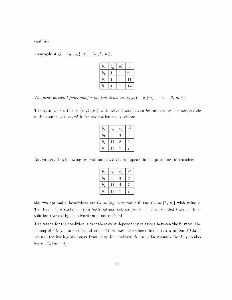
Example 4 G = fg1; g2g, B = fb1; b2; b3g,

bn q1n q2n rn

b1 1 1 6

b2 1 1 11

b3 1 1 14

The price discount functions for the two items are p1(m) = p2(m) = �m + 8, m � 4.

The optimal coalition is fb1; b2; b3g with value 1 and it can be induced by the compatible

optimal subcoalitions with the reservation cost division:

bn rn r1n r2n

b1 6 3 3

b2 11 5 6

b3 14 7 7

But suppose the following reservation cost division appears in the procedure of transfer:

bn rn r1n r2n

b1 6 4 2

b2 11 4 7

b3 14 7 7

the two optimal subcoalitions are C�1 = fb3g with value 0, and C�

2 = fb2; b3g with value 2.

The buyer b1 is excluded from both optimal subcoalitions. If he is excluded then the �nal

solution reached by the algorithm is not optimal.

The reason for the condition is that there exist dependency relations between the buyers: The

joining of a buyer to an optimal subcoalition may have some other buyers also join it(Claim

15) and the leaving of a buyer from an optimal subcoalition may have some other buyers also

leave it(Claim 14).

29

De�nition 8 (Supporter & Dependant) Suppose the buyers bi and bj are both included

in the optimal subcoalition Ck. If dropping bi causes the removal of bj from the optimal

subcoalition of gk, then bi is said to be a supporter of bj and bj is a dependant of bi with

respect to the item gk.

Even if a buyer is rejected by all the optimal subcoalitions temporarily it is possible that he

will get some virtual price transferred from his dependants and accepted by all the optimal

subcoalitions. This is like price ows from dependants to supporters. In Example 2 b1 is

a supporter of b2 with respect to g1 with the second reservation cost division. When b2

transfers 1 from g2 to g1, b1 and b2 are both accepted by C1 and then b1 has an o�er equal

to 1 to be transferred to g2 which makes him involved in C2 too. The condition of price ow

is considered in Option 1, which can be integrated into the main algorithm to improve the

solution quality at the expense of increasing the computational complexity. Recognizing all

of the supporters and dependants is intractable and the option of price ow can be realized

approximately by the greedy transfer procedure as follows. With linear price functions the

o�er of a member in a subcoalition is non-decreasing and the request of a nonmember is

non-increasing with the increasing of the virtual reservation cost of other buyers for the

item(Claim 12). For a buyer bn whose sum of o�ers cannot cover the sum of requests, the

items desired are visited one by one. When an item gk is visited, all the buyers desiring

gk transfer their extra virtual reservation cost(the o�ers) to gk from other items, and the

o�ers/requests of bn are recalculated. The visit to the next item is stopped when the sum of

o�ers covers the sum of requests, in which case a reservation cost division of bn is constructed

by some transfer to have bn included in all the desired optimal subcoalitions. If all the items

desired by bn have been visited and the stop condition is not reached, bn is excluded.

The algorithm of coalition formation for the problems with linear price functions is described

in Algorithm 3:

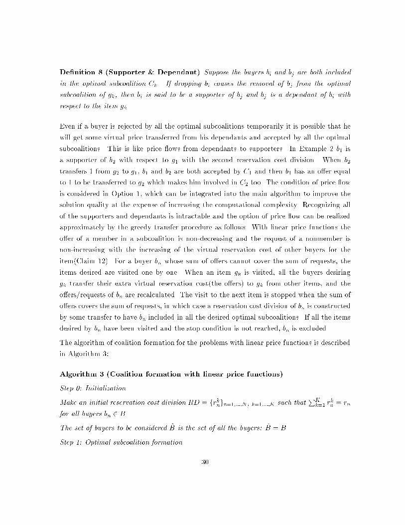
Algorithm 3 (Coalition formation with linear price functions)

Step 0: Initialization

Make an initial reservation cost division RD = frkngn=1;:::;N, k=1;:::;K such thatPKk=1 r

kn = rn

for all buyers bn 2 B.

The set of buyers to be considered B is the set of all the buyers: B = B.

Step 1: Optimal subcoalition formation

30

Construct the optimal subcoalition for each item following Algorithm 1 and go to Step 3.

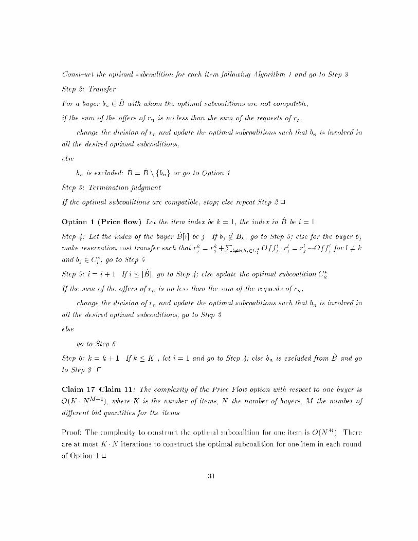
Step 2: Transfer

For a buyer bn 2 B with whom the optimal subcoalitions are not compatible,

if the sum of the o�ers of rn is no less than the sum of the requests of rn,

change the division of rn and update the optimal subcoalitions such that bn is involved in

all the desired optimal subcoalitions,

else

bn is excluded: B = B n fbng or go to Option 1.

Step 3: Termination judgment

If the optimal subcoalitions are compatible, stop; else repeat Step 2.2

Option 1 (Price ow) Let the item index be k = 1, the index in B be i = 1.

Step 4: Let the index of the buyer B[i] be j. If bj 62 Bk, go to Step 5; else for the buyer bj

make reservation cost transfer such that rkj = rkj +P

l6=k;bj2C�

lOff lj , r

lj = rlj �Off lj for l 6= k

and bj 2 C�l , go to Step 5.

Step 5: i = i+ 1. If i � jBj, go to Step 4; else update the optimal subcoalition C�k .

If the sum of the o�ers of rn is no less than the sum of the requests of rn,

change the division of rn and update the optimal subcoalitions such that bn is involved in

all the desired optimal subcoalitions, go to Step 3.

else

go to Step 6.

Step 6: k = k + 1. If k � K , let i = 1 and go to Step 4; else bn is excluded from B and go

to Step 3. 2

Claim 17 Claim 11: The complexity of the Price Flow option with respect to one buyer is

O(K �NM+1), where K is the number of items, N the number of buyers, M the number of

di�erent bid quantities for the items.

Proof: The complexity to construct the optimal subcoalition for one item is O(NM). There

are at most K �N iterations to construct the optimal subcoalition for one item in each round

of Option 1.2

31

Claim 18 The complexity of Algorithm 3 is: O(K � N2+M ) without Option 1 and O(K �

NM+3) with Option 1, where K is the number of items, N the number of buyers, M the

number of di�erent bid quantities for the items.

Proof: The complexity of the sub-algorithms are:

Construct the optimal subcoalition for one item: O(NM).

Construct the optimal subcoalitions for all items: O(K �NM).

Calculate the o�er(request) of one buyer with one item: O(NM).

Calculate the o�ers(requests) of one buyer with all items: O(K �NM).

With the number of buyers to be considered currently being jBj = n the largest number of

iterations needed without Option 1 to exclude a buyer is n � 1. Therefore in the worst case

the number of iterations needed without Option 1 is (N � 1) + (N � 2) + : : :+ 1 which is of

complexity O(N2).

Therefore the complexity of the algorithm is O(K � NM � (N2)) = O(K � N2+M) without

Option 1 and O(K �NM+1 � (N2)) = O(K �N3+M) with Option 1.2

7 Algorithm with general price discount functions

We can limit the number of iterations by reducing the number of buyers following the same

intuition in Algorithm 3. But Algorithm 3 is not applicable in the case with general price

functions since the number of iterations needed to exclude a buyer is not bounded by N any

more and so the polynomial complexity is not guaranteed. The reason for the situation is

that some buyers may be removed from the optimal subcoalition when a di�erent buyer is

added into it. Consequently it is possible that even after all the buyers have been visited

no one had ever been rejected by all the optimal subcoalitions but the optimal subcoalitions

have never been compatible either. To solve this problem, we make some modi�cation of the

transfer mechanism to reach a polynomial bound for the number of iterations. The idea is in

each round to try to keep the compatibility with respect to the buyers that have been visited.

For the buyer being visited consider the compatibility of the optimal subcoalitions one by

one, that is to say, instead of making transfer from multiple to multiple items simultaneously

make transfer from multiple items(source items) to one item(target item) at one time. If the

transfer cannot make the buyer accepted by the optimal subcoalition of the target item, then

32

the buyer is excluded, else consider the in uence of the transfer to the members in the old

optimal subcoalition of the target item. If some members that have been visited are removed

then try to recover them one by one. One that cannot be recovered is excluded, otherwise

if all are recovered, consider the next target item. Since decreasing the reservation cost of a

subcoalition member will not cause increase of other member's o�er(Claim 11), if the transfer

is optimistic(let the amount transferred out equal the o�er) the number of iterations for each

buyer and each item is bounded by the number of buyers maintained. Claim 13 guarantees

the stability of optimal subcoalitions of the source items. Therefore the number of iterations

to visit one buyer is bounded by K � N and the number of iterations needed to exclude a

buyer is bounded by K �N2.

It is not true that the optimal subcoalitions always exist for the instances with general price

functions. Example 3 is such a counter example. In Example 3 the reason for the non-

existence of compatible optimal subcoalitions is that the buyers a and b attract and resist

each other.

De�nition 9 (Attract) We say the buyer bi attracts bj if when the optimal subcoalitions

are compatible with respect to bi, there exists some item gk 2 Gi \ Gj such that bi 2 C�k

implies bj 2 C�k, where C

�k is the optimal subcoalition of the item gk.

De�nition 10 (Resist) We say the buyer bi resists bj if when the optimal subcoalitions are

compatible with respect to bi, bi 2 C�k1

implies bj 62 C�k1, and bi 62 C�

k2implies bj 2 C�

k2for

some item gk1 ; gk2 2 Gi \Gj, where C�k is the optimal subcoalition of the item gk.

When two buyers bi, bj attract and resist each other, there is no reservation cost division of

bi and bj such that the optimal subcoalitions are compatible with respect to both bi and bj .

Claim 19 There exist no reservation cost division of bi and bj such that the optimal sub-

coalitions C�k, k = 1; : : : ; K are compatible with respect to both bi and bj if bi and bj attract

and resist each other.

Proof: Suppose such a reservation cost division of bi and bj exists and the optimal subcoali-

tions C�k , k = 1; : : : ; K are compatible with respect to bi and bj . Let C =

SKk=1 C

�k and

s = C \ fbi; bjg. s 6= ; and s 6= fbi; bjg since bi and bj resist each other. Suppose s = fbig

33

without loss of generality. Since bi and bj attract each other there exist one item gk such that

bj 2 C�k . This contradicts bj 62 C. 2

The buyer exclusion scheme will exclude both of the two buyers bi and bj that attract and

resist each other and result in a cohesive coalition induced by compatible subcoalitions.

However, by merging bi and bj into a single buyer we increase their chance to stay. In

Example 3, if b1 and b2 merge as a single buyer b4 that requests 2 units of both g1 and g2

with reservation cost 6:5, then with the reservation cost division

bn r1n r2n rn

b4 3 3:5 6:5

b3 3 3 6

the optimal subcoalition of both g1 and g2 is fb4; b3g and the coalition induced fb4; b3g(fb1; b2; b3g)

is the optimal one of the original problem.

An option of buyer merging can be integrated into the main algorithm. When a buyer is

decided to be excluded in the main algorithm, use the option to judge if there is another

buyer such that they attract and resist each other. If the answer is positive then merge them

into a single buyer, and replace them with the new buyer, else exclude the buyer. In each

case the number of buyers is decreased by one.

If a buyer bn is produced by merging two buyers bi and bj, then bn is called an arti�cial buyer,

and bi and bj are called the component buyers of bn. A component buyer of an arti�cial buyer

could also be an arti�cial buyer. An arti�cial buyer can be regarded as a collection of the

real buyers that construct it nestingly.

We can divide the payo� in a subcoalition following the same way in Claim 6 when arti�cial

buyers are involved and then divide the payo� of an arti�cial buyer among its components by

some way(for example, by dividing evenly). Let P be a partition of an optimal subcoalition

C and P is composed of all the real buyers and arti�cial buyers in C. Then the resulting

payo� division is not in the core of C but in the pseudo-core(De�nition 11) of C with respect

to P if we consider the real buyers.

De�nition 11 (Pseudo-core) A payo� division XC for the coalition C is said to be in the

pseudo-core with respect to P = fS1; : : : ; SLg, a partition of C, if for any S0 � fS1; : : : ; SLg,

v(S0) � XC(S0)

34

When the partition P is composed of real buyers, the pseudo-core is identical to the core.

The payo� division for the coalition constructed by summing up the payo� for each buyer in

the optimal subcoalitions is also in the pseudo-core of the coalition.

Algorithm 4 (Coalition formation with general price functions)

Step 0: Initialization

Make an initial reservation cost division RD = frkngn=1;:::;N, k=1;:::;K such thatPKk=1 r

kn = rn

for all buyers bn 2 B. The set of buyers to be considered B is the set of all the buyers:

B = B. The set of buyers that have been visited and maintained �B = ;.

Step 1: Optimal subcoalition formation

Construct the optimal subcoalition for each item following Algorithm 1 and go to Step 3.

Step 2: Transfer

For a buyer bn 2 B with whom the optimal subcoalitions are not compatible, for each item gk

that qkn > 0 and bn 62 C�k ,

if the sum of o�ers of bn cannot cover Reqkn,

let B = B n fbng or go to Option 2, and then go to Step 3;

else

make the optimistic transfer for bn to gk such that rkn = rkn +Pj 6=k;bn2C

�

jOff jn, and

rjn = rjn �Off jn for j 6= k; bn 2 C�j , update the optimal subcoalition C�

k of gk.

If any buyer bi 2 �B is removed out of C�k ,

let bn = bi and repeat Step 2;

else

visit the next item.

Let �B = �B [ fbng and go to Step 3.

Step 3: Termination judgment

If the optimal subcoalitions are compatible, stop; else repeat Step 2. 2

Option 2 (Buyer merging) For each buyer bi 2 B construct an optimal subcoalition Cik

that includes bi for each item gk 2 Gi. Let Ai =SKk=1 C

ik and Ri =

SKk=1(B n Ci

k) \ Bk. If

35

there is a buyer bi 2 B such that bi; bn 2 Ai \An and bi; bn 2 Ri\Rn, merge bi and bn as an

arti�cial buyer s, let B = B n fbi; bng [ fsg; else B = B n fbng. 2

Claim 20 The complexity of Option 2 is O(K �NM+1), where K is the number of items, N

the number of buyers, M the number of di�erent bid quantities for the items.

Proof: For each buyer with respect to each item we need to construct an optimal subcoalition

that does not include that buyer. Since the complexity to construct an optimal subcoalition

is O(NM) when we have N buyers, the complexity of the option is O(K � N � (N � 1)M),

which is equal to O(K �NM+1).2

Claim 21 The complexity of Algorithm 4 is: O(K �N2+M) without Option 2, O(K �NM+3)

with Option 2, where K is the number of items, N the number of buyers, M the number of

di�erent bid quantities for the items.

Proof: With the number of buyers to be considered currently being jBj = n, for one buyer

b 2 B there need at most N � n + 1 iterations of constructing the optimal subcoalition

with respect to item gk. Therefore in the worst case when Option 2 is not applied the

complexity of the algorithm is KN �O(NM) +K(N � 1) �O((N � 1)M) + : : :+K �O(1M),

which is equal to O(KN2+M). When Option 2 is applied the complexity of the algorithm

is KN � O(NM+1) + K(N � 1) � O((N � 1)M+1) + : : : + K � O(1M+1), which is equal to

O(K �N3+M).2

8 Experiment

8.1 Instance generation

The framework of instance generation is partially inspired by [1]. An instance is character-

ized by three parameters: DS(Discount Slope) determines the magnitude of pro�t to form

coalitions, RBMI(the Ratio of Buyers preferring Multiple Items) models the extent of comple-

mentarity among the items, RBBR(the Ratio of Buyers Bidding at the Retail Prices) re ects

the extent of dependency among the buyers(to how much extent they need to form coalitions)

to win their bids.

Price schedule generation

36

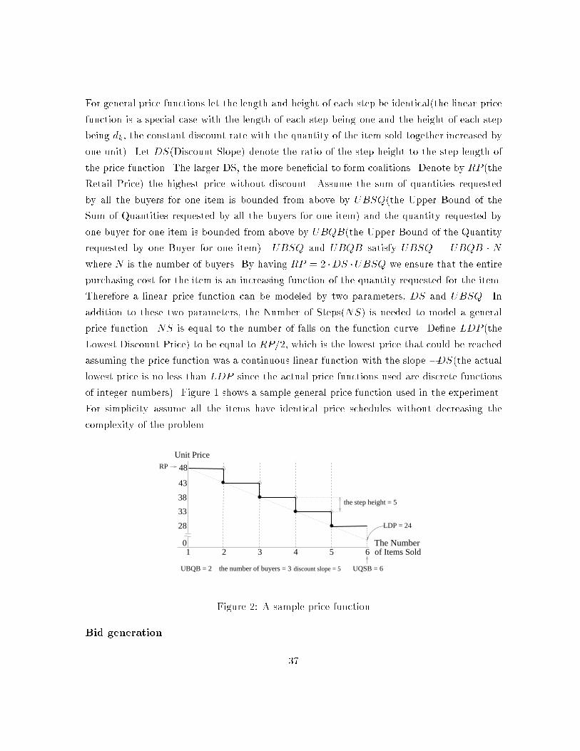
For general price functions let the length and height of each step be identical(the linear price

function is a special case with the length of each step being one and the height of each step

being dk, the constant discount rate with the quantity of the item sold together increased by

one unit). Let DS(Discount Slope) denote the ratio of the step height to the step length of

the price function. The larger DS, the more bene�cial to form coalitions. Denote by RP (the

Retail Price) the highest price without discount. Assume the sum of quantities requested

by all the buyers for one item is bounded from above by UBSQ(the Upper Bound of the

Sum of Quantities requested by all the buyers for one item) and the quantity requested by

one buyer for one item is bounded from above by UBQB(the Upper Bound of the Quantity

requested by one Buyer for one item). UBSQ and UBQB satisfy UBSQ = UBQB � N

where N is the number of buyers. By having RP = 2 �DS �UBSQ we ensure that the entire

purchasing cost for the item is an increasing function of the quantity requested for the item.

Therefore a linear price function can be modeled by two parameters, DS and UBSQ. In

addition to these two parameters, the Number of Steps(NS) is needed to model a general

price function. NS is equal to the number of falls on the function curve. De�ne LDP (the

Lowest Discount Price) to be equal to RP=2, which is the lowest price that could be reached

assuming the price function was a continuous linear function with the slope �DS(the actual

lowest price is no less than LDP since the actual price functions used are discrete functions

of integer numbers). Figure 1 shows a sample general price function used in the experiment.

For simplicity assume all the items have identical price schedules without decreasing the

complexity of the problem.

43

38

6

Unit Price

of Items Sold

28

52

33

48

4310

RP

UQSB = 6

the step height = 5

The Number

UBQB = 2 the number of buyers = 3

LDP = 24

discount slope = 5

Figure 2: A sample price function

Bid generation

37

Suppose before the decision of the reservation cost each buyer bn has a virtual reservation price

pkn for each item gk he desires. The reservation cost is decided by summing up the reservation

prices multiplied by the quantity he requests for each item, i.e., rn =PN

n=1 pkn � q

kn. Let the

lower bound of the virtual reservation price be equal to LDP and the upper bound equal to

RP . Let the ratio of buyers who have virtual reservation prices at RP equal to RBBR(the

Ratio of Buyers Bidding at the Retail Prices). Small RBBR means many of the buyers cannot

win their bids if they do not form coalitions. The virtual reservation prices of other buyers

are randomly distributed between LDP and RP .

The distribution of preferences for multiple items is modeled by RBMI(the Ratio of Buyers

preferring Multiple Items). RBMI is a vector frb1; : : : ; rbKg where rbk is the ratio of buyers

who desire k items andPK

k=1 rbk = 1. For example, when the number of items is 3, the

number of buyers is 10, RBMI = f0:2; 0:3; 0:5g means there are 2 buyers bid for 1 item,

3 buyers for 2 items, 5 buyers for 3 items. Large numbers at the end part of RBMI mean

that many items are complementary for many buyers. The number of desired items of each

buyer is randomly decided following the distribution consistent with RBMI . The quantities

requested by each buyer for each item desired are generated randomly in the range [1; UBQB].

8.2 Results

The simulation is based on the instances generated with combination of the parameter values

listed in Table 1. For each set of parameters several(we took the number 3) instances are

randomly generated. For each instance we construct the optimal coalition by exhaustive

search, and the approximate solution by Algorithm 3 with or without Option 1 supposing

linear price functions are used, and by Algorithm 4 with or without Option 2 supposing

general price functions are used. The average coalition value of the instances with identical

parameters is set as the coalition value for the condition with that set of parameters. The

comparison is made among the optimal value and the value of the coalitions obtained by

our algorithms with or without the options. The largest number of buyers is limited to 25

because of the complexity to compute the optimal value.

Comparison with respect to the number of buyers and the number of items:

We calculate the ratio of the approximate value over the optimal value and take the average

of the ratios under all the conditions with the same number of buyers and number of items.

Figure 3 shows the distribution of the average ratios with respect to the number of buyers

38

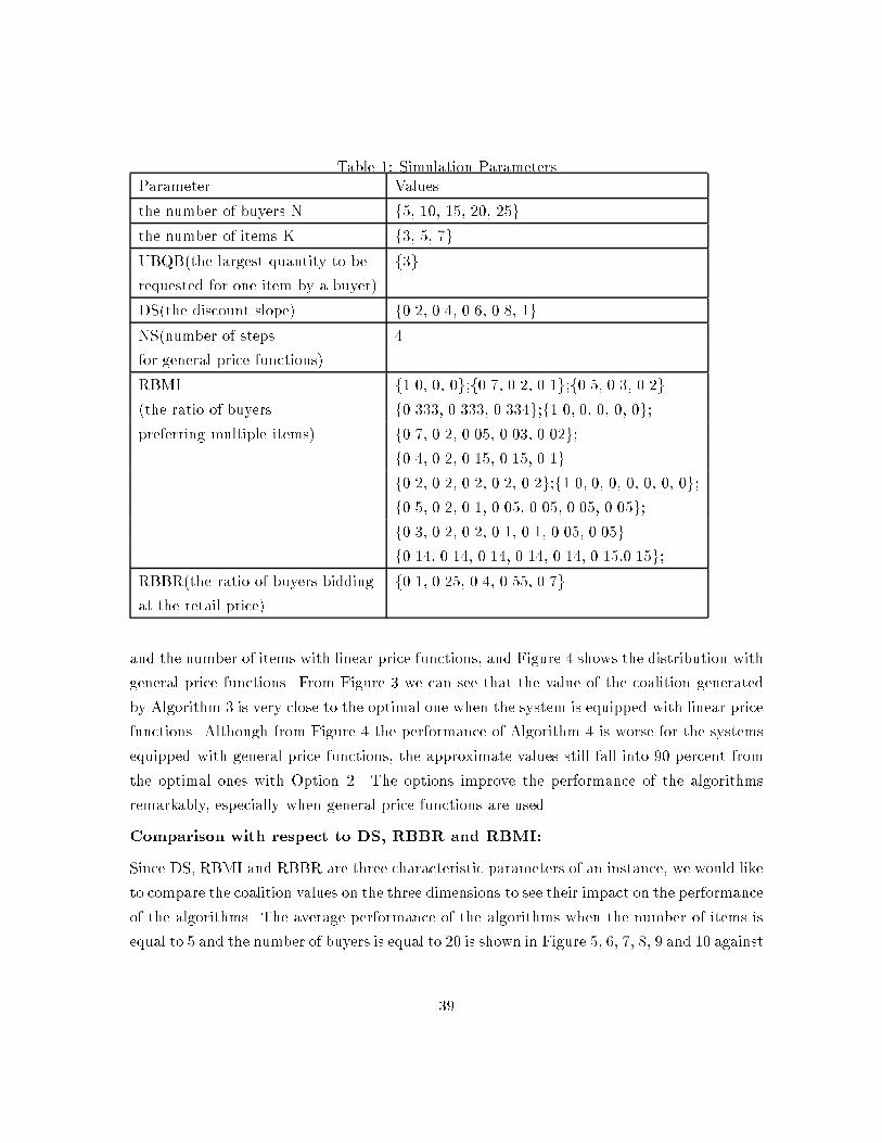
Table 1: Simulation Parameters

Parameter Values

the number of buyers N f5, 10, 15, 20, 25g

the number of items K f3, 5, 7g

UBQB(the largest quantity to be f3g

requested for one item by a buyer)

DS(the discount slope) f0.2, 0.4, 0.6, 0.8, 1g

NS(number of steps 4

for general price functions)

RBMI f1.0, 0, 0g;f0.7, 0.2, 0.1g;f0.5, 0.3, 0.2g

(the ratio of buyers f0.333, 0.333, 0.334g;f1.0, 0, 0, 0, 0g;

preferring multiple items) f0.7, 0.2, 0.05, 0.03, 0.02g;

f0.4, 0.2, 0.15, 0.15, 0.1g

f0.2, 0.2, 0.2, 0.2, 0.2g;f1.0, 0, 0, 0, 0, 0, 0g;

f0.5, 0.2, 0.1, 0.05, 0.05, 0.05, 0.05g;

f0.3, 0.2, 0.2, 0.1, 0.1, 0.05, 0.05g

f0.14, 0.14, 0.14, 0.14, 0.14, 0.15,0.15g;

RBBR(the ratio of buyers bidding f0.1, 0.25, 0.4, 0.55, 0.7g

at the retail price)

and the number of items with linear price functions, and Figure 4 shows the distribution with

general price functions. From Figure 3 we can see that the value of the coalition generated

by Algorithm 3 is very close to the optimal one when the system is equipped with linear price

functions. Although from Figure 4 the performance of Algorithm 4 is worse for the systems

equipped with general price functions, the approximate values still fall into 90 percent from

the optimal ones with Option 2. The options improve the performance of the algorithms

remarkably, especially when general price functions are used.

Comparison with respect to DS, RBBR and RBMI:

Since DS, RBMI and RBBR are three characteristic parameters of an instance, we would like

to compare the coalition values on the three dimensions to see their impact on the performance

of the algorithms. The average performance of the algorithms when the number of items is

equal to 5 and the number of buyers is equal to 20 is shown in Figure 5, 6, 7, 8, 9 and 10 against

39

DS, RBBR and RBMI. We can see that the performance of the algorithms hurts from the

increase of RBMI but is not monotone on DS or RBBR. The result is understandable since the

algorithms aim to generate compatible subcoalitions. When more items are complementary

to more buyers, it is more di�cult to �nd compatible subcoalitions.

Average computation time

The algorithms were implemented by VC++ 6.0 and run on Windows/NT platform. All

the experiments were performed on a Pentium 4/52M RAM personal computer. Figure 11

shows the average amount of time in CPU seconds that Algorithm 3 and 4 took to compute

a suboptimal coalition, with K = 5, UBQB = 2.

9 Conclusion

In this paper we analyze the coalition formation of buyers in a electronic marketplace where

sellers o�er price discount based on the quantity of items sold together and buyers have

preferences for combinations of items. Two approximation algorithms in polynomial time are

presented for the conditions with linear or general price functions. A payo� division rule is

proposed that is in the core with linear price functions and in the pseudo-core with general

price functions. Experimental results show that the algorithms give good ratio to the optimal

value.

In the situation considered in this paper, the buyers can only place one bid. More generally

a buyer may have desire for multiple bundles of items and needs to be allowed to place a bid

for each bundle. The relation between the bids can be OR or XOR. If there are exclusively

OR relations between the bids of one buyer, then we can generate a dummy buyer for each

bid of a buyer and this leads to a CCF problem with the dummy buyers. If some bids of a

buyer are in XOR, then we can construct all the maximal sets of uncon icting bids(a set is

maximal if there is no more quali�ed elements that can be added into it) for each buyer. The

optimal coalition can be obtained by solving a CCF problem for each combination of the sets

one from each buyer and choosing the optimal result.

References

[1] Junichi Yamamoto, Katia Sycara. A Stable and E�cient Buyer Coalition Formation

40

Scheme for E-Marketplaces. In Proceedings of the 5th International Conference on Au-

tonomous Agents, Montreal, CA, May 28 - June 1, 2001.

[2] Herv�e Moulin. Axioms of Cooperative Decision Making, Cambridge University Press,

1988.

[3] Donald M. Topkis. Supermodularity and Complementarity, Princeton University Press,

1998.

[4] Martin J. Osborne, Ariel Rubinstein. A Course in Game Theory, MIT Press, 1994.

[5] Roland Strausz. E�ciency in Sequential Partnerships. Journal of Economic Theory, 85:

140-156, 1999.

[6] Paul Belle amme. Stable Coalition Structures with Open Membership and Asymmetric

Firms. Games and Economic Behavior, 30: 1-21, 2000.

[7] F. Bloch. Sequential Formation of Coalitions in Games with Externalities and Fixed Payo�

Division. Games and Economic Behavior, 14(1): 90-123, 1996.

[8] S. Hart, M. Kurz. Endogenous Formation of Coalitions. Econometrica, 51(4): 1047-1064,

1983.

[9] R. E. Stearns. Convergent Transfer Schemes for N-Person Games. Transactions of the

American Mathematical Society, 134: 449-459, 1968.

[10] L. S. Wu. A Dynamic Theory for the Class of Games with Nonempty Cores. Siam Journal

of Applied Mathematics, 32: 328-338, 1977.

[11] A. Colorni, M. Dorigo, F. Ma�oli, V. Maniezzo, G. Righini, M. Trubian. Heuristics

From Nature for Hard Combinatorial Optimization Problems. International Transactions

in Operational Research, 3(1): 1-21, 1996.

[12] Sandip Sen, Partha Sarathi Dutta. Searching for optimal coalition structures. In Pro-

ceedings of the Fourth International Conference on MultiAgent Systems (ICMAS-2000),

Boston, Massachusetts, July 2000.

[13] K. Lerman, and O. Shehory. Coalition Formation for Large-Scale Electronic Markets.

In Proceedings of the Fourth International Conference on MultiAgent Systems (ICMAS-

2000), Boston, Massachusetts, July 2000.

41

[14] Tuomas W. Sandholm, Victor R. Lesser. Coalitions among Computationally Bounded

Agents. Arti�cial Intelligence, 94(1): 99-137, 1997.

[15] Onn Shehory, Sarit Kraus. Methods for Task Allocation via Agent Coalition Formation.

Arti�cial Intelligence Journal, 101(1-2): 165-200, May 1998.

[16] Fernando Tohm�e, Tuomas Sandholm. Coalition Formation Processes with Belief Revision

among Bounded-Rational Self-Interested Agents. Journal of Logic and Computation, 9(6):

793-815, 1999.

[17] Onn Shehory, Sarit Kraus, Osher Yadgar. Emergent Cooperative Goal-Satisfaction in

Large Scale Automated-Agent Systems. Arti�cial Intelligence, 110(1): 1-55, 1999.

[18] Maksim Tsvetovat, Katia Sycara. Customer Coalitions in the Electronic Marketplace. In

Proceedings of the 3rd Workshop on Agent Mediated Electronic Commerce(AMEC-2000),

2000.

[19] Onn Shehory, Sarit Kraus. Feasible Formation of Coalitions among Autonomous Agents

in Non-Super-Additive Environments. Computational Intelligence, 15(3): 218-251, 1999.

[20] Steven Ketchpel. Forming Coalitions in the Face of Uncertain Rewards. In Proceedings of

the Twelfth National Conference on Arti�cial Intelligence(AAAI-94), Seattle, WA, 1994.

[21] Gilad Zlotkin, Je�rey S. Rosenschein. Coalition, Cryptography, and Stability: Mecha-

nisms for Coalition Formation in Task Oriented Domains. In Proceedings of the Twelfth

National Conference on Arti�cial Intelligence(AAAI-94), Seattle, WA, 1994.

[22] E. M. Arkin, R. Hassin. On Local Search for Weighted k-Set Packing. In Proceedings of

the Seventh Annual Europe Symposium on Algorithms, Graz, Austria, Sep 15-17, 1997.

[23] B. Chandra, M. M. Halldorsson. Greedy Local Improvement and Weighted Set Packing

Approximation. In Proceedings of the 10th Annual SIAM-ACM Symposium on Discrete

Algorithms(SODA), 169-176, 1999.

[24] David B. Shmoys. Computing Near-Optimal Solutions to Combinatorial Optimization

Problems. DIMACS Series in Discrete Mathematics and Theoretical Computer Science

(20), W. Cook and L. Lovasz (eds.), AMS Publications, 355-397, 1995.

[25] Rassenti, V. Smith, and R. Bul�n. A Combinatorial Auction Mechanism for Airport

Time Slot Allocation. The RAND Journal of Economics, 13(2): 402-417, 1982.

42

[26] Peter R. Wurman, and Michael P. Wellman. AkBA: A Progressive, Anonymous-Price

Combinatorial Auction. In Proceedings of the 2nd ACM conference on Electronic com-

merce, Minneapolis, MN, October, 2000.

[27] Craig Boutilier, Mois�es Goldszmidt, Claire Monteleoni, and Bikash Sabata. Resource

Allocation Using Sequential Auctions. In Proceedings of the 2nd Workshop on Agent

Mediated Electronic Commerce(AMEC-1999), pages 131-152, 2000.

[28] Sven de Vries, and Rakesh Vohra. Combinatorial

Auctions: A Survey. http://www.kellogg.nwu.edu/faculty/vohra/htm/res.htm, January

2001.

[29] Arne Andersson, Mattias Tenhunen, and Fredrik Ygge. Integer Programming for Com-

binatorial Auction Winner Determination. In Proceedings of the Fourth International

Conference on MultiAgent Systems(ICMAS-2000), Boston, Massachusetts, July 2000.

[30] Noam Nisan. Bidding and Allocation in Combinatorial Auctions. In Proceedings of the

2nd ACM conference on Electronic commerce, Minneapolis, MN, October 2000.

[31] Yuzo Fujishima, Kevin Leyton-Brown, and Yoav Shoham. Taming the Computational

Complexity of Combinatorial Auctions. In Proceedings of the International Joint Confer-

ences on Arti�cial Intelligence(IJCAI), Stockholm, Sweden, July 1999.

[32] Yuko Sakurai, Makoto Yokoo, and Koji Kamei. An E�cient Approximate Algorithm

for Winner Determination in Combinatorial Auctions. In Proceedings of the 2nd ACM

conference on Electronic commerce, Minneapolis, MN, October 2000.

[33] Tuomas Sandholm. An Algorithm for Optimal Winner Determination in Combinatorial

Auctions. In Proceedings of the International Joint Conference on Arti�cial Intelligence

(IJCAI), Stockholm, Sweden, July 1999.

[34] Rica Gonen, and Daniel Lehmann. Optimal Solutions for Multi-Unit Combinatorial Auc-

tions: Branch and Bound Heuristics. In Proceedings of the 2nd ACM conference on Elec-

tronic commerce, Minneapolis, MN, October 2000.

[35] Kevin Leyton-Brown, Yoav Shoham, and Moshe Tennenholtz. An Algorithm for Multi-

Unit Combinatorial Auctions. In Proceedings of the Seventeenth National Conference on

Arti�cial Intelligence(AAAI-2000), pages 51-61, 2000.

43

[36] Karhan Akcoglu, James Aspnes, Bhaskar DasGupta, and Ming-Yang Kao. Opportu-

nity Cost Algorithms

for Combinatorial Auctions. http://dimacs.rutgers.edu/TechnicalReports/2000.html, DI-

MACS Technical Report, 2000.

[37] Michael H. Rothkopf, Aleksandar Pekec. Computationally Manageable Combinatorial

Auctions. Management Science, 44: 1131{1147, 1998.

[38] Sushil Bikhchandani, and Joseph M. Ostroy. The Package Assignment Model. Technical

report, University of California at Los Angeles, November 1998.

[39] D. C. Parkes, and L. Ungar. Iterative Combinatorial Auctions: Theory and Practice.

In Proceedings of 17th National Conference on Arti�cial Intelligence(AAAI-2000), pages

74-81, 2000.

[40] Paul Milgrom. Putting Auction Theory to Work: the Simultaneous ascending auction.

Technical Report Working Paper 98-002, Dept. of Economics, Stanford University, 1998.

[41] Mark M. Bykowsky, Robert J. Cull, John O. Ledyard. Mutually Destructive Bidding:

the FCC Auction Design Problem. Social Science Working Paper 916, California Institute

of Technology, 1995.

44

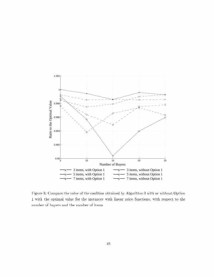
o3 items, with Option 1

7 items, with Option 15 items, with Option 1

3 items, without Option 15 items, without Option 17 items, without Option 1

xxx

oo

5 10 15 20 250.99

0.992

0.994

0.996

0.998

1

1.002

Number of Buyers

Rat

io to

the

Opt

imal

Val

ue

Number of Buyers

Rat

io to

the

Opt

imal

Val

ue

Figure 3: Compare the value of the coalition obtained by Algorithm 3 with or without Option

1 with the optimal value for the instances with linear price functions, with respect to the

number of buyers and the number of items

45

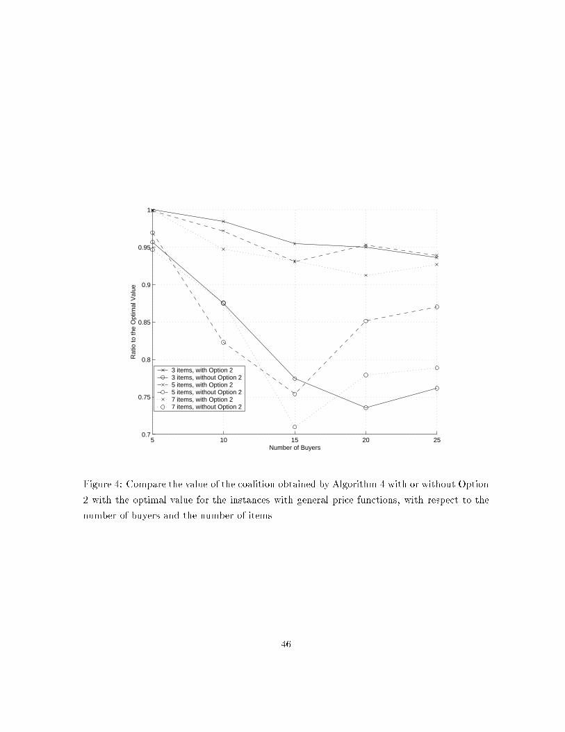
5 10 15 20 250.7

0.75

0.8

0.85

0.9

0.95

1

Number of Buyers

Rat

io to

the

Opt

imal

Val

ue

3 items, with Option 23 items, without Option 25 items, with Option 25 items, without Option 27 items, with Option 27 items, without Option 2

Figure 4: Compare the value of the coalition obtained by Algorithm 4 with or without Option

2 with the optimal value for the instances with general price functions, with respect to the

number of buyers and the number of items

46

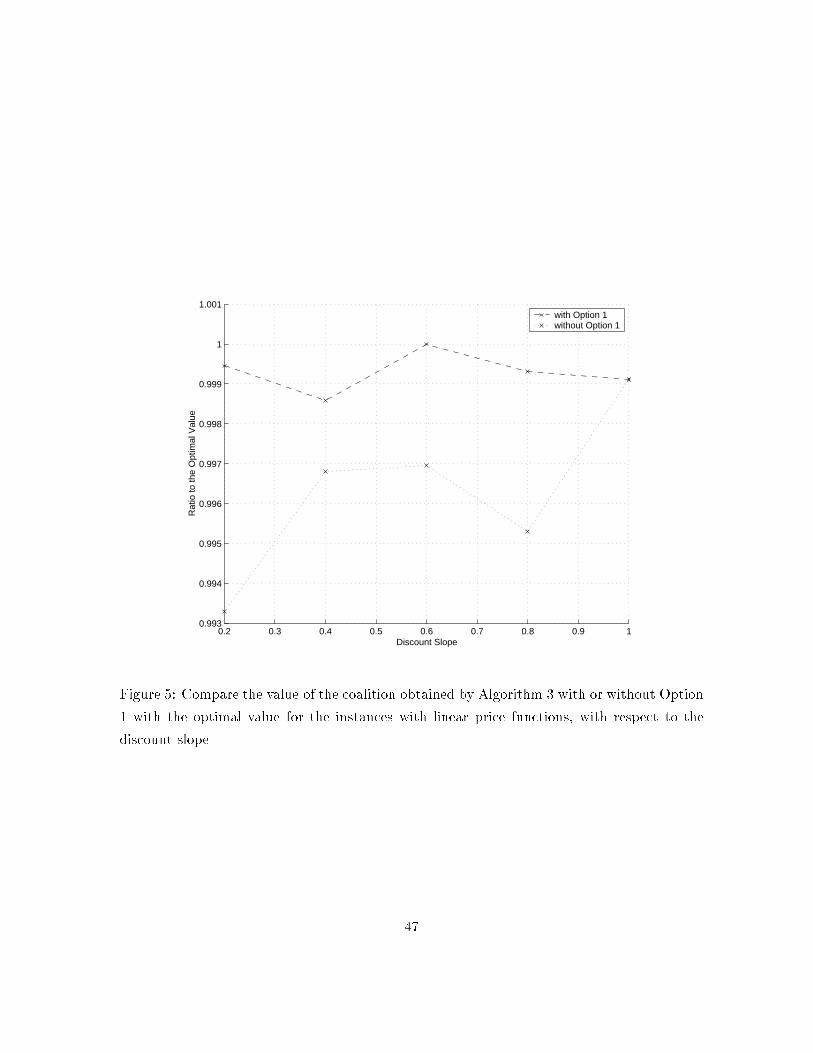
0.2 0.3 0.4 0.5 0.6 0.7 0.8 0.9 10.993

0.994

0.995

0.996

0.997

0.998

0.999

1

1.001

Discount Slope

Rat

io to

the

Opt

imal

Val

ue

with Option 1without Option 1

Figure 5: Compare the value of the coalition obtained by Algorithm 3 with or without Option

1 with the optimal value for the instances with linear price functions, with respect to the

discount slope

47

0.2 0.3 0.4 0.5 0.6 0.7 0.8 0.9 10.75

0.8

0.85

0.9

0.95

1

Discount Slope

Rat

io to

the

Opt

imal

Val

ue

with Option 2without Option 2

Figure 6: Compare the value of the coalition obtained by Algorithm 4 with or without Option

2 with the optimal value for the instances with general price functions, with respect to the

discount slope

48

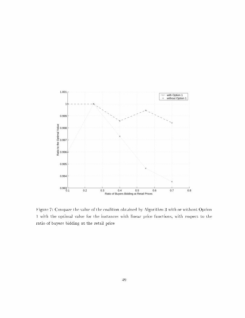
0.1 0.2 0.3 0.4 0.5 0.6 0.7 0.80.993

0.994

0.995

0.996

0.997

0.998

0.999

1

1.001

Ratio of Buyers Bidding at Retail Prices

Rat

io to

the

Opt

imal

Val

ue

with Option 1without Option 1

Figure 7: Compare the value of the coalition obtained by Algorithm 3 with or without Option

1 with the optimal value for the instances with linear price functions, with respect to the

ratio of buyers bidding at the retail price

49

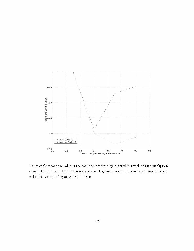
0.1 0.2 0.3 0.4 0.5 0.6 0.7 0.80.75

0.8

0.85

0.9

0.95

1

Ratio of Buyers Bidding at Retail Prices

Rat

io to

the

Opt

imal

Val

ue

with Option 2without Option 2

Figure 8: Compare the value of the coalition obtained by Algorithm 4 with or without Option

2 with the optimal value for the instances with general price functions, with respect to the

ratio of buyers bidding at the retail price

50

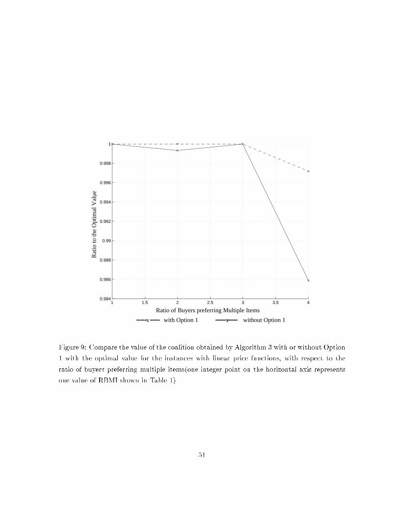
1 1.5 2 2.5 3 3.5 40.984

0.986

0.988

0.99

0.992

0.994

0.996

0.998

1

Ratio of Buyers Preferring Multiple Items

Rat

io to

the

Opt

imal

Val

ueR

atio

to th

e O

ptim

al V

alue

Ratio of Buyers preferring Multiple Items

with Option 1 without Option 1x x

Figure 9: Compare the value of the coalition obtained by Algorithm 3 with or without Option

1 with the optimal value for the instances with linear price functions, with respect to the

ratio of buyers preferring multiple items(one integer point on the horizontal axis represents

one value of RBMI shown in Table 1)

51

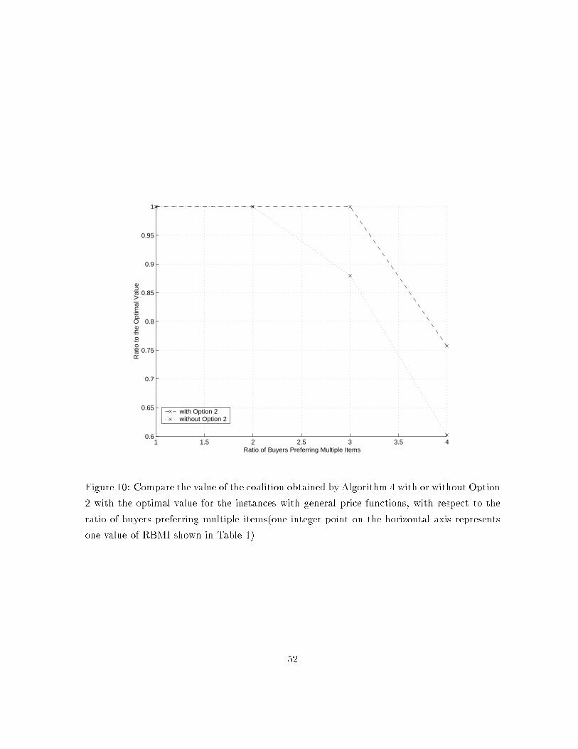
1 1.5 2 2.5 3 3.5 40.6

0.65

0.7

0.75

0.8

0.85

0.9

0.95

1

Ratio of Buyers Preferring Multiple Items

Rat

io to

the

Opt

imal

Val

ue

with Option 2without Option 2

Figure 10: Compare the value of the coalition obtained by Algorithm 4 with or without Option

2 with the optimal value for the instances with general price functions, with respect to the

ratio of buyers preferring multiple items(one integer point on the horizontal axis represents

one value of RBMI shown in Table 1)

52

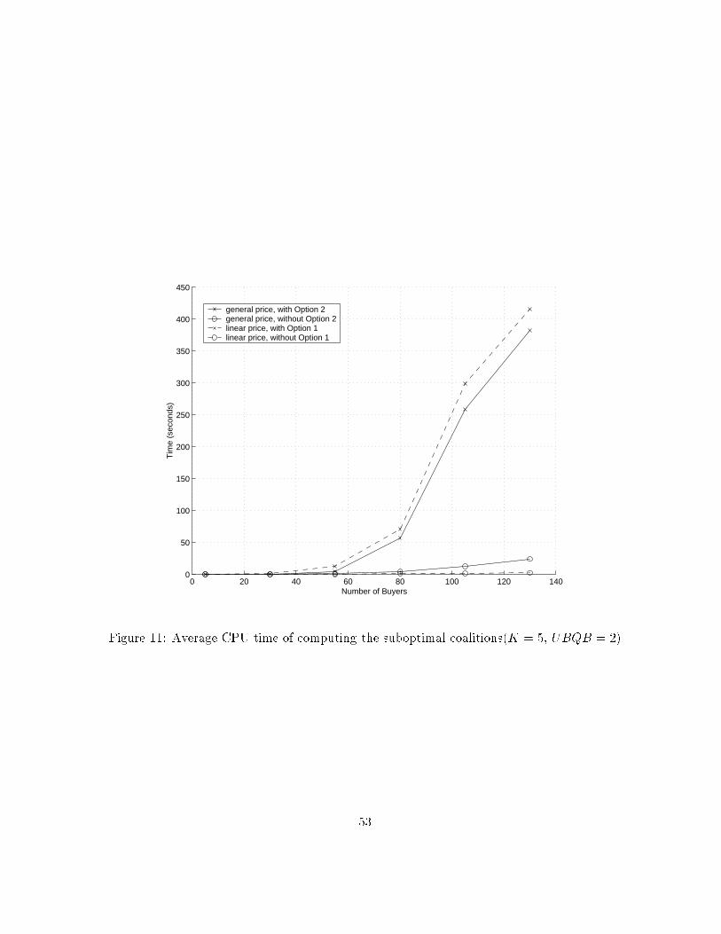
0 20 40 60 80 100 120 1400

50

100

150

200

250

300

350

400

450

Number of Buyers

Tim

e (s

econ

ds)

general price, with Option 2general price, without Option 2linear price, with Option 1linear price, without Option 1

Figure 11: Average CPU time of computing the suboptimal coalitions(K = 5, UBQB = 2)

53