Aircraftengineeringprinciples 140629023951-phpapp01 (1)
Jun 25, 2015
Welcome message from author
This document is posted to help you gain knowledge. Please leave a comment to let me know what you think about it! Share it to your friends and learn new things together.
Transcript


Aircraft Engineering Principles
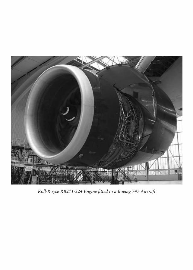
Roll-Royce RB211-524 Engine fitted to a Boeing 747 Aircraft

Aircraft Engineering Principles
Lloyd Dingle
Mike Tooley
AMSTERDAM • BOSTON • HEIDELBERG • LONDON • NEW YORK • OXFORD • PARISSAN DIEGO • SAN FRANCISCO • SINGAPORE • SYDNEY • TOKYO

Elsevier Butterworth HeinemannLinacre House, Jordan Hill, Oxford OX2 8DP30 Corporate Drive, Burlington, MA 01803
First published 2005Copyright © 2005, Lloyd Dingle and Mike Tooley. All rights reserved
The right of Lloyd Dingle and Mike Tooley to be identified as theauthors of this work has been asserted in accordance with theCopyright, Design and Patents Act 1988
No part of this publication may be reproduced in any material form(including photocopying or storing in any medium by electronic meansand whether or not transiently or incidentally to some other use of thispublication) without the written permission of the copyright holderexcept in accordance with the provisions of the Copyright, Designs andPatents Act 1988 or under the terms of a licence issued by the CopyrightLicensing Agency Ltd, 90 Tottenham Court Road, London,England W1T 4LP. Applications for the copyright holder’s writtenpermission to reproduce any part of this publication should be addressedto the publishers
British Library Cataloguing in Publication DataDingle, Lloyd
Aircraft engineering principles1. aerospace engineeringI. Title II. Tooley, Michael H. (Michael Howard), 1946–692.1
Library of Congress Cataloguing in Publication DataA catalogue record for this book is available from the Library of Congress
ISBN 0 7506 5015 X
For information on all Elsevier Butterworth-Heinemann publicationsvisit our website at www.books.elsevier.com
Typeset by Charon Tec Pvt. Ltd, Chennai, Indiawww.charontec.comPrinted and bound in Great Britain

Contents
Preface viiiAcknowledgements x
PART 1 INTRODUCTION 1Chapter 1 Introduction 3
1.1 The aircraft engineering industry 31.2 Differing job roles for aircraft maintenance certifying staff 31.3 Opportunities for training, education and career progression 71.4 CAA licence – structure, qualifications, examinations and levels 151.5 Overview of airworthiness regulation, aircraft maintenance and
its safety culture 18
PART 2 SCIENTIFIC FUNDAMENTALS 31Chapter 2 Mathematics 33
General introduction 33Non-calculator mathematics 34
2.1 Introduction 342.2 Arithmetic 342.3 Algebra 532.4 Geometry and trigonometry 732.5 Multiple choice questions 100
Chapter 3 Further mathematics 1093.1 Further algebra 1093.2 Further trigonometry 1183.3 Statistical methods 1313.4 Calculus 144
Chapter 4 Physics 1654.1 Summary 1654.2 Units of measurement 1654.3 Fundamentals 1704.4 Matter 1784.5 The states of matter 1824.6 Mechanics 1834.7 Statics 1844.8 Dynamics 2074.9 Fluids 2404.10 Thermodynamics 257
vi Contents
4.11 Light, waves and sound 2774.12 Multiple choice questions 297
PART 3 ELECTRICAL AND ELECTRONIC FUNDAMENTALS 309Chapter 5 Electrical fundamentals 311
5.1 Introduction 3115.2 Electron theory 3135.3 Static electricity and conduction 3155.4 Electrical terminology 3195.5 Generation of electricity 3225.6 DC sources of electricity 3265.7 DC circuits 3335.8 Resistance and resistors 3415.9 Power 3535.10 Capacitance and capacitors 3555.11 Magnetism 3695.12 Inductance and inductors 3795.13 DC motor/generator theory 3865.14 AC theory 3975.15 Resistive, capacitive and inductive circuits 4025.16 Transformers 4145.17 Filters 4185.18 AC generators 4235.19 AC motors 4295.20 Multiple choice questions 438
Chapter 6 Electronic fundamentals 4516.1 Introduction 4516.2 Semiconductors 4566.3 Printed circuit boards 5116.4 Servomechanisms 5156.5 Multiple choice questions 531
PART 4 FUNDAMENTALS OF AERODYNAMICS 539Chapter 7 Basic aerodynamics 541
7.1 Introduction 5417.2 A review of atmospheric physics 5417.3 Elementary aerodynamics 5457.4 Flight forces and aircraft loading 5617.5 Flight stability and dynamics 5707.6 Control and controllability 5797.7 Multiple choice questions 587
APPENDICES 595A Engineering licensing examinations 597B Organizations offering aircraft maintenance engineering training and
education 601

Contents vii
C The role of the European Aviation Safety Agency 603D Mathematical tables 605E System international and imperial units 615F Answers to “Test your understanding” 623
Index 637

This page intentionally left blank
Preface
The books in the series have been designed forboth independent and tutor assisted studies. Forthis reason they should prove particularly use-ful to the “self-starter” and to those wishingto update or upgrade their aircraft maintenancelicence. Also, the series should prove a usefulsource of reference for those taking ab initiotraining programmes in JAR 147 (now ECARPart-147) and FAR 147 approved organizationsand those on related aeronautical engineeringprogrammes in further and higher educationestablishments.
This book has primarily been written as one ina series of texts, designed to cover the essentialknowledge base required by aircraft certifyingmechanics, technicians and engineers engagedin engineering maintenance activities on com-mercial aircraft. In addition, this book shouldappeal to the members of the armed forces,and students attending training and educationalestablishments engaged in aircraft engineeringmaintenance and other related aircraft engineer-ing learning programmes.
In this book we cover in detail the under-pinning mathematics, physics, electrical andelectronic fundamentals, and aerodynamics nec-essary to understand the function and operationof the complex technology used in modern air-craft. The book is arranged into four majorsections:
• Introduction• Scientific fundamentals• Electrical and electronic fundamentals• Fundamentals of aerodynamics
In the Introductory section you will find infor-mation on the nature of the aircraft mainte-nance industry, the types of job role that youcan expect, the current methods used to trainand educate you for such roles and informa-tion on the examinations system directly relatedto civil aviation maintenance engineering. Inaddition, you will find information on typical
career progression routes, professional recogni-tion, and the legislative framework and safetyculture that is so much a part of our industry.
In the section on Scientific fundamentals westart by studying Module 1 of the JAR 66(now ECAR Part-66) syllabus (see qualificationsand levels) covering the elementary mathematicsnecessary to practice at the category B technicianlevel. It is felt by the authors, that this level of“non-calculator” mathematics is insufficient asa prerequisite to support the study of the physicsand the related technology modules, that are tofollow. For this reason, and to assist studentswho wish to pursue other related qualifications,a section has been included on “further math-ematics”. The coverage of JAR 66 Module 2on physics is sufficiently comprehensive and ata depth, necessary for both category B1 and B2technicians.
The section on Electrical and electronic fun-damentals comprehensively covers ECAR 66Module 3 and ECAR Part-66 Module 4 to aknowledge level suitable for category B2 avionictechnicians. Module 5 on Digital Techniquesand Electronic Instrument Systems will be cov-ered in the fifth book in the series, AvionicSystems.
This book concludes with a section on thestudy of Aerodynamics, which has been writtento cover ECAR Part-66 Module 8.
In view of the international nature of the civilaviation industry, all aircraft engineering main-tenance staff need to be fully conversant withthe SI system of units and be able to demon-strate proficiency in manipulating the “Englishunits” of measurement adopted by internationalaircraft manufacturers, such as the Boeing Air-craft Company. Where considered important,the English units of measure will be emphasizedalongside the universally recognized SI system.The chapter on physics (Chapter 4) provides athorough introduction to SI units, where youwill also find mention of the English system,

x Preface
with conversion tables between each systembeing provided at the beginning of Chapter 4.
To reinforce the subject matter for each majortopic, there are numerous worked examples andtest your knowledge written questions designedto enhance learning. In addition, at the endof each chapter you will find a selection ofmultiple-choice questions, that are graded tosimulate the depth and breadth of knowledgerequired by individuals wishing to practice at themechanic (category A) or technician (categoryB) level. These multiple choice question papersshould be attempted after you have completedyour study of the appropriate chapter. In thisway, you will obtain a clearer idea of how wellyou have grasped the subject matter at the mod-ule level. Note also that category B knowledgeis required by those wishing to practice at thecategory C or engineer level. Individuals hop-ing to pursue this route should make sure thatthey thoroughly understand the relevant infor-mation on routes, pathways and examinationlevels given later.
Further information on matters, such asaerospace operators, aircraft and aircraftcomponent manufacturers, useful web sites,regulatory authorities, training and educationalestablishments and comprehensive lists of terms,definitions and references, appear as appendices
at the end of the book. References are annotatedusing superscript numbers at the appropriatepoint in the text.
Lloyd DingleMike Tooley
Answers to questions
Answers to the “Test your understanding”questions are given in Appendix F. Solutionsto the multiple choice questions and generalquestions can be accessed by adopting tutorsand lecturers. To access this material visithttp://books.elsevier.com/manuals and followthe instructions on screen.
Postscript
At the time of going to press JAR 66 ad JAR 147are in the process of being superseded by theEuropean Civil Aviation Regulations (ECAR)66 and 147. Wherever in this volume referenceis made to JAR 66 and JAR 147, then by impli-cation, these are referring to ECAR Part-66 andECAR Part-147 (see Appendix C for details).

Acknowledgements
The authors would like to express their grati-tude to those who have helped in producing thisbook.
Jeremy Cox and Mike Smith of Britannia Air-ways, for access to their facilities and adviceconcerning the administration of civil aircraftmaintenance; Peter Collier, chairman of theRAeS non-corporate accreditation committee,for his advice on career progression routes;The Aerospace Engineering lecturing team at
Kingston University, in particular, Andrew Self,Steve Barnes, Ian Clark and Steve Wright, forproof reading the script; Jonathan Simpson andall members of the team at Elsevier, for theirpatience and perseverance. Finally, we wouldlike to say a big ‘thank you’ to Wendy andYvonne. Again, but for your support and under-standing, this book would never have beenproduced!

P A R T1
Introduction

This page intentionally left blank
C h a p t e r
1Introduction
1.1 The aircraft engineering industry
The global aircraft industry encompasses a vastnetwork of companies working either as largeinternational conglomerates or as individualnational and regional organizations. The twobiggest international aircraft manufacturers arethe American owned Boeing Aircraft Com-pany and the European conglomerate, Euro-pean Aeronautic Defence and Space Company(EADS), which incorporates airbus industries.These, together with the American giantLockheed-Martin, BAE Systems and aerospacepropulsion companies, such as Rolls-Royce andPratt and Whitney, employ many thousandsof people and have annual turnovers totallingbillions of pounds. For example, the recentlywon Lockheed-Martin contract for the Amer-ican Joint Strike Fighter (JSF) is estimated tobe worth 200 billion dollars, over the next 10years! A substantial part of this contract willinvolve BAE Systems, Rolls-Royce and other UKcompanies.
The airlines and armed forces of the worldwho buy-in aircraft and services from aerospacemanufacturers are themselves, very often, largeorganizations. For example British Airways ourown national carrier, even after recent down-sizing, employs around 50,000 personnel. UKairlines, in the year 2000, employed in total,just over 12,000 aircraft maintenance and over-haul personnel. Even after the events that tookplace on 11th September 2001, the requirementfor maintenance personnel is unlikely to fall. Arecent survey by the Boeing Corporation expectsto see the demand for aircraft and their associ-ated components and systems rise by 2005, tothe level of orders that existed prior to the tragicevents of 11th September 2001.
Apart from the airlines, individuals withaircraft maintenance skills may be employedin general aviation (GA), third-party overhaul
companies, component manufacturers or air-frame and avionic repair organizations. GAcompanies and spin-off industries employ largenumbers of skilled aircraft fitters. The UK armedforces collectively recruit around 1500 youngpeople annually for training in aircraft andassociated equipment maintenance activities.
Aircraft maintenance certifying staff arerecognized throughout Europe and indeed,throughout many parts of the world, thusopportunities for employment are truly global!In the USA approximately 10,000 airframe andpropulsion (A&P) mechanics are trained annu-ally; these are the USA equivalent of our ownaircraft maintenance certifying mechanics andtechnicians.
Recent surveys carried out for the UK sug-gest that due to demographic trends, increasingdemand for air travel and the lack of trained air-craft engineers leaving our armed forces, thereexists an annual shortfall of around 800 suit-ably trained aircraft maintenance and overhaulstaff. Added to this, the global and diversenature of the aircraft maintenance industry, itcan be seen that aircraft maintenance engineer-ing offers an interesting and rewarding career,full of opportunity.
1.2 Differing job roles for aircraftmaintenance certifying staff
Individuals may enter the aircraft maintenanceindustry in a number of ways and perform avariety of maintenance activities on aircraft oron their associated equipments and components.The nature of the job roles and responsibilitiesfor licensed certifying mechanics, techniciansand engineers are detailed below.
The routes and pathways to achieve these jobroles, the opportunities for career progression,the certification rights and the nature of the
4 Aircraft engineering principles
necessary examinations and qualifications aredetailed in the sections that follow.
1.2.1 The aircraft maintenancecertifying mechanic
Since the aircraft maintenance industry is highlyregulated, the opportunities to perform com-plex maintenance activities are dependent onthe amount of time that individuals spendon their initial and aircraft-type training, theknowledge they accrue and their length of expe-rience in post. Since the knowledge and experi-ence requirements are limited for the certifyingmechanic (see later), the types of maintenanceactivity that they may perform, are also lim-ited. Nevertheless, these maintenance activitiesrequire people with a sound basic education,who are able to demonstrate maturity and theability to think logically and quickly when act-ing under time constraints and other operationallimitations.
The activities of the certifying mechanicinclude the limited rectification of defects andthe capability to perform and certify minorscheduled line maintenance inspections, such asdaily checks. These rectification activities mightinclude tasks, such as a wheel change, replace-ment of a worn brake unit, navigation lightreplacement or a seat belt change. Scheduledmaintenance activities might include: replen-ishment of essential oils and lubricants, lubri-cation of components and mechanisms, paneland cowling removal and fit, replacement ofpanel fasteners, etc., in addition to the inspec-tion of components, control runs, fluid systemsand aircraft structures for security of attach-ment, corrosion, damage, leakage, chaffing,obstruction and general wear.
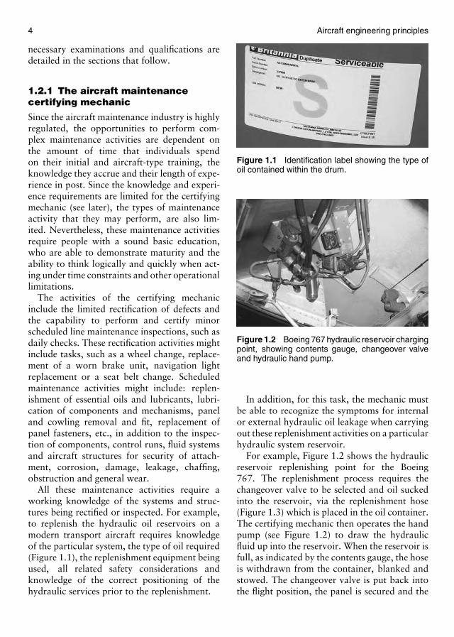
All these maintenance activities require aworking knowledge of the systems and struc-tures being rectified or inspected. For example,to replenish the hydraulic oil reservoirs on amodern transport aircraft requires knowledgeof the particular system, the type of oil required(Figure 1.1), the replenishment equipment beingused, all related safety considerations andknowledge of the correct positioning of thehydraulic services prior to the replenishment.
Figure 1.1 Identification label showing the type ofoil contained within the drum.
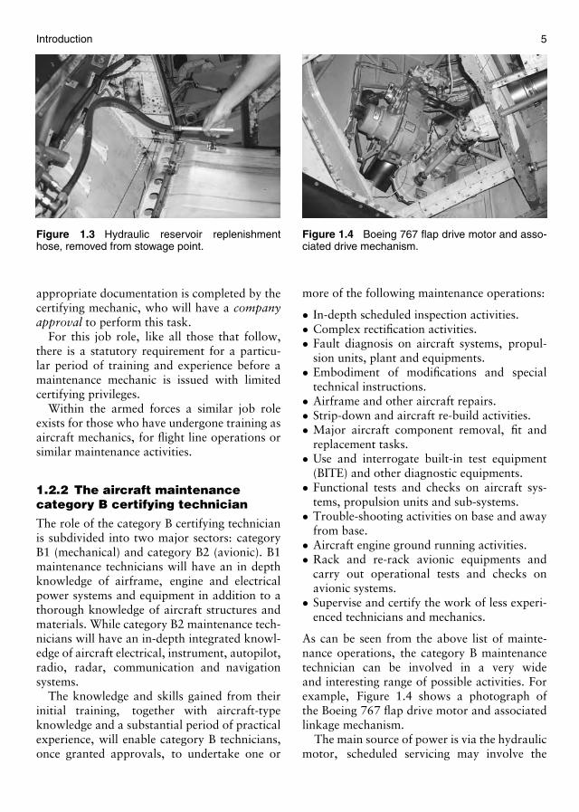
Figure 1.2 Boeing 767 hydraulic reservoir chargingpoint, showing contents gauge, changeover valveand hydraulic hand pump.
In addition, for this task, the mechanic mustbe able to recognize the symptoms for internalor external hydraulic oil leakage when carryingout these replenishment activities on a particularhydraulic system reservoir.
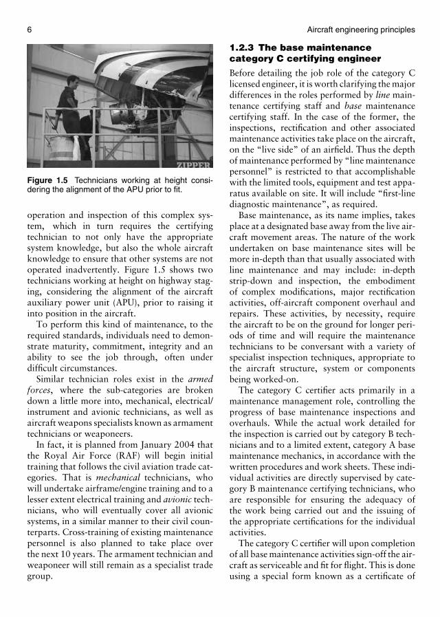
For example, Figure 1.2 shows the hydraulicreservoir replenishing point for the Boeing767. The replenishment process requires thechangeover valve to be selected and oil suckedinto the reservoir, via the replenishment hose(Figure 1.3) which is placed in the oil container.The certifying mechanic then operates the handpump (see Figure 1.2) to draw the hydraulicfluid up into the reservoir. When the reservoir isfull, as indicated by the contents gauge, the hoseis withdrawn from the container, blanked andstowed. The changeover valve is put back intothe flight position, the panel is secured and the
Introduction 5
Figure 1.3 Hydraulic reservoir replenishmenthose, removed from stowage point.
appropriate documentation is completed by thecertifying mechanic, who will have a companyapproval to perform this task.
For this job role, like all those that follow,there is a statutory requirement for a particu-lar period of training and experience before amaintenance mechanic is issued with limitedcertifying privileges.
Within the armed forces a similar job roleexists for those who have undergone training asaircraft mechanics, for flight line operations orsimilar maintenance activities.
1.2.2 The aircraft maintenancecategory B certifying technician
The role of the category B certifying technicianis subdivided into two major sectors: categoryB1 (mechanical) and category B2 (avionic). B1maintenance technicians will have an in depthknowledge of airframe, engine and electricalpower systems and equipment in addition to athorough knowledge of aircraft structures andmaterials. While category B2 maintenance tech-nicians will have an in-depth integrated knowl-edge of aircraft electrical, instrument, autopilot,radio, radar, communication and navigationsystems.
The knowledge and skills gained from theirinitial training, together with aircraft-typeknowledge and a substantial period of practicalexperience, will enable category B technicians,once granted approvals, to undertake one or
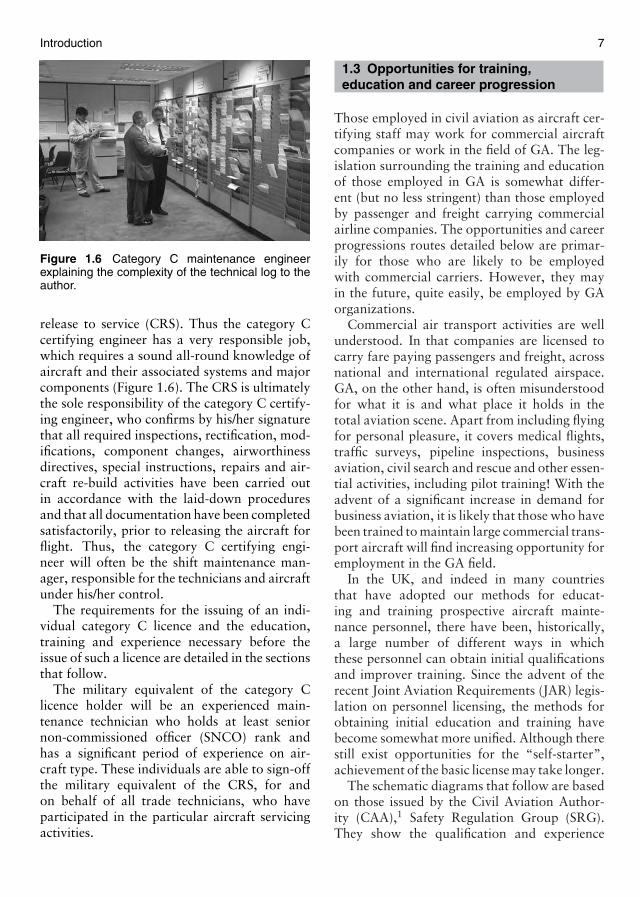
Figure 1.4 Boeing 767 flap drive motor and asso-ciated drive mechanism.
more of the following maintenance operations:
• In-depth scheduled inspection activities.• Complex rectification activities.• Fault diagnosis on aircraft systems, propul-
sion units, plant and equipments.• Embodiment of modifications and special
technical instructions.• Airframe and other aircraft repairs.• Strip-down and aircraft re-build activities.• Major aircraft component removal, fit and
replacement tasks.• Use and interrogate built-in test equipment
(BITE) and other diagnostic equipments.• Functional tests and checks on aircraft sys-
tems, propulsion units and sub-systems.• Trouble-shooting activities on base and away
from base.• Aircraft engine ground running activities.• Rack and re-rack avionic equipments and
carry out operational tests and checks onavionic systems.
• Supervise and certify the work of less experi-enced technicians and mechanics.
As can be seen from the above list of mainte-nance operations, the category B maintenancetechnician can be involved in a very wideand interesting range of possible activities. Forexample, Figure 1.4 shows a photograph ofthe Boeing 767 flap drive motor and associatedlinkage mechanism.
The main source of power is via the hydraulicmotor, scheduled servicing may involve the
6 Aircraft engineering principles
Figure 1.5 Technicians working at height consi-dering the alignment of the APU prior to fit.
operation and inspection of this complex sys-tem, which in turn requires the certifyingtechnician to not only have the appropriatesystem knowledge, but also the whole aircraftknowledge to ensure that other systems are notoperated inadvertently. Figure 1.5 shows twotechnicians working at height on highway stag-ing, considering the alignment of the aircraftauxiliary power unit (APU), prior to raising itinto position in the aircraft.
To perform this kind of maintenance, to therequired standards, individuals need to demon-strate maturity, commitment, integrity and anability to see the job through, often underdifficult circumstances.
Similar technician roles exist in the armedforces, where the sub-categories are brokendown a little more into, mechanical, electrical/instrument and avionic technicians, as well asaircraft weapons specialists known as armamenttechnicians or weaponeers.
In fact, it is planned from January 2004 thatthe Royal Air Force (RAF) will begin initialtraining that follows the civil aviation trade cat-egories. That is mechanical technicians, whowill undertake airframe/engine training and to alesser extent electrical training and avionic tech-nicians, who will eventually cover all avionicsystems, in a similar manner to their civil coun-terparts. Cross-training of existing maintenancepersonnel is also planned to take place overthe next 10 years. The armament technician andweaponeer will still remain as a specialist tradegroup.
1.2.3 The base maintenancecategory C certifying engineer
Before detailing the job role of the category Clicensed engineer, it is worth clarifying the majordifferences in the roles performed by line main-tenance certifying staff and base maintenancecertifying staff. In the case of the former, theinspections, rectification and other associatedmaintenance activities take place on the aircraft,on the “live side” of an airfield. Thus the depthof maintenance performed by “line maintenancepersonnel” is restricted to that accomplishablewith the limited tools, equipment and test appa-ratus available on site. It will include “first-linediagnostic maintenance”, as required.
Base maintenance, as its name implies, takesplace at a designated base away from the live air-craft movement areas. The nature of the workundertaken on base maintenance sites will bemore in-depth than that usually associated withline maintenance and may include: in-depthstrip-down and inspection, the embodimentof complex modifications, major rectificationactivities, off-aircraft component overhaul andrepairs. These activities, by necessity, requirethe aircraft to be on the ground for longer peri-ods of time and will require the maintenancetechnicians to be conversant with a variety ofspecialist inspection techniques, appropriate tothe aircraft structure, system or componentsbeing worked-on.
The category C certifier acts primarily in amaintenance management role, controlling theprogress of base maintenance inspections andoverhauls. While the actual work detailed forthe inspection is carried out by category B tech-nicians and to a limited extent, category A basemaintenance mechanics, in accordance with thewritten procedures and work sheets. These indi-vidual activities are directly supervised by cate-gory B maintenance certifying technicians, whoare responsible for ensuring the adequacy ofthe work being carried out and the issuing ofthe appropriate certifications for the individualactivities.
The category C certifier will upon completionof all base maintenance activities sign-off the air-craft as serviceable and fit for flight. This is doneusing a special form known as a certificate of
Introduction 7
Figure 1.6 Category C maintenance engineerexplaining the complexity of the technical log to theauthor.
release to service (CRS). Thus the category Ccertifying engineer has a very responsible job,which requires a sound all-round knowledge ofaircraft and their associated systems and majorcomponents (Figure 1.6). The CRS is ultimatelythe sole responsibility of the category C certify-ing engineer, who confirms by his/her signaturethat all required inspections, rectification, mod-ifications, component changes, airworthinessdirectives, special instructions, repairs and air-craft re-build activities have been carried outin accordance with the laid-down proceduresand that all documentation have been completedsatisfactorily, prior to releasing the aircraft forflight. Thus, the category C certifying engi-neer will often be the shift maintenance man-ager, responsible for the technicians and aircraftunder his/her control.
The requirements for the issuing of an indi-vidual category C licence and the education,training and experience necessary before theissue of such a licence are detailed in the sectionsthat follow.
The military equivalent of the category Clicence holder will be an experienced main-tenance technician who holds at least seniornon-commissioned officer (SNCO) rank andhas a significant period of experience on air-craft type. These individuals are able to sign-offthe military equivalent of the CRS, for andon behalf of all trade technicians, who haveparticipated in the particular aircraft servicingactivities.
1.3 Opportunities for training,education and career progression
Those employed in civil aviation as aircraft cer-tifying staff may work for commercial aircraftcompanies or work in the field of GA. The leg-islation surrounding the training and educationof those employed in GA is somewhat differ-ent (but no less stringent) than those employedby passenger and freight carrying commercialairline companies. The opportunities and careerprogressions routes detailed below are primar-ily for those who are likely to be employedwith commercial carriers. However, they mayin the future, quite easily, be employed by GAorganizations.
Commercial air transport activities are wellunderstood. In that companies are licensed tocarry fare paying passengers and freight, acrossnational and international regulated airspace.GA, on the other hand, is often misunderstoodfor what it is and what place it holds in thetotal aviation scene. Apart from including flyingfor personal pleasure, it covers medical flights,traffic surveys, pipeline inspections, businessaviation, civil search and rescue and other essen-tial activities, including pilot training! With theadvent of a significant increase in demand forbusiness aviation, it is likely that those who havebeen trained to maintain large commercial trans-port aircraft will find increasing opportunity foremployment in the GA field.
In the UK, and indeed in many countriesthat have adopted our methods for educat-ing and training prospective aircraft mainte-nance personnel, there have been, historically,a large number of different ways in whichthese personnel can obtain initial qualificationsand improver training. Since the advent of therecent Joint Aviation Requirements (JAR) legis-lation on personnel licensing, the methods forobtaining initial education and training havebecome somewhat more unified. Although therestill exist opportunities for the “self-starter”,achievement of the basic license may take longer.
The schematic diagrams that follow are basedon those issued by the Civil Aviation Author-ity (CAA),1 Safety Regulation Group (SRG).They show the qualification and experience
8 Aircraft engineering principles
routes/pathways for the various categories ofaircraft maintenance certifying staff, mentionedearlier.
1.3.1 Category A certifyingmechanics
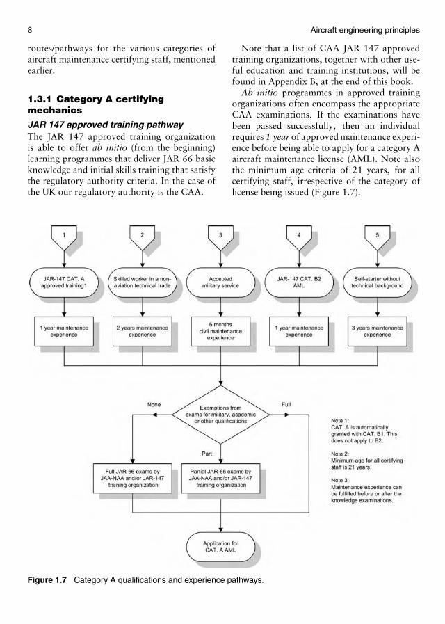
JAR 147 approved training pathwayThe JAR 147 approved training organizationis able to offer ab initio (from the beginning)learning programmes that deliver JAR 66 basicknowledge and initial skills training that satisfythe regulatory authority criteria. In the case ofthe UK our regulatory authority is the CAA.
Figure 1.7 Category A qualifications and experience pathways.
Note that a list of CAA JAR 147 approvedtraining organizations, together with other use-ful education and training institutions, will befound in Appendix B, at the end of this book.
Ab initio programmes in approved trainingorganizations often encompass the appropriateCAA examinations. If the examinations havebeen passed successfully, then an individualrequires 1 year of approved maintenance experi-ence before being able to apply for a category Aaircraft maintenance license (AML). Note alsothe minimum age criteria of 21 years, for allcertifying staff, irrespective of the category oflicense being issued (Figure 1.7).
Introduction 9
Skilled worker pathwayThe requirement of practical experience forthose entering the profession as non-aviationtechnical tradesmen is 2 years. This will enableaviation-orientated skills and knowledge to beacquired from individuals who will already havethe necessary basic fitting skills needed for manyof the tasks likely to be encountered by thecategory A certifying mechanic.
Accepted military service pathwayExperienced line mechanics and base mainte-nance mechanics, with suitable military expe-rience on live aircraft and equipments, will havetheir practical experience requirement reducedto 6 months. This may change in the futurewhen armed forces personnel leave after beingcross-trained.
Category B2 AML pathwayThe skills and knowledge required by categoryA certifying mechanics is a sub-set of thoserequired by B1 mechanical certifying techni-cians. Much of this knowledge and many of theskills required for category A maintenance tasksare not relevant by the category B2 avionic cer-tifying technician. Therefore, in order that thecategory B2 person gains the necessary skills andknowledge required for category A certification,1 year of practical maintenance experience isconsidered necessary.
Self-starter pathwayThis route is for individuals who may be takenon by smaller approved maintenance organiza-tions or be employed in GA, where companyapprovals can be issued on a task-by-task basis,as experience and knowledge are gained. Suchindividuals may already possess some generalaircraft knowledge and basic fitting skills by suc-cessfully completing a state funded educationprogramme. For example, the 2-year full-timediploma that leads to an aeronautical engineer-ing qualification (see Section 1.3.4).
However, if these individuals have not prac-ticed as a skill fitter in a related engineeringdiscipline, then it will be necessary to complete
the 3 years of practical experience applicable tothis mode of entry into the profession.
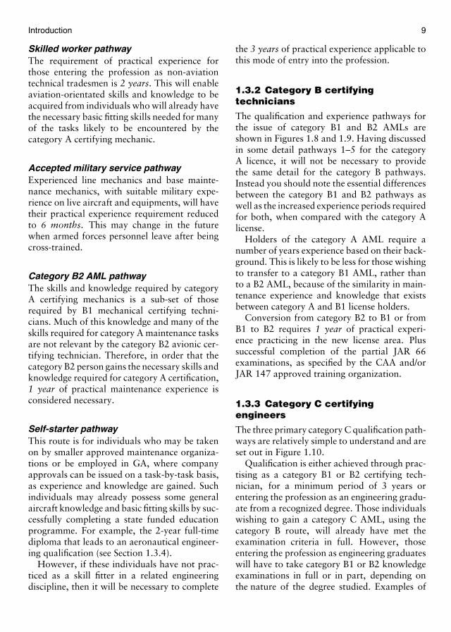
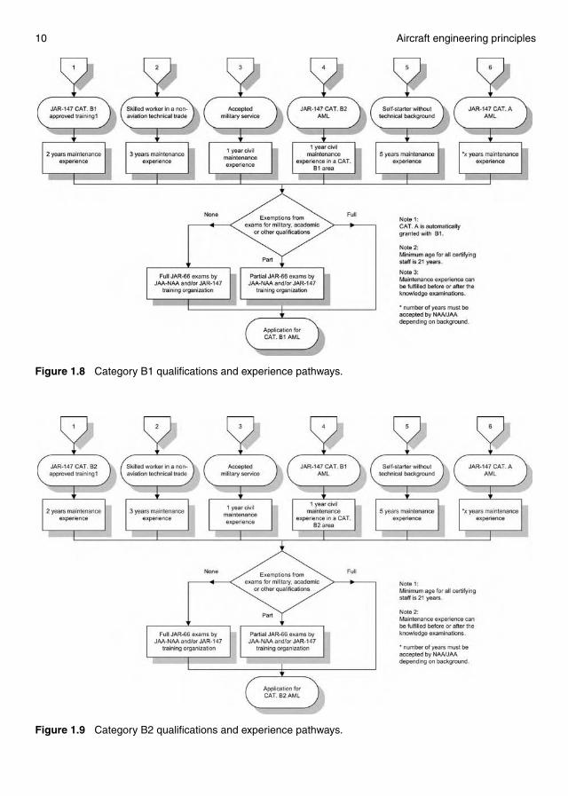
1.3.2 Category B certifyingtechnicians
The qualification and experience pathways forthe issue of category B1 and B2 AMLs areshown in Figures 1.8 and 1.9. Having discussedin some detail pathways 1–5 for the categoryA licence, it will not be necessary to providethe same detail for the category B pathways.Instead you should note the essential differencesbetween the category B1 and B2 pathways aswell as the increased experience periods requiredfor both, when compared with the category Alicense.
Holders of the category A AML require anumber of years experience based on their back-ground. This is likely to be less for those wishingto transfer to a category B1 AML, rather thanto a B2 AML, because of the similarity in main-tenance experience and knowledge that existsbetween category A and B1 license holders.
Conversion from category B2 to B1 or fromB1 to B2 requires 1 year of practical experi-ence practicing in the new license area. Plussuccessful completion of the partial JAR 66examinations, as specified by the CAA and/orJAR 147 approved training organization.
1.3.3 Category C certifyingengineers
The three primary category C qualification path-ways are relatively simple to understand and areset out in Figure 1.10.
Qualification is either achieved through prac-tising as a category B1 or B2 certifying tech-nician, for a minimum period of 3 years orentering the profession as an engineering gradu-ate from a recognized degree. Those individualswishing to gain a category C AML, using thecategory B route, will already have met theexamination criteria in full. However, thoseentering the profession as engineering graduateswill have to take category B1 or B2 knowledgeexaminations in full or in part, depending onthe nature of the degree studied. Examples of
10 Aircraft engineering principles
Figure 1.8 Category B1 qualifications and experience pathways.
Figure 1.9 Category B2 qualifications and experience pathways.
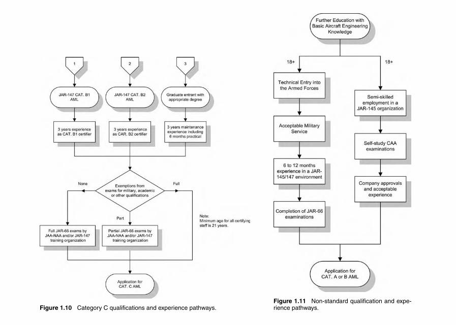
Figure 1.10 Category C qualifications and experience pathways.Figure 1.11 Non-standard qualification and expe-rience pathways.

12 Aircraft engineering principles
Figure 1.12 Routes to an honours degree and category A, B and C licenses.
non-standard entry methods and graduate entrymethods, together with the routes and pathwaysto professional recognition are given next.
1.3.4 Non-standard qualificationand experience pathways
Figure 1.11 illustrates in more detail two possi-ble self-starter routes. The first shows a possibleprogression route for those wishing to gain theappropriate qualifications and experience by ini-tially serving in the armed forces. The seconddetails a possible model for the 18+ schoolleaver employed in a semi-skilled role, within arelatively small aircraft maintenance company.
In the case of the semi-skilled self-starter, theexperience qualifying times would be depen-dent on individual progress, competence andmotivation. Also note that 18+ is considered tobe an appropriate age to consider entering theaircraft maintenance profession, irrespective ofthe type of license envisaged.
1.3.5 The Kingston qualificationand experience pathway
In this model, provision has been made for qual-ification and experience progression routes forcategory A, B and C AML approval and appro-priate professional recognition (Figure 1.12).
Introduction 13
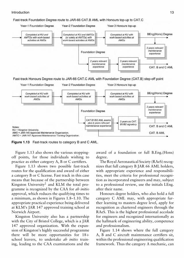
Figure 1.13 Fast-track routes to category B and C AML.
Figure 1.13 also shows the various stopping-off points, for those individuals wishing topractice as either category A, B or C certifiers.
Figure 1.13 shows two possible fast-trackroutes for the qualification and award of eithera category B or C license. Fast track in this casemeans that because of the partnership betweenKingston University2 and KLM the total pro-gramme is recognized by the CAA for ab initioapproval, which reduces the qualifying times toa minimum, as shown in Figures 1.8–1.10. Theappropriate practical experience being deliveredat KLM’s JAR 147 approved training school atNorwich Airport.
Kingston University also has a partnershipwith the City of Bristol College, which is a JAR147 approved organization. With the expan-sion of Kingston’s highly successful programmethere will be more opportunities for 18+school leavers, to undertake ab initio train-ing, leading to the CAA examinations and the
award of a foundation or full B.Eng.(Hons)degree.
The Royal Aeronautical Society (RAeS) recog-nizes that full category B JAR 66 AML holders,with appropriate experience and responsibili-ties, meet the criteria for professional recogni-tion as incorporated engineers and may, subjectto a professional review, use the initials I.Eng.after their name.
Honours degree holders, who also hold a fullcategory C AML may, with appropriate fur-ther learning to masters degree level, apply forrecognition as chartered engineers through theRAeS. This is the highest professional accoladefor engineers and recognized internationally asthe hallmark of engineering ability, competenceand professionalism.
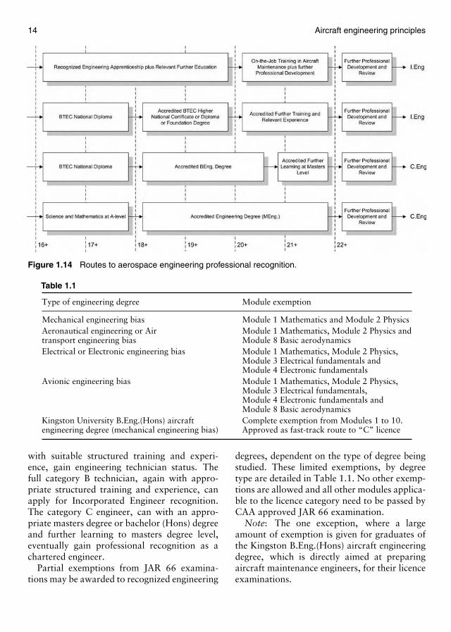
Figure 1.14 shows where the full categoryA, B and C aircraft maintenance certifiers sit,within the professional engineering qualificationframework. Thus the category A mechanic, can
14 Aircraft engineering principles
Figure 1.14 Routes to aerospace engineering professional recognition.
Table 1.1
Type of engineering degree Module exemption
Mechanical engineering bias Module 1 Mathematics and Module 2 PhysicsAeronautical engineering or Air Module 1 Mathematics, Module 2 Physics andtransport engineering bias Module 8 Basic aerodynamicsElectrical or Electronic engineering bias Module 1 Mathematics, Module 2 Physics,
Module 3 Electrical fundamentals andModule 4 Electronic fundamentals
Avionic engineering bias Module 1 Mathematics, Module 2 Physics,Module 3 Electrical fundamentals,Module 4 Electronic fundamentals andModule 8 Basic aerodynamics
Kingston University B.Eng.(Hons) aircraft Complete exemption from Modules 1 to 10.engineering degree (mechanical engineering bias) Approved as fast-track route to “C” licence
with suitable structured training and experi-ence, gain engineering technician status. Thefull category B technician, again with appro-priate structured training and experience, canapply for Incorporated Engineer recognition.The category C engineer, can with an appro-priate masters degree or bachelor (Hons) degreeand further learning to masters degree level,eventually gain professional recognition as achartered engineer.
Partial exemptions from JAR 66 examina-tions may be awarded to recognized engineering
degrees, dependent on the type of degree beingstudied. These limited exemptions, by degreetype are detailed in Table 1.1. No other exemp-tions are allowed and all other modules applica-ble to the licence category need to be passed byCAA approved JAR 66 examination.
Note: The one exception, where a largeamount of exemption is given for graduates ofthe Kingston B.Eng.(Hons) aircraft engineeringdegree, which is directly aimed at preparingaircraft maintenance engineers, for their licenceexaminations.
Introduction 15
1.4 CAA licence – structure,qualifications, examinations and levels
1.4.1 Qualifications structure
The licensing of aircraft maintenance engineersis covered by international standards that arepublished by the International Civil AviationOrganization (ICAO). In the UK, the Air Nav-igation Order (ANO) provides the legal frame-work to support these standards. The purposeof the licence is not to permit the holder to per-form maintenance but to enable the issue ofcertification for maintenance required under theANO legislation. This is why we refer to licensedmaintenance personnel as “certifiers”.
At present the CAA issue licences under twodifferent requirements depending on the maxi-mum take-off mass of the aircraft.
For aircraft that exceeds 5700 kg, licenses areissued under JAR 66. The JAR 66 license iscommon to all European countries who are fullmembers of the Joint Aviation Authority (JAA).The ideal being that the issue of a JAR 66 licenceby any full member country is then recognizedas having equal status in all other member coun-tries throughout Europe. There are currentlyover 20 countries throughout Europe that goto make-up the JAA. In US, the US FederalAviation Administration (USFAA) is the equiv-alent of the JAA. These two organizations havebeen harmonized to the point where for exam-ple, licences issued under JAR 66 are equiva-lent to those licences issued under FAR 66, incountries that adhere to FAA requirements.
Holders of licences issued under JAR 66requirements are considered to have achieved anappropriate level of knowledge and competence,that will enable them to undertake maintenanceactivities on commercial aircraft.
Licences for light aircraft (less than 5700 kg)and for airships, continue to be issued under theUK National Licensing Requirements laid downin British Civil Airworthiness Requirements(BCAR) Section L. The intention is that within afew years, light aircraft will be included withinJAR 66. At present, this has implications forpeople who wish to work and obtain licencesin GA, where many light aircraft are operated.
Much of the knowledge required for the JAR 66licence, laid down in this series, is also relevantto those wishing to obtain a Section L licencefor light aircraft. Although the basic Section Llicence is narrower (see Appendix B) and is con-sidered somewhat less demanding than the JAR66 licence it is, nevertheless, highly regarded asa benchmark of achievement and competencewithin the light aircraft fraternity.
As mentioned earlier, the JAR 66 license isdivided into categories A, B and C, and forcategory B license, there are two major careeroptions, either a mechanical or avionic techni-cian. For fear of bombarding you with too muchinformation, what was not mentioned earlierwas the further subdivisions for the mechanicallicense. These sub-categories are dependent onaircraft type (fixed or rotary wing) and on enginetype (turbine or piston). For clarity, all levelsand categories of license that may be issuedby the CAA/FAA or member National AviationAuthorities (NAA) are listed below.
Levels
Category A: Line maintenance certifyingmechanic
Category B1: Line maintenance certifyingtechnician (mechanical)
Category B2: Line maintenance certifyingtechnician (avionic)
Category C: Base maintenance certifyingengineer
Note: When introduced, the light AML will becategory B3.
Sub-category AA1: Aeroplanes turbineA2: Aeroplanes pistonA3: Helicopters turbineA4: Helicopters piston
Sub-category B1B1.1: Aeroplanes turbineB1.2: Aeroplanes pistonB1.3: Helicopters turbineB1.4: Helicopters piston
16 Aircraft engineering principles
Note that the experience requirements for allof the above licences are shown in Figures1.7–1.10.
Aircraft-type endorsements 3
Holders of JAR 66 aircraft maintenance licencesin category B1, B2 and C may apply for inclusionof an aircraft-type rating subject to meeting thefollowing requirements.
1. The completion of a JAR 147 approved orJAA/NAA approved type training course onthe type of aircraft for which approval isbeing sought and one which covers the sub-ject matter appropriate to the licence categorybeing endorsed.
2. Completion of a minimum period of practicalexperience on type, prior to application fortype rating endorsement.
Type training for category C differs from thatrequired for category B1 or B2, therefore cat-egory C type training will not qualify for typeendorsement in category B1 or B2. However,type courses at category B1 or B2 level mayallow the licence holder to qualify for categoryC level at the same time, providing they hold acategory C basic licence.
Licence holders seeking type rating endorse-ments from the CAA must hold a basic JAR 66licence granted by the UK CAA.
1.4.2 JAR 66 syllabus modules andapplicability
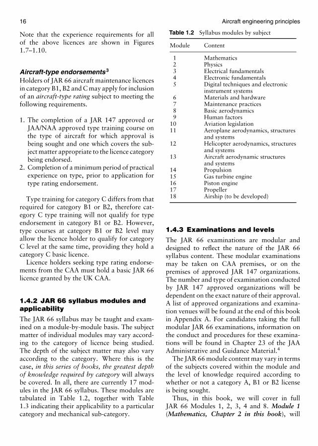
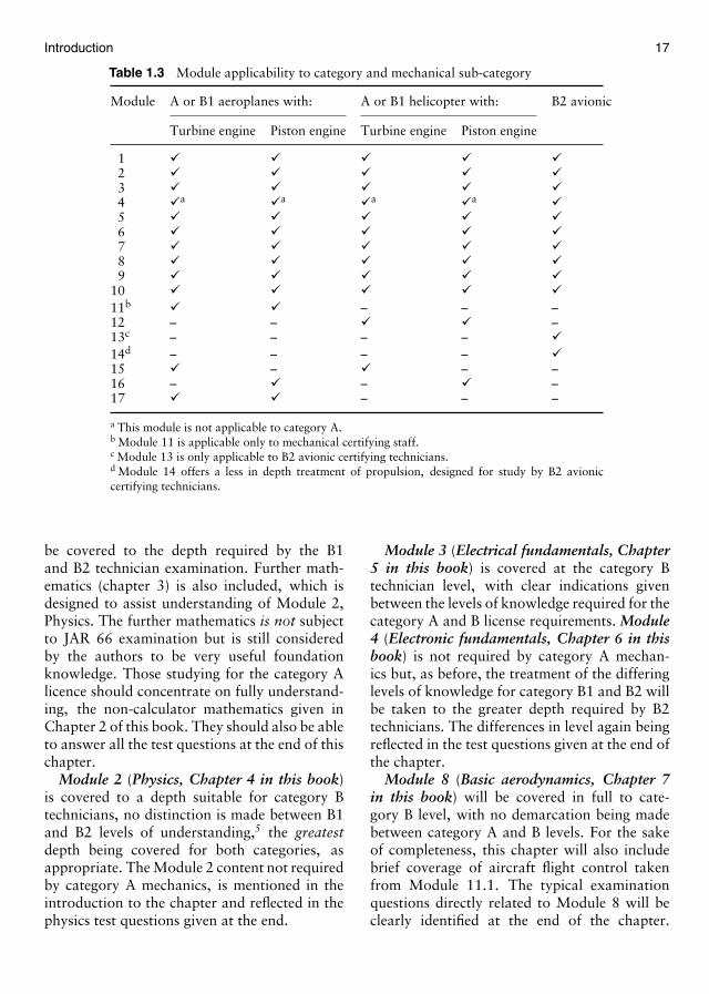
The JAR 66 syllabus may be taught and exam-ined on a module-by-module basis. The subjectmatter of individual modules may vary accord-ing to the category of licence being studied.The depth of the subject matter may also varyaccording to the category. Where this is thecase, in this series of books, the greatest depthof knowledge required by category will alwaysbe covered. In all, there are currently 17 mod-ules in the JAR 66 syllabus. These modules aretabulated in Table 1.2, together with Table1.3 indicating their applicability to a particularcategory and mechanical sub-category.
Table 1.2 Syllabus modules by subject
Module Content
1 Mathematics2 Physics3 Electrical fundamentals4 Electronic fundamentals5 Digital techniques and electronic
instrument systems6 Materials and hardware7 Maintenance practices8 Basic aerodynamics9 Human factors
10 Aviation legislation11 Aeroplane aerodynamics, structures
and systems12 Helicopter aerodynamics, structures
and systems13 Aircraft aerodynamic structures
and systems14 Propulsion15 Gas turbine engine16 Piston engine17 Propeller18 Airship (to be developed)
1.4.3 Examinations and levels
The JAR 66 examinations are modular anddesigned to reflect the nature of the JAR 66syllabus content. These modular examinationsmay be taken on CAA premises, or on thepremises of approved JAR 147 organizations.The number and type of examination conductedby JAR 147 approved organizations will bedependent on the exact nature of their approval.A list of approved organizations and examina-tion venues will be found at the end of this bookin Appendix A. For candidates taking the fullmodular JAR 66 examinations, information onthe conduct and procedures for these examina-tions will be found in Chapter 23 of the JAAAdministrative and Guidance Material.4
The JAR 66 module content may vary in termsof the subjects covered within the module andthe level of knowledge required according towhether or not a category A, B1 or B2 licenseis being sought.
Thus, in this book, we will cover in fullJAR 66 Modules 1, 2, 3, 4 and 8. Module 1(Mathematics, Chapter 2 in this book), will
Introduction 17
Table 1.3 Module applicability to category and mechanical sub-category
Module A or B1 aeroplanes with: A or B1 helicopter with: B2 avionic
Turbine engine Piston engine Turbine engine Piston engine
1 � � � � �2 � � � � �3 � � � � �4 �a �a �a �a �5 � � � � �6 � � � � �7 � � � � �8 � � � � �9 � � � � �
10 � � � � �11b � � – – –12 – – � � –13c – – – – �14d – – – – �15 � – � – –16 – � – � –17 � � – – –
a This module is not applicable to category A.b Module 11 is applicable only to mechanical certifying staff.c Module 13 is only applicable to B2 avionic certifying technicians.d Module 14 offers a less in depth treatment of propulsion, designed for study by B2 avioniccertifying technicians.
be covered to the depth required by the B1and B2 technician examination. Further math-ematics (chapter 3) is also included, which isdesigned to assist understanding of Module 2,Physics. The further mathematics is not subjectto JAR 66 examination but is still consideredby the authors to be very useful foundationknowledge. Those studying for the category Alicence should concentrate on fully understand-ing, the non-calculator mathematics given inChapter 2 of this book. They should also be ableto answer all the test questions at the end of thischapter.
Module 2 (Physics, Chapter 4 in this book)is covered to a depth suitable for category Btechnicians, no distinction is made between B1and B2 levels of understanding,5 the greatestdepth being covered for both categories, asappropriate. The Module 2 content not requiredby category A mechanics, is mentioned in theintroduction to the chapter and reflected in thephysics test questions given at the end.
Module 3 (Electrical fundamentals, Chapter5 in this book) is covered at the category Btechnician level, with clear indications givenbetween the levels of knowledge required for thecategory A and B license requirements. Module4 (Electronic fundamentals, Chapter 6 in thisbook) is not required by category A mechan-ics but, as before, the treatment of the differinglevels of knowledge for category B1 and B2 willbe taken to the greater depth required by B2technicians. The differences in level again beingreflected in the test questions given at the end ofthe chapter.
Module 8 (Basic aerodynamics, Chapter 7in this book) will be covered in full to cate-gory B level, with no demarcation being madebetween category A and B levels. For the sakeof completeness, this chapter will also includebrief coverage of aircraft flight control takenfrom Module 11.1. The typical examinationquestions directly related to Module 8 will beclearly identified at the end of the chapter.
18 Aircraft engineering principles
Full coverage of the specialist aeroplane aerody-namics, high-speed flight and rotor wing aero-dynamics, applicable to Modules 11 and 13will be covered in the third book in the series,Aircraft Aerodynamics, Structural Maintenanceand Repair.
Examination papers are mainly multiple-choice type but a written paper must also bepassed so that the licence may be issued. Can-didates may take one or more papers, at asingle examination sitting. The pass mark foreach multiple-choice paper is 75%! There isno longer any penalty marking for incorrectlyanswering individual multiple-choice questions.All multiple-choice questions set by the CAAand by approved organizations have exactly thesame form. That is, each question will contain astem (the question being asked), two distracters(incorrect answers) and one correct answer. Themultiple-choice questions given at the end ofeach chapter in this book are laid out in thisform.
All multiple-choice examination papers aretimed, approximately 1 min and 15 s, beingallowed for the reading and answering of eachquestion (see Table 1.4). The number of ques-tions asked depends on the module examinationbeing taken and on the category of licence beingsought. The structure of the multiple-choicepapers for each module together with the struc-ture of the written examination for issue of thelicense are given in Table 1.4.
More detailed and current information onthe nature of the license examinations can befound in the appropriate CAA documentation,6
from which the examination structure detailedin Table 1.4 is extracted.
Written paperThe written paper required for licence issue con-tains four essay questions. These questions aredrawn from the JAR 66 syllabus modules asfollows:
Module Paper Question7 Maintenance practices 29 Human factors 1
10 Aviation legislation 1
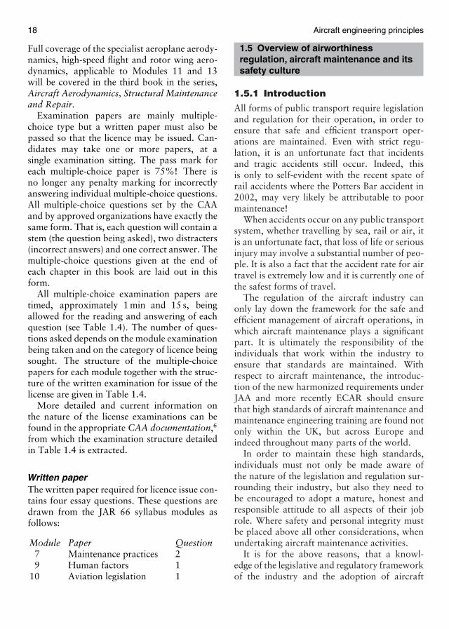
1.5 Overview of airworthinessregulation, aircraft maintenance and itssafety culture
1.5.1 Introduction
All forms of public transport require legislationand regulation for their operation, in order toensure that safe and efficient transport oper-ations are maintained. Even with strict regu-lation, it is an unfortunate fact that incidentsand tragic accidents still occur. Indeed, thisis only to self-evident with the recent spate ofrail accidents where the Potters Bar accident in2002, may very likely be attributable to poormaintenance!
When accidents occur on any public transportsystem, whether travelling by sea, rail or air, itis an unfortunate fact, that loss of life or seriousinjury may involve a substantial number of peo-ple. It is also a fact that the accident rate for airtravel is extremely low and it is currently one ofthe safest forms of travel.
The regulation of the aircraft industry canonly lay down the framework for the safe andefficient management of aircraft operations, inwhich aircraft maintenance plays a significantpart. It is ultimately the responsibility of theindividuals that work within the industry toensure that standards are maintained. Withrespect to aircraft maintenance, the introduc-tion of the new harmonized requirements underJAA and more recently ECAR should ensurethat high standards of aircraft maintenance andmaintenance engineering training are found notonly within the UK, but across Europe andindeed throughout many parts of the world.
In order to maintain these high standards,individuals must not only be made aware ofthe nature of the legislation and regulation sur-rounding their industry, but also they need tobe encouraged to adopt a mature, honest andresponsible attitude to all aspects of their jobrole. Where safety and personal integrity mustbe placed above all other considerations, whenundertaking aircraft maintenance activities.
It is for the above reasons, that a knowl-edge of the legislative and regulatory frameworkof the industry and the adoption of aircraft

Introduction 19
Table 1.4 Structure of JAR 66 multiple-choice examination papers
Module Number of Time allowed Module Number of Time allowedquestions (min) questions (min)
1 Mathematics 10 Aviation LegislationCategory A 16 20 Category A 40 50Category B1 30 40 Category B1 40 50Category B2 30 40 Category B2 40 502 Physics 11 Aeroplane aerodynamics, structures and systemsCategory A 30 40 Category A 100 125Category B1 50 65 Category B1 130 165Category B2 50 65 Category B2 – –3 Electrical fundamentals 12 Helicopter aerodynamics, structures and systemsCategory A 20 25 Category A 90 115Category B1 50 65 Category B1 115 145Category B2 50 65 Category B2 – –4 Electronic fundamentals 13 Aircraft aerodynamics, structures and systemsCategory A – – Category A – –Category B1 20 25 Category B1 – –Category B2 40 50 Category B2 130 1655 Digital techniques/electronic instrument systems 14 PropulsionCategory A 16 20 Category A – –Category B1 40 50 Category B1 – –Category B2 70 90 Category B2 25 306 Materials and hardware 15 Gas turbine engineCategory A 50 65 Category A 60 75Category B1 70 90 Category B1 90 115Category B2 60 75 Category B2 – –7 Maintenance practices 16 Piston engineCategory A 70 90 Category A 50 65Category B1 80 100 Category B1 70 90Category B2 60 75 Category B2 – –8 Basic aerodynamics 17 PropellerCategory A 20 25 Category A 20 25Category B1 20 25 Category B1 30 40Category B2 20 25 Category B2 – –9 Human factorsCategory A 20 25Category B1 20 25Category B2 20 25
Note: The time given for examinations may, from time to time, be subject to change. There is currently a review pending ofexaminations time based on levels. Latest information may be obtained from the CAA website.
maintenance safety culture, becomes a vital partof the education for all individuals wishing topractice as aircraft maintenance engineers. Setout in this section is a brief introduction to theregulatory and legislative framework, togetherwith maintenance safety culture and the vagariesof human performance. A much fuller coverageof aircraft maintenance legislation and safety
procedures will be found in, Aircraft Engineer-ing Maintenance Practices, the second book inthis series.
1.5.2 The birth of the ICAO
The international nature of current aircraftmaintenance engineering has already beenmentioned. Thus the need for conformity of
20 Aircraft engineering principles
standards to ensure the continued airworthinessof aircraft that fly through international airspaceis of prime importance.
As long ago as December 1944, a group of for-ward thinking delegates from 52 countries cametogether in Chicago, to agree and ratify the con-vention on international civil aviation. Thus theProvisional International Civil Aviation Orga-nization (PICAO) was established. It ran in thisform until March 1947, when final ratificationfrom 26 member countries was received and itbecame the ICAO.
The primary function of the ICAO, which wasagreed in principle at the Chicago Convention in1944, was to develop international air transportin a safe and orderly manner. More formerly,the 52 member countries agreed to undersign:
certain principles and arrangements inorder that international civil aviation maybe developed in a safe and orderly mannerand that international air transport servicesmay be established on the basis of equalityof opportunity and operated soundly andeconomically.
Thus in a spirit of cooperation, designed tofoster good international relationships, betweenmember countries, the 52 member states signedup to the agreement. This was a far-sighteddecision, which has remained substantiallyunchanged up to the present. The ICAO Assem-bly is the sovereign body of the ICAO respon-sible for reviewing in detail the work of ICAO,including setting the budget and policy for thefollowing 3 years.
The council, elected by the assembly for a3-year term, is composed of 33 member states.The council is responsible for ensuring that stan-dards and recommended practices are adoptedand incorporated as annexes into the conven-tion on international civil aviation. The councilis assisted by the Air Navigation Commissionto deal with technical matters, the Air Trans-port Committee to deal with economic mattersand the Committee on Joint Support of AirNavigation Services and the Finance Committee.
The ICAO also works closely with othermembers of the United Nations (UN) and othernon-governmental organizations such as the
International Air Transport Association (IATA)and the International Federation of Air LinePilots to name but two.
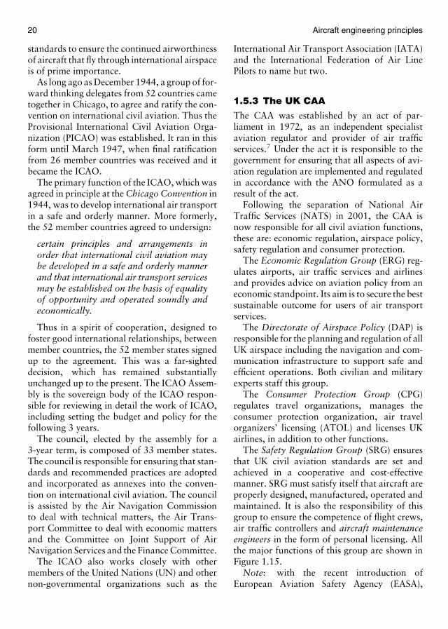
1.5.3 The UK CAA
The CAA was established by an act of par-liament in 1972, as an independent specialistaviation regulator and provider of air trafficservices.7 Under the act it is responsible to thegovernment for ensuring that all aspects of avi-ation regulation are implemented and regulatedin accordance with the ANO formulated as aresult of the act.
Following the separation of National AirTraffic Services (NATS) in 2001, the CAA isnow responsible for all civil aviation functions,these are: economic regulation, airspace policy,safety regulation and consumer protection.
The Economic Regulation Group (ERG) reg-ulates airports, air traffic services and airlinesand provides advice on aviation policy from aneconomic standpoint. Its aim is to secure the bestsustainable outcome for users of air transportservices.
The Directorate of Airspace Policy (DAP) isresponsible for the planning and regulation of allUK airspace including the navigation and com-munication infrastructure to support safe andefficient operations. Both civilian and militaryexperts staff this group.
The Consumer Protection Group (CPG)regulates travel organizations, manages theconsumer protection organization, air travelorganizers’ licensing (ATOL) and licenses UKairlines, in addition to other functions.
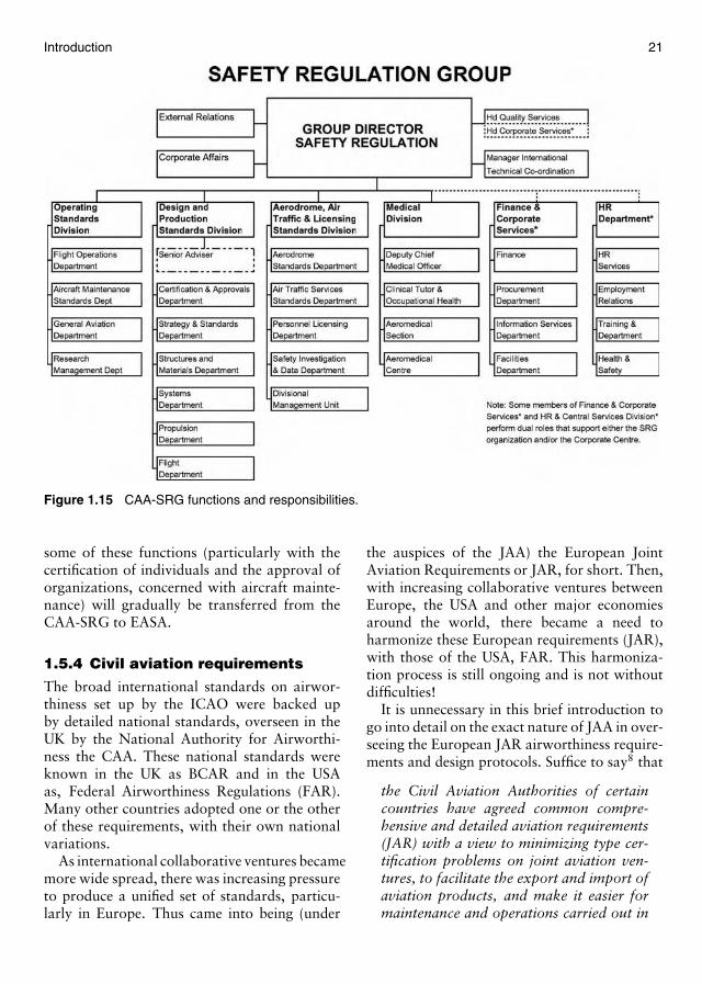
The Safety Regulation Group (SRG) ensuresthat UK civil aviation standards are set andachieved in a cooperative and cost-effectivemanner. SRG must satisfy itself that aircraft areproperly designed, manufactured, operated andmaintained. It is also the responsibility of thisgroup to ensure the competence of flight crews,air traffic controllers and aircraft maintenanceengineers in the form of personal licensing. Allthe major functions of this group are shown inFigure 1.15.
Note: with the recent introduction ofEuropean Aviation Safety Agency (EASA),
Introduction 21
Figure 1.15 CAA-SRG functions and responsibilities.
some of these functions (particularly with thecertification of individuals and the approval oforganizations, concerned with aircraft mainte-nance) will gradually be transferred from theCAA-SRG to EASA.
1.5.4 Civil aviation requirements
The broad international standards on airwor-thiness set up by the ICAO were backed upby detailed national standards, overseen in theUK by the National Authority for Airworthi-ness the CAA. These national standards wereknown in the UK as BCAR and in the USAas, Federal Airworthiness Regulations (FAR).Many other countries adopted one or the otherof these requirements, with their own nationalvariations.
As international collaborative ventures becamemore wide spread, there was increasing pressureto produce a unified set of standards, particu-larly in Europe. Thus came into being (under
the auspices of the JAA) the European JointAviation Requirements or JAR, for short. Then,with increasing collaborative ventures betweenEurope, the USA and other major economiesaround the world, there became a need toharmonize these European requirements (JAR),with those of the USA, FAR. This harmoniza-tion process is still ongoing and is not withoutdifficulties!
It is unnecessary in this brief introduction togo into detail on the exact nature of JAA in over-seeing the European JAR airworthiness require-ments and design protocols. Suffice to say8 that
the Civil Aviation Authorities of certaincountries have agreed common compre-hensive and detailed aviation requirements(JAR) with a view to minimizing type cer-tification problems on joint aviation ven-tures, to facilitate the export and import ofaviation products, and make it easier formaintenance and operations carried out in

22 Aircraft engineering principles
one country to be accepted by the CAA inanother country.
One or two of the more important require-ments applicable to aircraft maintenance orga-nizations and personnel are detailed below:
JAR 25 – Requirements for large aircraft (over5700 kg)
JAR E – Requirements for aircraft enginesJAR 21 – Requirements for products and parts
for aircraftJAR 66 – Requirements for aircraft engi-
neering certifying staff, includingthe basic knowledge requirements,upon which all the books in thisseries are based
JAR 145 – Requirements for organizations oper-ating large aircraft
JAR 147 – Requirements to be met by organi-zations seeking approval to conductapproved training/examinations ofcertifying staff, as specified in JAR 66.
1.5.5 Aircraft maintenanceengineering safety culture andhuman factors
If you have managed to plough your waythrough this introduction, you cannot havefailed to notice that aircraft maintenance engi-neering is a very highly regulated industry,where safety is considered paramount!
Every individual working on or around air-craft and/or their associated equipments, hasa personal responsibility for their own safetyand the safety of others. Thus, you will need tobecome familiar with your immediate work areaand recognize and avoid, the hazards associatedwith it. You will also need to be familiar withyour local emergency: first aid procedures, fireprecautions and communication procedures.
Thorough coverage of workshop, aircrafthangar and ramp safety procedures and pre-cautions will be found in Aircraft EngineeringMaintenance Practices, the second book in theseries.
Coupled with this knowledge on safety,all prospective maintenance engineers mustalso foster a responsible, honest, mature and
Figure 1.16 Control column, with base cover platefitted and throttle box assembly clearly visible.
professional attitude to all aspects of their work.You perhaps, cannot think of any circumstanceswhere you would not adopt such attitudes?However, due to the nature of aircraft main-tenance, you may find yourself working undervery stressful circumstances where your profes-sional judgement is tested to the limit!
For example, consider the following scenario.As an experienced maintenance technician,
you have been tasked with fitting the cover to thebase of the flying control column (Figure 1.16),on an aircraft that is going to leave the mainte-nance hanger on engine ground runs, before theovernight embargo on airfield noise comes intoforce, in 3 hours time. It is thus important thatthe aircraft is towed to the ground running area,in time to complete the engine runs before theembargo. This will enable all outstanding main-tenance on the aircraft to be carried out overnight and so ensure that the aircraft is madeready in good time, for a scheduled flight firstthing in the morning.
You start the task and when three quartersof the way through fitment of the cover, youdrop a securing bolt, as you stand up. Youthink that you hear it travelling across the flightdeck floor. After a substantial search by torch-light, where you look not only across the floor,but also around the base of the control columnand into other possible crevices, in the immedi-ate area, you are unable to find the small bolt.Would you:
(a) Continue the search for as long as possibleand then, if the bolt was not found, complete
Introduction 23
the fit of the cover plate and look for thebolt, when the aircraft returned from groundruns?
(b) Continue the search for as long as possi-ble and then, if the bolt was not found,inform the engineer tasked with carrying outthe ground runs, to be aware that a bolt issomewhere in the vicinity of the base of thecontrol column on the flight deck floor. Thencontinue with the fit of the cover?
(c) Raise an entry in the aircraft maintenance logfor a “loose article” on the flight deck. Thenremove the cover plate, obtain a source ofstrong light and/or a light probe kit and carryout a thorough search at base of control col-umn and around all other key controls, suchas the throttle box. If bolt is not found, allowaircraft to go on ground run and continuesearch on return?
(d) Raise an entry in the aircraft log for a “loosearticle” on the flight deck. Then immedi-ately seek advice from shift supervisor, as tocourse of action to be taken?
Had you not been an experienced technician,you would immediately inform your supervi-sor (action (d)) and seek advice as to the mostappropriate course of action. As an experiencedtechnician, what should you do? The courseof action to be taken, in this particular case,may not then be quite so obvious, it requiresjudgements to be made.
Quite clearly actions (a) and (b) would bewrong, no matter how much experience thetechnician had. No matter how long the searchcontinued, it would be essential to remove thecover plate and search the base of the con-trol column to ensure that it was not in thevicinity. Any loose article could dislodge duringflight and cause possible catastrophic jammingor fouling of the controls. If the engine run isto proceed, actions (a) and (b) are still not ade-quate. A search of the throttle box area for thebolt would also need to take place, as suggestedby action (c). Action (c) seems plausible, withthe addition of a good light source and thor-ough search of all critical areas, before the fitof the cover plate, seems a reasonable course ofaction to take, especially after the maintenance
log entry has been made, the subsequent searchfor the bolt, cannot be forgotten, so all is well?
However, if you followed action (c) youwould be making important decisions, on mat-ters of safety, without consultation. No matterhow experienced you may be, you are not nec-essarily aware of the total picture, whereasyour shift supervisor, may well be! The correctcourse of action, even for the most experiencedengineer would be action (d).
Suppose action (c) had been taken and on thesubsequent engine run the bolt, that had beenlodged in the throttle box, caused the throt-tle to jam in the open position. Then shuttingdown the engine, without first closing the throt-tle, could cause serious damage! It might havebeen the case that if action (d) had been fol-lowed, the shift supervisor may have been ina position to prepare another aircraft for thescheduled morning flight, thus avoiding the riskof running the engine, before the loose articlesearch had revealed the missing bolt.
In any event, the aircraft would not nor-mally be released for service until the missingbolt had been found, even if this required theuse of sophisticated radiographic equipment tofind it!
The above scenario illustrates some of the pit-falls, that even experienced aircraft maintenanceengineers may encounter, if safety is forgotten orassumptions made. For example, because youthought you heard the bolt travel across theflight deck, you may have assumed that it couldnot possibly have landed at the base of the con-trol column, or in the throttle box. This, ofcourse, is an assumption and one of the goldenrules of safety is never assume, check!
When the cover was being fitted, did you haveadequate lighting for the job? Perhaps with ade-quate lighting, it might have been possible totrack the path of the bolt, as it travelled acrossthe flight deck, thus preventing its loss in the firstplace.
Familiarity with emergency equipment andprocedures, as mentioned previously is an essen-tial part of the education of all aircraft main-tenance personnel. Reminders concerning theuse of emergency equipment will be found inhangars, workshops, repair bays and in many
24 Aircraft engineering principles
Figure 1.17 Typical aircraft hangar first aid station.
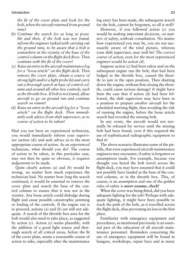
other areas where aircraft engineering mainte-nance is practiced. Some typical examples ofemergency equipment and warning notices areshown below. Figure 1.17 shows a typical air-craft maintenance hangar first aid station, com-plete with explanatory notices, first aid box andeye irritation bottles.
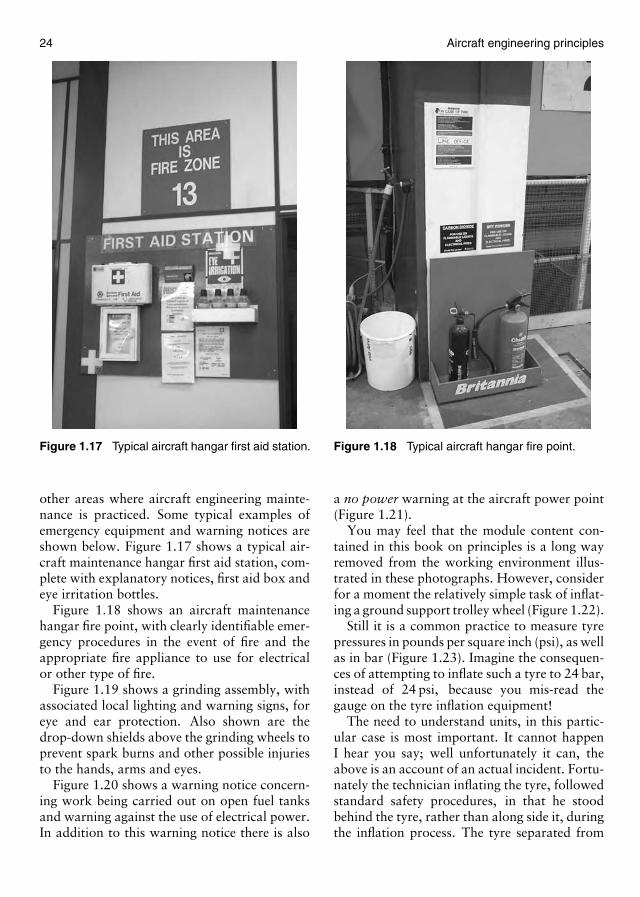
Figure 1.18 shows an aircraft maintenancehangar fire point, with clearly identifiable emer-gency procedures in the event of fire and theappropriate fire appliance to use for electricalor other type of fire.
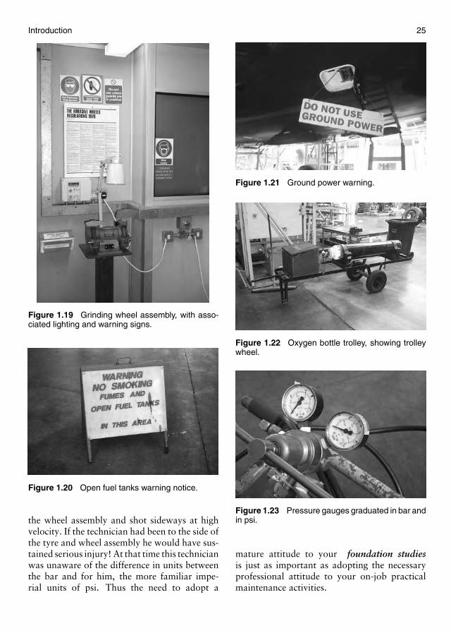
Figure 1.19 shows a grinding assembly, withassociated local lighting and warning signs, foreye and ear protection. Also shown are thedrop-down shields above the grinding wheels toprevent spark burns and other possible injuriesto the hands, arms and eyes.
Figure 1.20 shows a warning notice concern-ing work being carried out on open fuel tanksand warning against the use of electrical power.In addition to this warning notice there is also
Figure 1.18 Typical aircraft hangar fire point.
a no power warning at the aircraft power point(Figure 1.21).
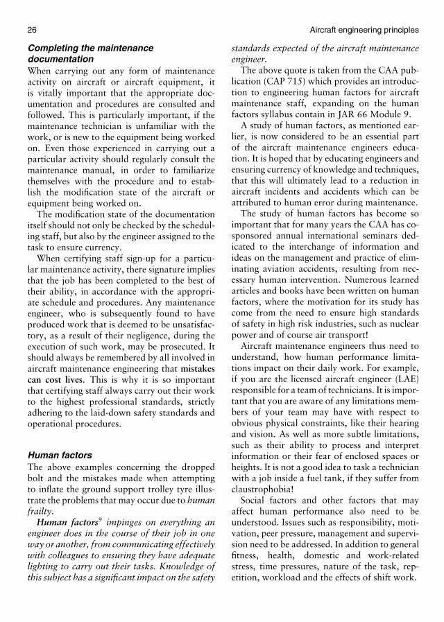
You may feel that the module content con-tained in this book on principles is a long wayremoved from the working environment illus-trated in these photographs. However, considerfor a moment the relatively simple task of inflat-ing a ground support trolley wheel (Figure 1.22).
Still it is a common practice to measure tyrepressures in pounds per square inch (psi), as wellas in bar (Figure 1.23). Imagine the consequen-ces of attempting to inflate such a tyre to 24 bar,instead of 24 psi, because you mis-read thegauge on the tyre inflation equipment!
The need to understand units, in this partic-ular case is most important. It cannot happenI hear you say; well unfortunately it can, theabove is an account of an actual incident. Fortu-nately the technician inflating the tyre, followedstandard safety procedures, in that he stoodbehind the tyre, rather than along side it, duringthe inflation process. The tyre separated from
Introduction 25
Figure 1.19 Grinding wheel assembly, with asso-ciated lighting and warning signs.
Figure 1.20 Open fuel tanks warning notice.
the wheel assembly and shot sideways at highvelocity. If the technician had been to the side ofthe tyre and wheel assembly he would have sus-tained serious injury! At that time this technicianwas unaware of the difference in units betweenthe bar and for him, the more familiar impe-rial units of psi. Thus the need to adopt a
Figure 1.21 Ground power warning.
Figure 1.22 Oxygen bottle trolley, showing trolleywheel.
Figure 1.23 Pressure gauges graduated in bar andin psi.
mature attitude to your foundation studiesis just as important as adopting the necessaryprofessional attitude to your on-job practicalmaintenance activities.
26 Aircraft engineering principles
Completing the maintenancedocumentationWhen carrying out any form of maintenanceactivity on aircraft or aircraft equipment, itis vitally important that the appropriate doc-umentation and procedures are consulted andfollowed. This is particularly important, if themaintenance technician is unfamiliar with thework, or is new to the equipment being workedon. Even those experienced in carrying out aparticular activity should regularly consult themaintenance manual, in order to familiarizethemselves with the procedure and to estab-lish the modification state of the aircraft orequipment being worked on.
The modification state of the documentationitself should not only be checked by the schedul-ing staff, but also by the engineer assigned to thetask to ensure currency.
When certifying staff sign-up for a particu-lar maintenance activity, there signature impliesthat the job has been completed to the best oftheir ability, in accordance with the appropri-ate schedule and procedures. Any maintenanceengineer, who is subsequently found to haveproduced work that is deemed to be unsatisfac-tory, as a result of their negligence, during theexecution of such work, may be prosecuted. Itshould always be remembered by all involved inaircraft maintenance engineering that mistakescan cost lives. This is why it is so importantthat certifying staff always carry out their workto the highest professional standards, strictlyadhering to the laid-down safety standards andoperational procedures.
Human factorsThe above examples concerning the droppedbolt and the mistakes made when attemptingto inflate the ground support trolley tyre illus-trate the problems that may occur due to humanfrailty.
Human factors9 impinges on everything anengineer does in the course of their job in oneway or another, from communicating effectivelywith colleagues to ensuring they have adequatelighting to carry out their tasks. Knowledge ofthis subject has a significant impact on the safety
standards expected of the aircraft maintenanceengineer.
The above quote is taken from the CAA pub-lication (CAP 715) which provides an introduc-tion to engineering human factors for aircraftmaintenance staff, expanding on the humanfactors syllabus contain in JAR 66 Module 9.
A study of human factors, as mentioned ear-lier, is now considered to be an essential partof the aircraft maintenance engineers educa-tion. It is hoped that by educating engineers andensuring currency of knowledge and techniques,that this will ultimately lead to a reduction inaircraft incidents and accidents which can beattributed to human error during maintenance.
The study of human factors has become soimportant that for many years the CAA has co-sponsored annual international seminars ded-icated to the interchange of information andideas on the management and practice of elim-inating aviation accidents, resulting from nec-essary human intervention. Numerous learnedarticles and books have been written on humanfactors, where the motivation for its study hascome from the need to ensure high standardsof safety in high risk industries, such as nuclearpower and of course air transport!
Aircraft maintenance engineers thus need tounderstand, how human performance limita-tions impact on their daily work. For example,if you are the licensed aircraft engineer (LAE)responsible for a team of technicians. It is impor-tant that you are aware of any limitations mem-bers of your team may have with respect toobvious physical constraints, like their hearingand vision. As well as more subtle limitations,such as their ability to process and interpretinformation or their fear of enclosed spaces orheights. It is not a good idea to task a technicianwith a job inside a fuel tank, if they suffer fromclaustrophobia!
Social factors and other factors that mayaffect human performance also need to beunderstood. Issues such as responsibility, moti-vation, peer pressure, management and supervi-sion need to be addressed. In addition to generalfitness, health, domestic and work-relatedstress, time pressures, nature of the task, rep-etition, workload and the effects of shift work.

Introduction 27
The nature of the physical environment inwhich maintenance activities are undertakenneeds to be considered. Distracting noise, fumes,illumination, climate, temperature, motion,vibration and working at height and in confinedspaces, all need to be taken into account.
The importance of good two-way communi-cation needs to be understood and practiced.Communication within and between teams,work logging and recording, keeping up-to-dateand the correct and timely dissemination ofinformation must also be understood.
The impact of human factors on performancewill be emphasized, wherever and whenever it isthought appropriate, throughout all the booksin this series. There will also be a section in thesecond book in this series, on Aircraft Engineer-ing Maintenance Practices, devoted to the studyof past incidents and occurrences that can beattributed to errors in the maintenance chain.This section is called learning by mistakes.
However, it is felt by the authors that humanfactors as contained in JAR 66 Module 9, isso vast that one section in a textbook, will notdo the subject justice. For this reason a list ofreferences are given at the end of this chapter,to which the reader is referred. In particular anexcellent introduction to the subject is providedin the CAA publication: CAP 715 – An Intro-duction to Aircraft Maintenance EngineeringHuman Factors for JAR 66.
We have talked so far about the nature ofhuman factors, but how do human factorsimpact on the integrity of aircraft maintenanceactivities? By studying previous aircraft inci-dents and accidents, it is possible to identifythe sequence of events which lead to the inci-dent and so implement procedures to try andavoid such a sequence of events, occurring inthe future.
1.5.6 The BAC One-Eleven accident
By way of an introduction to this process,we consider an accident that occurred toa BAC One-Eleven, on 10th June 1990 ataround 7.30 a.m. At this time the aircraft,which had taken off from Birmingham Airport,had climbed to a height of around 17,300 ft
Figure 1.24 A Boeing 767 left front windscreenassembly.
(5273 m) over the town of Didcot in Oxford-shire, when there was a sudden loud bang. Theleft windscreen, which had been replaced priorto the flight, was blown out under the effectsof cabin pressure when it overcame the reten-tion of the securing bolts, 84 of which, out of atotal of 90, were smaller than the specified diam-eter. The commander narrowly escaped death,when he was sucked halfway out of the wind-screen aperture and was restrained by cabincrew whilst the co-pilot flew the aircraft to asafe landing at Southampton Airport.
For the purposes of illustration, Figure 1.24shows a typical front left windscreen assemblyof a Boeing 767.
How could this happen? In short, a taskdeemed to be safety critical was carried out byone individual, who also carried total respon-sibility for the quality of the work achieved.The installation of the windscreen was nottested after fit. Only when the aircraft was at17,300 ft, was there sufficient pressure differen-tial to check the integrity of the work! The shiftmaintenance manager, who had carried out thework, did not achieve the quality standard dur-ing the fitting process, due to inadequate care,poor trade practices, failure to adhere to com-pany standards, use of unsuitable equipmentand long-term failure by the maintenance man-ager to observe the promulgated procedures.The airline’s local management product sam-ples and quality audits, had not detected theexistence of inadequate standards employed bythe shift maintenance manager because they did
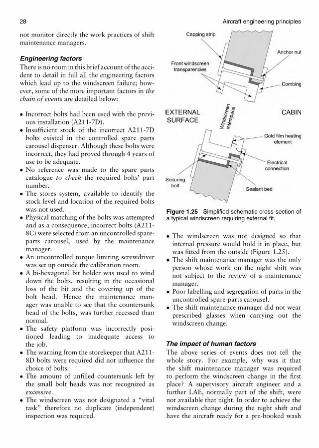
28 Aircraft engineering principles
not monitor directly the work practices of shiftmaintenance managers.
Engineering factorsThere is no room in this brief account of the acci-dent to detail in full all the engineering factorswhich lead up to the windscreen failure; how-ever, some of the more important factors in thechain of events are detailed below:
• Incorrect bolts had been used with the previ-ous installation (A211-7D).
• Insufficient stock of the incorrect A211-7Dbolts existed in the controlled spare partscarousel dispenser. Although these bolts wereincorrect, they had proved through 4 years ofuse to be adequate.
• No reference was made to the spare partscatalogue to check the required bolts’ partnumber.
• The stores system, available to identify thestock level and location of the required boltswas not used.
• Physical matching of the bolts was attemptedand as a consequence, incorrect bolts (A211-8C) were selected from an uncontrolled spare-parts carousel, used by the maintenancemanager.
• An uncontrolled torque limiting screwdriverwas set up outside the calibration room.
• A bi-hexagonal bit holder was used to winddown the bolts, resulting in the occasionalloss of the bit and the covering up of thebolt head. Hence the maintenance man-ager was unable to see that the countersunkhead of the bolts, was further recessed thannormal.
• The safety platform was incorrectly posi-tioned leading to inadequate access tothe job.
• The warning from the storekeeper that A211-8D bolts were required did not influence thechoice of bolts.
• The amount of unfilled countersunk left bythe small bolt heads was not recognized asexcessive.
• The windscreen was not designated a “vitaltask” therefore no duplicate (independent)inspection was required.
Figure 1.25 Simplified schematic cross-section ofa typical windscreen requiring external fit.
• The windscreen was not designed so thatinternal pressure would hold it in place, butwas fitted from the outside (Figure 1.25).
• The shift maintenance manager was the onlyperson whose work on the night shift wasnot subject to the review of a maintenancemanager.
• Poor labelling and segregation of parts in theuncontrolled spare-parts carousel.
• The shift maintenance manager did not wearprescribed glasses when carrying out thewindscreen change.
The impact of human factorsThe above series of events does not tell thewhole story. For example, why was it thatthe shift maintenance manager was requiredto perform the windscreen change in the firstplace? A supervisory aircraft engineer and afurther LAE, normally part of the shift, werenot available that night. In order to achieve thewindscreen change during the night shift andhave the aircraft ready for a pre-booked wash
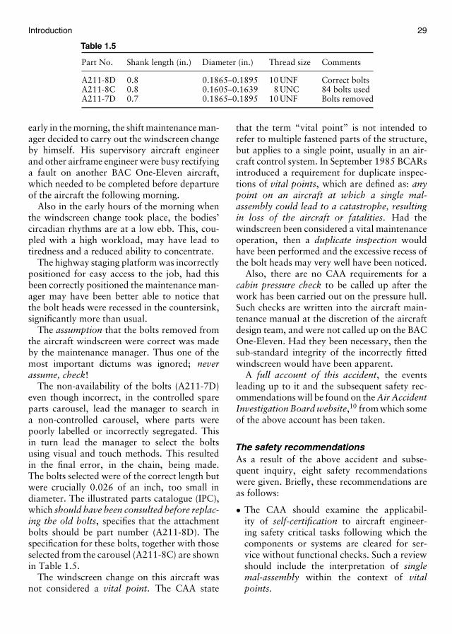
Introduction 29
Table 1.5
Part No. Shank length (in.) Diameter (in.) Thread size Comments
A211-8D 0.8 0.1865–0.1895 10 UNF Correct boltsA211-8C 0.8 0.1605–0.1639 8 UNC 84 bolts usedA211-7D 0.7 0.1865–0.1895 10 UNF Bolts removed
early in the morning, the shift maintenance man-ager decided to carry out the windscreen changeby himself. His supervisory aircraft engineerand other airframe engineer were busy rectifyinga fault on another BAC One-Eleven aircraft,which needed to be completed before departureof the aircraft the following morning.
Also in the early hours of the morning whenthe windscreen change took place, the bodies’circadian rhythms are at a low ebb. This, cou-pled with a high workload, may have lead totiredness and a reduced ability to concentrate.
The highway staging platform was incorrectlypositioned for easy access to the job, had thisbeen correctly positioned the maintenance man-ager may have been better able to notice thatthe bolt heads were recessed in the countersink,significantly more than usual.
The assumption that the bolts removed fromthe aircraft windscreen were correct was madeby the maintenance manager. Thus one of themost important dictums was ignored; neverassume, check!
The non-availability of the bolts (A211-7D)even though incorrect, in the controlled spareparts carousel, lead the manager to search ina non-controlled carousel, where parts werepoorly labelled or incorrectly segregated. Thisin turn lead the manager to select the boltsusing visual and touch methods. This resultedin the final error, in the chain, being made.The bolts selected were of the correct length butwere crucially 0.026 of an inch, too small indiameter. The illustrated parts catalogue (IPC),which should have been consulted before replac-ing the old bolts, specifies that the attachmentbolts should be part number (A211-8D). Thespecification for these bolts, together with thoseselected from the carousel (A211-8C) are shownin Table 1.5.
The windscreen change on this aircraft wasnot considered a vital point. The CAA state
that the term “vital point” is not intended torefer to multiple fastened parts of the structure,but applies to a single point, usually in an air-craft control system. In September 1985 BCARsintroduced a requirement for duplicate inspec-tions of vital points, which are defined as: anypoint on an aircraft at which a single mal-assembly could lead to a catastrophe, resultingin loss of the aircraft or fatalities. Had thewindscreen been considered a vital maintenanceoperation, then a duplicate inspection wouldhave been performed and the excessive recess ofthe bolt heads may very well have been noticed.
Also, there are no CAA requirements for acabin pressure check to be called up after thework has been carried out on the pressure hull.Such checks are written into the aircraft main-tenance manual at the discretion of the aircraftdesign team, and were not called up on the BACOne-Eleven. Had they been necessary, then thesub-standard integrity of the incorrectly fittedwindscreen would have been apparent.
A full account of this accident, the eventsleading up to it and the subsequent safety rec-ommendations will be found on the Air AccidentInvestigation Board website,10 from which someof the above account has been taken.
The safety recommendationsAs a result of the above accident and subse-quent inquiry, eight safety recommendationswere given. Briefly, these recommendations areas follows:
• The CAA should examine the applicabil-ity of self-certification to aircraft engineer-ing safety critical tasks following which thecomponents or systems are cleared for ser-vice without functional checks. Such a reviewshould include the interpretation of singlemal-assembly within the context of vitalpoints.
30 Aircraft engineering principles
• British Airways should review their qualityassurance system and reporting methods, andencourage their engineers to provide feedbackfrom the shop floor.
• British Airways should review the need tointroduce job descriptions and terms of ref-erence for engineering grades, including shiftmaintenance manager and above.
• British Airways should provide the mecha-nism for an independent assessment of stan-dards and conduct an in depth audit into workpractices at Birmingham Airport.
• The CAA should review the purpose andscope of their supervisory visits to airlineoperators.
• The CAA should consider the need for peri-odic training and testing of engineers to ensurecurrency and proficiency.
• The CAA should recognize the need for cor-rective glasses, if prescribed, in associationwith the undertaking of aircraft engineeringactivities.
• The CAA should ensure that, prior to theissue of an air traffic controller (ATC) rating,a candidate undertakes an approved courseof training, that includes the theoretical andpractical handling of emergency situations.
The above recommendations are far reachingand provide an example of human factorsinvolvement, far removed from the direct main-tenance activity, but very much impacting onthe chain of events leading to an accident orserious incident. It is these complex interac-tions that may often lead to maintenance errorsbeing made, with subsequent catastrophic con-sequences.
No matter how sophisticated the policiesand procedures may be, ultimately due to theinfluence of human factors, it is the integrity,attitude, education and professionalism of theindividual aircraft maintenance engineer, thatmatters most, in the elimination of maintenanceerrors.
1.5.7 Concluding remarks
It is hoped that this short introduction intothe aircraft maintenance industry has given you
an insight into the demanding and yet veryrewarding work, offered to aircraft maintenancecertifying staff. No matter at what point youwish to enter the industry, you will find routesand pathways that enable you to progress to anylevel, dependent only, on your own ambitionsand aspirations. The training and education toreach the top of any profession is often long andarduous and aircraft maintenance engineering isno exception!
The subject matter that follows may seem along way removed from the environment por-trayed in this introduction and yet, it formsa vital part of your initial educational devel-opment. Therefore, you should approach thesubjects presented in Chapters 2 and 3 of thisbook, with the same amount of enthusiasm anddedication as you will with the practical activi-ties you find yourself engaged in, when qualifiedto practice your profession.
The non-calculator mathematics, you areabout to meet, may seem deceptively simple.However, do remember that the pass rate is75%, as it is for all your JAR 66 examina-tions. This is likely to be significantly higher thanany other examination pass rate, you may haveencountered up till now. It is, therefore, veryimportant that you become familiar with all thesubject matter contained in the following chap-ters, if you are to be successful in your futureCAA examinations. There are numerous exam-ples, multiple-choice questions and other typesof questions provided to assist you in acquiringthe necessary standard.
References1. CAA-SRG Engineer Standards, papers 3–6 (May 2001).2. Kingston University, Rationale for Aerospace Pro-
grammes (May 2001).3. CAA-SRG, JAR-66 Information for New Applicants
Leaflet 2 Issue 16 (October 2001).4. JAA Administration and Guidance Material (1999).5. JAR-66 Appendix 2 Section 1 Levels (April 2002).6. CAA-SRG JAR-66 Syllabus and Examinations No. 6
(issued 16/10/01).7. CAA Corporate Information, page 1–3. (April 2002).8. JAR-66 Certifying Staff Maintenance, page F1 (April
2002).9. CAP715 An Introduction to Aircraft Maintenance
Human Factors for JAR-66 (January 2002).10. UK Air accident investigation branch (AAIB). www.dft.
gov.uk/stellent/groups/dft_accidentinvest_page.hcsp

P A R T2
Scientific fundamentals

This page intentionally left blank
C h a p t e r
2Mathematics
General introduction
This chapter aims to provide you with a soundfoundation in mathematical principles, whichwill enable you to solve mathematical, scientificand associated aircraft engineering problems atthe mechanic and technician level. Mathematicsis divided into two major parts: Non-calculatormathematics, which covers all of the mathemat-ics laid down in Joint Aviation Requirements(JAR) 66 Module 1, up to the level appropri-ate for aircraft maintenance category B certify-ing technicians. The other part of mathematicsis Further mathematics (Chapter 3), which inthe opinion of the authors, is necessary fora thorough understanding of the physics andelectrical principles that follow. A second objec-tive of Further mathematics is to provide themathematical base necessary for further aca-demic and professional progression, particularlyfor those individuals wishing to become Incor-porated Engineers, after successfully obtainingtheir category B license.
We start with some elementary arithmetic. Inparticular, we review the concepts of numberand the laws that need to be followed, when car-rying out arithmetic operations, e.g. addition,subtraction, multiplication and division. Theimportant concept of arithmetic estimates andestimation techniques involving various formsof number are also covered. While revising thefundamental principles of number, we considerboth explicit numbers and literal numbers (let-ters), in order to aid our understanding of notonly arithmetic operations, but also the alge-braic operations that will follow later. Decimalnumbers and the powers of 10 are then con-sidered, after which fractional numbers and themanipulation of fractions are covered.
The algebraic content of JAR 66 Module 1is introduced with the study of powers andexponents (indices) of numbers. This, together
with your previous knowledge of fractions andfractional numbers, will provide you with thetools necessary to manipulate algebraic expres-sions and equations. The essential skill of trans-position of formulae is also covered. This willbe a particularly useful mathematical tool, whenyou study your physics and electrical principles.We finish our study of algebra by consider-ing binary and other number systems and theirapplication to simple logic circuits.
In our study of geometry and trigonometry,we start by looking at the methods used for thegraphical solution of equations and other func-tions. This section clearly lays out the idea ofgraphical axes and scales. We then consider thenature and use of the trigonometric ratios andthe solution of right-angled triangles and the cir-cle. The nature and use of rectangular and polarco-ordinate representation systems, for findingbearings and angles of elevation and depressionare then considered. We finish our study of non-calculator mathematics with a study of the moreimportant theorems of the circle, together withsome geometric constructions, considered par-ticularly useful to solve engineering problems,in particular, as an aid to engineering drawingand marking out.
In our Further mathematics (Chapter 3) webuild on our initial study of algebra by consid-ering more complex algebraic and logarithmicexpressions, functions and formulae. We willuse our basic knowledge of graphs to repre-sent more complex algebraic and logarithmicfunctions and to solve equations and engineer-ing problems, which involve these functions. Inaddition, we will briefly introduce the conceptof complex numbers, which will be found par-ticularly valuable for those wishing to pursue anavionic pathway.
Our further study of trigonometry willinclude the use of trigonometric ratios to solveengineering problems involving measurement.
34 Aircraft engineering principles
Next, we introduce and use a variety of statis-tical methods to gather, manipulate and displayscientific and engineering data. We will thenconsider the ways in which the elementary rulesof calculus arithmetic may be used to solveproblems involving simple differentiation andintegration of algebraic and trigonometric func-tions. Finally, we use the calculus to solve someelementary engineering problems, which involverates of change and the summation of areas andvolumes.
In order to aid your understanding of mathe-matics, you will find numerous fully workedexamples and test your understanding exercises,spread throughout this chapter. In addition, typ-ical example JAR 66 license questions are givenat the end of this chapter.
Important note: Only very familiar units, suchas mass, weight, pressure, length, area and vol-ume are used in this part of the mathematics.The detailed study of units appears in the chap-ters on physics and electrical principles (Chap-ters 4 and 5, respectively), where their natureand use is fully explained. Some of the JAR66 questions, found at the end of this chapter,require the reader to have some understandingof units, which may be gained by studying othersections of the book (in particular, Chapter 4).
NON-CALCULATOR MATHEMATICS
2.1 Introduction
As mentioned earlier, this part of the mathe-matics has been written explicitly to cover all ofthe syllabus content laid down in JAR 66 Mod-ule 1. It can thus be studied independently, bythose only wishing to gain the knowledge neces-sary to pass the Civil Aviation Authority (CAA)examination for this module.
However, in order to offer the best chanceof success in the JAR 66 physics and electri-cal and electronic principles modules and asa preparation for further study, the authors,strongly recommend that you should alsostudy the further mathematics contained inChapter 3.
2.2 Arithmetic
2.2.1 Numbers and symbols
It is generally believed that our present num-ber system began with the use of the naturalnumbers, such as 1, 2, 3, 4, . . . . These wholenumbers, known as the positive integers, wereused primarily for counting. However, as timewent on, it became apparent that whole num-bers could not be used for defining certainmathematical quantities. For example, a periodin time might be between 3 and 4 days or thearea of a field might be between 2 and 3 acres(or whatever unit of measure was used at thetime). So the positive fractions were introduced,e.g. 1
2 , 14 and 3
4 . These two groups of numbers,the positive integers and the positive fractions,constitute what we call the positive rationalnumbers. Thus, 711 is an integer or whole num-ber, 1
4 is a positive fraction and 234 35 is a rational
number. In fact a rational number is any num-ber that can be expressed as the quotient of twointegers, i.e. any number that can be written inthe form a/b where a and b represent any inte-gers. Thus 2
5 , 89 and 1 are all rational numbers.
The number 1 can be represented by the quo-tient 1
1 = 1, in fact any number divided by itselfmust always be equal to 1.
The natural numbers are positive integers, butsuppose we wish to subtract a larger naturalnumber from a smaller natural number, e.g. 10subtracted from 7, we obviously obtain a num-ber which is less than zero, i.e. 7 − 10 = −3. Soour idea of numbers must be enlarged to includenumbers less than zero called negative numbers.The number zero (0) is unique, it is not a naturalnumber because all natural numbers representpositive integer values, i.e. numbers above zeroand quite clearly from what has been said, itis not a negative number either. It sits uniquelyon its own and must be added to our numbercollection.
Key pointThe natural numbers are known as positiveintegers.
Mathematics 35
So to the natural numbers (positive integers)we have added negative integers, the conceptof zero, positive rational numbers and nega-tive natural numbers. What about numbers like√
2? This is not a rational number because itcannot be represented by the quotient of twointegers. So yet another class of number needs tobe included, the irrational or non-rational num-bers. Together all, the above kinds of numbersconstitute the broad class of numbers known asreal numbers.
They include positive and negative terminat-ing and non-terminating decimals (e.g. ± 1
9 =±0.1111 . . . , 0.48299999, ±2.5, 1.73205 . . .).The real numbers are so called to distinguishthem from others, such as imaginary or com-plex numbers, the latter may be made up ofboth real and imaginary number parts. Com-plex numbers will not be considered during ourstudy of mathematics.
Key pointA rational number is any number that can beexpressed as the quotient of two integers, i.e. a/bwhere a and b are any two integers.
Although we have mentioned negative num-bers, we have not considered their arithmeticmanipulation. All positive and negative num-bers are referred to as signed numbers and theyobey the arithmetic laws of sign. Before we con-sider these laws, let us first consider what wemean by signed numbers.
Conventional representation of signed num-bers is shown below, with zero at the midpoint.Positive numbers are conventionally shown tothe right of zero and negative numbers tothe left:
· · · −4 −3 −2 −1 0 +1 +2 +3 +4 · · ·
The number of units a point is from zero,regardless of its direction, is called the abso-lute value of the number corresponding to thepoint on the above number system when pointsare drawn to scale. Thus the absolute value of apositive number, or of zero, is the number itself.While the absolute value of a negative number is
the number with its sign changed. For example,the absolute value of +10 is 10 and the abso-lute value of −10 is also 10. Now the absolutevalue of any number n is represented by the sym-bol |n|. Thus |+24| means the absolute value of+24. Which is larger, |+3| or |−14|?
I hope you said |−14| because its absolutevalue is 14, while that of |+3| is 3 and of course14 is larger than 3. We are now ready to considerthe laws of signs.
Key pointThe absolute value of any number n is alwaysits positive value or modulus and is representedby |n|.
The laws of signsYou are probably already familiar with theselaws, here they are:
First law: To add two numbers with likesigns, add their absolute values and prefix theircommon sign to the result.
This law works for ordinary arithmetic num-bers and simply defines what we have alwaysdone in arithmetic addition.
For example, 3 + 4 = 7 or in full (+3) +(+4) = +7.
After the introduction of the negative num-bers, the unsigned arithmetic numbers becamethe positive numbers, as illustrated above. Sonow all numbers may be considered either pos-itive or negative, and the laws of signs apply tothem all.
Does the above law apply to the addition oftwo negative numbers? From ordinary arith-metic we know that (−7) + (−5) = −12. Thisagain obeys the first law of signs, becausewe add their absolute value and prefix theircommon sign.
Second law: To add two signed numbers withunlike signs, subtract the smaller absolute valuefrom the larger and prefix the sign of the numberwith the larger absolute value to the results.
So following this rule, we get for example:
5+(−3) = 2; −12+9 = −3; 6+(−11) = −5
and so on.
36 Aircraft engineering principles
The numbers written without signs are, ofcourse, positive numbers. Notice that bracketshave been removed when not necessary.
Third law: To subtract one signed numberfrom another, change the sign of the number tobe subtracted and follow the rules for addition.
For example, if we subtract 5 from −3, weget −3 − (+5) = −3 + (−5) = −8.
Now what about the multiplication and divi-sion of negative and positive numbers, so as notto labour the point the rules for these operationsare combined in our fourth and final law.
Fourth law: To multiply (or divide) one signednumber by another, multiply (or divide) theirabsolute values; then, if the numbers have likesigns, prefix the plus sign to the result; if theyhave unlike signs, prefix the minus sign to theresult.
Therefore, applying this rule to the multipli-cation of two positive numbers, e.g. 3 × 4 = 12,12 × 8 = 96 . . . and so on, which of course, issimple arithmetic! Now applying the rule to themultiplication of mixed sign numbers we gete.g. −3 × 4 = −12, 12 × (−8) = −96 . . . and soon. We can show, equally well, that the aboverule yields similar results for division.
Example 2.1
Apply the fourth law to the following arithmeticproblems and determine the arithmetic result:(a) (−4)(−3)(−7) = ? (b) 14/−2 = ?(c) 5(−6)(−2) = ? (d) −22/−11 = ?
(a) In this example we apply the fourth lawtwice, (−4)(−3) = 12 (like signs) and so12(−7) = −84.
(b) 14/–2 applying the third law for unlike signsimmediately gives −7, the correct result.
(c) Again applying the third law twice. 5(−6) =−30 (unlike signs) and (−30)(−2) = 60.
(d) −22/−11 applying the third law for like signgives 2, the correct result.
The use of symbolsWe have introduced earlier the concept of sym-bols to represent numbers when we definedrational numbers where the letters a and bwere used to represent any integer. Look at
the symbols below, do they represent the samenumber?
IX; 9; nine; +√81
I hope you answered yes, since each expression isa perfectly valid way of representing the positiveinteger 9. In algebra we use letters to repre-sent Arabic numerals such numbers are calledgeneral numbers or literal numbers, as distin-guished from explicit numbers like 1, 2, 3, etc.Thus a literal number is simply a number repre-sented by a letter, instead of a numeral. Literalnumbers are used to state algebraic rules, lawsand formulae; these statements being made inmathematical sentences called equations.
If a is a positive integer and b is 1, what isa/b? I hope you were able to see that a/b = a.Any number divided by 1 is always itself. Thus,a/1 = a, c/1 = c, 45.6/1 = 45.6.
Suppose a is again any positive integer, butb is 0. What is the value of a/b? What we areasking is what is the value of any positive inte-ger divided by zero? Well the answer is that wereally do not know! The value of the quotienta/b, if b = 0, is not defined in mathematics. Thisis because there is no such quotient that meetsthe conditions required of quotients. For exam-ple, you know that to check the accuracy of adivision problem, you can multiply the quotientby the divisor to get the dividend. For example,if 21/7 = 3, then 7 is the divisor, 21 is the div-idend and 3 is the quotient and so 3 × 7 = 21,as expected. So, if 17/0 were equal to 17, then17 × 0 should again equal 17 but it does not!Or, if 17/0 were equal to zero, then 0 × 0 shouldequal 17 but again it does not. Any numbermultiplied by zero is always zero. Therefore,division of any number by zero (as well as zerodivided by zero) is excluded from mathematics.If b = 0, or if both a and b are zero, then a/b ismeaningless.
Key pointDivision by zero is not defined in mathematics.
When multiplying literal numbers together wetry to avoid the multiplication sign (×), this isbecause it can be easily mistaken for the letter x.

Mathematics 37
Thus, instead of writing a × b for the prod-uct of two general numbers, we write a · b (thedot notation for multiplication) or more usuallyjust ab to indicate the product of two generalnumbers a and b.
Example 2.2
If we let the letter n stand for any real num-ber, what does each of the following expressionsequal?(a) n/n = ? (b) n × 0 = ? (c) n × 1 = ?(d) n + 0 = ? (e) n − 0 = ? (f) n − n = ?(g) n/0 = ?
(a) n/n = 1, i.e. any number divided by itself isequal to 1.
(b) n × 0 = 0, any number multiplied by zero isitself zero.
(c) n × 1 = n, any number multiplied or dividedby 1 is itself.
(d) n + 0 = n, the addition of zero to any numberwill not alter that number.
(e) n − 0 = n, the subtraction of zero from anynumber will not alter that number.
(f) n − n = 0, subtraction of any number fromitself will always equal zero.
(g) n/0, division by zero is not defined inmathematics.
The commutative, associative anddistributive lawsWe all know that 6 × 5 = 30 and 5 × 6 = 30, sois it true that when multiplying any two num-bers together, the result is the same no matterwhat the order? The answer is yes. The aboverelationship may be stated as:
The product of two real numbers is the same nomatter in what order they are multiplied. Thatis, ab = ba this is known as the commutativelaw of multiplication.
If three or more real numbers are multipliedtogether, the order in which they are multi-plied still makes no difference to the product.For example, 3 × 4 × 5 = 60 and 5 × 3 × 4 = 60.This relationship may be stated formally as:
The product of three or more numbers isthe same no matter in what manner they are
grouped. That is, a(bc) = (ab)c; this is knownas the associative law of multiplication.
These laws may seem ridiculously simple, yetthey form the basis of many algebraic tech-niques, which you will be using later!
We also have commutative and associativelaws for addition of numbers, which by nowwill be quite obvious to you, here they are:
The sum of two numbers is the same no mat-ter in what order they are added. That is,a + b = b + a. This is known as the commutativelaw of addition.
The sum of three or more numbers is the sameno matter in what manner they are grouped.That is, (a + b) + c = a + (b + c). This is knownas the associative law of addition.
You may be wondering where the laws arefor subtraction. Well you have already coveredthese when we considered the laws of signs. Inother words, the above laws are valid no matterwhether or not the number is positive or neg-ative. So, for example, −8 + (16 − 5) = 3 and(−8 + 16) − 5 = 3
In order to complete our laws we need to con-sider the following problem: 4(5 + 6) = ? Wemay solve this problem in one of two ways,firstly by adding the numbers inside the bracketsand then multiplying the result by 4, this gives:4(11) = 44. Alternatively, we may multiply outthe bracket as follows: (4 × 5) + (4 × 6) = 20 +24 = 44. Thus, whichever method we choose,the arithmetic result is the same. This result istrue in all cases, no matter how many numbersare contained within the brackets!
So in general, using literal numbers we have:
a(b + c) = ab + ac
This is the distributive law. In words, it is rathercomplicated:
The distributive law states that: the product ofa number by the sum of two or more numbersis equal to the sum of the products of the firstnumber by each of the numbers of the sum.
Now, perhaps you can see the power of alge-bra in representing this law, it is a lot easier toremember than the wordy explanation!
38 Aircraft engineering principles
Remember that the distributive law is validno matter how many numbers are contained inthe brackets, and no matter whether the signconnecting them is a plus or minus. As you willsee later, this law is one of the most useful andconvenient rules for manipulating formulae andsolving algebraic expressions and equations.
Key pointThe commutative, associative and distributivelaws of numbers are valid for both positive andnegative numbers.
Example 2.3
If a = 4, b = 3 and c = 7, does
a(b − c) = ab − ac
The above expression is just the distributive law,with the sign of one number within the bracket,changed. This of course is valid since the signconnecting the numbers within the bracket maybe a plus or minus. Nevertheless, we will substi-tute the arithmetic values in order to check thevalidity of the expression.
Then:
4(3 − 7) = 4(3) − 4(7)
4(−4) = 12 − 28
−16 = −16
So, our law works irrespective of whether thesign joining the numbers is positive or negative.
Long multiplicationIt is assumed that the readers of this book will befamiliar with long multiplication and long divi-sion. However, with the arrival of the calculatorthese techniques are seldom used and quicklyforgotten. CAA license examinations, for cate-gory A and B certifying staff, do not allow theuse of calculators; so these techniques will needto be revised. One method of long multiplica-tion is given below. Long division will be foundin Section 2.3, where the technique is used forboth explicit and literal numbers!
Suppose we wish to multiply 35 by 24,i.e. 24 × 35. You may be able to work this out
in your head; we will use a particular method oflong multiplication to obtain the result.
The numbers are first set out, one under the
other, like this:3524
where the right-hand integers
5 and 4 are the units and the left-hand integersare the tens, i.e. 3 × 10 and 2 × 10. We multi-ply the tens on the bottom row by the tens andunits on the top row. So to start this process, weplace a nought in the units column underneaththe bottom row, then multiply the 2 by 5 to get1 × 10, carry the 1 into the tens column and addit to the product 2 × 3; i.e.:
35
24
0
then multiply the 2 ×5 = 10, put in the noughtof the ten and carry the one
35
24100
now multiply 2 × 3 = 6 (the tens) and add thecarried ten to it, to give 7, then
35
24
700
We now multiply the 4 units by 35. That is 4 ×5 = 20 put down the nought carry 2 into the tencolumn, then multiply the 4 units by the 3 tensor, 4 × 3 = 12 and add to it the 2 we carried togive 140, i.e.:
35
24700
140
All that remains for us to do now is add 700 to140 to get the result by long multiplication, i.e.:
35
24700
140840

Mathematics 39
So 35 × 24 = 840. This may seem a rather long-winded way of finding this product. You shouldadopt the method you are familiar with.
This process can be applied to the multiplica-tion of numbers involving hundreds, thousandsand decimal fractions, it works for them all!
For example, 3.5 × 2.4 could be set out in thesame manner as above, but the columns wouldbe for tenths and units, instead of units and tens.Then we would get:
3.5
2.47.0
1.48.4
Notice that in this case the decimal place hasbeen shifted two places to the left. If you do notunderstand why this has occurred you shouldstudy carefully the section on decimals andthe powers of 10 that follows.
Example 2.4
Multiply: (1) 350 × 25 (2) 18.8 × 1.25In both the cases, the multiplication is set out
as shown before.
1. With these figures, hundreds, tens and unitsare involved. You will find it easier to mul-tiply it by the smallest or the least complexnumber.
35025
Now we multiply by 25 in a similar
manner to the previous example.
Multiply first by the 2 × 10, which meansplacing a nought in the units column first. Thenmultiply 2 × 0, putting down below the line theresult, i.e. zero. Then: 2 × 5 = 1 × 10, again putdown the nought and carry the single hundred.So we get:
350
25100
We continue the process by multiplying 2 bythe 3 hundreds and adding the single hun-dred or 2 × 3 + 1 = 7 to give 7000 (remembering
the nought, we first put down). This part ofthe process was the equivalent of multiplying350 × 20 = 7000. So we get:
350
257000
We now multiply the number 350 by 5, where5 × 0 = 0; put it down below the line; 5 × 5 = 25put down the 5 and carry the 2. Finally,5 × 3 = 15, add the 2 you have just carried togive 17. So the total number below the 7000 is1750 = 350 × 5 and we get:
350
257000
1750
Finally we add the rows below the line to givethe result, i.e.:
350
257000
17508750
Then 350 × 25 = 8750.
2. For this example the multiplication is laid outin full, without explanation, just make sureyou can follow the steps.
18.8
1.2518800
3760
94023.500
Then, 18.8 × 1.25 = 23.5.Note that the decimal point is positioned three
places to the left, since there are three integersto the right of the decimal points.
You should now attempt the following exer-cise, without the aid of a calculator!
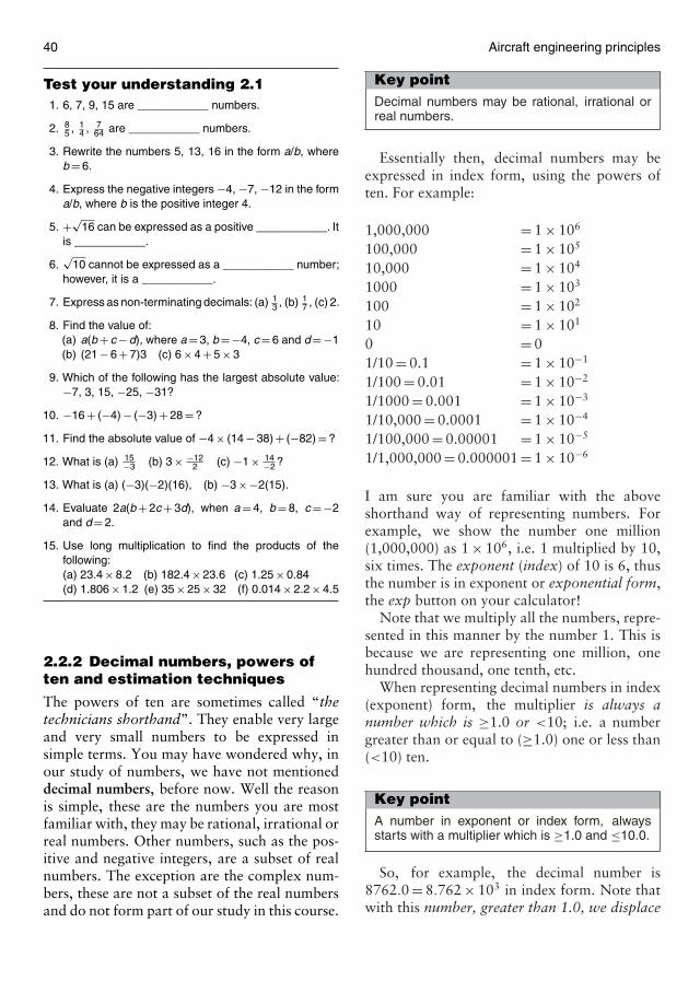
40 Aircraft engineering principles
Test your understanding 2.11. 6, 7, 9, 15 are ___________ numbers.
2. 85 , 1
4 , 764 are ___________ numbers.
3. Rewrite the numbers 5, 13, 16 in the form a/b, whereb = 6.
4. Express the negative integers −4, −7, −12 in the forma/b, where b is the positive integer 4.
5. +√16 can be expressed as a positive ___________. It
is ___________.
6.√
10 cannot be expressed as a ___________ number;however, it is a ___________.
7. Express as non-terminating decimals: (a) 13 , (b) 1
7 , (c) 2.
8. Find the value of:(a) a(b + c − d), where a = 3, b = −4, c = 6 and d = −1(b) (21 − 6 + 7)3 (c) 6 × 4 + 5 × 3
9. Which of the following has the largest absolute value:−7, 3, 15, −25, −31?
10. −16 + (−4) − (−3) + 28 = ?
11. Find the absolute value of −4 × (14 − 38) + (−82) = ?
12. What is (a) 15−3 (b) 3 × −12
2 (c) −1 × 14−2 ?
13. What is (a) (−3)(−2)(16), (b) −3 × −2(15).
14. Evaluate 2a(b + 2c + 3d), when a = 4, b = 8, c = −2and d = 2.
15. Use long multiplication to find the products of thefollowing:(a) 23.4 × 8.2 (b) 182.4 × 23.6 (c) 1.25 × 0.84(d) 1.806 × 1.2 (e) 35 × 25 × 32 (f) 0.014 × 2.2 × 4.5
2.2.2 Decimal numbers, powers often and estimation techniques
The powers of ten are sometimes called “thetechnicians shorthand”. They enable very largeand very small numbers to be expressed insimple terms. You may have wondered why, inour study of numbers, we have not mentioneddecimal numbers, before now. Well the reasonis simple, these are the numbers you are mostfamiliar with, they may be rational, irrational orreal numbers. Other numbers, such as the pos-itive and negative integers, are a subset of realnumbers. The exception are the complex num-bers, these are not a subset of the real numbersand do not form part of our study in this course.
Key pointDecimal numbers may be rational, irrational orreal numbers.
Essentially then, decimal numbers may beexpressed in index form, using the powers often. For example:
1,000,000 = 1 × 10⁶
100,000 = 1 × 10⁵
10,000 = 1 × 10⁴
1000 = 1 × 10³
100 = 1 × 10²
10 = 1 × 101
0 = 01/10 = 0.1 = 1 × 10⁻¹
1/100 = 0.01 = 1 × 10⁻²
1/1000 = 0.001 = 1 × 10⁻³
1/10,000 = 0.0001 = 1 × 10⁻⁴
1/100,000 = 0.00001 = 1 × 10⁻⁵
1/1,000,000 = 0.000001 = 1 × 10⁻⁶
I am sure you are familiar with the aboveshorthand way of representing numbers. Forexample, we show the number one million(1,000,000) as 1 × 10⁶, i.e. 1 multiplied by 10,six times. The exponent (index) of 10 is 6, thusthe number is in exponent or exponential form,the exp button on your calculator!
Note that we multiply all the numbers, repre-sented in this manner by the number 1. This isbecause we are representing one million, onehundred thousand, one tenth, etc.
When representing decimal numbers in index(exponent) form, the multiplier is always anumber which is ≥1.0 or <10; i.e. a numbergreater than or equal to (≥1.0) one or less than(<10) ten.
Key pointA number in exponent or index form, alwaysstarts with a multiplier which is ≥1.0 and ≤10.0.
So, for example, the decimal number is8762.0 = 8.762 × 10³ in index form. Note thatwith this number, greater than 1.0, we displace
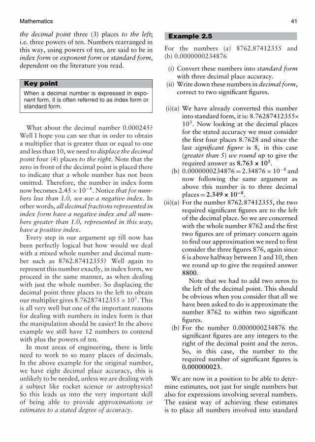
Mathematics 41
the decimal point three (3) places to the left;i.e. three powers of ten. Numbers rearranged inthis way, using powers of ten, are said to be inindex form or exponent form or standard form,dependent on the literature you read.
Key pointWhen a decimal number is expressed in expo-nent form, it is often referred to as index form orstandard form.
What about the decimal number 0.000245?Well I hope you can see that in order to obtaina multiplier that is greater than or equal to oneand less than 10, we need to displace the decimalpoint four (4) places to the right. Note that thezero in front of the decimal point is placed thereto indicate that a whole number has not beenomitted. Therefore, the number in index formnow becomes 2.45 × 10⁻⁴. Notice that for num-bers less than 1.0, we use a negative index. Inother words, all decimal fractions represented inindex form have a negative index and all num-bers greater than 1.0, represented in this way,have a positive index.
Every step in our argument up till now hasbeen perfectly logical but how would we dealwith a mixed whole number and decimal num-ber such as 8762.87412355? Well again torepresent this number exactly, in index form, weproceed in the same manner, as when dealingwith just the whole number. So displacing thedecimal point three places to the left to obtainour multiplier gives 8.76287412355 × 10³. Thisis all very well but one of the important reasonsfor dealing with numbers in index form is thatthe manipulation should be easier! In the aboveexample we still have 12 numbers to contendwith plus the powers of ten.
In most areas of engineering, there is littleneed to work to so many places of decimals.In the above example for the original number,we have eight decimal place accuracy, this isunlikely to be needed, unless we are dealing witha subject like rocket science or astrophysics!So this leads us into the very important skillof being able to provide approximations orestimates to a stated degree of accuracy.
Example 2.5
For the numbers (a) 8762.87412355 and(b) 0.0000000234876
(i) Convert these numbers into standard formwith three decimal place accuracy.
(ii) Write down these numbers in decimal form,correct to two significant figures.
(i)(a) We have already converted this numberinto standard form, it is: 8.76287412355×10³. Now looking at the decimal placesfor the stated accuracy we must considerthe first four places 8.7628 and since thelast significant figure is 8, in this case(greater than 5) we round up to give therequired answer as 8.763 × 10³.
(b) 0.0000000234876 = 2.34876 × 10⁻⁸ andnow following the same argument asabove this number is to three decimalplaces = 2.349 × 10⁻⁸.
(ii)(a) For the number 8762.87412355, the tworequired significant figures are to the leftof the decimal place. So we are concernedwith the whole number 8762 and the firsttwo figures are of primary concern againto find our approximation we need to firstconsider the three figures 876, again since6 is above halfway between 1 and 10, thenwe round up to give the required answer8800.
Note that we had to add two zeros tothe left of the decimal point. This shouldbe obvious when you consider that all wehave been asked to do is approximate thenumber 8762 to within two significantfigures.
(b) For the number 0.0000000234876 thesignificant figures are any integers to theright of the decimal point and the zeros.So, in this case, the number to therequired number of significant figures is0.000000023.
We are now in a position to be able to deter-mine estimates, not just for single numbers butalso for expressions involving several numbers.The easiest way of achieving these estimatesis to place all numbers involved into standard
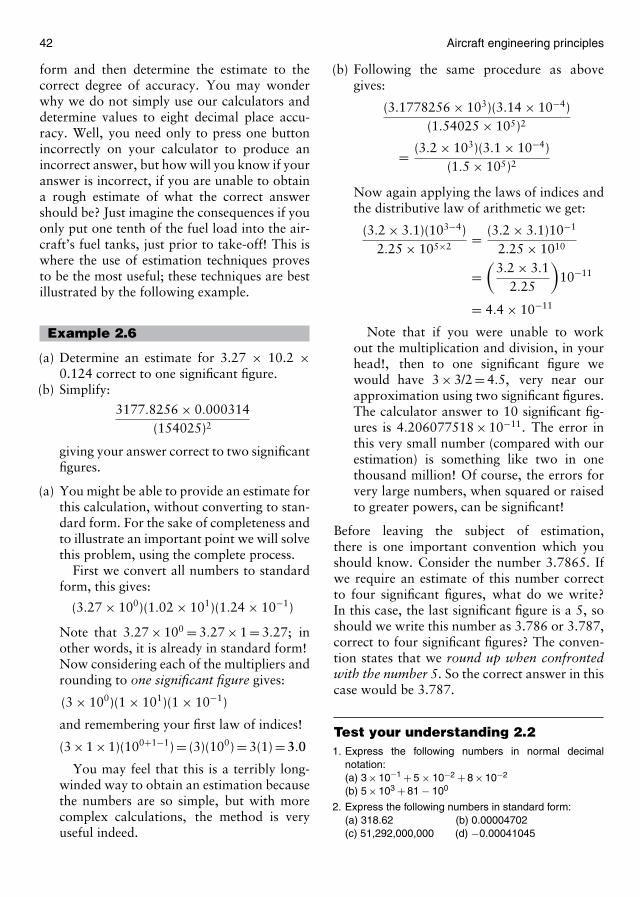
42 Aircraft engineering principles
form and then determine the estimate to thecorrect degree of accuracy. You may wonderwhy we do not simply use our calculators anddetermine values to eight decimal place accu-racy. Well, you need only to press one buttonincorrectly on your calculator to produce anincorrect answer, but how will you know if youranswer is incorrect, if you are unable to obtaina rough estimate of what the correct answershould be? Just imagine the consequences if youonly put one tenth of the fuel load into the air-craft’s fuel tanks, just prior to take-off! This iswhere the use of estimation techniques provesto be the most useful; these techniques are bestillustrated by the following example.
Example 2.6
(a) Determine an estimate for 3.27 × 10.2 ×0.124 correct to one significant figure.
(b) Simplify:
3177.8256 × 0.000314(154025)2
giving your answer correct to two significantfigures.
(a) You might be able to provide an estimate forthis calculation, without converting to stan-dard form. For the sake of completeness andto illustrate an important point we will solvethis problem, using the complete process.
First we convert all numbers to standardform, this gives:
(3.27 × 100)(1.02 × 101)(1.24 × 10⁻¹)
Note that 3.27 × 100 = 3.27 × 1 = 3.27; inother words, it is already in standard form!Now considering each of the multipliers androunding to one significant figure gives:
(3 × 100)(1 × 101)(1 × 10⁻¹)
and remembering your first law of indices!
(3 × 1 × 1)(100+1−1) = (3)(100) = 3(1) = 3.0
You may feel that this is a terribly long-winded way to obtain an estimation becausethe numbers are so simple, but with morecomplex calculations, the method is veryuseful indeed.
(b) Following the same procedure as abovegives:
(3.1778256 × 10³)(3.14 × 10⁻⁴)(1.54025 × 10⁵)2
= (3.2 × 10³)(3.1 × 10⁻⁴)(1.5 × 10⁵)2
Now again applying the laws of indices andthe distributive law of arithmetic we get:
(3.2 × 3.1)(103−4)2.25 × 105×2
= (3.2 × 3.1)10−1
2.25 × 1010
=(
3.2 × 3.12.25
)10−11
= 4.4 × 10⁻¹¹
Note that if you were unable to workout the multiplication and division, in yourhead!, then to one significant figure wewould have 3 × 3/2 = 4.5, very near ourapproximation using two significant figures.The calculator answer to 10 significant fig-ures is 4.206077518 × 10⁻¹¹. The error inthis very small number (compared with ourestimation) is something like two in onethousand million! Of course, the errors forvery large numbers, when squared or raisedto greater powers, can be significant!
Before leaving the subject of estimation,there is one important convention which youshould know. Consider the number 3.7865. Ifwe require an estimate of this number correctto four significant figures, what do we write?In this case, the last significant figure is a 5, soshould we write this number as 3.786 or 3.787,correct to four significant figures? The conven-tion states that we round up when confrontedwith the number 5. So the correct answer in thiscase would be 3.787.
Test your understanding 2.21. Express the following numbers in normal decimal
notation:(a) 3 × 10⁻¹ + 5 × 10⁻² + 8 × 10⁻²
(b) 5 × 10³ + 81 − 100
2. Express the following numbers in standard form:(a) 318.62 (b) 0.00004702(c) 51,292,000,000 (d) −0.00041045
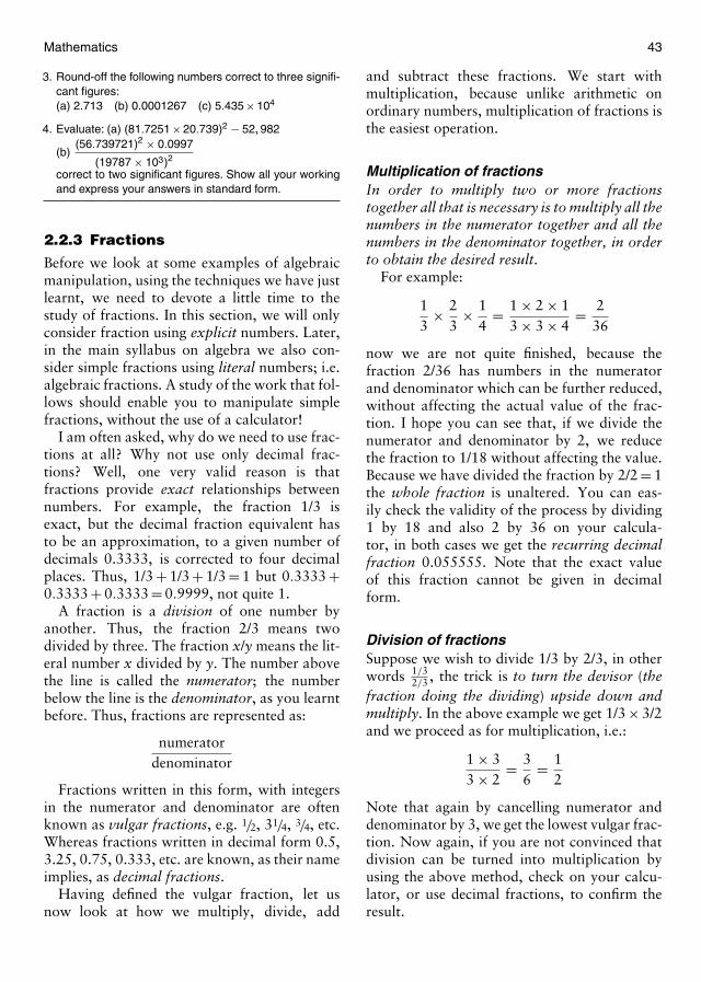
Mathematics 43
3. Round-off the following numbers correct to three signifi-cant figures:(a) 2.713 (b) 0.0001267 (c) 5.435 × 10⁴
4. Evaluate: (a) (81.7251 × 20.739)2 − 52, 982
(b)(56.739721)2 × 0.0997
(19787 × 103)2
correct to two significant figures. Show all your workingand express your answers in standard form.
2.2.3 Fractions
Before we look at some examples of algebraicmanipulation, using the techniques we have justlearnt, we need to devote a little time to thestudy of fractions. In this section, we will onlyconsider fraction using explicit numbers. Later,in the main syllabus on algebra we also con-sider simple fractions using literal numbers; i.e.algebraic fractions. A study of the work that fol-lows should enable you to manipulate simplefractions, without the use of a calculator!
I am often asked, why do we need to use frac-tions at all? Why not use only decimal frac-tions? Well, one very valid reason is thatfractions provide exact relationships betweennumbers. For example, the fraction 1/3 isexact, but the decimal fraction equivalent hasto be an approximation, to a given number ofdecimals 0.3333, is corrected to four decimalplaces. Thus, 1/3 + 1/3 + 1/3 = 1 but 0.3333 +0.3333 + 0.3333 = 0.9999, not quite 1.
A fraction is a division of one number byanother. Thus, the fraction 2/3 means twodivided by three. The fraction x/y means the lit-eral number x divided by y. The number abovethe line is called the numerator; the numberbelow the line is the denominator, as you learntbefore. Thus, fractions are represented as:
numeratordenominator
Fractions written in this form, with integersin the numerator and denominator are oftenknown as vulgar fractions, e.g. 1/2, 31/4, 3/4, etc.Whereas fractions written in decimal form 0.5,3.25, 0.75, 0.333, etc. are known, as their nameimplies, as decimal fractions.
Having defined the vulgar fraction, let usnow look at how we multiply, divide, add
and subtract these fractions. We start withmultiplication, because unlike arithmetic onordinary numbers, multiplication of fractions isthe easiest operation.
Multiplication of fractionsIn order to multiply two or more fractionstogether all that is necessary is to multiply all thenumbers in the numerator together and all thenumbers in the denominator together, in orderto obtain the desired result.
For example:
13
× 23
× 14
= 1 × 2 × 13 × 3 × 4
= 236
now we are not quite finished, because thefraction 2/36 has numbers in the numeratorand denominator which can be further reduced,without affecting the actual value of the frac-tion. I hope you can see that, if we divide thenumerator and denominator by 2, we reducethe fraction to 1/18 without affecting the value.Because we have divided the fraction by 2/2 = 1the whole fraction is unaltered. You can eas-ily check the validity of the process by dividing1 by 18 and also 2 by 36 on your calcula-tor, in both cases we get the recurring decimalfraction 0.055555. Note that the exact valueof this fraction cannot be given in decimalform.
Division of fractionsSuppose we wish to divide 1/3 by 2/3, in otherwords 1/3
2/3 , the trick is to turn the devisor (thefraction doing the dividing) upside down andmultiply. In the above example we get 1/3 × 3/2and we proceed as for multiplication, i.e.:
1 × 33 × 2
= 36
= 12
Note that again by cancelling numerator anddenominator by 3, we get the lowest vulgar frac-tion. Now again, if you are not convinced thatdivision can be turned into multiplication byusing the above method, check on your calcu-lator, or use decimal fractions, to confirm theresult.

44 Aircraft engineering principles
Addition of fractionsTo add fractions, we are required to use some ofour previous knowledge concerning factors. Inparticular, we need to determine the lowest com-mon multiple (LCM) of two or more numbers.That is, the smallest possible number which isa common multiple of two or more numbers.For example, 10 is a multiple of 5, 30 is a com-mon multiple of 5 and 3, but 15 is the LCM of5 and 3. Thus, 15 is the smallest possible num-ber which is exactly divisible by both 5 and 3.What is the LCM of 2, 3 and 4? One multipleis found simply as 2 × 3 × 4 = 24, but is this thelowest? Well, of course, it is not. The number4 is exactly divisible by 2, so is the number 24,to give 12 which is the LCM, well 12 is divisibleby the numbers 2, 3 and 4, but the number 6 isnot. So, 12 is the LCM of the three numbers 2,3 and 4.
So when adding fractions, why may it be nec-essary to find the LCM? We will illustrate theprocess by example.
Example 2.7
Add the following fractions:(a) 1
3 + 14 (b) 2
5 + 13 + 1
2
(a) We first determine the LCM of the numbersin the denominator. In this case the lowestnumber divisible by both 3 and 4 is 12. So12 is the LCM.
Now remembering that the whole idea ofadding fractions together is to create onefraction as their sum then we place the LCMbelow the denominators of all the fractionswe wish to add. In this case we get:
13 + 1
4
12
we now divide 3 into 12 to give 4 and thenmultiply 4 by the number in the numeratorof the fraction 1/3, in this case it is 1; so4 × 1 = 4, which is the result, that will nowbe placed above the 12. In a similar way, wenow consider the fraction 1/4 to be added,where 4 into 12 is 3 and 3 × 1 = 3. Thus, we
now have the numbers to be added as:
13 + 1
4
12= 4 + 3
12= 7
12
make sure you follow the rather complexlogic to obtain the numbers 4 and 3 abovethe denominator 12, as shown above. Againjust to remind you, let us consider the firstfraction to be added 1/3. We take the denom-inator of this fraction 3 and divide it into ourLCM, to give the result 4. We then multiplythis result (4 in our case) by the numerator ofthe fraction 1/3, which gives 4 × 1 = 4. Thisprocess is then repeated on the second frac-tion to be added, and so on. We then addthe numbers in the numerator to give therequired result.
(b) We follow the same process, as above toadd these three fractions together. The LCMis 30, I hope you can see this. Remember,even if you cannot find the LCM, multi-plying all the numbers in the denominatortogether will always produce a commonmultiple, which can always be used in thedenominator of the final fraction.
So we get:
25
+ 13
+ 12
= 12 + 10 + 1530
= 3730
= 1730
Again the number 12 was arrived at bydividing 5 into 30 to give 6 and then mul-tiplying this result by the numerator of thefirst fraction to give 2 × 6 = 12. The numbers1 and 15 were derived in the same way.
The result of adding the numbers in thenumerator of the final fraction gives 37/30,this is known as an improper fraction,because it contains a whole integer of 1 ormore and a fraction. The final result is foundsimply, by dividing the denominator (30)into the numerator (37) to give 1 and aremainder of 7/30.
Subtraction of fractionsIn the case of subtraction of fractions we fol-low the same procedure as with addition, untilwe obtained the numbers above the commondenominator. At which point we subtract them,
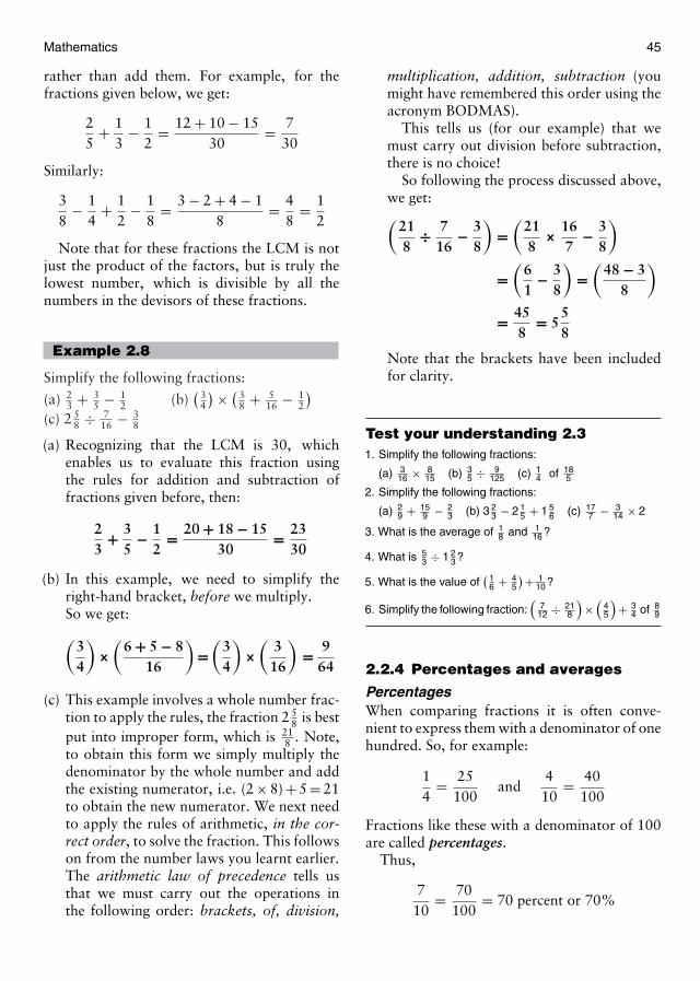
Mathematics 45
rather than add them. For example, for thefractions given below, we get:
25
+ 13
− 12
= 12 + 10 − 1530
= 730
Similarly:
38
− 14
+ 12
− 18
= 3 − 2 + 4 − 18
= 48
= 12
Note that for these fractions the LCM is notjust the product of the factors, but is truly thelowest number, which is divisible by all thenumbers in the devisors of these fractions.
Example 2.8
Simplify the following fractions:
(a) 23 + 3
5 − 12 (b)
( 34
)× ( 38 + 5
16 − 12
)(c) 2 5
8 ÷ 716 − 3
8
(a) Recognizing that the LCM is 30, whichenables us to evaluate this fraction usingthe rules for addition and subtraction offractions given before, then:
23
+ 35
− 12
= 20 + 18 − 1530
= 2330
(b) In this example, we need to simplify theright-hand bracket, before we multiply.So we get:
(34
)×(
6 + 5 − 816
)=(
34
)×(
316
)= 9
64
(c) This example involves a whole number frac-tion to apply the rules, the fraction 25
8 is bestput into improper form, which is 21
8 . Note,to obtain this form we simply multiply thedenominator by the whole number and addthe existing numerator, i.e. (2 × 8) + 5 = 21to obtain the new numerator. We next needto apply the rules of arithmetic, in the cor-rect order, to solve the fraction. This followson from the number laws you learnt earlier.The arithmetic law of precedence tells usthat we must carry out the operations inthe following order: brackets, of, division,
multiplication, addition, subtraction (youmight have remembered this order using theacronym BODMAS).
This tells us (for our example) that wemust carry out division before subtraction,there is no choice!
So following the process discussed above,we get:(
218
÷ 716
− 38
)=(
218
× 167
− 38
)
=(
61
− 38
)=(
48 − 38
)
= 458
= 558
Note that the brackets have been includedfor clarity.
Test your understanding 2.31. Simplify the following fractions:
(a) 316 × 8
15 (b) 35 ÷ 9
125 (c) 14 of 18
5
2. Simplify the following fractions:
(a) 29 + 15
9 − 23 (b) 3 2
3 − 2 15 + 1 5
6 (c) 177 − 3
14 × 2
3. What is the average of 18 and 1
16 ?
4. What is 53 ÷ 1 2
3 ?
5. What is the value of( 1
6 + 45
)+ 110 ?
6. Simplify the following fraction:(
712 ÷ 21
8
)×(
45
)+ 3
4 of 89
2.2.4 Percentages and averages
PercentagesWhen comparing fractions it is often conve-nient to express them with a denominator of onehundred. So, for example:
14
= 25100
and410
= 40100
Fractions like these with a denominator of 100are called percentages.
Thus,
710
= 70100
= 70 percent or 70%
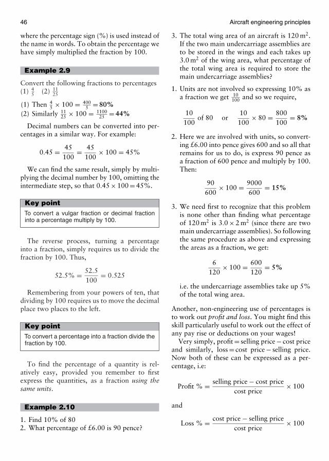
46 Aircraft engineering principles
where the percentage sign (%) is used instead ofthe name in words. To obtain the percentage wehave simply multiplied the fraction by 100.
Example 2.9
Convert the following fractions to percentages(1) 4
5 (2) 1125
(1) Then 45 × 100 = 400
5 = 80%(2) Similarly 11
25 × 100 = 110025 = 44%
Decimal numbers can be converted into per-centages in a similar way. For example:
0.45 = 45100
= 45100
× 100 = 45%
We can find the same result, simply by multi-plying the decimal number by 100, omitting theintermediate step, so that 0.45 × 100 = 45%.
Key pointTo convert a vulgar fraction or decimal fractioninto a percentage multiply by 100.
The reverse process, turning a percentageinto a fraction, simply requires us to divide thefraction by 100. Thus,
52.5% = 52.5100
= 0.525
Remembering from your powers of ten, thatdividing by 100 requires us to move the decimalplace two places to the left.
Key pointTo convert a percentage into a fraction divide thefraction by 100.
To find the percentage of a quantity is rel-atively easy, provided you remember to firstexpress the quantities, as a fraction using thesame units.
Example 2.10
1. Find 10% of 802. What percentage of £6.00 is 90 pence?
3. The total wing area of an aircraft is 120 m2.If the two main undercarriage assemblies areto be stored in the wings and each takes up3.0 m2 of the wing area, what percentage ofthe total wing area is required to store themain undercarriage assemblies?
1. Units are not involved so expressing 10% asa fraction we get 10
100 and so we require,
10100
of 80 or10100
× 80 = 800100
= 8%
2. Here we are involved with units, so convert-ing £6.00 into pence gives 600 and so all thatremains for us to do, is express 90 pence asa fraction of 600 pence and multiply by 100.Then:
90600
× 100 = 9000600
= 15%
3. We need first to recognize that this problemis none other than finding what percentageof 120 m2 is 3.0 × 2 m2 (since there are twomain undercarriage assemblies). So followingthe same procedure as above and expressingthe areas as a fraction, we get:
6120
× 100 = 600120
= 5%
i.e. the undercarriage assemblies take up 5%of the total wing area.
Another, non-engineering use of percentages isto work out profit and loss. You might find thisskill particularly useful to work out the effect ofany pay rise or deductions on your wages!
Very simply, profit = selling price − cost priceand similarly, loss = cost price − selling price.Now both of these can be expressed as a per-centage, i.e:
Profit % = selling price − cost pricecost price
× 100
and
Loss % = cost price − selling pricecost price
× 100
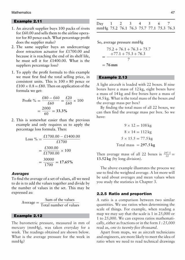
Mathematics 47
Example 2.11
1. An aircraft supplier buys 100 packs of rivetsfor £60.00 and sells them to the airline opera-tor for 80 pence each. What percentage profitdoes the supplier make?
2. The same supplier buys an undercarriagedoor retraction actuator for £1700.00 andbecause it is reaching the end of its shelf life,he must sell it for £1400.00. What is thesuppliers percentage loss?
1. To apply the profit formula to this examplewe must first find the total selling price, inconsistent units. This is 100 × 80 pence or£100 × 0.8 = £80. Then on application of theformula we get:
Profit % = £80 − £60£60
= £20£60
× 100
= 200060
= 33.3%
2. This is somewhat easier than the previousexample and only requires us to apply thepercentage loss formula. Then:
Loss % = £1700.00 − £1400.00£1700
= £300.00£1700.00
× 100
= 300001700
= 17.65%
AveragesTo find the average of a set of values, all we needto do is to add the values together and divide bythe number of values in the set. This may beexpressed as:
Average = Sum of the valuesTotal number of values
Example 2.12
The barometric pressure, measured in mm ofmercury (mmHg), was taken everyday for aweek. The readings obtained are shown below.What is the average pressure for the week inmmHg?
Day 1 2 3 4 5 6 7mmHg 75.2 76.1 76.3 75.7 77.1 75.3 76.3
So, average pressure mmHg
=75.2 + 76.1 + 76.3 + 75.7
+77.1 + 75.3 + 76.3
7= 76 mm
Example 2.13
A light aircraft is loaded with 22 boxes. If nineboxes have a mass of 12 kg, eight boxes havea mass of 14 kg and five boxes have a mass of14.5 kg. What is the total mass of the boxes andthe average mass per box?
By finding the total mass of all 22 boxes, wecan then find the average mass per box. So wehave:
9 × 12 = 108 kg
8 × 14 = 112 kg
5 × 15.5 = 77.5 kg
Total mass = 297.5 kg
Then average mass of all 22 boxes is 297.522 =
13.52 kg (by long division).
The above example illustrates the process weuse to find the weighted average. A lot more willbe said about averages and mean values whenyou study the statistics in Chapter 3.
2.2.5 Ratio and proportion
A ratio is a comparison between two similarquantities. We use ratios when determining thescale of things. For example, when reading amap we may say that the scale is 1 in 25,000 or1 to 25,000. We can express ratios mathemati-cally, either as fractions or in the form 1 : 25,000read as, one to twenty-five thousand.
Apart from maps, we as aircraft techniciansand engineers, are more likely to meet the idea ofratio when we need to read technical drawings
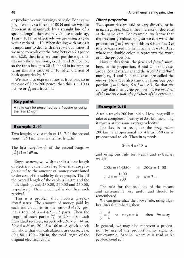
48 Aircraft engineering principles
or produce vector drawings to scale. For exam-ple, if we have a force of 100 N and we wish torepresent its magnitude by a straight line of aspecific length, then we may choose a scale say,1 cm = 10 N, so effectively we are using a scalewith a ratio of 1 : 10. When dealing with ratios itis important to deal with the same quantities. Ifwe need to work out the ratio between 20 penceand £2.0, then first, we must put these quanti-ties into the same units, i.e. 20 and 200 pence,so the ratio becomes 20 : 200 and in its simplestterms this is a ratio of 1 : 10, after division ofboth quantities by 20.
We may also express ratios as fractions, so inthe case of 20 to 200 pence, then this is 1 : 10 asbefore or 1
10 as a fraction.
Key pointA ratio can be presented as a fraction or usingthe is to (:) sign.
Example 2.14
Two lengths have a ratio of 13 : 7. If the secondlength is 91 m, what is the first length?
The first length = 137 of the second length =( 13
7
)91 = 169 m.
Suppose now, we wish to split a long lengthof electrical cable into three parts that are pro-portional to the amount of money contributedto the cost of the cable by three people. Then ifthe overall length of the cable is 240 m and theindividuals payed, £30.00, £40.00 and £50.00,respectively. How much cable do they eachreceive?
This is a problem that involves propor-tional parts. The amount of money paid byeach individual is in the ratio 3 : 4 : 5, giv-ing a total of 3 + 4 + 5 = 12 parts. Then thelength of each part = 240
12 or 20 m. So eachindividual receives, respectively, 20 × 3 = 60 m,20 × 4 = 80 m, 20 × 5 = 100 m. A quick checkwill show that our calculations are correct, i.e.60 + 80 + 100 = 240 m, the total length of theoriginal electrical cable.
Direct proportionTwo quantities are said to vary directly, or bein direct proportion, if they increase or decreaseat the same rate. For example, we know thatthe fraction 6
4 reduces to 23 so we can write the
proportion 64 = 3
2 we read this as 6 is to 4 as 3 isto 2 or expressed mathematically as 6 : 4 :: 3 : 2,where the double colon :: represents the wordas in the proportion.
Now in this form, the first and fourth num-bers, in the proportion, 6 and 2 in this case,are called the extremes and the second and thirdnumbers, 4 and 3 in this case, are called themeans. Now it is also true that from our pro-portion 6
4 = 32 then, 6 × 2 = 4 × 3. So that we
can say that in any true proportion, the productof the means equals the product of the extremes.
Example 2.15
A train travels 200 km in 4 h. How long will ittake to complete a journey of 350 km, assumingit travels at the same average velocity?
The key is to recognize the proportion;200 km is proportional to 4 h as 350 km isproportional to x h. Then in symbols:
200 : 4 :: 350 : x
and using our rule for means and extremes,we get:
200x = (4)(350) or 200x = 1400
and x = 1400200
or x = 7 h
The rule for the products of the meansand extremes is very useful and should beremembered!
We can generalize the above rule, using alge-bra (literal numbers), then:
xy
= ab
or x : y :: a : b then bx = ay
In general, we may also represent a propor-tion by use of the proportionality sign, ∝.For example, 2a ∝ 4a, where ∝ is read as ‘isproportional to’.
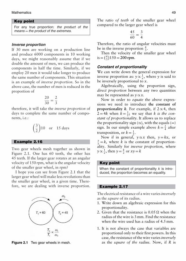
Mathematics 49
Key pointFor any true proportion: the product of themeans = the product of the extremes.
Inverse proportionIf 30 men are working on a production lineand produce 6000 components in 10 workingdays, we might reasonably assume that if wedouble the amount of men, we can produce thecomponents in half the time. Similarly, if weemploy 20 men it would take longer to producethe same number of components. This situationis an example of inverse proportion. So in theabove case, the number of men is reduced in theproportion of
2030
= 23
therefore, it will take the inverse proportion ofdays to complete the same number of compo-nents, i.e.: (
32
)10 or 15 days
Example 2.16
Two gear wheels mesh together as shown inFigure 2.1. One has 60 teeth, the other has45 teeth. If the larger gear rotates at an angularvelocity of 150 rpm, what is the angular velocityof the smaller gear wheel, in rpm?
I hope you can see from Figure 2.1 that thelarger gear wheel will make less revolutions thanthe smaller gear wheel, in a given time. There-fore, we are dealing with inverse proportion.
Figure 2.1 Two gear wheels in mesh.
The ratio of teeth of the smaller gear wheelcompared to the larger gear wheel is
4560
= 34
Therefore, the ratio of angular velocities mustbe in the inverse proportion 4
3 .Then the velocity of the smaller gear wheel
is = ( 43
)150 = 200 rpm.
Constant of proportionalityWe can write down the general expression forinverse proportion as: y ∝ 1
x , where y is said tobe inversely proportional to x.
Algebraically, using the proportion sign,direct proportion between any two quantitiesmay be represented as y ∝ x.
Now in order to equate the above expres-sions we need to introduce the constant ofproportionality k. For example, if 2 ∝ 4, then2 = 4k when k = 1
2 ; we say that k is the con-stant of proportionality. It allows us to replacethe proportionality sign (∝), with the equals (=)sign. In our simple example above k = 2
4 aftertransposition, or k = 1
2 .Now if in general, y ∝ x then, y = kx, or
yx = k, where k is the constant of proportion-ality. Similarly for inverse proportion, wherey ∝ 1
x , then y = kx or xy = k
Key pointWhen the constant of proportionality k is intro-duced, the proportion becomes an equality.
Example 2.17
The electrical resistance of a wire varies inverselyas the square of its radius.1. Write down an algebraic expression for this
proportionality.2. Given that the resistance is 0.05 � when the
radius of the wire is 3 mm. Find the resistancewhen the wire used has a radius of 4.5 mm.
1. It is not always the case that variables areproportional only to their first powers. In thiscase, the resistance of the wire varies inverselyas the square of the radius. Now, if R is
50 Aircraft engineering principles
the resistance and r the radius, then: R ∝ 1r2 ,
or R = kr2 . This is the required algebraic
expression.2. When R = 0.05 and r = 3, then 0.05 = k
32 andk = 0.45.Therefore, the final connecting equation isR = 0.45
r2 ; when r = 4.5, then R = 0.454.5 =
0.1 �.
The above example shows a typical engineeringuse for proportion. In the example that follows,we can write down some familiar scientific rela-tionships, using the rules for direct and inverseproportion.
Example 2.18
Write down the formulae to express thefollowing:1. The volume of a gas at constant temperature
is inversely proportional to the pressure.2. The electrical resistance of a wire varies
directly as the length and inversely as thesquare of the radius.
3. The kinetic energy of a body is jointly propor-tional to its mass and the square of its veloc-ity, when the constant of proportionality = 1
2 .
1. This should be familiar to you as Boyle’slaw. If we use the symbol V for volume andp for pressure, then V ∝ 1
p and introducingthe constant of proportionality k give therequired relationship as V = k
p , or pV = k (aconstant).
2. This is the same relationship that you met ear-lier, except the length l of the conductor isinvolved. So, if we again use R for resistanceand r for radius, then R ∝ l
r2 and again intro-
ducing the constant of proportionality we getR = kl
r2 .
Note that in the above case the resistance R isa function of two variables: the length l andthe radius r.
3. The kinetic energy (KE) is also dependent ontwo variables the mass (m) and the squareof the velocity (v2), both variables being indirect proportion. So you may write down
the relationship as KE ∝ mv2 and introduc-ing the constant of proportionality, whichin this case we are given as 1
2 , then therequired relationship is KE = 1
2 mv2. You willbe studying this relationship in your physics.
You will be using the ideas of proportion inthe next section on algebra, where we considerthe surface area and volume of regular solids.
Test your understanding 2.41. What is 15% of 50?
2. An airline engine repair bay has test equipment valued at£1.5 million. Each year 10% of the value of the test equip-ment is written off as depreciation. What is the value ofthe equipment after 2 full years?
3. An aircraft flies non-stop for 2.25 h and travels 1620 km.What is the aircraft’s average speed?
4. A car travels 50 km at 50 km/h and 70 km at 70 km/h.What is its average speed?
5. A car travels 205 km on 20 L of petrol. How much petrolis needed for a journey of 340 km?
6. Four men are required to produce a certain number ofcomponents in 30 h. How many men would be requiredto produce the same number of components in 6 h?
7. The cost of electroplating a square sheet of metal variesas the square of its length. The cost to electroplate asheet of metal with sides of 12 cm is £15.00. How muchwill it cost to electroplate a square piece of metal withsides of 15 cm.
8. If y − 3 is directly proportional to x2 and y = 5 when x = 2,find y when x = 8.
9. Write down the formula to express the height of a cone,when it varies directly as its volume and inversely as thesquare of the radius.
Before we leave our study of number, we needto consider one or two other number system,other than to the base 10.
2.2.6 Number systems
The decimal system of numbers we have beenstudying up till now use the integers 0–9. Thereare in fact 10 integers and for this reason weoften refer to the decimal system as the denary(ten) system.
Thus, for example, the denary number 245.5is equivalent to:
(2 × 10²) + (4 × 101) + (5 × 100) + (5 × 10⁻¹)
Mathematics 51
This arrangement of the number consists of aninteger ≥1.0 and ≤10.0 multiplied by the baseraised to the power; you have met this ideaearlier, when studying decimal numbers, powersof ten and estimation techniques.
In the binary system of numbers, the base is2 and so, for example, the denary number 43 tothe base 10, written as 4310 is equivalent to thenumber:
25 + 23 + 21 + 20 = 3210 + 810 + 210 + 110
Key pointIn the binary system of numbers the base is 2.
As a reminder and source of reference thebinary and denary equivalents for some impor-tant numbers related to computing are detailedbelow:
Binary2 27 26 25 24 23 22 21 20
Denary10 128 64 32 16 8 4 2 1
We are now in a position to be able to con-vert from denary to binary and binary to denarynumber systems.
To convert denary to binary, we repeatedlydivide by 2 and note the remainder at each stage.Then, for example, to convert the number 2510
to binary, we proceed as follows:
25/2 = 12 remainder 1 Least significantdigit (LSD)
12/2 = 6 remainder 06/2 = 3 remainder 03/2 = 1 remainder 11/2 = 0 remainder 1 Most significant
digit (MSD)
The binary2 equivalent of 2510 is 110012.Note the order in which the digits of the
binary number are laid out from the MSD tothe LSD; i.e. in reverse order to the successivedivision.
To convert binary to denary, we lay out thenumber in successive powers. For example, toconvert binary number 11012 into denary, we
proceed as follows:
11012
= (1 × 23) + (1 × 22) + (0 × 21) + (1 × 20)
= (1 × 8) + (1 × 4) + (0 × 2) + (1 × 1)
= 8 + 4 + 0 + 1 = 1310
When numbers are placed in binary form, wecan see from above that they consist of a num-ber of ones (1) and noughts (0). If in electroniclogic circuits we allow the binary digit “1” torepresent “ON” and the binary digit “0” to rep-resent “OFF”. We can apply this binary code toelectronic logic systems. It is this powerful appli-cation of binary numbers that makes their studyimportant. In order to get more digital infor-mation down computer communication lines,we can use another number system that allowsus to send 16 individual pieces of information(bytes) down parallel lines, all at the same time.This type of communication may be coded usinghexadecimal representation. Thus, for hexadec-imal numbers their base is 16. However, becausein our decimal number counting system we onlyhave 10 digits (0–9), we make up for this inthe hexadecimal system by allocating capital let-ters to the remaining decimal numbers 10–15(remembering that decimal zero is counted aspart of the 16 digit base). Hexadecimal repre-sentation, together with their denary and binaryequivalents, are shown in the Table 2.1.
Thus in a similar manner to before, the denarynumber 54210 may be represented as:
54210 = (5 × 10²) + (4 × 101) + (2 × 100)
which is equivalent to
21E16 = (2 × 162) + (1 × 161) + (E × 160).
To convert denary to hexadecimal, we repeat-edly divide by 16 in a similar manner to the wayin which we converted denary to binary. To con-vert the denary number 513610 to hexadecimal,we proceed as follows:
5136/16 = 321 remainder 0 LSD321/16 = 20 remainder 1
20/16 = 1 remainder 41/16 = 0 remainder 1 MSD

52 Aircraft engineering principles
Table 2.1 Denary, binary and hexadecimal numbersystems representation
Denary10 Binary2 Hexadecimal16
0 0000 01 0001 12 0010 23 0011 34 0100 45 0101 56 0110 67 0111 78 1000 89 1001 9
10 1010 A11 1011 B12 1100 C13 1101 D14 1110 E15 1111 F
So the hexadecimal16 equivalent of 513610 is141016.
Similarly, to convert the number 9410 tohexadecimal16, we proceed as follows:
94/16 = 5 remainder 14 (=E16)5/16 = 0 remainder 5
So the hexadecimal16 equivalent of 9410 is 5E16.To convert hexadecimal to denary, we pro-
ceed in a similar manner as for binary to denary.For example, to convert BA4516 to denary, weproceed as follows:
BA4516 = (B × 163) + (A × 162) + (4 × 161)
+ (5 × 160)
= (11 × 4096) + (10 × 256) + (4 × 16)
+ (5 × 1)
= (45056) + (2560) + (64) + (5)
= 4768510
The denary10 equivalent of hexadecimal numberBA4516 is 4768510.
To complete our very short study of numbersystems, it is worth considering how we converta denary number that has a decimal fraction aspart of the number. The process is quite logical
and relatively easy to follow. When dealing withthe fraction part of a binary number we applysuccessive multiplication until we reach unityfor the fractional part of the denary number.However, since we have applied multiplicationthe inverse arithmetic operation to that of divi-sion, then the MSD is the first remainder in themultiplication process.
Key pointWhen converting decimal fractions to binary weapply successive multiplication to the fractionalpart of the denary number.
Example 2.19
Convert denary number 39.62510 to binary2.Then proceeding in the normal way for the
non-fractional part of this number we get:
39/2 = 19 remainder 1 LSD19/2 = 9 remainder 1
9/2 = 4 remainder 14/2 = 2 remainder 02/2 = 1 remainder 01/2 = 0 remainder 1 MSD
Then 3910 = 100111
Also for the decimal fraction, applying suc-cessive multiplication, we get:
0.625 × 2 = 1.[250] MSD
0.250 × 2 = 0.[500]
0.500 × 2 = 1.000 LSD
Then 0.62510 = 0.1012
So, the denary number 39.62510 = 100111.1012.
Test your understanding 2.51. Convert the denary numbers to binary.
(a) 17 (b) 23 (c) 40
2. Convert the binary numbers to denary.(a) 1011 (b) 11111 (c) 1010101
3. Convert the denary numbers to hexadecimal.(a) 5890 (b) 16892
4. Convert the hexadecimal numbers to denary.(a) 6E (b) CF18
Mathematics 53
2.3 Algebra
2.3.1 Factors, powers andexponents
FactorsWhen two or more numbers are multipliedtogether, each of them, or the product of anynumber of them (apart from them all), is afactor of the product. This applies to explicitarithmetic numbers and to literal numbers.
So, for example, if we multiply the numbers 2and 6, we get that 2 × 6 = 12, thus 2 and 6 arefactors of the number 12. However, the number12 has more than one set of factors, 3 × 4 = 12so 3 and 4 are also factors of the number 12. Wecan also multiply 2 × 2 × 3 to get 12. Since thenumbers 2, 2 and 3 are yet another set of factorsof the number 12. Finally, you will rememberthat any number n multiplied by 1 is itself, orn × 1 = n. So every number has itself and 1 asfactors; 1 and n are considered trivial factorsand when asked to find the factors of an explicitor literal number, we will exclude the numberitself and 1.
Example 2.20
Find the factors of: (a) 8 (b) xy (c) 24 (d) abc(e) −m
(a) Apart from the trivial factors 1 and 8, whichwe agreed to ignore, the number 8 has onlythe factors 2 and 4, since 2 × 4 = 8, remem-ber that these factors can be presented inreverse order, 4 × 2 = 8, but 2 and 4 are stillthe only factors.
(b) Similarly, the literal number xy can only havethe factors x and y, if we ignore the trivialfactors. Thus, the numbers x and y multi-plied together to form the product xy arefactors of that product.
(c) The number 24 has several sets of factors,with varying numbers in each set. Firstwe find the number of sets with two factors,these are:
24 = 6 × 4
24 = 8 × 3
24 = 12 × 2
More than two factors:
24 = 2 × 2 × 6
24 = 4 × 3 × 2
24 = 2 × 2 × 2 × 3
However, if we look closely we see that thenumber 24 has only six different factors: 12,8, 6, 4, 3 and 2.
(d) So what about the factors in the number abc?Well, I hope you can see that the productof each individual factor a, b and c consti-tute one set of factors. Also ab and c; a andbc; and b and ac, form a further three sets.So extracting the different factors from thesesets we have: a, b, c, ab, ac and bc as thesix factors of the number abc.
(e) We have two sets of factors here 1 and –n,which is the trivial factor, but also the setn and −1, notice the subtlety with the signchange. When dealing with minus numbers,any two factors must have opposite signs.
Powers and exponentsWhen a number is the product of the same fac-tor multiplied by itself, this number is calleda power of the factor. For example, we knowthat 3 × 3 = 9. Therefore, we can say that 9 is apower of 3. To be precise, it is the second powerof 3, because two 3s are multiplied together toproduce 9. Similarly, 16 is the second power of4. We may use literal terminology to generalizethe relationship between powers and factors.
So the second power of a means a × a or (a · a),this is written as a2, where a is known as the base(factor) and 2 is the exponent (or index). Thuswriting the number 9 in exponent form we get9 = 32 where; 9 is the second power, 3 is thebase (factor) and 2 is the exponent (index).
The above ideal can be extended to writearithmetic numbers in exponent or index form.For example, 52 = 25, 92 = 81 and 33 = 27.Notice that the second power of 5 gives thenumber 25 or 5 × 5 = 25; similarly 33 meansthe third power of 3, literally 3 × 3 × 3 = 27.The idea of powers and exponents (indices) canbe extended to literal numbers. For example:a × a × a × a × a or a5 or in general am where a isthe base (factor) and the exponent m (or index)

54 Aircraft engineering principles
is any positive integer. am means a used as a fac-tor m times and is read as the “mth power ofa”. Note that since any number used as a fac-tor once would simply be the number itself, theindex (exponent) is not usually written; in otherwords a means a1.
Now, providing the base of two or more num-bers expressed in index (exponent) form are thesame, we can perform multiplication and divi-sion on these numbers, by adding or subtractingthe indices accordingly.
We will from now on refer to the exponent ofa number as its index, in order to avoid con-fusion with particular functions, such as theexponential function, which we study later.
Consider the following literal numbers inindex form:
x2 × x2 = (x × x)(x × x) = x × x × x × x = x4
x2 × x4 = (x × x)(x × x × x × x)= x × x × x × x × x × x = x6
x2
x2= x × x
x × x= x0 = 1
x2
x4= x × x
x × x × x × x= 1
x × x= x−2
What you are looking for is a pattern betweenthe first two literal numbers, which involve mul-tiplication and the second two which involvedivision.
For multiplication of numbers with the samebase, we add the indices and for division of num-bers with the same base, we subtract the indicesin the denominator (below the line) from thosein the numerator (above the line). Rememberalso that the base number x = x1.
We will now generalize our observations andso formulate the laws of indices.
2.3.2 The laws of indices
In the following laws a is the common base, mand n are the indices (exponents). Each law hasan example of its use alongside:
1. am × an = am+n 22 ×24 = 22+4 = 26 = 642. am
an = am−n 34
32 = 34−2 = 32= 9
3. (am)n = amn (22)3 = 22×3 = 26 = 64
4. a0 = 1 Any number raised to thepower 0 is always 1
5. amn = n
√am 27
43 = 3
√274 = 34 = 81
6. a−n = 1an 6−2 = 1
62 = 136
We need to study these laws carefully in orderto understand the significance of each.
Law 1: As you have already met, it enablesus to multiply numbers given in index form thathave a common base. In the example the com-mon base is 2, the first number raises this base(factor) to the power 2 and the second raises thesame base to the power 3. In order to find theresult we simply add the indices.
Law 2: We have again used when divid-ing numbers with a common base in this casethe base is 3. Note that since division is theopposite arithmetic operation to multiplication.It follows that we should perform the oppo-site arithmetic operation on the indices, that ofsubtraction. Remember we always subtract theindex in the denominator from the index in thenumerator.
Law 3: It is concerned with raising the powersof numbers. Do not mix this law up with law 1.When raising powers of numbers in index form,we multiple the indices.
Law 4: As you have also met, this law simplystates that any number raised to the power 0 isalways 1. Knowing that any number divided byitself is also 1, we can use this fact to show thata number raised to the power 0 is also 1. Whatwe need to do is use the second law concerningthe division of numbers in index form.
We know that9
9= 1 or
32
32 = 32−2 = 30 = 1
which shows that 30 = 1 and in fact because wehave used the second law of indices, this mustbe true in all cases.
Law 5: This, rather complicated looking, lawsimply enables us to find the decimal equivalentof a number in index form; where the index isa fraction. All that you need to remember isthat the index number above the fraction lineis raised to that power and the index numberbelow the fraction line has that number root.
So for the number 823 , we raise 8 to the power
2 and then take the cube root of the result.
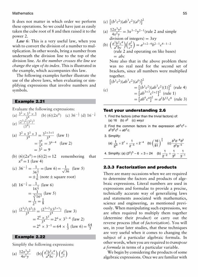
Mathematics 55
It does not matter in which order we performthese operations. So we could have just as easilytaken the cube root of 8 and then raised it to thepower 2.
Law 6: This is a very useful law, when youwish to convert the division of a number to mul-tiplication. In other words, bring a number fromunderneath the division line to the top of thedivision line. As the number crosses the line wechange the sign of its index. This is illustrated inthe example, which accompanies this law.
The following examples further illustrate theuse of the above laws, when evaluating or sim-plifying expressions that involve numbers andsymbols.
Example 2.21
Evaluate the following expressions:
(a) 32 × 33 × 334 (b) (6)(2x0) (c) 36− 1
2 (d) 16− 34
(e) (23)2(32)3
(34)
(a) 32 × 33 × 334 = 32+3+1
34 (law 1)
= 36
34 = 36−4 (law 2)
= 32 = 9
(b) (6)(2x0) = (6)(2) = 12 remembering thatx0 = 1 (law 4)
(c) 36− 12 = 1
3612
= (law 6) = 1√36
(law 5)
= ±16 (note ± square root)
(d) 16− 34 = 1
1634
(law 6)
= 14√
163(law 5)
= 123 = 1
8
(e) (23)2(32)334 = (23×2)(32×1)
34 (law 3)
= 26 × 33
34 = 26× 33−4 (law 2)
= 26 × 3−1 = 64 × 13 (law 6) = 64
3
Example 2.22
Simplify the following expressions:
(a) 12x3y2
4x2y(b)(
a3b2c4
a4bc
) (a2
c2
)
(c)[(b3c2)(ab3c2)(a0)
]2(a) 12x3y2
4x2y= 3x3−2y2−1(rule 2 and simple
division of integers) = 3xy
(b)(
a3b2c4
a4bc
)(a2
c2
)= a3+2−4b2−1c4−1−2
(rule 2 and operating on like bases)= abc
Note also that in the above problem therewas no real need for the second set ofbrackets, since all numbers were multipliedtogether.
(c)
[(b3c2)(ab3c2)(a0)
]2= [
(b3c2)(ab3c2)(1)]2 (rule 4)
= [ab3+3c2+2
]2 (rule 1)= [
ab6c4]2 = a2b12c8 (rule 3)
Test your understanding 2.61. Find the factors (other than the trivial factors) of:
(a) 16 (b) n2 (c) wxyz
2. Find the common factors in the expression ab2c2+a3b2c2 + ab2c.
3. Simplify:
(a) 123 × 27 × 1
2−5 × 2−4 (b)(
1681
) 34
(c)b3b−8b2
b0b−5
4. Simplify: (a) (22)3 – 6 × 3 + 24 (b)1
2−2+ 1
32− 1
3−1
2.3.3 Factorization and products
There are many occasions when we are requiredto determine the factors and products of alge-braic expressions. Literal numbers are used inexpressions and formulae to provide a precise,technically accurate way of generalizing lawsand statements associated with mathematics,science and engineering, as mentioned previ-ously. When manipulating such expressions, weare often required to multiply them together(determine their product) or carry out thereverse process (that of factorization). You willsee, in your later studies, that these techniquesare very useful when it comes to changing thesubject of a particular algebraic formula. Inother words, when you are required to transposea formula in terms of a particular variable.
We begin by considering the products of somealgebraic expressions. Once we are familiar with
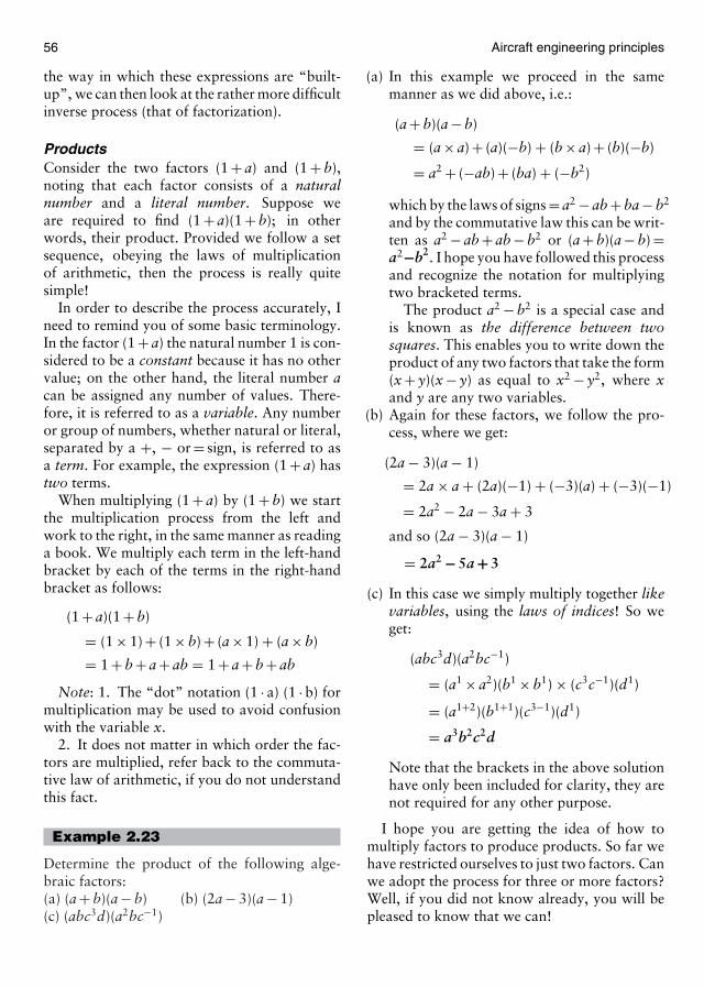
56 Aircraft engineering principles
the way in which these expressions are “built-up”, we can then look at the rather more difficultinverse process (that of factorization).
ProductsConsider the two factors (1 + a) and (1 + b),noting that each factor consists of a naturalnumber and a literal number. Suppose weare required to find (1 + a)(1 + b); in otherwords, their product. Provided we follow a setsequence, obeying the laws of multiplicationof arithmetic, then the process is really quitesimple!
In order to describe the process accurately, Ineed to remind you of some basic terminology.In the factor (1 + a) the natural number 1 is con-sidered to be a constant because it has no othervalue; on the other hand, the literal number acan be assigned any number of values. There-fore, it is referred to as a variable. Any numberor group of numbers, whether natural or literal,separated by a +, − or = sign, is referred to asa term. For example, the expression (1 + a) hastwo terms.
When multiplying (1 + a) by (1 + b) we startthe multiplication process from the left andwork to the right, in the same manner as readinga book. We multiply each term in the left-handbracket by each of the terms in the right-handbracket as follows:
(1 + a)(1 + b)
= (1 × 1) + (1 × b) + (a × 1) + (a × b)
= 1 + b + a + ab = 1 + a + b + ab
Note: 1. The “dot” notation (1 · a) (1 · b) formultiplication may be used to avoid confusionwith the variable x.
2. It does not matter in which order the fac-tors are multiplied, refer back to the commuta-tive law of arithmetic, if you do not understandthis fact.
Example 2.23
Determine the product of the following alge-braic factors:(a) (a + b)(a − b) (b) (2a − 3)(a − 1)(c) (abc3d)(a2bc−1)
(a) In this example we proceed in the samemanner as we did above, i.e.:
(a + b)(a − b)
= (a × a) + (a)(−b) + (b × a) + (b)(−b)
= a2 + (−ab) + (ba) + (−b2)
which by the laws of signs = a2 − ab + ba − b2
and by the commutative law this can be writ-ten as a2 − ab + ab − b2 or (a + b)(a − b) =a2−b2. I hope you have followed this processand recognize the notation for multiplyingtwo bracketed terms.
The product a2 − b2 is a special case andis known as the difference between twosquares. This enables you to write down theproduct of any two factors that take the form(x + y)(x − y) as equal to x2 − y2, where xand y are any two variables.
(b) Again for these factors, we follow the pro-cess, where we get:
(2a − 3)(a − 1)
= 2a × a + (2a)(−1) + (−3)(a) + (−3)(−1)
= 2a2 − 2a − 3a + 3
and so (2a − 3)(a − 1)
= 2a2 − 5a + 3
(c) In this case we simply multiply together likevariables, using the laws of indices! So weget:
(abc3d)(a2bc−1)
= (a1 × a2)(b1 × b1) × (c3c−1)(d1)
= (a1+2)(b1+1)(c3−1)(d1)
= a3b2c2d
Note that the brackets in the above solutionhave only been included for clarity, they arenot required for any other purpose.
I hope you are getting the idea of how tomultiply factors to produce products. So far wehave restricted ourselves to just two factors. Canwe adopt the process for three or more factors?Well, if you did not know already, you will bepleased to know that we can!

Mathematics 57
Example 2.24
Simplify the following:(a) (x + y)(x + y)(x − y)(b) (a + b)(a2 − ab + b2)
(a) This expression may be simplified by mul-tiplying out the brackets and collecting liketerms. I hope you recognize the fact that theproduct of (x + y)(x − y) is x2 − y2. Then allwe need to do is multiply this product by theremaining factor, we get:
(x + y)(x2 − y2) = x3 − xy2 + x2y − y3
Note that the convention of putting thevariables in alphabetical order and the factthat it does not matter in what order wemultiply the factors, the result will be thesame.
(b) This is a straightforward product, where
(a + b)(a2 − ab + b2)
= a3 − a2b + ab2 + a2b − ab2 + b3
= a3 + b3
Note that there are six terms resulting fromthe necessary six multiplications. When wecollect like-terms and add we are left withthe product known as the addition of cubes.
FactorizationFactorizing is the process of finding two or morefactors which, when multiplied together, willresult in the given expression. Therefore, fac-torizing is really the opposite of multiplicationor finding the product. It was for this reason thatwe first considered the simpler process of findingthe product.
Thus, for example, x(y + z) = xy + xz. Thisproduct resulted from the multiplication of thetwo factors x and (y + z). If we now unpick theproduct you should be able to see that x is acommon factor, that appears in both terms ofthe product.
What about the expression x2 − 16? I hopeyou are able to recognize the fact that thisexpression is an example of the differencebetween two squares. Therefore, we can write
down the factors immediately as (x + 4) and(x − 4), look back at Example 2.11, if you areunsure. We can check the validity of our factorsby multiplying and checking that the product weget is identical to the original expression, that wewere required to factorize, i.e.:
(x + 4)(x − 4) = x2 − 4x + 4x − 16= x2 − 16 as required.
Suppose you are asked to factorize the expres-sion a2 − 6a + 9, how do we go about it? Well,a good place to start is with the term involv-ing the highest power of the variable, i.e. is a2.Remember that when convention dictates, welayout our expression in descending powers ofthe unknown, starting with the highest powerpositioned at the extreme left-hand side of theexpression. a can only have factors of itself and 1or a and a, therefore, ignoring the trivial factors,a2 = a × a. At the other end of the expression,we have the natural number 9, this has the triv-ial factors 1 and 9 or the factors 3 and 3 or−3 and −3. Note the importance of consideringthe negative case, where from the laws of signs(−3)(−3) = 9. So now, we have several sets offactors we can try, these are:
(i) (a + 3)(a + 3) or (ii) (a − 3)(a − 3) or(iii) (a + 3)(a − 3)?
Now we could try multiplying up each setof factors until we obtained the required result,i.e. determine the factors by trial and error. Thisdoes become rather tedious when there are asignificant number of possibilities. So, beforeresorting to this method, we need to see if wecan eliminate some combinations of factors byapplying one or two simple rules.
I hope you can see why the factors (a + 3)(a − 3) can be immediately excluded. These arethe factors for the difference between squares,which is not the original expression we neededto factorize.
What about the factors (a + 3)(a + 3)? Boththe factors contain only positive terms, there-fore, any of their products must also be pos-itive by the laws of signs! In our expressiona2 − 6a + 9 there is a minus sign, so again this setof factors may be eliminated. This leaves us with

58 Aircraft engineering principles
the factors (a − 3)(a − 3) and on multiplicationwe get:
(a − 3)(a − 3) = a2 − 3a − 3a + 9 = a2 − 6a + 9
giving us the correct result.You might have noticed that we have left out
the sets of factors (a − 1)(a − 9), (a − 1)(a + 9),(a + 1)(a − 9) and (a + 1)(a + 9), from our orig-inal group of possibles! Well, in the case of(a + 1)(a + 9), this would be eliminated using thelaws of signs, but what about the rest?
There is one more very useful technique wecan employ, when considering just two factors.This technique enables us to check the accuracyof our factors by determining the middle term ofthe expression we are required to factorize. Soin our case for the expression a2 − 6a + 9, then−6a is the middle term.
The middle term is derived from our chosenfactors by multiplying the outer terms, multiply-ing the inner terms and adding.
So in the case of the correct factors (a − 3)(a − 3), the outer terms are a and −3, whichon multiplication (a)(−3) = −3a and similarlythe inner terms (−3)(a) = −3a and so theirsum = −3a + (−3a) = −6a, as required.
If we try this technique to any of the abovefactors involving 1 and 9, we will see thatthey can be quickly eliminated. For example,(a − 1)(a − 9) has an outer product of (a)(−9) =−9a and an inner product of (−1)(a) = −a,which when added = −9a − a = −10a, which ofcourse is incorrect.
Example 2.25
Factorize the expressions:(a) x2 + 2x − 8 and (b) 12x2 − 10x − 12
(a) To determine the factors for this expressionwe follow the same procedure as detailedabove.
First we consider the factors for the outerterm x2 (apart from the trivial factors), wehave x2 = x × x and the factors of −8 are(2)(4) or (−2)(4) or (4)(−2) or (1)(8) or(−1)(8) or (8)(−1). So by considering onlyouter and inner terms we have the following
possible combination of factors:
(x + 2)(x + 4), (x + 2)(x − 4),
(x − 2)(x − 4) and (x + 1)(x + 8),
(x + 1)(x − 8), (x − 1)(x + 8).
Now we eliminate the sets of factors thatonly have positive terms (by the law of signs).This leaves (x + 2)(x − 4), (x − 2)(x + 4),(x + 1)(x−8) and (x−1)(x+8). The last twosets of factors can be eliminated by applyingthe outer and inner term rule. If you applythis rule, neither of these sets give the cor-rect middle term. We are therefore left withthe two sets of factors: (x + 2)(x − 4) or(x − 2)(x + 4).
So let us try (x + 2)(x − 4), applying theouter and inner term rules, we get (x)(−4) = −4x and (2)(x) = 2x, which on addi-tion give −2x, but we require +2x, so theseare not the factors. Finally, we try (x − 2)(x + 4), where on application of the rule weget (x)(4) = 4x and (−2)(x) = −2x, whichon addition give 4x − 2x = 2x as required,where the factors of the expression x2 +2x − 8 are (x − 2) (x + 4).
(b) For the expression 12x2 −10x−12, we havethe added complication of several possibili-ties for the term involving the square of thevariable x, i.e. 12x2. This term could be theproduct of the factors: (x)(12x) or (2x)(6x)or (3x)(4x) and the right-hand term couldbe the product of the factors (−1)(12) or(1)(−12) or (−2)(6) or (2)(−6) or (−3)(4) or(3)(−4). By the rule of signs, no set of factorscan have all positive terms, so these can beeliminated from the possible solutions. Thisleaves us with:
set 1 (3x + 1)(x − 12), (3x − 1)(x + 12)
(x − 1)(3x + 12) or (x + 1)(3x − 12)
set 2 (3x + 2)(x − 6), (3x − 2)(x + 6)
(x + 2)(3x − 6), (x − 2)(3x + 6)
set 3 (3x + 3)(x − 4), (3x − 3)(x + 4)
(x + 3)(3x − 4), (x − 3)(3x + 4)
The choice of possible solution does seemto be getting complicated! However, if weapply the multiplication of outer terms, mul-tiplication of inner terms rule to sets 1 and 3,
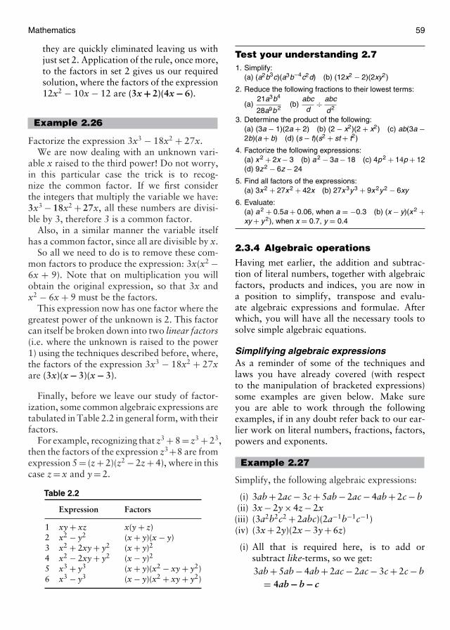
Mathematics 59
they are quickly eliminated leaving us withjust set 2. Application of the rule, once more,to the factors in set 2 gives us our requiredsolution, where the factors of the expression12x2 − 10x − 12 are (3x + 2)(4x − 6).
Example 2.26
Factorize the expression 3x3 − 18x2 + 27x.We are now dealing with an unknown vari-
able x raised to the third power! Do not worry,in this particular case the trick is to recog-nize the common factor. If we first considerthe integers that multiply the variable we have:3x3 − 18x2 + 27x, all these numbers are divisi-ble by 3, therefore 3 is a common factor.
Also, in a similar manner the variable itselfhas a common factor, since all are divisible by x.
So all we need to do is to remove these com-mon factors to produce the expression: 3x(x2 −6x + 9). Note that on multiplication you willobtain the original expression, so that 3x andx2 − 6x + 9 must be the factors.
This expression now has one factor where thegreatest power of the unknown is 2. This factorcan itself be broken down into two linear factors(i.e. where the unknown is raised to the power1) using the techniques described before, where,the factors of the expression 3x3 − 18x2 + 27xare (3x)(x − 3)(x − 3).
Finally, before we leave our study of factor-ization, some common algebraic expressions aretabulated in Table 2.2 in general form, with theirfactors.
For example, recognizing that z3 + 8 = z3 + 23,then the factors of the expression z3+8 are fromexpression 5 = (z + 2)(z2 − 2z + 4), where in thiscase z = x and y = 2.
Table 2.2
Expression Factors
1 xy + xz x(y + z)2 x2 − y2 (x + y)(x − y)3 x2 + 2xy + y2 (x + y)2
4 x2 − 2xy + y2 (x − y)2
5 x3 + y3 (x + y)(x2 − xy + y2)6 x3 − y3 (x − y)(x2 + xy + y2)
Test your understanding 2.71. Simplify:
(a) (a2b3c)(a3b−4c2d) (b) (12x2 − 2)(2xy2)
2. Reduce the following fractions to their lowest terms:
(a)21a3b4
28a9b 2(b)
abcd
÷ abc
d 2
3. Determine the product of the following:(a) (3a − 1)(2a + 2) (b) (2 − x2)(2 + x2) (c) ab(3a −2b)(a + b) (d) (s − t)(s2 + st + t2)
4. Factorize the following expressions:(a) x 2 + 2x − 3 (b) a 2 − 3a − 18 (c) 4p 2 + 14p + 12(d) 9z 2 − 6z − 24
5. Find all factors of the expressions:(a) 3x 2 + 27x 2 + 42x (b) 27x 3y 3 + 9x 2y 2 − 6xy
6. Evaluate:(a) a 2 + 0.5a + 0.06, when a = −0.3 (b) (x − y)(x 2 +xy + y 2), when x = 0.7, y = 0.4
2.3.4 Algebraic operations
Having met earlier, the addition and subtrac-tion of literal numbers, together with algebraicfactors, products and indices, you are now ina position to simplify, transpose and evalu-ate algebraic expressions and formulae. Afterwhich, you will have all the necessary tools tosolve simple algebraic equations.
Simplifying algebraic expressionsAs a reminder of some of the techniques andlaws you have already covered (with respectto the manipulation of bracketed expressions)some examples are given below. Make sureyou are able to work through the followingexamples, if in any doubt refer back to our ear-lier work on literal numbers, fractions, factors,powers and exponents.
Example 2.27
Simplify, the following algebraic expressions:
(i) 3ab + 2ac − 3c + 5ab − 2ac − 4ab + 2c − b(ii) 3x − 2y × 4z − 2x(iii) (3a2b2c2 + 2abc)(2a−1b−1c−1)(iv) (3x + 2y)(2x − 3y + 6z)
(i) All that is required here, is to add orsubtract like-terms, so we get:3ab + 5ab − 4ab + 2ac − 2ac − 3c + 2c − b
= 4ab − b − c

60 Aircraft engineering principles
(ii) Here you need to be aware of the law ofprecedence, this is derived from the lawsof arithmetic you learnt earlier. As an aidememoir we use the acronym: BODMAS, i.e.brackets, of, division, multiplication, addi-tion and finally subtraction. These opera-tions being performed in this order. Fromthis law we carry out multiplication beforeaddition or subtraction. So we get:
3x − 8yz − 2x = x − 8yz
(iii) With this expression, when multiplying upthe brackets, we need to remember the lawof indices for multiplication. Using this lawwe get:
6a2−1b2−1c2−1 + 4a1−1b1−1c1−1
= 6a1b1c1 + 4a0b0c0 = 6abc + 4
(Do not forget the 4! Remember that anynumber raised to the power zero is 1 and4 × 1 × 1 × 1 = 4.)
(iv) This is just the multiplication of brackets,where we multiply all terms in the right-hand bracket by both terms in the left-handbracket. We perform these multiplicationsas though we are reading a book from leftto right. Starting with (3x) × (2x) = 6x2,then (3x) × (−3y) = −9xy and so on. Wethen repeat the multiplications, using theright-hand term in the first bracket, i.e.(2y) × (2x) = 4xy and so on. So that beforeany simplification we should end up with2 × 3 = 6 terms:
(3x + 2y)(2x − 3y + 6z)
= 6x2 − 9xy + 18xz + 4xy − 6y2
+ 12yz (6 terms)
and so after simplification which involvesonly two like-terms in this case, we get:
6x2 − 5xy + 18xz − 6y2 − 12yz
Key pointRemember the laws of precedence by theacronym BODMAS, brackets, of, division, mul-tiplication, addition, subtraction.
Example 2.28
Factorize the following algebraic expressions:(i) −x2 + x + 6 (ii) 5x2y3 − 40z3x2
(iii) x2 − 4x − 165 (iv) 8x6 + 27y3
(i) This is a straightforward example of factor-izing a trinomial (an algebraic expression ofthree terms, with ascending powers of theunknown).
We simply follow the rules you studiedearlier. I will go through the procedure oncemore to remind you.
We first consider the left-hand term −x2,which obeying the rules of multiplicationmust have factors −x and x (ignoring triv-ial factors). Also for the right-hand term wehave 2 and 3 or the trivial factors 1 and 6.Again ignoring the trivial factors, we firsttry 2 and 3.
So we have the following sets of factors:
(−x + 2)(x + 3), (x + 2)(−x + 3)
(−x − 2)(x − 3), (x − 2)(−x − 3)
Now remembering the rule for determin-ing the middle term, i.e. addition of outerand inner products, then by trial and error,we eliminate all sets of factors, except thecorrect solution, which is (x + 2)(−x + 3).
(ii) Here the trick is to recognize the commonfactor/s and pull them out behind a bracket.In this case I hope you can see that x2 iscommon to both terms as is the number 5.
Then we can write the factors as:
5x2(y3 − 8z3)
Your answer can always be checked bymultiplying up the factors. You should, ofcourse, obtain the original expression pro-viding your factors are correct and yoursubsequent multiplication is also correct!
(iii) With this example, the only difficulty is inrecognizing possible factors for the ratherlarge number 165. Well, this is where it isuseful to know your 15 times table! Withtrial and error you should eventually findthat apart from the trivial factors, the num-bers 15 and 11 are factors of 165. Also
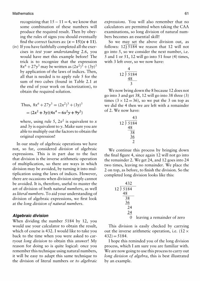
Mathematics 61
recognizing that 15 − 11 = 4, we know thatsome combination of these numbers willproduce the required result. Then by obey-ing the rules of signs you should eventuallyfind the correct factors as: (x − 15)(x + 11).
(iv) If you have faithfully completed all the exer-cises in test your understanding 2.6, youwould have met this example before! Thetrick is to recognize that the expression8x6 + 27y3 may be written as (2x2)3 + (3y)3
by application of the laws of indices. Then,all that is needed is to apply rule 5 for thesum of two cubes (found in Table 2.1 atthe end of your work on factorization), toobtain the required solution.
Thus, 8x6 + 27y3 = (2x2)3 + (3y)3
= (2x2 + 3y)(4x4 − 6x2y + 9y2)
where, using rule 5, 2x2 is equivalent to xand 3y is equivalent to y. Make sure you areable to multiply out the factors to obtain theoriginal expression!
In our study of algebraic operations we havenot, so far, considered division of algebraicexpressions. This is in part due to the factthat division is the inverse arithmetic operationof multiplication, so there are ways in whichdivision may be avoided, by turning it into mul-tiplication using the laws of indices. However,there are occasions when division simply cannotbe avoided. It is, therefore, useful to master theart of division of both natural numbers, as wellas literal numbers. To aid your understanding ofdivision of algebraic expressions, we first lookat the long division of natural numbers.
Algebraic divisionWhen dividing the number 5184 by 12, youwould use your calculator to obtain the result,which of course is 432. I would like to take youback to the time when you were asked to car-ryout long division to obtain this answer! Myreason for doing so is quite logical: once youremember this technique using natural numbers,it will be easy to adapt this same technique tothe division of literal numbers or to algebraic
expressions. You will also remember that nocalculators are permitted when taking the CAAexaminations, so long division of natural num-bers becomes an essential skill!
So we may set the above division out, asfollows: 12
)5184 we reason that 12 will not
go into 5, so we consider the next number, i.e.5 and 1 or 51, 12 will go into 51 four (4) times,with 3 left over, so we now have:
412)
518448
3
We now bring down the 8 because 12 does notgo into 3 and get 38, 12 will go into 38 three (3)times (3 × 12 = 36), so we put the 3 on top aswe did the 4 then we are left with a remainderof 2. We now have:
4312)
518448
3836
2
We continue this process by bringing downthe final figure 4, since again 12 will not go intothe remainder 2. We get 24, and 12 goes into 24two times, leaving no remainder. We place the2 on top, as before, to finish the division. So thecompleted long division looks like this:
43212)
518448
3836
2424
0 leaving a remainder of zero
This division is easily checked by carryingout the inverse arithmetic operation, i.e. (12 ×432) = 5184.
I hope this reminded you of the long divisionprocess, which I am sure you are familiar with.We are now going to use this process to carry outlong division of algebra, this is best illustratedby an example.
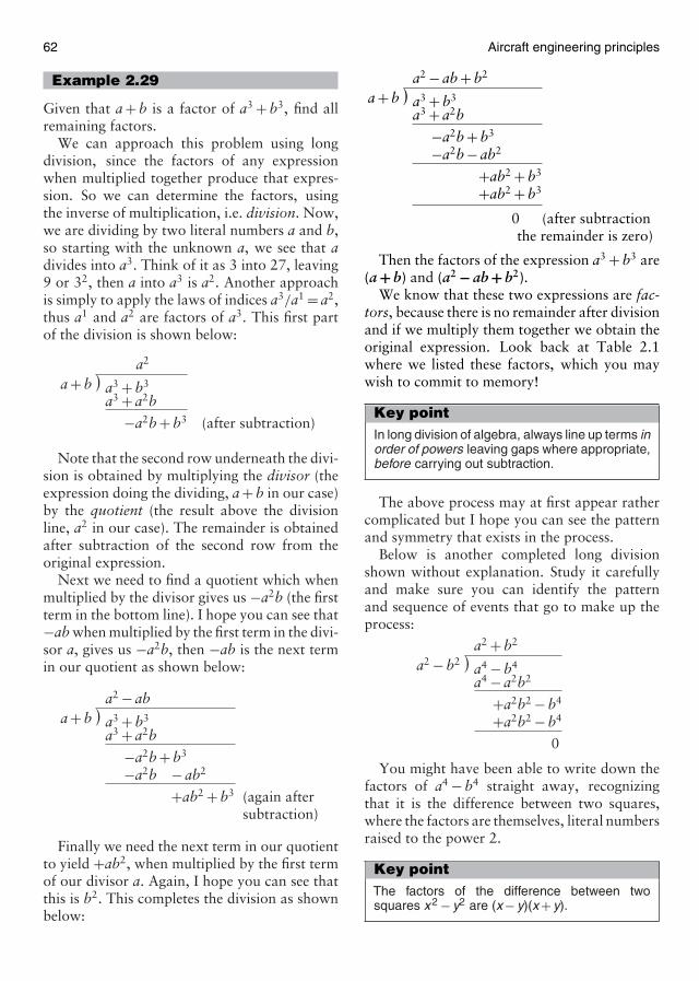
62 Aircraft engineering principles
Example 2.29
Given that a + b is a factor of a3 + b3, find allremaining factors.
We can approach this problem using longdivision, since the factors of any expressionwhen multiplied together produce that expres-sion. So we can determine the factors, usingthe inverse of multiplication, i.e. division. Now,we are dividing by two literal numbers a and b,so starting with the unknown a, we see that adivides into a3. Think of it as 3 into 27, leaving9 or 32, then a into a3 is a2. Another approachis simply to apply the laws of indices a3/a1 = a2,thus a1 and a2 are factors of a3. This first partof the division is shown below:
a2
a + b)
a3 + b3
a3 + a2b
−a2b + b3 (after subtraction)
Note that the second row underneath the divi-sion is obtained by multiplying the divisor (theexpression doing the dividing, a + b in our case)by the quotient (the result above the divisionline, a2 in our case). The remainder is obtainedafter subtraction of the second row from theoriginal expression.
Next we need to find a quotient which whenmultiplied by the divisor gives us −a2b (the firstterm in the bottom line). I hope you can see that−ab when multiplied by the first term in the divi-sor a, gives us −a2b, then −ab is the next termin our quotient as shown below:
a2 − aba + b
)a3 + b3
a3 + a2b
−a2b + b3
−a2b − ab2
+ab2 + b3 (again aftersubtraction)
Finally we need the next term in our quotientto yield +ab2, when multiplied by the first termof our divisor a. Again, I hope you can see thatthis is b2. This completes the division as shownbelow:
a2 − ab + b2
a + b)
a3 + b3
a3 + a2b
−a2b + b3
−a2b − ab2
+ab2 + b3
+ab2 + b3
0 (after subtractionthe remainder is zero)
Then the factors of the expression a3 + b3 are(a + b) and (a2 − ab + b2).
We know that these two expressions are fac-tors, because there is no remainder after divisionand if we multiply them together we obtain theoriginal expression. Look back at Table 2.1where we listed these factors, which you maywish to commit to memory!
Key pointIn long division of algebra, always line up terms inorder of powers leaving gaps where appropriate,before carrying out subtraction.
The above process may at first appear rathercomplicated but I hope you can see the patternand symmetry that exists in the process.
Below is another completed long divisionshown without explanation. Study it carefullyand make sure you can identify the patternand sequence of events that go to make up theprocess:
a2 + b2
a2 − b2)
a4 − b4
a4 − a2b2
+a2b2 − b4
+a2b2 − b4
0
You might have been able to write down thefactors of a4 − b4 straight away, recognizingthat it is the difference between two squares,where the factors are themselves, literal numbersraised to the power 2.
Key pointThe factors of the difference between twosquares x 2 − y2 are (x − y)(x + y).

Mathematics 63
The need for long division of algebra mayoccur in your future studies, should you berequired to deal with partial fractions. It is oftenuseful to be able to simplify rather complex alge-braic fractions into their simpler componentswhen trying to differentiate or integrate them.You will meet calculus arithmetic later, whereyou will be asked to carry out differentiationand integration of simple functions. You will bepleased to know that in this course you are notrequired to find partial fractions!
So far we have concentrated on long divisionof algebraic expressions, where the division isexact, but what happens if we are left with aremainder? Below is shown the division of twoexpressions which both yield a remainder:
1x2 − 1
)x2 + 1−(x2 − 1)
2
Therefore, x2 + 1x2 − 1
≡ 1 + 2x2 − 1
where ≡ means
“always equal to”.Similarly:
3x3 − x
)3x3 − x2 + 2−(3x3 −3x)
−x2 + 3x + 2
therefore,3x3 − x2 + 2
x3 − x≡ 3 +
(−x2 + 3x + 2x3 − x
)
In both the cases, the division has convertedan improper fraction into a proper fraction. Animproper algebraic fraction is one in which thehighest power in the numerator is greater thanor equal to (≥), the highest power in the denom-inator. Just to make sure you can distinguishbetween these two types of fraction, let us sub-stitute the natural number 2 for the unknownvariable x in the first of the two examples shownabove, i.e.:
x2 + 1x2 − 1
= (2)2 + 1(2)2 − 1
= 53
or 123
so 53 is a fraction in improper form and 1 2
3 is aproper fraction.
Note also that the proper fraction 1 23 is the
same as: 1 + 23 or 3
3 + 23 = 5
3With your study of mathematical fundamen-
tals and mastery of the above techniques youshould now be ready to tackle problems involv-ing the manipulation and transposition of for-mulae, which we consider next.
Test your understanding 2.81. Simplify the following algebraic expressions:
(a) 2xy + 4xyz − 2x + 4y + 2z + 2xz − xy + 4y − 2z −3xyz
(b) 2a(3b − c) + abc − ab + 2ac
2. Multiply out the brackets and simplify the expression:p(2qr − 5ps) + (p − q)(p + q) − 8s(p2 + 1) − p2 + q2
3. Factorize the following expressions:(a) u2 − 5u + 6 (b) 6a2b3c − 30abc + 12abc2
(c) 12x 2 − 8x − 10 (d) 2a3 + 2b3
4. Divide a3 − b3 by a − b and show that a − b is a factorof a3 − b3.
5. What is the quotient, when 2x 3 + x 2 − 2x − 1 is dividedby x 2 − 1?
2.3.5 Transposition of formulae
As mentioned earlier, formulae provide engi-neers with a method of writing down somerather complex relationships and ideas in a veryprecise and elegant way. For example, the for-mula v = u + at tells us that the final velocity (v)of say, an aircraft, is equal to its initial veloc-ity (u) plus its acceleration (a), multiplied bythe time (t) the aircraft is accelerating down therunway. If the aircraft is neither accelerating ordecelerating (negative acceleration), then v = ubecause the acceleration a = 0 and 0 × t = 0 asyou already know. I think you are already begin-ning to realize that to explain the meaning of onesimple formula requires rather a lot of words!It is for this reason that formulae are usedrather than just words to convey engineeringconcepts.
Note also that once the techniques for trans-posing (rearranging) formulae have been mas-tered, then solving algebraic equations becomesan easy application of these techniques!
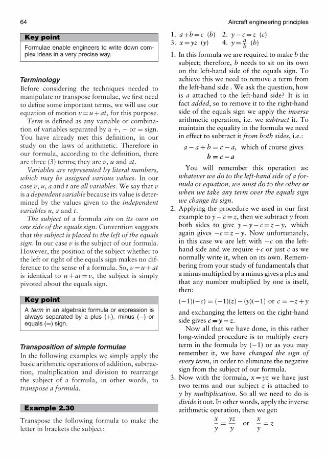
64 Aircraft engineering principles
Key pointFormulae enable engineers to write down com-plex ideas in a very precise way.
TerminologyBefore considering the techniques needed tomanipulate or transpose formulae, we first needto define some important terms, we will use ourequation of motion v = u + at, for this purpose.
Term is defined as any variable or combina-tion of variables separated by a +, − or = sign.You have already met this definition, in ourstudy on the laws of arithmetic. Therefore inour formula, according to the definition, thereare three (3) terms; they are v, u and at.
Variables are represented by literal numbers,which may be assigned various values. In ourcase v, u, a and t are all variables. We say that vis a dependent variable because its value is deter-mined by the values given to the independentvariables u, a and t.
The subject of a formula sits on its own onone side of the equals sign. Convention suggeststhat the subject is placed to the left of the equalssign. In our case v is the subject of our formula.However, the position of the subject whether tothe left or right of the equals sign makes no dif-ference to the sense of a formula. So, v = u + atis identical to u + at = v, the subject is simplypivoted about the equals sign.
Key pointA term in an algebraic formula or expression isalways separated by a plus (+), minus (−) orequals (=) sign.
Transposition of simple formulaeIn the following examples we simply apply thebasic arithmetic operations of addition, subtrac-tion, multiplication and division to rearrangethe subject of a formula, in other words, totranspose a formula.
Example 2.30
Transpose the following formula to make theletter in brackets the subject:
1. a +b = c (b) 2. y − c = z (c)3. x = yz (y) 4. y = a
b (b)
1. In this formula we are required to make b thesubject; therefore, b needs to sit on its ownon the left-hand side of the equals sign. Toachieve this we need to remove a term fromthe left-hand side . We ask the question, howis a attached to the left-hand side? It is infact added, so to remove it to the right-handside of the equals sign we apply the inversearithmetic operation, i.e. we subtract it. Tomaintain the equality in the formula we needin effect to subtract it from both sides, i.e.:
a − a + b = c − a, which of course givesb = c − a
You will remember this operation as:whatever we do to the left-hand side of a for-mula or equation, we must do to the other orwhen we take any term over the equals signwe change its sign.
2. Applying the procedure we used in our firstexample to y − c = z, then we subtract y fromboth sides to give y − y − c = z − y, whichagain gives −c = z − y. Now unfortunately,in this case we are left with −c on the left-hand side and we require +c or just c as wenormally write it, when on its own. Remem-bering from your study of fundamentals thata minus multiplied by a minus gives a plus andthat any number multiplied by one is itself,then:
(−1)(−c) = (−1)(z) − (y)(−1) or c = −z + y
and exchanging the letters on the right-handside gives c = y − z.
Now all that we have done, in this ratherlong-winded procedure is to multiply everyterm in the formula by (−1) or as you mayremember it, we have changed the sign ofevery term, in order to eliminate the negativesign from the subject of our formula.
3. Now with the formula, x = yz we have justtwo terms and our subject z is attached toy by multiplication. So all we need to do isdivide it out. In other words, apply the inversearithmetic operation, then we get:
xy
= yzy
orxy
= z

Mathematics 65
and reversing the formula about the equalssign gives: z = x
y4. With the formula y = a
b , then b is attached toa by division, so we multiply it out to give:
by = abb
or by = a
This leaves us with y attached to b by multi-plication so as to eliminate y we divide it out,then:
byy
= ay
or b = ay
as required
In the above examples I have shown everystep in full. We often leave out the intermedi-ate steps; e.g. if p = (q − m)/r and we wish tomake q the subject of the formula, then multiply-ing both sides by r gives pr = q − m and addingm to both sides we get pr + m = q and reversingthe formula, q = pr + m.
Key pointWhen transposing a formula for a variable, youare making that variable the subject of theformula.
Key pointAlways change the sign of a term, variable ornumber, when you cross the equals (=) sign.
Transposition of formulae with commonfactorsWhat about transposing simple formula withcommon factors? You have already learnt tofactorize, now we can put that knowledge togood use.
Example 2.31
Transpose the following formulae to make c thesubject:1. a = c + bc; 2. 2c = pq + cs; 3. x = ab + c
a + c
1. All we need to do here is to take out c asa common factor, then: a = c(1 + b); now
dividing through by the whole of the brack-eted expression, we get:
a1 + b
= c
and reversing the formula we get:
c = a1 + b
2. Transposition of this formula is essentiallythe same as in (1), except that we first needto collect all the terms involving the commonfactor onto one side of the formula so sub-tracting cs from both sides gives 2c − cs = pqand after taking out the common factor weget c(2 − s) = pq and after division by thewhole of the bracketed expression we get:
c = pq(2 − s)
or c = pq2 − s
since there is no longer any need for thebracket.
3. Now on multiplication of both sides by a + cwe get: x(a + c) = ab + c. Notice that we haveplaced a + c in brackets. This is very impor-tant because x is multiplied by both a and c.When transferring complicated expressionsfrom one side of the formula to the other,then a convenient way of doing it is to placethe expression in a bracket, then move it.
Now we can remove the brackets by mul-tiplying out, having transferred the wholeexpression, we get: ax + cx = ab + c and col-lecting the terms containing c onto one sidegives cx − c = ab − ax and taking out c asa common factor we get: c(x − 1) = ab − axand again after dividing out the bracketedexpression, we get:
c = (ab − ax)x − 1
or c = a(b − x)x − 1
Key pointWhen transposing for a variable that appearsmore than once, always collect the terms con-taining the variable, together, then factorize usinga bracket.
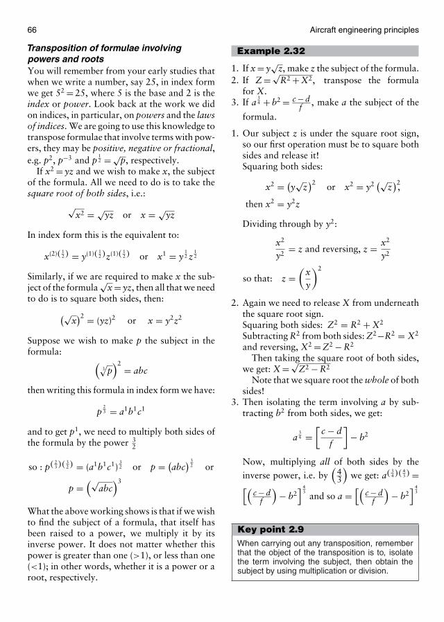
66 Aircraft engineering principles
Transposition of formulae involvingpowers and rootsYou will remember from your early studies thatwhen we write a number, say 25, in index formwe get 52 = 25, where 5 is the base and 2 is theindex or power. Look back at the work we didon indices, in particular, on powers and the lawsof indices. We are going to use this knowledge totranspose formulae that involve terms with pow-ers, they may be positive, negative or fractional,e.g. p2, p−3 and p
12 = √
p, respectively.If x2 = yz and we wish to make x, the subject
of the formula. All we need to do is to take thesquare root of both sides, i.e.:
√x2 = √
yz or x = √yz
In index form this is the equivalent to:
x(2)( 12 ) = y(1)( 1
2 )z(1)( 12 ) or x1 = y
12 z
12
Similarly, if we are required to make x the sub-ject of the formula
√x = yz, then all that we need
to do is to square both sides, then:
(√x)2 = (yz)2 or x = y2z2
Suppose we wish to make p the subject in theformula: (
3√
p)2 = abc
then writing this formula in index form we have:
p23 = a1b1c1
and to get p1, we need to multiply both sides ofthe formula by the power 3
2
so : p( 23 )(
32 ) = (a1b1c1)
32 or p = (
abc) 3
2 or
p =(√
abc)3
What the above working shows is that if we wishto find the subject of a formula, that itself hasbeen raised to a power, we multiply it by itsinverse power. It does not matter whether thispower is greater than one (>1), or less than one(<1); in other words, whether it is a power or aroot, respectively.
Example 2.32
1. If x = y√
z, make z the subject of the formula.2. If Z = √
R2 + X2, transpose the formulafor X.
3. If a34 + b2 = c − d
f , make a the subject of the
formula.
1. Our subject z is under the square root sign,so our first operation must be to square bothsides and release it!Squaring both sides:
x2 = (y√
z)2 or x2 = y2 (√z
)2,then x2 = y2z
Dividing through by y2:
x2
y2= z and reversing, z = x2
y2
so that: z =(
xy
)2
2. Again we need to release X from underneaththe square root sign.Squaring both sides: Z2 = R2 + X2
Subtracting R2 from both sides: Z2−R2 = X2
and reversing, X2 = Z2 − R2
Then taking the square root of both sides,we get: X = √
Z2 − R2
Note that we square root the whole of bothsides!
3. Then isolating the term involving a by sub-tracting b2 from both sides, we get:
a34 =
[c − d
f
]− b2
Now, multiplying all of both sides by the
inverse power, i.e. by(
43
)we get: a( 3
4 )(43 ) =[(
c − df
)− b2
] 43
and so a =[(
c − df
)− b2
] 43
Key point 2.9When carrying out any transposition, rememberthat the object of the transposition is to, isolatethe term involving the subject, then obtain thesubject by using multiplication or division.
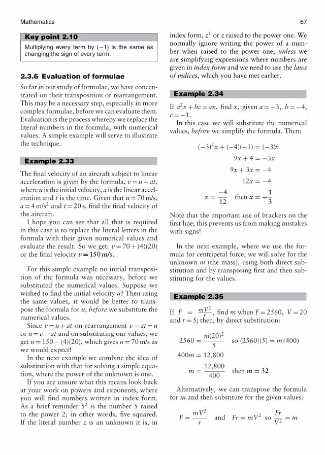
Mathematics 67
Key point 2.10Multiplying every term by (−1) is the same aschanging the sign of every term.
2.3.6 Evaluation of formulae
So far in our study of formulae, we have concen-trated on their transposition or rearrangement.This may be a necessary step, especially in morecomplex formulae, before we can evaluate them.Evaluation is the process whereby we replace theliteral numbers in the formula, with numericalvalues. A simple example will serve to illustratethe technique.
Example 2.33
The final velocity of an aircraft subject to linearacceleration is given by the formula, v = u + at,where u is the initial velocity, a is the linear accel-eration and t is the time. Given that u = 70 m/s,a = 4 m/s2 and t = 20 s, find the final velocity ofthe aircraft.
I hope you can see that all that is requiredin this case is to replace the literal letters in theformula with their given numerical values andevaluate the result. So we get: v = 70 + (4)(20)or the final velocity v = 150 m/s.
For this simple example no initial transposi-tion of the formula was necessary, before wesubstituted the numerical values. Suppose wewished to find the initial velocity u? Then usingthe same values, it would be better to trans-pose the formula for u, before we substitute thenumerical values.
Since v = u + at on rearrangement v − at = uor u = v − at and on substituting our values, weget u = 150 − (4)(20), which gives u = 70 m/s aswe would expect!
In the next example we combine the idea ofsubstitution with that for solving a simple equa-tion, where the power of the unknown is one.
If you are unsure what this means look backat your work on powers and exponents, whereyou will find numbers written in index form.As a brief reminder 52 is the number 5 raisedto the power 2; in other words, five squared.If the literal number z is an unknown it is, in
index form, z1 or z raised to the power one. Wenormally ignore writing the power of a num-ber when raised to the power one, unless weare simplifying expressions where numbers aregiven in index form and we need to use the lawsof indices, which you have met earlier.
Example 2.34
If a2x + bc = ax, find x, given a = −3, b = −4,c = −1.
In this case we will substitute the numericalvalues, before we simplify the formula. Then:
(−3)2x + (−4)(−1) = (−3)x
9x + 4 = −3x
9x + 3x = −4
12x = −4
x = −412
then x = −13
Note that the important use of brackets on thefirst line; this prevents us from making mistakeswith signs!
In the next example, where we use the for-mula for centripetal force, we will solve for theunknown m (the mass), using both direct sub-stitution and by transposing first and then sub-stituting for the values.
Example 2.35
If F = mV2
r , find m when F = 2560, V = 20and r = 5; then, by direct substitution:
2560 = m(20)2
5so (2560)(5) = m (400)
400m = 12,800
m = 12,800400
then m = 32
Alternatively, we can transpose the formulafor m and then substitute for the given values:
F = mV2
rand Fr = mV2 so
FrV2
= m
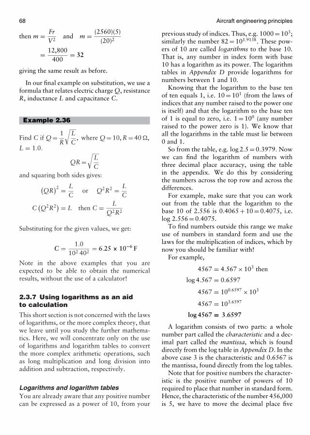
68 Aircraft engineering principles
then m = FrV2
and m = (2560)(5)(20)2
= 12,800400
= 32
giving the same result as before.
In our final example on substitution, we use aformula that relates electric charge Q, resistanceR, inductance L and capacitance C.
Example 2.36
Find C if Q = 1R
√LC
, where Q = 10, R = 40 �,
L = 1.0.
QR =√
LC
and squaring both sides gives:
(QR
)2 = LC
or Q2R2 = LC
C(Q2R2) = L then C = L
Q2R2
Substituting for the given values, we get:
C = 1.0102 402
= 6.25 × 10⁻⁶ F
Note in the above examples that you areexpected to be able to obtain the numericalresults, without the use of a calculator!
2.3.7 Using logarithms as an aidto calculation
This short section is not concerned with the lawsof logarithms, or the more complex theory, thatwe leave until you study the further mathema-tics. Here, we will concentrate only on the useof logarithms and logarithm tables to convertthe more complex arithmetic operations, suchas long multiplication and long division intoaddition and subtraction, respectively.
Logarithms and logarithm tablesYou are already aware that any positive numbercan be expressed as a power of 10, from your
previous study of indices. Thus, e.g. 1000 = 103;similarly the number 82 = 101.9138. These pow-ers of 10 are called logarithms to the base 10.That is, any number in index form with base10 has a logarithm as its power. The logarithmtables in Appendix D provide logarithms fornumbers between 1 and 10.
Knowing that the logarithm to the base tenof ten equals 1, i.e. 10 = 101 (from the laws ofindices that any number raised to the power oneis itself) and that the logarithm to the base tenof 1 is equal to zero, i.e. 1 = 100 (any numberraised to the power zero is 1). We know thatall the logarithms in the table must lie between0 and 1.
So from the table, e.g. log 2.5 = 0.3979. Nowwe can find the logarithm of numbers withthree decimal place accuracy, using the tablein the appendix. We do this by consideringthe numbers across the top row and across thedifferences.
For example, make sure that you can workout from the table that the logarithm to thebase 10 of 2.556 is 0.4065 + 10 = 0.4075, i.e.log 2.556 = 0.4075.
To find numbers outside this range we makeuse of numbers in standard form and use thelaws for the multiplication of indices, which bynow you should be familiar with!
For example,
4567 = 4.567 × 10³ then
log 4.567 = 0.6597
4567 = 100.6597 × 10³
4567 = 103.6597
log 4567 = 3.6597
A logarithm consists of two parts: a wholenumber part called the characteristic and a dec-imal part called the mantissa, which is founddirectly from the log table in Appendix D. In theabove case 3 is the characteristic and 0.6567 isthe mantissa, found directly from the log tables.
Note that for positive numbers the character-istic is the positive number of powers of 10required to place that number in standard form.Hence, the characteristic of the number 456,000is 5, we have to move the decimal place five
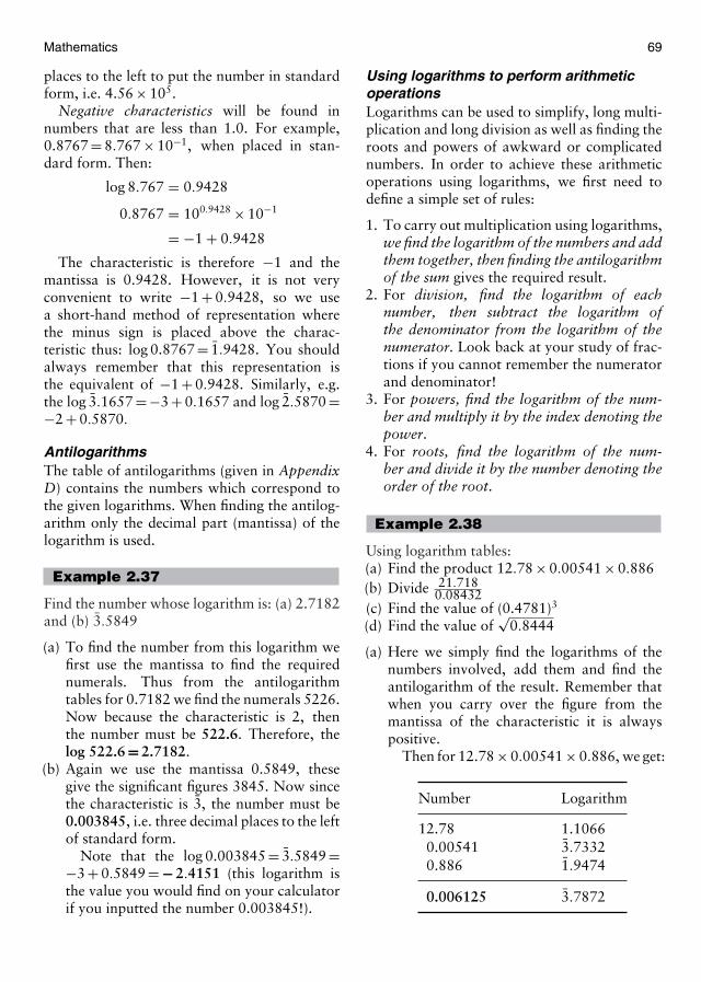
Mathematics 69
places to the left to put the number in standardform, i.e. 4.56 × 10⁵.
Negative characteristics will be found innumbers that are less than 1.0. For example,0.8767 = 8.767 × 10⁻¹, when placed in stan-dard form. Then:
log 8.767 = 0.9428
0.8767 = 100.9428 × 10−1
= −1 + 0.9428
The characteristic is therefore −1 and themantissa is 0.9428. However, it is not veryconvenient to write −1 + 0.9428, so we usea short-hand method of representation wherethe minus sign is placed above the charac-teristic thus: log 0.8767 = 1.9428. You shouldalways remember that this representation isthe equivalent of −1 + 0.9428. Similarly, e.g.the log 3.1657 = −3 + 0.1657 and log 2.5870 =−2 + 0.5870.
AntilogarithmsThe table of antilogarithms (given in AppendixD) contains the numbers which correspond tothe given logarithms. When finding the antilog-arithm only the decimal part (mantissa) of thelogarithm is used.
Example 2.37
Find the number whose logarithm is: (a) 2.7182and (b) 3.5849
(a) To find the number from this logarithm wefirst use the mantissa to find the requirednumerals. Thus from the antilogarithmtables for 0.7182 we find the numerals 5226.Now because the characteristic is 2, thenthe number must be 522.6. Therefore, thelog 522.6 = 2.7182.
(b) Again we use the mantissa 0.5849, thesegive the significant figures 3845. Now sincethe characteristic is 3, the number must be0.003845, i.e. three decimal places to the leftof standard form.
Note that the log 0.003845 = 3.5849 =−3 + 0.5849 = − 2.4151 (this logarithm isthe value you would find on your calculatorif you inputted the number 0.003845!).
Using logarithms to perform arithmeticoperationsLogarithms can be used to simplify, long multi-plication and long division as well as finding theroots and powers of awkward or complicatednumbers. In order to achieve these arithmeticoperations using logarithms, we first need todefine a simple set of rules:
1. To carry out multiplication using logarithms,we find the logarithm of the numbers and addthem together, then finding the antilogarithmof the sum gives the required result.
2. For division, find the logarithm of eachnumber, then subtract the logarithm ofthe denominator from the logarithm of thenumerator. Look back at your study of frac-tions if you cannot remember the numeratorand denominator!
3. For powers, find the logarithm of the num-ber and multiply it by the index denoting thepower.
4. For roots, find the logarithm of the num-ber and divide it by the number denoting theorder of the root.
Example 2.38
Using logarithm tables:(a) Find the product 12.78 × 0.00541 × 0.886(b) Divide 21.718
0.08432(c) Find the value of (0.4781)3
(d) Find the value of√
0.8444
(a) Here we simply find the logarithms of thenumbers involved, add them and find theantilogarithm of the result. Remember thatwhen you carry over the figure from themantissa of the characteristic it is alwayspositive.
Then for 12.78 × 0.00541 × 0.886, we get:
Number Logarithm
12.78 1.10660.00541 3.73320.886 1.9474
0.006125 3.7872
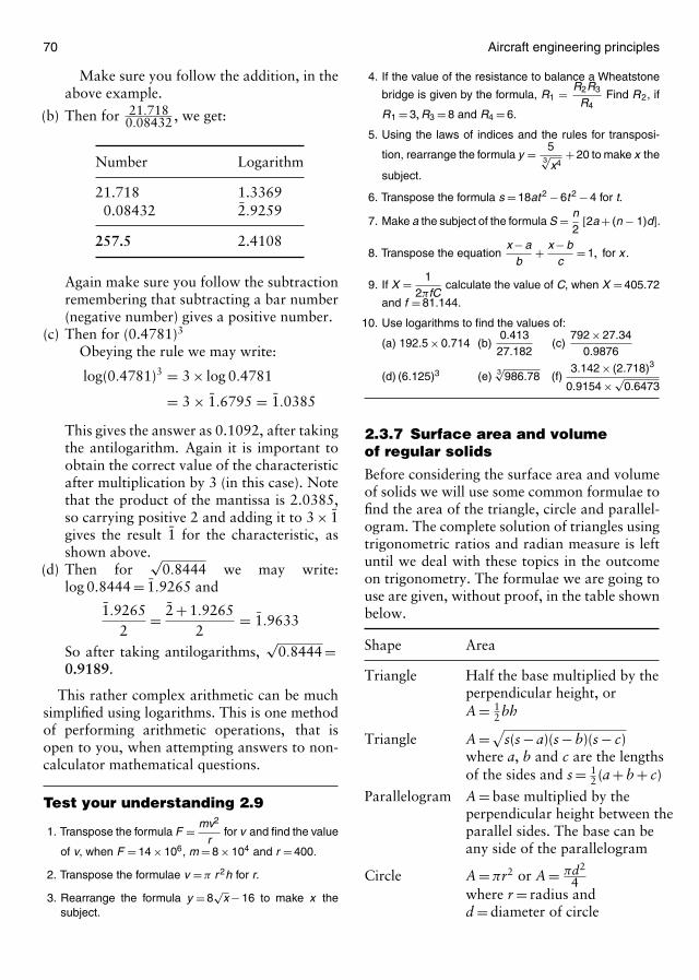
70 Aircraft engineering principles
Make sure you follow the addition, in theabove example.
(b) Then for 21.7180.08432 , we get:
Number Logarithm
21.718 1.33690.08432 2.9259
257.5 2.4108
Again make sure you follow the subtractionremembering that subtracting a bar number(negative number) gives a positive number.
(c) Then for (0.4781)3
Obeying the rule we may write:
log(0.4781)3 = 3 × log 0.4781
= 3 × 1.6795 = 1.0385
This gives the answer as 0.1092, after takingthe antilogarithm. Again it is important toobtain the correct value of the characteristicafter multiplication by 3 (in this case). Notethat the product of the mantissa is 2.0385,so carrying positive 2 and adding it to 3 × 1gives the result 1 for the characteristic, asshown above.
(d) Then for√
0.8444 we may write:log 0.8444 = 1.9265 and
1.92652
= 2 + 1.92652
= 1.9633
So after taking antilogarithms,√
0.8444 =0.9189.
This rather complex arithmetic can be muchsimplified using logarithms. This is one methodof performing arithmetic operations, that isopen to you, when attempting answers to non-calculator mathematical questions.
Test your understanding 2.9
1. Transpose the formula F = mv2
rfor v and find the value
of v, when F = 14 × 106, m = 8 × 10⁴ and r = 400.
2. Transpose the formulae v = π r 2h for r.
3. Rearrange the formula y = 8√
x − 16 to make x thesubject.
4. If the value of the resistance to balance a Wheatstone
bridge is given by the formula, R1 = R2R3
R4Find R2, if
R1 = 3, R3 = 8 and R4 = 6.
5. Using the laws of indices and the rules for transposi-
tion, rearrange the formula y = 53√
x4+ 20 to make x the
subject.
6. Transpose the formula s = 18at 2 − 6t 2 − 4 for t.
7. Make a the subject of the formula S = n2
[2a + (n − 1)d].
8. Transpose the equationx − a
b+ x − b
c= 1, for x .
9. If X = 12πfC
calculate the value of C, when X = 405.72
and f = 81.144.
10. Use logarithms to find the values of:
(a) 192.5 × 0.714 (b)0.413
27.182(c)
792 × 27.340.9876
(d) (6.125)3 (e) 3√986.78 (f)3.142 × (2.718)3
0.9154 × √0.6473
2.3.7 Surface area and volumeof regular solids
Before considering the surface area and volumeof solids we will use some common formulae tofind the area of the triangle, circle and parallel-ogram. The complete solution of triangles usingtrigonometric ratios and radian measure is leftuntil we deal with these topics in the outcomeon trigonometry. The formulae we are going touse are given, without proof, in the table shownbelow.
Shape Area
Triangle Half the base multiplied by theperpendicular height, orA = 1
2 bh
Triangle A =√s(s − a)(s − b)(s − c)where a, b and c are the lengthsof the sides and s = 1
2 (a + b + c)
Parallelogram A = base multiplied by theperpendicular height between theparallel sides. The base can beany side of the parallelogram
Circle A = πr2 or A = πd2
4where r = radius andd = diameter of circle
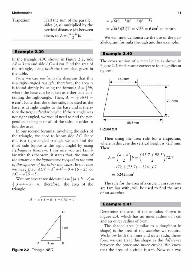
Mathematics 71
Trapezium Half the sum of the parallelsides (a, b) multiplied by thevertical distance (h) betweenthem, or A = (a + b
2)h
Example 2.39
In the triangle ABC shown in Figure 2.2, sideAB = 3 cm and side AC = 4 cm. Find the area ofthe triangle, using both the formulae, given inthe table.
Now we can see from the diagram that thisis a right-angled triangle; therefore, the area Ais found simply by using the formula A = 1
2 bh,where the base can be taken as either side con-taining the right-angle. Then, A = 1
2 (3)(4) =6 cm2. Note that the other side, not used as thebase, is at right angles to the base and is there-fore the perpendicular height. If the triangle wasnot right angled, we would need to find the per-pendicular height or all of the sides in order tofind the area.
In our second formula, involving the sides ofthe triangle, we need to know side AC. Sincethis is a right-angled triangle we can find thethird side (opposite the right angle) by usingPythagoras theorem. I am sure you are famil-iar with this theorem, it states that: the sum ofthe square on the hypotenuse is equal to the sumof the squares of the other two sides. In our casewe have that (AC)2 = 32 + 42 = 9 + 16 = 25 orAC = √
25 = 5.We now have three sides and s = 1
2 (a + b + c) =12 (3 + 4 + 5) = 6; therefore, the area of thetriangle:
A =√
s(s − a)(s − b)(s − c)
Figure 2.2 Triangle ABC.
= √6(6 − 3)(6 − 4)(6 − 5)
= √6(3)(2)(1) = √
36 = 6 cm2 as before.
We will now demonstrate the use of the par-allelogram formula through another example.
Example 2.40
The cross section of a metal plate is shown inFigure 2.3; find its area correct to four significantfigures.
Figure 2.3
Then using the area rule for a trapezium,where in this case the vertical height is 72.7 mm.Then:
A =(
a + b2
)h =
(45.7 + 98.5
2
)72.7
= (72.1)(72.7) = 5241.67
= 5242 mm2
The rule for the area of a circle, I am sure youare familiar with, will be used to find the areaof an annulus.
Example 2.41
Determine the area of the annulus shown inFigure 2.4, which has an inner radius of 5 cmand an outer radius of 8 cm.
The shaded area (similar to a doughnut inshape) is the area of the annulus we require.We know both the inner and outer radii, there-fore, we can treat this shape as the differencebetween the outer and inner circles. We knowthat the area of a circle is πr2. Now our two
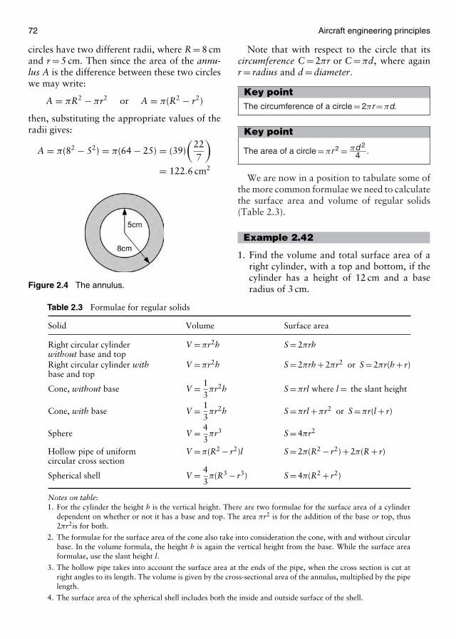
72 Aircraft engineering principles
circles have two different radii, where R = 8 cmand r = 5 cm. Then since the area of the annu-lus A is the difference between these two circleswe may write:
A = πR2 − πr2 or A = π(R2 − r2)
then, substituting the appropriate values of theradii gives:
A = π(82 − 52) = π(64 − 25) = (39)(
227
)= 122.6 cm2
Figure 2.4 The annulus.
Table 2.3 Formulae for regular solids
Solid Volume Surface area
Right circular cylinder V = πr2h S = 2πrhwithout base and topRight circular cylinder with V = πr2h S = 2πrh + 2πr2 or S = 2πr(h + r)base and top
Cone, without base V = 13
πr2h S = πrl where l = the slant height
Cone, with base V = 13
πr2h S = πrl + πr2 or S = πr(l + r)
Sphere V = 43
πr3 S = 4πr2
Hollow pipe of uniform V = π(R2 − r2)l S = 2π(R2 − r2) + 2π(R + r)circular cross section
Spherical shell V = 43
π(R3 − r3) S = 4π(R2 + r2)
Notes on table:1. For the cylinder the height h is the vertical height. There are two formulae for the surface area of a cylinder
dependent on whether or not it has a base and top. The area πr2 is for the addition of the base or top, thus2πr2is for both.
2. The formulae for the surface area of the cone also take into consideration the cone, with and without circularbase. In the volume formula, the height h is again the vertical height from the base. While the surface areaformulae, use the slant height l.
3. The hollow pipe takes into account the surface area at the ends of the pipe, when the cross section is cut atright angles to its length. The volume is given by the cross-sectional area of the annulus, multiplied by the pipelength.
4. The surface area of the spherical shell includes both the inside and outside surface of the shell.
Note that with respect to the circle that itscircumference C = 2πr or C = πd, where againr = radius and d = diameter.
Key pointThe circumference of a circle = 2πr = πd.
Key point
The area of a circle = πr 2 = πd 2
4 .
We are now in a position to tabulate some ofthe more common formulae we need to calculatethe surface area and volume of regular solids(Table 2.3).
Example 2.42
1. Find the volume and total surface area of aright cylinder, with a top and bottom, if thecylinder has a height of 12 cm and a baseradius of 3 cm.
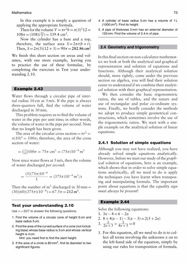
Mathematics 73
In this example it is simply a question ofapplying the appropriate formula.
Then for the volume V = πr2h = π(3)212 =108π = (108)( 22
7 ) = 339.4 cm3.Now the cylinder has a base and a top,
therefore, the surface area S = 2πr(h + r).Then, S = 2π(3)(12 + 3) = 90π = 282.86 cm2.
We finish this short section on areas and vol-umes, with one more example, leaving youto practice the use of these formulae, bycompleting the exercises in Test your under-standing 2.10.
Example 2.43
Water flows through a circular pipe of inter-nal radius 10 cm at 5 m/s. If the pipe is alwaysthree-quarters full, find the volume of waterdischarged in 30 min.
This problem requires us to find the volume ofwater in the pipe per unit time; in other words,the volume of water in the pipe per second. Notethat no length has been given.
The area of the circular cross section = πr2 =π(10)2 = 100π; therefore, the area of the crosssection of water:
= ( 34
)100π = 75π cm3 = (75π)10−4 m3
Now since water flows at 5 m/s, then the volumeof water discharged per second:
= (5)(75π)10−4
1= (375π)10−4 m3/s
Then the number of m3 discharged in 30 min =(30)(60)(375π)(10−4) = 67.5π = 212 m3.
Test your understanding 2.10Use π = 22/7 to answer the following questions.
1. Find the volume of a circular cone of height 6 cm andbase radius 5 cm.
2. Find the area of the curved surface of a cone (not includ-ing base) whose base radius is 3 cm and whose verticalheight is 4 cm.
Hint : you need first to find the slant height.
3. If the area of a circle is 80 mm2, find its diameter to twosignificant figures.
4. A cylinder of base radius 5 cm has a volume of 1 L(1000 cm3). Find its height.
5. A pipe of thickness 5 mm has an external diameter of120 mm. Find the volume of 2.4 m of pipe.
2.4 Geometry and trigonometry
In this final section on non-calculator mathemat-ics we look at both the analytical and graphicalrepresentation and solution of equations andfunctions. Although their analytical solutionshould, more rightly, come under the previoussection on algebra, you will find their solutioneasier to understand if we combine their analyti-cal solution with their graphical representation.
We then consider the basic trigonometricratios, the use of tables, and the nature anduse of rectangular and polar co-ordinate sys-tems. Finally, we briefly consider the methodswe adopt to produce simple geometrical con-structions, which sometimes involve the use ofthe trigonometric ratios. We start with a sim-ple example on the analytical solution of linearequations.
2.4.1 Solution of simple equations
Although you may not have realized, you havealready solved simple equations analytically.However, before we start our study of the graph-ical solution of equations, here is an example,which shows that in order to solve simple equa-tions analytically, all we need to do is applythe techniques you have learnt when transpos-ing and manipulating formula. The importantpoint about equations is that the equality signmust always be present!
Example 2.44
Solve the following equations:1. 3x − 4 = 6 − 2x2. 8 + 4(x − 1) − 5(x − 3) = 2(5 + 2x)3. 1
2x + 3 + 14x + 3 = 0
1. For this equation, all we need to do is to col-lect all terms involving the unknown x on tothe left-hand side of the equation, simply byusing our rules for transposition of formula.
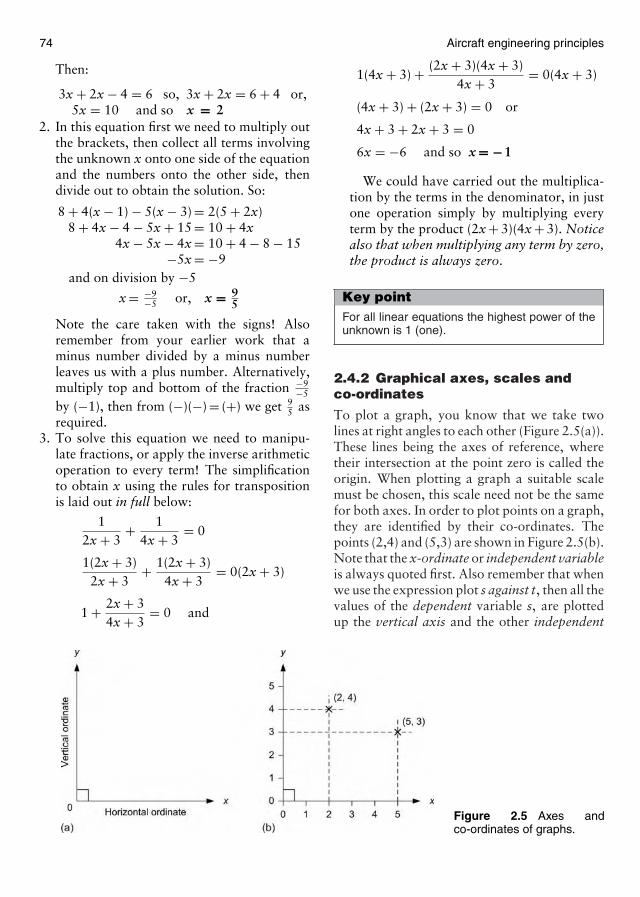
74 Aircraft engineering principles
Then:
3x + 2x − 4 = 6 so, 3x + 2x = 6 + 4 or,5x = 10 and so x = 2
2. In this equation first we need to multiply outthe brackets, then collect all terms involvingthe unknown x onto one side of the equationand the numbers onto the other side, thendivide out to obtain the solution. So:
8 + 4(x − 1) − 5(x − 3) = 2(5 + 2x)8 + 4x − 4 − 5x + 15 = 10 + 4x
4x − 5x − 4x = 10 + 4 − 8 − 15−5x = −9
and on division by −5
x = −9−5 or, x = 9
5
Note the care taken with the signs! Alsoremember from your earlier work that aminus number divided by a minus numberleaves us with a plus number. Alternatively,multiply top and bottom of the fraction −9
−5
by (−1), then from (−)(−) = (+) we get 95 as
required.3. To solve this equation we need to manipu-
late fractions, or apply the inverse arithmeticoperation to every term! The simplificationto obtain x using the rules for transpositionis laid out in full below:
12x + 3
+ 14x + 3
= 0
1(2x + 3)2x + 3
+ 1(2x + 3)4x + 3
= 0(2x + 3)
1 + 2x + 34x + 3
= 0 and
Figure 2.5 Axes andco-ordinates of graphs.
1(4x + 3) + (2x + 3)(4x + 3)4x + 3
= 0(4x + 3)
(4x + 3) + (2x + 3) = 0 or
4x + 3 + 2x + 3 = 0
6x = −6 and so x = −1
We could have carried out the multiplica-tion by the terms in the denominator, in justone operation simply by multiplying everyterm by the product (2x + 3)(4x + 3). Noticealso that when multiplying any term by zero,the product is always zero.
Key pointFor all linear equations the highest power of theunknown is 1 (one).
2.4.2 Graphical axes, scales andco-ordinates
To plot a graph, you know that we take twolines at right angles to each other (Figure 2.5(a)).These lines being the axes of reference, wheretheir intersection at the point zero is called theorigin. When plotting a graph a suitable scalemust be chosen, this scale need not be the samefor both axes. In order to plot points on a graph,they are identified by their co-ordinates. Thepoints (2,4) and (5,3) are shown in Figure 2.5(b).Note that the x-ordinate or independent variableis always quoted first. Also remember that whenwe use the expression plot s against t, then all thevalues of the dependent variable s, are plottedup the vertical axis and the other independent
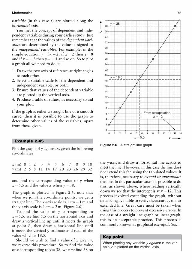
Mathematics 75
variable (in this case t) are plotted along thehorizontal axis.
You met the concept of dependent and inde-pendent variables during your earlier study. Justremember that the values of the dependent vari-ables are determined by the values assigned tothe independent variables. For example, in thesimple equation y = 3x + 2, if x = 2 then y = 8and if x = −2 then y = −4 and so on. So to plota graph all we need to do is:
1. Draw the two axis of reference at right anglesto each other.
2. Select a suitable scale for the dependent andindependent variable, or both.
3. Ensure that values of the dependent variableare plotted up the vertical axis.
4. Produce a table of values, as necessary to aidyour plot.
If the graph is either a straight line or a smoothcurve, then it is possible to use the graph todetermine other values of the variables, apartfrom those given.
Example 2.45
Plot the graph of y against x, given the followingco-ordinates
x (m) 0 1 2 3 4 5 6 7 8 9 10y (m) 2 5 8 11 14 17 20 23 26 29 32
and find the corresponding value of y whenx = 5.5 and the value x when y = 38.
The graph is plotted in Figure 2.6, note thatwhen we join the co-ordinate points, we get astraight line. The x-axis scale is 1 cm = 1 m andthe y-axis scale is 1 cm = 2 m (Figure 2.6).
To find the value of y corresponding tox = 5.5, we find 5.5 on the horizontal axis anddraw a vertical line up until it meets the graphat point P, then draw a horizontal line untilit meets the vertical y-ordinate and read of thevalue which is 18.5.
Should we wish to find a value of x given y,we reverse this procedure. So to find the valueof x corresponding to y = 38, we first find 38 on
y � 18.5
x � 5.5
From extrapolation, x � 12
y � 38
x
y
Figure 2.6 A straight line graph.
the y-axis and draw a horizontal line across tomeet the line. However, in this case the line doesnot extend this far, using the tabulated values. Itis, therefore, necessary to extend or extrapolatethe line. In this particular case it is possible to dothis, as shown above, where reading verticallydown we see that the intercept is at x = 12. Thisprocess involved extending the graph, withoutdata being available to verify the accuracy of ourextended line. Great care must be taken whenusing this process to prevent excessive errors. Inthe case of a straight line graph or linear graph,this is an acceptable practice. This process iscommonly known as graphical extrapolation.
Key pointWhen plotting any variable y against x, the vari-able y is plotted on the vertical axis.
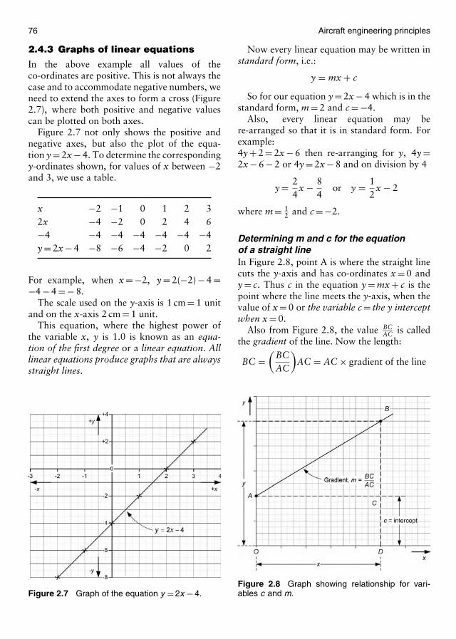
76 Aircraft engineering principles
2.4.3 Graphs of linear equations
In the above example all values of theco-ordinates are positive. This is not always thecase and to accommodate negative numbers, weneed to extend the axes to form a cross (Figure2.7), where both positive and negative valuescan be plotted on both axes.
Figure 2.7 not only shows the positive andnegative axes, but also the plot of the equa-tion y = 2x − 4. To determine the correspondingy-ordinates shown, for values of x between −2and 3, we use a table.
x −2 −1 0 1 2 32x −4 −2 0 2 4 6−4 −4 −4 −4 −4 −4 −4y = 2x − 4 −8 −6 −4 −2 0 2
For example, when x = −2, y = 2(−2) − 4 =−4 − 4 = − 8.
The scale used on the y-axis is 1 cm = 1 unitand on the x-axis 2 cm = 1 unit.
This equation, where the highest power ofthe variable x, y is 1.0 is known as an equa-tion of the first degree or a linear equation. Alllinear equations produce graphs that are alwaysstraight lines.
Figure 2.7 Graph of the equation y = 2x − 4.
Now every linear equation may be written instandard form, i.e.:
y = mx + c
So for our equation y = 2x − 4 which is in thestandard form, m = 2 and c = −4.
Also, every linear equation may bere-arranged so that it is in standard form. Forexample:4y + 2 = 2x − 6 then re-arranging for y, 4y =2x − 6 − 2 or 4y = 2x − 8 and on division by 4
y = 24
x − 84
or y = 12
x − 2
where m = 12 and c = −2.
Determining m and c for the equationof a straight lineIn Figure 2.8, point A is where the straight linecuts the y-axis and has co-ordinates x = 0 andy = c. Thus c in the equation y = mx + c is thepoint where the line meets the y-axis, when thevalue of x = 0 or the variable c = the y interceptwhen x = 0.
Also from Figure 2.8, the value BCAC is called
the gradient of the line. Now the length:
BC =(
BCAC
)AC = AC × gradient of the line
Figure 2.8 Graph showing relationship for vari-ables c and m.
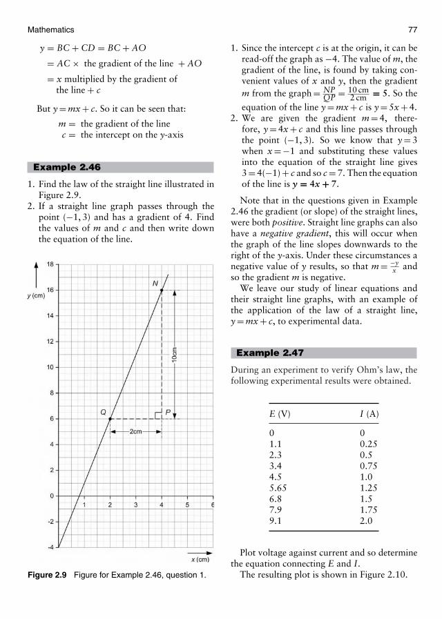
Mathematics 77
y = BC + CD = BC + AO
= AC × the gradient of the line + AO
= x multiplied by the gradient ofthe line + c
But y = mx + c. So it can be seen that:
m = the gradient of the linec = the intercept on the y-axis
Example 2.46
1. Find the law of the straight line illustrated inFigure 2.9.
2. If a straight line graph passes through thepoint (−1, 3) and has a gradient of 4. Findthe values of m and c and then write downthe equation of the line.
Figure 2.9 Figure for Example 2.46, question 1.
1. Since the intercept c is at the origin, it can beread-off the graph as −4. The value of m, thegradient of the line, is found by taking con-venient values of x and y, then the gradientm from the graph = NP
QP = 10 cm2 cm = 5. So the
equation of the line y = mx + c is y = 5x + 4.2. We are given the gradient m = 4, there-
fore, y = 4x + c and this line passes throughthe point (−1, 3). So we know that y = 3when x = −1 and substituting these valuesinto the equation of the straight line gives3 = 4(−1) + c and so c = 7. Then the equationof the line is y = 4x + 7.
Note that in the questions given in Example2.46 the gradient (or slope) of the straight lines,were both positive. Straight line graphs can alsohave a negative gradient, this will occur whenthe graph of the line slopes downwards to theright of the y-axis. Under these circumstances anegative value of y results, so that m = −y
x andso the gradient m is negative.
We leave our study of linear equations andtheir straight line graphs, with an example ofthe application of the law of a straight line,y = mx + c, to experimental data.
Example 2.47
During an experiment to verify Ohm’s law, thefollowing experimental results were obtained.
E (V) I (A)
0 01.1 0.252.3 0.53.4 0.754.5 1.05.65 1.256.8 1.57.9 1.759.1 2.0
Plot voltage against current and so determinethe equation connecting E and I.
The resulting plot is shown in Figure 2.10.

78 Aircraft engineering principles
Figure 2.10 Graph of E against I.
From the plot, it can be seen that the experi-mental data produces a straight line. Therefore,the equation connecting E and I is of theform y = mx + c. Since the graph goes directlythrough the origin, then the variable c = 0. Alsofrom the graph taking suitable values of E and I,the gradient m = 4.57 corrected to three signif-icant figures. So the equation connecting E andI is E = 4.57 I .
2.4.4 Quadratic equations
A quadratic equation is one in which theunknown variable is raised to the second power.For example, the equation x2 = 4 is perhapsone of the simplest of quadratic equations. Wecan solve this equation by taking the squareroot of both sides, something which you arefamiliar with, when transposing a formula.Then:
√x2 = √
4 or x = ±2. Note that even
for this simple equation there are two possi-ble solutions, either x = +2 or x = −2, remem-bering your laws of signs! When we squarea positive number we get a positive number(+2)(+2) = +4 or simply 4 also, (−2)(−2) = 4,from the laws of signs.
In general, a quadratic equation is of the typeax2 + bx + c = 0, where the constants a, b and ccan take any numerical value, positive or nega-tive, decimal or fraction. Like linear equations,quadratic equations do not always appear instandard form, i.e. they are not always arrangedin exactly the same order as their qualifyingequation, ax2 + bx + c = 0.
How is our simple equation x2 = 4 related toits qualifying equation? Well the coefficient ofx2 that is the number multiplying the x2 terma = 1. What about the constant b? Well there isno x term in our equation so b = 0. What aboutthe constant c? Our equation is not in standardform, because the equation should be equatedto zero. Then in standard form our equationbecomes x2 − 4 = 0 by simple transposition! Sonow we know that for our equation the con-stant term c = −4. A quadratic equation maycontain only the square of the unknown vari-able, as in our simple equation, or it may containthe square and the first power of the variable;e.g. x2 − 2x + 1 = 0. Also, the unknown vari-able may have up to two possible real solutions.The equations we deal with in this course willalways have at least one real solution.
There are several ways in which quadraticequations may be solved, that is finding thevalues of the unknown variable. We shall con-centrate on just three methods of solution; fac-torization, using the formula and solving bygraphical methods.
Solution of quadratic equations byfactorizationTake the equation x2 − 2x + 1 = 0. If we ignorefor the moment, the fact that this is an equationand concentrate on the expression x2 − 2x + 1,then you may remember how to find the factorsof this expression! Look back now at your workon factors to remind yourself.
I hope you were able to identify the factorsof this expression as (x − 1)(x − 1). Now all
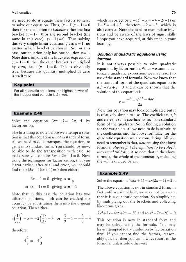
Mathematics 79
we need to do is equate these factors to zero,to solve our equation. Thus, (x − 1)(x − 1) = 0then for the equation to balance either the firstbracket (x − 1) = 0 or the second bracket (thesame in this case), (x − 1) = 0. Thus solvingthis very simple linear equation gives x = 1, nomatter which bracket is chosen. So, in thiscase, our equation only has one solution x = 1.Note that if anyone of the bracketed expressions(x − 1) = 0, then the other bracket is multipliedby zero, i.e. 0(x − 1) = 0. This is obviouslytrue, because any quantity multiplied by zerois itself zero.
Key pointFor all quadratic equations, the highest power ofthe independent variable is 2 (two).
Example 2.48
Solve the equation 3x2 − 5 = −2x − 4 byfactorization.
The first thing to note before we attempt a solu-tion is that this equation is not in standard form.All we need to do is transpose the equation, toget it into standard form. You should, by now,be able to do the transposition with ease, somake sure you obtain: 3x2 + 2x − 1 = 0. Nowusing the techniques for factorization, that youlearnt earlier, after trial and error, you shouldfind that: (3x − 1)(x + 1) = 0 then either:
3x − 1 = 0 giving x = 1
3or (x + 1) = 0 giving x = −1
Note that in this case the equation has twodifferent solutions, both can be checked foraccuracy by substituting them into the originalequation. Then either:
3(
13
)2
− 5 = −2(
13
)− 4 or
39
− 5 = −23
− 4
therefore:
−423
= −423
which is correct or 3(−1)2 − 5 = −4 − 2(−1) or3 − 5 = −4 + 2; therefore, − 2 = −2, which isalso correct. Note the need to manipulate frac-tions and be aware of the laws of signs, skillsI hope you have acquired, at this stage in yourlearning.
Solution of quadratic equations usingformulaIt is not always possible to solve quadraticequations by factorization. When we cannot fac-torize a quadratic expression, we may resort touse of the standard formula. Now we know thatthe standard form of the quadratic equation isax2 + bx + c = 0 and it can be shown that thesolution of this equation is:
x = −b ± √b2 − 4ac
2a
Now this equation may look complicated but itis relatively simple to use. The coefficients a, band c are the same coefficients, as in the standardform of the quadratic. So in finding a solutionfor the variable x, all we need to do is substitutethe coefficients into the above formulae, for thequadratic equation we are considering. All youneed to remember is that, before using the aboveformula, always put the equation to be solved,into standard form. Also note that in the aboveformula, the whole of the numerator, includingthe −b, is divided by 2a.
Example 2.49
Solve the equation 5x(x + 1) − 2x(2x − 1) = 20.
The above equation is not in standard form, infact until we simplify it, we may not be awarethat it is a quadratic equation. So simplifying,by multiplying out the brackets and collectinglike-terms gives:
5x2+5x−4x2+2x = 20 and so x2+7x−20 = 0
This equation is now in standard form andmay be solved using the formula. You mayhave attempted to try a solution by factorizationfirst. If you cannot find the factors, reason-ably quickly, then you can always resort to theformula, unless told otherwise!
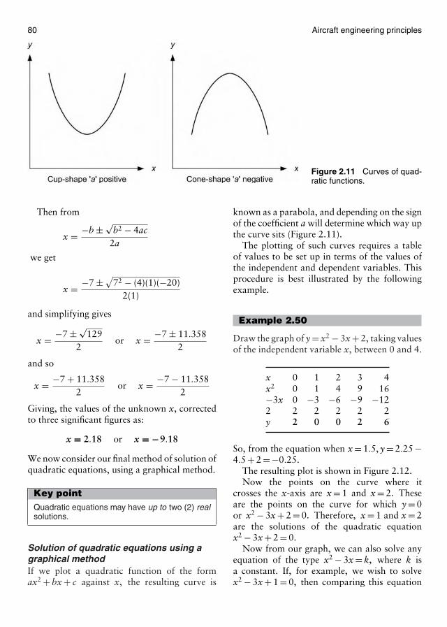
80 Aircraft engineering principles
Figure 2.11 Curves of quad-ratic functions.
Then from
x = −b ± √b2 − 4ac
2a
we get
x = −7 ±√72 − (4)(1)(−20)
2(1)
and simplifying gives
x = −7 ± √129
2or x = −7 ± 11.358
2
and so
x = −7 + 11.3582
or x = −7 − 11.3582
Giving, the values of the unknown x, correctedto three significant figures as:
x = 2.18 or x = −9.18
We now consider our final method of solution ofquadratic equations, using a graphical method.
Key pointQuadratic equations may have up to two (2) realsolutions.
Solution of quadratic equations using agraphical methodIf we plot a quadratic function of the formax2 + bx + c against x, the resulting curve is
known as a parabola, and depending on the signof the coefficient a will determine which way upthe curve sits (Figure 2.11).
The plotting of such curves requires a tableof values to be set up in terms of the values ofthe independent and dependent variables. Thisprocedure is best illustrated by the followingexample.
Example 2.50
Draw the graph of y = x2 − 3x + 2, taking valuesof the independent variable x, between 0 and 4.
x 0 1 2 3 4x2 0 1 4 9 16−3x 0 −3 −6 −9 −122 2 2 2 2 2y 2 0 0 2 6
So, from the equation when x = 1.5, y = 2.25 −4.5 + 2 = −0.25.
The resulting plot is shown in Figure 2.12.Now the points on the curve where it
crosses the x-axis are x = 1 and x = 2. Theseare the points on the curve for which y = 0or x2 − 3x + 2 = 0. Therefore, x = 1 and x = 2are the solutions of the quadratic equationx2 − 3x + 2 = 0.
Now from our graph, we can also solve anyequation of the type x2 − 3x = k, where k isa constant. If, for example, we wish to solvex2 − 3x + 1 = 0, then comparing this equation
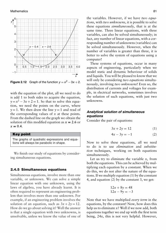
Mathematics 81
y
x
x � 0.4 x � 2.6
6
5
4
3
2
1
�1
00 0.5 1.0 1.5 2.0 2.5 3.0 3.5 4.0
Figure 2.12 Graph of the function y = x 2 − 3x + 2.
with the equation of the plot, all we need to dois add 1 to both sides to acquire the equation,y = x2 − 3x + 2 = 1. So that to solve this equa-tion, we need the points on the curve, wherey = 1. We then draw the line y = 1 and read ofthe corresponding values of x at these points.From the dashed line on the graph we obtain thesolution of this modified equation as x = 2.6 orx = 0.4.
Key pointThe graphs of quadratic expressions and equa-tions will always be parabolic in shape.
We finish our study of equations by consider-ing simultaneous equations.
2.4.5 Simultaneous equations
Simultaneous equations, involve more than onevariable, or unknown. We can solve a simplelinear equation with one unknown, using thelaws of algebra, you have already learnt. It isoften required to represent an engineering prob-lem that involves more than one unknown. Forexample, if an engineering problem involves thesolution of an equation, such as 3x + 2y = 12.How do we go about solving it? Well the answeris that a single equation with two unknowns, isunsolvable, unless we know the value of one of
the variables. However, if we have two equa-tions, with two unknowns, it is possible to solvethese equations simultaneously, that is at thesame time. Three linear equations, with threevariables, can also be solved simultaneously; infact, any number of linear equations, with a cor-responding number of unknowns (variables) canbe solved simultaneously. However, when thenumber of variables is greater than three, it isbetter to solve the system of equations using acomputer!
These systems of equations, occur in manyaspects of engineering, particularly when wemodel static and dynamic behaviour of solidsand liquids. You will be pleased to know that wewill only be considering two equations simulta-neously, involving two unknowns! Even so, thedistribution of currents and voltages for exam-ple, in electrical networks, sometimes involvesthe solution of such equations, with just twounknowns.
Analytical solution of simultaneousequationsConsider the pair of equations:
3x + 2y = 12 (1)
4x − 3y = −1 (2)
Now to solve these equations, all we needto do is to use elimination and substitu-tion techniques, working on both equationssimultaneously.
Let us try to eliminate the variable x, fromboth the equations. This can be achieved by mul-tiplying each equation by a constant. When wedo this, we do not alter the nature of the equa-tions. If we multiply equation (1) by the constant4, and equation (2) by the constant 3, we get:
12x + 8y = 4812x − 9y = −3
Note that we have multiplied every term in theequations, by the constant! Now, how does thishelp us to eliminate x? Well if we now add, bothequations together we end up with the first termbeing, 24x, this is not very helpful. However,
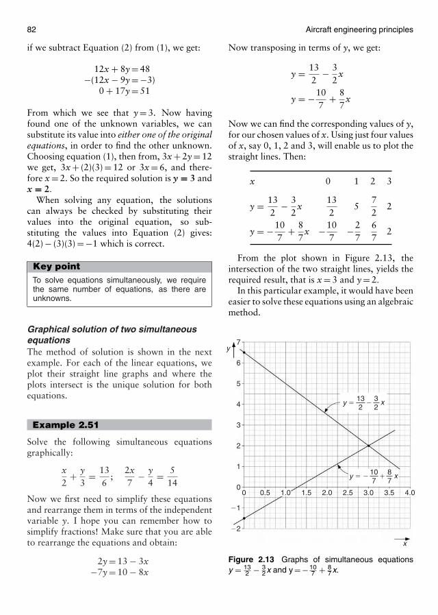
82 Aircraft engineering principles
if we subtract Equation (2) from (1), we get:
12x + 8y = 48−(12x − 9y = −3)
0 + 17y = 51
From which we see that y = 3. Now havingfound one of the unknown variables, we cansubstitute its value into either one of the originalequations, in order to find the other unknown.Choosing equation (1), then from, 3x + 2y = 12we get, 3x + (2)(3) = 12 or 3x = 6, and there-fore x = 2. So the required solution is y = 3 andx = 2.
When solving any equation, the solutionscan always be checked by substituting theirvalues into the original equation, so sub-stituting the values into Equation (2) gives:4(2) − (3)(3) = −1 which is correct.
Key pointTo solve equations simultaneously, we requirethe same number of equations, as there areunknowns.
Graphical solution of two simultaneousequationsThe method of solution is shown in the nextexample. For each of the linear equations, weplot their straight line graphs and where theplots intersect is the unique solution for bothequations.
Example 2.51
Solve the following simultaneous equationsgraphically:
x2
+ y3
= 136
;2x7
− y4
= 514
Now we first need to simplify these equationsand rearrange them in terms of the independentvariable y. I hope you can remember how tosimplify fractions! Make sure that you are ableto rearrange the equations and obtain:
2y = 13 − 3x−7y = 10 − 8x
Now transposing in terms of y, we get:
y = 132
− 32
x
y = −107
+ 87
x
Now we can find the corresponding values of y,for our chosen values of x. Using just four valuesof x, say 0, 1, 2 and 3, will enable us to plot thestraight lines. Then:
x 0 1 2 3
y = 132
− 32
x132
572
2
y = −107
+ 87
x −107
−27
67
2
From the plot shown in Figure 2.13, theintersection of the two straight lines, yields therequired result, that is x = 3 and y = 2.
In this particular example, it would have beeneasier to solve these equations using an algebraicmethod.
y
x
6
7
5
4
3
2
1
�1
�2
00 0.5 1.0 1.5 2.0 2.5 3.0 3.5 4.0
xy � 132
32
�
xy � � 107
87
�
Figure 2.13 Graphs of simultaneous equationsy = 13
2 − 32 x and y = − 10
7 + 87 x.
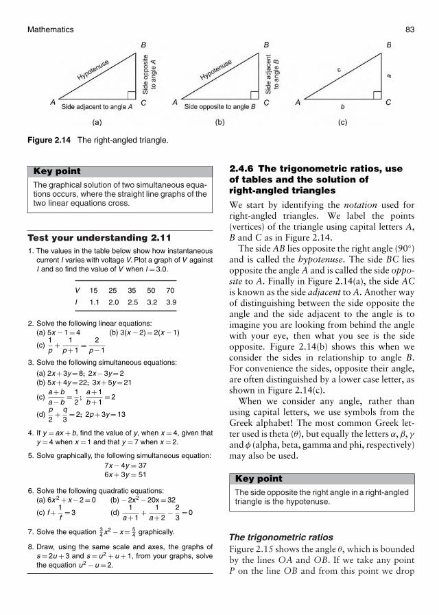
Mathematics 83
Figure 2.14 The right-angled triangle.
Key pointThe graphical solution of two simultaneous equa-tions occurs, where the straight line graphs of thetwo linear equations cross.
Test your understanding 2.111. The values in the table below show how instantaneous
current I varies with voltage V. Plot a graph of V againstI and so find the value of V when I = 3.0.
V 15 25 35 50 70
I 1.1 2.0 2.5 3.2 3.9
2. Solve the following linear equations:(a) 5x − 1 = 4 (b) 3(x − 2) = 2(x − 1)
(c)1p
+ 1p + 1
= 2p − 1
3. Solve the following simultaneous equations:
(a) 2x + 3y = 8; 2x − 3y = 2(b) 5x + 4y = 22; 3x + 5y = 21
(c)a + ba − b
= 12
;a + 1b + 1
= 2
(d)p2
+ q3
= 2; 2p + 3y = 13
4. If y = ax + b, find the value of y, when x = 4, given thaty = 4 when x = 1 and that y = 7 when x = 2.
5. Solve graphically, the following simultaneous equation:7x − 4y = 376x + 3y = 51
6. Solve the following quadratic equations:(a) 6x 2 + x − 2 = 0 (b) − 2x2 − 20x = 32
(c) f + 1f
= 3 (d)1
a + 1+ 1
a + 2− 2
3= 0
7. Solve the equation 34 x2 − x = 5
4 graphically.
8. Draw, using the same scale and axes, the graphs ofs = 2u + 3 and s = u2 + u + 1, from your graphs, solvethe equation u2 − u = 2.
2.4.6 The trigonometric ratios, useof tables and the solution ofright-angled triangles
We start by identifying the notation used forright-angled triangles. We label the points(vertices) of the triangle using capital letters A,B and C as in Figure 2.14.
The side AB lies opposite the right angle (90◦)and is called the hypotenuse. The side BC liesopposite the angle A and is called the side oppo-site to A. Finally in Figure 2.14(a), the side ACis known as the side adjacent to A. Another wayof distinguishing between the side opposite theangle and the side adjacent to the angle is toimagine you are looking from behind the anglewith your eye, then what you see is the sideopposite. Figure 2.14(b) shows this when weconsider the sides in relationship to angle B.For convenience the sides, opposite their angle,are often distinguished by a lower case letter, asshown in Figure 2.14(c).
When we consider any angle, rather thanusing capital letters, we use symbols from theGreek alphabet! The most common Greek let-ter used is theta (θ), but equally the letters α, β, γand φ (alpha, beta, gamma and phi, respectively)may also be used.
Key pointThe side opposite the right angle in a right-angledtriangle is the hypotenuse.
The trigonometric ratiosFigure 2.15 shows the angle θ, which is boundedby the lines OA and OB. If we take any pointP on the line OB and from this point we drop

84 Aircraft engineering principles
a perpendicular to the line OA to meet it at thepoint Q.
Then the ratioQPOP
is called the sine of angle AOB
OQOP
is called the cosine of angle AOB and
QPOQ
is called the tangent of the angle AOB.
The sine ratioIf we consider the triangle OPQ (Figure 2.16)from the point of view of the angle θ, then thesine (abbreviated to sin) of this angle
= oppositehypotenuse
, i.e. sin θ = QPOP
or sin θ = oq
similarly, the sine of the angle α
= oppositehypotenuse
, i.e. sin α = OQOP
or sin α = pq
If we know either the angle θ or α then wecan find the value of the sine ratio, for that par-ticular angle. To do this you may, up to now,have simply used your calculator. Since we areconsidering non-calculator mathematics we can
u
Figure 2.15 The right-angled triangle.
Figure 2.16 The sine of an angle.
only use drawing or tables to find the value ofthe sine ratio.
Key point
For any angle θ, then sin θ = side oppositehypotenuse .
Example 2.52
Find by drawing a suitable triangle, the value ofsin 30◦.
Then using a protractor, or by anothermethod, draw the lines AP and AQ which inter-sect at A, so that the angle PAQ = 30◦, as shownin Figure 2.17.
Along AQ measure off to a suitable scale AC(the hypotenuse), say 100 units. From point C,draw line CB perpendicular to AP. Measure CB,which will be found to be 50 units. Then:
sin 30◦ = 50100
= 0.5.
This method could be used to find the sine of anyangle; however, it is rather tedious and some-what limited in accuracy. Tables of sine ratioshave been compiled that allow us to find thesine of any angle. Table 2.4 shows an extractfrom the full table of natural sines, which willbe found in Appendix D.
From Table 2.4 it can be seen that angles aresubdivided into degrees (◦) and minutes (′) where1 min is equal to 1
60 of a degree. The equivalentdecimal fraction of each degree is also given atthe top of the table. We will demonstrate howto read Table 2.4, using an example.
P
Figure 2.17 Triangle ABC.
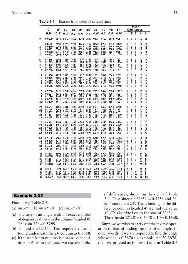
Mathematics 85
Table 2.4 Extract from table of natural sines
� � � � � � � � � �� � � � �
Example 2.53
Find, using Table 2.4:(a) sin 32◦ (b) sin 32◦24′ (c) sin 32◦28′.
(a) The sine of an angle with an exact numberof degrees is shown in the column headed 0′.Thus sin 32◦ = 0.5299.
(b) To find sin 32◦24′. The required value isfound underneath the 24′ column as 0.5358.
(c) If the number of minutes is not an exact mul-tiple of 6, as in this case, we use the tables
of differences, shown on the right of Table2.4. Thus since sin 32◦24′ = 0.5358 and 28′is 4′ more than 24′. Then, looking in the dif-ference column headed 4′ we find the value10. This is added on to the sine of 32◦24′.Then the sin 32◦28′ = 0.5358 + 10 = 0.5368.
Suppose we wish to carry out the inverse oper-ation to that of finding the sine of an angle. Inother words, if we are required to find the anglewhose sine is 0.3878 (in symbols, sin−10.3878)then we proceed as follows. Look in Table 2.4
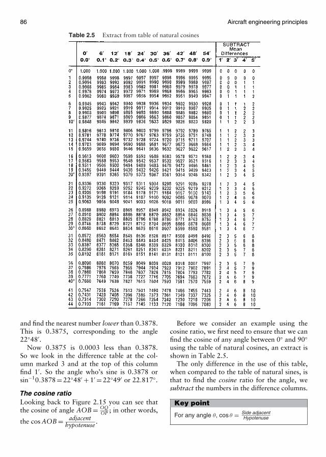
86 Aircraft engineering principles
Table 2.5 Extract from table of natural cosines
� � � � � � � � � �� � � � �
and find the nearest number lower than 0.3878.This is 0.3875, corresponding to the angle22◦48′.
Now 0.3875 is 0.0003 less than 0.3878.So we look in the difference table at the col-umn marked 3 and at the top of this columnfind 1′. So the angle who’s sine is 0.3878 orsin−10.3878 = 22◦48′ + 1′ = 22◦49′ or 22.817◦.
The cosine ratioLooking back to Figure 2.15 you can see thatthe cosine of angle AOB = OQ
OP ; in other words,
the cos AOB = adjacenthypotenuse .
Before we consider an example using thecosine ratio, we first need to ensure that we canfind the cosine of any angle between 0◦ and 90◦using the table of natural cosines, an extract isshown in Table 2.5.
The only difference in the use of this table,when compared to the table of natural sines, isthat to find the cosine ratio for the angle, wesubtract the numbers in the difference columns.
Key point
For any angle θ, cos θ = Side adjacentHypotenuse
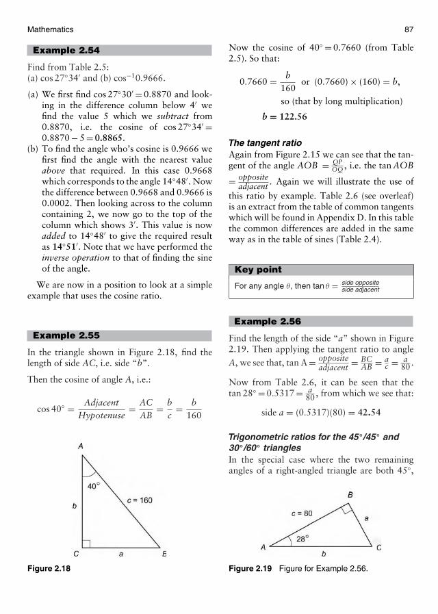
Mathematics 87
Example 2.54
Find from Table 2.5:(a) cos 27◦34′ and (b) cos−10.9666.
(a) We first find cos 27◦30′ = 0.8870 and look-ing in the difference column below 4′ wefind the value 5 which we subtract from0.8870, i.e. the cosine of cos 27◦34′ =0.8870 − 5 = 0.8865.
(b) To find the angle who’s cosine is 0.9666 wefirst find the angle with the nearest valueabove that required. In this case 0.9668which corresponds to the angle 14◦48′. Nowthe difference between 0.9668 and 0.9666 is0.0002. Then looking across to the columncontaining 2, we now go to the top of thecolumn which shows 3′. This value is nowadded to 14◦48′ to give the required resultas 14◦51′. Note that we have performed theinverse operation to that of finding the sineof the angle.
We are now in a position to look at a simpleexample that uses the cosine ratio.
Example 2.55
In the triangle shown in Figure 2.18, find thelength of side AC, i.e. side “b”.
Then the cosine of angle A, i.e.:
cos 40◦ = AdjacentHypotenuse
= ACAB
= bc
= b160
Figure 2.18
Now the cosine of 40◦ = 0.7660 (from Table2.5). So that:
0.7660 = b160
or (0.7660) × (160) = b,
so (that by long multiplication)
b = 122.56
The tangent ratioAgain from Figure 2.15 we can see that the tan-gent of the angle AOB = QP
OQ , i.e. the tan AOB
= oppositeadjacent . Again we will illustrate the use of
this ratio by example. Table 2.6 (see overleaf)is an extract from the table of common tangentswhich will be found in Appendix D. In this tablethe common differences are added in the sameway as in the table of sines (Table 2.4).
Key point
For any angle θ, then tan θ = side oppositeside adjacent
Example 2.56
Find the length of the side “a” shown in Figure2.19. Then applying the tangent ratio to angle
A, we see that, tan A = oppositeadjacent = BC
AB = ac = a
80 .
Now from Table 2.6, it can be seen that thetan 28◦ = 0.5317 = a
80 , from which we see that:
side a = (0.5317)(80) = 42.54
Trigonometric ratios for the 45◦/45◦ and30◦/60◦ trianglesIn the special case where the two remainingangles of a right-angled triangle are both 45◦,
Figure 2.19 Figure for Example 2.56.
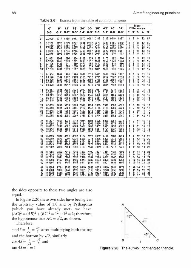
88 Aircraft engineering principles
Table 2.6 Extract from the table of common tangents
� � � � � � � � � �� � � � �
the sides opposite to these two angles are alsoequal.
In Figure 2.20 these two sides have been giventhe arbitrary value of 1.0 and by Pythagoras(which you have already met) we have:(AC)2 = (AB)2 + (BC)2 = 12 + 12 = 2; therefore,the hypotenuse side AC = √
2, as shown.Therefore:
sin 45 = 1√2
=√
22 after multiplying both the top
and the bottom by√
2, similarlycos 45 = 1√
2=
√2
2 and
tan 45 = 11 = 1 Figure 2.20 The 45◦/45◦ right-angled triangle.

Mathematics 89
Key pointIn a 45◦/45◦ right-angled triangle, the sides havethe ratios 1 :1 :
√2.
The square root of 2 is equal to 1.4142 cor-rected to four decimal places and is worth com-mitting to memory. Thus, for example, the sineand cosine of 45◦ =
√2
2 = 1.41422 = 0.7071 you
might like to check this in Tables 2.4 and 2.5!Also note an important relationship between
the sine, cosine and tangent ratios. From above:
sin 45cos 45
=√
22√2
2
=(√
22
)(2√2
)= 1 = tan 45
This relationship is not just true for 45◦, but istrue for any angle and may be generalized as:
sin θ
cos θ= tan θ
We now consider the 30◦/60◦ right-angled tri-angle, in a similar way to our 45◦/45◦ triangle.
An equilateral triangle is one in which all thesides are equal.
Key pointAn equilateral triangle is one in which all threesides are equal in length.
Figure 2.21 shows a triangle ABC in whicheach of the equal sides = 2 units. A perpendicu-lar is drawn from C to D, which bisects AB.
Figure 2.21 Construction for 30◦/60◦ triangle.
Now from Pythagorus for the right-angledtriangle ACD, we have that:
(CD)2 = (AC)2 − (AD)2 = 22 − 12 = 3,
therefore, side CD = √3
Now noting that all the angles of the triangleABC = 60 (remembering that there are 180 ina triangle) and that angle ACD = 30. Then thetrigonometric ratios for these two angles aregiven as follows:
sin 30 = 12
, cos 30 =√
32
, tan 30 = 1√3
=√
33
sin 60 =√
32
, cos 60 = 12
, tan 60 =√
31
= √3
Key pointIn a 30◦/60◦ right-angled triangle the sides havethe ratio 1 :
√3 :2.
Rectangular and polar co-ordinatesBefore we consider one or two simple appli-cations of the trigonometric ratios, such asangles of elevation and aircraft bearings, firstwe need to familiarize ourselves with the rectan-gular and polar co-ordinate systems. You havealready used rectangular co-ordinates, in yourearlier graphical work. Here we formalize thisco-ordinate system and discover how we canconvert from rectangular to polar co-ordinatesand vice versa.
Key pointRectangular co-ordinates are also known asCartesian co-ordinates.
A point on a graph can be defined in severalways. The two most common ways use eitherrectangular or polar co-ordinates.
Rectangular co-ordinates (Figure 2.22) usetwo perpendicular axis, normally labelled xand y. Where any point P is identified by its hor-izontal distance along the x-axis and its verticaldistance up the y-axis. Polar co-ordinates givethe distance r, from the origin O and the angle
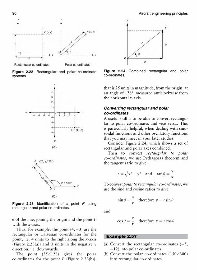
90 Aircraft engineering principles
Figure 2.22 Rectangular and polar co-ordinatesystems.
Figure 2.23 Identification of a point P usingrectangular and polar co-ordinates.
θ of the line, joining the origin and the point Pwith the x-axis.
Thus, for example, the point (4, −3) are therectangular or Cartesian co-ordinates for thepoint, i.e. 4 units to the right along the x-axis(Figure 2.23(a)) and 3 units in the negative ydirection, i.e. downwards.
The point (25∠128) gives the polarco-ordinates for the point P (Figure 2.23(b)),
r
Figure 2.24 Combined rectangular and polarco-ordinates.
that is 25 units in magnitude, from the origin, atan angle of 128◦, measured anticlockwise fromthe horizontal x-axis.
Converting rectangular and polarco-ordinatesA useful skill is to be able to convert rectangu-lar to polar co-ordinates and vice versa. Thisis particularly helpful, when dealing with sinu-soidal functions and other oscillatory functionsthat you may meet in your later studies.
Consider Figure 2.24, which shows a set ofrectangular and polar axes combined.
Then to convert rectangular to polarco-ordinates, we use Pythagoras theorem andthe tangent ratio to give:
r =√
x2 + y2 and tan θ = yx
To convert polar to rectangular co-ordinates, weuse the sine and cosine ratios to give:
sin θ = yr
therefore y = r sin θ
and
cos θ = xr
therefore x = r cos θ
Example 2.57
(a) Convert the rectangular co-ordinates (−5,−12) into polar co-ordinates.
(b) Convert the polar co-ordinates (150∠300)into rectangular co-ordinates.
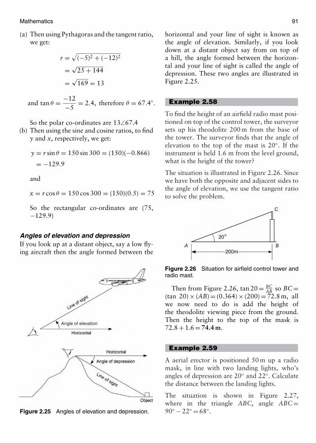
Mathematics 91
(a) Then using Pythagoras and the tangent ratio,we get:
r =√
(−5)2 + (−12)2
= √25 + 144
= √169 = 13
and tan θ = −12−5
= 2.4, therefore θ = 67.4◦.
So the polar co-ordinates are 13∠67.4(b) Then using the sine and cosine ratios, to find
y and x, respectively, we get:
y = r sin θ = 150 sin 300 = (150)(−0.866)
= −129.9
and
x = r cos θ = 150 cos 300 = (150)(0.5) = 75
So the rectangular co-ordinates are (75,−129.9)
Angles of elevation and depressionIf you look up at a distant object, say a low fly-ing aircraft then the angle formed between the
Angle of elevation
Figure 2.25 Angles of elevation and depression.
horizontal and your line of sight is known asthe angle of elevation. Similarly, if you lookdown at a distant object say from on top ofa hill, the angle formed between the horizon-tal and your line of sight is called the angle ofdepression. These two angles are illustrated inFigure 2.25.
Example 2.58
To find the height of an airfield radio mast posi-tioned on top of the control tower, the surveyorsets up his theodolite 200 m from the base ofthe tower. The surveyor finds that the angle ofelevation to the top of the mast is 20◦. If theinstrument is held 1.6 m from the level ground,what is the height of the tower?
The situation is illustrated in Figure 2.26. Sincewe have both the opposite and adjacent sides tothe angle of elevation, we use the tangent ratioto solve the problem.
Figure 2.26 Situation for airfield control tower andradio mast.
Then from Figure 2.26, tan 20 = BCAB so BC =
(tan 20) × (AB) = (0.364) × (200) = 72.8 m, allwe now need to do is add the height ofthe theodolite viewing piece from the ground.Then the height to the top of the mask is72.8 + 1.6 = 74.4 m.
Example 2.59
A aerial erector is positioned 50 m up a radiomask, in line with two landing lights, who’sangles of depression are 20◦ and 22◦. Calculatethe distance between the landing lights.
The situation is shown in Figure 2.27,where in the triangle ABC, angle ABC =90◦ − 22◦ = 68◦.
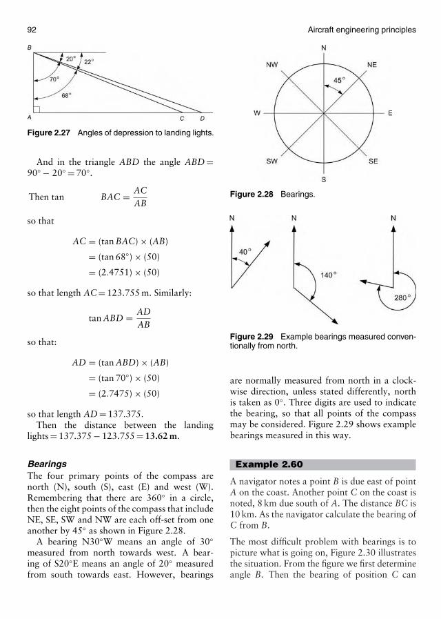
92 Aircraft engineering principles
Figure 2.27 Angles of depression to landing lights.
And in the triangle ABD the angle ABD =90◦ − 20◦ = 70◦.
Then tan BAC = ACAB
so that
AC = (tan BAC) × (AB)
= (tan 68◦) × (50)
= (2.4751) × (50)
so that length AC = 123.755 m. Similarly:
tan ABD = ADAB
so that:
AD = (tan ABD) × (AB)
= (tan 70◦) × (50)
= (2.7475) × (50)
so that length AD = 137.375.
Then the distance between the landinglights = 137.375 − 123.755 = 13.62 m.
BearingsThe four primary points of the compass arenorth (N), south (S), east (E) and west (W).Remembering that there are 360◦ in a circle,then the eight points of the compass that includeNE, SE, SW and NW are each off-set from oneanother by 45◦ as shown in Figure 2.28.
A bearing N30◦W means an angle of 30◦measured from north towards west. A bear-ing of S20◦E means an angle of 20◦ measuredfrom south towards east. However, bearings
Figure 2.28 Bearings.
Figure 2.29 Example bearings measured conven-tionally from north.
are normally measured from north in a clock-wise direction, unless stated differently, northis taken as 0◦. Three digits are used to indicatethe bearing, so that all points of the compassmay be considered. Figure 2.29 shows examplebearings measured in this way.
Example 2.60
A navigator notes a point B is due east of pointA on the coast. Another point C on the coast isnoted, 8 km due south of A. The distance BC is10 km. As the navigator calculate the bearing ofC from B.
The most difficult problem with bearings is topicture what is going on, Figure 2.30 illustratesthe situation. From the figure we first determineangle B. Then the bearing of position C can
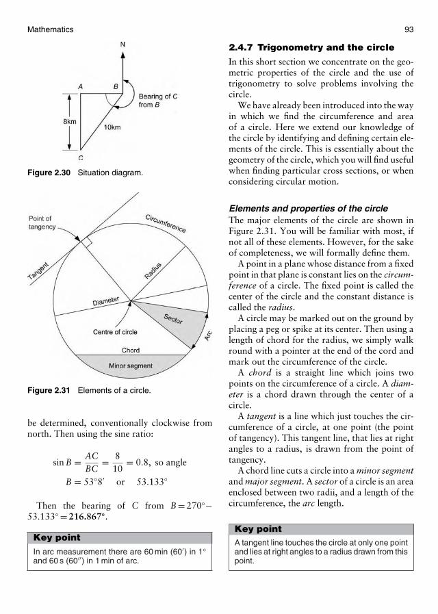
Mathematics 93
Figure 2.30 Situation diagram.
Figure 2.31 Elements of a circle.
be determined, conventionally clockwise fromnorth. Then using the sine ratio:
sin B = ACBC
= 810
= 0.8, so angle
B = 53◦8′ or 53.133◦
Then the bearing of C from B = 270◦−53.133◦ = 216.867◦.
Key pointIn arc measurement there are 60 min (60′) in 1◦and 60 s (60′′) in 1 min of arc.
2.4.7 Trigonometry and the circle
In this short section we concentrate on the geo-metric properties of the circle and the use oftrigonometry to solve problems involving thecircle.
We have already been introduced into the wayin which we find the circumference and areaof a circle. Here we extend our knowledge ofthe circle by identifying and defining certain ele-ments of the circle. This is essentially about thegeometry of the circle, which you will find usefulwhen finding particular cross sections, or whenconsidering circular motion.
Elements and properties of the circleThe major elements of the circle are shown inFigure 2.31. You will be familiar with most, ifnot all of these elements. However, for the sakeof completeness, we will formally define them.
A point in a plane whose distance from a fixedpoint in that plane is constant lies on the circum-ference of a circle. The fixed point is called thecenter of the circle and the constant distance iscalled the radius.
A circle may be marked out on the ground byplacing a peg or spike at its center. Then using alength of chord for the radius, we simply walkround with a pointer at the end of the cord andmark out the circumference of the circle.
A chord is a straight line which joins twopoints on the circumference of a circle. A diam-eter is a chord drawn through the center of acircle.
A tangent is a line which just touches the cir-cumference of a circle, at one point (the pointof tangency). This tangent line, that lies at rightangles to a radius, is drawn from the point oftangency.
A chord line cuts a circle into a minor segmentand major segment. A sector of a circle is an areaenclosed between two radii, and a length of thecircumference, the arc length.
Key pointA tangent line touches the circle at only one pointand lies at right angles to a radius drawn from thispoint.
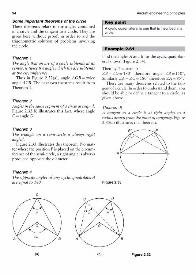
94 Aircraft engineering principles
Some important theorems of the circleThese theorems relate to the angles containedin a circle and the tangent to a circle. They aregiven here without proof, in order to aid thetrigonometric solution of problems involvingthe circle.
Theorem 1The angle that an arc of a circle subtends at itscenter, is twice the angle which the arc subtendsat the circumference.
Thus in Figure 2.32(a), angle AOB = twiceangle ACB. The next two theorems result fromTheorem 1.
Theorem 2Angles in the same segment of a circle are equal.Figure 2.32(b) illustrates this fact, where angleC = angle D.
Theorem 3The triangle on a semi-circle is always rightangled.
Figure 2.33 illustrates this theorem. No mat-ter where the position P is placed on the circum-ference of the semi-circle, a right angle is alwaysproduced opposite the diameter.
Theorem 4The opposite angles of any cyclic quadrilateralare equal to 180◦.
Figure 2.32
Key pointA cyclic quadrilateral is one that is inscribed in acircle.
Example 2.61
Find the angles A and B for the cyclic quadrilat-eral shown (Figure 2.34).
Then by Theorem 4:∠B + ∠D = 180◦ therefore angle ∠B = 110◦,Similarly ∠A + ∠C = 180◦ therefore ∠A = 85◦,
There are many theorems related to the tan-gent of a circle. In order to understand them, youshould be able to define a tangent to a circle, asgiven above.
Theorem 5A tangent to a circle is at right angles to aradius drawn from the point of tangency. Figure2.35(a) illustrates this theorem.
Figure 2.33
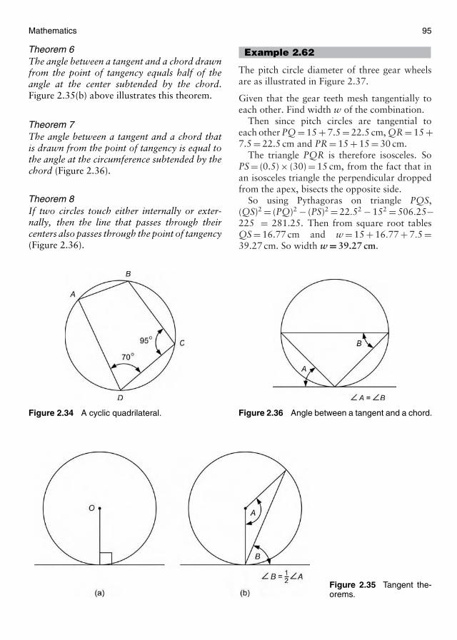
Mathematics 95
Theorem 6The angle between a tangent and a chord drawnfrom the point of tangency equals half of theangle at the center subtended by the chord.Figure 2.35(b) above illustrates this theorem.
Theorem 7The angle between a tangent and a chord thatis drawn from the point of tangency is equal tothe angle at the circumference subtended by thechord (Figure 2.36).
Theorem 8If two circles touch either internally or exter-nally, then the line that passes through theircenters also passes through the point of tangency(Figure 2.36).
Figure 2.34 A cyclic quadrilateral.
Figure 2.35 Tangent the-orems.
Example 2.62
The pitch circle diameter of three gear wheelsare as illustrated in Figure 2.37.
Given that the gear teeth mesh tangentially toeach other. Find width w of the combination.
Then since pitch circles are tangential toeach other PQ = 15 + 7.5 = 22.5 cm, QR = 15 +7.5 = 22.5 cm and PR = 15 + 15 = 30 cm.
The triangle PQR is therefore isosceles. SoPS = (0.5) × (30) = 15 cm, from the fact that inan isosceles triangle the perpendicular droppedfrom the apex, bisects the opposite side.
So using Pythagoras on triangle PQS,(QS)2 = (PQ)2 − (PS)2 = 22.52 − 152 = 506.25−225 = 281.25. Then from square root tablesQS = 16.77 cm and w = 15 + 16.77 + 7.5 =39.27 cm. So width w = 39.27 cm.
Figure 2.36 Angle between a tangent and a chord.
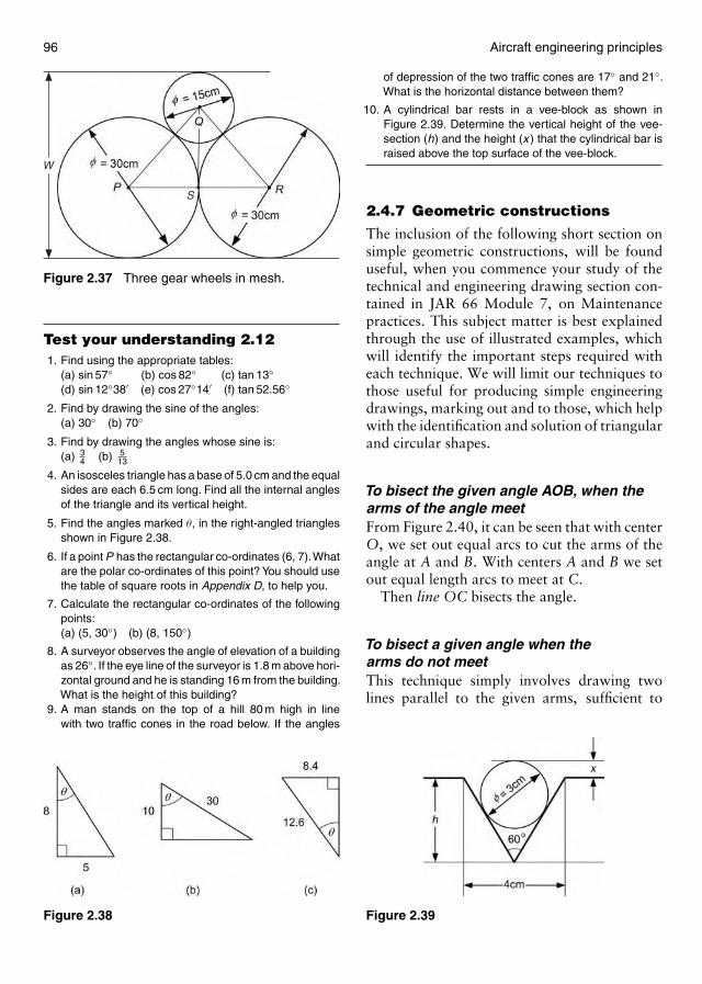
96 Aircraft engineering principles
S
W
Figure 2.37 Three gear wheels in mesh.
Test your understanding 2.121. Find using the appropriate tables:
(a) sin 57◦ (b) cos 82◦ (c) tan 13◦(d) sin 12◦38′ (e) cos 27◦14′ (f) tan 52.56◦
2. Find by drawing the sine of the angles:(a) 30◦ (b) 70◦
3. Find by drawing the angles whose sine is:(a) 3
4 (b) 513
4. An isosceles triangle has a base of 5.0 cm and the equalsides are each 6.5 cm long. Find all the internal anglesof the triangle and its vertical height.
5. Find the angles marked θ, in the right-angled trianglesshown in Figure 2.38.
6. If a point P has the rectangular co-ordinates (6, 7).Whatare the polar co-ordinates of this point? You should usethe table of square roots in Appendix D, to help you.
7. Calculate the rectangular co-ordinates of the followingpoints:(a) (5, 30◦) (b) (8, 150◦)
8. A surveyor observes the angle of elevation of a buildingas 26◦. If the eye line of the surveyor is 1.8 m above hori-zontal ground and he is standing 16 m from the building.What is the height of this building?
9. A man stands on the top of a hill 80 m high in linewith two traffic cones in the road below. If the angles
Figure 2.38
of depression of the two traffic cones are 17◦ and 21◦.What is the horizontal distance between them?
10. A cylindrical bar rests in a vee-block as shown inFigure 2.39. Determine the vertical height of the vee-section (h) and the height (x ) that the cylindrical bar israised above the top surface of the vee-block.
2.4.7 Geometric constructions
The inclusion of the following short section onsimple geometric constructions, will be founduseful, when you commence your study of thetechnical and engineering drawing section con-tained in JAR 66 Module 7, on Maintenancepractices. This subject matter is best explainedthrough the use of illustrated examples, whichwill identify the important steps required witheach technique. We will limit our techniques tothose useful for producing simple engineeringdrawings, marking out and to those, which helpwith the identification and solution of triangularand circular shapes.
To bisect the given angle AOB, when thearms of the angle meetFrom Figure 2.40, it can be seen that with centerO, we set out equal arcs to cut the arms of theangle at A and B. With centers A and B we setout equal length arcs to meet at C.
Then line OC bisects the angle.
To bisect a given angle when thearms do not meetThis technique simply involves drawing twolines parallel to the given arms, sufficient to
Figure 2.39
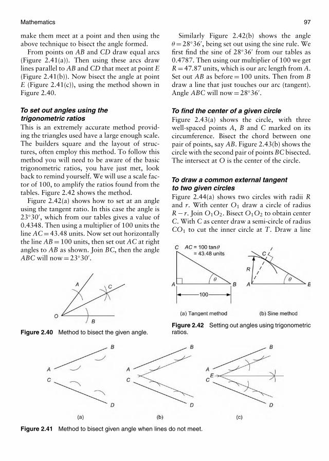
Mathematics 97
make them meet at a point and then using theabove technique to bisect the angle formed.
From points on AB and CD draw equal arcs(Figure 2.41(a)). Then using these arcs drawlines parallel to AB and CD that meet at point E(Figure 2.41(b)). Now bisect the angle at pointE (Figure 2.41(c)), using the method shown inFigure 2.40.
To set out angles using thetrigonometric ratiosThis is an extremely accurate method provid-ing the triangles used have a large enough scale.The builders square and the layout of struc-tures, often employ this method. To follow thismethod you will need to be aware of the basictrigonometric ratios, you have just met, lookback to remind yourself. We will use a scale fac-tor of 100, to amplify the ratios found from thetables. Figure 2.42 shows the method.
Figure 2.42(a) shows how to set at an angleusing the tangent ratio. In this case the angle is23◦30′, which from our tables gives a value of0.4348. Then using a multiplier of 100 units theline AC = 43.48 units. Now set out horizontallythe line AB = 100 units, then set out AC at rightangles to AB as shown. Join BC, then the angleABC will now = 23◦30′.
Figure 2.40 Method to bisect the given angle.
Figure 2.41 Method to bisect given angle when lines do not meet.
Similarly Figure 2.42(b) shows the angleθ = 28◦36′, being set out using the sine rule. Wefirst find the sine of 28◦36′ from our tables as0.4787. Then using our multiplier of 100 we getR = 47.87 units, which is our arc length from A.Set out AB as before = 100 units. Then from Bdraw a line that just touches our arc (tangent).Angle ABC will now = 28◦36′.
To find the center of a given circleFigure 2.43(a) shows the circle, with threewell-spaced points A, B and C marked on itscircumference. Bisect the chord between onepair of points, say AB. Figure 2.43(b) shows thecircle with the second pair of points BC bisected.The intersect at O is the center of the circle.
To draw a common external tangentto two given circlesFigure 2.44(a) shows two circles with radii Rand r. With center O1 draw a circle of radiusR − r. Join O1O2. Bisect O1O2 to obtain centerC. With C as center draw a semi-circle of radiusCO1 to cut the inner circle at T. Draw a line
Figure 2.42 Setting out angles using trigonometricratios.
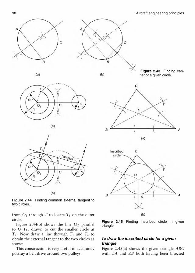
98 Aircraft engineering principles
Figure 2.43 Finding cen-ter of a given circle.
Figure 2.44 Finding common external tangent totwo circles.
from O1 through T to locate T1 on the outercircle.
Figure 2.44(b) shows the line O2 parallelto O1T1, drawn to cut the smaller circle atT2. Now draw a line through T1 and T2 toobtain the external tangent to the two circles asshown.
This construction is very useful to accuratelyportray a belt drive around two pulleys.
Figure 2.45 Finding inscribed circle in giventriangle.
To draw the inscribed circle for a giventriangleFigure 2.45(a) shows the given triangle ABCwith ∠A and ∠B both having been bisected
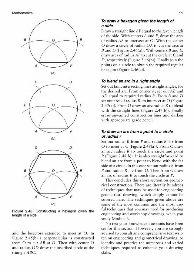
Mathematics 99
Figure 2.46 Constructing a hexagon given thelength of a side.
and the bisectors extended to meet at O. InFigure 2.45(b) a perpendicular is constructedfrom O to cut AB at D. Then with center Oand radius OD draw the inscribed circle of thetriangle ABC.
To draw a hexagon given the length ofa sideDraw a straight line AF equal to the given lengthof the side. With centers A and F, draw the arcsof radius AF to intersect at O. With the centerO draw a circle of radius OA to cut the arcs atB and D (Figure 2.46(a)). With centers B and E,draw arcs of radius AF to cut the circle at C andD, respectively (Figure 2.46(b)). Finally join thepoints on a circle to obtain the required regularhexagon (Figure 2.46(c)).
To blend an arc in a right angleSet out faint intersecting lines at right angles, forthe desired arc. From corner A, set out AB andAD equal to required radius R. From B and Dset out arcs of radius R, to intersect at O (Figure2.47(a)). From O draw an arc radius R to blendwith the straight lines (Figure 2.47(b)). Finallyerase unwanted construction lines and darkenwith appropriate grade pencil.
To draw an arc from a point to a circleof radius rSet out radius R from P and radius R + r fromO to meet at C (Figure 2.48(a)). From C drawan arc radius R to touch the circle and pointP (Figure 2.48(b)). It is also straightforward toblend an arc from a point to blend with the farside of a circle. In this case set out radius R fromP and radius R − r from O. Then from C drawan arc of radius R to touch the circle at P.
This concludes this short section on geomet-rical construction. There are literally hundredsof techniques that may be used for engineeringgeometrical drawing, which simply cannot becovered here. The techniques given above aresome of the most common and the most use-ful techniques that you may need for producingengineering and workshop drawings, when youstudy Module 6.
No test your knowledge questions have beenset for this section. However, you are stronglyadvised to consult any comprehensive text writ-ten on engineering and geometrical drawing, toidentify and practice the numerous and variedtechniques required to enhance your drawingskills.
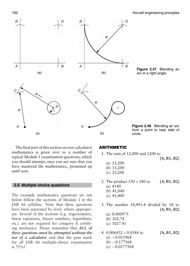
100 Aircraft engineering principles
Figure 2.47 Blending anarc in a right angle.
Figure 2.48 Blending an arcfrom a point to near side ofcircle.
The final part of this section on non-calculatormathematics is given over to a number oftypical Module 1 examination questions, whichyou should attempt, once you are sure that youhave mastered the mathematics, presented upuntil now.
2.5 Multiple choice questions
The example mathematics questions set outbelow follow the sections of Module 1 in theJAR 66 syllabus. Note that these questionshave been separated by level, where appropri-ate. Several of the sections (e.g. trigonometry,linear equations, binary numbers, logarithms,etc.) are not required for category A certify-ing mechanics. Please remember that ALL ofthese questions must be attempted without theuse of a calculator and that the pass markfor all JAR 66 multiple-choice examinationis 75%!
ARITHMETIC
1. The sum of 12,000 and 1200 is:[A, B1, B2]
(a) 12,200(b) 13,200(c) 23,200
2. The product 230 × 180 is: [A, B1, B2](a) 4140(b) 41,040(c) 41,400
3. The number 18,493.4 divided by 18 is:[A, B1, B2]
(a) 0.000973(b) 102.74(c) 1027.41
4. 0.006432 – 0.0184 is: [A, B1, B2](a) −0.011968(b) −0.177568(c) −0.0177568
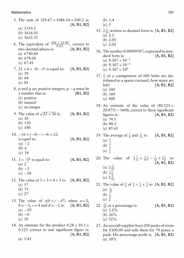
Mathematics 101
5. The sum of 329.67 + 1086.14 + 200.2 is:[A, B1, B2]
(a) 1319.3(b) 1616.01(c) 1632.31
6. The equivalent of 326 × 12.820.62 , correct to
two decimal places is: [A, B1, B2](a) 6740.84(b) 674.08(c) 67.41
7. 21 + 6 × (8 − 5) is equal to: [A, B1, B2](a) 39(b) 64(c) 81
8. p and q are positive integers, p − q must bea number that is: [B1, B2](a) positive(b) natural(c) an integer
9. The value of√
25 × 36 is: [A, B1, B2](a) 30(b) 150(c) 180
10. −16 + (−4) − (−4) + 22is equal to: [A, B1, B2](a) −2(b) 6(c) 14
11. 3 × −122 is equal to: [A, B1, B2]
(a) 2(b) −2(c) −18
12. The value of 5 × 3 + 4 × 3 is: [A, B1, B2](a) 57(b) 75(c) 27
13. The value of a(b + c − d2) when a = 2,b = −3, c = 4 and d = −2 is: [A, B1, B2](a) −10(b) −6(c) 10
14. An estimate for the product 4.28 × 10.1 ×0.125 correct to one significant figure is:
[A, B1, B2](a) 5.41
(b) 5.4(c) 5
15. 2 150 written in decimal form is: [A, B1, B2]
(a) 2.2(b) 2.01(c) 2.02
16. The number 0.00009307, expressed in stan-dard form is: [A, B1, B2](a) 9.307 × 10⁻⁵
(b) 9.307 × 10⁻⁴
(c) 9.307 × 10⁴
17. 25 of a consignment of 600 bolts are dis-tributed to a spares carousel, how many areleft? [A, B1, B2](a) 240(b) 360(c) 400
18. An estimate of the value of (80.125 ×20.875) − 1600, correct to three significantfigures is: [A, B1, B2](a) 74.1(b) 80.5(c) 85.61
19. The average of 14 and 1
12 is: [A, B1, B2](a) 1
3(b) 1
6(c) 1
8
20. The value of( 7
12 × 314
) − 116 + 2 1
8 is:[A, B1, B2]
(a) 2 316
(b) 2 14
(c) 2 516
21. The value of 34 of 1
3 ÷ 12 × 1
4 is: [A, B1, B2](a) 1
32(b) 1
8(c) 2
22. 1325 as a percentage is: [A, B1, B2](a) 5.2%(b) 26%(c) 52%
23. An aircraft supplier buys 200 packs of rivetsfor £100.00 and sells them for 70 pence apack. His percentage profit is: [A, B1, B2](a) 30%
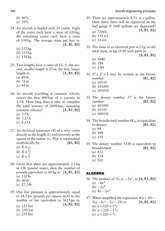
102 Aircraft engineering principles
(b) 40%(c) 59%
24. An aircraft is loaded with 20 crates. Eightof the crates each have a mass of 120 kg,the remaining crates each have a massof 150 kg. The average mass per box is:
[A, B1, B2](a) 132 kg(b) 135 kg(c) 138 kg
25. Two lengths have a ratio of 12 : 5, the sec-ond, smaller length is 25 m, the first, largerlength is: [A, B1, B2](a) 60 m(b) 72 m(c) 84 m
26. An aircraft travelling at constant velocitycovers the first 800 km of a journey in1.5 h. How long does it take to completethe total journey of 2800 km, assumingconstant velocity? [A, B1, B2](a) 3.5 h(b) 5.25 h(c) 6.25 h
27. An electrical resistance (R) of a wire variesdirectly as the length (L) and inversely as thesquare of the radius (r). This is representedsymbolically by: [B1, B2](a) R ∝ r
L2
(b) R ∝ L2
r(c) R ∝ L
r2
28. Given that there are approximately 2.2 kgin 1 lb (pound mass), then the number ofpounds equivalent to 60 kg is: [A, B1, B2](a) 132 lb(b) 60 lb(c) 27.3 lb
29. One bar pressure is approximately equalto 14.5 psi (pounds per square inch) so thenumber of bar equivalent to 3625 psi is:
[A, B1, B2](a) 125 bar(b) 250 bar(c) 255 bar
30. There are approximately 4.5 L in a gallon.How many litres will be registered on thefuel gauge if 1600 gallons are dispensed?
[A, B1, B2](a) 7200 L(b) 355.6 L(c) 55.6 L
31. The mass of an electrical part is 23 g, so thetotal mass, in kg, of 80 such parts is:
[A, B1, B2](a) 1840(b) 184(c) 1.84
32. 25 + 23 + 1 may be written as the binarynumber: [B1, B2](a) 10110(b) 101001(c) 101010
33. The denary number 37 is the binarynumber: [B1, B2](a) 101001(b) 10101(c) 100101
34. The hexadecimal number 6E16 is equivalentto denary: [B1, B2](a) 94(b) 108(c) 110
35. The denary number 5138 is equivalent tohexadecimal: [B1, B2](a) 412(b) 214(c) 321
ALGEBRA
36. The product of 3x, x, −2x2, is: [A, B1, B2](a) −6x4
(b) −5x4
(c) 4x − 2x2
37. When simplified the expression 4(a + 3b) −3(a − 4c) − 5(c − 2b) is: [A, B1, B2](a) a + 22b + 17c(b) a + 22b − 17c(c) a + 22b + 7c
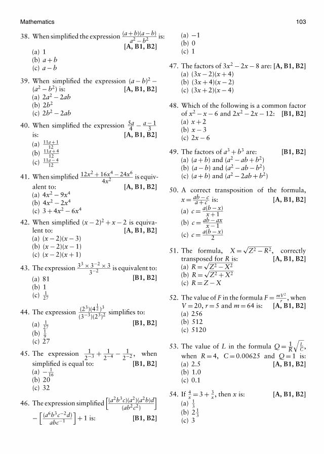
Mathematics 103
38. When simplified the expression (a + b)(a − b)a2 − b2 is:
[A, B1, B2](a) 1(b) a + b(c) a − b
39. When simplified the expression (a − b)2 −(a2 − b2) is: [A, B1, B2](a) 2a2 − 2ab(b) 2b2
(c) 2b2 − 2ab
40. When simplified the expression 5a4 − a − 1
3is: [A, B1, B2](a) 11a + 1
12(b) 11a + 4
12(c) 11a − 4
12
41. When simplified 12x2 + 16x4 − 24x6
4x2 is equiv-
alent to: [A, B1, B2](a) 4x2 − 9x4
(b) 4x2 − 2x4
(c) 3 + 4x2 − 6x4
42. When simplified (x − 2)2 + x − 2 is equiva-lent to: [A, B1, B2](a) (x − 2)(x − 3)(b) (x − 2)(x − 1)(c) (x − 2)(x + 1)
43. The expression 33 × 3−2 × 33−2 is equivalent to:
[B1, B2](a) 81(b) 1(c) 1
27
44. The expression (23)(412 )3
(3−3)(23)2simplifies to:
[B1, B2](a) 127
(b) 19
(c) 27
45. The expression 12−3 + 1
2−4 − 12−2 , when
simplified is equal to: [B1, B2](a) − 1
16(b) 20(c) 32
46. The expression simplified[(a2b3c)(a2)(a2b)d
(ab2c2)
]−[
(a6b3c−2d)abc−1
]+ 1 is: [B1, B2]
(a) −1(b) 0(c) 1
47. The factors of 3x2 − 2x − 8 are: [A, B1, B2](a) (3x − 2)(x + 4)(b) (3x + 4)(x − 2)(c) (3x + 2)(x − 4)
48. Which of the following is a common factorof x2 − x − 6 and 2x2 − 2x − 12: [B1, B2](a) x + 2(b) x − 3(c) 2x − 6
49. The factors of a3 + b3 are: [B1, B2](a) (a + b) and (a2 − ab + b2)(b) (a − b) and (a2 − ab − b2)(c) (a + b) and (a2 − 2ab + b2)
50. A correct transposition of the formula,x = ab − c
a + c is: [A, B1, B2]
(a) c = a(b − x)x + 1
(b) c = ab − axx − 1
(c) c = a(b − x)2
51. The formula, X = √Z2 − R2, correctly
transposed for R is: [A, B1, B2](a) R = √
Z2 − X2
(b) R = √Z2 + X2
(c) R = Z − X
52. The value of F in the formula F = mV2
r , whenV = 20, r = 5 and m = 64 is: [A, B1, B2](a) 256(b) 512(c) 5120
53. The value of L in the formula Q = 1R
√LC ,
when R = 4, C = 0.00625 and Q = 1 is:[A, B1, B2](a) 2.5
(b) 1.0(c) 0.1
54. If 4x = 3 + 3
x , then x is: [A, B1, B2](a) 1
3(b) 2 1
3(c) 3
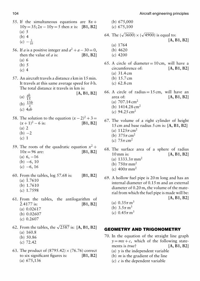
104 Aircraft engineering principles
55. If the simultaneous equations are 8x +10y = 35; 2x − 10y = 5 then x is: [B1, B2](a) 5(b) 4(c) − 3
10
56. If a is a positive integer and a2 + a − 30 = 0,then the value of a is: [B1, B2](a) 6(b) 5(c) 4
57. An aircraft travels a distance s km in 15 min.It travels at this same average speed for h h.The total distance it travels in km is:
[A, B1, B2](a) sh
15(b) 15h
s(c) 4sh
58. The solution to the equation (x − 2)2 + 3 =(x + 1)2 − 6 is: [B1, B2](a) 2(b) −2(c) 1
59. The roots of the quadratic equation x2 +10x = 96 are: [B1, B2](a) 6, −16(b) −6, 10(c) −6, 16
60. From the tables, log 57.68 is: [B1, B2](a) 1.7610(b) 1.7610(c) 1.7598
61. From the tables, the antilogarithm of2.4177 is: [B1, B2](a) 0.02617(b) 0.02607(c) 0.2607
62. From the tables, the√
2587 is: [A, B1, B2](a) 160.8(b) 50.86(c) 72.42
63. The product of (8795.42) × (76.76) correctto six significant figures is: [B1, B2](a) 675,136
(b) 675,000(c) 675,100
64. The (√
3600) × (√
4900) is equal to:[A, B1, B2]
(a) 1764(b) 4620(c) 4200
65. A circle of diameter = 10 cm, will have acircumference of: [A, B1, B2](a) 31.4 cm(b) 15.7 cm(c) 62.8 cm
66. A circle of radius = 15 cm, will have anarea of: [A, B1, B2](a) 707.14 cm2
(b) 1414.28 cm2
(c) 94.25 cm2
67. The volume of a right cylinder of height15 cm and base radius 5 cm is: [A, B1, B2](a) 1125π cm2
(b) 375π cm2
(c) 75π cm2
68. The surface area of a sphere of radius10 mm is: [A, B1, B2](a) 1333.3π mm2
(b) 750π mm2
(c) 400π mm2
69. A hollow fuel pipe is 20 m long and has aninternal diameter of 0.15 m and an externaldiameter of 0.20 m, the volume of the mate-rial from which the fuel pipe is made will be:
[A, B1, B2](a) 0.35π m3
(b) 3.5π m3
(c) 0.45π m3
GEOMETRY AND TRIGONOMETRY
70. In the equation of the straight line graphy = mx + c, which of the following state-ments is true? [A, B1, B2](a) y is the independent variable(b) m is the gradient of the line(c) c is the dependent variable
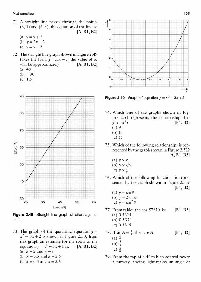
Mathematics 105
71. A straight line passes through the points(3, 1) and (6, 4), the equation of the line is:
[A, B1, B2](a) y = x + 2(b) y = 2x − 2(c) y = x − 2
72. The straight line graph shown in Figure 2.49takes the form y = mx + c, the value of mwill be approximately: [A, B1, B2](a) 40(b) −30(c) 1.5
Figure 2.49 Straight line graph of effort againstload.
73. The graph of the quadratic equation y =x2 − 3x + 2 is shown in Figure 2.50, fromthis graph an estimate for the roots of theequation y = x2 − 3x + 1 is: [A, B1, B2](a) x = 2 and x = 3(b) x = 0.5 and x = 2.5(c) x = 0.4 and x = 2.6
Figure 2.50 Graph of equation y = x 2 − 3x + 2.
74. Which one of the graphs shown in Fig-ure 2.51 represents the relationship thaty ∝ −x2? [B1, B2](a) A(b) B(c) C
75. Which of the following relationships is rep-resented by the graph shown in Figure 2.52?
[A, B1, B2](a) y ∝ x(b) y ∝ √
x(c) y ∝ 1
x
76. Which of the following functions is repre-sented by the graph shown in Figure 2.53?
[B1, B2](a) y = sin θ
(b) y = 2 sin θ
(c) y = sin2 θ
77. From tables the cos 57◦50′ is: [B1, B2](a) 0.5324(b) 0.5334(c) 0.5319
78. If sin A = 35 , then cos A: [B1, B2]
(a) 45
(b) 25
(c) 34
79. From the top of a 40 m high control towera runway landing light makes an angle of
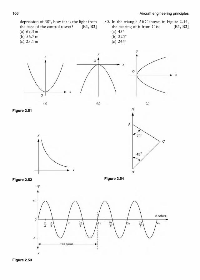
106 Aircraft engineering principles
depression of 30◦, how far is the light fromthe base of the control tower? [B1, B2](a) 69.3 m(b) 56.7 m(c) 23.1 m
Figure 2.51
Figure 2.52
Figure 2.53
80. In the triangle ABC shown in Figure 2.54,the bearing of B from C is: [B1, B2](a) 45◦(b) 225◦(c) 245◦
Figure 2.54
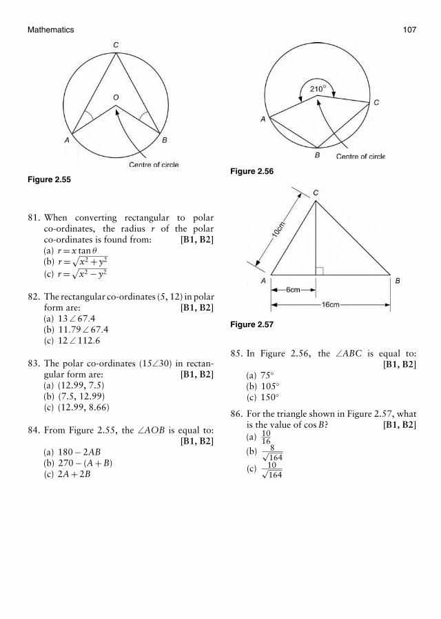
Mathematics 107
Figure 2.55
81. When converting rectangular to polarco-ordinates, the radius r of the polarco-ordinates is found from: [B1, B2](a) r = x tan θ
(b) r =√x2 + y2
(c) r =√x2 − y2
82. The rectangular co-ordinates (5, 12) in polarform are: [B1, B2](a) 13 ∠ 67.4(b) 11.79 ∠ 67.4(c) 12 ∠ 112.6
83. The polar co-ordinates (15∠30) in rectan-gular form are: [B1, B2](a) (12.99, 7.5)(b) (7.5, 12.99)(c) (12.99, 8.66)
84. From Figure 2.55, the ∠AOB is equal to:[B1, B2]
(a) 180 − 2AB(b) 270 − (A + B)(c) 2A + 2B
Figure 2.56
Figure 2.57
85. In Figure 2.56, the ∠ABC is equal to:[B1, B2]
(a) 75◦(b) 105◦(c) 150◦
86. For the triangle shown in Figure 2.57, whatis the value of cos B? [B1, B2](a) 10
16(b) 8√
164(c) 10√
164

This page intentionally left blank
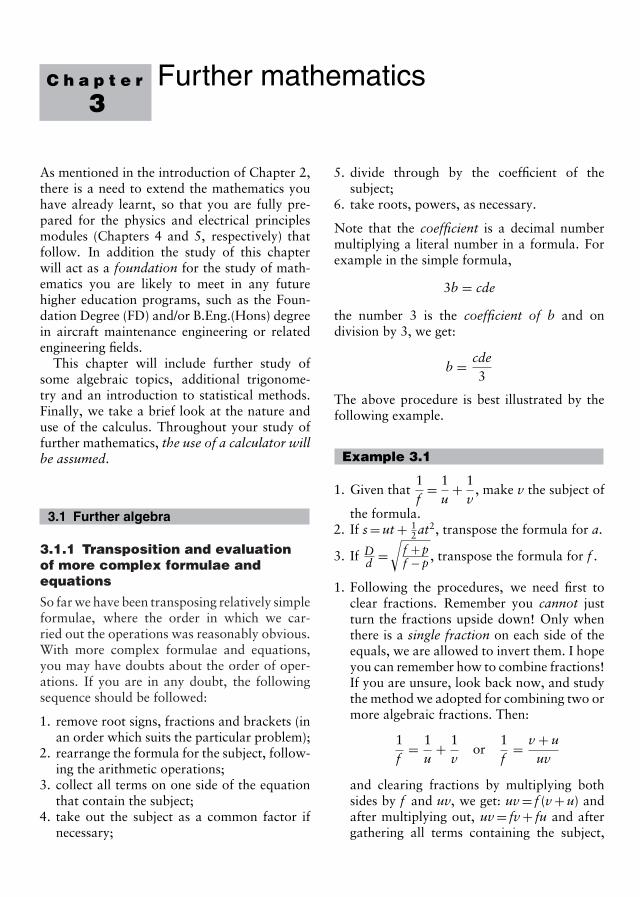
C h a p t e r
3Further mathematics
As mentioned in the introduction of Chapter 2,there is a need to extend the mathematics youhave already learnt, so that you are fully pre-pared for the physics and electrical principlesmodules (Chapters 4 and 5, respectively) thatfollow. In addition the study of this chapterwill act as a foundation for the study of math-ematics you are likely to meet in any futurehigher education programs, such as the Foun-dation Degree (FD) and/or B.Eng.(Hons) degreein aircraft maintenance engineering or relatedengineering fields.
This chapter will include further study ofsome algebraic topics, additional trigonome-try and an introduction to statistical methods.Finally, we take a brief look at the nature anduse of the calculus. Throughout your study offurther mathematics, the use of a calculator willbe assumed.
3.1 Further algebra
3.1.1 Transposition and evaluationof more complex formulae andequations
So far we have been transposing relatively simpleformulae, where the order in which we car-ried out the operations was reasonably obvious.With more complex formulae and equations,you may have doubts about the order of oper-ations. If you are in any doubt, the followingsequence should be followed:
1. remove root signs, fractions and brackets (inan order which suits the particular problem);
2. rearrange the formula for the subject, follow-ing the arithmetic operations;
3. collect all terms on one side of the equationthat contain the subject;
4. take out the subject as a common factor ifnecessary;
5. divide through by the coefficient of thesubject;
6. take roots, powers, as necessary.
Note that the coefficient is a decimal numbermultiplying a literal number in a formula. Forexample in the simple formula,
3b = cde
the number 3 is the coefficient of b and ondivision by 3, we get:
b = cde3
The above procedure is best illustrated by thefollowing example.
Example 3.1
1. Given that1f
= 1u
+ 1v
, make v the subject of
the formula.2. If s = ut + 1
2 at2, transpose the formula for a.
3. If Dd =
√f + pf − p , transpose the formula for f .
1. Following the procedures, we need first toclear fractions. Remember you cannot justturn the fractions upside down! Only whenthere is a single fraction on each side of theequals, we are allowed to invert them. I hopeyou can remember how to combine fractions!If you are unsure, look back now, and studythe method we adopted for combining two ormore algebraic fractions. Then:
1f
= 1u
+ 1v
or1f
= v + uuv
and clearing fractions by multiplying bothsides by f and uv, we get: uv = f (v + u) andafter multiplying out, uv = fv + fu and aftergathering all terms containing the subject,
110 Aircraft engineering principles
uv − fv = fu then removing the subject as acommon factor gives: v(u − f ) = fu and afterdivision of both sides by (u − f ) we finally get:
v = fuu − f
2. Following our procedure, there is really onlyone fraction which we can eliminate, it is 1
2 ,if we multiply every term by the inverse of a12 , i.e. 2
1 we get:
2s = 2ut + at2
Subtracting 2ut from both sides gives:2s − 2ut = at2 and dividing both sides by t2,then:
2s − 2utt2
= a
and reversing the formula and pulling out thecommon factor gives:
a = 2(s − ut)t2
Alternatively, remembering your laws ofindices, we can bring up the t2 term and writethe formula for a, as:
a = 2t−2(s − ut)
3. We again follow the procedure, first clear-ing roots, then fractions, in the followingmanner.
Squaring:(Dd
)2
= f + pf − p
orD2
d2= f + p
f − p
and multiplying both sides by the terms inthe denominator, or cross-multiplying d2
and (f − p) gives: D2(f − p) = d2(f + p) andD2f − D2p = d2f + d2p; so collecting termson one side containing the subject, we get:D2f − d2f = d2p + D2p.
After pulling out common factors, wehave: f (D2 − d2) = (d2 − D2)p and dividingboth sides by (D2 − d2) yields the result:
f = (d2 + D2)pD2 − d2
Example 3.2
If F = mV2
r , find m when F = 2560, V = 20 andr = 5.Then, by direct substitution:
2560 = m(20)2
5so (2560)(5) = m(400)
400m = 12800
m = 12,800400
then m = 32
Alternatively, we can transpose the formula form and then substitute for the given values:
F = mV2
rand Fr = mV2 so
FrV2
= m
then m = FrV2
and
m = (2560)(5)(20)2
= 12,800400
= 32
giving the same result as before.
In our final example on substitution, we use aformula that relates electric charge Q, resistanceR, inductance L and capacitance C.
Example 3.3
Find C if Q = 1R
√LC where Q = 10, R = 40 �,
L = 0.1.
QR =√
LC and squaring both sides gives:
(QR)2 = LC
or Q2R2 = LC
C(Q2R2) = L then, C = LQ2R2
Substituting for the given values, we get:
C = 0.1102 402
= 6.25 × 10⁻⁷ F
3.1.2 Logarithms and logarithmicfunctions
We have already studied the laws and use ofindices, and looked at logarithms, as a meansof simplifying arithmetic operations. We neededto use logarithm tables and antilogarithm tablesin order to do this. As you already know, the
Further mathematics 111
logarithm of a number is in fact its index. As areminder, e.g. 103 = 1000, the left-hand side ofthis equation 103 is the number 1000 written inindex form. The index 3 is in fact the logarithmof 1000. Check this by pressing your log buttonon your calculator (which is the logarithm to thebase 10), then key in the number 1000 and pressthe = button, you will obtain the number 3!
Manipulation of numbers, expressions andformulae, which are in index form, may besimplified by using logarithms. Another use forlogarithms (one which you have already met) isbeing able to reduce sometimes the more diffi-cult arithmetic operations of multiplication anddivision to those of addition and subtraction.This is often necessary when manipulating morecomplex algebraic expressions.
We start by considering the laws of loga-rithms, in a similar manner to the way in whichwe dealt with the laws of indices, earlier.
Key pointThe power or index of a number, when that num-ber is in index form, is also its logarithm, whentaken to the base of the number.
3.1.3 The laws of logarithms
The laws of logarithms are tabulated below,they are followed by simple examples of theiruse. In all these examples, we use common log-arithms, i.e. logarithms to the base 10. Laterwe will look at another type, the Naperian log-arithm, or natural logarithm, where the base isthe number e(2.71828 . . .):
Number Logarithmic law
1 If a = bc, then c = logb a2 loga MN = loga M + loga N
3 logaMN
= loga M − loga N
4 loga(Mn) = n loga M
5 logb M = loga Mloga b
Law 1All these laws look complicated, but you havealready used law 1, when you carried out the
calculator exercise above. So again, we knowthat 1000 = 103. Now if we wish to put thisnumber into linear form (decimal form), thenwe may do this by taking logarithms.
Following law 1, where in this case, a = 1000,b = 10 and c = 3 then: 3 = log10 1000. You havealready proved this fact on your calculator! Soyou are probably wondering why we need tobother with logarithms? Well in this case we aredealing with common logarithms, i.e. numbersin index form where the base of the logarithmis 10. We can also consider numbers in indexform, that are not to the base 10, as you willsee later. We may also be faced with a problemwhere the index (power) is not known.
Suppose we are confronted with this prob-lem: find the value of x, where 750 = 10x. Theanswer is not quite so obvious, but it can easilybe solved using our first law of logarithms. So,again following the law, i.e. taking logarithms tothe appropriate base we get: x = log10 750 andnow using our calculator, we get: x = 2.8751,correct to four significant figures.
Law 2One pair of factors for the number 1000 is 10and 100. Therefore according to the second law:loga(10)(100) = loga 10 + loga 100. If we chooselogarithms to the base 10, then we alreadyknow that the log10 1000 = 3. Then using ourcalculator again, we see that log10 10 = 1 andlog10 100 = 2. What this law enables us to do,is to convert the multiplication of numbers inindex form into that of addition. Compare thislaw with the first law of indices you studiedearlier! Also remember that we are at lib-erty to choose any base we wish, provided weare able to work in this base. Your calcula-tor only gives you logarithms to two bases,10 and e.
Law 3This law allows us to convert the division ofnumber in index form into that of subtrac-tion. When dealing with the transposition ofmore complex formulae, these conversions canbe particularly useful and help us with thetransposition.

112 Aircraft engineering principles
So using the law directly then, e.g.:
log101000
10= log10 100 = log10 1000−log10 10
or from your calculator 2 = 3 − 1.
Law 4This law states that if we take the logarithmof a number in index form Mn this is equalto the logarithm of the base of the num-ber loga M, multiplied by the index of thenumber nloga M. For example, log10(1002) =log1010000 = 2 log10100. This is easily con-firmed on your calculator as 4 = (2)(2).
Law 5This law is rather different from the others, inthat it enables us to change the base of a loga-rithm. This of course is very useful, if we haveto deal with logarithms, or formulae involvinglogarithms that have a base, not found on ourcalculator!
For example, suppose we wish to know thenumerical value of log2 64, then using law 5, wehave:
log2 64 = log10 64log10 2
= 1.8061799740.301029995
= 6, interesting!
If we use law 1, in reverse then log2 64 isequivalent to the number 64 = 26, which ofcourse is now easily verified by your calculator!This example again demonstrates that given anumber in index form (the index of that num-ber) is also its logarithm provided the logarithmhas the same base.
We will now consider, through example, oneor two engineering uses for the laws of commonand natural logarithms.
Key pointCommon logarithms have the base 10.
Example 3.4
An equation connecting the final velocity v of amachine with the machine variables, w, p and z,
is given by the formula v = 20
(wpz
). Transpose
the formula for w, and find its numerical valuewhen v = 15, p = 1.24, and z = 34.65.
This formula may be treated as a number inindex form. Therefore to find w, as the subjectof the formula, we need to apply the laws of log-arithms. The first step, in this type of problem, isto take logarithms of both sides. The base of thelogarithm chosen, is not important, provided weare able to find the numerical values of these log-arithms, when required. Thus, we generally takelogarithms to the base 10 or to the base e. As yet,we have not considered logarithms to the base e,we will take common logarithms of both sides.However, if the number or expression is not to abase of logarithms we can manipulate, then weare at liberty to change this base using law 5!
So, log10 v = log10 20
(wpz
)at this stage, taking
logarithms seems to be of little help! However, ifwe now apply the appropriate logarithmic laws,we will be able to make w the subject of theformula.
Applying law 4 to the right-hand side of theexpression we get:
log10 v =(
wpz
)log10 20
Then finding the numerical value of log10 20 =1.30103, we can now continue with thetransposition:
log10 v =(
wpz
)1.30103 or
log10 v1.30103
= wpz
and so, w = (pz)(log10 v)1.30103
Having transposed the formula for w, we cansubstitute the appropriate values for the vari-ables and find the numerical value of w.
Then:
w = (1.24)(34.65)(log10 15)1.30103
= (1.24)(34.65)(1.17609)1.30103
= 38.84

Further mathematics 113
3.1.4 Naperian logarithms andthe exponential function
If you look at your calculator you will see theln or Naperian logarithm button. The inverseof the Naperian logarithm function is ex orexp x, the exponential function. This logarithmis sometime known as the natural logarithm,because it is often used to model naturally occur-ring phenomena, such as the way things grow ordecay. In engineering, e.g. the decay of chargefrom a capacitor may be modeled using thenatural logarithm. It is therefore a very usefulfunction, and both the natural logarithm andits inverse, the exponential function, are veryimportant within engineering.
We will now consider the transposition of aformula that involves the use of natural loga-rithms and the logarithmic laws.
Example 3.5
Transpose the formula, b = loge t − a loge D tomake t the subject.
First, note that the natural or Naperian loga-rithm may be expressed as loge or ln, as on yourcalculator. Do not mix up the expression loge,or its inverse ex or exp x with the exponen-tial function (EXP) on your calculator, whichmultiplies a number by powers of 10!
We first use the laws of logarithms as follows:
b = loge t − loge Da from law 4
b = loge
(t
Da
)from law 3
Now, for the first time we take the inverse of thenatural logarithm or antilogarithm. Noting thatany function, multiplied by its inverse is 1 (one).Then multiplying both sides of our equation, bye, the inverse of ln(loge), we get:
eb = tDa
(since e is the inverse or antilogarithm ofloge = ln or (e)(loge) = 1), then: t = ebDa asrequired.
As mentioned before, the exponential func-tion ex or exp x and its inverse ln (natural
logarithm) have many uses in aircraft engineer-ing, because they can be used to model growthand decay. So the way solids expand, elec-trical resistance changes with temperature, asubstance cools, pressure changes with altitudeor capacitors discharge can all be modeled bythe exponential function.
Here are just two engineering examples of theuse of the exponential function.
Key pointNaperian or natural logarithms have the base e,where e � 2.718281828 corrected to nine deci-mal places.
Key pointThe inverse function of the Naperian logarithmis the exponential function which in symbols isexpressed as exp x or ex.
Example 3.6
If the pressure p at height h (in m) above theground is given by the relationship:
p = p0ehk
where p0 is the sea-level pressure of101325 Nm−2. Determine the value of theheight h, when the pressure at altitude p is70129 Nm−2 and k = −8152.
First we need to transpose the formula for h,this will involve taking natural logarithms, theinverse function of e
hk . Before we do so we will
first isolate the exponential term, then:pp0
= ehk
and taking logarithms gives:
loge
(pp0
)= h
kthen k loge
(pp0
)= h.
then substituting the given values,
h = (−8152) loge
(70129101325
)
= (−8152) loge(0.692)
= (−8152)(−0.368) = 3000 m
114 Aircraft engineering principles
corrected to four significant figures. Thus thealtitude h = 3000 m.
Our final example is concerned with the infor-mation contained in a radio communicationsmessage. It is not necessary to understand thebackground physics in order to solve the prob-lem, as you will see.
Example 3.7
It can be shown that the information content ofa message is given by:
I = log2
(1p
)Using the laws of logarithms show that theinformation content may be expressed asI = −log2(p) and find the information contentof the message if the chances of receiving the
code (p) is116
.
So we are being asked to show that:
I = log2
(1p
)= −log2(p)
the left-hand side of this expression may bewritten as log2(p−1). I hope you remember thelaws of indices! Now if we compare this expres-sion with law 4, where loga(Mn) = nloga Mthen in this case M = p and n = −1 so,log2(p−1) = −1 log2 p = −log2 p, as required.
Now to find the information content of themessage, we need to substitute the given value
of p = 116
into the equation:
log2(p−1) = log2
(1p
)= log2(16)
Now our problem is that we cannot easily findthe value of logarithms, to the base 2. However,if we use logarithmic law 5, then we get:
log2 16 = log10 16log10 2
= 4
Then the information content of the message = 4.
I hope you were able to follow the reasoning,in the above two, quite testing examples. Thereis just one more application of the laws of log-arithms that we need to cover. It is sometimes
very useful when considering experimental datato determine if such data can be related to a par-ticular law. If we can relate this data to the lawof a straight line y = mx + c, then we can easilydetermine useful results. Unfortunately, the datais not always related in this form. However, alot of engineering data follows the general formy = axn, where as before, x is the independentvariable, y is the dependent variable and in thiscase, a and n, are constants for the particularexperimental data being considered.
We can use a technique, involving logarithmsto reduce equations of the form y = axn to alinear form, following the law of the straightline, y = mx + c. The technique is best illustratedby the following example.
Example 3.8
The pressure p and volume v of a gas, at constanttemperature are related by Boyle’s law, whichcan be expressed as p = cv−0.7, where c is a con-stant. Show that the experimental values givenin the table follow this law, and from an appro-priate graph of the results, determine the valueof the constant c:
Volume v (m3) 1.5 2.0 2.5 3.0 3.5Pressure p 7.5 6.2 5.26 4.63 4.16(105 Nm−2)
The law is of the form p = axn. So takingcommon logarithms of both side of the lawp = cv−0.7
we get, log10 p = log10(cv−0.7)
and applying laws 2 and 4 to the right-hand sideof this equation gives:
log10 p = −0.7 log10 v + log10 c;
make sure you can see how to get this result.Then comparing this equation with the equationof a straight line y = mx + c, we see that:
y = log10 p, m = −0.7,
x = log10 v c = log10 c.
So we need to plot log10 p against log10 v (Fig-ure 3.1). A table of values and the resulting plot
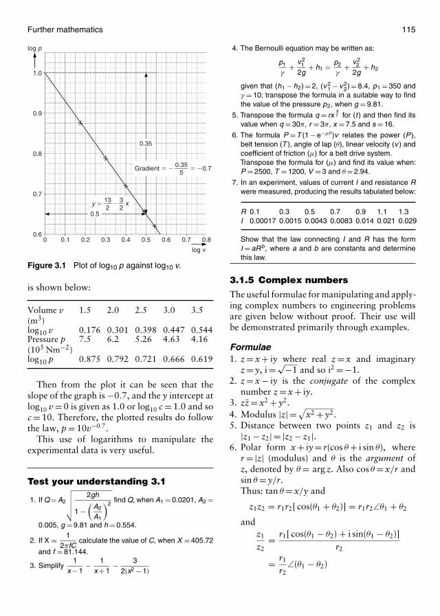
Further mathematics 115
1.0
0.9
0.8
0.7
0.60 0.1 0.2 0.3 0.4 0.5 0.6 0.7 0.8
xy � 132
32
�
Gradient � � 0.355
� �0.7
log v
log p
0.5
0.35
Figure 3.1 Plot of log10 p against log10 v.
is shown below:
Volume v 1.5 2.0 2.5 3.0 3.5(m3)log10 v 0.176 0.301 0.398 0.447 0.544Pressure p 7.5 6.2 5.26 4.63 4.16(105 Nm−2)log10 p 0.875 0.792 0.721 0.666 0.619
Then from the plot it can be seen that theslope of the graph is −0.7, and the y intercept atlog10 v = 0 is given as 1.0 or log10 c = 1.0 and soc = 10. Therefore, the plotted results do followthe law, p = 10v−0.7.
This use of logarithms to manipulate theexperimental data is very useful.
Test your understanding 3.1
1. If Q = A2
√√√√√2gh
1 −(
A2
A1
)2find Q, when A1 = 0.0201, A2 =
0.005, g = 9.81 and h = 0.554.
2. If X = 12πfC
calculate the value of C, when X = 405.72
and f = 81.144.
3. Simplify1
x − 1− 1
x + 1− 3
2(x2 − 1)
4. The Bernoulli equation may be written as:
p1
γ+ v 2
1
2g+ h1 = p2
γ+ v 2
2
2g+ h2
given that (h1 − h2) = 2, (v 21 − v 2
2) = 8.4, p1 = 350 andγ = 10; transpose the formula in a suitable way to findthe value of the pressure p2, when g = 9.81.
5. Transpose the formula q = rxst for (t ) and then find its
value when q = 30π, r = 3π, x = 7.5 and s = 16.
6. The formula P =T (1 − e−µθ)v relates the power (P ),belt tension (T ), angle of lap (θ), linear velocity (v ) andcoefficient of friction (µ) for a belt drive system.Transpose the formula for (µ) and find its value when:P = 2500, T = 1200, V = 3 and θ = 2.94.
7. In an experiment, values of current I and resistance Rwere measured, producing the results tabulated below:
R 0.1 0.3 0.5 0.7 0.9 1.1 1.3I 0.00017 0.0015 0.0043 0.0083 0.014 0.021 0.029
Show that the law connecting I and R has the formI = aRb, where a and b are constants and determinethis law.
3.1.5 Complex numbers
The useful formulae for manipulating and apply-ing complex numbers to engineering problemsare given below without proof. Their use willbe demonstrated primarily through examples.
Formulae1. z = x + iy where real z = x and imaginary
z = y, i = √−1 and so i2 = −1.2. z = x − iy is the conjugate of the complex
number z = x + iy.3. zz = x2 + y2.4. Modulus |z| =√x2 + y2.5. Distance between two points z1 and z2 is
|z1 − z2| = |z2 − z1|.6. Polar form x + iy = r(cos θ + i sin θ), where
r = |z| (modulus) and θ is the argument ofz, denoted by θ = arg z. Also cos θ = x/r andsin θ = y/r.Thus: tan θ = x/y and
z1z2 = r1r2[ cos(θ1 + θ2)] = r1r2∠θ1 + θ2
andz1
z2= r1[ cos(θ1 − θ2) + i sin(θ1 − θ2)]
r2
= r1
r2∠(θ1 − θ2)
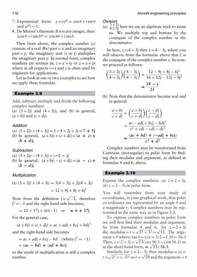
116 Aircraft engineering principles
7. Exponential form: z = reiθ = cos θ + i sin θ
and |eiθ| = 1.8. De Moivre’s theorem: If n is any integer, then:
(cos θ + i sin θ)n = cos nθ + i sin θ.
Then from above, the complex number (z)consists of a real (Re) part = x and an imaginarypart = y, the imaginary unit (i or j) multipliesthe imaginary part y. In normal form, complexnumbers are written as: z = x + iy or z = x + jywhere in all respects i = j and j is often used byengineers for applications.
Let us look at one or two examples to see howwe apply these formulae.
Example 3.9
Add, subtract, multiply and divide the followingcomplex numbers:(a) (3 + 2j) and (4 + 3j); and (b) in general,(a + bj) and (c + dj).
Addition(a) (3 + 2j) + (4 + 3j) = 3 + 4 + 2j + 3j = 7 + 5j(b) In general, (a + bj) + (c + dj) = (a + c) +
(b + d)j.
Subtraction(a) (3 + 2j) − (4 + 3j) = (−1 − j)(b) In general, (a + bj) − (c + dj) = (a − c) +
(b − d)j.
Multiplication
(a) (3 + 2j) × (4 + 3j) = 3(4 + 3j) + 2j(4 + 3j)
= 12 + 9j + 8j + 6j2
Now from the definition j = √−1, thereforej2 = −1 and the right-hand side becomes,
= 12 + 17j + (6)(−1) or = 6 + 17j
For the general case,
(a + bj) × (c + dj) = ac + adj + bcj + bdj2
and the right-hand side becomes
= ac + adj + bcj − bd (where j2 = −1)
= (ac − bd) + (ad + bc)j
so the result of multiplication is still a complexnumber.
Division(a) 3 + 2j
4 + 3j here we use an algebraic trick to assist
us. We multiply top and bottom by theconjugate of the complex number in thedenominator.
So here, z = 4 + 3j then z = 4 − 3j, where youwill observe from the formulae above that z isthe conjugate of the complex number z. So now,we proceed as follows:(
3 + 2j4 + 3j
)(4 − 3j4 − 3j
)= 12 − 9j + 8j − 6j2
16 + 12j − 12j − 9j2
= 18 − j25
(b) Note that the denominator became real andin general:
a + bjc + dj
=(
a + bjc + dj
)(c − djc − dj
)
= ac − adj + bcj − bdj2
c2 + cdj − cdj − dj2
= (ac + bd) + (−adj + bcj)c2 + d2
Complex numbers may be transformed fromCartesian (rectangular) to polar form by find-ing their modulus and argument, as defined informulae 4 and 6, above.
Example 3.10
Express the complex numbers: (a) z = 2 + 3j;(b) z = 2 − 5j in polar form.
You will remember from your study ofco-ordinates, in your graphical work, that polarco-ordinates are represented by an angle θ anda magnitude r. Complex numbers may be rep-resented in the same way as in Figure 3.2.
To express complex numbers in polar formwe will first find their modulus and argument.So from formulae 4 and 6, for z = 2 + 3jthe modulus = r = √
22 + 32 = √13. The argu-
ment = θ where: tan θ = y/x = 3/2 =1.5θ = 56.3Then, z = 2 + 3j = √
13( cos 56.3 + j sin 56.3) orin the short-hand form, = √
13∠56.3.Similarly for z = 2 − 5j then modulus = |z| =
r =√22 + (−5)2 so r = √29 and the argument = θ
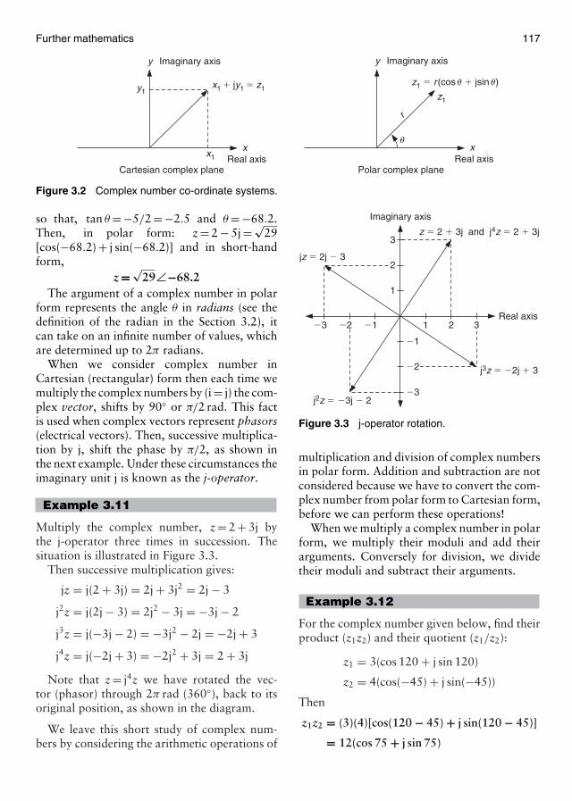
Further mathematics 117
Cartesian complex plane
x1
y1x1 � jy1 � z1
xReal axis
y Imaginary axis
Polar complex plane
y Imaginary axis
r
xReal axis
z1 � r(cos u � jsin u)
z1
u
Figure 3.2 Complex number co-ordinate systems.
so that, tan θ = −5/2 = −2.5 and θ = −68.2.Then, in polar form: z = 2 − 5j = √
29[cos(−68.2) + j sin(−68.2)] and in short-handform,
z = √29∠−68.2
The argument of a complex number in polarform represents the angle θ in radians (see thedefinition of the radian in the Section 3.2), itcan take on an infinite number of values, whichare determined up to 2π radians.
When we consider complex number inCartesian (rectangular) form then each time wemultiply the complex numbers by (i = j) the com-plex vector, shifts by 90◦ or π/2 rad. This factis used when complex vectors represent phasors(electrical vectors). Then, successive multiplica-tion by j, shift the phase by π/2, as shown inthe next example. Under these circumstances theimaginary unit j is known as the j-operator.
Example 3.11
Multiply the complex number, z = 2 + 3j bythe j-operator three times in succession. Thesituation is illustrated in Figure 3.3.
Then successive multiplication gives:
jz = j(2 + 3j) = 2j + 3j2 = 2j − 3
j2z = j(2j − 3) = 2j2 − 3j = −3j − 2
j3z = j(−3j − 2) = −3j2 − 2j = −2j + 3
j4z = j(−2j + 3) = −2j2 + 3j = 2 + 3j
Note that z = j4z we have rotated the vec-tor (phasor) through 2π rad (360◦), back to itsoriginal position, as shown in the diagram.
We leave this short study of complex num-bers by considering the arithmetic operations of
Imaginary axis
3
3
2
2
1
1
�3
�3
�2
�2
�1
�1
Real axis
z � 2 � 3j and j4z � 2 � 3j
jz � 2j � 3
j3z � �2j � 3
j2z � �3j � 2
Figure 3.3 j-operator rotation.
multiplication and division of complex numbersin polar form. Addition and subtraction are notconsidered because we have to convert the com-plex number from polar form to Cartesian form,before we can perform these operations!
When we multiply a complex number in polarform, we multiply their moduli and add theirarguments. Conversely for division, we dividetheir moduli and subtract their arguments.
Example 3.12
For the complex number given below, find theirproduct (z1z2) and their quotient (z1/z2):
z1 = 3(cos 120 + j sin 120)
z2 = 4(cos(−45) + j sin(−45))
Then
z1z2 = (3)(4)[cos(120 − 45) + j sin(120 − 45)]
= 12(cos 75 + j sin 75)
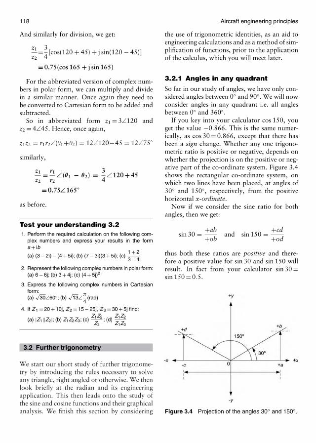
118 Aircraft engineering principles
And similarly for division, we get:
z1
z2=3
4[cos(120 + 45) + j sin(120 − 45)]
= 0.75(cos 165 + j sin 165)
For the abbreviated version of complex num-bers in polar form, we can multiply and dividein a similar manner. Once again they need tobe converted to Cartesian form to be added andsubtracted.
So in abbreviated form z1 = 3∠120 andz2 = 4∠45. Hence, once again,
z1z2 = r1r2∠(θ1+θ2) = 12∠120−45 = 12∠75◦
similarly,
z1
z2= r1
r2∠(θ1 − θ2) = 3
4∠120 + 45
= 0.75∠165◦
as before.
Test your understanding 3.21. Perform the required calculation on the following com-
plex numbers and express your results in the forma + ib
(a) (3 − 2i) − (4 + 5i); (b) (7 − 3i)(3 + 5i); (c)1 + 2i3 − 4i
2. Represent the following complex numbers in polar form:(a) 6 − 6j; (b) 3 + 4j; (c) (4 + 5j)2
3. Express the following complex numbers in Cartesianform:(a)
√30∠60◦; (b)
√13∠π
4(rad)
4. If Z 1 = 20 + 10j, Z 2 = 15 − 25j, Z 3 = 30 + 5j find:
(a) |Z1||Z2|; (b) Z1Z2Z3; (c)Z1Z2
Z3; (d)
Z1Z2
Z1Z3
3.2 Further trigonometry
We start our short study of further trigonome-try by introducing the rules necessary to solveany triangle, right angled or otherwise. We thenlook briefly at the radian and its engineeringapplication. This then leads onto the study ofthe sine and cosine functions and their graphicalanalysis. We finish this section by considering
the use of trigonometric identities, as an aid toengineering calculations and as a method of sim-plification of functions, prior to the applicationof the calculus, which you will meet later.
3.2.1 Angles in any quadrant
So far in our study of angles, we have only con-sidered angles between 0◦ and 90◦. We will nowconsider angles in any quadrant i.e. all anglesbetween 0◦ and 360◦.
If you key into your calculator cos 150, youget the value −0.866. This is the same numer-ically, as cos 30 = 0.866, except that there hasbeen a sign change. Whether any one trigono-metric ratio is positive or negative, depends onwhether the projection is on the positive or neg-ative part of the co-ordinate system. Figure 3.4shows the rectangular co-ordinate system, onwhich two lines have been placed, at angles of30◦ and 150◦, respectively, from the positivehorizontal x-ordinate.
Now if we consider the sine ratio for bothangles, then we get:
sin 30 = +ab+ob
and sin 150 = +cd+od
thus both these ratios are positive and there-fore a positive value for sin 30 and sin 150 willresult. In fact from your calculator sin 30 =sin 150 = 0.5.
Figure 3.4 Projection of the angles 30◦ and 150◦.
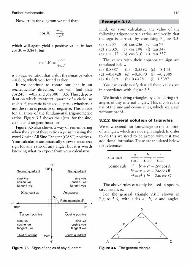
Further mathematics 119
Now, from the diagram we find that:
cos 30 = +oa+ob
which will again yield a positive value, in factcos 30 = 0.866, but
cos 150 = −oc+od
is a negative ratio, that yields the negative value−0.866, which you found earlier.
If we continue to rotate our line in ananticlockwise direction, we will find thatcos 240 = −0.5 and cos 300 = 0.5. Thus, depen-dent on which quadrant (quarter of a circle, soeach 90◦) the ratio is placed, depends whether ornot the ratio is positive or negative. This is truefor all three of the fundamental trigonometricratios. Figure 3.5 shows the signs, for the sine,cosine and tangent functions.
Figure 3.5 also shows a way of rememberingwhen the sign of these ratios is positive using theword Cosine All Sine Tangent (CAST) positives.Your calculator automatically shows the correctsign for any ratio of any angle, but it is worthknowing what to expect from your calculator!
Figure 3.5 Signs of angles of any quadrant.
Example 3.13
Find, on your calculator, the value of thefollowing trigonometric ratios and verify thatthe sign is correct, by consulting Figure 3.5:
(a) sin 57 (b) cos 236 (c) tan 97(d) sin 320 (e) cos 108 (f) tan 347(g) sin 137 (h) cos 310 (i) tan 237
The values with their appropriate sign aretabulated below:(a) 0.8387 (b) −0.5592 (c) −8.144(d) −0.6428 (e) −0.3090 (f) −0.2309(g) 0.6819 (h) 0.6428 (i) 1.5397
You can easily verify that all these values arein accordance with Figure 3.5.
We finish solving triangles by considering tri-angles of any internal angles. This involves theuse of the sine and cosine rules, which are givenwithout proof.
3.2.2 General solution of triangles
We now extend our knowledge to the solutionof triangles, which are not right angled. In orderto do this we need to be armed with just twoadditional formulae. These are tabulated belowfor reference:
Sine rulea
sin a= b
sin b= c
sin c
Cosine rule a2 = b2 + c2 − 2bc cos Ab2 = a2 + c2 − 2ac cos Bc2 = a2 + b2 − 2ab cos C
The above rules can only be used in specificcircumstances.
For the general triangle ABC shown inFigure 3.6, with sides a, b, c and angles,
Figure 3.6 The general triangle.
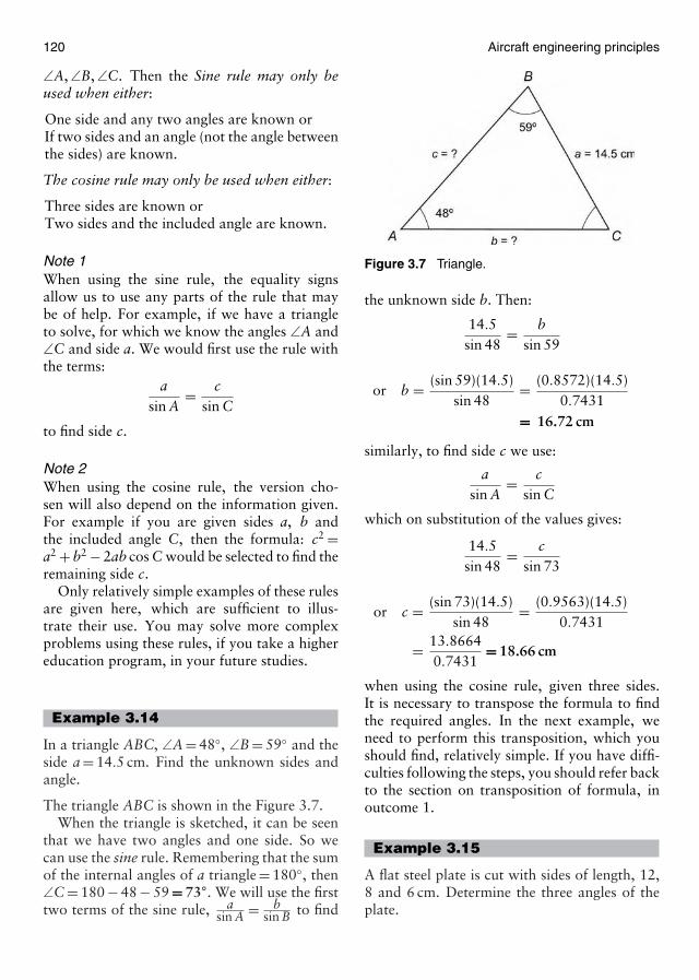
120 Aircraft engineering principles
∠A, ∠B, ∠C. Then the Sine rule may only beused when either:
One side and any two angles are known orIf two sides and an angle (not the angle betweenthe sides) are known.
The cosine rule may only be used when either:
Three sides are known orTwo sides and the included angle are known.
Note 1When using the sine rule, the equality signsallow us to use any parts of the rule that maybe of help. For example, if we have a triangleto solve, for which we know the angles ∠A and∠C and side a. We would first use the rule withthe terms:
asin A
= csin C
to find side c.
Note 2When using the cosine rule, the version cho-sen will also depend on the information given.For example if you are given sides a, b andthe included angle C, then the formula: c2 =a2 + b2 − 2ab cos C would be selected to find theremaining side c.
Only relatively simple examples of these rulesare given here, which are sufficient to illus-trate their use. You may solve more complexproblems using these rules, if you take a highereducation program, in your future studies.
Example 3.14
In a triangle ABC, ∠A = 48◦, ∠B = 59◦ and theside a = 14.5 cm. Find the unknown sides andangle.
The triangle ABC is shown in the Figure 3.7.When the triangle is sketched, it can be seen
that we have two angles and one side. So wecan use the sine rule. Remembering that the sumof the internal angles of a triangle = 180◦, then∠C = 180 − 48 − 59 = 73◦. We will use the firsttwo terms of the sine rule, a
sin A = bsin B to find
Figure 3.7 Triangle.
the unknown side b. Then:
14.5sin 48
= bsin 59
or b = (sin 59)(14.5)sin 48
= (0.8572)(14.5)0.7431
= 16.72 cm
similarly, to find side c we use:
asin A
= csin C
which on substitution of the values gives:
14.5sin 48
= csin 73
or c = (sin 73)(14.5)sin 48
= (0.9563)(14.5)0.7431
= 13.86640.7431
= 18.66 cm
when using the cosine rule, given three sides.It is necessary to transpose the formula to findthe required angles. In the next example, weneed to perform this transposition, which youshould find, relatively simple. If you have diffi-culties following the steps, you should refer backto the section on transposition of formula, inoutcome 1.
Example 3.15
A flat steel plate is cut with sides of length, 12,8 and 6 cm. Determine the three angles of theplate.
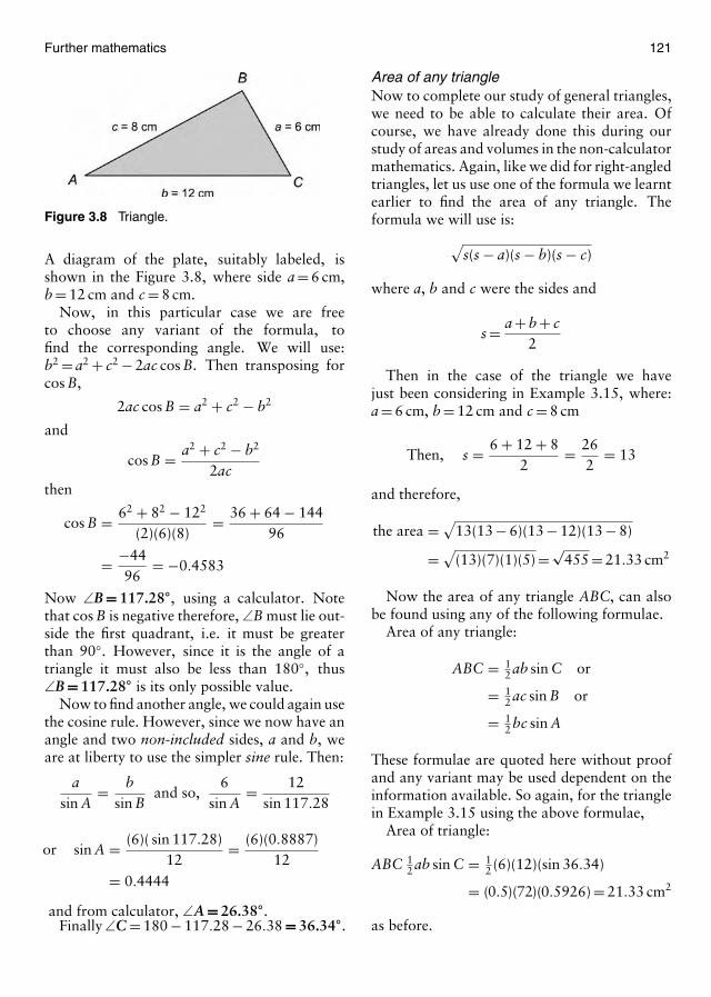
Further mathematics 121
Figure 3.8 Triangle.
A diagram of the plate, suitably labeled, isshown in the Figure 3.8, where side a = 6 cm,b = 12 cm and c = 8 cm.
Now, in this particular case we are freeto choose any variant of the formula, tofind the corresponding angle. We will use:b2 = a2 + c2 − 2ac cos B. Then transposing forcos B,
2ac cos B = a2 + c2 − b2
and
cos B = a2 + c2 − b2
2acthen
cos B = 62 + 82 − 122
(2)(6)(8)= 36 + 64 − 144
96
= −4496
= −0.4583
Now ∠B = 117.28◦, using a calculator. Notethat cos B is negative therefore, ∠B must lie out-side the first quadrant, i.e. it must be greaterthan 90◦. However, since it is the angle of atriangle it must also be less than 180◦, thus∠B = 117.28◦ is its only possible value.
Now to find another angle, we could again usethe cosine rule. However, since we now have anangle and two non-included sides, a and b, weare at liberty to use the simpler sine rule. Then:
asin A
= bsin B
and so,6
sin A= 12
sin 117.28
or sin A = (6)( sin 117.28)12
= (6)(0.8887)12
= 0.4444
and from calculator, ∠A = 26.38◦.Finally ∠C = 180 − 117.28 − 26.38 = 36.34◦.
Area of any triangleNow to complete our study of general triangles,we need to be able to calculate their area. Ofcourse, we have already done this during ourstudy of areas and volumes in the non-calculatormathematics. Again, like we did for right-angledtriangles, let us use one of the formula we learntearlier to find the area of any triangle. Theformula we will use is:√
s(s − a)(s − b)(s − c)
where a, b and c were the sides and
s = a + b + c2
Then in the case of the triangle we havejust been considering in Example 3.15, where:a = 6 cm, b = 12 cm and c = 8 cm
Then, s = 6 + 12 + 82
= 262
= 13
and therefore,
the area = √13(13 − 6)(13 − 12)(13 − 8)
= √(13)(7)(1)(5) = √
455 = 21.33 cm2
Now the area of any triangle ABC, can alsobe found using any of the following formulae.
Area of any triangle:
ABC = 12 ab sin C or
= 12 ac sin B or
= 12 bc sin A
These formulae are quoted here without proofand any variant may be used dependent on theinformation available. So again, for the trianglein Example 3.15 using the above formulae,
Area of triangle:
ABC 12 ab sin C = 1
2 (6)(12)(sin 36.34)
= (0.5)(72)(0.5926) = 21.33 cm2
as before.
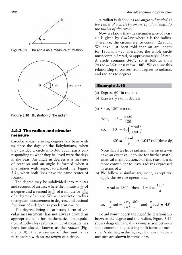
122 Aircraft engineering principles
Figure 3.9 The angle as a measure of rotation.
1 rad
Figure 3.10 Illustration of the radian.
3.2.3 The radian and circularmeasure
Circular measure using degrees has been withus since the days of the Babylonians, whenthey divided a circle into 360 equal parts cor-responding to what they believed were the daysin the year. An angle in degrees is a measureof rotation and an angle is formed when aline rotates with respect to a fixed line (Figure3.9), when both lines have the same center ofrotation.
The degree may be subdivided into minutesand seconds of an arc, where the minute is 1
60 ofa degree and a second is 1
60 of a minute or 13600
of a degree of an arc. We will restrict ourselvesto angular measurement in degrees, and decimalfractions of a degree, as you learnt earlier.
The degree, being an arbitrary form of cir-cular measurement, has not always proved anappropriate unit for mathematical manipula-tion. Another less arbitrary unit of measure hasbeen introduced, known as the radian (Fig-ure 3.10), the advantage of this unit is itsrelationship with an arc length of a circle.
A radian is defined as the angle subtended atthe center of a circle by an arc equal in length tothe radius of the circle.
Now we know that the circumference of a cir-cle is given by C = 2πr where r is the radius.Therefore, the circumference contain 2π radii.We have just been told that an arc lengthfor 1 rad is s = r. Therefore, the whole circlemust contain 2π rad, or approximately 6.28 rad.A circle contains 360◦, so it follows that:2π rad = 360◦ or π rad = 180◦. We can use thisrelationship to convert from degrees to radians,and radians to degrees.
Example 3.16
(a) Express 60◦ in radians
(b) Expressπ
4rad in degrees
(a) Since, 180◦ = π rad
then, 1◦ = π rad180
so, 60◦ = 60(
π rad180
)
60◦ = π rad3
or 1.047 rad (three dp)
Note that if we leave radians in terms of π wehave an exact value to use for further math-ematical manipulation. For this reason, it ismore convenient to leave radians expressedin terms of π.
(b) We follow a similar argument, except weapply the reverse operations.
π rad = 180◦ then 1 rad = 180◦
π
so,π
4rad =
(π
4
)180◦
πand
π
4rad = 45◦
To aid your understanding of the relationshipbetween the degree and the radian, Figure 3.11shows diagrammatically a comparison betweensome common angles using both forms of mea-sure. Note that, in the figure, all angles in radianmeasure are shown in terms of π.
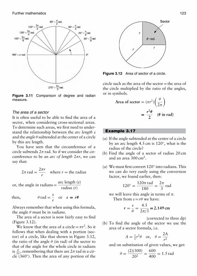
Further mathematics 123
Figure 3.11 Comparison of degree and radianmeasure.
The area of a sectorIt is often useful to be able to find the area of asector, when considering cross-sectional areas.To determine such areas, we first need to under-stand the relationship between the arc length sand the angle θ subtended at the center of a circleby this arc length.
You have seen that the circumference of acircle subtends 2π rad. So if we consider the cir-cumference to be an arc of length 2πr, we cansay that:
2π rad = 2πrr
where r = the radius
or, the angle in radians = arc length (s)radius (r)
then, θ rad = sr
or s = rθ
Always remember that when using this formula,the angle θ must be in radians.
The area of a sector is now fairly easy to find(Figure 3.12).
We know that the area of a circle = πr2. So itfollows that when dealing with a portion (sec-tor) of a circle, like that shown in Figure 3.12,the ratio of the angle θ (in rad) of the sector tothat of the angle for the whole circle in radiansis θ
2π, remembering that there are 2π rad in a cir-
cle (360◦). Then the area of any portion of the
Figure 3.12 Area of sector of a circle.
circle such as the area of the sector = the area ofthe circle multiplied by the ratio of the angles,or in symbols.
Area of sector = (πr2)(
θ
2π
)
= r2θ
2(θ in rad)
Example 3.17
(a) If the angle subtended at the center of a circleby an arc length 4.5 cm is 120◦, what is theradius of the circle?
(b) Find the angle of a sector of radius 20 cmand an area 300 cm2.
(a) We must first convert 120◦ into radians. Thiswe can do very easily using the conversionfactor, we found earlier, then:
120◦ = 120π rad180
= 2π
3rad
we will leave this angle in terms of π.Then from s = rθ we have:
r = sθ
= 4.52π/3
= 2.149 cm
(corrected to three dp)(b) To find the angle of the sector we use the
area of a sector formula, i.e.
A = 12 r2θ or, θ = 2A
r2
and on substitution of given values, we get:
θ = (2)(300)202
= 600400
= 1.5 rad
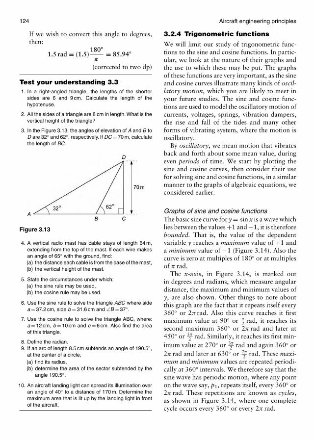
124 Aircraft engineering principles
If we wish to convert this angle to degrees,then:
1.5 rad = (1.5)180◦
π= 85.94◦
(corrected to two dp)
Test your understanding 3.31. In a right-angled triangle, the lengths of the shorter
sides are 6 and 9 cm. Calculate the length of thehypotenuse.
2. All the sides of a triangle are 8 cm in length. What is thevertical height of the triangle?
3. In the Figure 3.13, the angles of elevation of A and B toD are 32◦ and 62◦, respectively. If DC = 70 m, calculatethe length of BC.
Figure 3.13
4. A vertical radio mast has cable stays of length 64 m,extending from the top of the mast. If each wire makesan angle of 65◦ with the ground, find:(a) the distance each cable is from the base of the mast,(b) the vertical height of the mast.
5. State the circumstances under which:(a) the sine rule may be used,(b) the cosine rule may be used.
6. Use the sine rule to solve the triangle ABC where sidea = 37.2 cm, side b = 31.6 cm and ∠B = 37◦.
7. Use the cosine rule to solve the triangle ABC, where:a = 12 cm, b = 10 cm and c = 6 cm. Also find the areaof this triangle.
8. Define the radian.9. If an arc of length 8.5 cm subtends an angle of 190.5◦,
at the center of a circle,(a) find its radius,(b) determine the area of the sector subtended by the
angle 190.5◦.
10. An aircraft landing light can spread its illumination overan angle of 40◦ to a distance of 170 m. Determine themaximum area that is lit up by the landing light in frontof the aircraft.
3.2.4 Trigonometric functions
We will limit our study of trigonometric func-tions to the sine and cosine functions. In partic-ular, we look at the nature of their graphs andthe use to which these may be put. The graphsof these functions are very important, as the sineand cosine curves illustrate many kinds of oscil-latory motion, which you are likely to meet inyour future studies. The sine and cosine func-tions are used to model the oscillatory motion ofcurrents, voltages, springs, vibration dampers,the rise and fall of the tides and many otherforms of vibrating system, where the motion isoscillatory.
By oscillatory, we mean motion that vibratesback and forth about some mean value, duringeven periods of time. We start by plotting thesine and cosine curves, then consider their usefor solving sine and cosine functions, in a similarmanner to the graphs of algebraic equations, weconsidered earlier.
Graphs of sine and cosine functionsThe basic sine curve for y = sin x is a wave whichlies between the values +1 and −1, it is thereforebounded. That is, the value of the dependentvariable y reaches a maximum value of +1 anda minimum value of −1 (Figure 3.14). Also thecurve is zero at multiples of 180◦ or at multiplesof π rad.
The x-axis, in Figure 3.14, is marked outin degrees and radians, which measure angulardistance, the maximum and minimum values ofy, are also shown. Other things to note aboutthis graph are the fact that it repeats itself every360◦ or 2π rad. Also this curve reaches it firstmaximum value at 90◦ or π
2 rad, it reaches itssecond maximum 360◦ or 2π rad and later at450◦ or 5π
2 rad. Similarly, it reaches its first min-imum value at 270◦ or 3π
2 rad and again 360◦ or2π rad and later at 630◦ or 7π
2 rad. These maxi-mum and minimum values are repeated periodi-cally at 360◦ intervals. We therefore say that thesine wave has periodic motion, where any pointon the wave say, p1, repeats itself, every 360◦ or2π rad. These repetitions are known as cycles,as shown in Figure 3.14, where one completecycle occurs every 360◦ or every 2π rad.
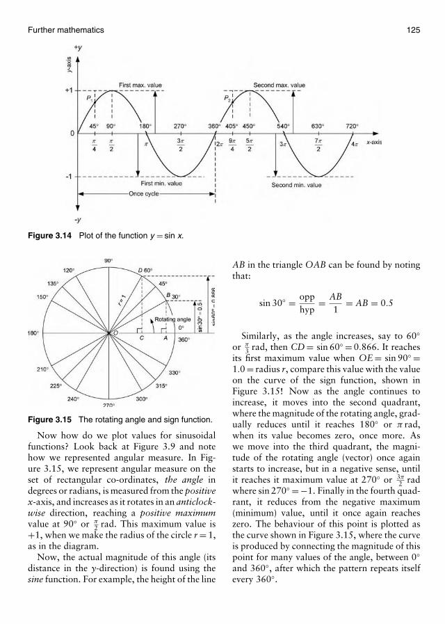
Further mathematics 125
Figure 3.14 Plot of the function y = sin x.
O
Figure 3.15 The rotating angle and sign function.
Now how do we plot values for sinusoidalfunctions? Look back at Figure 3.9 and notehow we represented angular measure. In Fig-ure 3.15, we represent angular measure on theset of rectangular co-ordinates, the angle indegrees or radians, is measured from the positivex-axis, and increases as it rotates in an anticlock-wise direction, reaching a positive maximumvalue at 90◦ or π
2 rad. This maximum value is+1, when we make the radius of the circle r = 1,as in the diagram.
Now, the actual magnitude of this angle (itsdistance in the y-direction) is found using thesine function. For example, the height of the line
AB in the triangle OAB can be found by notingthat:
sin 30◦ = opphyp
= AB1
= AB = 0.5
Similarly, as the angle increases, say to 60◦or π
3 rad, then CD = sin 60◦ = 0.866. It reachesits first maximum value when OE = sin 90◦ =1.0 = radius r, compare this value with the valueon the curve of the sign function, shown inFigure 3.15! Now as the angle continues toincrease, it moves into the second quadrant,where the magnitude of the rotating angle, grad-ually reduces until it reaches 180◦ or π rad,when its value becomes zero, once more. Aswe move into the third quadrant, the magni-tude of the rotating angle (vector) once againstarts to increase, but in a negative sense, untilit reaches it maximum value at 270◦ or 3π
2 radwhere sin 270◦ = −1. Finally in the fourth quad-rant, it reduces from the negative maximum(minimum) value, until it once again reacheszero. The behaviour of this point is plotted asthe curve shown in Figure 3.15, where the curveis produced by connecting the magnitude of thispoint for many values of the angle, between 0◦and 360◦, after which the pattern repeats itselfevery 360◦.
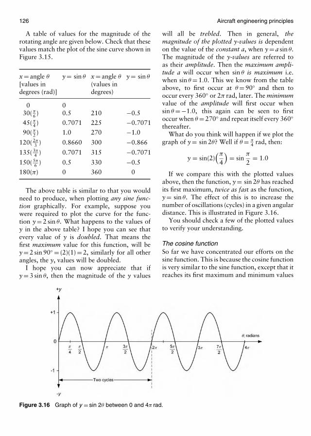
126 Aircraft engineering principles
A table of values for the magnitude of therotating angle are given below. Check that thesevalues match the plot of the sine curve shown inFigure 3.15.
x = angle θ y = sin θ x = angle θ y = sin θ
[values in (values indegrees (rad)] degrees)
0 030(π
6 ) 0.5 210 −0.5
45(π4 ) 0.7071 225 −0.7071
90(π2 ) 1.0 270 −1.0
120( 2π3 ) 0.8660 300 −0.866
135( 3π4 ) 0.7071 315 −0.7071
150( 5π6 ) 0.5 330 −0.5
180(π) 0 360 0
The above table is similar to that you wouldneed to produce, when plotting any sine func-tion graphically. For example, suppose youwere required to plot the curve for the func-tion y = 2 sin θ. What happens to the values ofy in the above table? I hope you can see thatevery value of y is doubled. That means thefirst maximum value for this function, will bey = 2 sin 90◦ = (2)(1) = 2, similarly for all otherangles, the y, values will be doubled.
I hope you can now appreciate that ify = 3 sin θ, then the magnitude of the y values
Figure 3.16 Graph of y = sin 2θ between 0 and 4π rad.
will all be trebled. Then in general, themagnitude of the plotted y-values is dependenton the value of the constant a, when y = a sin θ.The magnitude of the y-values are referred toas their amplitude. Then the maximum ampli-tude a will occur when sin θ is maximum i.e.when sin θ = 1.0. This we know from the tableabove, to first occur at θ = 90◦ and then tooccur every 360◦ or 2π rad, later. The minimumvalue of the amplitude will first occur whensin θ = −1.0, this again can be seen to firstoccur when θ = 270◦ and repeat itself every 360◦thereafter.
What do you think will happen if we plot thegraph of y = sin 2θ? Well if θ = π
4 rad, then:
y = sin(2)(π
4
)= sin
π
2= 1.0
If we compare this with the plotted valuesabove, then the function, y = sin 2θ has reachedits first maximum, twice as fast as the function,y = sin θ. The effect of this is to increase thenumber of oscillations (cycles) in a given angulardistance. This is illustrated in Figure 3.16.
You should check a few of the plotted valuesto verify your understanding.
The cosine functionSo far we have concentrated our efforts on thesine function. This is because the cosine functionis very similar to the sine function, except that itreaches its first maximum and minimum values
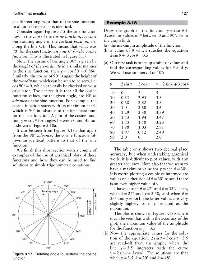
Further mathematics 127
at different angles to that of the sine function.In all other respects it is identical.
Consider again Figure 3.15 the sine functionnow in the case of the cosine function, we startour rotating angle in the vertical position, i.e.along the line OE. This means that what was90◦ for the sine function is now 0◦ for the cosinefunction. This is illustrated in Figure 3.17.
Now, the cosine of the angle 30◦ is given bythe height of the y-ordinate in a similar mannerto the sine function, then y = cos 30◦ = 0.866.Similarly, the cosine of 90◦ is again the height ofthe y-ordinate, which can be seen to be zero, i.e.cos 90◦ = 0, which can easily be checked on yourcalculator. The net result is that all the cosinefunction values, for the given angle, are 90◦ inadvance of the sine function. For example, thecosine function starts with its maximum at 0◦,which is 90◦ in advance of the first maximumfor the sine function. A plot of the cosine func-tion y = cos θ for angles between 0 and 4π radis shown in Figure 3.18a.
It can be seen from Figure 3.18a that apartfrom the 90◦ advance, the cosine function fol-lows an identical pattern to that of the sinefunction.
We finish this short section with a couple ofexamples of the use of graphical plots of thesefunctions and how they can be used to findsolutions to simple trigonometric equations.
Figure 3.17 Rotating angle to illustrate the cosinefunction.
Example 3.18
Draw the graph of the function y = 2 sin θ +3 cos θ for values of θ between 0 and 90◦. Fromthe graph find:(a) the maximum amplitude of the function(b) a value of θ which satisfies the equation
2 sin θ + 3 cos θ = 3.5
(a) Our first task is to set up a table of values andfind the corresponding values for θ and y.We will use an interval of 10◦:
θ 2 sin θ 3 cos θ y = 2 sin θ + 3 cos θ
0 0 3 310 0.35 2.95 3.320 0.68 2.82 3.530 1.0 2.60 3.640 1.29 2.30 3.5950 1.53 1.94 3.4760 1.73 1.50 3.2370 1.88 1.03 2.9180 1.97 0.52 2.4990 2.0 0 2.0
The table only shows two decimal placeaccuracy, but when undertaking graphicalwork, it is difficult to plot values, with anygreater accuracy. Note also that we seem tohave a maximum value for y when θ = 30◦.It is worth plotting a couple of intermediatevalues on either side of θ = 30◦ to see if thereis an even higher value of y.
I have chosen θ = 27◦ and θ = 33◦. Then,when θ = 27◦ and y = 3.58, and when θ =33◦ and y = 3.61, the latter values are veryslightly higher, so may be used as themaximum.
The plot is shown in Figure 3.18b whereit can be seen that within the accuracy of theplot, the maximum value of the amplitudefor the function is y = 3.5.
(b) Now the appropriate values for the solu-tion of the equation: 2 sin θ − 3 cos θ = 3.5are read-off from the graph, where theline y = 3.5 intersects with the curvey = 2 sin θ + 3 cos θ. The solutions are thatwhen y = 3.5, θ = 20◦ and θ = 48◦.
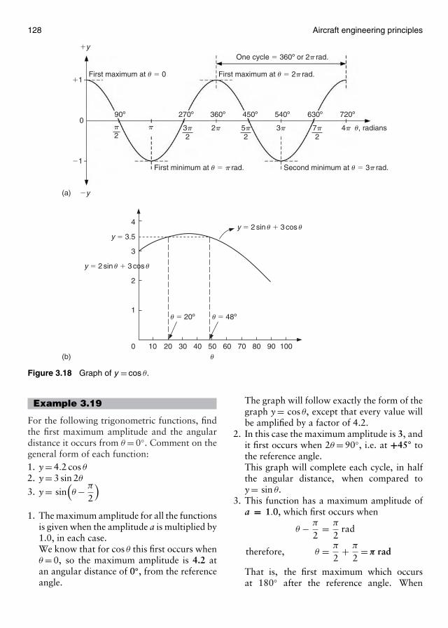
128 Aircraft engineering principles
(a)
(b)10
u � 20º
y � 2 sin u � 3 cos u
y � 2 sin u � 3 cos u
u
y � 3.5
u � 48º
0
1
2
3
4
20 30 40 50 60 70 80 90 100
First maximum at u � 0 First maximum at u � 2p rad.
First minimum at u � p rad. Second minimum at u � 3p rad.
One cycle � 360º or 2p rad.�y
�y
�1
�1
090º 270º 360º 450º 540º 630º 720º
3p2
2p 3p 4p u, radiansp 5p2
7p2
p2
Figure 3.18 Graph of y = cos θ.
Example 3.19
For the following trigonometric functions, findthe first maximum amplitude and the angulardistance it occurs from θ = 0◦. Comment on thegeneral form of each function:1. y = 4.2 cos θ
2. y = 3 sin 2θ
3. y = sin(θ − π
2
)1. The maximum amplitude for all the functions
is given when the amplitude a is multiplied by1.0, in each case.We know that for cos θ this first occurs whenθ = 0, so the maximum amplitude is 4.2 atan angular distance of 0◦, from the referenceangle.
The graph will follow exactly the form of thegraph y = cos θ, except that every value willbe amplified by a factor of 4.2.
2. In this case the maximum amplitude is 3, andit first occurs when 2θ = 90◦, i.e. at +45◦ tothe reference angle.This graph will complete each cycle, in halfthe angular distance, when compared toy = sin θ.
3. This function has a maximum amplitude ofa = 1.0, which first occurs when
θ − π
2= π
2rad
therefore, θ = π
2+ π
2= π rad
That is, the first maximum which occursat 180◦ after the reference angle. When
Further mathematics 129
compared to the function y = sin θ, eachvalue is found to be lagging by π
2 .
If you are finding it difficult to envisage whatis happening, sketch these functions, on thesame axes and make comparisons.
3.2.5 Trigonometric identities
Below will be found a few of the more com-mon and most useful trigonometric identities.These are given without proof and should beused as a tool to simplify expressions or placethem in another form for further manipulation.This technique is particularly useful for simpli-fication prior to carrying out integration, whichyou will meet later.
General identities1. cosec θ = 1
sin θ; sec θ = 1
cos θ; cot θ = 1
tan θ
2. tan θ = sin θcos θ
(you have met this identityalready!)
3. sin2 θ + cos2 θ = 1 where sin2 θ, is shorthand for (sin θ)2, etc.
4. tan2 θ + 1 = sec2 θ; cot2 θ + 1 = cosec2 θ
5. sin(A ± B) = sin A cos B ± cos A sin B6. cos(A ± B) = cos A cos B ∓ sin A sin B
7. tan(A ± B) = tan A ± tan B1 ± tan A tan B
Also from identities 4 to 7 above we get theDoubles and squares identities
8. sin 2A = 2 sin A cos A9. cos 2A = cos2 A − sin2 A = 2 cos2 A − 1
= 1 − 2 sin2 A10. tan 2A = 2 tan A
1 − tan2 A
Sums to products11. sin A + sin B = 2 sin A + B
2 cos A − B2
12. sin A − sin B = 2 cos A + B2 sin A − B
2
13. cos A + cos B = 2 cos A + B2 cos A − B
2
14. cos A − cos B = −2 sin A + B2 sin A − B
2
Products to sums15. sin A cos B = 1
2 [sin(A + B) + sin(A − B)]
16. cos A sin B = 12 [sin(A + B) − sin(A − B)]
17. cos A cos B = 12 [cos(A + B) + cos(A − B)]
18. sin A sin B = 12 [cos(A + B) − cos(A − B)]
All of the above identities take some timeto become familiar with, which are tabulatedabove as a source of reference. You will onlyneed to use them when simplification or achange of form of some trigonometric expres-sion is necessary for further manipulation.
There follows one or two examples, illustrat-ing the use of some of the above identities.
Example 3.20
Solve the following trigonometric equations:(a) 4 sin2 θ + 5 cos θ = 5(b) 3 tan2 θ + 5 = 7 sec θ
(a) The most difficult problem when manipulat-ing identities is to know where to start! Inthis equation, we have two unknowns (sineand cosine) so the most logical approachis to try and get the equation in terms ofone unknown, and this leads us to the useof an appropriate identity. We can in thiscase use one of the most important iden-tities: sin2 θ + cos2 θ = 1 (identity 3 fromabove), from which sin2 θ = 1 − cos2 θ andon substitution into Equation (a) gives:
4(1 − cos2 θ) + 5 cos θ = 5 or
− 4 cos2 θ + 5 cos θ − 1 = 0
This is now a quadratic equation, whichcan be solved in a number of ways; thesimplest being factorization!
Then,
(−4 cos θ + 1)(cos θ − 1) = 0
⇒ −4 cos θ = −1 or cos θ = 1
⇒ cos θ = 14
or cos θ = 1
so, θ = 75.5◦ or 0◦(b) Proceeding in a similar manner to (a), we
need a trigonometric identity which relatesto: tan θ and sec θ (look at identity 4).
Then: 3 tan2 θ + 5 = 7 sec θ and usingsec2 θ = 1 + tan2 θ or tan2 θ = sec2 θ − 1,
130 Aircraft engineering principles
We get:
3(sec2θ − 1) + 5 = 7 sec θ
⇒ 3 sec2 θ − 3 + 5 = 7 sec θ
⇒ 3 sec2 θ − 7 sec θ + 2 = 0
(again a quadratic equation) factorizinggives:
(3 sec θ − 1)( sec θ − 2) = 0
⇒ 3 sec θ = 1 or sec θ = 2(remembering that sec θ = 1
cos θ
)
Then: sec θ = 13
or sec θ = 2
so cos θ = 3 or cos θ = 12
Now, cos θ = 3 (is not permissible), sothere is only one solution, cos θ = 0.5 soθ = 60◦.
The following example shows one or twotechniques that may be used to verify trigono-metric identities involving, double angle andsums to products.
Example 3.21
Verify the following identities by showing thateach side of the equation is equal in all respects:(a) (sin θ + cos θ)2 ≡ 1 + sin 2θ
(b)sin 3θ − sin θ
cos θ − cos 3θ≡ cot 2θ
(a) Simply requires the left-hand side to bemanipulated algebraically to equal the right-hand side. So multiplying out gives:
(sin θ + cos θ)2 ≡ 1 + sin 2θ
sin2 θ + 2 sin θ cos θ + cos2 θ ≡sin2 θ + cos2 θ + 2 sin θ cos θ ≡
(and from sin2 θ + cos2 θ = 1) then,
1 + 2 sin θ cos θ ≡(and from identity 8, above)
1 + 2 sin θ ≡ 1 + sin 2θ
(as required)
(b) Again considering left-hand side and usingsums to products (identities 12 and 14)where:
sin A − sin B = 2 cosA + B
2sin
A − B
2
and cos A−cos B = −2 sinA+B
2sin
A−B
2
and A > B (A greater than B) then
sin3θ− sin θ = 2 cos(
3+12
)θ sin
(3−1
2
)θ
= 2 cos 2θ sin θ and
cosθ−cos3θ = −2 sin(
1 − 32
)θ
× sin(
1+32
)θ
cosθ−3 cosθ = −2 sin(−θ)(sin 2θ)
and from the fact that, sin (−θ) = −sin θ weget
cos θ − cos 3θ = 2 sin 2θ sin θ
therefore:sin 3θ − sin θ
cos θ − cos 3θ≡ 2 cos 2θ sin θ
2 sin 2θ sin θ
≡ cot 2θ
In the final example, you will see howtrigonometric identities may be used to evaluatetrigonometric ratios.
Example 3.22
If A is an acute angle and B is obtuse, wheresin A = 3
5 and cos B = − 513 , find the values of:
(a) sin(A + B)(b) tan(A + B)
(a) sin(A + B) = sin A cos B + cos A sin B (1)(from identity 5). In order to use this iden-tity we need to find the values of the ratiosfor sin A and cos B. So again we need tochoose an identity that allows us to find sin θ
or cos θ, in terms of each other.We know that sin2 B + cos2 B = 1; hence,
sin2 B = 1 − cos2 B. Therefore inserting
Further mathematics 131
values,
sin2 B = 1 − (− 513 )2B then
sin B = 1 − 25169 = 144
169
sin B = 1213
(Since B is obtuse, 90◦ < B < 180◦ and signratio is positive in second quadrant. Thenonly positive values of this ratio need to beconsidered.) Similarly:
sin2 A + cos2 A = 1 so, cos2 A = 1 − sin2 A
= 1 − 925
and cos A = 45
(Since angle A is <90◦, i.e. acute, only thepositive value is considered.) Now usingEquation (1) above:
sin(A + B) = sin A cos B + cos A sin B
= ( 35
) (− 513
)+ ( 45
) ( 1213
)= − 15
65 + 4865 then
sin(A + B) = 3356
Note the use of fractions to keep exactratios!
(b) For this part of the question we simply needto remember that:
sin Acos A
= tan A
and use inequality (7) in a similar way asbefore.
Then
tan A = sin Acos A
=3545
= ( 35
)( 54
) = 34 and
tan B = sin Bcos B
=1213
− 513
= ( 1213
)(− 135
) = − 125
and using identity 7,
tan(A + B) = tan A + tan B1 − tan A tan B
=34 − 12
5
1 − ( 34
)(− 125
)
and after multiplying every term in theexpression by 20 (the lowest common mul-tiple), we get:
tan(A + B) = 15 − 4820 + 36
= −3356
Test your understanding 3.41. Given that sin(θ + φ) = 0.6 and cos(θ + φ) = 0.9, find a
value for µ when µ = tan φ.
2. Verify the following identities:
(a) tan 3θ = sin θ + sin 3θ + sin 5θ
cos θ + cos 3θ + cos 5θ
(b) tan 2θ = 11 − tan θ
− 11 + tan θ
3. Express the following as ratios of single angles:
(a) sin 5θ cos θ + cos 5θ sin θ
(b) cos 9t cos 2t − sin 9t sin 2t
This ends our short excursion into trigono-metric identities and also our further study oftrigonometry. In Section 3.3 we will introducethe elementary ideas of statistics.
3.3 Statistical methods
Your view of statistics has probably beenformed from what you read in the papers, orwhat you see on the television. Results of surveysshow: which political party is going to win theelection, why men grow moustaches, if smok-ing damages your health, the average cost ofhousing by area, and all sorts of other interest-ing data! Well, statistics is used to analyse theresults of such surveys and when used correctly,it attempts to eliminate the bias which oftenappears when collecting data on controversialissues.
Statistics is concerned with collecting, sortingand analysing numerical facts which originatefrom several observations. These facts are col-lated and summarized then presented as tables,charts or diagrams, etc.
In this brief introduction to statistics welook at two specific areas. First, we consider thecollection and presentation of data in its various
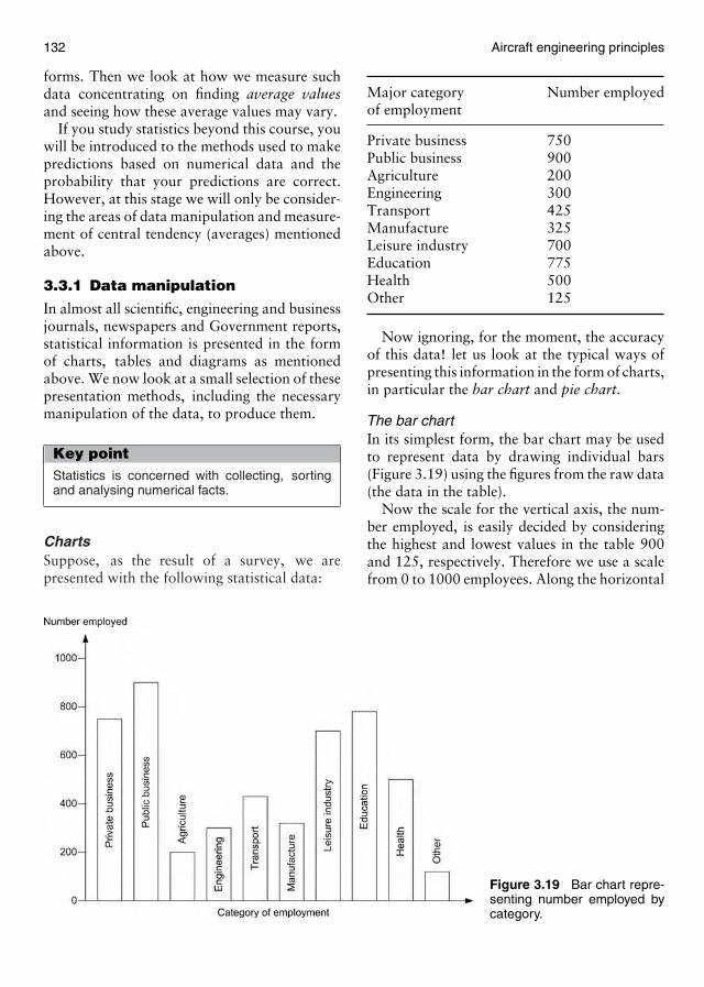
132 Aircraft engineering principles
forms. Then we look at how we measure suchdata concentrating on finding average valuesand seeing how these average values may vary.
If you study statistics beyond this course, youwill be introduced to the methods used to makepredictions based on numerical data and theprobability that your predictions are correct.However, at this stage we will only be consider-ing the areas of data manipulation and measure-ment of central tendency (averages) mentionedabove.
3.3.1 Data manipulation
In almost all scientific, engineering and businessjournals, newspapers and Government reports,statistical information is presented in the formof charts, tables and diagrams as mentionedabove. We now look at a small selection of thesepresentation methods, including the necessarymanipulation of the data, to produce them.
Key pointStatistics is concerned with collecting, sortingand analysing numerical facts.
ChartsSuppose, as the result of a survey, we arepresented with the following statistical data:
Figure 3.19 Bar chart repre-senting number employed bycategory.
Major category Number employedof employment
Private business 750Public business 900Agriculture 200Engineering 300Transport 425Manufacture 325Leisure industry 700Education 775Health 500Other 125
Now ignoring, for the moment, the accuracyof this data! let us look at the typical ways ofpresenting this information in the form of charts,in particular the bar chart and pie chart.
The bar chartIn its simplest form, the bar chart may be usedto represent data by drawing individual bars(Figure 3.19) using the figures from the raw data(the data in the table).
Now the scale for the vertical axis, the num-ber employed, is easily decided by consideringthe highest and lowest values in the table 900and 125, respectively. Therefore we use a scalefrom 0 to 1000 employees. Along the horizontal
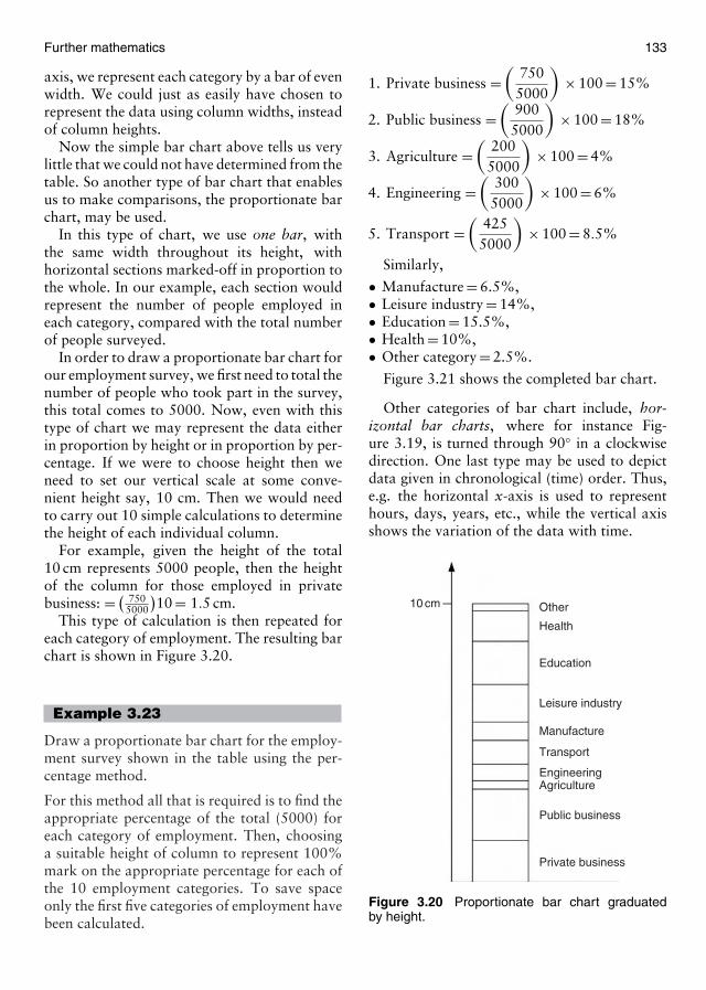
Further mathematics 133
axis, we represent each category by a bar of evenwidth. We could just as easily have chosen torepresent the data using column widths, insteadof column heights.
Now the simple bar chart above tells us verylittle that we could not have determined from thetable. So another type of bar chart that enablesus to make comparisons, the proportionate barchart, may be used.
In this type of chart, we use one bar, withthe same width throughout its height, withhorizontal sections marked-off in proportion tothe whole. In our example, each section wouldrepresent the number of people employed ineach category, compared with the total numberof people surveyed.
In order to draw a proportionate bar chart forour employment survey, we first need to total thenumber of people who took part in the survey,this total comes to 5000. Now, even with thistype of chart we may represent the data eitherin proportion by height or in proportion by per-centage. If we were to choose height then weneed to set our vertical scale at some conve-nient height say, 10 cm. Then we would needto carry out 10 simple calculations to determinethe height of each individual column.
For example, given the height of the total10 cm represents 5000 people, then the heightof the column for those employed in privatebusiness: = ( 750
5000
)10 = 1.5 cm.
This type of calculation is then repeated foreach category of employment. The resulting barchart is shown in Figure 3.20.
Example 3.23
Draw a proportionate bar chart for the employ-ment survey shown in the table using the per-centage method.
For this method all that is required is to find theappropriate percentage of the total (5000) foreach category of employment. Then, choosinga suitable height of column to represent 100%mark on the appropriate percentage for each ofthe 10 employment categories. To save spaceonly the first five categories of employment havebeen calculated.
1. Private business =(
7505000
)× 100 = 15%
2. Public business =(
9005000
)× 100 = 18%
3. Agriculture =(
2005000
)× 100 = 4%
4. Engineering =(
3005000
)× 100 = 6%
5. Transport =(
4255000
)× 100 = 8.5%
Similarly,
• Manufacture = 6.5%,• Leisure industry = 14%,• Education = 15.5%,• Health = 10%,• Other category = 2.5%.
Figure 3.21 shows the completed bar chart.
Other categories of bar chart include, hor-izontal bar charts, where for instance Fig-ure 3.19, is turned through 90◦ in a clockwisedirection. One last type may be used to depictdata given in chronological (time) order. Thus,e.g. the horizontal x-axis is used to representhours, days, years, etc., while the vertical axisshows the variation of the data with time.
10 cm Other
Health
Education
Leisure industry
Manufacture
Transport
EngineeringAgriculture
Public business
Private business
Figure 3.20 Proportionate bar chart graduatedby height.

134 Aircraft engineering principles
Other (2.5%)
Health (10%)
Education (15.5%)
Leisure industry (14%)
Manufacture (6.5%)
Transport (8.5%)
Engineering (6%)
Agriculture (4%)
Public business (18%)
Private business (15%)
Figure 3.21 Proportionate percentage bar chart.
Figure 3.22 (a) Chronological bar chart in correct proportion, (b) chronological bar chart with graded scale.
Example 3.24
Represent the following data on a chronologicalbar chart.
Year Number employed in generalengineering (thousands)
1995 8001996 7851997 6901998 6701999 590
Since we have not been asked to representthe data on any specific bar chart we willuse the simplest, involving only the raw data.Then, the only concern is the scale we shoulduse for the vertical axis. To present a truerepresentation, the scale should start from zeroand extend to say, 800 (Figure 3.22(a)). Ifwe wish to emphasize a trend, which is theway the variable is rising or falling with time wecould use a very much exaggerated scale (Fig-ure 3.22(b)). This immediately emphasizes thedownward trend since 1995.
Note that this data is fictitious (made-up) andused here, merely for emphasis!
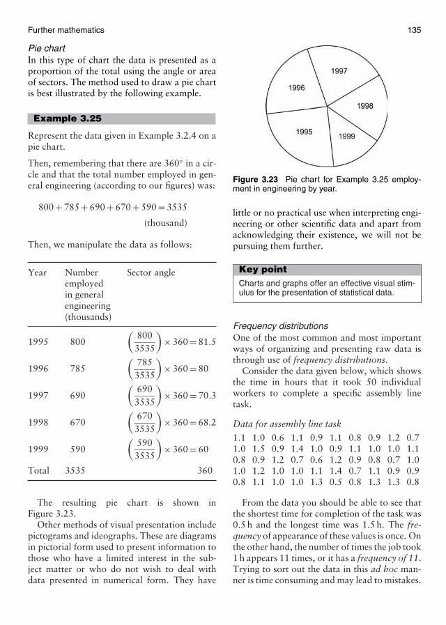
Further mathematics 135
Pie chartIn this type of chart the data is presented as aproportion of the total using the angle or areaof sectors. The method used to draw a pie chartis best illustrated by the following example.
Example 3.25
Represent the data given in Example 3.2.4 on apie chart.
Then, remembering that there are 360◦ in a cir-cle and that the total number employed in gen-eral engineering (according to our figures) was:
800 + 785 + 690 + 670 + 590 = 3535
(thousand)
Then, we manipulate the data as follows:
Year Number Sector angleemployedin generalengineering(thousands)
1995 800(
8003535
)× 360 = 81.5
1996 785(
7853535
)× 360 = 80
1997 690(
6903535
)× 360 = 70.3
1998 670(
6703535
)× 360 = 68.2
1999 590(
5903535
)× 360 = 60
Total 3535 360
The resulting pie chart is shown inFigure 3.23.
Other methods of visual presentation includepictograms and ideographs. These are diagramsin pictorial form used to present information tothose who have a limited interest in the sub-ject matter or who do not wish to deal withdata presented in numerical form. They have
Figure 3.23 Pie chart for Example 3.25 employ-ment in engineering by year.
little or no practical use when interpreting engi-neering or other scientific data and apart fromacknowledging their existence, we will not bepursuing them further.
Key pointCharts and graphs offer an effective visual stim-ulus for the presentation of statistical data.
Frequency distributionsOne of the most common and most importantways of organizing and presenting raw data isthrough use of frequency distributions.
Consider the data given below, which showsthe time in hours that it took 50 individualworkers to complete a specific assembly linetask.
Data for assembly line task
1.1 1.0 0.6 1.1 0.9 1.1 0.8 0.9 1.2 0.71.0 1.5 0.9 1.4 1.0 0.9 1.1 1.0 1.0 1.10.8 0.9 1.2 0.7 0.6 1.2 0.9 0.8 0.7 1.01.0 1.2 1.0 1.0 1.1 1.4 0.7 1.1 0.9 0.90.8 1.1 1.0 1.0 1.3 0.5 0.8 1.3 1.3 0.8
From the data you should be able to see thatthe shortest time for completion of the task was0.5 h and the longest time was 1.5 h. The fre-quency of appearance of these values is once. Onthe other hand, the number of times the job took1 h appears 11 times, or it has a frequency of 11.Trying to sort out the data in this ad hoc man-ner is time consuming and may lead to mistakes.
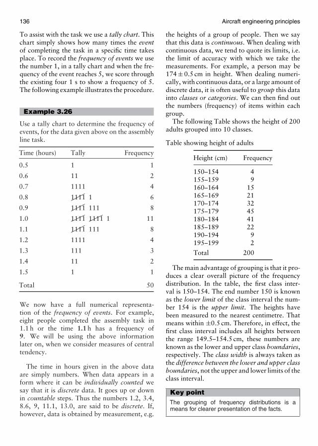
136 Aircraft engineering principles
To assist with the task we use a tally chart. Thischart simply shows how many times the eventof completing the task in a specific time takesplace. To record the frequency of events we usethe number 1, in a tally chart and when the fre-quency of the event reaches 5, we score throughthe existing four 1 s to show a frequency of 5.The following example illustrates the procedure.
Example 3.26
Use a tally chart to determine the frequency ofevents, for the data given above on the assemblyline task.
Time (hours) Tally Frequency
0.5
0.6
0.7
0.8
0.9
1.0
1.1
1.2
1.3
1.4
1.5
1
11
1111
1111 1
1111 111
1111 1111 1
1111 111
1111
111
11
1
1
2
4
6
8
11
8
4
3
2
1
Total 50
We now have a full numerical representa-tion of the frequency of events. For example,eight people completed the assembly task in1.1 h or the time 1.1 h has a frequency of9. We will be using the above informationlater on, when we consider measures of centraltendency.
The time in hours given in the above dataare simply numbers. When data appears in aform where it can be individually counted wesay that it is discrete data. It goes up or downin countable steps. Thus the numbers 1.2, 3.4,8.6, 9, 11.1, 13.0, are said to be discrete. If,however, data is obtained by measurement, e.g.
the heights of a group of people. Then we saythat this data is continuous. When dealing withcontinuous data, we tend to quote its limits, i.e.the limit of accuracy with which we take themeasurements. For example, a person may be174 ± 0.5 cm in height. When dealing numeri-cally, with continuous data, or a large amount ofdiscrete data, it is often useful to group this datainto classes or categories. We can then find outthe numbers (frequency) of items within eachgroup.
The following Table shows the height of 200adults grouped into 10 classes.
Table showing height of adults
Height (cm) Frequency
150–154 4155–159 9160–164 15165–169 21170–174 32175–179 45180–184 41185–189 22190–194 9195–199 2
Total 200
The main advantage of grouping is that it pro-duces a clear overall picture of the frequencydistribution. In the table, the first class inter-val is 150–154. The end number 150 is knownas the lower limit of the class interval the num-ber 154 is the upper limit. The heights havebeen measured to the nearest centimetre. Thatmeans within ±0.5 cm. Therefore, in effect, thefirst class interval includes all heights betweenthe range 149.5–154.5 cm, these numbers areknown as the lower and upper class boundaries,respectively. The class width is always taken asthe difference between the lower and upper classboundaries, not the upper and lower limits of theclass interval.
Key pointThe grouping of frequency distributions is ameans for clearer presentation of the facts.
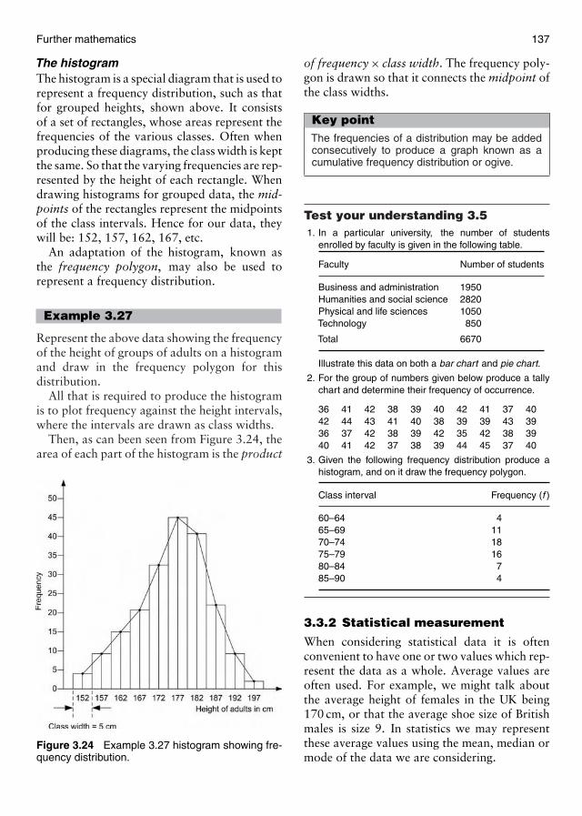
Further mathematics 137
The histogramThe histogram is a special diagram that is used torepresent a frequency distribution, such as thatfor grouped heights, shown above. It consistsof a set of rectangles, whose areas represent thefrequencies of the various classes. Often whenproducing these diagrams, the class width is keptthe same. So that the varying frequencies are rep-resented by the height of each rectangle. Whendrawing histograms for grouped data, the mid-points of the rectangles represent the midpointsof the class intervals. Hence for our data, theywill be: 152, 157, 162, 167, etc.
An adaptation of the histogram, known asthe frequency polygon, may also be used torepresent a frequency distribution.
Example 3.27
Represent the above data showing the frequencyof the height of groups of adults on a histogramand draw in the frequency polygon for thisdistribution.
All that is required to produce the histogramis to plot frequency against the height intervals,where the intervals are drawn as class widths.
Then, as can been seen from Figure 3.24, thearea of each part of the histogram is the product
Figure 3.24 Example 3.27 histogram showing fre-quency distribution.
of frequency × class width. The frequency poly-gon is drawn so that it connects the midpoint ofthe class widths.
Key pointThe frequencies of a distribution may be addedconsecutively to produce a graph known as acumulative frequency distribution or ogive.
Test your understanding 3.51. In a particular university, the number of students
enrolled by faculty is given in the following table.
Faculty Number of students
Business and administration 1950Humanities and social science 2820Physical and life sciences 1050Technology 850
Total 6670
Illustrate this data on both a bar chart and pie chart.
2. For the group of numbers given below produce a tallychart and determine their frequency of occurrence.
36 41 42 38 39 40 42 41 37 4042 44 43 41 40 38 39 39 43 3936 37 42 38 39 42 35 42 38 3940 41 42 37 38 39 44 45 37 40
3. Given the following frequency distribution produce ahistogram, and on it draw the frequency polygon.
Class interval Frequency (f )
60–64 465–69 1170–74 1875–79 1680–84 785–90 4
3.3.2 Statistical measurement
When considering statistical data it is oftenconvenient to have one or two values which rep-resent the data as a whole. Average values areoften used. For example, we might talk aboutthe average height of females in the UK being170 cm, or that the average shoe size of Britishmales is size 9. In statistics we may representthese average values using the mean, median ormode of the data we are considering.
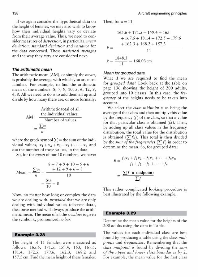
138 Aircraft engineering principles
If we again consider the hypothetical data onthe height of females, we may also wish to knowhow their individual heights vary or deviatefrom their average value. Thus, we need to con-sider measures of dispersion, in particular, meandeviation, standard deviation and variance forthe data concerned. These statistical averagesand the way they vary are considered next.
The arithmetic meanThe arithmetic mean (AM), or simply the mean,is probably the average with which you are mostfamiliar. For example, to find the arithmeticmean of the numbers: 8, 7, 9, 10, 5, 6, 12, 9,6, 8. All we need to do is to add them all up anddivide by how many there are, or more formally:
AM =Arithmetic total of allthe individual values
Number of values
=∑
nn
where the greek symbol∑= the sum of the indi-
vidual values, x1 + x2 + x3 + x4 + · · · + xn andn = the number of these values, in the data.
So, for the mean of our 10 numbers, we have:
Mean =∑
nn
=8 + 7 + 9 + 10 + 5 + 6
+ 12 + 9 + 6 + 8
10
= 8010
= 8
Now, no matter how long or complex the datawe are dealing with, provided that we are onlydealing with individual values (discreet data),the above method will always produce the arith-metic mean. The mean of all the x-values is giventhe symbol x, pronounced, x-bar.
Example 3.28
The height of 11 females were measured asfollows: 165.6, 171.5, 159.4, 163, 167.5,181.4, 172.5, 179.6, 162.3, 168.2 and157.3 cm. Find the mean height of these females.
Then, for n = 11:
x =
165.6 + 171.5 + 159.4 + 163+ 167.5 + 181.4 + 172.5 + 179.6+ 162.3 + 168.2 + 157.3
11
x = 1848.311
= 168.03 cm
Mean for grouped dataWhat if we are required to find the meanfor grouped data? Look back at the table onpage 136 showing the height of 200 adults,grouped into 10 classes. In this case, the fre-quency of the heights needs to be taken intoaccount.
We select the class midpoint x as being theaverage of that class and then multiply this valueby the frequency (f ) of the class, so that a valuefor that particular class is obtained (fx). Then,by adding up all class values in the frequencydistribution, the total value for the distributionis obtained
(∑fx). This total is then divided
by the sum of the frequencies(∑
f)
in order todetermine the mean. So, for grouped data:
x = f1x1 + f2x2 + f3x3 + · · · + fnxn
f1 + f2 + f3 + · · · + fn
=∑
(f × midpoint)∑
f
This rather complicated looking procedure isbest illustrated by the following example.
Example 3.29
Determine the mean value for the heights of the200 adults using the data in Table.
The values for each individual class are bestfound by producing a table using the class mid-points and frequencies. Remembering that theclass midpoint is found by dividing the sumof the upper and lower class boundaries by 2.For example, the mean value for the first class
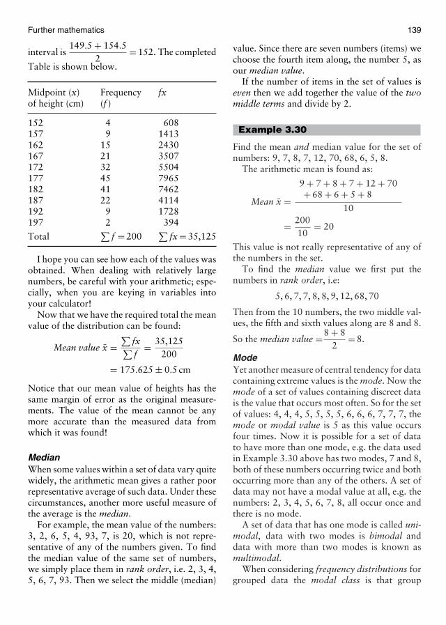
Further mathematics 139
interval is149.5 + 154.5
2= 152. The completed
Table is shown below.
Midpoint (x) Frequency fxof height (cm) (f )
152 4 608157 9 1413162 15 2430167 21 3507172 32 5504177 45 7965182 41 7462187 22 4114192 9 1728197 2 394
Total∑
f = 200∑
fx = 35,125
I hope you can see how each of the values wasobtained. When dealing with relatively largenumbers, be careful with your arithmetic; espe-cially, when you are keying in variables intoyour calculator!
Now that we have the required total the meanvalue of the distribution can be found:
Mean value x =∑
fx∑f
= 35,125200
= 175.625 ± 0.5 cm
Notice that our mean value of heights has thesame margin of error as the original measure-ments. The value of the mean cannot be anymore accurate than the measured data fromwhich it was found!
MedianWhen some values within a set of data vary quitewidely, the arithmetic mean gives a rather poorrepresentative average of such data. Under thesecircumstances, another more useful measure ofthe average is the median.
For example, the mean value of the numbers:3, 2, 6, 5, 4, 93, 7, is 20, which is not repre-sentative of any of the numbers given. To findthe median value of the same set of numbers,we simply place them in rank order, i.e. 2, 3, 4,5, 6, 7, 93. Then we select the middle (median)
value. Since there are seven numbers (items) wechoose the fourth item along, the number 5, asour median value.
If the number of items in the set of values iseven then we add together the value of the twomiddle terms and divide by 2.
Example 3.30
Find the mean and median value for the set ofnumbers: 9, 7, 8, 7, 12, 70, 68, 6, 5, 8.
The arithmetic mean is found as:
Mean x =9 + 7 + 8 + 7 + 12 + 70+ 68 + 6 + 5 + 8
10
= 20010
= 20
This value is not really representative of any ofthe numbers in the set.
To find the median value we first put thenumbers in rank order, i.e:
5, 6, 7, 7, 8, 8, 9, 12, 68, 70
Then from the 10 numbers, the two middle val-ues, the fifth and sixth values along are 8 and 8.
So the median value =8 + 82
= 8.
ModeYet another measure of central tendency for datacontaining extreme values is the mode. Now themode of a set of values containing discreet datais the value that occurs most often. So for the setof values: 4, 4, 4, 5, 5, 5, 5, 6, 6, 6, 7, 7, 7, themode or modal value is 5 as this value occursfour times. Now it is possible for a set of datato have more than one mode, e.g. the data usedin Example 3.30 above has two modes, 7 and 8,both of these numbers occurring twice and bothoccurring more than any of the others. A set ofdata may not have a modal value at all, e.g. thenumbers: 2, 3, 4, 5, 6, 7, 8, all occur once andthere is no mode.
A set of data that has one mode is called uni-modal, data with two modes is bimodal anddata with more than two modes is known asmultimodal.
When considering frequency distributions forgrouped data the modal class is that group
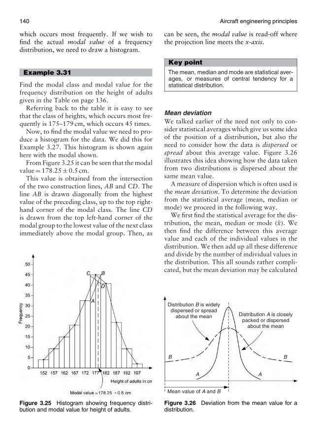
140 Aircraft engineering principles
which occurs most frequently. If we wish tofind the actual modal value of a frequencydistribution, we need to draw a histogram.
Example 3.31
Find the modal class and modal value for thefrequency distribution on the height of adultsgiven in the Table on page 136.
Referring back to the table it is easy to seethat the class of heights, which occurs most fre-quently is 175–179 cm, which occurs 45 times.
Now, to find the modal value we need to pro-duce a histogram for the data. We did this forExample 3.27. This histogram is shown againhere with the modal shown.
From Figure 3.25 it can be seen that the modalvalue = 178.25 ± 0.5 cm.
This value is obtained from the intersectionof the two construction lines, AB and CD. Theline AB is drawn diagonally from the highestvalue of the preceding class, up to the top right-hand corner of the modal class. The line CDis drawn from the top left-hand corner of themodal group to the lowest value of the next classimmediately above the modal group. Then, as
Figure 3.25 Histogram showing frequency distri-bution and modal value for height of adults.
can be seen, the modal value is read-off wherethe projection line meets the x-axis.
Key pointThe mean, median and mode are statistical aver-ages, or measures of central tendency for astatistical distribution.
Mean deviationWe talked earlier of the need not only to con-sider statistical averages which give us some ideaof the position of a distribution, but also theneed to consider how the data is dispersed orspread about this average value. Figure 3.26illustrates this idea showing how the data takenfrom two distributions is dispersed about thesame mean value.
A measure of dispersion which is often used isthe mean deviation. To determine the deviationfrom the statistical average (mean, median ormode) we proceed in the following way.
We first find the statistical average for the dis-tribution, the mean, median or mode (x). Wethen find the difference between this averagevalue and each of the individual values in thedistribution. We then add up all these differenceand divide by the number of individual values inthe distribution. This all sounds rather compli-cated, but the mean deviation may be calculated
Distribution B is widelydispersed or spread
about the mean Distribution A is closelypacked or dispersed
about the mean
Mean value of A and B
A A
BB
Figure 3.26 Deviation from the mean value for adistribution.
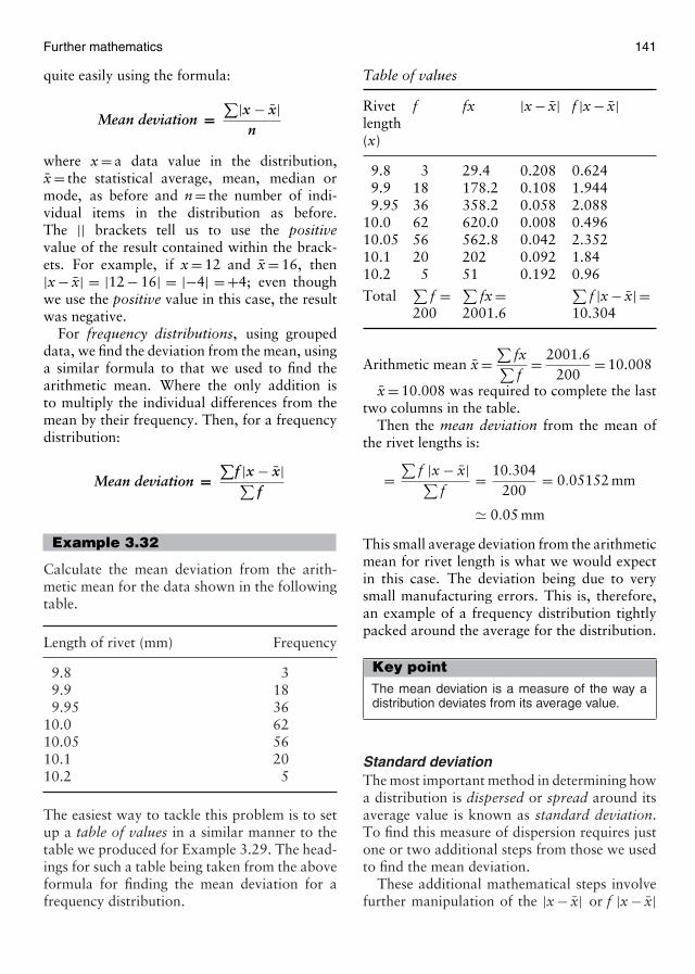
Further mathematics 141
quite easily using the formula:
Mean deviation =∑|x − x|
n
where x = a data value in the distribution,x = the statistical average, mean, median ormode, as before and n = the number of indi-vidual items in the distribution as before.The || brackets tell us to use the positivevalue of the result contained within the brack-ets. For example, if x = 12 and x = 16, then|x − x| = |12 − 16| = |−4| = +4; even thoughwe use the positive value in this case, the resultwas negative.
For frequency distributions, using groupeddata, we find the deviation from the mean, usinga similar formula to that we used to find thearithmetic mean. Where the only addition isto multiply the individual differences from themean by their frequency. Then, for a frequencydistribution:
Mean deviation =∑
f |x − x|∑f
Example 3.32
Calculate the mean deviation from the arith-metic mean for the data shown in the followingtable.
Length of rivet (mm) Frequency
9.8 39.9 189.95 36
10.0 6210.05 5610.1 2010.2 5
The easiest way to tackle this problem is to setup a table of values in a similar manner to thetable we produced for Example 3.29. The head-ings for such a table being taken from the aboveformula for finding the mean deviation for afrequency distribution.
Table of values
Rivet f fx |x − x| f |x − x|length(x)
9.8 3 29.4 0.208 0.6249.9 18 178.2 0.108 1.9449.95 36 358.2 0.058 2.088
10.0 62 620.0 0.008 0.49610.05 56 562.8 0.042 2.35210.1 20 202 0.092 1.8410.2 5 51 0.192 0.96
Total∑
f = ∑fx = ∑
f |x − x| =200 2001.6 10.304
Arithmetic mean x =∑
fx∑f
= 2001.6200
= 10.008
x = 10.008 was required to complete the lasttwo columns in the table.
Then the mean deviation from the mean ofthe rivet lengths is:
=∑
f |x − x|∑f
= 10.304200
= 0.05152 mm
� 0.05 mm
This small average deviation from the arithmeticmean for rivet length is what we would expectin this case. The deviation being due to verysmall manufacturing errors. This is, therefore,an example of a frequency distribution tightlypacked around the average for the distribution.
Key pointThe mean deviation is a measure of the way adistribution deviates from its average value.
Standard deviationThe most important method in determining howa distribution is dispersed or spread around itsaverage value is known as standard deviation.To find this measure of dispersion requires justone or two additional steps from those we usedto find the mean deviation.
These additional mathematical steps involvefurther manipulation of the |x − x| or f |x − x|

142 Aircraft engineering principles
values, we needed to find when calculating themean deviation for discreet or grouped data.The additional steps require us to first squarethese differences, then find their mean andfinally take their square root to reverse thesquaring process. This strange way of manip-ulating these differences is known as the rootmean square deviation or standard deviation,which is identified using the Greek symbolsigma (σ).
Thus, for frequency distributions withgrouped data we can represent these three fur-ther processes mathematically, as follows:
1. Square the differences and multiply by theirfrequency = f |x − x|2.
2. Sum all of these values and find their mean
=∑
f |x − x|2∑f this is a similar step to the way
in which we found the mean deviation. Thevalue of the deviation found at this stage isknown as the variance.
3. Now take the square root of these meansquares to reverse the squaring process
=√∑
f |x − x|2∑f
Then the standard deviation,
σ =√∑
f (x − x)2∑f
The || brackets have been replaced by ordi-nary brackets in this final version of the formula.This is because when we square any quantitywhether positive or negative the result is alwayspositive by the law of signs! It is, therefore, nolonger necessary to use the special brackets.
This particular value of deviation is more rep-resentative than the mean deviation value, wefound before, because it takes account of datathat may have large differences between items,in a similar way to the use of the mode andmedian, when finding average values.
When considering discreet ungrouped date,we apply the same steps as above to the differ-ences |x − x| and obtain,√∑
(x − x)2
n
therefore for ungrouped data, the standarddeviation:
σ =√∑
(x − x)2
n
Note that once again we have removed the spe-cial brackets for the same reason as given abovefor grouped data.
Key pointThe standard deviation as a measure of deviationfrom the statistical average takes into accountdata with extreme values; that is data that itstatistically skewed.
Example 3.33
For the set of numbers 8, 12, 11, 9, 16, 14,12, 13, 10, 9, find the arithmetic mean and thestandard deviation.
Like most of the examples concerning centraltendency and deviation measure, we will solvethis problem by setting up a table of values. Wewill also need to find the arithmetic mean beforewe are able to complete the table, where in thiscase for non-grouped data n = 10.
Then,
x =∑
xn
=8 + 12 + 11 + 9 + 16 + 14
+ 12 + 13 + 10 + 9
10
= 11410
= 11.4
Table of values
x (x − x) (x − x)2
8 −3.4 11.5612 0.6 0.3611 −0.4 0.16
9 −2.4 5.7616 4.6 21.1614 2.6 6.7612 0.6 0.3613 1.6 2.5610 −1.4 1.96
9 −2.4 5.76∑x = 114
∑(x − x)2 = 56.4
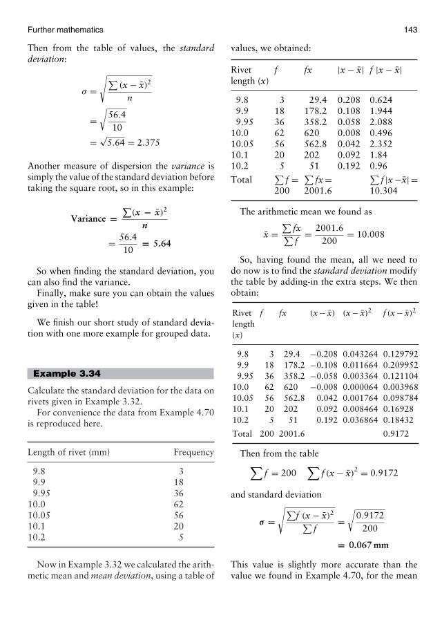
Further mathematics 143
Then from the table of values, the standarddeviation:
σ =√∑
(x − x)2
n
=√
56.410
= √5.64 = 2.375
Another measure of dispersion the variance issimply the value of the standard deviation beforetaking the square root, so in this example:
Variance =∑
(x − x)2
n
= 56.410
= 5.64
So when finding the standard deviation, youcan also find the variance.
Finally, make sure you can obtain the valuesgiven in the table!
We finish our short study of standard devia-tion with one more example for grouped data.
Example 3.34
Calculate the standard deviation for the data onrivets given in Example 3.32.
For convenience the data from Example 4.70is reproduced here.
Length of rivet (mm) Frequency
9.8 39.9 189.95 36
10.0 6210.05 5610.1 2010.2 5
Now in Example 3.32 we calculated the arith-metic mean and mean deviation, using a table of
values, we obtained:
Rivet f fx |x − x| f |x − x|length (x)
9.8 3 29.4 0.208 0.6249.9 18 178.2 0.108 1.9449.95 36 358.2 0.058 2.088
10.0 62 620 0.008 0.49610.05 56 562.8 0.042 2.35210.1 20 202 0.092 1.8410.2 5 51 0.192 0.96
Total∑
f = ∑fx = ∑
f |x −x| =200 2001.6 10.304
The arithmetic mean we found as
x =∑
fx∑f
= 2001.6200
= 10.008
So, having found the mean, all we need todo now is to find the standard deviation modifythe table by adding-in the extra steps. We thenobtain:
Rivet f fx (x − x) (x − x)2 f (x − x)2
length(x)
9.8 3 29.4 −0.208 0.043264 0.1297929.9 18 178.2 −0.108 0.011664 0.2099529.95 36 358.2 −0.058 0.003364 0.121104
10.0 62 620 −0.008 0.000064 0.00396810.05 56 562.8 0.042 0.001764 0.09878410.1 20 202 0.092 0.008464 0.1692810.2 5 51 0.192 0.036864 0.18432
Total 200 2001.6 0.9172
Then from the table∑f = 200
∑f (x − x)
2 = 0.9172
and standard deviation
σ =√∑
f (x − x)2∑f
=√
0.9172200
= 0.067 mm
This value is slightly more accurate than thevalue we found in Example 4.70, for the mean
144 Aircraft engineering principles
deviation = 0.05 mm but as you can see, there isalso a lot more arithmetic manipulation! Again,you should make sure that you are able to obtainthe additional values shown in the table.
Test your understanding 3.61. Calculate the mean of the numbers, 176.5, 98.6, 112.4,
189.8, 95.9 and 88.8.
2. Determine the mean, median and mode for the set ofnumbers, 9, 8, 7, 27, 16, 3, 1, 9, 4 and 116.
3. Estimates for the length of wood required for a shelf,were as follows:
Length (cm) 35 36 37 38 39 40 41 42
Frequency 1 3 4 8 6 5 3 2
Calculate the arithmetic mean and mean deviation.
4. Calculate the arithmetic mean and the mean deviationfor the data shown in the following table.
Length (mm) 167 168 169 170 171
Frequency 2 7 20 8 3
5. Calculate the standard deviation from the median value,for the numbers given in Question 2.
6. Tests were carried out on 50 occasions to determinethe percentage of green house gases in the emissionsfrom an internal combustion engine. The results fromthe tests showing the percentage of greenhouse gasrecorded, were as follows:
% Green house 3.2 3.3 3.4 3.5 3.6 3.7gas present
Frequency 2 12 20 8 6 2
Determine the arithmetic mean and the standard devi-ation for the greenhouse gases present.
3.4 Calculus
3.4.1 Introduction
Meeting the calculus for the first time is oftena rather daunting business. In order to appreci-ate the power of this branch of mathematics wemust first attempt to define it. So, what is thecalculus and what is its function?
Imagine driving a car or riding a motorcyclestarting from rest to over a measured distance,say 1 km. If your time for the run was 25 s,then we can find your average speed over themeasured kilometre from the fact that speed =distance/time. Then using consistent units youraverage speed would be 1000 m/25 s or 40 ms−1.This is fine but suppose you were testing thevehicle and we needed to know its accelerationafter you had driven 500 m. In order to find thiswe would need to determine how the vehiclespeed was changing at this exact point becausethe rate at which your vehicle speed changes isits acceleration. To find such things as rate ofchange of speed we can use the calculus.
The calculus is split into two major areasthe differential calculus and the integralcalculus.
The differential calculus is a branch of math-ematics concerned with finding how thingschange with respect to variables, such as time,distance or speed, especially when these changesare continually varying. In engineering, we areinterested in the study of motion and the waythis motion in machines, mechanisms and vehi-cles, varies with time and the way in whichpressure, density and temperature change withheight or time. Also, how electrical quantitiesvary with time, such as electrical charge, alter-nating current, electrical power, etc. All theseareas may be investigated using the differentialcalculus.
The integral calculus has two primary func-tions. The first function can be used to findthe length of arcs, surface areas or volumesenclosed by a surface. Its second function is thatof antidifferentiation. For example, if we use thedifferential calculus to find the rate of change ofdistance of our motorbike, with respect to time.In other words, we have found its instantaneousspeed. We can then use the inverse process,the integral calculus to determine the originaldistance covered by the motorbike, from itsinstantaneous speed.
The mathematical process we use when apply-ing the differential calculus is known as differ-entiation and when using the integral calculus,the mathematical process we apply is known asintegration.
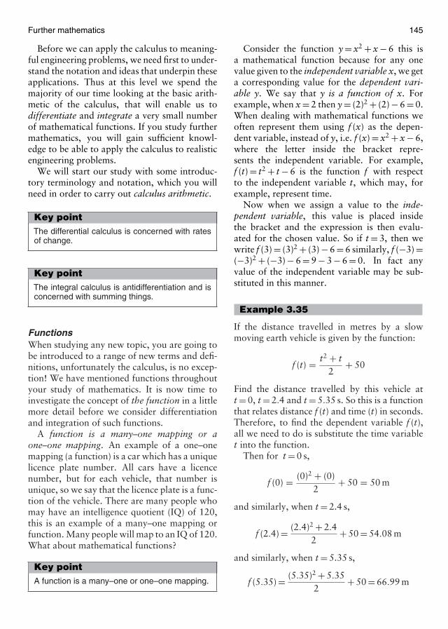
Further mathematics 145
Before we can apply the calculus to meaning-ful engineering problems, we need first to under-stand the notation and ideas that underpin theseapplications. Thus at this level we spend themajority of our time looking at the basic arith-metic of the calculus, that will enable us todifferentiate and integrate a very small numberof mathematical functions. If you study furthermathematics, you will gain sufficient knowl-edge to be able to apply the calculus to realisticengineering problems.
We will start our study with some introduc-tory terminology and notation, which you willneed in order to carry out calculus arithmetic.
Key pointThe differential calculus is concerned with ratesof change.
Key pointThe integral calculus is antidifferentiation and isconcerned with summing things.
FunctionsWhen studying any new topic, you are going tobe introduced to a range of new terms and defi-nitions, unfortunately the calculus, is no excep-tion! We have mentioned functions throughoutyour study of mathematics. It is now time toinvestigate the concept of the function in a littlemore detail before we consider differentiationand integration of such functions.
A function is a many–one mapping or aone–one mapping. An example of a one–onemapping (a function) is a car which has a uniquelicence plate number. All cars have a licencenumber, but for each vehicle, that number isunique, so we say that the licence plate is a func-tion of the vehicle. There are many people whomay have an intelligence quotient (IQ) of 120,this is an example of a many–one mapping orfunction. Many people will map to an IQ of 120.What about mathematical functions?
Key pointA function is a many–one or one–one mapping.
Consider the function y = x2 + x − 6 this isa mathematical function because for any onevalue given to the independent variable x, we geta corresponding value for the dependent vari-able y. We say that y is a function of x. Forexample, when x = 2 then y = (2)2 + (2) − 6 = 0.When dealing with mathematical functions weoften represent them using f (x) as the depen-dent variable, instead of y, i.e. f (x) = x2 + x − 6,where the letter inside the bracket repre-sents the independent variable. For example,f (t) = t2 + t − 6 is the function f with respectto the independent variable t, which may, forexample, represent time.
Now when we assign a value to the inde-pendent variable, this value is placed insidethe bracket and the expression is then evalu-ated for the chosen value. So if t = 3, then wewrite f (3) = (3)2 + (3) − 6 = 6 similarly, f (−3) =(−3)2 + (−3) − 6 = 9 − 3 − 6 = 0. In fact anyvalue of the independent variable may be sub-stituted in this manner.
Example 3.35
If the distance travelled in metres by a slowmoving earth vehicle is given by the function:
f (t) = t2 + t2
+ 50
Find the distance travelled by this vehicle att = 0, t = 2.4 and t = 5.35 s. So this is a functionthat relates distance f (t) and time (t) in seconds.Therefore, to find the dependent variable f (t),all we need to do is substitute the time variablet into the function.
Then for t = 0 s,
f (0) = (0)2 + (0)2
+ 50 = 50 m
and similarly, when t = 2.4 s,
f (2.4) = (2.4)2 + 2.42
+ 50 = 54.08 m
and similarly, when t = 5.35 s,
f (5.35) = (5.35)2 + 5.352
+ 50 = 66.99 m
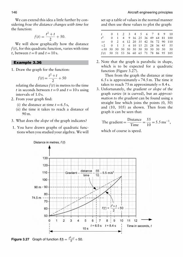
146 Aircraft engineering principles
We can extend this idea a little further by con-sidering how the distance changes with time forthe function:
f (t) = t2 + t2
+ 50.
We will show graphically how the distancef (t), for this quadratic function, varies with timet, between t = 0 and t = 10 s.
Example 3.36
1. Draw the graph for the function:
f (t) = t2 + t2
+ 50
relating the distance f (t) in metres to the timet in seconds between t = 0 and t = 10 s usingintervals of 1.0 s.
2. From your graph find:
(i) the distance at time t = 6.5 s,(ii) the time it takes to reach a distance of
90 m.
3. What does the slope of the graph indicates?
1. You have drawn graphs of quadratic func-tions when you studied your algebra. We will
Figure 3.27 Graph of function f(t) = t 2+t2 + 50.
set up a table of values in the normal mannerand then use these values to plot the graph:
t 0 1 2 3 4 5 6 7 8 9 10t2 0 1 4 9 16 25 36 49 64 81 100+t 0 2 6 12 20 35 42 56 72 90 110÷2 0 1 3 6 10 15 21 28 36 45 55+50 50 50 50 50 50 50 50 50 50 50 50f (t) 50 51 53 56 60 65 71 78 86 95 105
2. Note that the graph is parabolic in shape,which is to be expected for a quadraticfunction (Figure 3.27).
Then from the graph the distance at time6.5 s is approximately = 74.5 m. The time ittakes to reach 75 m approximately = 8.4 s.
3. Unfortunately, the gradient or slope of thegraph varies (it is curved), but an approxi-mation to the gradient can be found using astraight line which joins the points (0, 50)and (10, 105) as shown. Then from thegraph it can be seen that:
The gradient = DistanceTime
= 5510
= 5.5 ms−1,
which of course is speed.
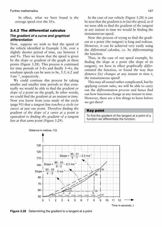
Further mathematics 147
In effect, what we have found is theaverage speed over the 10 s.
3.4.2 The differential calculus
The gradient of a curve and graphicaldifferentiationNow, suppose we wish to find the speed ofthe vehicle identified in Example 3.36, over aslightly shorter period of time, say between 1and 9 s. Then we know that the speed is givenby the slope or gradient of the graph at thesepoints (Figure 3.28). This process is continuedfor time periods of 3–8 s and finally 3–4 s, theresultant speeds can be seen to be, 5.5, 6.2 and5 ms−1, respectively.
We could continue this process by takingsmaller and smaller time periods so that even-tually we would be able to find the gradient orslope of a point on the graph, In other words,we could find the gradient at an instant in time.Now you know from your study of the circle(page 93) that a tangent line touches a circle (orcurve) at just one point. Therefore finding thegradient of the slope of a curve at a point isequivalent to finding the gradient of a tangentline at that same point (Figure 3.29).
Figure 3.28 Determining the gradient to a tangent at a point.
In the case of our vehicle (Figure 3.28) it canbe seen that the gradient is in fact the speed, so ifwe were able to find the gradient of the tangentat any instant in time we would be finding theinstantaneous speed.
Now this process of trying to find the gradi-ent at a point (the tangent) is long and tedious.However, it can be achieved very easily usingthe differential calculus, i.e. by differentiatingthe function.
Thus, in the case of our speed example, byfinding the slope at a point (the slope of itstangent), we have in effect graphically differ-entiated the function, or found the way thatdistance f(x) changes at any instant in time t,the instantaneous speed!
This may all sound rather complicated, but byapplying certain rules, we will be able to carryout the differentiation process and hence findout how functions change at any instant in time.However, there are a few things to learn beforewe get there!
Key pointTo find the gradient of the tangent at a point of afunction we differentiate the function.
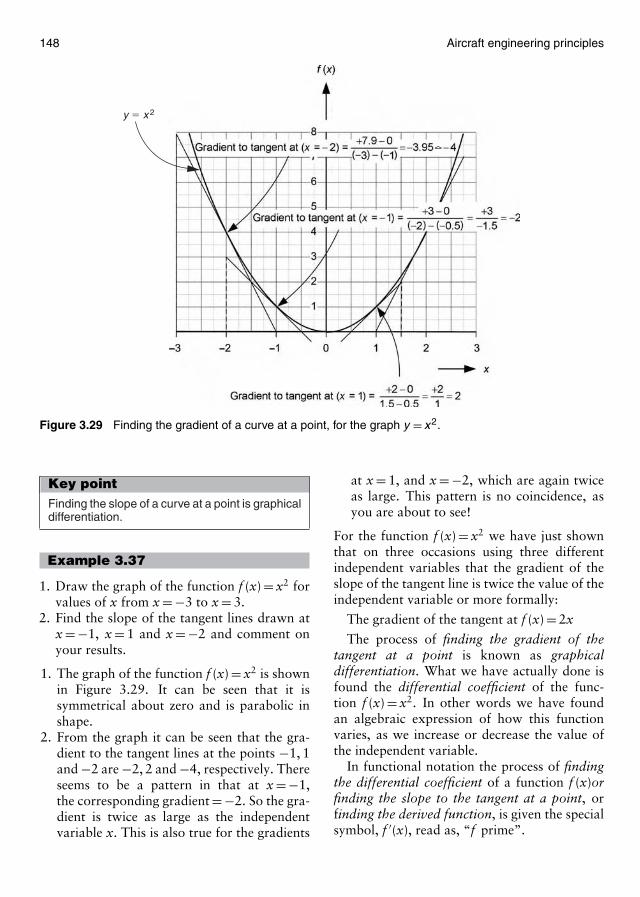
148 Aircraft engineering principles
y � x 2
�
Figure 3.29 Finding the gradient of a curve at a point, for the graph y = x2.
Key pointFinding the slope of a curve at a point is graphicaldifferentiation.
Example 3.37
1. Draw the graph of the function f (x) = x2 forvalues of x from x = −3 to x = 3.
2. Find the slope of the tangent lines drawn atx = −1, x = 1 and x = −2 and comment onyour results.
1. The graph of the function f (x) = x2 is shownin Figure 3.29. It can be seen that it issymmetrical about zero and is parabolic inshape.
2. From the graph it can be seen that the gra-dient to the tangent lines at the points −1, 1and −2 are −2, 2 and −4, respectively. Thereseems to be a pattern in that at x = −1,the corresponding gradient = −2. So the gra-dient is twice as large as the independentvariable x. This is also true for the gradients
at x = 1, and x = −2, which are again twiceas large. This pattern is no coincidence, asyou are about to see!
For the function f (x) = x2 we have just shownthat on three occasions using three differentindependent variables that the gradient of theslope of the tangent line is twice the value of theindependent variable or more formally:
The gradient of the tangent at f (x) = 2x
The process of finding the gradient of thetangent at a point is known as graphicaldifferentiation. What we have actually done isfound the differential coefficient of the func-tion f (x) = x2. In other words we have foundan algebraic expression of how this functionvaries, as we increase or decrease the value ofthe independent variable.
In functional notation the process of findingthe differential coefficient of a function f (x)orfinding the slope to the tangent at a point, orfinding the derived function, is given the specialsymbol, f ′(x), read as, “f prime”.
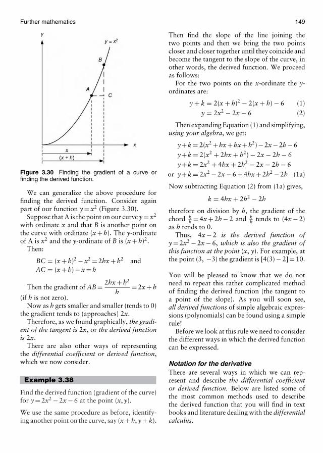
Further mathematics 149
Figure 3.30 Finding the gradient of a curve orfinding the derived function.
We can generalize the above procedure forfinding the derived function. Consider againpart of our function y = x2 (Figure 3.30).
Suppose that A is the point on our curve y = x2
with ordinate x and that B is another point onthe curve with ordinate (x + h). The y-ordinateof A is x2 and the y-ordinate of B is (x + h)2.
Then:
BC = (x + h)2 − x2 = 2hx + h2 andAC = (x + h) − x = h
Then the gradient of AB = 2hx + h2
h= 2x + h
(if h is not zero).Now as h gets smaller and smaller (tends to 0)
the gradient tends to (approaches) 2x.Therefore, as we found graphically, the gradi-
ent of the tangent is 2x, or the derived functionis 2x.
There are also other ways of representingthe differential coefficient or derived function,which we now consider.
Example 3.38
Find the derived function (gradient of the curve)for y = 2x2 − 2x − 6 at the point (x, y).
We use the same procedure as before, identify-ing another point on the curve, say (x + h, y + k).
Then find the slope of the line joining thetwo points and then we bring the two pointscloser and closer together until they coincide andbecome the tangent to the slope of the curve, inother words, the derived function. We proceedas follows:
For the two points on the x-ordinate the y-ordinates are:
y + k = 2(x + h)2 − 2(x + h) − 6 (1)y = 2x2 − 2x − 6 (2)
Then expanding Equation (1) and simplifying,using your algebra, we get:
y+k = 2(x2 +hx+hx+h2)−2x−2h−6y+k = 2(x2 + 2hx + h2) − 2x − 2h − 6y+k = 2x2 + 4hx + 2h2 − 2x − 2h − 6
or y+k = 2x2 − 2x − 6 + 4hx + 2h2 − 2h (1a)
Now subtracting Equation (2) from (1a) gives,
k = 4hx + 2h2 − 2h
therefore on division by h, the gradient of thechord k
h = 4x + 2h − 2 and kh tends to (4x − 2)
as h tends to 0.Thus, 4x − 2 is the derived function of
y = 2x2 − 2x − 6, which is also the gradient ofthis function at the point (x, y). For example, atthe point (3, −3) the gradient is [4(3) − 2] = 10.
You will be pleased to know that we do notneed to repeat this rather complicated methodof finding the derived function (the tangent toa point of the slope). As you will soon see,all derived functions of simple algebraic expres-sions (polynomials) can be found using a simplerule!
Before we look at this rule we need to considerthe different ways in which the derived functioncan be expressed.
Notation for the derivativeThere are several ways in which we can rep-resent and describe the differential coefficientor derived function. Below are listed some ofthe most common methods used to describethe derived function that you will find in textbooks and literature dealing with the differentialcalculus.
150 Aircraft engineering principles
These differing terms for finding the derivedfunction include:
• find the derived function of …• find the derivative of …• find the differential coefficient for …• differentiate …• find the rate of change of …• find the tangent to the function …• find the gradient of a function at a point …
This differing terminology is often confusingto beginners. It is further complicated by the factthat different symbols are used for the differ-entiation process (finding the derived function)based on the convention chosen.
We have been dealing with functional nota-tion, where for a function f (x) the first derivativeor first derived function is given as f ′(x). Ifwe were to carry out the differentiation pro-cess again on the first derived function then wesay we have found the second derivative f ′′(x)and so on.
We have used functional notation merely tointroduce the idea of the mathematical func-tion. We look next at the more common Leibniznotation, which we will use from now onthroughout the remainder of this book.
In Leibniz notation, the mathematical func-tion is represented conventionally as y(x) andits derived function or differential coefficientis represented as dy
dx . This expression for thederived function can be thought of as findingthe slope to the tangent of a point of a particularfunction, where we take a smaller and smallerbit of x (dx) and divide it into a smaller andsmaller bit of y (dy) until we get the slope of a
point dydx .
So, in Leibniz notation, for the functiony = x2 the differential coefficient is represented
as dydx = 2x, which we found earlier.
The second derivative in Leibniz notation isrepresented as d2y
dx2 , the third derivative is d3ydx3
and so on.One other complication arises with all nota-
tions, in that the notation differs according tothe variable being used! For example, if ourmathematical function is s(t), then in Leibniz
notation, its first derivative would be dsdt , as we
are differentiating the variable s with respect to
t. In the same way as with dydx we are differ-
entiating the variable y with respect to x. So in
general, dydx , ds
dt , dudv , represent the first derivative
of the functions, y, s and u, respectively.One final type of notation which is often
used in mechanics is dot notation. For exam-ple, where v, s, etc. means that the function isdifferentiated once (v) or twice (s) and so on.This notation will not be used in this book, butyou may meet it in your further studies.
So much for all the hard theory, we are nowgoing to use one or two rules to carry out thedifferentiation process which, once mastered, isreally quite simple!
Key point
In Leibniz notation dydx means that we find the first
derivative of the function y with respect to x.
Key pointIn functional notation f ′(x ) and f ′′(x ) are thefirst and second derivatives of the function f,respectively.
DifferentiationAs you will be aware by now the word dif-ferentiate is one of many ways of saying thatwe wish to find the derived function. Again,going back to the simple function y = x2, whenwe differentiated this function, we found thatits derived function was dy
dx = 2x. In a similarmanner when we carried out the differentia-tion process on the function y = 2x2 − 2x − 6 weobtained, dy
dx = 4x − 2.If we were to carry out the rather complex
process we used earlier on the following func-tions, y = 3x2, y = x3 and y = x3 + 3x2 − 2, wewould obtain, dy
dx = 6x, dydx = 3x2 and dy
dx = 3x2 +6x, respectively. I wonder if you can see a pat-tern in these results? They are grouped belowfor your convenience, can you spot a pattern?
Further mathematics 151
y = x2 dydx
= 2x
y = 3x2 dydx
= 6x
y = 2x2 − 2x − 6dydx
= 4x − 2
y = x3 dydx
= 3x2
y = x3 + 3x2 − 2dydx
= 3x2 + 6x
I hope you spotted that we seem to multiply bythe index (power) of the unknown, then we sub-tract (1) one from the index of the unknown. Forexample, with the function y = 3x2 the index is2 and (2)(3) = 6. Also the original index (power)of x was 2 and on subtracting 1 from this index
we get: x(2−1) = x1 = x so we finally get, dydx = 6x.
This technique can be applied to anyunknown raised to a power. We can write thisrule in general terms:
If y = xn then,dydx
= nxn−1
Or, in other words, to find the differential coef-ficient of the function y = xn we first multiplythe unknown variable by the index and thensubtract 1 from the index to form the new index.
Again, with this rather wordy explanation,you will appreciate the ease with which we canexpress this rule, using a formula!
You may be wondering why the constant(number) in the above functions seems to justdisappear. If you remember how we performedthe differentiation process, graphically, by find-ing the slope at a point on the function, then fora constant, such as y = −6, the graph is simple astraight horizontal line cutting the y-axis at −6therefore, its slope is zero, thus its derived func-tion is zero. This is true for any constant termno matter what its value.
If the function we are considering has morethan one term, e.g. y = x3 + 3x2 − 2, then wesimply apply the rule in sequence to each andevery term.
Example 3.39
Differentiate the following functions withrespect to the variable:
1. y = 3x3 − 6x2 − 3x + 82. y = 3
x − x3 + 6x−3
3. s = 3t3 − 16t2 + 6t−1
1. In this example we can simply apply the ruledydx = nxn−1 to each term in succession, so:
dydx
= (3)(3)x3−1−(2)(6)x2−1−(1)(3)x1−1 + 0
and remembering that any number raised tothe power zero is one, i.e. x0 = 1, then:
dydx
= 9x3−1 − 12x2−1 − 3x1−1 + 0
dydx
= 9x2 − 12x1 − 3x0
dydx
= 9x2 − 12x − 3
2. In this example, we need to simplify, beforewe use the rule. The simplification involvesclearing fractions. Then remembering thatx = x1 and that from your laws of indiceswhen you bring a number in index formover the fraction line, we change its sign,y = 3
x − x3 + 6x−3 becomes:
y = 3x1
− x3 + 6x−3 or
y = 3x−1 − x3 + 6x−3and applying the rule,
dydx
= (−1)(3)x−1−1 − (3)x3−1 − (3)(6)x−3−1
dydx
= −3x−2 − 3x2 − 18x−4
Notice how we have dealt with negativeindices. The rule can also be used whenfractional indices are involved.
3. The only change with this example is that itconcerns different variables. In this case weare asked to differentiate the function s withrespect to the variable t.
152 Aircraft engineering principles
So proceeding as before and simplifyingfirst, we get: s = 3t3 − 16t−2 + 6t−1 and thendifferentiating
dsdt
= (3)(3)t3−1 − (−2)(16)t−2−1
+ (−1)(6)t−1−1
dsdt
= 9t2 + 32t−3 − 6t−2
Note that you must take care with your signs!
Key pointTo find the first derivative of functions of the typey = ax n, we use the rule that dy
dx = nax n−1
The second derivativeIn the above example we found, in all cases, thefirst derivative. If we wish to find the secondderivative of a function, all we need to do isdifferentiate again. So in example 1.100 ques-tion 1, for the function y = 3x3 − 6x2 − 3x + 8,then:
dydx
= 9x2 − 12x − 3
and differentiating this function again, we get,
d2ydx2
= (2)(9)x2−1 + (1)(−12)x1−1
= 18x − 12x0 = 18x − 12
In the above example, notice the Leibnizterminology for the second differential.
Similarly for the function, s = 3t2 − 16t−2 +6t−1, then:
dsdt
= 9t2 + 32t−3 − 6t−2
and on differentiating this function again,we get,
d2sdt2
= (2)(9)t2−1 + (−3)(32)t−3−1
+ (−6)(−2)t−2−1
= 18t − 96t−4 + 12t−3
In this example notice once again the careneeded with signs.
Key pointd2ydx2 , f ′′(x ) and x are all ways of expressing thesecond derivative.
Rate of changeOne application of the differential calculus is tofind instantaneous rates of change. The exam-ple given at the beginning of this section con-cerned our ability to find how the speed of amotor vehicle changed at a particular point intime. In order to find the rate of change ofany function, we simply differentiate that func-tion (find its gradient) at the particular pointconcerned.
For example, given that y = 4x2 let us findits rate of change at the points, x = 2 andx = −4. Then all we need to do is differentiatethe function and then substitute in the desiredpoints.
Then, dydx = (2)(4)x = 8x and when x = 2,
dydx = (8)(2) = 16, thus the slope of the functionat x = 2 is 16 and this tells us how the functionis changing at this point.
Similarly, when x = −4, dydx = 8x = (−4)(8) =
−32. In this case the negative sign indicatesa negative slope, so the function is changingin the opposite sense compared with what washappening when x = 2.
Example 3.40
The distance (s) covered by a missile s =4.905t2 + 10t. Determine its rate of change ofdistance with respect to time (its speed), after(i) 4 s and (ii) 12 s have elapsed.
This is a simple rate of change problem hiddenin this rather wordy question!
To find rate of change of distance with respectto time; we need to find the differential coeffi-cient of the function. Then applying the rule:
dsdt
= (2)(4.905)t2−1 + 10t1−1 = 9.81t + 10
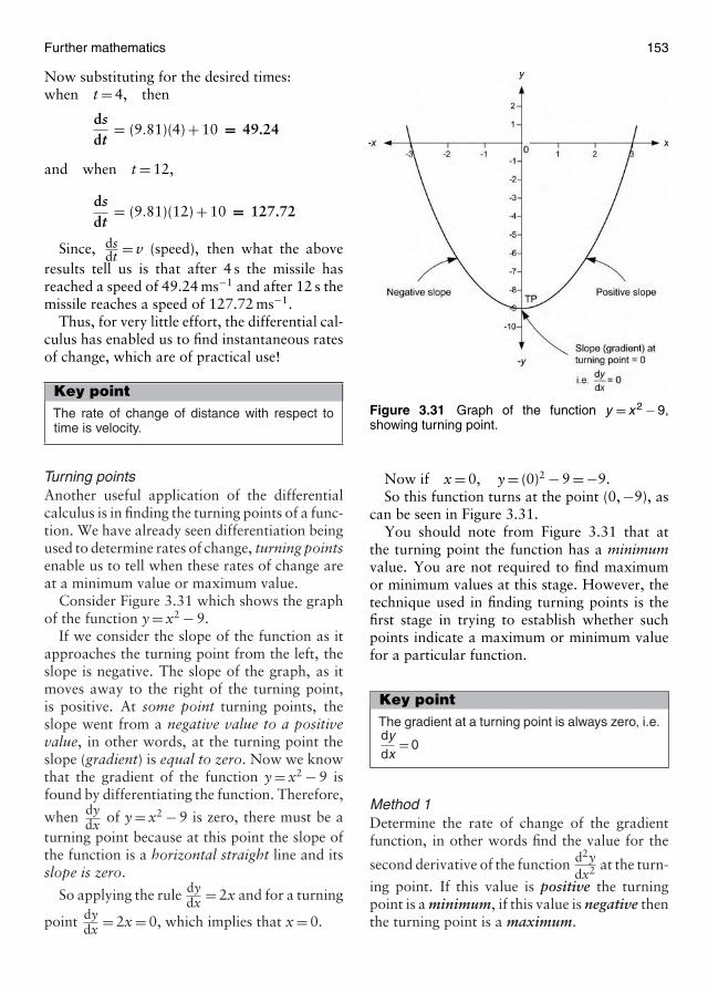
Further mathematics 153
Now substituting for the desired times:when t = 4, then
dsdt
= (9.81)(4) + 10 = 49.24
and when t = 12,
dsdt
= (9.81)(12) + 10 = 127.72
Since, dsdt = v (speed), then what the above
results tell us is that after 4 s the missile hasreached a speed of 49.24 ms−1 and after 12 s themissile reaches a speed of 127.72 ms−1.
Thus, for very little effort, the differential cal-culus has enabled us to find instantaneous ratesof change, which are of practical use!
Key pointThe rate of change of distance with respect totime is velocity.
Turning pointsAnother useful application of the differentialcalculus is in finding the turning points of a func-tion. We have already seen differentiation beingused to determine rates of change, turning pointsenable us to tell when these rates of change areat a minimum value or maximum value.
Consider Figure 3.31 which shows the graphof the function y = x2 − 9.
If we consider the slope of the function as itapproaches the turning point from the left, theslope is negative. The slope of the graph, as itmoves away to the right of the turning point,is positive. At some point turning points, theslope went from a negative value to a positivevalue, in other words, at the turning point theslope (gradient) is equal to zero. Now we knowthat the gradient of the function y = x2 − 9 isfound by differentiating the function. Therefore,
when dydx of y = x2 − 9 is zero, there must be a
turning point because at this point the slope ofthe function is a horizontal straight line and itsslope is zero.
So applying the rule dydx = 2x and for a turning
point dydx = 2x = 0, which implies that x = 0.
Figure 3.31 Graph of the function y = x 2 − 9,showing turning point.
Now if x = 0, y = (0)2 − 9 = −9.So this function turns at the point (0, −9), as
can be seen in Figure 3.31.You should note from Figure 3.31 that at
the turning point the function has a minimumvalue. You are not required to find maximumor minimum values at this stage. However, thetechnique used in finding turning points is thefirst stage in trying to establish whether suchpoints indicate a maximum or minimum valuefor a particular function.
Key pointThe gradient at a turning point is always zero, i.e.dydx
= 0
Method 1Determine the rate of change of the gradientfunction, in other words find the value for the
second derivative of the function d2ydx2 at the turn-
ing point. If this value is positive the turningpoint is a minimum, if this value is negative thenthe turning point is a maximum.
154 Aircraft engineering principles
For example, in the case of the above func-
tion y = x2 − 9 the second derivative is d2ydx2 = 2,
which is positive and so at the point (0, −9) wehave a minimum.
Method 2Consider the gradient of the curve close to theturning points, i.e. near either side. Then fora minimum the gradient goes from negative topositive and for a maximum the gradient goesfrom positive to negative.
Quite clearly, for the function y = x2 − 9, weapproach the turning point with a negative slopeand leave it with a positive slope, therefore, onceagain, at the point (0, −9) we have a minimum.
Key pointA turning point is minimum when the gradientgoes from negative to positive, as we approachand leave the turning point. It is maximum whenthe gradient goes from positive to negative.
Differentiation of elementary trigonometricand exponential functionsWe have so far concentrated our attention onfunctions of the type, axn ± axn−1 ± axn−2 ±· · · ± ax3 ± ax2 ± ax ± a, this general class offunctions are known as polynomials.
There are however, other mathematical func-tions that you have already met. These includetrigonometric functions, such as the sine andcosine. In addition you have met the exponen-tial function ex and its mathematical inverse theNaperian logarithm ln x.
Finding the differential coefficient of thesefunctions can be achieved by graphically differ-entiating them in a similar manner to the way weoriginally found the derived function for y = x2.If we were to carry out this exercise, we would beable to establish patterns and subsequent rules,as we did for polynomial functions.
Rather than going through this tedious pro-cess you will be pleased to note that these ruleshave been listed below (without proof) for yourconvenience!
Table of some standard derivatives
Rule number ydydx
1. xn nxn−1
2. axn naxn−1
3. sin ax a cos ax4. cos ax −a sin ax5. eax aeax
6. ln axdydx (ax)
ax
Now one or two of the above rules may looka little complex, but in practice they are allfairly straightforward to use. The easiest way toillustrate their use is through the examples thatfollow.
Example 3.41
Differentiate the following with respect to thevariable:
(a) y= sin3x; (b) u= cos2θ; (c) y=5 sin2θ−3 cosθ
(a) In this example we may follow rule 3, in thetable directly, noting that a = 3 then,
dydx
= a cos ax = 3 cos 3x
(b) The same approach is needed to solve thislittle problem, but noting that when we dif-ferentiate the cosine function, it has a signchange. Also we are differentiating the func-tion u with respect to θ. Then the differentialcoefficient, using rule 4, is given as:
dudθ
= −2 sin 2θ
(c) With this final problem, we simply use rule 3for differentiating sine followed by rule 4 fordifferentiating cosine. Noting that the num-bers 5 and −3 are not the constant a givenin the formulae in the table. We simply mul-tiply these numbers by a, when carrying out
Further mathematics 155
the differentiation process. So,
dydθ
= (2)(5) cos 2θ(−3)(−1) sin θ
= 10 cos 2θ + 3 sin θ
Note the effect of the sign change whendifferentiating the cosine function!
Key pointThe sign of the differential of the cosine functionis always negative.
Example 3.42
1. Find the differential coefficients of the follow-ing function y = e−2x
2. Find ddx (6 loge 3x)
3. Differentiate v = e3θ
2 − π ln 4θ
The above functions involve the use of rules 5and 6.
1. This is a direct application of rule 5 for theexponential function where a = −2. Remem-ber we are differentiating the function y withrespect to the variable x. The base e is simplya constant (a number), as mentioned beforethe value of e � 2.71828. It is a number likeπ, it has a limitless number of decimal places!
Thendydx
= (−2)e−2x = −2e−2x
2. This is yet another way of being asked todifferentiate a function. What it is really say-
ing is find dydx of the function y = 6 loge 3x.
Remember that when dealing with theNaperian log function loge f (x) = ln f (x),both methods of representing the Naperianlog function are in common use; so all weneed to do is apply rule 6 where the constanta = 3, in this case:
ddx
(6 loge 3x) = (6)dydx (3x)
3x= (6)(3)
3x
= 183x
= 6x
Note: when finding this differential we alsohad to apply rule 1 to the top part of the
fraction. Providing you follow rule 6 exactlylaying out all your working you should notmake mistakes.
3. For this example, we need to apply rule 5to the exponential function and then rule 6to the Naperian log function, noting that −π
is a constant and does not play any part inthe differentiation. We simply multiply thedifferential by it at the end of the process.Therefore:
dvdθ
= 3e3θ
2+ (−π)
dydθ
(4θ)
4θ
anddvdθ
= 1.5e3θ + (−π)44θ
dvdθ
= 1.5e3θ − 4π
4θ
anddvdθ
= 1.5e3θ − π
θ
This may look rather complicated but all wehave done is followed rule 6, as before.
Now being able to find the differential coeffi-cient of the functions in the above examples, isall very well, but what use is it all?
Well, as was the case with the general rulefor differentiating polynomial functions, we canalso apply these rules to solving simple rateof change problems. In our final example forthe differential calculus, we apply rules 5 and6 to rate of change of current in an electricalcircuit and rate of discharge from an electricalcapacitor. This is not as difficult as it sounds!
Example 3.43
1. An alternating voltage is given by the functionv = sin 2θ, where θ is the angular distancetravelled and v is the instantaneous voltage atthat angular distance (in radians). Determinethe way the voltage is changing with respectto distance, at θ = 2 and θ = 4 rad.
2. Suppose, the charge in a capacitor dischargesaccording to the function Q = ln 3t, whereQ = charge (in C) and t = time (ms). Deter-mine the rate of discharge at t = 4 ms.
1. All we are being asked is to find the rateof change of the voltage after a particular
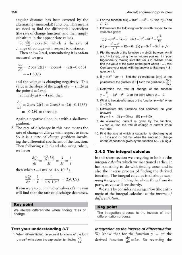
156 Aircraft engineering principles
angular distance has been covered by thealternating (sinusoidal) function. This meanswe need to find the differential coefficient(the rate of change function) and then simplysubstitute in the appropriate values.
So dvdθ
= 2 cos 2θ, which is the rate ofchange of voltage with respect to distance.
Then at θ = 2 rad, remembering it is radianmeasure! we get:
dvdθ
= 2 cos (2)(2) = 2 cos 4 = (2)(−0.653)
= −1.3073
and the voltage is changing negatively. Thisvalue is the slope of the graph of v = sin 2θ atthe point θ = 2 rad.
Similarly at θ = 4 rad, then
dvdθ
= 2 cos (2)(4) = 2 cos 8 = (2)(−0.1455)
= −0.291 to three dp.
Again a negative slope, but with a shallowergradient.
2. The rate of discharge in this case means therate of change of charge with respect to time.So it is a rate of change problem involv-ing the differential coefficient of the function.Then following rule 6 and also using rule 1,we have:
dQdt
=dQdt (3t)
3t= 3
3t= 1
t
then when t = 4 ms or 4 × 10⁻³ s,
dQdt
= 1t
= 14 × 10−3
= 250 C/s
If you were to put in higher values of time youwill find that the rate of discharge decreases.
Key pointWe always differentiate when finding rates ofchange.
Test your understanding 3.71. When differentiating polynomial functions of the form
y = ax n write down the expression for findingdydx
.
2. For the function f (x ) = 16x 2 − 3x 3 − 12 find f (3) andf (−2).
3. Differentiate the following functions with respect to thevariables given:
(i) y = 6x 2 − 3x − 2 (ii) s = 3t2 − 6t−1 + t−3
12
(iii) p = r 3 − r 2
r−1+ 12r − 6 (iv) y = 3x
92 − 5x
32 + √
x
4. Plot the graph of the function y = sin 2θ between θ = 0and θ = 2π rad, using the techniques you learnt in yourtrigonometry, making sure that (θ) is in radians. Thenfind the value of the slope at the point where θ = 2 rad.Compare your result with the answer to Example 4.81question 1.
5. If y = x 2 − 2x + 1, find the co-ordinates (x,y ) at the
point where the gradient is 6(
Hint: the gradient isdydx
).
6. Determine the rate of change of the function
y = x4
2− 3x3 + x2 − 3, at the point where x = −2.
7. What is the rate of change of the function y = 4ex whenx = 2.32.
8. Differentiate the functions and comment on youranswers(i) y = ln x (ii) y = 3 ln x (iii) y = ln 3x
9. An alternating current is given by the function,i = cos 3θ, find the rate of change of current whenθ = 1 rad.
10. Find the rate at which a capacitor is discharging att = 3 ms and t = 3.8 ms, when the amount of chargeon the capacitor is given by the function Q = 2.6 loget.
3.4.3 The integral calculus
In this short section we are going to look at theintegral calculus which we mentioned earlier. Ithas something to do with finding areas and isalso the inverse process of finding the derivedfunction. The integral calculus is all about sum-ming things, i.e. finding the whole thing from itsparts, as you will see shortly.
We start by considering integration (the arith-metic of the integral calculus) as the inverse ofdifferentiation.
Key pointThe integration process is the inverse of thedifferentiation process.
Integration as the inverse of differentiationWe know that for the function y = x2 the
derived function dydx = 2x. So reversing the
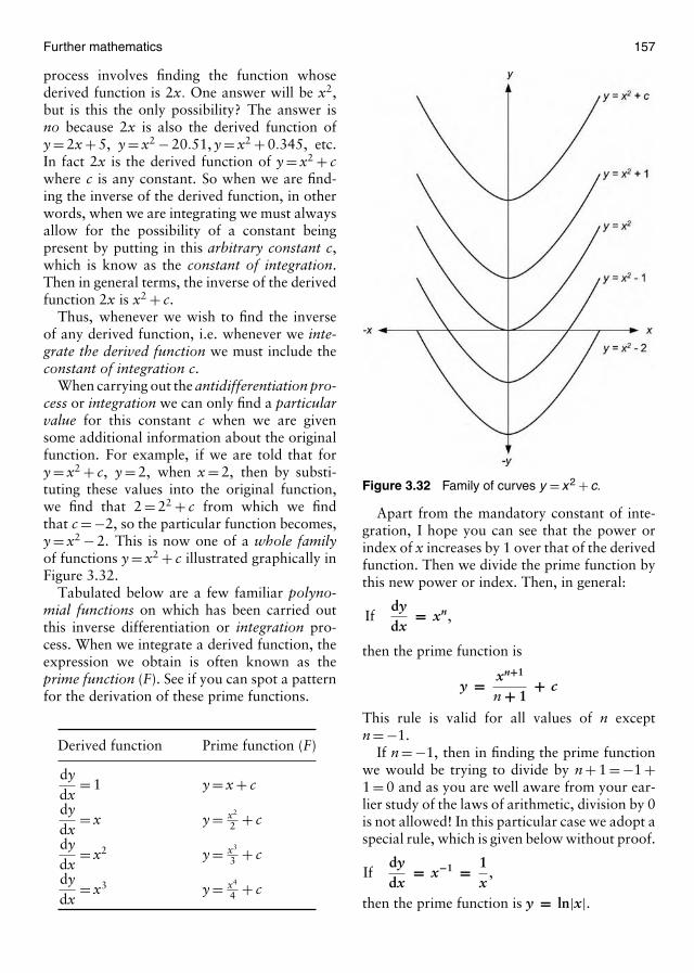
Further mathematics 157
process involves finding the function whosederived function is 2x. One answer will be x2,but is this the only possibility? The answer isno because 2x is also the derived function ofy = 2x + 5, y = x2 − 20.51, y = x2 + 0.345, etc.In fact 2x is the derived function of y = x2 + cwhere c is any constant. So when we are find-ing the inverse of the derived function, in otherwords, when we are integrating we must alwaysallow for the possibility of a constant beingpresent by putting in this arbitrary constant c,which is know as the constant of integration.Then in general terms, the inverse of the derivedfunction 2x is x2 + c.
Thus, whenever we wish to find the inverseof any derived function, i.e. whenever we inte-grate the derived function we must include theconstant of integration c.
When carrying out the antidifferentiation pro-cess or integration we can only find a particularvalue for this constant c when we are givensome additional information about the originalfunction. For example, if we are told that fory = x2 + c, y = 2, when x = 2, then by substi-tuting these values into the original function,we find that 2 = 22 + c from which we findthat c = −2, so the particular function becomes,y = x2 − 2. This is now one of a whole familyof functions y = x2 + c illustrated graphically inFigure 3.32.
Tabulated below are a few familiar polyno-mial functions on which has been carried outthis inverse differentiation or integration pro-cess. When we integrate a derived function, theexpression we obtain is often known as theprime function (F). See if you can spot a patternfor the derivation of these prime functions.
Derived function Prime function (F)
dydx
= 1 y = x + c
dydx
= x y = x2
2 + c
dydx
= x2 y = x3
3 + c
dydx
= x3 y = x4
4 + c
Figure 3.32 Family of curves y = x 2 + c.
Apart from the mandatory constant of inte-gration, I hope you can see that the power orindex of x increases by 1 over that of the derivedfunction. Then we divide the prime function bythis new power or index. Then, in general:
Ifdydx
= xn,
then the prime function is
y = xn+1
n + 1+ c
This rule is valid for all values of n exceptn = −1.
If n = −1, then in finding the prime functionwe would be trying to divide by n + 1 = −1 +1 = 0 and as you are well aware from your ear-lier study of the laws of arithmetic, division by 0is not allowed! In this particular case we adopt aspecial rule, which is given below without proof.
Ifdydx
= x−1 = 1x
,
then the prime function is y = ln|x|.

158 Aircraft engineering principles
Notice that we have to take the modulus orpositive value of x, when finding correspondingvalues of y. This is because the ln (loge) func-tion is not valid for all numbers ≤ 0 (less than orequal to zero).
Notation for the integralAs with differentiation, when we carry out inte-gration, we need to use the appropriate mathe-matical notation in order to convey our desireto integrate.
If y is a function of x, then∫
ydx represents theintegral of y with respect to the variable x. Theintegral sign
∫is the greek letter S, and indicates
that when carrying out the integration process,we are really carrying out a summing process.
Note: that in the same way that the d cannotbe separated from the y, in dy, neither can the
∫be separated from dx, if the integration is withrespect to x.
For example, if we wish to find the prime func-tion F, i.e. if we wish to integrate the functionx2 then this is represented as
∫x2 dx and using
the general rule, we see that∫x2 dx = xn+1
n + 1+ c = x2+1
2 + 1+ c = x3
3+ c,
which is in agreement with the prime functionor the integral shown in the table.
IntegrationWe have seen from above how to integrate ele-mentary polynomial functions, using the basicrule. In the example given next, we use therule successively to integrate general polyno-mial expression with respect to the variableconcerned.
Example 3.44
Integrate the following functions with respect tothe variables given.
1. y = 3x3 + 2x2 − 62. s = 5t−3 + t4 − 2t2
3. p = r−1 + r4
2
1. What we are being asked to do is findthe prime function F(y), or using the
conventional notation which we have justlearnt then we must find:
F(y) =∫
3x3 + 2x2 − 6 dx
In this case all we need to do is successivelyapply the basic rule, i.e.∫
3x3 + 2x2 − 6 dx
= (3)x3+1
3 + 1+ (2)
x2+1
2 + 1+ (−6)x0+1 + c
= 3x4
4+ 2x3
3− 6x + c
2. In this question we again apply the basic rulebut in terms of the different variables, so:∫
5t−3 + t4 − 2t2 dt
= (5)t−3+1
−3 + 1+ t4+1
4 + 1+ (−2)
t2+1
2 + 1+ c
= 5t−2
−2+ t5
5− 2t3
3+ c
With this question I hope you spotted imme-diately that for part of the function r−1, wecannot apply the general rule but must applythe special case where n = −1. So for theintegration we proceed as follows:∫
r−1 + r4
4dr = ln|r| +
(14
)r4+1
4 + 1+ c
= ln|r | + r5
20+ c
Notice also that dividing by 4 is the same asmultiplying by a 1
4 and that we multiply topsby tops and bottoms by bottoms to obtain thefinal values.
Key pointWhen finding indefinite integrals, we must alwaysinclude the constant of integration.
Some common integralsWe have seen now how to integrate poly-nomial expressions. We can also apply theinverse differentiation process to the sinusoidal,
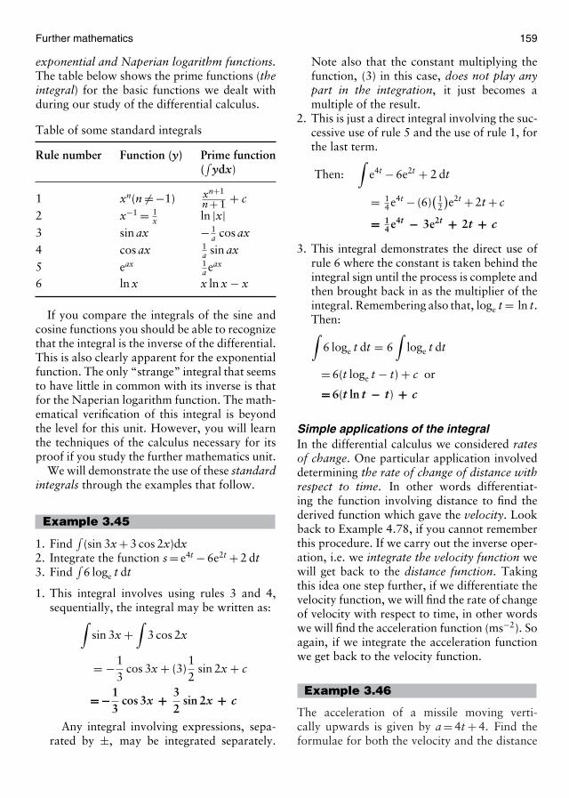
Further mathematics 159
exponential and Naperian logarithm functions.The table below shows the prime functions (theintegral) for the basic functions we dealt withduring our study of the differential calculus.
Table of some standard integrals
Rule number Function (y) Prime function(∫
ydx)
1 xn(n �= −1) xn+1
n + 1 + c
2 x−1 = 1x ln |x|
3 sin ax − 1a cos ax
4 cos ax 1a sin ax
5 eax 1a eax
6 ln x x ln x − x
If you compare the integrals of the sine andcosine functions you should be able to recognizethat the integral is the inverse of the differential.This is also clearly apparent for the exponentialfunction. The only “strange” integral that seemsto have little in common with its inverse is thatfor the Naperian logarithm function. The math-ematical verification of this integral is beyondthe level for this unit. However, you will learnthe techniques of the calculus necessary for itsproof if you study the further mathematics unit.
We will demonstrate the use of these standardintegrals through the examples that follow.
Example 3.45
1. Find∫
(sin 3x + 3 cos 2x)dx2. Integrate the function s = e4t − 6e2t + 2 dt3. Find
∫6 loge t dt
1. This integral involves using rules 3 and 4,sequentially, the integral may be written as:∫
sin 3x +∫
3 cos 2x
= −13
cos 3x + (3)12
sin 2x + c
= −13
cos 3x + 32
sin 2x + c
Any integral involving expressions, sepa-rated by ±, may be integrated separately.
Note also that the constant multiplying thefunction, (3) in this case, does not play anypart in the integration, it just becomes amultiple of the result.
2. This is just a direct integral involving the suc-cessive use of rule 5 and the use of rule 1, forthe last term.
Then:∫
e4t − 6e2t + 2 dt
= 14 e4t − (6)
( 12
)e2t + 2t + c
= 14 e4t − 3e2t + 2t + c
3. This integral demonstrates the direct use ofrule 6 where the constant is taken behind theintegral sign until the process is complete andthen brought back in as the multiplier of theintegral. Remembering also that, loge t = ln t.Then:∫
6 loge t dt = 6∫
loge t dt
= 6(t loge t − t) + c or
= 6(t ln t − t) + c
Simple applications of the integralIn the differential calculus we considered ratesof change. One particular application involveddetermining the rate of change of distance withrespect to time. In other words differentiat-ing the function involving distance to find thederived function which gave the velocity. Lookback to Example 4.78, if you cannot rememberthis procedure. If we carry out the inverse oper-ation, i.e. we integrate the velocity function wewill get back to the distance function. Takingthis idea one step further, if we differentiate thevelocity function, we will find the rate of changeof velocity with respect to time, in other wordswe will find the acceleration function (ms−2). Soagain, if we integrate the acceleration functionwe get back to the velocity function.
Example 3.46
The acceleration of a missile moving verti-cally upwards is given by a = 4t + 4. Find theformulae for both the velocity and the distance
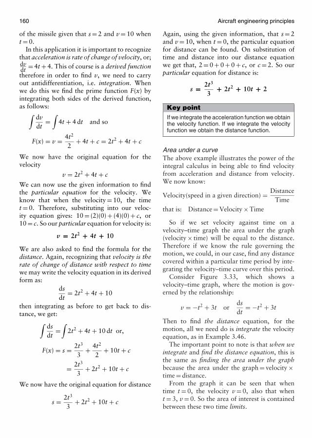
160 Aircraft engineering principles
of the missile given that s = 2 and v = 10 whent = 0.
In this application it is important to recognizethat acceleration is rate of change of velocity, or;dvdt = 4t + 4. This of course is a derived functiontherefore in order to find v, we need to carryout antidifferentiation, i.e. integration. Whenwe do this we find the prime function F(x) byintegrating both sides of the derived function,as follows:∫
dvdt
=∫
4t + 4 dt and so
F(x) = v = 4t2
2+ 4t + c = 2t2 + 4t + c
We now have the original equation for thevelocity
v = 2t2 + 4t + c
We can now use the given information to findthe particular equation for the velocity. Weknow that when the velocity = 10, the timet = 0. Therefore, substituting into our veloc-ity equation gives: 10 = (2)(0) + (4)(0) + c, or10 = c. So our particular equation for velocity is:
v = 2t2 + 4t + 10
We are also asked to find the formula for thedistance. Again, recognizing that velocity is therate of change of distance with respect to timewe may write the velocity equation in its derivedform as:
dsdt
= 2t2 + 4t + 10
then integrating as before to get back to dis-tance, we get:∫
dsdt
=∫
2t2 + 4t + 10 dt or,
F(x) = s = 2t3
3+ 4t2
2+ 10t + c
= 2t3
3+ 2t2 + 10t + c
We now have the original equation for distance
s = 2t3
3+ 2t2 + 10t + c
Again, using the given information, that s = 2and v = 10, when t = 0, the particular equationfor distance can be found. On substitution oftime and distance into our distance equationwe get that, 2 = 0 + 0 + 0 + c, or c = 2. So ourparticular equation for distance is:
s = 2t3
3+ 2t2 + 10t + 2
Key pointIf we integrate the acceleration function we obtainthe velocity function. If we integrate the velocityfunction we obtain the distance function.
Area under a curveThe above example illustrates the power of theintegral calculus in being able to find velocityfrom acceleration and distance from velocity.We now know:
Velocity(speed in a given direction) = DistanceTime
that is: Distance = Velocity × Time
So if we set velocity against time on avelocity–time graph the area under the graph(velocity × time) will be equal to the distance.Therefore if we know the rule governing themotion, we could, in our case, find any distancecovered within a particular time period by inte-grating the velocity–time curve over this period.
Consider Figure 3.33, which shows avelocity–time graph, where the motion is gov-erned by the relationship:
v = −t2 + 3t ordsdt
= −t2 + 3t
Then to find the distance equation, for themotion, all we need do is integrate the velocityequation, as in Example 3.46.
The important point to note is that when weintegrate and find the distance equation, this isthe same as finding the area under the graphbecause the area under the graph = velocity ×time = distance.
From the graph it can be seen that whentime t = 0, the velocity v = 0, also that whent = 3, v = 0. So the area of interest is containedbetween these two time limits.

Further mathematics 161
Figure 3.33 Velocity–time graph for the motionv = −t2 + 3t.
Now integrating our velocity equation in thenormal manner, gives:∫
v = dsdt
=∫
−t2 + 3t dt = s = −t3
3+ 3t2
2+ c
This distance equation is equivalent to the areaunder the graph, between time t = 0 and t = 3.
At time t = 0 the distance travelled s = 0 fromthe graph. The constant of integration c can befound by substituting these values of time anddistance into our distance equation:
s = −t3
3+ 3t2
2+ c, so 0 = 0 + 0 + c
therefore c = 0 and our particular distance equa-tion is,
s = −t3
3+ 3t2
2Now between our limits of time t = 0 to t = 3 s.The area under the graph indicates the distancetravelled. So at time t = 0, the distance trav-elled s = 0. At time t = 3, the area under thegraph is found by substituting time t = 3 intoour distance equation, then:
s = −t3
3+ 3t2
2= −(3)3
3+ (3)(32)
2
= −273
+ 272
= −9 + 13.5 = 4.5
Thus, in the above example, the area under thegraph = 4.5 = the distance travelled.
Key pointThe area under a velocity time curve is equal tothe distance.
The definite integralWhen we integrate between limits, such asthe time limits, given for the motion discussedabove. We say that we are finding the definiteintegral. All the integration that we have beendoing up till now has involved the constant ofintegration and we refer to this type of inte-gration as finding the indefinite integral, whichmust contain an arbitrary constant c.
The terminology for indefinite integration isthat which we have used so far, for examples:∫
−t2 + 3t dt the indefinite integral
When carrying out definite integration we placelimits on the integration sign, or summing sign,for examples:∫ 3
0−t2 + 3t dt the definite integral
To evaluate a definite integral, we first integratethe function, then we find the numerical valueof the integral at its upper and lower limits andsubtract the value of the lower limit from thatof the upper limit to obtain the required result.
So following this procedure for the definiteintegral shown above, which we used to findthe distance s, (area under a graph) from thevelocity–time graph, we get:
s =∫ 3
0−t2 + 3t dt =
[−t3
3+ 3t2
2+ c
]3
0
=(−27
3+ 27
2+ c
)−(
03
+ 02
+ c)
s = (−9 + 13.5 + c) − (0 + c)
= 4.5 + c − c = 4.5
Thus s = 4.5, we have found the area under thegraph using definite integration!
Note that when we subtract the upper limitvalue from the lower limit value, the constantof integration is eliminated. This will alwaysbe the case when evaluating definite integrals;therefore it need not be shown from now on.
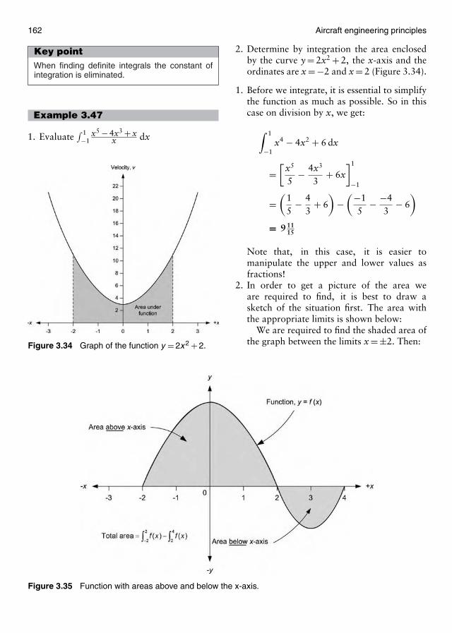
162 Aircraft engineering principles
Key pointWhen finding definite integrals the constant ofintegration is eliminated.
Example 3.47
1. Evaluate∫ 1−1
x5 − 4x3 + xx dx
Figure 3.34 Graph of the function y = 2x 2 + 2.
Figure 3.35 Function with areas above and below the x-axis.
2. Determine by integration the area enclosedby the curve y = 2x2 + 2, the x-axis and theordinates are x = −2 and x = 2 (Figure 3.34).
1. Before we integrate, it is essential to simplifythe function as much as possible. So in thiscase on division by x, we get:
∫ 1
−1x4 − 4x2 + 6 dx
=[
x5
5− 4x3
3+ 6x
]1
−1
=(
15
− 43
+ 6)
−(−1
5− −4
3− 6
)
= 9 1115
Note that, in this case, it is easier tomanipulate the upper and lower values asfractions!
2. In order to get a picture of the area weare required to find, it is best to draw asketch of the situation first. The area withthe appropriate limits is shown below:
We are required to find the shaded area ofthe graph between the limits x = ±2. Then:
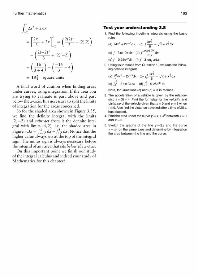
Further mathematics 163
∫ 2
−22x2 + 2 dx
=[
2x3
3+ 2x
]2
−2=(
2(2)3
3+ (2)(2)
)
−(
2(−2)3
3+ (2)(−2)
)
=(
163 + 4
)−(−16
3− 4
)
= 18 23 square units
A final word of caution when finding areasunder curves, using integration. If the area youare trying to evaluate is part above and partbelow the x-axis. It is necessary to split the limitsof integration for the areas concerned.
So for the shaded area shown in Figure 3.35;we find the definite integral with the limits(2, −2) and subtract from it the definite inte-gral with limits (4, 2), i.e. the shaded area inFigure 3.35 = ∫ 2
−2 y dx−∫ 42 y dx. Notice that the
higher value always sits at the top of the integralsign. The minus sign is always necessary beforethe integral of any area that sits below the x-axis.
On this important point we finish our studyof the integral calculus and indeed your study ofMathematics for this chapter!
Test your understanding 3.81. Find the following indefinite integrals using the basic
rules:
(a)∫
4x2 + 2x−3dx (b)∫ 3x
12
6− √
x + x32 dx
(c)∫−3 sin 2x dx (d)
∫ x cos 3x0.5x
dx
(e)∫ −0.25e3θdθ (f)
∫−3 loge x dx
2. Using your results from Question 1, evaluate the follow-ing definite integrals:
(a)∫ 2
0 4x2 + 2x−3dx (b)∫ 1
03x
12
6− √
x + x32 dx
(c)∫ π
20 −3 sin 2θ dθ (d)
∫ 21 −0.25e3θ dθ
Note, for Questions (c) and (d) θ is in radians.
3. The acceleration of a vehicle is given by the relation-ship a = 3t + 4. Find the formulae for the velocity anddistance of the vehicle given that s = 0 and v = 8 whent = 0. Also find the distance travelled after a time of 25 s,has elapsed.
4. Find the area under the curve y = x + x 2 between x = 1and x = 3.
5. Sketch the graphs of the line y = 2x and the curvey = x 2 on the same axes and determine by integrationthe area between the line and the curve.

This page intentionally left blank
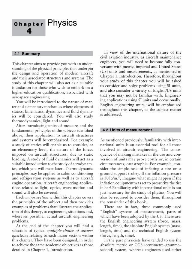
C h a p t e r
4Physics
4.1 Summary
This chapter aims to provide you with an under-standing of the physical principles that underpinthe design and operation of modern aircraftand their associated structures and systems. Thestudy of this chapter will also act as a suitablefoundation for those who wish to embark on ahigher education qualification, associated withaerospace engineering.
You will be introduced to the nature of mat-ter and elementary mechanics where elements ofstatics, kinematics, dynamics and fluid dynam-ics will be considered. You will also studythermodynamics, light and sound.
After introducing units of measure and thefundamental principles of the subjects identifiedabove, their application to aircraft structuresand systems will be emphasized. For examplea study of statics will enable us to consider, atan elementary level, the nature of the forcesimposed on aircraft structures, due to staticloading. A study of fluid dynamics will act as asuitable introduction to the study of aerodynam-ics, which you will meet later. Thermodynamicprinciples may be applied to cabin conditioningand refrigeration systems as well as to aircraftengine operation. Aircraft engineering applica-tions related to light, optics, wave motion andsound will also be covered.
Each major section within this chapter coversthe principles of the subject and then providesexamples of problems that illustrate the applica-tion of this theory, to engineering situations and,wherever possible, actual aircraft engineeringproblems.
At the end of the chapter you will find aselection of typical multiple-choice of answerquestions relating to each major section withinthis chapter. They have been designed, in orderto achieve the same academic objectives as thosedetailed in Chapter 1, Introduction.
In view of the international nature of thecivil aviation industry, as aircraft maintenanceengineers, you will need to become fully con-versant with metric, imperial and United States(US) units and measurements, as mentioned inChapter 1, Introduction. Therefore, throughoutyour study of this chapter you will be askedto consider and solve problems using SI units,and also consider a variety of English/US unitsthat you may not be familiar with. Engineer-ing applications using SI units and occasionally,English engineering units, will be emphasizedthroughout this chapter, as the subject matteris addressed.
4.2 Units of measurement
As mentioned previously, familiarity with inter-national units is an essential tool for all thoseinvolved in aircraft engineering. The conse-quence of making mistakes in the use and con-version of units may prove costly or, in certaincircumstances, catastrophic. For example, con-sider the simple task of inflating a tire on aground support trolley. If the inflation pressureis 30 lb/in.2, imagine what might happen if theinflation equipment was set to pressurize the tirein bar! Familiarity with international units is notjust necessary for the study of physics. You willalso be required to consider them, throughoutthe remainder of this book.
There are in fact, three commonly used“English” systems of measurement, parts ofwhich have been adopted by the US. These are:the English engineering system (force, mass,length, time), the absolute English system (mass,length, time) and the technical English system(force, length, time).
In the past physicists have tended to use theabsolute metric or CGS (centimetre–gramme–second) system, whereas engineers used either
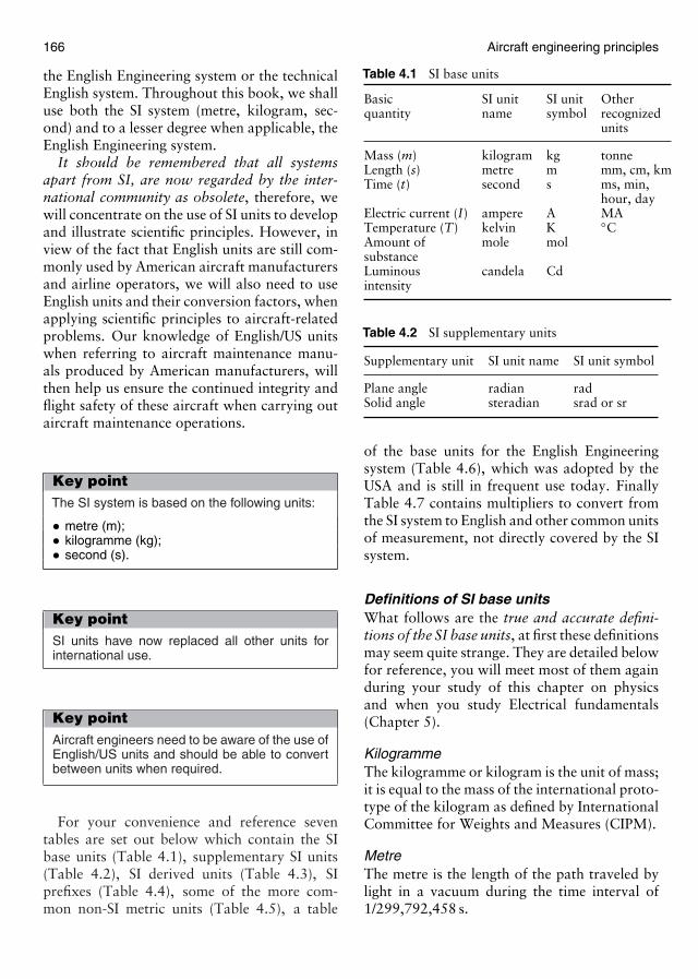
166 Aircraft engineering principles
the English Engineering system or the technicalEnglish system. Throughout this book, we shalluse both the SI system (metre, kilogram, sec-ond) and to a lesser degree when applicable, theEnglish Engineering system.
It should be remembered that all systemsapart from SI, are now regarded by the inter-national community as obsolete, therefore, wewill concentrate on the use of SI units to developand illustrate scientific principles. However, inview of the fact that English units are still com-monly used by American aircraft manufacturersand airline operators, we will also need to useEnglish units and their conversion factors, whenapplying scientific principles to aircraft-relatedproblems. Our knowledge of English/US unitswhen referring to aircraft maintenance manu-als produced by American manufacturers, willthen help us ensure the continued integrity andflight safety of these aircraft when carrying outaircraft maintenance operations.
Key pointThe SI system is based on the following units:
• metre (m);• kilogramme (kg);• second (s).
Key pointSI units have now replaced all other units forinternational use.
Key pointAircraft engineers need to be aware of the use ofEnglish/US units and should be able to convertbetween units when required.
For your convenience and reference seventables are set out below which contain the SIbase units (Table 4.1), supplementary SI units(Table 4.2), SI derived units (Table 4.3), SIprefixes (Table 4.4), some of the more com-mon non-SI metric units (Table 4.5), a table
Table 4.1 SI base units
Basic SI unit SI unit Otherquantity name symbol recognized
units
Mass (m) kilogram kg tonneLength (s) metre m mm, cm, kmTime (t) second s ms, min,
hour, dayElectric current (I) ampere A MATemperature (T) kelvin K ◦CAmount of mole molsubstanceLuminous candela Cdintensity
Table 4.2 SI supplementary units
Supplementary unit SI unit name SI unit symbol
Plane angle radian radSolid angle steradian srad or sr
of the base units for the English Engineeringsystem (Table 4.6), which was adopted by theUSA and is still in frequent use today. FinallyTable 4.7 contains multipliers to convert fromthe SI system to English and other common unitsof measurement, not directly covered by the SIsystem.
Definitions of SI base unitsWhat follows are the true and accurate defini-tions of the SI base units, at first these definitionsmay seem quite strange. They are detailed belowfor reference, you will meet most of them againduring your study of this chapter on physicsand when you study Electrical fundamentals(Chapter 5).
KilogrammeThe kilogramme or kilogram is the unit of mass;it is equal to the mass of the international proto-type of the kilogram as defined by InternationalCommittee for Weights and Measures (CIPM).
MetreThe metre is the length of the path traveled bylight in a vacuum during the time interval of1/299,792,458 s.
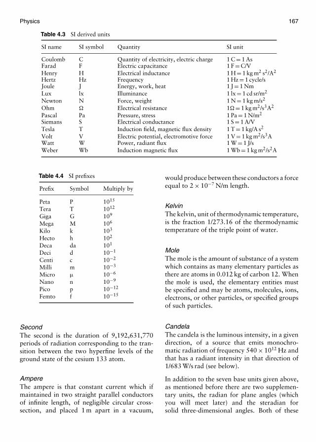
Physics 167
Table 4.3 SI derived units
SI name SI symbol Quantity SI unit
Coulomb C Quantity of electricity, electric charge 1 C = 1 AsFarad F Electric capacitance 1 F = C/VHenry H Electrical inductance 1 H = 1 kg m2 s2/A2
Hertz Hz Frequency 1 Hz = 1 cycle/sJoule J Energy, work, heat 1 J = 1 NmLux lx Illuminance 1 lx = 1 cd sr/m2
Newton N Force, weight 1 N = 1 kg m/s2
Ohm � Electrical resistance 1� = 1 kg m2/s3A2
Pascal Pa Pressure, stress 1 Pa = 1 N/m2
Siemans S Electrical conductance 1 S = 1 A/VTesla T Induction field, magnetic flux density 1 T = 1 kg/A s2
Volt V Electric potential, electromotive force 1 V = 1 kg m2/s3AWatt W Power, radiant flux 1 W = 1 J/sWeber Wb Induction magnetic flux 1 Wb = 1 kg m2/s2A
Table 4.4 SI prefixes
Prefix Symbol Multiply by
Peta P 1015
Tera T 1012
Giga G 109
Mega M 106
Kilo k 103
Hecto h 102
Deca da 101
Deci d 10−1
Centi c 10−2
Milli m 10−3
Micro µ 10−6
Nano n 10−9
Pico p 10−12
Femto f 10−15
SecondThe second is the duration of 9,192,631,770periods of radiation corresponding to the tran-sition between the two hyperfine levels of theground state of the cesium 133 atom.
AmpereThe ampere is that constant current which ifmaintained in two straight parallel conductorsof infinite length, of negligible circular cross-section, and placed 1 m apart in a vacuum,
would produce between these conductors a forceequal to 2 × 10⁻⁷ N/m length.
KelvinThe kelvin, unit of thermodynamic temperature,is the fraction 1/273.16 of the thermodynamictemperature of the triple point of water.
MoleThe mole is the amount of substance of a systemwhich contains as many elementary particles asthere are atoms in 0.012 kg of carbon 12. Whenthe mole is used, the elementary entities mustbe specified and may be atoms, molecules, ions,electrons, or other particles, or specified groupsof such particles.
CandelaThe candela is the luminous intensity, in a givendirection, of a source that emits monochro-matic radiation of frequency 540 × 1012 Hz andthat has a radiant intensity in that direction of1/683 W/s rad (see below).
In addition to the seven base units given above,as mentioned before there are two supplemen-tary units, the radian for plane angles (whichyou will meet later) and the steradian forsolid three-dimensional angles. Both of these
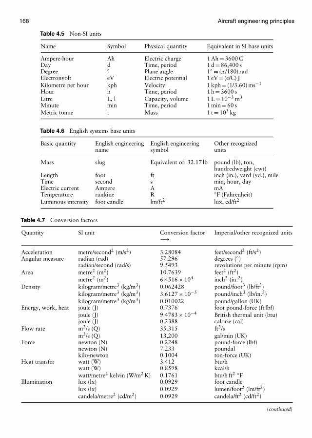
168 Aircraft engineering principles
Table 4.5 Non-SI units
Name Symbol Physical quantity Equivalent in SI base units
Ampere-hour Ah Electric charge 1 Ah = 3600 CDay d Time, period 1 d = 86,400 sDegree ◦ Plane angle 1◦ = (π /180) radElectronvolt eV Electric potential 1 eV = (e/C) JKilometre per hour kph Velocity 1 kph = (1/3.60) ms−1
Hour h Time, period 1 h = 3600 sLitre L, l Capacity, volume 1 L = 10−3 m3
Minute min Time, period 1 min = 60 sMetric tonne t Mass 1 t = 103 kg
Table 4.6 English systems base units
Basic quantity English engineering English engineering Other recognizedname symbol units
Mass slug Equivalent of: 32.17 lb pound (lb), ton,hundredweight (cwt)
Length foot ft inch (in.), yard (yd.), mileTime second s min, hour, dayElectric current Ampere A mATemperature rankine R ◦F (Fahrenheit)Luminous intensity foot candle lm/ft2 lux, cd/ft2
Table 4.7 Conversion factors
Quantity SI unit Conversion factor Imperial/other recognized units−→
Acceleration metre/second2 (m/s2) 3.28084 feet/second2 (ft/s2)Angular measure radian (rad) 57.296 degrees (◦)
radian/second (rad/s) 9.5493 revolutions per minute (rpm)Area metre2 (m2) 10.7639 feet2 (ft2)
metre2 (m2) 6.4516 × 104 inch2 (in.2)Density kilogram/metre3 (kg/m3) 0.062428 pound/foot3 (lb/ft3)
kilogram/metre3 (kg/m3) 3.6127 × 10⁻⁵ pound/inch3 (lb/in.3)kilogram/metre3 (kg/m3) 0.010022 pound/gallon (UK)
Energy, work, heat joule (J) 0.7376 foot pound-force (ft lbf)joule (J) 9.4783 × 10⁻⁴ British thermal unit (btu)joule (J) 0.2388 calorie (cal)
Flow rate m3/s (Q) 35.315 ft3/sm3/s (Q) 13,200 gal/min (UK)
Force newton (N) 0.2248 pound-force (lbf)newton (N) 7.233 poundalkilo-newton 0.1004 ton-force (UK)
Heat transfer watt (W) 3.412 btu/hwatt (W) 0.8598 kcal/hwatt/metre2 kelvin (W/m2 K) 0.1761 btu/h ft2 ◦F
Illumination lux (lx) 0.0929 foot candlelux (lx) 0.0929 lumen/foot2 (lm/ft2)candela/metre2 (cd/m2) 0.0929 candela/ft2 (cd/ft2)
(continued)

Physics 169
Table 4.7 (continued)
Quantity SI unit Conversion factor Imperial/other recognized units−→
Length metre (m) 1 × 10¹⁰ angstrommetre (m) 39.37008 inch (in.)metre (m) 3.28084 feet (ft)metre (m) 1.09361 yard (yd)kilometre (km) 0.621371 milekilometre (km) 0.54 nautical miles
Mass kilogram (kg) 2.20462 pound (lb)kilogram (kg) 35.27392 ounce (oz)kilogram (kg) 0.0685218 slugtonne (t) 0.984207 ton (UK)tonne (t) 1.10231 ton (US)
Moment, torque newton-metre (Nm) 0.73756 foot pound-force (ft lbf)newton-metre (Nm) 8.8507 inch pound-force (in. lbf)
Moment of inertia kilogram-metre squared 0.7376 slug-foot squared (slug ft2)(mass) (kgm2)Second moment millimeters to the fourth 2.4 × 10⁻⁶ inch to the fourth (in.4)of area (mm4)Power watt (W) 3.4121 British thermal unit/hour (btu/h)
watt (W) 0.73756 foot pound-force/second (ft lbf/s)kilowatt (kW) 1.341 horsepowerhorsepower (hp) 550 foot pound-force/second (ft.lbf/s)
Pressure, stress kilopascal (kPa) 0.009869 atmosphere (atm)kilopascal (kPa) 0.145 pound-force/inch2 (psi)kilopascal (kPa) 0.01 barkilopascal (kPa) 0.2953 inches of mercurypascal 1.0 newton/metre2 (N/m2)megapascal (MPa) 145.0 pound-force/inch2 (psi)
Temperature kelvin (K) 1.0 celsius (◦C)kelvin (K) 1.8 rankine (◦R)kelvin (K) 1.8 fahrenheit (◦F)kelvin (K) ◦C + 273.15kelvin (K) (◦F + 459.67)/1.8celsius (◦C) (◦F − 32)/1.8
Velocity metre/second (m/s) 3.28084 feet/second (ft/s)metre/second (m/s) 196.85 feet/minute (ft/min)metre/second (m/s) 2.23694 miles/hour (mph)kilometre/hour (kph) 0.621371 miles/hour (mph)kilometre/hour (kph) 0.5400 knot (international)
Viscosity (kinematic) square metre/second (m2/s) 1 × 10⁶ centi-stokesquare metre/second (m2/s) 1 × 10⁴ stokesquare metre/second (m2/s) 10.764 square feet/second (ft2/s)
Viscosity (dynamic) pascal second (Pa s) 1000 centipoise (cP)centipoise (cP) 2.419 pound/feet hour (lb/ft h)
Volume cubic metre (m3) 35.315 cubic feet (ft3)cubic metre (m3) 1.308 cubic yard (yd3)cubic metre (m3) 1000 litre (l)litre (l) 1.76 pint (pt) UKlitre (l) 0.22 gallon (gal) UK
To convert SI units to Imperial and other recognized units of measurement multiply the unit given by the conversion factor,i.e. in the direction of the arrow. To reverse the process, i.e. to convert from non-SI units to SI units divide by the conversionfactor.
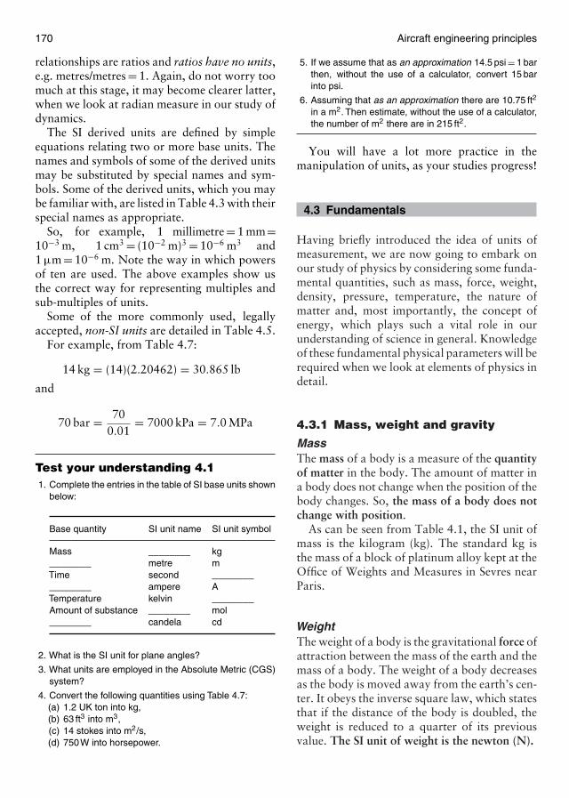
170 Aircraft engineering principles
relationships are ratios and ratios have no units,e.g. metres/metres = 1. Again, do not worry toomuch at this stage, it may become clearer latter,when we look at radian measure in our study ofdynamics.
The SI derived units are defined by simpleequations relating two or more base units. Thenames and symbols of some of the derived unitsmay be substituted by special names and sym-bols. Some of the derived units, which you maybe familiar with, are listed in Table 4.3 with theirspecial names as appropriate.
So, for example, 1 millimetre = 1 mm=10−3 m, 1 cm3 = (10−2 m)3 = 10−6 m3 and1 µm = 10−6 m. Note the way in which powersof ten are used. The above examples show usthe correct way for representing multiples andsub-multiples of units.
Some of the more commonly used, legallyaccepted, non-SI units are detailed in Table 4.5.
For example, from Table 4.7:
14 kg = (14)(2.20462) = 30.865 lb
and
70 bar = 700.01
= 7000 kPa = 7.0 MPa
Test your understanding 4.11. Complete the entries in the table of SI base units shown
below:
Base quantity SI unit name SI unit symbol
Mass ________ kg________ metre mTime second ________________ ampere ATemperature kelvin ________Amount of substance ________ mol________ candela cd
2. What is the SI unit for plane angles?
3. What units are employed in the Absolute Metric (CGS)system?
4. Convert the following quantities using Table 4.7:(a) 1.2 UK ton into kg,(b) 63 ft3 into m3,(c) 14 stokes into m2/s,(d) 750W into horsepower.
5. If we assume that as an approximation 14.5 psi = 1 barthen, without the use of a calculator, convert 15 barinto psi.
6. Assuming that as an approximation there are 10.75 ft2
in a m2. Then estimate, without the use of a calculator,the number of m2 there are in 215 ft2.
You will have a lot more practice in themanipulation of units, as your studies progress!
4.3 Fundamentals
Having briefly introduced the idea of units ofmeasurement, we are now going to embark onour study of physics by considering some funda-mental quantities, such as mass, force, weight,density, pressure, temperature, the nature ofmatter and, most importantly, the concept ofenergy, which plays such a vital role in ourunderstanding of science in general. Knowledgeof these fundamental physical parameters will berequired when we look at elements of physics indetail.
4.3.1 Mass, weight and gravity
MassThe mass of a body is a measure of the quantityof matter in the body. The amount of matter ina body does not change when the position of thebody changes. So, the mass of a body does notchange with position.
As can be seen from Table 4.1, the SI unit ofmass is the kilogram (kg). The standard kg isthe mass of a block of platinum alloy kept at theOffice of Weights and Measures in Sevres nearParis.
WeightThe weight of a body is the gravitational force ofattraction between the mass of the earth and themass of a body. The weight of a body decreasesas the body is moved away from the earth’s cen-ter. It obeys the inverse square law, which statesthat if the distance of the body is doubled, theweight is reduced to a quarter of its previousvalue. The SI unit of weight is the newton (N).
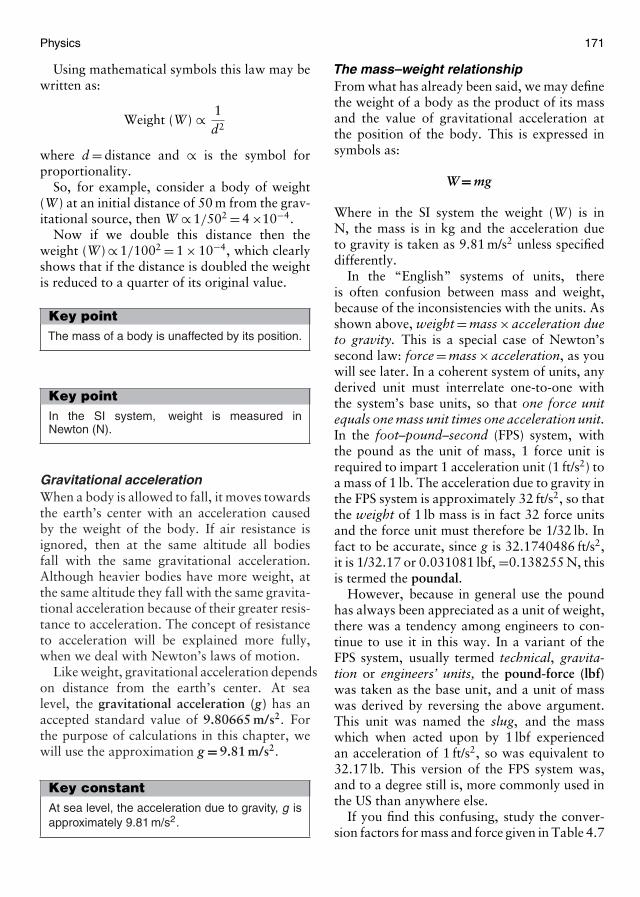
Physics 171
Using mathematical symbols this law may bewritten as:
Weight (W) ∝ 1d2
where d = distance and ∝ is the symbol forproportionality.
So, for example, consider a body of weight(W) at an initial distance of 50 m from the grav-itational source, then W ∝ 1/502 = 4 ×10⁻⁴.
Now if we double this distance then theweight (W) ∝ 1/1002 = 1 × 10⁻⁴, which clearlyshows that if the distance is doubled the weightis reduced to a quarter of its original value.
Key pointThe mass of a body is unaffected by its position.
Key pointIn the SI system, weight is measured inNewton (N).
Gravitational accelerationWhen a body is allowed to fall, it moves towardsthe earth’s center with an acceleration causedby the weight of the body. If air resistance isignored, then at the same altitude all bodiesfall with the same gravitational acceleration.Although heavier bodies have more weight, atthe same altitude they fall with the same gravita-tional acceleration because of their greater resis-tance to acceleration. The concept of resistanceto acceleration will be explained more fully,when we deal with Newton’s laws of motion.
Like weight, gravitational acceleration dependson distance from the earth’s center. At sealevel, the gravitational acceleration (g) has anaccepted standard value of 9.80665 m/s2. Forthe purpose of calculations in this chapter, wewill use the approximation g = 9.81 m/s2.
Key constantAt sea level, the acceleration due to gravity, g isapproximately 9.81 m/s2.
The mass–weight relationshipFrom what has already been said, we may definethe weight of a body as the product of its massand the value of gravitational acceleration atthe position of the body. This is expressed insymbols as:
W= mg
Where in the SI system the weight (W) is inN, the mass is in kg and the acceleration dueto gravity is taken as 9.81 m/s2 unless specifieddifferently.
In the “English” systems of units, thereis often confusion between mass and weight,because of the inconsistencies with the units. Asshown above, weight = mass × acceleration dueto gravity. This is a special case of Newton’ssecond law: force = mass × acceleration, as youwill see later. In a coherent system of units, anyderived unit must interrelate one-to-one withthe system’s base units, so that one force unitequals one mass unit times one acceleration unit.In the foot–pound–second (FPS) system, withthe pound as the unit of mass, 1 force unit isrequired to impart 1 acceleration unit (1 ft/s2) toa mass of 1 lb. The acceleration due to gravity inthe FPS system is approximately 32 ft/s2, so thatthe weight of 1 lb mass is in fact 32 force unitsand the force unit must therefore be 1/32 lb. Infact to be accurate, since g is 32.1740486 ft/s2,it is 1/32.17 or 0.031081 lbf, =0.138255 N, thisis termed the poundal.
However, because in general use the poundhas always been appreciated as a unit of weight,there was a tendency among engineers to con-tinue to use it in this way. In a variant of theFPS system, usually termed technical, gravita-tion or engineers’ units, the pound-force (lbf)was taken as the base unit, and a unit of masswas derived by reversing the above argument.This unit was named the slug, and the masswhich when acted upon by 1 lbf experiencedan acceleration of 1 ft/s2, so was equivalent to32.17 lb. This version of the FPS system was,and to a degree still is, more commonly used inthe US than anywhere else.
If you find this confusing, study the conver-sion factors for mass and force given in Table 4.7
172 Aircraft engineering principles
(See also Table E.7 of Appendix E and the exam-ples given at the end of this section). You shouldthen be able to form the connection associatingthese unfamiliar units for mass and force.
We now know that the mass of a bodydoes not change with changes in altitude butits weight and gravitational acceleration do.However, for bodies that do not move outsidethe earth’s atmosphere, the changes in gravita-tional acceleration (and therefore weight) aresmall enough to be ignored for most practi-cal purposes. We may therefore assume ourapproximation for g = 9.81 m/s2 to be reason-ably accurate, unless told otherwise.
To clarify the mass–weight relationship let usconsider an example calculation, using standardSI units.
Example 4.1
A missile having a mass of 25,000 kg is launchedfrom sea level on a course for the moon. If thegravitational acceleration of the moon is onesixth that on earth, determine the:(a) weight of the rocket at launch,(b) mass of the rocket on reaching the moon,(c) weight of the rocket on reaching the moon.
(a) Using the relationship W = mg, then theweight on earth;
W = (25,000 × 9.81)
= 245,250 N or 245.25 kN
(b) We know from our definition of mass, thatit does not change with change in positiontherefore the mass on the moon remains thesame as on earth i.e. 25,000 kg.
(c) We know that the gravitational accelerationon the moon is approximately 1/6 that onearth.
So gm =9.81/6 m/s2 =1.635 m/s2 and againfrom W = mgm then weight of rocket onthe moon = (25,000 × 1.635) = 40,875 N =40.875 kN.
Note: A much easier method of solution forpart (c) would have been to divide the weight onearth by 6.
Test your understanding 4.21. What happens to the weight of a body as it is moved
away from the center of the earth?
2. What is the SI unit of weight?
3. What is the approximate SI value for the accelerationdue to gravity at sea level?
4. If the capacity of a light aircraft’s fuel tanks is 800 UKgallons, what is the volume of the fuel in litres?
5. A light aircraft on take-off weighs 42,000 N, what is itsmass?
6. Define (a) the poundal and (b) pound-force (lbf).
4.3.2 Density and relative density
DensityThe density (ρ) of a body is defined as its massper unit volume. Combining the SI units formass and volume gives the unit of density askg/m3. Using symbols the formula for densityis given as:vspace*2pt
ρ = mV
where again the mass is in kg and the volumein m3.
You will see later, when you study the atmo-sphere, that density is temperature dependent.This is due to the change in volume caused bychanging temperature.
Key constantThe density of pure water at 4◦C is taken as1000 kg/m2.
Relative densityThe relative density of a body is the ratio ofthe density of the body with that of the den-sity of pure water measured at 4◦C. The densityof water under these conditions is 1000 kg/m3.Since relative density is a ratio it has no units.The old name for relative density was specificgravity (SG) and this is something you need tobe aware of in case you meet this terminologyin the future.
The density of some of the more commonengineering elements and materials is laid out in
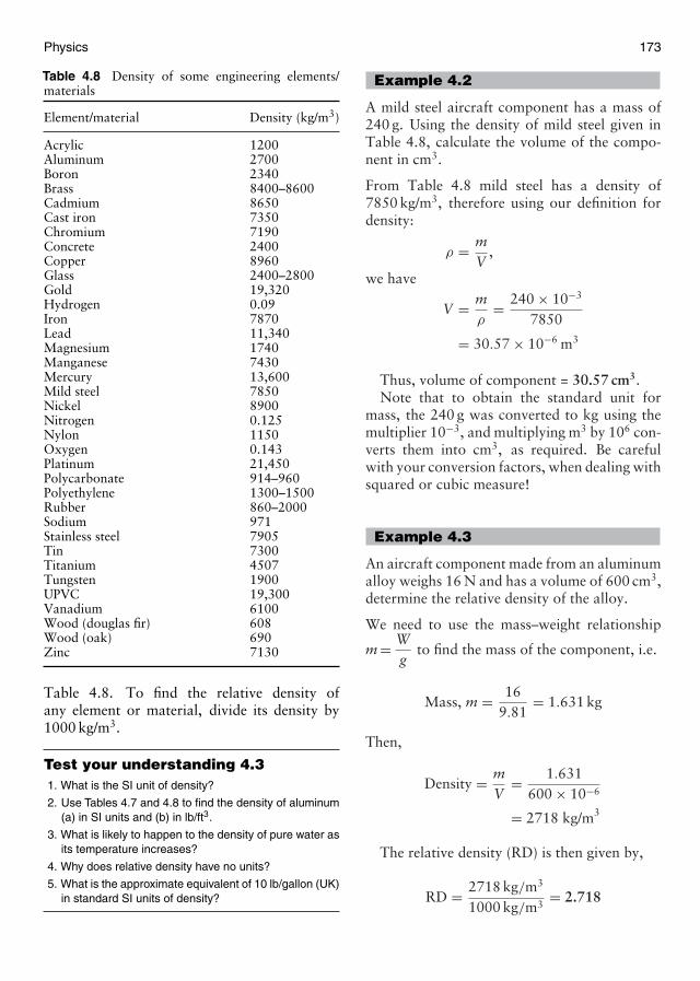
Physics 173
Table 4.8 Density of some engineering elements/materials
Element/material Density (kg/m3)
Acrylic 1200Aluminum 2700Boron 2340Brass 8400–8600Cadmium 8650Cast iron 7350Chromium 7190Concrete 2400Copper 8960Glass 2400–2800Gold 19,320Hydrogen 0.09Iron 7870Lead 11,340Magnesium 1740Manganese 7430Mercury 13,600Mild steel 7850Nickel 8900Nitrogen 0.125Nylon 1150Oxygen 0.143Platinum 21,450Polycarbonate 914–960Polyethylene 1300–1500Rubber 860–2000Sodium 971Stainless steel 7905Tin 7300Titanium 4507Tungsten 1900UPVC 19,300Vanadium 6100Wood (douglas fir) 608Wood (oak) 690Zinc 7130
Table 4.8. To find the relative density ofany element or material, divide its density by1000 kg/m3.
Test your understanding 4.31. What is the SI unit of density?
2. Use Tables 4.7 and 4.8 to find the density of aluminum(a) in SI units and (b) in lb/ft3.
3. What is likely to happen to the density of pure water asits temperature increases?
4. Why does relative density have no units?
5. What is the approximate equivalent of 10 lb/gallon (UK)in standard SI units of density?
Example 4.2
A mild steel aircraft component has a mass of240 g. Using the density of mild steel given inTable 4.8, calculate the volume of the compo-nent in cm3.
From Table 4.8 mild steel has a density of7850 kg/m3, therefore using our definition fordensity:
ρ = mV
,
we have
V = mρ
= 240 × 10−3
7850
= 30.57 × 10⁻⁶ m3
Thus, volume of component = 30.57 cm3.Note that to obtain the standard unit for
mass, the 240 g was converted to kg using themultiplier 10−3, and multiplying m3 by 106 con-verts them into cm3, as required. Be carefulwith your conversion factors, when dealing withsquared or cubic measure!
Example 4.3
An aircraft component made from an aluminumalloy weighs 16 N and has a volume of 600 cm3,determine the relative density of the alloy.
We need to use the mass–weight relationship
m = Wg
to find the mass of the component, i.e.
Mass, m = 169.81
= 1.631 kg
Then,
Density = mV
= 1.631600 × 10−6
= 2718 kg/m3
The relative density (RD) is then given by,
RD = 2718 kg/m3
1000 kg/m3= 2.718
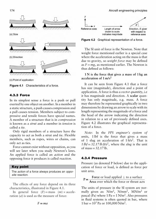
174 Aircraft engineering principles
Figure 4.1 Characteristics of a force.
4.3.3 Force
In its simplest sense a force is a push or pullexerted by one object on another. In a member ina static structure, a push causes compression anda pull causes tension. Members subject to com-pressive and tensile forces have special names.A member of a structure that is in compressionis known as a strut and a member in tension iscalled a tie.
Only rigid members of a structure have thecapacity to act as both a strut and tie. Flexiblemembers, such as ropes, wires or chains, canonly act as ties.
Force cannot exist without opposition, as youwill see later when you study Newton’s laws.An applied force is called an action and theopposing force it produces is called reaction.
Key pointThe action of a force always produces an oppo-site reaction.
The effects of any force depend on its threecharacteristics, illustrated in Figure 4.1.
In general force (F) = mass (m) × accele-ration (a) is used as the measure of force:
F = ma
Figure 4.2 Graphical representation of a force.
The SI unit of force is the Newton. Note thatweight force mentioned earlier is a special casewhere the acceleration acting on the mass is thatdue to gravity, so weight force may be definedas F = mg, as mentioned earlier. The Newton isthus defined as follows:
1 N is the force that gives a mass of 1 kg anacceleration of 1 m/s2
It can be seen from Figure 4.1 that a forcehas size (magnitude), direction and a point ofapplication. A force is thus a vector quantity, i.eit has magnitude and direction. A scalar quan-tity has only magnitude, e.g. mass. A forcemay therefore be represented graphically in twodimensions by drawing an arrow to scale with itslength representing the magnitude of a force andthe head of the arrow indicating the directionin relation to a set of previously defined axes.Figure 4.2 illustrates the graphical representa-tion of a force.
Note: In the FPS engineer’s system ofunits, 1 lbf is the force that gives a massof 1 slug an acceleration of 1 ft/s2. That is1 lbf = 32.17 lb ft/s2, where the slug is the unitof mass = 32.17 lb.
4.3.4 Pressure
Pressure (as denoted P below) due to the appli-cation of force or load, is defined as force perunit area.
P = Force or load applied ⊥ to a surfaceArea over which the force or thrust acts
The units of pressure in the SI system are nor-mally given as: N/m2, N/mm2, MN/m2 orpascal (Pa) where 1 Pa = 1 N/m2. Also pressuresin fluid systems is often quoted in bar, where1 bar = 105 Pa or 100,000 N/m2.
Physics 175
The bar should not be taken as the valuefor standard atmospheric pressure at sea level.The value quoted in bar for standard atmo-spheric pressure is 1.0132 bar or 101,320 N/m2
or 101.32 kPa. Much more will be said aboutatmospheric pressure, when we study the Inter-national Civil Aviation Organization (ICAO)standard atmosphere in the section on atmo-spheric physics.
Key constantStandard atmospheric pressure is 1.0132 bar or101,320 N/m2.
Example 4.4
The area of ground surface contained by theskirt of a hovercraft is 240 m2. The unladenweight of the craft is 480 kN and total ladenweight is 840 kN. Determine the minimum airpressure needed in the skirt to support the craftwhen unladen and when fully loaded.
When unladen:
Pressure = ForceArea
= 480 kN240 m2
= 2 kN/m2
When fully loaded:
Pressure = 840 kN240 m2
= 3.5 kN/m2
In practice the skirt would be inflated to thehigher of these two pressures and the craft (whenstatic) would rest in the water at the appropri-ate level.
Test your understanding 4.41. What are the three defining characteristics of any force?
2. Define (a) a scalar quantity and (b) a vector quantity,and give an example of each.
3. Give the general definition of force and explain howweight force varies from this definition.
4. Complete the following statement: “A strut is a memberin __________ and a tie is a member in ___________”.
5. Define pressure and include two possible SI units.
6. Using the appropriate table convert the following to thestandard SI unit of pressure: (a) 28 psi (b) 30 in.Hg.
4.3.5 Speed, velocity andacceleration
Speed may be defined as distance per unit time.Speed takes no account of direction and istherefore a scalar quantity.
The common SI units of speed are: kilometresper hour (kph) or metres per second (m/s).
In the aircraft industry we more commonlytalk about aircraft speed in knots (nautical milesper hour) or in miles per hour (mph). Machnumber is also used and we will talk more aboutthese units of speed later.
Example 4.5
Convert (a) 450 knots into kph and (b) 120 m/sinto mph.
We could simply multiply by the relevant con-version factors in Table 4.7, which for part (a) isthe reciprocal of 0.5400 or 1.852. Similarly forpart (b) the conversion factor is 2.23694. Letus see if we can derive these conversion factorsby addressing the problem in a rather circularmanner.
(a) Suppose we know that there are 6080 ft ina knot. Then, since there are 3.28084 ftin 1 m, there are 6080
3.28084 = 1853.18 m ina knot.
Therefore, 450 knots = 450 × 1853.18m/h or 833.93 kph.
Thus to convert knots to kph we need tomultiply them by 833.93
450 = 1.853, which totwo decimal places agrees with our tabulatedvalue.
(b) A conversion factor to convert m/s intomph may be found in a similar manner.In this case we start with the fact that1 m = 3.28084 ft and there are 5280 ft in amile, so:
120 m/s = 3.28084 × 120 feet per second
or
3.28084 × 1205280
miles per second
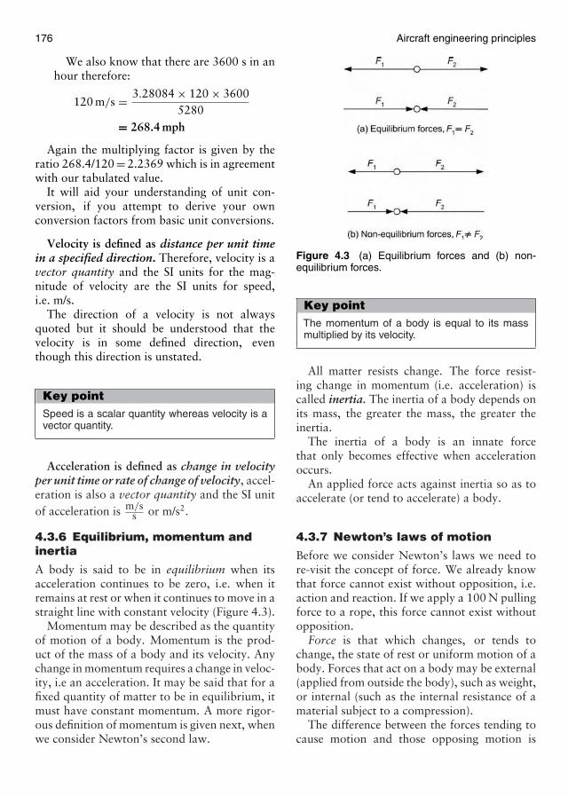
176 Aircraft engineering principles
We also know that there are 3600 s in anhour therefore:
120 m/s = 3.28084 × 120 × 36005280
= 268.4 mph
Again the multiplying factor is given by theratio 268.4/120 = 2.2369 which is in agreementwith our tabulated value.
It will aid your understanding of unit con-version, if you attempt to derive your ownconversion factors from basic unit conversions.
Velocity is defined as distance per unit timein a specified direction. Therefore, velocity is avector quantity and the SI units for the mag-nitude of velocity are the SI units for speed,i.e. m/s.
The direction of a velocity is not alwaysquoted but it should be understood that thevelocity is in some defined direction, eventhough this direction is unstated.
Key pointSpeed is a scalar quantity whereas velocity is avector quantity.
Acceleration is defined as change in velocityper unit time or rate of change of velocity, accel-eration is also a vector quantity and the SI unitof acceleration is m/s
s or m/s2.
4.3.6 Equilibrium, momentum andinertia
A body is said to be in equilibrium when itsacceleration continues to be zero, i.e. when itremains at rest or when it continues to move in astraight line with constant velocity (Figure 4.3).
Momentum may be described as the quantityof motion of a body. Momentum is the prod-uct of the mass of a body and its velocity. Anychange in momentum requires a change in veloc-ity, i.e an acceleration. It may be said that for afixed quantity of matter to be in equilibrium, itmust have constant momentum. A more rigor-ous definition of momentum is given next, whenwe consider Newton’s second law.
Figure 4.3 (a) Equilibrium forces and (b) non-equilibrium forces.
Key pointThe momentum of a body is equal to its massmultiplied by its velocity.
All matter resists change. The force resist-ing change in momentum (i.e. acceleration) iscalled inertia. The inertia of a body depends onits mass, the greater the mass, the greater theinertia.
The inertia of a body is an innate forcethat only becomes effective when accelerationoccurs.
An applied force acts against inertia so as toaccelerate (or tend to accelerate) a body.
4.3.7 Newton’s laws of motion
Before we consider Newton’s laws we need tore-visit the concept of force. We already knowthat force cannot exist without opposition, i.e.action and reaction. If we apply a 100 N pullingforce to a rope, this force cannot exist withoutopposition.
Force is that which changes, or tends tochange, the state of rest or uniform motion of abody. Forces that act on a body may be external(applied from outside the body), such as weight,or internal (such as the internal resistance of amaterial subject to a compression).
The difference between the forces tending tocause motion and those opposing motion is
Physics 177
called the resultant or out-of-balance force. Abody that has no out-of-balance external forceacting on it is in equilibrium and will not accel-erate. A body that has such an out-of-balanceforce will accelerate at a rate dependent on themass of the body and the magnitude of the out-of-balance force. The necessary opposition thatpermits the existence of the out-of-balance forceis provided by the force of inertia.
Newton’s first law of motion states that: abody remains in a state of rest or of uniformmotion in a straight line unless it is acted uponby some external resultant force.
Newton’s second law of motion states that:the rate of change of momentum of a body isdirectly proportional to the force producing thechange and takes place in the direction in whichthe force acts.
We defined force earlier as, force = mass ×acceleration. We also know that accelerationmay be defined as, change in velocity per unittime or rate of change in velocity. If we assumethat a body has an initial velocity u and a finalvelocity v, then the change in velocity is givenby (v – u) and so the rate of change of velocityor acceleration may be written as:
(v − u)t
where t is unit time
Key pointF = ma is a consequence of Newton’s secondlaw of motion.
So since F = ma, this may be written as:
F = m(v − u)t
and multiplying out the brackets gives:
F = mv − mut
Now we also know that momentum was definedearlier as mass × velocity. So the product mugives the initial moment of the body, prior tothe application of the force and mv gives thefinal momentum of the body. Thus the expres-sion (mv − mu) is the change in momentum and
so (mv − mu)t is the rate of change of momen-
tum and therefore Newton’s second law may beexpressed as:
F = mv − mut
or F = ma
Newton’s third law states that: to every actionthere is an equal and opposite reaction.
We will meet Newton’s law again when westudy aircraft motion and engine thrust.
4.3.8 Temperature
Temperature is a measure of the quantity ofenergy possessed by a body or substance, it isa measure of the molecular vibrations withinthe body. The more energetic these vibrationsbecome then the hotter will be the body or sub-stance. For this reason, in its simplest sense,temperature may be regarded as the “degree ofhotness of a body”. A more scientific definitionof temperature will be given when you studythermodynamics.
Test your understanding 4.51. Use the appropriate tables to convert the following units:
(a) 600 kph(b) 140 m/s
}into mph
(d) 80 ft/s(e) 540 mph(f) 240 knot
into m/s
(c) 25 m/s2 into ft/s2
2. Determine the acceleration in m/s2, when a force of1000 N is applied to a mass of 500 lb.
3. Define “inertia” and quote its units.
4. What may we write as the equivalent to the rate ofchange of momentum in Newton’s second law.
5. What in its simplest sense does temperature measure?
General Questions 4.1
1. A rocket launched into the earth’s atmo-sphere is subject to an acceleration due togravity of 5.2 m/s2. If the rocket has a massof 120,000 kg. Determine the weight of therocket: (a) on earth and (b) in orbit.
2. A solid rectangular body measures 1.5 m ×20 cm × 3 cm and has a mass of 54 kg.Calculate: (a) its volume in m3, (b) its densityin Pa and (c) its relative density.
3. An aircraft has four fuel tanks, two in eachwing. The outer tanks each have a volume of
178 Aircraft engineering principles
20 m3 and the inner tanks each have a volumeof 30 m3. The fuel used has a specific gravity(RD) of 0.85. Determine the weight of fuel(at sea level) carried when the tanks are full.
4. A body has a weight of 550 N on the surfaceof the earth:(a) What force is required to give it an accel-
eration of 6 m/s2?(b) What will be the inertia reaction of the
body when given this acceleration?
5. A Cessna 172 and a Boeing 747 are each givenan acceleration of 5 m/s2. To achieve this thethrust force produced by the Cessna’s enginesis 15 kN and the thrust force required by theBoeing 747 is 800 kN. Find the mass of eachaircraft.
4.4 Matter
4.4.1 Introduction
We have already defined mass as the amount ofmatter in a body but what is the nature of thismatter?
All matter or material is made up from ele-mentary building blocks that we know as atomsand molecules. The atom may be further sub-divided into protons, neutrons and electrons.Physicists have discovered many more elemen-tary sub-atomic particles that, for the purposesof this discussion, we do not need to consider.
A molecule consists of a collection of two ormore atoms, which are joined chemically, in acertain way, to give the material its macroscopicproperties. The act of joining atoms and/or join-ing molecules to form parent material is knownas chemical bonding. The driving force thatencourages atoms and molecules to combine incertain ways is energy. Like everything else innature, matter or material is formed as a conse-quence of the atoms and/or molecules combin-ing in such a way, that once formed, they attaintheir lowest energy state. We may define energyas the capacity to do work thus, like nature, wemeasure our efficiency with respect to work, interms of the least amount of energy we expend.Energy, work and power will be covered morefully later, when we study dynamics.
4.4.2 Chemical bonding
In order to fully understand the mechanisms ofbonding you will need to be aware of one or twoimportant facts about the atom and the relation-ship between the type of bond and the periodictable (Table 4.9) of the elements.
The nucleus of the atom consists of an associa-tion of protons and neutrons; the protons have aminute positive charge and the neutrons, as theirname suggests are electrically neutral. Surround-ing the nucleus in a series of discreet (measurablyseparate) energy bands, negative charged elec-trons orbit the nucleus (Figure 4.4). An atom iselectrically neutral, in that the number of posi-tively charged protons is matched by the equalbut opposite, negatively charged electrons. Elec-trons in the energy bands or shells closest to thenucleus are held tightly by electrostatic attrac-tion. In the outermost shells they are held lesstightly.
Key pointElectrons carry a negative charge and protonscarry a positive charge.
An ion is formed when an atom gains or loseselectrons, which disturbs the electrical neutralityof the original atom. For example, a positive ionis formed when an atom loses one or more of itsouter electrons.
The valence of an atom is related to the abilityof the atom to enter into chemical combinationwith other elements, this is often determined bythe number of electrons in the outer most lev-els, where the binding energy is least. Thesevalence shells are often known as s or p shellsthe letters refer to the shell to which the elec-trons belong. For example, magnesium whichhas 12 electrons, aluminum which has 13 elec-trons and germanium which has 32 electronscan be represented as follows:
Mg 1s2 2s2 2p6 3s2 valence = 2Al 1s2 2s2 2p6 3s2 3p1 valence = 3Ge 1s2 2s2 2p6 3s2 valence = 4
3p6 3d10 4s2 4p2
The numbers 1s, 2s, 2p, etc. relate to theshell level, the superscript numbers relate to the

Physics 179
Table 4.9 Periodic table of the elements
11HH
Li Be
12Mg
Ca Sc
Y
57 to71
Ti V Cr
Mo Tc
Re
Bh
W
Sg
Mn Fe
Ru
Os
Hs
Rh
Ir
Mt
Co Ni
Pd
Pt
Uun
Cu
Ag Cd
HgAu
Uuu
Zn
BB
13Al
Ga
In
Tl
CC NN
1515PP
AsAs
SbSb
Bi
OO FF
1717ClCl
BrBr
II
AtAt Rn
Xe
Kr
18Ar
3 4 55 66 77 88 99 10Ne
2He
1616SS
SeSe
TeTe
PoPo
1414SiSi
GeGe
Sn
Pb
Nb
Ta
Ha
Zr
Hf
Ku
89Ac
90Th
91Pa
92U
93Np
94Pu
95Am
96Cm
97Bk
98Cf
99Es
100Fm
101Md
102No
103Lr
La Ce Pr Nd Pm Sm Eu Gd Tb Dy Ho Er Tm Yb57 58 59 60 61 62 63 64 65 66 67 68 69 70 71
Lu
Sr
Ba
Ra89 to103
11Na
20 21 22 23 24 25 26 27 28 29 30 31 3333 3535 363434323219K
39 42 43 44 45 46 47 48 49 5151 5353 5452525041403837Rb
7574 76 77 78 8079 81 83 8585 8684848273725655Cs
Fr107106 108 109 110 1111051048887 112
Uub
Rare GasesNon-Metals
Metals Metalloids
Legend
I A II A III A IV A V A VI A VIIA 0
IIIB IVB VB VIB IBVIIB IIB
Lanthanides
Actinides
1
2
7
6
5
4
3
s2 p2s2 s2 p4s2 p1 s2 p5s1 s2 p3 s2 p6
d5 s1d3 s2 d10 s1d5 s2d2 s2 d7 s2 d8 s2 d10 s2d6 s2d1 s2
Transition elements
VIII
Inner Transition Elements
Figure 4.4 A simplified model of the atom.
number of electrons in that shell. Remember thetotal number of s and p electrons in the outer-most shell often account for the valence number.There is an exception to the above rule, thevalence may also depend on the nature of thechemical reaction.
Key pointThe valence of an element is identified by thecolumn in which it sits within the periodic table.
If an atom has a valence of zero, no electronsenter into chemical reactions and these are allexamples of inert or noble elements.
You may be wondering where all this talkof valence is leading us. By studying the peri-odic table (Table 4.9) you will hopefully be ableto see!
The rows in the periodic table correspondto the principle energy shells that contain theelectrons. The columns refer to the number ofelectrons present in the outermost sp energylevel and so correspond to the most commonvalence. Normally the elements in each columnhave similar properties and behavior.
The transition elements are so named becausesome of their inner shells are being filled pro-gressively as you move from left to right in thetable. For instance scandium (Sc) requires nineelectrons to completely fill its 3d shell, while at
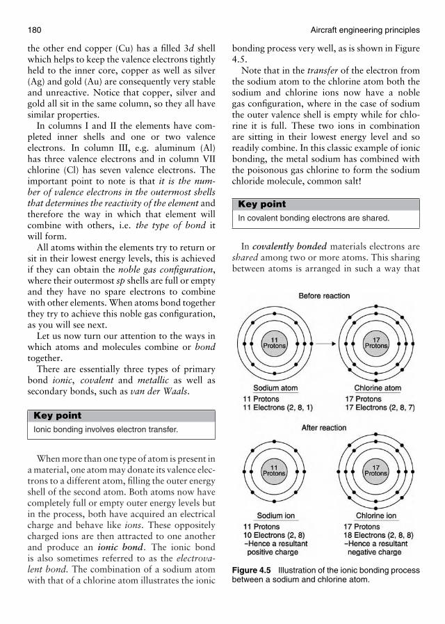
180 Aircraft engineering principles
the other end copper (Cu) has a filled 3d shellwhich helps to keep the valence electrons tightlyheld to the inner core, copper as well as silver(Ag) and gold (Au) are consequently very stableand unreactive. Notice that copper, silver andgold all sit in the same column, so they all havesimilar properties.
In columns I and II the elements have com-pleted inner shells and one or two valenceelectrons. In column III, e.g. aluminum (Al)has three valence electrons and in column VIIchlorine (Cl) has seven valence electrons. Theimportant point to note is that it is the num-ber of valence electrons in the outermost shellsthat determines the reactivity of the element andtherefore the way in which that element willcombine with others, i.e. the type of bond itwill form.
All atoms within the elements try to return orsit in their lowest energy levels, this is achievedif they can obtain the noble gas configuration,where their outermost sp shells are full or emptyand they have no spare electrons to combinewith other elements. When atoms bond togetherthey try to achieve this noble gas configuration,as you will see next.
Let us now turn our attention to the ways inwhich atoms and molecules combine or bondtogether.
There are essentially three types of primarybond ionic, covalent and metallic as well assecondary bonds, such as van der Waals.
Key pointIonic bonding involves electron transfer.
When more than one type of atom is present ina material, one atom may donate its valence elec-trons to a different atom, filling the outer energyshell of the second atom. Both atoms now havecompletely full or empty outer energy levels butin the process, both have acquired an electricalcharge and behave like ions. These oppositelycharged ions are then attracted to one anotherand produce an ionic bond. The ionic bondis also sometimes referred to as the electrova-lent bond. The combination of a sodium atomwith that of a chlorine atom illustrates the ionic
bonding process very well, as is shown in Figure4.5.
Note that in the transfer of the electron fromthe sodium atom to the chlorine atom both thesodium and chlorine ions now have a noblegas configuration, where in the case of sodiumthe outer valence shell is empty while for chlo-rine it is full. These two ions in combinationare sitting in their lowest energy level and soreadily combine. In this classic example of ionicbonding, the metal sodium has combined withthe poisonous gas chlorine to form the sodiumchloride molecule, common salt!
Key pointIn covalent bonding electrons are shared.
In covalently bonded materials electrons areshared among two or more atoms. This sharingbetween atoms is arranged in such a way that
Figure 4.5 Illustration of the ionic bonding processbetween a sodium and chlorine atom.
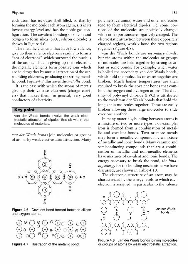
Physics 181
each atom has its outer shell filled, so that byforming the molecule each atom again, sits in itslowest energy level and has the noble gas con-figuration. The covalent bonding of silicon andoxygen to form silica (SiO2, silicon dioxide) isshown in Figure 4.6.
The metallic elements that have low valence,give up their valence electrons readily to form a“sea of electrons” which surround the nucleusof the atoms. Thus in giving up their electronsthe metallic elements form positive ions whichare held together by mutual attraction of the sur-rounding electrons, producing the strong metal-lic bond. Figure 4.7 illustrates the metallic bond.
It is the ease with which the atoms of metalsgive up their valence electrons (charge carri-ers) that makes them, in general, very goodconductors of electricity.
Key pointvan der Waals bonds involve the weak elec-trostatic attraction of dipoles that sit within themolecules of materials.
van der Waals bonds join molecules or groupsof atoms by weak electrostatic attraction. Many
Figure 4.6 Covalent bond formed between siliconand oxygen atoms.
Figure 4.7 Illustration of the metallic bond.
polymers, ceramics, water and other moleculestend to form electrical dipoles, i.e. some por-tions of the molecules are positively chargedwhile other portions are negatively charged. Theelectrostatic attraction between these oppositelycharged regions, weakly bond the two regionstogether (Figure 4.8).
van der Waals bonds are secondary bonds,but the atoms within the molecules or groupsof molecules are held together by strong cova-lent or ionic bonds. For example, when wateris boiled the secondary van der Waals bonds,which hold the molecules of water together arebroken. Much higher temperatures are thenrequired to break the covalent bonds that com-bine the oxygen and hydrogen atoms. The duc-tility of polyvinyl chloride (PVC) is attributedto the weak van der Waals bonds that hold thelong chain molecules together. These are easilybroken allowing these large molecules to slideover one another.
In many materials, bonding between atoms isa mixture of two or more types. For example,iron is formed from a combination of metal-lic and covalent bonds. Two or more metalsmay form a metallic compound, by a mixtureof metallic and ionic bonds. Many ceramic andsemiconducting compounds that are a combi-nation of metallic and non-metallic elementshave mixtures of covalent and ionic bonds. Theenergy necessary to break the bond, the bind-ing energy for the bonding mechanisms we havediscussed, are shown in Table 4.10.
The electronic structure of an atom may becharacterized by the energy levels to which eachelectron is assigned, in particular to the valence
Figure 4.8 van der Waals bonds joining moleculesor groups of atoms by weak electrostatic attraction.
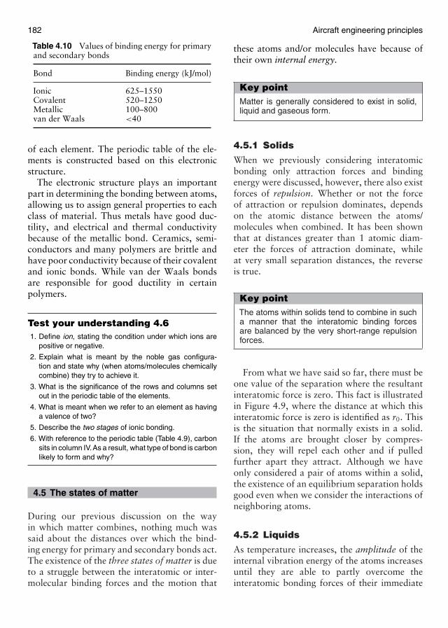
182 Aircraft engineering principles
Table 4.10 Values of binding energy for primaryand secondary bonds
Bond Binding energy (kJ/mol)
Ionic 625–1550Covalent 520–1250Metallic 100–800van der Waals <40
of each element. The periodic table of the ele-ments is constructed based on this electronicstructure.
The electronic structure plays an importantpart in determining the bonding between atoms,allowing us to assign general properties to eachclass of material. Thus metals have good duc-tility, and electrical and thermal conductivitybecause of the metallic bond. Ceramics, semi-conductors and many polymers are brittle andhave poor conductivity because of their covalentand ionic bonds. While van der Waals bondsare responsible for good ductility in certainpolymers.
Test your understanding 4.61. Define ion, stating the condition under which ions are
positive or negative.
2. Explain what is meant by the noble gas configura-tion and state why (when atoms/molecules chemicallycombine) they try to achieve it.
3. What is the significance of the rows and columns setout in the periodic table of the elements.
4. What is meant when we refer to an element as havinga valence of two?
5. Describe the two stages of ionic bonding.
6. With reference to the periodic table (Table 4.9), carbonsits in column IV.As a result, what type of bond is carbonlikely to form and why?
4.5 The states of matter
During our previous discussion on the wayin which matter combines, nothing much wassaid about the distances over which the bind-ing energy for primary and secondary bonds act.The existence of the three states of matter is dueto a struggle between the interatomic or inter-molecular binding forces and the motion that
these atoms and/or molecules have because oftheir own internal energy.
Key pointMatter is generally considered to exist in solid,liquid and gaseous form.
4.5.1 Solids
When we previously considering interatomicbonding only attraction forces and bindingenergy were discussed, however, there also existforces of repulsion. Whether or not the forceof attraction or repulsion dominates, dependson the atomic distance between the atoms/molecules when combined. It has been shownthat at distances greater than 1 atomic diam-eter the forces of attraction dominate, whileat very small separation distances, the reverseis true.
Key pointThe atoms within solids tend to combine in sucha manner that the interatomic binding forcesare balanced by the very short-range repulsionforces.
From what we have said so far, there must beone value of the separation where the resultantinteratomic force is zero. This fact is illustratedin Figure 4.9, where the distance at which thisinteratomic force is zero is identified as r0. Thisis the situation that normally exists in a solid.If the atoms are brought closer by compres-sion, they will repel each other and if pulledfurther apart they attract. Although we haveonly considered a pair of atoms within a solid,the existence of an equilibrium separation holdsgood even when we consider the interactions ofneighboring atoms.
4.5.2 Liquids
As temperature increases, the amplitude of theinternal vibration energy of the atoms increasesuntil they are able to partly overcome theinteratomic bonding forces of their immediate
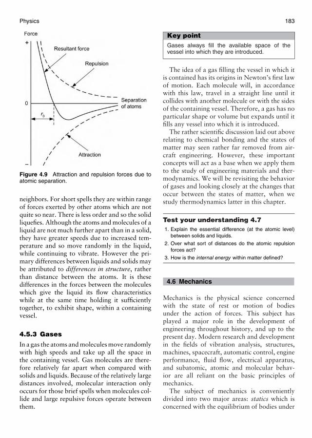
Physics 183
Figure 4.9 Attraction and repulsion forces due toatomic separation.
neighbors. For short spells they are within rangeof forces exerted by other atoms which are notquite so near. There is less order and so the solidliquefies. Although the atoms and molecules of aliquid are not much further apart than in a solid,they have greater speeds due to increased tem-perature and so move randomly in the liquid,while continuing to vibrate. However the pri-mary differences between liquids and solids maybe attributed to differences in structure, ratherthan distance between the atoms. It is thesedifferences in the forces between the moleculeswhich give the liquid its flow characteristicswhile at the same time holding it sufficientlytogether, to exhibit shape, within a containingvessel.
4.5.3 Gases
In a gas the atoms and molecules move randomlywith high speeds and take up all the space inthe containing vessel. Gas molecules are there-fore relatively far apart when compared withsolids and liquids. Because of the relatively largedistances involved, molecular interaction onlyoccurs for those brief spells when molecules col-lide and large repulsive forces operate betweenthem.
Key pointGases always fill the available space of thevessel into which they are introduced.
The idea of a gas filling the vessel in which itis contained has its origins in Newton’s first lawof motion. Each molecule will, in accordancewith this law, travel in a straight line until itcollides with another molecule or with the sidesof the containing vessel. Therefore, a gas has noparticular shape or volume but expands until itfills any vessel into which it is introduced.
The rather scientific discussion laid out aboverelating to chemical bonding and the states ofmatter may seen rather far removed from air-craft engineering. However, these importantconcepts will act as a base when we apply themto the study of engineering materials and ther-modynamics. We will be revisiting the behaviorof gases and looking closely at the changes thatoccur between the states of matter, when westudy thermodynamics latter in this chapter.
Test your understanding 4.71. Explain the essential difference (at the atomic level)
between solids and liquids.
2. Over what sort of distances do the atomic repulsionforces act?
3. How is the internal energy within matter defined?
4.6 Mechanics
Mechanics is the physical science concernedwith the state of rest or motion of bodiesunder the action of forces. This subject hasplayed a major role in the development ofengineering throughout history, and up to thepresent day. Modern research and developmentin the fields of vibration analysis, structures,machines, spacecraft, automatic control, engineperformance, fluid flow, electrical apparatus,and subatomic, atomic and molecular behav-ior are all reliant on the basic principles ofmechanics.
The subject of mechanics is convenientlydivided into two major areas: statics which isconcerned with the equilibrium of bodies under
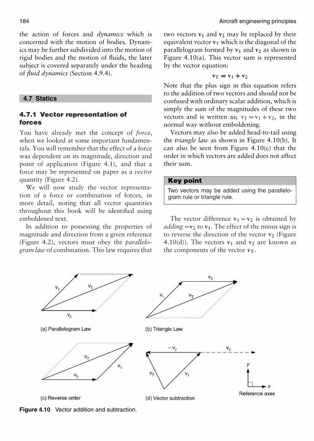
184 Aircraft engineering principles
the action of forces and dynamics which isconcerned with the motion of bodies. Dynam-ics may be further subdivided into the motion ofrigid bodies and the motion of fluids, the latersubject is covered separately under the headingof fluid dynamics (Section 4.9.4).
4.7 Statics
4.7.1 Vector representation offorces
You have already met the concept of force,when we looked at some important fundamen-tals. You will remember that the effect of a forcewas dependent on its magnitude, direction andpoint of application (Figure 4.1), and that aforce may be represented on paper as a vectorquantity (Figure 4.2).
We will now study the vector representa-tion of a force or combination of forces, inmore detail, noting that all vector quantitiesthroughout this book will be identified usingemboldened text.
In addition to possessing the properties ofmagnitude and direction from a given reference(Figure 4.2), vectors must obey the parallelo-gram law of combination. This law requires that
Figure 4.10 Vector addition and subtraction.
two vectors v1 and v2 may be replaced by theirequivalent vector vT which is the diagonal of theparallelogram formed by v1 and v2 as shown inFigure 4.10(a). This vector sum is representedby the vector equation:
vT = v1 + v2
Note that the plus sign in this equation refersto the addition of two vectors and should not beconfused with ordinary scalar addition, which issimply the sum of the magnitudes of these twovectors and is written as; vT = v1 + v2, in thenormal way without emboldening.
Vectors may also be added head-to-tail usingthe triangle law as shown in Figure 4.10(b). Itcan also be seen from Figure 4.10(c) that theorder in which vectors are added does not affecttheir sum.
Key pointTwo vectors may be added using the parallelo-gram rule or triangle rule.
The vector difference v1 − v2 is obtained byadding −v2 to v1. The effect of the minus sign isto reverse the direction of the vector v2 (Figure4.10(d)). The vectors v1 and v2 are known asthe components of the vector vT.
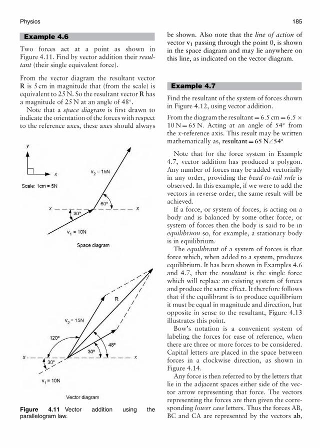
Physics 185
Example 4.6
Two forces act at a point as shown inFigure 4.11. Find by vector addition their resul-tant (their single equivalent force).
From the vector diagram the resultant vectorR is 5 cm in magnitude that (from the scale) isequivalent to 25 N. So the resultant vector R hasa magnitude of 25 N at an angle of 48◦.
Note that a space diagram is first drawn toindicate the orientation of the forces with respectto the reference axes, these axes should always
Figure 4.11 Vector addition using theparallelogram law.
be shown. Also note that the line of action ofvector v1 passing through the point 0, is shownin the space diagram and may lie anywhere onthis line, as indicated on the vector diagram.
Example 4.7
Find the resultant of the system of forces shownin Figure 4.12, using vector addition.
From the diagram the resultant = 6.5 cm = 6.5 ×10 N = 65 N. Acting at an angle of 54◦ fromthe x-reference axis. This result may be writtenmathematically as, resultant = 65 N∠54◦
Note that for the force system in Example4.7, vector addition has produced a polygon.Any number of forces may be added vectoriallyin any order, providing the head-to-tail rule isobserved. In this example, if we were to add thevectors in reverse order, the same result will beachieved.
If a force, or system of forces, is acting on abody and is balanced by some other force, orsystem of forces then the body is said to be inequilibrium so, for example, a stationary bodyis in equilibrium.
The equilibrant of a system of forces is thatforce which, when added to a system, producesequilibrium. It has been shown in Examples 4.6and 4.7, that the resultant is the single forcewhich will replace an existing system of forcesand produce the same effect. It therefore followsthat if the equilibrant is to produce equilibriumit must be equal in magnitude and direction, butopposite in sense to the resultant, Figure 4.13illustrates this point.
Bow’s notation is a convenient system oflabeling the forces for ease of reference, whenthere are three or more forces to be considered.Capital letters are placed in the space betweenforces in a clockwise direction, as shown inFigure 4.14.
Any force is then referred to by the letters thatlie in the adjacent spaces either side of the vec-tor arrow representing that force. The vectorsrepresenting the forces are then given the corre-sponding lower case letters. Thus the forces AB,BC and CA are represented by the vectors ab,
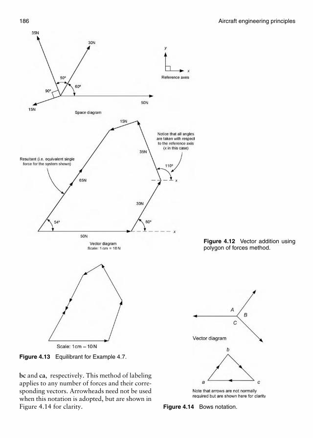
186 Aircraft engineering principles
Figure 4.12 Vector addition usingpolygon of forces method.
Figure 4.13 Equilibrant for Example 4.7.
bc and ca, respectively. This method of labelingapplies to any number of forces and their corre-sponding vectors. Arrowheads need not be usedwhen this notation is adopted, but are shown inFigure 4.14 for clarity. Figure 4.14 Bows notation.
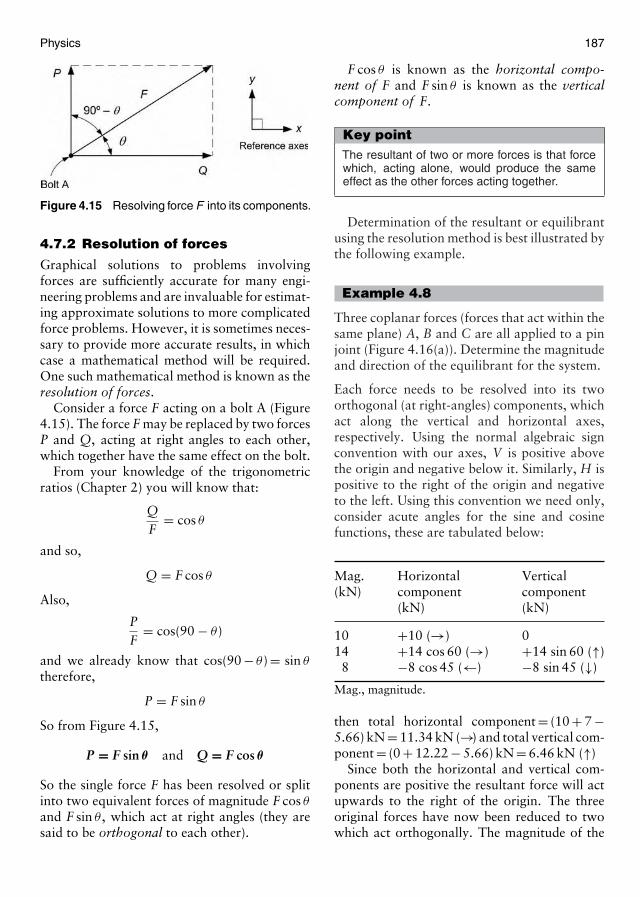
Physics 187
Figure 4.15 Resolving force F into its components.
4.7.2 Resolution of forces
Graphical solutions to problems involvingforces are sufficiently accurate for many engi-neering problems and are invaluable for estimat-ing approximate solutions to more complicatedforce problems. However, it is sometimes neces-sary to provide more accurate results, in whichcase a mathematical method will be required.One such mathematical method is known as theresolution of forces.
Consider a force F acting on a bolt A (Figure4.15). The force F may be replaced by two forcesP and Q, acting at right angles to each other,which together have the same effect on the bolt.
From your knowledge of the trigonometricratios (Chapter 2) you will know that:
QF
= cos θ
and so,
Q = F cos θ
Also,
PF
= cos(90 − θ )
and we already know that cos(90 − θ ) = sin θ
therefore,
P = F sin θ
So from Figure 4.15,
P = F sin θ and Q = F cos θ
So the single force F has been resolved or splitinto two equivalent forces of magnitude F cos θ
and F sin θ , which act at right angles (they aresaid to be orthogonal to each other).
F cos θ is known as the horizontal compo-nent of F and F sin θ is known as the verticalcomponent of F.
Key pointThe resultant of two or more forces is that forcewhich, acting alone, would produce the sameeffect as the other forces acting together.
Determination of the resultant or equilibrantusing the resolution method is best illustrated bythe following example.
Example 4.8
Three coplanar forces (forces that act within thesame plane) A, B and C are all applied to a pinjoint (Figure 4.16(a)). Determine the magnitudeand direction of the equilibrant for the system.
Each force needs to be resolved into its twoorthogonal (at right-angles) components, whichact along the vertical and horizontal axes,respectively. Using the normal algebraic signconvention with our axes, V is positive abovethe origin and negative below it. Similarly, H ispositive to the right of the origin and negativeto the left. Using this convention we need only,consider acute angles for the sine and cosinefunctions, these are tabulated below:
Mag. Horizontal Vertical(kN) component component
(kN) (kN)
10 +10 (→) 014 +14 cos 60 (→) +14 sin 60 (↑)
8 −8 cos 45 (←) −8 sin 45 (↓)
Mag., magnitude.
then total horizontal component = (10 + 7 −5.66) kN = 11.34 kN (→) and total vertical com-ponent = (0 + 12.22 − 5.66) kN = 6.46 kN (↑)
Since both the horizontal and vertical com-ponents are positive the resultant force will actupwards to the right of the origin. The threeoriginal forces have now been reduced to twowhich act orthogonally. The magnitude of the
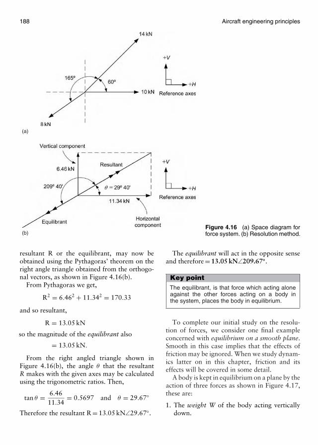
188 Aircraft engineering principles
(a)
(b)Figure 4.16 (a) Space diagram forforce system. (b) Resolution method.
resultant R or the equilibrant, may now beobtained using the Pythagoras’ theorem on theright angle triangle obtained from the orthogo-nal vectors, as shown in Figure 4.16(b).
From Pythagoras we get,
R2 = 6.462 + 11.342 = 170.33
and so resultant,
R = 13.05 kN
so the magnitude of the equilibrant also
= 13.05 kN.
From the right angled triangle shown inFigure 4.16(b), the angle θ that the resultantR makes with the given axes may be calculatedusing the trigonometric ratios. Then,
tan θ = 6.4611.34
= 0.5697 and θ = 29.67◦
Therefore the resultant R = 13.05 kN∠29.67◦.
The equilibrant will act in the opposite senseand therefore = 13.05 kN∠209.67◦.
Key pointThe equilibrant, is that force which acting aloneagainst the other forces acting on a body inthe system, places the body in equilibrium.
To complete our initial study on the resolu-tion of forces, we consider one final exampleconcerned with equilibrium on a smooth plane.Smooth in this case implies that the effects offriction may be ignored. When we study dynam-ics latter on in this chapter, friction and itseffects will be covered in some detail.
A body is kept in equilibrium on a plane by theaction of three forces as shown in Figure 4.17,these are:
1. The weight W of the body acting verticallydown.
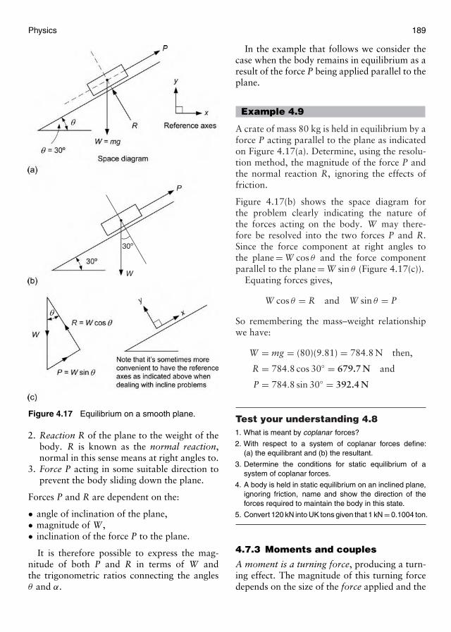
Physics 189
30º
W
Figure 4.17 Equilibrium on a smooth plane.
2. Reaction R of the plane to the weight of thebody. R is known as the normal reaction,normal in this sense means at right angles to.
3. Force P acting in some suitable direction toprevent the body sliding down the plane.
Forces P and R are dependent on the:
• angle of inclination of the plane,• magnitude of W ,• inclination of the force P to the plane.
It is therefore possible to express the mag-nitude of both P and R in terms of W andthe trigonometric ratios connecting the anglesθ and α.
In the example that follows we consider thecase when the body remains in equilibrium as aresult of the force P being applied parallel to theplane.
Example 4.9
A crate of mass 80 kg is held in equilibrium by aforce P acting parallel to the plane as indicatedon Figure 4.17(a). Determine, using the resolu-tion method, the magnitude of the force P andthe normal reaction R, ignoring the effects offriction.
Figure 4.17(b) shows the space diagram forthe problem clearly indicating the nature ofthe forces acting on the body. W may there-fore be resolved into the two forces P and R.Since the force component at right angles tothe plane = W cos θ and the force componentparallel to the plane = W sin θ (Figure 4.17(c)).
Equating forces gives,
W cos θ = R and W sin θ = P
So remembering the mass–weight relationshipwe have:
W = mg = (80)(9.81) = 784.8 N then,
R = 784.8 cos 30◦ = 679.7 N and
P = 784.8 sin 30◦ = 392.4 N
Test your understanding 4.81. What is meant by coplanar forces?
2. With respect to a system of coplanar forces define:(a) the equilibrant and (b) the resultant.
3. Determine the conditions for static equilibrium of asystem of coplanar forces.
4. A body is held in static equilibrium on an inclined plane,ignoring friction, name and show the direction of theforces required to maintain the body in this state.
5. Convert 120 kN into UK tons given that 1 kN = 0.1004 ton.
4.7.3 Moments and couples
A moment is a turning force, producing a turn-ing effect. The magnitude of this turning forcedepends on the size of the force applied and the
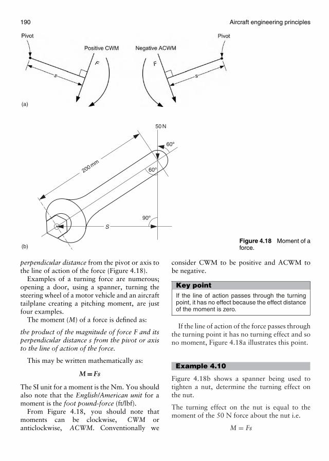
190 Aircraft engineering principles
(a)
(b)
200mm
90º
60º
60º
50 N
S
Figure 4.18 Moment of aforce.
perpendicular distance from the pivot or axis tothe line of action of the force (Figure 4.18).
Examples of a turning force are numerous;opening a door, using a spanner, turning thesteering wheel of a motor vehicle and an aircrafttailplane creating a pitching moment, are justfour examples.
The moment (M) of a force is defined as:
the product of the magnitude of force F and itsperpendicular distance s from the pivot or axisto the line of action of the force.
This may be written mathematically as:
M = Fs
The SI unit for a moment is the Nm. You shouldalso note that the English/American unit for amoment is the foot pound-force (ft/lbf).
From Figure 4.18, you should note thatmoments can be clockwise, CWM oranticlockwise, ACWM. Conventionally we
consider CWM to be positive and ACWM tobe negative.
Key pointIf the line of action passes through the turningpoint, it has no effect because the effect distanceof the moment is zero.
If the line of action of the force passes throughthe turning point it has no turning effect and sono moment, Figure 4.18a illustrates this point.
Example 4.10
Figure 4.18b shows a spanner being used totighten a nut, determine the turning effect onthe nut.
The turning effect on the nut is equal to themoment of the 50 N force about the nut i.e.
M = Fs
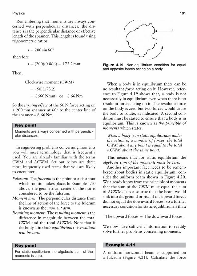
Physics 191
Remembering that moments are always con-cerned with perpendicular distances, the dis-tance s is the perpendicular distance or effectivelength of the spanner. This length is found usingtrigonometric ratios:
s = 200 sin 60◦
therefore
s = (200)(0.866) = 173.2 mm
Then,
Clockwise moment (CWM)
= (50)(173.2)
= 8660 Nmm or 8.66 Nm
So the turning effect of the 50 N force acting ona 200 mm spanner at 60◦ to the center line ofthe spanner = 8.66 Nm.
Key pointMoments are always concerned with perpendic-ular distances.
In engineering problems concerning momentsyou will meet terminology that is frequentlyused. You are already familiar with the termsCWM and ACWM. Set out below are threemore frequently used terms that you are likelyto encounter.
Fulcrum: The fulcrum is the point or axis aboutwhich rotation takes place. In Example 4.10above, the geometrical center of the nut isconsidered to be the fulcrum.
Moment arm: The perpendicular distance fromthe line of action of the force to the fulcrumis known as the moment arm.
Resulting moment: The resulting moment is thedifference in magnitude between the totalCWM and the total ACWM. Note that ifthe body is in static equilibrium this resultantwill be zero.
Key pointFor static equilibrium the algebraic sum of themoments is zero.
Figure 4.19 Non-equilibrium condition for equaland opposite forces acting on a body.
When a body is in equilibrium there can beno resultant force acting on it. However, refer-ence to Figure 4.19 shows that, a body is notnecessarily in equilibrium even when there is noresultant force, acting on it. The resultant forceon the body is zero but two forces would causethe body to rotate, as indicated. A second con-dition must be stated to ensure that a body is inequilibrium. This is known as the principle ofmoments which states:
When a body is in static equilibrium underthe action of a number of forces, the totalCWM about any point is equal to the totalACWM about the same point.
This means that for static equilibrium thealgebraic sum of the moments must be zero.
Another important fact needs to be remem-bered about bodies in static equilibrium, con-sider the uniform beam shown in Figure 4.20.We already know from the principle of momentsthat the sum of the CWM must equal the sumof ACWM. It is also true that the beam wouldsink into the ground or rise, if the upward forcesdid not equal the downward forces. So a furthernecessary condition for static equilibrium is that:
The upward forces = The downward forces.
We now have sufficient information to readilysolve further problems concerning moments.
Example 4.11
A uniform horizontal beam is supported ona fulcrum (Figure 4.21). Calculate the force
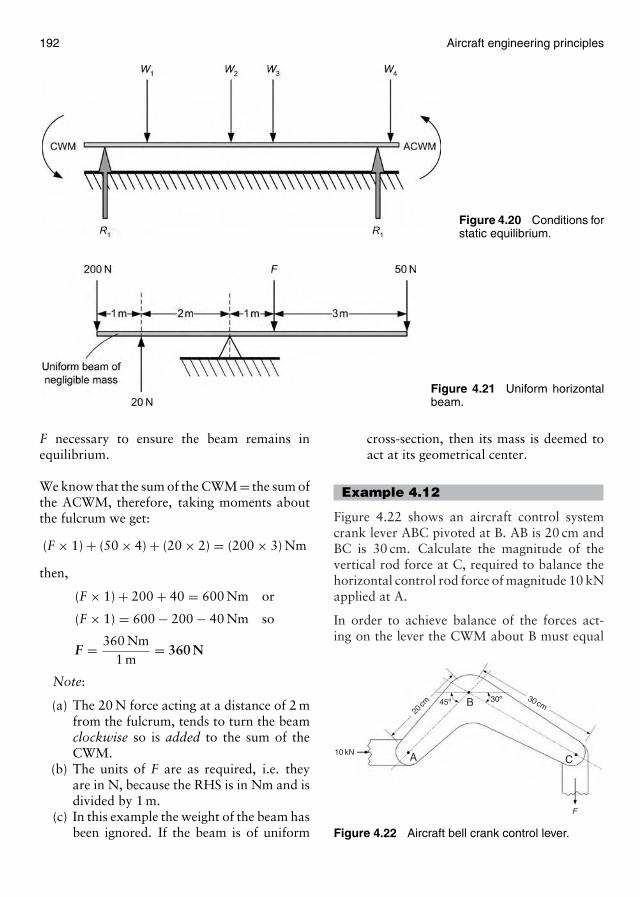
192 Aircraft engineering principles
Figure 4.20 Conditions forstatic equilibrium.
Figure 4.21 Uniform horizontalbeam.
F necessary to ensure the beam remains inequilibrium.
We know that the sum of the CWM = the sum ofthe ACWM, therefore, taking moments aboutthe fulcrum we get:
(F × 1) + (50 × 4) + (20 × 2) = (200 × 3) Nm
then,
(F × 1) + 200 + 40 = 600 Nm or
(F × 1) = 600 − 200 − 40 Nm so
F = 360 Nm1 m
= 360 N
Note:
(a) The 20 N force acting at a distance of 2 mfrom the fulcrum, tends to turn the beamclockwise so is added to the sum of theCWM.
(b) The units of F are as required, i.e. theyare in N, because the RHS is in Nm and isdivided by 1 m.
(c) In this example the weight of the beam hasbeen ignored. If the beam is of uniform
cross-section, then its mass is deemed toact at its geometrical center.
Example 4.12
Figure 4.22 shows an aircraft control systemcrank lever ABC pivoted at B. AB is 20 cm andBC is 30 cm. Calculate the magnitude of thevertical rod force at C, required to balance thehorizontal control rod force of magnitude 10 kNapplied at A.
In order to achieve balance of the forces act-ing on the lever the CWM about B must equal
10 kN A
B
C
F
45º 30º
20cm
30cm
Figure 4.22 Aircraft bell crank control lever.
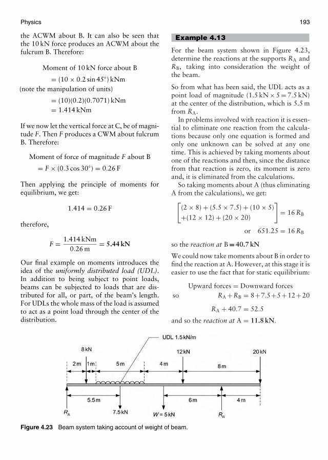
Physics 193
the ACWM about B. It can also be seen thatthe 10 kN force produces an ACWM about thefulcrum B. Therefore:
Moment of 10 kN force about B
= (10 × 0.2 sin 45◦) kNm(note the manipulation of units)
= (10)(0.2)(0.7071) kNm= 1.414 kNm
If we now let the vertical force at C, be of magni-tude F. Then F produces a CWM about fulcrumB. Therefore:
Moment of force of magnitude F about B
= F × (0.3 cos 30◦) = 0.26 F
Then applying the principle of moments forequilibrium, we get:
1.414 = 0.26 F
therefore,
F = 1.414 kNm0.26 m
= 5.44 kN
Our final example on moments introduces theidea of the uniformly distributed load (UDL).In addition to being subject to point loads,beams can be subjected to loads that are dis-tributed for all, or part, of the beam’s length.For UDLs the whole mass of the load is assumedto act as a point load through the center of thedistribution.
Figure 4.23 Beam system taking account of weight of beam.
Example 4.13
For the beam system shown in Figure 4.23,determine the reactions at the supports RA andRB, taking into consideration the weight ofthe beam.
So from what has been said, the UDL acts as apoint load of magnitude (1.5 kN × 5 = 7.5 kN)at the center of the distribution, which is 5.5 mfrom RA.
In problems involved with reaction it is essen-tial to eliminate one reaction from the calcula-tions because only one equation is formed andonly one unknown can be solved at any onetime. This is achieved by taking moments aboutone of the reactions and then, since the distancefrom that reaction is zero, its moment is zeroand, it is eliminated from the calculations.
So taking moments about A (thus eliminatingA from the calculations), we get:[
(2 × 8) + (5.5 × 7.5) + (10 × 5)
+(12 × 12) + (20 × 20)
]= 16 RB
or 651.25 = 16 RB
so the reaction at B = 40.7 kN
We could now take moments about B in order tofind the reaction at A. However, at this stage it iseasier to use the fact that for static equilibrium:
Upward forces = Downward forcesso RA +RB = 8+7.5+5+12+20
RA + 40.7 = 52.5
and so the reaction at A = 11.8 kN.

194 Aircraft engineering principles
4.7.4 Couples
So far we have restricted our problems onmoments to the turning effect of forces takenone at a time. A couple occurs when two equalforces acting in opposite directions have theirlines of action parallel.
Example 4.14
Figure 4.24 shows the turning effect of a couple,on a beam of regular cross-section.
Figure 4.24 Turning effect of a couple.
Taking moments about the center of gravity(CG) (the point at which all the weight of thebeam is deemed to act), we get:
(30 × 0.5) + (30 × 0.5) = turning moment
so turning moment of couple = 30 Nm.
Example 4.15
Figure 4.25 shows a beam of irregular cross-section, for this beam the couple will still tryto revolve about its CG.
Taking moments about the CG gives:
(30 × 0.75) + (30 × 0.25) = turning moment
so the moment of couple = 30 Nm.
It can be seen from the above two examplesthat the moment is the same in both the casesand is independent of the position of the ful-crum. Therefore, if the fulcrum is assumed to
Figure 4.25 Turning effect of a couple with irregularcross-section beam.
be located at the point of application of one ofthe forces, the moment of a couple is equal toone of the forces multiplied by the perpendicu-lar distance between them. Thus in both casesshown in Examples 4.14 and 4.15 the momentof the couple = 30 N × 1 m = 30 Nm, as before.
Another important application of the coupleis its turning moment or torque. The definitionof torque is as follows:
Torque is the turning moment of a coupleand is measured in Nm:torque (T) = force (F) × radius (r).
The turning moment of the couple givenabove in Example 4.15 is F × r = (30 N × 0.5 m)= 15 Nm.
Key pointThe moment of a couple = force × distancebetween forces and the turning moment =force × radius.
Example 4.16
A nut is to be torque loaded to a maximumof 100 Nm. What is the maximum force thatmay be applied, perpendicular to the end of thespanner, if the spanner is of length 30 cm?
Since T = F × r, then F = Tr
= 100 Nm30 cm
therefore, F = 333.3 N
Having studied moments, couples and turn-ing moments, we will now look at how these

Physics 195
concepts may be applied to simple aircraftweight and balance calculations.
Test your understanding 4.91. Define the moment of a force.
2. If the line of action of a force passes through the turningpoint, explain why this force has no turning effect.
3. If a force acts other than at a perpendicular distancefrom the turning point, explain how its turning momentcan be determined.
4. Define the terms: (a) fulcrum, (b) moment arm, (c)resulting moment and (d) reaction.
5. State the conditions for static equilibrium when a sys-tems of forces act on a simply supported beam.
6. Define the terms: (a) couple and (b) moment of a couple.
7. Use Table E.7 (Appendix E) to convert 80 ft lbf into Nm.
Figure 4.26 Determining air-craft CG.
4.7.5 Aircraft weight and balancecalculations
A static aircraft can be represented as a loadedbeam with the reactions taken by the under-carriage. So the loads on the undercarriagecan be calculated using our previous knowl-edge of moments. Determining the CG of anaircraft under different loading conditions is animportant safety consideration.
Figure 4.26(a) is a pictorial representation ofa typical passenger aircraft, showing how themajor parts of the aircraft, together with pas-sengers, crew and stores, may be represented aspoint loads and UDLs.
Figure 4.26(b) shows how, for the pur-pose of CG calculations, the weights of the
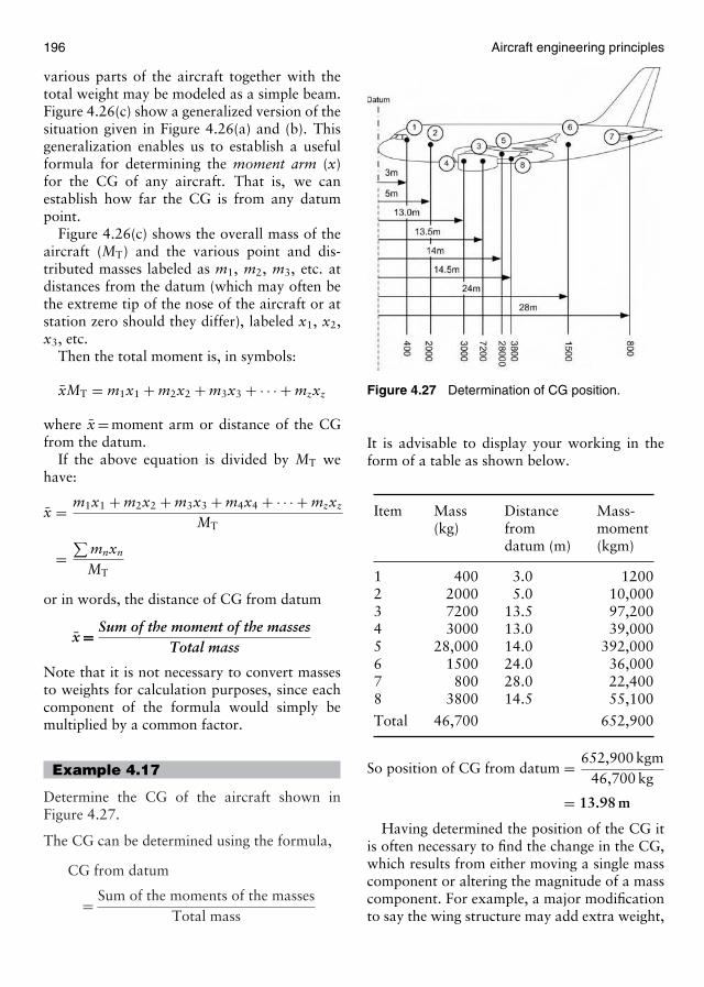
196 Aircraft engineering principles
various parts of the aircraft together with thetotal weight may be modeled as a simple beam.Figure 4.26(c) show a generalized version of thesituation given in Figure 4.26(a) and (b). Thisgeneralization enables us to establish a usefulformula for determining the moment arm (x)for the CG of any aircraft. That is, we canestablish how far the CG is from any datumpoint.
Figure 4.26(c) shows the overall mass of theaircraft (MT) and the various point and dis-tributed masses labeled as m1, m2, m3, etc. atdistances from the datum (which may often bethe extreme tip of the nose of the aircraft or atstation zero should they differ), labeled x1, x2,x3, etc.
Then the total moment is, in symbols:
xMT = m1x1 + m2x2 + m3x3 + · · · + mzxz
where x = moment arm or distance of the CGfrom the datum.
If the above equation is divided by MT wehave:
x = m1x1 + m2x2 + m3x3 + m4x4 + · · · + mzxz
MT
=∑
mnxn
MT
or in words, the distance of CG from datum
x = Sum of the moment of the massesTotal mass
Note that it is not necessary to convert massesto weights for calculation purposes, since eachcomponent of the formula would simply bemultiplied by a common factor.
Example 4.17
Determine the CG of the aircraft shown inFigure 4.27.
The CG can be determined using the formula,
CG from datum
= Sum of the moments of the massesTotal mass
Figure 4.27 Determination of CG position.
It is advisable to display your working in theform of a table as shown below.
Item Mass Distance Mass-(kg) from moment
datum (m) (kgm)
1 400 3.0 12002 2000 5.0 10,0003 7200 13.5 97,2004 3000 13.0 39,0005 28,000 14.0 392,0006 1500 24.0 36,0007 800 28.0 22,4008 3800 14.5 55,100
Total 46,700 652,900
So position of CG from datum = 652,900 kgm46,700 kg
= 13.98 m
Having determined the position of the CG itis often necessary to find the change in the CG,which results from either moving a single masscomponent or altering the magnitude of a masscomponent. For example, a major modificationto say the wing structure may add extra weight,
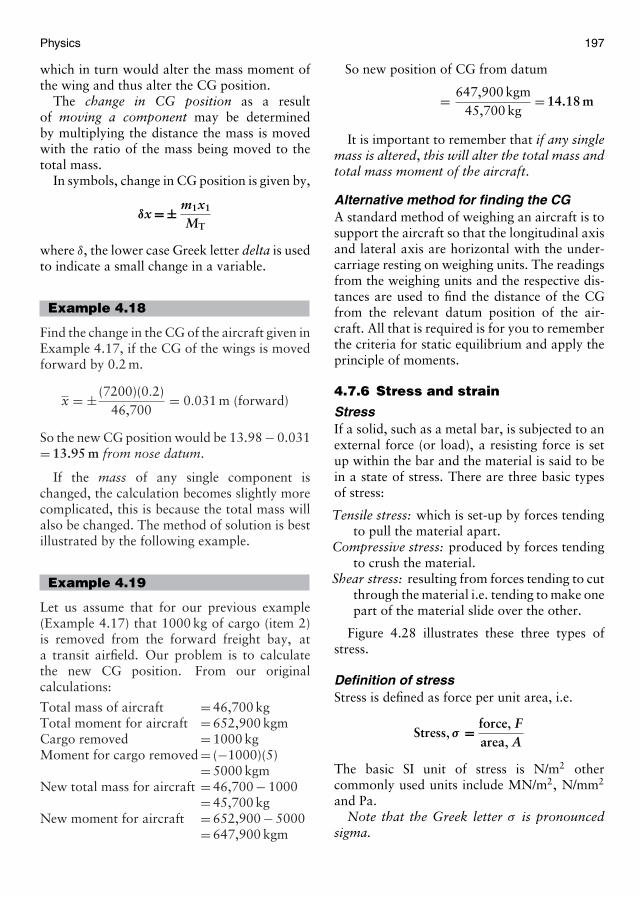
Physics 197
which in turn would alter the mass moment ofthe wing and thus alter the CG position.
The change in CG position as a resultof moving a component may be determinedby multiplying the distance the mass is movedwith the ratio of the mass being moved to thetotal mass.
In symbols, change in CG position is given by,
δx = ± m1x1
MT
where δ, the lower case Greek letter delta is usedto indicate a small change in a variable.
Example 4.18
Find the change in the CG of the aircraft given inExample 4.17, if the CG of the wings is movedforward by 0.2 m.
x = ± (7200)(0.2)46,700
= 0.031 m (forward)
So the new CG position would be 13.98 − 0.031= 13.95 m from nose datum.
If the mass of any single component ischanged, the calculation becomes slightly morecomplicated, this is because the total mass willalso be changed. The method of solution is bestillustrated by the following example.
Example 4.19
Let us assume that for our previous example(Example 4.17) that 1000 kg of cargo (item 2)is removed from the forward freight bay, ata transit airfield. Our problem is to calculatethe new CG position. From our originalcalculations:
Total mass of aircraft = 46,700 kgTotal moment for aircraft = 652,900 kgmCargo removed = 1000 kgMoment for cargo removed = (−1000)(5)
= 5000 kgmNew total mass for aircraft = 46,700 − 1000
= 45,700 kgNew moment for aircraft = 652,900 − 5000
= 647,900 kgm
So new position of CG from datum
= 647,900 kgm45,700 kg
= 14.18 m
It is important to remember that if any singlemass is altered, this will alter the total mass andtotal mass moment of the aircraft.
Alternative method for finding the CGA standard method of weighing an aircraft is tosupport the aircraft so that the longitudinal axisand lateral axis are horizontal with the under-carriage resting on weighing units. The readingsfrom the weighing units and the respective dis-tances are used to find the distance of the CGfrom the relevant datum position of the air-craft. All that is required is for you to rememberthe criteria for static equilibrium and apply theprinciple of moments.
4.7.6 Stress and strain
StressIf a solid, such as a metal bar, is subjected to anexternal force (or load), a resisting force is setup within the bar and the material is said to bein a state of stress. There are three basic typesof stress:
Tensile stress: which is set-up by forces tendingto pull the material apart.
Compressive stress: produced by forces tendingto crush the material.
Shear stress: resulting from forces tending to cutthrough the material i.e. tending to make onepart of the material slide over the other.
Figure 4.28 illustrates these three types ofstress.
Definition of stressStress is defined as force per unit area, i.e.
Stress, σ = force, Farea, A
The basic SI unit of stress is N/m2 othercommonly used units include MN/m2, N/mm2
and Pa.Note that the Greek letter σ is pronounced
sigma.
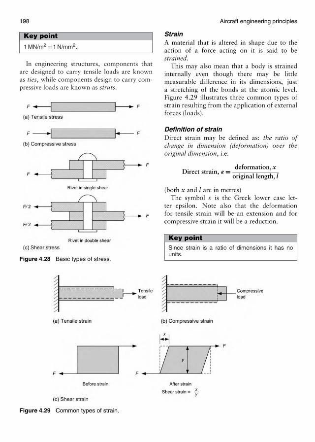
198 Aircraft engineering principles
Key point
1 MN/m2 = 1 N/mm2.
In engineering structures, components thatare designed to carry tensile loads are knownas ties, while components design to carry com-pressive loads are known as struts.
Figure 4.28 Basic types of stress.
xy
Figure 4.29 Common types of strain.
StrainA material that is altered in shape due to theaction of a force acting on it is said to bestrained.
This may also mean that a body is strainedinternally even though there may be littlemeasurable difference in its dimensions, justa stretching of the bonds at the atomic level.Figure 4.29 illustrates three common types ofstrain resulting from the application of externalforces (loads).
Definition of strainDirect strain may be defined as: the ratio ofchange in dimension (deformation) over theoriginal dimension, i.e.
Direct strain, ε = deformation, xoriginal length, l
(both x and l are in metres)The symbol ε is the Greek lower case let-
ter epsilon. Note also that the deformationfor tensile strain will be an extension and forcompressive strain it will be a reduction.
Key pointSince strain is a ratio of dimensions it has nounits.

Physics 199
Figure 4.30 Force–extension graph for a spring.
4.7.7 Hooke’s law
Hooke’s law states that:
Within the elastic limit of a material thechange in shape is directly proportional tothe applied force producing it.
A good example of the application of Hooke’slaw is the spring. A spring balance is usedfor measuring weight force, where an increasein weight will cause a corresponding extension(see Figure 4.30).
The stiffness (k) of a spring is the forcerequired to cause a certain (unit deflection):
Stiffness (k) = forcedeflection
SI units are N/m or Nm−1.The concept of stiffness will be looked at in
a moment, in the mean time here is a questionto consider. What does the slope of the graphin Figure 4.30 indicate?
4.7.8 Modulus
Modulus of elasticityBy considering Hooke’s law, it follows thatstress is directly proportional to strain, while
the material remains elastic. That is, while theexternal forces acting on the material are onlysufficient to stretch the atomic bonds, withoutfracture, so that the material may return to itsoriginal shape after the external forces have beenremoved.
Then from Hooke’s law and our definition ofstress and strain, we know that stress is directlyproportional to strain in the elastic range, i.e.
Stress ∝ strain
or Stress = strain × a constant
soStressStrain
= a constant (E)
This constant of proportionality, will dependon the material and is given the symbol E. It isknown as the modulus of elasticity and becausestrain has no units it has the same units asstress, because the modulus tends to have veryhigh values, GN/m2 or GPa are the preferred SIunits.
Key pointThe elastic modulus of a material may be takenas a measure of the stiffness of that material.
Modulus of rigidityThe relationship between the shear stress (τ )and shear strain (γ ) is known as the modulusof rigidity (G) i.e.
Modulusof rigidity = shear stress (τ )
shear strain (γ )
(G) GPa or GN/m2
Note that the symbol τ is the lower case Greekletter tau and the symbol γ is the lower caseGreek letter gamma.
Bulk modulusIf a body of volume v is subject to an increase ofexternal pressure dp which changes its volumeby δV , Figure 4.31, the deformation is a changein volume without a change in shape.
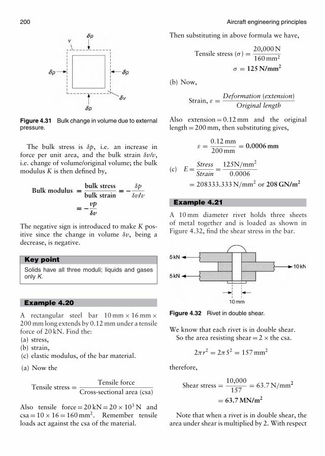
200 Aircraft engineering principles
Figure 4.31 Bulk change in volume due to externalpressure.
The bulk stress is δp, i.e. an increase inforce per unit area, and the bulk strain δv/v,i.e. change of volume/original volume; the bulkmodulus K is then defined by,
Bulk modulus = bulk stressbulk strain
= − δpδv/v
= −vpδv
The negative sign is introduced to make K pos-itive since the change in volume δv, being adecrease, is negative.
Key pointSolids have all three moduli; liquids and gasesonly K.
Example 4.20
A rectangular steel bar 10 mm × 16 mm ×200 mm long extends by 0.12 mm under a tensileforce of 20 kN. Find the:(a) stress,(b) strain,(c) elastic modulus, of the bar material.
(a) Now the
Tensile stress = Tensile forceCross-sectional area (csa)
Also tensile force = 20 kN = 20 × 103 N andcsa = 10 × 16 = 160 mm2. Remember tensileloads act against the csa of the material.
Then substituting in above formula we have,
Tensile stress (σ ) = 20,000 N160 mm2
σ = 125 N/mm2
(b) Now,
Strain, ε = Deformation (extension)Original length
Also extension = 0.12 mm and the originallength = 200 mm, then substituting gives,
ε = 0.12 mm200 mm
= 0.0006 mm
(c) E = StressStrain
= 125N/mm2
0.0006
= 208333.333 N/mm2 or 208 GN/m2
Example 4.21
A 10 mm diameter rivet holds three sheetsof metal together and is loaded as shown inFigure 4.32, find the shear stress in the bar.
Figure 4.32 Rivet in double shear.
We know that each rivet is in double shear.So the area resisting shear = 2 × the csa.
2πr2 = 2π52 = 157 mm2
therefore,
Shear stress = 10,000157
= 63.7 N/mm2
= 63.7 MN/m2
Note that when a rivet is in double shear, thearea under shear is multiplied by 2. With respect
Physics 201
to the load we know from Newton’s laws thatto every action there is an equal and oppositereaction, thus we only use the action or reactionof a force in our calculations, not both.
Test your understanding 4.101. In aircraft weight and balance calculations, write down
the formula that enables us to determine the CG froma datum.
2. When determining changes to the CG position.What dowe need to remember when the mass of an individualcomponent changes?
3. Define: (a) tensile stress, (b) shear stress and(c) compressive stress.
4. State Hooke’s law and explain its relationship to theelastic modulus.
5. Define spring stiffness and quote its SI unit.
6. Define in detail the terms: (a) elastic modulus, (b) shearmodulus and (c) bulk modulus.
7. Convert the following into N/m2: (a) 240 kN/m2,(b) 0.228 GPa, (c) 600 N/mm2, (d) 0.0033 N/mm2 and(e) 10 kN/mm2.
8. Explain the use of: (a) a strut and (b) a tie.
4.7.9 Some definitions ofmechanical properties
The mechanical properties of a material are con-cerned with its behavior under the action ofexternal forces. This is of particular importanceto aeronautical engineers when consideringmaterials for aircraft engineering applications.
The study of aircraft materials, structures andstructural maintenance is a major topic in itsown right and is considered more fully in a laterbook in this series. Here, we will concentrate ona few simple definitions of the more importantmechanical properties of materials that areneeded for our study of statics.
These properties include strength, stiffness,specific strength and stiffness, ductility, tough-ness, malleability and elasticity, in addition toothers given below. We have already consideredstiffness, which is measured by the elastic mod-ulus. Indirectly, we have also defined strengthwhen we considered the various forms of stressthat result from the loads applied on a material.However, a more formal definition of strengthfollows.
StrengthStrength may be defined simply as the appliedforce a material can withstand prior to fracture.In fact strength is measured by the yield stressσy or proof stress (see below) of a material. Thisstress is measured at a known percentage yield,for the material under test. Yielding occurs whenthe material is subject to loads that cause it toextend by a known fraction of its original length.For metals the measure of strength is often takenat the 0.2% yield or 0.2% proof stress.
Working stressFollowing on from the argument given above,we now need to define one or two addi-tional types of stress, since these measure thestrength characteristics of materials, under vary-ing circumstances.
Working stress is the stress imposed on thematerial as a result of the worst possible loadsthat the material is likely to sustain in service.These loads must be within the elastic range ofthe material.
Proof stressProof stress may be formally defined as: the ten-sile stress which when applied for a period of15 s and removed produces a permanent set ofa specified amount. For example, 0.2% proofstress will give an elongation of 0.2%, or 0.002times the original dimension.
Ultimate tensile stressThe ultimate tensile stress (UTS) of a mate-rial is given by the relationship, maximumload/original csa. Note that the UTS is a measureof the ultimate tensile strength of the mate-rial. The point U on the load–extension graph(Figure 4.33), shows maximum load, this mustbe divided by the original csa not that directlyunder the point U where the extension may havealtered the original csa.
Specific strengthAircraft materials needs to be as light and strongas possible in order to maximize the payloadthey may carry, while at the same time meet-ing the stringent safety requirements laid down

202 Aircraft engineering principles
Figure 4.33 Load–extension curve for a mild steeltest piece.
for their load bearing structures. Thus to bestructurally efficient aircraft need to be made oflow-density materials, which have the greateststrength. The ratio of the strength of a material(measured by its yield stress) to that of its densityis known as specific strength, i.e.
Specific strength = Yield stress (σy)Density (ρ)
SI units are J/kg.
Specific stiffnessIn a similar manner to the argument given above.The specific stiffness of a material is the ratio ofits stiffness (measured by its elastic modulus) tothat of its density, i.e.
Specific stiffness = Elastic modulus (E)Density (ρ)
SI units are again J/kg.
Key pointSpecific strength and specific stiffness are mea-sures of the structural efficiency of materials.
DuctilityAbility to be drawn out into threads or wire.Wrought iron, aluminum, copper and low-carbon steels are examples of ductile materials.
BrittlenessTendency to break easily or suddenly with littleor no prior extension. Cast iron, high-carbonsteels and glass are examples of brittle materials.
ToughnessAbility to withstand suddenly applied shockloads. Certain alloy steels, some plastics andrubber, are examples of tough materials.
MalleabilityAbility to be rolled into sheets or shapedunder pressure. Examples of malleable materialsinclude, gold, copper and lead.
ElasticityAbility of a material to return to its originalshape once external forces have been removed.Internal atomic binding forces are stretched butnot broken and act like minute springs to returnthe material to normal, once force has beenremoved. Rubber, mild- and medium-carbonsteels are good examples of elastic materials.
Safety factorsThe safety factor is used in the design of mate-rials subject to service loads, to give a marginof safety and take account of a certain factorof ignorance. Factors of safety vary in aircraftdesign, dependent on the structural sensitivityof the member under consideration. They areoften around 1.5, but can be considerably higherfor joints, fittings, castings and primary loadbearing structure in general.
4.7.10 Load–extension graphs
These show the results of mechanical tests usedto determine certain properties of a material. Forinstance, as a check to see if heat treatment orprocessing has been successful, a sample from abatch would be used for such tests.
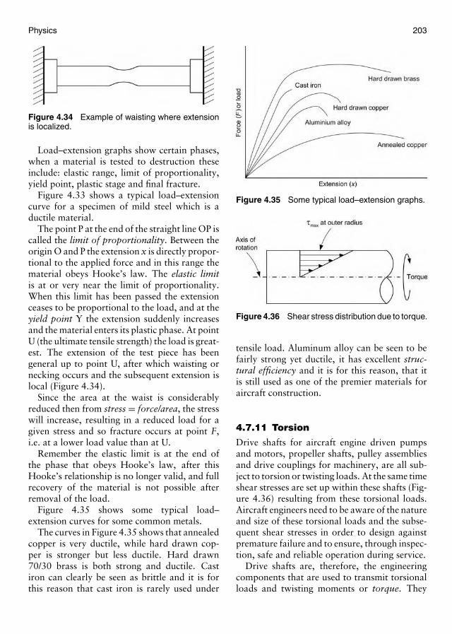
Physics 203
Figure 4.34 Example of waisting where extensionis localized.
Load–extension graphs show certain phases,when a material is tested to destruction theseinclude: elastic range, limit of proportionality,yield point, plastic stage and final fracture.
Figure 4.33 shows a typical load–extensioncurve for a specimen of mild steel which is aductile material.
The point P at the end of the straight line OP iscalled the limit of proportionality. Between theorigin O and P the extension x is directly propor-tional to the applied force and in this range thematerial obeys Hooke’s law. The elastic limitis at or very near the limit of proportionality.When this limit has been passed the extensionceases to be proportional to the load, and at theyield point Y the extension suddenly increasesand the material enters its plastic phase. At pointU (the ultimate tensile strength) the load is great-est. The extension of the test piece has beengeneral up to point U, after which waisting ornecking occurs and the subsequent extension islocal (Figure 4.34).
Since the area at the waist is considerablyreduced then from stress = force/area, the stresswill increase, resulting in a reduced load for agiven stress and so fracture occurs at point F,i.e. at a lower load value than at U.
Remember the elastic limit is at the end ofthe phase that obeys Hooke’s law, after thisHooke’s relationship is no longer valid, and fullrecovery of the material is not possible afterremoval of the load.
Figure 4.35 shows some typical load–extension curves for some common metals.
The curves in Figure 4.35 shows that annealedcopper is very ductile, while hard drawn cop-per is stronger but less ductile. Hard drawn70/30 brass is both strong and ductile. Castiron can clearly be seen as brittle and it is forthis reason that cast iron is rarely used under
Figure 4.35 Some typical load–extension graphs.
Figure 4.36 Shear stress distribution due to torque.
tensile load. Aluminum alloy can be seen to befairly strong yet ductile, it has excellent struc-tural efficiency and it is for this reason, that itis still used as one of the premier materials foraircraft construction.
4.7.11 Torsion
Drive shafts for aircraft engine driven pumpsand motors, propeller shafts, pulley assembliesand drive couplings for machinery, are all sub-ject to torsion or twisting loads. At the same timeshear stresses are set up within these shafts (Fig-ure 4.36) resulting from these torsional loads.Aircraft engineers need to be aware of the natureand size of these torsional loads and the subse-quent shear stresses in order to design againstpremature failure and to ensure, through inspec-tion, safe and reliable operation during service.
Drive shafts are, therefore, the engineeringcomponents that are used to transmit torsionalloads and twisting moments or torque. They
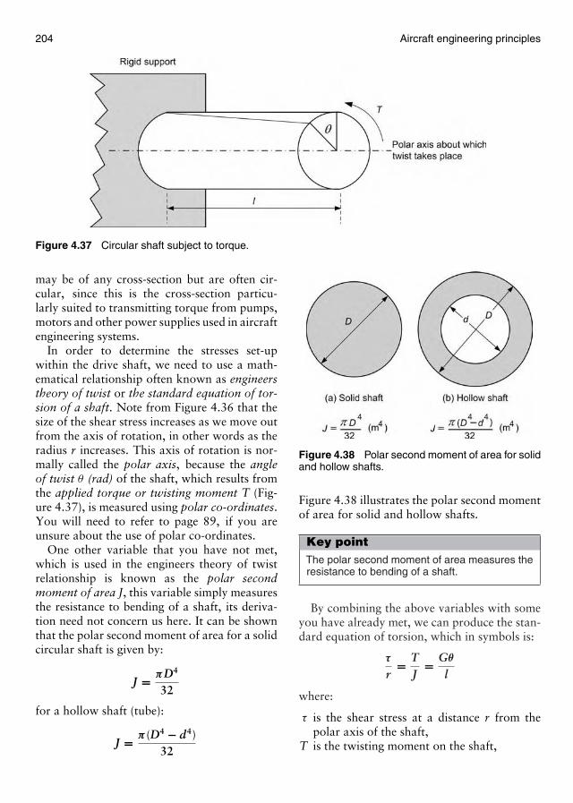
204 Aircraft engineering principles
Figure 4.37 Circular shaft subject to torque.
may be of any cross-section but are often cir-cular, since this is the cross-section particu-larly suited to transmitting torque from pumps,motors and other power supplies used in aircraftengineering systems.
In order to determine the stresses set-upwithin the drive shaft, we need to use a math-ematical relationship often known as engineerstheory of twist or the standard equation of tor-sion of a shaft. Note from Figure 4.36 that thesize of the shear stress increases as we move outfrom the axis of rotation, in other words as theradius r increases. This axis of rotation is nor-mally called the polar axis, because the angleof twist θ (rad) of the shaft, which results fromthe applied torque or twisting moment T (Fig-ure 4.37), is measured using polar co-ordinates.You will need to refer to page 89, if you areunsure about the use of polar co-ordinates.
One other variable that you have not met,which is used in the engineers theory of twistrelationship is known as the polar secondmoment of area J, this variable simply measuresthe resistance to bending of a shaft, its deriva-tion need not concern us here. It can be shownthat the polar second moment of area for a solidcircular shaft is given by:
J = πD4
32
for a hollow shaft (tube):
J = π (D4 − d4)32
Figure 4.38 Polar second moment of area for solidand hollow shafts.
Figure 4.38 illustrates the polar second momentof area for solid and hollow shafts.
Key pointThe polar second moment of area measures theresistance to bending of a shaft.
By combining the above variables with someyou have already met, we can produce the stan-dard equation of torsion, which in symbols is:
τ
r= T
J= Gθ
l
where:
τ is the shear stress at a distance r from thepolar axis of the shaft,
T is the twisting moment on the shaft,
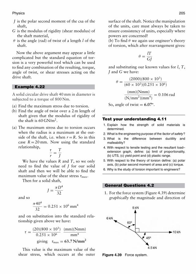
Physics 205
J is the polar second moment of the csa of theshaft,
G is the modulus of rigidity (shear modulus) ofthe shaft material,
θ is the angle (rad) of twist of a length l of theshaft.
Now the above argument may appear a littlecomplicated but the standard equation of tor-sion is a very powerful tool which can be usedto find any combination of the resulting, torque,angle of twist, or shear stresses acting on thedrive shaft.
Example 4.22
A solid circular drive shaft 40 mm in diameter issubjected to a torque of 800 Nm.
(a) Find the maximum stress due to torsion.(b) Find the angle of twist over a 2 m length of
shaft given that the modulus of rigidity ofthe shaft is 60 GN/m2.
(a) The maximum stress due to torsion occurswhen the radius is a maximum at the out-side of the shaft, i.e. when r = R. So in thiscase R = 20 mm. Now using the standardrelationship,
τ
r= T
JWe have the values R and T, so we only
need to find the value of J for our solidshaft and then we will be able to find themaximum value of the shear stress τmax.
Then for a solid shaft,
J = πD4
32and so
π404
32= 0.251 × 106 mm4
and on substitution into the standard rela-tionship given above we have:
τ = (20)(800 × 103)0.251 × 10⁶
(mm)(Nmm)mm4
giving τmax = 63.7 N/mm2
This value is the maximum value of theshear stress, which occurs at the outer
surface of the shaft. Notice the manipulationof the units, care must always be taken toensure consistency of units, especially wherepowers are concerned!(b) To find θ we again use engineer’s theoryof torsion, which after rearrangement gives:
θ = lTGJ
and substituting our known values for l, T,J and G we have:
θ = (2000)(800 × 103)(60 × 103)(0.251 × 10⁶)
(mm)(Nmm)
(N/mm2)(mm4)= 0.106 rad
So, angle of twist = 6.07◦.
Test your understanding 4.111. Explain how the strength of solid materials is
determined.
2. What is the engineering purpose of the factor of safety?
3. What is the difference between ductility andmalleability?
4. With respect to tensile testing and the resultant load–extension graph, define: (a) limit of proportionality,(b) UTS, (c) yield point and (d) plastic range.
5. With respect to the theory of torsion define: (a) polaraxis, (b) polar second moment of area and (c) torque.
6. Why is the study of torsion important to engineers?
General Questions 4.2
1. For the force system (Figure 4.39) determinegraphically the magnitude and direction of
Figure 4.39 Force system.
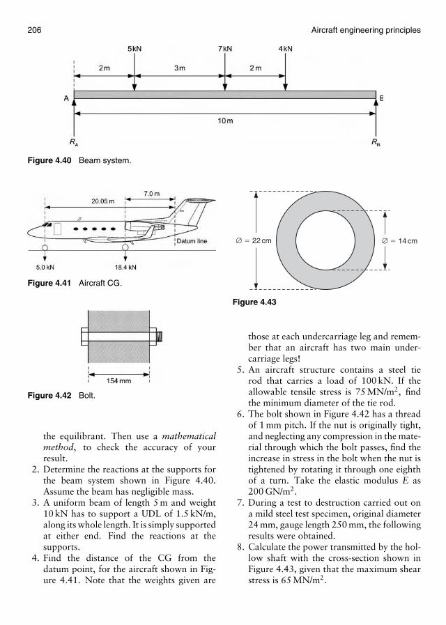
206 Aircraft engineering principles
Figure 4.40 Beam system.
Figure 4.41 Aircraft CG.
Figure 4.42 Bolt.
the equilibrant. Then use a mathematicalmethod, to check the accuracy of yourresult.
2. Determine the reactions at the supports forthe beam system shown in Figure 4.40.Assume the beam has negligible mass.
3. A uniform beam of length 5 m and weight10 kN has to support a UDL of 1.5 kN/m,along its whole length. It is simply supportedat either end. Find the reactions at thesupports.
4. Find the distance of the CG from thedatum point, for the aircraft shown in Fig-ure 4.41. Note that the weights given are
∅ � 14 cm∅ � 22 cm
Figure 4.43
those at each undercarriage leg and remem-ber that an aircraft has two main under-carriage legs!
5. An aircraft structure contains a steel tierod that carries a load of 100 kN. If theallowable tensile stress is 75 MN/m2, findthe minimum diameter of the tie rod.
6. The bolt shown in Figure 4.42 has a threadof 1 mm pitch. If the nut is originally tight,and neglecting any compression in the mate-rial through which the bolt passes, find theincrease in stress in the bolt when the nut istightened by rotating it through one eighthof a turn. Take the elastic modulus E as200 GN/m2.
7. During a test to destruction carried out ona mild steel test specimen, original diameter24 mm, gauge length 250 mm, the followingresults were obtained.
8. Calculate the power transmitted by the hol-low shaft with the cross-section shown inFigure 4.43, given that the maximum shearstress is 65 MN/m2.
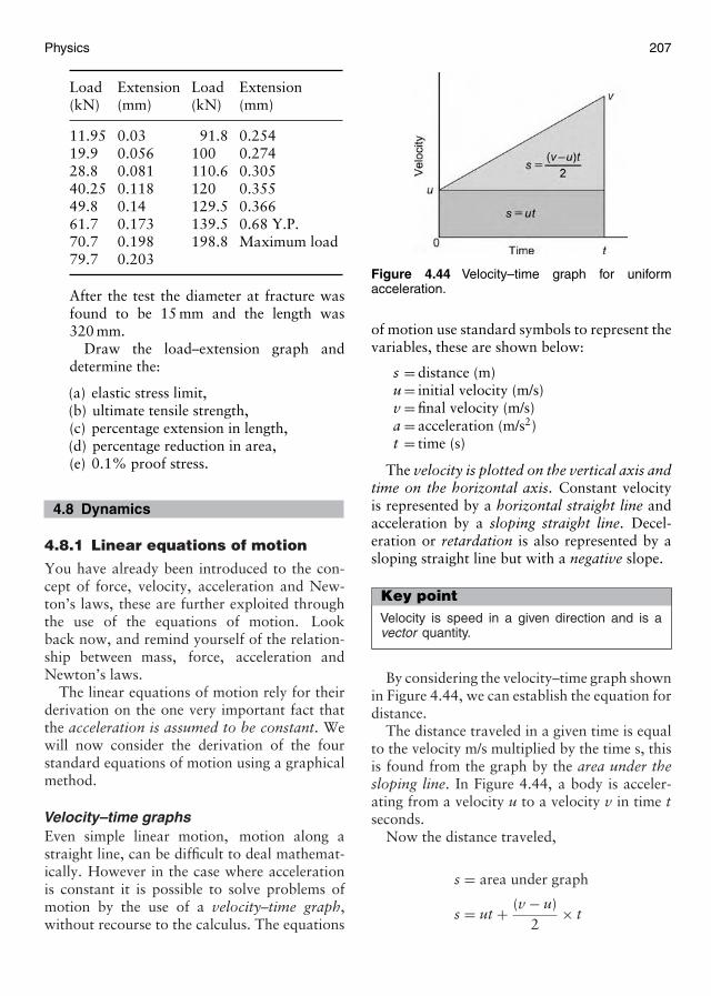
Physics 207
Load Extension Load Extension(kN) (mm) (kN) (mm)
11.95 0.03 91.8 0.25419.9 0.056 100 0.27428.8 0.081 110.6 0.30540.25 0.118 120 0.35549.8 0.14 129.5 0.36661.7 0.173 139.5 0.68 Y.P.70.7 0.198 198.8 Maximum load79.7 0.203
After the test the diameter at fracture wasfound to be 15 mm and the length was320 mm.
Draw the load–extension graph anddetermine the:
(a) elastic stress limit,(b) ultimate tensile strength,(c) percentage extension in length,(d) percentage reduction in area,(e) 0.1% proof stress.
4.8 Dynamics
4.8.1 Linear equations of motion
You have already been introduced to the con-cept of force, velocity, acceleration and New-ton’s laws, these are further exploited throughthe use of the equations of motion. Lookback now, and remind yourself of the relation-ship between mass, force, acceleration andNewton’s laws.
The linear equations of motion rely for theirderivation on the one very important fact thatthe acceleration is assumed to be constant. Wewill now consider the derivation of the fourstandard equations of motion using a graphicalmethod.
Velocity–time graphsEven simple linear motion, motion along astraight line, can be difficult to deal mathemat-ically. However in the case where accelerationis constant it is possible to solve problems ofmotion by the use of a velocity–time graph,without recourse to the calculus. The equations
Figure 4.44 Velocity–time graph for uniformacceleration.
of motion use standard symbols to represent thevariables, these are shown below:
s = distance (m)u = initial velocity (m/s)v = final velocity (m/s)a = acceleration (m/s2)t = time (s)
The velocity is plotted on the vertical axis andtime on the horizontal axis. Constant velocityis represented by a horizontal straight line andacceleration by a sloping straight line. Decel-eration or retardation is also represented by asloping straight line but with a negative slope.
Key pointVelocity is speed in a given direction and is avector quantity.
By considering the velocity–time graph shownin Figure 4.44, we can establish the equation fordistance.
The distance traveled in a given time is equalto the velocity m/s multiplied by the time s, thisis found from the graph by the area under thesloping line. In Figure 4.44, a body is acceler-ating from a velocity u to a velocity v in time tseconds.
Now the distance traveled,
s = area under graph
s = ut + (v − u)2
× t

208 Aircraft engineering principles
s = ut + vt2
− ut2
s = (2u + v − u)t2
Thus,
s = (u + v)t2
In a similar manner to above, one of the veloc-ity equations can also be obtained from thevelocity–time graph. Since the acceleration is therate of change of velocity with respect to time,the value of the acceleration will be equal tothe gradient of a velocity–time graph. Therefore,from Figure 4.44, we have:
Gradient = Change in velocityTime taken
= Acceleration
therefore acceleration is given by,
a = v − ut
or
v = u + at
The remaining equations of motion may bederived from the two equations found above.Try now, as an exercise in manipulating formu-lae, to obtain:
(a) the equation t = v − ua
,
(b) s = ut + 12 at2,
using the above equations.
Example 4.23
A body starts from rest and accelerates withconstant acceleration of 2.0 m/s2 up to a speedof 9 m/s. It then travels at 9 m/s for 15 s afterwhich, it is retarded to a speed of 1 m/s. If thecomplete motion takes 24.5 s, find the:(a) time taken to reach 9 m/s,(b) retardation,(c) total distance traveled.
The solution is made easier if we sketch a graphof the motion, as shown in Figure 4.45.
Figure 4.45 Velocity–time graph of the motion.
(a) We first tabulate the known values:
u = 0 m/s (we start from rest)
v = 9 m/s
a = 2 m/s2
t = ?
All we need to do now is select an equationwhich contains all the variables listed above,
i.e. v = u + at
and on transposing for t and substituting thevariables we get,
t = 9 − 02
so t = 4.5 s
(b) The retardation is found in a similar manner.
u = 9 m/s
v = 2 m/s
t = 5 s
a = ?
We again select an equation which con-tains the variables,
i.e. v = u + at
and on transposing for a and substituting thevariables we get,
a = 1 − 95
so a = −1.6 m/s2
(the −ve sign indicates a retardation)
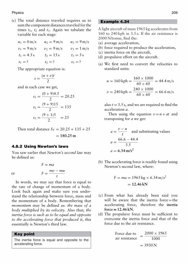
Physics 209
(c) The total distance traveled requires us tosum the component distances traveled for thetimes t1, t2 and t3. Again we tabulate thevariable for each stage:
u1 = 0 m/s u2 = 9 m/s u3 = 9 m/s
v1 = 9 m/s v2 = 9 m/s v3 = 1 m/s
t1 = 4.5 s t2 = 15 s t3 = 5 s
s1 = ? s2 = ? s3 = ?
The appropriate equation is:
s = (u + v)t2
and in each case we get,
s1 = (0 + 9)4.52
= 20.25
s2 = (9 + 9)152
= 135
s3 = (9 + 1)52
= 25
Then total distance ST = 20.25 + 135 + 25
= 180.25 m
4.8.2 Using Newton’s laws
You saw earlier that Newton’s second law maybe defined as:
F = ma
or F = mv − mut
In words, we may say that force is equal tothe rate of change of momentum of a body.Look back again and make sure you under-stand the relationship between force, mass andthe momentum of a body. Remembering thatmomentum may be defined as: the mass of abody multiplied by its velocity. Also that; theinertia force is such as to be equal and oppositeto the accelerating force that produced it, thisessentially is Newton’s third law.
Key pointThe inertia force is equal and opposite to theaccelerating force.
Example 4.24
A light aircraft of mass 1965 kg accelerates from160 to 240 kph in 3.5 s. If the air resistance is2000 N/tonne, find the:(a) average acceleration,(b) force required to produce the acceleration,(c) inertia force on the aircraft,(d) propulsive effort on the aircraft.
(a) We first need to convert the velocities tostandard units:
u = 160 kph = 160 × 100060 × 60
= 44.4 m/s
v = 240 kph = 240 × 100060 × 60
= 66.6 m/s
also t = 3.5 s, and we are required to find theacceleration a.
Then using the equation v = u + at andtransposing for a we get:
a = v − ut
and substituting values
a = 66.6 − 44.43.5
a = 6.34 m/s2
(b) The accelerating force is readily found usingNewton’s second law, where:
F = ma = 1965 kg × 6.34 m/s2
= 12.46 kN
(c) From what has already been said youwill be aware that the inertia force = theaccelerating force, therefore the inertiaforce = 12.46 kN.
(d) The propulsive force must be sufficient toovercome the inertia force and that of theforce due to the air resistance.
Force due toair resistance
= 2000 × 19651000
= 3930 N
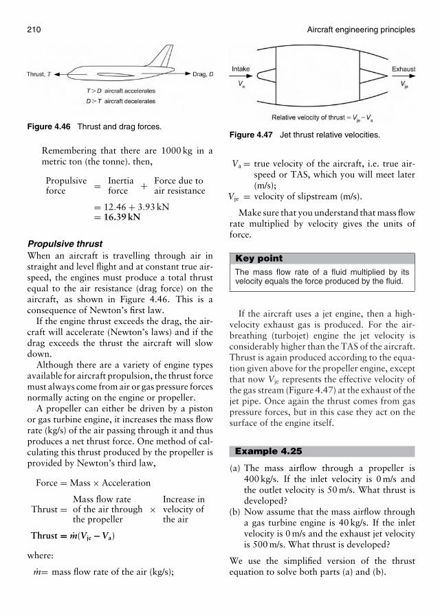
210 Aircraft engineering principles
Figure 4.46 Thrust and drag forces.
Remembering that there are 1000 kg in ametric ton (the tonne). then,
Propulsiveforce = Inertia
force + Force due toair resistance
= 12.46 + 3.93 kN= 16.39 kN
Propulsive thrustWhen an aircraft is travelling through air instraight and level flight and at constant true air-speed, the engines must produce a total thrustequal to the air resistance (drag force) on theaircraft, as shown in Figure 4.46. This is aconsequence of Newton’s first law.
If the engine thrust exceeds the drag, the air-craft will accelerate (Newton’s laws) and if thedrag exceeds the thrust the aircraft will slowdown.
Although there are a variety of engine typesavailable for aircraft propulsion, the thrust forcemust always come from air or gas pressure forcesnormally acting on the engine or propeller.
A propeller can either be driven by a pistonor gas turbine engine, it increases the mass flowrate (kg/s) of the air passing through it and thusproduces a net thrust force. One method of cal-culating this thrust produced by the propeller isprovided by Newton’s third law,
Force = Mass × Acceleration
Thrust =Mass flow rateof the air throughthe propeller
×Increase invelocity ofthe air
Thrust = m(Vje − Va)
where:
m= mass flow rate of the air (kg/s);
Figure 4.47 Jet thrust relative velocities.
Va = true velocity of the aircraft, i.e. true air-speed or TAS, which you will meet later(m/s);
Vje = velocity of slipstream (m/s).
Make sure that you understand that mass flowrate multiplied by velocity gives the units offorce.
Key pointThe mass flow rate of a fluid multiplied by itsvelocity equals the force produced by the fluid.
If the aircraft uses a jet engine, then a high-velocity exhaust gas is produced. For the air-breathing (turbojet) engine the jet velocity isconsiderably higher than the TAS of the aircraft.Thrust is again produced according to the equa-tion given above for the propeller engine, exceptthat now Vje represents the effective velocity ofthe gas stream (Figure 4.47) at the exhaust of thejet pipe. Once again the thrust comes from gaspressure forces, but in this case they act on thesurface of the engine itself.
Example 4.25
(a) The mass airflow through a propeller is400 kg/s. If the inlet velocity is 0 m/s andthe outlet velocity is 50 m/s. What thrust isdeveloped?
(b) Now assume that the mass airflow througha gas turbine engine is 40 kg/s. If the inletvelocity is 0 m/s and the exhaust jet velocityis 500 m/s. What thrust is developed?
We use the simplified version of the thrustequation to solve both parts (a) and (b).

Physics 211
Figure 4.48
(a) Thrust force = m(Vje − Va)= 400(50 − 0) = 20 kN
(b) Thrust force = m(Vje − Va)= 40(500 − 0) = 20 kN
Make sure you work through the above calcu-lations and understand the units.
This simplified example shows that in orderto develop similar amounts of thrust we mayaccelerate a large mass of air at relatively lowspeed or accelerate a small mass of air at rel-atively high speed. If, in the future, you studyaircraft propulsion in detail you will see that theformer method of developing thrust in a gas tur-bine engine, is more efficient. This is why theseengines are used in most modern commercialairliners.
Engine thrust is often quoted in lb, with thereference to force being ignored. When we useImperial units, the formula for thrust becomes:
Thrust force (lb) = wg
(Vje − Va)
where w = flow rate of air (lb/s), g = accelerationdue to gravity (32 ft/s2), Vje = velocity of slip-stream or exhaust (as before) but units are
ft/s, Va = aircraft velocity (TAS) but unitsare ft/s.
Using the above formula, with the unitsstated, will give thrust in lbf. We generally quotethrust in lb and simply ignore the reference toforce.
Example 4.26
A twin-engine gas turbine powered aircraft isat rest and preparing for take-off. Each enginemass airflow at take-off is 80 lb/s and theexhaust velocity for each engine is 1400 ft/s.What thrust is being produced by each engine?
Now, w = 80 lb/s, Va = 0 and Vje = 1400,
g = 32.2 ft/s2
Thrust = 8032.2
(1400 − 0) = 3478.3 lb
Test your understanding 4.12With reference to the velocity–time graphs shown overleaf(Figure 4.48), answer questions 1 to 8.

212 Aircraft engineering principles
Fill in the gaps for questions 1 to 8.
1. The slope of the velocity–time graph measures_______.
2. The area under a velocity–time graph determines_______.
3. Average velocity may be determined by dividing the_______, _______ by _______, _______.
4. Graph (a) is a graph of constant velocity thereforeacceleration is given by ________ and the distancetraveled is equal to __________.
5. Graph (b) shows uniformly accelerated motion there-fore the distance traveled is equal to __________.
6. Graph (c) shows _________, _________, _________.
7. Graph (d) represents uniformly accelerated motion hav-ing initial velocity u, final velocity v and acceleration a.So distanced traveled is equal to _________.
8. Graph (e) represents _________.
9. Define the terms: (a) inertia force and (b) momentum.
10. What is the essential difference between speed andvelocity?
11. If a rocket is sent to the moon, its mass remainsconstant but its weight changes, explain this statement.
12. Explain how the expression F = ma is related to therate of change of momentum with respect to Newton’ssecond law.
13. Define V je for (a) the propeller engine and (b) the jetengine.
14. Under what operating circumstances would the thrustproduced by a jet engine be a maximum?
4.8.3 Angular motion
You previously met the equations for linearmotion. A similar set of equations exists tosolve engineering problems that involve angu-lar motion as experienced, e.g. in the rotationof a drive shaft. The linear equations of motionmay be transformed to represent angular motionusing a set of equations that we will refer to asthe transformation equations. These are givenbelow, followed by the equations of angularmotion, which are compared with their linearequivalents.
Transformation equations
s = θrv = ωra = αr
where r = radius of body from center of rotationand θ , ω and α are the angular distance, angularvelocity and angular acceleration, respectively.
Angular equation Linear equationof motion of motion
θ = (ω1 + ω2)t/2 s = (u + v)t/2θ = ω1t + 1
2 αt2 s = ut + 12 at2
ω22 = ω2
1 + 2αθ v2 = u2 + 2 asα = (ω2 − ω1)/t a = (v − u)/t
Angular velocityAngular velocity (ω) refers to a body moving ina circular path and may be defined as:
ω = Angular distance moved (rad)Time taken (s)
or in symbols ω = θ /s (radians per second).Angular distance is measured in rad, you
should refer back to page 122 if you cannotremember the definition of the radian or howto convert radians to degrees and vice versa.
We are often given rotational velocity in rpm.It is therefore useful to be able to convert rpminto rad/s and vice versa.
Key point1 rev = 2π rad (from the definition of the radian).
Key point1 rpm = 2π rad/min = 2π /60 rad/s.
So, e.g. to convert 350 rpm into rad/s wemultiply by 2π /60, i.e.
350 rpm = 350 × 2π
60= 36.65 rad/s
Example 4.27
A 540 mm diameter wheel is rotating at1500/π rpm. Determine the angular velocity ofwheel in rad/s and the linear velocity of a pointon the rim of the wheel.
All we need to do to find the angular velocity isconvert rpm to rad/s, i.e.
Angular velocity (rad/s) = 1500π
× 2π
60= 50 rad/s
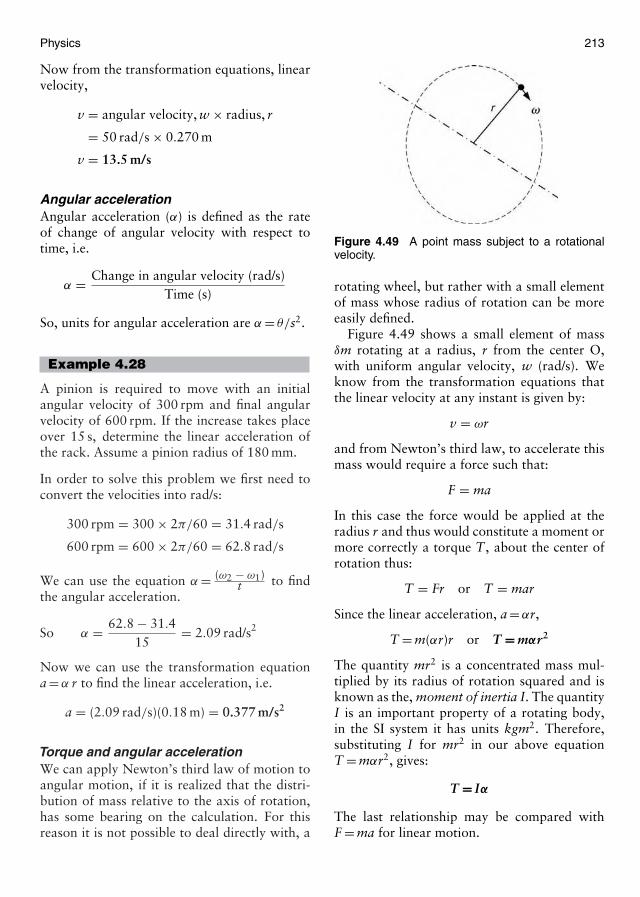
Physics 213
Now from the transformation equations, linearvelocity,
v = angular velocity, w × radius, r
= 50 rad/s × 0.270 m
v = 13.5 m/s
Angular accelerationAngular acceleration (α) is defined as the rateof change of angular velocity with respect totime, i.e.
α = Change in angular velocity (rad/s)Time (s)
So, units for angular acceleration are α = θ/s2.
Example 4.28
A pinion is required to move with an initialangular velocity of 300 rpm and final angularvelocity of 600 rpm. If the increase takes placeover 15 s, determine the linear acceleration ofthe rack. Assume a pinion radius of 180 mm.
In order to solve this problem we first need toconvert the velocities into rad/s:
300 rpm = 300 × 2π/60 = 31.4 rad/s
600 rpm = 600 × 2π/60 = 62.8 rad/s
We can use the equation α = (ω2 − ω1)t to find
the angular acceleration.
So α = 62.8 − 31.415
= 2.09 rad/s2
Now we can use the transformation equationa = α r to find the linear acceleration, i.e.
a = (2.09 rad/s)(0.18 m) = 0.377 m/s2
Torque and angular accelerationWe can apply Newton’s third law of motion toangular motion, if it is realized that the distri-bution of mass relative to the axis of rotation,has some bearing on the calculation. For thisreason it is not possible to deal directly with, a
Figure 4.49 A point mass subject to a rotationalvelocity.
rotating wheel, but rather with a small elementof mass whose radius of rotation can be moreeasily defined.
Figure 4.49 shows a small element of massδm rotating at a radius, r from the center O,with uniform angular velocity, w (rad/s). Weknow from the transformation equations thatthe linear velocity at any instant is given by:
v = ωr
and from Newton’s third law, to accelerate thismass would require a force such that:
F = ma
In this case the force would be applied at theradius r and thus would constitute a moment ormore correctly a torque T, about the center ofrotation thus:
T = Fr or T = mar
Since the linear acceleration, a = αr,
T = m(αr)r or T = mαr2
The quantity mr2 is a concentrated mass mul-tiplied by its radius of rotation squared and isknown as the, moment of inertia I. The quantityI is an important property of a rotating body,in the SI system it has units kgm2. Therefore,substituting I for mr2 in our above equationT = mαr2, gives:
T = Iα
The last relationship may be compared withF = ma for linear motion.
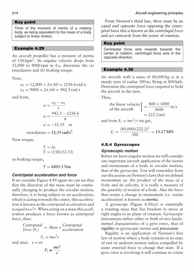
214 Aircraft engineering principles
Key pointThink of the moment of inertia of a rotatingbody, as being equivalent to the mass of a bodysubject to linear motion.
Example 4.29
An aircraft propeller has a moment of inertiaof 130 kgm2. Its angular velocity drops from12,000 to 9000 rpm in 6 s, determine the (a)retardation and (b) braking torque.
Now,
ω1 = 12,000 × 2π/60 = 1256.6 rad/sω2 = 9000 × 2π/60 = 942.5 rad/s
and from,
α = ω2 − ω1
t
α = 942.5 − 1256.66
α = −52.35 or
retardation = 52.35 rad/s2
Now torque,
T = IαT = (130)(52.35)
so braking torque,
T = 6805.5 Nm
Centripetal acceleration and forceIf we consider Figure 4.49 again we can see thatthat the direction of the mass must be contin-ually changing to produce the circular motion,therefore, it is being subject to an acceleration,which is acting towards the center, this accelera-tion is known as the centripetal acceleration andis equal to ω2r. When acting on a mass this accel-eration produces a force known as centripetalforce, thus:
Centripetalforce (Fc)
= Mass × Centripetalacceleration
Fc = mω2rand since v = ωr
Fc = mv2
r
From Newton’s third law, there must be anequal and opposite force opposing the centri-petal force this is known as the centrifugal forceand act outwards from the center of rotation.
Key pointCentripetal force acts inwards towards thecenter of rotation, centrifugal force acts in theopposite direction.
Example 4.30
An aircraft with a mass of 80,000 kg is in asteady turn of radius 300 m, flying at 800 kph.Determine the centripetal force required to holdthe aircraft in the turn.
Then,
the linear velocityof the aircraft
}= 800 × 1000
3600m/s
= 222.2 m/s
and from Fc = mv2/r we get,
Fc = (80,000)(222.2)2
300= 13.17 MN
4.8.4 Gyroscopes
Gyroscopic motionBefore we leave angular motion we will considerone important aircraft application of the inertiaand momentum of a body in circular motion,that of the gyroscope. You will remember fromour discussion on Newton’s laws that we definedmomentum as: the product of the mass of abody and its velocity, it is really a measure ofthe quantity of motion of a body. Also the forcethat resists a change in momentum (i.e. resistsacceleration) is known as inertia.
A gyroscope (Figure 4.50(a)) is essentiallya rotating mass that has freedom to move atright angles to its plane of rotation. Gyroscopicinstruments utilize either or both of two funda-mental characteristics of a gyro rotor, that ofrigidity or gyroscopic inertia and precession.
Rigidity is an application of Newton’s firstlaw of motion where a body remains in its stateof rest or uniform motion unless compelled bysome external force to change that state. If agyro rotor is revolving it will continue to rotate
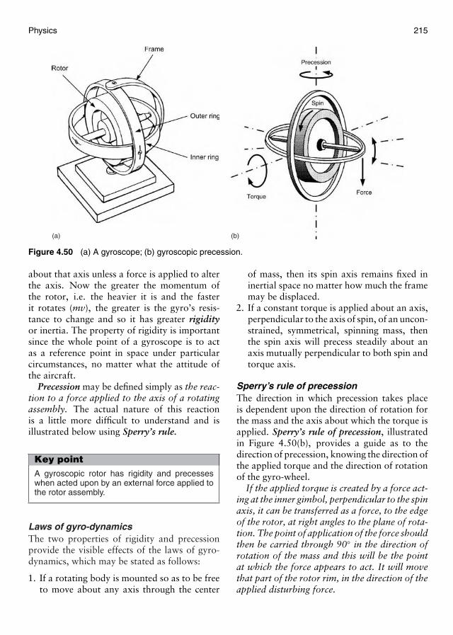
Physics 215
(a) (b)
Figure 4.50 (a) A gyroscope; (b) gyroscopic precession.
about that axis unless a force is applied to alterthe axis. Now the greater the momentum ofthe rotor, i.e. the heavier it is and the fasterit rotates (mv), the greater is the gyro’s resis-tance to change and so it has greater rigidityor inertia. The property of rigidity is importantsince the whole point of a gyroscope is to actas a reference point in space under particularcircumstances, no matter what the attitude ofthe aircraft.
Precession may be defined simply as the reac-tion to a force applied to the axis of a rotatingassembly. The actual nature of this reactionis a little more difficult to understand and isillustrated below using Sperry’s rule.
Key pointA gyroscopic rotor has rigidity and precesseswhen acted upon by an external force applied tothe rotor assembly.
Laws of gyro-dynamicsThe two properties of rigidity and precessionprovide the visible effects of the laws of gyro-dynamics, which may be stated as follows:
1. If a rotating body is mounted so as to be freeto move about any axis through the center
of mass, then its spin axis remains fixed ininertial space no matter how much the framemay be displaced.
2. If a constant torque is applied about an axis,perpendicular to the axis of spin, of an uncon-strained, symmetrical, spinning mass, thenthe spin axis will precess steadily about anaxis mutually perpendicular to both spin andtorque axis.
Sperry’s rule of precessionThe direction in which precession takes placeis dependent upon the direction of rotation forthe mass and the axis about which the torque isapplied. Sperry’s rule of precession, illustratedin Figure 4.50(b), provides a guide as to thedirection of precession, knowing the direction ofthe applied torque and the direction of rotationof the gyro-wheel.
If the applied torque is created by a force act-ing at the inner gimbol, perpendicular to the spinaxis, it can be transferred as a force, to the edgeof the rotor, at right angles to the plane of rota-tion. The point of application of the force shouldthen be carried through 90◦ in the direction ofrotation of the mass and this will be the pointat which the force appears to act. It will movethat part of the rotor rim, in the direction of theapplied disturbing force.
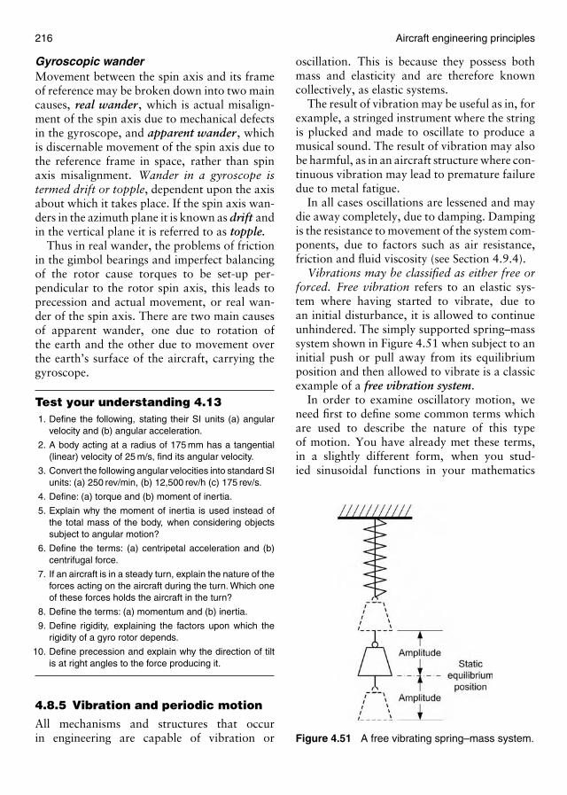
216 Aircraft engineering principles
Gyroscopic wanderMovement between the spin axis and its frameof reference may be broken down into two maincauses, real wander , which is actual misalign-ment of the spin axis due to mechanical defectsin the gyroscope, and apparent wander , whichis discernable movement of the spin axis due tothe reference frame in space, rather than spinaxis misalignment. Wander in a gyroscope istermed drift or topple, dependent upon the axisabout which it takes place. If the spin axis wan-ders in the azimuth plane it is known as drift andin the vertical plane it is referred to as topple.
Thus in real wander, the problems of frictionin the gimbol bearings and imperfect balancingof the rotor cause torques to be set-up per-pendicular to the rotor spin axis, this leads toprecession and actual movement, or real wan-der of the spin axis. There are two main causesof apparent wander, one due to rotation ofthe earth and the other due to movement overthe earth’s surface of the aircraft, carrying thegyroscope.
Test your understanding 4.131. Define the following, stating their SI units (a) angular
velocity and (b) angular acceleration.
2. A body acting at a radius of 175 mm has a tangential(linear) velocity of 25 m/s, find its angular velocity.
3. Convert the following angular velocities into standard SIunits: (a) 250 rev/min, (b) 12,500 rev/h (c) 175 rev/s.
4. Define: (a) torque and (b) moment of inertia.
5. Explain why the moment of inertia is used instead ofthe total mass of the body, when considering objectssubject to angular motion?
6. Define the terms: (a) centripetal acceleration and (b)centrifugal force.
7. If an aircraft is in a steady turn, explain the nature of theforces acting on the aircraft during the turn. Which oneof these forces holds the aircraft in the turn?
8. Define the terms: (a) momentum and (b) inertia.
9. Define rigidity, explaining the factors upon which therigidity of a gyro rotor depends.
10. Define precession and explain why the direction of tiltis at right angles to the force producing it.
4.8.5 Vibration and periodic motion
All mechanisms and structures that occurin engineering are capable of vibration or
oscillation. This is because they possess bothmass and elasticity and are therefore knowncollectively, as elastic systems.
The result of vibration may be useful as in, forexample, a stringed instrument where the stringis plucked and made to oscillate to produce amusical sound. The result of vibration may alsobe harmful, as in an aircraft structure where con-tinuous vibration may lead to premature failuredue to metal fatigue.
In all cases oscillations are lessened and maydie away completely, due to damping. Dampingis the resistance to movement of the system com-ponents, due to factors such as air resistance,friction and fluid viscosity (see Section 4.9.4).
Vibrations may be classified as either free orforced. Free vibration refers to an elastic sys-tem where having started to vibrate, due toan initial disturbance, it is allowed to continueunhindered. The simply supported spring–masssystem shown in Figure 4.51 when subject to aninitial push or pull away from its equilibriumposition and then allowed to vibrate is a classicexample of a free vibration system.
In order to examine oscillatory motion, weneed first to define some common terms whichare used to describe the nature of this typeof motion. You have already met these terms,in a slightly different form, when you stud-ied sinusoidal functions in your mathematics
Figure 4.51 A free vibrating spring–mass system.
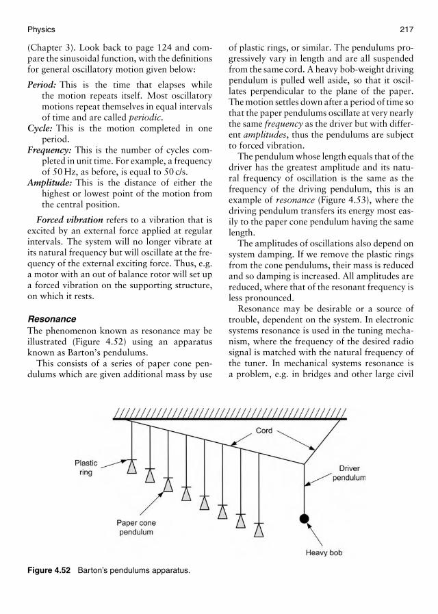
Physics 217
(Chapter 3). Look back to page 124 and com-pare the sinusoidal function, with the definitionsfor general oscillatory motion given below:
Period: This is the time that elapses whilethe motion repeats itself. Most oscillatorymotions repeat themselves in equal intervalsof time and are called periodic.
Cycle: This is the motion completed in oneperiod.
Frequency: This is the number of cycles com-pleted in unit time. For example, a frequencyof 50 Hz, as before, is equal to 50 c/s.
Amplitude: This is the distance of either thehighest or lowest point of the motion fromthe central position.
Forced vibration refers to a vibration that isexcited by an external force applied at regularintervals. The system will no longer vibrate atits natural frequency but will oscillate at the fre-quency of the external exciting force. Thus, e.g.a motor with an out of balance rotor will set upa forced vibration on the supporting structure,on which it rests.
ResonanceThe phenomenon known as resonance may beillustrated (Figure 4.52) using an apparatusknown as Barton’s pendulums.
This consists of a series of paper cone pen-dulums which are given additional mass by use
Figure 4.52 Barton’s pendulums apparatus.
of plastic rings, or similar. The pendulums pro-gressively vary in length and are all suspendedfrom the same cord. A heavy bob-weight drivingpendulum is pulled well aside, so that it oscil-lates perpendicular to the plane of the paper.The motion settles down after a period of time sothat the paper pendulums oscillate at very nearlythe same frequency as the driver but with differ-ent amplitudes, thus the pendulums are subjectto forced vibration.
The pendulum whose length equals that of thedriver has the greatest amplitude and its natu-ral frequency of oscillation is the same as thefrequency of the driving pendulum, this is anexample of resonance (Figure 4.53), where thedriving pendulum transfers its energy most eas-ily to the paper cone pendulum having the samelength.
The amplitudes of oscillations also depend onsystem damping. If we remove the plastic ringsfrom the cone pendulums, their mass is reducedand so damping is increased. All amplitudes arereduced, where that of the resonant frequency isless pronounced.
Resonance may be desirable or a source oftrouble, dependent on the system. In electronicsystems resonance is used in the tuning mecha-nism, where the frequency of the desired radiosignal is matched with the natural frequency ofthe tuner. In mechanical systems resonance isa problem, e.g. in bridges and other large civil
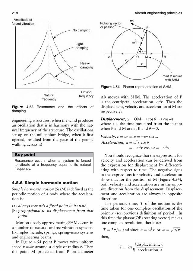
218 Aircraft engineering principles
Figure 4.53 Resonance and the effects ofdamping.
engineering structures, when the wind producesan oscillation that is in harmony with the nat-ural frequency of the structure. The oscillationsset-up on the millennium bridge, when it firstopened, resulted from the pace of the peoplewalking across it!
Key pointResonance occurs when a system is forcedto vibrate at a frequency equal to its naturalfrequency.
4.8.6 Simple harmonic motion
Simple harmonic motion (SHM) is defined as theperiodic motion of a body where the accelera-tion is:
(a) always towards a fixed point in its path,(b) proportional to its displacement from that
point.
Motion closely approximating SHM occurs ina number of natural or free vibration systems.Examples include, springs, spring–mass systemsand engineering beams.
In Figure 4.54 point P moves with uniformspeed v = ωr around a circle of radius r. Thenthe point M projected from P on diameter
Figure 4.54 Phasor representation of SHM.
AB moves with SHM. The acceleration of Pis the centripetal acceleration, ω2r. Then thedisplacement, velocity and acceleration of M arerespectively:
Displacement, x = OM = r cos θ = r cos ωtwhere t is the time measured from the instantwhen P and M are at B and θ = 0.
Velocity, v = ωr sin θ = −ωr sin ωt
Acceleration, a = ω2r cos θ
= −ω2r cos ωt = −ω2x
You should recognize that the expressions forvelocity and acceleration can be derived fromthe expression for displacement by differenti-ating with respect to time. The negative signsin the expressions for velocity and accelerationshow that for the position of M (Figure 4.54),both velocity and acceleration are in the oppo-site direction from the displacement. Displace-ment and acceleration are always in oppositedirections.
The periodic time, T of the motion is thetime taken for one complete oscillation of thepoint x (see previous definition of period). Inthis time the phasor OP (rotating vector) makesone complete revolution, therefore:
T = 2π/ω and since a = ω2x or ω = √a/x
then,
T = 2π
√displacement, xacceleration, a
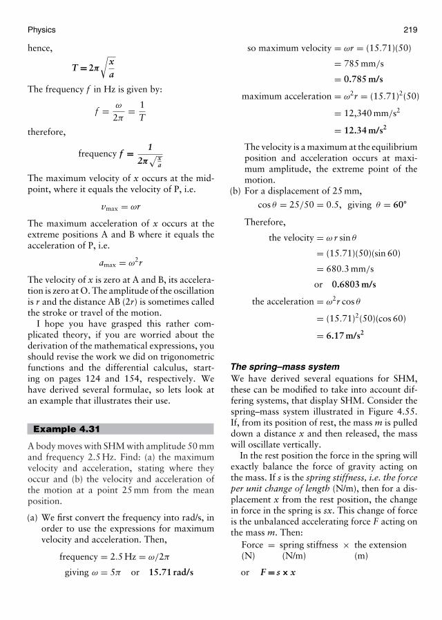
Physics 219
hence,
T = 2π
√xa
The frequency f in Hz is given by:
f = ω
2π= 1
T
therefore,
frequency f = 1
2π√ x
a
The maximum velocity of x occurs at the mid-point, where it equals the velocity of P, i.e.
vmax = ωr
The maximum acceleration of x occurs at theextreme positions A and B where it equals theacceleration of P, i.e.
amax = ω2r
The velocity of x is zero at A and B, its accelera-tion is zero at O. The amplitude of the oscillationis r and the distance AB (2r) is sometimes calledthe stroke or travel of the motion.
I hope you have grasped this rather com-plicated theory, if you are worried about thederivation of the mathematical expressions, youshould revise the work we did on trigonometricfunctions and the differential calculus, start-ing on pages 124 and 154, respectively. Wehave derived several formulae, so lets look atan example that illustrates their use.
Example 4.31
A body moves with SHM with amplitude 50 mmand frequency 2.5 Hz. Find: (a) the maximumvelocity and acceleration, stating where theyoccur and (b) the velocity and acceleration ofthe motion at a point 25 mm from the meanposition.
(a) We first convert the frequency into rad/s, inorder to use the expressions for maximumvelocity and acceleration. Then,
frequency = 2.5 Hz = ω/2π
giving ω = 5π or 15.71 rad/s
so maximum velocity = ωr = (15.71)(50)
= 785 mm/s
= 0.785 m/s
maximum acceleration = ω2r = (15.71)2(50)
= 12,340 mm/s2
= 12.34 m/s2
The velocity is a maximum at the equilibriumposition and acceleration occurs at maxi-mum amplitude, the extreme point of themotion.
(b) For a displacement of 25 mm,
cos θ = 25/50 = 0.5, giving θ = 60◦
Therefore,
the velocity = ω r sin θ
= (15.71)(50)(sin 60)
= 680.3 mm/s
or 0.6803 m/s
the acceleration = ω2r cos θ
= (15.71)2(50)(cos 60)
= 6.17 m/s2
The spring–mass systemWe have derived several equations for SHM,these can be modified to take into account dif-fering systems, that display SHM. Consider thespring–mass system illustrated in Figure 4.55.If, from its position of rest, the mass m is pulleddown a distance x and then released, the masswill oscillate vertically.
In the rest position the force in the spring willexactly balance the force of gravity acting onthe mass. If s is the spring stiffness, i.e. the forceper unit change of length (N/m), then for a dis-placement x from the rest position, the changein force in the spring is sx. This change of forceis the unbalanced accelerating force F acting onthe mass m. Then:
Force(N)
= spring stiffness(N/m)
× the extension(m)
or F = s × x
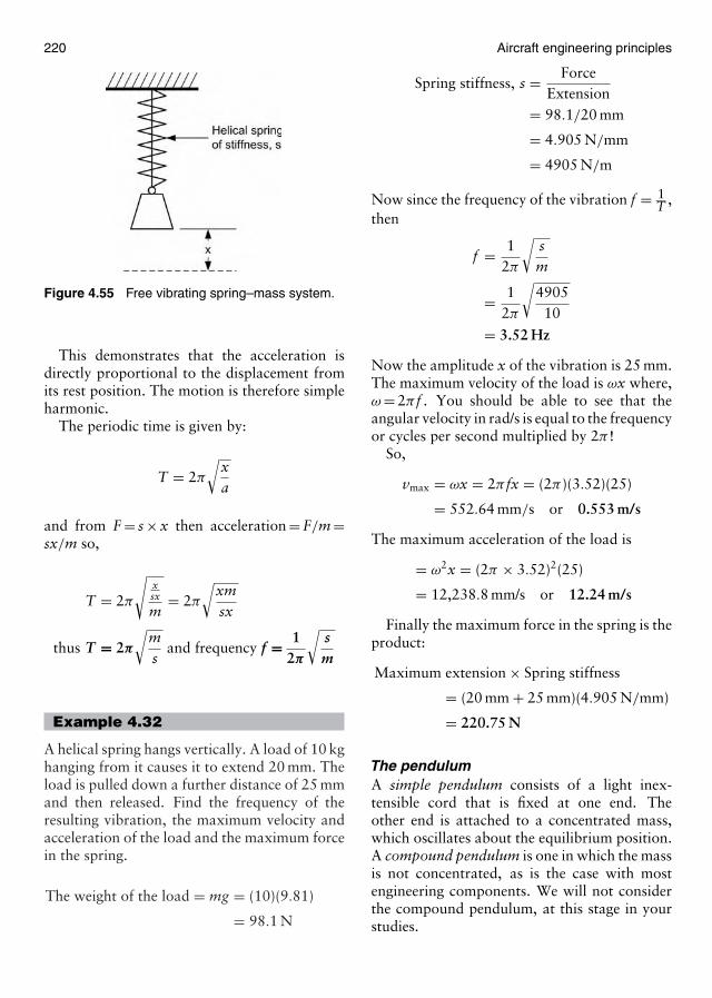
220 Aircraft engineering principles
Figure 4.55 Free vibrating spring–mass system.
This demonstrates that the acceleration isdirectly proportional to the displacement fromits rest position. The motion is therefore simpleharmonic.
The periodic time is given by:
T = 2π
√xa
and from F = s × x then acceleration = F/m =sx/m so,
T = 2π
√xsx
m= 2π
√xmsx
thus T = 2π
√ms
and frequency f = 12π
√sm
Example 4.32
A helical spring hangs vertically. A load of 10 kghanging from it causes it to extend 20 mm. Theload is pulled down a further distance of 25 mmand then released. Find the frequency of theresulting vibration, the maximum velocity andacceleration of the load and the maximum forcein the spring.
The weight of the load = mg = (10)(9.81)
= 98.1 N
Spring stiffness, s = ForceExtension
= 98.1/20 mm
= 4.905 N/mm
= 4905 N/m
Now since the frequency of the vibration f = 1T ,
then
f = 12π
√sm
= 12π
√4905
10
= 3.52 Hz
Now the amplitude x of the vibration is 25 mm.The maximum velocity of the load is ωx where,ω = 2π f . You should be able to see that theangular velocity in rad/s is equal to the frequencyor cycles per second multiplied by 2π !
So,
vmax = ωx = 2π fx = (2π )(3.52)(25)
= 552.64 mm/s or 0.553 m/s
The maximum acceleration of the load is
= ω2x = (2π × 3.52)2(25)
= 12,238.8 mm/s or 12.24 m/s
Finally the maximum force in the spring is theproduct:
Maximum extension × Spring stiffness
= (20 mm + 25 mm)(4.905 N/mm)
= 220.75 N
The pendulumA simple pendulum consists of a light inex-tensible cord that is fixed at one end. Theother end is attached to a concentrated mass,which oscillates about the equilibrium position.A compound pendulum is one in which the massis not concentrated, as is the case with mostengineering components. We will not considerthe compound pendulum, at this stage in yourstudies.

Physics 221
Figure 4.56 The simple pendulum.
From the Figure 4.56, the unbalanced restor-ing force which acts towards the center O, isgiven by the tangential component mg sin θ . Ifa is the acceleration of the bob along the arca due to the force mg sin θ then the equationof motion of the bob is, −mg sin θ = ma. Theminus sign indicates that the force is towards O,while the displacement x is measured along thearc from O in the opposite direction (remem-bering that the acceleration always acts in theopposite direction to the displacement).
Now when t is small, sin t ∼= t (rad). Also,from the equation for arc length s = rθ , thenx = lθ . You should refer back to radian measureon page 122, if you are unsure of this step!
Now, substituting these values into our equa-tion of motion:
−mg sin θ = ma
gives −mgθ = −mgxl
= ma
where −gx/l = a, is the component of g actingalong the arc therefore
a = −gxl
= −ω2x
(from our work before, where a = ω2x, thenω2 = g/l).
The motion of the bob is simple harmonic ifthe oscillations are of small amplitude, i.e. θ
does not exceed 10◦. The period T is then givenby
T = 2π
ω= 2π√
gl
thus,
T ∝√
lg
T is therefore independent of the amplitude ofthe oscillations and for constant g, it dependsonly on the length l of the pendulum.
Example 4.33
A simple pendulum has a period of 4.0 s and anamplitude of swing of 100 mm. Calculate themaximum magnitudes of (a) the velocity of thebob, (b) the acceleration of the bob.
(a) From T = 2π/ω, transposing for ω and sub-stituting for T we have ω = π/2 per second.The velocity will be a maximum at theequilibrium position where x = 0 and using:
ωmax = ± ωr = ± (π/2)(0.1) = 0.157 m/s
since maximum amplitude r = ±100 mm.(b) The acceleration is a maximum at the limits
of the swing, where x = r = ±100 mm andusing:
a = −ω2rthen
a = −(π/2)2(0.1) m/s2
a = −0.246 m/s2
Test your understanding 4.141. Explain the difference between free and forced
vibration.
2. Define the terms: (a) period, (b) cycle, (c) frequencyand (d) amplitude with respect to periodic motion.
3. Define resonance and give examples of where res-onance can be useful and where it is consideredharmful.
4. Define SHM.
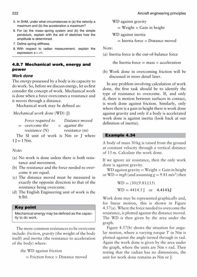
222 Aircraft engineering principles
5. In SHM, under what circumstances is (a) the velocity amaximum and (b) the acceleration a maximum?
6. For (a) the mass–spring system and (b) the simplependulum, explain with the aid of sketches how theamplitude is determined.
7. Define spring stiffness.
8. With respect to radian measurement, explain theexpression s = r θ .
4.8.7 Mechanical work, energy andpower
Work doneThe energy possessed by a body is its capacity todo work. So, before we discuss energy, let us firstconsider the concept of work. Mechanical workis done when a force overcomes a resistance andit moves through a distance.
Mechanical work may be defined as:
Mechanical work done (WD) (J)
=Force required toovercome theresistance (N)
×Distance movedagainst theresistance (m)
The SI unit of work is Nm or J where1 J = 1 Nm.
Note:
(a) No work is done unless there is both resis-tance and movement.
(b) The resistance and the force needed to over-come it are equal.
(c) The distance moved must be measured inexactly the opposite direction to that of theresistance being overcome.
(d) The English Engineering unit of work is theft lbf.
Key pointMechanical energy may be defined as the capac-ity to do work.
The more common resistances to be overcomeinclude: friction, gravity (the weight of the bodyitself) and inertia (the resistance to accelerationof the body) where:
the WD against friction
= Friction force × Distance moved
WD against gravity
= Weight × Gain in height
WD against inertia
= Inertia force × Distance moved
Note:
(a) Inertia force is the out-of-balance force
the Inertia force = mass × acceleration
(b) Work done in overcoming friction will bediscussed in more detail later.
In any problem involving calculation of workdone, the first task should be to identify thetype of resistance to overcome. If, and onlyif, there is motion between surfaces in contact,is work done against friction. Similarly, onlywhere there is a gain in height there is work doneagainst gravity and only if a body is acceleratedwork done is against inertia (look back at ourdefinition of inertia).
Example 4.34
A body of mass 30 kg is raised from the groundat constant velocity through a vertical distanceof 15 m. Calculate the work done.
If we ignore air resistance, then the only workdone is against gravity.
WD against gravity = Weight × Gain in heightor WD = mgh (and assuming g = 9.81 m/s2) then
WD = (30)(9.81)(15)
WD = 4414.5 J or 4.414 kJ
Work done may be represented graphically and,for linear motion, this is shown in Figure4.57(a). Where the force needed to overcome theresistance, is plotted against the distance moved.The WD is then given by the area under thegraph.
Figure 4.57(b) shows the situation for angu-lar motion, where a varying torque T in Nm isplotted against the angle turned through in rad.Again the work done is given by the area underthe graph, where the units are Nm × rad. Thennoting that the radian has no dimensions, theunit for work done remains as Nm or J.
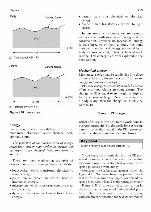
Physics 223
Figure 4.57 Work done.
EnergyEnergy may exist in many different forms, e.g.mechanical, electrical, nuclear, chemical, heat,light and sound.
The principle of the conservation of energystates that: energy may neither be created nordestroyed, only changed from one form toanother.
There are many engineering examples ofdevices that transform energy, these include the:
• loudspeaker which transforms electrical tosound energy,
• petrol engine which transforms heat tomechanical energy,
• microphone which transforms sound to elec-trical energy,
• dynamo transforms mechanical to electricalenergy,
• battery transforms chemical to electricalenergy,
• filament bulb transforms electrical to lightenergy.
In our study of dynamics we are primar-ily concerned with mechanical energy and itsconservation. Provided no mechanical energyis transferred to or from a body, the totalamount of mechanical energy possessed by abody remains constant, unless mechanical workis done. This concept is further explored in thenext section.
Mechanical energyMechanical energy may be subdivided into threedifferent forms; potential energy (PE), strainenergy and kinetic energy (KE).
PE is the energy possessed by a body by virtueof its position, relative to some datum. Thechange in PE is equal to its weight multipliedby the change in height. Since the weight ofa body is mg, then the change in PE may bewritten as:
Change in PE = mgh
which of course is identical to the work done inovercoming gravity. So, the work done in raisinga mass to a height is equal to the PE it possessesat that height, assuming no external losses.
Key pointStrain energy is a particular form of PE.
Strain energy is a particular form of PE pos-sessed by an elastic body that is deformed withinits elastic range, e.g. a stretched or compressedspring possesses strain energy.
Consider the spring arrangement shown inFigure 4.58. We know from our previous workthat the force required to compress or extend thespring is F = kx, where k is the spring constant.
Figure 4.58(a) shows a helical coil spring inthe unstrained, compressed and extended posi-tions. The force required to move the springvaries in direct proportion to the distance moved
224 Aircraft engineering principles
Figure 4.58 Spring system demonstrating strain energy.
(Figure 4.58(b)). Therefore:
Strain energy of springwhen compressedor extended
=Area under graph(force × distancemoved)
= 12 Fx J
and since F = kx, then substituting for F gives,
Strain energy of springin tension or compression = 1
2 kx2 J
A similar argument can be given for a springwhich is subject to twisting or torsion about itscenter (or polar axis). It can be shown that:
Strain energy of a spring when twisted
= 12 ktorθ
2 J (where θ = the angle of twist)
KE is energy possessed by a body by virtueof its motion. Translational KE, i.e. the KE ofa body travelling in a linear direction (straightline) is:
Translational KE (J) =
[mass (kg)×
velocity2(m/s)2
]2
Translation KE = 12 mv2
Flywheels are heavy wheel-shaped masses fit-ted to shafts in order to minimize sudden varia-tions in the rotational speed of the shaft, due tosudden changes in load. A flywheel is thereforea store of rotational KE.
Rotational KE can be defined in a similarmanner to translational KE, i.e.
Rotational KE = 12 Iω2 J
where I = mass moment of inertia (which youmet when we studied torsion).
Note: The moment of inertia of a rotatingmass I can be defined in general terms by theexpression I = Mk2 where M = the total mass ofthe rotating body and k = the radius of gyration,i.e. the radius from the center of rotation whereall of the mass is deemed to act. When we stud-ied torsion earlier we defined I for concentratedor point masses, where I = mr2. You shouldremember that I has different values for differ-ent rotating shapes. We will only be consideringcircular cross-sections, where I is defined asabove. One final point, try not to mix-up kfor the radius of gyration with k for the springconstant!
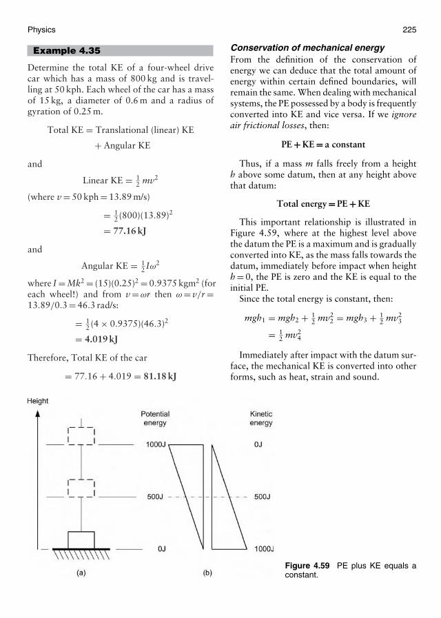
Physics 225
Example 4.35
Determine the total KE of a four-wheel drivecar which has a mass of 800 kg and is travel-ling at 50 kph. Each wheel of the car has a massof 15 kg, a diameter of 0.6 m and a radius ofgyration of 0.25 m.
Total KE = Translational (linear) KE
+ Angular KE
and
Linear KE = 12 mv2
(where v = 50 kph = 13.89 m/s)
= 12 (800)(13.89)2
= 77.16 kJ
and
Angular KE = 12 Iω2
where I = Mk2 = (15)(0.25)2 = 0.9375 kgm2 (foreach wheel!) and from v = ωr then ω = v/r =13.89/0.3 = 46.3 rad/s:
= 12 (4 × 0.9375)(46.3)2
= 4.019 kJ
Therefore, Total KE of the car
= 77.16 + 4.019 = 81.18 kJ
Figure 4.59 PE plus KE equals aconstant.
Conservation of mechanical energyFrom the definition of the conservation ofenergy we can deduce that the total amount ofenergy within certain defined boundaries, willremain the same. When dealing with mechanicalsystems, the PE possessed by a body is frequentlyconverted into KE and vice versa. If we ignoreair frictional losses, then:
PE + KE = a constant
Thus, if a mass m falls freely from a heighth above some datum, then at any height abovethat datum:
Total energy = PE + KE
This important relationship is illustrated inFigure 4.59, where at the highest level abovethe datum the PE is a maximum and is graduallyconverted into KE, as the mass falls towards thedatum, immediately before impact when heighth = 0, the PE is zero and the KE is equal to theinitial PE.
Since the total energy is constant, then:
mgh1 = mgh2 + 12 mv2
2 = mgh3 + 12 mv2
3
= 12 mv2
4
Immediately after impact with the datum sur-face, the mechanical KE is converted into otherforms, such as heat, strain and sound.
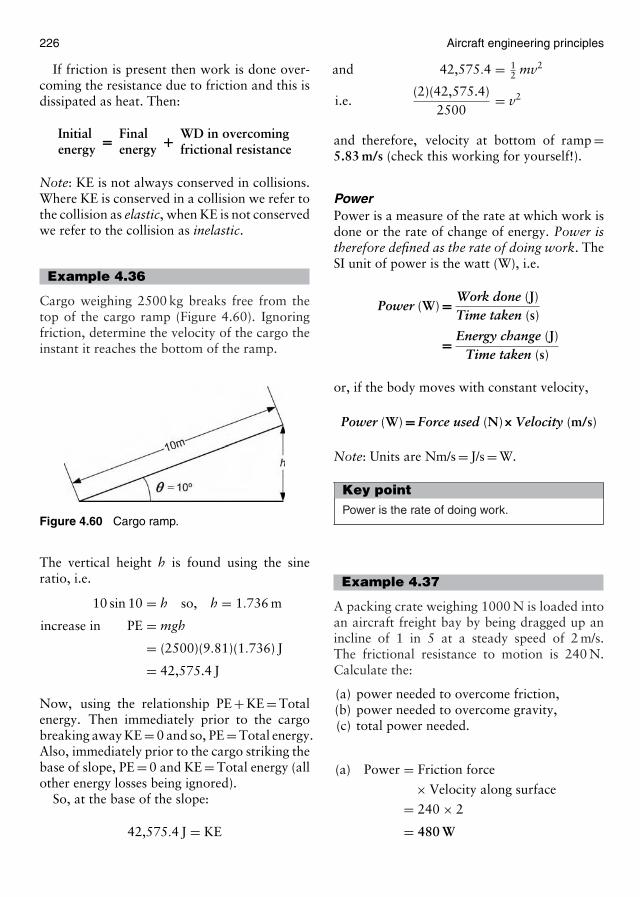
226 Aircraft engineering principles
If friction is present then work is done over-coming the resistance due to friction and this isdissipated as heat. Then:
Initialenergy = Final
energy + WD in overcomingfrictional resistance
Note: KE is not always conserved in collisions.Where KE is conserved in a collision we refer tothe collision as elastic, when KE is not conservedwe refer to the collision as inelastic.
Example 4.36
Cargo weighing 2500 kg breaks free from thetop of the cargo ramp (Figure 4.60). Ignoringfriction, determine the velocity of the cargo theinstant it reaches the bottom of the ramp.
Figure 4.60 Cargo ramp.
The vertical height h is found using the sineratio, i.e.
10 sin 10 = h so, h = 1.736 m
increase in PE = mgh
= (2500)(9.81)(1.736) J
= 42,575.4 J
Now, using the relationship PE + KE = Totalenergy. Then immediately prior to the cargobreaking away KE = 0 and so, PE = Total energy.Also, immediately prior to the cargo striking thebase of slope, PE = 0 and KE = Total energy (allother energy losses being ignored).
So, at the base of the slope:
42,575.4 J = KE
and 42,575.4 = 12 mv2
i.e.(2)(42,575.4)
2500= v2
and therefore, velocity at bottom of ramp =5.83 m/s (check this working for yourself!).
PowerPower is a measure of the rate at which work isdone or the rate of change of energy. Power istherefore defined as the rate of doing work. TheSI unit of power is the watt (W), i.e.
Power (W) = Work done (J)Time taken (s)
= Energy change (J)Time taken (s)
or, if the body moves with constant velocity,
Power (W) = Force used (N)× Velocity (m/s)
Note: Units are Nm/s = J/s = W.
Key pointPower is the rate of doing work.
Example 4.37
A packing crate weighing 1000 N is loaded intoan aircraft freight bay by being dragged up anincline of 1 in 5 at a steady speed of 2 m/s.The frictional resistance to motion is 240 N.Calculate the:
(a) power needed to overcome friction,(b) power needed to overcome gravity,(c) total power needed.
(a) Power = Friction force
× Velocity along surface
= 240 × 2
= 480 W
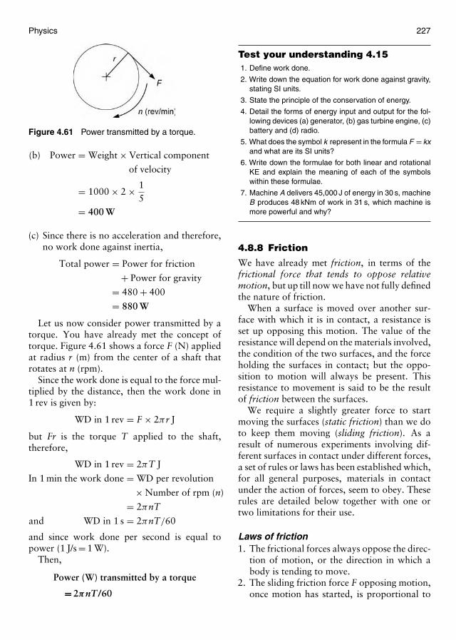
Physics 227
Figure 4.61 Power transmitted by a torque.
(b) Power = Weight × Vertical component
of velocity
= 1000 × 2 × 15
= 400 W
(c) Since there is no acceleration and therefore,no work done against inertia,
Total power = Power for friction
+ Power for gravity
= 480 + 400
= 880 W
Let us now consider power transmitted by atorque. You have already met the concept oftorque. Figure 4.61 shows a force F (N) appliedat radius r (m) from the center of a shaft thatrotates at n (rpm).
Since the work done is equal to the force mul-tiplied by the distance, then the work done in1 rev is given by:
WD in 1 rev = F × 2πr J
but Fr is the torque T applied to the shaft,therefore,
WD in 1 rev = 2πT J
In 1 min the work done = WD per revolution
× Number of rpm (n)
= 2πnT
and WD in 1 s = 2πnT/60
and since work done per second is equal topower (1 J/s = 1 W).
Then,
Power (W) transmitted by a torque
= 2πnT/60
Test your understanding 4.151. Define work done.
2. Write down the equation for work done against gravity,stating SI units.
3. State the principle of the conservation of energy.
4. Detail the forms of energy input and output for the fol-lowing devices (a) generator, (b) gas turbine engine, (c)battery and (d) radio.
5. What does the symbol k represent in the formula F = kxand what are its SI units?
6. Write down the formulae for both linear and rotationalKE and explain the meaning of each of the symbolswithin these formulae.
7. Machine A delivers 45,000 J of energy in 30 s, machineB produces 48 kNm of work in 31 s, which machine ismore powerful and why?
4.8.8 Friction
We have already met friction, in terms of thefrictional force that tends to oppose relativemotion, but up till now we have not fully definedthe nature of friction.
When a surface is moved over another sur-face with which it is in contact, a resistance isset up opposing this motion. The value of theresistance will depend on the materials involved,the condition of the two surfaces, and the forceholding the surfaces in contact; but the oppo-sition to motion will always be present. Thisresistance to movement is said to be the resultof friction between the surfaces.
We require a slightly greater force to startmoving the surfaces (static friction) than we doto keep them moving (sliding friction). As aresult of numerous experiments involving dif-ferent surfaces in contact under different forces,a set of rules or laws has been established which,for all general purposes, materials in contactunder the action of forces, seem to obey. Theserules are detailed below together with one ortwo limitations for their use.
Laws of friction1. The frictional forces always oppose the direc-
tion of motion, or the direction in which abody is tending to move.
2. The sliding friction force F opposing motion,once motion has started, is proportional to
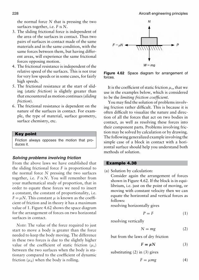
228 Aircraft engineering principles
the normal force N that is pressing the twosurfaces together, i.e. F ∝ N.
3. The sliding frictional force is independent ofthe area of the surfaces in contact. Thus twopairs of surfaces in contact made of the samematerials and in the same condition, with thesame forces between them, but having differ-ent areas, will experience the same frictionalforces opposing motion.
4. The frictional resistance is independent of therelative speed of the surfaces. This is not truefor very low speeds or in some cases, for fairlyhigh speeds.
5. The frictional resistance at the start of slid-ing (static friction) is slightly greater thanthat encountered as motion continues (slidingfriction).
6. The frictional resistance is dependent on thenature of the surfaces in contact. For exam-ple, the type of material, surface geometry,surface chemistry, etc.
Key pointFriction always opposes the motion that pro-duces it.
Solving problems involving frictionFrom the above laws we have established thatthe sliding frictional force F is proportional tothe normal force N pressing the two surfacestogether, i.e. F ∝ N. You will remember fromyour mathematical study of proportion, that inorder to equate these forces we need to inserta constant, the constant of proportionality, i.e.F = µN. This constant µ is known as the coeffi-cient of friction and in theory it has a maximumvalue of 1. Figure 4.62 shows the space diagramfor the arrangement of forces on two horizontalsurfaces in contact.
Note: The value of the force required to juststart to move a body is greater than the forceneeded to keep the body moving. The differencein these two forces is due to the slightly highervalue of the coefficient of static friction (µs)between the two surfaces when the body is sta-tionary compared to the coefficient of dynamicfriction (µd) when the body is rolling.
Figure 4.62 Space diagram for arrangement offorces.
It is the coefficient of static friction µs, that weuse in the examples below, which is consideredto be the limiting friction coefficient.
You may find the solution of problems involv-ing friction rather difficult. This is because it isoften difficult to visualize the nature and direc-tion of all the forces that act on two bodies incontact, as well as resolving these forces intotheir component parts. Problems involving fric-tion may be solved by calculation or by drawing.The following generalized example involving thesimple case of a block in contact with a hori-zontal surface should help you understand bothmethods of solution.
Example 4.38
(a) Solution by calculation:Consider again the arrangement of forcesshown in Figure 4.62. If the block is in equi-librium, i.e. just on the point of moving, ormoving with constant velocity then we canequate the horizontal and vertical forces asfollows:resolving horizontally gives
P = F (1)
resolving vertically
N = mg (2)
but from the laws of dry friction
F = µN (3)
substituting (2) in (3) gives
F = µmg (4)
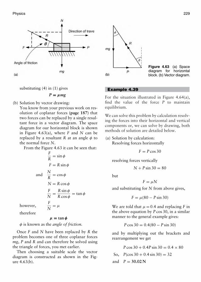
Physics 229
Figure 4.63 (a) Spacediagram for horizontalblock. (b) Vector diagram.
substituting (4) in (1) gives
P = µmg
(b) Solution by vector drawing:You know from your previous work on res-olution of coplanar forces (page 187) thattwo forces can be replaced by a single resul-tant force in a vector diagram. The spacediagram for our horizontal block is shownin Figure 4.63(a), where F and N can bereplaced by a resultant R at an angle φ tothe normal force N.
From the Figure 4.63 it can be seen that:FR
= sin φ
F = R sin φ
andNR
= cos φ
N = R cos φ
FN
= R sin φ
R cos φ= tan φ
however,FN
= µ
thereforeµ = tan φ
φ is known as the angle of friction.
Once F and N have been replaced by R theproblem becomes one of three coplanar forcesmg, P and R and can therefore be solved usingthe triangle of forces, you met earlier.
Then choosing a suitable scale the vectordiagram is constructed as shown in the Fig-ure 4.63(b).
Example 4.39
For the situation illustrated in Figure 4.64(a),find the value of the force P to maintainequilibrium.
We can solve this problem by calculation resolv-ing the forces into their horizontal and verticalcomponents or, we can solve by drawing, bothmethods of solution are detailed below.
(a) Solution by calculation:Resolving forces horizontally
F = P cos 30
resolving forces vertically
N + P sin 30 = 80
butF = µN
and substituting for N from above gives,
F = µ(80 − P sin 30)
We are told that µ = 0.4 and replacing F inthe above equation by P cos 30, in a similarmanner to the general example gives:
P cos 30 = 0.4(80 − P sin 30)
and by multiplying out the brackets andrearrangement we get
P cos 30 + 0.4P sin 30 = 0.4 × 80
So, P(cos 30 + 0.4 sin 30) = 32
and P = 30.02 N
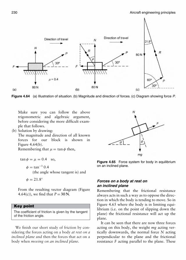
230 Aircraft engineering principles
Figure 4.64 (a) Illustration of situation. (b) Magnitude and direction of forces. (c) Diagram showing force P.
Make sure you can follow the abovetrigonometric and algebraic argument,before considering the more difficult exam-ple that follows.
(b) Solution by drawing:The magnitude and direction of all knownforces for our block is shown inFigure 4.64(b).Remembering that µ = tan φ then,
tan φ = µ = 0.4 so,
φ = tan−1 0.4(the angle whose tangent is) and
φ = 21.8◦
From the resulting vector diagram (Figure4.64(c)), we find that P = 30 N.
Key pointThe coefficient of friction is given by the tangentof the friction angle.
We finish our short study of friction by con-sidering the forces acting on a body at rest on ainclined plane and then the forces that act on abody when moving on an inclined plane.
Figure 4.65 Force system for body in equilibriumon an inclined plane.
Forces on a body at rest onan inclined planeRemembering that the frictional resistancealways acts in such a way as to oppose the direc-tion in which the body is tending to move. So inFigure 4.65 where the body is in limiting equi-librium (i.e. on the point of slipping down theplane) the frictional resistance will act up theplane.
It can be seen that there are now three forcesacting on this body, the weight mg acting ver-tically downwards, the normal force N actingperpendicular to the plane and the frictionalresistance F acting parallel to the plane. These
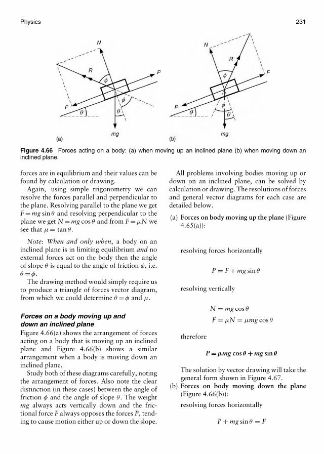
Physics 231
Figure 4.66 Forces acting on a body: (a) when moving up an inclined plane (b) when moving down aninclined plane.
forces are in equilibrium and their values can befound by calculation or drawing.
Again, using simple trigonometry we canresolve the forces parallel and perpendicular tothe plane. Resolving parallel to the plane we getF = mg sin θ and resolving perpendicular to theplane we get N = mg cos θ and from F = µN wesee that µ = tan θ .
Note: When and only when, a body on aninclined plane is in limiting equilibrium and noexternal forces act on the body then the angleof slope θ is equal to the angle of friction φ, i.e.θ = φ.
The drawing method would simply require usto produce a triangle of forces vector diagram,from which we could determine θ = φ and µ.
Forces on a body moving up anddown an inclined planeFigure 4.66(a) shows the arrangement of forcesacting on a body that is moving up an inclinedplane and Figure 4.66(b) shows a similararrangement when a body is moving down aninclined plane.
Study both of these diagrams carefully, notingthe arrangement of forces. Also note the cleardistinction (in these cases) between the angle offriction φ and the angle of slope θ . The weightmg always acts vertically down and the fric-tional force F always opposes the forces P, tend-ing to cause motion either up or down the slope.
All problems involving bodies moving up ordown on an inclined plane, can be solved bycalculation or drawing. The resolutions of forcesand general vector diagrams for each case aredetailed below.
(a) Forces on body moving up the plane (Figure4.65(a)):
resolving forces horizontally
P = F + mg sin θ
resolving vertically
N = mg cos θ
F = µN = µmg cos θ
therefore
P = µmg cos θ + mg sin θ
The solution by vector drawing will take thegeneral form shown in Figure 4.67.
(b) Forces on body moving down the plane(Figure 4.66(b)):
resolving forces horizontally
P + mg sin θ = F
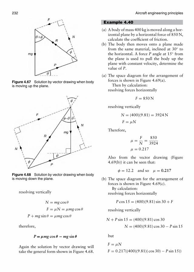
232 Aircraft engineering principles
Figure 4.67 Solution by vector drawing when bodyis moving up the plane.
Figure 4.68 Solution by vector drawing when bodyis moving down the plane.
resolving vertically
N = mg cos θ
F = µN = µmg cos θ
P + mg sin θ = µmg cos θ
therefore,
P = µmg cos θ − mg sin θ
Again the solution by vector drawing willtake the general form shown in Figure 4.68.
Example 4.40
(a) A body of mass 400 kg is moved along a hor-izontal plane by a horizontal force of 850 N,calculate the coefficient of friction.
(b) The body then moves onto a plane madefrom the same material, inclined at 30◦ tothe horizontal. A force P angle at 15◦ fromthe plane is used to pull the body up theplane with constant velocity, determine thevalue of P.
(a) The space diagram for the arrangement offorces is shown in Figure 4.69(a).
Then by calculation:resolving forces horizontally
F = 850 N
resolving vertically
N = (400)(9.81) = 3924 N
F = µN
Therefore,
µ = FN
= 8503924
µ = 0.217
Also from the vector drawing (Figure4.69(b)) it can be seen that:
φ = 12.2 and so µ = 0.217
(b) The space diagram for the arrangement offorces is shown in Figure 4.69(c).
By calculation:resolving forces horizontally
P cos 15 = (400)(9.81) sin 30 + F
resolving vertically
N + P sin 15 = (400)(9.81) cos 30
N = (400)(9.81) cos 30 − P sin 15
but
F = µN
F = 0.217((400)(9.81)( cos 30) − P sin 15))
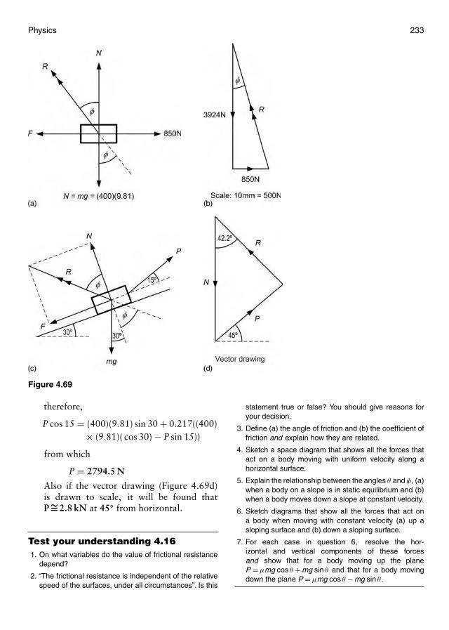
Physics 233
Figure 4.69
therefore,
P cos 15 = (400)(9.81) sin 30 + 0.217((400)× (9.81)( cos 30) − P sin 15))
from which
P = 2794.5 N
Also if the vector drawing (Figure 4.69d)is drawn to scale, it will be found thatP ∼= 2.8 kN at 45◦ from horizontal.
Test your understanding 4.161. On what variables do the value of frictional resistance
depend?
2. “The frictional resistance is independent of the relativespeed of the surfaces, under all circumstances”. Is this
statement true or false? You should give reasons foryour decision.
3. Define (a) the angle of friction and (b) the coefficient offriction and explain how they are related.
4. Sketch a space diagram that shows all the forces thatact on a body moving with uniform velocity along ahorizontal surface.
5. Explain the relationship between the angles θ and φ, (a)when a body on a slope is in static equilibrium and (b)when a body moves down a slope at constant velocity.
6. Sketch diagrams that show all the forces that act ona body when moving with constant velocity (a) up asloping surface and (b) down a sloping surface.
7. For each case in question 6, resolve the hor-izontal and vertical components of these forcesand show that for a body moving up the planeP = µmg cos θ + mg sin θ and that for a body movingdown the plane P = µmg cos θ − mg sin θ .
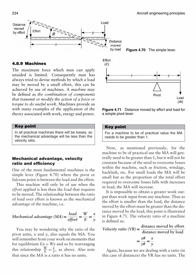
234 Aircraft engineering principles
Figure 4.70 The simple lever.
4.8.9 Machines
The maximum force which man can applyunaided is limited. Consequently man hasalways tried to devise methods by which a loadmay be moved by a small effort, this can beachieved by use of machines. A machine maybe defined as the combination of componentsthat transmit or modify the action of a force ortorque to do useful work. Machines provide uswith many examples of the application of thetheory associated with work, energy and power.
Key pointIn all practical machines there will be losses, sothe mechanical advantage will be less than thevelocity ratio.
Mechanical advantage, velocityratio and efficiency
One of the most fundamental machines is thesimple lever (Figure 4.70) where the pivot orfulcrum point is between the load and the effort.
This machine will only be of use when theeffort applied is less than the load that requiresto be moved. The relationship between the ratioof load over effort is known as the mechanicaladvantage of the machine, i.e.
Mechanical advantage (MA) = loadeffort
= WE
= xy
You may be wondering why the ratio of thepivot arms, x and y, also equals the MA. Youwill remember from your work on moments thatfor equilibrium Ex = Wy and so by rearrangingthis relationship W
E = xy , as above. Also note
that since the MA is a ratio it has no units.
Figure 4.71 Distance moved by effort and load fora simple pivot lever.
Key pointFor a machine to be of practical value the MAneeds to be greater than 1.
Now, as mentioned previously, for themachine to be of practical use the MA will gen-erally need to be greater than 1, but it will not beconstant because of the need to overcome losseswithin the machine, such as friction, windage,backlash, etc. For small loads the MA will besmall but as the proportion of the total effortrequired to overcome losses falls with increasesin load, the MA will increase.
It is impossible to obtain a greater work out-put than work input from any machine. Thus asthe effort is smaller than the load, the distancemoved by the effort must be greater than the dis-tance moved by the load, this point is illustratedin Figure 4.71. The velocity ratio of a machineis defined as:
Velocity ratio (VR) = distance moved by effortdistance moved by load
= xθ
yθ= x
y
Again, because we are dealing with a ratio (inthis case of distances) the VR has no units. The
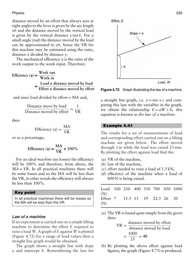
Physics 235
distance moved by an effort that always acts atright angles to the lever is given by the arc lengthxθ and the distance moved by the vertical loadis given by the vertical distance y tan θ . For asmall angle (rad) the distance moved by the loadcan be approximated to yθ , hence the VR forthis machine may be estimated using the ratio,distance x divided by distance y.
The mechanical efficiency η is the ratio of thework output to the work input. Therefore:
Efficiency (η) = Work outWork in
= Load × distance moved by loadEffort × distance moved by effort
and since load divided by effort = MA and,
Distance move by loadDistance moved by effort
= 1VR
then
Efficiency (η) = MAVR
or as a percentage;
Efficiency (η) = MAVR
× 100%
For an ideal machine (no losses) the efficiencywill be 100% and therefore, from above, theMA = VR. In all practical machines there willbe some losses and so the MA will be less thanthe VR, in other words the efficiency will alwaysbe less than 100%.
Key pointIn all practical machines there will be losses sothe MA will be less than the VR.
Law of a machineIf an experiment is carried out on a simple liftingmachine to determine the effort E required toraise a load W . A graph of E against W is plotted(Figure 4.72) for a range of load values then astraight line graph would be obtained.
The graph shows a straight line with slopea and intercept b. Remembering the law for
Figure 4.72 Graph illustrating the law of a machine.
a straight line graph, i.e. y = mx + c and com-paring this law with the variables in the graph,we obtain the relationship E = aW + b, thisequation is known as the law of a machine.
Example 4.41
The results for a set of measurements of loadand corresponding effort carried out on a liftingmachine are given below. The effort movedthrough 1 m while the load was raised 25 mm.By plotting the effort against load find the:
(a) VR of the machine,(b) law of the machine,(c) effort needed to raise a load of 1.5 kN,(d) efficiency of the machine when a load of
800 N is being raised.
Load 100 250 400 550 700 850 1000(N)Effort 7 11.5 15 19 22.5 26 30(N)
(a) The VR is found quite simply from the givendata:
VR = distance moved by effortdistance moved by load
= 100025
= 40
(b) By plotting the above effort against loadfigures, the graph (Figure 4.73) is produced.
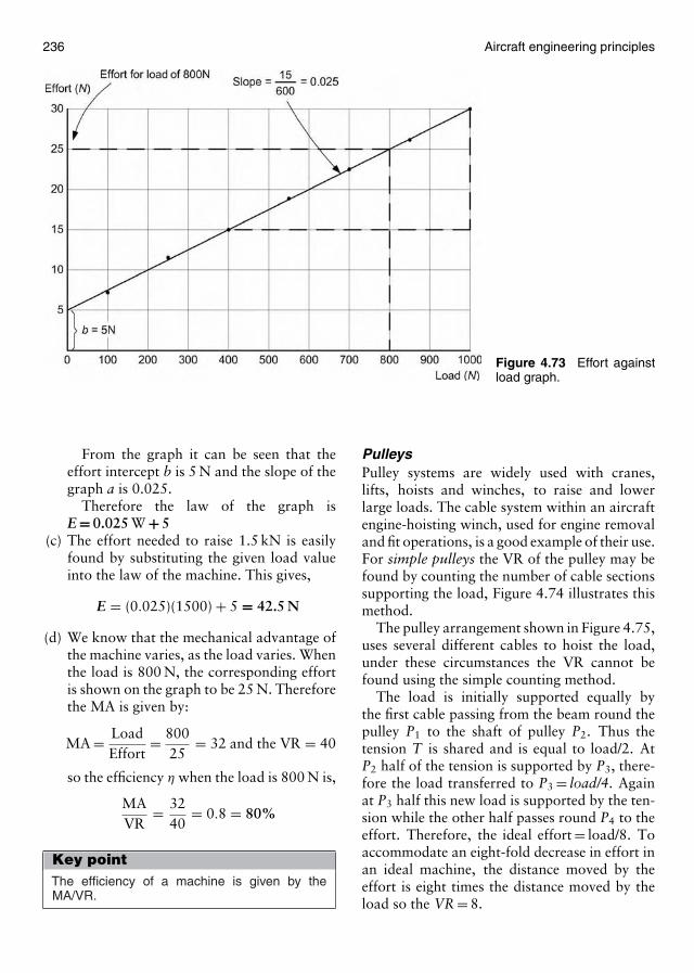
236 Aircraft engineering principles
Figure 4.73 Effort againstload graph.
From the graph it can be seen that theeffort intercept b is 5 N and the slope of thegraph a is 0.025.
Therefore the law of the graph isE = 0.025 W + 5
(c) The effort needed to raise 1.5 kN is easilyfound by substituting the given load valueinto the law of the machine. This gives,
E = (0.025)(1500) + 5 = 42.5 N
(d) We know that the mechanical advantage ofthe machine varies, as the load varies. Whenthe load is 800 N, the corresponding effortis shown on the graph to be 25 N. Thereforethe MA is given by:
MA = LoadEffort
= 80025
= 32 and the VR = 40
so the efficiency η when the load is 800 N is,
MAVR
= 3240
= 0.8 = 80%
Key pointThe efficiency of a machine is given by theMA/VR.
PulleysPulley systems are widely used with cranes,lifts, hoists and winches, to raise and lowerlarge loads. The cable system within an aircraftengine-hoisting winch, used for engine removaland fit operations, is a good example of their use.For simple pulleys the VR of the pulley may befound by counting the number of cable sectionssupporting the load, Figure 4.74 illustrates thismethod.
The pulley arrangement shown in Figure 4.75,uses several different cables to hoist the load,under these circumstances the VR cannot befound using the simple counting method.
The load is initially supported equally bythe first cable passing from the beam round thepulley P1 to the shaft of pulley P2. Thus thetension T is shared and is equal to load/2. AtP2 half of the tension is supported by P3, there-fore the load transferred to P3 = load/4. Againat P3 half this new load is supported by the ten-sion while the other half passes round P4 to theeffort. Therefore, the ideal effort = load/8. Toaccommodate an eight-fold decrease in effort inan ideal machine, the distance moved by theeffort is eight times the distance moved by theload so the VR = 8.
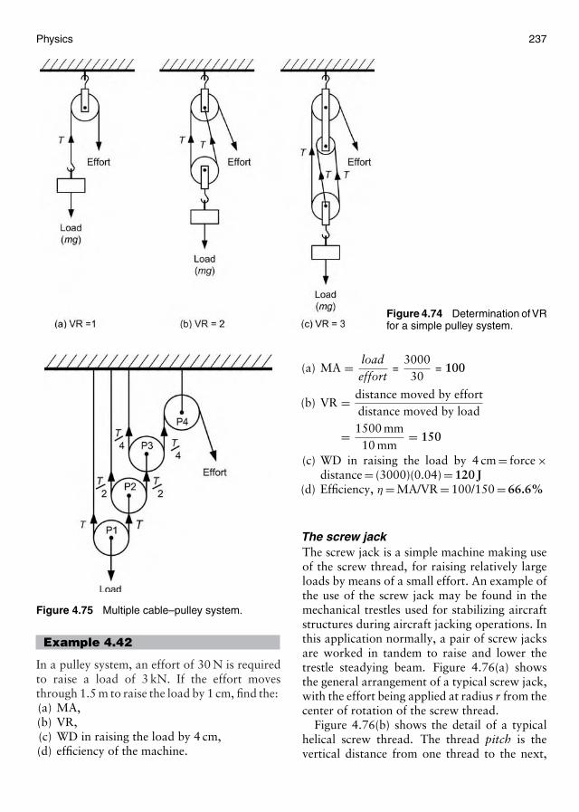
Physics 237
Figure 4.74 Determination ofVRfor a simple pulley system.
Figure 4.75 Multiple cable–pulley system.
Example 4.42
In a pulley system, an effort of 30 N is requiredto raise a load of 3 kN. If the effort movesthrough 1.5 m to raise the load by 1 cm, find the:(a) MA,(b) VR,(c) WD in raising the load by 4 cm,(d) efficiency of the machine.
(a) MA = loadeffort
=3000
30= 100
(b) VR = distance moved by effortdistance moved by load
= 1500 mm10 mm
= 150
(c) WD in raising the load by 4 cm = force ×distance = (3000)(0.04) = 120 J
(d) Efficiency, η = MA/VR = 100/150 = 66.6%
The screw jackThe screw jack is a simple machine making useof the screw thread, for raising relatively largeloads by means of a small effort. An example ofthe use of the screw jack may be found in themechanical trestles used for stabilizing aircraftstructures during aircraft jacking operations. Inthis application normally, a pair of screw jacksare worked in tandem to raise and lower thetrestle steadying beam. Figure 4.76(a) showsthe general arrangement of a typical screw jack,with the effort being applied at radius r from thecenter of rotation of the screw thread.
Figure 4.76(b) shows the detail of a typicalhelical screw thread. The thread pitch is thevertical distance from one thread to the next,
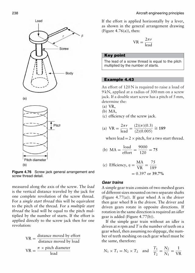
238 Aircraft engineering principles
Figure 4.76 Screw jack general arrangement andscrew thread detail.
measured along the axis of the screw. The leadis the vertical distance traveled by the jack forone complete revolution of the screw thread.For a single start thread this will be equivalentto the pitch of the thread. For a multiple startthread the lead will be equal to the pitch mul-tiplied by the number of starts. If the effort isapplied directly to the screw jack then for onerevolution:
VR = distance moved by effortdistance moved by load
VR = π × pitch diameterlead
If the effort is applied horizontally by a lever,as shown in the general arrangement drawing(Figure 4.76(a)), then:
VR = 2πrlead
Key pointThe lead of a screw thread is equal to the pitchmultiplied by the number of starts.
Example 4.43
An effort of 120 N is required to raise a load of9 kN, applied at a radius of 300 mm on a screwjack. If a double start screw has a pitch of 5 mm,determine the:(a) VR,(b) MA,(c) efficiency of the screw jack.
(a) VR = 2πrlead
= (2)(π )(0.3)(2)(0.005)
∼= 189
where lead = 2 × pitch, for a two start thread.
(b) MA = loadeffort
= 9000120
= 75
(c) Efficiency, η = MAVR
= 75189
= 0.397 or 39.7%
Gear trainsA simple gear train consists of two meshed gearsof different sizes mounted on two separate shafts(Figure 4.77(a)). If gear wheel A is the driverthen gear wheel B is the driven. The driver anddriven gears rotate in opposite directions. Ifrotation in the same direction is required an idlergear is added (Figure 4.77(b)).
If the simple gear train without an idler isdriven at n rpm and T is the number of teeth on agear wheel, then assuming no slippage, the num-ber of teeth meshing on each gear wheel must bethe same, therefore:
N1 × T1 = N2 × T2 andT1
T2= N2
N1= 1
VR
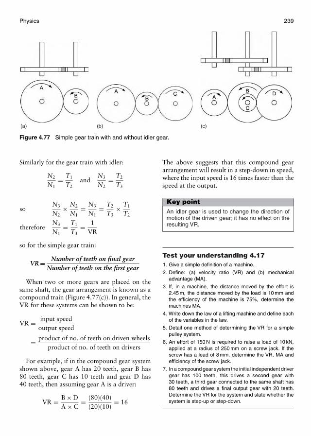
Physics 239
(a) (b) (c)
Figure 4.77 Simple gear train with and without idler gear.
Similarly for the gear train with idler:
N2
N1= T1
T2and
N3
N2= T2
T3
soN3
N2× N2
N1= N3
N1= T2
T3× T1
T2
thereforeN3
N1= T1
T3= 1
VR
so for the simple gear train:
VR = Number of teeth on final gearNumber of teeth on the first gear
When two or more gears are placed on thesame shaft, the gear arrangement is known as acompound train (Figure 4.77(c)). In general, theVR for these systems can be shown to be:
VR = input speedoutput speed
= product of no. of teeth on driven wheelsproduct of no. of teeth on drivers
For example, if in the compound gear systemshown above, gear A has 20 teeth, gear B has80 teeth, gear C has 10 teeth and gear D has40 teeth, then assuming gear A is a driver:
VR = B × DA × C
= (80)(40)(20)(10)
= 16
The above suggests that this compound geararrangement will result in a step-down in speed,where the input speed is 16 times faster than thespeed at the output.
Key pointAn idler gear is used to change the direction ofmotion of the driven gear; it has no effect on theresulting VR.
Test your understanding 4.171. Give a simple definition of a machine.
2. Define: (a) velocity ratio (VR) and (b) mechanicaladvantage (MA).
3. If, in a machine, the distance moved by the effort is2.45 m, the distance moved by the load is 10 mm andthe efficiency of the machine is 75%, determine themachines MA.
4. Write down the law of a lifting machine and define eachof the variables in the law.
5. Detail one method of determining the VR for a simplepulley system.
6. An effort of 150 N is required to raise a load of 10 kN,applied at a radius of 250 mm on a screw jack. If thescrew has a lead of 8 mm, determine the VR, MA andefficiency of the screw jack.
7. In a compound gear system the initial independent drivergear has 100 teeth, this drives a second gear with30 teeth, a third gear connected to the same shaft has80 teeth and drives a final output gear with 20 teeth.Determine the VR for the system and state whether thesystem is step-up or step-down.
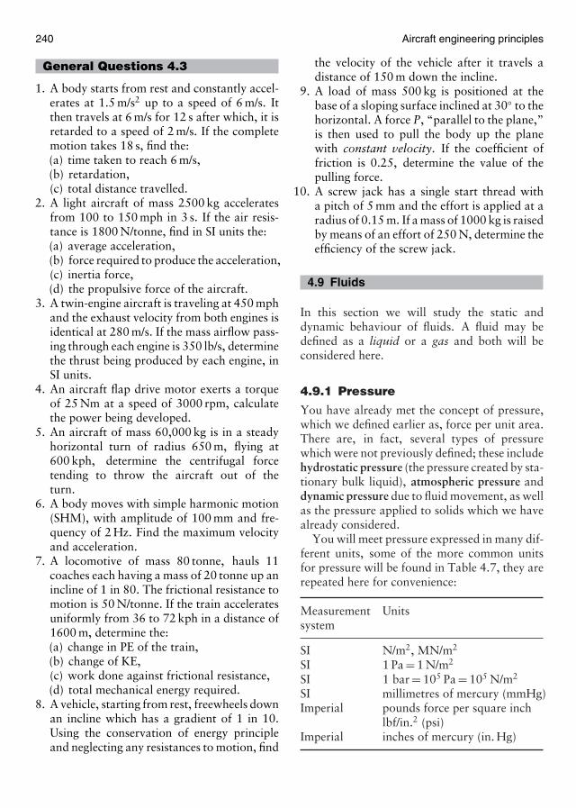
240 Aircraft engineering principles
General Questions 4.3
1. A body starts from rest and constantly accel-erates at 1.5 m/s2 up to a speed of 6 m/s. Itthen travels at 6 m/s for 12 s after which, it isretarded to a speed of 2 m/s. If the completemotion takes 18 s, find the:(a) time taken to reach 6 m/s,(b) retardation,(c) total distance travelled.
2. A light aircraft of mass 2500 kg acceleratesfrom 100 to 150 mph in 3 s. If the air resis-tance is 1800 N/tonne, find in SI units the:(a) average acceleration,(b) force required to produce the acceleration,(c) inertia force,(d) the propulsive force of the aircraft.
3. A twin-engine aircraft is traveling at 450 mphand the exhaust velocity from both engines isidentical at 280 m/s. If the mass airflow pass-ing through each engine is 350 lb/s, determinethe thrust being produced by each engine, inSI units.
4. An aircraft flap drive motor exerts a torqueof 25 Nm at a speed of 3000 rpm, calculatethe power being developed.
5. An aircraft of mass 60,000 kg is in a steadyhorizontal turn of radius 650 m, flying at600 kph, determine the centrifugal forcetending to throw the aircraft out of theturn.
6. A body moves with simple harmonic motion(SHM), with amplitude of 100 mm and fre-quency of 2 Hz. Find the maximum velocityand acceleration.
7. A locomotive of mass 80 tonne, hauls 11coaches each having a mass of 20 tonne up anincline of 1 in 80. The frictional resistance tomotion is 50 N/tonne. If the train acceleratesuniformly from 36 to 72 kph in a distance of1600 m, determine the:(a) change in PE of the train,(b) change of KE,(c) work done against frictional resistance,(d) total mechanical energy required.
8. A vehicle, starting from rest, freewheels downan incline which has a gradient of 1 in 10.Using the conservation of energy principleand neglecting any resistances to motion, find
the velocity of the vehicle after it travels adistance of 150 m down the incline.
9. A load of mass 500 kg is positioned at thebase of a sloping surface inclined at 30◦ to thehorizontal. A force P, “parallel to the plane,”is then used to pull the body up the planewith constant velocity. If the coefficient offriction is 0.25, determine the value of thepulling force.
10. A screw jack has a single start thread witha pitch of 5 mm and the effort is applied at aradius of 0.15 m. If a mass of 1000 kg is raisedby means of an effort of 250 N, determine theefficiency of the screw jack.
4.9 Fluids
In this section we will study the static anddynamic behaviour of fluids. A fluid may bedefined as a liquid or a gas and both will beconsidered here.
4.9.1 Pressure
You have already met the concept of pressure,which we defined earlier as, force per unit area.There are, in fact, several types of pressurewhich were not previously defined; these includehydrostatic pressure (the pressure created by sta-tionary bulk liquid), atmospheric pressure anddynamic pressure due to fluid movement, as wellas the pressure applied to solids which we havealready considered.
You will meet pressure expressed in many dif-ferent units, some of the more common unitsfor pressure will be found in Table 4.7, they arerepeated here for convenience:
Measurement Unitssystem
SI N/m2, MN/m2
SI 1 Pa = 1 N/m2
SI 1 bar = 105 Pa = 105 N/m2
SI millimetres of mercury (mmHg)Imperial pounds force per square inch
lbf/in.2 (psi)Imperial inches of mercury (in. Hg)

Physics 241
Figure 4.78 Illustration of fluid pressure laws.
The laws of fluid pressureFour basic factors or laws, govern the pressurewithin fluids.
With reference to Figure 4.78 these four lawsmay be defined as follows:
(a) Pressure at a given depth in a fluid is equalin all directions.
(b) Pressure at a given depth in a fluid is inde-pendent of the shape of the containing vesselin which it is held. In Figure 4.78(b) thepressure at point X, Y and Z is the same.
(c) Pressure acts at right angles to the surfacesof the containing vessel.
(d) When a pressure is applied to a fluid it istransmitted equally in all directions.
Hydrostatic pressurePressure at a point in a liquid can be determinedby considering the weight force of a fluid abovethe point. Consider Figure 4.79.
If the density of the liquid is known, then wemay express the weight of the liquid in terms ofits density and volume, since density is equal to
Figure 4.79 Pressure at a point in a liquid.
the mass divided by the volume. The mass of theliquid is given by:
m = ρ × A × h
where:m = mass of the liquidρ = densityA = cross-sectional areah = height
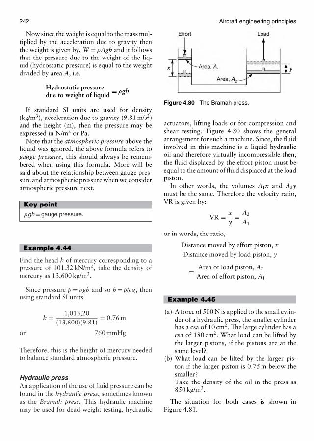
242 Aircraft engineering principles
Now since the weight is equal to the mass mul-tiplied by the acceleration due to gravity thenthe weight is given by, W = ρAgh and it followsthat the pressure due to the weight of the liq-uid (hydrostatic pressure) is equal to the weightdivided by area A, i.e.
Hydrostatic pressuredue to weight of liquid = ρgh
If standard SI units are used for density(kg/m3), acceleration due to gravity (9.81 m/s2)and the height (m), then the pressure may beexpressed in N/m2 or Pa.
Note that the atmospheric pressure above theliquid was ignored, the above formula refers togauge pressure, this should always be remem-bered when using this formula. More will besaid about the relationship between gauge pres-sure and atmospheric pressure when we consideratmospheric pressure next.
Key pointρgh = gauge pressure.
Example 4.44
Find the head h of mercury corresponding to apressure of 101.32 kN/m2, take the density ofmercury as 13,600 kg/m3.
Since pressure p = ρgh and so h = p/ρg, thenusing standard SI units
h = 1,013,20(13,600)(9.81)
= 0.76 m
or 760 mmHg
Therefore, this is the height of mercury neededto balance standard atmospheric pressure.
Hydraulic pressAn application of the use of fluid pressure can befound in the hydraulic press, sometimes knownas the Bramah press. This hydraulic machinemay be used for dead-weight testing, hydraulic
Figure 4.80 The Bramah press.
actuators, lifting loads or for compression andshear testing. Figure 4.80 shows the generalarrangement for such a machine. Since, the fluidinvolved in this machine is a liquid hydraulicoil and therefore virtually incompressible then,the fluid displaced by the effort piston must beequal to the amount of fluid displaced at the loadpiston.
In other words, the volumes A1x and A2ymust be the same. Therefore the velocity ratio,VR is given by:
VR = xy
= A2
A1
or in words, the ratio,
Distance moved by effort piston, xDistance moved by load piston, y
= Area of load piston, A2
Area of effort piston, A1
Example 4.45
(a) A force of 500 N is applied to the small cylin-der of a hydraulic press, the smaller cylinderhas a csa of 10 cm2. The large cylinder has acsa of 180 cm2. What load can be lifted bythe larger pistons, if the pistons are at thesame level?
(b) What load can be lifted by the larger pis-ton if the larger piston is 0.75 m below thesmaller?Take the density of the oil in the press as850 kg/m3.
The situation for both cases is shown inFigure 4.81.

Physics 243
Figure 4.81
(a) We know that P1 = P2, since pressure isapplied equally in all directions.
Therefore,
FA1
= WA2
or F = WA1
A2
then W = FA2/A1 and substituting valuesgives,
load,W = (500)(180 × 10−4)1 × 10−3
= 9000 N
(b) If the larger piston is 0.75 m below thesmaller piston, then pressure P2 will begreater than P1 due to the head of liquid.
P2 = P1 + ρgh
P1 = FA1
= 5001 × 10−3
= 50 × 104 N/m2
then
P2 = (50 × 104) + (850 × 9.81 × 0.75)
P2 = 50.6254 × 10⁴ N/m2
and
WL = P2A2 = (50.6254 × 10⁴)(180 × 10−4)
= 9112.57 N
Atmospheric pressureThe air surrounding the earth has mass andis acted upon by the earth’s gravity, thus itexerts a force over the earth’s surface. Thisforce per unit area is known as atmosphericpressure. At the earth’s surface at sea level,this pressure is found by measurement to be,101,320 N/m2 or in Imperial units 14.7 lbf/in.2.Thus 1 bar (105 N/m2) is approximately 14.5times larger than 1 lbf/in.2, this relationshipshould be remembered. Imagine the conse-quences if you inadvertently tried to inflate anaircraft tire to 150 bar, instead of 150 psi!
Outer space is a vacuum and is completelydevoid of matter, consequently there is no pres-sure in a vacuum. Therefore, pressure measure-ment relative to a vacuum is absolute. For mostpractical purposes it is only necessary to knowhow pressure varies from the earth’s atmo-spheric pressure. A pressure gauge is designedto read zero, when subject to atmospheric pres-sure, therefore if a gauge is connected to apressure vessel it will only read gauge pressure.So to convert gauge pressure to absolute pres-sure, atmospheric pressure must be added toit, i.e.
Absolutepressure = Gauge
pressure + atmosphericpressure
Example 4.46
Taking atmospheric pressure as 101,320 N/m2,convert the following gauge pressure into abso-lute pressure, give your answer in kN/m2 or kPa:(a) 400 kN/m2, (b) 20 MN/m2, (c) 5000 Pa and(d) 3000 psi.
We know from above that absolute pressure isequal to gauge pressure plus atmospheric pres-sure, therefore, the only real problem here is toensure the correct conversion of units.
Atmospheric pressure = 101.32 kN/m2.
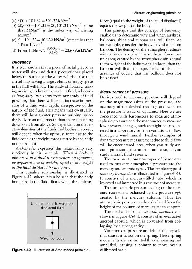
244 Aircraft engineering principles
(a) 400 + 101.32 = 501.32 kN/m2
(b) 20,000 + 101.32 = 20,101.32 kN/m2 (notethat MNm−2 is the index way of writingMN/m2)
(c) 5 + 101.32 = 106.32 kN/m2 (remember that1 Pa = 1 N/m2)
(d) From Table 4.7, 3000 psi0.145 = 20,689.6 kN/m2
BuoyancyIt is well known that a piece of metal placed inwater will sink and that a piece of cork placedbelow the surface of the water will rise, also thata steel ship having a large volume of empty spacein the hull will float. The study of floating, sink-ing or rising bodies immersed in a fluid, is knownas buoyancy. We know from our study of fluidpressure, that there will be an increase in pres-sure of a fluid with depth, irrespective of thenature of the fluid. This means that eventually,there will be a greater pressure pushing up onthe body from underneath than there is pushingdown on it from above. So dependent on the rel-ative densities of the fluids and bodies involved,will depend when the upthrust force due to thefluid equals the weight force exerted by the bodyimmersed in it.
Archimedes expresses this relationship verysuccinctly in his principle: When a body isimmersed in a fluid it experiences an upthrust,or apparent loss of weight, equal to the weightof the fluid displaced by the body.
This equality relationship is illustrated inFigure 4.82, where it can be seen that the bodyimmersed in the fluid, floats when the upthrust
Figure 4.82 Illustration of Archimedes principle.
force (equal to the weight of the fluid displaced)equals the weight of the body.
This principle and the concept of buoyancyenable us to determine why and when airships,balloons, ships and submarines, will float. Asan example, consider the buoyancy of a heliumballoon. The density of the atmosphere reduceswith altitude, so when the upthrust force (perunit area) created by the atmospheric air is equalto the weight of the helium and balloon, then theballoon will float at a specified altitude. Thisassumes of course that the balloon does notburst first!
Measurement of pressureDevices used to measure pressure will dependon the magnitude (size) of the pressure, theaccuracy of the desired readings and whetherthe pressure is static or dynamic. Here we areconcerned with barometers to measure atmo-spheric pressure and the manometer to measurelow pressure changes, such as might be encoun-tered in a laboratory or from variations in flowthrough a wind tunnel. Further examples ofdynamic pressure measurement due to fluid flowwill be encountered later, when you study air-craft pitot-static instruments and also, if youstudy aircraft fluid systems.
The two most common types of barometerused to measure atmospheric pressure are themercury and aneroid types. The simplest type ofmercury barometer is illustrated in Figure 4.83.It consists of a mercury-filled tube which isinverted and immersed in a reservoir of mercury.
The atmospheric pressure acting on the mer-cury reservoir is balanced by the pressure ρghcreated by the mercury column. Thus theatmospheric pressure can be calculated from theheight of the column of mercury it can support.
The mechanism of an aneroid barometer isshown in Figure 4.84. It consists of an evacuatedaneroid capsule, which is prevented from col-lapsing by a strong spring.
Variations in pressure are felt on the capsulethat causes it to act on the spring. These springmovements are transmitted through gearing andamplified, causing a pointer to move over acalibrated scale.
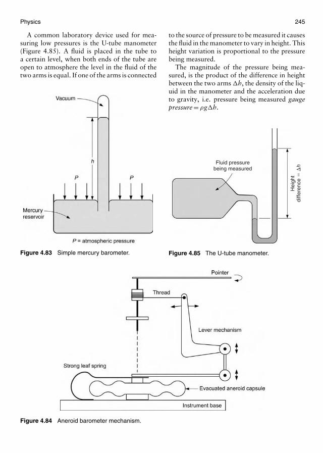
Physics 245
A common laboratory device used for mea-suring low pressures is the U-tube manometer(Figure 4.85). A fluid is placed in the tube toa certain level, when both ends of the tube areopen to atmosphere the level in the fluid of thetwo arms is equal. If one of the arms is connected
Figure 4.83 Simple mercury barometer.
Figure 4.84 Aneroid barometer mechanism.
to the source of pressure to be measured it causesthe fluid in the manometer to vary in height. Thisheight variation is proportional to the pressurebeing measured.
The magnitude of the pressure being mea-sured, is the product of the difference in heightbetween the two arms �h, the density of the liq-uid in the manometer and the acceleration dueto gravity, i.e. pressure being measured gaugepressure = ρg�h.
Fluid pressurebeing measured
Hei
ght
diffe
renc
e �
�h
Figure 4.85 The U-tube manometer.
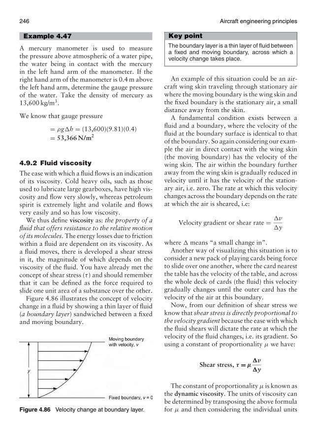
246 Aircraft engineering principles
Example 4.47
A mercury manometer is used to measurethe pressure above atmospheric of a water pipe,the water being in contact with the mercuryin the left hand arm of the manometer. If theright hand arm of the manometer is 0.4 m abovethe left hand arm, determine the gauge pressureof the water. Take the density of mercury as13,600 kg/m3.
We know that gauge pressure
= ρg�h = (13,600)(9.81)(0.4)= 53,366 N/m2
4.9.2 Fluid viscosity
The ease with which a fluid flows is an indicationof its viscosity. Cold heavy oils, such as thoseused to lubricate large gearboxes, have high vis-cosity and flow very slowly, whereas petroleumspirit is extremely light and volatile and flowsvery easily and so has low viscosity.
We thus define viscosity as: the property of afluid that offers resistance to the relative motionof its molecules. The energy losses due to frictionwithin a fluid are dependent on its viscosity. Asa fluid moves, there is developed a shear stressin it, the magnitude of which depends on theviscosity of the fluid. You have already met theconcept of shear stress (τ ) and should rememberthat it can be defined as the force required toslide one unit area of a substance over the other.
Figure 4.86 illustrates the concept of velocitychange in a fluid by showing a thin layer of fluid(a boundary layer) sandwiched between a fixedand moving boundary.
Figure 4.86 Velocity change at boundary layer.
Key pointThe boundary layer is a thin layer of fluid betweena fixed and moving boundary, across which avelocity change takes place.
An example of this situation could be an air-craft wing skin traveling through stationary airwhere the moving boundary is the wing skin andthe fixed boundary is the stationary air, a smalldistance away from the skin.
A fundamental condition exists between afluid and a boundary, where the velocity of thefluid at the boundary surface is identical to thatof the boundary. So again considering our exam-ple the air in direct contact with the wing skin(the moving boundary) has the velocity of thewing skin. The air within the boundary furtheraway from the wing skin is gradually reduced invelocity until it has the velocity of the station-ary air, i.e. zero. The rate at which this velocitychanges across the boundary depends on the rateat which the air is sheared, i.e:
Velocity gradient or shear rate = �v�y
where � means “a small change in”.Another way of visualizing this situation is to
consider a new pack of playing cards being forceto slide over one another, where the card nearestthe table has the velocity of the table, and acrossthe whole deck of cards (the fluid) this velocitygradually changes until the outer card has thevelocity of the air at this boundary.
Now, from our definition of shear stress weknow that shear stress is directly proportional tothe velocity gradient because the ease with whichthe fluid shears will dictate the rate at which thevelocity of the fluid changes, i.e. its gradient. Sousing a constant of proportionality µ we have:
Shear stress, τ = µ�v�y
The constant of proportionality µ is known asthe dynamic viscosity. The units of viscosity canbe determined by transposing the above formulafor µ and then considering the individual units
Physics 247
of the terms within the equation, i.e.
µ = τ�y�v
and substituting the units gives,
Nm2
× mm/s
= Ns/m2
If you have not completely followed the aboveargument do not worry, it is rather complex.Just remember that viscosity is the resistanceto fluid flow and that the units of dynamic vis-cosity in the SI system are Ns/m2. You may bewondering why we keep talking about dynamicviscosity, this is because another form of vis-cosity exists, which takes into consideration thedensity of the fluid, this is known as kinematicviscosity, ν, which is defined as:
Kinematic viscosity, ν = µ
ρ
and has units m2/s.For example the dynamic viscosity of air
at 20◦C is 1.81 × 10⁻⁵ Ns/m2 and so its kine-matic viscosity is given by dividing its dynamicviscosity by the density of air at this tempera-ture, that is 1.81 × 10⁻⁵/1.225 kg/m3 and thusν = 1.48 × 10⁻⁵ m2/s. Dynamic viscosity is fre-quently quoted in tables in preference to kine-matic viscosity because the density of a fluidvaries with its temperature.
Key pointKinematic viscosity is density dependent andtherefore varies with temperature.
Test your understanding 4.181. Convert 50 mmHg into in.Hg.
2. Convert (a) 200 MN/m2, (b) 80 kPa and (c) 72 bar intoimperial (psi).
3. State the fluid pressure laws upon which the operationprinciple of the hydraulic press depends.
4. If a hydraulic press has a VR = 180 and the load pistonis raised 10 cm, determine the distance travelled by theeffort piston in m.
5. Define: (a) gauge pressure and (b) absolute pressure.
6. State Archimedes principle and explain how this princi-ple relates to buoyancy.
7. Describe the operation of a mercury barometer.
8. If the difference in height of the mercury between thetwo arms of a U-tube manometer is 12.5 in. determinethe: (a) gauge pressure and (b) absolute pressure beingmeasured, in psi.
9. Explain the relationship between velocity gradient,shear stress and dynamic viscosity.
10. Show from the relationship ν = µ/ρ that the SI units forkinematic viscosity are m2/s.
4.9.3 Atmospheric physics
In order to understand the environment in whichaircraft fly, you will need to understand thenature of the changes that take place in ouratmosphere with respect to temperature, pres-sure and density.
GasesIn the study of gases we have to consider theabove interactions between temperature, pres-sure and density (remembering that density ismass per unit volume). A change in one of thesecharacteristics always produces a correspondingchange in at least one of the other two.
Unlike liquids and solids, gases have the char-acteristics of being easily compressible and ofexpanding or contracting readily in response tochanges in temperature. Although the charac-teristics themselves vary in degree for differ-ent gases, certain basic laws can be appliedto what we call a perfect gas. A perfect orideal gas is simply one, which has been shown(through experiment) to follow or adhere veryclosely to these gas laws. In these experimentsone factor, e.g. volume is kept constant whilethe relationship between the other two is inves-tigated. In this way it can be shown that:
1. The pressure of a fixed mass of gas isdirectly proportional to its absolute tempera-ture, providing the volume of the gas is keptconstant.
In symbols:
PT
= constant
(providing V remains constant)
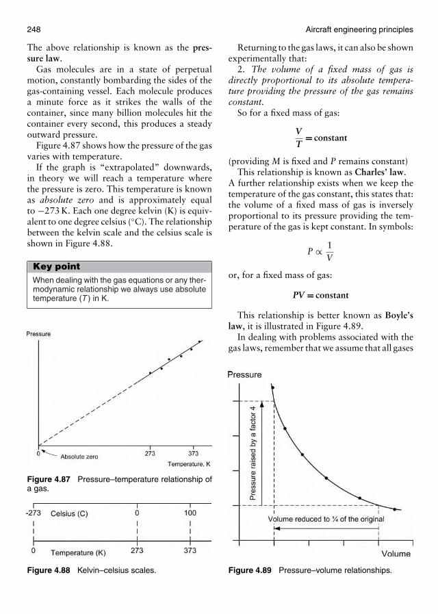
248 Aircraft engineering principles
The above relationship is known as the pres-sure law.
Gas molecules are in a state of perpetualmotion, constantly bombarding the sides of thegas-containing vessel. Each molecule producesa minute force as it strikes the walls of thecontainer, since many billion molecules hit thecontainer every second, this produces a steadyoutward pressure.
Figure 4.87 shows how the pressure of the gasvaries with temperature.
If the graph is “extrapolated” downwards,in theory we will reach a temperature wherethe pressure is zero. This temperature is knownas absolute zero and is approximately equalto −273 K. Each one degree kelvin (K) is equiv-alent to one degree celsius (◦C). The relationshipbetween the kelvin scale and the celsius scale isshown in Figure 4.88.
Key pointWhen dealing with the gas equations or any ther-modynamic relationship we always use absolutetemperature (T ) in K.
Figure 4.87 Pressure–temperature relationship ofa gas.
Figure 4.88 Kelvin–celsius scales.
Returning to the gas laws, it can also be shownexperimentally that:
2. The volume of a fixed mass of gas isdirectly proportional to its absolute tempera-ture providing the pressure of the gas remainsconstant.
So for a fixed mass of gas:
VT
= constant
(providing M is fixed and P remains constant)This relationship is known as Charles’ law.
A further relationship exists when we keep thetemperature of the gas constant, this states that:the volume of a fixed mass of gas is inverselyproportional to its pressure providing the tem-perature of the gas is kept constant. In symbols:
P ∝ 1V
or, for a fixed mass of gas:
PV = constant
This relationship is better known as Boyle’slaw, it is illustrated in Figure 4.89.
In dealing with problems associated with thegas laws, remember that we assume that all gases
Figure 4.89 Pressure–volume relationships.
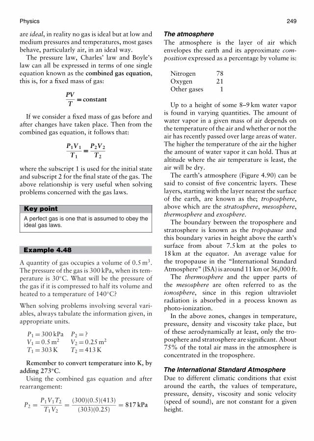
Physics 249
are ideal, in reality no gas is ideal but at low andmedium pressures and temperatures, most gasesbehave, particularly air, in an ideal way.
The pressure law, Charles’ law and Boyle’slaw can all be expressed in terms of one singleequation known as the combined gas equation,this is, for a fixed mass of gas:
PVT
= constant
If we consider a fixed mass of gas before andafter changes have taken place. Then from thecombined gas equation, it follows that:
P1V 1
T1= P2V 2
T2
where the subscript 1 is used for the initial stateand subscript 2 for the final state of the gas. Theabove relationship is very useful when solvingproblems concerned with the gas laws.
Key pointA perfect gas is one that is assumed to obey theideal gas laws.
Example 4.48
A quantity of gas occupies a volume of 0.5 m3.The pressure of the gas is 300 kPa, when its tem-perature is 30◦C. What will be the pressure ofthe gas if it is compressed to half its volume andheated to a temperature of 140◦C?
When solving problems involving several vari-ables, always tabulate the information given, inappropriate units.
P1 = 300 kPa P2 = ?V1 = 0.5 m2 V2 = 0.25 m2
T1 = 303 K T2 = 413 K
Remember to convert temperature into K, byadding 273◦C.
Using the combined gas equation and afterrearrangement:
P2 = P1V1T2
T1V2= (300)(0.5)(413)
(303)(0.25)= 817 kPa
The atmosphereThe atmosphere is the layer of air whichenvelopes the earth and its approximate com-position expressed as a percentage by volume is:
Nitrogen 78Oxygen 21Other gases 1
Up to a height of some 8–9 km water vaporis found in varying quantities. The amount ofwater vapor in a given mass of air depends onthe temperature of the air and whether or not theair has recently passed over large areas of water.The higher the temperature of the air the higherthe amount of water vapor it can hold. Thus ataltitude where the air temperature is least, theair will be dry.
The earth’s atmosphere (Figure 4.90) can besaid to consist of five concentric layers. Theselayers, starting with the layer nearest the surfaceof the earth, are known as the; troposphere,above which are the stratosphere, mesosphere,thermosphere and exosphere.
The boundary between the troposphere andstratosphere is known as the tropopause andthis boundary varies in height above the earth’ssurface from about 7.5 km at the poles to18 km at the equator. An average value forthe tropopause in the “International StandardAtmosphere” (ISA) is around 11 km or 36,000 ft.
The thermosphere and the upper parts ofthe mesosphere are often referred to as theionosphere, since in this region ultravioletradiation is absorbed in a process known asphoto-ionization.
In the above zones, changes in temperature,pressure, density and viscosity take place, butof these aerodynamically at least, only the tro-posphere and stratosphere are significant. About75% of the total air mass in the atmosphere isconcentrated in the troposphere.
The International Standard AtmosphereDue to different climatic conditions that existaround the earth, the values of temperature,pressure, density, viscosity and sonic velocity(speed of sound), are not constant for a givenheight.
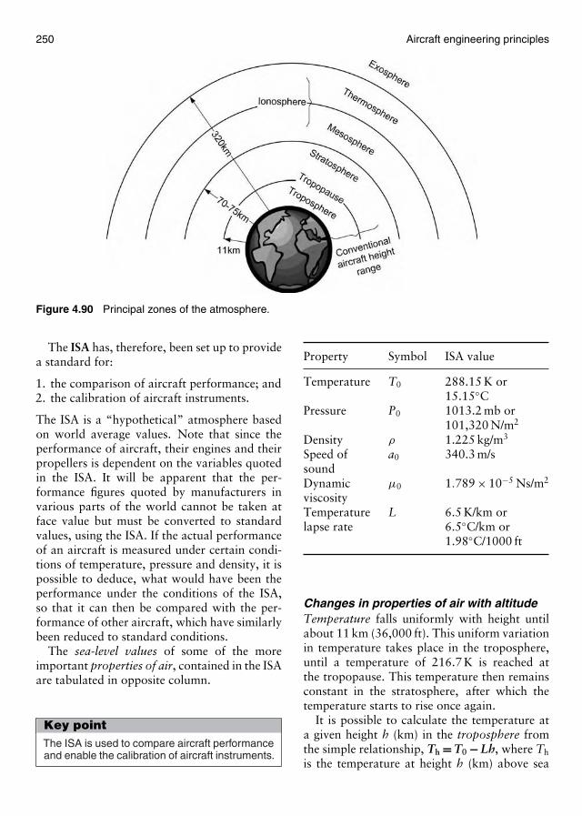
250 Aircraft engineering principles
Figure 4.90 Principal zones of the atmosphere.
The ISA has, therefore, been set up to providea standard for:
1. the comparison of aircraft performance; and2. the calibration of aircraft instruments.
The ISA is a “hypothetical” atmosphere basedon world average values. Note that since theperformance of aircraft, their engines and theirpropellers is dependent on the variables quotedin the ISA. It will be apparent that the per-formance figures quoted by manufacturers invarious parts of the world cannot be taken atface value but must be converted to standardvalues, using the ISA. If the actual performanceof an aircraft is measured under certain condi-tions of temperature, pressure and density, it ispossible to deduce, what would have been theperformance under the conditions of the ISA,so that it can then be compared with the per-formance of other aircraft, which have similarlybeen reduced to standard conditions.
The sea-level values of some of the moreimportant properties of air, contained in the ISAare tabulated in opposite column.
Key pointThe ISA is used to compare aircraft performanceand enable the calibration of aircraft instruments.
Property Symbol ISA value
Temperature T0 288.15 K or15.15◦C
Pressure P0 1013.2 mb or101,320 N/m2
Density ρ 1.225 kg/m3
Speed of a0 340.3 m/ssoundDynamic µ0 1.789 × 10⁻⁵ Ns/m2
viscosityTemperature L 6.5 K/km orlapse rate 6.5◦C/km or
1.98◦C/1000 ft
Changes in properties of air with altitudeTemperature falls uniformly with height untilabout 11 km (36,000 ft). This uniform variationin temperature takes place in the troposphere,until a temperature of 216.7 K is reached atthe tropopause. This temperature then remainsconstant in the stratosphere, after which thetemperature starts to rise once again.
It is possible to calculate the temperature ata given height h (km) in the troposphere fromthe simple relationship, Th = T0 − Lh, where Th
is the temperature at height h (km) above sea
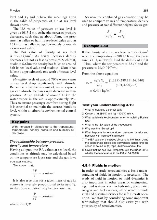
Physics 251
level and T0 and L have the meanings givenin the table of properties of air at sea levelshown above.
The ISA value of pressure at sea level isgiven as 1013.2 mb. As height increases pressuredecreases, such that at about 5 km, the pres-sure has fallen to half its sea-level value and at15 km it has fallen to approximately one-tenthits sea-level value.
The ISA value of density at sea levelis 1.225 kg/m3. As height increases densitydecreases but not as fast as pressure. Such that,at about 6.6 km the density has fallen to aroundhalf its sea-level value and at about 18 km it hasfallen to approximately one tenth of its sea-levelvalue.
Humidity levels of around 70% water vaporat sea level drop significantly with altitude.Remember that the amount of water vapor agas can absorb decreases with decrease in tem-perature. At an altitude of around 18 km thewater vapor in the air is approximately 4%.Thus to ensure passenger comfort during flightit is essential to maintain the correct humiditylevel, within an aircrafts environmental controlsystem.
Key pointWith increase in altitude up to the tropopause;temperature, density, pressure and humidity alldecrease.
The relationship between pressure,density and temperatureHaving adopted the ISA values at sea level, theconditions at altitude may be calculated basedon the temperature lapse rate and the gas lawsyou met earlier.
We know that,
PVT
= constant
It is also true that for a given mass of gas itsvolume is inversely proportional to its density,so the above equation may be re-written as:
PρT
= constant
where V ∝ 1/P.
So now the combined gas equation may beused to compare values of temperature, densityand pressure at two different heights. So we get:
P1
ρ1T1= P2
ρ2T2
Example 4.49
If the density of air at sea level is 1.225 kg/m3
when the temperature is 288.15 K and the pres-sure is 101,320 N/m2. Find the density of air at10 km, where the temperature is 223 K and thepressure is 26,540 N/m2.
From the above equation:
ρh = ρ0T0Ph
P0Th= (1.225)(288.15)(26, 540)
(101,320)(223)
= 0.414 kg/m3
Test your understanding 4.191. What is meant by a perfect gas?
2. Convert: (a) 280◦C and (b) −170◦C into K.
3. What variable is kept constant when formulating Boyle’slaw?
4. What is the ISA value of the tropopause?
5. Why was the ISA set up?
6. What happens to temperature, pressure, density andhumidity with increase in altitude?
7. The ISA value for the speed of sound is 340.3 m/s. Usingthe appropriate tables and conversion factors find thespeed of sound in: (a) mph, (b) knots and (c) ft/s.
8. Given that the sea-level temperature in the ISA is 20◦C,what is the temperature in the ISA at 34,000 ft?
4.9.4 Fluids in motion
In order to study aerodynamics a basic under-standing of fluids in motion is necessary. Thestudy of fluid in motion or fluid dynamics isalso important in other areas of engineering,e.g. fluid systems, such as hydraulic, pneumatic,oxygen and fuel systems, all of which providevital and essential services for safe aircraft oper-ation. We start by considering some importantterminology that should also assist you withyour study of aerodynamics.
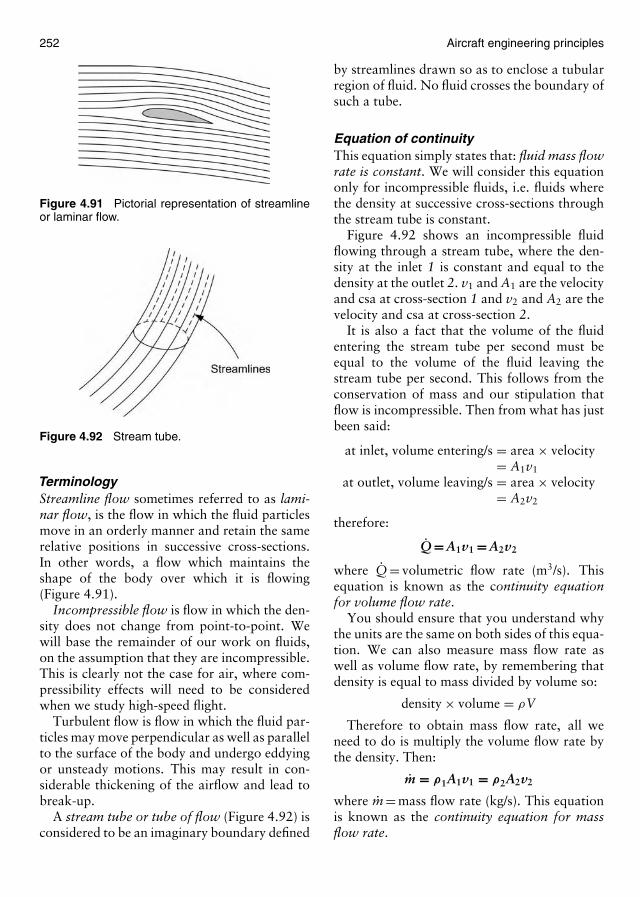
252 Aircraft engineering principles
Figure 4.91 Pictorial representation of streamlineor laminar flow.
Figure 4.92 Stream tube.
TerminologyStreamline flow sometimes referred to as lami-nar flow, is the flow in which the fluid particlesmove in an orderly manner and retain the samerelative positions in successive cross-sections.In other words, a flow which maintains theshape of the body over which it is flowing(Figure 4.91).
Incompressible flow is flow in which the den-sity does not change from point-to-point. Wewill base the remainder of our work on fluids,on the assumption that they are incompressible.This is clearly not the case for air, where com-pressibility effects will need to be consideredwhen we study high-speed flight.
Turbulent flow is flow in which the fluid par-ticles may move perpendicular as well as parallelto the surface of the body and undergo eddyingor unsteady motions. This may result in con-siderable thickening of the airflow and lead tobreak-up.
A stream tube or tube of flow (Figure 4.92) isconsidered to be an imaginary boundary defined
by streamlines drawn so as to enclose a tubularregion of fluid. No fluid crosses the boundary ofsuch a tube.
Equation of continuityThis equation simply states that: fluid mass flowrate is constant. We will consider this equationonly for incompressible fluids, i.e. fluids wherethe density at successive cross-sections throughthe stream tube is constant.
Figure 4.92 shows an incompressible fluidflowing through a stream tube, where the den-sity at the inlet 1 is constant and equal to thedensity at the outlet 2. v1 and A1 are the velocityand csa at cross-section 1 and v2 and A2 are thevelocity and csa at cross-section 2.
It is also a fact that the volume of the fluidentering the stream tube per second must beequal to the volume of the fluid leaving thestream tube per second. This follows from theconservation of mass and our stipulation thatflow is incompressible. Then from what has justbeen said:
at inlet, volume entering/s = area × velocity= A1v1
at outlet, volume leaving/s = area × velocity= A2v2
therefore:
Q = A1v1 = A2v2
where Q = volumetric flow rate (m3/s). Thisequation is known as the continuity equationfor volume flow rate.
You should ensure that you understand whythe units are the same on both sides of this equa-tion. We can also measure mass flow rate aswell as volume flow rate, by remembering thatdensity is equal to mass divided by volume so:
density × volume = ρV
Therefore to obtain mass flow rate, all weneed to do is multiply the volume flow rate bythe density. Then:
m = ρ1A1v1 = ρ2A2v2
where m = mass flow rate (kg/s). This equationis known as the continuity equation for massflow rate.
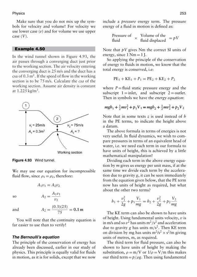
Physics 253
Make sure that you do not mix up the sym-bols for velocity and volume! For velocity weuse lower case (v) and for volume we use uppercase (V).
Example 4.50
In the wind tunnel shown in Figure 4.93, theair passes through a converging duct just priorto the working section. The air velocity enteringthe converging duct is 25 m/s and the duct has acsa of 0.3 m2. If the speed of flow in the workingsection is to be 75 m/s. Calculate the csa of theworking section. Assume air density is constantat 1.225 kg/m3.
Figure 4.93 Wind tunnel.
We may use our equation for incompressiblefluid flow, since ρ1 = ρ2, therefore:
A1v1 = A2v2
so A2 = A1v1
v2
and A2 = (0.3)(25)75
= 0.1 m
You will note that the continuity equation isfar easier to use than to verify!
The Bernoulli’s equationThe principle of the conservation of energy hasalready been discussed, earlier in our study ofphysics. This principle is equally valid for fluidsin motion, as it is for solids, except that we now
include a pressure energy term. The pressureenergy of a fluid in motion is defined as:
Pressure offluid
× Volume of thefluid displaced
= pV
Note that pV gives Nm the correct SI units ofenergy, since 1 Nm = 1 J.
So applying the principle of the conservationof energy to fluids in motion, we know that thetotal energy is conserved, i.e:
PE1 + KE1 + P1 = PE2 + KE2 + P2
where P = fluid static pressure energy and thesubscript 1 = inlet, and subscript 2 = outlet.Then in symbols we have the energy equation:
mgh1 + 12 mv2
1 + p1V 1 = mgh2 + 12 mv2
2 + p2V 2
Note that in some texts z is used instead of hin the PE terms, to indicate the height abovea datum.
The above formula in terms of energies is notvery useful. In fluid dynamics, we wish to com-pare pressures in terms of an equivalent head ofwater, i.e. we need each term in our formula tohave units of height, this is achieved by a littlemathematical manipulation!
Dividing each term in the above energy equa-tion by m gives us energy per unit mass, if at thesame time we divide each term by the accelera-tion due to gravity g, it can be seen immediatelyfrom the equation given below, that the PE termnow has units of height as required, but whatabout the other two terms?
h1 + v21
2g+ p1
V1
mg= h2 + v2
2
2g+ p2
V2
mg
The KE term can also be shown to have unitsof height. Using fundamental units velocity, v isin m/s and so v2 has units m2/s2 and accelerationdue to gravity g has units m/s2. Then KE termon division by mg has units m2/s2 × s2/m givingunits of metres, m, as required.
The third term for fluid pressure, can also beshown to have units of height by making thesubstitution, ρ = m/V or 1/ρ = V/m this makesour third term = p/ρg. Then using fundamental
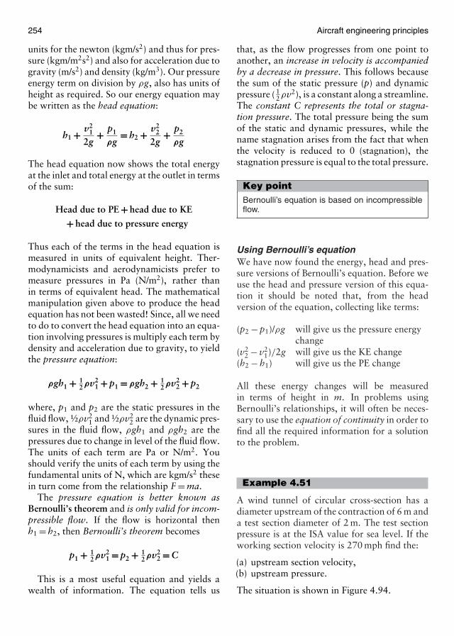
254 Aircraft engineering principles
units for the newton (kgm/s2) and thus for pres-sure (kgm/m2s2) and also for acceleration due togravity (m/s2) and density (kg/m3). Our pressureenergy term on division by ρg, also has units ofheight as required. So our energy equation maybe written as the head equation:
h1 + v21
2g+ p1
ρg= h2 + v2
2
2g+ p2
ρg
The head equation now shows the total energyat the inlet and total energy at the outlet in termsof the sum:
Head due to PE + head due to KE
+ head due to pressure energy
Thus each of the terms in the head equation ismeasured in units of equivalent height. Ther-modynamicists and aerodynamicists prefer tomeasure pressures in Pa (N/m2), rather thanin terms of equivalent head. The mathematicalmanipulation given above to produce the headequation has not been wasted! Since, all we needto do to convert the head equation into an equa-tion involving pressures is multiply each term bydensity and acceleration due to gravity, to yieldthe pressure equation:
ρgh1 + 12ρv2
1 + p1 = ρgh2 + 12ρv2
2 + p2
where, p1 and p2 are the static pressures in thefluid flow, ½ρv2
1 and ½ρv22 are the dynamic pres-
sures in the fluid flow, ρgh1 and ρgh2 are thepressures due to change in level of the fluid flow.The units of each term are Pa or N/m2. Youshould verify the units of each term by using thefundamental units of N, which are kgm/s2 thesein turn come from the relationship F = ma.
The pressure equation is better known asBernoulli’s theorem and is only valid for incom-pressible flow. If the flow is horizontal thenh1 = h2, then Bernoulli’s theorem becomes
p1 + 12ρv2
1 = p2 + 12ρv2
2 = C
This is a most useful equation and yields awealth of information. The equation tells us
that, as the flow progresses from one point toanother, an increase in velocity is accompaniedby a decrease in pressure. This follows becausethe sum of the static pressure (p) and dynamicpressure ( 1
2ρv2), is a constant along a streamline.The constant C represents the total or stagna-tion pressure. The total pressure being the sumof the static and dynamic pressures, while thename stagnation arises from the fact that whenthe velocity is reduced to 0 (stagnation), thestagnation pressure is equal to the total pressure.
Key pointBernoulli’s equation is based on incompressibleflow.
Using Bernoulli’s equationWe have now found the energy, head and pres-sure versions of Bernoulli’s equation. Before weuse the head and pressure version of this equa-tion it should be noted that, from the headversion of the equation, collecting like terms:
(p2 − p1)/ρg will give us the pressure energychange
(v22 − v2
1)/2g will give us the KE change(h2 − h1) will give us the PE change
All these energy changes will be measuredin terms of height in m. In problems usingBernoulli’s relationships, it will often be neces-sary to use the equation of continuity in order tofind all the required information for a solutionto the problem.
Example 4.51
A wind tunnel of circular cross-section has adiameter upstream of the contraction of 6 m anda test section diameter of 2 m. The test sectionpressure is at the ISA value for sea level. If theworking section velocity is 270 mph find the:
(a) upstream section velocity,(b) upstream pressure.
The situation is shown in Figure 4.94.

Physics 255
Figure 4.94 Wind tunnel.
(a) We first use the continuity equation to findthe upstream velocity v1. The csa A1 and A2
can be found using πr2, then:
A1 = 9π and A2 = π
So from
A1v1 = A2v2
we have
v1 = A2v2
A1= 1(270)
9= 30 mph
(b) To find the upstream pressure we will needto use Bernoulli’s equation, so we must firstconvert v1 and v2 into m/s.
Using Table 4.7,
v1 = 302.23694
= 13.4 m/s
and
v2 = 2702.23694
= 120.7 m/s
Then from Bernoulli’s equation, assumingthe wind tunnel is mounted horizontally,
p1 + ρv2
1
2= p2 + ρ
v22
2
and on rearrangement and substitution ofvalues then:
p1 = 101,320 + 1.2252
(120.72 − 13.42)
then,
upstream pressure p1 = 110,133 N/m2
Figure 4.95 The venturi tube and wing top section.
The venturi tubeAn important application of Bernoulli’s theoremis provided by the venturi tube (Figure 4.95(a)).
This arrangement shows a tube that grad-ually narrows to a throat, and then expandseven more gradually. If measurements are takenat the throat a decrease in pressure will beobserved. Now according to Bernoulli’s equa-tion a reduction in static pressure must beaccompanied by an increase in dynamic pres-sure, if the relationship is to remain constant.The increase in dynamic pressure is achievedby an increase in the velocity of the fluid as itreaches the throat. The effectiveness of the ven-turi tube as a means of causing a decrease inpressure below that of the atmosphere dependsvery much on its shape.
The venturi tube provides us with the keyfor the generation of lift. Imagine that the bot-tom cross-section of the tube is the top part ofan aircraft wing shown in cross-section (Figure4.95(b)). Then the increase in velocity of flowover the wing causes a corresponding reductionin pressure, below atmospheric. It is this reduc-tion in pressure which provides the lift forceperpendicular to the top surface of the wing, and
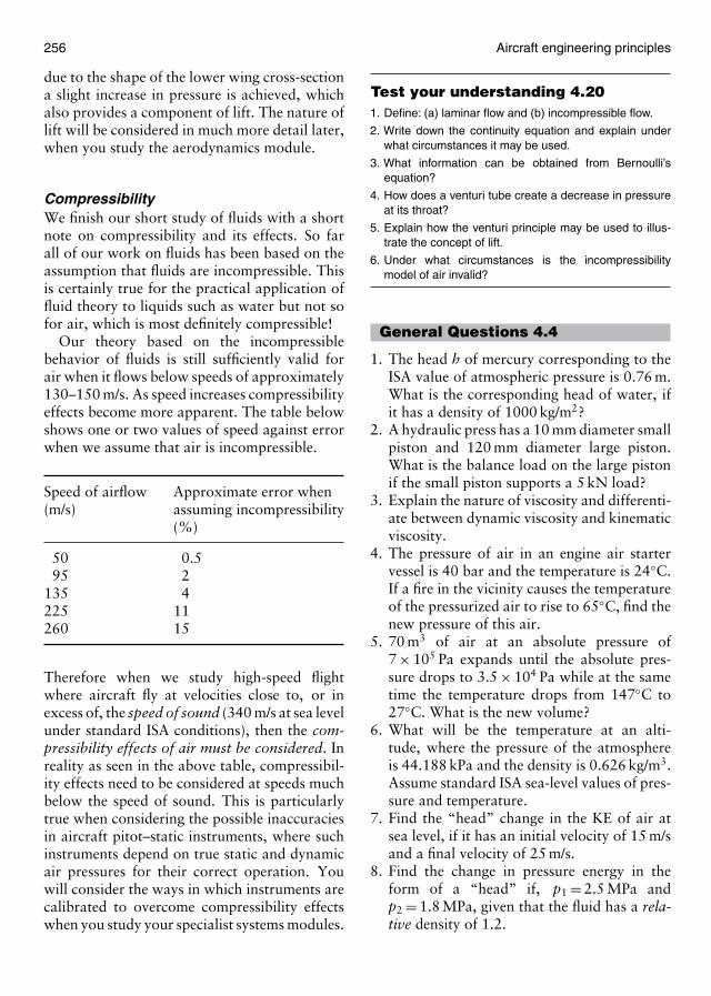
256 Aircraft engineering principles
due to the shape of the lower wing cross-sectiona slight increase in pressure is achieved, whichalso provides a component of lift. The nature oflift will be considered in much more detail later,when you study the aerodynamics module.
CompressibilityWe finish our short study of fluids with a shortnote on compressibility and its effects. So farall of our work on fluids has been based on theassumption that fluids are incompressible. Thisis certainly true for the practical application offluid theory to liquids such as water but not sofor air, which is most definitely compressible!
Our theory based on the incompressiblebehavior of fluids is still sufficiently valid forair when it flows below speeds of approximately130–150 m/s. As speed increases compressibilityeffects become more apparent. The table belowshows one or two values of speed against errorwhen we assume that air is incompressible.
Speed of airflow Approximate error when(m/s) assuming incompressibility
(%)
50 0.595 2
135 4225 11260 15
Therefore when we study high-speed flightwhere aircraft fly at velocities close to, or inexcess of, the speed of sound (340 m/s at sea levelunder standard ISA conditions), then the com-pressibility effects of air must be considered. Inreality as seen in the above table, compressibil-ity effects need to be considered at speeds muchbelow the speed of sound. This is particularlytrue when considering the possible inaccuraciesin aircraft pitot–static instruments, where suchinstruments depend on true static and dynamicair pressures for their correct operation. Youwill consider the ways in which instruments arecalibrated to overcome compressibility effectswhen you study your specialist systems modules.
Test your understanding 4.201. Define: (a) laminar flow and (b) incompressible flow.
2. Write down the continuity equation and explain underwhat circumstances it may be used.
3. What information can be obtained from Bernoulli’sequation?
4. How does a venturi tube create a decrease in pressureat its throat?
5. Explain how the venturi principle may be used to illus-trate the concept of lift.
6. Under what circumstances is the incompressibilitymodel of air invalid?
General Questions 4.4
1. The head h of mercury corresponding to theISA value of atmospheric pressure is 0.76 m.What is the corresponding head of water, ifit has a density of 1000 kg/m2?
2. A hydraulic press has a 10 mm diameter smallpiston and 120 mm diameter large piston.What is the balance load on the large pistonif the small piston supports a 5 kN load?
3. Explain the nature of viscosity and differenti-ate between dynamic viscosity and kinematicviscosity.
4. The pressure of air in an engine air startervessel is 40 bar and the temperature is 24◦C.If a fire in the vicinity causes the temperatureof the pressurized air to rise to 65◦C, find thenew pressure of this air.
5. 70 m3 of air at an absolute pressure of7 × 105 Pa expands until the absolute pres-sure drops to 3.5 × 10⁴ Pa while at the sametime the temperature drops from 147◦C to27◦C. What is the new volume?
6. What will be the temperature at an alti-tude, where the pressure of the atmosphereis 44.188 kPa and the density is 0.626 kg/m3.Assume standard ISA sea-level values of pres-sure and temperature.
7. Find the “head” change in the KE of air atsea level, if it has an initial velocity of 15 m/sand a final velocity of 25 m/s.
8. Find the change in pressure energy in theform of a “head” if, p1 = 2.5 MPa andp2 = 1.8 MPa, given that the fluid has a rela-tive density of 1.2.

Physics 257
4.10 Thermodynamics
Thermodynamics is the science that deals withvarious forms of energy and their transfor-mation from one form into another. Appliedthermodynamics is the specialist branch of thesubject that deals specifically with heat, mechan-ical and internal energies and their applica-tion to power production, air-conditioning andrefrigeration.
We start our study of applied thermodynam-ics (the area of specific interest to engineers) byconsidering a number of fundamental thermo-dynamic properties and relationships.
4.10.1 Fundamentals
TemperatureWe have already met temperature on severaloccasions during our study of physics, but as yet,we have not defined it in thermodynamic terms.
Temperature is a measure of the quantity ofenergy possessed by a body or substance. It mea-sures the vibration of the molecules, which formthe substance. These molecular vibrations onlycease when the temperature of the substancereaches absolute zero, i.e. −273.15◦C.
We have already met the celsius temperaturescale and you should now be able to convertdegrees centigrade into kelvin and vice versa, forcompleteness we need to see how the fahrenheitscale relates to these.
Figure 4.96 shows the relationship betweenthese three scales and indicates the commonboiling point of pure water and the melting pointof pure ice, for each set of units.
Key pointTemperature measures the energy possessed bythe vibration of the molecules that go to make upa substance.
Example 4.52
Convert 60◦C into (a) K and (b) ◦F.
(a) You already know that 1◦C = 1 K and that toconvert ◦C into K, we simply add 273, therefore60◦C + 273 = 333 K.
Figure 4.96 Relationship between celsius, kelvinand fahrenheit scales.
Note that to be strictly accurate we shouldadd 273.15, but for all practical purposes theapproximate value of 273 is adequate.(b) Now to convert 60◦C into ◦F we can use theinverse of the relationship given in Table E.7of Appendix E. Then ◦F = (◦C × 1.8) + 32 andsubstituting value gives,
(60◦C × 1.8) + 32 = 140◦F
Alternative versions of the formulae, to con-vert Fahrenheit to Celsius and vice versa, are:
◦F =(
◦C × 95
)+ 32 and ◦C = (◦F − 32) × 5
9
Note: The ◦F may be converted to absolutetemperature (K) by converting to ◦C and thenadding 273. ◦F may be converted to absolutetemperature on the Rankine scale by adding459.67. To convert from Rankine to K simplymultiply by 5/9.
So 140◦F + 459.67 = 599.67 R =599.67(5/9) = 333.15 K. For all our thermodynamicwork we will only use the Kelvin scale formeasuring absolute temperature.
Temperature measurementThe method used to measure temperaturedepends on the degree of hotness of the bodyor substance being measured. Measurement
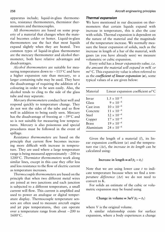
258 Aircraft engineering principles
apparatus include; liquid-in-glass thermome-ters, resistance thermometers, thermistor ther-mometers and thermocouples.
All thermometers are based on some prop-erty of a material that changes when the mate-rial becomes colder or hotter. Liquid-in-glassthermometers use the fact that most liquidsexpand slightly when they are heated. Twocommon types of liquid-in-glass thermometerare the mercury thermometer and alcohol ther-mometer, both have relative advantages anddisadvantages.
Alcohol thermometers are suitable for mea-suring temperatures down to −115◦C and havea higher expansion rate than mercury, so alarger containing tube may be used. They havethe disadvantage of requiring the addition of acolouring in order to be seen easily. Also, thealcohol tends to cling to the side of the glasstube and may separate.
Mercury thermometers conduct heat well andrespond quickly to temperature change. Theydo not wet the sides of the tube and so flowwell in addition to being easily seen. Mercuryhas the disadvantage of freezing at −39◦C andso is not suitable for measuring low tempera-tures. Mercury is also poisonous and specialprocedures must be followed in the event ofspillage.
Resistance thermometers are based on theprinciple that current flow becomes increas-ing more difficult with increase in tempera-ture. They are used where a large temperaturerange is being measured approximately −200 to1200◦C. Thermistor thermometers work alongsimilar lines, except in this case they offer lessand less resistance to the flow of electric currentas temperature increases.
Thermocouple thermometers are based on theprinciple that when two different metal wiresare joined at two junctions and each junctionis subjected to a different temperature, a smallcurrent will flow. This current is amplified andused to power an analogue or digital temper-ature display. Thermocouple temperature sen-sors are often used to measure aircraft engineand jet pipe temperatures, they can operateover a temperature range from about −200 to1600◦C.
Thermal expansionWe have mentioned in our discussion on ther-mometers that certain liquids expand withincrease in temperature, this is also the casewith solids. Thermal expansion is dependent onthe nature of the material and the magnitudeof the temperature increase. We normally mea-sure the linear expansion of solids, such as theincrease in length of a bar of the material, withgases (as you have already seen) we measurevolumetric or cubic expansion.
Every solid has a linear expansivity value, i.e.the amount the material will expand in m/K orm/◦C. This expansivity value is often referred toas the coefficient of linear expansion (α), sometypical values of α are given below:
Material Linear expansion coefficient α/◦C
Invar 1.5 × 10⁻⁶
Glass 9 × 10⁻⁶
Cast iron 10 × 10−6
Concrete 11 × 10−6
Steel 12 × 10−6
Copper 17 × 10−6
Brass 19 × 10−6
Aluminium 24 × 10−6
Given the length of a material (l), its lin-ear expansion coefficient (α) and the tempera-ture rise (�t), the increase in its length can becalculated using:
Increase in length = αl(t2 − t1)
Note that we are using lower case t to indi-cate temperature because when we find a tem-perature difference (�t) we do not need toconvert to K.
For solids an estimate of the cubic or volu-metric expansion may be found using
Change in volume = 3αV (t2 − t1)
where V is the original volume.A similar relationship exists for surface
expansion, where a body experiences a change

Physics 259
in area. In this case the linear expansion coeffi-cient is multiplied by 2, therefore,
Change in area = 2αA(t2 − t1)
where A is the original area.
Example 4.53
A steel bar has a length of 4.0 m at 10◦C.What will be the length of the bar when it isheated to 350◦C? If a sphere of diameter 15 cmis made from the same material what will bethe percentage increase in surface area, if thesphere is subject to the same initial and finaltemperatures?
Using α = 12 × 10−6 from the above table,increase in length of the bar is given by:
x = αl(t2 − t1) = (12 × 10−6)(4.0)(350 − 10)
= 0.0163 m
This can now be added to the original length togive the final length = 4.0 + 0.0163 = 4.0163 m.
Increase in surface area of the sphere = 2αA(t2 − t1). We first need to find the original surfacearea which is given by:
A = 4πr2 = 4π × (0.075)2 = 0.0707 m2
and from above, the increase in surface area
= (2)(12 × 10−6)(0.0707)(340)
= 5.769 × 10⁻⁶ m
Therefore the percentage increase in area
= increase in areaoriginal area
× 100
= 5.769 × 10⁻⁴
0.0707× 100 = 0.82%
Heat energyEnergy is the most important and fundamen-tal physical property of the universe. We havealready defined energy as, the capacity to dowork, more accurate it may be defined as: thecapacity to produce an effect. These effects areapparent during the process of energy transfer.
Figure 4.97 Heat energy transfer.
A modern idea of heat is that it is energy intransition and cannot be stored by matter. Heat(Q) may be defined as: transient energy broughtabout by the interaction of bodies by virtue oftheir temperature difference when they commu-nicate. Matter possesses stored energy but nottransient (moving) energy, such as heat or work.Heat energy can only travel or transfer from ahot body to a cold body, it cannot travel up hill,Figure 4.97 illustrates this fact.
Key pointHeat and work is energy in transit and cannot bestored by matter.
Within matter the amount of molecular vibra-tion determines the amount of KE a substancepossesses. For incompressible fluids (liquids) theamount of molecular vibration is relatively smalland can be neglected. For compressible fluidsand gases the degree of vibration is so large thatit has to be accounted for in thermodynamics.This KE is classified as internal energy (U) andis a form of stored energy.
Heat energy transferLiterature on heat transfer generally recognizesthree distinct modes of heat transmission, thenames of which will be familiar to you, i.e.conduction, convection and radiation. Techni-cally only conduction and radiation are trueheat transfer processes, because both of thesedepend totally and utterly on a temperature dif-ference being present. Convection also dependson the transportation of a mechanical mass.
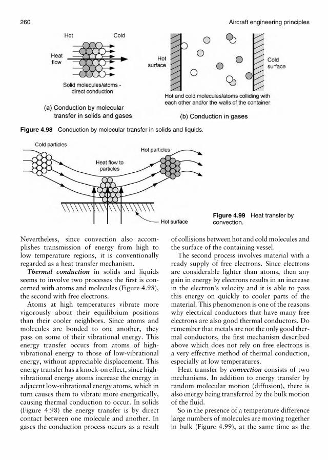
260 Aircraft engineering principles
Figure 4.98 Conduction by molecular transfer in solids and liquids.
Figure 4.99 Heat transfer byconvection.
Nevertheless, since convection also accom-plishes transmission of energy from high tolow temperature regions, it is conventionallyregarded as a heat transfer mechanism.
Thermal conduction in solids and liquidsseems to involve two processes the first is con-cerned with atoms and molecules (Figure 4.98),the second with free electrons.
Atoms at high temperatures vibrate morevigorously about their equilibrium positionsthan their cooler neighbors. Since atoms andmolecules are bonded to one another, theypass on some of their vibrational energy. Thisenergy transfer occurs from atoms of high-vibrational energy to those of low-vibrationalenergy, without appreciable displacement. Thisenergy transfer has a knock-on effect, since high-vibrational energy atoms increase the energy inadjacent low-vibrational energy atoms, which inturn causes them to vibrate more energetically,causing thermal conduction to occur. In solids(Figure 4.98) the energy transfer is by directcontact between one molecule and another. Ingases the conduction process occurs as a result
of collisions between hot and cold molecules andthe surface of the containing vessel.
The second process involves material with aready supply of free electrons. Since electronsare considerable lighter than atoms, then anygain in energy by electrons results in an increasein the electron’s velocity and it is able to passthis energy on quickly to cooler parts of thematerial. This phenomenon is one of the reasonswhy electrical conductors that have many freeelectrons are also good thermal conductors. Doremember that metals are not the only good ther-mal conductors, the first mechanism describedabove which does not rely on free electrons isa very effective method of thermal conduction,especially at low temperatures.
Heat transfer by convection consists of twomechanisms. In addition to energy transfer byrandom molecular motion (diffusion), there isalso energy being transferred by the bulk motionof the fluid.
So in the presence of a temperature differencelarge numbers of molecules are moving togetherin bulk (Figure 4.99), at the same time as the

Physics 261
individual motion of the molecules takes place.The cumulative effect of both of these energytransfer methods is referred to as heat transferby convection.
Radiation may be defined as the transfer ofenergy not requiring a medium through whichthe energy must pass, thus radiation can betransferred through empty space. Thermal radi-ation is attributed to the electron energy changeswithin atoms or molecules. As electron energylevels change, energy is released which trav-els in the form of electromagnetic waves ofvarying wavelength. You will meet electro-magnetic waves again when you study light.When striking a body the emitted radiation iseither absorbed by, reflected by, or transmittedthrough the body.
Specific heatFrom what has been said about heat transferabove, it will be apparent that different mate-rials have different capacities for absorbing andtransferring thermal energy. The thermal energyneeded to produce a temperature rise dependson; the mass of the material, type of materialand the temperature rise to which the materialis subjected.
Thus the inherent ability of a material toabsorb heat for a given mass and temperaturerise is dependent on the material itself. Thisproperty of the material is known as its specificheat capacity. In the SI system, the specific heatcapacity of a material is the same as the thermalenergy required to produce a 1 K rise in temper-ature in a mass of 1 kg. Therefore knowing themass of a substance and its specific heat capacity,it is possible to calculate the thermal energyrequired to produce any given temperature rise,from:
Thermal energy, Q = mc�t
where c = specific heat capacity of the material(J/kgK) and �t is the temperature change.
Example 4.54
How much thermal energy is required to raisethe temperature of 5 kg of aluminium from 20
to 40◦C? Take the specific heat capacity foraluminium as 900 J/kgK.
All that is required is to substitute the appropri-ate values directly into the equation:
Q = mc�t = (5)(900)(40 − 20)
= 90,000 J = 90 kJ
Another way of defining the specific heat capac-ity of any substance is: the amount of heatenergy required to raise the temperature of unitmass of the substance through one degree, underspecific conditions.
In thermodynamics two specified conditionsare used those of constant volume and constantpressure. With gases the two specific heats donot have the same value and it is essential thatwe distinguish between them.
Specific heat at constant volumeIf 1 kg of a gas is supplied with an amount ofheat energy sufficient to raise the temperature by1◦C or 1 K while the volume of the gas remainsconstant, then the amount of heat energy sup-plied is known as the specific heat capacity atconstant volume and is denoted by cv. Notethat under these circumstances (Figure 4.100(a))no work is done, but the gas has received anincrease in internal energy (U). The specific heatat constant volume for air (cv air) is 718 J/kgK,this constant is well worth memorizing!
Specific heat at constant pressureIf 1 kg of a gas is supplied with a quantity ofheat energy sufficient to raise the temperatureof the gas by 1◦C or 1 K while the pressure isheld constant, then the amount of heat energysupplied is known as the specific heat capacityat constant pressure and is denoted by cp.
This implies that when the gas has been heatedit will expand a distance h (Figure 4.100b), sowork has been done. Thus for the same amountof heat energy there has been an increase ininternal energy (U), plus work. The value ofcp is, therefore, greater than the correspondingvalue of cv.
The specific heat capacity at constant pres-sure for air (cp air) is 1005 J/kgK, again this is aconstant worth remembering.
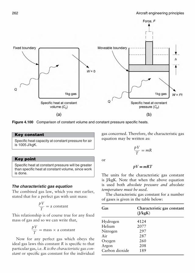
262 Aircraft engineering principles
Figure 4.100 Comparison of constant volume and constant pressure specific heats.
Key constantSpecific heat capacity at constant pressure for airis 1005 J/kgK.
Key pointSpecific heat at constant pressure will be greaterthan specific heat at constant volume, since workis done.
The characteristic gas equationThe combined gas law, which you met earlier,stated that for a perfect gas with unit mass:
pVT
= a constant
This relationship is of course true for any fixedmass of gas and so we can write that,
pVT
= mass × a constant
Now for any perfect gas which obeys theideal gas laws this constant R is specific to thatparticular gas, i.e. R is the characteristic gas con-stant or specific gas constant for the individual
gas concerned. Therefore, the characteristic gasequation may be written as:
pVT
= mR
or
pV = mRT
The units for the characteristic gas constantis J/kgK. Note that when the above equationis used both absolute pressure and absolutetemperature must be used.
The characteristic gas constant for a numberof gases is given in the table below:
Gas Characteristic gas constant(J/kgK)
Hydrogen 4124Helium 2077Nitrogen 297Air 287Oxygen 260Argon 208Carbon dioxide 189
Physics 263
The characteristic gas constant for air, fromthe above table, is R = 287 J/kgK. This is relatedto the specific heat capacities for air in the fol-lowing way, i.e. R = cp − cv, you should checkthis relationship by noting the above values of R,cp and cv for air. This relationship (R = cp − cv)is not only valid for air, it is also valid for anyperfect gas that follows the ideal laws.
Example 4.55
0.22 kg of gas at a temperature of 20◦C andpressure of 103 kN/m2 occupies a volume of0.18 m3. If the cv for the gas = 720 J/kgK,find the:(a) characteristic gas constant,(b) specific heat capacity at constant pressure.
(a) Using pV = mRT then on rearrangement,
R = pVmT
= (103 × 103)(0.18)(0.22)(293)
= 288 J/kgK
(b) from R = cp − cv, then,
cp = R + cv = 288 + 720 = 1008 J/kgK
Latent heatWhen a substance changes state, i.e. when heatis applied to a solid and it turns into a liquid andwith further heating the liquid turns into a gaswe say the substance has undergone a change instate. The three states of matter are solid, liquidand gas. Therefore, the heat energy added to asubstance does not necessary give rise to a mea-surable change in temperature, it may be used tochange the state of a substance, under these cir-cumstances we refer to the heat energy as latentor hidden heat.
Key pointLatent heat is heat added to a body withoutchange in temperature.
We refer to the thermal energy required tochange a solid material into a liquid as, the latentheat of fusion. For water, 334 kJ of thermal
energy are required to change 1 kg of ice at 0◦Cinto water at the same temperature. Thus thespecific latent heat of fusion for water is 334 kJ.In the case of latent heat, specific, refers to unitmass of the material, i.e. per kilogramme. So wedefine the specific latent heat of fusion of a sub-stance as: the thermal energy required to turn1 kg of a substance from a liquid into a solidwithout change in temperature.
If we wish to find the thermal energy requiredto change any amount of a substance from asolid into a liquid, then we use the relationship:
Q = mL
where L is the specific latent heat of thesubstance.
In a similar manner to the above argument:the thermal energy required to change 1 kg ofa substance from a liquid into a gas withoutchange in temperature, is known as the specificlatent heat of vaporization. Again, if we wish tofind the thermal energy required to change anyamount of a substance from a liquid into a gaswe use the relationship Q = mL, but in this caseL = the specific latent heat of vaporization.
The specific latent heat of vaporization forwater is 2.26 MJ/kgK.
Example 4.56
(a) How much heat energy is required to change3 kg of ice at 0◦C into water at 30◦C?
(b) What thermal energy is required to condense0.2 kg of steam into water at 100◦C?
(a) The thermal energy required to convert iceat 0◦C into water at 0◦C is calculated usingthe equation:
Q = mL
and substituting values we get,
Q = (3)(334 × 103) = 1.002 MJ
The 3 kg of water formed has to be heatedfrom 0 to 30◦C. The thermal energy requiredfor this is calculated using the equationQ = mc�t, you have already met this equa-tion when we studied specific heat earlier.
264 Aircraft engineering principles
So in this case
Q = (3)(4200)(30) = 378,000 J= 0.378 MJ
Then total thermal energy required = 1.002 +0.378 = 1.38 MJ
(b) In this case we simply use Q = mL, sincewe are converting steam to water at 100◦Cwhich is the vaporization temperature forwater into steam.
Then Q = (0.2)(2.226 × 10⁶) = 445.2 kJ
Note the large amounts of thermal energyrequired to change the state of a substance.This energy together with cooling by evapora-tion is used within aircraft air-conditioning andrefrigeration systems.
A liquid does not have to boil in order forit to change state, the nearer the temperatureis to the boiling point of the liquid, then thequicker the liquid will turn into a gas. At muchlower temperatures the change may take placeby a process of evaporation. The steam risingfrom a puddle, when the sun comes out after arainstorm, is an example of evaporation, wherewater vapour forms as steam, well below theboiling point of the water.
There are several ways that a liquid can bemade to evaporate more readily. These include;an increase in temperature that increases themolecular energy of the liquid sufficient for themore energetic molecules to escape from the liq-uid, reducing the pressure above the liquid inorder to allow less energetic molecules to escapeas a gas, increase the surface area, thus pro-viding more opportunity for the more energeticmolecules to escape or, by passing a gas over thesurface of the liquid to assist molecular escape.
An aircraft refrigeration system can be madeto work in exactly the same manner as a domes-tic refrigerator, where we use the fact that aliquid can be made to vaporize at any tem-perature by altering the pressure acting on it.Refrigerators use a fluid that has a very low boil-ing point, such as freon. We know from our lawsof thermodynamics that heat can only flow froma point of high temperature to one at a lowertemperature. If heat is to be made to flow inthe opposite direction some additional energyneeds to be supplied. In a refrigeration system
such as that illustrated in the block schematicdiagram (Figure 4.101), this additional sourceof energy is supplied by a compressor or pump.When the gas is compressed, its temperature israised and when the gas is allowed to expand itstemperature is lowered.
A reverse flow of heat is achieved by com-pressing the freon to a pressure high enoughso that its temperature is raised above that ofthe outside air. Heat will now flow from thehigh-temperature gas to the lower temperaturesurrounding air, thus lowering the heat energyof the gas. The gas is now allowed to expand to alower pressure, causing a drop in temperature.This drop in temperature now makes it coolerthan the surrounding air, so the air being cooled,acts as the heat source. Thus heat will now flowfrom the heat source, to the freon, which is nowcompressed again beginning a new cycle.
In a practical sense for the freon refrigera-tion system shown opposite, the refrigerationcycle operates as follows. Freon as a liquidis contained in the receiver under high pres-sure. It is allowed to flow through a valve intothe evaporator at reduced pressure, so now, atreduced pressure, the boiling temperature of thefreon is low enough to cool the surroundingair through heat exchange, this is the purposeof the refrigeration system! In turn, heat nowflows from the air to the freon, causing it toboil and vaporize. Cold freon vapor now entersthe compressor, where its pressure is raised,thereby raising its boiling point. The refriger-ant at high pressure and high temperature flowsinto the condenser, where heat flows from thefreon (refrigerant) to the outside air, condens-ing the vapor into a liquid. The cycle is repeatedto maintain the cooling space, through whichthe air passes, at the desired temperature.
Note that heat flows into the refrigerant fromthe air to be cooled, via the evaporator heatexchanger and heat flows from the refrigerantto the surrounding air via the condenser heatexchanger.
Key pointA refrigerant is a cryogenic (cold) fluid which hasa very low boiling temperature.
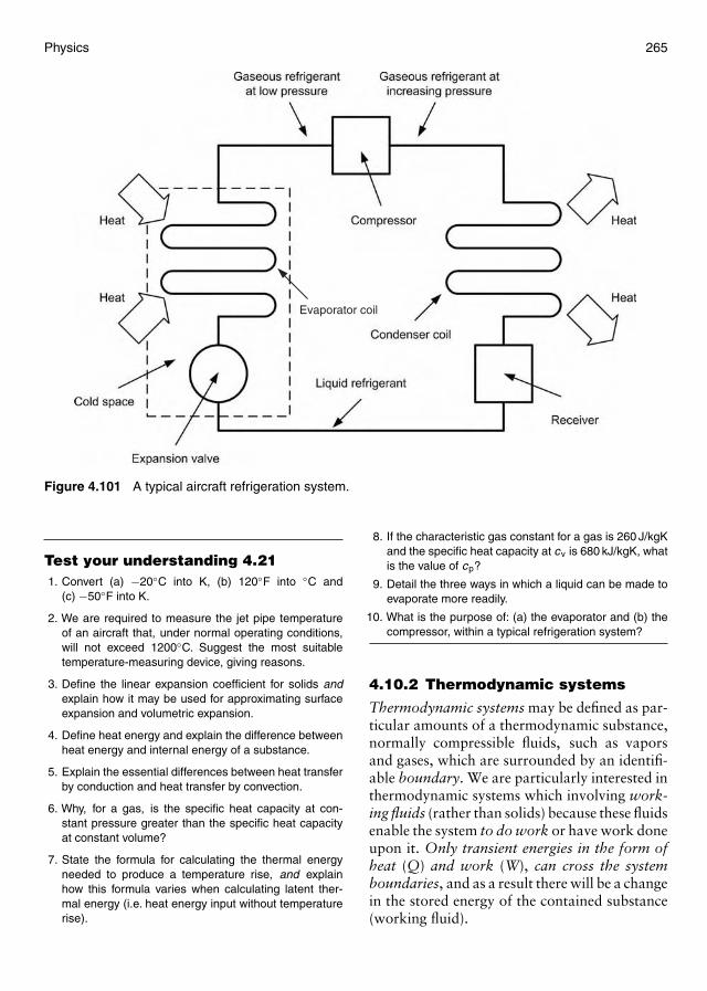
Physics 265
Evaporator coil
Figure 4.101 A typical aircraft refrigeration system.
Test your understanding 4.211. Convert (a) −20◦C into K, (b) 120◦F into ◦C and
(c) −50◦F into K.
2. We are required to measure the jet pipe temperatureof an aircraft that, under normal operating conditions,will not exceed 1200◦C. Suggest the most suitabletemperature-measuring device, giving reasons.
3. Define the linear expansion coefficient for solids andexplain how it may be used for approximating surfaceexpansion and volumetric expansion.
4. Define heat energy and explain the difference betweenheat energy and internal energy of a substance.
5. Explain the essential differences between heat transferby conduction and heat transfer by convection.
6. Why, for a gas, is the specific heat capacity at con-stant pressure greater than the specific heat capacityat constant volume?
7. State the formula for calculating the thermal energyneeded to produce a temperature rise, and explainhow this formula varies when calculating latent ther-mal energy (i.e. heat energy input without temperaturerise).
8. If the characteristic gas constant for a gas is 260 J/kgKand the specific heat capacity at cv is 680 kJ/kgK, whatis the value of cp?
9. Detail the three ways in which a liquid can be made toevaporate more readily.
10. What is the purpose of: (a) the evaporator and (b) thecompressor, within a typical refrigeration system?
4.10.2 Thermodynamic systems
Thermodynamic systems may be defined as par-ticular amounts of a thermodynamic substance,normally compressible fluids, such as vaporsand gases, which are surrounded by an identifi-able boundary. We are particularly interested inthermodynamic systems which involving work-ing fluids (rather than solids) because these fluidsenable the system to do work or have work doneupon it. Only transient energies in the form ofheat (Q) and work (W), can cross the systemboundaries, and as a result there will be a changein the stored energy of the contained substance(working fluid).

266 Aircraft engineering principles
Properties of thermodynamic systemsThe essential elements that go to make up athermodynamic system are:
(a) a working fluid, i.e. the matter which may ormay not cross the system boundaries, such aswater, steam, air, etc.,
(b) a heat source,(c) a cold body to promote heat flow and enable
heat energy transfer,(d) the system boundaries, which may or may
not be fixed.
The property of a working fluid is an observ-able quantity, such as pressure, temperature,etc. The state of a working fluid when it is agas, may be defined by any two unique proper-ties. For example, Boyle’s law defines the stateof the fluid by specifying the independent ther-modynamic properties of volume and pressure.
When a working fluid is subject to a process,then the fluid will have started with one set ofproperties and ended with another, irrespectiveof how the process took place or what happenedbetween the start and end states. For example, ifa fluid within a system has an initial pressure (p1)and temperature (T1) and is then compressedproducing an increase in pressure (p2) and tem-perature (T2), then we say that the fluid hasundergone a process from state 1 to state 2.
We say that work is transferred in a ther-modynamic system, if there is movement ofthe system boundaries, this concept is furtherexplored when we consider closed systems, next.
The closed systemThis type of system has a closed or fixed bound-ary containing a fixed amount of vapour or gas,while an exchange of heat and work may takeplace. An energy diagram of a typical closedsystem is shown in Figure 4.102.
Key pointIn a closed system there is no mass transfer ofsystem fluid.
The boundary of a closed system is not nec-essarily rigid, what makes the system closed isthe fact that no mass transfer of the system fluid
Figure 4.102 Closed system energy exchange.
Figure 4.103 Cylinder and piston assembly of theinternal combustion engine.
takes place, while an interchange of heat andwork take place.
Consider the well known example of a closedsystem, that of the cylinder and piston assemblyof an internal combustion engine (Figure 4.103).
The closed boundary is formed by the crownof the piston, the cylinder walls and the cylin-der head with the valves closed. The transientenergy being in the form of combustible fuel thatcreates a sudden pressure wave which forces thepiston down. Therefore as the piston moves, theboundaries of the system move. This movementcauses the system to do work (force × distance),on its surroundings. In this case the piston con-necting rod drives a crank, to provide motivepower.
Note that in a closed system, it requires move-ment of the system boundary for work to bedone by the system or on the system, thuswork (like heat) is a transient energy, it is notcontained within the system. There is also, nomass transfer of system fluid across the system
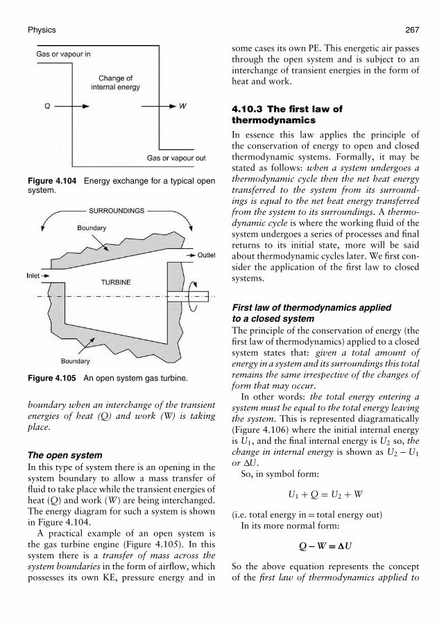
Physics 267
Figure 4.104 Energy exchange for a typical opensystem.
Figure 4.105 An open system gas turbine.
boundary when an interchange of the transientenergies of heat (Q) and work (W) is takingplace.
The open systemIn this type of system there is an opening in thesystem boundary to allow a mass transfer offluid to take place while the transient energies ofheat (Q) and work (W) are being interchanged.The energy diagram for such a system is shownin Figure 4.104.
A practical example of an open system isthe gas turbine engine (Figure 4.105). In thissystem there is a transfer of mass across thesystem boundaries in the form of airflow, whichpossesses its own KE, pressure energy and in
some cases its own PE. This energetic air passesthrough the open system and is subject to aninterchange of transient energies in the form ofheat and work.
4.10.3 The first law ofthermodynamics
In essence this law applies the principle ofthe conservation of energy to open and closedthermodynamic systems. Formally, it may bestated as follows: when a system undergoes athermodynamic cycle then the net heat energytransferred to the system from its surround-ings is equal to the net heat energy transferredfrom the system to its surroundings. A thermo-dynamic cycle is where the working fluid of thesystem undergoes a series of processes and finalreturns to its initial state, more will be saidabout thermodynamic cycles later. We first con-sider the application of the first law to closedsystems.
First law of thermodynamics appliedto a closed systemThe principle of the conservation of energy (thefirst law of thermodynamics) applied to a closedsystem states that: given a total amount ofenergy in a system and its surroundings this totalremains the same irrespective of the changes ofform that may occur.
In other words: the total energy entering asystem must be equal to the total energy leavingthe system. This is represented diagramatically(Figure 4.106) where the initial internal energyis U1, and the final internal energy is U2 so, thechange in internal energy is shown as U2 − U1
or �U.So, in symbol form:
U1 + Q = U2 + W
(i.e. total energy in = total energy out)In its more normal form:
Q − W = �U
So the above equation represents the conceptof the first law of thermodynamics applied to
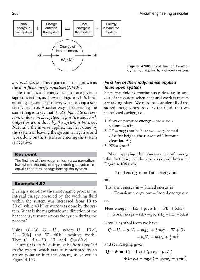
268 Aircraft engineering principles
Figure 4.106 First law of thermo-dynamics applied to a closed system.
a closed system. This equation is also known asthe non-flow energy equation (NFEE).
Heat and work energy transfer are given asign convention, as shown in Figure 4.106. Heatentering a system is positive, work leaving a sys-tem is negative. Another way of expressing thesame thing is to say that; heat supplied to the sys-tem, or done on the system, is positive and workoutput or work done by the system is positive.Naturally the inverse applies, i.e. heat done bythe system or leaving the system is negative andwork done on the system or entering the systemis negative.
Key pointThe first law of thermodynamics is a conservationlaw, where the total energy entering a system isequal to the total energy leaving the system.
Example 4.57
During a non-flow thermodynamic process theinternal energy possesed by the working fluidwithin the system was increased from 10 to30 kJ, while 40 kJ of work was done by the sys-tem. What is the magnitude and direction of theheat energy transfer across the system during theprocess?
Using Q − W = U2 − U1, where U1 = 10 kJ,U2 = 30 kJ and W = 40 kJ (positive work).Then, Q − 40 = 30 − 10 and Q = 60 kJ
Since Q is positive, it must be heat suppliedto the system, which may be represented by anarrow pointing into the system, as shown inFigure 4.105.
First law of thermodynamics appliedto an open systemSince the fluid is continuously flowing in andout of the system when heat and work transfersare taking place. We need to consider all of thestored energies possessed by the fluid, that wementioned earlier, i.e.
1. flow or pressure energy = pressure ×volume = pV;
2. PE = mgz (notice here we use z insteadof h for height, the reason will becomeclear later!);
3. KE = 12 mv2.
Now applying the conservation of energy(the first law) to the open system shown inFigure 4.106 then:
Total energy in = Total energy out
so,
Transient energy in + Stored energy in= Transient energy out + Stored energy out
or,
Heat energy + (IE1 + press E1 + PE1 + KE1)= work energy+ (IE2 +press E2 +PE2 +KE1)
Now in symbol form we have:
Q + U1 + p1V1 + mgz1 + 12 mv2
1 = W + U2
+ p2V2 + mgz2 + 12 mv2
2
and rearranging gives:
Q − W = (U2 − U1) + (p2V2 − p1V1)
+ (mgz2 − mgz1) + ( 12 mv2
2 − 12 mv2
1)
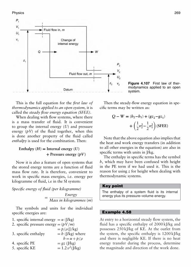
Physics 269
Figure 4.107 First law of ther-modynamics applied to an opensystem.
This is the full equation for the first law ofthermodynamics applied to an open system, it iscalled the steady flow energy equation (SFEE).
When dealing with flow systems, where thereis a mass transfer of fluid. It is convenientto group the internal energy (U) and pressureenergy (pV) of the fluid together, when thisis done another property of the fluid calledenthalpy is used for the combination. Then:
Enthalpy (H) = Internal energy (U )+ Pressure energy (pV )
Now it is also a feature of open systems thatthe stored energy terms are a function of fluidmass flow rate. It is therefore, convenient towork in specific mass energies, i.e. energy perkilogramme of fluid, i.e in the SI system:
Specific energy of fluid (per kilogramme)
= EnergyMass in kilogrammes (m)
The symbols and units for the individualspecific energies are:
1. specific internal energy = u (J/kg)2. specific pressure energy = (pV/m)
= p/ρ(J/kg)3. specific enthalpy = h (J/kg) where
h = u + p/ρ
4. specific PE = gz (J/kg)5. specific KE = 1.2 v2(J/kg)
Then the steady-flow energy equation in spe-cific terms may be written as:
Q − W = (h2−h1) + (gz2−gz1)
+(
12
v22−1
2v2
1
)(SFEE)
Note that the above equation also implies thatthe heat and work energy transfers (in additionto all other energies in the equation) are also inspecific terms with units in J/kg.
The enthalpy in specific terms has the symbolh, which may have been confused with heightin the PE term if we had used it. This is thereason for using z for height when dealing withthermodynamic systems.
Key pointThe enthalpy of a system fluid is its internalenergy plus its pressure–volume energy.
Example 4.58
At entry to a horizontal steady flow system, thefluid has a specific enthalpy of 2000 kJ/kg andpossesses 250 kJ/kg of KE. At the outlet fromthe system, the specific enthalpy is 1200 kJ/kgand there is negligible KE. If there is no heatenergy transfer during the process, determinethe magnitude and direction of the work done.
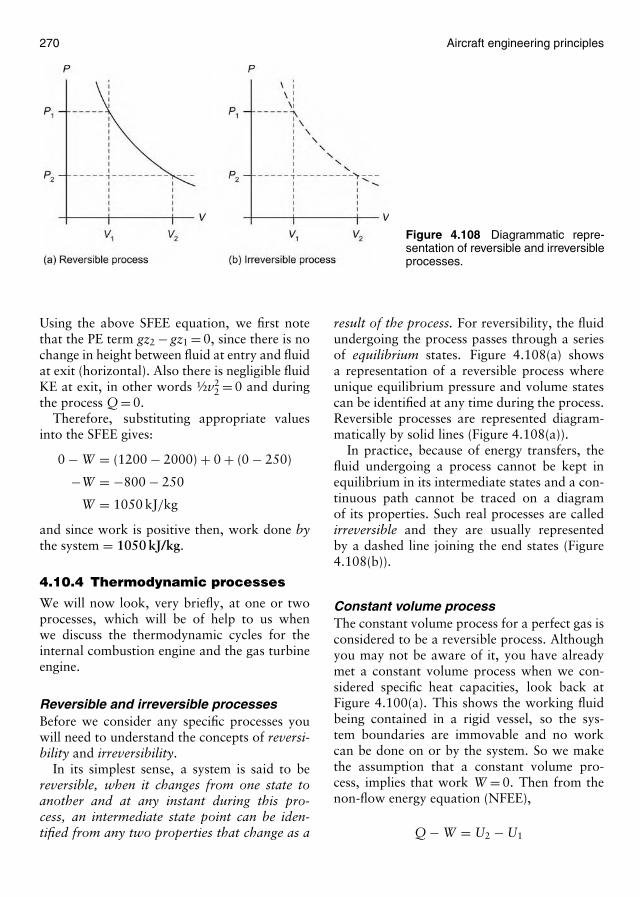
270 Aircraft engineering principles
Figure 4.108 Diagrammatic repre-sentation of reversible and irreversibleprocesses.
Using the above SFEE equation, we first notethat the PE term gz2 − gz1 = 0, since there is nochange in height between fluid at entry and fluidat exit (horizontal). Also there is negligible fluidKE at exit, in other words ½v2
2 = 0 and duringthe process Q = 0.
Therefore, substituting appropriate valuesinto the SFEE gives:
0 − W = (1200 − 2000) + 0 + (0 − 250)
−W = −800 − 250
W = 1050 kJ/kg
and since work is positive then, work done bythe system = 1050 kJ/kg.
4.10.4 Thermodynamic processes
We will now look, very briefly, at one or twoprocesses, which will be of help to us whenwe discuss the thermodynamic cycles for theinternal combustion engine and the gas turbineengine.
Reversible and irreversible processesBefore we consider any specific processes youwill need to understand the concepts of reversi-bility and irreversibility.
In its simplest sense, a system is said to bereversible, when it changes from one state toanother and at any instant during this pro-cess, an intermediate state point can be iden-tified from any two properties that change as a
result of the process. For reversibility, the fluidundergoing the process passes through a seriesof equilibrium states. Figure 4.108(a) showsa representation of a reversible process whereunique equilibrium pressure and volume statescan be identified at any time during the process.Reversible processes are represented diagram-matically by solid lines (Figure 4.108(a)).
In practice, because of energy transfers, thefluid undergoing a process cannot be kept inequilibrium in its intermediate states and a con-tinuous path cannot be traced on a diagramof its properties. Such real processes are calledirreversible and they are usually representedby a dashed line joining the end states (Figure4.108(b)).
Constant volume processThe constant volume process for a perfect gas isconsidered to be a reversible process. Althoughyou may not be aware of it, you have alreadymet a constant volume process when we con-sidered specific heat capacities, look back atFigure 4.100(a). This shows the working fluidbeing contained in a rigid vessel, so the sys-tem boundaries are immovable and no workcan be done on or by the system. So we makethe assumption that a constant volume pro-cess, implies that work W = 0. Then from thenon-flow energy equation (NFEE),
Q − W = U2 − U1
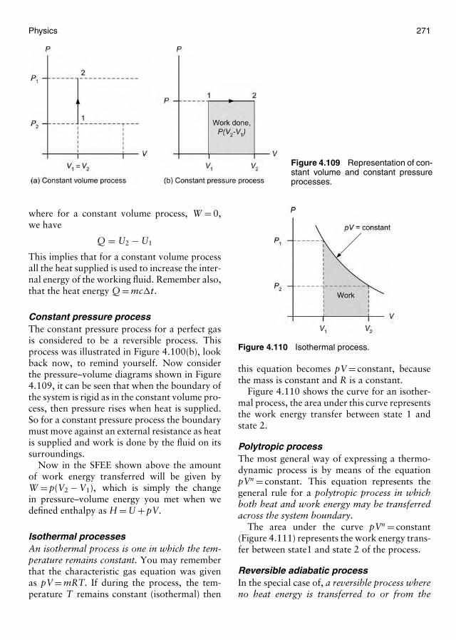
Physics 271
Figure 4.109 Representation of con-stant volume and constant pressureprocesses.
where for a constant volume process, W = 0,we have
Q = U2 − U1
This implies that for a constant volume processall the heat supplied is used to increase the inter-nal energy of the working fluid. Remember also,that the heat energy Q = mc�t.
Constant pressure processThe constant pressure process for a perfect gasis considered to be a reversible process. Thisprocess was illustrated in Figure 4.100(b), lookback now, to remind yourself. Now considerthe pressure–volume diagrams shown in Figure4.109, it can be seen that when the boundary ofthe system is rigid as in the constant volume pro-cess, then pressure rises when heat is supplied.So for a constant pressure process the boundarymust move against an external resistance as heatis supplied and work is done by the fluid on itssurroundings.
Now in the SFEE shown above the amountof work energy transferred will be given byW = p(V2 − V1), which is simply the changein pressure–volume energy you met when wedefined enthalpy as H = U + pV.
Isothermal processesAn isothermal process is one in which the tem-perature remains constant. You may rememberthat the characteristic gas equation was givenas pV = mRT. If during the process, the tem-perature T remains constant (isothermal) then
Figure 4.110 Isothermal process.
this equation becomes pV = constant, becausethe mass is constant and R is a constant.
Figure 4.110 shows the curve for an isother-mal process, the area under this curve representsthe work energy transfer between state 1 andstate 2.
Polytropic processThe most general way of expressing a thermo-dynamic process is by means of the equationpVn = constant. This equation represents thegeneral rule for a polytropic process in whichboth heat and work energy may be transferredacross the system boundary.
The area under the curve pVn = constant(Figure 4.111) represents the work energy trans-fer between state1 and state 2 of the process.
Reversible adiabatic processIn the special case of, a reversible process whereno heat energy is transferred to or from the
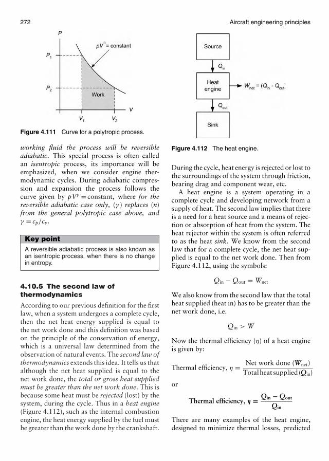
272 Aircraft engineering principles
Figure 4.111 Curve for a polytropic process.
working fluid the process will be reversibleadiabatic. This special process is often calledan isentropic process, its importance will beemphasized, when we consider engine ther-modynamic cycles. During adiabatic compres-sion and expansion the process follows thecurve given by pVγ = constant, where for thereversible adiabatic case only, (γ ) replaces (n)from the general polytropic case above, andγ = cp/cv.
Key pointA reversible adiabatic process is also known asan isentropic process, when there is no changein entropy.
4.10.5 The second law ofthermodynamics
According to our previous definition for the firstlaw, when a system undergoes a complete cycle,then the net heat energy supplied is equal tothe net work done and this definition was basedon the principle of the conservation of energy,which is a universal law determined from theobservation of natural events. The second law ofthermodynamics extends this idea. It tells us thatalthough the net heat supplied is equal to thenet work done, the total or gross heat suppliedmust be greater than the net work done. This isbecause some heat must be rejected (lost) by thesystem, during the cycle. Thus in a heat engine(Figure 4.112), such as the internal combustionengine, the heat energy supplied by the fuel mustbe greater than the work done by the crankshaft.
Figure 4.112 The heat engine.
During the cycle, heat energy is rejected or lost tothe surroundings of the system through friction,bearing drag and component wear, etc.
A heat engine is a system operating in acomplete cycle and developing network from asupply of heat. The second law implies that thereis a need for a heat source and a means of rejec-tion or absorption of heat from the system. Theheat rejector within the system is often referredto as the heat sink. We know from the secondlaw that for a complete cycle, the net heat sup-plied is equal to the net work done. Then fromFigure 4.112, using the symbols:
Qin − Qout = Wnet
We also know from the second law that the totalheat supplied (heat in) has to be greater than thenet work done, i.e.
Qin > W
Now the thermal efficiency (η) of a heat engineis given by:
Thermal efficiency, η = Net work done (Wnet)Totalheat supplied (Qin)
or
Thermal efficiency, η = Qin − Qout
Qin
There are many examples of the heat engine,designed to minimize thermal losses, predicted
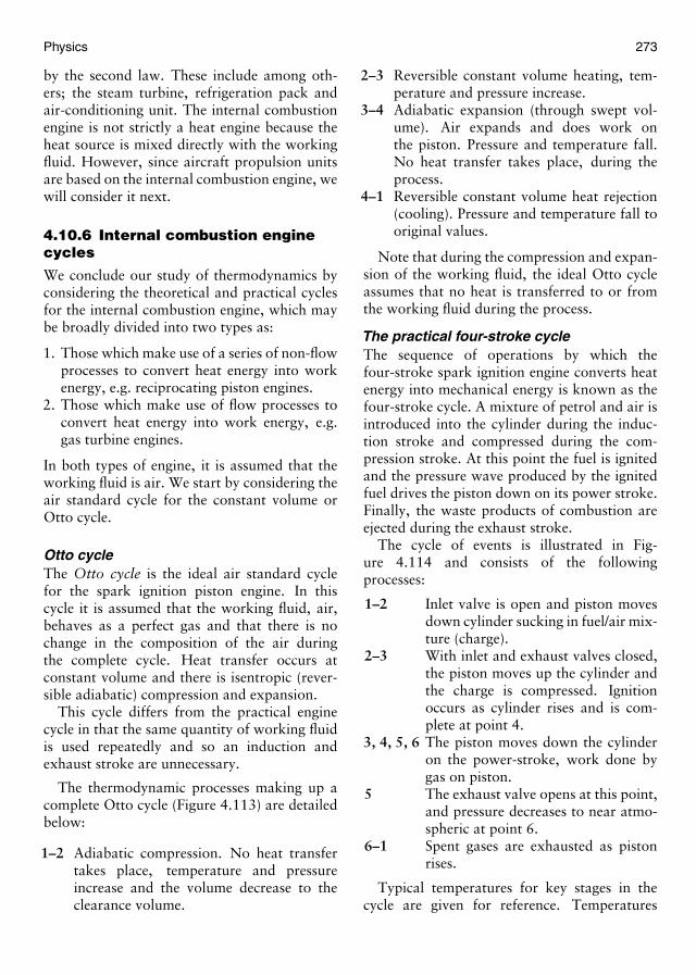
Physics 273
by the second law. These include among oth-ers; the steam turbine, refrigeration pack andair-conditioning unit. The internal combustionengine is not strictly a heat engine because theheat source is mixed directly with the workingfluid. However, since aircraft propulsion unitsare based on the internal combustion engine, wewill consider it next.
4.10.6 Internal combustion enginecycles
We conclude our study of thermodynamics byconsidering the theoretical and practical cyclesfor the internal combustion engine, which maybe broadly divided into two types as:
1. Those which make use of a series of non-flowprocesses to convert heat energy into workenergy, e.g. reciprocating piston engines.
2. Those which make use of flow processes toconvert heat energy into work energy, e.g.gas turbine engines.
In both types of engine, it is assumed that theworking fluid is air. We start by considering theair standard cycle for the constant volume orOtto cycle.
Otto cycleThe Otto cycle is the ideal air standard cyclefor the spark ignition piston engine. In thiscycle it is assumed that the working fluid, air,behaves as a perfect gas and that there is nochange in the composition of the air duringthe complete cycle. Heat transfer occurs atconstant volume and there is isentropic (rever-sible adiabatic) compression and expansion.
This cycle differs from the practical enginecycle in that the same quantity of working fluidis used repeatedly and so an induction andexhaust stroke are unnecessary.
The thermodynamic processes making up acomplete Otto cycle (Figure 4.113) are detailedbelow:
1–2 Adiabatic compression. No heat transfertakes place, temperature and pressureincrease and the volume decrease to theclearance volume.
2–3 Reversible constant volume heating, tem-perature and pressure increase.
3–4 Adiabatic expansion (through swept vol-ume). Air expands and does work onthe piston. Pressure and temperature fall.No heat transfer takes place, during theprocess.
4–1 Reversible constant volume heat rejection(cooling). Pressure and temperature fall tooriginal values.
Note that during the compression and expan-sion of the working fluid, the ideal Otto cycleassumes that no heat is transferred to or fromthe working fluid during the process.
The practical four-stroke cycleThe sequence of operations by which thefour-stroke spark ignition engine converts heatenergy into mechanical energy is known as thefour-stroke cycle. A mixture of petrol and air isintroduced into the cylinder during the induc-tion stroke and compressed during the com-pression stroke. At this point the fuel is ignitedand the pressure wave produced by the ignitedfuel drives the piston down on its power stroke.Finally, the waste products of combustion areejected during the exhaust stroke.
The cycle of events is illustrated in Fig-ure 4.114 and consists of the followingprocesses:
1–2 Inlet valve is open and piston movesdown cylinder sucking in fuel/air mix-ture (charge).
2–3 With inlet and exhaust valves closed,the piston moves up the cylinder andthe charge is compressed. Ignitionoccurs as cylinder rises and is com-plete at point 4.
3, 4, 5, 6 The piston moves down the cylinderon the power-stroke, work done bygas on piston.
5 The exhaust valve opens at this point,and pressure decreases to near atmo-spheric at point 6.
6–1 Spent gases are exhausted as pistonrises.
Typical temperatures for key stages in thecycle are given for reference. Temperatures
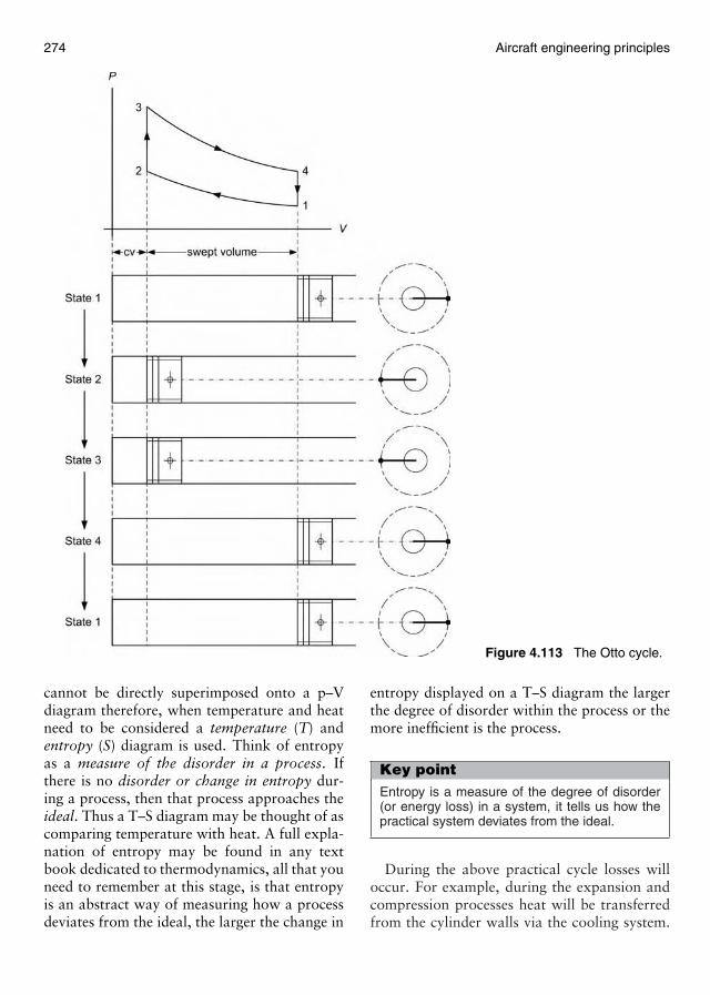
274 Aircraft engineering principles
Figure 4.113 The Otto cycle.
cannot be directly superimposed onto a p–Vdiagram therefore, when temperature and heatneed to be considered a temperature (T) andentropy (S) diagram is used. Think of entropyas a measure of the disorder in a process. Ifthere is no disorder or change in entropy dur-ing a process, then that process approaches theideal. Thus a T–S diagram may be thought of ascomparing temperature with heat. A full expla-nation of entropy may be found in any textbook dedicated to thermodynamics, all that youneed to remember at this stage, is that entropyis an abstract way of measuring how a processdeviates from the ideal, the larger the change in
entropy displayed on a T–S diagram the largerthe degree of disorder within the process or themore inefficient is the process.
Key pointEntropy is a measure of the degree of disorder(or energy loss) in a system, it tells us how thepractical system deviates from the ideal.
During the above practical cycle losses willoccur. For example, during the expansion andcompression processes heat will be transferredfrom the cylinder walls via the cooling system.
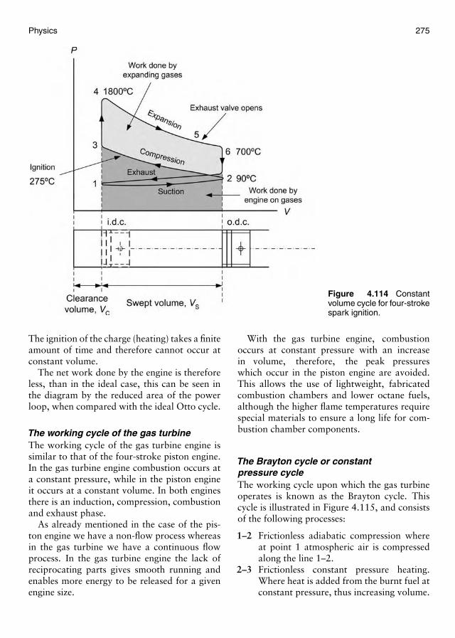
Physics 275
Figure 4.114 Constantvolume cycle for four-strokespark ignition.
The ignition of the charge (heating) takes a finiteamount of time and therefore cannot occur atconstant volume.
The net work done by the engine is thereforeless, than in the ideal case, this can be seen inthe diagram by the reduced area of the powerloop, when compared with the ideal Otto cycle.
The working cycle of the gas turbineThe working cycle of the gas turbine engine issimilar to that of the four-stroke piston engine.In the gas turbine engine combustion occurs ata constant pressure, while in the piston engineit occurs at a constant volume. In both enginesthere is an induction, compression, combustionand exhaust phase.
As already mentioned in the case of the pis-ton engine we have a non-flow process whereasin the gas turbine we have a continuous flowprocess. In the gas turbine engine the lack ofreciprocating parts gives smooth running andenables more energy to be released for a givenengine size.
With the gas turbine engine, combustionoccurs at constant pressure with an increasein volume, therefore, the peak pressureswhich occur in the piston engine are avoided.This allows the use of lightweight, fabricatedcombustion chambers and lower octane fuels,although the higher flame temperatures requirespecial materials to ensure a long life for com-bustion chamber components.
The Brayton cycle or constantpressure cycleThe working cycle upon which the gas turbineoperates is known as the Brayton cycle. Thiscycle is illustrated in Figure 4.115, and consistsof the following processes:
1–2 Frictionless adiabatic compression whereat point 1 atmospheric air is compressedalong the line 1–2.
2–3 Frictionless constant pressure heating.Where heat is added from the burnt fuel atconstant pressure, thus increasing volume.

276 Aircraft engineering principles
Figure 4.115 The Braytoncycle for a gas turbine.
3–4 Frictioness adiabatic expansion of thegases through the turbine.
4–1 Frictionless constant pressure heatrejection, through the jetpipe nozzle toatmosphere.
To ensure maximum thermal efficiency (seeexplanation of the second law) we require thehighest temperature of combustion (heat in) togive the greatest expansion of the gases. Therehas to be a limit on the temperature of the com-busted gases as they enter the turbine, whichis dictated by the turbine materials. Additionalcooling within the turbine, helps maximize thegas entry temperature to the turbine.
The practical Brayton cycleAlthough it can be seen from Figure 4.115 thatthe practical cycle follows fairly closely to theideal Brayton cycle, there are losses, which aredetailed as follows:
1. The air is not pure, it contains other gasesand water vapour.
2. Heat will be transferred to the materials ofthe compressor, turbine and exhaust units,so it is not a pure adiabatic process.
3. Due to dynamic problems, such as turbu-lence and flame stability in the combustionchamber, a constant temperature and hencea constant pressure cannot be maintained.
A further pressure loss occurs as a result ofthe burnt air causing an increase in volumeand hence a decrease in its density. Theselosses are indicated on the diagram by a dropbetween points 2 and 3.
4. The Brayton cycle assumes frictionless adi-abatic operation and this is not possible inpractice.
You will gain a detailed knowledge of theabove cycles, related to aircraft engines, shouldyou choose to study the propulsion modulesduring the course of your career.
Test your understanding 4.221. Define: (a) thermodynamic system, (b) heat, (c) work.
2. Under what circumstances is a closed system able todo work on its surroundings?
3. Write down (a) the NFEE, (b) the SFEE and define eachterm within each equation.
4. What is the essential difference between a closedsystem and an open system?
5. What is the difference between the enthalpy of a work-ing fluid and the internal energy of a working fluid, andunder what circumstances is each property used?
6. An irreversible process cannot exist in practice. Explainthis statement.
7. Define: (a) an isothermal process, (b) a polytropicprocess, (c) a reversible adiabatic process.
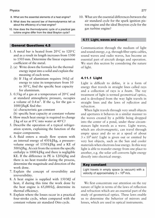
Physics 277
8. What are the essential elements of a heat engine?
9. What does the second law of thermodynamics tell usabout the efficiency of a heat engine?
10. How does the thermodynamic cycle of a practical gasturbine engine differ from the ideal Brayton cycle?
General Questions 4.5
1. A metal bar is heated from 20◦C to 120◦Cand as a result its length increases from 1500to 1503 mm. Determine the linear expansioncoefficient of the metal.
2. (a) Write down the formula for the thermalenergy input into a solid and explain themeaning of each term.
(b) If 3 kg of aluminium requires 54 kJ ofenergy to raise its temperature from 10to 30◦C, find the specific heat capacityfor aluminium.
3. 0.5 kg of a gas at a temperature of 20◦C andat standard atmospheric pressure, occupiesa volume of 0.4 m3. If the cp for the gas =1000 J/kgK find the:(a) characteristic gas constant(b) specific heat capacity at constant volume
4. How much heat energy is required to change2 kg of ice at 0◦C into water at 40◦C?
5. Describe the operation of a typical refriger-ation system, explaining the function of themajor components.
6. A fluid enters a steady flow system withan internal energy of 450 kJ/kg, a pressure–volume energy of 1550 kJ/kg and a KE of500 kJ/kg. At exit from the system the specificenthalpy is 1000 kJ/kg and there is negligibleKE. If the difference in PE is 120 kJ/kg andthere is no heat transfer during the process,determine the magnitude and direction of thework done.
7. Explain the concept of reversibility andirreversibility.
8. A heat engine is supplied with 150 MJ ofheat, if during this time the work done bythe heat engine is 65,000 kJ, determine itsthermal efficiency.
9. Explain where the losses occur in a practicalfour-stroke cycle, when compared with theconstant volume air standard Otto cycle.
10. What are the essential differences between theair standard cycle for the spark ignition pis-ton engine and the ideal Brayton cycle for thegas turbine engine?
4.11 Light, waves and sound
Communication through the medium of lightand sound energy, e.g. through fiber optic cables,sound waves and radio waves, has become anessential part of aircraft design and operation.We start this section by considering the natureof light.
4.11.1 Light
Light is difficult to define, it is a form ofenergy that travels in straight lines called raysand a collection of rays is a beam. The raytreatment of light is termed geometrical optics,and is developed from the way light travels instraight lines and the laws of reflection andrefraction.
When light travels through very small objectsand apertures it behaves in a similar manner tothe waves created by a pebble being droppedinto the center of a pond, under these circum-stances light travels as a wave. Light waves,which are electromagnetic, can travel throughempty space and do so at a speed of about3 × 108 m/s! Light is given out or emitted byvery hot objects, such as the Sun and coolermaterials when electrons lose energy. In this waylight is able to transfer energy from one place toanother, e.g. the solar cell converts light energydirectly into electrical energy.
Key constantLight travels in empty space (a vacuum) with avelocity of approximately 3 × 10⁸ m/s.
We first concentrate our attention on the raynature of light in terms of the laws of reflectionand refraction which are an essential part of thestudy of geometrical optics. These laws enableus to determine the behavior of mirrors andlenses, which are used in optical instruments.
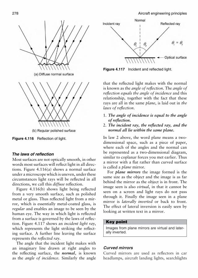
278 Aircraft engineering principles
Figure 4.116 Reflection of light.
The laws of reflectionMost surfaces are not optically smooth, in otherwords most surfaces will reflect light in all direc-tions. Figure 4.116(a) shows a normal surfaceunder a microscope which is uneven, under thesecircumstances light rays will be reflected in alldirections, we call this diffuse reflection.
Figure 4.116(b) shows light being reflectedfrom a very smooth surface, such as polishedmetal or glass. Thus reflected light from a mir-ror, which is essentially metal-coated glass, isregular and enables an image to be seen by thehuman eye. The way in which light is reflectedfrom a surface is governed by the laws of reflec-tion. Figure 4.117 shows an incident light ray,which represents the light striking the reflect-ing surface. A further line leaving the surfacerepresents the reflected ray.
The angle that the incident light makes withan imaginary line drawn at right angles tothe reflecting surface, the normal, is knownas the angle of incidence. Similarly the angle
Figure 4.117 Incident and reflected light.
that the reflected light makes with the normalis known as the angle of reflection. The angle ofreflection equals the angle of incidence and thisrelationship, together with the fact that theserays are all in the same plane, is laid out in thelaws of reflection.
1. The angle of incidence is equal to the angleof reflection.
2. The incident ray, the reflected ray, and thenormal all lie within the same plane.
In law 2 above, the word plane means a two-dimensional space, such as a piece of paper,where each of the angles and the normal canbe represented as a two-dimensional diagram,similar to coplanar forces you met earlier. Thusa mirror with a flat rather than curved surfaceis called a plane mirror.
For plane mirrors the image formed is thesame size as the object and the image is as farbehind the mirror as the object is in front. Theimage seen is also virtual, in that it cannot beseen on a screen and light rays do not passthrough it. Finally the image seen in a planemirror is laterally inverted or back to front.The effect of lateral inversion is easily seen bylooking at written text in a mirror.
Key pointImages from plane mirrors are virtual and later-ally inverted.
Curved mirrorsCurved mirrors are used as reflectors in carheadlamps, aircraft landing lights, searchlights
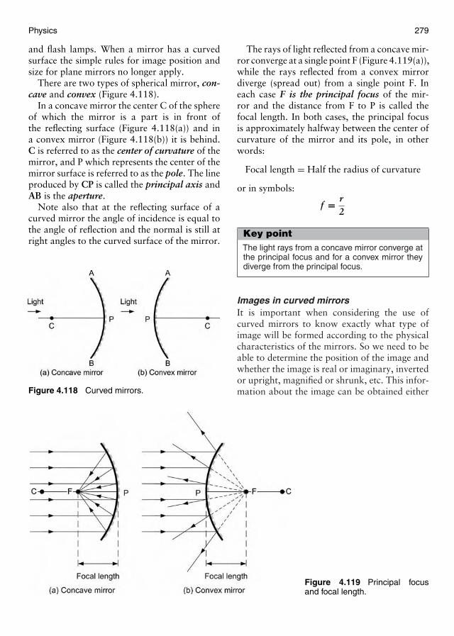
Physics 279
and flash lamps. When a mirror has a curvedsurface the simple rules for image position andsize for plane mirrors no longer apply.
There are two types of spherical mirror, con-cave and convex (Figure 4.118).
In a concave mirror the center C of the sphereof which the mirror is a part is in front ofthe reflecting surface (Figure 4.118(a)) and ina convex mirror (Figure 4.118(b)) it is behind.C is referred to as the center of curvature of themirror, and P which represents the center of themirror surface is referred to as the pole. The lineproduced by CP is called the principal axis andAB is the aperture.
Note also that at the reflecting surface of acurved mirror the angle of incidence is equal tothe angle of reflection and the normal is still atright angles to the curved surface of the mirror.
Figure 4.118 Curved mirrors.
Figure 4.119 Principal focusand focal length.
The rays of light reflected from a concave mir-ror converge at a single point F (Figure 4.119(a)),while the rays reflected from a convex mirrordiverge (spread out) from a single point F. Ineach case F is the principal focus of the mir-ror and the distance from F to P is called thefocal length. In both cases, the principal focusis approximately halfway between the center ofcurvature of the mirror and its pole, in otherwords:
Focal length = Half the radius of curvature
or in symbols:
f = r2
Key pointThe light rays from a concave mirror converge atthe principal focus and for a convex mirror theydiverge from the principal focus.
Images in curved mirrorsIt is important when considering the use ofcurved mirrors to know exactly what type ofimage will be formed according to the physicalcharacteristics of the mirrors. So we need to beable to determine the position of the image andwhether the image is real or imaginary, invertedor upright, magnified or shrunk, etc. This infor-mation about the image can be obtained either
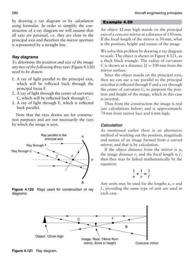
280 Aircraft engineering principles
by drawing a ray diagram or by calculationusing formulae. In order to simplify the con-struction of a ray diagram we will assume thatall rays are paraxial, i.e. they are close to theprincipal axis and therefore the mirror apertureis represented by a straight line.
Ray diagramsTo determine the position and size of the imageany two of the following three rays (Figure 4.120)need to be drawn:
1. A ray of light parallel to the principal axis,which will be reflected back through theprincipal focus F.
2. A ray of light through the center of curvatureC, which will be reflected back through C.
3. A ray of light through F, which is reflectedback parallel.
Note that the rays drawn are for construc-tion purposes and are not necessarily the raysby which the image is seen.
Figure 4.120 Rays used for construction of raydiagrams.
Figure 4.121 Ray diagram.
Example 4.59
An object 12 mm high stands on the principalaxis of a concave mirror at a distance of 150 mm.If the focal length of the mirror is 50 mm, whatis the position, height and nature of the image
We solve this problem by drawing a ray diagramto scale. The object is shown in Figure 4.121, asa thick black triangle. The radius of curvatureC is shown at a distance 2f = 100 mm from themirror surface.
Since the object stands on the principal axis,then we can use a ray parallel to the principalaxis that is reflected through F and a ray throughthe center of curvature C, to pinpoint the posi-tion and height of the image, which in this caseis inverted.
Thus from the construction the image is real(see calculations below) and is approximately74 mm from mirror face and 6 mm high.
CalculationAs mentioned earlier there is an alternativemethod of working out the position, magnitudeand nature of an image formed from a curvedmirror, and that is by calculation.
If the object distance from the mirror is u,the image distance v, and the focal length is f ,then they may be linked mathematically by theequation:
1u
+ 1v
= 1f
Any units may be used for the lengths u, v andf , providing the same type of unit are used ineach case.
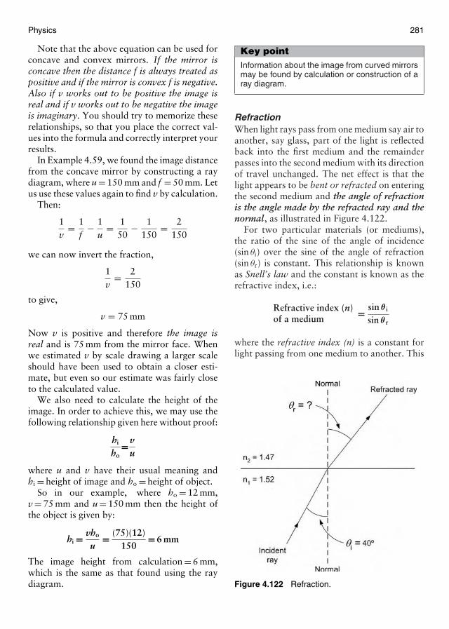
Physics 281
Note that the above equation can be used forconcave and convex mirrors. If the mirror isconcave then the distance f is always treated aspositive and if the mirror is convex f is negative.Also if v works out to be positive the image isreal and if v works out to be negative the imageis imaginary. You should try to memorize theserelationships, so that you place the correct val-ues into the formula and correctly interpret yourresults.
In Example 4.59, we found the image distancefrom the concave mirror by constructing a raydiagram, where u = 150 mm and f = 50 mm. Letus use these values again to find v by calculation.
Then:
1v
= 1f
− 1u
= 150
− 1150
= 2150
we can now invert the fraction,
1v
= 2150
to give,
v = 75 mm
Now v is positive and therefore the image isreal and is 75 mm from the mirror face. Whenwe estimated v by scale drawing a larger scaleshould have been used to obtain a closer esti-mate, but even so our estimate was fairly closeto the calculated value.
We also need to calculate the height of theimage. In order to achieve this, we may use thefollowing relationship given here without proof:
hi
ho=v
u
where u and v have their usual meaning andhi = height of image and ho = height of object.
So in our example, where ho = 12 mm,v = 75 mm and u = 150 mm then the height ofthe object is given by:
hi = vho
u= (75)(12)
150= 6 mm
The image height from calculation = 6 mm,which is the same as that found using the raydiagram.
Key pointInformation about the image from curved mirrorsmay be found by calculation or construction of aray diagram.
RefractionWhen light rays pass from one medium say air toanother, say glass, part of the light is reflectedback into the first medium and the remainderpasses into the second medium with its directionof travel unchanged. The net effect is that thelight appears to be bent or refracted on enteringthe second medium and the angle of refractionis the angle made by the refracted ray and thenormal, as illustrated in Figure 4.122.
For two particular materials (or mediums),the ratio of the sine of the angle of incidence(sin θi) over the sine of the angle of refraction(sin θr) is constant. This relationship is knownas Snell’s law and the constant is known as therefractive index, i.e.:
Refractive index (n)of a medium = sin θ i
sin θ r
where the refractive index (n) is a constant forlight passing from one medium to another. This
Figure 4.122 Refraction.
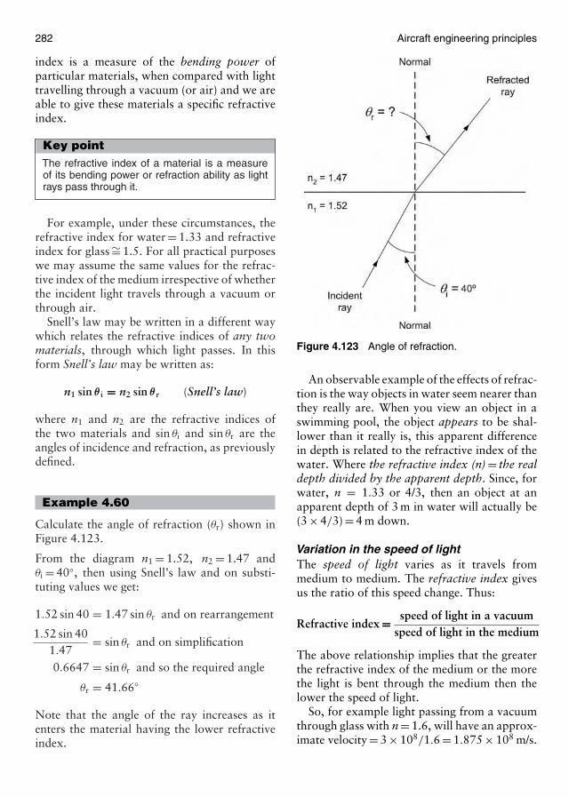
282 Aircraft engineering principles
index is a measure of the bending power ofparticular materials, when compared with lighttravelling through a vacuum (or air) and we areable to give these materials a specific refractiveindex.
Key pointThe refractive index of a material is a measureof its bending power or refraction ability as lightrays pass through it.
For example, under these circumstances, therefractive index for water = 1.33 and refractiveindex for glass ∼= 1.5. For all practical purposeswe may assume the same values for the refrac-tive index of the medium irrespective of whetherthe incident light travels through a vacuum orthrough air.
Snell’s law may be written in a different waywhich relates the refractive indices of any twomaterials, through which light passes. In thisform Snell’s law may be written as:
n1 sin θ i = n2 sin θ r (Snell’s law)
where n1 and n2 are the refractive indices ofthe two materials and sin θi and sin θr are theangles of incidence and refraction, as previouslydefined.
Example 4.60
Calculate the angle of refraction (θr) shown inFigure 4.123.
From the diagram n1 = 1.52, n2 = 1.47 andθi = 40◦, then using Snell’s law and on substi-tuting values we get:
1.52 sin 40 = 1.47 sin θr and on rearrangement
1.52 sin 401.47
= sin θr and on simplification
0.6647 = sin θr and so the required angle
θr = 41.66◦
Note that the angle of the ray increases as itenters the material having the lower refractiveindex.
Figure 4.123 Angle of refraction.
An observable example of the effects of refrac-tion is the way objects in water seem nearer thanthey really are. When you view an object in aswimming pool, the object appears to be shal-lower than it really is, this apparent differencein depth is related to the refractive index of thewater. Where the refractive index (n) = the realdepth divided by the apparent depth. Since, forwater, n = 1.33 or 4/3, then an object at anapparent depth of 3 m in water will actually be(3 × 4/3) = 4 m down.
Variation in the speed of lightThe speed of light varies as it travels frommedium to medium. The refractive index givesus the ratio of this speed change. Thus:
Refractive index = speed of light in a vacuumspeed of light in the medium
The above relationship implies that the greaterthe refractive index of the medium or the morethe light is bent through the medium then thelower the speed of light.
So, for example light passing from a vacuumthrough glass with n = 1.6, will have an approx-imate velocity = 3 × 10⁸/1.6 = 1.875 × 10⁸ m/s.
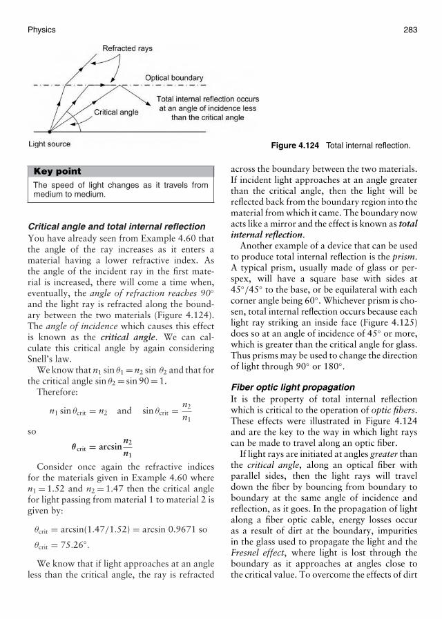
Physics 283
Figure 4.124 Total internal reflection.
Key pointThe speed of light changes as it travels frommedium to medium.
Critical angle and total internal reflectionYou have already seen from Example 4.60 thatthe angle of the ray increases as it enters amaterial having a lower refractive index. Asthe angle of the incident ray in the first mate-rial is increased, there will come a time when,eventually, the angle of refraction reaches 90◦and the light ray is refracted along the bound-ary between the two materials (Figure 4.124).The angle of incidence which causes this effectis known as the critical angle. We can cal-culate this critical angle by again consideringSnell’s law.
We know that n1 sin θ1 = n2 sin θ2 and that forthe critical angle sin θ2 = sin 90 = 1.
Therefore:
n1 sin θcrit = n2 and sin θcrit = n2
n1
so
θ crit = arcsinn2
n1
Consider once again the refractive indicesfor the materials given in Example 4.60 wheren1 = 1.52 and n2 = 1.47 then the critical anglefor light passing from material 1 to material 2 isgiven by:
θcrit = arcsin(1.47/1.52) = arcsin 0.9671 so
θcrit = 75.26◦.
We know that if light approaches at an angleless than the critical angle, the ray is refracted
across the boundary between the two materials.If incident light approaches at an angle greaterthan the critical angle, then the light will bereflected back from the boundary region into thematerial from which it came. The boundary nowacts like a mirror and the effect is known as totalinternal reflection.
Another example of a device that can be usedto produce total internal reflection is the prism.A typical prism, usually made of glass or per-spex, will have a square base with sides at45◦/45◦ to the base, or be equilateral with eachcorner angle being 60◦. Whichever prism is cho-sen, total internal reflection occurs because eachlight ray striking an inside face (Figure 4.125)does so at an angle of incidence of 45◦ or more,which is greater than the critical angle for glass.Thus prisms may be used to change the directionof light through 90◦ or 180◦.
Fiber optic light propagationIt is the property of total internal reflectionwhich is critical to the operation of optic fibers.These effects were illustrated in Figure 4.124and are the key to the way in which light rayscan be made to travel along an optic fiber.
If light rays are initiated at angles greater thanthe critical angle, along an optical fiber withparallel sides, then the light rays will traveldown the fiber by bouncing from boundary toboundary at the same angle of incidence andreflection, as it goes. In the propagation of lightalong a fiber optic cable, energy losses occuras a result of dirt at the boundary, impuritiesin the glass used to propagate the light and theFresnel effect, where light is lost through theboundary as it approaches at angles close tothe critical value. To overcome the effects of dirt
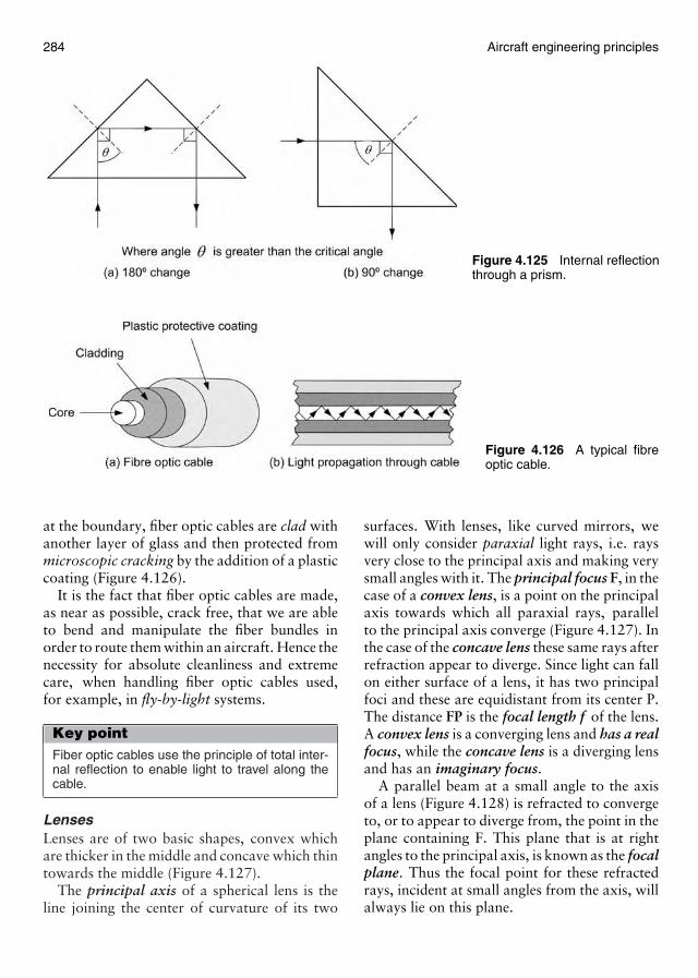
284 Aircraft engineering principles
Figure 4.125 Internal reflectionthrough a prism.
Figure 4.126 A typical fibreoptic cable.
at the boundary, fiber optic cables are clad withanother layer of glass and then protected frommicroscopic cracking by the addition of a plasticcoating (Figure 4.126).
It is the fact that fiber optic cables are made,as near as possible, crack free, that we are ableto bend and manipulate the fiber bundles inorder to route them within an aircraft. Hence thenecessity for absolute cleanliness and extremecare, when handling fiber optic cables used,for example, in fly-by-light systems.
Key pointFiber optic cables use the principle of total inter-nal reflection to enable light to travel along thecable.
LensesLenses are of two basic shapes, convex whichare thicker in the middle and concave which thintowards the middle (Figure 4.127).
The principal axis of a spherical lens is theline joining the center of curvature of its two
surfaces. With lenses, like curved mirrors, wewill only consider paraxial light rays, i.e. raysvery close to the principal axis and making verysmall angles with it. The principal focus F, in thecase of a convex lens, is a point on the principalaxis towards which all paraxial rays, parallelto the principal axis converge (Figure 4.127). Inthe case of the concave lens these same rays afterrefraction appear to diverge. Since light can fallon either surface of a lens, it has two principalfoci and these are equidistant from its center P.The distance FP is the focal length f of the lens.A convex lens is a converging lens and has a realfocus, while the concave lens is a diverging lensand has an imaginary focus.
A parallel beam at a small angle to the axisof a lens (Figure 4.128) is refracted to convergeto, or to appear to diverge from, the point in theplane containing F. This plane that is at rightangles to the principal axis, is known as the focalplane. Thus the focal point for these refractedrays, incident at small angles from the axis, willalways lie on this plane.
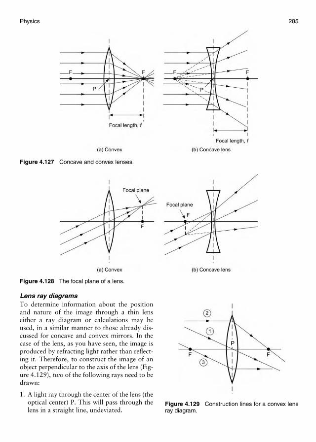
Physics 285
Figure 4.127 Concave and convex lenses.
Figure 4.128 The focal plane of a lens.
Lens ray diagramsTo determine information about the positionand nature of the image through a thin lenseither a ray diagram or calculations may beused, in a similar manner to those already dis-cussed for concave and convex mirrors. In thecase of the lens, as you have seen, the image isproduced by refracting light rather than reflect-ing it. Therefore, to construct the image of anobject perpendicular to the axis of the lens (Fig-ure 4.129), two of the following rays need to bedrawn:
1. A light ray through the center of the lens (theoptical center) P. This will pass through thelens in a straight line, undeviated.
Figure 4.129 Construction lines for a convex lensray diagram.
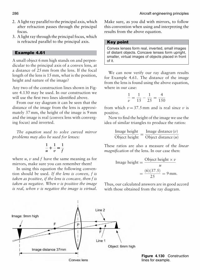
286 Aircraft engineering principles
2. A light ray parallel to the principal axis, whichafter refraction passes through the principalfocus.
3. A light ray through the principal focus, whichis refracted parallel to the principal axis.
Example 4.61
A small object 6 mm high stands on and perpen-dicular to the principal axis of a convex lens, ata distance of 25 mm from the lens. If the focallength of the lens is 15 mm, what is the position,height and nature of the image?
Any two of the construction lines shown in Fig-ure 4.130 may be used. In our construction wewill use the first two lines identified above.
From our ray diagram it can be seen that thedistance of the image from the lens is approxi-mately 37 mm, the height of the image is 9 mmand the image is real (convex lens with converg-ing focus) and inverted.
The equation used to solve curved mirrorproblems may also be used for lenses:
1u
+ 1v
= 1f
where u, v and f have the same meaning as formirrors, make sure you can remember them!
In using this equation the following conven-tion should be used. If the lens is convex, f istaken as positive, if the lens is concave, then f istaken as negative. When v is positive the imageis real, when v is negative the image is virtual.
Figure 4.130 Constructionlines for example.
Make sure, as you did with mirrors, to followthis convention when using and interpreting theresults from the above equation.
Key pointConvex lenses form real, inverted, small imagesof distant objects. Concave lenses form upright,smaller, virtual images of objects placed in frontof it.
We can now verify our ray diagram resultsfor Example 4.61. The distance of the imagefrom the lens is found using the above equation,where in our case:
1v
= 115
− 125
= 4150
from which v = 37.5 mm and is real since v ispositive.
Now to find the height of the image we use theidea of similar triangles to produce the ratios:
Image heightObject height
= Image distance (v)Object distance (u)
These ratios are also a measure of the linearmagnification of the lens. In our case then:
Image height = Object height × vu
= (6)(37.5)25
= 9 mm.
Thus, our calculated answers are in good accordwith those obtained from the ray diagram.
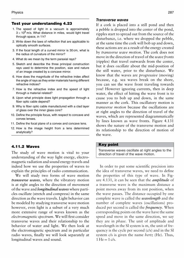
Physics 287
Test your understanding 4.231. The speed of light in a vacuum is approximately
3 × 10⁸ m/s. What distance in miles, would light travelthrough space, in 1 h?
2. Write down the laws of reflection that are applicable tooptically smooth surfaces.
3. If the focal length of a curved mirror is 30 cm, what isthe radius of curvature of the mirror?
4. What do we mean by the term paraxial rays?
5. Sketch and describe the three principal constructionrays used to determine the position, size and natureof an image created by a concave mirror.
6. How does the magnitude of the refractive index affectthe angle of rays as they enter materials having differentrefractive indices?
7. How is the refractive index and the speed of lightthrough a material related?
8. Upon what principle does light propagation through afiber optic cable depend?
9. Why is fiber optic cable manufactured with a clad layerof glass over the inner glass core?
10. Define the principle focus, with respect to concave andconvex lenses.
11. Define the focal plane of a convex and concave lens.
12. How is the image height from a lens determinedanalytically?
4.11.2 Waves
The study of wave motion is vital to yourunderstanding of the way light energy, electro-magnetic radiation and sound energy travels andindeed how we use the properties of waves toexplain the principles of radio communication.
We will study two forms of wave motiontransverse waves, where the vibratory motionis at right angles to the direction of movementof the wave and longitudinal waves where parti-cles oscillate (stretch and compress) in the samedirection as the wave travels. Light behavior canbe modeled by studying transverse wave motionhowever, even light is a subset of a very muchmore extensive range of waves known as theelectromagnetic spectrum. We will first considertransverse waves and their relationship to thebehavior of water and light. We then look atthe electromagnetic spectrum and in particularradio waves, finally we will look separately atlongitudinal waves and sound.
Transverse wavesIf a cork is placed into a still pond and thena pebble is dropped into the center of the pond,ripples start to spread out from the source of thedisturbance, i.e. where we dropped the pebble,at the same time the cork will bob up and down,these actions are as a result of the energy createdby transverse wave motion. The cork does notmove in the direction of travel of the wave fronts(ripples) that travel outwards from the center,but it does oscillate about the mid-position ofthe still water, prior to the disturbance. Weknow that the waves are progressive (moving)because, e.g. sea waves break on the shore,you can see the wave front traveling towardsyou! However ignoring currents, then in deepwater, the effect of hitting the wave front is tocause you to bob up and down, in the samemanner as the cork. This oscillatory motion istransverse motion because the oscillations areat right angles to the direction of travel of thewaves, which are represented diagrammaticallyby lines known as wave fronts. Figure 4.131shows the nature of the transverse motion andits relationship to the direction of motion ofthe wave.
Key pointTransverse waves oscillate at right angles to thedirection of travel of the wave motion.
In order to put some scientific precision intothe idea of transverse waves, we need to definethe properties of this type of wave. In Fig-ure 4.131, it can be seen that the amplitude ofa transverse wave is the maximum distance apoint moves away from its rest position, whenthe wave passes. The distance occupied by onecomplete wave is called the wavelength and thenumber of complete waves (oscillations) pro-duced per second is called the frequency. Whencorresponding points on the wave have the samespeed and move in the same direction, we saythey are in phase. The unit of amplitude andwavelength in the SI system is m, the unit of fre-quency is the cycle per second (c/s) and in the SIsystem c/s is given the name hertz (Hz). Thus,1 Hz = 1 c/s.

288 Aircraft engineering principles
Figure 4.131 Transverse wavemotion.
The speed of a wave (wavefront), its fre-quency and wavelength are linked by a simpleformula, which is given without proof below:
Wave speed = frequency × wavelength
or in symbols:
v = f λ
The equation v = f λ applies to any wave, thewave speed is found in m/s, when the frequencyis in Hz and the wavelength is in m. So, forexample if waves are produced 10 times a sec-ond, i.e. with a frequency of 10 Hz and the speedof wave propagation (wave speed) is 50 m/s,then the wavelength will be 50/10 or, λ = 5 m.
Wave behaviorThe nature of progressive waves can be demon-strated, using a ripple tank, which is a sophisti-cated water tank where parameters such as wavefrequency and amplitude can be varied and thecorresponding effects of the wave motion stud-ied. Through these studies, it can be shown thatwater waves behave in a very similar manner to
light. From observation it has been found thatwater waves are reflected by surfaces in exactlythe same way as light, so the same laws ofreflection apply. It is also true that water wavesundergo refraction or bending, when they areslowed down, in a similar manner to light. Ithas been observed, using the ripple tank, thatas waves enter shallower water they slow down.This reduction in speed causes a reduction inwavelength and as the waves close up on oneanother, they change their direction of travel.Two other important properties may be demon-strated using the ripple tank, they are wavediffraction and interference.
DiffractionWhen two plates, with a very narrow gapbetween them are placed in the path of progres-sive water waves (Figure 4.132), the waves thatpass through them spread out in all directionsand produce circular wavefronts.
This effect is known as diffraction or bend-ing of waves as they pass through very narrowgaps. If the gap between the plates is made much
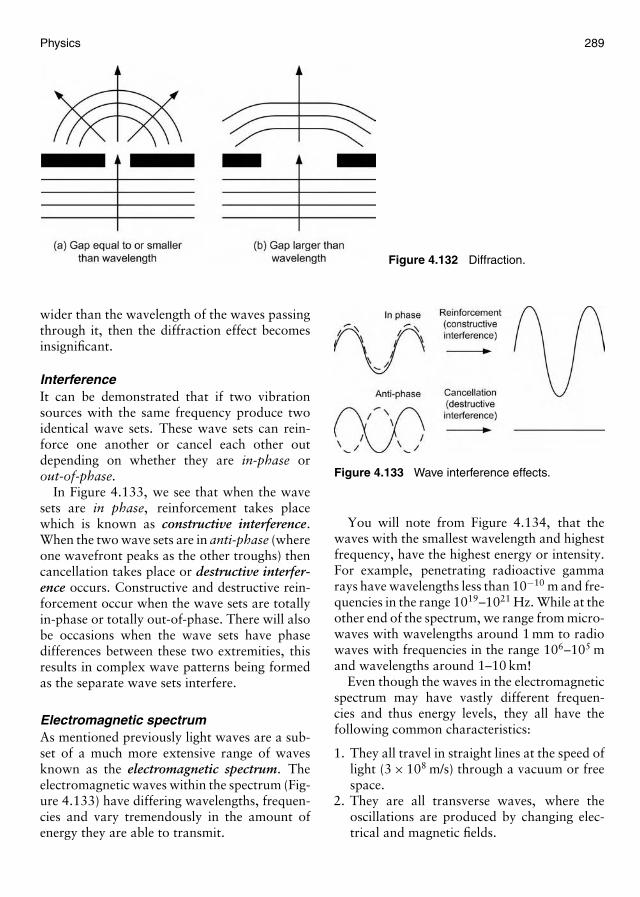
Physics 289
Figure 4.132 Diffraction.
wider than the wavelength of the waves passingthrough it, then the diffraction effect becomesinsignificant.
InterferenceIt can be demonstrated that if two vibrationsources with the same frequency produce twoidentical wave sets. These wave sets can rein-force one another or cancel each other outdepending on whether they are in-phase orout-of-phase.
In Figure 4.133, we see that when the wavesets are in phase, reinforcement takes placewhich is known as constructive interference.When the two wave sets are in anti-phase (whereone wavefront peaks as the other troughs) thencancellation takes place or destructive interfer-ence occurs. Constructive and destructive rein-forcement occur when the wave sets are totallyin-phase or totally out-of-phase. There will alsobe occasions when the wave sets have phasedifferences between these two extremities, thisresults in complex wave patterns being formedas the separate wave sets interfere.
Electromagnetic spectrumAs mentioned previously light waves are a sub-set of a much more extensive range of wavesknown as the electromagnetic spectrum. Theelectromagnetic waves within the spectrum (Fig-ure 4.133) have differing wavelengths, frequen-cies and vary tremendously in the amount ofenergy they are able to transmit.
Figure 4.133 Wave interference effects.
You will note from Figure 4.134, that thewaves with the smallest wavelength and highestfrequency, have the highest energy or intensity.For example, penetrating radioactive gammarays have wavelengths less than 10−10 m and fre-quencies in the range 1019–1021 Hz. While at theother end of the spectrum, we range from micro-waves with wavelengths around 1 mm to radiowaves with frequencies in the range 106–105 mand wavelengths around 1–10 km!
Even though the waves in the electromagneticspectrum may have vastly different frequen-cies and thus energy levels, they all have thefollowing common characteristics:
1. They all travel in straight lines at the speed oflight (3 × 10⁸ m/s) through a vacuum or freespace.
2. They are all transverse waves, where theoscillations are produced by changing elec-trical and magnetic fields.
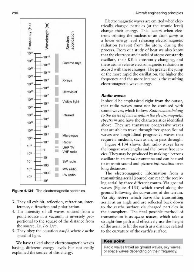
290 Aircraft engineering principles
Figure 4.134 The electromagnetic spectrum.
3. They all exhibit, reflection, refraction, inter-ference, diffraction and polarization.
4. The intensity of all waves emitted from apoint source in a vacuum, is inversely pro-portional to the square of the distance fromthe source, i.e. I ∝ 1/r2.
5. They obey the equation c = f λ where c = thespeed of light.
We have talked about electromagnetic waveshaving different energy levels but not reallyexplained the source of this energy.
Electromagnetic waves are emitted when elec-trically charged particles (at the atomic level)change their energy. This occurs when elec-trons orbiting the nucleus of an atom jump toa lower energy level releasing electromagneticradiation (waves) from the atom, during theprocess. From our study of heat we also knowthat the electrons and nuclei of atoms constantlyoscillate, their KE is constantly changing, andthese atoms release electromagnetic radiation inaccord with these changes. The greater the jumpor the more rapid the oscillation, the higher thefrequency and the more intense is the resultingelectromagnetic wave energy.
Radio wavesIt should be emphasized right from the outset,that radio waves must not be confused withsound waves, which follow. Radio waves belongto the series of waves within the electromagneticspectrum and have the characteristics identifiedabove. They are transverse progressive wavesthat are able to travel through free space. Soundwaves are longitudinal progressive waves thatrequire a medium, such as air, to pass through.
Figure 4.134 shows that radio waves havethe longest wavelengths and the lowest frequen-cies. They may be produced by making electronsoscillate in an aerial or antenna and can be usedto transmit sound and picture information overlong distances.
The electromagnetic information from atransmitting aerial (source) can reach the receiv-ing aerial by three different routes. Via groundwaves (Figure 4.135) which travel along theground following the curvatures of the terrain.Via sky waves which leave the transmittingaerial at an angle and are reflected back downto the earths surface via charged particles inthe ionosphere. The final possible method oftransmission is as space waves, which take astraight-line path and effectively use the heightof the aerial to hit the earth at a distance relatedto the curvature of the earth’s surface.
Key pointRadio waves travel as ground waves, sky wavesor space waves depending on their frequency.
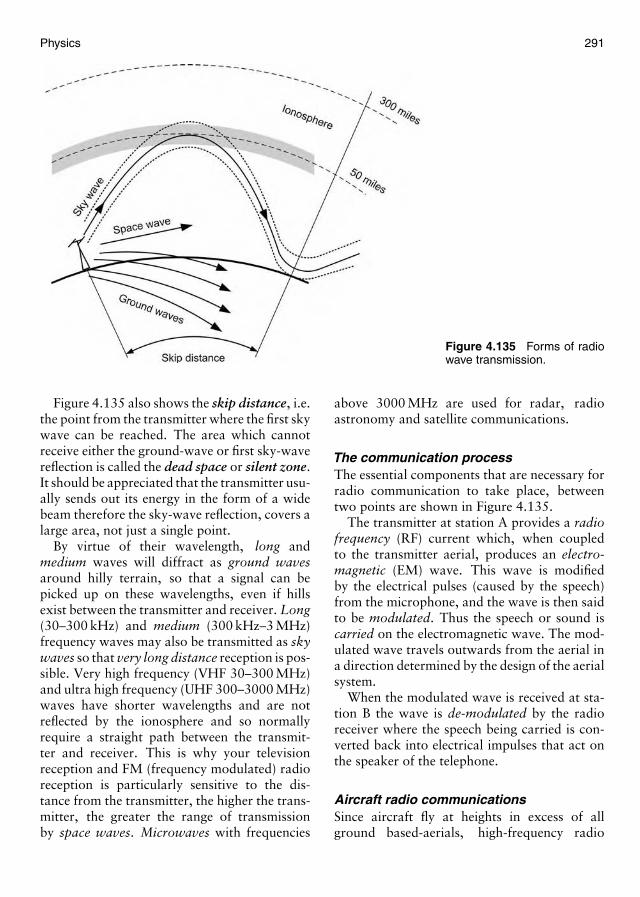
Physics 291
Figure 4.135 Forms of radiowave transmission.
Figure 4.135 also shows the skip distance, i.e.the point from the transmitter where the first skywave can be reached. The area which cannotreceive either the ground-wave or first sky-wavereflection is called the dead space or silent zone.It should be appreciated that the transmitter usu-ally sends out its energy in the form of a widebeam therefore the sky-wave reflection, covers alarge area, not just a single point.
By virtue of their wavelength, long andmedium waves will diffract as ground wavesaround hilly terrain, so that a signal can bepicked up on these wavelengths, even if hillsexist between the transmitter and receiver. Long(30–300 kHz) and medium (300 kHz–3 MHz)frequency waves may also be transmitted as skywaves so that very long distance reception is pos-sible. Very high frequency (VHF 30–300 MHz)and ultra high frequency (UHF 300–3000 MHz)waves have shorter wavelengths and are notreflected by the ionosphere and so normallyrequire a straight path between the transmit-ter and receiver. This is why your televisionreception and FM (frequency modulated) radioreception is particularly sensitive to the dis-tance from the transmitter, the higher the trans-mitter, the greater the range of transmissionby space waves. Microwaves with frequencies
above 3000 MHz are used for radar, radioastronomy and satellite communications.
The communication processThe essential components that are necessary forradio communication to take place, betweentwo points are shown in Figure 4.135.
The transmitter at station A provides a radiofrequency (RF) current which, when coupledto the transmitter aerial, produces an electro-magnetic (EM) wave. This wave is modifiedby the electrical pulses (caused by the speech)from the microphone, and the wave is then saidto be modulated. Thus the speech or sound iscarried on the electromagnetic wave. The mod-ulated wave travels outwards from the aerial ina direction determined by the design of the aerialsystem.
When the modulated wave is received at sta-tion B the wave is de-modulated by the radioreceiver where the speech being carried is con-verted back into electrical impulses that act onthe speaker of the telephone.
Aircraft radio communicationsSince aircraft fly at heights in excess of allground based-aerials, high-frequency radio
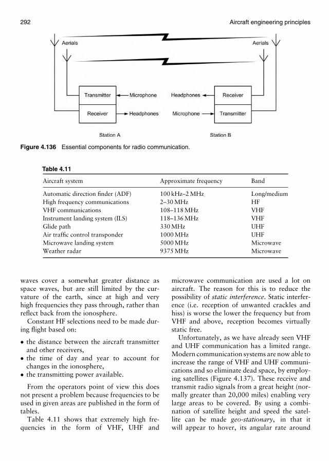
292 Aircraft engineering principles
Figure 4.136 Essential components for radio communication.
Table 4.11
Aircraft system Approximate frequency Band
Automatic direction finder (ADF) 100 kHz–2 MHz Long/mediumHigh frequency communications 2–30 MHz HFVHF communications 108–118 MHz VHFInstrument landing system (ILS) 118–136 MHz VHFGlide path 330 MHz UHFAir traffic control transponder 1000 MHz UHFMicrowave landing system 5000 MHz MicrowaveWeather radar 9375 MHz Microwave
waves cover a somewhat greater distance asspace waves, but are still limited by the cur-vature of the earth, since at high and veryhigh frequencies they pass through, rather thanreflect back from the ionosphere.
Constant HF selections need to be made dur-ing flight based on:
• the distance between the aircraft transmitterand other receivers,
• the time of day and year to account forchanges in the ionosphere,
• the transmitting power available.
From the operators point of view this doesnot present a problem because frequencies to beused in given areas are published in the form oftables.
Table 4.11 shows that extremely high fre-quencies in the form of VHF, UHF and
microwave communication are used a lot onaircraft. The reason for this is to reduce thepossibility of static interference. Static interfer-ence (i.e. reception of unwanted crackles andhiss) is worse the lower the frequency but fromVHF and above, reception becomes virtuallystatic free.
Unfortunately, as we have already seen VHFand UHF communication has a limited range.Modern communication systems are now able toincrease the range of VHF and UHF communi-cations and so eliminate dead space, by employ-ing satellites (Figure 4.137). These receive andtransmit radio signals from a great height (nor-mally greater than 20,000 miles) enabling verylarge areas to be covered. By using a combi-nation of satellite height and speed the satel-lite can be made geo-stationary, in that itwill appear to hover, its angular rate around

Physics 293
Figure 4.137 Satellite receiver and transmitter.
the world being synchronized to the earth’srotation rate.
Satellite communication can be used to pro-vide airborne telephone systems for passengersand also be used for satellite navigation usinggeo-stationary or low orbit satellites.
The Doppler effectWhen there is relative motion between a wavesource and an observer, a change in frequencytakes place; this is noticeable with any wavemotion, light, radio and sound. This change infrequency brought about by the relative motionis known as the Doppler effect.
An example with sound waves, commonlyquoted, is that of a train using its whistle whilepassing an observer. As the train approaches,the frequency heard by the observer is higherthan that emitted from the source. When thetrain passes the observer, there is a drop in pitchand as the train moves away from the observera lower frequency than that generated is heard.The same effect is noted if the observer movesand the sound source is stationary.
With respect to radio transmission, if therelative motion is such that a transmitter andreceiver are effectively moving towards eachother (e.g. closing aircraft), the received fre-quency will be higher than that transmitted.If moving away, the received frequency is lessthan that transmitted. An approximation of the
amount of change of frequency, Doppler shift,is given by:
Doppler shift =Transmitterfrequency × Relative
velocity
Velocity of radiowave propagation
So, for example if the transmitter frequency =100 MHz and the relative velocity betweenthe transmitter and receiver is 3600 km/h(1000 m/s), then:
Doppler shift frequency = (100 × 106)(1000)3 × 108
= 333.3 Hz
As can be seen this shift is very small, but doeshave practical applications. For example, therelative motion between a satellite and a survivalbeacon can give an indication of the location ofthe beacon. In the case of satellites that havevery high velocities, the Doppler shift (changein frequency) could be significant. Thus, if thesatellite is traveling with a component of itsvelocity directed toward the beacon, it receivesa higher frequency signal than that transmitted.Traveling away from the beacon, this situationis reversed and the satellite receives a lower fre-quency signal than that transmitted, thereforethere is a frequency change at the moment thesatellite passes the beacon.
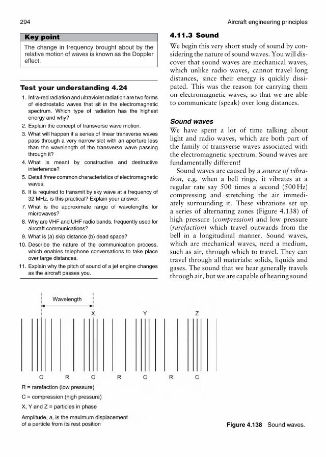
294 Aircraft engineering principles
Key pointThe change in frequency brought about by therelative motion of waves is known as the Dopplereffect.
Test your understanding 4.241. Infra-red radiation and ultraviolet radiation are two forms
of electrostatic waves that sit in the electromagneticspectrum. Which type of radiation has the highestenergy and why?
2. Explain the concept of transverse wave motion.
3. What will happen if a series of linear transverse wavespass through a very narrow slot with an aperture lessthan the wavelength of the transverse wave passingthrough it?
4. What is meant by constructive and destructiveinterference?
5. Detail three common characteristics of electromagneticwaves.
6. It is required to transmit by sky wave at a frequency of32 MHz, is this practical? Explain your answer.
7. What is the approximate range of wavelengths formicrowaves?
8. Why are VHF and UHF radio bands, frequently used foraircraft communications?
9. What is (a) skip distance (b) dead space?
10. Describe the nature of the communication process,which enables telephone conversations to take placeover large distances.
11. Explain why the pitch of sound of a jet engine changesas the aircraft passes you.
Figure 4.138 Sound waves.
4.11.3 Sound
We begin this very short study of sound by con-sidering the nature of sound waves. You will dis-cover that sound waves are mechanical waves,which unlike radio waves, cannot travel longdistances, since their energy is quickly dissi-pated. This was the reason for carrying themon electromagnetic waves, so that we are ableto communicate (speak) over long distances.
Sound wavesWe have spent a lot of time talking aboutlight and radio waves, which are both part ofthe family of transverse waves associated withthe electromagnetic spectrum. Sound waves arefundamentally different!
Sound waves are caused by a source of vibra-tion, e.g. when a bell rings, it vibrates at aregular rate say 500 times a second (500 Hz)compressing and stretching the air immedi-ately surrounding it. These vibrations set upa series of alternating zones (Figure 4.138) ofhigh pressure (compression) and low pressure(rarefaction) which travel outwards from thebell in a longitudinal manner. Sound waves,which are mechanical waves, need a medium,such as air, through which to travel. They cantravel through all materials: solids, liquids andgases. The sound that we hear generally travelsthrough air, but we are capable of hearing sound
Physics 295
under water and through solid objects, such asdoors, windows and walls.
The amplitude of a sound wave is relatedto the position of the particles of the mate-rial, through which the sound is traveling. Wesay that: the amplitude of the sound waveis the maximum displacement of a particlefrom its rest position and the distance betweentwo successive particles in-phase is the wave-length. Sound waves are longitudinal progres-sive waves where the particles, are compressedand rarefied (oscillate) in the same direction asthe wavefront is traveling.
Although there are significant differences inthe behavior of sound waves, like electromag-netic waves, they are governed by the fundamen-tal equation v = fλ except that v replaces c wherev = the speed of sound wave. You should alsoremember that sound waves, like other waveforms, can be reflected, refracted, diffracted anddisplay interference effects.
We have already considered the speed ofsound in some detail when we studied the atmo-sphere. You should remember that the speedof sound was temperature and density depen-dent. Thus, the speed of sound varies accordingto the nature of the material through which itpasses. For example, the speed of sound in air at15◦C = 340 m/s or 1120 ft/s, the speed of soundin water at 0◦C = 1400 m/s and the speed ofsound through concrete ∼=5000 m/s.
Note that the density dependence of the speedof sound is quite apparent from the above exam-ples, the speed of sound increases as it travelsthrough gases, liquids and solids, respectively.
Reflected soundWhen we hear an echo, we are hearing areflected sound a short time after the origi-nal sound. The time the echo, or reflectedsound, takes to reach us is a measure of howfar away the echo source is. This property ofreflection can be used with the echo sounder,when we wish to measure the depth of theseabed below the ship. Also by sending outultrasound pulses, we are able to determine thenature of any discontinuities (defects, cavities,cracks, flaws, porosity, etc.) in otherwise soundmaterial.
Ultrasound frequencies above the audiblerange (in excess of 20 kHz), may be generatedusing a piezoelectric probe which rests on thesurface of the material (Figure 4.139).
Then using the formula v = fλ and knowingthe frequency and wavelength of the generatedultrasound, the velocity of the ultrasound wavecan be determined. If in addition to the pulsetransmitter, a receiver measures the reflectedpulses from the discontinuity and bottom of thematerial, then the time difference between thetwo pulses will enable the depth of the flaw tobe established.
Perceiving soundThrough music, speech and other noises, ourears experience a range of different sounds. Allthese differences in the way we perceive sound,are dependent only on the differences in fre-quency and amplitude of the sound waves enter-ing our ears. We have already defined amplitude,as the maximum displacement of a particlefrom its rest position. For example, the moredistance air particles move from their rest posi-tion, when a loud speaker diaphragm oscillates,then the louder the sound we hear. In otherwords, the greater the amplitude the louder thesound.
Key pointThe greater the amplitude of the sound wave thelouder the sound.
The intensity of the sound wave is a measureof the energy passing through unit area everysecond. More formally: a sound wave has anintensity of 1 watt per square metre (1 W/m2)if 1 J of wave energy passes through 1 m2everysecond. Remember that 1 W is equal to 1 J/s.Mention has already been made of the pitch ofsound, when we considered the Doppler effectearlier.
Difference in pitch is perceived by us when wehear, e.g. different notes in music. Thus, highpitch sound such as that from a whistle, resultsfrom high frequencies and low pitch sound suchas that from a large drum, results from lowfrequencies.
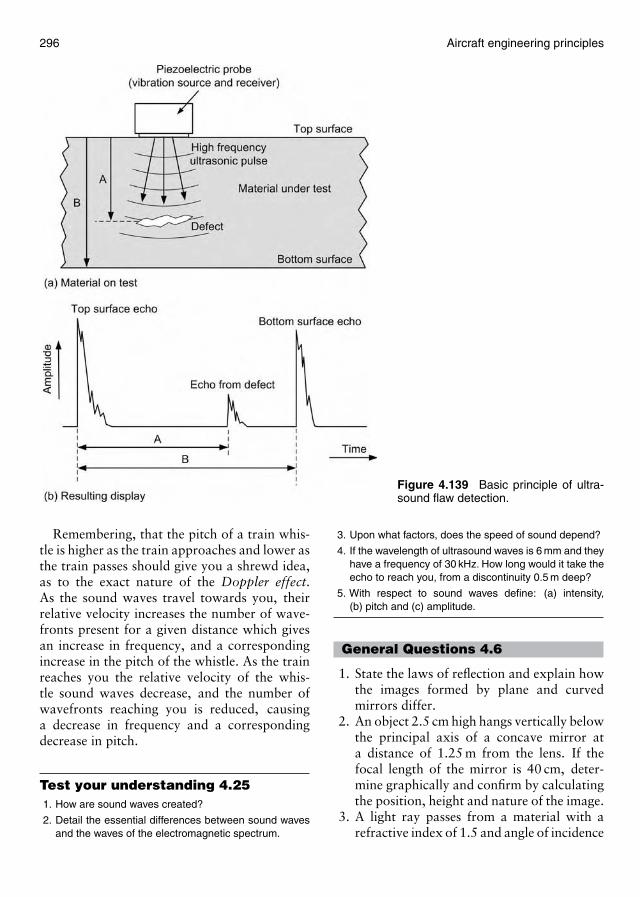
296 Aircraft engineering principles
Figure 4.139 Basic principle of ultra-sound flaw detection.
Remembering, that the pitch of a train whis-tle is higher as the train approaches and lower asthe train passes should give you a shrewd idea,as to the exact nature of the Doppler effect.As the sound waves travel towards you, theirrelative velocity increases the number of wave-fronts present for a given distance which givesan increase in frequency, and a correspondingincrease in the pitch of the whistle. As the trainreaches you the relative velocity of the whis-tle sound waves decrease, and the number ofwavefronts reaching you is reduced, causinga decrease in frequency and a correspondingdecrease in pitch.
Test your understanding 4.251. How are sound waves created?
2. Detail the essential differences between sound wavesand the waves of the electromagnetic spectrum.
3. Upon what factors, does the speed of sound depend?
4. If the wavelength of ultrasound waves is 6 mm and theyhave a frequency of 30 kHz. How long would it take theecho to reach you, from a discontinuity 0.5 m deep?
5. With respect to sound waves define: (a) intensity,(b) pitch and (c) amplitude.
General Questions 4.6
1. State the laws of reflection and explain howthe images formed by plane and curvedmirrors differ.
2. An object 2.5 cm high hangs vertically belowthe principal axis of a concave mirror ata distance of 1.25 m from the lens. If thefocal length of the mirror is 40 cm, deter-mine graphically and confirm by calculatingthe position, height and nature of the image.
3. A light ray passes from a material with arefractive index of 1.5 and angle of incidence
Physics 297
of 38◦, into another material with a refrac-tive index of 1.45, determine the angle ofrefraction of the light ray.
4. For the situation in question three above,determine the angle that refracts the beamalong the boundary between the twomaterials.
5. Explain, with the aid of a diagram, how lightis propagated along a fiber optic cable.
6. Sketch the ray diagram construction linesthat can be used to determine the image of anobject placed perpendicular to the principalaxis of a lens.
7. A wave has a velocity of 400 m/s, its fre-quency varies between 500 Hz and 5 kHz.What is the variation in wavelength?
8. Describe the common properties of all elec-tromagnetic waves.
9. Why is it necessary to modulate andde-modulate an electromagnetic carrierwave?
10. A satellite (in empty space) closes on a radiobeacon at a relative speed of 18,000 mph,determine the Doppler shift, if the transmit-ter frequency is 120 MHz.
4.12 Multiple choice questions
The example questions set out below followthe sections of Module 2 in the JAR 66 syllabus.In addition there are questions set on the atmo-spheric physics contained in Module 8 – Basicaerodynamics. It was felt that the subject mat-ter concerning atmospheric physics was betterplaced within this chapter.
Also note that the following questions havebeen separated by level, where appropriate.Much of the thermodynamics and all of thematerial on light and sound is not required forcategory A certifying mechanics. The categoryB questions have all been set at the highest B1level, for the subject matter in the mechanics andfluid mechanics sections.
Please remember that ALL these questionsmust be attempted without the use of a cal-culator and that the pass mark for all JAR 66multiple-choice examinations is 75%!
Units
1. The SI unit of mass is the: [A, B1, B2](a) newton(b) kilogram(c) pound
2. The SI unit of thermodynamic temperatureis the: [A, B1, B2](a) degree celsius(b) degree fahrenheit(c) kelvin
3. In the English engineering system, the unitof time is: [A, B1, B2]
(a) second(b) minute(c) hour
4. In the SI system the radian is a: [A, B1, B2](a) supplementary unit(b) base unit(c) measure of solid angle
5. In the SI system the unit of luminousintensity is the: [B1, B2](a) lux(b) candela(c) foot candle
6. 500 mV is the equivalent of: [A, B1, B2](a) 0.05 V(b) 0.5 V(c) 5.0 V
7. An area 40 cm long and 30 cm wide is actedupon by a load of 120 kN, this will createa pressure of: [A, B1, B2](a) 1 MN/m2
(b) 1 kN/m2
(c) 1200 N/m2
8. A light aircraft is filled with 400 imperialgallons of avation gasoline, given that alitre of aviation gasoline equals 0.22 impe-rial gallons, then the volume of the aircraftfuel tanks is approximately: [A, B1, B2](a) 88 L(b) 880 L(c) 1818 L
9. If one bar pressure is equivalent to 14.5 psi,then 290 psi is equivalent to: [B1, B2]
298 Aircraft engineering principles
(a) 20 kPa(b) 2.0 MPa(c) 2000 mbar
10. Given that the conversion factor from mphto m/s is approximately 0.45, then 760 mphis approximately equal to: [A, B1, B2](a) 1680 m/s(b) 380 m/s(c) 340 m/s
11. If the distance traveled by a satellite fromits gravitation source is doubled and thesatellite originally weighed 1600 N, then itsweight will be reduced to: [B1, B2](a) 1200 N(b) 800 N(c) 400 N
12. In the engineers version of the FPS sys-tem the amount of mass when acted uponby 1 lbf, experiencing an acceleration of1 ft/s2 is: [A, B1, B2](a) 1 lb(b) 1 lbf(c) 32.17 lb
Matter
13. Which of the following statements is true?[A, B1, B2]
(a) Protons carry a positive charge neutronscarry a negative charge
(b) Electrons carry a negative charge pro-tons have no charge
(c) Protons carry a positive charge, elec-trons carry a negative charge
14. The valence of an element is identifiedby the: [B1, B2](a) number of electrons in an atom of the
element(b) column in which it sits within the peri-
odic table(c) number of electrons in all of the p-shells
within the atom of the element
15. Ionic bonding involves: [A, B1, B2](a) electron transfer(b) the sharing of electrons(c) weak electrostatic attraction of dipoles
16. An ion is: [A, B1, B2](a) an atom with loosely bound electrons(b) a positively or negatively charged atom(c) an atom with a different number of
protons and neutrons
17. Matter is generally: [A, B1, B2](a) considered to exist in solid, liquid and
gaseous forms(b) made up from solid elements(c) considered to have an inter-atomic bind-
ing force of zero
18. Gases: [A, B1, B2](a) always fill the available space of their
containing vessel(b) are always made-up from single atoms(c) have molecules that always travel in
curved paths
Statics
19. A vector quantity: [A, B1, B2](a) is measured only by its sense and
direction(b) has both magnitude and direction(c) is represented by an arrow showing only
its magnitude
20. Two vector forces: [A, B1, B2](a) can only be added using the triangle rule(b) are always added using the head-to-
head rule(c) may be added head-to-tail using the
triangle law
21. The resultant of two or more forces, is thatforce which acting alone: [A, B1, B2](a) against the other forces in the system,
places the body in equilibrium(b) acts normal to all the other forces in the
system(c) produces the same effect as the other
forces acting together in the system
22. Figure 4.139 shows a spring with a pointerattached, hanging next to a scale. Three dif-ferent weights are hung from it in turn, asshown: [A, B1, B2]
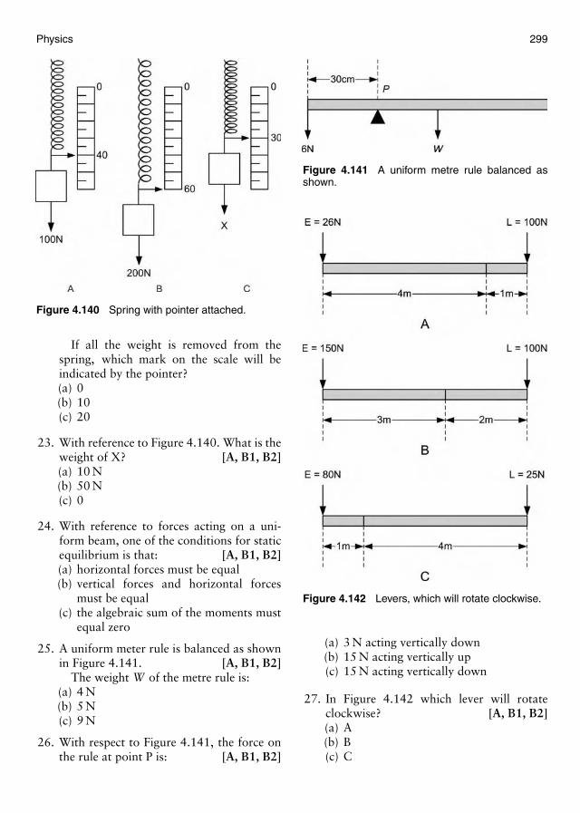
Physics 299
Figure 4.140 Spring with pointer attached.
If all the weight is removed from thespring, which mark on the scale will beindicated by the pointer?(a) 0(b) 10(c) 20
23. With reference to Figure 4.140. What is theweight of X? [A, B1, B2](a) 10 N(b) 50 N(c) 0
24. With reference to forces acting on a uni-form beam, one of the conditions for staticequilibrium is that: [A, B1, B2](a) horizontal forces must be equal(b) vertical forces and horizontal forces
must be equal(c) the algebraic sum of the moments must
equal zero
25. A uniform meter rule is balanced as shownin Figure 4.141. [A, B1, B2]
The weight W of the metre rule is:(a) 4 N(b) 5 N(c) 9 N
26. With respect to Figure 4.141, the force onthe rule at point P is: [A, B1, B2]
Figure 4.141 A uniform metre rule balanced asshown.
Figure 4.142 Levers, which will rotate clockwise.
(a) 3 N acting vertically down(b) 15 N acting vertically up(c) 15 N acting vertically down
27. In Figure 4.142 which lever will rotateclockwise? [A, B1, B2](a) A(b) B(c) C
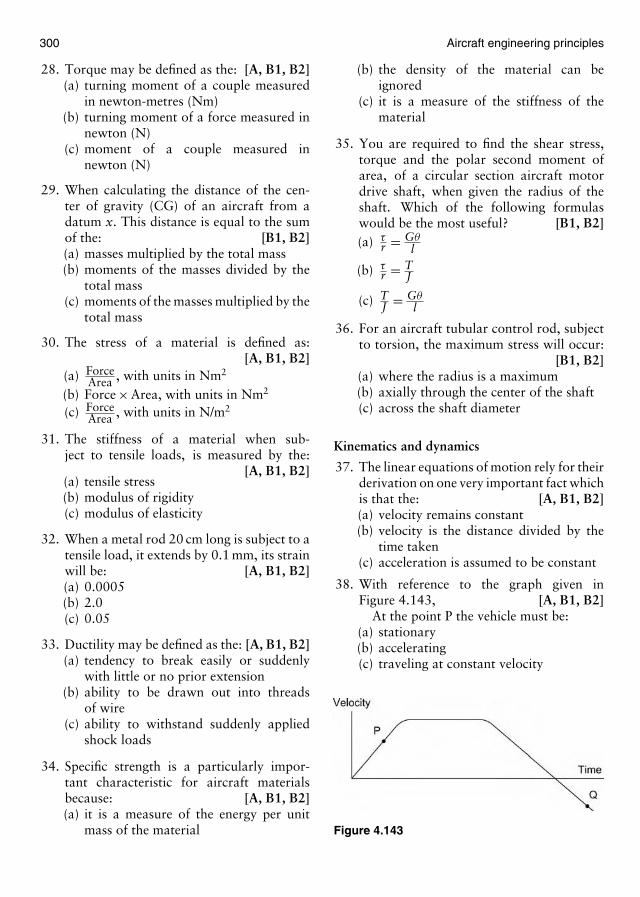
300 Aircraft engineering principles
28. Torque may be defined as the: [A, B1, B2](a) turning moment of a couple measured
in newton-metres (Nm)(b) turning moment of a force measured in
newton (N)(c) moment of a couple measured in
newton (N)
29. When calculating the distance of the cen-ter of gravity (CG) of an aircraft from adatum x. This distance is equal to the sumof the: [B1, B2](a) masses multiplied by the total mass(b) moments of the masses divided by the
total mass(c) moments of the masses multiplied by the
total mass
30. The stress of a material is defined as:[A, B1, B2]
(a) ForceArea , with units in Nm2
(b) Force × Area, with units in Nm2
(c) ForceArea , with units in N/m2
31. The stiffness of a material when sub-ject to tensile loads, is measured by the:
[A, B1, B2](a) tensile stress(b) modulus of rigidity(c) modulus of elasticity
32. When a metal rod 20 cm long is subject to atensile load, it extends by 0.1 mm, its strainwill be: [A, B1, B2](a) 0.0005(b) 2.0(c) 0.05
33. Ductility may be defined as the: [A, B1, B2](a) tendency to break easily or suddenly
with little or no prior extension(b) ability to be drawn out into threads
of wire(c) ability to withstand suddenly applied
shock loads
34. Specific strength is a particularly impor-tant characteristic for aircraft materialsbecause: [A, B1, B2](a) it is a measure of the energy per unit
mass of the material
(b) the density of the material can beignored
(c) it is a measure of the stiffness of thematerial
35. You are required to find the shear stress,torque and the polar second moment ofarea, of a circular section aircraft motordrive shaft, when given the radius of theshaft. Which of the following formulaswould be the most useful? [B1, B2](a) τ
r = Gθl
(b) τr = T
J
(c) TJ = Gθ
l
36. For an aircraft tubular control rod, subjectto torsion, the maximum stress will occur:
[B1, B2](a) where the radius is a maximum(b) axially through the center of the shaft(c) across the shaft diameter
Kinematics and dynamics
37. The linear equations of motion rely for theirderivation on one very important fact whichis that the: [A, B1, B2](a) velocity remains constant(b) velocity is the distance divided by the
time taken(c) acceleration is assumed to be constant
38. With reference to the graph given inFigure 4.143, [A, B1, B2]
At the point P the vehicle must be:(a) stationary(b) accelerating(c) traveling at constant velocity
Figure 4.143
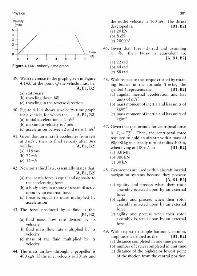
Physics 301
Figure 4.144 Velocity–time graph.
39. With reference to the graph given in Figure4.143, at the point Q the vehicle must be:
[A, B1, B2](a) stationary(b) traveling down hill(c) traveling in the reverse direction
40. Figure 4.144 shows a velocity–time graphfor a vehicle, for which the: [A, B1, B2](a) initial acceleration is 2 m/s2
(b) maximum velocity is 7 m/s(c) acceleration between 2 and 6 s is 1 m/s2
41. Given that an aircraft accelerates from restat 3 m/s2, then its final velocity after 36 swill be: [A, B1, B2](a) 118 m/s(b) 72 m/s(c) 12 m/s
42. Newton’s third law, essentially states that:[A, B1, B2]
(a) the inertia force is equal and opposite tothe accelerating force
(b) a body stays in a state of rest until actedupon by an external force
(c) force is equal to mass multiplied byacceleration
43. The force produced by a fluid is the:[B1, B2]
(a) fluid mass flow rate divided by itsvelocity
(b) fluid mass flow rate multiplied by itsvelocity
(c) mass of the fluid multiplied by itsvelocity
44. The mass airflow through a propeller is400 kg/s. If the inlet velocity is 50 m/s and
the outlet velocity is 100 m/s. The thrustdeveloped is: [B1, B2](a) 20 kN(b) 8 kN(c) 2000 N
45. Given that 1 rev = 2π rad and assumingπ = 22
7 , then 14 rev is equivalent to:[A, B1, B2]
(a) 22 rad(b) 44 rad(c) 88 rad
46. With respect to the torque created by rotat-ing bodies in the formula T = Iα, thesymbol I represents the: [B1, B2](a) angular inertial acceleration and has
units of m/s2
(b) mass moment of inertia and has units ofkg/m2
(c) mass moment of inertia and has units ofkg/m4
47. Given that the formula for centripetal force
is, Fc = mv2
r . Then, the centripetal forcerequired to hold an aircraft with a mass of90,000 kg in a steady turn of radius 300 m,when flying at 100 m/s is: [B1, B2](a) 3.0 MN(b) 300 kN(c) 30 kN
48. Gyroscopes are used within aircraft inertialnavigation systems because they possess:
[A, B1, B2](a) rigidity and precess when their rotor
assembly is acted upon by an externalforce
(b) agility and process when their rotorassembly is acted upon by an externalforce
(c) agility and precess when their rotorassembly is acted upon by an externalforce
49. With respect to simple harmonic motion,amplitude is defined as the: [B1, B2](a) distance completed in one time period(b) number of cycles completed in unit time(c) distance of the highest or lowest point
of the motion from the central position
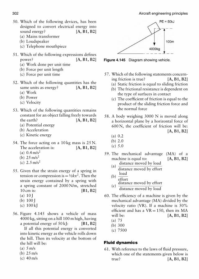
302 Aircraft engineering principles
50. Which of the following devices, has beendesigned to convert electrical energy intosound energy? [A, B1, B2](a) Mains transformer(b) Loudspeaker(c) Telephone mouthpiece
51. Which of the following expressions definespower? [A, B1, B2](a) Work done per unit time(b) Force per unit length(c) Force per unit time
52. Which of the following quantities has thesame units as energy? [A, B1, B2](a) Work(b) Power(c) Velocity
53. Which of the following quantities remainsconstant for an object falling freely towardsthe earth? [A, B1, B2](a) Potential energy(b) Acceleration(c) Kinetic energy
54. The force acting on a 10 kg mass is 25 N.The acceleration is: [A, B1, B2](a) 0.4 m/s2
(b) 25 m/s2
(c) 2.5 m/s2
55. Given that the strain energy of a spring intension or compression is = ½kx2. Then thestrain energy contained by a spring witha spring constant of 2000 N/m, stretched10 cm is: [B1, B2](a) 10 J(b) 100 J(c) 100 kJ
56. Figure 4.145 shows a vehicle of mass4000 kg, sitting on a hill 100 m high, havinga potential energy of 50 kJ: [B1, B2]
If all this potential energy is convertedinto kinetic energy as the vehicle rolls downthe hill. Then its velocity at the bottom ofthe hill will be:(a) 5 m/s(b) 25 m/s(c) 40 m/s
Figure 4.145 Diagram showing vehicle.
57. Which of the following statements concern-ing friction is true? [A, B1, B2](a) Static friction is equal to sliding friction(b) The frictional resistance is dependent on
the type of surfaces in contact(c) The coefficient of friction is equal to the
product of the sliding friction force andthe normal force
58. A body weighing 3000 N is moved alonga horizontal plane by a horizontal force of600 N, the coefficient of friction will be:
[A, B1, B2](a) 0.2(b) 2.0(c) 5.0
59. The mechanical advantage (MA) of amachine is equal to: [A, B1, B2]
(a)distance moved by loaddistance moved by effort
(b)loadeffort
(c)distance moved by effortdistance moved by load
60. The efficiency of a machine is given by themechanical advantage (MA) divided by thevelocity ratio (VR). If a machine is 50%efficient and has a VR = 150, then its MAwill be: [A, B1, B2](a) 75(b) 300(c) 7500
Fluid dynamics
61. With reference to the laws of fluid pressure,which one of the statements given below istrue? [A, B1, B2]
Physics 303
(a) Pressure acts vertically upwards from allsurfaces
(b) Pressure at a given depth depends on theshape of the containing vessel
(c) Pressure at a given depth in a fluid isequal in all directions
62. If the gauge pressure of a fluid is 200 kPaand atmospheric pressure is 100 kPa. Thenthe absolute pressure will be: [A, B1, B2](a) 2 kPa(b) 100 kPa(c) 300 kPa
63. If the density of mercury is 13,600 kg/m3
and we assume that the acceleration due togravity is 10 m/s2. Then a 10 cm column ofmercury will be the equivalent to a gaugepressure of: [A, B1, B2](a) 1360 Pa(b) 13,600 Pa(c) 1360 kPa
64. A man weighing 800 N is wearing snow-shoes. The area of each of his snow shoes is¼ m2. The pressure exerted on the groundby each of his snow shoes is: [A, B1, B2](a) 100 N/m2
(b) 400 N/m2
(c) 3200 N/m2
65. An object completely immersed in stillwater, will remain at a fixed depth, whenthe: [A, B1, B2](a) weight of the fluid displaced equals the
weight of the object(b) up thrust force reaches a uniform veloc-
ity(c) apparent loss of weight remains stable
66. The boundary layer: [B1, B2](a) remains stable at constant velocity(b) is the thin layer of fluid between the fixed
and moving boundary(c) has an exponential velocity gradient
between the fixed and moving boundary
67. Kinematic viscosity is: [A, B1, B2](a) equal to the dynamic viscosity multi-
plied by the velocity(b) density dependent and varies with
temperature
(c) pressure dependent and varies withweight
68. Streamline flow may be defined as:[A, B1, B2]
(a) flow in which fluid particles move per-pendicular and parallel to the surface ofthe body
(b) flow where the density does not changefrom point to point
(c) flow in which fluid particles movein an orderly manner and retain theshape of the body over which they areflowing
69. Given that a stream tube at a point, hasa cross-sectional area of 1.5 m2 and anincompressible fluid flows steadily past thispoint at 6 m/s. Then the volume flow ratewill be: [A, B1, B2](a) 9 m3/s(b) 4 m3/s(c) 0.25 m3/s
70. A wind tunnel is subject to an incompress-ible steady flow of air at 40 m/s, upstreamof the working section. If the cross-sectionalarea (csa) in the upstream part of the windtunnel is twice the csa of the workingsection then: [A, B1, B2](a) the working section velocity will be
1600 m/s(b) the working section velocity will be
twice that of the upstream velocity(c) the working section velocity will be half
that of the upstream velocity
71. The Bernoulli’s equation, which appliesthe conservation of energy to fluids inmotion, is represented in its energyform by: [B1, B2](a) ρgh1 + 1
2 mv21 + p1V1 = ρgh2 + 1
2 mv22 +
p1V1
(b) mgh1 + 12 mv2
1 + p1V1 = mgh2 + 12 mv2
2 +p2V2
(c) ρgh1 + 12ρv2
1 + p1 = ρgh2 + 12ρv2
2 + p2
72. As subsonic fluid flow passes through aVenturi tube, at the throat, the fluidpressure: [A, B1, B2](a) increases, the fluid velocity decreases
304 Aircraft engineering principles
(b) decreases and the fluid velocity decreases(c) decreases and the fluid velocity increases
Atmospheric physics
73. Starting at sea level the atmosphereis divided into the following regions:
[A, B1, B2](a) troposphere, stratosphere and
ionosphere(b) exosphere, troposphere and
stratosphere(c) troposphere, ionosphere and
stratosphere
74. Boyle’s law states that, the volume of a fixedmass of gas is inversely proportional to its:
[A, B1, B2](a) temperature providing the pressure of
the gas remains constant(b) pressure providing the temperature of
the gas remains constant(c) pressure providing the density of the gas
remains constant
76. The equation, PVT = constant, for an ideal
gas, is known as: [A, B1, B2](a) Charles’ law(b) Combined gas equation(c) Boyle’s law
77. In the characteristic gas equation given by:PV = mRT the symbol R is the: [B1, B2](a) universal gas constant with a value of
8314.4 J/kmol K(b) characteristic gas constant, that has
units of J/kg K(c) special gas constant, that has units of
kg/kmol K
78. If the temperature of the air in the atmo-sphere increases but the pressure remainsconstant, the density will: [A, B1, B2](a) decrease(b) remain the same(c) increase
79. The temperature at the tropopause in theInternational Standard Atmosphere (ISA) isapproximately: [A, B1, B2]
(a) −56 K(b) −56◦F(c) −56◦C
80. The ISA sea-level pressure is expressed as:[A, B1, B2]
(a) 29.92 mbar(b) 1 bar(c) 101,320 Pa
81. With increase in altitude, the speed of soundwill: [A, B1, B2](a) increase(b) decrease(c) remain the same
82. Temperature falls uniformly, with altitude,in the:(a) ionosphere(b) stratosphere(c) troposphere
83. The simple relationship Th = T0 − Lh maybe used to determine the temperature at agiven height h in km. Where the symbol Lin this equation represents the: [B1, B2](a) linear distance in meters between the
two altitudes(b) log-linear temperature drop measured in
Kelvin(c) the temperature lapse rate measured in
◦C/1000 m
84. A gas occupies a volume of 4 m3 at apressure of 400 kPa. At constant tempera-ture, the pressure is increased to 500 kPa.The new volume occupied by the gas is:
[A, B1, B2](a) 5 m3
(b) 3.2 m3
(c) 0.3 m3
Thermodynamics
85. The temperature of a substance is:[A, B1, B2]
(a) a measure of the energy possessedby the vibrating molecules of thesubstance
(b) a direct measure of the pressure energycontained within a substance
Physics 305
(c) directly dependent on the volume of thesubstance
86. The equivalent of 60 ◦C in Kelvin isapproximately: [A, B1, B2](a) 213 K(b) 273 K(c) 333 K
87. Alcohol thermometers are most suitablefor measuring: [A, B1, B2](a) jet pipe temperatures(b) cyrogenic substances(c) temperatures down to −115◦C
88. The increase in length of a solid bar 5 m inlength is = αl(t2 − t1). If the linear expan-sion coefficient for a solid is 2 × 10⁻⁶ andthe solid is subject to a temperature rise of100◦C. Then the increase in length will be:
[A, B1, B2](a) 1 × 10⁻³ m(b) 1 × 10⁻⁴ m(c) 1 × 10⁻⁵ m
89. The temperature of the melting point ofice and the boiling point of water are:
[A, B1, B2]Melting point Boiling point
(a) 0 K 373 K(b) 273 K 373 K(c) 173 K 273 K
90. Heat energy: [A, B1, B2](a) is the internal energy stored within a
body(b) travels from a cold body to a hot body(c) is transient energy
91. Heat transfer by conduction: [B1, B2](a) is where a large number of molecules
travel in bulk in a gas(b) involves energy transfer from atoms
with high vibration energy to thosewith low vibration energy
(c) involves changes in electron energy lev-els which emits energy in the form ofelectromagnetic waves
92. How much thermal energy is required toraise the temperature of 2 kg of aluminiumby 50◦C, if the specific heat capacity ofaluminium is 900 J/kgK
(a) 90 kJ(b) 22,500 J(c) 9000 J
93. The specific heat capacity at constantpressure, cp is: [B1, B2](a) less than the specific heat capacity
at constant volume, cv for the samesubstance
(b) based on constant volume heat transfer(c) always greater than cv
94. The specific latent heat of fusion of asubstance is the heat energy required to:
[B1, B2](a) change any amount of a substance from
a solid into a liquid(b) turn any amount of a substance from a
liquid into a solid(c) turn unit mass of a substance from a
liquid into a solid
95. A closed thermal system is one:[B1, B2]
(a) that always has fixed systemboundaries
(b) that always allows the mass transfer ofsystem fluid
(c) in which there is no mass transfer ofsystem fluid
96. The first law of thermodynamics appliedto a closed system, may be representedsymbolically by: [B1, B2](a) U1 + Q = U2 + W(b) Q + W = �U(c) U1 − Q = U2 + W
97. The enthalpy of a fluid is the combinationof: [B1, B2](a) kinetic energy + pressure energy(b) internal energy + pressure energy(c) potential energy + kinetic energy
98. An isentropic process is one in which:[B1, B2]
(a) the enthalpy remains constant(b) no heat energy is transferred to or from
the working fluid(c) both heat and work may be transferred
to or from the working fluid
306 Aircraft engineering principles
99. From the second law of thermodynamicsthe thermal efficiency (η) of a heat enginemay be defined as: [B1, B2]
(a) η = total heat suppledwork done
(b) η = Qout + Qin
Qout
(c) η = net work donetotal heat supplied
100. The ideal air standard Otto cycle is:[B1, B2]
(a) based on constant pressure heatrejection
(b) used as the basis for the aircraft gasturbine engine cycle
(c) based on constant volume heatrejection
101. Entropy is a measure of: [B1, B2](a) the degree of disorder in a system(b) is the product of internal energy and
pressure–volume energy(c) the adiabatic index of the system fluid
102. A polytropic process is: [B1, B2](a) one that obeys the law pvγ = c(b) one in which heat and work transfer
may take place(c) has constant entropy
Light and sound
103. Light: [B1, B2](a) is a longitudinal wave that travel
through air at 340 m/s(b) is an electromagnetic wave that travels
at 3 × 10⁸ m/s(c) cannot transfer energy from one place
to another
104. With respect to the laws of reflection:[B1, B2]
(a) the angle of incidence is equal to theangle of refraction
(b) the incident ray and the normal liewithin the same plane
(c) images from plane mirrors are real andlaterally converted
105. The light rays from a concave mirror:[B1, B2]
(a) converge at the principle focus(b) diverge at the principle focus(c) diverge at the pole which is approxi-
mately twice the radius of curvature
106. Given that 1u = 1
v + 1f , the object distance =
50 mm and the focal length = 150 mm,then the distance of the object from themirror is: [B1, B2](a) 37.5 mm(b) 75 mm(c) 150 mm
107. As light travels from one medium toanother medium with a greater refractiveindex, its speed: [B1, B2](a) is increased(b) remains the same(c) is decreased
108. Fibre optic cables use the principle of:[B1, B2]
(a) total external reflection to enable lightto travel along the cable
(b) internal refraction to enable light totravel along the cable
(c) total internal reflection to enable lightto travel along the cable
109. Convex lenses: [B1, B2](a) form real, inverted, small images of
distant objects(b) create virtual, inverted, small images of
near objects(c) produce images where the focal length
is always negative
110. Sound waves [B1, B2](a) are transverse waves that are able to
travel through a vacuum(b) form part of the electromagnetic spec-
trum, with low or high frequencies(c) are longitudinal waves that need a
medium through which to travel
111. The speed of a wavefront is linked by therelationship v = f λ. If given that the wavefrequency = 1 kHz and the speed of prop-agation is 100 m/s, then the wavelength is:
[B1, B2]
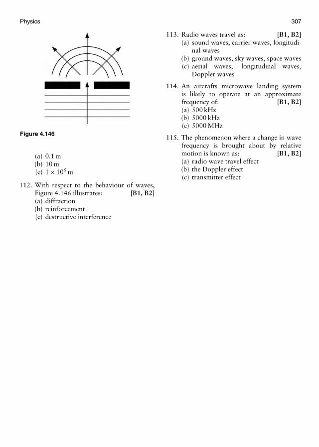
Physics 307
Figure 4.146
(a) 0.1 m(b) 10 m(c) 1 × 10⁵ m
112. With respect to the behaviour of waves,Figure 4.146 illustrates: [B1, B2](a) diffraction(b) reinforcement(c) destructive interference
113. Radio waves travel as: [B1, B2](a) sound waves, carrier waves, longitudi-
nal waves(b) ground waves, sky waves, space waves(c) aerial waves, longitudinal waves,
Doppler waves
114. An aircrafts microwave landing systemis likely to operate at an approximatefrequency of: [B1, B2](a) 500 kHz(b) 5000 kHz(c) 5000 MHz
115. The phenomenon where a change in wavefrequency is brought about by relativemotion is known as: [B1, B2](a) radio wave travel effect(b) the Doppler effect(c) transmitter effect

This page intentionally left blank

P A R T3
Electrical and electronicfundamentals

This page intentionally left blank
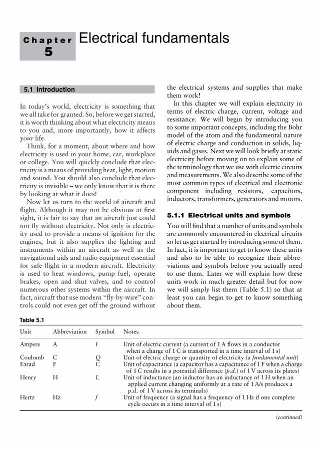
C h a p t e r
5Electrical fundamentals
5.1 Introduction
In today’s world, electricity is something thatwe all take for granted. So, before we get started,it is worth thinking about what electricity meansto you and, more importantly, how it affectsyour life.
Think, for a moment, about where and howelectricity is used in your home, car, workplaceor college. You will quickly conclude that elec-tricity is a means of providing heat, light, motionand sound. You should also conclude that elec-tricity is invisible – we only know that it is thereby looking at what it does!
Now let us turn to the world of aircraft andflight. Although it may not be obvious at firstsight, it is fair to say that an aircraft just couldnot fly without electricity. Not only is electric-ity used to provide a means of ignition for theengines, but it also supplies the lighting andinstruments within an aircraft as well as thenavigational aids and radio equipment essentialfor safe flight in a modern aircraft. Electricityis used to heat windows, pump fuel, operatebrakes, open and shut valves, and to controlnumerous other systems within the aircraft. Infact, aircraft that use modern “fly-by-wire” con-trols could not even get off the ground without
Table 5.1
Unit Abbreviation Symbol Notes
Ampere A I Unit of electric current (a current of 1 A flows in a conductorwhen a charge of 1 C is transported in a time interval of 1 s)
Coulomb C Q Unit of electric charge or quantity of electricity (a fundamental unit)Farad F C Unit of capacitance (a capacitor has a capacitance of 1 F when a charge
of 1 C results in a potential difference (p.d.) of 1 V across its plates)Henry H L Unit of inductance (an inductor has an inductance of 1 H when an
applied current changing uniformly at a rate of 1 A/s produces ap.d. of 1 V across its terminals)
Hertz Hz f Unit of frequency (a signal has a frequency of 1 Hz if one completecycle occurs in a time interval of 1 s)
(continued)
the electrical systems and supplies that makethem work!
In this chapter we will explain electricity interms of electric charge, current, voltage andresistance. We will begin by introducing youto some important concepts, including the Bohrmodel of the atom and the fundamental natureof electric charge and conduction in solids, liq-uids and gases. Next we will look briefly at staticelectricity before moving on to explain some ofthe terminology that we use with electric circuitsand measurements. We also describe some of themost common types of electrical and electroniccomponent including resistors, capacitors,inductors, transformers, generators and motors.
5.1.1 Electrical units and symbols
You will find that a number of units and symbolsare commonly encountered in electrical circuitsso let us get started by introducing some of them.In fact, it is important to get to know these unitsand also to be able to recognize their abbre-viations and symbols before you actually needto use them. Later we will explain how theseunits work in much greater detail but for nowwe will simply list them (Table 5.1) so that atleast you can begin to get to know somethingabout them.
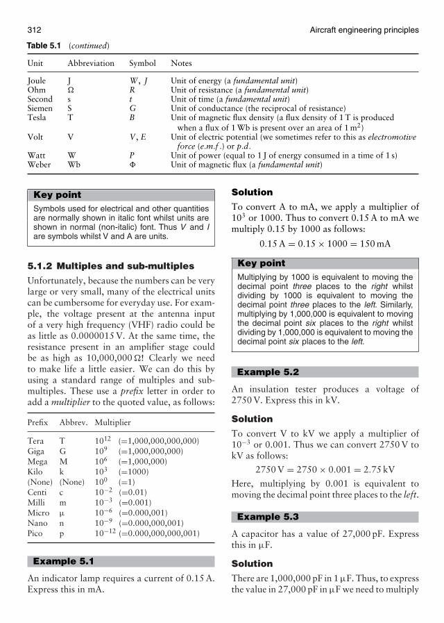
312 Aircraft engineering principles
Table 5.1 (continued)
Unit Abbreviation Symbol Notes
Joule J W , J Unit of energy (a fundamental unit)Ohm � R Unit of resistance (a fundamental unit)Second s t Unit of time (a fundamental unit)Siemen S G Unit of conductance (the reciprocal of resistance)Tesla T B Unit of magnetic flux density (a flux density of 1 T is produced
when a flux of 1 Wb is present over an area of 1 m2)Volt V V , E Unit of electric potential (we sometimes refer to this as electromotive
force (e.m.f .) or p.d.Watt W P Unit of power (equal to 1 J of energy consumed in a time of 1 s)Weber Wb � Unit of magnetic flux (a fundamental unit)
Key pointSymbols used for electrical and other quantitiesare normally shown in italic font whilst units areshown in normal (non-italic) font. Thus V and Iare symbols whilst V and A are units.
5.1.2 Multiples and sub-multiples
Unfortunately, because the numbers can be verylarge or very small, many of the electrical unitscan be cumbersome for everyday use. For exam-ple, the voltage present at the antenna inputof a very high frequency (VHF) radio could beas little as 0.0000015 V. At the same time, theresistance present in an amplifier stage couldbe as high as 10,000,000 �! Clearly we needto make life a little easier. We can do this byusing a standard range of multiples and sub-multiples. These use a prefix letter in order toadd a multiplier to the quoted value, as follows:
Prefix Abbrev. Multiplier
Tera T 1012 (=1,000,000,000,000)Giga G 109 (=1,000,000,000)Mega M 106 (=1,000,000)Kilo k 103 (=1000)(None) (None) 100 (=1)Centi c 10−2 (=0.01)Milli m 10−3 (=0.001)Micro µ 10−6 (=0.000,001)Nano n 10−9 (=0.000,000,001)Pico p 10−12 (=0.000,000,000,001)
Example 5.1
An indicator lamp requires a current of 0.15 A.Express this in mA.
Solution
To convert A to mA, we apply a multiplier of103 or 1000. Thus to convert 0.15 A to mA wemultiply 0.15 by 1000 as follows:
0.15 A = 0.15 × 1000 = 150 mA
Key pointMultiplying by 1000 is equivalent to moving thedecimal point three places to the right whilstdividing by 1000 is equivalent to moving thedecimal point three places to the left. Similarly,multiplying by 1,000,000 is equivalent to movingthe decimal point six places to the right whilstdividing by 1,000,000 is equivalent to moving thedecimal point six places to the left.
Example 5.2
An insulation tester produces a voltage of2750 V. Express this in kV.
Solution
To convert V to kV we apply a multiplier of10−3 or 0.001. Thus we can convert 2750 V tokV as follows:
2750 V = 2750 × 0.001 = 2.75 kV
Here, multiplying by 0.001 is equivalent tomoving the decimal point three places to the left.
Example 5.3
A capacitor has a value of 27,000 pF. Expressthis in µF.
Solution
There are 1,000,000 pF in 1 µF. Thus, to expressthe value in 27,000 pF in µF we need to multiply
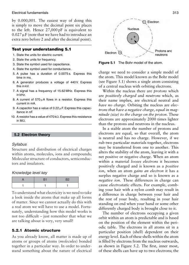
Electrical fundamentals 313
by 0.000,001. The easiest way of doing thisis simply to move the decimal point six placesto the left. Hence 27,000 pF is equivalent to0.027 µF (note that we have had to introduce anextra zero before 2 and after the decimal point).
Test your understanding 5.11. State the units for electric current.
2. State the units for frequency.
3. State the symbol used for capacitance.
4. State the symbol used for conductance.
5. A pulse has a duration of 0.0075 s. Express thistime in ms.
6. A generator produces a voltage of 440V. Expressthis in kV.
7. A signal has a frequency of 15.62 MHz. Express thisin kHz.
8. A current of 570 µA flows in a resistor. Express thiscurrent in mA.
9. A capacitor has a value of 0.22 µF. Express this capac-itance in nF.
10. A resistor has a value of 470 k�. Express this resistancein M�.
5.2 Electron theory
SyllabusStructure and distribution of electrical chargeswithin atoms, molecules, ions and compounds;Molecular structure of conductors, semiconduc-tors and insulators.
Knowledge level key
1
A
1
B1
1
B2
To understand what electricity is we need to takea look inside the atoms that make up all formsof matter. Since we cannot actually do this witha real atom we will have to use a model. Fortu-nately, understanding how this model works isnot too difficult – just remember that what weare talking about is very, very small!
5.2.1 Atomic structure
As you already know, all matter is made up ofatoms or groups of atoms (molecules) bondedtogether in a particular way. In order to under-stand something about the nature of electrical
Figure 5.1 The Bohr model of the atom.
charge we need to consider a simple model ofthe atom. This model known as the Bohr model(see Figure 5.1) shows a single atom consistingof a central nucleus with orbiting electrons.
Within the nucleus there are protons whichare positively charged and neutrons which, astheir name implies, are electrical neutral andhave no charge. Orbiting the nucleus are elec-trons that have a negative charge, equal in mag-nitude (size) to the charge on the proton. Theseelectrons are approximately 2000 times lighterthan the protons and neutrons in the nucleus.
In a stable atom the number of protons andelectrons are equal, so that overall, the atomis neutral and has no charge. However, if werub two particular materials together, electronsmay be transferred from one to another. Thisalters the stability of the atom, leaving it with anet positive or negative charge. When an atomwithin a material looses electrons it becomespositively charged and is known as a positiveion, when an atom gains an electron it has asurplus negative charge and so is known as anegative ion. These differences in charge cancause electrostatic effects. For example, comb-ing your hair with a nylon comb may result ina difference in charge between your hair andthe rest of your body, resulting in your hairstanding on end when your hand or some otherdifferently charged body is brought close to it.
The number of electrons occupying a givenorbit within an atom is predictable and is basedon the position of the element within the peri-odic table. The electrons in all atoms sit in aparticular position (shell) dependent on theirenergy level. Each of these shells within the atomis filled by electrons from the nucleus outwards,as shown in Figure 5.2. The first, inner most,of these shells can have up to two electrons; the
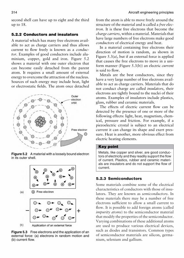
314 Aircraft engineering principles
second shell can have up to eight and the thirdup to 18.
5.2.2 Conductors and insulators
A material which has many free electrons avail-able to act as charge carriers and thus allowscurrent to flow freely is known as a conduc-tor. Examples of good conductors include alu-minium, copper, gold and iron. Figure 5.2shows a material with one outer electron thatcan become easily detached from the parentatom. It requires a small amount of externalenergy to overcome the attraction of the nucleus.Sources of such energy may include heat, lightor electrostatic fields. The atom once detached
Figure 5.2 A material with a loosely bound electronin its outer shell.
Figure 5.3 Free electrons and the application of anexternal force: (a) electrons in random motion and(b) current flow.
from the atom is able to move freely around thestructure of the material and is called a free elec-tron. It is these free electrons that become thecharge carriers, within a material. Materials thathave large numbers of free electrons make goodconductors of electrical energy and heat.
In a material containing free electrons theirdirection of motion is random, as shown inFigure 5.3(a), but if an external force is appliedthat causes the free electrons to move in a uni-form manner (Figure 5.3(b)) an electric currentis said to flow.
Metals are the best conductors, since theyhave a very large number of free electrons avail-able to act as charge carriers. Materials that donot conduct charge are called insulators, theirelectrons are tightly bound to the nuclei of theiratoms. Examples of insulators include plastics,glass, rubber and ceramic materials.
The effects of electric current flow can bedetected by the presence of one or more of thefollowing effects: light, heat, magnetism, chem-ical, pressure and friction. For example, if apiezoelectric crystal is subject to an electricalcurrent it can change its shape and exert pres-sure. Heat is another, more obvious effect fromelectric heating elements.
Key pointMetals, like copper and silver, are good conduc-tors of electricity and they readily support the flowof current. Plastics, rubber and ceramic materi-als are insulators and do not support the flow ofcurrent.
5.2.3 Semiconductors
Some materials combine some of the electricalcharacteristics of conductors with those of insu-lators. They are known as semiconductors. Inthese materials there may be a number of freeelectrons sufficient to allow a small current toflow. It is possible to add foreign atoms (calledimpurity atoms) to the semiconductor materialthat modify the properties of the semiconductor.Varying combinations of these additional atomsare used to produce various electrical devices,such as diodes and transistors. Common typesof semiconductor materials are silicon, germa-nium, selenium and gallium.

Electrical fundamentals 315
Key pointSemiconductors are pure insulating materialswith a small amount of an impurity elementpresent. Typical examples are silicon andgermanium.
5.2.4 Temperature effects
As stated earlier, all materials offer some resis-tance to current flow. In conductors the free elec-trons, rather than passing unobstructed throughthe material, collide with the relatively large andsolid nuclei of the atoms. As the temperatureincreases, the nuclei vibrate more energeticallyfurther obstructing the path of the free electrons,causing more frequent collisions. The result isthat the resistance of conductors increases withtemperature.
Due to the nature of the bonding in insulators,there are no free electrons, except that whenthermal energy increases as a result of a temper-ature increase, a few outer electrons manage tobreak free from their fixed positions and act ascharge carriers. The result is that the resistanceof insulators decreases as temperature increases.
Semiconductors behave in a similar mannerto insulators. At absolute zero (−273◦C) boththe types of material act as perfect insulators.However, unlike the insulator, as temperatureincreases in a semiconductor large numbers ofelectrons break free to act as charge carriers.
Figure 5.4 Variation of resistance with temperaturefor various materials.
Therefore, as temperature increases, the resis-tance of a semiconductor decreases rapidly.
By producing special alloys, such as eurekaand manganin that combine the effects of insu-lators and conductors, it is possible to produce amaterial where the resistance remains constantwith increase in temperature. Figure 5.4 showshow the resistance of insulators, semiconductorsand conductors change with temperature.
Test your understanding 5.21. In a stable neutral atom the number of _______ and
_______ are equal and there is no overall charge.
2. When an atom within a material losses electronsit becomes ________ charged and is known as a______________.
3. When an atom gains an electron it has a surplus_________ charge and so known as a ______________.
4. The electrical properties of a material are determinedby the number of ______________ present.
5. Materials that do not conduct electric charge are called_______.
6. Name two materials that act as good electricalconductors.
7. Name two materials that act as good electricalinsulators.
8. Name two semiconductor materials.
9. Explain briefly how the resistance of a metallic conduc-tor varies with temperature.
10. Explain briefly how the resistance of an insulator varieswith temperature.
5.3 Static electricity and conduction
SyllabusStatic electricity and distribution of electro-static charges; Electrostatic laws of attractionand repulsion; Units of charge, Coulomb’s law;Conduction of electricity in solids, liquids, gasesand a vacuum.
Knowledge level key
1
A
2
B1
2
B2
Electric charge is all around us. Indeed, manyof the everyday items that we use in the homeand at work rely for their operation on the exis-tence of electric charge and the ability to make
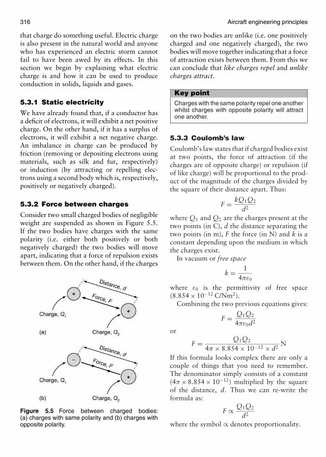
316 Aircraft engineering principles
that charge do something useful. Electric chargeis also present in the natural world and anyonewho has experienced an electric storm cannotfail to have been awed by its effects. In thissection we begin by explaining what electriccharge is and how it can be used to produceconduction in solids, liquids and gases.
5.3.1 Static electricity
We have already found that, if a conductor hasa deficit of electrons, it will exhibit a net positivecharge. On the other hand, if it has a surplus ofelectrons, it will exhibit a net negative charge.An imbalance in charge can be produced byfriction (removing or depositing electrons usingmaterials, such as silk and fur, respectively)or induction (by attracting or repelling elec-trons using a second body which is, respectively,positively or negatively charged).
5.3.2 Force between charges
Consider two small charged bodies of negligibleweight are suspended as shown in Figure 5.5.If the two bodies have charges with the samepolarity (i.e. either both positively or bothnegatively charged) the two bodies will moveapart, indicating that a force of repulsion existsbetween them. On the other hand, if the charges
Figure 5.5 Force between charged bodies:(a) charges with same polarity and (b) charges withopposite polarity.
on the two bodies are unlike (i.e. one positivelycharged and one negatively charged), the twobodies will move together indicating that a forceof attraction exists between them. From this wecan conclude that like charges repel and unlikecharges attract.
Key pointCharges with the same polarity repel one anotherwhilst charges with opposite polarity will attractone another.
5.3.3 Coulomb’s law
Coulomb’s law states that if charged bodies existat two points, the force of attraction (if thecharges are of opposite charge) or repulsion (ifof like charge) will be proportional to the prod-uct of the magnitude of the charges divided bythe square of their distance apart. Thus:
F = kQ1Q2
d2
where Q1 and Q2 are the charges present at thetwo points (in C), d the distance separating thetwo points (in m), F the force (in N) and k is aconstant depending upon the medium in whichthe charges exist.
In vacuum or free space
k = 14πε0
where ε0 is the permittivity of free space(8.854 × 10⁻¹² C/Nm2).
Combining the two previous equations gives:
F = Q1Q2
4πε0d2
or
F = Q1Q2
4π × 8.854 × 10−12 × d2N
If this formula looks complex there are only acouple of things that you need to remember.The denominator simply consists of a constant(4π × 8.854 × 10−12) multiplied by the squareof the distance, d. Thus we can re-write theformula as:
F ∝ Q1Q2
d2
where the symbol ∝ denotes proportionality.
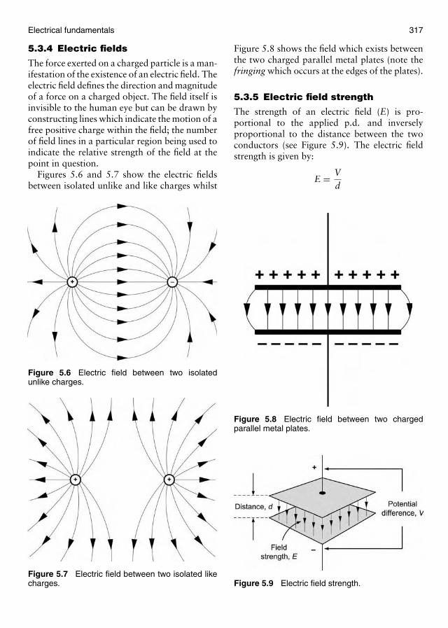
Electrical fundamentals 317
5.3.4 Electric fields
The force exerted on a charged particle is a man-ifestation of the existence of an electric field. Theelectric field defines the direction and magnitudeof a force on a charged object. The field itself isinvisible to the human eye but can be drawn byconstructing lines which indicate the motion of afree positive charge within the field; the numberof field lines in a particular region being used toindicate the relative strength of the field at thepoint in question.
Figures 5.6 and 5.7 show the electric fieldsbetween isolated unlike and like charges whilst
Figure 5.6 Electric field between two isolatedunlike charges.
Figure 5.7 Electric field between two isolated likecharges.
Figure 5.8 shows the field which exists betweenthe two charged parallel metal plates (note thefringing which occurs at the edges of the plates).
5.3.5 Electric field strength
The strength of an electric field (E) is pro-portional to the applied p.d. and inverselyproportional to the distance between the twoconductors (see Figure 5.9). The electric fieldstrength is given by:
E = Vd
Figure 5.8 Electric field between two chargedparallel metal plates.
Figure 5.9 Electric field strength.

318 Aircraft engineering principles
where E is the electric field strength (in V/m), Vis the applied p.d. (in V) and d is the distance(in m).
Example 5.4
Two charged particles are separated by a dis-tance of 25 mm. Calculate the force betweenthe two charges if one has a positive charge of0.25 µC and the other has a negative charge of0.4 µC. What will the relative direction of theforce be?
Solution
Now F = Q1Q2
4π × 8.854 × 10−12 × d2
where Q1 = 0.25 µC = 0.25 × 10⁻⁶ C, Q2 =0.4 µC = 0.4 × 10⁻⁶ C, and d = 2.5 mm =2.5 × 10⁻³ m, thus:
F = 0.25 × 10−6 × 0.4 × 10−6
4π × 8.854 × 10−12 × (2.5 × 10−3)2
= 0.1 × 10⁻¹²
4π × 8.854 × 10−12 × 6.25 × 10−6
or
F = 0.14π × 8.854 × 6.25 × 10−6
= 0.1695.39 × 10−6
= 1.438 × 10²
Hence F = 1.438 × 10² N = 143.8 N
Example 5.5
Two charged particles have the same positivecharge and are separated by a distance of 10 mm.If the force between them is 0.1 N, determine thecharge present.
Solution
Now F = Q1Q2
4π × 8.854 × 10−12 × d2
where F = 0.1 N, d = 0.01 m and Q1 = Q2 = Q,thus:
0.1 = QQ4π × 8.854 × 10−12 × (0.01)2
Re-arranging the formula to make Q the subjectgives:
Q2 = 0.1 × 4π × 8.854 × 10−12 × (0.01)2
or
Q =√
0.1 × 4π × 8.854 × 10−12 × (0.01)2
=√
4π × 8.854 × 10−17
=√
111.263 × 10−17 =√
11.1263 × 10⁻¹⁶
thus
Q = √11.1263 ×
√10−16 = 3.336 × 10⁻⁸ C
= 0.03336 µC
Example 5.6
Two parallel conductors are separated by a dis-tance of 25 mm. Determine the electric fieldstrength if they are fed from a 600 V directcurrent (DC) supply.
Solution
The electric field strength will be given by:
E = Vd
where V = 600 V and d = 25 mm = 0.025 m,thus:
E = 6000.025
= 24,000 V/m = 24 kV/m
Example 5.7
The field strength between the two parallelplates in a cathode ray tube is 18 kV/m. If theplates are separated by a distance of 21 mm,determine the p.d. that exists between the plates.
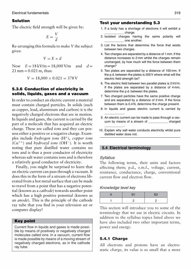
Electrical fundamentals 319
Solution
The electric field strength will be given by:
E = Vd
Re-arranging this formula to make V the subjectgives:
V = E × d
Now E = 18 kV/m = 18,000 V/m and d =21 mm = 0.021 m, thus:
V = 18,000 × 0.021 = 378 V
5.3.6 Conduction of electricity insolids, liquids, gases and a vacuum
In order to conduct an electric current a materialmust contain charged particles. In solids (suchas copper, lead, aluminium and carbon) it is thenegatively charged electrons that are in motion.In liquids and gases, the current is carried by thepart of a molecule that has acquired an electriccharge. These are called ions and they can pos-sess either a positive or a negative charge. Exam-ples include hydrogen ions (H+), copper ions(Cu++) and hydroxyl ions (OH−). It is worthnoting that pure distilled water contains noions and is thus a poor conductor of electricitywhereas salt water contains ions and is thereforea relatively good conductor of electricity.
Finally, you might be surprised to learn thatan electric current can pass through a vacuum. Itdoes this in the form of a stream of electrons lib-erated from a hot metal surface that can be madeto travel from a point that has a negative poten-tial (known as a cathode) towards another pointwhich has a high positive potential (known asan anode). This is the principle of the cathoderay tube that you find in your television set orcomputer display!
Key pointCurrent flow in liquids and gases is made possi-ble by means of positively or negatively chargedmolecules called ions. In a vacuum, current flowis made possible by means of a moving stream ofnegatively charged electrons, as in the cathoderay tube.
Test your understanding 5.31. If a body has a shortage of electrons it will exhibit a
___________ charge.2. Isolated charges having the same polarity will
___________ one another.
3. List the factors that determine the force that existsbetween two charges.
4. Two charges are separated by a distance of 1 mm. If thedistance increases to 2 mm whilst the charges remainunchanged, by how much will the force between themchange?
5. Two plates are separated by a distance of 100 mm. Ifthe p.d. between the plates is 200V where what will theelectric field strength be?
6. The electric field between two parallel plates is 2 kV/m.If the plates are separated by a distance of 4 mm,determine the p.d. between the plates.
7. Two charged particles have the same positive chargeand are separated by a distance of 2 mm. If the forcebetween them is 0.4 N, determine the charge present.
8. In liquids and gases electric current is carried by___________.
9. An electric current can be made to pass through a vac-uum by means of a stream of ___________ charged___________.
10. Explain why salt water conducts electricity whilst puredistilled water does not.
5.4 Electrical terminology
SyllabusThe following terms, their units and factorsaffecting them; p.d., e.m.f., voltage, current,resistance, conductance, charge, conventionalcurrent flow and electron flow.
Knowledge level key
1
A
2
B1
2
B2
This section will introduce you to some of theterminology that we use in electric circuits. Inaddition to the syllabus topics listed above wehave also included two other important terms,power and energy.
5.4.1 Charge
All electrons and protons have an electro-static charge, its value is so small that a more
320 Aircraft engineering principles
convenient unit of charge is needed for prac-tical use, which we call the coulomb. Onecoulomb C is the total charge Q of 6.21 × 10¹⁸
electrons. Thus a single electron has a charge of1.61 × 10−19 C.
5.4.2 Current
Current, I, is defined as the rate of flow of chargeand its unit is the ampere, A. One ampere isequal to one coulomb per second, or:
One ampere of current, I = Qt
where t is time in seconds.So, for example, if a steady current of 3 A
flows for 2 min, then the amount of chargetransferred will be:
Q = I × t = 3 A × 120 s = 360 C
Key pointCurrent is the rate of flow of charge.Thus, if morecharge moves in a given time, more current willbe flowing. If no charge moves then no current isflowing.
5.4.3 Conventional current andelectron flow
In Section 5.2.2 we described electric current interms of the organized movement of electronsin a metal conductor. Owing to their nega-tive charge, electrons will flow from a negativepotential to a more positive potential (recall thatlike-charges attract and unlike-charges repel).However, when we indicate the direction of cur-rent in a circuit we show it as moving from apoint that has the greatest positive potential toa point that has the most negative potential. Wecall this conventional current and, although itmay seem to be odd, you just need to rememberthat it flows in the opposite direction to that ofthe motion of electrons!
Key pointElectrons move from negative to positive whilstconventional current is assumed to flow frompositive to negative.
5.4.4 Potential difference (voltage)
The force that creates the flow of current (orrate of flow of charge carriers) in a circuit isknown as the e.m.f . and it is measured in volts(V). The p.d. is the voltage difference or voltagedrop between two points.
One volt is the p.d. between two points if onejoule of energy is required to move one coulombof charge between them. Hence:
V = WQ
where W is the energy and Q is the charge, asbefore. Energy is defined later in Section 5.4.8.
5.4.5 Resistance
All materials at normal temperatures oppose themovement of electric charge through them, thisopposition to the flow of the charge carriers isknown as the resistance R of the material. Thisresistance is due to collisions between the chargecarriers (electrons) and the atoms of the mate-rial. The unit of resistance is the ohm, withsymbol �.
Note that 1 V is the e.m.f. required to move6.21 × 1018 electrons (1 C) through a resistanceof 1 � in 1 s. Hence:
V =(
Qt
)× R
where Q is the charge, t is the time and R is theresistance.
Re-arranging this equation to make R thesubject gives:
R = V × tQ
�
We shall be looking at the important relation-ship between voltage, V , current, I and resis-tance, R, later on in Sections 5.7.1 and 5.7.2.
5.4.6 Conductance
Conductance is the inverse of resistance. In otherwords, as the resistance of a conductor increasesits conductance reduces, and vice versa. A mate-rial that has a low value of conductance will notconduct electricity as well as a material that has a
Electrical fundamentals 321
high conductance, and vice versa. You can thusthink of conductance as the lack of oppositionto the passage of charge carriers. The symbolused for conductance is G and its unit is theSiemen (S).
The following table shows the relative con-ductance of some common metals:
Metal Relative conductance(copper = 1)
Silver 1.06Copper (annealed) 1.00Copper (hard drawn) 0.97Aluminium 0.61Mild steel 0.12Lead 0.08
Key pointMetals, like copper and silver, are good con-ductors of electricity. Good conductors havelow resistance whilst poor conductors have highresistance.
Example 5.8
A current of 45 mA flows from one point in acircuit to another. What charge is transferredbetween the two points in 10 min?
Solution
Here we will use Q = I × twhere I = 45 mA = 0.045 A and t = 10 min =10 × 60 = 600 s, thus:
Q = 0.045 × 600 = 27 C
Example 5.9
A 28 V DC aircraft supply delivers a charge of5 C to a window heater every second. What isthe resistance of the heater?
Solution
Here we will use R = V × tQ
where V = 28 V, Q = 5 C and t = 1 s, thus:
R = V × tQ
= 28 V × 1 s5C
= 5.6 �
5.4.7 Power
Power, P, is the rate at which energy is convertedfrom one form to another and it is measuredin Watts. The larger the amount of power thegreater the amount of energy that is convertedin a given period of time.
1 watt = 1 joule per second or
Power, P = Energy, JTime, t
thus: P = Jt
W
5.4.8 Energy
Like all other forms of energy, electrical energyis the capacity to do work. Energy can be con-verted from one form to another. For examplean electric fire converts electrical energy intoheat. A filament lamp converts electrical energyinto light, and so on. Energy can only betransferred when a difference in energy levelsexists.
The unit of energy is the joule. Then, from thedefinition of power:
1 Joule = 1 Watt × 1 second
hence:
Energy, J = (Power, P) × (Time, t)
with units of (Watts × seconds)
thus: J = P × t W
Thus joules are measured in watt-seconds(Ws). If the power was to be measured in kilo-watts and the time in hours, then the unit ofelectrical energy would be the kilowatt-hour(kWh) (commonly knows as a unit of electricity).The electricity meter in your home recordsthe number of kilowatt-hours. In other words,it indicates the amount of energy that youhave used.
Example 5.10
An auxiliary power unit (APU) provides an out-put of 1.5 kW for 20 min. How much energy hasit supplied to the aircraft?
322 Aircraft engineering principles
Solution
Here we will use J = P × twhere P = 1.5 kW = 1500 W and t = 20 min= 20 × 60 = 1200 s, thus:
J = 1500 × 1200 = 1,800,000 J = 1.8 MJ
Note here that we have converted from J toMJ by moving the decimal point six places tothe left.
Example 5.11
A smoothing capacitor is required to store 20 Jof energy. How much power is required to storethis energy in a time interval of 0.5 s?
Solution
Re-arranging J = P × t to make P the subjectgives:
P = Jt
we can now find P when J = 20 J and t = 0.5 s,thus:
P = Jt
= 20 J0.5 s
= 40 W
Example 5.12
A main aircraft battery is used to start an engine.If the starter demands a current of 1000 A for30 s and the battery voltage remains at 12 Vduring this period, determine the amount ofelectrical energy required to start the engine.
Solution
Here we will use Q = I × twhere I = 1000 A and t = 30 s, thus:
Q = 1000 × 30 = 30,000 C
But
V = WQ
where W is the energy and Q is the charge.
∴ W = V × Q
= 12 × 30,000 = 360,000 = 360 kJ
Test your understanding 5.41. Current is defined as the rate of flow of ________ and
its unit is the ________.
2. Conventional current flows from ________ to ________.
3. Electron flow is from ________ to ________.
4. The unit of resistance is the ________ and its symbolis ________.
5. Which of the following materials: aluminium, copper,gold and silver is (a) the best and (b) the worst conductorof electricity?
6. A current of 1.5 A flows for 10 min. What charge istransferred?
7. The e.m.f. required to move 6.21 × 10¹⁸ electronsthrough a resistance of 1 � is ________.
8. The energy transferred by an electric circuit is theproduct of ________ and ________.
9. Explain briefly what is meant by the term, resistance.
10. Explain briefly the relationship between resistance andconductance.
5.5 Generation of electricity
SyllabusProduction of electricity by the following meth-ods: light, heat, friction, pressure, chemicalaction, magnetism and motion.
Knowledge level key
1
A
1
B1
1
B2
There are electrons and protons in the atomsof all materials but, to do useful work, chargesmust be separated in order to produce a p.d. thatwe can use to make current flow and do work.Since the generation of electric current is a fun-damental requirement in every aircraft we shallbe looking at this topic in much greater detaillater on. For now, we will briefly describe someof the available methods for separating chargesand creating a flow of current.
5.5.1 Friction
Static electricity can be produced by friction. Inthis method, electrons and protons in an insula-tor can be separated by rubbing two materialstogether in order to produce opposite charges.These charges will remain separated for sometime until they eventually leak away due to
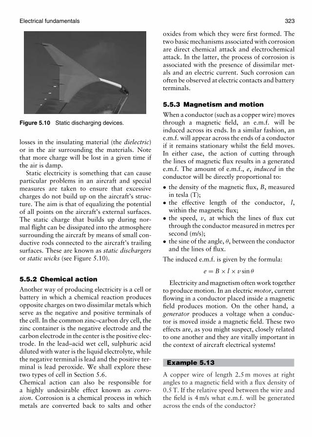
Electrical fundamentals 323
Figure 5.10 Static discharging devices.
losses in the insulating material (the dielectric)or in the air surrounding the materials. Notethat more charge will be lost in a given time ifthe air is damp.
Static electricity is something that can causeparticular problems in an aircraft and specialmeasures are taken to ensure that excessivecharges do not build up on the aircraft’s struc-ture. The aim is that of equalizing the potentialof all points on the aircraft’s external surfaces.The static charge that builds up during nor-mal flight can be dissipated into the atmospheresurrounding the aircraft by means of small con-ductive rods connected to the aircraft’s trailingsurfaces. These are known as static dischargersor static wicks (see Figure 5.10).
5.5.2 Chemical action
Another way of producing electricity is a cell orbattery in which a chemical reaction producesopposite charges on two dissimilar metals whichserve as the negative and positive terminals ofthe cell. In the common zinc–carbon dry cell, thezinc container is the negative electrode and thecarbon electrode in the center is the positive elec-trode. In the lead–acid wet cell, sulphuric aciddiluted with water is the liquid electrolyte, whilethe negative terminal is lead and the positive ter-minal is lead peroxide. We shall explore thesetwo types of cell in Section 5.6.Chemical action can also be responsible fora highly undesirable effect known as corro-sion. Corrosion is a chemical process in whichmetals are converted back to salts and other
oxides from which they were first formed. Thetwo basic mechanisms associated with corrosionare direct chemical attack and electrochemicalattack. In the latter, the process of corrosion isassociated with the presence of dissimilar met-als and an electric current. Such corrosion canoften be observed at electric contacts and batteryterminals.
5.5.3 Magnetism and motion
When a conductor (such as a copper wire) movesthrough a magnetic field, an e.m.f. will beinduced across its ends. In a similar fashion, ane.m.f. will appear across the ends of a conductorif it remains stationary whilst the field moves.In either case, the action of cutting throughthe lines of magnetic flux results in a generatede.m.f. The amount of e.m.f., e, induced in theconductor will be directly proportional to:
• the density of the magnetic flux, B, measuredin tesla (T);
• the effective length of the conductor, l,within the magnetic flux;
• the speed, v, at which the lines of flux cutthrough the conductor measured in metres persecond (m/s);
• the sine of the angle, θ, between the conductorand the lines of flux.
The induced e.m.f. is given by the formula:
e = B × l × v sin θ
Electricity and magnetism often work togetherto produce motion. In an electric motor, currentflowing in a conductor placed inside a magneticfield produces motion. On the other hand, agenerator produces a voltage when a conduc-tor is moved inside a magnetic field. These twoeffects are, as you might suspect, closely relatedto one another and they are vitally important inthe context of aircraft electrical systems!
Example 5.13
A copper wire of length 2.5 m moves at rightangles to a magnetic field with a flux density of0.5 T. If the relative speed between the wire andthe field is 4 m/s what e.m.f. will be generatedacross the ends of the conductor?
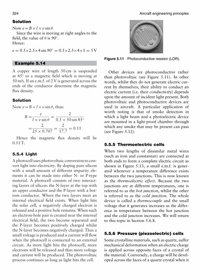
324 Aircraft engineering principles
Solution
Now e = B × l × v sin θ
Since the wire is moving at right angles to thefield, the value of θ is 90◦.Hence:
e = 0.5×2.5×4 sin 90◦ = 0.5×2.5×4×1 = 5 V
Example 5.14
A copper wire of length 50 cm is suspendedat 45◦ to a magnetic field which is moving at50 m/s. If an e.m.f. of 2 V is generated across theends of the conductor determine the magneticflux density.
Solution
Now e = B × l × v sin θ, thus:
B = el × v sin θ
= 20.5 × 50 sin 45◦
= 225 × 0.707
= 217.7
= 0.11
Hence the magnetic flux density will be0.11 T.
5.5.4 Light
A photocell uses photovoltaic conversion to con-vert light into electricity. By doping pure siliconwith a small amount of different impurity ele-ments it can be made into either N- or P-typematerial. A photocell consists of two interact-ing layers of silicon: the N-layer at the top withan upper conductor and the P-layer with a bot-tom conductor. Where the two layers meet aninternal electrical field exists. When light hitsthe solar cell, a negatively charged electron isreleased and a positive hole remains. When suchan electron-hole pair is created near the internalelectrical field, the two become separated andthe P-layer becomes positively charged whilstthe N-layer becomes negatively charged. Thus asmall voltage is produced and a current will flowwhen the photocell is connected to an externalcircuit. As more light hits the photocell, moreelectrons will be released and thus more voltageand current will be produced. The photovoltaicprocess continues as long as light hits the cell.
Figure 5.11 Photoconductive resistor (LDR).
Other devices are photoconductive ratherthan photovoltaic (see Figure 5.11). In otherwords, whilst they do not generate electric cur-rent by themselves, their ability to conduct anelectric current (i.e. their conductivity) dependsupon the amount of incident light present. Bothphotovoltaic and photoconductive devices areused in aircraft. A particular application ofworth noting is that of smoke detection inwhich a light beam and a photoelectric deviceare mounted in a light-proof chamber throughwhich any smoke that may be present can pass(see Figure 5.12).
5.5.5 Thermoelectric cells
When two lengths of dissimilar metal wires(such as iron and constantan) are connected atboth ends to form a complete electric circuit asshown in Figure 5.13, a small e.m.f. is gener-ated whenever a temperature difference existsbetween the two junctions. This is now knownas the thermoelectric effect. Because the twojunctions are at different temperatures, one isreferred to as the hot junction, whilst the otheris referred to as the cold junction. The wholedevice is called a thermocouple and the smallvoltage that it generates increases as the differ-ence in temperature between the hot junctionand the cold junction increases. We will returnto this topic in Section 5.6.8.
5.5.6 Pressure (piezoelectric) cells
Some crystalline materials, such as quartz, suffermechanical deformation when an electric chargeis applied across opposite faces of a crystal ofthe material. Conversely, a charge will be devel-oped across the faces of a quartz crystal when it
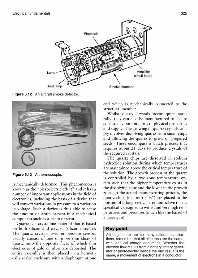
Electrical fundamentals 325
Figure 5.12 An aircraft smoke detector.
Figure 5.13 A thermocouple.
is mechanically deformed. This phenomenon isknown as the “piezoelectric effect” and it has anumber of important applications in the field ofelectronics, including the basis of a device thatwill convert variations in pressure to a variationin voltage. Such a device is thus able to sensethe amount of strain present in a mechanicalcomponent such as a beam or strut.
Quartz is a crystalline material that is basedon both silicon and oxygen (silicon dioxide).The quartz crystals used in pressure sensorsusually consist of one or more thin slices ofquartz onto the opposite faces of which filmelectrodes of gold or silver are deposited. Theentire assembly is then placed in a hermeti-cally sealed enclosure with a diaphragm at one
end which is mechanically connected to thestructural member.
Whilst quartz crystals occur quite natu-rally, they can also be manufactured to ensureconsistency both in terms of physical propertiesand supply. The growing of quartz crystals sim-ply involves dissolving quartz from small chipsand allowing the quartz to grow on preparedseeds. These encompass a batch process thatrequires about 21 days to produce crystals ofthe required crystals.
The quartz chips are dissolved in sodiumhydroxide solution during which temperaturesare maintained above the critical temperature ofthe solution. The growth process of the quartzis controlled by a two-zone temperature sys-tem such that the higher temperature exists inthe dissolving zone and the lower in the growthzone. In the actual manufacturing process, thequartz chips (or “nutrients”) are placed in thebottom of a long vertical steel autoclave that isspecifically designed to withstand very high tem-peratures and pressures (much like the barrel ofa large gun).
Key pointAlthough there are so many different applica-tions, remember that all electrons are the same,with identical charge and mass. Whether theelectron flow results from a battery, rotary gener-ator or photoelectric device the end result is thesame, a movement of electrons in a conductor.
326 Aircraft engineering principles
Test your understanding 5.51. Static electricity can be produced by rubbing two mate-
rials together in order to separate __________ and__________ charges.
2. Static electricity that builds up on the aircraft’s externalstructure can be dissipated by means of a _________________.
3. The two materials used in a conventional dry cell are__________ and __________.
4. In a lead–acid cell the electrolyte is dilute ___________________.
5. When a conductor moves in a magnetic field an__________ will be __________ in it.
6. A photocell uses __________ conversion to produceelectric current from light.
7. When light hits the surface of a photocell, a __________charged electron is released and a __________charged hole remains.
8. A typical application of photoelectricity in an aircraftis a __________.
9. A junction of dissimilar metal wires that generates asmall voltage when heated is known as a __________.
10. When a quartz crystal is deformed a small __________will appear across opposite faces of the crystal. This isoften referred to as the __________ effect.
5.6 DC sources of electricity
SyllabusConstruction and basic chemical action ofprimary cells, secondary cells, lead–acid cells,nickel–cadmium (Ni-Cd) cells, other alkalinecells; Cells connected in series and parallel;Internal resistance and its effect on a battery;Construction, materials and operation of ther-mocouples; Operation of photocells.
Knowledge level key
1
A
2
B1
2
B2
DC is the current that flows in one directiononly (recall from Section 5.4.3 that conventionalcurrent flows from positive to negative whilstelectrons travel in the opposite direction, fromnegative to positive). The most commonly usedmethod of generating DC is the electrochem-ical cell. In this section we shall describe thebasic principles of cells and batteries. We shall
also be looking at two other important devicesthat generate electric current, thermocouplesand photocells.
5.6.1 Cells and batteries
A cell is a device that produces a charge whena chemical reaction takes place. When severalcells are connected together they form a battery.Most aircraft have several batteries, the mostimportant of which are the main aircraft bat-teries. The two principal functions of the mainaircraft batteries are:
• to emergency electrical power in case of elec-trical generation system failure in flight;
• to provide an autonomous source of electri-cal power for starting engines or APU on theground or in flight.
Engine or APU starting requires high initialpeak current (sometimes over 1000 A) to over-come mechanical inertia followed by high cur-rent discharge (hundreds of amperes) during atime interval of typically 30 s. Several successiveattempts, which progressively deplete capacity,may be required, but because the duration isshort, starting usually determines what powercapacity the battery should have. Conversely,emergency loads usually determine what energythe battery should have.
The precise configuration of aircraft batter-ies depends both on aircraft complexity andairworthiness requirements. For example, oneor more batteries may be dedicated to sup-porting essential systems (such as avionics) for30–60 min without the voltage falling below aminimum level (typically 18 V). Furthermore,one battery may be dedicated to starting whilstthe other supports essential equipment duringengine start-up. When required, both batter-ies can then be connected in parallel to supportemergency loads. When alternative emergencypower generation is available, such as a ramair turbine (RAT), the battery may only beneeded for a few minutes during RAT deploy-ment or during a final (low-speed) approach toa runway.
Having briefly set the scene, we will nowlook briefly at the nature of cells and batteries
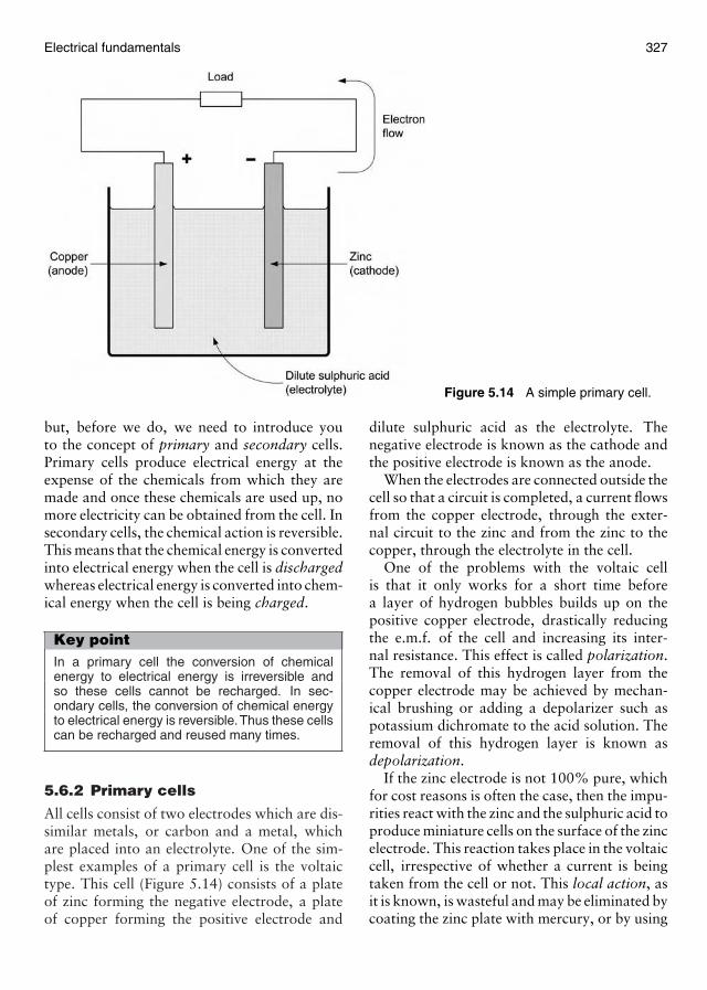
Electrical fundamentals 327
Figure 5.14 A simple primary cell.
but, before we do, we need to introduce youto the concept of primary and secondary cells.Primary cells produce electrical energy at theexpense of the chemicals from which they aremade and once these chemicals are used up, nomore electricity can be obtained from the cell. Insecondary cells, the chemical action is reversible.This means that the chemical energy is convertedinto electrical energy when the cell is dischargedwhereas electrical energy is converted into chem-ical energy when the cell is being charged.
Key pointIn a primary cell the conversion of chemicalenergy to electrical energy is irreversible andso these cells cannot be recharged. In sec-ondary cells, the conversion of chemical energyto electrical energy is reversible.Thus these cellscan be recharged and reused many times.
5.6.2 Primary cells
All cells consist of two electrodes which are dis-similar metals, or carbon and a metal, whichare placed into an electrolyte. One of the sim-plest examples of a primary cell is the voltaictype. This cell (Figure 5.14) consists of a plateof zinc forming the negative electrode, a plateof copper forming the positive electrode and
dilute sulphuric acid as the electrolyte. Thenegative electrode is known as the cathode andthe positive electrode is known as the anode.
When the electrodes are connected outside thecell so that a circuit is completed, a current flowsfrom the copper electrode, through the exter-nal circuit to the zinc and from the zinc to thecopper, through the electrolyte in the cell.
One of the problems with the voltaic cellis that it only works for a short time beforea layer of hydrogen bubbles builds up on thepositive copper electrode, drastically reducingthe e.m.f. of the cell and increasing its inter-nal resistance. This effect is called polarization.The removal of this hydrogen layer from thecopper electrode may be achieved by mechan-ical brushing or adding a depolarizer such aspotassium dichromate to the acid solution. Theremoval of this hydrogen layer is known asdepolarization.
If the zinc electrode is not 100% pure, whichfor cost reasons is often the case, then the impu-rities react with the zinc and the sulphuric acid toproduce miniature cells on the surface of the zincelectrode. This reaction takes place in the voltaiccell, irrespective of whether a current is beingtaken from the cell or not. This local action, asit is known, is wasteful and may be eliminated bycoating the zinc plate with mercury, or by using
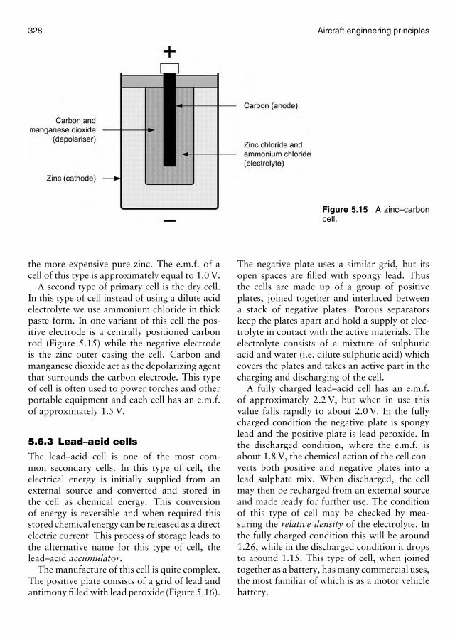
328 Aircraft engineering principles
Figure 5.15 A zinc–carboncell.
the more expensive pure zinc. The e.m.f. of acell of this type is approximately equal to 1.0 V.
A second type of primary cell is the dry cell.In this type of cell instead of using a dilute acidelectrolyte we use ammonium chloride in thickpaste form. In one variant of this cell the pos-itive electrode is a centrally positioned carbonrod (Figure 5.15) while the negative electrodeis the zinc outer casing the cell. Carbon andmanganese dioxide act as the depolarizing agentthat surrounds the carbon electrode. This typeof cell is often used to power torches and otherportable equipment and each cell has an e.m.f.of approximately 1.5 V.
5.6.3 Lead–acid cells
The lead–acid cell is one of the most com-mon secondary cells. In this type of cell, theelectrical energy is initially supplied from anexternal source and converted and stored inthe cell as chemical energy. This conversionof energy is reversible and when required thisstored chemical energy can be released as a directelectric current. This process of storage leads tothe alternative name for this type of cell, thelead–acid accumulator.
The manufacture of this cell is quite complex.The positive plate consists of a grid of lead andantimony filled with lead peroxide (Figure 5.16).
The negative plate uses a similar grid, but itsopen spaces are filled with spongy lead. Thusthe cells are made up of a group of positiveplates, joined together and interlaced betweena stack of negative plates. Porous separatorskeep the plates apart and hold a supply of elec-trolyte in contact with the active materials. Theelectrolyte consists of a mixture of sulphuricacid and water (i.e. dilute sulphuric acid) whichcovers the plates and takes an active part in thecharging and discharging of the cell.
A fully charged lead–acid cell has an e.m.f.of approximately 2.2 V, but when in use thisvalue falls rapidly to about 2.0 V. In the fullycharged condition the negative plate is spongylead and the positive plate is lead peroxide. Inthe discharged condition, where the e.m.f. isabout 1.8 V, the chemical action of the cell con-verts both positive and negative plates into alead sulphate mix. When discharged, the cellmay then be recharged from an external sourceand made ready for further use. The conditionof this type of cell may be checked by mea-suring the relative density of the electrolyte. Inthe fully charged condition this will be around1.26, while in the discharged condition it dropsto around 1.15. This type of cell, when joinedtogether as a battery, has many commercial uses,the most familiar of which is as a motor vehiclebattery.
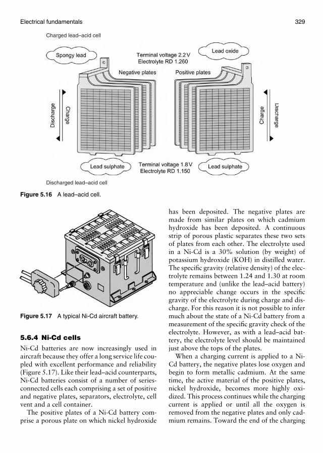
Electrical fundamentals 329
Charged lead–acid cell
Discharged lead–acid cell
Figure 5.16 A lead–acid cell.
Figure 5.17 A typical Ni-Cd aircraft battery.
5.6.4 Ni-Cd cells
Ni-Cd batteries are now increasingly used inaircraft because they offer a long service life cou-pled with excellent performance and reliability(Figure 5.17). Like their lead–acid counterparts,Ni-Cd batteries consist of a number of series-connected cells each comprising a set of positiveand negative plates, separators, electrolyte, cellvent and a cell container.
The positive plates of a Ni-Cd battery com-prise a porous plate on which nickel hydroxide
has been deposited. The negative plates aremade from similar plates on which cadmiumhydroxide has been deposited. A continuousstrip of porous plastic separates these two setsof plates from each other. The electrolyte usedin a Ni-Cd is a 30% solution (by weight) ofpotassium hydroxide (KOH) in distilled water.The specific gravity (relative density) of the elec-trolyte remains between 1.24 and 1.30 at roomtemperature and (unlike the lead–acid battery)no appreciable change occurs in the specificgravity of the electrolyte during charge and dis-charge. For this reason it is not possible to infermuch about the state of a Ni-Cd battery from ameasurement of the specific gravity check of theelectrolyte. However, as with a lead–acid bat-tery, the electrolyte level should be maintainedjust above the tops of the plates.
When a charging current is applied to a Ni-Cd battery, the negative plates lose oxygen andbegin to form metallic cadmium. At the sametime, the active material of the positive plates,nickel hydroxide, becomes more highly oxi-dized. This process continues while the chargingcurrent is applied or until all the oxygen isremoved from the negative plates and only cad-mium remains. Toward the end of the charging
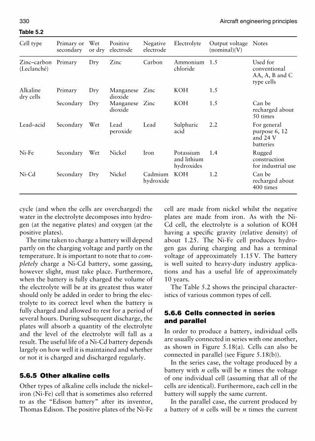
330 Aircraft engineering principles
Table 5.2
Cell type Primary or Wet Positive Negative Electrolyte Output voltage Notessecondary or dry electrode electrode (nominal)(V)
Zinc–carbon Primary Dry Zinc Carbon Ammonium 1.5 Used for(Leclanché) chloride conventional
AA, A, B and Ctype cells
Alkaline Primary Dry Manganese Zinc KOH 1.5dry cells dioxide
Secondary Dry Manganese Zinc KOH 1.5 Can bedioxide recharged about
50 timesLead–acid Secondary Wet Lead Lead Sulphuric 2.2 For general
peroxide acid purpose 6, 12and 24 Vbatteries
Ni-Fe Secondary Wet Nickel Iron Potassium 1.4 Ruggedand lithium constructionhydroxides for industrial use
Ni-Cd Secondary Dry Nickel Cadmium KOH 1.2 Can behydroxide recharged about
400 times
cycle (and when the cells are overcharged) thewater in the electrolyte decomposes into hydro-gen (at the negative plates) and oxygen (at thepositive plates).
The time taken to charge a battery will dependpartly on the charging voltage and partly on thetemperature. It is important to note that to com-pletely charge a Ni-Cd battery, some gassing,however slight, must take place. Furthermore,when the battery is fully charged the volume ofthe electrolyte will be at its greatest thus watershould only be added in order to bring the elec-trolyte to its correct level when the battery isfully charged and allowed to rest for a period ofseveral hours. During subsequent discharge, theplates will absorb a quantity of the electrolyteand the level of the electrolyte will fall as aresult. The useful life of a Ni-Cd battery dependslargely on how well it is maintained and whetheror not it is charged and discharged regularly.
5.6.5 Other alkaline cells
Other types of alkaline cells include the nickel–iron (Ni-Fe) cell that is sometimes also referredto as the “Edison battery” after its inventor,Thomas Edison. The positive plates of the Ni-Fe
cell are made from nickel whilst the negativeplates are made from iron. As with the Ni-Cd cell, the electrolyte is a solution of KOHhaving a specific gravity (relative density) ofabout 1.25. The Ni-Fe cell produces hydro-gen gas during charging and has a terminalvoltage of approximately 1.15 V. The batteryis well suited to heavy-duty industry applica-tions and has a useful life of approximately10 years.
The Table 5.2 shows the principal character-istics of various common types of cell.
5.6.6 Cells connected in seriesand parallel
In order to produce a battery, individual cellsare usually connected in series with one another,as shown in Figure 5.18(a). Cells can also beconnected in parallel (see Figure 5.18(b)).
In the series case, the voltage produced by abattery with n cells will be n times the voltageof one individual cell (assuming that all of thecells are identical). Furthermore, each cell in thebattery will supply the same current.
In the parallel case, the current produced bya battery of n cells will be n times the current
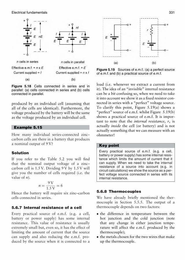
Electrical fundamentals 331
Figure 5.18 Cells connected in series and inparallel: (a) cells connected in series and (b) cellsconnected in parallel.
produced by an individual cell (assuming thatall of the cells are identical). Furthermore, thevoltage produced by the battery will be the sameas the voltage produced by an individual cell.
Example 5.15
How many individual series-connected zinc–carbon cells are there in a battery that producesa nominal output of 9 V?
Solution
If you refer to the Table 5.2 you will findthat the nominal output voltage of a zinc–carbon cell is 1.5 V. Dividing 9 V by 1.5 V willgive you the number of cells required (i.e. thevalue of n).
n = 9 V1.5 V
= 6
Hence the battery will require six zinc–carboncells connected in series.
5.6.7 Internal resistance of a cell
Every practical source of e.m.f. (e.g. a cell,battery or power supply) has some internalresistance. This value of resistance is usuallyextremely small but, even so, it has the effect oflimiting the amount of current that the sourcecan supply and also reducing the e.m.f. pro-duced by the source when it is connected to a
Figure 5.19 Sources of e.m.f.: (a) a perfect sourceof e.m.f. and (b) a practical source of e.m.f.
load (i.e. whenever we extract a current fromit). The idea of an “invisible” internal resistancecan be a bit confusing so, when we need to takeit into account we show it as a fixed resistor con-nected in series with a “perfect” voltage source.To clarify this point, Figure 5.19(a) shows a“perfect” source of e.m.f. whilst Figure 5.19(b)shows a practical source of e.m.f. It is impor-tant to note that the internal resistance, r, isactually inside the cell (or battery) and is notactually something that we can measure with anohmmeter!
Key pointEvery practical source of e.m.f. (e.g. a cell,battery or power supply) has some internal resis-tance which limits the amount of current that itcan supply. When we need to take the internalresistance of a source into account (e.g. incircuit calculations) we show the source as a per-fect voltage source connected in series with itsinternal resistance.
5.6.8 Thermocouples
We have already briefly mentioned the ther-mocouple in Section 5.5.5. The output of athermocouple depends on two factors:
• the difference in temperature between thehot junction and the cold junction (notethat any change in either junction tempe-rature will affect the e.m.f. produced by thethermocouple);
• the metals chosen for the two wires that makeup the thermocouple.
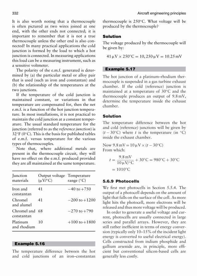
332 Aircraft engineering principles
It is also worth noting that a thermocoupleis often pictured as two wires joined at oneend, with the other ends not connected; it isimportant to remember that it is not a truethermocouple unless the other end is also con-nected! In many practical applications the coldjunction is formed by the load to which a hotjunction is connected. In measuring applicationsthis load can be a measuring instrument, such asa sensitive voltmeter.
The polarity of the e.m.f. generated is deter-mined by (a) the particular metal or alloy pairthat is used (such as iron and constantan) and(b) the relationship of the temperatures at thetwo junctions.
If the temperature of the cold junction ismaintained constant, or variations in thattemperature are compensated for, then the nete.m.f. is a function of the hot junction tempera-ture. In most installations, it is not practical tomaintain the cold junction at a constant temper-ature. The usual standard temperature for thejunction (referred to as the reference junction) is32◦F (0◦C). This is the basis for published tablesof e.m.f. versus temperature for the varioustypes of thermocouples.
Note that, where additional metals arepresent in the thermocouple circuit, they willhave no effect on the e.m.f. produced providedthey are all maintained at the same temperature.
Junction Output voltage Temperaturematerials (µV/◦C) range (◦C)
Iron and 41 −40 to +750constantan
Chromel 41 −200 to +1200and alumel
Chromel and 68 −270 to +790constantan
Platinum 10 +100 to +1800and rhodium
Example 5.16
The temperature difference between the hotand cold junctions of an iron–constantan
thermocouple is 250◦C. What voltage will beproduced by the thermocouple?
Solution
The voltage produced by the thermocouple willbe given by:
41 µV × 250◦C = 10, 250 µV = 10.25 mV
Example 5.17
The hot junction of a platinum–rhodium ther-mocouple is suspended in a gas turbine exhaustchamber. If the cold (reference) junction ismaintained at a temperature of 30◦C and thethermocouple produces an output of 9.8 mV,determine the temperature inside the exhaustchamber.
Solution
The temperature difference between the hotand cold (reference) junctions will be given by(t − 30◦C) where t is the temperature (in ◦C)inside the exhaust chamber.
Now 9.8 mV = 10 µV × (t − 30◦C)From which:
t = 9.8 mV10 µV/◦C
+ 30◦C = 980◦C + 30◦C
= 1010◦C
5.6.9 Photocells
We first met photocells in Section 5.5.4. Theoutput of a photocell depends on the amount oflight that falls on the surface of the cell. As morelight hits the photocell, more electrons will bereleased and thus more voltage will be produced.
In order to generate a useful voltage and cur-rent, photocells are usually connected in largeseries and parallel arrays. However, they arestill rather inefficient in terms of energy conver-sion (typically only 10–15% of the incident lightenergy is converted to useful electrical energy).Cells constructed from indium phosphide andgallium arsenide are, in principle, more effi-cient but conventional silicon-based cells aregenerally less costly.
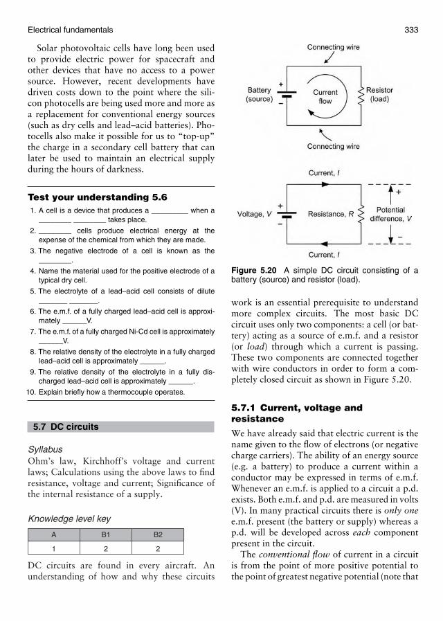
Electrical fundamentals 333
Solar photovoltaic cells have long been usedto provide electric power for spacecraft andother devices that have no access to a powersource. However, recent developments havedriven costs down to the point where the sili-con photocells are being used more and more asa replacement for conventional energy sources(such as dry cells and lead–acid batteries). Pho-tocells also make it possible for us to “top-up”the charge in a secondary cell battery that canlater be used to maintain an electrical supplyduring the hours of darkness.
Test your understanding 5.61. A cell is a device that produces a _________ when a
________ ________ takes place.
2. ________ cells produce electrical energy at theexpense of the chemical from which they are made.
3. The negative electrode of a cell is known as the________.
4. Name the material used for the positive electrode of atypical dry cell.
5. The electrolyte of a lead–acid cell consists of dilute_______ _______.
6. The e.m.f. of a fully charged lead–acid cell is approxi-mately ______V.
7. The e.m.f. of a fully charged Ni-Cd cell is approximately______V.
8. The relative density of the electrolyte in a fully chargedlead–acid cell is approximately ______.
9. The relative density of the electrolyte in a fully dis-charged lead–acid cell is approximately ______.
10. Explain briefly how a thermocouple operates.
5.7 DC circuits
SyllabusOhm’s law, Kirchhoff’s voltage and currentlaws; Calculations using the above laws to findresistance, voltage and current; Significance ofthe internal resistance of a supply.
Knowledge level key
1
A
2
B1
2
B2
DC circuits are found in every aircraft. Anunderstanding of how and why these circuits
Figure 5.20 A simple DC circuit consisting of abattery (source) and resistor (load).
work is an essential prerequisite to understandmore complex circuits. The most basic DCcircuit uses only two components: a cell (or bat-tery) acting as a source of e.m.f. and a resistor(or load) through which a current is passing.These two components are connected togetherwith wire conductors in order to form a com-pletely closed circuit as shown in Figure 5.20.
5.7.1 Current, voltage andresistance
We have already said that electric current is thename given to the flow of electrons (or negativecharge carriers). The ability of an energy source(e.g. a battery) to produce a current within aconductor may be expressed in terms of e.m.f.Whenever an e.m.f. is applied to a circuit a p.d.exists. Both e.m.f. and p.d. are measured in volts(V). In many practical circuits there is only onee.m.f. present (the battery or supply) whereas ap.d. will be developed across each componentpresent in the circuit.
The conventional flow of current in a circuitis from the point of more positive potential tothe point of greatest negative potential (note that
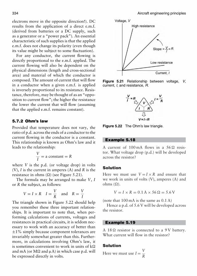
334 Aircraft engineering principles
electrons move in the opposite direction!). DCresults from the application of a direct e.m.f.(derived from batteries or a DC supply, suchas a generator or a “power pack”). An essentialcharacteristic of such supplies is that the appliede.m.f. does not change its polarity (even thoughits value might be subject to some fluctuation).
For any conductor, the current flowing isdirectly proportional to the e.m.f. applied. Thecurrent flowing will also be dependent on thephysical dimensions (length and cross-sectionalarea) and material of which the conductor iscomposed. The amount of current that will flowin a conductor when a given e.m.f. is appliedis inversely proportional to its resistance. Resis-tance, therefore, may be thought of as an “oppo-sition to current flow”; the higher the resistancethe lower the current that will flow (assumingthat the applied e.m.f. remains constant).
5.7.2 Ohm’s law
Provided that temperature does not vary, theratio of p.d. across the ends of a conductor to thecurrent flowing in the conductor is a constant.This relationship is known as Ohm’s law and itleads to the relationship:
VI
= a constant = R
where V is the p.d. (or voltage drop) in volts(V), I is the current in amperes (A) and R is theresistance in ohms (�) (see Figure 5.21).
The formula may be arranged to make V , Ior R the subject, as follows:
V = I × R I = VR
and R = VI
The triangle shown in Figure 5.22 should helpyou remember these three important relation-ships. It is important to note that, when per-forming calculations of currents, voltages andresistances in practical circuits, it is seldom nec-essary to work with an accuracy of better than±1% simply because component tolerances areinvariably somewhat greater than this. Further-more, in calculations involving Ohm’s law, itis sometimes convenient to work in units of k�
and mA (or M� and µA) in which case p.d. willbe expressed directly in volts.
Figure 5.21 Relationship between voltage, V,current, I, and resistance, R.
Figure 5.22 The Ohm’s law triangle.
Example 5.18
A current of 100 mA flows in a 56 � resis-tor. What voltage drop (p.d.) will be developedacross the resistor?
Solution
Here we must use V = I × R and ensure thatwe work in units of volts (V), amperes (A) andohms (�).
V = I × R = 0.1 A × 56 � = 5.6 V
(note that 100 mA is the same as 0.1 A)Hence a p.d. of 5.6 V will be developed across
the resistor.
Example 5.19
A 18 � resistor is connected to a 9 V battery.What current will flow in the resistor?
Solution
Here we must use I = VR
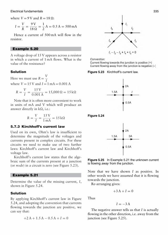
Electrical fundamentals 335
where V = 9 V and R = 18 �:
I = VR
= 9 V18 �
= 12
A = 0.5 A = 500 mA
Hence a current of 500 mA will flow in theresistor.
Example 5.20
A voltage drop of 15 V appears across a resistorin which a current of 1 mA flows. What is thevalue of the resistance?
Solution
Here we must use R = VI
where V = 15 V and I = 1 mA = 0.001 A
R = VI
= 15 V0.001 A
= 15,000 � = 15 k�
Note that it is often more convenient to workin units of mA and V which will produce ananswer directly in k�, i.e.:
R = VI
= 15 V1 mA
= 15 k�
5.7.3 Kirchhoff’s current law
Used on its own, Ohm’s law is insufficient todetermine the magnitude of the voltages andcurrents present in complex circuits. For thesecircuits we need to make use of two furtherlaws: Kirchhoff’s current law and Kirchhoff’svoltage law.
Kirchhoff’s current law states that the alge-braic sum of the currents present at a junction(or node) in a circuit is zero (see Figure 5.23).
Example 5.21
Determine the value of the missing current, I,shown in Figure 5.24.
Solution
By applying Kirchhoff’s current law in Figure5.24, and adopting the convention that currentsflowing towards the junction are positive, wecan say that:
+2 A + 1.5 A − 0.5 A + I = 0
Figure 5.23 Kirchhoff’s current law.
2A
1.5A
0.5A
I
Figure 5.24
2A
3A1.5A
0.5A
Figure 5.25 In Example 5.21 the unknown currentis flowing away from the junction.
Note that we have shown I as positive. Inother words we have assumed that it is flowingtowards the junction.
Re-arranging gives:
+3 A + I = 0
Thus
I = −3 A
The negative answer tells us that I is actuallyflowing in the other direction, i.e. away from thejunction (see Figure 5.25).
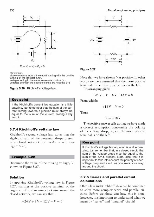
336 Aircraft engineering principles
Convention:Move clockwise around the circuit starting with the positiveterminal of the leargest e.m.f.Voltages acting in the same sense are positive (�)Voltages acting in the opposite sense are negative (�)
Figure 5.26 Kirchhoff’s voltage law.
Key pointIf the Kirchhoff’s current law equation is a littlepuzzling, just remember that the sum of the cur-rent flowing towards a junction must always beequal to the sum of the current flowing awayfrom it!
5.7.4 Kirchhoff’s voltage law
Kirchhoff’s second voltage law states that thealgebraic sum of the potential drops presentin a closed network (or mesh) is zero (seeFigure 5.26).
Example 5.22
Determine the value of the missing voltage, V ,shown in Figure 5.27.
Solution
By applying Kirchhoff’s voltage law in Figure5.27, starting at the positive terminal of thelargest e.m.f. and moving clockwise around theclosed network, we can say that:
+24 V + 6 V − 12 V − V = 0
Figure 5.27
Note that we have shown Vas positive. In otherwords we have assumed that the more positiveterminal of the resistor is the one on the left.
Re-arranging gives:
+24 V − V + 6 V − 12 V = 0
From which:
+18 V − V = 0
Thus:
V = +18 V
The positive answer tells us that we have madea correct assumption concerning the polarityof the voltage drop, V , i.e. the more positiveterminal is on the left.
Key pointIf Kirchhoff’s voltage law equation is a little puz-zling, just remember that, in a closed circuit, thesum of the voltage drops must be equal to thesum of the e.m.f. present. Note, also, that it isimportant to take into account the polarity of eachvoltage drop and e.m.f. as you work your wayaround the circuit.
5.7.5 Series and parallel circuitcalculations
Ohm’s law and Kirchhoff’s law can be combinedto solve more complex series and parallel cir-cuits. Before we show you how this is done,however, it is important to understand what wemean by “series” and “parallel” circuit!
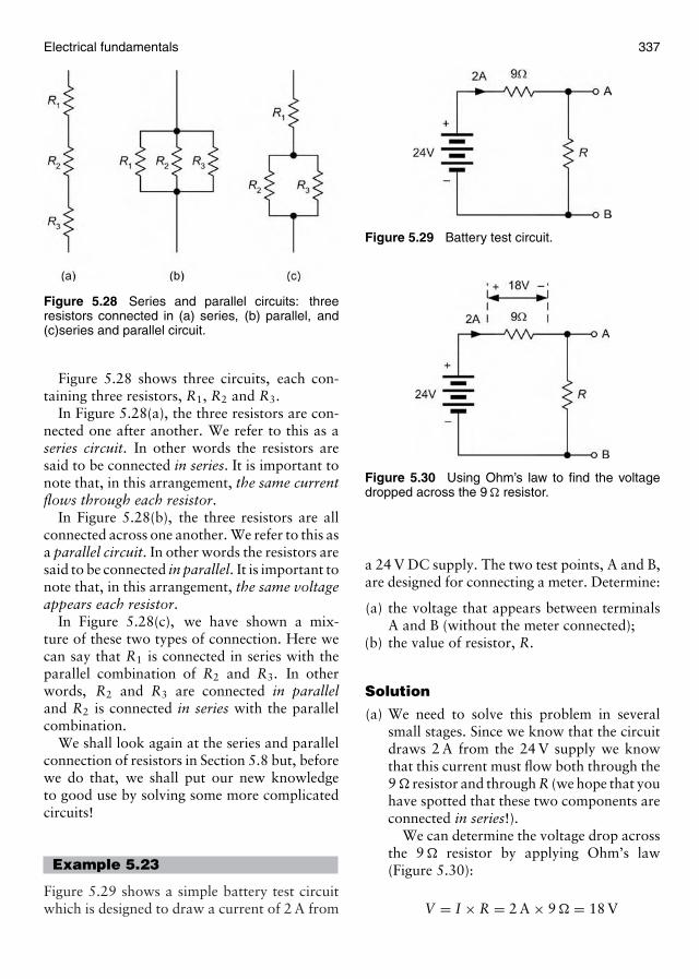
Electrical fundamentals 337
Figure 5.28 Series and parallel circuits: threeresistors connected in (a) series, (b) parallel, and(c)series and parallel circuit.
Figure 5.28 shows three circuits, each con-taining three resistors, R1, R2 and R3.
In Figure 5.28(a), the three resistors are con-nected one after another. We refer to this as aseries circuit. In other words the resistors aresaid to be connected in series. It is important tonote that, in this arrangement, the same currentflows through each resistor.
In Figure 5.28(b), the three resistors are allconnected across one another. We refer to this asa parallel circuit. In other words the resistors aresaid to be connected in parallel. It is important tonote that, in this arrangement, the same voltageappears each resistor.
In Figure 5.28(c), we have shown a mix-ture of these two types of connection. Here wecan say that R1 is connected in series with theparallel combination of R2 and R3. In otherwords, R2 and R3 are connected in paralleland R2 is connected in series with the parallelcombination.
We shall look again at the series and parallelconnection of resistors in Section 5.8 but, beforewe do that, we shall put our new knowledgeto good use by solving some more complicatedcircuits!
Example 5.23
Figure 5.29 shows a simple battery test circuitwhich is designed to draw a current of 2 A from
Figure 5.29 Battery test circuit.
Figure 5.30 Using Ohm’s law to find the voltagedropped across the 9 � resistor.
a 24 V DC supply. The two test points, A and B,are designed for connecting a meter. Determine:
(a) the voltage that appears between terminalsA and B (without the meter connected);
(b) the value of resistor, R.
Solution
(a) We need to solve this problem in severalsmall stages. Since we know that the circuitdraws 2 A from the 24 V supply we knowthat this current must flow both through the9 � resistor and through R (we hope that youhave spotted that these two components areconnected in series!).
We can determine the voltage drop acrossthe 9 � resistor by applying Ohm’s law(Figure 5.30):
V = I × R = 2 A × 9 � = 18 V
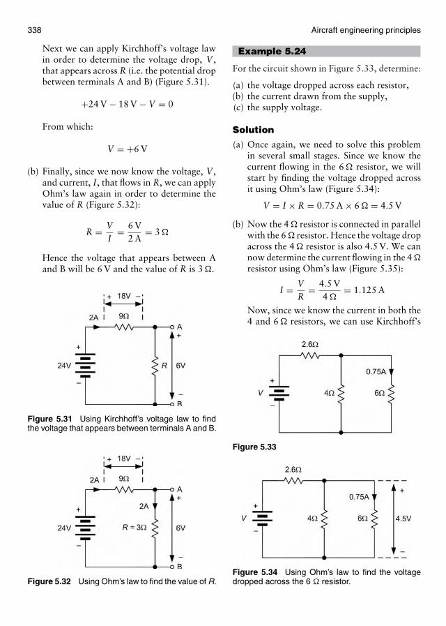
338 Aircraft engineering principles
Next we can apply Kirchhoff’s voltage lawin order to determine the voltage drop, V ,that appears across R (i.e. the potential dropbetween terminals A and B) (Figure 5.31).
+24 V − 18 V − V = 0
From which:
V = +6 V
(b) Finally, since we now know the voltage, V ,and current, I, that flows in R, we can applyOhm’s law again in order to determine thevalue of R (Figure 5.32):
R = VI
= 6 V2 A
= 3 �
Hence the voltage that appears between Aand B will be 6 V and the value of R is 3 �.
Figure 5.31 Using Kirchhoff’s voltage law to findthe voltage that appears between terminals A and B.
Figure 5.32 Using Ohm’s law to find the value of R.
Example 5.24
For the circuit shown in Figure 5.33, determine:
(a) the voltage dropped across each resistor,(b) the current drawn from the supply,(c) the supply voltage.
Solution
(a) Once again, we need to solve this problemin several small stages. Since we know thecurrent flowing in the 6 � resistor, we willstart by finding the voltage dropped acrossit using Ohm’s law (Figure 5.34):
V = I × R = 0.75 A × 6 � = 4.5 V
(b) Now the 4 � resistor is connected in parallelwith the 6 � resistor. Hence the voltage dropacross the 4 � resistor is also 4.5 V. We cannow determine the current flowing in the 4 �
resistor using Ohm’s law (Figure 5.35):
I = VR
= 4.5 V4 �
= 1.125 A
Now, since we know the current in both the4 and 6 � resistors, we can use Kirchhoff’s
Figure 5.33
Figure 5.34 Using Ohm’s law to find the voltagedropped across the 6 � resistor.
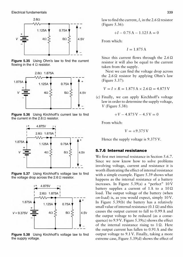
Electrical fundamentals 339
Figure 5.35 Using Ohm’s law to find the currentflowing in the 4 � resistor.
Figure 5.36 Using Kirchhoff’s current law to findthe current in the 2.6 � resistor.
Figure 5.37 Using Kirchhoff’s voltage law to findthe voltage drop across the 2.6 � resistor.
Figure 5.38 Using Kirchhoff’s voltage law to findthe supply voltage.
law to find the current, I, in the 2.6 � resistor(Figure 5.36):
+I − 0.75 A − 1.125 A = 0
From which:
I = 1.875 A
Since this current flows through the 2.6 �
resistor it will also be equal to the currenttaken from the supply.
Next we can find the voltage drop acrossthe 2.6 � resistor by applying Ohm’s law(Figure 5.37):
V = I × R = 1.875 A × 2.6 � = 4.875 V
(c) Finally, we can apply Kirchhoff’s voltagelaw in order to determine the supply voltage,V (Figure 5.38):
+V − 4.875 V − 4.5 V = 0
From which:
V = +9.375 V
Hence the supply voltage is 9.375 V.
5.7.6 Internal resistance
We first met internal resistance in Section 5.6.7.Since we now know how to solve problemsinvolving voltage, current and resistance it isworth illustrating the effect of internal resistancewith a simple example. Figure 5.39 shows whathappens as the internal resistance of a batteryincreases. In Figure 5.39(a) a “perfect” 10 Vbattery supplies a current of 1 A to a 10 �
load. The output voltage of the battery (whenon-load) is, as you would expect, simply 10 V.In Figure 5.39(b) the battery has a relativelysmall value of internal resistance (0.1 �) and thiscauses the output current to fall to 0.99 A andthe output voltage to be reduced (as a conse-quence) to 9.9 V. Figure 5.39(c) shows the effectof the internal resistance rising to 1 �. Herethe output current has fallen to 0.91 A and theoutput voltage to 9.1 V. Finally, taking a moreextreme case, Figure 5.39(d) shows the effect of
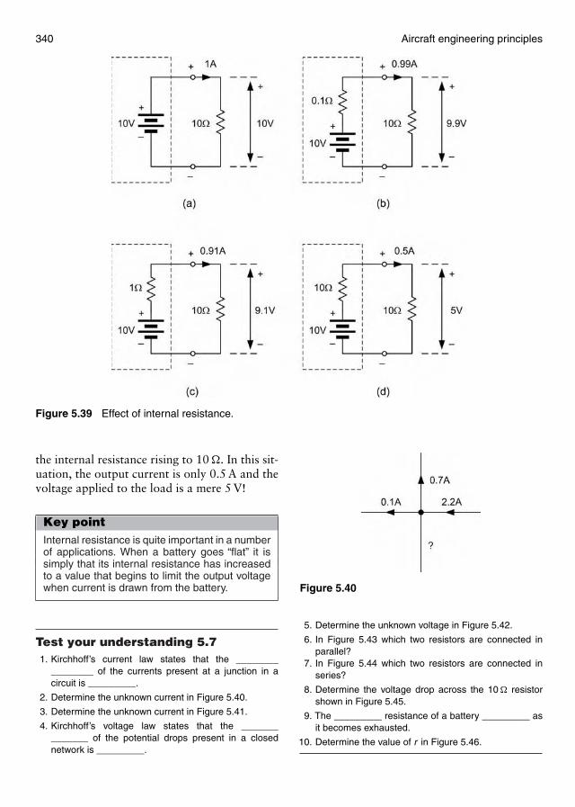
340 Aircraft engineering principles
Figure 5.39 Effect of internal resistance.
the internal resistance rising to 10 �. In this sit-uation, the output current is only 0.5 A and thevoltage applied to the load is a mere 5 V!
Key pointInternal resistance is quite important in a numberof applications. When a battery goes “flat” it issimply that its internal resistance has increasedto a value that begins to limit the output voltagewhen current is drawn from the battery.
Test your understanding 5.71. Kirchhoff’s current law states that the ________
________ of the currents present at a junction in acircuit is _________.
2. Determine the unknown current in Figure 5.40.
3. Determine the unknown current in Figure 5.41.
4. Kirchhoff’s voltage law states that the ______________ of the potential drops present in a closednetwork is _________.
Figure 5.40
5. Determine the unknown voltage in Figure 5.42.
6. In Figure 5.43 which two resistors are connected inparallel?
7. In Figure 5.44 which two resistors are connected inseries?
8. Determine the voltage drop across the 10 � resistorshown in Figure 5.45.
9. The _________ resistance of a battery _________ asit becomes exhausted.
10. Determine the value of r in Figure 5.46.
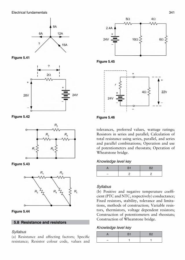
Electrical fundamentals 341
Figure 5.41
Figure 5.42
Figure 5.43
Figure 5.44
5.8 Resistance and resistors
Syllabus(a) Resistance and affecting factors; Specificresistance; Resistor colour code, values and
Figure 5.45
Figure 5.46
tolerances, preferred values, wattage ratings;Resistors in series and parallel; Calculation oftotal resistance using series, parallel, and seriesand parallel combinations; Operation and useof potentiometers and rheostats; Operation ofWheatstone bridge.
Knowledge level key
–
A
2
B1
2
B2
Syllabus(b) Positive and negative temperature coeffi-cient (PTC and NTC, respectively) conductance;Fixed resistors, stability, tolerance and limita-tions, methods of construction; Variable resis-tors, thermistors, voltage dependent resistors;Construction of potentiometers and rheostats;Construction of Wheatstone bridge.
Knowledge level key
–
A
1
B1
1
B2
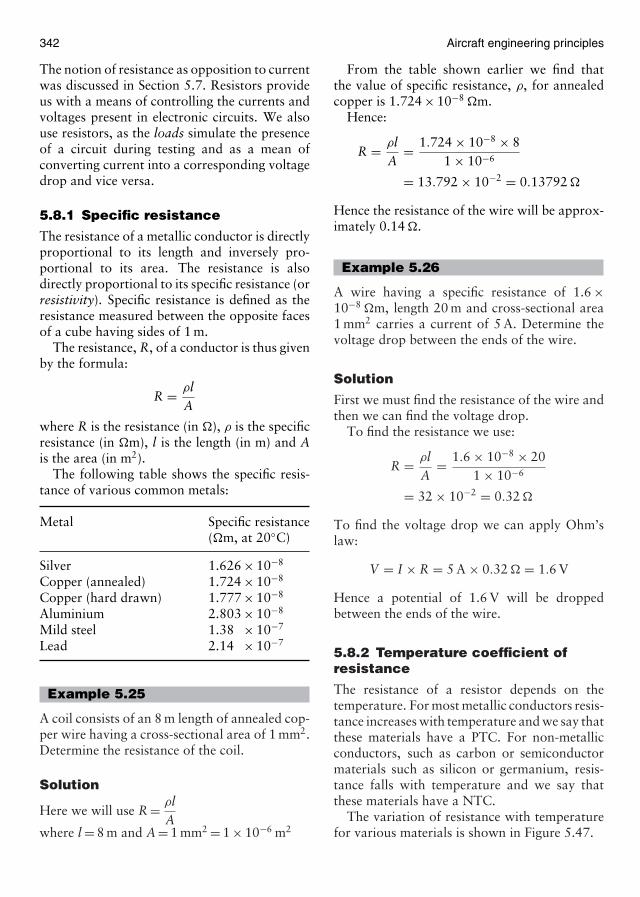
342 Aircraft engineering principles
The notion of resistance as opposition to currentwas discussed in Section 5.7. Resistors provideus with a means of controlling the currents andvoltages present in electronic circuits. We alsouse resistors, as the loads simulate the presenceof a circuit during testing and as a mean ofconverting current into a corresponding voltagedrop and vice versa.
5.8.1 Specific resistance
The resistance of a metallic conductor is directlyproportional to its length and inversely pro-portional to its area. The resistance is alsodirectly proportional to its specific resistance (orresistivity). Specific resistance is defined as theresistance measured between the opposite facesof a cube having sides of 1 m.
The resistance, R, of a conductor is thus givenby the formula:
R = ρlA
where R is the resistance (in �), ρ is the specificresistance (in �m), l is the length (in m) and Ais the area (in m2).
The following table shows the specific resis-tance of various common metals:
Metal Specific resistance(�m, at 20◦C)
Silver 1.626 × 10⁻⁸
Copper (annealed) 1.724 × 10⁻⁸
Copper (hard drawn) 1.777 × 10⁻⁸
Aluminium 2.803 × 10⁻⁸
Mild steel 1.38 × 10⁻⁷
Lead 2.14 × 10⁻⁷
Example 5.25
A coil consists of an 8 m length of annealed cop-per wire having a cross-sectional area of 1 mm2.Determine the resistance of the coil.
Solution
Here we will use R = ρlA
where l = 8 m and A = 1 mm2 = 1 × 10⁻⁶ m2
From the table shown earlier we find thatthe value of specific resistance, ρ, for annealedcopper is 1.724 × 10⁻⁸ �m.
Hence:
R = ρlA
= 1.724 × 10−8 × 81 × 10−6
= 13.792 × 10−2 = 0.13792 �
Hence the resistance of the wire will be approx-imately 0.14 �.
Example 5.26
A wire having a specific resistance of 1.6 ×10⁻⁸ �m, length 20 m and cross-sectional area1 mm2 carries a current of 5 A. Determine thevoltage drop between the ends of the wire.
Solution
First we must find the resistance of the wire andthen we can find the voltage drop.
To find the resistance we use:
R = ρlA
= 1.6 × 10−8 × 201 × 10−6
= 32 × 10−2 = 0.32 �
To find the voltage drop we can apply Ohm’slaw:
V = I × R = 5 A × 0.32 � = 1.6 V
Hence a potential of 1.6 V will be droppedbetween the ends of the wire.
5.8.2 Temperature coefficient ofresistance
The resistance of a resistor depends on thetemperature. For most metallic conductors resis-tance increases with temperature and we say thatthese materials have a PTC. For non-metallicconductors, such as carbon or semiconductormaterials such as silicon or germanium, resis-tance falls with temperature and we say thatthese materials have a NTC.
The variation of resistance with temperaturefor various materials is shown in Figure 5.47.
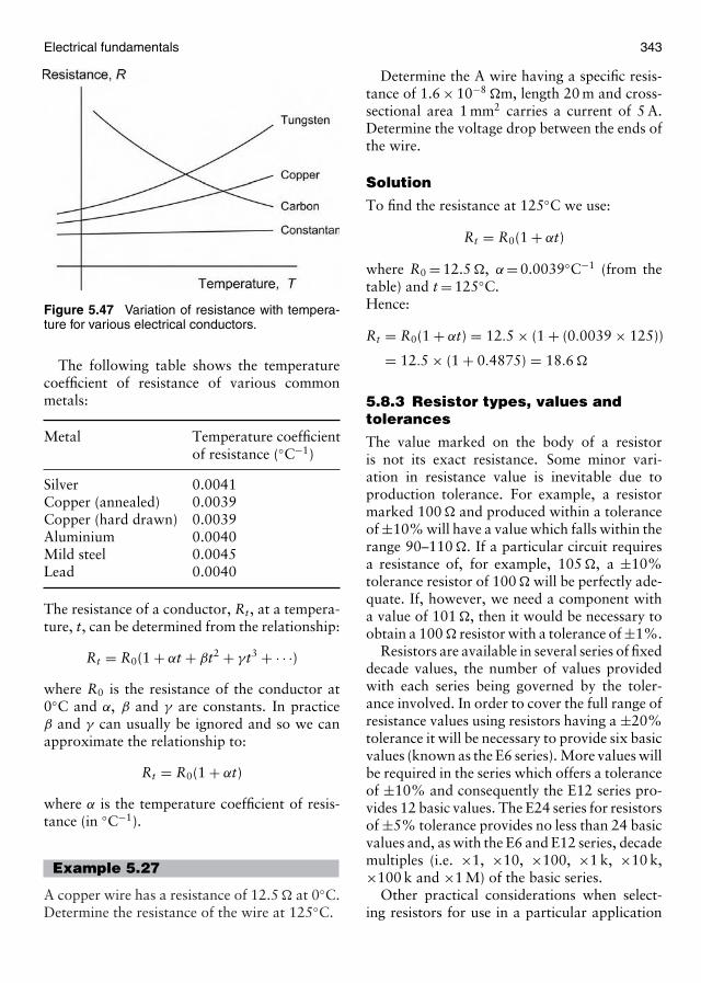
Electrical fundamentals 343
Figure 5.47 Variation of resistance with tempera-ture for various electrical conductors.
The following table shows the temperaturecoefficient of resistance of various commonmetals:
Metal Temperature coefficientof resistance (◦C−1)
Silver 0.0041Copper (annealed) 0.0039Copper (hard drawn) 0.0039Aluminium 0.0040Mild steel 0.0045Lead 0.0040
The resistance of a conductor, Rt, at a tempera-ture, t, can be determined from the relationship:
Rt = R0(1 + αt + βt2 + γt3 + · · ·)where R0 is the resistance of the conductor at0◦C and α, β and γ are constants. In practiceβ and γ can usually be ignored and so we canapproximate the relationship to:
Rt = R0(1 + αt)
where α is the temperature coefficient of resis-tance (in ◦C−1).
Example 5.27
A copper wire has a resistance of 12.5 � at 0◦C.Determine the resistance of the wire at 125◦C.
Determine the A wire having a specific resis-tance of 1.6 × 10⁻⁸ �m, length 20 m and cross-sectional area 1 mm2 carries a current of 5 A.Determine the voltage drop between the ends ofthe wire.
Solution
To find the resistance at 125◦C we use:
Rt = R0(1 + αt)
where R0 = 12.5 �, α = 0.0039◦C−1 (from thetable) and t = 125◦C.Hence:
Rt = R0(1 + αt) = 12.5 × (1 + (0.0039 × 125))
= 12.5 × (1 + 0.4875) = 18.6 �
5.8.3 Resistor types, values andtolerances
The value marked on the body of a resistoris not its exact resistance. Some minor vari-ation in resistance value is inevitable due toproduction tolerance. For example, a resistormarked 100 � and produced within a toleranceof ±10% will have a value which falls within therange 90–110 �. If a particular circuit requiresa resistance of, for example, 105 �, a ±10%tolerance resistor of 100 � will be perfectly ade-quate. If, however, we need a component witha value of 101 �, then it would be necessary toobtain a 100 � resistor with a tolerance of ±1%.
Resistors are available in several series of fixeddecade values, the number of values providedwith each series being governed by the toler-ance involved. In order to cover the full range ofresistance values using resistors having a ±20%tolerance it will be necessary to provide six basicvalues (known as the E6 series). More values willbe required in the series which offers a toleranceof ±10% and consequently the E12 series pro-vides 12 basic values. The E24 series for resistorsof ±5% tolerance provides no less than 24 basicvalues and, as with the E6 and E12 series, decademultiples (i.e. ×1, ×10, ×100, ×1 k, ×10 k,×100 k and ×1 M) of the basic series.
Other practical considerations when select-ing resistors for use in a particular application

344 Aircraft engineering principles
include temperature coefficient, noise perfor-mance, stability and ambient temperature range.The following table summarizes the propertiesof several of the most common types of resistor.
Example 5.28
A resistor has a marked value of 220 �. Deter-mine the tolerance of the resistor if it has ameasured value of 207 �.
Solution
The difference between the marked and mea-sured values of resistance (in other words theerror) is (220 � − 207 �) = 13 �. The toleranceis given by:
Tolerance = ErrorMarked value
× 100%
= 13 �
220 �× 100% = 5.9%
Example 5.29
A 9 V power supply is to be tested with a 39 �
load resistor. If the resistor has a tolerance of10%, determine:
(a) the nominal current taken from the supply,(b) the maximum and minimum values of sup-
ply current at either end of the tolerancerange for the resistor.
Solution
(a) If a resistor of exactly 39 � is used thecurrent, I, will be given by:
I = VR
= 9 V39 �
= 0.231 A = 231 mA
(b) The lowest value of resistance would be(39 � − 3.9 �) = 35.1 �. In which case thecurrent would be:
I = VR
= 9 V35.1 �
= 0.256 A = 256 mA
At the other extreme, the highest value ofresistance would be (39 � + 3.9 �) = 42.9 �.
In this case the current would be:
I = VR
= 9 V42.9 �
= 0.210 A = 210 mA
5.8.4 Power ratings
We have already mentioned that power dissi-pated by a resistor is determined by the productof the current flowing in the resistor and the volt-age (p.d.) dropped across it. The power rating(or “wattage rating”) of a resistor, on the otherhand, is the maximum power that the resistorcan safely dissipate. Power ratings are related tooperating temperatures and resistors should bederated at high temperatures. For this reason,in all situations where reliability is importantresistors should be operated at well below theirnominal maximum power rating.
Example 5.30
A resistor is rated at 5 W. If the resistor car-ries a current of 30 mA and has a voltage of150 V dropped across it determine the powerdissipated and whether or not this exceeds themaximum power rating.
Solution
We can determine the actual power dissipatedby applying the formula:
P = I × V
where I = 30 mA = 0.03 A and V = 150 V, thus
P = I × V = 0.03 A × 150 V = 4.5 W
This is just less than the power (wattage)rating of the resistor (5 W).
Example 5.31
A current of 100 mA (±20%) is to be drawnfrom a 28 V DC supply. What value and type ofresistor should be used in this application?
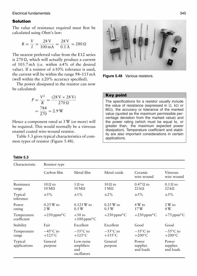
Electrical fundamentals 345
Solution
The value of resistance required must first becalculated using Ohm’s law:
R = VI
= 28 V100 mA
= 28 V0.1 A
= 280 �
The nearest preferred value from the E12 seriesis 270 �, which will actually produce a currentof 103.7 mA (i.e. within ±4% of the desiredvalue). If a resistor of ±10% tolerance is used,the current will be within the range 94–115 mA(well within the ±20% accuracy specified).
The power dissipated in the resistor can nowbe calculated:
P = V2
R= (28 V × 28 V)
270 �
= 784270
= 2.9 W
Hence a component rated at 3 W (or more) willbe required. This would normally be a vitreousenamel coated wire-wound resistor.
Table 5.3 gives typical characteristics of com-mon types of resistor (Figure 5.48).
Table 5.3
Characteristic Resistor type
Carbon film Metal film Metal oxide Ceramic Vitreouswire wound wire wound
Resistance 10 � to 1 � to 10 � to 0.47 � to 0.1 � torange 10 M� 10 M� 1 M� 22 k� 22 k�
Typical ±5% ±1% ±2% ±5% ±5%tolerance
Power 0.25 W to 0.125 W to 0.25 W to 4 W to 2 W torating 2 W 0.5 W 0.5 W 17 W 4 W
Temperature +250 ppm/◦C +50 to +250 ppm/◦C +250 ppm/◦C +75 ppm/◦Ccoefficient +100 ppm/◦C
Stability Fair Excellent Excellent Good Good
Temperature −45◦C to −55◦C to −55◦C to −55◦C to −55◦C torange +125◦C +125◦C +155◦C +200◦C +200◦C
Typical General Low-noise General Power Powerapplications purpose amplifiers purpose supplies supplies
and and loads and loadsoscillators
Figure 5.48 Various resistors.
Key pointThe specifications for a resistor usually includethe value of resistance (expressed in �, k� orM�), the accuracy or tolerance of the markedvalue (quoted as the maximum permissible per-centage deviation from the marked value) andthe power rating (which must be equal to, orgreater than, the maximum expected powerdissipation). Temperature coefficient and stabil-ity are also important considerations in certainapplications.

346 Aircraft engineering principles
Figure 5.49 The four-band resistorcolour code.
Figure 5.50 The five-band resistorcolour code.
5.8.5 Resistor colour codes
Carbon and metal oxide resistors are nor-mally marked with colour codes that indi-cate their value and tolerance. Two methods
of colour coding are in common use: oneinvolves four-coloured bands (see Figure 5.49)whilst the other uses five-coloured bands (seeFigure 5.50).
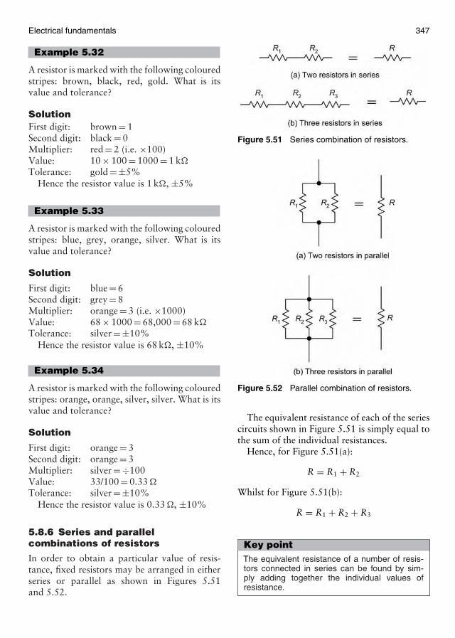
Electrical fundamentals 347
Example 5.32
A resistor is marked with the following colouredstripes: brown, black, red, gold. What is itsvalue and tolerance?
SolutionFirst digit: brown = 1Second digit: black = 0Multiplier: red = 2 (i.e. ×100)Value: 10 × 100 = 1000 = 1 k�
Tolerance: gold = ±5%Hence the resistor value is 1 k�, ±5%
Example 5.33
A resistor is marked with the following colouredstripes: blue, grey, orange, silver. What is itsvalue and tolerance?
Solution
First digit: blue = 6Second digit: grey = 8Multiplier: orange = 3 (i.e. ×1000)Value: 68 × 1000 = 68,000 = 68 k�
Tolerance: silver = ±10%Hence the resistor value is 68 k�, ±10%
Example 5.34
A resistor is marked with the following colouredstripes: orange, orange, silver, silver. What is itsvalue and tolerance?
Solution
First digit: orange = 3Second digit: orange = 3Multiplier: silver = ÷100Value: 33/100 = 0.33 �
Tolerance: silver = ±10%Hence the resistor value is 0.33 �, ±10%
5.8.6 Series and parallelcombinations of resistors
In order to obtain a particular value of resis-tance, fixed resistors may be arranged in eitherseries or parallel as shown in Figures 5.51and 5.52.
Figure 5.51 Series combination of resistors.
Figure 5.52 Parallel combination of resistors.
The equivalent resistance of each of the seriescircuits shown in Figure 5.51 is simply equal tothe sum of the individual resistances.
Hence, for Figure 5.51(a):
R = R1 + R2
Whilst for Figure 5.51(b):
R = R1 + R2 + R3
Key pointThe equivalent resistance of a number of resis-tors connected in series can be found by sim-ply adding together the individual values ofresistance.
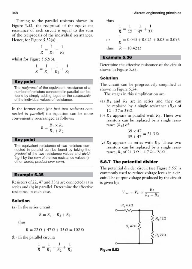
348 Aircraft engineering principles
Turning to the parallel resistors shown inFigure 5.52, the reciprocal of the equivalentresistance of each circuit is equal to the sumof the reciprocals of the individual resistances.Hence, for Figure 5.52(a):
1R
= 1R1
+ 1R2
whilst for Figure 5.52(b):
1R
= 1R1
+ 1R2
+ 1R3
Key pointThe reciprocal of the equivalent resistance of anumber of resistors connected in parallel can befound by simply adding together the reciprocalsof the individual values of resistance.
In the former case (for just two resistors con-nected in parallel) the equation can be moreconveniently re-arranged as follows:
R = R1 × R2
R1 + R2
Key pointThe equivalent resistance of two resistors con-nected in parallel can be found by taking theproduct of the two resistance values and divid-ing it by the sum of the two resistance values (inother words, product over sum).
Example 5.35
Resistors of 22, 47 and 33 � are connected (a) inseries and (b) in parallel. Determine the effectiveresistance in each case.
Solution
(a) In the series circuit:
R = R1 + R2 + R3
thus
R = 22 � + 47 � + 33 � = 102 �
(b) In the parallel circuit:
1R
= 1R1
+ 1R2
+ 1R3
thus1R
= 122
+ 147
+ 133
or1R
= 0.045 + 0.021 + 0.03 = 0.096
thus R = 10.42 �
Example 5.36
Determine the effective resistance of the circuitshown in Figure 5.53.
Solution
The circuit can be progressively simplified asshown in Figure 5.54.
The stages in this simplification are:
(a) R3 and R4 are in series and they canbe replaced by a single resistance (RA) of12 + 27 = 39 �.
(b) RA appears in parallel with R2. These tworesistors can be replaced by a single resis-tance (RB) of:
39 × 4739 + 47
= 21.3 �
(c) RB appears in series with R1. These tworesistors can be replaced by a single resis-tance, R, of 21.3 � + 4.7 � = 26 �.
5.8.7 The potential divider
The potential divider circuit (see Figure 5.55) iscommonly used to reduce voltage levels in a cir-cuit. The output voltage produced by the circuitis given by:
Vout = Vin × R2
R1 + R2
Figure 5.53
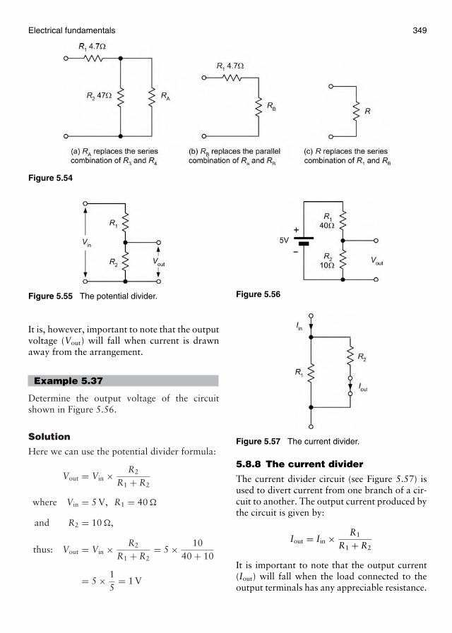
Electrical fundamentals 349
Figure 5.54
Figure 5.55 The potential divider.
It is, however, important to note that the outputvoltage (Vout) will fall when current is drawnaway from the arrangement.
Example 5.37
Determine the output voltage of the circuitshown in Figure 5.56.
Solution
Here we can use the potential divider formula:
Vout = Vin × R2
R1 + R2
where Vin = 5 V, R1 = 40 �
and R2 = 10 �,
thus: Vout = Vin × R2
R1 + R2= 5 × 10
40 + 10
= 5 × 15
= 1 V
Figure 5.56
Figure 5.57 The current divider.
5.8.8 The current divider
The current divider circuit (see Figure 5.57) isused to divert current from one branch of a cir-cuit to another. The output current produced bythe circuit is given by:
Iout = Iin × R1
R1 + R2
It is important to note that the output current(Iout) will fall when the load connected to theoutput terminals has any appreciable resistance.
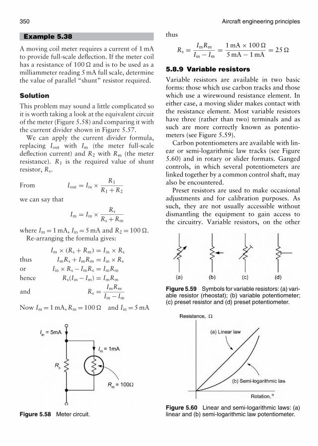
350 Aircraft engineering principles
Example 5.38
A moving coil meter requires a current of 1 mAto provide full-scale deflection. If the meter coilhas a resistance of 100 � and is to be used as amilliammeter reading 5 mA full scale, determinethe value of parallel “shunt” resistor required.
Solution
This problem may sound a little complicated soit is worth taking a look at the equivalent circuitof the meter (Figure 5.58) and comparing it withthe current divider shown in Figure 5.57.
We can apply the current divider formula,replacing Iout with Im (the meter full-scaledeflection current) and R2 with Rm (the meterresistance). R1 is the required value of shuntresistor, Rs.
From Iout = Iin × R1
R1 + R2
we can say that
Im = Iin × Rs
Rs + Rm
where Im = 1 mA, Iin = 5 mA and R2 = 100 �.Re-arranging the formula gives:
Im × (Rs + Rm) = Iin × Rs
thus ImRs + ImRm = Iin × Rs
or Iin × Rs − ImRs = ImRm
hence Rs(Iin − Im) = ImRm
and Rs = ImRm
Iin − Im
Now Im = 1 mA, Rm = 100 � and Iin = 5 mA
Figure 5.58 Meter circuit.
thus
Rs = ImRm
Iin − Im= 1 mA × 100 �
5 mA − 1 mA= 25 �
5.8.9 Variable resistors
Variable resistors are available in two basicforms: those which use carbon tracks and thosewhich use a wirewound resistance element. Ineither case, a moving slider makes contact withthe resistance element. Most variable resistorshave three (rather than two) terminals and assuch are more correctly known as potentio-meters (see Figure 5.59).
Carbon potentiometers are available with lin-ear or semi-logarithmic law tracks (see Figure5.60) and in rotary or slider formats. Gangedcontrols, in which several potentiometers arelinked together by a common control shaft, mayalso be encountered.
Preset resistors are used to make occasionaladjustments and for calibration purposes. Assuch, they are not usually accessible withoutdismantling the equipment to gain access tothe circuitry. Variable resistors, on the other
Figure 5.59 Symbols for variable resistors: (a) vari-able resistor (rheostat); (b) variable potentiometer;(c) preset resistor and (d) preset potentiometer.
Figure 5.60 Linear and semi-logarithmic laws: (a)linear and (b) semi-logarithmic law potentiometer.
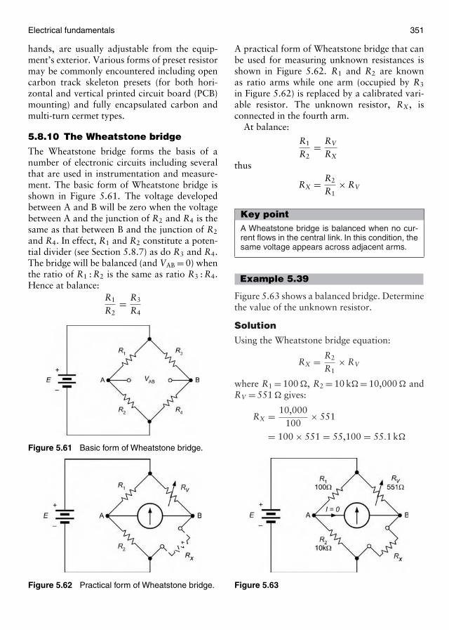
Electrical fundamentals 351
hands, are usually adjustable from the equip-ment’s exterior. Various forms of preset resistormay be commonly encountered including opencarbon track skeleton presets (for both hori-zontal and vertical printed circuit board (PCB)mounting) and fully encapsulated carbon andmulti-turn cermet types.
5.8.10 The Wheatstone bridge
The Wheatstone bridge forms the basis of anumber of electronic circuits including severalthat are used in instrumentation and measure-ment. The basic form of Wheatstone bridge isshown in Figure 5.61. The voltage developedbetween A and B will be zero when the voltagebetween A and the junction of R2 and R4 is thesame as that between B and the junction of R2
and R4. In effect, R1 and R2 constitute a poten-tial divider (see Section 5.8.7) as do R3 and R4.The bridge will be balanced (and VAB = 0) whenthe ratio of R1 : R2 is the same as ratio R3 : R4.Hence at balance:
R1
R2= R3
R4
Figure 5.61 Basic form of Wheatstone bridge.
Figure 5.62 Practical form of Wheatstone bridge.
A practical form of Wheatstone bridge that canbe used for measuring unknown resistances isshown in Figure 5.62. R1 and R2 are knownas ratio arms while one arm (occupied by R3
in Figure 5.62) is replaced by a calibrated vari-able resistor. The unknown resistor, RX, isconnected in the fourth arm.
At balance:
R1
R2= RV
RX
thus
RX = R2
R1× RV
Key pointA Wheatstone bridge is balanced when no cur-rent flows in the central link. In this condition, thesame voltage appears across adjacent arms.
Example 5.39
Figure 5.63 shows a balanced bridge. Determinethe value of the unknown resistor.
Solution
Using the Wheatstone bridge equation:
RX = R2
R1× RV
where R1 = 100 �, R2 = 10 k�= 10,000 � andRV = 551 � gives:
RX = 10,000100
× 551
= 100 × 551 = 55,100 = 55.1 k�
Figure 5.63
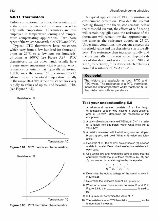
352 Aircraft engineering principles
5.8.11 Thermistors
Unlike conventional resistors, the resistance ofa thermistor is intended to change consider-ably with temperature. Thermistors are thusemployed in temperature sensing and temper-ature compensating applications. Two basictypes of thermistor are available: NTC and PTC.
Typical NTC thermistors have resistanceswhich vary from a few hundred (or thousand)ohms at 25◦C to a few tens (or hundreds)of ohms at 100◦C (see Figure 5.64). PTCthermistors, on the other hand, usually havea resistance–temperature characteristic whichremains substantially flat (typically at around100 �) over the range 0◦C to around 75◦C.Above this, and at a critical temperature (usuallyin the range 80–120◦C) their resistance rises veryrapidly to values of up to, and beyond, 10 k�
(see Figure 5.65).
Figure 5.64 NTC thermistor characteristics.
Figure 5.65 PTC thermistor characteristics.
A typical application of PTC thermistors isover-current protection. Provided the currentpassing through the thermistor remains belowthe threshold current, the effects of self-heatingwill remain negligible and the resistance of thethermistor will remain low (i.e. approximatelythe same as the resistance quoted at 25◦C).Under fault conditions, the current exceeds thethreshold value and the thermistor starts to self-heat. The resistance then increases rapidly andthe current falls to the rest value. Typical val-ues of threshold and rest currents are 200 and8 mA, respectively, for a device which exhibits anominal resistance of 25 � at 25◦C.
Key pointThermistors are available as both NTC andPTC types. The resistance of a PTC thermistorincreases with temperature whilst that for an NTCthermistor falls with temperatures.
Test your understanding 5.81. A wirewound resistor consists of a 2 m length
of annealed copper wire having a cross-sectionalarea of 0.5 mm2. Determine the resistance of thiscomponent.
2. A batch of resistors is marked “560 �, ±10%”. If a resis-tor is taken from this batch, within what limits will itsvalue be?
3. A resistor is marked with the following coloured stripes:brown, green, red, gold. What is its value and toler-ance?
4. Resistors of 10, 15 and 22 � are connected (a) in seriesand (b) in parallel. Determine the effective resistance ineach case.
5. Use Ohm’s law and Kirchhoff’s laws to show that theequivalent resistance, R, of three resistors, R1, R2 andR3, connected in parallel is given by the equation:
1R
= 1R1
+ 1R2
+ 1R3
6. Determine the output voltage of the circuit shown inFigure 5.66.
7. Determine the unknown current in Figure 5.67.
8. When no current flows across between X and Y inFigure 5.68, the __________ __________ is said tobe __________.
9. In Figure 5.68, determine the value of R.
10. The resistance of a PTC thermistor _________ as thetemperature increases.
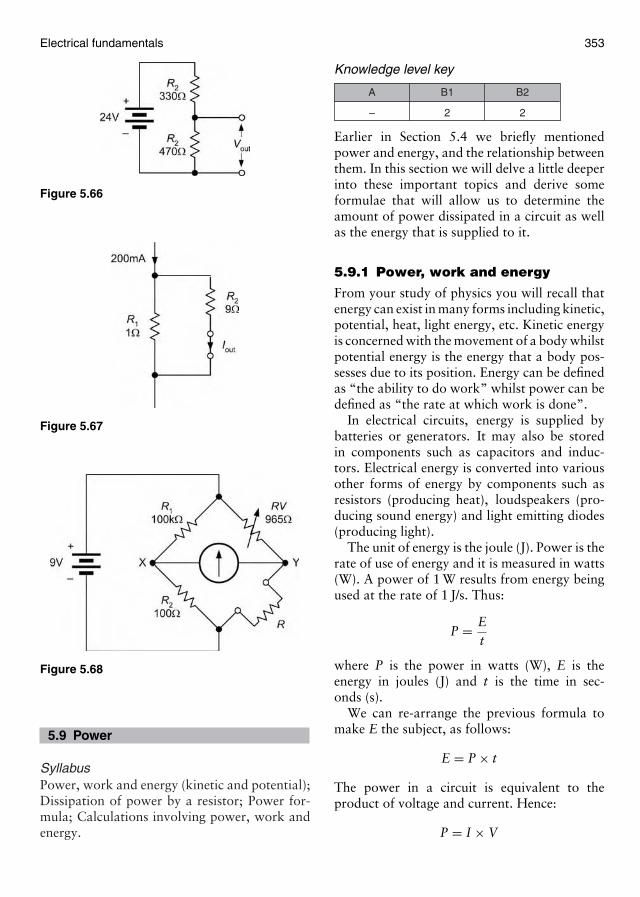
Electrical fundamentals 353
Figure 5.66
Figure 5.67
Figure 5.68
5.9 Power
SyllabusPower, work and energy (kinetic and potential);Dissipation of power by a resistor; Power for-mula; Calculations involving power, work andenergy.
Knowledge level key
–
A
2
B1
2
B2
Earlier in Section 5.4 we briefly mentionedpower and energy, and the relationship betweenthem. In this section we will delve a little deeperinto these important topics and derive someformulae that will allow us to determine theamount of power dissipated in a circuit as wellas the energy that is supplied to it.
5.9.1 Power, work and energy
From your study of physics you will recall thatenergy can exist in many forms including kinetic,potential, heat, light energy, etc. Kinetic energyis concerned with the movement of a body whilstpotential energy is the energy that a body pos-sesses due to its position. Energy can be definedas “the ability to do work” whilst power can bedefined as “the rate at which work is done”.
In electrical circuits, energy is supplied bybatteries or generators. It may also be storedin components such as capacitors and induc-tors. Electrical energy is converted into variousother forms of energy by components such asresistors (producing heat), loudspeakers (pro-ducing sound energy) and light emitting diodes(producing light).
The unit of energy is the joule (J). Power is therate of use of energy and it is measured in watts(W). A power of 1 W results from energy beingused at the rate of 1 J/s. Thus:
P = Et
where P is the power in watts (W), E is theenergy in joules (J) and t is the time in sec-onds (s).
We can re-arrange the previous formula tomake E the subject, as follows:
E = P × t
The power in a circuit is equivalent to theproduct of voltage and current. Hence:
P = I × V
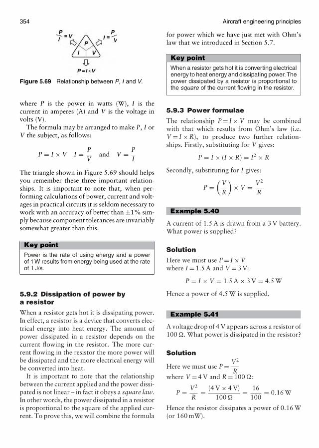
354 Aircraft engineering principles
Figure 5.69 Relationship between P, I and V.
where P is the power in watts (W), I is thecurrent in amperes (A) and V is the voltage involts (V).
The formula may be arranged to make P, I orV the subject, as follows:
P = I × V I = PV
and V = PI
The triangle shown in Figure 5.69 should helpsyou remember these three important relation-ships. It is important to note that, when per-forming calculations of power, current and volt-ages in practical circuits it is seldom necessary towork with an accuracy of better than ±1% sim-ply because component tolerances are invariablysomewhat greater than this.
Key pointPower is the rate of using energy and a powerof 1W results from energy being used at the rateof 1 J/s.
5.9.2 Dissipation of power bya resistor
When a resistor gets hot it is dissipating power.In effect, a resistor is a device that converts elec-trical energy into heat energy. The amount ofpower dissipated in a resistor depends on thecurrent flowing in the resistor. The more cur-rent flowing in the resistor the more power willbe dissipated and the more electrical energy willbe converted into heat.
It is important to note that the relationshipbetween the current applied and the power dissi-pated is not linear – in fact it obeys a square law.In other words, the power dissipated in a resistoris proportional to the square of the applied cur-rent. To prove this, we will combine the formula
for power which we have just met with Ohm’slaw that we introduced in Section 5.7.
Key pointWhen a resistor gets hot it is converting electricalenergy to heat energy and dissipating power.Thepower dissipated by a resistor is proportional tothe square of the current flowing in the resistor.
5.9.3 Power formulae
The relationship P = I × V may be combinedwith that which results from Ohm’s law (i.e.V = I × R), to produce two further relation-ships. Firstly, substituting for V gives:
P = I × (I × R) = I2 × R
Secondly, substituting for I gives:
P =(
VR
)× V = V2
R
Example 5.40
A current of 1.5 A is drawn from a 3 V battery.What power is supplied?
Solution
Here we must use P = I × Vwhere I = 1.5 A and V = 3 V:
P = I × V = 1.5 A × 3 V = 4.5 W
Hence a power of 4.5 W is supplied.
Example 5.41
A voltage drop of 4 V appears across a resistor of100 �. What power is dissipated in the resistor?
Solution
Here we must use P = V2
Rwhere V = 4 V and R = 100 �:
P = V2
R= (4 V × 4 V)
100 �= 16
100= 0.16 W
Hence the resistor dissipates a power of 0.16 W(or 160 mW).
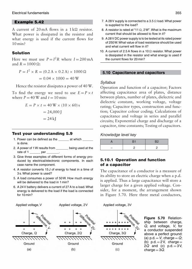
Electrical fundamentals 355
Example 5.42
A current of 20 mA flows in a 1 k� resistor.What power is dissipated in the resistor andwhat energy is used if the current flows for10 min?
Solution
Here we must use P = I2R where I = 200 mAand R = 1000 �:
P = I2 × R = (0.2 A × 0.2 A) × 1000 �
= 0.04 × 1000 = 40 W
Hence the resistor dissipates a power of 40 W.
To find the energy we need to use E = P × twhere P = 40 W and t = 10 min:
E = P × t = 40 W × (10 × 60) s
= 24,000 J
= 24 kJ
Test your understanding 5.91. Power can be defined as the ______ at which ______
is done.
2. A power of 1W results from _______ being used at therate of 1 ______ per _______.
3. Give three examples of different forms of energy pro-duced by electrical/electronic components. In eachcase name the component.
4. A resistor converts 15 J of energy to heat in a time of3 s. What power is used?
5. A load consumes a power of 50W. How much energywill be delivered to the load in 1 min?
6. A 24V battery delivers a current of 27 A to a load. Whatenergy is delivered to the load if the load is connectedfor 10 min?
Figure 5.70 Relation-ship between charge,Q, and voltage, V, fora conductor suspendedabove a perfect ground:(a) p.d.=V, charge = Q;(b) p.d.= 2V, charge =2Q and (c) p.d.= 3V,charge = 3Q.
7. A 28V supply is connected to a 3.5 � load. What poweris supplied to the load?
8. A resistor is rated at “11 �, 2W”. What is the maximumcurrent that should be allowed to flow in it?
9. A 28V DC power supply is to be tested at its rated powerof 250W.What value of load resistance should be usedand what current will flow in it?
10. A current of 2.5 A flows in a 10 � resistor. What poweris dissipated in the resistor and what energy is used ifthe current flows for 20 min?
5.10 Capacitance and capacitors
SyllabusOperation and function of a capacitor; Factorsaffecting capacitance area of plates, distancebetween plates, number of plates, dielectric anddielectric constant, working voltage, voltagerating; Capacitor types, construction and func-tion; Capacitor colour coding; Calculations ofcapacitance and voltage in series and parallelcircuits; Exponential charge and discharge of acapacitor, time constants; Testing of capacitors.
Knowledge level key
–
A
2
B1
2
B2
5.10.1 Operation and functionof a capacitor
The capacitance of a conductor is a measure ofits ability to store an electric charge when a p.d.is applied. Thus a large capacitance will store alarger charge for a given applied voltage. Con-sider, for a moment, the arrangement shownin Figure 5.70. Here three metal conductors,

356 Aircraft engineering principles
Figure 5.71 A simple parallel-platecapacitor.
of identical size and area, are suspended abovea perfectly conducting zero potential plane (orground). In Figure 5.70(a) the p.d., V , betweenthe conductor and ground produces a charge,Q. If the p.d. is doubled to 2 V, as shown inFigure 5.70(b), the charge increases to 2 V. Sim-ilarly if the p.d. increases to 3 V, as shown inFigure 5.70(c), the charge increases to 3Q. Thisshows that, for a given conductor, there is alinear relationship between the charge present,Q, and the p.d., V .
In practice we can alter the shape of a conduc-tor so that it covers a relatively large area overwhich the charge is distributed. This allows usto produce a relatively large value of charge foronly a relatively modest value of p.d. The result-ing component is used for storing charge and isknown as a capacitor (Figure 5.71).
If we plot charge, Q, against p.d., V , for acapacitor we arrive at a straight line law (asmentioned earlier in relation to Figure 5.70).The slope of this graph is an indication ofthe capacitance of the capacitor, as shown inFigure 5.72.
From Figure 5.72, the capacitance of a capac-itor is defined as follows:
Capacitance =charge on the
capacitor’s plates
potential differencebetween the plates
or in symbols
C = QV
where the charge, Q, is measured in coulombs(C) and the p.d., V , is measured in volts (V). Theunit of capacitance is the Farad (F) where onefarad of capacitance produces a charge of one
Figure 5.72 Charge, Q, plotted against p.d., V, forthree different values of capacitance.
coulomb when a p.d. of one volt is applied. Notethat, in practice, the farad is a very large unitand we therefore often deal with sub-multiplesof the basic unit such as µF (1 × 10⁻⁶ F),nF (1 × 10⁻⁹ F) and pF (1 × 10⁻¹² F).
For example if a potential of 200 V is requiredto create a charge of 400 µC on a capacitor thenthe capacitance of the capacitor (expressed in F)is given by:
C = QV
= 400 × 10−6 C200 V
= 2 × 10⁻⁶ F = 2 µF
We have already said that a capacitor is a devicefor storing electric charge. In effect, it is a reser-voir for charge. Typical applications for capaci-tors include reservoir and smoothing capacitorsfor use in power supplies, coupling alternatingcurrent (AC) signals between the stages of ampli-fiers and decoupling supply rails (i.e. effectivelygrounding the supply rails to residual AC signalsand noise). You will learn more about these par-ticular applications when you study Chapter 6but, for now, we will concentrate our efforts onexplaining how a capacitor works and what itdoes!
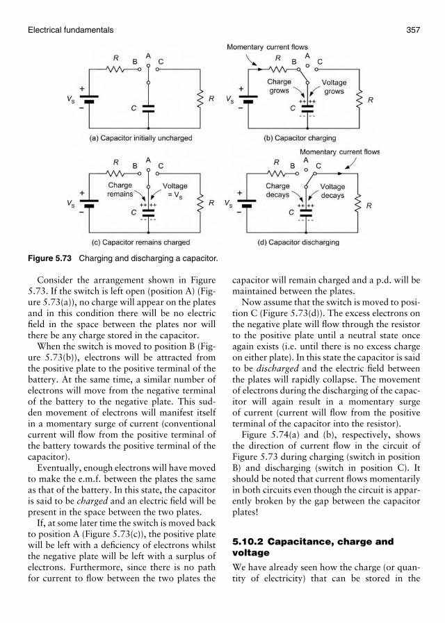
Electrical fundamentals 357
Figure 5.73 Charging and discharging a capacitor.
Consider the arrangement shown in Figure5.73. If the switch is left open (position A) (Fig-ure 5.73(a)), no charge will appear on the platesand in this condition there will be no electricfield in the space between the plates nor willthere be any charge stored in the capacitor.
When the switch is moved to position B (Fig-ure 5.73(b)), electrons will be attracted fromthe positive plate to the positive terminal of thebattery. At the same time, a similar number ofelectrons will move from the negative terminalof the battery to the negative plate. This sud-den movement of electrons will manifest itselfin a momentary surge of current (conventionalcurrent will flow from the positive terminal ofthe battery towards the positive terminal of thecapacitor).
Eventually, enough electrons will have movedto make the e.m.f. between the plates the sameas that of the battery. In this state, the capacitoris said to be charged and an electric field will bepresent in the space between the two plates.
If, at some later time the switch is moved backto position A (Figure 5.73(c)), the positive platewill be left with a deficiency of electrons whilstthe negative plate will be left with a surplus ofelectrons. Furthermore, since there is no pathfor current to flow between the two plates the
capacitor will remain charged and a p.d. will bemaintained between the plates.
Now assume that the switch is moved to posi-tion C (Figure 5.73(d)). The excess electrons onthe negative plate will flow through the resistorto the positive plate until a neutral state onceagain exists (i.e. until there is no excess chargeon either plate). In this state the capacitor is saidto be discharged and the electric field betweenthe plates will rapidly collapse. The movementof electrons during the discharging of the capac-itor will again result in a momentary surgeof current (current will flow from the positiveterminal of the capacitor into the resistor).
Figure 5.74(a) and (b), respectively, showsthe direction of current flow in the circuit ofFigure 5.73 during charging (switch in positionB) and discharging (switch in position C). Itshould be noted that current flows momentarilyin both circuits even though the circuit is appar-ently broken by the gap between the capacitorplates!
5.10.2 Capacitance, charge andvoltage
We have already seen how the charge (or quan-tity of electricity) that can be stored in the
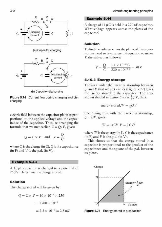
358 Aircraft engineering principles
Figure 5.74 Current flow during charging and dis-charging.
electric field between the capacitor plates is pro-portional to the applied voltage and the capac-itance of the capacitor. Thus, re-arranging theformula that we met earlier, C = Q/V , gives:
Q = C × V and V = QC
where Q is the charge (in C), C is the capacitance(in F) and V is the p.d. (in V).
Example 5.43
A 10 µF capacitor is charged to a potential of250 V. Determine the charge stored.
Solution
The charge stored will be given by:
Q = C × V = 10 × 10−6 × 250
= 2500 × 10−6
= 2.5 × 10−3 = 2.5 mC
Example 5.44
A charge of 11 µC is held in a 220 nF capacitor.What voltage appears across the plates of thecapacitor?
Solution
To find the voltage across the plates of the capac-itor we need to re-arrange the equation to makeV the subject, as follows:
V = QC
= 11 × 10−6 C220 × 10−9 F
= 50 V
5.10.3 Energy storage
The area under the linear relationship betweenQ and V that we met earlier (Figure 5.72) givesthe energy stored in the capacitor. The areashown shaded in Figure 5.75 is 1
2 QV, thus:
energy stored,W = 12 QV
Combining this with the earlier relationship,Q = CV , gives:
W = 12 (CV)V = 1
2 CV2
where W is the energy (in J), C is the capacitance(in F) and V is the p.d. (in V).
This shows us that the energy stored in acapacitor is proportional to the product of thecapacitance and the square of the p.d. betweenits plates.
Figure 5.75 Energy stored in a capacitor.
Electrical fundamentals 359
Example 5.45
A 100 µF capacitor is charged from a charge of20 V supply. How much energy is stored in thecapacitor?
Solution
The energy stored in the capacitor will begiven by:
W = 12 (C × V2) = 1
2 × 100 × 10−6 × (20)2
= 50 × 400 × 10−6 = 20,000 × 10−6
= 2 × 10⁻² J
Example 5.46
A capacitor of 47 µF is required to store energyof 40 J. Determine the p.d. required to do this.
Solution
To find the p.d. (voltage) across the plates of thecapacitor we need to re-arrange the equation tomake V the subject, as follows:
V =√
2EC
=√
2 × 4047 × 10−6
=√
8047
× 106
=√
1.702 × 106 = 1.3 × 103 = 1.3 kV
5.10.4 Factors affectingcapacitance
The capacitance of a capacitor depends upon thephysical dimensions of the capacitor (i.e. the sizeof the plates and the separation between them)and the dielectric material between the plates.The capacitance of a conventional parallel platecapacitor is given by:
C = ε0εrAd
where C is the capacitance (in F), ε0 is thepermittivity of free space, εr is the relative per-mittivity (or dielectric constant) of the dielectricmedium between the plates), A is the area of theplates (in m2) and d is the separation betweenthe plates (in m). The permittivity of free space,ε0, is 8.854 × 10⁻¹² F/m.
Some typical capacitor dielectric materialsand relative permittivity are given in thetable below:
Dielectric material Relative permittivity(free space = 1)
Vacuum 1Air 1.0006 (i.e. 1!)Polythene 2.2Paper 2–2.5Epoxy resin 4.0Mica 3–7Glass 5–10Porcelain 6–7Aluminium oxide 7Ceramic materials 15–500
Example 5.47
Two parallel metal plates each of area 0.2 m2
are separated by an air gap of 1 mm. Determinethe capacitance of this arrangement.
Solution
Here we must use the formula:
C = ε0εrAd
where A = 0.2 m2, d = 1 × 10⁻³ m, εr = 1 andε0 = 8.854 × 10⁻¹² F/m. Hence:
C = 8.854 × 10−12 × 1 × 0.21 × 10−3
= 1.7708 × 10⁻¹²
1 × 10−3
= 1.7708 × 10⁻⁹ F
= 1.7708 nF
Example 5.48
A capacitor of 1 nF is required. If a dielectricmaterial of thickness 0.5 mm and relative per-mittivity 5.4 is available, determine the requiredplate area.
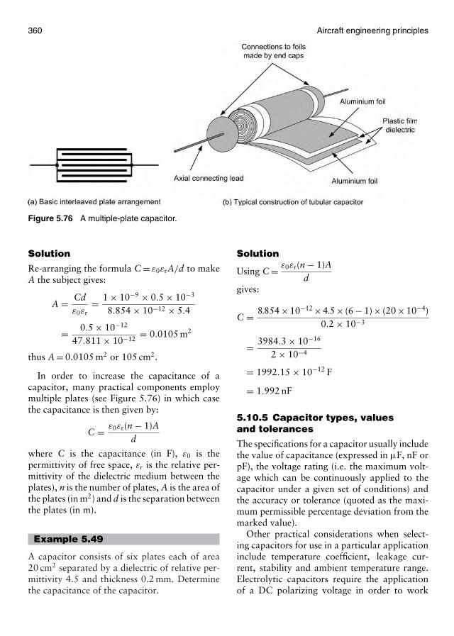
360 Aircraft engineering principles
Figure 5.76 A multiple-plate capacitor.
Solution
Re-arranging the formula C = ε0εrA/d to makeA the subject gives:
A = Cdε0εr
= 1 × 10−9 × 0.5 × 10−3
8.854 × 10−12 × 5.4
= 0.5 × 10⁻¹²
47.811 × 10−12= 0.0105 m2
thus A = 0.0105 m2 or 105 cm2.
In order to increase the capacitance of acapacitor, many practical components employmultiple plates (see Figure 5.76) in which casethe capacitance is then given by:
C = ε0εr(n − 1)Ad
where C is the capacitance (in F), ε0 is thepermittivity of free space, εr is the relative per-mittivity of the dielectric medium between theplates), n is the number of plates, A is the area ofthe plates (in m2) and d is the separation betweenthe plates (in m).
Example 5.49
A capacitor consists of six plates each of area20 cm2 separated by a dielectric of relative per-mittivity 4.5 and thickness 0.2 mm. Determinethe capacitance of the capacitor.
Solution
Using C = ε0εr(n − 1)Ad
gives:
C = 8.854×10−12 ×4.5× (6 − 1)× (20×10−4)0.2 × 10−3
= 3984.3 × 10−16
2 × 10−4
= 1992.15 × 10−12 F
= 1.992 nF
5.10.5 Capacitor types, valuesand tolerances
The specifications for a capacitor usually includethe value of capacitance (expressed in µF, nF orpF), the voltage rating (i.e. the maximum volt-age which can be continuously applied to thecapacitor under a given set of conditions) andthe accuracy or tolerance (quoted as the maxi-mum permissible percentage deviation from themarked value).
Other practical considerations when select-ing capacitors for use in a particular applicationinclude temperature coefficient, leakage cur-rent, stability and ambient temperature range.Electrolytic capacitors require the applicationof a DC polarizing voltage in order to work
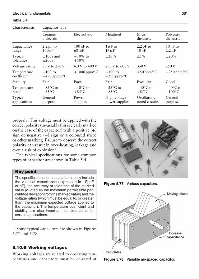
Electrical fundamentals 361
Table 5.4
Characteristic Capacitor type
Ceramic Electrolytic Metalised Mica Polyesterdielectric film dielectric dielectric
Capacitance 2.2 pF to 100 nF to 1 µF to 2.2 pF to 10 nF torange 100 nF 68 mF 16 µF 10 nF 2.2 µF
Typical ±10% and −10% to ±20% ±1% ±20%tolerance ±20% +50%
Voltage rating 50 V to 250 V 6.3 V to 400 V 250 V to 600 V 350 V 250 V
Temperature +100 to +1000 ppm/◦C +100 to +50 ppm/◦C +250 ppm/◦Ccoefficient −4700 ppm/◦C +200 ppm/◦C
Stability Fair Poor Fair Excellent Good
Temperature −85◦C to −40◦C to −25◦C to −40◦C to −40◦C torange +85◦C +85◦C +85◦C +85◦C +100◦C
Typical General Power High-voltage Oscillators, Generalapplications purpose supplies power supplies tuned circuits purpose
properly. This voltage must be applied with thecorrect polarity (invariably this is clearly markedon the case of the capacitor) with a positive (+)sign or negative (−) sign or a coloured stripeor other marking. Failure to observe the correctpolarity can result in over-heating, leakage andeven a risk of explosion!
The typical specifications for some commontypes of capacitor are shown in Table 5.4.
Key pointThe specifications for a capacitor usually includethe value of capacitance (expressed in µF, nFor pF), the accuracy or tolerance of the markedvalue (quoted as the maximum permissible per-centage deviation from the marked value) and thevoltage rating (which must be equal to, or greaterthan, the maximum expected voltage applied tothe capacitor). The temperature coefficient andstability are also important considerations forcertain applications.
Some typical capacitors are shown in Figures5.77 and 5.78.
5.10.6 Working voltages
Working voltages are related to operating tem-peratures and capacitors must be de-rated at
Figure 5.77 Various capacitors.
Figure 5.78 Variable air-spaced capacitor.
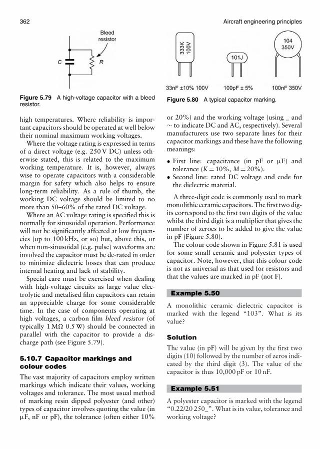
362 Aircraft engineering principles
Figure 5.79 A high-voltage capacitor with a bleedresistor.
high temperatures. Where reliability is impor-tant capacitors should be operated at well belowtheir nominal maximum working voltages.
Where the voltage rating is expressed in termsof a direct voltage (e.g. 250 V DC) unless oth-erwise stated, this is related to the maximumworking temperature. It is, however, alwayswise to operate capacitors with a considerablemargin for safety which also helps to ensurelong-term reliability. As a rule of thumb, theworking DC voltage should be limited to nomore than 50–60% of the rated DC voltage.
Where an AC voltage rating is specified this isnormally for sinusoidal operation. Performancewill not be significantly affected at low frequen-cies (up to 100 kHz, or so) but, above this, orwhen non-sinusoidal (e.g. pulse) waveforms areinvolved the capacitor must be de-rated in orderto minimize dielectric losses that can produceinternal heating and lack of stability.
Special care must be exercised when dealingwith high-voltage circuits as large value elec-trolytic and metalised film capacitors can retainan appreciable charge for some considerabletime. In the case of components operating athigh voltages, a carbon film bleed resistor (oftypically 1 M� 0.5 W) should be connected inparallel with the capacitor to provide a dis-charge path (see Figure 5.79).
5.10.7 Capacitor markings andcolour codes
The vast majority of capacitors employ writtenmarkings which indicate their values, workingvoltages and tolerance. The most usual methodof marking resin dipped polyester (and other)types of capacitor involves quoting the value (inµF, nF or pF), the tolerance (often either 10%
Figure 5.80 A typical capacitor marking.
or 20%) and the working voltage (using _ and∼ to indicate DC and AC, respectively). Severalmanufacturers use two separate lines for theircapacitor markings and these have the followingmeanings:
• First line: capacitance (in pF or µF) andtolerance (K = 10%, M = 20%).
• Second line: rated DC voltage and code forthe dielectric material.
A three-digit code is commonly used to markmonolithic ceramic capacitors. The first two dig-its correspond to the first two digits of the valuewhilst the third digit is a multiplier that gives thenumber of zeroes to be added to give the valuein pF (Figure 5.80).
The colour code shown in Figure 5.81 is usedfor some small ceramic and polyester types ofcapacitor. Note, however, that this colour codeis not as universal as that used for resistors andthat the values are marked in pF (not F).
Example 5.50
A monolithic ceramic dielectric capacitor ismarked with the legend “103”. What is itsvalue?
Solution
The value (in pF) will be given by the first twodigits (10) followed by the number of zeros indi-cated by the third digit (3). The value of thecapacitor is thus 10,000 pF or 10 nF.
Example 5.51
A polyester capacitor is marked with the legend“0.22/20 250_”. What is its value, tolerance andworking voltage?
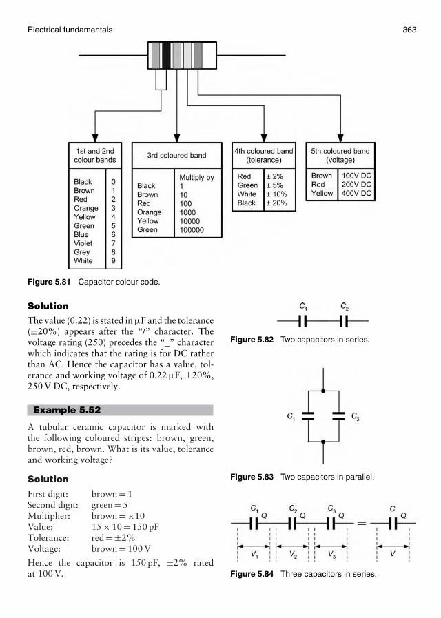
Electrical fundamentals 363
Figure 5.81 Capacitor colour code.
Solution
The value (0.22) is stated in µF and the tolerance(±20%) appears after the “/” character. Thevoltage rating (250) precedes the “_” characterwhich indicates that the rating is for DC ratherthan AC. Hence the capacitor has a value, tol-erance and working voltage of 0.22 µF, ±20%,250 V DC, respectively.
Example 5.52
A tubular ceramic capacitor is marked withthe following coloured stripes: brown, green,brown, red, brown. What is its value, toleranceand working voltage?
Solution
First digit: brown = 1Second digit: green = 5Multiplier: brown = ×10Value: 15 × 10 = 150 pFTolerance: red = ±2%Voltage: brown = 100 V
Hence the capacitor is 150 pF, ±2% ratedat 100 V.
Figure 5.82 Two capacitors in series.
Figure 5.83 Two capacitors in parallel.
Figure 5.84 Three capacitors in series.

364 Aircraft engineering principles
5.10.8 Capacitors in series andparallel
In order to obtain a particular value of capaci-tance, fixed capacitors may be arranged in eitherseries or parallel (Figures 5.82 and 5.83).
Now consider Figure 5.84 where C is theequivalent capacitance of three capacitors (C1,C2 and C3) connected in series.
The applied voltage, V , will be the sum ofthe voltages that appear across each capacitor.Thus:
V = V1 + V2 + V3
Now, for each capacitor, the p.d., V , across itsplates will be given by the ratio of charge, Q, tocapacitance, C. Hence:
V = QC
, V1 = Q1
C1, V2 = Q2
C2and
V3 = Q3
C3
Combining these equations gives: In the seriescircuit the same charge, Q, appears across eachcapacitor, thus:
Q = Q1 = Q2 = Q3
Hence:
QC
= QC1
+ QC2
+ QC3
From which:
1C
= 1C1
+ 1C2
+ 1C3
Key pointThe reciprocal of the equivalent capacitance of anumber of capacitors connected in series can befound by simply adding together the reciprocalsof the individual values of capacitance.
When two capacitors are connected in seriesthe equation becomes:
1C
= 1C1
+ 1C2
This can be arranged to give the slightly moreconvenient expression:
C = C1 × C2
C1 + C2
Note that the foregoing expression is only cor-rect for two capacitors. It cannot be extendedfor three or more!
Key pointThe equivalent capacitance of two capacitorsconnected in series can be found by taking theproduct of the two capacitance values and divid-ing it by the sum of the two capacitance values(in other words, product over sum).
Now consider Figure 5.85 where C is theequivalent capacitance of three capacitors (C1,C2 and C3) connected in series.
The total charge present, Q, will be the sum ofthe charges that appear in each capacitor. Thus:
Q = Q1 + Q2 + Q3
Now, for each capacitor, the charge present, Q,will be given by the product of the capacitance,C, and p.d., V . Hence:
Q = CV , Q1 = C1V1, Q2 = C2V2
and Q3 = C3V3
Combining these equations gives:
CV = C1V1 + C2V2 + C3V3
In the series circuit the same voltage, V , appearsacross each capacitor, thus:
V = V1 = V2 = V3
Figure 5.85 Three capacitors in parallel.

Electrical fundamentals 365
Hence:
CV = C1V + C2V + C3V
From which:
C = C1 + C2 + C3
When two capacitors are connected in series theequation becomes:
C = C1 + C2
Key pointThe equivalent capacitance of a number ofcapacitors connected in parallel can be found bysimply adding together the individual values ofcapacitance.
Example 5.53
Capacitors of 2.2 and 6.8 µF are connected(a) in series and (b) in parallel. Determine theequivalent value of capacitance in each case.
Solution
(a) Here we can use the simplified equation forjust two capacitors connected in series:
C = C1 × C2
C1 + C2= 2.2 × 6.8
2.2 + 6.8= 14.96
9
= 1.66 µF
(b) Here we use the formula for two capacitorsconnected in parallel:
C = C1 + C2 = 2.2 + 6.8 = 9 µF
Example 5.54
Capacitors of 2 and 5 µF are connected in seriesacross a 100 V DC supply. Determine:
(a) the charge on each capacitor and (b) thevoltage dropped across each capacitor.
Solution
(a) First we need to find the equivalent value ofcapacitance, C, using the simplified equationfor two capacitors in series:
C = C1 × C2
C1 + C2= 2 × 5
2 + 5= 10
7= 1.428 µF
Next we can determine the charge (notethat, since the capacitors are connected inseries, the same charge will appear in eachcapacitor):
Q = C × V = 1.428 × 100 = 142.8 µC
(b) In order to determine the voltage droppedacross each capacitor we can use:
V = QC
Hence, for the 2 µF capacitor:
V1 = QC1
= 142.8 × 10⁻⁶
2 × 10−6= 71.4 V
Similarly, for the 5 µF capacitor:
V2 = QC2
= 142.8 × 10⁻⁶
5 × 10−6= 28.6 V
We should now find that the total voltage(100 V) applied to the series circuit is the sumof the two capacitor voltages, i.e.:
V = V1 + V2 = 71.4 + 28.6 = 100 V
5.10.9 Capacitors charging anddischarging through a resistor
Networks of capacitors and resistors (known asC–R networks) form the basis of simple timingand delay circuits.
In many electrical/electronic circuits the vari-ation of voltage and current with time is impor-tant. In order to satisfy this requirement, simpleC–R networks have useful properties that wecan exploit. A simple C–R circuit is shown inFigure 5.86.
When the C–R network is connected toa constant voltage source (VS), as shown inFigure 5.87, the voltage (vC) across the (initially
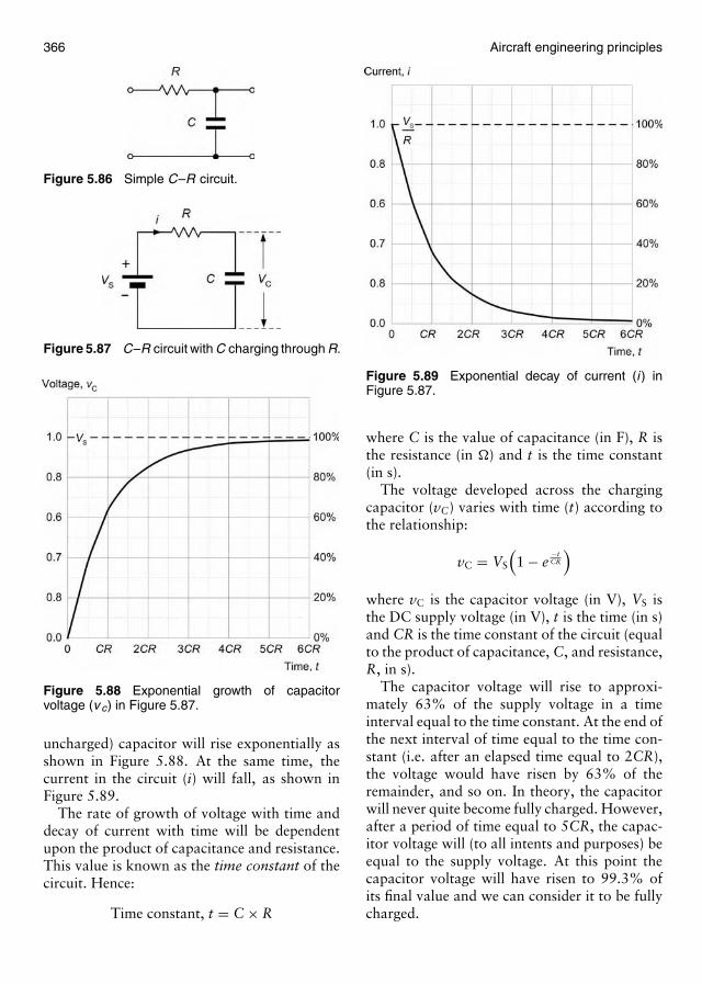
366 Aircraft engineering principles
Figure 5.86 Simple C–R circuit.
Figure 5.87 C–R circuit with C charging through R.
Figure 5.88 Exponential growth of capacitorvoltage (v c) in Figure 5.87.
uncharged) capacitor will rise exponentially asshown in Figure 5.88. At the same time, thecurrent in the circuit (i) will fall, as shown inFigure 5.89.
The rate of growth of voltage with time anddecay of current with time will be dependentupon the product of capacitance and resistance.This value is known as the time constant of thecircuit. Hence:
Time constant, t = C × R
Figure 5.89 Exponential decay of current (i ) inFigure 5.87.
where C is the value of capacitance (in F), R isthe resistance (in �) and t is the time constant(in s).
The voltage developed across the chargingcapacitor (vC) varies with time (t) according tothe relationship:
vC = VS
(1 − e
−tCR
)where vC is the capacitor voltage (in V), VS isthe DC supply voltage (in V), t is the time (in s)and CR is the time constant of the circuit (equalto the product of capacitance, C, and resistance,R, in s).
The capacitor voltage will rise to approxi-mately 63% of the supply voltage in a timeinterval equal to the time constant. At the end ofthe next interval of time equal to the time con-stant (i.e. after an elapsed time equal to 2CR),the voltage would have risen by 63% of theremainder, and so on. In theory, the capacitorwill never quite become fully charged. However,after a period of time equal to 5CR, the capac-itor voltage will (to all intents and purposes) beequal to the supply voltage. At this point thecapacitor voltage will have risen to 99.3% ofits final value and we can consider it to be fullycharged.
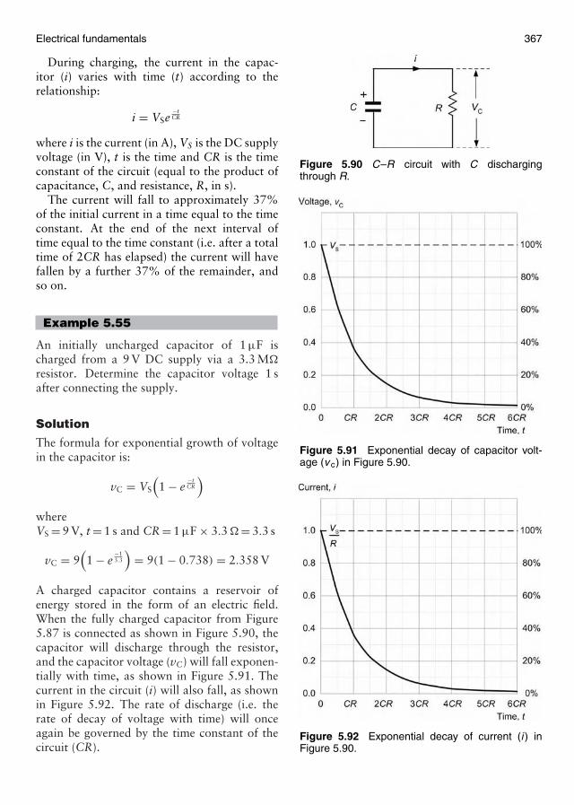
Electrical fundamentals 367
During charging, the current in the capac-itor (i) varies with time (t) according to therelationship:
i = VSe−tCR
where i is the current (in A), VS is the DC supplyvoltage (in V), t is the time and CR is the timeconstant of the circuit (equal to the product ofcapacitance, C, and resistance, R, in s).
The current will fall to approximately 37%of the initial current in a time equal to the timeconstant. At the end of the next interval oftime equal to the time constant (i.e. after a totaltime of 2CR has elapsed) the current will havefallen by a further 37% of the remainder, andso on.
Example 5.55
An initially uncharged capacitor of 1 µF ischarged from a 9 V DC supply via a 3.3 M�
resistor. Determine the capacitor voltage 1 safter connecting the supply.
Solution
The formula for exponential growth of voltagein the capacitor is:
vC = VS
(1 − e
−tCR
)whereVS = 9 V, t = 1 s and CR = 1 µF × 3.3 � = 3.3 s
vC = 9(1 − e
−13.3
)= 9(1 − 0.738) = 2.358 V
A charged capacitor contains a reservoir ofenergy stored in the form of an electric field.When the fully charged capacitor from Figure5.87 is connected as shown in Figure 5.90, thecapacitor will discharge through the resistor,and the capacitor voltage (vC) will fall exponen-tially with time, as shown in Figure 5.91. Thecurrent in the circuit (i) will also fall, as shownin Figure 5.92. The rate of discharge (i.e. therate of decay of voltage with time) will onceagain be governed by the time constant of thecircuit (CR).
Figure 5.90 C–R circuit with C dischargingthrough R.
Figure 5.91 Exponential decay of capacitor volt-age (v c) in Figure 5.90.
Figure 5.92 Exponential decay of current (i ) inFigure 5.90.

368 Aircraft engineering principles
The voltage developed across the dischargingcapacitor (vC) varies with time (t) according tothe relationship:
vC = VSe−tCR
where vC is the capacitor voltage (in V), VS isthe DC supply voltage (in V), t is the time (in s)and CR is the time constant of the circuit (equalto the product of capacitance, C, and resistance,R, in s).
The capacitor voltage will fall to approxi-mately 37% of the initial voltage in a time equalto the time constant. At the end of the next inter-val of time equal to the time constant (i.e. afteran elapsed time equal to 2CR) the voltage willhave fallen by 37% of the remainder, and so on.In theory, the capacitor will never quite becomefully discharged. After a period of time equal to5CR, however, the capacitor voltage will to allintents and purposes be zero. At this point thecapacitor voltage will have fallen below 1% ofits initial value. At this point we can consider itto be fully discharged.
As with charging, the current in the capac-itor (i) varies with time (t) according to therelationship:
i = VSe−tCR
where i is the current (in A), VS is the DC supplyvoltage (in V), t is the time and CR is the timeconstant of the circuit (equal to the product ofcapacitance, C, and resistance, R, in s).
The current will fall to approximately 37%of the initial current in a time equal to the timeconstant. At the end of the next interval of timeequal to the time constant (i.e. after a totaltime of 2CR has elapsed) the current will havefallen by a further 37% of the remainder, andso on.
Example 5.56
A 10 µF capacitor is charged to a potential of20 V and then discharged through a 47 k� resis-tor. Determine the time taken for the capacitorvoltage to fall below 10 V.
Solution
The formula for exponential decay of voltage inthe capacitor is:
vC = VSe−tCR
In this case, VS = 20 V and CR = 10 µF ×47 k�= 0.47 s and we need to find t whenvC = 10 V.
Re-arranging the formula to make t the sub-ject gives:
t = −CR × ln(
vC
VS
)thus:
t = −0.47 × ln(
1020
)= −0.47 × (−0.693)
= 0.325 s
In order to simplify the mathematics of exponen-tial growth and decay, the table below providesan alternative tabular method that may be usedto determine the voltage and current in a C–Rcircuit:
tCR
k (ratio of instantaneous value tofinal value)
Exponential growth Exponential decay
0.0 0.0000 1.00000.1 0.0951 0.90480.2 0.1812 0.8187 (see
Example 5.57)0.3 0.2591 0.74080.4 0.3296 0.67030.5 0.3935 0.60650.6 0.4511 0.54880.7 0.5034 0.49650.8 0.5506 0.44930.9 0.5934 0.40651.0 0.6321 0.36791.5 0.7769 0.22312.0 0.8647 0.13532.5 0.9179 0.08213.0 0.9502 0.04983.5 0.9698 0.03024.0 0.9817 0.01834.5 0.9889 0.01115.0 0.9933 0.0067
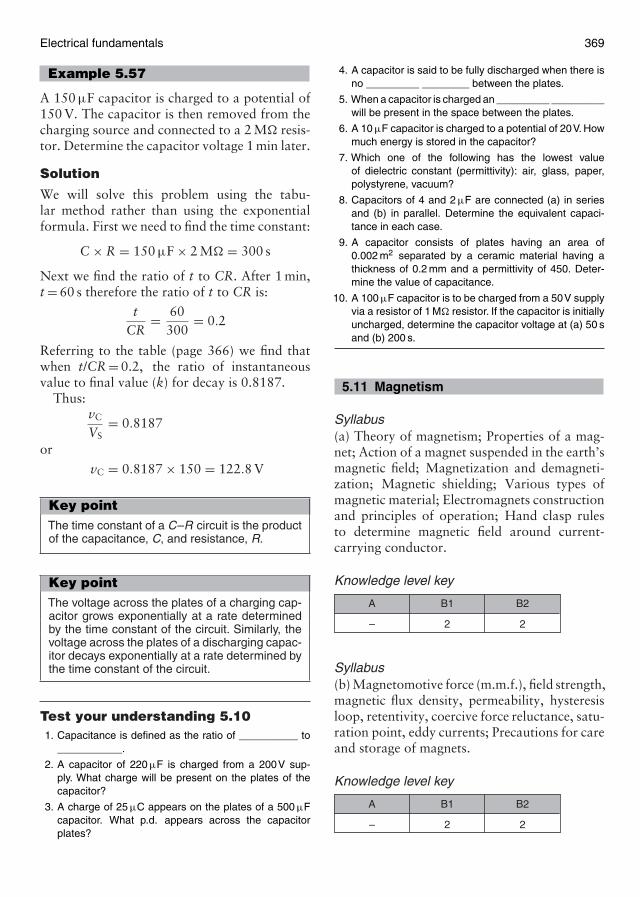
Electrical fundamentals 369
Example 5.57
A 150 µF capacitor is charged to a potential of150 V. The capacitor is then removed from thecharging source and connected to a 2 M� resis-tor. Determine the capacitor voltage 1 min later.
Solution
We will solve this problem using the tabu-lar method rather than using the exponentialformula. First we need to find the time constant:
C × R = 150 µF × 2 M� = 300 s
Next we find the ratio of t to CR. After 1 min,t = 60 s therefore the ratio of t to CR is:
tCR
= 60300
= 0.2
Referring to the table (page 366) we find thatwhen t/CR = 0.2, the ratio of instantaneousvalue to final value (k) for decay is 0.8187.
Thus:vC
VS= 0.8187
or
vC = 0.8187 × 150 = 122.8 V
Key pointThe time constant of a C–R circuit is the productof the capacitance, C, and resistance, R.
Key pointThe voltage across the plates of a charging cap-acitor grows exponentially at a rate determinedby the time constant of the circuit. Similarly, thevoltage across the plates of a discharging capac-itor decays exponentially at a rate determined bythe time constant of the circuit.
Test your understanding 5.101. Capacitance is defined as the ratio of __________ to
___________.
2. A capacitor of 220 µF is charged from a 200V sup-ply. What charge will be present on the plates of thecapacitor?
3. A charge of 25 µC appears on the plates of a 500 µFcapacitor. What p.d. appears across the capacitorplates?
4. A capacitor is said to be fully discharged when there isno _________ ________ between the plates.
5. When a capacitor is charged an _________ _________will be present in the space between the plates.
6. A 10 µF capacitor is charged to a potential of 20V. Howmuch energy is stored in the capacitor?
7. Which one of the following has the lowest valueof dielectric constant (permittivity): air, glass, paper,polystyrene, vacuum?
8. Capacitors of 4 and 2 µF are connected (a) in seriesand (b) in parallel. Determine the equivalent capaci-tance in each case.
9. A capacitor consists of plates having an area of0.002 m2 separated by a ceramic material having athickness of 0.2 mm and a permittivity of 450. Deter-mine the value of capacitance.
10. A 100 µF capacitor is to be charged from a 50V supplyvia a resistor of 1 M� resistor. If the capacitor is initiallyuncharged, determine the capacitor voltage at (a) 50 sand (b) 200 s.
5.11 Magnetism
Syllabus(a) Theory of magnetism; Properties of a mag-net; Action of a magnet suspended in the earth’smagnetic field; Magnetization and demagneti-zation; Magnetic shielding; Various types ofmagnetic material; Electromagnets constructionand principles of operation; Hand clasp rulesto determine magnetic field around current-carrying conductor.
Knowledge level key
–
A
2
B1
2
B2
Syllabus(b) Magnetomotive force (m.m.f.), field strength,magnetic flux density, permeability, hysteresisloop, retentivity, coercive force reluctance, satu-ration point, eddy currents; Precautions for careand storage of magnets.
Knowledge level key
–
A
2
B1
2
B2

370 Aircraft engineering principles
5.11.1 Magnetism and magneticmaterials
Magnetism is an effect created by moving theelementary atomic particles in certain materi-als such as iron, nickel and cobalt. Iron hasoutstanding magnetic properties and materialsthat behave magnetically, in a similar mannerto iron, are known as ferromagnetic materials.These materials experience forces that act onthem when placed near a magnet.
The atoms within these materials group insuch a way that they produce tiny individualmagnets with their own north and south poles.When subject to the influence of a magnet orwhen an electric current is passed through a coilsurrounding them, these individual tiny mag-nets line up and the material as a whole exhibitsmagnetic properties.
Figure 5.93(a) shows a ferromagnetic mate-rial that has not been influenced by the forcesgenerated from another magnet. In this case,the miniature magnets are oriented in a randommanner. Once the material is subject to the influ-ence of another magnet, then these miniaturemagnets line up (Figure 5.93(b)) and the mate-rial itself becomes magnetic with its own northand south poles.
Figure 5.93 The behaviour of ferromagneticmaterials.
5.11.2 Magnetic fields aroundpermanent magnets
A magnetic field of flux is the region in whichthe forces created by the magnet have influence.This field surrounds a magnet in all directions,being strongest at the end extremities of the mag-net, known as the poles. Magnetic fields aremapped by an arrangement of lines that givean indication of strength and direction of theflux as illustrated in Figure 5.94. When freelysuspended horizontally a magnet aligns itselfnorth and south parallel with the earth’s mag-netic field. Now because unlike poles attract, thenorth of the magnet aligns itself with the southmagnetic pole of the earth and the south poleof the magnet aligns itself with the earth’s northpole. This is why the extremities of the magnetare known as poles.
Permanent magnets should be carefully storedaway from other magnetic components and anysystems that might be affected by stray perma-nent fields. Furthermore, in order to ensure thata permanent magnet retains its magnetism it isusually advisable to store magnets in pairs usingsoft-iron keepers to link adjacent north andsouth poles. This arrangement ensures that thereis a completely closed path for the magnetic fluxproduced by the magnets.
Key pointA magnetic field of flux is the region in which theforces created by the magnet have influence.Thisfield surrounds a magnet in all directions and isconcentrated at the north and south poles of themagnet.
5.11.3 Electromagnetism
Whenever an electric current flows in a con-ductor a magnetic field is set up around theconductor in the form of concentric circles.The field is present along the whole length of theconductor and is strongest nearest to the con-ductor. Now like permanent magnets, this fieldalso has direction. The direction of the mag-netic field is dependent on the direction of thecurrent passing through the conductor and may
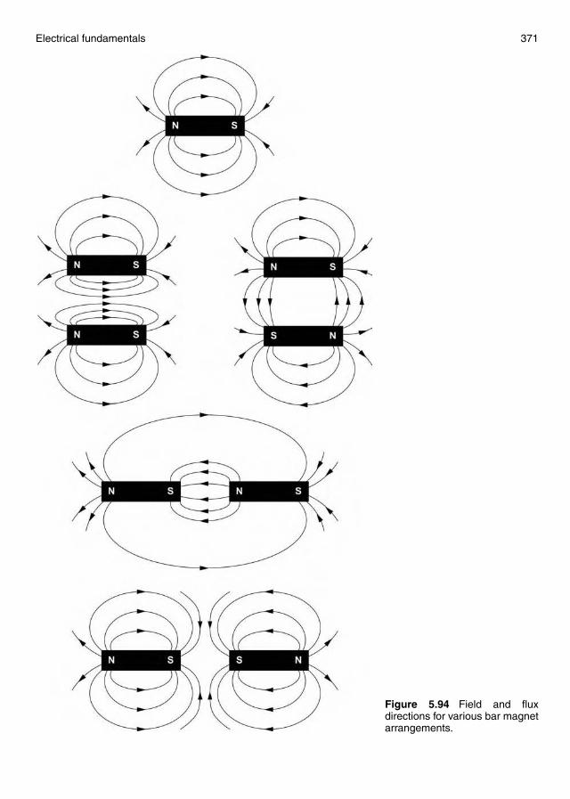
Electrical fundamentals 371
Figure 5.94 Field and fluxdirections for various bar magnetarrangements.
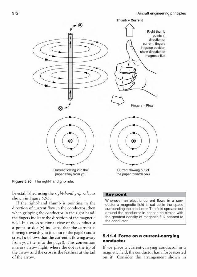
372 Aircraft engineering principles
Figure 5.95 The right-hand grip rule.
be established using the right-hand grip rule, asshown in Figure 5.95.
If the right-hand thumb is pointing in thedirection of current flow in the conductor, thenwhen gripping the conductor in the right hand,the fingers indicate the direction of the magneticfield. In a cross-sectional view of the conductora point or dot (•) indicates that the current isflowing towards you (i.e. out of the page!) and across (×) shows that the current is flowing awayfrom you (i.e. into the page!). This conventionmirrors arrow flight, where the dot is the tip ofthe arrow and the cross is the feathers at the tailof the arrow.
Key pointWhenever an electric current flows in a con-ductor a magnetic field is set up in the spacesurrounding the conductor. The field spreads outaround the conductor in concentric circles withthe greatest density of magnetic flux nearest tothe conductor.
5.11.4 Force on a current-carryingconductor
If we place a current-carrying conductor in amagnetic field, the conductor has a force exertedon it. Consider the arrangement shown in
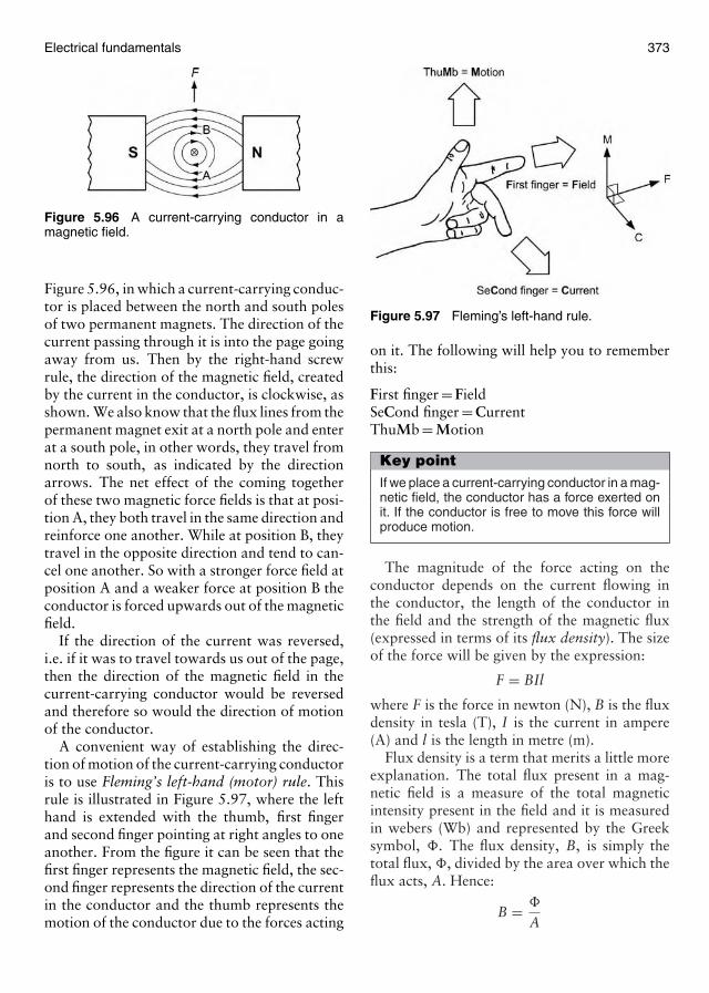
Electrical fundamentals 373
Figure 5.96 A current-carrying conductor in amagnetic field.
Figure 5.96, in which a current-carrying conduc-tor is placed between the north and south polesof two permanent magnets. The direction of thecurrent passing through it is into the page goingaway from us. Then by the right-hand screwrule, the direction of the magnetic field, createdby the current in the conductor, is clockwise, asshown. We also know that the flux lines from thepermanent magnet exit at a north pole and enterat a south pole, in other words, they travel fromnorth to south, as indicated by the directionarrows. The net effect of the coming togetherof these two magnetic force fields is that at posi-tion A, they both travel in the same direction andreinforce one another. While at position B, theytravel in the opposite direction and tend to can-cel one another. So with a stronger force field atposition A and a weaker force at position B theconductor is forced upwards out of the magneticfield.
If the direction of the current was reversed,i.e. if it was to travel towards us out of the page,then the direction of the magnetic field in thecurrent-carrying conductor would be reversedand therefore so would the direction of motionof the conductor.
A convenient way of establishing the direc-tion of motion of the current-carrying conductoris to use Fleming’s left-hand (motor) rule. Thisrule is illustrated in Figure 5.97, where the lefthand is extended with the thumb, first fingerand second finger pointing at right angles to oneanother. From the figure it can be seen that thefirst finger represents the magnetic field, the sec-ond finger represents the direction of the currentin the conductor and the thumb represents themotion of the conductor due to the forces acting
Figure 5.97 Fleming’s left-hand rule.
on it. The following will help you to rememberthis:
First finger = FieldSeCond finger = CurrentThuMb = Motion
Key pointIf we place a current-carrying conductor in a mag-netic field, the conductor has a force exerted onit. If the conductor is free to move this force willproduce motion.
The magnitude of the force acting on theconductor depends on the current flowing inthe conductor, the length of the conductor inthe field and the strength of the magnetic flux(expressed in terms of its flux density). The sizeof the force will be given by the expression:
F = BIl
where F is the force in newton (N), B is the fluxdensity in tesla (T), I is the current in ampere(A) and l is the length in metre (m).
Flux density is a term that merits a little moreexplanation. The total flux present in a mag-netic field is a measure of the total magneticintensity present in the field and it is measuredin webers (Wb) and represented by the Greeksymbol, �. The flux density, B, is simply thetotal flux, �, divided by the area over which theflux acts, A. Hence:
B = �
A
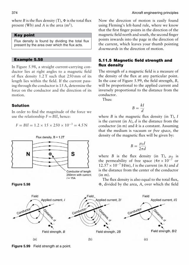
374 Aircraft engineering principles
where B is the flux density (T), � is the total fluxpresent (Wb) and A is the area (m2).
Key pointFlux density is found by dividing the total fluxpresent by the area over which the flux acts.
Example 5.58
In Figure 5.98, a straight current-carrying con-ductor lies at right angles to a magnetic fieldof flux density 1.2 T such that 250 mm of itslength lies within the field. If the current pass-ing through the conductor is 15 A, determine theforce on the conductor and the direction of itsmotion.
Solution
In order to find the magnitude of the force weuse the relationship F = BIl, hence:
F = BIl = 1.2 × 15 × 250 × 10−3 = 4.5 N
Figure 5.98
Figure 5.99 Field strength at a point.
Now the direction of motion is easily foundusing Fleming’s left-hand rule, where we knowthat the first finger points in the direction of themagnetic field north and south, the second fingerpoints inwards into the page in the direction ofthe current, which leaves your thumb pointingdownwards in the direction of motion.
5.11.5 Magnetic field strength andflux density
The strength of a magnetic field is a measure ofthe density of the flux at any particular point.In the case of Figure 5.99, the field strength, B,will be proportional to the applied current andinversely proportional to the distance from theconductor.
Thus:
B = kId
where B is the magnetic flux density (in T), Iis the current (in A), d is the distance from theconductor (in m) and k is a constant. Assumingthat the medium is vacuum or free space, thedensity of the magnetic flux will be given by:
B = µ0I2πd
where B is the flux density (in T), µ0 isthe permeability of free space (4π × 10−7 or12.57 × 10−7 H/m), I is the current (in A) and dis the distance from the center of the conductor(in m).
The flux density is also equal to the total flux,�, divided by the area, A, over which the field

Electrical fundamentals 375
acts. Thus:
B = �
A
where � is the flux (in Wb) and A is the area ofthe field (in m2).
In order to increase the strength of thefield, a conductor may be shaped into a loop(Figure 5.100) or coiled to form a solenoid(Figure 5.101).
Figure 5.100 Magnetic field around a singleturn loop.
Figure 5.101 Magnetic field around a coil orsolenoid.
Example 5.59
Determine the flux density produced at a dis-tance of 50 mm from a straight wire carrying acurrent of 20 A.
Solution
Applying the formula:
B = µ0I2πd
gives:
B = 12.57 × 10−7 × 206.28 × 5 × 10−3
= 251.431.4
× 10−4
= 8 × 10⁻⁴ T
or:
B = 0.8 mT
Example 5.60
A flux density of 2.5 mT is developed in freespace over an area of 20 cm2. Determine thetotal flux.
Solution
Re-arranging the formula B = �
Ato make � the
subject gives:
� = BA
thus:
� = 2.5 × 10−3 × 20 × 10−4
= 50 × 10−7 Wb or 5 µWb.
5.11.6 Magnetic circuits
Materials such as iron and steel possess con-siderably enhanced magnetic properties. Hencethey are employed in applications where it isnecessary to increase the flux density producedby an electric current. In effect, they allow us tochannel the electric flux into a magnetic circuit,as shown in Figure 5.102(b).

376 Aircraft engineering principles
In the circuit of Figure 5.102(b) the reluc-tance of the magnetic core is analogous to theresistance present in the electric circuit shownin Figure 5.102(a). We can make the fol-lowing comparisons between the two types of
Figure 5.102 Comparison of (a) electric and(b) magnetic circuits.
Figure 5.103 Leakage flux.
circuit:
Electric circuit Magnetic circuit
e.m.f. = V m.m.f. = N × IResistance = R Reluctance = SCurrent = I Flux = �
e.m.f. = current × m.m.f. = flux ×resistance reluctance
V = IR NI = S�
In practice, not all of the magnetic flux pro-duced in a magnetic circuit will be concentratedwithin the core and some leakage flux willappear in the surrounding free space (as shownin Figure 5.103). Similarly, if a gap appearswithin the magnetic circuit, the flux will tendto spread out as shown in Figure 5.104. Thiseffect is known as fringing.
Figure 5.104 Fringing.
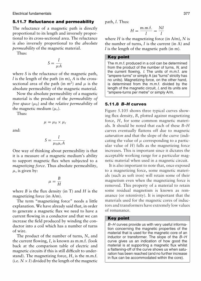
Electrical fundamentals 377
5.11.7 Reluctance and permeability
The reluctance of a magnetic path is directlyproportional to its length and inversely propor-tional to its cross-sectional area. The reluctanceis also inversely proportional to the absolutepermeability of the magnetic material.
Thus:
S = lµA
where S is the reluctance of the magnetic path,l is the length of the path (in m), A is the cross-sectional area of the path (in m2) and µ is theabsolute permeability of the magnetic material.
Now the absolute permeability of a magneticmaterial is the product of the permeability offree space (µ0) and the relative permeability ofthe magnetic medium (µr).
Thus:
µ = µ0 × µr
and:
S = lµ0µrA
One way of thinking about permeability is thatit is a measure of a magnetic medium’s abilityto support magnetic flux when subjected to amagnetizing force. Thus absolute permeability,µ, is given by:
µ = BH
where B is the flux density (in T) and H is themagnetizing force (in A/m).
The term “magnetizing force” needs a littleexplanation. We have already said that, in orderto generate a magnetic flux we need to have acurrent flowing in a conductor and that we canincrease the field produced by winding the con-ductor into a coil which has a number of turnsof wire.
The product of the number of turns, N, andthe current flowing, I, is known as m.m.f. (lookback at the comparison table of electric andmagnetic circuits if this is still difficult to under-stand). The magnetizing force, H, is the m.m.f.(i.e. N × I) divided by the length of the magnetic
path, l. Thus:
H = m.m.f.l
= NIl
where H is the magnetizing force (in A/m), N isthe number of turns, I is the current (in A) andl is the length of the magnetic path (in m).
Key pointThe m.m.f. produced in a coil can be determinedfrom the product of the number of turns, N, andthe current flowing, I. The units of m.m.f. are“ampere-turns” or simply A (as “turns” strictly hasno units). Magnetizing force, on the other hand,is determined from the m.m.f. divided by thelength of the magnetic circuit, l, and its units are“ampere-turns per metre” or simply A/m.
5.11.8 B–H curves
Figure 5.105 shows three typical curves show-ing flux density, B, plotted against magnetizingforce, H, for some common magnetic materi-als. It should be noted that each of these B–Hcurves eventually flattens off due to magneticsaturation and that the slope of the curve (indi-cating the value of µ corresponding to a partic-ular value of H) falls as the magnetizing forceincreases. This is important since it dictates theacceptable working range for a particular mag-netic material when used in a magnetic circuit.
It is also important to note that, once exposedto a magnetizing force, some magnetic materi-als (such as soft iron) will retain some of theirmagnetism even when the magnetizing force isremoved. This property of a material to retainsome residual magnetism is known as rem-anance (or retentivity). It is important that thematerials used for the magnetic cores of induc-tors and transformers have extremely low valuesof remanance.
Key pointB–H curves provide us with very useful informa-tion concerning the magnetic properties of thematerial that is used for the magnetic core of aninductor or transformer. The slope of the B–Hcurve gives us an indication of how good thematerial is at supporting a magnetic flux whilsta flattening-off of the curve shows us when satu-ration has been reached (and no further increasein flux can be accommodated within the core).

378 Aircraft engineering principles
Figure 5.105 Some typical B–Hcurves for common magnetic materials.
Example 5.61
Estimate the relative permeability of cast steel at(a) a flux density of 0.6 T and (b) a flux densityof 1.6 T.
Solution
From Figure 5.105, the slope of the graph atany point gives the value of µ at that point. Theslope can be found by constructing a tangent atthe point in question and finding the ratio ofvertical change to horizontal change.
(a) The slope of the graph, µ, at 0.6 T is
0.5500
= 1 × 10⁻³
Now since µ = µ0 × µr:
µr = µ
µ0= 1 × 10⁻³
12.57 × 10−7= 795
(b) The slope of the graph, µ, at 1.6 T is
0.061500
= 0.04 × 10⁻³
Now since µ = µ0 × µr:
µr = µ
µ0= 0.04 × 10⁻³
12.57 × 10−7= 31.8
Note: This example very clearly shows theeffect of saturation on the permeability of amagnetic material!
Example 5.62
A coil of 800 turns is wound on a closed mildsteel core having a length 600 mm and cross-sectional area 500 mm2. Determine the currentrequired to establish a flux of 0.8 mWb inthe core.
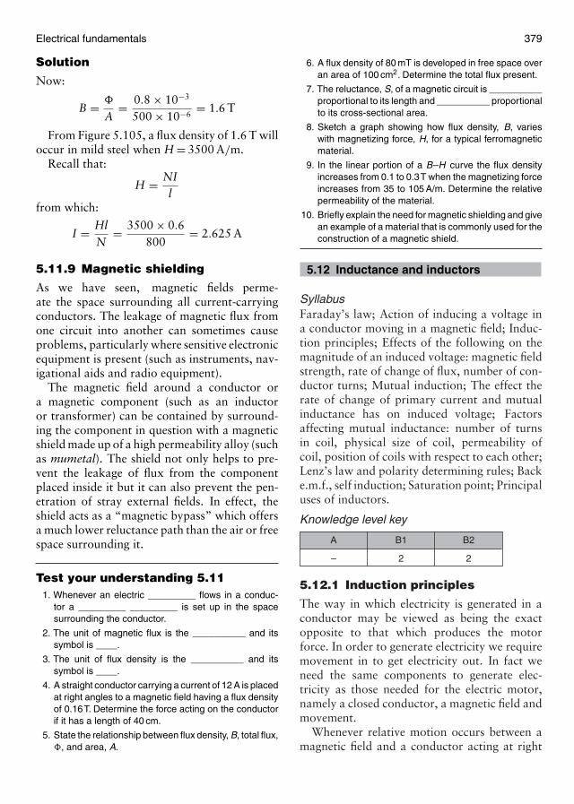
Electrical fundamentals 379
Solution
Now:
B = �
A= 0.8 × 10⁻³
500 × 10−6= 1.6 T
From Figure 5.105, a flux density of 1.6 T willoccur in mild steel when H = 3500 A/m.
Recall that:
H = NIl
from which:
I = HlN
= 3500 × 0.6800
= 2.625 A
5.11.9 Magnetic shielding
As we have seen, magnetic fields perme-ate the space surrounding all current-carryingconductors. The leakage of magnetic flux fromone circuit into another can sometimes causeproblems, particularly where sensitive electronicequipment is present (such as instruments, nav-igational aids and radio equipment).
The magnetic field around a conductor ora magnetic component (such as an inductoror transformer) can be contained by surround-ing the component in question with a magneticshield made up of a high permeability alloy (suchas mumetal). The shield not only helps to pre-vent the leakage of flux from the componentplaced inside it but it can also prevent the pen-etration of stray external fields. In effect, theshield acts as a “magnetic bypass” which offersa much lower reluctance path than the air or freespace surrounding it.
Test your understanding 5.111. Whenever an electric _________ flows in a conduc-
tor a _________ _________ is set up in the spacesurrounding the conductor.
2. The unit of magnetic flux is the __________ and itssymbol is ____.
3. The unit of flux density is the __________ and itssymbol is ____.
4. A straight conductor carrying a current of 12 A is placedat right angles to a magnetic field having a flux densityof 0.16T. Determine the force acting on the conductorif it has a length of 40 cm.
5. State the relationship between flux density, B, total flux,�, and area, A.
6. A flux density of 80 mT is developed in free space overan area of 100 cm2. Determine the total flux present.
7. The reluctance, S, of a magnetic circuit is __________proportional to its length and __________ proportionalto its cross-sectional area.
8. Sketch a graph showing how flux density, B, varieswith magnetizing force, H, for a typical ferromagneticmaterial.
9. In the linear portion of a B–H curve the flux densityincreases from 0.1 to 0.3T when the magnetizing forceincreases from 35 to 105 A/m. Determine the relativepermeability of the material.
10. Briefly explain the need for magnetic shielding and givean example of a material that is commonly used for theconstruction of a magnetic shield.
5.12 Inductance and inductors
SyllabusFaraday’s law; Action of inducing a voltage ina conductor moving in a magnetic field; Induc-tion principles; Effects of the following on themagnitude of an induced voltage: magnetic fieldstrength, rate of change of flux, number of con-ductor turns; Mutual induction; The effect therate of change of primary current and mutualinductance has on induced voltage; Factorsaffecting mutual inductance: number of turnsin coil, physical size of coil, permeability ofcoil, position of coils with respect to each other;Lenz’s law and polarity determining rules; Backe.m.f., self induction; Saturation point; Principaluses of inductors.
Knowledge level key
–
A
2
B1
2
B2
5.12.1 Induction principles
The way in which electricity is generated in aconductor may be viewed as being the exactopposite to that which produces the motorforce. In order to generate electricity we requiremovement in to get electricity out. In fact weneed the same components to generate elec-tricity as those needed for the electric motor,namely a closed conductor, a magnetic field andmovement.
Whenever relative motion occurs between amagnetic field and a conductor acting at right
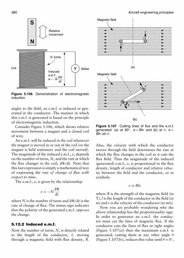
380 Aircraft engineering principles
Figure 5.106 Demonstration of electromagneticinduction.
angles to the field, an e.m.f. is induced or gen-erated in the conductor. The manner in whichthis e.m.f. is generated is based on the principleof electromagnetic induction.
Consider Figure 5.106, which shows relativemovement between a magnet and a closed coilof wire.
An e.m.f. will be induced in the coil wheneverthe magnet is moved in or out of the coil (or themagnet is held stationary and the coil moved).The magnitude of the induced e.m.f., e, dependson the number of turns, N, and the rate at whichthe flux changes in the coil, d�/dt. Note thatthis last expression is simply a mathematical wayof expressing the rate of change of flux withrespect to time.
The e.m.f., e, is given by the relationship:
e = −Nd�
dt
where N is the number of turns and d�/dt is therate of change of flux. The minus sign indicatesthat the polarity of the generated e.m.f. opposesthe change.
5.12.2 Induced e.m.f.
Now the number of turns, N, is directly relatedto the length of the conductor, l, movingthrough a magnetic field with flux density, B.
Figure 5.107 Cutting lines of flux and the e.m.f.generated: (a) at 90◦, e = Blv and (b) at θ, e =Blv sin θ.
Also, the velocity with which the conductormoves through the field determines the rate atwhich the flux changes in the coil as it cuts theflux field. Thus the magnitude of the induced(generated) e.m.f., e, is proportional to the fluxdensity, length of conductor and relative veloc-ity between the field and the conductor, or insymbols:
e ∝ Blv
where B is the strength of the magnetic field (inT), l is the length of the conductor in the field (inm) and v is the velocity of the conductor (in m/s).
Now you are probably wondering why theabove relationship has the proportionality sign.In order to generator an e.m.f. the conduc-tor must cut the lines of magnetic flux. If theconductor cuts the lines of flux at right angles(Figure 5.107(a)) then the maximum e.m.f. isgenerated; cutting them at any other angle θ
(Figure 5.107(b)), reduces this value until θ = 0◦,
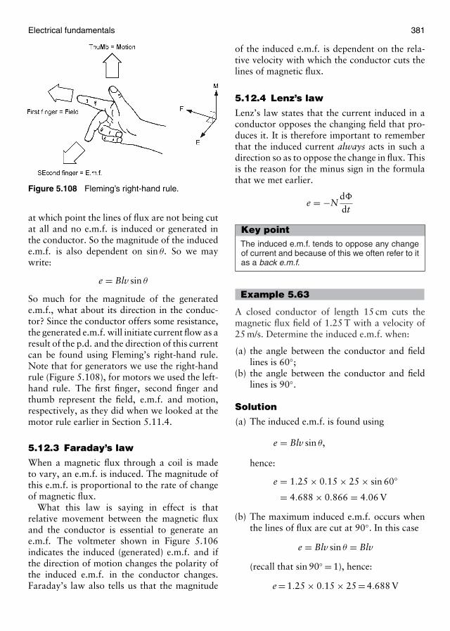
Electrical fundamentals 381
Figure 5.108 Fleming’s right-hand rule.
at which point the lines of flux are not being cutat all and no e.m.f. is induced or generated inthe conductor. So the magnitude of the inducede.m.f. is also dependent on sin θ. So we maywrite:
e = Blv sin θ
So much for the magnitude of the generatede.m.f., what about its direction in the conduc-tor? Since the conductor offers some resistance,the generated e.m.f. will initiate current flow as aresult of the p.d. and the direction of this currentcan be found using Fleming’s right-hand rule.Note that for generators we use the right-handrule (Figure 5.108), for motors we used the left-hand rule. The first finger, second finger andthumb represent the field, e.m.f. and motion,respectively, as they did when we looked at themotor rule earlier in Section 5.11.4.
5.12.3 Faraday’s law
When a magnetic flux through a coil is madeto vary, an e.m.f. is induced. The magnitude ofthis e.m.f. is proportional to the rate of changeof magnetic flux.
What this law is saying in effect is thatrelative movement between the magnetic fluxand the conductor is essential to generate ane.m.f. The voltmeter shown in Figure 5.106indicates the induced (generated) e.m.f. and ifthe direction of motion changes the polarity ofthe induced e.m.f. in the conductor changes.Faraday’s law also tells us that the magnitude
of the induced e.m.f. is dependent on the rela-tive velocity with which the conductor cuts thelines of magnetic flux.
5.12.4 Lenz’s law
Lenz’s law states that the current induced in aconductor opposes the changing field that pro-duces it. It is therefore important to rememberthat the induced current always acts in such adirection so as to oppose the change in flux. Thisis the reason for the minus sign in the formulathat we met earlier.
e = −Nd�
dt
Key pointThe induced e.m.f. tends to oppose any changeof current and because of this we often refer to itas a back e.m.f.
Example 5.63
A closed conductor of length 15 cm cuts themagnetic flux field of 1.25 T with a velocity of25 m/s. Determine the induced e.m.f. when:
(a) the angle between the conductor and fieldlines is 60◦;
(b) the angle between the conductor and fieldlines is 90◦.
Solution
(a) The induced e.m.f. is found using
e = Blv sin θ,
hence:
e = 1.25 × 0.15 × 25 × sin 60◦
= 4.688 × 0.866 = 4.06 V
(b) The maximum induced e.m.f. occurs whenthe lines of flux are cut at 90◦. In this case
e = Blv sin θ = Blv
(recall that sin 90◦ = 1), hence:
e = 1.25 × 0.15 × 25 = 4.688 V
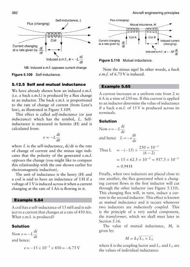
382 Aircraft engineering principles
Figure 5.109 Self-inductance.
5.12.5 Self and mutual inductance
We have already shown how an induced e.m.f.(i.e. a back e.m.f.) is produced by a flux changein an inductor. The back e.m.f. is proportionalto the rate of change of current (from Lenz’slaw), as illustrated in Figure 5.109.
This effect is called self-inductance (or justinductance) which has the symbol, L. Self-inductance is measured in henries (H) and iscalculated from:
e = −Ldidt
where L is the self-inductance, di/dt is the rateof change of current and the minus sign indi-cates that the polarity of the generated e.m.f.opposes the change (you might like to comparethis relationship with the one shown earlier forelectromagnetic induction).
The unit of inductance is the henry (H) anda coil is said to have an inductance of 1 H if avoltage of 1 V is induced across it when a currentchanging at the rate of 1 A/s is flowing in it.
Example 5.64
A coil has a self-inductance of 15 mH and is sub-ject to a current that changes at a rate of 450 A/s.What e.m.f. is produced?
Solution
Now e = −Ldidt
and hence:
e = −15 × 10−3 × 450 = −6.75 V
Figure 5.110 Mutual inductance.
Note the minus sign! In other words, a backe.m.f. of 6.75 V is induced.
Example 5.65
A current increases at a uniform rate from 2 to6 A in a time of 250 ms. If this current is appliedto an inductor determine the value of inductanceif a back e.m.f. of 15 V is produced across itsterminals.
Solution
Now e = −Ldidt
and hence L = −edtdi
Thus L = −(−15) × 250 × 10−3
(6 − 2)
= 15 × 62.5 × 10−3 = 937.5 × 10−3
= 0.94 H
Finally, when two inductors are placed close toone another, the flux generated when a chang-ing current flows in the first inductor will cutthrough the other inductor (see Figure 5.110).This changing flux will, in turn, induce a cur-rent in the second inductor. This effect is knownas mutual inductance and it occurs whenevertwo inductors are inductively coupled. Thisis the principle of a very useful component,the transformer, which we shall meet later inSection 5.16.
The value of mutual inductance, M, isgiven by:
M = k√
L1 × L2
where k is the coupling factor and L1 and L2 arethe values of individual inductance.
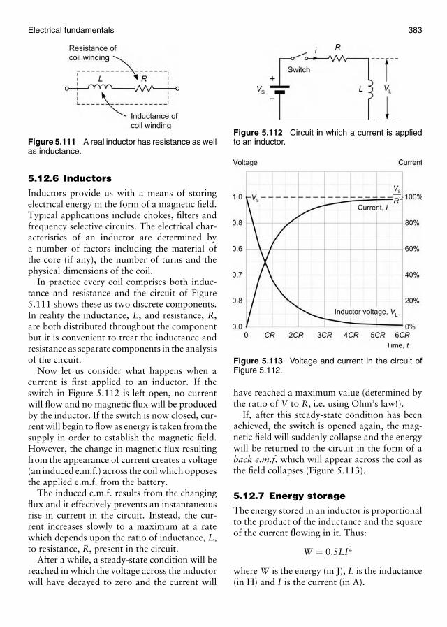
Electrical fundamentals 383
Figure 5.111 A real inductor has resistance as wellas inductance.
5.12.6 Inductors
Inductors provide us with a means of storingelectrical energy in the form of a magnetic field.Typical applications include chokes, filters andfrequency selective circuits. The electrical char-acteristics of an inductor are determined bya number of factors including the material ofthe core (if any), the number of turns and thephysical dimensions of the coil.
In practice every coil comprises both induc-tance and resistance and the circuit of Figure5.111 shows these as two discrete components.In reality the inductance, L, and resistance, R,are both distributed throughout the componentbut it is convenient to treat the inductance andresistance as separate components in the analysisof the circuit.
Now let us consider what happens when acurrent is first applied to an inductor. If theswitch in Figure 5.112 is left open, no currentwill flow and no magnetic flux will be producedby the inductor. If the switch is now closed, cur-rent will begin to flow as energy is taken from thesupply in order to establish the magnetic field.However, the change in magnetic flux resultingfrom the appearance of current creates a voltage(an induced e.m.f.) across the coil which opposesthe applied e.m.f. from the battery.
The induced e.m.f. results from the changingflux and it effectively prevents an instantaneousrise in current in the circuit. Instead, the cur-rent increases slowly to a maximum at a ratewhich depends upon the ratio of inductance, L,to resistance, R, present in the circuit.
After a while, a steady-state condition will bereached in which the voltage across the inductorwill have decayed to zero and the current will
Figure 5.112 Circuit in which a current is appliedto an inductor.
Figure 5.113 Voltage and current in the circuit ofFigure 5.112.
have reached a maximum value (determined bythe ratio of V to R, i.e. using Ohm’s law!).
If, after this steady-state condition has beenachieved, the switch is opened again, the mag-netic field will suddenly collapse and the energywill be returned to the circuit in the form of aback e.m.f. which will appear across the coil asthe field collapses (Figure 5.113).
5.12.7 Energy storage
The energy stored in an inductor is proportionalto the product of the inductance and the squareof the current flowing in it. Thus:
W = 0.5LI2
where W is the energy (in J), L is the inductance(in H) and I is the current (in A).
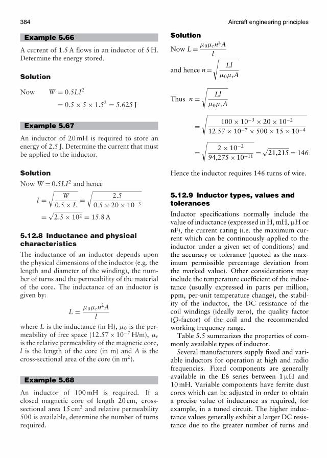
384 Aircraft engineering principles
Example 5.66
A current of 1.5 A flows in an inductor of 5 H.Determine the energy stored.
Solution
Now W = 0.5LI2
= 0.5 × 5 × 1.52 = 5.625 J
Example 5.67
An inductor of 20 mH is required to store anenergy of 2.5 J. Determine the current that mustbe applied to the inductor.
Solution
Now W = 0.5LI2 and hence
I =√
W0.5 × L
=√
2.50.5 × 20 × 10−3
=√
2.5 × 102 = 15.8 A
5.12.8 Inductance and physicalcharacteristics
The inductance of an inductor depends uponthe physical dimensions of the inductor (e.g. thelength and diameter of the winding), the num-ber of turns and the permeability of the materialof the core. The inductance of an inductor isgiven by:
L = µ0µrn2Al
where L is the inductance (in H), µ0 is the per-meability of free space (12.57 × 10⁻⁷ H/m), µr
is the relative permeability of the magnetic core,l is the length of the core (in m) and A is thecross-sectional area of the core (in m2).
Example 5.68
An inductor of 100 mH is required. If aclosed magnetic core of length 20 cm, cross-sectional area 15 cm2 and relative permeability500 is available, determine the number of turnsrequired.
Solution
Now L = µ0µrn2Al
and hence n =√
Llµ0µrA
Thus n =√
Llµ0µrA
=√
100 × 10−3 × 20 × 10−2
12.57 × 10−7 × 500 × 15 × 10−4
=√
2 × 10⁻²
94,275 × 10−11=√
21,215 = 146
Hence the inductor requires 146 turns of wire.
5.12.9 Inductor types, values andtolerances
Inductor specifications normally include thevalue of inductance (expressed in H, mH, µH ornF), the current rating (i.e. the maximum cur-rent which can be continuously applied to theinductor under a given set of conditions) andthe accuracy or tolerance (quoted as the max-imum permissible percentage deviation fromthe marked value). Other considerations mayinclude the temperature coefficient of the induc-tance (usually expressed in parts per million,ppm, per-unit temperature change), the stabil-ity of the inductor, the DC resistance of thecoil windings (ideally zero), the quality factor(Q-factor) of the coil and the recommendedworking frequency range.
Table 5.5 summarizes the properties of com-monly available types of inductor.
Several manufacturers supply fixed and vari-able inductors for operation at high and radiofrequencies. Fixed components are generallyavailable in the E6 series between 1 µH and10 mH. Variable components have ferrite dustcores which can be adjusted in order to obtaina precise value of inductance as required, forexample, in a tuned circuit. The higher induc-tance values generally exhibit a larger DC resis-tance due to the greater number of turns and

Electrical fundamentals 385
Table 5.5
Characteristic Inductor type
Single-layer open Multi-layer open Multi-layer Multi-layerpot cored iron cored
Core material Air Ferrite Air Ferrite Ferrite IronInductance range 50 nH 1 µH 5 µH 10 µH 1 mH 20 mH
to 10 µH to 100 µH to 500 µH to 1 mH to 100 mH to 20 HTypical tolerance ±10% ±10% ±10% ±10% ±10% ±10%Typical current 0.1 A 0.1 A 0.2 A 0.5 A 0.5 A 0.2 AratingTypical DC 0.05 � to 1 � 0.1 � to 10 � 1 � to 20 � 2 � to 100 � 2 � to 100 � 10 � to 400 �resistanceTypical Q-factor 60 80 100 80 40 20Typical frequency 5 MHz to 1 MHz to 200 kHz to 100 kHz to 1 kHz to 50 Hz torange 500 MHz 500 MHz 20 MHz 10 MHz 1 MHz 1 kHzTypical Tuned Tuned Filters Filters LF and MF LF chokesapplications circuits circuits and HF and HF chokes and and
transformers transformers transformers transformers
relatively small diameter of wire used in theirconstruction.
At medium and low frequencies, inductorsare often manufactured using one of a rangeof ferrite pot cores. The core material of theseinductors is commonly available in several andthe complete pot core assembly comprises amatched pair of core halves, a single-sectionbobbin, a pair of retaining clips and a coreadjuster. Effectively, the coil winding is totallyenclosed in a high permeability ferrite pot. Typ-ical values of inductance for these componentsrange between 100 µH and 100 mH with atypical saturation flux density of 250 mT.
Inductance values of iron cored inductors arevery much dependent upon the applied DC andtend to fall rapidly as the value of applied DCincreases and saturation is approached. Max-imum current ratings for larger inductors arerelated to operating temperatures and should bede-rated when high ambient temperatures areexpected. Where reliability is important, induc-tors should be operated at well below theirnominal maximum current ratings.
Finally, ferrite (a high permeability non-conductive magnetic material) is often used asthe core material for inductors used in high-frequency filters and as broadband transformers
Figure 5.114 Various inductors.
at frequencies of up to 30 MHz. At these fre-quencies, inductors can be realized very easilyusing these cores with just a few turns of wire(Figure 5.114)!
Key pointThe specifications for an inductor resistor usu-ally include the value of inductance (expressedin H, mH or µH), the current rating (quoted as themaximum permissible percentage deviation fromthe marked value) and the DC resistance (thisis the resistance of the coil windings measuredin �). The Q-factor and frequency range arealso important considerations for certain types ofinductor.
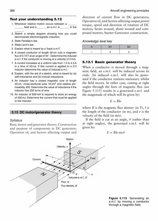
386 Aircraft engineering principles
Test your understanding 5.121. Whenever relative motion occurs between a ______
______ field and a ______ an e.m.f. is ______ in the______.
2. Sketch a simple diagram showing how you coulddemonstrate electromagnetic induction.
3. State Faraday’s law.
4. State Lenz’s law.
5. Explain what is meant by a “back e.m.f.”
6. A closed conductor of length 50 cm cuts a magneticflux of 0.75T at an angle of 45◦. Determine the inducede.m.f. if the conductor is moving at a velocity of 5 m/s.
7. A current increases at a uniform rate from 1.5 to 4.5 Ain a time of 50 ms. If this current is applied to a 2 Hinductor determine the value of induced e.m.f.
8. Explain, with the aid of a sketch, what is meant by (a)self-inductance and (b) mutual inductance.
9. An inductor has a closed magnetic core of length40 cm, cross-sectional area 10 cm2 and relative per-meability 450. Determine the value of inductance if theinductor has 250 turns of wire.
10. An inductor of 600 mH is required to store an energyof 400 mJ. Determine the current that must be appliedto the inductor.
5.13 DC motor/generator theory
SyllabusBasic motor and generator theory; Constructionand purpose of components in DC generator;Operation of, and factors affecting output and
Figure 5.115 Generating ane.m.f. by moving a conductorthrough a magnetic field.
direction of current flow in DC generators;Operation of, and factors affecting output powertorque, speed and direction of rotation of DCmotors; Series wound, shunt wound and com-pound motors; Starter-Generator construction.
Knowledge level key
–
A
2
B1
2
B2
5.13.1 Basic generator theory
When a conductor is moved through a mag-netic field, an e.m.f. will be induced across itsends. An induced e.m.f. will also be gener-ated if the conductor remains stationary whilstthe field moves. In either case, cutting at rightangles through the lines of magnetic flux (seeFigure 5.115) results in a generated e.m.f. andthe magnitude of which will be given by:
E = Blv
where B is the magnetic flux density (in T), l isthe length of the conductor (in m), and v is thevelocity of the field (in m/s).
If the field is cut at an angle, θ (rather thanat right angles), the generated e.m.f. will begiven by:
E = Blv sin θ
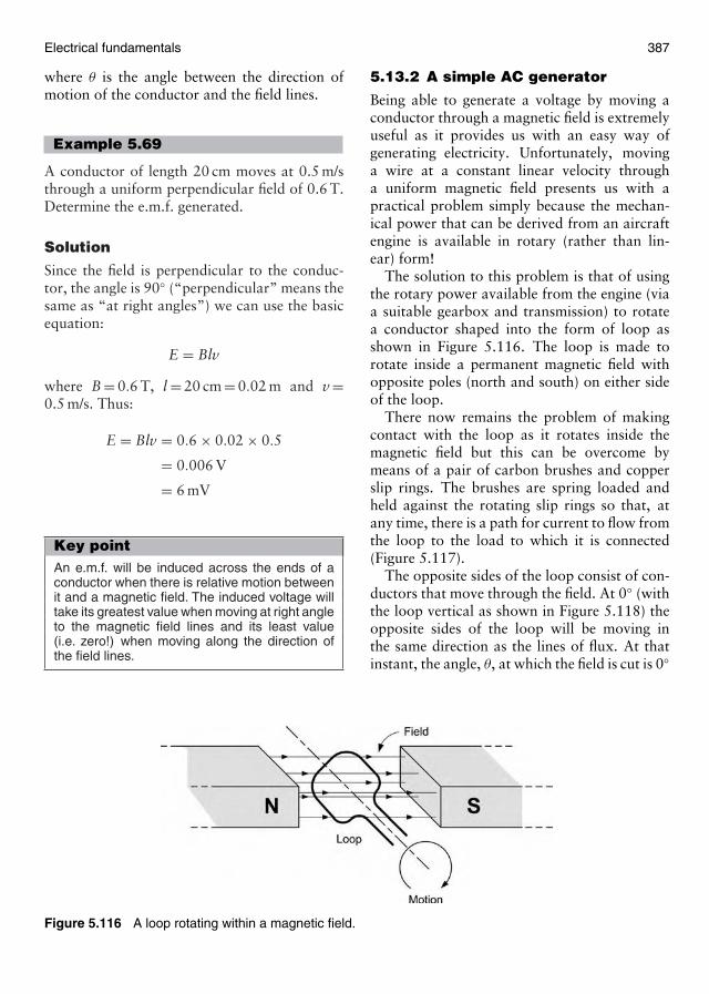
Electrical fundamentals 387
where θ is the angle between the direction ofmotion of the conductor and the field lines.
Example 5.69
A conductor of length 20 cm moves at 0.5 m/sthrough a uniform perpendicular field of 0.6 T.Determine the e.m.f. generated.
Solution
Since the field is perpendicular to the conduc-tor, the angle is 90◦ (“perpendicular” means thesame as “at right angles”) we can use the basicequation:
E = Blv
where B = 0.6 T, l = 20 cm = 0.02 m and v =0.5 m/s. Thus:
E = Blv = 0.6 × 0.02 × 0.5
= 0.006 V
= 6 mV
Key pointAn e.m.f. will be induced across the ends of aconductor when there is relative motion betweenit and a magnetic field. The induced voltage willtake its greatest value when moving at right angleto the magnetic field lines and its least value(i.e. zero!) when moving along the direction ofthe field lines.
Figure 5.116 A loop rotating within a magnetic field.
5.13.2 A simple AC generator
Being able to generate a voltage by moving aconductor through a magnetic field is extremelyuseful as it provides us with an easy way ofgenerating electricity. Unfortunately, movinga wire at a constant linear velocity througha uniform magnetic field presents us with apractical problem simply because the mechan-ical power that can be derived from an aircraftengine is available in rotary (rather than lin-ear) form!
The solution to this problem is that of usingthe rotary power available from the engine (viaa suitable gearbox and transmission) to rotatea conductor shaped into the form of loop asshown in Figure 5.116. The loop is made torotate inside a permanent magnetic field withopposite poles (north and south) on either sideof the loop.
There now remains the problem of makingcontact with the loop as it rotates inside themagnetic field but this can be overcome bymeans of a pair of carbon brushes and copperslip rings. The brushes are spring loaded andheld against the rotating slip rings so that, atany time, there is a path for current to flow fromthe loop to the load to which it is connected(Figure 5.117).
The opposite sides of the loop consist of con-ductors that move through the field. At 0◦ (withthe loop vertical as shown in Figure 5.118) theopposite sides of the loop will be moving inthe same direction as the lines of flux. At thatinstant, the angle, θ, at which the field is cut is 0◦

388 Aircraft engineering principles
Figure 5.117 Brush arrangement.
Figure 5.118 The e.m.f. generated at various angles.
and since the sine of 0◦ is 0 the generated volt-age (from E = Blv sin θ) will consequently alsobe zero.
If the loop has rotated to a position which is90◦ from that shown in Figure 5.118, the twoconductors will effectively be moving at right
angles to the field. At that instant, the generatede.m.f. will take a maximum value (since the sineof 90◦ is 1).
At 180◦ from the starting position the gener-ated e.m.f. will have fallen back to zero since,once again, the conductors are moving along
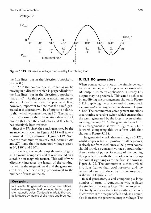
Electrical fundamentals 389
Figure 5.119 Sinusoidal voltage produced by the rotating loop.
the flux lines (but in the direction opposite tothat at 0◦).
At 270◦ the conductors will once again bemoving in a direction which is perpendicular tothe flux lines (but in the direction opposite tothat at 90◦). At this point, a maximum gener-ated e.m.f. will once again be produced. It is,however, important to note that the e.m.f. gen-erated at this instant will be of opposite polarityto that which was generated at 90◦. The reasonfor this is simply that the relative direction ofmotion (between the conductors and flux lines)has effectively been reversed.
Since E = Blv sin θ, the e.m.f. generated by thearrangement shown in Figure 5.118 will take asinusoidal form, as shown in Figure 5.119. Notethat the maximum values of e.m.f. occur at 90◦and 270◦, and that the generated voltage is zeroat 0◦, 180◦ and 360◦.
In practice, the single loop shown in Figure5.118 would comprise a coil of wire wound on asuitable non-magnetic former. This coil of wireeffectively increases the length of the conduc-tor within the magnetic field and the generatede.m.f. will then be directly proportional to thenumber of turns on the coil.
Key pointIn a simple AC generator a loop of wire rotatesinside the magnetic field produced by two oppo-site magnetic poles. Contact is made to the loopas it rotates by means of slip rings and brushes.
5.13.3 DC generators
When connected to a load, the simple genera-tor shown in Figure 5.118 produces a sinusoidalAC output. In many applications a steady DCoutput may be preferred. This can be achievedby modifying the arrangement shown in Figure5.118, replacing the brushes and slip rings witha commutator arrangement, as shown in Figure5.120. The commutator arrangement functionsas a rotating reversing switch which ensures thatthe e.m.f. generated by the loop is reversed afterrotating through 180◦. The generated e.m.f. forthis arrangement is shown in Figure 5.121. Itis worth comparing this waveform with thatshown in Figure 5.118.
The generated e.m.f. shown in Figure 5.121,whilst unipolar (i.e. all positive or all negative),is clearly far from ideal since a DC power sourceshould provide a constant voltage output ratherthan a series of pulses. One way of overcomingthis problem is with the use of a second loop(or coil) at right angles to the first, as shown inFigure 5.122. The commutator is then dividedinto four (rather than two) segments and thegenerated e.m.f. produced by this arrangementis shown in Figure 5.123.
In real generators, a coil comprising a largenumber of turns of conducting wire replacesthe single-turn rotating loop. This arrangementeffectively increases the total length of the con-ductor within the magnetic field and, as a result,also increases the generated output voltage. The
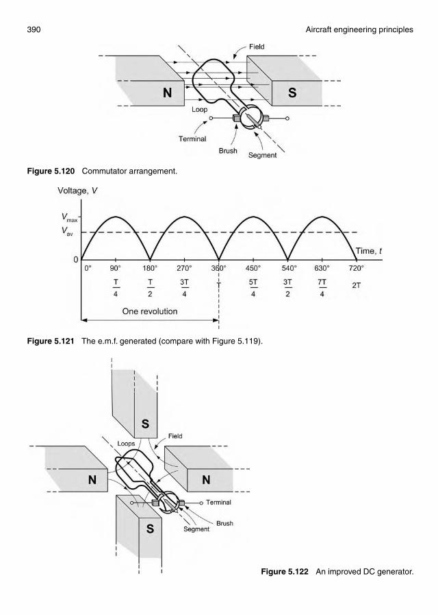
390 Aircraft engineering principles
Figure 5.120 Commutator arrangement.
Figure 5.121 The e.m.f. generated (compare with Figure 5.119).
Figure 5.122 An improved DC generator.
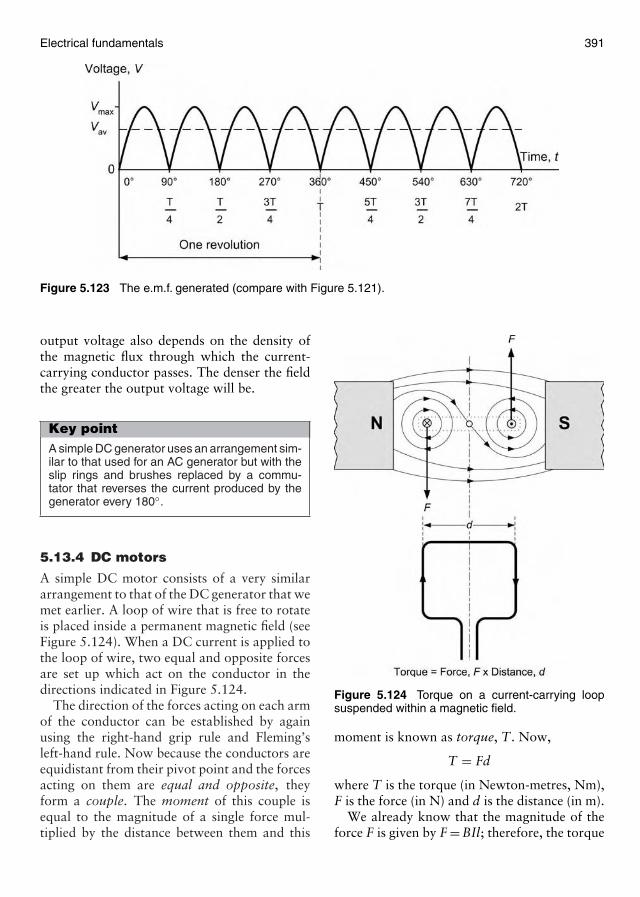
Electrical fundamentals 391
Figure 5.123 The e.m.f. generated (compare with Figure 5.121).
output voltage also depends on the density ofthe magnetic flux through which the current-carrying conductor passes. The denser the fieldthe greater the output voltage will be.
Key pointA simple DC generator uses an arrangement sim-ilar to that used for an AC generator but with theslip rings and brushes replaced by a commu-tator that reverses the current produced by thegenerator every 180◦.
5.13.4 DC motors
A simple DC motor consists of a very similararrangement to that of the DC generator that wemet earlier. A loop of wire that is free to rotateis placed inside a permanent magnetic field (seeFigure 5.124). When a DC current is applied tothe loop of wire, two equal and opposite forcesare set up which act on the conductor in thedirections indicated in Figure 5.124.
The direction of the forces acting on each armof the conductor can be established by againusing the right-hand grip rule and Fleming’sleft-hand rule. Now because the conductors areequidistant from their pivot point and the forcesacting on them are equal and opposite, theyform a couple. The moment of this couple isequal to the magnitude of a single force mul-tiplied by the distance between them and this
Figure 5.124 Torque on a current-carrying loopsuspended within a magnetic field.
moment is known as torque, T. Now,
T = Fd
where T is the torque (in Newton-metres, Nm),F is the force (in N) and d is the distance (in m).
We already know that the magnitude of theforce F is given by F = BIl; therefore, the torque
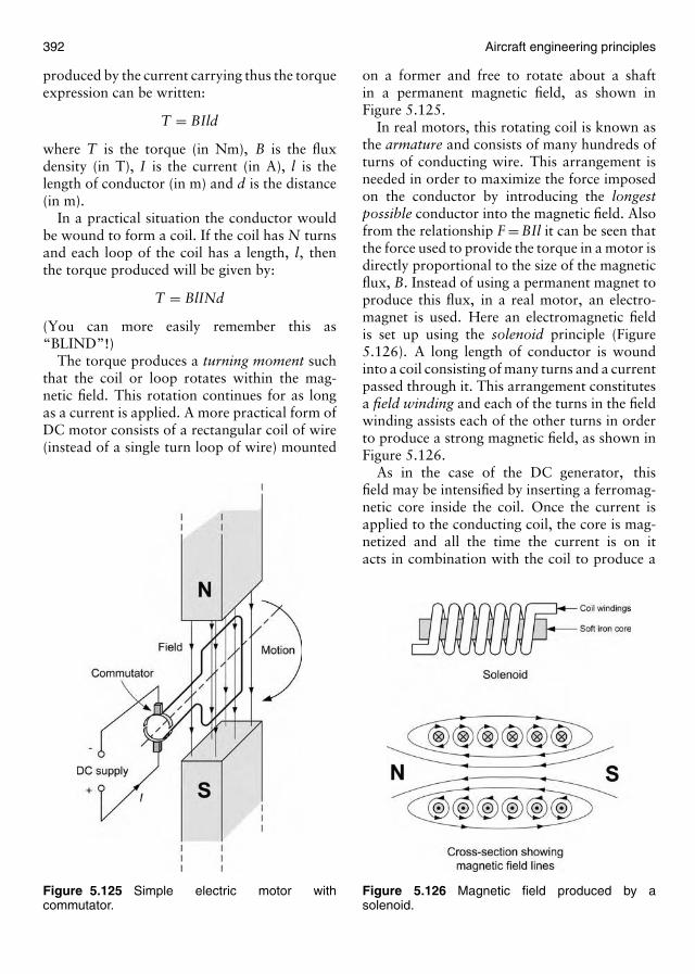
392 Aircraft engineering principles
produced by the current carrying thus the torqueexpression can be written:
T = BIld
where T is the torque (in Nm), B is the fluxdensity (in T), I is the current (in A), l is thelength of conductor (in m) and d is the distance(in m).
In a practical situation the conductor wouldbe wound to form a coil. If the coil has N turnsand each loop of the coil has a length, l, thenthe torque produced will be given by:
T = BlINd
(You can more easily remember this as“BLIND”!)
The torque produces a turning moment suchthat the coil or loop rotates within the mag-netic field. This rotation continues for as longas a current is applied. A more practical form ofDC motor consists of a rectangular coil of wire(instead of a single turn loop of wire) mounted
Figure 5.125 Simple electric motor withcommutator.
on a former and free to rotate about a shaftin a permanent magnetic field, as shown inFigure 5.125.
In real motors, this rotating coil is known asthe armature and consists of many hundreds ofturns of conducting wire. This arrangement isneeded in order to maximize the force imposedon the conductor by introducing the longestpossible conductor into the magnetic field. Alsofrom the relationship F = BIl it can be seen thatthe force used to provide the torque in a motor isdirectly proportional to the size of the magneticflux, B. Instead of using a permanent magnet toproduce this flux, in a real motor, an electro-magnet is used. Here an electromagnetic fieldis set up using the solenoid principle (Figure5.126). A long length of conductor is woundinto a coil consisting of many turns and a currentpassed through it. This arrangement constitutesa field winding and each of the turns in the fieldwinding assists each of the other turns in orderto produce a strong magnetic field, as shown inFigure 5.126.
As in the case of the DC generator, thisfield may be intensified by inserting a ferromag-netic core inside the coil. Once the current isapplied to the conducting coil, the core is mag-netized and all the time the current is on itacts in combination with the coil to produce a
Figure 5.126 Magnetic field produced by asolenoid.

Electrical fundamentals 393
permanent magnet, having its own north–southpoles.
Now returning to the simple motor illustratedin Figure 5.125, we know that when currentis supplied to the armature (rotor) a torque isproduced. In order to produce continuousrotary motion, this torque (turning moment)must always act in the same direction.
Therefore, the current in each of the armatureconductors must be reversed as the conductorpasses between the north and south magneticfield poles. The commutator acts like a rotatingswitch, reversing the current in each armatureconductor at the appropriate time to achieve thiscontinuous rotary motion. Without the presenceof a commutator in a DC motor, only a half-turnof movement is possible!
In Figure 5.127(a) the rotation of the arma-ture conductor is given by Fleming’s left-handrule. When the coil reaches a position mid-waybetween the poles (Figure 5.127(b)), no rota-tional torque is produced in the coil. At thisstage the commutator reverses the current in thecoil. Finally (Figure 5.127(c)) with the currentreversed, the motor torque now continues torotate the coil in its original direction.
Figure 5.127 Action of the commutator.
Key pointThe torque produced by a DC motor is directlyproportional to the product of the current flowingin the rotating armature winding.
Example 5.70
The rectangular armature shown in Figure5.128 is wound with 500 turns of wire. Whensituated in a uniform magnetic field of flux den-sity 300 mT, the current in the coil is 20 mA.Calculate the force acting on the side of thecoil and the maximum torque acting on thearmature.
Solution
With this arrangement the ends of the conductorare not within the influence of the magnetic fieldand therefore have no force exerted on them.Therefore, the force acting on one length ofconductor can be found from F = BIl, thus:
F = BIl
= (300 × 10−3)(20 × 10−3)(30 × 10−3)
= 1.8 × 10⁻⁴ N
Then the force on one side of the coil is 500times this value, thus:
F = 500 × 1.8 × 10−4 = 9 × 10⁻² N
Figure 5.128
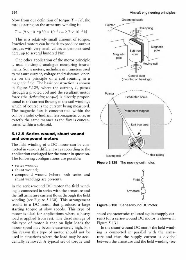
394 Aircraft engineering principles
Now from our definition of torque T = Fd, thetorque acting on the armature winding is:
T = (9 × 10⁻²)(30 × 10−3) = 2.7 × 10⁻³ N
This is a relatively small amount of torque.Practical motors can be made to produce outputtorques with very small values as demonstratedhere, up to several hundred Nm!
One other application of the motor principleis used in simple analogue measuring instru-ments. Some meters, including multimeters usedto measure current, voltage and resistance, oper-ate on the principle of a coil rotating in amagnetic field. The basic construction is shownin Figure 5.129, where the current, I, passesthrough a pivoted coil and the resultant motorforce (the deflecting torque) is directly propor-tional to the current flowing in the coil windingswhich of course is the current being measured.The magnetic flux is concentrated within thecoil by a solid cylindrical ferromagnetic core, inexactly the same manner as the flux is concen-trated within a solenoid.
5.13.5 Series wound, shunt woundand compound motors
The field winding of a DC motor can be con-nected in various different ways according to theapplication envisaged for the motor in question.The following configurations are possible:
• series wound;• shunt wound;• compound wound (where both series and
shunt windings are present).
In the series-wound DC motor the field wind-ing is connected in series with the armature andthe full armature current flows through the fieldwinding (see Figure 5.130). This arrangementresults in a DC motor that produces a largestarting torque at slow speeds. This type ofmotor is ideal for applications where a heavyload is applied from rest. The disadvantage ofthis type of motor is that on light loads themotor speed may become excessively high. Forthis reason this type of motor should not beused in situations where the load may be acci-dentally removed. A typical set of torque and
Figure 5.129 The moving-coil meter.
Figure 5.130 Series-wound DC motor.
speed characteristics (plotted against supply cur-rent) for a series-wound DC motor is shown inFigure 5.131.
In the shunt-wound DC motor the field wind-ing is connected in parallel with the arma-ture and thus the supply current is dividedbetween the armature and the field winding (see
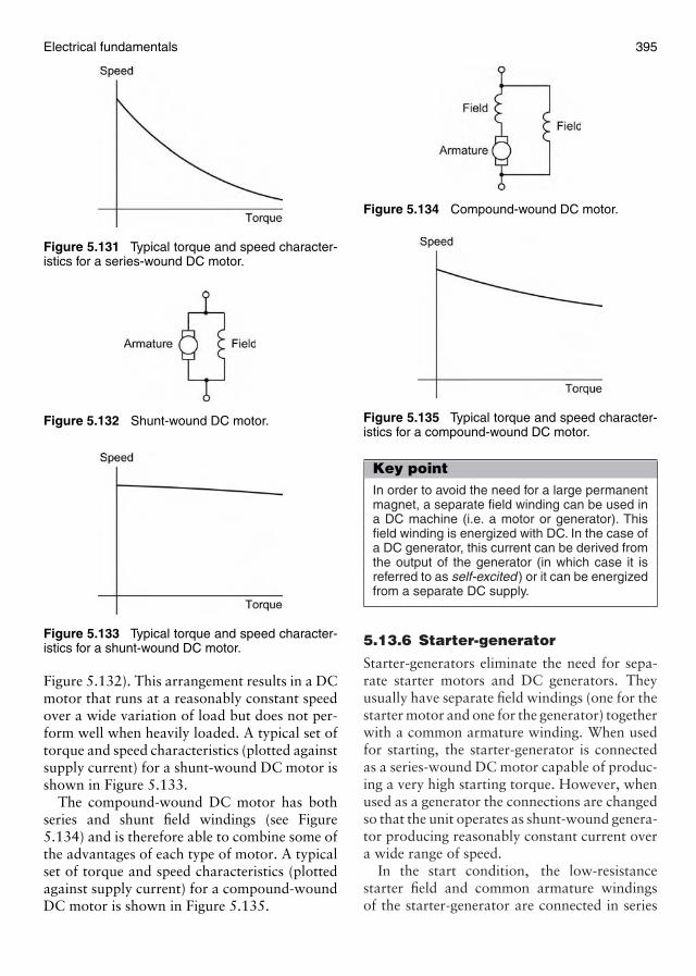
Electrical fundamentals 395
Figure 5.131 Typical torque and speed character-istics for a series-wound DC motor.
Figure 5.132 Shunt-wound DC motor.
Figure 5.133 Typical torque and speed character-istics for a shunt-wound DC motor.
Figure 5.132). This arrangement results in a DCmotor that runs at a reasonably constant speedover a wide variation of load but does not per-form well when heavily loaded. A typical set oftorque and speed characteristics (plotted againstsupply current) for a shunt-wound DC motor isshown in Figure 5.133.
The compound-wound DC motor has bothseries and shunt field windings (see Figure5.134) and is therefore able to combine some ofthe advantages of each type of motor. A typicalset of torque and speed characteristics (plottedagainst supply current) for a compound-woundDC motor is shown in Figure 5.135.
Figure 5.134 Compound-wound DC motor.
Figure 5.135 Typical torque and speed character-istics for a compound-wound DC motor.
Key pointIn order to avoid the need for a large permanentmagnet, a separate field winding can be used ina DC machine (i.e. a motor or generator). Thisfield winding is energized with DC. In the case ofa DC generator, this current can be derived fromthe output of the generator (in which case it isreferred to as self-excited ) or it can be energizedfrom a separate DC supply.
5.13.6 Starter-generator
Starter-generators eliminate the need for sepa-rate starter motors and DC generators. Theyusually have separate field windings (one for thestarter motor and one for the generator) togetherwith a common armature winding. When usedfor starting, the starter-generator is connectedas a series-wound DC motor capable of produc-ing a very high starting torque. However, whenused as a generator the connections are changedso that the unit operates as shunt-wound genera-tor producing reasonably constant current overa wide range of speed.
In the start condition, the low-resistancestarter field and common armature windingsof the starter-generator are connected in series

Figure 5.136 Starter-generator circuit showing contactors.
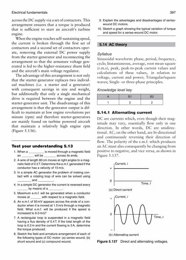
Electrical fundamentals 397
across the DC supply via a set of contactors. Thisarrangement ensures that a torque is producedthat is sufficient to start an aircraft’s turbineengine.
When the engine reaches self-sustaining speed,the current is broken through the first set ofcontactors and a second set of contactors oper-ate, removing the external DC power supplyfrom the starter-generator and reconnecting thearrangement so that the armature voltage gen-erated is fed to the higher-resistance shunt fieldand the aircraft’s main voltage regulator.
The advantage of this arrangement is not onlythat the starter-generator replaces two individ-ual machines (i.e. a starter and a generator)with consequent savings in size and weight,but additionally that only a single mechanicaldrive is required between the engine and thestarter-generator unit. The disadvantage of thisarrangement is that the generator output is dif-ficult to maintain at low engine revolutions perminute (rpm) and therefore starter-generatorsare mainly found on turbine powered aircraftthat maintain a relatively high engine rpm(Figure 5.136).
Test your understanding 5.131. When a _________ is moved through a magnetic field
an _______ will be _______ across its ends.
2. A wire of length 80 cm moves at right angles to a mag-netic field of 0.5T. Determine the e.m.f. generated if theconductor has a velocity of 15 m/s.
3. In a simple AC generator the problem of making con-tact with a rotating loop of wire can be solved using________ and _________.
4. In a simple DC generator the current is reversed every______ by means of a ________.
5. Maximum e.m.f. will be generated when a conductormoves at ______ with respect to a magnetic field.
6. An e.m.f. of 50 mV appears across the ends of a con-ductor when it is moved at 1.5 m/s through a magneticfield. What e.m.f. will be produced if the speed isincreased to 6.0 m/s?
7. A rectangular loop is suspended in a magnetic fieldhaving a flux density of 0.4T. If the total length of theloop is 0.2 m and the current flowing is 3 A, determinethe torque produced.
8. Sketch the field and armature arrangement of each ofthe following types of DC motor: (a) series wound, (b)shunt wound and (c) compound wound.
9. Explain the advantages and disadvantages of series-wound DC motors.
10. Sketch a graph showing the typical variation of torqueand speed for a series-wound DC motor.
5.14 AC theory
SyllabusSinusoidal waveform: phase, period, frequency,cycle; Instantaneous, average, root mean square(r.m.s), peak, peak-to-peak current values andcalculations of these values, in relation tovoltage, current and power; Triangular/squarewaves; Single- or three-phase principles.
Knowledge level key
1
A
2
B1
2
B2
5.14.1 Alternating current
DC are currents which, even though their mag-nitude may vary, essentially flow only in onedirection. In other words, DC are unidirec-tional. AC, on the other hand, are bi-directionaland continuously reversing their direction offlow. The polarity of the e.m.f. which producesan AC must also consequently be changing frompositive to negative, and vice versa, as shown inFigure 5.137.
Figure 5.137 Direct and alternating voltages.
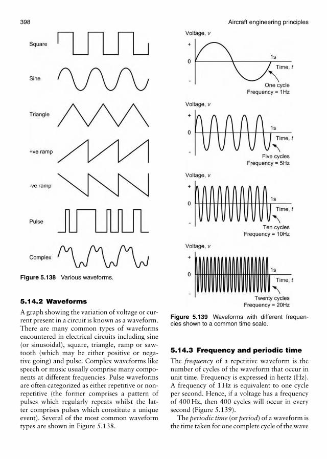
398 Aircraft engineering principles
Figure 5.138 Various waveforms.
5.14.2 Waveforms
A graph showing the variation of voltage or cur-rent present in a circuit is known as a waveform.There are many common types of waveformsencountered in electrical circuits including sine(or sinusoidal), square, triangle, ramp or saw-tooth (which may be either positive or nega-tive going) and pulse. Complex waveforms likespeech or music usually comprise many compo-nents at different frequencies. Pulse waveformsare often categorized as either repetitive or non-repetitive (the former comprises a pattern ofpulses which regularly repeats whilst the lat-ter comprises pulses which constitute a uniqueevent). Several of the most common waveformtypes are shown in Figure 5.138.
Figure 5.139 Waveforms with different frequen-cies shown to a common time scale.
5.14.3 Frequency and periodic time
The frequency of a repetitive waveform is thenumber of cycles of the waveform that occur inunit time. Frequency is expressed in hertz (Hz).A frequency of 1 Hz is equivalent to one cycleper second. Hence, if a voltage has a frequencyof 400 Hz, then 400 cycles will occur in everysecond (Figure 5.139).
The periodic time (or period) of a waveform isthe time taken for one complete cycle of the wave
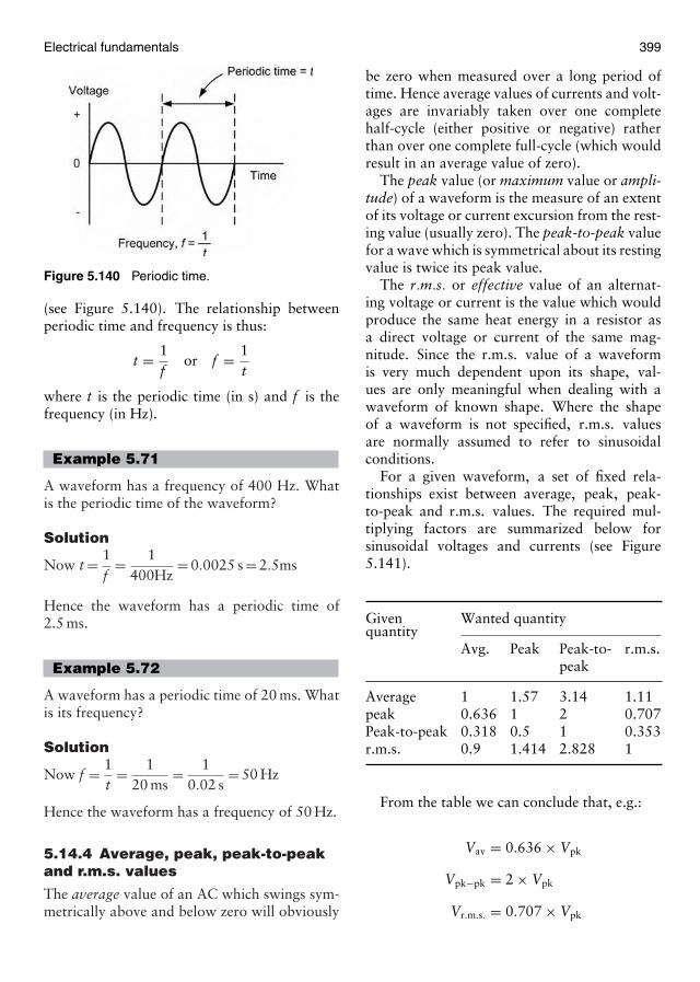
Electrical fundamentals 399
Figure 5.140 Periodic time.
(see Figure 5.140). The relationship betweenperiodic time and frequency is thus:
t = 1f
or f = 1t
where t is the periodic time (in s) and f is thefrequency (in Hz).
Example 5.71
A waveform has a frequency of 400 Hz. Whatis the periodic time of the waveform?
Solution
Now t = 1f
= 1400Hz
= 0.0025 s = 2.5ms
Hence the waveform has a periodic time of2.5 ms.
Example 5.72
A waveform has a periodic time of 20 ms. Whatis its frequency?
Solution
Now f = 1t
= 120 ms
= 10.02 s
= 50 Hz
Hence the waveform has a frequency of 50 Hz.
5.14.4 Average, peak, peak-to-peakand r.m.s. values
The average value of an AC which swings sym-metrically above and below zero will obviously
be zero when measured over a long period oftime. Hence average values of currents and volt-ages are invariably taken over one completehalf-cycle (either positive or negative) ratherthan over one complete full-cycle (which wouldresult in an average value of zero).
The peak value (or maximum value or ampli-tude) of a waveform is the measure of an extentof its voltage or current excursion from the rest-ing value (usually zero). The peak-to-peak valuefor a wave which is symmetrical about its restingvalue is twice its peak value.
The r.m.s. or effective value of an alternat-ing voltage or current is the value which wouldproduce the same heat energy in a resistor asa direct voltage or current of the same mag-nitude. Since the r.m.s. value of a waveformis very much dependent upon its shape, val-ues are only meaningful when dealing with awaveform of known shape. Where the shapeof a waveform is not specified, r.m.s. valuesare normally assumed to refer to sinusoidalconditions.
For a given waveform, a set of fixed rela-tionships exist between average, peak, peak-to-peak and r.m.s. values. The required mul-tiplying factors are summarized below forsinusoidal voltages and currents (see Figure5.141).
Given Wanted quantityquantity
Avg. Peak Peak-to- r.m.s.peak
Average 1 1.57 3.14 1.11peak 0.636 1 2 0.707Peak-to-peak 0.318 0.5 1 0.353r.m.s. 0.9 1.414 2.828 1
From the table we can conclude that, e.g.:
Vav = 0.636 × Vpk
Vpk−pk = 2 × Vpk
Vr.m.s. = 0.707 × Vpk
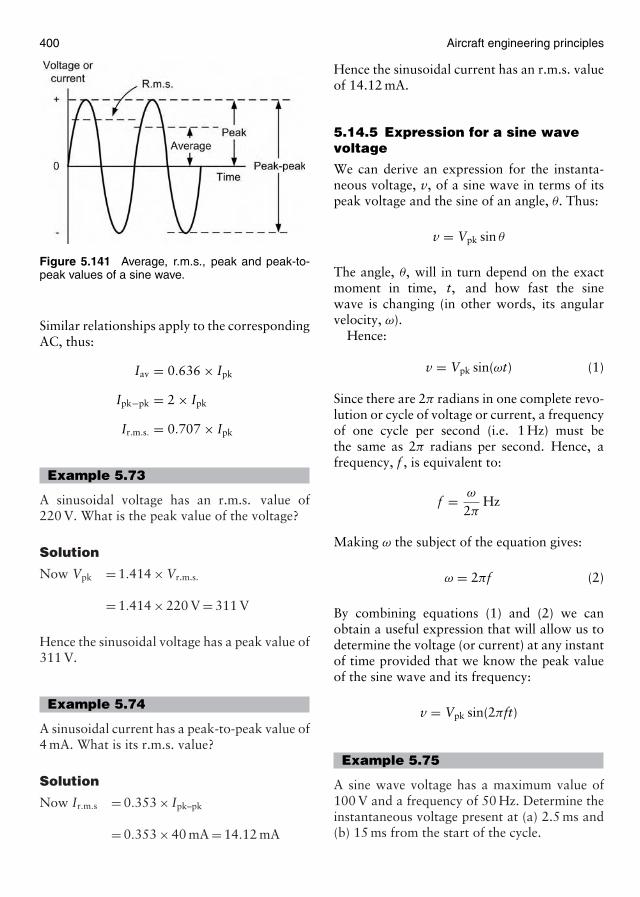
400 Aircraft engineering principles
Figure 5.141 Average, r.m.s., peak and peak-to-peak values of a sine wave.
Similar relationships apply to the correspondingAC, thus:
Iav = 0.636 × Ipk
Ipk−pk = 2 × Ipk
Ir.m.s. = 0.707 × Ipk
Example 5.73
A sinusoidal voltage has an r.m.s. value of220 V. What is the peak value of the voltage?
Solution
Now Vpk = 1.414 × Vr.m.s.
= 1.414 × 220 V = 311 V
Hence the sinusoidal voltage has a peak value of311 V.
Example 5.74
A sinusoidal current has a peak-to-peak value of4 mA. What is its r.m.s. value?
Solution
Now Ir.m.s = 0.353 × Ipk–pk
= 0.353 × 40 mA = 14.12 mA
Hence the sinusoidal current has an r.m.s. valueof 14.12 mA.
5.14.5 Expression for a sine wavevoltage
We can derive an expression for the instanta-neous voltage, v, of a sine wave in terms of itspeak voltage and the sine of an angle, θ. Thus:
v = Vpk sin θ
The angle, θ, will in turn depend on the exactmoment in time, t, and how fast the sinewave is changing (in other words, its angularvelocity, ω).
Hence:
v = Vpk sin(ωt) (1)
Since there are 2π radians in one complete revo-lution or cycle of voltage or current, a frequencyof one cycle per second (i.e. 1 Hz) must bethe same as 2π radians per second. Hence, afrequency, f , is equivalent to:
f = ω
2πHz
Making ω the subject of the equation gives:
ω = 2πf (2)
By combining equations (1) and (2) we canobtain a useful expression that will allow us todetermine the voltage (or current) at any instantof time provided that we know the peak valueof the sine wave and its frequency:
v = Vpk sin(2πft)
Example 5.75
A sine wave voltage has a maximum value of100 V and a frequency of 50 Hz. Determine theinstantaneous voltage present at (a) 2.5 ms and(b) 15 ms from the start of the cycle.
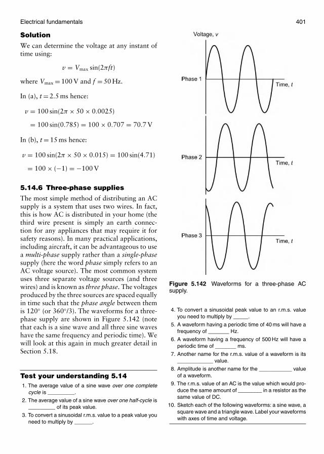
Electrical fundamentals 401
Solution
We can determine the voltage at any instant oftime using:
v = Vmax sin(2πft)
where Vmax = 100 V and f = 50 Hz.
In (a), t = 2.5 ms hence:
v = 100 sin(2π × 50 × 0.0025)
= 100 sin(0.785) = 100 × 0.707 = 70.7 V
In (b), t = 15 ms hence:
v = 100 sin(2π × 50 × 0.015) = 100 sin(4.71)
= 100 × (−1) = −100 V
5.14.6 Three-phase supplies
The most simple method of distributing an ACsupply is a system that uses two wires. In fact,this is how AC is distributed in your home (thethird wire present is simply an earth connec-tion for any appliances that may require it forsafety reasons). In many practical applications,including aircraft, it can be advantageous to usea multi-phase supply rather than a single-phasesupply (here the word phase simply refers to anAC voltage source). The most common systemuses three separate voltage sources (and threewires) and is known as three phase. The voltagesproduced by the three sources are spaced equallyin time such that the phase angle between themis 120◦ (or 360◦/3). The waveforms for a three-phase supply are shown in Figure 5.142 (notethat each is a sine wave and all three sine waveshave the same frequency and periodic time). Wewill look at this again in much greater detail inSection 5.18.
Test your understanding 5.141. The average value of a sine wave over one complete
cycle is _________.
2. The average value of a sine wave over one half-cycle is_________ of its peak value.
3. To convert a sinusoidal r.m.s. value to a peak value youneed to multiply by ______.
Figure 5.142 Waveforms for a three-phase ACsupply.
4. To convert a sinusoidal peak value to an r.m.s. valueyou need to multiply by _____.
5. A waveform having a periodic time of 40 ms will have afrequency of _______ Hz.
6. A waveform having a frequency of 500 Hz will have aperiodic time of _______ ms.
7. Another name for the r.m.s. value of a waveform is its____________ value.
8. Amplitude is another name for the ___________ valueof a waveform.
9. The r.m.s. value of an AC is the value which would pro-duce the same amount of ________ in a resistor as thesame value of DC.
10. Sketch each of the following waveforms: a sine wave, asquare wave and a triangle wave. Label your waveformswith axes of time and voltage.
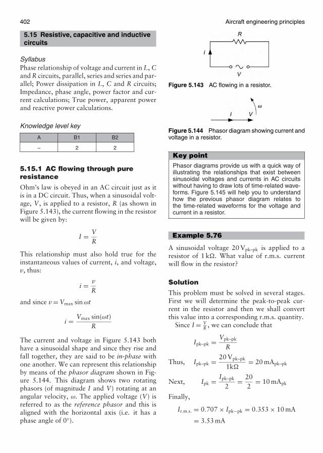
402 Aircraft engineering principles
5.15 Resistive, capacitive and inductivecircuits
SyllabusPhase relationship of voltage and current in L, Cand R circuits, parallel, series and series and par-allel; Power dissipation in L, C and R circuits;Impedance, phase angle, power factor and cur-rent calculations; True power, apparent powerand reactive power calculations.
Knowledge level key
–
A
2
B1
2
B2
5.15.1 AC flowing through pureresistance
Ohm’s law is obeyed in an AC circuit just as itis in a DC circuit. Thus, when a sinusoidal volt-age, V , is applied to a resistor, R (as shown inFigure 5.143), the current flowing in the resistorwill be given by:
I = VR
This relationship must also hold true for theinstantaneous values of current, i, and voltage,v, thus:
i = vR
and since v = Vmax sin ωt
i = Vmax sin(ωt)R
The current and voltage in Figure 5.143 bothhave a sinusoidal shape and since they rise andfall together, they are said to be in-phase withone another. We can represent this relationshipby means of the phasor diagram shown in Fig-ure 5.144. This diagram shows two rotatingphasors (of magnitude I and V) rotating at anangular velocity, ω. The applied voltage (V) isreferred to as the reference phasor and this isaligned with the horizontal axis (i.e. it has aphase angle of 0◦).
Figure 5.143 AC flowing in a resistor.
Figure 5.144 Phasor diagram showing current andvoltage in a resistor.
Key pointPhasor diagrams provide us with a quick way ofillustrating the relationships that exist betweensinusoidal voltages and currents in AC circuitswithout having to draw lots of time-related wave-forms. Figure 5.145 will help you to understandhow the previous phasor diagram relates tothe time-related waveforms for the voltage andcurrent in a resistor.
Example 5.76
A sinusoidal voltage 20 Vpk–pk is applied to aresistor of 1 k�. What value of r.m.s. currentwill flow in the resistor?
Solution
This problem must be solved in several stages.First we will determine the peak-to-peak cur-rent in the resistor and then we shall convertthis value into a corresponding r.m.s. quantity.
Since I = VR , we can conclude that
Ipk–pk = Vpk–pk
R
Thus, Ipk–pk = 20 Vpk–pk
1k�= 20 mApk–pk
Next, Ipk = Ipk–pk
2= 20
2= 10 mApk
Finally,
Ir.m.s. = 0.707 × Ipk−pk = 0.353 × 10 mA
= 3.53 mA
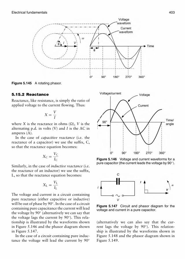
Electrical fundamentals 403
Figure 5.145 A rotating phasor.
5.15.2 Reactance
Reactance, like resistance, is simply the ratio ofapplied voltage to the current flowing. Thus:
X = VI
where X is the reactance in ohms (�), V is thealternating p.d. in volts (V) and I is the AC inamperes (A).
In the case of capacitive reactance (i.e. thereactance of a capacitor) we use the suffix, C,so that the reactance equation becomes:
XC = VC
IC
Similarly, in the case of inductive reactance (i.e.the reactance of an inductor) we use the suffix,L, so that the reactance equation becomes:
XL = VL
IL
The voltage and current in a circuit containingpure reactance (either capacitive or inductive)will be out of phase by 90◦. In the case of a circuitcontaining pure capacitance the current will leadthe voltage by 90◦ (alternatively we can say thatthe voltage lags the current by 90◦). This rela-tionship is illustrated by the waveforms shownin Figure 5.146 and the phasor diagram shownin Figure 5.147.
In the case of a circuit containing pure induc-tance the voltage will lead the current by 90◦
Figure 5.146 Voltage and current waveforms for apure capacitor (the current leads the voltage by 90◦).
Figure 5.147 Circuit and phasor diagram for thevoltage and current in a pure capacitor.
(alternatively we can also say that the cur-rent lags the voltage by 90◦). This relation-ship is illustrated by the waveforms shown inFigure 5.148 and the phasor diagram shown inFigure 5.149.
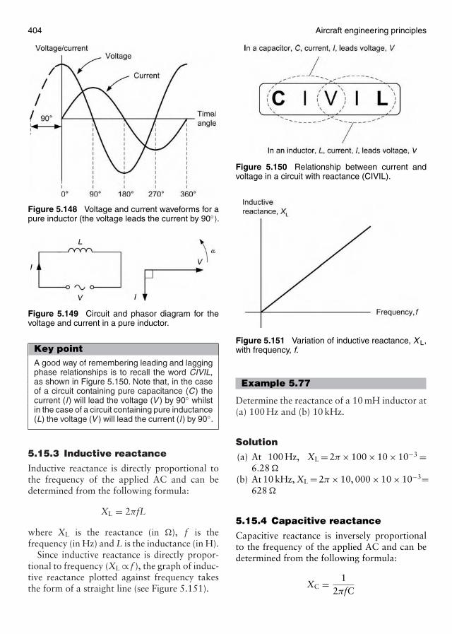
404 Aircraft engineering principles
Figure 5.148 Voltage and current waveforms for apure inductor (the voltage leads the current by 90◦).
Figure 5.149 Circuit and phasor diagram for thevoltage and current in a pure inductor.
Key pointA good way of remembering leading and laggingphase relationships is to recall the word CIVIL,as shown in Figure 5.150. Note that, in the caseof a circuit containing pure capacitance (C) thecurrent (I) will lead the voltage (V ) by 90◦ whilstin the case of a circuit containing pure inductance(L) the voltage (V ) will lead the current (I) by 90◦.
5.15.3 Inductive reactance
Inductive reactance is directly proportional tothe frequency of the applied AC and can bedetermined from the following formula:
XL = 2πfL
where XL is the reactance (in �), f is thefrequency (in Hz) and L is the inductance (in H).
Since inductive reactance is directly propor-tional to frequency (XL ∝ f ), the graph of induc-tive reactance plotted against frequency takesthe form of a straight line (see Figure 5.151).
Figure 5.150 Relationship between current andvoltage in a circuit with reactance (CIVIL).
Figure 5.151 Variation of inductive reactance, X L,with frequency, f.
Example 5.77
Determine the reactance of a 10 mH inductor at(a) 100 Hz and (b) 10 kHz.
Solution
(a) At 100 Hz, XL = 2π × 100 × 10 × 10−3 =6.28 �
(b) At 10 kHz, XL = 2π × 10, 000 × 10 × 10−3=628 �
5.15.4 Capacitive reactance
Capacitive reactance is inversely proportionalto the frequency of the applied AC and can bedetermined from the following formula:
XC = 12πfC
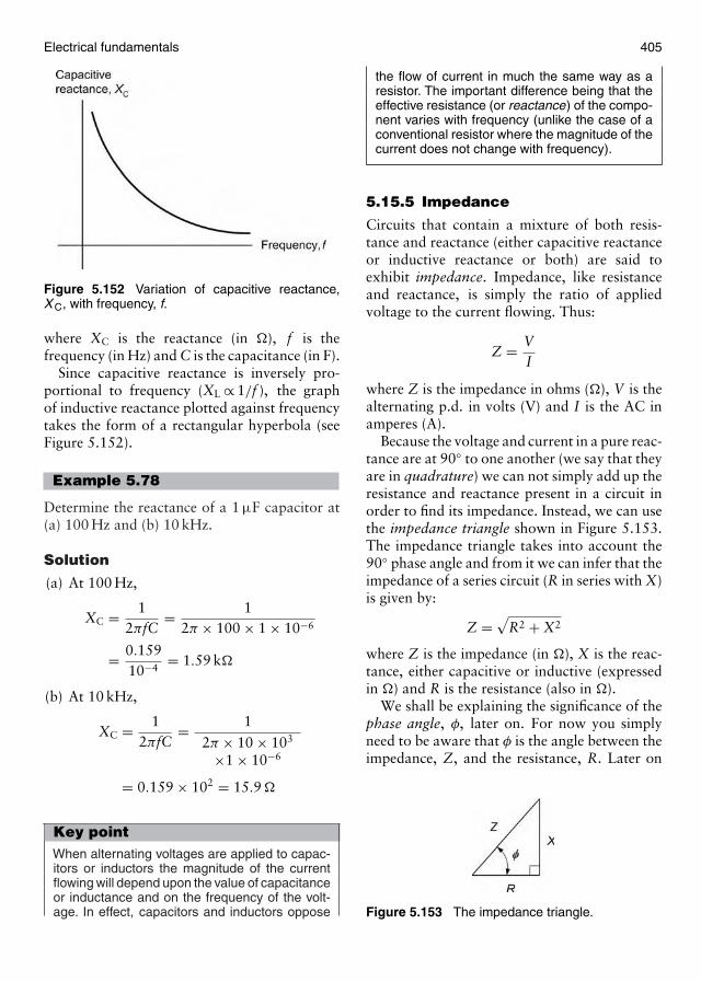
Electrical fundamentals 405
Figure 5.152 Variation of capacitive reactance,X C, with frequency, f.
where XC is the reactance (in �), f is thefrequency (in Hz) and C is the capacitance (in F).
Since capacitive reactance is inversely pro-portional to frequency (XL ∝ 1/f ), the graphof inductive reactance plotted against frequencytakes the form of a rectangular hyperbola (seeFigure 5.152).
Example 5.78
Determine the reactance of a 1 µF capacitor at(a) 100 Hz and (b) 10 kHz.
Solution
(a) At 100 Hz,
XC = 12πfC
= 12π × 100 × 1 × 10−6
= 0.15910−4
= 1.59 k�
(b) At 10 kHz,
XC = 12πfC
= 12π × 10 × 103
×1 × 10−6
= 0.159 × 102 = 15.9 �
Key pointWhen alternating voltages are applied to capac-itors or inductors the magnitude of the currentflowing will depend upon the value of capacitanceor inductance and on the frequency of the volt-age. In effect, capacitors and inductors oppose
the flow of current in much the same way as aresistor. The important difference being that theeffective resistance (or reactance) of the compo-nent varies with frequency (unlike the case of aconventional resistor where the magnitude of thecurrent does not change with frequency).
5.15.5 Impedance
Circuits that contain a mixture of both resis-tance and reactance (either capacitive reactanceor inductive reactance or both) are said toexhibit impedance. Impedance, like resistanceand reactance, is simply the ratio of appliedvoltage to the current flowing. Thus:
Z = VI
where Z is the impedance in ohms (�), V is thealternating p.d. in volts (V) and I is the AC inamperes (A).
Because the voltage and current in a pure reac-tance are at 90◦ to one another (we say that theyare in quadrature) we can not simply add up theresistance and reactance present in a circuit inorder to find its impedance. Instead, we can usethe impedance triangle shown in Figure 5.153.The impedance triangle takes into account the90◦ phase angle and from it we can infer that theimpedance of a series circuit (R in series with X)is given by:
Z =√
R2 + X2
where Z is the impedance (in �), X is the reac-tance, either capacitive or inductive (expressedin �) and R is the resistance (also in �).
We shall be explaining the significance of thephase angle, φ, later on. For now you simplyneed to be aware that φ is the angle between theimpedance, Z, and the resistance, R. Later on
Figure 5.153 The impedance triangle.
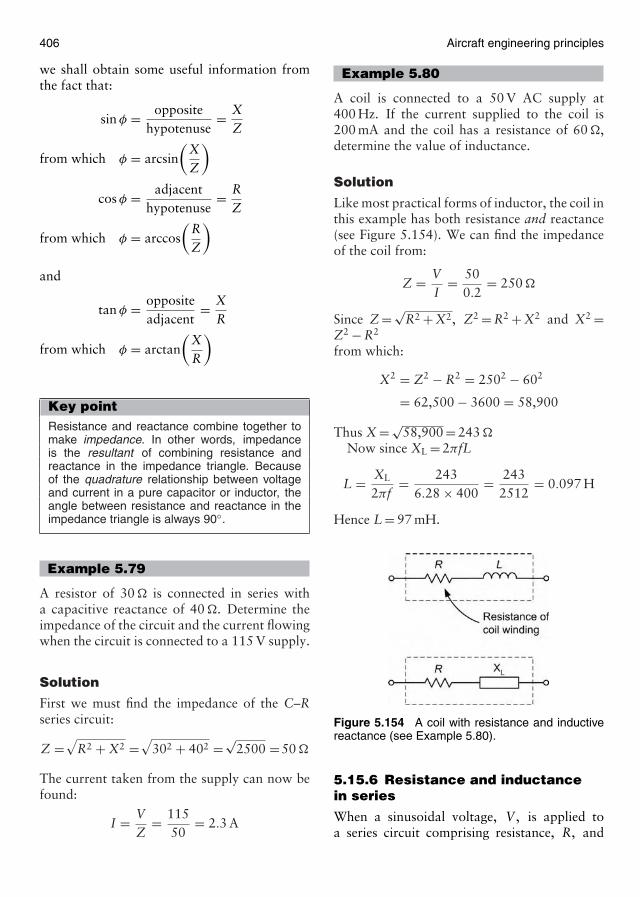
406 Aircraft engineering principles
we shall obtain some useful information fromthe fact that:
sin φ = oppositehypotenuse
= XZ
from which φ = arcsin(
XZ
)
cos φ = adjacenthypotenuse
= RZ
from which φ = arccos(
RZ
)
and
tan φ = oppositeadjacent
= XR
from which φ = arctan(
XR
)
Key pointResistance and reactance combine together tomake impedance. In other words, impedanceis the resultant of combining resistance andreactance in the impedance triangle. Becauseof the quadrature relationship between voltageand current in a pure capacitor or inductor, theangle between resistance and reactance in theimpedance triangle is always 90◦.
Example 5.79
A resistor of 30 � is connected in series witha capacitive reactance of 40 �. Determine theimpedance of the circuit and the current flowingwhen the circuit is connected to a 115 V supply.
Solution
First we must find the impedance of the C–Rseries circuit:
Z =√
R2 + X2 =√
302 + 402 =√2500 =50 �
The current taken from the supply can now befound:
I = VZ
= 11550
= 2.3 A
Example 5.80
A coil is connected to a 50 V AC supply at400 Hz. If the current supplied to the coil is200 mA and the coil has a resistance of 60 �,determine the value of inductance.
Solution
Like most practical forms of inductor, the coil inthis example has both resistance and reactance(see Figure 5.154). We can find the impedanceof the coil from:
Z = VI
= 500.2
= 250 �
Since Z = √R2 + X2, Z2 = R2 + X2 and X2 =
Z2 − R2
from which:
X2 = Z2 − R2 = 2502 − 602
= 62,500 − 3600 = 58,900
Thus X = √58,900 = 243 �
Now since XL = 2πfL
L = XL
2πf= 243
6.28 × 400= 243
2512= 0.097 H
Hence L = 97 mH.
Figure 5.154 A coil with resistance and inductivereactance (see Example 5.80).
5.15.6 Resistance and inductancein series
When a sinusoidal voltage, V , is applied toa series circuit comprising resistance, R, and
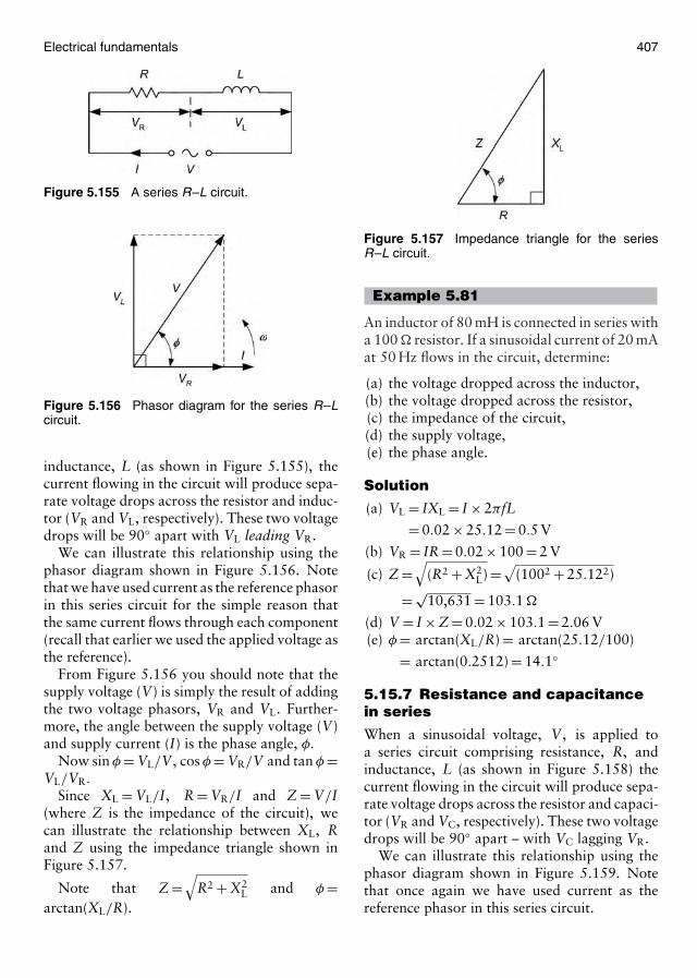
Electrical fundamentals 407
Figure 5.155 A series R–L circuit.
Figure 5.156 Phasor diagram for the series R–Lcircuit.
inductance, L (as shown in Figure 5.155), thecurrent flowing in the circuit will produce sepa-rate voltage drops across the resistor and induc-tor (VR and VL, respectively). These two voltagedrops will be 90◦ apart with VL leading VR.
We can illustrate this relationship using thephasor diagram shown in Figure 5.156. Notethat we have used current as the reference phasorin this series circuit for the simple reason thatthe same current flows through each component(recall that earlier we used the applied voltage asthe reference).
From Figure 5.156 you should note that thesupply voltage (V) is simply the result of addingthe two voltage phasors, VR and VL. Further-more, the angle between the supply voltage (V)and supply current (I) is the phase angle, φ.
Now sin φ = VL/V , cos φ = VR/V and tan φ =VL/VR.
Since XL = VL/I, R = VR/I and Z = V/I(where Z is the impedance of the circuit), wecan illustrate the relationship between XL, Rand Z using the impedance triangle shown inFigure 5.157.
Note that Z =√
R2 + X2L and φ =
arctan(XL/R).
Figure 5.157 Impedance triangle for the seriesR–L circuit.
Example 5.81
An inductor of 80 mH is connected in series witha 100 � resistor. If a sinusoidal current of 20 mAat 50 Hz flows in the circuit, determine:
(a) the voltage dropped across the inductor,(b) the voltage dropped across the resistor,(c) the impedance of the circuit,(d) the supply voltage,(e) the phase angle.
Solution
(a) VL = IXL = I × 2πfL
= 0.02 × 25.12 = 0.5 V
(b) VR = IR = 0.02 × 100 = 2 V
(c) Z =√
(R2 + X2L) =√(1002 + 25.122)
= √10,631 = 103.1 �
(d) V = I × Z = 0.02 × 103.1 = 2.06 V(e) φ = arctan(XL/R) = arctan(25.12/100)
= arctan(0.2512) = 14.1◦
5.15.7 Resistance and capacitancein series
When a sinusoidal voltage, V , is applied toa series circuit comprising resistance, R, andinductance, L (as shown in Figure 5.158) thecurrent flowing in the circuit will produce sepa-rate voltage drops across the resistor and capaci-tor (VR and VC, respectively). These two voltagedrops will be 90◦ apart – with VC lagging VR.
We can illustrate this relationship using thephasor diagram shown in Figure 5.159. Notethat once again we have used current as thereference phasor in this series circuit.
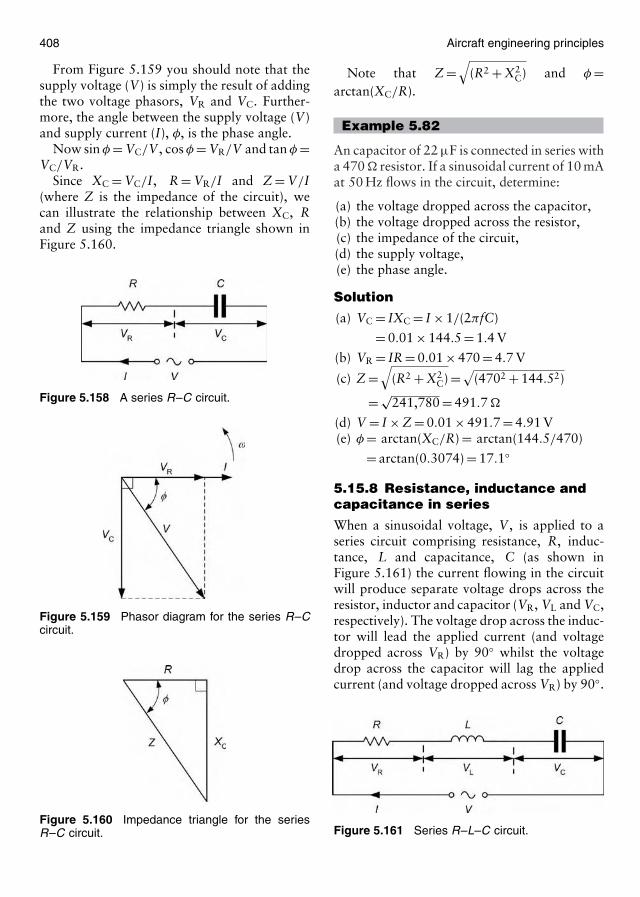
408 Aircraft engineering principles
From Figure 5.159 you should note that thesupply voltage (V) is simply the result of addingthe two voltage phasors, VR and VC. Further-more, the angle between the supply voltage (V)and supply current (I), φ, is the phase angle.
Now sin φ = VC/V , cos φ = VR/V and tan φ =VC/VR.
Since XC = VC/I, R = VR/I and Z = V/I(where Z is the impedance of the circuit), wecan illustrate the relationship between XC, Rand Z using the impedance triangle shown inFigure 5.160.
Figure 5.158 A series R–C circuit.
Figure 5.159 Phasor diagram for the series R–Ccircuit.
Figure 5.160 Impedance triangle for the seriesR–C circuit.
Note that Z =√
(R2 + X2C) and φ =
arctan(XC/R).
Example 5.82
An capacitor of 22 µF is connected in series witha 470 � resistor. If a sinusoidal current of 10 mAat 50 Hz flows in the circuit, determine:
(a) the voltage dropped across the capacitor,(b) the voltage dropped across the resistor,(c) the impedance of the circuit,(d) the supply voltage,(e) the phase angle.
Solution
(a) VC = IXC = I × 1/(2πfC)
= 0.01 × 144.5 = 1.4 V
(b) VR = IR = 0.01 × 470 = 4.7 V
(c) Z =√
(R2 + X2C) =√(4702 + 144.52)
= √241,780 = 491.7 �
(d) V = I × Z = 0.01 × 491.7 = 4.91 V(e) φ = arctan(XC/R) = arctan(144.5/470)
= arctan(0.3074) = 17.1◦
5.15.8 Resistance, inductance andcapacitance in series
When a sinusoidal voltage, V , is applied to aseries circuit comprising resistance, R, induc-tance, L and capacitance, C (as shown inFigure 5.161) the current flowing in the circuitwill produce separate voltage drops across theresistor, inductor and capacitor (VR, VL and VC,respectively). The voltage drop across the induc-tor will lead the applied current (and voltagedropped across VR) by 90◦ whilst the voltagedrop across the capacitor will lag the appliedcurrent (and voltage dropped across VR) by 90◦.
Figure 5.161 Series R–L–C circuit.
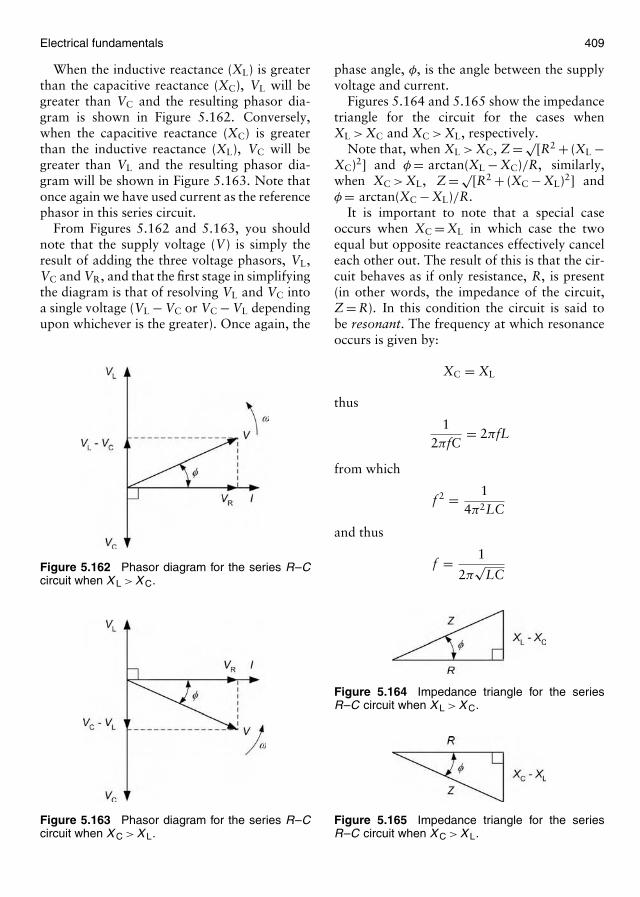
Electrical fundamentals 409
When the inductive reactance (XL) is greaterthan the capacitive reactance (XC), VL will begreater than VC and the resulting phasor dia-gram is shown in Figure 5.162. Conversely,when the capacitive reactance (XC) is greaterthan the inductive reactance (XL), VC will begreater than VL and the resulting phasor dia-gram will be shown in Figure 5.163. Note thatonce again we have used current as the referencephasor in this series circuit.
From Figures 5.162 and 5.163, you shouldnote that the supply voltage (V) is simply theresult of adding the three voltage phasors, VL,VC and VR, and that the first stage in simplifyingthe diagram is that of resolving VL and VC intoa single voltage (VL − VC or VC − VL dependingupon whichever is the greater). Once again, the
Figure 5.162 Phasor diagram for the series R–Ccircuit when X L > X C.
Figure 5.163 Phasor diagram for the series R–Ccircuit when X C > X L.
phase angle, φ, is the angle between the supplyvoltage and current.
Figures 5.164 and 5.165 show the impedancetriangle for the circuit for the cases whenXL > XC and XC > XL, respectively.
Note that, when XL > XC, Z = √[R2 + (XL −
XC)2] and φ = arctan(XL − XC)/R, similarly,when XC > XL, Z = √
[R2 + (XC − XL)2] andφ = arctan(XC − XL)/R.
It is important to note that a special caseoccurs when XC = XL in which case the twoequal but opposite reactances effectively canceleach other out. The result of this is that the cir-cuit behaves as if only resistance, R, is present(in other words, the impedance of the circuit,Z = R). In this condition the circuit is said tobe resonant. The frequency at which resonanceoccurs is given by:
XC = XL
thus
12πfC
= 2πfL
from which
f 2 = 14π2LC
and thus
f = 1
2π√
LC
Figure 5.164 Impedance triangle for the seriesR–C circuit when X L > X C.
Figure 5.165 Impedance triangle for the seriesR–C circuit when X C > X L.

410 Aircraft engineering principles
where f is the resonant frequency (in Hz), L isthe inductance (in H) and C is the capacitance(in F).
Example 5.83
A series circuit comprises an inductor of 80 mH,a resistor of 200 � and a capacitor of 22 µF. Ifa sinusoidal current of 40 mA at 50 Hz flows inthis circuit, determine:
(a) the voltage developed across the inductor,(b) the voltage dropped across the capacitor,(c) the voltage dropped across the resistor,(d) the impedance of the circuit,(e) the supply voltage,(f) the phase angle.
Solution
(a) VL = IXL = I × 2πfL = 0.04 × 25.12= 1 V
(b) VC = IXC = I × 1/(2πfC) = 0.04 ×144.5 = 5.8 V
(c) VR = IR = 0.04 × 200 = 8 V(d) Z =√R2 + (XC − XL)2
=√2002 + (144.5 − 25.12)2
= √54,252 = 232.9 �
(e) V = I × Z = 0.04 × 232.9 = 9.32 V(f) φ = arctan(XC − XL)/R = arctan(119.38/
200) = arctan(0.597) = 30.8◦
Example 5.84
A series circuit comprises an inductor of 10 mH,a resistor of 50 � and a capacitor of 40 nF.Determine the frequency at which this circuitis resonant and the current that will flow in itwhen it is connected to a 20 V AC supply at theresonant frequency.
Solution
Using:
f = 1
2π√
LC
where L = 10 × 10−3 H and C = 40 × 10−9 Fgives:
f = 1
6.28√
10 × 10−3 × 40 × 10−9
= 0.159√4 × 10−10
= 0.1592 × 10−5
= 0.1592 × 10−5
= 7950 = 7.95 kHz
At the resonant frequency the circuit willbehave as a pure resistance (recall that thetwo reactances will be equal but opposite) andthus the supply current at resonance can bedetermined from:
I = VZ
= VR
= 2050
= 0.4 A
5.15.9 Parallel and series–parallelAC circuits
As we have seen, in a series AC circuit the samecurrent flows through each component and thesupply voltage is found from the phasor sumof the voltage that appears across each of thecomponents present. In a parallel AC circuit,by contrast, the same voltage appears acrosseach branch of the circuit and the total cur-rent taken from the supply is the phasor sumof the currents in each branch. For this reasonwe normally use voltage as the reference quan-tity for a parallel AC circuit rather than current.Rather than simply quote the formulae, we shallillustrate the techniques for solving parallel, andseries–parallel AC circuits by taking some simpleexamples.
Example 5.85
A parallel AC circuit comprises a resistor, R, of30 � connected in parallel with a capacitor, C,of 80 µF. If the circuit is connected to a 240 V,50 Hz supply determine:
(a) the current in the resistor,(b) the current in the capacitor,(c) the supply current,(d) the phase angle.
Solution
Figure 5.166 shows the parallel circuit arrange-ment showing the three currents present; I1 (thecurrent in the resistor), I2 (the current in thecapacitor) and IS (the supply current). Figure5.167 shows the phasor diagram for the parallel
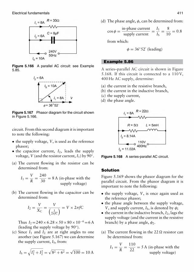
Electrical fundamentals 411
Figure 5.166 A parallel AC circuit: see Example5.85.
Figure 5.167 Phasor diagram for the circuit shownin Figure 5.166.
circuit. From this second diagram it is importantto note the following:
• the supply voltage, V , is used as the referencephasor;
• the capacitor current, I2, leads the supplyvoltage, V (and the resistor current, I1) by 90◦.
(a) The current flowing in the resistor can bedetermined from:
I1 = VR
= 24030
= 8 A (in-phase with thesupply voltage)
(b) The current flowing in the capacitor can bedetermined from:
I2 = VXC
= V(1
2πfC
) = V × 2πfC
Thus I2 =240×6.28×50×80×10−6 =6 A(leading the supply voltage by 90◦).
(c) Since I1 and I2 are at right angles to oneanother (see Figure 5.167) we can determinethe supply current, IS, from:
IS =√
I21 + I2
2 =√
82 + 62 = √100 = 10 A
(d) The phase angle, φ, can be determined from:
cos φ = in-phase currentsupply current
= I1
IS= 8
10= 0.8
from which:
φ = 36◦52′ (leading)
Example 5.86
A series–parallel AC circuit is shown in Figure5.168. If this circuit is connected to a 110 V,400 Hz AC supply, determine:
(a) the current in the resistive branch,(b) the current in the inductive branch,(c) the supply current,(d) the phase angle.
Figure 5.168 A series-parallel AC circuit.
Solution
Figure 5.169 shows the phasor diagram for theparallel circuit. From the phasor diagram it isimportant to note the following:
• the supply voltage, V , is once again used asthe reference phasor;
• the phase angle between the supply voltage,V , and supply current, IS, is denoted by φ;
• the current in the inductive branch, I2, lags thesupply voltage (and the current in the resistivebranch) by a phase angle, φ2.
(a) The current flowing in the 22 � resistor canbe determined from:
I1 = VR
= 11022
= 5 A (in-phase with thesupply voltage)

412 Aircraft engineering principles
Figure 5.169 Phasor diagram for the circuit shownin Figure 5.168.
(b) The current flowing in the capacitor can bedetermined from:
I2 = VZ
= V√R2 + X2
L
= V√R2 + (
2πf L)2
from which:
I2 = 110√52 + (
6.28 × 400 × 5 × 10−3)2
= 110√52 + (12.56)2
= 110√182.75
= 11013.52
= 8.14 A
Thus I2 = 8.14 A (lagging the supply voltageby φ2).
The phase angle for the inductive branch,φ2, can be determined from:
cos φ2 = R2
Z= 5
13.52= 0.37
or
sin φ2 = XL
Z= 12.56
13.52= 0.93
from which φ2 = 68.3◦Hence the current in the inductive branch
is 8.14 A lagging the supply voltage by 68.3◦.(c) In order to determine the supply current we
need to find the total in-phase current andthe total quadrature current (i.e. the totalcurrent at 90◦) as shown in Figure 5.170.
The total in-phase current, Ix, is given by:
Ix = I1 + I2 cos φ2 = 5 + (8.14 × 0.37)
= 5 + 3.01 = 8.01 A
Figure 5.170 Phasor diagram showing totalin-phase and total quadrature components inExample 5.86.
The total quadrature current, Iy, is given by:
Iy = I2 sin φ2 = 8.14 × 0.93 = 7.57 A
The supply current, IS, can now be deter-mined from:
IS =√
8.012 + 7.572 = √64.16 + 57.3
= √121.46 = 11.02 A
(d) The phase angle, φ, can be determined from:
cos φ = in-phase currentsupply current
= 8.0111.02
= 0.73
from which:
φ = 43.4◦ (lagging)
Key pointWe use current as the reference phasor inseries AC circuit because the same current flowsthrough each component. Conversely, we usevoltage as the reference phasor in a parallel ACcircuit because the same voltage appears acrosseach component.
5.15.10 Power factor
The power factor in an AC circuit containingresistance and reactance is simply the ratio oftrue power to apparent power. Hence:
Power factor = true powerapparent power
The true power in an AC circuit is the powerthat is actually dissipated as heat in the resistivecomponent. Thus:
True power = I2R
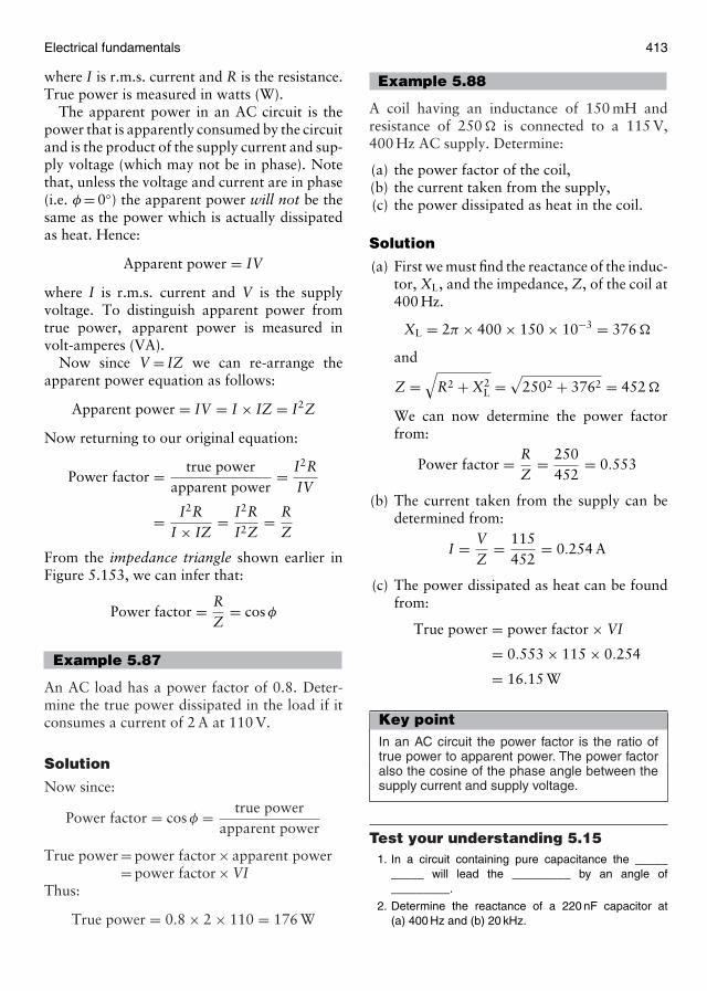
Electrical fundamentals 413
where I is r.m.s. current and R is the resistance.True power is measured in watts (W).
The apparent power in an AC circuit is thepower that is apparently consumed by the circuitand is the product of the supply current and sup-ply voltage (which may not be in phase). Notethat, unless the voltage and current are in phase(i.e. φ = 0◦) the apparent power will not be thesame as the power which is actually dissipatedas heat. Hence:
Apparent power = IV
where I is r.m.s. current and V is the supplyvoltage. To distinguish apparent power fromtrue power, apparent power is measured involt-amperes (VA).
Now since V = IZ we can re-arrange theapparent power equation as follows:
Apparent power = IV = I × IZ = I2Z
Now returning to our original equation:
Power factor = true powerapparent power
= I2RIV
= I2RI × IZ
= I2RI2Z
= RZ
From the impedance triangle shown earlier inFigure 5.153, we can infer that:
Power factor = RZ
= cos φ
Example 5.87
An AC load has a power factor of 0.8. Deter-mine the true power dissipated in the load if itconsumes a current of 2 A at 110 V.
Solution
Now since:
Power factor = cos φ = true powerapparent power
True power = power factor × apparent power= power factor × VI
Thus:
True power = 0.8 × 2 × 110 = 176 W
Example 5.88
A coil having an inductance of 150 mH andresistance of 250 � is connected to a 115 V,400 Hz AC supply. Determine:
(a) the power factor of the coil,(b) the current taken from the supply,(c) the power dissipated as heat in the coil.
Solution
(a) First we must find the reactance of the induc-tor, XL, and the impedance, Z, of the coil at400 Hz.
XL = 2π × 400 × 150 × 10−3 = 376 �
and
Z =√
R2 + X2L =
√2502 + 3762 = 452 �
We can now determine the power factorfrom:
Power factor = RZ
= 250452
= 0.553
(b) The current taken from the supply can bedetermined from:
I = VZ
= 115452
= 0.254 A
(c) The power dissipated as heat can be foundfrom:
True power = power factor × VI
= 0.553 × 115 × 0.254
= 16.15 W
Key pointIn an AC circuit the power factor is the ratio oftrue power to apparent power. The power factoralso the cosine of the phase angle between thesupply current and supply voltage.
Test your understanding 5.151. In a circuit containing pure capacitance the _____
_____ will lead the _________ by an angle of_________.
2. Determine the reactance of a 220 nF capacitor at(a) 400 Hz and (b) 20 kHz.
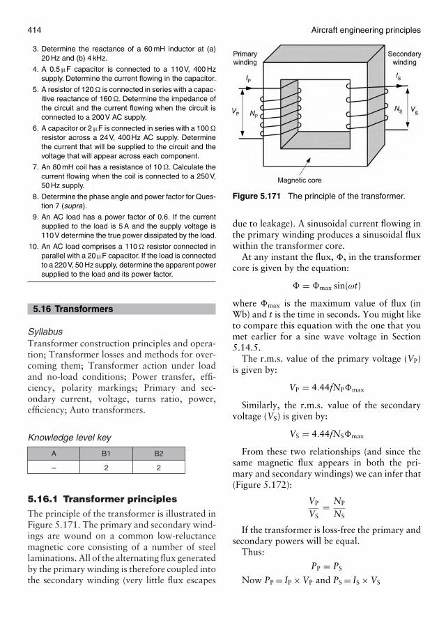
414 Aircraft engineering principles
3. Determine the reactance of a 60 mH inductor at (a)20 Hz and (b) 4 kHz.
4. A 0.5 µF capacitor is connected to a 110V, 400 Hzsupply. Determine the current flowing in the capacitor.
5. A resistor of 120 � is connected in series with a capac-itive reactance of 160 �. Determine the impedance ofthe circuit and the current flowing when the circuit isconnected to a 200V AC supply.
6. A capacitor or 2 µF is connected in series with a 100 �
resistor across a 24V, 400 Hz AC supply. Determinethe current that will be supplied to the circuit and thevoltage that will appear across each component.
7. An 80 mH coil has a resistance of 10 �. Calculate thecurrent flowing when the coil is connected to a 250V,50 Hz supply.
8. Determine the phase angle and power factor for Ques-tion 7 (supra).
9. An AC load has a power factor of 0.6. If the currentsupplied to the load is 5 A and the supply voltage is110V determine the true power dissipated by the load.
10. An AC load comprises a 110 � resistor connected inparallel with a 20 µF capacitor. If the load is connectedto a 220V, 50 Hz supply, determine the apparent powersupplied to the load and its power factor.
5.16 Transformers
SyllabusTransformer construction principles and opera-tion; Transformer losses and methods for over-coming them; Transformer action under loadand no-load conditions; Power transfer, effi-ciency, polarity markings; Primary and sec-ondary current, voltage, turns ratio, power,efficiency; Auto transformers.
Knowledge level key
–
A
2
B1
2
B2
5.16.1 Transformer principles
The principle of the transformer is illustrated inFigure 5.171. The primary and secondary wind-ings are wound on a common low-reluctancemagnetic core consisting of a number of steellaminations. All of the alternating flux generatedby the primary winding is therefore coupled intothe secondary winding (very little flux escapes
Figure 5.171 The principle of the transformer.
due to leakage). A sinusoidal current flowing inthe primary winding produces a sinusoidal fluxwithin the transformer core.
At any instant the flux, �, in the transformercore is given by the equation:
� = �max sin(ωt)
where �max is the maximum value of flux (inWb) and t is the time in seconds. You might liketo compare this equation with the one that youmet earlier for a sine wave voltage in Section5.14.5.
The r.m.s. value of the primary voltage (VP)is given by:
VP = 4.44fNP�max
Similarly, the r.m.s. value of the secondaryvoltage (VS) is given by:
VS = 4.44fNS�max
From these two relationships (and since thesame magnetic flux appears in both the pri-mary and secondary windings) we can infer that(Figure 5.172):
VP
VS= NP
NS
If the transformer is loss-free the primary andsecondary powers will be equal.
Thus:
PP = PS
Now PP = IP × VP and PS = IS × VS

Electrical fundamentals 415
Figure 5.172 Transformer turns and voltages.
So IP × VP = IS × VS
From which IPIS
= VSVP
and thus IPIS
= NSNP
Furthermore, assuming that no power is lostin the transformer (i.e. as long as the primaryand secondary powers are the same) we canconclude that:
IP
IS= NS
NP
The ratio of primary turns to secondary turns(NP/NS) is known as the turns ratio.
Furthermore, since ratio of primary voltageto primary turns is the same as the ratio ofsecondary turns to secondary voltage, we canconclude that, for a particular transformer:
Turns-per-volt (t.p.v.) = VP
NP= VS
NS
The t.p.v. rating can be quite useful when itcomes to designing transformers with multiplesecondary windings.
Example 5.89
A transformer has 2000 primary turns and 120secondary turns. If the primary is connectedto a 220 V AC mains supply, determine thesecondary voltage.
Solution
Since VPVS
= NPNS
we can conclude that:
VS = VPNS
NP= 220 × 120
2000= 13.2V
Example 5.90
A transformer has 1200 primary turns and isdesigned to operated with a 110 V AC supply.If the transformer is required to produce an out-put of 10 V, determine the number of secondaryturns required.
Solution
Since VPVS
= NPNS
we can conclude that:
NS = NPVS
VP= 1200 × 10
110= 109.1
Example 5.91
A transformer has a t.p.v. rating of 1.2. Howmany turns are required to produce secondaryoutputs of (a) 50 V and (b) 350 V?
Solution
Here we will use NS = t.p.v. × VS
(a) In the case of a 50 V secondary winding:
NS = 1.5 × 50 = 75 turns
(b) In the case of a 350 V secondary winding:
NS = 1.5 × 350 = 525 turns
Example 5.92
A transformer has 1200 primary turns and 60secondary turns. Assuming that the transformeris loss-free, determine the primary currentwhen a load current of 20 A is taken from thesecondary.
Solution
Since ISIP
= NPNS
we can conclude that:
IP = ISNS
NP= 20 × 60
1200= 1 A
5.16.2 Transformer applications
Transformers provide us with a means ofcoupling AC power from one circuit to anotherwithout a direct connection between the two.
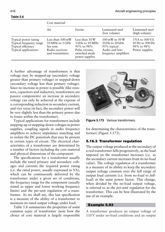
416 Aircraft engineering principles
Table 5.6
Core material
Air Ferrite Laminated steel Laminated steel(low volume) (high volume)
Typical power rating Less than 100 mW Less than 10 W 100 mW to 50 W 3 VA to 500 VATypical frequency range 10 MHz to 1 GHz 1 kHz to 10 MHz 50 Hz to 20 kHz 45 Hz to 500 HzTypical efficiency See note 95% to 98% 95% typical 90% to 98%Typical applications Radio receivers Pulse circuits, Audio and low- Power supplies
and transmitters switched mode frequency amplifierspower supplies
A further advantage of transformers is thatvoltage may be stepped-up (secondary voltagegreater than primary voltage) or stepped-down(secondary voltage less than primary voltage).Since no increase in power is possible (like resis-tors, capacitors and inductors, transformers arepassive components) an increase in secondaryvoltage can only be achieved at the expense ofa corresponding reduction in secondary current,and vice versa (in fact, the secondary power willbe very slightly less than the primary power dueto losses within the transformer).
Typical applications for transformers includestepping-up or stepping-down voltages in powersupplies, coupling signals in audio frequencyamplifiers to achieve impedance matching andto isolate the DC potentials that may be presentin certain types of circuit. The electrical char-acteristics of a transformer are determined bya number of factors including the core materialand physical dimensions of the component.
The specifications for a transformer usuallyinclude the rated primary and secondary volt-ages and currents the required power rating(i.e. the rated power, usually expressed in VA),which can be continuously delivered by thetransformer under a given set of conditions,the frequency range for the component (usuallystated as upper and lower working frequencylimits) and the per-unit regulation of a trans-former. As we shall see, this last specificationis a measure of the ability of a transformer tomaintain its rated output voltage under load.
Table 5.8 summarizes the properties of somecommon types of transformer (note how thechoice of core material is largely responsible
Figure 5.173 Various transformers.
for determining the characteristics of the trans-former) (Figure 5.173).
5.16.3 Transformer regulation
The output voltage produced at the secondary ofa real transformer falls progressively, as the loadimposed on the transformer increases (i.e. asthe secondary current increases from its no-loadvalue). The voltage regulation of a transformeris a measure of its ability to keep the secondaryoutput voltage constant over the full range ofoutput load currents (i.e. from no-load to full-load) at the same power factor. This change,when divided by the no-load output voltage,is referred to as the per-unit regulation for thetransformer. This can be best illustrated by theuse of an example.
Example 5.93
A transformer produces an output voltage of110 V under no-load conditions and an output
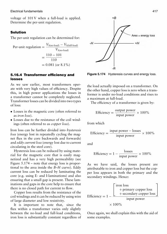
Electrical fundamentals 417
voltage of 101 V when a full-load is applied.Determine the per-unit regulation.
Solution
The per-unit regulation can be determined for:
Per-unit regulation = VS(no-load) − VS(full-load)
VS(no-load)
= 110 − 101110
= 0.081 (or 8.1%)
5.16.4 Transformer efficiency andlosses
As we saw earlier, most transformers oper-ate with very high values of efficiency. Despitethis, in high power applications the losses ina transformer cannot be completely neglected.Transformer losses can be divided into two typesof loss:
• Losses in the magnetic core (often referred toas iron loss).
• Losses due to the resistance of the coil wind-ings (often referred to as copper loss).
Iron loss can be further divided into hysteresisloss (energy lost in repeatedly cycling the mag-net flux in the core backwards and forwards)and eddy current loss (energy lost due to currentcirculating in the steel core).
Hysteresis loss can be reduced by using mate-rial for the magnetic core that is easily mag-netized and has a very high permeability (seeFigure 5.174 – note that energy loss is propor-tional to the area inside the B–H curve). Eddycurrent loss can be reduced by laminating thecore (e.g. using E- and I-laminations) and alsoensuring that a small gap is present. These lam-inations and gaps in the core help to ensure thatthere is no closed path for current to flow.
Copper loss results from the resistance of thecoil windings and it can be reduced by using wireof large diameter and low resistivity.
It is important to note that, since theflux within a transformer varies only slightlybetween the no-load and full-load conditions,iron loss is substantially constant regardless of
Figure 5.174 Hysteresis curves and energy loss.
the load actually imposed on a transformer. Onthe other hand, copper loss is zero when a trans-former is under no-load conditions and rises toa maximum at full-load.
The efficiency of a transformer is given by:
Efficiency = output powerinput power
× 100%
from which
Efficiency = input power − lossesinput power
× 100%
and
Efficiency = 1 − lossesinput power
× 100%
As we have said, the losses present areattributable to iron and copper loss but the cop-per loss appears in both the primary and thesecondary windings. Hence:
Efficiency = 1 −
iron loss
+ primary copper loss+ secondary copper loss
input power
× 100%
Once again, we shall explain this with the aid ofsome examples.
418 Aircraft engineering principles
Example 5.94
A transformer rated at 500 VA has an iron lossof 3 W and a full-load copper loss (primary plussecondary) of 7 W. Calculate the efficiency of thetransformer at 0.8 power factor.
Solution
The input power to the transformer will be givenby the product of the apparent power (i.e. thetransformer’s VA rating) and the power factor.
Hence:
Input power = 0.8 × 500 = 400 W
Now
Efficiency = 1 − (7 + 3)400
× 100% = 97.5%
Test your understanding 5.161. Sketch a diagram to illustrate the principle of the
transformer. Label your diagram.
2. The core of a power transformer is ___________ inorder to reduce _______ _______ current loss.
3. Sketch a B–H curve for the core material of a trans-former and explain how this relates to the energy lossin the transformer core.
4. A transformer has 480 primary turns and 120 sec-ondary turns. If the primary is connected to a 110VAC supply determine the secondary voltage.
5. A step-down transformer has a 220V primary and a24V secondary. If the secondary winding has 60 turns,how many turns are there on the primary?
6. A transformer has 440 primary turns and 1800 sec-ondary turns. If the secondary supplies a current of250 mA, determine the primary current (assume thatthe transformer is loss-free).
7. Show that, for a loss-free transformer,IPIS
= NS
NP.
8. Explain how copper loss occurs in a transformer. Howcan this loss be minimized?
9. A transformer produces an output voltage of 220Vunder no-load conditions and an output voltage of208V when full-load is applied. Determine the per-unitregulation.
10. A 1 kVA transformer has an iron loss of 15W anda full-load copper loss (primary plus secondary) of20W. Determine the efficiency of the transformer at0.9 power factor.
5.17 Filters
SyllabusOperation, application and uses of the followingfilters: low pass, high pass, band pass and bandstop.
Knowledge level key
–
A
1
B1
1
B2
5.17.1 Types of filter
Filters provide us with a means of passing orrejecting AC signals within a specified frequencyrange. Filters are used in a variety of appli-cations including amplifiers, radio transmittersand receivers. They also provide us with a meansof reducing noise and unwanted signals thatmight otherwise be passed along power lines.
Filters are usually categorized in terms of thefrequency range that they are designed to acceptor reject. Simple filters can be based aroundcircuit (or networks) of passive components (i.e.resistors, capacitors and inductors) whilst thoseused for signal (rather than power) applica-tions can be based on active components (i.e.transistors and integrated circuits).
Most filters are networks having four termi-nals; two of these terminals are used for theinput and two are used for the output. Notethat, in the case of an unbalanced network, oneof the input terminals may be linked directlyto one of the output terminals (in which casethis connection is referred to as common). Thisarrangement is shown in Figure 5.175.
The following types of filter are available:
• low-pass filter,• high-pass filter,
Figure 5.175 A four-terminal network.
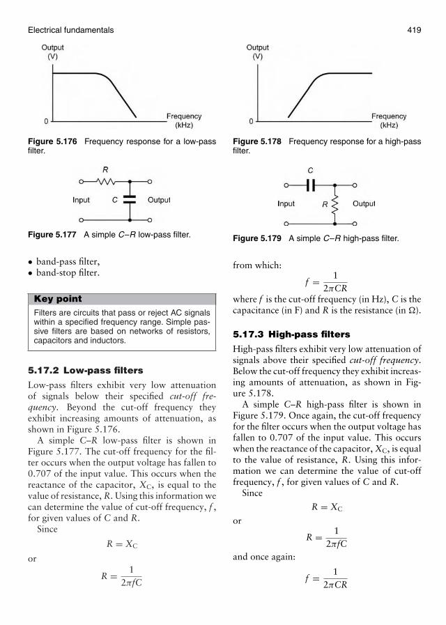
Electrical fundamentals 419
Figure 5.176 Frequency response for a low-passfilter.
Figure 5.177 A simple C–R low-pass filter.
• band-pass filter,• band-stop filter.
Key pointFilters are circuits that pass or reject AC signalswithin a specified frequency range. Simple pas-sive filters are based on networks of resistors,capacitors and inductors.
5.17.2 Low-pass filters
Low-pass filters exhibit very low attenuationof signals below their specified cut-off fre-quency. Beyond the cut-off frequency theyexhibit increasing amounts of attenuation, asshown in Figure 5.176.
A simple C–R low-pass filter is shown inFigure 5.177. The cut-off frequency for the fil-ter occurs when the output voltage has fallen to0.707 of the input value. This occurs when thereactance of the capacitor, XC, is equal to thevalue of resistance, R. Using this information wecan determine the value of cut-off frequency, f ,for given values of C and R.
Since
R = XC
or
R = 12πfC
Figure 5.178 Frequency response for a high-passfilter.
Figure 5.179 A simple C–R high-pass filter.
from which:
f = 12πCR
where f is the cut-off frequency (in Hz), C is thecapacitance (in F) and R is the resistance (in �).
5.17.3 High-pass filters
High-pass filters exhibit very low attenuation ofsignals above their specified cut-off frequency.Below the cut-off frequency they exhibit increas-ing amounts of attenuation, as shown in Fig-ure 5.178.
A simple C–R high-pass filter is shown inFigure 5.179. Once again, the cut-off frequencyfor the filter occurs when the output voltage hasfallen to 0.707 of the input value. This occurswhen the reactance of the capacitor, XC, is equalto the value of resistance, R. Using this infor-mation we can determine the value of cut-offfrequency, f , for given values of C and R.
Since
R = XC
or
R = 12πfC
and once again:
f = 12πCR
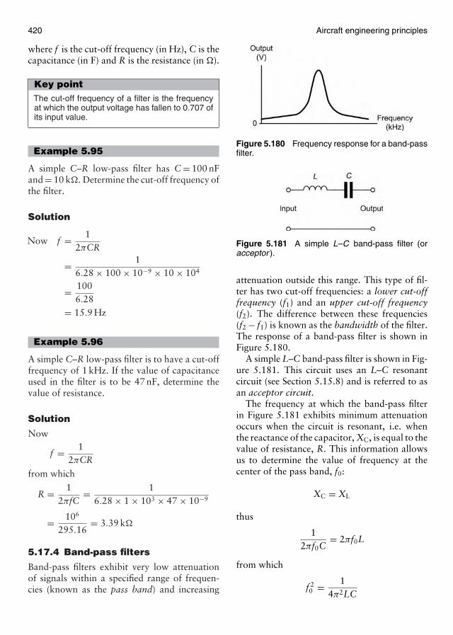
420 Aircraft engineering principles
where f is the cut-off frequency (in Hz), C is thecapacitance (in F) and R is the resistance (in �).
Key pointThe cut-off frequency of a filter is the frequencyat which the output voltage has fallen to 0.707 ofits input value.
Example 5.95
A simple C–R low-pass filter has C = 100 nFand = 10 k�. Determine the cut-off frequency ofthe filter.
Solution
Now f = 12πCR
= 16.28 × 100 × 10−9 × 10 × 104
= 1006.28
= 15.9 Hz
Example 5.96
A simple C–R low-pass filter is to have a cut-offfrequency of 1 kHz. If the value of capacitanceused in the filter is to be 47 nF, determine thevalue of resistance.
Solution
Now
f = 12πCR
from which
R = 12πfC
= 16.28 × 1 × 103 × 47 × 10−9
= 106
295.16= 3.39 k�
5.17.4 Band-pass filters
Band-pass filters exhibit very low attenuationof signals within a specified range of frequen-cies (known as the pass band) and increasing
Figure 5.180 Frequency response for a band-passfilter.
Figure 5.181 A simple L–C band-pass filter (oracceptor ).
attenuation outside this range. This type of fil-ter has two cut-off frequencies: a lower cut-offfrequency (f1) and an upper cut-off frequency(f2). The difference between these frequencies(f2 − f1) is known as the bandwidth of the filter.The response of a band-pass filter is shown inFigure 5.180.
A simple L–C band-pass filter is shown in Fig-ure 5.181. This circuit uses an L–C resonantcircuit (see Section 5.15.8) and is referred to asan acceptor circuit.
The frequency at which the band-pass filterin Figure 5.181 exhibits minimum attenuationoccurs when the circuit is resonant, i.e. whenthe reactance of the capacitor, XC, is equal to thevalue of resistance, R. This information allowsus to determine the value of frequency at thecenter of the pass band, f0:
XC = XL
thus
12πf0C
= 2πf0L
from which
f 20 = 1
4π2LC
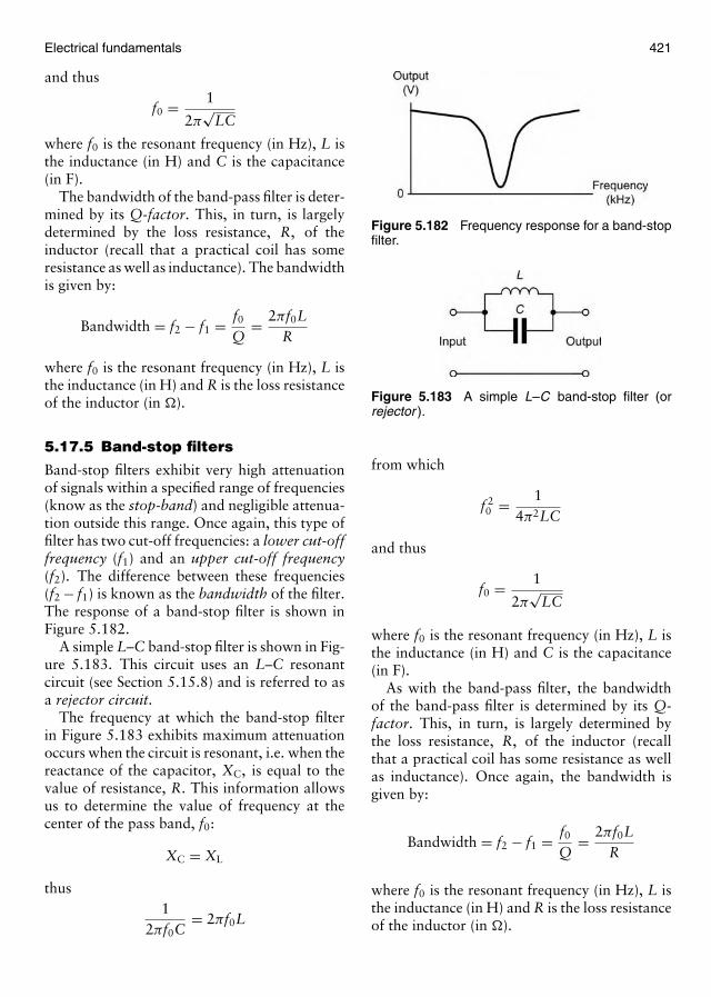
Electrical fundamentals 421
and thus
f0 = 1
2π√
LC
where f0 is the resonant frequency (in Hz), L isthe inductance (in H) and C is the capacitance(in F).
The bandwidth of the band-pass filter is deter-mined by its Q-factor. This, in turn, is largelydetermined by the loss resistance, R, of theinductor (recall that a practical coil has someresistance as well as inductance). The bandwidthis given by:
Bandwidth = f2 − f1 = f0
Q= 2πf0L
R
where f0 is the resonant frequency (in Hz), L isthe inductance (in H) and R is the loss resistanceof the inductor (in �).
5.17.5 Band-stop filters
Band-stop filters exhibit very high attenuationof signals within a specified range of frequencies(know as the stop-band) and negligible attenua-tion outside this range. Once again, this type offilter has two cut-off frequencies: a lower cut-offfrequency (f1) and an upper cut-off frequency(f2). The difference between these frequencies(f2 − f1) is known as the bandwidth of the filter.The response of a band-stop filter is shown inFigure 5.182.
A simple L–C band-stop filter is shown in Fig-ure 5.183. This circuit uses an L–C resonantcircuit (see Section 5.15.8) and is referred to asa rejector circuit.
The frequency at which the band-stop filterin Figure 5.183 exhibits maximum attenuationoccurs when the circuit is resonant, i.e. when thereactance of the capacitor, XC, is equal to thevalue of resistance, R. This information allowsus to determine the value of frequency at thecenter of the pass band, f0:
XC = XL
thus1
2πf0C= 2πf0L
Figure 5.182 Frequency response for a band-stopfilter.
Figure 5.183 A simple L–C band-stop filter (orrejector ).
from which
f 20 = 1
4π2LC
and thus
f0 = 1
2π√
LC
where f0 is the resonant frequency (in Hz), L isthe inductance (in H) and C is the capacitance(in F).
As with the band-pass filter, the bandwidthof the band-pass filter is determined by its Q-factor. This, in turn, is largely determined bythe loss resistance, R, of the inductor (recallthat a practical coil has some resistance as wellas inductance). Once again, the bandwidth isgiven by:
Bandwidth = f2 − f1 = f0
Q= 2πf0L
R
where f0 is the resonant frequency (in Hz), L isthe inductance (in H) and R is the loss resistanceof the inductor (in �).
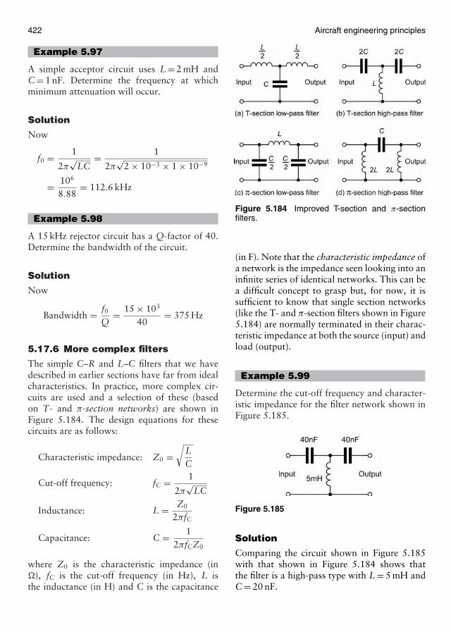
422 Aircraft engineering principles
Example 5.97
A simple acceptor circuit uses L = 2 mH andC = 1 nF. Determine the frequency at whichminimum attenuation will occur.
Solution
Now
f0 = 1
2π√
LC= 1
2π√
2 × 10−3 × 1 × 10−9
= 106
8.88= 112.6 kHz
Example 5.98
A 15 kHz rejector circuit has a Q-factor of 40.Determine the bandwidth of the circuit.
Solution
Now
Bandwidth = f0
Q= 15 × 103
40= 375 Hz
5.17.6 More complex filters
The simple C–R and L–C filters that we havedescribed in earlier sections have far from idealcharacteristics. In practice, more complex cir-cuits are used and a selection of these (basedon T- and π-section networks) are shown inFigure 5.184. The design equations for thesecircuits are as follows:
Characteristic impedance: Z0 =√
LC
Cut-off frequency: fC = 1
2π√
LC
Inductance: L = Z0
2πfC
Capacitance: C = 12πfCZ0
where Z0 is the characteristic impedance (in�), fC is the cut-off frequency (in Hz), L isthe inductance (in H) and C is the capacitance
Figure 5.184 Improved T-section and π-sectionfilters.
(in F). Note that the characteristic impedance ofa network is the impedance seen looking into aninfinite series of identical networks. This can bea difficult concept to grasp but, for now, it issufficient to know that single section networks(like the T- and π-section filters shown in Figure5.184) are normally terminated in their charac-teristic impedance at both the source (input) andload (output).
Example 5.99
Determine the cut-off frequency and character-istic impedance for the filter network shown inFigure 5.185.
Figure 5.185
Solution
Comparing the circuit shown in Figure 5.185with that shown in Figure 5.184 shows thatthe filter is a high-pass type with L = 5 mH andC = 20 nF.
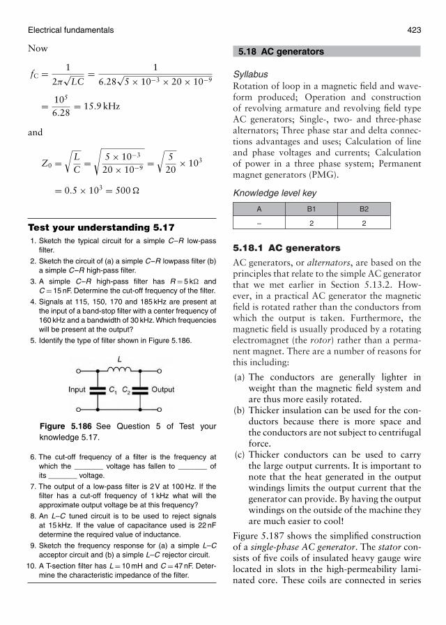
Electrical fundamentals 423
Now
fC = 1
2π√
LC= 1
6.28√
5 × 10−3 × 20 × 10−9
= 105
6.28= 15.9 kHz
and
Z0 =√
LC
=√
5 × 10⁻³
20 × 10−9=√
520
× 103
= 0.5 × 103 = 500 �
Test your understanding 5.171. Sketch the typical circuit for a simple C–R low-pass
filter.
2. Sketch the circuit of (a) a simple C–R lowpass filter (b)a simple C–R high-pass filter.
3. A simple C–R high-pass filter has R = 5 k� andC = 15 nF. Determine the cut-off frequency of the filter.
4. Signals at 115, 150, 170 and 185 kHz are present atthe input of a band-stop filter with a center frequency of160 kHz and a bandwidth of 30 kHz. Which frequencieswill be present at the output?
5. Identify the type of filter shown in Figure 5.186.
Figure 5.186 See Question 5 of Test yourknowledge 5.17.
6. The cut-off frequency of a filter is the frequency atwhich the _______ voltage has fallen to _______ ofits _______ voltage.
7. The output of a low-pass filter is 2V at 100 Hz. If thefilter has a cut-off frequency of 1 kHz what will theapproximate output voltage be at this frequency?
8. An L–C tuned circuit is to be used to reject signalsat 15 kHz. If the value of capacitance used is 22 nFdetermine the required value of inductance.
9. Sketch the frequency response for (a) a simple L–Cacceptor circuit and (b) a simple L–C rejector circuit.
10. A T-section filter has L = 10 mH and C = 47 nF. Deter-mine the characteristic impedance of the filter.
5.18 AC generators
SyllabusRotation of loop in a magnetic field and wave-form produced; Operation and constructionof revolving armature and revolving field typeAC generators; Single-, two- and three-phasealternators; Three phase star and delta connec-tions advantages and uses; Calculation of lineand phase voltages and currents; Calculationof power in a three phase system; Permanentmagnet generators (PMG).
Knowledge level key
–
A
2
B1
2
B2
5.18.1 AC generators
AC generators, or alternators, are based on theprinciples that relate to the simple AC generatorthat we met earlier in Section 5.13.2. How-ever, in a practical AC generator the magneticfield is rotated rather than the conductors fromwhich the output is taken. Furthermore, themagnetic field is usually produced by a rotatingelectromagnet (the rotor) rather than a perma-nent magnet. There are a number of reasons forthis including:
(a) The conductors are generally lighter inweight than the magnetic field system andare thus more easily rotated.
(b) Thicker insulation can be used for the con-ductors because there is more space andthe conductors are not subject to centrifugalforce.
(c) Thicker conductors can be used to carrythe large output currents. It is important tonote that the heat generated in the outputwindings limits the output current that thegenerator can provide. By having the outputwindings on the outside of the machine theyare much easier to cool!
Figure 5.187 shows the simplified constructionof a single-phase AC generator. The stator con-sists of five coils of insulated heavy gauge wirelocated in slots in the high-permeability lami-nated core. These coils are connected in series
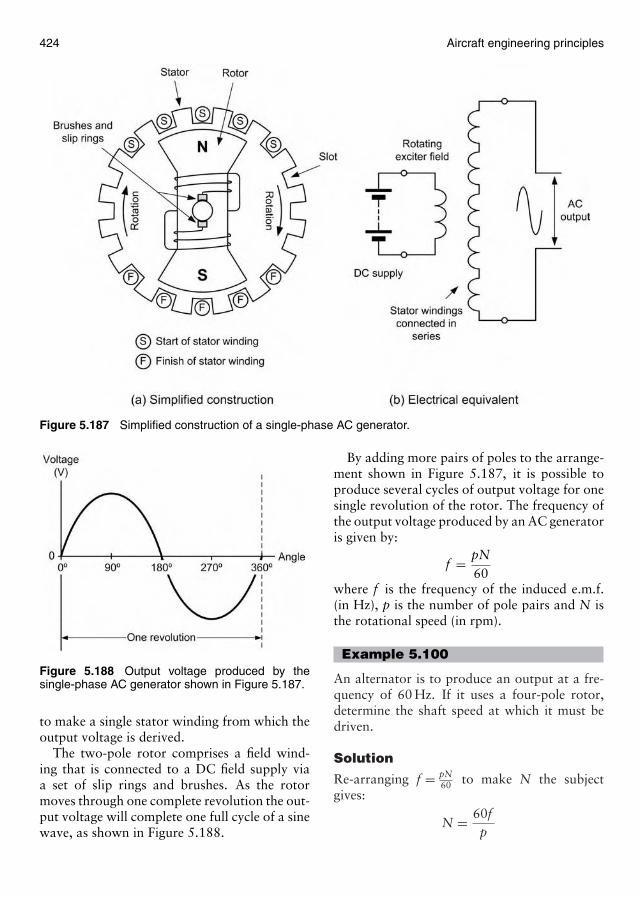
424 Aircraft engineering principles
Figure 5.187 Simplified construction of a single-phase AC generator.
Figure 5.188 Output voltage produced by thesingle-phase AC generator shown in Figure 5.187.
to make a single stator winding from which theoutput voltage is derived.
The two-pole rotor comprises a field wind-ing that is connected to a DC field supply viaa set of slip rings and brushes. As the rotormoves through one complete revolution the out-put voltage will complete one full cycle of a sinewave, as shown in Figure 5.188.
By adding more pairs of poles to the arrange-ment shown in Figure 5.187, it is possible toproduce several cycles of output voltage for onesingle revolution of the rotor. The frequency ofthe output voltage produced by an AC generatoris given by:
f = pN60
where f is the frequency of the induced e.m.f.(in Hz), p is the number of pole pairs and N isthe rotational speed (in rpm).
Example 5.100
An alternator is to produce an output at a fre-quency of 60 Hz. If it uses a four-pole rotor,determine the shaft speed at which it must bedriven.
Solution
Re-arranging f = pN60 to make N the subject
gives:
N = 60fp
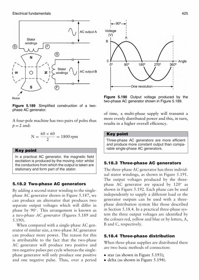
Electrical fundamentals 425
Figure 5.189 Simplified construction of a two-phase AC generator.
A four-pole machine has two pairs of poles thusp = 2 and:
N = 60 × 602
= 1800 rpm
Key pointIn a practical AC generator, the magnetic fieldexcitation is produced by the moving rotor whilstthe conductors from which the output is taken arestationary and form part of the stator.
5.18.2 Two-phase AC generators
By adding a second stator winding to the single-phase AC generator shown in Figure 5.187, wecan produce an alternator that produces twoseparate output voltages which will differ inphase by 90◦. This arrangement is known asa two-phase AC generator (Figures 5.189 and5.190).
When compared with a single-phase AC gen-erator of similar size, a two-phase AC generatorcan produce more power. The reason for thisis attributable to the fact that the two-phaseAC generator will produce two positive andtwo negative pulses per cycle whereas the single-phase generator will only produce one positiveand one negative pulse. Thus, over a period
Figure 5.190 Output voltage produced by thetwo-phase AC generator shown in Figure 5.189.
of time, a multi-phase supply will transmit amore evenly distributed power and this, in turn,results in a higher overall efficiency.
Key pointThree-phase AC generators are more efficientand produce more constant output than compa-rable single-phase AC generators.
5.18.3 Three-phase AC generators
The three-phase AC generator has three individ-ual stator windings, as shown in Figure 5.191.The output voltages produced by the three-phase AC generator are spaced by 120◦ asshown in Figure 5.192. Each phase can be usedindependently to supply a different load or thegenerator outputs can be used with a three-phase distribution system like those describedin Section 5.18.4. In a practical three-phase sys-tem the three output voltages are identified bythe colours red, yellow and blue or by letters, A,B and C, respectively.
5.18.4 Three-phase distribution
When three-phase supplies are distributed thereare two basic methods of connection:
• star (as shown in Figure 5.193);• delta (as shown in Figure 5.194).

426 Aircraft engineering principles
Figure 5.191 Simplified con-struction of a three-phase ACgenerator.
Figure 5.192 Output voltage produced by thethree-phase AC generator shown in Figure 5.191.
A complete star-connected three-phase distri-bution system is shown in Figure 5.195. Thisshows a three-phase AC generator connecteda three-phase load. Ideally, the load will bebalanced in which case all three-load resistances(or impedances) will be identical.
The relationship between the line and phasevoltages shown in Figure 5.195 can be deter-mined from the phasor diagram shown in Fig-ure 5.196. From this diagram it is important to
Figure 5.193 Star connection.
Figure 5.194 Delta connection.
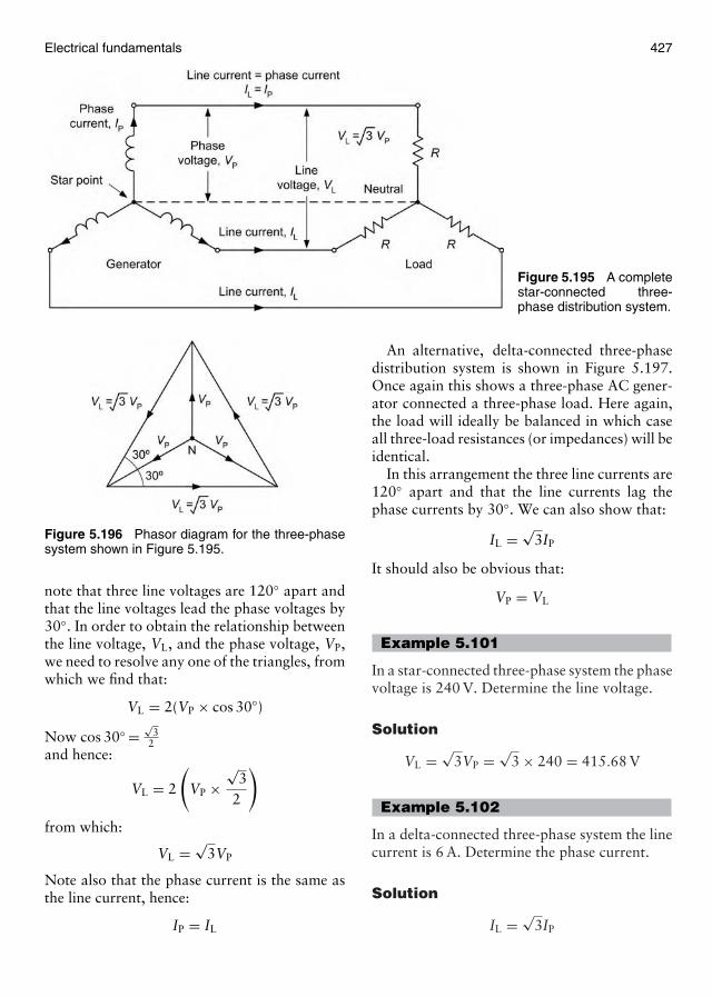
Electrical fundamentals 427
Figure 5.195 A completestar-connected three-phase distribution system.
Figure 5.196 Phasor diagram for the three-phasesystem shown in Figure 5.195.
note that three line voltages are 120◦ apart andthat the line voltages lead the phase voltages by30◦. In order to obtain the relationship betweenthe line voltage, VL, and the phase voltage, VP,we need to resolve any one of the triangles, fromwhich we find that:
VL = 2(VP × cos 30◦)
Now cos 30◦ =√
32
and hence:
VL = 2
(VP ×
√3
2
)
from which:
VL = √3VP
Note also that the phase current is the same asthe line current, hence:
IP = IL
An alternative, delta-connected three-phasedistribution system is shown in Figure 5.197.Once again this shows a three-phase AC gener-ator connected a three-phase load. Here again,the load will ideally be balanced in which caseall three-load resistances (or impedances) will beidentical.
In this arrangement the three line currents are120◦ apart and that the line currents lag thephase currents by 30◦. We can also show that:
IL = √3IP
It should also be obvious that:
VP = VL
Example 5.101
In a star-connected three-phase system the phasevoltage is 240 V. Determine the line voltage.
Solution
VL = √3VP = √
3 × 240 = 415.68 V
Example 5.102
In a delta-connected three-phase system the linecurrent is 6 A. Determine the phase current.
Solution
IL = √3IP
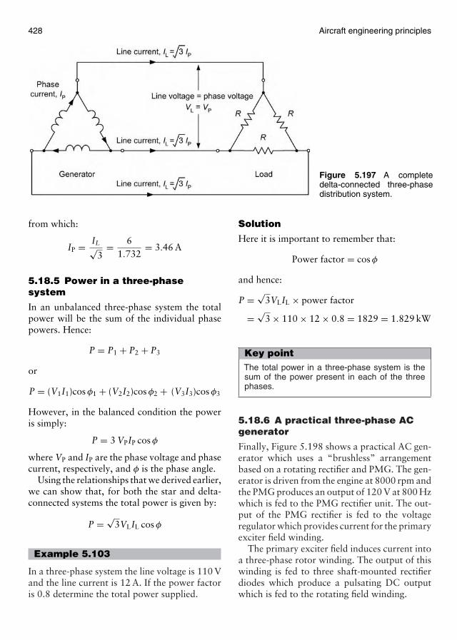
428 Aircraft engineering principles
Figure 5.197 A completedelta-connected three-phasedistribution system.
from which:
IP = IL√3
= 61.732
= 3.46 A
5.18.5 Power in a three-phasesystem
In an unbalanced three-phase system the totalpower will be the sum of the individual phasepowers. Hence:
P = P1 + P2 + P3
or
P = (V1I1)cos φ1 + (V2I2)cos φ2 + (V3I3)cos φ3
However, in the balanced condition the poweris simply:
P = 3 VPIP cos φ
where VP and IP are the phase voltage and phasecurrent, respectively, and φ is the phase angle.
Using the relationships that we derived earlier,we can show that, for both the star and delta-connected systems the total power is given by:
P = √3VLIL cos φ
Example 5.103
In a three-phase system the line voltage is 110 Vand the line current is 12 A. If the power factoris 0.8 determine the total power supplied.
Solution
Here it is important to remember that:
Power factor = cos φ
and hence:
P = √3VLIL × power factor
= √3 × 110 × 12 × 0.8 = 1829 = 1.829 kW
Key pointThe total power in a three-phase system is thesum of the power present in each of the threephases.
5.18.6 A practical three-phase ACgenerator
Finally, Figure 5.198 shows a practical AC gen-erator which uses a “brushless” arrangementbased on a rotating rectifier and PMG. The gen-erator is driven from the engine at 8000 rpm andthe PMG produces an output of 120 V at 800 Hzwhich is fed to the PMG rectifier unit. The out-put of the PMG rectifier is fed to the voltageregulator which provides current for the primaryexciter field winding.
The primary exciter field induces current intoa three-phase rotor winding. The output of thiswinding is fed to three shaft-mounted rectifierdiodes which produce a pulsating DC outputwhich is fed to the rotating field winding.
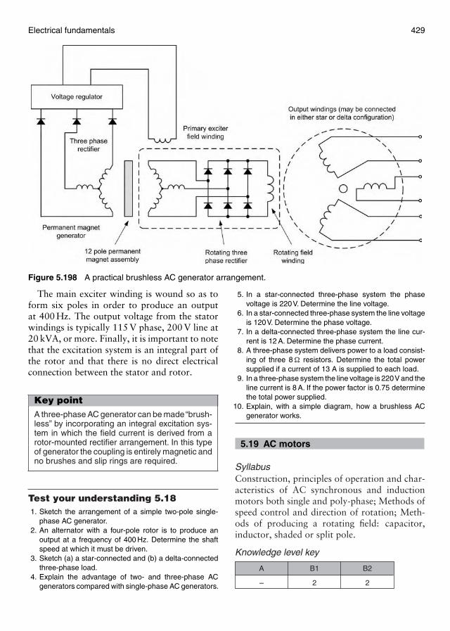
Electrical fundamentals 429
Figure 5.198 A practical brushless AC generator arrangement.
The main exciter winding is wound so as toform six poles in order to produce an outputat 400 Hz. The output voltage from the statorwindings is typically 115 V phase, 200 V line at20 kVA, or more. Finally, it is important to notethat the excitation system is an integral part ofthe rotor and that there is no direct electricalconnection between the stator and rotor.
Key pointA three-phase AC generator can be made“brush-less” by incorporating an integral excitation sys-tem in which the field current is derived from arotor-mounted rectifier arrangement. In this typeof generator the coupling is entirely magnetic andno brushes and slip rings are required.
Test your understanding 5.181. Sketch the arrangement of a simple two-pole single-
phase AC generator.2. An alternator with a four-pole rotor is to produce an
output at a frequency of 400 Hz. Determine the shaftspeed at which it must be driven.
3. Sketch (a) a star-connected and (b) a delta-connectedthree-phase load.
4. Explain the advantage of two- and three-phase ACgenerators compared with single-phase AC generators.
5. In a star-connected three-phase system the phasevoltage is 220V. Determine the line voltage.
6. In a star-connected three-phase system the line voltageis 120V. Determine the phase voltage.
7. In a delta-connected three-phase system the line cur-rent is 12 A. Determine the phase current.
8. A three-phase system delivers power to a load consist-ing of three 8 � resistors. Determine the total powersupplied if a current of 13 A is supplied to each load.
9. In a three-phase system the line voltage is 220V and theline current is 8 A. If the power factor is 0.75 determinethe total power supplied.
10. Explain, with a simple diagram, how a brushless ACgenerator works.
5.19 AC motors
SyllabusConstruction, principles of operation and char-acteristics of AC synchronous and inductionmotors both single and poly-phase; Methods ofspeed control and direction of rotation; Meth-ods of producing a rotating field: capacitor,inductor, shaded or split pole.
Knowledge level key
–
A
2
B1
2
B2
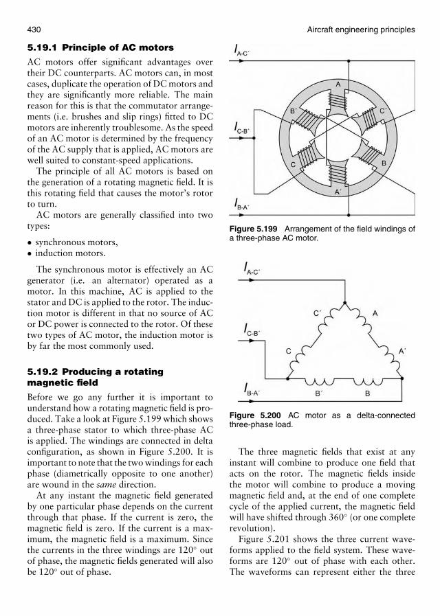
430 Aircraft engineering principles
5.19.1 Principle of AC motors
AC motors offer significant advantages overtheir DC counterparts. AC motors can, in mostcases, duplicate the operation of DC motors andthey are significantly more reliable. The mainreason for this is that the commutator arrange-ments (i.e. brushes and slip rings) fitted to DCmotors are inherently troublesome. As the speedof an AC motor is determined by the frequencyof the AC supply that is applied, AC motors arewell suited to constant-speed applications.
The principle of all AC motors is based onthe generation of a rotating magnetic field. It isthis rotating field that causes the motor’s rotorto turn.
AC motors are generally classified into twotypes:
• synchronous motors,• induction motors.
The synchronous motor is effectively an ACgenerator (i.e. an alternator) operated as amotor. In this machine, AC is applied to thestator and DC is applied to the rotor. The induc-tion motor is different in that no source of ACor DC power is connected to the rotor. Of thesetwo types of AC motor, the induction motor isby far the most commonly used.
5.19.2 Producing a rotatingmagnetic field
Before we go any further it is important tounderstand how a rotating magnetic field is pro-duced. Take a look at Figure 5.199 which showsa three-phase stator to which three-phase ACis applied. The windings are connected in deltaconfiguration, as shown in Figure 5.200. It isimportant to note that the two windings for eachphase (diametrically opposite to one another)are wound in the same direction.
At any instant the magnetic field generatedby one particular phase depends on the currentthrough that phase. If the current is zero, themagnetic field is zero. If the current is a max-imum, the magnetic field is a maximum. Sincethe currents in the three windings are 120◦ outof phase, the magnetic fields generated will alsobe 120◦ out of phase.
Figure 5.199 Arrangement of the field windings ofa three-phase AC motor.
Figure 5.200 AC motor as a delta-connectedthree-phase load.
The three magnetic fields that exist at anyinstant will combine to produce one field thatacts on the rotor. The magnetic fields insidethe motor will combine to produce a movingmagnetic field and, at the end of one completecycle of the applied current, the magnetic fieldwill have shifted through 360◦ (or one completerevolution).
Figure 5.201 shows the three current wave-forms applied to the field system. These wave-forms are 120◦ out of phase with each other.The waveforms can represent either the three
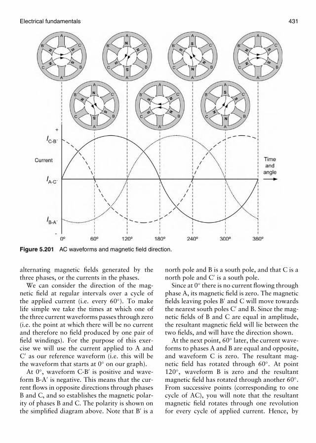
Electrical fundamentals 431
Figure 5.201 AC waveforms and magnetic field direction.
alternating magnetic fields generated by thethree phases, or the currents in the phases.
We can consider the direction of the mag-netic field at regular intervals over a cycle ofthe applied current (i.e. every 60◦). To makelife simple we take the times at which one ofthe three current waveforms passes through zero(i.e. the point at which there will be no currentand therefore no field produced by one pair offield windings). For the purpose of this exer-cise we will use the current applied to A andC′ as our reference waveform (i.e. this will bethe waveform that starts at 0◦ on our graph).
At 0◦, waveform C-B′ is positive and wave-form B-A′ is negative. This means that the cur-rent flows in opposite directions through phasesB and C, and so establishes the magnetic polar-ity of phases B and C. The polarity is shown onthe simplified diagram above. Note that B′ is a
north pole and B is a south pole, and that C is anorth pole and C′ is a south pole.
Since at 0◦ there is no current flowing throughphase A, its magnetic field is zero. The magneticfields leaving poles B′ and C will move towardsthe nearest south poles C′ and B. Since the mag-netic fields of B and C are equal in amplitude,the resultant magnetic field will lie between thetwo fields, and will have the direction shown.
At the next point, 60◦ later, the current wave-forms to phases A and B are equal and opposite,and waveform C is zero. The resultant mag-netic field has rotated through 60◦. At point120◦, waveform B is zero and the resultantmagnetic field has rotated through another 60◦.From successive points (corresponding to onecycle of AC), you will note that the resultantmagnetic field rotates through one revolutionfor every cycle of applied current. Hence, by
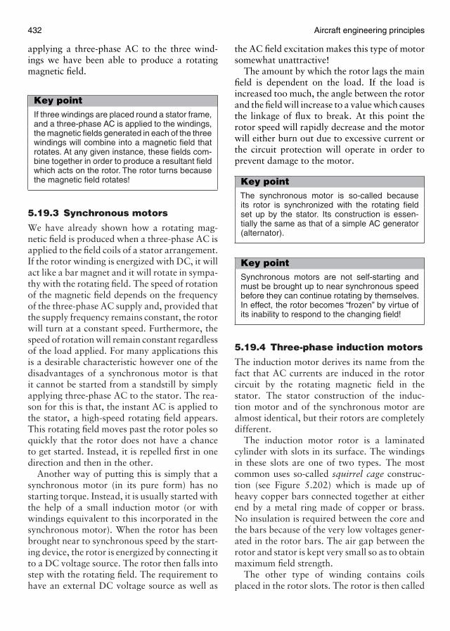
432 Aircraft engineering principles
applying a three-phase AC to the three wind-ings we have been able to produce a rotatingmagnetic field.
Key pointIf three windings are placed round a stator frame,and a three-phase AC is applied to the windings,the magnetic fields generated in each of the threewindings will combine into a magnetic field thatrotates. At any given instance, these fields com-bine together in order to produce a resultant fieldwhich acts on the rotor. The rotor turns becausethe magnetic field rotates!
5.19.3 Synchronous motors
We have already shown how a rotating mag-netic field is produced when a three-phase AC isapplied to the field coils of a stator arrangement.If the rotor winding is energized with DC, it willact like a bar magnet and it will rotate in sympa-thy with the rotating field. The speed of rotationof the magnetic field depends on the frequencyof the three-phase AC supply and, provided thatthe supply frequency remains constant, the rotorwill turn at a constant speed. Furthermore, thespeed of rotation will remain constant regardlessof the load applied. For many applications thisis a desirable characteristic however one of thedisadvantages of a synchronous motor is thatit cannot be started from a standstill by simplyapplying three-phase AC to the stator. The rea-son for this is that, the instant AC is applied tothe stator, a high-speed rotating field appears.This rotating field moves past the rotor poles soquickly that the rotor does not have a chanceto get started. Instead, it is repelled first in onedirection and then in the other.
Another way of putting this is simply that asynchronous motor (in its pure form) has nostarting torque. Instead, it is usually started withthe help of a small induction motor (or withwindings equivalent to this incorporated in thesynchronous motor). When the rotor has beenbrought near to synchronous speed by the start-ing device, the rotor is energized by connecting itto a DC voltage source. The rotor then falls intostep with the rotating field. The requirement tohave an external DC voltage source as well as
the AC field excitation makes this type of motorsomewhat unattractive!
The amount by which the rotor lags the mainfield is dependent on the load. If the load isincreased too much, the angle between the rotorand the field will increase to a value which causesthe linkage of flux to break. At this point therotor speed will rapidly decrease and the motorwill either burn out due to excessive current orthe circuit protection will operate in order toprevent damage to the motor.
Key pointThe synchronous motor is so-called becauseits rotor is synchronized with the rotating fieldset up by the stator. Its construction is essen-tially the same as that of a simple AC generator(alternator).
Key pointSynchronous motors are not self-starting andmust be brought up to near synchronous speedbefore they can continue rotating by themselves.In effect, the rotor becomes “frozen” by virtue ofits inability to respond to the changing field!
5.19.4 Three-phase induction motors
The induction motor derives its name from thefact that AC currents are induced in the rotorcircuit by the rotating magnetic field in thestator. The stator construction of the induc-tion motor and of the synchronous motor arealmost identical, but their rotors are completelydifferent.
The induction motor rotor is a laminatedcylinder with slots in its surface. The windingsin these slots are one of two types. The mostcommon uses so-called squirrel cage construc-tion (see Figure 5.202) which is made up ofheavy copper bars connected together at eitherend by a metal ring made of copper or brass.No insulation is required between the core andthe bars because of the very low voltages gener-ated in the rotor bars. The air gap between therotor and stator is kept very small so as to obtainmaximum field strength.
The other type of winding contains coilsplaced in the rotor slots. The rotor is then called
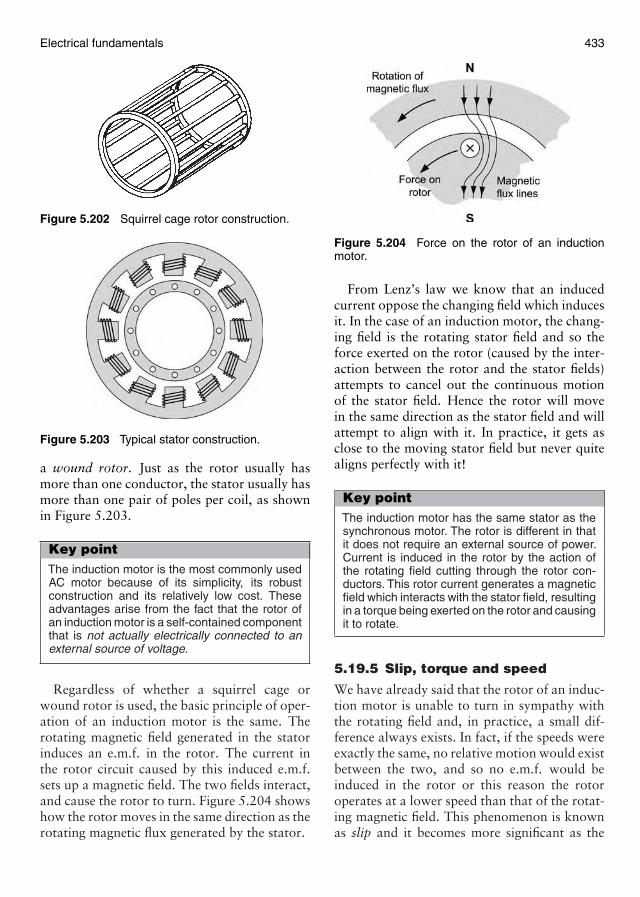
Electrical fundamentals 433
Figure 5.202 Squirrel cage rotor construction.
Figure 5.203 Typical stator construction.
a wound rotor. Just as the rotor usually hasmore than one conductor, the stator usually hasmore than one pair of poles per coil, as shownin Figure 5.203.
Key pointThe induction motor is the most commonly usedAC motor because of its simplicity, its robustconstruction and its relatively low cost. Theseadvantages arise from the fact that the rotor ofan induction motor is a self-contained componentthat is not actually electrically connected to anexternal source of voltage.
Regardless of whether a squirrel cage orwound rotor is used, the basic principle of oper-ation of an induction motor is the same. Therotating magnetic field generated in the statorinduces an e.m.f. in the rotor. The current inthe rotor circuit caused by this induced e.m.f.sets up a magnetic field. The two fields interact,and cause the rotor to turn. Figure 5.204 showshow the rotor moves in the same direction as therotating magnetic flux generated by the stator.
Figure 5.204 Force on the rotor of an inductionmotor.
From Lenz’s law we know that an inducedcurrent oppose the changing field which inducesit. In the case of an induction motor, the chang-ing field is the rotating stator field and so theforce exerted on the rotor (caused by the inter-action between the rotor and the stator fields)attempts to cancel out the continuous motionof the stator field. Hence the rotor will movein the same direction as the stator field and willattempt to align with it. In practice, it gets asclose to the moving stator field but never quitealigns perfectly with it!
Key pointThe induction motor has the same stator as thesynchronous motor. The rotor is different in thatit does not require an external source of power.Current is induced in the rotor by the action ofthe rotating field cutting through the rotor con-ductors. This rotor current generates a magneticfield which interacts with the stator field, resultingin a torque being exerted on the rotor and causingit to rotate.
5.19.5 Slip, torque and speed
We have already said that the rotor of an induc-tion motor is unable to turn in sympathy withthe rotating field and, in practice, a small dif-ference always exists. In fact, if the speeds wereexactly the same, no relative motion would existbetween the two, and so no e.m.f. would beinduced in the rotor or this reason the rotoroperates at a lower speed than that of the rotat-ing magnetic field. This phenomenon is knownas slip and it becomes more significant as the
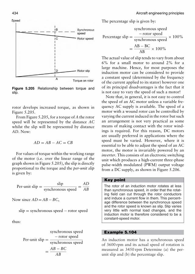
434 Aircraft engineering principles
Figure 5.205 Relationship between torque andslip.
rotor develops increased torque, as shown inFigure 5.205.
From Figure 5.205, for a torque of A the rotorspeed will be represented by the distance ACwhilst the slip will be represented by distanceAD. Now:
AD = AB − AC = CB
For values of torque within the working rangeof the motor (i.e. over the linear range of thegraph shown in Figure 5.205), the slip is directlyproportional to the torque and the per-unit slipis given by:
Per-unit slip = slipsynchronous speed
= ADAB
Now since AD = AB − BC,
slip = synchronous speed − rotor speed
thus:
Per-unit slip =synchronous speed
− rotor speed
synchronous speed
= AB − BCAB
The percentage slip is given by:
Percentage slip =synchronous speed
− rotor speed
synchronous speed× 100%
= AB − BCAB
× 100%
The actual value of slip tends to vary from about6% for a small motor to around 2% for alarge machine. Hence, for most purposes theinduction motor can be considered to providea constant speed (determined by the frequencyof the current applied to its stator) however oneof its principal disadvantages is the fact that itis not easy to vary the speed of such a motor!
Note that, in general, it is not easy to controlthe speed of an AC motor unless a variable fre-quency AC supply is available. The speed of amotor with a wound rotor can be controlled byvarying the current induced in the rotor but suchan arrangement is not very practical as somemeans of making contact with the rotor wind-ings is required. For this reason, DC motorsare usually preferred in applications where thespeed must be varied. However, where it isessential to be able to adjust the speed of an ACmotor, the motor is invariably powered by aninverter. This consists of an electronic switchingunit which produces a high-current three-phasepulse-width modulated (PWM) output voltagefrom a DC supply, as shown in Figure 5.206.
Key pointThe rotor of an induction motor rotates at lessthan synchronous speed, in order that the rotat-ing field can cut through the rotor conductorsand induce a current flow in them. This percent-age difference between the synchronous speedand the rotor speed is known as slip. Slip variesvery little with normal load changes, and theinduction motor is therefore considered to be aconstant-speed motor.
Example 5.104
An induction motor has a synchronous speedof 3600 rpm and its actual speed of rotation ismeasured as 3450 rpm Determine (a) the per-unit slip and (b) the percentage slip.
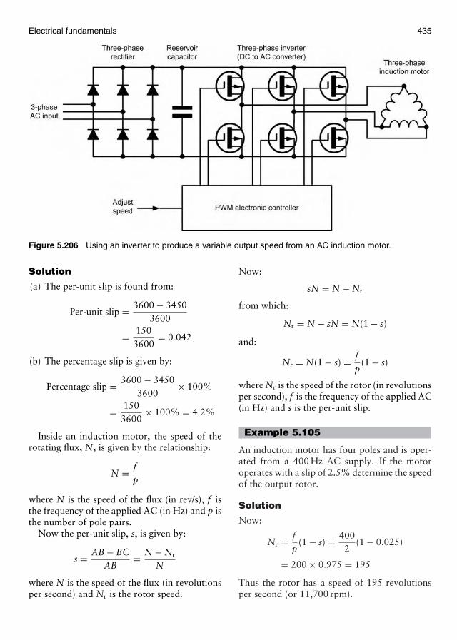
Electrical fundamentals 435
Figure 5.206 Using an inverter to produce a variable output speed from an AC induction motor.
Solution
(a) The per-unit slip is found from:
Per-unit slip = 3600 − 34503600
= 1503600
= 0.042
(b) The percentage slip is given by:
Percentage slip = 3600 − 34503600
× 100%
= 1503600
× 100% = 4.2%
Inside an induction motor, the speed of therotating flux, N, is given by the relationship:
N = fp
where N is the speed of the flux (in rev/s), f isthe frequency of the applied AC (in Hz) and p isthe number of pole pairs.
Now the per-unit slip, s, is given by:
s = AB − BCAB
= N − Nr
N
where N is the speed of the flux (in revolutionsper second) and Nr is the rotor speed.
Now:
sN = N − Nr
from which:
Nr = N − sN = N(1 − s)
and:
Nr = N(1 − s) = fp
(1 − s)
where Nr is the speed of the rotor (in revolutionsper second), f is the frequency of the applied AC(in Hz) and s is the per-unit slip.
Example 5.105
An induction motor has four poles and is oper-ated from a 400 Hz AC supply. If the motoroperates with a slip of 2.5% determine the speedof the output rotor.
Solution
Now:
Nr = fp
(1 − s) = 4002
(1 − 0.025)
= 200 × 0.975 = 195
Thus the rotor has a speed of 195 revolutionsper second (or 11,700 rpm).
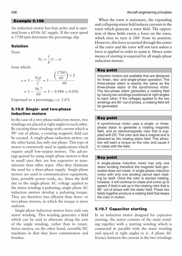
436 Aircraft engineering principles
Example 5.106
An induction motor has four poles and is oper-ated from a 60 Hz AC supply. If the rotor speedis 1700 rpm determine the percentage slip.
Solution
Now:
Nr = fp
(1 − s)
from which:
s = 1 − Nrpf
= 1 −
(1700
60
)× 2
60
= 1 − 56.760
= 1 − 0.944 = 0.056
Expressed as a percentage, i.e. 5.6%
5.19.6 Single- and two-phaseinduction motors
In the case of a two-phase induction motor, twowindings are placed at right angles to each other.By exciting these windings with current which is90◦ out of phase, a rotating magnetic field canbe created. A single-phase induction motor, onthe other hand, has only one phase. This type ofmotor is extensively used in applications whichrequire small low-output motors. The advan-tage gained by using single-phase motors is thatin small sizes they are less expensive to man-ufacture than other types. Also they eliminatethe need for a three-phase supply. Single-phasemotors are used in communication equipment,fans, portable power tools, etc. Since the fielddue to the single-phase AC voltage applied tothe stator winding is pulsating, single-phase ACinduction motors develop a pulsating torque.They are therefore less efficient than three- ortwo-phase motors, in which the torque is moreuniform.
Single-phase induction motors have only onestator winding. This winding generates a fieldwhich can be said to alternate along the axisof the single winding, rather than to rotate.Series motors, on the other hand, resemble DCmachines in that they have commutators andbrushes.
When the rotor is stationary, the expandingand collapsing stator field induces currents in therotor which generate a rotor field. The opposi-tion of these fields exerts a force on the rotor,which tries to turn it 180◦ from its position.However, this force is exerted through the centerof the rotor and the rotor will not turn unless aforce is applied in order to assist it. Hence somemeans of starting is required for all single-phaseinduction motors.
Key pointInduction motors are available that are designedfor three-, two- and single-phase operation. Thethree-phase stator is exactly the same as thethree-phase stator of the synchronous motor.The two-phase stator generates a rotating fieldby having two windings positioned at right anglesto each other. If the voltages applied to the twowindings are 90◦ out of phase, a rotating field willbe generated.
Key pointA synchronous motor uses a single- or three-phase stator to generate a rotating magneticfield, and an electromagnetic rotor that is sup-plied with DC.The rotor acts like a magnet and isattracted by the rotating stator field. This attrac-tion will exert a torque on the rotor and cause itto rotate with the field.
Key pointA single-phase induction motor has only onestator winding; therefore the magnetic field gen-erated does not rotate. A single-phase inductionmotor with only one winding cannot start rotat-ing by itself. Once the rotor is started rotating,however, it will continue to rotate and come up tospeed. A field is set up in the rotating rotor that is90◦ out of phase with the stator field. These twofields together produce a rotating field that keepsthe rotor in motion.
5.19.7 Capacitor starting
In an induction motor designed for capacitorstarting, the stator consists of the main wind-ing together with a starting winding which isconnected in parallel with the main windingand spaced at right angles to it. A phase dif-ference between the current in the two windings
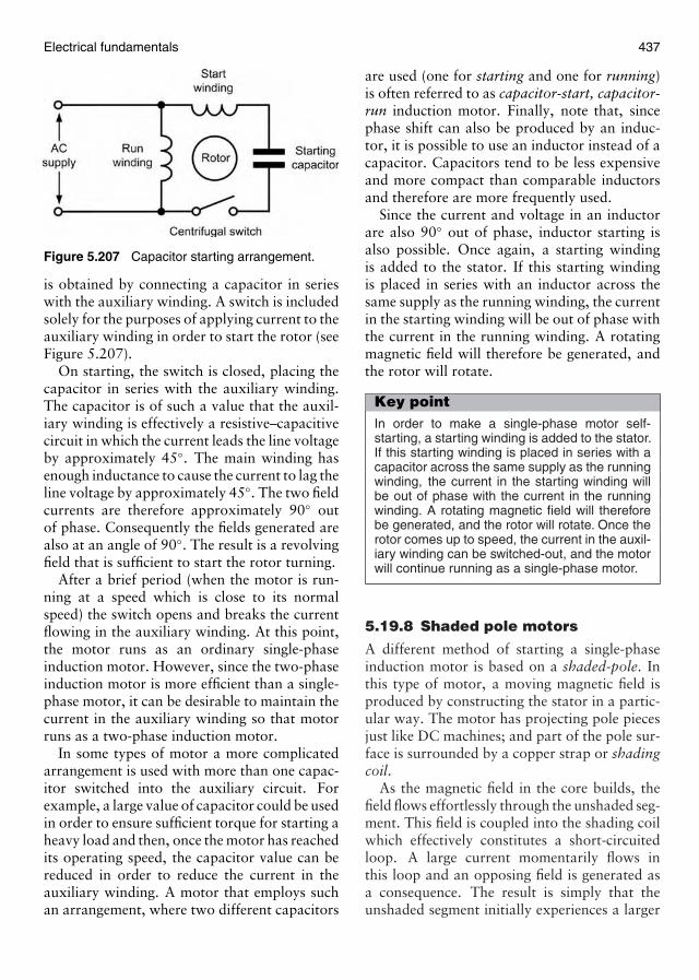
Electrical fundamentals 437
Figure 5.207 Capacitor starting arrangement.
is obtained by connecting a capacitor in serieswith the auxiliary winding. A switch is includedsolely for the purposes of applying current to theauxiliary winding in order to start the rotor (seeFigure 5.207).
On starting, the switch is closed, placing thecapacitor in series with the auxiliary winding.The capacitor is of such a value that the auxil-iary winding is effectively a resistive–capacitivecircuit in which the current leads the line voltageby approximately 45◦. The main winding hasenough inductance to cause the current to lag theline voltage by approximately 45◦. The two fieldcurrents are therefore approximately 90◦ outof phase. Consequently the fields generated arealso at an angle of 90◦. The result is a revolvingfield that is sufficient to start the rotor turning.
After a brief period (when the motor is run-ning at a speed which is close to its normalspeed) the switch opens and breaks the currentflowing in the auxiliary winding. At this point,the motor runs as an ordinary single-phaseinduction motor. However, since the two-phaseinduction motor is more efficient than a single-phase motor, it can be desirable to maintain thecurrent in the auxiliary winding so that motorruns as a two-phase induction motor.
In some types of motor a more complicatedarrangement is used with more than one capac-itor switched into the auxiliary circuit. Forexample, a large value of capacitor could be usedin order to ensure sufficient torque for starting aheavy load and then, once the motor has reachedits operating speed, the capacitor value can bereduced in order to reduce the current in theauxiliary winding. A motor that employs suchan arrangement, where two different capacitors
are used (one for starting and one for running)is often referred to as capacitor-start, capacitor-run induction motor. Finally, note that, sincephase shift can also be produced by an induc-tor, it is possible to use an inductor instead of acapacitor. Capacitors tend to be less expensiveand more compact than comparable inductorsand therefore are more frequently used.
Since the current and voltage in an inductorare also 90◦ out of phase, inductor starting isalso possible. Once again, a starting windingis added to the stator. If this starting windingis placed in series with an inductor across thesame supply as the running winding, the currentin the starting winding will be out of phase withthe current in the running winding. A rotatingmagnetic field will therefore be generated, andthe rotor will rotate.
Key pointIn order to make a single-phase motor self-starting, a starting winding is added to the stator.If this starting winding is placed in series with acapacitor across the same supply as the runningwinding, the current in the starting winding willbe out of phase with the current in the runningwinding. A rotating magnetic field will thereforebe generated, and the rotor will rotate. Once therotor comes up to speed, the current in the auxil-iary winding can be switched-out, and the motorwill continue running as a single-phase motor.
5.19.8 Shaded pole motors
A different method of starting a single-phaseinduction motor is based on a shaded-pole. Inthis type of motor, a moving magnetic field isproduced by constructing the stator in a partic-ular way. The motor has projecting pole piecesjust like DC machines; and part of the pole sur-face is surrounded by a copper strap or shadingcoil.
As the magnetic field in the core builds, thefield flows effortlessly through the unshaded seg-ment. This field is coupled into the shading coilwhich effectively constitutes a short-circuitedloop. A large current momentarily flows inthis loop and an opposing field is generated asa consequence. The result is simply that theunshaded segment initially experiences a larger
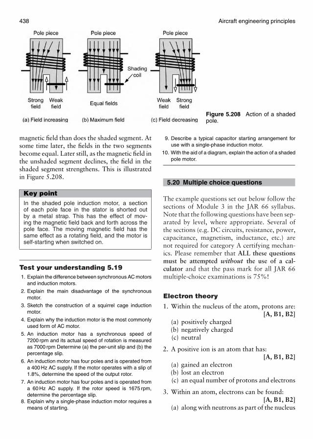
438 Aircraft engineering principles
Figure 5.208 Action of a shadedpole.
magnetic field than does the shaded segment. Atsome time later, the fields in the two segmentsbecome equal. Later still, as the magnetic field inthe unshaded segment declines, the field in theshaded segment strengthens. This is illustratedin Figure 5.208.
Key pointIn the shaded pole induction motor, a sectionof each pole face in the stator is shorted outby a metal strap. This has the effect of mov-ing the magnetic field back and forth across thepole face. The moving magnetic field has thesame effect as a rotating field, and the motor isself-starting when switched on.
Test your understanding 5.191. Explain the difference between synchronous AC motors
and induction motors.
2. Explain the main disadvantage of the synchronousmotor.
3. Sketch the construction of a squirrel cage inductionmotor.
4. Explain why the induction motor is the most commonlyused form of AC motor.
5. An induction motor has a synchronous speed of7200 rpm and its actual speed of rotation is measuredas 7000 rpm Determine (a) the per-unit slip and (b) thepercentage slip.
6. An induction motor has four poles and is operated froma 400 Hz AC supply. If the motor operates with a slip of1.8%, determine the speed of the output rotor.
7. An induction motor has four poles and is operated froma 60 Hz AC supply. If the rotor speed is 1675 rpm,determine the percentage slip.
8. Explain why a single-phase induction motor requires ameans of starting.
9. Describe a typical capacitor starting arrangement foruse with a single-phase induction motor.
10. With the aid of a diagram, explain the action of a shadedpole motor.
5.20 Multiple choice questions
The example questions set out below follow thesections of Module 3 in the JAR 66 syllabus.Note that the following questions have been sep-arated by level, where appropriate. Several ofthe sections (e.g. DC circuits, resistance, power,capacitance, magnetism, inductance, etc.) arenot required for category A certifying mechan-ics. Please remember that ALL these questionsmust be attempted without the use of a cal-culator and that the pass mark for all JAR 66multiple-choice examinations is 75%!
Electron theory
1. Within the nucleus of the atom, protons are:[A, B1, B2]
(a) positively charged(b) negatively charged(c) neutral
2. A positive ion is an atom that has:[A, B1, B2]
(a) gained an electron(b) lost an electron(c) an equal number of protons and electrons
3. Within an atom, electrons can be found:[A, B1, B2]
(a) along with neutrons as part of the nucleus
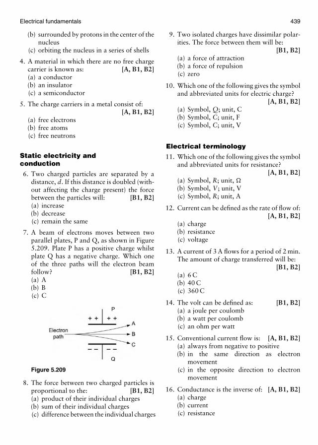
Electrical fundamentals 439
(b) surrounded by protons in the center of thenucleus
(c) orbiting the nucleus in a series of shells
4. A material in which there are no free chargecarrier is known as: [A, B1, B2](a) a conductor(b) an insulator(c) a semiconductor
5. The charge carriers in a metal consist of:[A, B1, B2]
(a) free electrons(b) free atoms(c) free neutrons
Static electricity andconduction
6. Two charged particles are separated by adistance, d. If this distance is doubled (with-out affecting the charge present) the forcebetween the particles will: [B1, B2](a) increase(b) decrease(c) remain the same
7. A beam of electrons moves between twoparallel plates, P and Q, as shown in Figure5.209. Plate P has a positive charge whilstplate Q has a negative charge. Which oneof the three paths will the electron beamfollow? [B1, B2](a) A(b) B(c) C
Figure 5.209
8. The force between two charged particles isproportional to the: [B1, B2](a) product of their individual charges(b) sum of their individual charges(c) difference between the individual charges
9. Two isolated charges have dissimilar polar-ities. The force between them will be:
[B1, B2](a) a force of attraction(b) a force of repulsion(c) zero
10. Which one of the following gives the symboland abbreviated units for electric charge?
[A, B1, B2](a) Symbol, Q; unit, C(b) Symbol, C; unit, F(c) Symbol, C; unit, V
Electrical terminology
11. Which one of the following gives the symboland abbreviated units for resistance?
[A, B1, B2](a) Symbol, R; unit, �
(b) Symbol, V ; unit, V(c) Symbol, R; unit, A
12. Current can be defined as the rate of flow of:[A, B1, B2]
(a) charge(b) resistance(c) voltage
13. A current of 3 A flows for a period of 2 min.The amount of charge transferred will be:
[B1, B2](a) 6 C(b) 40 C(c) 360 C
14. The volt can be defined as: [B1, B2](a) a joule per coulomb(b) a watt per coulomb(c) an ohm per watt
15. Conventional current flow is: [A, B1, B2](a) always from negative to positive(b) in the same direction as electron
movement(c) in the opposite direction to electron
movement
16. Conductance is the inverse of: [A, B1, B2](a) charge(b) current(c) resistance
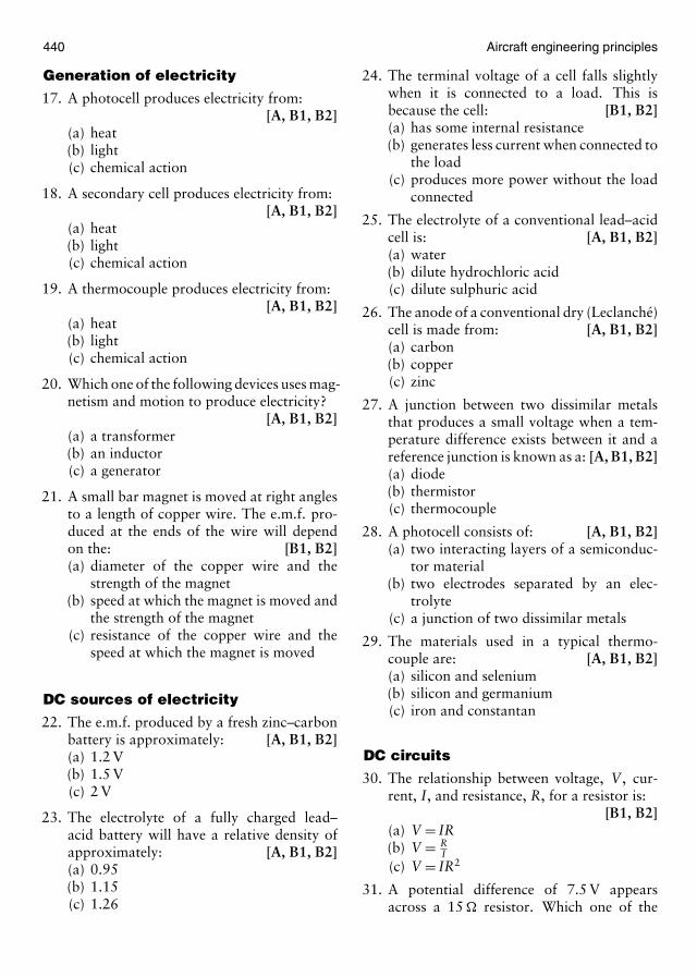
440 Aircraft engineering principles
Generation of electricity
17. A photocell produces electricity from:[A, B1, B2]
(a) heat(b) light(c) chemical action
18. A secondary cell produces electricity from:[A, B1, B2]
(a) heat(b) light(c) chemical action
19. A thermocouple produces electricity from:[A, B1, B2]
(a) heat(b) light(c) chemical action
20. Which one of the following devices uses mag-netism and motion to produce electricity?
[A, B1, B2](a) a transformer(b) an inductor(c) a generator
21. A small bar magnet is moved at right anglesto a length of copper wire. The e.m.f. pro-duced at the ends of the wire will dependon the: [B1, B2](a) diameter of the copper wire and the
strength of the magnet(b) speed at which the magnet is moved and
the strength of the magnet(c) resistance of the copper wire and the
speed at which the magnet is moved
DC sources of electricity
22. The e.m.f. produced by a fresh zinc–carbonbattery is approximately: [A, B1, B2](a) 1.2 V(b) 1.5 V(c) 2 V
23. The electrolyte of a fully charged lead–acid battery will have a relative density ofapproximately: [A, B1, B2](a) 0.95(b) 1.15(c) 1.26
24. The terminal voltage of a cell falls slightlywhen it is connected to a load. This isbecause the cell: [B1, B2](a) has some internal resistance(b) generates less current when connected to
the load(c) produces more power without the load
connected
25. The electrolyte of a conventional lead–acidcell is: [A, B1, B2](a) water(b) dilute hydrochloric acid(c) dilute sulphuric acid
26. The anode of a conventional dry (Leclanché)cell is made from: [A, B1, B2](a) carbon(b) copper(c) zinc
27. A junction between two dissimilar metalsthat produces a small voltage when a tem-perature difference exists between it and areference junction is known as a: [A, B1, B2](a) diode(b) thermistor(c) thermocouple
28. A photocell consists of: [A, B1, B2](a) two interacting layers of a semiconduc-
tor material(b) two electrodes separated by an elec-
trolyte(c) a junction of two dissimilar metals
29. The materials used in a typical thermo-couple are: [A, B1, B2](a) silicon and selenium(b) silicon and germanium(c) iron and constantan
DC circuits
30. The relationship between voltage, V , cur-rent, I, and resistance, R, for a resistor is:
[B1, B2](a) V = IR(b) V = R
I(c) V = IR2
31. A potential difference of 7.5 V appearsacross a 15 � resistor. Which one of the
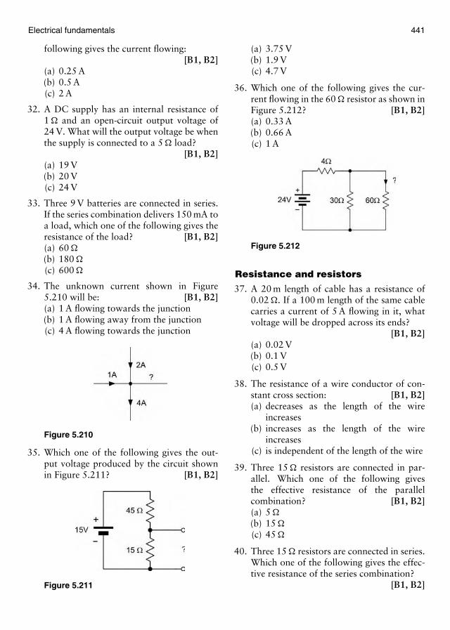
Electrical fundamentals 441
following gives the current flowing:[B1, B2]
(a) 0.25 A(b) 0.5 A(c) 2 A
32. A DC supply has an internal resistance of1 � and an open-circuit output voltage of24 V. What will the output voltage be whenthe supply is connected to a 5 � load?
[B1, B2](a) 19 V(b) 20 V(c) 24 V
33. Three 9 V batteries are connected in series.If the series combination delivers 150 mA toa load, which one of the following gives theresistance of the load? [B1, B2](a) 60 �
(b) 180 �
(c) 600 �
34. The unknown current shown in Figure5.210 will be: [B1, B2](a) 1 A flowing towards the junction(b) 1 A flowing away from the junction(c) 4 A flowing towards the junction
Figure 5.210
35. Which one of the following gives the out-put voltage produced by the circuit shownin Figure 5.211? [B1, B2]
Figure 5.211
(a) 3.75 V(b) 1.9 V(c) 4.7 V
36. Which one of the following gives the cur-rent flowing in the 60 � resistor as shown inFigure 5.212? [B1, B2](a) 0.33 A(b) 0.66 A(c) 1 A
Figure 5.212
Resistance and resistors
37. A 20 m length of cable has a resistance of0.02 �. If a 100 m length of the same cablecarries a current of 5 A flowing in it, whatvoltage will be dropped across its ends?
[B1, B2](a) 0.02 V(b) 0.1 V(c) 0.5 V
38. The resistance of a wire conductor of con-stant cross section: [B1, B2](a) decreases as the length of the wire
increases(b) increases as the length of the wire
increases(c) is independent of the length of the wire
39. Three 15 � resistors are connected in par-allel. Which one of the following givesthe effective resistance of the parallelcombination? [B1, B2](a) 5 �
(b) 15 �
(c) 45 �
40. Three 15 � resistors are connected in series.Which one of the following gives the effec-tive resistance of the series combination?
[B1, B2]
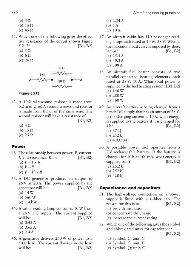
442 Aircraft engineering principles
(a) 5 �
(b) 15 �
(c) 45 �
41. Which one of the following gives the effec-tive resistance of the circuit shown Figure5.213? [B1, B2](a) 5 �
(b) 6 �
(c) 26 �
Figure 5.213
42. A 10 � wirewound resistor is made from0.2 m of wire. A second wirewound resistoris made from 0.5 m of the same wire. Thesecond resistor will have a resistance of:
[B1, B2](a) 4 �
(b) 15 �
(c) 25 �
Power
43. The relationship between power, P, current,I, and resistance, R, is: [B1, B2](a) P = I × R(b) P = R
I(c) P = I2 × R
44. A DC generator produces an output of28 V at 20 A. The power supplied by thegenerator will be: [B1, B2](a) 14 W(b) 560 W(c) 1.4 kW
45. A cabin reading lamp consumes 10 W froma 24 V DC supply. The current suppliedwill be: [B1, B2](a) 0.42 A(b) 0.65 A(c) 2.4 A
46. A generator delivers 250 W of power to a50 � load. The current flowing in the loadwill be: [B1, B2]
(a) 2.24 A(b) 5 A(c) 10 A
47. An aircraft cabin has 110 passenger read-ing lamps each rated at 10 W, 28 V. What isthe maximum load current imposed by theselamps? [B1, B2](a) 25.5 A(b) 39.3 A(c) 308 A
48. An aircraft fuel heater consists of twoparallel-connected heating elements eachrated at 28 V, 10 A. What total power issupplied to the fuel heating system? [B1, B2](a) 140 W(b) 280 W(c) 560 W
49. An aircraft battery is being charged from abench DC supply that has an output of 28 V.If the charging current is 10 A, what energyis supplied to the battery if it is charged for4 h? [B1, B2](a) 67 kJ(b) 252 kJ(c) 4.032 MJ
50. A portable power tool operates from a7 V rechargeable battery. If the battery ischarged for 10 h at 100 mA, what energy issupplied to it? [B1, B2](a) 25.2 kJ(b) 252 kJ(c) 420 kJ
Capacitance and capacitors
51. The high-voltage connection on a powersupply is fitted with a rubber cap. Thereason for this is to: [B1, B2](a) provide insulation(b) concentrate the charge(c) increase the current rating
52. Which one of the following gives the symboland abbreviated units for capacitance?
[B1, B2](a) Symbol, C; unit, C(b) Symbol, C; unit, F(c) Symbol, Q; unit, C
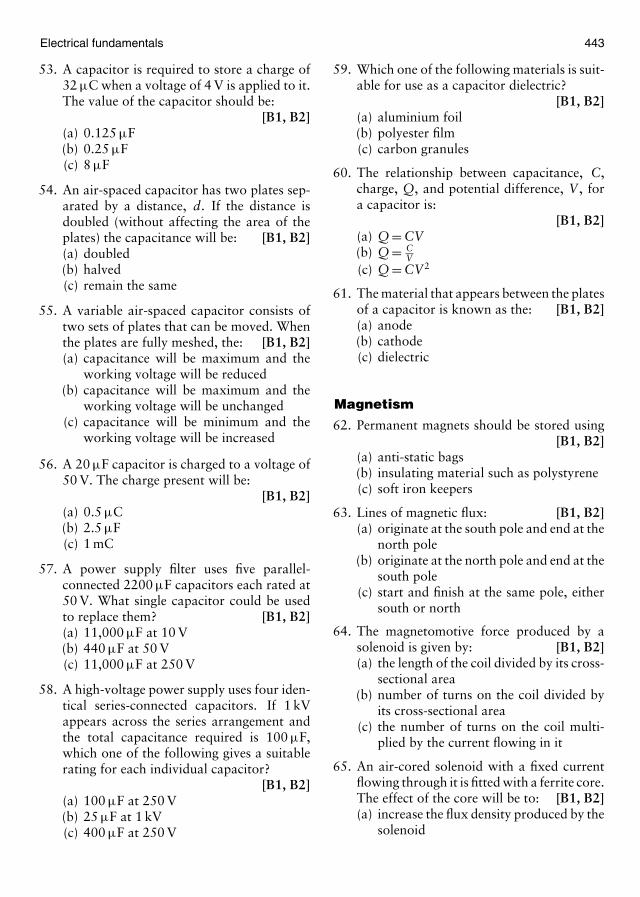
Electrical fundamentals 443
53. A capacitor is required to store a charge of32 µC when a voltage of 4 V is applied to it.The value of the capacitor should be:
[B1, B2](a) 0.125 µF(b) 0.25 µF(c) 8 µF
54. An air-spaced capacitor has two plates sep-arated by a distance, d. If the distance isdoubled (without affecting the area of theplates) the capacitance will be: [B1, B2](a) doubled(b) halved(c) remain the same
55. A variable air-spaced capacitor consists oftwo sets of plates that can be moved. Whenthe plates are fully meshed, the: [B1, B2](a) capacitance will be maximum and the
working voltage will be reduced(b) capacitance will be maximum and the
working voltage will be unchanged(c) capacitance will be minimum and the
working voltage will be increased
56. A 20 µF capacitor is charged to a voltage of50 V. The charge present will be:
[B1, B2](a) 0.5 µC(b) 2.5 µF(c) 1 mC
57. A power supply filter uses five parallel-connected 2200 µF capacitors each rated at50 V. What single capacitor could be usedto replace them? [B1, B2](a) 11,000 µF at 10 V(b) 440 µF at 50 V(c) 11,000 µF at 250 V
58. A high-voltage power supply uses four iden-tical series-connected capacitors. If 1 kVappears across the series arrangement andthe total capacitance required is 100 µF,which one of the following gives a suitablerating for each individual capacitor?
[B1, B2](a) 100 µF at 250 V(b) 25 µF at 1 kV(c) 400 µF at 250 V
59. Which one of the following materials is suit-able for use as a capacitor dielectric?
[B1, B2](a) aluminium foil(b) polyester film(c) carbon granules
60. The relationship between capacitance, C,charge, Q, and potential difference, V , fora capacitor is:
[B1, B2](a) Q = CV(b) Q = C
V(c) Q = CV2
61. The material that appears between the platesof a capacitor is known as the: [B1, B2](a) anode(b) cathode(c) dielectric
Magnetism
62. Permanent magnets should be stored using[B1, B2]
(a) anti-static bags(b) insulating material such as polystyrene(c) soft iron keepers
63. Lines of magnetic flux: [B1, B2](a) originate at the south pole and end at the
north pole(b) originate at the north pole and end at the
south pole(c) start and finish at the same pole, either
south or north
64. The magnetomotive force produced by asolenoid is given by: [B1, B2](a) the length of the coil divided by its cross-
sectional area(b) number of turns on the coil divided by
its cross-sectional area(c) the number of turns on the coil multi-
plied by the current flowing in it
65. An air-cored solenoid with a fixed currentflowing through it is fitted with a ferrite core.The effect of the core will be to: [B1, B2](a) increase the flux density produced by the
solenoid
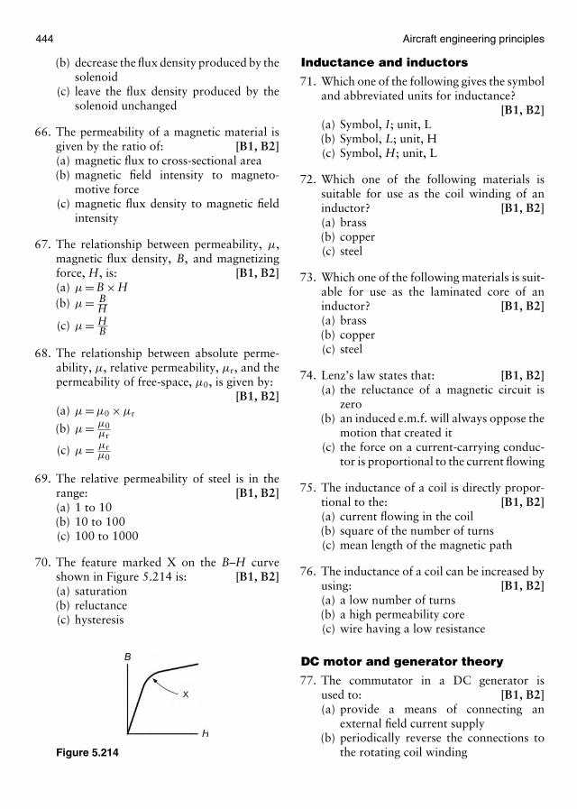
444 Aircraft engineering principles
(b) decrease the flux density produced by thesolenoid
(c) leave the flux density produced by thesolenoid unchanged
66. The permeability of a magnetic material isgiven by the ratio of: [B1, B2](a) magnetic flux to cross-sectional area(b) magnetic field intensity to magneto-
motive force(c) magnetic flux density to magnetic field
intensity
67. The relationship between permeability, µ,magnetic flux density, B, and magnetizingforce, H, is: [B1, B2](a) µ = B × H(b) µ = B
H
(c) µ = HB
68. The relationship between absolute perme-ability, µ, relative permeability, µr, and thepermeability of free-space, µ0, is given by:
[B1, B2](a) µ = µ0 × µr
(b) µ = µ0µr
(c) µ = µrµ0
69. The relative permeability of steel is in therange: [B1, B2](a) 1 to 10(b) 10 to 100(c) 100 to 1000
70. The feature marked X on the B–H curveshown in Figure 5.214 is: [B1, B2](a) saturation(b) reluctance(c) hysteresis
Figure 5.214
Inductance and inductors
71. Which one of the following gives the symboland abbreviated units for inductance?
[B1, B2](a) Symbol, I; unit, L(b) Symbol, L; unit, H(c) Symbol, H; unit, L
72. Which one of the following materials issuitable for use as the coil winding of aninductor? [B1, B2](a) brass(b) copper(c) steel
73. Which one of the following materials is suit-able for use as the laminated core of aninductor? [B1, B2](a) brass(b) copper(c) steel
74. Lenz’s law states that: [B1, B2](a) the reluctance of a magnetic circuit is
zero(b) an induced e.m.f. will always oppose the
motion that created it(c) the force on a current-carrying conduc-
tor is proportional to the current flowing
75. The inductance of a coil is directly propor-tional to the: [B1, B2](a) current flowing in the coil(b) square of the number of turns(c) mean length of the magnetic path
76. The inductance of a coil can be increased byusing: [B1, B2](a) a low number of turns(b) a high permeability core(c) wire having a low resistance
DC motor and generator theory
77. The commutator in a DC generator isused to: [B1, B2](a) provide a means of connecting an
external field current supply(b) periodically reverse the connections to
the rotating coil winding
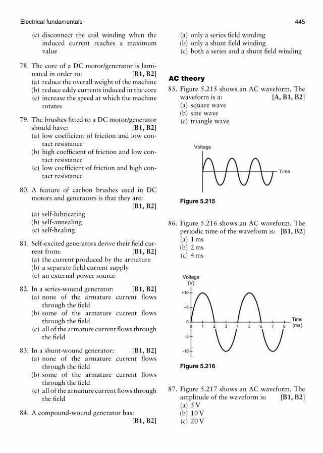
Electrical fundamentals 445
(c) disconnect the coil winding when theinduced current reaches a maximumvalue
78. The core of a DC motor/generator is lami-nated in order to: [B1, B2](a) reduce the overall weight of the machine(b) reduce eddy currents induced in the core(c) increase the speed at which the machine
rotates
79. The brushes fitted to a DC motor/generatorshould have: [B1, B2](a) low coefficient of friction and low con-
tact resistance(b) high coefficient of friction and low con-
tact resistance(c) low coefficient of friction and high con-
tact resistance
80. A feature of carbon brushes used in DCmotors and generators is that they are:
[B1, B2](a) self-lubricating(b) self-annealing(c) self-healing
81. Self-excited generators derive their field cur-rent from: [B1, B2](a) the current produced by the armature(b) a separate field current supply(c) an external power source
82. In a series-wound generator: [B1, B2](a) none of the armature current flows
through the field(b) some of the armature current flows
through the field(c) all of the armature current flows through
the field
83. In a shunt-wound generator: [B1, B2](a) none of the armature current flows
through the field(b) some of the armature current flows
through the field(c) all of the armature current flows through
the field
84. A compound-wound generator has:[B1, B2]
(a) only a series field winding(b) only a shunt field winding(c) both a series and a shunt field winding
AC theory
85. Figure 5.215 shows an AC waveform. Thewaveform is a: [A, B1, B2](a) square wave(b) sine wave(c) triangle wave
Figure 5.215
86. Figure 5.216 shows an AC waveform. Theperiodic time of the waveform is: [B1, B2](a) 1 ms(b) 2 ms(c) 4 ms
Figure 5.216
87. Figure 5.217 shows an AC waveform. Theamplitude of the waveform is: [B1, B2](a) 5 V(b) 10 V(c) 20 V
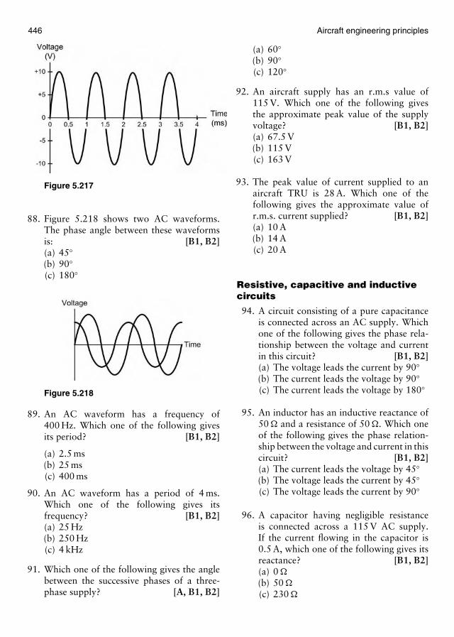
446 Aircraft engineering principles
Figure 5.217
88. Figure 5.218 shows two AC waveforms.The phase angle between these waveformsis: [B1, B2](a) 45◦(b) 90◦(c) 180◦
Figure 5.218
89. An AC waveform has a frequency of400 Hz. Which one of the following givesits period? [B1, B2]
(a) 2.5 ms(b) 25 ms(c) 400 ms
90. An AC waveform has a period of 4 ms.Which one of the following gives itsfrequency? [B1, B2](a) 25 Hz(b) 250 Hz(c) 4 kHz
91. Which one of the following gives the anglebetween the successive phases of a three-phase supply? [A, B1, B2]
(a) 60◦(b) 90◦(c) 120◦
92. An aircraft supply has an r.m.s value of115 V. Which one of the following givesthe approximate peak value of the supplyvoltage? [B1, B2](a) 67.5 V(b) 115 V(c) 163 V
93. The peak value of current supplied to anaircraft TRU is 28 A. Which one of thefollowing gives the approximate value ofr.m.s. current supplied? [B1, B2](a) 10 A(b) 14 A(c) 20 A
Resistive, capacitive and inductivecircuits
94. A circuit consisting of a pure capacitanceis connected across an AC supply. Whichone of the following gives the phase rela-tionship between the voltage and currentin this circuit? [B1, B2](a) The voltage leads the current by 90◦(b) The current leads the voltage by 90◦(c) The current leads the voltage by 180◦
95. An inductor has an inductive reactance of50 � and a resistance of 50 �. Which oneof the following gives the phase relation-ship between the voltage and current in thiscircuit? [B1, B2](a) The current leads the voltage by 45◦(b) The voltage leads the current by 45◦(c) The voltage leads the current by 90◦
96. A capacitor having negligible resistanceis connected across a 115 V AC supply.If the current flowing in the capacitor is0.5 A, which one of the following gives itsreactance? [B1, B2](a) 0 �
(b) 50 �
(c) 230 �
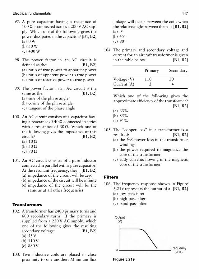
Electrical fundamentals 447
97. A pure capacitor having a reactance of100 � is connected across a 200 V AC sup-ply. Which one of the following gives thepower dissipated in the capacitor? [B1, B2](a) 0 W(b) 50 W(c) 400 W
98. The power factor in an AC circuit isdefined as the: [B1, B2](a) ratio of true power to apparent power(b) ratio of apparent power to true power(c) ratio of reactive power to true power
99. The power factor in an AC circuit is thesame as the: [B1, B2](a) sine of the phase angle(b) cosine of the phase angle(c) tangent of the phase angle
100. An AC circuit consists of a capacitor hav-ing a reactance of 40 � connected in serieswith a resistance of 30 �. Which one ofthe following gives the impedance of thiscircuit? [B1, B2](a) 10 �
(b) 50 �
(c) 70 �
101. An AC circuit consists of a pure inductorconnected in parallel with a pure capacitor.At the resonant frequency, the: [B1, B2](a) impedance of the circuit will be zero(b) impedance of the circuit will be infinite(c) impedance of the circuit will be the
same as at all other frequencies
Transformers
102. A transformer has 2400 primary turns and600 secondary turns. If the primary issupplied from a 220 V AC supply, whichone of the following gives the resultingsecondary voltage: [B1, B2](a) 55 V(b) 110 V(c) 880 V
103. Two inductive coils are placed in closeproximity to one another. Minimum flux
linkage will occur between the coils whenthe relative angle between them is: [B1, B2](a) 0◦(b) 45◦(c) 90◦
104. The primary and secondary voltage andcurrent for an aircraft transformer is givenin the table below: [B1, B2]
Primary Secondary
Voltage (V) 110 50Current (A) 2 4
Which one of the following gives theapproximate efficiency of the transformer?
[B1, B2](a) 63%(b) 85%(c) 91%
105. The “copper loss” in a transformer is aresult of: [B1, B2](a) the I2R power loss in the transformer
windings(b) the power required to magnetize the
core of the transformer(c) eddy currents flowing in the magnetic
core of the transformer
Filters
106. The frequency response shown in Figure5.219 represents the output of a: [B1, B2](a) low-pass filter(b) high-pass filter(c) band-pass filter
Figure 5.219
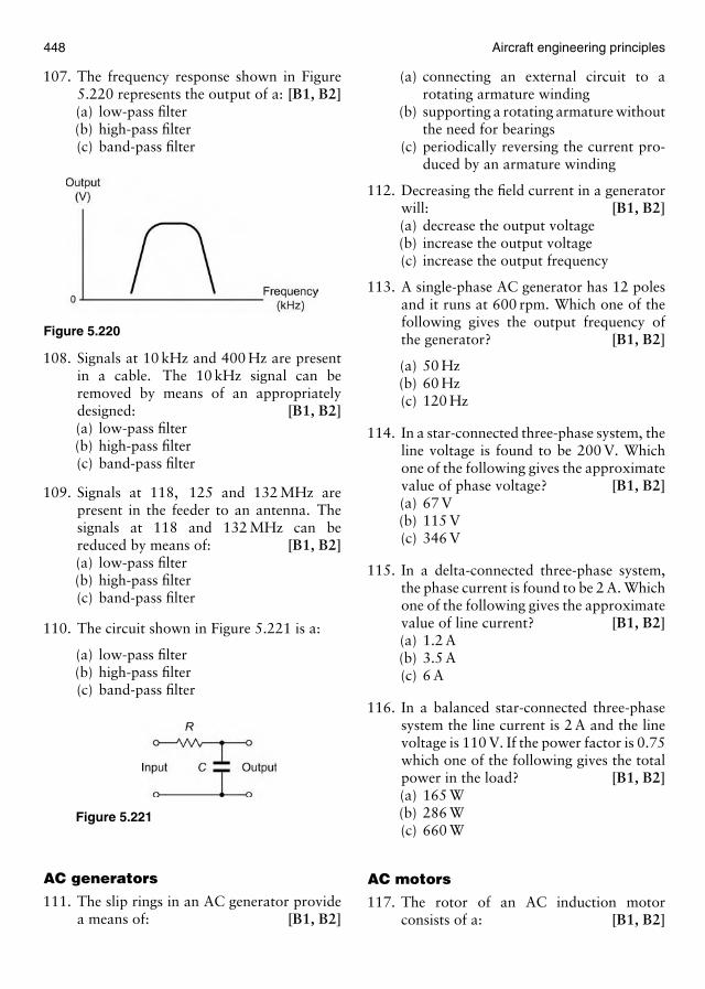
448 Aircraft engineering principles
107. The frequency response shown in Figure5.220 represents the output of a: [B1, B2](a) low-pass filter(b) high-pass filter(c) band-pass filter
Figure 5.220
108. Signals at 10 kHz and 400 Hz are presentin a cable. The 10 kHz signal can beremoved by means of an appropriatelydesigned: [B1, B2](a) low-pass filter(b) high-pass filter(c) band-pass filter
109. Signals at 118, 125 and 132 MHz arepresent in the feeder to an antenna. Thesignals at 118 and 132 MHz can bereduced by means of: [B1, B2](a) low-pass filter(b) high-pass filter(c) band-pass filter
110. The circuit shown in Figure 5.221 is a:
(a) low-pass filter(b) high-pass filter(c) band-pass filter
Figure 5.221
AC generators
111. The slip rings in an AC generator providea means of: [B1, B2]
(a) connecting an external circuit to arotating armature winding
(b) supporting a rotating armature withoutthe need for bearings
(c) periodically reversing the current pro-duced by an armature winding
112. Decreasing the field current in a generatorwill: [B1, B2](a) decrease the output voltage(b) increase the output voltage(c) increase the output frequency
113. A single-phase AC generator has 12 polesand it runs at 600 rpm. Which one of thefollowing gives the output frequency ofthe generator? [B1, B2]
(a) 50 Hz(b) 60 Hz(c) 120 Hz
114. In a star-connected three-phase system, theline voltage is found to be 200 V. Whichone of the following gives the approximatevalue of phase voltage? [B1, B2](a) 67 V(b) 115 V(c) 346 V
115. In a delta-connected three-phase system,the phase current is found to be 2 A. Whichone of the following gives the approximatevalue of line current? [B1, B2](a) 1.2 A(b) 3.5 A(c) 6 A
116. In a balanced star-connected three-phasesystem the line current is 2 A and the linevoltage is 110 V. If the power factor is 0.75which one of the following gives the totalpower in the load? [B1, B2](a) 165 W(b) 286 W(c) 660 W
AC motors
117. The rotor of an AC induction motorconsists of a: [B1, B2]

Electrical fundamentals 449
(a) laminated iron core inside a “squirrelcage” made from copper or aluminium
(b) series of coil windings on a laminatediron core with connections via slip rings
(c) single copper loop which rotates insidethe field created by a permanent magnet
118. The slip speed of an AC induction motoris the difference between the: [B1, B2](a) synchronous speed and the rotor speed(b) frequency of the supply and the rotor
speed(c) maximum speed and the minimum
speed
119. When compared with three-phase induc-tion motors, single-phase inductionmotors: [B1, B2]
(a) are not inherently “self starting”(b) have more complicated stator windings(c) are significantly more efficient
120. The use of laminations in the constructionof an electrical machine is instrumental inreducing the: [B1, B2](a) losses(b) output(c) weight
121. A three-phase induction motor has threepairs of poles and is operated from a 60 Hzsupply. Which one of the following givesthe motor’s synchronous speed? [B1, B2](a) 1200 rpm(b) 1800 rpm(c) 3600 rpm

This page intentionally left blank
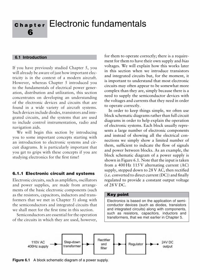
C h a p t e r
6Electronic fundamentals
6.1 Introduction
If you have previously studied Chapter 5, youwill already be aware of just how important elec-tricity is in the context of a modern aircraft.However, whereas Chapter 5 introduced youto the fundamentals of electrical power gener-ation, distribution and utilization, this sectionconcentrates on developing an understandingof the electronic devices and circuits that arefound in a wide variety of aircraft systems.Such devices include diodes, transistors and inte-grated circuits, and the systems that are usedto include control instrumentation, radio andnavigation aids.
We will begin this section by introducingyou to some important concepts starting withan introduction to electronic systems and cir-cuit diagrams. It is particularly important thatyou get to grips with these concepts if you arestudying electronics for the first time!
6.1.1 Electronic circuit and systems
Electronic circuits, such as amplifiers, oscillatorsand power supplies, are made from arrange-ments of the basic electronic components (suchas the resistors, capacitors, inductors and trans-formers that we met in Chapter 5) along withthe semiconductors and integrated circuits thatwe shall meet for the first time in this section.
Semiconductors are essential for the operationof the circuits in which they are used, however,
Figure 6.1 A block schematic diagram of a power supply.
for them to operate correctly; there is a require-ment for them to have their own supply and biasvoltages. We will explain how this works laterin this section when we introduce transistorsand integrated circuits but, for the moment, itis important to understand that most electroniccircuits may often appear to be somewhat morecomplex than they are, simply because there is aneed to supply the semiconductor devices withthe voltages and currents that they need in orderto operate correctly.
In order to keep things simple, we often useblock schematic diagrams rather than full circuitdiagrams in order to help explain the operationof electronic systems. Each block usually repre-sents a large number of electronic componentsand instead of showing all the electrical con-nections we simply show a limited number ofthem, sufficient to indicate the flow of signalsand power between blocks. As an example, theblock schematic diagram of a power supply isshown in Figure 6.1. Note that the input is takenfrom a 400 Hz 115 V alternating current (AC)supply, stepped down to 28 V AC, then rectified(i.e. converted to direct current (DC)) and finallyregulated to provide a constant output voltageof 28 V DC.
Key pointElectronics is based on the application of semi-conductor devices (such as diodes, transistorsand integrated circuits) along with components,such as resistors, capacitors, inductors andtransformers, that we met earlier in Chapter 5.
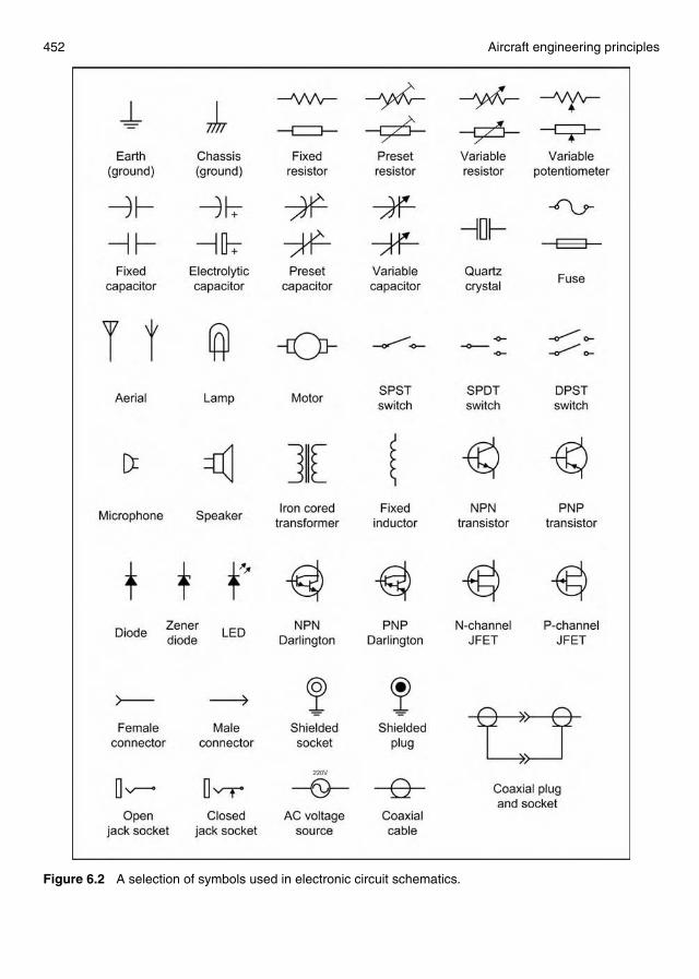
452 Aircraft engineering principles
Figure 6.2 A selection of symbols used in electronic circuit schematics.
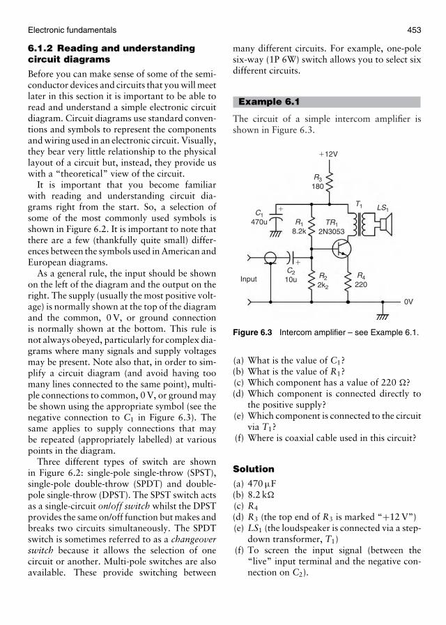
Electronic fundamentals 453
6.1.2 Reading and understandingcircuit diagrams
Before you can make sense of some of the semi-conductor devices and circuits that you will meetlater in this section it is important to be able toread and understand a simple electronic circuitdiagram. Circuit diagrams use standard conven-tions and symbols to represent the componentsand wiring used in an electronic circuit. Visually,they bear very little relationship to the physicallayout of a circuit but, instead, they provide uswith a “theoretical” view of the circuit.
It is important that you become familiarwith reading and understanding circuit dia-grams right from the start. So, a selection ofsome of the most commonly used symbols isshown in Figure 6.2. It is important to note thatthere are a few (thankfully quite small) differ-ences between the symbols used in American andEuropean diagrams.
As a general rule, the input should be shownon the left of the diagram and the output on theright. The supply (usually the most positive volt-age) is normally shown at the top of the diagramand the common, 0 V, or ground connectionis normally shown at the bottom. This rule isnot always obeyed, particularly for complex dia-grams where many signals and supply voltagesmay be present. Note also that, in order to sim-plify a circuit diagram (and avoid having toomany lines connected to the same point), multi-ple connections to common, 0 V, or ground maybe shown using the appropriate symbol (see thenegative connection to C1 in Figure 6.3). Thesame applies to supply connections that maybe repeated (appropriately labelled) at variouspoints in the diagram.
Three different types of switch are shownin Figure 6.2: single-pole single-throw (SPST),single-pole double-throw (SPDT) and double-pole single-throw (DPST). The SPST switch actsas a single-circuit on/off switch whilst the DPSTprovides the same on/off function but makes andbreaks two circuits simultaneously. The SPDTswitch is sometimes referred to as a changeoverswitch because it allows the selection of onecircuit or another. Multi-pole switches are alsoavailable. These provide switching between
many different circuits. For example, one-polesix-way (1P 6W) switch allows you to select sixdifferent circuits.
Example 6.1
The circuit of a simple intercom amplifier isshown in Figure 6.3.
�12V
R3180
R18.2k
R22k2
R4220
TR12N3053
C1470u
C210u
T1 LS1
Input
0V
�
�
Figure 6.3 Intercom amplifier – see Example 6.1.
(a) What is the value of C1?(b) What is the value of R1?(c) Which component has a value of 220 �?(d) Which component is connected directly to
the positive supply?(e) Which component is connected to the circuit
via T1?(f) Where is coaxial cable used in this circuit?
Solution
(a) 470 µF(b) 8.2 k�
(c) R4
(d) R3 (the top end of R3 is marked “+12 V”)(e) LS1 (the loudspeaker is connected via a step-
down transformer, T1)(f) To screen the input signal (between the
“live” input terminal and the negative con-nection on C2).
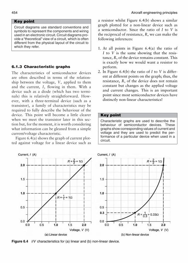
454 Aircraft engineering principles
Key pointCircuit diagrams use standard conventions andsymbols to represent the components and wiringused in an electronic circuit. Circuit diagrams pro-vide a “theoretical” view of a circuit, which is oftendifferent from the physical layout of the circuit towhich they refer.
6.1.3 Characteristic graphs
The characteristics of semiconductor devicesare often described in terms of the relation-ship between the voltage, V , applied to themand the current, I, flowing in them. With adevice such as a diode (which has two termi-nals) this is relatively straightforward. How-ever, with a three-terminal device (such as atransistor), a family of characteristics may berequired to fully describe the behaviour of thedevice. This point will become a little clearerwhen we meet the transistor later in this sec-tion but, for the moment, it is worth consideringwhat information can be gleaned from a simplecurrent/voltage characteristic.
Figure 6.4(a) shows the graph of current plot-ted against voltage for a linear device such as
Figure 6.4 I/V characteristics for (a) linear and (b) non-linear device.
a resistor whilst Figure 6.4(b) shows a similargraph plotted for a non-linear device such asa semiconductor. Since the ratio of I to V isthe reciprocal of resistance, R, we can make thefollowing inferences:
1. At all points in Figure 6.4(a) the ratio ofI to V is the same showing that the resis-tance, R, of the device remains constant. Thisis exactly how we would want a resistor toperform.
2. In Figure 6.4(b) the ratio of I to V is differ-ent at different points on the graph; thus, theresistance, R, of the device does not remainconstant but changes as the applied voltageand current changes. This is an importantpoint since most semiconductor devices havedistinctly non-linear characteristics!
Key pointCharacteristic graphs are used to describe thebehaviour of semiconductor devices. Thesegraphs show corresponding values of current andvoltage and they are used to predict the per-formance of a particular device when used in acircuit.
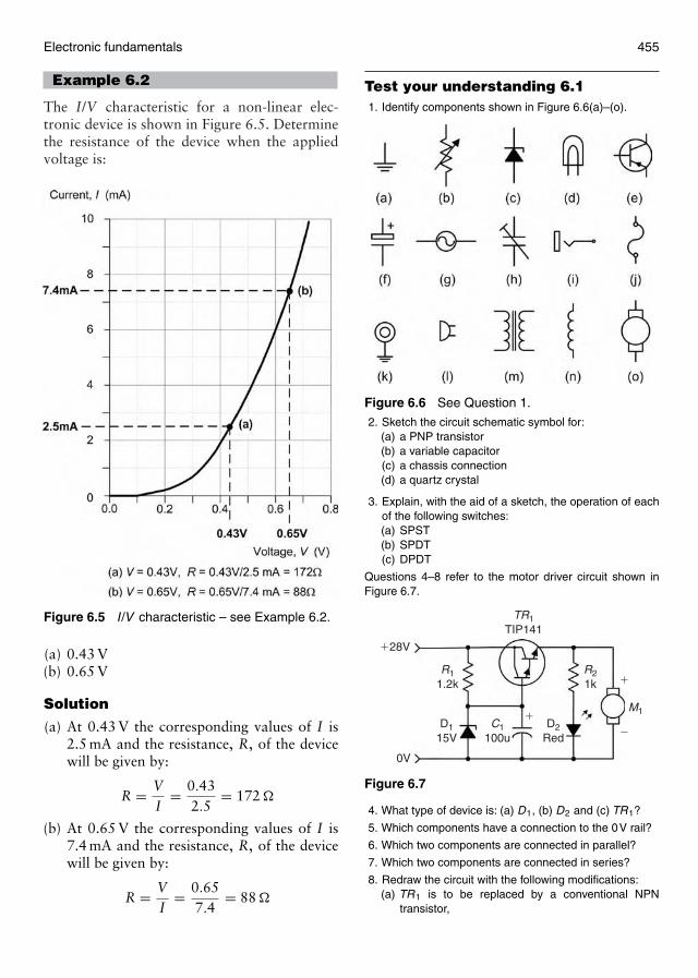
Electronic fundamentals 455
Example 6.2
The I/V characteristic for a non-linear elec-tronic device is shown in Figure 6.5. Determinethe resistance of the device when the appliedvoltage is:
Figure 6.5 I /V characteristic – see Example 6.2.
(a) 0.43 V(b) 0.65 V
Solution
(a) At 0.43 V the corresponding values of I is2.5 mA and the resistance, R, of the devicewill be given by:
R = VI
= 0.432.5
= 172 �
(b) At 0.65 V the corresponding values of I is7.4 mA and the resistance, R, of the devicewill be given by:
R = VI
= 0.657.4
= 88 �
Test your understanding 6.11. Identify components shown in Figure 6.6(a)–(o).
Figure 6.6 See Question 1.
2. Sketch the circuit schematic symbol for:(a) a PNP transistor(b) a variable capacitor(c) a chassis connection(d) a quartz crystal
3. Explain, with the aid of a sketch, the operation of eachof the following switches:(a) SPST(b) SPDT(c) DPDT
Questions 4–8 refer to the motor driver circuit shown inFigure 6.7.
�28V
R21k
R11.2k
M1
D2Red
TR1TIP141
C1100u
D115V
0V
�
�
�
Figure 6.7
4. What type of device is: (a) D1, (b) D2 and (c) TR1?
5. Which components have a connection to the 0V rail?
6. Which two components are connected in parallel?
7. Which two components are connected in series?
8. Redraw the circuit with the following modifications:(a) TR1 is to be replaced by a conventional NPN
transistor,

456 Aircraft engineering principles
(b) an SPST switch is to be placed in series with R1,(c) the value of C1 is to be increased to 220 µF,(d) the light emitting diode (LED) indicator and series
resistor are to be removed and replaced by a singlefixed capacitor of 470 nF.
9. Corresponding readings of current, I, and voltage, V, fora semiconductor device are given in the table below:
V (V) 0 0.1 0.2 0.3 0.4 0.5 0.6 0.7 0.8I (mA) 0 0.2 0.5 1.5 3.0 5.0 8.5 13.0 20.0
Plot the I/V characteristic for the device.
10. Determine the resistance of the device in Question 9,when the applied voltage is:(a) 0.35V(b) 0.75V
6.2 Semiconductors
6.2.1 Diodes
SyllabusDiode symbols; Diode characteristics and prop-erties; Diodes in series and parallel; Main char-acteristics and use of silicon (Si) controlled rec-tifiers (SCRs), LED, photo-conductive diode,varistor, rectifier diodes; Functional testing ofdiodes.
Knowledge level key
–
A
2
B1
2
B2
SyllabusMaterials, electron configuration, electricalproperties; P- and N-type materials: effects ofimpurities on conduction, majority and minor-ity carriers; P–N junction in a semiconductor,development of a potential across a P–N junc-tion in unbiased, forward- and reverse-biasedconditions; Diode parameters: peak inversevoltage (PIV), maximum forward current, tem-perature, frequency, leakage current, powerdissipation; Operation and function of diodesin the following circuits: clippers, clampers,full- and half-wave rectifiers, bridge rectifiers,voltage doublers and triplers; Detailed opera-tion and characteristics of the following devices:SCR, LED, Schottky diode, photo-conductive
diode, varactor diode, varistor, rectifier diodes,Zener diode.
Knowledge level key
–
A
–
B1
2
B2
Semiconductor materialsThis section introduces devices that are madefrom materials that are neither conductors norinsulators. These semiconductor materials formthe basis of many important electronic compo-nents, such as diodes, SCRs, triacs, transistorsand integrated circuits. We shall start with abrief introduction to the principles of semicon-ductors and then go on to examine the charac-teristics of each of the most common types thatyou are likely to meet.
You should recall that an atom contains bothnegative charge carriers (electrons) and positivecharge carriers (protons). Electrons each carry asingle unit of negative electric charge while pro-tons each exhibit a single unit of positive charge.Since atoms normally contain an equal numberof electrons and protons, the net charge presentwill be zero. For example, if an atom has 11 elec-trons, it will also contain 11 protons. The endresult is that the negative charge of the electronswill be exactly balanced by the positive chargeof the protons.
Electrons are in constant motion as they orbitaround the nucleus of the atom. Electron orbitsare organized into shells. The maximum num-ber of electrons present in the first shell is two,in the second shell eight and in the third, fourthand fifth shells it is 18, 32 and 50, respectively.In electronics only the electron shell furthermostfrom the nucleus of an atom is important. It isimportant to note that the movement of elec-trons between atoms involves only those presentin the outer valence shell (Figure 6.8).
If the valence shell contains the maximumnumber of electrons possible the electrons arerigidly bonded together and the material hasthe properties of an insulator. If, however, thevalence shell does not have its full comple-ment of electrons, the electrons can be easilydetached from their orbital bonds, and the
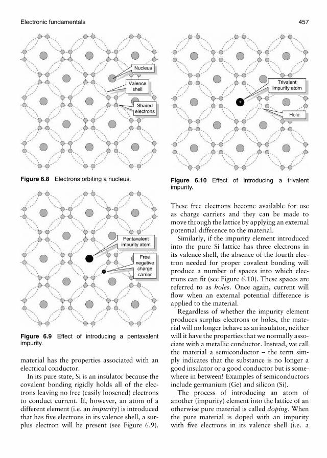
Electronic fundamentals 457
Figure 6.8 Electrons orbiting a nucleus.
Figure 6.9 Effect of introducing a pentavalentimpurity.
material has the properties associated with anelectrical conductor.
In its pure state, Si is an insulator because thecovalent bonding rigidly holds all of the elec-trons leaving no free (easily loosened) electronsto conduct current. If, however, an atom of adifferent element (i.e. an impurity) is introducedthat has five electrons in its valence shell, a sur-plus electron will be present (see Figure 6.9).
Figure 6.10 Effect of introducing a trivalentimpurity.
These free electrons become available for useas charge carriers and they can be made tomove through the lattice by applying an externalpotential difference to the material.
Similarly, if the impurity element introducedinto the pure Si lattice has three electrons inits valence shell, the absence of the fourth elec-tron needed for proper covalent bonding willproduce a number of spaces into which elec-trons can fit (see Figure 6.10). These spaces arereferred to as holes. Once again, current willflow when an external potential difference isapplied to the material.
Regardless of whether the impurity elementproduces surplus electrons or holes, the mate-rial will no longer behave as an insulator, neitherwill it have the properties that we normally asso-ciate with a metallic conductor. Instead, we callthe material a semiconductor – the term sim-ply indicates that the substance is no longer agood insulator or a good conductor but is some-where in between! Examples of semiconductorsinclude germanium (Ge) and silicon (Si).
The process of introducing an atom ofanother (impurity) element into the lattice of anotherwise pure material is called doping. Whenthe pure material is doped with an impuritywith five electrons in its valence shell (i.e. a
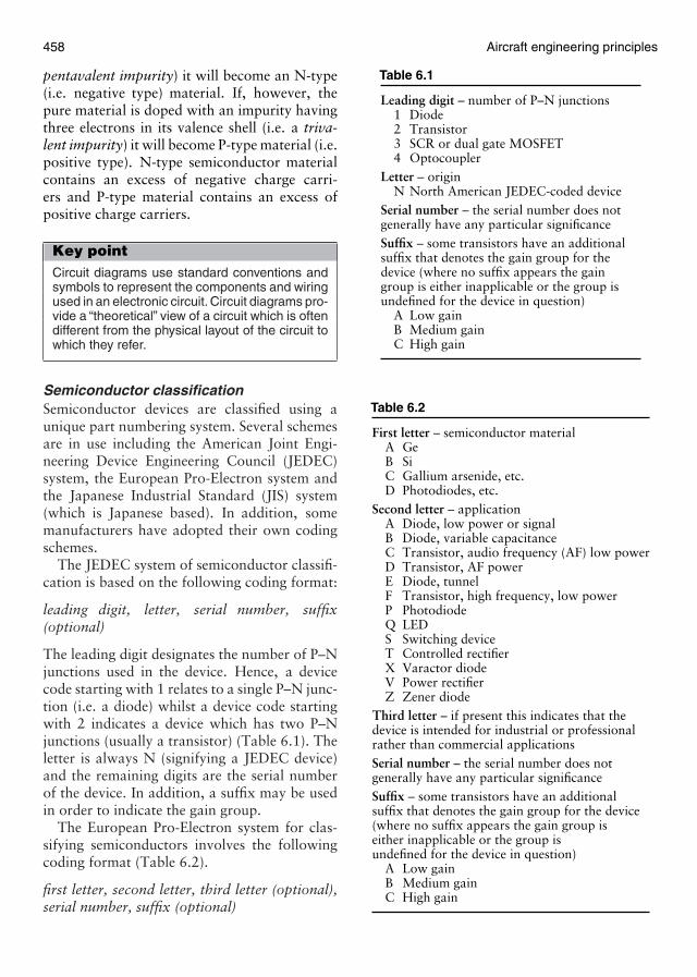
458 Aircraft engineering principles
pentavalent impurity) it will become an N-type(i.e. negative type) material. If, however, thepure material is doped with an impurity havingthree electrons in its valence shell (i.e. a triva-lent impurity) it will become P-type material (i.e.positive type). N-type semiconductor materialcontains an excess of negative charge carri-ers and P-type material contains an excess ofpositive charge carriers.
Key pointCircuit diagrams use standard conventions andsymbols to represent the components and wiringused in an electronic circuit. Circuit diagrams pro-vide a “theoretical” view of a circuit which is oftendifferent from the physical layout of the circuit towhich they refer.
Semiconductor classificationSemiconductor devices are classified using aunique part numbering system. Several schemesare in use including the American Joint Engi-neering Device Engineering Council (JEDEC)system, the European Pro-Electron system andthe Japanese Industrial Standard (JIS) system(which is Japanese based). In addition, somemanufacturers have adopted their own codingschemes.
The JEDEC system of semiconductor classifi-cation is based on the following coding format:
leading digit, letter, serial number, suffix(optional)
The leading digit designates the number of P–Njunctions used in the device. Hence, a devicecode starting with 1 relates to a single P–N junc-tion (i.e. a diode) whilst a device code startingwith 2 indicates a device which has two P–Njunctions (usually a transistor) (Table 6.1). Theletter is always N (signifying a JEDEC device)and the remaining digits are the serial numberof the device. In addition, a suffix may be usedin order to indicate the gain group.
The European Pro-Electron system for clas-sifying semiconductors involves the followingcoding format (Table 6.2).
first letter, second letter, third letter (optional),serial number, suffix (optional)
Table 6.1
Leading digit – number of P–N junctions1 Diode2 Transistor3 SCR or dual gate MOSFET4 Optocoupler
Letter – originN North American JEDEC-coded device
Serial number – the serial number does notgenerally have any particular significanceSuffix – some transistors have an additionalsuffix that denotes the gain group for thedevice (where no suffix appears the gaingroup is either inapplicable or the group isundefined for the device in question)
A Low gainB Medium gainC High gain
Table 6.2
First letter – semiconductor materialA GeB SiC Gallium arsenide, etc.D Photodiodes, etc.
Second letter – applicationA Diode, low power or signalB Diode, variable capacitanceC Transistor, audio frequency (AF) low powerD Transistor, AF powerE Diode, tunnelF Transistor, high frequency, low powerP PhotodiodeQ LEDS Switching deviceT Controlled rectifierX Varactor diodeV Power rectifierZ Zener diode
Third letter – if present this indicates that thedevice is intended for industrial or professionalrather than commercial applicationsSerial number – the serial number does notgenerally have any particular significanceSuffix – some transistors have an additionalsuffix that denotes the gain group for the device(where no suffix appears the gain group iseither inapplicable or the group isundefined for the device in question)
A Low gainB Medium gainC High gain
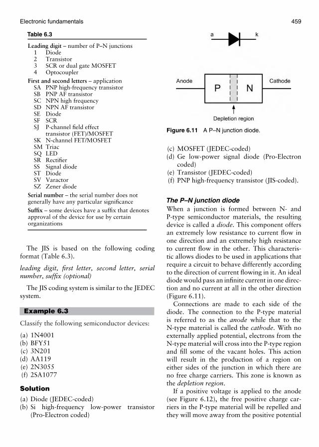
Electronic fundamentals 459
Table 6.3
Leading digit – number of P–N junctions1 Diode2 Transistor3 SCR or dual gate MOSFET4 Optocoupler
First and second letters – applicationSA PNP high-frequency transistorSB PNP AF transistorSC NPN high frequencySD NPN AF transistorSE DiodeSF SCRSJ P-channel field effect
transistor (FET)/MOSFETSK N-channel FET/MOSFETSM TriacSQ LEDSR RectifierSS Signal diodeST DiodeSV VaractorSZ Zener diode
Serial number – the serial number does notgenerally have any particular significanceSuffix – some devices have a suffix that denotesapproval of the device for use by certainorganizations
The JIS is based on the following codingformat (Table 6.3).
leading digit, first letter, second letter, serialnumber, suffix (optional)
The JIS coding system is similar to the JEDECsystem.
Example 6.3
Classify the following semiconductor devices:
(a) 1N4001(b) BFY51(c) 3N201(d) AA119(e) 2N3055(f) 2SA1077
Solution
(a) Diode (JEDEC-coded)(b) Si high-frequency low-power transistor
(Pro-Electron coded)
Figure 6.11 A P–N junction diode.
(c) MOSFET (JEDEC-coded)(d) Ge low-power signal diode (Pro-Electron
coded)(e) Transistor (JEDEC-coded)(f) PNP high-frequency transistor (JIS-coded).
The P–N junction diodeWhen a junction is formed between N- andP-type semiconductor materials, the resultingdevice is called a diode. This component offersan extremely low resistance to current flow inone direction and an extremely high resistanceto current flow in the other. This characteris-tic allows diodes to be used in applications thatrequire a circuit to behave differently accordingto the direction of current flowing in it. An idealdiode would pass an infinite current in one direc-tion and no current at all in the other direction(Figure 6.11).
Connections are made to each side of thediode. The connection to the P-type materialis referred to as the anode while that to theN-type material is called the cathode. With noexternally applied potential, electrons from theN-type material will cross into the P-type regionand fill some of the vacant holes. This actionwill result in the production of a region oneither sides of the junction in which there areno free charge carriers. This zone is known asthe depletion region.
If a positive voltage is applied to the anode(see Figure 6.12), the free positive charge car-riers in the P-type material will be repelled andthey will move away from the positive potential
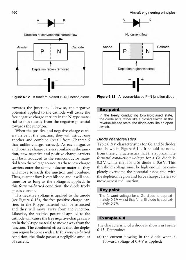
460 Aircraft engineering principles
Figure 6.12 A forward-biased P–N junction diode.
towards the junction. Likewise, the negativepotential applied to the cathode will cause thefree negative charge carriers in the N-type mate-rial to move away from the negative potentialtowards the junction.
When the positive and negative charge carri-ers arrive at the junction, they will attract oneanother and combine (recall from Chapter 5that unlike charges attract). As each negativeand positive charge carriers combine at the junc-tion, new negative and positive charge carrierswill be introduced to the semiconductor mate-rial from the voltage source. As these new chargecarriers enter the semiconductor material, theywill move towards the junction and combine.Thus, current flow is established and it will con-tinue for as long as the voltage is applied. Inthis forward-biased condition, the diode freelypasses current.
If a negative voltage is applied to the anode(see Figure 6.13), the free positive charge car-riers in the P-type material will be attractedand they will move away from the junction.Likewise, the positive potential applied to thecathode will cause the free negative charge carri-ers in the N-type material to move away from thejunction. The combined effect is that the deple-tion region becomes wider. In this reverse-biasedcondition, the diode passes a negligible amountof current.
Figure 6.13 A reverse-biased P–N junction diode.
Key pointIn the freely conducting forward-biased state,the diode acts rather like a closed switch. In thereverse-biased state, the diode acts like an openswitch.
Diode characteristicsTypical I/V characteristics for Ge and Si diodesare shown in Figure 6.14. It should be notedfrom these characteristics that the approximateforward conduction voltage for a Ge diode is0.2 V whilst that for a Si diode is 0.6 V. Thisthreshold voltage must be high enough to com-pletely overcome the potential associated withthe depletion region and force charge carriers tomove across the junction.
Key pointThe forward voltage for a Ge diode is approxi-mately 0.2V whilst that for a Si diode is approxi-mately 0.6V.
Example 6.4
The characteristic of a diode is shown in Figure6.15. Determine:
(a) the current flowing in the diode when aforward voltage of 0.4 V is applied;
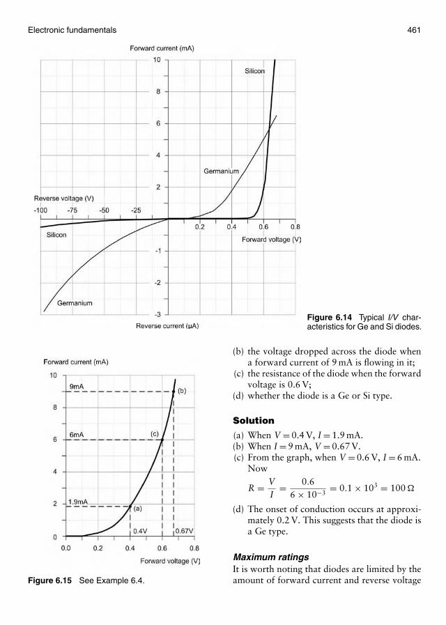
Electronic fundamentals 461
Figure 6.14 Typical I/V char-acteristics for Ge and Si diodes.
Figure 6.15 See Example 6.4.
(b) the voltage dropped across the diode whena forward current of 9 mA is flowing in it;
(c) the resistance of the diode when the forwardvoltage is 0.6 V;
(d) whether the diode is a Ge or Si type.
Solution
(a) When V = 0.4 V, I = 1.9 mA.(b) When I = 9 mA, V = 0.67 V.(c) From the graph, when V = 0.6 V, I = 6 mA.
Now
R = VI
= 0.66 × 10−3
= 0.1 × 103 = 100 �
(d) The onset of conduction occurs at approxi-mately 0.2 V. This suggests that the diode isa Ge type.
Maximum ratingsIt is worth noting that diodes are limited by theamount of forward current and reverse voltage
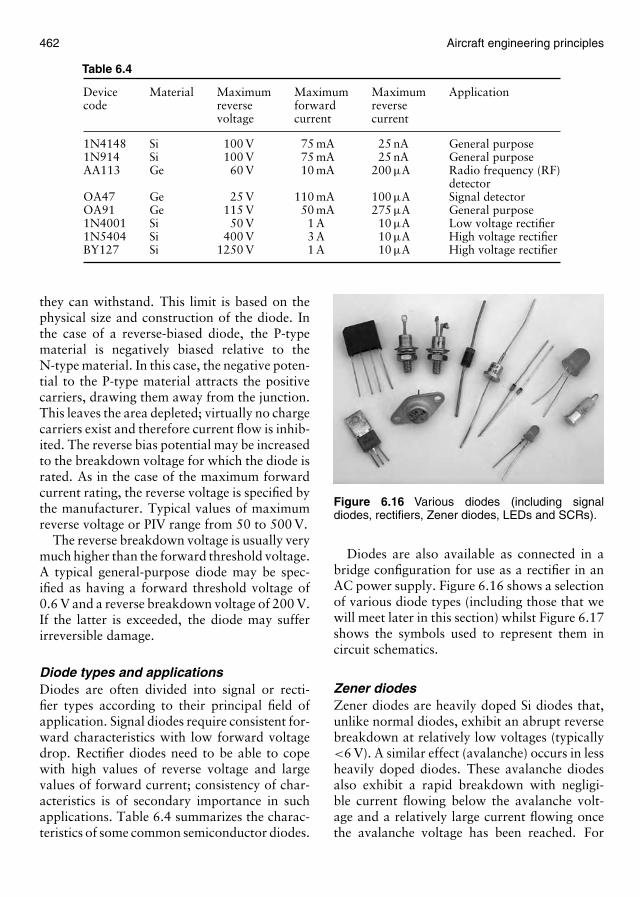
462 Aircraft engineering principles
Table 6.4
Device Material Maximum Maximum Maximum Applicationcode reverse forward reverse
voltage current current
1N4148 Si 100 V 75 mA 25 nA General purpose1N914 Si 100 V 75 mA 25 nA General purposeAA113 Ge 60 V 10 mA 200 µA Radio frequency (RF)
detectorOA47 Ge 25 V 110 mA 100 µA Signal detectorOA91 Ge 115 V 50 mA 275 µA General purpose1N4001 Si 50 V 1 A 10 µA Low voltage rectifier1N5404 Si 400 V 3 A 10 µA High voltage rectifierBY127 Si 1250 V 1 A 10 µA High voltage rectifier
they can withstand. This limit is based on thephysical size and construction of the diode. Inthe case of a reverse-biased diode, the P-typematerial is negatively biased relative to theN-type material. In this case, the negative poten-tial to the P-type material attracts the positivecarriers, drawing them away from the junction.This leaves the area depleted; virtually no chargecarriers exist and therefore current flow is inhib-ited. The reverse bias potential may be increasedto the breakdown voltage for which the diode israted. As in the case of the maximum forwardcurrent rating, the reverse voltage is specified bythe manufacturer. Typical values of maximumreverse voltage or PIV range from 50 to 500 V.
The reverse breakdown voltage is usually verymuch higher than the forward threshold voltage.A typical general-purpose diode may be spec-ified as having a forward threshold voltage of0.6 V and a reverse breakdown voltage of 200 V.If the latter is exceeded, the diode may sufferirreversible damage.
Diode types and applicationsDiodes are often divided into signal or recti-fier types according to their principal field ofapplication. Signal diodes require consistent for-ward characteristics with low forward voltagedrop. Rectifier diodes need to be able to copewith high values of reverse voltage and largevalues of forward current; consistency of char-acteristics is of secondary importance in suchapplications. Table 6.4 summarizes the charac-teristics of some common semiconductor diodes.
Figure 6.16 Various diodes (including signaldiodes, rectifiers, Zener diodes, LEDs and SCRs).
Diodes are also available as connected in abridge configuration for use as a rectifier in anAC power supply. Figure 6.16 shows a selectionof various diode types (including those that wewill meet later in this section) whilst Figure 6.17shows the symbols used to represent them incircuit schematics.
Zener diodesZener diodes are heavily doped Si diodes that,unlike normal diodes, exhibit an abrupt reversebreakdown at relatively low voltages (typically<6 V). A similar effect (avalanche) occurs in lessheavily doped diodes. These avalanche diodesalso exhibit a rapid breakdown with negligi-ble current flowing below the avalanche volt-age and a relatively large current flowing oncethe avalanche voltage has been reached. For

Electronic fundamentals 463
Figure 6.17 Diode symbols.
avalanche diodes, this breakdown voltage usu-ally occurs at voltages above 6 V. In practice,however, both types of diode are referred to asZener diodes. The symbol for a Zener diode wasshown earlier in Figure 6.17 whilst typical Zenerdiode characteristics are shown in Figure 6.18.
Though reverse breakdown is a highly unde-sirable effect in circuits that use conventionaldiodes, it can be extremely useful in the case ofZener diodes where the breakdown voltage isprecisely known. When a diode is undergoingreverse breakdown and provided its maximumratings are not exceeded, the voltage appear-ing across it will remain substantially constant(equal to the nominal Zener voltage) regardlessof the current flowing. This property makes theZener diode ideal for use as a voltage regulator.
Zener diodes are available in various fam-ilies (according to their general characteris-tics, encapsulations and power ratings) withreverse breakdown (Zener) voltages in the range2.4–91 V. Table 6.5 summarizes the character-istics of common Zener diodes. Figure 6.18 Typical Zener diode characteristic.
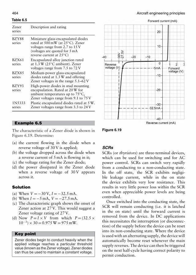
464 Aircraft engineering principles
Table 6.5
Zener Description and ratingseries
BZY88 Miniature glass-encapsulated diodesseries rated at 500 mW (at 25◦C). Zener
voltages range from 2.7 to 15 V(voltages are quoted for 5 mAreverse current at 25◦C)
BZX61 Encapsulated alloy junction ratedseries at 1.3 W (25◦C ambient). Zener
voltages range from 7.5 to 72 VBZX85 Medium-power glass-encapsulatedseries diodes rated at 1.3 W and offering
Zener voltages in the range 5.1–62 VBZY93 High-power diodes in stud mountingseries encapsulation. Rated at 20 W for
ambient temperatures up to 75◦C,Zener voltages range from 9.1 to 75 V
1N5333 Plastic encapsulated diodes rated at 5 W.series Zener voltages range from 3.3 to 24 V
Example 6.5
The characteristic of a Zener diode is shown inFigure 6.19. Determine:
(a) the current flowing in the diode when areverse voltage of 30 V is applied;
(b) the voltage dropped across the diode whena reverse current of 5 mA is flowing in it;
(c) the voltage rating for the Zener diode;(d) the power dissipated in the Zener diode
when a reverse voltage of 30 V appearsacross it.
Solution
(a) When V = −30 V, I = −32.5 mA.(b) When I = −5 mA, V = −27.5 mA.(c) The characteristic graph shows the onset of
Zener action at 27 V. This would suggest aZener voltage rating of 27 V.
(d) Now P = I × V from which P = (32.5 ×10−3) × 30 = 0.975 W = 975 mW.
Key pointZener diodes begin to conduct heavily when theapplied voltage reaches a particular thresholdvalue (known as the Zener voltage). Zener diodescan thus be used to maintain a constant voltage.
Figure 6.19
SCRsSCRs (or thyristors) are three-terminal devices,which can be used for switching and for ACpower control. SCRs can switch very rapidlyfrom a conducting to a non-conducting state.In the off state, the SCR exhibits negligi-ble leakage current, while in the on statethe device exhibits very low resistance. Thisresults in very little power loss within the SCReven when appreciable power levels are beingcontrolled.
Once switched into the conducting state, theSCR will remain conducting (i.e. it is latchedin the on state) until the forward current isremoved from the device. In DC applicationsthis necessitates the interruption (or disconnec-tion) of the supply before the device can be resetinto its non-conducting state. Where the deviceis used with an alternating supply, the device willautomatically become reset whenever the mainsupply reverses. The device can then be triggeredon the next half-cycle having correct polarity topermit conduction.

Electronic fundamentals 465
Like their conventional Si diode counterparts,SCRs have anode and cathode connections;control is applied by means of a gate terminal.The symbol for an SCR was shown earlier inFigure 6.17.
In normal use, an SCR is triggered into theconducting (on) state by means of the appli-cation of a current pulse to the gate terminal(see Figure 6.20). The effective triggering of anSCR requires a gate trigger pulse having a fastrise time derived from a low-resistance source.Triggering can become erratic when insufficient
Figure 6.20 Triggering a SCR.
Table 6.6
Type IF (AV) VRRM VGT IGT(A) (V) (V) (mA)
2N4444 5.1 600 1.5 30BT106 1.0 700 3.5 50BT152 13.0 600 1.0 32BTY79-400R 6.4 400 3.0 30TIC106D 3.2 400 1.2 0.2TIC126D 7.5 400 2.5 20
Table 6.7
Parameter Standard Standard High-efficiency HighLED LED LED intensity
Diameter (mm) 3 5 5 5Maximum forward current (mA) 40 30 30 30Typical forward current (mA) 12 10 7 10Typical forward voltage drop (V) 2.1 2.0 1.8 2.2Maximum reverse voltage (V) 5 3 5 5Maximum power dissipation (mW) 150 100 27 135Peak wavelength (nm) 690 635 635 635
gate current is available or when the gate currentchanges slowly.
Table 6.6 summarizes the characteristics ofseveral common SCRs.
Key pointSCRs are diodes that can be triggered into con-duction by applying a small current to their gateinput. SCRs are able to control large voltages andcurrents from a relatively small (low current, lowvoltage) signal.
LEDsLEDs can be used as general-purpose indica-tors and, compared with conventional filamentlamps, operate from significantly smaller volt-ages and currents. LEDs are also very muchmore reliable than filament lamps. Most LEDswill provide a reasonable level of light outputwhen a forward current of between 5 and 20 mAis applied.
LEDs are available in various formats withthe round types being most popular. RoundLEDs are commonly available in the 3 and 5 mm(0.2 in.) diameter plastic packages and also ina 5 mm × 2 mm rectangular format. The view-ing angle for round LEDs tends to be in theregion of 20◦–40◦, whereas for rectangular typesthis is increased to around 100◦. The symbolfor an LED was shown earlier in Figure 6.17.Table 6.7 summarizes the characteristics of sev-eral common types of LED.
In order to limit the forward current of anLED to an appropriate value, it is usuallynecessary to include a fixed resistor in series with

466 Aircraft engineering principles
Figure 6.21 See Example 6.6.
an LED indicator as shown in Figure 6.21. Thevalue of the resistor may be calculated from theformula:
R = V − VF
I
where VF is the forward voltage drop producedby the LED and V is the applied voltage. Notethat, for most common LED, VF is approxi-mately 2 V.
Example 6.6
A simple LED indicator circuit is shown inFigure 6.21. Determine the value for R andthe diode which is to operate with a current of10 mA and has a forward voltage drop of 2 V.
Solution
Using the formula,
R = V − VF
Igives:
R = 12 − 210 × 10−3
= 1 × 103 = 1 k�
Key pointLEDs produce light when a small current isapplied to them. They are generally smaller andmore reliable than conventional filament lampsand can be used to form larger and more complexdisplays.
Diodes in series and in parallelLike other components, diodes can be connectedin series and in parallel (see Figure 6.22). In the
Figure 6.22 (a) Series connected diodes (b) paral-lel connected diodes.
series case shown in Figure 6.22(a), the totalvoltage dropped across n diodes connected inseries will be n times the forward thresholdvoltage of a single diode. Thus, for two Si diodesconnected in series the forward voltage dropwill be approximately 2 × 0.6 or 1.2 V. It isalso worth noting that the same current flowsthrough each of the diodes. In the parallel caseshown in Figure 6.22(b), the total current willbe divided equally between the diodes (assumingthat they are identical) but the voltage droppedacross them will be the same as the forwardthreshold voltage of a single diode. Thus, fortwo Si diodes connected in parallel the forwardvoltage drop will be approximately 0.6 V butwith the current shared between them.
RectifiersSemiconductor diodes are commonly used toconvert AC to DC, in which case they arereferred to as rectifiers. The simplest form ofrectifier circuit makes use of a single diode and,since it operates on only either positive or neg-ative half-cycles of the supply, it is known as ahalf-wave rectifier.
Figure 6.23 shows a simple half-wave rectifiercircuit. The AC supply at 115 V is applied to theprimary of a step-down transformer (T1). Thesecondary of T1 steps down the 115 V 400 Hzsupply to 28.75 V root mean square (RMS) (theturns ratio of T1 will thus be 115/28.75 or 4 : 1).
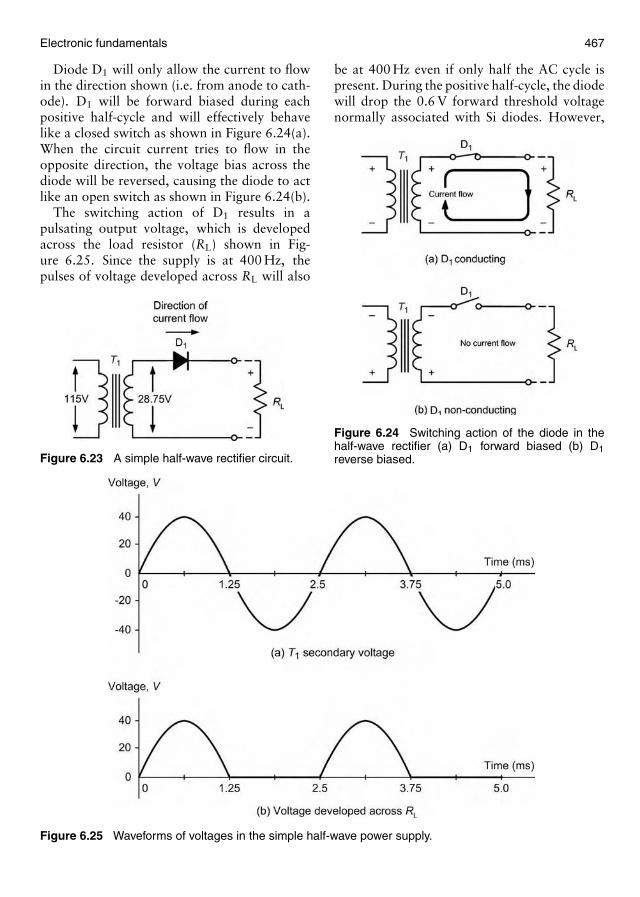
Electronic fundamentals 467
Diode D1 will only allow the current to flowin the direction shown (i.e. from anode to cath-ode). D1 will be forward biased during eachpositive half-cycle and will effectively behavelike a closed switch as shown in Figure 6.24(a).When the circuit current tries to flow in theopposite direction, the voltage bias across thediode will be reversed, causing the diode to actlike an open switch as shown in Figure 6.24(b).
The switching action of D1 results in apulsating output voltage, which is developedacross the load resistor (RL) shown in Fig-ure 6.25. Since the supply is at 400 Hz, thepulses of voltage developed across RL will also
Figure 6.23 A simple half-wave rectifier circuit.
Figure 6.25 Waveforms of voltages in the simple half-wave power supply.
be at 400 Hz even if only half the AC cycle ispresent. During the positive half-cycle, the diodewill drop the 0.6 V forward threshold voltagenormally associated with Si diodes. However,
Figure 6.24 Switching action of the diode in thehalf-wave rectifier (a) D1 forward biased (b) D1reverse biased.
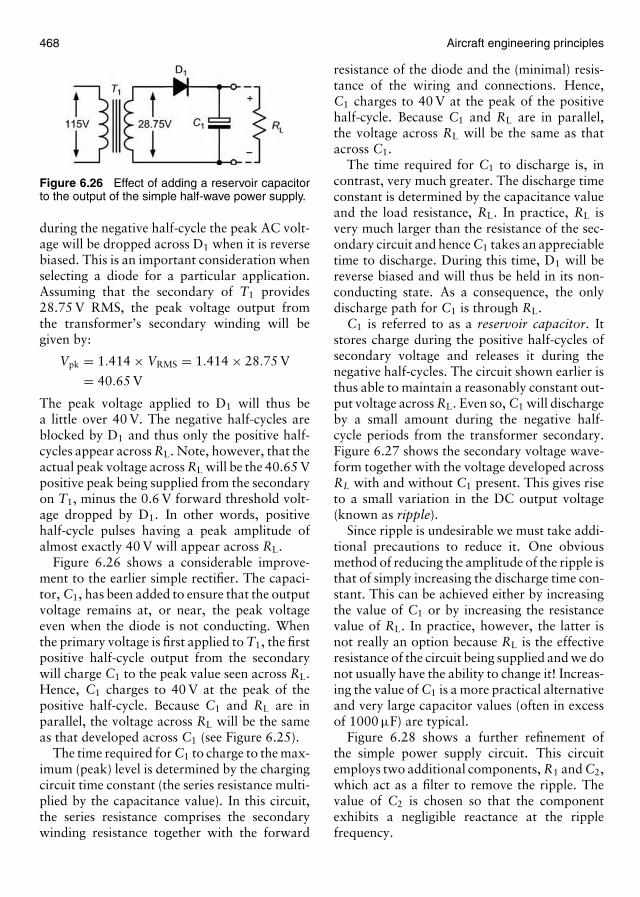
468 Aircraft engineering principles
Figure 6.26 Effect of adding a reservoir capacitorto the output of the simple half-wave power supply.
during the negative half-cycle the peak AC volt-age will be dropped across D1 when it is reversebiased. This is an important consideration whenselecting a diode for a particular application.Assuming that the secondary of T1 provides28.75 V RMS, the peak voltage output fromthe transformer’s secondary winding will begiven by:
Vpk = 1.414 × VRMS = 1.414 × 28.75 V
= 40.65 V
The peak voltage applied to D1 will thus bea little over 40 V. The negative half-cycles areblocked by D1 and thus only the positive half-cycles appear across RL. Note, however, that theactual peak voltage across RL will be the 40.65 Vpositive peak being supplied from the secondaryon T1, minus the 0.6 V forward threshold volt-age dropped by D1. In other words, positivehalf-cycle pulses having a peak amplitude ofalmost exactly 40 V will appear across RL.
Figure 6.26 shows a considerable improve-ment to the earlier simple rectifier. The capaci-tor, C1, has been added to ensure that the outputvoltage remains at, or near, the peak voltageeven when the diode is not conducting. Whenthe primary voltage is first applied to T1, the firstpositive half-cycle output from the secondarywill charge C1 to the peak value seen across RL.Hence, C1 charges to 40 V at the peak of thepositive half-cycle. Because C1 and RL are inparallel, the voltage across RL will be the sameas that developed across C1 (see Figure 6.25).
The time required for C1 to charge to the max-imum (peak) level is determined by the chargingcircuit time constant (the series resistance multi-plied by the capacitance value). In this circuit,the series resistance comprises the secondarywinding resistance together with the forward
resistance of the diode and the (minimal) resis-tance of the wiring and connections. Hence,C1 charges to 40 V at the peak of the positivehalf-cycle. Because C1 and RL are in parallel,the voltage across RL will be the same as thatacross C1.
The time required for C1 to discharge is, incontrast, very much greater. The discharge timeconstant is determined by the capacitance valueand the load resistance, RL. In practice, RL isvery much larger than the resistance of the sec-ondary circuit and hence C1 takes an appreciabletime to discharge. During this time, D1 will bereverse biased and will thus be held in its non-conducting state. As a consequence, the onlydischarge path for C1 is through RL.
C1 is referred to as a reservoir capacitor. Itstores charge during the positive half-cycles ofsecondary voltage and releases it during thenegative half-cycles. The circuit shown earlier isthus able to maintain a reasonably constant out-put voltage across RL. Even so, C1 will dischargeby a small amount during the negative half-cycle periods from the transformer secondary.Figure 6.27 shows the secondary voltage wave-form together with the voltage developed acrossRL with and without C1 present. This gives riseto a small variation in the DC output voltage(known as ripple).
Since ripple is undesirable we must take addi-tional precautions to reduce it. One obviousmethod of reducing the amplitude of the ripple isthat of simply increasing the discharge time con-stant. This can be achieved either by increasingthe value of C1 or by increasing the resistancevalue of RL. In practice, however, the latter isnot really an option because RL is the effectiveresistance of the circuit being supplied and we donot usually have the ability to change it! Increas-ing the value of C1 is a more practical alternativeand very large capacitor values (often in excessof 1000 µF) are typical.
Figure 6.28 shows a further refinement ofthe simple power supply circuit. This circuitemploys two additional components, R1 and C2,which act as a filter to remove the ripple. Thevalue of C2 is chosen so that the componentexhibits a negligible reactance at the ripplefrequency.
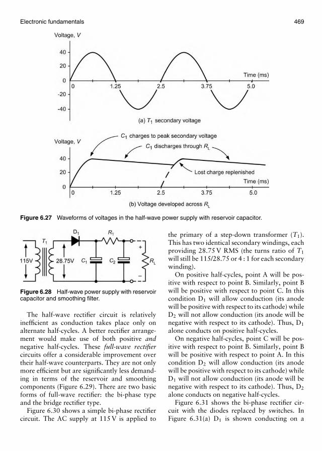
Electronic fundamentals 469
Figure 6.27 Waveforms of voltages in the half-wave power supply with reservoir capacitor.
Figure 6.28 Half-wave power supply with reservoircapacitor and smoothing filter.
The half-wave rectifier circuit is relativelyinefficient as conduction takes place only onalternate half-cycles. A better rectifier arrange-ment would make use of both positive andnegative half-cycles. These full-wave rectifiercircuits offer a considerable improvement overtheir half-wave counterparts. They are not onlymore efficient but are significantly less demand-ing in terms of the reservoir and smoothingcomponents (Figure 6.29). There are two basicforms of full-wave rectifier: the bi-phase typeand the bridge rectifier type.
Figure 6.30 shows a simple bi-phase rectifiercircuit. The AC supply at 115 V is applied to
the primary of a step-down transformer (T1).This has two identical secondary windings, eachproviding 28.75 V RMS (the turns ratio of T1
will still be 115/28.75 or 4 : 1 for each secondarywinding).
On positive half-cycles, point A will be pos-itive with respect to point B. Similarly, point Bwill be positive with respect to point C. In thiscondition D1 will allow conduction (its anodewill be positive with respect to its cathode) whileD2 will not allow conduction (its anode will benegative with respect to its cathode). Thus, D1
alone conducts on positive half-cycles.On negative half-cycles, point C will be pos-
itive with respect to point B. Similarly, point Bwill be positive with respect to point A. In thiscondition D2 will allow conduction (its anodewill be positive with respect to its cathode) whileD1 will not allow conduction (its anode will benegative with respect to its cathode). Thus, D2
alone conducts on negative half-cycles.Figure 6.31 shows the bi-phase rectifier cir-
cuit with the diodes replaced by switches. InFigure 6.31(a) D1 is shown conducting on a
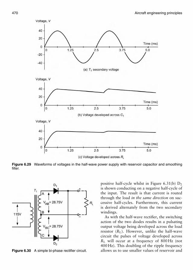
470 Aircraft engineering principles
Figure 6.29 Waveforms of voltages in the half-wave power supply with reservoir capacitor and smoothingfilter.
Figure 6.30 A simple bi-phase rectifier circuit.
positive half-cycle whilst in Figure 6.31(b) D2
is shown conducting on a negative half-cycle ofthe input. The result is that current is routedthrough the load in the same direction on suc-cessive half-cycles. Furthermore, this currentis derived alternately from the two secondarywindings.
As with the half-wave rectifier, the switchingaction of the two diodes results in a pulsatingoutput voltage being developed across the loadresistor (RL). However, unlike the half-wavecircuit the pulses of voltage developed acrossRL will occur at a frequency of 800 Hz (not400 Hz). This doubling of the ripple frequencyallows us to use smaller values of reservoir and
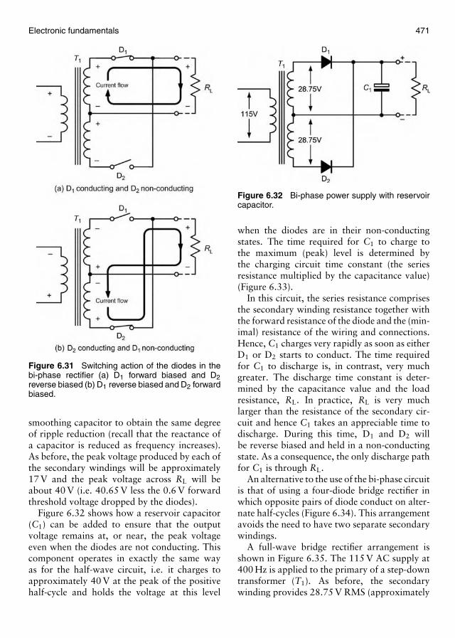
Electronic fundamentals 471
Figure 6.31 Switching action of the diodes in thebi-phase rectifier (a) D1 forward biased and D2reverse biased (b) D1 reverse biased and D2 forwardbiased.
smoothing capacitor to obtain the same degreeof ripple reduction (recall that the reactance ofa capacitor is reduced as frequency increases).As before, the peak voltage produced by each ofthe secondary windings will be approximately17 V and the peak voltage across RL will beabout 40 V (i.e. 40.65 V less the 0.6 V forwardthreshold voltage dropped by the diodes).
Figure 6.32 shows how a reservoir capacitor(C1) can be added to ensure that the outputvoltage remains at, or near, the peak voltageeven when the diodes are not conducting. Thiscomponent operates in exactly the same wayas for the half-wave circuit, i.e. it charges toapproximately 40 V at the peak of the positivehalf-cycle and holds the voltage at this level
Figure 6.32 Bi-phase power supply with reservoircapacitor.
when the diodes are in their non-conductingstates. The time required for C1 to charge tothe maximum (peak) level is determined bythe charging circuit time constant (the seriesresistance multiplied by the capacitance value)(Figure 6.33).
In this circuit, the series resistance comprisesthe secondary winding resistance together withthe forward resistance of the diode and the (min-imal) resistance of the wiring and connections.Hence, C1 charges very rapidly as soon as eitherD1 or D2 starts to conduct. The time requiredfor C1 to discharge is, in contrast, very muchgreater. The discharge time constant is deter-mined by the capacitance value and the loadresistance, RL. In practice, RL is very muchlarger than the resistance of the secondary cir-cuit and hence C1 takes an appreciable time todischarge. During this time, D1 and D2 willbe reverse biased and held in a non-conductingstate. As a consequence, the only discharge pathfor C1 is through RL.
An alternative to the use of the bi-phase circuitis that of using a four-diode bridge rectifier inwhich opposite pairs of diode conduct on alter-nate half-cycles (Figure 6.34). This arrangementavoids the need to have two separate secondarywindings.
A full-wave bridge rectifier arrangement isshown in Figure 6.35. The 115 V AC supply at400 Hz is applied to the primary of a step-downtransformer (T1). As before, the secondarywinding provides 28.75 V RMS (approximately
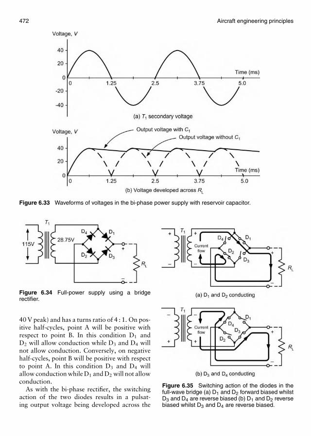
472 Aircraft engineering principles
Figure 6.33 Waveforms of voltages in the bi-phase power supply with reservoir capacitor.
Figure 6.34 Full-power supply using a bridgerectifier.
40 V peak) and has a turns ratio of 4 : 1. On pos-itive half-cycles, point A will be positive withrespect to point B. In this condition D1 andD2 will allow conduction while D3 and D4 willnot allow conduction. Conversely, on negativehalf-cycles, point B will be positive with respectto point A. In this condition D3 and D4 willallow conduction while D1 and D2 will not allowconduction.
As with the bi-phase rectifier, the switchingaction of the two diodes results in a pulsat-ing output voltage being developed across the
Figure 6.35 Switching action of the diodes in thefull-wave bridge (a) D1 and D2 forward biased whilstD3 and D4 are reverse biased (b) D1 and D2 reversebiased whilst D3 and D4 are reverse biased.
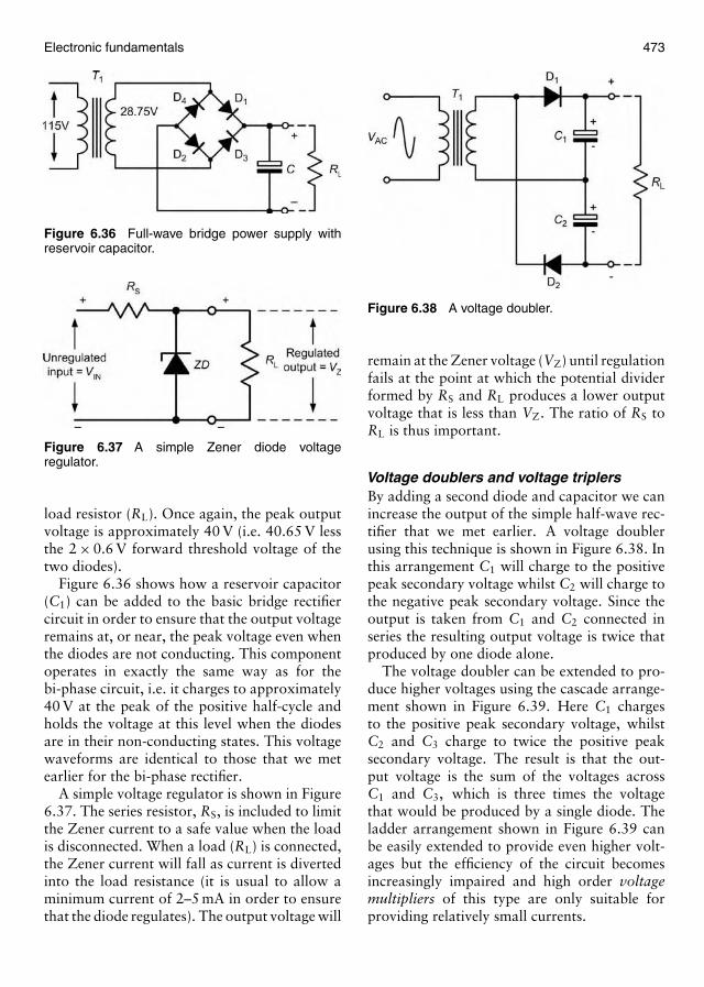
Electronic fundamentals 473
Figure 6.36 Full-wave bridge power supply withreservoir capacitor.
Figure 6.37 A simple Zener diode voltageregulator.
load resistor (RL). Once again, the peak outputvoltage is approximately 40 V (i.e. 40.65 V lessthe 2 × 0.6 V forward threshold voltage of thetwo diodes).
Figure 6.36 shows how a reservoir capacitor(C1) can be added to the basic bridge rectifiercircuit in order to ensure that the output voltageremains at, or near, the peak voltage even whenthe diodes are not conducting. This componentoperates in exactly the same way as for thebi-phase circuit, i.e. it charges to approximately40 V at the peak of the positive half-cycle andholds the voltage at this level when the diodesare in their non-conducting states. This voltagewaveforms are identical to those that we metearlier for the bi-phase rectifier.
A simple voltage regulator is shown in Figure6.37. The series resistor, RS, is included to limitthe Zener current to a safe value when the loadis disconnected. When a load (RL) is connected,the Zener current will fall as current is divertedinto the load resistance (it is usual to allow aminimum current of 2–5 mA in order to ensurethat the diode regulates). The output voltage will
Figure 6.38 A voltage doubler.
remain at the Zener voltage (VZ) until regulationfails at the point at which the potential dividerformed by RS and RL produces a lower outputvoltage that is less than VZ. The ratio of RS toRL is thus important.
Voltage doublers and voltage triplersBy adding a second diode and capacitor we canincrease the output of the simple half-wave rec-tifier that we met earlier. A voltage doublerusing this technique is shown in Figure 6.38. Inthis arrangement C1 will charge to the positivepeak secondary voltage whilst C2 will charge tothe negative peak secondary voltage. Since theoutput is taken from C1 and C2 connected inseries the resulting output voltage is twice thatproduced by one diode alone.
The voltage doubler can be extended to pro-duce higher voltages using the cascade arrange-ment shown in Figure 6.39. Here C1 chargesto the positive peak secondary voltage, whilstC2 and C3 charge to twice the positive peaksecondary voltage. The result is that the out-put voltage is the sum of the voltages acrossC1 and C3, which is three times the voltagethat would be produced by a single diode. Theladder arrangement shown in Figure 6.39 canbe easily extended to provide even higher volt-ages but the efficiency of the circuit becomesincreasingly impaired and high order voltagemultipliers of this type are only suitable forproviding relatively small currents.

474 Aircraft engineering principles
Clipping and clamping circuitsApart from their use as rectifiers, diodes arefrequently used in signal-processing circuits forclipping and clamping. In clipping applicationsdiodes are used to remove part of a waveform asshown in Figure 6.40. They do this by conduct-ing on the positive, negative or both half-cyclesof the AC waveform, effectively shunting thesignal to common. On the remaining part ofthe cycle they are non-conducting and thereforehave no effect on the shape of the waveform.
In clamping applications diodes can be usedto change the DC level present on a waveformso that the waveform is all positive or all nega-tive. Depending on which way it is connected,the diode conducts on either the negative- orpositive-going half-cycles of the input AC wave-form. The capacitor, C, charges to the peakvalue of the waveform, effectively lifting ordepressing the waveform so that it all lies either
Figure 6.39 A voltage tripler.
Figure 6.40 Clipping circuits (a) a positive edge clipper (b) a negative edge clipper (c) a symmetrical clipper.
above or below the zero voltage axis, as shownin Figure 6.41.
Varactor diodesWe have already shown that, when a diodeis operated in the reverse-biased condition, thewidth of the depletion region increases as theapplied voltage increases. Varying the width ofthe depletion region is equivalent to varying theplate separation of a very small capacitor suchthat the relationship between junction capac-itance and applied reverse voltage will looksomething like that shown in Figure 6.42.
We can put this effect to good use in circuitsthat require capacitance to be adjusted by means
Figure 6.41 Clamping circuits (a) a positive edgeclamp (b) a negative edge clamp.
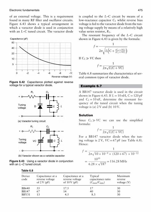
Electronic fundamentals 475
of an external voltage. This is a requirementfound in many RF filter and oscillator circuits.Figure 6.43 shows a typical arrangement inwhich a varactor diode is used in conjunctionwith an L–C tuned circuit. The varactor diode
Figure 6.42 Capacitance plotted against reversevoltage for a typical varactor diode.
Figure 6.43 Using a varactor diode in conjunctionwith an L–C tuned circuit.
Table 6.8
Device Capacitance at a Capacitance at a Typical Maximumcode reverse voltage reverse voltage capacitance ratio reverse
of 2 V (pF) of 10 V (pF) (Cmax/Cmin) voltage (V)
BB640 55 17.5 17 30BB147 67 14 40 30BBY31 13 4.5 8.3 30
is coupled to the L–C circuit by means of alow-reactance capacitor C1 whilst reverse biasvoltage is fed to the varactor diode from the tun-ing voltage supply by means of a relatively highvalue series resistor, R1.
The resonant frequency of the L–C circuitshown in Figure 6.43 is given by the formula:
f = 1
2π
√L(C + (C1 × VC)
(C1 + VC)
)If C1 � VC then
f = 12π
√L(C + VC)
Table 6.8 summarizes the characteristics of sev-eral common types of varactor diode.
Example 6.7
A BB147 varactor diode is used in the circuitshown in Figure 6.43. If L = 10 nH, C = 120 pFand C1 = 10 nF, determine the resonant fre-quency of the tuned circuit when the tuningvoltage is (a) 2 V and (b) 10 V.
Solution
Since C1 � VC we can use the simplifiedformula:
f = 12π
√L(C + VC)
For a BB147 varactor diode when the tun-ing voltage is 2 V, VC = 67 pF (see Table 6.8).Hence:
f = 1
2π√
10 × 10−9 × (120 + 67) × 10−12
= 1010
6.28 × √187
= 116.28 MHz
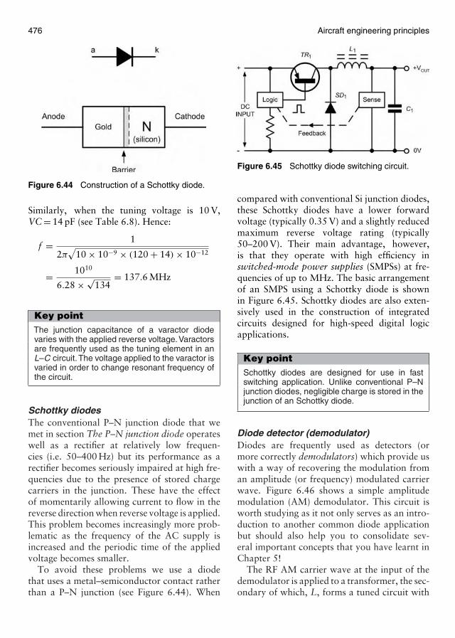
476 Aircraft engineering principles
Figure 6.44 Construction of a Schottky diode.
Similarly, when the tuning voltage is 10 V,VC = 14 pF (see Table 6.8). Hence:
f = 1
2π√
10 × 10−9 × (120 + 14) × 10−12
= 1010
6.28 × √134
= 137.6 MHz
Key pointThe junction capacitance of a varactor diodevaries with the applied reverse voltage.Varactorsare frequently used as the tuning element in anL–C circuit.The voltage applied to the varactor isvaried in order to change resonant frequency ofthe circuit.
Schottky diodesThe conventional P–N junction diode that wemet in section The P–N junction diode operateswell as a rectifier at relatively low frequen-cies (i.e. 50–400 Hz) but its performance as arectifier becomes seriously impaired at high fre-quencies due to the presence of stored chargecarriers in the junction. These have the effectof momentarily allowing current to flow in thereverse direction when reverse voltage is applied.This problem becomes increasingly more prob-lematic as the frequency of the AC supply isincreased and the periodic time of the appliedvoltage becomes smaller.
To avoid these problems we use a diodethat uses a metal–semiconductor contact ratherthan a P–N junction (see Figure 6.44). When
Figure 6.45 Schottky diode switching circuit.
compared with conventional Si junction diodes,these Schottky diodes have a lower forwardvoltage (typically 0.35 V) and a slightly reducedmaximum reverse voltage rating (typically50–200 V). Their main advantage, however,is that they operate with high efficiency inswitched-mode power supplies (SMPSs) at fre-quencies of up to MHz. The basic arrangementof an SMPS using a Schottky diode is shownin Figure 6.45. Schottky diodes are also exten-sively used in the construction of integratedcircuits designed for high-speed digital logicapplications.
Key pointSchottky diodes are designed for use in fastswitching application. Unlike conventional P–Njunction diodes, negligible charge is stored in thejunction of an Schottky diode.
Diode detector (demodulator)Diodes are frequently used as detectors (ormore correctly demodulators) which provide uswith a way of recovering the modulation froman amplitude (or frequency) modulated carrierwave. Figure 6.46 shows a simple amplitudemodulation (AM) demodulator. This circuit isworth studying as it not only serves as an intro-duction to another common diode applicationbut should also help you to consolidate sev-eral important concepts that you have learnt inChapter 5!
The RF AM carrier wave at the input of thedemodulator is applied to a transformer, the sec-ondary of which, L, forms a tuned circuit with
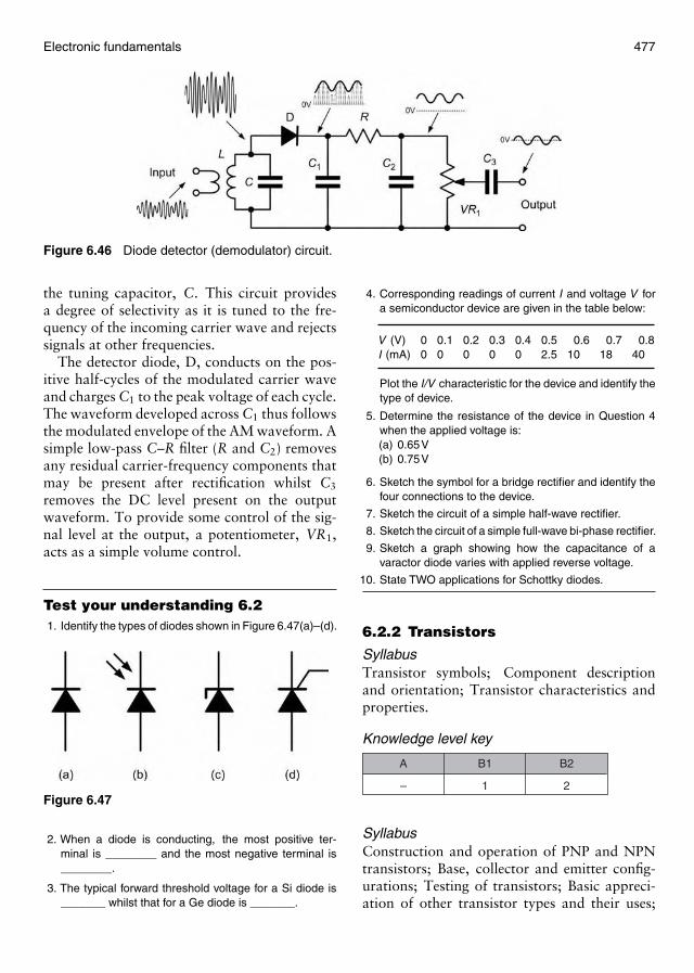
Electronic fundamentals 477
Figure 6.46 Diode detector (demodulator) circuit.
the tuning capacitor, C. This circuit providesa degree of selectivity as it is tuned to the fre-quency of the incoming carrier wave and rejectssignals at other frequencies.
The detector diode, D, conducts on the pos-itive half-cycles of the modulated carrier waveand charges C1 to the peak voltage of each cycle.The waveform developed across C1 thus followsthe modulated envelope of the AM waveform. Asimple low-pass C–R filter (R and C2) removesany residual carrier-frequency components thatmay be present after rectification whilst C3
removes the DC level present on the outputwaveform. To provide some control of the sig-nal level at the output, a potentiometer, VR1,acts as a simple volume control.
Test your understanding 6.21. Identify the types of diodes shown in Figure 6.47(a)–(d).
Figure 6.47
2. When a diode is conducting, the most positive ter-minal is ________ and the most negative terminal is________.
3. The typical forward threshold voltage for a Si diode is_______ whilst that for a Ge diode is _______.
4. Corresponding readings of current I and voltage V fora semiconductor device are given in the table below:
V (V) 0 0.1 0.2 0.3 0.4 0.5 0.6 0.7 0.8I (mA) 0 0 0 0 0 2.5 10 18 40
Plot the I/V characteristic for the device and identify thetype of device.
5. Determine the resistance of the device in Question 4when the applied voltage is:(a) 0.65V(b) 0.75V
6. Sketch the symbol for a bridge rectifier and identify thefour connections to the device.
7. Sketch the circuit of a simple half-wave rectifier.
8. Sketch the circuit of a simple full-wave bi-phase rectifier.
9. Sketch a graph showing how the capacitance of avaractor diode varies with applied reverse voltage.
10. State TWO applications for Schottky diodes.
6.2.2 Transistors
SyllabusTransistor symbols; Component descriptionand orientation; Transistor characteristics andproperties.
Knowledge level key
–
A
1
B1
2
B2
SyllabusConstruction and operation of PNP and NPNtransistors; Base, collector and emitter config-urations; Testing of transistors; Basic appreci-ation of other transistor types and their uses;
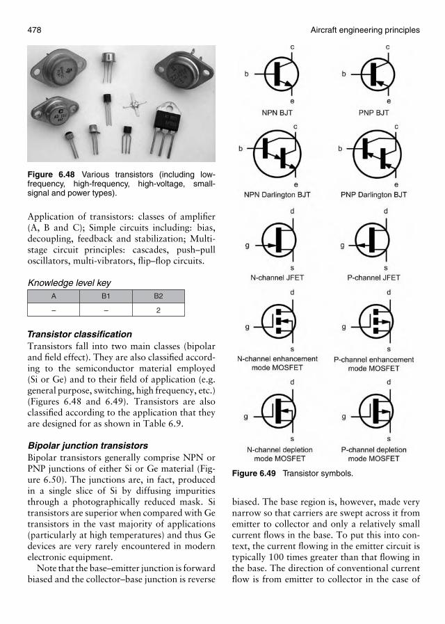
478 Aircraft engineering principles
Figure 6.48 Various transistors (including low-frequency, high-frequency, high-voltage, small-signal and power types).
Application of transistors: classes of amplifier(A, B and C); Simple circuits including: bias,decoupling, feedback and stabilization; Multi-stage circuit principles: cascades, push–pulloscillators, multi-vibrators, flip–flop circuits.
Knowledge level key
–
A
–
B1
2
B2
Transistor classificationTransistors fall into two main classes (bipolarand field effect). They are also classified accord-ing to the semiconductor material employed(Si or Ge) and to their field of application (e.g.general purpose, switching, high frequency, etc.)(Figures 6.48 and 6.49). Transistors are alsoclassified according to the application that theyare designed for as shown in Table 6.9.
Bipolar junction transistorsBipolar transistors generally comprise NPN orPNP junctions of either Si or Ge material (Fig-ure 6.50). The junctions are, in fact, producedin a single slice of Si by diffusing impuritiesthrough a photographically reduced mask. Sitransistors are superior when compared with Getransistors in the vast majority of applications(particularly at high temperatures) and thus Gedevices are very rarely encountered in modernelectronic equipment.
Note that the base–emitter junction is forwardbiased and the collector–base junction is reverse
Figure 6.49 Transistor symbols.
biased. The base region is, however, made verynarrow so that carriers are swept across it fromemitter to collector and only a relatively smallcurrent flows in the base. To put this into con-text, the current flowing in the emitter circuit istypically 100 times greater than that flowing inthe base. The direction of conventional currentflow is from emitter to collector in the case of
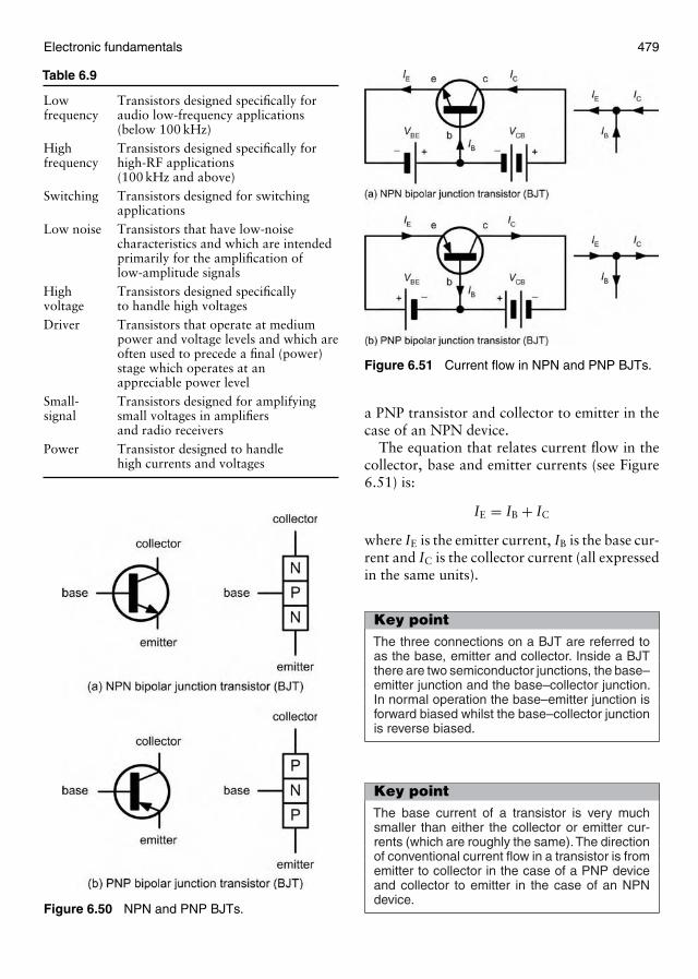
Electronic fundamentals 479
Table 6.9
Low Transistors designed specifically forfrequency audio low-frequency applications
(below 100 kHz)High Transistors designed specifically forfrequency high-RF applications
(100 kHz and above)Switching Transistors designed for switching
applicationsLow noise Transistors that have low-noise
characteristics and which are intendedprimarily for the amplification oflow-amplitude signals
High Transistors designed specificallyvoltage to handle high voltagesDriver Transistors that operate at medium
power and voltage levels and which areoften used to precede a final (power)stage which operates at anappreciable power level
Small- Transistors designed for amplifyingsignal small voltages in amplifiers
and radio receiversPower Transistor designed to handle
high currents and voltages
Figure 6.50 NPN and PNP BJTs.
Figure 6.51 Current flow in NPN and PNP BJTs.
a PNP transistor and collector to emitter in thecase of an NPN device.
The equation that relates current flow in thecollector, base and emitter currents (see Figure6.51) is:
IE = IB + IC
where IE is the emitter current, IB is the base cur-rent and IC is the collector current (all expressedin the same units).
Key pointThe three connections on a BJT are referred toas the base, emitter and collector. Inside a BJTthere are two semiconductor junctions, the base–emitter junction and the base–collector junction.In normal operation the base–emitter junction isforward biased whilst the base–collector junctionis reverse biased.
Key pointThe base current of a transistor is very muchsmaller than either the collector or emitter cur-rents (which are roughly the same).The directionof conventional current flow in a transistor is fromemitter to collector in the case of a PNP deviceand collector to emitter in the case of an NPNdevice.

480 Aircraft engineering principles
Figure 6.52 Input characteristic (IB/V BE) for anNPN BJT.
Example 6.8
A transistor operates with a collector currentof 100 mA and an emitter current of 102 mA.Determine the value of base current.
Solution
Now:
IE = IB + IC
thus:
IB = IE − IC
Hence:
IB = 102 − 100 = 2 mA
Bipolar transistor characteristicsThe characteristics of a BJT are usuallypresented in the form of a set of graphs relat-ing voltage and current present at the transistorsterminals. Figure 6.52 shows a typical inputcharacteristic (IB plotted against VBE) for anNPN BJT operating in common-emitter mode.In this mode, the input current is applied tothe base and the output current appears in thecollector (the emitter is effectively common toboth the input and output circuits).
Figure 6.53 Output characteristic (IC/V CE) for anNPN BJT.
The input characteristic shows that very littlebase current flows until the base–emitter voltageVBE exceeds 0.6 V. Thereafter, the base cur-rent increases rapidly (this characteristic bearsa close resemblance to the forward part of thecharacteristic for a Si diode).
Figure 6.53 shows a typical set of output (col-lector) characteristics (IC plotted against VCE)for an NPN bipolar transistor. Each curve cor-responds to a different value of base current.Note the “knee” in the characteristic belowVCE = 2 V. Also note that the curves are quiteflat. For this reason (i.e. since the collector cur-rent does not change very much as the collector–emitter voltage changes) we often refer to this asa constant current characteristic.
Figure 6.54 shows a typical transfer char-acteristic for an NPN BJT. Here IC is plottedagainst IB for a small-signal general-purposetransistor. The slope of this curve (i.e. the ratioof IC to IB) is the common-emitter current gainof the transistor. We shall explore this furtherin Section Current gain.
Transistor parametersThe transistor characteristics that we met in theprevious section provide us with some usefulinformation that can help us to model the
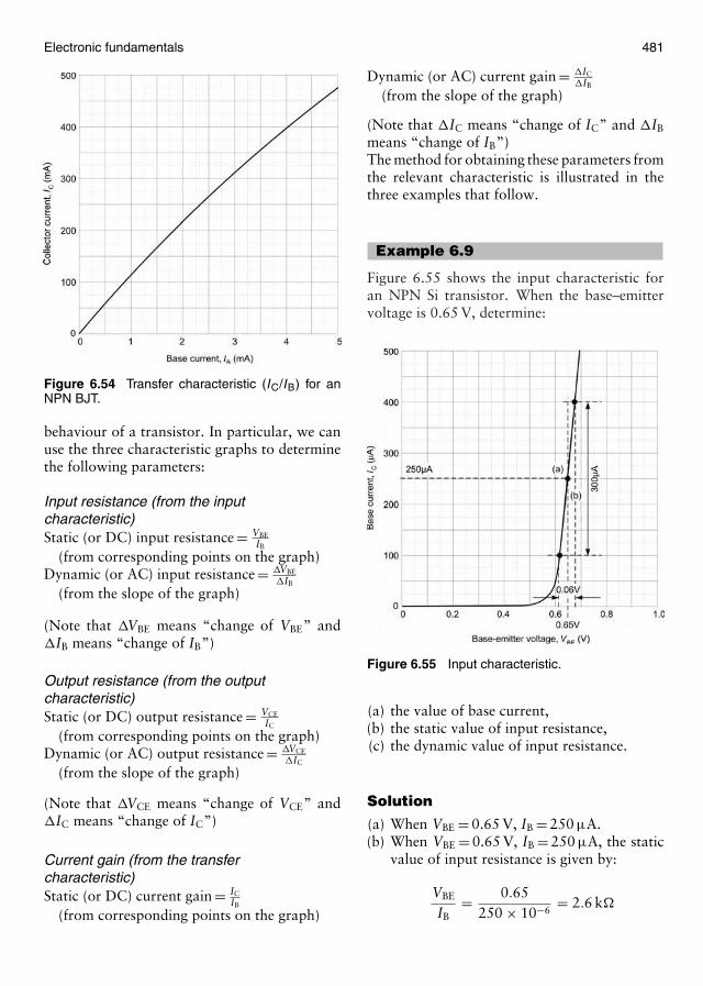
Electronic fundamentals 481
Figure 6.54 Transfer characteristic (IC/IB) for anNPN BJT.
behaviour of a transistor. In particular, we canuse the three characteristic graphs to determinethe following parameters:
Input resistance (from the inputcharacteristic)Static (or DC) input resistance = VBE
IB
(from corresponding points on the graph)Dynamic (or AC) input resistance = �VBE
�IB
(from the slope of the graph)
(Note that �VBE means “change of VBE” and�IB means “change of IB”)
Output resistance (from the outputcharacteristic)Static (or DC) output resistance = VCE
IC
(from corresponding points on the graph)Dynamic (or AC) output resistance = �VCE
�IC
(from the slope of the graph)
(Note that �VCE means “change of VCE” and�IC means “change of IC”)
Current gain (from the transfercharacteristic)Static (or DC) current gain = IC
IB
(from corresponding points on the graph)
Dynamic (or AC) current gain = �IC�IB
(from the slope of the graph)
(Note that �IC means “change of IC” and �IB
means “change of IB”)The method for obtaining these parameters fromthe relevant characteristic is illustrated in thethree examples that follow.
Example 6.9
Figure 6.55 shows the input characteristic foran NPN Si transistor. When the base–emittervoltage is 0.65 V, determine:
Figure 6.55 Input characteristic.
(a) the value of base current,(b) the static value of input resistance,(c) the dynamic value of input resistance.
Solution
(a) When VBE = 0.65 V, IB = 250 µA.(b) When VBE = 0.65 V, IB = 250 µA, the static
value of input resistance is given by:
VBE
IB= 0.65
250 × 10−6= 2.6 k�
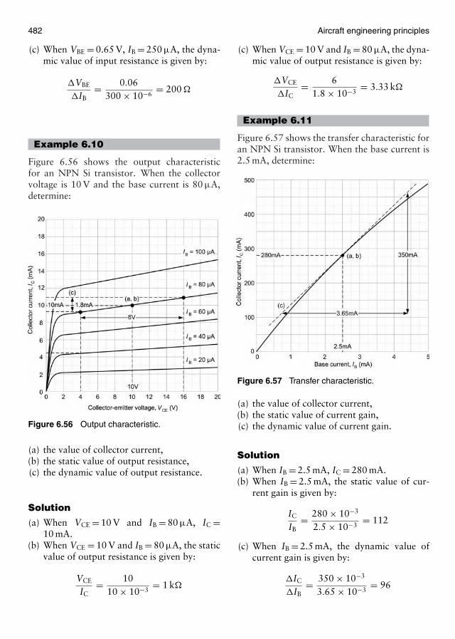
482 Aircraft engineering principles
(c) When VBE = 0.65 V, IB = 250 µA, the dyna-mic value of input resistance is given by:
�VBE
�IB= 0.06
300 × 10−6= 200 �
Example 6.10
Figure 6.56 shows the output characteristicfor an NPN Si transistor. When the collectorvoltage is 10 V and the base current is 80 µA,determine:
Figure 6.56 Output characteristic.
(a) the value of collector current,(b) the static value of output resistance,(c) the dynamic value of output resistance.
Solution
(a) When VCE = 10 V and IB = 80 µA, IC =10 mA.
(b) When VCE = 10 V and IB = 80 µA, the staticvalue of output resistance is given by:
VCE
IC= 10
10 × 10−3= 1 k�
(c) When VCE = 10 V and IB = 80 µA, the dyna-mic value of output resistance is given by:
�VCE
�IC= 6
1.8 × 10−3= 3.33 k�
Example 6.11
Figure 6.57 shows the transfer characteristic foran NPN Si transistor. When the base current is2.5 mA, determine:
Figure 6.57 Transfer characteristic.
(a) the value of collector current,(b) the static value of current gain,(c) the dynamic value of current gain.
Solution
(a) When IB = 2.5 mA, IC = 280 mA.(b) When IB = 2.5 mA, the static value of cur-
rent gain is given by:
IC
IB= 280 × 10−3
2.5 × 10−3= 112
(c) When IB = 2.5 mA, the dynamic value ofcurrent gain is given by:
�IC
�IB= 350 × 10−3
3.65 × 10−3= 96
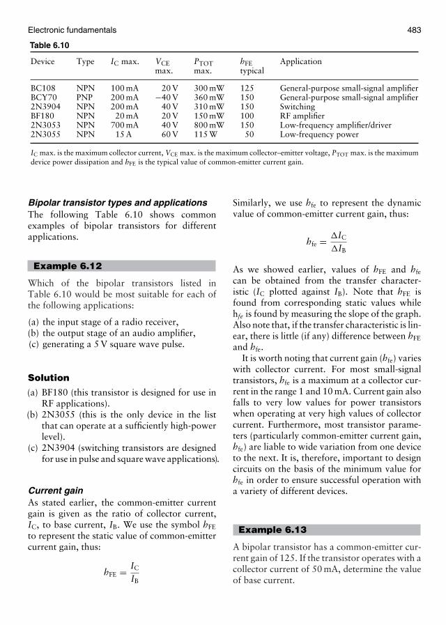
Electronic fundamentals 483
Table 6.10
Device Type IC max. VCE PTOT hFE Applicationmax. max. typical
BC108 NPN 100 mA 20 V 300 mW 125 General-purpose small-signal amplifierBCY70 PNP 200 mA −40 V 360 mW 150 General-purpose small-signal amplifier2N3904 NPN 200 mA 40 V 310 mW 150 SwitchingBF180 NPN 20 mA 20 V 150 mW 100 RF amplifier2N3053 NPN 700 mA 40 V 800 mW 150 Low-frequency amplifier/driver2N3055 NPN 15 A 60 V 115 W 50 Low-frequency power
IC max. is the maximum collector current, VCE max. is the maximum collector–emitter voltage, PTOT max. is the maximumdevice power dissipation and hFE is the typical value of common-emitter current gain.
Bipolar transistor types and applicationsThe following Table 6.10 shows commonexamples of bipolar transistors for differentapplications.
Example 6.12
Which of the bipolar transistors listed inTable 6.10 would be most suitable for each ofthe following applications:
(a) the input stage of a radio receiver,(b) the output stage of an audio amplifier,(c) generating a 5 V square wave pulse.
Solution
(a) BF180 (this transistor is designed for use inRF applications).
(b) 2N3055 (this is the only device in the listthat can operate at a sufficiently high-powerlevel).
(c) 2N3904 (switching transistors are designedfor use in pulse and square wave applications).
Current gainAs stated earlier, the common-emitter currentgain is given as the ratio of collector current,IC, to base current, IB. We use the symbol hFE
to represent the static value of common-emittercurrent gain, thus:
hFE = IC
IB
Similarly, we use hfe to represent the dynamicvalue of common-emitter current gain, thus:
hfe = �IC
�IB
As we showed earlier, values of hFE and hfe
can be obtained from the transfer character-istic (IC plotted against IB). Note that hFE isfound from corresponding static values whilehfe is found by measuring the slope of the graph.Also note that, if the transfer characteristic is lin-ear, there is little (if any) difference between hFE
and hfe.It is worth noting that current gain (hfe) varies
with collector current. For most small-signaltransistors, hfe is a maximum at a collector cur-rent in the range 1 and 10 mA. Current gain alsofalls to very low values for power transistorswhen operating at very high values of collectorcurrent. Furthermore, most transistor parame-ters (particularly common-emitter current gain,hfe) are liable to wide variation from one deviceto the next. It is, therefore, important to designcircuits on the basis of the minimum value forhfe in order to ensure successful operation witha variety of different devices.
Example 6.13
A bipolar transistor has a common-emitter cur-rent gain of 125. If the transistor operates with acollector current of 50 mA, determine the valueof base current.
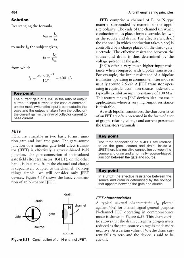
484 Aircraft engineering principles
Solution
Rearranging the formula,
hFE = IC
IB
to make IB the subject gives,
IB = IC
hFE
from which:
IB = 50 × 10−3
125= 400 µA
Key pointThe current gain of a BJT is the ratio of outputcurrent to input current. In the case of common-emitter mode (where the input is connected to thebase and the output is taken from the collector)the current gain is the ratio of collector current tobase current.
FETsFETs are available in two basic forms: junc-tion gate and insulated gate. The gate–sourcejunction of a junction gate field effect transis-tor (JFET) is effectively a reverse-biased P–Njunction. The gate connection of an insulatedgate field effect transistor (IGFET), on the otherhand, is insulated from the channel and chargeis capacitively coupled to the channel. To keepthings simple, we will consider only JFETdevices. Figure 6.58 shows the basic construc-tion of an N-channel JFET.
Figure 6.58 Construction of an N-channel JFET.
FETs comprise a channel of P- or N-typematerial surrounded by material of the oppo-site polarity. The ends of the channel (in whichconduction takes place) form electrodes knownas the source and drain. The effective width ofthe channel (in which conduction takes place) iscontrolled by a charge placed on the third (gate)electrode. The effective resistance between thesource and drain is thus determined by thevoltage present at the gate.
JFETs offer a very much higher input resis-tance when compared with bipolar transistors.For example, the input resistance of a bipolartransistor operating in common-emitter mode isusually around 2.5 k�. A JFET transistor oper-ating in equivalent common-source mode wouldtypically exhibit an input resistance of 100 M�!This feature makes JFET devices ideal for use inapplications where a very high-input resistanceis desirable.
As with bipolar transistors, the characteristicsof an FET are often presented in the form of a setof graphs relating voltage and current present atthe transistors terminals.
Key pointThe three connections on a JFET are referredto as the gate, source and drain. Inside aJFET there is a resistive connection between thesource and drain and a normally reverse-biasedjunction between the gate and source.
Key pointIn a JFET, the effective resistance between thesource and drain is determined by the voltagethat appears between the gate and source.
FET characteristicsA typical mutual characteristic (ID plottedagainst VGS) for a small-signal general-purposeN-channel FET operating in common-sourcemode is shown in Figure 6.59. This characteris-tic shows that the drain current is progressivelyreduced as the gate–source voltage is made morenegative. At a certain value of VGS the drain cur-rent falls to zero and the device is said to becut-off.
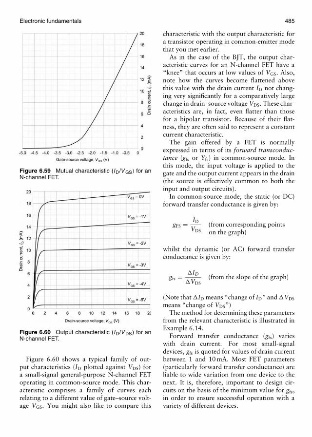
Electronic fundamentals 485
Figure 6.59 Mutual characteristic (ID/V GS) for anN-channel FET.
Figure 6.60 Output characteristic (ID/V DS) for anN-channel FET.
Figure 6.60 shows a typical family of out-put characteristics (ID plotted against VDS) fora small-signal general-purpose N-channel FEToperating in common-source mode. This char-acteristic comprises a family of curves eachrelating to a different value of gate–source volt-age VGS. You might also like to compare this
characteristic with the output characteristic fora transistor operating in common-emitter modethat you met earlier.
As in the case of the BJT, the output char-acteristic curves for an N-channel FET have a“knee” that occurs at low values of VGS. Also,note how the curves become flattened abovethis value with the drain current ID not chang-ing very significantly for a comparatively largechange in drain–source voltage VDS. These char-acteristics are, in fact, even flatter than thosefor a bipolar transistor. Because of their flat-ness, they are often said to represent a constantcurrent characteristic.
The gain offered by a FET is normallyexpressed in terms of its forward transconduc-tance (gfs or Yfs) in common-source mode. Inthis mode, the input voltage is applied to thegate and the output current appears in the drain(the source is effectively common to both theinput and output circuits).
In common-source mode, the static (or DC)forward transfer conductance is given by:
gFS = ID
VDS(from corresponding pointson the graph)
whilst the dynamic (or AC) forward transferconductance is given by:
gfs = �ID
�VDS(from the slope of the graph)
(Note that �ID means “change of ID” and �VDS
means “change of VDS”)The method for determining these parameters
from the relevant characteristic is illustrated inExample 6.14.
Forward transfer conductance (gfs) varieswith drain current. For most small-signaldevices, gfs is quoted for values of drain currentbetween 1 and 10 mA. Most FET parameters(particularly forward transfer conductance) areliable to wide variation from one device to thenext. It is, therefore, important to design cir-cuits on the basis of the minimum value for gfs,in order to ensure successful operation with avariety of different devices.
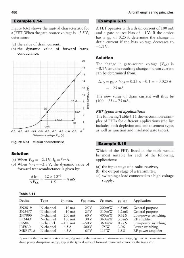
486 Aircraft engineering principles
Example 6.14
Figure 6.61 shows the mutual characteristic fora JFET. When the gate–source voltage is −2.5 V,determine:
(a) the value of drain current,(b) the dynamic value of forward trans-
conductance.
Figure 6.61 Mutual characteristic.
Solution
(a) When VGS = −2.5 V, ID = 5 mA.(b) When VGS = −2.5 V, the dynamic value of
forward transconductance is given by:
�ID
�VGS= 12 × 10−3
1.5= 8 mS
Table 6.11
Device Type ID max. VDS max. PD max. gfs typ. Application
2N2819 N-channel 10 mA 25 V 200 mW 4.5 mS General purpose2N5457 N-channel 10 mA 25 V 310 mW 1.2 mS General purpose2N7000 N-channel 200 mA 60 V 400 mW 0.32 S Low-power switchingBF244A N-channel 100 mA 30 V 360 mW 3.3 mS RF amplifierBSS84 P-channel −130 mA −50 V 360 mW 0.27 S Low-power switchingIRF830 N-channel 4.5 A 500 V 75 W 3.0 S Power switchingMRF171A N-channel 4.5 A 65 V 115 W 1.8 S RF power amplifier
ID max. is the maximum drain current, VDS max. is the maximum drain–source voltage, PD max. is the maximumdrain power dissipation and gfs typ. is the typical value of forward transconductance for the transistor.
Example 6.15
A FET operates with a drain current of 100 mAand a gate–source bias of −1 V. If the devicehas a gfs of 0.25 S, determine the change indrain current if the bias voltage decreases to−1.1 V.
Solution
The change in gate–source voltage (VGS) is−0.1 V and the resulting change in drain currentcan be determined from:
�ID = gfs × VGS = 0.25 × −0.1 = −0.025 A
= −25 mA
The new value of drain current will thus be(100 − 25) = 75 mA.
FET types and applicationsThe following Table 6.11 shows common exam-ples of FETs for different applications (the listincludes both depletion and enhancement typesas well as junction and insulated gate types).
Example 6.16
Which of the FETs listed in the table wouldbe most suitable for each of the followingapplications:
(a) the input stage of a radio receiver,(b) the output stage of a transmitter,(c) switching a load connected to a high-voltage
supply.
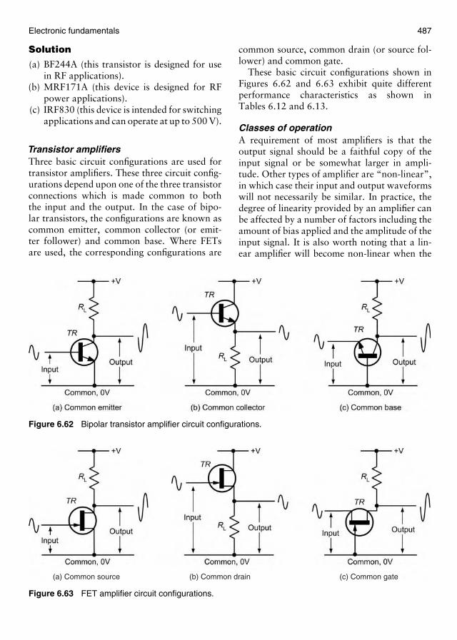
Electronic fundamentals 487
Solution
(a) BF244A (this transistor is designed for usein RF applications).
(b) MRF171A (this device is designed for RFpower applications).
(c) IRF830 (this device is intended for switchingapplications and can operate at up to 500 V).
Transistor amplifiersThree basic circuit configurations are used fortransistor amplifiers. These three circuit config-urations depend upon one of the three transistorconnections which is made common to boththe input and the output. In the case of bipo-lar transistors, the configurations are known ascommon emitter, common collector (or emit-ter follower) and common base. Where FETsare used, the corresponding configurations are
Figure 6.62 Bipolar transistor amplifier circuit configurations.
(a) Common source (b) Common drain (c) Common gate
Figure 6.63 FET amplifier circuit configurations.
common source, common drain (or source fol-lower) and common gate.
These basic circuit configurations shown inFigures 6.62 and 6.63 exhibit quite differentperformance characteristics as shown inTables 6.12 and 6.13.
Classes of operationA requirement of most amplifiers is that theoutput signal should be a faithful copy of theinput signal or be somewhat larger in ampli-tude. Other types of amplifier are “non-linear”,in which case their input and output waveformswill not necessarily be similar. In practice, thedegree of linearity provided by an amplifier canbe affected by a number of factors including theamount of bias applied and the amplitude of theinput signal. It is also worth noting that a lin-ear amplifier will become non-linear when the
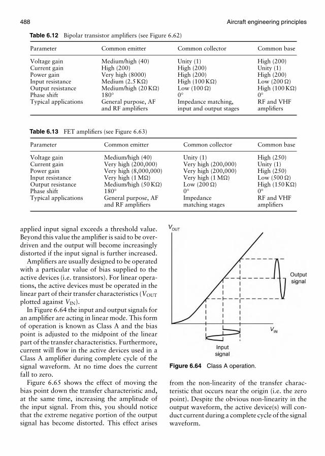
488 Aircraft engineering principles
Table 6.12 Bipolar transistor amplifiers (see Figure 6.62)
Parameter Common emitter Common collector Common base
Voltage gain Medium/high (40) Unity (1) High (200)Current gain High (200) High (200) Unity (1)Power gain Very high (8000) High (200) High (200)Input resistance Medium (2.5 K�) High (100 K�) Low (200 �)Output resistance Medium/high (20 K�) Low (100 �) High (100 K�)Phase shift 180◦ 0◦ 0◦Typical applications General purpose, AF Impedance matching, RF and VHF
and RF amplifiers input and output stages amplifiers
Table 6.13 FET amplifiers (see Figure 6.63)
Parameter Common emitter Common collector Common base
Voltage gain Medium/high (40) Unity (1) High (250)Current gain Very high (200,000) Very high (200,000) Unity (1)Power gain Very high (8,000,000) Very high (200,000) High (250)Input resistance Very high (1 M�) Very high (1 M�) Low (500 �)Output resistance Medium/high (50 K�) Low (200 �) High (150 K�)Phase shift 180◦ 0◦ 0◦Typical applications General purpose, AF Impedance RF and VHF
and RF amplifiers matching stages amplifiers
applied input signal exceeds a threshold value.Beyond this value the amplifier is said to be over-driven and the output will become increasinglydistorted if the input signal is further increased.
Amplifiers are usually designed to be operatedwith a particular value of bias supplied to theactive devices (i.e. transistors). For linear opera-tions, the active devices must be operated in thelinear part of their transfer characteristics (VOUT
plotted against VIN).In Figure 6.64 the input and output signals for
an amplifier are acting in linear mode. This formof operation is known as Class A and the biaspoint is adjusted to the midpoint of the linearpart of the transfer characteristics. Furthermore,current will flow in the active devices used in aClass A amplifier during complete cycle of thesignal waveform. At no time does the currentfall to zero.
Figure 6.65 shows the effect of moving thebias point down the transfer characteristic and,at the same time, increasing the amplitude ofthe input signal. From this, you should noticethat the extreme negative portion of the outputsignal has become distorted. This effect arises
Figure 6.64 Class A operation.
from the non-linearity of the transfer charac-teristic that occurs near the origin (i.e. the zeropoint). Despite the obvious non-linearity in theoutput waveform, the active device(s) will con-duct current during a complete cycle of the signalwaveform.

Electronic fundamentals 489
Figure 6.65 Reducing the bias point.
Figure 6.66 Class AB operation.
Now consider the case of reducing the biaseven further, while further increasing the ampli-tude of the input signal (see Figure 6.66). Herethe bias point has been set as the projected cut-off point. The negative-going portion of theoutput signal becomes cut-off (or clipped) andthe active device(s) will cease to conduct forthis part of the cycle. This mode of operationis known as Class AB.
Now let us consider what will happen ifno bias at all is applied to the amplifier (see
Figure 6.67 Class B operation.
VOUT
VIN
Outputsignal
Inputsignal
Figure 6.68 Class C operation.
Figure 6.67). The output signal will comprisea series of positive-going half-cycles and theactive devices will be conducting only duringhalf-cycles of the waveform (i.e. they will onlybe operating 50% of the time). This mode ofoperation is known as Class B and is commonlyused in push–pull power amplifiers where thetwo active devices in the output stage operateon alternate half-cycles of the waveform.
Finally, there is one more class of operationto consider. The input and output waveformsfor Class C operation are shown in Figure 6.68.Here the bias point is set at beyond the cut-off (zero) point and a very large input signalis applied. The output waveform will thencomprise a series of quite sharp positive-goingpulses. These pulses of current or voltage can be
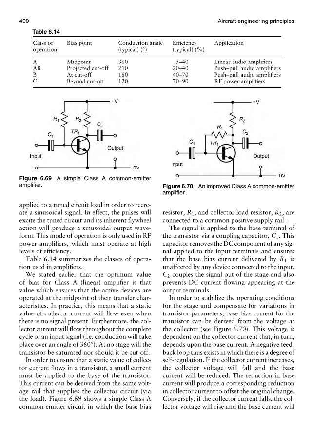
490 Aircraft engineering principles
Table 6.14
Class of Bias point Conduction angle Efficiency Applicationoperation (typical) (◦) (typical) (%)
A Midpoint 360 5–40 Linear audio amplifiersAB Projected cut-off 210 20–40 Push–pull audio amplifiersB At cut-off 180 40–70 Push–pull audio amplifiersC Beyond cut-off 120 70–90 RF power amplifiers
Figure 6.69 A simple Class A common-emitteramplifier.
applied to a tuned circuit load in order to recre-ate a sinusoidal signal. In effect, the pulses willexcite the tuned circuit and its inherent flywheelaction will produce a sinusoidal output wave-form. This mode of operation is only used in RFpower amplifiers, which must operate at highlevels of efficiency.
Table 6.14 summarizes the classes of opera-tion used in amplifiers.
We stated earlier that the optimum valueof bias for Class A (linear) amplifier is thatvalue which ensures that the active devices areoperated at the midpoint of their transfer char-acteristics. In practice, this means that a staticvalue of collector current will flow even whenthere is no signal present. Furthermore, the col-lector current will flow throughout the completecycle of an input signal (i.e. conduction will takeplace over an angle of 360◦). At no stage will thetransistor be saturated nor should it be cut-off.
In order to ensure that a static value of collec-tor current flows in a transistor, a small currentmust be applied to the base of the transistor.This current can be derived from the same volt-age rail that supplies the collector circuit (viathe load). Figure 6.69 shows a simple Class Acommon-emitter circuit in which the base bias
Figure 6.70 An improved Class A common-emitteramplifier.
resistor, R1, and collector load resistor, R2, areconnected to a common positive supply rail.
The signal is applied to the base terminal ofthe transistor via a coupling capacitor, C1. Thiscapacitor removes the DC component of any sig-nal applied to the input terminals and ensuresthat the base bias current delivered by R1 isunaffected by any device connected to the input.C2 couples the signal out of the stage and alsoprevents DC current flowing appearing at theoutput terminals.
In order to stabilize the operating conditionsfor the stage and compensate for variations intransistor parameters, base bias current for thetransistor can be derived from the voltage atthe collector (see Figure 6.70). This voltage isdependent on the collector current that, in turn,depends upon the base current. A negative feed-back loop thus exists in which there is a degree ofself-regulation. If the collector current increases,the collector voltage will fall and the basecurrent will be reduced. The reduction in basecurrent will produce a corresponding reductionin collector current to offset the original change.Conversely, if the collector current falls, the col-lector voltage will rise and the base current will
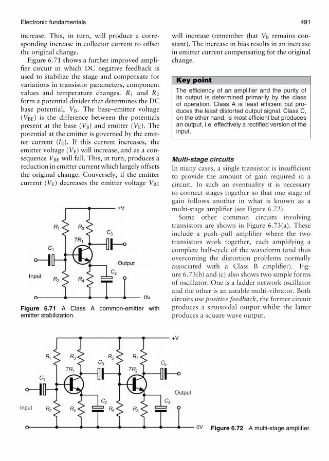
Electronic fundamentals 491
increase. This, in turn, will produce a corre-sponding increase in collector current to offsetthe original change.
Figure 6.71 shows a further improved ampli-fier circuit in which DC negative feedback isused to stabilize the stage and compensate forvariations in transistor parameters, componentvalues and temperature changes. R1 and R2
form a potential divider that determines the DCbase potential, VB. The base–emitter voltage(VBE) is the difference between the potentialspresent at the base (VB) and emitter (VE). Thepotential at the emitter is governed by the emit-ter current (IE). If this current increases, theemitter voltage (VE) will increase, and as a con-sequence VBE will fall. This, in turn, produces areduction in emitter current which largely offsetsthe original change. Conversely, if the emittercurrent (VE) decreases the emitter voltage VBE
Figure 6.71 A Class A common-emitter withemitter stabilization.
R1
TR1 TR2
R2 R4 R6 R8
R3C3
C1
C2 C4
C5
R5 R7
+V
0V
Output
Input
Figure 6.72 A multi-stage amplifier.
will increase (remember that VB remains con-stant). The increase in bias results in an increasein emitter current compensating for the originalchange.
Key pointThe efficiency of an amplifier and the purity ofits output is determined primarily by the classof operation. Class A is least efficient but pro-duces the least distorted output signal. Class C,on the other hand, is most efficient but producesan output, i.e. effectively a rectified version of theinput.
Multi-stage circuitsIn many cases, a single transistor is insufficientto provide the amount of gain required in acircuit. In such an eventuality it is necessaryto connect stages together so that one stage ofgain follows another in what is known as amulti-stage amplifier (see Figure 6.72).
Some other common circuits involvingtransistors are shown in Figure 6.73(a). Theseinclude a push–pull amplifier where the twotransistors work together, each amplifying acomplete half-cycle of the waveform (and thusovercoming the distortion problems normallyassociated with a Class B amplifier). Fig-ure 6.73(b) and (c) also shows two simple formsof oscillator. One is a ladder network oscillatorand the other is an astable multi-vibrator. Bothcircuits use positive feedback, the former circuitproduces a sinusoidal output whilst the latterproduces a square wave output.
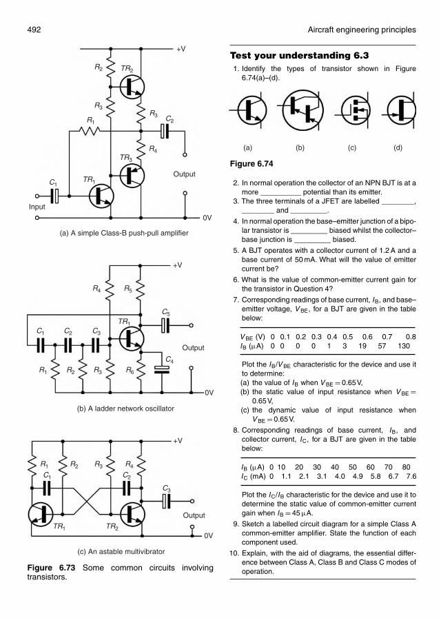
492 Aircraft engineering principles
TR1 TR2
C1 C2
C3
R4R3R2R1
+V
0V
Output
(c) An astable multivibrator
TR1
R4
C3
C4
C1 C2
C5
R5
R6R3R2R1
+V
0V
Output
(b) A ladder network oscillator
R1
TR1
TR3
TR2R2
R4
R3R3
C1
C2
+V
0V
Output
Input
(a) A simple Class-B push-pull amplifier
Figure 6.73 Some common circuits involvingtransistors.
Test your understanding 6.31. Identify the types of transistor shown in Figure
6.74(a)–(d).
(a) (b) (c) (d)
Figure 6.74
2. In normal operation the collector of an NPN BJT is at amore __________ potential than its emitter.
3. The three terminals of a JFET are labelled ________,________ and _________.
4. In normal operation the base–emitter junction of a bipo-lar transistor is _________ biased whilst the collector–base junction is _________ biased.
5. A BJT operates with a collector current of 1.2 A and abase current of 50 mA. What will the value of emittercurrent be?
6. What is the value of common-emitter current gain forthe transistor in Question 4?
7. Corresponding readings of base current, IB, and base–emitter voltage, V BE, for a BJT are given in the tablebelow:
V BE (V) 0 0.1 0.2 0.3 0.4 0.5 0.6 0.7 0.8IB (µA) 0 0 0 0 1 3 19 57 130
Plot the IB/V BE characteristic for the device and use itto determine:(a) the value of IB when V BE = 0.65V,(b) the static value of input resistance when V BE =
0.65V,(c) the dynamic value of input resistance when
V BE = 0.65V.
8. Corresponding readings of base current, IB, andcollector current, IC, for a BJT are given in the tablebelow:
IB (µA) 0 10 20 30 40 50 60 70 80IC (mA) 0 1.1 2.1 3.1 4.0 4.9 5.8 6.7 7.6
Plot the IC/IB characteristic for the device and use it todetermine the static value of common-emitter currentgain when IB = 45 µA.
9. Sketch a labelled circuit diagram for a simple Class Acommon-emitter amplifier. State the function of eachcomponent used.
10. Explain, with the aid of diagrams, the essential differ-ence between Class A, Class B and Class C modes ofoperation.
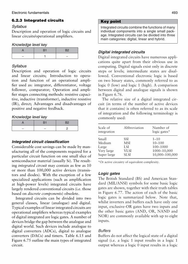
Electronic fundamentals 493
6.2.3 Integrated circuits
SyllabusDescription and operation of logic circuits andlinear circuits/operational amplifiers.
Knowledge level key
–
A
1
B1
–
B2
SyllabusDescription and operation of logic circuitsand linear circuits; Introduction to opera-tion and function of an operational ampli-fier used as: integrator, differentiator, voltagefollower, comparator; Operation and ampli-fier stages connecting methods: resistive capaci-tive, inductive (transformer), inductive resistive(IR), direct; Advantages and disadvantages ofpositive and negative feedback.
Knowledge level key
–
A
–
B1
2
B2
Integrated circuit classificationConsiderable cost savings can be made by man-ufacturing all of the components required for aparticular circuit function on one small slice ofsemiconductor material (usually Si). The result-ing integrated circuit may contain as few as 10or more than 100,000 active devices (transis-tors and diodes). With the exception of a fewspecialized applications (such as amplificationat high-power levels) integrated circuits havelargely rendered conventional circuits (i.e. thosebased on discrete components) obsolete.
Integrated circuits can be divided into twogeneral classes, linear (analogue) and digital.Typical examples of linear integrated circuits areoperational amplifiers whereas typical examplesof digital integrated are logic gates. A number ofdevices bridge the gap between the analogue anddigital world. Such devices include analogue todigital converters (ADCs), digital to analogueconverters (DACs) and timers. Table 6.15 andFigure 6.75 outline the main types of integratedcircuit.
Key pointIntegrated circuits combine the functions of manyindividual components into a single small pack-age. Integrated circuits can be divided into threemain categories: digital, linear and hybrid.
Digital integrated circuitsDigital integrated circuits have numerous appli-cations quite apart from their obvious use incomputing. Digital signals exist only in discretesteps or levels; intermediate states are disal-lowed. Conventional electronic logic is basedon two binary states, commonly referred to aslogic 0 (low) and logic 1 (high). A comparisonbetween digital and analogue signals is shownin Figure 6.76.
The relative size of a digital integrated cir-cuit (in terms of the number of active devicesthat it contains) is often referred to as its scaleof integration and the following terminology iscommonly used:
Scale of Abbreviation Number ofintegration logic gates*
Small SSI 1–10Medium MSI 10–100Large LSI 100–1000Very large VLSI 1000–10,000Super large SLSI 10,000–100,000
*Or active circuitry of equivalent complexity.
Logic gatesThe British Standard (BS) and American Stan-dard (MIL/ANSI) symbols for some basic logicgates are shown, together with their truth tablesin Figure 6.77. The action of each of the basiclogic gates is summarized below. Note that,whilst inverters and buffers each have only oneinput, exclusive-OR gates have two inputs andthe other basic gates (AND, OR, NAND andNOR) are commonly available with up to eightinputs.
BuffersBuffers do not affect the logical state of a digitalsignal (i.e. a logic 1 input results in a logic 1output whereas a logic 0 input results in a logic
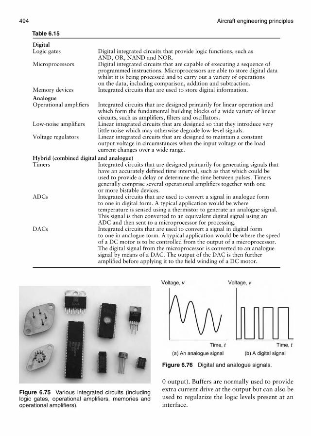
494 Aircraft engineering principles
Table 6.15
DigitalLogic gates Digital integrated circuits that provide logic functions, such as
AND, OR, NAND and NOR.Microprocessors Digital integrated circuits that are capable of executing a sequence of
programmed instructions. Microprocessors are able to store digital datawhilst it is being processed and to carry out a variety of operationson the data, including comparison, addition and subtraction.
Memory devices Integrated circuits that are used to store digital information.AnalogueOperational amplifiers Integrated circuits that are designed primarily for linear operation and
which form the fundamental building blocks of a wide variety of linearcircuits, such as amplifiers, filters and oscillators.
Low-noise amplifiers Linear integrated circuits that are designed so that they introduce verylittle noise which may otherwise degrade low-level signals.
Voltage regulators Linear integrated circuits that are designed to maintain a constantoutput voltage in circumstances when the input voltage or the loadcurrent changes over a wide range.
Hybrid (combined digital and analogue)Timers Integrated circuits that are designed primarily for generating signals that
have an accurately defined time interval, such as that which could beused to provide a delay or determine the time between pulses. Timersgenerally comprise several operational amplifiers together with oneor more bistable devices.
ADCs Integrated circuits that are used to convert a signal in analogue formto one in digital form. A typical application would be wheretemperature is sensed using a thermistor to generate an analogue signal.This signal is then converted to an equivalent digital signal using anADC and then sent to a microprocessor for processing.
DACs Integrated circuits that are used to convert a signal in digital formto one in analogue form. A typical application would be where the speedof a DC motor is to be controlled from the output of a microprocessor.The digital signal from the microprocessor is converted to an analoguesignal by means of a DAC. The output of the DAC is then furtheramplified before applying it to the field winding of a DC motor.
Figure 6.75 Various integrated circuits (includinglogic gates, operational amplifiers, memories andoperational amplifiers).
Figure 6.76 Digital and analogue signals.
0 output). Buffers are normally used to provideextra current drive at the output but can also beused to regularize the logic levels present at aninterface.
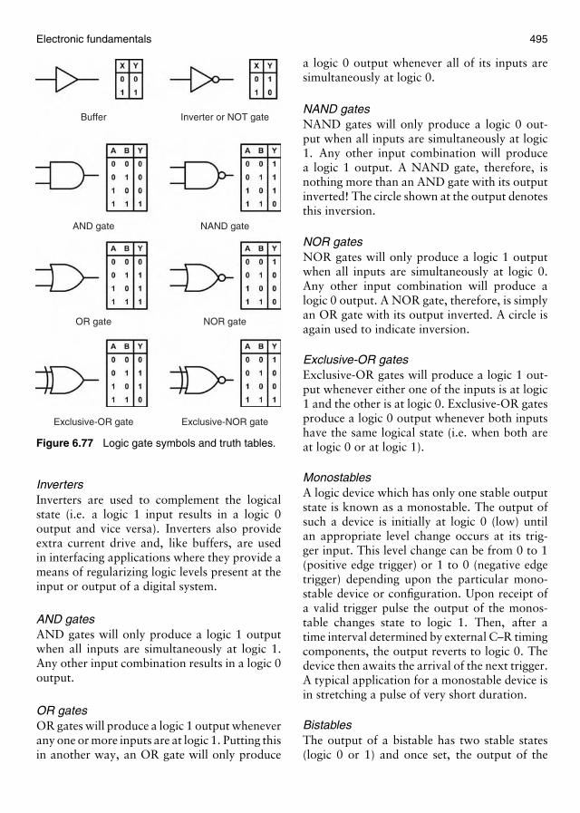
Electronic fundamentals 495
Buffer
AND gate NAND gate
Inverter or NOT gate
OR gate NOR gate
Exclusive-OR gate Exclusive-NOR gate
Figure 6.77 Logic gate symbols and truth tables.
InvertersInverters are used to complement the logicalstate (i.e. a logic 1 input results in a logic 0output and vice versa). Inverters also provideextra current drive and, like buffers, are usedin interfacing applications where they provide ameans of regularizing logic levels present at theinput or output of a digital system.
AND gatesAND gates will only produce a logic 1 outputwhen all inputs are simultaneously at logic 1.Any other input combination results in a logic 0output.
OR gatesOR gates will produce a logic 1 output wheneverany one or more inputs are at logic 1. Putting thisin another way, an OR gate will only produce
a logic 0 output whenever all of its inputs aresimultaneously at logic 0.
NAND gatesNAND gates will only produce a logic 0 out-put when all inputs are simultaneously at logic1. Any other input combination will producea logic 1 output. A NAND gate, therefore, isnothing more than an AND gate with its outputinverted! The circle shown at the output denotesthis inversion.
NOR gatesNOR gates will only produce a logic 1 outputwhen all inputs are simultaneously at logic 0.Any other input combination will produce alogic 0 output. A NOR gate, therefore, is simplyan OR gate with its output inverted. A circle isagain used to indicate inversion.
Exclusive-OR gatesExclusive-OR gates will produce a logic 1 out-put whenever either one of the inputs is at logic1 and the other is at logic 0. Exclusive-OR gatesproduce a logic 0 output whenever both inputshave the same logical state (i.e. when both areat logic 0 or at logic 1).
MonostablesA logic device which has only one stable outputstate is known as a monostable. The output ofsuch a device is initially at logic 0 (low) untilan appropriate level change occurs at its trig-ger input. This level change can be from 0 to 1(positive edge trigger) or 1 to 0 (negative edgetrigger) depending upon the particular mono-stable device or configuration. Upon receipt ofa valid trigger pulse the output of the monos-table changes state to logic 1. Then, after atime interval determined by external C–R timingcomponents, the output reverts to logic 0. Thedevice then awaits the arrival of the next trigger.A typical application for a monostable device isin stretching a pulse of very short duration.
BistablesThe output of a bistable has two stable states(logic 0 or 1) and once set, the output of the
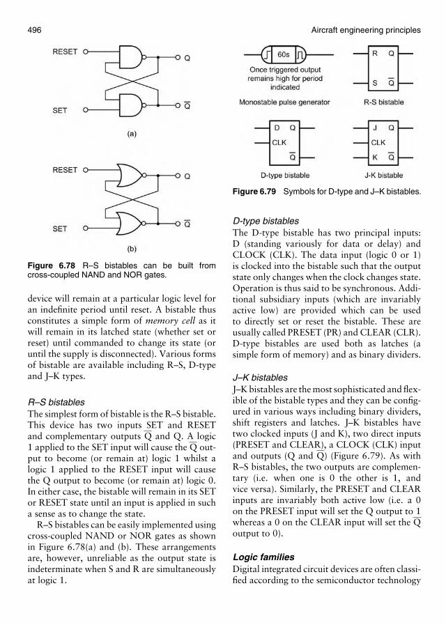
496 Aircraft engineering principles
Figure 6.78 R–S bistables can be built fromcross-coupled NAND and NOR gates.
device will remain at a particular logic level foran indefinite period until reset. A bistable thusconstitutes a simple form of memory cell as itwill remain in its latched state (whether set orreset) until commanded to change its state (oruntil the supply is disconnected). Various formsof bistable are available including R–S, D-typeand J–K types.
R–S bistablesThe simplest form of bistable is the R–S bistable.This device has two inputs SET and RESETand complementary outputs Q and Q. A logic1 applied to the SET input will cause the Q out-put to become (or remain at) logic 1 whilst alogic 1 applied to the RESET input will causethe Q output to become (or remain at) logic 0.In either case, the bistable will remain in its SETor RESET state until an input is applied in sucha sense as to change the state.
R–S bistables can be easily implemented usingcross-coupled NAND or NOR gates as shownin Figure 6.78(a) and (b). These arrangementsare, however, unreliable as the output state isindeterminate when S and R are simultaneouslyat logic 1.
Figure 6.79 Symbols for D-type and J–K bistables.
D-type bistablesThe D-type bistable has two principal inputs:D (standing variously for data or delay) andCLOCK (CLK). The data input (logic 0 or 1)is clocked into the bistable such that the outputstate only changes when the clock changes state.Operation is thus said to be synchronous. Addi-tional subsidiary inputs (which are invariablyactive low) are provided which can be usedto directly set or reset the bistable. These areusually called PRESET (PR) and CLEAR (CLR).D-type bistables are used both as latches (asimple form of memory) and as binary dividers.
J–K bistablesJ–K bistables are the most sophisticated and flex-ible of the bistable types and they can be config-ured in various ways including binary dividers,shift registers and latches. J–K bistables havetwo clocked inputs (J and K), two direct inputs(PRESET and CLEAR), a CLOCK (CLK) inputand outputs (Q and Q) (Figure 6.79). As withR–S bistables, the two outputs are complemen-tary (i.e. when one is 0 the other is 1, andvice versa). Similarly, the PRESET and CLEARinputs are invariably both active low (i.e. a 0on the PRESET input will set the Q output to 1whereas a 0 on the CLEAR input will set the Qoutput to 0).
Logic familiesDigital integrated circuit devices are often classi-fied according to the semiconductor technology
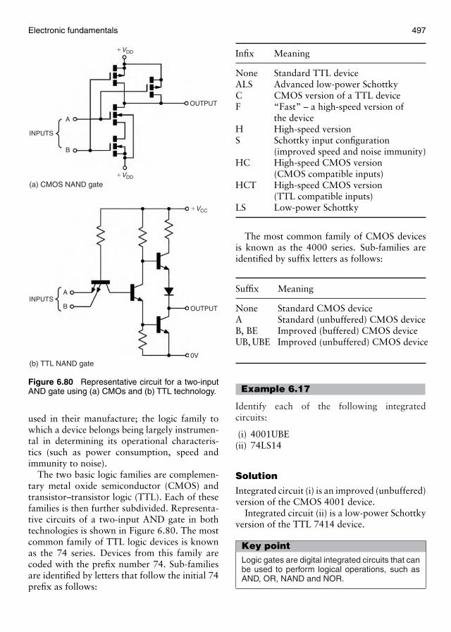
Electronic fundamentals 497
�VCC
OUTPUT
0V
INPUTSA
B
(a) CMOS NAND gate
(b) TTL NAND gate
�VDD
�VDD
OUTPUT
INPUTS
A
B
Figure 6.80 Representative circuit for a two-inputAND gate using (a) CMOs and (b) TTL technology.
used in their manufacture; the logic family towhich a device belongs being largely instrumen-tal in determining its operational characteris-tics (such as power consumption, speed andimmunity to noise).
The two basic logic families are complemen-tary metal oxide semiconductor (CMOS) andtransistor–transistor logic (TTL). Each of thesefamilies is then further subdivided. Representa-tive circuits of a two-input AND gate in bothtechnologies is shown in Figure 6.80. The mostcommon family of TTL logic devices is knownas the 74 series. Devices from this family arecoded with the prefix number 74. Sub-familiesare identified by letters that follow the initial 74prefix as follows:
Infix Meaning
None Standard TTL deviceALS Advanced low-power SchottkyC CMOS version of a TTL deviceF “Fast” – a high-speed version of
the deviceH High-speed versionS Schottky input configuration
(improved speed and noise immunity)HC High-speed CMOS version
(CMOS compatible inputs)HCT High-speed CMOS version
(TTL compatible inputs)LS Low-power Schottky
The most common family of CMOS devicesis known as the 4000 series. Sub-families areidentified by suffix letters as follows:
Suffix Meaning
None Standard CMOS deviceA Standard (unbuffered) CMOS deviceB, BE Improved (buffered) CMOS deviceUB, UBE Improved (unbuffered) CMOS device
Example 6.17
Identify each of the following integratedcircuits:
(i) 4001UBE(ii) 74LS14
Solution
Integrated circuit (i) is an improved (unbuffered)version of the CMOS 4001 device.
Integrated circuit (ii) is a low-power Schottkyversion of the TTL 7414 device.
Key pointLogic gates are digital integrated circuits that canbe used to perform logical operations, such asAND, OR, NAND and NOR.

498 Aircraft engineering principles
Key pointThe two main logic families are TTL and CMOS.Each of these families can be further subdividedinto a number of sub-families according to thetechnology used in their manufacture.
Logic circuit characteristicsLogic levels are simply the range of voltagesused to represent the logic states 0 and 1. Thelogic levels for CMOS differ markedly fromthose associated with TTL. In particular, CMOSlogic levels are relative to the supply voltageused whilst the logic levels associated with TTLdevices tend to be absolute. The following tableusually applies:
CMOS TTL
Logic 1 > 23 VDD >2 V
Logic 0 < 13 VDD <0.8 V
Indeterminate between 13 VDD between
and 23 VDD 0.8 and 2 V
Note: VDD is the positive supply associated withCMOS devices.
The noise margin is an important feature ofany logic device. Noise margin is a measureof the ability of the device to reject noise; thelarger the noise margin, the better is its abilityto perform in an environment in which noise is
Figure 6.81 Comparison of logic levels for 7400-series TTL and 4000-series CMOS devices.
present. Noise margin is defined as the differencebetween the minimum values of high-state out-put and high-state input voltage and the max-imum values of low-state output and low-stateinput voltage. Hence:
noise margin = VOH(MIN) − VIH(MIN)
or noise margin = VOL(MAX) − VIL(MAX)
where VOH(MIN) is the minimum value of high-state (logic 1) output voltage, VIH(MIN) is theminimum value of high-state (logic 1) inputvoltage, VOL(MAX) is the maximum value of low-state (logic 0) output voltage and VIL(MIN) is theminimum value of low-state (logic 0) input volt-age. The noise margin for standard 7400-seriesTTL is typically 400 mV whilst that for CMOSis 1
3 VDD as shown in Figure 6.81.The following Table 6.16 compares the more
important characteristics of various members ofthe TTL family with buffered CMOS logic.
Operational amplifiersOperational amplifiers are analogue integratedcircuits designed for linear amplification thatoffer near-ideal characteristics (virtually infinitevoltage gain and input resistance coupled withlow-output resistance and wide bandwidth).
Operational amplifiers can be thought of asuniversal “gain blocks” to which external com-ponents are added in order to define their func-tion within a circuit. By adding two resistors,
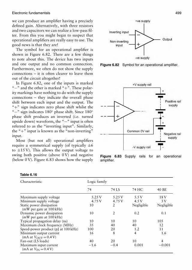
Electronic fundamentals 499
we can produce an amplifier having a preciselydefined gain. Alternatively, with three resistorsand two capacitors we can realize a low-pass fil-ter. From this you might begin to suspect thatoperational amplifiers are really easy to use. Thegood news is that they are!
The symbol for an operational amplifier isshown in Figure 6.82. There are a few thingsto note about this. The device has two inputsand one output and no common connection.Furthermore, we often do not show the supplyconnections – it is often clearer to leave themout of the circuit altogether!
In Figure 6.82, one of the inputs is marked“−” and the other is marked “+”. These polar-ity markings have nothing to do with the supplyconnections – they indicate the overall phaseshift between each input and the output. The“+” sign indicates zero phase shift whilst the“−” sign indicates 180◦ phase shift. Since 180◦phase shift produces an inverted (i.e. turnedupside down) waveform, the “−” input is oftenreferred to as the “inverting input”. Similarly,the “+” input is known as the “non-inverting”input.
Most (but not all) operational amplifiersrequire a symmetrical supply (of typically ±6to ±15 V). This allows the output voltage toswing both positive (above 0 V) and negative(below 0 V). Figure 6.83 shows how the supply
Table 6.16
Characteristic Logic family
74 74 LS 74 HC 40 BE
Maximum supply voltage 5.25 V 5.25 V 5.5 V 18 VMinimum supply voltage 4.75 V 4.75 V 4.5 V 3 VStatic power dissipation 10 2 Negligible Negligible(mW per gate at 100 kHz)
Dynamic power dissipation 10 2 0.2 0.1(mW per gate at 100 kHz)
Typical propagation delay (ns) 10 10 10 105Maximum clock frequency (MHz) 35 40 40 12Speed-power product (pJ at 100 kHz) 100 20 1.2 11Minimum output current 16 8 4 1.6(mA at VOUT = 0.4 V)
Fan-out (LS loads) 40 20 10 4Maximum input current −1.6 −0.4 0.001 −0.001(mA at VIN = 0.4 V)
Figure 6.82 Symbol for an operational amplifier.
Figure 6.83 Supply rails for an operationalamplifier.
500 Aircraft engineering principles
connections would appear if we decided toinclude them. Note that we usually have twoseparate supplies: a positive supply and anequal, but opposite, negative supply. The com-mon connection to these two supplies (i.e. the0 V rail) acts as the common rail in our cir-cuit. The input and output voltages are usuallymeasured relative to this rail.
Key pointOperational amplifiers are linear integrated cir-cuits that can be used as versatile “gain blocks”within a wide variety of linear circuits.
Operational amplifier parametersBefore we take a look at some of the characteris-tics of “ideal” and “real” operational amplifiers,it is important to define some of the terms andparameters that we apply to these devices.
Open-loop voltage gainThe open-loop voltage gain of an operationalamplifier is defined as the ratio of output volt-age to input voltage measured with no feedbackapplied. In practice, this value is exceptionallyhigh (typically >100,000) but is liable to con-siderable variation from one device to another.
Open-loop voltage gain may thus be thoughtof as the “internal” voltage gain of the device:
AVOL = VOUT
VIN
where AVOL is the open-loop voltage gain, VOUT
and VIN are the output and input voltages,respectively, under open-loop conditions.
In linear voltage amplifying applications, alarge amount of negative feedback will normallybe applied and the open-loop voltage gain can bethought of as the internal voltage gain providedby the device.
The open-loop voltage gain is often expressedin decibels (dB) rather than as a ratio. In thiscase:
AVOL = 20 log10VOUT
VIN
Most operational amplifiers have open-loopvoltage gains of 90 dB, or more.
Closed-loop voltage gainThe closed-loop voltage gain of an operationalamplifier is defined as the ratio of output voltageto input voltage measured with a small propor-tion of the output fed back to the input (i.e. withfeedback applied). The effect of providing neg-ative feedback is to reduce the loop voltage gainto a value that is both predictable and manage-able. Practical closed-loop voltage gains rangefrom 1 to several thousand but note that highvalues of voltage gain may make unacceptablerestrictions on bandwidth, seen later.
Closed-loop voltage gain is the ratio of outputvoltage to input voltage when negative feedbackis applied, hence:
AVCL = VOUT
VIN
where AVCL is the closed-loop voltage gain,VOUT and VIN are the output and input voltages,respectively, under closed-loop conditions. Theclosed-loop voltage gain is normally very muchless than the open-loop voltage gain.
Example 6.18
An operational amplifier operating with neg-ative feedback produces an output voltage of2 V when supplied with an input of 400 µV.Determine the value of closed-loop voltage gain.
Solution
Now:
AVCL = VOUT
VIN
thus:
AVCL = 2400 × 10−6
= 2 × 10⁶
400= 5000
Input resistanceThe input resistance of an operational amplifieris defined as the ratio of input voltage to inputcurrent expressed in ohms. It is often expedi-ent to assume that the input of an operational
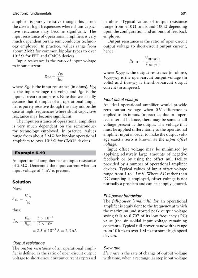
Electronic fundamentals 501
amplifier is purely resistive though this is notthe case at high frequencies where shunt capac-itive reactance may become significant. Theinput resistance of operational amplifiers is verymuch dependent on the semiconductor technol-ogy employed. In practice, values range fromabout 2 M� for common bipolar types to over1012 � for FET and CMOS devices.
Input resistance is the ratio of input voltageto input current:
RIN = VIN
IIN
where RIN is the input resistance (in ohms), VIN
is the input voltage (in volts) and IIN is theinput current (in amperes). Note that we usuallyassume that the input of an operational ampli-fier is purely resistive though this may not be thecase at high frequencies where shunt capacitivereactance may become significant.
The input resistance of operational amplifiersis very much dependent on the semiconduc-tor technology employed. In practice, valuesrange from about 2 M� for bipolar operationalamplifiers to over 1012 � for CMOS devices.
Example 6.19
An operational amplifier has an input resistanceof 2 M�. Determine the input current when aninput voltage of 5 mV is present.
Solution
Now:
RIN = VIN
IIN
thus:
IIN = VIN
RIN= 5 × 10⁻³
2 × 106
= 2.5 × 10⁻⁹ A = 2.5 nA
Output resistanceThe output resistance of an operational ampli-fier is defined as the ratio of open-circuit outputvoltage to short-circuit output current expressed
in ohms. Typical values of output resistancerange from <10 � to around 100 � dependingupon the configuration and amount of feedbackemployed.
Output resistance is the ratio of open-circuitoutput voltage to short-circuit output current,hence:
ROUT = VOUT(OC)
IOUT(SC)
where ROUT is the output resistance (in ohms),VOUT(OC) is the open-circuit output voltage (involts) and IOUT(SC) is the short-circuit outputcurrent (in amperes).
Input offset voltageAn ideal operational amplifier would providezero output voltage when 0 V difference isapplied to its inputs. In practice, due to imper-fect internal balance, there may be some smallvoltage present at the output. The voltage thatmust be applied differentially to the operationalamplifier input in order to make the output volt-age exactly zero is known as the input offsetvoltage.
Input offset voltage may be minimized byapplying relatively large amounts of negativefeedback or by using the offset null facilityprovided by a number of operational amplifierdevices. Typical values of input offset voltagerange from 1 to 15 mV. Where AC rather thanDC coupling is employed, offset voltage is notnormally a problem and can be happily ignored.
Full-power bandwidthThe full-power bandwidth for an operationalamplifier is equivalent to the frequency at whichthe maximum undistorted peak output voltageswing falls to 0.707 of its low-frequency (DC)value (the sinusoidal input voltage remainingconstant). Typical full-power bandwidths rangefrom 10 kHz to over 1 MHz for some high-speeddevices.
Slew rateSlew rate is the rate of change of output voltagewith time, when a rectangular step input voltage
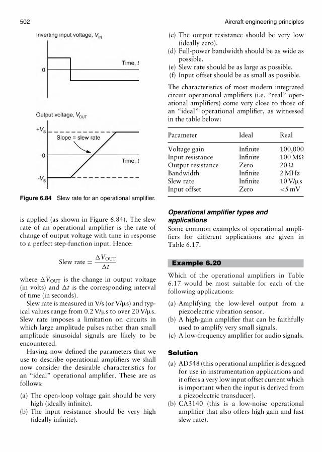
502 Aircraft engineering principles
Figure 6.84 Slew rate for an operational amplifier.
is applied (as shown in Figure 6.84). The slewrate of an operational amplifier is the rate ofchange of output voltage with time in responseto a perfect step-function input. Hence:
Slew rate = �VOUT
�t
where �VOUT is the change in output voltage(in volts) and �t is the corresponding intervalof time (in seconds).
Slew rate is measured in V/s (or V/µs) and typ-ical values range from 0.2 V/µs to over 20 V/µs.Slew rate imposes a limitation on circuits inwhich large amplitude pulses rather than smallamplitude sinusoidal signals are likely to beencountered.
Having now defined the parameters that weuse to describe operational amplifiers we shallnow consider the desirable characteristics foran “ideal” operational amplifier. These are asfollows:
(a) The open-loop voltage gain should be veryhigh (ideally infinite).
(b) The input resistance should be very high(ideally infinite).
(c) The output resistance should be very low(ideally zero).
(d) Full-power bandwidth should be as wide aspossible.
(e) Slew rate should be as large as possible.(f) Input offset should be as small as possible.
The characteristics of most modern integratedcircuit operational amplifiers (i.e. “real” oper-ational amplifiers) come very close to those ofan “ideal” operational amplifier, as witnessedin the table below:
Parameter Ideal Real
Voltage gain Infinite 100,000Input resistance Infinite 100 M�
Output resistance Zero 20 �
Bandwidth Infinite 2 MHzSlew rate Infinite 10 V/µsInput offset Zero <5 mV
Operational amplifier types andapplicationsSome common examples of operational ampli-fiers for different applications are given inTable 6.17.
Example 6.20
Which of the operational amplifiers in Table6.17 would be most suitable for each of thefollowing applications:
(a) Amplifying the low-level output from apiezoelectric vibration sensor.
(b) A high-gain amplifier that can be faithfullyused to amplify very small signals.
(c) A low-frequency amplifier for audio signals.
Solution
(a) AD548 (this operational amplifier is designedfor use in instrumentation applications andit offers a very low input offset current whichis important when the input is derived froma piezoelectric transducer).
(b) CA3140 (this is a low-noise operationalamplifier that also offers high gain and fastslew rate).
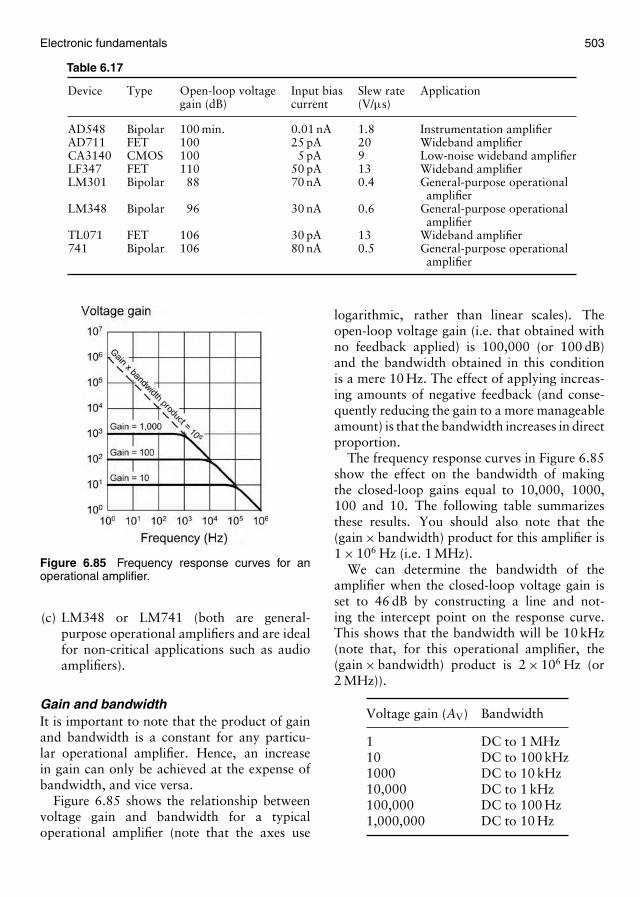
Electronic fundamentals 503
Table 6.17
Device Type Open-loop voltage Input bias Slew rate Applicationgain (dB) current (V/µs)
AD548 Bipolar 100 min. 0.01 nA 1.8 Instrumentation amplifierAD711 FET 100 25 pA 20 Wideband amplifierCA3140 CMOS 100 5 pA 9 Low-noise wideband amplifierLF347 FET 110 50 pA 13 Wideband amplifierLM301 Bipolar 88 70 nA 0.4 General-purpose operational
amplifierLM348 Bipolar 96 30 nA 0.6 General-purpose operational
amplifierTL071 FET 106 30 pA 13 Wideband amplifier741 Bipolar 106 80 nA 0.5 General-purpose operational
amplifier
Figure 6.85 Frequency response curves for anoperational amplifier.
(c) LM348 or LM741 (both are general-purpose operational amplifiers and are idealfor non-critical applications such as audioamplifiers).
Gain and bandwidthIt is important to note that the product of gainand bandwidth is a constant for any particu-lar operational amplifier. Hence, an increasein gain can only be achieved at the expense ofbandwidth, and vice versa.
Figure 6.85 shows the relationship betweenvoltage gain and bandwidth for a typicaloperational amplifier (note that the axes use
logarithmic, rather than linear scales). Theopen-loop voltage gain (i.e. that obtained withno feedback applied) is 100,000 (or 100 dB)and the bandwidth obtained in this conditionis a mere 10 Hz. The effect of applying increas-ing amounts of negative feedback (and conse-quently reducing the gain to a more manageableamount) is that the bandwidth increases in directproportion.
The frequency response curves in Figure 6.85show the effect on the bandwidth of makingthe closed-loop gains equal to 10,000, 1000,100 and 10. The following table summarizesthese results. You should also note that the(gain × bandwidth) product for this amplifier is1 × 106 Hz (i.e. 1 MHz).
We can determine the bandwidth of theamplifier when the closed-loop voltage gain isset to 46 dB by constructing a line and not-ing the intercept point on the response curve.This shows that the bandwidth will be 10 kHz(note that, for this operational amplifier, the(gain × bandwidth) product is 2 × 10⁶ Hz (or2 MHz)).
Voltage gain (AV) Bandwidth
1 DC to 1 MHz10 DC to 100 kHz1000 DC to 10 kHz10,000 DC to 1 kHz100,000 DC to 100 Hz1,000,000 DC to 10 Hz
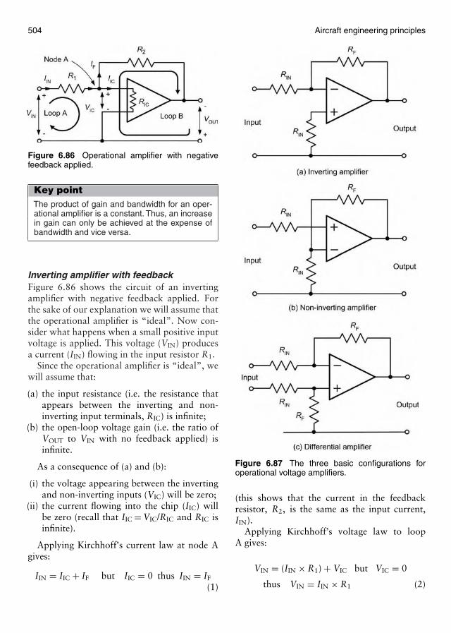
504 Aircraft engineering principles
Figure 6.86 Operational amplifier with negativefeedback applied.
Key pointThe product of gain and bandwidth for an oper-ational amplifier is a constant. Thus, an increasein gain can only be achieved at the expense ofbandwidth and vice versa.
Inverting amplifier with feedbackFigure 6.86 shows the circuit of an invertingamplifier with negative feedback applied. Forthe sake of our explanation we will assume thatthe operational amplifier is “ideal”. Now con-sider what happens when a small positive inputvoltage is applied. This voltage (VIN) producesa current (IIN) flowing in the input resistor R1.
Since the operational amplifier is “ideal”, wewill assume that:
(a) the input resistance (i.e. the resistance thatappears between the inverting and non-inverting input terminals, RIC) is infinite;
(b) the open-loop voltage gain (i.e. the ratio ofVOUT to VIN with no feedback applied) isinfinite.
As a consequence of (a) and (b):
(i) the voltage appearing between the invertingand non-inverting inputs (VIC) will be zero;
(ii) the current flowing into the chip (IIC) willbe zero (recall that IIC = VIC/RIC and RIC isinfinite).
Applying Kirchhoff’s current law at node Agives:
IIN = IIC + IF but IIC = 0 thus IIN = IF
(1)
Figure 6.87 The three basic configurations foroperational voltage amplifiers.
(this shows that the current in the feedbackresistor, R2, is the same as the input current,IIN).
Applying Kirchhoff’s voltage law to loopA gives:
VIN = (IIN × R1) + VIC but VIC = 0
thus VIN = IIN × R1 (2)
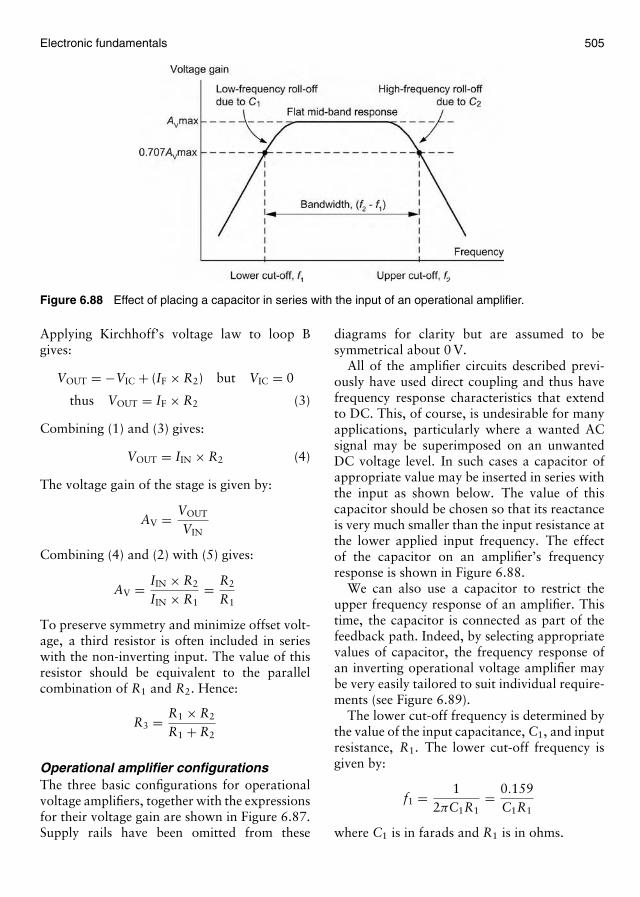
Electronic fundamentals 505
Figure 6.88 Effect of placing a capacitor in series with the input of an operational amplifier.
Applying Kirchhoff’s voltage law to loop Bgives:
VOUT = −VIC + (IF × R2) but VIC = 0
thus VOUT = IF × R2 (3)
Combining (1) and (3) gives:
VOUT = IIN × R2 (4)
The voltage gain of the stage is given by:
AV = VOUT
VIN
Combining (4) and (2) with (5) gives:
AV = IIN × R2
IIN × R1= R2
R1
To preserve symmetry and minimize offset volt-age, a third resistor is often included in serieswith the non-inverting input. The value of thisresistor should be equivalent to the parallelcombination of R1 and R2. Hence:
R3 = R1 × R2
R1 + R2
Operational amplifier configurationsThe three basic configurations for operationalvoltage amplifiers, together with the expressionsfor their voltage gain are shown in Figure 6.87.Supply rails have been omitted from these
diagrams for clarity but are assumed to besymmetrical about 0 V.
All of the amplifier circuits described previ-ously have used direct coupling and thus havefrequency response characteristics that extendto DC. This, of course, is undesirable for manyapplications, particularly where a wanted ACsignal may be superimposed on an unwantedDC voltage level. In such cases a capacitor ofappropriate value may be inserted in series withthe input as shown below. The value of thiscapacitor should be chosen so that its reactanceis very much smaller than the input resistance atthe lower applied input frequency. The effectof the capacitor on an amplifier’s frequencyresponse is shown in Figure 6.88.
We can also use a capacitor to restrict theupper frequency response of an amplifier. Thistime, the capacitor is connected as part of thefeedback path. Indeed, by selecting appropriatevalues of capacitor, the frequency response ofan inverting operational voltage amplifier maybe very easily tailored to suit individual require-ments (see Figure 6.89).
The lower cut-off frequency is determined bythe value of the input capacitance, C1, and inputresistance, R1. The lower cut-off frequency isgiven by:
f1 = 12πC1R1
= 0.159C1R1
where C1 is in farads and R1 is in ohms.
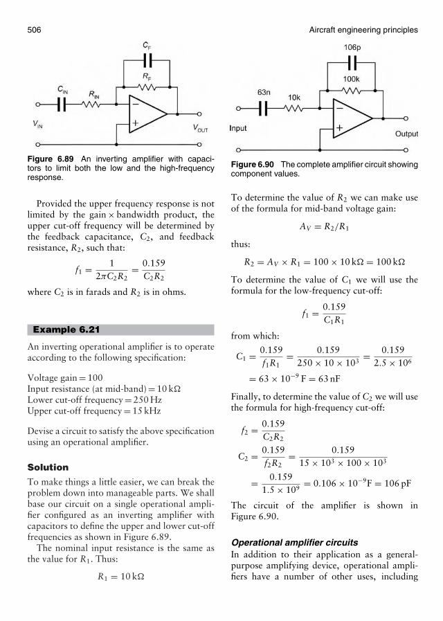
506 Aircraft engineering principles
Figure 6.89 An inverting amplifier with capaci-tors to limit both the low and the high-frequencyresponse.
Provided the upper frequency response is notlimited by the gain × bandwidth product, theupper cut-off frequency will be determined bythe feedback capacitance, C2, and feedbackresistance, R2, such that:
f1 = 12πC2R2
= 0.159C2R2
where C2 is in farads and R2 is in ohms.
Example 6.21
An inverting operational amplifier is to operateaccording to the following specification:
Voltage gain = 100Input resistance (at mid-band) = 10 k�
Lower cut-off frequency = 250 HzUpper cut-off frequency = 15 kHz
Devise a circuit to satisfy the above specificationusing an operational amplifier.
Solution
To make things a little easier, we can break theproblem down into manageable parts. We shallbase our circuit on a single operational ampli-fier configured as an inverting amplifier withcapacitors to define the upper and lower cut-offfrequencies as shown in Figure 6.89.
The nominal input resistance is the same asthe value for R1. Thus:
R1 = 10 k�
Figure 6.90 The complete amplifier circuit showingcomponent values.
To determine the value of R2 we can make useof the formula for mid-band voltage gain:
AV = R2/R1
thus:
R2 = AV × R1 = 100 × 10 k� = 100 k�
To determine the value of C1 we will use theformula for the low-frequency cut-off:
f1 = 0.159C1R1
from which:
C1 = 0.159f1R1
= 0.159250 × 10 × 103
= 0.1592.5 × 106
= 63 × 10−9 F = 63 nF
Finally, to determine the value of C2 we will usethe formula for high-frequency cut-off:
f2 = 0.159C2R2
C2 = 0.159f2R2
= 0.15915 × 103 × 100 × 103
= 0.1591.5 × 109
= 0.106 × 10⁻⁹F = 106 pF
The circuit of the amplifier is shown inFigure 6.90.
Operational amplifier circuitsIn addition to their application as a general-purpose amplifying device, operational ampli-fiers have a number of other uses, including
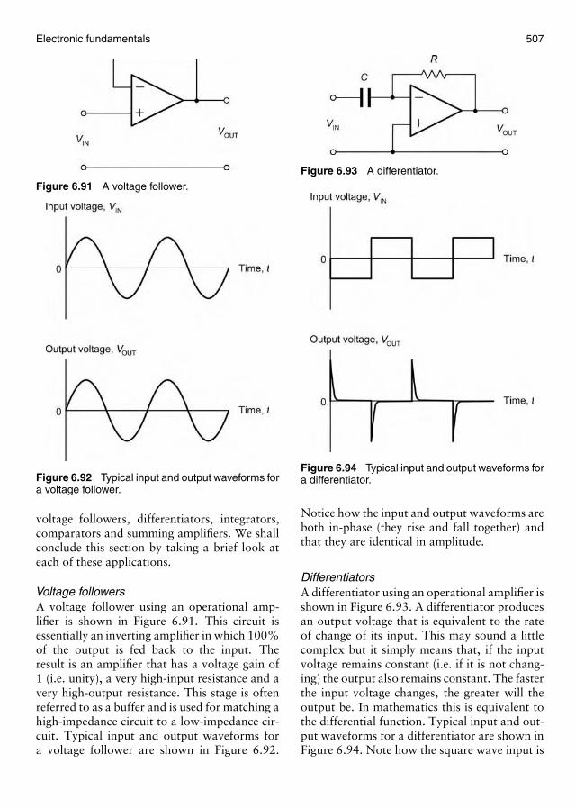
Electronic fundamentals 507
Figure 6.91 A voltage follower.
Figure 6.92 Typical input and output waveforms fora voltage follower.
voltage followers, differentiators, integrators,comparators and summing amplifiers. We shallconclude this section by taking a brief look ateach of these applications.
Voltage followersA voltage follower using an operational amp-lifier is shown in Figure 6.91. This circuit isessentially an inverting amplifier in which 100%of the output is fed back to the input. Theresult is an amplifier that has a voltage gain of1 (i.e. unity), a very high-input resistance and avery high-output resistance. This stage is oftenreferred to as a buffer and is used for matching ahigh-impedance circuit to a low-impedance cir-cuit. Typical input and output waveforms fora voltage follower are shown in Figure 6.92.
Figure 6.93 A differentiator.
Figure 6.94 Typical input and output waveforms fora differentiator.
Notice how the input and output waveforms areboth in-phase (they rise and fall together) andthat they are identical in amplitude.
DifferentiatorsA differentiator using an operational amplifier isshown in Figure 6.93. A differentiator producesan output voltage that is equivalent to the rateof change of its input. This may sound a littlecomplex but it simply means that, if the inputvoltage remains constant (i.e. if it is not chang-ing) the output also remains constant. The fasterthe input voltage changes, the greater will theoutput be. In mathematics this is equivalent tothe differential function. Typical input and out-put waveforms for a differentiator are shown inFigure 6.94. Note how the square wave input is
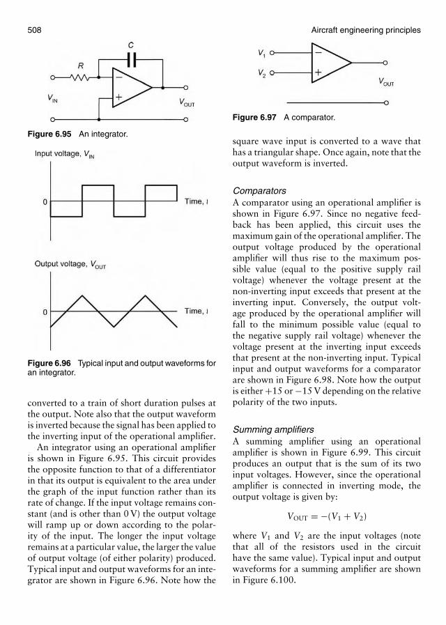
508 Aircraft engineering principles
Figure 6.95 An integrator.
Figure 6.96 Typical input and output waveforms foran integrator.
converted to a train of short duration pulses atthe output. Note also that the output waveformis inverted because the signal has been applied tothe inverting input of the operational amplifier.
An integrator using an operational amplifieris shown in Figure 6.95. This circuit providesthe opposite function to that of a differentiatorin that its output is equivalent to the area underthe graph of the input function rather than itsrate of change. If the input voltage remains con-stant (and is other than 0 V) the output voltagewill ramp up or down according to the polar-ity of the input. The longer the input voltageremains at a particular value, the larger the valueof output voltage (of either polarity) produced.Typical input and output waveforms for an inte-grator are shown in Figure 6.96. Note how the
Figure 6.97 A comparator.
square wave input is converted to a wave thathas a triangular shape. Once again, note that theoutput waveform is inverted.
ComparatorsA comparator using an operational amplifier isshown in Figure 6.97. Since no negative feed-back has been applied, this circuit uses themaximum gain of the operational amplifier. Theoutput voltage produced by the operationalamplifier will thus rise to the maximum pos-sible value (equal to the positive supply railvoltage) whenever the voltage present at thenon-inverting input exceeds that present at theinverting input. Conversely, the output volt-age produced by the operational amplifier willfall to the minimum possible value (equal tothe negative supply rail voltage) whenever thevoltage present at the inverting input exceedsthat present at the non-inverting input. Typicalinput and output waveforms for a comparatorare shown in Figure 6.98. Note how the outputis either +15 or −15 V depending on the relativepolarity of the two inputs.
Summing amplifiersA summing amplifier using an operationalamplifier is shown in Figure 6.99. This circuitproduces an output that is the sum of its twoinput voltages. However, since the operationalamplifier is connected in inverting mode, theoutput voltage is given by:
VOUT = −(V1 + V2)
where V1 and V2 are the input voltages (notethat all of the resistors used in the circuithave the same value). Typical input and outputwaveforms for a summing amplifier are shownin Figure 6.100.
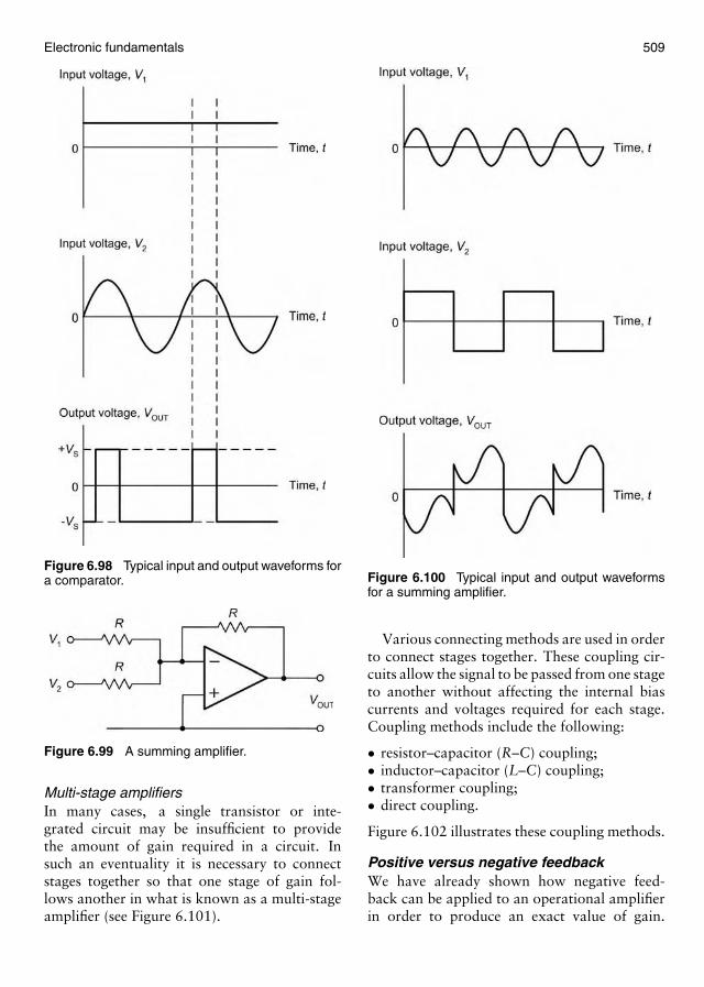
Electronic fundamentals 509
Figure 6.98 Typical input and output waveforms fora comparator.
Figure 6.99 A summing amplifier.
Multi-stage amplifiersIn many cases, a single transistor or inte-grated circuit may be insufficient to providethe amount of gain required in a circuit. Insuch an eventuality it is necessary to connectstages together so that one stage of gain fol-lows another in what is known as a multi-stageamplifier (see Figure 6.101).
Figure 6.100 Typical input and output waveformsfor a summing amplifier.
Various connecting methods are used in orderto connect stages together. These coupling cir-cuits allow the signal to be passed from one stageto another without affecting the internal biascurrents and voltages required for each stage.Coupling methods include the following:
• resistor–capacitor (R–C) coupling;• inductor–capacitor (L–C) coupling;• transformer coupling;• direct coupling.
Figure 6.102 illustrates these coupling methods.
Positive versus negative feedbackWe have already shown how negative feed-back can be applied to an operational amplifierin order to produce an exact value of gain.
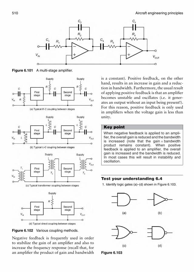
510 Aircraft engineering principles
Figure 6.101 A multi-stage amplifier.
Figure 6.102 Various coupling methods.
Negative feedback is frequently used in orderto stabilize the gain of an amplifier and also toincrease the frequency response (recall that, foran amplifier the product of gain and bandwidth
is a constant). Positive feedback, on the otherhand, results in an increase in gain and a reduc-tion in bandwidth. Furthermore, the usual resultof applying positive feedback is that an amplifierbecomes unstable and oscillates (i.e. it gener-ates an output without an input being present!).For this reason, positive feedback is only usedin amplifiers when the voltage gain is less thanunity.
Key pointWhen negative feedback is applied to an ampli-fier, the overall gain is reduced and the bandwidthis increased (note that the gain × bandwidthproduct remains constant). When positivefeedback is applied to an amplifier, the overallgain is increased and the bandwidth is reduced.In most cases this will result in instability andoscillation.
Test your understanding 6.41. Identify logic gates (a)–(d) shown in Figure 6.103.
Figure 6.103
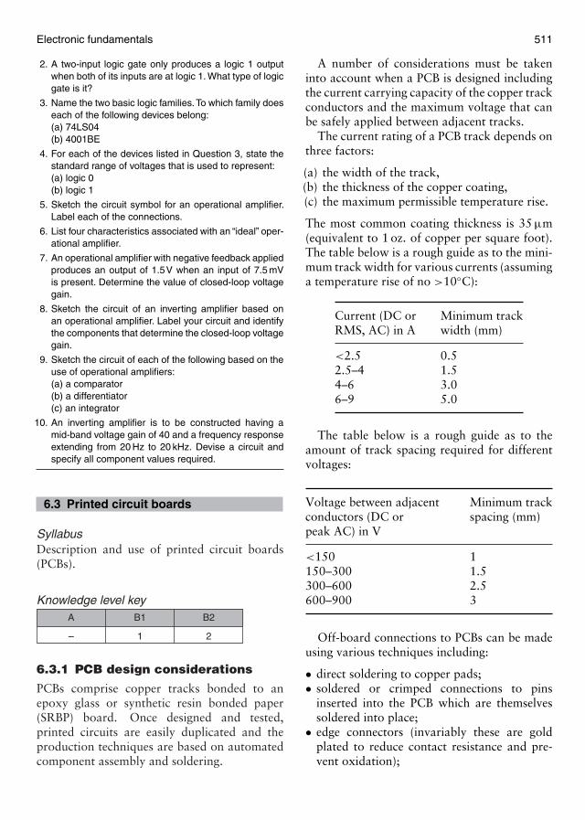
Electronic fundamentals 511
2. A two-input logic gate only produces a logic 1 outputwhen both of its inputs are at logic 1. What type of logicgate is it?
3. Name the two basic logic families. To which family doeseach of the following devices belong:(a) 74LS04(b) 4001BE
4. For each of the devices listed in Question 3, state thestandard range of voltages that is used to represent:(a) logic 0(b) logic 1
5. Sketch the circuit symbol for an operational amplifier.Label each of the connections.
6. List four characteristics associated with an “ideal” oper-ational amplifier.
7. An operational amplifier with negative feedback appliedproduces an output of 1.5V when an input of 7.5 mVis present. Determine the value of closed-loop voltagegain.
8. Sketch the circuit of an inverting amplifier based onan operational amplifier. Label your circuit and identifythe components that determine the closed-loop voltagegain.
9. Sketch the circuit of each of the following based on theuse of operational amplifiers:(a) a comparator(b) a differentiator(c) an integrator
10. An inverting amplifier is to be constructed having amid-band voltage gain of 40 and a frequency responseextending from 20 Hz to 20 kHz. Devise a circuit andspecify all component values required.
6.3 Printed circuit boards
SyllabusDescription and use of printed circuit boards(PCBs).
Knowledge level key
–
A
1
B1
2
B2
6.3.1 PCB design considerations
PCBs comprise copper tracks bonded to anepoxy glass or synthetic resin bonded paper(SRBP) board. Once designed and tested,printed circuits are easily duplicated and theproduction techniques are based on automatedcomponent assembly and soldering.
A number of considerations must be takeninto account when a PCB is designed includingthe current carrying capacity of the copper trackconductors and the maximum voltage that canbe safely applied between adjacent tracks.
The current rating of a PCB track depends onthree factors:
(a) the width of the track,(b) the thickness of the copper coating,(c) the maximum permissible temperature rise.
The most common coating thickness is 35 µm(equivalent to 1 oz. of copper per square foot).The table below is a rough guide as to the mini-mum track width for various currents (assuminga temperature rise of no >10◦C):
Current (DC or Minimum trackRMS, AC) in A width (mm)
<2.5 0.52.5–4 1.54–6 3.06–9 5.0
The table below is a rough guide as to theamount of track spacing required for differentvoltages:
Voltage between adjacent Minimum trackconductors (DC or spacing (mm)peak AC) in V
<150 1150–300 1.5300–600 2.5600–900 3
Off-board connections to PCBs can be madeusing various techniques including:
• direct soldering to copper pads;• soldered or crimped connections to pins
inserted into the PCB which are themselvessoldered into place;
• edge connectors (invariably these are goldplated to reduce contact resistance and pre-vent oxidation);
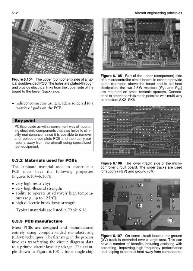
512 Aircraft engineering principles
Figure 6.104 The upper (component) side of a typ-ical double-sided PCB.The holes are plated-throughand provide electrical links from the upper side of theboard to the lower (track) side.
• indirect connector using headers soldered to amatrix of pads on the PCB.
Key pointPCBs provide us with a convenient way of mount-ing electronic components that also helps to sim-plify maintenance, since it is possible to removeand replace a complete PCB and then carry outrepairs away from the aircraft using specializedtest equipment.
6.3.2 Materials used for PCBs
The laminate material used to construct aPCB must have the following properties(Figures 6.104–6.107):
• very high resistivity;• very high-flexural strength;• ability to operate at relatively high tempera-
tures (e.g. up to 125◦C);• high dielectric breakdown strength.
Typical materials are listed in Table 6.18.
6.3.3 PCB manufacture
Most PCBs are designed and manufacturedentirely using computer-aided manufacturing(CAM) techniques. The first stage in the processinvolves transferring the circuit diagram datato a printed circuit layout package. The exam-ple shown in Figure 6.108 is for a single-chip
Figure 6.105 Part of the upper (component) sideof a microcontroller circuit board. In order to providesome clearance above the board and to aid heatdissipation, the two 2.5W resistors (R17 and R18)are mounted on small ceramic spacers. Connec-tions to other boards is made possible with multi-wayconnectors SK2–SK6.
Figure 6.106 The lower (track) side of the micro-controller circuit board. The wider tracks are usedfor supply (+5V) and ground (0V).
Figure 6.107 On some circuit boards the ground(0V) track is extended over a large area. This canhave a number of benefits including assisting withscreening, improving high-frequency performanceand helping to conduct heat away from components.
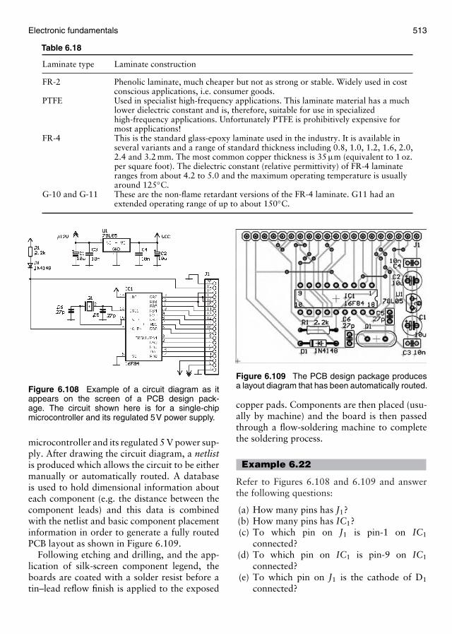
Electronic fundamentals 513
Table 6.18
Laminate type Laminate construction
FR-2 Phenolic laminate, much cheaper but not as strong or stable. Widely used in costconscious applications, i.e. consumer goods.
PTFE Used in specialist high-frequency applications. This laminate material has a muchlower dielectric constant and is, therefore, suitable for use in specializedhigh-frequency applications. Unfortunately PTFE is prohibitively expensive formost applications!
FR-4 This is the standard glass-epoxy laminate used in the industry. It is available inseveral variants and a range of standard thickness including 0.8, 1.0, 1.2, 1.6, 2.0,2.4 and 3.2 mm. The most common copper thickness is 35 µm (equivalent to 1 oz.per square foot). The dielectric constant (relative permittivity) of FR-4 laminateranges from about 4.2 to 5.0 and the maximum operating temperature is usuallyaround 125◦C.
G-10 and G-11 These are the non-flame retardant versions of the FR-4 laminate. G11 had anextended operating range of up to about 150◦C.
Figure 6.108 Example of a circuit diagram as itappears on the screen of a PCB design pack-age. The circuit shown here is for a single-chipmicrocontroller and its regulated 5V power supply.
microcontroller and its regulated 5 V power sup-ply. After drawing the circuit diagram, a netlistis produced which allows the circuit to be eithermanually or automatically routed. A databaseis used to hold dimensional information abouteach component (e.g. the distance between thecomponent leads) and this data is combinedwith the netlist and basic component placementinformation in order to generate a fully routedPCB layout as shown in Figure 6.109.
Following etching and drilling, and the app-lication of silk-screen component legend, theboards are coated with a solder resist before atin–lead reflow finish is applied to the exposed
Figure 6.109 The PCB design package producesa layout diagram that has been automatically routed.
copper pads. Components are then placed (usu-ally by machine) and the board is then passedthrough a flow-soldering machine to completethe soldering process.
Example 6.22
Refer to Figures 6.108 and 6.109 and answerthe following questions:
(a) How many pins has J1?(b) How many pins has IC1?(c) To which pin on J1 is pin-1 on IC1
connected?(d) To which pin on IC1 is pin-9 on IC1
connected?(e) To which pin on J1 is the cathode of D1
connected?
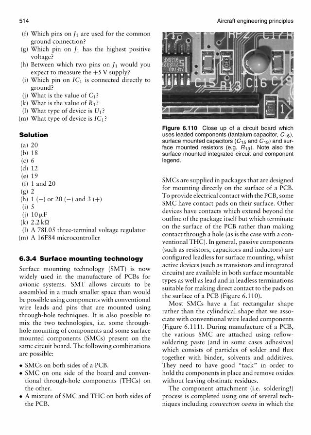
514 Aircraft engineering principles
(f) Which pins on J1 are used for the commonground connection?
(g) Which pin on J1 has the highest positivevoltage?
(h) Between which two pins on J1 would youexpect to measure the +5 V supply?
(i) Which pin on IC1 is connected directly toground?
(j) What is the value of C1?(k) What is the value of R1?(l) What type of device is U1?
(m) What type of device is IC1?
Solution
(a) 20(b) 18(c) 6(d) 12(e) 19(f) 1 and 20(g) 2(h) 1 (−) or 20 (−) and 3 (+)(i) 5(j) 10 µF(k) 2.2 k�
(l) A 78L05 three-terminal voltage regulator(m) A 16F84 microcontroller
6.3.4 Surface mounting technology
Surface mounting technology (SMT) is nowwidely used in the manufacture of PCBs foravionic systems. SMT allows circuits to beassembled in a much smaller space than wouldbe possible using components with conventionalwire leads and pins that are mounted usingthrough-hole techniques. It is also possible tomix the two technologies, i.e. some through-hole mounting of components and some surfacemounted components (SMCs) present on thesame circuit board. The following combinationsare possible:
• SMCs on both sides of a PCB.• SMC on one side of the board and conven-
tional through-hole components (THCs) onthe other.
• A mixture of SMC and THC on both sides ofthe PCB.
Figure 6.110 Close up of a circuit board whichuses leaded components (tantalum capacitor, C16),surface mounted capacitors (C15 and C19) and sur-face mounted resistors (e.g. R13). Note also thesurface mounted integrated circuit and componentlegend.
SMCs are supplied in packages that are designedfor mounting directly on the surface of a PCB.To provide electrical contact with the PCB, someSMC have contact pads on their surface. Otherdevices have contacts which extend beyond theoutline of the package itself but which terminateon the surface of the PCB rather than makingcontact through a hole (as is the case with a con-ventional THC). In general, passive components(such as resistors, capacitors and inductors) areconfigured leadless for surface mounting, whilstactive devices (such as transistors and integratedcircuits) are available in both surface mountabletypes as well as lead and in leadless terminationssuitable for making direct contact to the pads onthe surface of a PCB (Figure 6.110).
Most SMCs have a flat rectangular shaperather than the cylindrical shape that we asso-ciate with conventional wire leaded components(Figure 6.111). During manufacture of a PCB,the various SMC are attached using reflow-soldering paste (and in some cases adhesives)which consists of particles of solder and fluxtogether with binder, solvents and additives.They need to have good “tack” in order tohold the components in place and remove oxideswithout leaving obstinate residues.
The component attachment (i.e. soldering!)process is completed using one of several tech-niques including convection ovens in which the

Electronic fundamentals 515
Figure 6.111 Some PCB have componentsmounted on both sides. This shows part of the lower(track) side of a large PCB. All of the componentsmounted on this side of the board are surfacemounted types.
PCB is passed, using a conveyor belt, througha convection oven which has separate zonesfor preheating, flowing and cooling, and infra-red reflow in which infra-red lamps are used toprovide the source of heat.
Key pointModern SMCs take up considerably less spacethan conventional components that have con-necting leads or pins that require fitting throughholes in a PCB. SMCs need special handlingtechniques due to their small size and the needfor soldering direct to surface pads on the PCB.
Test your understanding 6.51. What is the most commonly used laminate material
used in the manufacture of PCBs?2. State THREE factors that determine the current carry-
ing capacity of the copper tracks on a PCB.3. List FOUR important characteristics of a material used
for the manufacture of a PCB.4. State ONE advantage and ONE disadvantage of PTFE
laminate when compared with FR-4 laminate.5. The maximum operating temperature for a PCB is usu-
ally quoted as 175◦C. Is this statement true or false?Explain your answer.
6. SMCs must be individually soldered in place. Is thisstatement true or false? Explain your answer.
7. Explain why FR-4 laminate is preferred to G-10 laminatein an aircraft PCB application.
8. Explain the purpose of the silk-screened legend thatappears on the component side of a PCB.
9. State the typical range of coating thicknesses for thecopper surface coating on a PCB.
10. Some of the stages that are involved in the productionof a PCB are listed below. Organize this list into thecorrect sequence:• drilling,• etching,• screen printing of component legend,• application of tin–lead reflow coating,• application of solder-resist coating.
6.4 Servomechanisms
SyllabusUnderstanding of the following terms: Open-and closed-loop systems, feedback, followup, analogue transducers; Principles of opera-tion and use of the following synchro-systemcomponents/features: resolvers, differential,control and torque, transformers, inductanceand capacitance transmitters.
Knowledge level key
–
A
1
B1
–
B2
SyllabusUnderstanding of the following terms: open andclosed loop, follow up, servomechanism, ana-logue, transducer, null, damping, feedbackand deadband; Construction operation and useof the following synchro-system components:resolvers, differential, control and torque, E andI transformers, inductance transmitters, capac-itance transmitters, synchronous transmitters;Servomechanism defects, reversal of synchro-leads, hunting.
Knowledge level key
–
A
–
B1
2
B2
6.4.1 Control systems
Control systems are used in aircraft, cars andmany other complex machines. A specific input,
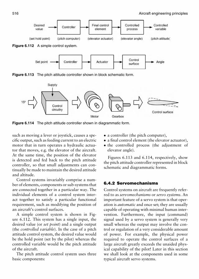
516 Aircraft engineering principles
Figure 6.112 A simple control system.
Figure 6.113 The pitch attitude controller shown in block schematic form.
Figure 6.114 The pitch attitude controller shown in diagrammatic form.
such as moving a lever or joystick, causes a spe-cific output, such as feeding current to an electricmotor that in turn operates a hydraulic actua-tor that moves, e.g. the elevator of the aircraft.At the same time, the position of the elevatoris detected and fed back to the pitch attitudecontroller, so that small adjustments can con-tinually be made to maintain the desired attitudeand altitude.
Control systems invariably comprise a num-ber of elements, components or sub-systems thatare connected together in a particular way. Theindividual elements of a control system inter-act together to satisfy a particular functionalrequirement, such as modifying the position ofan aircraft’s control surfaces.
A simple control system is shown in Fig-ure 6.112. This system has a single input, thedesired value (or set point) and a single output(the controlled variable). In the case of a pitchattitude control system, the desired value wouldbe the hold point (set by the pilot) whereas thecontrolled variable would be the pitch attitudeof the aircraft.
The pitch attitude control system uses threebasic components:
• a controller (the pitch computer),• a final control element (the elevator actuator),• the controlled process (the adjustment of
elevator angle).
Figures 6.113 and 6.114, respectively, showthe pitch attitude controller represented in blockschematic and diagrammatic forms.
6.4.2 Servomechanisms
Control systems on aircraft are frequently refer-red to as servomechanisms or servo systems. Animportant feature of a servo system is that oper-ation is automatic and once set; they are usuallycapable of operating with minimal human inter-vention. Furthermore, the input (command)signal used by a servo system is generally verysmall whereas the output may involve the con-trol or regulation of a very considerable amountof power. For example, the physical powerrequired to operate the control surfaces of alarge aircraft greatly exceeds the unaided phys-ical capability of the pilot! Later in this sectionwe shall look at the components used in sometypical aircraft servo systems.
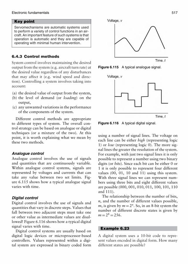
Electronic fundamentals 517
Key pointServomechanisms are automatic systems usedto perform a variety of control functions in an air-craft. An important feature of such systems is thatoperation is automatic and they are capable ofoperating with minimal human intervention.
6.4.3 Control methods
System control involves maintaining the desiredoutput from the system (e.g. aircraft turn rate) atthe desired value regardless of any disturbancesthat may affect it (e.g. wind speed and direc-tion). Controlling a system involves taking intoaccount:
(a) the desired value of output from the system,(b) the level of demand (or loading) on the
output,(c) any unwanted variations in the performance
of the components of the system.
Different control methods are appropriateto different types of system. The overall con-trol strategy can be based on analogue or digitaltechniques (or a mixture of the two). At thispoint, it is worth explaining what we mean bythese two methods.
Analogue controlAnalogue control involves the use of signalsand quantities that are continuously variable.Within analogue control systems, signals arerepresented by voltages and currents that cantake any value between two set limits. Fig-ure 6.115 shows how a typical analogue signalvaries with time.
Digital controlDigital control involves the use of signals andquantities that vary in discrete steps. Values thatfall between two adjacent steps must take oneor other value as intermediate values are disal-lowed! Figure 6.116 shows how a typical digitalsignal varies with time.
Digital control systems are usually based ondigital logic devices or microprocessor-basedcontrollers. Values represented within a digi-tal system are expressed in binary coded form
Figure 6.115 A typical analogue signal.
Figure 6.116 A typical digital signal.
using a number of signal lines. The voltage oneach line can be either high (representing logic1) or low (representing logic 0). The more sig-nal lines the greater the resolution of the system.For example, with just two signal lines it is onlypossible to represent a number using two binarydigits (or bits). Since each bit can be either 0 or1 it is only possible to represent four differentvalues (00, 01, 10 and 11) using this system.With three signal lines we can represent num-bers using three bits and eight different valuesare possible (000, 001, 010, 011, 100, 101, 110and 111).
The relationship between the number of bits,n, and the number of different values possible,m, is given by m = 2n. So, in an 8-bit system thenumber of different discrete states is given bym = 28 = 256.
Example 6.23
A digital system uses a 10-bit code to repre-sent values encoded in digital form. How manydifferent states are possible?
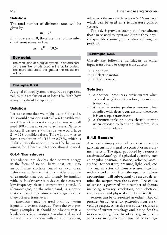
518 Aircraft engineering principles
Solution
The total number of different states will begiven by:
m = 2n
In this case n = 10, therefore, the total numberof different states will be:
m = 210 = 1024
Key pointThe resolution of a digital system is determinedby the number of bits used in the digital codes.The more bits used, the greater the resolutionwill be.
Example 6.24
A digital control system is required to representvalues to a resolution of at least 1%. With howmany bits should it operate?
Solution
Let us assume that we might use a 6-bit code.This would provide us with 26 = 64 possible val-ues. Clearly this is not enough because we willneed 100 values in order to achieve a 1% reso-lution. If we use a 7-bit code we would have27 = 128 possible values. This will allow us tohave a resolution of 1/128 or 0.78%, which isslightly better than the minimum 1% that we areaiming for. Hence, a 7-bit code should be used.
6.4.4 Transducers
Transducers are devices that convert energyin the form of sound, light, heat, etc. intoan equivalent electrical signal or vice versa.Before we go further, let us consider a coupleof examples that you will already be familiarwith. A loudspeaker is a device that convertslow-frequency electric current into sound. Athermocouple, on the other hand, is a devicethat converts temperature into voltage. Both ofthese act as a transducer.
Transducers may be used both as systeminputs and system outputs. From the two pre-vious examples, it should be obvious that aloudspeaker is an output transducer designedfor use in conjunction with an audio system,
whereas a thermocouple is an input transducerwhich can be used in a temperature controlsystem.
Table 6.19 provides examples of transducersthat can be used to input and output three phys-ical quantities: sound, temperature and angularposition.
Example 6.25
Classify the following transducers as eitherinput transducers or output transducers:
(a) a photocell(b) an electric motor(c) a thermocouple
Solution
(a) A photocell produces electric current whenexposed to light and, therefore, it is an inputtransducer.
(b) An electric motor produces motion whensupplied with electric current and, therefore,it is an output transducer.
(c) A thermocouple produces electric currentwhen exposed to heat and, therefore, it isan input transducer.
6.4.5 Sensors
A sensor is simply a transducer, that is used togenerate an input signal to a control or measure-ment system. The signal produced by a sensor isan electrical analogy of a physical quantity, suchas angular position, distance, velocity, accel-eration, temperature, pressure, light level, etc.The signals returned from a sensor, togetherwith control inputs from the operator (whereappropriate), will subsequently be used to deter-mine the output from the system. The choiceof sensor is governed by a number of factorsincluding accuracy, resolution, cost, electricalspecification and physical size (Table 6.20).
Sensors can be categorized as either active orpassive. An active sensor generates a current orvoltage output. A passive transducer requires asource of current or voltage and it modifies thisin some way (e.g. by virtue of a change in the sen-sor’s resistance). The result may still be a voltage
Electronic fundamentals 519
Table 6.19
Physical quantity Transducer Notes
Input transducersSound (pressure change) Dynamic Diaphragm attached to a coil is suspended in a magnetic
microphone field. Movement of the diaphragm causes current to beinduced in the coil.
Temperature Thermocouple Small e.m.f. generated at the junction between two dissimilarmetals (e.g. copper and constantan). Requires referencejunction and compensated cables for accurate measurement.
Angular position Rotary Fine wire resistive element is wound around a circularpotentiometer former. Slider attached to the control shaft makes
contact with the resistive element. A stable DC voltagesource is connected across the ends of the potentiometer.Voltage appearing at the slider will then be proportionalto angular position.
Output transducersSound (pressure change) Loudspeaker Diaphragm attached to a coil is suspended in a magnetic
field. Current in the coil causes movement of thediaphragm that alternately compresses and rarefies theair mass in front of it.
Temperature Resistive heating Metallic conductor is wound onto a ceramic or micaelement former. Current flowing in the conductor produces heat.
Angular position Stepper motor Multi-phase motor provides precise rotation in discretesteps of 15◦ (24 steps per revolution), 7.5◦ (48 steps perrevolution) and 1.8◦ (200 steps per revolution).
or current but it is not generated by the sensoron its own.
Sensors can also be classified as either digi-tal or analogue. The output of a digital sensorcan exist in only two discrete states, either “on”or “off”, “low” or “high”, “logic 1” or “logic0”, etc. The output of an analogue sensor cantake any one of an infinite number of voltage orcurrent levels. It is thus said to be continuouslyvariable.
Example 6.26
Classify the following sensors as either active orpassive sensors:
(a) a photocell(b) a photodiode(c) an LDR
Solution
(a) A photocell produces electric current whenexposed to light and, therefore, is an activesensor.
(b) A photodiode cannot generate an electriccurrent on its own and, therefore, is apassive sensor.
(c) An LDR cannot generate electric current onits own and, therefore, is a passive sensor.
Example 6.27
Classify the following sensors as either digital oranalogue sensors:
(a) a reed switch(b) a photodiode(c) an LDR
Solution
(a) A reed switch is either on or off and, there-fore, is a digital sensor.
(b) The current flowing through a thermistorvaries continuously with changes in tem-perature and, therefore, a thermistor is ananalogue sensor.
520 Aircraft engineering principles
Table 6.20
Physical parameters Type of sensors Notes
Angular position Resistive rotary position Rotary track potentiometer with linear law producessensor analogue voltage proportional to angular position.
Optical shaft encoder Encoded disk interposed between optical transmitterand receiver (infra-red LED and photodiode orphototransistor).
Differential transformer Transformer with fixed E-laminations and pivotedI-laminations acting as a moving armature.
Angular velocity Tachogenerator Small DC generator with linear output characteristic.Analogue output voltage proportional to shaft speed.
Toothed rotor tachometer Magnetic pick-up responds to the movement ofa toothed ferrous disk. The pulse repetition frequencyof the output is proportional to the angular velocity.
Flow Rotating vane flow sensor Turbine rotor driven by fluid. Turbine interruptsinfra-red beam. Pulse repetition frequency of outputis proportional to flow rate.
Linear position Resistive linear position Linear track potentiometer with linear law producessensor analogue voltage proportional to linear position.
Limited linear range.
Linear variable differential Miniature transformer with split secondary windingstransformer (LVDT) and moving core attached to a plunger. Requires AC
excitation and phase-sensitive detector.
Magnetic linear position Magnetic pick-up responds to movement of a toothedsensor ferrous track. Pulses are counted as the sensor moves
along the track.
Light level Photocell Voltage-generating device. The analogue output voltageproduced is proportional to light level.
Light-dependent resistor An analogue output voltage results from a change of(LDR) resistance within a cadmium sulphide (CdS) sensing
element. Usually connected as part of a potentialdivider or bridge.
Photodiode Two-terminal device connected as a current source.An analogue output voltage is developed across a seriesresistor of appropriate value.
Phototransistor Three-terminal device connected as a current source.An analogue output voltage is developed across a seriesresistor of appropriate value.
Liquid level Float switch Simple switch element that operates when a particularlevel is detected.
Capacitive proximity Switching device that operates when a particular levelswitch is detected. Ineffective with some liquids.
Diffuse scan proximity Switching device that operates when a particular levelswitch is detected. Ineffective with some liquids.
Pressure Microswitch pressure Microswitch fitted with actuator mechanism and rangesensor setting springs. Suitable for high-pressure applications.
(continued)
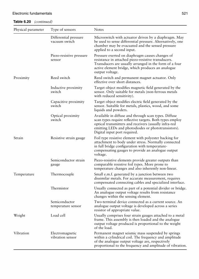
Electronic fundamentals 521
Table 6.20 (continued)
Physical parameter Type of sensors Notes
Differential pressure Microswitch with actuator driven by a diaphragm. Mayvacuum switch be used to sense differential pressure. Alternatively, one
chamber may be evacuated and the sensed pressureapplied to a second input.
Piezo-resistive pressure Pressure exerted on diaphragm causes changes ofsensor resistance in attached piezo-resistive transducers.
Transducers are usually arranged in the form of a fouractive element bridge, which produces an analogueoutput voltage.
Proximity Reed switch Reed switch and permanent magnet actuator. Onlyeffective over short distances.
Inductive proximity Target object modifies magnetic field generated by theswitch sensor. Only suitable for metals (non-ferrous metals
with reduced sensitivity).
Capacitive proximity Target object modifies electric field generated by theswitch sensor. Suitable for metals, plastics, wood, and some
liquids and powders.
Optical proximity Available in diffuse and through scan types. Diffuseswitch scan types require reflective targets. Both types employ
optical transmitters and receivers (usually infra-redemitting LEDs and photodiodes or phototransistors).Digital input port required.
Strain Resistive strain gauge Foil type resistive element with polyester backing forattachment to body under stress. Normally connectedin full bridge configuration with temperature-compensating gauges to provide an analogue outputvoltage.
Semiconductor strain Piezo-resistive elements provide greater outputs thangauge comparable resistive foil types. More prone to
temperature changes and also inherently non-linear.
Temperature Thermocouple Small e.m.f. generated by a junction between twodissimilar metals. For accurate measurement, requirescompensated connecting cables and specialized interface.
Thermistor Usually connected as part of a potential divider or bridge.An analogue output voltage results from resistancechanges within the sensing element.
Semiconductor Two-terminal device connected as a current source. Antemperature sensor analogue output voltage is developed across a series
resistor of appropriate value.Weight Load cell Usually comprises four strain gauges attached to a metal
frame. This assembly is then loaded and the analogueoutput voltage produced is proportional to the weightof the load.
Vibration Electromagnetic Permanent magnet seismic mass suspended by springsvibration sensor within a cylindrical coil. The frequency and amplitude
of the analogue output voltage are, respectivelyproportional to the frequency and amplitude of vibration.
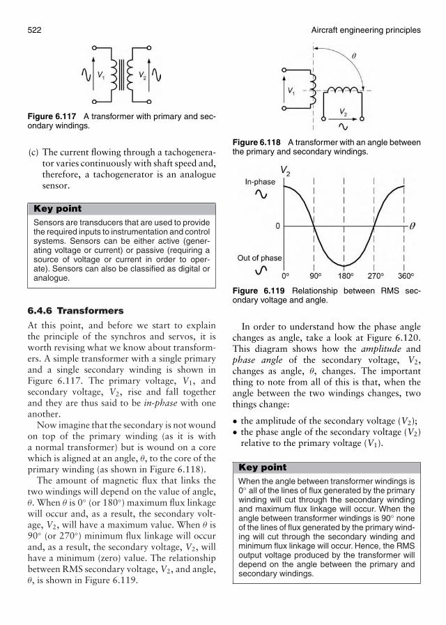
522 Aircraft engineering principles
Figure 6.117 A transformer with primary and sec-ondary windings.
(c) The current flowing through a tachogenera-tor varies continuously with shaft speed and,therefore, a tachogenerator is an analoguesensor.
Key pointSensors are transducers that are used to providethe required inputs to instrumentation and controlsystems. Sensors can be either active (gener-ating voltage or current) or passive (requiring asource of voltage or current in order to oper-ate). Sensors can also be classified as digital oranalogue.
6.4.6 Transformers
At this point, and before we start to explainthe principle of the synchros and servos, it isworth revising what we know about transform-ers. A simple transformer with a single primaryand a single secondary winding is shown inFigure 6.117. The primary voltage, V1, andsecondary voltage, V2, rise and fall togetherand they are thus said to be in-phase with oneanother.
Now imagine that the secondary is not woundon top of the primary winding (as it is witha normal transformer) but is wound on a corewhich is aligned at an angle, θ, to the core of theprimary winding (as shown in Figure 6.118).
The amount of magnetic flux that links thetwo windings will depend on the value of angle,θ. When θ is 0◦ (or 180◦) maximum flux linkagewill occur and, as a result, the secondary volt-age, V2, will have a maximum value. When θ is90◦ (or 270◦) minimum flux linkage will occurand, as a result, the secondary voltage, V2, willhave a minimum (zero) value. The relationshipbetween RMS secondary voltage, V2, and angle,θ, is shown in Figure 6.119.
Figure 6.118 A transformer with an angle betweenthe primary and secondary windings.
Figure 6.119 Relationship between RMS sec-ondary voltage and angle.
In order to understand how the phase anglechanges as angle, take a look at Figure 6.120.This diagram shows how the amplitude andphase angle of the secondary voltage, V2,changes as angle, θ, changes. The importantthing to note from all of this is that, when theangle between the two windings changes, twothings change:
• the amplitude of the secondary voltage (V2);• the phase angle of the secondary voltage (V2)
relative to the primary voltage (V1).
Key pointWhen the angle between transformer windings is0◦ all of the lines of flux generated by the primarywinding will cut through the secondary windingand maximum flux linkage will occur. When theangle between transformer windings is 90◦ noneof the lines of flux generated by the primary wind-ing will cut through the secondary winding andminimum flux linkage will occur. Hence, the RMSoutput voltage produced by the transformer willdepend on the angle between the primary andsecondary windings.
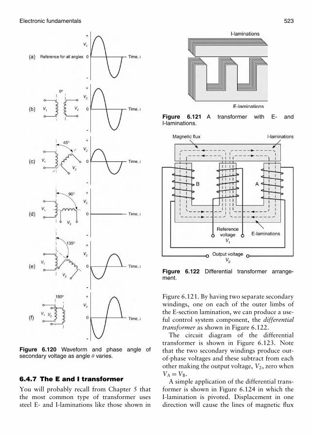
Electronic fundamentals 523
Figure 6.120 Waveform and phase angle ofsecondary voltage as angle θ varies.
6.4.7 The E and I transformer
You will probably recall from Chapter 5 thatthe most common type of transformer usessteel E- and I-laminations like those shown in
Figure 6.121 A transformer with E- andI-laminations.
Figure 6.122 Differential transformer arrange-ment.
Figure 6.121. By having two separate secondarywindings, one on each of the outer limbs ofthe E-section lamination, we can produce a use-ful control system component, the differentialtransformer as shown in Figure 6.122.
The circuit diagram of the differentialtransformer is shown in Figure 6.123. Notethat the two secondary windings produce out-of-phase voltages and these subtract from eachother making the output voltage, V2, zero whenVA = VB.
A simple application of the differential trans-former is shown in Figure 6.124 in which theI-lamination is pivoted. Displacement in onedirection will cause the lines of magnetic flux
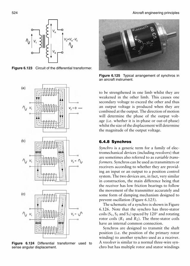
524 Aircraft engineering principles
Figure 6.123 Circuit of the differential transformer.
Figure 6.124 Differential transformer used tosense angular displacement.
Figure 6.125 Typical arrangement of synchros inan aircraft instrument.
to be strengthened in one limb whilst they areweakened in the other limb. This causes onesecondary voltage to exceed the other and thusan output voltage is produced when they arecombined at the output. The direction of motionwill determine the phase of the output volt-age (i.e. whether it is in-phase or out-of-phase)whilst the size of the displacement will determinethe magnitude of the output voltage.
6.4.8 Synchros
Synchro is a generic term for a family of elec-tromechanical devices (including resolvers) thatare sometimes also referred to as variable trans-formers. Synchros can be used as transmitters orreceivers according to whether they are provid-ing an input or an output to a position controlsystem. The two devices are, in fact, very similarin construction, the main difference being thatthe receiver has low friction bearings to followthe movement of the transmitter accurately andsome form of damping mechanism designed toprevent oscillation (Figure 6.125).
The schematic of a synchro is shown in Figure6.126. Note that the synchro has three-statorcoils (S1, S2 and S3) spaced by 120◦ and rotatingrotor coils (R1 and R2). The three-stator coilshave an internal common connection.
Synchros are designed to transmit the shaftposition (i.e. the position of the primary rotorwinding) to another synchro used as a receiver.A resolver is similar to a normal three-wire syn-chro but has multiple rotor and stator windings
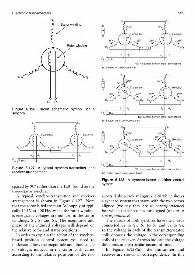
Electronic fundamentals 525
Figure 6.126 Circuit schematic symbol for asynchro.
R1 R2 R1 R2
S1S1
S2S2
S3 S3
Transmitter Receiver
Supply
Figure 6.127 A typical synchro-transmitter andreceiver arrangement.
spaced by 90◦ rather than the 120◦ found on thethree-stator synchro.
A typical synchro-transmitter and receiverarrangement is shown in Figure 6.127. Notethat the rotor is fed from an AC supply of typi-cally 115 V at 400 Hz. When the rotor windingis energized, voltages are induced in the statorwindings, S1, S2 and S3. The magnitude andphase of the induced voltages will depend onthe relative rotor and stator positions.
In order to explain the action of the synchro-based position control system you need tounderstand how the magnitude and phase angleof voltages induced in the stator coils variesaccording to the relative positions of the two
R2 R2R1 R1
S2 S2
S2 S2
S2 S2
S1 S1S3
26V
115V
R2 R2R1 R1
115V
R2 R2R1 R1
115V
(a) System in correspondence
(b) System out of correspondence
(c) System again in correspondence
NB: No current flows in stator connections
NB: No current flows in stator connections
NB: Current flows in stator connections
26V 26V 26V
26V 52V 26V
26V60º
60º
26V
26V 52V 52V26V
52V 52V
52V
26V 26V
Transmitter
Transmitter
Transmitter
Receiver
Receiver
Receiver
S
N
S
N
S
N
S3
S1 S1S3 S3
S1 S1S3 S3
Figure 6.128 A synchro-based position controlsystem.
rotors. Take a look at Figure 6.128 which showsa synchro system that starts with the two rotorsaligned (we say they are in correspondence)but which then becomes misaligned (or out ofcorrespondence).
The stators of both synchros have their leadsconnected S1 to S1, S2 to S2 and S3 to S3,so the voltage in each of the transmitter-statorcoils opposes the voltage in the correspondingcoils of the receiver. Arrows indicate the voltagedirections at a particular instant of time.
In Figure 6.128(a), the transmitter andreceiver are shown in correspondence. In this
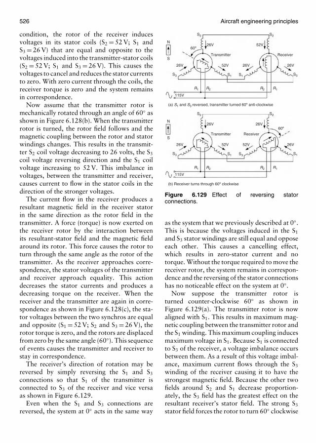
526 Aircraft engineering principles
condition, the rotor of the receiver inducesvoltages in its stator coils (S2 = 52 V; S1 andS3 = 26 V) that are equal and opposite to thevoltages induced into the transmitter-stator coils(S2 = 52 V; S1 and S3 = 26 V). This causes thevoltages to cancel and reduces the stator currentsto zero. With zero current through the coils, thereceiver torque is zero and the system remainsin correspondence.
Now assume that the transmitter rotor ismechanically rotated through an angle of 60◦ asshown in Figure 6.128(b). When the transmitterrotor is turned, the rotor field follows and themagnetic coupling between the rotor and statorwindings changes. This results in the transmit-ter S2 coil voltage decreasing to 26 volts, the S3
coil voltage reversing direction and the S1 coilvoltage increasing to 52 V. This imbalance involtages, between the transmitter and receiver,causes current to flow in the stator coils in thedirection of the stronger voltages.
The current flow in the receiver produces aresultant magnetic field in the receiver statorin the same direction as the rotor field in thetransmitter. A force (torque) is now exerted onthe receiver rotor by the interaction betweenits resultant-stator field and the magnetic fieldaround its rotor. This force causes the rotor toturn through the same angle as the rotor of thetransmitter. As the receiver approaches corre-spondence, the stator voltages of the transmitterand receiver approach equality. This actiondecreases the stator currents and produces adecreasing torque on the receiver. When thereceiver and the transmitter are again in corre-spondence as shown in Figure 6.128(c), the sta-tor voltages between the two synchros are equaland opposite (S1 = 52 V; S2 and S3 = 26 V), therotor torque is zero, and the rotors are displacedfrom zero by the same angle (60◦). This sequenceof events causes the transmitter and receiver tostay in correspondence.
The receiver’s direction of rotation may bereversed by simply reversing the S1 and S3
connections so that S1 of the transmitter isconnected to S3 of the receiver and vice versaas shown in Figure 6.129.
Even when the S1 and S3 connections arereversed, the system at 0◦ acts in the same way
R1 R1
S1S1
S2
S3
S2
S3
R2 R2
115V
26V 26V26V
26V
52V
52VN
S
60º
Transmitter Receiver
R1 R1
S3S1
S2
S3
S2
S1
R2 R2
115V
26V 26V
26V 26V
52V 52V
N
S
60º
Transmitter Receiver
(b) Receiver turns through 60º clockwise
(a) S1 and S3 reversed, transmitter turned 60º anti-clockwise
Figure 6.129 Effect of reversing statorconnections.
as the system that we previously described at 0◦.This is because the voltages induced in the S1
and S3 stator windings are still equal and opposeeach other. This causes a cancelling effect,which results in zero-stator current and notorque. Without the torque required to move thereceiver rotor, the system remains in correspon-dence and the reversing of the stator connectionshas no noticeable effect on the system at 0◦.
Now suppose the transmitter rotor isturned counter-clockwise 60◦ as shown inFigure 6.129(a). The transmitter rotor is nowaligned with S1. This results in maximum mag-netic coupling between the transmitter rotor andthe S1 winding. This maximum coupling inducesmaximum voltage in S1. Because S1 is connectedto S3 of the receiver, a voltage imbalance occursbetween them. As a result of this voltage imbal-ance, maximum current flows through the S3
winding of the receiver causing it to have thestrongest magnetic field. Because the other twofields around S2 and S1 decrease proportion-ately, the S3 field has the greatest effect on theresultant receiver’s stator field. The strong S3
stator field forces the rotor to turn 60◦ clockwise

Electronic fundamentals 527
into alignment with itself as shown in Figure6.129(b). At this point, the rotor of the receiverinduces cancelling voltages in its own stator coilsand causes the rotor to stop. The system isnow in correspondence. Note that by reversingS1 and S3, both synchro rotors turn the sameamount, but in opposite directions.
It is worth mentioning that the only sta-tor leads ever interchanged, for the purpose ofreversing receiver rotation, are S1 and S3. S2
cannot be reversed with any other lead, sinceit represents the electrical zero position of thesynchro. Furthermore, since the stator leads ina synchro are 120◦ apart, any change in the S2
connection will result in a 120◦ error in thesynchro-system together with a reversal of thedirection of rotation. Another potential prob-lem is the accidental reversal of the R1 and R2
leads on either the transmitter or receiver. Thiswill result in a 180◦ error between the two syn-chros whilst the direction of rotation remainsthe same.
6.4.9 Open- and closed-loop control
In a system that employs open-loop control, thevalue of the input variable is set to a given valuein the expectation that the output will reachthe desired value. In such a system there is noautomatic comparison of the actual output valuewith the desired output value in order to com-pensate for any differences. A simple open-loopsystem is shown in Figure 6.130.
A simple example of an open-loop controlmethod is the manual adjustment of the regu-lator that controls the flow of gas to a burneron the hob of a gas cooker. This adjustment iscarried out in the expectation that food will beraised to the correct temperature in a given timeand without burning. Other than the occasionalwatchful eye of the chef, there is no means ofautomatically regulating the gas flow in responseto the actual temperature of the food.
Figure 6.130 A simple open-loop system.
Clearly, open-loop control has some signif-icant disadvantages. What is required is somemeans of closing the loop in order to make acontinuous automatic comparison of the actualvalue of the output compared with the setting ofthe input control variable.
In the previous example, the chef actuallycloses the loop on an intermittent basis. Ineffect, the gas cooker relies on human inter-vention in order to ensure consistency of thefood produced. If our cooking only requiresboiling water, this intervention can be kept toa minimum, however, for “haute cuisine” werequire the constant supervision of a skilledhuman operator!
Within the context of a modern passenger air-craft it is simply impossible for the flight crewto manually operate all of the systems! Hence,we need to ensure that the aircraft’s controlsystems work with only a minimum of humanintervention.
All modern aircraft systems make use ofclosed-loop control. In some cases, the loopmight be closed by the pilot who determines thedeviation between the desired and actual output.In most cases, however, the action of the systemis made fully automatic and no human inter-vention is necessary other than initially settingthe desired value of the output. The principleof a closed-loop control system is shown inFigure 6.131.
In general, the advantages of closed-loopsystems can be summarized as follows:
1. Some systems use a very large number ofinput variables and it may be difficult orimpossible for a human operator to keeptrack of them.
2. Some processes are extremely complex andthere may be significant interaction betweenthe input variables.
3. Some systems may have to respond veryquickly to changes in variables (humanreaction at times may not be just fastenough).
4. Some systems require a very high degree ofprecision (human operators may be unableto work to a sufficiently high degree ofaccuracy).
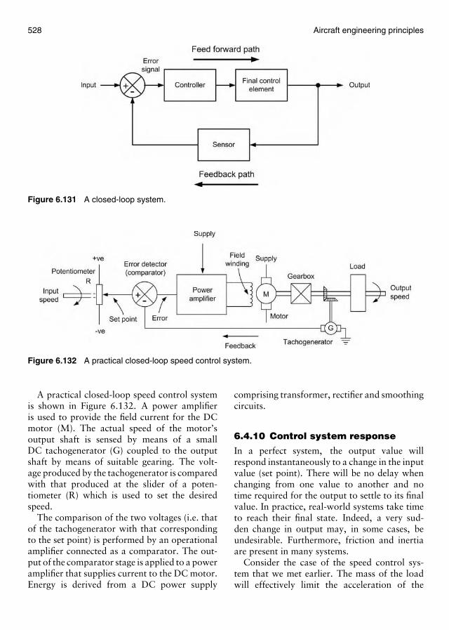
528 Aircraft engineering principles
Figure 6.131 A closed-loop system.
Figure 6.132 A practical closed-loop speed control system.
A practical closed-loop speed control systemis shown in Figure 6.132. A power amplifieris used to provide the field current for the DCmotor (M). The actual speed of the motor’soutput shaft is sensed by means of a smallDC tachogenerator (G) coupled to the outputshaft by means of suitable gearing. The volt-age produced by the tachogenerator is comparedwith that produced at the slider of a poten-tiometer (R) which is used to set the desiredspeed.
The comparison of the two voltages (i.e. thatof the tachogenerator with that correspondingto the set point) is performed by an operationalamplifier connected as a comparator. The out-put of the comparator stage is applied to a poweramplifier that supplies current to the DC motor.Energy is derived from a DC power supply
comprising transformer, rectifier and smoothingcircuits.
6.4.10 Control system response
In a perfect system, the output value willrespond instantaneously to a change in the inputvalue (set point). There will be no delay whenchanging from one value to another and notime required for the output to settle to its finalvalue. In practice, real-world systems take timeto reach their final state. Indeed, a very sud-den change in output may, in some cases, beundesirable. Furthermore, friction and inertiaare present in many systems.
Consider the case of the speed control sys-tem that we met earlier. The mass of the loadwill effectively limit the acceleration of the
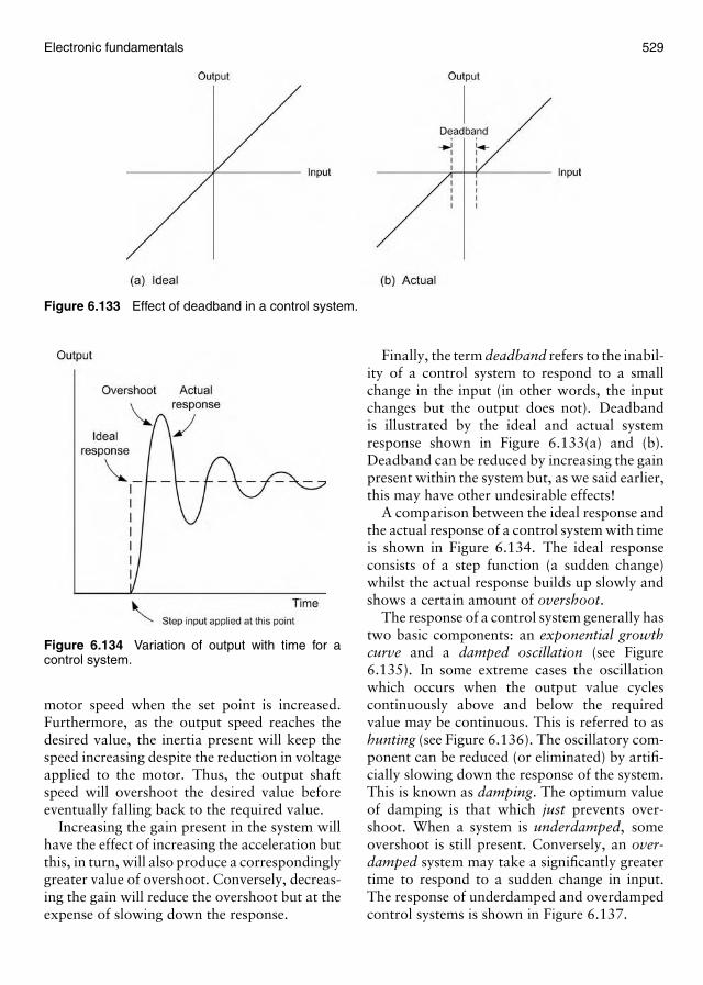
Electronic fundamentals 529
Figure 6.133 Effect of deadband in a control system.
Figure 6.134 Variation of output with time for acontrol system.
motor speed when the set point is increased.Furthermore, as the output speed reaches thedesired value, the inertia present will keep thespeed increasing despite the reduction in voltageapplied to the motor. Thus, the output shaftspeed will overshoot the desired value beforeeventually falling back to the required value.
Increasing the gain present in the system willhave the effect of increasing the acceleration butthis, in turn, will also produce a correspondinglygreater value of overshoot. Conversely, decreas-ing the gain will reduce the overshoot but at theexpense of slowing down the response.
Finally, the term deadband refers to the inabil-ity of a control system to respond to a smallchange in the input (in other words, the inputchanges but the output does not). Deadbandis illustrated by the ideal and actual systemresponse shown in Figure 6.133(a) and (b).Deadband can be reduced by increasing the gainpresent within the system but, as we said earlier,this may have other undesirable effects!
A comparison between the ideal response andthe actual response of a control system with timeis shown in Figure 6.134. The ideal responseconsists of a step function (a sudden change)whilst the actual response builds up slowly andshows a certain amount of overshoot.
The response of a control system generally hastwo basic components: an exponential growthcurve and a damped oscillation (see Figure6.135). In some extreme cases the oscillationwhich occurs when the output value cyclescontinuously above and below the requiredvalue may be continuous. This is referred to ashunting (see Figure 6.136). The oscillatory com-ponent can be reduced (or eliminated) by artifi-cially slowing down the response of the system.This is known as damping. The optimum valueof damping is that which just prevents over-shoot. When a system is underdamped, someovershoot is still present. Conversely, an over-damped system may take a significantly greatertime to respond to a sudden change in input.The response of underdamped and overdampedcontrol systems is shown in Figure 6.137.

530 Aircraft engineering principles
Figure 6.135 The two components present in the output of a typical control system.
Figure 6.136 Response of a control system show-ing hunting.
Test your understanding 6.61. Describe the operation of a servomechanism.
2. Explain the essential differences between analogueand digital control systems.
3. Identify a transducer for use in the followingapplications:
Figure 6.137 Effect of underdamping and over-damping on the response of a control system.
(a) producing a voltage that is proportional to the angleof a shaft;
(b) producing a current that depends on the incidentlight intensity;
(c) interrupting a current when the level of liquid in atank exceeds a certain value;
(d) generating heat when an electric current is applied.
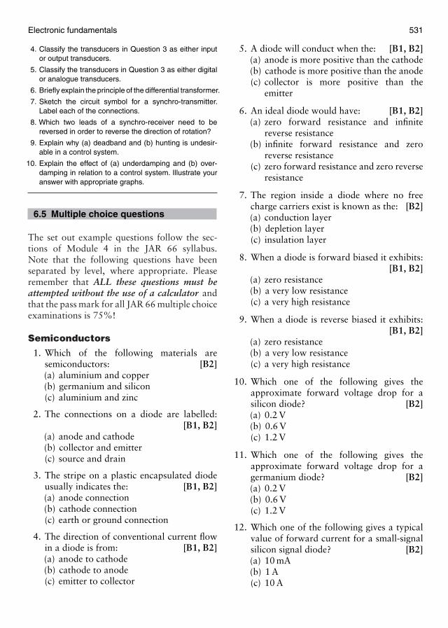
Electronic fundamentals 531
4. Classify the transducers in Question 3 as either inputor output transducers.
5. Classify the transducers in Question 3 as either digitalor analogue transducers.
6. Briefly explain the principle of the differential transformer.
7. Sketch the circuit symbol for a synchro-transmitter.Label each of the connections.
8. Which two leads of a synchro-receiver need to bereversed in order to reverse the direction of rotation?
9. Explain why (a) deadband and (b) hunting is undesir-able in a control system.
10. Explain the effect of (a) underdamping and (b) over-damping in relation to a control system. Illustrate youranswer with appropriate graphs.
6.5 Multiple choice questions
The set out example questions follow the sec-tions of Module 4 in the JAR 66 syllabus.Note that the following questions have beenseparated by level, where appropriate. Pleaseremember that ALL these questions must beattempted without the use of a calculator andthat the pass mark for all JAR 66 multiple choiceexaminations is 75%!
Semiconductors
1. Which of the following materials aresemiconductors: [B2](a) aluminium and copper(b) germanium and silicon(c) aluminium and zinc
2. The connections on a diode are labelled:[B1, B2]
(a) anode and cathode(b) collector and emitter(c) source and drain
3. The stripe on a plastic encapsulated diodeusually indicates the: [B1, B2](a) anode connection(b) cathode connection(c) earth or ground connection
4. The direction of conventional current flowin a diode is from: [B1, B2](a) anode to cathode(b) cathode to anode(c) emitter to collector
5. A diode will conduct when the: [B1, B2](a) anode is more positive than the cathode(b) cathode is more positive than the anode(c) collector is more positive than the
emitter
6. An ideal diode would have: [B1, B2](a) zero forward resistance and infinite
reverse resistance(b) infinite forward resistance and zero
reverse resistance(c) zero forward resistance and zero reverse
resistance
7. The region inside a diode where no freecharge carriers exist is known as the: [B2](a) conduction layer(b) depletion layer(c) insulation layer
8. When a diode is forward biased it exhibits:[B1, B2]
(a) zero resistance(b) a very low resistance(c) a very high resistance
9. When a diode is reverse biased it exhibits:[B1, B2]
(a) zero resistance(b) a very low resistance(c) a very high resistance
10. Which one of the following gives theapproximate forward voltage drop for asilicon diode? [B2](a) 0.2 V(b) 0.6 V(c) 1.2 V
11. Which one of the following gives theapproximate forward voltage drop for agermanium diode? [B2](a) 0.2 V(b) 0.6 V(c) 1.2 V
12. Which one of the following gives a typicalvalue of forward current for a small-signalsilicon signal diode? [B2](a) 10 mA(b) 1 A(c) 10 A
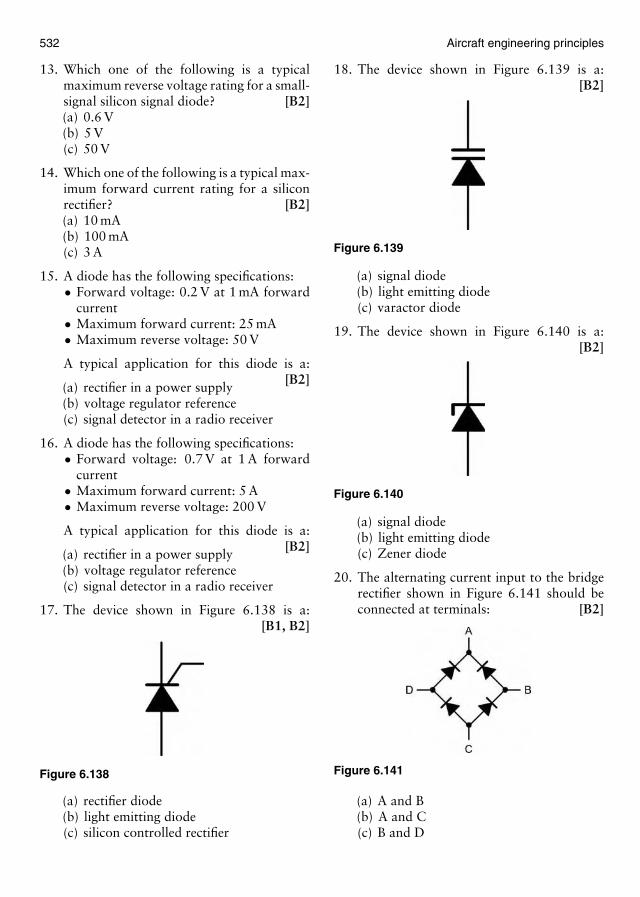
532 Aircraft engineering principles
13. Which one of the following is a typicalmaximum reverse voltage rating for a small-signal silicon signal diode? [B2](a) 0.6 V(b) 5 V(c) 50 V
14. Which one of the following is a typical max-imum forward current rating for a siliconrectifier? [B2](a) 10 mA(b) 100 mA(c) 3 A
15. A diode has the following specifications:• Forward voltage: 0.2 V at 1 mA forward
current• Maximum forward current: 25 mA• Maximum reverse voltage: 50 V
A typical application for this diode is a:[B2]
(a) rectifier in a power supply(b) voltage regulator reference(c) signal detector in a radio receiver
16. A diode has the following specifications:• Forward voltage: 0.7 V at 1 A forward
current• Maximum forward current: 5 A• Maximum reverse voltage: 200 V
A typical application for this diode is a:[B2]
(a) rectifier in a power supply(b) voltage regulator reference(c) signal detector in a radio receiver
17. The device shown in Figure 6.138 is a:[B1, B2]
Figure 6.138
(a) rectifier diode(b) light emitting diode(c) silicon controlled rectifier
18. The device shown in Figure 6.139 is a:[B2]
Figure 6.139
(a) signal diode(b) light emitting diode(c) varactor diode
19. The device shown in Figure 6.140 is a:[B2]
Figure 6.140
(a) signal diode(b) light emitting diode(c) Zener diode
20. The alternating current input to the bridgerectifier shown in Figure 6.141 should beconnected at terminals: [B2]
Figure 6.141
(a) A and B(b) A and C(c) B and D
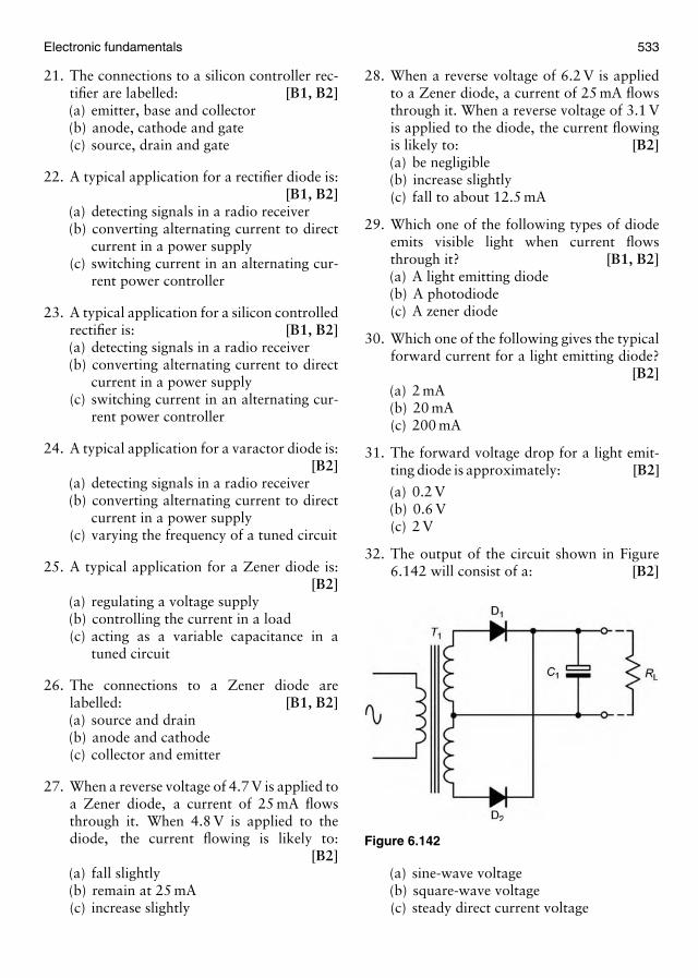
Electronic fundamentals 533
21. The connections to a silicon controller rec-tifier are labelled: [B1, B2](a) emitter, base and collector(b) anode, cathode and gate(c) source, drain and gate
22. A typical application for a rectifier diode is:[B1, B2]
(a) detecting signals in a radio receiver(b) converting alternating current to direct
current in a power supply(c) switching current in an alternating cur-
rent power controller
23. A typical application for a silicon controlledrectifier is: [B1, B2](a) detecting signals in a radio receiver(b) converting alternating current to direct
current in a power supply(c) switching current in an alternating cur-
rent power controller
24. A typical application for a varactor diode is:[B2]
(a) detecting signals in a radio receiver(b) converting alternating current to direct
current in a power supply(c) varying the frequency of a tuned circuit
25. A typical application for a Zener diode is:[B2]
(a) regulating a voltage supply(b) controlling the current in a load(c) acting as a variable capacitance in a
tuned circuit
26. The connections to a Zener diode arelabelled: [B1, B2](a) source and drain(b) anode and cathode(c) collector and emitter
27. When a reverse voltage of 4.7 V is applied toa Zener diode, a current of 25 mA flowsthrough it. When 4.8 V is applied to thediode, the current flowing is likely to:
[B2](a) fall slightly(b) remain at 25 mA(c) increase slightly
28. When a reverse voltage of 6.2 V is appliedto a Zener diode, a current of 25 mA flowsthrough it. When a reverse voltage of 3.1 Vis applied to the diode, the current flowingis likely to: [B2](a) be negligible(b) increase slightly(c) fall to about 12.5 mA
29. Which one of the following types of diodeemits visible light when current flowsthrough it? [B1, B2](a) A light emitting diode(b) A photodiode(c) A zener diode
30. Which one of the following gives the typicalforward current for a light emitting diode?
[B2](a) 2 mA(b) 20 mA(c) 200 mA
31. The forward voltage drop for a light emit-ting diode is approximately: [B2]
(a) 0.2 V(b) 0.6 V(c) 2 V
32. The output of the circuit shown in Figure6.142 will consist of a: [B2]
Figure 6.142
(a) sine-wave voltage(b) square-wave voltage(c) steady direct current voltage
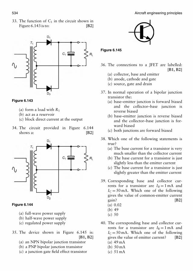
534 Aircraft engineering principles
33. The function of C1 in the circuit shown inFigure 6.143 is to: [B2]
Figure 6.143
(a) form a load with R1
(b) act as a reservoir(c) block direct current at the output
34. The circuit provided in Figure 6.144shows a: [B2]
Figure 6.144
(a) full-wave power supply(b) half-wave power supply(c) regulated power supply
35. The device shown in Figure 6.145 is:[B1, B2]
(a) an NPN bipolar junction transistor(b) a PNP bipolar junction transistor(c) a junction gate field effect transistor
Figure 6.145
36. The connections to a JFET are labelled:[B1, B2]
(a) collector, base and emitter(b) anode, cathode and gate(c) source, gate and drain
37. In normal operation of a bipolar junctiontransistor the:(a) base–emitter junction is forward biased
and the collector–base junction isreverse biased
(b) base–emitter junction is reverse biasedand the collector–base junction is for-ward biased
(c) both junctions are forward biased
38. Which one of the following statements istrue?(a) The base current for a transistor is very
much smaller than the collector current(b) The base current for a transistor is just
slightly less than the emitter current(c) The base current for a transistor is just
slightly greater than the emitter current
39. Corresponding base and collector cur-rents for a transistor are IB = 1 mA andIC = 50 mA. Which one of the followinggives the value of common-emitter currentgain? [B2](a) 0.02(b) 49(c) 50
40. The corresponding base and collector cur-rents for a transistor are IB = 1 mA andIC = 50 mA. Which one of the followinggives the value of emitter current? [B2](a) 49 mA(b) 50 mA(c) 51 mA
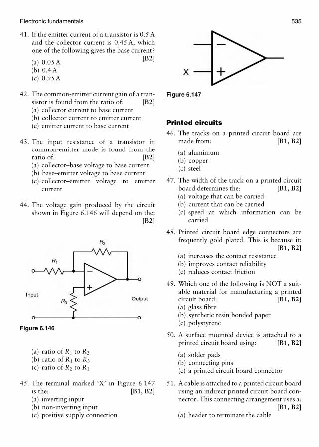
Electronic fundamentals 535
41. If the emitter current of a transistor is 0.5 Aand the collector current is 0.45 A, whichone of the following gives the base current?
[B2](a) 0.05 A(b) 0.4 A(c) 0.95 A
42. The common-emitter current gain of a tran-sistor is found from the ratio of: [B2](a) collector current to base current(b) collector current to emitter current(c) emitter current to base current
43. The input resistance of a transistor incommon-emitter mode is found from theratio of: [B2](a) collector–base voltage to base current(b) base–emitter voltage to base current(c) collector–emitter voltage to emitter
current
44. The voltage gain produced by the circuitshown in Figure 6.146 will depend on the:
[B2]
Figure 6.146
(a) ratio of R1 to R2
(b) ratio of R1 to R3
(c) ratio of R2 to R1
45. The terminal marked ‘X’ in Figure 6.147is the: [B1, B2](a) inverting input(b) non-inverting input(c) positive supply connection
Figure 6.147
Printed circuits
46. The tracks on a printed circuit board aremade from: [B1, B2]
(a) aluminium(b) copper(c) steel
47. The width of the track on a printed circuitboard determines the: [B1, B2](a) voltage that can be carried(b) current that can be carried(c) speed at which information can be
carried
48. Printed circuit board edge connectors arefrequently gold plated. This is because it:
[B1, B2](a) increases the contact resistance(b) improves contact reliability(c) reduces contact friction
49. Which one of the following is NOT a suit-able material for manufacturing a printedcircuit board: [B1, B2](a) glass fibre(b) synthetic resin bonded paper(c) polystyrene
50. A surface mounted device is attached to aprinted circuit board using: [B1, B2]
(a) solder pads(b) connecting pins(c) a printed circuit board connector
51. A cable is attached to a printed circuit boardusing an indirect printed circuit board con-nector. This connecting arrangement uses a:
[B1, B2](a) header to terminate the cable

536 Aircraft engineering principles
(b) series of soldered connections at the endof the cable
(c) number of individual crimpedconnections
Servomechanisms
52. A servo-based position control system is anexample of: [B1, B2](a) an open-loop system(b) an automatic closed-loop system(c) a system that exploits positive feedback
53. The output from a control system is usuallyreferred to as the: [B1, B2](a) set point(b) error signal(c) controlled variable
54. The input to a control system is usuallyreferred to as the: [B1, B2](a) set point(b) error signal(c) controlled variable
55. In a control system the difference betweenthe desired value and the actual value of theoutput is referred to as the: [B1, B2](a) error signal(b) demand signal(c) feedback signal
56. A signal that varies continuously from onelevel to another is called: [B1, B2](a) an error signal(b) a digital signal(c) an analogue signal
57. Digital signals vary: [B2](a) in discrete steps(b) continuously between set levels(c) slowly from one level to another level
58. In a digital control system values are rep-resented by an 8-bit code. How many dif-ferent values are possible in this system?
[B2](a) 8(b) 80(c) 256
59. A digital control system is required to havea resolution of 2%. With how many bitsshould it operate? [B2](a) 4(b) 5(c) 6
60. Which one of the following is an inputtransducer? [B1, B2](a) An actuator(b) A motor(c) A potentiometer
61. Which one of the following is an outputtransducer? [B1, B2](a) A heater(b) A photodiode(c) A potentiometer
62. A target modifies the electric field generatedby a sensor. This is the principle of the:
[B1, B2](a) optical proximity sensor(b) inductive proximity sensor(c) capacitive proximity sensor
63. A foil element with polyester backing isresin bonded to mechanical component.This is the principle of the: [B1, B2](a) resistive strain gauge(b) inductive strain gauge(c) capacitive strain gauge
64. Which one of the following sensor producesa digital output? [B2](a) Magnetic reed switch(b) Piezoelectric strain gauge(c) Light-dependent resistor
65. Which one of the following is an activesensor? [B1, B2](a) Tachogenerator(b) Resistive strain gauge(c) Light-dependent resistor
66. Minimum flux linkage will occur when twocoils are aligned at a relative angle of:
[B1, B2](a) 0◦(b) 45◦(c) 90◦
Electronic fundamentals 537
67. A differential transformer is made from:[B2]
(a) U- and I-laminations(b) E- and I-laminations(c) E- and H-laminations
68. The reference voltage in a differential trans-former is applied to a winding on: [B2](a) the center limb of the E-lamination(b) all three limbs of the E-laminations(c) one of the outer limbs of the E-
lamination
69. The laminations of a differential trans-former are usually made from: [B2](a) ceramic material(b) low permeability steel(c) high permeability steel
70. Identical root mean square voltages of26 V are measured across each of the sec-ondary windings of a differential trans-former. Which one of the following givesthe value of output voltage produced by thetransformer? [B2](a) 0 V(b) 26 V(c) 52 V
71. A synchro-transmitter is sometimes alsoreferred to as a: [B1, B2](a) linear transformer(b) variable transformer(c) differential transformer
72. How many stator connections are there in asynchro-transmitter? [B1, B2](a) 1(b) 2(c) 3
73. The alternating current supply to a synchro-transmitter is connected to the connectionsmarked: [B1, B2](a) R1 and R2
(b) S1 and S2
(c) S1, S2 and S3
74. A synchro-resolver has multiple rotor andstator windings spaced by: [B1, B2]
(a) 45◦(b) 90◦(c) 120◦
75. A conventional synchro-transmitter has sta-tor windings spaced by: [B1, B2](a) 45◦(b) 90◦(c) 120◦
76. When a synchro-transmitter and -receiversystem are in correspondence the current inthe stator windings will: [B1, B2](a) be zero(b) take a maximum value(c) be equal to the supply current
77. Which two synchro-leads should be reversedin order to reverse the direction of asynchro-receiver relative to a synchro-transmitter? [B2](a) R1 and R2
(b) S1 and S2
(c) S1 and S3
78. An open-loop control system is one inwhich: [B1, B2](a) no feedback is applied(b) positive feedback is applied(c) negative feedback is applied
79. A closed-loop control system is one inwhich: [B1, B2](a) no feedback is applied(b) positive feedback is applied(c) negative feedback is applied
80. In a closed-loop system the error signal canbe produced by: [B1, B2](a) an amplifier(b) a comparator(c) a tachogenerator
81. The range of outputs close to the zero pointthat a control system is unable to respondto is referred to as: [B2](a) hunting(b) deadband(c) overshoot

538 Aircraft engineering principles
82. Overshoot in a control system can bereduced by: [B2](a) increasing the gain(b) reducing the damping(c) increasing the damping
83. The output of a control system cycles con-tinuously above and below the required
value. This characteristic is known as:[B2]
(a) hunting(b) deadband(c) overshoot
P A R T4
Fundamentals ofaerodynamics

This page intentionally left blank
C h a p t e r
7Basic aerodynamics
7.1 Introduction
This chapter serves as an introduction to thestudy of aerodynamics. It covers in full allrequisite knowledge needed for the successfulstudy and completion of Basic aerodynamicsas laid down in Module 8 of the Joint AviationRequirements (JAR) 66 syllabus. The study ofelementary flight theory in this module formsan essential part of the knowledge needed forall potential practicing aircraft engineers, nomatter what their trade specialization. In partic-ular, there is a need for engineers to understandhow aircraft produce lift and how they arecontrolled and stabilized for flight. This knowl-edge will then assist engineers with their futureunderstanding of aircraft control systems andthe importance of the design features that areneeded to stabilize aircraft during all phases offlight.
In addition, recognition of the effects of care-less actions on aircraft aerodynamic performanceand the need to care for surface finish andstreamlining features will also be appreciatedthrough the knowledge gained from your studyof this module.
Our study of aerodynamics starts with a briefreminder of the important topics covered previ-ously when you considered the atmosphere andatmospheric physics. The nature and purposeof the International Standard Atmosphere (ISA)will be looked at again. We will also be draw-ing on your knowledge of fluids in motion forthe effects of airflow over aircraft and in orderto demonstrate the underlying physical princi-ples that account for the creation of aircraft liftand drag. We look in detail at the lift generatedby aerofoil sections and the methods adopted tomaximize the lift created by such lift producingsurfaces. Aircraft flight forces (lift, drag, thrustand weight) are then studied in some detailincluding their interrelationship during steady
state flight and during manoeuvres. The effectsand limitations of flight loads on the aircraftstructure will also be considered, as well as theeffects of aerofoil contamination, by such thingsas ice accretion.
Once the concepts of aircraft flight forces andperformance have been covered, we will con-sider the ways in which aircraft are controlledand stabilized and the relationship between air-craft control and stability. In addition to theprimary flight controls, we will briefly look atsecondary devices, including the methods usedto augment lift and dump lift when necessary.Only manual controls will be considered at thisstage, although the need for powered flightcontrol devices and systems will be mentioned.
Note: the study of flight control and basic con-trol devices does not form a part of Module 8,but is covered here for the sake of completeness.In particular, it will be found especially helpfulwhen we consider flight stability.
Full coverage of aircraft flight control, con-trol devices and high speed flight theory willbe found in the third book in the series Air-craft Aerodynamics, Structural Maintenanceand Repair , which is primarily aimed at thosepursuing a mechanical pathway. For thoseindividuals pursuing an avionic pathway, theappropriate aircraft aerodynamics and controlwill be covered in fifth book in the serieson Avionic Systems, which will essentially bedesigned to cover JAR 66 Module 13.
7.2 A review of atmospheric physics
You should have already covered in some detailthe nature of the atmosphere in your study ofPhysics. In particular, you should look back(pages 247–251) and remind yourself of thegas laws, the temperature, pressure and den-sity relationships, the variation of the air withaltitude and the need for the ISA. For your
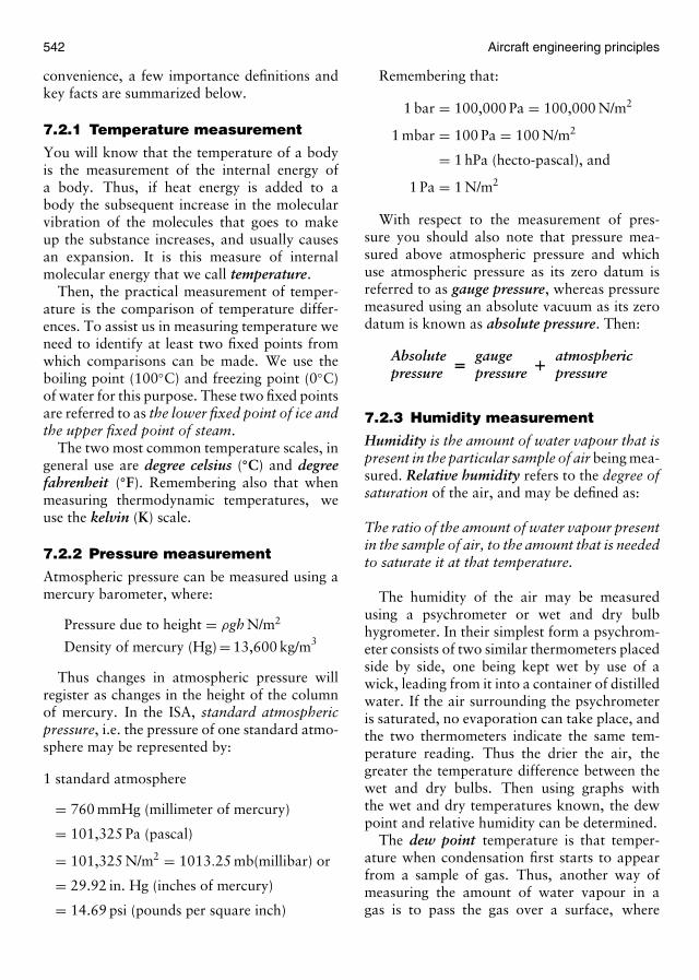
542 Aircraft engineering principles
convenience, a few importance definitions andkey facts are summarized below.
7.2.1 Temperature measurement
You will know that the temperature of a bodyis the measurement of the internal energy ofa body. Thus, if heat energy is added to abody the subsequent increase in the molecularvibration of the molecules that goes to makeup the substance increases, and usually causesan expansion. It is this measure of internalmolecular energy that we call temperature.
Then, the practical measurement of temper-ature is the comparison of temperature differ-ences. To assist us in measuring temperature weneed to identify at least two fixed points fromwhich comparisons can be made. We use theboiling point (100◦C) and freezing point (0◦C)of water for this purpose. These two fixed pointsare referred to as the lower fixed point of ice andthe upper fixed point of steam.
The two most common temperature scales, ingeneral use are degree celsius (◦C) and degreefahrenheit (◦F). Remembering also that whenmeasuring thermodynamic temperatures, weuse the kelvin (K) scale.
7.2.2 Pressure measurement
Atmospheric pressure can be measured using amercury barometer, where:
Pressure due to height = ρgh N/m2
Density of mercury (Hg) = 13,600 kg/m3
Thus changes in atmospheric pressure willregister as changes in the height of the columnof mercury. In the ISA, standard atmosphericpressure, i.e. the pressure of one standard atmo-sphere may be represented by:
1 standard atmosphere
= 760 mmHg (millimeter of mercury)
= 101,325 Pa (pascal)
= 101,325 N/m2 = 1013.25 mb(millibar) or
= 29.92 in. Hg (inches of mercury)
= 14.69 psi (pounds per square inch)
Remembering that:
1 bar = 100,000 Pa = 100,000 N/m2
1 mbar = 100 Pa = 100 N/m2
= 1 hPa (hecto-pascal), and
1 Pa = 1 N/m2
With respect to the measurement of pres-sure you should also note that pressure mea-sured above atmospheric pressure and whichuse atmospheric pressure as its zero datum isreferred to as gauge pressure, whereas pressuremeasured using an absolute vacuum as its zerodatum is known as absolute pressure. Then:
Absolutepressure = gauge
pressure + atmosphericpressure
7.2.3 Humidity measurement
Humidity is the amount of water vapour that ispresent in the particular sample of air being mea-sured. Relative humidity refers to the degree ofsaturation of the air, and may be defined as:
The ratio of the amount of water vapour presentin the sample of air, to the amount that is neededto saturate it at that temperature.
The humidity of the air may be measuredusing a psychrometer or wet and dry bulbhygrometer. In their simplest form a psychrom-eter consists of two similar thermometers placedside by side, one being kept wet by use of awick, leading from it into a container of distilledwater. If the air surrounding the psychrometeris saturated, no evaporation can take place, andthe two thermometers indicate the same tem-perature reading. Thus the drier the air, thegreater the temperature difference between thewet and dry bulbs. Then using graphs withthe wet and dry temperatures known, the dewpoint and relative humidity can be determined.
The dew point temperature is that temper-ature when condensation first starts to appearfrom a sample of gas. Thus, another way ofmeasuring the amount of water vapour in agas is to pass the gas over a surface, where

Basic aerodynamics 543
the temperature is gradually lowered, until themoisture from the gas starts to condense on thesurface. The “dew point” temperature is thenread off. The relative humidity is then obtainedby comparing the dew point temperature of thegas sample with its saturation temperature.
7.2.4 Density ratio and airspeed
The relationship between the density at sea levelin the ISA and the density at altitude, the densityratio σ has a special significance. It is used in thecalibration of pitot–static instruments to convertequivalent airspeed (EAS) to true airspeed (TAS)or vice versa, and is defined as:
σ = density at altitude (ρa)density at sea level (ρsl)in the ISA
Before we look at the relationship connectingEAS and TAS, it is first, worth defining threeimportant airspeeds:
• Indicated airspeed (IAS) is that speed shownby a simple airspeed indicator (ASI).
• Equivalent airspeed (EAS) is that speed thatwould be shown by an error-free ASI.
• True airspeed (TAS) is the actual speed of anaircraft relative to the air.
Much more will be said about aircraft pitot–static instruments, in a later volume in the series,for now we will define the simple relationshipconnecting EAS and TAS:
EAS = TAS√
σ or
VE = VT√
σ or VE = VT
√ρa
ρsl
Example 7.1
Given that an error-free ASI registers an EASof 220 m/s at an altitude where the density is0.885 kg/m3, determine the TAS of the aircraftat this altitude assuming that the aircraft flies instill air.
Remembering that sea level density in the ISAis 1.2256 kg/m3, then the density ratio:
σ = 0.8851.2256
= 0.7221
Therefore from the relationship given above:
VT = VE√σ
we find that
VT = 220√0.7221
= 2200.8498
= 258.9 m/s
You should also note that the density ratioσ = 1.0 at sea level, therefore, from the aboverelationship VE = VT.
7.2.5 Changes in the air withincreasing altitude• Static pressure decreases with altitude, but not
in a linear manner.• Air density which is proportional to pressure
also decreases, but at a different rate, to thatof pressure.
• Temperature also decreases with altitude, therate of decrease is linear, in the troposphereand may be found from the relationship:Th = T0 − Lh, in the ISA.
7.2.6 The International Civil AviationOrganization ISA
As you already know, the International CivilAviation Organization (ICAO) standard atmo-sphere as defined in ICAO document 7488/2 laysdown an arbitrary set of conditions, acceptedby the international community, as a basis forcomparison of aircraft and engine performanceparameters and for the calibration of aircraftinstruments.
The conditions adopted have been based onthose observed in a temperate climate at alatitude of 40◦ North up to an altitude of105,000 ft.
The principle conditions assumed in the ISAare summarized below for your convenience.
• Temperature 288.15 K or 15.15◦C• Pressure 1013.25 mb or 101,325 N/m2
• Density 1.2256 kg/m2
• Speed of sound 340.3 m/s• Gravitational acceleration 9.80665 m/s2
• Dynamic viscosity 1.789 × 10⁻⁵ N s/m2

544 Aircraft engineering principles
Figure 7.1 The ICAO standard atmosphere.
• Temperature lapse rate 6.5 K/km or 6.5◦C/km• Tropopause 11,000 m, 56.5◦C or 216.5 K
Note the following Imperial equivalents, whichare often quoted:
• Pressure 14.69 lb/in.2
• Speed of sound 1120 ft/s• Temperature lapse rate 1.98◦C per 1000 ft• Tropopause 36,090 ft• Stratopause 105,000 ft.
The changes in ICAO standard atmospherewith altitude are illustrated in Figure 7.1.Note that the temperature in the upper
stratosphere starts to rise again after 65,000 ftat a rate of 0.303◦C per 1000 ft or 0.994◦C per1000 m. At a height of 105,000 ft or approxi-mately 32,000 m, the chemosphere is deemed tobegin. The chemosphere is the collective namefor mesosphere, thermosphere and exosphere,which was previously identified, in atmosphericphysics.
Example 7.2
Find the temperature at an altitude of 6400 mand 18,000 ft in the ISA.
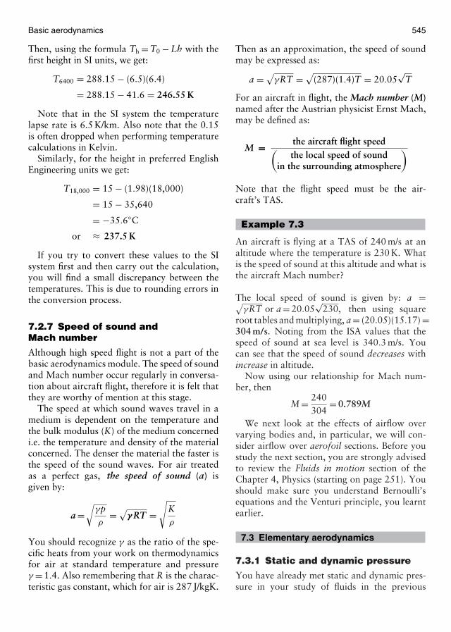
Basic aerodynamics 545
Then, using the formula Th = T0 − Lh with thefirst height in SI units, we get:
T6400 = 288.15 − (6.5)(6.4)
= 288.15 − 41.6 = 246.55 K
Note that in the SI system the temperaturelapse rate is 6.5 K/km. Also note that the 0.15is often dropped when performing temperaturecalculations in Kelvin.
Similarly, for the height in preferred EnglishEngineering units we get:
T18,000 = 15 − (1.98)(18,000)
= 15 − 35,640
= −35.6◦C
or ≈ 237.5 K
If you try to convert these values to the SIsystem first and then carry out the calculation,you will find a small discrepancy between thetemperatures. This is due to rounding errors inthe conversion process.
7.2.7 Speed of sound andMach number
Although high speed flight is not a part of thebasic aerodynamics module. The speed of soundand Mach number occur regularly in conversa-tion about aircraft flight, therefore it is felt thatthey are worthy of mention at this stage.
The speed at which sound waves travel in amedium is dependent on the temperature andthe bulk modulus (K) of the medium concernedi.e. the temperature and density of the materialconcerned. The denser the material the faster isthe speed of the sound waves. For air treatedas a perfect gas, the speed of sound (a) isgiven by:
a =√
γpρ
= √γ RT =
√Kρ
You should recognize γ as the ratio of the spe-cific heats from your work on thermodynamicsfor air at standard temperature and pressureγ = 1.4. Also remembering that R is the charac-teristic gas constant, which for air is 287 J/kgK.
Then as an approximation, the speed of soundmay be expressed as:
a = √γRT = √
(287)(1.4)T = 20.05√
T
For an aircraft in flight, the Mach number (M)named after the Austrian physicist Ernst Mach,may be defined as:
M = the aircraft flight speed(the local speed of sound
in the surrounding atmosphere
)
Note that the flight speed must be the air-craft’s TAS.
Example 7.3
An aircraft is flying at a TAS of 240 m/s at analtitude where the temperature is 230 K. Whatis the speed of sound at this altitude and what isthe aircraft Mach number?
The local speed of sound is given by: a =√γRT or a = 20.05
√230, then using square
root tables and multiplying, a = (20.05)(15.17) =304 m/s. Noting from the ISA values that thespeed of sound at sea level is 340.3 m/s. Youcan see that the speed of sound decreases withincrease in altitude.
Now using our relationship for Mach num-ber, then
M = 240304
= 0.789M
We next look at the effects of airflow overvarying bodies and, in particular, we will con-sider airflow over aerofoil sections. Before youstudy the next section, you are strongly advisedto review the Fluids in motion section of theChapter 4, Physics (starting on page 251). Youshould make sure you understand Bernoulli’sequations and the Venturi principle, you learntearlier.
7.3 Elementary aerodynamics
7.3.1 Static and dynamic pressure
You have already met static and dynamic pres-sure in your study of fluids in the previous

546 Aircraft engineering principles
chapter. Look back now at the energy andpressure versions of the Bernoulli’s equation inpage 253.
I hope you can see that a fluid in steadymotion has both static pressure energy anddynamic pressure energy (kinetic energy) due tothe motion. All Bernoulli’s equation showed wasthat for an ideal fluid.
The total energy in a steady streamline flowremains constant.
Staticpressureenergy
+dynamic(kinetic)energy
=constanttotalenergy
or in symbols:
p + 12ρv2 = C
In particular, you should note that with respectto aerodynamics, the dynamic pressure isdependent on the density of the air (treated as anideal fluid) and the velocity of the air. Thus, withincrease in altitude, there is a drop in densityand the dynamic pressure acting on the aircraftas a result of the airflow, will also drop withincrease in altitude. The static pressure of theair also drops with increase in altitude.
You have already met an application of theBernoulli’s equation when we considered theVenturi tube in our earlier studies of fluids inmotion; where from the above Bernoulli’s equa-tion, use was made of the fact that to maintainequality:
An increase in velocity will mean a decreasein static pressure, or alternatively, a decreasein velocity will mean an increase in staticpressure.
The above fact is key to the way aircraft wingsections create lift, as you will see later.
7.3.2 Subsonic airflow
Flow over a flat plateWhen a body is moved through the air, or anyfluid that has viscosity, such as water, there is aresistance produced which tends to oppose thebody. For example, if you are driving in an opentop car, there is a resistance from the air act-ing in the opposite direction to the motion of
the car. This air resistance can be felt on yourface or hands as you travel. In the aeronauticalworld, this air resistance is known as drag. It isundesirable for obvious reasons. For example,aircraft engine power is required to overcomethis air resistance and unwanted heat is gener-ated by friction as the air flows over the aircrafthull during flight.
We consider the effect of air resistance bystudying the behaviour of airflow over a flatplate. If a flat plate is placed edge on to the rela-tive airflow (Figure 7.2), then there is little or noalteration to the smooth passage of air over it.On the other hand, if the plate is offered into theairflow at some angle of inclination to it angle ofattack (AOA), it will experience a reaction thattends to both lift it and drag it back. This is thesame effect that you can feel on your hand whenplaced into the airflow as you are travelling, e.g.in the open topped car mentioned earlier. Theamount of reaction depends upon the speed andAOA between the flat plate and relative airflow.
As can be seen in Figure 7.2, when the flatplate is inclined at some AOA to the relative air-flow, the streamlines are disturbed. An upwashis created at the front edge of the plate causingthe air to flow through a more constricted area,in a similar manner to flow through the throatof a Venturi meter. The net result is that as theairflows through this restricted area, it speedsup. This in turn causes a drop in static pressureabove the plate (Bernoulli) when compared withthe static pressure beneath it resulting in a netupward reaction. After passing the plate, thereis a resulting downwash of the air stream.
The total reaction on the plate caused by itdisturbing the relative airflow has two vectorcomponents as shown in Figure 7.3. One atright angles to the relative airflow known aslift and the other parallel to the relative airflow,opposing the motion, known as drag.
The above drag force is the same as that men-tioned earlier, which caused a resistance to theflow of the air stream, over your hand.
Streamline flow, laminar flow andturbulent flowStreamline flow, sometimes referred to as vis-cous flow, is flow in which the particles of the
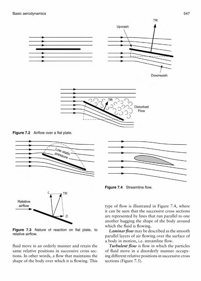
Basic aerodynamics 547
Figure 7.2 Airflow over a flat plate.
Figure 7.3 Nature of reaction on flat plate, torelative airflow.
fluid move in an orderly manner and retain thesame relative positions in successive cross sec-tions. In other words, a flow that maintains theshape of the body over which it is flowing. This
Figure 7.4 Streamline flow.
type of flow is illustrated in Figure 7.4, whereit can be seen that the successive cross sectionsare represented by lines that run parallel to oneanother hugging the shape of the body aroundwhich the fluid is flowing.
Laminar flow may be described as the smoothparallel layers of air flowing over the surface ofa body in motion, i.e. streamline flow.
Turbulent flow is flow in which the particlesof fluid move in a disorderly manner occupy-ing different relative positions in successive crosssections (Figure 7.5).

548 Aircraft engineering principles
Figure 7.5 Turbulent flow.
Figure 7.6 Airflow over an aerofoil section.
This motion results in the airflow thickeningconsiderably and breaking-up.
7.3.3 The aerofoil
In its simplest sense an aerofoil section maybe defined as that profile designed to obtain adesirable reaction from the air through whichit moves. In other words, an aerofoil is able toconvert air resistance into a useful force thatproduces lift for flight.
The cross-section of an aircraft wing, is a goodexample of an aerofoil section, where the topsurface usually has greater curvature than thebottom surface.
The air travelling over the cambered top sur-face of the aerofoil shown in Figure 7.6, which issplit as it passes around the aerofoil, will speedup, because it must reach the trailing edge of theaerofoil at the same time as the air that flowsunderneath the section. In doing so, there mustbe a decrease in the pressure of the airflow overthe top surface that results from its increase invelocity (Bernoulli).
Another way to think of it is to imagine thatthe top half of the aerofoil surface shown in
Figure 7.7 Top surface of aerofoil acting asbottom-half of a Venturi tube.
Figure 7.6 is in fact the bottom half of a Venturetube (Figure 7.7). Then, as the airflow passesthrough the restriction, there will be a corre-sponding increase in the speed of the airflow, ina similar manner to that created by the upwashfor a flat plate mentioned earlier.
Then again from Bernoulli’ equation, thisincrease in speed causes a correspondingdecrease in static pressure, as shown, which overthe surface of the aerofoil, will create the desiredlift force.
Aerofoil terminologyWe have started to talk about such terms as:camber, trailing edge and AOA without defin-ing them fully. Set out below are a few usefulterms and definitions about airflow and aerofoilsections that will be used frequently throughoutthe remainder of this chapter.
Camber is the term used for the upper andlower curved surfaces of the aerofoil section.Where the mean camber line is that line drawnhalfway between the upper and lower cambers.
Chord line is the line joining the centers ofcurvatures of the leading and trailing edges.Note that this line may fall outside the aerofoilsection dependent on the amount of camber ofthe aerofoil being considered.
Leading and trailing edge are those points onthe center of curvature of the leading and trailingpart of the aerofoil section that intersect with thechord line as shown in Figure 7.8
Angle of incidence (AOI) is the angle betweenthe relative airflow and the longitudinal axisof the aircraft. It is a built-in feature of theaircraft and is a fixed “rigging angle”. Onconventional aircraft, the AOI is designed tominimize drag during cruise thus maximizingfuel consumption!
Angle of attack (AOA) is the angle betweenthe chord line and the relative airflow. This will
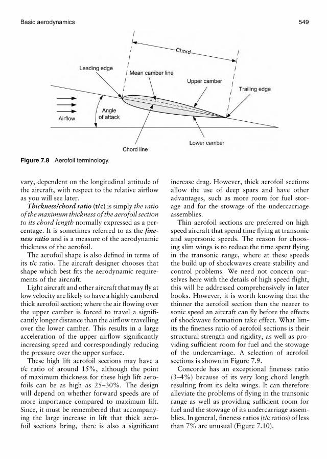
Basic aerodynamics 549
Figure 7.8 Aerofoil terminology.
vary, dependent on the longitudinal attitude ofthe aircraft, with respect to the relative airflowas you will see later.
Thickness/chord ratio (t/c) is simply the ratioof the maximum thickness of the aerofoil sectionto its chord length normally expressed as a per-centage. It is sometimes referred to as the fine-ness ratio and is a measure of the aerodynamicthickness of the aerofoil.
The aerofoil shape is also defined in terms ofits t/c ratio. The aircraft designer chooses thatshape which best fits the aerodynamic require-ments of the aircraft.
Light aircraft and other aircraft that may fly atlow velocity are likely to have a highly camberedthick aerofoil section; where the air flowing overthe upper camber is forced to travel a signifi-cantly longer distance than the airflow travellingover the lower camber. This results in a largeacceleration of the upper airflow significantlyincreasing speed and correspondingly reducingthe pressure over the upper surface.
These high lift aerofoil sections may have at/c ratio of around 15%, although the pointof maximum thickness for these high lift aero-foils can be as high as 25–30%. The designwill depend on whether forward speeds are ofmore importance compared to maximum lift.Since, it must be remembered that accompany-ing the large increase in lift that thick aero-foil sections bring, there is also a significant
increase drag. However, thick aerofoil sectionsallow the use of deep spars and have otheradvantages, such as more room for fuel stor-age and for the stowage of the undercarriageassemblies.
Thin aerofoil sections are preferred on highspeed aircraft that spend time flying at transonicand supersonic speeds. The reason for choos-ing slim wings is to reduce the time spent flyingin the transonic range, where at these speedsthe build up of shockwaves create stability andcontrol problems. We need not concern our-selves here with the details of high speed flight,this will be addressed comprehensively in laterbooks. However, it is worth knowing that thethinner the aerofoil section then the nearer tosonic speed an aircraft can fly before the effectsof shockwave formation take effect. What lim-its the fineness ratio of aerofoil sections is theirstructural strength and rigidity, as well as pro-viding sufficient room for fuel and the stowageof the undercarriage. A selection of aerofoilsections is shown in Figure 7.9.
Concorde has an exceptional fineness ratio(3–4%) because of its very long chord lengthresulting from its delta wings. It can thereforealleviate the problems of flying in the transonicrange as well as providing sufficient room forfuel and the stowage of its undercarriage assem-blies. In general, fineness ratios (t/c ratios) of lessthan 7% are unusual (Figure 7.10).
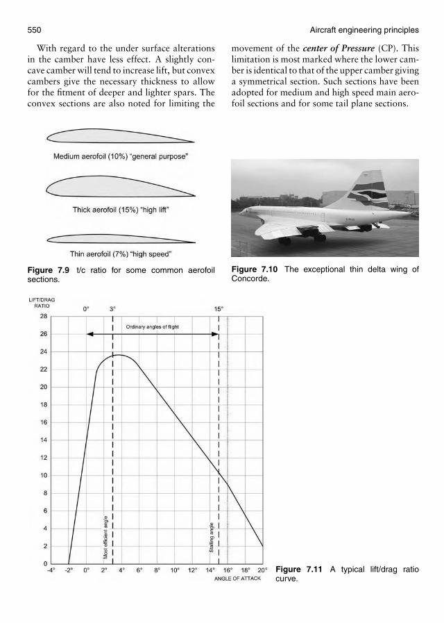
550 Aircraft engineering principles
With regard to the under surface alterationsin the camber have less effect. A slightly con-cave camber will tend to increase lift, but convexcambers give the necessary thickness to allowfor the fitment of deeper and lighter spars. Theconvex sections are also noted for limiting the
Figure 7.9 t/c ratio for some common aerofoilsections.
Figure 7.11 A typical lift/drag ratiocurve.
movement of the center of Pressure (CP). Thislimitation is most marked where the lower cam-ber is identical to that of the upper camber givinga symmetrical section. Such sections have beenadopted for medium and high speed main aero-foil sections and for some tail plane sections.
Figure 7.10 The exceptional thin delta wing ofConcorde.
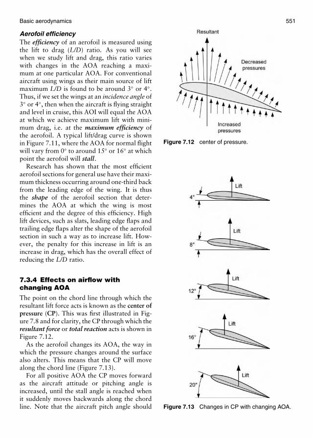
Basic aerodynamics 551
Aerofoil efficiencyThe efficiency of an aerofoil is measured usingthe lift to drag (L/D) ratio. As you will seewhen we study lift and drag, this ratio varieswith changes in the AOA reaching a maxi-mum at one particular AOA. For conventionalaircraft using wings as their main source of liftmaximum L/D is found to be around 3◦ or 4◦.Thus, if we set the wings at an incidence angle of3◦ or 4◦, then when the aircraft is flying straightand level in cruise, this AOI will equal the AOAat which we achieve maximum lift with mini-mum drag, i.e. at the maximum efficiency ofthe aerofoil. A typical lift/drag curve is shownin Figure 7.11, where the AOA for normal flightwill vary from 0◦ to around 15◦ or 16◦ at whichpoint the aerofoil will stall.
Research has shown that the most efficientaerofoil sections for general use have their maxi-mum thickness occurring around one-third backfrom the leading edge of the wing. It is thusthe shape of the aerofoil section that deter-mines the AOA at which the wing is mostefficient and the degree of this efficiency. Highlift devices, such as slats, leading edge flaps andtrailing edge flaps alter the shape of the aerofoilsection in such a way as to increase lift. How-ever, the penalty for this increase in lift is anincrease in drag, which has the overall effect ofreducing the L/D ratio.
7.3.4 Effects on airflow withchanging AOA
The point on the chord line through which theresultant lift force acts is known as the center ofpressure (CP). This was first illustrated in Fig-ure 7.8 and for clarity, the CP through which theresultant force or total reaction acts is shown inFigure 7.12.
As the aerofoil changes its AOA, the way inwhich the pressure changes around the surfacealso alters. This means that the CP will movealong the chord line (Figure 7.13).
For all positive AOA the CP moves forwardas the aircraft attitude or pitching angle isincreased, until the stall angle is reached whenit suddenly moves backwards along the chordline. Note that the aircraft pitch angle should
Figure 7.12 center of pressure.
Figure 7.13 Changes in CP with changing AOA.
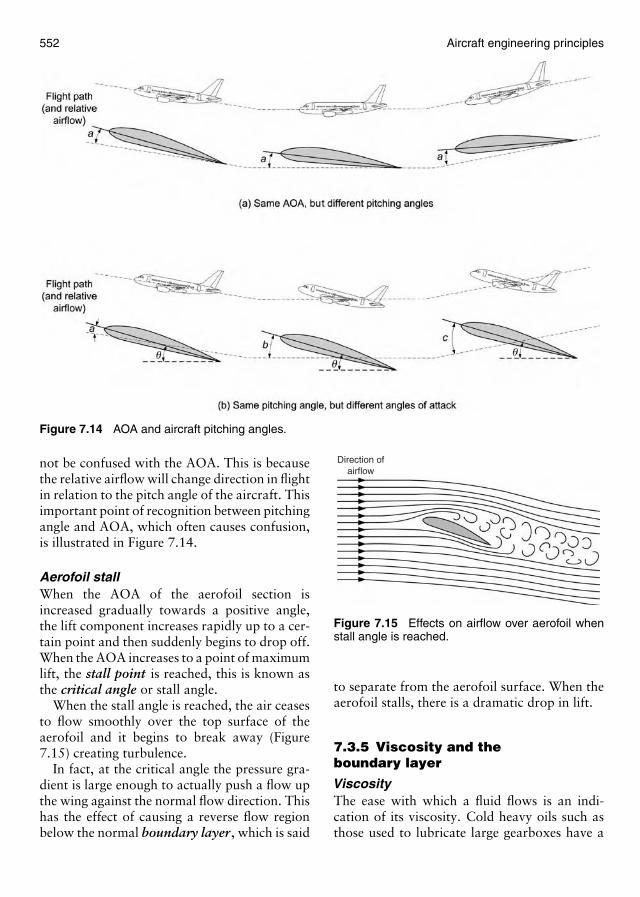
552 Aircraft engineering principles
Figure 7.14 AOA and aircraft pitching angles.
not be confused with the AOA. This is becausethe relative airflow will change direction in flightin relation to the pitch angle of the aircraft. Thisimportant point of recognition between pitchingangle and AOA, which often causes confusion,is illustrated in Figure 7.14.
Aerofoil stallWhen the AOA of the aerofoil section isincreased gradually towards a positive angle,the lift component increases rapidly up to a cer-tain point and then suddenly begins to drop off.When the AOA increases to a point of maximumlift, the stall point is reached, this is known asthe critical angle or stall angle.
When the stall angle is reached, the air ceasesto flow smoothly over the top surface of theaerofoil and it begins to break away (Figure7.15) creating turbulence.
In fact, at the critical angle the pressure gra-dient is large enough to actually push a flow upthe wing against the normal flow direction. Thishas the effect of causing a reverse flow regionbelow the normal boundary layer , which is said
Direction ofairflow
Figure 7.15 Effects on airflow over aerofoil whenstall angle is reached.
to separate from the aerofoil surface. When theaerofoil stalls, there is a dramatic drop in lift.
7.3.5 Viscosity and theboundary layer
ViscosityThe ease with which a fluid flows is an indi-cation of its viscosity. Cold heavy oils such asthose used to lubricate large gearboxes have a
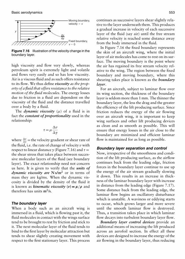
Basic aerodynamics 553
y
Moving boundary,velocity � v
Fixed boundary,v � 0
dvdy
Figure 7.16 Illustration of the velocity change in theboundary layer.
high viscosity and flow very slowly, whereaspetroleum spirit is extremely light and volatileand flows very easily and so has low viscosity.Air is a viscous fluid and as such offers resistanceto its flow. We thus define viscosity as the prop-erty of a fluid that offers resistance to the relativemotion of the fluid molecules. The energy lossesdue to friction in a fluid are dependent on theviscosity of the fluid and the distance travelledover a body by a fluid.
The dynamic viscosity (µ) of a fluid is infact the constant of proportionality used in therelationship:
τ = µ�v�y
where �v�y = the velocity gradient or shear rate of
the fluid, i.e. the rate of change of velocity v withrespect to linear distance y (Figure 7.16) and τ =the shear stress that takes place between succes-sive molecular layers of the fluid (see boundarylayer). The exact relationship need not concernus here. It is given to verify that the units ofdynamic viscosity are N s/m2 or in terms ofmass they are kg/ms. When the dynamic vis-cosity is divided by the density of the fluid itis known as kinematic viscosity (v) = µ/ρ andtherefore has units m2/s.
The boundary layerWhen a body such as an aircraft wing isimmersed in a fluid, which is flowing past it, thefluid molecules in contact with the wings surfacetend to be brought to rest by friction and stick toit. The next molecular layer of the fluid tends tobind to the first layer by molecular attraction buttends to shear slightly creating movement withrespect to the first stationary layer. This process
continues as successive layers shear slightly rela-tive to the layer underneath them. This producesa gradual increase in velocity of each successivelayer of the fluid (say air) until the free streamrelative velocity is reached some distance awayfrom the body immersed in the fluid.
In Figure 7.16 the fixed boundary representsthe skin of an aircraft wing, where the initiallayer of air molecules has come to rest on its sur-face. The moving boundary is the point wherethe air has regained its free stream velocity rel-ative to the wing. The region between the fixedboundary and moving boundary, where thisshearing takes place is known as the boundarylayer .
For an aircraft, subject to laminar flow overits wing section, the thickness of the boundarylayer is seldom more than 1 mm. The thinner theboundary layer, the less the drag and the greaterthe efficiency of the lift producing surface. Sincefriction reduces the energy of the air flowingover an aircraft wing, it is important to keepwing surfaces and other lift producing devicesas clean and as smooth as possible. This willensure that energy losses in the air close to theboundary are minimized and efficient laminarflow is maintained for as long as possible.
Boundary layer separation and controlNow, irrespective of the smoothness and condi-tion of the lift producing surface, as the airflowcontinues back from the leading edge, frictionforces in the boundary layer continue to use upthe energy of the air stream gradually slowingit down. This results in an increase in thick-ness of the laminar boundary layer with increasein distance from the leading edge (Figure 7.17).Some distance back from the leading edge, thelaminar flow begins an oscillatory disturbancewhich is unstable. A waviness or eddying startsto occur, which grows larger and more severeuntil the smooth laminar flow is destroyed.Thus, a transition takes place in which laminarflow decays into turbulent boundary layer flow.
Boundary layer control devices provide anadditional means of increasing the lift producedacross an aerofoil section. In effect all thesedevices are designed to increase the energy of theair flowing in the boundary layer, thus reducing
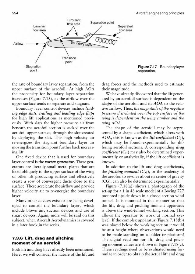
554 Aircraft engineering principles
Figure 7.17 Boundary layerseparation.
the rate of boundary layer separation, from theupper surface of the aerofoil. At high AOAthe propensity for boundary layer separationincreases (Figure 7.15), as the airflow over theupper surface tends to separate and stagnate.
Boundary layer control devices include lead-ing edge slats, trailing and leading edge flapsfor high lift applications as mentioned previ-ously. With slats the higher pressure air frombeneath the aerofoil section is sucked over theaerofoil upper surface, through the slot createdby deploying the slat. This high velocity airre-energizes the stagnant boundary layer airmoving the transition point further back increas-ing lift.
One fixed device that is used for boundarylayer control is the vortex generator . These gen-erators are literally small metal plates that arefixed obliquely to the upper surface of the wingor other lift producing surface and effectivelycreate a row of convergent ducts close to thesurface. These accelerate the airflow and providehigher velocity air to re-energize the boundarylayer.
Many other devices exist or are being devel-oped to control the boundary layer, whichinclude blown air, suction devices and use ofsmart devices. Again, more will be said on thissubject, when Aircraft Aerodynamics is coveredin a later book in the series.
7.3.6 Lift, drag and pitchingmoment of an aerofoil
Both lift and drag have already been mentioned.Here, we will consider the nature of the lift and
drag forces and the methods used to estimatetheir magnitude.
We have already discovered that the lift gener-ated by an aerofoil surface is dependent on theshape of the aerofoil and its AOA to the rela-tive airflow. Thus, the magnitude of the negativepressure distributed over the top surface of thewing is dependent on the wing camber and thewing AOA.
The shape of the aerofoil may be repre-sented by a shape coefficient, which alters withAOA, this is known as the lift coefficient (CL),which may be found experimentally for dif-fering aerofoil sections. A corresponding dragcoefficient (CD) may also be determined exper-imentally or analytically, if the lift coefficient isknown.
In addition to the lift and drag coefficients,the pitching moment (CM), or the tendency ofthe aerofoil to revolve about its center of gravity(CG), can also be determined experimentally.
Figure (7.18(a)) shows a photograph of theset-up for a 1 in 48 scale model of a Boeing 727mounted upside down in a closed section windtunnel. It is mounted in this manner so thatthe lift, drag and pitching moment apparatusis above the wind-tunnel working section. Thisallows the operator to work at normal eye-level. If the complex apparatus (Figure 7.18(b))was placed below the working section it wouldbe at a height where observations would needto be made standing on a ladder or platform!The digital read out for lift, drag and pitch-ing moment values are shown in Figure 7.18(c).These readings need to be evaluated using for-mulae in order to obtain the actual lift and drag
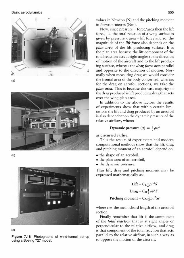
Basic aerodynamics 555
(a)
(c)
(b)
Figure 7.18 Photographs of wind-tunnel set-upusing a Boeing 727 model.
values in Newton (N) and the pitching momentin Newton-metres (Nm).
Now, since pressure = force/area then the liftforce, i.e. the total reaction of a wing surface isgiven by pressure × area = lift force and so, themagnitude of the lift force also depends on theplan area of the lift producing surface. It isthe plan area because the lift component of thetotal reaction acts at right angles to the directionof motion of the aircraft and to the lift produc-ing surface, whereas the drag force acts paralleland opposite to the direction of motion. Nor-mally when measuring drag we would considerthe frontal area of the body concerned, whereasfor the drag on aerofoil sections, we take theplan area. This is because the vast majority ofthe drag produced is lift producing drag that actsover the wing plan area.
In addition to the above factors the resultsof experiments show that within certain limi-tations the lift and drag produced by an aerofoilis also dependent on the dynamic pressure of therelative airflow, where:
Dynamic pressure (q) = 12ρv2
as discussed earlier.Thus the results of experiments and modern
computational methods show that the lift, dragand pitching moment of an aerofoil depend on:
• the shape of an aerofoil,• the plan area of an aerofoil,• the dynamic pressure.
Thus lift, drag and pitching moment may beexpressed mathematically as:
Lift = CL12ρv2S
Drag = CD12ρv2S
Pitching moment = CM12ρv2Sc
where c = the mean chord length of the aerofoilsection.
Finally remember that lift is the componentof the total reaction that is at right angles orperpendicular to the relative airflow, and dragis that component of the total reaction that actsparallel to the relative airflow, in such a way asto oppose the motion of the aircraft.
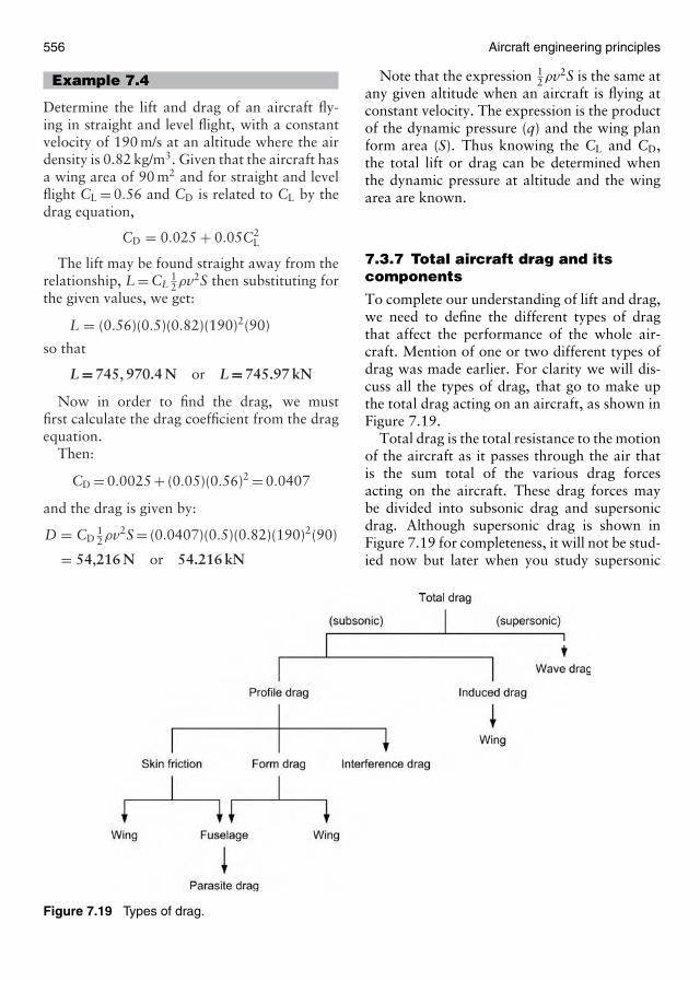
556 Aircraft engineering principles
Example 7.4
Determine the lift and drag of an aircraft fly-ing in straight and level flight, with a constantvelocity of 190 m/s at an altitude where the airdensity is 0.82 kg/m3. Given that the aircraft hasa wing area of 90 m2 and for straight and levelflight CL = 0.56 and CD is related to CL by thedrag equation,
CD = 0.025 + 0.05C2L
The lift may be found straight away from therelationship, L = CL
12ρv2S then substituting for
the given values, we get:
L = (0.56)(0.5)(0.82)(190)2(90)
so that
L = 745, 970.4 N or L = 745.97 kN
Now in order to find the drag, we mustfirst calculate the drag coefficient from the dragequation.
Then:
CD = 0.0025 + (0.05)(0.56)2 = 0.0407
and the drag is given by:
D = CD12ρv2S = (0.0407)(0.5)(0.82)(190)2(90)
= 54,216 N or 54.216 kN
Figure 7.19 Types of drag.
Note that the expression 12ρv2S is the same at
any given altitude when an aircraft is flying atconstant velocity. The expression is the productof the dynamic pressure (q) and the wing planform area (S). Thus knowing the CL and CD,the total lift or drag can be determined whenthe dynamic pressure at altitude and the wingarea are known.
7.3.7 Total aircraft drag and itscomponents
To complete our understanding of lift and drag,we need to define the different types of dragthat affect the performance of the whole air-craft. Mention of one or two different types ofdrag was made earlier. For clarity we will dis-cuss all the types of drag, that go to make upthe total drag acting on an aircraft, as shown inFigure 7.19.
Total drag is the total resistance to the motionof the aircraft as it passes through the air thatis the sum total of the various drag forcesacting on the aircraft. These drag forces maybe divided into subsonic drag and supersonicdrag. Although supersonic drag is shown inFigure 7.19 for completeness, it will not be stud-ied now but later when you study supersonic
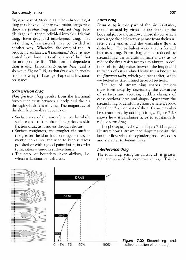
Basic aerodynamics 557
flight as part of Module 11. The subsonic flightdrag may be divided into two major categories:these are profile drag and induced drag. Pro-file drag is further subdivided into skin frictiondrag, form drag and interference drag. Thetotal drag of an aircraft may be divided inanother way. Whereby, the drag of the liftproducing surfaces, lift dependent drag, is sep-arated from those parts of the aircraft hull thatdo not produce lift. This non-lift dependentdrag is often known as parasite drag and isshown in Figure 7.19, as that drag which resultsfrom the wing to fuselage shape and frictionalresistance.
Skin friction dragSkin friction drag results from the frictionalforces that exist between a body and the airthrough which it is moving. The magnitude ofthe skin friction drag depends on:
• Surface area of the aircraft, since the wholesurface area of the aircraft experiences skinfriction drag, as it moves through the air.
• Surface roughness, the rougher the surfacethe greater the skin friction drag. Hence, asmentioned earlier, the need to keep surfacespolished or with a good paint finish, in orderto maintain a smooth surface finish.
• The state of boundary layer airflow, i.e.whether laminar or turbulent.
Figure 7.20 Streamlining andrelative reduction of form drag.
Form dragForm drag is that part of the air resistance,that is created by virtue of the shape of thebody subject to the airflow. Those shapes whichencourage the airflow to separate from their sur-face create eddies and the streamline flow isdisturbed. The turbulent wake that is formedincreases drag. Form drag can be reduced bystreamlining the aircraft in such a way as toreduce the drag resistance to a minimum. A def-inite relationship exists between the length andthickness of a streamlined body, this is known asthe fineness ratio, which you met earlier, whenwe looked at streamlined aerofoil sections.
The act of streamlining shapes reducestheir form drag by decreasing the curvatureof surfaces and avoiding sudden changes ofcross-sectional area and shape. Apart from thestreamlining of aerofoil sections, where we lookfor a finer t/c other parts of the airframe may alsobe streamlined, by adding fairings. Figure 7.20shows how streamlining helps to substantiallyreduce form drag.
The photographs shown in Figure 7.21, again,illustrate how a streamlined shape maintains thelaminar flow while the cylinder produces eddiesand a greater turbulent wake.
Interference dragThe total drag acting on an aircraft is greaterthan the sum of the component drag. This is
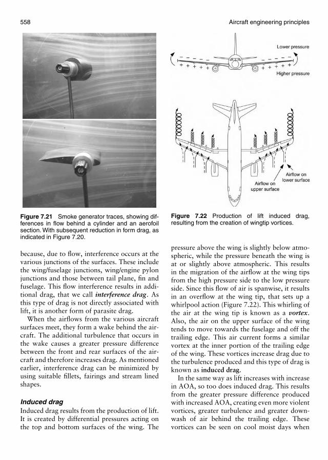
558 Aircraft engineering principles
Figure 7.21 Smoke generator traces, showing dif-ferences in flow behind a cylinder and an aerofoilsection. With subsequent reduction in form drag, asindicated in Figure 7.20.
because, due to flow, interference occurs at thevarious junctions of the surfaces. These includethe wing/fuselage junctions, wing/engine pylonjunctions and those between tail plane, fin andfuselage. This flow interference results in addi-tional drag, that we call interference drag. Asthis type of drag is not directly associated withlift, it is another form of parasite drag.
When the airflows from the various aircraftsurfaces meet, they form a wake behind the air-craft. The additional turbulence that occurs inthe wake causes a greater pressure differencebetween the front and rear surfaces of the air-craft and therefore increases drag. As mentionedearlier, interference drag can be minimized byusing suitable fillets, fairings and stream linedshapes.
Induced dragInduced drag results from the production of lift.It is created by differential pressures acting onthe top and bottom surfaces of the wing. The
Figure 7.22 Production of lift induced drag,resulting from the creation of wingtip vortices.
pressure above the wing is slightly below atmo-spheric, while the pressure beneath the wing isat or slightly above atmospheric. This resultsin the migration of the airflow at the wing tipsfrom the high pressure side to the low pressureside. Since this flow of air is spanwise, it resultsin an overflow at the wing tip, that sets up awhirlpool action (Figure 7.22). This whirling ofthe air at the wing tip is known as a vortex.Also, the air on the upper surface of the wingtends to move towards the fuselage and off thetrailing edge. This air current forms a similarvortex at the inner portion of the trailing edgeof the wing. These vortices increase drag due tothe turbulence produced and this type of drag isknown as induced drag.
In the same way as lift increases with increasein AOA, so too does induced drag. This resultsfrom the greater pressure difference producedwith increased AOA, creating even more violentvortices, greater turbulence and greater down-wash of air behind the trailing edge. Thesevortices can be seen on cool moist days when
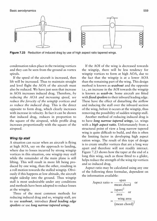
Basic aerodynamics 559
Figure 7.23 Reduction of induced drag by use of high aspect ratio tapered wings.
condensation takes place in the twisting vorticesand they can be seen from the ground as vortexspirals.
If the speed of the aircraft is increased, thenlift will be increased. Thus to maintain straightand level flight the AOA of the aircraft mustalso be reduced. We have just seen that increasein AOA increases induced drag. Therefore, byreducing the AOA and increasing speed, wereduce the ferocity of the wingtip vortices andso reduce the induced drag. This is the directopposite to form drag, which clearly increaseswith increase in velocity. In fact it can be shownthat induced drag, reduces in proportion tothe square of the airspeed, while profile dragincreases proportionally with the square of theairspeed.
Wing tip stallA situation can occur when an aircraft is flyingat high AOA, say on the approach to landing,where due to losses incurred by strong wingtipvortices in this situation, one wingtip may stallwhile the remainder of the main plane is stilllifting. This will result in more lift being pro-duced by one wing, than the other, resulting ina roll motion towards the stalled wingtip. Obvi-ously if this happens at low altitude, the aircraftmight sideslip into the ground. Thus wingtipstall is most undesirable under any conditionsand methods have been adopted to reduce lossesat the wingtip.
Three of the most common methods forreducing induced drag and so, wingtip stall, areto use washout, introduce fixed leading edgespoilers or use long narrow tapered wings.
If the AOI of the wing is decreased towardsthe wingtip, there will be less tendency forwingtip vortices to form at high AOA, due tothe fact that the wingtip is at a lower AOAthan the remaining part of the wing. This designmethod is known as washout and the oppositei.e., an increase in the AOI towards the wingtipis known as wash-in. Some aircraft are fittedwith fixed spoilers to their inboard leading edge.These have the effect of disturbing the airflowand inducing the stall over the inboard sectionof the wing, before it occurs at the wingtip, thusremoving the possibility of sudden wingtip stall.
Another method of reducing induced drag isto have long narrow tapered wings, i.e. wingswith a high aspect ratio. Unfortunately from astructural point of view a long narrow taperedwing is quite difficult to build, and this is oftenthe limiting factor in developing high aspectration wings. The result of this type of designis to create smaller vortices that are a long wayapart and therefore will not readily interact.Figure 7.23 shows how the taper at the end of along thin wing, such as those fitted to a glider,helps reduce the strength of the wing tip vorticesand so induced drag.
Aspect ratio may be calculated using any oneof the following three formulae, dependent onthe information available:
Aspect ratio = spanmean chord
or
= (span)2
areaor
= wing area(mean chord
)2
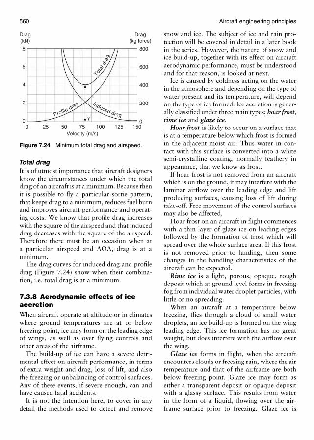
560 Aircraft engineering principles
00
2
4
6
8 800
600
400
200
0Y
Drag(kN)
Drag(kg force)
25 50 75Velocity (m/s)
100 125 150
Profiledrag Induced drag
Total
dra
g
Figure 7.24 Minimum total drag and airspeed.
Total dragIt is of utmost importance that aircraft designersknow the circumstances under which the totaldrag of an aircraft is at a minimum. Because thenit is possible to fly a particular sortie pattern,that keeps drag to a minimum, reduces fuel burnand improves aircraft performance and operat-ing costs. We know that profile drag increaseswith the square of the airspeed and that induceddrag decreases with the square of the airspeed.Therefore there must be an occasion when ata particular airspeed and AOA, drag is at aminimum.
The drag curves for induced drag and profiledrag (Figure 7.24) show when their combina-tion, i.e. total drag is at a minimum.
7.3.8 Aerodynamic effects of iceaccretion
When aircraft operate at altitude or in climateswhere ground temperatures are at or belowfreezing point, ice may form on the leading edgeof wings, as well as over flying controls andother areas of the airframe.
The build-up of ice can have a severe detri-mental effect on aircraft performance, in termsof extra weight and drag, loss of lift, and alsothe freezing or unbalancing of control surfaces.Any of these events, if severe enough, can andhave caused fatal accidents.
It is not the intention here, to cover in anydetail the methods used to detect and remove
snow and ice. The subject of ice and rain pro-tection will be covered in detail in a later bookin the series. However, the nature of snow andice build-up, together with its effect on aircraftaerodynamic performance, must be understoodand for that reason, is looked at next.
Ice is caused by coldness acting on the waterin the atmosphere and depending on the type ofwater present and its temperature, will dependon the type of ice formed. Ice accretion is gener-ally classified under three main types; hoar frost,rime ice and glaze ice.
Hoar frost is likely to occur on a surface thatis at a temperature below which frost is formedin the adjacent moist air. Thus water in con-tact with this surface is converted into a whitesemi-crystalline coating, normally feathery inappearance, that we know as frost.
If hoar frost is not removed from an aircraftwhich is on the ground, it may interfere with thelaminar airflow over the leading edge and liftproducing surfaces, causing loss of lift duringtake-off. Free movement of the control surfacesmay also be affected.
Hoar frost on an aircraft in flight commenceswith a thin layer of glaze ice on leading edgesfollowed by the formation of frost which willspread over the whole surface area. If this frostis not removed prior to landing, then somechanges in the handling characteristics of theaircraft can be expected.
Rime ice is a light, porous, opaque, roughdeposit which at ground level forms in freezingfog from individual water droplet particles, withlittle or no spreading.
When an aircraft at a temperature belowfreezing, flies through a cloud of small waterdroplets, an ice build-up is formed on the wingleading edge. This ice formation has no greatweight, but does interfere with the airflow overthe wing.
Glaze ice forms in flight, when the aircraftencounters clouds or freezing rain, where the airtemperature and that of the airframe are bothbelow freezing point. Glaze ice may form aseither a transparent deposit or opaque depositwith a glassy surface. This results from waterin the form of a liquid, flowing over the air-frame surface prior to freezing. Glaze ice is
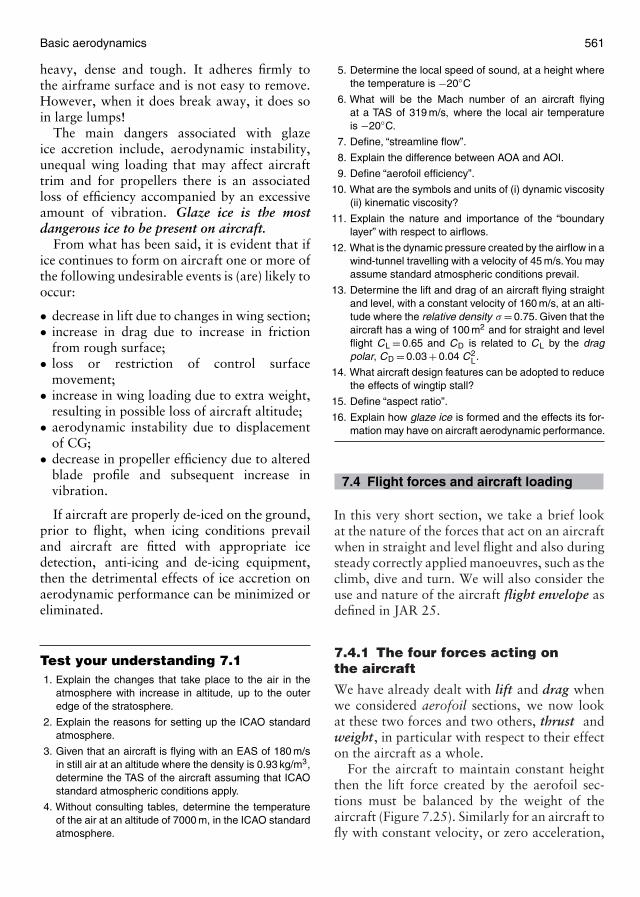
Basic aerodynamics 561
heavy, dense and tough. It adheres firmly tothe airframe surface and is not easy to remove.However, when it does break away, it does soin large lumps!
The main dangers associated with glazeice accretion include, aerodynamic instability,unequal wing loading that may affect aircrafttrim and for propellers there is an associatedloss of efficiency accompanied by an excessiveamount of vibration. Glaze ice is the mostdangerous ice to be present on aircraft.
From what has been said, it is evident that ifice continues to form on aircraft one or more ofthe following undesirable events is (are) likely tooccur:
• decrease in lift due to changes in wing section;• increase in drag due to increase in friction
from rough surface;• loss or restriction of control surface
movement;• increase in wing loading due to extra weight,
resulting in possible loss of aircraft altitude;• aerodynamic instability due to displacement
of CG;• decrease in propeller efficiency due to altered
blade profile and subsequent increase invibration.
If aircraft are properly de-iced on the ground,prior to flight, when icing conditions prevailand aircraft are fitted with appropriate icedetection, anti-icing and de-icing equipment,then the detrimental effects of ice accretion onaerodynamic performance can be minimized oreliminated.
Test your understanding 7.11. Explain the changes that take place to the air in the
atmosphere with increase in altitude, up to the outeredge of the stratosphere.
2. Explain the reasons for setting up the ICAO standardatmosphere.
3. Given that an aircraft is flying with an EAS of 180 m/sin still air at an altitude where the density is 0.93 kg/m3,determine the TAS of the aircraft assuming that ICAOstandard atmospheric conditions apply.
4. Without consulting tables, determine the temperatureof the air at an altitude of 7000 m, in the ICAO standardatmosphere.
5. Determine the local speed of sound, at a height wherethe temperature is −20◦C
6. What will be the Mach number of an aircraft flyingat a TAS of 319 m/s, where the local air temperatureis −20◦C.
7. Define, “streamline flow”.
8. Explain the difference between AOA and AOI.
9. Define “aerofoil efficiency”.
10. What are the symbols and units of (i) dynamic viscosity(ii) kinematic viscosity?
11. Explain the nature and importance of the “boundarylayer” with respect to airflows.
12. What is the dynamic pressure created by the airflow in awind-tunnel travelling with a velocity of 45 m/s.You mayassume standard atmospheric conditions prevail.
13. Determine the lift and drag of an aircraft flying straightand level, with a constant velocity of 160 m/s, at an alti-tude where the relative density σ = 0.75. Given that theaircraft has a wing of 100 m2 and for straight and levelflight CL = 0.65 and CD is related to CL by the dragpolar, CD = 0.03 + 0.04 C2
L.
14. What aircraft design features can be adopted to reducethe effects of wingtip stall?
15. Define “aspect ratio”.
16. Explain how glaze ice is formed and the effects its for-mation may have on aircraft aerodynamic performance.
7.4 Flight forces and aircraft loading
In this very short section, we take a brief lookat the nature of the forces that act on an aircraftwhen in straight and level flight and also duringsteady correctly applied manoeuvres, such as theclimb, dive and turn. We will also consider theuse and nature of the aircraft flight envelope asdefined in JAR 25.
7.4.1 The four forces acting onthe aircraft
We have already dealt with lift and drag whenwe considered aerofoil sections, we now lookat these two forces and two others, thrust andweight, in particular with respect to their effecton the aircraft as a whole.
For the aircraft to maintain constant heightthen the lift force created by the aerofoil sec-tions must be balanced by the weight of theaircraft (Figure 7.25). Similarly for an aircraft tofly with constant velocity, or zero acceleration,
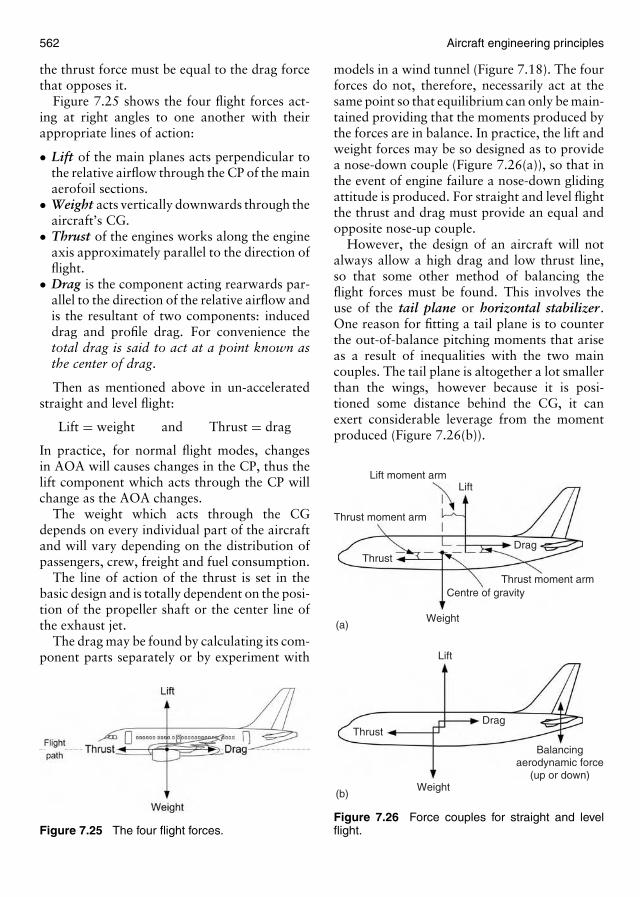
562 Aircraft engineering principles
the thrust force must be equal to the drag forcethat opposes it.
Figure 7.25 shows the four flight forces act-ing at right angles to one another with theirappropriate lines of action:
• Lift of the main planes acts perpendicular tothe relative airflow through the CP of the mainaerofoil sections.
• Weight acts vertically downwards through theaircraft’s CG.
• Thrust of the engines works along the engineaxis approximately parallel to the direction offlight.
• Drag is the component acting rearwards par-allel to the direction of the relative airflow andis the resultant of two components: induceddrag and profile drag. For convenience thetotal drag is said to act at a point known asthe center of drag.
Then as mentioned above in un-acceleratedstraight and level flight:
Lift = weight and Thrust = drag
In practice, for normal flight modes, changesin AOA will causes changes in the CP, thus thelift component which acts through the CP willchange as the AOA changes.
The weight which acts through the CGdepends on every individual part of the aircraftand will vary depending on the distribution ofpassengers, crew, freight and fuel consumption.
The line of action of the thrust is set in thebasic design and is totally dependent on the posi-tion of the propeller shaft or the center line ofthe exhaust jet.
The drag may be found by calculating its com-ponent parts separately or by experiment with
Figure 7.25 The four flight forces.
models in a wind tunnel (Figure 7.18). The fourforces do not, therefore, necessarily act at thesame point so that equilibrium can only be main-tained providing that the moments produced bythe forces are in balance. In practice, the lift andweight forces may be so designed as to providea nose-down couple (Figure 7.26(a)), so that inthe event of engine failure a nose-down glidingattitude is produced. For straight and level flightthe thrust and drag must provide an equal andopposite nose-up couple.
However, the design of an aircraft will notalways allow a high drag and low thrust line,so that some other method of balancing theflight forces must be found. This involves theuse of the tail plane or horizontal stabilizer .One reason for fitting a tail plane is to counterthe out-of-balance pitching moments that ariseas a result of inequalities with the two maincouples. The tail plane is altogether a lot smallerthan the wings, however because it is posi-tioned some distance behind the CG, it canexert considerable leverage from the momentproduced (Figure 7.26(b)).
Lift moment arm
Thrust moment arm
Thrust moment arm
Balancingaerodynamic force
(up or down)
Thrust
Thrust
Weight
Weight
(a)
(b)
Centre of gravity
Lift
Lift
Drag
Drag
Figure 7.26 Force couples for straight and levelflight.
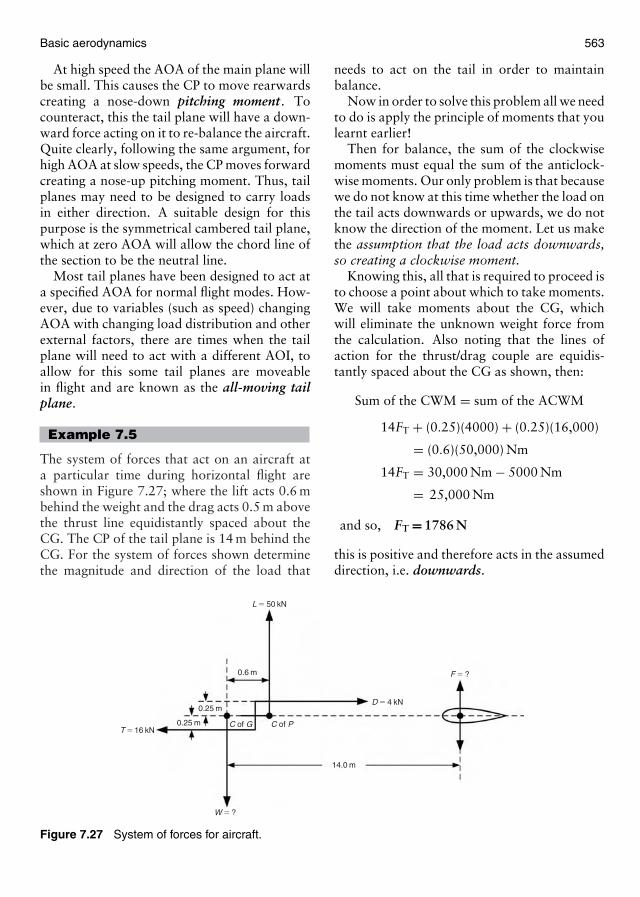
Basic aerodynamics 563
At high speed the AOA of the main plane willbe small. This causes the CP to move rearwardscreating a nose-down pitching moment. Tocounteract, this the tail plane will have a down-ward force acting on it to re-balance the aircraft.Quite clearly, following the same argument, forhigh AOA at slow speeds, the CP moves forwardcreating a nose-up pitching moment. Thus, tailplanes may need to be designed to carry loadsin either direction. A suitable design for thispurpose is the symmetrical cambered tail plane,which at zero AOA will allow the chord line ofthe section to be the neutral line.
Most tail planes have been designed to act ata specified AOA for normal flight modes. How-ever, due to variables (such as speed) changingAOA with changing load distribution and otherexternal factors, there are times when the tailplane will need to act with a different AOI, toallow for this some tail planes are moveablein flight and are known as the all-moving tailplane.
Example 7.5
The system of forces that act on an aircraft ata particular time during horizontal flight areshown in Figure 7.27; where the lift acts 0.6 mbehind the weight and the drag acts 0.5 m abovethe thrust line equidistantly spaced about theCG. The CP of the tail plane is 14 m behind theCG. For the system of forces shown determinethe magnitude and direction of the load that
T � 16 kN
W � ?
F � ?
L � 50 kN
D � 4 kN
0.6 m
0.25 m
14.0 m
0.25 m C of G C of P
Figure 7.27 System of forces for aircraft.
needs to act on the tail in order to maintainbalance.
Now in order to solve this problem all we needto do is apply the principle of moments that youlearnt earlier!
Then for balance, the sum of the clockwisemoments must equal the sum of the anticlock-wise moments. Our only problem is that becausewe do not know at this time whether the load onthe tail acts downwards or upwards, we do notknow the direction of the moment. Let us makethe assumption that the load acts downwards,so creating a clockwise moment.
Knowing this, all that is required to proceed isto choose a point about which to take moments.We will take moments about the CG, whichwill eliminate the unknown weight force fromthe calculation. Also noting that the lines ofaction for the thrust/drag couple are equidis-tantly spaced about the CG as shown, then:
Sum of the CWM = sum of the ACWM
14FT + (0.25)(4000) + (0.25)(16,000)
= (0.6)(50,000) Nm
14FT = 30,000 Nm − 5000 Nm
= 25,000 Nm
and so, FT = 1786 N
this is positive and therefore acts in the assumeddirection, i.e. downwards.
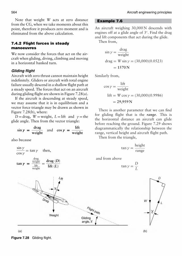
564 Aircraft engineering principles
Note that weight W acts at zero distancefrom the CG, when we take moments about thispoint, therefore it produces zero moment and iseliminated from the above calculation.
7.4.2 Flight forces in steadymanoeuvres
We now consider the forces that act on the air-craft when gliding, diving, climbing and movingin a horizontal banked turn.
Gliding flightAircraft with zero thrust cannot maintain heightindefinitely. Gliders or aircraft with total enginefailure usually descend in a shallow flight path ata steady speed. The forces that act on an aircraftduring gliding flight are shown in Figure 7.28(a).
If the aircraft is descending at steady speed,we may assume that it is in equilibrium and avector force triangle may be drawn as shown inFigure 7.28(b), where:
D = drag, W = weight, L = lift and γ = theglide angle. Then from the vector triangle:
sin γ = dragweight
and cos γ = liftweight
also because
sin γ
cos γ= tan γ then,
tan γ =drag
weightlift
weight
= drag (D)lift (L)
Figure 7.28 Gliding flight.
Example 7.6
An aircraft weighing 30,000 N descends withengines off at a glide angle of 3◦. Find the dragand lift components that act during the glide.
Then from,
sin γ = dragweight
drag = W sin γ = (30,000)(0.0523)
= 1570 N
Similarly from,
cos γ = liftweight
lift = W cos γ = (30,000)(0.9986)
= 29,959 N
There is another parameter that we can findfor gliding flight that is the range. This isthe horizontal distance an aircraft can glidebefore reaching the ground. Figure 7.29 showsdiagrammatically the relationship between therange, vertical height and aircraft flight path.
Then from the triangle,
tan γ = heightrange
and from above
tan γ = DL
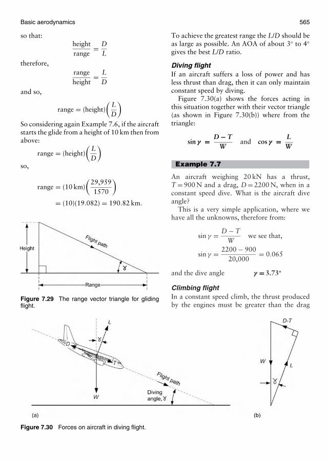
Basic aerodynamics 565
so that:heightrange
= DL
therefore,rangeheight
= LD
and so,
range = (height)(
LD
)So considering again Example 7.6, if the aircraftstarts the glide from a height of 10 km then fromabove:
range = (height)(
LD
)so,
range = (10 km)(
29,9591570
)
= (10)(19.082) = 190.82 km.
Figure 7.29 The range vector triangle for glidingflight.
Figure 7.30 Forces on aircraft in diving flight.
To achieve the greatest range the L/D should beas large as possible. An AOA of about 3◦ to 4◦gives the best L/D ratio.
Diving flightIf an aircraft suffers a loss of power and hasless thrust than drag, then it can only maintainconstant speed by diving.
Figure 7.30(a) shows the forces acting inthis situation together with their vector triangle(as shown in Figure 7.30(b)) where from thetriangle:
sin γ = D − TW
and cos γ = LW
Example 7.7
An aircraft weighing 20 kN has a thrust,T = 900 N and a drag, D = 2200 N, when in aconstant speed dive. What is the aircraft diveangle?
This is a very simple application, where wehave all the unknowns, therefore from:
sin γ = D − TW
we see that,
sin γ = 2200 − 90020,000
= 0.065
and the dive angle γ = 3.73◦
Climbing flightIn a constant speed climb, the thrust producedby the engines must be greater than the drag
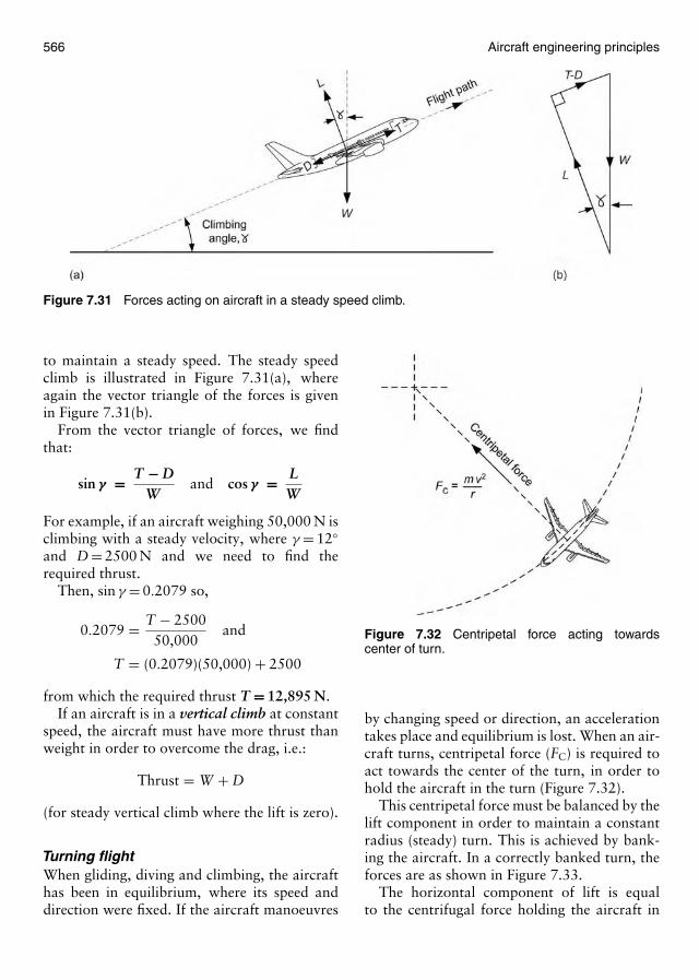
566 Aircraft engineering principles
Figure 7.31 Forces acting on aircraft in a steady speed climb.
to maintain a steady speed. The steady speedclimb is illustrated in Figure 7.31(a), whereagain the vector triangle of the forces is givenin Figure 7.31(b).
From the vector triangle of forces, we findthat:
sin γ = T − DW
and cos γ = LW
For example, if an aircraft weighing 50,000 N isclimbing with a steady velocity, where γ = 12◦and D = 2500 N and we need to find therequired thrust.
Then, sin γ = 0.2079 so,
0.2079 = T − 250050,000
and
T = (0.2079)(50,000) + 2500
from which the required thrust T = 12,895 N.If an aircraft is in a vertical climb at constant
speed, the aircraft must have more thrust thanweight in order to overcome the drag, i.e.:
Thrust = W + D
(for steady vertical climb where the lift is zero).
Turning flightWhen gliding, diving and climbing, the aircrafthas been in equilibrium, where its speed anddirection were fixed. If the aircraft manoeuvres
Figure 7.32 Centripetal force acting towardscenter of turn.
by changing speed or direction, an accelerationtakes place and equilibrium is lost. When an air-craft turns, centripetal force (FC) is required toact towards the center of the turn, in order tohold the aircraft in the turn (Figure 7.32).
This centripetal force must be balanced by thelift component in order to maintain a constantradius (steady) turn. This is achieved by bank-ing the aircraft. In a correctly banked turn, theforces are as shown in Figure 7.33.
The horizontal component of lift is equalto the centrifugal force holding the aircraft in
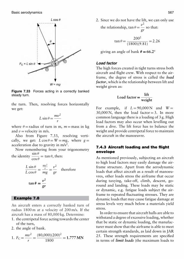
Basic aerodynamics 567
Figure 7.33 Forces acting in a correctly bankedsteady turn.
the turn. Then, resolving forces horizontallywe get:
L sin θ = mv2
r
where θ = radius of turn in m, m = mass in kgand v = velocity in m/s.
Also from Figure 7.33, resolving verti-cally, we get: L cos θ = W = mg, where g =acceleration due to gravity in m/s2.
Now remembering from your trigonometry
the identitysin θ
cos θ= tan θ, then:
L sin θ
L cos θ=
mv2
r
mg= v2
grtherefore
tan θ = v2
gr
Example 7.8
An aircraft enters a correctly banked turn ofradius 1800 m at a velocity of 200 m/s. If theaircraft has a mass of 80,000 kg. Determine:1. the centripetal force acting towards the center
of the turn,2. the angle of bank.
1. FC = mv2
r= (80,000)(200)2
1800= 1.777 MN
2. Since we do not have the lift, we can only use
the relationship, tan θ = v2
grso that:
tan θ = 2002
(1800)(9.81)= 2.26
giving an angle of bank θ = 66.2◦
Load factorThe high forces created in tight turns stress bothaircraft and flight crew. With respect to the air-frame, the degree of stress is called the loadfactor , which is the relationship between lift andweight given as:
Load factor = liftweight
For example, if L = 90,000 N and W =30,000 N, then the load factor = 3. In morecommon language there is a loading of 3 g. Highload factors may also occur when levelling outfrom a dive. The lift force has to balance theweight and provide centripetal force to maintainthe aircraft in the manoeuvre.
7.4.3 Aircraft loading and the flightenvelope
As mentioned previously, subjecting an aircraftto high load factors may easily damage the air-frame structure. Apart from the aerodynamicloads that affect aircraft as a result of manoeu-vres, other loads stress the airframe that occurduring taxying, take-off, climb, descent, go-round and landing. These loads may be staticor dynamic, e.g. fatigue loads subject the air-frame to repeated fluctuating stresses. They aredynamic loads that may cause fatigue damage atstress levels very much below a materials yieldstress.
In order to ensure that aircraft hulls are able towithstand a degree of excessive loading, whetherthat be static or dynamic loading, the manufac-turer must show that the airframe is able to meetcertain strength standards, as laid down in JAR25. These strength requirements are specifiedin terms of limit loads (the maximum loads to
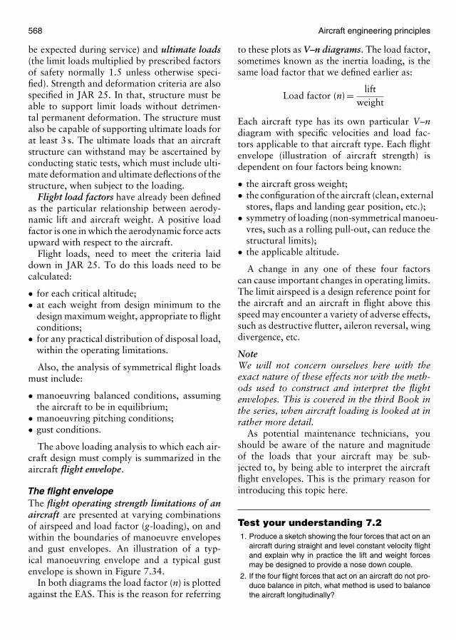
568 Aircraft engineering principles
be expected during service) and ultimate loads(the limit loads multiplied by prescribed factorsof safety normally 1.5 unless otherwise speci-fied). Strength and deformation criteria are alsospecified in JAR 25. In that, structure must beable to support limit loads without detrimen-tal permanent deformation. The structure mustalso be capable of supporting ultimate loads forat least 3 s. The ultimate loads that an aircraftstructure can withstand may be ascertained byconducting static tests, which must include ulti-mate deformation and ultimate deflections of thestructure, when subject to the loading.
Flight load factors have already been definedas the particular relationship between aerody-namic lift and aircraft weight. A positive loadfactor is one in which the aerodynamic force actsupward with respect to the aircraft.
Flight loads, need to meet the criteria laiddown in JAR 25. To do this loads need to becalculated:
• for each critical altitude;• at each weight from design minimum to the
design maximum weight, appropriate to flightconditions;
• for any practical distribution of disposal load,within the operating limitations.
Also, the analysis of symmetrical flight loadsmust include:
• manoeuvring balanced conditions, assumingthe aircraft to be in equilibrium;
• manoeuvring pitching conditions;• gust conditions.
The above loading analysis to which each air-craft design must comply is summarized in theaircraft flight envelope.
The flight envelopeThe flight operating strength limitations of anaircraft are presented at varying combinationsof airspeed and load factor (g-loading), on andwithin the boundaries of manoeuvre envelopesand gust envelopes. An illustration of a typ-ical manoeuvring envelope and a typical gustenvelope is shown in Figure 7.34.
In both diagrams the load factor (n) is plottedagainst the EAS. This is the reason for referring
to these plots as V–n diagrams. The load factor,sometimes known as the inertia loading, is thesame load factor that we defined earlier as:
Load factor (n) = liftweight
Each aircraft type has its own particular V–ndiagram with specific velocities and load fac-tors applicable to that aircraft type. Each flightenvelope (illustration of aircraft strength) isdependent on four factors being known:
• the aircraft gross weight;• the configuration of the aircraft (clean, external
stores, flaps and landing gear position, etc.);• symmetry of loading (non-symmetrical manoeu-
vres, such as a rolling pull-out, can reduce thestructural limits);
• the applicable altitude.
A change in any one of these four factorscan cause important changes in operating limits.The limit airspeed is a design reference point forthe aircraft and an aircraft in flight above thisspeed may encounter a variety of adverse effects,such as destructive flutter, aileron reversal, wingdivergence, etc.
NoteWe will not concern ourselves here with theexact nature of these effects nor with the meth-ods used to construct and interpret the flightenvelopes. This is covered in the third Book inthe series, when aircraft loading is looked at inrather more detail.
As potential maintenance technicians, youshould be aware of the nature and magnitudeof the loads that your aircraft may be sub-jected to, by being able to interpret the aircraftflight envelopes. This is the primary reason forintroducing this topic here.
Test your understanding 7.21. Produce a sketch showing the four forces that act on an
aircraft during straight and level constant velocity flightand explain why in practice the lift and weight forcesmay be designed to provide a nose down couple.
2. If the four flight forces that act on an aircraft do not pro-duce balance in pitch, what method is used to balancethe aircraft longitudinally?
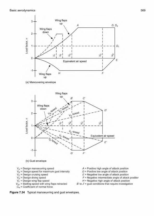
Basic aerodynamics 569
Figure 7.34 Typical manoeuvring and gust envelopes.
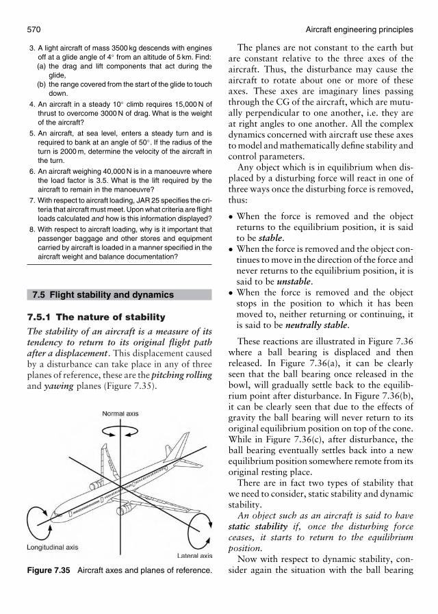
570 Aircraft engineering principles
3. A light aircraft of mass 3500 kg descends with enginesoff at a glide angle of 4◦ from an altitude of 5 km. Find:(a) the drag and lift components that act during the
glide,(b) the range covered from the start of the glide to touch
down.
4. An aircraft in a steady 10◦ climb requires 15,000 N ofthrust to overcome 3000 N of drag. What is the weightof the aircraft?
5. An aircraft, at sea level, enters a steady turn and isrequired to bank at an angle of 50◦. If the radius of theturn is 2000 m, determine the velocity of the aircraft inthe turn.
6. An aircraft weighing 40,000 N is in a manoeuvre wherethe load factor is 3.5. What is the lift required by theaircraft to remain in the manoeuvre?
7. With respect to aircraft loading, JAR 25 specifies the cri-teria that aircraft must meet. Upon what criteria are flightloads calculated and how is this information displayed?
8. With respect to aircraft loading, why is it important thatpassenger baggage and other stores and equipmentcarried by aircraft is loaded in a manner specified in theaircraft weight and balance documentation?
7.5 Flight stability and dynamics
7.5.1 The nature of stability
The stability of an aircraft is a measure of itstendency to return to its original flight pathafter a displacement. This displacement causedby a disturbance can take place in any of threeplanes of reference, these are the pitching rollingand yawing planes (Figure 7.35).
Figure 7.35 Aircraft axes and planes of reference.
The planes are not constant to the earth butare constant relative to the three axes of theaircraft. Thus, the disturbance may cause theaircraft to rotate about one or more of theseaxes. These axes are imaginary lines passingthrough the CG of the aircraft, which are mutu-ally perpendicular to one another, i.e. they areat right angles to one another. All the complexdynamics concerned with aircraft use these axesto model and mathematically define stability andcontrol parameters.
Any object which is in equilibrium when dis-placed by a disturbing force will react in one ofthree ways once the disturbing force is removed,thus:
• When the force is removed and the objectreturns to the equilibrium position, it is saidto be stable.
• When the force is removed and the object con-tinues to move in the direction of the force andnever returns to the equilibrium position, it issaid to be unstable.
• When the force is removed and the objectstops in the position to which it has beenmoved to, neither returning or continuing, itis said to be neutrally stable.
These reactions are illustrated in Figure 7.36where a ball bearing is displaced and thenreleased. In Figure 7.36(a), it can be clearlyseen that the ball bearing once released in thebowl, will gradually settle back to the equilib-rium point after disturbance. In Figure 7.36(b),it can be clearly seen that due to the effects ofgravity the ball bearing will never return to itsoriginal equilibrium position on top of the cone.While in Figure 7.36(c), after disturbance, theball bearing eventually settles back into a newequilibrium position somewhere remote from itsoriginal resting place.
There are in fact two types of stability thatwe need to consider, static stability and dynamicstability.
An object such as an aircraft is said to havestatic stability if, once the disturbing forceceases, it starts to return to the equilibriumposition.
Now with respect to dynamic stability, con-sider again the situation with the ball bearing
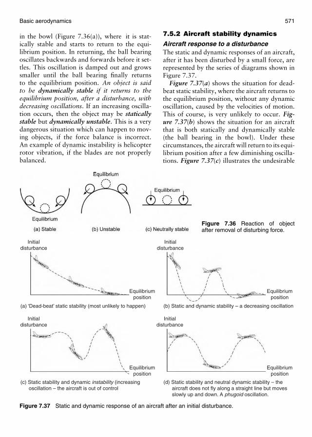
Basic aerodynamics 571
in the bowl (Figure 7.36(a)), where it is stat-ically stable and starts to return to the equi-librium position. In returning, the ball bearingoscillates backwards and forwards before it set-tles. This oscillation is damped out and growssmaller until the ball bearing finally returnsto the equilibrium position. An object is saidto be dynamically stable if it returns to theequilibrium position, after a disturbance, withdecreasing oscillations. If an increasing oscilla-tion occurs, then the object may be staticallystable but dynamically unstable. This is a verydangerous situation which can happen to mov-ing objects, if the force balance is incorrect.An example of dynamic instability is helicopterrotor vibration, if the blades are not properlybalanced.
Figure 7.36 Reaction of objectafter removal of disturbing force.
Initialdisturbance
Initialdisturbance
Equilibriumposition
(a) ‘Dead-beat’ static stability (most unlikely to happen) (b) Static and dynamic stability – a decreasing oscillation
(c) Static stability and dynamic instability (increasing oscillation – the aircraft is out of control
(d) Static stability and neutral dynamic stability – the aircraft does not fly along a straight line but moves slowly up and down. A phugoid oscillation.
Equilibriumposition
Equilibriumposition
Equilibriumposition
Initialdisturbance
Initialdisturbance
Figure 7.37 Static and dynamic response of an aircraft after an initial disturbance.
7.5.2 Aircraft stability dynamics
Aircraft response to a disturbanceThe static and dynamic responses of an aircraft,after it has been disturbed by a small force, arerepresented by the series of diagrams shown inFigure 7.37.
Figure 7.37(a) shows the situation for dead-beat static stability, where the aircraft returns tothe equilibrium position, without any dynamicoscillation, caused by the velocities of motion.This of course, is very unlikely to occur. Fig-ure 7.37(b) shows the situation for an aircraftthat is both statically and dynamically stable(the ball bearing in the bowl). Under thesecircumstances, the aircraft will return to its equi-librium position after a few diminishing oscilla-tions. Figure 7.37(c) illustrates the undesirable

572 Aircraft engineering principles
situation where the aircraft may be statically sta-ble but is dynamically unstable, in other words,the aircraft is out of control. This situationis similar to that of a suspension bridge thatoscillates at its resonant frequency, the oscilla-tions getting larger and larger until the bridgefails. It is worth noting here, that it is not pos-sible for an aircraft to be statically unstableand dynamically stable but the reverse situa-tion (Figure 7.37(c)) is possible. Figure 7.37(d)illustrates the situation for an aircraft that hasstatic stability and neutral dynamic stability.Under these circumstances the aircraft does notfly in a straight line but is subject to very largelow frequency oscillations known as phugoidoscillations.
Types of stabilityWhen considering stability, we assume thatthe CG of the aircraft continues to move ina straight line and that the disturbances to beovercome cause rotational movements about theCG. These movements can be:
• rolling movements about (around) the longi-tudinal axis – lateral stability;
• yawing movements about the normal axis –directional stability;
• pitching movements about the lateral axis –longitudinal stability.
Figure 7.38 illustrates the type of movement thatmust be damped, if the aircraft is to be consid-ered stable. Thus lateral stability is the inherentability of an aircraft to recover from a dis-turbance around the longitudinal plane (axis),i.e. rolling movements. Similarly, longitudinalstability is the inherent (built-in) ability of theaircraft to recover from disturbances aroundthe lateral axis i.e. pitching movements. Finally,directional stability is the inherent ability of theaircraft to recover from disturbances around thenormal axis.
There are many aircraft features specifi-cally designed to either aid stability or reducethe amount of inherent stability an aircraftpossesses, depending on aircraft configura-tion and function. We look at some of thesedesign features next when we consider lateral,
Figure 7.38 Rolling, yawing and pitchingmovements.
longitudinal and directional stability in a littlemore detail.
Lateral stabilityFrom what has been said above an aircraft haslateral stability if, following a roll displace-ment, a restoring moment is produced whichopposes the roll and returns the aircraft to awings level position. In that, aerodynamic cou-pling produces rolling moments that can setup side slip or yawing motion. It is thereforenecessary to consider these interactions whendesigning an aircraft to be inherently staticallystable in roll. The main contributors to lateralstatic stability are:
• wing dihedral,• sweepback,• high wing position,• keel surface.
A design feature that has the opposite effect tothose given above, i.e. that reduces stability isanhedral. The need to reduce lateral stabilitymay seem strange, but combat aircraft and manyhigh speed automatically controlled aircraft, useanhedral to provide more manoeuvrability.
Wing dihedral and lateral stabilityDihedral angle is defined as the upward incli-nation of the wings from the horizontal. Theamount of dihedral angle being dependenton aircraft type and wing configuration i.e.whether the wings are positioned high or low
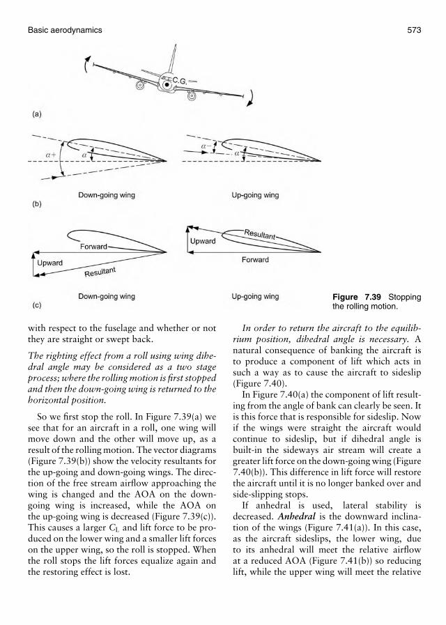
Basic aerodynamics 573
Figure 7.39 Stoppingthe rolling motion.
with respect to the fuselage and whether or notthey are straight or swept back.
The righting effect from a roll using wing dihe-dral angle may be considered as a two stageprocess; where the rolling motion is first stoppedand then the down-going wing is returned to thehorizontal position.
So we first stop the roll. In Figure 7.39(a) wesee that for an aircraft in a roll, one wing willmove down and the other will move up, as aresult of the rolling motion. The vector diagrams(Figure 7.39(b)) show the velocity resultants forthe up-going and down-going wings. The direc-tion of the free stream airflow approaching thewing is changed and the AOA on the down-going wing is increased, while the AOA onthe up-going wing is decreased (Figure 7.39(c)).This causes a larger CL and lift force to be pro-duced on the lower wing and a smaller lift forceson the upper wing, so the roll is stopped. Whenthe roll stops the lift forces equalize again andthe restoring effect is lost.
In order to return the aircraft to the equilib-rium position, dihedral angle is necessary. Anatural consequence of banking the aircraft isto produce a component of lift which acts insuch a way as to cause the aircraft to sideslip(Figure 7.40).
In Figure 7.40(a) the component of lift result-ing from the angle of bank can clearly be seen. Itis this force that is responsible for sideslip. Nowif the wings were straight the aircraft wouldcontinue to sideslip, but if dihedral angle isbuilt-in the sideways air stream will create agreater lift force on the down-going wing (Figure7.40(b)). This difference in lift force will restorethe aircraft until it is no longer banked over andside-slipping stops.
If anhedral is used, lateral stability isdecreased. Anhedral is the downward inclina-tion of the wings (Figure 7.41(a)). In this case,as the aircraft sideslips, the lower wing, dueto its anhedral will meet the relative airflowat a reduced AOA (Figure 7.41(b)) so reducinglift, while the upper wing will meet the relative
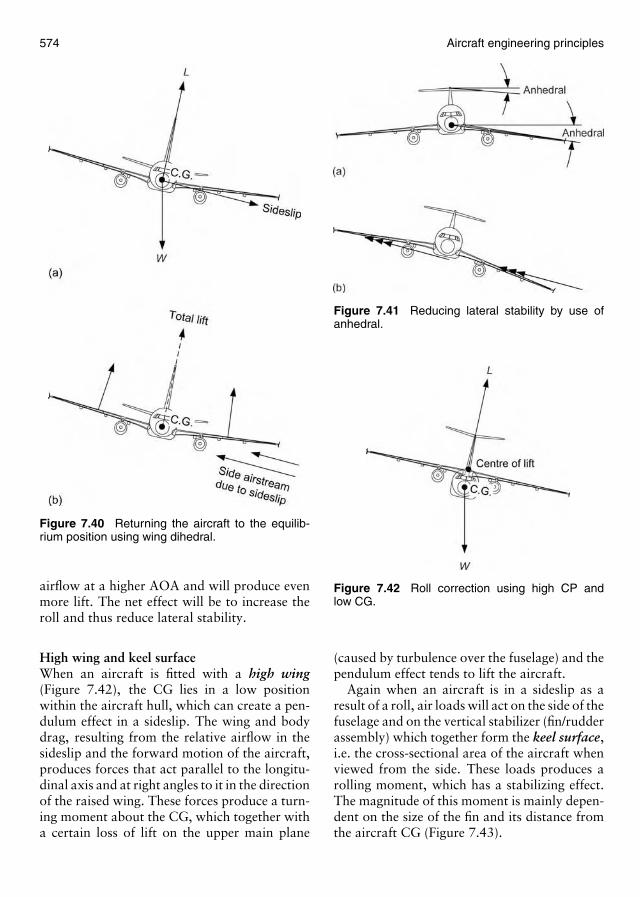
574 Aircraft engineering principles
Figure 7.40 Returning the aircraft to the equilib-rium position using wing dihedral.
airflow at a higher AOA and will produce evenmore lift. The net effect will be to increase theroll and thus reduce lateral stability.
High wing and keel surfaceWhen an aircraft is fitted with a high wing(Figure 7.42), the CG lies in a low positionwithin the aircraft hull, which can create a pen-dulum effect in a sideslip. The wing and bodydrag, resulting from the relative airflow in thesideslip and the forward motion of the aircraft,produces forces that act parallel to the longitu-dinal axis and at right angles to it in the directionof the raised wing. These forces produce a turn-ing moment about the CG, which together witha certain loss of lift on the upper main plane
Figure 7.41 Reducing lateral stability by use ofanhedral.
Figure 7.42 Roll correction using high CP andlow CG.
(caused by turbulence over the fuselage) and thependulum effect tends to lift the aircraft.
Again when an aircraft is in a sideslip as aresult of a roll, air loads will act on the side of thefuselage and on the vertical stabilizer (fin/rudderassembly) which together form the keel surface,i.e. the cross-sectional area of the aircraft whenviewed from the side. These loads produces arolling moment, which has a stabilizing effect.The magnitude of this moment is mainly depen-dent on the size of the fin and its distance fromthe aircraft CG (Figure 7.43).
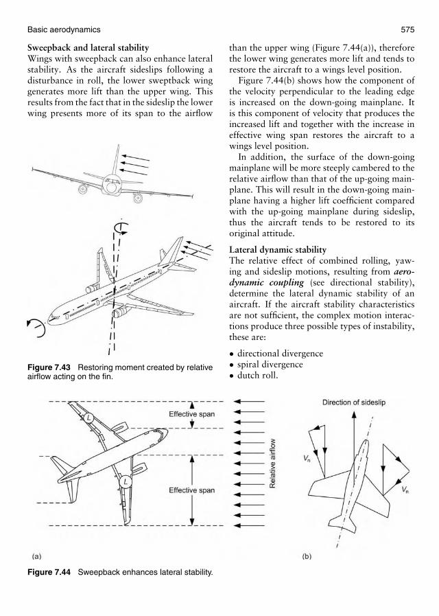
Basic aerodynamics 575
Sweepback and lateral stabilityWings with sweepback can also enhance lateralstability. As the aircraft sideslips following adisturbance in roll, the lower sweptback winggenerates more lift than the upper wing. Thisresults from the fact that in the sideslip the lowerwing presents more of its span to the airflow
Figure 7.43 Restoring moment created by relativeairflow acting on the fin.
Figure 7.44 Sweepback enhances lateral stability.
than the upper wing (Figure 7.44(a)), thereforethe lower wing generates more lift and tends torestore the aircraft to a wings level position.
Figure 7.44(b) shows how the component ofthe velocity perpendicular to the leading edgeis increased on the down-going mainplane. Itis this component of velocity that produces theincreased lift and together with the increase ineffective wing span restores the aircraft to awings level position.
In addition, the surface of the down-goingmainplane will be more steeply cambered to therelative airflow than that of the up-going main-plane. This will result in the down-going main-plane having a higher lift coefficient comparedwith the up-going mainplane during sideslip,thus the aircraft tends to be restored to itsoriginal attitude.
Lateral dynamic stabilityThe relative effect of combined rolling, yaw-ing and sideslip motions, resulting from aero-dynamic coupling (see directional stability),determine the lateral dynamic stability of anaircraft. If the aircraft stability characteristicsare not sufficient, the complex motion interac-tions produce three possible types of instability,these are:
• directional divergence• spiral divergence• dutch roll.
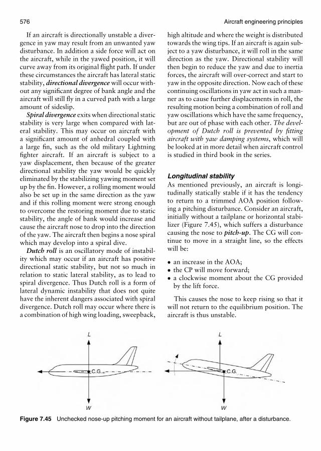
576 Aircraft engineering principles
If an aircraft is directionally unstable a diver-gence in yaw may result from an unwanted yawdisturbance. In addition a side force will act onthe aircraft, while in the yawed position, it willcurve away from its original flight path. If underthese circumstances the aircraft has lateral staticstability, directional divergence will occur with-out any significant degree of bank angle and theaircraft will still fly in a curved path with a largeamount of sideslip.
Spiral divergence exits when directional staticstability is very large when compared with lat-eral stability. This may occur on aircraft witha significant amount of anhedral coupled witha large fin, such as the old military Lightningfighter aircraft. If an aircraft is subject to ayaw displacement, then because of the greaterdirectional stability the yaw would be quicklyeliminated by the stabilizing yawing moment setup by the fin. However, a rolling moment wouldalso be set up in the same direction as the yawand if this rolling moment were strong enoughto overcome the restoring moment due to staticstability, the angle of bank would increase andcause the aircraft nose to drop into the directionof the yaw. The aircraft then begins a nose spiralwhich may develop into a spiral dive.
Dutch roll is an oscillatory mode of instabil-ity which may occur if an aircraft has positivedirectional static stability, but not so much inrelation to static lateral stability, as to lead tospiral divergence. Thus Dutch roll is a form oflateral dynamic instability that does not quitehave the inherent dangers associated with spiraldivergence. Dutch roll may occur where there isa combination of high wing loading, sweepback,
Figure 7.45 Unchecked nose-up pitching moment for an aircraft without tailplane, after a disturbance.
high altitude and where the weight is distributedtowards the wing tips. If an aircraft is again sub-ject to a yaw disturbance, it will roll in the samedirection as the yaw. Directional stability willthen begin to reduce the yaw and due to inertiaforces, the aircraft will over-correct and start toyaw in the opposite direction. Now each of thesecontinuing oscillations in yaw act in such a man-ner as to cause further displacements in roll, theresulting motion being a combination of roll andyaw oscillations which have the same frequency,but are out of phase with each other. The devel-opment of Dutch roll is prevented by fittingaircraft with yaw damping systems, which willbe looked at in more detail when aircraft controlis studied in third book in the series.
Longitudinal stabilityAs mentioned previously, an aircraft is longi-tudinally statically stable if it has the tendencyto return to a trimmed AOA position follow-ing a pitching disturbance. Consider an aircraft,initially without a tailplane or horizontal stabi-lizer (Figure 7.45), which suffers a disturbancecausing the nose to pitch-up. The CG will con-tinue to move in a straight line, so the effectswill be:
• an increase in the AOA;• the CP will move forward;• a clockwise moment about the CG provided
by the lift force.
This causes the nose to keep rising so that itwill not return to the equilibrium position. Theaircraft is thus unstable.

Basic aerodynamics 577
If the pitching disturbance causes a nose-down attitude, the CP moves to the rear andthe aircraft is again unstable (Figure 7.46).
For an aircraft to be longitudinal staticallystable, it must meet two criteria:
• A nose-down pitching disturbance must pro-duce aerodynamic forces to give a nose-uprestoring moment.
• This restoring moment must be large enoughto return the aircraft to the trimmed AOAposition after the disturbance.
Thus, the requirements for longitudinalstability are met by the tailplane (horizontal sta-bilizer). Consider now, the effects of a nose-uppitching moment on an aircraft with tailplane(Figure 7.47). The CG of the aircraft will stillcontinue to move around a vertical straight line.The effects will now be:
• an increase in AOA for both wing andtailplane;
• the CP will move forward and a lift force willbe produced by the tailplane;
Figure 7.46 Unchecked nose-down pitching moment for an aircraft without tailplane, after a disturbance.
Figure 7.47 Nose-up pitching moment being counteracted by tailplane restoring moment.
• the tailplane will provide an anticlockwiserestoring moment (LTy), i.e. greater than theclockwise moment (LWx), produced by thewing lift force as the CP moves forward.
A similar restoring moment is produced for anose-down disturbance except that the tailplanelift force acts downwards and the direction ofthe moments are reversed.
From the above argument, it can be seen thatthe restoring moment depends on:
• the size of the tailplane (or horizontalstabilizer);
• the distance of the tailplane behind the CG;• the amount of elevator movement (or com-
plete tailplane movement, in the case of air-craft with all-moving slab tailplanes) whichcan be used to increase tailplane lift force.
All of the above factors are limited, there-fore as a consequence, there will be a limit tothe restoring moment that can be applied. It istherefore necessary to ensure that the disturb-ing moment produced by the wing lift moment
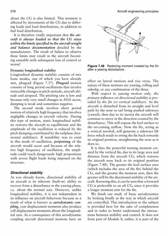
578 Aircraft engineering principles
about the CG is also limited. This moment isaffected by movements of the CG due to differ-ing loads and load distributions, in addition tofuel load distribution.
It is therefore vitally important that the air-craft is always loaded so that the CG stayswithin the limits specified in the aircraft weightand balance documentation detailed by themanufacturer. The result of failure to observethese limits may result in the aircraft becom-ing unstable with subsequent loss of control orworse!
Dynamic longitudinal stabilityLongitudinal dynamic stability consists of twobasic modes, one of which you have alreadymet, phugoid (Figure 7.37). Phugoid motionconsists of long period oscillations that involvenoticeable changes in pitch attitude, aircraft alti-tude and airspeed. The pitching rate is low andbecause only very small changes in AOA occur,damping is weak and sometimes negative.
The second mode involves short periodmotion of relatively high frequency that involvesnegligible changes in aircraft velocity. Duringthis type of motion, static longitudinal stabil-ity restores the aircraft to equilibrium and theamplitude of the oscillation is reduced by thepitch damping contributed by the tailplane (hor-izontal stabilizer). If instability was to existin this mode of oscillation, porpoising of theaircraft would occur and because of the rela-tive high frequency of oscillation, the ampli-tude could reach dangerously high proportionswith severe flight loads being imposed on thestructure.
Directional stabilityAs you already know, directional stability ofan aircraft is its inherent (built-in) ability torecover from a disturbance in the yawing plane,i.e. about the normal axis. However, unlikelongitudinal stability, it is not independent inits influence on aircraft behaviour because as aresult of what is known as aerodynamic cou-pling, yaw displacement moments also produceroll displacement moments about the longitudi-nal axis. As a consequence of this aerodynamiccoupling aircraft directional motions have an
Figure 7.48 Restoring moment created by the finafter a yawing disturbance.
effect on lateral motions and vice versa. Thenature of these motions are yawing, rolling andsideslip, or any combination of the three.
With respect to yawing motion only, theprimary influence on directional stability is pro-vided by the fin (or vertical stabilizer). As theaircraft is disturbed from its straight and levelpath by the nose or tail being pushed sideways(yawed), then due to its inertia the aircraft willcontinue to move in the direction created by thedisturbance. This will expose the keel surface tothe on-coming airflow. Now the fin, acting asa vertical aerofoil, will generate a sideways liftforce which tends to swing the fin back towardsits original position, straightening the nose as itdoes so.
It is thus the powerful turning moment cre-ated by the vertical fin, due to its large area anddistance from the aircraft CG, which restoresthe aircraft nose back to its original position(Figure 7.48). The greater the keel surface area(which includes the area of the fin) behind theCG, and the greater the moment arm, then thegreater will be the directional stability of the air-craft. Knowing this, it can be seen that a forwardCG is preferable to an aft CG, since it providesa longer moment arm for the fin.
We finish our study of basic aerodynamicsby looking briefly at the way in which aircraftare controlled. This introduction to the subjectis provided here for the sake of completenessand in order to better understand the interac-tions between stability and control. It does notform part of Module 8, rather, it is part of the
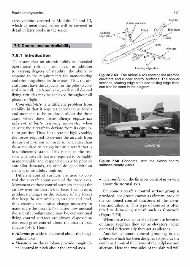
Basic aerodynamics 579
aerodynamics covered in Modules 11 and 13,which as mentioned before will be covered indetail in later books in the series.
7.6 Control and controllability
7.6.1 Introduction
To ensure that an aircraft fulfils its intendedoperational role it must have, in additionto varying degrees of stability, the ability torespond to the requirements for manoeuvringand trimming about its three axes. Thus the air-craft must have the capacity for the pilot to con-trol it in roll, pitch and yaw, so that all desiredflying attitudes may be achieved throughout allphases of flight.
Controllability is a different problem fromstability in that it requires aerodynamic forcesand moments to be produced about the threeaxes, where these forces always oppose theinherent stability restoring moments, whencausing the aircraft to deviate from its equilib-rium position. Thus if an aircraft is highly stable,the forces required to deviate the aircraft fromits current position will need to be greater thanthose required to act against an aircraft that isless inherently stable. This is one of the rea-sons why aircraft that are required to be highlymanoeuvrable and respond quickly to pilot orautopilot demands, are often designed with anelement of instability built-in.
Different control surfaces are used to con-trol the aircraft about each of the three axes.Movement of these control surfaces changes theairflow over the aircraft’s surface. This, in turn,produces changes in the balance of the forcesthat keep the aircraft flying straight and level,thus creating the desired change necessary tomanoeuvre the aircraft. No matter how unusualthe aircraft configuration may be, conventionalflying control surfaces are always disposed sothat each gives control about the aircraft axes(Figure 7.49). Thus:
• Ailerons provide roll control about the longi-tudinal axis.
• Elevators on the tailplane provide longitudi-nal control in pitch about the lateral axis.
Figure 7.49 The Airbus A320 showing the aileronselevators and rudder control surfaces. The spoilersections, leading edge slats and trailing edge flapscan also be seen in the diagram.
Figure 7.50 Concorde, with the elevon controlsurfaces clearly visible.
• The rudder on the fin gives control in yawingabout the normal axis.
On some aircraft a control surface group isprovided, one group known as elevons, providethe combined control functions of the eleva-tors and ailerons. This type of control is oftenfitted to delta-wing aircraft such as Concorde(Figure 7.50).
When these two control surfaces are loweredor raised together they act as elevators, whenoperated differentially they act as ailerons.
Another common control grouping is thetaileron, which has been designed to provide thecombined control functions of the tailplane andailerons. Here the two sides of the slab tail will
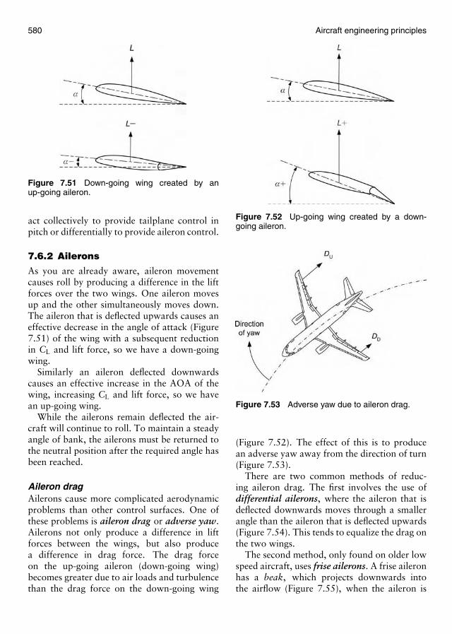
580 Aircraft engineering principles
Figure 7.51 Down-going wing created by anup-going aileron.
act collectively to provide tailplane control inpitch or differentially to provide aileron control.
7.6.2 Ailerons
As you are already aware, aileron movementcauses roll by producing a difference in the liftforces over the two wings. One aileron movesup and the other simultaneously moves down.The aileron that is deflected upwards causes aneffective decrease in the angle of attack (Figure7.51) of the wing with a subsequent reductionin CL and lift force, so we have a down-goingwing.
Similarly an aileron deflected downwardscauses an effective increase in the AOA of thewing, increasing CL and lift force, so we havean up-going wing.
While the ailerons remain deflected the air-craft will continue to roll. To maintain a steadyangle of bank, the ailerons must be returned tothe neutral position after the required angle hasbeen reached.
Aileron dragAilerons cause more complicated aerodynamicproblems than other control surfaces. One ofthese problems is aileron drag or adverse yaw.Ailerons not only produce a difference in liftforces between the wings, but also producea difference in drag force. The drag forceon the up-going aileron (down-going wing)becomes greater due to air loads and turbulencethan the drag force on the down-going wing
Figure 7.52 Up-going wing created by a down-going aileron.
Figure 7.53 Adverse yaw due to aileron drag.
(Figure 7.52). The effect of this is to producean adverse yaw away from the direction of turn(Figure 7.53).
There are two common methods of reduc-ing aileron drag. The first involves the use ofdifferential ailerons, where the aileron that isdeflected downwards moves through a smallerangle than the aileron that is deflected upwards(Figure 7.54). This tends to equalize the drag onthe two wings.
The second method, only found on older lowspeed aircraft, uses frise ailerons. A frise aileronhas a beak, which projects downwards intothe airflow (Figure 7.55), when the aileron is
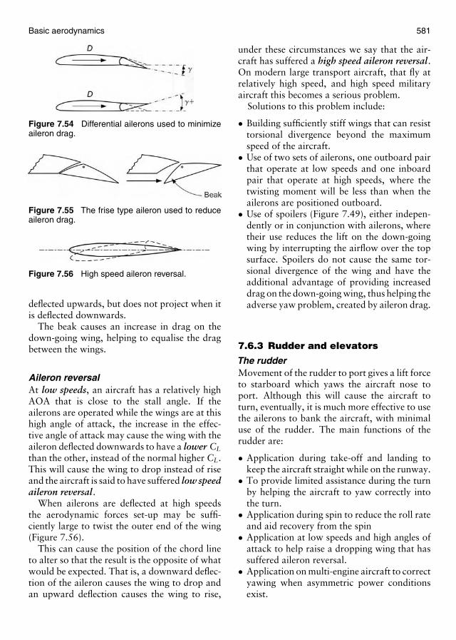
Basic aerodynamics 581
Figure 7.54 Differential ailerons used to minimizeaileron drag.
Figure 7.55 The frise type aileron used to reduceaileron drag.
Figure 7.56 High speed aileron reversal.
deflected upwards, but does not project when itis deflected downwards.
The beak causes an increase in drag on thedown-going wing, helping to equalise the dragbetween the wings.
Aileron reversalAt low speeds, an aircraft has a relatively highAOA that is close to the stall angle. If theailerons are operated while the wings are at thishigh angle of attack, the increase in the effec-tive angle of attack may cause the wing with theaileron deflected downwards to have a lower CL
than the other, instead of the normal higher CL.This will cause the wing to drop instead of riseand the aircraft is said to have suffered low speedaileron reversal.
When ailerons are deflected at high speedsthe aerodynamic forces set-up may be suffi-ciently large to twist the outer end of the wing(Figure 7.56).
This can cause the position of the chord lineto alter so that the result is the opposite of whatwould be expected. That is, a downward deflec-tion of the aileron causes the wing to drop andan upward deflection causes the wing to rise,
under these circumstances we say that the air-craft has suffered a high speed aileron reversal.On modern large transport aircraft, that fly atrelatively high speed, and high speed militaryaircraft this becomes a serious problem.
Solutions to this problem include:
• Building sufficiently stiff wings that can resisttorsional divergence beyond the maximumspeed of the aircraft.
• Use of two sets of ailerons, one outboard pairthat operate at low speeds and one inboardpair that operate at high speeds, where thetwisting moment will be less than when theailerons are positioned outboard.
• Use of spoilers (Figure 7.49), either indepen-dently or in conjunction with ailerons, wheretheir use reduces the lift on the down-goingwing by interrupting the airflow over the topsurface. Spoilers do not cause the same tor-sional divergence of the wing and have theadditional advantage of providing increaseddrag on the down-going wing, thus helping theadverse yaw problem, created by aileron drag.
7.6.3 Rudder and elevators
The rudderMovement of the rudder to port gives a lift forceto starboard which yaws the aircraft nose toport. Although this will cause the aircraft toturn, eventually, it is much more effective to usethe ailerons to bank the aircraft, with minimaluse of the rudder. The main functions of therudder are:
• Application during take-off and landing tokeep the aircraft straight while on the runway.
• To provide limited assistance during the turnby helping the aircraft to yaw correctly intothe turn.
• Application during spin to reduce the roll rateand aid recovery from the spin
• Application at low speeds and high angles ofattack to help raise a dropping wing that hassuffered aileron reversal.
• Application on multi-engine aircraft to correctyawing when asymmetric power conditionsexist.
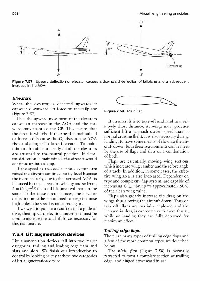
582 Aircraft engineering principles
Figure 7.57 Upward deflection of elevator causes a downward deflection of tailplane and a subsequentincrease in the AOA.
ElevatorsWhen the elevator is deflected upwards itcauses a downward lift force on the tailplane(Figure 7.57).
Thus the upward movement of the elevatorscauses an increase in the AOA and the for-ward movement of the CP. This means thatthe aircraft will rise if the speed is maintainedor increased because the CL rises as the AOArises and a larger lift force is created. To main-tain an aircraft in a steady climb the elevatorsare returned to the neutral position. If eleva-tor deflection is maintained, the aircraft wouldcontinue up into a loop.
If the speed is reduced as the elevators areraised the aircraft continues to fly level becausethe increase in CL due to the increased AOA, isbalanced by the decrease in velocity and so from,L = CL
12ρv2S the total lift force will remain the
same. Under these circumstances, the elevatordeflection must be maintained to keep the nosehigh unless the speed is increased again.
If we wish to pull an aircraft out of a glide ordive, then upward elevator movement must beused to increase the total lift force, necessary forthis manoeuvre.
7.6.4 Lift augmentation devices
Lift augmentation devices fall into two majorcategories, trailing and leading edge flaps andslats and slots. We finish our introduction tocontrol by looking briefly at these two categoriesof lift augmentation device.
Figure 7.58 Plain flap.
If an aircraft is to take-off and land in a rel-atively short distance, its wings must producesufficient lift at a much slower speed than innormal cruising flight. It is also necessary duringlanding, to have some means of slowing the air-craft down. Both these requirements can be meetby the use of flaps and slats or a combinationof both.
Flaps are essentially moving wing sectionswhich increase wing camber and therefore angleof attack. In addition, in some cases, the effec-tive wing area is also increased. Dependent ontype and complexity flap systems are capable ofincreasing CLmax by up to approximately 90%of the clean wing value.
Flaps also greatly increase the drag on thewings thus slowing the aircraft down. Thus ontake-off, flaps are partially deployed and theincrease in drag is overcome with more thrust,while on landing they are fully deployed formaximum effect.
Trailing edge flapsThere are many types of trailing edge flaps anda few of the more common types are describedbelow.
The plain flap (Figure 7.58) is normallyretracted to form a complete section of trailingedge, and hinged downward in use.
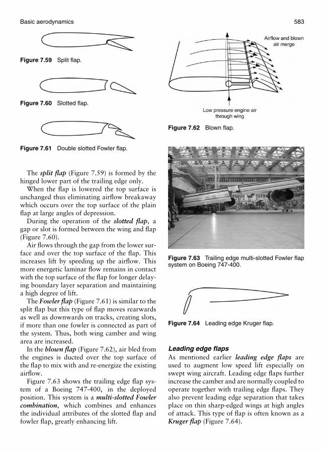
Basic aerodynamics 583
Figure 7.59 Split flap.
Figure 7.60 Slotted flap.
Figure 7.61 Double slotted Fowler flap.
The split flap (Figure 7.59) is formed by thehinged lower part of the trailing edge only.
When the flap is lowered the top surface isunchanged thus eliminating airflow breakawaywhich occurs over the top surface of the plainflap at large angles of depression.
During the operation of the slotted flap, agap or slot is formed between the wing and flap(Figure 7.60).
Air flows through the gap from the lower sur-face and over the top surface of the flap. Thisincreases lift by speeding up the airflow. Thismore energetic laminar flow remains in contactwith the top surface of the flap for longer delay-ing boundary layer separation and maintaininga high degree of lift.
The Fowler flap (Figure 7.61) is similar to thesplit flap but this type of flap moves rearwardsas well as downwards on tracks, creating slots,if more than one fowler is connected as part ofthe system. Thus, both wing camber and wingarea are increased.
In the blown flap (Figure 7.62), air bled fromthe engines is ducted over the top surface ofthe flap to mix with and re-energize the existingairflow.
Figure 7.63 shows the trailing edge flap sys-tem of a Boeing 747-400, in the deployedposition. This system is a multi-slotted Fowlercombination, which combines and enhancesthe individual attributes of the slotted flap andfowler flap, greatly enhancing lift.
Figure 7.62 Blown flap.
Figure 7.63 Trailing edge multi-slotted Fowler flapsystem on Boeing 747-400.
Figure 7.64 Leading edge Kruger flap.
Leading edge flapsAs mentioned earlier leading edge flaps areused to augment low speed lift especially onswept wing aircraft. Leading edge flaps furtherincrease the camber and are normally coupled tooperate together with trailing edge flaps. Theyalso prevent leading edge separation that takesplace on thin sharp-edged wings at high anglesof attack. This type of flap is often known as aKruger flap (Figure 7.64).
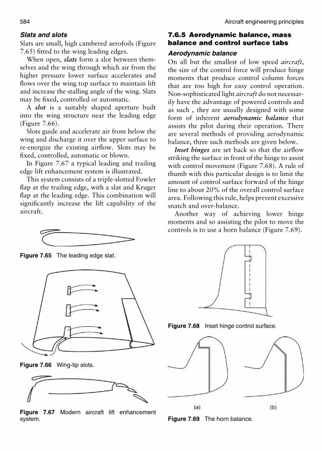
584 Aircraft engineering principles
Slats and slotsSlats are small, high cambered aerofoils (Figure7.65) fitted to the wing leading edges.
When open, slats form a slot between them-selves and the wing through which air from thehigher pressure lower surface accelerates andflows over the wing top surface to maintain liftand increase the stalling angle of the wing. Slatsmay be fixed, controlled or automatic.
A slot is a suitably shaped aperture builtinto the wing structure near the leading edge(Figure 7.66).
Slots guide and accelerate air from below thewing and discharge it over the upper surface tore-energize the existing airflow. Slots may befixed, controlled, automatic or blown.
In Figure 7.67 a typical leading and trailingedge lift enhancement system is illustrated.
This system consists of a triple-slotted Fowlerflap at the trailing edge, with a slat and Krugerflap at the leading edge. This combination willsignificantly increase the lift capability of theaircraft.
Figure 7.65 The leading edge slat.
Figure 7.66 Wing-tip slots.
Figure 7.67 Modern aircraft lift enhancementsystem.
7.6.5 Aerodynamic balance, massbalance and control surface tabs
Aerodynamic balanceOn all but the smallest of low speed aircraft,the size of the control force will produce hingemoments that produce control column forcesthat are too high for easy control operation.Non-sophisticated light aircraft do not necessar-ily have the advantage of powered controls andas such , they are usually designed with someform of inherent aerodynamic balance thatassists the pilot during their operation. Thereare several methods of providing aerodynamicbalance, three such methods are given below.
Inset hinges are set back so that the airflowstriking the surface in front of the hinge to assistwith control movement (Figure 7.68). A rule ofthumb with this particular design is to limit theamount of control surface forward of the hingeline to about 20% of the overall control surfacearea. Following this rule, helps prevent excessivesnatch and over-balance.
Another way of achieving lower hingemoments and so assisting the pilot to move thecontrols is to use a horn balance (Figure 7.69).
Figure 7.68 Inset hinge control surface.
Figure 7.69 The horn balance.
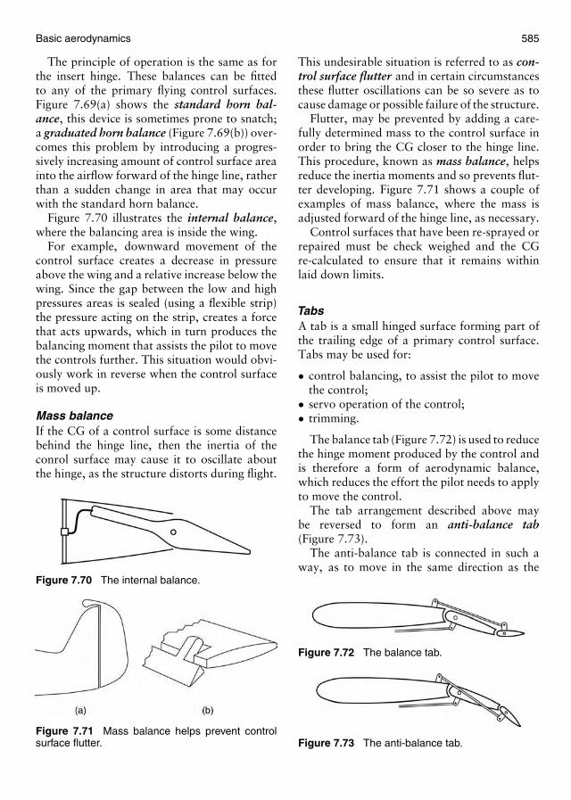
Basic aerodynamics 585
The principle of operation is the same as forthe insert hinge. These balances can be fittedto any of the primary flying control surfaces.Figure 7.69(a) shows the standard horn bal-ance, this device is sometimes prone to snatch;a graduated horn balance (Figure 7.69(b)) over-comes this problem by introducing a progres-sively increasing amount of control surface areainto the airflow forward of the hinge line, ratherthan a sudden change in area that may occurwith the standard horn balance.
Figure 7.70 illustrates the internal balance,where the balancing area is inside the wing.
For example, downward movement of thecontrol surface creates a decrease in pressureabove the wing and a relative increase below thewing. Since the gap between the low and highpressures areas is sealed (using a flexible strip)the pressure acting on the strip, creates a forcethat acts upwards, which in turn produces thebalancing moment that assists the pilot to movethe controls further. This situation would obvi-ously work in reverse when the control surfaceis moved up.
Mass balanceIf the CG of a control surface is some distancebehind the hinge line, then the inertia of theconrol surface may cause it to oscillate aboutthe hinge, as the structure distorts during flight.
Figure 7.70 The internal balance.
Figure 7.71 Mass balance helps prevent controlsurface flutter.
This undesirable situation is referred to as con-trol surface flutter and in certain circumstancesthese flutter oscillations can be so severe as tocause damage or possible failure of the structure.
Flutter, may be prevented by adding a care-fully determined mass to the control surface inorder to bring the CG closer to the hinge line.This procedure, known as mass balance, helpsreduce the inertia moments and so prevents flut-ter developing. Figure 7.71 shows a couple ofexamples of mass balance, where the mass isadjusted forward of the hinge line, as necessary.
Control surfaces that have been re-sprayed orrepaired must be check weighed and the CGre-calculated to ensure that it remains withinlaid down limits.
TabsA tab is a small hinged surface forming part ofthe trailing edge of a primary control surface.Tabs may be used for:
• control balancing, to assist the pilot to movethe control;
• servo operation of the control;• trimming.
The balance tab (Figure 7.72) is used to reducethe hinge moment produced by the control andis therefore a form of aerodynamic balance,which reduces the effort the pilot needs to applyto move the control.
The tab arrangement described above maybe reversed to form an anti-balance tab(Figure 7.73).
The anti-balance tab is connected in such away, as to move in the same direction as the
Figure 7.72 The balance tab.
Figure 7.73 The anti-balance tab.

586 Aircraft engineering principles
control surface so increasing the control col-umn loads. This tab arrangement is used to givethe pilot feel, so that the aircraft will not beoverstressed as a result of excessive movementof the control surface by the pilot.
The spring tab arrangement is such that tabmovement is proportional to the load on the
Figure 7.74 Spring tab operation.
Figure 7.75 Servo-tab arrangement.
Figure 7.76 A typical manual elevator trim system.
control rather than the control surface deflec-tion angle (Figure 7.74). Spring tabs are usedmainly to reduce control loads at high speeds.
The spring is arranged so that below a cer-tain speed it is ineffective (Figure 7.74(a)). Theaerodynamic loads are such that they are notsufficient to overcome the spring force and thetab remains in line with the primary controlsurface. As speed is increased the aerodynamicload acting on the tab is increased sufficiently toovercome the spring force and the tab moves inthe opposite direction to the primary control toprovide assistance (Figure 7.74(b)).
Servo tabThe servo tab is designed to operate the primarycontrol surface (Figure 7.75). Any deflection ofthe tab produces an opposite movement of thefree-floating primary control surface, therebyreducing the effort the pilot has to apply to flythe aircraft.
Trim tabThe trim tab is used to relieve the pilot from anysustained control force that may be needed to
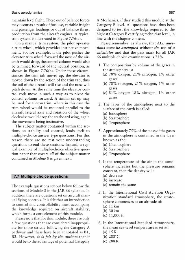
Basic aerodynamics 587
maintain level flight. These out of balance forcesmay occur as a result of fuel use, variable freightand passenger loadings or out of balance thrustproduction from the aircraft engines. A typicaltrim system is illustrated in Figure 7.76(a).
On a manual trim system, the pilot operatesa trim wheel, which provides instinctive move-ment. So, for example, if the pilot pushes theelevator trim wheel forward the nose of the air-craft would drop, the control column would alsobe trimmed forward of the neutral position, asshown in Figure 7.76(b). Under these circum-stances the trim tab moves up, the elevator ismoved down by the action of the trim tab, thusthe tail of the aircraft will rise and the nose willpitch down. At the same time the elevator con-trol rods move in such a way as to pivot thecontrol column forward. A similar set up maybe used for aileron trim, where in this case thetrim wheel would be mounted parallel to theaircraft lateral axis and rotation of the wheelclockwise would drop the starboard wing, againthe movement being instinctive.
The subject matter contained within the sec-tions on stability and control, lends itself tomultiple-choice answer type questions. For thisreason there are no test your understandingquestions to end these sections. Instead, a typ-ical example of multiple-choice objective ques-tion paper that covers all of the subject mattercontained in Module 8 is given next.
7.7 Multiple choice questions
The example questions set out below follow thesections of Module 8 in the JAR 66 syllabus. Inaddition there are questions set on aircraft man-ual flying controls. It is felt that an introductionto control and controllability must accompanythe knowledge required on aircraft stability,which forms a core element of this module.
Please note that for this module, there are onlya few questions that are considered inappropri-ate for those strictly following the Category Apathway and these have been annotated as B1,B2. However, it is felt by the authors that itwould be to the advantage of potential Category
A Mechanics, if they studied this module at theCategory B level. All questions have thus beendesigned to test the knowledge required to thehighest Category B certifying technician level, inline with the chapter content.
Please remember, as always, that ALL ques-tions must be attempted without the use of acalculator and that the pass mark for all JAR66 multiple-choice examinations is 75%.
1. The composition by volume of the gases inthe atmosphere is:(a) 78% oxygen, 21% nitrogen, 1% other
gases(b) 78% nitrogen, 21% oxygen, 1% other
gases(c) 81% oxygen 18% nitrogen, 1% other
gases
2. The layer of the atmosphere next to thesurface of the earth is called:(a) Ionosphere(b) Stratosphere(c) Troposphere
3. Approximately 75% of the mass of the gasesin the atmosphere is contained in the layerknown as the:(a) Chemosphere(b) Stratosphere(c) Troposphere
4. If the temperature of the air in the atmo-sphere increases but the pressure remainsconstant, then the density will:(a) decrease(b) increase(c) remain the same
5. In the International Civil Aviation Orga-nization standard atmosphere, the strato-sphere commences at an altitude of:(a) 11 km(b) 30 km(c) 11,000 ft
6. In the International Standard Atmosphere,the mean sea-level temperature is set at:(a) 15 K(b) 288◦C(c) 288 K
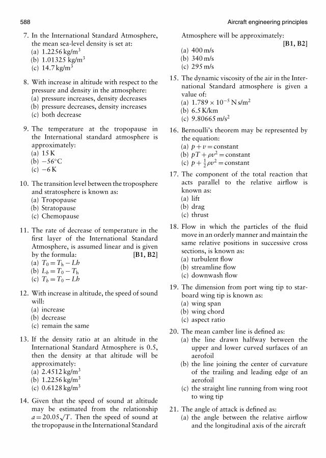
588 Aircraft engineering principles
7. In the International Standard Atmosphere,the mean sea-level density is set at:(a) 1.2256 kg/m3
(b) 1.01325 kg/m3
(c) 14.7 kg/m3
8. With increase in altitude with respect to thepressure and density in the atmosphere:(a) pressure increases, density decreases(b) pressure decreases, density increases(c) both decrease
9. The temperature at the tropopause inthe International standard atmosphere isapproximately:(a) 15 K(b) −56◦C(c) −6 K
10. The transition level between the troposphereand stratosphere is known as:(a) Tropopause(b) Stratopause(c) Chemopause
11. The rate of decrease of temperature in thefirst layer of the International StandardAtmosphere, is assumed linear and is givenby the formula: [B1, B2](a) T0 = Th − Lh(b) Lh = T0 − Th
(c) Th = T0 − Lh
12. With increase in altitude, the speed of soundwill:(a) increase(b) decrease(c) remain the same
13. If the density ratio at an altitude in theInternational Standard Atmosphere is 0.5,then the density at that altitude will beapproximately:(a) 2.4512 kg/m3
(b) 1.2256 kg/m3
(c) 0.6128 kg/m3
14. Given that the speed of sound at altitudemay be estimated from the relationshipa = 20.05
√T. Then the speed of sound at
the tropopause in the International Standard
Atmosphere will be approximately:[B1, B2]
(a) 400 m/s(b) 340 m/s(c) 295 m/s
15. The dynamic viscosity of the air in the Inter-national Standard atmosphere is given avalue of:(a) 1.789 × 10⁻⁵ N s/m2
(b) 6.5 K/km(c) 9.80665 m/s2
16. Bernoulli’s theorem may be represented bythe equation:(a) p + v = constant(b) pT + ρv2 = constant(c) p + 1
2ρv2 = constant
17. The component of the total reaction thatacts parallel to the relative airflow isknown as:(a) lift(b) drag(c) thrust
18. Flow in which the particles of the fluidmove in an orderly manner and maintain thesame relative positions in successive crosssections, is known as:(a) turbulent flow(b) streamline flow(c) downwash flow
19. The dimension from port wing tip to star-board wing tip is known as:(a) wing span(b) wing chord(c) aspect ratio
20. The mean camber line is defined as:(a) the line drawn halfway between the
upper and lower curved surfaces of anaerofoil
(b) the line joining the center of curvatureof the trailing and leading edge of anaerofoil
(c) the straight line running from wing rootto wing tip
21. The angle of attack is defined as:(a) the angle between the relative airflow
and the longitudinal axis of the aircraft
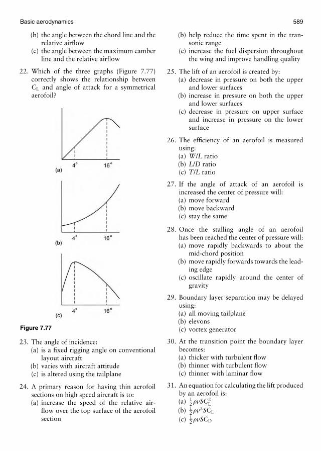
Basic aerodynamics 589
(b) the angle between the chord line and therelative airflow
(c) the angle between the maximum camberline and the relative airflow
22. Which of the three graphs (Figure 7.77)correctly shows the relationship betweenCL and angle of attack for a symmetricalaerofoil?
Figure 7.77
23. The angle of incidence:(a) is a fixed rigging angle on conventional
layout aircraft(b) varies with aircraft attitude(c) is altered using the tailplane
24. A primary reason for having thin aerofoilsections on high speed aircraft is to:(a) increase the speed of the relative air-
flow over the top surface of the aerofoilsection
(b) help reduce the time spent in the tran-sonic range
(c) increase the fuel dispersion throughoutthe wing and improve handling quality
25. The lift of an aerofoil is created by:(a) decrease in pressure on both the upper
and lower surfaces(b) increase in pressure on both the upper
and lower surfaces(c) decrease in pressure on upper surface
and increase in pressure on the lowersurface
26. The efficiency of an aerofoil is measuredusing:(a) W /L ratio(b) L/D ratio(c) T/L ratio
27. If the angle of attack of an aerofoil isincreased the center of pressure will:(a) move forward(b) move backward(c) stay the same
28. Once the stalling angle of an aerofoilhas been reached the center of pressure will:(a) move rapidly backwards to about the
mid-chord position(b) move rapidly forwards towards the lead-
ing edge(c) oscillate rapidly around the center of
gravity
29. Boundary layer separation may be delayedusing:(a) all moving tailplane(b) elevons(c) vortex generator
30. At the transition point the boundary layerbecomes:(a) thicker with turbulent flow(b) thinner with turbulent flow(c) thinner with laminar flow
31. An equation for calculating the lift producedby an aerofoil is:(a) 1
2ρvSC2L
(b) 12ρv2SCL
(c) 12ρvSCD
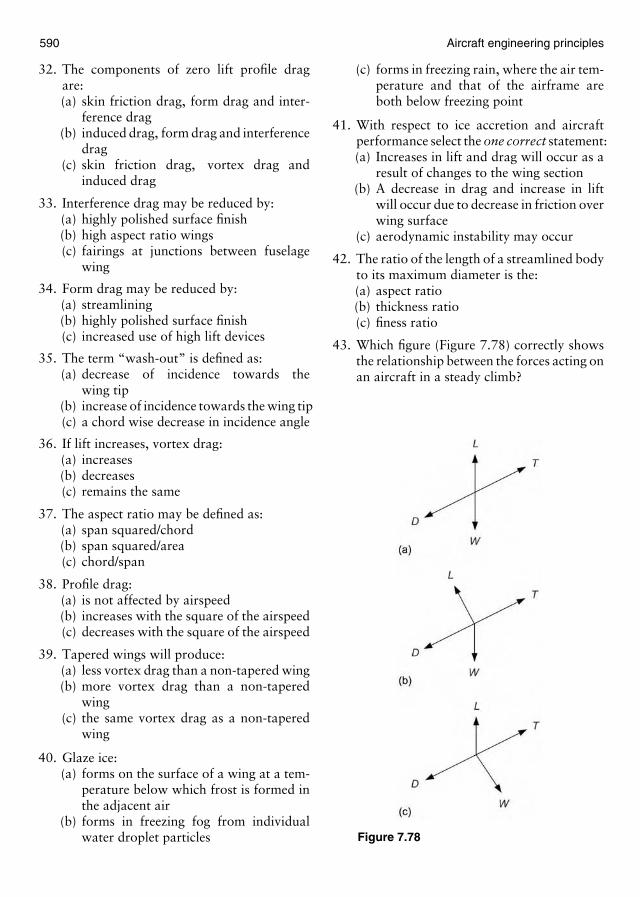
590 Aircraft engineering principles
32. The components of zero lift profile dragare:(a) skin friction drag, form drag and inter-
ference drag(b) induced drag, form drag and interference
drag(c) skin friction drag, vortex drag and
induced drag
33. Interference drag may be reduced by:(a) highly polished surface finish(b) high aspect ratio wings(c) fairings at junctions between fuselage
wing
34. Form drag may be reduced by:(a) streamlining(b) highly polished surface finish(c) increased use of high lift devices
35. The term “wash-out” is defined as:(a) decrease of incidence towards the
wing tip(b) increase of incidence towards the wing tip(c) a chord wise decrease in incidence angle
36. If lift increases, vortex drag:(a) increases(b) decreases(c) remains the same
37. The aspect ratio may be defined as:(a) span squared/chord(b) span squared/area(c) chord/span
38. Profile drag:(a) is not affected by airspeed(b) increases with the square of the airspeed(c) decreases with the square of the airspeed
39. Tapered wings will produce:(a) less vortex drag than a non-tapered wing(b) more vortex drag than a non-tapered
wing(c) the same vortex drag as a non-tapered
wing
40. Glaze ice:(a) forms on the surface of a wing at a tem-
perature below which frost is formed inthe adjacent air
(b) forms in freezing fog from individualwater droplet particles
(c) forms in freezing rain, where the air tem-perature and that of the airframe areboth below freezing point
41. With respect to ice accretion and aircraftperformance select the one correct statement:(a) Increases in lift and drag will occur as a
result of changes to the wing section(b) A decrease in drag and increase in lift
will occur due to decrease in friction overwing surface
(c) aerodynamic instability may occur
42. The ratio of the length of a streamlined bodyto its maximum diameter is the:(a) aspect ratio(b) thickness ratio(c) finess ratio
43. Which figure (Figure 7.78) correctly showsthe relationship between the forces acting onan aircraft in a steady climb?
Figure 7.78
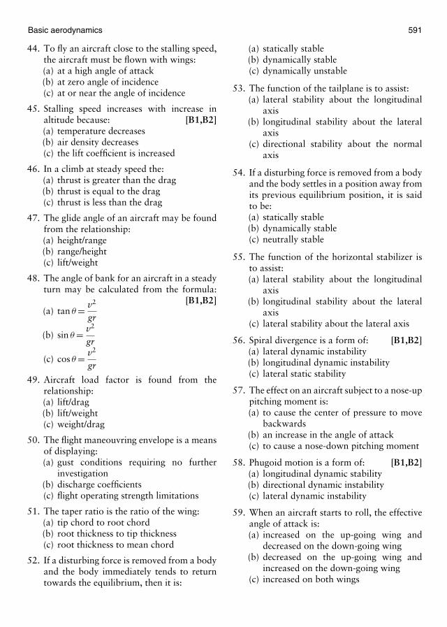
Basic aerodynamics 591
44. To fly an aircraft close to the stalling speed,the aircraft must be flown with wings:(a) at a high angle of attack(b) at zero angle of incidence(c) at or near the angle of incidence
45. Stalling speed increases with increase inaltitude because: [B1,B2](a) temperature decreases(b) air density decreases(c) the lift coefficient is increased
46. In a climb at steady speed the:(a) thrust is greater than the drag(b) thrust is equal to the drag(c) thrust is less than the drag
47. The glide angle of an aircraft may be foundfrom the relationship:(a) height/range(b) range/height(c) lift/weight
48. The angle of bank for an aircraft in a steadyturn may be calculated from the formula:
[B1,B2](a) tan θ = v2
gr
(b) sin θ = v2
gr
(c) cos θ = v2
gr
49. Aircraft load factor is found from therelationship:(a) lift/drag(b) lift/weight(c) weight/drag
50. The flight maneouvring envelope is a meansof displaying:(a) gust conditions requiring no further
investigation(b) discharge coefficients(c) flight operating strength limitations
51. The taper ratio is the ratio of the wing:(a) tip chord to root chord(b) root thickness to tip thickness(c) root thickness to mean chord
52. If a disturbing force is removed from a bodyand the body immediately tends to returntowards the equilibrium, then it is:
(a) statically stable(b) dynamically stable(c) dynamically unstable
53. The function of the tailplane is to assist:(a) lateral stability about the longitudinal
axis(b) longitudinal stability about the lateral
axis(c) directional stability about the normal
axis
54. If a disturbing force is removed from a bodyand the body settles in a position away fromits previous equilibrium position, it is saidto be:(a) statically stable(b) dynamically stable(c) neutrally stable
55. The function of the horizontal stabilizer isto assist:(a) lateral stability about the longitudinal
axis(b) longitudinal stability about the lateral
axis(c) lateral stability about the lateral axis
56. Spiral divergence is a form of: [B1,B2](a) lateral dynamic instability(b) longitudinal dynamic instability(c) lateral static stability
57. The effect on an aircraft subject to a nose-uppitching moment is:(a) to cause the center of pressure to move
backwards(b) an increase in the angle of attack(c) to cause a nose-down pitching moment
58. Phugoid motion is a form of: [B1,B2](a) longitudinal dynamic stability(b) directional dynamic instability(c) lateral dynamic instability
59. When an aircraft starts to roll, the effectiveangle of attack is:(a) increased on the up-going wing and
decreased on the down-going wing(b) decreased on the up-going wing and
increased on the down-going wing(c) increased on both wings
592 Aircraft engineering principles
60. To ensure longitudinal stability in flight, theposition of the center of gravity should:(a) be aft of the neutral point(b) coincide with the neutral point(c) be forward of the neutral point
61. Anhedral is defined as:(a) the upward and outward inclination of
the wings(b) the downward and outward inclination
of the aircraft wings(c) the forward sloping canard stabilizer
62. The fin of an aircraft helps to provide arestoring moment when an aircraft:(a) dives(b) pitches(c) yaws
63. The dihedral angle of a wing provides arestoring moment when an aircraft:(a) climbs(b) pitches(c) rolls
64. On a swept wing aircraft, that enters asideslip, the air velocity normal to the lead-ing edge increases: [B1, B2](a) on both wings(b) on the up-going wing(c) on the down-going wing
65. Control of yaw is mainly influenced by:(a) the fin(b) the rudder(c) the tailplane
66. Movement of an aircraft about its normalaxis is called(a) yawing(b) rolling(c) pitching
67. For a symmetrical aerofoil, downwarddeflection of a control surface:(a) increases both lift and drag(b) increases lift, decreases drag(c) decreases lift, increases drag
68. Different drag force between up-going anddown-going ailerons is counteracted by:(a) aerodynamic balance control
(b) static balance(c) differential aileron movement
69. The drag produced by aileron movement is:(a) greater on the down-going aileron(b) less on the down-going aileron(c) equal on both ailerons
70. At low speeds and at high angles of attackthe wing with the down-going aileron may:(a) bend(b) stall(c) twist
71. At high speeds, the wing with the down-going aileron may:(a) turn at wing tip(b) yaw at the wing tip(c) twist at the wing tip
72. The frise type aileron is used to:(a) increase directional control(b) reduce high speed aileron reversal(c) reduce aileron drag
73. The lift augmentation device shown in Fig-ure 7.79, is a:
Figure 7.79
(a) plain flap(b) Kruger flap(c) split flap
74. A Fowler flap:(a) increases the wing camber and the angle
of attack(b) increases the wing camber and reduces
the effective wing area(c) decrease the lift coefficient and stalling
angle
75. The device shown at the leading edge of theFigure 7.80 is:(a) flap(b) slat(c) slot
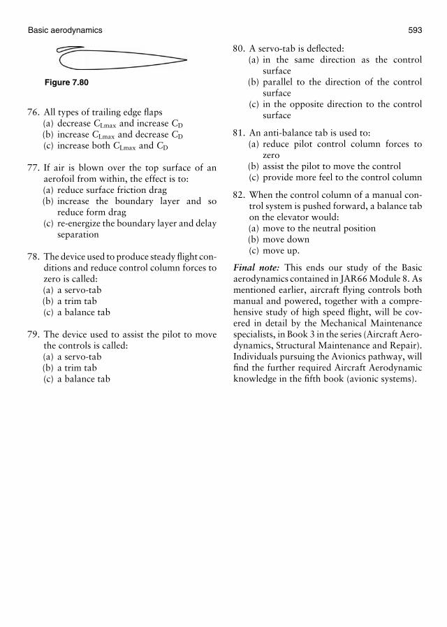
Basic aerodynamics 593
Figure 7.80
76. All types of trailing edge flaps(a) decrease CLmax and increase CD
(b) increase CLmax and decrease CD
(c) increase both CLmax and CD
77. If air is blown over the top surface of anaerofoil from within, the effect is to:(a) reduce surface friction drag(b) increase the boundary layer and so
reduce form drag(c) re-energize the boundary layer and delay
separation
78. The device used to produce steady flight con-ditions and reduce control column forces tozero is called:(a) a servo-tab(b) a trim tab(c) a balance tab
79. The device used to assist the pilot to movethe controls is called:(a) a servo-tab(b) a trim tab(c) a balance tab
80. A servo-tab is deflected:(a) in the same direction as the control
surface(b) parallel to the direction of the control
surface(c) in the opposite direction to the control
surface
81. An anti-balance tab is used to:(a) reduce pilot control column forces to
zero(b) assist the pilot to move the control(c) provide more feel to the control column
82. When the control column of a manual con-trol system is pushed forward, a balance tabon the elevator would:(a) move to the neutral position(b) move down(c) move up.
Final note: This ends our study of the Basicaerodynamics contained in JAR66 Module 8. Asmentioned earlier, aircraft flying controls bothmanual and powered, together with a compre-hensive study of high speed flight, will be cov-ered in detail by the Mechanical Maintenancespecialists, in Book 3 in the series (Aircraft Aero-dynamics, Structural Maintenance and Repair).Individuals pursuing the Avionics pathway, willfind the further required Aircraft Aerodynamicknowledge in the fifth book (avionic systems).

This page intentionally left blank

Appendices

This page intentionally left blank
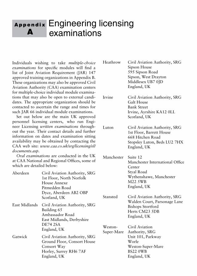
A p p e n d i x
AEngineering licensingexaminations
Individuals wishing to take multiple-choiceexaminations for specific modules will find alist of Joint Aviation Requirement (JAR) 147approved training organizations in Appendix B.These organizations may also be approved CivilAviation Authority (CAA) examination centersfor multiple-choice individual module examina-tions that may also be open to external candi-dates. The appropriate organization should becontacted to ascertain the range and times forsuch JAR 66 individual module examinations.
Set out below are the main UK approvedpersonnel licensing centers, who run Engi-neer Licensing written examinations through-out the year. Their contact details and furtherinformation on dates and examination sittingavailability may be obtained by contacting theCAA web site: www.caa.co.uk/srg/licensing/el/documents.asp.
Oral examinations are conducted in the UKat CAA National and Regional Offices, some ofwhich are detailed below:
Aberdeen Civil Aviation Authority, SRG1st Floor, North NorfolkHouse AnnexePitmedden RoadDyce, Aberdeen AB2 OBPScotland, UK
East Midlands Civil Aviation Authority, SRGBuilding 65Ambassador RoadEast Midlands, DerbyshireDE74 2SAEngland, UK
Gatwick Civil Aviation Authority, SRGGround Floor, Consort HouseConsort WayHorley, Surrey RH6 7AFEngland, UK
Heathrow Civil Aviation Authority, SRGSipson House595 Sipson RoadSipson, West DraytonMiddlesex UB7 0JDEngland, UK
Irvine Civil Aviation Authority, SRGGalt HouseBank StreetIrvine, Ayrshire KA12 0LLScotland, UK
Luton Civil Aviation Authority, SRG1st Floor, Barrett House668 Hitchen RoadStopsley Luton, Beds LU2 7HXEngland, UK
Manchester Suite 12Manchester International OfficeCenterStyal RoadWythenshawe, ManchesterM22 5WBEngland, UK
Stansted Civil Aviation Authority, SRGWalden Court, Parsonage LaneBishops StortfordHerts CM23 5DBEngland, UK
Weston- Civil AviationSuper-Mare Authority, SRG
Unit 101, ParkwayWorleWeston-Super-MareBS22 0WBEngland, UK

598 Aircraft engineering principles
Given below are some European JAR, NationalAviation Authorities (NAA), with their officecontact addresses as on July 2003.
Athens Ministry of Transport andCommunicationsCivil Aviation AuthorityPO Box 73751GR16604 HellinikoGreece
Berlin Luftfahrt-BundesamtAussenstelle Berlin Postfach 11D-12508 BerlinGermany
Berne Federal Office for Civil AviationMaulbeerstrasse 9Ch-3003 BerneSwitzerland
Brussels Administration del’AeronautiqueCentral Communication Nord4th Floor, Rue du Progres 80B01210 BrusselsBelgium
Copenhagen Civil Aviation AdministrationDepartment of AviationInspectionPO Box 744DK-2450 Copenhagen SVDenmark
Czech Civil Aviation AuthorityRepublic Czech Republic
Ruzyne Airport160 08 Praha 6Czech Republic
Dublin Irish Aviation AuthorityAirworthiness StandardsDepartment3rd Floor, Aviation HouseHawkins StreetDublin 2Ireland
Frankfurt Luftfahrt-BundesamtLanger Kornweg 19-23D-65451 KelsterbachGermany
Helsinki Civil Aviation AdministrationBox 50SF-01531 Helsinki-VantaaFinland
Hoofddorp Civil Aviation AuthorityThe NetherlandsPO Box 5752130 An HoofddorpThe Netherlands
Lisbon Direccao-Geral da Aviacao CivilDireccao Do MaterialAeronauticoRua B – Edificio No. 6Aeroporto de Lisboa1700 LisboaPortugal
Luxembourg Ministry of Transport19–21 Boulevard RoyalL-2938 LuxembourgLuxembourg
Madrid Ministerio de FomentoSubdireccion General de Controldel Transporte AereoPza. San Juan de la Cruz, s/n28071 MadridSpain
Malta The Director General of AviationMalta Department of CivilAviationMalta International AirportLuga LQA05Malta
Monaco Civil Aviation AuthorityHeliport de MonacoMC 98000 MonacoMonaco
Oslo Civil Aviation AdministrationHead OfficeAeronautical InspectionDepartmentPO Box 8124 DepartmentN-0032 OsloNorway

Engineering licensing examinations 599
Paris GS de L’Aviation Civile72-78 Grande Rue92310 Sevres, ParisFrance
Reykjavik Civil AviationAdministration (FMS)PO Box 50Reykjavik Airport212 ReykjavikIceland
Rome HQ Registro Aeronautico ItalianoVia di Villa Ricotti 4200161 RomaItaly
Stockholm LuftfartsverketFlight Safety DepartmentSurveyance SectionBergkallavagen 32Box 304192 30 SollentunaSweden
Vienna Federal Ministry of Science,Transport and the ArtsDepartment of Civil AviationRadetzkystrasse 2A-1030 ViennaAustria
Warszawa General Inspectorate ofCivil AviationGrojecka 1702-021 WarszawaPoland
Note: A current full list of all JAR-NAA officeswill be found in the Joint Aviation Authority(JAA) publication catalogue under its adminis-trative and guidance material in the JAR Direc-tory. General information on all related JARpublications may be found on the JAA website at: www.jaa.nl/catalogue/pubcat.html. Theabove list is correct at the time of going to thepress.

This page intentionally left blank

A p p e n d i x
BOrganizations offering aircraftmaintenance engineeringtraining and education
In the tables below, there will be found detailson a selection of UK and European organiza-tions known to the authors, who offer a varietyof aircraft maintenance engineering training andeducational programmes. Table B.1 providesdetails on those Joint Aviation Requirements(JAR) 147 approved organizations within the
Table B.1
Name and contact address of UK organization
ATC Lasham LtdLasham AirfieldLasham, Hampshire,GU34 5SP, UKAir Service Training (Engineering) LtdPerth AirportPerth, PH2 6NP, UKAirline Maintenance Training IncBuilding D1Fairoaks AirportChobham, SurreyGU24 8HX, UKBritannia AirwaysTechnical Training SchoolLuton Airport, LutonBedfordshire, LU2 9ND, UKCity of Bristol CollegeAshley Down, BristolBS7 9BU, UKKLM UK Engineering Ltd27 Hurricane WayNorwich AirportNorfolk, NR6 6HE, UKFLS Aerospace (UK) LtdLong Border RoadStanstead AirportEssex, CM24 1RE, UKMarshall of Cambridge Aerospace LtdTechnical Training DepartmentThe Airport, Cambridge, CB5 8RX, UK
UK, who offer ab initio and other forms oftraining for categories A and B certifying staff.Table B.2 provides similar detail to that given inTable B.1 for a selection of JAR 147 approvedEuropean organizations. A complete currentunabridged list of JAR 147 approved organi-zations may be found in the Joint Aviation
Table B.2
Name and contact address of European organization
Agusta S.P.A.Via G. Agusta 520Cascina Costa di Samarate (VA), ItalyAirbus1 Rond point Maurice Bellonte31707 Blagnac Cedex, FranceAustrian AirlinesOsterreichische LuftverkehrsAktiengesellschaftA-1300 Vienna Airport, AustriaDornier Luftfahrt GMBHAirport Oberpfaffenhofen82234 Wessling, GermanyEADS Airbus GMBHKreetslag 1021129 Hamburg, GermanyFLS Aerospace (IRL) LtdDublin AirportCounty Dublin, IrelandLufthansa Technical TrainingWeg beim Jager 19322335 Hamburg, GermanyScandinavian Airlines SystemMaintenance Training OrganizationArlanda Airport, S-19587 StockholmSwedenShannon Aerospace LtdShannon, County Clare, IrelandSwiss Aviation Training LtdCH-4002 Basel, Switzerland

602 Aircraft engineering principles
Table B.3
UK training and/or Contact address Type of courseeducational organization
Barry College Colcot Road JAR 66 theory, to practising aircraftBarry, Vale of Glamorgan engineering personnel. Other BTECCF62 8YJ, UK qualifications, using their good practicalwww.barry.ac.uk facilities.
Brooklands College Heath Road On-line learning programme that willWeybridge, eventually cover the associated theory forSurrey KT13 8TT, UK all JAR66 Modules.www.brooklands.ac.ukwww.jar66now.com
University of Bristol IGDS Office In conjunction with the University of the WestFaculty of Engineering of England, the Integrated Graduate DevelopmentUniversity of Bristol Scheme (IDGS) is offered. Primarily concernedUniversity Gate with aerospace design, manufacture andPark Row management; some maintenance technologyBristol BS1 5UB, UK biased modules offered.www.fen.bris.ac.uk/igds/aero
Coventry University School of Engineering Offers B.Eng. and I.Eng. degrees in aerospaceCoventry University systems technology. Novel delivery method withPrior Street strong aircraft technology focus.Coventry CV1 5FB, UKwww.coventry.ac.uk
Kingston University School of Engineering Offers a unique foundation degree (FD), withKingston University B.Eng. (Hons) top-up, covering JAR 66 skillsRoehampton Vale and knowledge that may lead to JAA categoriesFriars Avenue B and C licenses. Delivered in conjunction withLondon SW15 3DW, UK KLM, UK and City of Bristol College at variouswww.kingston.ac.uk venues. Particular routes are JAR 147 approved.
Macclesfield College Macclesfield College Offers JAR 66 modular programmes in mechanicalPark Lane, Macclesfield and avionic specialisms. In addition, mainstreamCheshire SK1 18L, UK BTEC qualifications are offered in aerospacewww.macclesfield.ac.uk engineering.
Newcastle College Newcastle College Offers a new 2 year full-time BTEC nationalRye Hill Campus diploma in aerospace engineering (mechanical).Scotswood Road This course acts as a suitable feeder for the JARNewcastle-upon-Tyne 66 program offered by Kingston University atTyne and Wear NE4 7SA, UK Newcastle Airport.
Northbrook College Northbrook College Offers JAR 66 modular training programmes, withShoreham Airport access to training aircraft and workshop facilities.West Sussex BN43 5FJ, UK In addition, mainstream BTEC qualifications inwww.northbrook.ac.uk aerospace engineering are also offered.
Oxford Aviation Engineer Training Offers modular JAR 66 tailor made courses,Training Oxford Aviation Training covering all JAR 66 modules. Also offers
Oxford Airport, Kidlington conversion courses particularly for conversionOxford OX5 1RA, UK of military personnel to civil aviation.www.oxfordaviation.co.uk
Authority (JAA) publication under mainte-nance, where the required publication is called147 list: JAR 147 approved organizations.Table B.3 provides details on UK educational
and training establishments, who offer pro-grammes, with an aircraft engineering main-tenance bias, which may or may not operateunder the auspices of a JAR 147 organization.
A p p e n d i x
CThe role of the European AviationSafety Agency
With an ever-expanding European Community(EC), where individual nations have a varietyof ways of administering and controlling theirown aviation industries, with varying degrees ofsafety, there has developed the need to providea unified regulatory framework for the Euro-pean aviation industry at large that is totallydedicated to aviation safety.
For these reasons, the EC and other entitiesinvolved in the sector have set up the Euro-pean Aviation Safety Agency (EASA), which willhave real authority for aviation safety, in asimilar manner to that of the Federal AviationAdministration (FAA) in the US.
Thus the primary aims of EASA, in accor-dance with EC Regulation 1592/2002, are to:
• draw-up common standards to ensure thehighest level of aviation safety,
• oversee their uniform application acrossEurope,
• promote these standards worldwide.
An additional aim for international stan-dards of aircraft environmental compatibility,for noise and emissions is already ensconced intoEuropean Union (EU) Regulations. However,with the formation of EASA the unification andharmonization of the technical rules and proce-dures will be much more easily administered andregulated.
So under EC Regulation 1592, the primaryobjectives of EASA are to:
• establish and maintain a high uniform levelof civil aviation safety and environmentalprotection in Europe;
• facilitate the free movement of goods, personsand services;
• promote cost efficiency in the regulatory andcertification process;
• assist member states in fulfilling their ICAOobligations on a common basis;
• promote worldwide community views regard-ing civil aviation safety standards.
In addition, EASA will develop its knowledgein all fields of aviation safety in order to assistCommunity legislators in the development ofcommon rules for:
• the certification of aeronautical products,parts and appliances;
• the approval of organizations and personnelengaged in the maintenance of these products;
• the approval of air operations;• the licensing of air crew;• the safety oversight of airports and air traffic
services operators.
Reference source: www.europa.eu.int/comm/transport/air/safety/agency_en.htm.
The establishment of the EASA will inevitablycause changes to the Joint Aviation Author-ity (JAA) system and organization. Since July2002 the JAA has actively participated in thetransition from the JAA system to EASA bydeveloping, in consultation with the EuropeanCommission, a transition plan that focuses onregulatory aspects.
One of the key issues is the interaction ofEASA rules with the already existing Euro-pean and National legislation. A core group ofexperts have been drafted to look into this issueand produce a report on regulatory interactions.The time frame for consultation is short if themanagement board of EASA are to reach deci-sions for starting the agency, as planned, on28th September 2003.
The above may have far-reaching implica-tions for the future role of the National AviationAuthorities (NAA), in particular in the caseof the UK, for the role of the Civil AviationAuthority (CAA) safety regulation group (SRG).
At present under regulation 1592 only thecertification of aeronautical products and the

604 Aircraft engineering principles
approval of organizations and maintenance per-sonnel are covered. Of particular interest toreaders of this book is the delivery to the ECof a draft report by the core group on theessential requirements for licensing. This report,to date, is not yet in the public domain. How-ever, it is unlikely to present any significantchanges to the existing regulations for engineerlicensing as contained in existing Joint AviationRequirement (JAR) publications.
Finally in the remit for the EASA, it is intendedthat they will look beyond EC borders, witha view to associating as many European part-ners as possible with their ever-evolving safetysystem.
Postscript
EASA (under their role for approving orga-nizations and personnel engaged in aircraft
maintenance), now have the responsibility forthe airworthiness and maintenance of JARs ofthe JAAs. Thus the relevant JARs would havebeen converted into implementing rules (IR)through Commission Regulation, acceptablemeans of compliance (AMC) or as certificationof specifications (CS).
JAR 147 and JAR 66 are now under theauspices of EASA as draft documents, CS 147and CS 166 respectively (ECAR PART-66,Draft 4.3).
ECAR PART-66 differs a little, if at all, fromthe existing JAR 66. However, as the in-houseexpertise grows within EASA, it is likely thatnew or additional rules for the training and edu-cation of maintenance personnel may well beintroduced.
For the latest information on the activitiesof EASA, you should consult their website:http://www.easa.eu.int/.

A p p e n d i x
DMathematical tables
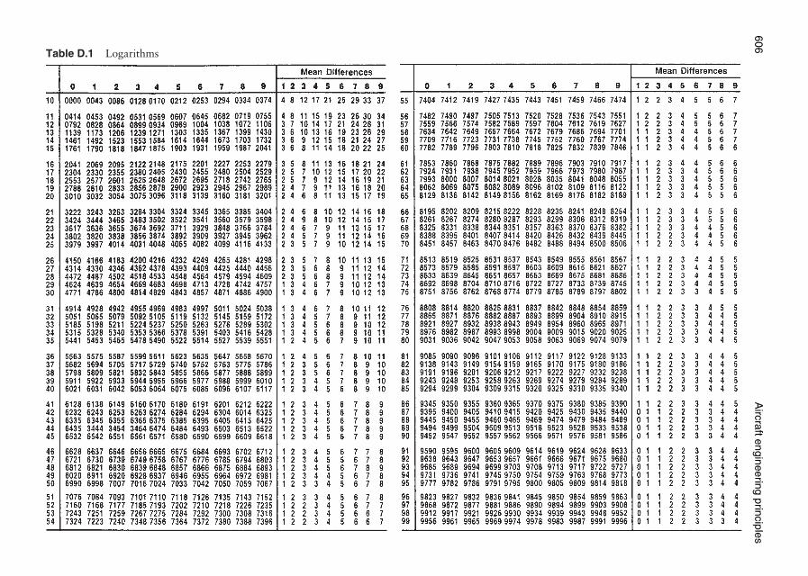
606A
ircraftengineeringprinciples
Table D.1 Logarithms
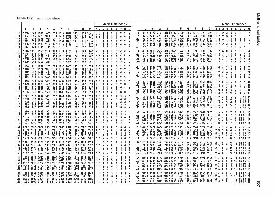
Mathem
aticaltables607
Table D.2 Antilogarithms
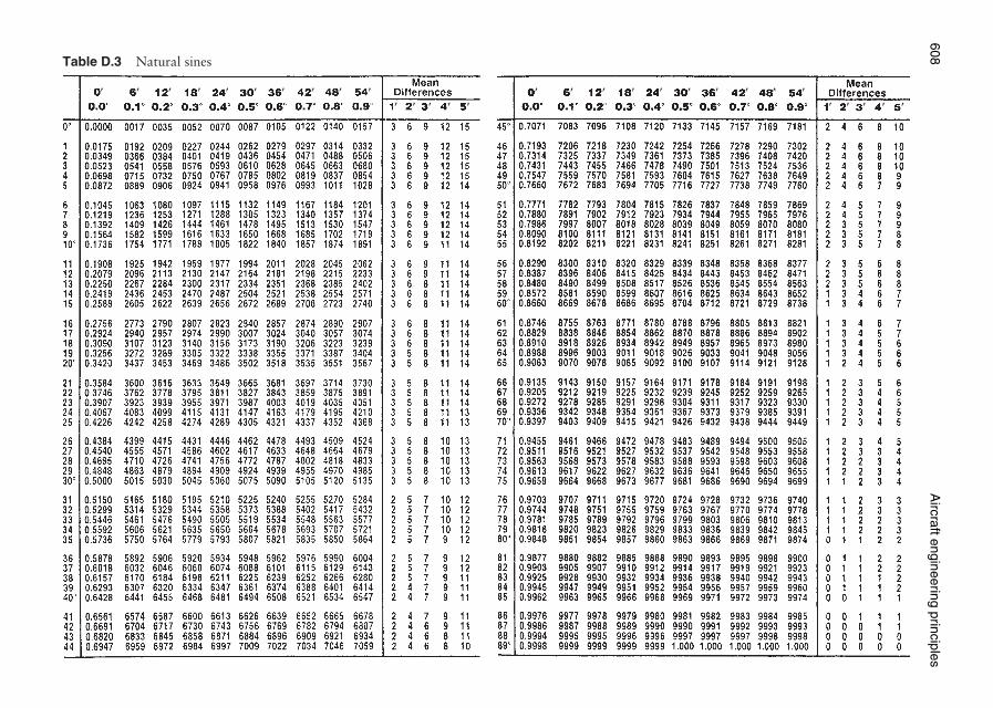
608A
ircraftengineeringprinciples
Table D.3 Natural sines
� � � � � � � � � �� � � � �
� � � � � � � � � �� � � � �

Mathem
aticaltables609
Table D.4 Natural cosines
� � � � � � � � � �� � � � �
� � � � � � � � � �� � � � �
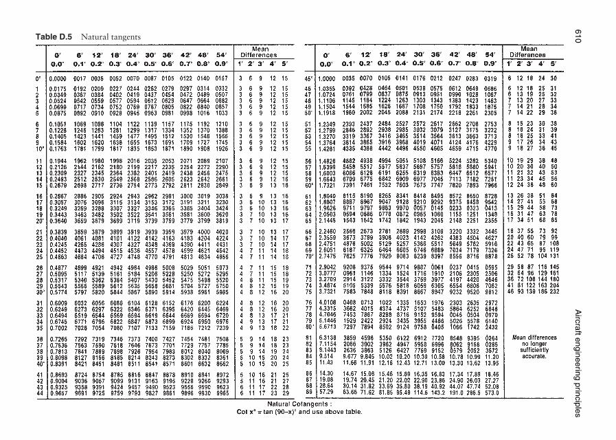
610A
ircraftengineeringprinciples
Table D.5 Natural tangents
� � � � � � � � � �� � � � �
� � � � � � � � � �� � � � �
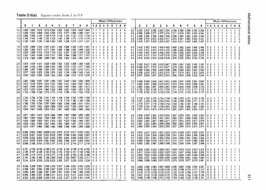
Mathem
aticaltables611
Table D.6(a) Square roots: from 1 to 9.9
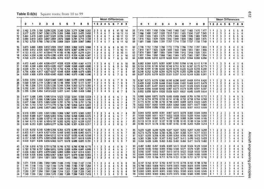
612A
ircraftengineeringprinciples
Table D.6(b) Square roots: from 10 to 99
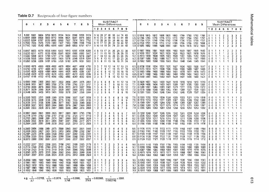
Mathem
aticaltables613
Table D.7 Reciprocals of four-figure numbers

This page intentionally left blank
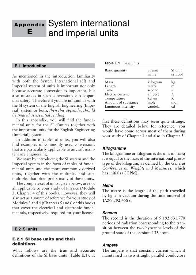
A p p e n d i x
ESystem internationaland imperial units
E.1 Introduction
As mentioned in the introduction familiaritywith both the System International (SI) andImperial system of units is important not onlybecause accurate conversion is important, butalso mistakes in such conversions can jeopar-dize safety. Therefore if you are unfamiliar withthe SI system or the English Engineering (Impe-rial) system or both, then this appendix shouldbe treated as essential reading!
In this appendix, you will find the funda-mental units for the SI d’unites together withthe important units for the English Engineering(Imperial) system.
In addition to tables of units, you will alsofind examples of commonly used conversionsthat are particularly applicable to aircraft main-tenance engineering.
We start by introducing the SI system and theImperial system in the form of tables of funda-mental units and the more commonly derivedunits, together with the multiples and sub-multiples that often prefix many of these units.
The complete set of units, given below, are notall applicable to your study of Physics (Module2, Chapter 4 of this book). However, they willalso act as a source of reference for your study ofModules 3 and 4 (Chapters 5 and 6 of this book)that cover the electrical and electronic funda-mentals, respectively, required for your license.
E.2 SI units
E.2.1 SI base units and theirdefinitions
What follows are the true and accuratedefinitions of the SI base units (Table E.1); at
Table E.1 Base units
Basic quantity SI unit SI unitname symbol
Mass kilogram kgLength metre mTime second sElectric current ampere ATemperature kelvin KAmount of substance mole molLuminous intensity candela cd
first these definitions may seem quite strange.They are detailed below for reference; youwould have come across most of them duringyour study of Chapter 4 and also in Chapter 5.
KilogrammeThe kilogramme or kilogram is the unit of mass;it is equal to the mass of the international proto-type of the kilogram, as defined by the GeneralConference on Weights and Measures, whichhas initials (CGPM).
MetreThe metre is the length of the path travelledby light in vacuum during the time interval of1/299,792,458 s.
SecondThe second is the duration of 9,192,631,770periods of radiation corresponding to the tran-sition between the two hyperfine levels of theground state of the caesium 133 atom.
AmpereThe ampere is that constant current which ifmaintained in two straight parallel conductors
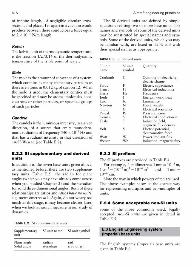
616 Aircraft engineering principles
of infinite length, of negligible circular cross-section, and placed 1 m apart in a vacuum wouldproduce between these conductors a force equalto 2 × 10⁻⁷ N/m length.
KelvinThe kelvin, unit of thermodynamic temperature,is the fraction 1/273.16 of the thermodynamictemperature of the triple point of water.
MoleThe mole is the amount of substance of a system,which contains as many elementary particles asthere are atoms in 0.012 kg of carbon 12. Whenthe mole is used, the elementary entities mustbe specified and may be atoms, molecules, ions,electrons or other particles, or specified groupsof such particles.
CandelaThe candela is the luminious intensity, in a givendirection, of a source that emits monochro-matic radiation of frequency 540 × 1012 Hz andthat has a radiant intensity in that direction of1/683 W/srad (see Table E.2).
E.2.2 SI supplementary and derivedunits
In addition to the seven base units given above,as mentioned before, there are two supplemen-tary units (Table E.2): the radian for planeangles (which you may have already come acrosswhen you studied Chapter 2) and the steradianfor solid three-dimensional angles. Both of theserelationships are ratios and ratios have no units,e.g. metres/metres = 1. Again, do not worry toomuch at this stage, it may become clearer later,when we look at radian measure in our study ofdynamics.
Table E.2 SI supplementary units
Supplementary SI unit name SI unit symbolunit
Plane angle radian radSolid angle steradian srad or sr
The SI derived units are defined by simpleequations relating two or more base units. Thenames and symbols of some of the derived unitsmay be substituted by special names and sym-bols. Some of the derived units, which you maybe familiar with, are listed in Table E.3 withtheir special names as appropriate.
Table E.3 SI derived units
SI unit SI unit Quantityname symbol
Coulomb C Quantity of electricity,electric charge
Farad F Electric capacitanceHenry H Electrical inductanceHertz Hz FrequencyJoule J Energy, work, heatLux lx LuminanceNewton N Force, weightOhm � Electrical resistancePascal Pa Pressure, stressSieman S Electrical conductanceTesla T Induction field,
magnetic flux densityVolt V Electric potential,
electromotive forceWatt W Power, radiant fluxWeber Wb Induction, magnetic flux
E.2.3 SI prefixes
The SI prefixes are provided in Table E.4.For example, 1 millimetre = 1 mm = 10−3 m,
1 cm3 = (10−2 m)3 = 10−6 m3 and 1 mm =10−6 km.
Note the way in which powers of ten are used.The above examples show us the correct wayfor representing multiples and sub-multiples ofunits.
E.2.4 Some acceptable non-SI units
Some of the more commonly used, legallyaccepted, non-SI units are given in detail inTable E.5.
E.3 English Engineering system(Imperial) base units
The English systems (Imperial) base units aregiven in Table E.6.

System international and imperial units 617
Table E.4 SI prefixes
Prefix Symbol Multiply by
Yotta Y 1024
Zetta Z 1021
Exa E 1018
Peta P 1015
Tera T 1012
Giga G 109
Mega M 106
Kilo k 103
Hecto h 102
Deca da 101
Deci d 10−1
Centi c 10−2
Milli m 10−3
Micro µ 10−6
Nano n 10−9
Pico p 10−12
Femto f 10−15
Atto a 10−18
Zepto z 10−21
Yocto y 10−24
Table E.5 Non-SI units
Name Symbol Physical quantity Equivalentin SI base units
Ampere-hour Ah Electric charge 1 Ah = 3600 CDay d Time, period 1 d = 86,400 sDegree ◦ Plane angle 1◦ = (π/180) radElectronvolt eV Electric potential 1 eV = (e/C) JKilometre per hour kph, km/h Velocity 1 kph = (1/3.6) m/sHour H Time, period 1 h = 3600 sLitre L, l Capacity, volume 1 L = 10−3 m3
Minute min Time, period 1 min = 60 sMetric tonne T Mass 1 t = 103 kg
Table E.6 English systems (Imperial) base units
Basic quantity English engineering name English engineering symbol Other recognized units
Mass Pound lb ton, hundredweight (cwt)Length Foot ft inch, yard, mileTime Second s min, hour, dayElectric current Ampere A mATemperature Rankin R ◦F (Fahrenheit)Luminous intensity Foot candle lm/ft2 lux, cd/ft2
E.4 Table of conversions
Throughout Table E.7 to convert SI units toImperial and other units of measurement, mul-tiply the unit given by the conversion factor, i.e.in the direction of the arrow. To reverse the pro-cess, i.e. to convert from non-SI units to SI units,divide by the conversion factor.
For example, from Table E.7:
14 kg = (14)(2.20462) = 30.865 lb
and 70 bar
= 700.01
= 7000 kPa or 7.0 MPa
E.5 Examples using the SI system
1. How many cubic centimetres (cc) are there ina cubic metre?When converting cubic measure, mistakesare often made. You need to remember

618 Aircraft engineering principles
Table E.7 Conversion factors
Quantity SI unit Conversion Imperial/other unitfactor →
Acceleration metre/second2(m/s2) 3.28084 feet/second2 (ft/s2)Angular measure radian (rad) 57.296 degrees (◦)
radian/second (rad/s) 9.5493 revolutions per minute (rpm)Area metre2 (m2) 10.7639 feet2 (ft2)
metre2 (m2) 6.4516 × 104 inch2 (in.2)Density kilogram/metre3 (kg/m3) 0.062428 pound/foot3 (lb/ft3)
kilogram/metre3 (kg/m3) 3.6127 × 10⁻⁵ pound/inch3 (lb/in.3)kilogram/metre3 (kg/m3) 0.010022 pound/gallon (UK)
Energy, work, heat joule (J) 0.7376 foot pound-force (ft lbf)joule (J) 9.4783 × 10⁻⁴ British thermal unit (btu)joule (J) 0.2388 calorie (cal)
Flow rate m3/s (Q) 35.315 ft3/sm3/s (Q) 13,200 gal/min (UK)
Force newton (N) 0.2248 pound-force (lbf)newton (N) 7.233 poundalkilo-newton 0.1004 ton-force (UK)
Heat transfer watt (W) 3.412 btu/hwatt (W) 0.8598 kcal/hwatt/metre2 kelvin (W/m2K) 0.1761 btu/h ft2 ◦F
Illumination lux (lx) 0.0929 foot candlelux (lx) 0.0929 lumen/foot2 (lm/ft2)candela/metre2 (cd/m2) 0.0929 candela/ft2 (cd/ft2)
Length metre (m) 1 × 10¹⁰ angstrommetre (m) 39.37008 inch (in.)metre (m) 3.28084 feet (ft)metre (m) 1.09361 yard (yd)kilometre (km) 0.621371 milekilometre (km) 0.54 nautical miles
Mass kilogram (kg) 2.20462 pound (lb)kilogram (kg) 35.27392 ounce (oz)kilogram (kg) 0.0685218 slugtonne (t) 0.984207 ton (UK)tonne (t) 1.10231 ton (US)
Moment, torque newton-metre (Nm) 0.73756 foot pound-force (ft lbf)newton-metre (Nm) 8.8507 inch pound-force (in.lbf)
Moment of inertia (mass) kilogram-metre squared (kg m2) 0.7376 slug-foot squared (slug ft2)Second moment of area millimetres to the fourth (mm4) 2.4 × 10⁻⁶ inch to the fourth (in.4)Power watt (W) 3.4121 British thermal unit/hour
(btu/h)watt (W) 0.73756 foot pound-force/second
(ft lbf/s)kilowatt (kW) 1.341 horsepowerhorsepower (hp) 550 foot pound-force/second
(ft lbf/s)Pressure, stress kilopascal (kPa) 0.009869 atmosphere (atm)
kilopascal (kPa) 0.145 pound-force/inch2 (psi)kilopascal (kPa) 0.01 barkilopascal (kPa) 0.2953 inches of mercurypascal 1.0 newton/metre2 (N/m2)megapascal (MPa) 145.0 pound-force/inch2 (psi)
(continued)
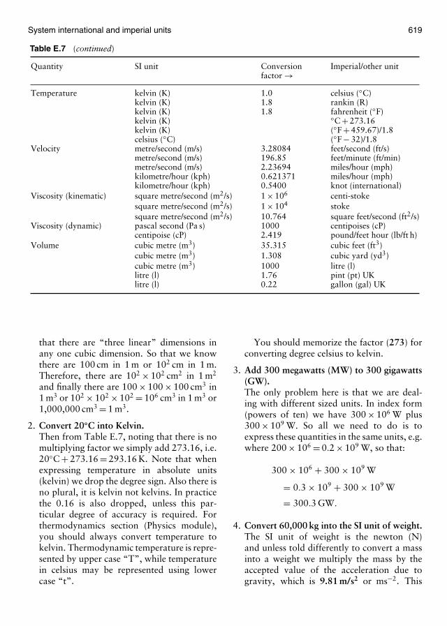
System international and imperial units 619
Table E.7 (continued)
Quantity SI unit Conversion Imperial/other unitfactor →
Temperature kelvin (K) 1.0 celsius (◦C)kelvin (K) 1.8 rankin (R)kelvin (K) 1.8 fahrenheit (◦F)kelvin (K) ◦C + 273.16kelvin (K) (◦F + 459.67)/1.8celsius (◦C) (◦F − 32)/1.8
Velocity metre/second (m/s) 3.28084 feet/second (ft/s)metre/second (m/s) 196.85 feet/minute (ft/min)metre/second (m/s) 2.23694 miles/hour (mph)kilometre/hour (kph) 0.621371 miles/hour (mph)kilometre/hour (kph) 0.5400 knot (international)
Viscosity (kinematic) square metre/second (m2/s) 1 × 10⁶ centi-stokesquare metre/second (m2/s) 1 × 10⁴ stokesquare metre/second (m2/s) 10.764 square feet/second (ft2/s)
Viscosity (dynamic) pascal second (Pa s) 1000 centipoises (cP)centipoise (cP) 2.419 pound/feet hour (lb/ft h)
Volume cubic metre (m3) 35.315 cubic feet (ft3)cubic metre (m3) 1.308 cubic yard (yd3)cubic metre (m3) 1000 litre (l)litre (l) 1.76 pint (pt) UKlitre (l) 0.22 gallon (gal) UK
that there are “three linear” dimensions inany one cubic dimension. So that we knowthere are 100 cm in 1 m or 102 cm in 1 m.Therefore, there are 102 × 102 cm2 in 1 m2
and finally there are 100 × 100 × 100 cm3 in1 m3 or 102 × 102 × 102 = 106 cm3 in 1 m3 or1,000,000 cm3 = 1 m3.
2. Convert 20◦C into Kelvin.Then from Table E.7, noting that there is nomultiplying factor we simply add 273.16, i.e.20◦C + 273.16 = 293.16 K. Note that whenexpressing temperature in absolute units(kelvin) we drop the degree sign. Also there isno plural, it is kelvin not kelvins. In practicethe 0.16 is also dropped, unless this par-ticular degree of accuracy is required. Forthermodynamics section (Physics module),you should always convert temperature tokelvin. Thermodynamic temperature is repre-sented by upper case “T”, while temperaturein celsius may be represented using lowercase “t”.
You should memorize the factor (273) forconverting degree celsius to kelvin.
3. Add 300 megawatts (MW) to 300 gigawatts(GW).The only problem here is that we are deal-ing with different sized units. In index form(powers of ten) we have 300 × 106 W plus300 × 109 W. So all we need to do is toexpress these quantities in the same units, e.g.where 200 × 106 = 0.2 × 10⁹ W, so that:
300 × 106 + 300 × 109 W
= 0.3 × 10⁹ + 300 × 109 W
= 300.3 GW.
4. Convert 60,000 kg into the SI unit of weight.The SI unit of weight is the newton (N)and unless told differently to convert a massinto a weight we multiply the mass by theaccepted value of the acceleration due togravity, which is 9.81 m/s2 or ms−2. This

620 Aircraft engineering principles
is another conversion factor that you shouldcommit to memory.
Then 60,000 kg = 60,000 × 9.81
= 588,600 N
(by long multiplication)
5. How many pascal are there in 270 bar?This requires us to divide by the conversionfactor (0.01) in Table E.7 to convert from barto kilopascal and then convert kilopascal topascal.
Then 270/0.01 = 27,000 kPa or
= 27,000 × 1000
= 27 × 106 Pa or 27 MPa
The following conversions will be particu-larly useful when you study stress and pres-sure and should be committed to memory:
• 1 N/m2 = 1 Pa• 100,000 N/m2 = 100,000 Pa = 1 × 10⁵ Pa =
1 bar• 1 MPa = 1 MN/m2 = 1 N/mm2
So in the above example:
270 bar = 270 × 105 Pa = 27 × 106 Pa
= 27 MPa
6. How many newton-metres (Nm) are there in600 MJ?This example introduces another importantrelationship, i.e.:
1 Nm = 1 J
The Nm is sometimes used as the unit ofwork, rather than the joule, which is oftenreserved for energy (the capacity to do work).
Thus 600 MJ = 600 mega-newton-metres,or 600 × 106 Nm, as required.
7. What is 36 kJ/h in watts?You will learn during your study of Chap-
ter 4 that the rate of doing work (Nm/s) orthe rate of the transfer of energy (J/s) is in factpower, where 1 W = 1 J/s (joule per second).When we refer to “unit time”, we are talking
about per second. Thus the transfer of energyper unit time (the rate of transfer) has unitsof J/s.
Now, for the above, we are saying that360 kJ (360,000 J) of energy is transferred perhour. Knowing that there are 3600 s in 1 h(Table E.5), then we have transferred:
360,000 J3600 s
= 100 J/s = 100 W (from above)
8. How many litres are there in 40 m3?This question is easily answered by consultingTable E.7, where 1 m3 = 1000 L, so that:
40 m3 = 40,000 L or 4 × 10⁴ L
This is another useful conversion factor tocommit to memory, 1 m3 = 1000 L.
Another useful conversion factor to memo-rize is that 1000 cc = 1 L. Thus, e.g. a 1000 ccengine is a 1 L engine.
E.6 Examples of useful conversions
1. Convert 10 kN into pound-force (lbf).This is simply done by multiplying the forcein newton by 0.2248 (Table E.7). Then,10,000 × 0.2248 = 2248 lbf. It may be easierto remember the rule of thumb approxima-tion that 1 N = 0.225 lb, then approximately4.45 N = 1 lb.
2. Convert 20,000 kg to pound-mass.Then we need to remember that, as a ruleof thumb, roughly, 2.2 lb = 1 kg. So that20,000 kg = 44,000 lb. In Table E.7 the moreexact conversion factor is given as 2.20462.
3. You are refuelling an aircraft, where the refu-elling vehicle is calibrating the fuel in Imperialgallons. You require 60,000 L of fuel to fillthe aircraft. How many Imperial gallons mustgo in?
This is, again, where you should rememberthe conversion factor and make sure you getyour conversion right!
1 L = 0.22 (UK) gallon
thus 60,000 L = 60,000 × 0.22
= 13,200 gallons
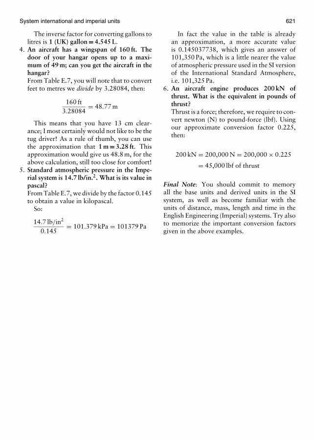
System international and imperial units 621
The inverse factor for converting gallons tolitres is 1 (UK) gallon = 4.545 L.
4. An aircraft has a wingspan of 160 ft. Thedoor of your hangar opens up to a maxi-mum of 49 m; can you get the aircraft in thehangar?From Table E.7, you will note that to convertfeet to metres we divide by 3.28084, then:
160 ft3.28084
= 48.77 m
This means that you have 13 cm clear-ance; I most certainly would not like to be thetug driver! As a rule of thumb, you can usethe approximation that 1 m = 3.28 ft. Thisapproximation would give us 48.8 m, for theabove calculation, still too close for comfort!
5. Standard atmospheric pressure in the Impe-rial system is 14.7 lb/in.2. What is its value inpascal?From Table E.7, we divide by the factor 0.145to obtain a value in kilopascal.
So:
14.7 lb/in2
0.145= 101.379 kPa = 101379 Pa
In fact the value in the table is alreadyan approximation, a more accurate valueis 0.145037738, which gives an answer of101,350 Pa, which is a little nearer the valueof atmospheric pressure used in the SI versionof the International Standard Atmosphere,i.e. 101,325 Pa.
6. An aircraft engine produces 200 kN ofthrust. What is the equivalent in pounds ofthrust?Thrust is a force; therefore, we require to con-vert newton (N) to pound-force (lbf). Usingour approximate conversion factor 0.225,then:
200 kN = 200,000 N = 200,000 × 0.225
= 45,000 lbf of thrust
Final Note: You should commit to memoryall the base units and derived units in the SIsystem, as well as become familiar with theunits of distance, mass, length and time in theEnglish Engineering (Imperial) systems. Try alsoto memorize the important conversion factorsgiven in the above examples.

This page intentionally left blank

A p p e n d i x
FAnswers to “Test yourunderstanding”
TYU 2.1
1. Natural numbers and positive integers2. Rational numbers3. 30
6 , 786 , 96
64. − 16
4 , − 284 , − 48
45. positive integer, 46. rational, real7. (a) 0.333333 (b) 0.142857 (c) 1.9999998. (a) 9 (b) 66 (c) 399. −31 = 31
10. 1111. 1412. (a) −5 (b) −18 (c) 713. (a) 96 (b) 9014. 8015. (a) 191.88 (b) 4304.64 (c) 1.05 (d) 2.1672
(e) 39200 (f) 0.1386
TYU 2.2
1. (a) 0.43 (b) 50802. (a) 3.1862 × 10² (b) 4.702 × 10⁻⁵
(c) 5.1292 × 10¹⁰ (d) −4.1045 × 10⁻⁴
3. (a) 2.71 (b) 0.000127 (c) 5.44 × 10⁴
4. (a) −5 × 10⁴ (b) 8.2 × 10⁻⁵
TYU 2.3
1. (a) 110 (b) 25
3 (c) 910
2. (a) 119 (b) 3 3
10 (c) 23. 3
324. 1.05. 16
15
6. 3845
TYU 2.4
1. 7.52. 1.215 million3. 720 km/h4. 60 km/h
5. 33.17 litres6. 20 men7. £23.448. y = 359. h = kV
r2
TYU 2.5
1. (a) 10001 (b) 10111 (c) 1010002. (a) 11 (b) 31 (c) 853. (a) 170216 (b) 41FC16
4. (a) 110 (b) 61208
TYU 2.6
1. (a) (2, 8), (4, 4), (2, 2, 2, 2) (b) (n, n)(c) (wx, yz), (wxy, z), (xyz, w), (wyz, x)
2. ab2c3. (a) 32 (b) 8
27 (c) b2
4. (a) 70 (b) 109
TYU 2.7
1. (a) a5b−1c3d (b) 4(6x3y2 − xy2)2. (a) 3
4 a−6b2 (b) d3. (a) 6a2 + 4a − 2 (b) 4 − x4 (c) 3a3b +
a2b2 − 2ab3 (d) s3 − t3
4. (a) (x + 3)(x − 1) (b) (a + 3)(a − 6)(c) (2p + 3) (2p + 4) (d) (3z + 4)(3z − 6)
5. (a) 3x(x+7)(x+2), (b) 3xy(3xy+2)(3xy−1)6. (a) 0 (b) 0.279
TYU 2.8
1. (a) xy + xyz + 2xz − 2x + 8y (b) 5ab + abc2. −13p2s + 2pqr − 8s3. (a) (u − 2)(u − 3) (b) 6abc(ab2 + 2c − 5)
(c) (3x−5)(4x+2) (d) (2a+2b)(a2 −ab+b2)4. (a − b)(a2 − ab + b2) = a3 − b3 so (a − b) is
a factor5. (x2−1)(2x+1) = 2x3+x2−2x−1 so (2x+1)
is the quotient
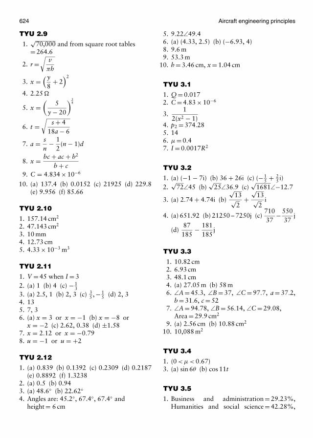
624 Aircraft engineering principles
TYU 2.9
1.√
70,000 and from square root tables= 264.6
2. r =√
vπh
3. x =(y
8+ 2
)2
4. 2.25 �
5. x =(
5y − 20
)34
6. t =√
s + 418a − 6
7. a = sn
− 12
(n − 1)d
8. x = bc + ac + b2
b + c9. C = 4.834 × 10⁻⁶
10. (a) 137.4 (b) 0.0152 (c) 21925 (d) 229.8(e) 9.956 (f) 85.66
TYU 2.10
1. 157.14 cm2
2. 47.143 cm2
3. 10 mm4. 12.73 cm5. 4.33 × 10⁻³ m3
TYU 2.11
1. V = 45 when I = 32. (a) 1 (b) 4 (c) − 1
33. (a) 2.5, 1 (b) 2, 3 (c) 3
5 , − 15 (d) 2, 3
4. 135. 7, 36. (a) x = 3 or x = −1 (b) x = −8 or
x = −2 (c) 2.62, 0.38 (d) ±1.587. x = 2.12 or x = −0.798. u = −1 or u = +2
TYU 2.12
1. (a) 0.839 (b) 0.1392 (c) 0.2309 (d) 0.2187(e) 0.8892 (f) 1.3238
2. (a) 0.5 (b) 0.943. (a) 48.6◦ (b) 22.62◦4. Angles are: 45.2◦, 67.4◦, 67.4◦ and
height = 6 cm
5. 9.22∠49.46. (a) (4.33, 2.5) (b) (−6.93, 4)8. 9.6 m9. 53.3 m
10. h = 3.46 cm, x = 1.04 cm
TYU 3.1
1. Q = 0.0172. C = 4.83 × 10⁻⁶
3.1
2(x2 − 1)4. p2 = 374.285. 146. µ = 0.47. I = 0.0017R2
TYU 3.2
1. (a) (−1 − 7i) (b) 36 + 26i (c) (− 15 + 2
5 i)2.
√72∠45 (b)
√25∠36.9 (c)
√1681∠−12.7
3. (a) 2.74 + 4.74i (b)
√13√2
+√
13√2
i
4. (a) 651.92 (b) 21250 – 7250j (c)71037
− 55037
j
(d)87185
− 181185
j
TYU 3.3
1. 10.82 cm2. 6.93 cm3. 48.1 cm4. (a) 27.05 m (b) 58 m6. ∠A = 45.3, ∠B = 37, ∠C = 97.7, a = 37.2,
b = 31.6, c = 527. ∠A = 94.78, ∠B = 56.14, ∠C = 29.08,
Area = 29.9 cm2
9. (a) 2.56 cm (b) 10.88 cm2
10. 10,088 m2
TYU 3.4
1. (0 < µ < 0.67)3. (a) sin 6θ (b) cos 11t
TYU 3.5
1. Business and administration = 29.23%,Humanities and social science = 42.28%,
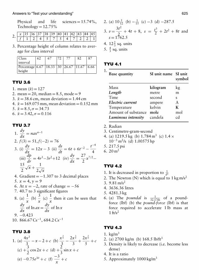
Answers to “Test your understanding” 625
Physical and life sciences = 15.74%,Technology = 12.75%
2. x 35 36 37 38 39 40 41 42 43 44 45f 1 2 4 5 7 5 4 7 2 2 1
3. Percentage height of column relates to aver-age for class interval
Class 62 67 72 77 82 87intervalPercentage 6.67 18.33 30 26.67 11.67 6.66height
TYU 3.6
1. mean (x) = 1272. mean = 20, median = 8.5, mode = 93. x = 38.6 cm, mean deviation = 1.44 cm4. x = 169.075 mm, mean deviation = 0.152 mm5. x = 8.5, σ = 34.736. x = 3.42, σ = 0.116
TYU 3.7
1.dydx
= naxn−1
2. f (3) = 51, f (−2) = 76
3. (i)dydx
= 12x − 3 (ii)dsdt
= 6t + 6t−2 − t−4
4
(iii)dpdr
= 4r3−3r2+12 (iv)dydx
= 272
x7/2−152
√x + 1
2√
x4. Gradient = −1.307 to 3 decimal places5. x = 4, y = 96. At x = −2, rate of change = −567. 40.7 to 3 significant figures
8. (a)1x
(b)3x
(c)1x
then it can be seen that
dydx
of In ax = dydx
of In x
9. −0.42310. 866.67 Cs−1, 684.2 Cs−1
TYU 3.8
1. (a)4x3
3− x − 2 + c (b)
x32
3− 2x
32
3+ 2x
52
5+ c
(c) +32
cos 2x + c (d) +23
sin x + c
(e) −0.75e3θ + c (f)−3x
+ c
2. (a) 10 512 (b) − 1
15 (c) −3 (d) −287.5
3. v = 3t2
2+ 4t + 8, s = t3
2 + 2t2 + 8t and
s = 1762.5
4. 12 23 sq. units
5. 43 sq. units
TYU 4.1
1.Base quantity SI unit name SI unit
symbol
Mass kilogram kgLength metre mTime second sElectric current ampere ATemperature kelvin KAmount of substance mole molLuminous intensity candela cd
2. Radian3. Centimetre-gram-second4. (a) 1219.5 kg (b) 1.784 m3 (c) 1.4 ×
10−3 m2/s (d) 1.00575 hp5. 217.5 psi6. 20 m2
TYU 4.2
1. It is decreased in proportion to 1d2
2. The Newton (N) which is equal to 1 kg m/s2
3. 9.81 m/s2
4. 3636.36 litres5. 4281.3 kg6. (a) The poundal is 1
32.17th of a pound-force (lbf) (b) the pound-force (lbf) is thatforce required to accelerate 1 lb mass at1 ft/s2
TYU 4.3
1. kg/m3
2. (a) 2700 kg/m (b) 168.5 lb/ft3
3. Density is likely to decrease (i.e. become lessdense)
4. It is a ratio5. Approximately 1000 kg/m3
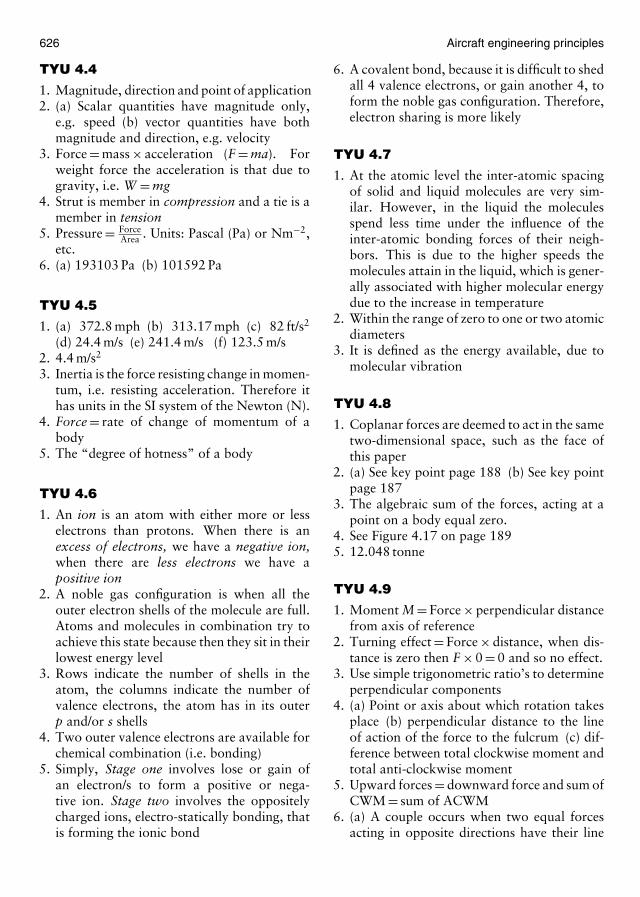
626 Aircraft engineering principles
TYU 4.4
1. Magnitude, direction and point of application2. (a) Scalar quantities have magnitude only,
e.g. speed (b) vector quantities have bothmagnitude and direction, e.g. velocity
3. Force = mass × acceleration (F = ma). Forweight force the acceleration is that due togravity, i.e. W = mg
4. Strut is member in compression and a tie is amember in tension
5. Pressure = ForceArea . Units: Pascal (Pa) or Nm−2,
etc.6. (a) 193103 Pa (b) 101592 Pa
TYU 4.5
1. (a) 372.8 mph (b) 313.17 mph (c) 82 ft/s2
(d) 24.4 m/s (e) 241.4 m/s (f) 123.5 m/s2. 4.4 m/s2
3. Inertia is the force resisting change in momen-tum, i.e. resisting acceleration. Therefore ithas units in the SI system of the Newton (N).
4. Force = rate of change of momentum of abody
5. The “degree of hotness” of a body
TYU 4.6
1. An ion is an atom with either more or lesselectrons than protons. When there is anexcess of electrons, we have a negative ion,when there are less electrons we have apositive ion
2. A noble gas configuration is when all theouter electron shells of the molecule are full.Atoms and molecules in combination try toachieve this state because then they sit in theirlowest energy level
3. Rows indicate the number of shells in theatom, the columns indicate the number ofvalence electrons, the atom has in its outerp and/or s shells
4. Two outer valence electrons are available forchemical combination (i.e. bonding)
5. Simply, Stage one involves lose or gain ofan electron/s to form a positive or nega-tive ion. Stage two involves the oppositelycharged ions, electro-statically bonding, thatis forming the ionic bond
6. A covalent bond, because it is difficult to shedall 4 valence electrons, or gain another 4, toform the noble gas configuration. Therefore,electron sharing is more likely
TYU 4.7
1. At the atomic level the inter-atomic spacingof solid and liquid molecules are very sim-ilar. However, in the liquid the moleculesspend less time under the influence of theinter-atomic bonding forces of their neigh-bors. This is due to the higher speeds themolecules attain in the liquid, which is gener-ally associated with higher molecular energydue to the increase in temperature
2. Within the range of zero to one or two atomicdiameters
3. It is defined as the energy available, due tomolecular vibration
TYU 4.8
1. Coplanar forces are deemed to act in the sametwo-dimensional space, such as the face ofthis paper
2. (a) See key point page 188 (b) See key pointpage 187
3. The algebraic sum of the forces, acting at apoint on a body equal zero.
4. See Figure 4.17 on page 1895. 12.048 tonne
TYU 4.9
1. Moment M = Force × perpendicular distancefrom axis of reference
2. Turning effect = Force × distance, when dis-tance is zero then F × 0 = 0 and so no effect.
3. Use simple trigonometric ratio’s to determineperpendicular components
4. (a) Point or axis about which rotation takesplace (b) perpendicular distance to the lineof action of the force to the fulcrum (c) dif-ference between total clockwise moment andtotal anti-clockwise moment
5. Upward forces = downward force and sum ofCWM = sum of ACWM
6. (a) A couple occurs when two equal forcesacting in opposite directions have their line
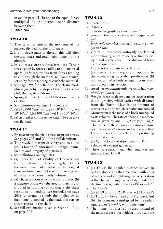
Answers to “Test your understanding” 627
of action parallel (b) one of the equal forcesmultiplied by the perpendicular distancebetween them
7. 108.5 Nm
TYU 4.10
1. Then x is the sum of the moments of themasses, divided by, the total mass.
2. If any single mass is altered, this will alterthe total mass and total mass moment of theaircraft
3. In all cases stress = force/area. (a) Tensilestress set up by forces tending to pull materialapart (b) Shear, results from forces tendingto cut through the material (c) Compressive,set up by forces tending to crush the material.
4. See page 199, for definition. The elastic mod-ulus is given by the slope of the Hooke’s lawplot; that is, stress/strain
5. Spring stiffness k = force/deflection so unitsof N/m
6. See definitions on pages 199 and 2007. (a) 240,000 N/m2 (b) 2.28×10⁸ N/m2 (c) 6 ×
108 N/m2 (d) 3300 N/m2 (e) 1.0×10¹⁰ N/m2
8. (a) strut takes compressive loads (b) a tie taketensile loads
TYU 4.11
1. By measuring the yield stress or proof stress.See pages 203 and 204 for a full definition
2. To provide a margin of safety and to allowfor “a factor of ignorance” in design, manu-facture and integrity of materials
3. See definitions on page 2044. (a) upper limit of validity of Hooke’s law
(b) the ultimate tensile strength, that isthe maximum load divided by the originalcross-sectional area (c) start of plastic phase(d) material is permanently deformed
5. (a) The axis about which the shaft rotates (b)a measure of the way the area or mass is dis-tributed in rotating solids, that is the shaftresistance to bending (see formulae on page203) (c) torque is simply the applied twist-ing moment, created by the load, that sets upshear stresses in the shaft
6. See full explanation given in Section 4.7.11on page 203
TYU 4.12
1. acceleration2. distance3. area under graph by time interval4. zero and the distance travelled is equal to vt5. 1
2 vt6. uniformly retarded motion. (1) s = ut + 1
2 at2;(2) variable
7. Graph (d) represents uniformly acceleratedmotion having initial velocity u, final veloc-ity v and acceleration a. So distanced trav-eled is equal to a.
8. Graph (e) represents a acceleration.9. (a) Inertia force is equal and opposite to
the accelerating force that produced it (b)momentum of a body is equal to its massmultiplied by its velocity
10. speed has magnitude only, velocity has mag-nitude and direction
11. Weight force is dependent on accelerationdue to gravity, which varies with distancefrom the Earth. Mass is the amount ofmatter in a body which remains unchanged
12. Momentum is the mass of a body multipliedby its velocity. The rate of change in momen-tum is given by mv − mu/t or m(v − u)/t.The latter of these two expressions is sim-ply mass × acceleration and we know thatForce = mass × the acceleration producingit. So that F = ma
13. (a) Vje = velocity of slipstream (b) Vje =velocity of exhaust gas stream
14. Thrust is a maximum, when engine is sta-tionary, then Va = 0
TYU 4.13
1. (a) This is the angular distance moved inradian, divided by the time taken with unitsof rad/s or rad s−1 (b) Angular accelerationis the change in angular velocity divided bythe time taken, with units of rad/s2 or rad s−2
2. 142.9 rad/s3. (a) 26.18 rad/s (b) 21.8 rad/s (c) 1100 rad/s4. (a) Torque = force × radius = Fr, units (Nm)
(b) The point mass multiplied by the radiussquared, or 1 = mk2, with units kgm2
5. The moment of inertia I, is used instead ofthe mass because it provides a more accurate
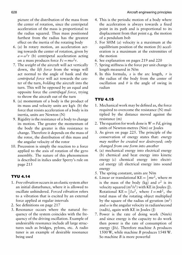
628 Aircraft engineering principles
picture of the distribution of the mass fromthe center of rotation, since the centripetalacceleration of the mass is proportional tothe radius squared. Thus mass positionedfurthest from the radius has the greatesteffect on the inertia of the rotating body
6. (a) In rotary motion, an acceleration act-ing towards the center of rotation, given bya = ω2r (b) centripetal acceleration actingon a mass produces force Fc = mω2r.
7. The weight of the aircraft will act verticallydown, the lift force from the wings willact normal to the angle of bank and thecentripetal force will act towards the cen-ter of the turn, holding the aircraft into theturn. This will be opposed by an equal andopposite force the centrifugal force, tryingto throw the aircraft out of the turn
8. (a) momentum of a body is the product ofits mass and velocity units are kg/s (b) theforce that resists acceleration of a body is itsinertia, units are Newton (N)
9. Rigidity is the resistance of a body to changeits motion. The greater the momentum ofthe body the greater is this resistance tochange. Therefore it depends on the mass ofthe rotor, the distribution of this mass andthe angular velocity of the rotor
10. Precession is simply the reaction to a forceapplied to the axis of rotation of the gyroassembly. The nature of this phenomenonis described in italics under Sperry’s rule onpage 215
TYU 4.14
1. Free vibration occurs in an elastic system afteran initial disturbance, where it is allowed tooscillate unhindered. Forced vibration refersto a vibration that is excited by an externalforce applied at regular intervals
2. See definitions on page 2173. Resonance occurs where the natural fre-
quency of the system coincides with the fre-quency of the driving oscillation. Example ofundesirable resonance include all large struc-tures such as bridges, pylons, etc. A radiotuner is an example of desirable resonancebeing used
4. This is the periodic motion of a body wherethe acceleration is always towards a fixedpoint in its path and is proportional to itsdisplacement from that point e.g. the motionof a pendulum bob
5. For SHM (a) velocity is a maximum at theequilibrium position of the motion (b) accel-eration is a maximum at the extremities ofthe motion
6. See explanation on pages 219 and 2207. Spring stiffness is the force per unit change in
length measured in N/m8. In this formula, s is the arc length, r is
the radius of the body from the center ofoscillation and θ is the angle of swing inradian
TYU 4.15
1. Mechanical work may be defined as, the forcerequired to overcome the resistance (N) mul-tiplied by the distance moved against theresistance (m)
2. The equation for work done is W = Fd, givingunits of Newton-metres (Nm) or Joules
3. As given on page 225. The principle of theconservation of energy states that: energymay neither be created nor destroyed; onlychanged from one form into another
4. (a) mechanical energy into electrical energy(b) chemical and heat energy into kineticenergy (c) chemical energy into electri-cal energy (d) electrical energy into soundenergy
5. The spring constant, units are N/m6. Linear or translational KE = 1
2 mv2, where mis the mass of the body (kg) and v2 is itsvelocity squared (m2/s2) with KE in Joules (J).Rotational KE = 1
2 Iω2, where I = mk2, thetotal mass of the rotating object multipliedby the square of the radius of gyration (m2)and ω is the angular velocity in radian/second(rad/s), again with KE in Joules (J)
7. Power is the rate of doing work (Nm/s)and since energy is the capacity to do workthen power is the rate of consumption ofenergy (J/s). Therefore machine A produces1500 W, while machine B produces 1548 W.So machine B is more powerful
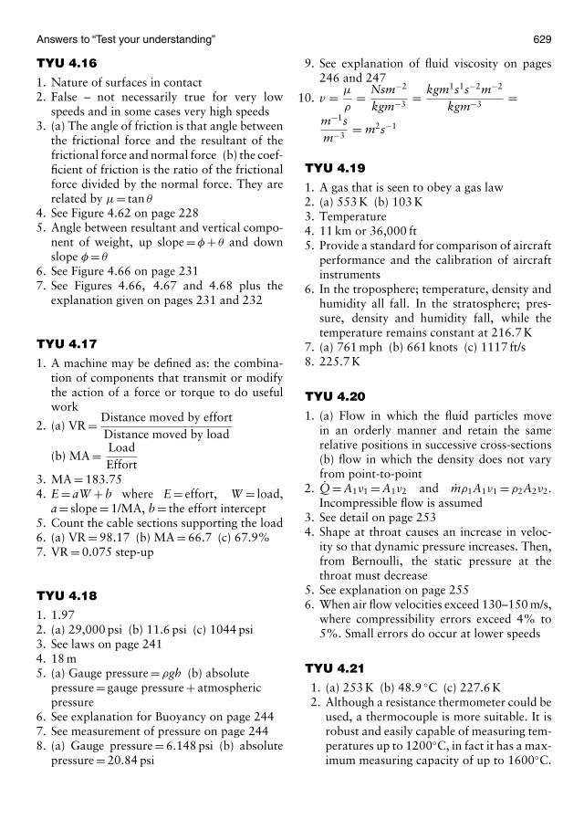
Answers to “Test your understanding” 629
TYU 4.16
1. Nature of surfaces in contact2. False – not necessarily true for very low
speeds and in some cases very high speeds3. (a) The angle of friction is that angle between
the frictional force and the resultant of thefrictional force and normal force (b) the coef-ficient of friction is the ratio of the frictionalforce divided by the normal force. They arerelated by µ = tan θ
4. See Figure 4.62 on page 2285. Angle between resultant and vertical compo-
nent of weight, up slope = φ + θ and downslope φ = θ
6. See Figure 4.66 on page 2317. See Figures 4.66, 4.67 and 4.68 plus the
explanation given on pages 231 and 232
TYU 4.17
1. A machine may be defined as: the combina-tion of components that transmit or modifythe action of a force or torque to do usefulwork
2. (a) VR = Distance moved by effortDistance moved by load
(b) MA = LoadEffort
3. MA = 183.754. E = aW + b where E = effort, W = load,
a = slope = 1/MA, b = the effort intercept5. Count the cable sections supporting the load6. (a) VR = 98.17 (b) MA = 66.7 (c) 67.9%7. VR = 0.075 step-up
TYU 4.18
1. 1.972. (a) 29,000 psi (b) 11.6 psi (c) 1044 psi3. See laws on page 2414. 18 m5. (a) Gauge pressure = ρgh (b) absolute
pressure = gauge pressure + atmosphericpressure
6. See explanation for Buoyancy on page 2447. See measurement of pressure on page 2448. (a) Gauge pressure = 6.148 psi (b) absolute
pressure = 20.84 psi
9. See explanation of fluid viscosity on pages246 and 247
10. v = µ
ρ= Nsm−2
kgm−3= kgm1s1s−2m−2
kgm−3=
m−1sm−3
= m2s−1
TYU 4.19
1. A gas that is seen to obey a gas law2. (a) 553 K (b) 103 K3. Temperature4. 11 km or 36,000 ft5. Provide a standard for comparison of aircraft
performance and the calibration of aircraftinstruments
6. In the troposphere; temperature, density andhumidity all fall. In the stratosphere; pres-sure, density and humidity fall, while thetemperature remains constant at 216.7 K
7. (a) 761 mph (b) 661 knots (c) 1117 ft/s8. 225.7 K
TYU 4.20
1. (a) Flow in which the fluid particles movein an orderly manner and retain the samerelative positions in successive cross-sections(b) flow in which the density does not varyfrom point-to-point
2. Q = A1ν1 = A1ν2 and mρ1A1ν1 = ρ2A2ν2.
Incompressible flow is assumed3. See detail on page 2534. Shape at throat causes an increase in veloc-
ity so that dynamic pressure increases. Then,from Bernoulli, the static pressure at thethroat must decrease
5. See explanation on page 2556. When air flow velocities exceed 130–150 m/s,
where compressibility errors exceed 4% to5%. Small errors do occur at lower speeds
TYU 4.21
1. (a) 253 K (b) 48.9 ◦C (c) 227.6 K2. Although a resistance thermometer could be
used, a thermocouple is more suitable. It isrobust and easily capable of measuring tem-peratures up to 1200◦C, in fact it has a max-imum measuring capacity of up to 1600◦C.
630 Aircraft engineering principles
There physical composition also makes ther-mocouples eminently suitable for this kindof harsh environment, where hot exhaustgas temperatures are being measured
3. α = the amount of a material will expandper ◦C or Kelvin: Surface expansion andvolumetric expansion can be approximatedusing 2α and 3α, respectively, as expansioncoefficients. See also page 258
4. Heat energy Q is the transient energybrought about by the interaction of bod-ies by virtue of their temperature differ-ence, when in contact. Internal energy ofa material is the energy of vibration of themolecules, which is directly proportional tothe temperature of the material
5. See explanation on pages 259–2616. Since, for a constant pressure process, vol-
ume change must take place, then pressure-volume work is done. So heat energy isrequired for both this work and for anyincrease in the internal energy (U), whilefor constant volume only internal energy isincreased
7. Q = mc�T but when calculating latent heatno temperature change takes place, so weuse Q = mL, where L = latent heat of evap-oration or condensation, as required
8. cp = 940 J/kgK9. Either increase temperature, reduce pres-
sure, or increase the surface area10. (a) The evaporator allows refrigerant to
absorb heat from the medium being cooled(b) the condenser allows heat to be dissi-pated to an external medium, so reducingthe temperature of the refrigerant
TYU 4.22
1. (a) A system where particular amounts ofa thermodynamic substance, normally com-pressible fluids, such as vapours and gases,are surrounded by an identifiable bound-ary (b) Heat Q, is energy in transit broughtabout by the interaction of bodies by virtueof their temperature difference when theycommunicate
2. When it has a moveable boundary3. (a) NFEE: Q−W = �U, where Q is the heat
energy entering or leaving the system, W is
work done by the system or on the system,�U is the change in internal energy of theworking fluid. All terms have units of theJoule (J) (b) SFEE: Q − W = (U2 − U1) +(p2V2 − p1V1) + (mgz2 − mgz1) + ( 1
2 mv22 −
12 mv2
1) where Q, W , and U2 − U1 or�U, have the same meaning as above.(p2V2 − p1V1) = the change in pressure/volume energy, within the working fluid,(mgz2 − mgz1) = the change in PE of theworking fluid and ( 1
2 mv22 − 1
2 mv21) = the
change in KE of the working fluid. See alsopages 269 and 270
4. In a closed system no working fluid crossesthe system boundary, as it does in an opensystem
5. Internal energy involves only the vibrationof the fluid molecules. Whereas, enthalpyis the combined energies both internal andpressure/volume of the fluid. Enthalpy isa very useful characteristic of the workingfluid used in open systems
6. According to the second law of thermody-namic and substantiated in practice, no ther-modynamic system can produce more workenergy than the heat energy supplied. Inother words Qin is always greater than Wout.With practical working systems, energy isdissipated as sound, heat etc and cannot bereversed back to its original form
7. (a) Isothermal – temperature remains con-stant (b) polytropic – both heat and workmay be transferred (c) reversible adiabatic– no heat energy is transferred to or fromthe working fluid
8. Heat source, engine, sink9. Net work done is always less than the heat
supplied10. See pages 275 and 276
TYU 4.23
1. Approximately 671 million miles2. The angle of incidence is equal to the angle
of reflection. The incident ray, the reflectedray and the normal all lie within the sameplane
3. 60 cm
Answers to “Test your understanding” 631
4. Rays close to the principal axis and there-fore, where the mirror aperture may berepresented by a straight line
5. See Figure 4.119 on page 2796. The angle of the refracted ray increases as
the light ray enters the material having thelower refractive index
7. The greater the refractive index of a mediumthen the lower the speed of light as it passesthrough it
8. Total internal reflection9. To reduce energy losses due to dirt at the
boundary and due to the Fresnel effect andimpurities in the glass
10. The principle focus for convex lenses is thepoint at which all paraxial rays converge. Inthe case of concave lenses these same raysafter refraction, appear to diverge
11. The plane that is at right angles to theprincipal axis is the focal plane
12. By using the relationship:
Imageheight =
imagedistance × object
height
objectdistance
TYU 4.24
1. Waves in the electromagnetic spectrum havevastly different frequencies. Their energy isin direct proportion to their frequency andinversely proportional to their wavelength.Thus for the above reason, ultraviolet waveswith the higher frequency, will have moreenergy than infrared waves
2. Simply that the oscillatory motion of thewave is at right angles to the direction oftravel of the wave front
3. Diffraction of transverse waves takes place,where they spread out to produce circularwave fronts
4. When two wave sets are in-phase, theyreinforce one another as they meet, cre-ating constructive interference. If they areout of phase peaks and troughs meet andcancel one another, causing destructiveinterference
5. See characteristics detailed on pages 289and 290
6. VHF waves have very short wavelengthsand are not reflected by the ionosphere andtherefore, it is not practical to transmit themas sky waves
7. Around 150 to 1
100 of a metre8. To reduce the possibility of static interfer-
ence, which is not a problem with VHF orUHF communication
9. (a) Skip distance, is the first point from thetransmitter at which the first sky wave canbe reached (b) Dead space, is the area thatcannot receive either ground waves or thefirst sky wave and is known as the silent zone
10. Carrier waves and satellite communication –see explanation on pages 289–291
11. This phenomena is due to a change infrequency brought about by the relativemotion, known as the Doppler effect
TYU 4.25
1. Sound waves are caused by a source of vibra-tion, creating pressure pulses
2. Sound waves are longitudinal mechanicalwaves that require a medium through whichto be transmitted and received. Electromag-netic waves travel at the speed of lightthrough a vacuum
3. The speed of sound depends on the tempera-ture and density of the material throughwhich the sound passes. The denser the mate-rial the faster the speed of sound
4. 5.55 ms5. (a) Intensity is a measure of the energy of the
sound passing through unit area every sec-ond and is measured in W/m2 (see page 295)(b) pitch is dependent on the frequency of thesound being generated. The higher the fre-quency the higher the pitch (c) amplitude, isthe maximum displacement of a particle fromits rest position. The greater the amplitude,the louder the sound
TYU 5.1
1. Ampere2. Hertz3. C4. G

632 Aircraft engineering principles
5. 7.5 ms6. 0.44 kV7. 15,620 kHz8. 0.57 mA9. 220 nF
10. 0.47 M�
TYU 5.2
1. protons, electrons2. positively, positive ion3. negative, negative ion4. free electrons5. insulators6. copper, silver (and other metals), carbon
(any two)7. plastics, rubber, and ceramic materials8. silicon, germanium, selenium, gallium (any
two)9. See page 315
10. See page 315
TYU 5.3
1. positive2. repel3. See page 3164. one quarter of the original force5. 2 kV/m6. 8 V7. 1.264 mC8. ions9. negatively, electrons
10. See page 319
TYU 5.4
1. charge, Ampere2. positive, negative3. negative, positive4. Ohm, �
5. (a) silver (b) aluminium6. 900 C7. 1V8. power, time9. See page 320
10. See page 320
TYU 5.5
1. positive, negative2. static discharger3. zinc, carbon4. sulphuric acid5. e.m.f., induced6. photovoltaic7. negatively, positively8. smoke detector9. thermocouple
10. piezoelectric
TYU 5.6
1. voltage, chemical reaction2. Primary3. cathode4. Carbon5. sulphuric acid6. 2.2 V7. 1.2 V8. 1.269. 1.15
10. See page 331
TYU 5.7
1. algebraic sum, zero2. 1.4 A flowing away from the junction3. 11 A flowing towards the junction4. algebraic sum, zero5. 6 V6. R4 and R5
7. R2 and R5
8. 12 V9. internal, falls
10. 0.36 �
TYU 5.8
1. 0.138 �
2. 504 � to 616 �
3. 1.5 k�, ±5%4. (a) 47 � (b) 4.71 �
5. See pages 334 and 3366. 14.1 V7. 20 mA8. Wheatstone Bridge, balanced9. 0.965 �
10. increases

Answers to “Test your understanding” 633
TYU 5.9
1. rate, work2. energy, Joule, second3. heat, resistor; light, lamp; sound, loud-
speaker4. 5 W5. 3 kJ6. 388.8 kJ7. 224 W8. 0.424 A9. 3.136 �
10. 75 kJ
TYU 5.10
1. charge, voltage2. 44 mC3. 0.05 V4. charge stored5. electric field6. 2 mJ7. vacuum8. (a) 1.33 µF (b) 6 µF9. 39.8 nF
10. (a) 19.7 V (b) 43.3 V
TYU 5.11
1. current, magnetic field2. Weber, Wb3. Tesla, T4. 0.768 N5. B = �/A6. 0.8 mWb7. directly, inversely8. See page 3779. 2,270
10. See page 379
TYU 5.12
1. magnetic, conductor, induced, conductor2. See page 3793. See page 3814. See page 3815. See page 3816. 1.326 V7. −120 V
8. See page 3829. 88.5 mH
10. 1.15 A
TYU 5.13
1. conductor, e.m.f., induced2. 6 V3. slip rings, brushes4. 180◦, commutator5. 90◦6. 200 mV7. 0.012 N8. See pages 394 and 3959. See page 394
10. See page 395
TYU 5.14
1. zero2. 0.6363. 1.4144. 0.7075. 25 Hz6. 2 ms7. effective8. peak9. heat
10. See page 398
TYU 5.15
1. current, voltage, 90◦2. (a) 1.81 k� (b) 36.1 �
3. (a) 7.54 � (b) 1.51 k�
4. 0.138 A5. 200 �, 1 A6. 0.108 A, 10.8 V (resistor), 21.465 V
(capacitor)7. 9.26 A8. 66.5◦, 0.3989. 330 W
10. 534 VA, 0.82
TYU 5.16
1. See page 4142. laminated, eddy current

634 Aircraft engineering principles
3. See page 4174. 27.5 V5. 550 turns6. 1.023 A7. See pages 414 and 4158. See page 4179. 0.0545 (or 5.45%)
10. 96.1%
TYU 5.17
1. See page 4192. See page 4193. 2.12 kHz4. 115 kHz, 185 kHz5. π-section low-pass filter6. output, 0.707, input7. 1.414 V8. 5.11 mH9. See pages 420 and 421
10. 462 �
TYU 5.18
1. See page 4232. 1,200 r.p.m.3. See pages 425 and 4264. See page 4255. 381.04 V6. 69.3 V7. 6.93 A8. 4.056 kW9. 2.286 kW
10. See pages 428 and 429
TYU 5.19
1. See page 4302. See page 4323. See page 4324. See page 4335. (a) 0.0277 (b) 2.77%6. 11,784 r.p.m.7. 6.9%8. See page 4369. See page 436
10. See pages 437 and 438
TYU 6.1
1. (a) earth (b) variable resistor (c) zenerdiode (d) lamp (e) PNP transistor (f) elec-trolytic (polarised) capacitor (g) AC gener-ator (or signal source) (h) pre-set capacitor(i) jack socket (female connector) (j) fise(k) coaxial connector (l) microphone (m)transformer (n) inductor (o) motor
2. See page 4523. See page 4534. (a) zener diode (b) light emitting diode
(LED) (c) NPN Darlington transistor5. D1, C1, D2, M1
6. D1 and C1
7. R2 and D2
8. See page 4529. See page 454 and Example 6.2
10. (a) 159 � (b) 46.9 �
TYU 6.2
1. (a) zener diode (b) light emitting diode (c)variable capacitance diode (d) light sensi-tive diode (photodiode)
2. anode, cathode3. 0.6 V, 0.2 V4. See page 461, silicon diode5. (a) 46.4 � (b) 27.8 �, see page 461 and
Example 6.46. See page 4637. See page 4678. See page 4709. See page 475
10. fast switching, switched-mode power sup-plies, high-speed digital logic (any two)
TYU 6.3
1. (a) NPN bipolar transistor (b) PNP Dar-lington transistor (c) N-channel enhance-ment mode MOSFET (d) N-channel JFET
2. positive3. gate, source, drain4. forward, reverse5. 1.25 A6. 247. (a) 34 µA (b) 19.1 k� (c) 2.7 k�, see
Example 6.9

Answers to “Test your understanding” 635
8. 98.9, see Example 6.119. See page 490
10. See pages 487, 488 and 489
TYU 6.4
1. (a) two-input AND gate (b) inverter orNOT gate (c) two-input NOR gate(d) three-input NAND gate
2. AND gate3. (a) low-power Schottky TTL (b) buffered
CMOS4. (a) TTL: 0 V to 0.8 V, CMOS: 0 to 1
3 VDD
(b) TTL: 2 V to 5 V, CMOS: 2/3 VDD to VDD
5. See page 4986. See page 4997. 2008. See pages 504, 505 and 5069. See pages 507 and 508
10. See page 506 and Example 6.21
TYU 6.5
1. FR-42. width of copper track, thickness of copper
track, permissible temperature rise3. See page 5124. advantage: low dielectric constant (there-
fore excellent at high frequencies), disad-vantage: very expensive
5. false, see Table 6.18 on page 5136. false, see page 5147. See Table 6.18 on page 5138. See pages 513 and 5149. See Table 6.18 on page 513
10. etching; drilling; screen printing of com-ponent legend; application of solder resistcoating; application of tin-lead reflowcoating
TYU 6.6
1. See page 5162. See page 5173. rotary potentiometer; light dependent resis-
tor (LDR); float switch; resistive heatingelement
4. input; input; input; input; output5. analogue; analogue; digital; analogue6. See pages 523 and 5247. See page 5248. S1 and S3
9. See page 52910. See pages 529 and 530
TYU 7.1
3) TAS = 209.2 m/s4) Temperature at altitude = 242.5 K5) Local speed of sound = 319 m/s6) Then from question 5, Mach no. = 1.0
10) (i) µ, Ns/m2 (ii) v, m2/s12) q = 1240.92 N/m2
TYU 7.2
3) (a) Drag = 2395 N and Lift = 34251 N(b) Range = 71.505 km
4) W = 69105 N5) V = 152.9 m/s6) Lift = 140 kN

This page intentionally left blank

Index
A320, 579AC, 397, 402
generator, 387, 389, 423, 424,425
motor, 430AC to DC conversion, 466ACWM, 190, 191ADC, 493, 494ADF, 292AM, 477AML, 8, 9, 13ANO, 15AND gate, 495AOA, 546, 548, 551, 552, 562,
563, 573AOI, 548APU, 6ATOL, 20Ab initio programme, 8Absolute permeability, 377Absolute pressure, 243Absolute value, 35Accelerating force, 209Acceleration, 175, 176, 207, 212Accepted military service
pathway, 9Acceptor circuit, 420Accretion of ice, 560Accumulator, 328Action, 174Aerodynamic balance, 584Aerodynamic coupling, 575Aerodynamics, 541Aerofoil, 548, 549, 550, 551, 552Addition of fractions, 44Adiabatic process, 271Adjacent side, 83Adverse yaw, 580Aileron, 579, 580, 581
drag, 580reversal, 581
Air, 250Accident Investigation Board,
29Navigation Order, 15Travel Organizers’ Licensing, 20traffic control transponder, 292
Airbus A320, 579Aircraft CG, 195
axes, 570battery, 326, 329
engineering industry, 3loading, 567maintenance licence, 8maintenance log, 23planes of reference, 570type endorsements, 16weight and balance, 195
Airflow, 547, 548, 552Airspeed, 543Airworthiness regulation, 18Alcohol thermometer, 258Algebra, 36, 53, 109Algebraic expressions, 59Algebraic operations, 59Alkaline cell, 330All-moving tail plane, 563Alternating current, 397Alternator, 423Ampere, 167, 311, 615Amplifier circuit, 487Amplitude, 217, 293
modulation, 475Analogue control, 517Analogue integrated circuit,
494Analogue signal, 494Aneroid barometer, 244, 245Anhedral, 572, 573, 574Angle:
of attack, 546, 548of depression, 91of elevation, 91of incidence, 278, 281, 548of reflection, 278of refraction, 281, 283of twist, 204
Angles in any quadrant, 118Angular:
acceleration, 213motion, 212velocity, 213
Annulus, 72Anode, 319, 459Antibalance tab, 585Anticlockwise moment, 190Antidifferentiation, 144, 157, 160Antilogarithm, 69, 113Aperture, 279Apparent power, 412, 413Apparent wander, 215Approximation, 41
Arc, 99, 100Archimedes principle, 243, 244Area, 70
of a sector, 123of a triangle, 121under a curve, 160
Arithmetic law of precedence, 45Arithmetic laws of sign, 35Arithmetic mean, 138Armature, 392Armed forces, 6Associative law, 37Astable multi-vibrator, 491, 492Atmosphere, 249Atmospheric physics, 247Atmospheric pressure, 175, 240,
243Atom, 178, 179, 313Atomic structure, 313Automatic direction finder, 292Auxiliary power unit, 6Avalanche effect, 462Average voltage, 399Averages, 45, 47Avionic technician, 6Axes, 74
B1, 5, 9B2, 5, 9BAC One-Eleven accident, 27BCAR, 15, 21BITE, 5BJT, 478, 479
amplifier circuit, 487characteristics, 480
BODMAS, 45, 60Back e.m.f., 381, 383Balance tab, 585Balanced network, 418Band-pass filter, 420Band-stop filter, 421Bandwidth, 420, 421, 501, 503,
505Bar, 175
chart, 132, 133, 134magnet, 371
Barometer, 244Barton’s pendulum, 217Base, 479Base units, 164Battery, 326Beam, 191, 192

638 Index
Bearings, 92Bell crank, 192Bending power, 282Bernoulli’s theorem, 253, 254,
255B–H curve, 377, 378, 417Bi-phase rectifier, 470, 471Bias point, 489Bimodal, 139Binary, 51, 52Binding energy, 181, 182Bipolar junction transistor, 479Bisecting an angle, 96Bistable, 495Blending an arc, 100Blown flap, 583Boeing 767, 4, 5, 27Bohr model of the atom, 313Bonding, 178Bonds, 180Boundaries, 136Boundary layer, 245, 246, 552,
553, 554Bow’s notation, 185, 186Boyle’s law, 114, 248Bramah press, 242Brayton cycle, 275, 276Breakdown voltage, 462Bridge rectifier, 471, 472British Civil Airworthiness
Requirements, 15Brittleness, 202Brush arrangement, 388Brushes, 387Brushless generator, 428, 429Buffer, 493Bulk:
modulus, 199strain, 199stress, 199
Buoyancy, 244
C–R high-pass filter, 419C–R low-pass filter, 419C–R network, 365, 366, 367C–R series circuit, 406CAA, 7, 8, 15, 20CAP 715, 26CAST, 119CG, 194, 195, 196CGS system of units, 165CIVIL, 404CMOS, 497CPG, 20CRS, 7CWM, 190, 191Cabin pressure check, 29Calculus, 144
Camber, 548Candela, 167, 616Capacitance, 356, 357, 359Capacitive reactance, 403, 404,
405Capacitor, 355, 356, 357, 360,
361, 362colour code, 363starting, 436, 437
Carbon potentiometer, 350Career progression, 7Category A, 8, 12, 15Category B, 9, 12, 13Category B1, 5, 10, 15Category B2, 5, 10, 15Category B2 AML pathway, 9Category C, 6, 7, 11, 12, 13, 15Cathode, 319, 459Cells, 326, 327, 328, 330Celsius scale, 257Center of curvature, 279Centi, 312Center of gravity, 194, 195, 196Center of pressure, 551Centripetal acceleration, 213Centripetal force, 213, 566Certificate of release to service, 7Certifiers, 15Certifying:
engineer, 6, 9mechanic, 4technician, 5, 9
Chain of events, 30Changeover switch, 453Characteristic, 454
gas equation, 262graphs, 454impedance, 422
Charge, 327, 329, 355, 356, 357carrier, 314
Charging, 357, 358, 365Charles’ law, 248Charts, 132Chemical bonding, 180Chicago Convention, 20Chlorine, 180Chord, 93, 95
line, 548ratio, 549
Cipolar junction transistor, 478Circle, 70, 72, 93, 94, 98
theorems, 94Circuit, 451
diagram, 453symbols, 452measure, 122
Circumference, 93City of Bristol College, 13
Civil Aviation Authority, 7Clamping, 474Class A, 488, 491Class AB, 489Class B, 489, 492Class C, 489Class midpoint, 138Class of operation, 487Class width, 136, 137Climbing flight, 565Clipping, 474Clockwise moment, 190Closed-loop control, 527Closed-loop voltage gain, 490Closed system, 266Co-ordinates, 74, 89, 90Coefficient of friction, 230Coefficient of linear expansion,
258Coil, 375Cold junction, 324Collector, 479Colour code, 346, 363Common, 453
base, 487collector, 487drain, 487emitter, 487, 490emitter amplifier, 490external tangent, 98factors, 60, 65gate, 487logarithms, 111, 112source, 487
Communication, 291, 292Commutative law, 37Commutator, 389, 390, 393Comparator, 508Complex conjugate, 115Complex numbers, 35, 115Complex vector, 117Complex wave, 398Compound pendulum, 220Compound wound, 394, 395Compressibility, 255Compression, 174, 294Compressive stress, 197Concave lens, 284, 285, 286Concave mirror, 279, 280Concorde, 579Conductance, 320Conduction of electricity, 319Conduction of heat, 259Conductor, 314Cone, 72Cone-shape, 80Conjugate, 115, 116Conservation of energy, 222

Index 639
Constant:current characteristic, 480of integration, 157of proportionality, 49pressure cycle, 275pressure process, 271volume process, 270, 271
Constructive interference, 289Consumer Protection Group, 20Continuity, 251Continuity equation, 252, 254Control column, 22Control methods, 517Control rod, 586Control system, 515, 528, 529Controllability, 579Convection, 260Conventional current, 320Conventional flow, 333Conversion factors, 168Convex lens, 284, 285, 286Convex mirror, 279Copper ion, 319Copper loss, 417Corrosion, 323Cosine function, 124, 126, 127Cosine ratio, 86Cosine rule, 119Coulomb, 311, 320Coulomb’s law, 316Couples, 189, 194, 391Coupling methods, 510Covalent bond, 180, 181, 182Critical angle, 283, 284, 552Cup-shape, 80Current, 314, 319, 320, 333
divider, 349gain, 481, 483
Curved mirror, 278, 281Cut-off frequency, 419, 420, 422Cycle, 217Cyclic quadrilateral, 95Cylinder, 72
D-type bistable 496DAC, 493, 494DAP, 20DC, 397DC generator, 389, 390, 391DC motor, 391, 394DPST, 453Damped oscillation, 529Damping, 217, 218, 529Darlington transistor, 478Data manipulation, 132Datum, 196Dead space, 291Deadband, 529
Decay, 366, 367Decimal form, 41Decimal numbers, 40Definite integral, 163Deflecting torque, 394Deformation, 198, 200Degree, 122Degree of accuracy, 41Delta, 425, 426Delta-connected load, 430Demodulated wave, 291Demodulator, 476, 477Denary, 51, 52Denominator, 43Density, 172, 173Density ratio, 543Dependent variable, 74, 75, 145Depletion region, 459Depolarization, 327Depression, 91Derivative notation, 149Derivatives, 156Derived function, 149, 150, 157Derived units, 167Destructive interference, 289Detector, 476, 477Diameter, 93Dielectric, 359, 361
constant, 359Differential aileron, 580Differential amplifier, 504Differential calculus, 144, 147Differential transformer, 523, 524Differentiation, 144, 150Differentiator, 507Diffraction, 288, 289Digital control, 517Digital integrated circuit, 494Digital signal, 494Dihedral angle, 572Diode, 459
characteristics, 460, 461detector, 476, 477symbols, 463
Diodes, 456–461, 462, 466Direct current, 397Direct proportion, 48Direct strain, 198Directional divergence, 575, 576Directional stability, 572, 578Directorate of Airspace Policy, 20Discharge, 327, 329Discharger, 323Discharging, 357, 358, 365Dispersion, 138Dissipation, 354Distribution, 425Distributive law, 37
Dividend, 36Diving flight, 565Division of fractions, 43Divisor, 36Doppler effect, 293, 296Double shear, 200Doubler, 473Drag, 210, 546, 554, 555, 556,
557, 562Drag coefficient, 554Drift, 216Drive shaft, 203, 204Ductility, 202Dutch roll, 575, 576Dynamic longitudinal stability,
578Dynamic pressure, 240, 545Dynamics, 207
of fluids, 251
E-laminations, 417, 523E.m.f., 320EADS, 3EAS, 543EASA, 20EM, 261ERG, 20East, 92Economic Regulation Group, 20Eddy current loss, 417Edison battery, 330Education, 7Effective span, 575Effective value, 399Efficiency, 234, 235, 417Elastic limit, 198, 203Elasticity, 202Electric circuit, 376Electric field, 317Electric field strength, 317Electrolyte, 328Electromagnetic:
induction, 380spectrum, 287, 289, 290wave, 291
Electromagnetism, 370Electron, 178, 179, 313, 314,
456, 457flow, 320orbit, 456
Electronic circuit, 451, 452Electrovalent bond, 180Elements, 180Elevation, 91Elevator, 579, 582
trim, 586Elevon, 579Emitter, 479

640 Index
Endorsements, 16Energy, 222, 321, 353
storage, 358, 383Engineering factors, 28Engineers theory of twist, 204English system of units, 168, 171Enthalpy, 269Entropy, 274Equation, 76, 81
of continuity, 252, 254of first degree, 76
Equations, 36, 73of motion, 207
Equilateral triangle, 89Equilibrant, 187Equilibrium, 176, 191, 270
forces, 176on a smooth plane, 189
Equivalent airspeed, 543Estimation technique, 40European Aviation Safety Agency,
20Evaluation of equations, 109Evaluation of formulae, 67Examinations, 16, 18, 19Exciter winding, 429Exclusive-OR gate, 495Exemption, 14Exosphere, 249Expansion, 258Exponent, 40Exponential:
decay, 366, 367form, 40function, 113, 154growth, 366
Exponents, 53External tangent, 98Extrapolation, 75
FAR, 21, 66, 15FET, 484
amplifier circuit, 487characteristics, 486
FPS system of units, 171, 174Factorization, 54, 57, 78Factors, 44, 53Fahrenheit scale, 257Family of curves, 157Farad, 311Faraday’s law, 381Fast-track routes, 13Federal Airworthiness
Regulations, 21Ferrite, 385Ferromagnetic material, 370Fiber, 283, 284
optic, 283
Field, 371, 374, 430strength, 374winding, 392
Filter, 418, 420, 421, 422, 451Final velocity, 177Fineness ratio, 557Fire point, 24First aid station, 24First degree equation, 76First law of thermodynamics, 267,
268First quadrant, 119First-line maintenance, 6Five-band colour code, 346Flap, 554, 582, 583Fleming’s rule, 373, 381Flight, 564, 565, 566
envelope, 568load factors, 568
Fluid dynamics, 251Fluid motion, 251Fluid pressure, 241Fluid viscosity, 246Fluids, 240Flux, 370, 371, 372, 414Flux density, 373, 374Fly-by-light system, 284Force, 174, 176
between atoms, 182, 183between charges, 316on a conductor, 372, 373
Forced vibration, 216, 217Forces acting on an aircraft, 561,
562Form drag, 557Formulae, 64, 67Forward conduction voltage,
460Forward transconductance, 485Forward-biased, 460Four-band colour code, 346Four-stroke cycle, 273, 275Fourth quadrant, 119Fowler flap, 583Fractions, 34, 43Free electron, 314Free vibration system, 216Frequency, 217, 219, 398, 399
distribution, 135of events, 136polygon, 137
Fresnel effect, 283Friction, 227Fringing, 317, 376Frise aileron, 580Fulcrum, 191Full-load, 416Full-power bandwidth, 501
Full-wave bridge rectifier, 471,473
Full-wave power supply, 472Full-wave rectifier, 469Functions, 145
GA, 3, 7Gain, 503Gas, 240, 247, 262
equation, 262laws, 248turbine, 275
Gases, 183Gauge pressure, 242, 243, 245Gear train, 238General numbers, 36General triangle, 119Generated e.m.f., 386Generator, 323, 386, 387, 389,
390, 423, 424, 425Geo-stationary satellite, 292Geometric construction, 96Geometry, 73Germanium, 457Giga, 312Glaze ice, 560Glide path, 292Gliding flight, 564Gradient, 76, 146, 147Graph, 75, 76, 78, 82Graphical axes, 74Graphical representation of a
force, 174Gravitational acceleration, 171Gravity, 170Greek alphabet, 83Grinding wheel assembly, 25Ground, 355, 453
power warning, 25waves, 291
Grouped data, 138Growth, 366Gyro-dynamics, 215Gyroscope, 214Gyroscopic procession, 214, 215Gyroscopic wander, 214
HF communications, 292Hair-spring, 394Half-wave power supply, 468,
469, 470Half-wave rectifier, 467Hangar fire point, 24Hangar first aid station, 24Head equation, 254Heat, 259
energy, 259engine, 272exchange, 264

Index 641
Henry, 311Hertz, 311Hexadecimal, 51, 52Hexagon, 99Hidden heat, 263High-pass filter, 419High-voltage capacitor, 362High wing, 574Histogram, 136Hoar frost, 560Holes, 457Honours degree, 13, 14Hooke’s law, 199, 203Horizontal:
axis, 75bar charts, 133component of a force, 187ordinate, 74stabilizer, 562
Horn balance, 584, 585Hot junction, 324Human factors, 22, 26, 27, 28, 30Humidity, 251
measurement, 542Hunting, 529Hybrid integrated circuit, 494Hydraulic press, 241Hydrogen ion, 319Hydrostatic pressure, 240, 241Hydroxyl ion, 319Hypotenuse, 83Hysteresis, 417Hysteresis curve, 417
I-laminations, 417, 523I/V characteristic, 454, 461IAS, 543IATA, 20ICAO, 15, 19, 20, 175
standard atmosphere, 544IGFET, 484ILS, 292ISA, 249, 250Ice accretion, 560Ideal gas, 247Ideal machine, 235Imaginary numbers, 35Impedance, 405, 406
triangle, 405, 407, 409, 413Improper algebraic fraction, 63Impurity, 457
atom, 314Inclined plane, 230Incompressible flow, 252Indefinite integral, 161Independent variable, 74, 75, 145Index form, 41Index of refraction, 281
Indicated airspeed, 543Indices, 54Induced e.m.f., 323, 380Induced drag, 558Inductance, 379, 382, 384Induction, 380Induction motor, 430, 432, 433,
436Inductive reactance, 403, 404, 405Inductively coupled circuits, 382Inductor, 379, 383, 384, 385Inertia, 176, 209Initial velocity, 177Input characteristic, 480Input offset voltage, 501Input resistance, 481Inscribed circle, 98Inset hinge, 584Instrument landing system, 292Insulator, 314Integers, 34Integral calculus, 144, 156Integral notation, 158Integrated circuit, 493, 494Integration, 144, 156, 157, 158,
160Integration between limits, 161Intercept, 76Intercom, 453Interference, 288, 289Interference drag, 557, 558Internal combustion engine, 273Internal energy, 182, 259, 269Internal resistance, 331, 339, 340International Air Transport
Association, 20International Civil Aviation
Organization, 15International Standard
Atmosphere, 249Inverse logarithm, 113Inverse proportion, 49Inverter, 434, 435Inverting amplifier, 504Ion, 313Ionic bond, 180, 182Ionosphere, 249Iron loss, 417Irrational numbers, 35Irreversible process, 270Isothermal process, 271
J-K bistable, 496J-operator, 117JAA, 15JAR 145, 22JAR 147, 8, 13, 22JAR 21, 22
JAR 25, 22JAR 66, 8, 15, 18, 22, 27
examinations, 19modules, 16, 17syllabus, 16
JAR E, 22JEDEC, 458JFET, 478, 484JIS, 458Jet engine, 210Jet thrust, 210Job roles, 3Joint Aviation Authority, 15Joint Aviation Requirements, 7,
21Joule, 312, 321
KE, 223, 224, 225, 226Keel surface, 574Kelvin, 167, 616Kelvin scale, 257Kilo, 312Kilogramme, 164, 615Kilowatt-hour, 321Kinematic viscosity, 247Kinetic energy, 223Kingston University, 13, 14Kingston qualification, 12Kirchhoff’s current law, 335Kirchhoff’s voltage law, 336Kruger flap, 583
L–C filter, 420, 421L–R network, 383L–R series circuit, 407LCM, 44LDR, 323LED, 465Ladder network oscillator, 491,
492Laminar flow, 252, 546, 547Laminations, 417, 523Latent heat, 263Lateral inversion, 278Lateral stability, 572, 575Lattice, 457Law of indices, 60Law of precedence, 60Laws of fluid pressure, 241Laws of friction, 227Laws of gases, 248Laws of gyro-dynamics, 215Laws of indices, 54Laws of logarithms, 111Laws of machines, 235Laws of motion, 176Laws of reflection, 278Laws of signs, 35

642 Index
Laws of thermodynamics, 267,272
Lead, 238Lead-acid cell, 328, 329, 330Leading edge flap, 583Leakage flux, 376Leibniz notation, 150Lens, 284, 285Lenz’s law, 381, 433Licensed engineer, 6Lift, 255, 546, 554, 562
coefficient, 554Light, 277, 282, 324
emitting diode, 465Limit loads, 567Limits of integration, 161Line current, 427, 428Line voltage, 427, 428Linear:
device, 454equation, 76equations of motion, 207expansion, 258factors, 59law, 350
Liquids, 182Literal numbers, 36, 61Load-extension curve, 201, 202,
203Load factor, 567, 568Loading, 567Local action, 327Logarithmic functions, 110Logarithmic law, 350Logarithms, 68, 69, 110, 111Logic families, 496Logic gate, 493Logic levels, 498Long division, 61Long multiplication, 38Long waves, 291Longitudinal stability, 572, 576,
578Loop, 375, 387, 391Loose article, 23Low-pass filter, 419Lower cut-off frequency, 420, 421Lower limit, 136Lowest common multiple, 44
MA, 234, 235MOSFET, 478Mach number, 545Machines, 234Magnetic:
circuit, 375, 376field strength, 374flux, 370
materials, 370shielding, 379
Magnetism, 323, 370Magnetizing force, 377Main aircraft battery, 326Maintenance documentation, 26Major segment, 93Malleability, 202Manometer, 244, 245, 246Mass, 170, 171, 174
balance, 585flow rate, 210, 252
Mass-weight relationship, 171Mathematics, 33Matter, 178, 182Maximum reverse voltage, 462Mean, 137, 138
deviation, 140, 141for grouped data, 138
Mechanic, 4Mechanical:
advantage, 234energy, 222, 225power, 226properties, 201technician, 6work, 222
Mechanics, 183Median, 139Medium waves, 291Mega, 312Mercury barometer, 244Mercury thermometer, 258Mesosphere, 249Metallic bond, 180, 181, 182Meter, 394Metre, 164, 615Micro, 312Microwave landing system, 292Microwaves, 291Milli, 312Minor segment, 93Mirror, 278, 279Modal value, 139Mode, 139Modulated wave, 291Module 1, 33Module 2, 17Module 3, 17Module 8, 17Module exemption, 14Modules, 16, 17Modulus of elasticity, 199Modulus of rigidity, 199Mole, 167, 616Molecule, 178, 313Moment, 390
arm, 191, 196
of a couple, 194of a force, 190
Moments, 189, 190Momentum, 176, 209Monostable, 495Motion, 207, 212Motor, 323, 391, 392, 432, 436Motor rule, 373Moving-coil meter, 394Multi-phase supply, 401Multi-stage amplifier, 491, 509Multimodal, 139
data, 139Multiple, 312
start thread, 238Multiplication of fractions, 43Multiplier, 312Mumetal, 379Mutual characteristic, 485Mutual inductance, 382
NAA, 15NAND gate, 495NATS, 20NFEE, 268, 270NOR gate, 495NPN, 478, 479NTC, 342, 352Nano, 312Naperial logarithms, 111, 113Naperian logarithm, 154, 159National Air Traffic Services, 20National Aviation Authorities,
15Natural cosines, 86Natural logarithms, 111, 113Natural numbers, 34, 61Natural sines, 85Natural tangents, 88Negative:
edge clamping, 474edge clipping, 474feedback, 509index, 41ion, 313numbers, 34ramp, 398
Network, 418Neutral point, 427Neutron, 178, 179, 313Newton’s laws, 209
of motion, 176, 177Ni-Cd cell, 329, 330Ni-Fe cell, 330Nickel-cadmium cell, 329No power warning, 24No-load, 416Noble gas, 180

Index 643
Node, 335Non-calculator mathematics, 34Non-flow energy equation, 268Non-inverting amplifier, 504Non-linear device, 454Non-standard pathway, 12North, 92Nose-down, 577Nose-up, 577Nucleus, 177, 178, 313Number systems, 50Numbers, 34Numerator, 43
OR gate, 495Ohm, 312Ohm’s law, 334On/off switch, 453Open-loop control, 527Open-loop voltage gain, 500Open fuel tanks, 25Open system, 267, 268, 269Operational amplifiers, 498, 500,
502, 504, 505Opposite side, 83Oscillator, 491, 492Oscillatory motion, 124Otto cycle, 273, 274Output characteristic, 480, 485Output resistance, 481Overshoot, 529Oxygen bottle trolley, 25
P–N junction, 459, 460P.d., 320PCB, 511PE, 223, 225, 226PICAO, 20PIV, 462PMG, 428, 429PNP, 478, 479PTC, 342, 352PVC, 181PWM, 434, 435Parabola, 80Parallelogram law of vector
addition, 184Parallel:
AC circuit, 410, 411, 413capacitors, 363, 364circuits, 336, 337resistors, 347
Parallel-plate capacitor, 356Parallelogram, 70Partial fractions, 63Pass band, 420Peak voltage, 399Peak-to-peak value, 399Pendulum, 220
Pentavalent impurity, 457, 458Per-unit regulation, 416Per-unit slip, 434Percentage slip, 434Percentages, 45Perfect gas, 247, 249Period, 217, 398Periodic motion, 216Periodic table, 178, 179Periodic time, 218, 398, 399Permanent magnet generator, 428,
429Permeability, 377
of free space, 377Permittivity, 359
of free space, 316Perpendicular height, 71Phase, 401
angle, 405current, 427, 428voltage, 427, 428
Phasor, 117, 218, 403Phasor diagram, 402, 407, 409,
427Photocell, 324, 332Photoconductive resistor, 323Phugoid, 578Physics, 163Pi-section filter, 422Pico, 312Pie chart, 135Piezoelectric cell, 324, 325Pipe, 72Pitch, 295Pitch-up, 576Pitching, 569, 572
moment, 554, 555, 563Plane mirror, 278Planes of reference, 570Point load, 193Polar co-ordinates, 89, 90Polar second moment of area,
204, 205Polarization, 327Pole, 370, 424
pair, 424Polytropic process, 271Porpoising, 578Positive edge clamping, 474Positive edge clipping, 474Positive feedback, 491, 509Positive fractions, 34Positive integers, 34Positive ramp, 398Potential difference, 320Potential divider, 348Potential energy, 223Potentiometer, 350
Poundal, 171Power, 221, 226, 227, 321, 353,
354factor, 412, 413pack, 334rating, 344supply, 451, 468, 469transmitted by a torque, 227
Powers, 53Powers of ten, 40Precedence law, 45Precession, 214, 215Prefix, 167, 312Preset resistor, 350Pressure, 174, 240, 241, 244, 250,
251, 545cell, 324density, 251energy, 269equation, 254gauges, 25measurement, 542
Pressure–temperature relationship,247
Pressure–volume relationship, 248Primary, 414
cell, 327Prime function, 157Principal axis, 279, 286Principal focus, 279, 286Principle of Archimedes, 244Principle of conservation of
energy, 223Principle of moments, 191Printed circuit board, 511, 512,
513, 514, 515Pro-Electron system, 458Products, 54, 55Professional recognition, 14Proof stress, 201Properties of air, 250Proportion, 47Proportionate bar chart, 133Propulsive thrust, 210Proton, 178, 179, 313, 456Provisional International Civil
Aviation Organization, 20Pulleys, 236Pulse, 398Pulse-width modulation, 434Push-pull amplifier, 492Pythagoras theorem, 71
Q-factor, 384, 421Quadrant, 118Quadratic equation, 78, 79, 80,
81Quadrature, 405, 406Qualifications, 8, 10, 15

644 Index
Quality factor, 384Quartz crystal, 324, 325
R-S bistable, 496R.m.s. value, 399, 400RAT, 326RAeS, 13RF, 291Radian, 122Radiation, 261Radio communication, 291, 292Radio frequency, 291Radio waves, 290Radius, 93Ram air turbine, 326Rankine scale, 257Rarefaction, 294Rate of change, 152, 153, 155,
159, 160Ratio, 47Rational number, 34Ratios, 170Ray diagram, 280, 285Reactance, 403, 404, 405Reaction, 174Real numbers, 35Real wander, 216Rectangular co-ordinates, 89, 90Rectifier, 451, 466, 467Reference junction, 332Reference phasor, 402Reflected sound, 295Reflection, 277Refracted ray, 281Refraction, 277, 281Refractive index, 281, 282Refrigeration system, 264Regulation, 416Regulator, 451Rejector circuit, 421Relative density, 172, 328Relative permeability, 377Relative permittivity, 359Reluctance, 377Reservoir capacitor, 468, 471,
472Resistance, 320, 333, 342, 345
thermometer, 258Resistivity, 342Resistor, 343, 345
colour code, 346Resolution of forces, 187Resolver, 524Resonance, 217, 218, 409Resultant force, 177, 191Resultant of forces, 187Resulting moment, 191Reverse breakdown voltage, 462
Reverse-biased, 460Reversible adiabatic process, 271Reversible process, 270Right circular cylinder, 72Right-angled triangle, 71, 83, 84,
88Right-hand grip rule, 372Right-hand rule, 381Rigidity, 199Rime ice, 560Rolling, 570, 572, 573Rotating phasor, 403Rotational KE, 224Rotor, 393, 423, 424, 426, 434Royal Aeronautical Society, 13Rudder, 579, 581
SCR, 464, 465SFEE, 267, 269, 270SG, 172SHM, 218, 219SI system of units, 164, 167, 615SMPS, 476SMT, 514SNCO, 7SPDT, 453SPST, 453SRG, 7, 20, 21Safety, 22
culture, 22factors, 202
Safety Regulation Group, 20Safety Regulation Group, 7, 20,
21Satellite, 292, 293Saturation, 377Schottky diode, 476Screw jack, 237Second, 167, 312, 615
derivative, 154law of thermodynamics, 272quadrant, 119
Secondary, 414Secondary cell, 327Seconds of arc, 122Section L, 15Sector, 93, 123Segment, 93, 389, 390Self-certification, 29Self-inductance, 382Self-starter, 7Self-starter pathway, 9Semiconductor, 314, 456, 458Sensor, 518, 519, 520, 521Series AC circuit, 407, 408, 412Series R–C circuit, 407Series R–L circuit, 406Series R–L–C circuit, 407
Series capacitors, 363, 364Series circuits, 336, 337Series resistors, 347Series wound, 394Series–parallel AC circuit, 410,
411Series-wound DC motor, 394, 395Servo tab, 586Servomechanisms, 516Shaded pole, 437, 438Shaded pole motor, 437Shading coil, 437Shear rate, 246Shear stress, 197, 203, 246Shells, 178, 179, 456Shielding, 379Shunt wound, 394, 395Sideslip, 574Siemen, 312, 321Silent zone, 291Silicon, 457Simple gear train, 238Simple harmonic motion, 218Simple pendulum, 220Simple pulleys, 236Simultaneous equation, 81, 82Sine function, 124, 126Sine method, 97Sine ratio, 84, 85Sine rule, 119Sine wave, 398, 400Single-phase AC generator, 423,
424Single-phase induction motor, 436Single-phase supply, 401Sinusoidal voltage, 389Skilled worker pathway, 9Skin friction drag, 557Skip distance, 291Sky wave, 290Slats, 554, 584Slew rate, 501, 502Slider, 350Sliding friction, 227Slip, 433, 434Slip ring, 388Slot, 424, 584Slotted flap, 583Snell’s law, 282, 283Sodium, 180Solenoid, 375, 392Solids, 182Solution of equations, 73, 78Sound intensity, 295Sound wave, 294, 295South, 92Space diagram, 186Space wave, 290, 291

Index 645
Specific gravity, 172Specific heat, 261, 262Specific resistance, 342Specific stiffness, 202Specific strength, 201Spectrum, 290Speed, 175, 176, 433Speed of light, 282Speed of sound, 295, 545Sperry’s rule, 215Sphere, 72Spherical mirror, 279Spherical shell, 72Spiral divergence, 575, 576Split flap, 583Spring, 199Spring–mass system, 216, 220Spring system, 222, 224Square roots, 66Square wave, 398Squirrel cage, 432, 433Stability, 570, 571, 572Stall point, 552Standard atmospheric pressure,
175, 544Standard derivatives, 156Standard deviation, 143, 144Standard equation of torsion, 204Standard form, 41Standard integrals, 161Star, 425, 426Star point, 427Start thread, 238Starter-generator, 395, 396Starting, 436States of matter, 182Static discharger, 323Static electricity, 316, 322Static equilibrium, 191Static friction, 227Static interference, 292Static pressure, 545Static stability, 570Statistical measurement, 137, 138Statistical methods, 131Statistics, 131Stator, 423, 424, 433, 526Steady flow energy equation, 269Step-down transformer, 451Stiffness, 199Straight line graph, 75Straight line law, 77Strain, 197, 198, 200Strain energy, 223, 224Stratosphere, 249Stream flow, 252Stream tube, 252Streamline flow, 251, 546, 547
Streamlining, 557Strength, 201Stress, 197, 200, 201Structural efficiency, 203Strut, 174Sub-multiple, 312Subsonic airflow, 546Subtraction of fractions, 44Summing amplifier, 508Supplementary units, 164Surface area, 70Surface mounting technology,
514Sweepback, 575Switched-mode power supply, 476Symbols, 34Symmetrical clipping, 474Synchro, 524, 525Synchronous motor, 430, 432
T-section filter, 422T.p.v., 415TAS, 210, 543TTL, 497Tabs, 585, 586Taileron, 579Tail plane, 562, 563Tally chart, 135Tangent, 147, 148Tangent method, 97Tangent ratio, 87Tangent to a circle, 93, 95, 98Technician, 5Technician’s shorthand, 40Temperature, 177, 250, 257Temperature coefficient of
resistance, 342, 343Temperature effects, 314Temperature measurement, 257,
542Tensile stress, 197Tension, 174Tera, 312Term, 64Tesla, 312Theorem of Pythagoras, 71Theorems of a circle, 94Thermal
conduction, 260efficiency, 272energy, 261expansion, 258
Thermistor, 352Thermistor thermometer, 258Thermocouple, 324, 331, 332
Thermometer, 258Thermodynamics, 267
first law, 267
processes, 268system, 265
Thermometer, 258Thermosphere, 249Three-phase:
AC generator, 425, 426, 428AC motor, 430distribution, 425induction motor, 432power, 428rectifier, 429, 435supply, 401
Thrust, 210, 211Third quadrant, 121Thyristor, 464Tie, 174Time constant, 366Tolerance, 343Topple, 216Torque, 194, 203, 204, 212, 226,
391, 433, 434Torque–speed characteristics, 395Torsion, 203Total internal reflection, 283Toughness, 202Training, 7Training pathways, 8Transducer, 518Transfer characteristic, 481Transformation equations, 212Transformer, 382, 414, 415, 416,
522efficiency, 417laminations, 417losses, 417
Transformer regulation, 416Transistor symbols, 478Transistors, 478Transition elements, 179Translation KE, 224Transposition of formulae, 63, 64,
109Transverse wave, 287, 288Triangle, 70, 71, 84Triangle law of vector addition,
184Triangle wave, 398Triangles, 119Trigonometric functions, 124, 154Trigonometric identities, 128Trigonometric ratios, 83Trigonometry, 73, 93, 118Trim tab, 586Trinomial, 60Tripler, 473, 474Trivalent impurity, 457, 458Tropopause, 250Troposphere, 249, 250

646 Index
True airspeed, 210, 543True power, 412, 413Tube of flow, 252Turbulent flow, 546, 547Turning:
effect, 190, 194flight, 566force, 189moment, 194, 392point, 153
Turns-per-volt, 415Twist, 203Two-phase AC generator, 425Two-phase induction motor, 436
U-tube manometer, 245UDL, 193, 195UHF, 292UTS, 201Ultimate tensile stress, 201Ultrasound, 295
flaw detection, 296Unbalanced network, 418Uniform acceleration, 207Uniform horizontal beam, 192Uniformly distributed load, 193Unimodal data, 139Units, 163, 164, 167, 168
electricity, 321Upper cut-off frequency, 420, 421Upper limit, 136Upwash, 546
VHF, 292VHF communications, 292
VR, 234, 235, 236, 237, 238Valence, 178, 179, 180
shell, 456Van der Walls bond, 180, 181,
182Varactor, 475
diode, 474tuning, 475
Variable, 64capacitor, 361, 475resistor, 350
Vector, 117, 174, 184addition, 185, 186diagram, 186subtraction, 184
Velocity, 159, 175, 176, 207, 212gradient, 246ratio, 234
Velocity–time graph, 161, 207,208, 211
Venturi tube, 255Vertical axis, 74Vertical component of a force,
187Vertical ordinate, 74Vibration, 216, 217Viscosity, 245, 246Volt, 312Voltage, 320, 333, 357
doubler, 473follower, 507gain, 500multiplier, 473regulation, 416tripler, 473, 474
Volume flow rate, 252Volume of a solid, 70
Waisting, 202Wander, 216Watt, 312, 321Wattage rating, 344Wave interference, 289Waveforms, 398Wavefront, 295Waves, 287Weather radar, 292Weber, 312Weight, 170, 171
force, 174West, 92Wheatstone bridge, 351Windscreen, 28Wing tip stall, 559Wirewound potentiometer, 350Work, 222, 353
done, 222Working stress, 201Working voltage, 361Wound rotor, 433Written paper, 18
X-ordinate, 74
Yaw, 581Yawing, 570, 572Yield stress, 201, 202
Zener diode, 462, 463Zener regulator, 473Zinc-carbon cell, 328, 330
Related Documents
![1 Estrategiadeempresayrhunr 131116113703 Phpapp01[1]](https://static.cupdf.com/doc/110x72/577c81001a28abe054ab1236/1-estrategiadeempresayrhunr-131116113703-phpapp011.jpg)