Agreement in late twentieth century Southern Hemisphere stratospheric temperature trends in observations and CCMVal-2, CMIP3, and CMIP5 models

Acc

epte

d A

rticl

e

© 2013 American Geophysical Union. All rights reserved.

Agreement in late twentieth century Southern Hemisphere stratospheric

temperature trends in observations and CCMVal-2, CMIP3 and CMIP5 models

Paul J. Young1,2,3, Amy H. Butler4, Natalia Calvo5,6,7, Leopold Haimberger8, Paul J.

Kushner9, Daniel R. Marsh6, William J. Randel6 and Karen H. Rosenlof2

1 Cooperative Institute for Research in the Environmental Sciences (CIRES), University

of Colorado, Boulder, Colorado, USA.

2 Chemical Sciences Division, NOAA Earth System Research Laboratory, Boulder,

Colorado, USA.

3 Now at Lancaster Environment Centre, Lancaster University, Lancaster, UK

4 NOAA Climate Prediction Center, College Park, Maryland, USA.

5 Departamento de Física de la Tierra II, Universidad Complutense de Madrid, Madrid,

Spain.

6 National Center for Atmospheric Research, Boulder, Colorado, USA.

7Advanced Study Program, NCAR, Boulder, Colorado, USA

8 Department for Meteorology and Geophysics, University of Vienna, Vienna, Austria.

9 Department of Physics, University of Toronto, Toronto, Ontario, Canada.

This article has been accepted for publication and undergone full scientific peer review but has not been through the copyediting, typesetting, pagination and proofreading process which may lead to differences between this version and the Version of Record. Please cite this article as an ‘Accepted Article’, doi: 10.1002/jgrd.50126

Acc

epte

d A

rticl

e


(Abstract)

We present a comparison of temperature trends using different satellite and radiosonde

observations and climate (GCM) and chemistry-climate model (CCM) output, focusing

on the role of photochemical ozone depletion in the Antarctic lower stratosphere during

the second half of the twentieth century. Ozone-induced stratospheric cooling peaks

during November at an altitude of approximately 100 hPa in radiosonde observations,

with 1969-1998 trends in the range -3.8 to -4.7 K / dec. This stratospheric cooling trend is

more than 50% greater than the previously estimated value of -2.4 K / dec [Thompson

and Solomon, 2002], which suggested that the CCMs were overestimating the

stratospheric cooling, and that the less complex GCMs forced by prescribed ozone were

matching observations better. Corresponding ensemble mean model trends are -3.8 K /

dec for the CCMs, -3.5 K / dec for the CMIP5 GCMs, and -2.7 K / dec for the CMIP3

GCMs. Accounting for various sources of uncertainty – including sampling uncertainty,

measurement error, model spread, and trend confidence intervals – observations, and

CCM and GCM ensembles are consistent in this new analysis. This consistency does not

apply to every individual that comprises the GCM and CCM ensembles, and some do not

show significant ozone-induced cooling. Nonetheless, analysis of the joint ozone and

temperature trends in the CCMs suggests that the modeled cooling/ozone-depletion

relationship is within the range of observations. Overall, this study emphasizes the need

to use a wide range of observations for model validation, as well as sufficient accounting

of uncertainty in both models and measurements.

Acc

epte

d A

rticl

e


Keywords: RICH-obs, RICH-tau, RAOBCORE, IUK, HadAT2, MSU, CCMVal, IPCC,

CMIP

Introduction

Observations [e.g., Randel and Wu, 1999; Thompson and Solomon, 2002] and models

[Gillett et al., 2011; Polvani et al., 2011] suggest that the strong decreasing trend in late

20th century springtime Antarctic stratospheric ozone [Solomon, 1999] is responsible for

most of the co-located and contemporaneous cooling trend [see also Forster et al., 2010].

Correctly modeling the stratospheric response to ozone depletion is essential to

understand the magnitude of its impacts, as well as to probe the processes that drive those

impacts. The influence of ozone depletion is felt far beyond the Antarctic stratosphere,

and is likely apparent in modulations of the global stratospheric circulation [Garny et al.,

2009; Mclandress and Shepherd, 2009], as well as in changes in the Southern

Hemisphere (SH) troposphere [e.g., Gillett and Thompson, 2003; Son et al., 2010;

Thompson et al., 2011], perhaps even extending to the subtropics [Kang et al., 2011].

Investigating the climate role of ozone changes was a goal of the second Chemistry-

Climate Model Validation (CCMVal-2) project [Eyring et al., 2008]. Analysis of the

chemistry-climate model (CCM) temperature trends from CCMVal-2 [Baldwin et al.,

2010] suggested that, on average, the modeled temperature trends associated with

Antarctic ozone depletion were too strongly negative, when compared to the radiosonde

trends calculated by Thompson and Solomon [2002] (hereafter TS02). Moreover, the

analysis found that an ensemble of climate models, from the World Climate Research

Programme's (WCRP) Coupled Model Intercomparison Project phase 3 (CMIP3) multi-

Acc

epte

d A

rticl

e


model dataset [Meehl et al., 2007], matched the same observed trend estimates better,

despite their far more limited representation of the stratosphere and their exclusion of

chemical processes important for ozone.

Here this temperature trend comparison is revisited, presenting an intercomparison of

modeled Antarctic temperature trends and those derived from a variety of observational

datasets, beyond those presented by TS02. Although the focus is on trends from

CCMVal-2, these are compared alongside the CMIP3 dataset, as used throughout the

Intergovernmental Panel on Climate Change (IPCC) Fourth Assessment Report (AR4)

[IPCC, 2007], as well as the CMIP5 dataset [Taylor et al., 2012], which will be used for

the IPCC Fifth Assessment Report (AR5). Overall, the results suggest that there is broad

consistency between the observed and the ensemble mean modeled ozone-related

cooling, although the magnitude varies between different models [Austin et al., 2009] and

between different observations [Randel et al., 2009], and is also sensitive to the time

period under consideration.

2. Model and observational data

Table 1 summarizes the model, radiosonde and satellite observational temperature data

used. For the radiosondes, whereas IUK and HadAT2 are already provided as monthly

mean data, monthly means for the RAOBCORE and RICH datasets were calculated from

daily data (averaging both the 00Z and 12Z soundings for each station, for better

temporal coverage), using only stations with < 20% missing data at 100 hPa (for the

period 1969-1998; same as TS02). Using this criterion means that 10 of the possible 18

station data were used. Both the RICH-obs and RICH-τ datasets have 32 ensemble

Acc

epte

d A

rticl

e


members, derived by varying parameters in the adjustment process [see Haimberger et

al., 2012]. Here only the means of the 32 member ensembles are considered, although we

note that there is good agreement between the polar cap mean (> 65°S) 1969-1998

November 100 hPa trends calculated using the individual ensemble members, with

variability less than 0.05 K / dec (1 standard deviation).

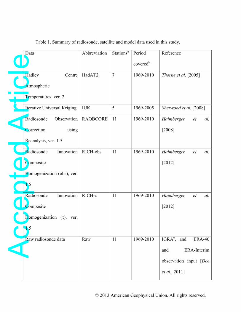
Figure 1 shows the location of the stations for each radiosonde dataset, highlighting in

red those stations that were included in the analysis of TS02 (the trends at the stations are

discussed in Section 3). As well as differing in the time period covered and number of

stations south of 65°S, each radiosonde dataset uses different methods to adjust the

temperature time series, in order to account for any artificial shifts, such as from

instrument or procedural changes. Furthermore, both the HadAT2 and IUK data stop at

30 hPa, whereas the RICH and RAOBCORE data extend to 10 hPa. Free [2011] showed

the differences between many of the same datasets for tropical temperature trends.

Further details concerning the radiosonde datasets and stations can be found in the

supplementary material (Table S1).

Lower stratospheric satellite brightness temperature data from the Microwave Sounding

Unit (MSU TLS) also form part of the analysis. The weighting function for the MSU TLS

data covers a broad vertical layer centered on ~80 hPa, with the half-power width

extending from 150-50 hPa [see Randel et al., 2009, their Fig. 1]. This weighting

function was applied to the radiosonde and model data for part of the analysis. The MSU

TLS data give complete zonal coverage, but there are no data poleward of 82.5°S.

Acc

epte

d A

rticl

e


Monthly zonal mean temperature and ozone data from the CCMVal-2 models were taken

from the REF-B1 experiment, which was configured to reproduce the composition of the

atmosphere from 1960 to 2006 [Morgenstern et al., 2010]. Ozone output was not

available for the AMTRAC3 and UMETRAC models. CMIP3 monthly zonal mean

temperature data were taken from the 20C3M experiment, which also aimed to reproduce

past climate (from the pre-industrial to the year 2000) [Meehl et al., 2007]. For CMIP3,

our study leaves out CNRM-CM3 and UKMO-HadCM3, as these models have

incomplete temperature data (missing data in the lower stratosphere), as well as UKMO-

HadCM3 having prescribed ozone trends twice as large as observed [Karpechko et al.,

2008]. GISS-EH and GISS-ER had an erroneously low ozone forcing [Miller et al.,

2006], though these models are still included in this analysis (see Figure S1). The CMIP3

models were sub-divided into those that included time varying prescribed ozone data

(“CMIP3 w/ozone”) and those that did not (“CMIP3 no ozone”), as has been done

previously [e.g., Cordero and Forster, 2006; Cai and Cowan, 2007; Karpechko et al.,

2008]. Monthly zonal mean temperatures from the CMIP5 historical experiment,

covering the pre-industrial to 2005 [see Taylor et al., 2012 and refs. therein], were also

considered. All of these models used some form of time-varying ozone, either calculating

concentrations interactively (in the manner of a CCM) or through using a prescribed

dataset (the dataset developed by Cionni et al. [2011] was recommended); Eyring et al.

[Long-term changes in tropospheric and stratospheric ozone and associated climate

impacts in CMIP5 simulations, submitted to Journal of Geophysical Research-

Atmospheres, 2012] describe further details related to the ozone concentrations in the

Acc

epte

d A

rticl

e


CMIP5 models. More information on the individual models from the CMIP3, CMIP5 and

CCMVal-2 datasets can be found in the supplementary material (Tables S2-S4).

For the three model datasets, where there was more than one realization available for a

given model, the intra-model ensemble mean was first determined before calculating the

overall dataset ensemble mean (i.e. each model was weighted equally).

Trends are mainly considered over the 30-year period 1969-1998, for consistency with

TS02 and Baldwin et al. [2010], and over the 21-year period 1979-1999, the period that

all observations and models have in common (Table 1). Observations show zonal

asymmetries in SH high latitude temperature trends for certain months [Hu and Fu, 2009:

Lin et al., 2009], which likely depend on trends and variability in wave driving, not

generally captured by climate models [Wang and Waugh, 2012]. As such, we only

consider zonal mean trends in the models and data (albeit a sparsely sampled zonal mean

for the radiosonde data). By not sampling at the radiosonde locations, this method could

bias the sampling of the models to the colder deep vortex. However, we demonstrate

below that the “zonal mean” radiosonde trends agree well with those calculated from the

MSU TLS data, which has near full coverage of the polar cap. Trends were calculated by

linear least squares regression on data binned by month (or season), with the statistical

error estimates adjusted to account for serial auto-correlation [as per Santer et al., 2000].

Unless stated, the quoted errors encompass the 95% confidence interval.

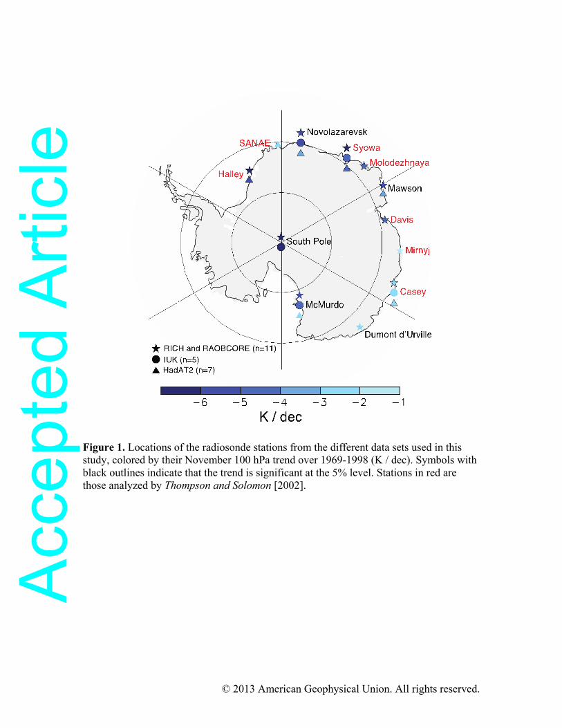
3. SH temperature trends results

Figure 2 shows the high latitude (>65°S) mean temperature trends for the radiosondes,

the CMIP3 w/ozone ensemble mean, the CMIP5 ensemble mean, and the CCMVal-2

Acc

epte

d A

rticl

e


ensemble mean, for the period 1969 to 1998 as a function of pressure and month (similar

to TS02, their Fig. 1). Trends for the RICH-τ and RAOBCORE data (not shown) are very

similar to RICH-obs, arising from the fact that those datasets use the same stations, and

the same break detection algorithm (see Table S1 in the supplementary material for more

information).

Both the radiosonde and model data show a strong and significant cooling in the lower

stratosphere, extending from ~200-50 hPa, and from at least October to December, as

also reported by TS02. The maximum cooling trend occurs for November at

approximately 100 hPa, although the trends differ both in magnitude and (less so)

spatiotemporal patterns. Comparing the radiosonde data shown in the top row of Figure

2, the maximum cooling trend is found in the IUK dataset (-4.7 ± 2.8 K / dec), followed

by the RICH-obs dataset (-4.1 ± 2.4 K / dec), with the HadAT2 data showing the weakest

cooling (-3.8 ± 2.4 K / dec). These are all stronger values than the -2.4 K / dec (-7.1 K /

30 a) trend reported by TS02, but more comparable with the -3.8 K / dec peak value

determined from radiosonde data by Thompson and Solomon [2005], although this covers

a different period (1979-2003). Like TS02 and Thompson and Solomon [2005], both the

IUK and RICH-obs data suggest that the significant lower stratospheric cooling trend

persists into March, whereas the trend stops in December with the HadAT2 data.

Why are the trends different between the radiosonde datasets? Figure 1 shows that the SH

mean temperature for each dataset is comprised of different stations, covering different

longitude and latitude ranges. At the lower latitudes, the stations may be occasionally

sampling air outside of the cold vortex [Hassler et al., 2011a] which weakens the trends

derived at these locations. For example, November 100 hPa trends at the South Pole

Acc

epte

d A

rticl

e


station (90°S) are in the range -6.0 to -7.1 K / dec, whereas they are between -2.3 and -2.5

K / dec for Casey (66°S) (see Table S1). Temperature trends at the continent edge may

also be impacted by the zonally asymmetric nature of the trend patterns [e.g. Lin et al.,

2009], although the degree of asymmetry depends on the month. Hence part of the reason

for the stronger cooling seen with the IUK data is that its mean is weighted towards

higher latitude stations. However, the RICH-obs, RICH-τ and RAOBCORE datasets

include more stations towards the edge of Antarctica compared to HadAT2, yet they still

have stronger cooling trends, suggesting that the spatial distribution of stations cannot

explain all the differences between datasets.

Figure 1 also indicates a range of values for the trend at a given station, depending on

dataset (see also Table S1). In general, the HadAT2 data show the weakest cooling for a

given station. This is particularly the case for McMurdo, Novolazarevsk and Mawson

stations, where the HadAT2 data is a factor of 1.5-1.7 lower than the maximum cooling

trend. Restricting the RICH-obs data to just the HadAT2 stations (also including SANAE,

which does not meet the < 20% missing data requirement) results in a trend of -4.7 ± 2.2

K / dec, i.e. more cooling than that calculated from the HadAT2 data. Restricting the

RICH-obs data to the IUK locations results in a trend of -4.6 ± 2.6 K / dec, i.e. slightly

less cooling than that for the IUK data.

Figure 2 shows that the peak cooling trends for the CMIP5 and CCMVal-2 model

ensembles are comparable to the radiosonde data, with November 100 hPa trend values

of -3.5 ± 0.3 K / dec and -3.8 ± 0.7 K / dec respectively. The trends are weaker for the

CMIP3 w/ozone ensemble, where the November 100 hPa trend is -2.7 ± 0.3 K / dec. The

smaller confidence interval in these trends is due to the substantial reduction in

Acc

epte

d A

rticl

e


interannual variability from averaging several models together, and it is not comparable

to the confidence intervals for the observed trends discussed above. Based on the data

from TS02, Baldwin et al. [2010] concluded that the CMIP3 w/ozone models had a more

favorable comparison with the observed trends than the CCMVal-2 models. However, the

broader range of radiosonde trends in Figure 2 suggests that the CCMVal-2 and CMIP5

ensemble means compare more favorably with observations than CMIP3 w/ozone.

In addition to the ozone induced cooling, the RICH-obs and IUK data also show a higher

altitude warming trend, occuring after the ozone cooling in IUK and at approximately the

same time as the ozone cooling with RICH-obs. A warming trend similar in magnitude

and timing to that of IUK is apparent in the CCMVal-2 ensemble mean trend, and (more

weakly) in the CMIP5 ensemble mean trend. From the individual models, a warming

trend is found in more than half of the CMIP5 models (Figure S2) and in 16 of the 17

CCMVal-2 models (Figure S3), although it is not always significant for either set of

models. Manzini et al. [2003] described a similar feature in their CCM study, attributing

it to increased downwelling (and compressional warming) due to enhanced gravity wave

propagation, itself due to the ozone-induced cooling. Thus, the presence of such a trend

could be an indicator of how well models perform in terms of middle atmosphere

dynamics, although further study is required.

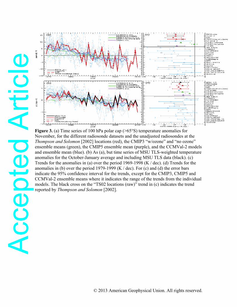
Figure 3 explores the modeled and observed polar cap (>65°S) temperatures in more

detail. Figure 3(a) shows the time series of November temperature anomalies from 1969

to 2010 (or the latest date for the given data; see Table 1). Figure 3(b) shows the time

series of October-January (ONDJ) averaged anomalies for the MSU TLS data, MSU

TLS-weighted radiosondes, and MSU TLS-weighted models. The ONDJ mean is used

Acc

epte

d A

rticl

e


here as this corresponds to the months where Baldwin et al. [2010] found that the

CCMVal-2 models agreed better with the observed trends of TS02. Notwithstanding that

the TS02 trends are smaller in magnitude than those from the other radiosonde datasets,

including summer months to calculate the mean trend goes some way to counter model

biases in the timing of the SH vortex breakup [Hurwitz et al., 2010; Butchart et al.,

2011]. Anomalies are computed relative to a 1979-1999 climatology. Note that using

anomalies removes systematic biases, identified as a particular issue for SH spring

temperatures in the CCMVal-2 models [Butchart et al., 2011].

For the individual CCMVal-2 models and observations, both sets of time series show the

large year-to-year variability characteristic of springtime lower stratospheric temperatures

[e.g., Young et al., 2011], although this is damped in Figure 3(b) by averaging over more

months. Time series for the model ensemble means show far less variability, as the noise

from individual models tends to cancel. The correlation between the anomalies for the

different radiosonde datasets is very high (r > 0.96), despite the different stations and

different adjustment methods. Furthermore, for Figure 3(b), the correlation between the

independent MSU TLS data and radiosondes is also very high (r > 0.93). As the MSU

dataset has complete zonal coverage (although stopping at 82.5°S), this suggests that the

radiosonde datasets are representative of the polar cap temperature, despite their more

limited spatial coverage.

Figure 3(c) shows the 1969-1998 trends for the time series in Figure 3(a), including the

trends calculated for the individual CCMVal-2 models as well as the radiosonde and

model ensemble mean trends discussed above. The error bars encompass the 95%

confidence interval for the trends for all cases except the model ensembles. Here, due to

Acc

epte

d A

rticl

e


aforementioned low variability in the ensemble mean time series, the error bars indicate

the range of the trends found from the individual models that comprise the ensemble

mean. For CCMVal-2 models with more than one ensemble member (CCSRNIES,

CMAM, LMDZrepro, SOCOL and WACCM), the data shown are just from the first

simulation (“run 1”) so as not to dampen the contribution of interannual variability to the

trend uncertainty. The trends calculated for the radiosondes and the CMIP3 w/ozone,

CMIP5 and CCMVal-2 ensembles all agree with each other within their uncertainty

ranges. The figure also shows the trend calculated using unadjusted (“raw”) radiosonde

data, for the same stations used by TS02. As seen with the adjusted radiosonde datasets,

this trend reflects a stronger cooling than that calculated by TS02 (indicated by the black

X), although, again, all are within each other’s uncertainty.

Figure 3(d) is similar to 3(c), but shows the 1979-1999 trends for the time series in Figure

3(b), which is the longest period common to all model and observational datasets. Again,

the trends for the observations and CMIP3 w/ozone, CMIP5 and CCMVal-2 ensembles

all agree within their statistical uncertainty. The close agreement of the MSU TLS and

radiosonde trends further underlines the representativeness of the radiosonde data for the

SH high latitudes, although the fact that the coverage of the MSU TLS data does not

extend to the pole could be impacting the strength of the cooling.

Figures 3(c) and (d) show that trends for the individual CCMVal-2 models cover a wide

range of values, wider than that for the other ensembles. Furthermore, while all the trends

are negative they are not all significant at the 5% level. For many CCMVal-2 models, the

error bars for the trends are greater than those for the observations, suggesting a larger

interannual variability in these models compared to the observations and a topic for

Acc

epte

d A

rticl

e


further study. The range of trends from these models is discussed further in Section 4.

That there is a spread of trend estimates is not unique to the CCMVal-2 dataset: figures in

the Supplementary Material show individual model trends over 1969-1998 as a function

of month and pressure for the CMIP3, CMIP5 and CCVal-2 models, emphasizing the

model diversity in this regard.

Figure 3 also includes the time series and trends from the CMIP3 no ozone ensemble,

which is markedly weaker than the other ensemble mean trends and the observations.

(Note that the “CMIP3 no ozone” trend in Figure 3(d) is not significant; the error bar only

indicates that all the models in this ensemble produce a negative trend.) The absence of

any significant negative trend for this set of models suggests that cooling from CO2

increases cannot explain the observed trends, confirming the role of ozone depletion as

the dominant driver of the SH lower stratospheric cooling at the end of the 20th century

[e.g., Shine et al., 2003; Karpechko et al., 2008].

We also note that the magnitude of the trends depends on the period over which they are

computed. Trends calculated from 1969 are generally lower in magnitude (i.e. less

cooling) when the end year is later in the record. For example, using the RICH-obs

November 100 hPa data, trends are in the range –3.7 to –4.3 K / dec with an end year

from 1998 through 2002, and –3.2 to –3.6 K / dec when the end year is from 2003

through 2010. A similar behavior is evident from the CCMVal-2 and CMIP5 ensemble

mean time series, where there is a monotonic decrease in the magnitude of the cooling

trend when the end year is after 1998. All of these trends are still significant at the 5%

level.

Acc

epte

d A

rticl

e


Visual inspection of the observed time series in Figure 3 does suggest a flattening out of

the trend towards the end of the record, although a longer time series would be needed to

diagnose a statistically significant change point. While there might be some expectation

of a reduction in the cooling trend, since we have now passed the peak CFC

concentration [Newman et al., 2007] and ozone loss rates have reduced [Hassler et al.,

2011b], there is large year-to-year variability in the stratospheric circulation and hence

temperatures. For example, the thus far unique SH sudden stratospheric warming in 2002

[e.g. Newman and Nash, 2005] is a notable anomaly in the record that can impact trend

assessments.

4. The relationship of ozone and temperature trends with CCMVal-2 models

As well as model-observation comparison for the magnitude of the trend, Baldwin et al.

[2010] considered how the austral spring temperature and ozone trends were related to

one another, in the individual models and in observations. They reported (their Figure

10.13) that CCMs qualitatively reproduced the observed correlation between weaker

(stronger) ozone depletion and weaker (stronger) 100 hPa cooling trends. But they also

suggested, based on TS02 and Halley station total ozone column observational data, that

the models overestimated the cooling for a given ozone loss. We revisit their analysis in

this section, using the expanded set of observations from the radiosonde datasets as well

as an expanded set of ozone column data.

Figure 4 shows the relationship between the September-December (SOND) ozone

column trend and ONDJ temperature trends for the individual CCMVal-2 models, the

CCMVal-2 ensemble mean, and observations. Figure 4(a) shows the relationship for the

Acc

epte

d A

rticl

e


1969-1998 trends, using the 100 hPa temperature [as per Baldwin et al., 2010], and

Figure 4(b) shows the relationship for the 1979-1999 trends, using MSU TLS and MSU

TLS-weighted temperature data. The MSU TLS data are useful for this case as there is

substantial overlap between the weighting function and the vertical region of greatest

Antarctic ozone depletion. Observed ozone column trends are from the mean of the four

Antarctic ozonesonde stations with the longest records: Faraday/Vernadsky (65°S,

64°W), Syowa (69°S, 40°E), Halley (76°S, 27°W), and South Pole (90°S, 25°W) [as per

Hassler et al., 2011a].

Error bars on the observations show the range of the trend values for the different

temperature datasets (horizontal bars) and different ozonesonde stations (vertical bars).

All the observed trends are significant at the 5% level. Error bars on the CCMVal-2

ensemble mean trend indicate the 95% confidence interval for the mean, determined from

the spread of the trends from the individual models. Acknowledging the distinctive

estimates of statistical uncertainty in the modeled and observed trends, the error bars for

the observations and CCMVal-2 ensemble mean trend overlap in both panels of Figure 4.

This further strengthens the case made in the previous section, that the CCMVal-2

ensemble mean matches the observations within the uncertainty of both, for both ozone

and temperature.

Individual CCMVal-2 models show a large scatter in their ozone and temperature trends,

as also shown in Figure 3. However, the dashed line in each panel of Figure 4 indicates

the positive (and significant) relationship between the modeled trends in lower

stratospheric temperatures and ozone column. Note that the regression is forced through

the origin, i.e. assuming zero temperature trend for zero ozone loss. If the regression is

Acc

epte

d A

rticl

e


not forced through zero, the resulting intercept suggests a positive temperature trend for

ozone loss less than 20 DU / dec, which may not be physical. The regression coefficients

for each panel are very similar. The regression coefficient for Figure 4(a) is 12.0 ± 1.8

DU dec-1 / K dec-1, and for Figure 4(b) it is 12.1 ± 2.3 DU dec-1 / K dec-1; i.e., an ozone

trend of 12 DU / dec is predicted to be accompanied by a temperature trend of 1 K / dec.

The gray shaded area in Figure 4 shows the 95% confidence interval for the linear

regression, estimated from the variance of the regression residuals [e.g., see Wilks, 2006].

The area estimates the uncertainty in the relationship between the trends in ozone column

and lower stratospheric temperature, as derived from the models: i.e., if we have a certain

trend in the ozone column, the gray indicates where we are 95% certain that the

corresponding temperature trend will lie (or vice versa). While the observed trends in

Figure 4 sit below the regression line, and therefore suggest a smaller temperature trend

for a given ozone change, they are within the shaded area. This would suggest that, at the

5% level, the CCMVal-2 models do not produce a stronger cooling for a given ozone

depletion compared to observations. Note that the observations still lie within the 95%

confidence interval if the regression is not forced through the origin. (Interestingly, the

95% confidence interval does not include the origin if the regression for Figure 4a is not

forced through it.)

Finally, Figure 4(a) also indicates the temperature trend calculated by TS02. For ONDJ

their estimated trend falls within the range of those estimated from the other datasets, but

only due to the inclusion of the HadAT2 data, which has a weaker cooling trend than the

other radiosonde datasets. From Figure 2 we see that the HadAT2 cooling trend does not

continue through the austral summer, as it does for the IUK and RICH-obs data.

Acc

epte

d A

rticl

e


Restricting the RICH-obs data to the HadAT2 stations does not change the month-

pressure trend pattern markedly from the full RICH-obs data in Figure 2(a), suggesting

that the more limited cooling in the HadAT2 data is related to the adjustment method,

rather than the spatial distribution of the stations.

5. Summary and conclusions

We have presented late 20th century, high latitude Southern Hemisphere (SH)

stratospheric temperature trends from several radiosonde datasets, satellite measurements,

and multi-model ensemble data from climate and chemistry-climate models. Except for

models that do not include ozone depletion, all the trends show strong cooling during

austral spring and summer, peaking in November at around 100 hPa. While the observed

cooling is dependent on the dataset, the magnitudes of the trends calculated here are more

than 50% stronger than those presented by Thompson and Solomon [2002] (TS02), often

used as a benchmark for modeling studies. However, once the statistical uncertainties are

taken into account, the trends from the multi-model ensembles and observations

(including TS02) agree with one another. Overall, the results suggest that there is not a

systematic bias towards excessive cooling in the ensemble mean SH lower stratosphere

temperatures determined from the latest generation of stratospheric chemistry-climate

models (CCMs). Furthermore, our results also suggest that ensemble mean temperature

trends determined from climate models also compare well to observed trends, provided

that the models include some representation of late 20th century ozone depletion [Cordero

and Forster, 2006].

Acc

epte

d A

rticl

e


While trends calculated from ensemble mean temperatures match observed trends well,

trends from the individual models show a large spread. Despite including the drivers of

ozone depletion, some of the CCMVal-2 models do not have significant austral spring

temperature trends. This range of model skill for stratospherically relevant parameters in

the CCMs has been explored in several other studies [e.g. Gettelman et al., 2010; Hegglin

et al., 2010; Butchart et al., 2011], and several shortcomings have been identified. In

particular, Butchart et al. [2011] highlighted a pervasive poor performance of the models

for the SH during austral spring, and several studies have indicated the large range of

modeled ozone trends [Eyring et al., 2006; Austin et al., 2009; Austin et al., 2010]. For

the climate models, the spread of the trends is generally less, likely due to the prevalence

of a prescribed ozone dataset rather than the more complex online calculation of ozone in

the CCMs. Nevertheless, for the CCMs there is a significant positive linear relationship

between the magnitude of the cooling trend and the magnitude of the ozone depletion,

and the observed temperature and ozone trends appear to conform to the same

relationship, within the statistical uncertainty. I.e., our results suggest that the models do

not systematically overestimate the cooling for a given ozone depletion.

Overall, we would recommend that multiple temperature datasets are used to understand

the evolution of stratospheric temperature, both for observational studies and model

evaluation, echoing the similar sentiments of Free [2010], Thorne et al. [2010], and

Calvo et al. [2012]. The latter study is especially pertinent here, as they evaluated SH

late-20th century temperature trends in a CCM using a range of datasets and found that

the modeled cooling trend agreed better with datasets other than TS02.

Acknowledgements

Acc

epte

d A

rticl

e


We thank Greg Bodeker, Nathan Gillett, Susan Solomon and Dave Thompson for

discussion and useful input. We thank Steve Sherwood and the Met Office for the

provision of the IUK (www.ccrc.unsw.edu.au/staff/profiles/sherwood/radproj/index.html)

and HadAT2 (www.metoffice.gov.uk/hadobs) radiosonde datasets, respectively. We

acknowledge the WCRP’s (World Climate Research Programme) Working Group on

Coupled Modelling, which is responsible for CMIP, and we thank the climate modeling

groups (as listed in Tables S2 and S3 of this paper) for producing and making available

their model output. For CMIP, the U.S. Department of Energy's Program for Climate

Model Diagnosis and Intercomparison provides coordinating support and led

development of software infrastructure in partnership with the Global Organization for

Earth System Science Portals. We acknowledge the Chemistry‐ Climate Model

Validation (CCMVal) Activity of WCRP’s SPARC (Stratospheric Processes and their

Role in Climate) project, and the participating model groups (as listed in Table S4 of this

paper), for organizing and coordinating the CCMVal-2 activity, and the British

Atmospheric Data Centre (BADC) for collecting and archiving the model output. Natalia

Calvo was partially supported by the Advanced Study Program from the National Center

for Atmospheric Research. The National Center for Atmospheric Research is operated by

the University Corporation for Atmospheric Research under sponsorship of the National

Science Foundation. Leopold Haimberger was supported by the Austrian Science Funds

(FWF) project P21772-N22. We thank Alexey Karpechko, Darryn Waugh and an

anonymous reviewer for their comments on an earlier version of the manuscript.

References

Acc

epte

d A

rticl

e


Austin, J., et al. (2009), Coupled chemistry climate model simulations of stratospheric temperatures and their trends for the recent past, Geophysical Research Letters, 36(13), L13809. Austin, J., et al. (2010), Chemistry-climate model simulations of spring Antarctic ozone, Journal of Geophysical Research, 115, D00M11. Butchart, N., et al. (2011), Multimodel climate and variability of the stratosphere, Journal of Geophysical Research, 116(D5), D05102. Cai, W., and T. Cowan (2007), Trends in Southern Hemisphere Circulation in IPCC AR4 Models over 1950–99: Ozone Depletion versus Greenhouse Forcing, Journal Of Climate, 20, 681-693. Calvo, N., R. R. Garcia, D. R. R. Marsh, M. J Mills, D. E. Kinnison, and P. J. Young (2012), Reconciling modeled and observed temperature trends over Antarctica, Geophysical Research Letters. Cionni, I., V. Eyring, J. F. Lamarque, W. J. Randel, D. S. Stevenson, F. Wu, G. E. Bodeker, T. G. Shepherd, D. T. Shindell, and D. W. Waugh (2011), Ozone database in support of CMIP5 simulations: results and corresponding radiative forcing, Atmospheric Chemistry and Physics Discussions, 11(4), 10875-10933. Cordero, E. C., and P. M. Forster (2006), Stratospheric variability and trends in models used for the IPCC AR4, Atmospheric Chemistry And Physics, 6, 5369-5380. Dee, D. P., et al. (2011), The ERA-Interim reanalysis: configuration and performance of the data assimilation system, Quarterly Journal Of The Royal Meteorological Society, 137(656), 553-597. Eyring, V., M. P. Chipperfield, M. A. Giorgetta, D. E. Kinnison, E. Manzini, K. Matthes, P. A. Newman, S. Pawson, T. G. Shepherd, and D. W. Waugh (2008), Overview of the new CCMVal reference and sensitivity simulations in support of upcoming ozone and climate assessments and the planned SPARC CCMVal, SPARC Newsletter, 30, 20-26. Eyring, V., et al. (2006), Assessment of temperature, trace species, and ozone in chemistry-climate model simulations of the recent past,, Journal of Geophysical Research, 111, D22308. Free, M. (2011), The Seasonal Structure of Temperature Trends in the Tropical Lower Stratosphere, Journal Of Climate, 24(3), 859-866. Garny, H., M. Dameris, and A. Stenke (2009), Impact of prescribed SSTs on climatologies and long-term trends in CCM simulations, Atmospheric Chemistry And Physics, 9(16), 6017-6031. Gettelman, A., et al. (2010), Multimodel assessment of the upper troposphere and lower stratosphere: Tropics and global trends, Journal of Geophysical Research, 115(null), D00M08. Gillett, N. P., and D. W. Thompson (2003), Simulation of recent Southern Hemisphere climate change, Science, 302(5643), 273-275. Gillett, N. P., et al. (2011), Attribution of observed changes in stratospheric ozone and temperature, Atmospheric Chemistry And Physics, 11(2), 599-609. Haimberger, L., C. Tavolato, and S. Sperka (2008), Toward Elimination of the Warm Bias in Historic Radiosonde Temperature Records—Some New Results from a Comprehensive Intercomparison of Upper-Air Data, Journal Of Climate, 21(18), 4587-4606.

Acc

epte

d A

rticl

e


Haimberger, L., C. Tavolato, and S. Sperka (2012), Homogenization of the global radiosonde temperature dataset through combined comparison with reanalysis background series and neighboring stations, Journal Of Climate, 120608133708009. Hassler, B., G. E. Bodeker, S. Solomon, and P. J. Young (2011a), Changes in the polar vortex: Effects on Antarctic total ozone observations at various stations, Geophysical Research Letters, 38, L01805. Hassler, B., J. S. Daniel, B. J. Johnson, S. Solomon, and S. J. Oltmans (2011b), An assessment of changing ozone loss rates at South Pole: Twenty-five years of ozonesonde measurements, Journal of Geophysical Research, 116(D22), D22301-. Hegglin, M. I., et al. (2010), Multimodel assessment of the upper troposphere and lower stratosphere: Extratropics, Journal of Geophysical Research, 115, D00M09. Hurwitz, M. M., P. A. Newman, F. Li, L. D. Oman, O. Morgenstern, P. Braesicke, and J. A. Pyle (2010), Assessment of the breakup of the Antarctic polar vortex in two new chemistry-climate models, Journal of Geophysical Research, 115(D7), D07105. Kang, S. M., L. M. Polvani, J. C. Fyfe, and M. Sigmond (2011), Impact of Polar Ozone Depletion on Subtropical Precipitation, Science, 332, 951-954. Karpechko, A. Y., N. P. Gillett, G. J. Marshall, and A. A. Scaife (2008), Stratospheric influence on circulation changes in the Southern Hemisphere troposphere in coupled climate models, Geophysical Research Letters, 35(20), L20806. Lin, P., Q. Fu, S. Solomon, and J. M. Wallace (2009), Temperature Trend Patterns in Southern Hemisphere High Latitudes: Novel Indicators of Stratospheric Change, Journal Of Climate, 22(23), 6325-6340. Manzini, E., B. Steil, C. Brühl, M. A. Giorgetta, and K. Krüger (2003), A new interactive chemistry-climate model: 2. Sensitivity of the middle atmosphere to ozone depletion and increase in greenhouse gases and implications for recent stratospheric cooling, Journal of Geophysical Research, 108(D14), 4429-. Mclandress, C., and T. G. Shepherd (2009), Simulated Anthropogenic Changes in the Brewer–Dobson Circulation, Including Its Extension to High Latitudes, Journal Of Climate, 22(6), 1516. Mears, C. A., and F. J. Wentz (2009), Construction of the Remote Sensing Systems V3.2 Atmospheric Temperature Records from the MSU and AMSU Microwave Sounders, Journal of Atmospheric and Oceanic Technology, 26(6), 1040-1056. Meehl, G. A., C. Covey, K. E. Taylor, T. Delworth, R. J. Stouffer, M. Latif, B. Mcavaney, and J. F. B. Mitchell (2007), The WCRP CMIP3 Multimodel Dataset: A New Era in Climate Change Research, Bulletin of the American Meteorological Society, 88(9), 1383-1394. Miller, R. L., G. A. Schmidt, and D. T. Shindell (2006), Forced annular variations in the 20th century Intergovernmental Panel on Climate Change Fourth Assessment Report models, Journal of Geophysical Research, 111(D18), D18101. Morgenstern, O., et al. (2010), Review of the formulation of present-generation stratospheric chemistry-climate models and associated external forcings, Journal of Geophysical Research, 115(null), D00M02. Newman, P. A., and E. R. Nash (2005), The Unusual Southern Hemisphere Stratosphere Winter of 2002, Journal Of The Atmospheric Sciences, 62(3), 614-628.

Acc

epte

d A

rticl

e


Newman, P. A., J. S. Daniel, D. W. Waugh, and E. R. Nash (2007), A new formulation of equivalent effective stratospheric chlorine (EESC), Atmospheric Chemistry And Physics, 7(17), 4537-4552. Polvani, L. M., D. W. Waugh, G. J. P. Correa, and S.-W. Son (2011), Stratospheric Ozone Depletion: The Main Driver of Twentieth-Century Atmospheric Circulation Changes in the Southern Hemisphere, Journal Of Climate, 24(3), 795-812. Randel, W. J., and F. Wu (1999), Cooling of the Arctic and Antarctic Polar Stratospheres due to Ozone Depletion, Journal Of Climate, 12(5), 1467-1479. Randel, W. J., et al. (2009), An update of observed stratospheric temperature trends, Journal of Geophysical Research, 114(D2), D02107-. Santer, B. D., T. M. L. Wigley, J. S. Boyle, D. J. Gaffen, J. J. Hnilo, D. Nychka, D. E. Parker, and K. E. Taylor (2000), Statistical significance of trends and trend differences in layer-average atmospheric temperature time series, Journal of Geophysical Research, 105(D6), 7337-7356. Sherwood, S. C., C. L. Meyer, R. J. Allen, and H. A. Titchner (2008), Robust Tropospheric Warming Revealed by Iteratively Homogenized Radiosonde Data, Journal Of Climate, 21(20), 5336-5352. Shine, K. P., et al. (2003), A comparison of model-simulated trends in stratospheric temperatures, Quarterly Journal Of The Royal Meteorological Society, 129(590), 1565-1588. Solomon, S. (1999), Stratospheric Ozone Depletion: A Review of Concepts and History, Reviews of Geophysics, 37, 275-316. Son, S. W., et al. (2010), Impact of stratospheric ozone on Southern Hemisphere circulation change: A multimodel assessment, Journal of Geophysical Research, 115, D00M07. Taylor, K. E., R. J. Stouffer, and G. A. Meehl (2012), An Overview of CMIP5 and the Experiment Design, Bulletin of the American Meteorological Society, 93, 485-498. Thompson, D. W., and S. Solomon (2002), Interpretation of Recent Southern Hemisphere Climate Change, Science, 296(5569), 895-899. Thompson, D. W. J., and S. Solomon (2005), Recent Stratospheric Climate Trends as Evidenced in Radiosonde Data: Global Structure and Tropospheric Linkages, Journal Of Climate, 18(22), 4785-4795. Thompson, D. W. J., S. Solomon, P. J. Kushner, M. H. England, K. M. Grise, and D. J. Karoly (2011), Signatures of the Antarctic ozone hole in Southern Hemisphere surface climate change, Nature Geoscience, 4(11), 741-749. Thorne, P. W., J. R. Lanzante, T. C. Peterson, D. J. Seidel, and K. P. Shine (2010), Tropospheric temperature trends: history of an ongoing controversy, Wiley Interdisciplinary Reviews: Climate Change, 2(1), 66-88. Thorne, P. W., D. E. Parker, S. F. B. Tett, P. D. Jones, M. McCarthy, H. Coleman, and P. Brohan (2005), Revisiting radiosonde upper air temperatures from 1958 to 2002, Journal of Geophysical Research, 110(D18), D18105-. Young, P. J., D. W. J. Thompson, K. H. Rosenlof, S. Solomon, and J.-F. Lamarque (2011), The seasonal cycle and interannual variability in stratospheric temperatures and links to the Brewer-Dobson circulation: An analysis of MSU and SSU data, Journal Of Climate, 110713113105003.

Acc

epte

d A

rticl

e


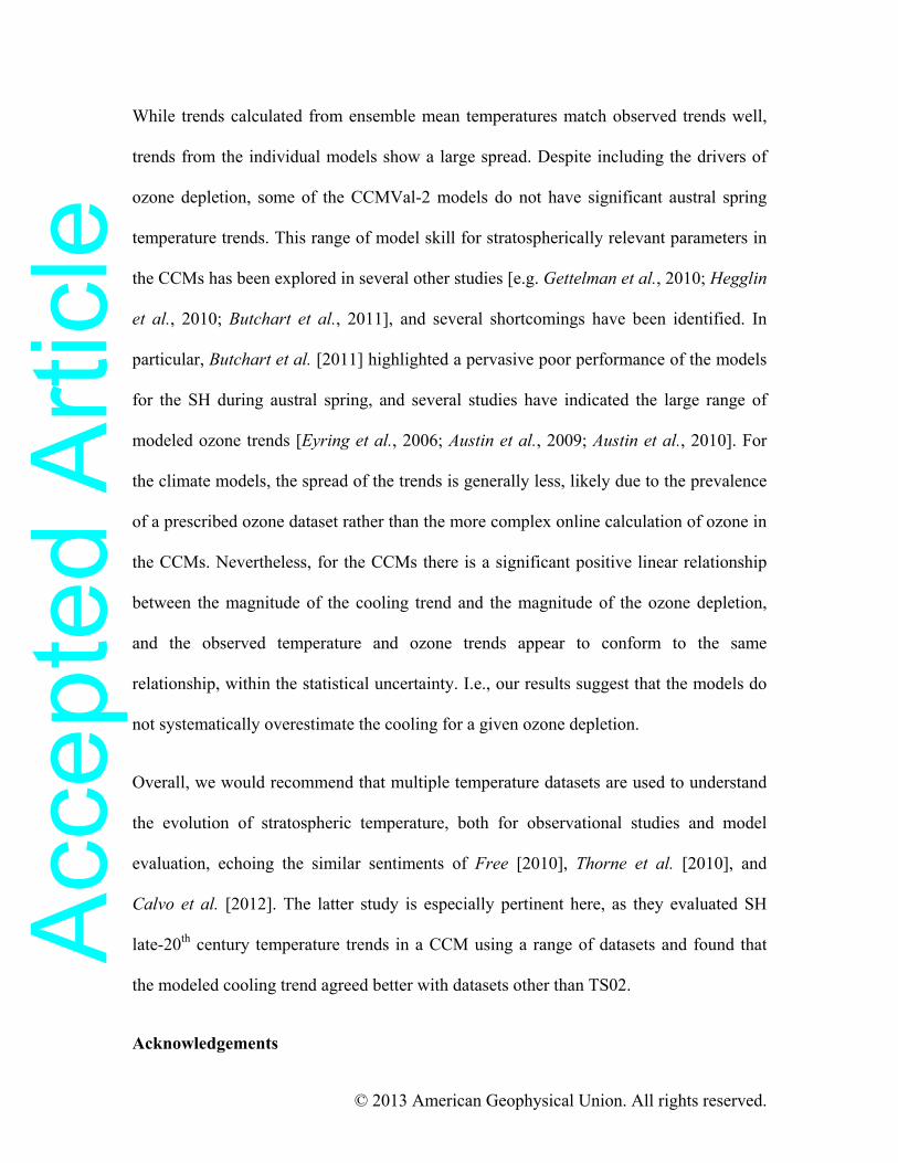
Table 1. Summary of radiosonde, satellite and model data used in this study.

Data Abbreviation Stationsa Period

coveredb

Reference

Hadley Centre

Atmospheric

Temperatures, ver. 2

HadAT2 7 1969-2010 Thorne et al. [2005]

Iterative Universal Kriging IUK 5 1969-2005 Sherwood et al. [2008]

Radiosonde Observation

Correction using

Reanalysis, ver. 1.5

RAOBCORE 11 1969-2010 Haimberger et al.

[2008]

Radiosonde Innovation

Composite

Homogenization (obs), ver.

1.5

RICH-obs 11 1969-2010 Haimberger et al.

[2012]

Radiosonde Innovation

Composite

Homogenization (τ), ver.

1.5

RICH-τ 11 1969-2010 Haimberger et al.

[2012]

Raw radiosonde data Raw 11 1969-2010 IGRAc, and ERA-40

and ERA-Interim

observation input [Dee

et al., 2011]

Acc

epte

d A

rticl

e


MSU lower stratosphere

temperatures, Remote

Systems Sensing, ver. 3.3

MSU TLS 1979-2010 Mears and Wentz [2009]

CCMVal-2 historical

(REF-B1) simulation

model output

CCMVal-2 1969-2000 Morgenstern et al.

[2010]

CMIP3 historical (20C3M)

simulation model output

CMIP3 1969-1999 Meehl et al. [2007]

CMIP5 historical (hist)

simulation model output

CMIP5 1969-2005 Taylor et al. [2012]

a For radiosonde data, the number of stations south of 65°S.

b The start date refers to first year used in this study. For CCMVal-2, CMIP3 and CMIP5,

the end date is the year for which all models still have output.

c Integrated Global Radiosonde Archive (http://www.ncdc.noaa.gov/oa/climate/igra/)

Acc

epte

d A

rticl

e


Figure 1. Locations of the radiosonde stations from the different data sets used in this study, colored by their November 100 hPa trend over 1969-1998 (K / dec). Symbols with black outlines indicate that the trend is significant at the 5% level. Stations in red are those analyzed by Thompson and Solomon [2002].

Acc

epte

d A

rticl

e


Figure 2. Southern hemisphere high latitude temperature trends over 1969-1998 (K / dec), as a function of month and pressure. Trends are shown for (a) RICH-obs, (b) HadAT2 and (c) IUK radiosondes, and the ensemble means of (d) the CMIP3 models (just those with ozone depletion), (e) the CMIP5 models and (f) the CCMVal-2 models. Radiosonde trends are calculated using the average of the temperatures for the stations poleward of 65°S, and model trends are calculated from the zonal mean temperatures for region poleward of 65°S. Color-filled contours indicate that the trend is significant at the 5% level. Contour spacing is 0.5 K / dec.

Acc

epte

d A

rticl

e


Figure 3. (a) Time series of 100 hPa polar cap (>65°S) temperature anomalies for November, for the different radiosonde datasets and the unadjusted radiosondes at the Thompson and Solomon [2002] locations (red), the CMIP3 “w/ozone” and “no ozone” ensemble means (green), the CMIP5 ensemble mean (purple), and the CCMVal-2 models and ensemble mean (blue). (b) As (a), but time series of MSU TLS-weighted temperature anomalies for the October-January average and including MSU TLS data (black). (c) Trends for the anomalies in (a) over the period 1969-1998 (K / dec). (d) Trends for the anomalies in (b) over the period 1979-1999 (K / dec). For (c) and (d) the error bars indicate the 95% confidence interval for the trends, except for the CMIP3, CMIP5 and CCMVal-2 ensemble means where it indicates the range of the trends from the individual models. The black cross on the “TS02 locations (raw)” trend in (c) indicates the trend reported by Thompson and Solomon [2002].

Acc

epte

d A

rticl

e


Figure 4. (a) Scatter plot of trends over 1969-1998 for September-December average total column ozone (DU / dec) against trends in October-January average 100 hPa temperature (K / dec), from the CCMVal-2 models (blue) and ozonesonde and radiosonde observations (red; see text). The temperature trend reported by Thompson and Solomon [2002] is also shown. (b) Similar to (a), but Trends over 1979-1999 for September-December average total column ozone (DU / dec) against trends in October- January average MSU TLS-weighted temperature (K / dec). Error bars on the multimodel mean trend indicate the 95% confidence interval for the mean, estimated using the standard error of the individual model trends. Error bars on the observed trends indicate the range of trends from the four ozonesonde stations (vertical) and from the different radiosonde datasets (horizontal). The dashed line indicates the best fit to the relationship of the ozone and temperature trends, forced through the origin, calculated from the models. The shaded grey area is the 95% confidence interval for the relationship, estimated from the variance of the regression residuals.

Agreement in late twentieth century Southern Hemisphere stratospheric temperature trends in observations and CCMVal-2, CMIP3, and CMIP5 models

Documents