AgMIP Regional Integrated Assessments Handbook

GUIDE FOR REGIONAL INTEGRATED ASSESSMENTS:

HANDBOOK OF METHODS AND PROCEDURESVERSION 5

2    

Guide for Regional Integrated Assessments:

Handbook of Methods and Procedures Version 5.0

AgMIP International Leaders Cynthia Rosenzweig, Jim Jones, Jerry Hatfield and John Antle

AgMIP Team Leaders Climate: Alex Ruane

Crops: Ken Boote and Peter Thorburn Regional Economics: John Antle and Roberto Valdivia

Information Technologies: Cheryl Porter and Sander Janssen

AgMIP Science Coordinator Alex Ruane ([email protected])

AgMIP International Coordinator

Carolyn Mutter ([email protected])

October 1, 2013

3    

Guidelines for Regional Integrated Assessments: Handbook of Methods and Procedures

Table of Contents

Introduction 4 Key Attributes of an AgMIP Regional Integrated Assessment 5 Core Climate Impact Questions 5 Key Regional Research Team Outputs 7 AgMIP Standardized Formats and Tools 9 Guidelines for Activities for AgMIP Regional Research Teams 10 1. Scoping of production systems and developing/refining research work plan for regional integrated assessment 10 2. Develop Representative Agricultural Pathways (RAPs) for use in regional

analysis of climate impact and adaptation 11 3. Assemble existing data from experiments and calibrate crop models 15 4. Assemble and quality-control current climate series 16 5. Assemble data and simulate crop models for analysis of yield variations 19 6. Assemble economic data for regional economic analysis and develop skills for using the regional economic model 21 7. Create downscaled climate scenarios 21 8. Conduct multiple crop/livestock model simulations 24 9. Analyze regional economic impacts of climate change without and

with adaptation using the regional economic model 26 10. Archive data and analyses results for integrated assessments 27 11. Disseminate integrated assessment results 28 Appendix 1. “Fast Track” Proof of Concept Integrated Assessment Exercise 30 Appendix 2. Calculating Statistics for Climate Impact Assessments Using

Crop/Livestock Model Simulations with the TOA-MD Model 32 Appendix 3. Crop Model Simulations for Integrated Assessments: User’s Guide 41

4    

Introduction The purpose of this handbook is to describe recommended methods for a trans-disciplinary, systems-based approach for regional-scale (local to national scale) integrated assessment of agricultural systems under future climate, bio-physical and socio-economic conditions. An earlier version of this Handbook was developed and used by several AgMIP Regional Research Teams (RRTs) in Sub-Saharan Africa (SSA) and South Asia (SA) (AgMIP Handbook version 4.2, www.agmip.org/regional-integrated-assessments-handbook/). In contrast to the earlier version, which was written specifically to guide a consistent set of integrated assessments across SSA and SA, this version is intended to be more generic such that the methods can be applied to any region globally. These assessments are the regional manifestation of research activities described by AgMIP in its online protocols document (available at www.agmip.org). AgMIP Protocols were created to guide climate, crop modeling, economic, and information technology components of its projects. Various regions of the world are now undertaking regional assessments following AgMIP protocols and integrated assessment procedures. This Handbook version also has a number of modifications to the methods and to our description of methods based on what was learned from the use and evaluation of the Handbook version 4.2. However, it is important to recognize that the procedures presented here were designed for the data available to the SSA and SA teams, for implementation of two crop models per integrated assessment region (at least DSSAT and APSIM), and for use of one socio-economic model (TOA-MD) in the integrated impact assessments. Going forward, we recommend the use of multiple crop and economic models when available, based in large part to lessons learned in the various crop model intercomparisons (e.g., Asseng et al. 2013; Rosenzweig et al., 2013) and on the global economic model intercomparisions (Nelson et al., 2013). We envision that specific choices of multiple models may vary among regions, but that a core set of models should be used such that results can be aggregated and compared across all regions. AgMIP regional integrated assessments require close coordination among economic, climate, crop modeling and IT team members within each regional team. Assessments should begin with regional teams working with stakeholders to define what outcomes are to be evaluated and then developing details of the specific production systems that need to be quantified. Each regional research team (RRT) should focus on impacts related to, at minimum, food production, income, and poverty in their regions; emphasizing important food crops and quantifying relevant uncertainties. Where appropriate, livestock components of production systems should be included. Then a plan of work should be developed by teams that will include AgMIP-recommended methods and procedures to accomplish integrated assessments and desired compatibility of outputs across regions. This handbook was written such that it represents a minimum approach that can be expanded upon in regions where available data and resources allow. The methods and core approach used by all interdisciplinary research teams need to be fundamentally consistent in order to enable meta-analyses and large-scale studies. Particular care must therefore be

5    

taken in introducing new methods and models that could potentially limit the ability of results to be compared beyond the immediate region. This handbook is a living document that will continue to evolve and be improved through input from the regions as they apply it to their own situations and gain experience in the methods that are aimed at helping to unify methods and outputs. Key Attributes of an AgMIP Regional Integrated Assessment - Designed with input from stakeholders and policymakers - Oriented upon production-systems-based approach (rather than specific fields)

potentially including multiple crops, livestock, aquaculture, and other sources of income. - Transdisciplinary in its linking of climate, biophysical, and socio-economic conditions

and responses. - Flexible in that its framework allows for the testing of adaptations and alternative models

and methods across a series of households in a given region. - Addresses core questions of climate impact on current and future production systems

(detailed in the next section) - Calibrated on current production system using available observed data with full and

open documentation. - Examines the impact of both mean climate changes and potential interactions with

climate variability - Presents results in a probabilistic manner with accounting of major uncertainties. - Utilizes consistent terminology across disciplines and among various AgMIP

assessments and initiatives. - Uploads results to an online AgMIP database for archival and cross-regional analyses

with full attribution of data providers and intellectual contributions. - Publishes findings in peer-reviewed journals and disseminates information to

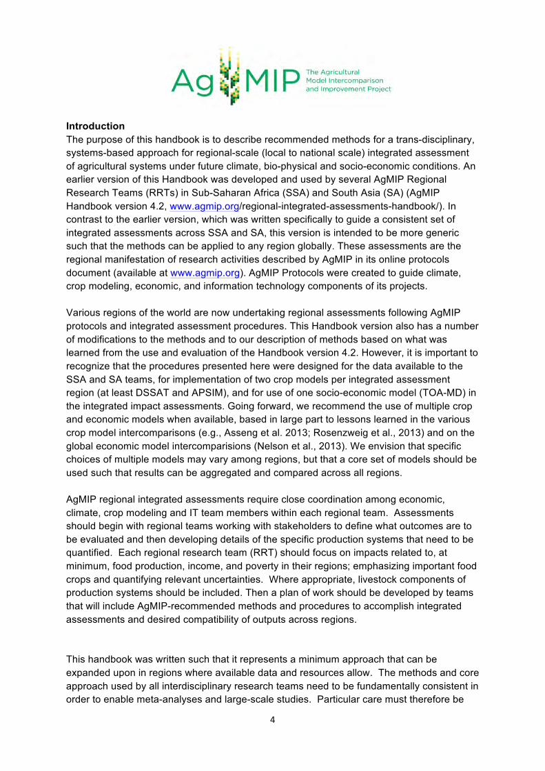
stakeholders. Core Climate Impact Questions AgMIP has identified the following core research questions that motivate research activities for regional integrated assessments (Figure 1): 1. What is the sensitivity of current agricultural production systems to climate change? This question addresses the isolated impacts of climate changes assuming that the production system does not change from its current state. 2. What is the impact of climate change on future agricultural production systems? This question evaluates the isolated role of climate impacts on the future production system, which will differ from the current production system due to development in the agricultural sector not directly motivated by climate changes. 3. What are the benefits of climate change adaptations? This question analyzes the benefit of potential adaptation options in the production system of the future, which may offset or capitalize on climate vulnerabilities identified in Core Question 2 above.

6    

Figure 1. Overview of core climate impact questions and the production system states that will be simulated.

The current production system is represented by the blue dot, while the production of the system is represented in three ways: assuming that there is no climate change (black), assuming that there is climate change and no

adaptation (red), and assuming that there is climate change and adaptation (green). The dashed line represents the evolution of the production system in response to development in the agricultural sector that is not directly motivated by climate change. Core Question 2 quantifies the impact of climate change on an adaptation-free

future affected by climate change, and the green line represents the benefits of adaptation in that future production system. Note that Core Question #1 cannot be depicted on this figure, as future climate impacts will necessarily encounter a different production system, however this question provides useful context on current

biophysical and socio-economic vulnerability that motivates initial investments in adaptation.

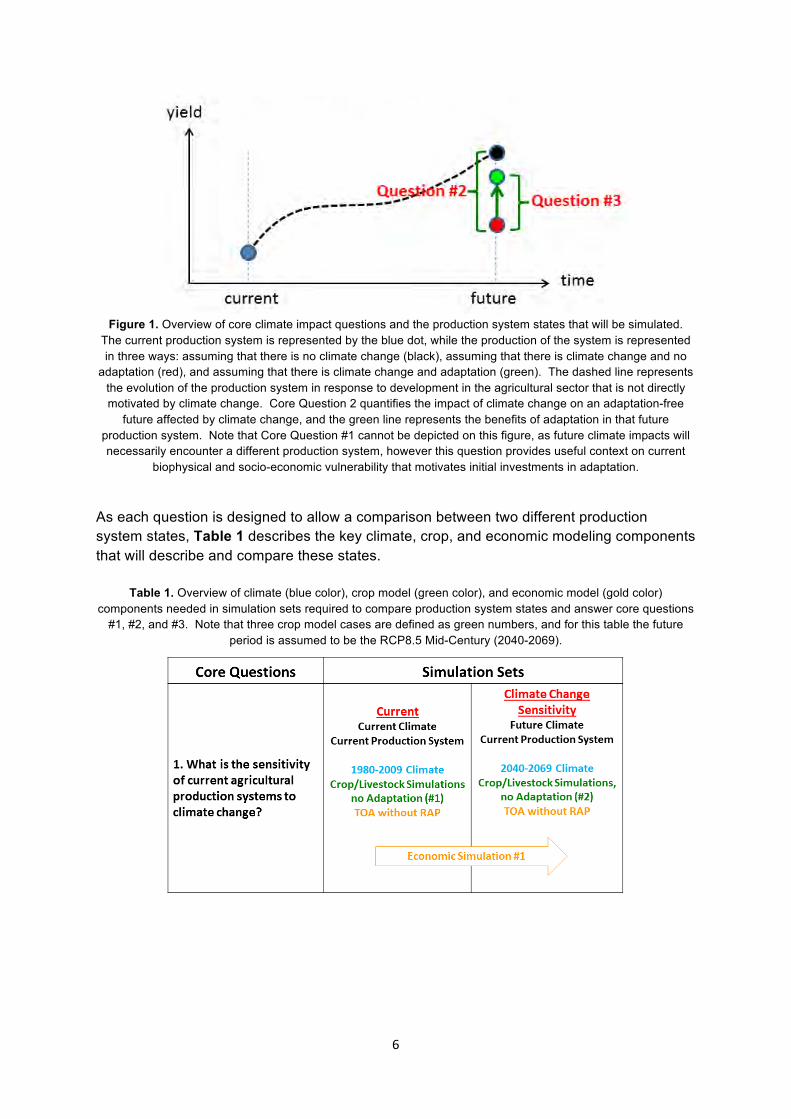
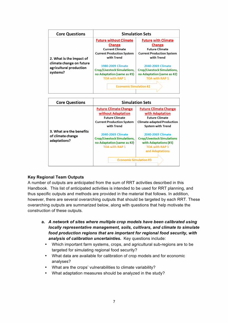
As each question is designed to allow a comparison between two different production system states, Table 1 describes the key climate, crop, and economic modeling components that will describe and compare these states.

Table 1. Overview of climate (blue color), crop model (green color), and economic model (gold color) components needed in simulation sets required to compare production system states and answer core questions

#1, #2, and #3. Note that three crop model cases are defined as green numbers, and for this table the future period is assumed to be the RCP8.5 Mid-Century (2040-2069).

7    

Key Regional Team Outputs A number of outputs are anticipated from the sum of RRT activities described in this Handbook. This list of anticipated activities is intended to be used for RRT planning, and thus specific outputs and methods are provided in the material that follows. In addition, however, there are several overarching outputs that should be targeted by each RRT. These overarching outputs are summarized below, along with questions that help motivate the construction of these outputs.

a. A network of sites where multiple crop models have been calibrated using locally representative management, soils, cultivars, and climate to simulate food production regions that are important for regional food security, with analysis of calibration uncertainties. Key questions include:

• Which important farm systems, crops, and agricultural sub-regions are to be targeted for simulating regional food security?

• What data are available for calibration of crop models and for economic analyses?

• What are the crops’ vulnerabilities to climate variability? • What adaptation measures should be analyzed in the study?

8    

b. A set of Representative Agricultural Pathways (RAPs) for each region for use in analyses of regional climate impacts and adaptation. Key questions include:

• What output variables from global models and analyses are key drivers of agricultural trends in the region (e.g., climate, commodity prices, population growth and GDP growth from Shared Socio-economic Pathways, and global representative agricultural pathways)?

• What key regional variables are likely to be affected by the higher level drivers (policy, socioeconomic, and technology)?

• What quantitative trends in each of the variables are needed to parameterize agricultural models (crop, livestock, and economic) for the regional integrated assessment?

• What qualitative storylines best describe each of these RAPs?

c. Characterization of historical agro-climate and climate change scenarios downscaled for use at the regional scale. Key questions include:

• What are the most important factors that drive climate impacts on a given crop/region?

• What types of climate changes are likely to impact the region? • What are the relative impacts of climate change and interannual variability? • Where are agro-climatic impacts likely to be most acute? • How certain are projections of future climate change?

d. Assessment of economic impacts for a subset of agricultural regions under

future climate change, adaptation and socio-economic scenarios. Key questions include:

• How will climate change affect the distribution of production, income, and poverty in the farm systems of a given region if adaptations do not occur?

• What are the projected adoption rates of climate-adapted systems? How will various adaptations affect the impacts of climate change? How will alternative socio-economic scenarios affect the impacts of climate change?

• How do uncertainties in key economic parameters affect the projected climate change impacts?

e. An adaptation package including agronomic, economic, and policy

adaptations that improve outcomes under future conditions. Key questions include:

• What farm-level management adaptations would be beneficial under future climate conditions?

• What changes to the production system would increase resilience to future climate challenges?

• How can these adaptations be represented consistently in crop and economic models?

f. Documentation for communication to the scientific community and to

stakeholders. This includes web sites, databases, scientific publications, and reports that have been communicated to stakeholders.

9    

AgMIP Standardized Formats and Tools To ensure consistency in the archival and translation of data and results from AgMIP integrated assessment regions, several standardized data formats have been created that will be referenced in the activities below. These standardized formats also ensure compatibility with stand-alone and web-based tools that will facilitate the execution of research activities and the dissemination of integrated assessment results.

- .AgMIP climate data format – Standardized format for climate series at a single location, featuring daily climate data and variables needed for crop modeling.

- Guide for Running AgMIP Climate Scenario Generation Tools with R – This “AgMIP Climate Scenarios Guidebook” describes how to access the data and suite of scripts required to produce AgMIP climate scenarios using the AgMIP methodologies, using .AgMIP-formatted climate data for both inputs and outputs.

- AgMIP Crop Experiment (ACE) database – contains site-based crop experiment or farm survey data using a harmonized format based on JavaScript Object Notation (JSON). The data objects are described as key-value pairs with flexible and extensible data descriptors based on the ICASA data standards. Data can be translated from raw format to ACE and from ACE to crop model-ready formats using the QuadUI desktop utility. These data should be archived in the ACE online database through the AgMIP Data Interchange (data.agmip.org).

- Data Overlay for Multi-model Export (DOME) - contains datasets for field overlays, or data which were not measured at the ACE sites, but are needed for crop modeling exercises. These data are estimated based on the best agronomic knowledge of cultural practices in the region. Seasonal Strategy DOME datasets contain baseline and future management and climate inputs which are used to modify existing site data for analysis of hypothetical scenarios. Each DOME dataset will be linked to one or more ACE datasets. These data should be archived in the DOME online database through the AgMIP Data Interchange (data.agmip.org).

- AgMIP Crop Model Output (ACMO) – Harmonized format for results of the crop model simulations. ACMO data are linked to both ACE and DOME data. These data should be archived in the ACMO online database through the AgMIP Data Interchange (data.agmip.org).

- Cultivar library – This conceptual database consists of a library of cultivar parameters used for various models. The parameter sets will be stored as JSON objects, files, or links to other sources. Cultivar datasets will also be linked to ACE, DOME and ACMO databases to ensure repeatability of simulations. (Not currently implemented.)

- Economic model input and output archives – This repository will store input and output data for the TOA model, in the form of Excel files. Each file will be associated with one or more ACMO datasets.

- DevRAP – Provides a structure to guide the process to develop Representative Agricultural Pathways (RAPs), to record and document the information systematically, and to translate RAPs into model-specific scenarios. We have designed a version called DevRAP v1.0 to provide a structured format for the parameters needed to run the TOA-MD model as well as crop models.

- AgMIP ftp site – A temporary ftp site has been established to archive data while the interfaces for other databases are prepared. This ftp site can be accessed at ftp://data.agmip.org using the usernames and passwords assigned to each team.

10    

- Data Journal – will be used to publish and permanently archive datasets which are complete and form the basis of journal articles, web visualizations, or other references. These published datasets will be assigned a DOI and can be cited with credit given to data authors, as in any other published work.  

Guidelines for Activities for AgMIP Regional Research Teams A list of characteristic activities for AgMIP Regional Projects includes eleven categories of activities along with methods that integrate across climate, crop modeling, economic, and IT teams. These are presented below. Figure 2 shows a schematic of the overall components of the integrated assessment process. Because of the importance of close collaboration among different disciplines (climate, crop, economic and livestock if included in the systems), regional teams may want to define a subset of the overall analysis to make sure that all team members learn how to best interact with other team members to achieve the overall results. For this reason, a set of “Fast Track” steps and procedures is suggested when new regional teams are first learning how to effectively use these methods (Appendix 1). Here, we present the overall activities needed to perform the entire integrated assessment.

Figure 2. AgMIP Regional IA Framework: Parallel development of system design, data and modeling to couple crop & livestock models with TOA-MD.

1. Scoping of production systems and developing/refining research work plan for

regional integrated assessment. The overall outputs from this set of activities is a report describing the region, crops selected for explicit modeling, characteristics of the broader agricultural systems, the availability of data (climate, crop, soil, and socioeconomic), and stakeholder interactions and inputs. Suggested components of this phase of the projects are as follows.

a. Review key project objectives, develop or refine research questions,

determine relevant stakeholders and policymakers, and assign team roles.

11    

b. Define key production systems to be studied and how they influence food

security in the region. Select crops and livestock that will be explicitly modeled in the study, other important components of the production system, and important sub regions that will be modeled in the study (Figure 3).

Figure 3. Example diagram describing the major elements and interactions of a production system. c. Select (multiple) crop models that will be used, keeping in mind that the aim

is to use at least the DSSAT and APSIM cropping system models across all regions. Assess the level of experience among team members with the selected models and identify additional capacity building needs.

d. Become familiar with the Tradeoff Analysis Multi-Dimensional Impact

Assessment Model (TOA-MD), the economic model that has been used in prior regional efforts, or equivalent regional economic model(s). Identify project team members who will work with the regional economic model. Evaluate regional economic model capacity-building needs and team members in the RRTs who would participate in this training.

e. Produce a work plan that includes responsible persons, activities, time

lines, and maps of regions showing administrative boundaries, regions that will be studied, and points showing where climate and crop data are available. The report will include specifics of the information obtained in the above points, including the plan for stakeholder engagement.

2. Develop Representative Agricultural Pathways (RAPs) for use in regional analysis of climate impact and adaptation. RAPs provide an overall narrative description of a

12    

plausible future development pathway, and also contain key variables with qualitative storylines and quantitative trends, consistent with higher-level pathways (e.g. SSPs, global RAPs developed by the AgMIP Global Modeling Group), see Box 1, Box 2, and Figure 4. Prices, policy and productivity trends should be consistent with the higher-level RAPs or scenarios that are available (SSPs, global RAPs, CCAFS regional scenarios). RAPs are translated into one or more scenarios (parameterizations) for the TOA-MD model and crop models. These scenarios represent a set of technology and management adaptations to climate change. These scenarios, developed for specific RAPs, will typically include changes in the types of crops or livestock produced and the way they are managed (e.g., use of fertilizers and improved crop cultivars).

Procedures for RAPs development should be based on the step-wise process as shown in Box 1, with input from all components (climate, crop, economic) of the AgMIP Regional Team. Outside experts may need to be consulted if there is an important area of expertise not represented within the team. Stakeholders should also be incorporated into RAPs developed, as described below.

Box 1. Overview of Step-wise Process for RAPs Development

1. A multi-disciplinary team of scientists and other experts is established. § Team members need to have knowledge of the agricultural systems and regions to be covered 2. The team reviews general goals and define the time period for analysis and selected higher-level

pathways (Shared Socio-economic Pathways, Global RAPs) to follow the nested approach (Figure 4) 3. Main drivers from higher level pathways are identified (and quantified if possible, e.g. outputs from

global models) 4. Based on drivers and specific agricultural systems, a draft of a title and a short narrative of a RAP is

constructed 5. Based on the draft narrative, the team identifies key parameters that will likely be affected by driving

forces 6. The team draft storylines for each one of the parameters (see Figure 5) 7. The team checks for consistency within the RAP components and with higher level pathways and

models’ outputs 8. Based on consistency check, agreement and confidence levels among team participants, steps 4 -7

are repeated until an acceptable draft of consistent storylines and levels of agreement and confidence are achieved.

9. The team identifies parameters that will need additional revision (expert opinion, modeled data, etc.) or that will likely be subject to sensitivity analysis.

10. The team elaborate full RAP narrative 11. The RAP narrative is documented and distributed to other experts, scientists and key stakeholders for

comments. 12. The final RAPs are distributed to the modeling teams for parameters quantification and scenario

development

13    

Figure 4. Developing RAPs and Scenarios: Use of a nested approach to assure consistency

Figure 5. Screenshot of the DevRAP tool v1.0

14    

a. Building the RAP narratives and quantitative trends. In this section we outline the steps to build RAPs narratives for AgMIP’s regional teams. RRTs should use the DevRAP tool (See Figure 5) to develop and document RAPs (Valdivia and Antle 2012).

1) Identify members of the RAPs development team. Key members of the research

team representing climate, crops & livestock, and economics. Outside members may be solicited if additional expertise is needed.

2) Define time period for analysis: AgMIP has designated four “time slices” in the 21st Century for analysis, current, early-century (2005-2039), mid-century (2040-2069) and late-Century (2070-2099).

3) Select higher-level pathways: Following the concept of a nested approach, relevant narratives and quantitative information from selected higher level pathways (e.g. SSPs, Global RAPs) need to be extracted. AgMIP regional teams are recommended to begin using SSP2 (see Box 2 for a summary description).

4) RAPs research process: a. First meeting:

i. Start with a “Business as usual” (BAU) RAP ii. Team members identify key parameters that will likely be affected by

higher level pathways and draft RAP narrative iii. Team members are assigned variables for research iv. Team members conduct research –use of templates for reporting and

supporting documentation. These templates can be distributed to experts for feedback

b. Second meeting: i. Team members report findings and discuss storylines for each

variable ii. BAU RAP is finalized using the DevRAP tool and complete the

following information: 1. Complete information for each parameter: 2. Direction, magnitude & rate of change 3. Narrative logic for changes 4. Check for internal consistence and with higher-level pathways

and models’ variables 5. Level of agreement among participants 6. Level of confidence among participants 7. If level of agreement and/or confidence are low, repeat

process until acceptable levels are achieved. 8. Assess whether one or more parameters need to be revised

by other experts or selected for sensitivity analysis. 9. Document source of information (pathway, model, literature,

expert). iii. Additional RAPs are identified iv. Process similar to BAU is carried out with additional background

research c. Meeting(s) to create additional RAPs –Follow similar steps as in a and b d. RAPs distributed to stakeholders and outside experts

5) Modelers develop Scenarios (see section below)

15    

b. Quantifying Economic Model Parameters. RAP narratives are next used to construct parameter sets for crop and livestock models and for economic models, including TOA-MD. Here we discuss creating parameters for TOA-MD using the DevRAP tool; research teams can create other parameter sheets for other models they may be using. The sheet SCEN_STi (where i=strata 1,2…) in the DevRAP tool is designed to create and document scenarios for the TOA-MD model. One or more scenarios can be constructed for each RAP as follows:

6) Create name and short narrative to describe the scenario: It is important to document the key characteristics of the scenario, thus the narrative and scenario name must contain elements to understand what the scenario is about.

7) Identify model parameters: The DevRAP tool includes the list of parameters used in the TOA-MD (see Figure 3). The team will identify the parameters that will be quantified for the specific scenario.

8) Quantify each parameter: use RAP information to assign a value to each parameter. Data for these parameters can be obtained from the literature, modeled or from expert judgment, and these need to be documented.

c. Quantifying Crop Model Management and Technology Inputs for Scenarios.

Similar to steps 6-8 above, the team will use the SCEN_CROPSM sheet in the DevRAP tool to quantify specific crop model parameters (fertilizer level, sowing density, improved cultivars, etc.) based on RAP narratives and scenario details (e.g., adaptation packages).

3. Assemble existing data from experiments and calibrate crop models. The target outputs from this set of activities are high quality data that are entered into the AgMIP ACE database and used for calibration of multiple crop models for selected sites. The data and model simulations will provide scientific evidence that the models are adapted to the crops and environmental conditions in the region and have cultivar characteristics/parameters that can be used to simulate the crops that are to be studied in the region. This is what is typically done in crop modeling training programs and in research projects. It is likely that the RRTs already have accomplished this for some subset of crops and crop models to be used in the studies. This activity is intended to document those data and past efforts, bring together new data, and ensure that the models to be used have gone through this phase of

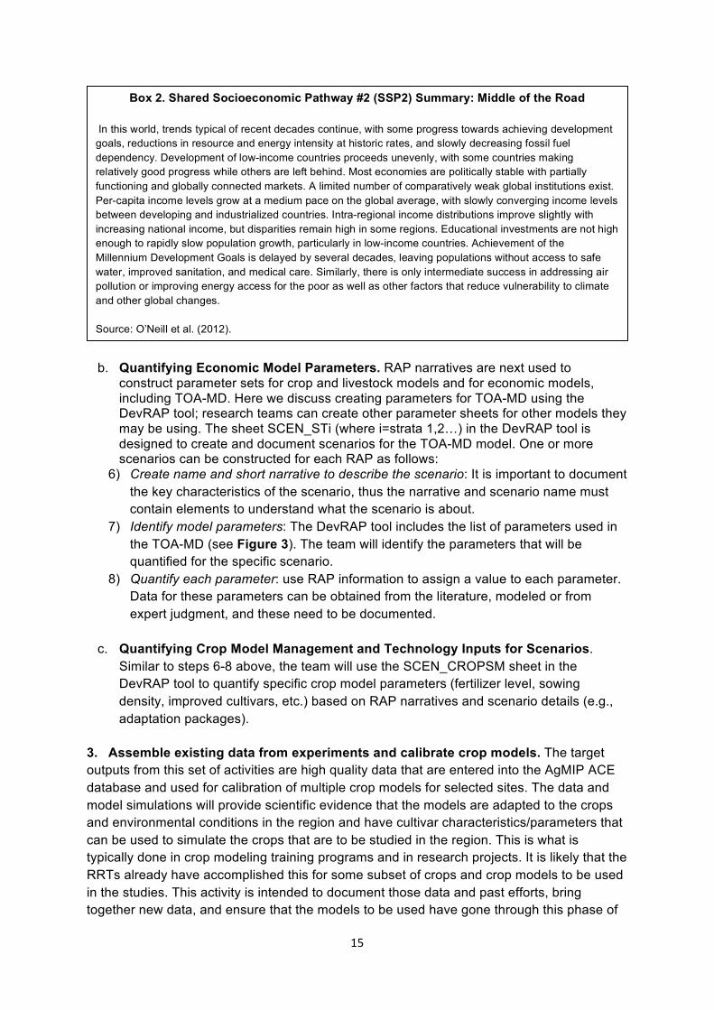
Box 2. Shared Socioeconomic Pathway #2 (SSP2) Summary: Middle of the Road In this world, trends typical of recent decades continue, with some progress towards achieving development goals, reductions in resource and energy intensity at historic rates, and slowly decreasing fossil fuel dependency. Development of low-income countries proceeds unevenly, with some countries making relatively good progress while others are left behind. Most economies are politically stable with partially functioning and globally connected markets. A limited number of comparatively weak global institutions exist. Per-capita income levels grow at a medium pace on the global average, with slowly converging income levels between developing and industrialized countries. Intra-regional income distributions improve slightly with increasing national income, but disparities remain high in some regions. Educational investments are not high enough to rapidly slow population growth, particularly in low-income countries. Achievement of the Millennium Development Goals is delayed by several decades, leaving populations without access to safe water, improved sanitation, and medical care. Similarly, there is only intermediate success in addressing air pollution or improving energy access for the poor as well as other factors that reduce vulnerability to climate and other global changes. Source: O’Neill et al. (2012).

16    

work. It is anticipated that there will be relatively few site-years with data for any of the selected crops, but those data will be made available in the ACE database and used to improve the adaptation of crop models for the regions. Suggested components of this activity are as follows.

a. Assemble data from past experiments for calibration of selected crop models to the region for selected crops. This includes crop, soil, and climate data for site-specific experiments and field trials in the region. This will require input from crop modelers, climate, and IT project team members. b. Input data into sentinel site ACE database for use in multiple crop models. c. Using the AgMIP IT tools, create input files for each crop model. d. Using methods provided by each crop modeling group (e.g., DSSAT, APSIM, perhaps others), simulate the sentinel site experiments and estimate cultivar-specific parameters to best simulate the experimental results. These results will help set cultivar characteristics and perhaps soil conditions for regional simulations to be carried out by the teams (see below). e. Secondary focus will be estimation of productivity parameters, relative to initial conditions, crop residue, soil organic matter pools, and soil fertility for the site-specific sentinel data (NOTE: these steps will be repeated to be more appropriate for the regional simulations where site-specific information is not available). g. Document model simulations (inputs, management, outputs, soil, climate, cultivar

coefficients) by placing them in the ACE database, along with explanatory text and appropriate tables and figures showing the quality of the calibration of cultivar coefficients.

4. Assemble and quality-control current climate series. The key products from this activity will be a high-quality version of in-situ climate observations in .AgMIP format for each location where crop models will be used, a file documenting the changes made to the original raw observations, and summary maps and statistics characterizing the region being analyzed. The following methods are recommended:

a. Assemble and assess quality of station observations. • Identify weather stations that best represent selected crop modeling regions. • Obtain as much of the 1980-2010 period as possible (Daily precipitation,

maximum and minimum temperatures, solar radiation or sunshine duration, wind speed, dew point temperature, vapor pressure, and relative humidity).

• Convert to .AgMIP units and format with missing data given a value of -99. The AgMIP format is described in the AgMIP protocols available at http://www.agmip.org.

• Name the climate series site with a 4-character code (first 2 characters from internet country code and second 2 characters representing location) following the guidelines in the AgMIP protocols (e.g. “NLHA” for Haarweg, Netherlands).

17    

• Begin a text file to document changes made in the quality assessment and quality control of the raw files (e.g., “NLHA.info”).

• Identify outlying (+/- 3 standard deviations probably deserves a closer look) and questionable data that may be corrupted. The best approach remains plotting out the dataset elements as time series to see if anything looks amiss.

• Check to see if data are plausible physically (e.g., questionable value supported by other variables), temporally (e.g., questionable value supported by preceding or following values), or spatially (e.g., questionable value supported by neighboring stations). If values are not plausible, replace with a value of -99.

• If vapor pressure, dewpoint temperature, or relative humidity correspond to a time of day other than mid-afternoon (~maximum temperature), approximate values at the time of day of maximum temperature will be computed, by conserving more robust dewpoint temperature or vapor pressures (which can be calculated using temperature at time of measurement) and then recalculating relative humidity using maximum temperature.

b. Obtain background daily climate time series (1980-2010) from the AgMERRA dataset provided by the AgMIP Climate Team (Ruane et al., in preparation). The output of this activity will be a complete set of estimated daily climate data for use in filling in missing data for observation stations. (If the observational dataset is fully complete this step may not be necessary). Until the AgMERRA dataset is fully accessible online, latitude and longitude coordinates for each location to be simulated may be sent to Alex Ruane ([email protected]) to obtain this dataset in the .AgMIP format.

c. Fill in missing/flagged observation data using station observations and the AgMERRA estimated climate series. Note that two overlapping observational sets may be combined in a similar manner. This set of activities will provide a continuous, complete, physically-consistent daily climate series from 1980-2010 in .AgMIP format for use with the crop models. Suggested steps are: • Go through station observations and fill in all data gaps as follows. • Use simple interpolations for short data gaps (e.g., if 3 or less days are missing

fill in by interpolating from good values on either side). Use caution if strong outlier exists on either side as this may not be an effective approach (e.g., if strong rain event precedes data gap we can’t assume that it will have persisted throughout gap.

• For moderate gaps (e.g., 4-10 days) use background dataset to fill in gaps and bias-correct using surrounding good data (adjust mean to ensure approximate continuity with beginning and end points).

• For longer gaps use background datasets to fill in gaps and bias-correct using climatological biases calculated by comparing background dataset to good station observations (e.g., if July Tmax in background dataset is typically 0.6˚C too warm, subtract 0.6˚C from background dataset when filling in a July data gap; if observed rainfall is typically only 90% of background rainfall in October, multiply background dataset by 0.9 to fill in October gaps).

• Ensure that filled in data are physically plausible by checking the following:

18    

o Relative humidity does not exceed 100% o Relative humidity, vapor pressure, and dewpoint temperature are

physically consistent at time of day of maximum temperature. o Solar radiation is not greater than astronomical maximum (can use

historical monthly maximum as proxy) or below zero. o Maximum temperature is at least 0.1˚C above minimum temperature.

d. Approximate climate time series in regions for integrated assessments. This set of activities produces a set of climate time series that corresponds to each crop or livestock modeling location in an integrated assessment region and forms the 1980-2009 (current) climate series identified in Table 1. (Note that this procedure is automated in the AgMIP Climate Scenarios Guidebook using the “farmclimate” routine). Working with the crop and economic modeling teams, recommended methods include: • Obtain desired latitudes and longitudes for each integrated assessment site to

be modeled. Name each station with a 4-character code. • Identify as many weather stations in (or nearby) region as possible. Quality

control these datasets following methods above, then assign each of the integrated assessment locations to the most representative weather station (“corresponding station” may not always be selected by geographic distance alone, but may also factor in climatic zones and/or elevation).

• If there are additional precipitation gauges (where other variables are not observed), determine which integrated assessment locations correspond to these and start with this precipitation record.

• Estimate differences in monthly climatologies between integrated assessment locations and corresponding station location using AgMERRA dataset (if distances are greater than ~50km) or WorldClim dataset (if distances are less than ~50km). Adjust corresponding station in a manner similar to the gap-filling bias adjustment to estimate integrated assessment climate series.

e. Create an AgMIP Agro-climatic Atlas for Current Period Climate. This atlas will contain maps of important agro-climatic variables for the region. Recommended methods include: • Generate regional maps of mean temperature and precipitation during historical

baseline period from observational data and from GCMs to be used in scenario generation.

• Identify agriculturally important climate metrics. If region is affected by a prominent monsoon, determine which monsoon metrics are important to regional agriculture. Compare climate information with planting rules of thumb from farmers and/or crop model configurations if possible.

• Calculate these metrics and produce maps using observational products during the historical baseline period (in consultation with local experts and stakeholders).

• Analyze uncertainty among observational products (if available) as reference for future uncertainties.

19    

5. Assemble data and simulate crop models for analysis of yield variations. The major outputs of this series of activities include simulations of yields by multiple crop models for multiple sites within the study region. Ideally, regional projects will use on-farm survey data for which the crop models can be used to simulate each field that was surveyed. This will provide simulated results for the “matched” case where the models use climate, soil, and management for each field to simulate productivity that is then “matched” with observed yields for each field. In order to simulate each field, the teams will need to make assumptions about crop model inputs that are needed but not collected in the farm surveys. These assumed inputs should be developed with advice from agronomists in the region, and they will be documented along with the observed field survey data for each simulated result. Crop modeling team members should analyze these matched results to be sure that they were correctly produced with well-defined and documented inputs and to be sure that results are reasonable. Invariably, there will be biases between simulated and observed survey data, and the modelers should analyze means, variances, biases, and other characteristics of the results prior to confirming that they are ready for use in the economic analyses. A summary spreadsheet file (ACMO) will be prepared by the crop modeling team for use by the economists. This file will document all of the inputs and assumptions used in the model simulations as well as provide a summary of crop productivity outputs (e.g., yield). If farm survey data are not available, crop modelers should work with multiple years of historical yield statistics at a district level. In this “unmatched” case, simulated yields cannot be matched one-to-one with observed farm field survey data, and variations in climate, soils, and management inputs across the region will need to be defined and sampled from. This should be done in a representative manner based on available information and expert opinion, particularly about variations in management practices across farms within the district. In this case, comparisons of crop model results will be aggregated to a district level for comparing with district yields and analyzed. Also, a report should be written on methods and results of crop model calibration, aggregation methods, uncertainty associated with seasons, and biases relative to regional aggregated yields.

Recommended steps include:

a. Matched Case. Assemble matched yield case data from household farm survey from sub-regions, where crop yield and minimal management (sowing date, fertilization, etc.) are available along with household economics information for 50 to 200 farmers. If it is not possible to simulate each field to produce matched outputs, crop modelers will need to use procedures for unmatched results (see 5.c. below and Appendix 2).

• Follow the more detailed instructions in Appendix 2. You will need to enter yield survey data into Matched_Survey_Data.Import.xlsx spreadsheets and download AgMIP Tools from the http://tools.agmip.org/ website.

• Work with regional Agronomists and Soil Scientists to identify the most likely soils for each field in the survey, and create the Field_Overlay spreadsheets that fill in the information missing from the survey, such as initial soil water, initial nitrate and ammonium, soil organic carbon degradation, fertilization dates, prior crop residue, etc. Work with Climate colleagues to identify climate information/sites.

• Use the QuadUI tool software to convert these spreadsheets into model-ready input files for multiple crop models.

• Use crop cultivar coefficients that have been calibrated with independent sentinel site data in the region (from procedure # 3 above).

20    

• Simulate the matched case survey data, compute means and standard deviation of observed and simulated. Analyze simulated results by computing various statistics and compare with observed statistics, including comparison of yield distributions, means, variances, and characteristics of bias between observed and simulated yields and outliers. Depending on these analyses, crop modelers may decide to accept these inputs as baseline soils and management conditions for further analyses or they may need to make changes in the assumptions in conjunction with agronomists familiar with production in the region. Standard output files (ACMO) are used to provide crop model inputs and outputs for use by economists. See Appendix 2 for advice on analyzing cumulate probability distributions.

b. Simulate Yields for Household Survey Farms. Using each crop model, simulate crop outputs accounting for the distribution of climate, soils, cultivars, and management present in the region for use in the economic model analyses. Crop modelers will create ACMO files that include metadata for all “production” inputs used to simulate the fields and a summary of yield results for each field. Methods include: • A distribution of production environments and management will be determined

based on the field surveys (or on unmatched distributions of inputs, see 5.d). Each RRT will determine the best source of information for creating these multiple within-region environments and management systems to best represent the inherent variability that exists in the region. This is an important decision that needs to be made by crop, climate, and economic team members working together.

• Model simulations will be conducted over the distribution of weather stations, soils information, sowing dates, cultivars, residue return, soil organic matter pools, and fertilization that represents the region being predicted. Prepare data file that contains all of the information used to produce the simulations and on key outputs such as crop yield for use by the economic team (ACMO file).

• Crop modeling teams should analyze results and write appropriate reports and publications documenting and interpreting the biophysical implications of climate change and RAP-based adaptation options that are included in the analyses.

• Document model simulations (inputs, management, outputs, soil, climate, cultivar coefficients) by placing them in the ACE database, along with explanatory text and appropriate tables and figures showing the yield probability distributions (using probability of exceedance), analyses of residuals.

• Create maps and summary statistics e.g., spatial distribution of climate, soils, management, and yields illustrated in GIS mapping methods

c. Unmatched Survey and Simulation Fields (or Regional Historic Yields). If there are no yield data available from household surveys, it will not be possible to simulate a yield for each farm as in the matched data case. In this case, crop modelers will need to work with economist team members and agronomists in the region to assemble information on variations in management and soils in the region for this “unmatched” case. Assemble soil, typical management, and typical cultivar information for the region along with long-term crop statistics data (for district level or higher) for use in evaluating crop model abilities to simulate regional yields and production. Methods for doing this are: • Yield statistics of crops will be collected for the region over historical time

periods of 30 years.

21    

• Cultivar life cycle information will be assumed correct from the site-specific sentinel site data.

• Survey information will be collected with input of agronomists and soil scientists, to represent the distribution of weather stations, soils information, sowing dates, cultivars, residue return, soil organic matter pools, and fertilization that represents the region being predicted.

• Use QuadUI software tool (as above) to create model-ready input files for multiple crop models to simulate historic observed years as well as future climate and adaptation-RAPs scenarios.

• Similar to the matched case (5.b), crop modelers will create ACMO files for use by economists and prepare reports and publications that describe and interpret biophysical results of the study.

• For purposes of evaluating crop model abilities for simulating regional or district-level yields, crop model teams should aggregate yearly simulated results (over climate sites, soils, sowing dates, cultivars, management) to the district level yield for comparison with historical district yields (e.g., comparing distributions of simulated and observed yields, mean annual bias, etc.).

• Document model simulations (inputs, management, outputs, soil, climate, cultivar coefficients) by placing them in the ACE database, along with explanatory text and appropriate tables and figures showing the yield distributions, analyses of interannual and spatial variations.

• Create maps and summary statistics e.g., spatial distribution of climate, soils, management, and yields illustrated in GIS mapping methods

6. Assemble economic data for regional economic analysis and develop skills for

using the regional economic model. Outputs from this set of activities include at least two economist members per project team that are capable of performing economic analyses in their respective regions and data assembled on baseline socioeconomic and agricultural production data in their regions. An output will be crop modelers and economists with experience in interdisciplinary collaboration in co-developing data sets for use by both teams (e.g., historical yields and socioeconomic survey data), with the data input to the AgMIP database. Another output is the TOA-MD model set up to simulate economic outcomes for the region, using baseline socioeconomic data. Specific steps include:

a. Identify economic survey data and corresponding study components (see the TOA-MD model and supporting documents for further details).

b. Work with the climate and crop model teams to produce and analyze baseline crop simulations for sites that are jointly selected for the region, based on available data from regional statistics and/or on-farm surveys. This step requires direct cooperation among disciplinary team members and relies on the above steps on collecting climate series and calibration of crop models for regional yields.

c. Estimate economic model parameters using the available data (see the TOA-MD model and supporting documents for details).

d. Prepare a report (following AgMIP template) describing the existing systems and documenting the data used for regional economic analysis and parameter estimates.

7. Create downscaled climate scenarios, based on AgMIP protocols, for use in the assessments of climate change studies, and provide future scenarios for use with crop

22    

models in the AgMIP database. Note that these procedures are captured in scripts contained in the AgMIP Guidebook for Climate Scenarios. A key output from this set of activities will be future climate scenarios derived from the latest IPCC climate models and downscaled for use in the target regions. These scenarios will be in the .AgMIP climate data format and ready for multiple crop model simulations of impacts and agricultural adaptation for each region. In addition, a climate atlas will be produced of important climate variables and derived agriculturally-important indices. These atlases will include maps for use in scientific publications and for communication of results to stakeholders.

a. Create CMIP5 delta-based climate scenarios. These scenarios will be based on historical baseline daily climate data, with each day’s weather variables perturbed using the changes in climate model outputs for future time periods versus those same model outputs for the historical time period. These scenarios are made using the “agmipsimpledelta” routines in the AgMIP Guidebook for Climate Scenarios, and will be created for each crop modeling site for the 5 GCMs emphasized for the core climate impact questions and for all 20 CMIP5 GCMs for the best-calibrated site in the region. Specific methods include: • For each of these sites, calculate monthly changes in corresponding mean

maximum temperature, minimum temperature, and precipitation by comparing future 30-year climate periods (AgMIP defines three main time periods: “near-term”=2010-2039; “mid-century”=2040-2069; and “end-of-century”=2070-2099) to the baseline climate period (1980-2009; use RCP 4.5 for 2006-2009 period) from the same GCM. The Mid-Century RCP8.5 is the priority period for assessment.

• Impose these monthly changes on baseline climate series for all selected sites by adding temperature changes to the baseline record and multiplying by a precipitation change factor.

• Assume that solar radiation, winds, and relative humidity are fixed at the same values that were in the historical time series. Ensure that vapor pressure, dewpoint temperatures, and relative humidity are physically consistent at time of maximum daily temperatures (warmer temperatures have higher vapor pressures and dewpoint temperature at same relative humidity).

• This will result in a 30-year .AgMIP-formatted climate series for a given future period and GCM. Scenarios should be constructed for all 20 CMIP5 climate models at the best-calibrated site in the region, while scenarios for the other crop modeling sites (farm survey sites) are only required for the 5 GCMs (CCSM4, GFDL-ESM2M, HadGEM2-ES, MIROC5, and MPI-ESM-MR) in focus for the core climate impact questions (identified as the 2040-2069 (future) climate series in Table 1.

b. Create AgMIP Agroclimatic Atlas that shows future climate change scenarios with uncertainties using maps with probabilities. These maps and summary results will be published and also communicated to stakeholders. Specific methods are: • Produce region-wide maps of CMIP5 climate change projections, including

median changes in mean quantities, variability, and extremes (along with corresponding uncertainties) for temperatures and precipitation.

23    

• Also produce maps for agriculturally important climate metrics under future climate conditions for comparing with those produced for historical baseline climates.

• Place growing season temperature and precipitation changes from the 5 core question GCMs in the context of the wider CMIP5 ensemble (e.g., with scatter plots or monthly box-and-whisker diagrams).

c. Create CMIP5 mean and variability change scenarios. This activity will produce .AgMIP-formatted climate scenarios including both monthly and sub-monthly changes in temperature and precipitation. These procedures are captured in the “agmipsimple_mandv” scripts in the AgMIP Guidebook for Climate Scenarios. In many regions there are not sufficient resources or available regional climate model (RCM) results to capture important uncertainty in climate projections, however where these are available they are particularly helpful for their representation of sub-seasonal metrics that are often affected by smaller-scale atmospheric dynamics. Suggested methods include: • Calculate monthly changes in mean maximum temperature, minimum

temperature, and precipitation by comparing future 30-year climate periods to the current climate period from the same GCM/RCM combination (where available).

• Calculate monthly changes in the standard deviation of maximum temperature, the standard deviation of minimum temperature, and the number of rainy days (precipitation>0.1 mm) by comparing future 30-year climate periods to the current climate period from the same GCM/RCM combination (where available). The shape parameter of the gamma distribution for wet events may also be of interest from RCM results, but is generally not of sufficient quality in GCM simulations.

• Impose these monthly changes on baseline climate series for all sites used in the analyses using a stretched distribution approach that adjusts each event by comparing existing and desired values by distributional percentiles.

• Assume that solar radiation, winds, and relative humidity daily variables from the historical daily climate records are unchanged. Ensure that vapor pressure, dewpoint temperatures, and relative humidity are physically consistent at time of maximum daily temperatures.

• Produce mean and variability change scenarios for all 20 CMIP5 GCMs at the best-calibrated site in each region.

d. Create Near-term climate scenarios (optional). This activity will produce .AgMIP-formatted climate scenarios for the Near-term (2010-2039) period, where the influence of climate variability is likely to be at least as large as that of climate change. Methodologies and tools for this procedure are based upon Greene et al. (2012a,b). While these methods are still under development, we outline them here: • Obtain long-term temperature and precipitation records from at least 1960-2010

(e.g., from CRU, GPCC, and University of Delaware sets) and CMIP5 GCM outputs over the 1960-2039 period.

• Calculate GCM-ensemble growing season precipitation and maximum and minimum temperatures to represent anthropogenic influence on region.

24    

• Smooth observations for each location using 30-year smoothing window representing long-term trend and variability.

• Subtract average of smoothed observations and GCM trend from annual series of growing season observations at each location to obtain time series of natural variability (may add weight to 30-year smoothed observations if circulation anomalies or thresholds are known to have responded to anthropogenic forcing).

• Transform the natural variability time series into principal components. • Use top 5-10 Empirical Orthogonal Functions (EOFs) to fit vector auto-

regressive model, and use this model to create 10,000 years of natural variability for each site.

• Select from the distribution of decadal rainfall totals in this record and from the distribution of CMIP5 GCM trends in order to create a 30-year Near-term scenario designed to examine particular vulnerabilities in the agricultural sector.

• Construct a daily time series in .AgMIP format that matches the seasonal properties in the Near-term scenario using analog months from the AgMERRA daily climate series used in Activity 4 above.

8. Conduct multiple crop/livestock model simulations at all crop/livestock modeling locations for the three cases identified in Table 1: #1) current climate with current production systems technology, #2) future climate scenario(s) with current production technology (no adaptation), and #3) future climate scenario(s) with adaptation. In addition, examine full GCM ensemble for a single, best-calibrated and representative site in each integrated assessment region (these latter results will not be passed on to economic analysis). Outputs should be reviewed by crop modeling team members working closely with economic and climate team members to ensure the results are plausible, e.g., that there are no unexplained outliers. When the team has finalized the crop model simulations and summarized outputs in the ACMO file, outputs from the three cases will be used by the economists in the TOA-MD economic model, and outputs from the single location GCM ensemble simulations will be used by the climate team members to place the subset of GCMs in context.

a. Simulate yield distribution across all farms for the core climate impact question cases. This includes simulation of responses across GCMs, farms, and across years within the 30-year periods. Multiple crop/livestock models will be used to simulate variations in climate, soils, and management, thus obtaining within-region variability of production. These results will be put into the AgMIP ACMO database for use in the economic analyses.

• Case #1: Current climate with current production systems technology: Simulate current period climate series (identified as planting years 1980-2009 in Table 1) for all farms using the 30-year climate series created in Activity 4 above, current production systems and a CO2 concentration of 360ppm for all years (see Table 2).

• Case #2: Future climate scenario(s) with current production technology (no adaptation): Simulate future period climate delta-based climate scenarios (beginning with RCP8.5 Mid-Century, identified as planting years 2040-2069 in

25    

Table 1) for all farms using the 30-year climate series created in Activity 7 above, current production systems and a CO2 concentration corresponding to the central year for all simulations (see Table 2). Run scenarios for at least the following GCMs: CCSM4, GFDL-ESM2M, HadGEM2-ES, MIROC5, and MPI-ESM-MR. This GCM subset was selected to save resources due to their long history of development and evaluation, a preference for higher resolution, and established performance in monsoon regions.

• Organize simulated yields and enter those results into the AgMIP Crop Model Output database (ACMO), which contains variables needed by the economic team members for the regional economic model analyses.

• Create and document an adaptation package via collaboration between the crop and economic modeling team. Adaptations connected to vulnerabilities identified in a comparison between Case #1 and Case #2 results are preferred (e.g., heat or drought-tolerant cultivars; dramatically shifted sowing dates; added irrigation; subsidies for improved seed). Improved management that is not directly linked with climate impacts on the region are better handled as part of the representative agricultural pathway that defines future production systems prior to climate change adaptations.

• Case #3: Future climate scenario(s) with current production technology with adaptation: Simulate future period climate delta-based climate scenarios (beginning with RCP8.5 Mid-Century, identified as planting years 2040-2069 in Table 1) for all farms using the 30-year climate series created in Activity 7 above, current production systems plus the adaptation package identified above in Activity 8a and a CO2 concentration corresponding to the central year for all simulations (see Table 2). Run scenarios for at least the following GCMs: CCSM4, GFDL-ESM2M, HadGEM2-ES, MIROC5, and MPI-ESM-MR.

• Summarize yield impacts in tables, graphs, and maps for publication and communication to stakeholders. Included in these tables, graphs, and maps should be: o within-region variability in impacts, and o uncertainties associated with crop models and climate models o Interpret reasons for variations among crop and climate models and

households

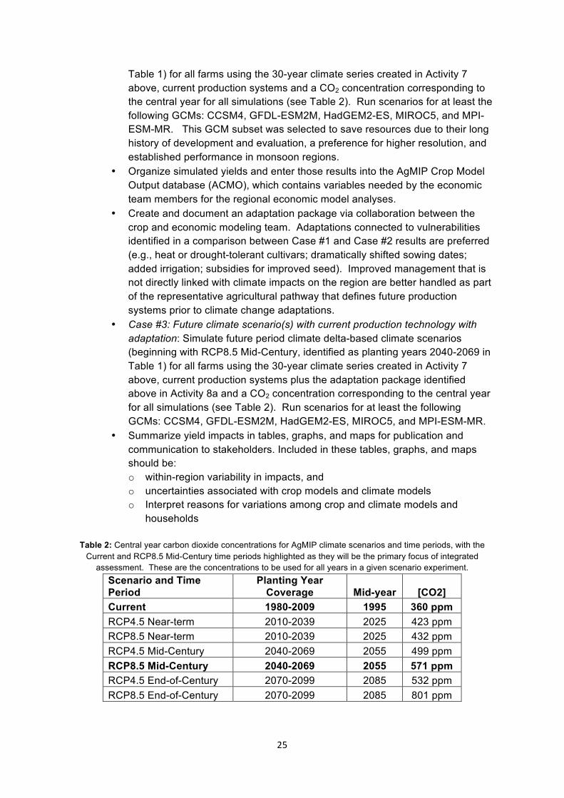
Table 2: Central year carbon dioxide concentrations for AgMIP climate scenarios and time periods, with the Current and RCP8.5 Mid-Century time periods highlighted as they will be the primary focus of integrated

assessment. These are the concentrations to be used for all years in a given scenario experiment. Scenario and Time Period

Planting Year Coverage Mid-year [CO2]

Current 1980-2009 1995 360 ppm RCP4.5 Near-term 2010-2039 2025 423 ppm RCP8.5 Near-term 2010-2039 2025 432 ppm RCP4.5 Mid-Century 2040-2069 2055 499 ppm RCP8.5 Mid-Century 2040-2069 2055 571 ppm RCP4.5 End-of-Century 2070-2099 2085 532 ppm RCP8.5 End-of-Century 2070-2099 2085 801 ppm

26    

b. Simulate impacts of full ensemble of climate changes from all 20 CMIP5 GCMs on single, best-calibrated site in integrated assessment region. Compare climate impacts from all 20 GCMs using both delta-based (mean changes only) and mean-and-variability scenarios, place the 5 GCM-subset in this broader context, and estimate influence of variability changes. If these simulations suggest that variability changes are substantially important, these scenarios may be used instead of the delta-based scenarios for core question economic analysis if resources allow. c. Simulate impacts from Near-term climate scenarios (optional). Conduct simulations for planting years 2010-2039 at the best-calibrated and most representative site using the Near-term climate scenarios created in Activity 7 above.

9. Analyze regional economic impacts of climate change without and with adaptation using the regional economic model. Outputs will be impacts of climate change on agricultural production, farm income and poverty, and projected rates of adoption of adapted systems. To the extent possible, teams should use these results of these sub-national analyses to draw implications for the national impacts, e.g., by extrapolating impacts to regions with similar production systems. The AgMIP regional integrated assessment framework is summarized in Figure 1.

a. Economist team members will use the methods outlined in Appendix 2 to use crop model simulated yields to estimate regional economic model parameters. b. The economist team members will use the TOA-MD (or similar) regional

economic model to analyze the impacts of climate change for each of the economic model simulations identified in Table 1, using crop/livestock model cases #1-#3, which together address the three core climate impact questions:

• 1. What is the sensitivity of current agricultural production systems to climate change?

• 2. What is the impact of climate change on future agricultural production systems?

• 3. What are the benefits of climate change adaptations? For this analysis the economists will first work with the crop modeling team to identify an adaptation package that includes crop/livestock and economic model parameters representing adaptations designed to address climate vulnerabilities and opportunities identified in questions 1 and 2 above.

c. These results will be summarized with graphs and reports for scientific publications and for dissemination to stakeholders.

10. Archive data and analyses of results for integrated assessments

An important output of integrated assessments will be databases for the regions that will include climate, soil, management, experiments, surveys, regional economic model parameters, and historical yields that will have been used for the analyses in this set of

27    

projects that will be highly valuable for additional future analyses as models improve, research and policy questions change, and adaptation approaches evolve. These archived data will be available for broad use, although it is recognized that some data used in the projects (such as daily climate data in some cases, or confidential survey data) may not be archived due to intellectual property rights and data policies. Additionally, archived results from climate, crop models, and economic models will serve as the source for various publications and presentations, including web-based information that will be made available for stakeholders. A well-documented archive of AgMIP experiments, outputs, and analysis tools will facilitate future improvements in capabilities to perform integrated assessments of climate change impacts and adaptation at site and aggregated scales.

Figure 4 presents a data flow diagram for AgMIP Regional Integrated Assessments. Data created using the tools and procedures outlined in this document should be archived in AgMIP databases. Research teams shall contribute data to ACE (AgMIP Crop Experiment), DOME (Data Overlay for Multi-model Export), ACMO (AgMIP Crop Model Output) and Regional Economic databases. The AgMIP IT Team will provide tools and training through the regional workshops and web tutorials so that RRTs can interact with the ACE, DOME , ACMO and regional economic databases directly through the AgMIP Data Interchange (data.agmip.org) which connects to AgMIP data nodes. This will allow for storage of standardized databases of crop experiments and yield trials for the region and outputs of crop model simulations.

Data to be archived includes: a. Climate data

• Observed weather data for crop model calibration • 1980-2010 quality-controlled daily climate data for use in the AgMIP regional

assessment • future ensembles of daily climate scenarios

b. Crop Modeling • Harmonized (ACE and DOME) data associated with detailed calibration data

from field experiments or other sources. • Calibrated cultivar parameters • Soil parameters as modified by modelers used in simulations • Harmonized data associated with farm survey sites for regional assessments

using baseline and future conditions (ACE and DOME data) • Crop model outputs for survey, baseline and various future climate conditions

(ACMO data) • Text summary of climate impacts on yield, considering crop management in

survey fields c. Economic data

• Inputs to regional economic models (including survey metadata) • DevRAP matrix spreadsheet including output data from global economic

models used in the RAPS and productivity trends – csv format. • Regional economic model outputs - Impacts of climate change on agricultural

production, farm income and poverty, and percentage of winners and losers and predicted adoption rates of adapted technologies in spreadsheet format.

A desktop utility is under development that will combine all of the steps required for a regional assessment researcher to input and manipulate farm survey data and convert to ACE format, create field overlay and seasonal strategy DOMEs, generate model-ready data for the user’s models of choice, harmonize simulated model outputs into ACMO format, and

28    

store all data to the server in linked ACE, DOME and ACMO databases. Users will also be able to use the utility to query the databases for existing datasets. The utility is a combination of the spreadsheet template data entry, ADA, QuadUI and ACMOUI with additional linkages to the online databases.

 other  nodes  ...ICRISAT  nodePaso  Fundo  node

Published  data

Gainesville  node

ACE database

ACMO database

DOME database

Data Journal

Cultivar library

Economic model input

archive

Economic model output

archive

Economic  modeling  data

Climate scientists

Crop modelers

Economic modelers

Historical weather data

GCMs and RCMs

Farm survey data

Regional  economic  model  outputs

ACMO

Daily  weather  data

Historical  climate  data

Future  climate  scenarios

Regional  economic  model  inputs

Harmonized  crop  model  data

ACE  data

DOME  data

ACMO

Other economic data

Detailed field experiment data* soils* management* observations* weather

Calibrated  cultivars

Data  ProductsResearch  ActivitiesRaw  Data

Figure 4. Data flow diagram for AgMIP Regional Integrated Assessments showing AgMIP data products and archive databases

11. Disseminate integrated assessment results. The key outputs from this set of activities include scientific publications, project reports, results summarized on regional web pages linked to the AgMIP web site, and workshops with stakeholders. Initial and ongoing interaction with stakeholder and policymaking communities are likely to be as valuable as

29    

the dissemination of results to these communities, as early and consistent interactions increase buy-in and help develop a more useful and efficient research project

a. Develop RRT-specific web pages for the AgMIP web site. The AgMIP IT Team will provide information on how to create region-specific web pages and will give regional IT team members access to create and maintain that web information. Each region will have its project goals and methods on the site as well as pictures of project activities, output tables, maps, and graphs, as well as news items, for example. b. Conduct project workshop with stakeholders. • Invite stakeholders to SSA and SA workshops • Organize stakeholder sessions at a region-specific workshops to keep them

informed and learn from them what information they need for their planning and policy-making responsibilities

c. Prepare scientific publications. AgMIP research is designed to provide results that are well-suited for peer-reviewed journal publications and informing national and regional publications related to climate vulnerabilities, economic development, and adaptation/mitigation planning relative to food production and food security.

30    

Appendix 1 “Fast Track” Proof of Concept Integrated Assessment Exercise

Because of the coordination needed among different science disciplines in the AgMIP regional integrated assessment efforts, each AgMIP regional team should perform a “proof of concept” assessment on a fast track to help everyone on the regional teams to understand their roles and the interactions that must take place among different disciplines. Accomplishing this will ensure that the mechanics of the process are understood and functioning, at which point it will be easier for all teams to proceed with their further, more detailed assessments. To do the fast track integrated assessment exercise, the team should select only one subregion, one crop, one crop model, and one climate site location; then simulate crop yields using the historical climate data for that one location and also simulate crop yields for one climate change scenario for the time period of 2040 – 2069 using the methods described above. Additional details are:

a. The entire regional team should identify one small sub-region where the fast track

assessment will be performed. Ideally, the sub-region should be an area in which household survey data are available with at least one climate data site within the area and where there are experimental data available in or nearby the area that can be used for calibrating one (or more) crop models.

b. The crop modelers will parameterize the crop models using available data from experiments, if this has not already been done. This will provide parameters for cultivar types that are currently being used in the region.

c. The economists should describe the site characteristics, including a map showing the farms and including management and farm characteristics.

d. Economists will provide the socioeconomic data, including farm site locations, to the crop modelers so that they can assemble the needed crop model inputs to run the crop models. Ideally, the socioeconomic survey data would have data on crop management practices (planting date, N application amounts) and on crop yield. For example, there may have been 80 farms surveyed with such data, and those farms would be used to assemble crop model input data for each farm, similar to the Machakos example that was used to demonstrate the approach.

e. The climate team members in the region will prepare and clean the historical climate series for one station in the region. This site will act as the baseline climate series for all crop modeling and analysis in the fast-track (including surrounding farms), and will also serve as the basis of one climate change scenario generated using the basic delta method that represents projected GCM changes. These climate series may be used in the crop model runs to compute the impacts of climate change (assuming no adaptation for this fast track).

f. The regional crop modelers will prepare input files for running one selected crop model (DSSAT or APSIM preferably) for each farm location in the selected study site/area. This includes assembling representative soils for the sites. The crop modelers will simulate each of the fields in the farm surveys, analyze simulated results relative to observed yields to evaluate reliability of results, and prepare a model output file ACMO) for documenting model inputs and outputs for use by economists in the TOA-MD analyses.

g. If socioeconomic data do not include farm site yields, then the crop modeling team members will use the procedures for calibrating and evaluating crop models for use in simulating mean yields for district or other administrative unit (see section 5c in this handbook). This alternate procedure will provide crop models ready for use in the region with estimates of average bias.

31    

h. The crop modelers will then simulate yields for each of the farm sites in the selected area using historical climate data (1980-2009 planting years) and repeat the simulations using the one selected climate scenario’s climate file. The modelers will assess yield results, evaluating how reasonable they are and produce an AgMIP Crop Model Output file (ACMO) that will be used by the economists in the TOA-MD analysis.

i. The economic team members will take crop model results and use the TOA-MD model to analyze the impacts of the climate change scenario on the distribution of economic impacts for the area.

j. The entire team will meet to evaluate the entire process and to discuss and interpret the results.

k. After the proof of concept study, the team will be ready to design its assessments of impacts and adaptation options based on the RAPs, more advanced climate scenarios, and a better representation of climate and crop model uncertainties.

Table 1. Regional Research Team Activities. This is a checklist of activities that should be coordinated across team members in each RRT such that each RRT can produce comparable integrated assessments, as noted in

the timeline of activities.

Task 1. Scoping of cropping systems and developing/refining research work plan

2. Develop Representative Adaptation Pathways (RAPs) for climate change

3. Assemble Existing Data from Experiments and Calibrate Crop Models

4. Assemble and Quality Control Historical Baseline Climate Series.

5. Assemble Data and Simulate Crop Models for Analysis of Yield Variations.

6. Assemble Socioeconomic Data; Develop Skills for Regional Economic Analyses 7. Create Downscaled Climate Scenarios 8. Simulate Productivity Impacts of Climate Change; Analyze Adaptation Options

9. Analyze Economic Impacts of Climate Change and Adaptation Approaches

10. Archive Data and Analyses Results for Integrated Assessments

11. Disseminate Integrated Assessment Results

32    

Appendix 2 Calculating Statistics for Climate Impact Assessments Using Crop/Livestock Model Simulations with the TOA-MD Model

John Antle and Roberto Valdivia

September 2013

Introduction

This document describes how crop model simulations and Representative Agricultural Pathways can be used with TOA-MD to implement assessments of climate change impact and adaptation using matched and unmatched data. We use the case of a population of heterogeneous farms with a single stratum and one production activity to illustrate the methods.

The first section presents concepts and definitions. The second section describes the approach to compare the impacts of current climate vs future climate for the modeled production system. This approach can be used for climate sensitivity analysis for current world conditions and not technological trend, or future world with technological trend and RAPs. The third section (forthcoming) shows how to use results of first part for analysis of adaptation to climate change.

1. Concepts, Definitions and Assumptions

Incorporating Spatial and Temporal Variability

We know yields and related outcomes (economic returns) vary over space and time, and this variation is important to understand vulnerability of farms to climate change. Therefore we need to project these distributions into the future for climate impact assessment.

We can describe a variable such as a yield for a production system h used at location j at time t as yhjt. Let µhj be the mean for farm j obtained by averaging its values of yhjt over time and let µht be the mean for year t obtained by averaging yhjt over all farms in that year. We will say that µhj is the time-averaged mean for farm j and µht is the spatially-averaged mean for year t. Similarly, we can decompose the variance of yhjt into spatial and temporal components. For impact assessment, we are interested in populations rather than individuals, so we will focus on the distributions for the population for each year in the analysis, and we will also be interested in outcomes over multiple-year periods. To obtain meaningful approximations to the distribution of outcome variables for the TOA-MD model, we often need to stratify populations of farms that come from different sub-populations or different time periods. For example, in a given year, we may need to stratify farms geographically or by socio-economic characteristics such as size or ownership of livestock. With the time dimension in the analysis, stratifying by year is likely to be important because weather distributions shift substantially year-to-year.

Our goal is to use the available data to estimate these variances using the data we have:

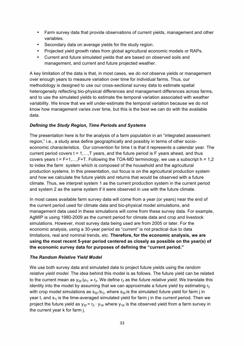
33    

• Farm survey data that provide observations of current yields, management and other variables.

• Secondary data on average yields for the study region. • Projected yield growth rates from global agricultural economic models or RAPs. • Current and future simulated yields that are based on observed soils and

management, and current and future projected weather.

A key limitation of the data is that, in most cases, we do not observe yields or management over enough years to measure variation over time for individual farms. Thus, our methodology is designed to use our cross-sectional survey data to estimate spatial heterogeneity reflecting bio-physical differences and management differences across farms, and to use the simulated yields to estimate the temporal variation associated with weather variability. We know that we will under-estimate the temporal variation because we do not know how management varies over time, but this is the best we can do with the available data.

Defining the Study Region, Time Periods and Systems

The presentation here is for the analysis of a farm population in an “integrated assessment region,” i.e., a study area define geographically and possibly in terms of other socio-economic characteristics. Our convention for time t is that it represents a calendar year. The current period covers t = 1,…,T years, and the future period is F years ahead, and thus covers years t = F+1,…,F+T. Following the TOA-MD terminology, we use a subscript h = 1,2 to index the farm system which is composed of the household and the agricultural production systems. In this presentation, our focus is on the agricultural production system and how we calculate the future yields and returns that would be observed with a future climate. Thus, we interpret system 1 as the current production system in the current period and system 2 as the same system if it were observed in use with the future climate.

In most cases available farm survey data will come from a year (or years) near the end of the current period used for climate data and bio-physical model simulations, and management data used in these simulations will come from these survey data. For example, AgMIP is using 1980-2009 as the current period for climate data and crop and livestock simulations. However, most survey data being used are from 2005 or later. For the economic analysis, using a 30-year period as “current” is not practical due to data limitations, real and nominal trends, etc. Therefore, for the economic analysis, we are using the most recent 5-year period centered as closely as possible on the year(s) of the economic survey data for purposes of defining the “current period.”

The Random Relative Yield Model

We use both survey data and simulated data to project future yields using the random relative yield model. The idea behind this model is as follows. The future yield can be related to the current mean as y2jt /µ1j ≡ rjt. We define rjt as the future relative yield. We translate this identity into the model by assuming that we can approximate a future yield by estimating rjt with crop model simulations as s2jt /s1j, where s2jt is the simulated future yield for farm j in year t, and s1j is the time-averaged simulated yield for farm j in the current period. Then we project the future yield as y2jt = rjt ⋅ y1jk where y1jk is the observed yield from a farm survey in the current year k for farm j.

34    

Matched and Un-Matched Data

Two situations may be encountered with analysis using this type of farm survey data:

Matched Data: a crop yield can be simulated for each survey farm, for each crop in the system for which a crop model is available. This is true when weather and soil data can be associated with each survey farm, and some crop management data are included in the survey.

Data matching is possible in most cases where farm survey data are available and some kind of information is included in the survey to identify the survey farms’ locations. Ideally, the spatial identifier is the farm’s spatial coordinates (or even better, the centroids of individual fields). Note that when spatial coordinates are not included in a survey, they can be approximated with other location identifiers. For example, a legal address or village name may be available, and this may be used to approximate the spatial coordinates of the farm.

It is important to note that the matching of weather and soil data to survey farms will typically require using the best approximation possible given available data, because farm-specific weather and soils data are almost never available. Nevertheless, as long as weather and soil data can be assigned to each survey farm through some reasonable procedure, the term “matched data” is used, because with the farm specific management data, it is possible to simulate yields for each farm.

Un-Matched Data: a distinct crop yield cannot be simulated for each survey farm; however, spatially varying weather and soil data are available to run crop model simulations with representative management for the region.

Note that in the un-matched case, it is possible to estimate a simulated yield distribution that corresponds to the population of farms represented by the survey; however, it is not possible to match simulated yields to the survey farms.

Variable Definitions

t = time (calendar year)

T = length of current time period and future time period (years, first year = 1)

F = beginning of future time period (year)

h = system index = 1,2

j = farm index, j = 1,…,J farms in data sample representing the integrated assessment region study area

k = year when survey data were collected

ph = representative output price (currency units/kg) in the current or future period

yhjt = crop yield (kg/ha)

µ1j = time-averaged mean of yields y1jt for farm j for the current period

µ2j = time-averaged mean of yields y2jt for farm j for the future period

Y1k = mean of observed yields y1jk in the survey data for current year k

35    

Y1 = mean of yields averaged over all years in the current period, obtained from secondary data in the study area

γ = exogenous growth rate of regional average yields between the current and future periods associated with technological change not accounted for in future crop or livestock model simulations (% per year)

Γ = (1 + γ)F = compounded yield growth factor between current and future periods

βyk = Y1/Y1k = normalization factor used to scale survey data yields to the current period mean

shjt = simulated crop yield (kg/ha)

shj = simulated crop yield for farm j time-averaged over the current or future period

bhjt = shjt /yhjt = bias in simulated crop yield (note, can only be observed for current period)

rj = s2j /s1j = time-averaged relative yield for farm j

rhjt = shjt /s1j = relative yield for farm j (not time-averaged).

Note, r1jt represents time variation of yields in the current period, and r2jt represents time variation in the future period.

ahjt = total crop area on the farm (ha)

Rhjt = revenue = pht ⋅ yhjt ⋅ ahjt (currency units/farm/time)

Rhj = time-averaged revenue (currency units/farm)

Chjt = production cost (currency units/farm/time)

κhjt = Chjt /ahjt yhjt = average production cost (currency units/kg)

mhjt = (ph – κhjt)/ph = profit margin (%)

Chj = time-averaged production cost (currency units/farm)

C1 = mean of production cost averaged over all years in the current period, obtained from secondary data in the study area (if available)

βck = C1/C1k = normalization factor used to scale production cost survey data to the current period mean (note, If βck can’t be estimated, then use βck = βyk to assume that production costs from survey data deviates from what is representative for the current period and costs are normalized by the same factor as yields; or use βck = 1 when cost data is representative for the current period).

Ghjt = Chjt/Rhjt = production cost relative to revenue (unit-free)

Ghj = Chj/Rhj = time-averaged production cost relative to time-averaged revenue (unit-free)

Vhjt = Rhjt – Chjt = crop net returns for the farm (currency units/time)

Vhj = average of Vhjt over current or future time (currency units)

Implementing Impact and Adaptation Analysis with RAPs

36    

When RAPs are used to construct future parameters, output prices and costs of production can be modified in the construction of the variables and statistics for systems 1 or 2 as appropriate. Note also that RAPs should include projections of productivity growth rates associated with technological change between the current and future periods. As noted below, the method presented here assumes that technological change is not accounted for in crop or livestock model simulations and thus must be incorporated into the projected yields for the future period.

Assumptions

A1: The distribution of µ1j (the true time-averaged mean of farm j in the current period) is approximated by the distribution of y1jk in the current year k in which the spatial yield distribution is observed. This assumption allows us to use the observed yield in year k, normalized to the mean of the current period, as a proxy for µ1j. However, since we know that the observed yields for each farm will vary from the average in the current period, we know that the projected future yields include this variation. Thus, we need to take care in using data from the current period. The more years of data that can be used, the more we can average out the individual-year variation from the current period data, and doing so should result in better estimates of µ1j and thus better projections of future yields.

A2: Crop simulation biases are the same in the present and future, implying they are location-specific but time invariant, i.e., bhjt = bj for all j. Since we cannot observe future biases, there is no way to relax (or invalidate) this assumption (although, we could test its validity with historical data). Note shjt = bj yhjt; thus A2 implies that we can use relative simulated yields to approximate relative actual yields because s2jt/s1j = bj y2jt /bj µ1j = y2jt/µ1j = r2jt. The same logic follows for the time-averaged relative yield rj.

A3: G1jt = G2jt = G1j. The ratio of cost/revenue is the same in systems 1 and 2 for all years. Note, this is equivalent to the assumption that average cost per unit of output, κhjt,is a constant across farms and time that is proportional to output price; i.e. Chjt = κhjt * yhjt*ahjt, κhjt = κh for all j and t, and κ1/p1 = κ2/p2. Equivalently, this is the assumption that the profit margin mhjt is the same in the present and the future. This assumption provides a standardized way to project future cost based on current costs, but note that this assumption can be modified to fit a future situation where costs are expected to deviate from this relationship. For example, if labor costs are a large share of cost of production and are expected to increase faster than output price, the analyst might assume that κ1/p1 < κ2/p2 or that the profit margin is lower in the future.

A4: Yields in the integrated assessment region grow at rate γ, and crop model simulations for the future period do not incorporate factors accounting for this growth between the current and future periods. In the approach presented here, we assume that there is an independent yield growth factor associated with technological change that is not accounted for in crop model simulations. However, if all technological change is accounted for in the crop model simulation methodology, then the growth factor Γ should be set equal to 1.

A5: Area allocated to the crop is constant within the current and within the future time period (but not necessarily the same between the two periods). This assumption is based on the

37    

premise that data on area variation over time are not available within the current period, and are not modeled for the future period; alternatively, the analyst can use year-specific data if such information is available.

2. Modeling Climate Impacts

This section presents step-wise procedures for calculations of future-period model parameters.

Matched Data, Time-Averaged Method

Step MA1: Calculate the future relative yields for each farm j = 1,…,J in the survey:

s1j = average of s1jt over t

r2j = s2j/s1j

Step MA2: Survey data provide observations of y1jk. Calculate system 1 variables for each farm in the survey data for the current period as:

µ1j = βyk ⋅ y1jk,

R1j = p1 ⋅ a1j ⋅ µ1j,

G1j = βck ⋅ C1j/R1j,

V1j = R1j – βck ⋅ C1j

Note: p1 is a representative price, adjusted to the current period average as necessary. βk is the normalization factor used to adjust observed yields in the data to the current period population average. The current period is defined as the five-year period centered as closely as possible on the year(s) of the economic survey data. Minor crops and livestock are not normalized.

Step MA3: calculate system 2 variables for each farm in the survey data for the future period:

µ2j = r2j ⋅ µ1j ⋅ Γ

R2j = p2 ⋅ a2j ⋅ µ2j

C2j = G1j ⋅ R2j

V2j = R2j – C2j = (1 – G1j) ⋅ R2j

Note: Γ is the factor used to adjust for future trends, if appropriate. p2 is a representative price derived from model projects or RAPs as appropriate.

Step MA4: Using the data from MA2 and MA3, calculate the means for R1j, C1j, R2j and C2j, and the standard deviations of V1j and V2j, where the calculations for the future period made over all farms and future growing seasons.

38    

Step MA5: Calculate RHO12 as the correlation between V1j and V2j.

Note: RHO12 may be over-estimated using these procedures due to the under-estimation of future yield variation by crop or livestock models. Therefore the upper bound on RHO12 is set at 0.95. That is, if the estimated value of RHO12 is greater than 0.95, the value of 0.95 should be used.

Matched Data, Time-Varying Method

Step MV1: Calculate current and future relative yields for each farm j = 1,…,J in the survey data over t = 1,…,T years in the current period:

s1j = average of s1jt over t

r1jt = s1jt/s1j

r2jt = s2jt/s1j

Step MV2: Survey data provide observations of y1jk. Calculate system 1 variables for each farm in the survey data for all current years as:

µ1j = βyk ⋅ y1jk,

y1jt = βyk ⋅ r1jt ⋅ y1jk , for t ≠ k

y1jt = βyk ⋅ y1jk , for t = k (for t=k, the observed values are scaled to the current mean)

R1jt = p1 ⋅ a1jk ⋅ y1jt,

G1j = βck ⋅ C1jk/R1jk,

C1jt = G1j ⋅ R1jt

V1jt = R1jt – βck ⋅ C1jt

Step MV3: calculate system 2 variables for each farm in the survey data for all years t = F,…,F+T:

y2jt = r2jt ⋅ µ1j ⋅ Γ

R2jt = p2 ⋅ a2jk ⋅ y2jt

C2jt = G1j ⋅ R2jt

V2jt = R2jt – C2jt = (1 – G1j) ⋅ R2jt

Step MV4: Using the data from MV2 and MV3, calculate the means for R1jt, C1jt, R2jt and C2jt, and the standard deviations of V1jt and V2jt by year for the years in the analysis.

Step MV5: Calculate RHO12 for each pair of years in the analysis using the corresponding values of V1jt and V2jt.

Unmatched Data, Time Averaged Method

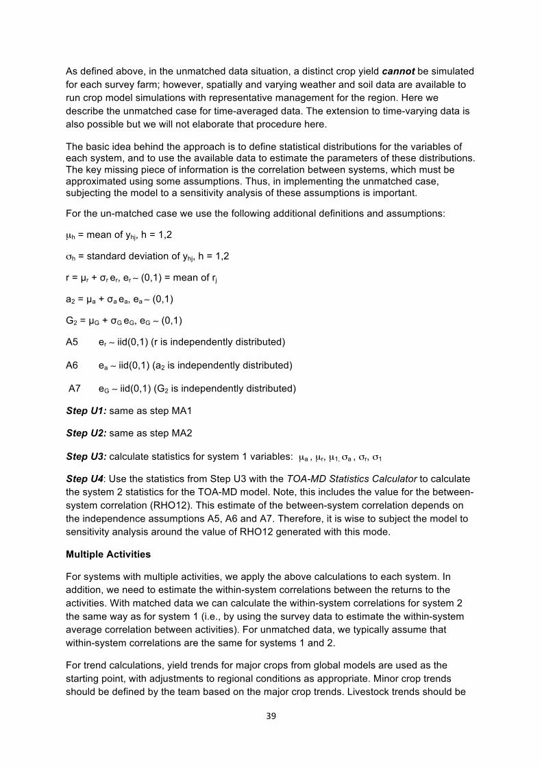
39    

As defined above, in the unmatched data situation, a distinct crop yield cannot be simulated for each survey farm; however, spatially and varying weather and soil data are available to run crop model simulations with representative management for the region. Here we describe the unmatched case for time-averaged data. The extension to time-varying data is also possible but we will not elaborate that procedure here.

The basic idea behind the approach is to define statistical distributions for the variables of each system, and to use the available data to estimate the parameters of these distributions. The key missing piece of information is the correlation between systems, which must be approximated using some assumptions. Thus, in implementing the unmatched case, subjecting the model to a sensitivity analysis of these assumptions is important.

For the un-matched case we use the following additional definitions and assumptions:

µh = mean of yhj, h = 1,2

σh = standard deviation of yhj, h = 1,2

r = µr + σr er, er ∼ (0,1) = mean of rj

a2 = µa + σa ea, ea ∼ (0,1)

G2 = µG + σG eG, eG ∼ (0,1)

A5 er ∼ iid(0,1) (r is independently distributed)

A6 ea ∼ iid(0,1) (a2 is independently distributed)

A7 eG ∼ iid(0,1) (G2 is independently distributed)

Step U1: same as step MA1

Step U2: same as step MA2

Step U3: calculate statistics for system 1 variables: µa , µr, µ1, σa , σr, σ1

Step U4: Use the statistics from Step U3 with the TOA-MD Statistics Calculator to calculate the system 2 statistics for the TOA-MD model. Note, this includes the value for the between-system correlation (RHO12). This estimate of the between-system correlation depends on the independence assumptions A5, A6 and A7. Therefore, it is wise to subject the model to sensitivity analysis around the value of RHO12 generated with this mode.

Multiple Activities

For systems with multiple activities, we apply the above calculations to each system. In addition, we need to estimate the within-system correlations between the returns to the activities. With matched data we can calculate the within-system correlations for system 2 the same way as for system 1 (i.e., by using the survey data to estimate the within-system average correlation between activities). For unmatched data, we typically assume that within-system correlations are the same for systems 1 and 2.

For trend calculations, yield trends for major crops from global models are used as the starting point, with adjustments to regional conditions as appropriate. Minor crop trends should be defined by the team based on the major crop trends. Livestock trends should be

40    

based on global model trends for milk and meat as appropriate, adjusted to regional conditions.

41    

Appendix 3 Crop Model Simulations for Integrated Assessments: User’s Guide

K. J. Boote, C. Porter, C. Villalobos, J. Hargreaves, J. Antle, R. Valdivia, and J. W. Jones

December 3, 2012

Introduction

This document describes AgMIP tools and procedures for using farm household survey data to create input files that are formatted for use in different crop models. It also describes the crop model output files that are needed for input to the TOA-MD economic model for integrated climate assessments. These files and procedures are provided for the “Matched Data” case, which means that a distinct crop yield can be simulated for each surveyed farm field, for each crop in the survey for which one or more crop models are available. In order to simulate each farm field that is in a survey, a minimum set of input variables is needed by crop models. Generally, farm survey data do not include all variables needed by crop models to simulate crop growth and yield. Thus, in order to simulate yields for the fields, assumptions have to be made about a number of input variables that are missing. Some models have used their own built-in default values for missing inputs. However, this is not an acceptable practice. It is highly important that the assumptions about missing input values are transparent to users, consistent across all models used in the integrated assessments, and clearly documented. Furthermore, users need to have the ability to set missing values that best represent the farming systems that are being analyzed, and these will vary across regions.

Data collected in farm surveys vary considerably from study to study. Here, we define the absolute minimum farm survey data necessary in order to approximately simulate each field’s yield for the matched data case. We also define the minimum set of data needed to simulate crop growth and yield when the models are used to simulate water and N limited production. Because of the need to supplement farm field survey data with assumed values, two files are needed to provide all of the information needed to create crop model-ready input files: 1) the farm survey data, and 2) a corresponding file that contains the assumed variable values that are needed to quantify all required input variables that are not in the survey data. We describe these two files needed by AgMIP software to produce crop model-ready input files and give an example of each. In addition, we describe a third file needed for setting up multi-year runs (baseline, climate scenarios, and RAPs). We also describe the software that does the translations and the model output file that is needed by the TOA-MD model for the integrated assessment.

Managing and Documenting Crop Model Inputs

Table A3.1 presents file types that can be used to import data to the AgMIP data translation tools. Templates of each file type are provided for users to enter data observed at their research or survey sites. These templates contain headers which correspond to variables in

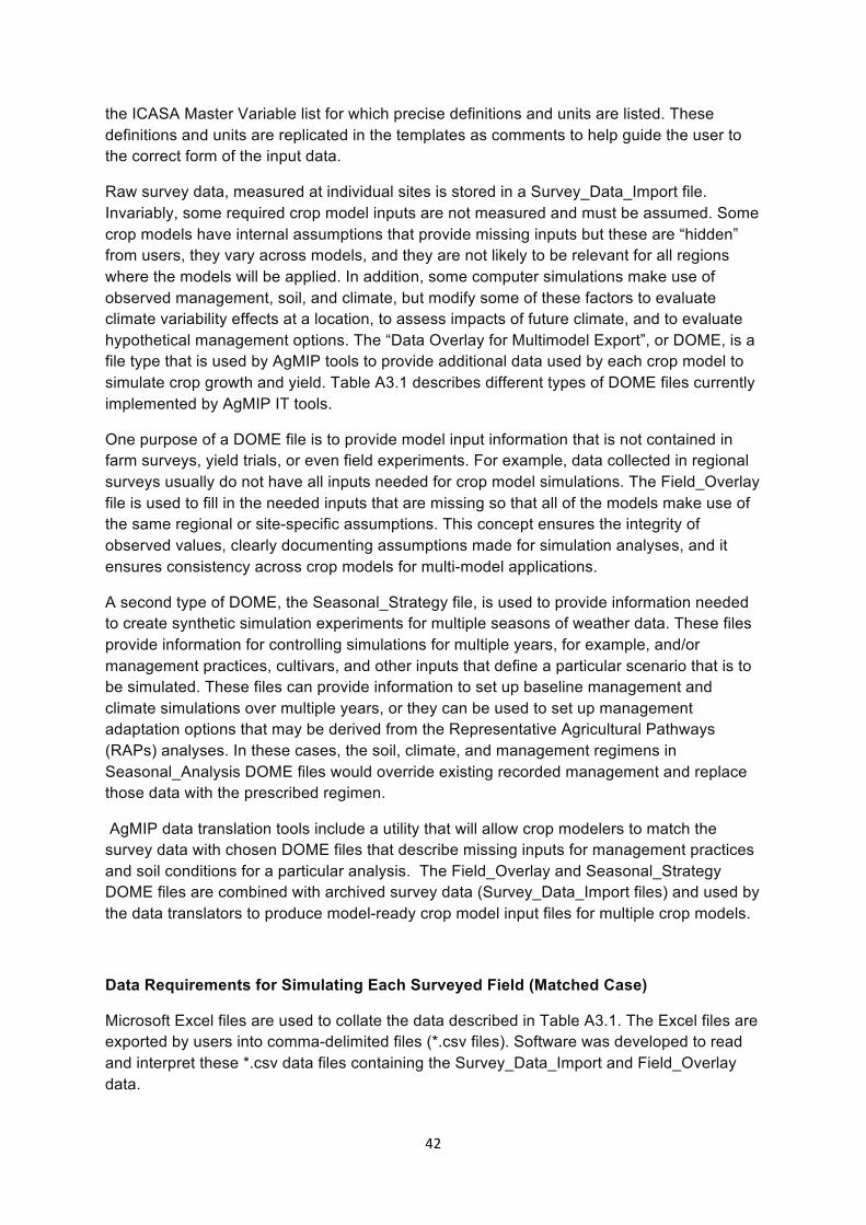
42    

the ICASA Master Variable list for which precise definitions and units are listed. These definitions and units are replicated in the templates as comments to help guide the user to the correct form of the input data.

Raw survey data, measured at individual sites is stored in a Survey_Data_Import file. Invariably, some required crop model inputs are not measured and must be assumed. Some crop models have internal assumptions that provide missing inputs but these are “hidden” from users, they vary across models, and they are not likely to be relevant for all regions where the models will be applied. In addition, some computer simulations make use of observed management, soil, and climate, but modify some of these factors to evaluate climate variability effects at a location, to assess impacts of future climate, and to evaluate hypothetical management options. The “Data Overlay for Multimodel Export”, or DOME, is a file type that is used by AgMIP tools to provide additional data used by each crop model to simulate crop growth and yield. Table A3.1 describes different types of DOME files currently implemented by AgMIP IT tools.

One purpose of a DOME file is to provide model input information that is not contained in farm surveys, yield trials, or even field experiments. For example, data collected in regional surveys usually do not have all inputs needed for crop model simulations. The Field_Overlay file is used to fill in the needed inputs that are missing so that all of the models make use of the same regional or site-specific assumptions. This concept ensures the integrity of observed values, clearly documenting assumptions made for simulation analyses, and it ensures consistency across crop models for multi-model applications.

A second type of DOME, the Seasonal_Strategy file, is used to provide information needed to create synthetic simulation experiments for multiple seasons of weather data. These files provide information for controlling simulations for multiple years, for example, and/or management practices, cultivars, and other inputs that define a particular scenario that is to be simulated. These files can provide information to set up baseline management and climate simulations over multiple years, or they can be used to set up management adaptation options that may be derived from the Representative Agricultural Pathways (RAPs) analyses. In these cases, the soil, climate, and management regimens in Seasonal_Analysis DOME files would override existing recorded management and replace those data with the prescribed regimen.

AgMIP data translation tools include a utility that will allow crop modelers to match the survey data with chosen DOME files that describe missing inputs for management practices and soil conditions for a particular analysis. The Field_Overlay and Seasonal_Strategy DOME files are combined with archived survey data (Survey_Data_Import files) and used by the data translators to produce model-ready crop model input files for multiple crop models.

Data Requirements for Simulating Each Surveyed Field (Matched Case)

Microsoft Excel files are used to collate the data described in Table A3.1. The Excel files are exported by users into comma-delimited files (*.csv files). Software was developed to read and interpret these *.csv data files containing the Survey_Data_Import and Field_Overlay data.

43    

The Survey_Data_Import file must be created from the field survey information, with one line per farm-field that was sampled in the survey. Table A3.2 lists the data that are required in this file. Generally, household survey information includes crop yield, some management information, and economic data on a per farm-field basis, which may be in any format (e.g., Excel, ASCII, or print form). If the data are not in correct units or definitions (dry matter or ear versus grain), conversions are needed prior to entering data into the Survey_Data_Import spreadsheet. Table A3.3 lists an absolute minimum set of observations from field surveys; unless these data are available or can be estimated from the raw survey data, the crop models cannot be used to simulate matched field yields for the TOA-MD economic model analyses. Typically, users can use the field LAT/LONG (preferred) or the village location for use in interpolating climate data for the site and for selecting an appropriate set of soil properties.

An example Survey_Data_Import file is provided with this document that contains the field survey data along with soil and climate data for the fields in the format needed by AgMIP software. Each tab (worksheet) in the file must be saved as a separate comma-delimited (*.csv) file.

Soil and climate data are typically not collected in farm surveys, so these data must be provided by users who are preparing the survey Excel data file for use by AgMIP software. Climate data may be provided in *.AgMIP format (the standard format used by the AgMIP climate team) as an alternative to comma-delimited (*.csv) format.

A second set of Excel files, the Field_Overlay DOME files, contain all assumptions about crop management and initial conditions that are rarely or never measured in the household surveys. There may be up to one Field_Overlay file per field if fields are highly different and need different assumptions about required inputs that were not measured. [These initial conditions and management assumptions are not trivial and can make a large difference in simulated yield. See later discussion describing how Agronomists and experts in the region need to be consulted in order to create this file.] Table A3.4 provides a list of the currently-defined minimum management and initial soil condition information needed by crop models (that are likely not provided in the household survey). These data are entered into the Field_Overlay file for use by AgMIP software to fill data not available in the farm survey data. The overlay files also document explicit assumptions made and used consistently across all crop models for the simulations. The Field_Overlay file along with the corresponding Survey_Data_Import Excel file provide all of the input data currently needed to run crop models for the matched field survey of observed yields. Later, we will describe an additional Seasonal_Strategy.xlsx type of DOME file that will be additionally needed to run multiple year baseline and multiple year climate scenarios as well as RAPs.

Software for Producing Crop Model Input Files

QuadUI is a desktop utility that reads survey and DOME data and translates to model-ready format. This software reads all field information contained in the matched Survey_Data_Import file and the associated Field_Overlay files and creates DSSAT and APSIM model input files. Translators for other models are being integrated into QuadUI as they are developed by the various crop modeling teams.

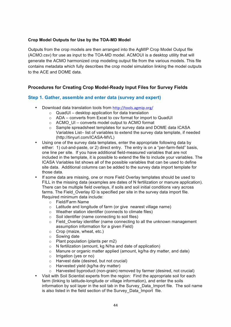
44    

Crop Model Outputs for Use by the TOA-MD Model

Outputs from the crop models are then arranged into the AgMIP Crop Model Output file (ACMO.csv) for use as input to the TOA-MD model. ACMOUI is a desktop utility that will generate the ACMO harmonized crop modeling output file from the various models. This file contains metadata which fully describes the crop model simulation linking the model outputs to the ACE and DOME data.

Procedures for Creating Crop Model-Ready Input Files for Survey Fields

Step 1. Gather, assemble and enter data (survey and expert)

• Download data translation tools from http://tools.agmip.org/ o QuadUI – desktop application for data translation o ADA – converts from Excel to csv format for import to QuadUI o ACMO_UI – converts model output to ACMO format o Sample spreadsheet templates for survey data and DOME data ICASA

Variables List– list of variables to extend the survey data template, if needed (http://tinyurl.com/ICASA-MVL)

• Using one of the survey data templates, enter the appropriate following data by either: 1) cut-and-paste, or 2) direct entry. The entry is on a “per-farm-field” basis, one line per site. If you have additional field-measured variables that are not included in the template, it is possible to extend the file to include your variables. The ICASA Variables list shows all of the possible variables that can be used to define site data. Additional columns can be added to the survey data import template for those data.

• If some data are missing, one or more Field Overlay templates should be used to FILL in the missing data (examples are dates of N fertilization or manure application). There can be multiple field overlays, if soils and soil initial conditions vary across farms. The Field_Overlay ID is specified per site in the survey data import file. Required minimum data include:

o Field/Farm Name o Latitude and longitude of farm (or give nearest village name) o Weather station identifier (connects to climate files) o Soil identifier (name connecting to soil files) o Field_Overlay identifier (name connecting to all the unknown management

assumption information for a given Field) o Crop (maize, wheat, etc.) o Sowing date o Plant population (plants per m2) o N fertilization (amount, kg N/ha and date of application) o Manure or organic matter applied (amount, kg/ha dry matter, and date) o Irrigation (yes or no) o Harvest date (desired, but not crucial) o Harvested yield (kg/ha dry matter) o Harvested byproduct (non-grain) removed by farmer (desired, not crucial)

• Visit with Soil Scientist experts from the region: Find the appropriate soil for each farm (linking to latitude-longitude or village information), and enter the soils information by soil layer in the soil tab in the Survey_Data_Import file. The soil name is also listed in the field section of the Survey_Data_Import file.

45    

• There will be one or more Field_Overlay sheet, in which you will enter expert knowledge of Agronomists and Soil Scientists to define all the missing information that is not available in the household survey data, defining probable initial conditions related to initial soil water, initial soil mineral N (NO3 & NH4), soil organic carbon, prior crop residue, prior root residue, shape of initial mineral N, shape of SOC, shape of inert SOC, and shape of probable rooting profile. Do not attempt to simulate without a field overlay file, as data will inevitably be missing and model defaults incorrect.

o Field_Overlay files will tend to be soil-related for initial conditions for water, mineral N, SOC, SOM, residue, rooting shape where soils are different.

o Field_Overlay files may also be sowing-related (plant population) or fertility management-related (fertilizer/manure).

Step 2. Save Survey_Data_Import and Field_Overlay Data to csv format

• Using the ADA utility, save Survey_Data_Import sheets in comma delimited (csv) format, one for field, one for soil, and one for each climate file, zipped into a single archive. Caution: Do not open the *.csv files again with Excel, as they ARE NOT true spreadsheets and do not correctly convert back into Excel files; the date format can revert to a machine-dependent format.

• Using the ADA utility, save the Field_Overlay spreadsheets in comma delimited (csv) format, zipped into a single archive.

Step 3. Translate data files to model-ready formats • Run QuadUI by double-clicking on the QuadUI.bat file. Respond to the on-screen

requests for location of zipped Survey csv files and zipped Field_Overlay csv files, as well as the placement for the output crop model files. If you are not successful, view the QuadUI log report in the QuadUI folder.

• Your ending point will be files for running crop models, i.e., Files X, A, SOIL.SOL, *.CUL, *.WTH for DSSAT, and similar files for APSIM or other crop models. In the case of DSSAT or APSIM, simulations can be run by double-clicking the DOS batch file that was created with the translations.

Step 4. Check and correct missing/invalid model input data and run simulations

• Run the crop model. With APSIM, load the simulation and view the log. With DSSAT, look at the Error.OUT and the Warning.OUT files. These files will tell you if the climate file or cultivar were not found, or if some variables such as sowing date or plant population were missing. With APSIM, after the issues in the LOG are dealt with, run the simulation. APSIM produces summary files (*.sum) which are a log of significant events and warnings/fatal errors. The summary files need to be checked for errors which may need to be corrected, otherwise the error in simulated yields may be significant. If there are failures, go back to the Survey_Data_Import and Field_Overlay DOME files. Common errors include:

o If plant population (or other) was not in the Survey_Data_Import file, and is not found, then you did not connect the Field_Overlay file correctly.

o Field_Overlay name was not entered in the survey template exactly as in the Field_Overlay file. In this case, no Field_Overlay data were found.

• Evaluate the outputs. In DSSAT, look at the Evaluate.Out file which will list both the simulated and the observed yield. In APSIM, there is a single line output for each simulation. The APSIM-simulated yield values will need to be aggregated (assembled) into one file. The observed yields are in the Survey_Data_Import file and will need to be matched per field.

46    

Step 5. Create AgMIP Crop Model Output (ACMO) File for use by Economic Team Members The ACMO file is partially created by QuadUI at translation time in the form of the ACMO_meta.dat file which contains metadata in one line per field so that all of the information used to simulate results for the fields is documented in a way that users could reproduce the results. Running ACMOUI, a desktop utility, will complete the ACMO file with the selected crop model simulated outputs. Note that the ACMO files contain raw simulated results for each field, not aggregated or adjusted in any way. This will ensure integrity of both inputs and model outputs. Table A3.5 lists all of the variables that ACMO contains along with information on variables created by QuadUI and those that must be added by crop modelers.

Create Crop Model-Ready Input Files for Simulating Multi-Year Baseline, Climate, and RAPs Scenarios (Using Strategy_Analysis files)

A Seasonal_Strategy type of DOME file will be created to assist multi-year simulations for baseline and climate scenarios, both with and without RAPs. The starting point will be the Survey_Data_Import and the Field_Overlay files that were already created for the surveyed fields. In this case, the Survey_Data_Import file, in addition to having a Field_Overlay ID per field, will also have a Seasonal_Strategy ID (possibly just one for all farms in the survey). Examples of what is in that file include:

• For Baseline Multi-Year: auto-sowing rules • For Future Climate Scenarios: auto-sowing rules, plus link to new weather station IDs • Translating RAPS into management using the Seasonal Strategy (RAPs can led to

improved crop and soil management practices including improved genetic technology). Specifics include:

o Auto-sowing, possibly modified for earlier/shorter sowing window because of better machinery

o Weather station ID o changed plant population, o improved or alternative crop cultivar, o changed N fertilization, o increased prior root and surface residue (because of better fertilization-

population-cultivar) o other adaptation strategies, as needed

To run a Seasonal Strategy, repeat all of the steps for baseline analysis, using the Survey_Data_Import and Field_Overlay files, but now the Seasonal_Strategy DOME files are also prepared using the spreadsheet templates. Each of the three sets of files (Survey_Data_Import, Field_Overlay, and Seasonal_Strategy) should be compressed into separate zip files for import to QuadUI.

Notes on Use of Field_Overlay Files

• Function and Purpose of multiple Field_Overlay files

47    

o Fill in data that crop models need that are almost never available in household survey, such as initial soil water, initial soil nitrate and ammonium, soil organic carbon pools (SOM3 for DSSAT-CENTURY, and inert SOC for APSIM), and rooting depth (see Table A3.4). The shape of these listed variables by soil depth is also generally missing.

o Fill in needed data missing from household survey, such as root residue from prior crop, surface residue from prior crop, sowing date, sowing depth, plant population, amounts and dates of fertilizer or manure applied.

o Link to cultivar ID and model specific cultivar ID o It can be used to set automatic sowing rules for each field in the survey, if

planting dates were not recorded. • Where to get Field_Overlay information? First, DO NOT use crop model defaults, as

the model defaults are wrong and differ among crop models. Often defaults use zero or unity values when not appropriate and these are not region-specific. Secondly, this must be done in close collaboration with local agronomists and soil scientists.

o Agronomists and soil scientists in the region who know production practices for the crop and region in question. Although they may not give specific values for the needed inputs, they will likely provide very useful ranges of likely missing input information.

o Soil survey information (linking to latitude-longitude coordinates for field). o Country-wide statistics (amount of N fertilization per hectare), but this is not

region- or crop-specific. o Pre-simulations with crop models with correct soil organic carbon and SOM3

(or inert SOC) pools, for setting SOM3 and inert SOC to give the low non-fertilized non-legume yields for the region (requires knowledge of unfertilized yield for region). Take the mineral nitrate and ammonium from the values simulated at the end of the “prior” season.

o Make sure that the assumed values that you use in the Field_Overlay file are consistent with all of the expert knowledge and soil survey information, and document how these values were developed.

• Principles for use of Field_Overlay files: o First obtain knowledge from agronomists, soil scientists, and soil surveys. o Do not use model defaults for missing information o Then use QUADUI with Survey_Data_Import and multiple Field_Overlay

files, to create model-ready files for simulation. o Simulate farmer fields (n = 50 to 150)

Summary of Simulation Runs Needed for Integrated Assessments

Crop modeling teams need make several separate sets of simulation runs and prepare several ACMO files for the integrated assessments. The ACMO will be provided to the Economic modelers for use in the TOA-MD analyses. Specifically, the following set of runs will need to be made, each with its corresponding ACMO file:

1. Matched simulations, with observed inputs and raw crop model results (not bias-corrected). This set of runs will require the Survey_Data_Import field survey file along with the Field_Overlay file.

2. Simulation Set #1. Current system simulation results, multiple years (e.g., 30 years), which means current climate and current management conditions. This set of runs will require the same two files above in addition to a Seasonal_Strategy file that will set up the multi-year simulations.

3. Simulation Set #2. Climate change simulated results, multiple years (e.g., 30) using current management with future climate conditions. This allows paired climate

48    

change impact assessments. This set of runs will also require the same two files above in addition to a Seasonal_Strategy file that will set up the multi-year simulations, this time using a future climate scenario.

4. Simulation Set #3. Climate change simulated results, multiple years (e.g., 30) using adaption management with future climate conditions. This allows paired climate change impact assessments. This set of runs will also require the same two files above in addition to a Seasonal_Strategy file that will set up the multi-year simulations, this time using a future climate scenario. Adaptation scenarios include improved cultivars, different fertilization, and altered sowing dates, consistent with RAPs.

5. Archive model simulations (inputs, management, outputs, soil, climate, cultivar coefficients, simulated outputs) by placing them in the ACE, DOME and ACMO databases.

6. Document simulations with explanatory text and appropriate tables and figures showing the yield distributions and analyses of interannual and spatial variations. Create maps and summary statistics e.g., spatial distribution of climate, soils, management, and yields illustrated in GIS mapping methods.

Guidelines for Analysis of Crop Model Simulated Outputs for Matched Fields

Crop modelers should analyze model outputs prior to use of the data in the regional economic analysis. This is very important to ensure quality control of the process and that crop modelers are able to understand the variability in results. It is also important that crop modelers will be able to conclude that simulated yields are reasonable representations of water and nitrogen-limited yields, recognizing that other factors, such as other soil nutrients and pests, are likely to contribute to actual yields in a region and that these factors could vary considerably over space and time. We have provided suggestions for analyzing crop model outputs, including computation of means, distribution of observed and simulated yields, computation of mean bias between observed and simulated yields, and analysis of outliers.

• Evaluate Simulated and Observed Yields for Mean, Bias, and Distribution • Place simulated yield and observed yields into a spreadsheet, computing means and

standard deviation. Compute bias of the mean observed yield divided by mean simulated yield. We do not recommend computing bias of individual fields if there are any zero simulated yield values, as that will give error.

• Rank the observed yields and simulated yields from high to low and compute cumulative probability distributions of observed and simulated yields.

• Attempt to identify outliers and reasons for high mean bias as well as large differences between cumulative distributions of simulated and observed yields. These analyses may help crop modelers critically evaluate some of the input assumptions in the Field_Overlay file, for example, relative to the information from regional agronomists and other sources that were used to set the values. If there is a large bias, it would be good to review the inputs and results with agronomists. We do not recommend any type of calibration for reducing the bias; this is intended to improve the reliability of the process and results. These analyses may be useful in reporting and in publishing crop model results; only the final raw field-by-field simulated yields will be used in the ACMO file. Some ideas to consider as you analyze results are:

o If bias (observed over simulated) is dramatically different from 1.00 (for example 0.5 or 1.5), there may be problems in Field_Overlay assumptions.

49    

Bias is driven by the mean simulated and observed yields. For example, a high bias of 1.5 or more could indicate that soil N availability (SOM3, initial nitrate, initial ammonium) or soil water availability (initial or capacity) is not high enough. A low bias of 0.5 (model simulates too high) could indicate too much soil N availability or too much water availability.

o The full range of the cumulative distribution is driven not just by the management and climate, but also by the extent of range of initial nitrate, ammonium, SOC, SOM, DUL-LL, and initial soil water found across all the farms. If that range of inputs is small (because of inadequate Field_Overlay entry), then the simulated distribution of yields could be insufficient.

o Strong left tails in simulated distribution (or observed) are indicators of crop failures (zero and very low yields). If left tails is too strong in simulated, then you may need to increase initial soil water content to reduce the instance of simulated germination failures, or increase rooting depth or DUL-LL to minimize crop failures during reproductive growth.

o Strong right tails in simulated or observed distributions are indicators of high yields. If simulated right tails are too strong (or too little) where the water and N stresses are minimum, one can make the case that genetic yield potential of the cultivar is too high (or too low).

o These “indicator” problems are given, not for the purpose of re-calibrating the crop models to fit the distribution, but for the purpose of highlighting the need for obtaining correct Field_Overlay information in the first place.

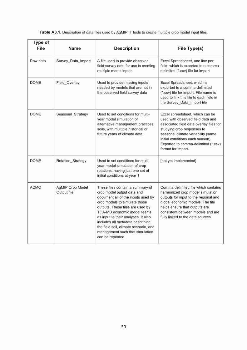
50    

Table A3.1. Description of data files used by AgMIP IT tools to create multiple crop model input files.

Type of File Name Description File Type(s)

Raw data Survey_Data_Import A file used to provide observed field survey data for use in creating multiple model inputs

Excel Spreadsheet, one line per field, which is exported to a comma-delimited (*.csv) file for import

DOME Field_Overlay Used to provide missing inputs needed by models that are not in the observed field survey data

Excel Spreadsheet, which is exported to a comma-delimited (*.csv) file for import. File name is used to link this file to each field in the Survey_Data_Import file

DOME Seasonal_Strategy Used to set conditions for multi-year model simulation of alternative management practices, soils, with multiple historical or future years of climate data.

Excel spreadsheet, which can be used with observed field data and associated field data overlay files for studying crop responses to seasonal climate variability (same initial conditions each season). Exported to comma-delimited (*.csv) format for import.

DOME Rotation_Strategy Used to set conditions for multi-year model simulation of crop rotations, having just one set of initial conditions at year 1

[not yet implemented]

ACMO AgMIP Crop Model Output file

These files contain a summary of crop model output data and document all of the inputs used by crop models to simulate those outputs. These files are used by TOA-MD economic model teams as input to their analyses. It also includes all metadata describing the field soil, climate scenario, and management such that simulation can be repeated.

Comma delimited file which contains harmonized crop model simulation outputs for input to the regional and global economic models. The file helps ensure that outputs are consistent between models and are fully linked to the data sources.

51    

Table A3.2. List of variables in the household survey FIELD data needed to run crop models. These data are in the Survey_Data_Import.xlsx EXCEL file. Note that some of these data may not have been collected in the

survey but are provided later by those who are preparing the data for translation by AgMIP software tools into model-specific input files needed to run each crop model.

Data Type Units Variable Name

Field/Farm name EXNAME

Field overlay name(s) FIELD_OVERLAY

Seasonal strategy name(s) SEASONAL_STRATEGY

Latitude dec. degrees FL_LAT

Longitude dec. degrees FL_LONG

Weather station identifier to link to site information WST_ID

Soil profile identifier SOIL_ID

Planting date yyyy-mm-dd PDATE

Crop ID (see list of codes above) code CRID

Total seasonal N applied kg[N]/ha FEN_TOT

Manure/Organic matter applied kg[DM]/ha OMAMT

Harvest date yyyy-mm-dd HDATE

Harvest yield (dry wt) kg[dry]/ha HWAH

By-product removed at harvest as dry wt kg[dry]/ha BWAH Indicates whether the field has been irrigated Y or N IRRIG

Notes (as desired, optional) TR_NOTES

52    

Table A3.3. List of observations that are considered absolute minimum in order to simulate each field in the survey using management, climate, and soil information for the field, the “matched data” case.

1. Village name for climate data interpolation, which will almost always have to be done). 2. Farm/field name (This plus village name provides the unique field name for the simulation and

location is used to identify a suitable soil to obtain soil inputs needed for the model. 3. Crop species 4. Sowing date (yyyy-mm-dd). 5. Mineral N fertilizer amount used (elemental N applied per ha, or at least categories that can

be consistently interpreted to estimate amounts, such as none, low, medium, and high) 6. Farmyard manure or organic matter applied. If not given, we would assume that it is zero. 7. Whether irrigated or not. Probably, this is rare in most of our AgMIP SSA and SA projects,

except for rice. Also could include total irrigation for the season in mm (IRR_TOT). 8. Grain yield (dry weight per ha, or otherwise indicate basis and units for yield in survey data.

Table A3.4. A list of the minimum management and initial soil condition information needed by crop models that is probably not provided by household yield survey. **indicates data hopefully provided from survey.

1. Cultivar ID (link to model-specific cultivar) 2. Sowing date (yyyy-mm-dd)** 3. Sowing depth (cm), 4. Plant population (plants/m2) ** 5. Mineral N fertilizer amount used (kg elemental N applied per ha), dates of application (yyyy-

mm-dd or days after sowing), percentages for split amounts? ** 6. Farmyard manure or organic matter applied (kg DM per ha) and dates of application (yyyy-

mm-dd or days after sowing).** 7. Whether irrigated or not.** 8. Root residue from prior crop (kg/ha) 9. Surface residue from prior crop (kg/ha) 10. Maximum rooting depth (and shape relative to 1.0 in topsoil) 11. Initial soil water (zero to 100% of available) (for each layer, or shape?) 12. Initial soil nitrate and ammonium (for each layer or shape in profile if kg N/ha total?) 13. Soil organic carbon pools (fraction SOM3 for DSSAT-CENTURY, or fraction inert SOC for

APSIM), by each layer, or shape.

53    

Table A3.5. List of variables contained in the ACMO file for documenting crop model runs and for use by economic modelers in the TOA-MD analyses. Also the table shows which variables are created automatically by the AgMIP IT Tool, QuadUI and which must be added by crop modelers.

Variable Name Definition Units Metadata or Crop Model input summary data (provided by QuadUI)

EID Experiment ID

SUITE_ID Suite identification, for linking groups of sites or experiments

RUN# Simulation order FIELD_OVERLAY Name of field overlay(s) SEASONAL_STRATEGY Name of seasonal strategy(ies)

EXNAME Name of experiment, field test or survey

TRT_NAME Name of treatment CLIM_ID 4-character Climate ID code

CLIM_REP Climate replication number for multiple realizations of climate data

REG_ID Region ID STRATUM Regional stratum identification number RAP_ID RAP ID

MAN_ID Management regimen ID, for multiple management regimens per RAP

INSTITUTION Names of institutions involved in collection of field or survey data

ROTATION Crop rotation indicator (=1 to indicate that this is a continuous, multi-year simulation, =0 for single year simulations)

WSTA_ID Weather station ID SOIL_ID Soil ID FL_LAT Site Latitude decimal degrees FL_LONG Site Longitude decimal degrees CRID_text Crop type (common name) CUL_ID Crop model-specific cultivar ID CUL_NAME Cultivar name SDAT Start of simulation date yyyy-mm-dd PDATE Planting date yyyy-mm-dd HWAH Observed harvested yield, dry weight kg/ha CWAH Observed total above-ground biomass at harvest kg/ha

HDATE Observed harvest date yyyy-mm-dd IR#C Total number of irrigation events

IR_TOT Total amount of irrigation mm IROP_text Type of irrigation application

FE_# Total number of fertilizer applications

FEN_TOT Total N applied kg[N]/ha FEP_TOT Total P applied kg[P]/ha

54    

FEK_TOT Total K applied kg[K]/ha OM_TOT Manure and applied oganic matter kg/ha TI_# Total number of tillage applications

TIIMP_text Tillage type (hand, animal or mechanized)

Crop model simulation output data (provided by the crop modeler)

CROP_MODEL Short name of crop model used for simulations (e.g., DSSAT, APSIM, Aquacrop, STICS, etc.)

MODEL_VER Model name and version number of the crop model used to generate simulated outputs

HWAH_S Simulated harvest yield, dry matter kg/ha CWAH_S Simulated above-ground biomass at harvest, dry

matter kg/ha

ADAT_S Simulated anthesis date yyyy-mm-dd MDAT_S Simulated maturity date yyyy-mm-dd HADAT_S Simulated harvest date yyyy-mm-dd LAIX_S Simulated leaf area index, maximum m2/m2 PRCP_S Total precipitation from planting to harvest mm ETCP_S Simulated evapotranspiration, planting to harvest mm NUCM_S Simulated N uptake during season kg/ha NLCM_S Simulated N leached up to harvest maturity kg/ha