Rochester Institute of Technology Rochester Institute of Technology RIT Scholar Works RIT Scholar Works Theses 2006 Advanced Thermodynamic Analyses of Energy Intensive Building Advanced Thermodynamic Analyses of Energy Intensive Building Mechanical Systems Mechanical Systems Erin N. George Follow this and additional works at: https://scholarworks.rit.edu/theses Recommended Citation Recommended Citation George, Erin N., "Advanced Thermodynamic Analyses of Energy Intensive Building Mechanical Systems" (2006). Thesis. Rochester Institute of Technology. Accessed from This Thesis is brought to you for free and open access by RIT Scholar Works. It has been accepted for inclusion in Theses by an authorized administrator of RIT Scholar Works. For more information, please contact [email protected].

Welcome message from author
This document is posted to help you gain knowledge. Please leave a comment to let me know what you think about it! Share it to your friends and learn new things together.
Transcript
Rochester Institute of Technology Rochester Institute of Technology
RIT Scholar Works RIT Scholar Works
Theses
2006
Advanced Thermodynamic Analyses of Energy Intensive Building Advanced Thermodynamic Analyses of Energy Intensive Building
Mechanical Systems Mechanical Systems
Erin N. George
Follow this and additional works at: https://scholarworks.rit.edu/theses
Recommended Citation Recommended Citation George, Erin N., "Advanced Thermodynamic Analyses of Energy Intensive Building Mechanical Systems" (2006). Thesis. Rochester Institute of Technology. Accessed from
This Thesis is brought to you for free and open access by RIT Scholar Works. It has been accepted for inclusion in Theses by an authorized administrator of RIT Scholar Works. For more information, please contact [email protected].
ADVANCED THERMODYNAMIC ANALYSES OF ENERGY
INTENSIVE BUILDING MECHANICAL SYSTEMS
By
ERIN N. GEORGE
A Thesis Submitted in Partial Fulfillment of the Requirement
for Master of Science in Mechanical Engineering
Approved by:
Department of Mechanical Engineering Committee
Dr. Margaret Bailey - Thesis Advisor
Dr. Robert Stevens
Dr. Frank Sciremammano
Dr. Edward Hensel- Dept. Representative
Rochester Institute of Technology
Rochester, New York 14623
March 2006
PERMISSION TO REPRODUCE THE THESIS
Title ofThesis
ADVANCED THERMODYNAMIC ANALYSES OF ENERGY
INTENSIVE BUILDINGMECHANICAL SYSTEMS
I, ERIN N. GEORGE, hereby grant permission to the Wallace Memorial Library of
Rochester Institute ofTechnology to reproduce my thesis in the whole or part. Any
reproduction will not be for commercial use or profit.
March 2006
ABSTRACT
A review ofpast research reveals that while exergetic analysis has been performed on various
building mechanical systems, there has not been extensive efforts in the areas of air
distribution systems or cooling plants. Motivations for this new work include demonstrating
the merits of exergetic analysis in association with retrocommissioning (RCX) an existing
building air handling unit (AHU), as well as conducting an advanced analysis on an existing
chiller. The following research demonstrates the benefits of including a second law analysis
in order to improve equipment operation based on lowered energy consumption and
improved operation, and as a means for system healthmonitoring.
Particularly, exergetic analysis is not often performed in the context of RCX, therefore this
research will provide insight to those considering incorporating exergetic analysis in their
RCX assessments. A previously developed RCX test for assessing an AHU on a college
campus, as well as data collected from the testing is utilized for an advanced thermodynamic
analysis. The operating data is analyzed using the first and second laws of thermodynamics
and subsequent recommendations are made for retrofit design solutions to improve the
system performance and occupant comfort. The second law analysis provides beneficial
information for determining retrofit solutions with minimal additional data collection and
calculations. The thermodynamic methodology is then extended to a building's cooling plant
which utilizes a vapor compression refrigeration cycle (VCRC) chiller. Existing chiller
operational data is processed and extracted for use in this analysis. As with the air handling
unit analysis, the second law analysis of the VCRC chiller provides insight on irreversibility
in
locations that would not necessarily be determined from a first law analysis. The VCRC
chiller data, originally collected several years ago for the design of an automated fault
detection and diagnosis methodology, is utilized. Chiller plant data representing normal
operation, as well as faulty operation is used to develop a chiller model for assessing
component performance and health monitoring. Based on RCX activities and
thermodynamic analyses, conclusions are drawn on the utility of using exergetic analysis in
energy intensive building mechanical systems in order to improve system operation. Unique
models are developed using the software program Engineering Equation Solver (EES). The
models developed are shown to properly predict performance of the systems as well as serve
as a means of system health monitoring. The results show the utility of the model and
illustrate system performance.
IV

ACKNOWLEDGEMENTS
I would like to thank my advisor, Dr. Margaret Bailey, for her continued support for this
research. Her excitement and enthusiasm were appreciated, and I not only consider her an
advisor but also a friend.
I would like to thankmy husband, Matt, for being patient and encouraging, and myMother,
Sue, for inspiring and encouraging me to pursue myMasters degree. I would also like to
thank my family, for their support in helping me achieve my dreams.

TABLE OF CONTENTS
ABSTRACT Ill
ACKNOWLEDGEMENTS V
TABLE OF CONTENTS VI
LIST OF TABLES IX
LIST OF FIGURES XI
NOMENCLATURE XII
1 INTRODUCTION AND LITERATURE REVIEW 1
1.1 Motivation 2
1.2 Statement ofWork 4
1.3 Literature Review 5
1.3.1 Exergy 5
1.3.1.1 Additional benefit ofsecond law analysis 6
1.3.1.2 Exergy Optimization 8
1.3.1.3 Exergy and building systems 10
1.3.1.4 DeadState 15
1.3.1.5 FaultDetection andDiagnosis 17
1.3.2 Retrocommissioning 19
2 BACKGROUND 23
2.1 Thermodynamics 23
2.2 EES 27
2.3 Devices 30
2.3.1 AirHandling Unit Coils 31
2.3.1.1 Cooling Coil 31
2.3.1.2 Heating Coil 32
2.3.2 Fans 33
2.3.3 Economizer 33
2.3.4 Filters 34
2.3.5 Electrical Components and Controls 35
2.3.6 Vapor Compression Refrigeration Cycle Chillers 36
2.3.6.1 Condenser 38
2.3.6.2 Expansion Valve 39
2.3.6.3 Evaporator 39
2.3.6.4 Compressor 39
2.3.7 Summary 40
3 EXPERIMENTAL RESEARCH 41
3.1 Testing Procedure forAirHandlingUnit 42
3.1.1 Sensor Verification 43
3.1.2 System Control Response Test 45
3.1.3 Pre-functional Tests 45
VI

3.1.3.1 Fan Pre-functional Tests 45
3.1.3.2 Coil Pre-functional Test 46
3.1.3.3 Economizer Pre-functional Test 48
3.1.4 Functional Tests 49
3.1.4.1 Fan Functional Test 50
3.1.4.2 Coil Functional Test 50
3.1.4.3 Economizer Functional Test 51
3.2 Air Handling UnitExperimentalDataCollection 52
3.2.1 Fan Data Collection 53
3.2.2 Coil Data Collection 55
3.2.3 Economizer Data Collection 57
3.3 VCRC Chiller Experimental Data Collection 59
3.3.1 Data Collection Process 62
3.3.1.1 Normal Data Collection 62
3.3.1.2 Refrigerant Under- and Over-Charge Data Collection 62
3.3.1.3 Oil Under-Charge Data Collection 63
3.3.2 Available ChillerData 63
3.4 VCRC ChillerData 64
3.4.1 NormalData 64
3.4.2 Refrigerant Under- and Over-Charge data 66
3.4.3 Oil Under-Charge Data 68
AIR HANDLING UNIT MODEL 70
4.1 Air HandlingUnit analysis 70
4.1.1 Supply andReturn Fan analysis 72
4.1.1.1 Energy analysis ofthe Fans 73
4.1.1.2 Exergy analysis ofFans 74
4.1.2 Coil analysis. 77
4.1.2.1 Coil Effectiveness 78
4.1.2.2 Exergy analysis ofthe Coil 80
4.1.3 Economizer analysis 83
4.1.4 DeadState Verification 85
4.2 Conclusions 87
VCRC CHILLERMODEL 94
5 . 1 Vapor CompressionRefrigeration Cycle ChillerAnalysis 94
5.1.1 Vapor Compression Refrigeration Cycle Chiller EffectivenessAnalysis 97
5.1.2 VCRC Chiller Exergy analysis 102
5.2 Fault VersusNormalOperationAnalysis 105
5 .3 Vapor CompressionRefrigeration Cycle ChillerResults - Normal and
FaultOperation 106
5.4 Chiller Conclusions 118
CONCLUSIONS 121
6.1 Summary 121
6.2 GeneralConclusions 122
6.3 AHUModelConclusions 123
vn

6.4 VCRCChillerModel Conclusions 126
6.5 Recommendations forFutureWork 127
REFERENCES 129
APPENDIXA 134
APPENDIX B 147
APPENDIX C 160
C.l EES Code forAHU Fans 160
C.2 EES Code forAHU Fans -Reference StateVariance Study 166
C.3 EES Code forAHU Coil 170
C.4 EES Code forAHU Economizer 176
C.5 EES CODE FORVCRC CHILLER MODEL 179
APPENDLX D RETROCOMMISSIONING TEST PLANS FOR AIRHANDLING UNIT
182
vm

LIST OF TABLES
Table 3.1 : Building 70 AHUFunctional test data for supply and return fans
(4/8/05) 54
Table 3.2: Variation in duct static pressure set points 54
Table 3.3: Building 70 AHU Coil performance test data collected (4/15/05) .... 56
Table 3.4: Building 70 AHU Collected data for economizer tests (4/15/05) 58
Table 3.5:'Normal'
chiller LVIPC data (10/28/96) 65
Table 3.6:Normal chiller CMS data (10/28/96) 65
Table 3.7: Final values fornormalVCRC analysis 66
Table 3.8: Final values for 45% refrigerant chargeVCRC analysis 67
Table 3.9: Final values for 50% refrigerant chargeVCRC analysis 67
Table 3.10: Final values for 55% refrigerant chargeVCRC analysis 67
Table 3.11: Final values for 105% refrigerant chargeVCRC analysis 68
Table 3.12: Final values for 105% refrigerant chargeVCRC analysis 68
Table 3.13: Final values for 50% oil chargeVCRC analysis 69
Table 3.14: Final values for 85% oil chargeVCRC analysis 69
Table 4. 1 : Supply and return fan first law efficiencies forBuilding 70 AHU... 74
Table 4.2: Reference environment data for exergy analysis 75
Table 4.3: Exergy results forAHU supply and return fans 76
Table 4.4: Effectiveness results forAHU heating coil 79
Table 4.5: Reference environment for coil analysis 80
Table 4.6: Exergy results forAHU coil analysis 82
Table 4.7: Results forAHU economizer analysis 84
Table 4.8: Variance in dead state for justification of selected dead state 87
Table 4.9: Summary of dead state variation values 87
Table 4.10: EES results from first and second law analysis on fans, coil, and
ECONOMIZER 88
Table 5.1: VCRC ChillerNormal case results for enthalpy and entropy 97
Table 5.2: VCRC ChillerNormal case results for condenser and evaporator
effectiveness 101
Table 5.3: Reference environment forVCRCChiller analysis 102
Table 5.4: VCRC ChillerNormal case results for exergy destroyed and exergetic
EFFICIENCY 105
Table 5.5: Summary of completeVCRC Chillernormal results 107
Table 5.6: VCRC Chiller refrigerant under-charge results 1 10
Table 5.7: Side by side comparison of normal case B and 45% refrigerant charge
Ill
Table 5.8: Side by side comparison of normal case B and 50% refrigerant charge
112
Table 5.9: Side by side comparison of normal casesA and B and 45%, 50%, and 55%
REFRIGERANT CHARGE 113
Table 5.10: Results for refrigerant over-chargeVCRC Chiller analysis 1 14
Table 5.11: Results for oil under-chargeVCRC Chiller analysis 115
IX
Table 5.12: Side by side comparison of normal caseA and 50% oil charge 116
Table 5.13: Side by side comparison of normal case B and 85% oil charge 117
x

LIST OF FIGURES
Figure 2.1 : EES Equationswindow showing example code 29
Figure 2.2: EES solution window showing example results 29
Figure 2.3: AirHandlingUnitDiagram 31
Figure 2.4: Heating andCoolingCoil Schematics (courtesy of D. Esposito) .... 32
Figure 2.5: Supply andReturn Fan schematics (courtesy of D. Esposito) 33
Figure 2.6: Economizer Schematic (courtesy of D. Esposito) 34
Figure 2.7: Filter Schematic (courtesy of D. Esposito) 35
Figure 2.8: Vapor compression refrigeration loop diagram (central loopworking
fluid is R-22) 37
Figure 2.9: T-s diagram fornormal vs. faulty operation for vapor compression
refrigeration CYCLE 38
Figure 3.1: Flow chart of RCX process forAHU 43
Figure 3.2: Portion of generalAHURCX test including system control response
AND FIELD CALIBRATION CHECK 44
Figure 3.3: Portion of Fan Performance RCX test showing pre-functional
CHECKLIST 46
Figure 3.4: Portion of Coil Performance RCX test showing pre-functional
CHECKLIST 48
Figure 3.5: Portion of Economizer Performance RCX test showing pre-functional
checklist 49
Figure 3.6: Portion of Fan Performance RCX test showing functional test 50
Figure 3.7: Portion of Coil PerformanceRCX test showing functional test .... 51
Figure 3.8: Portion of Coil PerformanceRCX test showing functional test .... 52
Figure 3.9: Am.HandlingUnit Diagram 53
Figure 3.10: Diagram of data collection locations for heating coil 56
Figure 3.11: Diagram of data collection locations for cooling coil 57
Figure 3.12: Instrumentation locations in chiller for experimental data
collection [Bailey 1998a] 61
Figure 4. 1 : Air handling unit diagram displaying state points for EES 71
Figure 4.2: AHU Fan EES code for set point 2 72
Figure 5.1 : VCRCChiller diagram from EES 96
XI
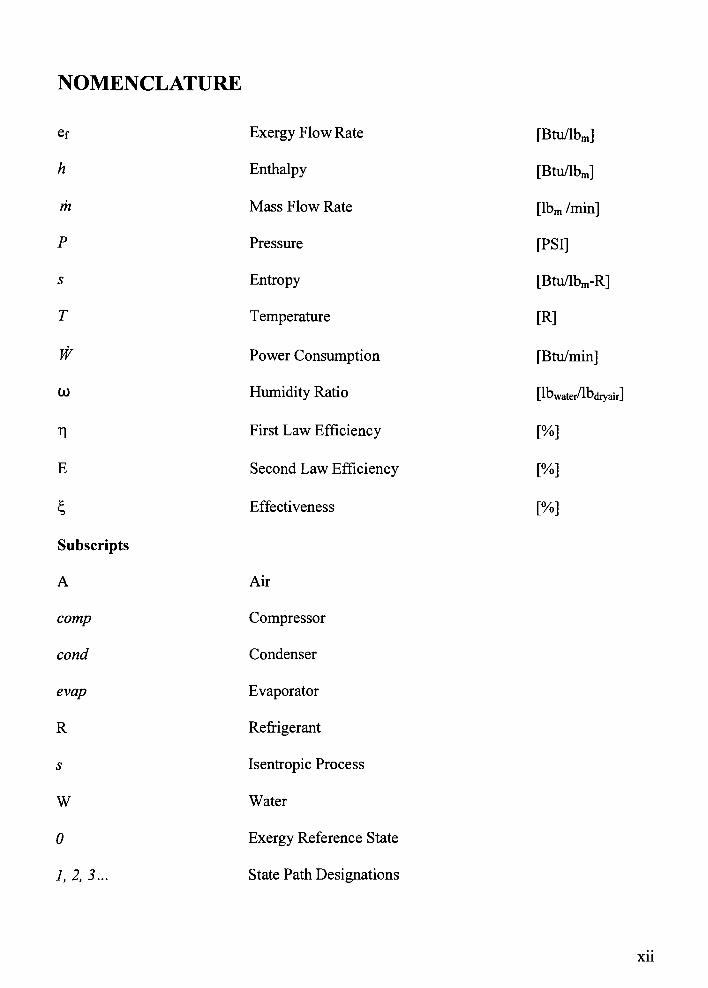
NOMENCLATURE
ef Exergy FlowRate
h Enthalpy
m Mass Flow Rate
P Pressure
s Entropy
T Temperature
W Power Consumption
0) Humidity Ratio
Tl First Law Efficiency
E Second Law Efficiency
S Effectiveness
Subscripts
A Air
comp Compressor
cond Condenser
evap Evaporator
R Refrigerant
s Isentropic Process
W Water
0 Exergy Reference State
1, 2, 3... State Path Designations
[Btu/lbm]
[Btu/lbm]
[lbm /min]
[PSI]
[Btu/lbm-R]
[R]
[Btu/min]
[lbwater'lbdryair]
Xll
1 Introduction and Literature Review
Commercial buildings use air handling units (AHU) and chillers as a means to heat and cool
the building space. Air handling units are responsible for circulating the air, as well as
heating and cooling it through integral coils, as needed. Chillers serve an important function
of cooling the air by providing chilled water to the AHU cooling coil, as well as providing
chilled water to the building. These systems utilize large amounts of electrical energy, and
building owners look for ways to reduce the associated energy consumption while still
providing the necessary environment to building occupants.
Many building mechanical systems have on-board sensors that are used for general operation
of the controls system. Typically in retrocommissioning (RCX), to assess the performance of
a system, a small amount of data is collected and a basic analysis is conducted, using many
assumptions and basic equations based on the first law of thermodynamics. This can be
quick and effective, although additional insight into the performance can be gained from
additional analysis with little or no additional data collection. This supplemental analysis,
which utilizes the second law of thermodynamics, may provide much more information
about the system with very little additional time investment.
Retrocommissioning (RCX) examines existing buildings and systems that may or may not
degrade after periods of extended use. An RCX provider will carry out a methodical effort to
uncover inefficiencies and ensure that the specified systems are functioning without any
major operating, control or maintenance problems. This is done by a review of the existing
system compared with the original design specifications. RCX offers building owners cost
saving opportunities by reducing energy waste, preventing premature equipment failure,
maintaining a productive working environment for occupants, reducing risk associated with
expensive capital improvements and can increase the asset value of a facility. Further
research and information on RCX will be discussed later in this chapter.
This research aims to show the benefit of including exergy analysis in addition to the first
law analysis, both in retrocommissioning and for health monitoring of a system. A more
robust method for improving performance can be obtained with minimal additional steps, and
losses can be pinpointed. As long as additional data collection is not necessary or excessive,
it is feasible for the heating, ventilation, air conditioning and refrigeration (HVAC) industry
to use exergy analysis more frequently.
1.1 Motivation
There are several areas ofmotivation for this research, including its contribution to literature
regarding second law analysis of building mechanical systems, extension of
retrocommissioning to include second law analysis, and applying the analysis to existing data
through developed computer models. Additional motivations include using exergy analysis
for health assessment of the components as well as environmental conservation that can
result from improved system performance.
The first motivation is to solve an inverse problem. Large amounts of data are available in
the case ofboth the AHU and vapor compression refrigeration cycle (VCRC) chiller systems.
Little or no analysis is done on the available data. In the case of the chiller, previous research
done by Bailey [1998a] utilized a "blackbox"
method to monitor the health of the system.
This work aims to use the available data to predict performance and health of the systems
under various load and operational scenarios and replace the black box with a
thermodynamic model. Health monitoring can be important to the life and operation of the
equipment, as well as the performance of the system.
The second motivation is using results from a retrocommissioning test to conduct a first and
second law analysis to gain insight to the performance of the system in question. This
analysis includes developing a computer model that can be used to determine many
characteristics of the performance of the system. The model developed can be utilized for
retrocommissioning data collected in the future as well as with previous data collected.
The third motivation for this research is to contribute additional information to existing
literature about the merits of conducting second law analyses on building mechanical systems
to assess performance. Although some research has been done in this area as discussed in
Section 1.2, the specifics of each system as well as each analysis and the context in which it
is conducted can have great variance, so this research may be useful to future investigations
in filling in the gaps.
In addition to the previously mentioned motivations, a desire to reduce negative impacts on
the environment leads to a desire to find ways to reduce energy consumption and improve
performance ofbuilding mechanical systems.
1.2 Statement ofWork
An AHU and VCRC chiller system will be analyzed using the principles of the first and
second law of thermodynamics, as well as heat transfer principles. The objective of this
research is to show the benefits of exergetic analysis on these building mechanical systems
for healthmonitoring, and determining where performance can be improved.
Two models will be developed, one for the AHU and one for the chiller, breaking down each
sub-component of the system for the purposes of conducting the analysis. For the AHU, the
data is collected for the purpose of retrocommissioning, a process which will be further
explained in Section 1.3.2. The first and second law analyses will then be conducted using
this data, and a detailed model will be developed. This model can be used with future data to
analyze an AHU system similar to the one in this research. A first law analysis utilizes the
first law of thermodynamics and energy formulations, while the second law analysis refers to
an analysis based on the second law of thermodynamics and exergy formulations. More
thermodynamics background is in Chapter 2.
The second model, developed for the VCRC chiller system, utilizes data previously collected
for a fault detection and diagnosis (FDD) analysis, which will be discussed further in Section
1.3.1.5. The research will show that the existing data can be utilized in the chiller model to
determine the performance of the system with regard to the first and second laws of
thermodynamics, as well as performance of the heat exchangers from a heat transfer
perspective.
Conclusions are drawn regarding the usefulness of the first and second law analysis for
assessing the performance of the two systems, health monitoring of the systems, as well as
the benefit of the models developed for analyzing existing data.
1.3 Literature Review
A literature review was conducted to determine what previous research has been done that
will be useful to the current research. The literature review is broken into two main
categories, each with their own subcategories. The two main groups include Exergy (Section
1.3.1) and Retrocommissioning (Section 1.3.2).
1.3.1 Exergy
Exergy is the maximum theoretical work obtainable by comparing a system to a reference
environment (dead state). It is treated as a property and unlike energy is not conserved.
Exergy can be destroyed by irreversibilities in a system and can be transferred to or from a
system accompanyingmass flow and energy transfers. A more detailed description of exergy
and exergy analysis can be found in Section 2. 1 .
Past research in the area of exergy was broken up into five main groups pertaining to this
subject area. These categories include how the second law is more useful than the first,
exergy optimization, exergy and building systems, dead state selection, and FDD and health
monitoring. Literature will be presented for each of these groups to lay the groundwork for
the research that will be presented in the following chapters.
1.3.1.1 Additional benefit ofsecond law analysis
Research has concluded that exergetic analysis can provide additional benefit to a first law
(or energy) analysis. Rosen et al. [2004a, 2004b] explain that exergy is a measure of the
quality of energy, and that exergy is consumed in real processes. Exergetic analysis can help
determine where inefficiencies exist, while an energetic analysis cannot. Evaluating exergy
links the system being analyzed to the surrounding environment, which an energy analysis
does not. In the research done by Rosen, a first law efficiency for a chiller of 94% is
calculated, which indicates an efficient component. An exergetic analysis reveals a second
law efficiency of 28%, which leads to the conclusion that the chiller was not very efficient.
Using exergy analysis allows for a more useful comparison of efficiencies. Based on
previous research, Fartaj et al. [2004] state that exergy analysis is more accurate, reliable and
useful that energy analysis. In their analysis of a transcritical carbon dioxide refrigeration
system, it is determined that the use of exergy analysis, and more specifically the ability of
this analysis to pinpoint irreversibilities, allows one to improve the system by focusing on the
areas with the highest irreversibilities. Other research, including Schmidt et al. [2003]
reaches similar conclusions regarding the benefit of exergetic analysis.
Bailey et al. [2006] present a first and second law analysis for a culm (coal processing
byproduct) fed cogeneration plant. Two measures of the first law are presented, including
thermal efficiency and coefficient of utilization, which is similar to thermal efficiency
however it also accounts for process load. The exergetic analysis includes determination of
exergy destroyed, change in exergy, and exergetic efficiencies of the components and
system. The second law results are able to show components with high exergy destruction,
and thus provide a more accurate picture of the system performance. The additional analysis
enhances the results from the first law analysis, and the exergetic analysis presented is useful
for the current research even though the system studied is very different.
Using building mechanical systems, Schmidt et al. [2003] present an investigation showing
how an exergy analysis in conjunction with an energy analysis is more beneficial than a
simple energy analysis alone. Steady state conditions are assumed, and energy, exergy and
entropy balances are formulated. A pre-design analysis tool is presented for use and applied
to a case study of a residential building. A decrease in the energy and exergy flow is due to
irreversibilities in the processes as well as energy and exergy dissipation to the environment.
The final value of energy left is much higher than the amount of exergy, which is expected.
Exergy loss in the boiler is the greatest concern for the case presented. Although the case is
presented for a residential building, the results and analysis are applicable to the current
research.
Wepfer et al. [1979] present HVAC processes such as adiabatic mixing, steam-spray
humidification, and adiabatic evaporation, among others. The concept of available energy, or
exergy, is applied to these analyses. It is concluded that this type of analysis (second law
based) is invaluable for assessing wastes in energy and inefficiencies. The basic
relationships of available energy as it relates to various HVAC processes are shown, rather
than complex formulations and analyses. In addition, a discussion of dead state is discussed
which will be further explored in Section 1.3.1.4. Follow up work by Gaggioli [1981]
continues this research in showing the benefit of second law analysis by analyzing an HVAC
system and total energy plant using second law analysis.
This past research reveals the benefit of second law analysis over first law analysis. This led
to the conclusion to include a second law analysis for the purposes of analyzing the current
systems. Based on past research, it is expected that the second law analysis will be beneficial
to the current research.
1.3.1.2 Exergy Optimization
There have been many approaches to exergy analysis for a wide range of applications.
Often, several methods are applied to a single system to determine the most valuable analysis
technique while obtaining exergy results. In addition to a typical exergetic analysis, some
research performs exergy optimization techniques. Although the optimization techniques are
not specifically applicable to the present research, the exergetic analysis performed in
conjunction with the optimization is helpful to the current research. Exergy optimization is
optimization of a system based on exergymethods.
For example, three methods for optimization of air conditioning systems are presented by
Marietta [2001]. The research is an extension of previous work done using the Szargut-
Tsatsaronis method. This work is extended to also include the Montecarlo and the Lagrange
multipliers methods. The case presented is an all-air air-conditioning system run in summer
months with air recirculation. The exergoeconomic analysis is presented, and the three
8
methods are compared. Exergoeconomics combines exergy and economic analysis to
determine operational cost and the cost of inefficiencies and losses within the system.
Findings of the research state that the Szargut-Tsatsaronis method is preferable for large,
complex systems, although it does have some downfalls. The Montecarlo method is ideal for
simple systems, and large iterations may be necessary resulting in longer run times. For
systems where a detailed mathematical model is available, the Lagrange multipliers method
is recommended. The exergy analysis performed in conjunction to these optimization
methods includes use of exergetic efficiency, exergy flows, and first law measures including
coefficient of performance (COP). The optimization methods were not of use to the current
research; however this past study in general provides good insight to exergetic analysis of
complex systems.
Van Gool et al. [1989] presented a process improvement index for rating various systems and
pointing out where exergy is lost. The index developed is for an ammonia production
application. For the exergy analysis, it is required that the process is steady state and
material flows that can be described thermodynamically must connect irreversible sections.
The exergy analysis presented includes calculation of exergy flows, and exergetic efficiency.
It is found that for plant data, the enthalpy does not always sum to zero, and if this is true, the
calculated exergy loss may be flawed with large errors. This improvement index allows
operations to be ordered by their potential improvement.
Reseach in the area of exergy optimization shows various approaches to exergy and
optimization that are used to understand the types of exergy analysis that have been
reseached in the past in order to gain a full understanding of this research field.
1.3.1.3 Exergy and building systems
Exergy analysis has been utilized for building systems in many scenarios. These building
systems include boilers, chillers, and refrigeration cycles, among other things. An analysis of
several design options for a residential HVAC system is presented by Wu and Zmeureanu
[2004]. An energy, entropy, and exergy analysis was implemented. The options are
considered for peak and annual operating conditions. A case study of a house in Montreal
was presented. Seventeen design alternatives were presented that outline various
combinations of heating, ventilation, and domestic hot water. An exergy analysis was
performed, and the HVAC system was simplified using a block diagram. It was concluded
that exergetic analysis helped to pinpoint inefficient areas, and exergy analysis can be a great
addition to energy and entropy analysis for evaluating the performance ofHVAC systems.
Alpuche et al. [2004] attempt to bring heat and humidity considerations, along with exergy
analysis, to the study of HVAC equipment and occupant comfort. They address the current
standard from the American Society of Heating Refrigeration and Air Conditioning
Engineers (ASHRAE) for thermal comfort in various seasons and conditions. Although it is
proposed that the standard be readdressed, the current standard is utilized for the purpose of
the research. A novel reference environment was used in the research; the ambient
temperature and humidity were considered on an hourly basis for the reference state. The
analysis worked well for the air cooling analysis. The final findings included that the
10
reference state chosen was beneficial to the results, and it was concluded that the availability
ofhourlymeteorological data is essential to the type of analysis conducted.
An exergetic analysis was conducted for several psychrometric processes relating to HVAC
by Qureshi and Zubair [2003]. The use of psychrometrics is important to the HVAC
industry because of the existence of moist air that needs conditioning. The psychrometric
processes addressed include simple mixing, steam spray humidification, adiabatic
evaporation, evaporative cooling, and cooling with heating and humidification. These
steady-state, steady flow processes are analyzed using the first and second law of
thermodynamics. Findings include that increasing the relative humidity of the entering air
stream increases exergetic efficiency.
An exergetic analysis is conducted on a vapor compression refrigeration plant by Aprea et al.
[2003]. The plant is unique because it works as both a water chiller and heat pump, using
refrigerant-22, with refrigerant 417A as an alternate. The overall plant exergetic efficiency is
calculated, along with exergy destroyed for all of the subcomponents, including compressor,
expansion valve, evaporator, and the condenser. A key finding is that the COP increases as
the inlet water temperature increases when operating in water chiller mode, and while the
water mass flow remains constant. Exergy destroyed values are compared for each
component using the two refrigerants, and the R22 causes less exergy destruction in all four
components (compressor, condenser, evaporator, and valve) In general, the analysis revealed
a higher exergetic efficiency and COP for the R22 refrigerant. This research is beneficial to
11
the current research because it analyzes a VCRC chiller with R22 from an exergy
perspective; however the goals and motivations for the two studies are completely different.
An exergy index system is applied for a boiler in the sugar cane industry. Fehr [1995]
conducts an energy and exergy analysis. Although energy analysis can be enriched by
exergy analysis, the exergy account cannot exist without an energy investigation. Exergetic
analysis and flow diagrams are used to show the losses in the system, with a significant
amount of exergy destruction occurring at the burner and radiation furnace. The overall
findings include that the boiler is a poor exergetic performer, and the overall system
efficiency is very low (9.5%).
An ammonia-water absorption chiller is analyzed by Ezzine et al. [2004] using the second
law of thermodynamics. Special care was taken to avoid large temperature differences in the
streams for the heat exchangers. The energy and entropy balance, and irreversibility are
calculated. Most of irreversibility was from the absorber, heat exchangers, first condenser,
and "second boiler". The component with the greatest potential to improve the chiller
efficiency was the absorber. Components were compared on a basis of the performance
coefficient. Although the work presented is for an absorption chiller rather than VCRC
chiller, the exergy analysis and its benefits were a useful base for the current research to
show what types of exergy analysis are being performed for chiller systems.
Tsatsaronis [2002] addresses the avoidable part of exergy destruction in compressors,
turbines, heat exchangers, and combustions chambers. The efficiencies and performance can
12
be improved by focusing on the places where exergy destruction can be avoided. It points
out that exergetic efficiency cannot be compared for unlike components (heat exchanger,
turbine, etc). The research presented does not directly apply to the current research due to
the heavy focus on exergoeconomics, however the introduction and background is useful to
the current research.
Nikulshin et al. [2002] present proofs and theory behind an exergy graph analysis method. It
is a qualitative analysis taking into account energy and exergy. It is asserted that the most
efficient approach to exergy analysis is that of graph theory. Six proofs are presented and the
complex energy-intensive system is broken into elements. This novel method is applied to
an air refrigeration system, which demonstrates the applicability. This approach to exergy
analysis is highly mathematic, and may not be accepted in the HVAC industry unless the
specifics of the analysis were hidden within a model.
Franconi and Brandemuehl [1999] compare HVAC systems, including variableair-volume
(VAV) and constant air-volume (CAV), using the first and second laws of thermodynamics.
The building studied was a large office building, and TRNSYS [1996] software was utilized
for simulations of energy use data. Building heating and cooling loads were separated, and
energy flows were calculated. The benefits of a CAV to VAV retrofit are discussed with
mention of energy reduction and equipment size reduction. The researchshows the practical
applications of the second law analysis and the value of exergy analysis is shown to be useful
for the additional insight it provides over the first law.
13
Shao [1989] divided a refrigeration system into two parts for analysis. These two parts
included components that input exergy, and those that consume exergy. Four theorems
relating to exergy analysis are presented, including the determinery theorem, correlation
theorem, a new approach for obtaining exergy efficiency, and the thermodynamic cell. The
ammonia absorption refrigeration system addressed is used for food preservation and
includes four main subsystems including compression, condenser, distribution, and storage.
Optimization of the system is attempted through an exergy analysis. A two-factor method is
utilized for the optimization that considers exergy utilization and possibility of performance
improvement and breaks the system into cells. There were four cells with significant
contribution efficiencies, and these should be targeted for improvement first.
Durmus. [2003] studies the energy savings in heat exchangers. The heat exchanger analysis
is conducted for an experimental set-up consisting of a double pipe heat exchanger with the
outer tube containing saturated water vapor while the inner tube contains air. The exergy
analysis is presented, including calculation of the efficiency, heat transfer, heat loss, and
exergy loss of the heat exchanger. The exergy analysis aids in determining that the use of
turbulators for this particular application would be useful. The heat exchanger first and
second law analysis is useful for any non-mixing heat exchanger where an exergy analysis is
desired, and applies to the current research where several non-mixing heat exchangers are
studied.
Understanding exergy analysis for building mechanical systems is important in the
development of the current reseach. Portions of previous research are useful to developing
14
the current equations and assumptions. Analyses on subcomponents and systems similar to
those in the proposed research are helpful and help lay the groundwork for development of
the current analysis.
1.3.1.4 DeadState
Exergy analysis uses a reference environment as a baseline for the system being analyzed.
All systems interact with the surrounding environment; the environment in which the system
is contained is significant rather than the immediate surroundings. The environment is taken
to be compressible, with uniform temperature and pressure, and the environment is assumed
to be without irreversibility. The term "deadstate"
refers to the state at which the system and
the environment lack the ability to spontaneously interact. The value of exergy at this state is
zero. Typical environmental conditions are normally used (14.7 psi and 77F) according to
Moran et al. [2000]. Energy that is higher than this dead state has the potential for use.
Chengqin et al. [2002] suggest a novel selection of dead state. Typically the dead state is
chosen as atmospheric conditions (To, Po, Wo), however it is proposed that for HVAC
systems this could lead to an underestimation of exergy efficiency because the effluent of a
minor amount of condensed water would lead to a great exergy loss. It is suggested that a
dead state of ambient temperature with a saturated humidity ratio (To, Po, Wo,s) would not
only avoid the previously discussed underestimation, but also simplify the analysis. This
dead state is particularly significant for evaporative cooling systems because the air leaving
the system is at saturation. This dead state selection may only be useful for evaporative
cooling. Alpuche et al. [2004] present a novel reference state that uses ambient conditions
that vary every hour according to conditions. Since ambient conditions are changing in the
current research, dead state selection was important to the analysis.
15
Wepfer et al. [1979] model HVAC systems thermodynamically, including analysis of
available energy. The working fluid is moist air, which is treated as a mixture of dry air and
water vapor. Several psychrometric HVAC processes are analyzed, including adiabatic
mixing, steam spray humidification, adiabatic evaporation, dehumidification, and direct-
expansion cooling. The dead state selected is 35C (95F), 0.101 MPa (1 atm), and 0.01406
humidity ratio of water vapor to air (75F wet-bulb). These conditions represent summer
outside air conditions. Additional studies were done on varying the dead state for the
available energy analysis. A follow-up at the end of the paper discusses that there is no
standard reference level for available energy analysis, and that To is the ambient dry-bulb
temperature, coo is the outdoor humidity ratio value at that instant, and Po is barometric
pressure. A standard reference state previously used by Obert and Gaggioli [1963] was 60 F
and 1 atm. Finally, it is also suggested that for systems that operate over a period of time it
may be necessary to use data averages or sum instantaneous performances over various time
periods.
Rosen and Dincer [2003] analyze the effects of energy and exergy results from varying dead
state properties. They explain that the dead state normally chosen is Po of 100 kPa (14.5 psi),
and T0 between 273.15 K (32 F) and 323.15 K (122 F). An exergy analysis is conducted
over a range ofdead state properties. A complex system case study, a coal-fired electrical
generating station, was used to demonstrate the analysis,and consisted of approximately 30
state points. Efficiencies were also calculated for the overall plant. The efficiencies varied
not more than 2% with a dead state temperature change of20 K. It was shown that most of
16
the exergy losses were associated with consumption, such as within boilers, and most of the
energy losses were associated with heat rejection, such as in the condenser. In the first
appendix, a detailed energetic efficiency analysis is presented. The research concludes that
although the results depend on the values of the dead state, the main exergy and energy
results are not highly sensitive to variations of these properties. The dead state justification
for the current research, presented in Section 4.1.1.3, agrees with these findings.
The research done in the area of exergy dead state gives a good idea of an appropriate dead
state, however since there are a few possible dead states, the conclusion from previous
research is that a dead state variance study should be conducted as part of the current
research to verify that the chosen dead state is the most appropriate. The dead state
verification can be found in Section 4. 1 .4.
1.3.1.5 FaultDetection andDiagnosis
Fault detection and diagnosis (FDD) can be used to determine faults that occur in building
systems as there are many possible faults that building mechanical equipment can have. The
International Energy Agency (IEA) developed a Building Optimization and Fault Diagnosis
Source Book under Annex 25 [Hyvarinen, 1996] to address FDD and optimization in
building systems. As presented by Hyvarinen, faults can be detected and often pinpointed
with the use of real-time and automated FDD systems. Detection of such faults leads to
increased energy savings, reduction ofmaintenance costs, and reduction of health and safety
risks. Several common and problematic faults are presented, including lack of refrigerant.
Lack of refrigerant is the root of several serious failures for VCRC components, and
negatively impact efficiency of the unit. Refrigerant losses can occur during normal
17
operation or during faulty operation through holes in refrigerant tubing, losses at the
compressor seal, or losses at service valves. Detecting refrigerant loss before it is too severe
can have a positive financial and safety impact. One indicator of refrigerant loss noted is that
it causes low compressor suction pressure and leads to insufficient cooling. The current
research addresses refrigerant loss in a VCRC chiller system and analyzes various severities
of refrigerant loss.
Bailey and Kreider [2001] discuss various FDD methodologies for a VCRC chiller including
a detailed literature review of recent advances in FDD. The motivations for improving the
current FDD system include improving energy efficiency, minimizing health and
environmental risks, and prolonging equipment life. System faults, such as refrigerant and
oil leaks, adversely effect chiller efficiency as well as pose health risks to both individuals
and the environment. In the paper, literature is presented outlining pattern recognition to
detect faults, use of expert systems, and neural networks in conjunction with FDD
methodology. The current research is also concerned with addressing system efficiency and
health-monitoring in a VCRC chiller.
Past research in the area ofFDD shows the types ofwork being done in the area of FDD, and
did not reveal any work being done with exergy analysis in conjunctionwith FDD and health
monitoring. The idea of incorporating exergy analysis with health monitoring was drawn
from finding a lack of the use of exergy analysis with FDD, and the conclusions from the
previous sections that exergy analysis can provide great insight to systemoperation.
18
1.3.2 Retrocommissioning
Literature discussing retrocommissioning of building systems is not heavily prevalent in
article databases. In this section, a brief retrocommissioning/commissioning background is
provided to aid understanding, following by a presentation of literature on the topic.
Building commissioning is a systematic analysis performed on new construction projects as a
process of verifying proper system operation and validate that the intended system design
was followed for the building. Retrocommissioning (RCX) is somewhat more elusive
because it examines existing buildings and systems that may or may not have degraded after
periods of extended use. RCX provides a new beginning to an existing HVAC system. An
RCX agent carries out a methodical effort to uncover inefficiencies and ensure that the
specified systems are functioning without major operating, control or maintenance problems.
This is done by a review of the existing system compared with the original design
specifications and drawings. RCX offers building owners cost saving opportunities by
reducing energy waste, preventing premature equipment failure, maintaining a productive
working environment for occupants, reducing risk associated with expensive capital
improvements, and possibly increasing the asset value of a facility. In addition, RCX updates
building documentation, provides appropriate training to the building's operating staff, and
organizes maintenance and balancing schedules and procedures. There are many ways of
approaching RCX, and a wide range of issues that could be addressed, depending on the type
of system analyzed and the scope of the project.
19
Research in the field of commissioning is much less prevalent than case studies and reports
on commissioning projects. Commissioning is a practice-based field, rather than research-
based. Standards have been developed by organizations such as Portland Energy
Conservation, Inc. (PECI) and National Environmental Balancing Bureau (NEBB). It is
unknown how widely accepted these standards are, and no evidence was found that there is
one preferred standard in the HVAC industry. While different by definition, commissioning
and retrocommissioning share many of the same policies and procedures; therefore past
research related to commissioning is relevant for RCX.
Information and sample calculations are presented byNewell [2004] for a large chilled water
plant on a campus setting. Commissioning is defined here as ensuring system operation by
"achieving an effective, efficient system that meets client'sexpectations."
While
commissioning can be partially avoided by proper building design and installation, there are
inevitably many buildings that need some form of commissioning. Ideas for balancing
pumps, cooling towers and chillers are presented, as well as example calculations and
scenarios.
A technique used by Claridge et al. [2004], called Continuous Commissioning is one
approach to commissioning by which the results of commissioning are continually
reexamined to ensure changes made to the system were appropriate and that no additional
changes are necessary. This technique has proven to be successful by Claridge et al. The
commissioning process is typical; however the follow-up method differs. Two categories are
used to classify buildings to show the effectiveness of the commissioning follow-up;
20
buildings with recent retrofits and buildings without recent upgrades. Recent retrofits could
skew the efficiency improvement results if these two categories were not created. The steps
of this commissioning process include involvement of facility staff, developing a baseline,
completing a detailed facility survey, commissioning the equipment, commissioning the
entire facility, and finally monitoring the commissioning to report the savings achieved.
Common problems in systems and their applicable solutions are pointed out. The final
recommendation is that changes should be reexamined after a period of time to ensure they
are continually performing as expected.
Portland Energy Conservation, Inc. (PECI) presents a four step method which involves the
planning phase, investigation, implementation, and hands-offphase presented by Friedman et
al. [2003]. Retrocommissioning is not recommended for building components nearing the
end of their intended life, but more for newer equipment that could use improvement in order
to increase efficiency and prolong its life. Energy Use Indexes (EUI's) are presented for
various types of buildings, and are used to compare building energy use. Many of the
common problems found during retrocommissioning are revealed, including improperly
calibrated controls, and equipment running more than necessary. This information is useful
to the current research to provide insight to common problems that may be encountered
through RCX activities.
Retrommissioning is conducted on central chilled and hot water systems by Deng et al.
[2002]. Several general areas for improvement in these systems are discussed, including
proper sizing of chillers, variable chilled water flow rates, lowering source steam pressure,
21
and developing schedules such as water supply temperature reset and differential pressure
reset schedules. One focus of the paper is on hot and chilled water pumps. Data including
chilled and hot water flow rates, pressures, temperatures, as well as variable frequency drive
(VFD) speeds and control valve positions are monitored to determine unnecessary pumping
power and efficiency losses. It is also recommended that maintenance and calibration be
conducted routinely for improved data quality. Deng also conducted a case study of several
hot and chilledwater loops to determine where improvements could be made. One important
finding was that sixteen rental chillers set up to meet anticipated loads were no longer
necessary once the RCX was implemented on the system. The study resulted in substantial
pump power and energy efficiency savings. One recommendation is that RCX address an
entire system (in this case several buildings) rather than individual buildings. Also, it is
recommended that following up on the changes made to the system as a result of the RCX is
essential to a successful RCX project.
Research in the area of retrocommissioning provides insight to the types of analysis done for
RCX activities. A review of past research reveals a lack of exergy analysis in conjunction
with RCX. Again, since previous research has shown the benefit of exergy analysis for
building mechanical systems, it is like that exergy analysis could also prove useful in the area
of retrocommissioning.
22
2 Background
This research focuses on building mechanical systems including air handling units (AHU)
and VCRC chillers. Understanding the operation of these components andthen-
subcomponents is important to understanding the analysis conducted. The first part of this
chapter discusses an introduction to thermodynamic concepts that will be utilized,
Engineering Equation Solver (EES), retrocommissioning (RCX), and component functions.
The later part of this chapter outlines the methodology and steps used to collect data from
these components for use in the analysis presented in Chapters 4 and 5.
2.1 Thermodynamics
Thermodynamic analysis can be conducted for a system to determine various characteristics
of how the system is behaving. While there are many forms of thermodynamics analysis,
two common approaches utilize the first and second laws of thermodynamics.
The first law of thermodynamics is a statement of the conservation of energy of a system
energy can not be created or destroyed. A mathematical equation associated with the first
law of thermodynamics is AU=Q-W, which reads that the change in internal energy of the
system is equal to the net heat transfer in and out minus the net work in and out (which
accounts for the net energy transfer to the system). The first law of thermodynamics can be
used to determine the heat and work transfer into and out of the system, as well as
determining the efficiency of the system or individual components from an energy
perspective.
23
The second law of thermodynamics is expressed by two statements. The Clausius statement
of the second law of thermodynamics states that "it is impossible for any system to operate in
such a way that the sole result would be an energy transfer by heat from a cooler to a hotter
body."
The Kelvin-Planck statement of the second law is "it is impossible for any system to
operate in a thermodynamic cycle and deliver a net amount ofwork to its surroundings while
receiving energy by heat transfer from a single thermalreservoir"
[Moran et al. 2000]. These
statements generally mean that energy naturally tends to flow from areas of higher energy to
lower energy, and that it does not spontaneously flow in the opposite direction. For example,
heat flows from a hot reservoir to a cold reservoir spontaneously, but work is required for the
opposite flow to occur (thus the heat cannot flow naturally backward).
When discussing the second law of thermodynamics, one must also address the concept of
irreversibility in a system. According to Moran et al. [2000], a system is irreversible if it
cannot be returned to its initial state after a process has occurred. This also applies for the
surroundings of the system. If gas leaks from a container to its surroundings, it cannot and
will not spontaneously return to the confined container. This is an example of an irreversible
process. In building systems, energy can be lost to the surroundings, such as in the form of
heat loss to the surroundings.
The maximum theoretic work obtainable is known as exergy. Exergy is treated as a property,
and unlike energy is not conserved. Exergy can be destroyed by irreversibilities in a system
and can be transferred to or from a system, like losses accompanying heat transfer to
surroundings. Exergy is found by comparing the system, either a closed system or a control
24
volume, to a reference environment. This environment is the surroundings of the system, and
its properties are not affected by interactions between the system and the immediate
surroundings. Exergy is a potential for use; only the energy that is greater than the reference
environment is used. Exergy analysis, also known as availability analysis, uses the
conservation of mass and conservation of energy in combination with the second law of
thermodynamics. Like first law based efficiencies, exergetic efficiency is useful for finding
ways to improve energy consumption. It is particularly useful for determining more efficient
resource use since it aids in pinpointing losses, including locations types and magnitudes
[Moran etal., 2000].
on flow exergy at a specified state is shown in Equation 2.1.
E = {U + KE + PE-U0) + p0(V-V0)-T0(S-S0) 2.1
where U= Internal Energy
KE = Kinetic Energy
PE = Potential Energy
p= Pressure
V= Volume
T= Temperature
S = Entropy
The subscript 0 represents the reference environment or dead state. The change in exergy
between two states can also be found by the difference in exergy at each state, and is the
foundation of exergy balancing. The rate of exergy change must be balanced for exergy
analysis. The rate of exergy transfer and the rate of exergydestruction are balanced with the
rate of exergy change. Exergy is transferred through heat transfer, work, and flow in and out
25
of the system. Equation 2.2 shows the specific flow exergy, gf, which is used to account for
exergy transfer by work and mass flow.
ef =h-h0-T0(s-sQ)+KE + PE 2.2
Where h = specific enthalpy. The control volume exergy rate balance is shown in Equation
2.3.
dF ( 7i"
=S l~t Qj-^+ltm,ej,-,ZmteJk-Ed 2.3dt
iT
\ ) J
m is the mass flow rate. Qj is heat transfer associated with surrounding"j"
where the
temperature is Tj and the dead state is at To. Wcv is any work into or out of the system not
accounted for in the specific flow exergy. Ed is the rate of exergy destruction due to
irreversibilities in the control volume, ef is the specific flow exergy (as presented in Equation
2.2) and the subscripts i and e represent inlet and exit respectively. At steady state, this
equation is set equal to zero. The exergy rate balance is used to find the exergetic efficiency,
also known as the second law efficiency.
For heat exchangers withoutmixing, the exergetic efficiency is shown in Equation 2.4.
g/3 /
m
mAe,A -e
e =ac/4 */3/
2A
, [ef} ef2 )
The variables mc and mh represent the cold and hot mass flow rate, respectively. The four
ef's represent the exergy flow rates associated with each flow, where subscripts'3'
and'4'
correspond to the cold stream inlet and exit, respectively, and'1'
and'2'
correspond to the
hot stream inlet and exit, respectively.
26
For direct contact heat exchangers, such as an economizer, Equation 2.5 shows the exergetic
efficiency.
M2(e/3-e/2)=
7 r Z.D
^lle/l-e/3J
The variable m is the mass flow rate of air, where subscript'2'
represents the inlet cold
stream, and subscript'
1'
represents the inlet hot stream. Also, ef represents the exergy flow
rate, where subscripts'1'
and'2'
are as previously stated, and subscript'3'
represents the
mixed outlet stream.
Equation 2.6 shows the exergetic efficiency calculation for a fan.
e =n-A 2.6
-w
In this case, m is the mass flow rate of air passing through the fan, and W is the power into
the fan, where the'-'
sign simply denotes power in. As before, ef represents the exergy flow
rate where subscript'2'
is the out flow and subscript'
1'
is the in flow.
2.2 EES
The computer software Engineering Equation Solver (EES) is utilized in this research to
develop several system models. EES can solve sets of algebraic equations, differential
equations, and produce plots, among other things.For this research, there were three primary
uses of EES. It was utilized to solve sets of thermodynamic equations, utilize a vast table of
thermo-physical property functions, and generate property plots for data. EES is a powerful
27
tool for engineering thermodynamic analyses because of the ability to utilize property data.
Built-in tables for many common fluids allow the user to calculate properties (such as
enthalpy or entropy) from a set of specified inputs. Dozens of math functions are also
available for utilization in EES, including unit conversion functions.
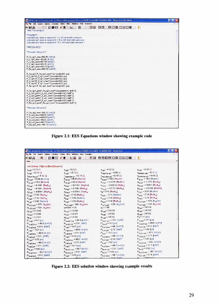
To develop a model in EES, sets of equations and variable definitions are entered in the
'Equations Window'. Figure 2.1 shows a picture of the 'EquationsWindow'
showing an
example of code. Utilizing a'Solve'
button, the equations are solved using the information
given, and solutions can be viewed in the 'Solutions Window'. The solutions window is
shown in Figure 2.2. There is also a 'FormattedEquations'
window where equations can be
checked in a more readable fashion. The 'DiagramWindow'
allows the user to create a
schematic of the system for visualization. Inputs can be added to this diagram such that a
user can change the input right from the diagram screen and recalculate a solution. More
information on EES can be found at fchart.com
28
** Ffe E* Search Otftons CafculMB T-sUm Plots Widows Help Eianplas
l-^-_^_^_U_BfiBU_Ci
&H:^;'
| iQio. / \u\ m 1Isln'
nm sjninnjisiDBi i ?
""AHU Fan Arietysis
NOTE***
subscnplspl relarsto setpoinl 1 1 in WCductstaiic pressure
subscnpi sp2 refers to oet pomi 2. 1 .25in, WC dud sialic pressure
subscript sp3 refers lo set pomi 3. 1 .5 in. WC dud static pressure"
"PRESSURES"
"Pressure. Set point1"
P_lo_spl_inwc40S ?B{mH20}P 2 spl inwc-405.96 {mH20}P_3.8p1Jmvci407.783 {inH20>P_4_epl_inwr>406 20-[inH2O}P_5_spljnwc-106733 pnH2QJP_5a_8p1_inwc-406 733 f>nH20>
P_1 o_sp1 -P_1Q_spl_inwc"
ConvertfinH20. psi)
P_2_sp 1 "P_2_sp 1Jnwc"
Conv8rt[inH20. psi)P_3_spl -P_3_spl Convart(inH20. psi)P_4_spl-P_1_sp1Jnwc*CorrwertCinH20. psi)P_5_sp1 -P_5_sp1 Corrvert(mH20, psi)
P_5a_5pl"P_5o_sp1_im*c*Convert(inH20.psi)
P_l e_spl_psf-P_l e_spljnwc"
Conuart(mH20. lbfflt"2)
P_2_5p1jDsr-P_2_spl_irrwc-Convert(inH20.lbVfl'-2)P_3_8pl_psr-P_3_epl_inwc*Convert^nH20.Miff2)P_4_sp1 J3sfP4_&pl
Jnwc"
Convert(inH20, Ibl/ff2)
P_5_sp1_p3^P_5_&p1J/wcJ"Convert(inH20.lblAl'%2)P_5Q_8p1_psf-P_5o_ap1jnwc*Canv8rt(inH20. Ibf/lt"2)
"Pressure. Set point2M
P la sp2 inwc-106.79{inH2O}P_2_sp2_irrwc-405.93 {inH20}P_3_sp2jnwc-406.033 {mH20>P A sp2 inwc=40e.20{inH2O>P_5_8p2_inwc-40G 733{lnH20}P_5a_sp2_mwc406 733{inM20}
Figure 2.1: EES Equations window showing example code
*** Ffc fdl Search Options Ofculdto Tabtes Hots Windows Help Eiamples
rfAHU 1 6JAN06, EES rSoUjliliriJ
_ 5 X
&:&! IN i&Hiaivi M@ m m H BBSSDIDSDi j ?
Man [
Unit Settings: [P]/[psia]/nbm/[degrees'
urt-SMSH 8.SP2-13.5H .jrt-naH ss,pi 60.05 [-]
e.^2 -6318 H wa-K.i3H ltelUTnlsn.it.1" 51 2 H 1rumlan.2-'l033[-]
lietuntoutLj-H02 H WW-..* 60l-l 1hwW.tl.p2" 63 87 H 1=opIvI,jp3 -6565[-]
Eijpl 50.66 ptu/min] r-ijp2- 95.85 (BUVmin] E^^j -1065 [Btu/min] E*l -159 2[Bt.iA.iin)
Ed,w2-|7"2P,u'nl ^dssp3-1908Plu/mi"] Briwi- -0 1 729 [Btu/lbm] eri2--01773 Plu',bnO
el2.q>3 -,e'19 P**^ el3tp, --O.01115 [Btu/lbm] e0tp2- 0.006139 [Blu/lbJ ensp -0.O2911pu^bJ
e,4:p1* -0 1 084 [Btu/lbm] 0Ujp2 --0109B [Btu/lbJ eBUp3 --0H23 [EJ/lbJ el5jpt 'tl5'99 [Btu/lbm]
el5.!p2 -0 05811 [Bco/lbJ el5oJ -0-0581 9 [Btu/lbJ h-21 51 [Btu/lbJ h^,- 26 91 [Blu/lbm]
h2*>2" 27 9 Ptu'lbtnl h2,*p3
" 27"9 WbrJ h3l "2719 [Btu/lbm] h3^- 27.39 [Btu/lbJ
h33p3-27 83[BtU/1b,J n!pl "33 56 [Btu/lbm] h4^2.33 41[Btu/lbn| (14^3.33 35 pu/lbj
h5*>1" 33 E5 PVlbm] h^j- 33.56 [Blu/lbJ "5.0,3
" 33 [Btu/lbJ "tl3l-1508 fV")
mB^2"1575 Pbm'mm] m.2.34D3" 1 E65 Pb>n] "! "13M Pb>in! H5^-I Pbn/)
^.^pS"1560 [lb>"n] percent = 100 4.0- D Q06 ^,.0.01228
+2^2-0.01215 fep3-001266 ?3jp1- 0.01 226 +3^2-0.01215
4H.P3-0.0126S ?4JP, -0.01371 +)Jp2-0 01362 +,^3-0 01352
4,, -0.01371 ?5^- 0.01 362 ?5^-0 01352 ptt- 11.7 ipsa
PlMrt"'W Plwlj.-*6-8^20) pipi^-2"B l'w/h2] PWWM
Pit*-wi!"Haii PkwAoX -2"6 I'M"2! Pw-K'H Plw^n-c-4"88!"*20]
Plp3( '8116 Pblflfl Pj^,- 14.67 [psi] P2..p1>,^-106P''H2O) P2t.cf2"2 P^2!
P202- 14.67 [psi] P2.m^>=" "5 9 f'nH2] PZ.P2JU.-21'2 PW'I P2.3-15[psi]
P2.*l**- 105.9 [inH20] P2,3,.ZH1 W2] P3tpl-H73[p5,l P3.pbn-7-8['"H2]
p3.i,i"2121 l"*2! P3<w2-H.71 [P*l] P3.w2Jc-PnH20] Ps^p^'2'23 l|bvt,2l
P3Jp3-H?5[p.a P3jp3i- 10B.3 PnH20] Pa^fljrf-^IIIWW P,^,, -14.67 [psi]
P^iw-^^nHZO] Pfl^i^-2113 M*2! P4j|J2-14.67[psi] P4jpie-m6.2PnH20]
P.^l"2"3 [iw!l P4jp3-H.67[Pi] P^3in.-B.2[lnH20J Pwrt'""!^
PsMfl-MMW] P5i.,lJn-6.7PnH20] P^piwC2"6 [W2! P5,JBJ-H-69[PSI1
P5W!**,-H6.7 D"H2O0 Pswapa 2,1B fiw2l Pswps-'IMIp5'] P5.Jp3T-7[|*l20l
Psuvajri -2116 l"5""2!
_fi nKICg (nnl
PiBl- 11.69 [psi]_E
'nr-- 7 BayflQ]
P5.,plJn-?[l"H20]
l: - au nhta2l
P5..P1.BC2'16 Pb^
Figure 2.2: EES solution window showing example results
29
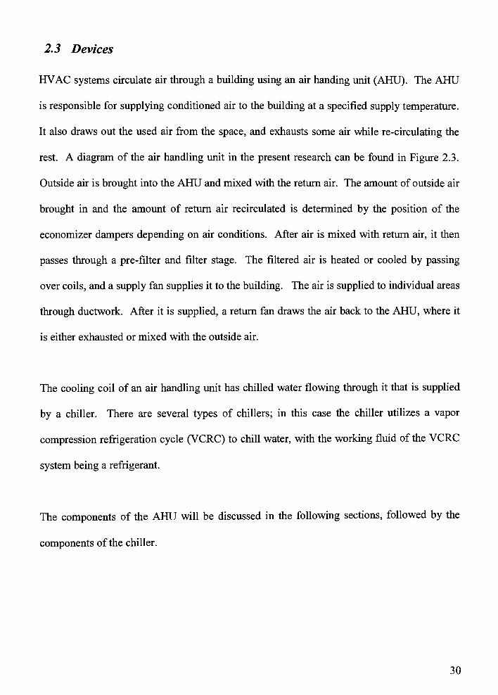
2.3 Devices
HVAC systems circulate air through a building using an air handing unit (AHU). The AHU
is responsible for supplying conditioned air to the building at a specified supply temperature.
It also draws out the used air from the space, and exhausts some air while re-circulating the
rest. A diagram of the air handling unit in the present research can be found in Figure 2.3.
Outside air is brought into the AHU and mixed with the return air. The amount of outside air
brought in and the amount of return air recirculated is determined by the position of the
economizer dampers depending on air conditions. After air is mixed with return air, it then
passes through a pre-filter and filter stage. The filtered air is heated or cooled by passing
over coils, and a supply fan supplies it to the building. The air is supplied to individual areas
through ductwork. After it is supplied, a return fan draws the air back to the AHU, where it
is either exhausted or mixed with the outside air.
The cooling coil of an air handling unit has chilled water flowing through it that is supplied
by a chiller. There are several types of chillers; in this case the chiller utilizes a vapor
compression refrigeration cycle (VCRC) to chill water, with the working fluid of the VCRC
system being a refrigerant.
The components of the AHU will be discussed in the following sections, followed by the
components of the chiller.
30

ExhaustAir
Economizer
Outside Air
Return*
Air
Return Fan
Heating CoolingCoil Coil SupplyFan
SupplyAir
Filter
Figure 2.3: Air Handling Unit Diagram
2.3 . 1 Air Handling Unit Coils
The coils provide a means for heating and cooling the mixed air before it is supplied to the
building. The air supply passes over the heating or cooling coil and heat transfer occurs
between the air and the coil. The season dictates which coil is in primary operation. Cold
temperatures require heating from the heating coil, while warm temperatures require cooling
from the cooling coil. The heating and cooling coils act as heat exchangers in the AHU
system as the air is passed over the coils. The heating and cooling coil can be seen in Figure
2.3.
2.3.1.1 Cooling Coil
When the supply air is warmer than the supply airtemperature set point, the cooling coils are
activated. Chilled water pumps circulate water from a chillers evaporator through the
31
cooling coils to cool the air as it flows over the coils. The cooling of humid air causes
condensation, so a drip pan and drain are needed under the cooling coil. This prevents
standing water that can damage components and allow mold and other microorganisms to
grow and circulate through the air system. When outside air temperatures permit, more cool
air is brought into the system for free cooling. This function is controlled by the economizer,
and means the air does not need to be conditioned and can serve as a natural form ofcooling.
Using free cooling minimizes energy consumption because little or no energy is required to
heat or cool this air. An additional diagram of the cooling coil, including sensor locations,
can be found in Figure 2.4.
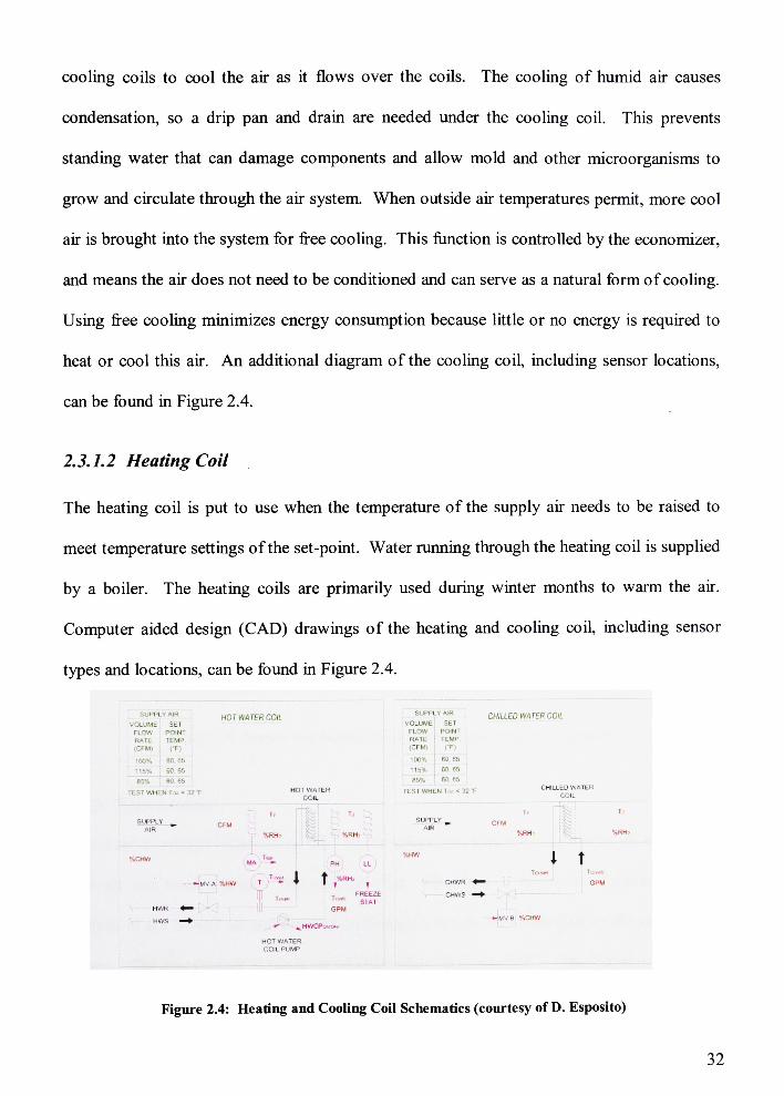
2.3.1.2 Heating Coil
The heating coil is put to use when the temperature of the supply air needs to be raised to
meet temperature settings of the set-point. Water running through the heating coil is supplied
by a boiler. The heating coils are primarily used during winter months to warm the air.
Computer aided design (CAD) drawings of the heating and cooling coil, including sensor
types and locations, can be found in Figure 2.4.
SUPPLY am
VOLUME sei
Fl -'.-. POINT
RATE 1E1W
' 1 m
S3% 6C 3S
Eft '.
so es
test whe N To* < 12 T
HOT WATER COILsupply AM
, CHILLED WATER COILVOLUME SEI
FLOW POINT
RAIL TEMP
|CFM) IT]
100% 60 8b
lv:. 60 65
80% 60 6b
HOI WAFER TEST WHEN 1 o. 12 TCHILLEPKMEH
COIL COIL
SUPPLY
AIR
1
V,RH
A -PH LL
t 1t' X t *RHtJmV-A W T - ? I CHWR
FREEZE CHVl'SI... TM
9[M
HWR 4^ GPM
HVS -^r*
.,HWCPo/.t>*
HOT WATER
COIL PUMP
T< ij
%RH' %RHi
i tTi *w
| GPM
M B SCMW
Figure 2.4: Heating and Cooling Coil Schematics (courtesy ofD. Esposito)
32
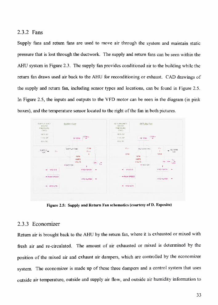
2.3.2 Fans
Supply fans and return fans are used to move air through the system and maintain static
pressure that is lost through the ductwork. The supply and return fans can be seen within the
AHU system in Figure 2.3. The supply fan provides conditioned air to the building while the
return fan draws used air back to the AHU for reconditioning or exhaust. CAD drawings of
the supply and return fan, including sensor types and locations, can be found in Figure 2.5.
In Figure 2.5, the inputs and outputs to the VFD motor can be seen in the diagram (in pink
boxes), and the temperature sensor located to the right of the fan in both pictures.
SUPPL DUC
STATE
SUPPLY FAN
PRESSIFRE
rwq
D'
SF CFM.CPMs-
B5 - SI'
SUPPLY _
R
SUPPLY FAN
RPM
AMPS
CFM
Ptwi
r
VOLTS DA -
MOTOR
r
VFD SlS jPROF BACH, "
-RUN SPEED
VFO ALARM -
- VFDILCK
RETURN DUC1
STATIC
PRESSURE
1"WC>
;!.',"
. i p
RETURN FAN
H VFDS.S
"RUN SPEED
CFM-u
KF CFM -
HLIUKNFAN PlS
KRH
Kfc'UKN
AMPS
VOLTS
-MOTOR
R<*
T
HH -
%RH
FKQF8ACK
UFO ALARM -
Figure 2.5: Supply and Return Fan schematics (courtesy ofD. Esposito)
2.3.3 Economizer
Return air is brought back to the AHU by the return fan, where it is exhausted or mixed with
fresh air and re-circulated. The amount of air exhausted or mixed is determined by the
position of the mixed air and exhaust air dampers, which are controlled by the economizer
system. The economizer is made up of these three dampers and a control system that uses
outside air temperature, outside and supply air flow, and outside air humidity information to
33
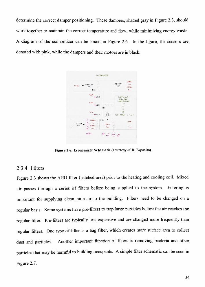
determine the correct damper positioning. These dampers, shaded gray in Figure 2.3, should
work together to maintain the correct temperature and flow, while minimizing energy waste.
A diagram of the economizer can be found in Figure 2.6. In the figure, the sensors are
denoted with pink, while the dampers and their motors are in black.
ECMMZER
CFM
RETURN K.
AIH%RH*
CFMm "EXHAUST
AEK
NC
WiA
-MDC.
%MA
-MOB
IfcOA
-MOA
SUPPLr A*R
St f POINT
TEMPER/'-TURE
i I i
65
TESTWHEN T*m<32T
crM -
T
\ - y ->
H.O
r
OUTSIDE_
AIR
O CtM .. H
To.
F%RH*
M tv
c '
CFM.
CFMo. MP -
ma ..
P<"Dm
Figure 2.6: Economizer Schematic (courtesy ofD. Esposito)
2.3.4 Filters
Figure 2.3 shows the AHU filter (hatched area) prior to the heating and cooling coil. Mixed
air passes through a series of filters before being supplied to the system. Filtering is
important for supplying clean, safe air to the building. Filters need to be changed on a
regular basis. Some systems have pre-filters to trap large particles before the air reaches the
regular filter. Pre-filters are typically less expensive and are changed more frequently than
regular filters. One type of filter is a bag filter, which creates more surface area to collect
dust and particles. Another important function of filters is removing bacteria and other
particles that may be harmful to buildingoccupants. A simple filter schematic can be seen in
Figure 2.7.
34
MIXEU d
AIR'"''
*
Figure 2.7: Filter Schematic (courtesy ofD. Esposito)
2.3.5 Electrical Components and Controls
The air handling unit contains several electrical parts such as temperature sensors, fan
motors, pressure sensors, and controls. Some sensors installed in air handling unit are
measured and viewed on WebCTRL. WebCTRL is the web-based control system used to
monitor and control the AHU and its subcomponents. The VFD fan motor unit requires three
phase power in which voltage can exceed 200 volts. Due to electrical currents ability to flow
between the phases, a ground neutral wire is not necessary to complete the circuit and
therefore saves on installation costs.
The automatic two-position control device opens or closes the circuits whenever the
measured variable exceeds the set point of the device. For example, a high pressure safety
switch opens the supply fan operating circuit when discharge pressure (measured variable)
rises above the safety switch set point. In contrast, when the pressure drops below the set
point, the switch closes and allows the supply fan to resume the operation. The variable
35
point with a two-position device would be efficient within 4% from the set point. There are
modulating thermostats in the building to control the variable air volume (VAV) boxes for
each zone, and regulate the comfort temperature for consumers. An analog device generates
varying output signal that shows the magnitude of the process control point and helps reduce
the consumption of energy.
The controller is a device in a control loop that receives the output signal from the sensor,
compares the process control point with the set point, calculates the difference, and generates
an output signal that controls the flow of energy of an air handling unit process. The energy
flowing into the process will maintain the controlled variable at its set point. The controller
is vital for the air handling unit to prevent damages when there is any situation that allows
the emergency power mode to be switched on.
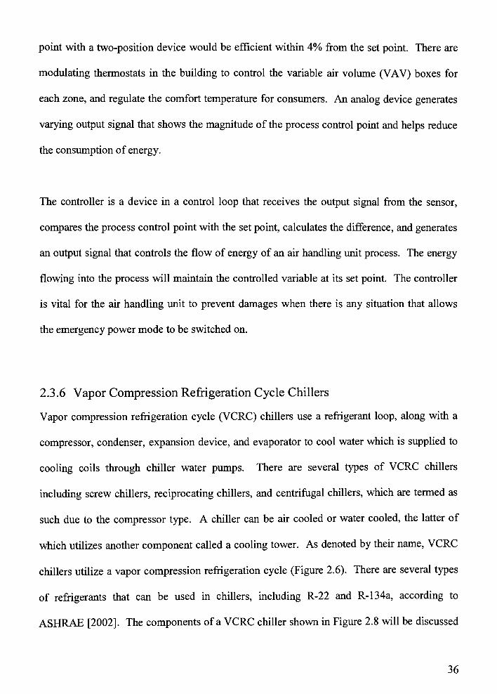
2.3.6 Vapor Compression Refrigeration Cycle Chillers
Vapor compression refrigeration cycle (VCRC) chillers use a refrigerant loop, along with a
compressor, condenser, expansion device, and evaporator to cool water which is supplied to
cooling coils through chiller water pumps. There are several types of VCRC chillers
including screw chillers, reciprocating chillers, and centrifugal chillers, which are termed as
such due to the compressor type. A chiller can be air cooled or water cooled, the latter of
which utilizes another component called a cooling tower. As denoted by their name, VCRC
chillers utilize a vapor compression refrigeration cycle (Figure 2.6). There are several types
of refrigerants that can be used in chillers, including R-22 and R-134a, according to
ASHRAE [2002]. The components of a VCRC chiller shown in Figure 2.8 will be discussed
36
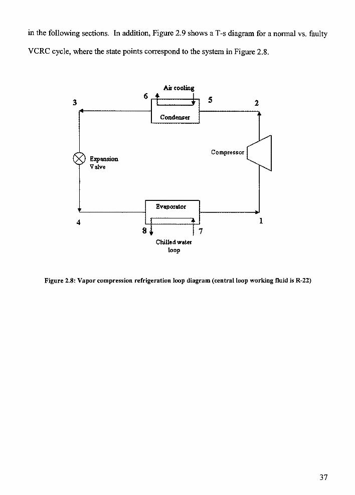
in the following sections. In addition, Figure 2.9 shows a T-s diagram for a normal vs. faulty
VCRC cycle, where the state points correspond to the system in Figure 2.8.
Air cooling
H 1
Condenser
Expansion
Valve
Compressor
Evenorator
nChilledwater
loop
Figure 2.8: Vapor compression refrigeration loop diagram (central loop working fluid is R-22)
37
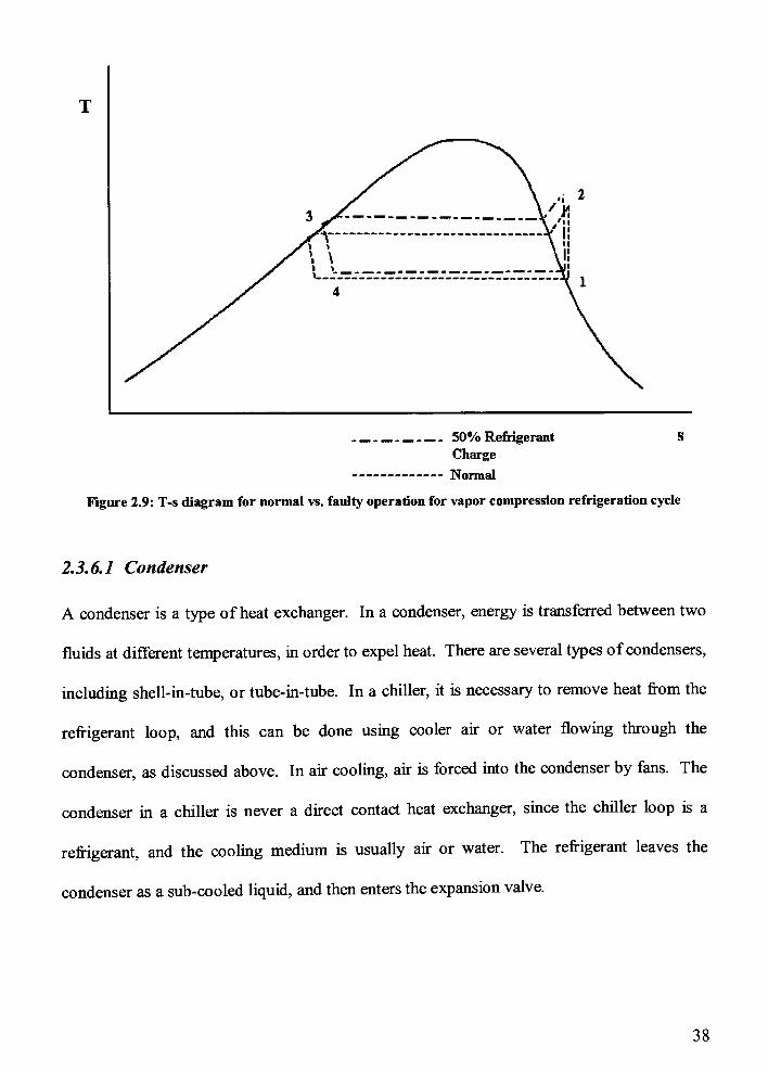
50% Refrigerant
Charge
Normal
Figure 2.9: T-s diagram for normal vs. faulty operation for vapor compression refrigeration cycle
2.3.6.1 Condenser
A condenser is a type ofheat exchanger. In a condenser, energy is transferred between two
fluids at different temperatures, in order to expel heat. There are several types ofcondensers,
including shell-in-tube, or tube-in-tube. In a chiller, it is necessary to remove heat from the
refrigerant loop, and this can be done using cooler air or water flowing through the
condenser, as discussed above. In air cooling, air is forced into the condenser by fans. The
condenser in a chiller is never a direct contact heat exchanger, since the chiller loop is a
refrigerant, and the cooling medium is usually air or water. The refrigerant leaves the
condenser as a sub-cooled liquid, and then enters the expansion valve.
38
2.3.6.2 Expansion Valve
An expansion valve exists in a refrigeration loop between the condenser and evaporator. The
purpose is to allow the sub-cooled liquid to expand to release the pressure created by the
compressor. This is often modeled as a throttling process. The exiting refrigerant is atwo-
phase liquid-vapor mixture. Upon leaving the expansion valve, refrigerant flows to the
evaporator, as shown in Figure 2.8.
2.3.6.3 Evaporator
Like the condenser, the evaporator is also a heat exchanger. The evaporator, shown in Figure
2.8, operates on the low pressure side of the refrigeration loop and takes the heat out of the
water returning from the coil. The evaporator is a shell-in-tube heat exchanger, where the
refrigerant runs through the inner tube and the chilled water runs through the shell. Upon
entering the evaporator, the refrigerant is a two-phase, liquid-vapor mixture. The heat being
added through the evaporator causes the refrigerant to vaporize. Refrigerant then enters the
compressor as super heated vapor.
2.3.6.4 Compressor
A compressor serves an important role in a chiller. Compressors are used to raise the
pressure of the refrigerant, using compression. Upon leaving the compressor, the refrigerant
is a superheated vapor. Compressing the refrigerant causes the temperature and pressure to
rise significantly. Electrical work must be put into the compressor for this change to occur.
After being compressed, the refrigerant again enters the condenser.
39
2.3.7 Summary
The devices that make up the AHU and VCRC chiller will be studied in detail using both the
first and second laws of thermodynamics in the following chapters. The AHU devices
(supply and return fans, heating and cooling coil, and economizer) will be analyzed in
Chapter 4, and the VCRC chiller devices (compressor, condenser, and evaporator) will be
analyzed in Chapter 5. First, a detailed look at the data collected from these devices is
presented in Chapter 3.
40
3 Experimental Research
Data was collected for an air handling unit in conjunction with a Senior Design I & II (0304-
630/631) capstone design project by a group of senior mechanical and electrical engineering
students including the author. The goal of the project was to create a retrocommissioning
(RCX) test plan for Facilities Management Services (FMS) at the Rochester Institute of
Technology campus, and then implement the plan on an air handling unit in one of the
campus'
mechanical rooms. The student team developed a preliminary RCX test plan which
was used to begin testing. Upon completion of data collection, the data was analyzed using
thermodynamic equations developed by the team. The analysis included a first and second
law analysis of the key components of the system. Results were discussed with the project
sponsor, FMS, and recommendations were made for system improvements. The testing
procedure used for collecting the AHU data will be outlined in the following sections,
followed by a section describing the collected data.
After the AHU sections, VCRC chiller data collection is described. Data was collected for a
VCRC chiller as part of past research conducted at the University of Colorado which
developed an automated fault detection and diagnosis (FDD) method to detect several
different types of chiller fault cases. These faults, including refrigerant leakage, oil leakage,
fan fouling, among others, were imposed on the chiller equipment and an arrayof data points
were collected to monitor and train the automated system to detect these faults. This
previously collected data is utilized in this research to develop and validate a chiller model
which will be used to determine thermodynamic performance of the chiller under normal as
well as fault operation.
41
Section 3.1 and 3.2 will discuss data collection and specific data for the AHU, while section
3.3 and 3.4 will discuss data collection and specific data for the VCRC chiller.
3.1 TestingProcedureforAirHandling Unit
Data was collected for an AHU with the help of a team from Facilities Management. Before
testing began, a balancing agent was hired to verify proper testing procedures and obtain
baseline data for use in sensor verification. Data was collected over a several week period in
the months ofMarch and April of 2005. The time period is significant due to the outside air
temperatures associated with the season in upstate New York, and the amount of heating and
cooling necessary for the given temperatures. The testing procedure includes different types
of tests, including sensor verification, system control response, pre-functional tests, and
functional tests. Sensor verification is preformed to ensure data collecting using sensor
values is accurate. System control response testing is necessary to verify the control system
is operating properly. Pre-functional tests check for operational performance of the system
components, and do not involve data collection. Finally, data is collected through a series of
functional tests performed for each component. A flow chart of the general
retrocommissioning steps is in Figure 3.1.
42
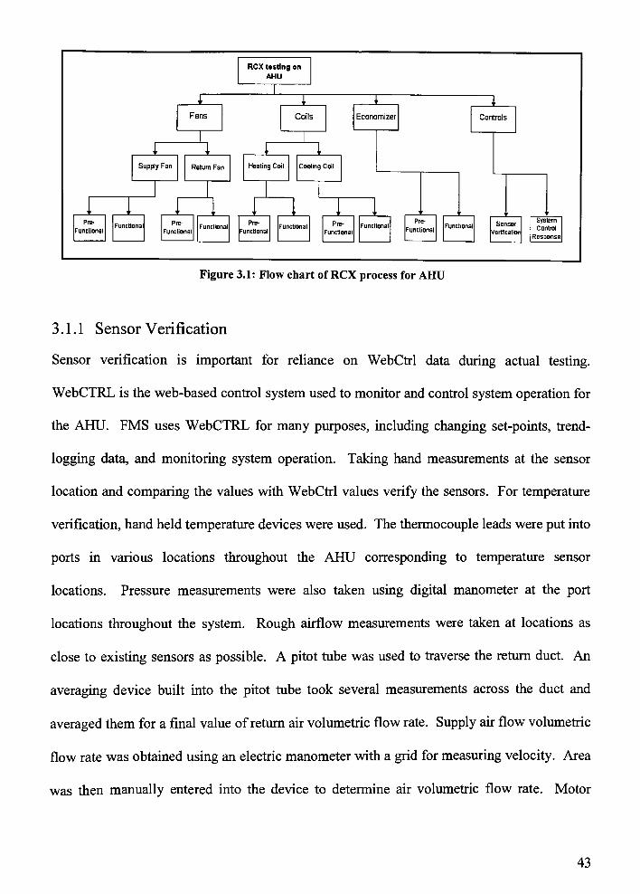
RCX tasting en
AHU
Fans Coils Economizer
Pre-
Functlonai
Supply Fan Return Fan
Pre-
Functional
Healing Coil Cooling Coit
Pre-
Functlona!
Controls
Pre-
Functional
Pre-
FunctionalSensor
Verification
System
Control
Response
Figure 3.1: Flow chart ofRCX process for AHU
3.1.1 Sensor Verification
Sensor verification is important for reliance on WebCtrl data during actual testing.
WebCTRL is the web-based control system used to monitor and control system operation for
the AHU. FMS uses WebCTRL for many purposes, including changing set-points,trend-
logging data, and monitoring system operation. Taking hand measurements at the sensor
location and comparing the values with WebCtrl values verify the sensors. For temperature
verification, hand held temperature devices were used. The thermocouple leads were put into
ports in various locations throughout the AHU corresponding to temperature sensor
locations. Pressure measurements were also taken using digital manometer at the port
locations throughout the system. Rough airflow measurements were taken at locations as
close to existing sensors as possible. A pitot tube was used to traverse the return duct. An
averaging device built into the pitot tube took several measurements across the duct and
averaged them for a final value of return air volumetric flow rate. Supply air flow volumetric
flow rate was obtained using an electric manometer with a grid for measuring velocity. Area
was then manually entered into the device to determine air volumetric flow rate. Motor
43

rotation speed values (RPM) were taken with hand measurements using a tachometer at 30
and 60 Hz (half and full speed, respectively). The corresponding CFM was also taken to
develop RPM relationships. Once two RPM values were established with corresponding
frequencies, the frequency can be read off the variable frequency drive (VFD) for any speed
and the corresponding RPM can be calculated. In most cases, several readings were taken
for each data point to establish an average. A section of the general AHU RCX test is shown
in Figure 3.2. The'P'
and'F'
check boxes represent pass and fail, respectively. The details
of the system control response portion are discussed in Section 3.1.2.
System Control Response
Item Tested Control FResponse Alarm Response
SF S/S H/O/A & Schedule oP dF nP gF
SF Proof cP a F ? P ? F
SF Static Ctrl SP SP Actual aP dF
SF Safety Interlock dP n F dP oF
SF Freezestat dP dF qP oF
SF Fire Interlock rP nF dP nF
RF S/S H/O/A & Schedule dP dF dP nF
RF Proof nP dF dP nF
RF Static Ctrl SP SP Actual dP rF
RF Safety Interlock oP n F nP nF
RF Freezestat dP dF oP cF
RF Fire Interlock dP dF nP nF
Field Calibration Check
Item Tested TestResults Alarm Response
OA Sensor - Temp cP nF dP nF
RA Sensor - Temp oP n F aP nF
MA Sensor - Temp oP nF nP n F
DA Sensor - Temp nP dF nP nF
DA Sensor - Pressure dP dF ? P oF
Filter Proof Sensor gP dF dP dF
Pump Proof Sensor ? P d F dP ? F
Figure 3.2: Portion of general AHU RCX test including system control response and field calibration
check
44
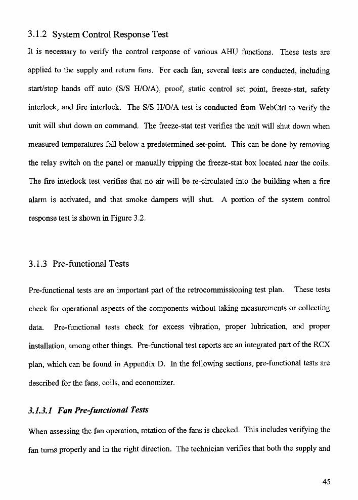
3.1.2 System Control Response Test
It is necessary to verify the control response of various AHU functions. These tests are
applied to the supply and return fans. For each fan, several tests are conducted, including
start/stop hands off auto (S/S H/O/A), proof, static control set point, freeze-stat, safety
interlock, and fire interlock. The S/S H/O/A test is conducted from WebCtrl to verify the
unit will shut down on command. The freeze-stat test verifies the unit will shut down when
measured temperatures fall below a predetermined set-point. This can be done by removing
the relay switch on the panel or manually tripping the freeze-stat box located near the coils.
The fire interlock test verifies that no air will be re-circulated into the building when a fire
alarm is activated, and that smoke dampers will shut. A portion of the system control
response test is shown in Figure 3.2.
3.1.3 Pre-functional Tests
Pre-functional tests are an important part of the retrocommissioning test plan. These tests
check for operational aspects of the components without taking measurements or collecting
data. Pre-functional tests check for excess vibration, proper lubrication, and proper
installation, among other things. Pre-functional test reports are an integrated part of the RCX
plan, which can be found in Appendix D. In the following sections, pre-functional tests are
described for the fans, coils, and economizer.
3.1.3.1 Fan Pre-functional Tests
When assessing the fan operation, rotation of the fans ischecked. This includes verifying the
fan turns properly and in the right direction. The technician verifies that both the supply and
45
return fan do not have excessive noise and vibration. The cleanliness of the fan, motor, and
cage is observed. The motor and blower sheave condition are checked, and proper alignment
is also verified using a straight edge. The belts are examined for proper tension, and
evidence of wear and cracking. The fan and motor are checked for proper lubrication. The
technician verifies that the fans are not over- or under-lubricated. If any fan pre-functional
tests are included in a preventative maintenance (PM) schedule, the results are verified and
the date of the most recent PM test is noted. An example of the fan pre-functional checklist
can be found in Figure 3.3.
Fan Pre-functional Checklist
Item TestedPass/Fail
NotesSupply Return
Rotation Pass Pass
Excessive Vibration Pass Pass Moderate Vibration
Excessive Noise Pass Pass
Cage Cleanness Pass Pass
Motor Sheave Condition Pass Pass
Blower Sheave Condition Pass Pass
Sheave Alignment Pass Pass
Belt Tension Pass Pass
Belt Cracking Pass Pass Beits Recently Replaced
BeltWear Pass Pass
Fan Lubrication Completed Pass Pass Wiped Off Excess Grease
Motor Lubrication Completed Didn't test
Figure 3.3: Portion of Fan Performance RCX test showing pre-functional checklist
3.1.3.2 CoilPre-functional Test
The coil pre-functional test checklist from the coil performance test can be found in Figure
3.4. Coils are checked for cleanliness and damage. This includes bent and dented fins, or
damage to the incoming coils. The coil piping insulation should be intact. The coil strainer
is checked for cleanliness. This may take time, and could already be part of a PM schedule.
The coil pump operation is also checked. This may be obvious for coils currently in use, and
46
would need to be verified for coils not in season. The valves are checked for leaking when
they are closed, and it is verified that the valve packing and the pneumatic diaphragm are not
leaking, where applicable. The coil fittings are checked to verify there is no leakage. No
standing water can be present under the coil, and any fungal growth in the area is
unacceptable. For the cooling coil, the condensate area is visually checked. The condensate
drain pan function is checked for proper operation, and the pan is clean and free from leaks.
There must not be evidence of cool water blow off. Cool water blow offwould be evident if
there was water on the supply fan or in the area downstream from the cooling coil or in the
supply duct. The coil control valve is checked for open/close test, fail-safe test, and that it
maintains target. For the heating coil, performing a freeze stat test can satisfy these.
47
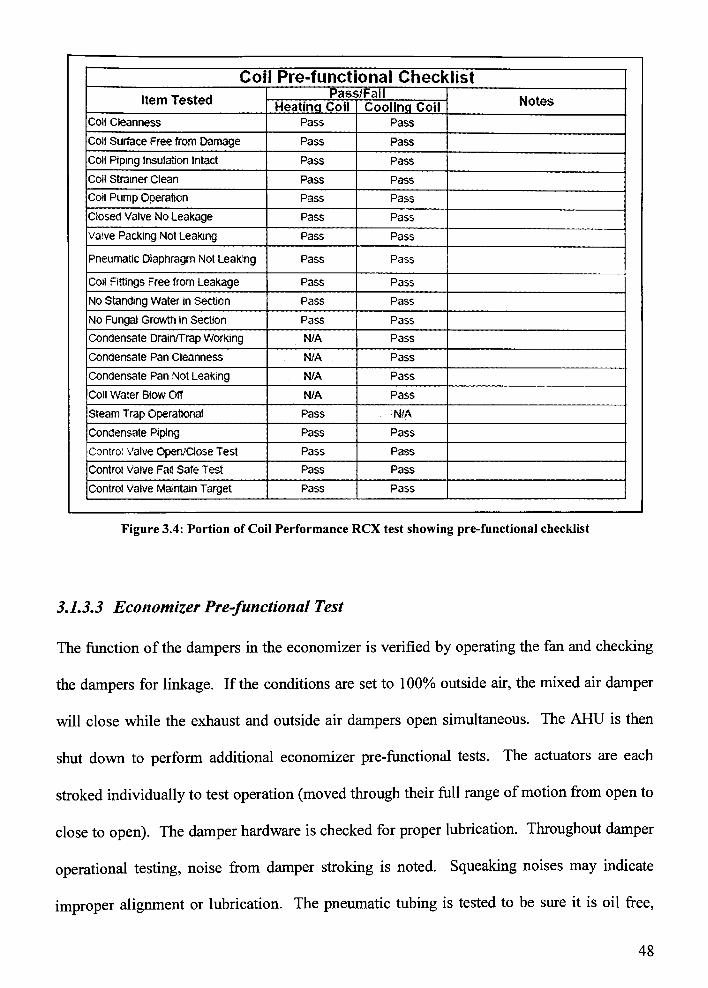
Coil Pre-functional Checklist
Item TestedPass/Fail
NotesHeatinq Coil Coolinq Coil
Coil Cleanness Pass Pass
Coil Surface Free from Damage Pass Pass
Coil Piping Insulation Intact Pass Pass
Coil Strainer Clean Pass Pass
Coil Pump Operation Pass Pass
Closed Valve No Leakage Pass Pass
Valve Packing Not LeaKing Pass Pass
Pneumatic Diaphragm Not Leaking Pass Pass
Coil Fittings Free from Leakage Pass Pass
No Standing Water in Section Pass Pass
No Fungal Growth in Section Pass Pass
Condensate Drain/Trap Working N/A Pass
Condensate Pan Cleanness N/A Pass
Condensate Pan Not Leaking N/A Pass
CoilWater Blow Off N/A Pass
Steam Trap Operational Pass N/A
Condensate Piping Pass Pass
Control Valve Open/Close Test Pass Pass
Control Valve Fai Safe Test Pass Pass
Control Valve Maintain Target Pass Pass
Figure 3.4: Portion ofCoil Performance RCX test showing pre-functional checklist
3.1.3.3 Economizer Pre-functional Test
The function of the dampers in the economizer is verified by operating the fan and checking
the dampers for linkage. If the conditions are set to 100% outside air, the mixed air damper
will close while the exhaust and outside air dampers open simultaneous. The AHU is then
shut down to perform additional economizer pre-functional tests. The actuators are each
stroked individually to test operation (moved through their full range ofmotion from open to
close to open). The damper hardware is checked for proper lubrication. Throughout damper
operational testing, noise from damper stroking is noted. Squeaking noises may indicate
improper alignment or lubrication. The pneumatic tubing is tested to be sure it is oil free,
48
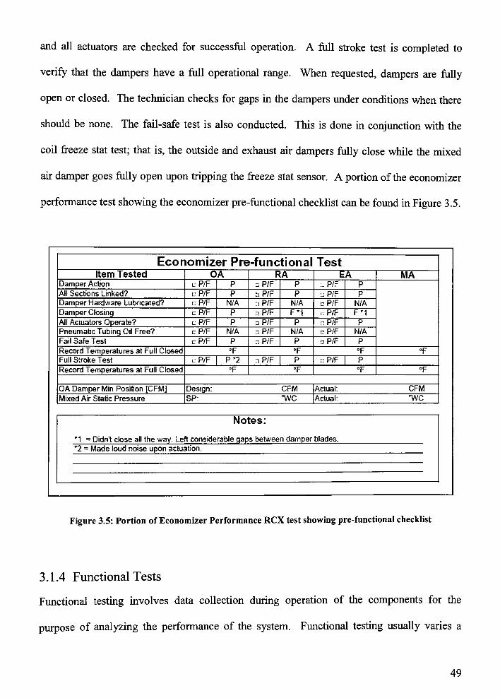
and all actuators are checked for successful operation. A full stroke test is completed to
verify that the dampers have a full operational range. When requested, dampers are fully
open or closed. The technician checks for gaps in the dampers under conditions when there
should be none. The fail-safe test is also conducted. This is done in conjunction with the
coil freeze stat test; that is, the outside and exhaust air dampers fully close while the mixed
air damper goes fully open upon tripping the freeze stat sensor. A portion of the economizer
performance test showing the economizer pre-functional checklist can be found in Figure 3.5.
Economizer Pre-functional TestItem Tested OA RA EA MA
DamperAction cP/F P iuP/F P L.P/F P
All Sections Linked? cPIF P aP/F P LiP/F P
Damper Hardware Lubricated? r:P/F N/A aP/F N/A cP/F N/A
Damper Closing cP/F P aP/F F*1 cP/F F*1
All Actuators Operate? lPIF P dP/F P -. P'F P
Pneumatic Tubing Oil Free? cP/F N/A nP/F N/A cP/F N/A
Fail Safe Test cP/F P nP/F P nP,'F P
Record Temperatures at Full Closed F F F F
Full Stroke Test cP/F | P'2 r,P/F | P ? P/F | P
Record Temperatures at Full Closed F F F F
OA Damper Min Position [CFM] Design: CFM Actual. CFM
Mixed Air Static Pressure SP: "WC Actual: "WC
Notes:
"1 = Didn't close all the way. Left considerable gaps between damper blades.
*2 = Made loud noise upon actuation.
Figure 3.5: Portion ofEconomizer Performance RCX test showing pre-functional checklist
3.1.4 Functional Tests
Functional testing involves data collection during operation of the components for the
purpose of analyzing the performance of the system. Functional testing usually varies a
49
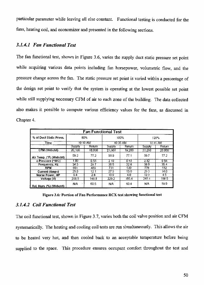
particular parameter while leaving all else constant. Functional testing is conducted for the
fans, heating coil, and economizer and presented in the following sections.
3.1.4.1 Fan Functional Test
The fan functional test, shown in Figure 3.6, varies the supply duct static pressure set point
while acquiring various data points including fan horsepower, volumetric flow, and the
pressure change across the fan. The static pressure set point is varied within a percentage of
the design set point to verify that the system is operating at the lowest possible set point
while still supplying necessary CFM of air to each zone of the building. The data collected
also makes it possible to compute various efficiency values for the fans, as discussed in
Chapter 4.
Fan Functional Test
% of Duct Static Press. 80% 100% 120%
Time 10:10AM 10:35 AM 10:45 AM
Supply Return Supply Return Supply Return
CFM (Webctrl) 20.100 18,6615 2 i ,000 19.200 22,266 26,866
Air Temp. (F> (Webctrl)59.2 77.2 58.9 77.1 59.7 77.2
A Pressure ("WC) 1.80 0.53 2 10 0 53 2.42 0.56
Frequency. Hz 34.5 297 36 5 32 8 38.9 35.4
RPM 691 4,39 731 539 778 582
Current (Amps) 25.5 12.1 27.5 130 29 3 14.0
Horse Power, HP 94 2.8 109 4.0 12.9 4.5
Voltage (V) 209.5 148.8 229 2 165.4 248.4 188.5
Rel. Hum. (%) (Webctrl)N/A 60.5 N/A 60.4 N/A 59.9
Figure 3.6: Portion ofFan Performance RCX test showing functional test
3.1.4.2 Coil Functional Test
The coil functional test, shown in Figure 3.7, varies both the coil valve position and air CFM
systematically. The heating and cooling coil tests are run simultaneously. This allows the air
to be heated very hot, and then cooled back to an acceptable temperature before being
supplied to the space. This procedure ensures occupant comfort throughout the test and
50
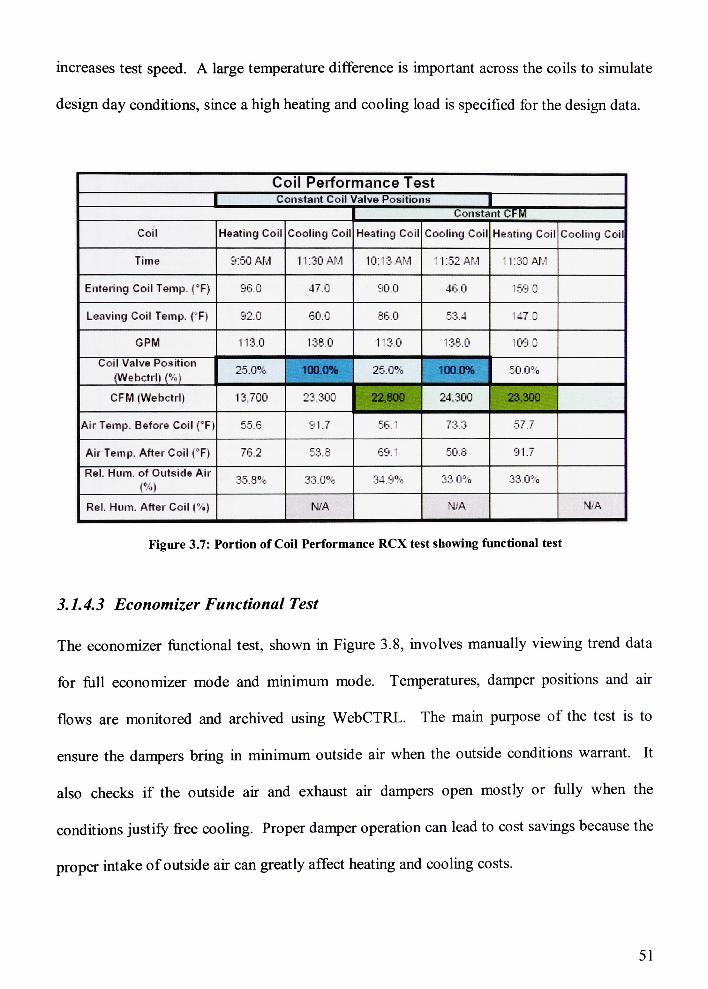
increases test speed. A large temperature difference is important across the coils to simulate
design day conditions, since a high heating and cooling load is specified for the design data.
Coil Performance Test
| Constant Coil Valve Positions jjConstant CFM
Coil Heating Coil Cooling Coil Heating Coil Cooling Coil Heating Coil Cooling Coil
Time 5:50 AM 11:30AM 10:13 AM 11:52 AM 11:30 AM
Entering Coil Temp. (F) 56.0 47.0 90.0 460 159 0
Leaving Coil Temp. (F) 92.0 60.0 86.0 53.4 U7 0
GPM 113.0 136.0 113.0 138.0 109 0
Coil Valve Position
(Webctrli {%)25.0% 100.0% 25.0% 100.0% 50.0%
CFM (Webctrli 13 700 23 300 22,800 24,300 23,300
Air Temp. Before Coil (F| 55.6 9 1 .7 56.'
73 3 57.7
Air Temp. After Coil (*F) 76.2 53 8 69.1 50.8 91.7
Rel. Hum. of Outside Air
(%)35 B% 33.0% 34.9% 33.0% 33.0%
Rel. Hum. After Coil (%) N/A N/A N/A
Figure 3.7: Portion ofCoil Performance RCX test showing functional test
3.1.4.3 Economizer Functional Test
The economizer functional test, shown in Figure 3.8, involves manually viewing trend data
for full economizer mode and minimum mode. Temperatures, damper positions and air
flows are monitored and archived using WebCTRL. The main purpose of the test is to
ensure the dampers bring in minimum outside air when the outside conditions warrant. It
also checks if the outside air and exhaust air dampers open mostly or fully when the
conditions justify free cooling. Proper damper operation can lead to cost savings because the
proper intake ofoutside air can greatly affect heating and cooling costs.
51
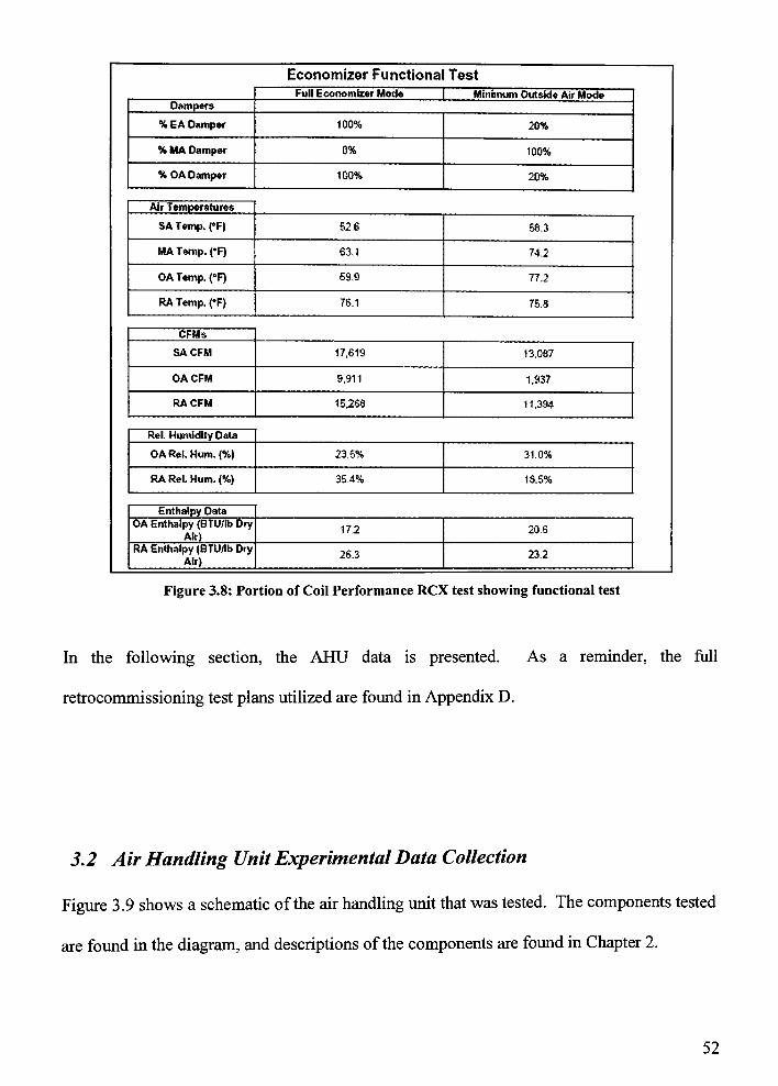
Economizer Functional Test
Full EconomizerMode | Minimum Outside Air Mode
Dampers
% EA Damper 100% 20%
% MA Damper 0% 100%
% OADamper 100% 20%
AirTemperatures
SA Temp. f>F) 52.6 58.3
MA Temp. fF) 63.1 74.2
OA Temp. (F) 59.9 77.2
RA Temp. (*F) 76.1 75.8
CFMs
SACFM 17,619 13.087
OACFM 9,911 1,937
RACFM 15,268 11,394
Rel. HumidityData
OARel.Hum.(%) 23.5% 31.0%
RA Rel. Hum. (%) 35.4% 18.5%
Enthalpy Data
OA Enthalpy (BTU/lb DryAir)
17.2 20.S
RA Enthalpy (BTUflb Dry
Air)26.3 23.2
Figure 3.8: Portion ofCoil Performance RCX test showing functional test
In the following section, the AHU data is presented. As a reminder, the full
retrocommissioning test plans utilized are found in Appendix D.
3.2 AirHandling UnitExperimentalData Collection
Figure 3.9 shows a schematic of the air handling unit that was tested. The components tested
are found in the diagram, and descriptions of the components are found in Chapter 2.
52
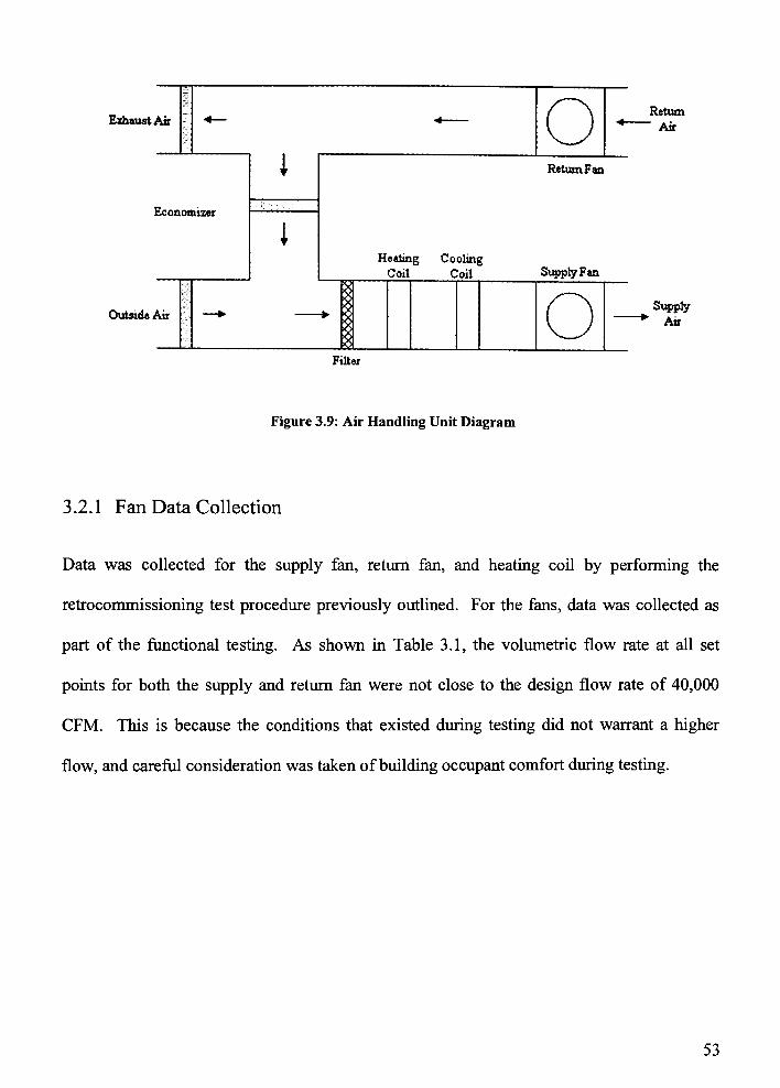
ExhaustAir
Economizer
OutsideAir
Return*
Air
ReturnFan
Healing CoolingCoil Coil SupplyFan
SupplyAir
Filter
Figure 3.9: Air Handling Unit Diagram
3.2.1 FanData Collection
Data was collected for the supply fan, return fan, and heating coil by performing the
retrocommissioning test procedure previously outlined. For the fans, data was collected as
part of the functional testing. As shown in Table 3.1, the volumetric flow rate at all set
points for both the supply and return fan were not close to the design flow rate of 40,000
CFM. This is because the conditions that existed during testing did not warrant a higher
flow, and careful consideration was taken ofbuilding occupant comfort during testing.
53
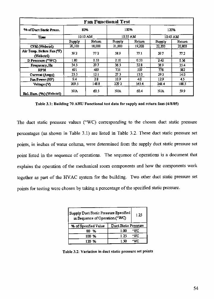
Fail Functional Test
% ofDuct Static Press. 80% 100% 120%
Time 10:10 AM 10:35 AM 10:45 AM
Supply Return Supply Return Supply Return
CFM (Webctrl) 20,100 18,000 21,000 19,200 22,200 20.80D
Air Temp.Before Fan (F)
(Webctrl)55.2 77.2 58.9 77.1 59.7 77.2
D Pressure ("WC) 1.S0 0.53 2.10 0.53 2.42 0.56
Frequency,Hz 34.5 29.7 36.5 32.8 38.9 35.4
RPM 691 489 731 539 778 582
Current (Amps) 25.5 12.1 27.5 13.0 29.3 14.0
Fan Power (HP) 9.4 2.8 10.9 4.0 12.9 4.5
Voltage (V) 203.5 143.8 229.2 165.4 248.4 188.5
Rel. Hum. (<W>) (Webctrl)N/A 60.5 N/A 60.4 N/A 59.9
Table 3.1: Building 70 AHU Functional test data for supply and return fans (4/8/05)
The duct static pressure values ("WC) corresponding to the chosen duct static pressure
percentages (as shown in Table 3.1) are listed in Table 3.2. These duct static pressure set
points, in inches of water column, were determined from the supply duct static pressure set
point listed in the sequence of operations. The sequence of operations is a document that
explains the operation of the mechanical room components and how the components work
together as part of the HVAC system for the building. Two other duct static pressure set
points for testing were chosen by taking a percentage of the specified static pressure.
SupplyDuct Static Pressure Specified
in Sequence ofOperation("WC)
1.25
% ofSpecifiedValue Duct Static Pressure
SD % 1.D0 "WC
100 % 1.25 "WC
12D % 1.50 "WC
Table 3.2: Variation in duct static pressure set points
54
According to Table 3.2, the specified duct static pressure from the sequence of operations
was1.25"
WC. Duct static pressure set points of1.00"
WC and1.50"
WC were also tested,
which represent 80% and 120% of the specified value, respectively.
3.2.2 Coil Data Collection
The heating and cooling coil tests were done simultaneously. Not enough information was
available to conduct a complete analysis on cooling coil data due to dilemmas with collecting
condensate flow rate; however, data was still taken during the testing phase. The collection
of the coil data successfully maintains occupant comfort because the air is first heated very
high by the heating coil, satisfying the heating coil test, and then cooled back to a typical
supply temperature by the cooling coil, satisfying the cooling coil test. Data collected while
conducting the heating and cooling coil testing can be found in Table 3.3. Figures 3.10 and
3.11 show the locations of data collection in red, which correspond to data collected in Table
3.3.
55
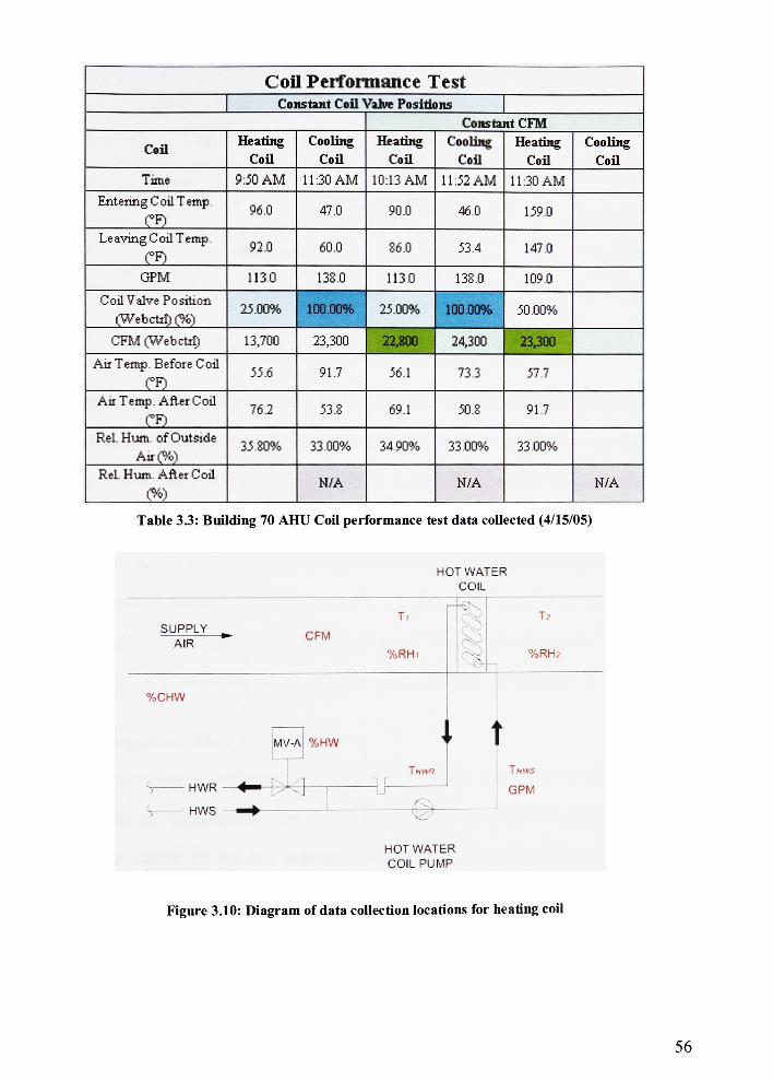
Coil Performance Test
Constant Coil Valve Positions
Constant CFM
CoilHeating
Coil
CoolingCoil
HeatingCoil
CoolingCoil
HeatingCoil
Cooling
Coil
Time 9:50 AM 11:30 AM 10:13 AM 11:52 AM 11:30 AM
Entering C oil T emp.
(F)96.0 47.0 90.0 46.0 159.0
Leaving Coil Temp .
CF)92.0 60.0 86.0 53.4 147.0
GPM 113.0 138 0 113.0 138.0 109.0
Coil Valve Position
(WebCtrl) (%)25.00% 100.00% 25.00% 100.00% 50.00%
CFM (Webctrl) 13,700 23,300 22,800 24,300 23,300
Air Temp. Before Coil
(F)55.6 91.7 56.1 73.3 57.7
Air Temp. AfterCoil
CF)76.2 53.8 69.1 50.8 91.7
Rel. Hum. ofOutside
Air(%)35.80% 33.00% 34.90% 33.00% 33.00%
Rel. Hum. After Coil
(%)N/A N/A N/A
Table 33: Building 70 AHU Coil performance test data coUected (4/15/05)
HOT WATER
COIL
SUPPLY
AIRCFM
%RH;
<,:
T?
%RH?
%CHW
HWR
HWS
MV-A %HW
ThWR
4f
T.iws
GPM
HOT WATER
COIL PUMP
Figure 3.10: Diagram of data collection locations for heating coil
56
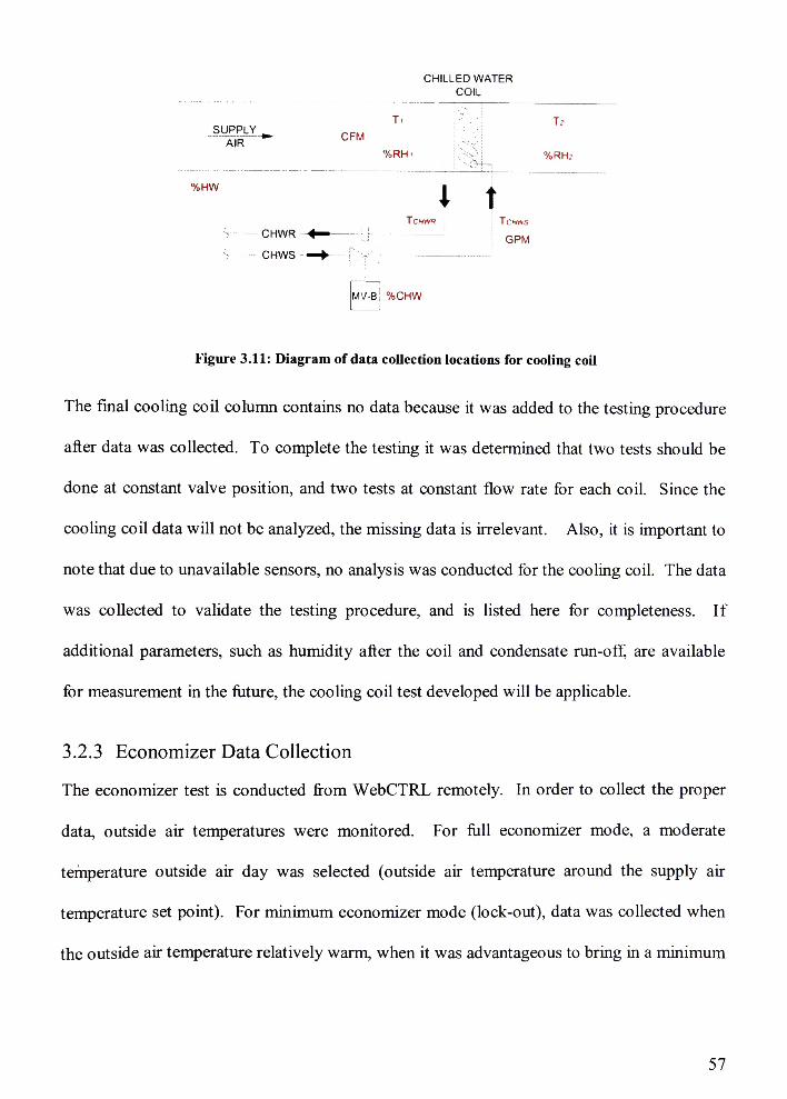
CHILLED WATER
COIL
%RH< %RH?
%HW
Tctivm
I tS CHWR -^
s chws -^*- f.:-.
Tchtvs
GPM
MV-Bi %CHW
Figure 3.11: Diagram of data collection locations for cooling coil
The final cooling coil column contains no data because it was added to the testing procedure
after data was collected. To complete the testing it was determined that two tests should be
done at constant valve position, and two tests at constant flow rate for each coil. Since the
cooling coil data will not be analyzed, the missing data is irrelevant. Also, it is important to
note that due to unavailable sensors, no analysis was conducted for the cooling coil. The data
was collected to validate the testing procedure, and is listed here for completeness. If
additional parameters, such as humidity after the coil and condensate run-off, are available
for measurement in the future, the cooling coil test developed will be applicable.
3.2.3 Economizer Data Collection
The economizer test is conducted from WebCTRL remotely. In order to collect the proper
data, outside air temperatures were monitored. For full economizer mode, a moderate
temperature outside air day was selected (outside air temperature around the supply air
temperature set point). For minimum economizer mode (lock-out), data was collected when
the outside air temperature relatively warm, when it was advantageous to bring in a minimum
57
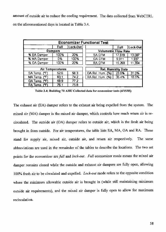
amount of outside air to reduce the cooling requirement. The data collected from WebCTRL
on the aforementioned days is located in Table 3.4.
Economizer Functional Test
Full Lock-Out Full Lock-Out
Dampers Volumetric Flow Rate
% EA Damper 100% 20% SACFM 17,619 13,087
% MA Damper 0% 100% OACFM 9,911 1,937
% OA Damper 1DD% 20% RACFM 15,268 11,394
Air Tern peratures Rel. Humidity Data
SATemp. ("F) 52.6 58.3 OA Rel. Hum. (%) 23.5% 31 .0%
MA Temp. (F) 63. 1 74.2 RA Rel. Hum. (%) 35.4% 18.5%
OATemp. (F) 59.9 77.2
RA Temp. (F) 76.1 75.8
Table 3.4: Building 70 AHU Collected data for economizer tests (4/15/05)
The exhaust air (EA) damper refers to the exhaust air being expelled from the system. The
mixed air (MA) damper is the mixed air damper, which controls how much return air is re
circulated. The outside air (OA) damper refers to outside air, which is the fresh air being
brought in from outside. For air temperatures, the table lists SA, MA, OA and RA. These
stand for supply air, mixed air, outside air, and return air respectively. The same
abbreviations are used in the remainder of the tables to describe the locations. The two set
points for the economizer are full and lock-out. Full economizer mode means the mixed air
damper remains closed while the outside and exhaust air dampers are fully open, allowing
100% fresh air to be circulated and expelled. Lock-out mode refers to the opposite condition
where the minimum allowable outside air is brought in (while still maintaining minimum
outside air requirements), and the mixed air damper is fully open to allow for maximum
recirculation.
58
Next, the chiller experimental data collection plan and chiller data will be discussed. Section
3.3 explains the experimental data collection, and Section 3.4 presents the actual data utilized
for the current healthmonitoring model development.
3.3 VCRC Chiller ExperimentalData Collection
Chiller data was collected as part of a doctoral dissertation in a dissertation by Bailey
[1998a]. The research involved fault detection and diagnosis (FDD), and several ranges of
fault conditions were imposed on the chiller while data was collected, including refrigerant
and oil charge loss. More information on the fault cases is found in the upcoming sections.
The experimental data was obtained from a Trane 70-ton RTUA Air Cooled Chiller located
in the Joint Center for Energy Management Karl Larson Laboratory (JCEM) at The
University of Colorado, Boulder [Bailey, 1998b]. The chiller has a remote Trane 50-ton
CAUA air cooled refrigerant condenser. According to Bailey, the chiller has two helical
rotary compressors each run with their own independent refrigerant circuit using R-22. The
shell-in-tube evaporator is shared, with a dual circuit configuration. The compressor in the
system has two rotors, a male and female. The compressor capacity is controlled by the
position of two solenoid valves located along the rotors. The condenser in the system is air-
cooled with six constant speed fans, three fans on each circuit. Between the condenser and
evaporator is an electronic expansion valve that causes a pressure drop between the high and
low pressure sides of the system. Its control is based on a sensor at the inlet of the
compressor. The evaporator a direct-expansion fully insulated shell-and-tube type with the
low pressure refrigerant flowing through the inner tube and water flowing through the outer
shell.
59
Two different DAQ systems were utilized for data collection: a laboratory monitoring system
(CMS) and a personal computer loaded with the chiller manufacturers monitoring system
(LVIPC). The LVIPC system is utilized for built-in control and monitoring. For each
system, a list ofdata collection points was specified.
The chiller plant was equipped with several sensors for this data collection, including
pressure transducers, type T-thermocouples, thermisters for evaporating refrigerant
temperature, and resistance temperature detector (RTD) temperature sensors. The data
loggers obtain data every 15 seconds. Figure 3.12 is a diagram of the sensor locations and
types.
60

1- liquid line
r O |AIR COOLED
CONDENSER
Tootdoor*.
<y-'discharge
* discharge
OIL
COOLER
oELECTRONIC
EXPANSION
VALVE
OXvap
Legend
Q point raoniloiedbythe chiller controls package
^ pint monitoredbyCMS
chflfed water piping
refrigerant piping
oil piping
Figure 3.12: Instrumentation locations in chiller for experimental data collection [Bailey 1998a]
Black sensor locations shown in Figure 3.12 represent points monitored by the CMS system,
while white sensor locations represent points monitored by the chiller controls package. The
central loop contains R-22, the lower path through the evaporator is chilled water flow to and
from the coils, and the upper flow through the condenser is cooling air. The dashed lines
through the oil cooler are oil piping.
61
3.3.1 Data Collection Process
3.3.1.1 NormalData Collection
Several baseline tests (normal) were collected through the data acquisition system. Normal
data and subsequent analysis is used as a baseline for comparison of the fault cases. Normal
data is considered to be 100% system refrigerant and oil charge.
3.3.1.2 Refrigerant Under- and Over-ChargeData Collection
The refrigerant charge testing began at -60% charge (40% total refrigerant charge) and the
refrigerant charge percentage was increased in increments of 5% for each test until the
maximum test value of +30% charge (130% total refrigerant charge) was reached. The
charge percentages are in reference to the manufacturer's recommended level, which is used
as 0% under-charge, or 100% total refrigerant charge. For each charge variance test
described above, data was collected using the previously described data collection systems,
LVIPC and CMS.
After fully draining the lines, refrigerant was added to the system at the suction side of the
compressor until a 40% total refrigerant charge condition was reached, and the system was
allowed to steady (evaporating refrigerant pressure stabilized) before data was collected. For
each new test, refrigerant was added incrementally in this fashion until the maximum over
charge test was complete. The system and refrigerant was then drained and returned to
normal. In addition, for these tests, a load profile was developed and utilized to simulate
typical operation of the chiller for an office building in Denver in July.
62
3.3.1.3 Oil Under-ChargeData Collection
Oil undercharge tests were performed in a similar fashion to the refrigerant under- and over
charge tests described in Section 3.3.1.1. Oil under-charge cases included -50%, -27%, and
15% undercharge (50%, 73%, and 85% total oil charge, respectively).
Oil was completely removed from the system, and then added to the charge level desired for
the first test. Oil was added to the system at the compressor suction service valve, and the
system was allowed to steady (evaporating refrigerant pressure stabilized) before data was
collected. As with refrigerant charge testing, the same load profile was utilized to dictate
chiller load throughout the test.
3.3.2 Available Chiller Data
Temperature and pressure data was collected not only for a normal condition, but several
fault conditions as well. These include air cooled condenser fouling, loss of a condenser fan,
refrigerant under- and over-charge, and oil under- and over-charge. For this research, the
elements of [Bailey 1998a] that will be utilized include normal data, refrigerant under- and
over-charge, and oil under-charge. Analyzing this data will help with development of the
health-monitoring model.
When the chiller experiences refrigerant or oil charge different from the specified charge
value, the system behaves differently, and in some cases severe refrigerant or oil loss can
drastically affect the performance of the system. In a working chiller, refrigerant or oil
63
charge loss can damage the system, as well as have negative health and environmental effects
if left unchecked.
3.4 VCRC ChillerData
As previously discussed, data was compiled from existing data collected from two different
data acquisition systems. In the research done by Bailey [1998a], the CMS data and LVIPC
data were not mixed within the same analysis. It is unknown how reliable results would be
from mixing the data, particularly data points of pressure and temperature. However, in
order to utilize the models developed, some of the CMS data must be used in conjunction
with the LVIPC data. Great care was taken to utilize as little CMS data as possible. The
CMS data used will be discussed later in this section.
3.4.1 Normal Data
For the LVIPC data, 52 fields ofdata were collected at a rate often samples per minute. The
data was collected around the month of October, 1996. Relevant data extracted from the
LVIPC data is shown in Table 3.5. Headings were interpreted to determine what state point
the data corresponded to. Data was averaged over the entire test to account for start up time
in testing, and to overcome any slight inconsistencies or errors in singledata points. Of the
many data fields, only a fraction was utilized for this research.Examples of other data fields
included fault modes, such as high pressure cutout or maximumcompressor load flag, which
were not necessary for the current model development.
64
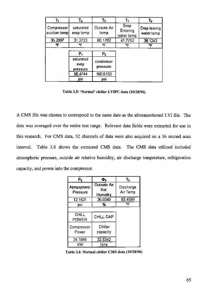
Ti T* T5 T7 T8
Compressor
suction temp
saturated
evap temp
Outside Air
temp
Evap
Enteringwater temp
Evap leavingwater temp
35.2997 31 .2723 6D.17B2 41.7752 3B.1243
F F F F F
Pi P2
saturated
evap
pressure
condenser
pressure
56.4744 160.6153
psi psi
Table 3.5:'Normal'
chiller LVIPC data (10/28/96)
A CMS file was chosen to correspond to the same date as the aforementioned LVI file. The
data was averaged over the entire test range. Relevant data fields were extracted for use in
this research. For CMS data, 52 channels of data were also acquired on a 16 second scan
interval. Table 3.6 shows the extracted CMS data. The CMS data utilized included
atmospheric pressure, outside air relative humidity, air discharge temperature, refrigeration
capacity, and power into the compressor.
Ps Os T6
Atmospheric
Pressure
Outside Air
Rel.
Humidity
Discharge
Air Temp
12.1521 35.0349 83.4599
psi % F
CHILL
POWERCHILL CAP
Compressor
Power
Chiller
capacity
34.1845 32.5342
kW tons
Table 3.6: Normal chiller CMS data (10/28/96)
65
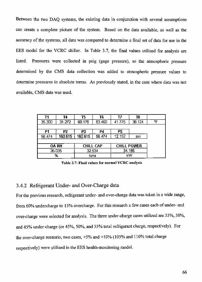
Between the two DAQ systems, the existing data in conjunction with several assumptions
can create a complete picture of the system. Based on the data available, as well as the
accuracy of the systems, all data was compared to determine a final set of data for use in the
EES model for the VCRC chiller. In Table 3.7, the final values utilized for analysis are
listed. Pressures were collected in psig (gage pressure), so the atmospheric pressure
determined by the CMS data collection was added to atmospheric pressure values to
determine pressures in absolute terms. As previously stated, in the case where data was not
available, CMS data was used.
T1 T4 T5 T6 T7 TB
35.300 31 .272 60.17B 83.460 41 .775 38.124 "F
P1 P2 P3 P4 P5
56.474 160.615 160.615 56.474 12.152 psi
OARH CHILL CAP CHILL POWER
35.035 32.534 34.1B5
% tons kW
Table 3.7: Final values for normal VCRC analysis
3.4.2 Refrigerant Under- and Over-Charge data
For the previous research, refrigerantunder- and over-charge data was taken in a wide range,
from 60% undercharge to 15% overcharge. For this research a few cases each ofunder- and
over-charge were selected for analysis. The three under-charge cases utilized are 55%, 50%,
and 45% under-charge (or 45%, 50%, and 55% total refrigerant charge, respectively). For
the over-charge scenario, two cases, +5% and +10% (105% and 110% total charge
respectively) were utilized in the EES health-monitoring model.
66
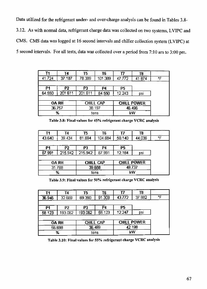
Data utilized for the refrigerant under- and over-charge analysis can be found in Tables 3.8-
3.12. As with normal data, refrigerant charge data was collected on two systems, LVIPC and
CMS. CMS data was logged at 16 second intervals and chiller collection system (LVIPC) at
5 second intervals. For all tests, data was collected over a period from 7:10 am to 3:00 pm.
T1 T4 T5 T6 T7 T8
41 .724 37.187 78.389 1Q1.3B9 47.772 41.B74 nF
P1 P2 P3 P4 P5
64.550 201.611 201.611 64.550 12.243 psi
OARH CHILL CAP CHILL POWER
36.757 3B.197 46.496
% tons kW
Table 3.8: Final values for 45% refrigerant charge VCRC analysis
T1 T4 T5 T6 T7 T8
43.640 39.434 81 .694 104.684 50.140 44.036 DF
P1 P2 P3 P4 P5
67.991 215.942 215.942 67.991 12.184 psi
OARH CHILL CAP CHILL POWER
31.76B 39.658 4B.737
% tons kW
Table 3.9: Final values for 50% refrigerant charge VCRC analysis
T1 T4 T5 T6 T7 T8
36.946 32.669 69.390 91.309 43.772 37.982 "F
P1 P2 P3 P4 P5
58.123 193.062 193.062 5B.123 12.247 psi
OARH CHILL CAP CHILL POWER
56.698 36.489 42.198
% tons kW
Table 3.10: Final values for 55% refrigerant charge VCRC analysis
67
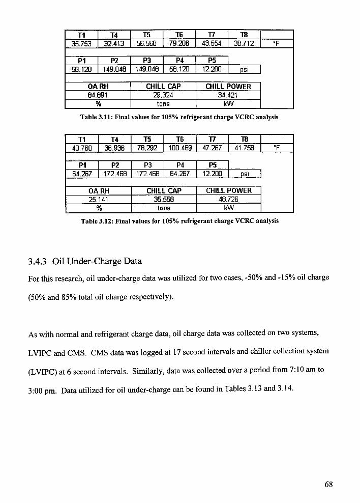
T1 T4 T5 T6 T7 T8
35.753 32.413 56.568 79.206 43.554 38.712 "F
P1 P2 P3 P4 P5
58.120 149.048 149.04B 58.120 12.200 psi
OARH CHILL CAP CHILL POWER
84.B91 29.324 34.421
% tons kW
Table 3.11: Final values for 105% refrigerant charge VCRC analysis
T1 T4 T5 T6 T7 T8
40.760 36.936 78.292 100.469 47.267 41.758 "F
P1 P2 P3 P4 P5
64.267 172.468 172.46B 64.267 12.200 psi
OARH CHILL CAP CHILL POWER
25.141 35.558 48.726
% tons kW
Table 3.12: Final values for 105% refrigerant charge VCRC analysis
3.4.3 Oil Under-Charge Data
For this research, oil under-charge data was utilized for two cases, -50% and -15% oil charge
(50% and 85% total oil charge respectively).
As with normal and refrigerant charge data, oil charge datawas collected on two systems,
LVIPC and CMS. CMS data was logged at 17 second intervals and chiller collection system
(LVIPC) at 6 second intervals. Similarly, datawas collected over a period from 7:10 am to
3:00 pm. Data utilized for oil under-charge can be found in Tables 3.13and 3.14.
68
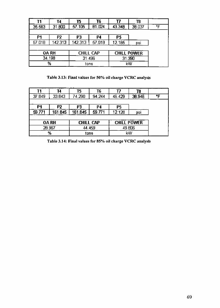
T1 T4 T5 T6 T7 T8
35.563 31 .BOO 57.105 B1 .024 43.34B 38.037 "F
P1 P2 P3 P4 P5
57.018 142.313 142.313 57.01 B 12.165 psi
OARH CHILL CAP CHILL POWER
34.198 31 .496 31.390
% tons kW
Table 3.13: Final values for 50% oil charge VCRC analysis
T1 T4 T5 T6 T7 T8
37.849 33.843 74.290 94.244 46.429 38.946 F
P1 P2 P3 P4 P5
59.771 161.845 161.845 59.771 12.128 psi
OARH CHILL CAP CHILL POWER
28.967 44.459 49.806
% tons kW
Table 3.14: Final values for 85% oil charge VCRC analysis
69
4 Air Handling Unit Model
This chapter will discuss the data collection, analysis and results from the AHU. The data is
a result of a process developed in conjunction with a Senior Design I & II (0304-630/631)
capstone design team and the process was refined several times in order to obtain the most
necessary and accurate information.
4.1 AirHandling Unit analysis
Before the air handling unit analysis was conducted, a list of assumptions was made. The
following are assumptions used throughout the AHU thermodynamic analysis:
Steady State analysis
Control volume (CV) is around the AHU with mass flow in and out of the CV
consisting of:
Cold water
Hot water
Outside air
Exhaust air
Return air
Supply air
Control volume is adiabatic
Incompressible flow of air
Air is an ideal gas
Constant cp for air at 56F
Change in kinetic and potential energy is neglected for air and water
70
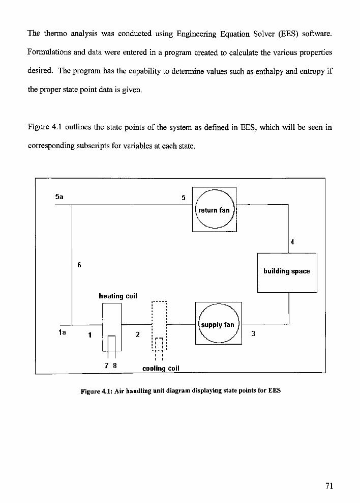
The thermo analysis was conducted using Engineering Equation Solver (EES) software.
Formulations and data were entered in a program created to calculate the various properties
desired. The program has the capability to determine values such as enthalpy and entropy if
the proper state point data is given.
Figure 4.1 outlines the state points of the system as defined in EES, which will be seen in
corresponding subscripts for variables at each state.
5a 5
y4
6
building space
heating coil
r_i
I i
i I
- (supply fan )1a
, 2 3
i i
i i
7 8cooling coil
Figure 4.1: Air handling unit diagram displaying state points for EES
71
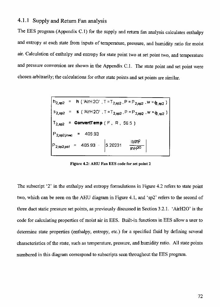
4.1.1 Supply and Return Fan analysis
The EES program (Appendix C.l) for the supply and return fan analysis calculates enthalpy
and entropy at each state from inputs of temperature, pressure, and humidity ratio for moist
air. Calculation of enthalpy and entropy for state point two at set point two, and temperature
and pressure conversion are shown in the Appendix C.l. The state point and set point were
chosen arbitrarily; the calculations for other state points and set points are similar.
h2,sP2=
h('AirH20'.T=T2iSp2 P =
P2,sp2 'w =<fe,sp2 )
s2iSp2= s ('AirH20',T=T2|Sp2 P =
P2,sp2 >w =<fe,sp2 )
T2,SP2=
ConvertTemp (F,R, 56.5 )
P2,sP2,inwC= 405.93
P2,sp2,pSf= 405.93 5.20231
Ibf/ft2
InH20
Figure 4.2: AHU Fan EES code for set point 2
The subscript'2'
in the enthalpy and entropy formulations in Figure 4.2 refers to state point
two, which can be seen on the AHU diagram in Figure 4.1, and'sp2'
refers to the second of
three duct static pressure set points, as previously discussed in Section 3.2.1.'AirH20'
is the
code for calculating properties ofmoist air in EES. Built-in functions in EES allow a user to
determine state properties (enthalpy, entropy, etc.) for a specified fluid by defining several
characteristics of the state, such as temperature, pressure, and humidity ratio. All state points
numbered in this diagram correspond to subscripts seen throughout the EES program.
72
In order to maintain proper units for calculations, temperatures and pressures were converted
using the Convert function in EES. These conversions are shown in Figure 4.2. Temperature
is converted from Fahrenheit to Rankine, and pressure is converted from inches H2O to lb/ft2.
These new values for T2 and P2 are utilized by the software for all calculations
After successfully calculating the entropy and enthalpy for all state points where sufficient
datawas collected, energy and exergy calculations could proceed.
4.1.1.1 Energy analysis ofthe Fans
To calculate the efficiency of the supply fan, the relationships shown in the EES code in
Appendix C.l were developed. The work into the supply fan is 10.9 horsepower (hp). This
is converted using the Convert function, to lbrft/min.
The first law efficiency of the fans is determined using Equation 4. 1 .
nJ-^* 4.1
-W
where V is volumetric flow rate, Ap is the change in static pressure across the fan, and W is
the work into the fan. In the EES code, the value is also changed to a percentage my
multiplying by the variablepercent.
Similar equations were used to determine the first law efficiency results for the return fan
using statepoints 4 and 5 at all three duct static pressure set points. The results for the first
law efficiency at all set points for both the supply and return fan can be found in Table 4.1 .
73
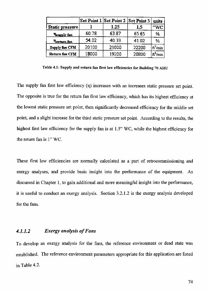
Set Point 1 Set Point 2 Set Point 3 units
Static pressure 1 1.25 1.5 "WC
"Hfupply fen 60.78 63.87 65.65 %
T|xeturn fen 54.02 40.33 41.02 %
Supply fan CFM 20100 21000 22200 ft /min
Return fen CFM 18000 19200 20800 ft /min
Table 4.1: Supply and return fan first law efficiencies for Building 70 AHU
The supply fan first law efficiency (n) increases with an increases static pressure set point.
The opposite is true for the return fan first law efficiency, which has its highest efficiency at
the lowest static pressure set point, then significantly decreased efficiency for the middle set
point, and a slight increase for the third static pressure set point. According to the results, the
highest first law efficiency for the supply fan is at 1 WC, while the highest efficiency for
the return fan is1"
WC.
These first law efficiencies are normally calculated as a part of retrocommissioning and
energy analyses, and provide basic insight into the performance of the equipment. As
discussed in Chapter 1, to gain additional and more meaningful insight into the performance,
it is useful to conduct an exergy analysis. Section 3.2.1.2 is the exergy analysis developed
for the fans.
4.1.1.2 Exergy analysis ofFans
To develop an exergy analysis for the fans, the reference environment or dead state was
established. The reference environment parameters appropriate for this application are listed
in Table 4.2.
74
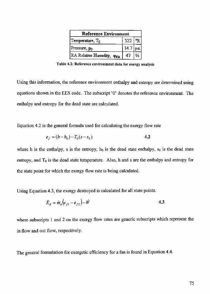
Reference Environment
Temperature, To 522 "R
Pressure, pD 14.7 psi
RA Relative Humidity, qj^ 47 %
Table 4.2: Reference environment data for exergy analysis
Using this information, the reference environment enthalpy and entropy are determined using
equations shown in the EES code. The subscript'0'
denotes the reference environment. The
enthalpy and entropy for the dead state are calculated.
Equation 4.2 is the general formula used for calculating the exergy flow rate
ef=(h-hQ)-T0(s-s0) 4.2
where h is the enthalpy, s is the entropy, ho is the dead state enthalpy, so is the dead state
entropy, and To is the dead state temperature. Also, h and s are the enthalpy and entropy for
the state point for which the exergy flow rate is being calculated.
Using Equation 4.3, the exergy destroyed is calculated for all state points.
Ed=rha{efl-ef2)-W 4.3
where subscripts 1 and 2 on the exergy flow rates are generic subscripts which represent the
in flow and out flow, respectively.
The general formulation for exergetic efficiency for a fan is found in Equation 4.4.
75
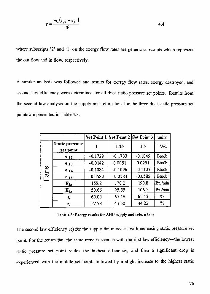
s =a{e/2-ef\)
-W
4.4
where subscripts'2'
and'
1'
on the exergy flow rates are generic subscripts which represent
the out flow and in flow, respectively.
A similar analysis was followed and results for exergy flow rates, exergy destroyed, and
second law efficiency were determined for all duct static pressure set points. Results from
the second law analysis on the supply and return fans for the three duct static pressure set
points are presented in Table 4.3.
Set Point 1 Set Point 2 Set Point 3 miits
0)
CD
LL
Static pressure
set point
1 1.25 1.5 "WC
f2 -0.1729 -0.1733 -0.1849 Btu/lb
*f3 -0.0142 0.0081 0.0291 Btu/lb
*f4 -0.1084 -0.1096 -0.1123 Btu/lb
f5 -0.0580 -0.0584 -0.0582 Btu/lb
Ea, 159.2 170.2 190.8 Btu/min
Ear 50.66 95.85 106.5 Btu/min
. 60.05 63.18 65.13 %
*r 57.33 43.50 44.22 %
Table 4.3: Exergy results for AHU supply and return fans
The second law efficiency (e) for the supply fan increases with increasing static pressure set
point. For the return fan, the same trend is seen as with the first lawefficiencythe lowest
static pressure set point yields the highest efficiency, and then a significant drop is
experienced with the middle set point, followed by a slight increase to the highest static
76
pressure set point. For both fans, the exergy destroyed increases with increased set point.
The supply fan's highest efficiencies occur at the third set point, however this is the point at
which the supply fan experiences the highest amount of exergy destroyed. For the return fan,
the highest efficiencies are at the lowest static pressure set point, and also experience the
lowest exergy destroyed. These efficiency results mean that while the supply fan is most
efficient around the middle or high set point, the return fan is most efficient at the low set
point. Also, the exergy destroyed results lead to the conclusion that the best static pressure
set point is the lowest set point for both the supply fan and the return fan. Therefore, it is the
recommendation that the lowest static pressure set point be maintained as long as supply air
requirements can be maintained. This duct static pressure was tested under real operation at
the time of data collection, and over a trial period of one week all VAV box air flow
requirements were satisfied. This test, along with calculations showing the benefit of
reducing the supply duct static pressure support the conclusion that the duct static pressure
should be lowered to one inch in the water column.
4.1.2 Coil analysis
In a similar fashion to Section 4.1.1, the measured information surrounding the coils is an
input to the EES program. Pressures and temperatures are entered and converted to the
appropriate units using the'convert'
function, and like before the corresponding enthalpies
and entropies are calculated. Unlike the fan analysis, where the working fluid is moist air,
the coil analysis has two fluids; air crossing over the coils within the AHU, and water from
the hot and cold water loops passes through the heating and cooling coil, respectively. This
is taken into consideration when calculating enthalpy and entropy. EES code for the coil
77
analysis is shown in Appendix C.3. In this case, it is important to note that the three set
points utilized are different than the set points in the fan analysis. For example, set point'2'
is also used, but unlike the fan set point'2'
which referred to the second duct static pressure
set point, the second coil set point refers to 25% coil valve position opening and 22,800 CFM
air volumetric flow rate across the coil.
For the coil analysis, the state points'
1'
and'2'
correspond to the points in the air stream
before and after the coil, and the state points'7'
and'8'
correspond to the entering and
exiting hot water flow, respectively, as shown in Figure 4.1. It is important to note that
according to the fluid specified, various data points are necessary to calculate the enthalpy.
In this case, for the air the temperature is needed, and for water the temperature and quality
are needed.
4.1.2.1 CoilEffectiveness
The first law measure of coil efficiency is the coil effectiveness. This is based on
thermodynamics and heat transfer formulations. The coil effectiveness calculation is shown
in Equations 4.5 through 4.9. In the analysis, cPiC is the specific heat of the cold stream at
constant pressure, and cp,h is the specific heat of the hot stream at constant pressure. The
variable qc is the actual heat for the colder flow, while qmax is the maximum possible heat
transfer rate. Cc is the heat capacity rate for the colder flow, and Cmin is equal to Cc or Ch,
whichever is smaller (Cc in this case). T's correspond to temperatures. The ratio of qc to
qmax is the coil effectiveness .
78
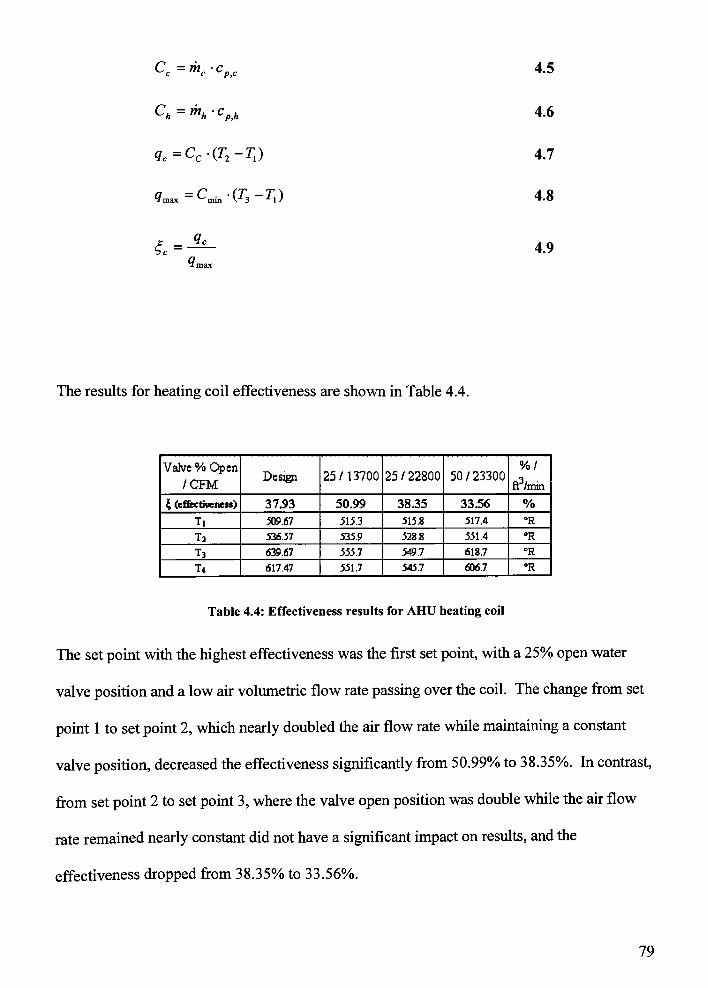
Cc=c -Cp,c
Ch=Tnh-Cp,h
qc=Cc-(T2-T,)
*7max '"'min'
V-*3*
1 )
L =
4.5
4.6
4.7
4.8
4.9
The results for heating coil effectiveness are shown in Table 4.4.
Valve % Open
/CFMDesign 25/13700 25/22800 50 / 23300
%/
ft /min
| (eflfectiveneH) 37.93 50.99 38.35 33.56 %
Ti 509.67 515.3 515.8 517.4 R
T3 536.57 535.9 528.8 551.4 R
T3 639.67 555.7 549.7 618.7 R
T4 617.47 551.7 545.7 606.7 R
Table 4.4: Effectiveness results for AHU heating coil
The set point with the highest effectiveness was the first set point, with a 25% open water
valve position and a low air volumetric flow rate passing over the coil. The change from set
point 1 to set point 2, which nearly doubled the air flow rate while maintaining a constant
valve position, decreased the effectiveness significantly from 50.99% to 38.35%. In contrast,
from set point 2 to set point 3, where the valve open position was double while the air flow
rate remained nearly constant did not have a significant impact on results, and the
effectiveness dropped from 38.35% to 33.56%.
79
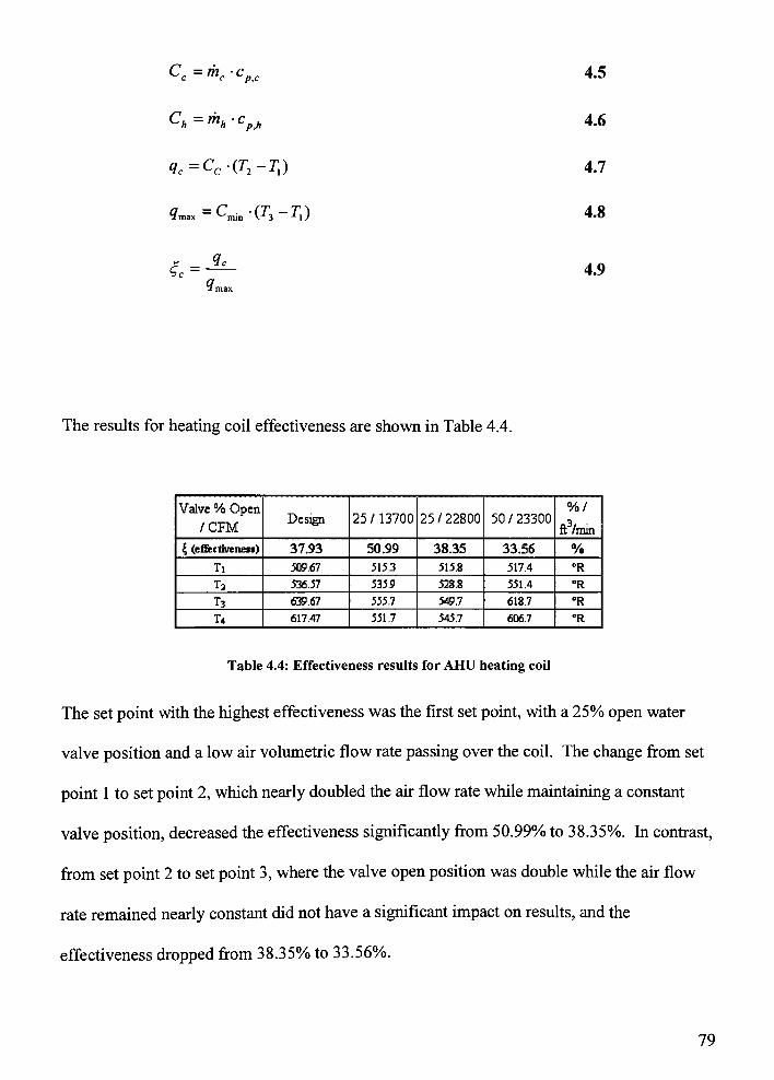
Cc=r"c-CP,c
Ch=h-Cp,h
qc=Cc-(T2-Tx)
1^=CmiD-(T,-Tl)
Zc =
4.5
4.6
4.7
4.8
4.9
The results for heating coil effectiveness are shown in Table 4.4.
Valve % Open
/CFMDesign 25/13700 25 / 22800 50 / 23300
%/
ft /min
4 (effectiveneis) 37.93 50.99 38.35 33.56 %
Ti 509.67 515.3 515.8 517.4 "R
T3 536.57 535.9 528.8 551.4 R
T3 639.67 555.7 549.7 618.7 "R
T4 617.47 551.7 545.7 606.7 R
Table 4.4: Effectiveness results for AHU heating coil
The set point with the highest effectiveness was the first set point, with a 25% open water
valve position and a low air volumetric flow rate passing over the coil. The change from set
point 1 to set point 2, which nearly doubled the air flow rate while maintaining a constant
valve position, decreased the effectiveness significantly from 50.99% to 38.35%. In contrast,
from set point 2 to set point 3, where the valve open position was double while the air flow
rate remained nearly constant did not have asignificant impact on results, and the
effectiveness dropped from 38.35% to 33.56%.
79
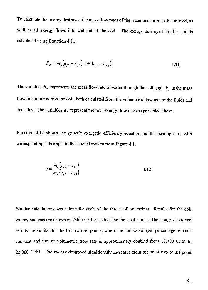
To calculate the exergy destroyed the mass flow rates of the water and air must be utilized, as
well as all exergy flows into and out of the coil. The exergy destroyed for the coil is
calculated using Equation 4.11.
Ed=rhw(efl -efS)+ma(efl -efl) 4.11
The variable mw represents the mass flow rate ofwater through the coil, and ma is the mass
flow rate of air across the coil, both calculated from the volumetric flow rate of the fluids and
densities. The variables ef represent the four exergy flow rates as presented above.
Equation 4.12 shows the generic exergetic efficiency equation for the heating coil, with
corresponding subscripts to the studied system from Figure 4.1.
..*-f"-'"\ 4.12
Similar calculations were done for each of the three coil set points. Results for the coil
exergy analysis are shown in Table 4.6 for each of the three set points. The exergy destroyed
results are similar for the first two set points, where the coil valve open percentage remains
constant and the air volumetric flow rate is approximately doubled from 13,700 CFM to
22,800 CFM. The exergy destroyed significantly increases from set point two to set point
81
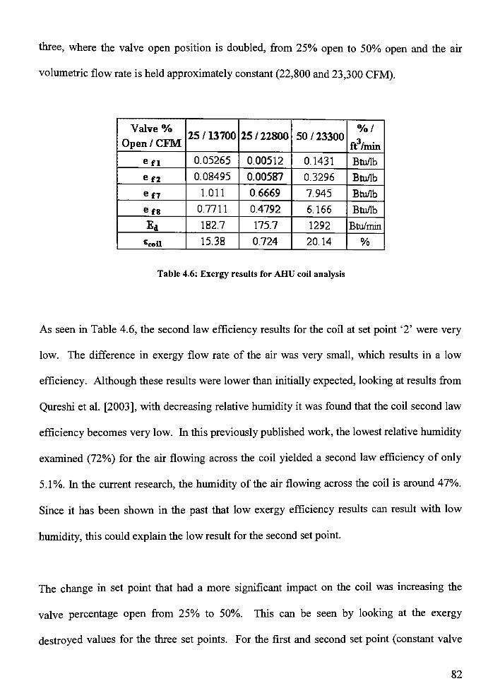
three, where the valve open position is doubled, from 25% open to 50% open and the air
volumetric flow rate is held approximately constant (22,800 and 23,300 CFM).
Valve %
Open / CFM25 / 13700 25/22800 50/23300
%/
ft /min
efi 0.05265 0.00512 0.1431 Btu/lb
efj 0.08495 0.00587 0.3296 Btu/lb
ef7 1.011 0.6669 7.945 Btu/lb
e8 0.7711 0.4792 6.166 Btu/lb
Ed 182.7 175.7 1292 Btu/min
^coil 15.38 0.724 20.14 %
Table 4.6: Exergy results for AHU coil analysis
As seen in Table 4.6, the second law efficiency results for the coil at set point'2'
were very
low. The difference in exergy flow rate of the air was very small, which results in a low
efficiency. Although these results were lower than initially expected, looking at results from
Qureshi et al. [2003], with decreasing relative humidity it was found that the coil second law
efficiency becomes very low. In this previously published work, the lowest relative humidity
examined (72%) for the air flowing across the coil yielded a second law efficiency of only
5.1%. In the current research, the humidity of the air flowing across the coil is around 47%.
Since it has been shown in the past that low exergy efficiency results can result with low
humidity, this could explain the low result for the second set point.
The change in set point that had a more significant impact on the coil was increasing the
valve percentage open from 25% to 50%. This can be seen by looking at the exergy
destroyed values for the three set points. For the first and second set point (constant valve
82
percentage), the exergy destroyed is approximately equal. Between the second and third set
points (air flow rate approximately constant, valve position increased from 25 to 50%), the
exergy destroyed more than doubles. Based on the fact that the exergy efficiency values
fluctuate between the set points, the other two determining factors (effectiveness and exergy
destroyed) lead to the conclusion that the first set point is the most efficient, because it has
the lowest exergy destroyed. It also has the highest effectiveness. This analysis also shows
that the second law does not specifically show a clearer picture of performance than the
effectiveness analysis. A building owner must operate the equipment at set points necessary
to maintain occupant comfort; therefore there may not be a set point value that can be
consistently changed to reduce costs associated with the heating coil.
4. 1 .3 Economizer analysis
The economizer analysis follows models for simple mixing. Collected data, which can be
seen in Section 3.2.3, consists of temperatures, damper percentages, flow rates, and humidity
information. Using this along with calculated pressure information, enthalpy and entropy is
determined. EES code for the economizer is shown in Appendix C.4.
The exergy reference environment is defined similarly to the past AHU analyses, since the
only working fluid in the economizer isair. The exergy flow rate is calculated, as shown in
Equation 4.13.
ef=(h-h0)-T0(s-s0)4.13
The formulation for exergy destroyed in the economizer is shown inEquation 4.14.
83
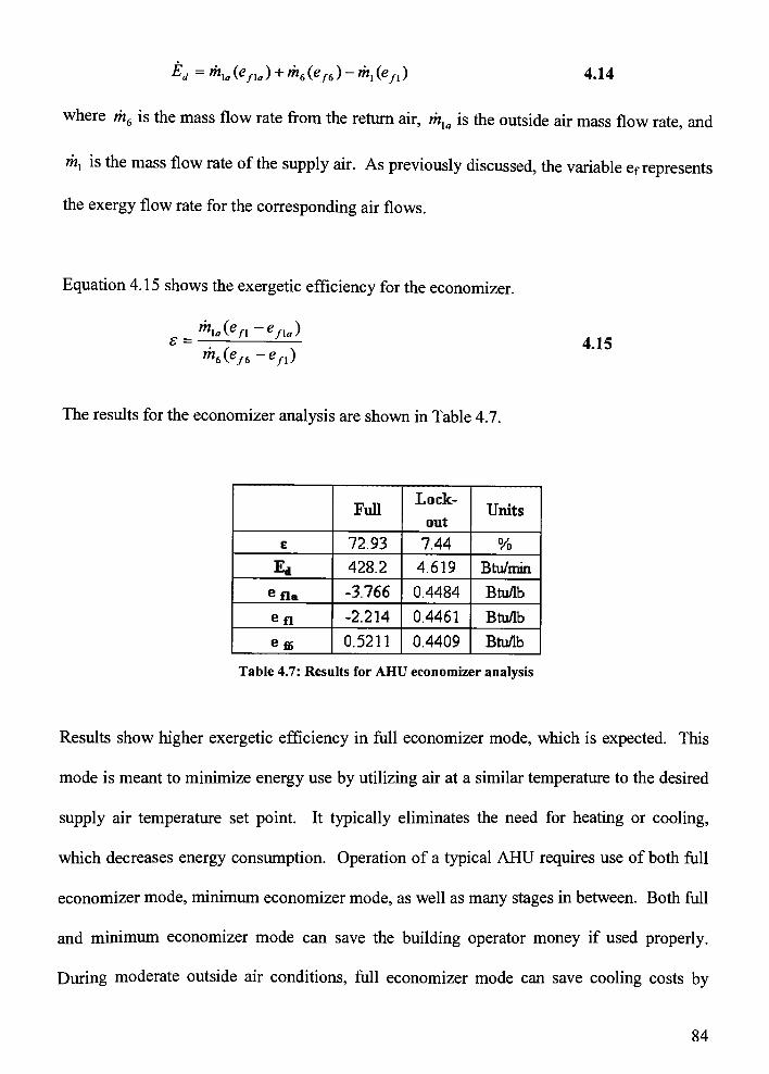
K =
mla (efla ) + m6 (ef6 )-
/n, (efl ) 4.14
where m6 is the mass flow rate from the return air, w]a is the outside air mass flow rate, and
m, is the mass flow rate of the supply air. As previously discussed, the variable ef represents
the exergy flow rate for the corresponding air flows.
Equation 4.15 shows the exergetic efficiency for the economizer.
i>/i-e/iJ=
^6(e/6-e/l)4.15
The results for the economizer analysis are shown in Table 4.7.
FullLock
out
Units
E 72.93 7.44 %
Ed 428.2 4.619 Btu/min
efla -3.766 0.4484 Btu/lb
en -2.214 0.4461 Btu/lb
efl! 0.5211 0.4409 Btu/lb
Table 4.7: Results for AHU economizer analysis
Results show higher exergetic efficiency in full economizer mode, which is expected. This
mode is meant to minimize energy use by utilizing air at a similar temperature to the desired
supply air temperature set point. It typically eliminates the need for heating or cooling,
which decreases energy consumption. Operation of a typical AHU requires use of both full
economizer mode, minimum economizer mode, as well as many stages in between. Both full
and minimum economizer mode can save the building operator money if used properly.
During moderate outside air conditions, full economizer mode can save cooling costs by
84
using "free cooling", while during very extreme outside air conditions (hot or cold),
minimum economizer mode can reduce heating and cooling costs. Therefore, a specific
recommendation cannot be made to operate at a particular mode more often. However,
when conditions warrant, both of these energy savings modes can be utilized.
4. 1 .4 Dead State Verification
When determining the dead state for the exergetic analysis, several possibilities were
considered. To justify the chosen dead state, two other logical dead states were chosen for
comparison. This comparison was conducted using the fan exergetic analysis and varying
the dead state.
The actual dead state chosen consisted of a temperature of 522 R (62 F), 14.7 psi, and 47%
relative humidity. This yielded a humidity ratio of 0.006 lb w/lb dry air- The pressure chosen
was equal to the measured outside atmospheric pressure during testing. The relative
humidity was approximately equal to the average relative humidity throughout the testing.
The temperature was difficult to determine. The approximate temperature in the immediate
surroundings of the AHU (in the mechanical room) was 78 F. However, the cause of this
temperature was not likely due to heat given off by the AHU but rather from other
components outside the control volume. The outside temperature was between 45 and 50 F.
Therefore, a temperature of approximately 62F was used for the dead state temperature
taking both of these environments intoconsideration.
This assumed dead state was compared to two other options in order to verify if it was a
reasonable selection and its significance on exergy results.
85
The first dead state it was compared to had a temperature of 78 F, a pressure of 14.68 psi,
and a relative humidity of 50%. This led to a humidity ratio of 0.0105 lb w/lb dry air from the
psychrometric chart. This dead state represented the conditions within the mechanical room,
which were the immediate surroundings of the AHU. The results for this state can be seen in
Table 4.3 as reference state 2.
The second dead state used for comparison had a temperature of45F, a pressure of 14.7 psi,
a relative humidity of 47% and therefore a humidity ratio of 0.0035 lb w/lb dry air- This dead
state closely represented the actual outside conditions during data collection. The results for
this state can be seen in Table 4.3, reference state 3.
The results, as seen in Table 4.3, showed that varying the dead state did not have a significant
impact on the results. The exergetic efficiencies er and es varied by a few percentage points
at most, such as from 49.39% to 51.81% in the case of sr from dead state 1 to dead state 3,
and the exergy destroyed values were similar. The analysis also showed that the actual dead
state values used (reference state 1) produced results which fell between the two tested
comparison cases (reference states 2 and 3), which show the dead state assumption was
appropriate. Note that in Table 4.2, the dead state selected is reference state 1.
86
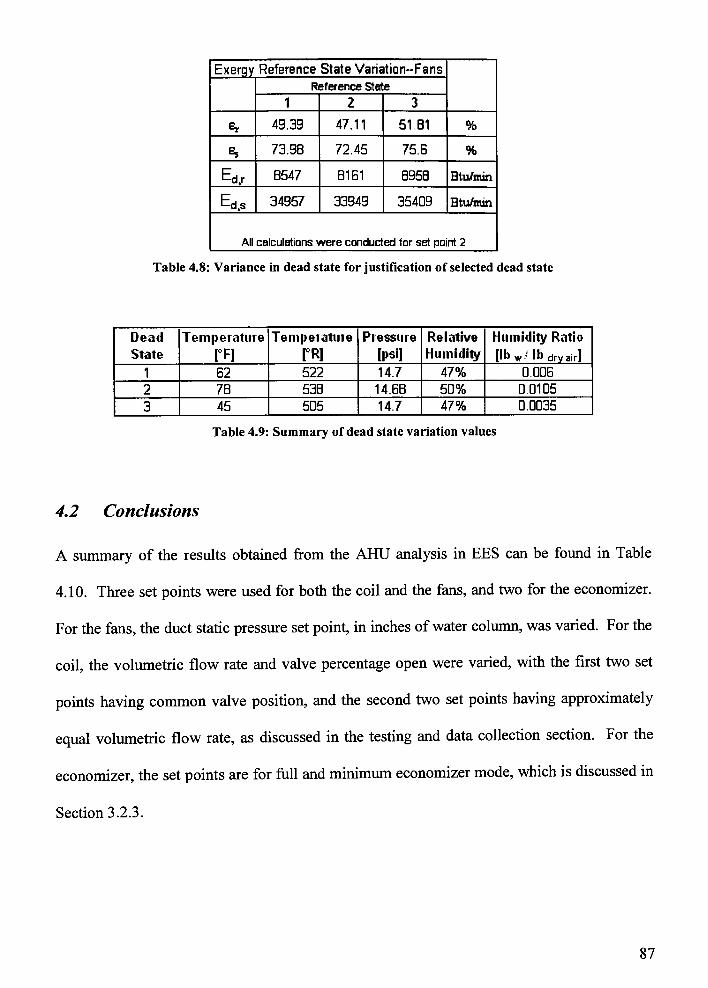
Exergy Reference State Variation-Fans
Reference State
1 2 3
^r 49.39 47.11 51 .81 %
Es 73.98 72.45 75.6 %
Ed,r B547 B1B1 B958 Btu/min
Ed,s 34957 33949 35409 Btu/min
All calculations were conducted lor set point 2
Table 4.8: Variance in dead state for justification of selected dead state
Dead
State
Temperature Temperature
rR]
Pressure
[psi]
Relative
Humidity
Humidity Ratio
[lb w/ lb drv air]
1 62 522 14.7 47% 0.006
2 78 538 14.68 50% 0.0105
3 45 505 14.7 47% 0.0035
Table 4.9: Summary of dead state variation values
4.2 Conclusions
A summary of the results obtained from the AHU analysis in EES can be found in Table
4.10. Three set points were used for both the coil and the fans, and two for the economizer.
For the fans, the duct static pressure set point, in inches ofwater column, was varied. For the
coil, the volumetric flow rate and valve percentage open were varied, with the first two set
points having common valve position, and the second two set points having approximately
equal volumetric flow rate, as discussed in the testing and data collection section. For the
economizer, the set points are for full and minimumeconomizer mode, which is discussed in
Section 3.2.3.
87
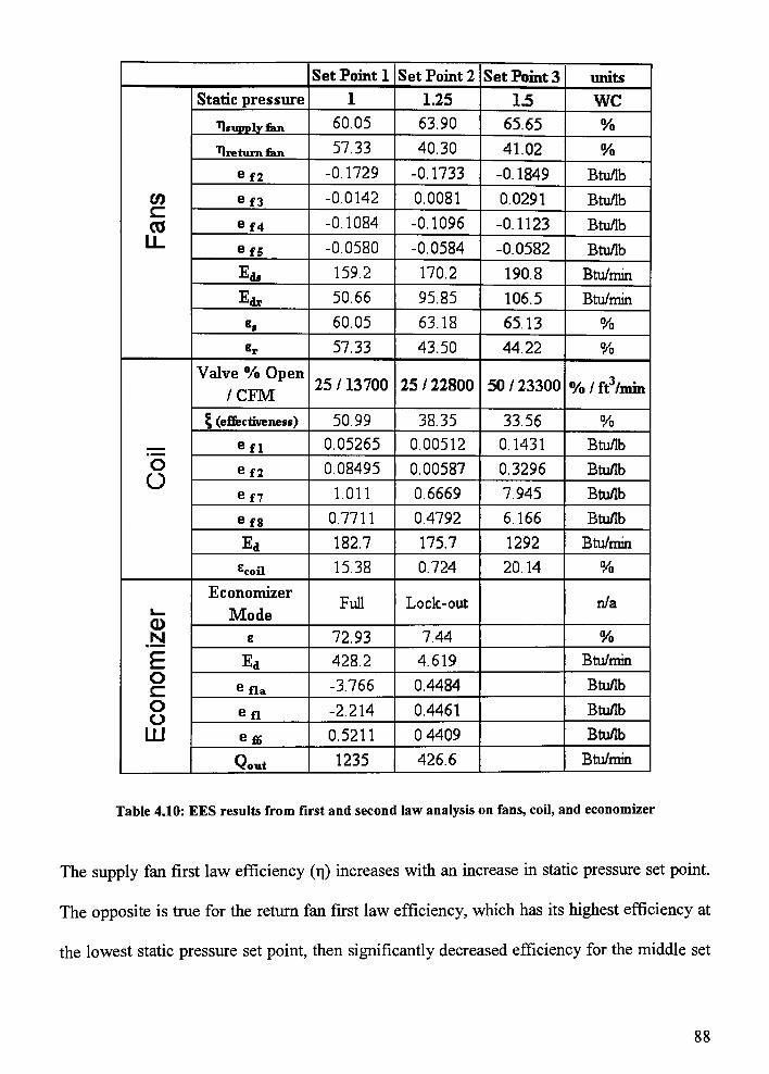
Set Point 1 Set Point 2 Set Point 3 units
CO
CO
LL
Static pressure 1 1.25 1.5 WC
"Hjupply tail 60.05 63.90 65.65 %
Ireturn fan 57.33 40.30 41.02 %
ef2 -0.1729 -0.1733 -0.1849 Btu/lb
ef3 -0.0142 0.0081 0.0291 Btu/lb
ef4 -0.1084 -0.1096 -0.1123 Btu/lb
efs -0.0580 -0.0584 -0.0582 Btu/lb
Ea, 159.2 170.2 190.8 Btu/min
Ej,. 50.66 95.85 106.5 Btu/min
Ss 60.05 63.18 65.13 %
Er 57.33 43.50 44.22 %
o
o
Valve % Open
/CFM25 / 13700 25/22800 50 / 23300 %/ft3/min
J (effectiveness) 50.99 38.35 33.56 %
efl 0.05265 0.00512 0.1431 Btu/lb
ef2 0.08495 0.00587 0.3296 Btu/lb
ef7 1.011 0.6669 7.945 Btu/lb
ef8 0.7711 0.4792 6.166 Btu/lb
Ed 182.7 175.7 1292 Btu/min
&COJ1 15.38 0.724 20.14 %
N
oc
oCJ
LU
Economizer
ModeFull Lock-out n/a
E 72.93 7.44 %
Ed 428.2 4.619 Btu/min
efla -3.766 0.4484 Btu/lb
en -2.214 0.4461 Btu/lb
eus 0.5211 0.4409 Btu/lb
Qo^t 1235 426.6 Btu/min
Table 4.10: EES results from first and second law analysis on fans, coil, and economizer
The supply fan first law efficiency (r|) increases with an increase in static pressure set point.
The opposite is true for the return fan first law efficiency, which has its highest efficiency at
the lowest static pressure set point, then significantly decreased efficiency for the middle set
88
point, and a slight increase for the third static pressure set point. The return fan operation is
based on the supply fan operation, which may explain the reverse trend for first law
efficiencies.
According to the results, the highest first law efficiency for the supply fan is set point 3,
while the highest efficiency for the return fan is set point 1 . These first law efficiencies are
normally calculated as a part of retrocommissioning and energy analyses, and provide basic
insight into the performance of the equipment. From this first law analysis, it is difficult to
determine the best duct static pressure set point.
The second law efficiency (e) for the supply fan increases with increasing static pressure set
point. For the return fan, the same trend is seen as with the first law efficiency the lowest
static pressure set point yields the highest efficiency, and then a significant drop is
experienced with the middle set point, followed by a slight increase to the highest static
pressure set point. This is the same trend that was seen for the return fan.
For both fans, the exergy destroyed increases with increased set point. The supply fan's
highest efficiencies occur at the third set point, however this is the point at which the supply
fan experiences the highest amount of exergy destroyed. For the return fan, the highest
efficiencies are at the lowest static pressure set point, and also experience the lowest exergy
destroyed. These efficiency results mean that while the supplyfan is most efficient around
the middle or high set point, the return fan is most efficient at the low set point. The exergy
destroyed results lead to the conclusion that the best static pressure set point is the lowest set
89
point for both the supply fan and the return fan. Therefore, it is the recommendation that the
lowest static pressure set point be maintained as long as supply air requirements can be
maintained in the most critical building zones. The comparison of first and second law
analysis results reveal that the second law analysis plays a key role in determining the best
duct static pressure set point. Without the more advanced thermodynamic analysis, a
building owner may not conclude that the lowest set point is in fact the best choice.
Lowering this duct static pressure set point can save building owners money because less
power to the fan is necessary to maintain this lower duct static pressure.
For the coil, the set point with the highest effectiveness was the first set point, with a 25%
open water valve position and a low air volumetric flow rate passing over the coil. The
change from set point 1 to set point 2, which nearly doubled the air flow rate while
maintaining a constant valve position, decreased the effectiveness significantly from 50.99%
to 38.35%. In contrast, from set point 2 to set point 3, where the valve open position was
double while the air flow rate remained nearly constant did not have as significant of an
impact on results, and the effectiveness dropped from 38.35% to 33.56%.
The exergy destroyed results are similar for the first two set points, where the coil valve open
percentage remains constant and the air volumetric flow rate is approximately doubled from
13,700 CFM to 22,800 CFM. The exergy destroyed significantly increases from set point
two to set point three, where the valve open position is doubled, from 25% open to 50% open
and the air volumetric flow rate is held approximately constant (22,800 and 23,300 CFM). It
90
is expected that this exergy destroyed value will be higher because the temperature increase
associated with increasing the valve open percentage.
As seen in Table 4.6, the second law efficiency results for the second coil set point were very
low. Although these results were lower than initially expected, looking at results from
Qureshi et al. [2003], with decreasing relative humidity it was found that the coil second law
efficiency becomes very low. In this previously published work, the lowest humidity
examined (72%) for the air flowing across the coil yielded a second law efficiency of only
5.1%. In the current research, the humidity of the air flowing across the coil is around 47%.
This could explain the low exergy efficiency for set point '2'. No conclusions could be
drawn for the reason this set point showed different results from the other two set points.
The change in set point that had a more significant impact on the coil was increasing the
valve percentage open from 25% to 50%. This can be seen by looking at the exergy
destroyed values for the three set points. For the first and second set point (constant valve
percentage), the exergy destroyed is approximately equal. Between the second and third set
points (air flow rate approximately constant, valve position increased from 25 to 50%), the
exergy destroyed more than doubles. Based on the fact that the exergy efficiency values vary
between the set points, the other two determining factors (effectiveness and exergy
destroyed) lead to the conclusion that the first set point is the most efficient, because it has
the lowest exergy destroyed. It also has the highest effectiveness. However, it is difficult to
determine what set points are practical to maintain from a building operational and occupant
comfort point of view. The exergy analysis did not necessarily produce more clear results of
91
performance in the case of the coil analysis. In terms of health monitoring of the coils, it is
unclear whether the exergy analysis aids in this area.
Results show higher exergetic efficiency in full economizer mode, which is expected. This
mode is meant to minimize energy use by utilizing air at a similar temperature to the desired
supply air temperature set point. It typically eliminates the need for heating or cooling,
which decreases energy consumption. Operation of a typical AHU requires use of both full
economizer mode, minimum economizer mode, as well as many stages in between. Both full
and minimum economizer mode can save the building operator money if used properly.
During moderate outside air conditions, full economizer mode can save cooling costs by
using "free cooling", while during very extreme outside air conditions (hot or cold),
minimum economizer mode can reduce heating and cooling costs. Therefore, a specific
recommendation cannot be made to operate at a particular mode more often. However,
when conditions warrant, both of these energy savings modes can be utilized.
In the fans, the exergy analysis provided great benefit and insight to the performance of the
equipment. Particularly, with the fans, the included exergetic analysis clarified which set
point would have the best performance. Also, the exergy destroyed in the heating coil helped
clarify the best set point. The economizer analysis verified the RCX data collection
methodology, and showed the benefit of full economizer mode. The three components were
tested under different conditions, so it would not be a safe assumption to compare the
performance on all three components with one another to determine where the most energy
savings exists, however the first and second law analysis will be useful in determining set
92

points at which the performance is better, and with additional set points tested, an optimal set
point could be determined.
93
5 VCRC ChillerModel
This chapter will discuss the data collection, analysis and results from the VCRC chiller.
Initially, assumptions will be presented, followed by a detailed description of the analysis
conducted in the model, and results from the normal chiller data as well as the fault cases
analyzed. Conclusions about the results are drawn in the final section. The utility of the
model presented for health monitoring and performance prediction of the VCRC chiller
system is shown.
5.1 Vapor Compression Refrigeration Cycle ChillerAnalysis
In the following analysis, several assumptions were made. Most of the assumptions
correspond to those typically made for an ideal VCRC analysis. After assessing the available
data, it is necessary to make these ideal VCRC assumptions due to the amount and type of
existing data. Several key data points were missing, and inconsistencies existed between the
two types of data (LVIPC and CMS) that made it impossible to mix some of the data points
from the two sets. Also, it is important to minimize the amount of additional instrumentation
necessary in the system in order to increase the likelihood that this methodology will be
accepted by the HVAC field, as discussed in Chapter 1 . Although the working cycle is of
course not ideal, more data collection would be necessary before they could be removed.
Therefore, the ideal VCRC assumptions will be utilized, although it is recommended for
future work that more data points be collected to remove some of the ideal VCRC
assumptions.
94
The assumptions are as follows:
Each component is analyzed as a control volume at steady state
No pressure drop through heat exchangers
Compressor and expansion valve operation are adiabatic
Kinetic and potential energy changes are negligible throughout cycle
Isenthalpic expansion valve operation
Isentropic compression
State 3 (between condenser and valve) exists as a saturated liquid (quality is equal to
zero)
Additional assumptions include incompressible flow of air, air is an ideal gas, and constant cp
for air at the inlet outside air temperature. The sign convention used is work into the
compressor is negative.
The first and second law thermodynamic analysis was conducted using Engineering Equation
Solver (EES) software, which is commercially available (see Section 2.2). Formulations and
raw data were entered in a program created to calculate the various properties (enthalpy,
entropy, etc) desired through look-up tables. The program determines properties such as
enthalpy and entropy if the proper state point data is given. State points are defined and the
inputs to the program include the temperature and pressure data for those state points
extracted from the existing averaged VCRC chiller data library, including normal and fault
data, as well as compressor power and chiller capacity. The chiller normal and fault data is
presented in Chapter 3.
95
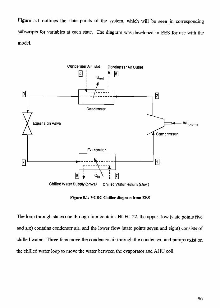
Figure 5.1 outlines the state points of the system, which will be seen in corresponding
subscripts for variables at each state. The diagram was developed in EES for use with the
model.
CondenserAir Inlet CondenserAir Outlet
@Joutt HI
-fc= f J
Condenser
Expansion Valve n Wiin,camp
j i Compressor
Evaporator
0
Chilled Water Supply (chws) Chilled Water Return (chwr)
Figure 5.1: VCRC Chiller diagram from EES
The loop through states one through four contains HCFC-22, the upper flow (state points five
and six) contains condenser air, and the lower flow (state points seven and eight) consists of
chilled water. Three fans move the condenser air through the condenser, and pumps exist on
the chilled water loop to move the water between the evaporator and AHU coil.
96
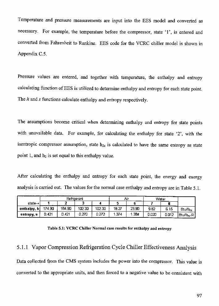
Temperature and pressure measurements are input into the EES model and converted as
necessary. For example, the temperature before the compressor, state T, is entered and
converted from Fahrenheit to Rankine. EES code for the VCRC chiller model is shown in
Appendix C.5.
Pressure values are entered, and together with temperature, the enthalpy and entropy
calculating function ofEES is utilized to determine enthalpy and entropy for each state point.
The h and s functions calculate enthalpy and entropy respectively.
The assumptions become critical when determining enthalpy and entropy for state points
with unavailable data. For example, for calculating the enthalpy for state '2', with the
isentropic compressor assumption, state h2s is calculated to have the same entropy as state
point 1, and h2 is set equal to this enthalpy value.
After calculating the enthalpy and entropy for each state point, the energy and exergy
analysis is carried out. The values for the normal case enthalpy and entropy are in Table 5.1.
state-*
Refric erant Air Water
1 2 3 4 5 6 7 8
enthalpy, h 174.90 184.90 102.30 102.30 1B.27 23.90 9.B2 B.15 Btu/lhm
entropy, s D.421 0.421 0.270 0.272 1.374 1.3B4 0.020 0.012 Btu/lbm-R
Table 5.1: VCRC Chiller Normal case results for enthalpy and entropy
5.1.1 Vapor Compression Refrigeration Cycle Chiller Effectiveness Analysis
Data collected from the CMS system includes the power into the compressor. This value is
converted to the appropriate units, and then forced to a negative value to be consistent with
97
the sign convention that work into the control volume is negative. In the EES code shown in
Appendix C.5, Ccompis the power into the compressor in kW, Wjncompbtu is the power into the
compressor in Btu/min after a conversion is performed, and Wjncomp is the power into the
compressor with the sign convention applied (power in is negative).
Mass flow rates are determined for the refrigerant, cooling air, and chilled water. To
determine mass flow rate of the refrigerant, the work into the compressor and the enthalpy
values of the refrigerant flowing into and out of the compressor are used. . The mass flow
rates of air and water are also determined. The mass flow rate of air is determined from the
calculated refrigerant mass flow rate and enthalpy values of the refrigerant and air flowing in
to and out of the condenser. The mass flow rate of water is determined knowing the chiller
capacity and the enthalpy value ofwater flowing in and out of the evaporator.
In the code shown in Appendix C.5, mR is the mass flow rate of the refrigerant, ma is the
mass flow rate of air, and mw is the mass flow rate of water. The subscripts'1'
and'2'
on h
represent the suction and outlet states of the compressor. The subscripts'2'
and'3'
are the
entering and leaving refrigerant flow in the condenser, while'5'
and'6'
are the entering and
leaving air flow of the condenser. Finally, subscripts'7'
and'8'
are entering and leaving
water flow for the evaporator. Cap is the chiller capacity, a value measured by the CMS
system. A condenser efficiency variable, r|Cond is included in this formulation, which is set to
a value of one (100%); however this can be adjusted ifmore data is available. The same is
done for the evaporator efficiency variable, r|evap- Although the actual condenser and
evaporator may not experience 100% efficiency, the actual efficiency is unknown. The
98
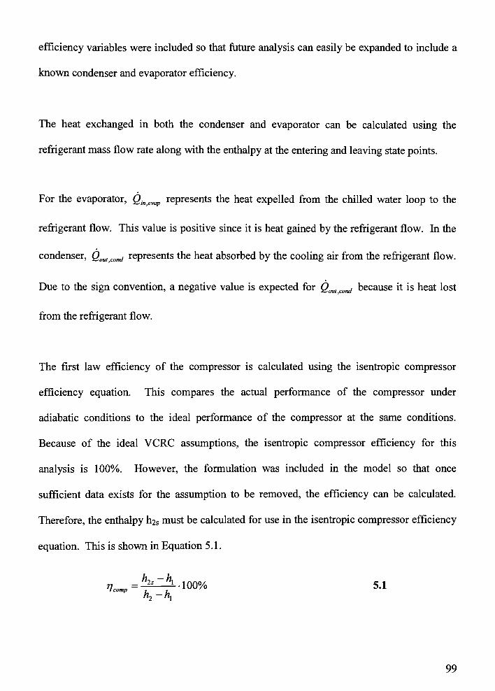
efficiency variables were included so that future analysis can easily be expanded to include a
known condenser and evaporator efficiency.
The heat exchanged in both the condenser and evaporator can be calculated using the
refrigerant mass flow rate along with the enthalpy at the entering and leaving state points.
For the evaporator, Qinevap represents the heat expelled from the chilled water loop to the
refrigerant flow. This value is positive since it is heat gained by the refrigerant flow. In the
condenser, g0,;Com/ represents the heat absorbed by the cooling air from the refrigerant flow.
Due to the sign convention, a negative value is expected for Qmlcond because it is heat lost
from the refrigerant flow.
The first law efficiency of the compressor is calculated using the isentropic compressor
efficiency equation. This compares the actual performance of the compressor under
adiabatic conditions to the ideal performance of the compressor at the same conditions.
Because of the ideal VCRC assumptions, the isentropic compressor efficiency for this
analysis is 100%. However, the formulation was included in the model so that once
sufficient data exists for the assumption to be removed, the efficiency can be calculated.
Therefore, the enthalpy li2s must be calculated for use in the isentropic compressor efficiency
equation. This is shown in Equation 5.1.
?jcnm=h2s~hl
-100% 5.1lcomp
h2-\
99
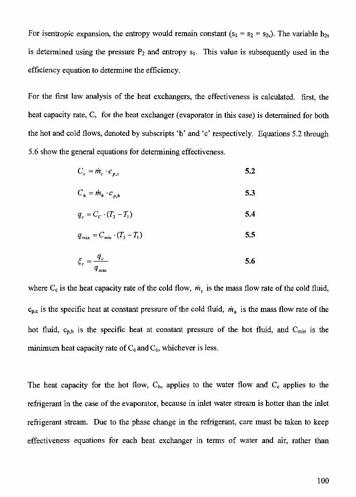
For isentropic expansion, the entropy would remain constant (si=
s2=
s2s). The variable h2s
is determined using the pressure P2 and entropy si. This value is subsequently used in the
efficiency equation to determine the efficiency.
For the first law analysis of the heat exchangers, the effectiveness is calculated, first, the
heat capacity rate, C, for the heat exchanger (evaporator in this case) is determined for both
the hot and cold flows, denoted by subscripts'h'
and'c'
respectively. Equations 5.2 through
5.6 show the general equations for determining effectiveness.
Cc=mc-cpc 5.2
Ch=rnh-cP,h 5.3
<7c=cc.(r2-7;) 5.4
tfmax ^min-C^-7,) 5-5
= 5.6
"max
where Cc is the heat capacity rate of the cold flow, mc is the mass flow rate of the cold fluid,
cp>c is the specific heat at constant pressure of the cold fluid, mh is the mass flow rate of the
hot fluid, cp,h is the specific heat at constant pressure of the hot fluid, and Cmjn is the
minimum heat capacity rate ofCc and Cc, whichever is less.
The heat capacity for the hot flow, Ch, applies to the water flow and Cc applies to the
refrigerant in the case of the evaporator, because in inlet water stream is hotter than the inlet
refrigerant stream. Due to the phase change in the refrigerant, care must be taken to keep
effectiveness equations for each heat exchanger in terms of water and air, rather than
100
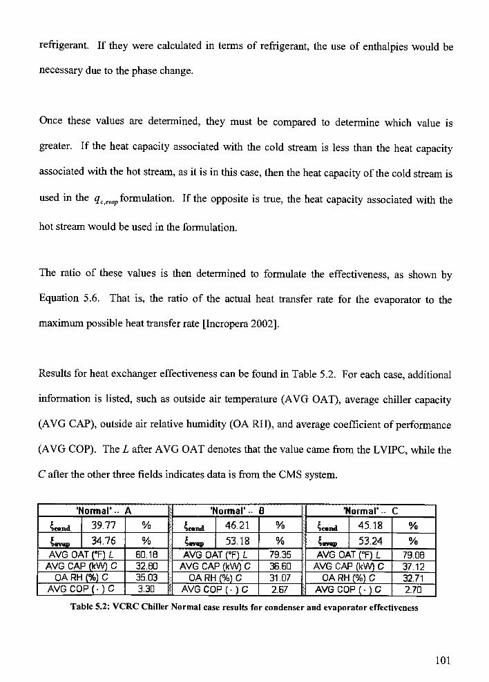
refrigerant. If they were calculated in terms of refrigerant, the use of enthalpies would be
necessary due to the phase change.
Once these values are determined, they must be compared to determine which value is
greater. If the heat capacity associated with the cold stream is less than the heat capacity
associated with the hot stream, as it is in this case, then the heat capacity of the cold stream is
used in the qcevap formulation. If the opposite is true, the heat capacity associated with the
hot stream would be used in the formulation.
The ratio of these values is then determined to formulate the effectiveness, as shown by
Equation 5.6. That is, the ratio of the actual heat transfer rate for the evaporator to the
maximum possible heat transfer rate [Incropera 2002].
Results for heat exchanger effectiveness can be found in Table 5.2. For each case, additional
information is listed, such as outside air temperature (AVG OAT), average chiller capacity
(AVG CAP), outside air relative humidity (OA RH), and average coefficient of performance
(AVG COP). The L after AVG OAT denotes that the value came from the LVIPC, while the
C after the other three fields indicates data is from the CMS system.
I\ormal'
- A ) "Normal'
- BNormal"
~ C
Scond 39.77 % Scond 46.21 % 1 Scond 45.18 %
Sevap 34.76 % tjevap 53.18 % Sevap 53.24 /o
AVG OAT (F) L BO. 18 AVG OAT (F) L 79.35 AVG OAT (F) L 79.0B
AVG CAP (kW) C 32.B0 AVG CAP (kW) C 36.60 AVG CAP (kW) C 37.12
OA RH (%) C 35.03 OA RH (%) C 31.07 OA RH (%) C 32.71
AVGCOP(-)C 3.30 f AVGCOP(-)C 2.67 AVGCOP(-)C 2.70
Table 5.2: VCRC Chiller Normal case results for condenser and evaporator effectiveness
101
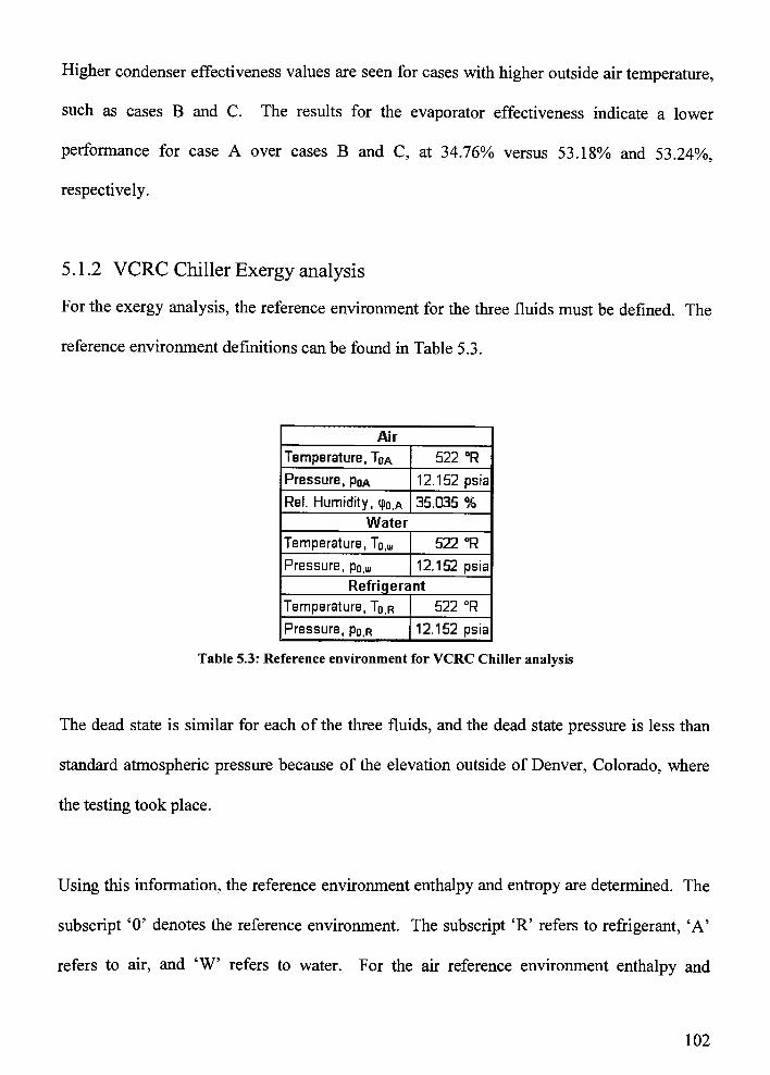
Higher condenser effectiveness values are seen for cases with higher outside air temperature,
such as cases B and C. The results for the evaporator effectiveness indicate a lower
performance for case A over cases B and C, at 34.76% versus 53.18% and 53.24%,
respectively.
5.1.2 VCRC Chiller Exergy analysis
For the exergy analysis, the reference environment for the three fluids must be defined. The
reference environment definitions can be found in Table 5.3.
Air
Temperature, Tqa 522 R
Pressure, pda 12.152 psia
Rel. Humidity, q>o,A 35.035 %
Water
Temperature, Tdi(U 522 R
Pressure, po, 12.152 psia
Refrigerant
Temperature, Tq,r 522 R
Pressure, p0,R 12.152 psia
Table 5.3: Reference environment for VCRC Chiller analysis
The dead state is similar for each of the three fluids, and the dead state pressure is less than
standard atmospheric pressure because of the elevation outside of Denver, Colorado, where
the testing took place.
Using this information, the reference environment enthalpy and entropy are determined. The
subscript'0'
denotes the reference environment. The subscript'R'
refers to refrigerant,'A'
refers to air, and 'W refers to water. For the air reference environment enthalpy and
102
entropies, the humidity ratio, w, is needed to define the state. This value is determined using
the properties, including relative humidity, and a psychrometric chart.
Refrigerant:
h0R =h('R22'
,T=T0r,P
= Por )
s0R= s
CR22'
,T=T0r,P
= Por )
Air:
h0A = h ('AirH20'
,T =T0A ,
P = P0a . w =w0A )
s0A= s ( "AirH2a ,
T =T0A ,P = Pqa . w =w0A )
Water:
how = h (Water'
,T =T0W ,
P = Pow )
sow= s (
Water'
,T =T0W ,
P = Pow )
For the exergy analysis it is necessary to calculate exergy flow rate for all flows in the
system. As previously mentioned, the exergy flow rate is the exergy transfer accompanying
mass flow. As a reminder, the general exergy flow rate equation is shown in Equation 5.7.
ef=(h-h0)-T0(s-s0) 5.7
where h is the enthalpy, ho is the dead state enthalpy, To is the dead state temperature, s is the
enthalpy and so is the dead state enthalpy.
The flow exergy allows us to calculate the exergy destroyed, which is useful to pinpoint
irreversibilities in the system. Exergy destroyed is calculated for the compressor, condenser,
and evaporator. The exergy destroyed values are affected by the use of an ideal cycle over an
103

actual cycle. The exergy destroyed for the compressor will be zero; however as with
previous calculations the exergy destroyed calculations are included in the analysis for future
use, in case actual VCRC cycle is used. The general exergy destroyed calculations use
Equations 5.8, 5.9, and 5.10.
Ed,c0mp =mR-(efl-ef2)-W 5.8
Ed,evap=
R (g/4"
g/l) +K'
0/7~
^J%) 5.9
Ed,COnd =a (e/s~
e/6) + mR (e/2-
ef3) 5.10
The variable W is the power into the compressor. In this case, mR is the mass flow rate of
the refrigerant, mA is the mass flow rate of the air, and mw is the mass flow rate of the
refrigerant.
Finally, the exergetic efficiency of the three components, compressor, condenser, and
evaporator, are calculated using Equations 5.11, 5.12, and 5.13.
5.11c
comp
ef2 ef\
-w
mR
100%
pevap
mR-(efl-
~/4)
mw-{e}1 -/s)
A-(e/<, -efi)
^cond ,
100% 5.12
100% 5.13
^(e/2-e/3)
Each equation is multiplied by 100% in order to report the exergetic efficiency as a
percentage. As previously mentioned, the value of ecomp is 100% due to unavoidable
assumptions.
104

The results for the exergetic efficiency and exergy destroyed for normal data can be found in
Table 5.4. Note that compressor value were removed due to redundancy (sCOmp= 100%,
Ed,comP= 0 Btu/min)
"Normal"
-A | "Normar - B J^ Normal"
- C
'comd 38.54 % ! \ *comd 83.32 % i ^cond 80.60 %
29.81 % l 1 g 25.45 % Eevap 25.29 %
t!>d,CDnd451.3 Btu/min ;
-^dfCond206.6 Btu/min !
-^d,cond251.9 Btu/min
J*d,evap 685.6 Btu/min i j? *"JdjCWfl(p752.2 Btu/min t^d,rvap 763.3 Btu/min
AVG OAT ffl L B0.1B \i AVG OAT (F) L 79.35 | AVG OAT (F) L 79.08
AVG CAP (kW) C 32.80 1\ AVG CAP (kW) C 36.60 I AVGCAP(kW)C 37.12
OA RH (%) C 35.D3 1 OA RH (%) C 31.07 OA RH (%) C 32.71
AVG COP ( - ) C 3.30 AVG COP ( - ) C 2.67!*v AVG COP ( - ) C 2.70
Table 5.4: VCRC Chiller Normal case results for exergy destroyed and exergetic efficiency
The condenser exergetic efficiency is much higher for cases B and C, which have
approximately 20F higher outside air temperature. The greater change in temperature across
the condenser results in an increase in exergetic efficiency. The evaporator exergetic
efficiency decreases slightly from 29.81% to 25.45% and 25.29% from A to B and C
respectively. The exergy destroyed values follow the opposite trend, as expected. When
exergetic efficiencies increase between cases, the corresponding exergy destroyed decreases,
and vice versa.
5.2 Fault Versus Normal Operation Analysis
The previous examples and results presented in Chapter 5 apply to the normal data collected
and analyzed. In addition to analyzing the normal data for the VCRC chiller, data for
refrigerantunder- and over-charge and oil under-charge were analyzed. A similar analysis
follows for all sets of data, and the collected data inputs (temperature, pressure, etc) are
105
changed in the model. In the future, the EES model developed to analyze the chiller could be
utilized to obtain energy and exergy results for the additional faults cases that were inflicted
on the chiller system that were not analyzed as a part of this research, such as oil overcharge,
air cooled condenser fouling, and loss of an air cooled condenser fan.
Data from the analyzed fault cases is found in Chapter 3. This data, along with the analysis
developed in the previous section, yields results for the fault scenarios analyzed in Section
5.3.
5.3 Vapor Compression Refrigeration Cycle ChillerResults - Normal and
Fault Operation
The results obtained from normal VCRC chiller analysis are included in Table 5.5. Results
are shown for the evaporator, compressor, and condenser. Due to the assumptions made, the
first and second law efficiencies for the compressor were 100%, and the value for exergy
destroyed was zero. The upper eleven fields in Table 5.5 are results from the analysis
described above, while the lower four fields are collected data from either LVIPC designated
'L'
in Table 5.5, and CMS, denoted 'C in Table 5.5, respectively. The lower four fields are
helpful for comparison of results.
106
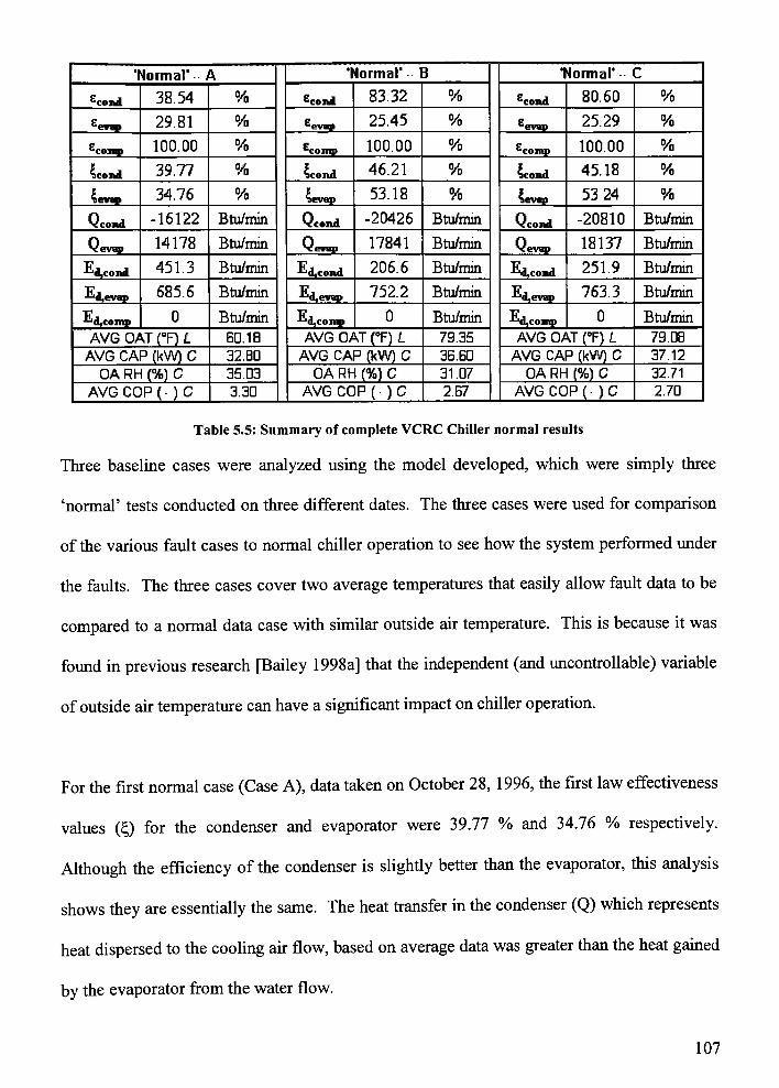
formal'-- A"Normal"
- 3"Normal"
-- c
cond 38.54 % ^cond 83.32 % cond 80.60 %
'evap29.81 % 'evnp
25.45 % 25.29 %
*comp 100.00 % 'comp 100.00 %'comp 100.00 %
Scond 39.77 % Scond 46.21 % Scond 45.18 %
Sevap 34.76 % Sevap 53.18 % Sevap 53.24 %
Second -16122 Btu/min Vcond -20426 Btu/minVcond -20810 Btu/min
Vevap14178 Btu/min Vevap 17841 Btu/min
Vevap18137 Btu/min
-'^d.coiid451.3 Btu/min
-*^d,cond206.6 Btu/min t^djCond 251.9 Btu/min
d,evaD 685.6 Btu/min t^d,evap 752.2 Btu/min t!>d,evap 763.3 Btu/min
'-'djComp0 Btu/min -^djconqr
0 Btu/min E'&fComg0 Btu/min
AVG OAT (F) L 60.18 AVG OAT (F) L 79.35 AVG OAT (F) L 79.08
AVG CAP (kW) C 32.B0 AVG CAP (kW) C 36.60 AVG CAP (kW) C 37.12
OA RH (%) C 35.03 OA RH (%) C 31.07 OA RH (%) C 32.71
AVG COP ( - ) C 3.30 AVG COP (-
) C 2.67 AVGCOP(-)C 2.70
Table 5.5: Summary of complete VCRC Chiller normal results
Three baseline cases were analyzed using the model developed, which were simply three
'normal'
tests conducted on three different dates. The three cases were used for comparison
of the various fault cases to normal chiller operation to see how the system performed under
the faults. The three cases cover two average temperatures that easily allow fault data to be
compared to a normal data case with similar outside air temperature. This is because it was
found in previous research [Bailey 1998a] that the independent (and uncontrollable) variable
ofoutside air temperature can have a significant impact on chiller operation.
For the first normal case (Case A), data taken on October 28, 1996, the first law effectiveness
values () for the condenser and evaporator were 39.77 % and 34.76 % respectively.
Although the efficiency of the condenser is slightlybetter than the evaporator, this analysis
shows they are essentially the same. The heat transfer in the condenser (Q) which represents
heat dispersed to the cooling air flow, based on average data was greater than the heat gained
by the evaporator from the water flow.
107
The evaporator analysis revealed a higher exergy destroyed ( ED ) than the exergy destroyed
in the condenser for Normal Case A. This is consistent with the first law efficiency values;
the condenser performs better than the evaporator. For the second law efficiency (e), the
model predicts the condenser to have a better performance than the evaporator. This finding
is the same as with the first law analysis, however based on the second law, the performance
of the condenser is approximately 9% higher than the evaporator, while the effectiveness
analysis only predicted a 5% increase in performance between the two heat exchangers. This
leads to the conclusion that although the first law analysis suggests that the condenser and
evaporator were closer to equal in performance, the second law analysis reveals a noticeably
better performance in the condenser compared with the evaporator. This is likely due to the
higher change in temperature across the condenser.
For the second set of normal data, denoted by'B'
in Table 5.5, the effectiveness calculations
for the condenser and evaporator are 46.21% and 53.18 % respectively. Unlike normal case
A, the condenser for the normal B analysis has a slightly lower performance than the
evaporator.
In this case, the exergy destroyed is much higher in the evaporator. For the exergetic
efficiency, the condenser performance is predicted to be higher, although according to the
exergetic analysis, the performance is significantly higher forthe condenser, at 83.32%, than
the evaporator, at 25.45%.
108
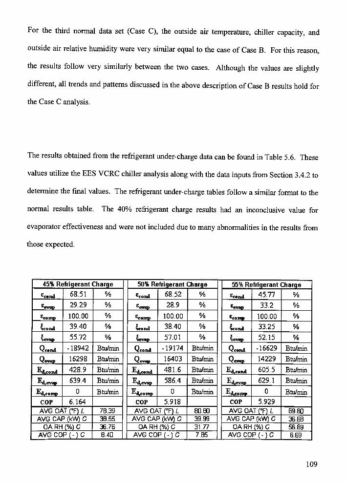
For the third normal data set (Case C), the outside air temperature, chiller capacity, and
outside air relative humidity were very similar equal to the case of Case B. For this reason,
the results follow very similarly between the two cases. Although the values are slightly
different, all trends and patterns discussed in the above description ofCase B results hold for
the Case C analysis.
The results obtained from the refrigerant under-charge data can be found in Table 5.6. These
values utilize the EES VCRC chiller analysis along with the data inputs from Section 3.4.2 to
determine the final values. The refrigerant under-charge tables follow a similar format to the
normal results table. The 40% refrigerant charge results had an inconclusive value for
evaporator effectiveness and were not included due to many abnormalities in the results from
those expected.
45% Refrigerant Charge 50% Refrigerant Charge 55% Refrigerant Charqe
cond 68.51 % ^cond 68.52 % cond 45.77 %
^evap 29.29 % ^evap 28.9 % &evap 33.2 %
comp 100.00 % ecomp 100.00 % ^cornp 100.00 %
Scond 39.40 % Scond 38.40 % Scond 33.25 %
Sevap55.72 % Sevap
57.01 % Sevap 52.15 %
Wcond -18942 Btu/min ^ccond -19174 Btu/min Vfcond -16629 Btu/min
Xevap16298 Btu/min
Vevap16403 Btu/min Vfevap 14229 Btu/min
-^diCond428.9 Btu/min
-"dgcond481.6 Btu/min
-"dgcond605.5 Btu/min
-E'dlevap639.4 Btu/min
lid,evap586.4 Btu/min t->d,evap 629.1 Btu/min
-^dcomp0 Btu/min
-"dgComp0 Btu/min -^djcoiin*
0 Btu/min
COP 6.164 COP 5.918 COP 5.929
AVG OAT (F) L 78.39 AVG OAT (F) L B0.8D AVG OAT (F) L 69.60
AVG CAP (kW) C 3B.55 AVG CAP (kW) C 39.99 AVG CAP (kW) C 36.68
OA RH (%) C 36.76 OA RH (%) C 31.77 OA RH (%) C 56.69
AVG COP ( - ) C B.40 AVG COP ( - ) C 7.85 AVGCOP(-)C 6.69
109
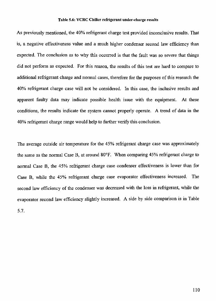
Table 5.6: VCRC Chiller refrigerant under-charge results
As previously mentioned, the 40% refrigerant charge test provided inconclusive results. That
is, a negative effectiveness value and a much higher condenser second law efficiency than
expected. The conclusion as to why this occurred is that the fault was so severe that things
did not perform as expected. For this reason, the results of this test are hard to compare to
additional refrigerant charge and normal cases, therefore for the purposes of this research the
40% refrigerant charge case will not be considered. In this case, the inclusive results and
apparent faulty data may indicate possible health issue with the equipment. At these
conditions, the results indicate the system cannot properly operate. A trend of data in the
40% refrigerant charge range would help to further verify this conclusion.
The average outside air temperature for the 45% refrigerant charge case was approximately
the same as the normal Case B, at around 80F. When comparing 45% refrigerant charge to
normal Case B, the 45% refrigerant charge case condenser effectiveness is lower than for
Case B, while the 45% refrigerant charge case evaporator effectiveness increased. The
second law efficiency of the condenser was decreased withthe loss in refrigerant, while the
evaporator second law efficiency slightly increased. A side by side comparison is in Table
5.7.
110
formal'
- 3 45% Refrigerant Charge
^cond 83.32 % cond 68.51 %
c
evap25.45 %
^evap29.29 %
^comp 100.00 %'comp 100.00 %
Scond 46.21 %Scond 39.40 %
Sevap53.18 %
Sevap55.72 %
Vcond -20426 Btu/min Vcond -18942 Btu/min
Vfevap17841 Btu/min
Vevap16298 Btu/min
J-'d,coid 206.6 Btu/min"dicond
428.9 Btu/min
-c,d,evap752.2 Btu/min p
-1Ld,evap639.4 Btu/min
^djComp0 Btu/min p 0 Btu/min
COP 6.901 COP 6.164
AVG OAT (F) L 79.35 AVG OAT (F) L 7B.39
AVG CAP (kW) C 36.60 AVG CAP (kW) C 3B.55
OA RH (%) C 31.07 OA RH {%) C 36.76
AVG COP ( - ) C 2.67 AVGCOP(-)C 8.40
Table 5.7: Side by side comparison of normal case B and 45% refrigerant charge
When analyzing the 50% refrigerant under-charge data, which also had a similar outside air
temperature to normal case B, similar results could be seen. A side by side comparison of
50% refrigerant charge and normal case B is in Table 5.8. Particularly, the decrease in
condenser second law efficiency compared to normal case B and slight increase in evaporator
second law efficiency. The effectiveness values of the condenser and evaporator in the 50%
refrigerant charge case were 38.40% and 57.01%, respectively. Overall, weighing the results
of the second law analysis more important than effectiveness, there is not much change
between the 45% refrigerant charge and 50% refrigerant charge cases, and both show
significant deviations from normal B case, mainly in the form of decreased condenser
performance. It is also important to note that the COP determined from the CMS system
(last line in Table 5.7) is higher for the fault case. In previous work done by Bailey [1998] it
was determined that when simply looking at COP of normal vs. fault operation, the specified
111
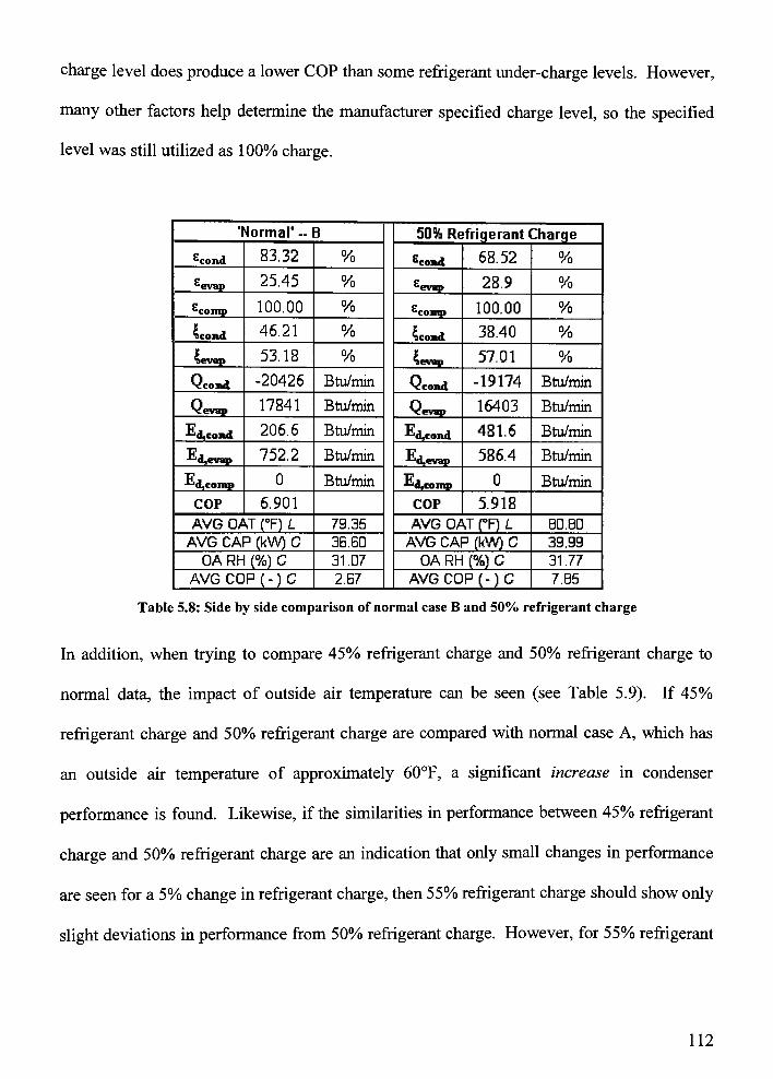
charge level does produce a lower COP than some refrigerant under-charge levels. However,
many other factors help determine the manufacturer specified charge level, so the specified
level was still utilized as 100% charge.
formal"
- B 50% Refrigerant Charqe
cond 83.32 % cond 68.52 %
Eevap
25.45 %evap
28.9 %
comp 100.00 % ^comjt 100.00 %
Scond 46.21 % Scond 38.40 %
Sevap53.18 %
Sevap 57.01 %
Vcond -20426 Btu/min *<cond -19174 Btu/min
Vrfevap17841 Btu/min Vfevap 16403 Btu/min
p-^djcond
206.6 Btu/min p"djcond
481.6 Btu/min
"djevap752.2 Btu/min p
-"djevap586.4 Btu/min
"P 0 Btu/min p 0 Btu/min
COP 6.901 COP 5.918
AVG OAT (F) L 79.35 AVG OAT (F) L B0.BD
AVG CAP (kW) C 36.60 AVG CAP (kW) C 39.99
OA RH (%) C 31.07 OA RH (%) C 31.77
AVG COP ( - ) C 2.67 AVGCOP(-)C 7.B5
Table 5.8: Side by side comparison of normal case B and 50% refrigerant charge
In addition, when trying to compare 45% refrigerant charge and 50% refrigerant charge to
normal data, the impact of outside air temperature can be seen (see Table 5.9). If 45%
refrigerant charge and 50% refrigerant charge are compared with normal case A, which has
an outside air temperature of approximately 60F, a significant increase in condenser
performance is found. Likewise, if the similarities in performance between 45% refrigerant
charge and 50% refrigerant charge are an indication that only small changes in performance
are seen for a 5% change in refrigerant charge, then 55% refrigerant charge should show only
slight deviations in performance from 50% refrigerant charge. However, for 55% refrigerant
112
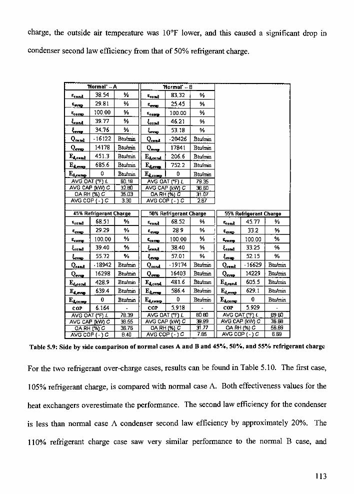
charge, the outside air temperature was 10F lower, and this caused a significant drop in
condenser second law efficiency from that of 50% refrigerant charge.
'Normal*
-A
'Normal'
- 3
cond 38.54 % ^cond 83.32 %
&evBj 29.81 % ^evop 25.45 %
Ecomp 100.00 %^comp 100.00 %
Scond 39.77 % Scond 46.21 %
Sevap34.76 %
Sevap53.18 %
Nfcond -16122 Btu/min Qcond -20426 Btu/min
Vevap14178 Btu/min Qeve. 17841 Btu/min
^d,cond 451.3 Btu/min-"dfCond
206.6 Btu/min
E^evap 685.6 Btu/min ^ievip 752.2 Btu/min
"djgoing0 Btu/min "d^conqt
0 Btu/min
AVG OAT (F) L 60. 18 AVG OAT (F) L 79.35
AVG CAP (kW) C 32.80 AVG CAP (kW) C 36.60
OA RH (%) C 35.03 OA RH (%) C 31.07
AVG COP ( - ) C 3.30 AVG COP ( - ) C 2.67
45% Refrigerant 1Charge 50% Refrigerant iZharge 55% Refrigerant Zharge
cond 68.51 % cond 68.52 % ^cond 45.77 %
Eerap 29.29 %'evap
28.9 % Sevan 33.2 %
^coirrp 100.00 %^comp 100.00 % ^comp 100.00 %
Scond 39.40 % Scond 38.40 % Scond 33.25 %
Sevap55.72 % Sevap 57.01 %
Sevap52.15 %
Qcond -18942 Btu/min Vcond -19174 Btu/min Qcond -16629 Btu/min
Vevep 16298 Btu/min VJevap 16403 Btu/min Vevap 14229 Btu/min
-^dfCond428.9 Btu/min
-"dfCond481.6 Btu/min
-^djCond605.5 Btu/min
-^(^evap639.4 Btu/min Ed,evp 586.4 Btu/min
-B'd.evap629.1 Btu/min
*-,d]coiinp0 Btu/min
-^drComp0 Btu/min
-^djComp0 Btu/min
COP 6.164 - COP 5.918 - COP 5.929 -
AVG OAT (F) L 7B.39 AVG OAT (DF) L 80.80 AVG OAT (F) L 69.60
AVG CAP (kW) C 3B.55 AVG CAP (kW) C 39.99 AVG CAP (kW) C 36.68
OA RH (%) C 36.76 OA RH (%) C 31.77 OA RH (%) C 56.69
AVGC0P(-)C B.40 AVG COP ( - ) C 7.B5 AVG COP ( - ) C E.E9
Table 5.9: Side by side comparison of normal cases A and B and 45%, 50%, and 55% refrigerant charge
For the two refrigerant over-charge cases, results can be found in Table 5.10. The first case,
105% refrigerant charge, is compared with normal case A. Both effectiveness values for the
heat exchangers overestimate the performance. The second law efficiency for the condenser
is less than normal case A condenser second law efficiency by approximately 20%. The
110% refrigerant charge case saw very similar performance to the normal B case, and
113
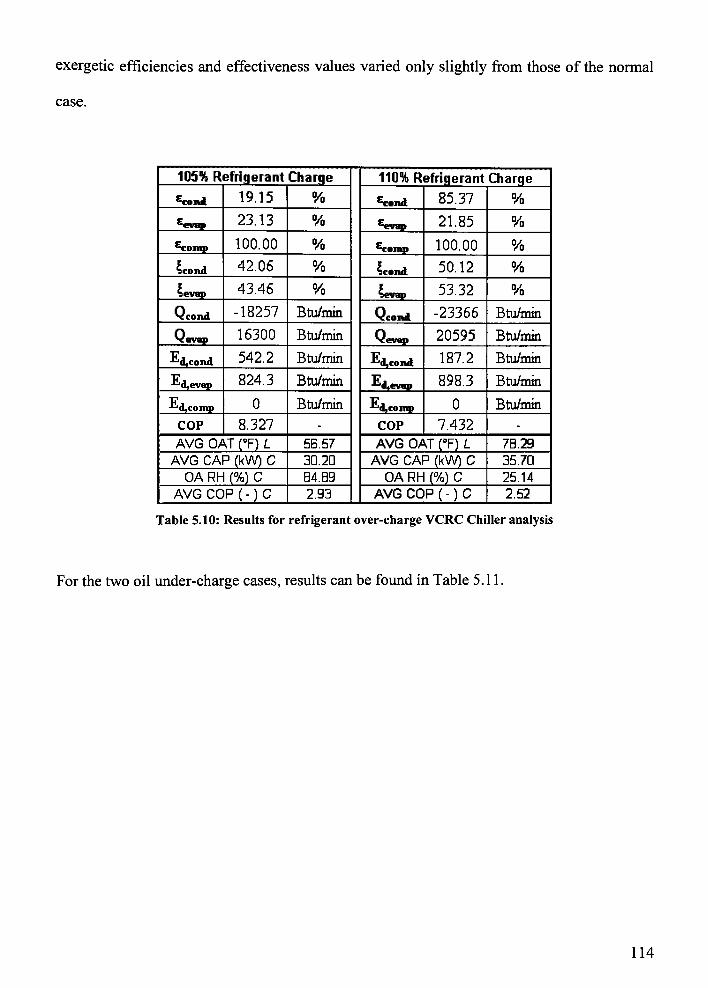
exergetic efficiencies and effectiveness values varied only slightly from those of the normal
case.
105% Refrigerant Charge 110% Refrigerant Charge
scond 19.15 % Gcond 85.37 %
*evap23.13 % Sevap 21.85 %
'comp 100.00 % ^courts 100.00 %
Scond 42.06 % Scond 50.12 %
Sevap 43.46 % Sevap 53.32 %
Second -18257 Btu/min Vcond -23366 Btu/min
VeTevap 16300 Btu/minVcTevap 20595 Btu/min
p^dcond
542.2 Btu/min-"dcond
187.2 Btu/min
-i-<d,evap824.3 Btu/min djCvap 898.3 Btu/min
p 0 Btu/min-'-'djcomp
0 Btu/min
COP 8.327 - COP 7.432 -
AVG OAT (F) L 56.57 AVG OAT (DF) L 7B.29
AVG CAP (kW) C 30.20 AVG CAP (kW) C 35.70
OA RH (%) C B4.B9 OA RH (%) C 25.14
AVG COP ( - ) C 2.93 AVG COP (-
) C 2.52
Table 5.10: Results for refrigerant over-charge VCRC Chiller analysis
For the two oil under-charge cases, results can be found in Table 5.11.
114
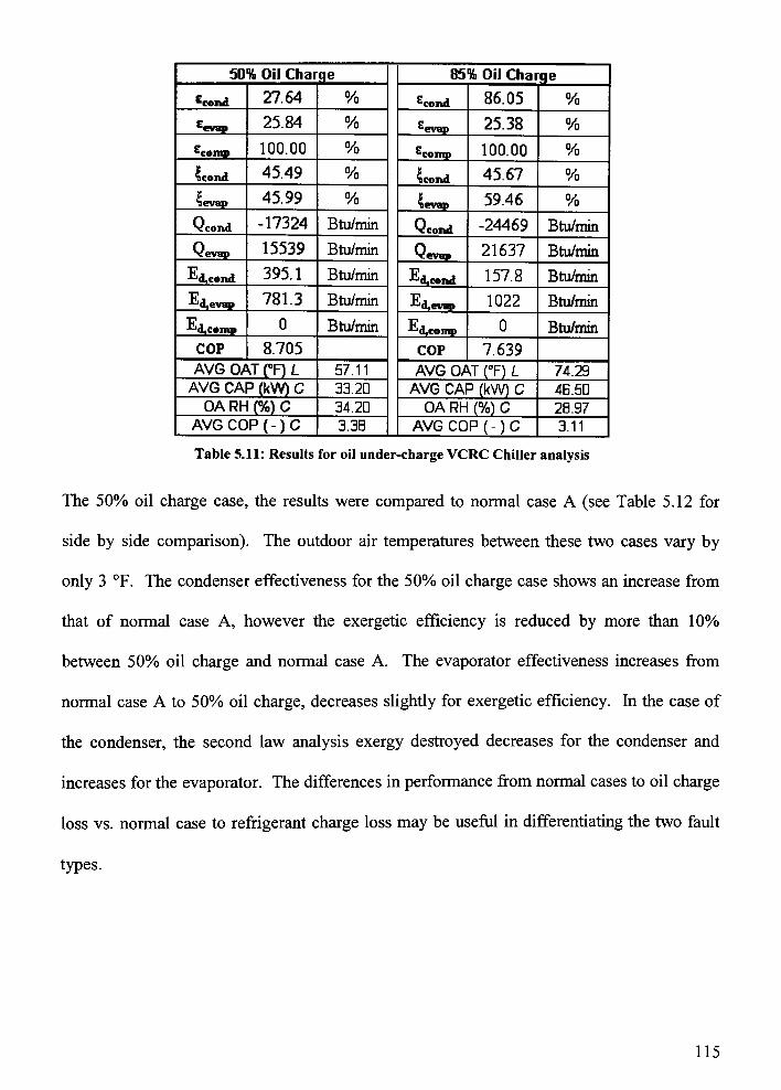
50% Oil Charge 85% Oil Charge
econd 27.64 /o cond 86.05 %
evap 25.84 %'evap 25.38 %
comp 100.00 % comp 100.00 %
Scond 45.49 % Scond 45.67 %
Sevap 45.99 %Sevap 59.46 %
>fcond -17324 Btu/minxcond -24469 Btu/min
Vevap15539 Btu/min
Vevap21637 Btu/min
-^dcond395.1 Btu/min
-"drcond157.8 Btu/min
pJ-1d,evap 781.3 Btu/min^djevap
1022 Btu/min
p-^dtcomp
0 Btu/min pJ-,d,conn) 0 Btu/min
COP 8.705 COP 7.639
AVG OAT (F) L 57.11 AVG OAT (F) L 74.29
AVG CAP (kW) C 33.20 AVG CAP (kW) C 4B.50
OA RH (%) C 34.20 OA RH (%) C 2B.97
AVG COP ( - ) C 3.38 AVGCOP(-)C 3.11
Table 5.11: Results for oil under-charge VCRC Chiller analysis
The 50% oil charge case, the results were compared to normal case A (see Table 5.12 for
side by side comparison). The outdoor air temperatures between these two cases vary by
only 3 F. The condenser effectiveness for the 50% oil charge case shows an increase from
that of normal case A, however the exergetic efficiency is reduced by more than 10%
between 50% oil charge and normal case A. The evaporator effectiveness increases from
normal case A to 50% oil charge, decreases slightly for exergetic efficiency. In the case of
the condenser, the second law analysis exergy destroyed decreases for the condenser and
increases for the evaporator. The differences in performance from normal cases to oil charge
loss vs. normal case to refrigerant charge loss may be useful in differentiating the two fault
types.
115
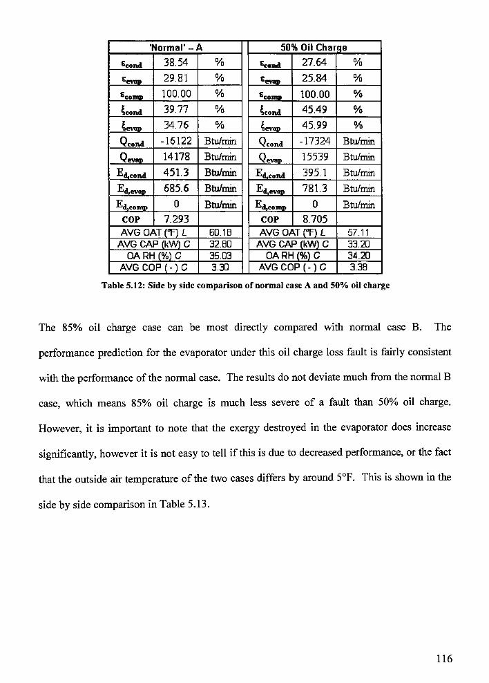
Normal1
-A 50% Oil Charge
econd 38.54 % 'cond 27.64 %
^evap29.81 % c
evap25.84 %
comp 100.00 %'comp 100.00 %
Scond 39.77 % Scond 45.49 %
Sevap34.76 % Sevap 45.99 %
Vcond -16122 Btu/minVcond -17324 Btu/min
Vevap14178 Btu/min
Vevap15539 Btu/min
-'-'dgcond451.3 Btu/min
-*-Jd,cond395.1 Btu/min
^'d.evap 685.6 Btu/mind,evap 781.3 Btu/min
p-^djComp
0 Btu/min p 0 Btu/min
COP 7.293 COP 8.705
AVG OAT (F) L 60. 1B AVG OAT (F) L 57.11
AVG CAP (kW) C 32.B0 AVG CAP (kW) C 33.20
OA RH (%) C 35.03 OA RH (%) C 34.20
AVG COP ( - ) C 3.30 AVGCOP(-)C 3.3S
Table 5.12: Side by side comparison of normal case A and 50% oil charge
The 85% oil charge case can be most directly compared with normal case B. The
performance prediction for the evaporator under this oil charge loss fault is fairly consistent
with the performance of the normal case. The results do not deviate much from the normal B
case, which means 85% oil charge is much less severe of a fault than 50% oil charge.
However, it is important to note that the exergy destroyed in the evaporator does increase
significantly, however it is not easy to tell if this is due to decreased performance, orthe fact
that the outside air temperature of the two cases differs by around 5F. This is shown in the
side by side comparison in Table 5.13.
116
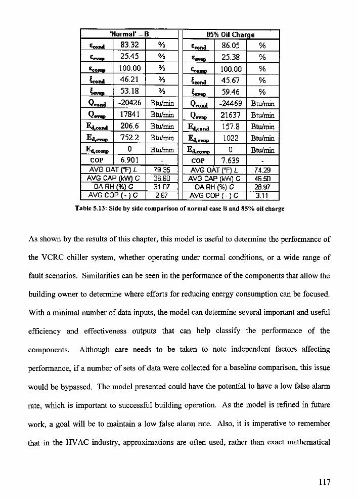
formal*
- B 85% Oil Charge
^cond 83.32 % cond 86.05 %
**evap25.45 %
&evap 25.38 %
^comm 100.00 % comp 100.00 %
Scond 46.21 % Scond 45.67 %
Sevap53.18 %
Sevap 59.46 %
Vcond -20426 Btu/minVcond -24469 Btu/min
Vevap 17841 Btu/minVevap
21637 Btu/min
-^(Ucond206.6 Btu/min p
-"dgcond157.8 Btu/min
p-"djevap
752.2 Btu/min^devap
1022 Btu/min
p-^dTComp
0 Btu/min-^dtcomp
0 Btu/min
COP 6.901 - COP 7.639 -
AVG OAT (F) L 79.35 AVG OAT (F) L 74.29
AVG CAP (kW) C 36.60 AVG CAP (kW) C 46.50
OA RH (%) C 31.07 OA RH (%) C 2B.97
AVGCOP(-)C 2.67 AVGCOP(-)C 3.11
Table 5.13: Side by side comparison of normal case B and 85% oil charge
As shown by the results of this chapter, this model is useful to determine the performance of
the VCRC chiller system, whether operating under normal conditions, or a wide range of
fault scenarios. Similarities can be seen in the performance of the components that allow the
building owner to determine where efforts for reducing energy consumption can be focused.
With a minimal number of data inputs, the model can determine several important and useful
efficiency and effectiveness outputs that can help classify the performance of the
components. Although care needs to be taken to note independent factors affecting
performance, if a number of sets of data were collected for a baseline comparison, this issue
would be bypassed. The model presented could have the potential to have a low false alarm
rate, which is important to successful building operation. As the model is refined in future
work, a goal will be to maintain a low false alarm rate. Also, it is imperative to remember
that in the HVAC industry, approximations are often used, rather than exact mathematical
117
and statistical methods. It is important that the amount of data collected, whether by hand or
by data acquisition system, is not too intensive in order for this model to be of use in the
field. A methodology that included implementation of excessive instrumentation or time
intensive retraining of technicians would not be widely accepted by this industry due to the
time and effort they are looking to spend to get a similar output.
The model and results show viability of using exergetic analysis for the purposes of health
monitoring. It utilizes existing data to determine performance. In terms of health
monitoring, the model can successfully produce results with similarities that can be utilized
for health monitoring of the system components. Deviations in performance between normal
and faulty data are detected, which can be used for health monitoring.
If more data were obtained for various temperature scenarios, this model may be useful in
actually classifying whether a fault has occurred, and therefore could be used asa predictor.
It is unknown without further analysis whether the model could actually produce results
specific enough in nature to differentiate between the various fault cases, but with enough
baseline data, the model is capable of determining if operation is deviating from normal.
Further research in this area could be expanded to collect additional data and utilize the
model developed in this research to determine trends necessary to classify the various fault
cases based on output from the model.
5.4 Chiller Conclusions
As previously mentioned, three baseline cases were analyzed using the model developed.
The three cases were used for comparison of the various fault cases to normal chiller
118
operation to see how the system performed under the faults. The three cases cover two
average temperatures that easily allow fault data to be compared to a normal data case with
similar outside air temperature. This is because it was found in previous research [Bailey
1998a] that the independent (and uncontrollable) variable of outside air temperature can have
a significant impact on chiller operation.
This model is useful to determine the performance of the VCRC chiller system, whether
operating under normal conditions, or a wide range of fault scenarios. Trends can be seen in
the performance of the components that allow the building owner to determine where efforts
for reducing energy consumption can be focused. With a minimal number of data inputs, the
model can determine several important and useful efficiency and effectiveness outputs that
can help classify the performance of the components. Although care needs to be taken to
note independent factors affecting performance, if a number of sets ofdata were collected for
a baseline comparison, this issue would be bypassed.
The model presented shows deviations in efficiencies and exergy destroyed from normal to
faulty operation. This can be used to determine if the equipment is operating properly or a
fault has occurred. The results show the viability of using exergy analysis for health
monitoring. To continue this research, several steps should be taken to expand the model and
increase accuracy, as discussed in Section 6.5.
If more data were obtained for various temperature scenarios, this model may be useful in
actually classifying whether a fault has occurred, andtherefore could be used as a predictor.
119
It is unknown without further analysis whether the model could actually produce results
specific enough in nature to differentiate between the various fault cases, but it is predicted
that with enough baseline data, the model is capable of determining if operation is deviating
from normal.
120
6 Conclusions
In this chapter, a summary of the research is presented, general conclusions are summarized,
and conclusions from the AHU and VCRC chiller models will be discussed. Conclusions are
followed by recommendations for future work.
6.1 Summary
In Chapter One, a literature review is presented ofprevious research in the field of the second
law of thermodynamics, the benefits of exergy analysis over energy analysis, as well as the
concept of exergy applied to various building mechanical systems. The field of
retrocommissioning is also researched as it pertains to the AHU studied in the first portion of
the research. The current research in an expansion on exergy analyses for building systems
in a new context, which includes both exergy analysis in conjunction with
retrocommissioning, and exploring the viability of exergy analysis for health monitoring of
VCRC chiller systems.
Background for the systems studied is presented in Chapter 2. The components and
subcomponents of air handling units and VCRC chillers are presented and described. Chapter
3 discusses the experimental data collection for the two models developed, including the data
collection for the AHU in conjunction with a capstone design project in the area of
retrocommissioning, as well as the VCRC chiller data collected as part of a doctoral
dissertation. Data from both experiments is presented as it pertains to the current analysis
and research.
121
Chapter 4 discusses the analysis conducted using the AHU data. Sections of important code
are shown and the progression of the analysis is presented, including examples for various
calculations and data points. The energy and exergy analysis for all of the AHU
subcomponents are outlined, followed by results and conclusions about the utility of the
model developed as well as the benefit of the second law analysis in the research. In this
chapter, a dead state variance study is also presented to validate the dead state selected for
the analysis. Results and conclusions for the AHU subcomponents are presented.
In Chapter 5, the VCRC chiller analysis and model are presented. Like with the AHU,
sections of the model are discussed, including energy and exergy analysis for the
subcomponents. The analysis is conducted for normal data as well as a range of fault
scenarios. Results and conclusions are presented for both normal and fault data.
The following sections will summarize important conclusions and offer recommendations for
further research in this area.
6.2 General Conclusions
Both the AHU and VCRC chiller model are able to successfully determine the first and
second law performance of the subcomponents. The models developed are useful for solving
an inverse problem with collected or existing data. This analysis provides insight to the
performance of the sub-components, and helps determine where energy consumption
improvement efforts should be focused, or at which set point equipment should be run.
122
The inclusion of second law analysis helps to provide additional insight to system
performance without extra data points which is consistent with research presented in Chapter
1 . Care is taken to keep the models relatively simplistic so that they will be easily accepted
in the HVAC industry. The methods provide valuable insight to building owners about
system and subcomponent performance and health monitoring, and show the benefit of
exergy analysis in the context ofRCX and health monitoring ofVCRC chiller systems, both
ofwhich should be further explored.
6.3 AHUModel Conclusions
After review of the results from the AHU model, several conclusions are drawn.
For the fan analysis the first law analysis did not pinpoint a specific set point that
was the most efficient; however after conducting a second law analysis, the
exergy destroyed results lead to the conclusion that the best static pressure set
point is the lowest set point for both the supply and return fan.
It is recommended that the lowest static pressure set point be maintained as long
as supply air requirements are satisfied.
The first and second law analysis reveals several things about the system performance:
The trends in efficiency between the first and secondlaw analysis make it difficult to
determine which set point produces the best efficiency.
Relying on the exergy destroyed value, it is clearthat the lowest duct static pressure
set point is in fact the most efficient. Without the more advanced thermodynamic
analysis, a building owner may not conclude that thelowest set point is in fact the
best choice.
123
Lowering the duct static pressure set point can save building owners money because
less power to the fan is necessary to maintain this lower duct static pressure.
The benefits of exergy analysis are shown, and the fan model successfully predicts
performance of the component utilizing the RCX data previously collected.
For the AHU heating coil, the following conclusions are drawn:
The low values for the coil second law efficiency for the second set point may be
explained by work done by Qureshi et al. [2003]. The exergy destroyed in the
heating coil is similar for both the first and second set points(1.00"
WC and1.25"
WC), and much higher for the third set point (1 WC).
Increasing the valve percentage open from 25% to 50% has a more significant impact
than increasing air volumetric flow rate. Based on the fact that the exergetic
efficiency values are very low for all three set points, the other two determining
factors (effectiveness and exergy destroyed) lead to the conclusion that the first set
point is the most efficient, because it has the lowest exergy destroyed. It also has the
highest effectiveness.
In this case the exergetic efficiencies did not necessarily provide a better picture of
the performance. The variance in the results shows the difference in efficiency for
various set points; however a change in coil operational points is necessary to
maintain occupant comfort.
For the economizer analysis, the following conclusions are made:
124
Results show higher exergetic efficiency in full economizer mode, which is expected.
This mode is meant to minimize energy use by utilizing outdoor air at a similar
temperature to the desired supply air temperature set point. It typically eliminates the
need for heating or cooling of the supply air, which decreases energy consumption
associated with hot and chilled water production.
There is more heat lost in full economizer mode than in lock-out mode, and similarly
there is greater exergy destroyed for full mode comparedwith lock-outmode.
In all three sub-components, the exergy analysis provides great benefit and insight to the
performance of the equipment. Particularly, with the fans, the included exergetic analysis
clarifies which set point would have the best performance. Also, the exergy destroyed in the
heating coil helps clarify the best set point. The first and second law analyses are useful in
determining set points which yield better performance. The model developed is useful for
health monitoring, and along with the RCX process can help determine the system health and
performance.
Exergy analysis in the context of retrocommissioning provides insight into where exergy is
being destroyed. There are few additional data points that are necessary to conduct the
second law analysis, but the additional benefit is significant. It is the recommendation that
portions of the second law analysis be included in RCX activities for a better picture of
system performance. The model presented, including first and second law analysis, can be
utilized to determine performance of an AHU particularly while obtaining data during
retrocommissioning of the equipment. The RCX work done is helpful to the building owner
125
because the reduced set points will conserve energy, and pre-functional testing and
sensor/control system verification helps to optimize the system.
6.4 VCRCChillerModel Conclusions
The following VCRC chiller conclusions were drawn:
The effectiveness of the condenser and evaporator are determined to be
approximately equal after the first law analysis.
After conducting a second law analysis, it is revealed that the efficiencies and
differences in exergy destroyed are not similar, and the condenser has much better
performance than the evaporator.
This difference in performance indicates measures to improve evaporator efficiency
should be taken.
The conclusion that the first law is unable to properly classify the performance of the
devices is made.
The true performance is clarified after the second law analysis is conducted, and it is
revealed that the condenser outperformed the evaporator.
Many similarities in data are seen when comparing the normal case results to the various
fault scenarios. The conclusions drawn from this part of the research include:
In several cases, such as 45% refrigerant charge and 50% oil charge, the exergy
analysis provides more useful information than analyzing the heat exchanger
effectiveness.
126
It is concluded that the model could be viable for analyzing the fault case
performance and it would be beneficial to explore further development of this
method. However, it is also noted that ifmore baseline and fault data is available, the
model may be useful in predicting whether or not the chiller is experiencing a fault, or
even which particular fault is taking place.
In the research pertaining to the chiller, an inverse problem is successfully solved. A
previous "blackbox"
method for monitoring system health is replaced with a thermodynamic
model using exergetic analysis that is capable of predicting performance and health
monitoring insight under various load and operational scenarios.
6.5 Recommendationsfor Future Work
In the future, this work could be extended to additional types of building equipment, such as
boilers. It could also be expanded to similar equipment that may have different
configurations to the devices studied. The model presented would need slight modifications
to accommodate different systems and components, as AHUs and VCRC chillers often differ
in configuration. In addition, tying in an economic and exergoeconomic analysis into the
research would be useful for building owners, who are concerned with the cost savings these
methods may bring.
It is recommended that the models developed be enhanced to reduce the number of
assumptions made, particularly the idealized cycle assumption for the VCRC chiller model.
127
To verify the improved model, an additional experimental test plan is required in order to
collect sufficient data for the new model. It is also recommended that data be collected with
the intent of model verification. Alternative averaging methods could be used with the
existing raw VCRC chiller data. While the previously collected data is sufficient for
showing the viability of exploring this method further, more care could be taken with future
data collection to gather information from the specific data points necessary for this model,
as well as synching the data collection between data systems and components. If this is done,
a single AHU model can be developed (compared with the component-by-component model
presented here) and the VCRC chiller data would be more robust.
As discussed in Chapter 5, one area for further research is to collect additional data to
determine the utility of the VCRC chiller model presented for predicting if a fault has taken
place, and what specific fault has taken place. This would provide additional benefit of the
model for healthmonitoring.
In addition, further models and guidelines for retrocommissioning building systems with the
use of second law analysis would be helpful to the HVAC industry. Additional contributions
to the literature on this subject would provide supplementary resources to building owners
looking to improve the performance of their equipment with an expanded analysis and test
plan.
128
REFERENCES
Akpinar, E., Bicer, Y. [2005]. Investigation of heat transfer and exergy loss in a concentric
double pipe exchanger equipped with swirl generators. International Journal of
Thermal Sciences, Vol. 44, pp. 598-607.
Aprea, C, Mastrullo R, Renno, C. [2003]. An analysis of the Performances of a Vapour
Compression PlantWorking Both as aWater Chiller and a Heat Pump Using R22 and
R417A. Applied Thermal Engineering, Vol. 24, pp.487-499.
Alpuche, M., Heard, C, Best, R., Rojas, J. [2004]. Exergy analysis of air cooling systems in
buildings in hot humid climates. Applied Thermal Engineering, Vol. 25, pp. 507-517.
ASHRAE [2002]. ASHRAE Handbook - 2002 HVAC refrigeration, Atlanta: American
Society ofHeating, Refrigerating, and Air Conditioning Engineers, Inc.
Bailey, M.B. [1998a]. The Design and Viability of a Probabilistic Fault Detection and
Diagnosis Method of Vapor Compression Cycle Equipment. Ph.D. Dissertation,
Department ofCivil Engineering, University ofColorado.
Bailey, M.B. [1998b] System performance characteristics of a helical rotary screw air-cooled
chiller operating over a range of refrigerant charge conditions. ASHRAE
Transactions, V. 105, No. 2. pp. 274-285.
Bailey, M., Curtiss, P., Blanton, P., McBrayer, B. [2006] Exergetic, thermal, and externalities
analyses of a cogeneration plant, ASMEJournal ofSolar Energy Engineering, V. 128,
Issue 1,2006.
Bailey, M.B., Kreider, J.F., [2001]. Research survey of automated fault detection and
diagnosis. ECOS 2001 Proceedings, International Conference on Efficiency, Costs,
Optimization, Simulation andEnvironmental Impact ofEnergy Systems andFirst
129
International Conference onApplied Thermodynamics, Istanbul Technical
University, Turkey, July.
Chengqin, R, Nianping, L., Guangfa, T. [2002]. Principles ofExergy analysis in HVAC and
Evaluation ofEvaporative Cooling Schemes. Building andEnvironment, Vol. 37, pp.
1045-1055.
Claridge, D., Liu, M., Cho, S. [2004]. Is Commissioning Once Enough? Energy
Engineering, Vol. 101, No. 4, pp. 7-19.
Deng S., Turner, W. D., Claridge, D. E., Liu, M., Bruner, H, Chen, H., and Wei, G. [2002].
Retrocommissioning of Chilled Water/Hot Water Systems. ASHRAE Transactions -
Research, Vol. 108, Pt. II, pp. 75-81.
Durmus, A. [2003]. Heat transfer and exergy loss in cut out conical turbulators. Energy
Conservation &Management, Vol. 45, pp. 785-796.
Ezzine, B., Barhoumi, M., Mejbri, K., Chemkhi, S., Bellagi, A. [2004]. Solar Cooling with
the Absorption Principle: first and second law analysis of an Ammonia-Water
Double-Generator Absorption Chiller. Desalination, Vol. 168, pp. 137-144.
Fartaj, A., Ting, D.S.K, Yang, W.W. [2004]. second law analysis of the transcritical CO2
refrigeration cycle. Energy Conversion &Management, Vol. 45, pp. 2269-2281.
Fehr, M. [1995]. The Exergy Carry-Over Index for a Utility System. Heat Recovery Systems
& CHP, Vol 15, No. 8, pp.797-801.
Franconi, Ellen. [1998]. Measuring Advances in HVAC Distribution System Design.
Assistant Secretary for Energy Efficiency and Renewable Energy. 11 July 2005
<http://www.osti.gov/bridge/servlets/purl/7603 1 1 -tp3Qls/webviewable/7603 1 1 .pdf>.
130
Franconi, E., Brandemuehl, M. [1999]. second law Study of HVAC Distribution System
Performance. ASHRAE Transactions, Vol. 105, pp. 1237-1246.
Friedman, H., Potter, A., Haasl, T., Claridge, D., Cho, S. [2003]. Presistence of Benefits
from New Building Commissioning. National Conference on Building
Commissioning, May 20-22.
Gaggioli, R. A., Wepfer, W. J. [1981]. Second Law Analysis ofBuilding Systems. Energy
Conservation andManagement, Vol. 21, Issue 1, pp. 65-75.
Gladstone, J., Bevrit, W. [1997]. HVAC Testing, Adjusting, and Balancing Manual.
McGraw-Hill, Boston, MA,3rd
Edition.
Hyvarinen, J., and S. Karki, Editors, [1996]. "Building Optimisation and Fault Diagnosis
System Source Book", IEA Annex 25: Real Time Simulation ofHVAC systemsfor
Building Optimization, Fault detection andDiagnosis, Technical Research Centre of
Finland, Laboratory ofHeating and Ventilation.
Incropera, F. P., DeWitt, D. P. [2002]. Fundamentals ofHeat and Mass Transfer. John
Wiley & Sons, Inc., Hoboken, NJ,5th
Edition.
Lu, L., Cai, W., Soh, Y., Xie, L., Li, S. [2003]. HVAC sytemoptimizationcondenser
water loop. Energy Conversion &Management, Vol. 45, pp.613-630.
Marietta, L. [2001]. A Comparison of Methods of Optimizing Air-Conditioning Sustems
According to the Exergonomic Approach. Transactions of the ASME, Vol. 123, pp.
304-310.
Moran, M.J. and Shapiro, H.N. [2000]. Fundamentals ofEngineering thermodynamics.
JohnWiley & Sons, Inc., New York, NY, 4th Edition.
131
Newell, D. A. [2004]. Commissioning Chilled Water Plants on Large Campus Settings.
Heating/Piping/Air Conditioning Engineering, Vol. 76, pp. 24.
Nikulshin, V., Bailey, M., Nikulshina, V. [2002]. Thermodynamic analysis of air refrigerator
on exergy graph. Proceedings of Joint meeting of the International Institute of
Refrigeration, Sections B and E on ZERO LEAKAGE - MINIMUM CHARGE:
Efficient Systems for Refrigeration, Air Conditioning and Heat Pumps, Stockholm,
Sweden, August.
Obert, E., Gaggioli, R. [1963]. Thermodynamics. McGraw-Hill, N.Y.,2nd
Edition.
Qureshi, B., Zubair S. [2003]. Application of exergy analysis to various psychrometric
processes. International Journal ofEnergy Research, Vol. 27, pp. 1079-1094.
Rosen, M., Le, M., Dincer, I.. [2004a]. Exergetic analysis of Cogeneration-Based District
Energy Systems. Proc. Instn Mech. Engrs Vol 218 Part A: J. Power and Energy.
Rosen, M.., Dincer, I. [2003]. Effect of varying dead-state properties on energy and exergy
analyses of thermal systems. International Journal of Thermal Sciences, Vol 43,
pp.121-133.
Rosen, Marc A., Minn N. Le, and Ibrahim Dincer. [2004b]. Efficiency analysis of a
Cogeneration and District Energy System. Applied Thermal Engineering, Vol 25,
pp.147-159.
Schmidt, D. and Shukuya, M. [2003]. New ways towards increased efficiency in the
utilization of energy flows in buildings. Proceedings of the 2nd International
Conference on Building Physics, 14-18 September 2003, Leuven, Belgium, pp. 671-
681
132
Shao, Y. [1989]. A thermodynamic analysis and optimization of a larger refrigeration
system. IEEE, No. 899347, pp. 2549-2554.
Tsatsaronis, George, and Moung-Ho Park. [2002]. On Avoidable and Unavoidable Exergy
Destructions and Investment Costs in Thermal Systems. Energy Conservation &
Management, Vol 43, pp.1259-1270.
TRNSYS [1996]. TRNSYS - A transient system simulation program. Solar Energy Lab,
University ofWisconsin, Madison.
Van Gool, W., Hoogendoorn, A. J., Kumrnel, R., Groscurth, H-M. [1989]. Energy analysis
and Optimization ofEnergy Systems. IEEE, No. 899256, pp. 1923-1928.
Wang, Y-W., Cai, W-J., Soh, Y-C, Li, S-J., Xie, L. [2004]. A simplified model of cooling
coils for control and optimization of HVAC systems. Energy Conservation &
Management, Vol. 45, pp. 2915-2930.
Wang, S., Wang, J-B. [2002]. Automatic sensor evaluation in BMS commissioning of
building refrigeration systems. Automation in Construction, Vol. 11, pp.59-73.
Wepfer, W., Gaggioli, R, Obert, E. [1979]. Proper evaluation of available energy for
HVAC. ASHRAE Transactions, Vol. 85, pp. 214-230.
Wu, X. W., Zmeureanu, R. [2004]. Exergy analysis ofHVAC systems for a house in
Montreal. 06 Feb 2006
<http://www.esim.ca/2004/documents/proceedings/PA105FiNAL.pdf>.
133
AppendixA
ASEE Conference Paper
Retrocommissioning (RCX) Mechanical Systems on a University Campus:
Student Capstone Experience
Erin N. George
Dr. Margaret B. Bailey, P.E.
Abstract
Senior engineering students at Rochester Institute of Technology are required to complete a 22-week
culminating project prior to graduating. This multidisciplinary project assembles teams of students in various
engineering majors to work together on an engineering design project sponsored by industry or an academic
client. There are a wide range ofprojects available to students, and all stages of the projects are completed from
introductory information given by the sponsor, development of possible design concepts, selection of final
concept, analysis and completion of final prototype. In the following paper, the capstone design project process
is presented from a student perspective, including a breakdown of the twelve-step process used by the design
groups, a course assessment from the student team, as well as details of a specific project as it pertains to the
various phases of design. The project involves the development of a retrocommissioning (RCX) test plan for
evaluating an existing air handling unit (AHU) on a college campus, in order to reduce energy consumption,
improve occupant comfort, and prolong equipment operation. The test plan is implemented and test results are
analyzed as part of the student's capstone design experience. In addition, a first and second law thermodynamic
analysis is conducted. Based on the team findings, a comprehensive RCX test plan is developed for use on air
handling units throughout campus and recommendations are made for retrofit design solutions to improve
system performance.
KeyWords
Retrocommissioning, Air Handling Unit (AHU), Energy, Exergy, Heating, Ventilation, and Air Conditioning
(HVAC), Student Capstone Design
Introduction
The multidisciplinary design project brings a group of senior engineering students together for a 22-week
project to enhance the principles learned in coursework and expose students to working in multidisciplinary
groups in a final culminating project before graduation.
A twelve facet design process is followed for the project. The twelve step process developed in includes the
following facet1:
1 . Needs Assessment
2. Concept Development
3. Feasibility Assessment
4. TradeoffAssessment
5. Engineering Analysis

6. Preliminary Design Synthesis
7. EngineeringModels
8. Detailed Design DFx
9. Production Planning
10. Pilot Production
1 1 . Commercial Production
12. Product Stewardship
Strong emphasis is placed on completing the first ten facets, with the pilot production piece and a final
presentation due at the end of the project time period. Eleven weeks into the project, a preliminary design
review occurs to measure progress of the project.
Students are encouraged to iterate during various facets of the design process, when necessary. Each project is
unique; the requirements and final product differ greatly depending on the needs of the project sponsor, who is
typically an industrial or an academic sponsor.
Previously, Stiebitz et al. discussed the Capstone Design Process at the college from an education and
administrative perspective2. The design process was outlined and learning objectives of the program were
discussed. Gannon et al. presented their project on Solid Oxide Fuel Cells at an international fuel cell
conference, and described their design process with heavy emphasis on the initial design facets and much less
emphasis on engineering analysis and detailed design3.
In the following paper, one project will be described while pointing out the various design process facets
completed. The lead author was a student on the team, and all work performed and described is from the student
perspective. The co-author was the project faculty mentor and had constant involvement in the project. Ways
in which the project guidelines were tailored to a specific project and how the project was successful and
beneficial to the students and the project sponsor will be discussed. All facets of the project will be presented
both from a course perspective as well as the perspective of the specific project. Special attention is paid to
presenting an actual portion of testing results, analysis results, and details of the final test plan to show the level
of engineering involved in the design project and the project process as conducted by the student team.
The project presented is titled Retrocommissioning (RCX) BuildingMechanical Systems in Building 70. The
team consisted of four mechanical and one electrical engineering students. The project sponsor was Facilities
Management Services on the college campus.
The following is background information relating to this project. Building commissioning is a term associated
with new construction projects as a process of ensuring that new buildings and their heating, ventilation, and air
conditioning (HVAC) systems perform as designed. Retrocommissioning (RCX) is somewhat more elusive
because it examines existing buildings and HVAC systems that may degrade after periods of extended use.
RCX can provide a new beginning to an existing HVAC system. An RCX agent will carry out a methodical
effort to uncover inefficiencies and ensure that the specified systems are functioning without any major
operating, control, or maintenance problems.This is accomplished by a detailed review of the existing system
compared with the original design specifications. RCX offers building owners cost saving opportunities by
reducing energy waste, preventingpremature equipment failure, maintaining a productive working environment
for occupants, reducing risk associated with expensivecapital improvements, and increasing the asset value of a
135
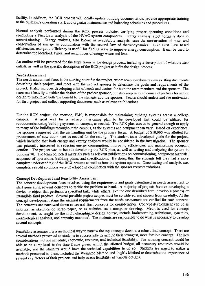
facility. In addition, the RCX process will ideally update building documentation, provide appropriate trainingto the building's operating staff, and organize maintenance and balancing schedules and procedures.
Normal analysis performed during the RCX process includes verifying proper operating conditions and
conducting a First Law analysis of the HVAC system components. Exergy analysis is not normally done in
commissioning. Exergy analysis, also known as availability analysis, uses the conservation of mass and
conservation of energy in combination with the second law of thermodynamics. Like First Law based
efficiencies, exergetic efficiency is useful for finding ways to improve energy consumption. It can be used to
determine the locations, types, and magnitudes ofenergy waste and loss.
An outline will be presented for the steps taken in the design process, including a description of what the stepentails, as well as the specific description of the RCX project as it fits the design process.
Needs Assessment
The needs assessment facet is the starting point for the project, where team members review existing documents
describing their project, and meet with the project sponsor to determine the goals and requirements of the
project. It also includes developing a list ofneeds and desires for both the team members and the sponsor. The
teammust heavily consider the desires of the project sponsor, but also keep in mind course objectives for seniordesign to maximize both the benefit to the students and the sponsor. Teams should understand the motivation
for their project and collect supporting documents such as relevant publications.
For the RCX project, the sponsor, FMS, is responsible for maintaining building systems across a college
campus. A goal was for a retrocommissioning plan to be developed that could be utilized for
retrocommissioning building systems on campus, as needed. The RCX plan was to be general enough to apply
to many of the buildings throughout the campus, as the systems and equipment can vary. Based on experience,
the sponsor suggested that the air handling unit be the primary focus. A budget of $10,000 was allotted for
procurement of new equipment as needed for the testing. The student team developed goals for the project,
which included that both energy and exergy analyses would be considered in the investigation. The sponsor
was primarily interested in reducing energy consumption, improving efficiencies, and maintaining occupant
comfort. The project was to include developing the RCX plan, as well as testing and analyzing the system in
building 70. The team collected materials such as relevant publications on commissioning, equipment manuals,
sequence of operations, building plans, and specifications. By doing this, the students felt they had a more
complete understanding of the RCX process as well as how the system operates. Once testing and analysis was
complete, retrofit solutions were developed in conjunction with the sponsor recommendations.
Concept Development and Feasibility Assessment
The concept development facet involves using the requirements and goals determined in needs assessment to
start generating several concepts to tackle the problem at hand. A majority of projects involve developing a
device or object that performs a specified task, while others, like the one described here, develop a process or
intangible final product. Several possible project scopes must be considered and chosen from carefully. At the
concept development stage the original requirements from the needs assessment are verified for each concept.
The concepts are narrowed down to several final concepts for consideration. Concept development can be as
informal as sketches on scrap paper, or as technical as a computer drawing. Methods used for concept
development, as taught by the multi-disciplinary design course, include brainstorming techniques, synectics,
morphological analysis, and empathy methods2. The students areresponsible to do what is necessary to develop
several concepts.
Feasibility assessment is a methodical way to narrow the top concepts down to a robust final concept. There are
several methods presented to students to successfully determine their strongest, most feasible concept. The key
considerations include schedule, economic, resource, and technical feasibility.The winning concept would be
able to be completed in the time frame given, within the allotted budget, all necessary resources would be
available, and the students would have the technical capabilities to do so. Students are urged to utilize a
methods presented to them, included the Weighted Method and Pugh's Method to determine the importance of
several key factors of their projects and help assess feasibility ofvarious designs.
136

For the RCX project, the students chose the scope of work was chosen as the AHU in the building 70mechanical system. An air handling unit alone was chosen primarily for time considerations. After the studentgroup weighed the various options, it was not feasible to develop a test plan, conduct tests, and complete ananalysis on a larger system, such as all mechanical room components or for the entire building HVAC systemThis decision met the sponsor requirements and suggestions. The formats of the tests were also determinedAfter considering several formats, a combination of documents was chosen. It was decided that the test sheetswould be printed copies on which a technician could write values while testing. This document would bemodeled in a popular spreadsheet program so that in the future, computerized data entry would be possibleAlso, the analysis would be conducted using the program after the data was entered from testing. This optionwas the most feasible because other software options had licensing issues. The sponsor was in agreement thatthis was the most practical concept. The sponsor has access to the proposed software and will not need topurchase additional programs.
From a schedule perspective, the feasibility analysis performed by the student group deemed this concept wasfeasible because it did not require the team members to learn an alternate programming technique, since thechosen program is user friendly and all team members had sufficient knowledge of the software. A preliminaryequipment list was developed in parallel with the testing procedure and test points. This was modified based ona list of existing testing equipment already owned by the sponsor. A preliminary test plan was developed by themidpoint of the project, and modifications were made throughout the testing process.
Trade-Off Assessment
It is often the case that the feasibility assessment brings a few final concepts to the forefront, rather than justone. It is then necessary to conduct a trade-off assessment. In this approach, a numbering concept is applied tojudge which aspects are more significant than others in order to determine a final concept for the project. This
step is not necessary if the feasibility assessment produces a clear idea of the best final concept for the variousconstraints.
The team determined it was not necessary to conduct a trade-off assessment for the RCX project. An exampleof a trade-off assessment a team may have to conduct could be deciding between a heavier inexpensive
material, and a light weight but more costly material when developing a prototype where both weight of the
component and cost to build are essential factors. The team would then have to decide which feature was moreimportant and decide how to proceed.
Engineering Analysis
Engineering analysis is important to create a robust design. The type of analysis conducted varies from project
to project, but it is ultimately necessary for all projects. Students will formulate and solve problems to
determine the thickness, material types, final temperature, etc. as it relates to their project. For this portion of
the project, it is the hope that students will draw from their previous coursework to develop equations and verifyparameters. However, the analysis may require them to learn something from a new area not previously learned
in classes, or combine new knowledge with previous coursework. The teams have faculty available for
assistance throughout the project, and a faculty team mentor to check progress and assist when students need
help.
The students on the RCX team developed a spreadsheet containing all of their formulations and calculations.
They utilized knowledge from thermodynamics, heat transfer, fluid mechanics, and advanced thermodynamics
courses, as well as common equations used in the HVAC field. The analysis was developed before any actual
data was acquired. Unlike projects where a prototype is developed, this project needed to conduct testing as a
major portion of the project. The test results were then used in the analysis to come to some final conclusions.
The following assumptions were made while conducting the analysis. The system was considered at steady
state because the system was allowed to reach equilibrium before collecting data at each set point. The control
volume (CV) was taken around the physical boundary of the AHU and was assumed to be adiabatic. The mass
137

flow in and out of this control volume included chilled water, hot water, outside air, exhaust air, return air and
supply air. The air flow was assumed to be incompressible, and air was treated as an ideal gas. A constant
specific heat at constant pressure (cp) was assumed for air. Kinetic and potential energy were ignored for air
and water flows associated with the AHU.
The analysis developed is presented in the "Results and RetrofitSolutions"
section along with the results from
this analysis.
Preliminary Design Synthesis
For preliminary design, teams must begin the initial stages of preparation for production, including developingbill ofmaterial lists, initial component drawings and selecting possible suppliers for components.
For the RCX team, preliminary design included determining preliminary procedures for testing, compiling
existing testing procedures conducted by FMS, and a review of instrumentation. The instrumentation review
the students conducted included taking inventory on existing equipment as well as verifying up to date
calibration for the instrumentation. No new equipment or calibration certifications were necessary, however if
they were it is important to follow through on procuring new equipment and updating certifications at this time
so testing can take place on time.
Engineering Models
For most projects it is necessary to complete engineering models using modeling software package. These
models compliment the final prototype and may be used when having components made. For some projects,
engineering models may be computer program code, a stress analysis model, or a mechanical drawing,
depending on the nature of the project. Models are usually created on the component level as well as a final
assembly level and are used to show proofof concept2.
The engineering models for the RCX project consisted of CAD drawings for each component, as well as the
system as a whole. An example ofone drawing produced by the team can be seen in Figure 1 .
138
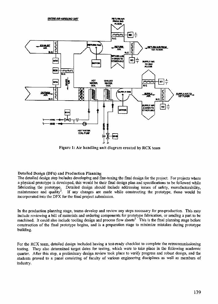
fMlREAJRHANDLmmr
Figure 1 : Air handling unit diagram created by RCX team
Detailed Design (DFx) and Production PlanningThe detailed design step includes developing and fine-tuning the final design for the project. For projects wherea physical prototype is developed, this would be their final design plan and specifications to be followed while
fabricating the prototype. Detailed design should include addressing issues of safety, manufacturability,
maintenance and quality2. If any changes are made while constructing the prototype, those would be
incorporated into the DFX for the final project submission.
In the production planning stage, teams develop and review any steps necessary for pre-production. This may
include reviewing a bill ofmaterials and ordering components for prototype fabrication, or sending a part to be
machined. It could also include tooling design and process flowsheets2
This is the final planning stage before
construction of the final prototype begins, and is a preparation stage to minimize mistakes during prototype
building.
For the RCX team, detailed design included having a test-ready checklist to complete the retrocommissioning
testing. They also determined target dates for testing, which were to take place in the following academic
quarter. After this step, a preliminary design review took place to verify progress and robust design, and the
students proved to a panel consisting of faculty of various engineering disciplines as well as members of
industry.
139
Production planning included reviewing the test check-lists developed in previous stages before proceedingwith testing, and verifying that proper instrumentation was available for testing.
Pilot Production
The pilot production phase includes creating a working prototype for the final concept. The usability of the
prototype varies depending on the project requirements and budget and range from a scaled model version to a
fully functioning device that is immediately put to use. Depending on the project, teams may utilize a machine
shop, order components, and assemble a final working prototype based on the detailed design previouslycompleted. The groups are all required to do a prototype demonstration to showcase their work, and prove that
it functions properly.
The RCX project didn't involve making a prototype device, but rather a final draft of the testing document,which was the final product requested by the sponsor. The document had undergone several revisions by the
team, particularly after the testing phase where procedures and data points were solidified. The testing was an
important part of pilot production, because it validated the test procedure and pointed out places where minor
adjustments were necessary. In addition to the test plans, final results from the system tested were summarized
and presented to the sponsor along with recommended retrofit solutions.
Testing and data collection were completed using the retrocommissioning test plans developed. Testingtechniques and practices were verified by a balancing agent. The students conducted all aspects of testingexcept one circumstance where a safety and liability issue came up. Two to three technicians were available at
all times to assist with conducting tests to ensure proper operation of the equipment, as well as offer their expert
knowledge of the system and controls necessary to change test parameters. The testing and data collection is
described as follows in Sensor Verification, Pre-Functional Tests, and Functional Tests sections.
Verification of the extensive RCX tests developed by the team was one result of the project. A second result of
the project includes numerical data obtained from testing and analysis, which is discussed in "Results and
Retrofit DesignSolutions"
Sensor Verification
The first task for testing was to verify the sensor readings for the web-based control system. This was done by
taking hand measurements in the same location as the sensors. Several measurements were taken and averaged
to verify that sensors were performing within their published specifications. These sensors included
temperature, pressure, and volumetric flow rate. The damper percentage, and voltage and amperage of the
Variable Frequency Drive (VFD) were also checked with rough measurements or visual inspection. The
validity of the sensor output was assessed, taking into account accuracy of the sensors, accuracy of the
measurement devices, and conditions under which the sensors were tested. For example, some temperature
sensors are averaging sensors, which obtain and averagetemperature measurements over a ten foot length, and
the temperature probe utilized measured at a single location. In this case, it was likely that the existing sensor
would deliver more accurate results than a handheld device. Such factors were taken into account where
applicable. With the exception of one, all of the sensors were determined to be accurate, and tests proceeded
with using web-based control system values as actual values. The supply air CFM sensor was dirty, and was
deemed acceptable after it was wiped clean.
Pre-functional Tests
Pre-functional tests are an important part of the retrocommissioning test plan. These tests check for
operational aspects of the components without taking measurements or collecting data. Pre-functional tests
check for excess vibration, proper lubrication, and proper installation, among other things.
140

After researching the subject and brainstorming, the students decided the key things to verify for the fanpre-
functional tests are rotation, vibration, cleanliness, lubrication, sheaves, and belts. The fan rotation should be
verified it should rotate easily and in the proper direction. There should not be excessive noise or vibration.
The fan and fan blades should have good overall cleanliness. If not, it is a sign that something else may be
working improperly. Fan and motor lubrication should be checked. The sheaves should be properly aligned,
and the belts should be in good condition.
Important aspects of the coil pre-functional tests include cleanliness, fin damage, insulation, pump operation,
leakage, and standing water. A lack of cleanliness on the fins could disrupt proper heat transfer. Fin damage
should not be excessive, and the insulation on all pipes should be intact and in good condition. The pump
should be operating properly, and the pump, pipes, and fittings should be free from leakage. It is very important
that the condensate drain is working properly, and there is no standing water under the coil, as it can lead to
fungal growth and pose a health hazard to building occupants.
The function and operation of the dampers should be checked in the economizer pre-functional test. Other
aspects such as linkage, lubrication, and proper closure should be verified. Dampers should operate properly
when stroked individually or as a unit. They should fully open and close upon command. They should not
squeak or otherwise indicate a lack ofproper lubrication.
Control pre-functional tests conducted include start/stop hands off auto, and freeze stat. The start/stop handsoff
auto (S/S H/O/A) will verify that the unit can be properly shut down remotely from the web-based control
system. The freeze stat test verifies the system properly reacts to freezing conditions as a safety measure to
protect the coils. For the purposes of testing, the freeze stat is tripped with a false temperature as to not damage
the coils.
The team decided, with input from the FMS technicians, that the results ofpre-functional testing for the
building 70 AHU were satisfactory but many items were identified. A majority ofpre-functional tests passed.
The following are issues encountered in testing:
A cleanliness issue was encountered in the supply fan. The supply fan blades and the CFM sensor
were dirty. The CFM sensor was wiped clean while the fan was left untouched. If dirt is on the CFM
sensor, the air flow into the sensor will be obstructed, giving an inaccurate reading. Fan cleaning
should be done as part of a preventative maintenance (PM) schedule.
The fan bearings were over lubricated on the backside of the return fan. There was excess grease in
the area that was wiped clean.
There were fins dented for both coils, but it was not substantial. If toomuch damage is evident, the
fins can be straightened with a combing tool.
The damper hardware did not appear to be lubricated, although for this particular economizer it may
not necessary. However, a squeaking noise was heard when thedampers moved.
The exhaust air damper was mostly closed when set to0%. There was a slight gap between the blades.
The mixed air damper was not fully closed when set to 0%. The outside air damper closure showed
the greatest discrepancy, because there was approximately three eighths of an inch gap between the
blades. This may be because the damperis below its normal operating range at 0%. The failure of the
dampers to close raises a red flag, and the issue will be assessed afterfunctional testing.
141
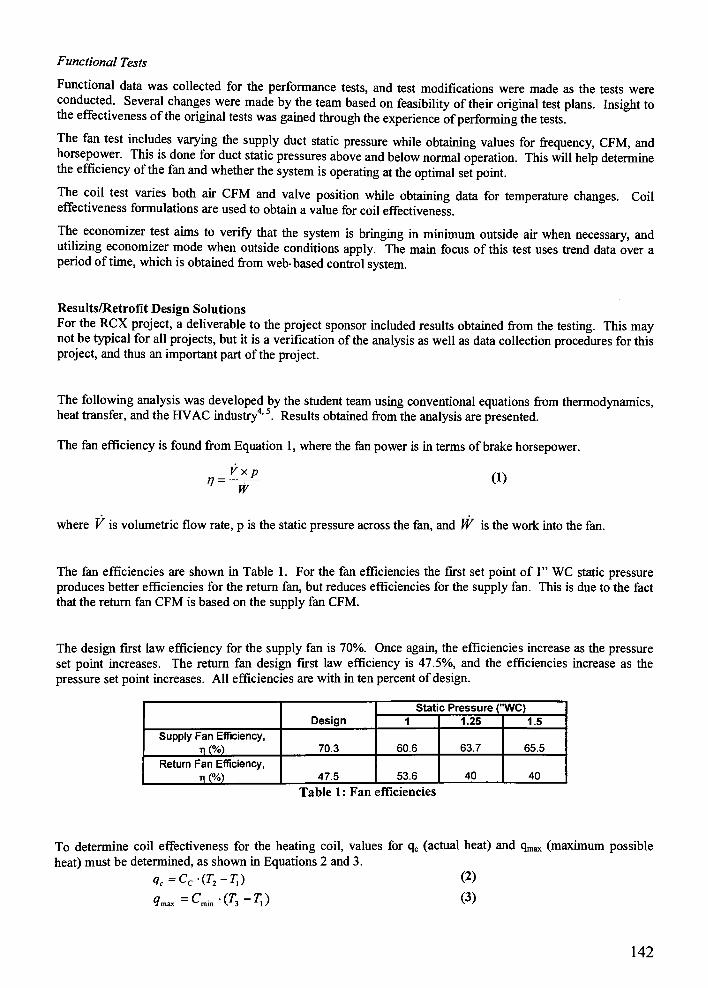
Functional Tests
Functional data was collected for the performance tests, and test modifications were made as the tests were
conducted. Several changes were made by the team based on feasibility of their original test plans. Insight tothe effectiveness of the original tests was gained through the experience ofperforming the tests.
The fan test includes varying the supply duct static pressure while obtaining values for frequency, CFM, andhorsepower. This is done for duct static pressures above and below normal operation. This will help determinethe efficiency of the fan and whether the system is operating at the optimal set point.
The coil test varies both air CFM and valve position while obtaining data for temperature changes. Coil
effectiveness formulations are used to obtain a value for coil effectiveness.
The economizer test aims to verify that the system is bringing in minimum outside air when necessary, and
utilizing economizer mode when outside conditions apply. The main focus of this test uses trend data over a
period of time, which is obtained from web-based control system.
Results/Retrofit Design Solutions
For the RCX project, a deliverable to the project sponsor included results obtained from the testing. This maynot be typical for all projects, but it is a verification of the analysis as well as data collection procedures for this
project, and thus an important part of the project.
The following analysis was developed by the student team using conventional equations from thermodynamics,heat transfer, and the HVAC
industry4' 5. Results obtained from the analysis are presented.
The fan efficiency is found from Equation 1, where the fan power is in terms ofbrake horsepower.
Vxp
W(1)
where V is volumetric flow rate, p is the static pressure across the fan, and W is the work into the fan.
The fan efficiencies are shown in Table 1. For the fan efficiencies the first set point of1"
WC static pressure
produces better efficiencies for the return fan, but reduces efficiencies for the supply fan. This is due to the fact
that the return fan CFM is based on the supply fan CFM.
The design first law efficiency for the supply fan is 70%. Once again, the efficiencies increase as the pressure
set point increases. The return fan design first law efficiency is 47.5%, and the efficiencies increase as the
pressure set point increases. All efficiencies are with in ten percent ofdesign.
Design
Static Pressure ("WC)
1 1.25 1.5
Supply Fan Efficiency,
n (%) 70.3 60.6 63.7 65.5
Return Fan Efficiency,
n <%) 47.5 53.6 40 40
Table 1: Fan efficiencies
To determine coil effectiveness for the heating coil, values for qc (actual heat) and qn
heat) must be determined, as shown in Equations 2 and 3.
<7,=CV(7-2-7;) (2)
=C^-(T,-TX) (3)
(maximum possible
142
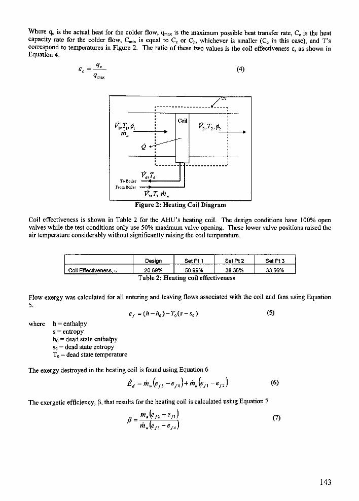
Where qc is the actual heat for the colder flow, qmax is the maximum possible heat transfer rate, Cc is the heat
capacity rate for the colder flow, C^ is equal to Cc or Ch, whichever is smaller (Cc in this case), and T's
correspond to temperatures in Figure 2. The ratio of these two values is the coil effectiveness , as shown in
Equation 4.
s,=
(4)
*i.rA
V TToBoiler *
Prom Boiler
KT, rhv
Figure 2: Heating Coil Diagram
Coil effectiveness is shown in Table 2 for the AHU's heating coil. The design conditions have 100% open
valves while the test conditions only use 50% maximum valve opening. These lower valve positions raised the
air temperature considerablywithout significantly raising the coil temperature.
Design Set Pt 1 Set Pt 2 Set Pt 3
Coil Effectiveness, 6 20.69% 50.99% 38.35% 33.56%
Table 2: Heating coil effectiveness
Flow exergy was calculated for all entering and leaving flows associated with the coil and fans using Equation
5.
ef=(h-h0)-T0(s-s0) (5)
where h = enthalpy
s = entropy
ho= dead state enthalpy
s0= dead state entropy
T0 = dead state temperature
The exergy destroyed in the heating coil is found using Equation 6
K=J$n -ef*)+rila(efi ~efi) (6)
The exergetic efficiency, p\ that results for the heating coil is calculated using Equation 7
_^(g/2-g/i)
^(e/3-e/4)
(7)
143
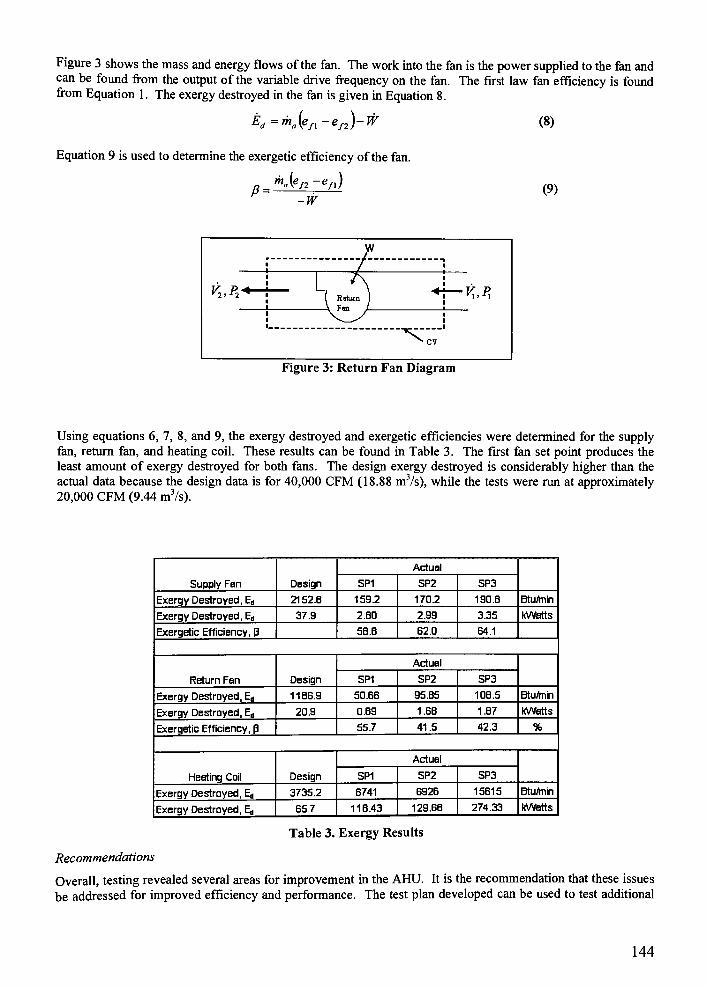
Figure 3 shows the mass and energy flows of the fan. The work into the fan is the power supplied to the fan andcan be found from the output of the variable drive frequency on the fan. The first law fan efficiency is found
from Equation 1. The exergy destroyed in the fan is given in Equation 8.
K =rha(efl-ef2)-W (8)
Equation 9 is used to determine the exergetic efficiency of the fan.
P =
{e,2 C/l )-w
(9)
w/
_
7
[ Return I
V Fit'
<i V p^i v\'r\vl>il'+-'
\^y. . ....
^CV
Figure 3: Return Fan Diagram
Using equations 6, 7, 8, and 9, the exergy destroyed and exergetic efficiencies were determined for the supply
fan, return fan, and heating coil. These results can be found in Table 3. The first fan set point produces the
least amount of exergy destroyed for both fans. The design exergy destroyed is considerably higher than the
actual data because the design data is for 40,000 CFM (18.88 m3/s), while the tests were run at approximately
20,000 CFM (9.44 m3/s).
Supply Fen Design
Actual
SP1 SP2 SP3
Exergy Destroyed, Ea 2152.8 159.2 170.2 190.8 Btu/rnin
Exergy Destroyed, Ed 37.9 2.BO 2.99 3.35 KWstts
Exergetic Efficiency, p 58 .B 62.0 64.1
Return Fan Design
Actual
SP1 SP2 SP3
Exergy Destroyed, E,, 11B6.9 50.66 95.85 106.5 Btu/rnin
Exergy Destroyed, E 20.9 0.89 1.68 1.87 KWatts
Exergetic Efficiency, P 55.7 41.5 42.3 %
Heating Coil Design
Actual
SP1 SP2 SP3
Exergy Destroyed, Eu 3735.2 6741 6926 15615 Btu/rnin
Exergy Destroyed, Ed 65.7 118.43 129.68 274.33 kWatts
Table 3. Exergy Results
Recommendations
Overall, testing revealed several areas for improvement in the AHU. It is the recommendation that these issues
be addressed for improved efficiency and performance. The test plan developed can be used to test additional
144
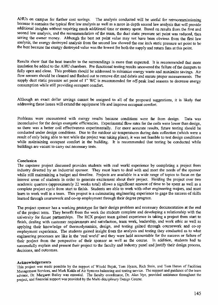
AHUs on campus for further cost savings. The analysis conducted will be useful for retrocommissioningbecause it contains the typical first law analysis as well as a more in-depth second law analysis that will provide
additional insights without requiring much additional time or money spent. Based on results from the first and
second law analysis, and the recommendation of the team, the duct static pressure set point was reduced, thus
saving the owner money. Although the best set point value may not have been obvious from the first law
analysis, the exergy destroyed analysis from the second law showed the one inch static pressure set point to bethe best because the exergy destroyed value was the lowest for both the supply and return fans at this point.
Results show that the heat transfer to the surroundings is more than expected. It is recommended that more
insulation be added to the AHU chambers. Pre-functional testing results uncovered the failure of the dampers to
fully open and close. This problem should be addressed to minimize energy waste and maximize savings. Air
flow sensors should be cleaned and flushed out to remove dirt and debris and ensure proper measurements. The
supply duct static pressure set point of1"
WC is recommended for off-peak load seasons to decrease energyconsumption while still providing occupant comfort.
Although an exact dollar savings cannot be assigned to all of the proposed suggestions, it is likely that
addressing these issues will extend the equipment life and improve occupant comfort.
Problems were encountered with exergy results because conditions were far from design. Data was
inconclusive for the design exergetic efficiencies. Experimental flow rates for the coils were lower than design,so there was a better coil effectiveness experimentally. For more accurate results, future testing should be
conducted under design conditions. Due to the outdoor air temperatures during data collection (which were aresult of only being able to test while the project was taking place), it was not feasible to test design conditionswhile maintaining occupant comfort in the building. It is recommended that testing be conducted while
buildings are vacant to carry out necessary tests.
Conclusion
The capstone project discussed provides students with real world experience by completing a project from
industry directed by an industrial sponsor. They must learn to deal with and meet the needs of the sponsor
while still maintaining a budget and timeline. Projects are available in a wide range of topics to focus on the
interest areas of students in order to generate excitement about their project. Holding the project over two
academic quarters (approximately 22 weeks total) allows a significant amount of time to be spent as well as a
complete project cycle from start to finish. Students are able to work with other engineering majors, and must
learn to work well in a team. This project is a culminating engineering experience to gage the success of skills
learned through coursework and co-op employment through their degree program.
The project sponsor has a working prototype for their design problem and necessary documentation at the end
of the project term. They benefit from the work the students complete and developing a relationship with the
university for future partnerships. The RCX project team gained experience in taking a project from start to
finish, dealing with customer requirements and satisfaction, team work, leadership, and work ethic as well as
applying their knowledge of thermodynamics, design, and testing gained through coursework and co-op
employment experience. The students gained insight from the analysis and testing they conducted as to what
engineering processes are like in the 'realworld'
and they were held accountable for the success or failure of
their project from the perspective of their sponsor as well as the course. In addition, students had to
successfully explain and present their project to the faculty and industry panel and justify their design process,
decisions, and outcomes.
Acknowledgements
This project was made possible by the support of Witold Bujak, Tom Hyzen, Rich Stein, and Tom Heron of Facilities
Management Services, andMark Kukla ofAir Systems balancing and testing service. The support and guidance of the team
advisor, Dr. Margaret Bailey was essential. The faculty coordinator, Dr. Alan Nye, provided assistance throughout the
project, andfinancial support was provided by the Multi-disciplinary Design Course.
145
References
1
Hensel, E. and Stiebitz, P. The Student's EDGE: An Engineering Design GuidE. 2003. Rochester Institute of
Technology. 03 Mar. 2004 <http://designserver.rit.edu/>.
2
Stiebitz, P., Hensel, E., Mozrall, J.. Multidisciplinary EngineeringDesign at RIT. Proceedings of the 2004
American Society OfEngineering Education Annual Conference & Exposition 2004.
3
Gannon, J., Bailey,M., White, D., and Yu-Chuan Yang, R. SOFCDurability Test StandDesign Challenges
andProcesses. Lucerne Fuel Cell Forum, 2004.
4
Gladstone, J., and Bevirt, W.D.. HVAC Testing. Adjusting, and BalancingManual. 1981. 3rd ed. New York,
NY: McGraw-Hill, 1997.5
Moran, M. J., and Shapiro, H.N.. Fundamentals ofEngineering Thermodynamics. 1988. 4th ed. New York,
NY: JohnWiley&Sons, Inc., 2000.
146
Appendix B
ASME Conference Paper
Proceedings of ISEC2006
ASME International Solar Energy Conference
July 8-13, 2006, Denver, CO
ISEC2006-99080
EXERGETIC ANALYSIS FOR IMPROVING THE OPERATION OF BUILDING
MECHANICAL SYSTEMS: RESULTS AND RECOMMENDATIONS
Erin N. George
Rochester Institute ofTechnology
Dr.Margaret B. Bailey, P.E.
Rochester Institute ofTechnology
ABSTRACT
A review ofpast research reveals that while exergetic analysis has been performed on various buildingmechanical systems, there has not been extensive efforts in the areas of retrocommissioning air distribution
systems or fault detection for cooling plants. Motivations for this new work include demonstrating the merits
of exergetic analysis in association with retrocommissioning (RCX) an existing building air handling unit
(AHU), as well as conducting an advanced analysis on an existing chiller for the purposes ofhealth monitoring.
The following research demonstrates the benefits of including a second law analysis in order to improve
equipment operation based on lowered energy consumption and improved operation, and as a means for system
healthmonitoring.
Particularly, exergetic analysis is not often performed in the context of RCX, therefore this research
will provide insight to those considering incorporating exergetic analysis in their RCX assessments. A
previously developed RCX test for assessing an AHU on a college campus, as well as data collected from the
testing is utilized for an advanced thermodynamic analysis. The operating data is analyzed using the first and
second laws of thermodynamics and subsequent recommendations are made for retrofit design solutions to
improve the system performance. The second law analysis provides beneficial information for determiningretrofit solutions with minimal additional data collection and calculations. The thermodynamic methodology is
then extended to a building's cooling plant which utilizes a vapor compression refrigeration cycle (VCRC)chiller. Existing chiller operational data is processed and extracted for use in this analysis. As with the air
147
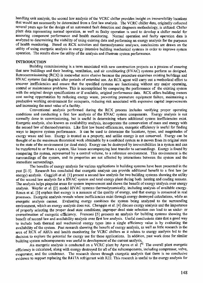
handling unit analysis, the second law analysis of the VCRC chiller provides insight on irreversibility locationsthat would not necessarily be determined from a first law analysis. The VCRC chiller data, originally collectedseveral years ago for the design of an automated fault detection and diagnosis methodology, is utilized. Chiller
plant data representing normal operation, as well as faulty operation is used to develop a chiller model for
assessing component performance and health monitoring. Normal operation and faulty operation data is
analyzed to determining the viability ofusing existing data and performing an exergy analysis for the purposesof health monitoring. Based on RCX activities and thermodynamic analyses, conclusions are drawn on the
utility of using exergetic analysis in energy intensive building mechanical systems in order to improve system
operation. The results show the utility of the analysis and illustrate system performance.
INTRODUCTION
Building commissioning is a term associated with new construction projects as a process of ensuringthat new buildings and their heating, ventilation, and air conditioning (HVAC) systems perform as designed.
Retrocommissioning (RCX) is somewhat more elusive because the procedure examines existing buildings andHVAC systems that degrade after periods of extended use. An RCX agent will carry out a methodical effort to
uncover inefficiencies and ensure that the specified systems are functioning without any major operating,
control or maintenance problems. This is accomplished by comparing the performance of the existing system
with the original design specifications or if available, original performance data. RCX offers building owners
cost saving opportunities by reducing energy waste, preventing premature equipment failure, maintaining a
productive working environment for occupants, reducing risk associated with expensive capital improvements
and increasing the asset value ofa facility.Conventional analysis performed during the RCX process includes verifying proper operating
conditions and conducting a first law analysis of the HVAC system components. Exergy analysis is not
normally done in commissioning, but is useful in determining where additional system inefficiencies exist.
Exergetic analysis, also known as availability analysis, incorporates the conservation of mass and energy with
the second law of thermodynamics. Like first law based efficiencies, exergetic efficiency is useful for findingways to improve system performance. It can be used to determine the locations, types, and magnitudes of
exergy waste and loss. Exergy is treated as a property, and unlike energy is not conserved. Exergy can be
thought of as the maximum theoretical work obtainable by a combined system as it moves from its original state
to the state of the environment (or dead state). Exergy can be destroyed by irreversibilities in a system and can
be transferred to or from a system, like losses accompanying heat transfer to surroundings. Exergy is found by
comparing the system, represented by a control volume, to a reference environment. This environment is the
surroundings of the system, and its properties are not affected by interactions between the system and the
immediate surroundings.
The benefits of exergy analysis for various applications in building systems have been presented in the
past [1-5]. Research has concluded that exergetic analysis can provide additional benefit to a first law (or
energy) analysis. Gaggioli et al. [1] present a second law analysis for two building systems showing the utilityof the second law analysis for a HVAC system and total energy plant during both heating and cooling seasons.
The analysis helps pinpoint areas for system improvement and shows the benefit of exergy analysis over energy
analysis. Wepfer et al. [2] model HVAC systems thermodynamically, including analysis of available energy.
Rosen et al. [3] explain that exergy is a measure of the quality of energy, and that exergy is consumed in real
processes. Exergetic analysis reveals where inefficiencies exist through exergy destroyed calculations, while an
energetic analysis cannot. Evaluating exergy combines the system being analyzed to the surrounding
environment, which an energy analysis does not. Chengqin et al. [4] discuss exergy analysis and the importance
of properly selecting the proper dead state conditions; improper dead state selection can lead to an under- or
overestimation of exergetic efficiency. Franconi [5] presents an analysis for building systems showing the
benefit of second law and availability analysis over first law analysis. Useful conclusions state that a good way
to include both thermal and mechanical energy types into a single efficiency value is by evaluating the
availability of the system. Past research showing the benefit of exergy analysis, as well as little research in the
area of RCX of AHUs and health monitoring for VCRC chillers as it relates to exergy analysis led to the
decision to explore the potential for exergy use for these applications. In addition, past work done for similar
building system subcomponents was useful in development of the current analysis.
An exergetic analysis is conducted on a VCRC plant by Aprea et al.[6) The overall plant exergetic
efficiency is calculated, along with exergy destroyed for all of the subcomponents, including compressor, valve,
evaporator, and the condenser. The research shows through exergetic analysis that there is no conclusive
evidence to support replacing the R417A refrigerant with R22. This research is useful to the exergy analysis for
148

the current VCRC system. An ammonia-water chiller is analyzed by Ezzine et al.[7!
using the second law of
thermodynamics. The energy and entropy balance, irreversibility, and performance coefficient (PC) were
calculated. Most of the irreversibility was from the absorber, heat exchangers, first condenser, and second
boiler. Although the type of chiller is different, the analysis done for the heat exchangers is pertinent to the
current research.
Since past research has shown the benefit of exergy analysis in building systems, the current researchprovides an extension looking at how exergy analysis can benefit in the area of retrocommissioning as well as
health monitoring for a VCRC chiller system. In each case, existing data is utilized for the analysis conducted.
Although a detailed analysis for components and building systems may be useful for some
applications, the practicality of the analysis must be considered for retrocommissioning. It has been shown that
a second law analysis will be beneficial, however since retrocommissioning typically does not focus on heavilymathematic analysis, this will be kept in mind while developing the following second law analysis for the
retrocommissioning test plan.
The RCX plan and AHU data collection was completed by a senior multi-disciplinary student capstone
engineering design team in conjunction with the Facilities Management Services group on a university campus.
An AHU within a building mechanical room was utilized to collect data for analysis, and existing specifications
of this system were used for all calculations. The aforementioned mechanical room resides in an academic
building consisting of three floors the first two contain classrooms, offices and computer labs, and the third
floor houses the mechanical room penthouse. The major goal of the student team's project was to develop a
retrocommissioning test plan for an AHU, test a specific AHU (Figure 1) using the test plan developed, and
complete a first and second law analysis on the system using the collected data. The project described here was
subsequently expanded and continued by a member of the design team as part of a graduate thesis, includinginterpretation ofpreviously collected chiller data.
The analyzed chiller data was collected as part of a doctoral dissertation [8]. This research involved
developing a fault detection and diagnosis (FDD) methodology, and several ranges of fault conditions were
imposed on the chiller (Figure 2) while data was collected. The experimental data was obtained from a
commercially available 70-ton air cooled chiller located in the Joint Center for Energy Management Karl
Larson Laboratory (JCEM) at The University ofColorado, Boulder. The chiller has a remote 50-ton air cooled
refrigerant condenser. The chiller has two helical rotary compressors each on an independent refrigerant circuit,
both using HCFC-22. The shell-in-tube evaporator is shared, with a dual circuit configuration.
Baseline ('Normal') data was collected through two data acquisition (DAQ) systems, including a laboratory
monitoring system (CMS) and a personal computer loaded with software compatible with the chiller's internal
communication bus. Commercially available chillers are equipped with several sensors, including pressure
transducers, type T thermocouples, thermisters for evaporating refrigerant temperature, and RTD temperature
sensors.
149
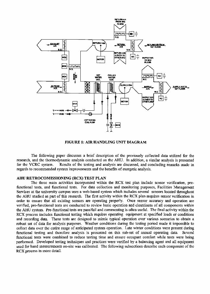
FIGURE 1: Am HANDLING UNIT DIAGRAM
The following paper discusses a brief description of the previously collected data utilized for the
research, and the thermodynamic analysis conducted on the AHU. In addition, a similar analysis is presented
for the VCRC system. Results of the testing and analysis are discussed, and concluding remarks made in
regards to recommended system improvements and the benefits ofexergetic analysis.
AHU RETROCOMISSIONING (RCX) TEST PLAN
The three main activities incorporated within the RCX test plan include sensor verification,pre-
functional tests, and functional tests. For data collection and monitoring purposes, Facilities Management
Services at the university campus uses a web-based system which includes several sensors located throughout
the AHU studied as part of this research. The first activity within the RCX plan requires sensor verification in
order to ensure that all existing sensors are operating properly. Once sensor accuracy and operation are
verified, pre-functional tests are conducted to review basic operation and cleanliness of all components within
the AHU system. Pre-functional tests are pass/fail and commenting is often useful. The final activity within the
RCX process includes functional testing which requires operating equipment at specified loads or conditions
and recording data. These tests are designed to mimic typical operation over various scenarios to obtain a
robust set of data for analysis purposes. Weather conditions during the testing period made it impossible to
collect data over the entire range of anticipated system operation. Late winter conditions were present duringfunctional testing and therefore analysis is presented on this sub-set of annual operating data. Several
functional tests were combined to reduce testing time and ensure occupant comfort while tests were beingperformed. Developed testing techniques and practices were verified by a balancing agent and all equipment
used for hand measurements on-site was calibrated. The following subsections describe each component of the
RCX process in more detail.

COOLED
CONDENSER
1outdoorair .
-p-
*&BGkBQt &KklX&
OIL
COOLER
^ELECTRONIC
\) EXPANSION
VALVE
9L *-$ope:rbe<ai
EVAPORATOR
fFIGURE 2: VCRC CHILLER DIAGRAM (INCLUDING SENSOR LOCATIONS)
Functional Tests
Functional data was collected for the performance tests, and test modifications were made as the tests
were conducted. Several changes were made based on feasibility of the original test plans. The fan test includes
varying the supply duct static pressure while obtaining values for air volumetric flow rate and fan horsepower.
This test is performed for duct static pressures above and below the normal system set point. This process aides
in determining if the system is operating at its optimal static pressure set point. A reduction in the static
pressure set point can increase energy efficiency.
The heating and cooling coil tests vary air volumetric flow rate and hot or chilled water valve position
while obtaining data for air and water temperature changes. Coil effectiveness formulations are used to obtain a
value for coil effectiveness. The economizer test aims to verify that the system is bringing in minimum outside
air when necessary, and utilizing economizer mode when appropriate based on outside conditions. The main
focus of this test uses trend data over a period of time, which is obtained from the control system.
ANALYSIS AND RESULTS
In this section, the main governing equations will first be presented, followed by a specific look at the
analysis conducted on the primary system components, including the economizer, coil, and fans for the AHU,
and the chiller's condenser, evaporator and compressors. A discussion of the results will follow.
AHU Analysis
Several assumptions were made while conducting the AHU analysis. The system was considered at
steady state because the system was allowed to reach equilibrium before collecting data at each set point. The
control volume (CV) was taken around the physical boundary of the AHU and was assumed to be adiabatic.
The mass flow in and out of this control volume included chilled water, hot water, outside air, exhaust air,
return air and supply air. The air flow was assumed to be incompressible, and air was treated as an ideal gas. A
constant specific heat at constant pressure (cp) was assumed for air at the outside air temperature. Changes in
kinetic and potential energies were ignored for air and water flows associated with the AHU.
The following AHU analysis was developed using well accepted fundamental equations [9-11]. The
fan efficiency is found from Equation 1, where the fan power is in terms ofbreak horsepower.
VxApIF*6356
(1)
151
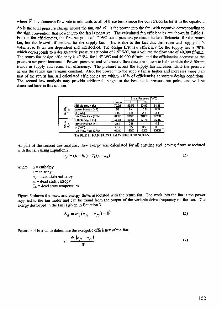
where V is volumetric flow rate in add units to all of these terms since the conversion factor is in the equation,
Ap is the total pressure change across the fan, and W is the power into the fan, with negative corresponding to
the sign convention that power into the fan is negative. The calculated fan efficiencies are shown in Table 1 .
For the fan efficiencies, the first set point of1"
WC static pressure produces better efficiencies for the return
fan, but the lowest efficiencies for the supply fan. This is due to the fact that the return and supply fan's
volumetric flows are dependent and interlocked. The design first law efficiency for the supply fan is 70%,
which corresponds to a design static pressure set point of1.5"
WC, but a volumetric flow rate of40,000 ft3/min.
The return fan design efficiency is 47.5%, for1.5"
WC and 40,000 ftVmin, and the efficiencies decrease as the
pressure set point increases. Power, pressure, and volumetric flow data are shown to help explain the different
trends in supply and return fan efficiency. The pressure across the supply fan increases while the pressure
across the return fan remains constant. Also, the power into the supply fan is higher and increases more than
that of the return fan. All calculated efficiencies are within -10% of efficiencies at system design conditions.
The second law analysis may provide additional insight to the best static pressure set point, and will be
discussed later in this section.
Design
Static Pressure "WC)
1 1.25 1.5
>>
C/3
Efficiency, n (%) 70.29 60.56 63.65 64.98
power into fan (HP) 53 9.4 10.9 12.9
p ("WC) 5.92 1.B 2.1 2.4
Vol Flow Rate (CFM) 4000D 2D10D 21000 22200
Efficiency, n (%) 47.48 50.57 37.76 36.36
power into fan (HP) 28. 1 2.B 4 4.5
p ("WC) 2.12 0.5 0.5 0.5
Vol Flow Rate (CFM) 4D00D 10000 19200 20B00
TABLE 1: FAN FIRST LAW EFFICIENCIES
As part of the second law analysis, flow exergy was calculated for all entering and leaving flows associated
with the fans using Equation 2.
ef=(h-h0)-T0(s-s0) (2)
where h = enthalpy
s = entropy
ho= dead state enthalpy
s0= dead state entropy
T0 = dead state temperature
Figure 3 shows the mass and energy flows associated with the return fan. The work into the fan is the power
supplied to the fan motor and can be found from the output of the variable drive frequency on the fan. The
exergy destroyed in the fan is given in Equation 3.
Ed=ma(en-efl)-W (3)
Equation 4 is used to determine the exergetic efficiency of the fan.
s =ma{e/2-efl) (4)
-W
152

z.,
7 i
All'1*4
j ( R.urn
*'
Vl
: vly i
^CV
FIGURE 3: RETURN FAN DIAGRAM
Using equations 3 and 4, the exergy destroyed and exergetic efficiencies were determined for the
supply and return fans. These results can be found in Table 2.
Set Point 1 Set Point 2 Set Point 3 units
Static pressure
set point
1 1.25 1.5 "WC
Ea, 159.2 170.2 190.8 Btu/min
Ejr 50.66 95.85 106.5 Btu/min
. 60.05 63.18 65.13 %
r 57.33 43.50 44.22 %
llsupply fan 60.56 63.65 64.98 %
lireturn fan 50.57 37.76 36.36 %
TABLE 2: FAN FIRST AND SECOND LAW EFFICIENCIES
The first fan set point produces the least amount of exergy destroyed for both fans. The design exergy
destroyed is considerably higher than the actual data because the design data is for 40,000 CFM (18.88 m3/s),
while the RCX tests were run at approximately 20,000 CFM (9.44 m3/s). The exergy destroyed analysis from
the second law showed the1"
WC static pressure set point to be ideal because the exergy destroyed value was
the lowest for both the supply and return fans at this point. The supply duct static pressure set point of1"
WC is
recommended for off-peak load seasons to decrease energy consumption while still providing occupant comfort.
This duct static pressure was tested by the building owner to verify that the most critical zone (variable air
volume box) requirements were satisfied, and it was shown that the air flow requirements were still met.
For the coil analysis, only the heating coil's operation was analyzed. The cooling coil
was not analyzed because no method was in place for measuring condensate from the cooling
coil. To determine coil effectiveness for the heating coil, values for qc (actual heat) and qmsx
(maximum possible heat) must be determined, as shown in Equations 5 and 6.
qc=Cc-{T2-T{) (5)
Qm=C^-{T,-Tx) (6)
where qc is the actual heat transfer to the air , qmax is the maximum theoretical heat transfer
rate to the air, Cc is the heat capacity rate for the air flow, Cmin is equal to Cc or Ch,
whichever is smaller (Cc in this case), and T's correspond to temperatures in Figure 4. The
ratio of these two values is the coil effectiveness , as shown in Equation 7.
=_*- (7)
153

V TTo Boiler *
FromBoiler >
V3,T3 m
FIGURE 4: HEATING COIL DIAGRAM
Calculated values for the AHU heating coil effectiveness are shown in Table 3. The design conditions have
100% open valves on the heating coil piping while the test conditions only use 50% maximum valve opening.
The first set point was picked at an arbitrary volumetric flow value (13,700 ft3/min) and 25% valve opening.
For the second set point, the volumetric flow was approximately doubled, while the valve percent open
remained the same. For the third set point the valve position was opened to 50% while the volumetric flow rate
remained approximately constant (with respect to the second set point).
Valve % Open
/CFMDesign 25 / 13700 25/22800 50 / 23300
%/
ft /min
(eflertivcnefi) 3753 50.99 38.35 3356 %
Ti 509.67 515.3 515.8 517.4 "R
Tj 536 .57 5359 528.8 551.4 R
T3 639.67 5551 549.7 618.7 R
T 617.47 551.7 545.7 6D6.7 "R
TABLE 3: HEATING COIL EFFECTIVENESS
As part of the second law analysis, flow exergy was calculated for all entering and leavingflows associated with the heating coil using Equation 2.
The exergy destroyed in the heating coil is found using Equation 8 with subscripts
again referring to flows shown in Figure 4.
K = <(efi -ef^)+1na(efx -e/2) <8>
The exergetic efficiency, s, that results for the heating coil is calculated using Equation 9
w(/2-/i) m
1=
ww(ef, -e\'/3 *f*>
Using Equations 8 and 9, the exergy destroyed and exergetic efficiencies were determined for the
heating coil. These results can be found in Table 4.
154
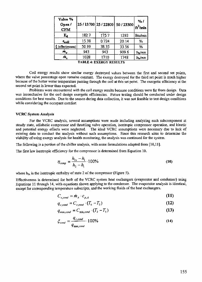
Valve %
Open/
CFM
25 / 13700 25/22800 50/23300%/
ft /min
Ed 1S2.7 175.7 1292 Btu/min
coil 15.38 0.724 20.14 %
\ (effectiveness) 50.99 38.35 33.56 %
mv 943 943 909.6 lbm/min
n*. 1028 1710 1748 lbm/min
TABLE 4: EXERGY RESULTS
Coil exergy results show similar exergy destroyed values between the first and second set points,
where the valve percentage open remains constant. The exergy destroyed for the third set point is much higher
because of the hotter water temperature passing through the coil at this set point. The exergetic efficiency at the
second set point is lower than expected.
Problems were encountered with the coil exergy results because conditions were far from design. Data
was inconclusive for the coil design exergetic efficiencies. Future testing should be conducted under design
conditions for best results. Due to the season during data collection, it was not feasible to test design conditions
while considering the occupant comfort
VCRC System Analysis
For the VCRC analysis, several assumptions were made including analyzing each subcomponent at
steady state, adiabatic compressor and throttling valve operation, isentropic compressor operation, and kinetic
and potential energy effects were neglected. The ideal VCRC assumptions were necessary due to lack of
existing data to conduct the analysis without such assumptions. Since this research aims to determine the
viability ofusing exergy analysis for health monitoring, the analysis was continued for the system.
The following is a portion of the chiller analysis, with some formulations adapted from [10,1 1].
The first law isentropic efficiency for the compressor is determined from Equation 10.
V,comph2-hx
100% (10)
where h^ is the isentropic enthalpy of state 2 of the compressor (Figure 5).
Effectiveness is determined for both of the VCRC system heat exchangers (evaporator and condenser) using
Equations 1 1 through 14, with equations shown applying to the condenser. The evaporator analysis is identical,
except for corresponding temperature subscripts, and the working fluids of the heat exchangers.
^c,cond ~
mA 'Cp,A
Qc,cond~ ^c,cond
'
\*6 *5'
rlmax,cond~
min,cond v 2 5/
He,condh cond
100%
(11)
(12)
(13)
(14)
i max.cond
155
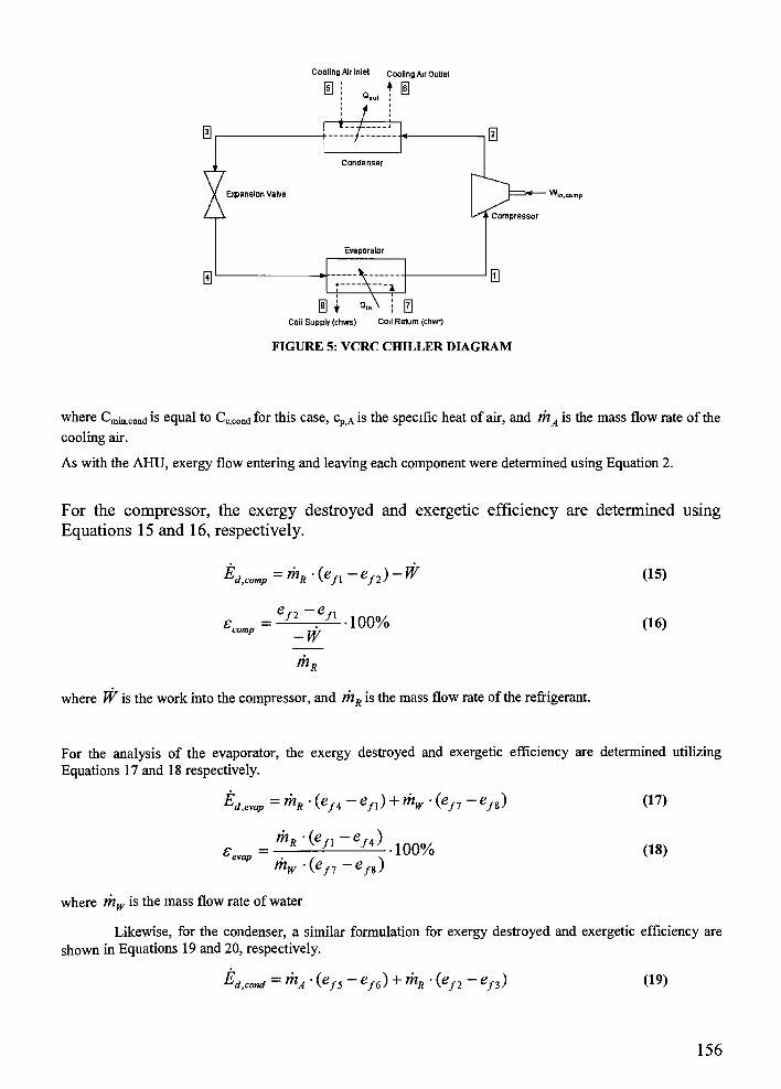
Cooling Air Inlet Cooling Air Outlet
0Q t 0
S
Expansion Valve
0
0
Evaporator
@
Compressor
0
0Coil Supply (chws) Coil Return (chwi)
FIGURE 5: VCRC CHILLER DIAGRAM
where Cmin^ondis equal to Cccondfor this case, cpAis the specific heat of air, and mA is the mass flow rate of the
cooling air.
As with the AHU, exergy flow entering and leaving each component were determined using Equation 2.
For the compressor, the exergy destroyed and exergetic efficiency are determined using
Equations 15 and 16, respectively.
Ed,Comp=rnR-(efl-ef2)-W
comp
ef2 ef\
-w
100%
(15)
(16)
mL
where W is the work into the compressor, and mR is the mass flow rate of the refrigerant.
For the analysis of the evaporator, the exergy destroyed and exergetic efficiency are determined utilizing
Equations 17 and 1 8 respectively.
Ed,evap=
R 0/4~
g/l) +W'
0/7~
ef%)
^0/i-e/4)
evap
mw-{efl-en)
100%
(17)
(18)
where mw is the mass flow rate ofwater.
Likewise, for the condenser, a similar formulation for exergy destroyed and exergetic efficiency are
shown in Equations 19 and 20, respectively.
Ed,COnd =A O/s -ef6) +mR-
(ef2-
ef3) (19)
156
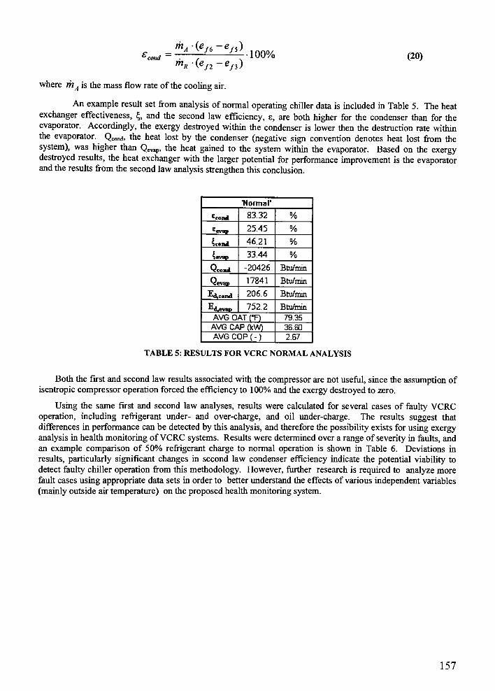
e^, =A /6
^-100%'cond
R-{en-en)(20)
where am^ is the mass flow rate of the cooling air.
An example result set from analysis of normal operating chiller data is included in Table 5. The heat
exchanger effectiveness, \, and the second law efficiency, e, are both higher for the condenser than for theevaporator. Accordingly, the exergy destroyed within the condenser is lower then the destruction rate withinthe evaporator. Qcond, the heat lost by the condenser (negative sign convention denotes heat lost from the
system), was higher than Qevap, the heat gained to the system within the evaporator. Based on the exergydestroyed results, the heat exchanger with the larger potential for performance improvement is the evaporatorand the results from the second law analysis strengthen this conclusion.
'Normal1
Econd 83.32 %
evaj> 25.45 %
Scond 46.21 %
Sevap33.44 %
Xcond -20426 Btu/min
Qevap 17841 Btu/min
-"djcond206.6 Btu/min
C,d,evajj_752.2 Btu/min
AVG OAT (F) 79.35
AVG CAP (kW) 3B.6D
AVG COP ( - ) 2.67
TABLE 5: RESULTS FOR VCRC NORMAL ANALYSIS
Both the first and second law results associated with the compressor are not useful, since the assumption of
isentropic compressor operation forced the efficiency to 100% and the exergy destroyed to zero.
Using the same first and second law analyses, results were calculated for several cases of faulty VCRC
operation, including refrigerant under- and over-charge, and oil under-charge. The results suggest that
differences in performance can be detected by this analysis, and therefore the possibility exists for using exergyanalysis in health monitoring ofVCRC systems. Results were determined over a range of severity in faults, andan example comparison of 50% refrigerant charge to normal operation is shown in Table 6. Deviations in
results, particularly significant changes in second law condenser efficiency indicate the potential viability to
detect faulty chiller operation from this methodology. However, further research is required to analyze more
fault cases using appropriate data sets in order to better understand the effects ofvarious independent variables
(mainly outside air temperature) on the proposed health monitoring system.
157
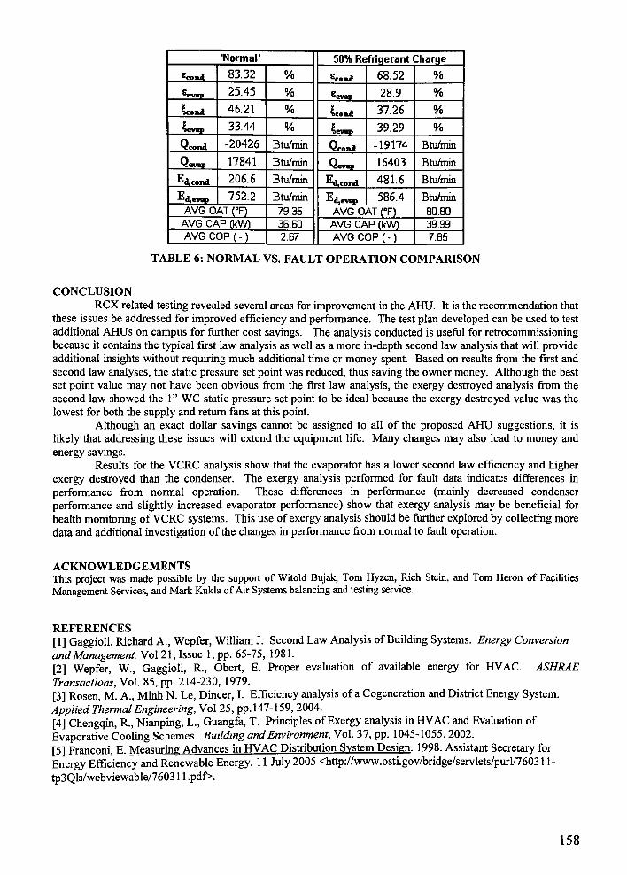
'Normal'
50% Refriqerant Charge
'cond 83.32 % cond 68.52 %
'evap 25.45 %"evap 28.9 %
Scond 46.21 % Scond 37.26 %
Sevap 33.44 %Sevap
39.29 %
Vcond -20426 Btu/minVcond -19174 Btu/min
Vevap 17841 Btu/minvevap
16403 Btu/min
-"dfCond206.6 Btu/min J-'dfCond 481.6 Btu/min
Erevan 752.2 Btu/rnin J-'djevap 586.4 Btu/min
AVG OAT (F) 79.35 AVG OAT fF) B0.B0
AVG CAP (kW) 36.60 AVG CAP (kW) 39.99
AVG COP ( - ) 2.67 AVG COP ( - ) 7.85
TABLE 6: NORMAL VS. FAULT OPERATION COMPARISON
CONCLUSION
RCX related testing revealed several areas for improvement in the AHU. It is the recommendation that
these issues be addressed for improved efficiency and performance. The test plan developed can be used to test
additional AHUs on campus for further cost savings. The analysis conducted is useful for retrocommissioning
because it contains the typical first law analysis as well as a more in-depth second law analysis that will provide
additional insights without requiring much additional time or money spent. Based on results from the first and
second law analyses, the static pressure set point was reduced, thus saving the owner money. Although the best
set point value may not have been obvious from the first law analysis, the exergy destroyed analysis from the
second law showed the1"
WC static pressure set point to be ideal because the exergy destroyed value was the
lowest for both the supply and return fans at this point.
Although an exact dollar savings cannot be assigned to all of the proposed AHU suggestions, it is
likely that addressing these issues will extend the equipment life. Many changes may also lead to money and
energy savings.
Results for the VCRC analysis show that the evaporator has a lower second law efficiency and higher
exergy destroyed than the condenser. The exergy analysis performed for fault data indicates differences in
performance from normal operation. These differences in performance (mainly decreased condenser
performance and slightly increased evaporator performance) show that exergy analysis may be beneficial for
health monitoring ofVCRC systems. This use of exergy analysis should be further explored by collecting more
data and additional investigation of the changes in performance from normal to fault operation.
ACKNOWLEDGEMENTS
This project was made possible by the support of Witold Bujak, Tom Hyzen, Rich Stein, and Tom Heron of Facilities
Management Services, andMark Kukla ofAir Systems balancing and testing service.
REFERENCES
[1] Gaggioli, Richard A., Wepfer, William J. Second Law Analysis ofBuilding Systems. Energy Conversion
andManagement, Vol 21, Issue 1, pp. 65-75, 1981.
[2] Wepfer, W., Gaggioli, R, Obert, E. Proper evaluation of available energy for HVAC. ASHRAE
Transactions, Vol. 85, pp. 214-230, 1979.
[3] Rosen, M. A., Minh N. Le, Dincer, I. Efficiency analysis ofa Cogeneration and District Energy System.
Applied Thermal Engineering, Vol 25, pp. 147-159, 2004.
[4] Chengqin, R, Nianping, L., Guangfa, T. PrinciplesofExergy analysis in HVAC and Evaluation of
Evaporative Cooling Schemes. Building andEnvironment, Vol. 37, pp. 1045-1055, 2002.
[5] Franconi, E. Measuring Advances in HVAC Distribution System Design. 1998. Assistant Secretary for
Energy Efficiency and Renewable Energy. 1 1 July 2005 <http://www.osti.gov/bridge/servlets/purl/76031 1-
tp3Qls/webviewable/7603 1 1 .pdf>.
158
[6] Aprea, C, Mastrullo R., Renno, C. An analysis of the Performances of aVapour Compression Plant
Working Both as aWater Chiller and aHeat Pump Using R22 and R417A. Applied ThermalEngineering, Vol.
24, pp.487-499, 2003.
[7] Ezzine, B., Barhoumi, M., Mejbri, K., Chemkhi, S., Bellagi, A. Solar Cooling with the Absorption
Principle: first and second law analysis of an Ammonia-Water Double-Generator Absorption Chiller.
Desalination, Vol. 168, pp.137-144, 2004.
[8] Bailey, M.B. The Design and Viability ofa Probabilistic Fault Detection and DiagnosisMethod ofVapor
Compression Cycle Equipment. Ph.D. Dissertation, Department ofCivil Engineering, University ofColorado,1998.
[9] Gladstone, J., Bevirt, W. D. HVAC Testing. Adjusting, and BalancingManual. 1981. 3rd ed. New York,
NY: McGraw-Hill, 1997.
[10] Moran, M. J., Shapiro, H. N. Fundamentals ofEngineering Thermodynamics. 1988. 4th ed. New York,NY: JohnWiley&Sons, Inc., 2000.
[1 1] Incropera, F. P., DeWitt, D. P. Fundamentals ofHeat andMass Transfer.5th
ed. New York, NY: John
Wiley& Sons, Inc., 2002
159
Appendix C
C. 1 EES CodeforAHUFans
"AHU Fan Analysis
***NOTE***
subscript spl refers to set point 1, 1 in. WC duct static pressure
subscript sp2 refers to set point 2, 1.25 in. WC duct static pressure
subscript sp3 refers to set point 3, 1.5 in. WC duct static pressure
"PRESSURES"
"Pressure, Set point1"
P_la_spl_inwc=4 06.7 8 {inH20}
P_2_spl_inwc=405.98 {inH20}
P_3_spl_inwc=407.783 {inH20}
P_4_spl_inwc=406.20 {inH20}
P_5_spl_inwc=4 06.733 {inH20}
P_5a_spl_inwc=4 06.7 33 {inH20}
P_la_spl=P_la_spl_inwc* Convert (inH20, psi)P_2_spl=P_2_spl_inwc* Convert (inH20, psi)P_3_spl=P_3_spl_inwc* Convert (inH20, psi)P_4_spl=P_4_spl_inwc* Convert (inH20, psi)P_5_spl=P_5_spl_inwc* Convert (inH20, psi)P_5a_spl=P_5a_spl_inwc* Convert (inH20, psi)
P_la_spl_psf=P_la_spl_inwc* Convert (inH20, lbf/ftA2)P_2_spl_psf=P_2_spl_inwc* Convert (inH20, lbf/ftA2)P_3_spl_psf=P_3_spl_inwc* Convert (inH20, lbf/ft/v2)P_4_spl_psf=P_4_spl_inwc* Convert (inH20, lbf/ftA2)P_5_spl_psf=P_5_spl_inwc* Convert (inH20, lbf/ftA2)P_5a_spl_psf=P_5a_spl_inwc* Convert (inH20, lbf/ftA2)
"Pressure, Set point2"
P_la_sp2_inwc=406.78 {inH20}
P_2_sp2_inwc=405.93 {inH20}
P_3_sp2_inwc=4 08.033 {inH20}
P_4_sp2_inwc=4 06.20 {inH20}
P_5_sp2_inwc=406.733 {inH20}
P_5a_sp2_inwc=406.733 {inH20}
P_la_sp2=4 06.78* Convert (inH20, psi)P_2_sp2=405.93* Convert (inH20, psi)P_3_sp2=408.033* Convert (inH20, psi)P_4_sp2=406.20* Convert (inH20, psi)
P_5_sp2=406.7 33* Convert (inH20, psi)
P5a_sp2=406.733* Convert (inH20, psi)
160

P_la_sp2_psf=406.78* Convert (inH20, lbf /ftA2)P_2_sp2_psf=4 05.93* Convert (inH20, lbf/ftA2)
P_3_sp2_psf=408 .
033* Convert (inH20, lbf /ftA2)P_4_sp2_psf=406.20* Convert (inH20, lbf/ftA2)P_5_sp2_psf=406.733*
Convert (inH20, lbf/ftA2)P_5a_sp2_psf=406.733* Convert (inH20, lbf/ftA2)
"Pressure, Set point3"
P_la_sp3_inwc=406.7 8 {inH20}
P_2_sp3_inwc=405.8 63 {inH20}
P_3_sp3_inwc=4 08.283 {inH20}
P_4_sp3_inwc=406.17 {inH20}
P_5_sp3_inwc=4 06.733 {inH20}
P_5a_sp3_inwc=406.733 {inH20}
P_la_sp3=4 06.78* Convert (inH20, psi)
P_2_sp3=4 05.8 63* Convert (inH20, psi)P_3_sp3=408.283* Convert (inH20, psi)
P_4_sp3=406.17* Convert (inH20, psi)P_5_sp3=406.733* Convert (inH20, psi)P_5a_sp3=406.733* Convert (inH20, psi)
P_la_sp3_psf=406.78* Convert (inH20, lbf/ftA2)P_2_sp3_psf=405.863* Convert (inH20, lbf/ftA2)P_3_sp3_psf=408.283* Convert (inH20, lbf/ftA2)
P_4_sp3_psf=406.17* Convert (inH20, lbf /ftA2)P_5_sp3_psf=406.733* Convert (inH20, lbf /ftA2)
P 5a sp3psf=406.733* Convert (inH20, lbf /ftA2)
"TEMPERATURE"
"Temperature, Set Point1"
T_la_spl=ConvertTemp ('F
'
, 'R',44.7)
T_2_spl=ConvertTemp ('F', 'R',56.5)
T_3_spl=ConvertTemp ( 'F', 'R', 57. 603)
T_4_spl=ConvertTemp ( 'F', 'R',77.2)
T_5_spl=ConvertTemp ( 'F*, 'R', 77. 5 67)
T_5a_spl=ConvertTemp (' F'
,
' R'
,77 . 567 )
T_6_spl=ConvertTemp( 'F', 'R', 77. 567)
"Temperature, Set Point2"
T_la_sp2=ConvertTemp ('F\ 'R',45.8)
T_2_sp2=ConvertTemp ( 'F', 'R',56.5)
T_3_sp2=ConvertTemp ('F'
, *R',57.72)
T_4_sp2=ConvertTemp ( 'F', 'R',77.1)
T_5_sp2=ConvertTemp ('F','R',77.59)
T_5a_sp2=ConvertTemp (F'
,
'R'
, 77 . 59)
T_6_sp2=ConvertTemp ('F','R',77.59)
"Temperature, Set Point3"
T la sp3=ConvertTemp( 'F', 'R',45.8)
161

T_2_sp3=ConvertTemp ('F
'
, 'R',57.2)
T_3_sp3=ConvertTemp ( 'F', 'R', 58. 571)
T_4_sp3=ConvertTemp ( 'F', 'R',77.2)
T_5_sp3=ConvertTemp ('F', 'R', 77-71)
T_5a_sp3=ConvertTemp ( 'F*,'R'
,77.71)
T_6_sp3=ConvertTemp('F','R'
,77.71)
"HUMIDITY RATIO"
"Humidity Ratio, Set Point1"
phi_2_spl=. 01228
phi_3_spl=. 01228
phi_4_spl=. 01371
phi_5_spl=. 01371
"Humidity Ratio, Set Point2"
phi_2_sp2=. 0124 5
phi_3_sp2=. 01245
phi_4_sp2=. 01362
phi_5_sp2=. 01362
"Humidity Ratio, Set Point3"
phi_2_sp3=. 01266
phi_3_sp3=. 01266
phi_4_sp3=. 01352
phi_5 sp3=. 01352
"ENTHALPY"
"Enthalpy, Set Point1"
h_2_spl=Enthalpy(AirH20,T=T_2_spl,P=P_2_spl,W=phi_2_spl) {Btu/lb}
h_3_spl=Enthalpy (AirH20, T=T_3_spl , P=P_3_spl , W=phi_3_spl ) {Btu/lb }
h_4_spl=Enthalpy(AirH20,T=T_4_spl,P=P_4_spl,W=phi_4_spl) {Btu/lb}
h_5_spl=Enthalpy (AirH20, T=T_5_spl, P=P_5_spl, W=phi_5_spl) {Btu/lb}
"Enthalpy, Set Point2"
h_2_sp2=Enthalpy {AirH20, T=T_2_sp2 , P=P_2_sp2 , W=phi_2_sp2 ) {Btu/lb }
h_3_sp2=Enthalpy (AirH20, T=T_3_sp2 , P=P_3_sp2 , W=phi_3_sp2 ) {Btu/lb }
h_4_sp2=Enthalpy (AirH20, T=T_4_sp2 , P=P_4_sp2 , W=phi_4_sp2 ) {Btu/lb }
h_5_sp2=Enthalpy (AirH20, T=T_5_sp2 , P=P_5_sp2 , W=phi_5_sp2 ) {Btu/lb }
"Enthalpy, Set Point3"
h_2_sp3=Enthalpy (AirH20, T=T_2_sp3 , P=P_2_sp3 ,W=phi_2_sp3 ) {Btu/lb }
h_3_sp3=Enthalpy(AirH20,T=T_3_sp3,P=P_3_sp3,W=phi_3_sp3) {Btu/lb}
h_4_sp3=Enthalpy(AirH20,T=T_4_sp3,P=P_4_sp3,W=phi_4_sp3) {Btu/lb}
h_5_sp3=Enthalpy {AirH20, T=T_5_sp3 , P=P_5_sp3 , W=phi_5_sp3 ) {Btu/lb }
"ENTROPY"
"Entropy, Set Point1"
s_2_spl=Entropy(AirH20,T=T_2_spl,P=P_2_spl,W=phi_2_spl) {Btu/lb}
s_3_spl=Entropy(AirH20,T=T_3_spl,P=P_3_spl,W=phi_3_spl) {Btu/lb}
s_4_spl=Entropy (AirH20, T=T_4_spl , P=P_4_spl ,W=phi_4_spl ) {Btu/lb }
s_5_spl=Entropy (AirH20, T=T_5_spl , P=P_5_spl , W=phi_5_spl ) {Btu/lb }
162
"Entropy, Set Point2"
s_2_sp2=Entropy(AirH20,T=T_2_sp2,P=P_2_sp2,W=phi_2_sp2) {Btu/lb}
s_3_sp2=Entropy(AirH20,T=T_3_sp2,P=P_3_sp2,W=phi_3_sp2) {Btu/lb}
s_4_sp2=Entropy (AirH20, T=T_4_sp2 , P=P_4_sp2 , W=phi_4_sp2 ) {Btu/lb }
s_5_sp2=Entropy (AirH20, T=T_5_sp2 , P=P_5_sp2 ,W=phi_5_sp2 ) {Btu/lb }
"Entropy, Set Point3"
s_2_sp3=Entropy(AirH20,T=T_2_sp3,P=P_2_sp3,W=phi_2_sp3) {Btu/lb}
s_3_sp3=Entropy(AirH20,T=T_3_sp3,P=P_3_sp3,W=phi_3_sp3) {Btu/lb}
s_4_sp3=Entropy(AirH20,T=T_4_sp3,P=P_4_sp3,W=phi_4_sp3) {Btu/lb}
s_5_sp3=Entropy(AirH20,T=T_5_sp3,P=P_5_sp3,W=phi_5_sp3) {Btu/lb}
". . . ,
ir
"EFFICIENCY"
"Efficiency, Set Point1"
percent=100 {%}
W_dot_2_3_spl_hp=-9.4 {HP} "work into the supplyfan"
W_dot_2_3_spl=-9.4* Convert (HP, lbf-ft/min) "work into the supplyfan"
W_dot_2_3_spl_btu=-9. 4*Convert (HP, BTU/min) {BTU/min}
VFR_dot_2_3_spl=2 0100 {CFM} "volumetric flow rate through the supplyfan"
eta_supplyfan_spl= ( (VFR_dot_2_3_spl* (P_3_spl_psf-P_2_spl_psf ) ) /(-
W_dot_2_3_spl) ) *percent {%} "efficiency of the supplyfan"
W_dot_4_5_spl_hp=-2 . 8 {HP} "work into the returnfan"
W_dot_4_5_spl=-2 .
8* Convert (HP, lbf-ft/min)
W_dot_4_5_spl_btu=-2.8*Convert(HP, BTU/min) {BTU/min}
VFR_dot_4_5_spl=18000 {CFM} "volumetric flow rate through the return
fan"
eta_returnfan_spl= ((VFR_dot_4_5_spl* (P_5_spl_psf-P_4_spl_psf ) ) /
(-
W_dot_4_5_spl) ) ^percent {%} "efficiency of the returnfan"
"Efficiency, Set Point2"
W_dot_2_3_sp2_hp=-10. 9 {HP} "work into the supplyfan"
W_dot_2_3_sp2=-10. 9* Convert (HP, lbf-ft/min) "work into the supplyfan"
W_dot_2_3_sp2_btu=-10.9*Convert (HP, BTU/min) {BTU/min}
VFR_dot_2_3_sp2=21000 {CFM} "volumetric flow rate through the supplyfan"
eta_supplyfan_sp2= ((VFR_dot_2_3_sp2* (P_3_sp2_psf-P_2_sp2_psf ) ) /
(-
W_dot_2_3_sp2) ) *percent {%} "efficiency of the supplyfan"
W_dot_4_5_sp2_hp=-4 {HP} "work into the returnfan"
W_dot_4_5_sp2=-4* Convert (HP, lbf-ft/min)
W_dot_4_5_sp2_btu=-4*Convert (HP, BTU/min) {BTU/min}
VFR_dot_4_5_sp2=19200 {CFM} "volumetric flow rate through the return
fan"
eta_returnfan_sp2= (
(VFR_dot_4_5_sp2* (P_5_sp2_psf-P_4_sp2_psf ) ) / (-
W_dot_4_5_sp2 ) ) *percent {%} "efficiency of the returnfan"
"Efficiency, Set Point3"
W_dot_2_3_sp3_hp=-12.9 {HP} "work into the supplyfan"
W_dot_2_3_sp3=-12.9* Convert (HP, lbf-ft/min) "work into the supplyfan"
W dot 2 3_sp3_btu=-12.9*Convert(HP, BTU/min) {BTU/min}
163
VFR_dot_2_3_sp3=22200 {CFM} "volumetric flow rate through the supplyfan"
eta_supplyfan_sp3= ((VFR_dot_2_3_sp3* (P_3_sp3_psf-P_2_sp3_psf ) ) / (-
W_dot_2_3_sp3 ) ) ^percent {%} "efficiency of the supplyfan"
W_dot_4_5_sp3_hp=-4.5 {HP} "work into the returnfan"
W_dot_4_5_sp3=-4 .
5*Convert (HP, lbf-ft/min)
W_dot_4_5_sp3_btu=-4.5*Convert (HP, BTU/min) {BTU/min}
VFR_dot_4_5_sp3=20800 {CFM} "volumetric flow rate through the return
fan"
eta_returnfan_sp3= ( (VFR_dot_4_5_sp3* (P_5_sp3_psf-P_4_sp3_psf ) ) /(-
W_dot_4_5_sp3) ) *percent {%} "efficiency of the returnfan"
"EXERGY"
T_0=522{R} "Dead statetemperature"
P_0=P_la_sp2 {psi} "Dead statepressure"
phi_0=.006 "for 47% rel humidity, 62 degF"
h_0=Enthalpy(airH2O,T=T_0,P=P_0,W=phi_0) "Dead stateenthalpy"
s_0=Entropy (airH2O,T=T_0,P=P_0,W=phi_0) "Dead stateentropy"
"EXERGY FLOWRATE"
"Exergy Flow Rate, Set Point1"
e_f2_spl= (h_2_spl-h_0)-T_0*
(s_2_spl-s_0) "flow exergies in and out for
the supplyfan"
e_f3_spl=(h_3_spl-h_0)-T_0*
(s_3_spl-s_0)
e_f4_spl= (h_4_spl-h_0)-T_0*
(s_4_spl-s_0) "flow exergies in and out for
the returnfan"
e_f5_spl=(h_5_spl-h_0)-T_0*
(s_5_spl-s_0)
"Exergy Flow Rate, Set Point2"
e_f2_sp2=(h_2_sp2-h_0)-T_0*
(s_2_sp2-s_0) "flow exergies in and out for
the supplyfan"
e_f3_sp2=(h_3_sp2-h_0)-T_0*
(s_3_sp2-s_0)
e_f4_sp2=(h_4_sp2-h_0)-T_0*
(s_4_sp2-s_0) "flow exergies in and out for
the returnfan"
e_f5_sp2=(h_5_sp2-h_0)-T_0*(s_5_sp2-s_0)
"Exergy Flow Rate, Set Point3"
e_f2_sp3=(h_2_sp3-h_0)-T_0*
(s_2_sp3-s_0) "flow exergies in and out for
the supplyfan"
e_f3_sp3=(h_3_sp3-h_0)-T_0*(s_3_sp3-s_0)
e_f4_sp3=(h_4_sp3-h_0)-T_0* (s_4_sp3-s_0) "flow exergies in and out for
the returnfan"
e_f5_sp3= (h_5_sp3-h_0 ) -T_0*
( s_5_sp3-s_0 )
"EXERGYDESTROYED"
rho=.075 {lbm/ft3} "density ofair"
"Exergy Destroyed, Set Point1"
m dot a 2 3_spl=VFR_dot_2_3_spl*rho "mass flow rate at supplyfan"
164
m_dot_a_4_5_spl=VFR_dot_4_5_spl*rho "mass flow rate at returnfan"
E_dot_ds_spl=m_dot_a_2_3_spl* (e_f2_spl-e_f3_spl) -W_dot_2_3_spl_btu "Exergydestroyed by supply
fan"
E_dot_dr_spl=m_dot_a_4_5_spl* (e_f4_spl-e_f5_spl) -W_dot_4_5_spl_btu
"Exergy destroyed by returnfan"
"Exergy Destroyed, Set Point2"
m_dot_a_2_3_sp2=VFR_dot_2_3_sp2*rho "mass flow rate at supplyfan"
m_dot_a_4_5_sp2=VFR_dot_4_5_sp2*rho "mass flow rate at returnfan"
E_dot_ds_sp2=m_dot_a_2_3_sp2* (e_f2_sp2-e_f3_sp2 ) -W_dot_2_3_sp2_btu "Exergydestroyed by supply
fan"
E_dot_dr_sp2=m_dot_a_4_5_sp2* (e_f4_sp2-e_f5_sp2 ) -W_dot_4_5_sp2_btu
"Exergy destroyed by returnfan"
"Exergy Destroyed, Set Point3"
m_dot_a_2_3_sp3=VFR_dot_2_3_sp3*rho "mass flow rate at supplyfan"
m_dot_a_4_5_sp3=VFR_dot_4_5_sp3*rho "mass flow rate at returnfan"
E_dot_ds_sp3=m_dot_a_2_3_sp3* (e_f2_sp3-e_f3_sp3) -W_dot_2_3_sp3_btu "Exergydestroyed by supply
fan"
E_dot_dr_sp3=m_dot_a_4_5_sp3* (e_f4_sp3-e_f5_sp3) -W_dot_4_5_sp3_btu
"Exergy destroyed by returnfan"
"EXERGYEFFICIENCY"
"Exergy Efficiency, Set Point1"
epsilon_s_spl=m_dot_a_2_3_spl* (e_f3_spl-e_f2_spl) / (-W_dot_2_3_spl_btu) *100
{%} "Exergy efficiency supplyfan"
epsilon_r_spl=m_dot_a_4_5_spl* (e_f5_spl-e_f4_spl) / (-W_dot_4_5_spl_btu) *100
{%} "Exergy efficiency returnfan"
"Exergy Efficiency, Set Point2"
epsilon_s_sp2=m_dot_a_2_3_sp2* (e_f3_sp2-e_f2_sp2) / (-W_dot_2_3_sp2_btu) *100
{%} "Exergy efficiency supplyfan"
epsilon_r_sp2=m_dot_a_4_5_sp2* (e_f5_sp2-e_f4_sp2) / (-W_dot_4_5_sp2_btu) *100
{%} "Exergy efficiency returnfan"
"Exergy Efficiency, Set Point3"
epsilon_s_sp3=m_dot_a_2_3_sp3* (e_f3_sp3-e_f2_sp3) / (-W_dot_2_3_sp3_btu) *100
{%} "Exergy efficiency supplyfan"
epsilon_r_sp3=m_dot_a_4_5_sp3* (e_f5_sp3-e_f4_sp3) / (-W_dot_4_5_sp3_btu) *100
{%} "Exergy efficiency returnfan"
165
C.2 EES Code for AHU Fans - Reference State Variance Study
" * **note * * *
subscript spl refers to set point 1, 1 in. WC duct static pressure
subscript sp2 refers to set point 2, 1.25 in. WC duct static pressure
subscript sp3 refers to set point 3, 1.5 in. WC duct static pressure
"PRESSURES"
"Pressure, Set point2"
P_la_sp2_inwc=4 06.7 8 {inH20}
P_2_sp2_inwc=4 05.93 {inH20}
P_3_sp2_inwc=408.033 {inH20}
P_4_sp2_inwc=4 06.20 {inH20}
P_5_sp2_inwc=406.7 33 {inH20}
P_5a_sp2_inwc=406.733 {inH20}
P_la_sp2=406.78* Convert (inH20, psi)P_2_sp2=405.93* Convert (inH20, psi)P_3_sp2=408.033* Convert (inH20, psi)P_4_sp2=406.20* Convert (inH20, psi)P_5_sp2=406.733* Convert (inH20, psi)P_5a_sp2=406.733* Convert (inH20, psi)
P_la_sp2_psf=4 06.7 8* Convert (inH20, lbf /ftA2)P_2_sp2_psf=405.93* Convert (inH20, lbf /ftA2)
P_3_sp2_psf=4 08 .
033* Convert (inH20, lbf /ftA2)
P_4_sp2_psf=4 0 6.20* Convert (inH20, lbf/ftA2)P_5_sp2_psf=406.733* Convert (inH20, lbf /ftA2)
P5a_sp2_psf=406.733* Convert (inH20, lbf /ftA2)
"TEMPERATURES"
"Temperature, Set Point2"
T_la_sp2=ConvertTemp ('F', 'R',45.8)
T_2_sp2=ConvertTemp ( 'F', 'R',56.5)
T_3_sp2=ConvertTemp ( 'F', 'R',57.72)
T_4_sp2=ConvertTemp ('F', 'R',77.1)
T_5_sp2=ConvertTemp ('F','R',77.59)
T_5a_sp2=ConvertTemp('F', 'R',77.59)
T 6 sp2=ConvertTemp('F', 'R',77.59)
"HUMIDITYRATIO"
"Humidity Ratio, Set Point2"
phi_2_sp2=. 01245
phi_3_sp2=. 01245
phi_4_sp2=. 01362
phi_5_sp2=. 01362
"ENTHALPY"
166
"Enthalpy, Set Point2"
h_2_sp2=Enthalpy (AirH20, T=T_2_sp2 , P=P_2_sp2 ,W=phi_2_sp2 ) {Btu/lb }
h_3_sp2=Enthalpy (AirH20, T=T_3_sp2 , P=P_3_sp2 ,W=phi_3_sp2 ) {Btu/lb }
h_4_sp2=Enthalpy(AirH20,T=T_4_sp2,P=P_4_sp2,W=phi_4_sp2) {Btu/lb}
h_5_sp2=Enthalpy(AirH20,T=T_5_sp2,P=P_5 sp2,W=phi 5_sp2) {Btu/lb}
"ENTROPY"
"Entropy, Set Point2"
s_2_sp2=Entropy (AirH20, T=T_2_sp2 , P=P_2_sp2 ,W=phi_2_sp2 ) {Btu/lb }
s_3_sp2=Entropy (AirH20, T=T_3_sp2 , P=P_3_sp2 ,W=phi_3_sp2 ) {Btu/lb }
s_4_sp2=Entropy (AirH20, T=T_4_sp2 , P=P_4_sp2 ,W=phi_4_sp2 ) {Btu/lb }
s_5_sp2=Entropy (AirH20, T=T_5_sp2 , P=P_5_sp2 ,W=phi_5_sp2 ) {Btu/lb }
"Efficiency, Set Point2"
W_2_3_sp2_hp=-10.9 {HP} "work into the supplyfan"
W_2_3_sp2=-10.9* Convert (HP, lbf-ft/min) "work into the supplyfan"
W_2_3_sp2_btu=-10.9*Convert (HP, BTU/min) {BTU/min}
VFR_2_3 sp2=21000 {CFM} "volumetric flow rate through the supplyfan"
W_4_5_sp2_hp=-4 {HP} "work into the returnfan"
W_4_5_sp2=-4* Convert (HP, lbf-ft/min)
W_4_5_sp2_btu=-4*Convert (HP, BTU/min) {BTU/min}
VFR 4_5_sp2=19200 {CFM} "volumetric flow rate through the returnfan"
"EXERGY"
"Reference State1-"
T_0_l=522 [R] "Dead statetemperature"
P_0_l=P_la_sp2 {psi} "Dead statepressure"
phi_0_l=.006 "for 47% rel humidity, 62 degF"
h_0_l=Enthalpy ( airH20, T=T_0_1 , P=P_0_1 ,W=phi_0_l )
s 0 l=Entropy(airH2O,T=T_0_l,P=P_0_l,W=phi_0_l)
"Dead stateenthalpy"
"Dead stateentropy"
"Reference State 2--standard atmospheric conditions, temperature,
estimated rel humidity in Mech.room"
T_0_2=538 [R] "Dead statetemperature"
P_0_2=14.68 [psi] "Dead statepressure"
phi_0_2=.0105 "for 50% rel humidity, 78 degF"
h_0_2=Enthalpy ( airH20, T=T_0_2 , P=P_0_2 ,W=phi_0_2 )
s_0_2=Entropy ( airH20, T=T_0_2 ,P=P_0_2 ,
W=phi_0_2 )
"Reference State 3 actual outsideconditions"
T_0_3=505[R] "Dead statetemperature"
P_0_3=14.700 [psi] "Dead statepressure"
phi_0_3=.0035 "for 47% rel humidity, 45 degF"
h_0_3=Enthalpy ( airH20, T=T_0_3 , P=P_0_3 , W=phi_0_3 )
s 0 3=Entropy(airH2O,T=T_0_3,P=P_0_3,W=phi_0_3)
"Dead stateenthalpy"
"Dead stateentropy"
"Dead state enthalpy"
"Dead state entropy"
167
"FLOW EXERGYRATE"
"Exergy Flow Rate, Set Point 2, exergy reference state1"
e_f2_sp2_l=(h_2_sp2-h_0_l)-T_0_l*(s_2_sp2-s_0_l) "flow exergies in and
out for the supplyfan"
e_f3_sp2_l=(h_3_sp2-h_0_l)-T_0_l*(s_3_sp2-s_0_l)
e_f4_sp2_l=(h_4_sp2-h_0_l)-T_0_l*(s_4_sp2-s_0_l) "flow exergies in and
out for the returnfan"
e_f5_sp2_l= (h_5_sp2-h_0_l ) -T_0_1 *( s_5_sp2-s_0_l )
"Exergy Flow Rate, Set Point 2, exergy reference state2"
e_f2_sp2_2=(h_2_sp2-h_0_2)-T_0_2*
(s_2_sp2-s_0_2) "flow exergies in and
out for the supplyfan"
e_f3_sp2_2=(h_3_sp2-h_0_2)-T_0_2*
(s_3_sp2-s_0_2)
e_f4_sp2_2=(h_4_sp2-h_0_2)-T_0_2*
(s_4_sp2-s_0_2) "flow exergies in and
out for the returnfan"
e_f5_sp2_2=(h_5_sp2-h_0_2)-T_0_2*
(s_5_sp2-s_0_2)
"Exergy Flow Rate, Set Point 2, exergy reference state3"
e_f2_sp2_3=(h_2_sp2-h_0_3)-T_0_3*
(s_2_sp2-s_0_3) "flow exergies in and
out for the supplyfan"
e_f3_sp2_3=(h_3_sp2-h_0_3)-T_0_3*
(s_3_sp2-s_0_3)
e_f4_sp2_3=(h_4_sp2-h_0_l)-T_0_3*
(s_4_sp2-s_0_3) "flow exergies in and
out for the returnfan"
e f5_sp2 3=(h_5_sp2-h_0_l)-T_0_3* (s_5_sp2-s 0 3)
"EXERGYDESTROYED"
rho=.075 {lbm/ft3} "density ofair"
m_a_2_3_sp2=VFR_2_3_sp2*rho "mass flow rate at supplyfan"
m_a_4_5_sp2=VFR_4_5_sp2*rho "mass flow rate at returnfan"
"Exergy Destroyed, Set Point 2, exergy reference state1"
E_ds_sp2_l=m_a_2_3_sp2* (e_f3_sp2_l-e_f2_sp2_l) -W_2_3_sp2_btu "Exergydestroyed by supply
fan"
E_dr_sp2_l=m_a_4_5_sp2* (e_f5_sp2_l-e_f4_sp2_l) -W_4_5_sp2_btu "Exergy
destroyed by returnfan"
"Exergy Destroyed, Set Point 2, exergy reference state2"
E_ds_sp2_2=m_a_2_3_sp2* (e_f3_sp2_2-e_f2_sp2_2) -W_2_3_sp2_btu "Exergydestroyed by supply
fan"
E_dr_sp2_2=m_a_4_5_sp2* (e_f5_sp2_2-e_f4_sp2_2) -W_4_5_sp2_btu "Exergydestroyed by return
fan"
"Exergy Destroyed, Set Point 2, exergy reference state3"
E_ds_sp2_3=m_a_2_3_sp2* (e_f3_sp2_3-e_f2_sp2_3) -W_2_3_sp2_btu "Exergydestroyed by supply
fan"
168
E_dr_sp2_3=m_a_4_5_sp2* (e_f5_sp2_3-e_f4_sp2_3) -W_4_5_sp2_btu "Exergydestroyed by return
fan"
"EXERGYEFFICIENCY"
"Exergy Efficiency, Set Point 2, exergy reference state1"
epsilon_s_sp2_l=m_a_2_3_sp2* (e_f3_sp2_l-e_f2_sp2_l) / (-W_2_3_sp2_btu) {%}
"Exergy efficiency supplyfan"
epsilon_r_sp2_l=m_a_4_5_sp2* (e_f5_sp2_l-e_f4_sp2_l) / (-W_4_5_sp2_btu) {%}
"Exergy efficiency returnfan"
"Exergy Efficiency, Set Point 2, exergy reference state2"
epsilon_s_sp2_2=m_a_2_3_sp2* (e_f3_sp2_2-e_f2_sp2_2) / (-W_2_3_sp2_btu) {%}
"Exergy efficiency supplyfan"
epsilon_r_sp2_2=m_a_4_5_sp2* (e_f5_sp2_2-e_f4_sp2_2) / (-W_4_5_sp2_btu) {%}
"Exergy efficiency returnfan"
"Exergy Efficiency, Set Point 2, exergy reference state3"
epsilon_s_sp2_3=m_a_2_3_sp2* (e_f3_sp2_3-e_f2_sp2_3) / (-W_2_3_sp2_btu) { % }
"Exergy efficiency supplyfan"
epsilon_r_sp2_3=m_a_4_5_sp2* (e_f5_sp2_3-e_f4_sp2_3) / (-W_4_5_sp2_btu) {%}
"Exergy efficiency returnfan"
169
C.3 EES Code for AHU Coil
"Heating coilanalysis"
"PRESSURE"
"Pressure, Set Point1"
P_l_spl_inwc=406.883 {inH20}
P_2_spl_inwc=4 06.883 {inH20}
P_l_spl=(406.883)* Convert (inH20, psi) {psi}
P_2_spl=(406.883)* Convert (inH20, psi) {psi}
"Pressure, Set Point2"
P_l_sp2_inwc=4 06.783 {inH20}
P_2_sp2_inwc=406.783 {inH20}
P_l_sp2=(406.783)*Convert (inH20, psi) {psi}
P_2_sp2=(406.783)* Convert (inH20, psi) {psi}
"Pressure, Set Point3"
P_l_sp3_inwc=406.7 33 {inH20}
P_2_sp3_inwc=406.7 33 {inH20}
P_l_sp3=(406.733)* Convert (inH20, psi) {psi}P_2_sp3=(406.733)* Convert (inH20, psi) {psi}
"TEMPERATURE"
"Temperature, Set Point1"
T_l_spl=Converttemp('F', 'R', 55.6)
T_2_spl=Converttemp ('F
'
,
'R
'
, 76.2)
T_7_spl=Converttemp('F'
,
'R'
, 96)
T_8_spl=Converttemp( 'F', 'R', 92)
"Temperature, Set Point2"
T_l_sp2=Converttemp( 'F', 'R', 56.1)
T_2_sp2=Converttemp ( 'F','R', 69.1)
T_7_sp2=Converttemp ( 'F', 'R', 90)
T_8_sp2=Converttemp ('F'
,
'R'
, 86)
"Temperature, Set Point2"
T_l_sp3=Converttemp ('F'
,
'R'
, 57.7)
T_2_sp3=Converttemp('F','R'
, 91.7)T_7_sp3=Converttemp('F'
,
'R'
, 159)
T 8 sp3=Converttemp('F','R'
, 147)
"Density"
rho_a=.075 {lb/ft3} "density ofair"
rho w=8.3454 {lb/gal} "density ofwater"
"FLOWRATES"
"Subscript a denotes air and subscript w denoteswater'
"Flow Rates, Set Point1"
170

VFR_dot_a_spl=13700 [ftA3/min] "volumetric flow rate of air acrosscoil"
VFR_dot_w_spl=113 [gal/min] "volumetric flow rate of water throughcoil"
m_dot_a_spl=VFR_dot_a_spl*rho_a "mass flow rate of air acrosscoil"
m_dot_w_spl=VFR_dot_w_spl*rho_w "mass flow rate of water throughcoil"
"Flow Rates, Set Point2"
VFR_dot_a_sp2=22800 [ftA3/min] "volumetric flow rate of air acrosscoil"
VFR_dot_w_sp2=113 [gal/min] "volumetric flow rate of water throughcoil"
m_dot_a_sp2=VFR_dot_a_sp2*rho_a "mass flow rate of air acrosscoil"
m_dot_w_sp2=VFR_dot_w_sp2*rho_w "mass flow rate of water throughcoil"
"Flow Rates, Set Point3"
VFR_dot_a_sp3=23300 [ftA3/min] "volumetric flow rate of air acrosscoil"
VFR_dot_w_sp3=109 [gal/min] "volumetric flow rate of water throughcoil"
m_dot_a_sp3=VFR_dot_a_sp3*rho_a "mass flow rate of air acrosscoil"
m_dot_w_sp3=VFR_dot_w_sp3*rho_w "mass flow rate of water throughcoil"
"Moist AirData"
"Location la is OUTSIDEAIR"
VFR_dot_la_spl=7 916.832
VFR_dot_la_sp2=1162 6. 68
VFR_dot_la_sp3=12309.44
m_dot_la_spl=VFR_dot_la_spl*rho_a
m_dot_la_sp2=VFR_dot_la_sp2*rho_a
m_dot_la_sp3=VFR_dot_la_sp3*rho_a
P_g_la_spl=4 . 1295
P_g_la_sp2=4 . 3054
P_g_la_sp3=5.1912
phi_la_spl=. 358
phi_la_sp2=.34 9
phi_la_sp3=.330
P_v_la_spl=P_g_la_spl*phi_la_spl
P_v_la_sp2=P_g_la_sp2*phi_la_sp2
P_v_la_sp3=P_g_la_sp3*phi_la_sp3
w_la_spl=0.622* (P_v_la_spl/ (P_l_spl_inwc-P_v_la_spl) )
w_la_sp2=0.622*
(P_v_la_sp2/ (P_l_sp2_inwc-P_v_la_sp2) )
w_la_sp3=0.622* (P_v_la_sp3/ (P_l_sp3_inwc-P_v_la_sp3) )
"Location 6 is RETURN AIR/RECIRCULATEDAIR"
VFR_dot_6_spl=5783.17
VFR_dot_6_sp2=l 1147
VFR_dot_6_sp3=10990.6 [ftA3/min]
m_dot_6_spl=VFR_dot_6_spl*rho_a
m_dot_6_sp2=VFR_dot_6_sp2*rho_a
m_dot_6_sp3=VFR_dot_6_sp3*rho_a
P_g_6_spl=12.807
P_g_6_sp2=12.8 92
P_g_6_sp3=12 .348
phi_6_spl=.420
phi_6_sp2=.4 52
171

phi_6_sp3=.194
P_v_6_spl=P_g_6_spl*phi_6_spl
P_v_6_sp2=P_g_6_sp2*phi_6_sp2
P_v_6_sp3=P_g_6_sp3*phi_6_sp3
P=406.733
w_6_spl=0.622* (P_v_6_spl/ (P-P_v_6_spl) )
w_6_sp2=0.622*
(P_v_6_sp2/ (P-P_v_6_sp2) )w_6_sp3=0.622*
(P_v_6_sp3/ (P-P_v_6_sp3) )
w_l_spl=( (w_la_spl*m_dot_la_spl) + (w_6_spl*m_dot_6_spl) ) /m_dot_a_spl
w_l_sp2= ( (w_la_sp2*m_dot_la_sp2) + (w_6_sp2*m_dot_6_sp2) ) /m_dot_a_sp2
w_l_sp3= ( (w_la_sp3*m_dot_la_sp3) + (w_6_sp3*m_dot_6_sp3) ) /m_dot_a_sp3
"w2 is equal to wl across the heatingcoil"
w_2_spl=w_l_spl
w_2_sp2=w_l_sp2
w_2_sp3=w_l_sp3
IT
"ENTHALPY"
"Enthalpy, Set Point1"
h_l_spl=Enthalpy ( airH20, T=T_l_spl , P=P_l_spl , w=w_l_spl )
h_2_spl=Enthalpy(airH20,T=T_2_spl, P=P_2_spl, w=w_2_spl)
h_7_spl=Enthalpy (water, T=T_7_spl,x=0)
h_8_spl=Enthalpy (water, T=T_8_spl,x=0)
"Enthalpy, Set Point2"
h_l_sp2=Enthalpy ( airH20, T=T_l_sp2 ,P=P_l_sp2 , w=w_l_sp2 )
h_2_sp2=Enthalpy (airH20, T=T_2_sp2, P=P_2_sp2, w=w_2_sp2)
h_7_sp2=Enthalpy (water, T=T_7_sp2,x=0)
h_8_sp2=Enthalpy (water, T=T_8_sp2,x=0)
"Enthalpy, Set Point3"
h_l_sp3=Enthalpy ( airH20, T=T_l_sp3 , P=P_l_sp3 , w=w_l_sp3 )
h_2_sp3=Enthalpy ( airH20, T=T_2_sp3 ,P=P_2_sp3 , w=w_2_sp3 )
h_7_sp3=Enthalpy (water, T=T_7_sp3,x=0)
h 8 sp3=Enthalpy (water, T=T_8_sp3,x=0)
"ENTROPY"
"Entropy, Set Point1"
s_l_spl=Entropy(airH20,T=T_l_spl,P=P_l_spl,w=w_l_spl)
s_2_spl=Entropy(airH20,T=T_2_spl,P=P_2_spl,w=w_2_spl)
s_7_spl=Entropy (water, T=T_7_spl, x=0)
s_8_spl=Entropy (water, T=T_8_spl , x=0 )
"Entropy, Set Point2"
s_l_sp2=Entropy ( airH20, T=T_l_sp2 ,P=P_l_sp2 , w=w_l_sp2 )
s_2_sp2=Entropy ( airH20, T=T_2_sp2 ,P=P_2_sp2 , w=w_2_sp2 )
s~7_sp2=Entropy(water,T=T_7_sp2,x=0)
s~8_sp2=Entropy (water, T=T_8_sp2 , x=0 )
172
"Entropy, Set Point2"
s_l_sp3=Entropy(airH20,T=T_l_sp3,P=P_l_sp3,w=w_l_sp3)
s_2_sp3=Entropy ( airH20, T=T_2_sp3 , P=P_2_sp3 ,w=w_2_sp3 )
s_7_sp3=Entropy (water, T=T_7_sp3, x=0)
s_8_sp3=Entropy (water, T=T_8_sp3, x=0)
"ExergyAnalysis"
"Reference State"
"Air"
T_0=522 [R] "Dead StateTemp"
P_0=406.783*Convert (inH20,psi) "Dead StatePressure"
RH_0=0.4 5
w_0=0.0055
h_0=Enthalpy ( airH20, T=T_0 , P=P_0 , w=w_0 )
s_0=Entropy(airH2O,T=T 0,P=P 0,w=w 0)
"Dead StateEnthalpy"
"Dead StateEntropy"
"Water"
T_0_W=522 {R} "Dead StateTemp"
P_0_W=406.783*convert (inH20,psi) {inH20} "Dead StatePressure"
h_0_W=Enthalpy (Water, T=T_0_W,P=P_0_W) "Dead StateEnthalpy"
s_0_W=Entropy (Water, T=T_0_W, P=P_0_W) "Dead StateEntropy"
"EXERGY FLOWRATE"
"Exergy Flow Rate, Set Point1"
e_fl_spl=(h_l_spl-h_0)- (T_0*(s_l_spl-s_0) ) "Exergy flow air into
coil"
e_f2_spl=(h_2_spl-h_0)-T_0*
(s_2_spl-s_0) "Exergy flow air out ofcoil"
e_f7_spl=(h_7_spl-h_0_W)-T_0_W*
(s_7_spl-s_0_W) "Exergy flow water intocoil"
e_f8_spl=(h_8_spl-h_0_W)-T_0_W*
(s_8_spl-s_0_W) "Exergy flow water out of
coil"
"Exergy Flow Rate, Set Point2"
{e_fl_sp2=(h_l_sp2-h_0)-T_0*
(s_l_sp2-s_0) "Exergy flow air into coil"
e_f2_sp2=(h_2_sp2-h_0)-T_0*
(s_2_sp2-s_0) "Exergy flow air out ofcoil"
e_f7_sp2=(h_7_sp2-h_0_W)-T_0_W*(s_7_sp2-s_0_W) "Exergy flow water intocoil"
e_f8_sp2=(h_8_sp2-h_0_W)-T_0_W*
(s_8_sp2-s_0_W) "Exergy flow water out of
coil"}
e_fl_sp2=(h_l_sp2-h_0)-T_0*
(s_l_sp2-s_0) "Exergy flow air into coil"
e_f2_sp2=(h_2_sp2-h_0)-T_0*
(s_2_sp2-s_0) "Exergy flow air out ofcoil"
e_f7_sp2=(h_7_sp2-h_0_W)-T_0_W*(s_7_sp2-s_0_W) "Exergy flow water intocoil"
e_f8_sp2=(h_8_sp2-h_0_W)-T_0_W*
(s_8_sp2-s_0_W) "Exergy flow water out of
coil"
"Exergy Flow Rate, Set Point3"
e_fl_sp3=(h_l_sp3-h_0)-T_0*
(s_l_sp3-s_0) "Exergy flow air into coil"
e_f2_sp3=(h_2_sp3-h_0)-T_0* (s_2_sp3-s_0) "Exergy flow air out ofcoil"
e_f7_sp3=(h_7_sp3-h_0_W)-T_0_W*
(s_7_sp3-s_0_W) "Exergy flow water intocoil"
173
e_f8_sp3=(h_8_sp3-h_0_W)-T_0_W*(s_8_sp3-s_0_W) "Exergy flow water out of
coil"
"EXERGYDESTROYED"
"Exergy Destroyed, Set Point1"
E_dot_d_spl=m_dot_w_spl* (e_f7_spl-e_f8_spl)+m_dot_a_spl* (e_fl_spl-
e_f2_spl) "ExergyDestroyed"
"Exergy Destroyed, Set Point2"
E_dot_d_sp2=m_dot_w_sp2* (e_f7_sp2-e_f8_sp2)+m_dot_a_sp2* (e_f l_sp2-
e_f2_sp2) "ExergyDestroyed"
"Exergy Destroyed, Set Point3"
E_dot_d_sp3=m_dot_w_sp3* (e_f7_sp3-e_f8_sp3)+m_dot_a_sp3* (e_f l_sp3-
e_f2_sp3) "ExergyDestroyed"
h ii
"EXERGYEFFICIENCY"
"Exergy Efficiency, Set Point1"
epsilon_coil_spl= (m_dot_a_spl* (e_f2_spl-e_fl_spl) ) /(m_dot_w_spl* (e_f7_spl-
e_f8_spl) ) *100 "Exergetic efficiency of thecoil"
"Exergy Efficiency, Set Point2"
epsilon_coil_sp2=(m_dot_a_sp2* (e_f2_sp2-e_f l_sp2) ) /(m_dot_w_sp2* (e_f7_sp2-
e_f8_sp2) ) *100 "Exergetic efficiency of thecoil"
"Exergy Efficiency, Set Point3"
epsilon_coil_sp3= (m_dot_a_sp3* (e_f2_sp3-e_f l_sp3) ) /(m_dot_w_sp3* (e_f7_sp3-
e_f8_sp3) ) *100 "Exergetic efficiency of thecoil"
"COILEFFECTIVENESS"
"Coil Effectiveness, Set point1"
c_pa_spl=CP(air, T=T_l_spl) "specific heat ofair"
c pw=0.444 "specific heat of watervapor"
C_c_spl=m_dot_a_spl*c_pa_spl "Heat capacity rate,cold"
C~h~spl=m_dot_w_spl*c_pw "Heat capacity rate,hot"
C min spl=C_c_spl "min heat capacity rate is the cold heat capacityrate"
q~c_spl=C_c~spl* (T_2_spl-T_l_spl) "(cold) heattransfer"
q_max_spl=C_min_spl* (T_7_spl-T_l_spl) "maximum heattransfer"
xi c_spl=q_c_spl/q_max_spl "coileffectiveness"
"Coil Effectiveness, Set point2"
c_pa_sp2=CP(air,T=T_l_sp2) "specific heat ofair"
C_c_sp2=m_dot_a_sp2*c_pa_sp2 "Heat capacity rate,cold"
C_h_sp2=m_dot_w_sp2*c_pw "Heat capacity rate,hot"
C_min_sp2=C_c_sp2 "min heat capacity rate is the cold heat capacityrate"
q~c_sp2=C_c_sp2* (T_2_sp2-T_l_sp2) "(cold) heattransfer"
q~max_sp2=C_min_sp2* (T_7_sp2-T_l_sp2) "maximum heattransfer"
174
xi_c_sp2=q_c_sp2/q_max_sp2 "coil effectiveness (based on cold)
"Coil Effectiveness, Set point3"
c_pa_sp3=CP(air,T=T_l_sp3) "specific heat ofair"
C_c_sp3=m_dot_a_sp3*c_pa_sp3 "Heat capacity rate,cold"
C_h_sp3=m_dot_w_sp3*c_pw "Heat capacity rate,hot"
C_min_sp3=C_c_sp3 "min heat capacity rate is the cold heat capacityrate'
q_c_sp3=C_c_sp3*
(T_2_sp3-T_l_sp3) "(cold) heattransfer"
q_max_sp3=C_min_sp3*
(T_7_sp3-T_l_sp3) "maximum heattransfer"
xi_c_sp3=q_c_sp3/q_max_sp3 "coil effectiveness (based on cold)"
175
0.4 EES Code forAHU Economizer
"Economizer"
"for the economizer there are only 2 set points. Set point 1 is full
economizer mode, and set point 2 is minimum economizermode"
"TEMPERATURES"
"Temperatures, Set Point1"
T_6_spl=converttemp ( F, R, 7 6 . 1 )
T_l_spl=converttemp(F,R, 63. 1)
T_la_spl=converttemp (F,R, 59. 9)
"Temperatures, Set Point2"
T_6_sp2=converttemp ( F, R, 75 . 8 )
T_l_sp2=converttemp ( F, R, 74 . 2 )
T_la_sp2=converttemp ( F, R, 77 . 2 )
"PRESSURES"
"Pressure, Set Point1"
P_6_spl_inwc=4 06.733 [inH20]
P_l_spl_inwc=4 0 6.833 [inH20]
P_la_spl_inwc=406.833 [inH20]
P_6_spl=P_6_spl_inwc*Convert (inH20,psi)
P_l_spl=P_l_spl_inwc*Convert (inH20,psi)
P_la_spl=P_la_spl_inwc*Convert (inH20,psi)
"Pressure, Set Point2"
P_6_sp2_inwc=406.733 [inH20]
P_l_sp2_inwc=406.933 [inH20]
P_la_sp2_inwc=406.933 [inH20]
P_6_sp2=P_6_sp2_inwc*Convert ( inH20, psi )
P_l_sp2=P_l_sp2_inwc*Convert (inH20,psi)
P_la_sp2=P_la_sp2_inwc*Convert (inH20,psi)
"DENSITY"
rho a=0.075 {lbm/ftA3}
"AIR FLOWRATES"
"Flow Rates, Set Point1"
V_dot_6_spl=77 08 {CFM}"return"
V_dot_l_spl=17619 {CFM}"supply"
V_dot_la_spl=9911 {CFM}"outside"
m_dot_6_spl=V_dot_6_spl*rho_a {lbm/min}
m_dot_l_spl=V_dot_l_spl*rho_a {lbm/min}
m dot la_spl=V_dot_la_spl*rho_a {lbm/min}
176
"Flow Rates, Set Point2"
V_dot_6_sp2=11150 {CFM}"return"
V_dot_l_sp2=13087 {CFM}"supply"
V_dot_la_sp2=1937 {CFM} "outside"
m_dot_6_sp2=V_dot_6_sp2*rho_a { lbm/min}
m_dot_l_sp2=V_dot_l_sp2*rho_a {lbm/min}
m_dt_la_sp2=V_dot_la_sp2*rho_a {lbm/min}
"RELATIVE HUMIDITY"
"Relative Humidity, Set Point1"
phi_la_spl=.235
phi_6_spl=. 354
phi_l_spl=( (m_dot_6_spl*phi_6_spl) + (m_dot_la_spl*phi_la_spl) ) /m_dot_l_spl
"Relative Humidity, Set Point2"
phi_la_sp2=.31
phi_6_sp2=.185
Phi_1_sp2= ( (m_dot_6_sp2*phi_6_sp2) + (m_dot_la_sp2*phi_la_sp2) ) /m_dot_l_sp2
"HUMIDITY RATIO"
"Humidity Ratio, Set Point1"
sat_P_6_spl=. 25538
sat_P_la_spl=. 44 611
PP_w_6_spl=sat_P_6_spl*phi_6_spl
PP_w_la_spl=sat_P_la_spl*phi_la_spl
w_6_spl=0 .
622*(PP_w_6_spl/ (P_6_spl_inwc-PP_w_6_spl) )
w_la_spl=0.622*
(PP_w_la_spl/ (P_la_spl_inwc-PP_w_la_spl) )w_l_spl= ( (m_dot_6_spl*w_6_spl) + (m_dot_la_spl*w_la_spl) ) /m_dot_l_spl
"Humidity Ratio, Set Point2"
sat_P_6_sp2=. 46269
sat_P_la_sp2=.44168
PP_w_6_sp2=sat_P_6_sp2*phi_6_sp2
PP_w_la_sp2=sat_P_la_sp2*phi_la_sp2
w_6_sp2=0 .
622*(PP_w_6_sp2/ (P_6_sp2_inwc-PP_w_6_sp2) )
w_la_sp2=0.622*
(PP_w_la_sp2/ (P_la_sp2_inwc-PP_w_la_sp2) )w_l_sp2= ( (m_dot_6_sp2*w_6_sp2) + (m_dot_la_sp2*w_la_sp2) ) /m dot 1 sp2
"ENTHALPY"
"Enthalpy, Set Point1"
h_6_spl=enthalpy ( airH20, T=T_6_spl , P=P_6_spl , w=w_6_spl )
h_l_spl=enthalpy(airH20, T=T_l_spl, P=P_l_spl, w=w_l_spl)
h_la_spl=enthalpy (airH20, T=T_la_spl , P=P_la_spl , w=w_la_spl )
"Enthalpy, Set Point2"
h_6_sp2=enthalpy ( airH20, T=T_6_sp2 , P=P_6_sp2 , w=w_6_sp2 )
h_l_sp2=enthalpy ( airH20, T=T_l_sp2 , P=P_l_sp2 , w=w_l_sp2 )
h_la_sp2=enthalpy ( airH20, T=T_la_sp2 , P=P_la_sp2 , w=w_la_sp2 )
177
"ENTROPY"
"Entropy, Set Point1"
s_6_spl=entropy (airH20, T=T_6_sp2 , P=P_6_sp2 ,w=w_6_sp2 )
s_l_spl=entropy (airH20, T=T_l_sp2 , P=P_l_sp2 ,w=w_l_sp2 )
s_la_spl=entropy ( airH20, T=T_la_sp2 ,P=P_la_sp2 ,
w=w_la_sp2 )
"Entropy, Set Point2"
s_6_sp2=entropy (airH20, T=T_6_sp2 , P=P_6_sp2 ,w=w_6_sp2 )
s_l_sp2=entropy ( airH20, T=T_l_sp2 , P=P_l_sp2 ,w=w_l_sp2 )
s_la_sp2=entropy ( airH20, T=T_la_sp2 , P=P_la_sp2 ,w=w_la_sp2 )
Q_dot_out_spl=(m_dot_la_spl*h_la_spl) + (m_dot_6_spl*h_6_spl)
(m_dot_l_spl*h_l_spl)Q_dot_out_sp2=
(m_dot_la_sp2*h_la_sp2) + (m_dot_6_sp2*h_6_sp2)(m_dot_l_sp2 *h_l_sp2 )
"Exergy DeadState"
T_0=521.67 [R]
P_0=P_la_spl
w_0=.0035
phi_0=.31
h_0=enthalpy ( airH20 , T=T_0 , P=P_0 , w=w_0 )
s_0=entropy(airH2O,T=T 0,P=P 0,w=w 0)
"EXERGY FLOWRATE"
"Exergy Flow Rate, Set Point1"
e_f_6_spl=(h_6_spl-h_0)-T_0*
(s_6_spl-s_0)
e_f (h_l_spl-h_0 )-T_0*
( s_l_spl-s_0 )
e_f_la_spl=(h_la_spl-h_0)-T_0*
(s_la_spl-s_0)
"Exergy Flow Rate, Set Point2"
e_f_6_sp2=(h_6_sp2-h_0)-T_0*
(s_6_sp2-s_0)e_f_l_sp2=(h_l_sp2-h_0)-T_0*
(s_l_sp2-s_0)e_f_la_sp2=(h_la_sp2-h_0)-T_0*
(s_la_sp2-s_0)
"EXERGYDESTROYED"
"Exergy Destroyed, Set Point1"
E_dot_d_spl= (m_dot_la_spl* (e_f_la_spl) ) +(m_dot_6_spl*
(e_f_6_spl) )-
(m_dot_l_spl*(e_f_l_spl) )
"Exergy Destroyed, Set Point2"
E_dot_d_sp2= (m_dot_la_sp2* (e_f_la_sp2) ) +(m_dot_6_sp2*
(e_f_6_sp2) ) -
(m_dot_l_sp2* (e_f_l_sp2) )
"EXERGETICEFFICIENCY"
"Exergetic Efficiency, Set Point1"
epsilon_spl=(m_dot_la_spl*
(e_f_l_spl-e_f_la_spl) ) / (m_dot_6_spl* (e_f_6_spl-
e_f_l_spl) )
"Exergetic Efficiency, Set Point2"
epsilon_sp2=(m_dot_la_sp2* (e_f_l_sp2-e_f_la_sp2) ) / (m_dot_6_sp2* (e_f_6_sp2-
e f 1 sp2) )
178
C.5 EES Code for VCRC Chillermodel
"ChillerAnalysis"
C_comp=34.184 [kW] "Chillerpower"
Cap=32.53*convert ('tons'
,
'Btu/min') "refrigeration
capacity"
COP=3.302 [-]
W_dot_in_comp_btu=C_comp*convert (' kW'
,
'Btu/min'
) "outside air relative
humidity35.035%"
W_dot_in_comp= (-1) *W_dot_in_comp_btu "negative to account for sign
convention that work into the comp isnegative"
"Temperature"
T_1=C0NVERTTEMP ( 'F','R'
,35.2997)
T_2=temperature (R22,h=h_2, s=s_2)
T_3=temperature (R22, P=P_3, s=s_3)T_4=CONVERTTEMP('F'
, 'R', 31. 272)
T_5=CONVERTTEMP (' F'
, 'R', 60.178)T_6=CONVERTTEMP('F'
, 'R', 83. 459)
T_7=C0NVERTTEMP (' F'
, 'R', 41.775)
T_8=C0NVERTTEMP ('F'
,
'R'
,38.124)
"Pressure"
"! P_l = P_4 and P
P_l=56. 474+12. 152
P_2=160. 615+12. 152
P_3=160. 615+12. 152
P_4=56. 474+12. 152
P_5=12.152
P 6=12.152
2 = P 3 for idealVCRC"
"Enthalpy"
"!h_4 assumed= h_3 for ideal VCRC, quality of
"! h_2 = h_2s for idealVCRC"
h_l=enthalpy ( R2 2 , T=T_1 , P=P_1 )
h_2s=enthalpy (R22 ,P=P_2 , s=s_l )
h_2=h_2s
h_3=enthalpy(R22,P=P_3, x=0)
h_4=h_3
h_5=enthalpy(airH2O,T=T_5,P=P_5,w=.0035)
h_6=enthalpy(airH2O,T=T_6,P=P_6,w=.0035)
h_7=enthalpy (water, T=T_7,X=0)
h 8=enthalpy (water, T=T_8, X=0)
h 3 set to0"
"Entropy"
"! s_2 assumed = s_l for ideal
VCRC"
s l=entropy(R22,T=T_l,P=P_l)
179

s_2=s_l
s_3=entropy(R22,P=P_3,x=0)
s_4=entropy (R22, h=h_3, T=T_4 )
s_5=entropy(airH2O,T=T_5,P=P_5,w=.0035)
s_6=entropy (airH20, T=T_6, P=P_6, w=. 0035)
s_7=entropy (water, T=T_7 , x=0 )
s_8=entropy (water, T=T_8,x=0)
reference environment
"refrigerantR-22"
T_0R=522 {R}
P_0R=12.152 {psi}
h_0R=enthalpy(R22, T=T_0R, P=P_0R) {Btu/lb_m}
s_0R=entropy(R22, T=T_0R, P=P_0R) {Btu/lb_m-R}
"moistair"
T_0A=522 {R}
P_0A=12.152{psi}
"outside air relative humidity35.035%"
w_0A=.0035
h_0A=enthalpy(airH2O, T=T_0A, P=P_0A, w=w_0A) {Btu/lb_m}
s_OA=entropy(airH20, T=T_0A, P=P OA, w=w OA) {Btu/lb m-R}
"water"
{T_0W=522}
T_0W=522
P_0W=12.152{psi}
h_0W=enthalpy (water, T=T_0W, P=P_0W) {Btu/lb_m}
s_0W=entropy (water, T=T_0W, P=P_0W) {Btu/lb_m-R}
-Exergy-
"
exergy flow"
e_fl=(h_l-h_0R)-T_0R*(s_l-s_0R)
e_f2=(h_2-h_0R)-T_0R*(s_2-s_0R)
e_f3= (h_3-h_0R)-T_0R*
( s_3-s_0R)e_f4=(h_4-h_0R)-T_0R*
(s_4-s_0R)
e_f5= (h_5-h_0A)-T_0A*
(s_5-s_0A)
e_f6=(h_6-h_0A)-T_0A*(s_6-s_0A)
e_f7=(h_7-h_0W)-T_0W*
(s_7-s_0W) {Btu/lb_m}e_f8=(h_8-h_0W)-T_0W*
(s_8-s_0W) {Btu/lb_m}
"
Exergy Destroyed "
"efficiencies of the heat exchangers are included in model for future use,
for now assumed100%"
eta_cond=l
eta_evap=l
m_dot_R=-W_dot_in_comp/ (h_2-h_l) "mass flow rate ofrefrigerant"
m_dot_A=m_dot_R*
(h_2-h_3) /(eta_cond*
(h_6-h_5) ) "mass flow rate of coolingair"
E_dot_d_comp=(m_dot_R* (e_f l-e_f2) ) -W_dot_in_comp "exergy destroyed in thecompressor"
180

E_dot_d_cond=m_dot_A* (e_f5-e_f6) +m_dot_R* (e_f2-e_f3)E_dot_d_evap=m_dot_R* (e_f4-e_f1) +m_dot_W*
(e_f7-e_f8) "exergy destroyed in
theevaporator"
m_dot_W=Cap/(eta_evap*
(h_7-h_8) )
"
exergetic efficiency"
epsilon_comp= (e_f2-e_f1) / (-W_dot_in_comp/m_dot_R) *100 "exergetic
efficiency ofcompressor"
epsilon_evap=(m_dot_W*
(e_f7-e_f8) ) / (m_dot_R* (e_fl-e_f4) ) *100 {%}
"exergetic efficiency ofevaporator"
epsilon_cond=(m_dot_A* (e_f6-e_f5) ) /(m_dot_R*
(e_f2-e_f3) ) *100 {%}
"exergetic efficiency ofcondenser"
Q_dot_in_evap=m_dot_R*(h_l-h_4)
Q_dot_out_cond=m_dot_R* (h_3-h_2 )
{beta= (Q_dot_in_evap) / (W_dot_in_comp) }"COP"
beta=(h_l-h_4) / (h_2-h_l)
"
First law efficiencies & effectiveness-
"Compressor isentropicefficiency"
eta c=(h 2s-h l)/(h 2-h 1)*100 {%}
"Heat ExchangerEffectiveness"
"! constant specific heats assumed for water, refrigerant,air"
c_pa=CP (air, T=T_5) {Btu/lb-R} "specific heat of air at inlettemperature"
c_pw=SPECHEAT (water, T=T_7 , x=0) {Btu/lb-R} "specific heat of water at
inlet watertemperature"
c_pr=.303 {Btu/lb-R}
"condenser"
C_c_cond=m_dot_A*c_pa "Heat capacity rate,cold"
C_h_cond=m_dot_R*c_pr "Heat capacity rate,hot"
q_c_cond=C_c_cond*
(T_6-T_5) "heattransfer"
q_max_cond=C_c_cond*
(T_2-T_5) "maximum heattransfer"
xi_cond=q_c_cond/q_max_cond*100 { % }
"evaporator"
C_c_evap=m_dot_R*c_pr "Heat capacity rate,cold"
C_h_evap=m_dot_W*c_pw "Heat capacity rate,hot"
q_h_evap=C_h_evap*
(T_7-T_8)"heat
transfer"
q_max_evap=C_h_evap*
(T_7-T_4) "maximum heattransfer"
xi_evap=q_h_evap/q_max_evap*100 { % }
x_4=quality (R22 , T=T_4 ,h=h_4 )
v_l=volume (R22 , T=T_1 , P=P_1 )
v_2=volume ( R2 2 , T=T_2 , P=P_2 )
v_3=volume (R22 , T=T_3 , x=0 )
v 4=volume(R22,T=T 4,h=h 4)
181
Appendix D Retrocommissioning Test Plans forAir Handling Unit
Retrocommissioning (RCX) test plans for air handling unit (AHU) at Rochester Institute of
Technology, building 70
Developed in conjunction with Senior Design I & II (0304-630/631), winter/spring 2005,
Project #05306
182
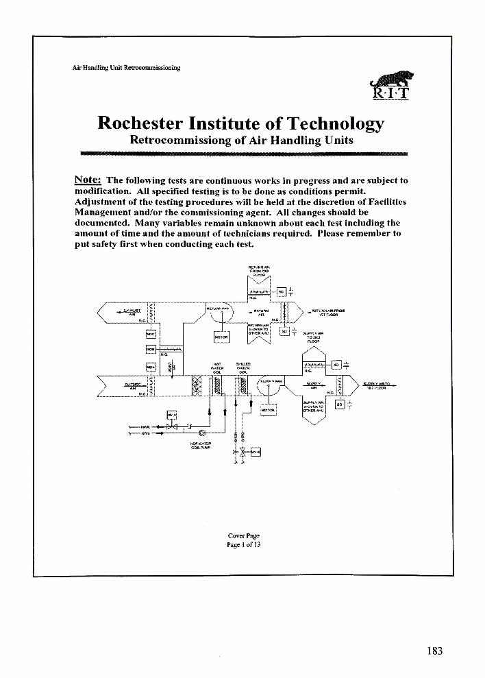
AirHandlingUnit Retrocommissioning
IT
Rochester Institute ofTechnologyRetrocomm issiong ofAir Handling Units
Note: The following tests are continuous works in progress and are subject to
modification. All specified testing is to be done as conditions permit.
Adjustment of the testing procedures will be held at the discretion ofFacilities
Management and/or the commissioning agent. All changes should be
documented. Many variables remain unknown about each test including the
amount of time and the amount of technicians required. Please remember to
put safety first when conducting each test.
tuLXL
..W.OOM -
kc
WU ' *'**\/\
is
OTHERAHU
WATER *MCt&lCQt. CCh.
B* Hft* - D>*0 i
If-
^ hvkv fr1 i
<:
Cover Page
Page 1 of 13
183

AirHandling Unit Retrocommissioning
General AHU Test
*
Date of Test: 4/8/2005
Technicians: RCX Senior Design Team
Richard Stein
Tom Hyzen
Procedure:
Verify that the sensors are accurate by comparing hand measurements to what is
shown inWebCTRL. Use pre-drilled ports, for temperature and pressure
measurements.
Incorporate the system control response test with the pre-functional checklist from
the coil, fan and economizer tests.
Accentable Results: All items tested shall nass.
System Control Response
Item Tested Control Response Alarm Response
SF S/S H/O/A & Schedule r-P nF nP nF
SF Proof rP nF dP nF
SF Static Ctrl SP SP Actual nP n F
SF Safety Interlock rP nF rP nF
SF Freezestat nP n F dP ? F
SF Fire Interlock oP nF cP nF
RF S/S H/O/A & Schedule rP nF aP dF
RF Proof nP nF nP nF
RF Static Ctrl SP SP Actual nP nF
RF Safety Interlock nP nF oP nF
RF Freezestat dP dF dP nF
RF Fire Interlock rP r.F nP nF
Field Calibration Check
Item Tested Test Results Alarm Response
OA Sensor - Temp oP nF nP nF
RA Sensor - Temp nP nF r,P nF
MA Sensor - Temp dP nF nP nF
DA Sensor - Temp dP nF DP nF
DA Sensor - Pressure oP nF r.P nF
Filter Proof Sensor nP nF nP dF
Pump Proof Sensor cP a F cP oF
General AHU Test
Page 2 of 13
184
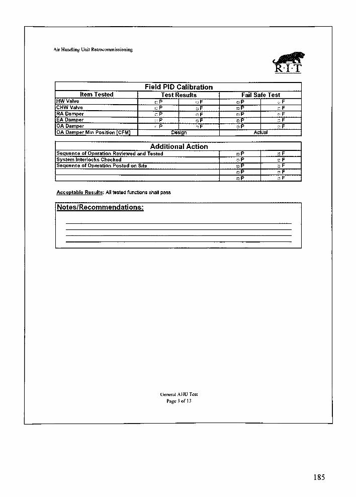
Air Handling Unit Retrocommissioning
rTt
Field PID Calibration
Item Tested Test Results Fail Safe Test
HW Valve cP oF nP dF
CHW Valve cP oF dP nF
RA Damper nP nF dP nF
EA Damper nP oF dP nF
OA Damper rP nF oP nF
OA Damper Min Position [CFM] Design Actual
Additional ActionSequence of Operation Reviewed and Tested nP nF
System Interlocks Checked oP ? F
Sequence of Operation Posted on Site oP nF
oP nF
oP nF
Acceptable Results: All tested functions shall pass
Notes/Recommendations:
General AHU Test
Page 3 of 13
185
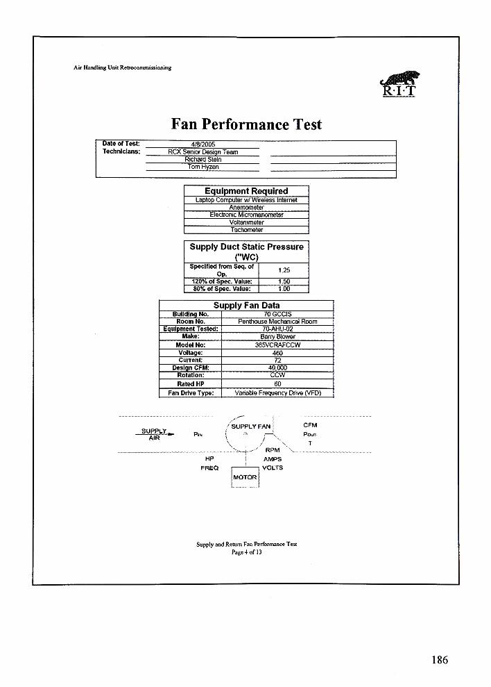
Air Handling Unit Retrocommissioning
IT
Fan Performance Test
Date of Test: 4/8/2005
Technicians: RCX SeniorDesign Team
Richard Stein
Tom Hyzen
Equipment Required
Laptop Computerw/Wireless Internet
Anemometer
Electronic Micromanometer
VcJtammeter
Tachometer
Supply Duct Static Pressure
("WC)Specified from Seq. of
Op.1.25
120% of Spec. Value: 1.50
80% of Spec. Value: 1.00
Supply Fan Data
Building No. 70GCCIS
Room No. PenthouseMechanical Room
Equipment Tested: 70-AHU-02
Make: BarryBlower
Model No: 365VCRAFCCW
Voltage: 460
Current 72
Design CFM: 40,000
Rotation: ccw
Rated HP 60
Fan Drive Type: Variable Frequency Drive (VFD)
/SUPPLY FAN ISUPPLY
AIRPlM f
!
^
\
HP
FREQ
MOTOR
1 XRPM
AMPS
VOLTS
CFM
PtXiT
T
Supply and Return Fan Performance Test
Paget ofl3
186
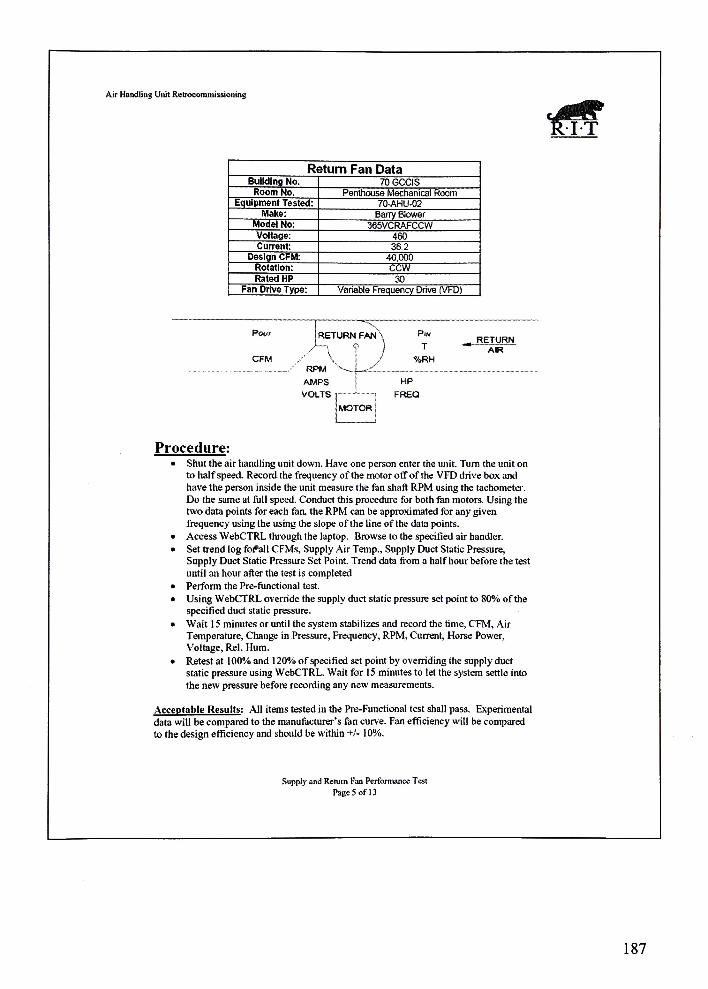
AirHandling Unit Retrocommissioning
Return Fan DataBuilding No. 70 GCCIS
Room No. PenthouseMechanical Room
Equipment Tested: 70-AHU-02
Make: Barry BlowerModel No: 365VCRAFCCW
Voltage: 460
Current: 36.2
Design CFM: 40,000
Rotation: CCW
Rated HP 30
Fan DriveType: Variable Frequency Drive (VFD)
Pow
CFM
RETURN
'
V
'
RPM s
FAN\* )y
Pw
T
%RH
RETURN
AIR
AMPS HP
FREO.VOLIS
MOTOR |
Procedure:
Shut the air handling unit down. Have one person enter the unit Turn the unit onto halfspeed. Record the frequency ofthe motor offof the VFD drive box and
have theperson inside the unit measure the fan shaft RPM using the tachometer.
Do the same at full speed. Conduct this procedure for both fan motors. Using thetwo data points for each fan, theRPM can be approximated for any given
frequency using the using the slope of the line of the data points.
AccessWebCTRL through the laptop. Browse to the specified air handier.
Set trend log foftl ICFMs, SupplyAirTemp., SupplyDuct Static Pressure,
SupplyDuct Static Pressure Set Point Trend data from a half hour before the test
until an hour after the test is completed
Perform the Pre-functional test.
UsingWebCTRL override the supply duct static pressure set point to 80% of the
specified duct static pressure.
Wait 1 5 minutes or until the system stabilizes and record the time. CFM,Air
Temperature, Change in Pressure, Frequency, RPM, Current, Horse Power,
Voltage, Rel. Hum.
Retest at 100% and 120% ofspecified set point by overriding the supply duct
static pressureusingWebCTRL. Wait for 15 minutes to let the system settle into
the new pressure before recording any new measurements.
Acceptable Results: All items tested in the Pre-Functional test shall pass. Experimental
data will be compared to the manufacturer's fan curve. Fan efficiency will be compared
to the design efficiency and should be within+/- 10%.
Supply and Return Fan PerformanceTest
Page5ofl3
187
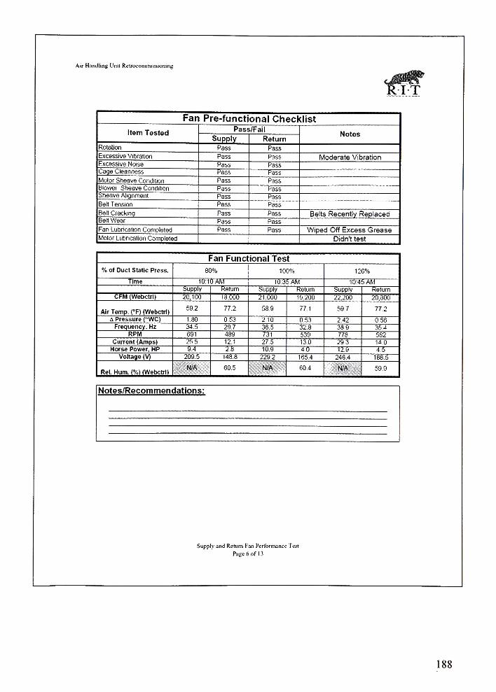
Air Handling Unit Retrocommissioning
Fan Pre-functional Checklist
Item TestedPass/Fail
NotesSupply Return
Rotation Pass Pass
Excessive Vibration Pass Pass Moderate VibrationExcessive Noise Pass Pass
Cage Cleanness Pass Pass
Motor Sheave Condition Pass Pass
Blower Sheave Condition Pass Pass
Sheave Alignment Pass Pass
Belt Tension Pass Pass
Belt Cracking Pass Pass Belts Recently ReplacedBeit Wear Pass Pass
Fan Lubrication Completed Pass Pass Wiped Off Excess Grease
Motor Lubrication Completed Didn't test
Fan Functional Test
% of Duct Static Press. 80% 100% 120%
Time 10:10 AM 10:35 AM 10:45 AM
Supply Return Supply Return Supply Return
CFM (Webctrl) 0,100 13,000 21,000 19,200 22,200 20,800
Air Temp. fF) (Webctrl)69.2 77.2 58.9 77.1 59.7 77.2
A Pressure ("WC) 1 80 0.53 2.10 0.53 242 0.56
Frequency, Hz 34.5 29.7 36.5 32.8 38.9 35.4
RPM 691 489 731 539 778 582
Current (Amps) 25.5 12.1 275 13.0 293 14.0
Horse Power. HP 9.4 2.8 10.9 40 12.9 4.5
Voltage (V) 209.5 148.8 229.2 165.4 248.4 188.5
Rel. Hum. (%KWebctrl)n/a : 60.5
*
N/A 60.4 N/A 59.9
Notes/Recommendations:
Supply and Return Fan Performance Test
Page 6 ofO
188
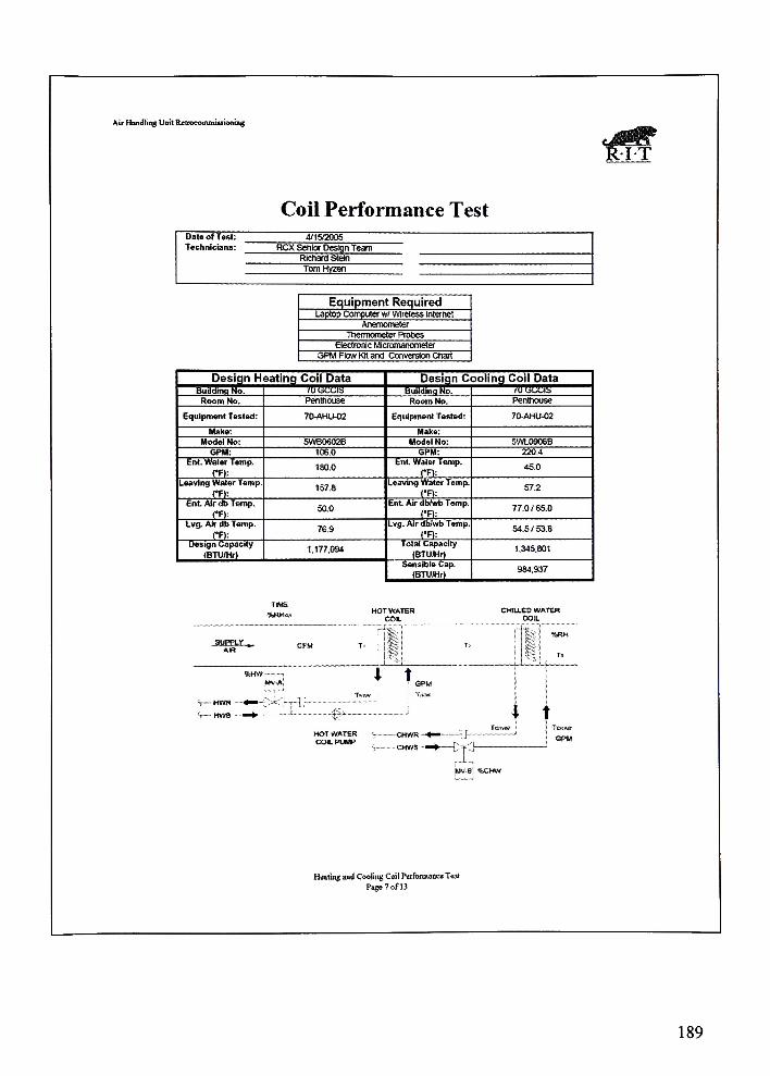
Air HandlingUnit Retroco iruwissiontng
R-FT
Coil Performance Test
DateofTest:
Technicians:
4/132005
RCXSeniorDesign Team
Richard Stein
TomHvzen
Equipment Required
Laptop computerw wireless
Thermometer Probes
Electronic Mlcromanometer
GPM Flow Kit and Conversion Chart
Design Heating Coil Data Design Cooling Coil Data
Buadinn No. Building No. 70 5CCIS
Room No. Pentnouse Room No. Penthouse
Equipment Tested: 70-AHU-02 Equipment Tested; 70-AHU-O2
Make: Make:
Model No: 5WB06026 Model No: 5WL0906B
GPM: 106.0 OPM: 2204
Ent. WaterTemp.
CR:180.0
Ent Water Temp.
TF):45.0
LeavingWaterTemp,
CF):157.8
LeavingWater Temp.
("Ft:575
Ent. Air db Temp,50.0
Ent Air <lb/wb Temp.
CR:77.0 /65.0
Lvg. Air db Temp.
TF):76.9
Lvg.Air db/wb Temp.
CR:54.5/53.8
Design Capacity(BTUfflrt
1.177,094Total Capacity
(BTUJHr)1,345.601
Sensible Cap.
(BTUJHr)984.937
TIMEHOTWATER
coa.
\; .
CHILLED WAItR
COIL
IS*
I t
<> Mvrs + tMOT WATER
coa. PUMP
-CHWR-
-CHWS-
i:MV 9 %CHW
Holing and Cooling Coil PerformanceT
Pge7ofl3
189
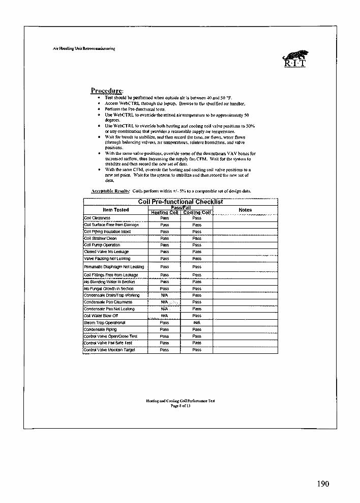
AirHandlingUnitRetrocotnmi&siontng
Procedure:* Test should be performed when outside air is between 40 and 50 "P.
? AccessWebCTRL through the laptop. Browse to the specified air handler.
* Perform the Pre-functional tests.
Use WebCTRL to override the mixed air temperature to be approximately 50
degrees.
Use WebCTRL to override both heating and cooling coil valve positions to 50%
or any combination that provides a reasonable supply air temperature.
Wait for trends to stabilize, and then record the time, air flows, water flows
(through balancing valves), air temperatures, relative humidities, and valve
positions.
? With the same valve positions, override some of the downstream VAV boxes for
increased airflow, thus increasing the supply fan CFM. Wait for the system to
stabilize and then record the new set ofdata.
With the same CFM, override the heating and cool ing coll valve positions to a
new set point. Wait for the system to stabilize and then record the new set of
data.
Acceptable Results: Coils perform within +/- 5% to a comparable set ofdesign data.
Coil Pre-functional Checklist
Item TestedPass/Fall
NotesHeatlnq Coll Cooling Coil
Coil Cleanness Pass Pass
Coll Sistace Free from Damage Pass Pass
Coll Piping Insulation Intact Pass Pass
Coil Strainer Clean Pass Pass
Co9 Pump Operation Pass Pass
Closed Valve No Leakage Pass Pass
Valve Packing Not Leaking Pass Pass
Pneumatic Diaphragm Not Leaking Pass Pass
Coll Fittings Free from Leakage Pass Pass
No StandingWater in Section Pass Pass
No Fungal Growth in Section Pass Pass
Condensate Drain/TrapWorking N/A Pass
Condensate Pan Cleanness WAp~k. Pass
Condensate Pan Not Leaking N/A Pass
CollWaterBlowOff N/A Pass
Steam TrapOperational Pass f*A
Condensate Piping Pass Pass
Control Valve Open/Close Test Pass Pass
Control valve Fan Sate Test Pass Pass
ControlVah/e Maintain Target Pass Pass
Healing uiul Cooling Ceil Performance Test
Pago S of 13
190
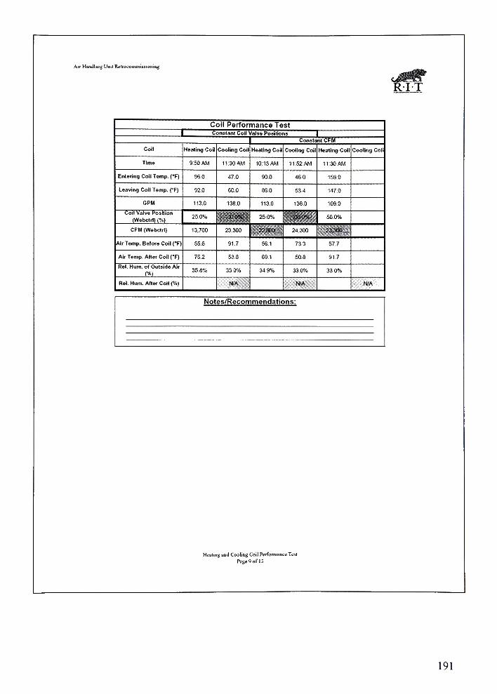
Air Handling Unit RettocommUsioruag
Coil Performance Test
Constant Coil Valve Positions
Constant CFM
Coil Heating Ceil Cooling Coil Heating Co8 Cooling Coil Heating Coil Cooling Coil
Time 9:50 AM 11:30 AM 10:13 AM 11:52 AM 11:30 AM
Entering Coil Temp. (*F) 96.0 47.0 90.0 460 159.0
Leaving Coll Temp. (F) 92.0 60.0 86.0 53.4 147.0
GPM 113.0 138.0 1130 138.0 109.0
Coil Valve Position
(Webctrl) (%)25.0% Ot :% I 25 0% jjg(nno% 50.0%
CFM (Webctrl) 13,700 23,300 22,800 24.300 23,300
AirTemp. Before Coil (*R 55.6 91.7 56.1 73.3 57.7
Air Temp. After Coil ("F) 76.2 53.8 69.1 50.8 91.7
Rel. Hum. of Outside Air
(%)35.8% 33.0% 34.9% 33.0% 33.0%
Rel. Hum. After Coil (":) N/A N/A N/A
Notes/Recommendations:
Heuting annf Cooling Coil Performance Test
Page 9 of 13
191
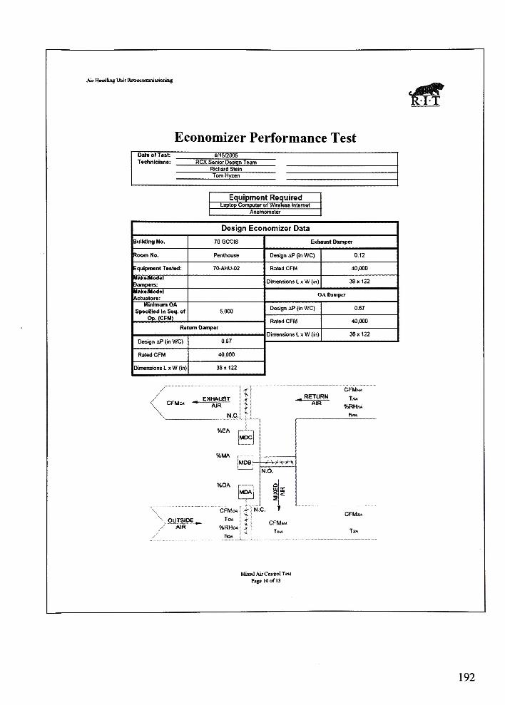
AirHandlingUnit Retrocomjiusuwoiung;
Economizer Performance Test
Oat* ofTest: 4/15/2005
Technicians: RCX SeniorDesiqn Team
Richard Stein
TbmHyzen
Equipment Required
LaptopComputer/Wireless internet
Design Economizer Data
Building No. 70GCCIS Exhaust Damper
Room No. Penthouse Design AP (in WC) 0.12
Equipment Tested: 70-AHU-02 Rated CFM 40,000
Make/Model
Dampers:Dimensions L xW (m) 38x122
Make/Model
Actuators:OADamper
Minimum OA
Specified In Seq. of
Op. (CFM)
5,000Design aP (inWC) 0.67
Rated CFM 40,000
Return Damper
Dimensions L x W (m) 38x122
Design AP (inWC) 0.67
Rated CFM 40,000
DimensionsL xW (in) 38x122
/"
CFMs.EXHAUST
AIR
N.C,
%CA
%MA
%OA
\ qtJTStoe_/
"
MR
,RETURN
AR
VV/WV
N.O.
a
a2
CFMoa
To*
%RHm
no*
N.C.
CFIM*m
CFMw
%RHf*
CFMs.
Ts
MixedAirControlTest
PgWof13
192
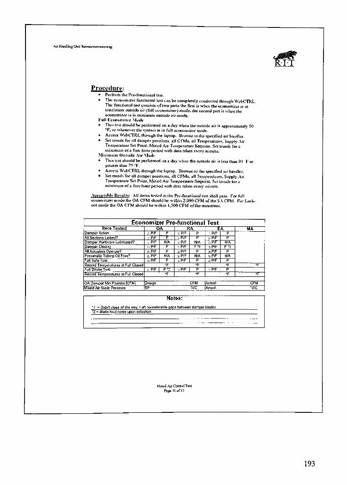
.AirHandlingUnit Retrocomnu.'wioning
ROT
Procedure:
Perform the Pre-functional test.
The economizer functional test can be completely conducted through WebCTRL.The functional test consists of two parts the first is when the economizer is inmaximum outside air (full economizer)mode, the second part is when theeconomizer is in minimum outside airmode.
full ICeonumizcr Mode
This test should be performed on a daywhen the outside air is approximately 50F. orwhenever the system is in full economizermode.
? AccessWebCTRL through the laptop. Browse to tbe specified air handler.Set trends for all damper positions, all CFMs, all Temperatures, SupplyAirTemperature Set Point, Mixed Air Temperature Setpoint, Set trends for aminimum ofa four hour period with data taken every minute,
Minimum Outside Air Mode
This test should be performed on a day when the outside air is less than 30 F or
greater titan 75 F.
? AccessWebCTRL through the laptop. Browse to the specified air handler.
Set trends for all dumper positions, all CFMs, all Temperatures, SupplyAirTemperature Set Point, Mixed Air Temperature Setpoint, Set trends for a
minimum ofa four hour period with data taken every minute.
Acceptable Results: All items tested in the Pre-functional test shall pass. For full
economizer mode the OA CFM should be within 2.000 CFM of the S.A CFM. For Lock
outmode the OA CFM should be within 1 ,500 CFM oftheminimum.
Economizer Pre-functional TestItem Tested OA RA EA MA
Damper Action cP/F P = p/f P -iP/F P
All Sections Linked? c P/F P nP/F P oP/F P
Damper Hardware Lubricated? :. P/F N/A nP/F N/A dP/F N/A
Damper Closing = P/F P - P/F F'1 a P/F FM
AllActuatorsOperate? r.Plf P = P/F P = P/F P
Pneumatic Tubing Oil Free? -Pff N/A a P/F N/A = P/F N/A
Fail Safe Test cP/F P ^P/F P a P/F P
Record Temperatures at Full Closed F F F F
Full Stroke Test cPIF | P'2 :.iP/F | P -P/F | P
Record Temperatures at Ful: Closed F F f F
OA Damper Min Position (CFM) Design. CFM Actual: CFM
Mated Air Static PressureSP-
"WC Actual: "WC
Notes:
"1 = Didn't cbse ali the way. Left considerable gap3 between damper blades
*2 = Made iouri noise upon actuation
Mixed AirControl Test
Pajpe II of 13
193
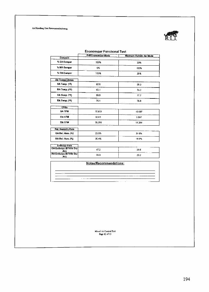
AirHandlingUnit Reroc<>miiiis$ioflig
r-ft
Economizer Functional Test
Full EconomizerMode | Minimum Outside AirModeOatnpers
%EA Damper 100% 20%
%MA Damper 0% 100%
%OADamper 100% 20%
AirTemperatures
SA Temp. ("F) 52.6 SS.3
MA Temp. <*F) 63.1 74.2
OATemp. (') S9.9 77.2
RATmp,('F) 76.1 7S.8
CFMs
SACFM 17,619 13,087
OACFM 9,91 J 1,937
RACFM 15,268 11,394
Rel. HumidityData
OA Rel. Hum. (%) 23.5% 31.0%
RA Rel. Hum. (%) 35.4% 18 5%
Enthalpy Data
OA Enthalpy (BTU/lb Dry
Air)172 20.6
RA Enthalpy (BTU/lb Dry
Air)263 23.2
Notes/Recommendations:
Mixed AirControlTest
Page 12 of 13
194
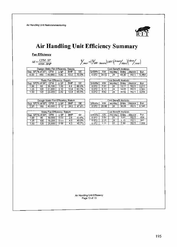
Air Handling Unit Retrocommissioning
Air Handling Unit Efficiency SummaryFan Efficiency
CFM-SPSE=-
6356 BHP \/kW-lKHesYkn\%ays)\ '/n$/ =[%.
year \/kfV- /tours)
Design Static Fan Efficienc/, Supply Cost BenefitAnalysis
Sup. SP %ofSP CFM ASP BHP SE S/KWhr KW hrs/day $/day daystyr. $/yr.
6.00 480 40,000 5.92 53.0 70.3% 0.072 39,52 24 68.30 182.5 12,464
Static Fan Efficiency, Supply Cost BenefitAnalysis
Sup. SP %ofSP CFM ASP BHP SE $/KWhr KW hrs/day $/day days/yr. $A/r.
1.00 80 20.100 180 9.4 60.6% 0.072 7.01 24 12.11 182 5 2,211
1.25 100 21,000 2.10 10.9 63.7% 0.072 8.13 24 14.05 182.5 2,563
1.50 120 22.200 2.42 12.9 65.5% 0.072 9.62 24 16.62 182 5 3,034
Design Static Fan Efficiency, Return Cost BenefitAnalysis
Sup. SP %ofSP CFM ASP BHP SE $,KWhr KW hrs/day $/day days/yr. $/yr.
2.25 180 40,000 2 12 28.0 47.6% 0.072 20.88 24 36.08 182 5 6 585
Static Fan Efficiency, Return
Sup. SP % of SP CFM ASP BHP SE
1.00 80 18.000 0.53 2.8 53.6%
1.25 100 19.200 0.53 4.0 40.0%
1.50 120 20,800 0.56 4.5 40.7%
Cost Benefit Analysis
S/KWhr KW hrs/day $/day days/yr $'yr.
0.072 2.09 24 3.61 182.5 658
0.072 2 98 24 5 15 1 82 5 941
0.072 3 36 24 5 80 182 5 1.053
Air Handling Unit Efficiency
Page 13 of 13
195
Related Documents


