Advanced Derivatives: Course Notes Richard C. Stapleton 1 1 Department of Accounting and Finance, Strathclyde University, UK.

Welcome message from author
This document is posted to help you gain knowledge. Please leave a comment to let me know what you think about it! Share it to your friends and learn new things together.
Transcript
Advanced Derivatives: Course Notes
Richard C. Stapleton1
1Department of Accounting and Finance, Strathclyde University, UK.

Advanced Derivatives 1
1 The Binomial Model
• Assume that we know that the stock price follows a geometric processwith constant proportionate up and down movements, u and d:
S
q
q
��
�
@@
@
Su
Sd
��
�
@@
@
@@
@
��
�
Su2....
Sud....
Sd2....
Sun
Sun−1d
��
�
@@
@
@@
@
��
�
@@
@
��
�
@@
@
��
�
where q is the probability of an up move.

Advanced Derivatives 2
• A contingent claim (for example a call or a put option) has a price g(S)which follows the process:
g(S)
q
q
��
�
@@
@
g(Su)
g(Sd)
��
�
@@
@
@@
@
��
�
g(Su2)....
g(Sud)....
g(Sd2)....
g(Sun)
g(Sun−1d)
��
�
@@
@
@@
@
��
�
@@
@
��
�
@@
@
��
�
• Define the hedge ratio:
δ1 =g(Su)− g(Sd)
Su− Sd
Lemma 1 The portfolio of δ1 stocks and 1 short contingent claim has ariskless payoff at t = 1 equal to
g(Su)d− g(Sd)u
u− d

Advanced Derivatives 3
Proposition 1.1 Suppose the price of a stock and a contingent claim followthe processes above, then the no-arbitrage price of the contingent claim is
g(S) =[pg(Su) + (1 − p)g(Sd)]
R
where
p =R− d
u− d
and R is 1+ risk-free rate.
Corollary 1 Suppose the price of a stock and a contingent claim follow theprocesses above, then the no-arbitrage price of the contingent claim is
g(S) =[png(Sun) + pn−1(1 − p)g(Sun−1d)n+ ....+ pn−r(1 − p)rg(Sun−rdr) n!
r!(n−r)!+ ...]
Rn
wheren! = n(n− 1)(n− 2)...(2)(1),
n!
r!(n− r)!
is the number of paths leading to node r, and
r is the number of down moves of the process.
Example 1: A Call Option
A call option with maturity T and strike price K has a payoff max[ST −K, 0]at time T .
Rng(St) =[pn(Stu
n −K) + pn−1(1 − p)n(Stun−1d−K) + ....+ pn−r(1 − p)r(Stu
n−rdr −K) n!r!(n−r)!
Rn
Rng(St)
St
= pnun + pn−1(1 − p)un−1dn+ .... + pn−r(1 − p)run−rdr n!
r!(n− r)!
− k
[pn + pn−1(1 − p)n+ .... + pn−r(1 − p)r n!
r!(n− r)!
]
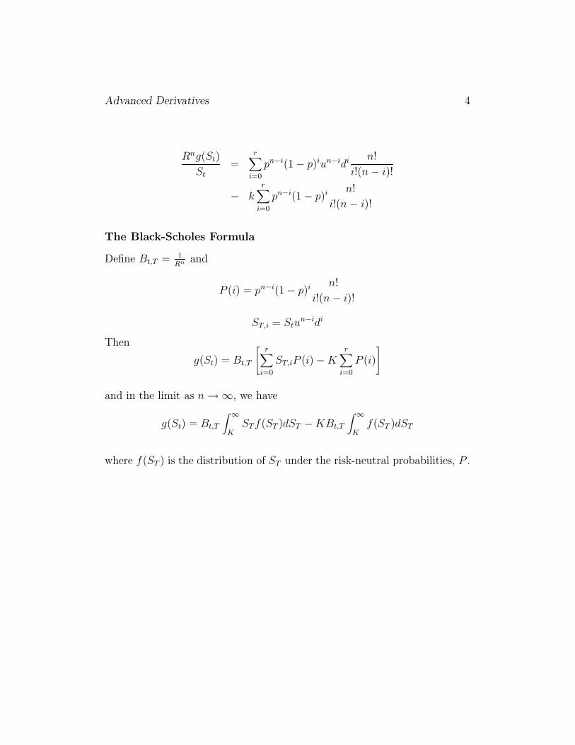
Advanced Derivatives 4
Rng(St)
St=
r∑
i=0
pn−i(1 − p)iun−idi n!
i!(n− i)!
− kr∑
i=0
pn−i(1 − p)i n!
i!(n− i)!
The Black-Scholes Formula
Define Bt,T = 1Rn and
P (i) = pn−i(1 − p)i n!
i!(n− i)!
ST,i = Stun−idi
Then
g(St) = Bt,T
[r∑
i=0
ST,iP (i) −Kr∑
i=0
P (i)
]
and in the limit as n→ ∞, we have
g(St) = Bt,T
∫ ∞
KSTf(ST )dST −KBt,T
∫ ∞
Kf(ST )dST
where f(ST ) is the distribution of ST under the risk-neutral probabilities, P .

Advanced Derivatives 5
Proof of Proposition 1.1
From lemma 1 the payoff on the hedge portfolio of δ1 stocks and one shortoption is
g(Su)d− g(Sd)u
u− d
Since the payoff is risk free its value must be
δ1S − g(S) =g(Su)d− g(Sd)u
R(u− d)
Hence
g(S) =g(Su) − g(Sd)
u− d− g(Su)d− g(Sd)u
R(u− d)
=Rg(Su) −Rg(Sd) − g(Su)d+ g(Sd)u
R(u− d)
=1
R
[g(Su)
(R− d
u− d
)− g(Sd)
(u−R
u− d
)]
=1
R[g(Su)p− g(Sd)(1− p)]
where
p =R− d
u− d
1 − p =u−R
u− d

Advanced Derivatives 6
Assume the asset price follows the log-binomial process:
q
q
��
�
@@
@
ln(u)
ln(d)
��
�
@@
@
@@
@
��
�
2ln(u)....
ln(u) + ln(d)....
2ln(d)....
(n − r)ln(u) + rln(d)
��
�
@@
@
@@
@
��
�
@@
@
��
�
@@
@
��
�
If xn follows the above process, the logarithm of xn has a mean:
n[q ln(u) + (1 − q) ln(d)] = µ(T − t)
a variance:n[q(1 − q)(ln(u) − ln(d))2] = σ2(T − t).
Lemma 2 Assume that two lognormally distributed stocks have the samevolatility, σ, and have mean, µj, j = 1, 2. Then the lognormal distributionscan be approximated with log-binomial distributions with (u, d, q1 = 0.5) and(u, d, q2) for large n.

Advanced Derivatives 7
Proposition 1.2 Consider two stocks with prices S1 = S2 and volatility σand a derivative with exercise priceK. Let the derivative prices be g(S1), g(S2).Then, regardless of the drifts µ1, µ2
g(S1) = g(S2)
Proof
We consider the hedge ratio for each option in state u at time 1. First wehave
g(S1u2) = g(S2u
2)
g(S1ud) = g(S2ud)
The hedge ratio for option 1 is
δ1,1,u =g(S1u
2) − g(S1ud)
S1(u− d)= δ1,2,u
Now consider a portfolio of two stocks and two options costing
δ1,1,uS1u− g(S1u) − [δ1,2,uS2u− g(S2u)] = −g(S1u) + g(S2u)
This portfolio provides a risk-free return equal to
δ1,1,uS1u2 − g(S1u
2) − [δ1,2,uS2u2 − g(S2u
2)] = 0
It follows thatg(S1u) = g(S2u)
By a similar argumentg(S1d) = g(S2d)
and alsog(S1) = g(S2)
Advanced Derivatives 8
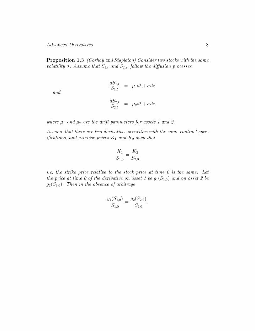
Proposition 1.3 (Corhay and Stapleton) Consider two stocks with the samevolatility σ. Assume that S1,t and S2,T follow the diffusion processes
and
dS1,t
S1,t= µ1dt+ σdz
dS2,t
S2,t= µ2dt+ σdz
where µ1 and µ2 are the drift parameters for assets 1 and 2.
Assume that there are two derivatives securities with the same contract spec-ifications, and exercise prices K1 and K2 such that
K1
S1,0=
K2
S2,0
i.e. the strike price relative to the stock price at time 0 is the same. Letthe price at time 0 of the derivative on asset 1 be g1(S1,0) and on asset 2 beg2(S2,0). Then in the absence of arbitrage
g1(S1,0)
S1,0=g2(S2,0)
S2,0.

Advanced Derivatives 9
2 The Black-Scholes and Black Models
Given the Mean-irrelevance Theorem, an option can be valued by valuing anequivalent option on a ‘risk-neutral’ stock, with volatility σ. We need thefollowing:
Lemma 3 The value of a call option on a risk-neutral stock, i.e. a stock,paying no dividends, that has a price
St = Bt,TE(ST ),
isCt = Bt,TE[max(ST −K, 0)].
Hence, if ST is lognormal, a call option on a risk-neutral stock has a value:
Ct = Bt,TF [g(ST )],
where F (.) denotes ‘forward price of’, and
g(ST ) = max(ST −K, 0)
F [g(ST )]
St= E
[max
(ST
St− k, 0
)]
=∫ ∞
k
(ST
St− k
)f(ST
St
)d(ST
St
)
=∫ ∞
ln(k)(ez − k) f(z)d(z)
where k = KSt
and z = ln(
ST
St
)

Advanced Derivatives 10
Lemma 4 If f(y) is normal with mean µ and standard deviation σ then
1.∫ ∞
af(y)d(y) = N
(µ− a
σ
)
and
2.∫ ∞
aeyf(y)d(y) = N
(µ− a
σ+ σ
)eµ+ 1
2σ2
with
3.
E(ey) = eµ+ 12σ2
We have in this case
µ = E[ln(ST
St
)]
andσ2 = σ2(T − t)
From risk neutrality E(ST ) = F and hence, using the Lemma 4, 3
E[ST
St
]=F
St= eµ+ 1
2σ2(T−t)
and it follows that
µ = ln(F
St
)− 1
2σ2(T − t)
Hence, choosing a = ln(k) = ln(
KSt
),
∫ ∞
af(z)d(z) = N
(µ− a
σ
)= N
ln(
FSt
)− 1
2σ2(T − t) − ln
(KSt
)
σ√T − t
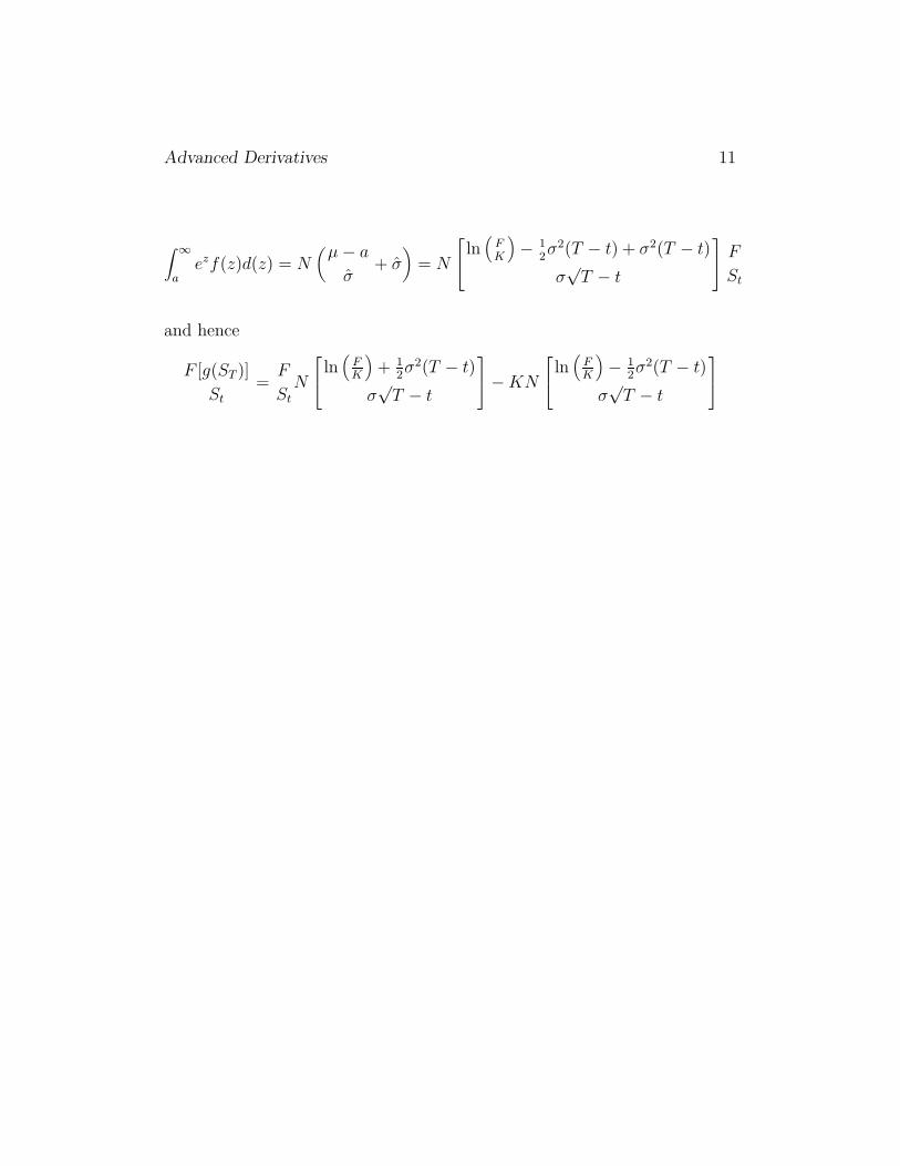
Advanced Derivatives 11
∫ ∞
aezf(z)d(z) = N
(µ− a
σ+ σ
)= N
ln
(FK
)− 1
2σ2(T − t) + σ2(T − t)
σ√T − t
FSt
and hence
F [g(ST )]
St
=F
St
N
ln(
FK
)+ 1
2σ2(T − t)
σ√T − t
−KN
ln(
FK
)− 1
2σ2(T − t)
σ√T − t

Advanced Derivatives 12
A Proof of the Black Model (Forward Version) Assume the followingthe process for the forward price of the asset:
F ��
�
@@
@
Fu
Fd
��
�
@@
@
@@
@
��
�
Fu2....
Fud....
Fd2....
and for the forward price of a contingent claim:
Cf ��
�
@@
@
Cfu
Cfd
��
�
@@
@
@@
@
��
�
Cfuu....
Cfud....
Cfdd....

Advanced Derivatives 13
Proposition 2.1 Suppose the forward prices of a stock and a contingentclaim follow the processes above, then the no-arbitrage forward price of thecontingent claim is
Cf = [p′Cfu + (1 − p′)Cf
d ]
where
p′ =1 − d
u− d
If an option pays max(ST −K, 0), after n sub-periods, then its forward priceis given by
Cf = E [max(ST −K, 0)]
where the expectation E(.) is taken over the probabilities p′. Also,
Cf
F= E
[max(
ST
F− k′, 0)
]
= pnun + pn−1(1 − p)un−1dn+ ....+ pn−r(1 − p)run−rdr n!
r!(n− r)!
− k′[pn + pn−1(1 − p)n+ .... + pn−r(1 − p)r n!
r!(n− r)!
]
=∫ ∞
ln(k′)(ez − k′)f(z)dz
where k′ = KF
and z = ln(
ST
F
).
To value the option we again take the case of a ‘risk-neutral’ stock, whereE(ST ) = F . Let
µ = E[ln(ST
F
)]
We then have
E[ST
F
]=E[ST ]
F= 1 = eµ+ 1
2σ2
It follows that
µ = −1
2σ2(T − t)
Hence, choosing a = ln(k′) = ln(
KF
),

Advanced Derivatives 14
∫ ∞
af(z)d(z) = N
(µ− a
σ
)= N
−
12σ2(T − t) + ln
(FK
)
σ√T − t
∫ ∞
aezf(z)d(z) = N
(µ− a
σ+ σ
)= N
ln
(FK
)− 1
2σ2(T − t) + σ2(T − t)
σ√T − t
and hence
Cf
F= N
ln(
FK
)+ 1
2σ2(T − t)
σ√T − t
− K
FN
ln(
FK
)− 1
2σ2(T − t)
σ√T − t
and
Cf
F= N(d1) −
K
FN(d2)
Cf = FN(d1) −KN(d2)
The spot price of the option is
C = Bt,TFN(d1) − Bt,TKN(d2)
Advanced Derivatives 15
Example 1: A Call Option, Non-Dividend Paying Stock
St = Bt,TF
impliesC = StN(d1) −Bt,TKN(d2)
as in Black-Scholes. Note proof has not assumed constant (non-stochasticinterest rates.
Example 2: A Stock Paying Dividends
Assume that dividends are paid at a continuous rate d. The forward price ofthe stock is
F = Ft,T = Ste(r−d)(T−t)
C = Bt,TSte(r−d)(T−t)N(d1) −Bt,TKN(d2)
C = Ste(−d)(T−t)N(d1) −Bt,TKN(d2)
sinceBt,T = s−r(T−t)

Advanced Derivatives 16
3 Hedge Ratios in the Black-Scholes and Black
Models
We need to know the following sensitivities:
1. The call delta
∆c =∂Ct
∂St
2. The put delta
∆p =∂Pt
∂St
3. The put and the call gamma
Γ =∂
∂St
[∂Ct
∂St
]=
∂
∂St
[∂Pt
∂St
]
4. The vega of a call or put option:
V =∂Ct
∂σ
5. The theta of a call or put option:
Θc =∂Ct
∂t

Advanced Derivatives 17
The Black-Scholes Model: No Dividends
C = StN(d1) −Bt,TKN(d2)
where
d1 =ln(
FK
)+ σ2(T−t)
2
σ√T − t
,
d2 =ln(
FK
)− σ2(T−t)
2
σ√T − t
.
Lemma 5
n(d2)K
F= n(d1)
Lemma 6 (Differential Calculus) 1. Chain rule
∂f(g(x))
∂x= g′(x)f ′[(g(x)]
2. Product rule
∂[f(x)(g(x)]
∂x= f ′(x)g(x) + g′(x)f(x)]
Proposition 3.1 In the Black-Scholes model, the delta of a call option isgiven by
∆c =∂Ct
∂St= N(d1)

Advanced Derivatives 18
Proof
Using lemma 7,
∂Ct
∂St= N(d1) + StN
′(d1)∂d1
∂St−Ke−r(T−t)N ′(d2)
∂d2
∂St
Then, note that d2 = d1 − σ√
T−t2
implies ∂d2
∂St= ∂d1
∂St. Hence,
∂Ct
∂St
= N(d1) +∂d1
∂St
[StN
′(d1) −Ke−r(T−t)N ′(d2)]
and using lemma 5,
∂Ct
∂St
= N(d1) +∂d1
∂St
[StN
′(d2)K
F−Ke−r(T−t)N ′(d2)
]
From forward parityF = Ste
r(T−t)
and hence∂Ct
∂St= N(d1)
Corollary 2 (Put Option Delta) From put-call parity
Ct − Pt = St −KBt,T
Hence,∂Ct
∂St
− ∂Pt
∂St
= 1
∆p =∂Pt
∂St
= N(d1) − 1
Corollary 3 (Put, Call Gamma)
∂
∂St
[∂Ct
∂St
]=
∂
∂St
[∂Pt
∂St
]
= N ′(d1)∂d1
∂St
= n(d1)1
Stσ√T − t

Advanced Derivatives 19
Using a similar method, it is possible to establish
1. The vega of a call option
∂Ct
∂σ= St
√T − tN ′(d1)
and using put-call parity,
∂Pt
∂σ=∂Ct
∂σ
2. The theta of call option
∂Ct
∂t=StN
′(d1)σ
2√T − t
− rKe−r(T−t)N(d2)
and using put-call parity
∂Pt
∂t=∂Ct
∂t+ rKe−r(T−t)
Hedge Ratios: Options on Dividend Paying Stocks
For a stock which pays a continuous dividend at a rate d,
Ct = Ste−d(T−t)N(d1) −Ke−r(T−t)N(d2)
where
d1 =ln(St/K) + (r − d+ σ2)(T − t)/2
σ√T − t
d2 = d1 − σ√T − t
since, from forward parity,
F = Ste(r−d)(T−t)
and hence
d1 =ln(
FK
)+ σ2(T−t)
2
σ√T − t
=ln(
St
K
)+(r − d+ σ2
2
)(T − t)
σ√T − t
Advanced Derivatives 20
It follows that the call delta is
∆c =∂Ct
∂St
= e−δ(T−t)N(d1)
Also, for foreign exchange options
∆c =∂Ct
∂St
= e−rf (T−t)N(d1)
where rf is the foreign risk-free rate of interest.
Hedge Ratios: Futures-Style Options
Let H be the futures price of the asset at time t, for time T delivery. TheBlack formula gives a (futures) call value:
Ch = HN(d1) −KN(d2)
with
d1 =ln(
HK
)+ σ2(T−t)
2
σ√T − t
d2 = d1 − σ√T − t
Note that the Black formula will hold if the underlying futures price followsa geometric brownian motion. [The proof is the same as the forward proofabove.] Then we have:
Proposition 3.2 (Call Delta: Futures-Style Options)
Assume that the option is traded on a marked-to-market basis, then the fu-tures price of the call is given by
Ch = HN(d1) −KN(d2)
and the call delta (in terms of futures positions) is
∆c =∂Ch
∂H= N(d1)

Advanced Derivatives 21
Proof
For the price Ch, see Satchell, Stapleton and Subrahmanyam (1997). For thehedge ratio, a reworking of Lemma 5 yields in this case
(K
H
)n(d2) = n(d1)
Using this and the same steps as in the proof of proposition 3.1 we get theresult.
Corollary 4 (Libor Futures Options)
Assuming these are European-style, marked-to-market options, then a put onthe futures price has a value
Pt = [(1 −Ht,T )N(d1) − (1 −K)N(d2)]
where
d1 =ln(
1−H1−K
)+ σ2(T−t)
2
σ√T − t
d2 = d1 − σ√T − t
where H is the futures price and K is the strike price. The delta hedge ratio,in terms of the underlying Libor futures contract is
∂P h
∂(1 −H)= N(d1)
∂P h
∂(H)= −N(d1)
Proof
The futures price of the option can be established for Libor options by assum-ing that the futures rate follows a lognormal diffusion process (limit of thegeometric binomial process as n → ∞). The hedge ratio can be establishedby reworking Lemma 5 to obtain
(1 −K
1 −H
)n(d2) = n(d1)
Advanced Derivatives 22
3.1 Hull’s Treatment of ‘Futures Options’
There are three issues to consider here:
1. Options on futures. These are options to enter a futures contract,at a fixed futures price K. However, since in all cases, the maturity ofthe option is the same as the maturity of the underlying futures, theseoptions have the same payoff as options on spot prices, if exercised atmaturity. The main difference is in the valuation of the American-style,early exercise feature (CME v PHILX).
2. Futures-style options. On many exchanges (ex. LIFFE) options aretraded on a marked-to-market basis, just like the underlying futures.Hull does not deal with the valuation of these options.
3. Hedging with futures Any option could be hedged with futures (notnecessarily options on futures.
3.2 A Digression on Futures v Forwards
Hull’s treatment assumes that there is no significant difference between fu-tures prices and forward prices. [Hull uses the same symbol F for the futuresprice and the forward price of an asset.] However, this is not true in the caseinterest rate contracts (especially long-term contracts). Also in the case ofoptions, small differences are magnified.
A long (x = 0) [short (x = 1)] futures contract made at time t, with maturityT , to buy [sell] an asset at a price Ht,T has a payoff profile:
(−1)x [Ht+1,T −Ht,T ] (−1)x [Ht+2,T −Ht+1,T ] · · · (−1)x [HT,T −HT−1,T ]
On the other hand, a forward contract pays (−1)x [ST − Ft,T ] at time T.
Pricing
Assume no dividends (up to contract maturity)
Ft,T = St/Bt,T = Ster(T−t)
Advanced Derivatives 23
Ht,T = Ft,T + cov
Hull assumes Ft,T = Ht,T [For hedging this is OK, since ∆Ft,T ≈ ∆Ht,T ]Under risk neutrality:
Ht,T = Et(ST )
and, if interest rates are non-stochastic,
Ft,T = Et(ST )
also. However, in general there is a bias due to the covariance term.
Hedging
Forward paysFt+1,T − Ft,T
at T , which is worth(Ft+1,T − Ft,T )Bt+1,T
at t + 1. Futures paysHt+1,T −Ht,T
at t+1, hence the hedge ratios for options, in terms of forwards and futures,are quite different to one another.
Hull does not value ‘futures-style’ options. His formula for the spot priceof a futures option assumes zero covariance between interest rates and theaset price. What if there is a significant correlation (bond options, LIBORfutures options)?
If the forward price of the asset follows a GBM, then the Black model holds,with forward price in the formula. Then the spot price of the option is
C = Bt,TFN(d1) − Bt,TKN(d2)
But from SSS (1997) this requires gt,T to be lognormal, if the pricing kernelis lognormal.
Conclusion. If Black model holds for futures-style options, it is not likely tohold for spot-style (because of stochastic discounting). It should be estab-lished using a forward hedging argument, not a futures hedging argument asin Hull.

Advanced Derivatives 24
4 Approximating Diffusion Processes
Definitions
1. A lognormal diffusion process (geometric Brownian motion) for St:
dSt = µStdt+ σStdz
ordSt
St
= µdt+ σdz
In discrete form:St+1 − St
St= mµ+
√mσεt+1
where m is the length of the time period (in years), and ε ∼ N(0, 1)Also, we can write
d ln(St) = (µ− 1
2σ2)dt+ σdz
ln(St+1) − ln(St) = (µ− 1
2σ2)m+ σ
√mεt+1
2. A constant elasticity of variance (CEV) process for St:
dSt = µStdt+ σSγt dz
(If γ = 1, lognormal diffusion. If γ = 0, St is normal.) In discrete form:
St+1 − St = mµSt +√mσSγ
t εt+1
vart(St+1 − St) = mσ2S2γt
∂vart(St+1 − St)
∂St= 2mγσ2S2γ−1
t
The elasticity of variance is
∂vart(St+1 − St)
∂St
St
vart(St+1 − St)= 2γ
Example: γ = 0.5,√
process of Cox, Ingersoll and Ross (1985)
Advanced Derivatives 25
3. A generalized CEV process:
dSt = µ(St, t)Stdt+ σ(t)Sγt dz
If γ = 0, σ(t) = σ, and µ(St, t)St = β(α− St)
dSt = β(α− St)dt+ σdz
This is the Ornstein-Uhlenbeck process, as used in Vasicek (1976)model.
Approximation methods: Lognormal Diffusions
Assume we want to approximate the process
dSt = µStdt+ σStdz
with a multiplicative binomial with constant u and d movements. Fromlecture 1, the approximated mean µ and standard deviation σ are given by:
µT = n[q ln(u) + (1 − q) ln(d)] (1)
σ2T = n[q(1 − q)(ln(u) − ln(d))2] (2)
We need to choose u, d, q so that
µT → µT, σT → σT, n→ ∞
1. The Cox-Rubinstein Solution
Choose the restriction ud = 1, then if u = eσ√
Tn , and
q =1
2
1 +
µ
σ
√T
n
we have µ = µ. Also, σ → σ, for n → ∞. To prove this note that
ud = 1 implies d = e−σ√
Tn and ln(d) = − ln(u), and substitution in (1)
and (2) gives the result, since q → 12
as n→ ∞.

Advanced Derivatives 26
2. The Hull-White Solution
Choose q = 0.5, then the solution to equations (1) and (2), with µ andσ substituted for µ and σ is
ln(u) =
√σ2T
n+µT
n
3. The HSS Solution
Suppose we are given a set of expected prices E0(St) for each t, as wellas the volatility σ. HSS first construct a process for xt = St
E0(St), where
E0(xt) = 1. To do this, choose q = 12, u = 2 − d, and
d =2
e2σ√
Tn + 1
.
Then we have E0(xt) = 1 and σ = σ.
Recombining Trees: The Nelson-Ramaswamy Method
[Note: NR use the notation σ for the standard deviation in a Brownianmotion, rather than the conventional standard deviation of the logarithmin a geometric Brownian motion. In this section we will use σ′ for the NRσ to distinguish it from the volatility (annualised standard deviation of thelogarithm), σ.]
NR consider the general process:
dyt = µ′(y, t) + σ′(y, t)dwt
where, for example,
µ′(y, t) = µ(St, t)St
σ′(y, t) = σ(t)Sγt
If the volatility of the process changes over time, the binomial tree approxi-mation may not combine:
Example 1 GCEV process with γ = 1, µ(St, t) = µ
dSt = µStdt+ σ(t)Stdz
Advanced Derivatives 27
Lemma 7 The CEV process approximation is recombining if and only ifγ = 0, 1.
1. µ is irrelevant to the recombination issue, so take µ = 0. Recombinationrequires
S0 + σSγ0 − σ(S0 + σSγ
0 )γ = S0 − σSγ0 + σ(S0 − σSγ
0 )γ
If γ = 0:S0 + σ − σ = S0 − σ + σ
If γ = 1:
S0 + σS0 − σ(S0 + σS0) = S0 − σS0 + σ(S0 − σS0)
2. Take the case where S0 = 1
S2,u,d = 1 + σ − σ(1 + σ)γ 6= 1 − σ + σ(1 − σ)γ
NR split the period [0, T ] into n sub-periods of length h = Tn. After k sub-
periods, yhk goes to y+(hk, yhk) with probability q and to y−(hk, yhk), withprobability (1−q). The annualised drift and variance of the process are givenby
hµ′h(y, t) = q[y+ − y] + (1 − q)[[y− − y]
hσ′2(y, t) = q[y+ − y]2 + (1 − q)[[y− − y]2
(NR eq 11-12).
1. NR first construct a non-recombining tree. In this tree y goes to y+ =y +
√hσ′(y, t) with probability q = 1
2+
√h µ′(y,t)
2σ′(y,t), and to y+ = y −√
hσ′(y, t) with probability (1 − q).
2. NR then define a transformation of the process, such that the binomialtree recombines. They choose [NR (25)]
x(y, t) =∫ y dz
σ′(z, t)

Advanced Derivatives 28
in discrete form,
x(y, t) =t∑
1
∆yτ
σ′(y, τ)=
∆y1
σ′(y, 1)+
∆y2
σ′(y, 2)+ ....+
∆yt
σ′(y, t)
3. NR then define a reverse transformation:
y[x(y, t)] : x(y, t) −→ x(y, t)σ′(y, t)
Proposition 4.1 (Nelson and Ramaswamy)
Suppose yt is given by the non-recombining tree [NR(21-23)], the transformedprocess defined by [NR (25-26)] is a simple tree. If we choose the probabilityof an up-move to match the conditional mean by making
q =hµ′ + y(x, t) − y−(x, t)
y+(x, t) − y−(x, t)
Then µ′ → µ′ and σ′ → σ′, as n→ ∞.
Proof
By construction the mean is exact, since
q(y+ − y−) = hµ′ + y − y−
implies thatqy+ + (1 − q)y− = y + hµ′,
i.e. µ′ = µ′.
The conditional variance is exact if q = 0.5. Also q → 0.5 as n→ ∞
Advanced Derivatives 29
5 Multivariate Processes: The HSS Method
Motivation
• For many problems we need to approximate multiple-variable diffusionprocesses
• It may be reasonable to assume that prices (or rates) follow lognormaldiffusions
• From NR if ln(Xt) = xt is given by
dxt = µ(xt)dt+ σ(t)dz
we can build a ’simple’ tree for xt and choose the probability of anup-move
qt−1 =µ(xt−1) + xt−1 − x−t
x+t − x−t
(3)
HSS assumptions
• Xi is lognormal for all dates ti, with given mean E(Xi).
• For dates ti, we are given the local volatilities σi−1,i, and the uncondi-tional volatilities σ0,i.
• Approximate with a binomial process with ni sub-periods.
• Add a second (or more) variable Yi, where (Xi, Yi) are joint log-normal,correlated variables.
Relation to NR: One-Variable Case
Assume an Ornstein-Uhlenbeck process for xt:
dxt = κ(a− xt)dt+ σdz.
In discrete formxi − xi−1 = k(a− xi−1) + σεt,

Advanced Derivatives 30
xi = ka+ b′x1−k + ε′i (4)
andvar(xi) = (1 − k)2var(xi−1) + var(ε′i)
In annualised form
t2iσ20,ti
= (1 − k)2tiσ20,ti
+ (ti − ti−1)σ2ti−1,ti
.
Hence, if we are given the mean reversion rate k, and the conditional volatil-ities, σi−1,i, we can compute the unconditional volatilities, σti .
However, the linear regression (4) is valid for any lognormal variables. Wedo not need to assume a, k are constant or that σt−1,t = σ.
To obtain the probability in NR, assume a binomial density, ni = 1 for all i,in HSS [eq(10)]. This gives
qi−1,r =ai + bixi−1,r − (i− 1 − r) ln(ui) − (r + 1) ln(di)
[ln(ui) − ln(di)], (5)
However,
x−t = (i− 1 − r) ln(ui) + (r + 1) ln(di)
x+t = (i− r) ln(ui) + r ln(di)
x+t − x−t = ln(ui) − ln(di)
Hence (5) is equivalent to (3) with ai + bixi−1,r = xt−1 + µ(xt−1).
In general, the probability of an up-move is given by HSS [eq(10)]
qi−1,r =ai + bixi−1,r − (Ni−1 − r) ln(ui) − (ni + r) ln(di)
ni[ln(ui) − ln(di)], (6)
where Ni =∑i
1 nl. An example: Let ni = 2, for all i, then for i = 2 andr = 0, we have
q1,0 =a2 + b2x1,0 + (2 − 0) ln(u2) − 2 ln(d2)
2[ln(u2) − ln(d2)],
Advanced Derivatives 31
Proposition 5.1 (HSS) Suppose that ui and di are chosen by
di =2
1 + e2σi−1,i
√ti−ti−1
ni
ui = 2 − di
and the probability of an up move is
qi−1,r =ai + bixi−1,r − (Ni−1 − r) ln(ui) − (ni + r) ln(di)
ni[ln(ui) − ln(di)],
where Ni =∑i
1 nl. Then µ→ µ and σ → σ, as n→ ∞.
Proof
See HSS (1995).
A Multivariate Extension of HSS
In Peterson and Stapleton (2002) the original two variable version of HSS(eq 13, p1140), is modified, extended (to three variables) and implemented.It is illustrated by pricing a ’Power Reverse Dual’ a derivative that dependson the process for two interest rates and an exchange rate.
First, we assume, that
xt = ln[Xt/E(Xt)],
yt = ln[Yt/E(Yt)],
follow mean reverting Ornstein-Uhlenbeck processes, where:
dxt = κ1(φt − xt)dt+ σx(t)dW1,t
dyt = κ2(θt − yt)dt+ σy(t)dW2,t, (7)
where E(dW1,tdW2,t) = ρdt. In (7), φt and θt are constants and κ1 and κ2
are the rates of mean reversion of xt and yt respectively. As in Amin(1995),

Advanced Derivatives 32
it is useful to re-write these correlated processes in the orthogonalized form:
dxt = κ1(φt − xt)dt+ σx(t)dW1,t
dyt = κ2(θt − yt)dt+ ρσy(t)dW1,t +√
1 − ρ2σy(t)dW3,t, (8)
where E(dW1,tdW3,t) = 0. Then, rearranging and substituting for dW1,t in(43), we can write
dyt = κ2(θt − yt)dt− βx,y [κ1(φt − xt)] dt+ βx,ydxt +√
1 − ρ2σy(t)dW3,t.
In this bivariate system, we treat xt as an independent variable and yt as thedependent variable. The discrete form of the system can be written as follows:
xt = αx,t + βx,txt−1 + εx,t
yt = αy,t + βy,tyt−1 + γy,txt−1 + δy,txt + εy,t, (9)
Advanced Derivatives 33
Proposition 5.2 (Approximation of a Two-Variable Diffusion Process)Suppose that Xt, Yt follows a joint lognormal process, where E0(Xt) = 1, E0(Yt) =1 ∀t, and where
xt = αx,t + βx,txt−1 + εx,t
yt = αy,t + βy,tyt−1 + γy,txt−1 + δy,txt + εy,t
Let the conditional logarithmic standard deviation of Jt be denoted as σj(t)for J = (X, Y ), where
σ2j (t) = var(εj,t) (10)
If Jt is approximated by a log-binomial distribution with binomial densityNt = Nt−1 +nt and if the proportionate up and down movements, ujt and djt
are given by
djt =2
1 + exp(2σj(t)√τt/nt)
ujt = 2 − djt
and the conditional probability of an up-move at node r of the lattice is givenby
qjt−1,r =Et−1(jt) − (Nt−1 − r) ln(ujt) − (nt + r) ln(djt)
nt[ln(ujt) − ln(djt)]
then the unconditional mean and volatility of the approximated process ap-proach their true values, i.e., E0(Jt) → 1 and σj,t → σj,t as n→ ∞.

Advanced Derivatives 34
Steps in HSS: Single Factor Tree (n = 1 case)
Assume we are given b in the regression (mean reversion):
xi = ai + bxi−1 + εi
Also, we are given the local volatilities σi−1,i.
1. Compute
di =2
1 + e2σi−1,i√
ti−ti−1
ui = 2 − di
2. Compute the nodal values for the unit mean tree
ui−ri dr
i
3. Compute the unconditional voltilities using
tiσ20,i = b2ti−1σ
20,i−1 + (ti − ti−1)σ
2i−1,i
starting with i = 1.
4. Compute the constant coefficients:
ai = −1
2tiσ
20,i + b
1
2ti−1σ
20,i−1
5. Compute the probabilities
qi−1,r =ai + bxi−1,r − (i− 1 − r) ln(ui) − r ln(di) − ln(di)
ln(ui) − ln(di),
6. Given the unconditional expectations E0(Xi) compute the nodal values
Xi,r = E0(Xi)ui−ri dr
i
Advanced Derivatives 35
6 Interest-rate Models
6.1 No-arbitrage and Equilibrium Models
Equilibrium Interest-rate Models
An equilibrium interest-rate model assumes a stochastic process for the in-terest rate and derives a process for bond prices, assuming a value for themarket price of risk.
No-arbitrage Interest-rate Models
A no-arbitrage interest-rate model assumes the current term structure ofbond prices and builds a process for interest rates (and bond prices) that isconsistent with this given term structure. In a no-arbitrage model, no bondcan stochasticaly dominate another.
Proposition 6.1 [No-Arbitrage Condition] A sufficient condition for noarbitrage is that the forward price of a zero-coupon bond is given by
Et(Bt+1,T ) =Bt,T
Bt,t+1
where the expectation is taken under the risk-neutral measure.
Examples:
1. The Vasicek (1977) model (Equilibrium Model)
• Assumes short rate (rt) follows a normal distribution process
• Assumes that short rate mean reverts at a constant rate
• Derives equilibrium bond prices for all maturities
drt = κ(a− rt)dt+ σ′dz.
In discrete form:
rt − rt−1 = k(a− rt−1) + σ′εt,
Advanced Derivatives 36
2. The Ho-Lee model
• Assumes that the zero-coupon bonds follow a log-binomial process.
• This implies that the short rate (rt) follows a normal distributionprocess, in the limit.
• Takes bond prices, and hence forward prices, (at t = 0) as given.
• The model builds a process for the forward prices of the set ofzero-coupon bonds.
• No-arbitrage model, prices European-style bond options
3. The Black-Karasinski model
• Assumes short rate (rt) follows a lognormal distribution process
• It derives from a prior model, the Black-Derman-Toy model, whichdid not have mean reversion.
d ln(rt) = κ[θ(t) − ln(rt)]dt+ σ(t)dz.
ln(rt) − ln(rt−1) = k[θ(t) − ln(rt)] + εt
• Takes bond prices, or futures rates (at t = 0) as given
• No-arbitrage model, prices European-style, American-style bondoptions
• Unconditional volatility (caplet vol) in the BK model:
var[ln(rt)] = (1 − k)2var[ln(rt−1)] + var(εt)
√tσ0,t = (1 − k)
√t− 1σ0,t−1 + σt−1,t
A Recombining BK model using HSS
To use the HSS method we follow the steps:
1. Given the local volatilities, σ(t), and the mean reversion, k, we firstbuild a tree of xt, with E0(xt) = 1, for all xt.

Advanced Derivatives 37
2. Then multiply by the expectations of rt under the risk-neutral measure.The following result establishes that these expectations are the futuresLIBOR, h0,t
The following lemma states that, given the definition of the LIBOR futurescontract, the futures LIBOR is the expected value of the spot rate, underthe risk-neutral measure.
Lemma 8 (Futures LIBOR) In a no-arbitrage economy, the time-t futuresLIBOR, for delivery at T , is the expected value, under the risk-neutral mea-sure, of the time-T spot LIBOR, i.e.
ft,T = Et(rT )
Also, if rT is lognormally distributed under the risk-neutral measure, then:
ln(ft,T ) = Et[ln(rT )] +vart[ln(rT )]
2,
where the operator “var” refers to the variance under the risk-neutral mea-sure.
Proof
The price of the futures LIBOR contract is by definition
Ft,T = 1 − ft,T (11)
and its price at maturity is
FT,T = 1 − fT,T = 1 − rT . (12)
From Cox, Ingersoll and Ross (1981), the futures price Ft,T is the value, attime t, of an asset that pays
VT =1 − rT
Bt,t+1Bt+1,t+2...BT−1,T
(13)
Advanced Derivatives 38
at time T , where the time period from t to t+1 is one day. In a no-arbitrageeconomy, there exists a risk-neutral measure, under which the time-t valueof the payoff is
Ft,T = Et(VTBt,t+1Bt+1,t+2...BT−1,T ). (14)
Substituting (13) in (14), and simplifying then yields
Ft,T = Et(1 − rT ) = 1 − Et(rT ). (15)
Combining (15) with (11) yields the first statement in the lemma. The secondstatement in the lemma follows from the assumption of the lognormal processfor rT and the moment generating function of the normal distribution. 2
Lemma 8 allows us to substitute the futures rate directly for the expectedvalue of the LIBOR in the process assumed for the spot rate. In particular,the futures rate has a zero drift, under the risk-neutral measure.
The Vasicek Model
Proposition 6.2 [Mean and Variance in the Vasicek Model] Assumethat the short-term interest rate is given by
d rt = κ(a− rt) + σ dz
where dz is normally distributed with zero mean and unit variance. Then theconditional mean of rs is
Et(rs) = a + (rt − a)e−κ(s−t), t ≤ s
and the conditional variance of rs is
vart(rs) =σ2
2κ(1 − e−2κ(s−t)), t ≤ s

Advanced Derivatives 39
A Classification of Spot-Rate Models
Assume that the short-term rate of interest follows the GCEV process
drt = µ(rt, t)rtdt+ σ(t)rγt dz.
1. If γ = 0, µ(rt, t)rt = κ(a− rt), σ(t) = σ,
drt = κ(a− rt) + σdz
as in Vasicek (true process) and Hull-White (risk-neutral process).
Extensions: Hull-White two-factor model.
2. If γ = 1, µ(rt, t) = µ,
drt = µrtdt+ σ(t)dz
as in Black, Derman and Toy model (risk-neutral process)
dln(rt) = κ[θ(t) − ln(rt)]dt+ σ(t)dz
as in Black-Karasinski model.
Extensions: Peterson, Stapleton, Subrahmanyam two-factor model.
3. If γ = 0.5, µ(rt, t)rt = α(θ − rt),
drt = α(θ − rt) + σ√rt
as in CIR model.
Extensions: Credit risk factor, stochastic volatility models.
Advanced Derivatives 40
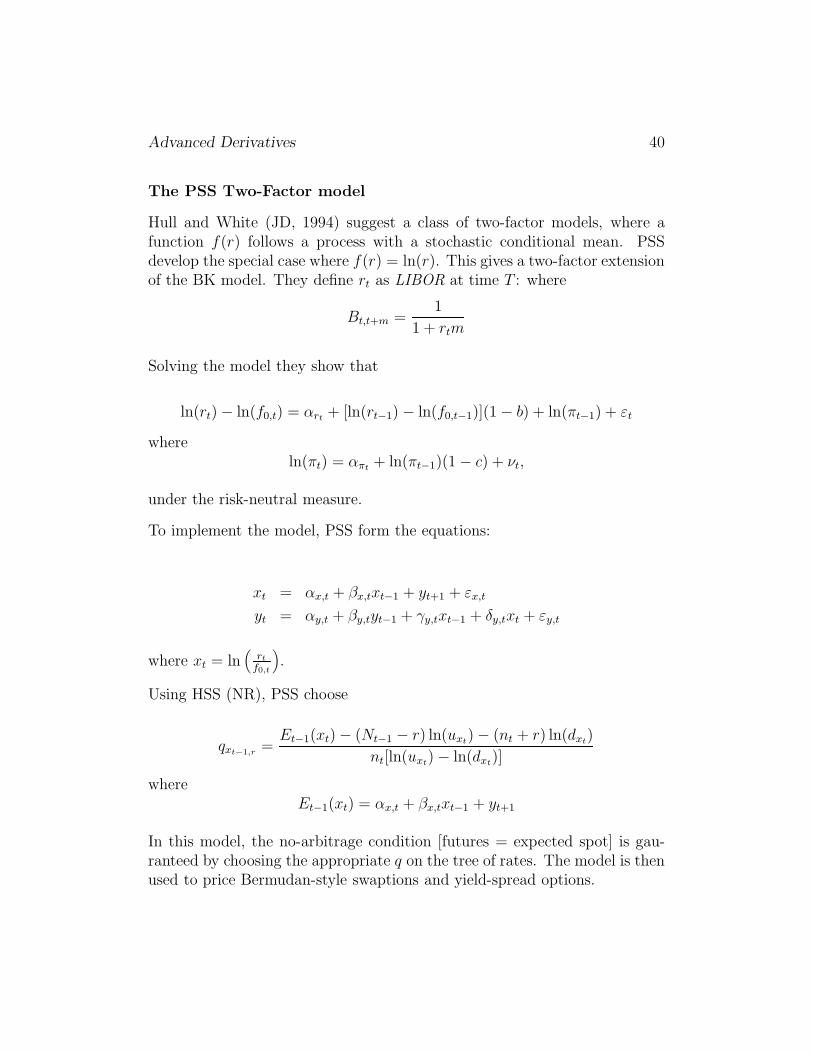
The PSS Two-Factor model
Hull and White (JD, 1994) suggest a class of two-factor models, where afunction f(r) follows a process with a stochastic conditional mean. PSSdevelop the special case where f(r) = ln(r). This gives a two-factor extensionof the BK model. They define rt as LIBOR at time T : where
Bt,t+m =1
1 + rtm
Solving the model they show that
ln(rt) − ln(f0,t) = αrt + [ln(rt−1) − ln(f0,t−1)](1 − b) + ln(πt−1) + εt
whereln(πt) = απt + ln(πt−1)(1 − c) + νt,
under the risk-neutral measure.
To implement the model, PSS form the equations:
xt = αx,t + βx,txt−1 + yt+1 + εx,t
yt = αy,t + βy,tyt−1 + γy,txt−1 + δy,txt + εy,t
where xt = ln(
rt
f0,t
).
Using HSS (NR), PSS choose
qxt−1,r =Et−1(xt) − (Nt−1 − r) ln(uxt) − (nt + r) ln(dxt)
nt[ln(uxt) − ln(dxt)]
whereEt−1(xt) = αx,t + βx,txt−1 + yt+1
In this model, the no-arbitrage condition [futures = expected spot] is gau-ranteed by choosing the appropriate q on the tree of rates. The model is thenused to price Bermudan-style swaptions and yield-spread options.
Advanced Derivatives 41
7 The Ho-Lee Model
Features of the model
• The model prices interest-rate derivatives, given the current term-structure of bond prices, and given a binomial process for the term-structure evolution
• One-factor (any bond or interest rate) generates the whole term struc-ture
• It is analogous to the Cox, Ross, Rubinstein (limit Black-Scholes) modelfor bond options
• The model is Arbitrage-Free (AR)
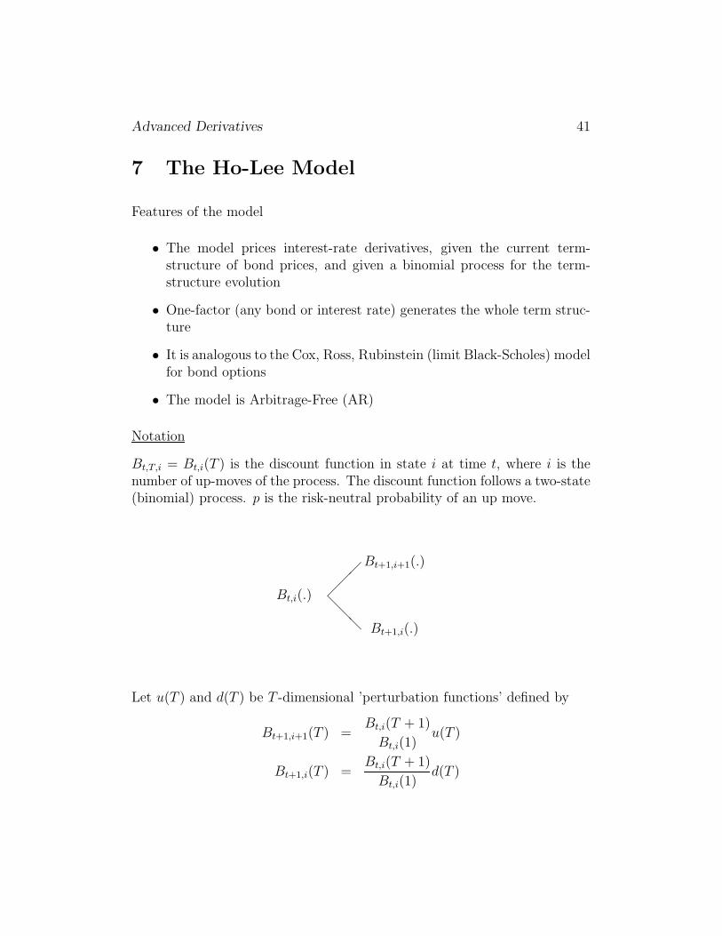
Notation
Bt,T,i = Bt,i(T ) is the discount function in state i at time t, where i is thenumber of up-moves of the process. The discount function follows a two-state(binomial) process. p is the risk-neutral probability of an up move.
Bt,i(.) ��
�
@@
@
Bt+1,i+1(.)
Bt+1,i(.)
Let u(T ) and d(T ) be T -dimensional ’perturbation functions’ defined by
Bt+1,i+1(T ) =Bt,i(T + 1)
Bt,i(1)u(T )
Bt+1,i(T ) =Bt,i(T + 1)
Bt,i(1)d(T )

Advanced Derivatives 42
Proposition 7.1 [Ho-Lee Process]
1. A constant, time-independent risk-neutral probability p exists and forany T
p =1 − d(T )
u(T ) − d(T )
2. The process recombines only if a δ exists such that
u(T ) =1
p+ (1 − p)δT
Proof
a) Form a portfolio with 1 bond of maturity T and α bonds of maturity τ .The cost of the portfolio is, at time t, is BT +αBτ (dropping subscripts t, i).The return on the portfolio in the up state at t+ 1 is
BT
B1u(T − 1) + α
Bτ
B1u(τ − 1)
In the down-state it is
BT
B1
d(T − 1) + αBτ
B1
d(τ − 1)
Choose α = α∗ so that these are equal, that is
α∗ =d(T − 1)BT − u(T − 1)BT
u(τ − 1)Bτ − d(τ − 1)Bτ=BT [d(T − 1) − u(T − 1)]
Bτ [u(τ − 1) − d(τ − 1)]
With α = α∗, the discounted value of the return must equal the cost, hence
BT + α∗Bτ = BT [d(T − 1)] + [α∗d(τ − 1)]Bτ
and this implies1 − d(T )
u(T ) − d(T )= p
which is a constant (for a proof, see exercise 8.1)
b)
Advanced Derivatives 43
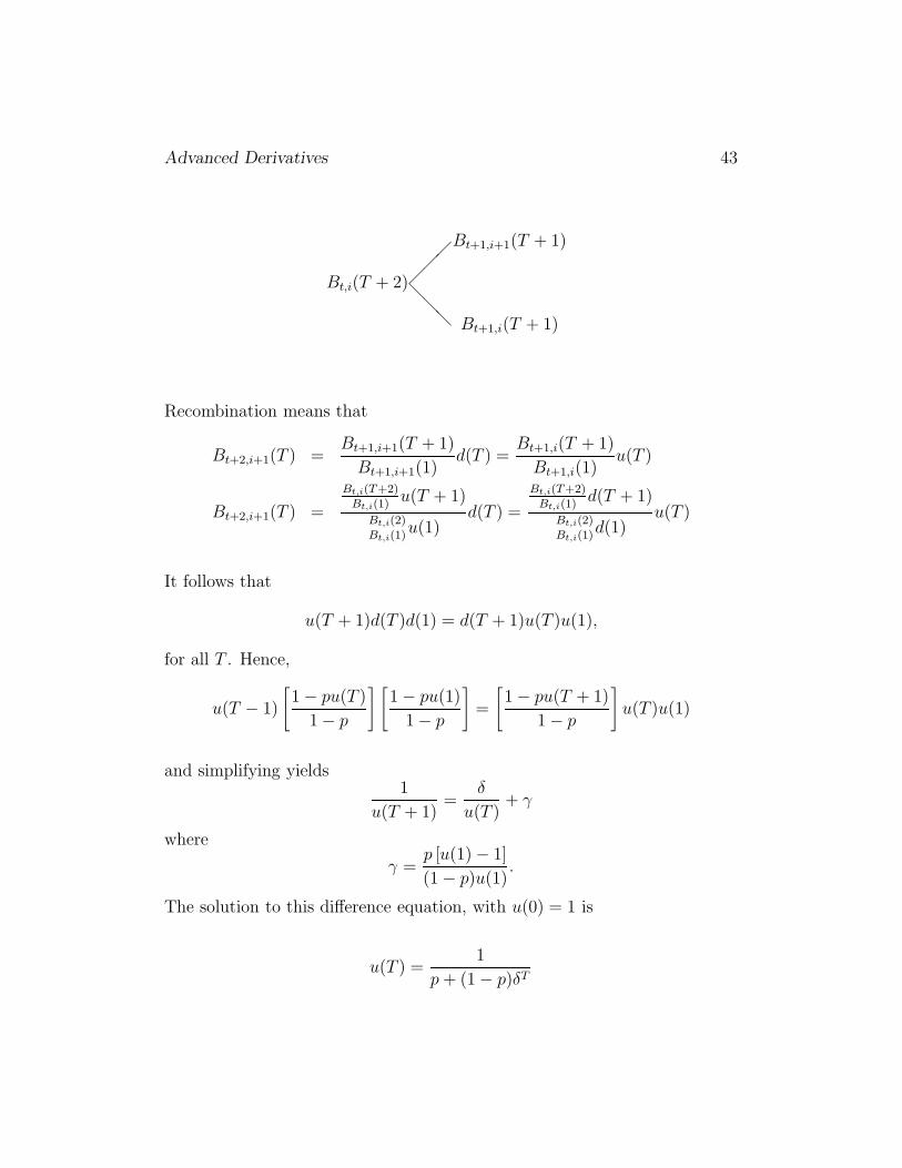
Bt,i(T + 2)��
�
@@
@
Bt+1,i+1(T + 1)
Bt+1,i(T + 1)
Recombination means that
Bt+2,i+1(T ) =Bt+1,i+1(T + 1)
Bt+1,i+1(1)d(T ) =
Bt+1,i(T + 1)
Bt+1,i(1)u(T )
Bt+2,i+1(T ) =
Bt,i(T+2)
Bt,i(1)u(T + 1)
Bt,i(2)
Bt,i(1)u(1)
d(T ) =
Bt,i(T+2)
Bt,i(1)d(T + 1)
Bt,i(2)
Bt,i(1)d(1)
u(T )
It follows that
u(T + 1)d(T )d(1) = d(T + 1)u(T )u(1),
for all T . Hence,
u(T − 1)
[1 − pu(T )
1 − p
] [1 − pu(1)
1 − p
]=
[1 − pu(T + 1)
1 − p
]u(T )u(1)
and simplifying yields1
u(T + 1)=
δ
u(T )+ γ
where
γ =p [u(1) − 1]
(1 − p)u(1).
The solution to this difference equation, with u(0) = 1 is
u(T ) =1
p+ (1 − p)δT

Advanced Derivatives 44
and using part a),
d(T ) =δT
p+ (1 − p)δT.
Proposition 7.2 [Contingent Claims in the Ho-Lee Model] Considera contingent claim paying C(t, i) at time t, in state i, then its value at timet− 1 is
C(t− 1, i) = {p[C(t, i+ 1)] + (1 − p)[C(t, i)]}Bt−1,i
Proof
Form a portfolio of one discount bond with maturity t plus α contingentclaims. Choose α so that the portfolio is risk free. The result then follows asin CRR (1979).
Note, if we know the process for Bt(1) and p, we can price any contingentclaim. This is a one-factor model result.

Advanced Derivatives 45
Steps for Constructing the Ho-Lee Model
1. Use market data to estimate the set of zero-coupon bond prices att = 0.
2. Use forward parity to compute the one-period-ahead forward prices att = 0, for each bond, B0,1,n, where
B0,1,n =B0,n
B0,1
3. Compute the up and down movements u(T ) and d(T ) for times tomaturity T = 1, 2, ..., n, where
d(T ) =δT
0.5(1 + δT )
u(T ) = 2 − d(T )
4. Compute Bu1,n in the up-state using
Bu1,n = B0,1,nu(n− 1)
Then compute Bd1,n in the down-state using
Bd1,n = B0,1,nd(n− 1)
5. Compute the set of forward prices at t = 1 in the up-state, Bu1,2,n, using
forward parity. Then compute the set of forward prices at t = 1 in thedown-state, Bd
1,2,n.
6. Starting in the up-state at t = 1 compute Buu2,n (in the up-up state at
t = 2) using the method in step 4, then compute Bud2,n and Bdd
2,n.
7. After step 6 you should have a term structure of zero-coupon bondprices at each date and in each state. Use these to compute interestrates (yields for example) or coupon bond prices, as required:
Advanced Derivatives 46
(a) Use
Bst,n =
1
(1 + yst,n)n−t
to compute the n− t year maturity yield rate in state s at time t.
(b) UseBc,s
t,n = cBst,1 + cBs
t,2 + ...cBst,n +Bs
t,n
to compute the price of an n−m maturity bond, with coupon c,in state s.
8. Compute the price of an interest-rate derivative by starting at the ma-turity date of the derivative, working out the expected value using theprobability p = 0.5, and discounting by the one-period zero-couponbond price, using
Cst =
[Cs+1
t+1 0.5 + Cst+10.5
]Bs
t,1
where s indicates the state at time t by the number of up-moves of theprocess from 0 to t.

Advanced Derivatives 47
8 The LIBOR Market Model
8.1 Origins of the LMM
• Forward Rate Models (HJM) and Forward Price Models (Ho-Lee)
• Black Model for Caplet Pricing
Brace, Gatarek and Musiela (BGM) and Miltersen, Sandmann and Sonder-man (MSS) build a forward LIBOR model consistent with the Black Modelholding for each Caplet. Note that the BK model is not consistent with theBlack model (in spite of its lognormal assumption).
Heath-Jarrow-Morton, Forward-Rate Models
HJM models build the process for the forward interest rate. Similar to Ho-Lee, but forward rate, not forward price. For example, the Brace-Gatarak-Musiela (BGM) model builds a process for the forward LIBOR. Usually as-sume a convenient volatility process (ex. constant vol). The models are usedfor pricing complex interest-rate derivatives.
Proposition 8.1 [The Black Model: Interest-Rate Caplet]
caplett =A
1 + ft,t+T δδ[ft,t+TN(d1) − kN(d2)]Bt,t+T
where
d1 =ln(
ft,t+T
k) + σ2T/2
σ√T
d2 = d1 − σ√T
Advanced Derivatives 48
Main Features of the LMM
The main features of the LMM are as follows:
• Forward rates are conditional lognormal over each discrete period oftime.
• The first input is the term structure of forward rates at time t = 0.
• This complete term structure of forward rates is perturbed over eachtime period, t
• The methodology is similar to Ho-Lee, but uses forward rates ratherthan forward bond prices
• The interest rate generated is usually 3-month LIBOR.
8.2 No-Arbitrage Pricing
We start by considering some implications of no-arbitrage. First, we assumethe following no-arbitrage relationships hold, where expectations are takenunder the risk-neutral measure. We also assume that the zero-coupon bondprices Bt,t+1 are stochastic. For convenience, write E0 as E.
Lemma 9 (No-Arbitrage Pricing) If no dividend is payable on an asset:
1. the spot price of the asset is
S0 = B0,1E[B1,2E1[B2,3E2[...Bt−1,tEt−1(St)]]]
2. and the t-period forward price of the asset
F0,t = S0/B0,t

Advanced Derivatives 49
Proposition 8.2 (Zero-Coupon Bond Forward Prices) When expecta-tions are taken under the risk-neutral measure: The t-period forward price ofa t+ T -period maturity zero-coupon bond is
E(B1,t,t+T ) − B0,t,t+T = −B0,1
B0,t
cov(B1,t,t+T , B1,t)
Proof
From no-arbitrage:
B0,t = B0,1E(B1,t),
B0,t+T = B0,1E(B1,t+T ).
From forward parity:B1,t+T = B1,t,t+TB1,t,
hence taking expectations and using the definition of covariance,
E(B1,t+T ) = E(B1,t,t+T )E(B1,t) + cov(B1,t,t+T , B1,t)
Substituting for the expected bond prices
B0,t+T
B0,1
= E(B1,t,t+T )B0,t
B0,1
+ cov(B1,t,t+T , B1,t)
and multiplying by B0,1 and deviding by B0,t yields
B0,t+T
B0,t= E(B1,t,t+T ) +
B0,1
B0,tcov(B1,t,t+T , B1,t)
and since, from forward parity
B0,t+T
B0,t= B0,t,t+T
then we have
E(B1,t,t+T ) − B0,t,t+T = −B0,1
B0,tcov(B1,t,t+T , B1,t)
Advanced Derivatives 50
Corollary 5 One-Period Ahead Forward Prices
Let t = 1, thenE(B0,T+1) −B0,1,T+1
and henceB0,1,T+1 = E(B1,2B1,2,T+1)
Also, with T = 1,
B0,1,2 = E(B1,2)
8.3 The LIBOR Market Model: Notation
• Bt,t+δ = Value at t of a zero-coupon bond paying 1 unit of currency att+ δ.
• δ = Interest-rate reset interval (ex. 3 months) as a proportion of a year
• Bt,t+T = Value at t of a zero-coupon bond paying 1 unit of currency att+ T .
• Bt,t+T,t+T+δ = Forward price at t for delivery of a zero-coupon bond(with maturity δ) at T .
• ft,t+T = T -period forward LIBOR at time t if T = 0, ft,t is the spotLIBOR at t.
• Note that in this notation
Bt,t+T,t+T+δ =1
1 + ft,t+T δ

Advanced Derivatives 51
Definition 8.1 A Forward Rate Agreement (FRA) on δ-periodLIBOR, withmaturity t, has a payoff
(ft,t − k)δ
1 + ft,tδ
at date t.
Proposition 8.3 (Drift of the One-Period Forward rate)
Since a one-period FRA struck at the forward rate f0,1 has a zero value:
E
[(f1,1 − f0,1)δ
1 + δf1,1
]= 0.
It follows that
E
(δf1,1
1 + δf1,1
)=
δf0,1
1 + δf0,1.
Also
E(δf1,1) − δf0,1 = −cov(δf1,1,
1
1 + δf1,1
)(1 + δf0,1) ≥ 0
Hence, the drift of the forward rate is given by
E(f1,1) − f0,1 = −(
1
δ
)cov
(δf1,1,
1
1 + δf1,1
)(1 + δf0,1) ≥ 0
Proof
Expanding the lhs of the second equation, using the definition of covarianceand employing Corollary 5 yields the Proposition.
Advanced Derivatives 52
Proposition 8.4 (Drift of Two-Period Forward) Since a two-period FRAhas a zero value:
E
[(δ(f1,2 − f0,2)
1 + δf2,2
)1
1 + δf1,1
]= 0.
It follows that
E(f1,2) − f0,2 = −(
1
δ
)cov
[δf1,2,
1
1 + δf1,1
· 1
1 + δf1,2
](1 + δf0,1) (1 + δf0,2)
Proof
Expanding the lhs, using the definition of covariance and employing Corollary5 yields the Proposition.
Lemma 10 (Covariances and Covariances of Logarithms) From Tay-lor’s Theorem we can write
lnX = ln a+1
a(X − a) + ...
lnY = ln b +1
b(Y − b) + ...
Hence
cov(lnX, lnY ) ≈ 1
a
1
bcov(X, Y )
Applying this we have for example:
cov(ln(f1,t), ln(f1,τ )) ≈1
f0,t
1
f0,τcov(f1,t, f1,τ )
Lemma 11 (Stein’s Lemma) For joint normal variables, x, y:
cov(x, g(y)) = E(g′(y))cov(x, y)
Hence, if x = lnX and y = lnY Then
cov(lnX, ln
(1
1 + Y
))= E
[ −Y1 + Y
]cov (lnX, lnY )
Advanced Derivatives 53
Proposition 8.5 (Drift of the One-Period Forward rate)
From Proposition 8.3 we have
E(f1,1) − f0,1 = −(
1
δ
)cov
(δf1,1,
1
1 + δf1,1
)(1 + δf0,1)
Using Lemma 10 and Lemma 11 we have
E(f1,1) − f0,1 = cov [ln(f1,1), ln(f1,1)]f0,1δf0,1
1 + f0,1δ
and the annualised drift of the one-period forward rate is
E(f1,1) − f0,1 = δσ0,0f0,1δf0,1
1 + δf0,1
Proof
For notational simplicity, we write ft,t+T δ as ft,t+T . First, consider the driftof the one-period forward. From Proposition 8.3 we have
E0(f1,1) − f0,1 = −cov(f1,1,
1
1 + f1,1
)(1 + f0,1)
Using lemma 10
cov
(f1,1,
1
1 + f1,1
)= cov
[ln(f1,1) ln
(1
1 + f1,1
)]f0,1/(1 + f0,1),
Hence,
E0(f1,1) − f0,1 = −cov[ln(f1,1) ln
(1
1 + f1,1
)]/f0,1).
Now using Lemma 11
cov
(ln(f1,1), ln
(1
1 + f1,1
))= cov [ln(f1,1), ln(f1,1)]
[−f0,1
1 + f0,1
],
and hence
E(f1,1) − f0,1 = cov [ln(f1,1), ln(f1,1)]f0,1f0,1
1 + f0,1.
Advanced Derivatives 54
Finally, remembering that ft,t+T δ was written as ft,t+T ,
E(δf1,1) − δf0,1 = cov [ln(δf1,1), ln(δf1,1)]δf0,1δf0,1
1 + δf0,1
.
and
E(f1,1) − f0,1 = cov [ln(f1,1), ln(f1,1)]f0,1δf0,1
1 + f0,1δ.
Now if we define the volatility of the forward rate on an annualised basis, by
δσ2T = vart[ln(ft,t+T )]
the annualised drift of the forward rate is, where δ is the length of the timestep,
E(f1,1) − f0,1
f0,1
= δσ0,0δf0,1
1 + δf0,1

Advanced Derivatives 55
Proposition 8.6 (Drift of the Two-Period Forward rate)
Consider the drift of the two-period forward rate, from Proposition 8.4
E(f1,2) − f0,2 = −(
1
δ
)cov
[δf1,2,
1
1 + δf1,1· 1
1 + δf1,2
](1 + δf0,1) (1 + δf0,2)
Using Lemma 10 and Lemma 11 we have
E(f1,2) − f0,2
f0,2= δ
[σ0,1
δf0,1
1 + δf0,1+ σ1,1
δf0,1
1 + δf0,1
]
Proposition 8.7 The BGM Model
E(f1,T ) − f0,T
f0,T= δ
[δf0,1
1 + δf0,1σ0,T−1 +
δf0,2
1 + δf0,2σ1,T−1 + · · ·+ δf0,T
1 + δf0,TσT−1,T−1
]
and given time homogeneous covariances:
E(ft+1,t+T ) − ft,t+T
ft,t+T
= δ
[δft,t+1
1 + δft,t+1
σ0,T−1 +δft,t+2
1 + δft,t+2
σ1,T−1 + · · ·+ δft,t+T
1 + δft,t+T
σT−1,T−1
]

Advanced Derivatives 56
9 Implementing and Calibrating the LMM
9.1 The Yield Curve
As in the Ho-Lee Model (and all HJM models), the model inputs the initialterm structure of zero-coupon bond prices, or forward LIBOR. We assumethat the forward LIBOR curve is available with maturities equal to eachre-set date Note that this is in contrast with the BK model, which requiresiteration to match the yield curve (or inputs the futures rates).
Given the notation ft,t+T the initial forward curve input is
f0,T , T = 0, 1, 2, ....N − 1
where the reset intervals are indexed 1, 2, ..., N − 1
9.2 Caplet Volatilities and Forward Volatilities
Definitions
We have to be careful since there are several different definitions of volatility.These come from:
1. Variance of bond prices
vart−1(lnBt,t+T )
This is bond price volatility (used by BGM and Hull, ch 24).
2. conditional variance of LIBOR
vart−1(ln rt)
This is local volatility (as in the BK model)
3. Unconditional variance of LIBOR
var0(ln rt)
This is the unconditional volatility of LIBOR often referred to as the’caplet volatility’ since it can be estimated from cap prices.

Advanced Derivatives 57
4. Variance of forward LIBOR
vart−1(ln ft,t+T )
This is the (local) volatility of the forward LIBOR rate
Notation
• Caplet Volatilitiescapvolt,T
is the caplet volatility (annualised) observed at t for caplets with ma-turity t + T .
• Forward LIBOR volatilitiesfvolt,T
is the volatility (annualised) of the T th forward rate, at time t
However, we can drop the subscript t, if we assume that forward volsdepend only on the maturity of the forward, as in Ho-Lee. Then wedenote the volatility as σT .
• In the multi-factor LMM, we will use
σT (i)
for the volatility at time t of the T th forward arising from the i thfactor.
The Relationship Between Caplet Vols and Forward Vols
The forward rates follow an approximate random walk. Hence,
T capvol2T = fvol20,T−1 + fvol21,T−2 + .... + fvol2T−1,0
(T − 1)capvol2T−1 = fvol20,T−2 + fvol21,T−3 + .... + fvol2T−2,0
... = ...
1capvol21 = fvol20,0
Advanced Derivatives 58
Computing Forward Volatilities
The equations above can be solved for the forward vols only if additionalrestrictions are imposed. A reasonable assumption, may be to assume timehomogenous forward volatilities, as in the Ho-Lee model. If we assume thatthe volatilities are only dependent on the forward maturity T , and not onwhere we are in the tree, we have
fvol1,T = fvol2,T = .... = fvolt,T = σT
We can then solve the system of equations for the forward volatilities usingthe ’bootstrap’ equations:
capvol21 = σ20
2capvol22 = σ20 + σ2
1
3capvol23 = σ20 + σ2
1 + σ22
... = ...
T capvol2T = σ20 + σ2
1 + σ22 + ...+ σ2
T−1
9.3 The Factor Model and Forward Covariances
Assume that each forward rate is generated by a factor model with I inde-pendent factors:
ft,t+T = ft−1,t+T + dt−1,t+T +I∑
i=1
λt(i)σT (i)ft−1,t+T
where d is the drift per period. with the restriction:
I∑
i=1
σT (i)2 = σ2T
For example, if I = 1,
ft,t+T = ft−1,t+T + dt−1,t+T + λt(1)σTft−1,t+T

Advanced Derivatives 59
If I = 2,
ft,t+T = ft−1,t+T + dt−1,t+T + λt(1)σT (1)ft−1,t+T + λt(2)σT (2)ft−1,t+T
with the restriction:σT (1)2 + σT (2)2 = σ2
T
In this case
ft,t+T − ft−1,t+T
ft−1,t+T
= dt−1,t+T /ft−1,t+T + λ1σT (1) + λ2σT (2)
ft,t+τ − ft−1,t+τ
ft−1,t+τ
= dt−1,t+τ/ft−1,t+τ + λ1στ (1) + λ2στ (2)
It follows that
cov[ln(ft,t+T ), ln(ft,t+τ )] = δσT (1)στ (1) + δσT (2)στ (2).
This equation allows us to compute the covariance matrix of the forwardrates.

Advanced Derivatives 60
9.4 Steps for Building A One-Factor, Three-period LMM
Inputs
1. Input time-0 structure of forward LIBOR rates
f0,0, f0,1, f0,2, f0,3
2. Input time-0 structure of caplet volatilities
capvol1, capvol2, capvol3
Computing Forward Volatilities
The forward volatilities solve the following ’bootstrap’ equations:
capvol21 = σ20
2capvol22 = σ20 + σ2
1
3capvol23 = σ20 + σ2
1 + σ22
Computing Covariances
Compute array of στ,T , for τ = 1, 2, 3 and T = 1, 2, 3, using
στ,T = στσT (16)
Building the Factor Binomial Trees
The binomial tree for the factor has an unconditional mean of 0 and a con-ditional variance of δ. Hence
λt+1 = ±√δ
We have, assuming probabilities, p = 0.5,
Et(λt+1) = 0
Advanced Derivatives 61
vart(λt+1) = δ.
The Evolution of the Forward rates
Let dt,t+T denote the drift of the T th forward rate, ft,t+T , from time t totime t+ 1. At t = 0 we have:
d0,0 = δf0,1δf0,1
1 + δf0,1σ0,0
d0,1 = δf0,2
[δf0,1
1 + δf0,1σ0,1 +
δf0,2
1 + δf0,2σ1,1
]
d0,2 = δf0,3
[δf0,1
1 + δf0,1σ0,2 +
δf0,2
1 + δf0,2σ1,2 +
δf0,3
1 + δf0,3σ2,2
]
and
f1,1 = f0,1 + d0,0 + λ1σ0f0,1
f1,2 = f0,2 + d0,1 + λ1σ1f0,2
f1,3 = f0,3 + d0,2 + λ1σ2f0,3
The drift from time 1 to time 2 is
d1,1 = δf1,2δf1,2
1 + δf1,2σ0,0
d1,3 = δf1,3
[δf1,2
1 + δf1,2σ0,1 +
δf1,3
1 + δf1,3σ1,1
]
f2,2 = f1,2 + d1,1 + λ2σ0f1,2
f2,3 = f1,3 + d1,2 + λ2σ1f1,3
The drift from time 2 to time 3 is
d2,2 = δf2,3δf2,3
1 + δf2,3σ0,0

Advanced Derivatives 62
f3,3 = f2,3 + d2,2 + λ3σ0f2,3 (17)
Bond Prices
First compute the spot one-period bond prices Bt,t+1,i. These are given by
B0,1 =1
1 + δf0,0
B1,2 =1
1 + δf1,1
,
B2,3 =1
1 + δf2,2
,
B3,4 =1
1 + δf3,3
,
Caplet Prices
The European-style Caplet is priced using the equations:
C3 = max(f3,3 − k, 0)AδB3,4
C2 = E2(C3)B2,3
C1 = E1(C2)B1,2
C0 = E0(C1)B0,1
A Bermudan-style Caplet is priced using:
BM3 = max(f3,3 − k, 0)AδB3,4
BM2 = max[(f2,2 − k)Aδ,E2(BM3)B2,3]
BM1 = max[(f1,1 − k)Aδ,E1(BM2)B2,3]
BM0 = E0(BM1)B0,1
Advanced Derivatives 63
Extending of the LMM to Two Factors
Hull shows how the model can be extended to two or more factors. Essen-tially, we allow the covariance matrix to be generated by two factors:
Computing Factor Loadings
1. Input constants a1,0, .... [for convenience, assume a1,T = (a1,0)T+1, then
only input a1,0.]
2. Compute the relative factor loadings for factor 2 using:
a2,T = (1 − (a1,T )2)0.5 (18)
3. Compute the absolute factor loadings for factor 1 and 2 using:
σT (1) = a1,TσT (19)
σT (2) = a2,TσT (20)
Computing Covariances
Compute array of στ,T , for τ = 0, 1, ..., 20 and T = 0, 1, ..., 20, using
στ,T = στ (1)σT (1) + στ (2)σT (2) (21)
Building the Factor Binomial Trees
The binomial trees for factor 1, 2: λ1,t and λ2,t have an unconditional meanof 0 and a conditional variance of 1. Hence
λ1,t+1 = ±√δ
λ2,t+1 = ±√δ.
We have, assuming probabilities p = 0.5,
E(λ1,t+1) = 0
vart(λ1,t+1) = δ.
f1,T = f0,T + d0,T + λ1,1σT (1)f0,T + λ2,1σT (2)f0,T (22)

Advanced Derivatives 64
9.5 The HSS Version of the LMM: A Re-combiningNode Methodology
The models suggested in this section use the methodology suggested in Nelsonand Ramaswamy, RFS, 1990, Ho, Stapleton and Subrahmanyam, RFS, 1995.The basic intuition: we first build a recombining binomial tree with thecorrect volatility characteristics. Then we adjust the probabilities of movingup the tree to reflect the correct drift of the process.
From Ito’s lemma, the drift of ln x is :
d ln x =dx
x− 1
2σ2
Hence, if dx is the drift in the process, we can compute the drift in thelogarithm of the process.
For example, from t = 0 to t = 1, the drift in the zero th forward is
d0,0 = δf0,1δf0,1
1 + δf0,1
σ0,0
and the drift of the logarithm is
m0,0 = d ln(d0,0) = δ
[f0,1
1 + f0,1σ0,0 −
1
2σ2
0,0
].
The probability, q0,0, of an up-move (for the case of n = 1) has to satisfy:
q0,0 ln(f1,1,u) + (1 − q0,0) ln(f1,1,d) = ln(f0,1) +m0,1
Hence, if u0 and d0 are the proportionate up and down moves for a 0-periodmaturity forward rate, over the first period, we have
q0,0 =− ln(d0) +m0,0
ln(u0) − ln(d0)
Now consider the drift from t = 1 to t = 2 of the forward f1,2, assuming thatwe are at f1,2,0.

Advanced Derivatives 65
The probability p1,0 has to satisfy:
q1,0 ln(f2,2,0) + (1 − q1,0) ln(f2,2,1) = ln(f1,2,0) +m1,1,0
Hence,
q1,0 =ln(u1) +m1,1,0 − ln(u0) − ln(d0)
ln(u0) − ln(d0)

Advanced Derivatives 66
9.6 Notes for Constructing the LMM-2-Factor ModelSpreadsheet: HSS Method.
Forward Volatilities and Covariances
Inputs
1. Input time 0 structure of forward LIBOR rates
f0,T , T = 0, 1, ..., N
2. Input time 0 structure of caplet volatilities
capvolt, t = 1, 2, .., N
Compute Forward Volatilities
The forward volatilities solve the following ’bootstrap’ equations:
capvol21 = σ20 (23)
2capvol22 = σ20 + σ2
1 (24)
3capvol23 = σ20 + σ2
1 + σ22 (25)
... = ...
Ncapvol2N = σ20 + σ2
1 + ... + σ2N−1 (26)
Computing Factor Loadings
1. Input constants a0(1), ...., aN−1(1) [for convenience, assume aT (1) =(a0(1))T+1, then only input a0(1).]
2. Compute the relative factor loadings for factor 2 using:
aT (2) = (1 − aT (1)2)0.5 T = 0, 1, ..., N − 1 (27)
3. Compute the absolute factor loadings for factor 1 and 2 using:
σT (1) = aT (1)σT , T = 0, 1, ..., N − 1 (28)
σT (2) = aT (2)σT , T = 0, 1, ..., N − 1 (29)

Advanced Derivatives 67
Compute Covariances
Compute array of στ,T (i), for factors i = 1, 2 and for τ = 0, 1, ..., N − 1 andT = 0, 1, ..., N − 1, using
στ,T (i) = στ (i)σT (i) (30)
The Evolution of the Forward rates
In the HSS method, the T -period forward rate at time t, in state r, s, [afterr down-moves in factor 1 and s down-moves in factor 2] is given by
ft,t+T,r,s = ft−1,t+T [uT (1)]t−r[dT (1)]r[uT (2)]t−s[dT (2)]s (31)
where
dT (i) =2
1 + e2σT (i)√
δ
uT (i) = 2 − dT (i),
fort = 1, 2, ..., N
T = 0, 1, ..., N − t.
Here we have assumed that volatilities are time independent (i.e. they aredependent only on maturity T )
Forward Rate Drifts and HSS Probabilities
Let mt,t+T (i) denote the drift per period of the T -period forward rate at timet due to factor i. In general, the drift of the forward rate at time t is
mt,t+T,r,s(i) = δ
[δft,t+1,r,s
1 + δft,t+1,r,sσ0,T (i) +
δft,t+2,r,s
1 + δft,t+2,r,sσ1,T (i) + ... +
δft,t+T,r,s
1 + δft,t+T,r,sσT,T (i) − [σT,T (i)]2
2
]
and the probability of an up move is
qt,t+T,r,s(i) = [mt,t+T,r,s(i) + (t− r) lnuT+1(i) + r ln dT+1(i) − (t− r) lnuT (i) − r ln dT (i)
− ln dT (i)]/[ln uT (i) − ln dT (i)].
Advanced Derivatives 68
Bond Prices
First, compute the forward prices:
Bt,t+T,t+T+1,r,s =1
1 + δft,t+T,r,s
, T = 0, 1, 2, ...,
Then the long bond prices are given by:
Bt,t+T+1,r,s = Bt,t+T,r,sBt,t+T,t+T+1,r,s
Caplet Prices
The European-style Caplet is priced using the equations:
caplet(t + T, t, r, s) = max(f3,3 − k, 0)Aδ
where A Bermudan-style Caplet is priced using:
BM3 = max(f3,3 − k, 0)Aδ
BM2 = max[(f2,2 − k)Aδ,E2(BM3)B2,3]
BM1 = max[(f1,1 − k)Aδ,E1(BM2)B2,3]
BM0 = E0(BM1)B0,1
Advanced Derivatives 69
10 Pricing Defaultable Bonds
General Approaches:
• Fundamental, structural models. These value bonds as options on anunderlying value process. Example: Merton model
• Reduced form models. Assume an exogenous probability of default(hazard rate), plus a recovery rate. Examples: Duffie and Singleton,Jarrow and Turnbull
Recovery rate assumptions
1. Recovery of principal (face value) [RP]
2. Recovery of treasury (present value) [RT]
3. Recovery of market value [RMV]
Notation
• Let qt be the risk-neutral probability of default over period t to t+ 1.
• Let Bt,T be the value of a defaultable zero-coupon bond, with finalmaturity T .
• Let ψt+1 be the dollar amount paid on the bond, in the event of adefault.
• Let bt,T be the value of a risk-free zero-coupon bond.
Then taking the expectation under the risk-neutral measure over the jointdistribution we can write:
Bt,T = [qtEt(ψt+1) + (1 − qt)Et(Bt+1,T )]bt,t+1 (32)
where Bt+1,T is the value of the bond in the event of no default at time t+1.If the par value of the bond is 1 we then have

Advanced Derivatives 70
1. RP has Et(ψt+1) = δt
2. RT has Et(ψt+1) = δtbt+1,T
3. RMV hasEt(ψt+1) = δtEt(Bt+1,T ) (33)
Substituting (33) in (32), we have
Bt,T = [qtδt + (1 − qt)]Et(Bt+1,T )bt,t+1 (34)
In a LIBOR model, we let
bt,t+1 =1
1 + rth,
Bt,T = [qtδt + (1 − qt)]Et(Bt+1,T )1
1 + rth
In a similar manner to DS, we define a ’risk adjusted’ rate Rt such that
Bt,T =1
1 +RthEt(Bt+1,T ) = [qtδt + (1 − qt)]Et(Bt+1,T )
1
1 + rth
which implies thatRt ≈ rt + qt(1 − δt)/h
10.1 A Credit Spread LIBOR Model
In Peterson and Stapleton (Pricing of Options on Credit-Sensitive Bonds) theLondon Interbank Offer Rate (LIBOR) is modelled as a lognormal diffusionprocess under the risk-neutral measure. Then, as in PSS, the second factorgenerating the term structure is the premium of the futures LIBOR over thespot LIBOR.
Advanced Derivatives 71
The second factor generating the premium is contemporaneously independentof the LIBOR. However, in order to guarantee that the no-arbitrage conditionis satisfied, future outcomes of spot LIBOR are related to the current futuresLIBOR. This creates a lag-dependency between spot LIBOR and the secondfactor. In addition ,the one-period credit-adjusted discount rate, appropriatefor discounting credit-sensitive bonds, is given by the product of the one-period LIBOR and a correlated credit factor. We assume that this creditfactor, being an adjustment to the short-term LIBOR, is independent of thefutures premium.
This leads to the following set of equations:
We let (xt, yt, zt) be a joint stochastic process for three variables representingthe logarithm of the spot LIBOR, the logarithm of the futures-premiumfactor, and the logarithm of the credit premium factor.
We then have:
dxt = µ(x, y, t)dt+ σx(t)dW1,t (35)
dyt = µ(y, t)dt+ σy(t)dW2,t (36)
dzt = µ(z, t)dt+ σz(t)dW3,t (37)
where E (dW1,tdW3,t) = ρ, E (dW1,tdW2,t) = 0, E (dW2,tdW3,t) = 0.
Here, the drift of the xt variable, in equation (35), depends on the level ofxt and also on the level of yt, the futures premium variable. Clearly, if thecurrent futures is above the spot, then the spot is expected to increase. Themean drift of xt thus allows us to reflect both mean reversion of the spot andthe dependence of the future spot on the futures rate.
The drift of the yt variable, in equation (36), also depends on the level of yt,reflecting possible mean reversion in the futures premium factor. Note thatequations (35) and (36) are identical to those in the two-factor risk-free bondmodel of Peterson, Stapleton and Subrahmanyam (2001).
The additional equation, equation (37), allows us to model a mean-revertingcredit-risk factor. Also the correlation between the innovations dW1,t and
Advanced Derivatives 72
dW3,t enables us to reflect the possible correlation of the credit-risk premiumand the short rate.
First, we assume, as in HSS, that xt, yt and zt follow mean-reverting Ornstein-Uhlenbeck processes:
dxt = κ1(a1 − xt)dt+ yt−1 + σx(t)dW1,t (38)
dyt = κ2(a2 − yt)dt+ σy(t)dW2,t, (39)
dzt = κ3(a3 − zt)dt+ σz(t)dW3,t, (40)
where E (dW1,tdW3,t) = ρdt, E (dW1,tdW2,t) = 0, E (dW2,tdW3,t) = 0. andwhere the variables mean revert at rates κj to aj, for j = x, y, z.
As in Amin(1995), it is useful to re-write these correlated processes in theorthogonalized form:
dxt = κ1(a1 − xt)dt+ yt−1 + σx(t)dW1,t (41)
dyt = κ2(a2 − yt)dt+ σy(t)dW2,t (42)
dzt = κ3(a3 − zt)dt+ ρσz(t)dW1,t +√
1 − ρ2σz(t)dW4,t, (43)
where E(dW1,tdW4,t) = 0. Then, rearranging and substituting for dW1,t in(43), we can write
dzt = κ3(a3 − zt)dt− βx,z [κ1(a1 − xt)] dt+ βx,zdxt +√
1 − ρ2σz(t)dW4,t.
In this trivariate system, yt is an independent variable and xt and zt aredependent variables. The discrete form of the system can be written asfollows:
Related Documents