Advanced Classification - PBworks

109Advanced Classification

Advanced Classification 109

Advanced Classification

Introduction Classification is the process of sorting pixels into a finite number of individual classes, or categories of data based on their data file values. If a pixel satisfies a certain set of criteria, then the pixel is assigned to the class that corresponds to that criteria.

There are two ways to classify pixels into different categories:

• supervised

• unsupervised

Supervised vs. Unsupervised Classification

Supervised classification is more closely controlled by you than unsupervised classification. In this process, you select pixels that represent patterns you recognize or that you can identify with help from other sources. Knowledge of the data, the classes desired, and the algorithm to be used is required before you begin selecting training samples.

By identifying patterns in the imagery, you can train the computer system to identify pixels with similar characteristics. By setting priorities to these classes, you supervise the classification of pixels as they are assigned to a class value. If the classification is accurate, then each resulting class corresponds to a pattern that you originally identified.

Unsupervised classification is more computer-automated. It allows you to specify parameters that the computer uses as guidelines to uncover statistical patterns in the data.

In this tour guide, you perform both a supervised and an unsupervised classification of the same image file.

All of the data used in this tour guide are in the <ERDAS_Data_Home>/examples directory. You should copy the germtm.img file to a different directory so that you can have write permission to this file.

Approximate completion time for this tour guide is 2 hours.

110 Advanced Classification

Perform Supervised Classification

This section shows how the Supervised Classification tools allow you to control the classification process.

You perform the following operations in this section:

• Define signatures.

• Evaluate signatures.

• Process a supervised classification.

Define Signatures using Signature Editor

The ERDAS IMAGINE Signature Editor allows you to create, manage, evaluate and edit signatures (.sig extension). The following types of signatures can be defined:

• parametric (statistical)

• nonparametric (feature space)

In this section, you define the signatures using the following operations:

• Collect signatures from the image to be classified using the area of interest (AOI) tools.

• Collect signatures from the Feature Space image using the AOI tools and Feature Space tools.

Preparation

ERDAS IMAGINE must be running and a Viewer must be open.

1. Select File -> Open -> Raster Layer from the Viewer menu bar, or click

the Open icon on the Viewer toolbar to display the image file to be classified.

The Select Layer To Add dialog opens.


2. In the Select Layer To Add dialog File name section, select germtm.img, which is located in the <ERDAS_Data_Home>/examples directory. This is the image file that is going to be classified.

3. Click the Raster Options tab at the top of the dialog, and then set the Layers to Colors to 4, 5, and 3 (Red, Green, and Blue, respectively).

4. Click the Fit to Frame option to enable it.

5. Click OK in the Select Layer To Add dialog.

The file germtm.img displays in the Viewer. If you would like to see only the image in the Viewer and not the surrounding black space, right-click in the Viewer and select Fit Window to Image.

Open Signature Editor

1. Click the Classifier icon on the ERDAS IMAGINE icon panel.

The Classification menu displays.

Click

Set values to 4, 5, 3

Fit to Frame

Click here to display the image

Click here to selectthe raster options


2. Select Signature Editor from the Classification menu to start the Signature Editor.

The Signature Editor opens.

3. In the Classification menu, click Close to remove this menu from the screen.

4. In the Signature Editor, select View -> Columns.

The View Signature Columns dialog opens.

Click here to start theSignature Editor


5. In the View Signature Columns dialog, right-click in the first column, labeled Column, to access the Row Selection menu. Click Select All.

6. Shift-click Red, Green, and Blue in Column boxes 3, 4, and 5 to deselect these rows.

These are the CellArray columns in the Signature Editor that you remove to make it easier to use. These columns can be reinstated at any time.

7. In the View Signature Columns dialog, click Apply.

The Red, Green, and Blue columns are deleted from the Signature Editor.

8. Click Close in the View Signature Columns dialog.

Use AOI Tools to Collect Signatures

The AOI tools allow you to select the areas in an image to be used as signatures. These signatures are parametric because they have statistical information.

1. Select AOI -> Tools from the Viewer menu bar.

The AOI tool palette displays.

These rows

be selected should not


2. Use the Zoom In tool on the Viewer toolbar to zoom in on one of the light green areas in the germtm.img file in the Viewer.

3. In the AOI tool palette, click the Polygon icon .

4. In the Viewer, draw a polygon around the green area you just magnified. Click to draw the vertices of the polygon. Middle-click or double-click to close the polygon (depending on what is set in Session -> Preferences).

After the AOI is created, a bounding box surrounds the polygon, indicating that it is currently selected. These areas are agricultural fields.

Select tool

Polygon tool

Region growing (seed) tool


5. In the Signature Editor, click the Create New Signature(s) from AOI icon

or select Edit -> Add from the menu bar to add this AOI as a signature.

6. In the Signature Editor, click inside the Signature Name column for the signature you just added. Change the name to Agricultural Field_1, then press Enter on the keyboard.

7. In the Signature Editor, hold in the Color column next to Agricultural Field_1 and select Green.

8. Zoom in on one of the light blue/cyan areas in the germtm.img file in the Viewer.

9. Draw a polygon as you did in step 2. through step 4..

These areas are also agricultural fields.

10. After you create the AOI, a bounding box surrounds the polygon, indicating that it is currently selected. In the Signature Editor, click the

Create New Signature(s) from AOI icon , or select Edit -> Add to add this AOI as a signature.

11. In the Signature Editor, click inside the Signature Name column for the signature you just added. Change the name to Agricultural Field_2, then press Enter on the keyboard.

12. In the Signature Editor, hold in the Color column next to Agricultural Field_2 and select Cyan.

Select Neighborhood Options

This option determines which pixels are considered contiguous (that is, they have similar values) to the seed pixel or any accepted pixels.

1. Select AOI -> Seed Properties from the Viewer menu bar.


The Region Growing Properties dialog opens.

2. Click the Neighborhood icon in the Region Growing Properties dialog.

This option specifies that four pixels are to be searched. Only those pixels above, below, to the left, and to the right of the seed or any accepted pixels are considered contiguous.

3. Under Geographic Constraints, the Area checkbox should be turned on to constrain the region area in pixels. Enter 300 into the Area number field and press Enter on your keyboard.

This is the maximum number of pixels that are in the AOI.

4. Enter 10.00 in the Spectral Euclidean Distance number field.

The pixels that are accepted in the AOI are within this spectral distance from the mean of the seed pixel.

5. Next, click Options in the Region Growing Properties dialog.

The Region Grow Options dialog opens.

6. In the Region Grow Options dialog, make sure that the Include Island Polygons checkbox is turned on in order to include polygons in the growth region.

7. Click Close in the Region Grow Options dialog.

Enter 300 here

Enter 10 here

Click here to create an AOI at the Inquire Cursor


Create an AOI

1. In the AOI tool palette, click the Region Grow icon .

2. Click inside a bright red area in the germtm.img file in the Viewer.

This is a forest area. A polygon opens and a bounding box surrounds the polygon, indicating that it is selected.

3. In the Region Growing Properties dialog, enter new numbers in the Area and Spectral Euclidean Distance number fields (for example, 500 for Area and 15 for Spectral Euclidean Distance) to see how this modifies the AOI polygon.

4. In the Region Growing Properties dialog, click Redo to modify the AOI polygon with the new parameters.


Add a Signature

1. After the AOI is created, click the Create New Signature(s) from AOI

icon in the Signature Editor to add this AOI as a signature.

2. In the Signature Editor, click inside the Signature Name column for the signature you just added. Change the name to Forest_1, then press Enter on the keyboard.

3. In the Signature Editor, hold in the Color column next to Forest_1 and select Yellow.

4. In the Region Growing Properties dialog, enter 300 in the Area number field.

Add Another Signature

1. In the Viewer, select Utility -> Inquire Cursor.

The Inquire Cursor dialog opens and the inquire cursor (a white crosshair) is placed in the Viewer. The inquire cursor allows you to move to a specific pixel in the image and use it as the seed pixel.


2. Drag the intersection of the inquire cursor to a dark red area in the germtm.img file in the Viewer. This is also a forest area.

3. In the Region Growing Properties dialog, click Grow at Inquire. Wait for the polygon to display.



5. In the Signature Editor, click inside the Signature Name column for the signature you just added. Change the name to Forest_2, then press Enter on the keyboard.

6. In the Signature Editor, hold in the Color column next to Forest_2 and select Pink.

7. Click Close in the Inquire Cursor dialog and the Region Growing Properties dialog.

Arrange Layers

1. Now that you have the parametric signatures collected, you do not need the AOIs in the Viewer. Select View -> Arrange Layers from the Viewer menu bar.


The Arrange Layers dialog opens.

2. In the Arrange Layers dialog, right-hold over the AOI Layer button and select Delete Layer from the AOI Options menu.

3. Click Apply in the Arrange Layers dialog to delete the AOI layer.

4. You are asked if you want to save the changes before closing. Click No.

5. In the Arrange Layers dialog, click Close.

Create Feature Space Image

The ERDAS IMAGINE Feature Space tools allow you to interactively define areas of interest (polygons or rectangles) in the Feature Space image(s). A Feature Space signature (nonparametric) is based on the AOI(s) in the Feature Space image. Use this technique to extract a signature for water.

1. Select Feature -> Create -> Feature Space Layers from the Signature Editor menu bar.

The Create Feature Space Images dialog opens.

Right-hold over thisbutton to delete theAOI layer

Click here to applythe changes you havemade to the Viewer


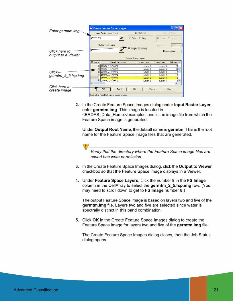
2. In the Create Feature Space Images dialog under Input Raster Layer, enter germtm.img. This image is located in <ERDAS_Data_Home>/examples, and is the image file from which the Feature Space image is generated.

Under Output Root Name, the default name is germtm. This is the root name for the Feature Space image files that are generated.

Verify that the directory where the Feature Space image files are saved has write permission.

3. In the Create Feature Space Images dialog, click the Output to Viewer checkbox so that the Feature Space image displays in a Viewer.

4. Under Feature Space Layers, click the number 8 in the FS Image column in the CellArray to select the germtm_2_5.fsp.img row. (You may need to scroll down to get to FS Image number 8.)

The output Feature Space image is based on layers two and five of the germtm.img file. Layers two and five are selected since water is spectrally distinct in this band combination.

5. Click OK in the Create Feature Space Images dialog to create the Feature Space image for layers two and five of the germtm.img file.

The Create Feature Space Images dialog closes, then the Job Status dialog opens.

Enter germtm.img

Click

Click here to

Click here to

output to a Viewer

create image

germtm_2_5.fsp.img


After the process is complete, a Viewer (Viewer #2) opens, displaying the Feature Space image.

6. Click OK in the Job Status dialog to close this dialog.

Link Cursors in Image/Feature Space

The Linked Cursors utility allows you to directly link a cursor in the image Viewer to the Feature Space viewer. This shows you where pixels in the image file are located in the Feature Space image.

1. In the Signature Editor dialog, select Feature -> View -> Linked Cursors.

The Linked Cursors dialog opens.

Click here

this dialog to close


2. Click Select in the Linked Cursors dialog to define the Feature Space viewer that you want to link to the Image Viewer.

3. Click in Viewer #2 (the Viewer displaying the Feature Space image).

The Viewer number field in the Linked Cursors dialog changes to 2. You could also enter a 2 in this number field without having to click the Select button.

4. In the Linked Cursors dialog, click Link to link the Viewers, then click in the Viewer displaying germtm.img.

The linked inquire cursors (white crosshairs) open in the Viewers.

5. Drag the inquire cursor around in the germtm.img Viewer (Viewer #1) to see where these pixels are located in the Feature Space image. Notice where the water areas are located in the Feature Space image. These areas are black in the germtm.img file (Viewer #1).

You may need to use the Zoom In By 2 and Zoom Out By 2 options (accessed with a right-click in the Viewer containing the file germtm.img) to locate areas of water.

Define Feature Space Signature

Any Feature Space AOI can be defined as a nonparametric signature in your classification.

1. Right-click inside the Viewer containing the Feature Space image and select Zoom -> Zoom In By 2 until you can see the area beneath the inquire cursor clearly.

2. Use the polygon AOI tool to draw a polygon in the Feature Space image. Draw the polygon in the area that you identified as water.

The Feature Space signature is based on this polygon.

Click to select the Feature Spaceviewer

This is

Click to linkthe Viewers

Click to unlink Viewers

Click to closethis dialog

set to 2




4. The signature you have just added is a nonparametric signature. Select Feature -> Statistics from the Signature Editor menu bar to generate statistics for the Feature Space AOI.

A Job Status dialog displays, stating the progress of the function.

5. When the function is 100% complete, click OK in the Job Status dialog.

The Feature Space AOI now has parametric properties.

6. In the Signature Editor, click inside the Signature Name column for the signature you just added. Change the name to Water, then press the Enter key on the keyboard.

7. In the Signature Editor, hold in the Color column next to Water and select Blue.

8. In the Linked Cursors dialog, click Unlink to unlink the viewers.

The inquire cursors are removed from the viewers.

9. In the Linked Cursors dialog, click Close.

Draw a polygon in the area

as water identified


10. Now that you have the nonparametric signature collected, you do not need the AOI in the Feature Space viewer. Select View -> Arrange Layers from the Viewer #2 menu bar.


11. In the Arrange Layers dialog, right-hold over the AOI Layer button and select Delete Layer from the AOI Options dropdown list.

12. Click Apply in the Arrange Layers dialog to delete the AOI layer.



15. Practice taking additional signatures using any of the signature-generating techniques you have learned in the steps above. Extract at least five signatures.

16. After you have extracted all the signatures you wish, select File -> Save As from the Signature Editor menu bar.

The Save Signature File As dialog opens.

17. Use the Save Signature File As dialog to save the signature set in the Signature Editor (for example, germtm_siged.sig).

18. Click OK in the Save Signature File As dialog.

Use Tools to Evaluate Signatures

Once signatures are created, they can be evaluated, deleted, renamed, and merged with signatures from other files. Merging signatures allows you to perform complex classifications with signatures that are derived from more than one training method (supervised and/or unsupervised, parametric and nonparametric).

Next, the following tools for evaluating signatures are discussed:

• alarms

• contingency matrix

• feature space to image masking

• signature objects

• histograms

• signature separability

• statistics


When you use one of these tools, you need to select the appropriate signature(s) to be used in the evaluation. For example, you cannot use the signature separability tool with a nonparametric (Feature Space) signature.

Preparation

You should have at least ten signatures in the Signature Editor, similar to the following:

Set Alarms

The Signature Alarm utility highlights the pixels in the Viewer that belong to, or are estimated to belong to a class according to the parallelepiped decision rule. An alarm can be performed with one or more signatures. If you do not have any signatures selected, then the active signature, which is next to the >, is used.

1. In the Signature Editor, select Forest_1 by clicking in the > column for that signature. The alarm is performed with this signature.

2. In the Signature Editor menu bar, select View -> Image Alarm.

The Signature Alarm dialog opens.

3. Click Edit Parallelepiped Limits in the Signature Alarm dialog to view the limits for the parallelepiped.

Click to change theparallelepiped limits


The Limits dialog opens.

4. In the Limits dialog, click Set to define the parallelepiped limits.

The Set Parallelepiped Limits dialog opens.

The Signature Alarm utility allows you to define the parallelepiped limits by either:

• the minimum and maximum for each layer in the signature, or

• a specified number of standard deviations from the mean of the signature.

5. If you wish, you can set new parallelepiped limits and click OK in the Set Parallelepiped Limits dialog, or simply accept the default limits by clicking OK in the Set Parallelepiped Limits dialog.

The new/default limits display in the Limits CellArray.

6. Click Close in the Limits dialog.

7. In the Signature Alarm dialog, click OK.

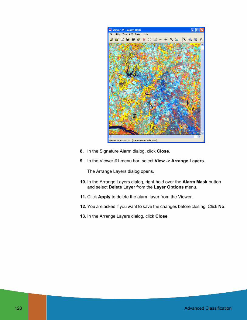
The alarmed pixels display in the Viewer in yellow. You can use the toggle function (Utility -> Flicker) in the Viewer to see how the pixels are classified by the alarm.

Be sure that there are no AOI layers open on top of the Alarm Mask Layer. You can use View -> Arrange Layers to remove any AOI layers present in the Viewer.


8. In the Signature Alarm dialog, click Close.

9. In the Viewer #1 menu bar, select View -> Arrange Layers.


10. In the Arrange Layers dialog, right-hold over the Alarm Mask button and select Delete Layer from the Layer Options menu.

11. Click Apply to delete the alarm layer from the Viewer.




Evaluate Contingency

1. In the Signature Editor, select all of the signatures by Shift-clicking in the first row of the Class column and then dragging down through the other classes.

2. In the Signature Editor menu bar, select Evaluate -> Contingency.

The Contingency Matrix dialog opens.

Contingency Matrix

The Contingency Matrix utility allows you to evaluate signatures that have been created from AOIs in the image. This utility classifies only the pixels in the image AOI training sample, based on the signatures. It is usually expected that the pixels of an AOI are classified to the class that they train. However, the pixels of the AOI training sample only weight the statistics of the signature. They are rarely so homogenous that every pixel actually becomes assigned to the expected class. The Contingency Matrix utility can be performed with multiple signatures. If you do not have any signatures selected, then all of the signatures are used.

The output of the Contingency Matrix utility is a matrix of percentages that allows you to see how many pixels in each AOI training sample were assigned to each class. In theory, each AOI training sample would be composed primarily of pixels that belong to its corresponding signature class.

The AOI training samples are classified using one of the following classification algorithms:

• parallelepiped

• feature space

• maximum likelihood

• Mahalanobis distance


3. In the Contingency Matrix dialog, click the Non-parametric Rule dropdown list and select Feature Space.

See the chapter "Classification" in the ERDAS Field Guide for more information on decision rules.

4. Click OK in the Contingency Matrix dialog to start the process.

A Job Status dialog displays, stating the progress of the function.

5. When the process is 100% complete, click OK in the Job Status dialog.

The IMAGINE Text Editor opens (labelled Editor:, Dir), displaying the error matrix.

Click to selectFeature Space

Click to start the process


6. After viewing the reference data in the Text Editor, select File -> Close from the menu bar.

7. Deselect the signatures that were selected by right-clicking in the Class column and choosing Select None from the Row Selection menu.

Generate a Mask from a Feature Space Signature

The Feature Space to Image Masking utility allows you to generate a mask from a Feature Space signature (that is, the AOI in the Feature Space image). Once the Feature Space signature is defined as a mask, the pixels under the mask are identified in the image file and highlighted in the Viewer. This allows you to view which pixels would be assigned to the Feature Space signature’s class. A mask can be generated from one or more Feature Space signatures. If you do not have any signatures selected, then the active signature, which is next to the >, is used.

The image displayed in Viewer #1 must be the image from which the Feature Space image was created.


1. In the Signature Editor, select Feature -> Masking -> Feature Space to Image.

The FS to Image Masking dialog opens.

2. In the Signature Editor, click in the > row for Water to select that signature.

The mask is generated from this Feature Space signature.

3. Disable the Indicate Overlap checkbox, and click Apply in the FS to Image Masking dialog to generate the mask in Viewer #1.

A mask is placed in the Viewer.

4. In the FS to Image Masking dialog, click Close.

5. Deselect the Water feature.

This checkbox should be turned off (disabled)

Click to create the mask


View Signature Objects

The Signature Objects dialog allows you to view graphs of signature statistics so that you can compare signatures. The graphs display as sets of ellipses in a Feature Space image. Each ellipse is based on the mean and standard deviation of one signature. A graph can be generated for one or more signatures. If you do not have any signatures selected, then the active signature, which is next to the >, is used. This utility also allows you to show the mean for the signature for the two bands, a parallelepiped, and a label.

1. In the Signature Editor menu bar, select Feature -> Objects.

The Signature Objects dialog opens.

2. In the Signature Editor, select the signatures for Agricultural Field_1 and Forest_1 by clicking in the Class row for Agricultural Field_1 and Shift-clicking in the Class row for Forest_1.

3. In the Signature Objects dialog, confirm that the Viewer number field is set for 2.

4. Set the Std. Dev. number field to 4.

5. Enable the Label checkbox by clicking on it.

6. Click OK in the Signature Objects dialog.

The ellipses for the Agricultural Field_1 and Forest_1 signatures display in the Feature Space viewer.

Enter 2 here

Enter 4 here

Click here to start the process


7. In the Signature Objects dialog, click Close.

Compare Ellipses

By comparing the ellipses for different signatures for a one band pair, you can easily see if the signatures represent similar groups of pixels by seeing where the ellipses overlap on the Feature Space image.

• When ellipses do not overlap, the signatures represent a distinct set of pixels in the two bands being plotted, which is desirable for classification. However, some overlap is expected, because it is rare that all classes are totally distinct.

When the ellipses do overlap, then the signatures represent similar pixels, which is not desirable for classification.


8. Deselect the signatures for Agricultural Field_1 and Forest_1.

Plot Histograms

The Histogram Plot Control Panel allows you to analyze the histograms for the layers to make your own evaluations and comparisons. A histogram can be created with one or more signatures. If you create a histogram for a single signature, then the active signature, which is next to the >, is used. If you create a histogram for multiple signatures, then the selected signatures are used.

1. In the Signature Editor, move the > prompt to the signature for Agricultural Field_1 by clicking under the > column.

2. In the Signature Editor menu bar, select View -> Histograms or click

the Histogram icon .

The Histogram Plot Control Panel and the Histogram dialogs open.

3. In the Histogram Plot Control Panel dialog, change the Band No number field to 5 in order to view the histogram for band 5 (that is, layer 5).

4. Click Plot.

The Histogram dialog changes to display the histogram for band 5. You can change the different plot options and select different signatures to see the differences in histograms for various signatures and bands.

Enter 5 here

Click here to create histogram plot


5. In the Histogram Plot Control Panel dialog, click Close. The two Histogram dialogs close.

Compute Signature Separability

The Signature Separability utility computes the statistical distance between signatures. This distance can be used to determine how distinct your signatures are from one another. This utility can also be used to determine the best subset of layers to use in the classification.

The distances are based on the following formulas:

• euclidean spectral distances between their means

• Jeffries-Matusita distance

• divergence

• transformed divergence

The Signature Separability utility can be performed with multiple signatures. If you do not have any signatures selected, then all of the parametric signatures are used.

1. In the Signature Editor, select all of the parametric signatures.

2. In the Signature Editor menu bar, select Evaluate -> Separability.

The Signature Separability dialog opens.

Set this number

Click here

Click here to start process

field to 3


3. In the Signature Separability dialog, set the Layers Per Combination number field to 3, so that three layers are used for each combination.

4. Click Transformed Divergence under Distance Measure to use the divergence algorithm for calculating the separability.

5. Confirm that the Summary Report radio button is turned on under Report Type, in order to output a summary of the report.

The summary lists the separability listings for only those band combinations with best average and best minimum separability.

6. In the Signature Separability dialog, click OK to begin the process.

When the process is complete, the IMAGINE Text Editor opens, displaying the report.

This report shows that layers (that is, bands) 2, 4, and 5 are the best layers to use for identifying features.

7. In the Text Editor menu bar, select File -> Close to close the Editor.


8. In the Signature Separability dialog, click Close.

Check Statistics

The Statistics utility allows you to analyze the statistics for the layers to make your own evaluations and comparisons. Statistics can be generated for one signature at a time. The active signature, which is next to the >, is used.

1. In the Signature Editor, move the > prompt to the signature for Forest_1.

2. In the Signature Editor menu bar, select View -> Statistics or click the

Statistics icon .

The Statistics dialog opens.

3. After viewing the information in the Statistics dialog, click Close.

Perform Supervised Classification

The decision rules for the supervised classification process are multilevel:

• nonparametric

• parametric

In this example, use both nonparametric and parametric decision rules.

See the chapter "Classification" in the ERDAS Field Guide for more information on decision rules.


1. In the Signature Editor, select all of the signatures so that they are all used in the classification process (if none of the signatures are selected, then they are all used by default).

Nonparametric

If the signature is nonparametric (that is, Feature Space AOI), then the following decision rules are offered:

• feature space

• parallelepiped

With nonparametric signatures you must also decide the overlap rule and the unclassified rule.

NOTE: All signatures have a nonparametric definition, due to their parallelepiped boundaries.

Parametric

For parametric signatures, the following decision rules are provided:

• maximum likelihood

• Mahalanobis distance

• minimum distance

In this tour guide, use the maximum likelihood decision rule.

Output File

The Supervised Classification utility outputs a thematic raster layer (.img extension) and/or a distance file (.img extension). The distance file can be used for post-classification thresholding. The thematic raster layer automatically contains the following data:

• class values

• class names

• color table

• statistics


2. In the Signature Editor menu bar, select Classify -> Supervised to perform a supervised classification.

NOTE: You may also access the Supervised Classification utility from the Classification dialog.

The Supervised Classification dialog opens.

3. In the Supervised Classification dialog, under Output File, type in germtm_superclass.img.

This is the name for the thematic raster layer.

4. Click the Output Distance File checkbox to activate it.

In this example, you are creating a distance file that can be used to threshold the classified image file.

5. Under Filename, enter germtm_distance.img in the directory of your choice.

This is the name for the distance image file.

NOTE: Make sure you remember the directory in which the output file is saved. It is important when you are trying to display the output file in a Viewer.

Select Attribute Options

1. In the Output File section of the Supervised Classification dialog, click Attribute Options.

Click to select

Click to start the process

Click to define attributes for signatures

Enter Click to create

Enter Maximum Likelihood

here

Click to select Feature Space

germtm_distance.img here

germtm_superclass.img a distance file


The Attribute Options dialog opens.

The Attribute Options dialog allows you to specify the statistical information for the signatures that you want to be in the output classified layer. The statistics are based on the data file values for each layer for the signatures, not the entire classified image file. This information is located in the Raster Attribute Editor.

2. In the Attribute Options dialog, click Minimum, Maximum, Mean, and Std. Dev., so that the signatures in the output thematic raster layer have this statistical information.

3. Confirm that the Layer checkbox is turned on, so that the information is presented in the Raster Attribute Editor by layer.

4. In the Attribute Options dialog, click Close to remove this dialog.

Classify the Image

1. In the Supervised Classification dialog, click the Non-parametric Rule dropdown list to select Feature Space.

You do not need to use the Classify Zeros option here because there are no background zero data file values in the germtm.img file.

2. Click OK in the Supervised Classification dialog to classify the germtm.img file using the signatures in the Signature Editor.

A Job Status dialog displays, indicating the progress of the function.

3. When the process is 100% complete, click OK in the Job Status dialog.

Click here

Click here to close this dialog


See the chapter “Classification” in the ERDAS Field Guide for information about how the pixels are classified.

4. Select File -> Close from the Signature Editor menu bar. Click Yes when asked if you would like to save the changes to the Signature Editor.

5. Select File -> Close to dismiss Viewer #2.

6. You do not need to save changes to the AOI in the Signature Editor, so click No on that message dialog.

7. Click Close in the AOI tool palette.

8. Select File -> Clear from the Viewer #1 menu bar.

9. Proceed to:

• “Perform Unsupervised Classification” to classify the same image using the ISODATA algorithm.

• “Evaluate Classification” to analyze the classes and test the accuracy of the classification, or

The super classification image is pictured on the left, and the distance image is pictured on the right.


Perform Unsupervised Classification

This section shows you how to create a thematic raster layer by letting the software identify statistical patterns in the data without using any ground truth data.

ERDAS IMAGINE uses the ISODATA algorithm to perform an unsupervised classification. The ISODATA clustering method uses the minimum spectral distance formula to form clusters. It begins with either arbitrary cluster means or means of an existing signature set, and each time the clustering repeats, the means of these clusters are shifted. The new cluster means are used for the next iteration.

The ISODATA utility repeats the clustering of the image until either a maximum number of iterations has been performed, or a maximum percentage of unchanged pixel assignments has been reached between two iterations.

Performing an unsupervised classification is simpler than a supervised classification, because the signatures are automatically generated by the ISODATA algorithm.

In this example, you generate a thematic raster layer using the ISODATA algorithm.


Preparation You must have ERDAS IMAGINE running.

1. Click the Classifier icon in the ERDAS IMAGINE icon panel to start the Classification utility.

The Classification menu opens.

Generate Thematic Raster Layer

1. Select Unsupervised Classification from the Classification menu to perform an unsupervised classification using the ISODATA algorithm.

The Unsupervised Classification dialog opens.

Click here to start the Unsupervised Classification utility


2. Click Close in the Classification menu to clear it from the screen.

3. In the Unsupervised Classification dialog under Input Raster File, enter germtm.img. This is the image file that you are going to classify.

4. Under Output Cluster Layer, enter germtm_isodata.img in the directory of your choice.

This is the name for the output thematic raster layer.

5. Click Output Signature Set to turn off the checkbox.

For this example, do not create a signature set. The Output Signature Set file name part is disabled.

Set Initial Cluster Options

The Clustering Options allow you to define how the initial clusters are generated.

1. Confirm that the Initialize from Statistics radio button under Clustering Options is turned on.

This generates arbitrary clusters from the file statistics for the image file.

2. Enter a 10 in the Number of Classes number field.

Enter germtm.img here Click here to turn off

Enter germtm_isodata.img

Enter 10 here to generate 10 classes (that is, signatures)

Enter 24 for the maximum

process can run

This should be

Click here to

the Output Signature Set

here

file name part

set to .950

start the process

number of times the


Set Processing Options

The Processing Options allow you to specify how the process is performed.

1. Enter 24 in the Maximum Iterations number field under Processing Options.

This is the maximum number of times that the ISODATA utility reclusters the data. It prevents this utility from running too long, or from potentially getting stuck in a cycle without reaching the convergence threshold.

2. Confirm that the Convergence Threshold number field is set to .95.

3. Click OK in the Unsupervised Classification dialog to start the classification process. The Unsupervised Classification dialog closes automatically.

A Job Status dialog displays, indicating the progress of the function.

4. Click OK in the Job Status dialog when the process is 100% complete.

5. Proceed to the Evaluate Classification section to analyze the classes so that you can identify and assign class names and colors.

Evaluate Classification

After a classification is performed, the following methods are available for evaluating and testing the accuracy of the classification:

• classification overlay

• thresholding

• recode classes

• accuracy assessment

Convergence Threshold

The convergence threshold is the maximum percentage of pixels that has cluster assignments that can go unchanged between iterations. This threshold prevents the ISODATA utility from running indefinitely.

By specifying a convergence threshold of .95, you are specifying that as soon as 95% or more of the pixels stay in the same cluster between one iteration and the next, the utility should stop processing. In other words, as soon as 5% or fewer of the pixels change clusters


See the chapter "Classification" in the ERDAS Field Guide for information on accuracy assessment.

Create Classification Overlay

In this example, use the Raster Attribute Editor to compare the original image data with the individual classes of the thematic raster layer that was created from the unsupervised classification (germtm_isodata.img). This process helps identify the classes in the thematic raster layer. You may also use this process to evaluate the classes of a thematic layer that was generated from a supervised classification.

Preparation ERDAS IMAGINE should be running and you should have a Viewer open.

1. Select File -> Open -> Raster Layer from the Viewer menu bar, or click

the Open icon in the toolbar to display the germtm.img continuous raster layer.

The Select Layer To Add dialog opens.

2. In the Select Layer To Add dialog under File name, select germtm.img.

3. Click the Raster Options tab at the top of the Select Layer To Add dialog.

4. Set Layers to Colors at 4, 5, and 3.

5. Click OK in the Select Layer To Add dialog to display the image file.

6. Click the Open icon again in the Viewer toolbar to display the thematic raster layer, germtm_isodata.img, over the germtm.img file.

Click this file tabto see the rasteroptions

Click here to selectgermtm.img


7. Under File name, open the directory in which you previously saved germtm_isodata.img by entering the directory path name in the text entry field and pressing the Enter key on your keyboard.

8. Click the Raster Options tab at the top of the Select Layer To Add dialog.

9. Click Clear Display to turn off this checkbox.

10. Click OK in the Select Layer To Add dialog to display the image file.

Open Raster Attribute Editor

1. Select Raster -> Attributes from the Viewer menu bar.

The Raster Attribute Editor displays.

2. In the Raster Attribute Editor, select Edit -> Column Properties to rearrange the columns in the CellArray so that they are easier to view.

The Column Properties dialog opens.


3. In the Column Properties dialog under Columns, select Opacity, then click Up to move Opacity so that it is under Histogram.

4. Select Class_Names, then click Up to move Class_Names so that it is under Color.

5. Click OK in the Column Properties dialog to rearrange the columns in the Raster Attribute Editor.

The Column Properties dialog closes.

The data in the Raster Attribute Editor CellArray should appear similar to the following example:

Analyze Individual Classes

Before you can begin to analyze the classes individually, you need to set the opacity for all of the classes to zero.

Click here tomove the selected column up

Click here to rearrangethe columns

Click here to movethis column


1. In the Raster Attribute Editor, click the word Opacity at the top of the Opacity column to select all of the classes. The column turns cyan in color.

2. Right-hold on the word Opacity and select Formula from the Column Options menu.

The Formula dialog opens.

3. In the Formula dialog, click 0 in the number pad.

A 0 is placed in the Formula field.

4. In the Formula dialog, click Apply to change all of the values in the Opacity column to 0, and then click Close.

5. Right-click in the Opacity column heading and choose Select None from the Column Options menu.

6. In the Raster Attribute Editor, hold on the color patch under Color for Class 1 in the CellArray and change the color to Yellow. This provides better visibility in the Viewer.

Click here to

Click here to

Click here to close this dialog

the Formula enter a 0 in

to the Opacity apply a 0 value

column


7. Change the Opacity for Class 1 in the CellArray to 1 and then press Enter on the keyboard. This class shows in the Viewer.

NOTE: If you cannot see any yellow areas within the Viewer extent, you can right-click and select Zoom -> Zoom Out By 2 from the Quick View menu until yellow areas display within the Viewer.

8. In the Viewer menu bar, select Utility -> Flicker to analyze which pixels have been assigned to this class.

The Viewer Flicker dialog opens.

9. Turn on the Auto Mode in the Viewer Flicker dialog.

The flashing yellow pixels in the germtm.img file are the pixels Class 1. These areas are water.


10. In the Raster Attribute Editor, click inside the Class_Names column for Class 1. Change this name to Water and then press the Enter key on the keyboard.

11. In the Raster Attribute Editor, hold on the Color patch for Water. Select Blue from the dropdown list.

12. After you are finished analyzing this class, click Cancel in the Viewer Flicker dialog and set the Opacity for Water back to 0. Press the Enter key on the keyboard.

13. Change the Color for Class 2 in the CellArray to Yellow for better visibility in the Viewer.

14. Change the Opacity for Class 2 to 1 and press the Enter key on the keyboard. This class shows in the Viewer.

Use the Flicker Utility

1. In the Viewer menu bar, select Utility -> Flicker to analyze which pixels were assigned to this class.


2. Turn on the Auto Mode in the Viewer Flicker dialog.


The flashing pixels in the germtm.img file should be the pixels of Class 2. These are forest areas.

3. In the Raster Attribute Editor, click inside the Class_Names column for Class 2. (You may need to double-click in the column.) Change this name to Forest, then press the Enter key on the keyboard.

4. In the Raster Attribute Editor, hold on the Color patch for Forest and select Pink from the dropdown list.

5. After you are finished analyzing this class, click Cancel in the Viewer Flicker dialog and set the Opacity for Forest back to 0. Press the Enter key on the keyboard.

6. Repeat these steps with each class so that you can see how the pixels are assigned to each class. You may also try selecting more than one class at a time.

7. Continue assigning names and colors for the remaining classes in the Raster Attribute Editor CellArray.

8. In the Raster Attribute Editor, select File -> Save to save the data in the CellArray.

9. Select File -> Close from the Raster Attribute Editor menu bar.

10. Select File -> Clear from the Viewer menu bar.

Use Thresholding The Thresholding utility allows you to refine a classification that was performed using the Supervised Classification utility. The Thresholding utility determines which pixels in the new thematic raster layer are most likely to be incorrectly classified.

This utility allows you to set a distance threshold for each class in order to screen out the pixels that most likely do not belong to that class. For all pixels that have distance file values greater than a threshold you set, the class value in the thematic raster layer is set to another value.

The threshold can be set:

• with numeric input, using chi-square statistics, confidence level, or Euclidean spectral distance, or

• interactively, by viewing the histogram of one class in the distance file while using the mouse to specify the threshold on the histogram graph.

Since the chi-square table is built-in, you can enter the threshold value in the confidence level unit and the chi-square value is automatically computed.


In this example, you threshold the output thematic raster layer from the supervised classification (germtm_superclass.img).

Preparation

ERDAS IMAGINE must be running and you must have germtm_superclass.img displayed in a Viewer.

1. Click the Classifier icon in the ERDAS IMAGINE icon panel to start the Classification utility.


2. Select Threshold from the Classification menu to start the Threshold dialog.

The Threshold dialog opens.


4. In the Threshold dialog, select File -> Open or click the Open icon to define the classified image and distance image files.

The Open Files dialog opens.

Select Classified and Distance Images

1. In the Open Files dialog under Classified Image, open the directory in which you previously saved germtm_superclass.img by entering the directory path name in the text window and pressing Enter on your keyboard.

Click here to load files

Type in the correct

then press Enter herepath name and


2. Select the file germtm_superclass.img from the list of files in the directory you just opened.

This is the classified image file that is going to be thresholded.

3. In the Open Files dialog, under Distance Image, open the directory in which you previously saved germtm_distance.img by entering the directory path name in the text entry field and pressing Enter on your keyboard.

4. Select the file germtm_distance.img from the list of files in the directory you just opened.

This is the distance image that was created when the germtm_superclass.img file was created. A distance image file for the classified image is necessary for thresholding.

5. Click OK in the Open Files dialog to load the files.

6. In the Threshold dialog, select View -> Select Viewer and then click in the Viewer that is displaying the germtm_superclass.img file.

Compute and Evaluate Histograms

1. In the Threshold dialog, select Histograms -> Compute.

The histograms for the distance image file are computed. There is a separate histogram for each class in the classified image file.

The Job Status dialog opens as the histograms are computed. This dialog automatically closes when the process is completed.


2. If desired, select Histograms -> Save to save this histogram file.

3. In the CellArray of the Threshold dialog, move the > prompt to the Agricultural Field_2 class by clicking under the > column in the cell for Class 2.

4. Select Histograms -> View.

The Distance Histogram for Agricultural Field_2 displays.

5. Select the arrow on the X axis of the histogram graph to move it to the position where you want to threshold the histogram.

The Chi-Square value in the Threshold dialog is updated for the current class (Agricultural Field_2) as you move the arrow.

6. In the Threshold dialog CellArray, move the > prompt to the next class.

The histogram updates for this class.

7. Repeat the steps, thresholding the histogram for each class in the Threshold dialog CellArray.

See the chapter "Classification" in the ERDAS Field Guide for information on thresholding.

8. After you have thresholded the histogram for each class, click Close in the Distance Histogram dialog.

Apply Colors

1. In the Threshold dialog, select View -> View Colors -> Default Colors.

Click here to

Hold arrow under histogram and drag it to here

close dialog


Use the default setting so that the thresholded pixels appear black and those pixels remaining appear in their classified color in the thresholded image.

2. In the Threshold dialog, select Process -> To Viewer.

The thresholded image is placed in the Viewer over the germtm_superclass.img file. Yours likely looks different from the one pictured here.

Use the Flicker Utility

1. In the Viewer menu bar, select Utility -> Flicker to see how the classes were thresholded.


2. When you are finished observing the thresholding, click Cancel in the Viewer Flicker dialog.


3. In the Viewer, select View -> Arrange Layers.


4. In the Arrange Layers dialog, right-hold over the thresholded layer (Threshold Mask) and select Delete Layer from the Layer Options menu.

5. Click Apply and then Close in the Arrange Layers dialog. When asked if you would like to save your changes, click No.

6. In the Threshold dialog, select Process -> To File.

The Threshold to File dialog opens.

Process Threshold

1. In the Threshold to File dialog under Output Image, enter the name germtm_thresh.img in the directory of your choice.

This is the file name for the thresholded image.

2. Click OK to output the thresholded image to a file.

The Threshold to File dialog closes.

3. Wait for the thresholding process to complete, and then select File -> Close from the Threshold dialog menu bar.

4. Select File -> Clear from the Viewer menu bar.

NOTE: The output file that is generated by thresholding a classified image can be further analyzed and modified in various ERDAS IMAGINE utilities, including the Image Interpreter, Raster Attribute Editor, and Spatial Modeler.


Use Accuracy Assessment

The Accuracy Assessment utility allows you to compare certain pixels in your thematic raster layer to reference pixels, for which the class is known. This is an organized way of comparing your classification with ground truth data, previously tested maps, aerial photos, or other data.

In this example, you perform an accuracy assessment using the output thematic raster layer from the supervised classification (germtm_superclass.img).

Preparation

ERDAS IMAGINE must be running and you must have germtm.img displayed in a Viewer.

1. Click the Classifier icon in the ERDAS IMAGINE icon panel.


Recode Classes

After you analyze the pixels, you may want to recode the thematic raster layer to assign a new class value number to any or all classes, creating a new thematic raster layer using the new class numbers. You can also combine classes by recoding more than one class to the same new class number. Use the Recode function under Interpreter (icon) -> GIS Analysis to recode a thematic raster layer.

NOTE: See the chapter "Geographic Information Systems" in the ERDAS Field Guide for more information on recoding.


2. Select Accuracy Assessment from the Classification menu to start the Accuracy Assessment utility.

The Accuracy Assessment dialog opens.

Check the Accuracy Assessment CellArray

The Accuracy Assessment CellArray contains a list of class values for the pixels in the classified image file and the class values for the corresponding reference pixels. The class values for the reference pixels are input by you. The CellArray data reside in the classified image file (for example, germtm_superclass.img).


2. In the Accuracy Assessment dialog, select File -> Open or click the

Open icon .

Click here to start theAccuracy AssessmentUtility


The Classified Image dialog opens.

3. In the Classified Image dialog, under File name, open the directory in which you previously saved germtm_superclass.img by entering the directory path name in the text entry field and pressing Enter on your keyboard.

4. Select the file germtm_superclass.img from the list of files in the directory you just opened.

This is the classified image file that is used in the accuracy assessment.

5. Click OK in the Classified Image dialog to load the file.

6. In the Accuracy Assessment dialog, select View -> Select Viewer or

click the Select Viewer icon , then click in the Viewer that is displaying the germtm.img file.

7. In the Accuracy Assessment dialog, select View -> Change Colors.

The Change colors dialog opens.

In the Change colors dialog, the Points with no reference color patch should be set to White. These are the random points that have not been assigned a reference class value.

Enter the correctpath name here

Select

from this list the file

Click here

This color should

This color should be set to yellow

be set to white


The Points with reference color patch should be set to Yellow. These are the random points that have been assigned a reference class value.

8. Click OK in the Change colors dialog to accept the default colors.

Generate Random Points

The Add Random Points utility generates random points throughout your classified image. After the points are generated, you must enter the class values for these points, which are the reference points. These reference values are compared to the class values of the classified image.

1. In the Accuracy Assessment dialog, select Edit -> Create/Add Random Points.

The Add Random Points dialog opens.

2. In the Add Random Points dialog, enter a 10 in the Number of Points number field and press Enter on your keyboard.

In this example, you generate ten random points. However, to perform a proper accuracy assessment, you should generate 250 or more random points.

3. Confirm that the Search Count is set to 1024.

Click here to start

The Distribution Parameters

Enter 10 here

the process

should be Random


This means that a maximum of 1024 points are analyzed to see if they meet the defined requirements in the Add Random Points dialog. If you are generating a large number of points and they are not collected before 1024 pixels are analyzed, then you have the option to continue searching for more random points.

NOTE: If you are having problems generating a large number of points, you should increase the Search Count to a larger number.

The Distribution Parameters should be set to Random.

4. Click OK to generate the random points.

The Add Random Points dialog closes and the Job Status dialog opens.

This dialog automatically closes when the process is completed. A list of the points is shown in the Accuracy Assessment CellArray.

5. In the Accuracy Assessment dialog, select View -> Show All.

All of the random points display in the germtm.img file in the Viewer. These points are white.


6. Analyze and evaluate the location of the reference points in the Viewer to determine their class value. In the Accuracy Assessment CellArray Reference column, enter your best guess of a reference relating to the perceived class value for the pixel below each reference point.

As you enter a value for a reference point, the color of the point in the Viewer changes to yellow.

If you were performing a proper accuracy assessment, you would be using ground truth data, previously tested maps, aerial photos, or other data.

7. In the Accuracy Assessment dialog, select Edit -> Show Class Values.

The class values for the reference points appear in the Class column of the CellArray.

8. In the Accuracy Assessment dialog, select Report -> Options. The Error Matrix, Accuracy Totals, and Kappa Statistics checkboxes should be turned on.

The accuracy assessment report includes all of this information.


See the chapter "Classification" in the ERDAS Field Guide for information on the error matrix, accuracy totals, and Kappa statistics.

9. In the Accuracy Assessment dialog, select Report -> Accuracy Report.

The accuracy assessment report displays in the IMAGINE Text Editor.

10. In the Accuracy Assessment dialog, select Report -> Cell Report.

The accuracy assessment report displays in a second ERDAS IMAGINE Text Editor. The report lists the options and windows used in selecting the random points.

11. If you like, you can save the cell report and accuracy assessment reports to text files.

12. Select File -> Close from the menu bars of both ERDAS IMAGINE Text Editors.

13. In the Accuracy Assessment dialog, select File -> Save Table to save the data in the CellArray.

The data are saved in the classified image file (germtm_superclass.img).

14. Select File -> Close from the Accuracy Assessment dialog menu bar.

15. If you are satisfied with the accuracy of the classification, select File -> Close from the Viewer menu bar.

If you are not satisfied with the accuracy of the classification, you can further analyze the signatures and classes using methods discussed in this tour guide. You can also use the thematic raster layer in various ERDAS IMAGINE utilities, including the Image Interpreter, Raster Editor, and Spatial Modeler to modify the file.

Using the Grouping Tool

This section shows you how to use the Class Grouping Tool to assign the classes associated with an Unsupervised Classification and group them into their appropriate target classes. This tour is intended to demonstrate several methods for collecting classes, not to provide a comprehensive guide to grouping an entire Landsat image.


Setting Up a Class Grouping Project

In this example, you take a Landsat image that has been classified into 235 classes using the ISODATA and the Maximum Likelihood classifications. These 235 classes are grouped into a more manageable number of Land Use categories.

Preparation

1. Start ERDAS IMAGINE.

2. Copy the file loudoun_maxclass.img from the <ERDAS_Data_Home>/examples directory into a directory in which you have write permission.

Starting the Class Grouping Tool

1. Click the Classifier icon on the ERDAS IMAGINE icon panel.


2. Select Grouping Tool from the Classification menu to start the Signature Editor.

The Select image to group dialog opens.

3. Navigate to the directory into which you copied the file loudoun_maxclass.img. Select it from the list of files and click OK.

The Class Grouping Tool and a Viewer displaying the selected image file open.

Click here to

Grouping Toolstart the


4. To view the entire image, right-click in the Viewer and select Fit Image to Window from the Quick View menu.

Class Grouping Tool Terminology

Classes are individual clusters of pixels with similar spectral characteristics. These clusters are the result of the unsupervised classification.

Target Classes are the final landuse or landcover categories for which you are interpreting.

Class Groups are the saved groups of classes that represent a single target class.

Working GroupCellArray

Class GroupsCellArray

Target ClassesCellArray

Menu Bar

Toolbars

Click Here to Set upthe Target Classes


Set Up the Target Classes

1. Click the Setup Target Classes button above the Target Classes CellArray. The Edit Target Classes dialog opens.

2. Place the cursor in the Target Class Name field and type Water. Click the Add -> button.

Water now appears in the list of Target Classes.

3. Add Agriculture, Forest, and Urban classes.

4. Once you have finished adding Target Classes, click the OK button on the Edit Target Classes dialog.

You may return to this dialog and add more Target Classes at any point during the grouping process.

The Target Classes you have added display in the Target Classes CellArray.

Now that the Target Classes are set up, you can assign target colors.

5. Click in the color block next to the Water Target Class. Select Blue from the Color dropdown list. Continue assigning colors to the Target Classes until colors have been assigned to each of them.

Type the targetclass name here

Click Add->

Displays the number of Class Groups

Target ClassNames

Click here to change the Target Color

in the Target Class


Collecting Class Groups The main goal of a Class Grouping project is to gather classes of pixels which have common traits into the same Target Classes. To do this, you must select the classes and save them to Class Groups. Class Groups are, as the name suggests, groups of classes that share similar traits; usually these are classes that are in the same landuse category. The Class Groups are themselves members of the Target Classes into which the image is being stratified.

There are numerous ways to collect Class Groups. This tour guide demonstrates how to use the Cursor Point Mode, the AOI Tool, and the Ancillary Data Tool to collect Class Groups.

Using the Cursor Point Mode

1. In the Viewer, right-click and select Inquire Cursor from the Quick View menu. The Inquire Cursor dialog displays.

2. In the X field, enter 280135.655592. Enter 4321633.145953 into the Y field. Press Enter on your keyboard.

3. In the Viewer, click on the Zoom In icon and zoom in on the lake identified by the Inquire Cursor.

The caret (>) indicates the currently selected Target Class


4. Click Close on the Inquire Cursor dialog.

5. Select the Cursor Point Mode icon on the Class Grouping Tool toolbar. The cursor changes to a crosshair when it is placed in the Viewer.

6. In the Viewer, place the crosshair cursor over the lake and click.

The lake, and all pixels belonging to the same classification as the pixel you selected, are highlighted in the Viewer.


The selected class also highlights in the Working Group CellArray.

7. Click the X in the WG column to clear the currently highlighted class from both the CellArray and the Viewer.

8. Now place the crosshair cursor over the lake. Click and drag the cursor in a short line over the lake. All of the classes that the cursor passes over are selected in the Working Groups CellArray.

All pixels in

class are the same

highlighted

The Row is highlighted,and the WG (WorkingGroup) column has an Xindicating that this classis a member of the currentWorking Group.


This provides a much better selection, but there is still some speckling in the selection.

9. Right-click inside the Viewer and select Zoom -> Zoom In By 2 to see even more detail.

This will help you select nonhighlighted pixels more easily.

10. Hold down the Shift key on the keyboard, and then click one of the unselected pixels.

Note this adds all of the pixels to the currently selected classes in the Working Group. As pixels representing classes are selected, the corresponding Class row highlights in the Working Group CellArray.

11. Now hold down the Ctrl key on the keyboard and click one of the highlighted pixels. All of the pixels that belong to the same class as this pixel are removed from the selection.

NOTE: The Shift and Ctrl keys may also be used to select and deselect classes directly in the Working Classes CellArray.

Start the

Finish the

All of the

line here

line here

classes that the cursor passes over are highlighted


12. Continue to collect the water classes of this lake using the Shift and Ctrl keys.

13. Use the Toggle Highlight icon to turn off the highlighting and see the actual pixels you have selected.

Include the class if:

• adding the class fills the holes in the existing selection,

• adding the class supplements the edges of the existing selection,

• removing the class opens significant holes in the selection, or

• adding the class reduces the overall complexity of the selection.

Exclude the class if

• adding the class creates speckles in places where there were none before,

• removing the class removes speckles in the overall image, or

• removing the class reduces the overall complexity of the selection.

Your selections should look similar to this:

Filling in the Holes and Removing the Speckle

The initial step in any collection method can leave either holes—unselected classes that are “islands” within the class—or speckles—selected classes that are “islands” outside of the majority of the selected classes. To increase the accuracy of your Class Groups,


14. Save the Working Group as a Class Group by clicking the Save As New Group button above the Class Groups CellArray.

Using the AOI Tools

1. In the Viewer, right-click and select Inquire Cursor from the Quick View menu. The Inquire Cursor dialog displays.

2. In the Inquire Cursor dialog, enter 261278.630592 in the X: field and 4334243.327665 in the Y: field.

3. Use the Zoom In icon to zoom in on the lake identified by the Inquire Cursor.

Note that all of the pixels that belong to these classes are selected

Click here to save the Working Group as a new Class Group


,

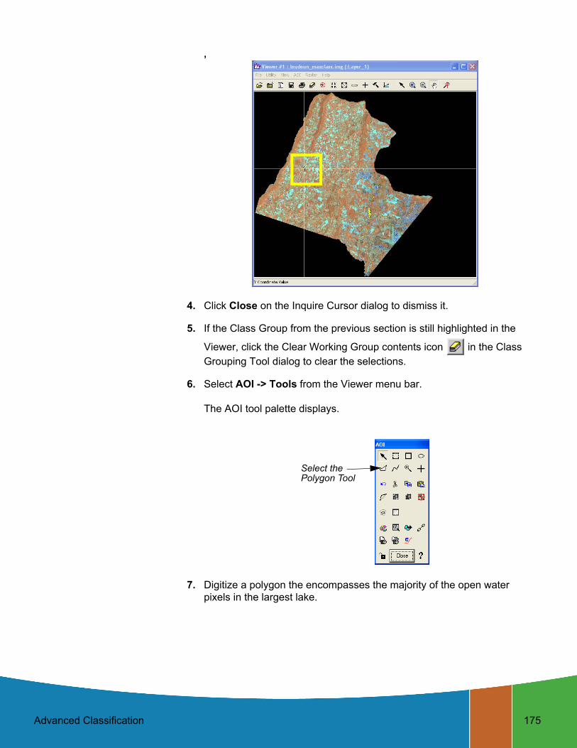
4. Click Close on the Inquire Cursor dialog to dismiss it.

5. If the Class Group from the previous section is still highlighted in the

Viewer, click the Clear Working Group contents icon in the Class Grouping Tool dialog to clear the selections.

6. Select AOI -> Tools from the Viewer menu bar.

The AOI tool palette displays.

7. Digitize a polygon the encompasses the majority of the open water pixels in the largest lake.

Select the Polygon Tool


8. In the Class Grouping Tool toolbar, click the Use Current AOI to Select

Classes icon .

All of the classes that are contained within the currently selected AOI are highlighted in the Working Group CellArray.

9. Using the techniques outlined in Using the Cursor Point Mode on page 169, fill in the holes in the selections for these lakes.

10. In the Class Groups CellArray, make sure that the caret > is in the row

for the Water_1 class, then click the Union icon .

This adds the classes saved in the water_1 Class Group to the classes that are currently selected in the Working Group CellArray.

11. Click the Save button above the Class Groups CellArray to save all of the selected classes in the Working Group CellArray.

12. In the Class Groups CellArray, click in the Water_1 cell. This group represents the open water land use category, so change the Group Name by typing Open.

NOTE: The Target Class Name is already a stored part of the Class Group name, so there is no need to repeat it in the Class Group name.

13. In the Class Grouping Tool dialog, click the Clear Working Group

contents icon to clear the selections.


Next, remove the AOI you created.

14. Select View -> Arrange Layers from the Viewer menu bar.

15. Right-click on the AOI layer and select Delete Layer from the AOI Options menu.

16. Click Apply in the Arrange Layers dialog.

17. Click No in the Verify Save on Close dialog prompting you to save the AOI to a file.

18. Click Close in the Arrange Layers dialog.

19. Click Close on the AOI tool palette to remove it from your display.


Using the Ancillary Data Tool

It would take a very long time to collect all of the classes in a large image using only the simple tools outlined above. To save time, you should quickly group all of the classes into Class Groups and then refine these initial groupings to more accurately define the study area.

Definitions of Boolean Operators

The Class Grouping Tools provides four boolean operators that allow you to refine the selections in your Class Groups.

Intersection of Sets: The intersection of two sets is the set of elements that is common to both sets.

Union of Sets: The union of two sets is the set obtained by combining the members of each set.

Exclusive-Or (XOR) of Sets: The Exclusive-Or of two sets is the set of elements belonging to one but not both of the given sets.

Subtraction of Sets: The subtraction of set B from set A yields a set that contains all data from A that is not contained in B.


The Ancillary Data Tool provides a means of performing this quick initial grouping. By using previously collected data, such as ground truth data or a previous classification of the same area, you can quickly group your image, and then concentrate on evaluating and correcting the groups.

The thematic file used as the Ancillary Data file need not cover the entire area, but it must at least overlap with the area being grouped.

Setting Up the Ancillary Data Classes

1. In the Class Grouping Tool toolbar, click the Start Ancillary Data Tool

icon .

Two dialogs display, the Ancillary Data Tool dialog and the Ancillary Class Assignments dialog.

2. In the Ancillary Class Assignments dialog, select File -> Set Ancillary Data Layer.

The File Chooser opens.

3. Select loudoun_lc.img from the <ERDAS_Data_Home>/examples directory, then click OK.

A Performing Summary progress meter displays.

4. When the summary is complete, click OK to dismiss the progress meter (if your Preferences are not set so that it closes automatically).

The summary process does three things:

• populates the Ancillary Class Assignments CellArray with information from the ancillary data file,

• provides summary values relating the ancillary data file to the file being grouped in the Ancillary Data Tool CellArray, and

• adds three new columns (Diversity, Majority, and Target %) to the Working Group CellArray in the Class Grouping Tool.

For a more detailed explanation of each of these dialogs and their contents, please see the ERDAS IMAGINE On-Line Help.


In the Ancillary Class Assignments dialog CellArray, the rows represent the classes from the ancillary data file (loudoun_lc.img) and the columns represent the information from the file being grouped (loudoun_maxclass.img).

5. In the Ancillary Class Assignments dialog CellArray, scroll down until you see Low Intensity Residential in the Class Name column of the CellArray.

You may want to expand the size of the Class Names column in the Ancillary Class Assignments CellArray so that you can read the entire Class Name.

6. Click in the corresponding Urban column of the CellArray to assign this class to the Urban Target Class.

The X moves from the Water column (the first column in the CellArray) to the Urban column.

7. Repeat this step for the High Intensity Residential and Commercial/Industrial/Transportation classes to add them to the Urban class as well.

8. Continue arranging the Xs in the Ancillary Class Assignments dialog so that they properly relate the named classes from the ancillary data file to the remaining Target Classes, which are Agriculture and Forest. If the ancillary data classes do not have labels (Ancillary Classes/Class Names), leave the corresponding X in the Water column.

Click here to relatethe Ancillary Data classes to the TargetClasses in the imagebeing grouped


Collecting Groups Using the Majority Approach

In most cases, this approach would be the first step you took in the grouping process. As a first step, this process would result in a completely grouped image that had no Similarities and no Conflicts between Target Classes.

We have already begun collecting Class Groups, and this causes some conflicts between Target Classes.

Once you have assigned the ancillary data classes to the Target Classes, you may minimize the Ancillary Data Tool and the Ancillary Class Assignments dialogs.

1. In the Working Group CellArray on the Class Grouping Tool, right-click in the numbered row labels. Select Criteria... from the Row Selection menu.

The Selection Criteria dialog displays.

2. In the Columns area, click Majority to set the selection criteria.

3. In the Target Classes section of the Class Grouping Tool dialog, select the Water Target Class by placing the caret > in the Water row.

4. In the Selection Criteria dialog, click the Select button.

Click Majorityto specify the selection criteria

Make sure that the caret > is in this row


All of the classes that best represent the selected Target Class are highlighted in the Working Group section of the Class Grouping tool.

5. In the Class Groups area of the Class Grouping Tool, click the Save As New Group button.

The selected classes are added as a new class group.

6. Change the name of the new group by selecting the Water_2 text and typing Majority.

This helps you keep track of how the Class Group was collected.

7. Repeat step 3. through step 6. for each of the Target Classes, moving the caret in the Target Classes CellArray to the next Target Class each time.

8. When you are finished, click the Close button on the Selection Criteria dialog.

9. Save the Grouping Process by selecting File -> Save Image... from the Class Grouping Tool menu bar.

This provides a broad grouping of all the classes in the image, and each Class Group must be closely examined to determine the accuracy of the Majority grouping.

10. Click Close in the Ancillary Data Tool dialog.

11. Click Close in the Ancillary Class Assignments dialog.

12. Click the Clear Working Group Contents icon in the Class Grouping Tool dialog to prepare for the next section.

Next, you can learn how to find the grouping conflicts and some strategies for resolving them.

Click here to save the classes as a new group

Change the name of the new groupto Majority


Identifying and Resolving Similarities and Conflicts

The Class Grouping Tool allows there to be any number of Class Groups representing each Target Class, and there is no restriction on whether or not these groups overlap or conflict with each other. It is frequently the case that a single class may properly belong with more than one target class. These classes are termed conflicted classes, and they generally are a source of speckle in the resulting final classification.

Both Similarity and Conflict are measures of shared classes. Similar classes are shared by other groups within the same Target Class, while conflicted classes shared by groups under a different Target Class.

1. In the Target Classes section of the Class Grouping Tool dialog, select the Water Target Class by placing the caret > in the Water row.

2. In the Class Groups section of the Class Grouping Tool dialog, select the Open Class Group by placing the caret > in the Open row.

3. In the Class Groups section of the Class Grouping Tool dialog, click the Load button.


Notice the Similarity and Conflict numbers displayed just under the Working Group CellArray:

Place the

...and then click Load to highlightthe classes in theWorking GroupsCellArray

carets >here...


The Similarity statistics are calculated between the Working Groups and the selected Class Group. These are the same, so we would expect there to be the same number of Similarities and Classes Selected, and this is the case.

4. In the Class Grouping Tool toolbar, click the Toggle Similarity/Conflict

icon to highlight the other Target Classes that have classes in common with the Working Group (which is exactly the same as the Open Class Group).

Number of similaritiesbetween the Working Group and the selectedClass Group

Number of conflictsbetween the WorkingGroup and the selectedClass Group

Number of selected classes in the WorkingGroup CellArray


5. Select the Agriculture Target Class by placing the caret > in the Agriculture row.

NOTE: The contents of the Working Group CellArray do not change when you change the selected Target Class, but the contents of the Similarity and Conflict statistics have reversed.

6. To identify the classes that these two Target Classes have in common,

click the Intersect Working Group with Current Group icon .

For more information on Boolean operators, see “Definitions of Boolean Operators”.

This loads the intersection of the classes included in the Working Group (Water, Open) and the selected Class Group (Agriculture, Majority).

The Target Classesand Class Groupsthat share classesare highlighted


7. In the Viewer, zoom in on the classes that are currently selected. These classes are located in the Lakes you collected with the AOI Tool.

8. Use the Toggle Highlighting icon to view the pixels in question.

These pixels belong in the Water Target Class and not in the Agriculture Target Class. Next, you remove these classes from the Agriculture Target Class

9. Make sure the caret > is still in the Agriculture Target Class and the Majority Class Group.

10. Click the XOR Working Group and Current Group icon .

This loads all of the classes in the selected Class Group (Agriculture, Majority) without any of the classes that were previously highlighted in the CellArray (the conflicted classes).

11. In the Class Groups area of the Class Grouping Tool dialog, click the Save button to save the Agriculture, Majority Class Group without the conflicted classes.

12. In the Class Grouping Tool toolbar, click the Save icon to save the grouping process to the image file.

Coloring the Thematic Table

Sometimes it is helpful to judge your progress by seeing the entire picture. The Class Grouping Tool provides a mechanism for you to see how the grouping process is progressing.

1. In the Class Grouping Tool menu bar, select Colors -> Set to target colors.

The colors in the T column in the Working Groups CellArray change to reflect the colors of the associated Target Classes.

Classes that are conflictedor are not included in anyTarget Class are highlighted


All of the classes that have not been grouped into Target Classes or are in conflict with other Target Classes are highlighted. These conflicted or unassigned classes must be resolved.

2. If a class is highlighted but has been assigned a target color, it is included in more than one target class. Use the techniques described in “Identifying and Resolving Similarities and Conflicts” to resolve the conflict.

After you have resolved some of the conflicts, you can refresh the classes that remain unresolved by clearing the current working group and then selecting Colors -> Set to target colors in the Class Grouping Tool menu bar.

3. If a class is highlighted but has not been assigned a target color (that is, the colors in the C and T column of the Working Group CellArray are the same), the class has not yet been collected in any group. Use the techniques described in Using the Cursor Point Mode to collect these classes into their groups.

4. To change back to the standard color table display in the Viewer, click

the Standard Color Table icon .

5. To view the thematic color table display in the Viewer, click the

Thematic Color Table icon .

6. When you have finished the grouping process, click the icon to display the Thematic colors in the Viewer, then select File -> Save -> Top Layer As.... Save the image as loudoun_strata.img.

You can separately load that image in a Viewer to compare it to the original image, loudon_maxclass.img.


Close and Exit

1. Select File -> Close from the Class Grouping Tool menu bar.

2. Select File -> Close from the Viewer menu bar.

Using Fuzzy Recode

This section shows you how to recode an image after it has been grouped. a file that has had its spectral classes grouped into informational groups. Fuzzy Recode is used to recode a preprocessed unsupervised image after it has been grouped with the Class Grouping Tool. However, these informational groups may contain some overlap where certain classes belong to more than one group. The Fuzzy Recode process resolves this by using a weighted convolution window to look at each pixel with respect to each of its neighbors and then recoding the pixel into the most likely group.

The recoding is not just per pixel, but it looks at all the pixels in the neighborhood using the following formula.


When recoding an image, use the generated image from the grouping tool.

Fuzzy Recode Formula

When beginning the Fuzzy Recode process, the Normalized class/group confidences are first calculated using the following equation:

Where:

Vp[k] = the normalized membership confidence for class k in the pth

group.

Up = the user defined group confidence for the pth group.

= the sum of the user-defined group confidences for

groups with a membership in class k

The following equation is then used to perform a convolution on the class/group confidence table:

Where:

p = the current group being recoded

q = target class of group p

i = row index of the window

j = column index of window

s = size of the window (3, 5, or 7)

W = spatial weight table for the window (optional)

k = class value of the pixel at i, j

Vp[k] = total confidence of window for target class q

fp = 1 if group p belongs to class q, otherwise 0.

The center pixel is assigned the class with the maximum Tq.

Vp k[ ] Upn 1–

Σp 0=

Up k[ ]⁄=

n 1–

Σp 0=

Up k[ ]

Tqs 1–Σ

i 0=

s 1–Σ

j 0=Wij

n 1–Σ

p 0=× Vp k[ ] fp×=


Starting the Fuzzy Recode Process

1. Select Fuzzy Recode from the Classification menu.

2. Navigate to the directory in which the generated grouping tool image is located. Click on the file to enter it as the Input Classified File.

3. Navigate to a directory in which you have write permission. Enter a name for the Output Classified File.

4. Accept all defaults and Click OK.

5. Open a Viewer and display the recoded image.

6. Select Session -> EXIT IMAGINE if you want to end your session.


Advanced Classification - PBworks

Documents