Adjoint variable method for time-harmonic Maxwell equations

Adjoint variable method fortime-harmonic Maxwell equations

Stephane Durand and Ivan CimrakDepartment of Mathematical Analysis, Ghent University,

Ghent, Belgium, and

Peter SergeantDepartment of Electrical Energy, Systems and Automation,

Ghent University, Ghent, Belgium andDepartment of Electrotechnology, Faculty of Applied Engineering Sciences,

University College Ghent, Ghent, Belgium

Abstract

Purpose – The purpose of this paper is to study the optimization problem of low-frequency magneticshielding using the adjoint variable method (AVM). This method is compared with conventionalmethods to calculate the gradient.

Design/methodology/approach – The equation for the vector potential (eddy currents model) inappropriate Sobolev spaces is studied to obtain well-posedness. The optimization problem is formulated interms of a cost functional which depends on the vector potential and its rotation. Convergence of a steepestdescent algorithm to a stationary point of this functional is proved. Finally, some numerical results for anaxisymmetric induction heater are presented.

Findings – Using Friedrichs’ inequality, the existence and uniqueness of the vector potential, itsgradient and the corresponding adjoint variable can be proved. From the numerical results, it is concludedthat the AVM is advantageous if the number of parameters to optimize is larger than two.

Research limitations/implications – The AVM is only faster than conventional methods if thegradients can be calculated with sufficient accuracy.

Originality/value – Theoretical results for eddy currents model are often based on a non-vanishingconductivity. The theoretical value of this paper is the presence of non-conducting materials in the domain.From a practical viewpoint, it has been demonstrated that the AVM can yield a significant reduction ofcomputational time for advanced optimization problems.

Keywords Eddy currents, Numerical analysis, Optimization techniques

Paper type Research paper

1. Introduction and definition of the problemLet V be a simply connected and bounded Lipschitz domain in R3. The problem ofmagnetic shielding can be formulated in terms of the vector potential A as follows. ForJe [ L 2ðVÞ3 consider the problem (Sergeant et al., 2008):

7 £ ðm217 £AÞ þ ivsA ¼ Je in V; ð1Þ

The current issue and full text archive of this journal is available at

www.emeraldinsight.com/0332-1649.htm

Stephane Durand is supported by the BOF grant number 01D28807 of Ghent University.Ivan Cimrak and Peter Sergeant are supported by the Fund for Scientific Research-FlandersFWO (Belgium). The work is also supported by the FWO project G.0082.06, by the GOA projectBOF 07/GOA/006 and the IAP project P6/21. Special thanks to Professor Marian Slodicka for hisuseful advice. The authors would also like to thank the reviewers for their useful remarks.

COMPEL28,5

1202

COMPEL: The International Journalfor Computation and Mathematics inElectrical and Electronic EngineeringVol. 28 No. 5, 2009pp. 1202-1215q Emerald Group Publishing Limited0332-1649DOI 10.1108/03321640910969458

7 · ðeAÞ ¼ 0 in V; ð2Þ

A £ n ¼ 0 on ›V; ð3Þ

where v is a real positive parameter and m, s, e are real functions of space butindependent of A (linear materials). We will prove existence and uniqueness of thesolution to equations (1)-(3) in appropriate spaces. Remark that the system of equations(1)-(3) is analogous to the eddy currents model. This model is coercive if theconductivity sðxÞ is positive and existence and uniqueness of the weak solution inH ðcurl;VÞ is straightforward (Krızek and Neittaanmaki, 1996, p. 223). We will allowfor vanishing conductivity and prove coercivity using Friedrichs’ inequality, for ageneral geometry of the conductors. The systems (1) and (2) with vanishingconductivity was studied in Ammari et al. (2000) for V ¼ R3, in relation to the eddycurrents model, using the asymptotic behaviour of the fields at infinity. In Rodrıguezet al. (2003), the existence and uniqueness is proved for a general topology of theconductors, by dividing the domain into a conducting and an isolating part. In thispaper, we consider the systems (1)-(3) on the whole domain V.

The aim of magnetic shielding is to find the geometry sðxÞ;mðxÞ; JeðxÞ, such that themagnetic field in a target region is minimized. Therefore, a cost functional is constructedwhich depends explicitly and implicitly (via the vector potential) on the geometry(Sergeant et al., 2008). From the mathematical viewpoint, only the implicit dependence onthe geometry is interesting, because then an expression for the Gateaux derivative ofA with respect to variations in the geometry needs to be calculated. An elegant way to dothis is by considering the problem adjoint to equations (1)-(3).

The cost functional is numerically minimized for the axisymmetric induction heater,described in Sergeant et al. (2008). We will compare the steepest descent (SD) algorithmwith a conjugate gradients (CG) method, both with computation of the gradients eitherby the conventional approach (using small perturbations in the parameters) or by theadjoint variable method (AVM). Similar approach has been successfully used in shapeoptimization problems (Cimrak and Melicher, 2007; Melicher et al., 2008).

OverviewIn the next section, we will set up the variational formulation of equations (1)-(3) in thecorrect space. In this space, we can prove Friedrichs’ inequality, which is needed for thecoercivity of our problem. In Section 3, the Gateaux derivative of the cost functional iscalculated. The existence and uniqueness of the Gateaux derivative of A as a solution ofthe sensitivity equation, is proved in Section 4. Based on the weak formulation and thederivative of the cost functional we construct the adjoint system in Section 5. We prove theconvergence of our numerical method to a stationary point in Section 6. Finally,we compare several computational algorithms in Section 7.

2. Weak formulationConsider the system of equations (1)-(3). We put some assumptions on the realfunctions e ;s and m, based on physical properties of permittivity, permeability andconductivity:

H1. Suppose that there exist constants emin; emax;smax;mmin;mmax , 1 such thatfor e [ W 1;1ðVÞ, s [ L1ðVÞ and m [ L1ðVÞ holds:

Adjoint variablemethod

1203

emax $ e $ emin . 0; 0 # s # smax; 0 , mmin # m # mmax:

We introduce some functional spaces based on the notation from (Monk, 2003):

XN ¼ u [ H ðcurl;VÞ> H ðdiv;VÞju £ n ¼ 0 on ›V;

W eN ¼ u [ H ðcurl;VÞ> H ðdiv;VÞj7 · ðeuÞ ¼ 0 in V and u £ n [ ðL2

t ð›VÞÞ3;

W eN ;0 ¼ W e

N > XN :

Each of these spaces is provided with the usual graph norm, e.g. in W eN we consider the

norm (k · k2 is the standard L 2ðVÞ-norm):

kukW eN¼ kujj

22 þ k7 ·ujj

22 þ k7 £ ujj

22 þ ku £ njj

22

1=2

:

We introduce the sesquilinear form aðv;uÞ ¼ ðm217 £ v;7 £ uÞ2 iv ðs v;uÞ and thelinear functional f 1ðvÞ ¼ ðv; JeÞ, with ðu; vÞ ¼

RVu ·vdx the standard L 2ðVÞ3 inner

product ( u is the complex conjugate of u). Motivated by the equation for vectorpotential equation (1) with the condition (2) and considering boundary condition (3), wedefine the notion of a weak solution to our problem.

Definition 1. A vector potential A [ W eN ;0 is called a weak solution to equations

(1)-(3) if the following identity holds for all v [ W eN ;0:

aðv;AÞ ¼ f 1ðvÞ: ð4Þ

In order to prove existence and uniqueness of the weak solution, we will need thefollowing theorem, based on Monk (2003, Corollary 3.51). In Monk (2003), this theoremis proved for e ¼ 1. With the following lemma, the proof can be extended to thespace W e

N .Lemma 1. The space W e

N is compactly embedded in L 2ðVÞ3.Proof. This is a consequence of the continuous embedding of W e

N in H 1=2ðVÞ3

(Monk, 2003, Theorem 3.47) and the compact embedding of H 1=2ðVÞ3 in L 2ðVÞ3

(Sobolev embedding theorem). ATheorem 1. Suppose that V is a bounded simply connected Lipschitz domain

with connected boundary. There exists a constant CF . 0 such that for everyu [ W e

N :

kuk2 # CF ðk7 £ uk2 þ ku £ nk2Þ: ð5Þ

Proof. Suppose the result is false. Then there exists a sequence un , W eN such

that k7 £ unk2 þ kun £ nk2 # 1=n, with kunk2 ¼ 1. By Lemma 1 there is aconvergent subsequence unk, such that unk ! u in L 2ðVÞ3, with u [ W e

N . Sincekunkk2 ! 1, we conclude u – 0 (adapted proof from Monk, 2003).

On the other hand, 7 £ u ¼ 0, since 7 £ unk ! 0. Therefore, there exists a functionp [ H 1ðVÞ for which u ¼ 7p. This function satisfies the equation 7 · ðe7pÞ ¼ 0 on V.From u £ n ¼ 0, we have that p is constant along ›V or shifting p by a constant, p ¼ 0on ›V. Under H1 there is only one solution for p, namely p ¼ 0 in V. Hence, u ¼ 0, incontradiction with the above argumentation. A

COMPEL28,5

1204

As equation (5) are usually referred to as Friedrichs’ inequalities. In the space W eN ;0,

this inequality reduces to:

kuk2 # CFk7 £ uk2: ð6Þ

Note that the constant CF does not depend on e .Theorem 2. (Existence and uniqueness of the weak solution). Under H1 on

functions s; e and m, there exists a unique weak solution to equations (1)-(3), for everyJe [ L 2ðVÞ3. Moreover, this solution satisfies:

k7 £Ak2 # mmaxCFkJek2; kAk2 # mmaxC2FkJek2:

Proof. For every:

u [ W eN ;0 : kujj

2H ðcurl;VÞ # kujj

2W e

N ;0# 1 þ

k7ek1

emin

2 !

kujj22 þ k7 £ ujj

22;

thus the graph norm in W eN ;0 is equivalent to the standard H ðcurl;VÞ-norm. Continuity

of aðv;uÞ and f 1ðvÞ is obtained from:

jaðv;uÞj # jðm217 £ v;7 £ uÞj þ vjðsv;uÞj

# m21mink7 £ vk2k7 £ uk2 þ vsmaxkvk2kuk2

# C 0kvkH ðcurl;VÞkukH ðcurl;VÞ:

j f 1ðvÞj # kJek2kvk2 # kJek2kvkH ðcurl;VÞ:

Coercivity of a ðv;uÞ we get by writing aðu;uÞ ¼ x2 iy with x ¼ ðm217 £ u;7 £ uÞand y ¼ v ðsu;uÞ. H1 ensures that x and y are real and positive. Therefore:

jaðu;uÞj $ m21maxk7 £ ujj

22: ð7Þ

With Friedrichs’ inequality (6), we also obtain:

jaðu;uÞj $m21

max

C2F

kujj22:

Addition of both inequalities proves coercivity of aðv;uÞ in H ðcurl;VÞ and thus inW e

N ;0. By the Lax-Milgram theorem (Monk, 2003), there exists a unique weak ofsolution (4) in W e

N ;0.The bounds for 7 £A and A follow from equation (7) and Friedrichs’ inequality.A

3. Optimization problemThe previous theorem states that for suitable data functions s; e ;m and Je, the vectorpotential A is uniquely determined by systems (1)-(3). In most applications one is notinterested in the direct calculation ofA, but rather looks for a suitable geometry (s;m andJe, briefly noted by p), such that the solution for A satisfies certain restrictions. This isexpressed by the cost functionalF(p) which reaches a minimum for the optimal geometry.It can consist of terms proportional to 7 £A (restrictions on magnetic induction B),

Adjoint variablemethod

1205

proportional toA (restrictions on electric field or induced currents) or proportional to otherphysical or geometrical parameters. We will consider the cost functional:

FðpÞ ¼

ZVTA

j7 £AðpÞj2dxþ

ZVP

sjAðpÞj2dx; ð8Þ

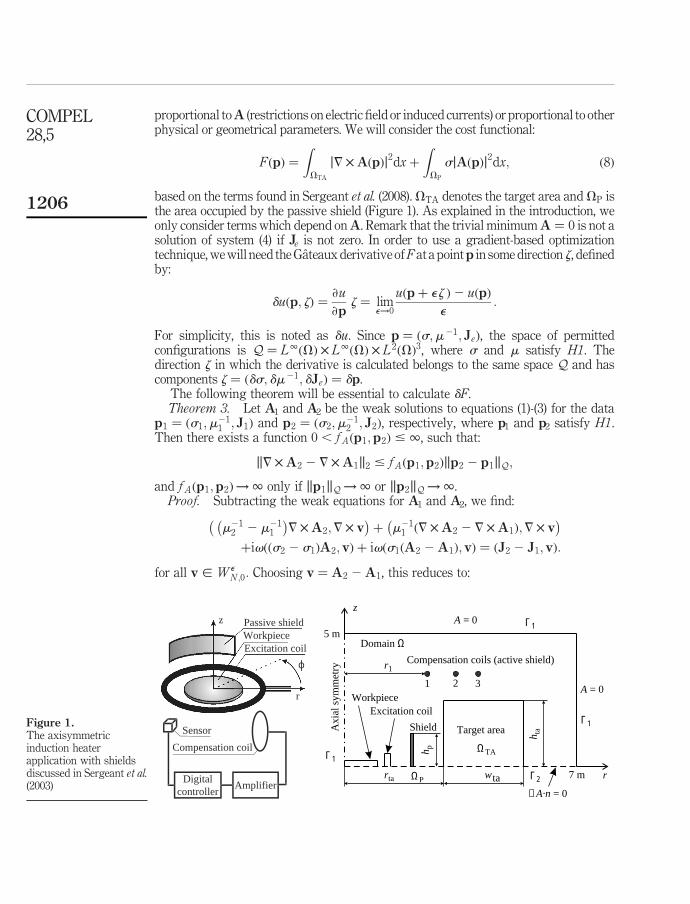
based on the terms found in Sergeant et al. (2008). VTA denotes the target area and VP isthe area occupied by the passive shield (Figure 1). As explained in the introduction, weonly consider terms which depend onA. Remark that the trivial minimum A ¼ 0 is not asolution of system (4) if Je is not zero. In order to use a gradient-based optimizationtechnique, we will need the Gateaux derivative ofF at a pointp in some direction z, definedby:

duðp; zÞ ¼›u

›pz ¼

e!0lim

uðpþ ez Þ2 uðpÞ

e:

For simplicity, this is noted as du. Since p ¼ ðs;m21; JeÞ, the space of permittedconfigurations is Q ¼ L1ðVÞ £ L1ðVÞ £ L 2ðVÞ3, where s and m satisfy H1. Thedirection z in which the derivative is calculated belongs to the same space Q and hascomponents z ¼ ðds; dm21; dJeÞ ¼ dp.

The following theorem will be essential to calculate dF.Theorem 3. Let A1 and A2 be the weak solutions to equations (1)-(3) for the data

p1 ¼ ðs1;m211 ; J1Þ and p2 ¼ ðs2;m

212 ; J2Þ, respectively, where p1 and p2 satisfy H1.

Then there exists a function 0 , f Aðp1;p2Þ # 1, such that:

k7 £A2 2 7 £A1k2 # f Aðp1;p2Þkp2 2 p1kQ;

and f Aðp1;p2Þ!1 only if kp1kQ !1 or kp2kQ !1.Proof. Subtracting the weak equations for A1 and A2, we find:

m212 2 m21

1

7 £A2;7 £ v

þ m21

1 ð7 £A2 2 7 £A1Þ;7 £ v

þivððs2 2 s1ÞA2; vÞ þ ivðs1ðA2 2A1Þ; vÞ ¼ ðJ2 2 J1; vÞ:

for all v [ W eN ;0: Choosing v ¼ A2 2A1, this reduces to:

Figure 1.The axisymmetricinduction heaterapplication with shieldsdiscussed in Sergeant et al.(2003)

WorkpieceExcitation coil

Sensor

Digitalcontroller

Amplifier

Compensation coil

Passive shield

r

ϕ

rta

Target area

z

r

h ta

wta

Shield

Excitation coil

5 m

7 m

Workpiece

Domain Ω

A = 0

A = 0

Axi

al s

ymm

etry

∆A·n = 0

h p

r1Compensation coils (active shield)

1 2 3

Γ1

Γ1

Γ1

Γ2

ΩTA

ΩP

z

COMPEL28,5

1206

ffiffiffiffiffiffiffiffim21

1

qð7 £A2 2 7 £A1Þ

2

2 þ ivkffiffiffiffiffis1

pðA2 2A1Þjj

22

¼ ðJ2 2 J1;A2 2A1Þ2 m212 2 m21

1

7 £A2;7 £A2 2 7 £A1

2 ivððs2 2 s1ÞA2;A2 2A1Þ:

Taking the modulus of both sides and applying Friedrichs’ inequality, we obtain:

k7 £A2 2 7 £A1k2 # mmax;1 CFkJ2 2 J1k2 þ k7 £A2k2km212

2m21

1 k1 þ vCFkA2k2ks2 2 s1k1:

The inequality still holds if we swap the indices 1 and 2. AFrom this theorem we conclude that if p2 converges to p1 in the space Q, then

7 £A2 ! 7 £A1 inL 2ðVÞ3 and thus (using Friedrichs’ inequality)A2 !A1 inL 2ðVÞ3.In other words, the vector potential and its rotation depend continuously on the data.

Theorem 4. If we denote the first term of equation (8) as FB and the second term asFP, then the Gateaux derivative of the cost functional can be calculated as:

dFBðp; z Þ ¼ ð7 £ dA;7 £AÞVTAþ ð7 £A;7 £ dAÞVTA

; ð9Þ

dFP ðp; z Þ ¼ ðdsA;AÞVPþ ðsA; dAÞVP

þ ðsdA;AÞVP; ð10Þ

where dA is the solution of the sensitivity equation defined in Definition 2.Proof. We apply the definition of the Gateaux derivative:

dFB ¼e!0lim

1

e

ZVTA

ð7 £Aðpþ ez ÞÞ · ð7 £Aðpþ ez ÞÞdx

2

ZVTA

ð7 £AðpÞÞ · ð7 £AðpÞÞdx

:

This can be manipulated to:

e!0lim

1

e

ZVTA

ð7 £Aðpþ ez Þ2 7 £AðpÞÞ ·7 £Aðpþ ezÞdx

þ

ZVTA

7 £AðpÞ · 7 £Aðpþ ez Þ2 7 £AðpÞ

dx

:

Theorem 3 assures us that lime!07 £Aðpþ ezÞ ¼ 7 £AðpÞ. The existence of thelimit of the first factor is proved by the existence and uniqueness theorem for thesensitivity equation (Theorem 5). Since the limits of both factors exist, we can calculatethem independently and we obtain the desired expression. For dFP the proof isanalogous. A

4. Sensitivity equationTo calculate dFðp; zÞ with equations (9)-(10), we need to know dAðp; zÞ. Therefore, wedifferentiate the weak equation (4) with respect to p to obtain a PDE for dA. Takingequation (4) for p and afterwards for pþ ez we have:

Adjoint variablemethod

1207

ðm217£ v;7£AðpÞÞ2 iv ðsv;AðpÞÞ ¼ ðv;JeÞ;

ððm21 þ edm21Þ7£ v;7£Aðpþ ez ÞÞ2 ivððsþ edsÞv;Aðpþ ez ÞÞ ¼ ðv;Je þ edJeÞ:

In the next step, we subtract both equalities, divide by e and take the limit e! 0. Withsimilar manipulations as in the proof of Theorem 4, we obtain:

ðm217£ v;7£ dAÞ2 iv ðsv;dAÞ ¼ ðv;dJeÞ þ iv ðdsv;AÞ2 ðdm217£ v;7£AÞ:

We receive the same bilinear form aðv;uÞ as in equation (4), but a different right-handside functional. Let us define the following functional:

f 2ðvÞ :¼2ðdm217£ v;7£AðpÞÞ þ ivðdsv;AðpÞÞ þ ðv;dJeÞ:

Definition 2. The sensitivity equation results in seeking such dA [ W eN ;0 for which

aðv; dAÞ ¼ f 2ðvÞ holds for all v [ W eN ;0:

Theorem 5. (Existence and uniqueness for sensitivity equation). Under H1 onfunctions s; e and m, there exists a unique solution to the sensitivity equation.

Proof. Continuity and coercivity of aðv;uÞ in W eN ;0 have been proved in the proof

of Theorem 2. We prove the continuity of f 2ðvÞ:

j f 2ðvÞj # 1jðdm217 £ v;7 £AÞj þ vjðdsv;AÞj þ jðv; dJeÞj

# ðkdJek2 þ vkdsk1kAk2Þkvk2 þ kdm21k1k7 £Ak2k7 £ vk2

# CkvkH ðcurl;VÞ:

For the last inequality we used Theorem 2, which assures the existence andboundedness of A and 7 £A for every configuration p.

From the Lax-Milgram theorem we conclude the existence and uniqueness ofdAðp; dpÞ for every p; dp [ Q. A

Remark 1. We want to calculate the minimum of the cost functional by agradient-based optimization procedure (SD and CG). Suppose the space Q isapproximated by a d-dimensional space, spanned by the basis functionsei; i ¼ 1; . . . ; d. To determine the gradient of the cost functional, we need to calculatedAðp; eiÞ for every i ¼ 1; . . . ; d and AðpÞ (the functional f 2ðvÞ depends on AðpÞ). Thus,every iteration of the optimization procedure requires to solve d þ 1 PDE’s. This is verytime consuming and can be avoided using the adjoint equation.

5. Adjoint systemFrom Theorem 2 it follows that aðv;uÞ is a bounded sesquilinear form from W e

N ;0 £W e

N ;0 to C. Therefore, there exist unique bounded linear operators A and A*, such thataðv;uÞ ¼ ðAðvÞ;uÞ2 ¼ ðv;A*ðuÞÞ2 (Conway, 1985). With these operators we can definethe adjoint problem.

Definition 3. The adjoint problem of the sensitivity equation (Definition 2) withderivatives (9)-(10) of the cost functional, is to find j [ W e

N ;0 such that:

aðv; jÞ ¼ ðv;A*ðjÞÞ2 ¼ f 3ðvÞ; ð11Þ

COMPEL28,5

1208

for all v [ W eN ;0, where we defined the functional f 3 as:

f 3ðvÞ ¼ ð7 £ v;7 £AÞVTAþ ð7 £A;7 £ vÞVTA

þ ðsA; vÞVPþ ðv;sAÞVP

:

Remark 2. The adjoint problem requires the knowledge of the vector potential A(p).We first need to solve equation (4) before we can calculate j. The function j is theadjoint variable of our system. One can easily see that f 3 is related to dF (it contains allterms with dA). Moreover, f 3ðvÞ is a real number, such that aðv; jÞ ¼ aðj; vÞ for all v.

Proofs of the following two theorems are analogous to the proofs of Theorems 5 and3 so we skip them.

Theorem 6. (Existence and uniqueness for adjoint problem) Under H1 on functionss; e and m, there exists a unique solution to the adjoint problem (11). This solution isbounded by kJek2, i.e. there exists a constant C1 such that:

1

CF

kjk2 # k7 £ jk2 # C1kJek2: ð12Þ

Theorem 7. Consider two configurations p1 and p2, which satisfy H1. Suppose A i isthe solution of equation (4) for configuration pi and ji is the corresponding adjointvariable, i ¼ 1; 2. There exists a function 0 , f jðp1;p2Þ # 1, such that:

k7 £ j2 2 7 £ j1k2 # f jðp1;p2Þkp2 2 p1kQ;

and f jðp1;p2Þ!1 only if kp1kQ !1 or kp2kQ !1.Now we consider a certain configuration p [ Q. The previous theorem proves the

existence of a unique adjoint variable jðpÞ [ W eN ;0. From Theorem 5 we know that

the Gateaux derivative dAðp; dpÞ exists for every dp and is unique in W eN ;0. The

corresponding Gateaux derivative of the cost functional can be expressed as a functionof the adjoint variable. Indeed:

dFðp; dpÞ ¼ ðdsA;AÞVPþ ðdA;A*ðjÞÞ; ðdefinition f 3Þ

¼ ðdsA;AÞVPþ f 2ðjÞ; ðsensitivity equation Definition 2Þ

¼ ðdsA;AÞVP2 ðdm217 £ j;7 £AðpÞÞ þ ivðdsj;AðpÞÞ þ ðj; dJeÞ:

Remark 3. Once we have calculated A(p) from the weak formulation (4) and jðpÞfrom the adjoint problem (11), equation (13) gives us the Gateaux derivative of the costfunctional in any direction dp ¼ ðds; dm21; dJeÞ. This implies that only two(complex-valued) PDE’s need to be solved in every iteration of the optimizationprocedure. The d components of the gradient of the cost functional can then becalculated from equation (13) with dp ¼ e i (Remark 1). Compared to the regularmethod of optimization in which d þ 1 PDE’s are solved, this means a significantreduction of the computational time for large systems.

6. Convergence of numerical methodTo calculate the minimum of the functional F(p) we use the method of SD iterativelygenerating:

pnþ1 ¼ pn 2 tn›pFðpnÞ; ð13Þ

Adjoint variablemethod

1209

where ›p denotes the vector of partial derivatives to every component of the vector p ofoptimizing parameters. To verify that this is a relaxation sequence ðFðpnþ1Þ , FðpnÞÞwe apply the following theorem (Vainberg, 1973, Lemma 11.2).

Lemma 2. Suppose that Q is a real reflexive Banach space and Q* is a space withGateaux-differentiable norm. Further assume F(x) is a real Gateaux-differentiablefunctional bounded below and increasing, and its gradient satisfies the Lipschitzcondition kDFðxþ hÞ2 DFðxÞkQ* # CFkhkQ:

Then equation (13) is a relaxation process and limn!1›pFðpnÞ ¼ 0 as soon as1=4 # tnCF # 1=2.

Remark 4. DFðxÞ is an operator from Q to R such that DFðxÞ : h! dFðx; hÞ.Based on the remark in Vainberg (1973, p. 93), the first condition of Lemma 2 can be

relaxed to the case where Q is the dual of a separable normed space. Since L1ðVÞ ¼L 1ðVÞ* and L 2ðVÞ3 ¼ L 2ðVÞ3*, we have L1ðVÞ £ L1ðVÞ £ L 2ðVÞ3 ¼ ðL 1ðVÞ£L 1ðVÞ £ L 2ðVÞ3Þ*. The first condition is clearly satisfied (LpðVÞ is separable for1 # p , 1).

The multipliers tn can be chosen such that the last condition is satisfied.Moreover, the cost functional satisfies the Lipschitz condition. Indeed, from equation(13) we get:

dFðpþ h; zÞ ¼ ðdsAðpþ hÞ;Aðpþ hÞÞ þ ðjðpþ hÞ; dJeÞ2 ðdm217 £ jðpþ hÞ;7

£Aðpþ hÞÞ2 ivðdsjðpþ hÞ;Aðpþ hÞÞ;

dFðp; zÞ ¼ ðdsAðpÞ;AðpÞÞ þ ðjðpÞ; dJeÞ2 ðdm217 £ jðpÞ;7 £AðpÞÞ

2 ivðdsjðpÞ;AðpÞÞ:

Subtraction of both equations and application of Theorems 2, 3, 6 and 7 proves theexistence of CF such that:

kzkQ¼1supjdFðpþ h; zÞ2 dFðp; zÞj # CFkhkQ:

To make sure the functional F(p) is increasing, we can add a regularization termakpkQ. This term assures us that limkpkQ!1FðpÞ ¼ 1, which is a sufficient conditionfor F to be increasing.

With this regularization term, the conditions of Lemma 2 are satisfied and themethod of SD results in a relaxation sequence, which converges to a stationary point ofF. Since F is not convex, this is the best we can get.

7. Numerical experiment with application to magnetic shieldingThe aim of the numerical example is twofold: to verify the convergence behaviour ofSD and to compare several optimization algorithms: the SD method, the CG method,and a genetic algorithm. The gradients for the first two algorithms are calculated eitherby the AVM or by the conventional approach (using small perturbations in theparameters). The numerical example deals with the design of a passive and activeshield for the axisymmetric induction heater discussed in Sergeant et al. (2003) andshown in Figure 1.

COMPEL28,5

1210

Workpiece is of circular shape with outer radius 191 mm, height 10 mm and is madeof aluminum with permeability m0 and conductivity 3.7 £ 107 S/m. Around theworkpiece there is an excitation coil with inner radius 201.2 mm, cross-section height16 mm and width 1.5 mm. Through the coil the current of 4,000 A occurs withfrequency 1,000 Hz. Passive shield is made of a material with conductivity5.9 £ 106 S/m and permeability 372m0 The inner radius is 300 mm, half height isbetween 10 and 200 mm and thickness is 0.65 mm. Active coils are located 1.15 m abovethe symmetry plane and the radial positions vary between 250 and 900 mm. Finally,the target area is located such that the inner radius is 0.5 m, cross section height is0.8 m and width is 1 m.

The parameters to optimize are the height of the passive shield, and/or currents andpositions of active shield coils. The currents in these compensation coils are chosensuch that they reduce the magnetic field by generating a counter field. Moreover, thecost function consists of five contributions that are modelled in the same adjointsystem. The AVM has been validated for this numerical application in Sergeant et al.(2008).

For the axisymmetric induction heater, the systems (1)-(3) can be reduced to a 2Dcylindrical model, described by the variational equation (Sergeant et al., 2008):

ðm217AðpÞ;7wÞ þ ðrmðpÞÞ21AðpÞ;›w

›r

þ ðivsðpÞAðpÞ;wÞ ¼ ð J eðpÞ;wÞ; ð14Þ

with boundary conditions (Figure 1) A ¼ 0 on G1 and 7A ·n ¼ 0 on G2.The cost functional consists of five terms concerning the reduction of the magnetic

field in the target area, the dissipation in the passive shield, the dissipation in theactive shield, the change of the heating of the workpiece by the adding of shieldsand the volume of the passive shield. Explicit expressions for these terms can befound in Sergeant et al. (2008). From mathematical point of view only the terms whichdepend on A or 7 £A (equation (8)) are interesting. Other terms are explicitfunctions of the optimization parameters and bring no difficulties to the optimizationprocedure.

The gradient-based minimization algorithms start from an initial guess p0 that is forall considered optimization cases the same as in Sergeant et al. (2008). The geneticalgorithm starts by generating a random set of parameters vectors.

7.1 Gradient-adjoint algorithm

(1) n ¼ 0 and estimate the initial value p0.

(2) Compute AðpnÞ from the direct problem setting p ¼ pn.

(3) Compute j from the dual problem using AðpnÞ instead of AðpÞ.

(4) Using the explicit expression for the derivative dF based on the adjoint variablej, compute gn ¼ ›FðpnÞ=›p:

(5) When using CG, calculate Lpn ¼ ðgn þ bnLpn21Þ with bn ¼ðgTn gnÞ=ðg

Tn21gn21Þ and Lp0 ¼ g0.

(6) By a line search algorithm, determine the optimal step tn.

(7) Compute pnþ1 ¼ pn 2 tngn (SD) or pnþ1 ¼ pn 2 tnLpn (CG).

Adjoint variablemethod

1211

(8) If convergence is reached (controlling, e.g. the difference FðpnÞ2 Fðpnþ1Þ) thenstop, otherwise set n :¼ nþ 1 and go to Step 2 of the algorithm.

The gradient-adjoint optimization algorithm can in principle be seen as a classicalgradient algorithm that tries to minimize a cost function by iteratively evaluating afinite element model (FEM) (Step (2)). There is however one major difference: thegradients are obtained by solving another (adjoint) FEM (Step (3)) and by using thesolution in an expression for the gradient (Step (4)). In the classical algorithm,the gradients are determined by applying perturbations in the parameters, whichyields as many evaluations of the FEM as the dimension of the parameter space.

7.2 Comparison of optimization techniquesTwo cases are considered. For each case, optimizations are carried out using fivealgorithms, namely a genetic algorithm and four gradient algorithms: the SD methodand the CG method, both using either conventional gradients or the AVM.

For both cases, the optimization algorithms are compared (Table I). In both cases,the radius of the passive shield (0.3 m) and the vertical position of the compensationcoils (1.15 m) were not optimized.

7.2.1 Optimization of both the passive and the active shield with one coil (fourparameters). The complex current I r1 þ jI i1 (between 2400 and þ400 A, which is 10per cent of the excitation current), the horizontal position r1 of the active coil (between0.250 and 0.900 m), and the height of the passive shield are optimized (between 10 and200 mm). With conventional gradients, the SD and CG reach an acceptable solution,and the CG reaches it much faster than the SD. The SD is slow although the step lengthof the line search is optimized. The curved flat valley requires to update the gradientregularly. This results in many iterations – the iterations can be recognized inFigure 2(a) by the small peaks – and each iteration can decrease the function valueonly slightly. With the AVM, the SD and CG find a rather bad solution; they stopbefore finding a good solution. It is interesting to notice in Figure 2(a) that the dashedline (adjoint) regularly reaches high-function values, whereas the solid line(conventional) does not. The reason is that the gradient of the passive shield heightis not very accurate (because of the high permeability and conductivity, seeSergeant et al., 2008), so that the line search is slower. For this case, the adjointapproach is fast, but does not yield the best solution. The best solution is found by theGA, but only after a huge number of function evaluations.

Case 1 Case 2Optimized parameters hp; I r1; I i1; r1 I ri; I ii; ri; i ¼ 1; . . . ; 3

SD conv. 173/2.9129 302/2.8776SD adj. 16/2.9423 166/2.8681CG conv. 53/2.9125 157/2.8668CG adj. 35/2.9362 94/2.8481Gen. alg. 600/2.9077 840/2.8635

Note: Evaluations/Fmin

Table I.Comparison ofoptimization techniquesconcerning number offunction evaluations andoptimal cost value Fmin

for several shieldingproblems

COMPEL28,5

1212

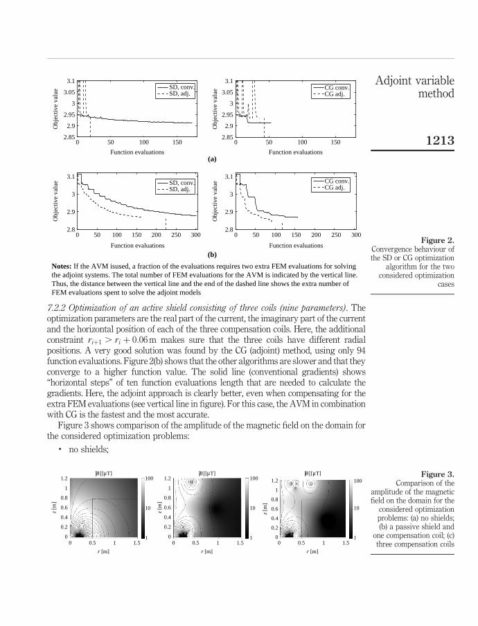
7.2.2 Optimization of an active shield consisting of three coils (nine parameters). Theoptimization parameters are the real part of the current, the imaginary part of the currentand the horizontal position of each of the three compensation coils. Here, the additionalconstraint riþ1 . ri þ 0:06 m makes sure that the three coils have different radialpositions. A very good solution was found by the CG (adjoint) method, using only 94function evaluations. Figure 2(b) shows that the other algorithms are slower and that theyconverge to a higher function value. The solid line (conventional gradients) shows“horizontal steps” of ten function evaluations length that are needed to calculate thegradients. Here, the adjoint approach is clearly better, even when compensating for theextra FEM evaluations (see vertical line in figure). For this case, the AVM in combinationwith CG is the fastest and the most accurate.

Figure 3 shows comparison of the amplitude of the magnetic field on the domain forthe considered optimization problems:

. no shields;

Figure 3.Comparison of the

amplitude of the magneticfield on the domain for the

considered optimizationproblems: (a) no shields;(b) a passive shield and

one compensation coil; (c)three compensation coils

1.2 100

10

1

1

0.8

0.6

0.4

0.2

00 0.5 1 1.5

r [m]

z [m

]

|B| [µT]1.2 100

10

1

1

0.8

0.6

0.4

0.2

00 0.5 1 1.5

r [m]

z [m

]

|B| [µT]1.2 100

10

1

1

0.8

0.6

0.4

0.2

00 0.5 1 1.5

r [m]

z [m

]

|B| [µT]

Figure 2.Convergence behaviour ofthe SD or CG optimization

algorithm for the twoconsidered optimization

cases

0 50 100 150

(a)

(b)

2.85

2.9

2.95

3

3.05

3.1

Function evaluations

Obj

ectiv

e va

lue SD, conv.

SD, adj.

0 50 100 1502.85

2.9

2.95

3

3.05

3.1

Function evaluations

Obj

ectiv

e va

lue CG conv.

CG adj.

0 50 100 150 200 250 3002.8

2.9

3

3.1

Function evaluations

Notes: If the AVM isused, a fraction of the evaluations requires two extra FEM evaluations for solvingthe adjoint systems. The total number of FEM evaluations for the AVM is indicated by the vertical line.Thus, the distance between the vertical line and the end of the dashed line shows the extra number ofFEM evaluations spent to solve the adjoint models

Obj

ectiv

e va

lue

0 50 100 150 200 250 3002.8

2.9

3

3.1

Function evaluations

Obj

ectiv

e va

lueSD, conv.

SD, adj.CG conv.CG adj.

Adjoint variablemethod

1213

. a passive shield and one compensation coil; and

. three compensation coils.

8. ConclusionsWe studied the problem of magnetic shielding from a theoretical point of view. Weestablished a rigorous theoretical framework for the application in Sergeant et al. (2008).Existence and uniqueness of the solution and its Gateaux derivative are proved inappropriate Sobolev spaces. An adjoint variable was defined to minimize the costfunctional and convergence of a SD sequence to a stationary point is proved.

Finally, we presented some numerical results for the case of an axisymmetricinduction heater. Several types of gradient algorithms using an adjoint system werecompared to conventional gradient methods and to a genetic algorithm for the designof a passive and active shield. For less than three parameters to optimize, the adjointapproach seems to be slower than the conventional approach. For more parameters tooptimize, the adjoint approach is usually faster than the conventional approach. TheCG method is usually faster than the steepest decent method, regardless of how thegradients are calculated. The adjoint approach yields accurate gradients for changingpositions of coils, and changing currents. It is less accurate for changes in the passiveshield height, because of the high permeability in combination with high conductivitycausing skin effect, and the thin structure. The inaccuracy slows down the line searchin SD and CG. We conclude that the AVM is advantageous regardless of the type ofgradient algorithm, on two conditions: the gradients should have sufficient accuracy –this should be checked before optimization – and the number of parameters tooptimize should be at least three.

References

Ammari, H., Buffa, A. and Nedelec, J.-C. (2000), “A justification of eddy currents model for theMaxwell equations”, SIAM Journal of Applied Mathematics, Vol. 60 No. 5, pp. 1805-23.

Cimrak, I. and Melicher, V. (2007), “Sensitivity analysis framework for micromagnetism withapplication to the optimal shape design of magnetic random access memories”, InverseProblems, Vol. 23 No. 2, pp. 563-88.

Conway, J. (1985), A Course in Functional Analysis, Springer, New York, NY.

Krızek, M. and Neittaanmaki, P. (1996), Mathematical and Numerical Modelling in ElectricalEngineering, Kluwer Academic, Dordrecht.

Melicher, V., Cimrak, I. and van Keer, R. (2008), “Level set method for optimal shape design ofMRAM core. Micromagnetic approach”, Physica B: Condensed Matter, Vol. 403 Nos 2/3,pp. 308-11.

Monk, P. (2003), Finite Element Methods for Maxwell’s Equations, Numerical Mathematics andScientific Computation, Oxford University Press, New York, NY.

Rodrıguez, A., Fernandes, P. and Valli, A. (2003), “Weak and strong formulations for thetime-harmonic eddy-current problem in general multi-connected domains”, EuropeanJournal of Applied Mathematics, Vol. 14, pp. 387-406.

Sergeant, P., Dupre, L., de Wulf, M. and Melkebeek, J. (2003), “Optimizing active and passivemagnetic shields in induction heating by a genetic algorithm”, IEEE Transactions onMagnetics, Vol. 39 No. 6, pp. 3486-96.

COMPEL28,5

1214

Sergeant, P., Cimrak, I., Melicher, V., Dupre, L. and van Keer, R. (2008), “Adjoint variable methodfor the study of combined active and passive magnetic shielding”, Mathematical Problemsin Engineering, Article ID 369125.

Vainberg, M. (1973), Variational Method and Method of Monotone Operators in the Theory ofNonlinear Equations, Wiley, New York, NY.

Corresponding authorStephane Durand can be contacted at: [email protected]

Adjoint variablemethod

1215

To purchase reprints of this article please e-mail: [email protected] visit our web site for further details: www.emeraldinsight.com/reprints