Adaptive Finite Element Methods Lecture 1: A Posteriori Error Estimation Ricardo H. Nochetto Department of Mathematics and Institute for Physical Science and Technology University of Maryland, USA www2.math.umd.edu/ ˜ rhn 7th Z¨ urich Summer School, August 2012 A Posteriori Error Control and Adaptivity

Welcome message from author
This document is posted to help you gain knowledge. Please leave a comment to let me know what you think about it! Share it to your friends and learn new things together.
Transcript

Adaptive Finite Element MethodsLecture 1: A Posteriori Error Estimation
Ricardo H. Nochetto
Department of Mathematics andInstitute for Physical Science and Technology
University of Maryland, USA
www2.math.umd.edu/˜rhn
7th Zurich Summer School, August 2012A Posteriori Error Control and Adaptivity
Outline Polynomial Interpolation Model Problem A Posteriori Error Analysis Surveys
Outline
Piecewise Polynomial Interpolation in Sobolev Spaces
Model Problem and FEM
FEM: A Posteriori Error Analysis
Surveys
Adaptive Finite Element Methods Lecture 1: A Posteriori Error Estimation Ricardo H. Nochetto

Outline Polynomial Interpolation Model Problem A Posteriori Error Analysis Surveys
Outline
Piecewise Polynomial Interpolation in Sobolev Spaces
Model Problem and FEM
FEM: A Posteriori Error Analysis
Surveys
Adaptive Finite Element Methods Lecture 1: A Posteriori Error Estimation Ricardo H. Nochetto
Outline Polynomial Interpolation Model Problem A Posteriori Error Analysis Surveys
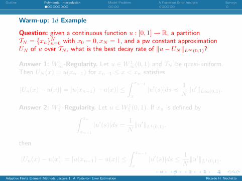
Warm-up: 1d Example
Question: given a continuous function u : [0, 1] → R, a partitionTN = xnN
n=0 with x0 = 0, xN = 1, and a pw constant approximationUN of u over TN , what is the best decay rate of ‖u− UN‖L∞(0,1)?
Answer 1: W 1∞-Regularity. Let u ∈ W 1
∞(0, 1) and TN be quasi-uniform.Then UN (x) = u(xn−1) for xn−1 ≤ x < xn satisfies
|Un(x)− u(x)| = |u(xn−1)− u(x)| ≤∫ xn−1
x
|u′(s)|ds 41N‖u′‖L∞(0,1).
Answer 2: W 11 -Regularity. Let u ∈ W 1
1 (0, 1). If xn is defined by∫ xn
xn−1
|u′(s)|ds =1N‖u′‖L1(0,1),
then
|Un(x)− u(x)| = |u(xn−1)− u(x)| ≤∫ xn−1
x
|u′(s)|ds ≤ 1N‖u′‖L1(0,1).
Adaptive Finite Element Methods Lecture 1: A Posteriori Error Estimation Ricardo H. Nochetto

Outline Polynomial Interpolation Model Problem A Posteriori Error Analysis Surveys
Warm-up: 1d Example
Question: given a continuous function u : [0, 1] → R, a partitionTN = xnN
n=0 with x0 = 0, xN = 1, and a pw constant approximationUN of u over TN , what is the best decay rate of ‖u− UN‖L∞(0,1)?
Answer 1: W 1∞-Regularity. Let u ∈ W 1
∞(0, 1) and TN be quasi-uniform.Then UN (x) = u(xn−1) for xn−1 ≤ x < xn satisfies
|Un(x)− u(x)| = |u(xn−1)− u(x)| ≤∫ xn−1
x
|u′(s)|ds 41N‖u′‖L∞(0,1).
Answer 2: W 11 -Regularity. Let u ∈ W 1
1 (0, 1). If xn is defined by∫ xn
xn−1
|u′(s)|ds =1N‖u′‖L1(0,1),
then
|Un(x)− u(x)| = |u(xn−1)− u(x)| ≤∫ xn−1
x
|u′(s)|ds ≤ 1N‖u′‖L1(0,1).
Adaptive Finite Element Methods Lecture 1: A Posteriori Error Estimation Ricardo H. Nochetto

Outline Polynomial Interpolation Model Problem A Posteriori Error Analysis Surveys
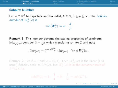
Sobolev Number
Let ω ⊂ Rd be Lipschitz and bounded, k ∈ N, 1 ≤ p ≤ ∞. The Sobolevnumber of W k
p (ω) is
sob(W kp ) := k − d
p.
Remark 1. This number governs the scaling properties of seminorm|v|W k
p (ω): consider x = 1hx which transforms ω into ω and note
|v|W kp (bω) = hsob(W k
p )|v|W kp (ω) ∀v ∈ W k
p (ω).
Remark 2. Let d = 1 and ω = (0, 1). Then W 1∞(ω) is the linear (and
usual) Sobolev scale of L∞(ω), but W 11 (ω) is in the nonlinear scale of
L∞(ω), i.e.
sob(W 11 ) = 1− 1
1= 0− 1
∞= sob(L∞).
Adaptive Finite Element Methods Lecture 1: A Posteriori Error Estimation Ricardo H. Nochetto
Outline Polynomial Interpolation Model Problem A Posteriori Error Analysis Surveys
Sobolev Number
Let ω ⊂ Rd be Lipschitz and bounded, k ∈ N, 1 ≤ p ≤ ∞. The Sobolevnumber of W k
p (ω) is
sob(W kp ) := k − d
p.
Remark 1. This number governs the scaling properties of seminorm|v|W k
p (ω): consider x = 1hx which transforms ω into ω and note
|v|W kp (bω) = hsob(W k
p )|v|W kp (ω) ∀v ∈ W k
p (ω).
Remark 2. Let d = 1 and ω = (0, 1). Then W 1∞(ω) is the linear (and
usual) Sobolev scale of L∞(ω), but W 11 (ω) is in the nonlinear scale of
L∞(ω), i.e.
sob(W 11 ) = 1− 1
1= 0− 1
∞= sob(L∞).
Adaptive Finite Element Methods Lecture 1: A Posteriori Error Estimation Ricardo H. Nochetto

Outline Polynomial Interpolation Model Problem A Posteriori Error Analysis Surveys
Conforming Meshes: The Bisection Method and REFINE
• Labeling of a sequence of conforming refinements T0 ≤ T1 ≤ T2 ford = 2 (similar but much more intricate for d > 2)
0
00 0
0 0
0
0
11
1 1
11
1
1
1
1 1
2
2
2 2
2
2
2
2
2
2
2 2
3
33
3
• Shape regularity: the shape-regularity constant of any T ∈ T solelydepends on the shape-regularity constant of T0.
• Nested spaces: refinement leads to V(T ) ⊂ V(T∗) because T ≤ T∗.• Monotonicity of meshsize function hT : if hT |T := hT := |T |1/d, then
hT∗ ≤ hT for T∗ ≥ T , and reduction property with b ≥ 1 bisections
hT∗ |T ≤ 2−b/dhT |T ∀T ∈ T \ T∗.
Adaptive Finite Element Methods Lecture 1: A Posteriori Error Estimation Ricardo H. Nochetto

Outline Polynomial Interpolation Model Problem A Posteriori Error Analysis Surveys
Complexity of REFINE
I Recursive bisection of T3 (sequence of compatible bisection patches)
3
1 2
3
2
2
2 2
1
3
1 2
3
22
2
3
3
3
3
4
4 4
4
3
1 2
3
2
22
2
3
33
3
I Naive estimate is NOT valid with Λ0 independent of refinement level
#T∗ −#T ≤ Λ0 #M
I Complexity of REFINE (Binev, Dahmen, DeVore ’04 (d = 2), andStevenson’ 07 (d > 2)): If T0 has a suitable labeling, then there existsa constant Λ0 > 0 only depending on T0 and d such that for all k ≥ 1
#Tk −#T0 ≤ Λ0
k−1∑j=0
#Mj .
Adaptive Finite Element Methods Lecture 1: A Posteriori Error Estimation Ricardo H. Nochetto

Outline Polynomial Interpolation Model Problem A Posteriori Error Analysis Surveys
Piecewise Polynomial Interpolation
Quasi-local error estimate: if 0 ≤ t ≤ s ≤ n + 1 (n ≥ 1 polynomialdegree) and 1 ≤ p, q ≤ ∞ satisfy sob(W s
p ) > sob(W tq ), then for all
T ∈ T
‖Dt(v − IT v)‖Lq(T ) . hsob(W s
p )−sob(W tq )
T ‖Dsv‖Lp(NT (T )),
where NT (T ) is a discrete neighborhood of T and IT is a quasiinterpolation operator (Clement or Scott-Zhang). If sob(W s
p ) > 0, then vis Holder continuous, IT can be replaced by the Lagrange interpolationoperator, and NT (T ) = T .
• Quasi-uniform meshes: if 1 ≤ s ≤ n + 1 and u ∈ Hs(Ω), then
‖∇(v − IT v)‖L2(Ω) 4 |v|Hs(Ω)(#T )−s−1
d .
• Optimal error decay: If s = n + 1 (linear Sobolev scale), then
‖∇(v − IT v)‖L2(Ω) 4 |v|Hn+1(Ω)(#T )−nd .
Adaptive Finite Element Methods Lecture 1: A Posteriori Error Estimation Ricardo H. Nochetto
Outline Polynomial Interpolation Model Problem A Posteriori Error Analysis Surveys
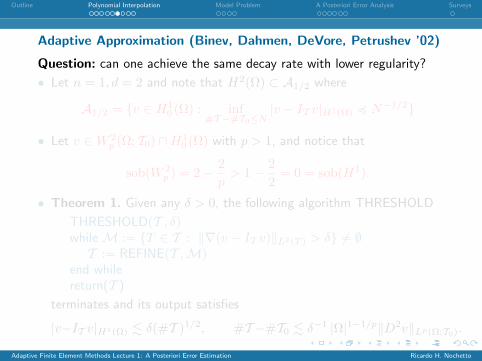
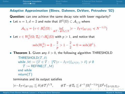
Adaptive Approximation (Binev, Dahmen, DeVore, Petrushev ’02)
Question: can one achieve the same decay rate with lower regularity?
• Let n = 1, d = 2 and note that H2(Ω) ⊂ A1/2 where
A1/2 = v ∈ H10 (Ω) : inf
#T −#T0≤N|v − IT v|H1(Ω) 4 N−1/2
• Let v ∈ W 2p (Ω; T0) ∩H1
0 (Ω) with p > 1, and notice that
sob(W 2p ) = 2− 2
p> 1− 2
2= 0 = sob(H1).
• Theorem 1. Given any δ > 0, the following algorithm THRESHOLD
THRESHOLD(T , δ)while M := T ∈ T : ‖∇(v − IT v)‖L2(T ) > δ 6= ∅T := REFINE(T ,M)
end whilereturn(T )
terminates and its output satisfies
|v−IT v|H1(Ω) . δ(#T )1/2, #T −#T0 . δ−1 |Ω|1−1/p‖D2v‖Lp(Ω;T0).
Adaptive Finite Element Methods Lecture 1: A Posteriori Error Estimation Ricardo H. Nochetto
Outline Polynomial Interpolation Model Problem A Posteriori Error Analysis Surveys
Adaptive Approximation (Binev, Dahmen, DeVore, Petrushev ’02)
Question: can one achieve the same decay rate with lower regularity?
• Let n = 1, d = 2 and note that H2(Ω) ⊂ A1/2 where
A1/2 = v ∈ H10 (Ω) : inf
#T −#T0≤N|v − IT v|H1(Ω) 4 N−1/2
• Let v ∈ W 2p (Ω; T0) ∩H1
0 (Ω) with p > 1, and notice that
sob(W 2p ) = 2− 2
p> 1− 2
2= 0 = sob(H1).
• Theorem 1. Given any δ > 0, the following algorithm THRESHOLD
THRESHOLD(T , δ)while M := T ∈ T : ‖∇(v − IT v)‖L2(T ) > δ 6= ∅T := REFINE(T ,M)
end whilereturn(T )
terminates and its output satisfies
|v−IT v|H1(Ω) . δ(#T )1/2, #T −#T0 . δ−1 |Ω|1−1/p‖D2v‖Lp(Ω;T0).
Adaptive Finite Element Methods Lecture 1: A Posteriori Error Estimation Ricardo H. Nochetto

Outline Polynomial Interpolation Model Problem A Posteriori Error Analysis Surveys
Proof of Theorem 1
1. If r := sob(W 2p )− sob(H1) = 2− 2
p > 0, ET := ‖∇(v− IT v)‖L2(T )
for T ∈ T , thenET . hr
T ‖D2v‖Lp(T ),
we deduce that THRESHOLD terminates in finite steps k(δ) ≥ 1.2. Decompose M := ∪k
j=0Mj into the sets Pj of market elements T :
2−(j+1) ≤ |T | < 2−j ⇒ 2−(j+1)/2 ≤ hT < 2−j/2.
Elements of Pj are disjoint for otherwise they are contained in oneanother contradicting the definition. Hence
2−(j+1) #Pj ≤ |Ω| ⇒ #Pj ≤ |Ω| 2j+1.
3. Since δ ≤ ET . 2−(j/2)r‖D2v‖Lp(T ) for T ∈ Pj , we get
δp #Pj . 2−(j/2)rp∑
T∈Pj
‖D2v‖pLp(T ) ≤ 2−(j/2)rp ‖D2v‖p
Lp(Ω;T0),
whence#Pj . δ−p 2−(j/2)rp ‖D2v‖p
Lp(Ω;T0).
Adaptive Finite Element Methods Lecture 1: A Posteriori Error Estimation Ricardo H. Nochetto

Outline Polynomial Interpolation Model Problem A Posteriori Error Analysis Surveys
4. The crossover takes place for j0 such that
2j0+1|Ω| = δ−p 2−j0rp2 ‖D2v‖p
Lp(Ω;T0)⇒ 2j0 ≈ δ−1 ‖D
2v‖Lp(Ω;T0)
|Ω|1/p.
5. Compute
#M =∑
j
#Pj . |Ω|∑j≤j0
2j + δ−p ‖D2v‖pLp(Ω;T0)
∑j>j0
(2−rp/2)j
.(δ−1 + δ−pδp−1
)︸ ︷︷ ︸=2δ−1
|Ω|1−1/p ‖D2v‖Lp(Ω;T0).
Apply Theorem about complexity of REFINE to arrive at
#T −#T0 . #M . δ−1 |Ω|1−1/p ‖D2v‖Lp(Ω;T0).
6. Upon termination of THRESHOLD, ET ≤ δ for all T ∈ T , whence
|v − IT v|2H1(Ω) =∑T∈T
E2T ≤ δ2 #T .
Adaptive Finite Element Methods Lecture 1: A Posteriori Error Estimation Ricardo H. Nochetto

Outline Polynomial Interpolation Model Problem A Posteriori Error Analysis Surveys
Remarks on Adaptive Approximation
• Let v ∈ H10 (Ω) ∩W 2
p (Ω; T0), n = 1, d = 2, p > 1. For N > #T0 thereexists T ∈ T such that
|v− IT v|H1(Ω) . |Ω|1−1/p ‖D2v‖Lp(Ω;T0)N−1/2, #T −#T0 . N.
Choose δ = |Ω|1−1/p ‖D2v‖Lp(Ω)N−1 in algorithm THRESHOLD.
• W 2p (Ω; T0) ⊂ A1/2 for d = 2 and p > 1. All geometric singularities for
d = 2 (corner and interfaces) satisfy this (Nicaise’ 94).
• For arbitrary n ≥ 1, d ≥ 2, comparing Sobolev numbers yields
n + 1− d
p> sob(H1) = 1− d
2⇒ p >
2d
2n + d.
This may give p < 1 and corresponding Besov space Bn+1p,p (Ω). Proof
above works. Regularity theory for elliptic PDE is incomplete for p < 1.
• Anisotropic elements: Isotropic refinement is not always optimal ford = 3.
Adaptive Finite Element Methods Lecture 1: A Posteriori Error Estimation Ricardo H. Nochetto

Outline Polynomial Interpolation Model Problem A Posteriori Error Analysis Surveys
Outline
Piecewise Polynomial Interpolation in Sobolev Spaces
Model Problem and FEM
FEM: A Posteriori Error Analysis
Surveys
Adaptive Finite Element Methods Lecture 1: A Posteriori Error Estimation Ricardo H. Nochetto
Outline Polynomial Interpolation Model Problem A Posteriori Error Analysis Surveys
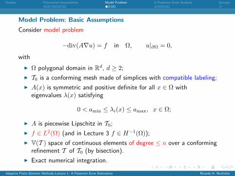
Model Problem: Basic Assumptions
Consider model problem
−div(A∇u) = f in Ω, u|∂Ω = 0,
with
I Ω polygonal domain in Rd, d ≥ 2;
I T0 is a conforming mesh made of simplices with compatible labeling;
I A(x) is symmetric and positive definite for all x ∈ Ω witheigenvalues λ(x) satisfying
0 < amin ≤ λi(x) ≤ amax, x ∈ Ω;
I A is piecewise Lipschitz in T0;
I f ∈ L2(Ω) (and in Lecture 3 f ∈ H−1(Ω));I V(T ) space of continuous elements of degree ≤ n over a conforming
refinement T of T0 (by bisection).
I Exact numerical integration.
Adaptive Finite Element Methods Lecture 1: A Posteriori Error Estimation Ricardo H. Nochetto

Outline Polynomial Interpolation Model Problem A Posteriori Error Analysis Surveys
Galerkin Method
I Function space: V := H10 (Ω).
I Bilinear form: B : V× V → R
B(v, w) :=∫
Ω
A∇v · ∇w ∀v, w ∈ V.
Then solution u of model problem satisfies
u ∈ V : B(u, v) = 〈f, v〉 ∀v ∈ V.
I Finite element space: If Pn(T ) denote polynomials of degree ≤ nover T , then
V(T ) := v ∈ H10 (Ω) : v|T ∈ Pn(T ) ∀T ∈ T .
I Galerkin solution: The discrete solution U = UT satisfies
U ∈ V(T ) : B(U, V ) = 〈f, V 〉 ∀V ∈ V(T ).
Adaptive Finite Element Methods Lecture 1: A Posteriori Error Estimation Ricardo H. Nochetto

Outline Polynomial Interpolation Model Problem A Posteriori Error Analysis Surveys
Galerkin Method (Continued)
I Residual: R ∈ V ∗ = H−1(Ω) is given by
〈R, v〉 := 〈f, v〉 − B(U, v) = B(u− U, v) ∀v ∈ V.
I Galerkin Orthogonality: 〈R, V 〉 = 〈f, V 〉−B(U, V ) ∀V ∈ V(T ).
I Quasi-Best (Cea Lemma): α1 ≤ α2 coercivity and continuityconstants of B
α1‖u− U‖2V ≤ B(u− U, u− U) = B(u− U, u− V )≤ α2‖u− U‖V‖u− V ‖V ∀V ∈ V(T ).
⇒ ‖u− U‖V ≤α2
α1inf
V ∈V(T )‖u− V ‖V.
I Approximation Class As: Let 0 < s ≤ n/d (n ≥ 1) and
As :=
v ∈ V : |u|s := supN>0
(Ns inf
#T −#T0≤Ninf
V ∈V(T )‖v − V ‖V
)⇒ ∃ T ∈ T : #T −#T0 ≤ N, inf
V ∈V(T )‖v − V ‖V ≤ |v|sN−s.
Adaptive Finite Element Methods Lecture 1: A Posteriori Error Estimation Ricardo H. Nochetto

Outline Polynomial Interpolation Model Problem A Posteriori Error Analysis Surveys
A Priori Error Analysis
If u ∈ As, 0 < s ≤ n/d, there exists T ∈ T with #T −#T0 ≤ N and
‖u− U‖V ≤α2
α1|u|sN−s.
I If n = 1, d = 2, p > 1, and u ∈ V ∩W 2p (Ω; T0), then THRESHOLD
shows that |u|1/2 4 ‖D2u‖Lp(Ω;T0) whence (optimal estimate)
∃ T ∈ T : #T −#T0 ≤ N, ‖u− U‖V 4 ‖D2u‖Lp(Ω;T0)N−1/2.
I THRESHOLD needs access to the element interpolation error ET
and so to the unknown u. It is thus not practical.
I The a posteriori error analysis provides a tool to extract this missinginformation from the residual R. This is discussed next.
I The a priori analysis is valid for a bilinear for B on a Hilbert space Vthat is continuous and satisfies a discrete inf-sup condition
|B(v, w)| ≤ α1‖v‖V‖w‖V ∀v, w ∈ V;
α2‖V ‖V ≤ supW∈V
B(V,W )‖W‖V
∀V ∈ V(T ).Adaptive Finite Element Methods Lecture 1: A Posteriori Error Estimation Ricardo H. Nochetto
Outline Polynomial Interpolation Model Problem A Posteriori Error Analysis Surveys
Outline
Piecewise Polynomial Interpolation in Sobolev Spaces
Model Problem and FEM
FEM: A Posteriori Error Analysis
Surveys
Adaptive Finite Element Methods Lecture 1: A Posteriori Error Estimation Ricardo H. Nochetto

Outline Polynomial Interpolation Model Problem A Posteriori Error Analysis Surveys
Error-Residual Equation (Babuska-Miller’ 87)
• Since 〈R, v〉 = 〈f, v〉−B(U, v) = B(u−U, v) for all v ∈ V, we deduce
‖u− U‖V ≤1α1‖R‖V∗ ≤
α2
α1‖u− U‖V.
• Residual representation: elementwise integration by parts yields
〈R, v〉 =∑T∈T
∫T
f + div(A∇U)︸ ︷︷ ︸=r
v +∑S∈S
∫S
[A∇U ] · ν︸ ︷︷ ︸=j
v ∀v ∈ V
where r = r(U), j = j(U) are the interior and jump residuals.
• Localization: The Courant (hat) basis φzz∈N (T ) satisfy thepartition of unity property
∑z∈N (T ) φz = 1. Therefore, for all v ∈ V,
〈R, v〉 =∑
z∈N (T )
〈R, vφz〉 =∑
z∈N (T )
( ∫ωz
rvφz +∫
γz
jvφz
).
• Galerkin orthogonality:∫
ωzrφz +
∫γz
jφz = 0 ∀z ∈ N0(T )
Adaptive Finite Element Methods Lecture 1: A Posteriori Error Estimation Ricardo H. Nochetto

Outline Polynomial Interpolation Model Problem A Posteriori Error Analysis Surveys
Reliability: Global Upper A Posteriori Bound
• Exploit Galerkin orthogonality
〈R, v〉 =∑
z∈N (T )
( ∫ωz
r(v − αz(v))φz +∫
γz
j(v − αz(v))φz
)and take αz(v) :=
Rωz
vφzRωz
φzif z is interior and αz(v) = 0 if z ∈ ∂Ω.
• Use Poincare inequality in ωz
‖v − αz(v)‖L2(ωz) ≤ C0hz‖∇v‖L2(ωz) ∀z ∈ N (T )
and a scaled trace lemma, to deduce∣∣〈R, vφz〉∣∣ 4
(hz‖rφ1/2
z ‖L2(ωz) + h1/2z ‖jφ1/2
z ‖L2(γz)
)‖∇v‖L2(ωz).
• Sum over z ∈ N (T ) and use∑
z∈N (T ) ‖∇v‖2L2(ωz) 4 ‖∇v‖2L2(Ω) to get
‖R‖V∗ 4( ∑
z∈N (T )
h2z‖rφ1/2
z ‖2L2(ωz) + hz‖jφ1/2z ‖2L2(γz)
)1/2
.
Adaptive Finite Element Methods Lecture 1: A Posteriori Error Estimation Ricardo H. Nochetto

Outline Polynomial Interpolation Model Problem A Posteriori Error Analysis Surveys
Upper A Posteriori Bound (Continued)
• Use that hz 4 h(x) for all x ∈ ωz, and∑
z∈N (T ) φz = 1, to derive
‖R‖V ∗ 4(‖hr‖2L2(Ω) + ‖h1/2j‖2L2(Γ)
)1/2
in terms of weighted (and computable) L2 norms of the residuals.
• Upper bound: Introduce element indicators ET (U, T )
ET (U, T )2 = h2T ‖r‖2L2(T ) + hT ‖j‖2L2(∂T )
and error estimator ET (U)2 =∑
T∈T ET (U, T )2. Then
‖u− U‖V ≤1α1‖R‖V ∗ 4
1α1ET (U).
• Jump residual dominates interior residual: Let rz = 〈r,φz〉〈φz,1〉 ∈ R and
note∫
ωzr(v − αz(v))φz =
∫ωz
(r − rz)(v − αz(v))φz. Then
⇒ ‖R‖V∗ 4( ∑
z∈N (T )
h2z‖(r − rz)φ1/2
z ‖2L2(ωz) + hz‖jφ1/2z ‖2L2(γz)
)1/2
.
Adaptive Finite Element Methods Lecture 1: A Posteriori Error Estimation Ricardo H. Nochetto

Outline Polynomial Interpolation Model Problem A Posteriori Error Analysis Surveys
Efficiency: Local Lower A Posteriori Bound (n = 1) (Verfurth’89)
• Local dual norms: for v ∈ H10 (ω) we have
〈R, v〉 = B(u−U, v) ≤ α2‖u−U‖V‖v‖V ⇒ ‖R‖H−1(ω) ≤ α2‖u−U‖V
• Interior residual: take ω = T ∈ T and note 〈R, v〉 =∫
Trv. Then
‖R‖H−1(T ) = ‖r‖H−1(T )
• Overestimation: Poincare inequality yields ‖r‖H−1(T ) 4 hT ‖r‖L2(T )∫T
rv ≤ ‖r‖L2(T )‖v‖L2(T ) 4 hT ‖r‖L2(T )‖∇v‖L2(T )
• Pw constant r: Let η ∈ H10 (T ), |T | 4
∫T
η, ‖∇η‖L∞(T ) 4 h−1T . Then
‖r‖2L2(T ) 4∫
T
r(rη) ≤ ‖r‖H−1(T )‖r‖L2(T )‖∇η‖L∞(T )
4 h−1T ‖r‖H−1(T )‖r‖L2(T ) ⇒ hT ‖r‖L2(T ) 4 ‖r‖H−1(T )
Adaptive Finite Element Methods Lecture 1: A Posteriori Error Estimation Ricardo H. Nochetto

Outline Polynomial Interpolation Model Problem A Posteriori Error Analysis Surveys
Lower A Posteriori Bound (Continued)
• Oscillation of r: hT ‖r − rT ‖L2(T ) with meanvalue rT . Then
hT ‖r‖L2(T ) 4 ‖R‖H−1(T ) + hT ‖r − rT ‖L2(T )
• Data oscillation: if A is pw constant, then r = f and
hT ‖r − rT ‖L2(T ) = hT ‖f − fT ‖L2(T ) = oscT (f, T )
• Oscillation of j: likewise hS‖j − jS‖L2(S) with meanvalue jS and
h1/2S ‖j‖L2(S) 4 ‖R‖H−1(ωS) + h
1/2S ‖j − jS‖L2(S) + hS‖r‖L2(ωS)
where ωS = T1 ∪ T2 with T1 ∩ T2 = S and T1, T2 ∈ T .
• Local lower bound: let ωT = ∪S∈∂T ωS and the local oscillation beoscT (U, ωT ) := ‖h(r − r)‖L2(ωT ) + ‖h1/2(j − j)‖L2(∂T ). Then
ET (U, T ) 4 α2‖∇(u− U)‖L2(ωT ) + oscT (U, ωT ).
Adaptive Finite Element Methods Lecture 1: A Posteriori Error Estimation Ricardo H. Nochetto

Outline Polynomial Interpolation Model Problem A Posteriori Error Analysis Surveys
Lower A Posteriori Bound (Continued)
• Higher order: we expect oscT (U, ωT ) ‖∇(u−U)‖L2(ωT ) as hT → 0.
• Marking: if ET (U, T ) 4 ‖∇(u− U)‖L2(ωT ) and ET (U, T ) is largerelative to ET (U), then T contains a large portion of the error. Toimprove the solution U effectively, such T must be split giving rise toa procedure that tries to equidistribute errors.
• Global lower bound: we have ET (U) 4 α2‖u−U‖V + oscT (U) where
oscT (U) = ‖h(r − r)‖L2(Ω) + ‖h1/2(j − j)‖L2(Γ).
• Discrete local lower bound (Dorfler’96, Morin, N, Siebert’00):
ET (U, T ) 4 α2‖∇(U∗ − U)‖L2(ωT ) + oscT (U, ωT ).
provided the interior of T and each of its sides contain a node ofT∗ ≥ T (interior node property).
Adaptive Finite Element Methods Lecture 1: A Posteriori Error Estimation Ricardo H. Nochetto

Outline Polynomial Interpolation Model Problem A Posteriori Error Analysis Surveys
Outline
Piecewise Polynomial Interpolation in Sobolev Spaces
Model Problem and FEM
FEM: A Posteriori Error Analysis
Surveys
Adaptive Finite Element Methods Lecture 1: A Posteriori Error Estimation Ricardo H. Nochetto

Outline Polynomial Interpolation Model Problem A Posteriori Error Analysis Surveys
Surveys
• R.H. Nochetto Adaptive FEM: Theory and Applications toGeometric PDE, Lipschitz Lectures, Haussdorff Center forMathematics, University of Bonn (Germany), February 2009 (seewww.hausdorff-center.uni-bonn.de/event/2009/lipschitz-nochetto/).
• R.H. Nochetto, K.G. Siebert and A. Veeser, Theory ofadaptive finite element methods: an introduction, in Multiscale,Nonlinear and Adaptive Approximation, R. DeVore and A. Kunoth eds,Springer (2009), 409-542.
• R.H. Nochetto and A. Veeser, Primer of adaptive finite elementmethods, in Multiscale and Adaptivity: Modeling, Numerics andApplications, CIME Lectures, eds R. Naldi and G. Russo, Springer (toappear).
Adaptive Finite Element Methods Lecture 1: A Posteriori Error Estimation Ricardo H. Nochetto
Related Documents
![Interpolation & Polynomial Approximation [0.125in]3.625in0 ...mamu/courses/231/Slides/CH03_1A.pdf · Interpolation & Polynomial Approximation Lagrange Interpolating Polynomials I](https://static.cupdf.com/doc/110x72/5d2dac6988c99309368c7428/interpolation-polynomial-approximation-0125in3625in0-mamucourses231slidesch031apdf.jpg)