Adaptive domain decomposition methods for finite and boundary element equations

Adaptive Domain Decomposition Methodsfor Finite and Boundary Element Equations �byG. Haase, B. Heise, M. Kuhn and U. Langer(Johannes Kepler University Linz)AbstractThe use of the FEM and BEM in di�erent subdomains of a non{overlapping DomainDecomposition (DD) and their coupling over the coupling boundaries (interfaces) bringsabout several advantages in many practical applications. The paper presents parallelsolvers for large-scaled coupled FE{BE{DD equations approximating linear and nonlinearplane magnetic �eld problems as well as plane linear elasticity problems. The parallelalgorithms presented are of asymptotically optimal, or, at least, almost optimal complexityand of high parallel e�ciency.Key words: Linear and nonlinear elliptic boundary value problems, magnetic �eld prob-lems, elasticity problems, domain decomposition, �nite elements, boundary ele-ments, coupling, solvers, preconditioners, parallel algorithmsAMS (MOS) subject classi�cation: 65N55, 65N22, 65F10, 65N30,65N38, 65Y05, 65Y101 IntroductionThe Domain Decomposition (DD) approach o�ers many opportunities to marry the advan-tages of the Finite Element Method (FEM) to those of the Boundary Element Method (BEM)in many practical applications. For instance, in the magnetic �eld computation for electricmotors, we can use the BEM in the air subdomains including the exterior of the motor moresuccessfully than the FEM which is prefered in ferromagnetic materials where non{linearitiescan occur in the partial di�erential equation (PDE), or in subdomains where the right{handside does not vanish [23, 34]. The same is true for many problems in solid mechanics [31] andin other areas of research. A very straightforward and promising technique for the couplingof FEM and BEM was proposed by M. Costabel [7] and others [6, 33] In the di�erent subdo-mains of a non{overlapping domain decomposition, we use either the standard �nite element(FE) Galerkin method or a mixed{type boundary element (BE) Galerkin method which areweakly coupled over the coupling boundaries (interfaces) �C . The mixed BE Galerkin methodmakes use of the full Cauchy data representation on the BE subdomain boundaries via theCalder�on projector.The main aim of the project was the design, analysis and implementation of fast andwell adapted parallel solvers for large-scale coupled FE/BE{equations approximating plane,linear and nonlinear magnetic �eld problems including technical magnetic �eld problems(e.g. electric motors). To be speci�c, we consider a characteristical cross-section, which liesin the (x; y)-plane of the R3, of the original electromagnetic device that is to be modelled.Let us assume that 0 � R2 is a bounded simply connected domain and that homogeneous�This research has been supported by the German Research Foundation DFG within the Priority ResearchProgramme "Boundary Element Methods" under the grant La 767/1.1

Dirichlet boundary conditions are given on �D = @0. Formally the nonlinear magnetic �eldproblem can be written as follows [25]�div (�(x; jru(x)j)ru(x)) = S(x) + @H0y(x)@x � @H0x(x)@y ; x 2 (1)u(x) = 0; x 2 �D (2)ju(x)j ! 0 for jxj ! 1; (3)with := R2 n �0. The solution u is the z{component Az of the vector potential ~A =(Ax; Ay; Az)T introduced in the Maxwell equation. The component of the current density,which acts orthogonal to the cross-section being considered, is represented by S(x), whereasH0x and H0y stand for sources associated with permanent magnets that may occur and �(:)denotes a coe�cient depending on the material and on the gradient jru(x)j (induction). Now,we introduce the exterior domain + by de�ning a, so called, coupling boundary �+ := @+.The de�nition of �+ is restricted by the conditions�(x) = �p 8x 2 +; (supp S [ supp H0) � ��; diam(�0 [ ��) < 1; (4)where � := R2 n (�+[ �0): Note that the condition diam(�0[ ��) < 1 is only technical andcan be ful�lled by scaling the problem appropriately. Besides the decomposition � = ��[ �+,we allow the inner domain � to be decomposed further following the natural decompositionof � according to the change of data:�� = NM[j=1 �j; with i \ j = ; 8i 6= j: (5)In Section 2 (see also Appendix A), we present an automatic and adaptive domain de-composition procedure providing such a decomposition of into p subdomains (p = numberof processors to be used) and such controlling data for the distributed mesh generator [11]that we can expect a well load-balanced performance of our solver.In Section 3, we consider linear plane magnetic �eld problems for which a domain decom-position according to Section 2 is available. Now, we can make use of the advantages of amixed variational DD FE/BE discretization and propose an algorithm for solving the linearcoupled FE/BE equations. First of all, the coupled FE/BE equations can be reformulated asa linear system with a symmetric, but inde�nite system matrix. We provide a preconditioningand a parallelization of Bramble/Pasciak's Conjugate Gradient (CG) method [2] applied tothe symmetric and inde�nite system (18). The components of the preconditioner can be cho-sen such that the resulting algorithm is, at least, almost asymptotically optimal with respectto the operation count and quite robust with respect to complicated geometries, jumpingcoe�cients and mesh grading near singularities (see numerical results given in Sect. 3 and in[30]). Using a special DD data distribution, we parallelize the preconditioning equation andthe remaining algorithm in such a way that the same amount of communication is needed asin the earlier introduced and well studied parallel PCG for solving symmetric and positivede�nite FE equations [17, 18] (see Appendix B).Section 4 is devoted to the description of the Full-DD-Newton{Solver for nonlinear mag-netic �eld problems. In every nested Newton step we use basically the linear DD{solver givenin Section 3.In Section 5, we apply our linear DD{solver to plane linear elasticity problems mod-elled by Lam�e's system of PDEs. An appropriate adaptation of the components of the DD{preconditioner results in a parallel solver the e�ciency of which is comparable to that of thesolver for the linear magnetic �eld problems described in Section 3.In Section 6, we brie y describe the software package FEM BEM [14] and draw someconclusions. All numerical results presented in this paper were obtained by the use of thepackage FEM BEM. The code runs on various parallel computers and programming plat-forms including PVM (see, e.g., [28]). 2

2 Adaptive Domain Decomposition Preprocessing2.1 The DD-Data PartitioningIn this section, we focus our interest on how a decomposition of the domain into a givennumber of subdomains can be obtained from the natural decomposition into domains accord-ing to the change of materials (5). We are interested in well load-balanced decompositionsespecially in the case of discretizations which are adapted to singularities.We assume that a triangular-based description of the geometry of the problem under con-sideration is given. Besides the geometrical data each triangle is characterized by a parameterpointing to that of the NM material-regions the triangle belongs to. Note that interfaces be-tween di�erent materials, i.e. the boundaries of the j's (cf. (5)), are represented by edges ofthe triangulation. We are interested in a decomposition into p � NM subdomains� = [i2I �i; where p := + and �j = [i2Ij �i 8j = 1; : : : ; NM (6)where the sets of indices are given by I := f1; : : : ; pg andIj � I? := f1; : : : ; p� 1g ; NM[j=1 Ij = I?; Ij \ Ik = ; 8j 6= k;i.e., the subdomains j determined by the materials may be decomposed further (see, e.g., [19]).We assume that there exist open balls Bri and Bri (i 2 I?) with positive radii ri and ri, suchthat Bri � i � Bri and 0 < c � ri=ri � c 8i 2 I? with �xed (i-independent) constantsc and c. Note, in the case of being bounded we had I? := f1; : : : ; pg and in the followingall terms induced by p, which then stands for the exterior domain, would vanish.Although the algorithm being used for decomposing is based upon a given triangulationof the domain it is of advantage to use a special DD-data structure as input for DD-basedalgorithms running on massively parallel computers.Thus, starting o� with a given triangular-based geometrical description (�.tri{�le)we wish to end up with a well-balanceddecomposition of our problem which is de-scribed by using some DD-data format(�.dd{�le). Figure 1 on the right showsthe interactions between the preprocessingcodes Decomp, Tri2DD and AdapMeshand the �le-types �.tri, �.dd, and �.fb be-ing involved. In the simplest case the pro-cess starts, on the top of the diagram, withapplying Decomp to a �.tri{�le which re-sults in a decomposition as de�ned in (6),i.e. each triangle is assigned to one of thei's, i 2 I: The output of this process isalso a �.tri{�le which then

�� � *.tri?Decomp�� � *.tri AdapMeshSSSoSSSo�� � �� � �� � ? - -

���/���/*.fb *.triTri2DD *.ddFigure 1: The Preprocessing.is converted into a �.dd{�le by applying the program Tri2DD. In our case, such a �.dd{�leis the input for the parallel code FEM BEM [14]. Because of the simple structure of theDD-data format being used it is quite easy to implement additional re�nement informationconcerning, e.g., singularities into the �.dd{�le. In the latter case the mesh created from this�le may di�er signi�cantly from the one described by the original �.tri{�le. As a consequencewe have to expect a bad load balance. This problem can be solved by applying the programAdapMesh which simulates the mesh generation as it occurs in the parallel program using,optionally, adaptivity information which may be obtained from a coarse-grid computation.Thus, AdapMesh creates a �.tri{�le which is the input for restarting the cycle with Decomp.3

Note, in the optimal case with respect to the load balance the mesh used for computations(i.e. the one created from a �.dd{�le within FEM BEM ) would coincide with the meshbeing used for the decomposition.2.2 A Short Description of the Preprocessing CodesAt this place, we are going to explain the codes and the main ideas they are based on. Moreinformation and technical details can be found in the forthcoming documentation [12]. Firstwe give a short description of the codes.Decomp decomposes single-material domains using the spectral bisection method (sbm) [42].That is, as long as there are less than p subdomains the largest subdomain accordingto the number of triangles is divided into two new subdomains by the sbm. As a result,each triangle is assigned to one of the subdomains.Tri2DD converts triangular-based data into the DD-data format. The algorithm is based onthe de�nition of edges which then de�ne the faces. Note, interfaces between di�erentmaterials will be maintained as they were given in the original �.tri-�le. On the otherhand the arti�cially created boundaries within one material are smoothed.AdapMesh creates a mesh based on DD-data using, optionally, adaptivity information. Theresulting �.tri-�le can be used as input for Decomp.During the preprocessing we are concerned with two types of describing data. The �rstone (�.tri-�les) is based on nodes (characterized by their coordinates) which de�ne the edges(straight lines or arcs of circles are allowed) and, �nally, triangles de�ned by their edges.Each of the triangles is characterized by two additional parameters, where only one of thempointing to the material the triangle belongs to has to be initialized from the very beginning.The second one describes the mapping of the triangles on the subdomains and it is de�nedas a result of decomposing .The second type of data (�.dd-�les) follows the DD-data format described in [14]. Itis based on de�ning cross-points numbered globally which then de�ne edges. Main objectsare faces described by edges. The faces, or a union of them, are mapped onto the array ofprocessors. The �.fb-�les are auxiliary �les (optional) and contain controlling data or �xedcross-points as it occurs in our example (see below).2.3 Example: Direct Current MotorNow we apply our preprocessing tools to a model of a direct current motor (dc-motor) withpermanent excitation (see also Fig. 2 and 3 in [24] for a detailed description of the machine).We start with a �.tri-�le with 18 di�erent material regions as shown on the left in Figure 5(Appendix A) . After applying Decomp, Tri2DD and one full cycle we have obtained the�.dd-�le which represents the decomposition as shown on the right in Figure 5. Note theadditional cross-points especially on the outer circle which have been pre-de�ned in a �.fb{�le. In our case no additional re�nement information have been used so that the seconddecomposition (Figure 5) did not di�er signi�cantly from the �rst one which were alreadyobtained after applying Decomp and Tri2DD. Figure 6 (Appendix A) shows, on the left, themesh being �nally used as initial mesh for computations and, on the right, the equipotentiallines of the solution.4

3 Parallel Solution of Linear Coupled BE/FE{Equations Ap-proximating Linear Magnetic Field Problems3.1 A Mixed Variational FormulationLet us �rst consider a linear (� = �(x)) magnetic �eld problem of the form (1) - (3) for whicha domain decomposition according to Section 2 is available. In particular, we assume thatthe index set I = IF [IB can be decomposed into two disjoint sets of indices IF and IB suchthat p 2 IB ; (7)(supp S(:) [ supp H0(:)) \ i = ; 8i 2 IB ; (8)�(x) = �i = const 8i 2 IB: (9)For each i (i 2 I) the index i belongs to one of the two index sets IB and IF accordingto the discretization method applied to i, where IB and IF stand for BEM and FEM,respectively.Following M.Costabel [7], G.C.Hsiao and W.L.Wendland [33] and others, we can rewritethe weak formulation of the boundary value problem (1) - (3) by means of partial integrationin the boundary element subdomains i; i 2 IB and by the use of Calder�on's representationof the full Cauchy data as a mixed DD coupled domain and boundary integral variationalproblem: Find (�; u) 2 V := ��U0 such thata(�; u; �; v) = hF; vi 8(�; v) 2 V; (10)where a(�; u; �; v) := aB(�; u; �; v) + aF (u; v)aB(�; u; �; v) := Xi2IBnfpg �i �hDiui; vii�i + 12h�i; vii�i + h�i;Kivii�i+h�i;Vi�ii�i � h�i;Kiuii�i � 12 h�i; uii�i�+ �p �hDpup; vpi�+ � 12h�p; vpi�+ + h�p;Kpvpi�++h�p;Vp�pi�+ � h�p;Kpupi�+ + 12h�p; upi�+�aF (u; v) := Xi2IF Zi �(x)rTu(x)rv(x) dxhF; vi := Xi2IF Zi �S(x)v(x)�H0y(x)@v(x)@x + H0x(x)@v(x)@y � dxh�i; vii�i := Z�i �ivi ds and vi = vj@i ; ui = uj@i ; �i := @i;with the well-known boundary integral operators Vi;Ki;Di de�ned by the relationVi�i(x) := R�i E(x; y)�i(y) dsyKivi(x) := R�i @yE(x; y)vi(y) dsyDiui(x) := �@x R�i @yE(x; y)ui(y) dsy (11)and with the fundamental solutionE(x; y) = � 12� log jx� yj (12)5

of the Laplacian. The mapping properties of the boundary integral operators (11) on Sobolevspaces are now well known [8]. The spaces U0 and � are de�ned by the relationsU0 := fu 2 H1(�) : uj�BE 2 H1=2(�BE); uj@0 = 0g� := n� = (�i)i2IB : �i 2 H�1=2(�i); i 2 IBo = Qi2IB �i; (13)with �i = H�1=2(�i); i 2 IB. Further we use the notation �BE := Si2IB @i n �D;�FE :=Si2IF @i n�D;�C := �BE [�FE and F := Si2IF i. Introducing in V := ��U0 the normk(�; u)kV := �k�k2� + kuj�BEk2H1=2(�BE) + kuk2H1(F )�1=2 (14)with k�k2� = Pi2IB k�ik2H�1=2(�i) and kuj�BEk2H1=2(�BE) = Pi2IB kuik2H1=2(�i);then one can prove that the bilinear form a(.,.) isV{elliptic andV{bounded provided that thedomain decomposition satis�es the conditions imposed on above (see also [33]). Therefore,the existence and uniqueness of the solution are a direct consequence of the Lax{Milgramtheorem.3.2 The Coupled BE/FE DiscretizationNow, we can de�ne the nodal FE/BE basis of piecewise linear trial functions based upon aregular triangulation of the subdomains i; i 2 IF and the according discretization of theboundary pieces �ij = �i \ �j, i; j 2 I:� = [�1; : : : ; �N� ; �N�+1; : : : ; �N�+NC ; �N�+NC+1; : : : ; �N ];where N = N� + NC + NI and NI = Pi2IF NI;i, N� = Pi2IB N�;i. Here, �1; : : : ; �N� arethe basis functions for approximating � on �i, i 2 IB, �N�+1; : : : ; �N�+NC represent u on�C and �N�+NC+1; : : : ; �N�+NC+NI approximate u in i, i 2 IF . The de�nition of the �nitedimensional subspaces of �;U0 and V�h := span [�1; �2; : : : ; �N� ];Uh := span [�N�+1; : : : ; �N�+NC ; �N�+NC+1; : : : ; �N ];Vh := �h �Uhallows us to formulate the discrete problem as follows: Find uh 2 Vh such thata(uh; vh) = hF; vhi 8vh 2 Vh: (15)The isomorphism � : RN ! Vh leads to the linear system:0B@ K� �K�C 0KC� KC KCI0 KIC KI 1CA0B@ u�uCuI 1CA = 0B@ f�fCfI 1CA ; (16)where the block entries are de�ned by(K�u�;v�) = Xi2IB �ih�i;Vi�ii�i with �i = ��iu�i ; �i = ��iv�i ;(KC�u�;vC) = Xi2IBnfpg �ifh�i;Kivii�i + 12 h�i; vii�ig+�pfh�p;Kpvpi�p � 12h�p; vpi�pgK�C = KTC�KC = KCB +KCF ; with(KCBuC ;vC) = Xi2IB �ihDiui; vii�i ; ui = �CiuCi ; vi = �CivCi and6

KCF KCIKIC KI ! uCuI ! ; vCvI !! = Xi2IF Zi �(x)rTurv dx;where ujF = �FuF ; vjF = �FvF . Here, ��i (i 2 IB) and �Ci (i 2 I) contain the basisfunctions for approximating � and u on @i, respectively. The basis functions in �F are usedto approximate u in i (i 2 IF ). The FE entries, especiallyKI , are sparse matrices, whereasthe BE blocks are fully populated.3.3 The Parallel Solver3.3.1 Bramble-Pasciak's Transformation and Spectral Equivalence ResultsThe nonsymmetric, positive de�nite system (16) can be solved approximately by Bram-ble/Pasciak's CG method [2]. The method requires a preconditioner C� which can be invertedeasily and which ful�lls the spectral equivalence inequalities �C� � K� � �C�; with � > 1: (17)With the de�nitionsK1 = K�; f1 = f�; K12 = KT21 = (�K�C 0)K2 = KC KCIKIC KI ! ; f2 = �fC�fI ! :we can reformulate (16) as a symmetric but inde�nite system: K1 K12K21 �K2 ! u1u2 ! = f1f2 ! : (18)Following Bramble and Pasciak [2] this system can be transformed intoGu = p; where (19)G := C�1� K1 C�1� K12K21C�1� (K1 � C�) K2 +K21C�1� K12 ! ; p = C�1� f1K21C�1� f1 � f2 ! :Then, the matrix G is self-adjoint and positive de�nite with respect to the scalar product[:; :] which is de�ned by [w;v] := ((K1 � C�)w1;v1) + (w2;v2): (20)Moreover, G is spectrally equivalent to the regularisator R, whereR := I 00 K2 +K21K�11 K12 ! :Bramble and Pasciak [2] proved the spectral equivalence inequalities� [Rv;v] � [Gv;v] � � [Rv;v] 8v 2 RN ; (21)where � = 0@1 + �2 +s�+ �24 1A�1 and � = 1 +p�1� � (22)with � = 1� (1= �). Thus, we have to �nd a preconditioner C2 for the matrixK2 +K21K�11 K12 = KC +KC�K�1� K�C KCIKIC KI !: (23)7

The DD preconditioner de�ned byC2 = IC KCIB�TI0 II ! CC 00 CI ! IC 0B�1I KIC II ! (24)is spectrally equivalent to K2 +K21K�11 K12 if we have preconditioners CI and CC ful�llingthe inequalities CCC � ~SC +KC�K�1� K�C � CCC ; (25) ICI � KI � ICI ; (26)where ~SC = KC � KCIK�1I KIC + KCI(K�1I � B�TI )KI(K�1I � B�1I )KIC ; and BI is anappropriately chosen non-singular matrix [37].Lemma 1 If the symmetric and positive de�nite block preconditioners CI = diag(CI;i)i2IFand CC satisfy the spectral equivalence inequalities (25) and (26) with positive constants C , C , I , I , then the spectral equivalence inequalities 2C2 � K2 +K21K�11 K12 � 2C2 (27)hold for the preconditioner C2 de�ned in (24) with the constants 2 = minf C ; Ig� 1�q �1+� � ; 2 = maxf C ; Ig � 1 +q �1+� � : (28)Here � = �(S�1C TC) denotes the spectral radius of S�1C TC , with the FE Schur complementSC and the operator TC being de�ned bySC = oK C� oK CIK�1I oK IC and TC = oK CI(K�1I �B�TI )KI(K�1I �B�1I ) oK IC ;respectively. oK C ; oK CI and oK IC denote the non-zero FE blocks of KC ; KCI and KIC ,respectively.The proof is given in [37], it applies the classical FE DD spectral equivalence result provedin [17, 18]. With (22), we conclude the following theorem.THEOREM 1 If the conditions imposed on C�, CC , CI , and BI , especially (17), (25) and(26) are satis�ed, then the FE/BE DD preconditionerC = diag(I1; C2) (29)is self-adjoint and positive de�nite with respect to the inner product [:; :] and satis�es thespectral equivalence inequalities [C v;v] � [Gv;v] � [C v;v] 8v 2 RN ; (30)with the constants = � minn1; 2o and = � max f1; 2g ;where �, �, 2, 2 are given in (22) and (28), respectively.8

3.3.2 The Parallel PCG AlgorithmFor the vectors belonging to the inner coupling boundary �C we de�ne two types of distribu-tion called overlapping (type 1) and adding (type 2):type 1: uC ;wC ; sC are stored in Pi as uC;i = AC;iuC (analogous wC;i, sC;i)type 2: rC ;vC ; fC are stored in Pi as rC;i;vC;i; fC;i such thatrC =Ppi=1ATC;irC;i (analogous vC ; fC),where the matrices AC;i are the \C-block" of the Boolean subdomain connectivity matrixAi which maps some overall vector of nodal parameters into the superelement vector ofparameters associated with the subdomain �i only. Pi denotes the ith processor.Using this notation and the operators introduced in the previous section we can formulatean improved version of the PCG-algorithm presented in [37] with a given accuracy " asstopping criterion. This parallel PCG-algorithm is given in Appendix B.Note the vectors zi = (z�;i; zC;i; z�C;i)T and hi = (h�;i;hC;i;h�C;i)T which have beeninserted additionally in order to achieve a synchronization between the FEM and BEM pro-cessors especially in step 1 (matrix-times-vector operation). Without this synchronization onehas to expect a computation time per iteration which is, depending on the problem, up to 30per cent higher. The de�nition of the vector pi avoids the computation of C�;ir�;i (occurredoriginally in step 4) which is not necessarily available (C�;i is de�ned such that the inverseoperation C�1�;iw�;i can be performed easily).3.3.3 On the Components of the PreconditionerThe performance of our algorithm depends heavily on the right choice of the components C�;CC ; CI and BI de�ning the preconditioner C (see Theorem 1). C�; CI and BI are block-diagonal matrices with the blocks C�;i; CI;i and BI;i, respectively. In our experiments, thefollowing components have turned out to be the most e�cient ones:CI;i: (Vmn) Multigrid V-cycle with m pre- and n post-smoothingsteps in the Multiplicative Schwarz Method [18, 15].C�;i: (Circ) Scaled single layer potential BE matrix for a uniformlydiscretized circle. This matrix is circulant and easily invert-ible [39].(Hyp) C�1�;i = T Ti ~M�1h;iKC;i ~M�1h;i Ti as proposed by Stein-bach [43].BI;i: (HExt) Implicitly de�ned by hierarchical extension (formallyEIC;i = �B�1I;iKIC;i) [20].CC : (S-BPX) Bramble/Pasciak/Xu type preconditioner [44].(BPS-D) Bramble/Pasciak/Schatz type preconditioner [3, 9].(mgD) KC�(IC�MC)�1; (KC�uC ;vC) =Pi2I �ihDiui; vii, asdescribed in [5].These preconditioners CI , CC , C�, and the basis transformation BI satisfy the conditionsstated in Theorem 1. In particular, inequalities (26) for CI are ful�lled with constants I , Iindependent of the discretization parameter h [18, 15, 20]. The preconditioner C� is scaledsuch that � > 1, and � in (17) remains independent of h for both, (Circ) and (Hyp).In the case (Hyp), C�1�;i involves a basis transformation Ti, a modi�ed mass-matrix ~Mh;iand the hypersingular operator KC;i, and property (17) for C� is due to properties of thecorresponding continuous operators V�1i and Di [43].With respect to BI , the constant � in (28) can be estimated by� � �2k(1 + c1 l)2 � �2k(1 + c2(lnh�1))2;9

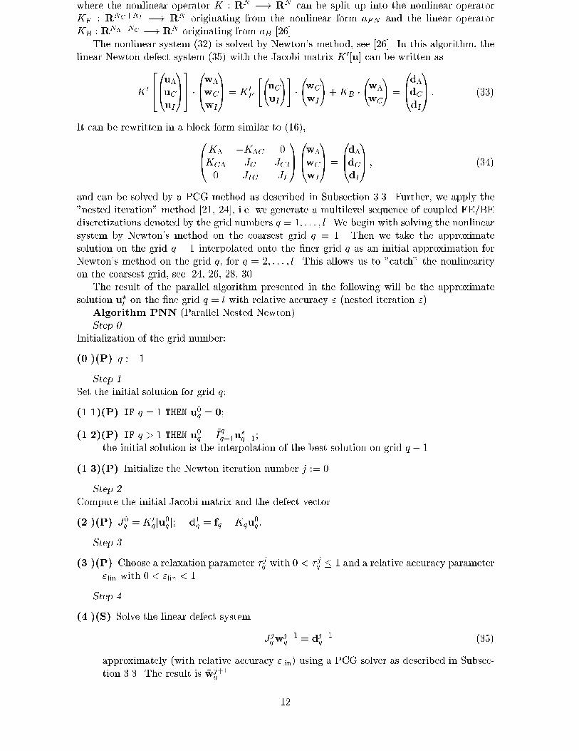
cf. [20], with k being the number of local multigrid iterations, l being the number of grids,the h-independent multigrid rate � < 1, and the h-independent constants ci. Thus, � isindependent of h if k = O(ln lnh�1).In the (S-BPX) case, the inequalities in (25) hold with an h-independent constant C ,and C � c3(1+�) [20, 44]. Therefore, we can prove for (S-BPX) that = � c4(1+�)(p�+p1 + �)2 = O(1) if k = O(ln lnh�1). However, in the range of practical applications, thismeans k = 1 ! For (BPS-D), the estimate C= C � c5(1 + (lnh�1)2)(1 + �) has been proved[3]. In the case (mgD), CC arises from the hypersingular operator and C�1C is realized via astandard multi-grid procedure applied to the global operator (assembled over the subdomains)KC� which is the discretization of a pseudo-di�erential operator of order one. KC� becomespositive de�nite after implementing the Dirichlet boundary conditions. We can get an estimateof the same type as for (S-BPX). Note that the FE/BE{Schur-complement energy is equivalentto the k:k2H1=2(�C){norm (see, e.g., [3, 5, 9]).Consequently, we can estimate the numerical e�ort Q to obtain a relative accuracy " byQ = O(h�2 lnh�1 ln lnh�1 ln"�1) for the (BPS-D) case, and by Q = O(h�2 ln lnh�1 ln"�1)in the (S-BPX) case, i.e. almost optimal. If a BPX-type extension [38] is applied instead of(HExt) in a nested iteration approach [21], we can prove that Q = O(h�2), i.e., we obtain anoptimal method.Preconditioners C�;i for K�;i and CC for the FE/BE Schur complement derived on thebasis of boundary element techniques can also be found in [35, 39]. The construction ofe�cient FE Schur complement preconditioners was one of the main topics in the research onFE-DD-methods (see Proceedings of the annual DD-conferences since 1987).3.4 Numerical ResultsThe electromagnet as shown in Figure 2 serves now as test example for exterior magnetic �eldproblems which lead to the variational form (10). The copper domains (I, II), where we have aII

I

III IVV

VI

VII

VIII

Figure 2: The magnet and the subdomains being used (left) and the equipotential lines ofthe solution (right).current density of the strength S and �S, respectively, and the iron domain (III), are squareswith the edges being 16cm long. The material dependent coe�cients (air: IV{VIII) are givenby �Cu = 795779:0AmV�1s�1; �air = 795774:4AmV�1s�1; �Fe = 1000:0AmV�1s�1:We will compare two di�erent coupling procedures. On the one hand we use the naturalboundary (of the metallic material) as coupling boundary and on the other hand we introducea circle with the radius 50cm as coupling boundary. The advantage of the second method isthat we obtain circulant matrices which can be generated very fast whereas the �rst methodrequires the generation of fully populated matrices. A disadvantage of the second method is10

FEM: I-VIIBEM: VIII FEM: I-IIIBEM: IV-VIII FEM: I-IIIBEM: exteriorl I(") CPU I(") CPU I(") CPU1 15 0.6 17 0.5 14 0.32 19 0.9 18 1.0 19 0.63 20 1.6 19 1.9 20 1.74 21 5.2 21 5.2 21 5.95 23 20.5 22 18.8 22 22.5N(5) 67329 18429 16129Table 1: Number of unknowns (N), iteration count (I("), " = 10�6), CPU time in seconds.The experiments were carried out on a Power-XPlorer using 8 or 4 processors, respectively.that additional subdomains and, thus, additional unknowns have to be introduced. For thisexample, the uniqueness of the solution is guaranteed by the radiation condition, even if noDirichlet boundary �D is present. The radiation condition is implicitly contained in our BEdiscretization.Numerical results are given in Table 1. The operators C�, CC , CI , BI have been chosenas follows: C�;i : Circ (i = 8) and Hyp (i 2 IB n f8g) CC : S-BPXCI;i : V11 (i 2 IF ) BI;i : HExt (i 2 IF ):Comparing the three choices of the subdomains and their discretization, we observe thatin the �rst choice (column 1) much time is spent for handling the FEM subdomains IV, Vwith many interior nodes. We may conclude that the BEM (column 2) is recommended forsubdomains with a high ratio between the numbers of interior FEM nodes and the boundarynodes. The choice of the rectangular coupling boundary (column 3) increases the BEM systemgeneration e�ort, but the total time remains nearly the same since the number of BEMunknowns (and subdomains) is reduced. Finally we observe that the number of iterations isindependent of the combination of BE/FE discretizations being used.4 Parallel Solution of Coupled BE/FE{Equations Approxi-mating Nonlinear Magnetic Field Problems4.1 The Nested-DD-Newton-SolverLet us consider now a nonlinear magnetic �eld problem, i.e., we allow ferromagnetic materialswith non-constant permeability � to be in the FE subdomains. Then, the mixed DD coupledvariational problem can be written as follows: Find (�; u) 2 V := ��U0 such thataN (�; u; �; v) = hF; vi 8(�; v) 2 V; (31)where a(�; u; �; v) := aB(�; u; �; v) + aFN (u; v)aFN (u; v) := Xi2IF Zi �(x; jruj)rTu(x)rv(x) dxand aB being de�ned as in (10). We refer to [25, 30] for the analysis of nonlinear magnetic�eld problems. Consequently, the discretization results in a nonlinear system [26]K 0B@u�uCuI1CA = KF uCuI!+KB � u�uC! = 0B@f�fCfI1CA ; (32)11

where the nonlinear operator K : RN �! RN can be split up into the nonlinear operatorKF : RNC+NI �! RN originating from the nonlinear form aFN and the linear operatorKB : RN�+NC �! RN originating from aB [26].The nonlinear system (32) is solved by Newton's method, see [26]. In this algorithm, thelinear Newton defect system (35) with the Jacobi matrix K 0[u] can be written asK 0 2640B@u�uCuI1CA375 �0B@w�wCwI1CA = K 0F " uCuI!# � wCwI!+KB � w�wC! = 0B@d�dCdI1CA : (33)It can be rewritten in a block form similar to (16),0B@K� �K�C 0KC� JC JCI0 JIC JI1CA0B@w�wCwI1CA = 0B@d�dCdI1CA ; (34)and can be solved by a PCG method as described in Subsection 3.3. Further, we apply the"nested iteration" method [21, 24], i.e. we generate a multilevel sequence of coupled FE/BEdiscretizations denoted by the grid numbers q = 1; : : : ; l. We begin with solving the nonlinearsystem by Newton's method on the coarsest grid q = 1. Then we take the approximatesolution on the grid q � 1 interpolated onto the �ner grid q as an initial approximation forNewton's method on the grid q, for q = 2; : : : ; l. This allows us to "catch" the nonlinearityon the coarsest grid, see [24, 26, 28, 30].The result of the parallel algorithm presented in the following will be the approximatesolution u?l on the �ne grid q = l with relative accuracy " (nested iteration ").Algorithm PNN (Parallel Nested Newton)Step 0Initialization of the grid number:(0.)(P) q := 1.Step 1Set the initial solution for grid q:(1.1)(P) IF q = 1 THEN u0q = 0;(1.2)(P) IF q > 1 THEN u0q = ~Iqq�1u?q�1;the initial solution is the interpolation of the best solution on grid q � 1.(1.3)(P) Initialize the Newton iteration number j := 0.Step 2Compute the initial Jacobi matrix and the defect vector(2.)(P) J0q = K 0q[u0q ]; d1q = fq �Kqu0q :Step 3(3.)(P) Choose a relaxation parameter � jq with 0 < � jq � 1 and a relative accuracy parameter"lin with 0 < "lin < 1.Step 4(4.)(S) Solve the linear defect system J jqwj+1q = dj+1q (35)approximately (with relative accuracy "lin) using a PCG solver as described in Subsec-tion 3.3. The result is ~wj+1q . 12

Step 5Correct the solution:(5.)(P) uj+1q = ujq + � jq ~wj+1q .Step 6Control the convergence (parameter c� is chosen a priori with c� < 1):(6.1)(P) Compute the new defect vector and the new Jacobi matrixdj+2q = fq �Kquj+1q ; J j+1q = K 0q[uj+1q ];(6.2)(C) Compute defect normsdj+1q = kdj+1q k; dj+2q = kdj+2q k;(6.3)(P) IF dj+2q � dj+1q THEN 0B@ � jq := min(c� � jq ; � jq dj+1qdj+1q + dj+2q ) ;GOTO Step 5 1CA;(6.4)(P) IF dj+2q � "d1q THEN 0B@ u?q := uj+1q ;IF q < l THEN (q := q + 1; GOTO Step 1 );IF q = l THEN EXIT; 1CA;(6.5)(P) Perform a further Newton step:j := j + 1;GOTO Step 3.In this description, (P) indicates that the step is performed completely in parallel, i.e.,independently on the processors. The solver (S) includes parallel independent parts, commu-nication between processors handling neighbouring subdomains, and global communication,cf. Subsection 3.3. Note, (C) indicates that global communication is necessary. Obviously, theonly additional communication (compared with solving a linear problem) is the computationof global defect norms.4.2 Numerical Results

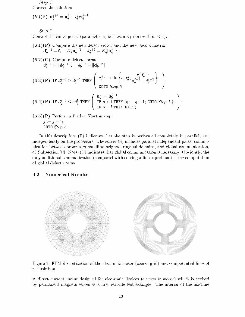
Figure 3: FEM discretization of the electronic motor (coarse grid) and equipotential lines ofthe solution.A direct current motor designed for electronic devices (electronic motor) which is excitedby permanent magnets serves as a �rst real-life test example. The interior of the machine13

is discretized by �nite elements (cf. Figure 3). Calculations have been made for both themachine with homogeneous Dirichlet conditions on its boundary and the in�nite domain withSommerfeld's radiation condition where the in�nite exterior domain is discretized by BEM. Inorder to obtain e�ciency results, we consider additionally two model problems representing aquarter and a half of the whole machine, i.e. we discretize only sectors of 90 and 180 degrees,respectively, and impose Dirichlet conditions on the boundary.Example Dirichlet Dirichlet Dirichlet radiationb. c. b. c. b. c. conditionsubdomains 16 FEM 32 FEM 64 FEM 63 FEM1 BEMNo. of unknowns 374 129 734 199 1 514 008 1 489 416Newton it. 4 5 4 4CG iter. 1st grid 6,11/16,11 6,11/14,11,12 6,11/15,11 6,11/16,13CG iter. 2nd grid 9,10 9,11 9,11 9,11CG iter. 3rd grid 10,12 10,12 10,12 11,13CG iter. 4th grid 11,13 11,13 11,13 11,14CG iter. 5th grid 11,15 11,15 11,15 12,15Newton it. 4 4 4 4CG iter. 6th grid 12,16,9,17 12,17,10,16 13,16,10,16 13,16,10,16generation 21.8 21.6 23.2 26.4linear solver 63.4 64.9 71.7 85.6Total time 85.2 86.5 94.9 112.0Scale-up (norm.) 1.0 ! 1.933 ! 3.633Scaled e�. (rel.) 1.0 ! 0.966 ! 0.908Time in seconds, scale-up (normalized) and scaled e�ciency (relative) on a GC-Power Plususing 16, 32, 64 processors, respectively; 2 Newton iterations on the grids 2{5, relativeaccuracy " = 10�6.Table 2: Performance for a practical problem (electronic motor).The components of the PNN algorithm are chosen in the standard way [23, 24, 28]. Inparticular, the parameter "lin can be adapted to the quadratic convergence speed of theNewton method [24, 30]. Here, a slash (/) marks the change from "lin = 10�2 to "lin = 10�4in the accuracy of the CG solver. The components of the PCG solver have been chosen asfollows: C�;i : Circ (i 2 IB) CC : BPS-DCI;i : V11 (i 2 IF ) BI;i : HExt (i 2 IF ):The components involved and the numerical e�ort for nonlinear problems are discussed in[26]. Numerical results are given in Table 2. We present further results, in particular withrespect to e�ciency, in [30]. Computations with up to 128 processors are documented in[26, 27]. In [28], the application of a parallelized global multigrid method based on DD ideasin Step 4 of the algorithm PNN is discussed. Further, in [29], we demonstrate that the CGwith a global BPX or a global multigrid preconditioner yields a robust solver for practicalproblems.The second practical example, a technical direct current motor (dc motor, see Subsec-tion 2.3), is to demonstrate the complete algorithm. Starting with a user mesh, we applyan automatic domain decomposition procedure (see Subsection 2.3 and Appendix A) and aparallel mesh generator, the basic ideas of which are presented in [11], to obtain the initialmesh (q = 1), which is to be re�ned four times to get the �nal mesh for our computations(q = l = 5). We present the numerical results in Table 3 and the level lines of the solution in14

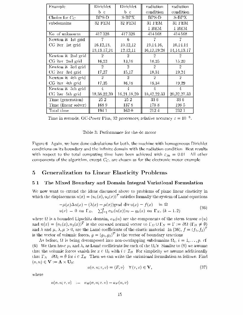
Example Dirichlet Dirichlet radiation radiationb. c. b. c. condition conditionChoice for CC BPS-D S-BPX BPS-D S-BPXsubdomains 32 FEM 32 FEM 31 FEM 31 FEM1 BEM 1 BEMNo. of unknowns 417 328 417 328 414 568 414 568Newton it. 1st grid 7 6 7 7CG iter. 1st grid 16,12,13, 10,12,12 19,14,16, 10,14,1413,13,17,24 12,12,11 16,12,19,28 14,14,13,17Newton it. 2nd grid 2 2 2 2CG iter. 2nd grid 16,23 13,16 18,25 15,20Newton it. 3rd grid 2 2 2 2CG iter. 3rd grid 17,27 15,17 18,31 19,24Newton it. 4th grid 2 2 2 2CG iter. 4th grid 17,35 16,18 18,34 19,29Newton it. 5th grid 4 4 4 4CG iter. 5th grid 18,38,22,30 16,21,18,20 18,42,22,33 20,32,27,33Time (generation) 25.2 25.2 33.6 33.6Time (linear solver) 168.9 137.8 178.8 198.5Total time 194.1 163.0 212.4 232.1Time in seconds, GC-Power Plus, 32 processors; relative accuracy " = 10�6:Table 3: Performance for the dc motor.Figure 6. Again, we have done calculations for both, the machine with homogeneous Dirichletconditions on its boundary and the in�nite domain with the radiation condition. Best resultswith respect to the total computing time have been achieved with "lin = 0:01. All othercomponents of the algorithm, except CC , are chosen as for the electronic motor example.5 Generalization to Linear Elasticity Problems5.1 The Mixed Boundary and Domain Integral Variational FormulationWe now want to extend the ideas discussed above to problems of plane linear elasticity inwhich the displacement u(x) = (u1(x); u2(x))T satis�es formally the system of Lam�e equations��(x)�u(x)� (�(x) + �(x))grad divu(x) = f(x) in u(x) = 0 on �D; P2l=1 �kl(u(x))nl = gk(x) on �N ; (k = 1; 2) (36)where is a bounded Lipschitz domain, �kl(u) are the components of the stress tensor �(u)and n(x) = (n1(x); n2(x))T is the outward normal vector to �D [ �N = � := @ (�D 6= ;)and � and �, �; � > 0; are the Lam�e coe�cients of the elastic material. In (36), f = (f1; f2)Tis the vector of volumic forces, g = (g1; g2)T is the vector of boundary tractions.As before, is being decomposed into non-overlapping subdomains i; i = 1; : : : ; p, cf.(6). We then have �i and �i as Lam�e coe�cients for each of the i's. Similar to (8) we assumethat the volumic forces vanish for x 2 i with i 2 IB. For simplicity we assume additionallythat �N \@i = ; for i 2 IB. Then we can write the variational formulation as follows: Find(�; u) 2 V := ��U0: a(�; u; �; v) = hF; vi 8 (�; v) 2 V; (37)where a(�; u; �; v) := aB(�; u; �; v) + aF (u; v)15

aB(�; u; �; v) := Xi2IB �i �hDiui; vii�i + 12 h�i; vii�i + h�i;Kivii�i+h�i;Vi�ii�i � h�i;Kiuii�i � 12h�i; uii�i�aF (u; v) := Xi2IF Zi 0@�i div u(x) div v(x) + 2�i 2Xk;l=1 �kl(u) �kl(v)1A dxhF; vi := Xi2IF Zi f(x) v(x) dx + Z�N g(x) v(x) ds;with the duality pairing h:; :i, the traces ui = uj@i and the boundary tractions � = [�i]i2IBbelonging to @i and the strain �kl(u) := (@uk=@xl + @ul=@xk)=2: Note, for simplicity wehave assumed that is bounded such that, in contrary to Section 3.1, special terms for theexterior domain do not occur in the de�nition of aB(:; :). Nevertheless, the ideas presentedabove concerning exterior problems can be applied analogously.Let the spaces U0 and � be de�ned as follows:U0 := fu 2 [H1()]2 : uj�BE 2 H1=2(�BE); uj�D = 0g� := Qi2IB hH�1=2(@i)i2 ;where �BE := Si2IB @i n�D;�FE := Si2IF @i n�D;�C := �BE [�FE. Let F := [i2IFi,then we consider the following norm in V:k(�; u)kV := (k�k2� + kuk2H1=2(�BE) + kuk2H1(F ))1=2: (38)The boundary integral operators Vi, Ki and Di are de�ned as in (11), where @(:) has to bereplaced by the operator T (:) which is de�ned in its strong form as T (:) := 2�@(:)+�ndiv u+�n � curl(:) and in its weak form by the �rst Green formula. For E(x; y) we now have toinsert the well known Kelvin fundamental solution (see, e.g., [6]). The variational formulation(37) has a unique solution provided that the single layer potential operators Vi are positivede�nite (H�1=2(@i){elliptic) [6, 32, 40].Similar to Section 3.2 we discretize (37) to obtain a system of equations which is manipu-lated in the same way as discussed in Section 3.3.1. This leads again to a symmetric, positivede�nite system matrix. Thus, the parallel solution can be performed in a similar fashionprovided suitable preconditioners C�, CC , CI and BI are known (see Section 5.2 and [40]).5.2 Numerical ResultsI II

IIIIV

V

VI VII

VIII

water

Dirichlet b.c.

Diri

chle

t b.c

.

Dirichlet b.c. Dirichlet b.c.Figure 4: The subdomains and the BE discretization of the 1st level (left) and the deformed(magni�cation factor 100) FE grid of the 2nd level (right).As a test problem we consider a model of dam �lled with water as sketched in Figure 4. Asindicated there, boundary conditions are given on �D (zero displacement) and on �N (zero or16

BEM: I-VIII FEM: III-VIIIBEM: I-II FEM: I-VIIIl I(") CPU I(") CPU I(") CPU2 27 4.9 25 4.6 25 3.93 27 8.8 28 8.8 28 7.94 28 24.1 30 27.9 31 22.85 29 85.9 31 104.9 32 81.3s(5) 49.5 68.5 63.8N(5) 6470 78130 119318Table 4: Levels (l), pure solution time (s), number of unknowns (N), iteration count (I(")," = 10�6), CPU time in seconds for the dam-problem. The experiments were carried out ona Power-XPlorer using 8 processors.according to the water pressure, respectively). The Lam�e constants are given for rock (I-II)by �r = 7:265e4MPa; �r = 3:743e4MPa and for concrete (III-VIII) by �c = 9:2e6MPa; �c =9:2e6MPa: For the results presented in Table 4, the operators C�, CC , CI , BI have beenchosen as follows:C�;i : mgV (i 2 IB) CC : mgDCI;i : V11(HExt+S) (i 2 IF ) BI;i : HExt+S (i 2 IF ):Here, (mgV) stands for a multigrid-based preconditioner for the single layer potential (see [1]).Furthermore, new algorithms for CI;i and BI;i have been used. In particular, the hierarchicalextension (HExt+S) has been improved by a coarse grid solver and smoothing on the otherlevels [13].The BE discretization of the 1st level and the FE discretization of the 2nd level (deformedmesh) are shown in Figure 4. We use piecewise linear trial functions for the displacements andpiecewise constants for the boundary tractions. The entries of the BE matrices are computedfully analytically.In Table 4 we present several combinations of FE/BE discretizations. Looking at the CPU-time we observe that the FE discretization (column 3) leads to the best results. However, ifwe are interested in the pure solving time s(:) (s(5) for the 5th level is given in Table 4) theBE discretization (�rst column) is of advantage.6 Concluding Remarks and GeneralizationsThe DD-method has turned out to be a powerful tool for establishing the coupled FE/BEvariational formulation and for solving the discrete systems e�ciently on massively parallelcomputers. The results presented here have been obtained using the code FEM BEM [14]which can solve linear and non-linear magnetic �eld problems as well as problems arising inlinear elasticity. The high e�ciency and the scalability of the algorithm has been demon-strated [5, 16, 30, 26, 28, 36].Comparison of "local" DD methods described in this paper with "global" multigrid meth-ods implemented on massively parallel machines as well as workstation clusters is given in[28]. The use and the parallelization of "global\ methods is also discussed in [4]. Othercoupling and solution techniques are studied in [10, 41, 43].The techniques presented here can be generalized to the 3D case provided that fastmatrix-by-vector multiplication routines for the BE matrices, e.g. based on Panel-Clustering-Techniques developed in [22], and asymptotically optimal, or almost optimal components CI(e.g. multigrid preconditioners), BI [38], CC (e.g. BPX) and C� [35, 39, 40] of the precondi-tioners are available. 17

References[1] J. H. Bramble, Z. Leyk, and J. E. Pasciak. The analysis of multigrid algorithms forpseudodi�erential operators of order minus one. Math. Comp., 63:461{478, 1994.[2] J. H. Bramble and J. E. Pasciak. A preconditioning technique for inde�nite systemsresulting from mixed approximations of elliptic problems. Mathematics of Computation,50(181):1{17, 1988.[3] J. H. Bramble, J. E. Pasciak, and A. H. Schatz. The construction of preconditioners forelliptic problems by substructuring I { IV. Mathematics of Computation, 1986, 1987,1988, 1989. 47, 103{134, 49, 1{16, 51, 415{430, 53, 1{24.[4] U. Brink, M. Kreienmeyer, and E. Stein. Di�erent methodologies for coupled BEM andFEM with implementation on parallel computers. In Reports from the Final Confer-ence of the Priority Research Programme Boundary Element Methods 1989{1995, (W.Wendland ed.), Stuttgart, October 1995, Berlin, 1996, Springer Verlag.[5] C. Carstensen, M. Kuhn, and U. Langer. Fast parallel solvers for symmetric boundaryelement domain decomposition equations. Report 499, Johannes Kepler University Linz,Institute of Mathematics, 1995.[6] C. Carstensen and P. Wriggers. On the symmetric boundary element method and thesymmetric coupling of boundary elements and �nite elements. IMA Journal of NumericalAnalysis, 1996. Submitted.[7] M. Costabel. Symmetric methods for the coupling of �nite elements and boundaryelements. In C. A. Brebbia, W. L. Wendland, and G. Kuhn, editors, Boundary ElementsIX, pages 411{420. Springer{Verlag, 1987.[8] M. Costabel. Boundary integral operators on Lipschitz domains: Elementary results.SIAM J. Math. Anal., 19:613{626, 1988.[9] M. Dryja. A capacitance matrix method for Dirichlet problems on polygonal regions.Numerische Mathematik, 39(1):51{64, 1982.[10] S. A. Funken and E. P. Stephan. Fast solvers with multigrid preconditioners for linearFEM{BEM coupling. Preprint, Universit�at Hannover, Institut f�ur Angewandte Mathe-matik, Hannover, 1995.[11] G. Globisch. PARMESH - a parallel mesh generator. Parallel Computing, 21(3):509{524,1995.[12] M. Goppold, G. Haase, B. Heise, and M. Kuhn. Preprocessing in BE/FE domain de-composition methods. Technical Report, Johannes Kepler University Linz, 1996. InPreparation.[13] G. Haase. Hierarchical extension operators plus smoothing in domain decompositionpreconditioners. Report 497, Johannes Kepler University Linz, Institute of Mathematics,1995.[14] G. Haase, B. Heise, M. Jung, and M. Kuhn. FEM BEM - a parallel solver for linearand nonlinear coupled FE/BE-equations. DFG-Schwerpunkt "Randelementmethoden",Report 94-16, University Stuttgart, 1994.[15] G. Haase and U. Langer. The non-overlapping domain decomposition multiplicativeSchwarz method. International Journal of Computer Mathematics, 44:223{242, 1992.18

[16] G. Haase and U. Langer. The e�cient parallel solution of PDEs. Computers Math.Applic., 1996. To appear.[17] G. Haase, U. Langer, and A. Meyer. A new approach to the Dirichlet domain decom-position method. In S. Hengst, editor, Fifth Multigrid Seminar, Eberswalde 1990, pages1{59, Berlin, 1990. Karl{Weierstrass{Institut. Report R{MATH{09/90.[18] G. Haase, U. Langer, and A. Meyer. The approximate dirichlet domain decomposi-tion method. Part I: An algebraic approach. Part II: Applications to 2nd-order ellipticboundary value problems. Computing, 47:137{151 (Part I), 153{167 (Part II), 1991.[19] G. Haase, U. Langer, and A. Meyer. Domain decomposition preconditioners with inexactsubdomain solvers. J. of Num. Lin. Alg. with Appl., 1:27{42, 1992.[20] G. Haase, U. Langer, A. Meyer, and S. V. Nepomnyaschikh. Hierarchical extensionoperators and local multigrid methods in domain decomposition preconditioners. East-West J. Numer. Math., 2(3):173{193, 1994.[21] W. Hackbusch. Multi{Grid methods and applications, volume 4 of Springer Series inComputational Mathematics. Springer{Verlag, Berlin, 1985.[22] W. Hackbusch, L. Lage, and S. A. Sauter. On the e�cient realization of sparse matrixtechniques for integral equations with focus on panel clustering, cubature and softwaredesign aspects. In Reports from the Final Conference of the Priority Research ProgrammeBoundary Element Methods 1989{1995, (W. Wendland ed.), Stuttgart, October 1995,Berlin, 1996, Springer Verlag.[23] B. Heise. Mehrgitter{Newton{Verfahren zur Berechnung nichtlinearer magnetischerFelder. Wissenschaftliche Schriftenreihe 4/1991, Technische Universit�at Chemnitz, 1991.[24] B. Heise. Nonlinear �eld calculations with multigrid-Newton methods. IMPACT ofComputing in Science and Engineering, 5:75{110, 1993.[25] B. Heise. Analysis of a fully discrete �nite element method for a nonlinear magnetic �eldproblem. SIAM J. Numer. Anal., 31(3):745{759, 1994.[26] B. Heise. Nonlinear �eld simulation with FE domain decomposition methods on massivelyparallel computers. 1995. Submitted to Surveys on Mathematics for Industry.[27] B. Heise. Nonlinear simulation of electromagnetic �elds with domain decompositionmethods on MIMD parallel computers. Journal of Computational and Applied Mathe-matics, 62, 1995. To appear.[28] B. Heise and M. Jung. Comparison of parallel solvers for nonlinear elliptic problemsbased on domain decomposition ideas. Report 494, Johannes Kepler University Linz,Institute of Mathematics, 1995.[29] B. Heise and M. Jung. Robust parallel multilevel methods. 1995. Submitted for Publi-cation.[30] B. Heise and M. Kuhn. Parallel solvers for linear and nonlinear exterior magnetic �eldproblems based upon coupled FE/BE formulations. Computing, 1996. To appear. AlsoReport No. 486, Inst. of Mathematics, Univ. Linz, 1995.[31] S. Holzer. On the engineering analysis of 2D problems by the symmetric Galerkin bound-ary element method and coupled BEM/FEM. In J. H. Kane, G. Maier, N. Tosaka, andS. N. Atluri, editors, Advances in boundary element techniques, Berlin / New York /Heidelberg, 1992. Springer. 19

[32] G. C. Hsiao, B. N. Khoromskij, and W. L. Wendland. Boundary integral operators anddomain decomposition. Preprint 94{11, Universit�at Stuttgart, Mathematisches InstitutA, Stuttgart, 1994.[33] G. C. Hsiao and W. L. Wendland. Domain decomposition in boundary element methods.In Proc. of IV Int. Symposium on Domain Decomposition Methods, (R. Glowinski, Y.A. Kuznetsov, G. Meurant, J. P�eriaux, O. B. Widlund eds.), Moscow, May 1990, pages41{49, Philadelphia, 1991. SIAM Publ.[34] B. N. Khoromskij, G. E. Mazurkevich, and E. P. Zhidkov. Domain decomposition methodfor magnetostatics nonlinear problems in combined formulation. Sov. J. Numer. Anal.Math. Modelling, 5(2):111{136, 1990.[35] B. N. Khoromskij and W. L. Wendland. Spectrally equivalent preconditioners for bound-ary equations in substructuring techniques. East{West Journal of Numerical Mathemat-ics, 1(1):1{26, 1992.[36] M. Kuhn and U. Langer. Parallel algorithms for symmetric boundary element equations.ZAMM, 1995. Submitted for publication.[37] U. Langer. Parallel iterative solution of symmetric coupled FE/BE- equations via domaindecomposition. Contemporary Mathematics, 157:335{344, 1994.[38] S. V. Nepomnyaschikh. Optimal multilevel extension operators. Preprint SPC 95{3,Technische Universit�at Chemnitz{Zwickau, Fakult�at f�ur Mathematik, 1995.[39] S. Rjasanow. Vorkonditionierte iterative Au �osung von Randelementgleichungen f�urdie Dirichlet{Aufgabe. Wissenschaftliche Schriftenreihe 7/1990, Technische Universit�atChemnitz, 1990.[40] S. Rjasanow. Optimal preconditioner for boundary element formulation of the dirichletproblem in elasticity. Math. Methods in the Applied Sciences, 18:603{613, 1995.[41] E. Schnack and K. T�urke. Coupling of FEM and BEM for elastic structures. In Re-ports from the Final Conference of the Priority Research Programme Boundary ElementMethods 1989{1995, (W. Wendland ed.), Stuttgart, October 1995, Berlin, 1996, SpringerVerlag.[42] H. D. Simon. Partitioning of unstructured problems for parallel processing. Comput.System in Eng., 2:135{148, 1991.[43] O. Steinbach and W. L. Wendland. E�cient preconditioners for boundary element meth-ods and their use in domain decomposition. DFG-Schwerpunkt "Randelementmetho-den", Report 95-19, University Stuttgart, 1995.[44] C. H. Tong, T. F. Chan, and C. J. Kuo. A domain decomposition preconditioner basedon a change to a multilevel nodal basis. SIAM J. Sci. Stat. Comput., 12(6):1486{1495,1991.

20

A The Direct Current Motor

Figure 5: Initial triangular-based description and �nal decomposition of the dc-motor into 32subdomains.

Figure 6: The mesh of the 1st level and the equipotential lines of the solution (dc-motor).

21

B The Parallel AlgorithmFEM (i 2 IF ) BEM (i 2 IB)0. Starting stepChoose an initial guess u = u0ui = " uC;iuI;i # ui = " u�;iuC;i #rI;i = fI;i �KIC;iuC;i �KI;iuI;i v�;i = f�;i �K�;iu�;i +K�C;iuC;ir�;i = C�1�;iv�;irC;i = fC;i �KC;iuC;i �KCI;iuI;i rC;i = fC;i �KC;iuC;i �KC�;iu�;irC;i = rC;i �KC�;ir�;ivC;i = rC;i �KCI;iB�TI;i rI;i w�;i = r�;i; pi = v�;ivC;i = rC;i; z�;i = K�;iw�;iwC;i = AC;iwC wC = C�1C Ppi=1ATC;ivC;i ! wC;i = AC;iwCwI;i = C�1I;i rI;i �B�1I;iKIC;iwC;i z�C;i = K�C;iwC;i; zC;i = KC;iwC;is = w s = w�i = rTC;iwC;i + rTI;iwI;i �i = rTC;iwC;i +wT�;i(z�;i � pi)� = �0 =Ppi=1 �iIteration1. vI;i = KIC;isC;i +KI;isI;i w�;i = z�;i � z�C;iv�;i = C�1�;iw�;ivC;i = KC;isC;i +KCI;isI;i vC;i = zC;i +KC�;i(s�;i � v�;i)�i = vTCsC + vTI;isI;i �i = vTC;isC;i + vT�;iz�;i �wT�;is�;i� =Ppi=1 �i� = �=� � = �=�2. ui = ui + �si ui = ui + �siri = ri � �vi ri = ri � �vi3. vC;i = rC;i �KCI;iB�TI;i rI;i vC;i = rC;i; h�;i = K�;ir�;iwC;i = AC;iwC wC = C�1C Ppi=1ATC;ivC;i ! wC;i = AC;iwCwI;i = C�1I;i rI;i �B�1I;iKIC;iwC;i w�;i = r�;i; pi = pi � �w�;ih�C;i = K�C;iwC;ihC;i = KC;iwC;i4. �i = rTC;iwC;i + rTI;iwI;i �i = rTC;iwC;i + hT�;ir�;i � pTi r�;i� =Ppi=1 �i� = �=� � = �=�5. si = wi + �si si = wi + �si; zi = hi + �zi6. If � � "2 � �0, then STOPelse goto step 1.22