ERROR ANALYSIS FOR A FINITE ELEMENT APPROXIMATION OF ELLIPTIC DIRICHLET BOUNDARY CONTROL PROBLEMS S. MAY * , R. RANNACHER *‡ , AND B. VEXLER †‡ Abstract. We consider the Galerkin finite element approximation of an elliptic Dirichlet bound- ary control model problem governed by the Laplacian operator. The functional theoretical setting of this problem uses L 2 controls and a “very weak” formulation of the state equation. However, the corresponding finite element approximation uses standard continuous trial and test functions. For this approximation, we derive a priori error estimates of optimal order, which are confirmed by numerical experiments. The proofs employ duality arguments and known results from the L p error analysis for the finite element Dirichlet and Neumann projection. Key words. Dirichlet boundary control, finite elements, a priori error estimates. AMS subject classifications. 65K10, 65N30, 65N21, 49M25, 49K20. 1. Introduction and statement of results. We consider the following elliptic Dirichlet boundary control problem posed on a convex polygonal domain Ω ⊂ R 2 with boundary Γ = ∂ Ω: min J (u, q) := 1 2 ku - u d k 2 L 2 (Ω) + α 2 kqk 2 L 2 (Γ) (1.1) with respect to {u, q} , under the constraint -Δu = f in Ω, u = q on Γ. (1.2) Here, u d and f are sufficiently smooth prescribed functions, while α> 0 is a regularization parameter. For simplicity, we assume that at least u d ,f ∈ L 2 (Ω) . The natural functional analytic setting of this problem, which is also most convenient for numerical approximation, uses Q := L 2 (Γ) as “control space”. This prohibits the choice of the associated “state space” to be H 1 (Ω) as the trace operator γ : H 1 (Ω) → L 2 (Γ) is not surjective. To overcome this dilemma, we use a “very weak” formulation of the state equation (1.2) allowing for solutions u ∈ L 2 (Ω) (see Grisvard [9], [10], and Berggren [3]): For given q ∈ L 2 (Γ) find u ∈ L 2 (Ω) such that -(u, Δϕ)+ hq,∂ n ϕi =(f,ϕ) ∀ϕ ∈ H 1 0 (Ω) ∩ H 2 (Ω). (1.3) Here, (·, ·)=(·, ·) L 2 (Ω) is the L 2 inner product on the domain Ω and h·, ·i = h·, ·i L 2 (Γ) that on its boundary Γ . The corresponding norms are k·k = k·k L 2 (Ω) and |·| = |·| L 2 (Γ) , respectively. There are alternative variational formulations of Dirichlet boundary optimal control problems of the type (1.1), (1.2). For a brief survey, we refer to Kunisch/Vexler [12]. However, the formulation considered here appears to be the most attractive one from the computational point of view. The finite element discretization of this optimization problem uses a standard weak formulation of the state equation which is possible due to higher regularity of * Institute of Applied Mathematics, University of Heidelberg, Im Neuenheimer Feld 294, D-69120 Heidelberg, Germany. † Centre for Mathematical Sciences, Technische Universit¨at M¨ unchen, Bolzmannstraße 3, D-85747 Garching b. M¨ unchen, Germany ‡ This work has been supported by the German Research Foundation (DFG) within the Priority Programme 1253 “Optimization with Partial Differential Equations”. 1

Welcome message from author
This document is posted to help you gain knowledge. Please leave a comment to let me know what you think about it! Share it to your friends and learn new things together.
Transcript

ERROR ANALYSIS FOR A FINITE ELEMENT APPROXIMATIONOF ELLIPTIC DIRICHLET BOUNDARY CONTROL PROBLEMS
S. MAY∗, R. RANNACHER∗‡ , AND B. VEXLER†‡
Abstract. We consider the Galerkin finite element approximation of an elliptic Dirichlet bound-ary control model problem governed by the Laplacian operator. The functional theoretical settingof this problem uses L2 controls and a “very weak” formulation of the state equation. However,the corresponding finite element approximation uses standard continuous trial and test functions.For this approximation, we derive a priori error estimates of optimal order, which are confirmed bynumerical experiments. The proofs employ duality arguments and known results from the Lp erroranalysis for the finite element Dirichlet and Neumann projection.
Key words. Dirichlet boundary control, finite elements, a priori error estimates.
AMS subject classifications. 65K10, 65N30, 65N21, 49M25, 49K20.
1. Introduction and statement of results. We consider the following ellipticDirichlet boundary control problem posed on a convex polygonal domain Ω ⊂ R2 withboundary Γ = ∂Ω :
min J(u, q) := 12‖u− ud‖
2L2(Ω) + α
2 ‖q‖2L2(Γ) (1.1)
with respect to u, q , under the constraint
−∆u = f in Ω, u = q on Γ. (1.2)
Here, ud and f are sufficiently smooth prescribed functions, while α > 0 is aregularization parameter. For simplicity, we assume that at least ud, f ∈ L2(Ω) .The natural functional analytic setting of this problem, which is also most convenientfor numerical approximation, uses Q := L2(Γ) as “control space”. This prohibits thechoice of the associated “state space” to be H1(Ω) as the trace operator γ : H1(Ω)→L2(Γ) is not surjective. To overcome this dilemma, we use a “very weak” formulationof the state equation (1.2) allowing for solutions u ∈ L2(Ω) (see Grisvard [9], [10],and Berggren [3]): For given q ∈ L2(Γ) find u ∈ L2(Ω) such that
−(u,∆ϕ) + 〈q, ∂nϕ〉 = (f, ϕ) ∀ϕ ∈ H10 (Ω) ∩H2(Ω). (1.3)
Here, (·, ·) = (·, ·)L2(Ω) is the L2 inner product on the domain Ω and 〈·, ·〉 = 〈·, ·〉L2(Γ)
that on its boundary Γ . The corresponding norms are ‖ · ‖ = ‖ · ‖L2(Ω) and | · | =| · |L2(Γ) , respectively. There are alternative variational formulations of Dirichletboundary optimal control problems of the type (1.1), (1.2). For a brief survey, werefer to Kunisch/Vexler [12]. However, the formulation considered here appears to bethe most attractive one from the computational point of view.
The finite element discretization of this optimization problem uses a standardweak formulation of the state equation which is possible due to higher regularity of
∗Institute of Applied Mathematics, University of Heidelberg, Im Neuenheimer Feld 294, D-69120Heidelberg, Germany.†Centre for Mathematical Sciences, Technische Universitat Munchen, Bolzmannstraße 3, D-85747
Garching b. Munchen, Germany‡This work has been supported by the German Research Foundation (DFG) within the Priority
Programme 1253 “Optimization with Partial Differential Equations”.
1

2 S. MAY, R. RANNACHER, AND B. VEXLER
the actual solution pair u, q . For this approximation the estimate
|q − qh|+ ‖u− uh‖ = O(h1−1/p) (1.4)
has been given in Casas/Raymond [5] for a problem with additional inequality con-straints for the control q , which was expected to be only suboptimal for the state.The contribution of this paper consists in the improved L2-error estimate
‖u− uh‖ = O(h3/2−1/p). (1.5)
and in “optimal-order” error estimates with respect to weaker norms of the form
|q − qh|H−1/2(Γ) = O(h3/2−1/p−1/r), ‖u− uh‖H−1(Ω) = O(h2−1/p−1/r). (1.6)
Here, the values of p ∈ [2, pd∗) and r ∈ [2, pΩ∗ ) depend on the regularity of the data
and the limited elliptic regularity on domains with corners, respectively. Further, forthe associated adjoint state the error estimate
‖z − zh‖ = O(h2−1/p−1/r) (1.7)
is obtained. In view of the results of the computational experiments presented atthe end of this paper, these estimates for the primal state and the control seem tobe order-optimal. For maximum regularity, e.g., for smooth data on a rectangulardomain, almost the order O(h2) of convergence is obtained which is best possible forlinear or bilinear finite elements. The proofs employ duality arguments based on theKKT system (Karush-Kuhn-Tucker system) associated to the optimization problem(1.1), (1.2) and uses various results from the finite element error analysis in Lp forp 6= 2 .
The contents of this paper is organized as follows. Section 2 contains the varia-tional formulation of the Dirichlet boundary control problem and its Galerkin finiteelement approximation. This includes the derivation of the continuous and discreteKKT systems representing the first order necessary optimality conditions which formthe basis of the error analysis. In Section 3 several auxiliary results on elliptic regu-larity and finite element approximation are provided. These are used in Section 4 toprove some suboptimal-order error estimates, followed by the final optimal-order onesin Section 5. The last Section 6 contains the results of some test calculations madeto check the theoretical predictions.
2. The Dirichlet boundary control problem.
2.1. The state equation in “very weak” form. For later use, we providesome notation and results from the theory of Sobolev spaces and elliptic boundaryvalue problems. The standard Sobolev spaces on Ω and Γ will be denoted by Hs(Ω) ,Hs
0(Ω) , W s,p(Ω) , and Hs(Γ) , respectively, for s ∈ R+ and 1 ≤ p ≤ ∞ (seeAdams/Fournier [1]). For functions v ∈ H1(Ω) the “strong” traces v|Γ ∈ L2(Γ)exist and form the natural “trace space” H1/2(Γ) equipped with the generic norm
|v|H1/2(Γ) := inf‖ψ‖H1(Ω), ψ ∈ H1(Ω), ψ|Γ = v
.
Accordingly, we have the following “trace inequality” for functions v ∈ H1(Ω) :
|v|H1/2(Γ) ≤ c‖v‖H1(Ω). (2.1)
FINITE ELEMENTS FOR ELLIPTIC BOUNDARY CONTROL 3
For right hand side f ∈ L2(Ω) and boundary function q ∈ H1/2(Γ) the boundaryvalue problem (1.2) has a standard “weak” solution u ∈ H1(Ω) , which is determinedby u|Γ = q and
(∇u,∇ϕ) = (f, ϕ) ∀ϕ ∈ H10 (Ω). (2.2)
For q = 0 , this weak solution is in H2(Ω) as Ω is a convex polygonal domain.Furthermore, it obeys the a priori bound
‖u‖H2(Ω) ≤ c‖f‖. (2.3)
Let H−1/2(Γ) denote the dual space of H1/2(Γ) equipped with the natural norm
|v|H−1/2(Γ) := supχ∈H1/2(Γ)
〈v, χ〉|χ|H1/2(Γ)
.
For functions v ∈ H2(Ω) the gradient ∇v has a trace ∇v|Γ ∈ H1/2(Γ)2 . On adomain with smooth boundary Γ the outer normal unit vector n is continuous and,thus, the normal derivative ∂nv = n · ∇v ∈ H1/2(Γ) is well defined for functionsv ∈ H2(Ω) and satisfies
|∂nv|H1/2(Γ) ≤ c‖v‖H2(Ω), v ∈ H2(Ω). (2.4)
This estimate does not make sense if Γ is polygonal, i.e. only Lipschitz continuous.But for v ∈ H2(Ω), we still have ∂nv|Γi
∈ H1/2(Γi) on each of the straight compo-nents Γi, i = 1, . . . ,m, of Γ . Accordingly, we introduce the space H1/2(Γ) := q ∈L2(Γ), q ∈ H1/2(Γi), i = 1, . . . ,m . Further, on L2(Γ) , we define the dual norm
|v|H−1/2(Γ) := supψ∈H1
0 (Ω)∩H2(Ω)
〈v, ∂nψ〉‖ψ‖H2(Ω)
≤ supχ∈H1/2(Γ)
〈v, χ〉|χ|H1/2(Γ)
and denote by H−1/2(Γ) the completion of L2(Γ) with respect to this norm. In thecase of a smooth boundary Γ , the mapping ∂n : H1
0 (Ω) ∩H2(Ω)→ H1/2(Γ) is ontoand we therefore have H−1/2(Γ) = H−1/2(Γ) .
The following lemma states the well-posedness of the general boundary value prob-lem (1.3) in the “very weak” form. As a special case it also guarantees the existenceof the “very weak” harmonic extension of general boundary data q ∈ H−1/2(Γ) .
Lemma 2.1. For any given q ∈ H−1/2(Γ) the state equation in its “very weak”form (1.3) possesses a unique solution u = u(q) ∈ L2(Ω) . There holds the a prioriestimate
‖u‖ ≤ c|q|H−1/2(Γ) + c‖f‖H−2(Ω), (2.5)
where H−2(Ω) denotes the dual space of H10 (Ω) ∩H2(Ω) .
Proof. First, suppose that q ∈ H1/2(Γ) and f ∈ H−1(Ω) . Then, there exists aunique “weak” solution u = u(q) ∈ H1(Ω) of the boundary value problem (2.2). Byintegration by parts, we find that this solution fulfills
−(u,∆ϕ) + 〈q, ∂nϕ〉 = (f, ϕ) ∀ϕ ∈ H10 (Ω) ∩H2(Ω).
To prove the a priori estimate, we use a duality argument. Let w ∈ H10 (Ω) be the
solution of the auxiliary problem
−∆w = u in Ω, w|Γ = 0.

4 S. MAY, R. RANNACHER, AND B. VEXLER
By elliptic regularity, we have w ∈ H2(Ω) and conclude
‖u‖2 = (u,−∆w) = (f, w)− 〈q, ∂nw〉.
Hence, using the dual norms defined above gives us
‖u‖2 ≤ c‖f‖H−2(Ω) + |q|H−1/2(Γ)
‖w‖H2(Ω).
Since ‖w‖H2(Ω) ≤ c‖u‖ , the a priori estimate (2.5) follows. Now, since the subspacesH−1(Ω) ⊂ H−2(Ω) and H1/2(Γ) ⊂ H−1/2(Γ) are dense, the existence of a solutionto the very weak variational problem for given data f ∈ H−2(Ω) and q ∈ H−1/2(Γ)follows by a standard continuation argument. The a priori bound (2.5) carries overto these solutions by continuity and therefore also implies uniqueness.
We will call a function v ∈ L2(Ω) “very weakly harmonic” if it satisfies
(v,∆ϕ)− 〈q, ∂nϕ〉 = 0 ∀ϕ ∈ H10 (Ω) ∩H2(Ω), (2.6)
with some function q ∈ H−1/2(Γ) . Then, the function q is the “very weak” trace ofv on Γ . For this, almost by definition, we have the following trace estimate:
|q|H−1/2(Γ) = supψ∈H1
0 (Ω)∩H2(Ω)
(v,∆ψ)‖ψ‖H2(Ω)
≤ c‖v‖. (2.7)
We also call Bq := v the “harmonic extension” of the boundary data q ∈ H−1/2(Γ)to Ω . For q ∈ H1/2(Γ) , there holds Bq ∈ H1(Ω) and
(∇Bq,∇ϕ) = 0 ∀ϕ ∈ H10 (Ω), Bq|Γ = q. (2.8)
In the course of the further analysis, we will frequently use certain Sobolev traceinequalities and a priori bounds for the harmonic extension. From Grisvard [9, The-orem 1.5.1.2 f.] and the literature cited therein, we have the following result.
Lemma 2.2. Let Ω ∈ Rd be a bounded domain with Lipschitz boundary Γ . For1 < p <∞ and s < 1 + 1/p , such that s− 1/p is not an integer, the trace operatoris continuously defined from W s,p(Ω) onto W s−1/p,p(Γ) , with a right continuousinverse, and there holds
|v|W s−1/p,p(Γ) ≤ c‖v‖W s,p(Ω). (2.9)
Particularly, the harmonic extension is continuously defined from W s−1/p,p(Γ) intoW s,p(Ω) and satisfies
‖Bq‖W s,p(Ω) ≤ c|q|W s−1/p,p(Γ). (2.10)
We note that in [9] the result of Lemma 2.2 is stated for 1/p < s < 1 + 1/p , andonly the existence of a linear extension operator satisfying (2.10) is claimed. Here, weassume that the estimate (2.9) holds for the slightly larger parameter range 0 < s <1 + 1/p and that the estimate (2.10) actually holds for the harmonic extension.
The following lemmas collect some further properties of the trace operator andthe harmonic extension which are not directly contained in Lemma 2.2.
Lemma 2.3. Let Ω ⊂ R2 be a bounded convex polygonal domain with bound-ary Γ .
FINITE ELEMENTS FOR ELLIPTIC BOUNDARY CONTROL 5
(i) For any fixed p > 2 , the trace operator is continuously defined from W 1/2,p(Ω)into Lp(Γ) and there holds
|v|Lp(Γ) ≤ c‖v‖W 1/2,p(Ω). (2.11)
(ii) For v ∈ H10 (Ω) ∩W 2,p(Ω) , 2 < p < pΩ
∗ , with pΩ∗ defined in (2.32) below, the
normal derivative ∂nv exists in W 1−1/p,p(Γ) and there holds
|∂nv|W 1−1/p,p(Γ) ≤ c‖v‖W 2,p(Ω). (2.12)
In the exceptional case p = 2, the normal derivative ∂nv exists in Hs(Γ) for 0 ≤s < 1/2 and there holds
|∂nv|Hs(Γ) ≤ c‖v‖H2(Ω). (2.13)
(iii) For q ∈ H1−1/p(Γ) , 2 ≤ p <∞ , the normal derivative ∂nBq ∈ H−1/p(Γ) existsand there holds
|∂nBq|H−1/p(Γ) ≤ c|q|H1−1/p(Γ). (2.14)
In all cases the constants c may depend on p or s , respectively.Proof. (i) For the estimate (2.11), we refer to Scott [17].
(ii) The estimate (2.12) can be derived by using the estimate (2.11) for the partialderivatives ∂iv and observing that ∂nv(x) → 0 as x approaches a corner point ofΓ . For details see Jakovlev [11] where also the estimate (2.13) can be found.(iii) For q ∈ H1−1/p(Γ) the results of Lemma 2.2, for s = 3/2 − 1/p , imply thatBq ∈ H3/2−1/p(Ω) and thus ∇Bq ∈ H1/2−1/p(Ω)2 . Then, again using Lemma 2.2,we obtain ∂nBq ∈ H−1/p(Γ) and the asserted estimate (2.14). This completes theproof.
Lemma 2.4. For functions v ∈W 1,p(Ω) , 1 < p <∞ , there holds
|v|Lp(Γ) ≤ ε‖∇v‖Lp(Ω) + cp1
p−1 ε−1
p−1 ‖v‖Lp(Ω), 0 < ε ≤ 1. (2.15)
Proof. For completeness, we supply the simple proof (see also Grisvard [9, Theo-rem 1.5.1.10]. Let p′ = p(p− 1)−1 . By the usual trace inequality for W 1,1 functions,there holds
|v|pLp(Γ) ≤ c‖vp‖L1(Ω) + c‖∇vp‖L1(Ω).
Then, using Holder’s and Young’s inequality gives us
|v|pLp(Γ) ≤ c‖v‖pLp(Ω) + cp‖∇v‖Lp(Ω)‖vp−1‖Lp′ (Ω)
= c‖v‖pLp(Ω) +(ε‖∇v‖Lp(Ω)
)(cε−1p‖v‖p−1
Lp(Ω)
)≤ c‖v‖pLp(Ω) + εp‖∇v‖pLp(Ω) + cp
′pp′ε−p
′‖v‖pLp(Ω).
This implies the asserted estimate.
6 S. MAY, R. RANNACHER, AND B. VEXLER
2.2. The optimization problem. For deriving existence results for the opti-mization problem considered, we define the “solution operator” S : L2(Γ) → L2(Ω)by Sq = u(q) = u and
−(u,∆ϕ) + 〈q, ∂nϕ〉 = (f, ϕ) ∀ϕ ∈ H10 (Ω) ∩H2(Ω).
This operator is affine linear and continuous due to the a priori estimate (2.5). Then,the optimization problem can be rephrased in the following compact form:
j(q) := J(Sq, q)→ min for q ∈ L2(Γ). (2.16)
Lemma 2.5. The optimization problem (1.1) together with the very weak formu-lation (1.3) of the state equation possesses a uniquely determined solution u, q ∈L2(Ω)×L2(Γ) . This solution satisfies the necessary and in this case also the sufficientoptimality condition
〈j′(q), χ〉 = 0 ∀χ ∈ L2(Γ), (2.17)
with the derivative j′(q) : L2(Γ)→ L2(Γ)∗ ' L2(Γ) .Proof. (i) The proof of existence is by the direct method of variational calculus.
The reduced functional j(·) is bounded from below on L2(Γ) and strictly convex sincethe solution operator S is affine linear. Therefore, it is weakly lower semicontinuousin L2(Γ) . Hence, there exists a minimizing sequence (qk)k∈N , infq∈L2(Γ) j(q) =limk→∞ j(qk) , which is bounded in L2(Γ) due to the coercivity of j(·) on L2(Γ) .For any of its weak accumulation points q there holds j(q) ≤ limk→∞ j(qk) . Suchan accumulation point is a unique global minimum of the reduced functional.(ii) To prove the necessary optimality condition, we note that
1ε
(j(q + εχ)− j(q)
)≥ 0,
for any χ ∈ L2(Γ) . Then, letting ε → 0 yields 〈j′(q), χ〉 ≥ 0 for all χ ∈ L2(Γ) ,which implies (2.17). As the reduced cost functional is strictly convex, the condition(2.17) is not only necessary but also sufficient.
Lemma 2.6. The directional derivative of j(·) at some point q ∈ L2(Γ) is givenby
j′(q)(χ) = α〈q, χ〉 − 〈∂nz, χ〉 (2.18)
for χ ∈ L2(Γ) , where z = z(q) ∈ H10 (Ω) ∩ H2(Ω) is the solution of the associated
“adjoint problem”
−(ψ,∆z) = (Sq − ud, ψ) ∀ψ ∈ L2(Ω). (2.19)
Proof. We introduce the Lagrangian functional L : L2(Ω) × L2(Γ) × H10 (Ω) ∩
H2(Ω)→ R by L(u, q, z) := J(u, q) + (f, z) + (u,∆z) − 〈q, ∂nz〉 . Then, with u(q) = Sq ,there holds j(q) = J(u(q), q) = L(u(q), q, z(q)) , and for χ ∈ L2(Γ) :
j′(q)(χ) = L′u(u(q), q, z(q))(u′q(q)(χ)) + L′q(u(q), q, z(q))(χ)
+ L′z(u(q), q, z(q))(z′q(q)(χ)).
FINITE ELEMENTS FOR ELLIPTIC BOUNDARY CONTROL 7
Since by construction L′u(u(q), q, z(q))(·) = 0 and L′z(u(q), q, z(q))(·) = 0 , we obtain
j′(q)(χ) = L′q(u(q), q, z(q))(χ) = α〈χ, q〉 − 〈χ, ∂nz〉,
which proves the asserted representation.As a consequence of the foregoing lemmas, we have the following result.Lemma 2.7. The solution of the optimization problem (1.1), (1.3) is characterized
by the Euler-Lagrange principle stating that the pair u, q ∈ L2(Ω) × L2(Γ) is asolution if and only if there exists an “adjoint state” z ∈ H1
0 (Ω) ∩H2(Ω) , such thatthe triplet u, q, z solves the “optimality system” (Karush-Kuhn-Tucker system)
−(u,∆ϕ) + 〈q, ∂nϕ〉 = (f, ϕ) ∀ϕ ∈ H10 (Ω) ∩H2(Ω), (2.20)
α〈q, χ〉 − 〈∂nz, χ〉 = 0 ∀χ ∈ L2(Γ), (2.21)
−(ψ,∆z)− (u, ψ) = −(ud, ψ) ∀ψ ∈ L2(Ω). (2.22)
Proof. Let u, q ∈ L2(Ω) × L2(Γ) be a solution of the optimization problem.Then, by definition there hold (2.20) and (2.22). The necessary condition (2.17) andthe representation (2.18) of j′(·) imply (2.21). In turn, for each solution u, q, z ∈L2(Ω)×L2(Γ)×H1
0 (Ω)∩H2(Ω) of the KKT system, the necessary (and sufficient)optimality condition (2.17) is satisfied implying that q is a minimum.
2.3. Galerkin finite element approximation. For the approximation of theoptimization problem (1.1), (1.3), we consider a finite element method. Let Vh ⊂H1(Ω) be finite element subspaces defined on meshes Th = K consisting of trian-gles or quadrilaterals and satisfying the usual conditions of shape and size regular-ity. These meshes are characterized by the mesh-width parameter h ∈ (0, 1] whereh ≈ maxdiam(K), K ∈ Th . Further, we set Vh,0 := Vh ∩ H1
0 (Ω) and let V ∂h bethe trace space corresponding to Vh . For simplicity, we only consider lowest-orderfinite elements, i.e., piecewise linear or bilinear trial and test functions. The discretesolutions uh, qh ∈ Vh × V ∂h are determined by the discrete optimization problems
J(uh, qh) = minuh∈Vh,qh∈V ∂
h
J(uh, qh), (2.23)
under the constraints
(∇uh,∇ϕh) = (f, ϕh) ∀ϕh ∈ Vh,0, uh|Γ = qh . (2.24)
By analogous arguments as used for the continuous optimization problem (1.1), (1.3),we see that their discrete counterparts (2.23), (2.24) possess uniquely determinedsolutions. These solutions may be computed by applying the gradient or the Newtonmethod for the discrete reduced functional jh(qh) := J(Shqh, qh) , which requires theevaluation of first and second directional derivatives of jh(·) . Here, Sh : V ∂h → Vhdenotes the discrete solution operator defined by Shqh = uh(qh) = uh and (2.24).This equation may be rewritten in the form
(∇vh,∇ϕh) + (∇Bhqh,∇ϕh) = (f, ϕh) ∀ϕh ∈ Vh,0, (2.25)
for the function vh := uh − Bhqh ∈ Vh,0 , where Bh : V ∂h → Vh is an arbitraryextension operator of discrete boundary data to all of Ω .
8 S. MAY, R. RANNACHER, AND B. VEXLER
Lemma 2.8. With the foregoing notation the first directional derivative of jh(·)at some point qh ∈ V ∂h is given by
j′h(qh)(χh) = α〈χh, qh〉+ (Bhχh, uh − ud)− (∇Bhχh,∇zh), (2.26)
for χh ∈ V ∂h , where uh = Shqh and zh = zh(qh) ∈ Vh,0 is the solution of the“discrete adjoint problem”
(∇ψh,∇zh) = (uh − ud, ψh) ∀ψh ∈ Vh,0. (2.27)
Proof. The argument is analogous to that used in Lemma 2.6 on the continuouslevel. For the discrete Lagrangian functional Lh : Vh,0 × V ∂h × Vh,0 → R , defined by
Lh(vh, qh, zh) := J(vh +Bhqh, qh) + (f, zh)− (∇vh,∇zh)− (∇Bhqh,∇zh),
we have jh(qh) = J(vh +Bhqh, qh) = Lh(vh, qh, zh(qh)) . Further,
j′h(qh)(χh) = L′h,v(vh, qh, zh(qh))(v′h,q(χh)) + L′h,q(vh, qh, zh(qh))(χh)
+ L′h,z(vh, qh, zh(qh))(z′h,q(qh)(χh))
= L′h,q(vh, qh, zh(qh))(χh)
= (vh +Bhqh − ud, Bhχh) + α〈χh, qh〉 − (∇Bhχh,∇zh)= (uh − ud, Bhχh) + α〈χh, qh〉 − (∇Bhχh,∇zh),
which proves the asserted representation.As a consequence of the foregoing lemma, we obtain the following result which is
analogous to the corresponding one on the continuous level, Lemma 2.7:Lemma 2.9. The solution of the discrete optimization problem (2.23), (2.24) is
characterized by the Euler-Lagrange principle stating that the pair uh, qh ∈ Vh×V ∂his a solution if and only if there exists an “adjoint state” zh ∈ Vh,0 , such that thetriplet uh, qh, zh solves the discrete KKT system
uh|Γ = qh, (∇uh,∇ϕh) = (f, ϕh) ∀ϕh ∈ Vh,0, (2.28)
α〈qh, χh〉+ (uh, Bhχh)− (∇Bhχh,∇zh) = (ud, Bhχh) ∀χh ∈ V ∂h , (2.29)(∇ψh,∇zh)− (uh, ψh) = −(ud, ψh) ∀ψh ∈ Vh,0. (2.30)
The solution uh, qh, zh is independent of the particular choice of the extensionoperator Bh .
The numerical results for this approximation presented in Section 6 suggest thefollowing partially “optimal” rates of convergence under generic assumptions on theregularity of the solution:
h1−1/r|q − qh|+ h1/2−1/r‖u− uh‖+ ‖z − zh‖ = O(h2−1/p−1/r). (2.31)
Here, 2 ≤ r < pΩ∗ ≤ ∞ and 2 ≤ p < pd∗ ≤ p∗ , p∗ := minpd∗, pΩ
∗ are essentiallydetermined by the regularity z ∈ H1
0 (Ω) ∩W 2,p∗(Ω) , depending on the maximuminterior angle ωmax of the polygonal domain Ω like
pΩ∗ =
2ωmax
2ωmax − π, (2.32)

FINITE ELEMENTS FOR ELLIPTIC BOUNDARY CONTROL 9
including the special case pΩ∗ = ∞ for ω = π
2 , and the regularity of the data ud ∈Lp
d∗(Ω) , pd∗ > 2 . These convergence rates turn out to be better for weaker error
measures, e.g., for the mean values:
|〈q − qh, 1〉|+ |(u− uh, 1)| = O(h2−1/p−1/r). (2.33)
It is the main goal of the following analysis to provide theoretical support for thesepractically observed convergence rates. This will also cover the case of solutions withreduced regularity induced by irregular data.
Remark 1. The assumption that the domain Ω is polygonal and convex ismade for simplifying the arguments in the proofs. A curved boundary complicates thenumerical approximation while “reentrant corners” reduce the solution’s regularity.On a general polygonal (or piecewise smoothly bounded) domain, the optimizationproblem is well-posed if in the state equation (1.3) the test space D(∆) := ϕ ∈H1
0 (Ω), ∆ϕ ∈ L2(Ω) is used.
2.4. The KKT systems of the optimization problems. The error analysisof the finite element approximation (2.23), (2.24) of the optimization problem (1.1),(1.3) is based on their equivalent formulation in terms of the corresponding KKT sys-tems. We begin by recasting the KKT system (2.20), (2.21), (2.22) in a form whichcan be approximated by a standard finite element method using only continuous trialand test functions. This is possible, since the solution of the very weak optimalitysystem (2.20), (2.21), (2.22) turns out to be more regular than required for its def-inition. For later use, we determine its degree of regularity, which is guaranteed ingeneral on a convex polygonal domain. Actually, the regularity of the solution pairu, q is essentially determined by that of the adjoint state z .
Lemma 2.10. Suppose that f ∈ L2(Ω) and ud ∈ Lpd∗(Ω) , pd∗ > 2 . Let pΩ
∗ ≥ 2 bedefined by (2.32) and p∗ := minpd∗, pΩ
∗ . Then, the solution u, q ∈ L2(Ω)×L2(Γ)of the optimization problem (1.1), (1.3) and the associated adjoint state z ∈ H1
0 (Ω)∩H2(Ω) determined by (2.19) have the additional regularity properties
u, q ∈ H3/2−1/p(Ω)×H1−1/p(Γ), z ∈W 2,p(Ω), 2 ≤ p < p∗. (2.34)
Proof. By Lemma 2.7, the triplet u, q, z satisfies the equations (2.20), (2.21),(2.22). Since q ∈ L2(Γ) , according to Berggren [3], we have u ∈ Hs(Ω) for 0 ≤s < 1
2 and therefore u ∈ Lp(Ω) for some p > 2 . Let this p be chosen such thatp < p∗ . This in turn implies that z ∈ W 2,p(Ω) for this p > 2 (see Grisvard [9]).Hence, ∂nz ∈ W 1−1/p,p(Γ) by Lemma 2.3(ii). Then, from (2.21), we infer thatq ∈ W 1−1/p,p(Γ) ⊂ H1−1/p(Γ) ⊂ H1/2(Γ) . Using this in (2.20) yields u ∈ H1(Ω) ,i.e., u is the usual “weak” H1 solution of the boundary value problem (1.2). Byelliptic regularity theory, this implies z ∈ W 2,p(Ω) for 2 ≤ p < p∗ . Finally, in viewof Lemma 2.2, by elliptic regularity theory, u|Γ = q ∈ W 1−1/p,p(Γ) ⊂ H1−1/p(Γ)implies that u ∈ H3/2−1/p(Ω) , which completes the proof.
Remark 2. The right hand side in the equation for z is u− ud . Hence, underthe mere assumption that ud ∈ L∞(Ω) , in general, we cannot expect z ∈ W 2,∞(Ω)or higher regularity, even on a rectangle. This restricts all our results to the case2 ≤ p < ∞ with constants blowing up as p → ∞ . However, in the special caseωmax = π
2 , we have (2.34) with p = ∞ , provided that ud ∈ Cγ(Ω) for some γ > 0and ud(xi) = 0 in all cornerpoints xi of Ω . This follows from Grisvard [9] due to the
10 S. MAY, R. RANNACHER, AND B. VEXLER
fact that u(xi) = q(xi) = α−1∂nz(xi) = 0 , cf. the argument in the proof of Lemma2.3 (ii), and u ∈ Cγ(Ω) by an embedding theorem.
Next, we rewrite equation (2.21) using equation (2.22) to obtain
α〈q, χ〉 − 〈∂nz, χ〉 = α〈q, χ〉 − (∆z, Bχ)− (∇z,∇Bχ)= α〈q, χ〉+ (u− ud, Bχ),
where Bχ ∈ H1(Ω) is the harmonic extension of the boundary function χ ∈ H1/2(Γ)defined by (2.8). Hence, in view of Lemma 2.10, the solution u, q, z ∈ H3/2−1/p(Ω)×W 1−1/p,p(Γ)× [H1
0 (Ω) ∩W 2,p(Ω)] of (2.20), (2.21), (2.22) also satisfies the followingset of equations:
u|Γ = q, (∇u,∇ϕ) = (f, ϕ) ∀ϕ ∈ H10 (Ω), (2.35)
α〈q, χ〉+ (u, Bχ) = (ud, Bχ) ∀χ ∈ H1/2(Γ), (2.36)
(∇ψ,∇z)− (u, ψ) = −(ud, ψ) ∀ψ ∈ H10 (Ω). (2.37)
In order to remove the nonhomogeneous boundary condition, we introduce the func-tion v := u− Bq ∈ H1
0 (Ω) . Then, the triplet v, q, z ∈ H10 (Ω)×H1/2(Γ)×H1
0 (Ω)satisfies the system
(∇v,∇ϕ) = (f, ϕ) ∀ϕ ∈ H10 (Ω), (2.38)
α〈q, χ〉+ (v +Bq,Bχ) = (ud, Bχ) ∀χ ∈ H1/2(Γ), (2.39)
(∇ψ,∇z)− (v +Bq, ψ) = −(ud, ψ) ∀ψ ∈ H10 (Ω). (2.40)
The corresponding finite element approximation uh, qh, zh ∈ Vh × V ∂h × Vh,0 ischaracterized by the discrete KKT system (see Lemma 2.7)
uh|Γ = qh, (∇uh,∇ϕh) = (f, ϕh) ∀ϕh ∈ Vh,0, (2.41)
α〈qh, χh〉+ (uh, Bhχh)− (∇zh,∇Bhχh) = (ud, Bhχh) ∀χh ∈ V ∂h , (2.42)(∇ψh,∇zh)− (uh, ψh) = −(ud, ψh) ∀ψh ∈ Vh,0, (2.43)
or incorporating the nonhomogeneous boundary condition for uh into the variationalformulation:
(∇vh,∇ϕh) + (∇Bhqh,∇ϕh) = (f, ϕh) ∀ϕh ∈ Vh,0, (2.44)
α〈qh, χh〉+ (vh +Bhqh, Bhχh)− (∇zh,∇Bhχh) = (ud, Bhχh) ∀χh ∈ V ∂h , (2.45)(∇ψh,∇zh)− (vh +Bhqh, ψh) = −(ud, ψh) ∀ψh ∈ Vh,0, (2.46)
where vh := uh − Bhqh ∈ Vh,0 . The solution of this system is independent of theparticular choice of the extension operator Bh : V ∂h → Vh .
From now on, we choose Bh to be the “discrete harmonic extension” defined by
(∇Bhqh,∇ϕh) = 0 ∀ϕh ∈ Vh,0, Bhqh|Γ = qh. (2.47)
Then, the system (2.44), (2.45), (2.46) reduces to
(∇vh,∇ϕh) = (f, ϕh) ∀ϕh ∈ Vh,0, (2.48)
α〈qh, χh〉+ (vh +Bhqh, Bhχh) = (ud, Bhχh) ∀χh ∈ V ∂h , (2.49)(∇ψh,∇zh)− (vh +Bhqh, ψh) = (ud, ψh) ∀ψh ∈ Vh,0. (2.50)
FINITE ELEMENTS FOR ELLIPTIC BOUNDARY CONTROL 11
Writing the equations for v, q, z for discrete test functions and subtracting thecorresponding discrete equations (2.48), (2.49), (2.50) yields the following equationsfor the errors ev := v − vh , eq := q − qh , and ez := z − zh :
(∇ev,∇ϕh) = 0 ∀ϕh ∈ Vh,0, (2.51)
α〈eq, χh〉+ (v +Bq − ud, Bχh)− (vh +Bhqh − ud, Bhχh) = 0 ∀χh ∈ V ∂h , (2.52)(∇ez,∇ψh)− (ev +Bq −Bhqh, ψh) = 0 ∀ψh ∈ Vh,0. (2.53)
Remark 3. Notice that, since Bh 6= B , the system (2.48), (2.49), (2.50) is notthe Galerkin approximation of (2.38), (2.39), (2.40). In this situation the generalparadigm that “Galerkin discretization” and “optimization” (i.e. forming the neces-sary optimality condition) commute does not hold. This essentially complicates theerror analysis as several additional terms need to estimated, which originate from thelacking Galerkin orthogonality of the approximation.
Remark 4. The choice of B : H1/2(Γ) → H1(Ω) and Bh : V ∂h → Vh as theharmonic, respectively, discrete harmonic extension operators is for convenience ofthe argument used in the following error analysis. Actually, the continuous as well asthe discrete optimal solutions are independent of this particular choice. For practicalcomputations Bh is usually chosen to satisfy Bhqh(ai) = 0 in all interior nodalpoints ai.
3. Auxiliary estimates.
3.1. Auxiliary error and stability estimates. Next, we collect some knownresults on the approximation behavior of finite element methods.
(I) We will use the following “inverse estimate” for finite element functions χh ∈ V ∂h(notice that Γ is one-dimensional):
|χh|Hr(Γ) ≤ chs−r|χh|Hs(Γ), (3.1)
for 0 ≤ s ≤ r ≤ 1 . This can be proven by combining estimates in Ciarlet [7] andBrenner/Scott [4] with standard results from operator interpolation theory.
(II) Let Ih : C(Ω)→ Vh and Ih : C(Γ)→ V ∂h denote the natural nodal interpolationoperators which satisfy (see Ciarlet [7] and Brenner/Scott [4])
‖∇(v − Ihv)‖Lp(Ω) ≤ ch‖∇2v‖Lp(Ω), (3.2)
for v ∈ W 2,p(Ω) , 1 ≤ p ≤ ∞ . The interpolation operator Ih is local, but onlydefined for continuous functions. A locally defined quasi-interpolation operator Ih :L2(Ω) → Vh has been devised by Scott/Zhang [18]. This operator preserves (poly-nomial) boundary conditions and satisfies Ih|Vh
= id . For this, there holds the sameestimate (3.2) as for the standard nodal interpolation Ih and in addition the estimates
‖v − Ihv‖+ h‖∇(v − Ihv)‖ ≤ chs‖v‖Hs(Ω), 1 ≤ s ≤ 2, (3.3)
for v ∈ Hs(Ω).
(III) The L2 projection P ∂h : L2(Γ)→ V ∂h is defined by
〈q − P ∂h q, χh〉 = 0 ∀χh ∈ V ∂h .

12 S. MAY, R. RANNACHER, AND B. VEXLER
By standard results for finite elements there holds the error estimate (see Ciarlet [7],Brenner/Scott [4], and Casas/Raymond [6])
|q − P ∂h q|Lp(Γ) + hs|P ∂h q|W s,p(Γ) ≤ chs|q|W s,p(Γ), 0 ≤ s ≤ 1, 1 < p <∞, (3.4)
for q ∈W s,p(Γ).
(IV) For a function u ∈ H10 (Ω) let RDh u ∈ Vh,0 denote the corresponding “Ritz
projection” (“Dirichlet projection”) defined by
(∇(u−RDh u),∇ϕh) = 0 ∀ϕh ∈ Vh,0.
We recall the following standard results from the literatureLemma 3.1. On a convex polygonal domain, the “Ritz projection” RDh : H1
0 (Ω)→Vh,0 satisfies the stability estimate
‖∇RDh u‖Lp(Ω) ≤ c‖∇u‖Lp(Ω), 1 < p ≤ ∞, (3.5)
for u ∈W 1,p(Ω) . Furthermore, there holds the error estimate
‖u−RDh u‖Lp(Ω) + h‖u−RDh u‖W 1,p(Ω) ≤ ch2‖u‖W 2,p(Ω), 2 ≤ p < pΩ∗ . (3.6)
Proof. The proofs can be extracted from the results in Rannacher/Scott [15].
(V) Finally, we introduce the “Neumann projection” RNh u ∈ Vh of a function u ∈H1(Ω) defined by
(∇(u−RNh u),∇ϕh) + (u−RNh u, ϕh) = 0 ∀ϕh ∈ Vh.
For this approximation, we recall the following results from the literature.Lemma 3.2. On a convex polygonal domain, the “Neumann projection” RNh
satisfies the error estimate
‖u−RNh u‖Lp(Ω) + h1/p|u−RNh u|Lp(Γ) ≤ ch2‖u‖W 2,p(Ω), (3.7)
for qΩ∗ < p < pΩ
∗ , where qΩ∗ = pΩ
∗ (pΩ∗ − 1)−1.
Proof. The bound for the first term in (3.7) can be obtained by combining (in anontrivial way) results from Rannacher/Scott [15] and Scott [16], which hold for qΩ
∗ <p < pΩ
∗ . One of these results is the estimate ‖∇(u − RNh u)‖Lp(Ω) ≤ ch‖u‖W 2,p(Ω) .Then, the bound for the second term in (3.7) follows by using the relation (2.15) withε := h1−1/p ,
|u−RNh u|Lp(Γ) ≤ cε‖∇(u−RNh u)‖Lp(Ω) + cε−1/(p−1)‖u−RNh u‖Lp(Ω)
≤ ch1−1/p‖∇(u−RNh u)‖Lp(Ω) + ch−1/p‖u−RNh u‖Lp(Ω)
≤ ch2−1/p‖u‖W 2,p(Ω).
This completes the proof.
FINITE ELEMENTS FOR ELLIPTIC BOUNDARY CONTROL 13
3.2. Properties of discrete harmonic extension. In this section, we providesome a priori bounds and error estimates for the discrete harmonic extensions.
Lemma 3.3. For the discrete harmonic extension Bhqh ∈ Vh of the boundarydata qh ∈ V ∂h there hold the a priori estimates
‖∇Bhqh‖ ≤ c|qh|H1/2(Γ), (3.8)
‖Bhqh‖ ≤ c|qh|, (3.9)
‖∇Bhqh‖Lp(Ω) ≤ ch1/p−1|qh|Lp(Γ), 1 < p <∞. (3.10)
Proof. (i) The poof is by referring back to the corresponding estimates for B .For the modified interpolation operator Ih in (3.3) there holds (Bh − IhB)qh|Γ = 0 .Hence by the properties of Bh and the estimate (3.3) for s = 1 , we have
‖∇Bhqh‖2 = (∇Bhqh,∇(Bh − IhB)qh) + (∇Bhqh,∇IhBqh)
≤ ‖∇Bhqh‖‖∇IhBqh‖ ≤ c‖∇Bhqh‖‖Bqh‖H1(Ω).
Then, the stability estimate (2.10) yields (3.8),
‖∇Bhqh‖ ≤ c‖Bqh‖H1(Ω) ≤ c|qh|H1/2(Γ).
(ii) Next, let w ∈ H10 (Ω) ∩H2(Ω) be the solution of the auxiliary problem
−∆w = Bhqh in Ω, w|Γ = 0.
Then, using several of the foregoing estimates in a standard way, we obtain
‖Bhqh‖2 = (Bhqh,−∆w) = (∇Bhqh,∇w)− 〈qh, ∂nw〉= (∇Bhqh,∇(w −RDh w))− 〈qh, ∂nw〉≤ ‖∇Bhqh‖‖∇(w −RDh w)‖+ |qh|‖w‖H2(Ω)
≤ ch|qh|H1/2(Γ) + |qh|
‖w‖H2(Ω)
≤ c|qh|‖Bhqh‖.
This yields (3.9).(iii) To prove (3.10), we recall the estimate
‖∇v‖Lp(Ω) ≤ c supw∈W 1,q
0 (Ω)
(∇v,∇w)‖∇w‖Lq(Ω)
, (3.11)
which holds for 1 < p < ∞ and q = p(p − 1)−1 , particularly on convex polygonaldomains. This follows from a result in Alkhutov/Kondratev [2], which states that theboundary value problem
−∆u = f in Ω, u|Γ = 0,
possesses for f ∈W−1,p(Ω) a uniquely determined solution u ∈W 1,p0 (Ω) satisfying
‖u‖W 1,p(Ω) ≤ c‖f‖W−1,p(Ω).
14 S. MAY, R. RANNACHER, AND B. VEXLER
For given qh ∈ V ∂h let Bhqh ∈ Vh denote that extension which coincides with qh ateach nodal point ai ∈ Γ , but vanishes at each interior nodal point ai ∈ Ω . Then, forvh := Bhqh − Bhqh ∈ Vh,0 there holds
(∇vh,∇ϕh) = (∇Bhqh,∇ϕh)− (∇Bhqh,∇ϕh) = −(∇Bhqh,∇ϕh), ϕh ∈ Vh,0.
Now, let v ∈ H10 (Ω) be defined by the equation
(∇v,∇ϕ) = −(∇Bhqh,∇ϕ) ∀ϕ ∈ H10 (Ω).
Then, vh can be viewed as the Ritz projection of v . The estimate (3.11) implies that‖∇v‖Lp(Ω) ≤ c‖∇Bhqh‖Lp(Ω) . Then, by Lemma 3.1, we obtain the estimate
‖∇vh‖Lp(Ω) ≤ c‖∇Bhqh‖Lp(Ω), 1 < p <∞.
This implies that
‖∇Bhqh‖Lp(Ω) ≤ ‖∇vh‖Lp(Ω) + ‖∇Bhqh‖Lp(Ω) ≤ c‖∇Bhqh‖Lp(Ω). (3.12)
Therefore it remains to estimate the norm ‖∇Bhqh‖Lp(Ω) , which is localized to astrip Sh along the boundary of width h . For this purpose let T ∈ Th be a cell of thedecomposition of Ω , which nontrivially intersects the boundary: ΓT := T ∩ Ω 6= ∅ .Then, by a standard argument employing transformations to a reference unit cell,there holds
‖∇Bhqh‖pLp(T ) ≤ ch1−p‖qh‖pLp(ΓT ),
and summing this over all such cells belonging to the strip Sh ,
‖∇Bhqh‖Lp(Sh) ≤ ch1/p−1|qh|Lp(Γ).
This proves the asserted estimate.Lemma 3.4. For the harmonic extensions B : H1(Γ)→ H3/2(Ω) and Bh : V ∂h →
Vh there hold the error estimates
‖∇(B −Bh)qh‖ ≤ ch1/2−1/p|qh|H1−1/p(Γ), (3.13)
(ψ, (B −Bh)qh) ≤ ch2−1/p−1/r|qh|H1−1/p(Γ)‖ψ‖Lr(Ω), (3.14)
for qh ∈ V ∂h , ψ ∈ Lr(Ω) , 2 ≤ r ≤ p < pΩ∗ . Particularly, there holds
‖(B −Bh)qh‖ ≤ ch3/2−1/p|qh|H1−1/p(Γ). (3.15)
Proof. Notice that Bhqh ∈ Vh is just the Ritz projection of Bqh correspondingto the same boundary values qh ∈ V ∂h ,
(∇(B −Bh)qh,∇ϕh) = 0 ∀ϕh ∈ Vh,0, (B −Bh)qh|Γ = 0.
(i) For the modified interpolation operator Ih defined in (3.3) there holds (IhB −Bh)qh|Γ = 0 . Hence,
‖∇(B −Bh)qh‖2 = (∇(B −Bh)qh,∇(B − IhB)qh)
≤ ‖∇(B −Bh)qh‖‖∇(B − IhB)qh‖.

FINITE ELEMENTS FOR ELLIPTIC BOUNDARY CONTROL 15
The interpolation estimate (3.3) together with the stability estimate (2.10) yields
‖∇(B − IhB)qh‖ ≤ ch1/2−1/p‖Bqh‖H3/2−1/p(Ω)
≤ ch1/2−1/p|qh|H1−1/p(Γ),
which proves the estimate (3.13).
(ii) For an arbitrary but fixed ψ ∈ Lr(Ω) let w ∈ H10 (Ω) be the solution of the
auxiliary problem
−∆w = ψ in Ω, w|Γ = 0
satisfying w ∈ W 2,r(Ω) , for 2 ≤ r < pΩ∗ , and ‖w‖W 2,r(Ω) ≤ c‖ψ‖Lr(Ω) (see Gris-
vard [9]). Then, with the Neumann projection RNh : H1(Ω) → Vh and observing(B −Bh)qh|Γ = 0 ,
(ψ, (B −Bh)qh) = −(∆w, (B −Bh)qh) = (∇w,∇(B −Bh)qh)
= (∇(w −RNh w),∇(B −Bh)qh) + (∇RNh w,∇(B −Bh)qh)=: Λ1 + Λ2.
The two terms Λ1 and Λ2 are estimated separately using the properties of B andRNh :
Λ1 = (∇(w −RNh w),∇(B −Bh)qh)
= (∇(w −RNh w),∇Bqh) + (w −RNh w,Bhqh)
= 〈w −RNh w, ∂nBqh〉 − (w −RNh w,∆Bqh) + (w −RNh w,Bhqh)
= −〈RNh w, ∂nBqh〉+ (w −RNh w,Bhqh).
The first term on the right is estimated using the inverse estimate (3.1), the a prioriestimate (2.14), and the error estimate (3.7) as follows:
−〈RNh w, ∂nBqh〉 ≤ |RNh w|H1/p(Γ)|∂nBqh|H−1/p(Γ)
≤ ch−1/p|RNh w| |qh|H1−1/p(Γ)
≤ ch−1/p|w −RNh w|Lr(Γ)|qh|H1−1/p(Γ)
≤ ch2−1/r−1/p‖w‖W 2,r(Ω)|qh|H1−1/p(Γ)
≤ ch2−1/r−1/p‖ψ‖Lr(Ω)|qh|H1−1/p(Γ).
For the second term, by similar but simpler arguments we have
(w −RNh w,Bhqh) ≤ ‖w −RNh w‖‖Bhqh‖≤ ch2‖ψ‖Lr(Ω)|qh|H1−1/p(Γ).
Thus,
Λ1 ≤ ch2−1/r−1/p‖ψ‖Lr(Ω)|qh|H1−1/p(Γ).
Next, we denote by ai the nodal points of the mesh Th and by ϕih the correspondingnodal basis functions satisfying ‖∇ϕih‖L2(supp(ϕi
h)) ≤ c . Then, using the properties
16 S. MAY, R. RANNACHER, AND B. VEXLER
of the harmonic extensions, we estimate as follows:
Λ2 = (∇RNh w,∇(B −Bh)qh) =∑ai∈Ω
RNh w(ai)(∇ϕih,∇(B −Bh)qh)
=∑ai∈Γ
RNh w(ai)(∇ϕih,∇(B −Bh)qh)
≤∑ai∈Γ
|RNh w(ai)|‖∇ϕih‖L2(supp(ϕih))‖∇(B −Bh)qh‖L2(supp(ϕi
h))
≤ ch−1/2( ∑ai∈Γ
h|RNh w(ai)|2)1/2( ∑
ai∈Γ
‖∇(B −Bh)qh‖2L2(supp(ϕih))
)1/2
≤ ch−1/2|RNh w − w|‖∇(B −Bh)qh‖.
Then, by the estimates (3.7) of Lemma 3.2 and the already proved estimate (3.13),
Λ2 ≤ ch−1/2h2−1/r‖w‖W 2,r(Ω)h1/2−1/p|qh|H1−1/p(Γ)
≤ ch2−1/r−1/p‖ψ‖Lr(Ω)|qh|H1−1/p(Γ).
Combining the estimates for Λ1 and Λ2 , we obtain
(ψ, (B −Bh)qh) ≤ ch2−1/p−1/r‖ψ‖Lr(Ω)|qh|H1−1/p(Γ),
which proves the estimate (3.14).
(iii) The L2-norm estimate (3.15) follows from (3.14) by setting ψ := (B−Bh)qh andr = 2 . This completes the proof.
4. Basic error estimates. In the following, we will use the quantity
Σp := |q|H1−1/p(Γ) + ‖f‖+ ‖z‖W 2,p(Ω),
which is bounded for 2 ≤ p < p∗ , according to Lemma 2.10, with p∗ := minpd∗, pΩ∗ .
The constants cα appearing below may blow up for p → p∗ . We begin with theestimate of the reduced state error.
Lemma 4.1. For the reduced state error ev = v − vh there holds
‖ev‖ ≤ ch2‖f‖. (4.1)
Proof. The function v = u − Bq ∈ H10 (Ω) is the solution of the boundary value
problem
−∆v = f in Ω, v|Γ = 0,
and vh ∈ Vh,0 denotes its Ritz projection satisfying
(∇ev,∇ϕh) = 0, ϕh ∈ Vh,0.
Since f ∈ L2(Ω) , we have v ∈ H2(Ω) and the estimate (3.6) of Lemma 3.1 yieldsthe asserted error estimate.
As starting point for the estimate of the control, we recall the perturbed Galerkinorthogonality equation (2.52),
α〈eq, χh〉+ (u− ud, Bχh)− (uh − ud, Bhχh) = 0, χh ∈ V ∂h , (4.2)
FINITE ELEMENTS FOR ELLIPTIC BOUNDARY CONTROL 17
where u = v +Bq and uh = vh +Bhqh . This can be rearranged into the form
α〈eq, χh〉 = −(Bq −Bhqh, Bhχh)− (v − vh, Bhχh)− (u− ud, (B −Bh)χh). (4.3)
Theorem 4.2. For the control error eq := q−qh and the state error eu := u−uhthere holds the estimate
|eq|+ ‖eu‖ ≤ cαh1−1/pΣp, (4.4)
for 2 ≤ p < p∗ , where cα ≈ 1 + α−1 .Proof. (i) We begin with the relation
α|eq|2 = α〈eq, q − P ∂h q〉+ α〈eq, P ∂h eq〉.
Setting χh := P ∂h eq = P ∂h q − qh in (4.3) and rearranging terms, we obtain
α〈eq, P ∂h eq〉 = −(Bq −Bhqh, BhP ∂h eq)− (v − vh, BhP ∂h eq)− (u− ud, (B −Bh)P ∂h eq)
= (Bq −Bhqh, (B −Bh)P ∂h q)− (Bq −Bhqh, B(P ∂h q − q))− (Bq −Bhqh, Bq −Bhqh)− (v − vh, BhP ∂h eq)− (u− ud, (B −Bh)P ∂h eq).
Combining this with the first equation results in
α|eq|2 + ‖Bq −Bhqh‖2 = α〈eq, q − P ∂h q〉+ (Bq −Bhqh, (B −Bh)P ∂h q)
− (Bq −Bhqh, B(P ∂h q − q))− (v − vh, BhP ∂h eq)− (u− ud, (B −Bh)P ∂h eq).
(4.5)
The five terms on the right hand side of (4.5) will be treated separately.First term: By the error estimate (3.4) for P ∂h ,
α〈eq, q − P ∂h q〉 ≤ α|eq| |q − P ∂h q| ≤ cαh1−1/p|eq| |q|H1−1/p(Γ)
≤ α4 |eq|
2 + cαh2−2/p|q|2H1−1/p(Γ).
Second term: By the L2 error estimate (3.15) and the stability estimate (3.4),
(Bq −Bhqh, (B −Bh)P ∂h q) ≤ 14‖Bq −Bhqh‖
2 + ‖(B −Bh)P ∂h q‖2
≤ 14‖Bq −Bhqh‖
2 + ch3−2/p|P ∂h q|2H1−1/p(Γ)
≤ 14‖Bq −Bhqh‖
2 + ch3−2/p|q|2H1−1/p(Γ).
Third term: By the stability estimate (2.10) and the error estimate (3.4),
−(Bq −Bhqh, B(P ∂h q − q)) ≤ 14‖Bq −Bhqh‖
2 + ‖B(P ∂h q − q)‖2
≤ 14‖Bq −Bhqh‖
2 + c|P ∂h q − q|2
≤ 14‖Bq −Bhqh‖
2 + ch2−2/p|q|2H1−1/p(Γ).
Fourth term: By the estimate (3.9) of Lemma 3.3, the L2 stability of the projectionP ∂h , and the estimate (4.1) of Lemma 4.1,
−(v − vh, BhP ∂h eq) ≤ ‖v − vh‖‖BhP ∂h eq‖ ≤ c‖v − vh‖ |P ∂h eq|≤ c‖v − vh‖ |eq| ≤ c
α‖v − vh‖2 + α
4 |eq|2
≤ cαh
4‖f‖2 + α4 |eq|
2.

18 S. MAY, R. RANNACHER, AND B. VEXLER
Fifth term: We recall that z ∈ H10 (Ω)∩H2(Ω) satisfies −∆z = u−ud in Ω . Hence,
observing that (B −Bh)P ∂h eq|Γ = 0 , with p′ = p(p − 1)−1 ≤ 2 , and using theproperties of the harmonic extension operators B and Bh , we deduce that
−(u− ud, (B −Bh)P ∂h eq) = (∆z, (B −Bh)P ∂h eq)
= −(∇z,∇(B −Bh)P ∂h eq) + 〈∂nz, (B −Bh)P ∂h eq〉= (∇(z − Ihz),∇BhP ∂h eq).
Further, using the interpolation error estimate (3.2), the a priori estimate (3.10) ofLemma 3.3, and the L2 stability of the projection P ∂h
−(u− ud, (B −Bh)P ∂h eq) ≤ ‖∇(z − Ihz)‖Lp(Ω)‖∇BhP ∂h eq‖Lp′ (Ω)
≤ ch‖z‖W 2,p(Ω)h1/p′−1|P ∂h eq|
= ch1−1/p‖z‖W 2,p(Ω)|P ∂h eq|≤ cα−1h2−2/p‖z‖2W 2,p(Ω) + α
4 |eq|2.
Collecting the foregoing estimates, we obtain
α|eq|2 + ‖Bq −Bhqh‖2 ≤ 34α|eq|
2 + c(1 + α)h2−2/p|q|2H1−1/p(Γ) + 12‖Bq −Bhqh‖
2
+ cα−1h4‖f‖2 + cα−1h2−2/p‖z‖2W 2,p(Ω),
and absorbing terms into the left hand side,
α|eq|2 ≤ ch2−2/p|q|2H1−1/p(Γ) + cα−1h4‖f‖2 + h2−2/p‖z‖2W 2,p(Ω)
.
This proves the asserted estimate of |eq| .(ii) Further, observing that eu = ev + Bq − Bhqh and the estimate (4.1) of Lemma4.1 for ‖ev‖ , we obtain the estimate of ‖eu‖ .
Remark 5. The estimate of the control error provided by Theorem 4.2 is order-optimal with respect to the regularity of the solution, but that for the state error isonly suboptimal. The latter will be improved in the next section.
Corollary 4.3. The discrete controls admit the uniform bound
|qh|H1−1/p(Γ) ≤ cαΣp, 2 ≤ p < p∗. (4.6)
Proof. Using the foregoing results together with the estimate (3.4) for the L2
projection P ∂h , we estimate as follows:
|qh|H1−1/p(Γ) ≤ |qh − P ∂h q|H1−1/p(Γ) + |P ∂h q − q|H1−1/p(Γ) + |q|H1−1/p(Γ)
≤ ch−1+1/p|qh − P ∂h q|+ c|q|H1−1/p(Γ)
≤ ch−1+1/p|eq|+ |q − P ∂h q|
+ c|q|H1−1/p(Γ)
≤ ch−1+1/p|eq|+ c|q|H1−1/p(Γ)
≤ cα|q|H1−1/p(Γ) + ‖f‖+ ‖z‖W 2,p(Ω)
.
This implies the asserted estimate.

FINITE ELEMENTS FOR ELLIPTIC BOUNDARY CONTROL 19
5. Improved error estimates. The orders of convergence derived in the pre-ceding section for the state u may not be optimal as is demonstrated by the numericalresults presented in Section 6, below. The key to improved error estimates for thestate is the proof of higher order error estimates for the control in norms weaker thanthe L2 norm. To this end, we will employ duality arguments based on the KKTsystem. The modified KKT system (2.38), (2.39), (2.40) can be written in compactform for the triplet X := v, q, z ∈ H1
0 (Ω)×H1/2(Γ)×H10 (Ω) as follows:
A(X,Φ) = F (Φ), (5.1)
for all Φ = ϕz, ϕq, ϕv ∈ H10 (Ω)×H1/2(Γ)×H1
0 (Ω) , with the bilinear form
A(X,Φ) := (∇v,∇ϕv) + α〈q, ϕq〉+ (v +Bq,Bϕq) + (∇z,∇ϕz)− (v +Bq, ϕz)
and the right hand side
F (Φ) := (f, ϕv)− (ud, ϕz) + (ud, Bϕq).
For a given linear functional J(·) let W = wv, wq, wz ∈ H10 (Ω)×H1/2(Γ)×H1
0 (Ω)be the solution of the dual problem
A(Ψ,W ) = J(Ψ) ∀Ψ = ψz, ψq, ψv. (5.2)
For J(Ψ) = Ju(ψv) + Jq(ψq) + Jz(ψz) this is equivalent to the system
(∇ψv,∇wv) = Ju(ψv) ∀ψv ∈ H10 (Ω), (5.3)
α〈ψq, wq〉+ (Bψq, Bwq)− (Bψq, wv) = Jq(ψq) ∀ψq ∈ H1/2(Γ), (5.4)
(∇ψz,∇wz)− (ψz, wv) + (ψz, Bwq) = Jz(ψz) ∀ψz ∈ H10 (Ω). (5.5)
In the special case J(Ψ) = Jq(ψq) , the first equation (5.3) has the unique solutionwv = 0 , and we obtain the triangular system
α〈ψq, wq〉+ (Bψq, Bwq) = Jq(ψq) ∀ψq ∈ H1/2(Γ), (5.6)
(∇ψz,∇wz) + (ψz, Bwq) = 0 ∀ψz ∈ H10 (Ω). (5.7)
By coercivity arguments it is easily seen that for Jq(·) ∈ L2(Γ)∗ there is a uniquesolution wq, wz ∈ L2(Γ)×H1
0 (Ω) .Lemma 5.1. For Jq(Ψ) = (Bψq, ψ) with a fixed ψ ∈ Lr(Ω) , 2 ≤ r < pΩ
∗ ,the solution wq, wz of the dual system (5.6), (5.7) has the regularity wq, wz ∈H1−1/r(Γ)×W 2,r(Ω) and there holds the a priori estimate
|wq|H1−1/r(Γ) + ‖wz‖W 2,r(Ω) ≤ cα−1‖ψ‖Lr(Ω). (5.8)
Proof. For Bwq ∈ L2(Ω) , we infer that wz ∈ H10 (Ω) ∩H2(Ω) . Since (5.6) also
holds for ψq ∈ L2(Γ) , we can test with ψq = wq , which gives us
α|wq|+ ‖Bwq‖ ≤ c‖ψ‖.
Further, by elliptic regularity, we have ‖wz‖H2(Ω) ≤ c‖ψ‖ . Next, we employ a dualityargument. Let η ∈ H1
0 (Ω) be the weak solution of the auxiliary problem
−∆η = ψ −Bwq in Ω.

20 S. MAY, R. RANNACHER, AND B. VEXLER
Since Bwq − ψ ∈ L2(Ω) , we have η ∈ H2(Ω) , and ∂nη|Γ ∈ Hs(Γ) for 0 ≤ s < 1/2by Lemma 2.3. Further,
‖η‖H2(Ω) + |∂nη|Hs(Γ) ≤ c‖ψ‖.
Then, from
α〈χ,wq〉 = (Bχ,ψ −Bwq) = −(Bχ,∆η) = (∇Bχ,∇η) + 〈χ, ∂nη〉 = 〈χ, ∂nη〉
we infer that also wq = α−1∂nη ∈ Hs(Γ) . In view of the Lemma 2.2 this im-plies that Bwq ∈ Hs+1/2(Ω) . As s can be taken arbitrarily close to 1/2 , by theSobolev embedding theorem we conclude that Bwq ∈ Lr(Ω) for r ≥ 2 as consideredand ‖Bwq‖Lr(Ω) ≤ c‖ψ‖ . Now, this implies that η ∈ H1
0 (Ω) ∩W 2,r(Ω) and con-sequently, in virtue of Lemma 2.3, wq = α−1∂nη ∈ W 1−1/r,r(Γ) ⊂ H1−1/r(Γ) and‖wq‖H1−1/r(Γ) ≤ cα−1‖ψ‖Lr(Ω) . Finally, again by elliptic regularity theory, we obtainwz ∈ H1
0 (Ω)∩W 2,r(Ω) and ‖wz‖W 2,r(Ω) ≤ cα−1‖ψ‖Lr(Ω) . This completes the proof.
Theorem 5.2. For the control error eq := q − qh and any ψ ∈ Lr(Ω) thereholds
(Beq, ψ) ≤ c2αh2−1/p−1/rΣp‖ψ‖Lr(Ω), (5.9)
for 2 ≤ p < p∗ (depending on the regularity of the data and the domain) and 2 ≤r < pΩ
∗ (depending on the regularity of the domain), where c2α ≈ 1 + α−2 .
Proof. We use the dual problem described above with ψ ∈ Lp(Ω) . Taking thetest pair ψq, ψz = eq, ev in the equations (5.6) and (5.7) gives us
α〈eq, wq〉+ (Beq, Bwq) = (Beq, ψ), (5.10)(∇ev,∇wz) + (ev, Bwq) = 0. (5.11)
Then, subtracting the L2 projection P ∂hwq ∈ V ∂h in (5.10), yields
(Beq, ψ) = α〈eq, wq − P ∂hwq〉+ (Beq, B(wq − P ∂hwq))+ α〈eq, P ∂hwq〉+ (Beq, BP ∂hw
q).(5.12)
We recall the Galerkin orthogonality relations (2.51), (2.52), (2.53):
(∇ev,∇ϕh) = 0 ∀ϕh ∈ Vh,0, (5.13)
α〈eq, χh〉+ (v +Bq − ud, Bχh)− (vh +Bhqh − ud, Bhχh) = 0 ∀χh ∈ V ∂h , (5.14)(∇ez,∇ψh)− (ev +Bq −Bhqh, ψh) = 0 ∀ψh ∈ Vh,0. (5.15)
FINITE ELEMENTS FOR ELLIPTIC BOUNDARY CONTROL 21
We also set χh = P ∂hwq in (5.14) and rearrange terms to obtain
0 = α〈eq, P ∂hwq〉+ (v +Bq − ud, BP ∂hwq)− (vh +Bhqh − ud, BhP ∂hwq)= α〈eq, P ∂hwq〉+ (Beq, BP ∂hw
q)− (Beq, (B −Bh)P ∂hwq)− (Beq, BhP ∂hw
q)
+ (v +Bq − ud, BP ∂hwq)− (vh +Bhqh − ud, BhP ∂hwq)= α〈eq, P ∂hwq〉+ (Beq, BP ∂hw
q)− (Beq, (B −Bh)P ∂hwq)− (Beq, BhP ∂hw
q)
+ (v +Bq − ud, (B −Bh)P ∂hwq) + (v +Bq − ud, BhP ∂hwq)
− (vh +Bhqh − ud, BhP ∂hwq)= α〈eq, P ∂hwq〉+ (Beq, BP ∂hw
q)− (Beq, (B −Bh)P ∂hwq)
+ (ev +Bq −Bhqh −Beq, BhP ∂hwq) + (u− ud, (B −Bh)P ∂hwq)
= α〈eq, P ∂hwq〉+ (Beq, BP ∂hwq)− (Beq, (B −Bh)P ∂hw
q)
+ (ev, BhP ∂hwq) + ((B −Bh)qh, BhP ∂hw
q) + (u− ud, (B −Bh)P ∂hwq).
Combining this with (5.12) gives us
(Beq, ψ) = α〈eq, wq − P ∂hwq〉+ (Beq, B(wq − P ∂hwq))+ (Beq, (B −Bh)P ∂hw
q)− (ev, BhP ∂hwq)
− ((B −Bh)qh, BhP ∂hwq)− (u− ud, (B −Bh)P ∂hw
q).
(5.16)
The six terms on the right hand side of (5.16) will be treated separately with the sixthterm being the most difficult one.
First term: By the properties of the L2 projection P ∂h and the error estimate (3.4),for 2 ≤ p ≤ p∗ , 2 ≤ r ≤ pΩ
∗ ,
α〈eq, wq − P ∂hwq〉 = α〈q − P ∂h q, wq − P ∂hwq〉≤ α|q − P ∂h q| |wq − P ∂hwq|≤ cαh1−1/p|q|H1−1/p(Γ)h
1−1/r|wq|H1−1/r(Γ)
≤ cαh2−1/p−1/rΣp|wq|H1−1/r(Γ).
Second term: By the stability estimate (2.10), the error estimate (3.4), and the esti-mate (4.4) of Theorem 4.2, for 2 ≤ p ≤ pd∗ , 2 ≤ r ≤ pΩ
∗ ,
(Beq, B(wq − P ∂hwq)) ≤ ‖Beq‖‖B(wq − P ∂hwq)‖≤ c|eq| |wq − P ∂hwq|≤ cαh1−1/pΣph1−1/r|wq|H1−1/r(Γ)
= cαh2−1/p−1/rΣp|wq|H1−1/r(Γ).
Third term: By the stability estimate (2.10), the error estimate (3.15) of Lemma 3.4,the result (4.4) of Theorem 4.2, and the stability estimate (3.4), for 2 ≤ p ≤ pd∗ ,
(Beq, (B −Bh)P ∂hwq) ≤ ‖Beq‖‖(B −Bh)P ∂hw
q‖≤ c|eq|h3/2−1/r|P ∂hwq|H1−1/r(Γ)
≤ cαh1−1/pΣph3/2−1/r|P ∂hwq|H1−1/r(Γ)
≤ cαh5/2−1/p−1/rΣp|wq|H1−1/r(Γ).
22 S. MAY, R. RANNACHER, AND B. VEXLER
Fourth term: By the error estimate (4.1) of Lemma 4.1, the stability estimates (3.9)of Lemma 3.3 and (3.4),
−(ev, BhP ∂hwq) ≤ ‖ev‖‖BhP ∂hwq‖≤ ch2‖f‖ |P ∂hwq|≤ ch2Σp|wq|H1−1/r(Γ).
Fifth term: By the error estimate (3.14) of Lemma 3.4, the stability estimates (3.8),(3.9) of Lemma 3.3, the stability estimate (4.6) of Corollary 4.3, the stability estimate(3.4), for 2 ≤ r ≤ pΩ
∗ and 2 ≤ p ≤ p∗ ,
−((B −Bh)qh, BhP ∂hwq) ≤ ch2−1/r−1/p|qh|H1−1/p(Γ)‖BhP ∂hwq‖Lr(Ω)
≤ ch2−1/r−1/p|qh|H1−1/p(Γ)‖BhP ∂hwq‖H1(Ω)
≤ ch2−1/r−1/p|qh|H1−1/p(Γ)|P ∂hwq|H1/2(Γ)
≤ cαh2−1/r−1/pΣp|wq|H1−1/r(Γ).
Sixth term: To estimate the sixth term, we recall that z ∈ H10 (Ω) ∩H2(Ω) satisfies
−∆z = u− ud in Ω . Hence, we can use the error estimate (3.14) of Lemma 3.4 andthe stability estimate (3.4) to obtain, for 2 ≤ r ≤ pΩ
∗ , 2 ≤ p ≤ p∗ ,
−(u− ud, (B −Bh)P ∂hwq) ≤ ch2−1/p−1/r‖z‖W 2,p(Ω)|P ∂hwq|H1−1/r(Γ)
≤ ch2−1/p−1/rΣp|wq|H1−1/r(Γ).
Combining all these estimates gives us
(Beq, ψ) ≤ cαh2−1/p−1/rΣp|wq|H1−1/r(Γ),
and hence in view of Lemma 5.1,
(Beq, ψ) ≤ c2αh2−1/p−1/rΣp‖ψ‖Lr(Ω).
This completes the proof.Corollary 5.3. For the control error eq := q − qh and the state error eu :=
u− uh there holds
|eq|H−1/2(Γ) + ‖eu‖ ≤ c2αh3/2−1/pΣp, (5.17)
for 2 ≤ p < p∗ , where c2α ≈ 1 + α−2 .Proof. (i) Observing that Beq is harmonic, by the trace extimate (2.7), we have
|eq|H−1/2(Γ) ≤ c‖Beq‖.
Taking ψ := Beq in the estimate (5.9) of Theorem 5.2 for r = 2 , we obtain
‖Beq‖ ≤ c2αh3/2−1/pΣp, (5.18)
which implies the first part of the assertion.(ii) From the identity
(eu, ψ) = (ev, ψ) + ((B −Bh)qh, ψ) + (Beq, ψ), (5.19)

FINITE ELEMENTS FOR ELLIPTIC BOUNDARY CONTROL 23
we conclude that
‖eu‖ ≤ ‖ev‖+ ‖(B −Bh)qh‖+ ‖Beq‖.
Hence, by the estimate (4.1) of Lemma 4.1, the estimate (3.15) of Lemma 3.4, andthe just proven estimate (5.18),
‖eu‖ ≤ ch2‖f‖+ ch3/2−1/p|qh|H1−1/p(Γ) + c2αh3/2−1/pΣp.
In view of the estimate (4.6), this implies the second part of the assertion.Corollary 5.4. For the primal state error eu := u − uh and the adjoint state
error ez := z − zh there holds
‖eu‖H−1(Ω) + ‖ez‖ ≤ c2αh2−1/p−1/rΣp, (5.20)
for 2 ≤ p < p∗ and 2 ≤ r < pΩ∗ , where c2α ≈ 1 + α−2 .
Proof. (i) We recall the identity (5.19). By Lemma 4.1, Lemma 3.4 and Theorem5.2, we obtain
(eu, ψ) ≤ ch2‖f‖+ h2−1/r−1/p|qh|H1−1/p(Γ) + c2αh
2−1/p−1/rΣp‖ψ‖Lr(Ω),
for 2 ≤ p ≤ p∗ and 2 ≤ r < pΩ∗ . By arguments already used before, this implies
‖eu‖H−1(Ω) = supψ∈H1(Ω)
(eu, ψ)‖ψ‖H1(Ω)
≤ c2αh2−1/p−1/rΣp.
(ii) For proving the error estimate of the adjoint state, we recall the equation (2.53)in the form
(∇ez,∇ψh) = (eu, ψh), ψh ∈ Vh,0. (5.21)
The adjoint state z ∈ H10 (Ω) is determined by the boundary value problem
−∆z = u− ud in Ω, z|Γ = 0,
and has the regularity z ∈ W 2,p(Ω) , with 2 ≤ p < p∗ . Let w ∈ H10 (Ω) ∩H2(Ω) be
the solution of the auxiliary problem
−∆w = ez in Ω, w|Γ = 0,
satisfying ‖w‖H2(Ω) ≤ c‖ez‖ . Then, using (2.53), we conclude
‖ez‖2 = (∇ez,∇(w −RDh w)) + (∇ez,∇RDh w)
= (∇(z − Ihz),∇(w −RDh w)) + (eu, RDh w)
≤ ‖∇(z − Ihz)‖‖∇(w −RDh w)‖+ ‖eu‖H−1(Ω)‖RDh w‖H1(Ω)
≤ ch2‖z‖H2(Ω)‖w‖H2(Ω) + c2αh2−1/p−1/rΣp‖w‖H2(Ω)
≤ ch2 + c2αh
2−1/p−1/r
Σp‖ez‖.
This proves the asserted estimate.Corollary 5.5. For the primal state error eu := u− uh and the control error
eq := q − qh there holds
|(eu, 1)|+ |〈eq, 1〉| ≤ c2αh2−1/p−1/rΣp, (5.22)
24 S. MAY, R. RANNACHER, AND B. VEXLER
for 2 ≤ p < p∗ and 2 ≤ r < pΩ∗ , where c2α ≈ 1 + α−2 .
Proof. In view of
|(eu, 1)| ≤ |Ω|1/2 supϕ∈H1(Ω)
(eu, ϕ)‖ϕ‖H1(Ω)
= |Ω|1/2‖eu‖H−1(Ω),
the first part of the asserted estimate follows from Corollary 5.4. Next, we recall theGalerkin orthogonality relation (2.52) in the form
α〈eq, χh〉 = −(u− ud, Bχh) + (uh − ud, Bhχh) ∀χh ∈ V ∂h .
Hence observing that the function χh ≡ 1 satisfies χh ∈ V ∂h and Bχh ≡ Bhχh ≡ 1 ,it follows that
α〈eq, 1〉 = −(eu, 1).
This implies the second part of the asserted estimate.Remark 6. The numerical experiments shown in the next section indicate that
for the adjoint state there may hold the improved error estimate
‖ez‖ ≤ c2αh2−1/rΣp, 2 ≤ r < pΩ∗ . (5.23)
6. Numerical tests. In this section, we present some numerical results obtainedfor the optimization problem (1.1), (1.2) by the discretization described above. Thepurpose is to clarify the convergence rates to be expected for several configurations.For the computation the software libraries GASCOIGNE [8] and RoDoBo [14] havebeen used. Three different configurations have been considered in order to illustratethe sharpness of our theoretically derived error estimates:
1. Regular domain (unit square) and known analytic solution.2. General domain with ωmax = 5
6π and unknown solution.3. Regular domain (unit square) and “singular” data.
6.1. Example on unit square with known analytic solution. The domainis the unit square Ω = (0, 1)2 and the data is chosen as
f = − 4α , ud = −
(2 + 1
α
)(x(1− x) + y(1− y)) , α = 0.01,
such that the optimal solution is given by q = − 1α (x(1− x) + y(1− y)) , u =
− 1α (x(1− x) + y(1− y)) and z = xy(1−x)(1−y) . The obtained results are presented
in Tables 6.1, 6.2 and 6.3. The test on uniform cartesian meshes shows second-orderconvergence for all quantities which is probably due to superapproximation effectswhich are not captured by our analysis. These effects disappear on irregular meshesand the observed orders of convergence agree well with the theoretically predictedrates.
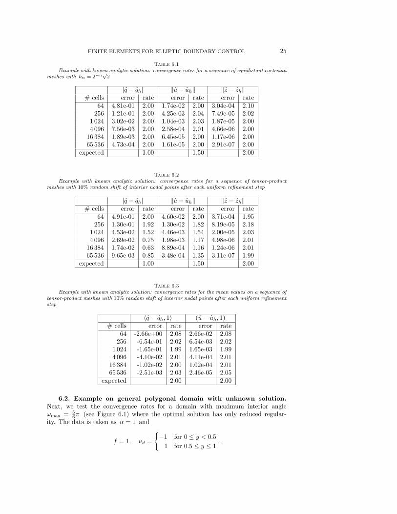
FINITE ELEMENTS FOR ELLIPTIC BOUNDARY CONTROL 25
Table 6.1Example with known analytic solution: convergence rates for a sequence of equidistant cartesian
meshes with hn = 2−n√
2
|q − qh| ‖u− uh‖ ‖z − zh‖# cells error rate error rate error rate
64 4.81e-01 2.00 1.74e-02 2.00 3.04e-04 2.10256 1.21e-01 2.00 4.25e-03 2.04 7.49e-05 2.02
1 024 3.02e-02 2.00 1.04e-03 2.03 1.87e-05 2.004 096 7.56e-03 2.00 2.58e-04 2.01 4.66e-06 2.00
16 384 1.89e-03 2.00 6.45e-05 2.00 1.17e-06 2.0065 536 4.73e-04 2.00 1.61e-05 2.00 2.91e-07 2.00
expected 1.00 1.50 2.00
Table 6.2Example with known analytic solution: convergence rates for a sequence of tensor-product
meshes with 10% random shift of interior nodal points after each uniform refinement step
|q − qh| ‖u− uh‖ ‖z − zh‖# cells error rate error rate error rate
64 4.91e-01 2.00 4.60e-02 2.00 3.71e-04 1.95256 1.30e-01 1.92 1.30e-02 1.82 8.19e-05 2.18
1 024 4.53e-02 1.52 4.46e-03 1.54 2.00e-05 2.034 096 2.69e-02 0.75 1.98e-03 1.17 4.98e-06 2.01
16 384 1.74e-02 0.63 8.89e-04 1.16 1.24e-06 2.0165 536 9.65e-03 0.85 3.48e-04 1.35 3.11e-07 1.99
expected 1.00 1.50 2.00
Table 6.3Example with known analytic solution: convergence rates for the mean values on a sequence of
tensor-product meshes with 10% random shift of interior nodal points after each uniform refinementstep
〈q − qh, 1〉 (u− uh, 1)# cells error rate error rate
64 -2.66e+00 2.08 2.66e-02 2.08256 -6.54e-01 2.02 6.54e-03 2.02
1 024 -1.65e-01 1.99 1.65e-03 1.994 096 -4.10e-02 2.01 4.11e-04 2.01
16 384 -1.02e-02 2.00 1.02e-04 2.0165 536 -2.51e-03 2.03 2.46e-05 2.05
expected 2.00 2.00
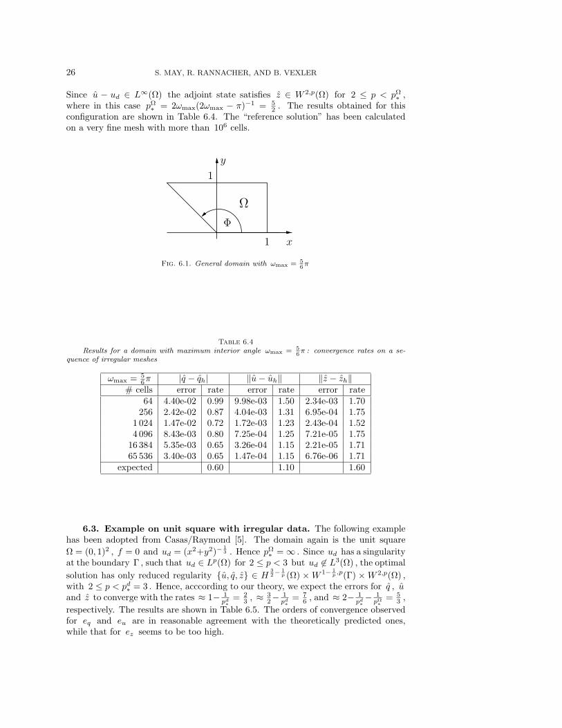
6.2. Example on general polygonal domain with unknown solution.Next, we test the convergence rates for a domain with maximum interior angleωmax = 5
6π (see Figure 6.1) where the optimal solution has only reduced regular-ity. The data is taken as α = 1 and
f = 1, ud =
−1 for 0 ≤ y < 0.5
1 for 0.5 ≤ y ≤ 1.
26 S. MAY, R. RANNACHER, AND B. VEXLER
Since u − ud ∈ L∞(Ω) the adjoint state satisfies z ∈ W 2,p(Ω) for 2 ≤ p < pΩ∗ ,
where in this case pΩ∗ = 2ωmax(2ωmax − π)−1 = 5
2 . The results obtained for thisconfiguration are shown in Table 6.4. The “reference solution” has been calculatedon a very fine mesh with more than 106 cells.
1
1
x
Ω
y
Φ
Fig. 6.1. General domain with ωmax = 56π
Table 6.4Results for a domain with maximum interior angle ωmax = 5
6π : convergence rates on a se-
quence of irregular meshes
ωmax = 56π |q − qh| ‖u− uh‖ ‖z − zh‖
# cells error rate error rate error rate64 4.40e-02 0.99 9.98e-03 1.50 2.34e-03 1.70
256 2.42e-02 0.87 4.04e-03 1.31 6.95e-04 1.751 024 1.47e-02 0.72 1.72e-03 1.23 2.43e-04 1.524 096 8.43e-03 0.80 7.25e-04 1.25 7.21e-05 1.75
16 384 5.35e-03 0.65 3.26e-04 1.15 2.21e-05 1.7165 536 3.40e-03 0.65 1.47e-04 1.15 6.76e-06 1.71
expected 0.60 1.10 1.60
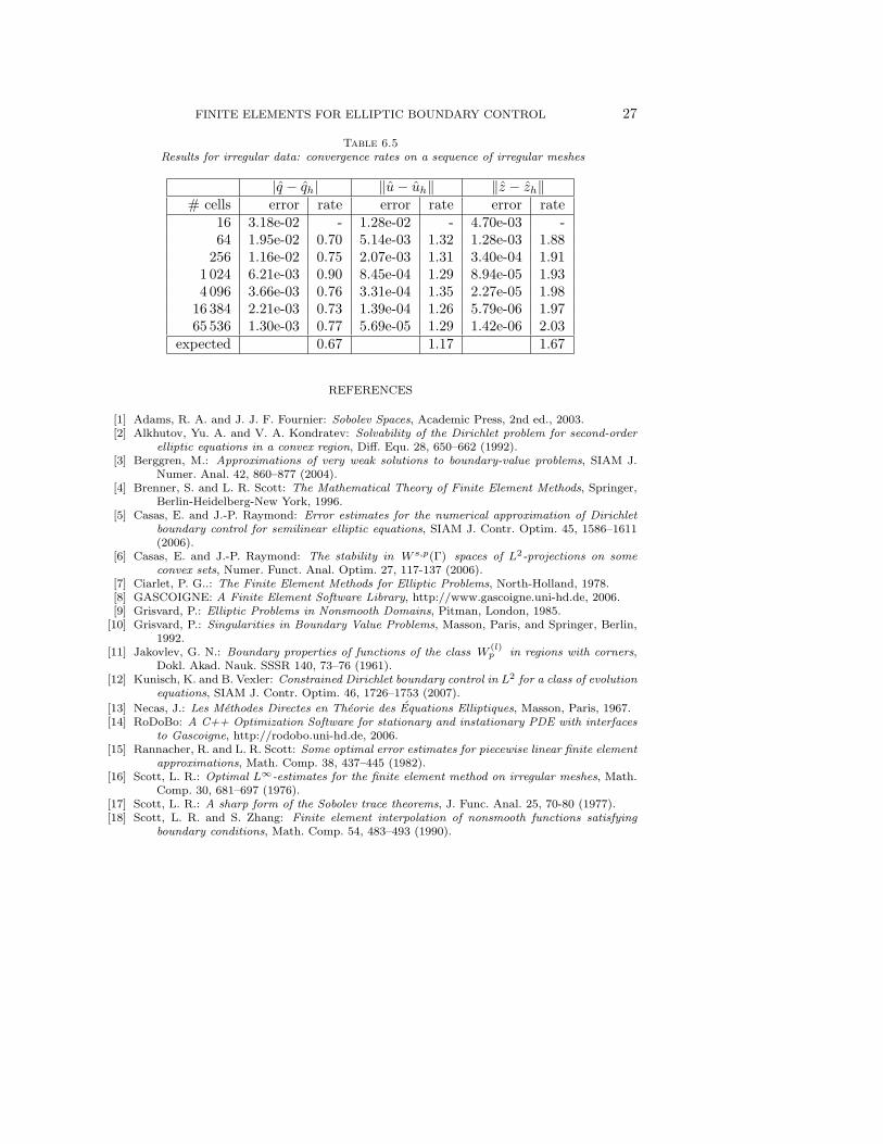
6.3. Example on unit square with irregular data. The following examplehas been adopted from Casas/Raymond [5]. The domain again is the unit squareΩ = (0, 1)2 , f = 0 and ud = (x2+y2)−
13 . Hence pΩ
∗ =∞ . Since ud has a singularityat the boundary Γ , such that ud ∈ Lp(Ω) for 2 ≤ p < 3 but ud 6∈ L3(Ω) , the optimalsolution has only reduced regularity u, q, z ∈ H
32−
1p (Ω) ×W 1− 1
p ,p(Γ) ×W 2,p(Ω) ,with 2 ≤ p < pd∗ = 3 . Hence, acccording to our theory, we expect the errors for q , uand z to converge with the rates ≈ 1− 1
pd∗
= 23 , ≈ 3
2−1pd∗
= 76 , and ≈ 2− 1
pd∗− 1pΩ∗
= 53 ,
respectively. The results are shown in Table 6.5. The orders of convergence observedfor eq and eu are in reasonable agreement with the theoretically predicted ones,while that for ez seems to be too high.
FINITE ELEMENTS FOR ELLIPTIC BOUNDARY CONTROL 27
Table 6.5Results for irregular data: convergence rates on a sequence of irregular meshes
|q − qh| ‖u− uh‖ ‖z − zh‖# cells error rate error rate error rate
16 3.18e-02 - 1.28e-02 - 4.70e-03 -64 1.95e-02 0.70 5.14e-03 1.32 1.28e-03 1.88
256 1.16e-02 0.75 2.07e-03 1.31 3.40e-04 1.911 024 6.21e-03 0.90 8.45e-04 1.29 8.94e-05 1.934 096 3.66e-03 0.76 3.31e-04 1.35 2.27e-05 1.98
16 384 2.21e-03 0.73 1.39e-04 1.26 5.79e-06 1.9765 536 1.30e-03 0.77 5.69e-05 1.29 1.42e-06 2.03
expected 0.67 1.17 1.67
REFERENCES
[1] Adams, R. A. and J. J. F. Fournier: Sobolev Spaces, Academic Press, 2nd ed., 2003.[2] Alkhutov, Yu. A. and V. A. Kondratev: Solvability of the Dirichlet problem for second-order
elliptic equations in a convex region, Diff. Equ. 28, 650–662 (1992).[3] Berggren, M.: Approximations of very weak solutions to boundary-value problems, SIAM J.
Numer. Anal. 42, 860–877 (2004).[4] Brenner, S. and L. R. Scott: The Mathematical Theory of Finite Element Methods, Springer,
Berlin-Heidelberg-New York, 1996.[5] Casas, E. and J.-P. Raymond: Error estimates for the numerical approximation of Dirichlet
boundary control for semilinear elliptic equations, SIAM J. Contr. Optim. 45, 1586–1611(2006).
[6] Casas, E. and J.-P. Raymond: The stability in W s,p(Γ) spaces of L2-projections on someconvex sets, Numer. Funct. Anal. Optim. 27, 117-137 (2006).
[7] Ciarlet, P. G..: The Finite Element Methods for Elliptic Problems, North-Holland, 1978.[8] GASCOIGNE: A Finite Element Software Library, http://www.gascoigne.uni-hd.de, 2006.[9] Grisvard, P.: Elliptic Problems in Nonsmooth Domains, Pitman, London, 1985.
[10] Grisvard, P.: Singularities in Boundary Value Problems, Masson, Paris, and Springer, Berlin,1992.
[11] Jakovlev, G. N.: Boundary properties of functions of the class W(l)p in regions with corners,
Dokl. Akad. Nauk. SSSR 140, 73–76 (1961).[12] Kunisch, K. and B. Vexler: Constrained Dirichlet boundary control in L2 for a class of evolution
equations, SIAM J. Contr. Optim. 46, 1726–1753 (2007).
[13] Necas, J.: Les Methodes Directes en Theorie des Equations Elliptiques, Masson, Paris, 1967.[14] RoDoBo: A C++ Optimization Software for stationary and instationary PDE with interfaces
to Gascoigne, http://rodobo.uni-hd.de, 2006.[15] Rannacher, R. and L. R. Scott: Some optimal error estimates for piecewise linear finite element
approximations, Math. Comp. 38, 437–445 (1982).[16] Scott, L. R.: Optimal L∞-estimates for the finite element method on irregular meshes, Math.
Comp. 30, 681–697 (1976).[17] Scott, L. R.: A sharp form of the Sobolev trace theorems, J. Func. Anal. 25, 70-80 (1977).[18] Scott, L. R. and S. Zhang: Finite element interpolation of nonsmooth functions satisfying
boundary conditions, Math. Comp. 54, 483–493 (1990).
Related Documents