Adaptive Correctness Monitoring for Wireless Sensor ... · Adaptive Correctness Monitoring for Wireless Sensor Networks Using Hierarchical Distributed Run-Time Invariant Checking

Adaptive Correctness Monitoring for Wireless Sensor Networks

Using Hierarchical Distributed Run-Time Invariant Checking

Douglas Herbert, Vinaitheerthan Sundaram, Yung-Hsiang Lu, Saurabh Bagchi, and Zhiyuan Li∗

School of Electrical and Computer Engineering, ∗ Department of Computer Science

Purdue University, West Lafayette, IN 47907

{herbertd, vsundar, yunglu, and sbagchi} @purdue.edu, [email protected]

This paper presents a hierarchical approach for detecting faults in wireless sensor networks (WSNs)

after they have been deployed. The developers of WSNs can specify “invariants” that must be

satisfied by the WSNs. We present a framework, Hierarchical SEnsor Network Debugging (H-

SEND), for lightweight checking of invariants. H-SEND is able to detect a large class of faults

in data gathering WSNs and leverages the existing message flow in the network by buffering and

piggybacking messages. H-SEND checks as closely to the source of a fault as possible, pinpointing

the fault quickly and efficiently in terms of additional network traffic. Therefore, H-SEND is

suited to bandwidth or communication energy constrained networks. A specification expression is

provided for specifying invariants so that a protocol developer can write behavioral level invariants.

We hypothesize that data from sensor nodes does not change dramatically, but rather changes

gradually over time. We extend our framework for the invariants that include values determined

at run time in order to detect the violation of data trends. The value range can be based on

information local to a single node or the surrounding nodes’ values. Using our system, developers

can write invariants to detect data trends without prior knowledge of correct values. Automatic

value detection can be used to detect anomalies that were not previously possible. To demonstrate

the benefits of run-time range detection and fault checking, we construct a prototype WSN using

CO2 and temperature sensors coupled to Mica2 motes. We show that our method can detect

sudden changes of the environments with little overhead in communication, computation, and

storage.

Categories and Subject Descriptors: C.2.1 [Computer-Communication Networks]: Network Architecture and Design –Distributed Networks,

Network Communications, Packet NetworksGeneral Terms: Fault tolerance and diagnostics, In-network processing and aggregation, Network

protocols, Programming models and languages, Data integrity

Additional Key Words and Phrases: Invariants, Correctness Monitoring, Run-time, Tools

1. INTRODUCTION

Wireless Sensor Networks (WSNs) enable continuous data collection or rare event detection in large, hazardous or

remote areas. The data being collected can be critical. Detecting indoor air quality or tracking tank movement are

two examples from civilian and military domains. WSNs are comprised of many sensors that may fail for many

reasons. Faults may come from incorrect sensor network protocols. Distributed protocols are widely recognized as

being difficult to design [1]. WSNs present unique challengesbecause of the lack of sophisticated debugging tools

and the difficulty of testing after deployment. Even after extensive testing, faults may still occur due to environment

conditions, such as high temperatures. While this is true of many systems, this is especially true with WSNs as they

ACM Journal Name, Vol. V, No. N, Month 20YY, Pages 1–20.

are in situ in physical environments that may be changing over the period of deployment. Regardless of design or

validation, sensors can still be damaged by unexpected factors such as storms, hail, animals, or flood.

Run-time techniques are required to detect faults in order to maintain high-fidelity data in the presence of possible

faults from design, implementation, or a hostile environment. Earlier work for run-time observation in wired networks

[2], [3], [4] does not directly apply to WSNs as they are resource-limited. It is essential to minimize the overhead of

storage, computation, and communication in observation and detection. We develop a framework called Hierarchical

SEnsor Network Debugging (H-SEND) [5] to observe node conditions and network traffic for detecting symptoms

of faults. H-SEND differs from existing work in that it is specialized for large scale WSNs. H-SEND has four key

features: (a) During program development, a programmer canspecify important properties as “invariants” that should

never be violated in the network’s operation. (b) When the program is compiled, the code for checking invariants is

automatically inserted. An invariant may be checked locally by an individual node or remotely by sending messages

to another node for detecting faults that cannot be determined by a single sensor node. (c) After deployment, the

inserted code is used to detect abnormal behavior of the network. At run-time, the system can compare against fixed

values, or data trends. An anomaly is detected by when an invariant is violated. An invariant may include a fixed value

determined at compile time, or a data trend observed at run time. Once detected, an anomaly can trigger several actions,

such as increasing logging details or reporting faults to the base station. (d) After a fault is detected, it is reported to

the programmer and a new program is uploaded to the relevant nodes through multi-hop wireless reprogramming.

H-SEND is designed for WSNs with the following special consideration:

(a) Our approach has small overhead in storage, computation, and network. H-SEND checks invariants through a

hierarchy without sending all observed variables to a central location for detection. Instead, invariants are checked

at the closest nodes where the requisite information is available. We present the analysis of the overhead in Section

4.4.

(b) H-SEND assists programmers by automatically (or semi-automatically) determining where to insert invariant

checking code and when to send messages that include observed variables. A programmer only needs to specify

the invariants and the variables to be observed. Our tool candetermine the locations to insert code for checking

invariants and send observed information.

(c) Using H-SEND, faults may be detected by comparing the values from multiple nodes. H-SEND can observe data

trends that are determined only at run-time, such as temperature changes in a wildlife reserve. In normal operations,

temperatures do not change suddenly. A sudden rise of temperature may be caused by fire and must be reported

immediately. We can compare current values against historical values on an individual node (temporal trend) or the

current values on surrounding nodes (spatial trend).

(d) H-SEND can handle WSNs with heterogeneous nodes that are organized as hierarchies. Different nodes may check

different types of invariants and also by performing remotechecking when observed information is aggregated.

We construct a prototype WSN to demonstrate H-SEND through a leader election and data gathering protocol in

a hierarchical configuration. Some invariants are local to anode but others are collective to a cluster or the entire

network. We choose a representative leader election protocol called LEACH (Low-Energy Adaptive Clustering Hier-

archy) [6], [7]. LEACH assigns cluster heads in a “near round-robin manner” to evenly distribute energy drain. A set

of invariants is inserted into the application code. We detect both temporal and spatial trends based on data collected

from our CO2 and temperature sensors coupled to Mica2 motes with custom built power supply and interface circuits.

2

Sensed Data,

StationBase

SensingNode

SensingNode

SensingNode

ClusterHead

SensingNode

SensingNode

SensingNode

ClusterHead

Sensed DataConsumer

SoftwareDeveloper

Invariants,Errors

ProgramCorrections

Fig. 1. Overview of the framework for fault detection, propagation, diagnosis, and repair.

We use simulations to measure the overhead of the augmented code in our approach. The experiments and simulations

show that data trends can be observed and used to detect anomaly with small overhead.

2. RELATED WORK

2.1 Sensor Programming Environment and Simulation

A typical hierarchical sensor network is shown in Figure 1. Once sensor network software is created by a developer, it

may be uploaded to individual sensors by utilizing distributed propagation techniques over the radio link [8] as illus-

trated in Figure 1. Berkeley Mica Motes [9] are widely used sensor nodes for experiments. Mica nodes use TinyOS as

the run-time environment. TinyOS provides an event-based simulator, TOSSIM, that can be used to simulate a network

of varying node size [10]. TOSSIM compiles from the same source code as the Mica platform Our experiments use

TOSSIM because it scales to large numbers of nodes easily. TOSSIM provides deterministic results so it is a better

test bed in contrast to the non-deterministic results provided by real-life execution. Finally, TOSSIM allows us to sep-

arate instrumentation code from the actual code running on each node so we can measure the nodes’ behavior without

perturbing the network’s normal operations. To increase the accuracy of our simulation, we inject sensed values from

actual sensors, and use these values to simulate data collection.

2.2 Program Monitoring and Profiling

Program monitoring and profiling have been developed for wired networks [2], [3], [4]. One approach is to directly

modify binary code [11] using binary analysis tools to insert instrumentation code to monitor program operation. This

approach detects faults in programs while operating in a real environment. DIDUCE [12] instruments source code

and formulates hypotheses of possible rules about correct program operations. DIDUCE uses machine learning by

starting with strict rules that are gradually relaxed to allow new program behavior. Formal methods have been used to

prove programs from a theoretical view [13]. Analysis of program operations with an SQL-like language is used for

correctness monitoring in [14]. Adding hardware to monitormemory changes for checking at run-time is discussed

in [15], [16]. Several studies discuss how to find invariantsfor programs [17], [18], [19]. These studies provide the

foundation for using invariants in WSNs but existing approaches cannot be applied to WSNs directly because the

observation algorithms may execute at a location far away from nodes where data are collected, adding significant

network traffic to propagate data. WSNs are resource-limited; hence, invariant checking must be efficient in using the

3

sensor nodes’ communication and computation.

2.3 Clustering

WSNs are distributed systems. Distributed algorithms have been studied in [20]. WSNs differ from wired distributed

systems because sensors have stringent resource constraints, including energy, storage, and computation capability.

To conserve energy, some routing protocols use hierarchiesamong sensor nodes [21], [22], preventing all nodes from

relaying all messages (i.e., routing by “flooding”). Sensornodes are often divided into clusters and a special node

or “cluster head” (CH) in each cluster relays messages between clusters or to a base station. Cluster heads can be

chosen in several ways. If sensor nodes are heterogeneous, the nodes that have more resources are selected as cluster

heads. For homogeneous nodes, they can take turns playing the role of the cluster head through leader election

protocols [23], [24], [25].

2.4 Fault Detection and Recovery

Studies have been conducted to observe run-time behavior for wired networks [2], [3], [4]. In these studies, the

observed node and the observer are different and this approach provides several advantages: (a) An observer may be

a monolithic entity with perfect knowledge of the observed node. (b) An observer may be fault-proof or may only fail

in constrained ways, such as fail-silence. (c) An observer may have abundant resources. fault observation in resource-

constrained WSNs has also been studied. Several projects uselocal observation whereby nodes oversee traffic passing

through the neighbor nodes [26], [27], [28], [29], [30], [31], [32]. Each node can both sense the environment and

observe other nodes. Previous work uses local observation to build trust relationships among nodes in networks [29],

[27], detect attacks [28], [30], or discover routes with certain properties, such as a node becoming disconnected [26].

Huang et al. [30] propose distributed intrusion observation for ad-hoc networks. Their paper uses machine learning to

choose the parameters needed to accurately detect faults. Intrusion detection systems exist [33], [34]. However, the

knowledge in these systems is built by each individual node without the need for coordination, and no information is

transmitted to remote nodes. Smith et al. [35] detect protocol faults for ad-hoc networks. After faults are detected, new

programs may be sent to the sensor nodes through the same wireless network for transmitting data. Deluge [36] allows

program replacement by propagating new program images overwireless networks. In our previous work [37], we

present a method to enable neighbor observation in resource-constrained environments and to provide the structures

and the state to be maintained at each node. We analyze the capabilities and the limitations of local observation for

WSNs.

2.5 Estimation and Approximate Agreement

A summary of approximate agreement upon a single value is provided by Lynch [20]. Lamport et al. [40] formulates

the Byzantine Generals problem of gaining distributed consensus in the presence of faults. It is shown that for3N + 1

nodes reporting binary (true or false) data, the correct value can be determined if no more thanN nodes report

incorrect values. Maheney et al. [41] shows that continuousvalue estimation requires fewer correct nodes to achieve

consensus for a given degree of fault tolerance. Two-thirdsof nodes performing correctly guarantees convergence

of their algorithm, and between one-third and two-thirds ofnodes performing correctly will allow their algorithm to

detect that too many faults have occurred to determine correctness or show that the divergence is bounded. Marzullo

et al. [42] provides an algorithm to obtain inexact agreement for continuous valued data, and presents a method of

transforming a process control program for better fault tolerance. They demonstrate how to modify specifications to

4

H-SEND Sympathy DICAS Send to Base Daicon DIDUCE

Mobility Yes Yes Yes Yes No No

Hierarchy Yes No Yes Yes No No

Learning Yes Not Yet No No Yes Yes

Resource

Efficient Yes Yes Yes No No No

Aggregation Yes Yes No Yes No No

Designed

for Security No No Yes No No No

Add/Remove

Nodes Yes No Yes Yes No No

Table I. Matrix of Capabilities of Fault Observation Methods

Sympathy [38], DICAS [39],

Daicon [18], DIDUCE [12]

accommodate uncertainty.

2.6 Benefits of CO2 Monitoring

Many studies have provided the relationship between the concentration of carbon dioxide (CO2) and indoor air quality

[43] [44] [45]. In an office building, occupants (i.e. people) are the primary source of CO2. High levels of CO2

(usually above 1000 parts per million, or ppm) are connectedwith sick building syndrome (SBS) symptoms. As a

reference, the CO2 level in outdoor air is usually below 350 ppm. Even though CO2 levels are not a direct indicator of

indoor air quality, the CO2 levels can provide indirect information of ventilation efficiency, SBS, respiratory disease,

and occupant absence. Every year, approximately 4 million deaths occur due to viral respiratory infections [46]. Liao

et al. [46] develop a model for the infection of influenza and severe acute respiratory syndrome (SARS) for indoor

environment. Studies show that increasing ventilation canreduce the infection of airborne diseases [47], [46], [48],

[49]. Ventilation volume for un-instrumented spaces is commonly collected with a device that fits over the supply

vent, and forces air to flow through the measurement device asshown in Figure 2. This method device with only one

data point. We use multiple CO2 sensors as indicators of ventilation volume and transmit sensor readings to a central

location using wireless sensor nodes. Sensor data are collected continuously and automatically without the need of a

human worker. We believe this type of application will be widely deployed because of (a) the low cost of sensors, and

(b) the real time feedback they provide in control system. Ithas been shown that demand controlled ventilation can

save energy [50], [51]. WSNs substantially reduce the cost byremoving the need of long cables for communication

cables between sensors and the control center.

2.7 Comparison and Our Contributions

Table I summarizes the capabilities of several related projects. In this table, we adopt the following definitions:

—“Mobility” is the ability of nodes to move over time.

—“Hierarchy” refers to a tiered arrangement of nodes.

—“Learning” indicates the ability to estimate correct values at run time.

—“Resource Efficient” shows if hardware resource usage is a concern.

—“Aggregation” is the ability to combine data together.

5

Fig. 2. Device for measuring airflow volume

—“Designed for Security” states if security is a main goal of the design.

—“Add/Remove nodes” shows if it is possible to change the number of nodes at run-time.

Sympathy [38] transmits metrics such as network link quality and routing stability back to the base station for

analysis. Sympathy assumes high throughput of the network and all data for correctness checking are sent to the base

station. Dicas [39] places additional nodes to monitor wireless communication for detecting faults. Send-to-base is a

simple method where the developer manually inserts code to send all variables to be monitored back to the base station.

Daicon [18] and DIDUCE [12] observe the behavior of programsto automatically create invariants; developers are

not required to specify invariants. Automatic creation is performed by first creating strict invariants. As the programs

execute, the invariants are gradually relaxed to accommodate new correct behavior. Neither Daicon nor DIDUCE is

designed for distributed or resource-constrained systemslike WSNs.

This paper extends our previous work [5] where we introduce observing variables specified by a developer through

invariants to detect faults. This prior work used invariants determined at compile-time. This paper includes a detailed

study how to use the same infrastructure with the addition ofrun-time determined invariants which have changing

parameters, and validates this approaches on data collected from real sensors. We construct a WSN to measure indoor

CO2 and temperature levels and demonstrate that our framework can correctly detect data trends and sudden changes

of the levels as violations of invariants.

3. TECHNIQUES FOR FAULT DETECTION, DIAGNOSIS, AND REPAIR

3.1 Overview

Our system determines the health of a WSN by detecting software faults or sudden changes of data trends, propagating

the information to the base station, assisting a programmerto diagnose the faults, and then distributing correct software

after the programmer fixes the faults. Our approach addresses “What is observed and when?”, and “How is a fault

detected?”.

3.1.1 What is observed and when?.Invariants are classified in several ways:

Local invariantsare formed from variables resident on the same node (henceforth referred to as local variables,

not to be confused with local variables within a function) only and multi-node invariantsfrom a mix of local and

non-local variables. Local invariants can be checked at anypoint where the constituent variables are in scope, while

remote invariants can be checked when the set of network messages carrying all the non-local variables have been

6

successfully received and the local variables are in scope.

Stateless invariantsandstateful invariants. For the invariants on a single node, stateless invariants are always true

for the node, irrespective of the node’s operation states. Stateful invariants are true only when the node is in a particular

execution state.

Compile-time determined invariantsandRun-time determined invariants. Compile-time determined invariants com-

pare variables and program conditions against values that do not change. Run-time determined invariants usespatial

trendingto compare variables and program conditions against other neighboring nodes ortemporal trendingto com-

pare against prior history. An example of a compile-time determined invariants is “Sensed temperature is between 10

and 30 degrees Celsius.” An example of a run-time determinedinvariant utilizing history is “Temperature does not

change by more than 10% in a period of 60 seconds.” A run-time determined invariant can check the condition “All

nodes report temperatures that are within 1 standard deviation of each other.” H-SEND allows different classes of

invariants to detect different faults.

3.1.2 How is a fault detected?.A fault is detected when one or multiple invariants are violated. The verification

of a local invariant involves some computation without additional communication. One of the benefits of performing

temporal trending is that expensive communication is required only when a fault is detected. The verification of a

remote invariant involves additional communication. Spatial trending requires communication energy to propagate

values, but requires less memory because a history buffer does not need to be kept. WSNs are energy bound so nodes

are often put to sleep for conserving energy and sending debug information separately can use a significant amount

of energy. An alternative is to piggy-back invariant information onto data messages that contain sensed data. This

reduces the cost of communication — the fixed cost is amortized. Additionally, this removes interference with any

existing node sleep-awake protocol. However, this impliesthat the fault can be propagated only when a data message

is generated. Such delay, fortunately, is bounded and an analysis is presented in Section 4.4.

3.2 Invariant Grammar

Invariants are specified in source code in the form:

[scope modifier() [where (condition modifier)]] require ( rule);

An example isforall(HS NODES) where (node==HS CLUSTERHEAD) require (HS HIGH, a <

MAXHOPS). HS NODESrefers to all nodes, andHS CLUSTERHEADrefers to the current cluster head. This invariant

checks thata is less thanMAXHOPS.

The scope modifier may includeforall or exists . If there is no scope modifier, the invariant applies to only the

local node. The scope modifierforall indicates that the invariant holds for every node. The scopemodifierexists

indicates that it holds for at least one node. The condition modifier where indicates that a condition is present to act

as a filter upon the scope. Several enumerated values are available to use for this purpose:HS NODESfor all nodes,

HS CLUSTERHEADfor cluster heads, andHS BASESTATIONfor the base station. Local and remote variables can

also be used. Therule may use remote variables, local variables, variables from asingle function or variables from

multiple functions in defining the expression.

Placement will specify the scope of an invariant. If an invariant is to hold for a single statement, then the specification

is placed immediately after that statement. If an invariantis specified for an entire function, then the specification

is placed at the beginning of the function body. If an invariant must be satisfied no matter which function is being

7

executed, then the specification is placed at the beginning of a program module, i.e. a source file in the NesC language.

Theforall scope modifier can be applied to functions. The entire set of functions is denoted byHS FUNCTIONS.

For example,forall(HS FUNCTIONS) require (HS CLUSTERHEAD == message.sender); means

that the sender of any message must be the current cluster head, regardless of which function is being executed.

Receiving a message from any other node indicates a fault. Additionally, we identify the most recently received

message by the variableMIN , and the most recently sent message by the variableMOUT. MALL refers to all mes-

sages and the nodes identification number byNODEID . The forall andexists quantifiers can be applied to

both messages and node IDs. The fields.sender and .type can be accessed for messages. For all data, the

.age field is incremented each time a new piece of data is sampled and evaluated, and can be used to perform

historical analysis. For example,forall(M IN) where ((M IN.type == M5) && (M IN.age < 20))

require (M IN.sender == 5); reads “For the last 20 messages received, all messages of theM5 type must

come from node number five.”

In the prior example, the value “5” is determined at compile-time and checked at run-time. This restricts the applica-

bility of invariants because some values may be specific to the deployment environment. A programmer does not have

to rely on compile-time values when creating invariants. Run-time determined values can be used for invariants using

spatial trendingor temporal trending. The former compares a value against the values from other neighboring nodes;

the latter compares the current value with earlier values. To specify trending, one can use the additional reserved

keywordtrend ; it allows WSN developers to specify invariants using run-time determined values. One example of

trending is to detect the meanµ and the standard deviationσ of sensed data.

An example of a trending invariant isforall (sensedData) where (sensedData.age < 10)

require (trend(sensedData,1)) , which allows a program to perform temporal trending and compare

sensed data over time and trigger a fault message. If any sensed value is more than one standard deviation away

from the mean of the last 10 samples, a fault is detected. Another invariant,forall (HS NODES) require

(trend(sensedData,1)) , performs spatial trending by comparing an individual nodes data against the values

collected by all the other nodes. A violation occurs if the difference exceeds one standard deviation.

3.3 Invariant Examples

H-SEND can be used to detect data trends and faults in WSN operations, such as leader election, time synchronization,

and location estimation. We use leader election as an example here and as a case study in Section 4 to illustrate H-

SEND’s capability. We use several types of messages as examples listed in Table II. Message “M1: Election” initiates

an election, upon which nodes randomly respond by sending “M4: I’m a new cluster head” to other nodes, and the old

cluster head responds with “M7: Relieve cluster head.” Sensing nodes then send “M2: Data” messages to the cluster

head, which combines the messages and sends “M3: Aggregate Data” to the base station. If a cluster head disappears,

a node will broadcast “M6: My cluster head is unavailable” toall nodes.

The invariants listed below can be specified in the program using the format shown in Section 3.2. The following

list shows (a) possible invariants for the protocol in English, (b) the invariant specification grammar, (c) whether the

invariant has fixed parameters (compile-time) or the systems learns parameters (run-time) (d) if state is kept, and (e)

what type of fault is detected.

1. Rule: If a node detects unavailability of a cluster head, anew cluster head should take over withinX time units:

Invariant: forall(M OUT) exists(M IN) where ((M OUT.type == M6) && (M IN.type ==

8

Message Function

M1: Election Initiate the election process for a CH (cluster head)

M2: Data Send sensed data from a node to a CH

M3: Aggregate Data Aggregate data in a CH and send to base station

M4: I’m a new CH Inform the nodes that the sender is a new CH

M5: I’m a CH Send periodic “keep-alive” to nodes in the cluster

M6: My CH is unavailable Realize my CH is unreachable and send to the base station

M7: Relieve CH Inform the other nodes that the CH intends to relinquish

its role due to, for example, impending energy exhaustion

Table II. Messages used for cluster formation

M4)) require ((M IN.time - M OUT.time > 0) && (M IN.time - M OUT.time < X));

NesC checking code inserted by H-SEND code augmenter:

int lastM4MinMsgTime;

if((M_OUT == M6) && (((lastM4MinMsgTime - M_OUT.time) < 0) | |

((lastM4MinMsgTime - M_OUT.time) > X))) {

/ * Create and send fault packet * /

}

if(M_IN.type == M4)

lastM4MinMsgTime = M_IN.time;

Type: Compile-time/Stateful/Implementation Fault

2. Rule: A node is no more thanX hops from a cluster head:

Invariant: forall(HS NODES) where (M IN.sender == HS CLUSTERHEAD) require

(M IN.hops <= X);

NesC checking code inserted by H-SEND code augmenter:

if((M_IN.sender == HS_CLUSTERHEAD} && (M_IN.hops > X) {

/ * Create and send fault packet * /

}

Type: Compile-time/Stateless/Scalability Fault

3. Rule: Sensed data value stored in variable sensedValue does not differ among nodes by more than 3 standard

deviations.

Invariant: forall(NODES) require (trend(sensedValue,3));

NesC checking code inserted by H-SEND code augmenter to be evaluated at base station:

9

//Retain values between calls

static int data[MAX_NODES]; static int index = 0;

int i; int mean = 0; int stddev = 0;

// Insert into array with latest data from other nodes.

data[NODE_ID] = M_IN.sensedValue;

// Calculate Mean

for(i = 0; i < MAX_NODES; i++) { mean += data[i]; }

mean = mean / MAX_NODES;

// Calculate Standard Deviation

for(i = 0; i < MAX_NODES; i++) { stddev += (data[i] - mean)ˆ2; }

stddev = sqrt(stddev/MAX_NODES);

// Check against tolerance

for(i = 0; i < MAX_NODES; i++)

if((data[i] < (mean - 3 * stddev)) || data[i] > (mean + 3 * stddev)))

{ / * Create and send fault packet * / }

Type: Run-time/Stateful/Scalability Fault

From the list of examples, we can see that checking invariants in not an onerous task. The computation is small,

consisting of an equality or inequality check and calculating the conjunction or disjunction of multiple boolean values.

4. CASE-STUDY: DEBUGGING A DISTRIBUTED LEADER ELECTION PROTOCOL

In this section we demonstrate the capabilities the H-SEND fault detection approach. We implement leader election

to show a wide range of compile-time determined invariants,and we use data collected from our testbed of CO2

and temperature sensors to show how to determine the historysize and tolerance needed to use run-time determined

invariants effectivly.

4.1 LEACH

We implemented the LEACH (Low-Energy Adaptive Clustering Hierarchy) cluster based leader election protocol for

WSNs [6], [7]. In LEACH, the nodes organize themselves into clusters, with one node acting as the head in each

cluster. LEACH randomizes which node is selected as the headin order to evenly distribute the responsibility among

nodes and to prevent draining the battery of one node too quickly. A cluster head compresses data (also calleddata

fusion) before sending the data to the base station. LEACH assumes that all nodes are synchronized and divides

election into rounds. Nodes can be added or removed at the beginning of each round. In each round, a node decides

whether to become a head using the following probability. Supposep is the desired percentage of cluster heads (5%

is suggested in [6]). If a node has not been a head in the last1p

rounds, the node chooses to become a head with

10

P(Cluster Head)

Choose Cluster Headand Send Join

Wait for Join Message

ScheduleWait for TDMA

Collect Dataand Forwardto Base Station

Restructuring

Send Data

Sensing

TDMAScheduleMessage

DataMessage

Join Message

Send Cluster HeadAdvertise Message

Receive Cluster HeadAdvertise Message

Send TDMA Schedule

Sent Join

Message

TDMA

Slot Over

TDMA

Slot Begin

Join Period Ends

Sent TDMA Schedule

Advertise Message

Received

TDMA Schedule

Send Advertise Message

Advertise

Period Ends

1 − P(Cluster Head)

Fig. 3. State Diagram of the LEACH Protocol

probability p

1−p×(r mod 1

p), wherer is the current round. After1

prounds, all nodes are eligible to become cluster heads

again. If a node decides to become a head, the node broadcastsa message to the other nodes. The other nodes joins

a cluster whose leader’s broadcast message has the greatestsignal strength. In the case of a tie, a random cluster

is chosen. LEACH is used in many other studies, such as [52], [53], [54] because LEACH is efficient, simple to

implement, and resilient to node faults.

Figure 3 shows the states of the LEACH protocol. Each solid arrow indicates an event that causes a state change,

and each dashed arrow indicates a communication message. Invariants can be easily created from this state diagram.

If a node is in a certain state, and any event occurs for which the state diagram is not defined, an fault has occurred.

Possible invariants for the LEACH protocol include “only inthe ’Wait for Join Message State’ should a ’Join Message’

be received” or “A node should only receive a ’TDMA schedule’in the ’wait for TDMA schedule state’ ”. The compiler

can then insert code for these compile-time invariant to check the health of a node or the network.

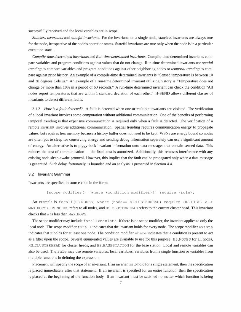
4.2 Carbon Dioxide and Temperature Measurement

A picture of a sensor node from our data collection test bed isshown in Figure 4. Each sensor node contains a

Crossbow MPR400CB (Mica2) sensor mote coupled to a SenseAiraSense carbon dioxide (CO2) and temperature

(a) (b)

Fig. 4. CO2 and Temperature Sensing Node (a) The internal components (b) The node as seen from the outside (ink pen is shown for size reference).

11

sensor through a custom interface circuit. Power is supplied to the CO2 and temperature sensor by an unregulated 24

volt AC transformer. A 5 volt transformer is regulated to 3 volts by an external voltage regulation circuit and provides

power to the rest of the interface board and the sensor mote. The interface board scales the analog output of the aSense

to a range acceptable to the mote, and adds diode limiters to protect the sensor mote from electrical damage. All

circuits use precision potentiometers which were tuned using a digital multi-meter to reduce losses in accuracy due

to power fluctuations and signal scaling. The CO2 and temperature data are sensed by the on board 10-bit analogto

digital converter of the mote, and forwarded to the base station where the values are recorded and archived. Figure 5

shows the readings from multiple locations inside a studentlounge on our campus. Some people find this room ideal

for napping, and this may be explained by the high concentration of CO2. We use data collected from these sensors to

evaluate the performance of run-time determined invariants performing both spatial and temporal trending.

4.3 Examples of Invariant Violation

At present, all invariants are manually inserted but insertion can be done by a compiler as explained in Section 3.3.

This automatic invariant-insertion tool is under development. In our experiments, we originally intended to write

“correct” code first and then intentionally inject faults later. However, we encountered unexpected behavior by the

nodes and decided to insert invariants first to help us isolate the fault (or faults). We observed that some nodes entered

the “Cluster Head Advertise” state at wrong time. The fault was a state-transition violation. An invariant required that

“Restructuring State” be the previous state before the “Send Cluster Head Advertise Message” state. This is a binary

example: there is only one correct previous state. If the previous state is incorrect, the invariant is violated. After this

invariant was inserted, we discovered an fault in our LEACH implementation. When the invariant was violated, a fault

was reported at the node level. Without this distributed debugging system, a simple fault would have been difficult to

diagnose. This shows that a binary invariant can be very helpful. An invariant can also include numeric quantities. For

example, we can observe the signal strength received by eachnode in order to analyze the health of the network. An

invariant can be written to ensure that the signal strength from a cluster head does not vary above 50%. If this invariant

is violated, a fault is reported. This report can assist the protocol designer to decide whether a more robust (and higher

overhead) protocol should be chosen.

4.4 Analysis

This section analyzes the overhead, time to detect faults, trending parameter selection and code size.

0 0.5 1 1.5 2900

1000

1100

1200

1300

1400

Time (hour)

CO

2 Le

vel (

ppm

)

CO2 Levels in a Student Lounge

People Enteringand Leavingthe Lounge

No Air Circulation

CirculatingIndoor Air

Turn on WindowFan to BringExternal Air

Relocate the sensor inside the lounge

Fig. 5. CO2 Levels Observed in Multiple Locations In and Around StudentLounge

12

20 40 60 80 100 1200

0.5

1

1.5

2

2.5

3

3.5

4

x 105

Number of Nodes

Byt

es T

rans

mitt

ed

Num Packets vs. Network Size

Cluster + Base DebuggingCluster DebuggingNo Debugging

Fig. 6. Network Traffic vs. Network Size

4.4.1 Network Traffic Scaling.Since sensor nodes have limited energy, they should send as little information as

possible to conserve energy. LEACH uses data fusion to reduce the amount of network traffic. We analyze the network

overhead of H-SEND as follows. Letmc andmb represent the size of a message sent from a node to its clusterhead

and the base station. Letf be the fusion factor. For example,f is 10 if the cluster head summarizes 10 samples

and sends the average to the base station. Letδ be the additional amount of information sent by each node forfault

detection. The value ofδ is zero if no information is transmitted for detecting faults. The total amount of data sent in

the whole wireless network can be expressed as∑

∀x∈ nodes

∑

messagesfrom x

(mc + mb

f+ δ). One goal of the H-SEND approach is

to minimize the communication overhead. Supposem1 is the total amount of information transmitted in the network

without any detection messages (i.e.δ = 0). Let m2 be the amount of information with detection messages. The

overhead is defined asm2−m1

m1

. In H-SEND, nodes only forward debugging data to cluster heads, and cluster heads

only forward debugging data to the base station (i.e. upwards). No debugging data is sent back down to nodes from

higher levels of the hierarchy. The rationale is that diagnosis needs to aggregate information only. Therefore, adding

nodes results in a linear increase in network traffic. The case study presented here observed three variables at the

cluster level, and six variables at the network level. Figure 6 shows that the traffic grows linearly for network sizes

between 5 and 125 nodes. This figure shows three lines: (a) no fault detection. This has the same amount of traffic

as node-level detection. (b) cluster-level detection, and(c) cluster and base-level detection. The vertical axis shows

the number of bytes transmitted. The actual amount depends the duration of the simulated network. Regardless of the

duration, the ratio of(b)(a) and (c)(a) is approximately 1.64 and 1.95, respectively. In other words, the percentage of the

network overhead is nearly a constant. Detecting faults as close to the source as possible allows H-SEND to reduce

the amount of traffic sent over the network. The worst case scenario is to send all data to the base-station, and perform

data-analysis at the base station. Through simulation, it was found that the H-SEND method resulted in a 7% message

reduction size vs. sending all data needed to evaluate invariants to the base station.

4.4.2 Detection Time.To further reduce network traffic, observed detection data is piggy-backed onto data mes-

sages through the network as part of normal operation. This saves the fixed cost of communicating a new packet, such

as the cost of the header bytes accompanying each packet (7 bytes out of the default size of 36 bytes for the Mica2

13

0 4 8 12 16 20 24 28 32 36 40 44 480

10

20

30

40

50

60

70

80

90

100

Time To Detect (Time Slices)

% E

rror

s

Fusion Factor 1xFusion Factor 10x

(a)

0 4 8 12 16 20 24 28 32 36 40 44 480

10

20

30

40

50

60

70

80

90

100

Time To Detect (Time Slices)

% E

rror

s

Fusion Factor 1xFusion Factor 10x

(b)

Fig. 7. Simulated Results for Detection Time. (a) Node-Level (b) Cluster-Level

platform). Piggy-backing data adds a bounded latency to detection, as data is held at the node or cluster level until a

data message is sent to the next level. Due to bounded detection time, all faults are reported, and there are no losses.

If piggy backing is not used, fault propagation delay is of the order of communication delay. If the fault is delay

sensitive, an additional strategy that can be used in addition to piggy-backing is generating an explicit control message

if the delay goes above a threshold. Piggy-backing fault messages causes bounded delays. Detection time is defined as

the time period between when a node detects a fault, and the base station receives the message indicating a fault. The

worst-case detection time occurs when a node transmits datain the first transmit slot and detects a fault in the very next

slot, and must wait for all nodes in it’s cluster to transmit (n-1 slots). It must then wait for the network to restructure,

and then the same node must be assigned to the last transmit slot (n-1 slots). Analytically, we can define the worst case

detection time as: 2×(Number of Transmit Slots-1)+Number of Slots to Restructure. This equation was confirmed by

simulation. The LEACH protocol has 4 slots of administrative overhead. In [7] it is found that 5% of nodes acting as

cluster head is ideal, yielding an average cluster size of 20nodes with 20 time slots to broadcast results. Using these

parameters, the worst-case detection time is 42 time slots.The data fusion factor will affect the detection time, as

higher fusion factors result in fewer messages. As a result,detection time increases when the fusion factor increases.

Figure 7 (a) shows a histogram of node-level detection time at fusion factors of 1 and 10. As the figure shows, most

faults can be detected within 4 time slots. When the fusion factor is higher, the figure shows that detection time in-

creases. Figure 7 (b) shows the detection time for cluster level fault detection. The detection time is significantly less

than at the node level, because cluster heads communicate with the base station much more often.

4.4.3 Choosing Trending Parameters.Trending accuracy is closely related to the tolerance allowed. In our exper-

iments, the tolerance is measured by multiples of the standard deviationx · σ. The natural amount of variation in a

WSN is sensor and environment specific. Harsh environments may correctly sense a large amount of variation with

no fault occurrences, such as seismic sensors for earth quakes. Many applications, however, will report small amount

of variation, such as indoor CO2 sensing. To determine the tolerance (x above), one must consider what variation is

seen in normal operating conditions is, and choose a tolerance slightly above this. Ifx is too small, normal runtime

variance will trigger faults. Ifx is too large, faults may not be detected. Hence,x must be larger than the natural

variation of correct data, but smaller than abnormal suddenchanges. The WSN developer must also determine the

amount of history to use (y) for temporal trending. Ify is too small, the amount of history is insufficient to observe

the trend. Ify is too large, the trend is influenced by data collected in the remote past. The history size (y above) is

14

also directly related to the amount of memory temporal trending consumed at run-time, and therefore it is desirable to

chose the smallest history size that can capture enough datato locate faults. We show in the following paragraphs how

to determine appropriate values for bothx (the tolerance) andy (the history size) for trending based on empirical data.

To demonstrate a real world example of choosing the proper tolerance and history size, we collected data from

two CO2 and temperature sensors placed on different sides of an approximately 50 meter square student lab with two

occupants for 2 hours under indoor office building conditions. Care was taken to not perturb the environment. Normal

building ventilation was present, and the single door to thehallway was left open to simulate normal conditions.

Data was sampled every 30 seconds, and the base station logged the data to permanent storage during collection. We

repeated the data collection with a student holding a 1500 watt personal hair dryer to one node temporarily at two

different times during the experiment. The hair dryer causes a quick spike in temperature to 50 degrees Celsius, the

maximum temperature the sensor can measure, before the temperature falls back towards ambient room temperature.

Additionally, we recorded an increase in CO2 level when the student was operating the hair dryer, from theincrease in

air flow over the sensor and the close proximity of the student. We use this data collected with the hair dryer blowing

to represent a malfunctioning sensor or a sudden change of the environment. The CO2 and temperature data of both

the normal case, and the hair dryer case is shown in Figure 8.

To evaluate trending performance across a wide range of tolerances and history sizes, we inserted the data collected

above into a TOSSIM simulation where nodes use it as their sensed values in a 20 node simulation of a network

running the LEACH protocol. TOSSIM allows us to use the same sensed data in multiple simulations of different

tolerance and history values. The sensed data from node 1 simulated the sensed data for one node, the data from node

2 simulated sensed data for 18 other nodes, and the remainingnode served as the base station. We inserted run-time

determined invariants into the application code to performtrending on (1) the time between cluster elections, (2) the

number of members in an individual cluster, (3) the number ofclusters, (4) the number of bytes transmitted between

elections, (5) the value of the sensed CO2 data, and (6) the value of the sensed temperature data.

To determine the appropriate tolerance for spatial trending, we simulated a network performing spatial trending with

tolerances of 1, 2, 3, 4, and 5 standard deviations for the value ofx with both the normal data, and the hair dryer data

representing faults. We recorded the number of faults that were detected by trend monitoring, and show the results

in Figure 9 which shows that at a tolerance of 4 standard deviation no errors are reported for correct data, and 310

errors are reported for the hair dryer simulated fault data.We can see from the figure that a tolerance value lower

than 4 shows a similar number of errors in both the correct data and hair dryer data, and is therefore not tight enough.

Tolerances larger than 4 standard deviations do not detect the errors in faulty data, and are therefore too loose.

To determine the appropriate tolerance and history size fortemporal trending, we simulated a network performing

temporal trending with tolerances from 1 to 5 standard deviations for x, and with history sizes of 4, 8, 16, and 32

sensor readings fory. We simulated nodes sensing both correct and hair dryer induced faulty data. We counted the

errors for each set of parameters and show the results in Figure 9. A history size of 16 sensed readings, with a tolerance

of 3 standard deviations shows an order of magnitude more faults in the hairdryer case, compared with the normal data

case. A window size of 32 with 4 standard deviations also shows an order of magnitude more faults in the hairdryer

case than in the normal data case. In this particular application we find both pairs of parameters to perform excellent

temporal and spatial trending, but we recommend 3 standard deviations with a history size of 16 due to the reduced

memory requirement.

15

0 0.5 1 1.5 2450

500

550

600

650

CO2 Data Normal Over Time

Hours

Co2

(pp

m)

Node 1Node 2

(a)

0 0.5 1 1.5 220

25

30

35

40

45

50Temperature Data Normal Over Time

Hours

Tem

pera

ture

(de

gree

s ce

lsiu

s)

Node 1Node 2

(b)

0 0.5 1 1.5 2450

500

550

600

650

CO2 Data with Hairdryer over time

Hours

Co2

(pp

m)

Node 1Node 2

(c)

0 0.5 1 1.5 220

25

30

35

40

45

50Temperature Data with Hairdryer over time

Hours

Tem

pera

ture

(de

gree

s ce

lsiu

s)

Node 1Node 2

(d)

Fig. 8. (a) CO2 Data and (b) Temperature Data Collected with Normal Conditions (c) CO2 Data and (d) Temperature Data Collected with Hair

Dryer induced Fault Conditions

4.4.4 Code Size.When implementing the LEACH protocol, all nodes except the base station must use the same

binary image because all nodes can be cluster heads at some point. The data reported in Table III was collected with -

O1 optimization, based on binary images for the Mica2 platform. The column for ROM indicates the code size written

to the flash memory. The column for RAM indicates the memory requirement at run-time. The baseline includes

the program that performs the basic sensor functionality and LEACH leader election. Adding node level observation

increases the code size by 9% (1283811744 −1). Adding all levels of observation increases the code size by 11% (1304011744 −1).

The increased RAM size comes from the additional bytes in thebuffers for each packet.

5. CONCLUSION AND FUTURE WORK

This paper presents a hierarchical approach for detecting software faults for WSNs. The detection is divided into

multiple levels: node, cluster, and base station. Programmers specify the conditions (called invariants) that have to

be satisfied. Correct values can be specified in source code and determined at compile-time, or trending can be used

to determine correct value ranges at run-time. It is possible to to insert invariants by a compiler automatically. Our

method is distributed and has low overhead in code size and network traffic. While our method applies to a wide range

16

1 2 3 4 50

1000

2000

3000

4000

5000

Standard Deviations

Num

ber

Err

ors

Temporal Trending Errors Reported from Differant History Buffer Lengths

4 Normal Samples4 Hairdryer Samples8 Normal Samples8 Hairdryer Samples16 Normal Samples16 Hairdryer Samples32 Normal Samples32 Hairdryer Samples

(a)

1 2 3 4 50

100

200

300

400

Standard Deviations

Num

ber

Err

ors

Spatial Trending Errors Reported

Normal SamplesHairdryer Samples

(b)

Fig. 9. Number of Faults for Different Sigma on Normal and Erroneous Data (a) Temporal Trending (b) Spatial Trending.

Components ROM Size RAM Size

LEACH without observation 11744 1466

LEACH with node level 12838 1470

observation

LEACH with node, and 12906 1530

cluster level observation

LEACH with node, cluster, and 13040 1639

base station level observation

Table III. Code Size of H-SEND in Bytes

of protocols, we use a leader election protocol as a case study, and show run-time trending performance on CO2 and

temperature data. The H-SEND approach is designed to be tiedinto other existing technologies. For future work,

we would like to address ways of detecting scenarios that trend monitoring can not detect, such as sensor calibration

shifting. We plan to implement automatic invariant insertion by a compiler. We would also like to further automate

correctness monitoring by using offline invariant detection tools and incorporate their results into on-line operating

17

networks automatically. In this manner, developers can usecomputer tools to determine which invariants should be

evaluated, and have code generated to perform that evaluation without human interaction.

ACKNOWLEDGMENTS

Doug Herbert is supported by the Tellabs Fellowship from Purdue’s Center for Wireless Systems and Applications.

This project is supported in part by the National Science Foundation grant CNS 0509394 and by Purdue Research

Foundation. Any opinions, findings, and conclusions or recommendations in the projects are those of the authors and

do not necessarily reflect the views of the sponsors.

REFERENCES

G. Tel. Topics in Distributed Algorithms. InChapter 3: Assertional Verification. Cambridge University Press, 1991.

Michel Diaz, Guy Juanole, and Jean-Pierre Courtiat. Observer-A Concept for Formal On-Line Validation of Distributed Systems.IEEE Trans-

actions on Software Engineering, 20(12), 1994.

Gunjan Khanna, Padma Varadharajan, and Saurabh Bagchi. SelfChecking Network Protocols: A Monitor Based Approach. InInternational

Symposium on Reliable Distributed Systems, pages 18–30, 2004.

Mohammad Zulkernine and Rudolph E. Seviora. A Compositional Approach to Monitoring Distributed Systems. InInternational Conference

on Dependable Systems and Networks, pages 763–772, 2002.

Douglas Herbert, Yung-Hsiang Lu, Saurabh Bagchi, and Zhiyuan Li. Detection and Repair of Software Errors in Hierarchical Sensor Networks.

In IEEE International Conference on Sensor Networks, Ubiquitous, and Trustworthy Computing, pages 403–410, 2006.

Wendi B Heinzelman, Anantha P Chandrakasan, and Hari Balakrishnan. An Application-Specific Protocol Architecture for Wireless Microsensor

Networks.IEEE Transactions on Wireless Communications, 1(4):660–670, October 2002.

Wendi Rabiner Heinzelman, Anantha Chandrakasan, and Hari Balakrishnan. Energy-Efficient Communication Protocol for Wireless Microsen-

sor Networks. InHawaii International Conference on System Sciences, volume 2, pages 1–10, 2000.

Jonathan W Hui and David Culler. The Dynamic Behavior of a DataDissemination Protocol for Network Programming at Scale. InInternational

Conference on Embedded Networked Sensor Systems, pages 81–94, 2004.

Jason L Hill and David E Culler. Mica: A Wireless Platform forDeeply Embedded Networks.IEEE Micro, 22(6):12–24, November-December

2002.

Philip Levis, Nelson Lee, Matt Welsh, and David Culler. TOSSIM: Accurate and Scalable Simulation of Entire TinyOS Applications. In

International Conference on Embedded Networked Sensor Systems, pages 126–137, 2003.

Naveen Kumar, Bruce R Childers, and Mary Lou Soffa. Low Overhead Program Monitoring and Profiling. InACM SIGPLAN-SIGSOFT

Workshop on Program Analysis for Software Tools and Engineering, pages 28–34, 2005.

Sudheendra Hangal and Monica S. Lam. Tracking Down Software Bugs Using Automatic Anomaly Detection. InInternational Conference on

Software Engineering, pages 291–301, 2002.

Dick Hamlet. Invariants and State in Testing and Formal Methods. In ACM SIGPLAN-SIGSOFT Workshop on Program Analysis for Software

Tools and Engineering, pages 48–51, 2005.

Simon Goldsmith, Robert O’Callahan, and Alex Aiken. Relational Queries Over Program Traces. InACM SIGPLAN Conference on Object

Oriented Programming Systems Languages and Applications, pages 385–402, 2005.

Yuanyuan Zhou, Pin Zhou, Feng Qin, Wei Liu, and Josep Torrellas. Efficient and Flexible Architectural Support for DynamicMonitoring. ACM

Transactions on Architecture and Code Optimization, 2(1):3–33, March 2005.

Jin-Yi Wang, Yen-Shiang Shue, T N Vijaykumar, and Saurabh Bagchi. Pesticide: Using SMT Processors to Improve Performance of Pointer

Bug Detection. InIEEE International Conference on Computer Design, 2006.

Jeff H. Perkins and Michael D. Ernst. Efficient Incremental Algorithms for Dynamic Detection of Likely Invariants. InACM SIGSOFT

International Symposium on Foundation of Software Engineering, pages 23–32, 2004.

Michael D Ernst, Jake Cockrell, William G Griswold, and David Notkin. Dynamically Discovering Likely Program Invariants to Support

Program Evolution.IEEE Transactions on Software Engineering, 27(2):99–123, February 2001.

18

I-Ling Yen, Farokh B Bastani, and David J Taylor. Design of Multi-Invariant Data Structures for Robust Shared Accesses in Multiprocessor

Systems.IEEE Transactions on Software Engineering, 27(3):193–207, March 2001.

Nancy A Lynch.Distributed Algorithms. Morgan Kaufmann, 1996.

Stanislava Soro and Wendi B Heinzelman. Prolonging the Lifetime of Wireless Sensor Networks via Unequal Clustering. InIEEE International

Parallel and Distributed Processing Symposium, page 236b, 2005.

Mohamed Younis, Moustafa Youssef, and Khaled Arisha. Energy-Aware Routing in Cluster-based Sensor Networks. InIEEE International

Symposium on Modeling, Analysis and Simulation of Computerand Telecommunications Systems, pages 129–136, 2002.

Shiomi Dolev, Amos Israeli, and Shlomo Moran. Uniform Dynamic Self-Stabilizing Leader Election.IEEE Transactions on Parallel and

Distributed Systems, 8(4):424–440, April 1997.

Koji Nakano and Stephan Olariu. A Survey on Leader Election Protocols for Radio Networks. InInternational Symposium on Parallel Archi-

tectures, Algorithms and Networks, pages 63–68, 2002.

Gurdip Singh. Leader Election in the Presence of Link Failures. IEEE Transactions on Parallel and Distributed Systems, 7(3):231–236, March

1996.

Asis Nasipuri, Robert Castaneda, and Samir R. Das. Performance of Multipath Routing for On-Demand Protocols in Mobile Ad Hoc Networks.

Mobile Networking Applications, 6(4):339–349, 2001.

Asad Amir Pirzada and Chris McDonald. Establishing Trust in Pure Ad-Hoc Networks. InConference on Australasian Computer Science, 2004.

Sergio Marti, T. J. Giuli, Kevin Lai, and Mary Baker. Mitigating Routing Misbehavior in Mobile Ad Hoc Networks. InInternational Conference

on Mobile Computing and Networking, pages 255–265, 2000.

Sonja Buchegger and Jean-Yves Le Boudec. Performance Analysis of the CONFIDANT Protocol. InACM International Symposium on Mobile

Ad Hoc Networking & Computing, pages 226–236, 2002.

Yi an Huang and Wenke Lee. A Cooperative Intrusion DetectionSystem for Ad Hoc Networks. InACM workshop on Security of Ad Hoc and

Sensor Networks, pages 135–147, 2003.

Issa Khalil, Saurabh Bagchi, and Ness B. Shroff. MOBIWORP: Mitigation of the Wormhole Attack in Mobile Multihop WirelessNetworks. In

IEEE International Conference on Security and Privacy in Communication Networks, 2006.

Issa Khalil, Saurabh Bagchi, and Ness B. Shroff. LITEWORP: ALightweight Countermeasure for the Wormhole Attack in Multihop Wireless

Networks. InIEEE International Conference on Dependable Systems and Networks, 2005.

Giovanni Vigna, Sumit Gwalani, Kavitha Srinivasan, Elizabeth M. Belding-Royer, and Richard A. Kemmerer. An Intrusion Detection Tool for

AODV-Based Ad hoc Wireless Networks. InIEEE Annual Computer Security Applications Conference, 2004.

Sirisha R. Medidi, Muralidhar Medidi, , and Sireesh Gavini.Detecting Packet-dropping faults in Mobile ad-hoc Networks. In IEEE ASILOMAR

Conference on Signals, Systems and Computers, 2003.

Bradley R. Smith, Shree Murthy, and J. J. Garcia-Luna-Aceves. Securing Distance-Vector Routing Protocols, 1997.

Jonathan W. Hui and David Culler. The Dynamic Behavior of a Data Dissemination Protocol for Network Programming at Scale. InACM

International Conference on Embedded Networked Sensor Systems, pages 81–94, 2004.

Issa Khalil, Saurabh Bagchi, and Ness B. Shroff. LITEWORP: ALightweight Countermeasure for the Wormhole Attack in Multihop Wireless

Networks. InInternational Conference on Dependable Systems and Networks, pages 612–621, 2005.

Nithya Ramanathan, Kevin Chang, Rahul Kapur, Lewis Girod, Eddie Kohler, and Deborah Estrin. Sympathy for the Sensor Network Debugger.

In International Conference On Embedded Networked Sensor Systems, pages 255–267, 2005.

Issa Khalil, Saurabh Bagchi, and Cristina Nina-Rotaru. DICAS: Detection, Diagnosis, and Isolation of Control Attacksin Sensor Networks. In

International Conference on Security and Privacy for Emerging Areas in Communications Networks, pages 89–100, 2005.

Leslie Lamport, Robert Shostak, and Marshell Pease. The Byzantine Generals Problem.ACM Transactions on Programming Languages and

Systems, 4(3):382–401, July 1982.

Stephen R. Mahaney and Fred B. Schneider. Inexact Agreement:Accuracy, Precision, and Graceful Degradation.ACM Symposium on Principles

of Distributed Computing, pages 237–249, 1985.

Keith Marzullo. Tolerating Failures of Continuous-ValuedSensors.ACM Transactions on Computer Systems, 8(4):284–304, November 1990.

O A Seppanen, W J Fisk, and M J Mendell. Association of Ventilation Rates and CO2 Concentrations with Health and Other Responses in

Commercial and Institutional Buildings.Indoor Air, pages 226–252, 1999.

19

C A Erdmann, K C Stiener, and M G Apte. Indoor Carbon Dioxide Concentrations and Sick Building Syndrome Symptoms in the Base Study

Revisited: Analysis of the 100 Building Dataset. InIndoor Air, pages 443–448, 2002.

Donald K Milton, P Mark Glencross, and Michael D Walters. Risk of Sick Leave Associated with Outdoor Air Supply Rate, Humidification,

and Occupant Complaints.Indoor Air, 10(4):212–221, December 2000.

Chung-Min Liao, Chao-Fang Chang, and Huang-Min Liang. A Probabilistic Transmission Dynamic Model to Access Indoor Airborne Infection

Risks.Risk Analysis, 25(5):1097–1107, 2005.

Ignatius T.S. Yu, Yuguo Li, Tze Wai Wong, Wilson Tam, Andy T. Chan, Joseph H.W. Lee, Dennis Y.C. Leung, and Tommy Ho. Evidence of

Airborne Transmission of the Severe Acute Respiratory Syndrome Virus. The New England Journal of Medicine, 350(17):1731–1739, April

2004.

Theodore A Myatt, Sebastian L Johnston, Zhengfa Zuo, MattewWand, Tatiana Kebadze, Stephen Rudnick, and Donald K Milton. Detection

of Airborne Rhinovirus and Its Relation to Outdoor Air Supply in Office Environments.American Journal of Respiratory and Critical Care

Medicine, 169:1187–1190, 2004.

S. N. Rudnick and D. K. Milton. Risk of Indoor Airborne Infection Transmission Estimated from Carbon Dioxide Concentration. Indoor Air,

13(3):237–245, September 2003.

F. Haghighat and G. Donnini. IAQ and energy-management by demand controlled ventilation.Environmental technology, 13(4):351–359, 1992.

SJ Emmerich. Demand-controlled ventilation in multi-zone office building.Fuel and Energy Abstracts, 37(4):294–294, 1996.

Stephanie Lindsey, Cauligi Raghavendra, and Krishna M Sivalingam. Data Gathering Algorithms in Sensor Networks Using Energy Metrics.

IEEE Transactions on Parallel and Distributed Systems, 13(9):924–935, September 2002.

Rex Min, Manish Bhardwaj, Seong-Hwan Cho, Eugene Shih, Amit Sinha, Alice Wang, and Anantha Chandrakasan. Low-Power Wireless Sensor

Networks. InInternational Conference on VLSI Design, pages 205–210, 2001.

Siva D Muruganathan, Daniel C F Ma, Rolly I Bhasin, and Abraham O Fapojuwo. A Centralized Energy-Efficient Routing Protocol for Wireless

Sensor Networks.IEEE Communications Magazine, 43(3):8–13, March 2005.

20