Adaptive Duty Cycling in Sensor Networks with Energy ...ise.tamu.edu/people/faculty/Gautam/papers/duty_jour.pdf · Adaptive Duty Cycling in Sensor Networks with Energy Harvesting

1

Adaptive Duty Cycling in Sensor Networks withEnergy Harvesting using Continuous-Time Markov

Chain and Fluid ModelsWai Hong Ronald Chan∗, Pengfei Zhang†, Ido Nevat†, Sai Ganesh Nagarajan†,

Alvin Valera‡, Hwee-Xian Tan‡ and Natarajan Gautam§∗Mechanical Engineering, Stanford University, California, United States †Institute for Infocomm Research (I2R),

Singapore ‡School of Information Systems, Singapore Management University (SMU), Singapore§Industrial and Systems Engineering, Texas A&M University, Texas, United States

Abstract—The dynamic and unpredictable nature of energyharvesting sources available for wireless sensor networks, andthe time variation in network statistics like packet transmissionrates and link qualities, necessitate the use of adaptive dutycycling techniques. Such adaptive control allows sensor nodesto achieve long-run energy neutrality, where energy supply anddemand are balanced in a dynamic environment such that thenodes function continuously.

In this paper, we develop a new framework enabling anadaptive duty cycling scheme for sensor networks that takesinto account the node battery level, ambient energy that can beharvested, and application-level QoS requirements. We modelthe system as a Markov Decision Process (MDP) that modifiesits state transition policy using reinforcement learning. The MDPuses Continuous Time Markov Chains (CTMCs) to model thenetwork state of a node in order to obtain key QoS metricslike latency, loss probability and power consumption, as well asto model the node battery level taking into account physicallyfeasible rates of change. We show that with an appropriate choiceof the reward function for the MDP, as well as a suitable learningrate, exploitation probability and discount factor, the need tomaintain minimum QoS levels for optimal network performancecan be balanced with the need to promote the maintenanceof a finite battery level to ensure node operability. Extensivesimulation results show the benefit of our algorithm for differentreward functions and parameters.

I. INTRODUCTION

Wireless sensor networks (WSNs) can be used in a largenumber of applications, such as environmental and structuralhealth monitoring, weather forecasting [1]–[3], surveillance,health care, and home automation [4]. A key challenge thatconstrains the operation of sensor networks is limited lifetimearising from the finite energy storage in each node [5].However, recent advances in energy harvesting technologiesare enabling the deployment of sensor nodes that are equippedwith a replenishable supply of energy [6]–[10]. These tech-niques can potentially eliminate the limited lifetime problemin sensor networks and enable perpetual operation without theneed for battery replacement, which is not only labourious andexpensive, but also infeasible in certain situations.

Despite this, the uninterrupted operation of energyharvesting-powered wireless sensor networks (EH-WSNs)remains a major challenge, due to the unpredictable anddynamic nature of the harvestable energy supply [5], [11].

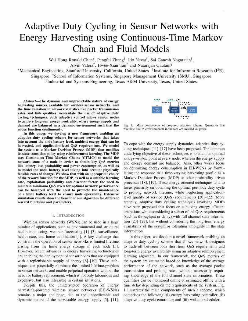
Fig. 1. Main components of proposed adaptive scheme. Quantities thatfluctuate due to environmental influences are marked in green.

To cope with the energy supply dynamics, adaptive duty cy-cling techniques [11]–[17] have been proposed. The commonunderlying objective of these techniques is to attain an optimalenergy-neutral point at every node, wherein the energy supplyand energy demand are balanced. Also, other works focuson optimizing energy consumption in EH-WSNs by formu-lating the response to a time-varying harvesting profile as aMarkov Decision Process (MDP) or other probability-drivenprocesses [18], [19]. These energy-oriented techniques tend tofocus primarily on obtaining the optimal per-node duty cycleto prolong network lifetime, while neglecting application-level quality of service (QoS) requirements [20]–[22]. Morerecently, adaptive duty cycling techniques involving MDPshave been proposed that focus on achieving energy efficientoperations while considering a subset of the QoS requirements(such as throughput or delay) with full channel state informa-tion [23]–[27], but without considering the long-term energyavailability of the system or tolerating ambiguity in the stateinformation.

In this paper, we develop a novel framework enabling anadaptive duty cycling scheme that allows network designersto trade-off between both short-term QoS requirements andlong-term energy availability using an adaptive reinforcementlearning algorithm. In our framework, the QoS metrics ofthe system are estimated based on knowledge of the averageperformance of the network, such as the average packettransmission and probing rates, without necessarily requir-ing knowledge of the full channel state information. Thesequantities can be monitored online or estimated offline with atime delay depending on the requirements of the system. Fig.1 illustrates the main components of such a scheme, whichcomprises the following: (i) energy harvesting controller; (ii)adaptive duty cycle controller; and (iii) wakeup scheduler.

The energy harvesting controller provides information onthe amount of harvested energy that is currently available,while predicting the harvested energy available within the nextfew hours, depending on the diurnal cycles of the energysources. The adaptive duty cycle controller computes theoptimal operating duty cycle based on user inputs (in the formof application QoS requirements) and the available amountof harvested energy. The wakeup scheduler will then: (i)manage the sleep and wake interfaces of each node, basedon the recommended operating duty cycle, and (ii) providefeedback to the adaptive duty cycle controller on the energyconsumption of and remaining energy in the node. Thisfeedback loop allows the duty cycle controller to adapt itsduty cycle, based on the harvested and remaining energies -in order to meet QoS requirements - via operating policiessuch as energy neutrality.

In our previous work [28], we developed a duty cycle con-troller key to the energy-aware operations of a sensor network.Using a Continuous Time Markov Chain (CTMC) model, wederived key QoS metrics including loss probability, latency,as well as power consumption, as functions of the duty cycle.(We define these metrics more explicitly in Section III-B.)We then formulated and solved the optimal operating dutycycle as a non-linear optimization problem, using latency andloss probability as the constraints. We validated our CTMCmodel through Monte Carlo simulations and demonstrated thata Markovian duty cycling scheme can outperform periodicduty cycling schemes. In this paper, we extend the previouswork and enhance the duty cycle controller by considering thebattery level and energy harvesting rate. We then formulatethe adaptive duty cycle problem as a MDP model. The statesof the MDP model correspond to the energy consumptionrates at which the node can operate. The actions refer to thetransition rates between the various duty cycle values that thenode can adopt. The reward function is derived based on theQoS parameters derived in the previous paper, as well as onthe energy availability of the battery based on a fluid model[29]–[31] that indicates the ability of the node to functioncontinuously. While finding the optimal duty cycle schemeto operate under is a nonconvex optimization problem whichis hard to implement on-line, we propose a relatively simpleon-line approach which uses reinforcement learning [32], [33]to heuristically update the reward function to approximateconvergence. We also use extensive simulations to show thatthe MDP converges to a desirable result quickly, and tocompare our approach with a random approach to demonstratethe performance of the MDP scheme.

In this work, we make several key contributions: (i) weenable a WSN to determine its duty cycle control throughsimultaneous consideration of the energy supply dynamicsand application-level QoS requirements; (ii) we establisha reward framework that allows the network to tune therelative importance of the energy availability and the QoSrequirements; (iii) we implement a reinforcement learningalgorithm that converges to a desirable solution quickly andwith lower computational complexity than convergence to afully optimal solution; and (iv) we allow the system to adaptto changes in the environment and/or the network that occur

at timescales larger than the convergence time of the learningcurve. In Fig. 2, we provide an approximate comparison ofthe timescales involved in our system.

The rest of the paper is organized as follows. Section IIprovides details on the key assumptions used in the systemmodel for a battery-free framework. In Section III, we derivenetwork performance metrics using a CTMC model. Weextend the system model to incorporate battery levels inSection IV, and describe the behaviour of the battery withanother CTMC model in Section V. In Section VI, we allowthe system to determine the optimal rates of transition betweenits constituent states using a MDP model. Simulation resultsare presented in Section VII. Section VIII concludes thepaper.

II. SYSTEM MODEL FOR BATTERY-FREE FRAMEWORK

In this Section, we develop a probabilistic model thatdescribes the features of a single WSN node, i.e. data re-ception from other nodes and data transmission towards thegateway (GW) via another node. Both this node and itsrecipient node are duty cycled, and several QoS parametersare investigated as functions of this duty cycle. Under theframework developed in this Section, we do not considerthe role of energy harvesting. Thus, we assume the networkis powered by mains electricity, and the effective batterycapacity of each node is unlimited (although we would stilltry to minimise the energy consumption of each node). InSection IV, we will generalise our framework by consideringenergy harvesting nodes.

We now present all the statistical assumptions of ourframework and provide details of various system componentsrequired, such as the traffic model, channel model and packettransmission schemes. The notation used in this section isshown in Table I.

1) Node State: Each node vj is in one of the followingstates Nj ∈ {0, 1} at any point in time, where Nj = 0and Nj = 1 denote that vj is in the asleep and awakestates respectively. The duration t that node vj is in eachof the states Nj is a random variable that follows anexponential distribution:

p (t) =

{γi · e−γi·t t ≥ 0

0 t < 0,(1)

where γi, i ∈ {0, 1} are the rates of the asleep and awakestates. The average long-term fraction of time that thenode is awake is given by q = 1

γ1·T where T = 1γ0

+ 1γ1

is the average cycle time.2) Traffic Model: The number of data packets d0 generated

by each node follows a Poisson distribution with an aver-age rate of λ0 packets per unit time, i.e., d0 ∼ Pois(λ0).In addition, the node receives dn packets from all of itsneighbours according to a Poisson process dn ∼ Pois(λ).

3) Wireless Channel Model: The time-varying wireless linkquality is modelled by the classical Gilbert-Elliot Marko-vian model [34], [35] with two states L ∈ {0, 1}, whereL = 0 and L = 1 denote that the channel quality isbad and good respectively. The duration t that a node is

2

Fig. 2. Comparison of timescales involved in our system.

TABLE INOTATION USED IN SECTION II

Notation Description Valuevj j-th node N.A.vk Downstream node N.A.Nj Awake or Asleep states of vj {0, 1}γi Respective rates of asleep (Nj = i = 0) / awake (Nj = i = 1) states R+

T Average cycle time 1γ0

+ 1γ1

q Average long-term fraction of time in which node is in the awake state 1γ1T

λ0 Average self-packet generation rate R+

λ Average received-packet rate from nearby nodes R+

d0 Number of self-packets generated by each node d0 ∼Pois(λ0)dn Number of received-packets from nearby nodes dn ∼Pois(λ)L Wireless link quality {0, 1}ci Average rate of bad (i = 0) and good (i = 1) link quality states R+

β Probabilities of successfully delivered data packets when channel is in bad link quality state [0,1]α Probabilities of successfully delivered data packets when channel is in good link quality state [0,1]θg Intensities of probing when channel is good R+

θb Intensities of probing when channel is bad R+

Xn No Retransmissions N.A.Xr Retransmissions N.A.λg Average number of successfully received packets at a node under good channel conditions R+

λb Average number of successfully received packets at a node under bad channel conditions R+

Pasleep Power consumption of a node in the asleep state R+

Pawake Power consumption of a node in the awake state R+

Pprobe Power consumption of probing mechanism R+

εtx Energy consumed to transmit a single data packet R+

in each of the channel states is a random variable thatfollows an exponential distribution:

p (t) =

{ci · e−ci·t t ≥ 0

0 t < 0,(2)

where ci, i ∈ {0, 1} are the respective rates of the badand good states. We let β and α denote the probabilitiesof successfully delivered data packets when the channelis in the bad and good states respectively. Acknowl-edgment packets are assumed to always be deliveredsuccessfully.

4) Probing Mechanism: The network utilizes probes todetermine if an arbitrary downstream node vk is in anawake state Nk = 1, prior to the commencement ofdata transmission. The probing mechanism is modelledas a Poisson process, with intensities θg and θb when thechannel quality is good and bad respectively. The recep-tion of a probe-acknowledgment by the transmitter nodevj indicates that vk is awake; vj will then instantaneouslytransmit all its data packets to vk.

5) Transmission Schemes: We consider two transmission

schemes:a) No Retransmissions: data packets that have not been

successfully delivered to the receiver (due to poorchannel quality) will not be retransmitted. The corre-sponding average numbers of packets that successfullyarrive at a node under good and poor channel condi-tions are denoted as λg and λb respectively, whereλb =

β·λg

α . We denote this scheme by Xn.b) Retransmissions: data packets are retransmitted un-

til they are successfully delivered to the receiver.The corresponding average number of packets thatsuccessfully arrive under this scheme is λ, whereλg = λb = λ. The effective packet arrival rate whenthe node is in the awake state is λ

q . We denote thisscheme by Xr.

6) Power Consumption Parameters: The power consump-tions of a node in the asleep and awake states are Pasleep

and Pawake respectively. The power consumption of theprobing mechanisms is denoted as Pprobe. The energyincurred to transmit a single data packet is Etx.

With these definitions, we now present in the next Section

3

a probabilistic model based on a Continuous Time MarkovChain (CTMC) model, and derive the QoS parameters ofinterest.

III. CTMC MODEL FOR NODE PERFORMANCE STATE(BATTERY-FREE; FIXED DUTY CYCLE)

In this Section, we design a probabilistic model to de-scribe the performance of a single node in the WSN for afixed duty cycle q. To this end, we model the system as aCTMC, as shown in Fig. 3. In addition, we assume that thesystem evolves independently of the battery level, as we willbe using this model to generate instantaneous QoS metricsfor the system, assuming in addition that the timescale ofenergy fluctuations exceeds the timescale of packet trafficequilibration (i.e. the convergence time of this CTMC). Thenotation used in this section is shown in Table II.

0, 1, 0,0

0, 1, 1,0

0, 0, 0,0

0, 0, 1,0

l0

B, 0, 0,0

l0

B, 0, 1,0

l0+lb/q

B, 1, 0,0

l0+lb/q

B, 1, 1,0

qb

…

…

…

…

0, 1, 0,1

0, 1, 1,1

0, 0, 0,1

0, 0, 1,1

l0

B, 0, 0,1

l0

B, 0, 1,1

l0+lg/q

B, 1, 0,1

l0+lg/q

B, 1, 1,1

qg

…

…

…

…

c0

c1

c0

c1

Fig. 3. CTMC model of a two-node section of a network. The CTMC isguided by the transition rate matrix Q.

A. CTMC State Space Model

We consider a 4-tuple CTMC state space as follows:1) Node buffer: Each node has a FIFO buffer of finite size

B. The number of packets in the finite queue is denotedby b ∈ {0, 1, . . . , B}.

2) Node state: As mentioned in Section II, each node vjis in state Nj ∈ {0, 1} at any one time, depending onwhether it is asleep (Nj = 0) or awake (Nj = 1).

3) Downstream node state: An arbitrary downstream (re-ceiving) node vk is in state Nk ∈ {0, 1} at any one time,depending on whether it is asleep (Nk = 0) or awake(Nk = 1).

4) Link quality: The wireless link quality is in state L ∈{0, 1} at any one time, depending on whether the channelis bad (L = 0) or good (L = 1). (We note that it isstraightforward to extend the analysis to multiple linkquality states.)

Given these definitions, the state space S can be written asthe following Cartesian product S = {0, 1, . . . , B}×{0, 1}×{0, 1} × {0, 1} ∈ R|b|×|Nj |×|Nk|×|L|. The correspondingcardinality of the state space is given by |S| = 8(B + 1).

B. QoS metric definitions

We now present the following key QoS metrics of interest:• loss probability due to wireless channel transmission

errors and packet drops arising from buffer overflows,denoted π (q);

• latency incurred by holding packets in the transmissionqueue, denoted ` (q);

• and average power consumption incurred by a node,denoted ρ (q).

In the next Lemma we present the derived expressionsfor these QoS metrics for the two cases under consideration,namely the Retransmissions and No Retransmissions schemes.

Lemma 1. QoS metrics under Retransmissions schemeThe QoS parameters are given by (5).

Proof. See Appendix A.

Lemma 2. QoS metrics under No Retransmissions schemeThe QoS parameters are given by (6).

Proof. See Appendix B.

By defining parameters (e.g. packet arrival rates λ0 andλ, probing intensities θg and θb, and maximum buffer sizeB) of the transitive matrix Q according to parameters of theactual sensor network, we can obtain the optimal duty cycleq in terms of the asleep and awake rates γ0 and γ1. This ispresented next.

C. Optimal Duty Cycle

To find the optimal duty cycle, different criteria can beconsidered. Here, we choose to find the duty cycle which min-imizes the power consumption, while satisfying application-level QoS constraints. We note that other criteria could beconsidered and our framework is general enough to handlethem as well.

For our criterion, the resulting optimisation problem isgiven as follows:

q = argminq

ρ(q) subject to π(q) ≤ π0, `(q) ≤ `0, q ≥ 0

(3)where π0 and `0 are pre-defined latency and loss thresholds.

Recall that γ1 and γ0 can be expressed as functions of qand the average cycle time T as follows:

γ1 =1

T · qγ0 =

1

T · (1− q)(4)

Thus, we can further simplify the optimisation problem toa single parameter optimization problem by defining T andsolving for γ1 and γ0. Hence, even though the optimizationproblem in (3) does not have an analytical closed formexpression, it is easy to find the optimal q (denoted q∗)numerically via simple evaluation on a finely divided grid.In Fig. 4, we plot the optimal duty cycle of the system afterconstraint optimization for various latency and loss probabilityconstraints, as well as for different sets of system parameters.Note that there are regions in which the constraints cannot besatisfied simultaneously.

IV. SYSTEM MODEL FOR FRAMEWORK WITH FINITEBATTERY LEVEL AND ENERGY HARVESTING

In this Section and the next, we develop a frameworkthat describes the evolution of the battery level of a single

4

TABLE IINOTATION USED IN SECTION III

Notation Description ValueB FIFO buffer size Z+

b Number of packets in finite queue b ∈ {0, 1, · · · , B}Nk Awake or Asleep states of vk {0, 1}S State space {0, 1, · · · , B} × {0, 1} × {0, 1} × {0, 1}sk Arbitrary state sk ∈ Spk Steady-state probability of state sk (0, 1)Q Transition matrix of CTMC for node performance states N.A.π(q) Loss probability [0, 1]b Average number of packets in the buffer R+

λe Effective packet arrival rate at the node R+

`(q) Latency ` = bλe

ρ(q) Average power consumption of node vj R+

π (q) =

1∑k=0

pB,1,0,k(λ/q + λ0)

λ/q + λ0 + γ0 + γ1 + ck+

1∑k=0

pB,1,1,k(λ/q + λ0)

λ/q + λ0 + 2γ1 + θ + ck+

1∑k=0

pB,0,0,kλ0

λ0 + 2γ0 + ck+

1∑k=0

pB,0,1,kλ0

λ0 + γ0 + γ1 + ck

` (q) =1

λ+ λ0

B∑b=0

1∑i=0

1∑j=0

1∑k=0

bpb,i,j,k

ρ (q) = Pasleep

B∑b=0

1∑j=0

1∑k=0

pb,0,j,k + Pawake

B∑b=0

1∑j=0

1∑k=0

pb,1,j,k + Pprobe

B∑b=1

1∑j=0

1∑k=0

pb,1,j,k + (λ

1− β/α+ λ0)Etx

(5)

π (q) =pB,1,0,0(λb/q + λ0)

λb/q + λ0 + γ0 + γ1 + c0+

pB,1,1,0(λb/q + λ0)

λb/q + λ0 + 2γ1 + θ + c0+

pB,0,0,0λ0

λ0 + 2γ0 + c0+

pB,0,1,0λ0

λ0 + γ0 + γ1 + c0+

pB,1,0,1(λg/q + λ0)

λg/q + λ0 + γ0 + γ1 + c1+

pB,1,1,1(λg/q + λ0)

λg/q + λ0 + 2γ0 + γ1 + c1+

pB,0,0,1λ0

λ0 + 2γ0 + c1+

pB,0,1,1λ0

λ0 + γ0 + γ1 + c1

` (q) =1

λb + λ0

B∑b=0

1∑i=0

1∑j=0

bpb,i,j,0 +1

λg + λ0

B∑b=0

1∑i=0

1∑j=0

bpb,i,j,1

ρ (q) = Pasleep

B∑b=0

1∑j=0

1∑k=0

pb,0,j,k + Pawake

B∑b=0

1∑j=0

1∑k=0

pb,1,j,k + Pprobe

B∑b=1

1∑j=0

1∑k=0

pb,1,j,k + (λ+ λ0)Etx

(6)

Latency constraint l0

Loss

probabilityconstraintπ0

0.2 0.4 0.6 0.8 10.01

0.02

0.03

0.04

0.05

0.06

0.07

0.08

0.09

0.1

0.65

0.7

0.75

0.8

0.85

0.9

0.95

(a)

Latency constraint l0

Loss

probabilityconstraintπ0

0.2 0.4 0.6 0.8 10.01

0.02

0.03

0.04

0.05

0.06

0.07

0.08

0.09

0.1

0.86

0.88

0.9

0.92

0.94

0.96

0.98

(b)

Latency constraint l0

Loss

probabilityconstraintπ0

0.2 0.4 0.6 0.8 10.01

0.02

0.03

0.04

0.05

0.06

0.07

0.08

0.09

0.1

0.6

0.65

0.7

0.75

0.8

0.85

0.9

0.95

(c)

Fig. 4. Optimal duty cycle as a function of the QoS constraints for different sets of system parameters. The optimal duty cycle is represented by a colourwhose corresponding value can be read off from the colour bar. Steps are observed because the duty cycle was sampled discretely.

node with finite battery capacity and the capability to harvestenergy from the environment. Under the constraints of thisframework, we eventually identify a set of variables that

can be designed to control the performance of the network,namely the transition rates that govern the transition of thebattery state between different rates of energy harvesting and

5

consumption. The consumption rates were previously derivedin Section III. Note that the battery states in this Section andthe next are distinct from the CTMC states of Sections IIand III, which describe the network status and capacity of thenode.

Here, we provide details of additional system componentsrequired in this framework, in particular the battery model andits time evolution. The notation used in this section is shownin Table III.

1) Battery Model: The battery level X(t) of the sensor nodeis treated in a continuous fashion, i.e. X(t) ∈ R andX(t) ∈ [0, C], where C is the capacity of the batteryand t ≥ 0.

2) Rate of Change of Battery Level: In reality, the rateof change of X(t) can take any value in a continuous,bounded interval [Xmin, Xmax] where Xmin and Xmax arethe minimum and maximum possible rates determinedby the battery chemistry, the maximum harvesting poweravailable, and the maximum power consumption of thenode.We model this with a fluid model by sampling mn possi-ble rates within this interval, and defining the cardinalityof the state space of the battery to be mn. Let Z(t) be thestate of the battery at time t. When Z(t) is in some statei ∈ T = {1, 2, . . . ,mn}, the evolution of the processsatisfies

dX(t)

dt=

max(0, ri) if X(t) = 0,

ri if 0 < X(t) < C,

min(0, ri) if X(t) = C,

(7)

where ri is the rate governing the process evolutioncorresponding to state i provided the battery is neitherfull nor empty. In this model, if the battery is full,the rate of change of X(t) with respect to time cannottake positive values; if the battery is empty, the rate ofchange of X(t) with respect to time cannot take negativevalues. This allows us to model the continuous natureof the battery level using a set of discrete states thatbest describe the time evolution of the battery level bycharacterizing the most common rates of change in thebattery level.Physically, the change in the battery level X(t) is drivenby two processes: the harvesting of energy from thesurroundings at rate hk, and the consumption of energyby the system at rate ul.a) Discretized Energy Harvesting Rate: In reality, the

energy harvesting rate hk can take any value betweenzero and the maximum physically possible harvestingrate hmax. We model this by sampling m possibleharvesting rates between zero and hmax.

b) Discretized Energy Consumption Rate: In reality,the energy consumption rate ul can take any valuebetween zero and the maximum physically possibleconsumption rate umax. We model this by samplingn possible consumption rates between zero and umax.As demonstrated in our previous paper [28], ul can bemodelled as a monotonic function of the duty cycle q.

c) Discretized Rate of Change of Battery Level: Now,we set k, l ∈ Z , k ∈ (0,m] and l ∈ (0, n], and wedefine

rn(k−1)+l = hk − ul, (8)

choosing {hk} and {ul} such that the resulting ri areunique. Note Xmin = −umax and Xmax = hmax.

V. CTMC MODEL FOR NODE BATTERY STATE(VARIABLE DUTY CYCLE)

With the model described in the previous Section, wecan now extend our framework so that it also captures thetime evolution of the battery level of a single node in thenetwork. Based on this extended framework, we can therebydescribe the energy availability of the battery in terms of aprobabilistic description of the amount of time the batterylevel is above zero, as well as a transition rate matrix thatdescribes the transition of the system from one set of energyharvesting and consumption rates to another set. By isolat-ing the transitions between different harvesting rates fromthe transitions between different consumption rates, we thenseparate the influences of the environment from a potentialset of user inputs for system optimization. The notation usedin this section is shown in Table IV.

A. Characteristics of CTMC describing transitions betweenbattery states

Here, we introduce a CTMC that describes the transitionsbetween the mn battery states. This allows us to concretelyset up the battery model, as well as to generate the energyavailability required for the reward function of the Markovdecision process (MDP) to be presented in Section VI.

Suppose the CTMC has a generator matrix QMDPe =

[qe,ij ]. Let us define a drift matrix

D =

r1

r2 0. . .

0 rmn

. (9)

In addition, let

πij(t) = Pr(Z(t) = j|Z(0) = i), i, j ∈ T (10)

and

πj = limt→∞

Pr(Z(t) = j|Z(0) = i), i, j ∈ T. (11)

In other words, πij(t) is the probability that the batteryis in state j at time t given that it was initially in state i,and πj is the limit of πij(t) as t goes to infinity, assumingthe CTMC has a stationary distribution. As in the resultsof Section III, the steady-state probabilities πj should thensatisfy peQMDP

e = 0 and∑

j∈T πj = 1, where pe =[π1 π2 . . . π|T |].

6

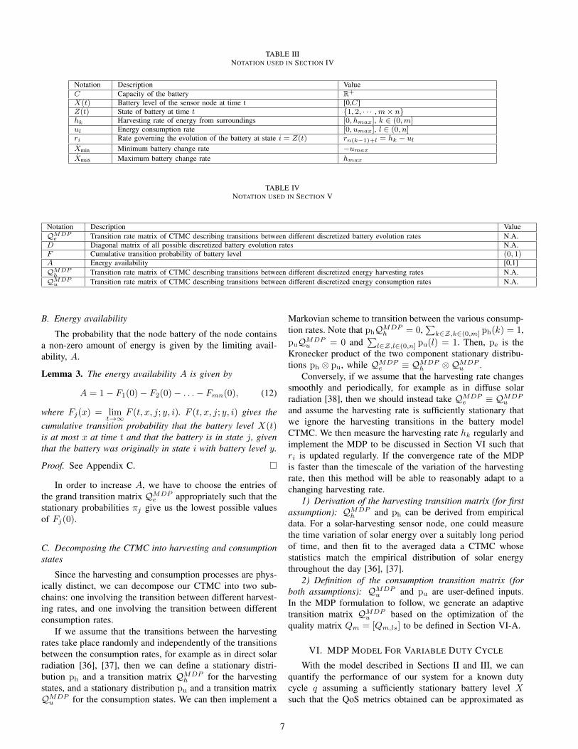
TABLE IIINOTATION USED IN SECTION IV

Notation Description ValueC Capacity of the battery R+

X(t) Battery level of the sensor node at time t [0,C]Z(t) State of battery at time t {1, 2, · · · ,m× n}hk Harvesting rate of energy from surroundings [0, hmax], k ∈ (0,m]ul Energy consumption rate [0, umax], l ∈ (0, n]ri Rate governing the evolution of the battery at state i = Z(t) rn(k−1)+l = hk − ul

Xmin Minimum battery change rate −umax

Xmax Maximum battery change rate hmax

TABLE IVNOTATION USED IN SECTION V

Notation Description ValueQMDP

e Transition rate matrix of CTMC describing transitions between different discretized battery evolution rates N.A.D Diagonal matrix of all possible discretized battery evolution rates N.A.F Cumulative transition probability of battery level (0, 1)A Energy availability [0,1]QMDP

h Transition rate matrix of CTMC describing transitions between different discretized energy harvesting rates N.A.QMDP

u Transition rate matrix of CTMC describing transitions between different discretized energy consumption rates N.A.

B. Energy availability

The probability that the node battery of the node containsa non-zero amount of energy is given by the limiting avail-ability, A.

Lemma 3. The energy availability A is given by

A = 1− F1(0)− F2(0)− . . .− Fmn(0), (12)

where Fj(x) = limt→∞

F (t, x, j; y, i). F (t, x, j; y, i) gives thecumulative transition probability that the battery level X(t)is at most x at time t and that the battery is in state j, giventhat the battery was originally in state i with battery level y.

Proof. See Appendix C.

In order to increase A, we have to choose the entries ofthe grand transition matrix QMDP

e appropriately such that thestationary probabilities πj give us the lowest possible valuesof Fj(0).

C. Decomposing the CTMC into harvesting and consumptionstates

Since the harvesting and consumption processes are phys-ically distinct, we can decompose our CTMC into two sub-chains: one involving the transition between different harvest-ing rates, and one involving the transition between differentconsumption rates.

If we assume that the transitions between the harvestingrates take place randomly and independently of the transitionsbetween the consumption rates, for example as in direct solarradiation [36], [37], then we can define a stationary distri-bution ph and a transition matrix QMDP

h for the harvestingstates, and a stationary distribution pu and a transition matrixQMDP

u for the consumption states. We can then implement a

Markovian scheme to transition between the various consump-tion rates. Note that phQMDP

h = 0,∑

k∈Z,k∈(0,m] ph(k) = 1,puQMDP

u = 0 and∑

l∈Z,l∈(0,n] pu(l) = 1. Then, pe is theKronecker product of the two component stationary distribu-tions ph ⊗ pu, while QMDP

e ≡ QMDPh ⊗QMDP

u .Conversely, if we assume that the harvesting rate changes

smoothly and periodically, for example as in diffuse solarradiation [38], then we should instead take QMDP

e ≡ QMDPu

and assume the harvesting rate is sufficiently stationary thatwe ignore the harvesting transitions in the battery modelCTMC. We then measure the harvesting rate hk regularly andimplement the MDP to be discussed in Section VI such thatri is updated regularly. If the convergence rate of the MDPis faster than the timescale of the variation of the harvestingrate, then this method will be able to reasonably adapt to achanging harvesting rate.

1) Derivation of the harvesting transition matrix (for firstassumption): QMDP

h and ph can be derived from empiricaldata. For a solar-harvesting sensor node, one could measurethe time variation of solar energy over a suitably long periodof time, and then fit to the averaged data a CTMC whosestatistics match the empirical distribution of solar energythroughout the day [36], [37].

2) Definition of the consumption transition matrix (forboth assumptions): QMDP

u and pu are user-defined inputs.In the MDP formulation to follow, we generate an adaptivetransition matrix QMDP

u based on the optimization of thequality matrix Qm = [Qm,ls] to be defined in Section VI-A.

VI. MDP MODEL FOR VARIABLE DUTY CYCLE

With the model described in Sections II and III, we canquantify the performance of our system for a known dutycycle q assuming a sufficiently stationary battery level Xsuch that the QoS metrics obtained can be approximated as

7

instantaneous. Using this information, we can now constructa duty cycle policy that allows our system to respond toenvironmental variations, such as the sunlight available to asolar-harvesting node, while cognizant of the QoS targets thatthe system is required to fulfil. The effectiveness of the policyis measured both by the QoS targets, for which a model wasprovided in Sections II and III, and by the battery level, forwhich a model was provided in Sections IV and V. In addition,the policy is used to determine a good set of transition ratesbetween the various consumption rates described in SectionV-C. The notation used in this section is shown in Table V.

A. MDP for Variable Duty Cycle with Reinforcement Learn-ing

In principle, we could try out every single possibility ofq for every possible harvesting rate hk and consumption rateul to determine the best q for each rate of change of thebattery level ri. However, this is likely to be costly in termsof both time and computational resources. By formulating ourproblem as a Markov Decision Process (MDP) driven by areinforcement learning algorithm, we could possibly reducethe number of computations, perform them online instead ofoffline, and make our system adaptive to changing systemparameters, such as the instantaneous packet transmission andprobing rates.

A MDP is useful to describe a decision making processthat allows the system to transit between a set of states.MDPs have been used in various works to control dutycycling and channel usage in WSNs [39]–[43]. The decisionmaker has a set of actions that can be chosen to describethe state transitions. Each state transition is associated withan immediate scalar reward, which is given to the decision-maker or learner. Here, the goal of the reinforcement learningalgorithm is to take actions, transit from one state to another,and maximize the expected sum of the rewards in the long run.To keep track of its rewards, the system maintains a qualityfunction for each state-action pair, which is a cumulativemeasure of the rewards obtained so far, and consults this totake an action (with greedy probability εt). Thus, by takingactions, obtaining rewards and updating the quality matrixbased on this reward, the learner finally converges to a policywhich approaches maximum return of rewards.

1) States: We define the set F of states fl where l ∈ Z andl ∈ (0, n] such that each state corresponds to a uniqueconsumption rate ul.

2) Actions: We define the set G of actions gs such thateach action corresponds to a CTMC transition matrixQMDP

u,s corresponding to transitions between differentdiscretized energy consumption rates. The action spacecan be designed such that each QMDP

u,s has a differentstationary distribution. Different actions will then signifydifferent duty cycle probability distributions in the limitof infinite time. For example, we could design an actionthat constrains the duty cycle to frequently take a lowvalue, and another action that constraints it to frequentlytake a high value. The size of the square matrix QMDP

u,s isn. Here, we sample the entire space of possible QMDP

u to

obtain a representative set of transition matrices that spanthe space and are physically convenient to implement.

3) Rewards: Based on the requirements of the user, be it aneed to conserve energy aggressively, to consume energyaggressively, or to maintain a minimum level of QoSstatistics by achieving a balance between conservationand consumption, one can define an appropriate rewardfunction to achieve one’s objective. Here, we define areward function that incorporates both QoS statistics andsome measure of the amount of energy available to thesystem to balance the QoS requirements and the energyneeds of the system. Since the consumption rate ul is afunction of the duty cycle q, we can use the QoS statisticsderived in Section III to derive a reward for each statein the MDP.In this work, we examine two different reward functions.The first reward function is an n-dimensional rewardcolumn vector with the following constituent entries forthe corresponding states l

W (l) = −wππ(l)−w``(l)/`∗(l)−wρρ(l)+wAA, (13)

for some arbitrary weights wπ , w`, wρ and wA ∈ R+,and where `∗(l) = B/(λ(ul)+λ0(ul)). This definition ofthe reward offers a high reward for a low loss probability,low latency, low energy consumption and high energyavailability A. Note that since A is dependent on sometransition matrix that governs the time evolution of thesystem, W (l) is not strictly a function of only the systemstate l, but is a non-stationary function that varies withtime.The second reward function is a similar column vectorwith the following constituent entries

W (l) =

{w+ π(l) < π0, `(l) < `0, ρ(l) < ρ0, A ∈ A0 = [A0,−, A0,+)

w− otherwise

(14)

involving the latency and loss thresholds π0 and `0defined earlier in Section III, as well as analogous powerconsumption and availability thresholds ρ0 and A0. Inthis case, the reward takes one of two discrete valuesw+ or w− instead of a continuous spectrum of values inthe earlier example.The continuous function (13) enables users to finetunethe balance between energy availability and QoS re-quirements, while the thresholding function (14) enablesusers who are aware of the thresholds that the system isrequired to satisfy, such as network engineers, to providea clear system input.

4) Quality: Last but not least, we associate each state fl andaction gs with a quality Qm,ls.

In Fig. 5, we use a state machine diagram to illustrate thestate and action spaces of the MDP.

8

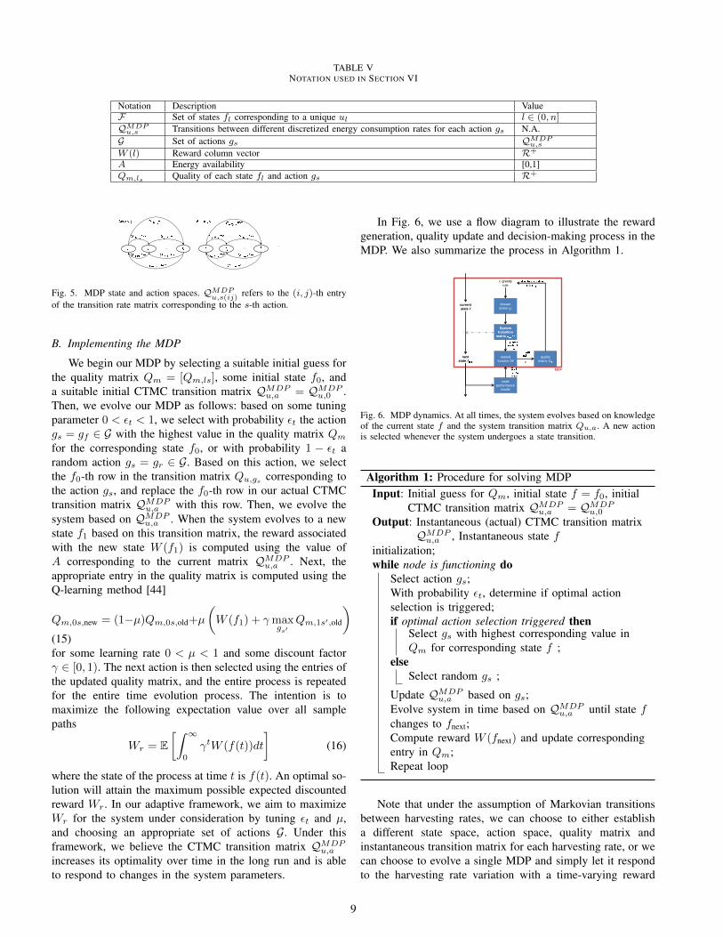
TABLE VNOTATION USED IN SECTION VI

Notation Description ValueF Set of states fl corresponding to a unique ul l ∈ (0, n]

QMDPu,s Transitions between different discretized energy consumption rates for each action gs N.A.

G Set of actions gs QMDPu,s

W (l) Reward column vector R+

A Energy availability [0,1]Qm,ls Quality of each state fl and action gs R+

Fig. 5. MDP state and action spaces. QMDPu,s(ij)

refers to the (i, j)-th entryof the transition rate matrix corresponding to the s-th action.

B. Implementing the MDP

We begin our MDP by selecting a suitable initial guess forthe quality matrix Qm = [Qm,ls], some initial state f0, anda suitable initial CTMC transition matrix QMDP

u,a = QMDPu,0 .

Then, we evolve our MDP as follows: based on some tuningparameter 0 < εt < 1, we select with probability εt the actiongs = gf ∈ G with the highest value in the quality matrix Qm

for the corresponding state f0, or with probability 1 − εt arandom action gs = gr ∈ G. Based on this action, we selectthe f0-th row in the transition matrix Qu,gs corresponding tothe action gs, and replace the f0-th row in our actual CTMCtransition matrix QMDP

u,a with this row. Then, we evolve thesystem based on QMDP

u,a . When the system evolves to a newstate f1 based on this transition matrix, the reward associatedwith the new state W (f1) is computed using the value ofA corresponding to the current matrix QMDP

u,a . Next, theappropriate entry in the quality matrix is computed using theQ-learning method [44]

Qm,0s,new = (1−µ)Qm,0s,old+µ

(W (f1) + γmax

gs′Qm,1s′,old

)(15)for some learning rate 0 < µ < 1 and some discount factorγ ∈ [0, 1). The next action is then selected using the entries ofthe updated quality matrix, and the entire process is repeatedfor the entire time evolution process. The intention is tomaximize the following expectation value over all samplepaths

Wr = E[∫ ∞

0

γtW (f(t))dt

](16)

where the state of the process at time t is f(t). An optimal so-lution will attain the maximum possible expected discountedreward Wr. In our adaptive framework, we aim to maximizeWr for the system under consideration by tuning εt and µ,and choosing an appropriate set of actions G. Under thisframework, we believe the CTMC transition matrix QMDP

u,a

increases its optimality over time in the long run and is ableto respond to changes in the system parameters.

In Fig. 6, we use a flow diagram to illustrate the rewardgeneration, quality update and decision-making process in theMDP. We also summarize the process in Algorithm 1.

Fig. 6. MDP dynamics. At all times, the system evolves based on knowledgeof the current state f and the system transition matrix Qu,a. A new actionis selected whenever the system undergoes a state transition.

Algorithm 1: Procedure for solving MDPInput: Initial guess for Qm, initial state f = f0, initial

CTMC transition matrix QMDPu,a = QMDP

u,0

Output: Instantaneous (actual) CTMC transition matrixQMDP

u,a , Instantaneous state finitialization;while node is functioning do

Select action gs;With probability εt, determine if optimal actionselection is triggered;if optimal action selection triggered then

Select gs with highest corresponding value inQm for corresponding state f ;

elseSelect random gs ;

Update QMDPu,a based on gs;

Evolve system in time based on QMDPu,a until state f

changes to fnext;Compute reward W (fnext) and update correspondingentry in Qm;Repeat loop

Note that under the assumption of Markovian transitionsbetween harvesting rates, we can choose to either establisha different state space, action space, quality matrix andinstantaneous transition matrix for each harvesting rate, or wecan choose to evolve a single MDP and simply let it respondto the harvesting rate variation with a time-varying reward

9

(in particular the variation in A). The first option is morerigorous and is likely to provide better convergence, but thesecond option could be more convenient and less intensiveto implement. Under the assumption of a smooth variation ofthe harvesting rate, we can evolve the MDP as it is and allowit to respond to harvesting rate variations with a time-varyingreward, provided the MDP convergence timescale is shorterthan the harvesting rate variation timescale.

VII. SIMULATION RESULTS

In this Section, we present some results obtained usingMonte Carlo simulations of a single node involving the simul-taneous time evolution of the CTMCs describing the networkand battery states of the node, and of the MDP describing theevolution of the duty cycle of the node. We first describe theparameters and the MDP formulation used in the simulation.We then discuss the impact of the reinforcement learningparameters, and evaluate the performance of our algorithm forboth the continuous and discrete reward functions highlightedin Section VI.

A. Simulation set-upThe network parameters used in our simulations are de-

scribed in Table VI. For simplicity, we consider the case wherethe node in question does not generate its own packets. Also,we first consider the case where the link quality betweenthe nodes in the network is always good (so there is nodifference between the Retransmissions and No Retransmis-sions schemes), and where the energy harvesting rate adoptsa constant value of 0.3 energy units per unit time for theduration of the learning. (We relax the link quality andconstant harvesting rate assumptions in Sections VII-E andVII-F respectively.) For the chosen set of network parameters,this bounds the possible battery evolution rates between about-0.03 and 0.07 energy units per unit time. Finally, we assignour battery a capacity of 0.05 energy units.

For our MDP, we consider a relatively small state spacewith 9 states, involving the regularly-spaced duty cycles {0.1,0.2, · · · , 0.9}, as well as a relatively small action space with5 actions, to make the conclusions we derive from our sim-ulations clearer. The infinitesimal generators correspondingto the five actions are detailed in Appendix D, and havecorresponding stationary distributions that are centred aroundstates 1, 3, 5, 7 and 9 respectively. In all trials, we initialize ourMDP with a randomly chosen state, an all-zero quality matrix,and a state transition matrix where all inter-state transitionshave a rate of 0.1 transitions per unit time, and force the MDPto select an action immediately.

B. Reinforcement learning parametersWe highlight the effects of varying the learning rate µ,

the exploitation probability εt, and the discount factor γ.In particular, we note the trade-off between decreasing theresponse time of the system and maintaining the stabilityof the convergence of the learning curves, and make theobservation that the reinforcement learning algorithm usedin our simulations outperforms a random decision-makingscheme.

1) Effects of varying learning rate µ: In Fig. 7, weobserve that a higher µ increases the learning ability of thesystem by decreasing the convergence time, but results inhigher-frequency and larger fluctuations in the learned qualityvalues.

2) Effects of varying exploitation probability εt: In Fig. 8,we again observe that a higher εt decreases the convergencetime of the system at the expense of higher-frequency andlarger fluctuations in the learned quality values. In Fig. 9, weobserve that as εt increases, the distribution deviates morestrongly from a uniform distribution for the odd-numberedstates, which is what we would expect in a system thatselects its actions randomly. In addition, as εt increases, thestandard deviations of the probabilities decrease, suggestingconvergence towards a desirable stationary distribution. Bychoosing a non-zero εt, we obtain a scheme that outperformsa random decision-making policy.

3) Effects of varying discount factor γ: Without a suf-ficiently large γ, the randomness inherent in a MDP, andespecially in the reward function we selected due to theconstantly varying nature of A, may impede the learning ofthe system. In Fig. 10, we observe that only with a sufficientlylarge γ does effective learning take place in the system.

C. Performance of algorithm: Continuous reward function

The performance of our algorithm depends on our systemobjectives, as well as the reward function implemented in ourMDP. An appropriate choice of the reward function can shiftthe behaviour of the system. Here, we consider the rewardfunction (13), and look at the effects of varying the weights.

1) Effects of energy availability on system: We expect thatin a system that places great emphasis on energy availability,the average duty cycle will be low in order to ensure thebattery does not expend all its energy; conversely, in a systemthat places little emphasis on energy availability, the averageduty cycle will then be governed by the QoS metrics, whichare likely to push the duty cycle higher to ensure effectivetransmission. This intuition is validated by the results in Figs.11 and 13a.

2) Effects of latency on system: We similarly expect thatwhen emphasis on latency is high, the average duty cyclewill be high to maintain the QoS standards; conversely, whenemphasis on latency is low, the average duty cycle will thenbe lower to conserve energy and meet the power consumptionand energy availability requirements. This intuition is vali-dated by the results in Figs. 12 and 13b.

D. Performance of algorithm: Reward function with thresh-olding

1) Convergence analysis: Figure 14 plots the quality fora single state and action with respect to different values ofpower and latency thresholds in order to demonstrate theconvergence of the algorithm. When the power threshold isincreased with all other thresholds fixed, the magnitude of thequality and the convergence time decrease. When the latencythreshold is increased with all other thresholds fixed, themagnitude of the quality and the convergence time increase.

10

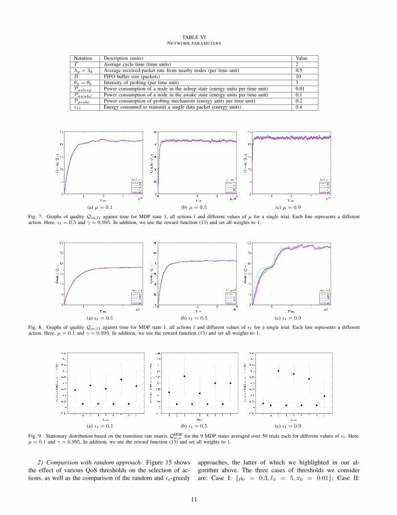
TABLE VINETWORK PARAMETERS

Notation Description (units) ValueT Average cycle time (time units) 2λg = λb Average received-packet rate from nearby nodes (per time unit) 0.5B FIFO buffer size (packets) 10θg = θb Intensity of probing (per time unit) 3Pasleep Power consumption of a node in the asleep state (energy units per time unit) 0.01Pawake Power consumption of a node in the awake state (energy units per time unit) 0.1Pprobe Power consumption of probing mechanism (energy units per time unit) 0.2εtx Energy consumed to transmit a single data packet (energy units) 0.4

(a) µ = 0.1 (b) µ = 0.5 (c) µ = 0.9

Fig. 7. Graphs of quality Qm,l1 against time for MDP state 1, all actions l and different values of µ for a single trial. Each line represents a differentaction. Here, εt = 0.5 and γ = 0.995. In addition, we use the reward function (13) and set all weights to 1.

(a) εt = 0.1 (b) εt = 0.5 (c) εt = 0.9

Fig. 8. Graphs of quality Qm,l1 against time for MDP state 1, all actions l and different values of εt for a single trial. Each line represents a differentaction. Here, µ = 0.1 and γ = 0.995. In addition, we use the reward function (13) and set all weights to 1.

(a) εt = 0.1 (b) εt = 0.5 (c) εt = 0.9

Fig. 9. Stationary distribution based on the transition rate matrix QMDPu,a for the 9 MDP states averaged over 50 trials each for different values of εt. Here,

µ = 0.1 and γ = 0.995. In addition, we use the reward function (13) and set all weights to 1.

2) Comparison with random approach: Figure 15 showsthe effect of various QoS thresholds on the selection of ac-tions, as well as the comparison of the random and εt-greedy

approaches, the latter of which we highlighted in our al-gorithm above. The three cases of thresholds we considerare: Case I: {ρ0 = 0.3, `0 = 5, π0 = 0.01}; Case II:

11

(a) γ = 0.1 (b) γ = 0.5 (c) γ = 0.995

Fig. 10. Graphs of quality Qm,l1 against time for MDP state 1, all actions l and different values of γ for a single trial. Each line represents a differentaction. Here, µ = 0.1 and εt = 0.5. In addition, we use the reward function (13) and set all weights to 1.

(a) wA = 0.01 (b) wA = 1 (c) wA = 1000

Fig. 11. Stationary distribution based on the transition rate matrix QMDPu,a for the 9 MDP states averaged over 50 trials each for different values of wA.

Here, εt = 0.5, µ = 0.1 and γ = 0.995. In addition, we use the reward function (13) and set all other weights to 1.

(a) w` = 0.01 (b) w` = 1 (c) w` = 1000

Fig. 12. Stationary distribution based on the transition rate matrix QMDPu,a for the 9 MDP states averaged over 50 trials each for different values of w`. Here,

εt = 0.5, µ = 0.1 and γ = 0.995. In addition, we use the reward function (13) and set all other weights to 1.

(a) Varying wA (b) Varying w`

Fig. 13. Plot of average duty cycle versus (a) wA, holding all other weights constant at 1 and (b) w`, holding all other weights constant at 1, using (13)and averaging over 50 trials for each wA and w` respectively. Here, εt = 0.5, µ = 0.1 and γ = 0.995.

12

(a) Power (b) Latency

Fig. 14. Graphs of quality Qm,11 against time for state 1 and action 1, and for different power (ρ0) and latency (`0) thresholds. Here, εt = 0.9 andγ = 0.995. For (a), `0 = π0 = A0,+ = 1 and A0,− = 0, and for (b), ρ0 = π0 = 0.7, A0,+ = 1 and A0,− = 0.

{ρ0 = 0.32, `0 = 5, π0 = 0.01}; Case III: {ρ0 = 0.33, `0 =0.91, π0 = 4E-5}. Here, we do not consider the effects ofenergy availability by taking A0 = [0, 1).

Figure 16 shows the optimal sets of duty cycles forthe three cases in order to satisfy the QoS thresholds. InCase I, the corresponding optimal state is 4. In Case II, thecorresponding optimal states are 5, 6 and 7. In Case III, thecorresponding optimal states are 7, 8 and 9. This agrees withthe results shown in Fig. 15 when εt = 0.9, keeping in mindthat our action space tends to direct the system towards theodd-numbered states only. When εt = 0, the scheme reducesto a random approach where the states are chosen randomlyand the stationary probabilities of states 1, 3, 5, 7 and 9 areuniform.

0.1 0.2 0.3 0.4 0.5 0.6 0.7 0.8 0.90

0.01

0.02

0.03

Fraction of time node is awake

Pac

ket L

oss

Pro

babi

lity

0.1 0.2 0.3 0.4 0.5 0.6 0.7 0.8 0.90

5

10

15

20

Fraction of time node is awake

Ave

rage

Lat

ency

0.1 0.2 0.3 0.4 0.5 0.6 0.7 0.8 0.90.2

0.25

0.3

0.35

0.4

Fraction of time node is awake

Ave

rage

Pow

er C

onsu

med

Case ICase III

Case II

Fig. 16. Optimal sets of duty cycles for each case without considering theenergy availability A.

3) Effects of energy availability: As seen in the previoussubsection, the QoS thresholds can help to choose a set ofoptimal duty cycles. However, the energy availability dependson the attainment of equilibrium by the whole system, andthe derivation of the optimal set of duty cycles is not asstraightforward.

a) Simulation settings: In this section, we modify thelearning rate µ to be inversely proportional to the total timespent in the current state [32] in order to handle the variationin the energy availability. In addition, we select a subset of theaction space in which the system’s steady state probabilitiesare centred around states 3, 5, 7 and 9 to better illustrate theeffects of varying A0.

b) Convergence analysis: The convergence of the al-gorithm with the presence of the energy availability termis not as fast with the learning rates used in the previoussections. Hence, we use a learning rate that decreases with

total time elapsed in the current state (including past transi-tions) to speed up convergence. Figure 17 demonstrates theconvergence of the learned quality values and the emergenceof an optimal action. As seen in Fig. 17a, low values of A0

result in an action that favours a higher duty cycle and lowerenergy availability, and vice versa as evident from Figs. 17band 17c.

c) Analysis of steady state probabilities: Fig. 18ademonstrates that when energy availability is not consideredand when all the duty cycles satisfy the given QoS thresholds,the steady state probabilities learned are almost uniform withhigh standard deviation. This changes in Figs. 18b to 18d,where we see that a low A0 selects higher duty cycles and ahigh A0 selects lower duty cycles on average.

d) Summary: For greater clarity, the results above aresummarised in Fig. 19. These graphs demonstrate that anincrease in A0 decreases the average duty cycle and promotesthe selection of actions favouring states that correspond tolower duty cycles.

4) Remarks: As we mentioned earlier, the continuousreward function (13) enables finetuning of the balance be-tween energy availability and QoS requirements, while thethresholding reward function (14) enables clear demarcationsof the boundaries of the system, provided the intersection ofthe threshold requirements is physically achievable. Our re-sults demonstrate that the convergence characteristics of bothreward mechanisms are comparable and can simultaneouslytake into consideration short-term QoS requirements and long-term energy availability standards.

E. Varying link quality

We now consider the effects of variable link quality asdiscussed in the system model in Section II. Here, we use thethresholding reward function (14) analogous to the results inSection VII-D.

1) Convergence analysis: Figure 20 demonstrates theconvergence of the learned quality values for different powerthresholds when the channel can exist in either the good or badstate, for both the Retransmissions and No Retransmissionsschemes.

2) Comparison with random approach: Figure 21 com-pares the random and εt-greedy approaches, for the Retrans-missions (Case I) and No Retransmissions (Case II) schemes.

13

(a) Case I (b) Case II (c) Case III

Fig. 15. Comparison of the εt-greedy approach highlighted in our algorithm above (εt = 0.9, blue) with a random approach (εt = 0, red) using the averagestationary probability of each state over 20 trials for three different cases of thresholds. The more probable states obtained from our algorithm (in blue) agreewell with the optimal duty cycles predicted in Fig. 16.

0 0.5 1 1.5 2

x 104

−1.5

−1

−0.5

0

0.5

1

1.5

Time

Qua

lity

Qm

,5

Action 1Action 2Action 3Action 4

(a) A0 ∈ [0.4, 0.45)

0 0.5 1 1.5 2

x 104

−1

−0.5

0

0.5

1

1.5

2

2.5

3

3.5

Time

Qua

lity

Qm

,5

Action 1Action 2Action 3Action 4

(b) A0 ∈ [0.5, 0.55)

0 0.5 1 1.5 2

x 104

−0.5

0

0.5

1

1.5

2

2.5

3

Time

Qua

lity

Qm

,5

Action 1Action 2Action 3Action 4

(c) A0 ∈ [0.6, 0.65)

Fig. 17. Graphs of Qm,5 against time for different ranges of A0. Here, π0 = 0.02, `0 = 9, ρ0 = 0.33, εt = 0.9 and γ = 0.995.

0 0.2 0.4 0.6 0.8 10

0.05

0.1

0.15

0.2

0.25

0.3

0.35

0.4

States

Sta

tiona

ry D

istr

ibut

ion

Pro

babi

litie

s

(a) A0 ∈ [0, 1)

0 0.2 0.4 0.6 0.8 10

0.05

0.1

0.15

0.2

0.25

0.3

0.35

0.4

0.45

States

Sta

tiona

ry D

istr

ibut

ion

Pro

babi

litie

s

(b) A0 ∈ [0.4, 0.45)

0 0.2 0.4 0.6 0.8 10

0.05

0.1

0.15

0.2

0.25

0.3

0.35

States

Sta

tiona

ry D

istr

ibut

ion

Pro

babi

litie

s

(c) A0 ∈ [0.5, 0.55)

0 0.2 0.4 0.6 0.8 10

0.05

0.1

0.15

0.2

0.25

0.3

0.35

0.4

States

Sta

tiona

ry D

istr

ibut

ion

Pro

babi

litie

s

(d) A0 ∈ [0.6, 0.65)

Fig. 18. Graphs of steady state probabilities averaged over 20 trials, for different ranges of A0. Here, π0 = 0.02, `0 = 9, ρ0 = 0.33, εt = 0.9 andγ = 0.995.

0.4 0.5 0.6

0.4

0.5

0.6

0.7

0.8

0.9

1

A0

Ave

rage

dut

y cy

cle

(a) Average duty cycle for different A0

0 0.2 0.4 0.6 0.8 10

0.05

0.1

0.15

0.2

0.25

0.3

0.35

States

Sta

tiona

ry D

istr

ibut

ion

Pro

babi

litie

s

A

0=0.4

A0=0.5

A0=0.6

(b) Average steady state probabilities fordifferent A0

Fig. 19. Graphs of (a) the duty cycle for different ranges of A0 plotted against the median of A0 and (b) the steady state probabilities for different rangesof A0, both averaged over 20 trials. Here, π0 = 0.02, `0 = 9, ρ0 = 0.33, εt = 0.9 and γ = 0.995.

The thresholds and parameters adopted in these two Casesare identical to those adopted in Fig. 20. The correspondingoptimal state for both Cases is 1, and we demonstrate in Fig.

21 that our algorithm is able to learn this optimal condition.

14

(a) (b)

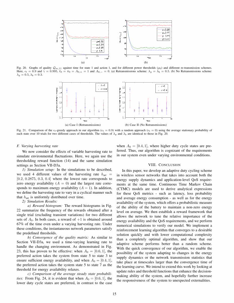
Fig. 20. Graphs of quality Qm,11 against time for state 1 and action 1, and for different power thresholds (ρ0) and different re-transmission schemes.Here, εt = 0.9 and γ = 0.995, `0 = π0 = A0,+ = 1 and A0,− = 0. (a) Retransmissions scheme: λg = λb = 0.5. (b) No Retransmissions scheme:λg = 0.5, λb = 0.3.

(a) Case I (Retransmissions) (b) Case II (No Retransmissions)

Fig. 21. Comparison of the εt-greedy approach in our algorithm (εt = 0.9) with a random approach (εt = 0) using the average stationary probability ofeach state over 10 trials for two different cases of thresholds. The values of λg and λb are identical to those in Fig. 20.

F. Varying harvesting rateWe now consider the effects of variable harvesting rate to

simulate environmental fluctuations. Here, we again use thethresholding reward function (14) and the same simulationsettings as Section VII-D3a.

1) Simulation setup: In the simulations to be described,we used 4 different values of the harvesting rate harr =[0.2, 0.2875, 0.3, 0.4] where the lowest rate corresponds tozero energy availability (A = 0) and the largest rate corre-sponds to maximum energy availability (A = 1). In addition,we define the harvesting rate to vary in a cyclical manner suchthat harr is uniformly distributed over time.

2) Simulation Results:a) Reward histogram: The reward histograms in Fig.

22 summarize the frequency of the rewards obtained after asingle trial (excluding transient variations) for two differentsets of A0. In both cases, a reward of +1 is obtained around67% of the time even under a varying harvesting rate. Underthese conditions, the instantaneous network parameters satisfythe predefined thresholds.

b) Convergence of the quality matrix: As similar toSection VII-D3a, we used a time-varying learning rate tohandle the changing environment. As demonstrated in Fig.23, this has proven to be effective: when A0 = [0.6, 1], thepreferred action takes the system from state 5 to state 3 toensure sufficient energy availability, and when A0 = [0.4, 1],the preferred action takes the system state 5 to state 7 as thethreshold for energy availability relaxes.

c) Comparison of the average steady state probabili-ties: From Fig. 24, it is evident that when A0 = [0.6, 1], thelower duty cycle states are preferred, in contrast to the case

when A0 = [0.4, 1], where higher duty cycle states are pre-ferred. Thus, our algorithm is cognizant of the requirementsin our system even under varying environmental conditions.

VIII. CONCLUSION

In this paper, we develop an adaptive duty cycling schemein wireless sensor networks that takes into account both theenergy supply dynamics and application-level QoS require-ments at the same time. Continuous Time Markov Chain(CTMC) models are used to derive analytical expressionsfor these QoS metrics - such as latency, loss probabilityand average energy consumption - as well as for the energyavailability of the system, which offers a probabilistic measureof the ability of the battery to maintain a non-zero energylevel on average. We then establish a reward framework thatallows the network to tune the relative importance of theenergy availability and the QoS requirements, and we performnumerical simulations to verify our model. We implement areinforcement learning algorithm that converges to a desirablesolution quickly and with lower computational complexitythan a completely optimal algorithm, and show that ouradaptive scheme performs better than a random scheme.With the quick convergence of our algorithm, we enable thepossibility of the system adapting to changes in the energysupply dynamics or the network transmission statistics thattake place at timescales larger than the convergence time ofthe learning curve. We intend to extend this work by looking atupdate rules and threshold functions that enhance the decision-making ability of the system, and hopefully further increasethe responsiveness of the system to unexpected externalities.

15

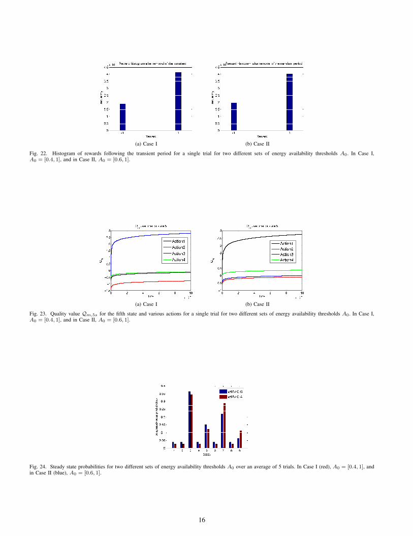
(a) Case I (b) Case II

Fig. 22. Histogram of rewards following the transient period for a single trial for two different sets of energy availability thresholds A0. In Case I,A0 = [0.4, 1], and in Case II, A0 = [0.6, 1].

(a) Case I (b) Case II

Fig. 23. Quality value Qm,5s for the fifth state and various actions for a single trial for two different sets of energy availability thresholds A0. In Case I,A0 = [0.4, 1], and in Case II, A0 = [0.6, 1].

Fig. 24. Steady state probabilities for two different sets of energy availability thresholds A0 over an average of 5 trials. In Case I (red), A0 = [0.4, 1], andin Case II (blue), A0 = [0.6, 1].

16

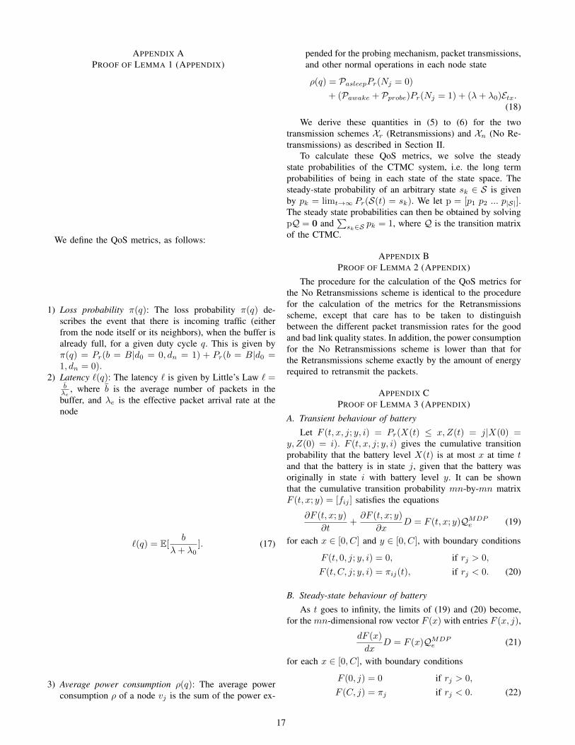
APPENDIX APROOF OF LEMMA 1 (APPENDIX)

We define the QoS metrics, as follows:

1) Loss probability π(q): The loss probability π(q) de-scribes the event that there is incoming traffic (eitherfrom the node itself or its neighbors), when the buffer isalready full, for a given duty cycle q. This is given byπ(q) = Pr(b = B|d0 = 0, dn = 1) + Pr(b = B|d0 =1, dn = 0).

2) Latency `(q): The latency ` is given by Little’s Law ` =bλe

, where b is the average number of packets in thebuffer, and λe is the effective packet arrival rate at thenode

`(q) = E[b

λ+ λ0]. (17)

3) Average power consumption ρ(q): The average powerconsumption ρ of a node vj is the sum of the power ex-

pended for the probing mechanism, packet transmissions,and other normal operations in each node state

ρ(q) = PasleepPr(Nj = 0)

+ (Pawake + Pprobe)Pr(Nj = 1) + (λ+ λ0)Etx.(18)

We derive these quantities in (5) to (6) for the twotransmission schemes Xr (Retransmissions) and Xn (No Re-transmissions) as described in Section II.

To calculate these QoS metrics, we solve the steadystate probabilities of the CTMC system, i.e. the long termprobabilities of being in each state of the state space. Thesteady-state probability of an arbitrary state sk ∈ S is givenby pk = limt→∞ Pr(S(t) = sk). We let p = [p1 p2 ... p|S|].The steady state probabilities can then be obtained by solvingpQ = 0 and

∑sk∈S pk = 1, where Q is the transition matrix

of the CTMC.

APPENDIX BPROOF OF LEMMA 2 (APPENDIX)

The procedure for the calculation of the QoS metrics forthe No Retransmissions scheme is identical to the procedurefor the calculation of the metrics for the Retransmissionsscheme, except that care has to be taken to distinguishbetween the different packet transmission rates for the goodand bad link quality states. In addition, the power consumptionfor the No Retransmissions scheme is lower than that forthe Retransmissions scheme exactly by the amount of energyrequired to retransmit the packets.

APPENDIX CPROOF OF LEMMA 3 (APPENDIX)

A. Transient behaviour of battery

Let F (t, x, j; y, i) = Pr(X(t) ≤ x,Z(t) = j|X(0) =y, Z(0) = i). F (t, x, j; y, i) gives the cumulative transitionprobability that the battery level X(t) is at most x at time tand that the battery is in state j, given that the battery wasoriginally in state i with battery level y. It can be shownthat the cumulative transition probability mn-by-mn matrixF (t, x; y) = [fij ] satisfies the equations

∂F (t, x; y)

∂t+

∂F (t, x; y)

∂xD = F (t, x; y)QMDP

e (19)

for each x ∈ [0, C] and y ∈ [0, C], with boundary conditions

F (t, 0, j; y, i) = 0, if rj > 0,

F (t, C, j; y, i) = πij(t), if rj < 0. (20)

B. Steady-state behaviour of battery

As t goes to infinity, the limits of (19) and (20) become,for the mn-dimensional row vector F (x) with entries F (x, j),

dF (x)

dxD = F (x)QMDP

e (21)

for each x ∈ [0, C], with boundary conditions

F (0, j) = 0 if rj > 0,

F (C, j) = πj if rj < 0. (22)

17

We see thatF ′ = F (QMDP

e D−1), (23)

which leads us to guess the solutions F (x) = eλxφ where λis a scalar and φ is an mn-dimensional row vector. It can beshown that the general solution to (23) is given by F (x) =∑i∈T

aieλixφi, where λi are the generalized eigenvalues and

φi the generalized eigenvectors of the equation

φi(λiD −QMDPe ) = 0 (24)

or((QMDP )Te − λiD

T )φTi = 0. (25)

In other words, λi and φTi are the eigenvectors of

(D−1)T (QMDP )Te = ((QMDP )eD−1)T .

The coefficients ai are given by the solutions to∑i∈T

aiφi(j) = 0 if j ∈ T+,∑i∈T

aiφi(j)eλiC = πj if j ∈ T−, (26)

where T+ and T− contain the elements of T where thecorresponding rate rj is positive and negative respectively.Note that keeping all else constant, a higher C results in lowerai and thus a larger A.

APPENDIX DACTION SPACE OF MDP USED FOR SIMULATIONS

(APPENDIX)

The infinitesimal generators corresponding to the fiveactions are such that they encourage the system to transitionto states 1, 3, 5, 7 and 9 respectively. An action that transitionsthe system to some state i has an infinitesimal generator wherestate i has a transition rate of 0.1 to all other states, and allother states have transition rates of 0.9 to state i and 0.1 toall other states. For example, for action 1, the infinitesimalgenerator is

QMDPu,1 =

−0.8 0.1 0.1 0.1 0.1 0.1 0.1 0.1 0.10.9 −1 0.0143 0.0143 0.0143 0.0143 0.0143 0.0143 0.01430.9 0.0143 −1 0.0143 0.0143 0.0143 0.0143 0.0143 0.01430.9 0.0143 0.0143 −1 0.0143 0.0143 0.0143 0.0143 0.01430.9 0.0143 0.0143 0.0143 −1 0.0143 0.0143 0.0143 0.01430.9 0.0143 0.0143 0.0143 0.0143 −1 0.0143 0.0143 0.01430.9 0.0143 0.0143 0.0143 0.0143 0.0143 −1 0.0143 0.01430.9 0.0143 0.0143 0.0143 0.0143 0.0143 0.0143 −1 0.01430.9 0.0143 0.0143 0.0143 0.0143 0.0143 0.0143 0.0143 −1

.

(27)

18

REFERENCES

[1] A. Kottas, Z. Wang, and A. Rodrguez, “Spatial modeling for risk as-sessment of extreme values from environmental time series: a bayesiannonparametric approach,” Environmetrics, vol. 23, no. 8, 2012.

[2] C. Fonseca and H. Ferreira, “Stability and contagion measures forspatial extreme value analyses,” arXiv preprint arXiv:1206.1228, 2012.

[3] J. P. French and S. R. Sain, “Spatio-temporal exceedance locations andconfidence regions,” Annals of Applied Statistics. Prepress, 2013.

[4] I. Akyildiz, W. Su, Y. Sankarasubramaniam, and E. Cayirci, “Wirelesssensor networks: a survey,” Computer networks, vol. 38, no. 4, pp.393–422, 2002.

[5] W. K. Seah, Z. A. Eu, and H.-P. Tan, “Wireless sensor networks poweredby ambient energy harvesting (wsn-heap)-survey and challenges,” in1st International Conference on Wireless Communication, VehicularTechnology, Information Theory and Aerospace & Electronic SystemsTechnology. IEEE, 2009, pp. 1–5.

[6] V. Raghunathan, A. Kansal, J. Hsu, J. Friedman, and M. Srivastava,“Design considerations for solar energy harvesting wireless embeddedsystems,” Fourth International Symposium on Information Processingin Sensor Networks, pp. 457 – 462, April 2005.

[7] M. Gorlatova, P. Kinget, I. Kymissis, D. Rubenstein, X. Wang, andG. Zussman, “Challenge: ultra-low-power energy-harvesting active net-worked tags (enhants),” Proceedings of the 15th annual internationalconference on Mobile computing and networking, pp. 253–260, 2009.

[8] C. Bergonzini, D. Brunelli, and L. Benini, “Algorithms for harvestedenergy prediction in batteryless wireless sensor networks,” 3rd Interna-tional Workshop on Advances in sensors and Interfaces, pp. 144 –149,June 2009.

[9] D. Hasenfratz, A. Meier, C. Moser, J.-J. Chen, and L. Thiele, “Analysis,comparison, and optimization of routing protocols for energy harvestingwireless sensor networks,” IEEE International Conference on SensorNetworks, Ubiquitous, and Trustworthy Computing (SUTC), pp. 19 –26,June 2010.

[10] S. Sudevalayam and P. Kulkarni, “Energy harvesting sensor nodes:Survey and implications,” IEEE Communications Surveys Tutorials,no. 99, pp. 1–19, 2010.

[11] A. Kansal, J. Hsu, S. Zahedi, and M. B. Srivastava, “Power managementin energy harvesting sensor networks,” ACM Trans. Emb. Comput. Sys.,vol. 6, pp. 1–38, Sep. 2007.

[12] J. Hsu, S. Zahedi, A. Kansal, M. Srivastava, and V. Raghunathan,“Adaptive duty cycling for energy harvesting systems,” in Proceedingsof the 2006 international symposium on low power electronics anddesign. ACM, 2006, pp. 180–185.

[13] C. Vigorito, D. Ganesan, and A. Barto, “Adaptive control of duty cyclingin energy-harvesting wireless sensor networks,” in Proc. IEEE SECON,2007.

[14] Y. Gu, T. Zhu, and T. He, “Esc: Energy synchronized communicationin sustainable sensor networks,” in Proc. IEEE ICNP, 2009.

[15] T. Zhu, Z. Zhong, Y. Gu, T. He, and Z.-L. Zhang, “Leakage-awareenergy synchronization for wireless sensor networks,” in Proc. ACMMobiSys, 2009.

[16] V. Sharma, U. Mukherji, V. Joseph, and S. Gupta, “Optimal energymanagement policies for energy harvesting sensor nodes,” IEEE Trans-actions on Wireless Communications, vol. 9, no. 4, pp. 1326–1336,2010.

[17] C. Moser, J.-J. Chen, and L. Thiele, “An energy management frameworkfor energy harvesting embedded systems,” ACM Journal on EmergingTechnologies in Computing Systems (JETC), vol. 6, no. 2, p. 7, 2010.

[18] A. Sinha and A. Chandrakasan, “Dynamic power management inwireless sensor networks,” Design & Test of Computers, IEEE, vol. 18,no. 2, pp. 62–74, 2001.

[19] M. Gorlatova, A. Wallwater, and G. Zussman, “Networking low-power energy harvesting devices: Measurements and algorithms,” IEEETransactions on Mobile Computing, vol. 12, no. 9, pp. 1853–1865, Sept2013.

[20] K. Sohrabi, J. Gao, V. Ailawadhi, and G. J. Pottie, “Protocols for self-organization of a wireless sensor network,” IEEE personal communica-tions, vol. 7, no. 5, pp. 16–27, 2000.

[21] W. B. Heinzelman, A. L. Murphy, H. S. Carvalho, and M. A. Perillo,“Middleware to support sensor network applications,” IEEE Network,vol. 18, no. 1, pp. 6–14, 2004.

[22] J. Yick, B. Mukherjee, and D. Ghosal, “Wireless sensor networksurvey,” Computer networks, vol. 52, no. 12, pp. 2292–2330, 2008.

[23] J. Lei, R. Yates, and L. Greenstein, “A generic model for optimizingsingle-hop transmission policy of replenishable sensors,” Wireless Com-munications, IEEE Transactions on, vol. 8, no. 2, pp. 547–551, 2009.

[24] A. Seyedi and B. Sikdar, “Energy efficient transmission strategies forbody sensor networks with energy harvesting,” Communications, IEEETransactions on, vol. 58, no. 7, pp. 2116–2126, 2010.

[25] H. Li, N. Jaggi, and B. Sikdar, “Relay scheduling for cooperative com-munications in sensor networks with energy harvesting,” IEEE Trans-actions on Wireless Communications, vol. 10, no. 9, pp. 2918–2928,September 2011.

[26] A. Sultan, “Sensing and transmit energy optimization for an energyharvesting cognitive radio,” Wireless Communications Letters, IEEE,vol. 1, no. 5, pp. 500–503, 2012.

[27] P. Blasco, D. Gunduz, and M. Dohler, “A learning theoretic approach toenergy harvesting communication system optimization,” IEEE Transac-tions on Wireless Communications, vol. 12, no. 4, pp. 1872–1882, April2013.

[28] R. Chan, P. Zhang, W. Zhang, I. Nevat, A. Valera, H.-X. Tan, andN. Gautam, “Adaptive duty cycling in sensor networks via continuoustime markov chain modeling,” Accepted by ICC 2015, June 2015.

[29] V. G. Kulkarni, “Fluid models for single buffer systems,” Frontiersin queueing: Models and applications in science and engineering, pp.321–338, 1997.

[30] G. L. Jones, P. G. Harrison, U. Harder, and T. Field, “Fluid queuemodels of battery life,” in 2011 IEEE 19th International Symposium onModeling, Analysis & Simulation of Computer and TelecommunicationSystems (MASCOTS). IEEE, 2011, pp. 278–285.

[31] N. Gautam and A. Mohapatra, “Efficiently operating wireless nodespowered by renewable energy sources,” IEEE Journal on Selected Areasin Communications (To appear), 2015.

[32] A. G. Barto, Reinforcement learning: An introduction. MIT press,1998.

[33] L. P. Kaelbling, M. L. Littman, and A. W. Moore, “Reinforcementlearning: A survey,” Journal of artificial intelligence research, pp.237–285, 1996.

[34] E. N. Gilbert, “Capacity of a burst-noise channel,” Bell System TechnicalJournal, vol. 39, no. 5, 1960.

[35] E. O. Elliot, “Estimates of error rates for codes on burst-noise channels,”Bell System Technical Journal, vol. 42, no. 5, 1963.

[36] P. Poggi, G. Notton, M. Muselli, and A. Louche, “Stochastic studyof hourly total solar radiation in corsica using a markov model,”International Journal of Climatology, vol. 20, no. 14, pp. 1843–1860,2000.

[37] O. Kwon, Y.-J. Yoon, S. K. Moon, H.-J. Choi, and J. H. Shim, “Estima-tion of singapores hourly solar radiation using hybrid-markov transitionmatrices method,” International Journal of Precision Engineering andManufacturing, vol. 14, no. 2, pp. 323–327, 2013.

[38] R. Jayaraman and D. L. Maskell, “Temporal and spatial variations ofthe solar radiation observed in singapore,” Energy Procedia, vol. 25,pp. 108–117, 2012.

[39] Z. Liu and I. Elhanany, “Rl-mac: A qos-aware reinforcement learningbased mac protocol for wireless sensor networks,” in Proceedings ofthe 2006 IEEE International Conference on Networking, Sensing andControl. IEEE, 2006, pp. 768–773.

[40] ——, “Rl-mac: a reinforcement learning based mac protocol for wire-less sensor networks,” International Journal of Sensor Networks, vol. 1,no. 3, pp. 117–124, 2006.

[41] G. Ghidini and S. K. Das, “An energy-efficient markov chain-basedrandomized duty cycling scheme for wireless sensor networks,” inDistributed Computing Systems (ICDCS), 2011 31st International Con-ference on. IEEE, 2011, pp. 67–76.

[42] M. Bkassiny, S. K. Jayaweera, and K. A. Avery, “Distributed reinforce-ment learning based mac protocols for autonomous cognitive secondaryusers,” in Wireless and Optical Communications Conference (WOCC),2011 20th Annual. IEEE, 2011, pp. 1–6.

[43] G. Ghidini and S. K. Das, “Energy-efficient markov chain-based dutycycling schemes for greener wireless sensor networks,” ACM Journalon Emerging Technologies in Computing Systems (JETC), vol. 8, no. 4,p. 29, 2012.

[44] C. J. Watkins and P. Dayan, “Q-learning,” Machine learning, vol. 8, no.3-4, pp. 279–292, 1992.

19