UDC631 ISSN 1333 - 2651 UNIVERSITY OF ZACREB FACULTY OF ACRICULTURE ACRICULTURAL ENCINEERlNC DEPARTMENT FACULTy OF ACRICULTURE UNtVERStTy OF OSTJEK FACULTY OF ACRICULTURE UNIVERSITY OF MARIBOR AGRICULTURAL INSTITUTE OF SLOVENIA H U NCARIAN I NSTITUTE OF ACRICU LTU RAL ENC I N EERl NC CROATIAN ACRICULTURAL ENCINEERING SOCTETY ftffiAAESEE4r PROCEEDINCS OFTHE 36. INTERNATIONAT SYMPOSIUM ON AGRICULTURAT ENGI NEERI NC ActualTasks on Agricultural neer I Engi ng t; € N c, ) 4 o |lI II 11) I = F o 4 I F g o

Welcome message from author
This document is posted to help you gain knowledge. Please leave a comment to let me know what you think about it! Share it to your friends and learn new things together.
Transcript
U D C 6 3 1 I S S N 1 3 3 3 - 2 6 5 1
UNIVERSITY OF ZACREB FACULTY OF ACRICULTUREACRICULTURAL ENCINEER lNC DEPARTMENTFACULTy OF ACRICULTURE UNtVERStTy OF OSTJEKFACULTY OF ACRICULTURE UNIVERSITY OF MARIBORAGRICULTURAL INST ITUTE OF SLOVENIAH U NCARIAN I NST ITUTE OF ACRICU LTU RAL ENC I N EER l NCCROATIAN ACRICULTURAL ENCINEERING SOCTETY
ftffiAAESEE4ryi@PROCEEDINCS OF THE
36. INTERNATIONAT SYMPOSIUM ONAGRICULTURAT ENGI NEERI NC
ActualTasks onAgricultural neer IEngi ng
t;
€
N
c,
)4o|lIII
11)
I
=F
o4I
F
g
o

SVEUČILIŠTE U ZAGREBU AGRONOMSKI FAKULTETZAVOD ZA MEHANIZACIJU POLJOPRIVREDE
POLJOPRIVREDNI FAKULTET SVEUČILIŠTA U OSIJEKU FAKULTETA ZA KMETIJSTVO UNIVERZE V MARIBORU
KMETIJSKI INŠTITUT SLOVENIJE MAĐARSKI INSTITUT ZA POLJOPRIVREDNU TEHNIKU HRVATSKA UDRUGA ZA POLJOPRIVREDNU TEHNIKU
AAESEE
AKTUALNI ZADACI MEHANIZACIJE
POLJOPRIVREDE
ZBORNIK RADOVA 36. MEÐUNARODNOG SIMPOZIJA IZ PODRUČJA
MEHANIZACIJE POLJOPRIVREDE
OPATIJA, 11. - 15. veljače 2008.
IzdavačiPublished by
Sveučilište u Zagrebu, Agronomski fakultet, Zavod za mehanizaciju poljoprivrede, Svetošimunska 25, 10000 Zagreb HINUS, Miramarska 13 b, Zagreb
Glavni i odgovorni urednik Chief editor
Silvio Košutiće-mail: [email protected]
Tehnički urednik Technical editor
Hrvoje Zrnčić
Organizacijski odbor Organising committee
Krešimir Čopec, Goran Fabijanić, Dubravko Filipović, Zlatko Gospodarić, Igor Kovačev,Ðuro Banaj, Robert Zimmer, Viktor Jejčić,Miran Lakota, Tomaž Poje
Znanstveni odbor Scientific committee
Nikolay Mihailov (Bulgaria), Silvio Košutić,Robert Zimmer, (Croatia), Peter Schulze-Lammers, Joachim Müller (Germany), Daniele De Wrachien, Ettore Gasparetto (Italy), Linus U. Opara (Oman), Maohua Wang (P.R. China), Victor Ros (Romania), Milan Martinov (Serbia), Jaime Ortiz-Canavate (Spain), Vilas M. Salokhe (Thailand), Bill A. Stout (USA)
NakladaNumber of copies
200
ISSN 1333-2651
http://atae.agr.hr
Slika s naslovnice korištena je dobrotom autora gospodina Dušana JejčičaCover painting is printed by courtesy of author Mr Dušan JejčičOblikovanje naslovnice / Cover design: Marko Košutić
Radovi iz Zbornika su od 1997. indeksirani u bazama podataka:Papers from the proceedings have been indexed since 1997 into databases:
Current Contents Proceedings, ISI - Index to Scientific & Technical Proceedings, CAB International - Agricultural Engineering Abstracts, Cambridge Scientific Abstracts - Conference Papers Index, InterDok.
SPONZORI – SPONSORS
MINISTARSTVO ZNANOSTI, OBRAZOVANJA I ŠPORTA REPUBLIKE HRVATSKE
MINISTARSTVO POLJOPRIVREDE, ŠUMARSTVA I VODNOG GOSPODARSTVA
INAZAGREB
AGROGROMSAMOBOR
SIPŠEMPETER, SLOVENIJA
POLJONOVASESVETE
GRAMIP – TPS DUBRAVA
INTERSTEPVELIKA GORICA
AGROMARKETINGZAGREB
PREDGOVOR - PREFACE
Sustavnim radom organizacijskog tima, a uz stalnu potporu kolega iz struke, strukovnih udruga (HUPT i HAD), trgovačkih kuća-predstavnika svjetskih proizvođača poljoprivred-nih strojeva i opreme, Ministarstva znanosti obrazovanja i športa i Ministarstva poljopriv-rede, šumarstva i vodnog gospodarstva, te međunarodnih udruga Poljoprivredne tehnike (EurAgEng, CIGR, AAAE i AAESEE) dospjeli smo do 36. Simpozija ”Aktualni zadaci mehanizacije poljoprivrede”. Tijekom proteklih godina obišli smo slijedeće gradove, do-maćine simpozija: Zagreb (’70, ‘82), Zadar (’75, ‘87), Poreč (’77, ‘81), Split (’78, ’85), Opatija (’79, ’83, ’84, ’88, ’90, ’94 – ’08), Šibenik (’80), Rovinj (’86), Trogir (’89), Stubičke toplice (‘92) Pula (’91, ’93). Dakle, najveći broj godina, ukupno 19, grad domaćinbila je Opatija. Ukupan broj radova od 1.425, varirao je 20 – 83, prosječno 44.5 radova, a ukupan broj stranica svih Zbornika je 13.432 s variranjem 58 – 900, prosječno 419.8. Ovaj 36. po redu Zbornik sadrži 63 rada sa slijedećim učešćem: Bugarska, Bijelorusija, Češka, Indija, Litva i Sjedinjene Američke Države (1), Italija i Njemačka (2), Mađarska i Turska (3), Bosna – Hercegovina (4), Srbija i Kina (5), Hrvatska (8), Slovenija (9) i Rumunjska (16). Zahvaljujemo svim sponzorima koji su svojom potporom omogućili održavanje ovak-vog skupa, autorima referata, kao i svim učesnicima na interesu. Posebno se zahvaljujemo Ministarstvu znanosti i tehnologije Republike Hrvatske na stalnoj potpori. Svim sudionici-ma želimo ugodan boravak u Opatiji za vrijeme održavanja Simpozija.
Continuous work of organizing team with long-term support of our colleagues, our associations (CAES, CSA), commercial representatives of the world famous agricultural machinery and equipment producers, Ministry of sciences, education and sport, Ministry of agriculture, forestry and water management and finally world known associations for agri-cultural engineering (EurAgEng, CIGR, AAAE and AAESEE) has brought us to the 36th
symposium ”Actual tasks on Agricultural Engineering”. During all that years host towns were as follows: Zagreb (’70, ‘82), Zadar (’75, ‘87), Poreč (’77, ‘81), Split (’78, ’85), Opatija (’79, ’83, ’84, ’88, ’90, ’94 – ’08), Šibenik (’80), Rovinj (’86), Trogir (’89), Stubičke toplice (‘92) Pula (’91, ’93). So, Opatija was our favourite town with 19 years in total. Total number of published papers was 1,425 with variations 20 to 83 per proceedings, in average 44.5 papers. Total number of pages was 13,432 with variations of 58 to 900 per proceedings, in average 419.8 pages. This proceedings contains 63 papers among them are: Bulgaria, Belarussia, Czech, India, Lithuania and USA with 1, Italy and Germany with 2, Hungary and Turkey with 3, Bosnia – Herzegovina with 4, Serbia and China with 5 , Croatia with 8, Slovenia with 9 and Romania with 16 papers. We would like to thank authors, reviewers, participants and especially sponsors for their contribution to organise the symposium. We especially emphasize sponsoring of Ministry of Sciences education and sport of Republic of Croatia who support us for 13 years. Finally we wish all participants, our colleagues pleasant time and company during symposium.
Chief Editor Zagreb, siječanj - January 2008. Prof. dr. sc. Silvio Košutić
36. Symposium "Actual Tasks on Agricultural Engineering", Opatija, Croatia, 2008.
SADRŽAJ – CONTENTS
S. Mambretti, D. De Wrachien, E. Larcan....................................................................... 13 Tok nanosa i branom uzrokovani prekidni naplavni valovi: Dinamika reologije i modeliranjeDebris flow and dam-break flooding waves: Dynamics rheology and modelling
S. Mambretti, E. Larcan, D. De Wrachien....................................................................... 35 Tok nanosa i branom uzrokovani prekidni naplavni valovi: Model kalibracije i usporedba s probnim testovima Debris flow and dam-break flooding waves: Model calibration and comparison with experimental tests
A. K. Goel ............................................................................................................................ 47 Razvoj modela otjecanja oborina za brežuljkasto porječje regije donji Shivaliks u Indiji Development of a rainfall runoff model for hilly watershed in lower Shivaliks region of India
R. Miodragovic, M. Djevic................................................................................................. 57 Rezultati testiranja mobilnih irigacijskih sustava kišenjem Results of testing mobile raining irrigation systems in crop production
J. Zhang, Y. Sheng, Y. Zhao, P. Yang .............................................................................. 65 Automatski, precizni sustav irigacije u proizvodnji pamuka An automatic precision irrigation system for cotton field
V. Borovikov........................................................................................................................ 71 Poboljšanje općih parametara diesel motora traktora učinkovitijim punjenjem goriva-zraka Improvement of general parameters of tractor diesel by more effective use of fuel-air charge
V. Jejčič, T. Poje, T. Godeša .............................................................................................. 79 Mogućnost uporabe biljnog ulja za pogon traktora i drugih vozila Possibilites of running tractors and vehicles by plant oil
R. Rosca, I. Tenu, P. Carlescu, E. Rakosi, G. Manolache............................................... 93 Model trakcije kotača s pneumatikom Tire traction models - Comparative analysis and validation
36. Symposium "Actual Tasks on Agricultural Engineering", Opatija, Croatia, 2008.
V. Jurić, T. Jurić, D. Kiš, R. Kiš, I. Plaščak................................................................... 105 Poljoprivredni traktori kao čimbenik sigurnosti prometa Agricultural tractors as factors in traffic safety
S. Şt. Biriş, E. Maican, V. Vladuţ, G. Paraschiv, M. Manea, S. Bungescu.................. 115 Studija kinematike gibanje čestica tla djelovanjem predplužnjaka Study regarding the soil particles kinematics during the ante-mouldboard tillage tools working process
I. Ţenu, P. Cojocariu, R. Rosca, P. Carlescu ................................................................. 127 Testiranje složenog agregata za istovremenu obradu tla i sjetvu strnina The achivement and experimentation of one complex unit for total tillage and sowing of the soil for straw crops
G. Paraschiv, E. Maican, S.-Ş. Biriş, S. Bungescu......................................................... 135 Razvoj i ispitivanje oruđa za obradu tla u održivoj poljoprivredi Researches regarding the development of a soil preparation unit according to the demands of sustainable agriculture
L. Savin, R. Nikolić, M. Simikić, T. Furman, M. Tomić, S. Đurić, J. Vasin............... 145 Analiza utjecaja zbijenosti tla uvratina i unutrašnjeg dijela polja na urod pšenice The analysis of soil compaction influence on wheat yield on headlands and inner part of field
B. Bagarić, V. Zebec, M. Kufner, R. Zimmer................................................................ 155 Poljoprivredna mehanizacija u proizvodnji pšenice različitim sustavima obrade tla Farm machinery for winter wheat production by different soil tillage systems
M. Sagadin, M. Lešnik, S. Vajs, M. Lakota, D. Stajnko, B. Muršec, P. Vindiš.......... 163 Ekonomski učinki direktne setve Economic impact of direct maize sowing
Z. Meng , C. Zhao, W. Huang , W. Hu , X. Wang, L. Chen ......................................... 169 Razvoj i ocjena učinkovitosti nadzornog sustava raspodjeljivača granula promjenjive doze temeljenog na standardu ISO 11783 Development and performance assessment of a variable rate granule applicator control system based on ISO 11783
T. Poje, T. Godeša, V. Jejčić, Š. Modic, G. Urek, M. Lakota, M. Sagadin,G. Leskošek, M. Rak-Cizej .............................................................................................. 181 Prva iskustva suzbijanja odrasle kukuruzne zlatice u Sloveniji First experience in the control of western corn roothworm adults in Slovenia
G. Leskošek, T. Poje ......................................................................................................... 189Snaga potrebna za pogon raspršivača u hmeljarstvu Power required for driving mistblower used in hop protection
36. Symposium "Actual Tasks on Agricultural Engineering", Opatija, Croatia, 2008.
E. Kilic, I. Celen, T. Atkas ............................................................................................... 197 Određivanje nekih značajki dijelova ventila membranskih pumpi prskalica Research on the determination of some properties of valve parts of diaphragm pumps used in sprayers
D. Stajnko, M. Lakota, B. Muršec, M. Sagadin............................................................. 207 Utjecaj različite visine reze na utrošak goriva komunalne kosilice Antonio Carraro The effect of the various cutting height on fuel consumption of the lawn mower Antonio Carraro
T. Poje ................................................................................................................................ 215 Energetske karakteristike malčera Ino Euro Open 280 s pokretnim poklopcem Energetic characteristics of Ino Euro Open 280 mulcher with adjustable cover
V. Moise, G. Voicu, E. Maican ........................................................................................ 221 Strukturalna kinematička i kinetostatička analiza sustava čišćenja kombajna Structural kinematical and kinetostatic analysis of the cereal harvester cleaning system
R. Bernik, F. Vučajnk ...................................................................................................... 233 Gubici zrna pri žetvi ozimog ječma i pšenice kombajnom Deutz Fahr Powerliner 4035 H Harvesting losses of Deutz Fahr Powerliner 4035 H in winter barley and winter wheat
C. Jantschke, S. Phupaichitkun, K. Koeller................................................................... 243 Prikupljanje podataka svojstava površinskog sloja tla fuzijom senzora Top soil properties acquisition by a novel fusion of sensors
J. Wu, C. Liu, Y. Chen, S. Sui, L. Feng .......................................................................... 253 Studija kvantitativnih metoda spektroskopske analize u području blizu infracrvenog dijela spektraStudy on quantitative methods in near infrared spectroscopy analysis
V. Corluka, M. Mesic, Z. Valter...................................................................................... 265 Temeljni pristup analize i identifikacije organskih veza u prehrambenoj industriji spektrometrijom u području blizu infracrvenog dijela spektra Basic access in analysis and identification organic bonds in food industry use NIR spectrometry
F. Mariaşiu, B. Varga, D. Baldean.................................................................................. 275 Razmatranje studije pouzdanosti poljoprivrednih sustava Bayes-ovim teoremom Considerations about the reliability’s study of the agricultural systems using Bayes theorems
S. - T. Bungescu, S. - Ş. Biris, V. Vladut, G. Paraschiv................................................. 281 Istraživanje raspodjele i determinacije opterećenja na površini rešetkaste odgrnjače s ciljem modeliranja i optimizacije Researches regarding the stress distribution determination appearing on the lamellar mouldboard surface with a view to modelling and optimization
36. Symposium "Actual Tasks on Agricultural Engineering", Opatija, Croatia, 2008.
C. Târcolea, T. Căsăndroiu, G. Voicu ............................................................................ 293 Stohastički model simulacije procesa separacije zrna na sitima kombajna Stochastic models for simulating seed separation process on harvester sieves
E. Maican, V. Moise, S.-Ş. Biriş....................................................................................... 307 Numeričko određivanje maksimalnog pomaka osi vitla i kose žitnog kombajna Numerical calculus of the maximum displacement between the reel’s axes and cutter bar from combine harvester
V. V. Safta.......................................................................................................................... 317 CAD metodologija sustava čišćenja gomolja krumpira sukcesivnim kotrljajućim konvejerima CAD methodology of the bulb and potato impurities cleaning systems composed of successive rolling conveyors
J. Čepl ................................................................................................................................ 329 Kartiranje pojave korova- bitan dio sustava precizne poljoprivrede Mapping weed occurrence - an important part of precision farming system
J. Zhou, M. Zang, S. Li, M. Wang, S I. Li...................................................................... 339 Primjena sustava pomoćne navigacije i praćenja u poljoprivredi An accessorial navigation and survelliance system used in agriculture
N. Starčević, C. Thullner, M. Bux, J. Müller ................................................................. 347 Planiranje staza kretanja robota za obradu komunalnog mulja simulacijom trajektorija Path planning for sludge processing robot by means of trajectory simulations
Y. Zhang, M. Li, J. Qiao, G. Liu ..................................................................................... 359 Segmentacijski algoritam za raspoznavanje plodova jabuka umjetnom neuralnom mrežom A segmentation algorithm for apple fruit recognition using artificial neural network
M. Sun, S. Zhang, D. An, Y. Wei, Y. Wang ................................................................... 369 Raspoznavanje sljubljenih zrna riže u binarnom prikazu Recognition of conjoint grains of rice in binary images
B. Evastatiev, N. Mihailov................................................................................................ 379 Istraživanje teperaturnih polja na farmi brojlera sa zimskom ventilacijom Investigation of the temperature field in a broiler fram with winter ventilation
B. Kavolelis, A. Jasinskas................................................................................................. 387 Stvaranje vodene pare u staji za krave Water vapour production of cowshed
I. Petric, A. Šestan, I. Alibašić ......................................................................................... 393 Djelovanje inicijalnog sadržaja vode na aerobno kompostiranje gnoja peradi s pšeničnomslamomEffect of initial moisture content on aerobic composting of poultry manure with wheat straw
36. Symposium "Actual Tasks on Agricultural Engineering", Opatija, Croatia, 2008.
R. Polat, F. Kaplan ........................................................................................................... 405Određivanje fizičko mehaničkih svojstava stabljike pamuka Determination of cutting properties of cotton stalk
T. Aktas.............................................................................................................................. 413 Utjecaj sadržaja vode na termička svojstva sjemena suncokreta The effect of moisture content on the thermal properties of sunflower seeds (Helianthus annus L.)
H. Keran, N. Đonlagić, M. Salkić, N. Ahemtović, S. Mulahalilović............................. 425 Fizičko-kemijski pokazatelji kvalitete sušenog povrća iz A.D. “Semberka”, Janja, Bosna i HercegovinaPhysical-chemical parameters of quality of dried vegetables from “Semberka” Janja, Bosnia and Herzegovina
S. Grujić, K. Plavšić, M. Jašić, S. Blagojević ................................................................. 431 Utjecaj vrste i koncentracije aditiva na senzorna svojstva voćnog želea Influence of additive type and concentration on fruit jelly sensory quality
M.-A. Poiana, D. Miogradean, D. Raba, I. Gergen ....................................................... 441 Utjecaj “starenja”na boju i antioksidantna svojstva crvenog vina The ageing influence on the chromatic and antioxidant characteristics of red wines
M. Salkić, M. Jašić, H. Keran, H. Pašalić....................................................................... 451 Određivanje L-askorbinske kiseline izravnom ultraljubičastom spektrofotometrijom Determination of L-ascorbic acid using direct ultraviolet spectrophotometry
D. Miličević, V. Piližota, H. Pašalić, N. Nedić, A. Begić-Akagić, M. Aljić,M. Šabanović ..................................................................................................................... 459 Sprječavanje degradacije fenolnih tvari u nekim kultiviranim i autohtonim sortama jabuka Prevention of degradation of phenolic compounds in some kind of ancient and cultivated varieties of apples
D. Sotin, F. Radu, D. Dogaru, P. Paul............................................................................. 469 Istraživanje utjecaja hiperakumulacije teških metala na sustav sinigrin-myrosinase Brassicanigra-eResearches regarding the influence of hyperaccumulation of heavy metals on the sinigrin-myrosinase system activity in Brassica nigra
M. Martinov, D. Adamovic, B. Veselinov, M. Matavuly, S. Bojic, I. Mujic................ 479 Praksi orjentirano istraživanje sušenja kamilice i mente umjetnim sušenjem Practice oriented investigation of chamomile and peppermint drying in batch dryers
D. Mnerie, G. V. Anghel................................................................................................... 491 Mogućnosti primjene liofilizacije u poljoprivredi Some applications of lyophilization in agriculture

36. Symposium "Actual Tasks on Agricultural Engineering", Opatija, Croatia, 2008.
M. Djevic, A. Dimitrijevic, S. Blazin............................................................................... 497 Energetska učinkovitost proizvodnje rajčice u grijanom i negrijanom stakleniku Energy efficiency of tomato production in heated and non-heated greenhouse
M. Balan, M. Damian, L. Jantschi .................................................................................. 507 Sustav motrenja sunčeve radijacije Solar radiation monitoring system
B. Muršec, P. Vindiš, M. Lakota, D. Stajnko, M. Sagadin ........................................... 519 Konstrukcija za proizvodnju bioplina Construction for biogas production
R. Bernik, A. Zver ............................................................................................................ 527Optimizacija smjese kukuruzne silaže pri dobivanju bioplina Optimisation of the corn silage mixture in the generation of biogas
M. Balan, M. Damian, L. Jantschi, I. Ion....................................................................... 535 Studija utjecaja nekih radnih uvjeta na učinkovitost toplinskih crpki Study concerning the influence of some working conditions on the heat pumps performances
F. Mariaşiu, N. Burnete.................................................................................................... 545 Studija kompatibilnosti biogoriva i elastomernih brtvila elemenata pročistača ulja The study concerning the biofuels and elastomer sealing elements of the oil filter compatibility
L. Magó.............................................................................................................................. 553 Određivanje granične veličine imanja glede racionalnog opremanja mehanizacijom matematičkim modeliranjem Determination of farm size limit of reasonable mechanisation by modelling
J. Hajdú, L. Magó............................................................................................................. 567Mehaniziranost mađarske poljoprivrede danas Mechanization of the Hungarian agriculture in present days
G. Dukić, D. Turkalj......................................................................................................... 577 Racionalizacija isporuke žitarica i uljarica modelom čekanja u redu Rationalization of cereal and oil crops delivery process by means of queuing models
D. Dukić, I. Alerić ............................................................................................................. 587 Računalna optimizacija angažmana poljoprivredne mehanizacija Computer optimization of agricultural machinery assigment
I. Husti ............................................................................................................................... 597 Aktualni zadaci i mogućnosti inoviranja mađarske poljoprivrede Actual tasks and possibilities in the Hungarian agriculture innovation
36. Symposium "Actual Tasks on Agricultural Engineering", Opatija, Croatia, 2008.
M. Sesar ............................................................................................................................. 605 Analiza stajališta poljoprivrednika osiječko-baranjske županije glede mehanizacije poljoprivredeAnalysisi of farmer’s opinion in Osijek-Baranja county regarding agricultural engineering
D. Mnerie, D. Tucu, G. V. Anghel, T. Slavici................................................................. 617 Studija integracijskih kapaciteta poljoprivredno-prehrambenih sustava Study about integration capacity of systems for agro-food production
M. Tratnik, I. Gverić, R. Franić...................................................................................... 623 Kolebljivost cijena voća i žita i ekonomska opravdanost infrastrukturnih objekata za čuvanje i hlađenje: pro et contra Fruit and cereals price fluctuations and economic justifiability of infrastructural facilities for storage and cooling: pro et contra
M. Jančić............................................................................................................................ 633Proizvodnja na mini gredicama kao uvjet dobivanja pogodnog oblika korjena mrkve Producing on mini bars as condition for getting regular shape of carrot root
KOMERCIJALNE PORUKE......................................................................................... 641 COMMERCIAL NOTES
36. Symposium "Actual Tasks on Agricultural Engineering", Opatija, Croatia, 2008.
13
36.
SIMPOZIJAKTUALNI ZADACIMEHANIZACIJE POLJOPRIVREDE
UDC556.5:631.6
Izvorni znanstveni radOriginal scientific paper
DEBRIS FLOW AND DAM-BREAK FLOODING WAVES: DYNAMICS RHEOLOGY AND MODELLING
STEFANO MAMBRETTI1, DANIELE DE WRACHIEN2, ENRICO LARCAN1
1 DIIAR, Politecnico di Milano, Italy 2 Department of Agricultural Hydraulics, State University of Milan, Italy
E-mail: [email protected]
ABSTRACT
To predict flood and debris flow dynamics a numerical model, based on 1D De Saint Venant (SV) equations, was developed. The McCormack – Jameson shock capturing scheme was employed for the solution of the equations, written in a conservative law form. This technique was applied to determine both the propagation and the profile of a two – phase debris flow resulting from the instantaneous and complete collapse of a storage dam.
The full two – phase model features mass and momentum conservation equations for each phase, along with an interaction force between the two phases. The latter eases, on one hand, the propagation of the solid phase, while, on the other hand, plays a friction role with regard to the clear water.
On the whole, the model proposed can easily be extended to channels with arbitrary cross sections for debris flow routing, as well as for solving different problems of unsteady flow in open channels by incorporating the appropriate initial and boundary conditions.
The great advantages of the technique developed are based on the strong shock capturing ability of the McCormack – Jameson numerical scheme as well as on the simplicity of application of the resulting algorithm when considering 1D debris flow phenomena.
Key words: Debris flow, dam-break, rheological behaviour of the mixtu-res, two-phase modelling
INTRODUCTION
A thorough understanding of the mechanism triggering and mobilising debris flow phenomena plays a role of paramount importance for designing suitable prevention and
S. Mambretti, D. De Wrachien, E. Larcan
14
mitigation measures. Achieving a set of debris flow constitutive equations is a task which has been given particular attention by the scientific community (Julien and O’Brien, 1985; Chen, 1988; Takahashi, 2000). To properly tackle this problem relevant theoretical and experimental studies have been carried out during the second half of the last century.
Research work on theoretical studies has traditionally specialised in different mathema-tical models. They can be roughly categorized on the basis of three characteristics: the presence of bed evolution equation, the number of phases and the rheological model applied to the flowing mixture (Ghilardi et al., 2000).
Most models are based on the conservation of mass and momentum of the flow, but only a few of them take into account erosion / deposition processes affecting the temporal evolution of the channel bed.
Debris flow are mixtures of water and clastic material with high coarse particle contents, in which collisions between particles and dispersive stresses are the dominant mechanisms in energy dissipation. Therefore, their nature mainly changes according to the sediment concentration and characteristics of the sediment size (Hui – Pang and Fang – Wu, 2003).
The rheological property of a debris flow depends on a variety of factors, such as suspended solid concentration, cohesive property, particle size distribution, particle shape, grain friction and pore pressure.
Various researchers have developed models of debris flow rheology. These models can be classified as: Newtonian models (Johnson, 1970; Trunk et al., 1986), linear and non linear viscoplastic models (O’Brien et al., 1993), dilatant fluid models (Bagnold, 1954; Takahashi, 1978), dispersive or turbulent stress models (Arai and Takahashi, 1986), biviscous modified Bingham model (Dent and Lang, 1983), and frictional models (Norem et al., 1990; Iverson, 1997). Among these, linear (Bingham) or non – linear (Herschel – Bulkey) viscoplastic models are widely used to describe the rehology of laminar debris / mud flows (Jan, 1997; Coussot, 1997).
Because a debris flow, essentially, constitutes a multiphase system, any attempt at modelling this phenomenon that assumes, as a simplified hypothesis, homogeneous mass and constant density, conceals the interactions between the phases and prevents the possibility of investigating further mechanisms such as the effect of sediment separation (grading).
Modelling the fluid as a two – phase mixture overcomes most of the limitations mentioned above and allows for a wider choice of rheological models such as: Bagnold’s dilatant fluid hypothesis (Takahashi and Nakagawa, 1994; Shieh et al., 1996), Chézy type equation with constant value of the friction coefficient (Hirano et al., 1997; Armanini and Fraccarollo, 1997), models with cohesive yield stress (Honda and Egashira, 1997) and the generalized viscoplastic fluid Chen’s model (Chen and Ling, 1997).
Notwithstanding all these efforts, some phenomenological aspects of debris flow have not been understood yet, and something new has to be added to the description of the process to reach a better assessment of the events. In this contest, the mechanism of dam – break wave should be further investigated. So far, this aspect has been analysed by means of the single – phase propagation theory for clear water, introducing in the De Saint Venant

Debris flow and dam-break flooding waves: dynamics rheology and modelling
15
(SV) equations a dissipation term to consider fluid rheology (Coussot, 1994; Fread and Jin, 1997).
Many other models, the so – called quasi – two – phase – models use SV equations, together with erosion / deposition and mass conservation equations for the solid phase, and take into account mixture of varying concentrations. All these models feature monotonic velocity profiles that, generally, do not agree with experimental and field data.
In the present report a 1D two – phase model for debris flow propagation is proposed. SV equations, modified for including erosion / deposition processes along the mixture path, are used for expressing conservation of mass and momentum for the two phases of the mixture. The scheme is validated for dam – break problems comparing numerical results with experimental data. Comparisons are made between both wave depths and front propagation velocities obtained respectively on the basis of laboratory tests and with predictions from the numerical model proposed by McCormack – Jameson (McCormack, 1969; Jameson, 1982). These comparisons allow the assessment of the model performance and suggest feasible development of the research.
THEORETICAL BACKGROUND
Debris flow resulting from a sudden collapse of a dam (dam – break) are often characterised by the formation of shock waves caused by many factors such as valley contractions, irregular bed slope and non – zero tailwater depth. It is commonly accepted that a mathematical description of these phenomena can be accomplished by means of 1D SV equations (Bellos and Sakkas, 1987; Bechteler et al., 1992; Aureli et al., 2000).
During the last Century, much effort has been devoted to the numerical solution of the SV equations, mainly driven by the need for accurate and efficient solvers for the disconti-nuities in dam – break problems.
A rather simple form of the dam failure problem in a dry channel was first solved by Ritter (1892) who used the SV equations in the characteristic form, under the hypothesis of instantaneous failure in a horizontal rectangular channel without bed resistance. Later on, Stoker (1949), on the basis of the work of Courant and Friedrichs (1948), extended the Ritter solution to the case of wet downstream channel. Dressler (1952, 1958) used a perturbation procedure to obtain a first – order correction for resistance effects to represent submerging waves in a roughing bed.
Lax and Wendroff (1960) pioneered the use of numerical methods to calculate the hyperbolic conservation laws. McCormack (1969) introduced a simpler version of the Lax – Wendroff scheme, which has been widely used in aerodynamics problems. Van Leer (1977) extended the Godunov scheme to second – order accuracy by following the Monotonic Upstream Schemes for Conservation Laws (MUSCL) approach. Chen (1980) and Chen and Ambruster (1980) applied the method of characteristics, including bed resistance effects, to solve dam – break problems for reservoir of finite length.
Hunt (1982) proposed a kinematic wave approximation for dam failure in a dry sloping channel.

S. Mambretti, D. De Wrachien, E. Larcan
16
Flux splitting based schemes, like that of the implicit Beam – Warming (1976), where applied to solve open channel flow problems without source terms and, in general, reported good results. However, these schemes are only first order accurate in space and employ the flux splitting in an non conservative way. When applied to some cases of dam – break problems, these tools gave much slower front celerity and higher front height when com-pared to experimental tests. Later, Jha et al. (1996) proposed a modification for achieving full conservative form of both the continuity and momentum equations, employing the use of the Roe average approximate Jacobian (Roe, 1981). This produced significant improve-ment in the accuracy of the results.
Total Variation Diminishing (TVD) and Essentially Non Oscillation (ENO) schemes were introduced by Harten (1983) and Harten and Osher (1987) for efficiently solving 1D gas dynamic problems. Their main property is that they are second order accurate and oscillation free across discontinuities.
Recently, several 1D and 2D models using approximate Riemann solvers have been reported in the literature. Such models have been found very successful in solving open channel flow and dam – break problems. Zhao et al. (1994) reported implementation of an approximate Riemann solver with Osher scheme in finite volume and later extended that work by including flux – vector splitting and flux – difference splitting (Zhao et al., 1996).
In the past ten years, further numerical methods to solve flood routing and dam – break problems, have been developed, that include the use of finite elements or discrete / distinct element methods (Asmar et al., 1997; Rodriguez et al., 2006).
Finite Element Methods (FEMs) have certain advantages over finite different methods, mainly in relation to the flexibility of the grid network that can be employed, especially in 2D flow problems.
In this context, Hicks and Steffer (1992) used the Characteristic Dissipative Galerking (CDG) finite element method to solve 1D dam – break problems for variable width channels.
The McCormack predictor – corrector explicit scheme is widely used for solving dam – break problems, due to the fact that it is a shock – capturing technique, with second order accuracy both in time and in space, and that the artificial dissipation terms TVD correction, can be easily introduced (Garcia and Kahawita, 1986; Garcia Navarro and Saviron, 1992).
The main disadvantage of this solver regards the restriction to the time step size in order to satisfy Courant – Friedrichs – Lewy (CFL) stability condition. However, this is not a real problem for dam – break debris flow phenomena that require short time step to describe the evolution of the discharge. To ease the time step restriction, implicit methods could be considered. In this case, the variables are calculated simultaneously at a new time level, through the resolution of a system with as many unknowns as grid points. For non – linear problems, such as the SV equations, the resulting system of equations is also non – linear and either a linearisation or an iterative procedure is required. This extra computation time is, usually, compensated by the possibility of achieving unconditional or near unconditional stability for the scheme or allowing the use of very high CFL numbers. To this end, implicit TVD schemes have been proved to be unconditionally stable, even when a linearisation technique is applied to solve a non – linear hyperbolic equation (Yee, 1987; 1989). Attempts along this line of work were presented by Alcrudo et al. (1994) introducing in the
Debris flow and dam-break flooding waves: dynamics rheology and modelling
17
McCormack scheme TVD corrections to reduce spurious oscillations around discontinui-ties, both for 1D and 2D flow problems and by Delis et al. (2000) developing new implicit TVD methods to solve SV equations.
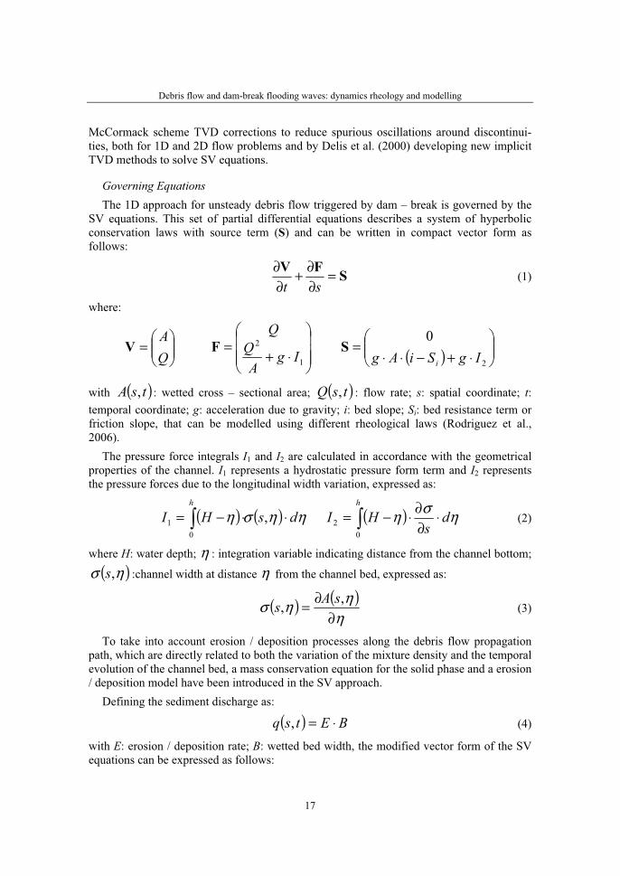
Governing Equations The 1D approach for unsteady debris flow triggered by dam – break is governed by the
SV equations. This set of partial differential equations describes a system of hyperbolic conservation laws with source term (S) and can be written in compact vector form as follows:
SFV =∂∂+
∂∂
st (1)
where:
⎟⎟
⎠
⎞
⎜⎜
⎝
⎛
=QA
V⎟⎟
⎟
⎠
⎞
⎜⎜
⎜
⎝
⎛
⋅+=
1
2
IgA
F ( ) ⎟⎟
⎠
⎞
⎜⎜
⎝
⎛
⋅+−⋅⋅=
2
0IgSiAg i
S
with ( )tsA , : wetted cross – sectional area; ( )tsQ , : flow rate; s: spatial coordinate; t:temporal coordinate; g: acceleration due to gravity; i: bed slope; Si: bed resistance term or friction slope, that can be modelled using different rheological laws (Rodriguez et al., 2006).
The pressure force integrals I1 and I2 are calculated in accordance with the geometrical properties of the channel. I1 represents a hydrostatic pressure form term and I2 represents the pressure forces due to the longitudinal width variation, expressed as:
( ) ( ) ηηση dsHIh
⋅⋅−= ∫ ,0
1 ( ) ηση ds
HIh
⋅∂∂⋅−= ∫
02 (2)
where H: water depth; η : integration variable indicating distance from the channel bottom;
( )ησ ,s :channel width at distance η from the channel bed, expressed as:
( ) ( )η
ηησ∂
∂= ,, sAs (3)
To take into account erosion / deposition processes along the debris flow propagation path, which are directly related to both the variation of the mixture density and the temporal evolution of the channel bed, a mass conservation equation for the solid phase and a erosion / deposition model have been introduced in the SV approach.
Defining the sediment discharge as:
( ) BEtsq ⋅=, (4)
with E: erosion / deposition rate; B: wetted bed width, the modified vector form of the SV equations can be expressed as follows:

S. Mambretti, D. De Wrachien, E. Larcan
18
SFV =∂∂+
∂∂
st (5)
where:
⎟
⎟
⎟
⎠
⎞
⎜
⎜
⎜
⎝
⎛
⋅=
AcQA
s
V⎟
⎟
⎟
⎟
⎠
⎞
⎜
⎜
⎜
⎜
⎝
⎛
⋅
⋅+=
Qc
IgA
s
1
2
F( )
( )⎟
⎟
⎟
⎠
⎞
⎜
⎜
⎜
⎝
⎛
⋅⋅⋅+−⋅=
BcEIgSiAg
tsq
i
*
2
,S
with cs: volumetric solid concentration in the mixture; c*: bed volumetric solid concentra-tion.
Two Phase Mathematical Model Debris flow is, essentially, a multiphase system, so modelling the flow as a two – phase
mixture is the best way to predict these phenomena. The change in debris flow density can be modelled through mass and momentum balance of both phases (solid and liquid) and interactions between the two could be assessed by means of appropriate additional terms (Wallis, 1962; Wang and Hutter, 1999).
The erosion / deposition rate is, generally, controlled by the excess of the local instanta-neous concentration over the equilibrium concentration. Egashira and Ashida (1987) and Honda and Egashira (1997) computed this rate by means of a simple relationship, while Takahashi et al. (1987) proposed semi – empirical expressions. All these models ignore the spatial and temporal variations of debris flow density in the momentum balance equations.
In the present work granular and liquid phases are considered. The model includes two mass and momentum balance equations for both the liquid and solid phases respectively. The interaction between phases is simulated according to Wan and Wang hypothesis (1984). The system is completed with equations to estimate erosion / deposition rate deri-ved from the Egashira and Ashida relationship and by the assumption of the Mohr – Coulomb failure criterion for non cohesive materials.
Mass and momentum equations for the liquid phase Mass and momentum equations for water can be expressed in conservative form as:
( ) ( )( )0
,,=
∂⋅∂
+∂
∂t
tsAcs
tsQ ll (6)
FsHJiAcg
AcQ
stQ
ll
ll −⎟⎠
⎞
⎜
⎝
⎛
∂∂−−⋅⋅⋅=
⎟
⎟
⎠
⎞
⎜
⎜
⎝
⎛
⋅⋅
∂∂+
∂∂ 2
β (7)
with ( )tsQl , : flow discharge; cl: volumetric concentration of water in the mixture; β :
momentum correction coefficient that we will assume to take the value 1=β from now
Debris flow and dam-break flooding waves: dynamics rheology and modelling
19
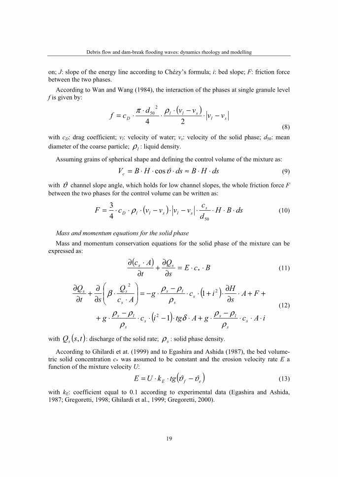
on; J: slope of the energy line according to Chézy’s formula; i: bed slope; F: friction force between the two phases.
According to Wan and Wang (1984), the interaction of the phases at single granule level f is given by:
( )sl
sllD vv
vvdcf −⋅
−⋅⋅
⋅⋅=
24
250 ρπ
(8) with cD: drag coefficient; vl: velocity of water; vs: velocity of the solid phase; d50: mean diameter of the coarse particle; lρ : liquid density.
Assuming grains of spherical shape and defining the control volume of the mixture as:
dsHBdsHBVc ⋅⋅≈⋅⋅⋅= ϑcos (9)
with ϑ channel slope angle, which holds for low channel slopes, the whole friction force Fbetween the two phases for the control volume can be written as:
( ) dsBHdc
vvvvcF sslsllD ⋅⋅⋅⋅−⋅−⋅⋅⋅=
5043 ρ (10)
Mass and momentum equations for the solid phase Mass and momentum conservation equations for the solid phase of the mixture can be
expressed as:
( )BcE
sQ
tAc ss ⋅⋅=
∂∂
+∂
⋅∂* (11)
( )
( ) iAcgAtgicg
FAsHicg
AcQ
stQ
ss
lss
s
ls
ss
ls
s
ss
⋅⋅⋅−
⋅+⋅⋅−⋅⋅−
⋅+
++⋅∂∂⋅+⋅⋅
−⋅−=
⎟
⎟
⎠
⎞
⎜
⎜
⎝
⎛
⋅⋅
∂∂+
∂∂
ρρρδ
ρρρ
ρρρβ
1
1
2
22
(12)
with ( )tsQs , : discharge of the solid rate; sρ : solid phase density.
According to Ghilardi et at. (1999) and to Egashira and Ashida (1987), the bed volume-tric solid concentration c* was assumed to be constant and the erosion velocity rate E a function of the mixture velocity U:
( )efE tgkUE ϑϑ −⋅⋅= (13)
with kE: coefficient equal to 0.1 according to experimental data (Egashira and Ashida, 1987; Gregoretti, 1998; Ghilardi et al., 1999; Gregoretti, 2000).
S. Mambretti, D. De Wrachien, E. Larcan
20
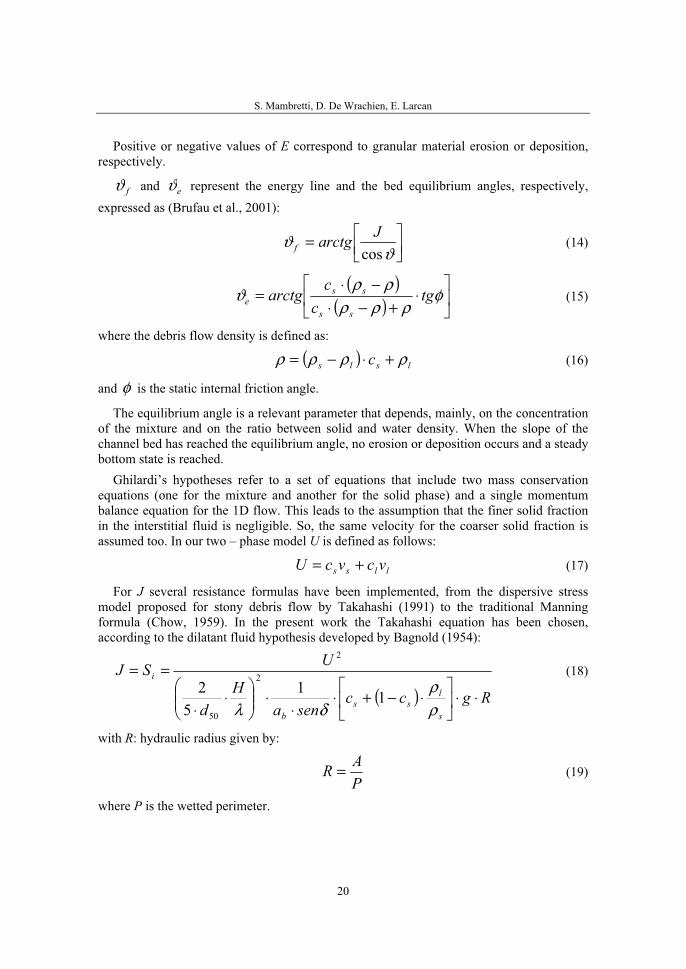
Positive or negative values of E correspond to granular material erosion or deposition, respectively.
fϑ and eϑ represent the energy line and the bed equilibrium angles, respectively, expressed as (Brufau et al., 2001):
⎥⎦
⎤
⎢⎣
⎡=ϑ
ϑcos
Jarctgf (14)
( )( ) ⎥
⎦
⎤
⎢
⎣
⎡
⋅+−⋅
−⋅= φ
ρρρρρϑ tg
cc
arctgss
sse (15)
where the debris flow density is defined as:
( ) lsls c ρρρρ +⋅−= (16)
and φ is the static internal friction angle.
The equilibrium angle is a relevant parameter that depends, mainly, on the concentration of the mixture and on the ratio between solid and water density. When the slope of the channel bed has reached the equilibrium angle, no erosion or deposition occurs and a steady bottom state is reached.
Ghilardi’s hypotheses refer to a set of equations that include two mass conservation equations (one for the mixture and another for the solid phase) and a single momentum balance equation for the 1D flow. This leads to the assumption that the finer solid fraction in the interstitial fluid is negligible. So, the same velocity for the coarser solid fraction is assumed too. In our two – phase model U is defined as follows:
llss vcvcU += (17)
For J several resistance formulas have been implemented, from the dispersive stress model proposed for stony debris flow by Takahashi (1991) to the traditional Manning formula (Chow, 1959). In the present work the Takahashi equation has been chosen, according to the dilatant fluid hypothesis developed by Bagnold (1954):
( ) Rgccsena
Hd
USJ
s
lss
b
i
⋅⋅⎥
⎦
⎤
⎢
⎣
⎡
⋅−+⋅⋅
⋅⎟⎟
⎠
⎞
⎜⎜
⎝
⎛
⋅⋅
==
ρρ
δλ11
52
2
50
2
(18)
with R: hydraulic radius given by:
PAR = (19)
where P is the wetted perimeter.
Debris flow and dam-break flooding waves: dynamics rheology and modelling
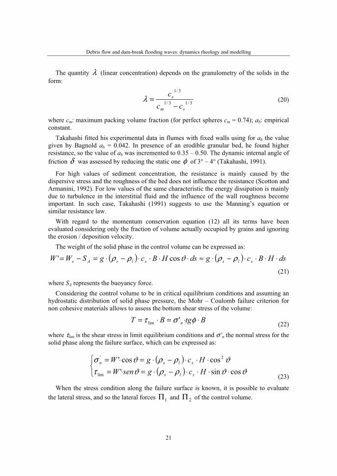
21
The quantity λ (linear concentration) depends on the granulometry of the solids in the form:
3/13/1
3/1
sm
s
ccc
−=λ (20)
where cm: maximum packing volume fraction (for perfect spheres cm = 0.74); ab: empirical constant.
Takahashi fitted his experimental data in flumes with fixed walls using for ab the value given by Bagnold ab = 0.042. In presence of an erodible granular bed, he found higher resistance, so the value of ab was incremented to 0.35 – 0.50. The dynamic internal angle of friction δ was assessed by reducing the static one φ of 3° – 4° (Takahashi, 1991).
For high values of sediment concentration, the resistance is mainly caused by the dispersive stress and the roughness of the bed does not influence the resistance (Scotton and Armanini, 1992). For low values of the same characteristic the energy dissipation is mainly due to turbulence in the interstitial fluid and the influence of the wall roughness become important. In such case, Takahashi (1991) suggests to use the Manning’s equation or similar resistance law.
With regard to the momentum conservation equation (12) all its terms have been evaluated considering only the fraction of volume actually occupied by grains and ignoring the erosion / deposition velocity.
The weight of the solid phase in the control volume can be expressed as:
( ) ( ) dsHBcgdsHBcgSWW slsslsAs ⋅⋅⋅⋅−⋅≈⋅⋅⋅⋅−⋅=−= ρρϑρρ cos' (21)
where SA represents the buoyancy force. Considering the control volume to be in critical equilibrium conditions and assuming an
hydrostatic distribution of solid phase pressure, the Mohr – Coulomb failure criterion for non cohesive materials allows to assess the bottom shear stress of the volume:
BtgBT n ⋅⋅=⋅= φστ 'lim (22)
where τlim is the shear stress in limit equilibrium conditions and σ’n the normal stress for the solid phase along the failure surface, which can be expressed as:
( )( )
⎩
⎨
⎧
⋅⋅⋅⋅−⋅=⋅=⋅⋅⋅−⋅=⋅=
ϑϑρρϑτϑρρϑσ
cossin'coscos'
lim
2'
HcgsenWHcgW
sls
slsn
(23)
When the stress condition along the failure surface is known, it is possible to evaluate the lateral stress, and so the lateral forces 1Π and 2Π of the control volume.
S. Mambretti, D. De Wrachien, E. Larcan
22
For mild bed slopes, the dynamic internal angle δ and the static one φ are equal in critical equilibrium conditions, so the shear stress τlim can be written as:
( ) ϑϑρρτ sincoslim ⋅⋅⋅−⋅−= Hcg sls (24)
Finally, the difference between lateral forces 1Π and 2Π and the bottom shear stress τlim of the control volume become:
( ) ( ) dsAsHicgds
s sls ⋅⋅∂∂⋅+⋅⋅−⋅−=⋅
∂Π∂
−=Π−Π 2121 1ρρ (25)
( ) ( ) dsAtgicgBtgT slsn ⋅⋅⋅−⋅⋅−⋅=⋅⋅= φρρφσ 2lim 1' (26)
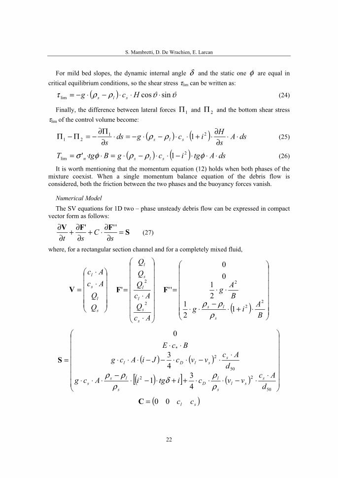
It is worth mentioning that the momentum equation (12) holds when both phases of the mixture coexist. When a single momentum balance equation of the debris flow is considered, both the friction between the two phases and the buoyancy forces vanish.
Numerical Model The SV equations for 1D two – phase unsteady debris flow can be expressed in compact
vector form as follows:
SFFV =∂
∂⋅+∂∂+
∂∂
sC
st'''
(27)
where, for a rectangular section channel and for a completely mixed fluid,
⎟⎟
⎟
⎟
⎟
⎠
⎞
⎜⎜
⎜
⎜
⎜
⎝
⎛
⋅⋅
=
s
l
s
l
AcAc
V
⎟
⎟
⎟
⎟
⎟
⎟
⎟
⎠
⎞
⎜
⎜
⎜
⎜
⎜
⎜
⎜
⎝
⎛
⋅
⋅=
AcQ
AcQQQ
s
s
l
l
s
l
2
2
'F
( )⎟⎟
⎟
⎟
⎟
⎟
⎟
⎠
⎞
⎜⎜
⎜
⎜
⎜
⎜
⎜
⎝
⎛
⋅+⋅−
⋅⋅
⋅⋅=
BAig
BAg
s
ls2
2
2
121
21
00
''
ρρρ
F
( ) ( )
( )[ ] ( )⎟
⎟
⎟
⎟
⎟
⎟
⎟
⎠
⎞
⎜
⎜
⎜
⎜
⎜
⎜
⎜
⎝
⎛
⋅⋅−⋅⋅⋅++⋅−⋅
−⋅⋅⋅
⋅⋅−⋅⋅−−⋅⋅⋅
⋅⋅
=
50
22
50
2
*
431
43
0
dAc
vvcitgiAcg
dAc
vvcJiAcg
BcE
ssl
s
lD
s
lss
sslDl
ρρδ
ρρρ
S
( )sl cc00=C
Debris flow and dam-break flooding waves: dynamics rheology and modelling
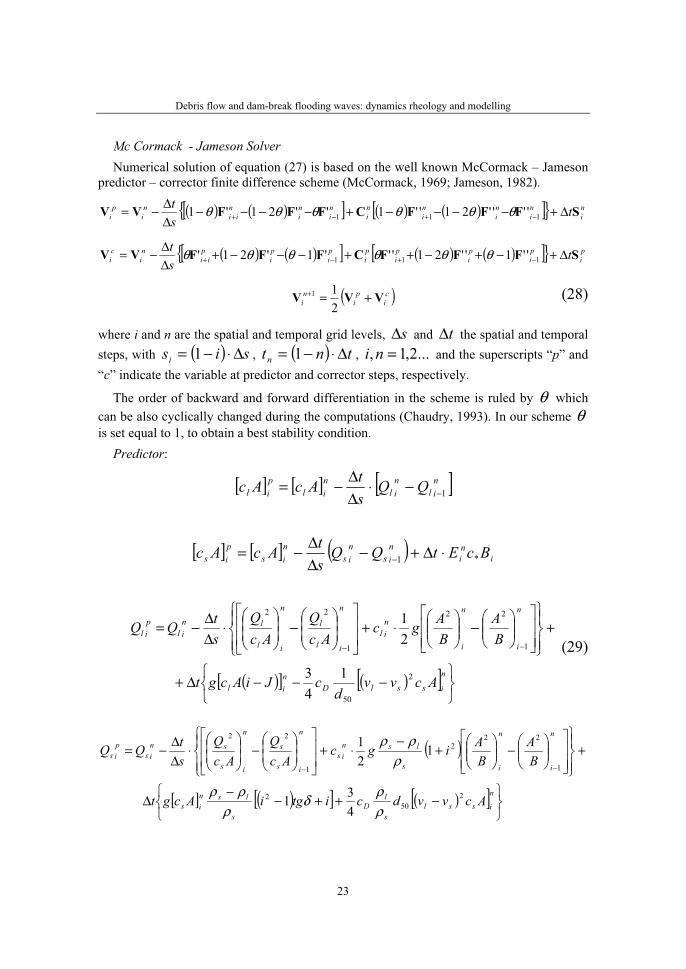
23
Mc Cormack - Jameson Solver Numerical solution of equation (27) is based on the well known McCormack – Jameson
predictor – corrector finite difference scheme (McCormack, 1969; Jameson, 1982).
( ) ( )[ ] ( ) ( )[ ]{ } ni
ni
ni
ni
ni
ni
ni
nii
ni
pi t
st SFFFCFFFVV Δ+−−−−+−−−−
ΔΔ−= −+−+ 111 ''''21''1''21'1 θθθθθθ
( ) ( )[ ] ( ) ( )[ ]{ } pi
pi
pi
pi
pi
pi
pi
pii
ni
ci t
st SFFFCFFFVV Δ+−+−++−−−+
ΔΔ−= −+−+ 111 ''1''21'''1'21' θθθθθθ
( )ci
pi
ni VVV +=+
211 (28)
where i and n are the spatial and temporal grid levels, sΔ and tΔ the spatial and temporal steps, with ( ) sisi Δ⋅−= 1 , ( ) tntn Δ⋅−= 1 , ...2,1, =ni and the superscripts “p” and “c” indicate the variable at predictor and corrector steps, respectively.
The order of backward and forward differentiation in the scheme is ruled by θ which can be also cyclically changed during the computations (Chaudry, 1993). In our scheme θis set equal to 1, to obtain a best stability condition.
Predictor:
[ ] [ ] [ ]nil
nil
nil
pil QQ
stAcAc 1−−⋅
ΔΔ−=
[ ] [ ] ( ) ini
nis
nis
nis
pis BcEtQQ
stAcAc *1 ⋅Δ+−
ΔΔ−= −
( )[ ] ( )[ ]⎭
⎬
⎫
⎩
⎨
⎧
−−−Δ+
+⎪⎭
⎪
⎬
⎫
⎪⎩
⎪
⎨
⎧
⎥
⎥
⎦
⎤
⎢
⎢
⎣
⎡
⎟⎟
⎠
⎞
⎜⎜
⎝
⎛
−⎟⎟
⎠
⎞
⎜⎜
⎝
⎛
⋅+⎥
⎥
⎦
⎤
⎢
⎢
⎣
⎡
⎟
⎟
⎠
⎞
⎜
⎜
⎝
⎛
−⎟
⎟
⎠
⎞
⎜
⎜
⎝
⎛
⋅ΔΔ−=
−−
n
isslDnil
n
i
n
i
nil
n
il
l
n
il
lnil
pil
Acvvd
cJiAcgt
BA
BAgc
AcQ
AcQ
stQQ
2
50
1
22
1
22
143
21
(29)
( )
[ ] ( )[ ] ( )[ ]⎭
⎬
⎫
⎩
⎨
⎧
−++−−
Δ
+⎪⎭
⎪
⎬
⎫
⎪⎩
⎪
⎨
⎧
⎥
⎥
⎦
⎤
⎢
⎢
⎣
⎡
⎟⎟
⎠
⎞
⎜⎜
⎝
⎛
−⎟⎟
⎠
⎞
⎜⎜
⎝
⎛
+−
⋅+⎥
⎥
⎦
⎤
⎢
⎢
⎣
⎡
⎟
⎟
⎠
⎞
⎜
⎜
⎝
⎛
−⎟
⎟
⎠
⎞
⎜
⎜
⎝
⎛
⋅ΔΔ−=
−−
n
issls
lD
s
lsnis
n
i
n
is
lsnis
n
is
s
n
is
snis
pis
AcvvdcitgiAcgt
BA
BAigc
AcQ
AcQ
stQQ
250
2
1
222
1
22
431
121
ρρδ
ρρρ
ρρρ
S. Mambretti, D. De Wrachien, E. Larcan
24
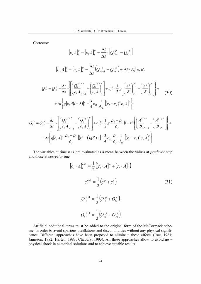
Corrector:
[ ] [ ] [ ]pil
pil
nil
cil QQ
stAcAc −⋅
ΔΔ−= +1
[ ] [ ] ( ) ip
ipis
pis
nis
cis BcEtQQ
stAcAc *1 ⋅Δ+−
ΔΔ−= +
( )[ ] ( )[ ]⎭
⎬
⎫
⎩
⎨
⎧
−−−Δ+
+⎪⎭
⎪
⎬
⎫
⎪⎩
⎪
⎨
⎧
⎥
⎥
⎦
⎤
⎢
⎢
⎣
⎡
⎟⎟
⎠
⎞
⎜⎜
⎝
⎛
−⎟⎟
⎠
⎞
⎜⎜
⎝
⎛
⋅+⎥
⎥
⎦
⎤
⎢
⎢
⎣
⎡
⎟
⎟
⎠
⎞
⎜
⎜
⎝
⎛
−⎟
⎟
⎠
⎞
⎜
⎜
⎝
⎛
⋅ΔΔ−=
++
p
isslDpil
p
i
p
i
pil
p
il
l
p
il
lnil
cil
Acvvd
cJiAcgt
BA
BAgc
AcQ
AcQ
stQQ
2
50
2
1
22
1
2
143
21
(30)
( )
[ ] ( )[ ] ( )[ ]⎭
⎬
⎫
⎩
⎨
⎧
−++−−
Δ+
+⎪⎭
⎪
⎬
⎫
⎪⎩
⎪
⎨
⎧
⎥
⎥
⎦
⎤
⎢
⎢
⎣
⎡
⎟⎟
⎠
⎞
⎜⎜
⎝
⎛
−⎟⎟
⎠
⎞
⎜⎜
⎝
⎛
+−
⋅+⎥
⎥
⎦
⎤
⎢
⎢
⎣
⎡
⎟
⎟
⎠
⎞
⎜
⎜
⎝
⎛
−⎟
⎟
⎠
⎞
⎜
⎜
⎝
⎛
⋅ΔΔ−=
++
p
issls
lD
s
lspis
p
i
p
is
lspis
p
is
s
p
is
snis
cis
Acvvd
citgiAcgt
BA
BAigc
AcQ
AcQ
stQQ
2
50
2
2
1
22
2
1
2
1431
121
ρρ
δρ
ρρ
ρρρ
The variables at time n+1 are evaluated as a mean between the values at predictor step and those at corrector one:
[ ] [ ] [ ]( )cil
pil
nil AcAcAc ⋅+⋅=⋅ +
211
( )ci
pi
ni ccc +=+
211 (31)
( )cil
pil
nil QQQ +=+
211
( )cis
pis
nis QQQ +=+
211
Artificial additional terms must be added to the original form of the McCormack sche-me, in order to avoid spurious oscillations and discontinuities without any physical signifi-cance. Different approaches have been proposed to eliminate these effects (Roe, 1981; Jameson, 1982; Harten, 1983; Chaudry, 1993). All these approaches allow to avoid no – physical shock in numerical solutions and to achieve suitable results.
Debris flow and dam-break flooding waves: dynamics rheology and modelling
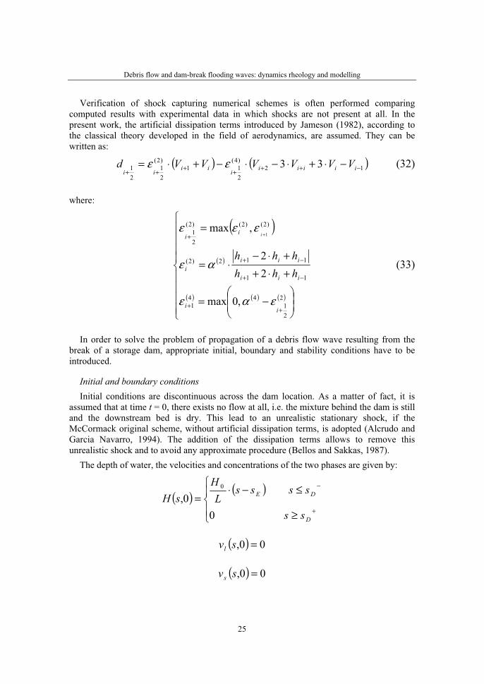
25
Verification of shock capturing numerical schemes is often performed comparing computed results with experimental data in which shocks are not present at all. In the present work, the artificial dissipation terms introduced by Jameson (1982), according to the classical theory developed in the field of aerodynamics, are assumed. They can be written as:
( ) ( )12)4(
211
)2(
21
21 33 −++
++
++−⋅+⋅−⋅−+⋅= iiiiiiiiii
VVVVVVd εε (32)
where:
( )
( )
( ) ( ) ( )⎪
⎪
⎪
⎪
⎩
⎪
⎪
⎪
⎪
⎨
⎧
⎟
⎟
⎠
⎞
⎜
⎜
⎝
⎛
−=
+⋅++⋅−
⋅=
=
++
−+
−+
+ +
2
21
441
11
112)2(
)2()2()2(
21
,0max
22
,max1
ii
iii
iiii
ii
hhhhhh
i
εαε
αε
εεε
(33)
In order to solve the problem of propagation of a debris flow wave resulting from the break of a storage dam, appropriate initial, boundary and stability conditions have to be introduced.
Initial and boundary conditions Initial conditions are discontinuous across the dam location. As a matter of fact, it is
assumed that at time t = 0, there exists no flow at all, i.e. the mixture behind the dam is still and the downstream bed is dry. This lead to an unrealistic stationary shock, if the McCormack original scheme, without artificial dissipation terms, is adopted (Alcrudo and Garcia Navarro, 1994). The addition of the dissipation terms allows to remove this unrealistic shock and to avoid any approximate procedure (Bellos and Sakkas, 1987).
The depth of water, the velocities and concentrations of the two phases are given by:
( ) ( )⎪⎩
⎪
⎨
⎧
≥
≤−⋅=
+
−
D
DE
ss
ssssL
HsH
00,
0
( ) 00, =svl
( ) 00, =svs
S. Mambretti, D. De Wrachien, E. Larcan
26
( )⎪⎩
⎪
⎨
⎧
≥
≤=
+
−
D
Dinitss
ss
sscsc
00, (34)
( )⎪⎩
⎪
⎨
⎧
≥
≤=
+
−
D
Dinitll
ss
sscsc
00,
where H0: initial depth behind the dam; L = sD-sE: length of the reservoir; sD, sE: abscissas of the dam site and the reservoir end; cs init, cl init: initial solid and liquid concentration upstream of the dam, while the relation between the concentration of the two phases is:
1=+ sl cc (35)
In the case of a partial dam – break, internal boundary conditions at the dam – site cross section are needed. The kind and form of the conditions needed depend on the assumptions made regarding the development of the breach and flow conditions existing at the breach (Shamber and Katopodes, 1984).
Regarding the boundary conditions, to evaluate predictor step at the node ( )1, +ni , the
variable values at the grid points ( )ni ,1− , ( )ni, and ( )ni ,1+ must be known. This implies that to properly apply the McCormack solver at the boundary node of the upstream solid wall, when the depth of the mixture is not zero at the upstream end of the reservoir, the following symmetric conditions for depth and volumetric concentrations, and anti – symmetric conditions for velocities should be defined.
( ) ( )jHjH ,1,1 =− ( ) ( )jAjA ,1,1 =−
( ) ( )jvjv ll ,1,1 −=− ( ) ( )jQjQ ll ,1,1 −=−
( ) ( )jvjv ss ,1,1 −=− or rather ( ) ( )jQjQ ss ,1,1 −=− (36)
( ) ( )jcjc ll ,1,1 =− ( ) ( )jAcjAc ll ,1,1 =−
( ) ( )jcjc ss ,1,1 =− ( ) ( )jAcjAc ss ,1,1 =−
No problem arises for the assessment of the correct step, due to the fact that every computation code refers to grid points inside the domain. It is worth underlying that the McCormack scheme has a strong shock – capturing capability. Thus, it can be used for the solution of the unsteady flow equations, in conservative law form, either when the flow is wholly gradually varied or the latter is affected with surges or shocks. This is the case of a

Debris flow and dam-break flooding waves: dynamics rheology and modelling
27
dam – break flow advancing down a river with an initial flow, and it constitutes the so – called wet – bed dam – break problem (Bellos and Sakkas, 1987).
Stability conditions In order to satisfy the numerical stability requirements, the time step has to abide by the
Courant – Friedrichs – Lewy (CFL) criterion (Courant et al., 1967; Sweby, 1984), which is a necessary but not sufficient condition:
[ ]cUxCt R +
Δ⋅=Δmax
(37)
where c: celerity of a small flow disturbance, defined by:
BAgc ⋅= (38)
and CR: Courant number.
For a fixed spatial grid, the minimum value of tΔ satisfying Eq. 37 is determined at the end of the computation for a given time step. This value is then used as the time increment for the computation during the next step. In this way the largest possible time increment can be utilized at each time step. This process required the calibration of three coefficients: the drag coefficient cD and the two Jameson parameters of artificial viscosity ( )2α and ( )4α .Their values are:
2.0=Dc , ( ) 5.02 =α , ( ) 2.04 =αIn the developed code a fixed and very small value of tΔ has been set at the beginning
of the simulations, verifying during the run that the CFL condition was assured, being always the Courant number CR < 0.8.
CONCLUSIONS
Studies of dam – break flow consider, mainly, conditions of clear – water surges. However, under natural conditions a dam – break flow can generate extensive debris in the valley downstream of the dam. The presence of such debris may significantly influence surge height and speed. As a matter of fact debris flow differs from other unconfined flows in two main respects: the nature of both the flow material and the flow itself. So, achieving a set of debris flow constitutive equations is a task which has been given particular attention during the second half of last Century. Most models are based on a rheological approach, which has the drawback of providing equations that require a large number of parameters that depend on the vast range of flow regimes that can occur. One alternative is that of developing and using simple models to focus attention on one salient feature of debris flow modelling, mainly the dynamic aspect. From this point of view the constitutive equations must be compatibly incorporated into the conservation equations in order to obtain a realistic representation of the phenomenon. This problem immediately leads to experimental studies on debris flow: there is, as yet, relatively scarcity of experimental
S. Mambretti, D. De Wrachien, E. Larcan
28
data, the only ones that allow effective verifications of the constitutive models proposed, in different flow situations and the estimation of the rheological parameters they contain. Lastly, field studies are probably the most difficult and costly study approach of debris flows: the difficulties encountered are connected to their considerable complexity and the difficulty of direct observation.
In this context, the present paper describes the main features and characteristics of a numerical model suitable to solve the SV equations, modified for including two – phase debris flow phenomena, and able to assess the depth of the wave and the velocities of both the liquid and solid phases of no – stratified (mature) flow, following dam – break events.
The model is based on mass and momentum conservation equations for both liquid and solid phases. The McCormack – Jameson two – step explicit scheme with second order accuracy was employed for the solution of the equations, written in a conservative – law form. The technique was applied for determining both the propagation and the profile of a debris flow wave resulting from the instantaneous and complete collapse of a storage dam. The actual initial and boundary conditions for the problem considered, i.e. a zero flow depth at the leading front of the wave, were used in the application of the numerical technique.
In order to describe stratified (immature) flow, it is necessary to widen the reach of the model and to take into account mass and momentum conservation equations for each phase and layer. Momentum conservation equations describe energy exchanges between the two phases in the same layer and between layers, while mass conservation equations describe mass exchange between layers. Within this ground, in order to analyse reverse grading (sorting) it is necessary to analyse the wave propagation process, when the solid phase is composed of no – homogeneous material. In this case the model should be improved in order to feature the distribution of the material of different size of the solid phase: larger size material positioned in the front and in the top of the wave, and finer one in the bottom and in the tail.
LIST OF SYMBOLS
ab Bagnold experimental constant [ ] c celerity [m/s]c* bed volumetric solid concentration [ ] cD drag coefficient [ ] cl volumetric concentration of water [ ] cs volumetric concentration of solid phase [ ] cm maximum concentration of the solid material when packed [ ] d50 mean diameter of granular material [m]ds spatial step [m]dt temporal step [s]f force transmitted by water to a solid particle [N]
Debris flow and dam-break flooding waves: dynamics rheology and modelling
29
g gravity acceleration [m/s2]i channel slope [ ] kE empiric coefficient of Ghilardi model [ ] q specific flow rate of the subtracted solid material [m2/s]s spatial coordinate t temporal coordinate vl water mean velocity [m/s]vs solid mean velocity [m/s]A wetted cross – section area [m2]B wetted bed width [m]CR Courant number [ ] E erosion/deposition velocity of granular material [m/s]F interaction force between solid and liquid phases [N]H depth [m]J water head loss given by Chézy formula [ ] Ql water discharge [m3/s]Qs solid phase discharge [m3/s]R hydraulic radius [m]SA Archimedes buoyancy [N]Si bed resistance term [ ] T bottom stress force for solid phase [N]U characteristic velocity of the mixture [m/s]Vc control volume [m3]W’ solid phase weight reduced of Archimedes buoyancy [N]Ws solid phase weight [N]
α(2) Jameson artificial viscosity coefficient [m/s]
α(4) Jameson artificial viscosity coefficient [m/s]
β momentum coefficient [ ]
δ dynamic friction angle of granular material [°]
φ static friction angle of granular material [°]
η distance from the channel bottom [m]
λ linear concentration [ ]
ϑ bed inclination [º]

S. Mambretti, D. De Wrachien, E. Larcan
30
ϑe equilibrium angle [º]
ϑf energy line angle [º]
Π1,Π2 forces on control volume lateral surfaces [N]
ρ mixture volumetric density [kg/m3]
ρl water density [kg/m3]
ρs solid phase density [kg/m3]
σ generic section width [m]
σ’n normal stress along failure surface for solid phase [Pa]
τlim shear stress in limit equilibrium conditions [Pa]
REFERENCES
1. Alcrudo F., Garcia Navarro P., “Computing two – dimensional flood propagation with a high resolution extension of McCormack’s method” in Proc. of International Conference on Modelling of Flooding Propagation over Initially Dry Areas, Milan, 1994
2. Arai M., Takahashi T., “The Karman constant of the flow laden with high sediment” in Proc. of the 3rd International Symposium on River Sedimentation University of Missisipi, 1986, pp. 824 – 833
3. Armanini A., Fraccarollo L., “Critical conditions for debris flow” in Debris Flow Hazard Mitigation: Mechanics, Prediction and Assessment, Eds. Chen, New York, 1997, pp. 434 – 443
4. Asmar B.N., Lanston P.A., Ergenzinger Z., “The potential of the discrete method to simulate debris flow” in Proceeding of the First International Conference on Debris Flow Hazard Mitigation: Mechanics, Prediction and Assessment, Eds. Chen, New York, 1997
5. Aureli F., Maione U., Mignosa P., Tomirotti M., “Fenomeni di moto vario conseguenti al crollo di opere di ritenuta”, parte I: modellazione numerica e confronto con dati sperimentali di letteratura, L’Acqua n. 4, 1998 (in Italian)
6. Bagnold R.A., “Experiments on a gravity – free dispersion of large solid spheres in a Newtonian fluid under shear” in Proceedings of the Royal Society of London, Series A, 225, 1954, pp. 49 – 63
7. Beam W.M., Warming R.F., “An implicit finite – difference algorithm for hyperbolic system in conservation – law form” Journal of Computational Physics, 22, 1976, pp. 87 – 110
8. Bechteler W., Kulisch H., Nujic M., “2D dam – break flooding wave: comparison between experimental and calculated results” Floods and Flood Management, Ed. Saul, Dodrecht, 1992
9. Bellos V., Sakkas J.G., “1D dam – break flood propagation on dry bed” Journal of Hydraulic Engineering, 1987, ASCE 113(12), pp. 1510 – 1524
10. Brufau P., Garcia – Navarro P., Ghilardi P., Natale L., Savi F., “1D Mathematical modelling of debris flow” Journal of Hydraulic Research, 38, 2001, pp. 435 – 446
11. Chaudry M.H., “Open – Channel Flow”, New Jersey, 1993

Debris flow and dam-break flooding waves: dynamics rheology and modelling
31
12. Chen C.J., “Laboratory verification of a dam – break flood model” Journal of Hydraulic DivisionASCE, 106(4), 1980, pp. 535 – 556
13. Chen L.C., “Generalized viscoplastic modelling of debris flow” Journal of Hydraulic Engineering, 1988, 114, pp. 237 – 258
14. Chen C.L., Ambruster J.T., “Dam – break wave model. Formulation and verification” Journal of Hydraulic Division, ASCE 106(5), 1980, pp. 747 – 767
15. Chen C.L., Ling C.H., “Resistance formulas in hydraulics based models for routing debris flow” in Debris Flow Hazard Mitigation: Mechanics, Prediction and Assessment, Eds. Chen, New York, 1997, pp. 360 – 372
16. Chow V.T., “Open Channel Hydraulics” McGraw Hill, 1959
17. Courant R., Friedrichs K.O., “Supersonic flow and shock wave” Interscience Publisher Inc., New York, 1948
18. Courant R., Friedrichs K.O., Lewy H., “On the partial differential equation of mathematical physics” IBM Journal, 11, 1967, pp. 215 – 234
19. Coussot P., “Steady, laminar, flow of concentrated mud suspensions in open channel”, Journal of Hydraulic Research, Vol. 32 n. 4, pp.535-559, 1994
20. Coussot P., “Mudflow rheology and dynamics” Rotterdam, 1997
21. Delis A.J., Skeels C.P., Ryrie S.C., “Implicit high – resolution methods for modelling one – dimensional open channel flow” Journal of Hydraulics Research 38(3), 2000, pp. 369 – 382
22. Dent J.D., Lang T.E., “A biviscous modified Binghman model of snow avalanche motion” Annalsof Glaciology, 4, 1983, pp. 42 – 46
23. Dressler R.F. “Hydraulic resistance effect upon the dam – break functions” Proc. of Royal Society of London A(257), 1952, pp. 185 – 198
24. Dressler R.F. “Unsteady non – linear waves in damping channels” Journal of the National Bureau of Standards 2(3), 1958, pp. 217 – 225
25. Egashira S., Ashida K., “Sediment transport in steep slope flumes”, Proc. of RoC Japan Joint Seminar on Water Resources,1987
26. Fread D. L., Jin M., “One-dimensional Routing of Mud/Debris flows using NWS FLDWAV Model”, in Proc. of First International Conference on Debris Flow Hazards Mitigation: Mechanics, Prediction and Assessment, San Francisco, California, 7-9 agosto 1997
27. Garcia R., Kahawita R.A., “Numerical solution of the De Saint Venant equations with the McCormack finite – difference scheme” International Journal of Numerical Methods in Fluids,1986, 6, pp. 259 – 274
28. Garcia Navarro P., Saviròn J.M., “McCormack methods for numerical simulation of 1D discontinuous unsteady open channel flow” Journal of Hydraulic Research, 1992, 30(1), pp. 313 – 327
29. Ghilardi P., Natale L., Savi F., “Two mathematical models simulating a real-world debris-flow”, Proc.IAHR Symposium on River, Coastal and Estuarine Morphodynamics, Genova, 1999
30. Ghilardi P., Natale L., Savi F., “Debris flow propagation and deposition on urbanized alluvial fans”, Excerpta, 14, 2000, pp. 7 – 20
S. Mambretti, D. De Wrachien, E. Larcan
32
31. Gregoretti C., “Fronte di debris-flow. Composizione e celerità”, L’acqua n. 6, pp. 29-39, 1998 (in Italian)
32. Gregoretti C., “Stima della velocità massima del fronte di una colata detritica che si propaga in un alveo torrentizio”, Idra 2000 (in Italian)
33. Harten A., “High resolution schemes for hyperbolic conservation laws” Journal of Computational Physics, 49, 1983, pp. 357 – 394
34. Harten A., Osher S., “Uniformly high – order accurate non – oscillatory schemes” SIAM Journal of Numerical Analysis 24(2), 1987, pp. 279 – 309
35. Hicks F.E., Steffer P.M., “Characteristic dissipative Galerking scheme for open channel flow” Journal of Hydraulic Engineering ASCE, 118(2), 1992, pp. 337 – 352
36. Hirano M., Hasada T., Banihabib M.E., Kawahasa K., “Estimation of hazard area due to debris flow” in Debris Flow Hazard Mitigation: Mechanics, Prediction and Assessment, Eds. Chen, New York, 1997, pp. 697 – 706
37. Honda N., Egashira S., “Prediction of debris flow characteristics in mountain torrents” in DebrisFlow Hazard Mitigation: Mechanics, Prediction and Assessment, Eds. Chen, New York, 1997, pp. 707 – 716
38. Hui – Pang L., Fang – Wu T., “Sediment concentration distribution of debris flow“ Journal of Hydraulic Engineering, 129(12), 2003, pp. 995 – 1000
39. Hunt B., “Asymptotic solution for dam – break problems” Journal of Hydraulic Division ASCE, 108(1), 1982, pp. 115 – 126
40. Iverson R.M. “The physics of debris flow” Geophysics 35(3), 1997, pp. 245 – 296
41. Jameson A., “Transonic airfoil calculation using the Euler equations” Numerical Models in Aeronautical Fluid Dynamics, Ed. P.L. Roe, 1982, Academic Press, New York
42. Jan C.D., “A study on the numerical modelling of debris flow” in Debris Flow Hazard Mitigation: Mechanics, Prediction and Assessment, Eds. Chen, New York, 1997, pp. 717 – 726
43. Jha A.K., Akiyama J., Vra M., “A fully conservative Beam and Warming scheme for transient open channel flows” Journal of Hydraulic Research 34(5), 1996, pp. 605 – 621
44. Johnson A.M. “Physical processes in geology” Freeman Ed., San Francisco, 1970
45. Julien P.Y., O’Brien J.S., “Physical properties and mechanics of hyperconcentrated sediment flows” in Proceeding Spec. Conference on Delineation of Landslides, Flash Flood and Debris Flow Utah, USA, 1985, pp. 260 – 279
46. Lax P., Wendroff B., “Systems of conservation laws” Comp. on Pure and Applied Mathematics13, 1960, pp. 217 – 237
47. McCormack R.W., “The effect of viscosity in hypervelocity impact cratering” AIAA Paper, 1969, 75-1
48. Norem H., Locat J., Schieldrop B., “An approach to the physics and the modelling of the submarine flowslides” Marine Geotechnical 9, 1990, pp. 93 - 111
49. O’Brien J.S., Julien P.J., Fullerton W.T., “Two – dimensional water flow and mudflow simulation”, Journal of Hydraulic Engineering, 1993, 119, pp. 244 – 261

Debris flow and dam-break flooding waves: dynamics rheology and modelling
33
50. Ritter A. “Die Fortplanzung der Wasserwellen” Zeitschrift des Vereines Deutscher Ingenieure36(3), 1892, pp. 947 – 954 (in German)
51. Rodriguez C., Blanco A., Garcia R., “Comparison of 1D debris flow modelling approaches using a high resolution and non – oscillatory numerical scheme on the finite volume methods”, Proceeding of the 1st International Conference on Monitoring, Simulation, Prevention and Remediation of Dense and Debris Flow, Eds. Lorenzini and Brebbia, Rhodes, 2006
52. Roe P.L. “Approximate Riemann solver, parameters vectors and difference schemes” Journal of Computational Physics, 43, 1981, pp. 357 – 372
53. Schamber D.R., Katopodes N.D., “One – dimensional model for partially breached dams” Journal of Hydraulic Engineering, 110, 1984, pp. 1086 – 1102
54. Scotton P., Armanini A., “Experimental investigation of roughness effects of debris flow channels” 6th Workshop on Two – Phase Flow Prediction, Erlangen, 1992
55. Shieh C.L., Jan C.D., Tsai Y.F., “A numerical simulation of debris flow and its applications” Natural Hazards, 1996, 13, pp.39 – 54
56. Stoker J.J. “The breaking of waves in shallow water” Annuals New York Academy of Science51(3), 1949, pp.360 – 375
57. Sweby P.K., “High resolution schemes using flux limiters for hyperbolic conservation laws” SIAM Journal of Numerical Analysis, 21, 1984, pp. 995 – 1011
58. Takahashi T. “Mechanical aspects of debris flow” Journal of the Hydraulic Division ASCE, 104, 1978 pp. 1153 – 1169
59. Takahashi T. “Debris flow” International Association for Hydraulic Research, Balkema, Rotterdam, 1991
60. Takahashi T, “Initiation of flow of various types of debris flow” Proceeding Second International Conference on Debris Flow Hazard Mitigation: Mechanics, Prediction and Assessment, Eds. Wieczorak and Naeser, Rotterdam, 2000, pp. 15 – 25
61. Takahashi T., Nakagawa H., Kuang S., “Estimation of debris flow hydrograph on varied slope bed” Proceedings of the Corvallis Symposium, 1987
62. Trunk F.J., Dent J.D., Lang T.E., “Computer modelling of large rock slides” Journal of Geotechnical Engineering ASCE, 112(3), 1986, pp. 348 – 360
63. Van Leer B., “Towards the ultimate conservative difference scheme” Journal of Computational Physics 23, 1977, pp. 263 – 275
64. Wallis G. B., “One-dimensional Two-phase Flow”, Mc Graw Hill Book Company, 1962, in particular Par. 3.3 “One-dimensional separated flow in which the phases are considered separately”;
65. Wan Z., Wang Y., “Hyper – concentrated flow” International Association for Hydraulic Research monograph, The Netherlands, 1984
66. Wang Y., Hutter K., “A constitutive model of multiphase mixtures and its application in shearing flows of a satured solid-fluid mixtures”, Granular Matter, 1(4), pp. 163 – 181, 1999
67. Yee H.C., “Construction of explicit and implicit symmetric TVD schemes and their applications” Journal of Computational Physics 68, 1987, pp. 151 – 162

S. Mambretti, D. De Wrachien, E. Larcan
34
68. Yee H.C., “A class of high resolution explicit and implicit shock capturing methods” NASA, TM – 101088, 1989
69. Zhao D.H., Shen H.W., Tabios G.Q., Lai J.S., Tan W.Y., “Finite – volume two – dimensional unsteady flow model for river basins” Journal of Hydraulic Engineering ASCE, 120(7), 1994, pp. 863 – 883
70. Zhao D.H., Shen H.W., Lai J.S., Tabios G.Q., “Approximate Riemann solvers in FVM for 2D hydraulic shock wave modelling” Journal of Hydraulic Engineering ASCE, 122(12), 1996, pp. 692 – 702
36. Symposium "Actual Tasks on Agricultural Engineering", Opatija, Croatia, 2008.
35
36.
SIMPOZIJAKTUALNI ZADACIMEHANIZACIJE POLJOPRIVREDE
UDC556.5:631.6
Izvorni znanstveni radOriginal scientific paper
DEBRIS FLOW AND DAM-BREAK FLOODING WAVES: MODEL CALIBRATION AND COMPARISON WITH
EXPERIMENTAL TESTS STEFANO MAMBRETTI1, ENRICO LARCAN1, DANIELE DE WRACHIEN2
1 DIIAR, Politecnico di Milano, Italy 2 Department of Agricultural Hydraulics, State University of Milan, Italy
E-mail: [email protected]
ABSTRACT
To predict flood and debris flow dynamics a numerical two phase model, based on 1D De Saint Venant (SV) equations, was developed.
To validate the model, comparisons have been made between its predictions and laboratory measurements concerning flows of water and homogeneous granular mixtures in a uniform geometry flume reproducing dam – break waves. Agreements between computational and experimental results are considered very satisfactory for mature (non – stratified) debris flows, which embrace most real cases. To better predict immature (stratified) flows, the model should be improved in order to feature, in a more realistic way, the distribution of the particles of different size within the mixture.
On the whole, the model proposed can easily be extended to channels with arbitrary cross sections for debris flow routing, as well as for solving different problems of unsteady flow in open channels by incorporating the appropriate initial and boundary conditions.
Key words: Debris flow, dam-break, rheological behaviour of the mixtur-es, two-phase modelling
INTRODUCTION
A thorough understanding of the mechanism triggering and mobilising debris flow phenomena plays a role of paramount importance for designing suitable prevention and mitigation measures. Achieving a set of debris flow constitutive equations is a task which has been given particular attention by the scientific community (Julien and O’Brien, 1985;

S. Mambretti, E. Larcan, D. De Wrachien
36
Chen, 1988; Takahashi, 2000). To properly tackle this problem relevant theoretical and experimental studies have been carried out during the second half of the last century.
In a previous work, Mambretti et al. (2008) developed a 1D two – phase mathematical model based on De Saint Venant (SV) equations for debris flow phenomenon, using the McCormack – Jameson integration scheme (McCormack, 1969; Jameson, 1982). Unlike the so – called quasi – two – phase – models – which use SV equations, together with erosion / deposition and mass conservation equations for the solid phase, and take into account mixtures of varying concentrations featuring monotonic velocity profiles that, generally, do not agree with experimental and field data – the model proposed includes two mass and momentum balance equations for each phase, along with an interaction force between the two phases. The latter eases, on one hand, the propagation of the solid phase, while, on the other hand, plays a friction role with regard to the clear water.
In this paper, the scheme is validated for dam – break problems comparing numerical results with experimental data. Comparisons are made between both wave depths and front propagation velocities obtained respectively on the basis of laboratory tests and with predictions from the numerical model. These comparisons allow the assessment of the model performance and suggest feasible development of the research.
EXPERIMENTAL RESULTS AND TEST CONDITIONS
To validate the model, comparisons have been made between its predictions and experimental results carried out in the Hydraulic Laboratory of the Politecnico di Milano. The tests were performed with flows of water and homogeneous granular mixtures in a uniform geometry flume reproducing dam- break waves (Larcan et al., 2002; 2006). The experimental set – up consisted of a loading tank (dimensions 0.5 m x 0.5 m x 0.9 m) with a downstream wall made of sluice gate, a pneumatic control device and a very short opening time (0.3 s) (Figure 1).
Figure 1 Experimental set – up.

Debris flow and dam-break flooding waves: model calibration and comparison with experimental tests
37
The mixture flowed in a 6 m long channel of square section (0.5 m x 0.5 m) and adjustable slope. To enable camera recordings, one of the flume lateral walls contained glass windows.
Experimental tests were performed by changing the channel slope, the bottom roughness (smooth bottom made of galvanised plate or rough bottom covered with an homogeneous layer of gravel, with d50 = 0.005 m), the solid material characteristics (vedril:
31168 mkg=ρ , d50 = 0.003 m; or gravel: 32621 m
kg=ρ d50 = 0.005 m) and the
volumetric concentration of the mixture. Recordings were made with a Sony Digital Handcam, model DCR – TRV32 E camera,
which had an acquisition velocity of 25 frames per second, and were electronically elaborated. Table 1 reports the full list of the experimental tests performed. Each run was repeated three times to allow debris flow recordings along three adjacent windows (Bertalli et al., 2002). In the tests, all parts of each run, which allowed a clear reading of the mixture’s behaviour in its different phases, were used. As a consequence, the same run could be used to assess front, body or end of the wave characteristics.
Table 1 Experimental runs list
Channel slope Loading tank bottom Channel bottom
Granularmaterial
employedConcentration [%]
3.2° Plane Smooth Vedril 20, 40, 60
Vedril 20, 40, 60 Smooth
Gravel 20, 40, 60
Vedril 20, 40, 60 5° Inclined
RoughGravel 20, 40, 60
Vedril 20, 40, 60 Smooth
Gravel 20, 40, 60
Vedril 20, 40, 60 10° Inclined
RoughGravel 20
Plane Smooth Vedril 20, 40, 60
Vedril 20, 40, 60 Smooth
Gravel 20, 40, 60
Vedril 20, 40, 60
15°Inclined
RoughGravel 20, 40, 60
Vedril 20, 40, 60 Smooth
Gravel 20, 40, 60
Vedril 20, 40, 60 20° Inclined
RoughGravel 20, 40
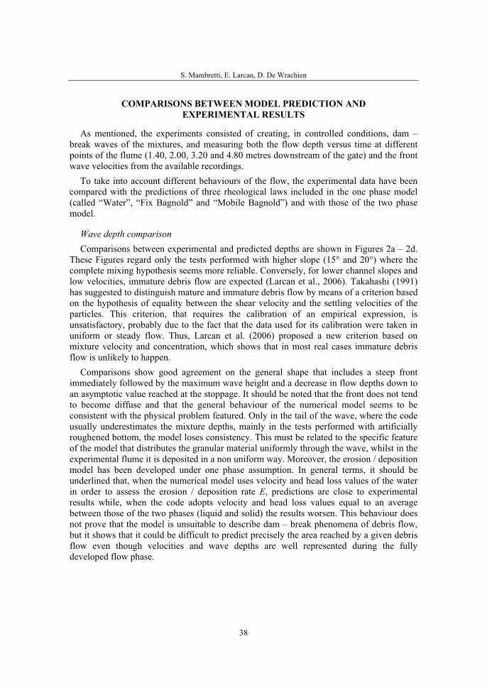
S. Mambretti, E. Larcan, D. De Wrachien
38
COMPARISONS BETWEEN MODEL PREDICTION AND EXPERIMENTAL RESULTS
As mentioned, the experiments consisted of creating, in controlled conditions, dam – break waves of the mixtures, and measuring both the flow depth versus time at different points of the flume (1.40, 2.00, 3.20 and 4.80 metres downstream of the gate) and the front wave velocities from the available recordings.
To take into account different behaviours of the flow, the experimental data have been compared with the predictions of three rheological laws included in the one phase model (called “Water”, “Fix Bagnold” and “Mobile Bagnold”) and with those of the two phase model.
Wave depth comparison Comparisons between experimental and predicted depths are shown in Figures 2a – 2d.
These Figures regard only the tests performed with higher slope (15° and 20°) where the complete mixing hypothesis seems more reliable. Conversely, for lower channel slopes and low velocities, immature debris flow are expected (Larcan et al., 2006). Takahashi (1991) has suggested to distinguish mature and immature debris flow by means of a criterion based on the hypothesis of equality between the shear velocity and the settling velocities of the particles. This criterion, that requires the calibration of an empirical expression, is unsatisfactory, probably due to the fact that the data used for its calibration were taken in uniform or steady flow. Thus, Larcan et al. (2006) proposed a new criterion based on mixture velocity and concentration, which shows that in most real cases immature debris flow is unlikely to happen.
Comparisons show good agreement on the general shape that includes a steep front immediately followed by the maximum wave height and a decrease in flow depths down to an asymptotic value reached at the stoppage. It should be noted that the front does not tend to become diffuse and that the general behaviour of the numerical model seems to be consistent with the physical problem featured. Only in the tail of the wave, where the code usually underestimates the mixture depths, mainly in the tests performed with artificially roughened bottom, the model loses consistency. This must be related to the specific feature of the model that distributes the granular material uniformly through the wave, whilst in the experimental flume it is deposited in a non uniform way. Moreover, the erosion / deposition model has been developed under one phase assumption. In general terms, it should be underlined that, when the numerical model uses velocity and head loss values of the water in order to assess the erosion / deposition rate E, predictions are close to experimental results while, when the code adopts velocity and head loss values equal to an average between those of the two phases (liquid and solid) the results worsen. This behaviour does not prove that the model is unsuitable to describe dam – break phenomena of debris flow, but it shows that it could be difficult to predict precisely the area reached by a given debris flow even though velocities and wave depths are well represented during the fully developed flow phase.
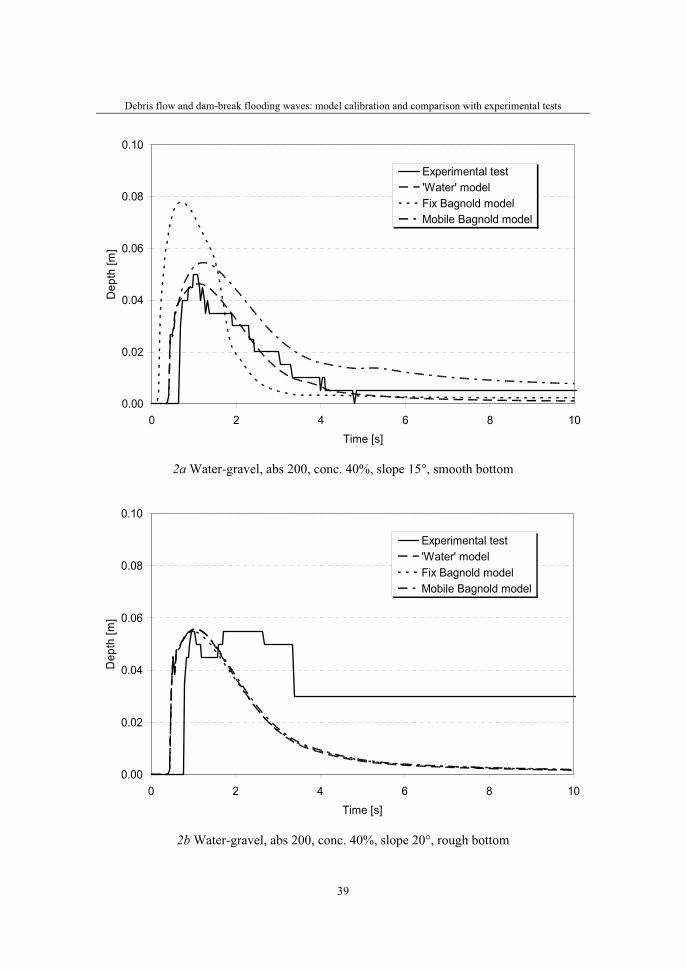
Debris flow and dam-break flooding waves: model calibration and comparison with experimental tests
39
0.00
0.02
0.04
0.06
0.08
0.10
0 2 4 6 8 10Time [s]
Dep
th [m
]
Experimental test'Water' modelFix Bagnold modelMobile Bagnold model
2a Water-gravel, abs 200, conc. 40%, slope 15°, smooth bottom
0.00
0.02
0.04
0.06
0.08
0.10
0 2 4 6 8 10Time [s]
Dep
th [m
]
Experimental test'Water' modelFix Bagnold modelMobile Bagnold model
2b Water-gravel, abs 200, conc. 40%, slope 20°, rough bottom

S. Mambretti, E. Larcan, D. De Wrachien
40
0.00
0.02
0.04
0.06
0.08
0.10
0 2 4 6 8 10Time [s]
Dep
th [m
]
Experimental test'Water' modelFix Bagnold modelMobile Bagnold model
2c Water-vedril, abs 200, conc. 40%, slope 15°, smooth bottom
0.00
0.02
0.04
0.06
0.08
0.10
0 2 4 6 8 10Time [s]
Dep
th [m
]
Experimental test'Water' modelFix Bagnold modelMobile Bagnold model
2d Water-vedril, abs 200, conc.40%, slope 20°, rough bottom
Figure 2 Debris flow wave in some characteristic sections of the experimental channel. Comparison between mathematical model and experimental results
Debris flow and dam-break flooding waves: model calibration and comparison with experimental tests
41
Front velocity comparison Table 2 shows a comparison between the velocities of the front of the wave measured by
the recordings and the velocities predicted by the numerical model. It could be said that, except for few cases, the match is quite good and the agreement between computed and experimental results is very satisfactory.
According to Figures 2a – 2d and to Table 2, each flow appears to be divided into a starting phase, a fully developed flow phase, and a stopping phase.
The initial situation could be described as a static condition – all velocities equal to zero being the opening of the gate followed by the occurrence of a velocity affecting progressively all the length of the flume.
At the same time, the maximum wave depth decreases under the effort of gravity. The main features of the fully developed flow phase are a slow decrease of the maximum flow depth and a constant velocity for the front propagation, the latter being valid during the whole starting and fully developed flow phases. The stopping phase is characterised by a fast decrease of both maximum flow depth and front velocity down to zero. This behaviour, that features a theoretical dam – break problem determined by a shock wave, is satisfactorily described by the numerical model.
Table 2 Comparison between measured and predicted velocities.
Experimentalvelocity
[m/s]
Modelvelocity
[m/s]
Error
[%]
Conc. 20% 2.50 2.76 9.4
Slope 15° Conc. 40% 2.50 2.59 3.5
Conc. 60 % 2.50 1.99 -25.0
Conc. 20% 3.33 3.00 -11.0
Slope 20° Conc. 40% 2.50 2.72 8.0
Conc. 60 % 2.14 2.33 8.0
Comparison between different models To further assess the capability of the model proposed to reproduce debris flow pheno-
mena, comparisons have been made between experimental results and those predicted by three models: one – phase, quasi two – phase and fully two – phase model (Figures 3a – 3b). The Figures point out clearly that the two – phase model provides a better approxima-tion of the laboratory data, both in the peak and in the depth of deposited material data.
Figures 4a – 4b show the comparison between water and solid phase velocities obtained by the two – phase model. The laboratory data are not reported due to the fact that the experimental set – up does not allow their measurements. It is worth mentioning that in the tests where gravel is used the numerical model gives water velocities always larger than that of the solid particles, according to experimental observations. In the tests performed
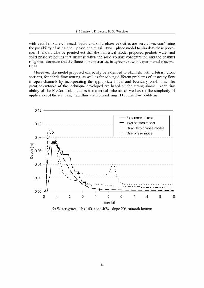
S. Mambretti, E. Larcan, D. De Wrachien
42
with vedril mixtures, instead, liquid and solid phase velocities are very close, confirming the possibility of using one – phase or a quasi – two – phase model to simulate these proce-sses. It should also be pointed out that the numerical model proposed predicts water and solid phase velocities that increase when the solid volume concentration and the channel roughness decrease and the flume slope increases, in agreement with experimental observa-tions.
Moreover, the model proposed can easily be extended to channels with arbitrary cross sections, for debris flow routing, as well as for solving different problems of unsteady flow in open channels by incorporating the appropriate initial and boundary conditions. The great advantages of the technique developed are based on the strong shock – capturing ability of the McCormack – Jameson numerical scheme, as well as on the simplicity of application of the resulting algorithm when considering 1D debris flow problems.
0.00
0.02
0.04
0.06
0.08
0.10
0.12
0 1 2 3 4 5 6 7 8 9 10Time [s]
Dep
th [m
]
Experimental testTwo phases modelQuasi two phases modelOne phase model
3a Water-gravel, abs 140, conc.40%, slope 20°, smooth bottom
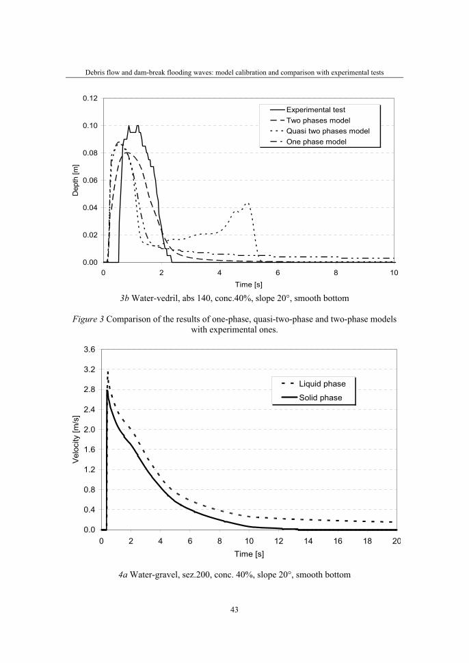
Debris flow and dam-break flooding waves: model calibration and comparison with experimental tests
43
0.00
0.02
0.04
0.06
0.08
0.10
0.12
0 2 4 6 8 10Time [s]
Dep
th [m
]
Experimental testTwo phases modelQuasi two phases modelOne phase model
3b Water-vedril, abs 140, conc.40%, slope 20°, smooth bottom
Figure 3 Comparison of the results of one-phase, quasi-two-phase and two-phase models with experimental ones.
0.0
0.4
0.8
1.2
1.6
2.0
2.4
2.8
3.2
3.6
0 2 4 6 8 10 12 14 16 18 20Time [s]
Vel
ocity
[m/s
]
Liquid phase
Solid phase
4a Water-gravel, sez.200, conc. 40%, slope 20°, smooth bottom
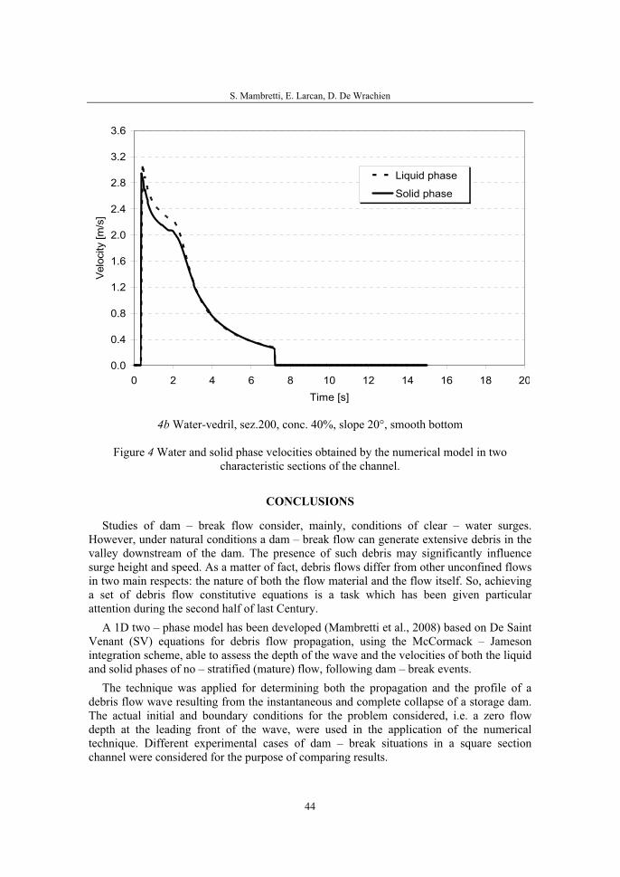
S. Mambretti, E. Larcan, D. De Wrachien
44
0.0
0.4
0.8
1.2
1.6
2.0
2.4
2.8
3.2
3.6
0 2 4 6 8 10 12 14 16 18 20Time [s]
Vel
ocity
[m/s
]
Liquid phase
Solid phase
4b Water-vedril, sez.200, conc. 40%, slope 20°, smooth bottom
Figure 4 Water and solid phase velocities obtained by the numerical model in two characteristic sections of the channel.
CONCLUSIONS
Studies of dam – break flow consider, mainly, conditions of clear – water surges. However, under natural conditions a dam – break flow can generate extensive debris in the valley downstream of the dam. The presence of such debris may significantly influence surge height and speed. As a matter of fact, debris flows differ from other unconfined flows in two main respects: the nature of both the flow material and the flow itself. So, achieving a set of debris flow constitutive equations is a task which has been given particular attention during the second half of last Century.
A 1D two – phase model has been developed (Mambretti et al., 2008) based on De Saint Venant (SV) equations for debris flow propagation, using the McCormack – Jameson integration scheme, able to assess the depth of the wave and the velocities of both the liquid and solid phases of no – stratified (mature) flow, following dam – break events.
The technique was applied for determining both the propagation and the profile of a debris flow wave resulting from the instantaneous and complete collapse of a storage dam. The actual initial and boundary conditions for the problem considered, i.e. a zero flow depth at the leading front of the wave, were used in the application of the numerical technique. Different experimental cases of dam – break situations in a square section channel were considered for the purpose of comparing results.

Debris flow and dam-break flooding waves: model calibration and comparison with experimental tests
45
Agreements between computational and experimental results regarding both wave front – advance and stage hydrographs are considered very satisfactory.
In order to describe stratified (immature) flow, it is necessary to widen the reach of the model and to take into account mass and momentum conservation equations for each phase and layer. Momentum conservation equations describe energy exchanges between the two phases in the same layer and between layers, while mass conservation equation describe mass exchange between layers. Within this ground, in order to analyse reverse grading (sorting) it is necessary to analyse the wave propagation process, when the solid phase is composed of no – homogeneous material. In this case the model should be improved in order to feature the distribution of the material of different size of the solid phase: larger size material positioned in the front and in the top of the wave, and finer one in the bottom and in the tail.

S. Mambretti, E. Larcan, D. De Wrachien
46
REFERENCES
1. Bertalli L., Larcan E., Mambretti S., “Leggi di resistenza al moto nelle colate di detriti conseguenti al crollo di dighe. 2. Modello numerico e confronti con i risultati sperimentali.” In Proceedings 28° Convegno di Idraulica e Costruzioni Idrauliche, Potenza, 16 – 19 settembre 2002 (in Italian)
2. Chen L.C., “Generalized viscoplastic modelling of debris flow” Journal of Hydraulic Engineering, 1988, 114, pp. 237 – 258
3. Jameson A., “Transonic airfoil calculation using the Euler equations” Numerical Models in Aeronautical Fluid Dynamics, Ed. P.L. Roe, 1982, Academic Press, New York
4. Julien P.Y., O’Brien J.S., “Physical properties and mechanics of hyperconcentrated sediment flows” in Proceeding Spec. Conference on Delineation of Landslides, Flash Flood and Debris Flow Utah, USA, 1985, pp. 260 – 279
5. Larcan E., Mambretti S., Orsi E., “Leggi di resistenza al moto nelle colate di detriti conseguenti al crollo di dighe. 1. Apparato sperimentale e primi risultati.” Proceedings on 28° Convegno di Idraulica e Costruzioni Idrauliche, Potenza, 16 – 19 September 2002 (in Italian)
6. Larcan E., Mambretti S., Pulecchi M., “A procedure for the evaluation of debris flow stratification.” Proceedings of the 1st International Conference on Monitoring, Simulation, Prevention and Remediation of Dense and Debris flow Eds. Lorenzini, Brebbia and Emmauouloudis, 7 – 9 June 2006, Rhodes, Greece
7. Mambretti S., De Wrachien D., Larcan E., “Debris flow and dam-break flooding waves : dynamics rheology and modelling.” 36th International Symposium - Actual Tasks on Agricultural Engineering. 11-15 February 2008 ,Opatija ,Croatia
8. McCormack R.W., “The effect of viscosity in hypervelocity impact cratering” AIAA Paper, 1969, 75-1
9. Takahashi T. “Debris flow” International Association for Hydraulic Research, Balkema, Rotterdam, 1991
10. Takahashi T, “Initiation of flow of various types of debris flow” Proceeding Second International Conference on Debris Flow Hazard Mitigation: Mechanics, Prediction and Assessment, Eds. Wieczorak and Naeser, Rotterdam, 2000, pp. 15 – 25
36. Symposium "Actual Tasks on Agricultural Engineering", Opatija, Croatia, 2008.
47
36.
SIMPOZIJAKTUALNI ZADACIMEHANIZACIJE POLJOPRIVREDE
UDC628.36:631.626
Izvorni znanstveni radOriginal scientific paper
DEVELOPMENT OF A RAINFALL RUNOFF MODEL FOR A HILLY WATERSHED IN LOWER SHIVALIKS
REGION OF INDIA A.K. GOEL
Research Engineer, Department of Agricultural Engineering, CSK HP Agricultural University, Palampur-176 062 (HP), INDIA
SUMMARY
The runoff estimation is a complex phenomenon and requires lot of para-meters to asses the reliable values. The selection of a particular method of runoff estimation depends upon the requirements of the user (accuracy, simplification, amount of desired information), the problem, the approach (availability of data, computation facility) and the economics. It is conceivable that a given approach will seldom satisfy all of these requirements. To establish the relationship between rainfall and runoff would require space time distribution of rainfall and infiltration, watershed physiographic characteristics, physical laws including equation of continuity and momentum as well as friction laws, antecedent moisture condition, and initial and boundary conditions. However, a major constraint for runoff estimation from a watershed is scarcity and poor quality of data related to soil, climate, topography, vegetation and land use and it is the main limiting factor for development of a runoff model for any catchment. Therefore, the paucity of data forces one to adopt simple correlation for the estimation of runoff. Hence, a regression technique has been adopted here to develop best-fit regional rainfall runoff relationship by making use of observed weekly rainfall and runoff data from 24th to 37th week for the period from 1971-1997. The work has been carried out for Soan river catchment falling in Shivalik hills of subs Himalayas in India. For the estimation of weekly runoff for the Soan catchment, the straight-line equation was found to be the best-fit equation out of 25 equations tried under the present study. To estimate runoff for the study area, this single best-fit equation in respect of all the effective monsoon weeks will be a good tool for field staff/engineers of the Soil and Water Conservation Wing of the Department of Agriculture.
Key words: rainfall, runoff estimation, Soan catchment, Himalayas, Shivaliks

A.K. Goel
48
INTRODUCTION
The phenomenon of watershed runoff is complex and our understanding of physical principles and the mathematical formulations governing it is limited. The choice of a particular method of runoff estimation depends upon the requirements of the user, the problem, the approach (availability of data and computation facility) and the economics. One single method will rarely fulfill all the requirements. The present study has been undertaken on Soan catchment to develop the best-fit regional rainfall-runoff relationship on weekly basis for the study area falling in Una district of Himachal Pradesh, India with an area of 1204 km2. It lies in lower Shivaliks in district Una of Himachal Pradesh and falls between 75o 58’ 17” E to 76o 23’ 13” E longitude and 31o 17’ 30” N to 31o 50’ 10” N latitude. The catchment is mostly hilly with altitude varying from 340 m at Santokhgarh to 980 m above mean sea level at Chintpurni temple.
The average monsoon (rainy season) and annual rainfall of the study area are 779.8 and 1074.0 mm, respectively with respective values of the standard deviation as 322 and 419 mm. The annual rainfall in study area varied from 491.9 to 1534.6 mm, where as the monsoon season’s rainfall varied from 261.3 to 1354.4 mm during the period under study. The weekly average runoff for the study period from 1971-1997 during monsoon months of July and August varied from 17.2 to 43.4 mm with the lowest value in week No.27 and highest value in week No.31. About 70per cent of the time the runoff was in the range of 2 to 10 m3/s whereas the runoff more than 200 m3/s occurred only for one percent of the time. For about 10 percent of the time, the runoff values were in the range of 10-20 m3/s, where as, very low values of runoff in the range of 0 to 2 m3/s, were noticed in about 7 percent of the runoff days.
Some research workers in the field of hydrology and soil and water conservation have also suggested and carefully applied a few empirical methods of runoff estimation viz., Rational, Cook’s, Curve Number and Soil Conservation Service method (Varshney, 1979 and Subramanya, 1996). A program was developed by Kolb (1986), which provides a least square curve fit on x and y data on the basis of 25 equations which computes equation coefficients, correlation coefficient and best fit equations. An effort has been made here to insure that accurate results are obtained using this program. Moreover, several research workers have suggested the regression technique for various Indian and African catchments for development of runoff models (Rao, 1982; Kothyari and Garde, 1991; Vandeweile etal., 1992; Onyado and Sharma, 1995). With this in view, the rainfall runoff relationships for various active weeks have been worked out for the study area using weekly rainfall and runoff values from 1971-97.
METHODS
The network of data recording in the study area is not very sound as it should have been for a mountainous catchment. The rainfall data were available for only one meteorological station in Una district of Himachal Pradesh, India, where as, these should have been collected from at least 4-5 stations keeping in view the size of the catchment. The short term and fragmented data for some stations (not maintained by Indian Meteorology Department) has not been included in this study as it would not have served the purpose.

Development of a rainfall runoff model for a hilly watershed in lower Shivaliks region of India
49
Many investigators used annual rainfall for the analysis of aridity, droughts and floo-ds/runoff, because of its easy availability and simpler computations involved. Monthly rainfall data were found to be appropriate in analysing the drought conditions with respect to climatic aridity, agricultural production and stream flow forecasting. However, these are inadequate to represent soil moisture deficiencies occurring at various stages of crop growth and water needs over shorter periods. The longer periods equal to one month or more may miss the probable irrigation intervals though the probability fitting may be satisfactory where as, too short an interval, i.e., one day brings out so much variation that probability fitting becomes almost impossible. Moreover, irrigation is hardly planned on day-to-day basis. Keeping the practical utility of the analysis in mind, the rainfall and runoff data have been analysed on weekly basis for the area for planning of any water management system.
Rainfall data The daily rainfall data of 30 years starting from 1968 to 1997 have been collected from
meteorological observatory of Una district of Himachal Pradesh located at an altitude of 340 m above mean sea level. The data were recorded through non-recording type of rain gauge. The daily rainfall values of seven days starting from Ist January were added to transform into weekly rainfall data series for the purpose of frequency analysis. As per the standard weeks prescribed by Indian Meteorology Department, Pune, the first week was taken from January 1 – 7 and then onwards up to 52nd week (Dec. 25-31). In Himachal Pradesh, the monsoon normally sets in from 24th week (2nd week of June) and the period continues till 37th week i.e., mid September, when rains recede sufficiently. There is again dry spell from mid September to November and therefore only 14 weeks (24th to 37th) have been considered as active weeks for this study. Singh and Bhandari (1998) and Rana and Thakur (1998) have reported active weeks from 25th to 35th for Solan and Kullu areas of Himachal Pradesh, respectively.
The weekly rainfall data from 24th to 37th week for the period 1968 to 1997 of the station under study (Una Observatory) can be expressed in double subscripted form as ‘r i, j’ , i =1, 2, 3, …N, year index and j =1, 2, 3,…52, week index, representing rainfall in the jth week of the ith year. The data may also be represented in the matrix form as shown in Table 1. Each column of the Table 1 representing the time series for a particular week has been considered for the data analysis in the present study.
Table 1 Matrix of weekly rainfall
r 1, 1 . . . r 1, 23 r 1, 24 r 1, 25 . . . r 1, 36 r 1, 37 r 1, 38 . . . r 1, 52
r 2, 1 . . . r 2, 23 r 2, 24 r 2, 25 . . . r 2, 36 r 2, 37 r 2, 38 . . . r 2, 52
. . . . . . . . . . . . . . . . . . . . . . . . . . . . . . . . . A = . . . . . . . . . . . . . . . . . . . . . . . . . . . . . . . . .
. . . . . . . . . . . . . . . . . . . . . . . . . . . . . . . . . r N, 1 . . . r N, 23 r N, 24 r N, 25 . . . r N, 36 r N, 37 r N, 38 . . . r N, 52
Dry weeks Active weeks Dry weeks

A.K. Goel
50
Runoff data The daily runoff data recorded at Santokhgarh bridge on the Soan river for the period
1971 to 1997 were collected from the office of Senior Hydrologist of Government of Himachal Pradesh, Flood Control Division, Department of Irrigation and Public Health and Office of the Bhakra Beas Management Board. The runoff was being measured by float method considering five segments of the river bed width. The velocity of each segment was determined by float for a run of 30m and multiplied by the corresponding cross sectional area to determine runoff rate for that particular segment. The runoff rates of different segments were then added to know the total runoff of the river. The total runoff volume per day was calculated by multiplying runoff rate with time of run. The depth of daily runoff was determined by dividing the volume of runoff per day with catchment area of Soan i.e., 1204 km2. The daily data of seven days starting from January 1 were added to transform into weekly runoff data time series. The weekly runoff data may be represented in double subscripted form as, ‘q i , j’ , i =1, 2, 3, …N, year index and j =1, 2, 3,…52, week index. That is, ‘q i , j’ represents runoff in the jth week of the ith year.
To develop week wise best-fit rainfall runoff relationship for the study area, twenty-five equations as suggested by Kolb (1986) have been tried for all the active weekly series under this study (Table 2).
Table 2 Different regression equations applied for rainfall-runoff modeling
Name of the equation Equation Equation No. Straight line xbay += (1)
Line through origin xby = (2)
Reciprocal straight line xba
1y+
=(3)
Line and reciprocal xcxbay ++=
(4)
Hyperbolaxbay +=
(5)
Reciprocal hyperbola bxa
xy+
=(6)
Second order hyperbola 2xc
xbay ++=
(7)
Parabola 2xcxbay ++= (8)
Parabola at origin 2xbxay += (9)
Power bxay = (10)
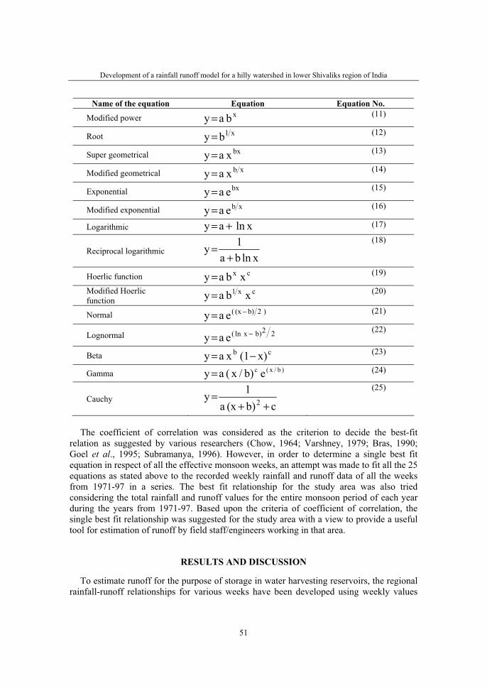
Development of a rainfall runoff model for a hilly watershed in lower Shivaliks region of India
51
Name of the equation Equation Equation No.
Modified power xbay = (11)
Root x1by = (12)
Super geometrical bxxay = (13)
Modified geometrical xbxay = (14)
Exponential bxeay = (15)
Modified exponential xbeay = (16)
Logarithmic xlnay += (17)
Reciprocal logarithmic xlnba
1y+
=(18)
Hoerlic function cx xbay = (19)
Modified Hoerlic function
cx1 xbay = (20)
Normal )2b)(x(eay −= (21)
Lognormal 22b)xln(eay −=(22)
Beta cb x)(1xay −= (23)
Gamma )b/x(c eb)/x(ay = (24)
Cauchycb)(xa
1y 2 ++=
(25)
The coefficient of correlation was considered as the criterion to decide the best-fit relation as suggested by various researchers (Chow, 1964; Varshney, 1979; Bras, 1990; Goel et al., 1995; Subramanya, 1996). However, in order to determine a single best fit equation in respect of all the effective monsoon weeks, an attempt was made to fit all the 25 equations as stated above to the recorded weekly rainfall and runoff data of all the weeks from 1971-97 in a series. The best fit relationship for the study area was also tried considering the total rainfall and runoff values for the entire monsoon period of each year during the years from 1971-97. Based upon the criteria of coefficient of correlation, the single best fit relationship was suggested for the study area with a view to provide a useful tool for estimation of runoff by field staff/engineers working in that area.
RESULTS AND DISCUSSION
To estimate runoff for the purpose of storage in water harvesting reservoirs, the regional rainfall-runoff relationships for various weeks have been developed using weekly values
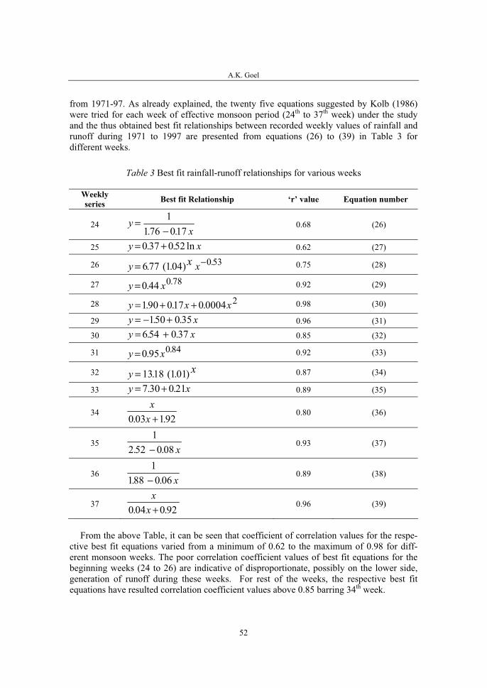
A.K. Goel
52
from 1971-97. As already explained, the twenty five equations suggested by Kolb (1986) were tried for each week of effective monsoon period (24th to 37th week) under the study and the thus obtained best fit relationships between recorded weekly values of rainfall and runoff during 1971 to 1997 are presented from equations (26) to (39) in Table 3 for different weeks.
Table 3 Best fit rainfall-runoff relationships for various weeks
Weeklyseries Best fit Relationship ‘r’ value Equation number
24 yx
=−1
176 017. .0.68 (26)
25 y x= +0 37 0 52. . ln 0.62 (27)
26 y xx= −677 104 0 53. ( . ) . 0.75 (28)
27 y x= 0 44 0 78. . 0.92 (29)
28 y x x= + +190 017 0 0004 2. . . 0.98 (30)
29 y x= − +150 0 35. . 0.96 (31)
30 y x= +6 54 0 37. . 0.85 (32)
31 y x= 0 95 0 84. . 0.92 (33)
32 y x= 1318 101. ( . ) 0.87 (34)
33 y x= +7 30 0 21. . 0.89 (35)
34x
x0 03 192. .+0.80 (36)
351
2 52 0 08. .− x0.93 (37)
361
188 0 06. .− x0.89 (38)
37x
x0 04 0 92. .+ 0.96 (39)
From the above Table, it can be seen that coefficient of correlation values for the respe-ctive best fit equations varied from a minimum of 0.62 to the maximum of 0.98 for diff-erent monsoon weeks. The poor correlation coefficient values of best fit equations for the beginning weeks (24 to 26) are indicative of disproportionate, possibly on the lower side, generation of runoff during these weeks. For rest of the weeks, the respective best fit equations have resulted correlation coefficient values above 0.85 barring 34th week.

Development of a rainfall runoff model for a hilly watershed in lower Shivaliks region of India
53
The best-fit relationship was also established considering the total rainfall and runoff observed for the entire monsoon period of each year during the years from 1971 to 97, which is as follows. y = 54.5 + 0.36 x (r = 0.66) (40)
Where,x = Total observed rainfall (mm) during monsoon season y = Total estimated runoff (mm) during monsoon seasonHadda and Kukal (1991) have recommended the value of correlation coefficient as 0.77
based upon analysis of rainfall and runoff data and this value of coefficient of correlation can be used for appropriate estimation of runoff water and designing soil and water conservation structures needed in catchment area. It can be seen that the parabolic equation for the 28th week has yielded the maximum correlation coefficient of 0.98 (Table 4). Although, the parabolic form of relationship did not prove the best fit relationship for other weekly series, still it was verified for all the weeks with a view to establish its applicability for the study area. The thus resulted parabolic equations for all the weekly series of rainfall and runoff and the respective correlation coefficients are presented in Table 4.
Table 4 Best fit parabolic relationships of rainfall-runoff for various weeks
Weeklyseries Best fit Relationship ‘r’
valueEquationnumber
24 y x x= − + −189 0 43 0 004 2. . . 0.45 (41)
25 y x x= + −130 0 02 0 0007 2. . . 0.50 (42)
26 y x x= − +5 64 016 0 005 2. . . 0.65 (43)
27 y x x= − + −2 3 0 33 0 0007 2. . . 0.81 (44)
28 y x x= + +190 017 0 0004 2. . . 0.98 (45)
29 y x= − +110 0 34. . 0.96 (46)
30 y x x= + +658 0 23 0 0009 2. . . 0.84 (47)
31 y x x= − + −4 98 0 81 0 002 2. . . 0.87 (48)
32 y x x= + +14 55 019 0 0004 2. . . 0.71 (49)
33 y x x= + −378 0 36 0 0004 2. . . 0.88 (50)
34 y x x= + −0 46 0 40 0 0020 2. . . 0.71 (51)
35 y x x= + +514 0 34 0 0002 2. . . 0.92 (52)

A.K. Goel
54
Weeklyseries Best fit Relationship ‘r’
valueEquationnumber
36 y x x= + +589 017 0 0004 2. . . 0.85 (53)
37 y x x= + +4 45 0 37 0 0007 2. . . 0.80 (54)
It is clear from the Table that this particular form of the equation also does not fit well for the beginning weeks (24th to 26th) as the correlation coefficient values (0.45 to 0.65) are in an unacceptable range. However, for the rest of the weeks, barring 32nd and 34th, the parabolic equations fit well resulting correlation coefficient values more than 0.77.
In order to determine a single general equation for runoff estimation in respect of all the weeks for the study area, an attempt was made to establish a best fit equation among all the 25 forms of equations by considering recorded weekly rainfall and runoff data of all the active monsoon weeks from 1971-97 in series, that is 378 values of each variable. The straight line equation with correlation coefficient as 0.75 has been found as the best fit equation for estimation of runoff for the study area which is given below.
y = 0.74 + 0.30 x (r = 0.75) (55)
Where,x = Observed weekly rainfall, mm y = Estimated weekly runoff, mm Although, the resulting correlation coefficient value is little less than 0.77 as suggested
by Hadda and Kukal (1991), yet this relationship may be accepted for runoff estimation in the study area so that the computational complexities arising due to use of individual relationship for an individual monsoon week may be avoided or minimised. In addition, this single best fit relationship for the entire active monsoon period will be a good tool for runoff estimation in the hands of field engineers/staff of soil and water conservation wing of the Government of Himachal Pradesh. Thus, this single best fit relationship i.e., Eq. (55) has been adopted for estimation of runoff in respect of different active monsoon weeks considered under the present study.
As a principle, the design capacity of water harvesting structure is normally decided on the basis of the expected value of peak runoff for the anticipated life of the structure. The peak value is determined from the past records. But, in practice especially in hills, it may not be possible to harvest the total generated runoff from a catchment due to topographical, social, environmental and economical reasons. A number of researchers (Gupta et al., 1975; Verma, 1987 and Shrivastava et al., 1998) therefore, have suggested the probability approach and considered the runoff available at 60 to 70 per cent probability as the design capacity for designing the water harvesting structures. In the present study, since the rainfall data was arranged in descending order for probability analysis of rainfall and frequent intense storms occur in hills, the probability of occurrence of intense storm is low i.e., normally less than 60 percent probability level. Secondly, for beginning and ending monsoon weeks (No. 24, 25, 36 and 37), no rainfall was received at probability level of more than 50 per cent. In view of the above, the rainfall at 50 per cent probability level has
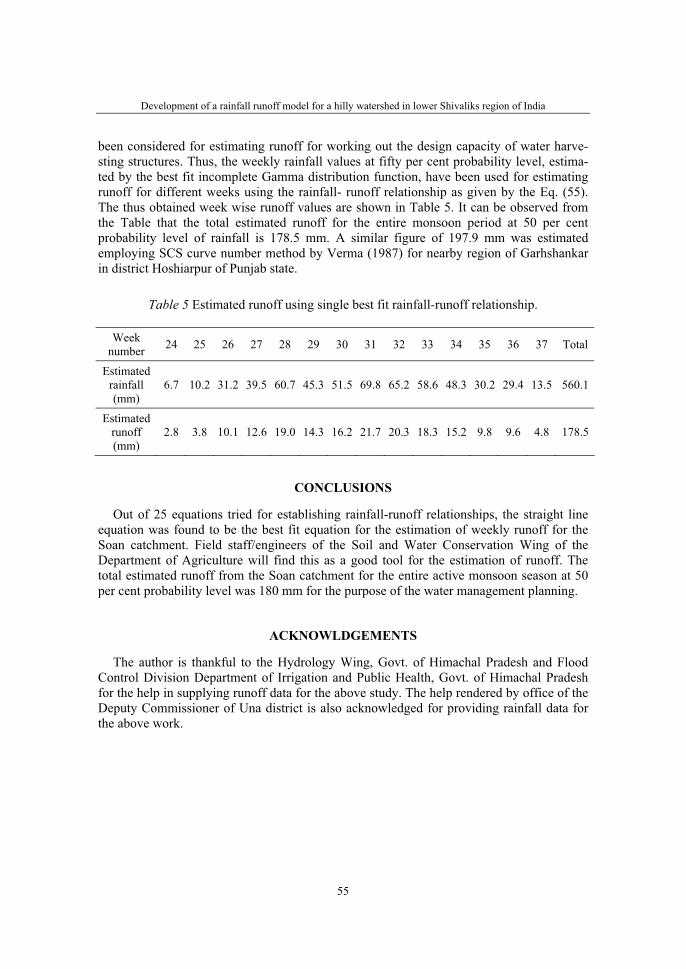
Development of a rainfall runoff model for a hilly watershed in lower Shivaliks region of India
55
been considered for estimating runoff for working out the design capacity of water harve-sting structures. Thus, the weekly rainfall values at fifty per cent probability level, estima-ted by the best fit incomplete Gamma distribution function, have been used for estimating runoff for different weeks using the rainfall- runoff relationship as given by the Eq. (55). The thus obtained week wise runoff values are shown in Table 5. It can be observed from the Table that the total estimated runoff for the entire monsoon period at 50 per cent probability level of rainfall is 178.5 mm. A similar figure of 197.9 mm was estimated employing SCS curve number method by Verma (1987) for nearby region of Garhshankar in district Hoshiarpur of Punjab state.
Table 5 Estimated runoff using single best fit rainfall-runoff relationship.
Weeknumber 24 25 26 27 28 29 30 31 32 33 34 35 36 37 Total
Estimatedrainfall(mm)
6.7 10.2 31.2 39.5 60.7 45.3 51.5 69.8 65.2 58.6 48.3 30.2 29.4 13.5 560.1
Estimatedrunoff(mm)
2.8 3.8 10.1 12.6 19.0 14.3 16.2 21.7 20.3 18.3 15.2 9.8 9.6 4.8 178.5
CONCLUSIONS
Out of 25 equations tried for establishing rainfall-runoff relationships, the straight line equation was found to be the best fit equation for the estimation of weekly runoff for the Soan catchment. Field staff/engineers of the Soil and Water Conservation Wing of the Department of Agriculture will find this as a good tool for the estimation of runoff. The total estimated runoff from the Soan catchment for the entire active monsoon season at 50 per cent probability level was 180 mm for the purpose of the water management planning.
ACKNOWLDGEMENTS
The author is thankful to the Hydrology Wing, Govt. of Himachal Pradesh and Flood Control Division Department of Irrigation and Public Health, Govt. of Himachal Pradesh for the help in supplying runoff data for the above study. The help rendered by office of the Deputy Commissioner of Una district is also acknowledged for providing rainfall data for the above work.
A.K. Goel
56
REFERENCES
1. Chow, V.T. (1964). Hand book of Applied Hydrology. McGraw Hill Co., New York.
2. Goel, A.K., Sharma, P.D. and Rana, R.S. (1995). Rainfall runoff relationship for Soan river catchment in Shivalik hills of Himachal Pradesh. Paper presented in XXX Annual Convention of Indian Society of Agricultural Engineers (Apr, 15-17) at TNAU, Coimbatore, India.
3. Gupta, S. K., Rambabu and Tejwani, K.G. (1975). Weekly rainfall of India for Planning cropping programme. Soil Conservation Digest. 3(1):31-39.
4. Hadda, M. S. and Kukal, S. S. (1991). Relationships among rainfall, runoff and soil loss for the design of soil and water conservation works in sub montane Punjab. Soil Use and Management.7(1): 45-67.
5. Kolb, W.M. (1986). Curve fitting for programmable calculations. IMTECH P.O. Box 1402. Bowie M D, USA.
6. Kothyari, U. C. and Garde, R. J. (1991). Annual runoff estimation for catchments in India. Journal of Water Resources Planning and Management. 117(1): 1-10.
7. Onyado, J. O. and Sharma, T. C. 1995. Simulation of direct runoff volumes and peak rates for rural catchments in Kenya, East Africa. Hydrological Sciences Journal. 40(3): 367-80.
8. Rana, R.S. and Thakur, D.R. (1998). Rainfall analysis for crop planning in Kullu Valley of Himachal Pradesh. Ind. J. Soil Cons. 26(2): 144-46.
9. Rao, R.A. P. (1982). Some drainage characters of north Saurashtra Coast (In: Merh, S. S. (Ed.). First National Seminar on Quarternary Environments, Recent Researches in Geology, Vol. 9. Hundustan Publishing Corp. New Delhi. p. 75-86.
10. Shrivastava, S.K., Misra, S.K., Sahu, A.K., Ahmed, M. and Borah, S.(1998). Probability analysis of rainfall for crop planning at N. Lakhimpur, Assam. Ind. J. Soil Cons. 26(2): 162-165.
11. Singh, M. and Bhandari, A. R.(1998). Wet and dry spells analysis using Markov chain model for mid hills region of Himachal Pradesh. Ind. J. Soil Cons. 26(2): 147-152.
12. Subramanya, K. 1996. Engineering Hydrology. Tata McGraw Hill Co., New Delhi.
13. Vandewiele, G. L. , Xu, C.Y. and Ni, L. W. (1992). Methodology and comparative study of monthly water balance models in Belgium, China and Burma. Journal of Hydrology. 134: (1/4): 315-47.
14. Varshney, R.S. (1979). Engineering Hydrology. Nem Chand & Bros. Pub. Roorkee (UP).
15. Verma, H.N. (1987). Studies of an efficient use of rainwater for rainfed crops. Ph.D thesis. Division of Agricultural Engineering. IARI, New Delhi.
36. Symposium "Actual Tasks on Agricultural Engineering", Opatija, Croatia, 2008.
57
36.
SIMPOZIJAKTUALNI ZADACIMEHANIZACIJE POLJOPRIVREDE
UDC631.674.5:633.1
Izvorni znanstveni radOriginal scientific paper
RESULTS TESTING OF MOBILE RAINING IRRIGATION SYSTEMS IN CROP PRODUCTION
RAJKO MIODRAGOVIC, MILAN DJEVIC
Faculty of agriculture, Nemanjina 6, 11080 Beograd-Zemun, YU
ABSTRACT
This paper provides the synthesis of a long lasting research of mobile raining irrigation systems in crop and vegetable production. The research included three types of mobile self-propelled rain guns and one linear representing both broadcasting and covering concepts. The paper is aimed at determining exploitation parameters and yielding effects in cropping. Field testing and exploitation monitoring in adequate seasonal use provided the indicators of energy consumption, productivity and work quality.
The productivity of self-propelled rain guns ranged from 0.11 to 0.20 ha/h with energy consumption from 104 to 150.20 kWh/ha. The linear productivity ranged between 2.0 and 2.6 ha/h with energy consumption of 45.73 kWh/ha.
Extremely significant yield increase was recorded in greenbeans, maize (corn, popcorn, sweet corn) and seed maize production in comparison with dry cropp-ing alternative.
Key words: drought, water, self - propelled rain guns, linear, energy consum-ption, productivity, fuel consumption.
INTRODUCTION
Intensive plant production is not possible without irrigation. It is becoming a primary determining factor of this production, as much important as some unsolved problems from fields of soil tillage and chemical treating of crops. In 1975, 16,60 % of the entire world agricultural soils was irrigated. Also, 30 - 40 % of world food production was realized from these soils.
The amount of irrigated soils is increasing by annual rate of 10 million ha on average, which means the total of 500 million ha under irrigation until 2000.
Percentage of irrigated surfaces in our country is constantly about 2 %. Increasing of this amount is one of the most important conditions for intensification of plant production.
R. Miodragovic, M. Djevic
58
The method of overpressure irrigation is dominant in our plant production, and most frequently is realized as raining irrigation. A large number of technical solutions is adapted to various production conditions. Criteria for optimal choice means interaction of natural, agrotechnical, technological, technical and material factors.
MATERIAL AND METHOD
Field research included exploitation monitoring aimed at determining the following parameters
- systems productivity - fuel consumption - quality of operation - raining norm achievement - irrigation effects on the growing plant yields.
The following concrete measurements were performed: - fuel consumption by the “full tank” method- water residue height by rainmeter dimensions 300 x 300 mm designed at the
Institute of Agricultural Technics, Faculty of Agriculture in Zemun, - moving speed on a 30 m path, - standard field wheel sliding.
The research and testing were performed at the two localities:
• Experimental irrigation field of the Institute for Maize Production in Zemun Polje in the period of May-August 1997. Three mobile types of a self-propelled raining gun were tested.
• Production fields of the PKB-Beograd in the season 2006, in the period of June-July. Self-propelled linear device was tested.
RESULTS AND DISCUSSION
The research was based upon the testing of three mobile self-propelled raining guns and one linear device as the representatives of both emission and covering irrigation concepts. The soil type in the field in Zemun Polje was carbonate free chernozem with maize hybrids ZP-599, ZP-670, ZP-677, ZP-678, ZP-704. The PKB location was characterized by two soil types such as chernozem with the signs of gley and meadow black soil on loessial bank with green beans, silage maize and seed maize.
The irrigated fields were characterized by uneven relief and rectangular shape. Technical characteristics of the self-propelled raining gun are shown in Table 1.
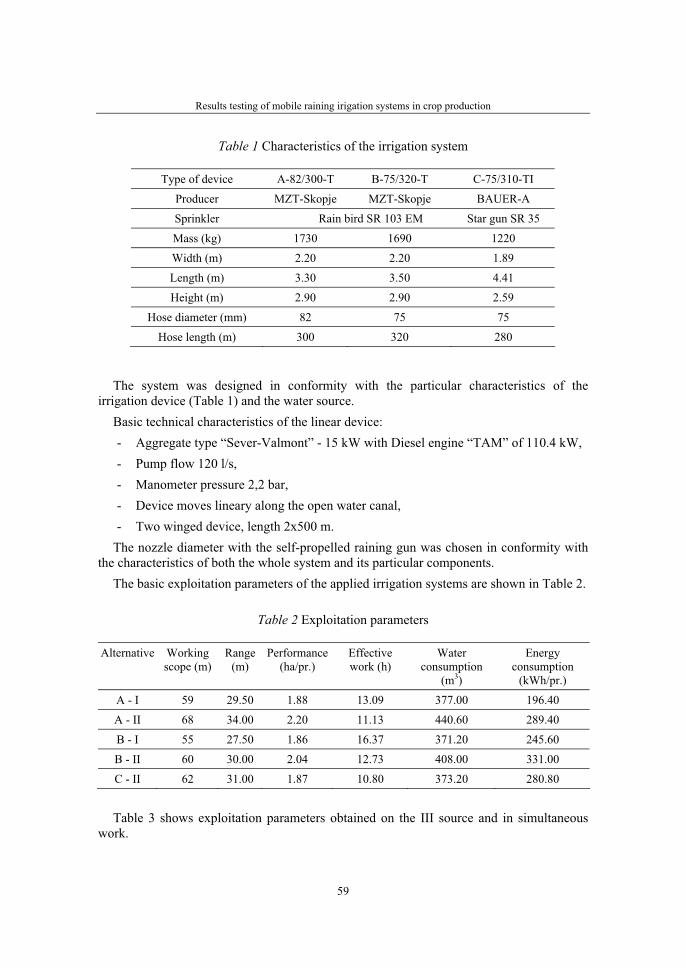
Results testing of mobile raining irigation systems in crop production
59
Table 1 Characteristics of the irrigation system
Type of device A-82/300-T B-75/320-T C-75/310-TI
Producer MZT-Skopje MZT-Skopje BAUER-A
Sprinkler Rain bird SR 103 EM Star gun SR 35
Mass (kg) 1730 1690 1220
Width (m) 2.20 2.20 1.89
Length (m) 3.30 3.50 4.41
Height (m) 2.90 2.90 2.59
Hose diameter (mm) 82 75 75
Hose length (m) 300 320 280
The system was designed in conformity with the particular characteristics of the irrigation device (Table 1) and the water source.
Basic technical characteristics of the linear device: - Aggregate type “Sever-Valmont” - 15 kW with Diesel engine “TAM” of 110.4 kW, - Pump flow 120 l/s, - Manometer pressure 2,2 bar, - Device moves lineary along the open water canal, - Two winged device, length 2x500 m.
The nozzle diameter with the self-propelled raining gun was chosen in conformity with the characteristics of both the whole system and its particular components.
The basic exploitation parameters of the applied irrigation systems are shown in Table 2.
Table 2 Exploitation parameters
Alternative Workingscope (m)
Range(m)
Performance(ha/pr.)
Effectivework (h)
Waterconsumption
(m3)
Energyconsumption
(kWh/pr.)
A - I 59 29.50 1.88 13.09 377.00 196.40
A - II 68 34.00 2.20 11.13 440.60 289.40
B - I 55 27.50 1.86 16.37 371.20 245.60
B - II 60 30.00 2.04 12.73 408.00 331.00
C - II 62 31.00 1.87 10.80 373.20 280.80
Table 3 shows exploitation parameters obtained on the III source and in simultaneous work.
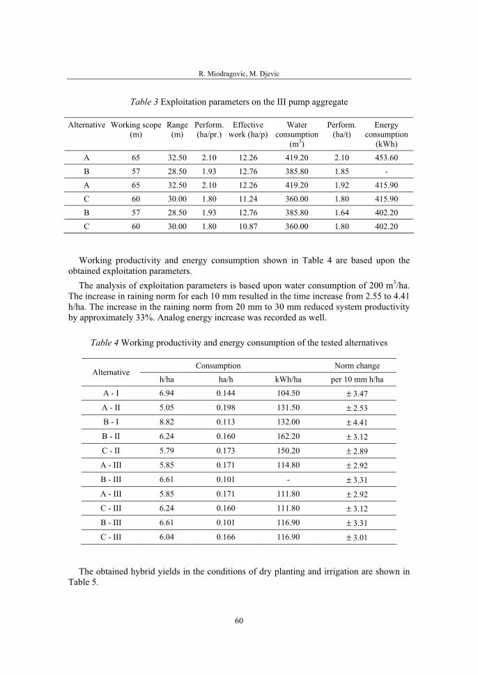
R. Miodragovic, M. Djevic
60
Table 3 Exploitation parameters on the III pump aggregate
Alternative Working scope (m)
Range(m)
Perform.(ha/pr.)
Effectivework (ha/p)
Waterconsumption
(m3)
Perform.(ha/t)
Energyconsumption
(kWh)
A 65 32.50 2.10 12.26 419.20 2.10 453.60
B 57 28.50 1.93 12.76 385.80 1.85 -
A 65 32.50 2.10 12.26 419.20 1.92 415.90
C 60 30.00 1.80 11.24 360.00 1.80 415.90
B 57 28.50 1.93 12.76 385.80 1.64 402.20
C 60 30.00 1.80 10.87 360.00 1.80 402.20
Working productivity and energy consumption shown in Table 4 are based upon the obtained exploitation parameters.
The analysis of exploitation parameters is based upon water consumption of 200 m3/ha. The increase in raining norm for each 10 mm resulted in the time increase from 2.55 to 4.41 h/ha. The increase in the raining norm from 20 mm to 30 mm reduced system productivity by approximately 33%. Analog energy increase was recorded as well.
Table 4 Working productivity and energy consumption of the tested alternatives
Consumption Norm change Alternative
h/ha ha/h kWh/ha per 10 mm h/ha
A - I 6.94 0.144 104.50 ± 3.47
A - II 5.05 0.198 131.50 ± 2.53
B - I 8.82 0.113 132.00 ± 4.41
B - II 6.24 0.160 162.20 ± 3.12
C - II 5.79 0.173 150.20 ± 2.89
A - III 5.85 0.171 114.80 ± 2.92
B - III 6.61 0.101 - ± 3.31
A - III 5.85 0.171 111.80 ± 2.92
C - III 6.24 0.160 111.80 ± 3.12
B - III 6.61 0.101 116.90 ± 3.31
C - III 6.04 0.166 116.90 ± 3.01
The obtained hybrid yields in the conditions of dry planting and irrigation are shown in Table 5.
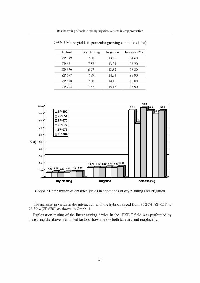
Results testing of mobile raining irigation systems in crop production
61
Table 5 Maize yields in particular growing conditions (t/ha)
Hybrid Dry planting Irrigation Increase (%)
ZP 599 7.08 13.78 94.60
ZP 651 7.57 13.34 76.20
ZP 670 6.97 13.82 98.30
ZP 677 7.39 14.33 93.90
ZP 678 7.50 14.16 88.80
ZP 704 7.82 15.16 93.90
Dry planting Irrigation Increase (%)
7.08 7.57 6.97 7.39 7.5 7.8213.7813.3413.8214.3314.1615.16
94.6
76.2
98.393.9
88.893.9
0
10
20
30
40
50
60
70
80
90
100
% (t)
Dry planting Irrigation Increase (%)
ZP 599ZP 651ZP 670ZP 677ZP 678ZP 704
Graph 1 Comparation of obtained yields in conditions of dry planting and irrigation
The increase in yields in the interaction with the hybrid ranged from 76.20% (ZP 651) to 98.30% (ZP 670), as shown in Graph. 1.
Exploitation testing of the linear raining device in the “PKB ” field was performed by measuring the above mentioned factors shown below both tabelary and graphically.
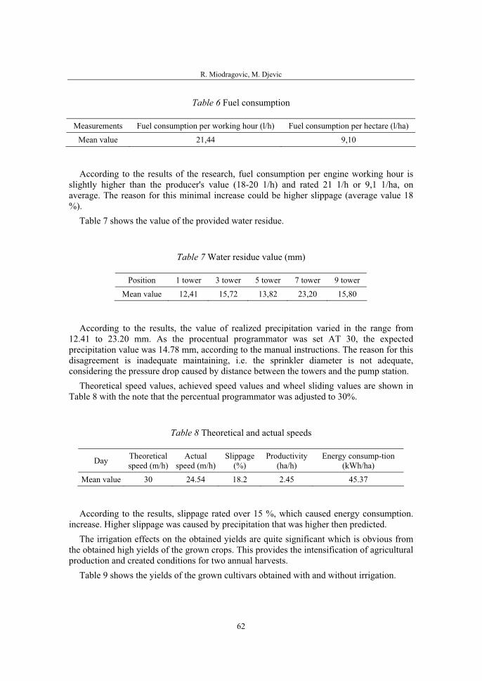
R. Miodragovic, M. Djevic
62
Table 6 Fuel consumption
Measurements Fuel consumption per working hour (l/h) Fuel consumption per hectare (l/ha)
Mean value 21,44 9,10
According to the results of the research, fuel consumption per engine working hour is slightly higher than the producer's value (18-20 1/h) and rated 21 1/h or 9,1 1/ha, on average. The reason for this minimal increase could be higher slippage (average value 18 %).
Table 7 shows the value of the provided water residue.
Table 7 Water residue value (mm)
Position 1 tower 3 tower 5 tower 7 tower 9 tower
Mean value 12,41 15,72 13,82 23,20 15,80
According to the results, the value of realized precipitation varied in the range from 12.41 to 23.20 mm. As the procentual programmator was set AT 30, the expected precipitation value was 14.78 mm, according to the manual instructions. The reason for this disagreement is inadequate maintaining, i.e. the sprinkler diameter is not adequate, considering the pressure drop caused by distance between the towers and the pump station.
Theoretical speed values, achieved speed values and wheel sliding values are shown in Table 8 with the note that the percentual programmator was adjusted to 30%.
Table 8 Theoretical and actual speeds
Day Theoreticalspeed (m/h)
Actualspeed (m/h)
Slippage(%)
Productivity(ha/h)
Energy consump-tion (kWh/ha)
Mean value 30 24.54 18.2 2.45 45.37
According to the results, slippage rated over 15 %, which caused energy consumption. increase. Higher slippage was caused by precipitation that was higher then predicted.
The irrigation effects on the obtained yields are quite significant which is obvious from the obtained high yields of the grown crops. This provides the intensification of agricultural production and created conditions for two annual harvests.
Table 9 shows the yields of the grown cultivars obtained with and without irrigation.
Results testing of mobile raining irigation systems in crop production
63
Table 9 Irrigation effects on maize yields in the raining field
Yield (t/ha)
Plant 1995. 1996. 1997.
Non irrigated Irrigated Non irrigated Irrigated Non irrigated Irrigated
greanbean 4,1 8,0 4,8 8,2 4,5 9,0
silage maize 25,8 32,5 20,0 28,0 26,5 33,4
seed maize 2,7 4,0 1,5 3,1 2,9 5,1
non irig. 1995 irigated 1995 non irig. 1996 irigated 1996 non irig. 1997 irigated 19970
5
10
15
20
25
30
35
Yiel
d (t/
ha)
non irig. 1995 irigated 1995 non irig. 1996 irigated 1996 non irig. 1997 irigated 1997
greanbeansilage maizeseed maize
Graf 2 Yields of grown plants obtained with and without irrigation
The obtained results lead to the conclusion that significantly higher yields were obtained in irrigation conditions thus justifying (Graf. 2) the application of the tested irrigation systems combined with proper work organization and rational utilization.
CONCLUSION
The basic precondition for the optimum utilization of the irrigation systems is the coordination of system parameters.
For this purpose, nozzle diameter, pressure and water flow parameters are defined for each particular source and type of device.
Work productivity and energy consumption in effective time depend upon the raining quantity per single throughput.
Productivity of a linear was 2,3 up to 2,8 ha/h. Energy consumption of tested irrigation systems was 125,3 kWh/ha for self-propelled raining gun and for linear 45,37 kWh/ha. Difference was very significant (36,21 %) and ilustrates benefits of the linear system.
R. Miodragovic, M. Djevic
64
Linear raining irrigation devices are up-to-date devices for intensive raining which require expert and efficient manpower in both the field of handling and in the field of designing the programmes of their utilization.
The extremely significant increase in yield is provided by the use of irrigation (it varies from crop to crop) thus justifying the investments in particular irrigation systems.
REFERENCES
1. Avakumović, D. (1994): Navodnjavanje. Građevinski fakultet Univerziteta u Beogradu.
2. Vasić, G., Branka Kresović, Tolimir, M. (1994): Efekti navodnjavanja mašina tipa “RAINGER” i “LINEAR” na prinos gajenih useva. Seminar agronoma. Zbornik radova Instituta za ratarstvo i povrtarstvo, 119-127.
3. Đević, M., Kresović Branka (1993): Mobile irrigation systems in maize production. Review of Research Work at the Faculty of Agriculture, Vol. 40 No 1, 131-135.
4. Mančev, S. (1996): Primena linijskog uređaja za navodnjavanje kišenjem u uslovima gazdinstva PDS “PKB Opovo”. Diplomski rad. Poljoprivredni fakultet. Beograd.
5. Ćorović, R. (1992): Projektovanje meliorativnih sistema. Poljoprivredni fakultet. Beograd.
6. Belami, A., Ofen, A. (1986): Irrigation engineering, IESP.
36. Symposium "Actual Tasks on Agricultural Engineering", Opatija, Croatia, 2008.
65
36.
SIMPOZIJAKTUALNI ZADACIMEHANIZACIJE POLJOPRIVREDE
UDC631.67:631.51
Prethodno priopćenjePreliminary communication
AN AUTOMATIC PRECISION IRRIGATION SYSTEM FOR COTTON FIELD
JUN ZHANG1, YINGWU SHENG2, YANDONG ZHAO3, PING YANG1
1College of Information, Beijing Union University, Beijing, 100101, China, email: [email protected]
2Management Bureau of Dagu River, Qingdao, 266232, China 3College of Industry, Beijing Forestry University, Beijing, 100083, China
SUMMARY
An automatic precision irrigation control system for cotton field is presented in this paper, which consists of host computer, slave computer controller, different kinds of sensors, valve controller, communication module, and system software. The system can collect and monitor field environmental parameters such as soil moisture, soil temperature, atmosphere temperature, field evaporat-ion amount and precipitation etc. By combining field environmental parameters with mathematical model, the irrigation time and irrigation quantity for cotton filed can be predicted. The different irrigation strategy can be adopted automatically according to the water-required rules of different cotton growing periods. This system had been used in the cotton field for precision irrigation in Langfang experimental farm of Soil and Fertilizer Institute, Chinese Academy of Agricultural Sciences from 2005 to 2006. Under the same environmental condition, the automatic irrigation system has higher cotton yield and uses less water quantity than the manual irrigation system. The results show that the automatic precision irrigation control system for cotton field can reduce irrigation cost and improve cotton yield.
Key words: Precision Irrigation, Sensor, Automatic Control, Cotton Field
INTRODUCTION
Field environmental parameter collection is one of the critical problems in precision agriculture (Zhao et al., 2002). Once the field environmental parameters are collected precisely on real time, agronomic recommendations are available and correct strategy can be executed in time (Zhang et al., 2002). In the past, field environmental information, such as soil water content and field evaporation amount, was obtained by sampling in field and
J. Zhang, Y. Sheng, Y. Zhao, P. Yang
66
analyzing in lab. This method wastes much time and energy, and it cannot get real-time data. Computer measurement system can obtain all kinds of field real-time data automatically by using different kinds of sensors, so that the production efficiency can be improved greatly (Sun et al., 2006). In order to realize precision farm application, such as precision irrigation, computer control system should also be adopted besides computer measurement system (Yang et al., 2006; Xin et al., 2005).
A computer automatic measurement and control system for cotton field precision irrigation is developed in this paper. This system consists of host computer, slave computer controller, different kinds of sensors, valve controller, communication module, and system software. Field environmental parameters, such as soil moisture, soil temperature, atmosphere temperature, field evaporation amount and precipitation etc, can be collected and monitored by the system. By analyzing these environmental data with mathematical model, the irrigation time and irrigation quantity for cotton field can be determined. Therefore the system can adopt different irrigation strategy automatically according to the water-required rules of different cotton growing periods. This system had been used for the cotton field precision irrigation in Langfang experimental farm of Soil and Fertilizer Institute, Chinese Academy of Agricultural Sciences from 2005 to 2006. The results show that the automatic precision irrigation control system can save water and improve production efficiency greatly.
COMPONENTS OF AUTOMATIC PRECISION IRRIGATION SYSTEM
The automatic precision irrigation control system consists of hardware components and system software combined with irrigation control algorithm.
Hardware Components Hardware components include host computer, slave computer controller, communication
module, different kinds of sensors and electromagnetic valve. By cooperating with management software, the main functions of host computer in the
control center are to process data, monitor the system operation, and control the system de-vices properly. Because the control center room is far away from the field, communication transfer by cable is not economic and convenient. Therefore the communication between host computer in the control center and slave computer controller in the field is realized by SRWF-105 wireless communication module. SRWF-105 module provides two serial-communication interfaces, i.e. COM1 is UART interface of TTL voltage and COM2 is standard RS-232/RS-485 interface. The module is used to realize remote communication within 2K meters between slave computer controller and host computer.
Micro-controller-unit SPCE061A is used as the core of slave computer controller. The slave computer controller consists of micro-controller-unit, extended memory, LCD displayer, keyboard, and RS-485 interface. The main functions of slave computer controller include collecting data, storing data, processing data, transmitting data, displaying data, and turning on/off the electromagnetic valves.
Different kinds of sensors and electromagnetic valves are linked to slave computer cont-roller by RS-485 interfaces. The sensors include twenty soil water sensors, one atmosphere

An automatic precision irrigation system for cotton field
67
temperature sensor, one soil temperature sensor, one field evaporation sensor, and one precipitation sensor. Field bus technique is adopted to collect the field environmental para-meters such as soil moisture, soil temperature, atmosphere temperature, field evaporation amount and precipitation precisely on real time. Furthermore, the system controls the turning on/off of electromagnetic valves according to control algorithm to realize saving water irrigation automatically.
Figure1 Automatic irrigation control system structure
System Software and Irrigation Control Algorithm Host computer monitor software is programmed by Visual Basic language. Slave comp-
uter control software is developed by C language and Assembly language. The system can operate under host computer monitoring or under only slave computer control without host computer monitoring. Host computer monitor software consists of data collection module, data processing module, communication module, and management module.
According to different water demand in different cotton growth stages and cotton expert database, and combining with field environmental parameters, mathematical model for cotton irrigation is developed. The maximum and minimum thresholds of soil water contents under different conditions are preset. When soil water content is detected to be lower than the minimum threshold, electromagnetic valve is turned on automatically. While soil water content is detected to be higher than the maximum threshold, electromagnetic valve is turned off automatically. This control algorithm is simple and reliable.
RESULTS AND DISCUSSION
Irrigation Scheme ImplementThe experiment was conducted in Langfang experimental farm (39.4N.116.4E) of Soil
and Fertilizer Institute, Chinese Academy of Agricultural Sciences from 2005 to 2006. The
soilwatersensor
atmospheretemperature
sensor
soiltemperature
sensor
fieldevaporation
sensor
wireless communication
host computer
slave computer controller
precipitationsensor
valveand
controller
RS - 485 field bus
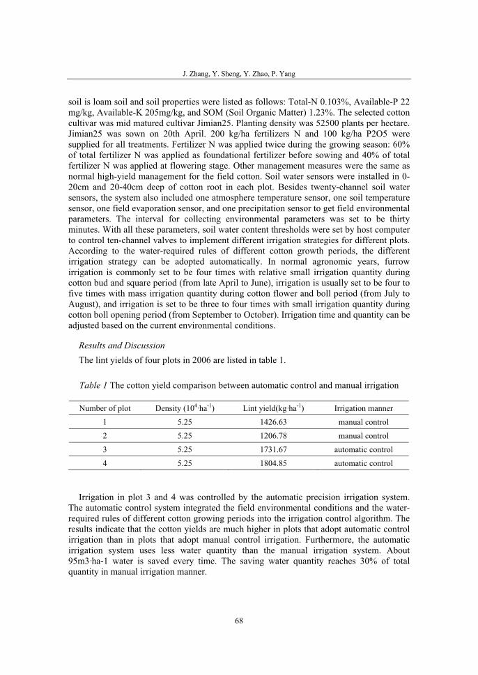
J. Zhang, Y. Sheng, Y. Zhao, P. Yang
68
soil is loam soil and soil properties were listed as follows: Total-N 0.103%, Available-P 22 mg/kg, Available-K 205mg/kg, and SOM (Soil Organic Matter) 1.23%. The selected cotton cultivar was mid matured cultivar Jimian25. Planting density was 52500 plants per hectare. Jimian25 was sown on 20th April. 200 kg/ha fertilizers N and 100 kg/ha P2O5 were supplied for all treatments. Fertilizer N was applied twice during the growing season: 60% of total fertilizer N was applied as foundational fertilizer before sowing and 40% of total fertilizer N was applied at flowering stage. Other management measures were the same as normal high-yield management for the field cotton. Soil water sensors were installed in 0-20cm and 20-40cm deep of cotton root in each plot. Besides twenty-channel soil water sensors, the system also included one atmosphere temperature sensor, one soil temperature sensor, one field evaporation sensor, and one precipitation sensor to get field environmental parameters. The interval for collecting environmental parameters was set to be thirty minutes. With all these parameters, soil water content thresholds were set by host computer to control ten-channel valves to implement different irrigation strategies for different plots. According to the water-required rules of different cotton growth periods, the different irrigation strategy can be adopted automatically. In normal agronomic years, furrow irrigation is commonly set to be four times with relative small irrigation quantity during cotton bud and square period (from late April to June), irrigation is usually set to be four to five times with mass irrigation quantity during cotton flower and boll period (from July to August), and irrigation is set to be three to four times with small irrigation quantity during cotton boll opening period (from September to October). Irrigation time and quantity can be adjusted based on the current environmental conditions.
Results and Discussion The lint yields of four plots in 2006 are listed in table 1.
Table 1 The cotton yield comparison between automatic control and manual irrigation
Number of plot Density (104·ha-1) Lint yield(kg·ha-1) Irrigation manner
1 5.25 1426.63 manual control
2 5.25 1206.78 manual control
3 5.25 1731.67 automatic control
4 5.25 1804.85 automatic control
Irrigation in plot 3 and 4 was controlled by the automatic precision irrigation system. The automatic control system integrated the field environmental conditions and the water-required rules of different cotton growing periods into the irrigation control algorithm. The results indicate that the cotton yields are much higher in plots that adopt automatic control irrigation than in plots that adopt manual control irrigation. Furthermore, the automatic irrigation system uses less water quantity than the manual irrigation system. About 95m3·ha-1 water is saved every time. The saving water quantity reaches 30% of total quantity in manual irrigation manner.
An automatic precision irrigation system for cotton field
69
CONCLUSIONS
The precision irrigation control technique is critical for precision farming (Sun et al., 2005). The automatic precision irrigation control system studied in this paper, which combines automatic control technique and irrigation technique, can realize remote wireless control. Different irrigation strategy can be adopted automatically according to the environmental conditions and the water-required rules of different cotton growing periods. The experiments indicate that the control system can reduce irrigation cost, save water, save labor force, and improve cotton yield greatly. Therefore it has promising potential in precision agricultural applications. Further work is planned to integrate fertilizer-required rules of different cotton growth periods into the mathematical model, and then develop a precision irrigation and fertilization system (Liu et al., 2006).
ACKNOWLEDGMENTS
This research has been supported by National Natural Science Foundation Project under Grant No. 30671715.
REFERENCE
1. Liu Xiuzhen, Zheng Decong, Ma Jun, et al. (2006). Accurate to irrigate and apply fertilizer automatic research of administrative system and realize. Journal of Soil and Water Conservation, 20(5): 197-200
2. Sun Li, Chen Xi, Wang Jun, et al. (2006). The application of automatic control system for drip irrigation under plastic film on cotton farming. Journal of Arid Land Resources and Environment, 20(1): 184-189
3. Sun Li, Zhang Qing, Chen Xi, et al. (2005). Application of the integrated precision farming system of cotton growing in Xinjiang Region. Transactions of the Chinese Society of Agricultural Engineering, 21(8): 83-88
4. Xin Xiuli, Xu Fu’an, Xu Mengxiong, et al. (2005). A computer system for controlling irrigation and collecting information in cotton field. Journal of Irrigation and Drainage, 24(1): 77-80
5. Yang Qing, Pang Shujie, Yang Chenghai, et al. (2006). Variable rate irrigation control system integrated with GPS and GIS. Transactions of the Chinese Society of Agricultural Engineering, 22 (10): 134- 138
6. Zhang Naiqian, Wang Maohua, Wang Ning. (2002). Precision agriculture — a worldwide overview. Computers and Electronics in Agriculture, 36: 13-132
7. Zhao Yandong, Wang Yiming. (2002). Study on the measurement of soil water content based on the principle of standing-wave ratio. Transactions of the Chinese Society for Agricultural Machinery, 33(4): 109-111
8. Zhao Yandong, Wang Yiming. (2002). Analysis of Sensitivity of soil moisture measurement based on standing-wave ratio. Transactions of the Chinese Society of Agricultural Engineering, 18(2): 5-8

36. Symposium "Actual Tasks on Agricultural Engineering", Opatija, Croatia, 2008.
71
36.
SIMPOZIJAKTUALNI ZADACIMEHANIZACIJE POLJOPRIVREDE
UDC631.372:621.436
Izvorni znanstveni radOriginal scientific paper
IMPROVEMENT OF GENERAL PARAMETERS OF TRACTOR DIESEL BY MORE EFFECTIVE USE OF
FUEL-AIR CHARGE VALENTIN BOROVIKOV
Belarussian State Agrarian Technical University, e-mail: [email protected]
SUMMARY
Wide application of diesels as field engines and growth of oil-products prices compel researchers to develop the scientific-technical suggestions to modernize diesels and improve their operation parameters. First, the ecological and power-economic parameters as the general ones.
More effective use of a fuel-air charge of a tractor diesel is considerable reserve to improve the general diesel parameters. In this paper the influence of the relative volume of the recessed piston combustion chamber (CC) on the general diesel parameters was studied.
The relative volume of the CC is the relation Vch/Vtv, there Vch – the volume of the CC, Vtv – the total volume of the in-cylinder space in the position of the piston in a Top Dead Centre (TDC).
The description of the own technical suggestion accordingly to this technical direction to improve the general parameters of the diesel D65N and the research results are given.
Too, the technical solution which excludes “dead volumes” below intake and exhaust valves of a tractor diesel are suggested.
Key words: diesel, technical suggestions, increase of relative volume of a recessed piston combustion chamber, improvement of diesel parameters
INTRODUCTION
Effective use of a fuel-air charge in a tractor diesel with the recessed piston CC is a considerable reserve to improve the ecological and power-economic parameters of the diesel engines. A number of publications are devoted to this problem. This paper is based on the publications [1, 2, 3].
V. Borovikov
72
There are the authors affirm that the value of the relative volume of the recessed piston CC has the significant influence on the operation process of the diesel and on its general parameters. In this case, the relative volume of the CC is defined as the relation Vch/Vtv,there Vch – the volume of the CC, Vtv – the total volume of the in-cylinder space in the position of the piston in TDC.
Usually, the alteration of the relative volume of the CC is accompanied by the negative alterations of the design and regime parameters of the diesel. Then the effect from the innovation is the result of the combined action of the positive and negative factors.
The purpose of the publishing paper is to analyse the known technical information about the effectiveness of the said technical direction to improve the general diesel parameters, to publish the results of the own experimental studies on this theme and to give the technical suggestion on the further development of this direction.
METHODS
The experimentally obtained dependences of the influence of the value of the relative volume of the recessed piston CC on the general parameters of the diesel D -240 are given in the PhD thesis [1]. The experiment was carried out with the step-by-step deepening the CC without the alteration of the design of the narrow throat of the CC. The dependences were obtained during the experimental studies at the Production Corporation "Minsk Motor Plant ". The tendencies which were established by the author Dr Ch.Drobyshevskiy, they can be considered as the principally existing at the present time also.
The physical phenomenon of the process which takes place under the alteration of the relative volume of the CC consists of the following.
Under the position of the piston in TDC during the beginning of the combustion stroke the diesel fuel effectively burns only: in the volume of the recessed piston CC and in the part of the volume of the clearance between the piston and the cylinder head if this volume part is above the CC.
The remaining parts of the volume of the in-cylinder space (the position is examined when the piston is in TDC) do not ensure the effective combustion. There is the "damping" of the flame and the formation of the toxic products of the incomplete combustion of the fuel in these volumes.
The mentioned volumes, the “dead” volumes, of the ineffective combustion of the diesel are:
• the volume part of the clearance between the piston and the cylinder head, which are not situated above the CC;
• the ring volume, formed by the inner surface of the cylinder bore and the external surface of the piston head, the said ring volume begins from the piston top until the first compression ring.
The widely known technical solutions to increase the relative volume of the CC are following. For example, an installation of a teflon ring above a metal of a wet cylinder sleeve as the sealing of the joint "cylinder – head of cylinder block". This technical solution
Improvement of general parameters of tractor diesel by more effective use of fuel-air charge
73
is used at the diesels of the Production Corparation “Minsk Motor Plant". This teflon ring, in one of its functions, fills the annular volume above the cylinder sleeve, excluding the penetration of the fuel-air charge into the annular volume. Correspondingly, it excludes the ineffective combustion of the fuel-air mixture in the said annular volume.
Another technical solution widely used by many motor-building companies is replacing an upper compression ring maximally closely to a fire surface of a piston head. This technical solution decreases an annular volume, a dead volume, around the piston above the said ring.
The own research experience of the author of this paper confirms the considerable effectiveness of the realization of the idea to increase the relative volume of a recessed piston CC of a tractor diesel.
In this case the perspective for the design works in this direction should be estimated. At the present time there are two trends in the development of the designs of the recessed piston CC of tractor diesels.
The first tendency assumes the "disclosure" of the CC. In this case, the advantages are: the lower heat tenses in the edges of the CC, the exclusion of the formation of the thermal-fatigue cracks and the decrease crumbling off the CC edges, the decrease of the heat losses into the piston body and the decrease of the temperatures of the piston group. The energy of fuel-air mixing in this case is determined mainly by the energy of the fuel injection. This tendency is supported by the application of the fuel injection systems with the high pressure of the injection, for example, the systems of the type Common Rail.
In accordance with the another tendency the producers of tractor diesels continue to use the recessed piston CC, which have the narrow throat.
Such CC due to the effective use of the energy of the compressed fuel-air charge and turbulizing action of the throat edges of the CC - improve fuel-air mixing and ensure the more complete combustion of the fuel. I.e., in this case, the energy of mixing is the amount of the fuel injection energy and the kinetic energy of the air charge being displaced into the CC under piston moving to TDC for the compression stroke.
To use the turbulizing action of the edges of the narrow throat of the CC and to exclude overheating the edges, either the intensive cooling of the pistons or the two-piece pistons with the upper steel parts and the aluminum piston skirts are applied, usually.
Obviously that the diesels having the CC designs in accordance with the first trend of the development have the less volumes of the ineffective combustion and their negative influence on the fuel combustion decreases.
In the diesels having the CC with the narrow throat, in accordance with the second trend, the negative influence of the volumes of the ineffective combustion is more considerable because of their larger value.
In accordance with the request of the Rybinsk Diesel Plant the author of this paper jointly with Dr Ch.Drobyshevskiy proposed and experimentally evaluated the technical suggestion to improve the power- economic and ecological parameters of the diesel D65N by increasing the relative volume of the recessed piston CC.
It was suggested to apply the piston with the deeper recessed piston CC.
V. Borovikov
74
In this case we should expect that the decrease the ratio of compression will make the power-economic diesel parameters worse. On another side, applying the deeper CC increases the relation volume of the CC and improves the fuel combustion.
The resultant action of these two factors was determined by the experimental motor studies.
The experimental studies were carried out at the engines laboratory of the Belarussian State Agrarian Technical University. B-type diesel D65N of the production of the Rybinsk Diesel Plant has four cylinders, in-line, dimension S/D=130/110, direct injection, liquid cooling, the nominal engine speed 1750 rpm.
The experiment motor studies were conducted in accordance with the State Standard No. 18509-88 “Tractor and combine diesel engines. Methods of bench tests”.
The diesel was mounted at the brake stand and in the two series of experiment was alternately completed by the pistons of the model 240-1004021А, by the nominal volume of the CC 60.0 cm3 (the regular assembly) and by the pistons of the model 245-1004021, by the nominal volume of the CC 64.5 cm3, being used for the diesels with the pressure charging of the production of the Production Corporation "Minsk Motor Plant".
Before the motor experiment the measurement of the clearances above the pistons in the all cylinders of the diesel were carried out by the method of the lead "witnesses". Also, the measurement of the under-valve volumes of the head of the cylinder block was carried out. The head of the cylinder block was removed from the engine for this purpose.
Furthermore, under the installation of the nonstandard pistons of the model 245-1004021 by the method of the lead "witnesses" the initial clearances above the pistons were determined, and by the selection of the gaskets practically the equal clearances in the diesel of the regular and experimental completions were mounted. The difference of the clearances above the piston did not exceed 0.04 mm. Thus, the average in-cylinder volume above the pistons was experimentally determined. The average annular volume between the piston and the cylinder was calculated.
The calculation according to the obtained data indicated that the application of the nonstandard pistons with the deeper CC reduced the ratio of compression of the diesel from 17.2 to 16.2. In this case, the relative volume of the CC increased from 0.788 to 0.800.
Before the experiment study the diesel in the experimental completion passed the motor running-in during 10 hours.
The power curves and the series of the load characteristics were got. The effectiveness of the technical solution was examined by the comparative estimation, firstly, of the parameter of the specific effective fuel consumption in the zone of the diesel operation, which is close to the nominal engine regime, Fig. 1.
The analysis of the load characteristic, Fig. 1, shows that the specific effective fuel consumption in the zone of the nominal regime was improved, not less than by 8,0 g/(kWh). The temperature of the waste gases in this case was reduced by 40 oC. This proves the authenticity of the previous affirmation about the improvement of the diesel efficiency. The brake power increased by 0,35 kW. It is interesting that the air excess ratio increased by 0.05. Probably, it is explained by the reduction in the temperature of the piston head and by the improvement of the air admission of the diesel in this case.
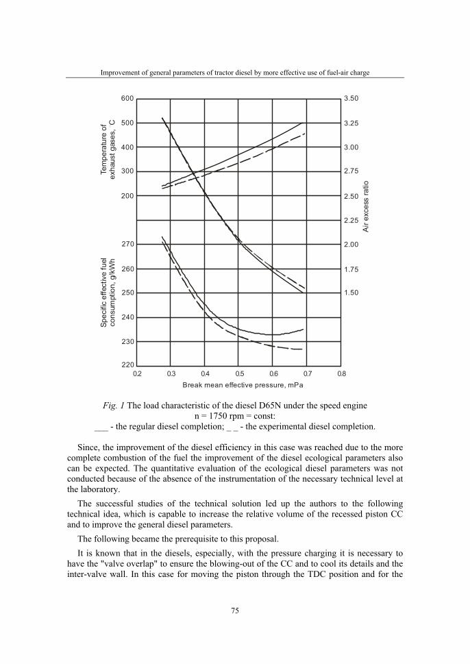
Improvement of general parameters of tractor diesel by more effective use of fuel-air charge
75
0.2 0.3 0.4 0.5 0.6 0.7 0.8Break mean effective pressure, mPa
220
230
240
260
250
270
200
300
400
500
600Te
mpe
ratu
reof
exha
ust g
ases
, C
Spec
ific
effe
ctiv
efu
elco
nsum
ptio
n, g
/kW
h
1 50.
1.75
2.00
2.25
2.50
2.75
3.00
3.25
3.50
Air
exce
ssra
tio
Fig. 1 The load characteristic of the diesel D65N under the speed enginen = 1750 rpm = const:
___ - the regular diesel completion; _ _ - the experimental diesel completion.
Since, the improvement of the diesel efficiency in this case was reached due to the more complete combustion of the fuel the improvement of the diesel ecological parameters also can be expected. The quantitative evaluation of the ecological diesel parameters was not conducted because of the absence of the instrumentation of the necessary technical level at the laboratory.
The successful studies of the technical solution led up the authors to the following technical idea, which is capable to increase the relative volume of the recessed piston CC and to improve the general diesel parameters.
The following became the prerequisite to this proposal. It is known that in the diesels, especially, with the pressure charging it is necessary to
have the "valve overlap" to ensure the blowing-out of the CC and to cool its details and the inter-valve wall. In this case for moving the piston through the TDC position and for the
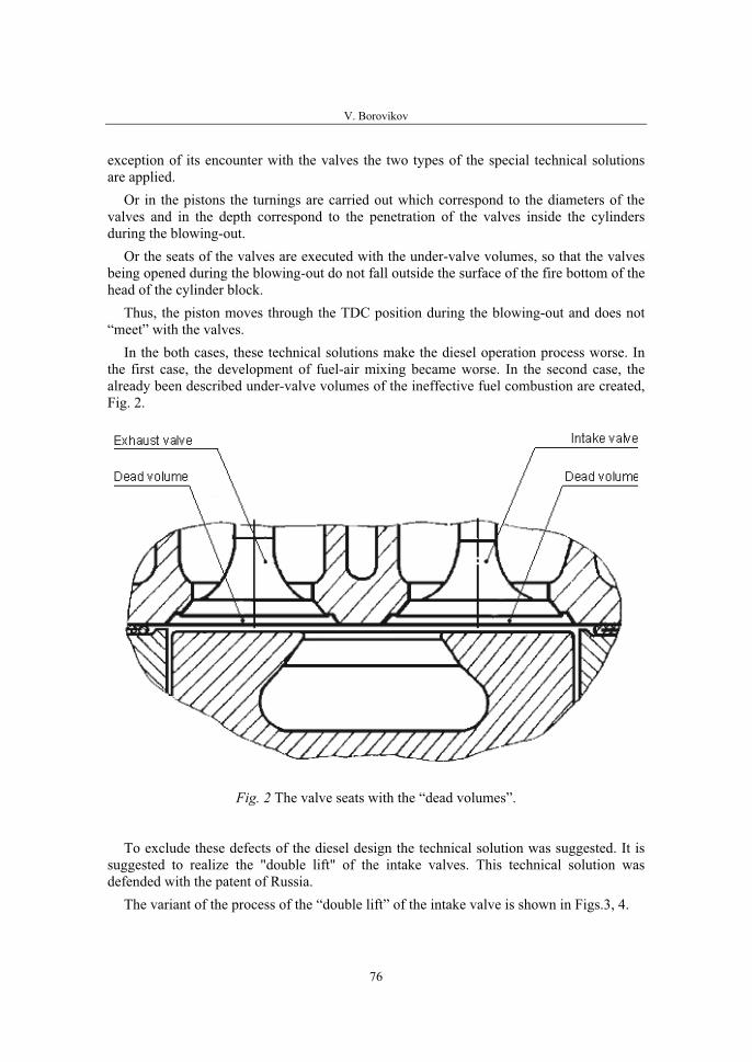
V. Borovikov
76
exception of its encounter with the valves the two types of the special technical solutions are applied.
Or in the pistons the turnings are carried out which correspond to the diameters of the valves and in the depth correspond to the penetration of the valves inside the cylinders during the blowing-out.
Or the seats of the valves are executed with the under-valve volumes, so that the valves being opened during the blowing-out do not fall outside the surface of the fire bottom of the head of the cylinder block.
Thus, the piston moves through the TDC position during the blowing-out and does not “meet” with the valves.
In the both cases, these technical solutions make the diesel operation process worse. In the first case, the development of fuel-air mixing became worse. In the second case, the already been described under-valve volumes of the ineffective fuel combustion are created, Fig. 2.
Fig. 2 The valve seats with the “dead volumes”.
To exclude these defects of the diesel design the technical solution was suggested. It is suggested to realize the "double lift" of the intake valves. This technical solution was defended with the patent of Russia.
The variant of the process of the “double lift” of the intake valve is shown in Figs.3, 4.
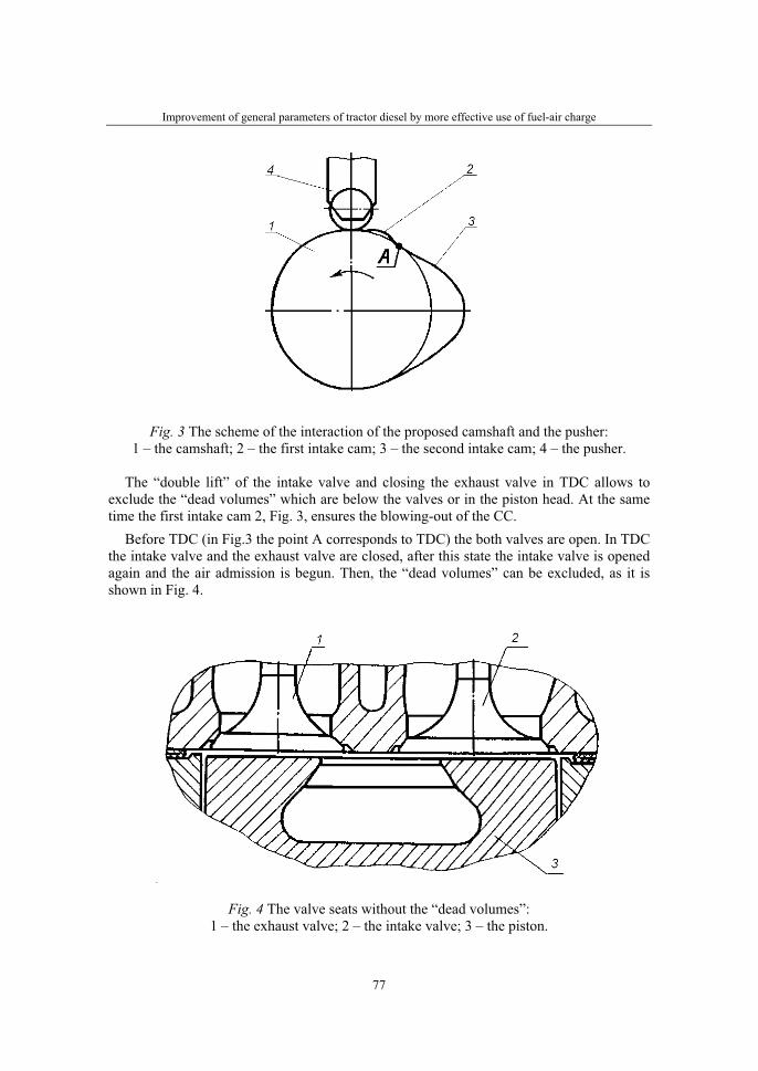
Improvement of general parameters of tractor diesel by more effective use of fuel-air charge
77
Fig. 3 The scheme of the interaction of the proposed camshaft and the pusher:1 – the camshaft; 2 – the first intake cam; 3 – the second intake cam; 4 – the pusher.
The “double lift” of the intake valve and closing the exhaust valve in TDC allows to exclude the “dead volumes” which are below the valves or in the piston head. At the same time the first intake cam 2, Fig. 3, ensures the blowing-out of the CC.
Before TDC (in Fig.3 the point A corresponds to TDC) the both valves are open. In TDC the intake valve and the exhaust valve are closed, after this state the intake valve is opened again and the air admission is begun. Then, the “dead volumes” can be excluded, as it is shown in Fig. 4.
Fig. 4 The valve seats without the “dead volumes”: 1 – the exhaust valve; 2 – the intake valve; 3 – the piston.
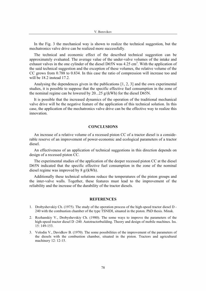
V. Borovikov
78
In the Fig. 3 the mechanical way is shown to realize the technical suggestion, but the mechatronics valve drive can be realized more successfully.
The technical and economic effect of the described technical suggestion can be approximately evaluated. The average value of the under-valve volumes of the intake and exhaust valves in the one cylinder of the diesel D65N was 4.25 cm3. With the application of the said technical suggestion and the exception of these volumes, the relative volume of the CC grows from 0.788 to 0.834. In this case the ratio of compression will increase too and will be 18.2 instead 17.2.
Analysing the dependences given in the publications [1, 2, 3] and the own experimental studies, it is possible to suppose that the specific effective fuel consumption in the zone of the nominal regime can be lowered by 20...25 g/(kWh) for the diesel D65N.
It is possible that the increased dynamics of the operation of the traditional mechanical valve drive will be the negative feature of the application of this technical solution. In this case, the application of the mechatronics valve drive can be the effective way to realize this innovation.
CONCLUSIONS
An increase of a relative volume of a recessed piston CC of a tractor diesel is a conside-rable reserve of an improvement of power-economic and ecological parameters of a tractor diesel.
An effectiveness of an application of technical suggestions in this direction depends on design of a recessed piston CC.
The experimental studies of the application of the deeper recessed piston CC at the diesel D65N indicated that the specific effective fuel consumption in the zone of the nominal diesel regime was improved by 8 g/(kWh).
Additionally these technical solutions reduce the temperatures of the piston groups and the inter-valve walls. Together, these features must lead to the improvement of the reliability and the increase of the durability of the tractor diesels.
REFERENCES
1. Drobyshevskiy Ch. (1975). The study of the operation process of the high-speed tractor diesel D -240 with the combustion chamber of the type TSNIDI, situated in the piston. PhD thesis. Minsk.
2. Rozhanskiy V., Drobyshevskiy Ch. (1980). The some ways to improve the parameters of the high-speed tractor diesel D -240. Autotractorbuilding. Theory and design of mobile machines. Iss. 15: 149-153.
3. Volodin V., Davidkov B. (1970). The some possibilities of the improvement of the parameters of the diesels with the combustion chamber, situated in the piston. Tractors and agricultural machinery 12: 12-15.

36. Symposium "Actual Tasks on Agricultural Engineering", Opatija, Croatia, 2008.
79
36.
SIMPOZIJAKTUALNI ZADACIMEHANIZACIJE POLJOPRIVREDE
UDK631.372:665.3Pregledni radReview paper
MOGUĆNOST UPORABE BILJNOG ULJA ZA POGON TRAKTORA I DRUGIH VOZILA
VIKTOR JEJČIČ1, TOMAŽ POJE2, TONE GODEŠA2
1Kmetijski inštitut Slovenije, Oddelek za kmetijsko tehniko,Hacquetova 17, SI - 1000 Ljubljana, [email protected]
SAŽETAK
Uporaba biljnog ulja za energetske svrhe na dieselskim motorima traktora, teretnih vozila, komunalnih vozila, radnih strojeva, kogeneracijskih jedinica za proizvodnju električne i toplotne energije itd. predstavlja opciju za sadašnju uporabu mineralnog dieselskog goriva. Uporaba biljnog ulja ne nepreuređenimdieselskim motorima nije moguća jer može prouzročiti teška oštećenja motora. Da postignemo kompletan proces izgaranja u dieselskom motoru biljno ulje mora biti raspršeno jednako kvalitetno kao i mineralno dieselsko gorivo. Za postizanje toga viskoznost biljnog ulja mora odgovarati viskoznosti mineralnog dieselskog goriva. Viskoznost biljnog ulja vrlo je ovisna o temperaturi: čim je viša temperatura biljnog ulja tim je niža njegova viskoznosti. Grijanje biljnog ulja smanjuje njegovu viskoznost i sprječava mogućnost oštećenja visokotlačne crpke za uštrcavanje goriva (veliko trenje između radnih elemenata crpke pri visokoj viskoznosti ulja uzrokuje velike radne otpore, koji su štetni za različite dijelove crpke). Grijanje biljnog ulja također smanjuje mogućnost oštećenja brizgaljki i klipnih prstena zbog nekompletnog izgaranja koje se pojavljuje kod goriva visoke viskoznosti. Za potrebe istraživanja na Kmetijskom inštitutu Slovenije – Odjel za poljoprivrednu tehniku, preuredili smo motor traktora AGT 835 tako da može raditi na biljno ulje.
Ključne riječi: biljno ulje, bio-gorivo, traktor, vozila
UVOD
Ugljični dioksid koji nastaje kod izgaranja biomase ne pridonosi opterećivanju okoliša sa plinovima koji stvaraju efekt staklenika. Biomasa koja nastaje u poljoprivredi upotrebljava se kao izvor hrane za ljude i životinje, za preradu u različite sirovine za odjeću i druge proizvode te goriva a dio se u obliku organskih otpadaka vraća neposredno u tlo. Pored tvrdih i tekućih produkata biomase postoje i tekuća goriva iz biomase odnosno biogoriva.
V. Jejčič, T. Poje, T. Godeša
80
Biogoriva se mogu upotrebljavati kao nadomjestak ili dodatak gorivima koja imaju porijeklo iz nafte, za upotrebu u transportu i različitim područjima ljudskih aktivnosti. Od tekućih goriva iz biomase najznačajnija biogoriva su trenutno: bioetanol, biometanol, biljno ulje i biodiesel. U zadnjem razdoblju pored biodiesela za pogon dieselskih motora različitihvozila i radnih strojeva, sve veći značaj dobiva i biljno ulje koje se može u rafiniranom ili nerafiniranom obliku upotrijebiti za pogon prerađenih dieselskih motora. Energetska upora-ba biljnog ulja u motorima (dieselski motori na radnim strojevima, traktorima, teretnim vozilima, komunalnim vozilima, kogeneratorskim jedinicama za proizvodnju električne i toplotne energije itn.) je aktualna opcija za sadašnja fosilna goriva (dieselsko gorivo mineralnog porijekla). Biljno ulje kao energent postaje sve više zanimljivo zbog stalnog rasta cijena fosilnih goriva i problema sa očuvanjem okoline sa kojima se sve više susrećečovječanstvo. Vrlo važno je da je biljno ulje iz biljaka za proizvodnju ulja dostižno prakti-čno u cijeloj Evropi. Sjeverni dijelovi Evrope prikladniji su za proizvodnju uljane repice a južni za proizvodnju suncokreta, soje itn. U drugim dijelovima svijeta upotrebljava se za proizvodnju ulja palma, jatropa itn. Na svijetu postoji više od 4000 biljnih vrsta Riva et all (2) iz kojih se može proizvoditi biljno ulje. Biljna ulja predstavljaju dio uskladištene sunčane energije pomoću prirodnih procesa koji se odvijaju u samoj biljci.
Ulje za spomenutu upotrebu može se proizvoditi mehaničkim procesom ekstrakcije – prešanja ili industrijskim načinom – ekstrakcijom pomoću topiva. Proces proizvodnje ulja prešanjem ne iziskuje složene strojeve u usporedbi sa industrijskim procesom proizvodnje ulja ekstrakcijom sa topivima. Značajna odlika mehaničkog procesa prešanja je da su potrebni niski utrošci energije te da nije potrebna upotreba kemikalija za ekstrakciju (ekološko sporno). Strojevi za mehaničko prešanje ulja djeluju kontinuirano i ne iziskuju posebnog dodatnog angažiranja radne snage kod samog rada. Na području biogoriva u zadnje vrijeme u Sloveniji se događaju velike promjene kao posljedica aktivnosti glede potrebe za određenim stupnjem samoopskrbe energijom, očuvanja okoline i uključivanja poljodjelstva u proizvodne procese za biogoriva. U sklopu strateškog cilja Slovenije za povećanje stupnja samoopskrbe energijom poljodjelstvo može odigrati značajnu ulogu na području alternativnih izvora energije osobito kod biogoriva na osnovu ulja iz uljane repice. Promjenom zakona o trošarini u prosincu 2003, biogoriva su bila opredijeljena kao pogonska goriva sa trošarinom 0 %. Slijedeći korak prema poticanju upotrijebe biogoriva bio je uređen sa prijenosom Direktive EU o promociji uporabe biogoriva i drugih obnov-ljivih goriva za promet, koja članice stimulira ka povećanju udjela biogoriva u ukupnoj uporabi goriva za transport na 5,75 % do kraja 2010. U pravilniku je određena minimalna godišnja prosječna količina biogoriva u svim gorivima koja su dana u promet na područjuSlovenije u promet za pogon motornih vozila i to 2007 godine najmanje 2 %, 2008 godine najmanje 3 %, 2009 godine najmanje 4 % i 2010 godine najmanje 5 %. Osiguranje minimalnih sadržaja biogoriva je i obaveza distributera motornih goriva.
RAZVOJ DIESELSKIH MOTORA POGONJENIH BILJNIM ULJEM
Dieselski motor dobio je ime po svojem izumitelju (Rudolf Diesel, 1858 – 1913), koji je motor razvio 1892 godine.
Osnovna zamisao Diesela bila je da bi za pogon motor upotrijebio prah iz ugljena koji je bio raspoloživ u velikim količinama. Pokusi sa prahom iz ugljena na njegovom motoru nisu
Mogućnost upotrebe biljnog ulja za pogon traktora i drugih vozila
81
se pokazali kao osobito uspješni, zato je Diesel počeo isprobavati i druga tekuća goriva. Za pokuse je upotrijebio različite frakcije nafte i različita biljna ulja. Kao zanimljivost potrebno je spomenuti da je Diesel predstavio već 1900 godine na svjetskoj izložbi u Parizu motor koji je za pogon koristio ulje iz kikirikija. Ideja za to je došla od francuske vlade koja je tražila mogućnost za proizvodnju goriva u njihovim afričkim kolonijama Mitelbach et all (1). Angažirali su samog Diesela koji je počeo eksperimentirati sa njegovim motorom koji je kao gorivo uporabljao različita biljna ulja. Diesel je 1911 izjavio »Moj motor može uporabiti različita biljna ulja što može značajno doprinjeti razvoju poljoprivrede«. Godine 1912 izjavio je vizionarske riječi » Uporaba biljnih ulja za pogon strojeva se trenutno činibeznačajnom ali spomenuta ulja u budućnosti biti će jednako značajna kao nafta i ugljen u današnje vrijeme«. I druge evropske države su slijedile primjeru Francuske, npr.: Belgija, Italija, Njemačka i Velika Britanija. U razdoblju između dva svjetska rata kada su naftni derivati bili jeftini, interes za biljno ulje kao energent ponovno je pao na minimum Mitelbach et all (1). Ponovno se je interes za to gorivo povećao u vrijeme drugog svjetskog rata zbog nestašice naftnih derivata. Nakon drugog svjetskog rata interes ponovno padne praktično na nulu i probudi se u početku sedamdesetih godina prošlog stoljeća nakon prve naftne krize. Pored spomenutog problema naftne krize, znanstvenici su počeli javnost sve više upozoravati na negativne posljedice globalnog zagrijavanja zbog sve veće uporabe fosilnih goriva za različite aktivnosti čovječanstva. Dodatno su se u razvijenim državama Evrope počeli pojavljivati veliki suficiti hrane tako da je bilo potrebno pronaći dodatne poticaje za poljodjelstvo. Rješenje se je pojavilo u obliku davno zaboravljenog biljnog ulja iz različitih uljarica, za pogon dieselskih motora. Svjedoci smo da su se vizionarske riječioca dieselskog motora ostvarile i da su biljna ulja za energetske svrhe konačno počeladobivati na većem značenju krajem dvadesetog i početkom dvadeset i prvog stoljeća.Zanimljivo je spomenuti da je Njemačka kao vodeća velesila na području proizvodnje i uporabe biodiesela, vodeća i na području uporabe biljnog ulja za pogon dieselskih motora. U godini 2006 uporabila je 628 492 t biljnog ulja za pogon dieselskih motora na različitimvozilima i za stacionarnu uporabu (kogeneracija električne i toplinske energije).
Pionir na području prerade dieselskih motora na biljno ulje u novije vrijeme bilo je nje-mačko poduzeće Elsbett koje je na početku sedamdesetih godina prošlog stoljeća ponudilo njemačkom tržištu prvi motor koji je bio prilagođen za uporabu biljnog ulja. Motor je imao poseban oblik komore za izgaranje (sferični oblik) u samom klipu, posebne visokotlačnebrizgaljke za uštrcavanje goriva koje su gorivo uštrcale u sam centar komore u klipu, zagrijavanje biljnog ulja zbog smanjivanja njegove viskoznosti itd. Poduzeće je takve motore ugrađivalo u različita motorna vozila. Problem je bila visoka cijena motora tako da u razdoblju relativno jeftinih naftnih derivata nije bilo većeg interesa za njihovu primjenu. Poduzeće je tehnologiju za proizvodnju motora prodalo u Kinu. Danas su u Elsbett-u aktivni sa proizvodnjom posebnih kompleta za preradu postojećih dieselskih motora na osobnim i teretnim vozilima, građevinskim strojevima, traktorima itd. Pored spomenutog Elsbett-a u Njemačkoj danas postoji još nekoliko desetaka poduzeća koja se bave sa spomenutim poslom. Slična poduzeća pojavila su se i u drugim evropskim državama i u SAD. Proizvođači su ustanovili da je potrebno pristupiti preradi postojećeg motora jer je to najjeftinije rješenje za uporabnika odnosno omogućava da odmah započnemo upotrebljavati alternativni energent. Biljno ulje je jeftinije od mineralnoga dieselskog goriva (nema troša-rine na biljno ulje) u EU. Npr. za teretna vozila prerada se u Njemačkoj isplati već nakon 50000 prevoženih kilometara. U Sloveniji se je time počelo prvo baviti poduzeće Hocem iz
V. Jejčič, T. Poje, T. Godeša
82
Logatca. Zajedno sa poduzećem Agromehanika iz Kranja i Kmetijskim Inštitutom Slove-nije – Odjelom za poljoprivrednu tehniku predstavili su traktor AGT 835, koji ima sistem za upotrebu biljnog ulja (sistem sa dva rezervoara goriva).
ENERGETSKE PREDNOSTI BILJNOG ULJA KAO ENERGENTA
• diverzifikacija i povećanje mogućih alternativa za goriva za proizvodnju termalne snage
• tekuće gorivo visoke energetske vrijednosti koje se može proizvoditi jednostavnim pos-tupkom mehaničke ekstrakcije iz sjemena uljarica (prešanje sjemena uljarica sa prešama za uljarice)
• tehnologija za proizvodnju ulja postupkom mehaničke ekstrakcije je cjenovno dostupna širem krugu uporabnika
• mala potrošnja energije za proizvodnju čistog biljnog ulja iz sjemena uljarica (niža potrošnja energije u usporedbi sa proizvodnjom biodiesela ili bioetanola)
• dostupno na obiteljskim gospodarstvima koja proizvode uljanu repicu ili druge uljarice i bave se postupkom hladnog prešanja ulja
• cijena biljnog ulja je zanimljiva (cijena se kreće od 0,65 – 0,8 EUR/l u EU)
• kod decentralizirane proizvodnje ulja za energetske svrhe postupkom hladnog ili toplog prešanja sjemena uljarica, nastaje kao sporedni produkt krma za prehranu životinja (uljana sačma odnosno peleti)
• niži transportni troškovi goriva zbog lokalne proizvodnje
EKOLOŠKE PREDNOSTI BILJNOG ULJA KAO ENERGENTA
• obnovljivi izvor energije
• zatvoreni krug CO2
• bio razgradljivo (u tri tjedna razgradi se 99 % u slučaju razlivanja po tlu)
• nije toksično (nema opasnosti udisanja toksičnih ili karcinogenih plinova kod izgaranja, nema opasnosti u doticaju s kožom)
• minimalno zagađivanje okoline u slučaju razlivanja kod transporta i manipulacije (razred 0 glede zagađivanja vode)
• smanjene emisije plinova koji tvore efekt staklenika CO2, CO, PAH, ugljikovodika itd., kod izgaranja u dieselskim motorima
• nema emisija sumpora
• emisija čvrstih dijelova, kod izgaranja smanjene su 50 – 70 % u usporedbi sa mineral-nim dieselskim gorivom
• potpuno izgaranje zbog veće količine O2 u gorivu (nema crnog dima iz ispušne cijevi kod preopterećenja motora)

Mogućnost upotrebe biljnog ulja za pogon traktora i drugih vozila
83
• ne hlapi u zrak kao mineralna goriva
• jednostavna proizvodnja (nema kemijskog procesiranja)
• teško upaljivo (sigurno kod manipulacije, transporta i skladištenja zbog visoke temperature paljenja)
• gorivo se transportira lokalno a ne iz udaljenih dijelova svijeta, posljedično manje zagađivanje okoline zbog kraćih transportnih putova goriva
GOSPODARSKE PREDNOSTI BILJNOG ULJA KAO ENERGENTA
• uključivanje poljodjelstva u lanac opskrbljivača energijom
• postrani proizvod ulja upotrebljava se za prehranu životinja (manja ovisnost od uvoza krme iz inozemstva), veća ponuda krme na domaćem tržištu znači i posljedično niže cijene hrane (mesa)
• otvaranje novih radnih mjesta u poljodjelstvu i prerađivačkoj industriji
• nova rješenja na području dieselskih motora i njihove nove izvedbe za pogon na biljna ulja predstavljaju mogućnost za otvaranje novih radnih mjesta u industriji i drugim djelatnostima
POLJODJELSKE PREDNOSTI DECENTRALIZIRANE PROIZVODNJE ULJARICA ZA ENERGETSKE SVRHE
• postrani produkt koji se upotrebljava za prehranu životinja ili kao energent
• iskorištavanje zemljišta koja se zarašćuju za proizvodnju uljane repice
• mogućnost proizvodnje uljane repice na zemljištima koja moraju obavezno mirovati (trenutno u poljodjelskoj politici EU ali ne zna se da li će ta mogućnost biti na snazi i u budućnosti)
• subvencije za energetske usjeve u EU (uljana repica, suncokret itd.)
• uljana repica važna je za plodored
• visoka hranjiva vrijednost uljane sačme iz sjemena uljane repice (u sačmi je kod postupka hladnog prešanja 10 – 17 % ulja)
KVALITETA BILJNOG ULJA
Za razliku od biodieselskog goriva za koje postoji standard u EU, biljno ulje još uvijek nema standarda kao gorivo. Na poticaj nekih institucija i proizvođača iz EU pripremljen je prijedlog standarda za biljno ulje iz uljane repice namijenjeno za energetske svrhe. Kvalitetno biljno ulje za pogon dieselskih motora mora imati čim niži sadržaj fosfora (pod 10 mg/kg) i čvrstih dijelova (nečistoća). Fosfor je prisutan u obliku fosfornih lipida. Većakoličina fosfora povećava mogućnost oksidacije ulja te mogućnost vezivanja vode te kao
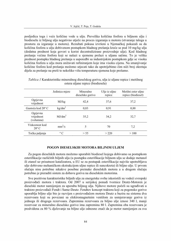
V. Jejčič, T. Poje, T. Godeša
84
posljedica toga i veće količine vode u ulju. Prevelika količina fosfora u biljnom ulju i biodieselu iz biljnog ulja negativno utječe na proces izgaranja u motoru (stvaranje taloga u prostoru za izgaranje u motoru). Rezultati pokusa izvršeni u Njemačkoj pokazali su da količina fosfora u ulju dobivenom postupkom hladnog prešanja kreće se pod 10 mg/kg ulja (dodatna prednost koja govori u korist decentralizirane proizvodnje ulja). Kod hladnog prešanja većina fosfora koji se nalazi u sjemenu prelazi u uljanu sačmu. To je velika prednost postupka hladnog prešanja u usporedbi sa industrijskim postupkom gdje se visoka količina fosfora u ulju mora snižavati rafiniranjem koje ima visoku cijenu. Na smanjivanje količine fosfora kod prešanja možemo utjecati tako da upotrijebimo čim niži broj okretaja dijela za prešanje na preši te nekoliko višu temperaturu sjemena koje prešamo.
Tablica 1 Karakteristike mineralnog dieselskog goriva, ulja iz uljane repice i metilnog estera uljane repice (biodiesela)
Jedinica mjere Mineralno dieselsko gorivo
Ulje iz uljne repice
Metilni ester uljne repice (biodiesel)
Ogrjevnavrijednost MJ/kg 42,4 37,6 37,2
Gustoća kod 20º C kg/dm3 0,83 0,91 0,88
Ogrjevnavrijednost(volumna)
MJ/dm3 35,2 34,2 32,7
Viskoznost kod 20º C mm2/s 5 70 7,2
Točka paljenja º C > 55 > 220 > 100
POGON DIESELSKIH MOTORA BILJNIM ULJEM
Za pogon dieselskih motora možemo uporabiti biodiesel kojega dobivamo sa postupkom esterifikacije različitih biljnih ulja (u postupku esterifikacije biljnom ulju se dodaje metanol ili etanol uz prisutnost katalizatora, u EU se za postupak esterifikacije najviše upotrebljava ulje dobiveno mehaničkom ekstrakcijom uljne repice ili suncokreta) ili biljno ulje. U prvom slučaju nisu potrebne nikakve posebne preinake dieselskih motora a u drugom slučajupotrebno je preraditi sistem za dobavu goriva na dieselskim motorima.
Sve pozitivne karakteristike biljnih ulja za energetske svrhe iskoristili su vodeći evropski proizvođači motora i traktora. Od 2007 u serijskoj ponudi tvornice Deutz-Motoren je dieselski motor namijenjen za uporabu biljnog ulja. Njihove motore počeli su ugrađivati u traktore proizvođači Fendt i Same-Deutz. Fendtov koncept traktora koji za pogonsko gorivo uporablja biljno ulje bio je razvijen s proizvođačem motora Deutz a bazira na sistemu dva rezervoara koji su povezani sa elektromagnetnim ventilom za usmjeravanje goriva iz jednoga ili drugoga rezervoara. Zapremina rezervoara za biljno ulje iznosi 340 l, manji rezervoar za mineralno dieselsko gorivo ima zapreminu 80 l. Zapremina oba rezervoara je predviđena za 80 % djelovanje na biljno ulje odnosno znači da je motor namijenjen za sva
Mogućnost upotrebe biljnog ulja za pogon traktora i drugih vozila
85
vozila koja najviše vremena djeluju sa visokim opterećenjem motora. Motor se prvo pokrene dieselskim gorivom i zagrije na radnu temperaturu. Automatski preklop na ulje nastupi kada je ulje pred grijano na 70 ºC pomoću zagrijane vode iz motornog hladnjaka ili kad izlazna snaga motora postigne 25 % maksimalnog opterećenja motora za više od 30 sekundi. Kada spomenuti uvjeti nisu postignuti sistem automatsko preklopi na mineralno dieselsko gorivo. Vodovi i ventil kroz koje je protjecalo biljno ulje pročiste se mineralnim dieselskim gorivom. Taj postupak traje nekoliko sekundi te spriječi ulazak biljnog ulja u mineralno dieselsko gorivo. Kada uporabnik gasi motor mora preklopiti ručno na mineralno dieselsko gorivo (postoji mogućnost da to izvrši i automatski sistem kod gašenja motora. Uporabnik može na terminalu u svakom trenutku vidjeti koje gorivo je u trenutnoj upotrebi.
Za stacionarne svrhe MAN (4) je razvio sisteme sa dieselskim motorom i električnimgeneratorom namijenjene za kogeneraciju električne i toplinske energije iz biljnih ulja, otpadnih jestivih ulja i životinjskih masti. Nekoliko velikih sistema za kogeneraciju električne i toplotne energije već radi u Belgiji i Njemačkoj a u planu su i nova postrojenja. Npr. jedan sistem, koji radi ima nazivnu električnu snagu 85 MW a u pripremi su i većisistemi. MAN zagovara i upotrebu velikih dieselskih motora na biljno ulje, koji su namijenjeni za pogon lokomotiva i brodova. Pored MAN-a na tom području aktivno je i poduzeće SISU koje ima stacionarne aplikacije a u pripremi su i traktori Valmet koji će biti opremljeni sa SISU motorima koji koriste biljno ulje. SISU isto tako proučava mogućnostrazvoja »hibridnog« motora koji bi mogao raditi na mineralno dieselesko gorivo, biodiesel, biljno ulje te bioetanol. U Sloveniji se je pojavila domaća Agromehanika sa traktorima snage od 35 – 50 KM na biljno ulje a postoji i desetak automobila koje su pojedinci preradili tako da mogu raditi na biljno ulje.
POGON DRUGIH MOTORA I STROJEVA
Biljno ulje može se upotrijebiti i za pogon različitih varijanti Stirlingovih motora. U tom slučaju gorivo kontinuirano izgara u posebnom gorioniku izvan motora. Stirlingov motor se upotrebljava u stacionarnim jedinicama za kogeneraciju električne i toplotne energije. Manje je osjetljiv na kvalitetu goriva zbog neprekidnog vanjskog izgaranja goriva (gorivo slično izgara kao gorivo u plinskim turbinama). Od 20 – 80 % suviška zraka u mješavini i neprekidno izgaranje bez hlađenja plamena osiguravaju skoro potpuno izgaranje goriva. U ispušnom plinu je vrlo malo dima a zagađivanje ispušnim plinovima je minimalno. Potrošnja goriva je ekonomična i može se usporediti sa dieselskim motorima sa direktnim uštrcavanjem goriva kod istih brojeva okretaja motora. Mogu se upotrijebiti najrazličitijevrste goriva jer nemaju posebnih zahtjeva glede cetanskog ili oktanskog broja (zato je biljno ulje vrlo značajan energent za Stirling motore). Motor nije bučan tako da prigušivačnije potreban, prouzrokuje samo 25 % buke motora sa kompresijskim paljenjem. Ventili i mehanizam za upravljanje ventila nisu potrebni što znači još manji nivo buke. Iskorištenje je barem takovo kao kod dieselskih motora.
Pokusi se vrše i sa posebnim mikroturbinama (npr. američka turbina Capstone C 30 snage 30 kW). Mikroturbine imaju niže emisije ispušnih plinova, niže akustičke emisije, dalji interval rada, lakšu integraciju u sisteme grijanja zbog konstantnog nivoa temperature. Pošto nemaju dijelova, koji se taru (npr. klipovi kod motora sa unutrašnjim izgaranjem) djeluje turbina skoro bez trenja. Rade jednakomjerno bez trešnje, mogu upotrebljavati
V. Jejčič, T. Poje, T. Godeša
86
najrazličitije vrste goriva, u ispušnim plinovima nema štetnih supstanci tako da je zagađivanje okoline minimalno a intervali potrebni za održavanje vrlo su dugački. Mikro turbine su vrlo prikladne i za područja gdje je potrebno očuvati podzemne vode jer mikroturbina Capstone C 30 ima posebne ležajeve koji ne trebaju podmazivanja te hlađenjaulja a gorivo je bio razgradljivo. Mogu se uporabiti i za osjetljivo direktno sušenje npr. različitih sjemena zbog neotrovnih ispušnih plinova.
Gorionici na biljno ulje namijenjeni za sušenje poljodjelskih proizvoda, pripremu sanitarne vode, grijanje itn., opremljeni su posebnim dijelom za pred grijanje ulja zbog smanjivanja njegove viskoznosti. Dovodne cijevi imaju nešto veći promjer što značimogućnost većeg protoka ulja koje je više viskozno.
KAKAV MORA BITI DIESELSKI MOTOR ZA POGON NA BILJNO ULJE
Neki korisnici kao i znanstvenici probali su po uzoru samoga Diesela upotrebljavati biljno ulje direktno na motorima koji nisu bili prilagođeni za to gorivo. Na starijim izvedbama dieselskih motora posebno onima sa indirektnim uštrcavanjem goriva (motori sa pretkomorom) i linijskim klipnim izvedbama visokotlačnih crpki za gorivo, u početnim fazama upotrebe nisu opazili nekih posebnih problema. Međutim nakon duže upotrebe takvih motora počeli su se pojavljivati veći problemi. Rezultati istraživanja su pokazali da su i najjednostavnije i robusne izvedbe spomenutih motora otkazale negdje iza 500 sati rada. Problemi, koji bili evidentirani odnosili su se na: začepljivanje filtra za gorivo, stvaranje obloga u komori za izgaranje, stvaranju obloga na visokotlačnim brizgaljkama, oštećenim klipnim prstenima itd. Postavilo se je pitanje zašto je do toga došlo? Odgovor leži u konstrukciji današnjih dieselskih motora te samom gorivu. Razvoj suvremenih dieselskih motora bio je usmjeren zbog odlične dostupnosti mineralnoga dieselskog goriva do sada logično u smjer tih goriva. Biljna ulja imaju karakteristike izgaranja vrlo sličnemineralnom dieselskom gorivu ali njihova viskoznost je previsoka za suvremene visokotlačne crpke za gorivo i ostale elemente u sistemu za dobavu goriva. Visoka viskoznost prouzrokuje začepljivanje vodova za gorivo, filtra i visokotlačnih brizgaljki. Istraživanja su pokazala da visoka viskoznost rezultira u nepotpunoj atomizaciji (raspršivanju kapljica goriva) biljnog ulja a posljedica toga je sprječavanje kompletnog izgaranja većih kapljica goriva i nastajanje taloga iz ugljika. Iz toga proizlazi da se biljna ulja ne mogu upotrebljavati direktno u dieselskim motorima. Za smanjivanje viskoznosti biljnog ulja razvijene su tri metode: transesterifikacija ulja (komercijalno ime biodiesel), miješanje ulja sa mineralnim dieselskim gorivom te zagrijavanje. Prve dvije metode su zahtjevnije zato se je kao najprimjernija pokazala zadnja metoda. Pored svega nabrojenoga istraživanja su pokazala da ima biljno ulje dalje zakašnjenje početka izgaranja i sporije izgaranje posebno kod nižih opterećenja motora a to rezultira u kasnijem izgaranju i kasnijem taktu ekspanzije motora (podešavanje vremena uštrcavanja goriva rješava u najvećoj mjeri te probleme).
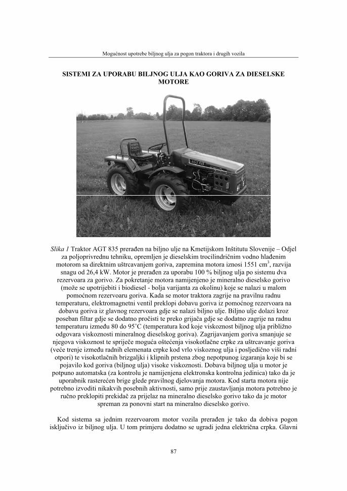
Mogućnost upotrebe biljnog ulja za pogon traktora i drugih vozila
87
SISTEMI ZA UPORABU BILJNOG ULJA KAO GORIVA ZA DIESELSKE MOTORE
Slika 1 Traktor AGT 835 prerađen na biljno ulje na Kmetijskom Inštitutu Slovenije – Odjel za poljoprivrednu tehniku, opremljen je dieselskim trocilindričnim vodno hlađenim
motorom sa direktnim uštrcavanjem goriva, zapremina motora iznosi 1551 cm3, razvija snagu od 26,4 kW. Motor je prerađen za uporabu 100 % biljnog ulja po sistemu dva
rezervoara za gorivo. Za pokretanje motora namijenjeno je mineralno dieselsko gorivo (može se upotrijebiti i biodiesel - bolja varijanta za okolinu) koje se nalazi u malom
pomoćnom rezervoaru goriva. Kada se motor traktora zagrije na pravilnu radnu temperaturu, elektromagnetni ventil preklopi dobavu goriva iz pomoćnog rezervoara na dobavu goriva iz glavnog rezervoara gdje se nalazi biljno ulje. Biljno ulje dolazi kroz
poseban filtar gdje se dodatno pročisti te preko grijača gdje se dodatno zagrije na radnu temperaturu između 80 do 95˚C (temperatura kod koje viskoznost biljnog ulja približno odgovara viskoznosti mineralnog dieselskog goriva). Zagrijavanjem goriva smanjuje se
njegova viskoznost te spriječe moguća oštećenja visokotlačne crpke za uštrcavanje goriva (veće trenje između radnih elemenata crpke kod vrlo viskoznog ulja i posljedično viši radni
otpori) te visokotlačnih brizgaljki i klipnih prstena zbog nepotpunog izgaranja koje bi se pojavilo kod goriva (biljnog ulja) visoke viskoznosti. Dobava biljnog ulja u motor je
potpuno automatska (za kontrolu je namijenjena elektronska kontrolna jedinica) tako da je uporabnik rasterećen brige glede pravilnog djelovanja motora. Kod starta motora nije
potrebno izvoditi nikakvih posebnih aktivnosti, samo prije zaustavljanja motora potrebno je ručno preklopiti prekidač za prijelaz na mineralno dieselsko gorivo tako da je motor
spreman za ponovni start na mineralno dieselsko gorivo.
Kod sistema sa jednim rezervoarom motor vozila prerađen je tako da dobiva pogon isključivo iz biljnog ulja. U tom primjeru dodatno se ugradi jedna električna crpka. Glavni
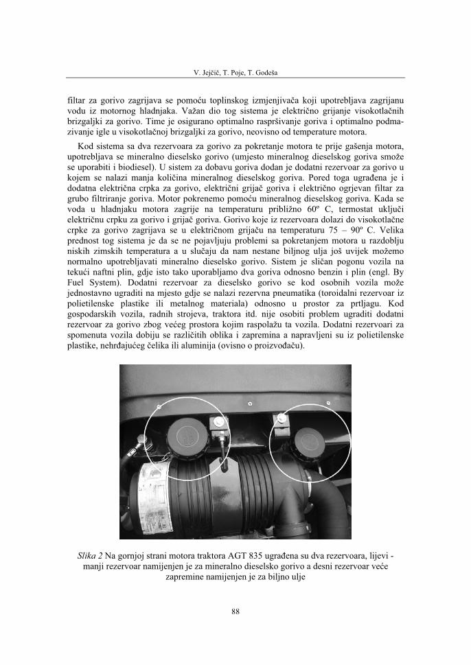
V. Jejčič, T. Poje, T. Godeša
88
filtar za gorivo zagrijava se pomoću toplinskog izmjenjivača koji upotrebljava zagrijanu vodu iz motornog hladnjaka. Važan dio tog sistema je električno grijanje visokotlačnihbrizgaljki za gorivo. Time je osigurano optimalno raspršivanje goriva i optimalno podma-zivanje igle u visokotlačnoj brizgaljki za gorivo, neovisno od temperature motora.
Kod sistema sa dva rezervoara za gorivo za pokretanje motora te prije gašenja motora, upotrebljava se mineralno dieselsko gorivo (umjesto mineralnog dieselskog goriva smože se uporabiti i biodiesel). U sistem za dobavu goriva dodan je dodatni rezervoar za gorivo u kojem se nalazi manja količina mineralnog dieselskog goriva. Pored toga ugrađena je i dodatna električna crpka za gorivo, električni grijač goriva i električno ogrjevan filtar za grubo filtriranje goriva. Motor pokrenemo pomoću mineralnog dieselskog goriva. Kada se voda u hladnjaku motora zagrije na temperaturu približno 60º C, termostat uključielektričnu crpku za gorivo i grijač goriva. Gorivo koje iz rezervoara dolazi do visokotlačnecrpke za gorivo zagrijava se u električnom grijaču na temperaturu 75 – 90º C. Velika prednost tog sistema je da se ne pojavljuju problemi sa pokretanjem motora u razdoblju niskih zimskih temperatura a u slučaju da nam nestane biljnog ulja još uvijek možemo normalno upotrebljavati mineralno dieselsko gorivo. Sistem je sličan pogonu vozila na tekući naftni plin, gdje isto tako uporabljamo dva goriva odnosno benzin i plin (engl. By Fuel System). Dodatni rezervoar za dieselsko gorivo se kod osobnih vozila može jednostavno ugraditi na mjesto gdje se nalazi rezervna pneumatika (toroidalni rezervoar iz polietilenske plastike ili metalnog materiala) odnosno u prostor za prtljagu. Kod gospodarskih vozila, radnih strojeva, traktora itd. nije osobiti problem ugraditi dodatni rezervoar za gorivo zbog većeg prostora kojim raspolažu ta vozila. Dodatni rezervoari za spomenuta vozila dobiju se različitih oblika i zapremina a napravljeni su iz polietilenske plastike, nehrđajućeg čelika ili aluminija (ovisno o proizvođaču).
Slika 2 Na gornjoj strani motora traktora AGT 835 ugrađena su dva rezervoara, lijevi - manji rezervoar namijenjen je za mineralno dieselsko gorivo a desni rezervoar veće
zapremine namijenjen je za biljno ulje
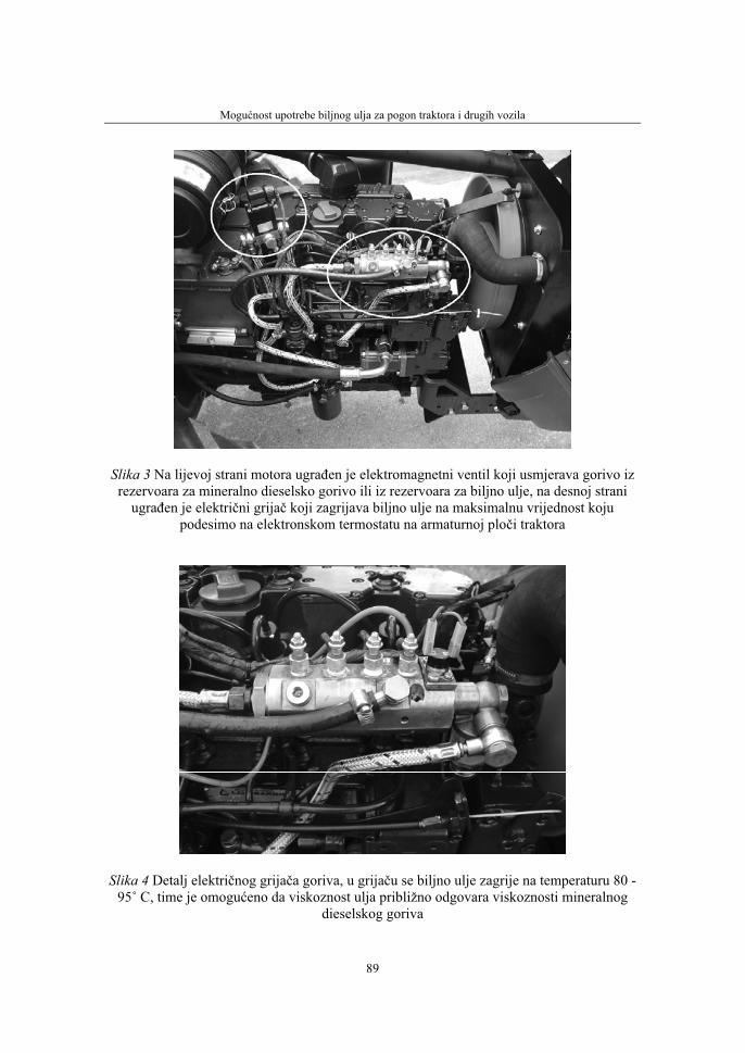
Mogućnost upotrebe biljnog ulja za pogon traktora i drugih vozila
89
Slika 3 Na lijevoj strani motora ugrađen je elektromagnetni ventil koji usmjerava gorivo iz rezervoara za mineralno dieselsko gorivo ili iz rezervoara za biljno ulje, na desnoj strani
ugrađen je električni grijač koji zagrijava biljno ulje na maksimalnu vrijednost koju podesimo na elektronskom termostatu na armaturnoj ploči traktora
Slika 4 Detalj električnog grijača goriva, u grijaču se biljno ulje zagrije na temperaturu 80 - 95˚ C, time je omogućeno da viskoznost ulja približno odgovara viskoznosti mineralnog
dieselskog goriva

V. Jejčič, T. Poje, T. Godeša
90
ZAKLJUČAK
Energetska uporaba biljnog ulja u motorima (dieselski motori na traktorima, građevin-skim i radnim strojevima, transportnim i komunalnim vozilima, kogeneratorskim jedinica-ma za proizvodnju električne i toplotne energije, brodovima, lokomotivama itn.) je aktualna opcija za fosilna goriva odnosno mineralno dieselsko gorivo.
Za pogon prerađenih dieselskih motora pored sirovih i rafiniranih biljnih ulja mogu se upotrijebiti i otpadna jestiva ulja i životinjske masti. Biljna ulja imaju karakteristike izgaranja vrlo slične mineralnom dieselskom gorivu ali njihova viskoznost je previsoka za suvremene visokotlačne crpke za gorivo i ostale elemente u sistemu za dobavu goriva. Visoka viskoznost prouzrokuje začepljivanje vodova za gorivo, filtra i visokotlačnihbrizgaljki. Više istraživača je ustanovilo da visoka viskoznost rezultira u nepotpunoj atomizaciji (raspršivanju kapljica goriva) biljnog ulja a posljedica toga je sprječavanjekompletnog izgaranja većih kapljica goriva i nastajanje taloga iz ugljika. Iz toga proizlazi da se biljna ulja ne mogu upotrebljavati direktno u dieselskim motorima, motore je potrebno prilagoditi. Motori se prilagođuju na dva načina. Kod sistema sa jednim rezervoarom motor traktora odnosno vozila je prerađen tako da dobiva pogon isključivo iz biljnog ulja. Taj sistem je zahtjevan za ugradnju zato je danas najviše u uporabi sistem sa dva rezervoara. Kod sistema sa dva rezervoara za gorivo za pokretanje motora te prije gašenja motora upotrebljava se mineralno dieselsko gorivo (umjesto mineralnog dieselskog goriva smože se uporabiti i biodiesel).U Evropi je već nekoliko većih proizvođača motora i traktora ponudilo tržištu izvedbe dieselskih motora koji su prerađeni tako da mogu upotrebljavati za pogon biljno ulje. U budućnosti važnu ulogu imati će i Stirlingov motor te turbine na biljno ulje. Velika prednost je da kod spomenutih strojeva kvaliteta goriva – biljnog ulja nije toliko važna kao kod dieselskih motora.
LITERATURA
1. Mittelbach, M., Remschmidt, C.: Biodiesel, The comprehensive handbook, Graz 2004, str. 254 – 255
2. Riva, G., Sissot F.: CIGR Handbook of Agricultural Engineering, Volume V - Energy & Biomass Engineering, pog. 3.1.2, Biomass Resources, ASAE, St. Joseph MI SAD 1999, s. 164 – 201
3. Biodiesel & Co.: Extracts from the UFOP report 2006/2007, Union zur Förderung von Oel und Proteinpflanzen e.v., Berlin 2007
4. MAN B&W Diesel AG, Bio fuels for Diesel Engines, 2004
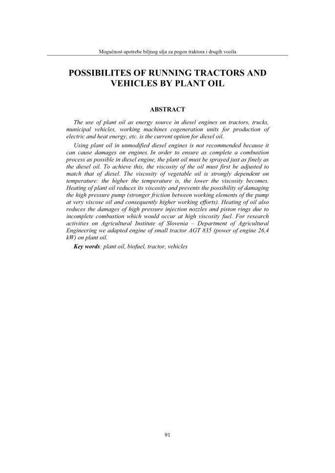
Mogućnost upotrebe biljnog ulja za pogon traktora i drugih vozila
91
POSSIBILITES OF RUNNING TRACTORS AND VEHICLES BY PLANT OIL
ABSTRACT
The use of plant oil as energy source in diesel engines on tractors, trucks, municipal vehicles, working machines cogeneration units for production of electric and heat energy, etc. is the current option for diesel oil.
Using plant oil in unmodified diesel engines is not recommended because it can cause damages on engines. In order to ensure as complete a combustion process as possible in diesel engine, the plant oil must be sprayed just as finely as the diesel oil. To achieve this, the viscosity of the oil must first be adjusted to match that of diesel. The viscosity of vegetable oil is strongly dependent on temperature: the higher the temperature is, the lower the viscosity becomes. Heating of plant oil reduces its viscosity and prevents the possibility of damaging the high pressure pump (stronger friction between working elements of the pump at very viscose oil and consequently higher working efforts). Heating of oil also reduces the damages of high pressure injection nozzles and piston rings due to incomplete combustion which would occur at high viscosity fuel. For research activities on Agricultural Institute of Slovenia – Department of Agricultural Engineering we adapted engine of small tractor AGT 835 (power of engine 26,4 kW) on plant oil.
Key words: plant oil, biofuel, tractor, vehicles

36. Symposium "Actual Tasks on Agricultural Engineering", Opatija, Croatia, 2008.
93
36.
SIMPOZIJAKTUALNI ZADACIMEHANIZACIJE POLJOPRIVREDE
UDC631.372:629.11.012.7
Stručni radExpert paper
TIRE TRACTION MODELS – COMPARATIVE ANALYSIS AND VALIDATION
1ROSCA RADU, 1TENU IOAN, 1CARLESCU PETRU, 2RAKOSI EDWARD,2MANOLACHE GHEORGHE
1University of Agricultural Sciences Iasi, Romania; 2Technical University "Gh. Asachi" Iasi, Romania.
SUMMARY
The paper presents a comparative analysis of different tire traction models. The model developed by the authors, starting from a Bekker type pressure-sinkage relationship, was compared with the Wismer&Luth, the MacLaurin and the Gee-Clough models, in terms of specific net traction coefficient. Traction force and traction efficiency were also calculated.
In order to validate the theoretical results, field tests were developed, using the U-650 tractor, equipped with the P2V plow. Variation of plow width and depth allowed different traction forces and drive wheel slips to be obtained. During the experiments, drive wheel slip and net traction force were measured directly, for wheel slip up to 30%.
The results predicted by the proposed model fit well the experimental results; the average differences between calculated and measured data did not exceed 0.25…0.4 kN for the traction force and 4…5% for the traction efficiency.
Applying the original Gee-Clough and Wismer&Luth equations leads to significant differences compared to experimental data over the entire range of wheel slip values (0 to 100%). When the MacLaurin wheel numeric is used in the Gee-Clough and Wismer&Luth equations, the specific net traction coefficient given by the Wismer&Luth model matches the experimental data and the values given by the proposed model when drive wheel slip does not exceed 28…29%.
Keywords: tire traction, wheel slip, traction models
INTRODUCTION
Accurate prediction of the traction performance of a tractor wheel depends largely on the model of the tire-terrain interaction. Some models use analytical approaches (commercial
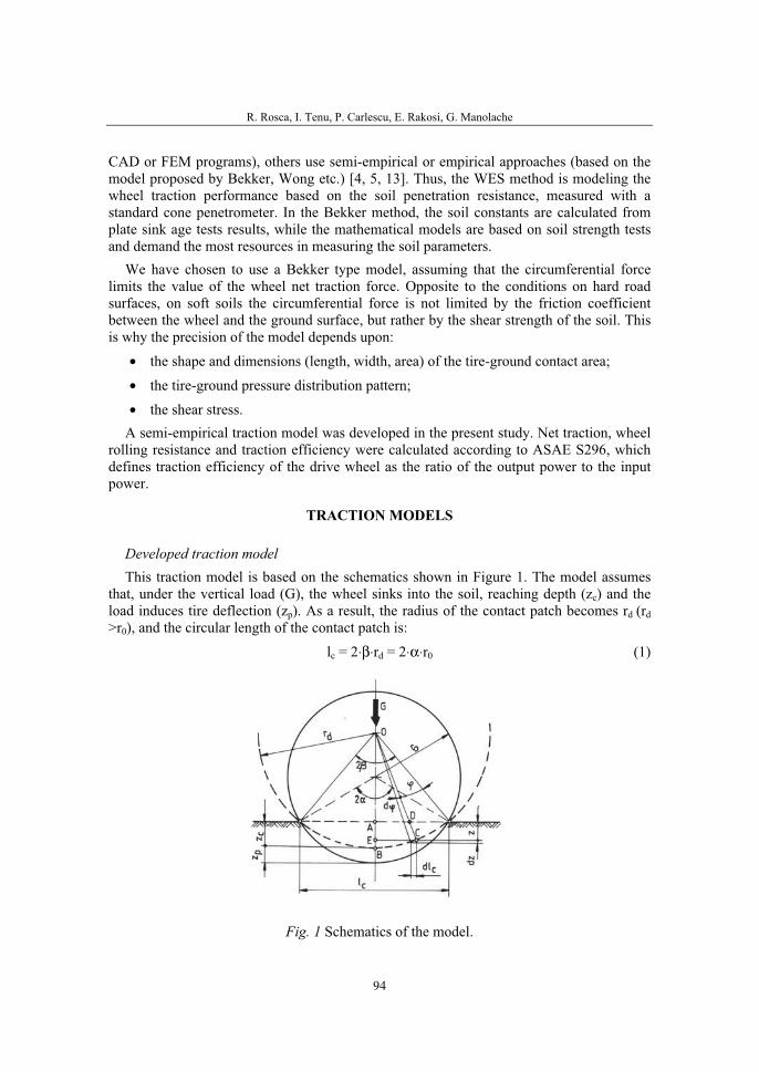
R. Rosca, I. Tenu, P. Carlescu, E. Rakosi, G. Manolache
94
CAD or FEM programs), others use semi-empirical or empirical approaches (based on the model proposed by Bekker, Wong etc.) [4, 5, 13]. Thus, the WES method is modeling the wheel traction performance based on the soil penetration resistance, measured with a standard cone penetrometer. In the Bekker method, the soil constants are calculated from plate sink age tests results, while the mathematical models are based on soil strength tests and demand the most resources in measuring the soil parameters.
We have chosen to use a Bekker type model, assuming that the circumferential force limits the value of the wheel net traction force. Opposite to the conditions on hard road surfaces, on soft soils the circumferential force is not limited by the friction coefficient between the wheel and the ground surface, but rather by the shear strength of the soil. This is why the precision of the model depends upon:
• the shape and dimensions (length, width, area) of the tire-ground contact area;
• the tire-ground pressure distribution pattern;
• the shear stress. A semi-empirical traction model was developed in the present study. Net traction, wheel
rolling resistance and traction efficiency were calculated according to ASAE S296, which defines traction efficiency of the drive wheel as the ratio of the output power to the input power.
TRACTION MODELS
Developed traction model This traction model is based on the schematics shown in Figure 1. The model assumes
that, under the vertical load (G), the wheel sinks into the soil, reaching depth (zc) and the load induces tire deflection (zp). As a result, the radius of the contact patch becomes rd (rd>r0), and the circular length of the contact patch is:
lc = 2⋅β⋅rd = 2⋅α⋅r0 (1)
Fig. 1 Schematics of the model.
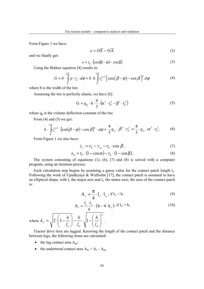
Tire traction models – comparative analysis and validation
95
From Figure 1 we have:
AOEOz −= (2) and we finally get:
( )[ ]β−ϕ−β⋅= coscosrz d (3) Using the Bekker equation [4] results in:
( )2 2
1
0 0
cos cosnn
d dG b p r d b k r dβ β
φ β ϕ β ϕ+= ⋅ ⋅ ⋅ = ⋅ − −⎡ ⎤⎣ ⎦∫ ∫
(4)
where b is the width of the tire. Assuming the tire is perfectly elastic, we have [8]:
( )2d
320
3p rr
34bqG ⋅β−⋅α⋅⋅⋅= (5)
where qp is the volume deflection constant of the tire. From (4) and (5) we get:
( )[ ]∫ +⋅−−⋅⋅ +β
ϕβϕβ2
0
1 coscos drk nnd .
34
34 2
0323 rqrq pdp ⋅⋅⋅=⋅⋅ αβ (6)
From Figure 1 we also have:
βcos00 ⋅−−= rzrz pc , (7)
( ) ( )β−⋅−α−⋅= cos1rcos1rz d0p , (8) The system consisting of equations (1), (6), (7) and (8) is solved with a computer
program, using an iteration process. Each calculation step begins by assuming a guess value for the contact patch length lc.
Following the work of Upadhyaya & Wulfsohn [17], the contact patch is assumed to have an elliptical shape, with lc the major axis and lw the minor axis; the area of the contact patch is:
wct ll4
A ⋅⋅π= , if lw < b, (9)
( )fwc
t k44llA ⋅−π⋅⋅= , if lw = b, (10)
where
2
2 1 1fw w w
b b bkl l l
⎛ ⎞ ⎛ ⎞
= ⋅ − − ⋅ −⎜ ⎟ ⎜ ⎟
⎝ ⎠ ⎝ ⎠
.
Tractor drive tires are lugged. Knowing the length of the contact patch and the distance between lugs, the following items are calculated:
• the lug contact area Apr;
• the undertread contact area Abr = At – Apr.
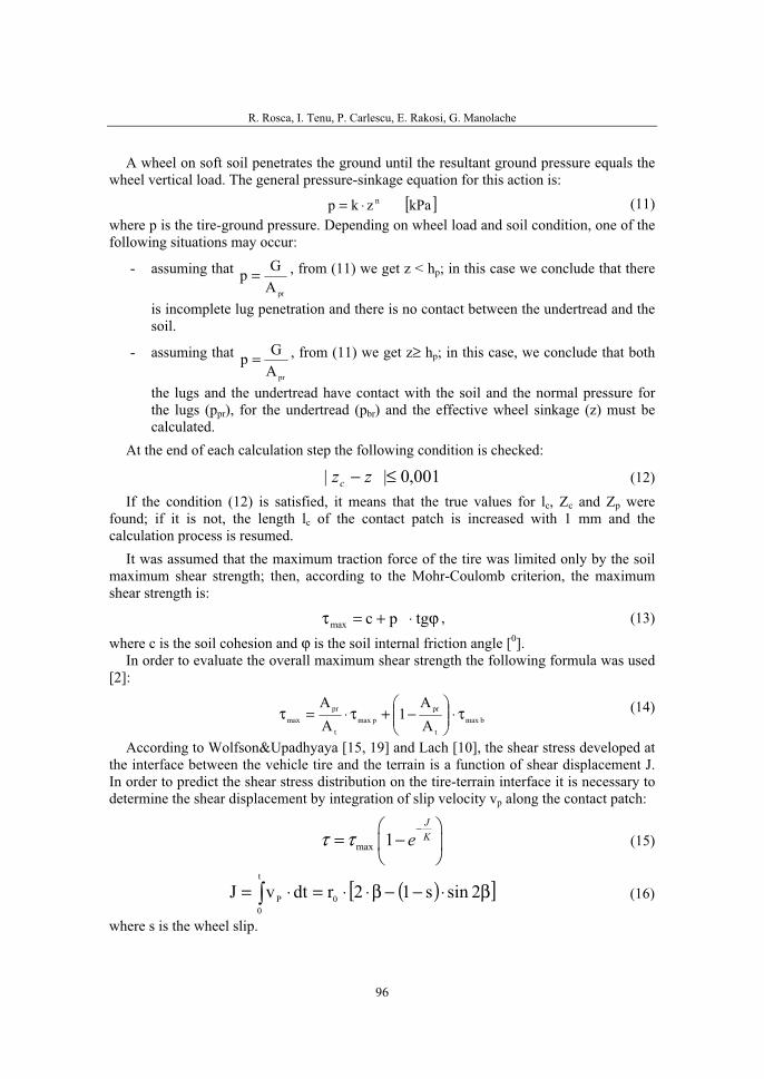
R. Rosca, I. Tenu, P. Carlescu, E. Rakosi, G. Manolache
96
A wheel on soft soil penetrates the ground until the resultant ground pressure equals the wheel vertical load. The general pressure-sinkage equation for this action is:
[ ]kPazkp n⋅= (11)where p is the tire-ground pressure. Depending on wheel load and soil condition, one of the following situations may occur:
- assuming that prA
Gp = , from (11) we get z < hp; in this case we conclude that there
is incomplete lug penetration and there is no contact between the undertread and the soil.
- assuming that prA
Gp = , from (11) we get z≥ hp; in this case, we conclude that both
the lugs and the undertread have contact with the soil and the normal pressure for the lugs (ppr), for the undertread (pbr) and the effective wheel sinkage (z) must be calculated.
At the end of each calculation step the following condition is checked:
001,0|| ≤− zzc (12)If the condition (12) is satisfied, it means that the true values for lc, Zc and Zp were
found; if it is not, the length lc of the contact patch is increased with 1 mm and the calculation process is resumed.
It was assumed that the maximum traction force of the tire was limited only by the soil maximum shear strength; then, according to the Mohr-Coulomb criterion, the maximum shear strength is:
ϕ⋅+=τ tgpcmax , (13)
where c is the soil cohesion and ϕ is the soil internal friction angle [0].In order to evaluate the overall maximum shear strength the following formula was used
[2]:
bmaxt
prpmax
t
prmax A
A1
AA
τ⋅⎟⎟
⎠
⎞
⎜⎜
⎝
⎛
−+τ⋅=τ (14)
According to Wolfson&Upadhyaya [15, 19] and Lach [10], the shear stress developed at the interface between the vehicle tire and the terrain is a function of shear displacement J. In order to predict the shear stress distribution on the tire-terrain interface it is necessary to determine the shear displacement by integration of slip velocity vp along the contact patch:
max 1JKeτ τ
−⎛ ⎞
= −⎜ ⎟
⎝ ⎠
(15)
( )[ ]β⋅−−β⋅⋅=⋅= ∫ 2sins12rdtvJ 0
t
0P (16)
where s is the wheel slip.
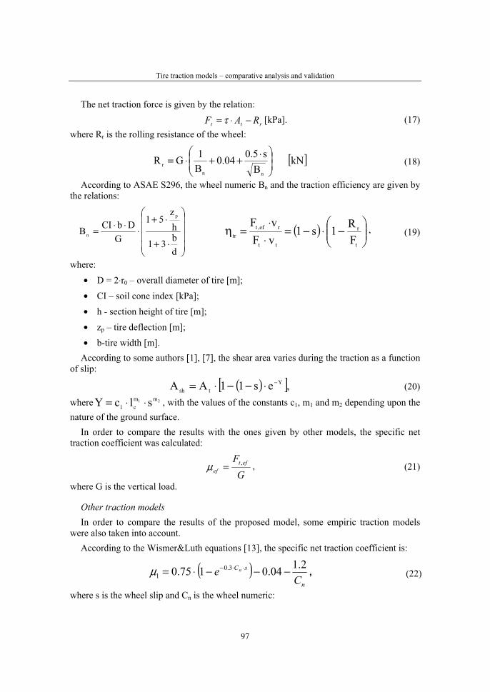
Tire traction models – comparative analysis and validation
97
The net traction force is given by the relation:
rtt RAF −⋅= τ [kPa]. (17) where Rr is the rolling resistance of the wheel:
[ ]kNB
s5.004.0B1GR
nnr
⎟
⎟
⎠
⎞
⎜
⎜
⎝
⎛ ⋅++⋅= (18)
According to ASAE S296, the wheel numeric Bn and the traction efficiency are given by the relations:
⎟
⎟
⎟
⎟
⎠
⎞
⎜
⎜
⎜
⎜
⎝
⎛
⋅+
⋅+⋅⋅⋅=
db31
hz
51
GDbCIB
p
n ( )⎟⎟
⎠
⎞
⎜⎜
⎝
⎛
−⋅−=⋅⋅
=ηt
r
tt
ref,ttr F
R1s1vFvF
, (19)
where:
• D = 2⋅r0 – overall diameter of tire [m];
• CI – soil cone index [kPa];
• h - section height of tire [m];
• zp – tire deflection [m];
• b-tire width [m]. According to some authors [1], [7], the shear area varies during the traction as a function
of slip:
( )[ ],es11AA Ytsh
−⋅−−⋅= (20)
where 21 mmc1 slcY ⋅⋅= , with the values of the constants c1, m1 and m2 depending upon the
nature of the ground surface. In order to compare the results with the ones given by other models, the specific net
traction coefficient was calculated:
GF eft
ef,=μ , (21)
where G is the vertical load.
Other traction models In order to compare the results of the proposed model, some empiric traction models
were also taken into account. According to the Wismer&Luth equations [13], the specific net traction coefficient is:
( )n
sC
Ce n
2.104.0175.0 3.01 −−−⋅= ⋅⋅−μ , (22)
where s is the wheel slip and Cn is the wheel numeric:
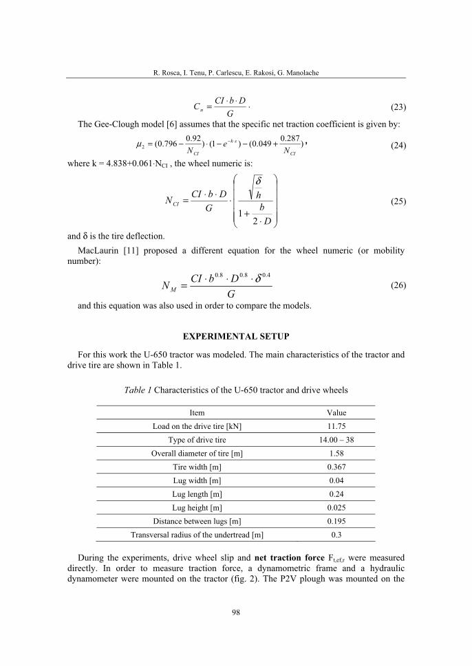
R. Rosca, I. Tenu, P. Carlescu, E. Rakosi, G. Manolache
98
GDbCICn
⋅⋅= . (23)
The Gee-Clough model [6] assumes that the specific net traction coefficient is given by:
)287.0049.0()1()92.0796.0(2CI
sk
CI Ne
N+−−⋅−= ⋅−μ , (24)
where k = 4.838+0.061⋅NCI , the wheel numeric is:
⎟⎟
⎟
⎟
⎟
⎠
⎞
⎜⎜
⎜
⎜
⎜
⎝
⎛
⋅+
⋅⋅⋅=
Db
hG
DbCINCI
21
δ
(25)
and δ is the tire deflection. MacLaurin [11] proposed a different equation for the wheel numeric (or mobility
number):
GDbCIN M
4.08.08.0 δ⋅⋅⋅= (26)
and this equation was also used in order to compare the models.
EXPERIMENTAL SETUP
For this work the U-650 tractor was modeled. The main characteristics of the tractor and drive tire are shown in Table 1.
Table 1 Characteristics of the U-650 tractor and drive wheels
Item Value
Load on the drive tire [kN] 11.75
Type of drive tire 14.00 – 38
Overall diameter of tire [m] 1.58
Tire width [m] 0.367
Lug width [m] 0.04
Lug length [m] 0.24
Lug height [m] 0.025
Distance between lugs [m] 0.195
Transversal radius of the undertread [m] 0.3
During the experiments, drive wheel slip and net traction force Ft,ef,r were measured directly. In order to measure traction force, a dynamometric frame and a hydraulic dynamometer were mounted on the tractor (fig. 2). The P2V plough was mounted on the

Tire traction models – comparative analysis and validation
99
dynamometric frame (7). The gross traction force and traction efficiency (ηtr,e) were determined assuming that Ft = Ft,ef,r + Rr, with a formula derived from ASAE S296 standard:
( ) trr,ef,t
rr,ef,t
tt
rr,ef,te.tr vRF
vFvFvF
⋅+⋅
=⋅
⋅=η . (25)
Fig. 2 Dynamometric frame mount; 1, 3, 4-lifting arms; 2-hydraulic lifting cylinder;5-frame arms; 6-dynamometric frame; 7-hydraulic cylinder of the dynamometer
Variation of plow width and depth allowed different traction forces and drive wheel slips to be obtained. During the experiments, drive wheel slip and net traction force Ft,ef,r were measured directly. The experimental data were collected during field tests of the U650+P2V ploughing unit (aiming to evaluate the quality of the plough’s working process, fig. 3); during these tests drive wheel slip was not allowed to exceed 30% because such high values must be avoided during the ploughing process. Soil characteristics of the test field are shown in Table 2.
width: 50 cm
400
500
600
700
800
900
1000
1100
2 3 4 5 6 7 8 9 10
km/h
daN
depth: 20 cm
depth: 25 cm
depth: 30 cm
width: 60 cm
400
500
600
700
800
900
1000
1100
2 3 4 5 6 7 8
km/h
daN
depth: 20 cm
depth: 25 cm
depth: 30 cm
Fig. 3 Traction resistance during ploughing

R. Rosca, I. Tenu, P. Carlescu, E. Rakosi, G. Manolache
100
Tire deflection under vertical load was measured under static conditions, in a previous series of experiments. The vertical axle load, as affected by the plow resistance, was calculated with the formula (see also fig. 4 for notations):
LhFM
YY xxrs
⋅+−= 22 , (26)
where Y2s is the static axle load and Mr is the wheel torque; the following particular conditions were considered: horizontal plane (α=0), constant speed of the tractor (v=ct.), plough weight supported by the ground wheel.
Table 2 Characteristics of the test soil
Item Value
Soil deformation modulus, K [m] 0.05
k 55 Coefficients for the sinkage equation
n 1.3
Soil cohesion, c [kPa] 25
Angle of internal friction, ϕ [0] 32
Cone penetrometer index, CI [kPa] 970
Fig. 4 Effect of ploughing resistance over the axle load
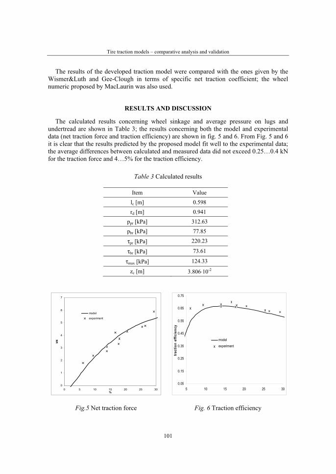
Tire traction models – comparative analysis and validation
101
The results of the developed traction model were compared with the ones given by the Wismer&Luth and Gee-Clough in terms of specific net traction coefficient; the wheel numeric proposed by MacLaurin was also used.
RESULTS AND DISCUSSION
The calculated results concerning wheel sinkage and average pressure on lugs and undertread are shown in Table 3; the results concerning both the model and experimental data (net traction force and traction efficiency) are shown in fig. 5 and 6. From Fig. 5 and 6 it is clear that the results predicted by the proposed model fit well to the experimental data; the average differences between calculated and measured data did not exceed 0.25…0.4 kN for the traction force and 4…5% for the traction efficiency.
Table 3 Calculated results
Item Value
lc [m] 0.598
rd [m] 0.941
ppr [kPa] 312.63
pbr [kPa] 77.85
τpr [kPa] 220.23
τbr [kPa] 73.61
τmax [kPa] 124.33
zc [m] 3.806⋅10-2
0
1
2
3
4
5
6
7
0 5 10 15 20 25 30%
kN
model
experiment
0.05
0.15
0.25
0.35
0.45
0.55
0.65
0.75
5 10 15 20 25 30
tract
ion
effic
ienc
y
model
experiment
Fig.5 Net traction force Fig. 6 Traction efficiency

R. Rosca, I. Tenu, P. Carlescu, E. Rakosi, G. Manolache
102
The maximum traction efficiency is reached when wheel slip is comprised between 10 and 17%; these predictions were confirmed by the experimental data (Fig. 6). Referring to the traction force (Fig. 5), the best fit between model and experimental data is also achieved when wheel slip is within the above mentioned range. Both experimental and calculated data show that the maximum traction efficiency is reached for traction forces between 2.5 and 3.7 kN.
Fig. 7 presents a comparison between the different models mentioned at subtitle 2.2 and the developed traction model.
Applying the original Gee-Clough and Wismer&Luth equations (1 and 2, Fig. 7) lead to significant differences compared to experimental data over the entire range of values for wheel slip (0 to 100%). When the MacLaurin wheel numeric is used in the Gee-Clough and Wismer&Luth equations (instead of the original relations), the specific net traction coefficient given by the Wismer&Luth model matches the experimental data and the values given by the proposed model if drive wheel slip is does not exceed 28…29% (4, Fig. 7).
Because the experimental data were collected during field tests of a ploughing unit, no experimental data was available for drive wheel slip over 30% and no assumption can be made regarding the accuracy of the proposed model when wheel slip exceeds this limit. Nevertheless, traction theory states that specific net traction coefficient increases until it reaches a peak value and then decreases; the proposed model is the only one (among the other models taken into account in this study, including model 4) that displays a similar behavior.
0
0.1
0.2
0.3
0.4
0.5
0.6
0.7
0.8
0 20 40 60 80 100%
modelWismer&LuthGee-CloughexperimentWismer&Luth with NMGee-Clough with NM
1
2, 3 4
5
Fig. 7 Specific net traction coefficient; 1-Wismer&Luth model; 2-Gee-Clough model;3-Gee-Clough model using the Mac Laurin wheel numeric; 4-Wismer&Luth model using
the Mac Laurin wheel numeric; 5-developed model
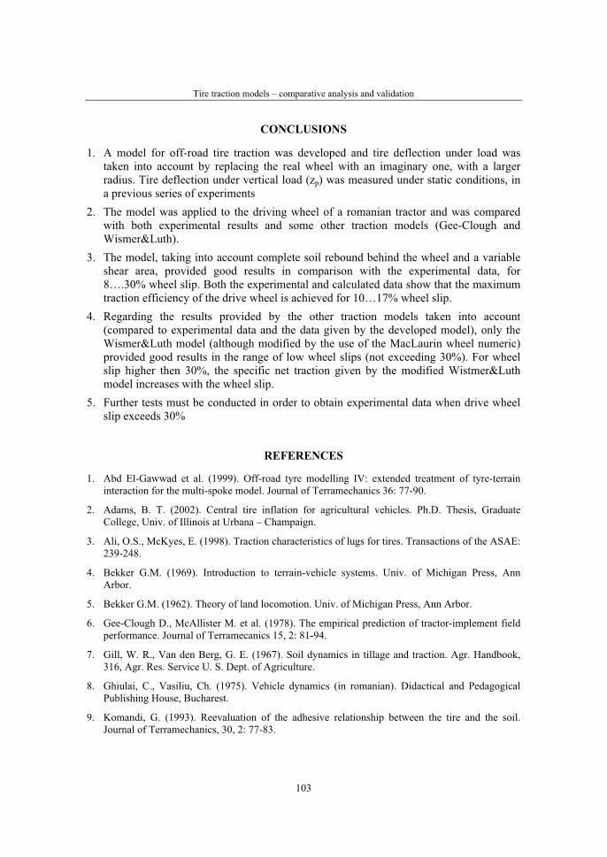
Tire traction models – comparative analysis and validation
103
CONCLUSIONS
1. A model for off-road tire traction was developed and tire deflection under load was taken into account by replacing the real wheel with an imaginary one, with a larger radius. Tire deflection under vertical load (zp) was measured under static conditions, in a previous series of experiments
2. The model was applied to the driving wheel of a romanian tractor and was compared with both experimental results and some other traction models (Gee-Clough and Wismer&Luth).
3. The model, taking into account complete soil rebound behind the wheel and a variable shear area, provided good results in comparison with the experimental data, for 8….30% wheel slip. Both the experimental and calculated data show that the maximum traction efficiency of the drive wheel is achieved for 10…17% wheel slip.
4. Regarding the results provided by the other traction models taken into account (compared to experimental data and the data given by the developed model), only the Wismer&Luth model (although modified by the use of the MacLaurin wheel numeric) provided good results in the range of low wheel slips (not exceeding 30%). For wheel slip higher then 30%, the specific net traction given by the modified Wistmer&Luth model increases with the wheel slip.
5. Further tests must be conducted in order to obtain experimental data when drive wheel slip exceeds 30%
REFERENCES
1. Abd El-Gawwad et al. (1999). Off-road tyre modelling IV: extended treatment of tyre-terrain interaction for the multi-spoke model. Journal of Terramechanics 36: 77-90.
2. Adams, B. T. (2002). Central tire inflation for agricultural vehicles. Ph.D. Thesis, Graduate College, Univ. of Illinois at Urbana – Champaign.
3. Ali, O.S., McKyes, E. (1998). Traction characteristics of lugs for tires. Transactions of the ASAE: 239-248.
4. Bekker G.M. (1969). Introduction to terrain-vehicle systems. Univ. of Michigan Press, Ann Arbor.
5. Bekker G.M. (1962). Theory of land locomotion. Univ. of Michigan Press, Ann Arbor.
6. Gee-Clough D., McAllister M. et al. (1978). The empirical prediction of tractor-implement field performance. Journal of Terramecanics 15, 2: 81-94.
7. Gill, W. R., Van den Berg, G. E. (1967). Soil dynamics in tillage and traction. Agr. Handbook, 316, Agr. Res. Service U. S. Dept. of Agriculture.
8. Ghiulai, C., Vasiliu, Ch. (1975). Vehicle dynamics (in romanian). Didactical and Pedagogical Publishing House, Bucharest.
9. Komandi, G. (1993). Reevaluation of the adhesive relationship between the tire and the soil. Journal of Terramechanics, 30, 2: 77-83.
R. Rosca, I. Tenu, P. Carlescu, E. Rakosi, G. Manolache
104
10. Lach, B. (1996). The influence of tire inflation pressure – a comparison between simulation and experiment. In: Proc. of the 1st East European Conference of the ISTVS, Wroclaw.
11. MacLaurin B. (2007). Comparing the NRMM (VCI), MMP and VLCI traction models. Journal of Terramechanics, 44: 43-51.
12. Rosca, R. Rakosi, E., Manolache, Gh. (2004). Wheel Traction Prediction - A Comparison Between Models and Experimental Data. SAE Technical Paper Series 2004-01-2707.
13. Saarilahti, M. (2002). Development of a protocol for ecoefficient wood harvesting on sensitive sites – Soil interaction model. Contract QLK5 – 1999 – 00991, pp.15-30, Univ. of Helsinki, Dept. of forest resource management.
14. Schmid, I. C. (1995). Interaction of the vehicle terrain results from 10 years research at IK. Journal of Terramechanics, 32, 1: 3-27.
15. Upadhyaya, S.K., Dvoralai, Wulfson, Jubbal, G. (1989). Traction prediction equations for radial ply tyres. Journal of Terramechanics, 26, 2: 149-175.
16. Upadhyaya, S.K., Dvoralai, Wulfson, Jubbal, G. (1990). Review of traction prediction equations. ASAE Paper 90 – 1573, St. Joseph, Michigan.
17. Upadhyaya, S.K., Dvoralai, Wulfson (1990). Relationship between tire deflection characteristics and 2-D tire contact area. Transactions of the ASAE, 33,1: 25-30.
18. Wolf, D., Shmulevich, I., Mussel, U. (1996). Wheel traction prediction on hard soil. Transactions of the ASAE, 39, 4: 1275-1283.
19. Wulfson Dvoralai, Upadhyaya, S.K. (1992). Prediction of traction and soil compaction using three-dimensional soil-tyre contact profile. Journal of Terramechanics, 29, 6: 541-564.
***, ASAE D497.7 (1999). Agricultural Machinery Management Data. St. Joseph, Michigan, U.S.A.
36. Symposium "Actual Tasks on Agricultural Engineering", Opatija, Croatia, 2008.
105
36.
SIMPOZIJAKTUALNI ZADACIMEHANIZACIJE POLJOPRIVREDE
UDK631.372:656
Tehnička bilješkaTechnical note
POLJOPRIVREDNI TRAKTORI KAO ČIMBENIKSIGURNOSTI PROMETA
VLADO JURIĆ1, TOMISLAV JURIĆ2, DARKO KIŠ2, RUDOLF EMERT 2,IVAN PLAŠČAK2
1 Policijska postaja Vinkovci, Bana Jelačića 4, 32100 Vinkovci 2 Poljoprivredni fakultet u Osijeku, Trg Svetog Trojstva 3, 31000 Osijek
SAŽETAK
Poljoprivredni traktori kao bitni čimbenici poljoprivredne proizvodnje, poglavito tržišno orijentirane, svojom tehničkom ispravnošću značajno utječu na sigurnost cestovnog prometa u kojem sudjeluju kao prometala. Redovite i ispravne mjere servisno-preventivnog održavanja poljoprivrednih traktora uz povećanje uporabne pouzdanosti i vijeka uporabe poljoprivrednog traktora zna-čajno podižu razinu sigurnosti prometa. U cilju utvrđivanja tehničke ispravnosti traktora koji sudjeluju u javnom prometu te koji pristupaju tehničkom pregledu učinjeno je istraživanje na području Vukovarsko-srijemske županije glede utvrđivanja istog. U svrhu utvrđivanja broja registriranih traktora na obiteljskim gospodarstvima i starosti traktora obavljena je anketa na 107 obiteljskih gospodarstava ove županije. Rezultati istraživanja ukazuju da je na obiteljskim gospodarstvima još znatno visok broj traktora koji nisu registrirani (53,3 %). Značajan je i postotni udio neispravnih traktora (23,33 %) koji sudjeluju u javnom prometu kao i neispravnih traktora (15 %) koji su pristupili tehničkompregledu. U posljednjih deset godina smanjuje se broj nesreća u kojima sudjeluju poljoprivredni traktori.
Ključne riječi: traktor, sigurnost u prometu, servisno-preventivno održavanje
UVOD
Uporaba visoko sofisticiranih poljoprivrednih strojeva stvara preduvjete tržišno konku-rentnoj poljoprivrednoj proizvodnji. Uvjetovana optimalnim agrotehničkim rokovima za pojedine poljoprivredne kulture, sezonskim karakterom uporabe, gibanjem po proizvodnim površinama, ali i javnim prometnicama, uporaba poljoprivrednih strojeva značajno ovisi o servisno-preventivnom održavanju. Budući da poljoprivredni traktori sudjeluju kao prometala u javnom prometu od iznimne je važnosti njihova tehnička ispravnost. Stoga se
V. Jurić, T. Jurić, D. Kiš, R. Emert, I. Plaščak
106
za poljoprivredne traktore i prikolice moraju obavljati redoviti tehnički pregledi, sukladno Zakonu o sigurnosti prometa na cestama (N.N. 105/04).
Servisno-preventivno održavanje provođenjem točno definiranih radnih operacija, koje se provode u određenim vremenskim intervalima, ima za cilj povisiti učinak, uporabnu pouzdanost i vijek uporabe poljoprivrednih strojeva. Redovite mjere održavanja utječu na povećanje sigurnosti prometa smanjujući mogućnost prometne nezgode, Jurić i dr. (2001). Da kvaliteta servisno-preventivnog održavanja na obiteljskim gospodarstvima nije na prihvatljivoj razini ukazuju dosadašnja istraživanja Emert i dr. (1996), Jurić i dr. (2001). Značajan čimbenik koji utječe na sigurnost prometa je vrlo visoka prosječna starost poljoprivrednih traktora na obiteljskim gospodarstvima (16,5 godina), Jurić i dr. (2006). Rotim i dr. (2001), analizirajući odnos broja nastradalih osoba i broja prometnih nezgoda u kojima su određena prometala sudjelovala, ukazuje na povećanu vjerojatnost stradavanja osoba koja koriste moped, traktor, bicikl, motocikl ili zaprežno vozilo, a obzirom na korisnike drugih prometala.
Činjenica da je sigurnost prometa vrlo značajan čimbenik cestovnog prometa te da Republika Hrvatska prema prihvaćenim kriterijima za ocjenu iste zauzima vrlo loše mjesto među europskim državama (među posljednjima), Happ i dr. (2005) ukazuje na nužnost svih mjera za podizanje razine sigurnosti. U tom cilju svakako treba poraditi na educiranju vlasnika poljoprivrednih traktora glede servisno-preventivnog održavanja napominju Jurić i dr. (2001). Upravo stoga, kvalitetno servisno-preventivno održavanje uz edukaciju rukovatelja poljoprivrednih strojeva čimbenici su podizanja razine sigurnosti prometa.
METODIKA I CILJ ISTRAŽIVANJA
Istraživanje je imalo za cilj predočiti značaj servisno-preventivnog održavanja kao čimbenika povećanja sigurnosti cestovnog prometa u kojem poljoprivredni traktori i prikolice sudjeluju kao prometala. Radi se o jednom od pionirskih empirijskih istraživanja koje će dati sugestije za buduća istraživanja sličnog sadržaja. Osim spomenute metodološke uporabne vrijednosti rezultata, autori se nadaju da će se prvenstveno postići praktična korist od konkretnih istraživačkih zaključaka.
U tu je svrhu od 08. do 16. svibnja 2006. godine obavljena preventivna akcija policijskih službenika Postaje prometne policije Vinkovci u cilju utvrđivanja tehničke ispravnosti traktora koji sudjeluju u prometu. Akcija je provedena u mjestima Novi Jankovci, Markušica, Srijemske Laze, Orolik, Slakovci i Šidski Banovci. U svakom navedenom mjestu Vukovarsko-srijemske županije obavljen je nadzor deset (10) poljoprivrednih traktora. S ciljem utvrđivanja tehničke ispravnosti traktora koji pristupaju tehničkom pregledu obavilo se utvrđivanje ispravnosti traktora u tri naselja Vukovarsko-srijemske županije (Gaboš, Ostrovo i Tordinci) pri samom tehničkom pregledu. Pri tome je obavljen tehnički pregled stotinu (100) traktora (40 traktora u Gabošu, 30 traktora u Ostrovu te 30 traktora u Tordincima).
U cilju utvrđivanja starosti traktora i broja registriranih traktora na obiteljskim gospodar-stvima dizajnirana je anketa i učinjeno je anketiranje 107 obiteljskih gospodarstava na području Vukovarsko-srijemske županije (Stari Mikanovci, Lovas, Vođinci, Tovarnik, Mohovo, Otok, Prkovci, Gradište, Jarmina, Ilok, Gunja, Petrovci, Rokovci, Retkovci,

Poljoprivredni traktori kao čimbenik sigurnosti prometa
107
Cerna, Novi Mikanovci, Bobota i Vinkovci). Podaci su prikupljeni metodom osobnog intervjua, a ispitanici su definirani kao vlasnici obiteljskih poljoprivrednih gospodarstava. Strukturirani je anketni upitnik, pored 6 općih, sadržavao i 24 specifična pitanja s mno-štvom ponuđenih odgovora, posebno dizajniranih za potrebe ovog istraživanja koje Zavod za poljoprivrednu tehniku Poljoprivrednog fakulteta u Osijeku provodi već više od četiri (4) godine.
Svrha provedenog istraživanja je snimiti stanje, ali i saznati razloge tehničke neisprav-nosti traktora i prikolica kao prometala kao i njihovog nedovoljnog održavanja od strane vlasnika, kako bi se mogli dati prijedlozi za eventualnu dodatnu edukaciju vlasnika obitelj-skih poljoprivrednih gospodarstava, i uopće unaprjeđenje sigurnosti u prometu. U tom smislu rezultati su namijenjeni i autori se nadaju da će koristiti stanicama za tehničkipregled vozila te u znanstvenoistraživačke svrhe, kao i u svrhu dodatne edukacije ciljanih skupina stručnjaka iz prakse održavanja i popravka vozila, ali i u svrhu prevencije sigurno-sti prometa. U radu su korištene metode deskriptivne statistike (numeričke i grafičke).
REZULTATI I RASPRAVA O REZULTATIMA ISTRAŽIVANJA
Anketirana obiteljska gospodarstva raspolažu sa 195 traktora različite snage, starosti i tipa. Prosječna starost traktora iznosi 17,7 godina, a postotni udio poljoprivrednih traktora u pojedinim skupinama starosti predočena je u tablici 1.
Tablica 1 Starost poljoprivrednih traktora na obiteljskim gospodarstvima
Godina starosti Postotni udio (%) Postotni kumulativ (%)
0 -4 7,70 7,70
5 -9 8,72 16,42
10 - 14 7,70 24,12
15 – 19 27,17 51,29
20 – 24 24,61 75,90
24 i više 24,10 100,00
Σ 100,00 Izvor: Anketa Zavoda za poljoprivrednu tehniku Poljoprivrednog fakulteta u Osijeku (2003.-2007.)
Broj je od 104 neregistrirana traktora dosta visok (53,3 % ukupnog broja traktora), a kao glavni razlog zašto nisu registrirali svoje traktore vlasnici navode nedostatak novčanihsredstava. Službeni pokazatelji (Bilten o sigurnosti prometa 2005. godine) ukazuju na povećanje registriranih traktora na području Vukovarsko-srijemske županije, tablica 2., kao i znatno veći broj traktora u vlasništvu fizičkih osoba obzirom na pravne osobe.
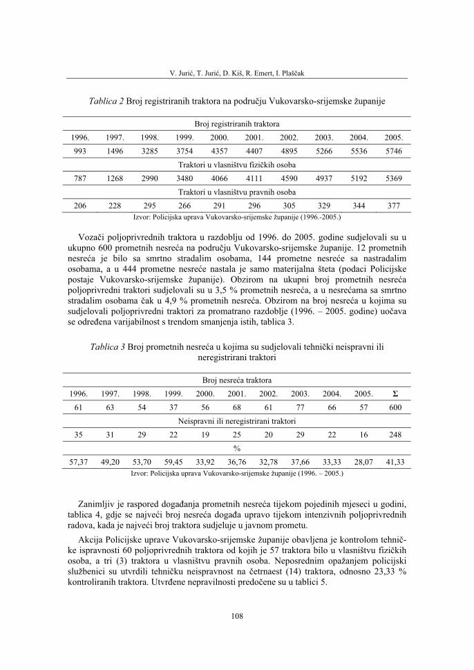
V. Jurić, T. Jurić, D. Kiš, R. Emert, I. Plaščak
108
Tablica 2 Broj registriranih traktora na području Vukovarsko-srijemske županije
Broj registriranih traktora
1996. 1997. 1998. 1999. 2000. 2001. 2002. 2003. 2004. 2005.
993 1496 3285 3754 4357 4407 4895 5266 5536 5746
Traktori u vlasništvu fizičkih osoba
787 1268 2990 3480 4066 4111 4590 4937 5192 5369
Traktori u vlasništvu pravnih osoba
206 228 295 266 291 296 305 329 344 377 Izvor: Policijska uprava Vukovarsko-srijemske županije (1996.-2005.)
Vozači poljoprivrednih traktora u razdoblju od 1996. do 2005. godine sudjelovali su u ukupno 600 prometnih nesreća na području Vukovarsko-srijemske županije. 12 prometnih nesreća je bilo sa smrtno stradalim osobama, 144 prometne nesreće sa nastradalim osobama, a u 444 prometne nesreće nastala je samo materijalna šteta (podaci Policijske postaje Vukovarsko-srijemske županije). Obzirom na ukupni broj prometnih nesrećapoljoprivredni traktori sudjelovali su u 3,5 % prometnih nesreća, a u nesrećama sa smrtno stradalim osobama čak u 4,9 % prometnih nesreća. Obzirom na broj nesreća u kojima su sudjelovali poljoprivredni traktori za promatrano razdoblje (1996. – 2005. godine) uočavase određena varijabilnost s trendom smanjenja istih, tablica 3.
Tablica 3 Broj prometnih nesreća u kojima su sudjelovali tehnički neispravni ili neregistrirani traktori
Broj nesreća traktora
1996. 1997. 1998. 1999. 2000. 2001. 2002. 2003. 2004. 2005. Σ
61 63 54 37 56 68 61 77 66 57 600
Neispravni ili neregistrirani traktori
35 31 29 22 19 25 20 29 22 16 248
%
57,37 49,20 53,70 59,45 33,92 36,76 32,78 37,66 33,33 28,07 41,33 Izvor: Policijska uprava Vukovarsko-srijemske županije (1996. – 2005.)
Zanimljiv je raspored događanja prometnih nesreća tijekom pojedinih mjeseci u godini, tablica 4, gdje se najveći broj nesreća događa upravo tijekom intenzivnih poljoprivrednih radova, kada je najveći broj traktora sudjeluje u javnom prometu.
Akcija Policijske uprave Vukovarsko-srijemske županije obavljena je kontrolom tehnič-ke ispravnosti 60 poljoprivrednih traktora od kojih je 57 traktora bilo u vlasništvu fizičkihosoba, a tri (3) traktora u vlasništvu pravnih osoba. Neposrednim opažanjem policijski službenici su utvrdili tehničku neispravnost na četrnaest (14) traktora, odnosno 23,33 % kontroliranih traktora. Utvrđene nepravilnosti predočene su u tablici 5.
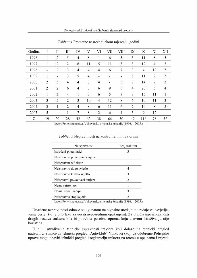
Poljoprivredni traktori kao čimbenik sigurnosti prometa
109
Tablica 4 Prometne nesreće tijekom mjeseci u godini
Godina I II III IV V VI VII VIII IX X XI XII 1996. 1 2 5 4 8 1 6 5 5 11 8 5 1997. 1 2 2 6 11 5 11 3 3 12 4 3 1998. - 2 3 4 4 4 6 7 3 4 12 5 1999. 1 - 3 5 4 - - - 8 11 2 3 2000. 2 3 4 4 3 4 - 5 7 14 7 3 2001. 2 2 6 4 3 6 9 5 4 20 3 4 2002. 1 3 - 1 3 6 5 7 8 15 11 1 2003. 3 5 2 3 10 4 12 8 6 10 11 3 2004. 3 1 2 4 8 6 11 6 2 10 8 5 2005. 5 - 1 7 8 2 6 4 3 9 12 - Σ 19 20 28 42 62 38 66 50 49 116 78 32
Izvor: Policijska uprava Vukovarsko-srijemske županije (1996. – 2005.)
Tablica 5 Nepravilnosti na kontroliranim traktorima
Neispravnost Broj traktora
Istrošeni pneumatici 3
Neispravno pozicijsko svijetlo 1
Neispravan reflektor 1
Neispravno dugo svjetlo 4
Neispravno kratko svjetlo 3
Neispravni pokazivači smjera 2
Nema retrovizor 1
Nema signalizaciju 3
Neispravna stop svjetla 2 Izvor: Policijska uprava Vukovarsko-srijemske županije (1996. – 2005.)
Utvrđene nepravilnosti odnose se uglavnom na signalne uređaje te uređaje za osvjetlja-vanje ceste (što je bilo lako za uočiti neposrednim opažanjem). Za utvrđivanje ispravnosti drugih sustava traktora bila bi potrebita posebna oprema koja u ovom istraživanju nije korištena.
U cilju utvrđivanja tehničke ispravnosti traktora koji dolaze na tehnički pregled nadzornici Stanice za tehnički pregled „Auto-klub“ Vinkovci (koji uz odobrenje Policijske uprave mogu obaviti tehnički pregled i registraciju traktora na terenu u općinama i mjesti-

V. Jurić, T. Jurić, D. Kiš, R. Emert, I. Plaščak
110
ma Županije) obavili su nadzor 100 traktora. Od 100 pregledanih traktora njih 15 nije bilo tehnički ispravno (15 %), a nepravilnosti su se uglavnom očitovale neispravnim svjetlima, neispravnim pokazivačima smjera i reflektorima za rad te neispravnim stop svjetlima i pneumaticima.
Redovite mjere servisno-preventivnog održavanja značajan su čimbenik koji utječe na sigurnost prometa. Traktorist bi pri dobro organiziranom servisno-preventivnom održava-nju u okviru dnevnog tehničkog održavanja (prije početka rada sa strojem) trebao obaviti provjeru funkcionalnosti pojedinih sustava (sustav za kočenje, sustav za upravljanje) te signalizacije i osvjetljenja, Emert i dr. (1995). Značaj redovitih mjera servisno-preventiv-nog održavanja time je veći što obiteljska gospodarstva raspolažu s velikim brojem starih i dotrajalih traktora prosječne starosti 17,7 godina. Na problem velikog broja dotrajalih traktora na obiteljskim gospodarstvima i visoke prosječne starosti (16,5 godina i 14,5 godina) ukazuju Jurić i dr. (2006) te Jurić i dr. (2001).
Službeni pokazatelji o broju registriranih traktora za promatrano razdoblje (1996. – 2005.) ukazuju na povećanje broja registriranih traktora što je vjerojatno posljedica stupanja na snagu Zakona o sigurnosti na cestama, ali i visokih novčanih kazni koje su predviđene u slučaju zatjecanja neregistriranog traktora u prometu. Značajan broj traktora registriran je kod fizičkih osoba, što je i za očekivati, budući da se poljoprivredna proizvodnja orijentira na obiteljska gospodarstva. Porast registriranih traktora u vlasništvu pravnih osoba je znatno manji, a kao jedan od razloga može se razmatrati činjenica da su pravne osobe (poljoprivredna poduzeća) u najvećoj mjeri registrirali svoje traktore, što nije bio slučaj kod fizičkih osoba.
No, zabrinjavajući su pokazatelji o broju registriranih traktora na anketiranim obitelj-skim gospodarstvima gdje je svega 47,21 % traktora registrirano. Značajna financijska sredstva potrebita za registriranje traktora, starost ili tehnička neispravnost nikako nisu i ne smiju biti opravdanje za vrlo visok broj traktora bez tehničkog pregleda 52,79 %. Ovu činjenicu potvrđuje podatak da su u promatranom razdoblju (1996. – 2005- godina) u čak41,33 % prometnih nesreća sudjelovali tehnički neispravni ili neregistrirani traktori. Iako se postotni udio neregistriranih i neispravnih traktora, prema službenim pokazateljima, smanjuje od 57,37 % (1996. godine) do 28,07 % (2005. godine) on je još uvijek visok. Na problem neregistriranih traktora na obiteljskim gospodarstvima (36 % ) ukazuju Jurić i dr (2006).
Veliki broj katastarskih čestica poljoprivrednih površina zahtijeva gibanje traktora javnim prometnicama što uz ovako veliki broj neregistriranih traktora značajno utječe na sigurnost prometa.
Najveći broj prometnih nesreća u kojima sudjeluju poljoprivredni traktori događa se tijekom sezone obavljanja poljoprivrednih radova (travanj – studeni). Izrazito visoki broj prometnih nesreća tijekom listopada (116) i studenog (78) u kojima sudjeluju poljoprivredni traktori treba promatrati i u kontekstu loših vremenskih prilika (magla, kraćidani, iznošenje blata na cestu i ino), gdje su znatno veći rizici nastanka prometne nesreće.
Rezultati akcije Postaje prometne policije Vinkovci glede utvrđivanja tehničkeispravnosti poljoprivrednih traktora ukazuju na visoki postotni udio neispravnih traktora (23,33 %) koji su sudjelovali u javnom prometu. Neispravnosti na traktorima utvrđenetijekom akcije (svijetla, pokazivači smjera, stop svijetla i ino) bile bi otklonjene prije
Poljoprivredni traktori kao čimbenik sigurnosti prometa
111
sudjelovanja u javnom prometu da su vlasnici poljoprivrednih traktora obavili redovite mjere servisno-preventivnog održavanja. Relativno visok postotni udio (15 %) traktora nije bio tehnički ispravan na tehničkom pregledu što upućuje da vlasnici traktora još nisu svjesni značenja i važnosti tehničke ispravnosti njihovih traktora kao sudionika javnog prometa.
ZAKLJUČCI
Provedenim istraživanjem tehničke ispravnosti poljoprivrednih traktora koji sudjeluju u javnom prometu i pristupaju tehničkom pregledu, te anketiranjem obiteljskih gospodarstava mogu se donijeti slijedeći zaključci:
• obiteljska gospodarstva raspolažu velikim brojem traktora različitog tipa i različitesnage s visokom prosječnom starosti od 17,7 godina;
• u posljednjih deset godina se smanjuje broj prometnih nesreća u kojima sudjeluju poljoprivredni traktori;
• iako službena evidencija pokazuje povećanje broja registriranih traktora na području Vukovarsko-srijemske županije, rezultati ankete na obiteljskim gospodarstvima ukazuju na još visok postotni udio (52,79 %) neregistriranih traktora;
• rezultati akcije Postaje prometne policije Vinkovci u cilju utvrđivanja tehničkeispravnosti poljoprivrednih traktora u javnom prometu ukazuju na visok postotni udio neispravnih traktora (23,33 %);
• značajan je postotni udio (15 %) tehnički neispravnih traktora na tehničkompregledu;
• utvrđene nepravilnosti na poljoprivrednim traktorima uglavnom su posljedica lošeg provođenja mjera servisno-preventivnog održavanja i
• trebalo bi raditi na educiranju vlasnika traktora da spoznaju značaj servisno-preventivnog održavanja kako za uporabnu pouzdanost i dulji vijek uporabe traktora tako i za sigurnost prometa.
V. Jurić, T. Jurić, D. Kiš, R. Emert, I. Plaščak
112
LITERATURA
1. **** Analize prometnih nesreća Postaje prometne policije Vinkovci, Vinkovci.
2. **** BILTEN o sigurnosti cestovnog prometa 2005., Ministarstvo unutarnjih poslova, Zagreb.
3. **** Zakon o sigurnosti prometa na cestama, N.N. 105/04., Zagreb.
4. Alreck, P. L., Settle, R. B. (1995). The Survey Research Handbook. 2nd Ed.. Guidelines and Strategies for Conducting a Survey, Irwin, Chicago.
5. Cochran, W. G. (1977). Sampling Techniques. Wiley, New York.
6. Czaja, R., Blair, J. (1996). Designing Surveys. Pine Forge Press, London.
7. Emert, R., Jurić, T., Banaj, Đ. (1996): Mjere za poboljšanje razine održavanja poljoprivrednih strojeva na malim gospodarstvima, Zbornik radova "Aktualni zadaci mehanizacije poljoprivrede", Opatija, 43-48.
8. Emert, R., Jurić, T., Filipović, D., Štefanek, E. (1995): Održavanje traktora i poljoprivrednih strojeva, Sveučilišni udžbenik, Osijek.
9. Happ, Z., Vidović, T. (2005): Upravljanje sustavom sigurnosti cestovnog prometa, Suvremeni promet, Zagreb, 226-229.
10. Jurić, T., Bulajić, S., Gili, D., Emert, R., Kiš, D., Plaščak, I., Šumanovac, L (2006): Zbrinjavanje rabljenog ulja na obiteljskim gospodarstvima, Zbornik radova «Aktualni zadaci mehanizacije poljoprivrede, Opatija.
11. Jurić, T., Emert, R., Šumanovac, L., Horvat, D. (2001): Provođenje mjera održavanja na obiteljskim gospodarstvima, «Actual tasks on agricultural engineering» Proceedings 29. International Symposium on Agricultural Engineering, Opatija, 43-51.
12. Jurić, T., Emert, R., Šumanovac, L., Jurić. V. (2001): Značaj servisno preventivnog održavanja za sigurnost prometa, 37. Znanstveni skup hrvatskih agronoma, Opatija, 156.
13. Jurić, T., Vučinić, V., Durmić, T., Emert, R., Kiš, D., Kraljević, D., Plaščak, I. (2006): Zbrinjavanje rabljenog ulja kao čimbenik očuvanja okoliša, 41. Hrvatski i 1. međunarodniznanstveni simpozij agronoma, Opatija, 255 – 256.
14. Jurić, V. (2006): Servisno-preventivno održavanje poljoprivrednih traktora kao čimbeniksigurnosti prometa, Diplomski rad, Vinkovci.
15. Kish, L. (1965). Survey Sampling. Wiley, New York.
16. Rotim, F., Mihoci, F., Cerovac Vesna (2001): Hrvatska: sigurnost cestovnog prometa u 2000. godini, Suvremeni promet, Zagreb, 536-539.
17. Tryfos, P. (1996). Sampling Methods for Applied Research. Wiley, New York.
Poljoprivredni traktori kao čimbenik sigurnosti prometa
113
AGRICULTURAL TRACTORS AS FACTORS IN TRAFFIC SAFETY
VLADO JURIĆ1, TOMISLAV JURIĆ2, DARKO KIŠ2, RUDOLF EMERT2,IVAN PLAŠČAK2
1 Policijska postaja Vinkovci, Bana Jelačića 4, 32100 Vinkovci 2 Poljoprivredni fakultet u Osijeku, Trg Svetog Trojstva 3, 31000 Osijek
SUMMARY
Agricultural tractors are important factors of a competitive agricultural production. They are engaged in traffic as motorized vehicles so that their technical corectness is of major importance. Safty level of traffic and the life of a tractor could be highly improved by regular and proper service-preventive maintenance. A research in the Vukovar-Srijem county was conducted in relation with the determination of the technical correctness of the tractors both subject to technical inspection and engaged in traffic. Furthermore, a survey including 107 family farms of the county was conducted in order to establish the number of registered tractors as well as their age. The results showed a high number of unregistered tractors (53.3%). The percentege of faulty tractors is also high (23.33%), and despite that they take part in traffic. The percentege of faulty tractors which were subject to technical inspection is also high (15%). In the last ten years the number of tractor accidents has decreased.
Key words: Tractor, traffic safety, service-preventive maintenance


36. Symposium "Actual Tasks on Agricultural Engineering", Opatija, Croatia, 2008.
115
36.
SIMPOZIJAKTUALNI ZADACIMEHANIZACIJE POLJOPRIVREDE
UDC631.312:631.51
Prethodno priopćenjePreliminary communication
STUDY REGARDING THE SOIL PARTICLES’ KINEMATICS DURING THE ANTE-MOLDBOARD
TILLAGE TOOL’S WORKING PROCESS S.ŞT. BIRIŞ1), E. MAICAN1), V. VLADUŢ
2), G. PARASCHIV1), M. MANEA1),S. BUNGESCU3)
1)”Politehnica” University of Bucharest Romania, 2)INMA Bucharest Romania,
3)Agricultural University of Timisoara Romania
SUMMARY
The plough body with ante-moldboard is a Romanian tillage tool, designed to be a component part of the variable-width ploughs, accomplishing a better incorporation in soil of the vegetable residues, a better disaggregating of the furrow, a better leveling of ploughed soil and a better furrow overturning.
In order to find the ante-mouldboard tillage tool’s influence over the working process, it is necessary to know the trajectories, speeds and accelerations of soil particles. These parameters allow calculating the mechanical work which is necessary to overcome the friction and adherence forces, the furrow’s weight and inertia of mass force.
The soil particles trajectories on the active surface of plough body with ante-moldboard were experimentally determined through identification of particles’ tracks on these surfaces which were preliminarily covered with a layer of paint or lacquer.
In this paper it is presented a complex mathematical model regarding the soil particles kinematics on the plough body with ante-moldboard, which was subsequent, used to design a simulation computer program. Finally, the simulation result for the Romanian P-2VA plough body with ante-moldboard is presented.
Key words: Moldboard, ante-moldboard, plough, soil particle, tillage process

S.Şt. Biriş, E. Maican, V. Vladuţ, G. Paraschiv, M. Manea, S. Bungescu
116
INTRODUCTION
Up to the present, due to its exceptional complexity, a kinematical study of the handling of soil particles by mouldboard ploughs has not been realized in Romania. For the same reasons, only few studies have been made over the world, one of them begins that of O’Callaghan and McCoy in 1965 [1]. For the improvement of the mouldboard’s active surfaces, the creation of a semi empirical model and of a program for computer simulation was necessary; which will allow the study of particles’ kinematics on those complex surfaces. The identification of points’ co-ordinate on the soil particles’ trajectory left on mouldboards, previously covered with paint or lacquer, is necessary for this semi empirical model. There were identified scratches on the active surface, at 2 cm distance from one another. Polynomial functions which make the connection between point’s co-ordinates on soil particles trajectory have been obtained by computation.
The kinematical study of the soil particles, moving on an active surface of a digger-plough with ante-mouldboard is presented as part of this article. The digger-plough with ante-mouldboard is a new type of tool of the plough, made in Romania (Figure 1), which provides a complete soil incorporation of the vegetation residues, insensitive to the plough’s working-depth, a better crumbling of the soil and a better alignment of the ploughing surface, due to the furrow’s overturning with an 180 degrees angle [2,3,4,5].
Fig. 1 The plough-body with ante-mouldboard
For the theoretical study of the furrow slice kinematics under the operation of the digger-plough with ante-mouldboard the following hypothesis are made [3, 5]:
• The digger-plough with ante-mouldboard is considered to be motionless, the furrow slice is moving with the same speed and contrary to the constant moving speed of the plough thus the furrow slice has no acceleration on the moving direction (Ox), its movement being a swivelling one on a crossing-surface.
• The superior furrow-slice remains in contact with the ante-mouldboard, and the inferior one remains in contact with the mouldboard on the entire surface of the digger-plough.
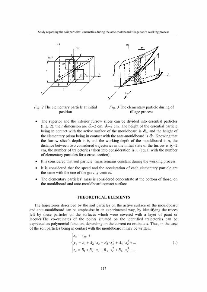
Study regarding the soil particles' kinematics during the ante-moldboard tillage tool's working process
117
Fig. 2 The elementary particle at initial position
Fig. 3 The elementary particle during of tillage process
• The superior and the inferior furrow slices can be divided into essential particles (Fig. 2), their dimension are δx=2 cm, δy=2 cm. The height of the essential particle being in contact with the active surface of the mouldboard is δzi, and the height of the elementary prism being in contact with the ante-mouldboard is δzj. Knowing that the furrow slice’s depth is b, and the working-depth of the mouldboard is a, the distance between two considered trajectories in the initial state of the furrow is δy=2cm, the number of trajectories taken into consideration is nt (equal with the number of elementary particles for a cross-section).
• It is considered that soil particle’ mass remains constant during the working process.
• It is considered that the speed and the acceleration of each elementary particle are the same with the one of the gravity centres.
• The elementary particles’ mass is considered concentrate at the bottom of those, on the mouldboard and ante-mouldboard contact surface.
THEORETICAL ELEMENTS
The trajectories described by the soil particles on the active surface of the mouldboard and ante-mouldboard can be emphasise in an experimental way, by identifying the traces left by these particles on the surfaces which were covered with a layer of paint or lacquer.The co-ordinates of the points situated on the identified trajectories can be expressed as polynomial function, depending on the current co-ordinate x. Thus, in the case of the soil particles being in contact with the mouldboard it may be written:
⎪
⎪
⎩
⎪⎪
⎨
⎧
+⋅+⋅+⋅+=
+⋅+⋅+⋅+=
⋅=
...
...3
42
321
34
2321
cccc
cccc
xcc
xBxBxBBz
xAxAxAAy
tvx
(1)
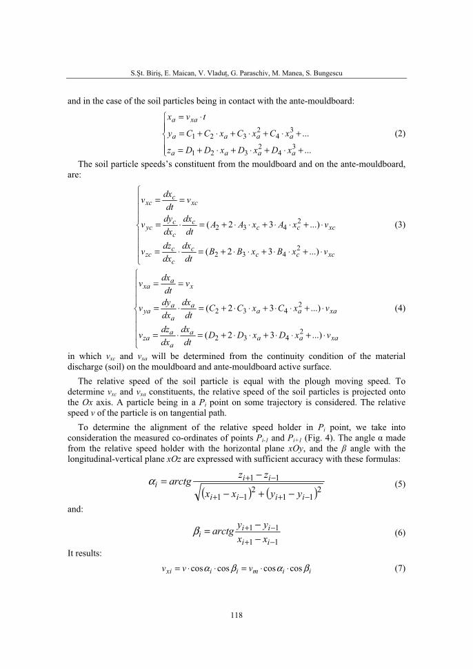
S.Şt. Biriş, E. Maican, V. Vladuţ, G. Paraschiv, M. Manea, S. Bungescu
118
and in the case of the soil particles being in contact with the ante-mouldboard:
⎪
⎪
⎩
⎪⎪
⎨
⎧
+⋅+⋅+⋅+=
+⋅+⋅+⋅+=
⋅=
...
...3
42
321
34
2321
aaaa
aaaa
xaa
xDxDxDDz
xCxCxCCy
tvx
(2)
The soil particle speeds’s constituent from the mouldboard and on the ante-mouldboard, are:
⎪
⎪
⎪
⎩
⎪
⎪
⎪
⎨
⎧
⋅+⋅⋅+⋅⋅+=⋅=
⋅+⋅⋅+⋅⋅+=⋅=
==
xcccc
c
czc
xcccc
c
cyc
xcc
xc
vxBxBBdt
dxdxdzv
vxAxAAdt
dxdxdyv
vdt
dxv
...)32(
...)32(
2432
2432 (3)
⎪
⎪
⎪
⎩
⎪
⎪
⎪
⎨
⎧
⋅+⋅⋅+⋅⋅+=⋅=
⋅+⋅⋅+⋅⋅+=⋅=
==
xaaaa
a
aza
xaaaa
a
aya
xa
xa
vxDxDDdt
dxdxdzv
vxCxCCdt
dxdxdyv
vdt
dxv
...)32(
...)32(
2432
2432 (4)
in which vxc and vxa will be determined from the continuity condition of the material discharge (soil) on the mouldboard and ante-mouldboard active surface.
The relative speed of the soil particle is equal with the plough moving speed. To determine vxc and vxa constituents, the relative speed of the soil particles is projected onto the Ox axis. A particle being in a Pi point on some trajectory is considered. The relative speed v of the particle is on tangential path.
To determine the alignment of the relative speed holder in Pi point, we take into consideration the measured co-ordinates of points Pi-1 and Pi+1 (Fig. 4). The angle α made from the relative speed holder with the horizontal plane xOy, and the β angle with the longitudinal-vertical plane xOz are expressed with sufficient accuracy with these formulas:
( ) ( )2112
11
11
−+−+
−+
−+−
−=iiii
iii
yyxx
zzarctgα (5)
and:
11
11
−+
−+−−=
ii
iii xx
yyarctgβ (6)
It results:
iimiixi vvv βαβα coscoscoscos ⋅⋅=⋅⋅= (7)
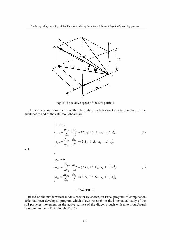
Study regarding the soil particles' kinematics during the ante-moldboard tillage tool's working process
119
Fig. 4 The relative speed of the soil particle
The acceleration constituents of the elementary particles on the active surface of the mouldboard and of the ante-mouldboard are:
⎪
⎪
⎪
⎩
⎪
⎪
⎪
⎨
⎧
⋅+⋅⋅+⋅=⋅=
⋅+⋅⋅+⋅=⋅=
=
243
243
...)62(
...)62(
0
xccc
c
zczc
xccc
c
ycyc
xc
vxBBdt
dxdxdva
vxAAdt
dxdxdv
a
a
(8)
and:
⎪
⎪
⎪
⎩
⎪
⎪
⎪
⎨
⎧
⋅+⋅⋅+⋅=⋅=
⋅+⋅⋅+⋅=⋅=
=
243
243
...)62(
...)62(
0
xaaa
a
zaza
xaaa
a
yaya
xa
vxDDdt
dxdxdva
vxCCdt
dxdxdv
a
a
(9)
PRACTICE
Based on the mathematical models previously shown, an Excel program of computation table had been developed, program which allows research on the kinematical study of the soil particles movement on the active surface of the digger-plough with ante-mouldboard belonging to the P-2VA plough (Fig. 5).
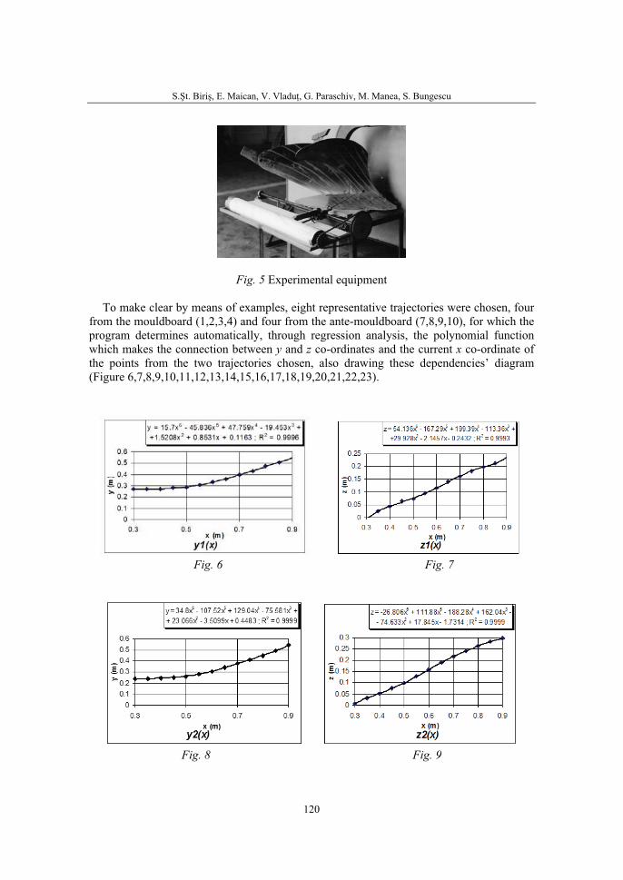
S.Şt. Biriş, E. Maican, V. Vladuţ, G. Paraschiv, M. Manea, S. Bungescu
120
Fig. 5 Experimental equipment
To make clear by means of examples, eight representative trajectories were chosen, four from the mouldboard (1,2,3,4) and four from the ante-mouldboard (7,8,9,10), for which the program determines automatically, through regression analysis, the polynomial function which makes the connection between y and z co-ordinates and the current x co-ordinate of the points from the two trajectories chosen, also drawing these dependencies’ diagram (Figure 6,7,8,9,10,11,12,13,14,15,16,17,18,19,20,21,22,23).
Fig. 6 Fig. 7
Fig. 8 Fig. 9
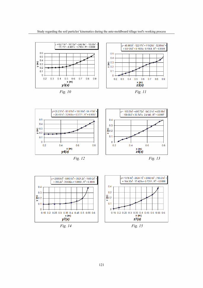
Study regarding the soil particles' kinematics during the ante-moldboard tillage tool's working process
121
Fig. 10 Fig. 11
Fig. 12 Fig. 13
Fig. 14 Fig. 15
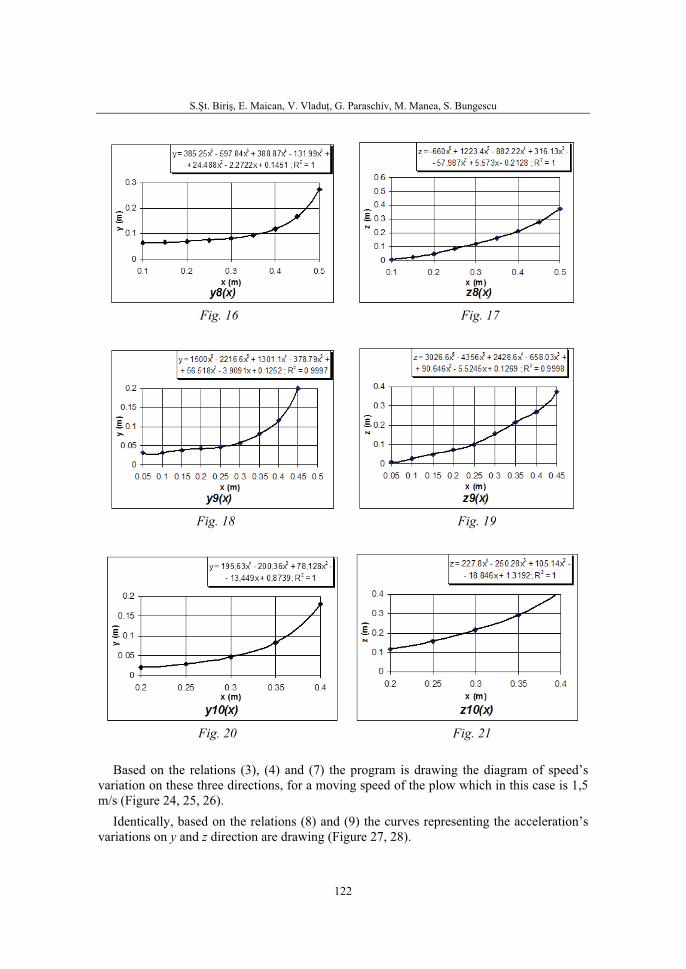
S.Şt. Biriş, E. Maican, V. Vladuţ, G. Paraschiv, M. Manea, S. Bungescu
122
Fig. 16 Fig. 17
Fig. 18 Fig. 19
Fig. 20 Fig. 21
Based on the relations (3), (4) and (7) the program is drawing the diagram of speed’s variation on these three directions, for a moving speed of the plow which in this case is 1,5 m/s (Figure 24, 25, 26).
Identically, based on the relations (8) and (9) the curves representing the acceleration’s variations on y and z direction are drawing (Figure 27, 28).
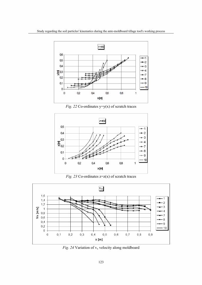
Study regarding the soil particles' kinematics during the ante-moldboard tillage tool's working process
123
Fig. 22 Co-ordinates y=y(x) of scratch traces
Fig. 23 Co-ordinates z=z(x) of scratch traces
Fig. 24 Variation of vx velocity along moldboard
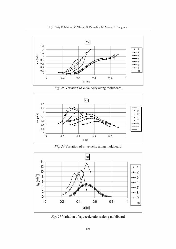
S.Şt. Biriş, E. Maican, V. Vladuţ, G. Paraschiv, M. Manea, S. Bungescu
124
Fig. 25 Variation of vy velocity along moldboard
Fig. 26 Variation of vz velocity along moldboard
Fig. 27 Variation of ay accelerations along moldboard

Study regarding the soil particles' kinematics during the ante-moldboard tillage tool's working process
125
Fig. 28 Variation of az accelerations along moldboard
CONCLUSIONS
1. This study allows the computer simulation of the mowing process of the soil particles on some trajectories, identified by experimental measurements on the active surface of the digger-plough with ante-mouldboard.
2. The elaborated computation program allows the checking of the lateral misalignment condition corresponding to the furrow slice (0,6 m/s < vy < 1,2 m/s). As you can see in this case (Figure 25), this condition is fulfilled with a working speed of 1,5 m/s.
3. The relations (8) and (9) allow the determination of the acceleration’s constituents of the soil particles, making the first step in improving the complete study of soil particles’ dynamics under the digger-plough operation.

S.Şt. Biriş, E. Maican, V. Vladuţ, G. Paraschiv, M. Manea, S. Bungescu
126
REFERENCES
1. J. R. O’Callaghan, J. G. McCoy, 1965, The handling of soil by mouldboard ploughs, J. of Agric. Eng. Res, Vol. 10, No. 1, pp. 23-35.
2. P. Babiciu, S. Şt. Biriş, 1998, Antecormana – un nou organ de lucru pentru pluguri, Proceeding of the “TransArgaTech ‘98” Conference, Technical University of Cluj-Napoca, pp. 39-42.
3. P. Babiciu, S. Şt. Biriş, 1998, Teoria procesului de lucru a antecormanei, Proceeding of the “TransAgraTech ‘98” Conference, Technical University of Cluj-Napoca, pp. 43-50.
4. S. Şt. Biriş, P. Babiciu, 1998, Metoda analitică de proiectare a unei antecormane, Proceeding of the “TransAgraTech ‘98” Conference, Technical University of Cluj-Napoca, pp. 51-56.
5. Biriş S.Şt., 1999, Cercetări privind realizarea şi verificarea unui pachet de programe pentru proiectarea pe calculator a suprafeţelor active ale trupiţelor. Doctoral thesis, Polytechnic University of Bucharest.
36. Symposium "Actual Tasks on Agricultural Engineering", Opatija, Croatia, 2008.
127
36.
SIMPOZIJAKTUALNI ZADACIMEHANIZACIJE POLJOPRIVREDE
UDC631.51:633.2
Stručni radExpert paper
THE ACHIEVEMENT AND EXPERIMENTATION OF ONE COMPLEX UNIT FOR TOTAL TILLAGE AND
SOWING OF THE SOIL FOR STRAW CROPS IOAN ŢENU, PETRU COJOCARIU, RADU ROSCA, PETRICA CARLESCU
University of Agricultural Sciences and Veterinary Medicine from Iaşi, Department of Agricultural Machines, [email protected], tel. 004 0232407558
ABSTRACT
We present within paper the results of the experimental tests concerning the usage of the one complex unit which operates in unit with T 190 VALTRA tractor and which tills by one passing the germinating bed preparation and sowing of straw crops. For tillage of the germinating bed, the unit is equipped by soil loosening elements and vertical rotor harrow and for sowing we used a universal sowing machine having central distribution and two disc shares .We determined in these conditions the energetic and qualitative indices of the unit.
Key words: tillage, sowing, complex unit
MATERIALS AND METHODES
The (AGPS-24DR) complex aggregate is used for the preparing of germination bed and sowing, after it was done, separately, the soil basic work with mouldboard plough. In this way, it is carried out , by only one passing, the preparing of germination bed and sowing. The complex aggregate have in its structure two machines: a (FRB-3) rotary harrow with vertical rotors, in front of aggregate, and an (SPU-24DR) universal pneumatic sowing machine at its rear. The complex aggregate working width is of 3 meters.
The research team established that it can be obtained better results, regarding soil preservation, if the soil is no-tillaged. More of that, it was established that the soil basic work, without up-setting the ploughing, must not be done as a separate work.
In this way we considered that the complex aggregate AGPS-24DR could be adapted to make the soil basic work, without up-setting the ploughing, fact which drives at decreasing the destructive effects among soil, it decreases also the energy consumption and increase working productivity.
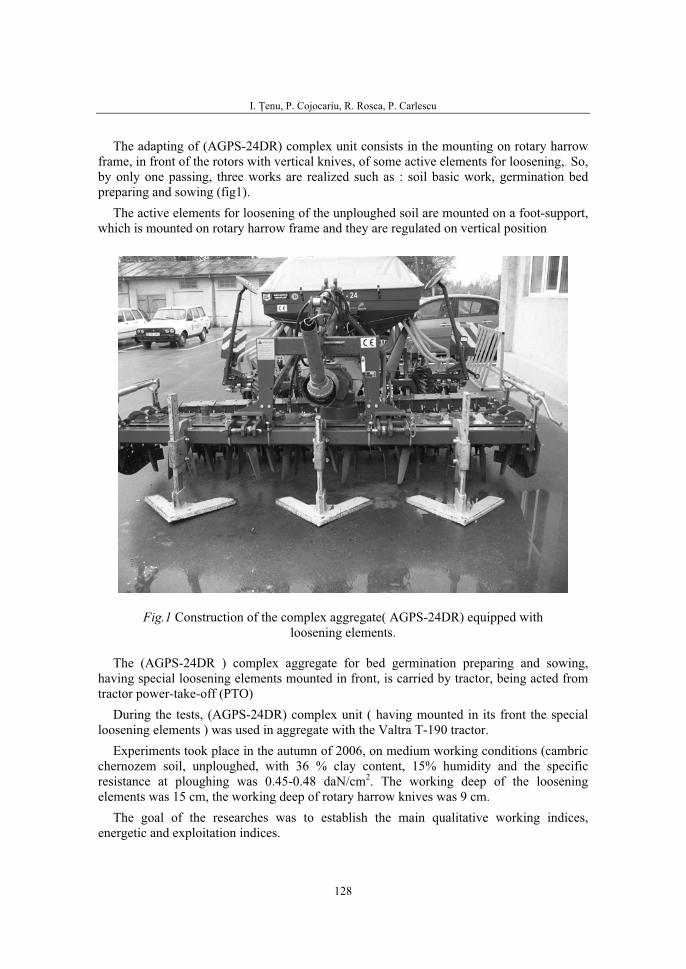
I. Ţenu, P. Cojocariu, R. Rosca, P. Carlescu
128
The adapting of (AGPS-24DR) complex unit consists in the mounting on rotary harrow frame, in front of the rotors with vertical knives, of some active elements for loosening,. So,by only one passing, three works are realized such as : soil basic work, germination bed preparing and sowing (fig1).
The active elements for loosening of the unploughed soil are mounted on a foot-support, which is mounted on rotary harrow frame and they are regulated on vertical position
Fig.1 Construction of the complex aggregate( AGPS-24DR) equipped withloosening elements.
The (AGPS-24DR ) complex aggregate for bed germination preparing and sowing, having special loosening elements mounted in front, is carried by tractor, being acted from tractor power-take-off (PTO)
During the tests, (AGPS-24DR) complex unit ( having mounted in its front the special loosening elements ) was used in aggregate with the Valtra T-190 tractor.
Experiments took place in the autumn of 2006, on medium working conditions (cambric chernozem soil, unploughed, with 36 % clay content, 15% humidity and the specific resistance at ploughing was 0.45-0.48 daN/cm2. The working deep of the loosening elements was 15 cm, the working deep of rotary harrow knives was 9 cm.
The goal of the researches was to establish the main qualitative working indices, energetic and exploitation indices.
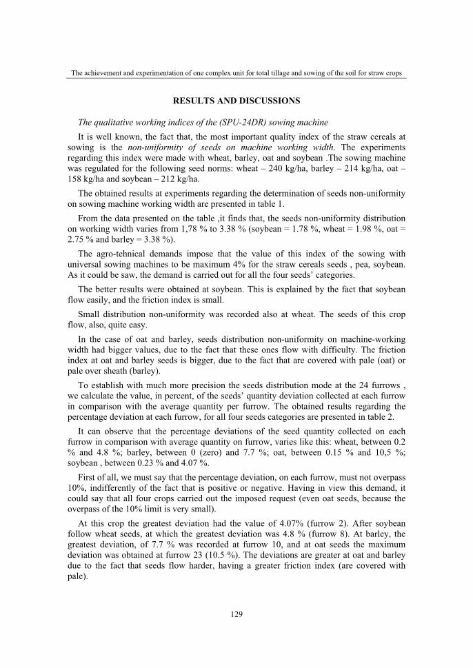
The achievement and experimentation of one complex unit for total tillage and sowing of the soil for straw crops
129
RESULTS AND DISCUSSIONS
The qualitative working indices of the (SPU-24DR) sowing machine It is well known, the fact that, the most important quality index of the straw cereals at
sowing is the non-uniformity of seeds on machine working width. The experiments regarding this index were made with wheat, barley, oat and soybean .The sowing machine was regulated for the following seed norms: wheat – 240 kg/ha, barley – 214 kg/ha, oat – 158 kg/ha and soybean – 212 kg/ha.
The obtained results at experiments regarding the determination of seeds non-uniformity on sowing machine working width are presented in table 1.
From the data presented on the table ,it finds that, the seeds non-uniformity distribution on working width varies from 1,78 % to 3.38 % (soybean = 1.78 %, wheat = 1.98 %, oat = 2.75 % and barley = 3.38 %).
The agro-tehnical demands impose that the value of this index of the sowing with universal sowing machines to be maximum 4% for the straw cereals seeds , pea, soybean. As it could be saw, the demand is carried out for all the four seeds’ categories.
The better results were obtained at soybean. This is explained by the fact that soybean flow easily, and the friction index is small.
Small distribution non-uniformity was recorded also at wheat. The seeds of this crop flow, also, quite easy.
In the case of oat and barley, seeds distribution non-uniformity on machine-working width had bigger values, due to the fact that these ones flow with difficulty. The friction index at oat and barley seeds is bigger, due to the fact that are covered with pale (oat) or pale over sheath (barley).
To establish with much more precision the seeds distribution mode at the 24 furrows , we calculate the value, in percent, of the seeds’ quantity deviation collected at each furrow in comparison with the average quantity per furrow. The obtained results regarding the percentage deviation at each furrow, for all four seeds categories are presented in table 2.
It can observe that the percentage deviations of the seed quantity collected on each furrow in comparison with average quantity on furrow, varies like this: wheat, between 0.2 % and 4.8 %; barley, between 0 (zero) and 7.7 %; oat, between 0.15 % and 10,5 %; soybean , between 0.23 % and 4.07 %.
First of all, we must say that the percentage deviation, on each furrow, must not overpass 10%, indifferently of the fact that is positive or negative. Having in view this demand, it could say that all four crops carried out the imposed request (even oat seeds, because the overpass of the 10% limit is very small).
At this crop the greatest deviation had the value of 4.07% (furrow 2). After soybean follow wheat seeds, at which the greatest deviation was 4.8 % (furrow 8). At barley, the greatest deviation, of 7.7 % was recorded at furrow 10, and at oat seeds the maximum deviation was obtained at furrow 23 (10.5 %). The deviations are greater at oat and barley due to the fact that seeds flow harder, having a greater friction index (are covered with pale).
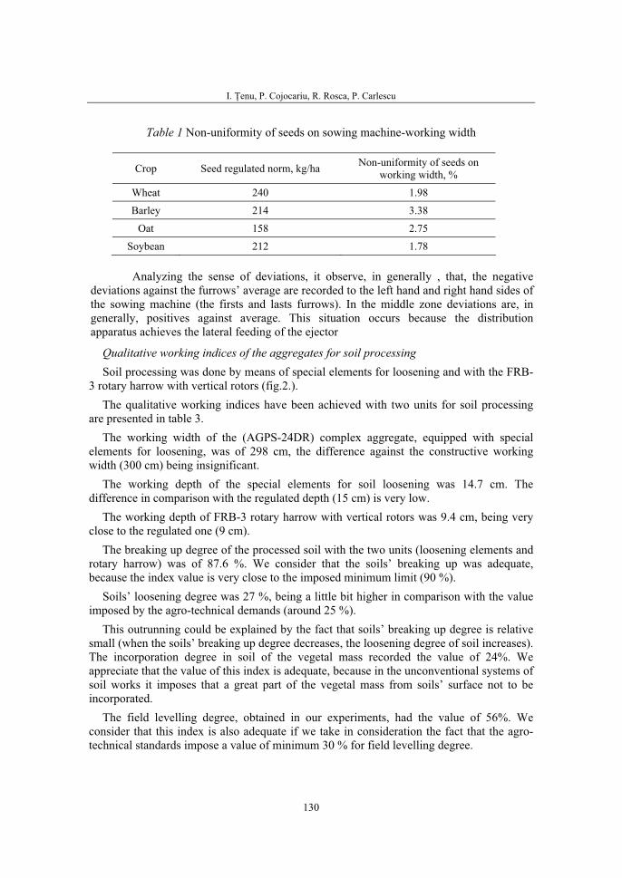
I. Ţenu, P. Cojocariu, R. Rosca, P. Carlescu
130
Table 1 Non-uniformity of seeds on sowing machine-working width
Crop Seed regulated norm, kg/ha Non-uniformity of seeds on working width, %
Wheat 240 1.98
Barley 214 3.38
Oat 158 2.75
Soybean 212 1.78
Analyzing the sense of deviations, it observe, in generally , that, the negative deviations against the furrows’ average are recorded to the left hand and right hand sides of the sowing machine (the firsts and lasts furrows). In the middle zone deviations are, in generally, positives against average. This situation occurs because the distribution apparatus achieves the lateral feeding of the ejector
Qualitative working indices of the aggregates for soil processing Soil processing was done by means of special elements for loosening and with the FRB-
3 rotary harrow with vertical rotors (fig.2.). The qualitative working indices have been achieved with two units for soil processing
are presented in table 3. The working width of the (AGPS-24DR) complex aggregate, equipped with special
elements for loosening, was of 298 cm, the difference against the constructive working width (300 cm) being insignificant.
The working depth of the special elements for soil loosening was 14.7 cm. The difference in comparison with the regulated depth (15 cm) is very low.
The working depth of FRB-3 rotary harrow with vertical rotors was 9.4 cm, being very close to the regulated one (9 cm).
The breaking up degree of the processed soil with the two units (loosening elements and rotary harrow) was of 87.6 %. We consider that the soils’ breaking up was adequate, because the index value is very close to the imposed minimum limit (90 %).
Soils’ loosening degree was 27 %, being a little bit higher in comparison with the value imposed by the agro-technical demands (around 25 %).
This outrunning could be explained by the fact that soils’ breaking up degree is relative small (when the soils’ breaking up degree decreases, the loosening degree of soil increases). The incorporation degree in soil of the vegetal mass recorded the value of 24%. We appreciate that the value of this index is adequate, because in the unconventional systems of soil works it imposes that a great part of the vegetal mass from soils’ surface not to be incorporated.
The field levelling degree, obtained in our experiments, had the value of 56%. We consider that this index is also adequate if we take in consideration the fact that the agro-technical standards impose a value of minimum 30 % for field levelling degree.
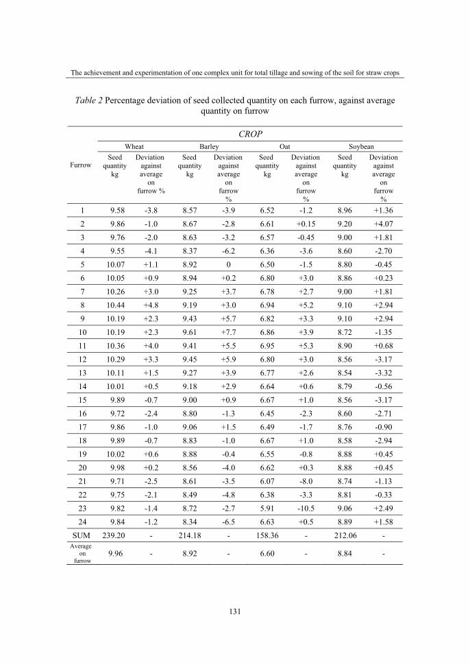
The achievement and experimentation of one complex unit for total tillage and sowing of the soil for straw crops
131
Table 2 Percentage deviation of seed collected quantity on each furrow, against average quantity on furrow
CROPWheat Barley Oat Soybean
FurrowSeed
quantitykg
Deviationagainstaverage
onfurrow %
Seedquantity
kg
Deviationagainstaverage
onfurrow
%
Seedquantity
kg
Deviationagainstaverage
onfurrow
%
Seedquantity
kg
Deviationagainstaverage
onfurrow
%1 9.58 -3.8 8.57 -3.9 6.52 -1.2 8.96 +1.36
2 9.86 -1.0 8.67 -2.8 6.61 +0.15 9.20 +4.07
3 9.76 -2.0 8.63 -3.2 6.57 -0.45 9.00 +1.81
4 9.55 -4.1 8.37 -6.2 6.36 -3.6 8.60 -2.70
5 10.07 +1.1 8.92 0 6.50 -1.5 8.80 -0.45
6 10.05 +0.9 8.94 +0.2 6.80 +3.0 8.86 +0.23
7 10.26 +3.0 9.25 +3.7 6.78 +2.7 9.00 +1.81
8 10.44 +4.8 9.19 +3.0 6.94 +5.2 9.10 +2.94
9 10.19 +2.3 9.43 +5.7 6.82 +3.3 9.10 +2.94
10 10.19 +2.3 9.61 +7.7 6.86 +3.9 8.72 -1.35
11 10.36 +4.0 9.41 +5.5 6.95 +5.3 8.90 +0.68
12 10.29 +3.3 9.45 +5.9 6.80 +3.0 8.56 -3.17
13 10.11 +1.5 9.27 +3.9 6.77 +2.6 8.54 -3.32
14 10.01 +0.5 9.18 +2.9 6.64 +0.6 8.79 -0.56
15 9.89 -0.7 9.00 +0.9 6.67 +1.0 8.56 -3.17
16 9.72 -2.4 8.80 -1.3 6.45 -2.3 8.60 -2.71
17 9.86 -1.0 9.06 +1.5 6.49 -1.7 8.76 -0.90
18 9.89 -0.7 8.83 -1.0 6.67 +1.0 8.58 -2.94
19 10.02 +0.6 8.88 -0.4 6.55 -0.8 8.88 +0.45
20 9.98 +0.2 8.56 -4.0 6.62 +0.3 8.88 +0.45
21 9.71 -2.5 8.61 -3.5 6.07 -8.0 8.74 -1.13
22 9.75 -2.1 8.49 -4.8 6.38 -3.3 8.81 -0.33
23 9.82 -1.4 8.72 -2.7 5.91 -10.5 9.06 +2.49
24 9.84 -1.2 8.34 -6.5 6.63 +0.5 8.89 +1.58
SUM 239.20 - 214.18 - 158.36 - 212.06 - Average
onfurrow
9.96 - 8.92 - 6.60 - 8.84 -
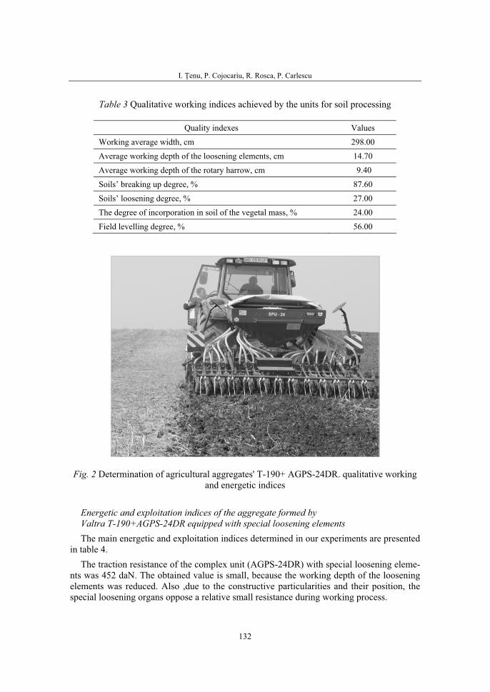
I. Ţenu, P. Cojocariu, R. Rosca, P. Carlescu
132
Table 3 Qualitative working indices achieved by the units for soil processing
Quality indexes Values
Working average width, cm 298.00
Average working depth of the loosening elements, cm 14.70
Average working depth of the rotary harrow, cm 9.40
Soils’ breaking up degree, % 87.60
Soils’ loosening degree, % 27.00
The degree of incorporation in soil of the vegetal mass, % 24.00
Field levelling degree, % 56.00
Fig. 2 Determination of agricultural aggregates' T-190+ AGPS-24DR. qualitative working and energetic indices
Energetic and exploitation indices of the aggregate formed by Valtra T-190+AGPS-24DR equipped with special loosening elements The main energetic and exploitation indices determined in our experiments are presented
in table 4. The traction resistance of the complex unit (AGPS-24DR) with special loosening eleme-
nts was 452 daN. The obtained value is small, because the working depth of the loosening elements was reduced. Also ,due to the constructive particularities and their position, the special loosening organs oppose a relative small resistance during working process.
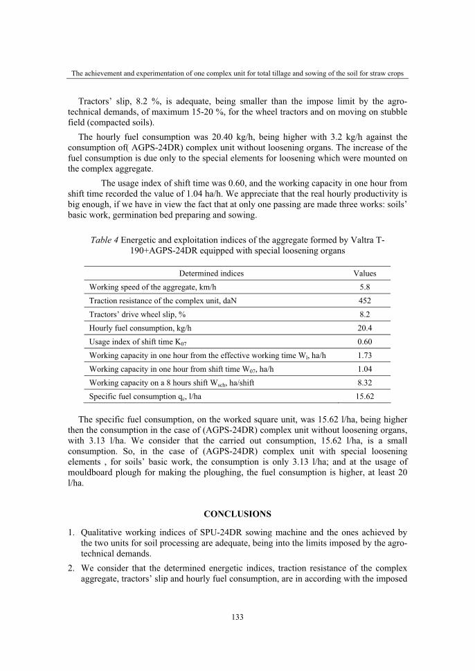
The achievement and experimentation of one complex unit for total tillage and sowing of the soil for straw crops
133
Tractors’ slip, 8.2 %, is adequate, being smaller than the impose limit by the agro-technical demands, of maximum 15-20 %, for the wheel tractors and on moving on stubble field (compacted soils).
The hourly fuel consumption was 20.40 kg/h, being higher with 3.2 kg/h against the consumption of( AGPS-24DR) complex unit without loosening organs. The increase of the fuel consumption is due only to the special elements for loosening which were mounted on the complex aggregate.
The usage index of shift time was 0.60, and the working capacity in one hour from shift time recorded the value of 1.04 ha/h. We appreciate that the real hourly productivity is big enough, if we have in view the fact that at only one passing are made three works: soils’ basic work, germination bed preparing and sowing.
Table 4 Energetic and exploitation indices of the aggregate formed by Valtra T-190+AGPS-24DR equipped with special loosening organs
Determined indices Values
Working speed of the aggregate, km/h 5.8
Traction resistance of the complex unit, daN 452
Tractors’ drive wheel slip, % 8.2
Hourly fuel consumption, kg/h 20.4
Usage index of shift time K07 0.60
Working capacity in one hour from the effective working time Wl, ha/h 1.73
Working capacity in one hour from shift time W07, ha/h 1.04
Working capacity on a 8 hours shift Wsch, ha/shift 8.32
Specific fuel consumption qc, l/ha 15.62
The specific fuel consumption, on the worked square unit, was 15.62 l/ha, being higher then the consumption in the case of (AGPS-24DR) complex unit without loosening organs, with 3.13 l/ha. We consider that the carried out consumption, 15.62 l/ha, is a small consumption. So, in the case of (AGPS-24DR) complex unit with special loosening elements , for soils’ basic work, the consumption is only 3.13 l/ha; and at the usage of mouldboard plough for making the ploughing, the fuel consumption is higher, at least 20 l/ha.
CONCLUSIONS
1. Qualitative working indices of SPU-24DR sowing machine and the ones achieved by the two units for soil processing are adequate, being into the limits imposed by the agro-technical demands.
2. We consider that the determined energetic indices, traction resistance of the complex aggregate, tractors’ slip and hourly fuel consumption, are in according with the imposed

I. Ţenu, P. Cojocariu, R. Rosca, P. Carlescu
134
demands. Hourly fuel consumption is much smaller in comparison with the summed consumption of those three units for making in a separate way of the works: ploughing, germination bed preparing , sowing.
3. Working capacity of the (AGPS-24DR) complex unit equipped with special loosening elements is, also, much higher than the working capacity of ploughing aggregates, germination bed preparing aggregates and sowing aggregates, used when a new crop is settled up.
4. Fuel consumption per hectare of the (AGPS-24DR) complex unit with special loosening elements is much smaller than the one in the case in which are made three different works: ploughing, germination bed preparing and sowing.
5. By decreasing the aggregates’ numbers of passing on the same field the destructive effects of the passing are diminished.
REFERENCES
1. Jităreanu, G. şi colab., 2007, Tehnologii şi maşini pentru mecanizarea lucrărilor solului în vederea practicării conceptului de agricultură durabilă. Edit. Ion Ionescu de la Brad Iaşi,
2. Neagu, Tr. şi colab., Studiul comparativ al plugului de destinaţie generală, al plugului cu organe paraplow şi al afânătorului adânci cizel. Lucr. ştiinţ., seria Agronomie, vol. 34, Universitatea Agronomică din Iaşi, 1992.
3. Neagu, Tr., Agregat complex pentru prelucrarea solului în fâşii, semănat erbicidat şi fertilizat AFSP-4. Lucr. ştiinţ., seria Horticultură, vol. 29, Institutul Agronomic din Iaşi, 1985.
4. Pirnă, I. şi colab., Utilaje noi în tehnologiile de lucrare a solului şi pregătit patul germinativ realizate de INMA Bucureşti. Lucr. ştiinţ., INMA Bucureşti, 2001.
5. Vlăduţ V. şi colab., Studiu privind reducerea forţelor şi a energiei necesare pentru lucrarea solului prin efectul de electro-osmoză. Lucr. ştiinţ. INMA Bucureşti, 2000.
36. Symposium "Actual Tasks on Agricultural Engineering", Opatija, Croatia, 2008.
135
36.
SIMPOZIJAKTUALNI ZADACIMEHANIZACIJE POLJOPRIVREDE
UDC631.317:631.43
Stručni radExpert paper
RESEARCHES REGARDING THE DEVELOPMENT OF A SOIL PREPARATION UNIT, ACCORDING TO THE
DEMANDS OF SUSTAINABLE AGRICULTURE 1GIGEL PARASCHIV, 1EDMOND MAICAN, 1SORIN-ŞTEFAN BIRIŞ,
2SORIN BUNGESCU
1“Politehnica” University of Bucharest, Romania 2Agricultural University of Timişoara, Romania
SUMMARY
Researches regarding new soil preparation technologies that can lead to a reduced degree of soil degradation are worldwide under way. Mostly, the outcome of a new technology is a machine with improved performances. Once Romania joined the European Union, many researchers from our country have focused their efforts towards finding technologies and soil preparation machines that meet the demands of sustainable agriculture.
This paper presents an agricultural machine made of a plough and a tillage cutter, driven by means of a 65 HP tractor. The advantage of this system consists of an optimum soil preparation in only one pass, taking into account the subsequent seeding process. The machine was tested on specific soils from southern part of Romania. Results were compared with those from classic technologies used in the preparation of germinating layer. Among other advantages, reduced fuel consumption (which also means a reduced degree of pollution) and also a reduced soil compaction are the most important aspects revealed by experiments.
Key words: tillage cutter, ploughing, fuel consumption, soil compaction
INTRODUCTION
Starting from the idea that the soil is a humanity wealth, researchers all over the world are looking permanently for new solutions of agricultural machinery that better protects the soil during its preparation.
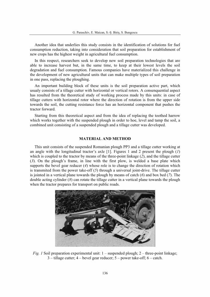
G. Paraschiv, E. Maican, S.-Ş. Biriş, S. Bungescu
136
Another idea that underlies this study consists in the identification of solutions for fuel consumption reduction, taking into consideration that soil preparation for establishment of new crops has the highest weight in agricultural fuel consumption.
In this respect, researchers seek to develop new soil preparation technologies that are able to increase harvest but, in the same time, to keep at their lowest levels the soil degradation and fuel consumption. Famous companies have materialized this challenge in the development of new agricultural units that can make multiple types of soil preparation in one pass, replacing the ploughing.
An important building block of these units is the soil preparation active part, which usualy consists of a tillage cutter with horizontal or vertical rotors. A consenquential aspect has resulted from the theoretical study of working process made by this units: in case of tillage cutters with horizontal rotor where the direction of rotation is from the upper side towards the soil, the cutting resistance force has an horizontal component that pushes the tractor forward.
Starting from this theoretical aspect and from the idea of replacing the toothed harrow which works together with the suspended plough in order to hoe, level and tamp the soil, a combined unit consisting of a suspended plough and a tillage cutter was developed.
MATERIAL AND METHOD
This unit consists of the suspended Romanian plough PP3 and a tillage cutter working at an angle with the longitudinal tractor’s axle [1]. Figures 1 and 2 present the plough (1)which is coupled to the tractor by means of the three-point linkage (2), and the tillage cutter (3). On the plough’s frame, in line with the first plow, is welded a base plate which supports the bevel gear reducer (4) whose role is to change the direction of rotation which is transmited from the power take-off (5) through a universal joint-drive. The tillage cutter is jointed in a vertical plane towards the plough by means of catch (6) and box bed (7). The double acting cylinder (8) can rotate the tillage cutter in a vertical plane towards the plough when the tractor prepares for transport on public roads.
Fig. 1 Soil preparation experimental unit: 1 – suspended plough; 2 – three-point linkage;3 – tillage cutter; 4 – bevel gear reducer; 5 – power take-off; 6 – catch.
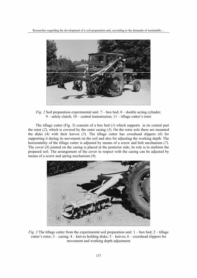
Researches regarding the development of a soil preparation unit, according to the demands of sustainable ...
137
Fig. 2 Soil preparation experimental unit: 7 – box bed; 8 – double acting cylinder;9 – safety clutch; 10 – central transmission; 11 – tillage cutter’s rotor
The tillage cutter (Fig. 3) consists of a box bed (1) which supports in its central part the rotor (2), which is covered by the outer casing (3). On the rotor axle there are mounted the disks (4) with their knives (5). The tillage cutter has crosshead slippers (6) for supporting it during its movement on the soil and also for adjusting the working depth. The horizontality of the tillage cutter is adjusted by means of a screw and bolt mechanism (7).The cover (8) jointed on the casing is placed at the posterior side; its role is to uniform the prepared soil. The arrangement of the cover in respect with the casing can be adjusted by means of a screw and spring mechanism (9).
Fig. 3 The tillage cutter from the experimental soil preparation unit: 1 – box bed; 2 – tillage cutter’s rotor; 3 – casing; 4 – knives holding disks; 5 – knives; 6 – crosshead slippers for
movement and working depth adjustment
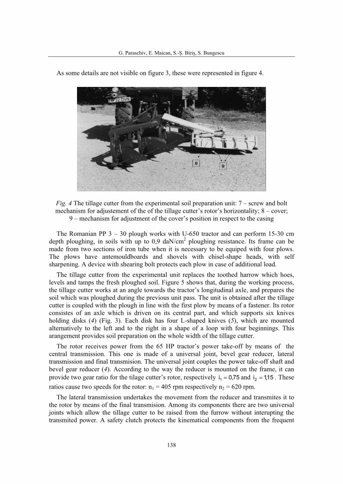
G. Paraschiv, E. Maican, S.-Ş. Biriş, S. Bungescu
138
As some details are not visible on figure 3, these were represented in figure 4.
Fig. 4 The tillage cutter from the experimental soil preparation unit: 7 – screw and bolt mechanism for adjustement of the of the tillage cutter’s rotor’s horizontality; 8 – cover;
9 – mechanism for adjustment of the cover’s position in respect to the casing
The Romanian PP 3 – 30 plough works with U-650 tractor and can perform 15-30 cm depth ploughing, in soils with up to 0,9 daN/cm2 ploughing resistance. Its frame can be made from two sections of iron tube when it is necessary to be equiped with four plows. The plows have antemouldboards and shovels with chisel-shape heads, with self sharpening. A device with shearing bolt protects each plow in case of additional load.
The tillage cutter from the experimental unit replaces the toothed harrow which hoes, levels and tamps the fresh ploughed soil. Figure 5 shows that, during the working process, the tillage cutter works at an angle towards the tractor’s longitudinal axle, and prepares the soil which was ploughed during the previous unit pass. The unit is obtained after the tillage cutter is coupled with the plough in line with the first plow by means of a fastener. Its rotor consistes of an axle which is driven on its central part, and which supports six knives holding disks (4) (Fig. 3). Each disk has four L-shaped knives (5), which are mounted alternatively to the left and to the right in a shape of a loop with four beginnings. This arangement provides soil preparation on the whole width of the tillage cutter.
The rotor receives power from the 65 HP tractor’s power take-off by means of the central transmission. This one is made of a universal joint, bevel gear reducer, lateral transmission and final transmision. The universal joint couples the power take-off shaft and bevel gear reducer (4). According to the way the reducer is mounted on the frame, it can provide two gear ratio for the tilage cutter’s rotor, respectively 75,0i1 = and 15,1i2 = . These ratios cause two speeds for the rotor: n1 = 405 rpm respectively n2 = 620 rpm.
The lateral transmission undertakes the movement from the reducer and transmites it to the rotor by means of the final transmision. Among its components there are two universal joints which allow the tillage cutter to be raised from the furrow without interupting the transmited power. A safety clutch protects the kinematical components from the frequent
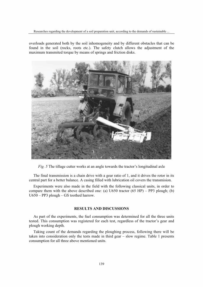
Researches regarding the development of a soil preparation unit, according to the demands of sustainable ...
139
overloads generated both by the soil inhomogeneity and by different obstacles that can be found in the soil (rocks, roots etc.). The safety clutch allows the adjustment of the maximum transmited torque by means of springs and friction disks.
Fig. 5 The tillage cutter works at an angle towards the tractor’s longitudinal axle
The final transmission is a chain drive with a gear ratio of 1, and it drives the rotor in its central part for a better balance. A casing filled with lubrication oil covers the transmision.
Experiments were also made in the field with the following classical units, in order to compare them with the above described one: (a) U650 tractor (65 HP) – PP3 plough; (b) U650 – PP3 plough – GS toothed harrow.
RESULTS AND DISCUSSIONS
As part of the experiments, the fuel consumption was determined for all the three units tested. This consumption was registered for each test, regardless of the tractor’s gear and plough working depth.
Taking count of the demands regarding the ploughing process, following there will be taken into consideration only the tests made in third gear – slow regime. Table 1 presents consumption for all three above mentioned units.
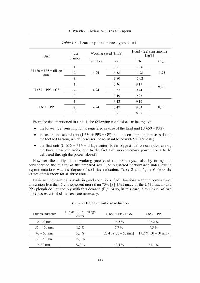
G. Paraschiv, E. Maican, S.-Ş. Biriş, S. Bungescu
140
Table 1 Fuel consumption for three types of units
Working speed [km/h] Hourly fuel consumption [kg/h]Unit Test
numbertheoretical real Chi Chm
1. 3,61 11,86
2. 3,58 11,98 U 650 + PP3 + tillage cutter
3.
4,24
3,60 12,02
11,95
1. 3,36 9,15
2. 3,27 9,24 U 650 + PP3 + GS
3.
4,24
3,49 9,22
9,20
1. 3,42 9,10
2. 3,47 9,03 U 650 + PP3
3.
4,24
3,51 8,85
8,99
From the data mentioned in table 1, the following conclusion can be argued:
• the lowest fuel consumption is registered in case of the third unit (U 650 + PP3);
• in case of the second unit (U650 + PP3 + GS) the fuel consumption increases due to the toothed harrow, which increases the resistant force with 50...150 daN;
• the first unit (U 650 + PP3 + tillage cutter) is the biggest fuel consumption among the three presented units, due to the fact that supplementary power needs to be delivered through the power take-off.
However, the utility of the working process should be analysed also by taking into consideration the quality of the prepared soil. The registered performance index during experimentations was the degree of soil size reduction. Table 2 and figure 6 show the values of this index for all three units.
Basic soil preparation is made in good conditions if soil fractions with the conventional dimension less than 5 cm represent more than 75% [3]. Unit made of the U650 tractor and PP3 plough do not comply with this demand (Fig. 6) so, in this case, a minimum of two more passes with disk harrows are necessary.
Table 2 Degree of soil size reduction
Lumps diameter U 650 + PP3 + tillage cutter U 650 + PP3 + GS U 650 + PP3
> 100 mm - 16,5 % 22,2 %
50 – 100 mm 1,2 % 7,7 % 9,5 %
40 – 50 mm 5,2 % 23,4 % (30 – 50 mm) 17,2 % (30 – 50 mm)
30 – 40 mm 15,6 %
< 30 mm 78,0 % 52,4 % 51,1 %
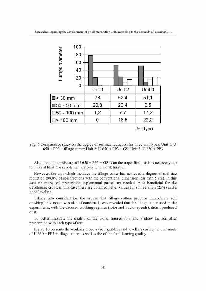
Researches regarding the development of a soil preparation unit, according to the demands of sustainable ...
141
020406080
100
Unit type
Lum
ps d
iam
eter
< 30 mm 78 52,4 51,130 - 50 mm 20,8 23,4 9,550 - 100 mm 1,2 7,7 17,2> 100 mm 0 16,5 22,2
Unit 1 Unit 2 Unit 3
Fig. 6 Comparative study on the degree of soil size reduction for three unit types: Unit 1: U 650 + PP3 + tillage cutter; Unit 2: U 650 + PP3 + GS; Unit 3: U 650 + PP3
Also, the unit consisting of U 650 + PP3 + GS is on the upper limit, so it is necessary too to make at least one supplementary pass with a disk harrow.
However, the unit which includes the tillage cutter has achieved a degree of soil size reduction (98,8% of soil fractions with the conventional dimension less than 5 cm). In this case no more soil preparation suplemental passes are needed. Also beneficial for the developing crops, in this case there are obtained better values for soil aeration (25%) and a good leveling.
Taking into consideration the argues that tillage cutters produce immoderate soil crushing, this aspect was also of concern. It was revealed that the tillage cutter used in the experiments, with the choosen working regimes (rotor and tractor speeds), didn’t produced dust.
To better illustrate the quality of the work, figures 7, 8 and 9 show the soil after preparation with each type of unit.
Figure 10 presents the working process (soil grinding and levelling) using the unit made of U 650 + PP3 + tillage cutter, as well as the of the final farming quality.

G. Paraschiv, E. Maican, S.-Ş. Biriş, S. Bungescu
142
Fig. 7 Tillage quality made withU 650 + PP3 + tillage cutter
Fig. 8 Tillage quality made withU 650 + PP3 + GS
Fig. 9 Tillage quality made withU 650 + PP3
Fig. 10 Working process withU 650 + PP3 + tillage cutter
CONCLUSIONS
As it was mentioned in the former chapter, the fuel consumption for the U 650 + PP3 + tillage cutter unit is higher than for the other two units. But, if the farming quality is considered, this unit if by far superior in comparison with the other two. In order to have the same quality with the other units, there are necessary multiple supplemetary passes that finally contribute to a higher fuel consumption.
Figure 11 shows a comparative study for different kind of units, from a fuel consumption point of view. The degree of soil grinding was considered the same for each unit, namely the farming quality is adequat for sowing.
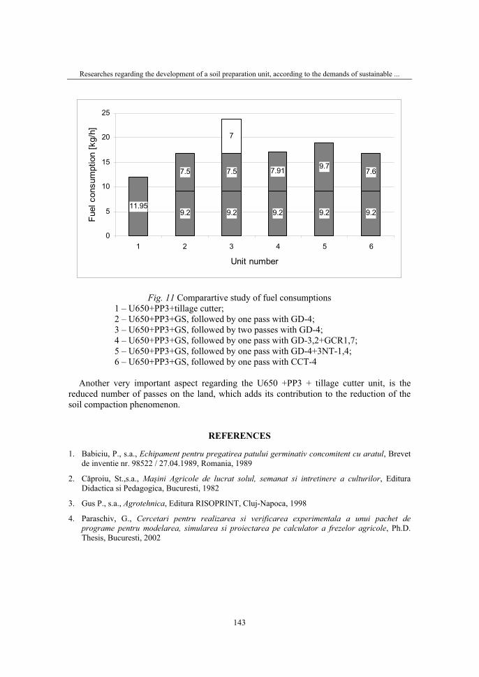
Researches regarding the development of a soil preparation unit, according to the demands of sustainable ...
143
11.959.2 9.2 9.2 9.2 9.2
7.5 7.5 7.91 9.77.6
7
0
5
10
15
20
25
1 2 3 4 5 6
Unit number
Fuel
con
sum
ptio
n [k
g/h]
Fig. 11 Comparartive study of fuel consumptions 1 – U650+PP3+tillage cutter;2 – U650+PP3+GS, followed by one pass with GD-4; 3 – U650+PP3+GS, followed by two passes with GD-4; 4 – U650+PP3+GS, followed by one pass with GD-3,2+GCR1,7; 5 – U650+PP3+GS, followed by one pass with GD-4+3NT-1,4; 6 – U650+PP3+GS, followed by one pass with CCT-4
Another very important aspect regarding the U650 +PP3 + tillage cutter unit, is the reduced number of passes on the land, which adds its contribution to the reduction of the soil compaction phenomenon.
REFERENCES
1. Babiciu, P., s.a., Echipament pentru pregatirea patului germinativ concomitent cu aratul, Brevet de inventie nr. 98522 / 27.04.1989, Romania, 1989
2. Căproiu, St.,s.a., Maşini Agricole de lucrat solul, semanat si intretinere a culturilor, Editura Didactica si Pedagogica, Bucuresti, 1982
3. Gus P., s.a., Agrotehnica, Editura RISOPRINT, Cluj-Napoca, 1998
4. Paraschiv, G., Cercetari pentru realizarea si verificarea experimentala a unui pachet de programe pentru modelarea, simularea si proiectarea pe calculator a frezelor agricole, Ph.D. Thesis, Bucuresti, 2002

36. Symposium "Actual Tasks on Agricultural Engineering", Opatija, Croatia, 2008.
145
36.
SIMPOZIJAKTUALNI ZADACIMEHANIZACIJE POLJOPRIVREDE
UDC631.431.73:633.11:635.076
Stručni radExpert paper
THE ANALYSIS OF SOIL COMPACTION INFLUENCE ON WHEAT YIELD ON HEADLANDS AND INNER PART
OF FIELDS L. SAVIN1, R. NIKOLIĆ1, M. SIMIKIĆ1, T. FURMAN1, M. TOMIĆ1 , S. ĐURIĆ1,
J. VASIN2
1University of Novi Sad, Faculty of Agriculture, Novi Sad, Dositeja Obradovića Sq. 8, 21000 Novi Sad, Serbia, e-mail: [email protected]
2Institute of Field and Vegetable Crops, Maksima Gorkog 30, 21000 Novi Sad, Serbia
SUMMARY
This paper shows the results of analysis of soil compaction influence on wheat yield on headland and inner part of a field, chemical and biological changes in soil. During the 5 years investigation, soil compaction at sowing was 30.56% greater on headland than in the inner part, while during harvest, there was an increase of 37.65% in soil compaction.
Large number of passages, which caused intensified soil compaction on head-lands, poor conditions for the root system development, and poor microbiological activities led to yield reduction, which was 31.55% in total mass and 26.39% in dry grain mass. Chemical analysis of soil on headland and in the inner part of a field showed higher humus concentration on headlands, due to poor microbiolo-gical activities.
Key words: headland, soil compaction, soil chemical properties, yield, wheat
INTRODUCTION
This paper shows the results of analysis of soil compaction influence on wheat yield on headland and inner part of a field. The tractor and mobile system motions can be divided into two groups: movement on the inner part of a field and movement on headlands. The both mentioned types of movement lead to soil compaction, but with different intensity, Ronai (1989) and Schwngart (1991). The movement of tractors and other mobile systems on headland result in greater soil compaction because of the slower motion during the turnings. The lower movement speeds allow soil to be subjected to the effects of normal pressure for a longer period, which enables its greater compaction. Besides lower speeds,
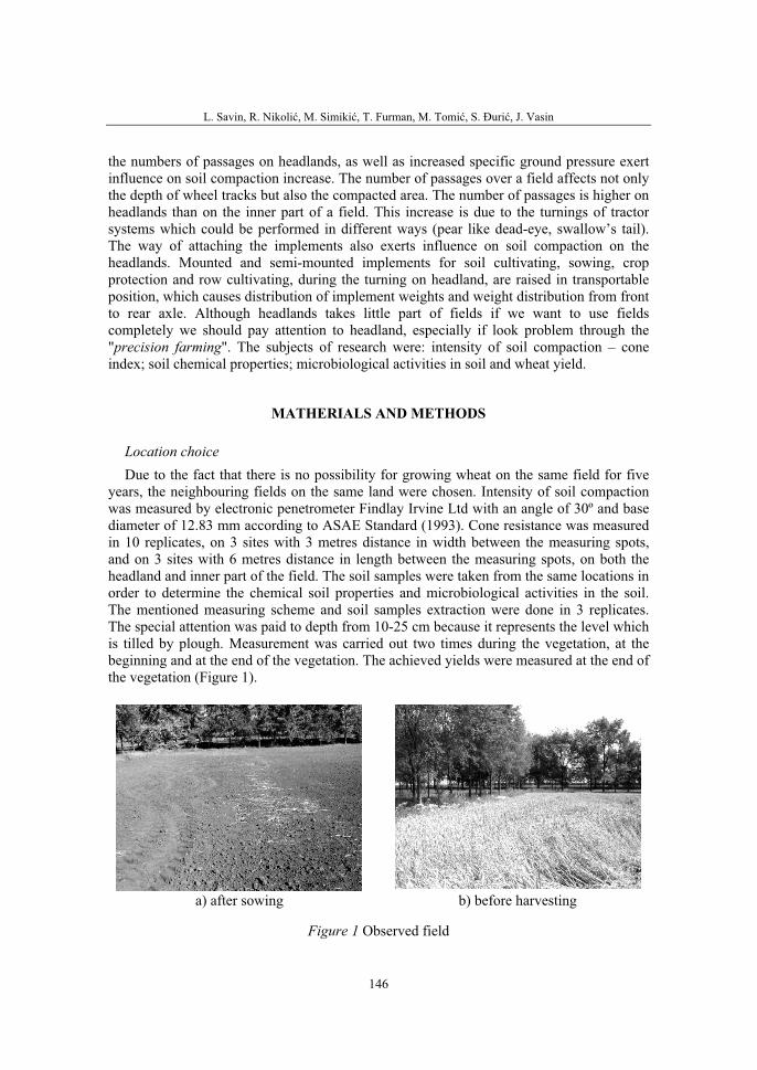
L. Savin, R. Nikolić, M. Simikić, T. Furman, M. Tomić, S. Đurić, J. Vasin
146
the numbers of passages on headlands, as well as increased specific ground pressure exert influence on soil compaction increase. The number of passages over a field affects not only the depth of wheel tracks but also the compacted area. The number of passages is higher on headlands than on the inner part of a field. This increase is due to the turnings of tractor systems which could be performed in different ways (pear like dead-eye, swallow’s tail). The way of attaching the implements also exerts influence on soil compaction on the headlands. Mounted and semi-mounted implements for soil cultivating, sowing, crop protection and row cultivating, during the turning on headland, are raised in transportable position, which causes distribution of implement weights and weight distribution from front to rear axle. Although headlands takes little part of fields if we want to use fields completely we should pay attention to headland, especially if look problem through the "precision farming". The subjects of research were: intensity of soil compaction – cone index; soil chemical properties; microbiological activities in soil and wheat yield.
MATHERIALS AND METHODS
Location choiceDue to the fact that there is no possibility for growing wheat on the same field for five
years, the neighbouring fields on the same land were chosen. Intensity of soil compaction was measured by electronic penetrometer Findlay Irvine Ltd with an angle of 30º and base diameter of 12.83 mm according to ASAE Standard (1993). Cone resistance was measured in 10 replicates, on 3 sites with 3 metres distance in width between the measuring spots, and on 3 sites with 6 metres distance in length between the measuring spots, on both the headland and inner part of the field. The soil samples were taken from the same locations in order to determine the chemical soil properties and microbiological activities in the soil. The mentioned measuring scheme and soil samples extraction were done in 3 replicates. The special attention was paid to depth from 10-25 cm because it represents the level which is tilled by plough. Measurement was carried out two times during the vegetation, at the beginning and at the end of the vegetation. The achieved yields were measured at the end of the vegetation (Figure 1).
a) after sowing b) before harvesting
Figure 1 Observed field
The analysis of soil compaction influence on wheat yield on headlands and inner part of fields
147
The experiment lasted 5 years - from 2003 to 2007 and the results were published by Jarak et al. (2004, 2005 and 2006), Nikolic et al. (2006), Savin et al. (2003 and 2004) and Simikic et al. (2005). In order to examine the headlands, fields next to the road were chosen so that the turning of tractor and mobile systems could be performed only on the field, thus forming the headland. The width of a headland was 12 m. The type of soil was chernozem calcareous on loess terrace.
Applied production technologyFor winter wheat production the tillage was conventional, done with ploughs. The same
agro technique was repeated during all researched years (Table 1). Pre culture was always soybean. During the research years, the same tractors, implements and harvester were used.
Table 1 Technology for wheat production
Tractor Implement No Field operation Power
(kW)Weight
(kg)Working width
(m)Weight
(kg)
1. Fertilizing 60 3900 18 312
2. Primary tillage 172 9220 2 2500
3. Secondary tillage and sowing 172 9220 4 989
4. Fertilizing 60 3900 18 312
5. Crop protection 60 3900 18 1508
6. Fertilizing 60 3900 18 312
7. Crop protection 60 3900 18 1508
8. Harvesting 216 6 11864 Four passages, 2 for supplementary feed and 2 for wheat protection, were made between sowing and harvesting.
Investigation of the soil chemical properties Laboratory analyses included the following parameters of soil fertility:
• pH value in soil suspension with potassium chloride (10 g : 25 cm3, determined potentiometrically),
• CaCO3 content – by the volumetric method, with a calcimeter after Scheibler.
• humus content – by the method of Tjurin;
• total content of nitrogen - by CHNS analyzer
• available phosphorus (extraction with ammonium lactate) - AL method; phosphorus content by the blue method in a spectrophotometer
• available potassium (extraction with ammonium lactate) - AL method; potassium content determined by the flame photometer

L. Savin, R. Nikolić, M. Simikić, T. Furman, M. Tomić, S. Đurić, J. Vasin
148
Investigation of the microbiological activities in soil Microbiological activity was investigated according to the total number of micro-
organisms, nitric bacteria and dehydrogenase activity. The number of micro-organisms was determined after sowing a rarified soil suspension on suitble supplementary feed. Total number of micro-organisms was determined according to the Poshon and Tardiux method (1963). Nitric bacteria occurence was determined on Fyodor dish by a method involving fertilizing drops (Anderson, 1965). The number of micro-organisms was determined for 1 gram of completely dry soil. Dehydrogenase activity was determined by spectrometric method according to Thalmannu (1968).
RESULTS
In 2006, in the sowing phase, cone index on headlands amounted 1.45 MPa, while in the inner part of a field, it was 1.05 MPa. Both results apply to a depth of 7-21 cm (Figure 2). The same measurements made before the harvest resulted in 1.42 MPa and 0.97 MPa, respectively for headlands and the inner part of the field.
0
0,5
1
1,5
2
2,5
3
3,5
4
4,5
0 10 20 30 40
Depth (cm)
Con
e in
dex
(MP
a)
Inner part of field Headland
0
0,5
1
1,5
2
2,5
3
3,5
4
4,5
0 5 10 15 20 25 30 35
Depth (cm)
Con
e ind
ex (M
Pa)
Inner part of field Headland
a) after sowing b) before harvesting
Figure 2 Intensity of soil compaction, 2006/2007
Cone index depends on soil moisture to a considerable extent. The greatest soil compact-ion on headlands occurred in 2002 and 2003 during harvesting, with an increase of 45.50%, whereas soil moisture was lowest, 9.62% (Table 2). The slightest difference in cone index, measured after sowing and before harvesting, was in 2006 and 2007, due to higher soil moisture before harvesting. Furthermore, the spring of 2007 was particularly rainy, resulting in high soil moisture at different depths and during harvesting. On average the cone index on headlands after sowing was 30.56% higher in comparison with the inner part of a field. The passages formed during spraying and fertilizing caused more intensive soil compaction on headlands, and it was 37.65% higher, compared with the remaining field area.
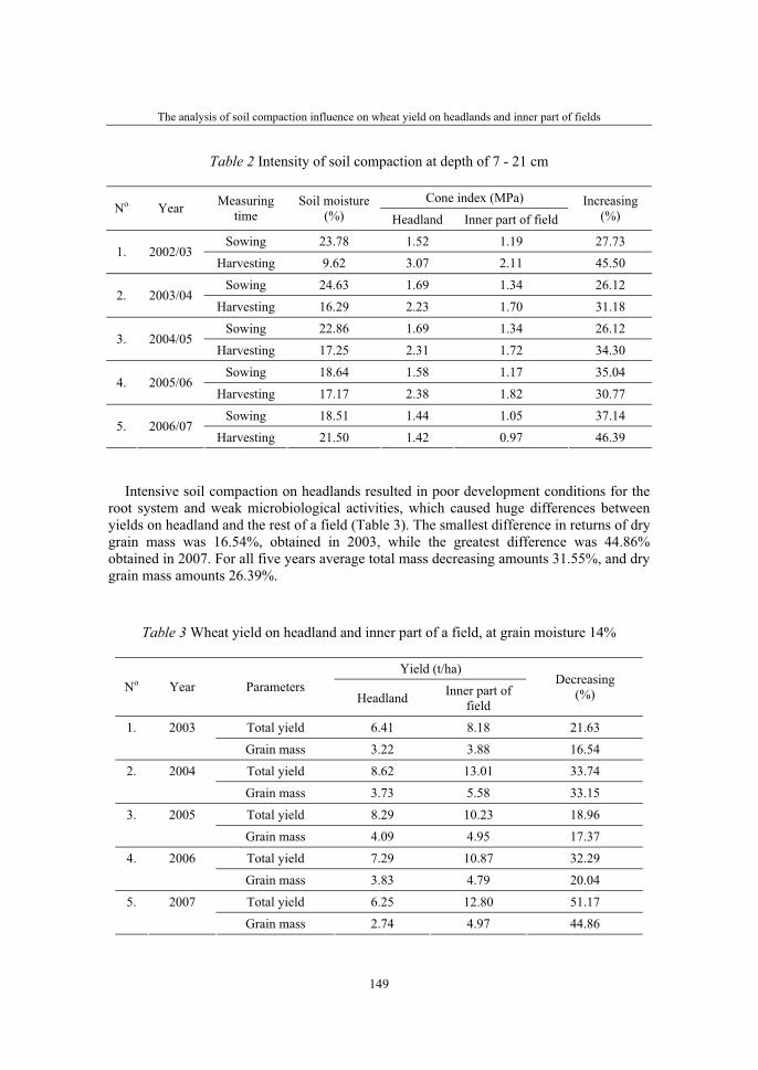
The analysis of soil compaction influence on wheat yield on headlands and inner part of fields
149
Table 2 Intensity of soil compaction at depth of 7 - 21 cm
Cone index (MPa) No Year Measuring
timeSoil moisture
(%) Headland Inner part of field Increasing
(%)
Sowing 23.78 1.52 1.19 27.73 1. 2002/03
Harvesting 9.62 3.07 2.11 45.50
Sowing 24.63 1.69 1.34 26.12 2. 2003/04
Harvesting 16.29 2.23 1.70 31.18
Sowing 22.86 1.69 1.34 26.12 3. 2004/05
Harvesting 17.25 2.31 1.72 34.30
Sowing 18.64 1.58 1.17 35.04 4. 2005/06
Harvesting 17.17 2.38 1.82 30.77
Sowing 18.51 1.44 1.05 37.14 5. 2006/07
Harvesting 21.50 1.42 0.97 46.39
Intensive soil compaction on headlands resulted in poor development conditions for the root system and weak microbiological activities, which caused huge differences between yields on headland and the rest of a field (Table 3). The smallest difference in returns of dry grain mass was 16.54%, obtained in 2003, while the greatest difference was 44.86% obtained in 2007. For all five years average total mass decreasing amounts 31.55%, and dry grain mass amounts 26.39%.
Table 3 Wheat yield on headland and inner part of a field, at grain moisture 14%
Yield (t/ha) No Year Parameters
Headland Inner part of field
Decreasing(%)
Total yield 6.41 8.18 21.63 1. 2003
Grain mass 3.22 3.88 16.54
Total yield 8.62 13.01 33.74 2. 2004
Grain mass 3.73 5.58 33.15
Total yield 8.29 10.23 18.96 3. 2005
Grain mass 4.09 4.95 17.37
Total yield 7.29 10.87 32.29 4. 2006
Grain mass 3.83 4.79 20.04
Total yield 6.25 12.80 51.17 5. 2007
Grain mass 2.74 4.97 44.86

L. Savin, R. Nikolić, M. Simikić, T. Furman, M. Tomić, S. Đurić, J. Vasin
150
Soil chemical properties were determined so that the influence of soil compaction on crop yield could be observed. In the case of wheat, the tested soil samples taken from different parts of the fields belong to the class of mild alkaline soils (Table 4), according to the pH value determined in soil suspension with KCl solution.
Table 4 Soil chemical properties
Year
2002/03 2003/04 2004/05 2005/06 2006/07 Soil chemical
propertiesLocation of the sample
Depthof the
sample(cm)
sowing harwesting sowing harwesting sowing harwesting sowing harwesting sowing harwesting
headland 10-25 7.33 7.46 7.46 6.85 7.40 7.54 7.41 7.50 7.43 7.68 in KCL
inner part 10-25 7.40 7.48 7.50 6.86 7.61 7.75 7.54 7.69 7.52 7.67
headland 10-25 8.46 8.22 8.35 7.58 8.38 8.34 8.58 8.57 8.41 8.41 pH
in H2Oinner part 10-25 8.57 8.44 8.46 7.86 8.48 8.50 8.66 8.62 8.44 8.53
headland 10-25 10.54 10.92 10.72 9.65 11.16 11.73 9.80 9.80 23.83 22.56 CaCO3
%inner part 10-25 10.72 11.34 14.16 11.75 11.61 11.87 10.21 10.21 27.78 24.07
headland 10-25 3.84 3.71 3.62 3.89 3.48 3.23 4.22 3.87 3.47 3.29 Humus
% inner part 10-25 3.50 3.41 3.74 3.35 3.26 3.18 4.04 3.75 3.45 3.32
headland 10-25 0.25 0.26 0.24 0.26 0.25 0.26 0.25 0.27 0.24 0.23 Total N %
inner part 10-25 0.266 0.27 0.26 0.23 0.25 0.26 0.27 0.26 0.23 0.21
headland 10-25 28.19 26.48 29.1 28.2 24.68 20.18 32.20 23.13 23.83 21.4 AL-P2O5
mg/100 g inner part 10-25 25.20 21.72 24.7 22.1 20.21 17.24 29.13 21.83 22.4 20.06
headland 10-25 20.82 17.28 17.7 16.4 22.18 20.36 27.57 24.53 14.77 12.87 AL-K2Omg/100 g
inner part 10-25 17.70 15.93 22.3 14.5 18.41 14.61 25.97 18.50 11.70 8.24
According to the CaCO3 level in the soil, the soil samples belong to the class of carbo-nate-rich soils. The soil samples taken from the ploughed layer (10-25 cm) of headlands contain higher level of humus (a class of humus soils) in comparison to those taken from the central part of the field (a class of low humus soils). The average content of humus on headlands during five-year investigation amounts 3.66%, while in the inner part of fields is smaller and amounts 3.50%. This could be related to greater soil compaction on headlands which contributes to the reduction of microbiological activity and intensity of humus mineralization. According to the total level of nitrogen, surface samples belong to the class of soil with high level. During the five-year investigation, the average content of total N on headlands and in the inner part of fields was the same and amounted 0.25%.

The analysis of soil compaction influence on wheat yield on headlands and inner part of fields
151
Values of the tested macronutrient content – phosphorus and potassium, show that the tested soils on headlands belong to the class with high content. Samples from the central part of the field belong to the class with high level of phosphorus and extremely high level of potassium. The average content of phosphorus on headlands amounts 25.74 mg/100g, while in the inner part of fields is smaller and amounts 22.46 mg/100g. The average content of potassium on headlands amounts 19.45 mg/100g, while in the inner part of fields is smaller and amounts 16.79 mg/100g. The lowest potassium content was measured in 2006 and 2007, which could be explained by poor fertilization during previous years.
Micro-organisms are live constituents of the soil, but also the indicators of favourable soil conditions for agricultural production. In these researches the values of microbiological parameters point to substantial number and activity of micro-organisms in the tested soil samples, what is understandable for the tested type of the soil (chernozem calcareous). However, the differences can be observed between the soil samples taken from the headland and those taken from the inner part of the field. The total number of micro-organisms and nitric bacteria was higher in the inner part of the field, which could be explained by deteriorated structure and weak soil aeration on headlands, caused by frequentstepping (Table 5). The average number of micro-organisms on headlands amounts 7.92 TN (log No), while in the inner part of fields is higher and amounts 8.11 TN (log No). The average number of nitric bacteria on headlands amounts 3.48 Azb (log No), while in the inner part of fields is higher and amounts 3.55 Azb (log No).
Table 5 Microbiological soil structure
Year
2003/04 2004/05 2005/06 2006/07 Microbiological
soil structure Location of the sample
Depth of the
sample(cm)
sowing harvesting sowing harvesting sowing harvesting sowing harvesting
headland 10-25 7.94 7.95 9.01 8.55 7.86 7.44 7.64 6.93 Total number of microorganisms– TN (log No) inner part 10-25 8.28 8.34 9.29 8.60 8.32 7.68 7.70 7.11
headland 10-25 3.14 2.78 3.39 3.44 4.50 4.26 2.98 3.39 Number of nitric bacteria – Azb
(log No) inner part 10-25 3.13 2.97 3.41 3.44 4.51 4.25 3.07 3.65
headland 10-25 1462 850 1463 1022 1320 1190 890 960 Dehydrogenase activity (mg TPF
g-1 land) inner part 10-25 1414 1075 1414 1366 1314 1200 1020 1130

L. Savin, R. Nikolić, M. Simikić, T. Furman, M. Tomić, S. Đurić, J. Vasin
152
CONCLUSIONS
On the basis of the research carried out, following conclusions can be formulated:
• an average increasing of soil compaction on headlands with regard to the rest of a field was 30.56% after sowing and 37.65% before harvesting;
• yield decrease on headlands was approximately 26% compared with the inner part of a field;
• soil samples from headlands contain higher level of humus (a class of humus soils) in comparison with those taken from the inner part of the field (a class of low humus soils), which is explained by greater soil compaction on headlands, reduction of microbiological activity and intensity of humus mineralization;
• number of the tested micro-organism groups is high and typical for the tested type of soil. Total number of micro-organisms and nitric bacteria was higher in the inner part of the field, which could be explained by deteriorated structure and weak soil aeration on headlands.
• subsoiler should be used on headlands for better soil aeration.
The analysis of soil compaction influence on wheat yield on headlands and inner part of fields
153
REFERENCES
1. Anderson, G.R. ,1965. : Ecology of Azotobacter in soil of the palouse region I.Occurence. Soil Sci., 86, 57 –65.
2. ASAE Standard, Soil cone penetrometer, 1993.
3. Jarak M., Đurić S., Najdenovska O. (2004). The effect of compacting of soil on the microbiological activity under different plants. Tractors i power machines, Vol. 9, No. 4, p. 88-92.
4. Jarak M., Furman T., Gligorić R., Đurić S., Savin L., Jeličić Z. (2005). Soil properties and wheat and maize yield on headland. Tractors i power machines, Vol. 10, No. 3, p. 98-103.
5. Jarak M. e Hajnal T. (2006). The total number of microorganisms, number of fungi and azotobacter in compacted and noncompacted soil. Tractors i power machines, Vol. 11, No. 5, p. 37-40.
6. Nikolić R., Savin L., Furman T., Tomić M., Gligorić R., Simikić M., Sekulić P., Vasin J., KekićM., Bertok Z. (2006). The influence of compaction on changes in soil and maize, sunflower, soybean and sugar beet yield. Tractors i power machines, Vol. 11, No. 5, p. 25-31.
7. Pochon, J. and Tardieux, P. (1962 ) : Techniques d analzse en microbiologie du sol, Paris.
8. Ronai Đ. (1989). The influence of tyre design on soil compaction of agricultural land. Agrotehničar, Vol. 25, No. 7/8, p. 37-39.
9. Savin L., Furman T., Vasin J., Hadžić V. (2003). The analysis of influence of soil compaction on maize and wheat yield on headlands. Tractors i power machines, Vol. 8, No. 4, p. 145-149.
10. Savin L., Furman T., Vasin J., Hadžić V. (2004). The analysis of influence of soil compaction on maize and wheat yield on headlands. Tractors i power machines, Vol. 9, No. 4, p. 93-98.
11. Schwngart H. (1991): Measurement of contact area, contact preasure and compaction under tires in soft soil. Journal of Teramechanics, Vol. 28, No. 4, p. 309-318.
12. Simikić M., Nikolić R., Savin L., Hadžić V., Sekulić P., Jarak M., Furman T., Tomić M., Vasin J. (2005). The influence of tractors and mobile systems on contents of fertilizers in soil. Tractors i power machines, Vol. 10, No. 1, p. 21-98.
13. Thalmann, A. (1968): Zur Methodikde Bestimmung der Dehydrogenase aktivitat im Boden mittels Triphenyltetrazoliumchlorid (TTC ). Landwirsch. Forsch., 21, 249 – 257.

36. Symposium "Actual Tasks on Agricultural Engineering", Opatija, Croatia, 2008.
155
36.
SIMPOZIJAKTUALNI ZADACIMEHANIZACIJE POLJOPRIVREDE
UDK631.17:631.51:633.11
Stručni radExpert paper
POLJOPRIVREDNA MEHANIZACIJA U PROIZVODNJI PŠENICE PRI RAZLIČITIM SUSTAVIMA OBRADE TLA BRANIMIR BAGARIĆ, VLADIMIR ZEBEC, MIRKO KUFNER, ROBERT ZIMMER
Poljoprivredni fakultet u Osijeku, Sveučilište Josipa Jurja Strossmayera u Osijeku,Trg sv. Trojstva 3, 31000 Osijek, [email protected], [email protected]
SAŽETAK
Na pokusnoj parceli pilot projekta „Znanjem u proizvodnju hrane“ radne površine 9 x 1800 m2 (16200 m2) postavljen je pokus s 3 varijante obrade tla konvencionalna, reducirana i no-tillage u 3 repeticije. Predusjev je šećerna repa. Obrada tla i priprema za sjetvu obavljene su 4. listopada 2006. godine. Oranje je obavljeno lemešnim plugom Regent-Saturn 700 SCX priključenim na traktor snage 129 kW. Tanjuranje je obavljeno tanjuračom OLT-Neretva, priključenomna traktor snage 136 kW.Prema rezultatima analize tla i pretkulturi aplicirano je granulirano mineralno gnojivo UREA. Sjetva varijateta Mura s podešenom normom od 197 kg obavljena je za sve repeticije i varijante sijačicom John Deere 750 A.. Radni zahvat sijačice je 6m, priključena na traktor snage 136 kW, s pogonom na sva četiri kotača s udvojenim pneumaticima. Žetva su obavili kombajni domaće proizvodnje Đuro Đaković tip Hydroliner 36.20 opremljeni žitnim adapterom radnog zahvata 5,5 m. Najmanji prinos od 3,103 t ha-1 izmjeren je na no-tillage varijanti obrade tla bez aplikacije dušika, a najviši od 5,078 t ha-1
ostvaren je na konvencionalnoj varijanti obrade tla sa aplikacijom dušika u dozi od 140 kg ha-1.
Ključne riječi: konvencionalna, reducirana, no tillage, obrada tla, prinos
UVOD
Pšenica je u Republici Hrvatskoj najzastupljenija žitarica. U 2006 godini ukupne zasija-ne površine pod pšenicom iznosile su 177.403 hektara (6). Od toga je 134.090 zasijano od strane OPG, dok su pravne osobe 2006. godine pod pšenicom imale zasijano 43.313 hektara. Ovaj znanstveno-istraživački rad rezultat je Pilot projekta „Znanjem u proizvodnju hrane“. Tradicionalna praksa u obradi tla temelji se na različitim zahvatima osnovne obrade kojima se tlo dovodi u grudasto stanje i dalje se zahvatima predsjetvene pripreme usitnjava, ponovo zbija i ravna (1, 3). Moderniji pristup, odnosno uvođenje reducirane obrade tla u
B. Bagarić, V. Zebec, M. Kufner, R. Zimmer
156
tehnologiju proizvodnje strnih žitarica i okopavina sve se više primjenjuje u RH (4, 5). Neki autori govore i o trećoj zoni, koja bi bila rezervirana za prolaze transportnih sredstava ili kotača traktora pri obavljanju svih zahvata u uzgoju kultura. To su tzv. "stalni tragovi" koji bi bitno smanjili gaženja po tlu namjenjenom za normalan rast i razvoj usjeva.
Tradicionalnoj obradi tla sve više se nameću:- novija dostignuća znanosti o tlu - dostignuća na polju poljodjelske tehnike (strojevi i oruđa)- zahtjevi prakse za pojednostavljenjem obrade tla
Cilj istraživanja je utvrditi mogućnosti primjene različitih sustava obrade tla, te utvrditi agrotehničke razlike između varijanti i njihov utjecaj na prinos i ekonomske pokazatelje (2).
MATERIJAL I METODE
Istraživanja na ozimoj pšenici obavljena su na proizvodnim poljima «Žito» d.d., „Agrar-Novi d.o.o., Antunovac. Istraživanje se temeljilo na tri različita sustava obrade tla i tri razine opskrbljenosti dušikom. Dimenzije osnovne parcele obrade tla je 1800m2(18m x 100m), a osnovna gnojidbena parcela je 600m2 (6m x 100m). Pokus je izveden u tri repeticije slučajnog rasporeda parcela. Repeticije su odjeljene zaštitnim pojasevima širine 20 m, radi izbjegavanja gaženja pokusnih parcelica prilikom rada agregata. Ukupna površina obuhvatila je 4 ha (tretmani obrade tla + zaštitni pojasevi).
Sa istraživane površine uzeti su uzorci tla za uobičajene analize radi utvrđivanja općihkarakteristika hranidbenog potencijala tla. Na temelju rezultata kemijske analize utvrđenoje kako je tlo zadovoljavajuće kvalitete (humus, pH) te da sadrži dovoljne količine P i K koji će biti potrebni pšenici u nadolazećoj vegetaciji. Kao predusjev ozimoj pšenici bila je šećerna repa što je bila otegotna okolnost s obzirom na zbijenost tla (posljedica korištenja teške mehanizacije pri vađenju šećerne repe). Gnojidba usjeva je obavljena u više obroka, i to: u jesen prije obrade tla i u prihranama u proljeće. Gnojidbeni tretmani temeljili su se na dvije razine opskrbljenosti dušikom (140 kg čistog N ha-1 i 80 kg čistog N ha-1) uz kontrolu bez aplikacije dušičnih gnojiva. Vaganje uroda obavljeno je stacionarnom vagom na ekonomiji tvrtke Žito d.d. Agrar-Novi d.o.o., Antunovac. Izvor meteoroloških podataka je Hrvatska kontrola zračne plovidbe d.o.o. Zagreb Podružnica Osijek Odjel zrakoplovne meteorologije. Obrada tla i priprema za sjetvu obavljene su 4. listopada 2007. godine. Varijante obrade tla bile su slijedeće:
OranjeOranje je obavljeno lemešnim plugom tipa Regent Saturn 700 SCX priključenim na
traktor John Deere 7810 snage 129 kW s pogonom na sva četiri kotača, godina proizvodnje 1998, dimenzije pneumatika 18.4 R42 i 16.9 R28. Na operaciju oranja utjecali su faktor klimatskih čimbenika i pretkultura. Šećerna repa kao pretkultura s obzirom na broj prohoda u samoj operaciji vađenja repe je nepovoljno utjecala na stanje zbijenosti tla, što je uz nepovoljne klimatske uvjete (vrlo niska količina oborina) bitno otežala i utjecala na samu

Poljoprivredna mehanizacija u proizvodnji pšenice pri različitim sustavima obrade tla
157
operaciju oranja. Podešenost pluga: horizontalno dobro, vertikalno loše (mali kut odbaci-vanja čestice). Slaganje mekote dobar, čistoća brazde loša.
Tablica 1 Varijante obrade tla, tehnološke operacije i termini obavljanja
Varijanta obrade tla Tehnološka operacija Datum rada Oranje 4. listopada 2006.
Tanjuranje 4. listopada 2006 KonvencionalnaSjetva 10. listopada 2006
Tanjuranje-višekratno 4. listopada 2006 Reducirana
Sjetva 10. listopada 2006 No-tillage Sjetva 10. listopada 2006
Dubina oranja: s obzirom na izmjerene vrijednosti dubine oranja tla ova operacija pripada kategoriji dubokog oranja tla.
Brzina oranja: s obzirom na uvjete prosječna brzina oranja iznosila je 6,5 km h-1 što predstavlja optimum. Širina oranja: radni zahvat jednog plužnog tijela iznosio je 60 cm, što obzirom n podešenost pluga iznosi 240 cm u jednom prohodu.
Tablica 2 Dubina oranja (cm)
Varijanta 2 Varijanta 6 Varijanta 9
31, 32, 30, 33, 31 31, 33.5, 33, 30, 32.5 33, 33, 33, 31, 31
TanjuranjeTanjuranje je obavljeno tanjuračom OLT tip Neretva 64 (zahvat=6,8 m, ø56 cm, razmak
tanjura 22 cm), priključenom na traktor John Deere 8200 snage 136 kW, s pogonom na sva četiri kotača i udvojenim stražnjim pneumaticima (dimenzije pneumatika 20.8R42 4X i 16.9 R30), godina proizvodnje 1998,. Traktor je imao 4070 radnih sati, a prosječnapotrošnja goriva pri ovoj operaciji prema ugrađenom uređaju je bila oko 22 l h-1. Operacija tanjuranja na pokusu: zapažena je potrošenost prednjih tanjura na tanjurači. Obavljena su 2 prohoda na svim parcelama. Zbog stanja vlage u tlu i pretkulture, operacija je u prvom prohodu bila znatno otežana.
Raspodjeljivanje umjetnog gnojiva Ova tehnološka operacija jednaka je za sve varijante obrade tla. Raspodjela gnojiva
obavljena je u 3 faze. Osnovna gnojidba obavljena je 2. listopada 2006. Prema rezultatima analize tla i pretkulturi aplicirano je granulirano mineralno gnojivo UREA. Prva prihrana obavljena je 22. veljače 2007. Prema postavkama pokusa na dušik aplicirano je granulirano mineralno gnojivo KAN u različitim dozama po ha. Obje prihrane obavljene su centrifugal-
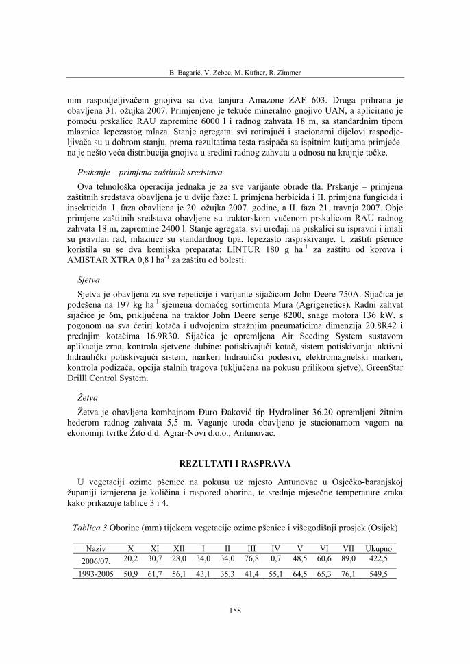
B. Bagarić, V. Zebec, M. Kufner, R. Zimmer
158
nim raspodjeljivačem gnojiva sa dva tanjura Amazone ZAF 603. Druga prihrana je obavljena 31. ožujka 2007. Primjenjeno je tekuće mineralno gnojivo UAN, a aplicirano je pomoću prskalice RAU zapremine 6000 l i radnog zahvata 18 m, sa standardnim tipom mlaznica lepezastog mlaza. Stanje agregata: svi rotirajući i stacionarni dijelovi raspodje-ljivača su u dobrom stanju, prema rezultatima testa rasipača sa ispitnim kutijama primjeće-na je nešto veća distribucija gnojiva u sredini radnog zahvata u odnosu na krajnje točke.
Prskanje – primjena zaštitnih sredstava Ova tehnološka operacija jednaka je za sve varijante obrade tla. Prskanje – primjena
zaštitnih sredstava obavljena je u dvije faze: I. primjena herbicida i II. primjena fungicida i insekticida. I. faza obavljena je 20. ožujka 2007. godine, a II. faza 21. travnja 2007. Obje primjene zaštitnih sredstava obavljene su traktorskom vučenom prskalicom RAU radnog zahvata 18 m, zapremine 2400 l. Stanje agregata: svi uređaji na prskalici su ispravni i imali su pravilan rad, mlaznice su standardnog tipa, lepezasto rasprskivanje. U zaštiti pšenice koristila su se dva kemijska preparata: LINTUR 180 g ha-1 za zaštitu od korova i AMISTAR XTRA 0,8 l ha-1 za zaštitu od bolesti.
SjetvaSjetva je obavljena za sve repeticije i varijante sijačicom John Deere 750A. Sijačica je
podešena na 197 kg ha-1 sjemena domaćeg sortimenta Mura (Agrigenetics). Radni zahvat sijačice je 6m, priključena na traktor John Deere serije 8200, snage motora 136 kW, s pogonom na sva četiri kotača i udvojenim stražnjim pneumaticima dimenzija 20.8R42 i prednjim kotačima 16.9R30. Sijačica je opremljena Air Seeding System sustavom aplikacije zrna, kontrola sjetvene dubine: potiskivajući kotač, sistem potiskivanja: aktivni hidraulički potiskivajući sistem, markeri hidraulički podesivi, elektromagnetski markeri, kontrola podizača, opcija stalnih tragova (uključena na pokusu prilikom sjetve), GreenStar Drilll Control System.
ŽetvaŽetva je obavljena kombajnom Đuro Đaković tip Hydroliner 36.20 opremljeni žitnim
hederom radnog zahvata 5,5 m. Vaganje uroda obavljeno je stacionarnom vagom na ekonomiji tvrtke Žito d.d. Agrar-Novi d.o.o., Antunovac.
REZULTATI I RASPRAVA
U vegetaciji ozime pšenice na pokusu uz mjesto Antunovac u Osječko-baranjskojžupaniji izmjerena je količina i raspored oborina, te srednje mjesečne temperature zraka kako prikazuje tablice 3 i 4.
Tablica 3 Oborine (mm) tijekom vegetacije ozime pšenice i višegodišnji prosjek (Osijek)
Naziv X XI XII I II III IV V VI VII Ukupno 2006/07. 20,2 30,7 28,0 34,0 34,0 76,8 0,7 48,5 60,6 89,0 422,5
1993-2005 50,9 61,7 56,1 43,1 35,3 41,4 55,1 64,5 65,3 76,1 549,5
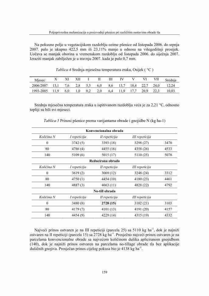
Poljoprivredna mehanizacija u proizvodnji pšenice pri različitim sustavima obrade tla
159
Na pokusno polje u vegetacijskom razdoblju ozime pšenice od listopada 2006. do srpnja 2007. palo je ukupno 422,5 mm ili 23,11% manje u odnosu na višegodišnji prosijek. Uočava se manjak oborina u vremenskom razdoblju od listopada 2006. do siječnja 2007. Izraziti manjak zabilježen je u travnju 2007. kada je palo 0,7 mm.
Tablica 4 Srednja mjesečna temperatura zraka, Osijek ( °C )
Mjesec X XI XII I II III IV V VI VII Srednja2006/2007 13,1 7,6 2,8 5,5 6,0 8,6 13,7 18,4 22,7 24,0 12,24 1993-2005 11,9 6,0 1,0 0,2 2,0 6,4 11,9 17,7 20,9 22,3 10,03
Srednja mjesečna temperatura zraka u ispitivanom razdoblju veća je za 2,21 °C, odnosno topliji su bili svi mjeseci.
Tablica 5 Prinosi pšenice prema varijantama obrade i gnojidbe N (kg ha-1)
Konvencionalna obrada Količina N I repeticija II repeticija III repeticija
0 3742 (5) 3393 (18) 3298 (27) 3478
80 4786 (4) 4455 (16) 4358 (26) 4533
140 5109 (6) 5015 (17) 5110 (25) 5078
Reducirana obrada Količina N I repeticija II repeticija III repeticija
0 3619 (2) 3069 (12) 3248 (24) 3312
80 4750 (1) 4454 (10) 4180 (23) 4461
140 4887 (3) 4663 (11) 4828 (22) 4792
No-till obrada Količina N I repeticija II repeticija III repeticija
0 3480 (8) 2728 (15) 3102 (21) 3103
80 4179 (7) 4101 (13) 4191 (20) 4157
140 4454 (9) 4229 (14) 4315 (19) 4332
Najveći prinos ostvaren je na III repeticiji (parcela 25) sa 5110 kg ha-1, dok je najniži ostvaren na II repeticiji (parcela 15) sa 2728 kg ha-1. Prosječno najveći prinos ostvaren je na parcelama konvencionalne obrade sa najvećom količinom dušika apliciranom gnojidbom (140), dok je najniži prinos ostvaren na parcelama no-tillage obrade tla bez aplikacije dušičnih gnojiva. Prosječan prinos cijelog pokusa bio je 4138 kg ha-1.
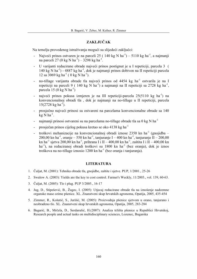
B. Bagarić, V. Zebec, M. Kufner, R. Zimmer
160
ZAKLJUČAK
Na temelju provedenog istraživanja mogući su slijedeći zaključci:- Najveći prinos ostvaren je na parceli 25 ( 140 kg N ha-1) – 5110 kg ha-1, a najmanji
na parceli 27 (0 kg N ha-1) – 3298 kg ha-1.- U varijanti reducirane obrade najveći prinos postignut je u I repeticiji, parcela 3 (
140 kg N ha-1) - 4887 kg ha-1, dok je najmanji prinos dobiven na II repeticiji parcela 12 sa 3069 kg ha-1 ( 0 kg N ha-1).
- no-tillage varijanta obrade tla najveći prinos od 4454 kg ha-1 ostvarila je na I repeticiji na parceli 9 ( 140 kg N ha-1) a najmanji na II repeticiji sa 2728 kg ha-1,parcela 15 (0 kg N ha-1)
- najveći prinos pokusa izmjeren je na III repeticiji-parcela 25(5110 kg ha-1) na konvencionalnoj obradi tla , dok je najmanji na no-tillage u II repeticiji, parcela 15(2728 kg ha-1).
- prosječno najveći prinosi su ostvareni na parcelama konvencionalne obrade sa 140 kg N ha-1.
- najmanji prinosi ostvareni su na parcelama no-tillage obrade tla sa 0 kg N ha-1
- prosječan prinos cijelog pokusa kretao se oko 4138 kg ha-1
- troškovi mehanizacije na konvencionalnoj obradi iznose 2350 kn ha-1 (gnojidba – 200,00 kn ha-1, oranje – 550 kn ha-1, tanjuranje I – 400 kn ha-1, tanjuranje II – 200,00 kn ha-1 sjetva 200,00 kn ha-1, prihrana I i II – 400,00 kn ha-1, zaštita I i II – 400,00 kn ha-1), na reduciranoj obradi troškovi su 1800 kn ha-1 (bez oranja), dok je iznos troškova na no-tillage iznosio 1200 kn ha-1 (bez oranja i tanjuranja).
LITERATURA
1. Čuljat, M. (2001): Tehnika obrade tla, gnojidbe, zaštite i sjetve. PUP, 1/2001., 25-26
2. Swalow A. (2003): Yields are the key to cost control. Farmer's Weckly, 11/2003., vol. 139, 60-63.
3. Čuljat, M. (2005): Tlo i plug. PUP 3/2005., 16-17
4. Jug, D., Stipešević, B., Žugec, I. (2005): Utjecaj reducirane obrade tla na iznošenje nadzemne organske mase ozime pšenice. XL. Znanstveni skup hrvatskih agronoma, Opatija, 2005, 435-454
5. Zimmer, R., Košutić, S., Jurišić, M. (2005): Proizvodnja pšenice sjetvom u orano, tanjurano i neobrađeno tlo. XL. Znanstveni skup hrvatskih agronoma, Opatija, 2005, 283-284
6. Bagarić, B., Mrčela, D., Serdarušić, H.(2007): Analiza tržišta pšenice u Republici Hrvatskoj, Research people and actual tasks on multidisciplinary sciences, Lozenec, Bugarska
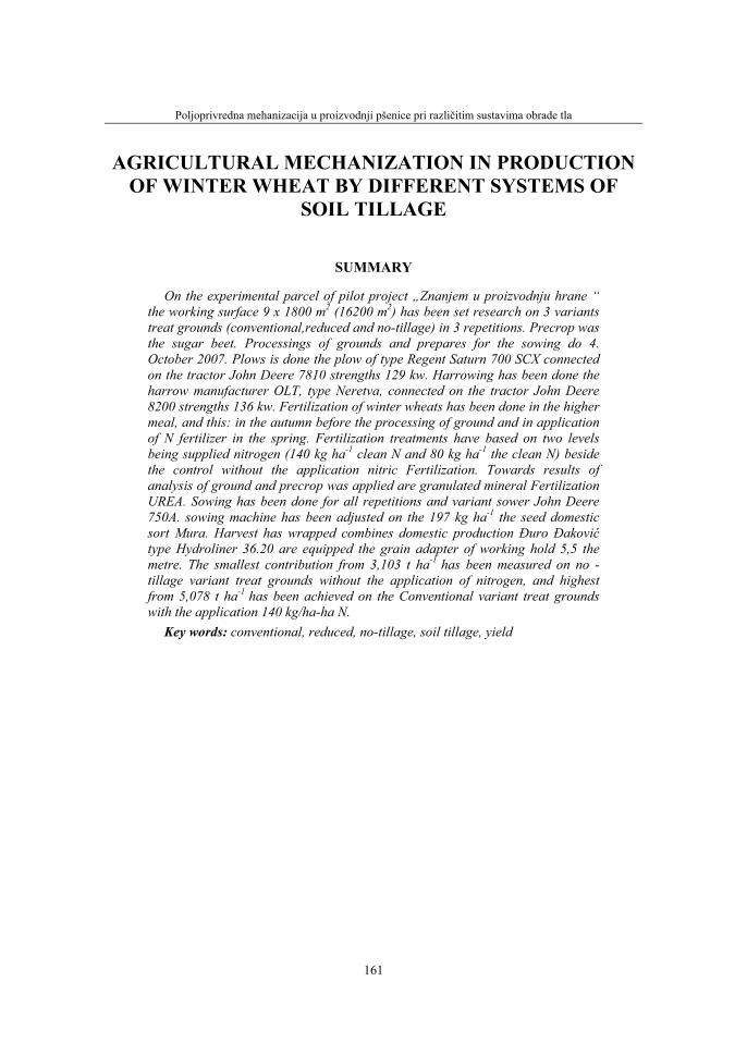
Poljoprivredna mehanizacija u proizvodnji pšenice pri različitim sustavima obrade tla
161
AGRICULTURAL MECHANIZATION IN PRODUCTION OF WINTER WHEAT BY DIFFERENT SYSTEMS OF
SOIL TILLAGE
SUMMARY
On the experimental parcel of pilot project „Znanjem u proizvodnju hrane “ the working surface 9 x 1800 m2 (16200 m2) has been set research on 3 variants treat grounds (conventional,reduced and no-tillage) in 3 repetitions. Precrop was the sugar beet. Processings of grounds and prepares for the sowing do 4. October 2007. Plows is done the plow of type Regent Saturn 700 SCX connected on the tractor John Deere 7810 strengths 129 kw. Harrowing has been done the harrow manufacturer OLT, type Neretva, connected on the tractor John Deere 8200 strengths 136 kw. Fertilization of winter wheats has been done in the higher meal, and this: in the autumn before the processing of ground and in application of N fertilizer in the spring. Fertilization treatments have based on two levels being supplied nitrogen (140 kg ha-1 clean N and 80 kg ha-1 the clean N) beside the control without the application nitric Fertilization. Towards results of analysis of ground and precrop was applied are granulated mineral Fertilization UREA. Sowing has been done for all repetitions and variant sower John Deere 750A. sowing machine has been adjusted on the 197 kg ha-1 the seed domestic sort Mura. Harvest has wrapped combines domestic production Đuro Đakovićtype Hydroliner 36.20 are equipped the grain adapter of working hold 5,5 the metre. The smallest contribution from 3,103 t ha-1 has been measured on no -tillage variant treat grounds without the application of nitrogen, and highest from 5,078 t ha-1 has been achieved on the Conventional variant treat grounds with the application 140 kg/ha-ha N.
Key words: conventional, reduced, no-tillage, soil tillage, yield

36. Symposium "Actual Tasks on Agricultural Engineering", Opatija, Croatia, 2008.
163
36.
SIMPOZIJAKTUALNI ZADACIMEHANIZACIJE POLJOPRIVREDE
UDK631.53.041:633.15
Prethodno priopćenjePreliminary communication
EKONOMSKI UČINKI DIREKTNE SETVE KORUZE M. SAGADIN, M. LEŠNIK, S. VAJS, M. LAKOTA, D. STAJNKO,
B. MURŠEC, P. VINDIŠ
Fakulteta za kmetijstvo, Vrbanska 30, SI-2000 Maribor, Slovenija e-mail: [email protected]
POVZETEK
V prispevku so predstavljeni rezultati in izsledki primerjalnega poljskega poskusa direktne setve koruze (Zea mays L.) hibrida Unixx Duo, posejane v travinje brez predhodne obdelave tal (no-tillage) in v konvencionalno pripravlje-na tla. Poskus se je izvajal na dveh ločenih lokacijah. Setev je bila izvedena s štirivrstno nošeno pnevmatsko sejalnico Monosem NX. Sejalnica je namenjena za direktno in konvencionalno setev z natančnim odlaganjem semena in dozatorji za mineralno gnojilo. Analiza rezultatov pridelkov zelene mase in suhe snovi ne kaže statistično značilnih razlik, medtem ko analiza stroškov obdelave, kaže velike prihranke pri direktni setvi koruze.
Ključne besede: direktna setev, konvencionalna obdelava tal, sejalnice za presledno setev, pridelek, koruza, stroški obdelave tal
UVOD
Vsakoletno padanje odkupnih cen kmetijskih pridelkov glede na cene kmetijskega repromateriala, vzpodbuja tako pridelovalce kot strokovnjake k uvajanju novih tehnologij, ki zmanjšujejo stroške pridelave, z zmanjševanjem porabe energije in delovnega časa.
Direktna setev brez obdelave tal se v svetu uporablja že vrsto let, še posebej v ZDA, kjer se na ta način sejejo različne poljedelske kulture na več kot 15 milijonih hektarjev kmetijskih površin. Ta način pridelave se počasi širi tudi v Evropo (Zimmer 1997). Tehnologija direktne setve je večini slovenskih pridelovalcev slabo poznana. Maloštevilni poskusi uvajanja so se večinoma končali neuspešno. Zaradi slabega poznavanja tehnologije, predvsem pa zaradi uporabe neustreznih sejalnic, je prihajalo do slabega vznika posejanih poljščin in posledično do nadpovprečne zapleveljenosti in nizkih pridelkov. Posledica tega je nenaklonjenost do uvajanja vseh novih tehnologij pridelovanja. Velika večina površin se še vedno obdeluje na konvencionalni način, reducirajoča obdelava se uvaja počasi, direktno setev pa se uporablja le pri dosejavanju travno – deteljnih mešanic v travno rušo.

M. Sagadin, M. Lešnik, S. Vajs, M. Lakota, D. Stajnko, B. Muršec, P. Vindiš
164
Avtorji navajajo primerjave različnih načinov obdelave tal, pri katerih so količinepridelkov zelo različne. Bayhan in sod. (2006) podaja zanimivo študijo petih načinov obdelave tal in direktne setve, kjer slednja dosega povsem primerljive pridelke, kot ostali načini. Direktna setev daje v njihovih poskusih celo višji pridelek (63,9 Mt/ha) kot konvencionalno pridelana koruza (60,1 Mt/ha). Večina avtorjev navaja manjše pridelke koruze pri direktni setvi. Košutić in sod. (2001) so poročali o 2,8 % manjšem pridelku, ki pa med vsemi v poskusu primerjanimi načini obdelave ni bil najmanjši. Poskus, ki so ga izvedli Linden in sod. (2000) ne kaže razlik v prvih petih letih, kasneje pa je bil pridelek pri direktni setvi nekoliko manjši, kot pri konvencionalni obdelavi in setvi.
Za konvencionalno obdelovanje tal porabimo veliko energije in časa. Kar 55 – 65 % energije pri pridelavi se porabi za pripravo tal za setev (Pellizzi in sod. 1988). Za konvencionalno pripravo tal in setev se povprečno porabi 41,15 l dizelskega goriva/ha, medtem ko se za direktno setev porabi le 7,14 l goriva/ha (Košutić in sod. 2000).
MATERIALI IN METODE
Na dveh ločenih lokacijah je bil v letu 2007 postavljen primerjalni poskus zasnovan v naključnih blokih v štirih ponovitvah v katerem smo opravili primerjavo med konvencionalno in direktno setvijo koruze. Predhodna poljščina na lokaciji Univerzitetnega kmetijskega centra Fakultete za kmetijstvo (46°31'N, 15°38'E) je bila pšenica, ki je bila posejana v konvencionalno obdelana tla. Strnišče je bilo obdelano z enim prehodom podrahljalnika, v kombinaciji s setvijo ozelenitve s travno deteljno mešanico. Na drugi lokaciji v Sestržah (46°21'N, 15°41'E) je bila izvedena setev v trajni travnik. Na obeh lokacijah so bila na delu njive s konvencionalno obdelavo pet dni pred setvijo tla zorana s tribrazdnim obračalnim plugom in en dan pred setvijo obdelana z vrtavkasto brano.
Setev koruze (Zea mays L.) hibrida Unixx Duo je bila izvedena, 20. aprila 2007, s pnevmatsko podtlačno sejalnico proizvajalca Monosem, s sejalnimi elementi NX, ki so namenjeni za "mulch" in direktno setev. Sejalnica ima masivni nosilni okvir in tehta z dodatnim trosilnikom mineralnih gnojil 1800 kg. Vsak sejalni element ima na ogrodje pritrjen dvojni disk za vlaganje mineralnega gnojila in je gledano v smeri vožnje pomaknjen v levo ali desno za 5 cm. Sejalni agregati imajo spredaj dva prstasta čistilnadiska, ki odmikata rastlinske ostanke pred diskom za rahljanje tal. Sledi dvojni disk za odpiranje sejalne brazde, ki je postavljen malo pred podporno – globinskima kolesoma, ki odlično sledita terenu in s tem omogočata natančno nastavljeno globino setve. Takoj za sejalnima lemežema oziroma za mestom, kjer izpada seme iz sejalne cevi, je pritisni kolut širine 2 cm. Ta izpadlo seme pritisne v dno sejalne brazde in s tem omogoči dober vznik semena. Kolesi za zapiranje sejalne brazde še dodatno pritisneta tla ob seme. Sejalnica ima kljub veliki masi sejalnih agregatov še dodatne vzmeti, ki pritiskajo agregate v tla in s tem omogočijo pritisk na dvojni sejalni disk do 200 kg.
Setvena norma je bila 100.000 semen/ha pri medvrstni razdalji 0,7 m. Vsaka poskusna parcela je bila široka 2,8 m in dolga 30 m.
Temeljno gnojenje z mineralnimi gnojili je bilo izvedeno ob setvi s 350 kg/ha NPK 15-15-15. Posevek je bil dognojen, 16. maja 2007, s 300 kg KAN/ha. Parcele za direktno setev smo teden pred setvijo poškropili s herbicidom Boom efekt (5 l/ha) ob porabi 300 l vode

Ekonomski učinki direktne setve koruze
165
na hektar. Konvencionalno obdelane parcele so bile poškropljene po setvi s herbicidom Terano (1kg/ha) in Herbocid (2 l/ha) in prav tako s 300 l vode na hektar.
Slika 1 Sejalni agregat sejalnice Monosem NX (A – dva diska za vlaganje mineralnega gnoja, B – dva prstasta čistilna diska, C – disk za rahljanje tal, D – dva diska za odpiranje sejalne brazde, E – dve gumijasti podporno – globinski kolesi, F- pritisni kolut, G – dve
kolesi za zapiranje sejalne brazde, H – izmetalni agregat, I – nasipnica) Picture 1 Seed metering unit Monosem NX (A – Fertilizer applicator, B – d Trash wheel, C
– Low till disc, D – Seed disc, E – Narrow Gauge wheel, F- Press wheel, G – Packing wheels, H – Metering box, I – hopper
Ocenjevanje pridelka je bilo opravljeno na polju s tehtanjem nadzemne mase rastlin z elektronsko tehtnico. Odvzeti so bili tudi vzorci za ocenjevanje suhe snovi. Ročno smo poželi koruznico s 10 m2 iz sredine vseh parcelic in jo stehtali svežo. Na podlagi podatkov o vsebnosti vlagi smo opravili preračun pridelka v obliki kg suhe snovi na hektar.
REZULTATI IN DISKUSIJA
Podani rezultati pridelka suhe mase so preračunani glede na laboratorijsko ugotovljeno suho snov iz pridelkov sveže mase. Povprečja so podana v tabeli 1.
V tabeli 1 podani rezultati meritev pridelka kažejo, da je na obeh lokacijah povprečnipridelek celotne rastline nekoliko manjši pri obravnavanjih z direktno setvijo. Statističniizračun po metodi standardne deviacije med variantama na lokaciji v Sestržah ne kaže statistično signifikantnih razlik, medtem ko se na lokaciji Pohorski dvor pridelka statistično

M. Sagadin, M. Lešnik, S. Vajs, M. Lakota, D. Stajnko, B. Muršec, P. Vindiš
166
razlikujeta. Na prvi lokaciji je ravna in rahla površina trajnega travnika omogočala zelo kvalitetno setev in s tem, enakomeren in hiter vznik semen. Mladostni razvoj rastlin je kljub rahli suši takoj po setvi zaostajal le za nekaj dni za koruzo, posejano v konvencionalno obdelana tla.
Tabela 1 Povprečni pridelki v obeh obravnavanjih na dveh lokacijah. Table 1 Average yields for both treatments from both trial locations
Način obdelave
Loka
cija Povprečen
pridelek sveže mase (kg/ha)
Suhasnov(%)
Povprečen pridelek suhe mase (kg/ha)
± st. odklon
Najmanjšipridelek(kg/ha)
Največjipridelek(kg/ha)
Direktna setev 45.300 56,4 19.752 ± 1397,23 18.354,77 21.149,23
Kovencionalnaobdelava Se
strž
e
45.700 55,7 20.227 ± 1559,37 18.667,63 21.786,37
Direktna setev 51.200 60,6 20.164 ± 997,15 19.166,85 21.161,15
Kovencionalnaobdelava Po
hors
kidv
or
60.100 63,1 22.192 ± 765,64 21.426,36 22.957,64
V slabših talnih razmerah je bila posejana koruza na lokaciji Pohorski dvor. Poletna strniščna obdelava tal in setev ozelenitve je bila zelo slabo opravljena. Velike grude in globoke jame je sejalnica odlično kopirala in odlagala seme na primerno globino, vendar je kljub temu prišlo do slabšega vznika. Veliko semen odloženih in nepokritih v luknjah je propadlo, zaradi kratkotrajne suše takoj po setvi, pa so se razmaknile sejalne brazde, kar je povzročilo izsušitev semen. Verjetno je zaradi vseh navedenih dejstev tudi pridelek nekoliko manjši in bi bil v optimalnih talnih razmerah, povsem primerljiv s pridelkom v konvencionalno pripravljenih tleh.
Tabela 2 Stroški obdelave tal (povzeto iz: Verregnungssätze ab 2007)Table 2 Tillage costs (information source: Verregnungssätze ab 2007)
Stroški konvencionalne obdelave (EUR/ha)
Stroški direktne setve (EUR/ha)
Oranje 82
Brananje z vrtavkasto brano 55
Setev s trošenjem mineralnih gnojil 45 80
Škropljenje 27 27
Skupaj EUR/ha 209 107
V tabeli 2 je podana primerjava stroškov konvencionalne obdelave tal in direktne setve, ki je povzeta iz kataloga strojnih uslug strojnega krožka v Aiblingu v Nemčiji. V skupnih stroških so zajeta le opravila, ki se opravijo v času setve in so nujna za kakovostno setev v lažjih tleh.
Ekonomski učinki direktne setve koruze
167
Verjetno je pri konvencionalni obdelavi v težjih tleh potrebno še kakšno dodatno opravilo (brananje s krožno brano, ravnanje tal z vlačo, valjanje posevka…), ki pa ni vključeno v to primerjavo. Prav tako je cena sredstev za zatiranje plevelov gledano na hektar v konvencionalni pridelavi nekoliko višja od cene 5-tih litrov Boom efekta, ki se porabi v sistemu direktne setve.
Preprosta primerjava stroškov kaže, da se le-ti pri direktni setvi skoraj prepolovijo v najbolj ugodnih razmerah. Stroški opravil po setvi koruze (dognojevanje, naknadno škropljenje, spravilo, ...) so v obeh primerih skoraj enaki in v večji meri ne vplivajo na lastno ceno pridelka.
Razlika v stroških obdelave tal (98 EUR/ha) predstavlja v letošnjem letu okoli 5 ton pridelka silaže na hektar oziroma okoli 450 kg suhega zrnja na hektar. Potrebno je poudariti, da so se cene pridelkov v letošnjem letu zelo povišale in bodo verjetno v naslednjih letih padle na razumno raven, kar bo vplivalo na stroškovno in cenovna razmerja med obema načinoma pridelovanja. Pridelek 5 ton sveže mase silaže oziroma 450 kg suhega zrnja predstavlja 7 in 10 % celotnega pridelka na hektar. Po podatkih iz literature se zaradi direktne setve koruze pridelek povprečno zmanjša za manjši odstotek od zgoraj navedenega, kar pomeni, da preprosti izračun kaže v prid direktni setvi.
ZAKLJUČEK
Direktna setev koruze verjetno daje nekoliko manjše pridelke, vendar je ob bistveno manjših stroških, dobiček na enoto lahko enak ali celo nekoliko višji, kot pri konven-cionalni setvi. To velja tako za lažja tla, kjer so pridelki primerljivi (v našem poskusu), kot tudi v težjih tleh, kjer so pridelki manjši, vendar je v takšnih tleh tudi konvencionalna obdelava tal težavnejša in s tem dražja.
Tehnologija direktne setve prispeva tudi k manjšemu onesnaževanju okolja, saj se porabi manj energije (goriva) in posledično se zmanjšajo tudi izpusti izpušnih plinov v ozračje (Filipović 2006).
Z večletno uporabo tehnologij direktno setvijo lahko značilno izboljšamo strukturo tal, zadrževalno sposobnost tal za vodo in hranila in celovito povečamo rodovitnost. S tem postanejo takšne njive manj izpostavljene sušnemu stresu in izkoristki ob gnojenju dodanih hranil se povečajo. Vpliv na povečanje rodovitnosti tal navadno ni ekonomsko izvrednosten, pa bi moral biti, če bi želeli dobiti natančno primerjavo učinkov obeh primerjanih pridelovalnih sistemov.
V vsakem primeru bo v bodoče potrebno temeljito preučiti tehnologijo pridelave, ki bo omogočala predvsem ohranjanje rodovitnosti tal, v povezavi z obveznim kolobarjenjem poljščin.
M. Sagadin, M. Lešnik, S. Vajs, M. Lakota, D. Stajnko, B. Muršec, P. Vindiš
168
LITERATURA
1. Bayhan Y., Kayisoglu B., Gonulol E., Yalcin H., Sungur N. (2006). Possibilities of direct drilling and reduced tillage in second crop silage corn. Soil and Tillage Research, Volume 88, Issues 1-2, July 2006, Pages 1-7
2. Filipović D., Kosutić S., Gospodarić Z., Zimmer R., Banaj Đ. (2006). The possibilities of fuel savings and the reduction of CO2 emissions in the soil tillage in Croatia. Agriculture, Ecosystems & Environment Volume 115, Issues 1-4, July 2006, Pages 290 - 294
3. Košutić S., Filipović D., Gospodarić Z. (2001). Maize and winter wheat production with different soil tilage systems on silty loam. Agricultural and food science in Finland, Vol. 10(2001), Pages 81 - 90
4. Verregnungssätze ab 2007 (2007). Maschinen- und Betriebshilfsring Aibling – Miesbach – München e.V.
5. Zimmer R., Miloš B., Milaković Z., Kržek Ž. (1997). Usporedba konvencionalne i nulte obrade tla u proizvodnji kukuruza. 25. Symposium »Actual Task on Agricultural Engenering«, Pages 155 - 190
ECONOMIC IMPACT OF DIRECT SOWING OF MAIZE
ABSTRACT
The paper presents the results and findings of a field experiment aimed at comparing two different tillage systems - direct sowing of maize (Zea mays L.) in the no-till grassland and conventional tillage system, and the tillage costs. The experiment was carried out at two locations. The sowing was performed with a four-row Monosem NX pneumatic precision planter intended for direct and conventional sowing with precise seed and mineral fertilizer metering units. No statistically significant differences in maize dry matter yield were observed between both production systems, but the analysis of tillage costs showed significant tillage costs savings achieved by direct maize sowing.
Key words: direct sowing, no-tillage, conventional tillage, planters, yield, maize production, tillage costs
36. Symposium "Actual Tasks on Agricultural Engineering", Opatija, Croatia, 2008.
169
36.
SIMPOZIJAKTUALNI ZADACIMEHANIZACIJE POLJOPRIVREDE
UDC621.317.791:631.333:631.82
Stručni radExpert paper
DEVELOPMENT AND PERFORMANCE ASSESSMENT OF A VARIABLE RATE GRANULE APPLICATOR
CONTROL SYSTEM BASED ON ISO 11783
ZHIJUN MENG, CHUNJIANG ZHAO, WENQIAN HUANG, WEIQIANG HU,XIU WANG, LIPING CHEN
National Engineering Research Center for Information Technology in Agriculture, Shuguang Huayuan Middle Road 11#, Beijing,100097, P.R. China,
Phone:86-10-51503425, E-mail: [email protected])
ABSTRACT
Variable rate controlling technology is an essential component of the preci-sion agriculture production system. This project details the development and dynamic performance assessment of a variable rate granule applicator control system based on ISO 11783. The control system consists of field computer, DGPS, main controller, electro-hydraulic proportional valve and hydraulic motor, ground speed measurement module and parallel guidance light bar. These different microcontroller-driven nodes are connected as a distributed controller area network, and ISO 11783 was selected as the basis communication protocol of the whole system. The field computer is developed using PC/104 CPU module and a CAN adaptor, which use WinCE.net as the real-time embedded operation system. Variable rate control and guidance software was development based on embedded COM-GIS. The main controller uses TI’s DSP as micro-controller, a kind of improved PID control arithmetic for granule application rate control. MCS51 Single chip was selected for guidance light bar node, which use a row of indicator LEDs to guide drivers along the anticipant path. Ground speed measurement node measures the periods of pulses generated by Hall effect sensor fixed on the tractor driven wheel to calculate the ground speed. Application protocols for data communication are defined based on ISO 11783. Field testing program involved laying out a regular array of 16×6 and an anomalous plastic trays for fixed-rate application and variable-rate application by making reference to ASAE standard S341.2. Response time and system delay was evaluated to demonstrate system dynamic characteristics. Infield testing result also shows that each of bus nodes could work well and simultaneously over CAN
Z. Meng , C. Zhao, W. Huang , W. Hu , X. Wang, L. Chen
170
bus, and the closed loop control system can achieve application rate accuracy levels well within the desired range.
Key words: Variable-rate application, DGPS, ISO11783, GIS
INTRODUCTION
Chemical fertilizer plays an important role in the agricultural production in China. According to statistics, in the past 40 years, the total amount of fertilizer to that of grain and cotton yield as well as the amount of fertilizer application in the unit area to that of grain and cotton yield showed positive correlations. About 30% to 50% of the increase of yield came from the fertilzer application (Yang Liping, 2001, Zeng Xibo, 2004). Fertilizer is the materials which take the most investment in the agricultural production. Among the various materials used in the agricultural production, the charge of the fertilizer is the most expensive one. It was estimated that fertilizer inputs was accounted for 30% to 40% of the materials and energy inputs, in some areas with high yield, even for 50%. The expenditure of fertilizer-purchase reached 180 billion in 2004. However, mass application of chemicals in agriculture resulted in contamination of environment and agricultural products, which can not be negalected in the construction of “harmonious society”and realization of “susta-inable development”in China.
Variable rate technology is an effective way for reasonable fertilizer application and resources saving, which could increase the fertilzier utilization, reduce the fertilizer waste and decrease pollution to the farmland environment and groundwater by applying the fertilizer in accordance with the fertilzier-demand in different specific site in the field. Many researchers have done a lot of research work on variable rate appliction of fertilizer. C.Yang (2001) designed to adapt a variable rate control system to an existing liquid fertilizer applicator to vary rates of two fertilizers simultaneously and to evaluate its static and dynamic performance and field application accuracy. J.P.Fulton(2001) described assessment of the application accuracy and distribution of a VRT spinner fertilizer spreader. It is reported that coefficient of variations above 20% were calculated for the average transverse spread patterns for different uniform application rate test. Michihisa Iida (2001) developed a kind of map-based variable rate granular applicator with DC motor drive metering device for paddy field, which could apply the NK fertilizer at the error of 4.6 % and the P fertilizer at the error of 2.3 % in the bench test.
Compare with these research work, researchers in China mainly focus on introduction and assimilation of varialbe rate technology in recent years. It is lack of research and development on key technology for variable rate appliction suitable for China agricultrue production situation.
The objectives of the present research were to: (1) develop a distributed variable rate granular applictor based on ISO 11783, which included field computer and variable rate appliction software, electro-hydrolic drive system for the applicator, main controller and ground speed mesearurement unit and parallel guidance unit, (2) assess performance of this variable rate granule applicator control system and conduct static and dynamic test to assess error of this map-based system and (3) evaluate dynamic response characteristic for the variable rate granule application system by calculating system delay time.

Development and performance assessment of a variable rate granule applicator control system based on ISO ...
171
SYSTEM DESIGN
Overview of Sysem Design There are two methodologies for implementing variable rate application of fertilizer, one
is map-based methods and the other is sensor-based. A typical map-based system is detailed in this research, which included DGPS, field computer, variable rate application controller, ground speed measurement unit and parallel guidance unit. These different microcontroller-driven nodes are connected as a distributed controller area network, and ISO 11783 was selected as the basis communication protocol of the map-based variable rate granular application system. System diagram is shown as Fig.1
ISO 11783 has been developed to meet the needs for electronic communication between tractor and implements, between components within tractors, within implements and within other self-propelled agricultural machines. ISO 11783 is based on CAN 2.0B protocol and defines the interpretation of the 29 bits in the identifier of CAN frames as well as the interpretation of the data. Two types of identifier structures or protocol data units (PDU) are defined. PDU type 1 is defined for point to point communication and PDU type2 for broadcasting message. Messages in ISO 11783 are normally composed of a single CAN frame when data length is no longer than 64 bits, but can be composed of multiple frames when data is longer than 64 bits.
There are many kinds of message were defined for data communication among different ECU nodes in variable rate application system. Fertilizer application rate controlling message, actual application rate message, ground speed message and navigation controlling message are 4 typical messages. Fertilizer application rate controlling message is the rate control command from field computer node to main variable rate controller node and actual application rate message is fertilizer application rate data return to field computer. Ground
��������� ��� ����� �����������
��
������������
�
��������
Figure 1 System Diagram
��������������� �
Z. Meng , C. Zhao, W. Huang , W. Hu , X. Wang, L. Chen
172
speed message is a broadcasting message on the bus which is measured by ground speed unit and navigation controlling message is from field computer to lightbar unit for auxiliary navigation.
Following is the explanation for above 4 typical messages PDU identification design based on ISO 11783.
(1) ECU source address: According to ISO 11783 protocols, 208-240 is source address reserved for user defined ECU. In this system, 0XD5 (213) is allocated for field computer, 0XD6 (214) for variable rate controller, 0XD7 (215) for ground speed unit and 0XD8 (216) for lightbar unit for auxiliary navigation.
(2) Priority: Following the priority design principles of ISO 11783, fertilizing control message and navigate control message are assigned priority of 3 and other messages assigned 6.
(3) Data length: Considering the requirements of transmitting message of all the nodes, the length of data field is designed 8 bytes to avoid multi-frame transmission.
(4) Data frame format: The message point to point transmission is used between the field computer and variable rate controller, whose PF is set 230 and 231. Field computer communicates with the auxiliary parallel guidance unit and PF is set 239(EF), which is the reserved field format for user-define according to ISO 11783 protocol. The PF of ground speed message is set 255, which is a broadcast message field format for users-define. When PF is less than 239, PS represents the destination address. If PF is equal to 255, PS could be set any value between 0 and 255. It is set 01 in this system.
Field ComputerField computer acts as operator interface for the map-based variable rate application sys-
tem, which store application map and related operation data. Field computer is developed based on PC104 embedded CPU module, some peripherals devices such as memory, display, input/output and a CAN adapter were integrated. Diagram of field computer is shown as Fig.2.
A kind of embedded real-time multi-tasking operation system suitable for field computer hardware was developed based on Microsoft Wince.NET. Development of field computer operation system including hardware layer, OEM adoption layer, BootLoader, configure file and some hardware driver development. PlatformBuilder from Microsoft was used as special tool for RTOS development. Figure 3 is the prototype of field computer.
Software running on field computer for variable rate control and auxiliary guidance was development based on embedded COM-GIS with eMbedded Visual C++ integrated development environment. A kind of commercially available embedded COM-GIS product eSupermap was used as middleware for development such functions as application map display, classification & render, zoom in & zoom out and so on. CAN bus Initialization, real time application map recognition according to current GPS coordinate and variable rate control was fulfilled for the system. Fig.4 show the diagram of variable rate application software and Fig.5 show some screen shots of variable rate application control software running on field computer.

Development and performance assessment of a variable rate granule applicator control system based on ISO ...
173
Variable Rate Application Controller Feed roller metering mechanism for chemical fertilizer application was widely used in
China. Variable rate fertilizer application system was designed for this metering mecha-nism. Research dictated that working length and rotation speed of feed roller has a significant effect on the feeding ability. Longer working length will introduce less unifor-
GPSData
Processing
VRAControl
AuxiliaryGuidanceModule
WinCE.NETKernel
WinCE.NET RTOS for Field Computer
eSuperMap
Map-based VRT Application
Figure 4 Diagram of VRT application
Figure 5 Screen shot of VRA application
Figure 2 Diagram of Field Figure 3 Field Computer
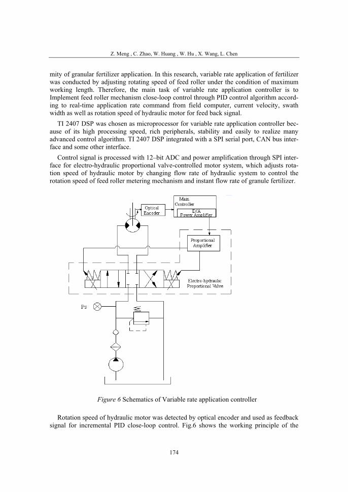
Z. Meng , C. Zhao, W. Huang , W. Hu , X. Wang, L. Chen
174
mity of granular fertilizer application. In this research, variable rate application of fertilizer was conducted by adjusting rotating speed of feed roller under the condition of maximum working length. Therefore, the main task of variable rate application controller is to Implement feed roller mechanism close-loop control through PID control algorithm accord-ing to real-time application rate command from field computer, current velocity, swath width as well as rotation speed of hydraulic motor for feed back signal.
TI 2407 DSP was chosen as microprocessor for variable rate application controller bec-ause of its high processing speed, rich peripherals, stability and easily to realize many advanced control algorithm. TI 2407 DSP integrated with a SPI serial port, CAN bus inter-face and some other interface.
Control signal is processed with 12–bit ADC and power amplification through SPI inter-face for electro-hydraulic proportional valve-controlled motor system, which adjusts rota-tion speed of hydraulic motor by changing flow rate of hydraulic system to control the rotation speed of feed roller metering mechanism and instant flow rate of granule fertilizer.
Rotation speed of hydraulic motor was detected by optical encoder and used as feedback signal for incremental PID close-loop control. Fig.6 shows the working principle of the
Figure 6 Schematics of Variable rate application controller
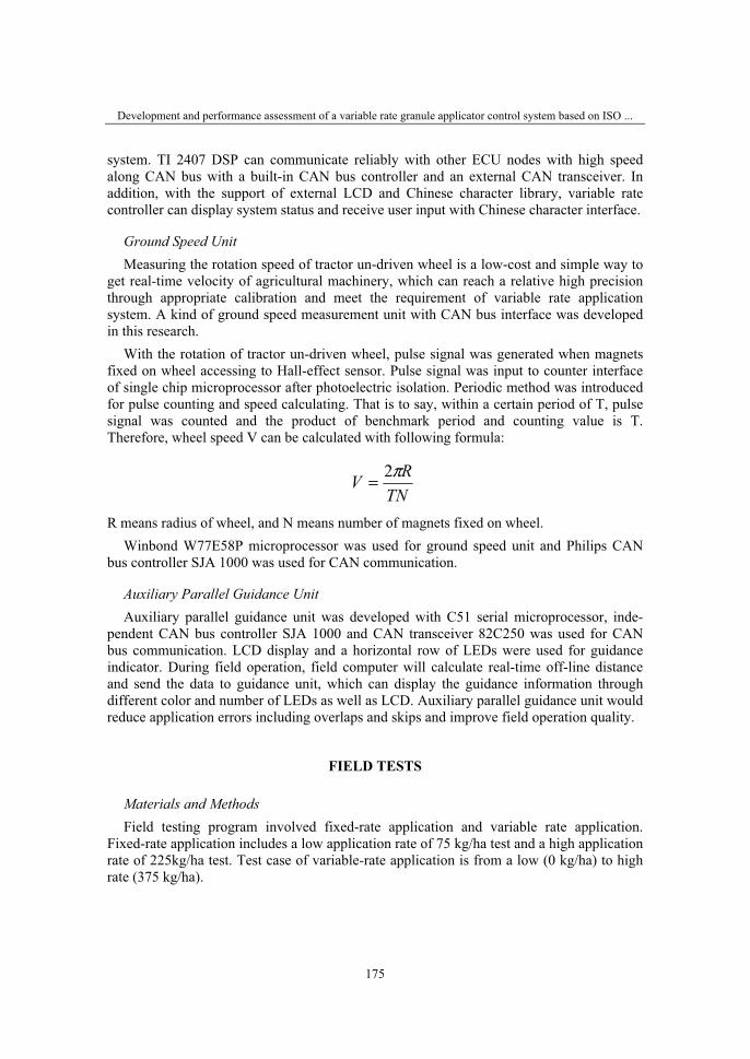
Development and performance assessment of a variable rate granule applicator control system based on ISO ...
175
system. TI 2407 DSP can communicate reliably with other ECU nodes with high speed along CAN bus with a built-in CAN bus controller and an external CAN transceiver. In addition, with the support of external LCD and Chinese character library, variable rate controller can display system status and receive user input with Chinese character interface.
Ground Speed Unit Measuring the rotation speed of tractor un-driven wheel is a low-cost and simple way to
get real-time velocity of agricultural machinery, which can reach a relative high precision through appropriate calibration and meet the requirement of variable rate application system. A kind of ground speed measurement unit with CAN bus interface was developed in this research.
With the rotation of tractor un-driven wheel, pulse signal was generated when magnets fixed on wheel accessing to Hall-effect sensor. Pulse signal was input to counter interface of single chip microprocessor after photoelectric isolation. Periodic method was introduced for pulse counting and speed calculating. That is to say, within a certain period of T, pulse signal was counted and the product of benchmark period and counting value is T. Therefore, wheel speed V can be calculated with following formula:
TNRV π2=
R means radius of wheel, and N means number of magnets fixed on wheel.Winbond W77E58P microprocessor was used for ground speed unit and Philips CAN
bus controller SJA 1000 was used for CAN communication.
Auxiliary Parallel Guidance Unit Auxiliary parallel guidance unit was developed with C51 serial microprocessor, inde-
pendent CAN bus controller SJA 1000 and CAN transceiver 82C250 was used for CAN bus communication. LCD display and a horizontal row of LEDs were used for guidance indicator. During field operation, field computer will calculate real-time off-line distance and send the data to guidance unit, which can display the guidance information through different color and number of LEDs as well as LCD. Auxiliary parallel guidance unit would reduce application errors including overlaps and skips and improve field operation quality.
FIELD TESTS
Materials and Methods Field testing program involved fixed-rate application and variable rate application.
Fixed-rate application includes a low application rate of 75 kg/ha test and a high application rate of 225kg/ha test. Test case of variable-rate application is from a low (0 kg/ha) to high rate (375 kg/ha).

Z. Meng , C. Zhao, W. Huang , W. Hu , X. Wang, L. Chen
176
Data Collection(1) Fixed-rate application test
Fixed-rate application test covers a 4�24m rectangle area, a 16�6 matrix of pans was lay out for fertilizer collection. Each plastic pan is 36.5cm long, 26.5cm wide and 15cm high.(2) Variable rate application test
Similar with fixed-rate application test, a 34�6 matrix of pans was placed in a 4�24mrectangle area. Application rate is 0kg/ha during 10m long area along tractor travel direction and application rate of the other 10m long area is 375kg/ha. In order to capture system delay and dynamic characteristic, there are several rows of pans was placed without separation along the both sides of dividing line from low application rate(0 kg/ha) to high application rate(375kg/ha).
Fertilizer in each collection pans was collected into plastic bags and weighted respectively using a electronic balance with 0.01g accuracy.
Results AnalysisTest cases of 75kg/ha and 225kg/ha have been repeated and there are 4 cases of tests all
together for fixed-rate application test. Result is shown as Table 1.
Figure 7 Collection pan matrix variable-rate application test
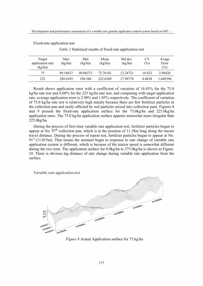
Development and performance assessment of a variable rate granule applicator control system based on ISO ...
177
Fixed-rate application test Table 1 Statistical results of fixed-rate application test
Targetapplication rate
(kg/ha)
Max(kg/ha)
Min(kg/ha)
Mean(kg/ha)
Std dev.(kg/ha)
CV(%)
Avage Error(%)
75 99.18627 49.06373 72.76181 12.24721 16.832 2.98426
225 249.6385 190.386 222.6389 17.99778 8.0838 1.049396
Result shows application rates with a coefficient of variation of 16.83% for the 75.0 kg/ha rate test and 8.08% for the 225 kg/ha rate test, and comparing with target application rate, average application error is 2.98% and 1.05% respectively. The coefficient of variation of 75.0 kg/ha rate test is relatively high mainly because there are few fertilizer particles in the collection pan and easily affected by soil particles mixed into collection pans. Figures 8 and 9 present the fixed-rate application surface for the 75.0kg/ha and 225.0kg/ha application rates. The 75.0 kg/ha application surface appears somewhat more irregular than 225.0kg/ha.
During the process of first time variable rate application test, fertilizer particles began to appear at No. 97th collection pan, which is at the position of 11.38m long along the tractor travel distance. During the process of repeat test, fertilizer particles began to appear at No. 91st (11.015m). That means the moment begin to response to rate change of variable rate application system is different, which is because of the tractor speed is somewhat different during the two tests. The application surface for 0.0kg/ha to 375.0kg/ha is shown as Figure. 10. There is obvious lag distance of rate change during variable rate application from the surface.
Variable rate application test
Figure 8 Actual Application surface for 75 kg/ha��
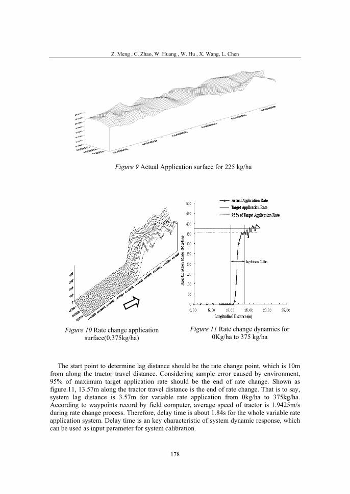
Z. Meng , C. Zhao, W. Huang , W. Hu , X. Wang, L. Chen
178
The start point to determine lag distance should be the rate change point, which is 10m from along the tractor travel distance. Considering sample error caused by environment, 95% of maximum target application rate should be the end of rate change. Shown as figure.11, 13.57m along the tractor travel distance is the end of rate change. That is to say, system lag distance is 3.57m for variable rate application from 0kg/ha to 375kg/ha. According to waypoints record by field computer, average speed of tractor is 1.9425m/s during rate change process. Therefore, delay time is about 1.84s for the whole variable rate application system. Delay time is an key characteristic of system dynamic response, which can be used as input parameter for system calibration.
Figure 9 Actual Application surface for 225 kg/ha
Figure 10 Rate change application surface(0,375kg/ha)
Figure 11 Rate change dynamics for 0Kg/ha to 375 kg/ha
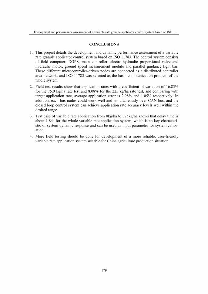
Development and performance assessment of a variable rate granule applicator control system based on ISO ...
179
CONCLUSIONS
1. This project details the development and dynamic performance assessment of a variable rate granule applicator control system based on ISO 11783. The control system consists of field computer, DGPS, main controller, electro-hydraulic proportional valve and hydraulic motor, ground speed measurement module and parallel guidance light bar. These different microcontroller-driven nodes are connected as a distributed controller area network, and ISO 11783 was selected as the basis communication protocol of the whole system.
2. Field test results show that application rates with a coefficient of variation of 16.83% for the 75.0 kg/ha rate test and 8.08% for the 225 kg/ha rate test, and comparing with target application rate, average application error is 2.98% and 1.05% respectively. In addition, each bus nodes could work well and simultaneously over CAN bus, and the closed loop control system can achieve application rate accuracy levels well within the desired range.
3. Test case of variable rate application from 0kg/ha to 375kg/ha shows that delay time is about 1.84s for the whole variable rate application system, which is an key characteri-stic of system dynamic response and can be used as input parameter for system calibr-ation.
4. More field testing should be done for development of a more reliable, user-friendly variable rate application system suitable for China agriculture production situation.

Z. Meng , C. Zhao, W. Huang , W. Hu , X. Wang, L. Chen
180
REFERENCES
1. Yang Liping, Jin Jiyun, Bai Youlu, Huang Shaowen�Soil Nutrient Comprehensive Evaluation and Balanced Fertilization. Precision agriculture and soil nutrient management, China Land Press, 2001.9 (In Chinese)
2. Zeng Xibo, Hu Xueyu, Hu Xiuqin. Current Status and Future Trends of China Fertilizer Industry. Science & Technology Review, 2002(8)�36-39(In Chinese)
3. Zeng Xibo, Li Jumei. Fertilizer Application and Its Affect to Grain Production in Different Area of China. Agricultural Sciences in China .2004�37(3)�387-392(In Chinese)
4. C. Yang, J. H. Everitt, J. M. Bradford.2001. Comparisons of Uniform and Variable Rate Nitrogen and Phosphorus Fertilizer Applications for Grain Sorghum. Transactions of the ASAE Vol. 44(2): 201-209.
5. J.P.Fulton et al. 2001. Performance Assessment and Model Development of a Variable-Rate, Spinner-Disc Fertilizer Applicator. Transactions of the ASAE Vol.44(5)
6. J. P. Fulton, S. A. Shearer, S. F. Higgins et al.2005. Distribution Pattern Variability of Granular VRT Applicators. Transactions of the ASAE Vol. 48(6): 2053-2064.2005
7. Motaz KHILAEL, Michihisa IIDA, Mikio UMEDA.2004. Development of a Metering Device for Organic and Chemical Fertilizers Applicator. Journal of the Japanese Society of Agricultural machinery/ Vol.66(5).2004
8. Wei, J., N. Zhang, N. Wang et al. 2001. Design of an embedded weed-control system using controller area network (CAN). ASAE Paper No. 013033. St. Joseph, Mich.: ASAE
9. Weisberg, P., R. Benneweis, and M. Bloom. 1993. Air seeder monitor/controller communications system. SAE Paper No.932430. Warrendale, Pa.: SAE.
10. Y. Hamada , Y. Matsuo , and A. Ogura.2004. Software Framework for Agricultural Vehicle Navigation. Automation Technology for Off-Road Equipment, Conference Proceedings. 7-8 October 2004 (Kyoto, Japan). Pp 283-291. ASAE Pub #701P1004
36. Symposium "Actual Tasks on Agricultural Engineering", Opatija, Croatia, 2008.
181
36.
SIMPOZIJAKTUALNI ZADACIMEHANIZACIJE POLJOPRIVREDE
UDK632.768:632.93:633.15](497.4)
Stručni rad radExpert paper
PRVA ISKUSTVA SUZBIJANJA ODRASLE KUKURUZNE ZLATICE U SLOVENIJI
T. POJE1, T. GODEŠA1, V. JEJČIČ1, Š. MODIC1, G. UREK1, M. LAKOTA2,M. SAGADIN2, G. LESKOŠEK3, M. RAK – CIZEJ3
1 Kmetijski inštitut Slovenije, Hacquetova 17, SI – 1000 LjubljanaE-mail: [email protected]
2 Fakulteta za kmetijstvo, Vrbanska 30, SI – 2000 Maribor 3 Inštitut za hmeljarstvo in pivovarstvo Slovenije, Cesta žalskega tabora 2, SI – 3310 Žalec
SAŽETAK
Pojava kukuruzne zlatice donosi nove zahtjeve pred strojeve za aplikaciju insekticida. Suzbijanje odrasle kukuruzne zlatice otežano je zbog visine usjeva kukuruza. U radu su predstavljene eksploatacijske karakteristike raspršivača sa topom. Ventilator je kod raspršivača veliki potrošač pogonske snage i to u prvoj brzini multiplikatora iznosi 31,4 kW, a u drugoj znatnih 54,9 kW. Zagonska snaga još je veća. Pri povećanju tlaka tekućine kod raspršivanja ustanovljen je linearan porast potrebne snage sa R2 većim od 0,96.
Ključne riječi: kukuruzna zlatica, suzbijanje, raspršivač sa topom, potrebna snaga
UVOD
Kukuruzna zlatica ili Diabratica virgifera virgifera LeConte štetni je kukac koji uništava usjeve kukuruza. U SAD-u predstavlja jednog od najznačajnijih štetočina kukuruza. U Evropi je prvi put nađena 1992. godine u Srbiji, u blizini aerodroma Surčin. U Hrvatskoj je prvi put viđena 1995. godine na području Županje. U Sloveniji smo prvu pojavu ovog štetočina registrirali u godini 2003 i to u istočnom dijelu Slovenije, Prekmurju i Podravju, te u zapadnom dijelu države, Goriškom. Zaključujemo da se radi širenju zbijenih populacija sa istoka (Madžarska, Hrvatska) i zapada (Italija). Najveću štetu na kukuruzu prouzrokuje larva koja živi u tlu gdje vrta in ogrize korijene sve do osnove. Kukci se prehranjuju cvjetnim prahom na metlicama i svilom na klipovima. Najznačajnija mjera suzbijanja i sprečavanja širenja kukuruzne zlatice je primjeran plodored. Sve to nalaže i Odluka evropske komisije i slovenski pravilnik o fitosanitarnim mjerama za preprečivanje širenja
T. Poje, T. Godeša, V. Jejčič, Š. Modic, G. Urek, M. Lakota, M. Sagadin, G. Leskošek, M. Rak-Cizej
182
kukuruzne zlatice. Za suzbijanje zlatice od posebnog značaja je uništavanje korova i samoniklog kukuruza, obrada tla, gnojenje itd. Putem škropljenja usjeva pokušavamo postići dvostruki učinak: smanjiti neposrednu štetu, koju prouzrokuju kukci nagrizanjem svile i prije svega spriječiti odlaganje jajašca i na taj način smanjiti populacijsku gustoćularvi u slijedećoj godini.
Insekticidi se nanose u slučaju kada želimo spriječiti neposrednu štetu koju prouzrokuju kukci nagrizanjem svile (gluhoća klipova) ili pak spriječiti izlijeganje jajašca, čimeutječemo na populacijsku gustoću larvi u slijedećoj godini. U tu svrhu upotrebljavaju se različiti insekticidi, koje nanosimo na biljke kukuruza krajem srpnja i u prvoj polovini kolovoza. U tom periodu kukuruz je već veći od 2 m i to je glavni ograničavajući kriterij za upotrebu klasične mehanizacije za nanošenje fitofarmaceutskih sredstava (FFS).
Odrasli usjev kukuruza predstavlja nov ciljni prostor, koji zbog svoje specifičnostiiskazuje oštra ograničenja pri uporabi strojeva za nanošenje FFS. Nemoguća je upotreba klasičnih strojeva za površinsko nanošenje (prskalica sa armaturom za prskanje), jer ne možemo voziti traktorom iznad usjeva, koji je visok 3 m in više. Drugi problem je kvaliteta, odnosno kvantiteta nanosa škropiva na ciljnu površinu biljaka (područje klipa) unutar tako visoke in guste sastojine.
Zbog visokog kukuruza u vrijeme škropljenja ne možemo uporabiti klasične prskalice. Jedina mogućnost je visoko namještenje armature – iznad usjeva kukuruza i vožnja po njivi. Pri tome dolazi do "pregaženja" dvaju redova između kotača traktora. Šteta koja nastaje kod toga, zavisi o odmicanju traktora od tla i o odrvenjenosti stabala kukuruza. Ako su stabla manje odrvenjela, nakon prohoda traktora ne slome se, nego se većim dijelom podignu i prinos se zbog toga bitno ne smanji. Rezultati istrage (Rosner 2005) pokazuju da gubici prinosa na području prohoda traktora kod jače odrvenjelih biljaka koje su poprskane kasnije, 11.8.2004, iznose 87%, a kod manje odrvenjelih biljaka, škropljenih 2.8.2004, gubici iznose samo 35 %. Gubici prinosa na cjelokupnoj površini zbog oštećenja biljaka pri škropljenju zavisni su i od radne širine prskalice obzirom na širinu parcele. To vrijedi i za proizvodnju zrnja. Ako pak proizvodimo silažni kukuruz za krmu ili za biomasu, onda možemo požnjevenu masu tih dviju vrsta (ili više obzirom na širinu opreme pri škropljenju) upotrijebiti i zbog toga dolazi manjih gubitaka.
Zbog boljeg nanosa FFS na cjelokupni prostor usjeva, naročito na područje klipova, gdje se na svili zadržavaju odrasli kukci, moguće je na armaturo namjestiti cijevne produžetke na čijem kraju se nalaze po dvije mlaznice. Potrebno je prepraviti postojeće armature kako bi bili nastavci za mlaznice, odnosno produžeci na jednakim udaljenostima kao što je odaljenost između redova usjeva.
Slijedeća mogućnost za bolji prodor FFS na prostor usjeva predstavlja uporaba potpore zračnoga toka, koja je prigrađena na nekim prskalicama. Pri tom sistemu opet je nekoliko problematična visina zbog stabilnosti agregata.
Zrakoplovi za aplikaciju pesticida primjenjuju se naročito u Madžarskoj, ali to je neprimjerno sa stanovišta očuvanja okoliša zbog drifta, posebice na manjim površinama, kao što je običaj kod nas. Uporaba zrakoplova ima i određene prednosti: nema mehaničkihoštećenja usjeva, ne dolazi do zbijanja tla a i nanos FFS je učinkovit.
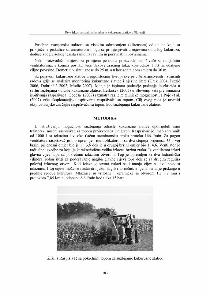
Prva iskustva suzbijanja odrasle kukuruzne zlatice u Slovenji
183
Posebne, namjenske traktore sa visokim odmicanjem (klirensom) od tla na koje su priključene prskalice sa armaturom mogu se primjenjivati u usjevima odraslog kukuruza, doduše zbog visokog težišta samo na ravnim in poravnatim površinama.
Neki proizvođači strojeva za primjenu pesticida proizvode razpršivače sa radijalnim ventilatorima, s kojima postižu veće tlakove zračnog toka, koji odnosi FFS na udaljene ciljne površine. Dometi u visinu iznose do 25 m, a u horizontalnom smjeru do 36 m.
Sa pojavom kukuruzne zlatice u jugoistočnoj Evropi sve je više znanstvenih i stručnihradova gdje se analizira monitoring kukuruzne zlatice i njezine štete (Urek 2004, Ivezić2006, Dobrinčić 2002, Modic 2007). Manje je ispitano područje prskanja insekticida u svrhu suzbijanja odrasle kukuruzne zlatice. Leskošek (2007) u Sloveniji vrši preliminarna ispitivanja raspršivača, Godeša (2007) razmatra različite tehničke mogućnosti, a Poje et al. (2007) vrše eksploatacijska ispitivanja raspršivača sa topom. Cilj ovog rada je utvrditi eksploatacijske značajke raspršivača sa topom kod suzbijanja kukuruzne zlatice.
METODIKA
U istraživanju mogućnosti suzbijanja odrasle kukuruzne zlatice upotrijebili smo traktorski nošeni raspršivač sa topom proizvođača Unigreen. Raspršivač je imao spremnik od 1000 l za tekućinu i visoko tlačnu membransku crpku protoka 166 l/min. Za pogon ventilatora raspršivač je bio opremljen multiplikatorom sa dva stupnja prijenosa. U prvoj brzini prijenosni omjer bio je 1 : 3,6 dok je u drugoj brzini omjer bio 1: 4,6. Ventilator je radijalne izvedbe za koju je karakteristična velika izlazna brzina zraka. Iz ventilatora izlazi glavna cijev topa sa pokretnim izlaznim otvorom. Top je opremljen sa dva hidrauličkacilindra, jedan služi za podešavanje nagiba glavne cijevi topa dok se sa drugim regulira položaj izlaznog otvora. Kod izlaznog otvora nalazi se i manja cijev sa dva nosioca mlaznica. I toj cijevi može se nastaviti njezin nagib i to ručno, a njena svrha je prskanje u prednje redove kukuruza. Mlaznice su vrtložne i keramičke sa otvorom 1,8 i 2 mm i protokom 7,85 l/min, odnosno 8,6 l/min kod tlaka 15 bara.
Slika 1 Raspršivač sa pokretnim topom za suzbijanje kukuruzne zlatice
T. Poje, T. Godeša, V. Jejčič, Š. Modic, G. Urek, M. Lakota, M. Sagadin, G. Leskošek, M. Rak-Cizej
184
U vidu eksploatacijskih karakteristika istraživali smo potrebnu snagu za pogon rasprši-vača sa topom preko priključnog vratila traktora kod različitog prijenosnog omjera i namještenja pokretne cijevi topa. Za pogon raspršivača upotrijebili smo traktor Fendt 714 Vario nazivne snage motora 111 kW. Mjerni lanac bio je sastavljena od tri dijela: senzora, digitalnog mjernog pojačala i PC računala za prijem i obradu mjernog signala. Okretni moment i broj okretaja priključnog vratila mjerili smo pomoću dinamometra za mjerenje momenta i prigrađenog senzora vrtnje (T30 FN Hottinger Baldwin Messtechnik). Digitalno pojačalo bio je SPIDER 8 Hottinger Baldwin Messtechnik. Frekvencija uzimanja podataka iznosila je 10 Hz dok je dužina pojedinog mjerenja ovisila o vremenskom toku rada sa raspršivačem. Iz izmjerenog momenta i broja okretaja na priključnom vratilu izračunata je potrebna snaga za pogon priključka preko priključnog vratila.
Snaga za pogon:
P = Mp ω (1)
P = Mn30p π (2)
Značenje oznaka: Pp - potrebna snaga za pogon raspršivača W M – moment na priključnom vratilu Nm
ω - kutna brzina rad n – broj okretaja priključnog vratila min-1
REZULTATI
Eksploatacijske karakteristike raspršivača utvrđivali smo na usjevu kukuruza na području osrednje i istočne Slovenije. Izvedena su mjerenja kod kojih smo upotrijebili čistuvodu i mjerenja kod kojih smo upotrijebili adekvatni insekticid. U istraživanjima biološke efikasnosti insekticida upotrijebili smo deltametrinski produkt DECIS 2,5 EC. U usporedbi sa kontrolom ustanovljena je 85 % efikasnost upotrijebljenog insekticida. Pokazalo se je da se može takvom aplikacijom pesticida znatno smanjiti populacija kukaca. Sa vodoosjetljivim mjernim listićima utvrđeno je da se može raspršivačem sa topom kvalitetno izvoditi aplikaciju škropiva između 15 i 20 metara radne širine u zavisnosti od razvojnog stadija usjeva kukuruza. Pri prolazu raspršivača pored kukuruza veliki tok zraka kojeg ostvaruje ventilator nekoliko savije stabljiku kukuruza (radi nastalog vjetra). Posle prolaza raspršivača kukuruz se vraća u prvobitan položaj. Kod naših ispitivanja nismo primijetili oštećenje kukuruza uslijed toka zraka.
Kod raspršivača ventilator je velik potrošač snage (energije). Za sam zagon raspršivačabio je u prvoj brzini ventilatora izmjeren maksimalan moment 813 Nm i najveća potrebna snaga 46,8 kW. Ako se multiplikator prebaci u drugu (bržu) brzinu tada je kod zagona stroja izmjeren maksimalni moment 1142 Nm te zagonska snaga 68 kW. Kod normalnog rada raspršivača u prvoj brzini ventilatora izmjeren je prosječni moment 531 Nm dok je u drugoj brzini izmjereno 947 Nm. Prosječno potrebna snaga za pogon stroja u prvoj brzini ventilatora iznosi 31,4 kW, a u drugoj brzini ventilatora 54,9 kW.

Prva iskustva suzbijanja odrasle kukuruzne zlatice u Slovenji
185
-10
0
10
20
30
40
50
60
70
80
0 10 20 30 40 50 60 70 80 90 100 110 120 130 140
VRIJEME (s)
SNA
GA
(kW
)
2. BRZINA
1. BRZINA
Slika 2 Potrebna snaga na priključnom vratilu traktora za pogon raspršivača s obzirom na stupanj prijenosa multiplikatora ventilatora
Obavljena su i mjerenja potrebne snage za pogon kod različitog tlaka crpke. Tlak smo mijenjali od 5 do 20 bara sa razmakom od 5 bara. Mjerenje je bilo izvedeno tako sa manjom kako i sa većom brzinom prijenosa multiplikatora. Iz pojedinih mjerenja izvučenaje prosječna snaga za pojedini tlak i brzinu. Iz ovih vrijednosti izračunata je linearna regresija za obije brzine multiplikatora. Obadvije imaju vrlo visoki R2
čija je vrijednost iznad 0,96. Sa povećanjem tlaka raste i potrebna snaga za pogon raspršivača.
y = 188,12x + 45013R2 = 0,9605
y = 200,41x + 25933R2 = 0,9859
0
10000
20000
30000
40000
50000
60000
0 5 10 15 20 25
TLAK (bar)
SNA
GA
(W)
1. BRZINA 2. BRZINA Linearno (2. BRZINA) Linearno (1. BRZINA)
Slika 3 Potrebna snaga za pogon raspršivača kod različite brzine okretanja ventilatora i različitog tlaka tekućine
Raspršivač ima savitljivi (pokretni) top kome se može podešavati nagib cijevi topa i nagib samog izlaznog otvora. Položaj cijevi topa također utječe na potrebnu snagu za pogon ventilatora. Mjerenja su izvedena kod različite brzine okretanja ventilatora te kod nagiba glavne cijevi topa između 40 i 90 stupnjeva. Izlazna glava bila je uvijek podešena vodoravno. Iz pojedinih mjerenja izračunata je prosječna snaga i dalje je izračunata linearna regresija. Sa povećavanjem kuta nagiba cijevi pada potrebna snaga za pogon ventilatora.
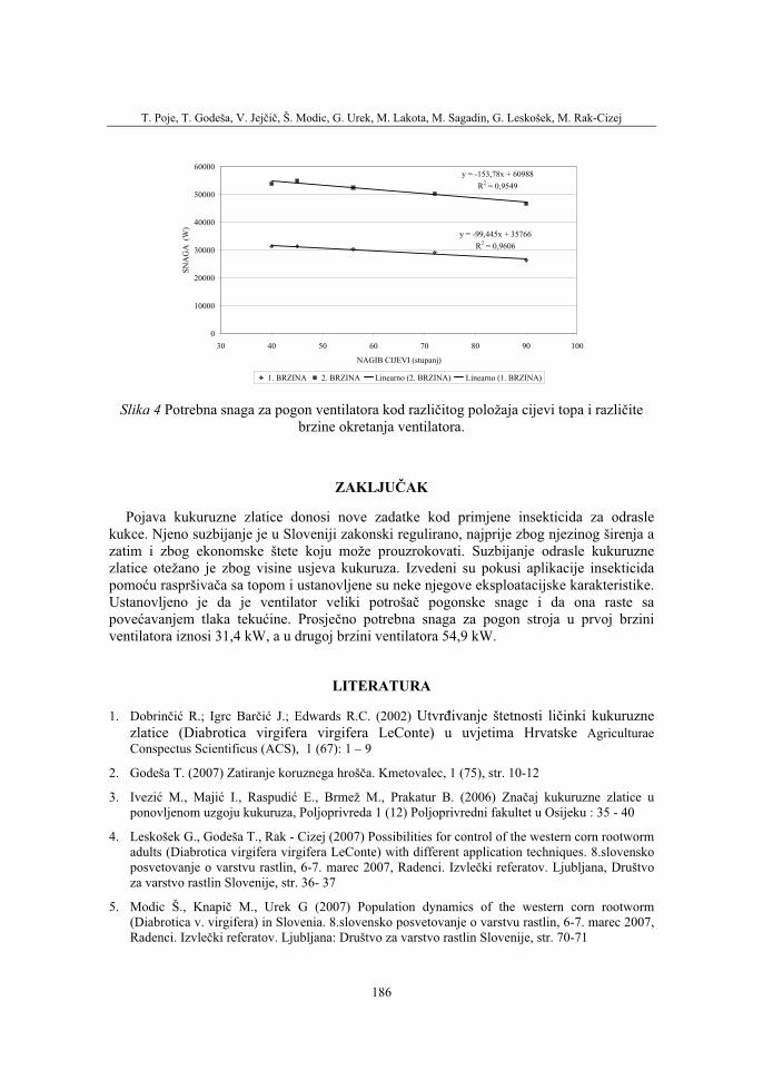
T. Poje, T. Godeša, V. Jejčič, Š. Modic, G. Urek, M. Lakota, M. Sagadin, G. Leskošek, M. Rak-Cizej
186
y = -153,78x + 60988R2 = 0,9549
y = -99,445x + 35766R2 = 0,9606
0
10000
20000
30000
40000
50000
60000
30 40 50 60 70 80 90 100
NAGIB CIJEVI (stupanj)
SNA
GA
(W
)
1. BRZINA 2. BRZINA Linearno (2. BRZINA) Linearno (1. BRZINA)
Slika 4 Potrebna snaga za pogon ventilatora kod različitog položaja cijevi topa i različitebrzine okretanja ventilatora.
ZAKLJUČAK
Pojava kukuruzne zlatice donosi nove zadatke kod primjene insekticida za odrasle kukce. Njeno suzbijanje je u Sloveniji zakonski regulirano, najprije zbog njezinog širenja a zatim i zbog ekonomske štete koju može prouzrokovati. Suzbijanje odrasle kukuruzne zlatice otežano je zbog visine usjeva kukuruza. Izvedeni su pokusi aplikacije insekticida pomoću raspršivača sa topom i ustanovljene su neke njegove eksploatacijske karakteristike. Ustanovljeno je da je ventilator veliki potrošač pogonske snage i da ona raste sa povećavanjem tlaka tekućine. Prosječno potrebna snaga za pogon stroja u prvoj brzini ventilatora iznosi 31,4 kW, a u drugoj brzini ventilatora 54,9 kW.
LITERATURA
1. Dobrinčić R.; Igrc Barčić J.; Edwards R.C. (2002) Utvrđivanje štetnosti ličinki kukuruzne zlatice (Diabrotica virgifera virgifera LeConte) u uvjetima Hrvatske Agriculturae Conspectus Scientificus (ACS), 1 (67): 1 – 9
2. Godeša T. (2007) Zatiranje koruznega hrošča. Kmetovalec, 1 (75), str. 10-12
3. Ivezić M., Majić I., Raspudić E., Brmež M., Prakatur B. (2006) Značaj kukuruzne zlatice u ponovljenom uzgoju kukuruza, Poljoprivreda 1 (12) Poljoprivredni fakultet u Osijeku : 35 - 40
4. Leskošek G., Godeša T., Rak - Cizej (2007) Possibilities for control of the western corn rootworm adults (Diabrotica virgifera virgifera LeConte) with different application techniques. 8.slovensko posvetovanje o varstvu rastlin, 6-7. marec 2007, Radenci. Izvlečki referatov. Ljubljana, Društvo za varstvo rastlin Slovenije, str. 36- 37
5. Modic Š., Knapič M., Urek G (2007) Population dynamics of the western corn rootworm (Diabrotica v. virgifera) in Slovenia. 8.slovensko posvetovanje o varstvu rastlin, 6-7. marec 2007, Radenci. Izvlečki referatov. Ljubljana: Društvo za varstvo rastlin Slovenije, str. 70-71

Prva iskustva suzbijanja odrasle kukuruzne zlatice u Slovenji
187
6. Poje T., Godeša T., Jejčič V., Urek G., Modic Š., Leskošek G., Rak – Cizej M., Sagadin M., Lakota M. (2007) Pršilnik s pršilnim topom Unigreen APC 1000. Tehnika in narava 3 (11), ČZD Kmečki glas, str. 25-27
7. Rosner, J., Foltin, K., Pichler, H., Neururer, H., Rödler G.: Der Maiswurzelbohrer in Österreich und Strategien seiner Bekämpfung. http://root.lako.at/versuche/pflanzenbau/pfls_dueng/diabrotica_2005.pdf
8. Urek G., Modic Š. (2004) Occurrence of the Western Corn Rootworm (Diabrotica virgifera virgifera le Conte) in Slovenia. Acta agriculturae Slovenica 1 (83): 5-13
T. Poje, T. Godeša, V. Jejčič, Š. Modic, G. Urek, M. Lakota, M. Sagadin, G. Leskošek, M. Rak-Cizej
188
FIRST EXPERIENCES IN THE CONTROL OF ADULT WESTERN CORN ROOTWORM IN SLOVENIA
ABSTRACT
The appearance of western corn rootworm brings new challenges to machines used for pesticide spraying. The control of western corn rootworm is difficult due to the height of the maize crop. The current paper presents the exploitation characteristics of mistblower with cannon. Ventilator of mistblower is a big consumer of driving power amounting at the first speed of multiplier to 31.4 kW and at the second speed to 54.9 kW. The starting power is even higher. At the increase of liquid pressure during spraying a linear growth of the required power with R2 higher than 0.96 was determined.
Key words: western corn rootworm, control, mistblower with cannon, required power
36. Symposium "Actual Tasks on Agricultural Engineering", Opatija, Croatia, 2008.
189
36.
SIMPOZIJAKTUALNI ZADACIMEHANIZACIJE POLJOPRIVREDE
UDK631.348.45:633.791
Stručni radExpert paper
SNAGA POTREBNA ZA POGON RASPRŠIVAČA U HMELJARSTUVG. LESKOŠEK1 , T. POJE2
1 Inštitut za hmeljarstvo in pivovarstvo Slovenije, Cesta žalskega tabora 2, SI – 3310 Žalec E-mail: [email protected]
2 Kmetijski inštitut Slovenije, Hacquetova 17, SI – 1000 Ljubljana E-mail: [email protected]
SAŽETAK
U hmeljarstvu se upotrebljavaju specijalne izvedbe raspršivača sa ugrađenimventilatorima, koji mogu biti veliki potrošači energije. Na osnovu izmjerenog momenta i broja okretaja priključnog vratila ustanovili smo potrebnu snagu za pogon troje različitih raspršivača kod različite brzine okretanja ventilatora. Raspršivač sa oznakom C u višoj brzini okretanja ventilatora angažira 53,2 kW snage, što je previše za normalan rad s plantažnim traktorom. Raspršivačioznake A i B zbog konstrukcije, odnosno manjeg prijenosnog omjera na multiplikatoru angažiraju od 29 do 38 kW pogonske snage bez obzira na stupanj prijenosa kod ventilatora.
Ključne riječi: hmelj,raspršivač, ventilator, potrebna snaga
UVOD
U Sloveniji se vlastitim zakonodavstvom na području poljoprivrede među ciljevima agrarne politike posebice naglašava zaštita poljoprivrednih zemljišta od zagađivanja i nesmotrene eksploatacije kao i realizacija principa zaštite okoliša i očuvanja prirode. Uz temeljnu gospodarsku i socijalnu ulogu poljoprivrede moramo biti usmjereni ka poticanju okolišu prijazne poljoprivredne djelatnosti koja bi održavala različitost životinjskih i biljnih vrsta, očuvala plodnost tla i štitila prirodne uvjete potrebne za život u tlu, vodi i zraku. Temeljni zadatak tehnike aplikacije pesticida je dakle smotreno, gospodarno i za okoliš prihvatljivo nanošenje adekvatno pripremljenih kemijskih produkata na ciljne površine, koje istovremeno znači i određenu intervenciju u prostor. Ako ih dakle hoćemo učinkovito i sigurno primjenjivati, moramo puno znati o njima samima, a vrlo dobro moramo poznavati i odgovarajuće strojeve i uređaje, jer njihova primjerna kvaliteta i pravilno rukovanje s

G. Leskošek, T. Poje
190
njima omogućuju veću efikasnost kemijskih sredstava i manji unos neželjenih tvari u okoliš (Leskošek 2004). Aplikacija fitofarmaceutskih sredstava (FFS) po nasadima hmelja zbog specifičnosti nasada spada među zahtjevnije radove. Nasad hmelja je gust i visok nasad i kod 2,4 m udaljenosti među redovima na jednom hektaru obično se nalazi i do 4200 biljaka. Kod nas su nasadi hmelja u prosjeku visoka između 6 i 7 m, a indeks lisne površine u zavisnosti od sorte iznosi od 9 do 13. Usprkos intenzivnim nastojanjima za pronalaskom drugih načina, odnosno postupaka nanošenja FFS, kod nas je još uvijek rašireno klasičnoraspršivanje nasada hmelja. Pri tretiranju nasada upotrebljavamo vučene aksijalne raspršivače kapacitete zračnog puhala između 90000 m3 i 120000 m3 koji usisavaju zrak straga i pod kutom 90° ispuhavaju ga u nasad (Kač 1989). U konvencionalnoj proizvodnji usprkos mnogim obavljenim pokusima još se uvijek upotrebljavaju velike količine vode. Preporučena potrošnja vode je dakle 400 l po metru visine hmelja (Žolnir 1991, 1993). Usprkos velikoj količini potrošene vode i učinka raspršivača nemoguće je osigurati ravnomjernost nanosa FFS. Do lokalnih predoziranja dolazi prije svega u redovima uz koloteke gdje je udio depozita toliki da može prouzrokovati slijevanje kapljica i otjecanje, dok je kvaliteta depozicije u drugom i trećem redu od koloteka, naročito u vrhu biljke, bitno manja.
Glavnina proučavanja upotrebe raspršivača u hmeljarstvu vrši se na području kvalitete nanosa FFS i efikasnosti pojedinih FFS. Poje (2000, 2001 i 2007) ispituje potrebnu snagu za pogon raspršivača sa promjenljivom količinom zraka, angažiranom snagom za pogon crpke, a vrši i proučavanja potrebne snage za pogon raspršivača za hmeljarstvo. U hmeljarstvu se upotrebljavaju specijalne izvedbe traktora – plantažne traktore, kod kojih je pogonska snaga limitirana i kod najsnažnijih traktora iznosi maksimalno 66 do 76 kW (90 do 100 KS). Raspršivač može biti sa svojim ventilatorom dosta veliki potrošač pogonske energije traktora. Cilj rada je ustanoviti potrebnu snagu za pogon različitih raspršivača zbog limitirane snage traktorskog motora plantažnih traktora.
METODIKA
U vidu eksploatacijskih karakteristika istraživali smo potrebnu snagu za pogon različitihraspršivača koji se upotrebljavaju u hmeljarstvu. Za pogon raspršivača upotrijebili smo traktor Steyr 495 Kompakt, nazivne snage motora 66 kW. Mjerni lanac bio je sastavljen od tri dijela: senzora, digitalnog mjernog pojačala i PC računala za prijem i obradu mjernog signala. Okretni moment i broj okretaja priključnog vratila mjerili smo pomoćudinamometra za mjerenje momenta i prigrađenog senzora vrtnje (T30 FN Hottinger Baldwin Messtechnik). Digitalno pojačalo bio je SPIDER 8 Hottinger Baldwin Messtechnik. Frekvencija uzimanja podataka iznosila je 10 Hz, dok je dužina pojedinog mjerenja ovisila o vremenskom toku rada sa raspršivačem. Iz izmjerenog momenta i broja okretaja na priključnom vratilu izračunata je potrebna snaga za pogon priključka preko priključnog vratila.
Snaga za pogon:
P = Mp ω (1)
P = Mn30p π (2)
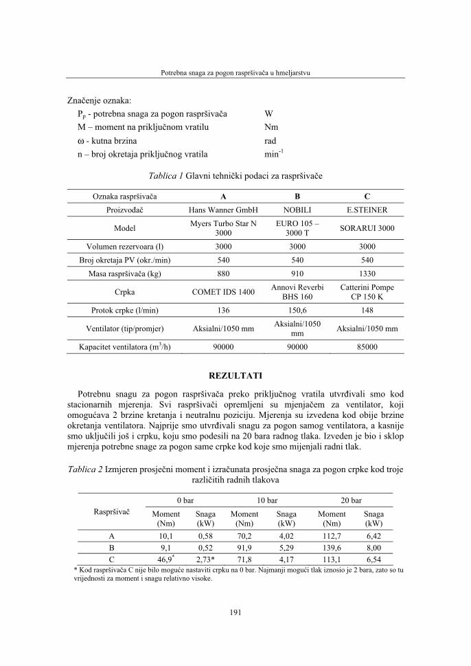
Potrebna snaga za pogon raspršivača u hmeljarstvu
191
Značenje oznaka: Pp - potrebna snaga za pogon raspršivača W M – moment na priključnom vratilu Nm ω - kutna brzina rad n – broj okretaja priključnog vratila min-1
Tablica 1 Glavni tehnički podaci za raspršivače
Oznaka raspršivača A B C Proizvođač Hans Wanner GmbH NOBILI E.STEINER
Model Myers Turbo Star N 3000
EURO 105 – 3000 T SORARUI 3000
Volumen rezervoara (l) 3000 3000 3000
Broj okretaja PV (okr./min) 540 540 540
Masa raspršivača (kg) 880 910 1330
Crpka COMET IDS 1400 Annovi Reverbi BHS 160
Catterini Pompe CP 150 K
Protok crpke (l/min) 136 150,6 148
Ventilator (tip/promjer) Aksialni/1050 mm Aksialni/1050mm Aksialni/1050 mm
Kapacitet ventilatora (m3/h) 90000 90000 85000
REZULTATI
Potrebnu snagu za pogon raspršivača preko priključnog vratila utvrđivali smo kod stacionarnih mjerenja. Svi raspršivači opremljeni su mjenjačem za ventilator, koji omogućava 2 brzine kretanja i neutralnu poziciju. Mjerenja su izvedena kod obije brzine okretanja ventilatora. Najprije smo utvrđivali snagu za pogon samog ventilatora, a kasnije smo uključili još i crpku, koju smo podesili na 20 bara radnog tlaka. Izveden je bio i sklop mjerenja potrebne snage za pogon same crpke kod koje smo mijenjali radni tlak.
Tablica 2 Izmjeren prosječni moment i izračunata prosječna snaga za pogon crpke kod troje različitih radnih tlakova
0 bar 10 bar 20 bar Raspršivač Moment
(Nm)Snaga(kW)
Moment(Nm)
Snaga(kW)
Moment(Nm)
Snaga(kW)
A 10,1 0,58 70,2 4,02 112,7 6,42 B 9,1 0,52 91,9 5,29 139,6 8,00 C 46,9* 2,73* 71,8 4,17 113,1 6,54
* Kod raspršivača C nije bilo moguće nastaviti crpku na 0 bar. Najmanji mogući tlak iznosio je 2 bara, zato so tu vrijednosti za moment i snagu relativno visoke.
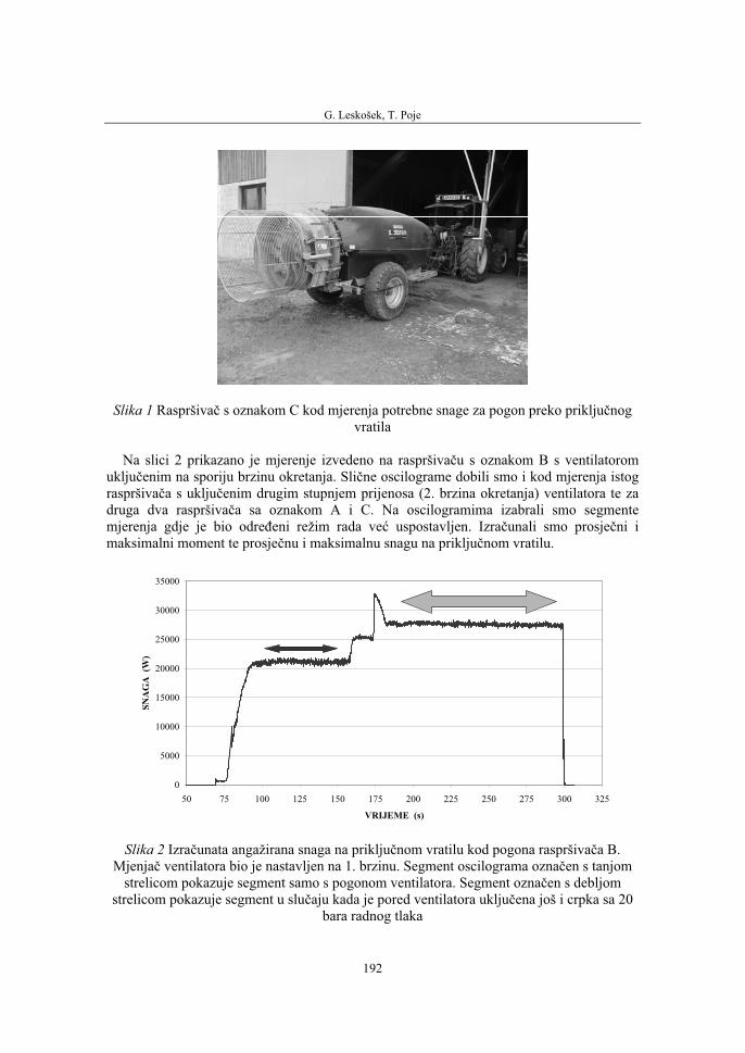
G. Leskošek, T. Poje
192
Slika 1 Raspršivač s oznakom C kod mjerenja potrebne snage za pogon preko priključnogvratila
Na slici 2 prikazano je mjerenje izvedeno na raspršivaču s oznakom B s ventilatorom uključenim na sporiju brzinu okretanja. Slične oscilograme dobili smo i kod mjerenja istog raspršivača s uključenim drugim stupnjem prijenosa (2. brzina okretanja) ventilatora te za druga dva raspršivača sa oznakom A i C. Na oscilogramima izabrali smo segmente mjerenja gdje je bio određeni režim rada već uspostavljen. Izračunali smo prosječni i maksimalni moment te prosječnu i maksimalnu snagu na priključnom vratilu.
0
5000
10000
15000
20000
25000
30000
35000
50 75 100 125 150 175 200 225 250 275 300 325
VRIJEME (s)
SNA
GA
(W
)
Slika 2 Izračunata angažirana snaga na priključnom vratilu kod pogona raspršivača B. Mjenjač ventilatora bio je nastavljen na 1. brzinu. Segment oscilograma označen s tanjom
strelicom pokazuje segment samo s pogonom ventilatora. Segment označen s debljom strelicom pokazuje segment u slučaju kada je pored ventilatora uključena još i crpka sa 20
bara radnog tlaka
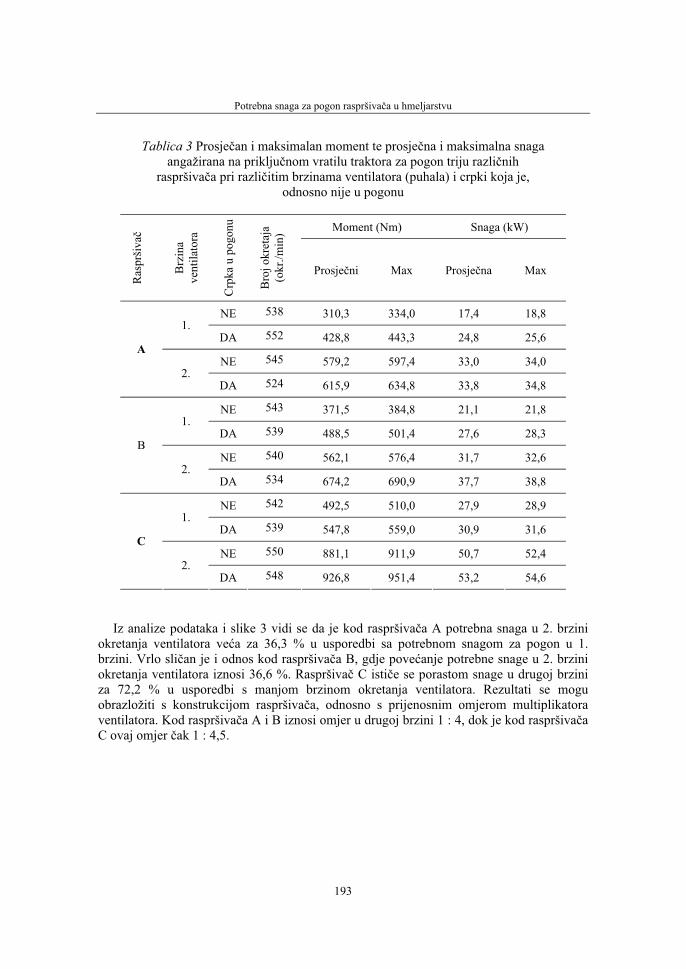
Potrebna snaga za pogon raspršivača u hmeljarstvu
193
Tablica 3 Prosječan i maksimalan moment te prosječna i maksimalna snagaangažirana na priključnom vratilu traktora za pogon triju različnih
raspršivača pri različitim brzinama ventilatora (puhala) i crpki koja je,odnosno nije u pogonu
Moment (Nm) Snaga (kW)
Ras
prši
vač
Brz
ina
vent
ilato
ra
Crp
ka u
pog
onu
Bro
j okr
etaj
a (o
kr./m
in)
Prosječni Max Prosječna Max
NE 538 310,3 334,0 17,4 18,8 1.
DA 552 428,8 443,3 24,8 25,6
NE 545 579,2 597,4 33,0 34,0 A
2.DA 524 615,9 634,8 33,8 34,8
NE 543 371,5 384,8 21,1 21,8 1.
DA 539 488,5 501,4 27,6 28,3
NE 540 562,1 576,4 31,7 32,6 B
2.DA 534 674,2 690,9 37,7 38,8
NE 542 492,5 510,0 27,9 28,9 1.
DA 539 547,8 559,0 30,9 31,6
NE 550 881,1 911,9 50,7 52,4 C
2.DA 548 926,8 951,4 53,2 54,6
Iz analize podataka i slike 3 vidi se da je kod raspršivača A potrebna snaga u 2. brzini okretanja ventilatora veća za 36,3 % u usporedbi sa potrebnom snagom za pogon u 1. brzini. Vrlo sličan je i odnos kod raspršivača B, gdje povećanje potrebne snage u 2. brzini okretanja ventilatora iznosi 36,6 %. Raspršivač C ističe se porastom snage u drugoj brzini za 72,2 % u usporedbi s manjom brzinom okretanja ventilatora. Rezultati se mogu obrazložiti s konstrukcijom raspršivača, odnosno s prijenosnim omjerom multiplikatora ventilatora. Kod raspršivača A i B iznosi omjer u drugoj brzini 1 : 4, dok je kod raspršivačaC ovaj omjer čak 1 : 4,5.
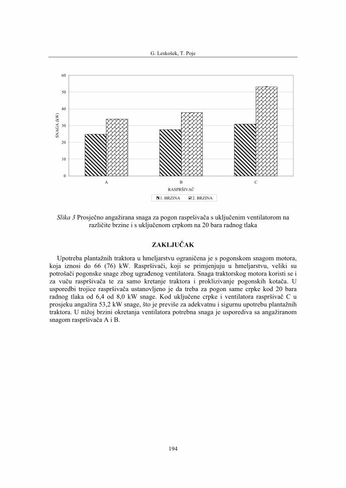
G. Leskošek, T. Poje
194
0
10
20
30
40
50
60
A B C
RASPRŠIVAČ
SNA
GA
(kW
)
1. BRZINA 2. BRZINA
Slika 3 Prosječno angažirana snaga za pogon raspršivača s uključenim ventilatorom na različite brzine i s uključenom crpkom na 20 bara radnog tlaka
ZAKLJUČAK
Upotreba plantažnih traktora u hmeljarstvu ograničena je s pogonskom snagom motora, koja iznosi do 66 (76) kW. Raspršivači, koji se primjenjuju u hmeljarstvu, veliki su potrošači pogonske snage zbog ugrađenog ventilatora. Snaga traktorskog motora koristi se i za vuču raspršivača te za samo kretanje traktora i proklizivanje pogonskih kotača. U usporedbi trojice raspršivača ustanovljeno je da treba za pogon same crpke kod 20 bara radnog tlaka od 6,4 od 8,0 kW snage. Kod uključene crpke i ventilatora raspršivač C u prosjeku angažira 53,2 kW snage, što je previše za adekvatnu i sigurnu upotrebu plantažnih traktora. U nižoj brzini okretanja ventilatora potrebna snaga je usporediva sa angažiranom snagom raspršivača A i B.
Potrebna snaga za pogon raspršivača u hmeljarstvu
195
LITERATURA
1. Leskošek G. (2004) Razvoj metod za tehnično in zakonodajno obravnavo pojavov zanašanja (drifta) in analizo depozitov pri aplikaciji fitofarmacevtskih sredstev v hmeljarstvu. 42. seminar o hmeljarstvu, Žalec: 10 s.
2. Kač M. (1989) Spritzverfahren mit Axialgebleasen in Hopfenanlagen. Proceedings of the Technical Commission I.H.G.C. of the XXXVIIth International Hop Congress. Leon, Spain, 31. July - 3. August, 1989.
3. Poje T. (2000) Potrošnja energije raspršivača s promjenljivom količinom zraka. Zbornik radova 28. međunarodnog simpozija Aktualni zadaci mehanizacije poljoprivrede. Agronomski fakultet, Zagreb: 227-232
4. Poje T. (2001) Eksploatacijske karakteristike pumpe za prskalice BM 105/20 Agromehanika. Zbornik radova 29. međunarodnog simpozija Aktualni zadaci mehanizacije poljoprivrede. Agronomski fakultet, Zagreb: 253-258
5. Poje T. (2007) Poročilo o potrebni moči za pogon pršilnikov, Kmetijski inštitut Slovenije - Študije po naročilu, Ljubljana: 6 s.
6. Žolnir M. (1991) Control of Aphids by reduced spray volume. Scientific Commision of the Hop Grower’ Convevention, Freising .
7. Žolnir M. (1993) Nekatere kvalitativne značilnosti nanosa škropiva v območju delovne širine pršilnika pri pršenju hmeljišč. Zbornik predavanj in referatov s 1. slovenskega posvetovanja o varstvu rastlin. Sekcija za varstvo rastlin pri Zvezi društev kmetijskih inženirjev in tehnikov Slovenije, Ljubljana: 237 - 249
POWER REQUIRED FOR DRIVING OF MISTBLOWER USED IN HOP GROWING
ABSTRACT
In hop production specially made mistblowers with built in ventilators are used which have proven as big energy spenders. On the basis of torque measured and number of revolutions of PTO shaft, power required for driving of three different mistblowers at different rotation speed of ventilator was determined. Mistblower designated with the sign C engages 53.2 kW of power at higher rotation speed, which is a too high value for normal work with plantation tractor. Mistblowers designated A and B engage from 29 to 38 kW driving power due to their construction type and lower gear ratio on multiplier regardless of gear ratio of ventilator.
Key words: hop, mistblower, ventilator, required power

36. Symposium "Actual Tasks on Agricultural Engineering", Opatija, Croatia, 2008.
197
36.
SIMPOZIJAKTUALNI ZADACIMEHANIZACIJE POLJOPRIVREDE
UDC621.65
Stručni radExpert paper
RESEARCH ON THE DETERMINATION OF SOME PROPERTIES OF VALVE PARTS OF DIAPHRAGM
PUMPS USED IN SPRAYERS E. KILIC1, I. CELEN2, T. AKTAS2
1Department of Automotive Industry, Tekirdag Vocational Training School, Namik Kemal University, Tekirdag, Turkey.
2Department of Agricultural Machinery, Agricultural Faculty, Namik Kemal University, Tekirdag, Turkey. Corresponding author: [email protected]
SUMMARY
One of the most important things for plant protection that is performed by using sprayers is to determine whether any spray system works within desired limits or not. The changing of spraying characteristics happens by different spray equipment under different working and application conditions. For this reason, which part or parts of sprayers affect the spraying characteristics and how this happens must be determined. At the same time, the effects of different applications and working conditions on the spraying characteristics must also be determined carefully. In this way, it can be decided that spraying and sprayers are suitable for a particular aim.
In this research, corrosion in valve parts and valve springs of sprayer pumps were investigated, and toward achieving this goal, a total of 200 springs (100 new unused springs and 100 used springs) were examined. After the tests, spring coefficient values, displacement amounts, and frequencies were determined. Changes in new and used springs were determined by using the research findings.
In this study, all the valves used for tests had plastic trunks. These valves were different from the materials of flat discs. When valves were examined, it was found that all parts of valves except spring itself can be produced fully with plastic materials or they can be produced partially out of plastic (trunk) and metal materials (other parts). Measurements showed that flat discs made of metal material are thicker than the others. Also, big differences between the measurement results of new plastic and metal materials were not observed. The reason for this can be attributed to the fact that plastic materials are produced by a casting process. Measurement differences are observed in metal parts because
E. Kilic, I. Celen, T. Aktas
198
these parts are produced one by one manually. In the research region, it was determined that 73% valves are made of plastic materials.
Flat disc thickness (B1) values were found to be thicker in metal discs than in plastic discs. B1 values were found to be 2.52 mm for plastic materials and 1.40-2.52 for metal materials. After using these valves, plastic discs became 4% thinner and metal discs became 45% thinner than new valves. Flat disc diameter (B3) decreased for used valves. This decrease was found to be 3.5% for metal discs and 1.34 % for plastic discs. The total height of valve head (B2) decreased 17.61% for plastic heads and 39.6% for metal heads. The height of bearing part of valve head (B4) decreased 13 % for plastic heads and 14% for metal heads. The diameter of bearing part of valve head (B5) decreased due to the stroke of flat disc to valve head. Corrosion ratios were found to be 2.34 % for metal valve heads and 0.6 % for plastic heads.
Key words: valve, pump, sprayer, corrosion
INTRODUCTION
Agricultural mechanization plays a very crucial role in increasing crop yields year by year. In today’s world, agricultural mechanization serves a couple of purposes: to enhance the effectiveness of other agricultural applications, to provide economic efficiency of agricultural business, and to improve the working conditions of the farmers. For the crop yields of any country to reach sufficient levels to maintain the people of that country, it is necessary to make the best use of the production surplus, to increase the types of crops and to integrate technological advances into the business of agriculture.
At the heart of all these advances should lay the need to increase the efficiency of unit production both quantitatively and qualitatively and to make the best use of the agricultural potential. Increasing the crop yield for unit area of land depends on two important factors: fight against agricultural illnesses and pesticides. To get the maximum benefit from agricultural pests, the pesticides should sprayed onto the appropriate places of any plant in equal amounts and should also be applied economically in a environmentally-friendly manner with minimum or possibly no amount of environmental risk.
The critical factor in the fight against agricultural war on pesticides with sprayers is to determine whether spraying is applied in the target amounts set previously. To do so, it is required that spraying characteristics of a spraying machine and the factors which have effects on those characteristics be determined. In chemical applications, plant types, climate conditions, pesticide standards, the time of spraying, the size of drop diameter, the chemical ingredient of the liquid and the ratio of surface coating all play a role.
Spraying characteristics can vary depending on the spraying machines with varying degrees of structural properties, different applications, and working conditions. Therefore, it is necessary to fully determine the effects of functional components of the spraying machine on the spraying along with the impacts of different applications and different working conditions. However, it is only in this way that the suitability of the spraying and the machine used to spray the field can be determined.
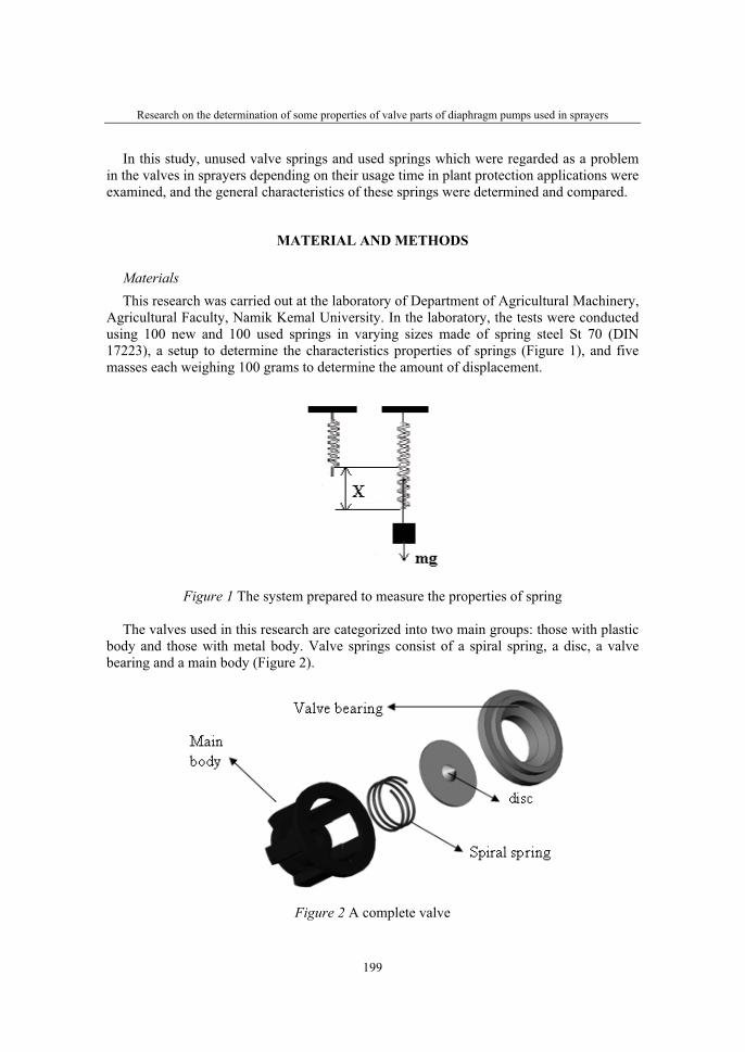
Research on the determination of some properties of valve parts of diaphragm pumps used in sprayers
199
In this study, unused valve springs and used springs which were regarded as a problem in the valves in sprayers depending on their usage time in plant protection applications were examined, and the general characteristics of these springs were determined and compared.
MATERIAL AND METHODS
MaterialsThis research was carried out at the laboratory of Department of Agricultural Machinery,
Agricultural Faculty, Namik Kemal University. In the laboratory, the tests were conducted using 100 new and 100 used springs in varying sizes made of spring steel St 70 (DIN 17223), a setup to determine the characteristics properties of springs (Figure 1), and five masses each weighing 100 grams to determine the amount of displacement.
Figure 1 The system prepared to measure the properties of spring
The valves used in this research are categorized into two main groups: those with plastic body and those with metal body. Valve springs consist of a spiral spring, a disc, a valve bearing and a main body (Figure 2).
Figure 2 A complete valve
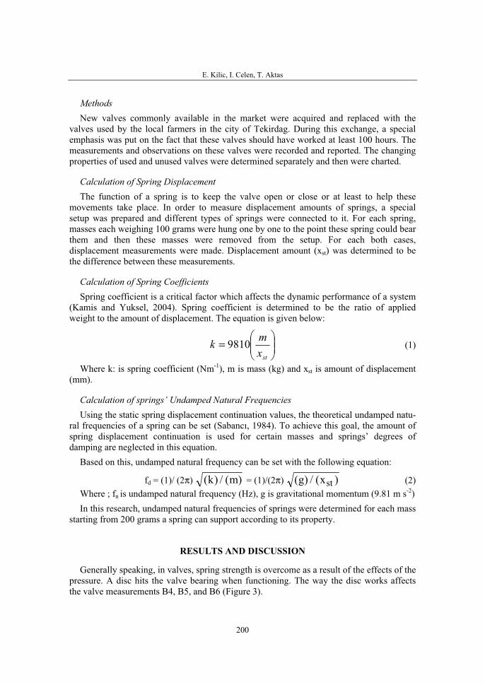
E. Kilic, I. Celen, T. Aktas
200
MethodsNew valves commonly available in the market were acquired and replaced with the
valves used by the local farmers in the city of Tekirdag. During this exchange, a special emphasis was put on the fact that these valves should have worked at least 100 hours. The measurements and observations on these valves were recorded and reported. The changing properties of used and unused valves were determined separately and then were charted.
Calculation of Spring Displacement The function of a spring is to keep the valve open or close or at least to help these
movements take place. In order to measure displacement amounts of springs, a special setup was prepared and different types of springs were connected to it. For each spring, masses each weighing 100 grams were hung one by one to the point these spring could bear them and then these masses were removed from the setup. For each both cases, displacement measurements were made. Displacement amount (xst) was determined to be the difference between these measurements.
Calculation of Spring Coefficients Spring coefficient is a critical factor which affects the dynamic performance of a system
(Kamis and Yuksel, 2004). Spring coefficient is determined to be the ratio of applied weight to the amount of displacement. The equation is given below:
⎟⎟
⎠
⎞
⎜⎜
⎝
⎛
=stx
mk 9810 (1)
Where k: is spring coefficient (Nm-1), m is mass (kg) and xst is amount of displacement (mm).
Calculation of springs’ Undamped Natural Frequencies Using the static spring displacement continuation values, the theoretical undamped natu-
ral frequencies of a spring can be set (Sabancı, 1984). To achieve this goal, the amount of spring displacement continuation is used for certain masses and springs’ degrees of damping are neglected in this equation.
Based on this, undamped natural frequency can be set with the following equation:
fd = (1)/ (2π) ( ) / ( )k m = (1)/(2π) ( ) / ( )g xst (2) Where ; fn is undamped natural frequency (Hz), g is gravitational momentum (9.81 m s-2)In this research, undamped natural frequencies of springs were determined for each mass
starting from 200 grams a spring can support according to its property.
RESULTS AND DISCUSSION
Generally speaking, in valves, spring strength is overcome as a result of the effects of the pressure. A disc hits the valve bearing when functioning. The way the disc works affects the valve measurements B4, B5, and B6 (Figure 3).

Research on the determination of some properties of valve parts of diaphragm pumps used in sprayers
201
In this study, all the valves used for tests had plastic trunks. These valves were different from the materials of flat discs. When valves were examined, it was found that all parts of valves except spring itself can be produced fully with plastic materials or they can be produced partially out of plastic (trunk) and metal materials (other parts). Observations showed that flat discs made of metal material are thicker than the others. Also, big differences between the measurement results of new plastic and metal materials were not observed. The reason for this can be attributed to the fact that plastic materials are produced by a casting process. Measurement differences are observed in metal parts because these parts are produced one by one manually. In the research region, it was determined that 73% of valves are made of plastic materials.
When the unused springs were examined, the measurement results (B1, B2, B3, B4, B5, B6) were determined as they were given in Table 1. The differences in these values were thought to be the highest corrosion ratio.
B1 value is thinner in metal materials compared to plastic materials. This value for unused valves with plastic materials was found to be on average, 2.52, but it varied between 1.40 and 2.52 for metal materials. After the valves were used, the materials became thinner: 4% for plastic materials and 45% for metal materials. B3 value showed corrosion for unused valves. This ration was 3.5% for metal materials and 1.34% for plastic materials.
B2 value was examined and found to be 17.61% in plastic materials, and 39.6% for metal materials. For B4 values, the change was determined to be 14% for metal materials, and 13% for plastic materials.
B5 value showed corrosion since disc hit the valve bearing. The ratio of corrosion was 2.34% in metal materials, and 0.6% in plastic materials.
Figure 3 Disc and valve bearing measurements
In Table 2, the values (A) for changes in base heights for old and new valves can be seen. When spring disc pressurizes on the spring, it hits the S surface as seen in Figure 4. This surface is made of plastic, and as it is used it shows corrosion. When used and unused valves were compared, these surfaces were examined. As a result, it was found that the plastic disc corroded at a percentage of 17.87, while the metal disc became corroded at a percentage of 8.18.
B3
B4
B5
B6
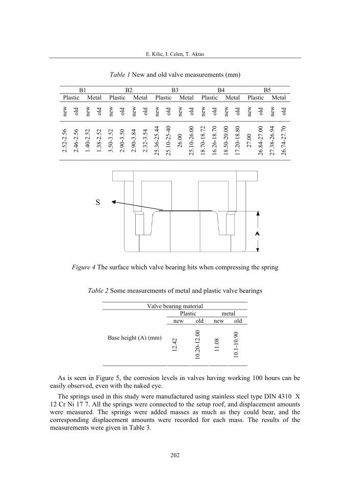
E. Kilic, I. Celen, T. Aktas
202
Table 1 New and old valve measurements (mm)
B1 B2 B3 B4 B5 Plastic Metal Plastic Metal Plastic Metal Plastic Metal Plastic Metal
new
old
new
old
new
old
new
old
new
old
new
old
new
old
new
old
new
old
new
old
2.52
-2.5
6
2.46
-2.5
6
1.40
-2.5
2
1.38
-2.5
2
3.50
-3.5
2
2.90
-3.5
0
2.90
-3.8
4
2.32
-3.5
4
25.3
6-25
.44
25.1
0-25
-40
26.0
0
25.1
0-26
.00
18.7
0-18
.72
16.2
6-18
.70
18.5
0-20
.00
17.2
0-18
.80
27.0
0
26.8
4-27
.00
27.3
8-26
.94
26.7
4-27
.70
Figure 4 The surface which valve bearing hits when compressing the spring
Table 2 Some measurements of metal and plastic valve bearings
Valve bearing material Plastic metal
new old new old
Base height (A) (mm)
12.4
2
10.2
0-12
.00
11.0
8
10.1
-10.
90
As is seen in Figure 5, the corrosion levels in valves having working 100 hours can be easily observed, even with the naked eye.
The springs used in this study were manufactured using stainless steel type DIN 4310 X 12 Cr Ni 17 7. All the springs were connected to the setup roof, and displacement amounts were measured. The springs were added masses as much as they could bear, and the corresponding displacement amounts were recorded for each mass. The results of the measurements were given in Table 3.
S
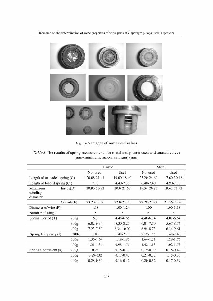
Research on the determination of some properties of valve parts of diaphragm pumps used in sprayers
203
Figure 5 Images of some used valves
Table 3 The results of spring measurements for metal and plastic used and unused valves (min-minimum, max-maximum) (mm)
Plastic Metal Not used Used Not used Used Length of unloaded spring (C) 20.08-21.44 10.00-18.40 23.20-24.60 17.60-30.48 Length of loaded spring (C1) 7.10 4.40-7.30 6.40-7.40 4.90-7.70 Maximum windingdiameter
Inside(D) 20.90-20.92 20.0-21.60 19.54-20.36 19.62-21.92
Outside(E) 23.20-23.50 22.0-23.70 22.28-22.82 21.56-23.90 Diameter of wire (F) 1.18 1.00-1.24 1.00 1.00-1.18 Number of Rings 5 5 6 6 Spring Period (T) 200g 5.3 4.48-6.65 4.48-6.34 4.01-6.64
300g 6.02-6.34 5.30-8.27 6.01-7.50 5.67-8.74 400g 7.23-7.50 6.34-10.00 6.94-8.73 6.34-9.61
Spring Frequency (f) 200g 1.86 1.48-2.20 2.19-1.55 1.48-2.46 300g 1.56-1.64 1.19-1.86 1.64-1.31 1.28-1.73
400g 1.31-1.36 0.98-1.56 1.42-1.13 1.02-1.55 Spring Coefficient (k) 200g 0.28 0.18-0.39 0.19-0.39 0.18-0.49
300g 0.29-032 0.17-0.42 0.21-0.32 1.15-0.36 400g 0.28-0.30 0.16-0.42 0.20-0.32 0.17-0.39

E. Kilic, I. Celen, T. Aktas
204
Figure 6 Some used valve springs
CONCLUSIONS
A carefully selected valve spring should make the valve open and close at the right time depending on the pump working pressure, working conditions, and system temperature. Along with these factors, spring coefficient plays an important role in achieving a reliable and safe valve performance. The selection of the springs in valves has an important effect on the valve performance. Improving the valve performance relies on a quality spring which acts as the controller of valve timing.
In a valve mechanism simply consisting of a mass and a spring system, as the spring coefficient increased, the response time of the system decreased.
Depending of how hard a spring is, the response time of a system will increase. However, it is also necessary to increase the pressure to open the valve. If a hard spring is used in any system, then during the closing of the valve, spring will hit the disc and valve bearing much faster. This will, in turn, increase the extent of corrosion and will lower valve strength. Corrosion on the valve will also negatively affect pump performance. If springs are soft, then the valves will not close at the requested point, and this will worsen the response time of the pump. Selecting the right spring will increase the valve strength and improve pump performance.
Thanks to the effects of chemicals, it was observed that cross sections of springs became thinner. As the thickness of wire decreased, displacement amount increased, and spring coefficient and natural frequency decreased. This meant that the spring became softer. Because of the effects of the agricultural pesticides, disc and valve bearings became corroded.
Due to assembly errors, springs did not properly function and sprang out of its axis. As a result, the degree of friction between the springs and the main body increased, thereby causing the spring to become thinner.
The selection of appropriate spring material and investigating different spring types will both eliminate valve corrosion and increase valve performance.
Research on the determination of some properties of valve parts of diaphragm pumps used in sprayers
205
It was observed that new springs have different coiling numbers. This would negatively affect the spring coefficient and spring frequency.
The size of plastic discs and plastic valve bearings showed no variations; however, there were some variations in the size of metal discs and metal valve bearings.
Since plastic valve mechanisms were produced using a mould the parts were produced to a certain standard, all having the equal measurements, but metal valves were manufactured manually, and this, in turn, caused some differences in the measurements of the parts.
Deep scratches were observed on the surface of the disc (Figure 5). These scratches were found to be the results of corrosive effects of such materials as dust and dirty air which were mixed with the agricultural pesticides on the disc surfaces. In this reason, the filtering mechanism in the system should be made to work effectively.
Improving pump valves will lower pump valve maintenance costs.Determining the valve defects and removing them will increase the pump performance.It is determined that as new masses were added to the spring, amount of displacement
increased proportionally. Natural frequency is in inverse proportion to mass increases. As natural frequency decreases, amount of displacement increases.
REFERENCES
1. Kamis Z., Yuksel I. (2004). An investigation of effect of applied electrical voltage on system dynamic behavior and energy consumption of an electromechanical valve actuator. G.Ü. Fen Bilimleri Dergisi 17 (3) :161-177.
2. Sabanci A. (1984). Tarım traktörlerinde titreşim sorunları ve sürücü oturaklarının yalıtım ozellikleri uzerinde bir araştırma. TZDK Profession Publications :35, Ankara, Turkey.


36. Symposium "Actual Tasks on Agricultural Engineering", Opatija, Croatia, 2008.
207
36.
SIMPOZIJAKTUALNI ZADACIMEHANIZACIJE POLJOPRIVREDE
UDK621.182.3:631.352:665.75
Stručni radExpert paper
UTJECAJ VISINE OTKOSA TRAVE NA POTROŠNJU GORIVA KOSILICE ZA PARKOVE
ANTONIO CARRARO D. STAJNKO, M. LAKOTA, B. MURŠEC, M. SAGADIN
Univerza v Mariboru, Fakulteta za kmetijstvo, Katedra za Biosistemsko inženirstvo, Vrbanska 30, 2000 Maribor, Slovenija
e-mail [email protected]
SAŽETAK
Proučavan je utjecaj visine otkosa na potrošnju goriva i utrošeno vrijeme prilikom košnje rotacionom kosilicom za parkove Antonio Carraro TTR 4400 HST. Trava se svaki put kosila nakon što je postigla visinu 12 cm na tri različitevisine A – 8 cm, B – 6 cm i C – 4 cm. Za vrijeme dvomjesečnog pokusa na visinu A pokošeno je četiri puta, na B pet puta a na C šest puta. Kod varijante A prosječna potrošnja goriva iznosi 51,79 ml (12,33 l/ha), a prosječan utrošak vremena 52,33 sekundi (3h 57 min/ha), dok se kod varijante B povećala na 59,00 ml (14,05 l/ha) i 59,7 sekundi (3h 57 min/ha) odnosno na 74,31 ml (17,63 l/ha) i 74,37 sekundi (4h 55 min/ha) u varijanti C. Varijanta A statistički je značajnomanja od B i C, a također B od A i C. Zbog različitog intenziteta košnje trave te prema prosječno potrošenom gorivu i potrebnom vremenu po jednom hektaru u proučavanim uvjetima trave najprihvatljiva bi bila visina otkosa od 6 cm što je ispitano u varijanti B.
Ključne riječi: košnja, kosilica za parkove, trava, utrošak goriva, utrošak vremena
UVOD
Pri negovanju večjih površin okrasnih trat se srečujemo s problemom optimalne višine košnje in določitve intervala košnje. Pri zelo nizki košnji je stroj zaradi rastlinske mase zelo obremenjen, zato se zaradi počasne košnje povečujeta tako poraba goriva kot časa.Podobno naraščata poraba goriva in časa tudi pri zelo visoki košnji, saj se povečuje število košenj v sezoni-
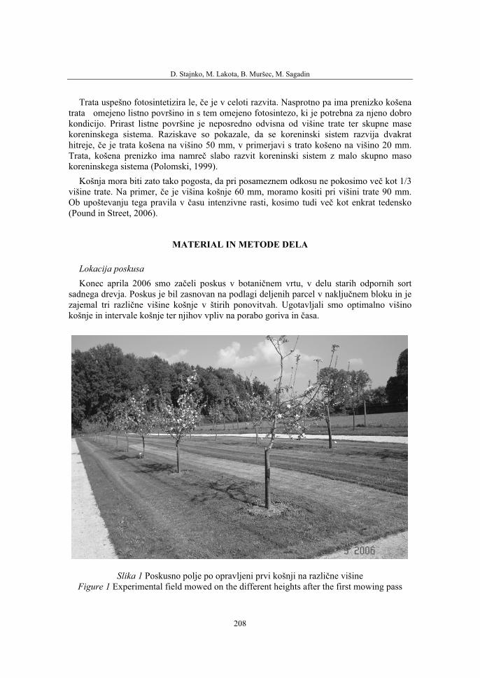
D. Stajnko, M. Lakota, B. Muršec, M. Sagadin
208
Trata uspešno fotosintetizira le, če je v celoti razvita. Nasprotno pa ima prenizko košena trata omejeno listno površino in s tem omejeno fotosintezo, ki je potrebna za njeno dobro kondicijo. Prirast listne površine je neposredno odvisna od višine trate ter skupne mase koreninskega sistema. Raziskave so pokazale, da se koreninski sistem razvija dvakrat hitreje, če je trata košena na višino 50 mm, v primerjavi s trato košeno na višino 20 mm. Trata, košena prenizko ima namreč slabo razvit koreninski sistem z malo skupno maso koreninskega sistema (Polomski, 1999).
Košnja mora biti zato tako pogosta, da pri posameznem odkosu ne pokosimo več kot 1/3 višine trate. Na primer, če je višina košnje 60 mm, moramo kositi pri višini trate 90 mm. Ob upoštevanju tega pravila v času intenzivne rasti, kosimo tudi več kot enkrat tedensko (Pound in Street, 2006).
MATERIAL IN METODE DELA
Lokacija poskusa Konec aprila 2006 smo začeli poskus v botaničnem vrtu, v delu starih odpornih sort
sadnega drevja. Poskus je bil zasnovan na podlagi deljenih parcel v naključnem bloku in je zajemal tri različne višine košnje v štirih ponovitvah. Ugotavljali smo optimalno višino košnje in intervale košnje ter njihov vpliv na porabo goriva in časa.
Slika 1 Poskusno polje po opravljeni prvi košnji na različne višine Figure 1 Experimental field mowed on the different heights after the first mowing pass
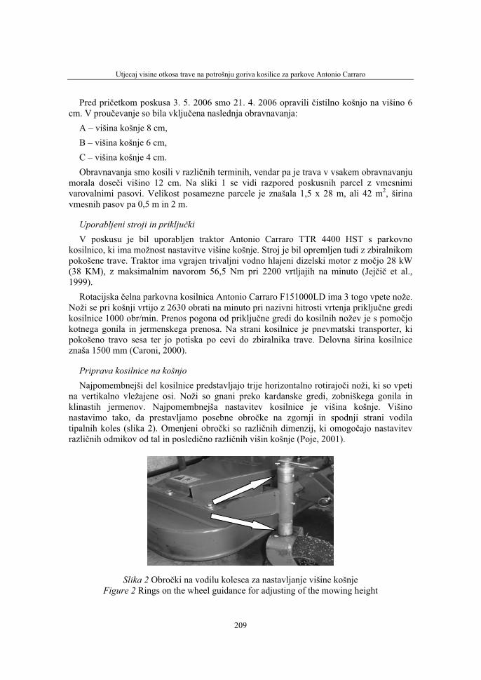
Utjecaj visine otkosa trave na potrošnju goriva kosilice za parkove Antonio Carraro
209
Pred pričetkom poskusa 3. 5. 2006 smo 21. 4. 2006 opravili čistilno košnjo na višino 6 cm. V proučevanje so bila vključena naslednja obravnavanja:
A – višina košnje 8 cm, B – višina košnje 6 cm, C – višina košnje 4 cm. Obravnavanja smo kosili v različnih terminih, vendar pa je trava v vsakem obravnavanju
morala doseči višino 12 cm. Na sliki 1 se vidi razpored poskusnih parcel z vmesnimi varovalnimi pasovi. Velikost posamezne parcele je znašala 1,5 x 28 m, ali 42 m2, širina vmesnih pasov pa 0,5 m in 2 m.
Uporabljeni stroji in priključkiV poskusu je bil uporabljen traktor Antonio Carraro TTR 4400 HST s parkovno
kosilnico, ki ima možnost nastavitve višine košnje. Stroj je bil opremljen tudi z zbiralnikom pokošene trave. Traktor ima vgrajen trivaljni vodno hlajeni dizelski motor z močjo 28 kW (38 KM), z maksimalnim navorom 56,5 Nm pri 2200 vrtljajih na minuto (Jejčič et al., 1999).
Rotacijska čelna parkovna kosilnica Antonio Carraro F151000LD ima 3 togo vpete nože. Noži se pri košnji vrtijo z 2630 obrati na minuto pri nazivni hitrosti vrtenja priključne gredi kosilnice 1000 obr/min. Prenos pogona od priključne gredi do kosilnih nožev je s pomočjokotnega gonila in jermenskega prenosa. Na strani kosilnice je pnevmatski transporter, ki pokošeno travo sesa ter jo potiska po cevi do zbiralnika trave. Delovna širina kosilnice znaša 1500 mm (Caroni, 2000).
Priprava kosilnice na košnjo Najpomembnejši del kosilnice predstavljajo trije horizontalno rotirajoči noži, ki so vpeti
na vertikalno vležajene osi. Noži so gnani preko kardanske gredi, zobniškega gonila in klinastih jermenov. Najpomembnejša nastavitev kosilnice je višina košnje. Višino nastavimo tako, da prestavljamo posebne obročke na zgornji in spodnji strani vodila tipalnih koles (slika 2). Omenjeni obročki so različnih dimenzij, ki omogočajo nastavitev različnih odmikov od tal in posledično različnih višin košnje (Poje, 2001).
Slika 2 Obročki na vodilu kolesca za nastavljanje višine košnje Figure 2 Rings on the wheel guidance for adjusting of the mowing height

D. Stajnko, M. Lakota, B. Muršec, M. Sagadin
210
Paziti moramo, da je odmik vseh tipalnih koles nastavljen na isto kombinacijo obročkov,saj v nasprotnem primeru vsa kolesca ne nalegajo enakomerno na površino. Posledica je lahko neenakomerno pokošena trava, poleg tega pa je stroj izpostavljen poškodbam zaradi neenakomernih obremenitev.
Preden smo začeli kositi, smo parkovni kosilnik pripravili za meritve. Za ugotavljanje količine porabljenega goriva smo namestili menzuro z volumnom 250 ml in jo pritrdili na stebriček ob zbiralniku trave. Povezali smo jo s cevmi za dovajanje goriva in povratnega voda goriva.
Slika 3 Menzura za merjenje količine porabljenega goriva (levo) in vijak za nastavitev hitrosti vožnje na stopalki (puščica desno)
Figure 3 The test tube for measuring the quantity of fuel spent (left) and the screw for adjusting the driving speed (arrow at right)
Ker ima traktor Antonio Carraro TTR 4400 HST brezstopenjski hidrostatični menjalnik, pri katerem je hitrost vožnje zelo odvisna od »človeškega faktorja«, smo na stopalko za spreminjanje hitrosti namestili vijak. Z vrtenjem vijaka smo tako določali dolžino hoda stopalke in s tem tudi delovno hitrost. Delovno hitrost smo nastavili pri neobremenjenem stroju na 2 km/h in vožnji po ravnem.
Direktno merjenje hitrosti s pomočjo traktorskih instrumentov je sicer možno, vendar pa smo zaradi natančnosti meritev čas vožnje merili s štoparico in kasneje izračunali hitrost iz prevožene poti in časa.
Višino trate smo določali s pomočjo plošče velikosti 500 mm x 500 mm in debeline 3 mm. Plošča iz pleksi stekla je imela na sredini luknjo premera 14 mm. Merjenje višine smo izvedli tako, da smo ploščo položili na trato ter skozi luknjo z merilom izmerili razdaljo plošče od tal. Višino smo določil iz povprečja desetih merjenj na naključnih mestih.

Utjecaj visine otkosa trave na potrošnju goriva kosilice za parkove Antonio Carraro
211
REZULTATI
V tabeli 1 so prikazani termini košnje pri posameznem obravnavanju, iz katerih se lepo vidi, da z večanem odkosa raste potreben čas za obnovo trave in se število košenj manjše. Tako je bilo pri obravnavanju A (8 cm) opravljenih 6 košenj, pri B (6 cm) 5 in pri C (4 cm) samo 4 košnje.
Tabela 1 Termini košenj po obravnavanjih v času trajanja poskusa Table 1 Mowing days at different variants during the experiment
Obrav. 3.5. 10.5. 13.5. 16.5. 18.5. 25.5. 26.5. 5.6. 9.6. 13.6. 22.6 23.6.
A * * * * *
B * * * * *
C * * * *
* košnja
Vpliv višine košnje na porabo goriva V tabeli 2 se vidi, da smo pri obravnavanju C (4 cm) odvzemali največ zelene mase, zato
je bila tudi poraba goriva pri posamezni košnji največja (74,31 ml – 17,63 l/ha). Z manjšanjem višine odkosa pa se je povprečna poraba goriva zmanjšala na 59,00 ml – 14,05 l/ha (B) oziroma 51,79 ml – 12,33 l/ha (A). Natančnejša statistična analiza s pomočjo LSD testa je nadalje pokazala, da je nasprotno skupna poraba goriva štirih košenj pri obravnavanju A večja od porabe pri obravnavanju B in C, ob enem pa se tudi poraba goriva B značilno razlikuje od porabe goriva pri obravnavanju A in C.
Tabela 2 Povprečna poraba goriva v posamezni košnji po obravnavanjih (ml) Table 2 The average fuel consumption at each variant (ml)
1.košnja
2.košnja
3.košnja
4.košnja
5.košnja
6.košnja Skupaj Povprečna Povprečna
(l/ha)
A-8 cm 49,75 53,00 52,00 50,75 51,75 53,50 310,75 51,79 12,33
B-6 cm 57,25 59,75 61,25 61,50 55,25 295,00 59,00 14,05
C-4 cm 82,00 74,00 68,75 72,50 297,25 74,31 17,63
Vpliv višine košnje na porabo časa V tabeli 3 je prikazana poraba časa pri posameznih košnjah in obravnavanjih. Ker smo
pri obravnavanju A odvzemali najmanj zelene mase, je bila tudi poraba časa pri enkratni košnji najmanjša in je povprečno znašala 52,33 sekund. Nasprotno pa je z večanjem višine
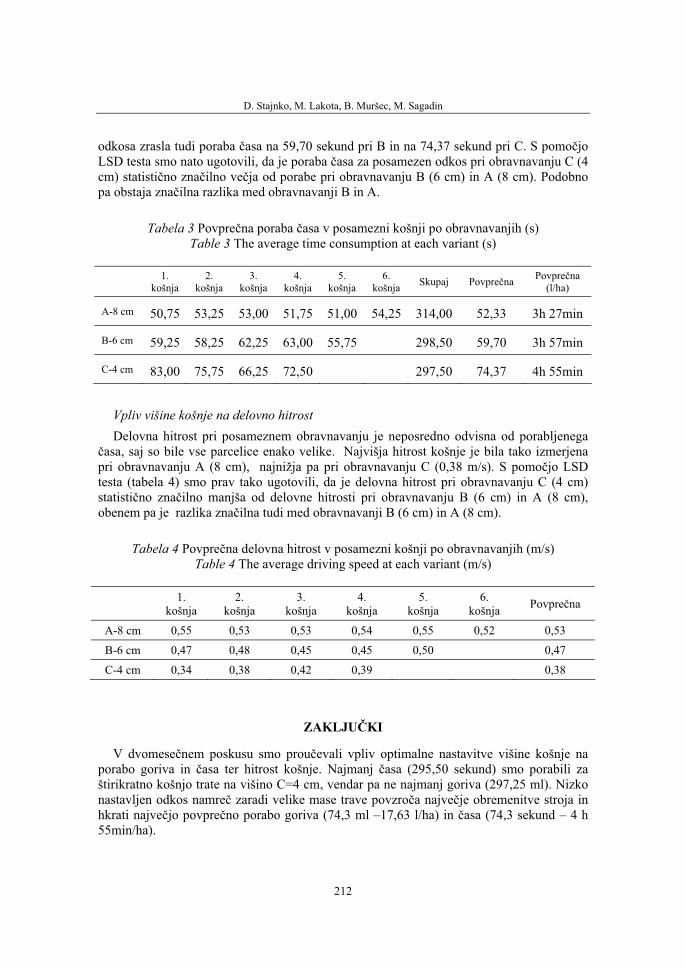
D. Stajnko, M. Lakota, B. Muršec, M. Sagadin
212
odkosa zrasla tudi poraba časa na 59,70 sekund pri B in na 74,37 sekund pri C. S pomočjoLSD testa smo nato ugotovili, da je poraba časa za posamezen odkos pri obravnavanju C (4 cm) statistično značilno večja od porabe pri obravnavanju B (6 cm) in A (8 cm). Podobno pa obstaja značilna razlika med obravnavanji B in A.
Tabela 3 Povprečna poraba časa v posamezni košnji po obravnavanjih (s) Table 3 The average time consumption at each variant (s)
1.košnja
2.košnja
3.košnja
4.košnja
5.košnja
6.košnja Skupaj Povprečna Povprečna
(l/ha)
A-8 cm 50,75 53,25 53,00 51,75 51,00 54,25 314,00 52,33 3h 27min
B-6 cm 59,25 58,25 62,25 63,00 55,75 298,50 59,70 3h 57min
C-4 cm 83,00 75,75 66,25 72,50 297,50 74,37 4h 55min
Vpliv višine košnje na delovno hitrost Delovna hitrost pri posameznem obravnavanju je neposredno odvisna od porabljenega
časa, saj so bile vse parcelice enako velike. Najvišja hitrost košnje je bila tako izmerjena pri obravnavanju A (8 cm), najnižja pa pri obravnavanju C (0,38 m/s). S pomočjo LSD testa (tabela 4) smo prav tako ugotovili, da je delovna hitrost pri obravnavanju C (4 cm) statistično značilno manjša od delovne hitrosti pri obravnavanju B (6 cm) in A (8 cm), obenem pa je razlika značilna tudi med obravnavanji B (6 cm) in A (8 cm).
Tabela 4 Povprečna delovna hitrost v posamezni košnji po obravnavanjih (m/s) Table 4 The average driving speed at each variant (m/s)
1.košnja
2.košnja
3.košnja
4.košnja
5.košnja
6.košnja Povprečna
A-8 cm 0,55 0,53 0,53 0,54 0,55 0,52 0,53
B-6 cm 0,47 0,48 0,45 0,45 0,50 0,47
C-4 cm 0,34 0,38 0,42 0,39 0,38
ZAKLJUČKI
V dvomesečnem poskusu smo proučevali vpliv optimalne nastavitve višine košnje na porabo goriva in časa ter hitrost košnje. Najmanj časa (295,50 sekund) smo porabili za štirikratno košnjo trate na višino C=4 cm, vendar pa ne najmanj goriva (297,25 ml). Nizko nastavljen odkos namreč zaradi velike mase trave povzroča največje obremenitve stroja in hkrati največjo povprečno porabo goriva (74,3 ml –17,63 l/ha) in časa (74,3 sekund – 4 h 55min/ha).
Utjecaj visine otkosa trave na potrošnju goriva kosilice za parkove Antonio Carraro
213
Pri drugem obravnavanju (B=6 cm) je skupna količina porabljenega goriva za petkratno košnjo 295 ml sicer najmanjša, vendar pa je skupna poraba časa 298,50 sekund le minimalno (1,25 sekunde) večja od najmanjše skupne porabe izmerjene pri najnižji višini košnje. Povprečna poraba goriva in časa pri posamezni košnji pa se je zmanjšala na 59 ml (14,05 l/ha) oziroma 59,7 sekund (3h 57 min/ha).
Največ goriva (310,75 ml) in časa (314 sekund) smo v celotnem opazovanem obdobju porabili pri šestkratni košnji na višino A=8 cm, čeprav smo za posamezen odkos povprečno porabili najmanj goriva (51,9 ml – 12,33 l/ha) in časa (52,3 sekund – 3h 27 min/ha).
S stališča enkratne košnje 6,5 ha velikega botaničnega vrta pa so veliko pomembnejši podatki o hektarski porabi iz katerih lahko sklepamo, da je glede porabljenega goriva (12,33 l/ha) in časa (3h 27min/ha) najugodnejša varianta A=8 cm. Vendar je v tem primeru interval košnje 7 do 10 dni prekratek in zahteva preveliko frekvenco ponovitev.
Če dodatno upoštevamo delovno hitrost, storilnost, biološke potrebe travne ruše, maksimalne obremenitve stroja, obračalne hode in ostale dejavnike, ki so specifični za posamezno trato, je naša ocena, da je najprimernejša višina košnje z obravnavanim strojem Antonio Carraro TTR 4400 HST B=6 cm, pri kateri v poprečju za košnjo enega hektarja trate porabimo 14,05 l goriva in 3h 57 min časa.
LITERATURA
1. Caroni, M., 2000. User and maintenance manual and safety rules for mowers, Cuneo, 118 str.
2. Jejčič, V., Poje, T., Gjergek, T., 1999. Antonio Carraro–Tigretrac. Tehnika in narava, 3, s. 4.
3. Poje, T., 2001. Komunalni Antonio Carraro TTR 4400 HST. Tehnika in narava, 5, s. 35.
4. Polomski, B., 1999. Mowing Lawns. The Clemson university cooperative extension service,
5. http://www.hgic.clemson.edu (17. 11. 2006).
6. Pound, W. E., Street, J. R. 2006. Lawn Mowing http://www.ohioline.osu.edu/hyg-fact/4000/4020.html (17.11. 2006), p.1-4
D. Stajnko, M. Lakota, B. Muršec, M. Sagadin
214
THE EFFECT OF THE DIFFERENT MOWING HEIGHT ON THE FUEL CONSUMPTION OF THE LAWN
MOWER ANTONIO CARRARO University of Maribor, Faculty of Agriculture, Vrbanska 30, 2000 Maribor, Slovenija
ABSTRACT
The influence of the mowing height on the fuel as well as time consumption was researched during the precise field experiment (May – July 2007). When using the lawn mower Antonio Carraro TTR 4400 HST, the lawn was mowed each time it reached the height of 12 cm, By decreasing the mowing height from A – 8 cm to B – 6 cm and C – 4 cm, the number of treatment increased A (four times), B (five times) and C (six times). It was proved that the differences in the average time and fuel consumptions were rising significantly: A (52,33 sec -3h 57 min/ha, 51.79 ml – 12,33 l/ha), B (59,70 sec – 3h 57 min/ha, 59,00 ml – 14,05 l/ha) and C (74,37 sec – 4h 55 min/ha, 74.31 ml – 17,63 l/ha). According to the different mowing frequency of the lawn mower, the treatment B with the average consumption of 14,05 l fuel and 3h 57 min per hectare was recommended for the selected lawn conditions.
Key words: mow, lawn mower, fuel consumption, time consumption
36. Symposium "Actual Tasks on Agricultural Engineering", Opatija, Croatia, 2008.
215
36.
SIMPOZIJAKTUALNI ZADACIMEHANIZACIJE POLJOPRIVREDE
UDK631.35:631.544.72
Stručni radExpert paper
ENERGETSKE KARAKTERISTIKE MALČERA INO EURO OPEN 280 SA POKRETNIM POKLOPCEM
T. POJE
Kmetijski inštitut Slovenije, Oddelek za kmetijsko tehnikoHacquetova 17, SI – 1000 Ljubljana
E-mail: [email protected]
SAŽETAK
Na malčeru INO EURO OPEN 280 ispitivali smo odabrane energetske karakteristike. Na osnovu izmjerenog momenta i broja okretaja na priključnomvratilu traktora, koje je pokretalo neopterećen i opterećen malčer, izračunata je potrebna snaga za pogon malčera. Mjerenja su izvedena kod različitih brzina kretanja i kod različitog položaja pokretnog poklopca. Ustanovili smo da je snaga potrebna za zagon 22,4 kW, dok je za pogon neopterećenog malčerapotrebno 12,2 kW. Zaštita od preopterećenja se aktivira kod 103 kW angažirane snage. Kod zatvorenog poklopca izvedena su mjerenja pri brzini kretanja od 6,6 do 9,3 km/h, dok je potrebna snaga za pogon iznosila između 37,4 i 64,1 kW. Kod otvorenog poklopaca brzina kretanja iznosila je do 12,3 km/h, a prosječnapotrebna snaga do 49,1 kW.
Ključne riječi: malčer, pokretni poklopac, moment na priključnom vratilu, potrebna snaga, specifična energija
UVOD
Značaj malčera sve je veći kako u poljoprivredi tako i u komunali. Proizvođači malčeraproizvode veliki broj različitih modela koji se razlikuju po vrsti radnih elementa (čekića,noževa, itd.). U Sloveniji Jejčič (1997), Poje (2003, 2006, 2007) testiraju ratarske i komunalne malčere glede potrebne snage i drugih eksploatacijskih karakteristika u realnim uvjetima. Poje (2005) analizira smjer razvoja strojeva za sitnjenje biljnih ostataka, Godeša et al. (2006) vrše mjerenja na malčerima s novom generacijom rotora. U NjemačkojBrunotte sa suradnicima (1995) detaljno istražuje mehanizaciju za održavanje površina pod ugarom. Istraživanja su fokusirana u kakvoću sitnjenja i potrebnu snagu za pogon kod različitih radnih elemenata i različitih strojeva.

T. Poje
216
U radu je prikazana analiza potrebne snage za pogon malčera INO EURO OPEN 280 s pokretnim poklopcem i rotorom, gdje su radni elementi (čekići) raspodijeljeni po spirali sa 45 stupnjeva.
MATERIJAL I METODE RADA
Eksploatacijske karakteristike proučavali smo na malčeru INO EURO OPEN 280. Glavni tehnički podaci predstavljeni su u tablici 1.
Tablica 1 Tehnički podaci proizvođača za malčer
Proizvođač INO Industrijska oprema Brežice
Model EURO OPEN 280
Radna širina (cm) 268
Broj okretaja priključnog vratila (min-1) 540/1000
Broj čekića 32
Masa (kg) 780
Brzina okretanja rotora (min-1) 2243
U vidu eksploatacijskih karakteristika istraživali smo potrebnu snagu za pogon malčera preko priključnog vratila traktora kod različitog opterećenja i različitog namještenja pokretnog poklopca. Sama istraživanja izvedena su kod različite brzine kretanja traktora. Za pogon malčera upotrijebili smo traktor Landini Legend 160 Deltashift sa maksimalnom snagom motora 123 kW.
Mjerni lanac bio je sastavljena od tri dijela: senzora, digitalnog mjernog pojačala i PC računala za prijem i obradu mjernog signala. Okretni moment i broj okretaja priključnogvratila mjerili smo pomoću dinamometra za mjerenje momenta i prigrađenog senzora vrtnje (T30 FN Hottinger Baldwin Messtechnik). Digitalno pojačalo bio je SPIDER 8 Hottinger Baldwin Messtechnik. Frekvencija uzimanja podataka iznosila je 100 Hz, dok je dužina pojedinog mjerenja ovisila o vremenskom toku rada sa malčerom. Iz izmjerenog momenta i broja okretaja na priključnom vratilu izračunata je potrebna snaga za pogon priključkapreko priključnog vratila.
Snaga za pogon:
P = Mp ω (1)
P = Mn30p π (2)
Značenje oznaka: Pp - potrebna snaga za pogon malčera W

Energetske karakteristike malčera INO EURO OPEN 280 s pokretnim poklopcem
217
M – moment na priključnom vratilu Nm
ω - kutna brzina rad n – broj okretaja priključnog vratila min-1
Mjerenje snage potrebne za rad malčera EURO OPEN 280 izveli smo na travnjaku, na kojem je gustoća biljki iznosila 0,68 kg/m2. Kod sitnjenja biljne mase varirali smo brzinu kretanja (opterećenje malčera) i poziciju pokretnog poklopca.
REZULTATI RADA I DISKUSIJA
Mjerenjem momenta i broja okretaja na priključnom vratilu traktora izračunali smo potrebnu snagu za pogon malčera preko priključnog vratila kod različite brzine kretanja i različite pozicije poklopca. Rezultati mjerenja i izračunata potrebna snaga na priključnomvratilu prikazani su u tablici 2. Za pogon mulčera izmjereno je na priključnom vratilu 928 Nm zakretnog momenta i zagonska snaga je pri tom iznosila 22,4 kW. Za pogon neopterećenog malčera, gdje se je priključno vratilo okretalo sa 1019 okr./min, bio je izmjeren prosječni moment 115 Nm, dok je pogonska snaga iznosila u prosjeku 12,2 kW.
Prijenos snage iz multiplikatora do rotora s radnim elementima izveden je pomoćuprijenosa putem remena, koji ujedno može služiti i kao zaštita malčera pred preopterećenjem. Kod ispitivanog malčera remeni su proklizali kad je prosječni izmjereni moment iznosio 1311 Nm. Tada se je broj okretaja već dosta smanjio od nazivnog 1000 okr./min i u prosjeku proklizavanja remena iznosio je 752 okr./min. Kod proklizavanja remena izmjereno je u prosjeku 103 kW angažirane snage na priključnom vratilu traktora.
-20000
0
20000
40000
60000
80000
100000
120000
140000
10 20 30 40 50 60 70 80 90
VRIJEME (s)
SNA
GA
(W
)
Slika 1 Oscilogram angažirane snage na priključnom vratilu kod pogona malčera.Strelicama je označeno proklizavanje remena, odnosno aktiviranje zaštite malčera pred
preopterećenjem
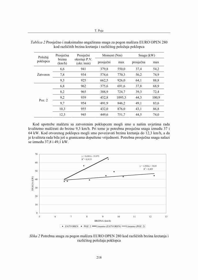
T. Poje
218
Tablica 2 Prosječno i maksimalno angažirana snaga za pogon malčera EURO OPEN 280 kod različitih brzina kretanja i različitog položaja poklopca
Moment (Nm) Snaga (kW) Položajpoklopca
Prosječnabrzina(km/h)
Prosječniokretaji P.V.
(okr./min) prosječni max prosječna max
6,6 941 379,8 550,0 37,4 54,2
7,8 934 574,6 770,3 56,2 74,9 Zatvoren
9,3 925 662,5 926,0 64,1 88,8
6,8 962 375,6 691,6 37,8 68,9
8,2 965 388,9 724,7 39,3 72,4
9,2 939 452,8 1095,3 44,3 100,9
9,7 954 491,9 846,2 49,1 83,6
10,3 955 432,0 876,0 43,1 86,8
Poz. 2
12,3 945 449,6 751,7 44,5 74,0
Kod upotrebe malčera sa zatvorenim poklopcem mogli smo u našim uvjetima rada kvalitetno malčirati do brzine 9,3 km/h. Pri tome je potrebna prosječna snaga između 37 i 64 kW. Kod otvorenog poklopca mogli smo povećavati brzinu kretanja do 12,3 km/h, a da je kvaliteta rada bila još u granicama dopuštene vrijednosti. Potrebna prosječna snaga nalazi se između 37,8 i 49,1 kW.
y = 1,3826x + 30,03R2 = 0,409
0
10
20
30
40
50
60
70
5 6 7 8 9 10 11 12 13
BRZINA (km/h)
SNA
GA
(kW
)
ZATVOREN POZ. 2 Linearno (ZATVOREN) Linearno (POZ. 2)
y = 9,4301x - 21,972R2 = 0,9153
Slika 2 Potrebna snaga za pogon malčera EURO OPEN 280 kod različitih brzina kretanja i različitog položaja poklopca
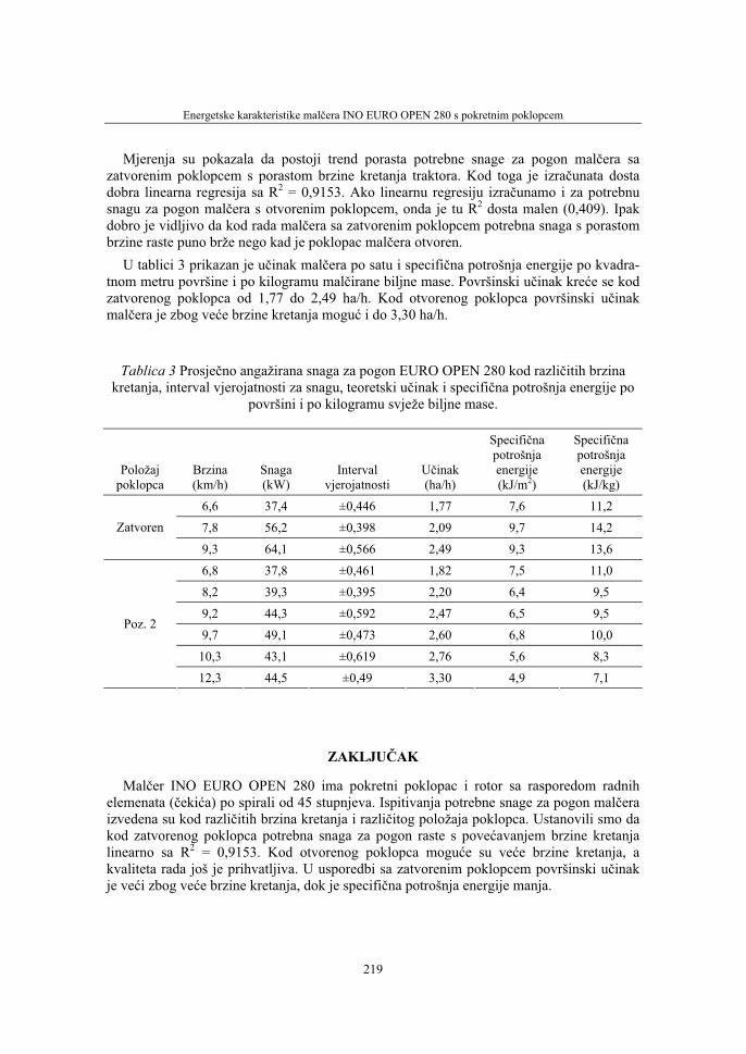
Energetske karakteristike malčera INO EURO OPEN 280 s pokretnim poklopcem
219
Mjerenja su pokazala da postoji trend porasta potrebne snage za pogon malčera sa zatvorenim poklopcem s porastom brzine kretanja traktora. Kod toga je izračunata dosta dobra linearna regresija sa R2 = 0,9153. Ako linearnu regresiju izračunamo i za potrebnu snagu za pogon malčera s otvorenim poklopcem, onda je tu R2 dosta malen (0,409). Ipak dobro je vidljivo da kod rada malčera sa zatvorenim poklopcem potrebna snaga s porastom brzine raste puno brže nego kad je poklopac malčera otvoren.
U tablici 3 prikazan je učinak malčera po satu i specifična potrošnja energije po kvadra-tnom metru površine i po kilogramu malčirane biljne mase. Površinski učinak kreće se kod zatvorenog poklopca od 1,77 do 2,49 ha/h. Kod otvorenog poklopca površinski učinakmalčera je zbog veće brzine kretanja moguć i do 3,30 ha/h.
Tablica 3 Prosječno angažirana snaga za pogon EURO OPEN 280 kod različitih brzina kretanja, interval vjerojatnosti za snagu, teoretski učinak i specifična potrošnja energije po
površini i po kilogramu svježe biljne mase.
Položajpoklopca
Brzina(km/h)
Snaga(kW)
Intervalvjerojatnosti
Učinak(ha/h)
Specifičnapotrošnjaenergije(kJ/m2)
Specifičnapotrošnjaenergije(kJ/kg)
6,6 37,4 ±0,446 1,77 7,6 11,2
7,8 56,2 ±0,398 2,09 9,7 14,2 Zatvoren
9,3 64,1 ±0,566 2,49 9,3 13,6
6,8 37,8 ±0,461 1,82 7,5 11,0
8,2 39,3 ±0,395 2,20 6,4 9,5
9,2 44,3 ±0,592 2,47 6,5 9,5
9,7 49,1 ±0,473 2,60 6,8 10,0
10,3 43,1 ±0,619 2,76 5,6 8,3
Poz. 2
12,3 44,5 ±0,49 3,30 4,9 7,1
ZAKLJUČAK
Malčer INO EURO OPEN 280 ima pokretni poklopac i rotor sa rasporedom radnih elemenata (čekića) po spirali od 45 stupnjeva. Ispitivanja potrebne snage za pogon malčeraizvedena su kod različitih brzina kretanja i različitog položaja poklopca. Ustanovili smo da kod zatvorenog poklopca potrebna snaga za pogon raste s povećavanjem brzine kretanja linearno sa R2 = 0,9153. Kod otvorenog poklopca moguće su veće brzine kretanja, a kvaliteta rada još je prihvatljiva. U usporedbi sa zatvorenim poklopcem površinski učinakje veći zbog veće brzine kretanja, dok je specifična potrošnja energije manja.
T. Poje
220
LITERATURA
1. Brunotte J., Biller R.H., Kruse W. (1995) Mechanisierung der Pflege stillgelegter Flaechen, Deutschen Landwirtschafts-Gesellschaft, Frankfurt, 16 s.
2. Godeša T., Poje T. (2006) Poročilo o preizkušanju mulčerjev z novo generacijo rotorjev. Kmetijski inštitut Slovenije, Ljubljana, 18 s.
3. Jejčič V., Poje T. (1997) Mulčer Willibald SHU 280. ČZD Kmečki glas – Tehnika in narava, 1(4): 12 - 13
4. Poje T., Jejčič V. (2005) Smeri razvoja strojev za drobljenje rastlinskih ostankov. Kmetijski inštitut Slovenije - Študije po naročilu 463, Ljubljana, 68 s.
5. Poje T. (2006) Mulčer INO EURO 250. ČZD Kmečki glas - Tehnika in narava 10(4): 16 - 18,
6. Poje T. (2003) Komunalni mulčer INO MK 160. ČZD Kmečki glas - Tehnika in narava, 7(4): 8 – 9
7. Poje T. (2007) Poročilo o preizkušanju mulčerjev INO EURO 280 in EURO OPEN 280. Kmetijski inštitut Slovenije - Študije po naročilu, Ljubljana, 26 s.
ENERGETIC CHARACTERISTICS OF INO EURO OPEN 280 MULCHER WITH VARIABLE COVER
ABSTRACT
Selected energetic characteristics of INO EURO OPEN 280 mulcher were studied. On the basis of measured torque and number of revolutions of PTO shaft driving unloaded and loaded mulcher the power required for driving of the mulcher was calculated. Measurements were performed at different driving velocities and different positions of variable cover. It was established that the starting power requirement was 22.4 kW while for driving of unloaded mulcher 12.2 kW were required. The protection from overloading is activated at 103 kW required power. When the cover was closed measurements were carried out at 6.6 to 9.3 km/h driving velocities and the power required for driving ranged between 37.4 and 64.1 kW. When the cover was open the driving velocity amounted to 12.3 km/h and the average power requirement was up to49.1 kW.
Key words: mulcher, variable cover, torque on PTO shaft, power requirement, specific energy

36. Symposium "Actual Tasks on Agricultural Engineering", Opatija, Croatia, 2008.
221
36.
SIMPOZIJAKTUALNI ZADACIMEHANIZACIJE POLJOPRIVREDE
UDC631.354.027
Stručni radExpert paper
STRUCTURAL, KINEMATICAL AND KINETOSTATIC ANALYSIS OF THE CLEANING SYSTEM FROM
CEREAL HARVESTERS VICTOR MOISE, GHEORGHE VOICU, EDMOND MAICAN
„Politehnica” University of Bucharest, Faculty of Biotechnical Systems Engineering Splaiul Independentei, no.313, 060032, Bucharest, Romania
e-mail: [email protected]
SUMMARY
This paper presents the structural, kinematical and kinetostatic analysis of the cereal harvester’s cleaning system. A computer programme with functions and procedures for each component module of the cleaning system was developed. The calculated results were graphically represented, in order to have a clearer picture over kinematical and kinetostatic parameters. Thus, it is revealed that these parameters for the Romanian harvesters are similar with those from well known models: New Holland, Massey Ferguson, Laverda etc.
Key words: mechanism, cleaning system, structure, kinematics, kinetostatics, diagrams.
INTRODUCTION
A cereal harvester’s good operation is strictly tied to the seeds separation from chaff, chopped straws and unthreshed ears. This challenge can be achieved only through a detailed study of the operating condition’s parameters, concerning oscillation frequency, speeds’ and accelerations’ magnitude and direction of the points from the sieves and grain pan. These parameters should contribute to a higher flow rate, with minimum seeds losses and impurities in the grain tank.
This paper presents the cleaning system’s kinematical and kinetostatic analysis of the driving systems from some Romanian cereal harvesters and not only. The calculus also takes into consideration the grain pan’s mechanism. The analysis is made by means of modular groups, each of them with their own computer procedures. Therefore, it is necessary first to reveal these modules in order to write the mathematical formulas for each.

V. Moise, G. Voicu, E. Maican
222
STRUCTURAL ANALYSIS OF THE CLEANING SYSTEMS’ DRIVING MECHANISMS FROM CEREAL HARVESTERS
This chapter presents the structural analysis of the cleaning systems’ driving mechani-sms from Romanian and international cereal harvesters.
Figures 1, 2 and 3 present the skeleton diagrams of the cleaning system’s driving mecha-nisms from Romanian C-110, C-140 and DROPIA-1810 cereal harvesters. Figure 4 shows the structural and multi-polar diagrams from the above mentioned combines, as well as their structural relation. Thus, it can be observed from figure 4 that, for each of the three harvesters, the driving system (together with the grain pan) consists of the Z(0) base, R(1)driving group and RRR(2,3), RRR(4,5) and RRR(6,7) aspect 1 dyads [1,2,3,4,5]. Therefore, the computer programme is the same for each driving system, the only difference being the input data.
G
F ED
C AB
HI4
4'
5
12
36
6'
6"
J7
Fig. 1 Skeleton diagram of the cleaning system’s driving mechanism from C-110 harvester
G
FE
D
C AB
HI
J4
4'5
12
36
6'
6"
7S
P N
Fig. 2 Skeleton diagram of the cleaning system’s driving mechanism from C-140 harvester
G
FE
D
C AB
HI
J4
4'5
12
36
6'
6"
7S
P N
Fig. 3 Skeleton diagram of the cleaning system’s driving mechanism from DROPIA-1810 harvester
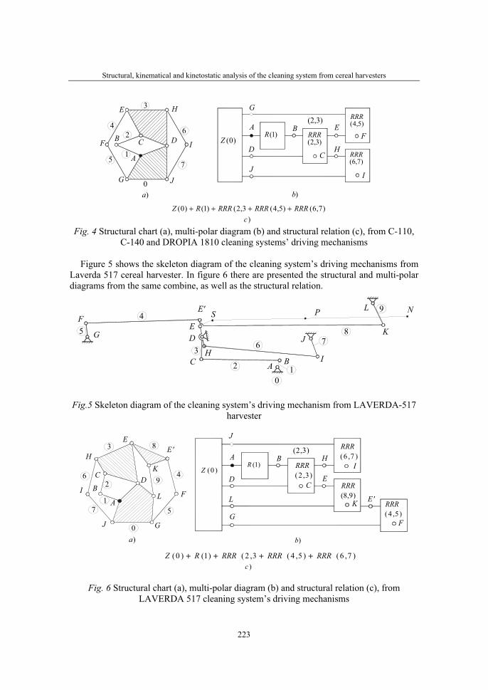
Structural, kinematical and kinetostatic analysis of the cleaning system from cereal harvesters
223
2
3
4
5
6(2,3)
A
B C D
E
F
G
H
I
J
1
0
7
)3,2(RRR
)7,6(RRR
)5,4(RRR
)7,6()5,4(3,2()1()0( RRRRRRRRRRZ ++++
)b)a
)1(RA B
CD
F
G
IJ
H)0(Z
)c
E
Fig. 4 Structural chart (a), multi-polar diagram (b) and structural relation (c), from C-110, C-140 and DROPIA 1810 cleaning systems’ driving mechanisms
Figure 5 shows the skeleton diagram of the cleaning system’s driving mechanisms from Laverda 517 cereal harvester. In figure 6 there are presented the structural and multi-polar diagrams from the same combine, as well as the structural relation.
G
FED
C A BH
I
J
4
5
12
3 6 7
0
E'
K
L
8
S P N9
Fig.5 Skeleton diagram of the cleaning system’s driving mechanism from LAVERDA-517 harvester
2
3
4
5
6
(2,3)
A
B
C D
E
F
G
H
I
J
1
0
7
)b)a
)1(RA B
CD E
FG
IH
)0(Z
)c
8
9
E'
K
E'
J
KLL
)3,2(RRR
)7,6(RRR
)9,8(RRR
)5,4(RRR
)7,6()5,4(3,2()1()0( RRRRRRRRRRZ ++++
Fig. 6 Structural chart (a), multi-polar diagram (b) and structural relation (c), from LAVERDA 517 cleaning system’s driving mechanisms
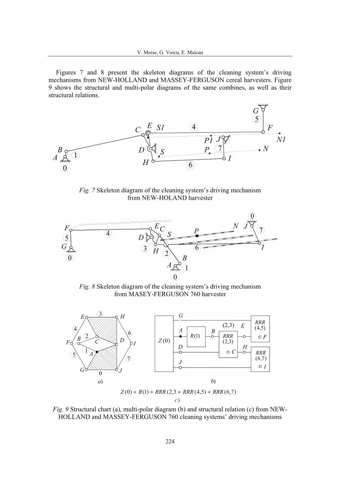
V. Moise, G. Voicu, E. Maican
224
Figures 7 and 8 present the skeleton diagrams of the cleaning system’s driving mechanisms from NEW-HOLLAND and MASSEY-FERGUSON cereal harvesters. Figure 9 shows the structural and multi-polar diagrams of the same combines, as well as their structural relations.
G
FE
D
C
AB
H I
J4
16
7
0
S P N
5S1
P1 N1
Fig. 7 Skeleton diagram of the cleaning system’s driving mechanismfrom NEW-HOLAND harvester
G
F ED
C
AB
H I
J5
1
23 6
7
0
4
0
0
S PN
Fig. 8 Skeleton diagram of the cleaning system’s driving mechanismfrom MASEY-FERGUSON 760 harvester
2
3
4
5
6(2,3)
A
B C D
E
F
G
H
I
J
1
0
7
)3,2(RRR
)7,6()5,4(3,2()1()0( RRRRRRRRRRZ ++++
)b)a
)1(RA B
CD
E
F
G
IJ
H
)c
)5,4(RRR
)7,6(RRR
)0(Z
Fig. 9 Structural chart (a), multi-polar diagram (b) and structural relation (c) from NEW-HOLLAND and MASSEY-FERGUSON 760 cleaning systems’ driving mechanisms

Structural, kinematical and kinetostatic analysis of the cleaning system from cereal harvesters
225
It can be observed from figure 4 that the driving systems of these two combines consist of the Z(0) base, R(1) driving group and RRR(2,3), RRR(4,5) and RRR(6,7) aspect 1 dyads [1,2,3,4,5].
KINEMATICAL ANALYSIS OF THE CLEANING SYSTEMS’ DRIVING MECHANISMS FROM CEREAL HARVESTERS
The kinematical analysis algorithm is described for DROPIA 1810 Romanian harvester. For the other combines only graphical results are presented.
Figure 10 reveals the angles between the vectors attached to the mechanism’s compo-nents and the positive direction of the Ax axes. In order to parametrically calculate them (as well as their order one and two derivatives), computer procedures for the component modules (determined in chapter 2) were used. Thus, linear and angular mechanism’s dimensions, initial position and angular velocity of component (1) are used.
The computer program was based on the multi-polar diagram (Fig. 4, b) and also on the adequate structural relation (Fig. 4, c). On this line, it was first cinematically studied the R(1) driving group, then the RRR(2,3) dyad and finally the RRR(4,5), RRR(6,7) dyads. The kinematical parameters’ lettering was made according to the skeleton diagram from figure 10.
3
G
HC
A
2
6
1B
F
54
E
D 7
J
I
1ϕ7ϕ
4ϕ5ϕ
3ϕ
2ϕ 6ϕ
0
S PN
Sα
x
ψy
Fig.10 Definition of the positional kinematical parameters of the cleaningsystem’s driving mechanism from DROPIA 1810 harvester
Within the framework of the mechanism’s kinematical analysis there were calculated the kinematical parameters of all the mechanism’s components, considering the angular velocity of element (1) to be constant. Results were saved as data files. Based on them, kinematical parameters variation charts were made. Figures 11 and 12 show the mechani-sm’s elements velocities and angular velocities variation charts in relation to ϕ1 angle.
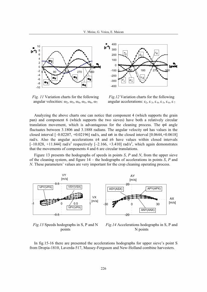
V. Moise, G. Voicu, E. Maican
226
-10-8-6-4-202468
10
0 90 180 270 360
-400
-300
-200
-100
0
100
200
300
400
0 90 180 270 360
Fig. 11 Variation charts for the following angular velocities: ω2, ω3, ω4, ω5, ω6, ω7
Fig.12 Variation charts for the following angular accelerations: ε2, ε 3, ε 4, ε 5, ε 6, ε 7
Analyzing the above charts one can notice that component 4 (which supports the grain pan) and component 6 (which supports the two sieves) have both a relatively circular translation movement, which is advantageous for the cleaning process. The ϕ4 angle fluctuates between 3.1806 and 3.1888 radians. The angular velocity ω4 has values in the closed interval [–0.02207, +0.02196] rad/s, and ω6 in the closed interval [0.0644,+0.0618] rad/s. Also the angular accelerations ε4 and ε6 have values within closed intervals [–10.028, +11.844] rad/s2 respectively [–2.166, +3.410] rad/s2, which again demonstrates that the movements of components 4 and 6 are circular translations.
Figure 13 presents the hodographs of speeds in points S, P and N, from the upper sieve of the cleaning system, and figure 14 – the hodographs of accelerations in points S, P and N. These parameters’ values are very important for the crop cleaning operating process.
-0.5
0
0.5
-1 -0.5 0 0.5 1
VY[m/s]
VX[m/s]
VSY(VSX) VPY(VPX)
VPY(VPX)
-20
0
20
-30 0 30
AY[m/s]
AX[m/s]
ASY(ASX)
ANY(ANX)
APY(APX)
Fig.13 Speeds hodographs in S, P and N points
Fig.14 Accelerations hodographs in S, P and N points
In fig.15-16 there are presented the accelerations hodographs for upper sieve’s point S from Dropia-1810, Laverda-517, Massey-Ferguson and New-Holland combine harvesters.
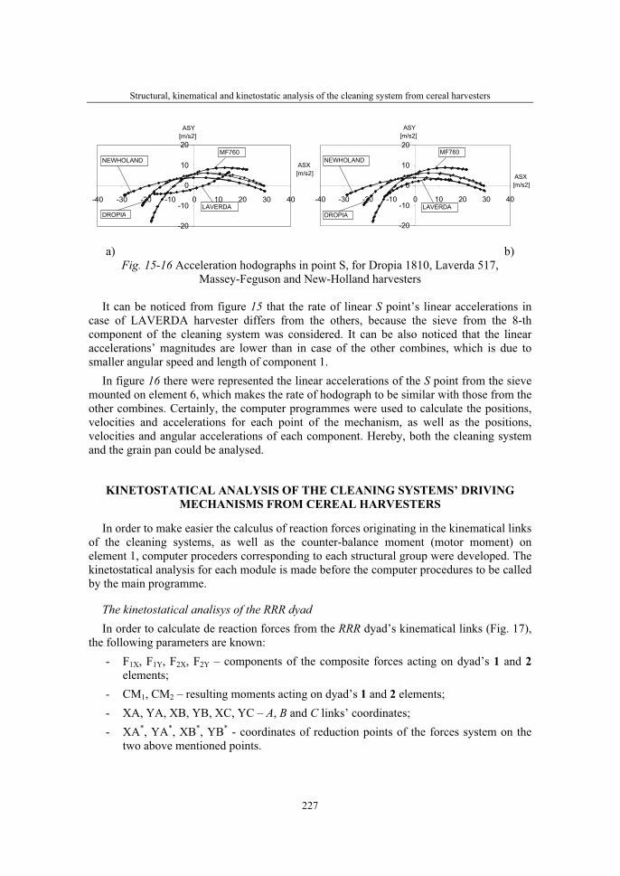
Structural, kinematical and kinetostatic analysis of the cleaning system from cereal harvesters
227
-20
-10
0
10
20
-40 -30 -20 -10 0 10 20 30 40
DROPIA
ASY [m/s2]
ASX[m/s2]
MF760NEWHOLAND
LAVERDA
-20
-10
0
10
20
-40 -30 -20 -10 0 10 20 30 40
DROPIA
ASY [m/s2]
ASX[m/s2]
MF760NEWHOLAND
LAVERDA
a) b) Fig. 15-16 Acceleration hodographs in point S, for Dropia 1810, Laverda 517,
Massey-Feguson and New-Holland harvesters
It can be noticed from figure 15 that the rate of linear S point’s linear accelerations in case of LAVERDA harvester differs from the others, because the sieve from the 8-th component of the cleaning system was considered. It can be also noticed that the linear accelerations’ magnitudes are lower than in case of the other combines, which is due to smaller angular speed and length of component 1.
In figure 16 there were represented the linear accelerations of the S point from the sieve mounted on element 6, which makes the rate of hodograph to be similar with those from the other combines. Certainly, the computer programmes were used to calculate the positions, velocities and accelerations for each point of the mechanism, as well as the positions, velocities and angular accelerations of each component. Hereby, both the cleaning system and the grain pan could be analysed.
KINETOSTATICAL ANALYSIS OF THE CLEANING SYSTEMS’ DRIVING MECHANISMS FROM CEREAL HARVESTERS
In order to make easier the calculus of reaction forces originating in the kinematical links of the cleaning systems, as well as the counter-balance moment (motor moment) on element 1, computer proceders corresponding to each structural group were developed. The kinetostatical analysis for each module is made before the computer procedures to be called by the main programme.
The kinetostatical analisys of the RRR dyad In order to calculate de reaction forces from the RRR dyad’s kinematical links (Fig. 17),
the following parameters are known: - F1X, F1Y, F2X, F2Y – components of the composite forces acting on dyad’s 1 and 2
elements;- CM1, CM2 – resulting moments acting on dyad’s 1 and 2 elements;- XA, YA, XB, YB, XC, YC – A, B and C links’ coordinates; - XA*, YA*, XB*, YB* - coordinates of reduction points of the forces system on the
two above mentioned points.
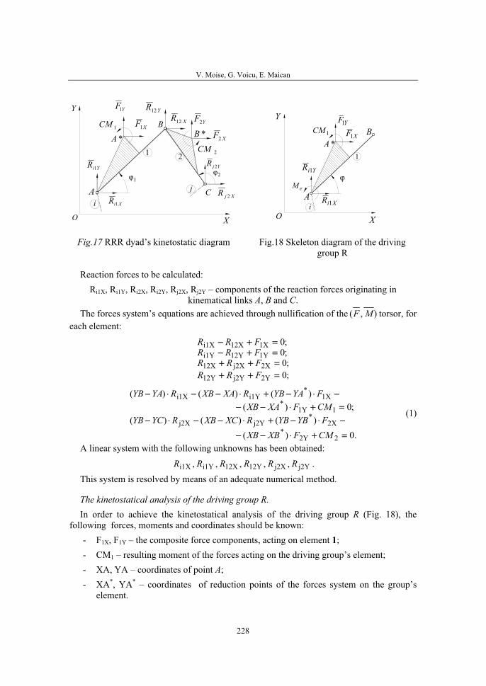
V. Moise, G. Voicu, E. Maican
228
YF1
XjR 2
XF11CM
2CM*A *B
CXiR 1
YiR 1
XR12
YR12
YF2
XF2
1 2
i
j1ϕ 2ϕ
YjR 2
A
Y
XO
B YF1
XF11CM*A
B
X
ϕYiR 1
1
Y
OXiR 1i
AeM
Fig.17 RRR dyad’s kinetostatic diagram Fig.18 Skeleton diagram of the driving group R
Reaction forces to be calculated: Ri1X, Ri1Y, Ri2X, Ri2Y, Rj2X, Rj2Y – components of the reaction forces originating in
kinematical links A, B and C.The forces system’s equations are achieved through nullification of the ( , )F M torsor, for
each element:
;0;0;0;0
2Yj2Y12Y2Xj2X12X
1Y12Yi1Y1X12Xi1X
=++=++=+−=+−
FRRFRRFRRFRR
.0)()()()(
;0)()()()(
22Y*
2X*
j2Yj2X
11Y*
1X*
i1Yi1X
=+⋅−−−⋅−+⋅−−⋅−=+⋅−−
−⋅−+⋅−−⋅−
CMFXBXBFYBYBRXCXBRYCYB
CMFXAXBFYAYBRXAXBRYAYB
(1)
A linear system with the following unknowns has been obtained:
j2Yj2X12Y12Xi1Yi1X ,,,,, RRRRRR .This system is resolved by means of an adequate numerical method.
The kinetostatical analysis of the driving group R. In order to achieve the kinetostatical analysis of the driving group R (Fig. 18), the
following forces, moments and coordinates should be known: - F1X, F1Y – the composite force components, acting on element 1;- CM1 – resulting moment of the forces acting on the driving group’s element; - XA, YA – coordinates of point A;- XA*, YA* – coordinates of reduction points of the forces system on the group’s
element.
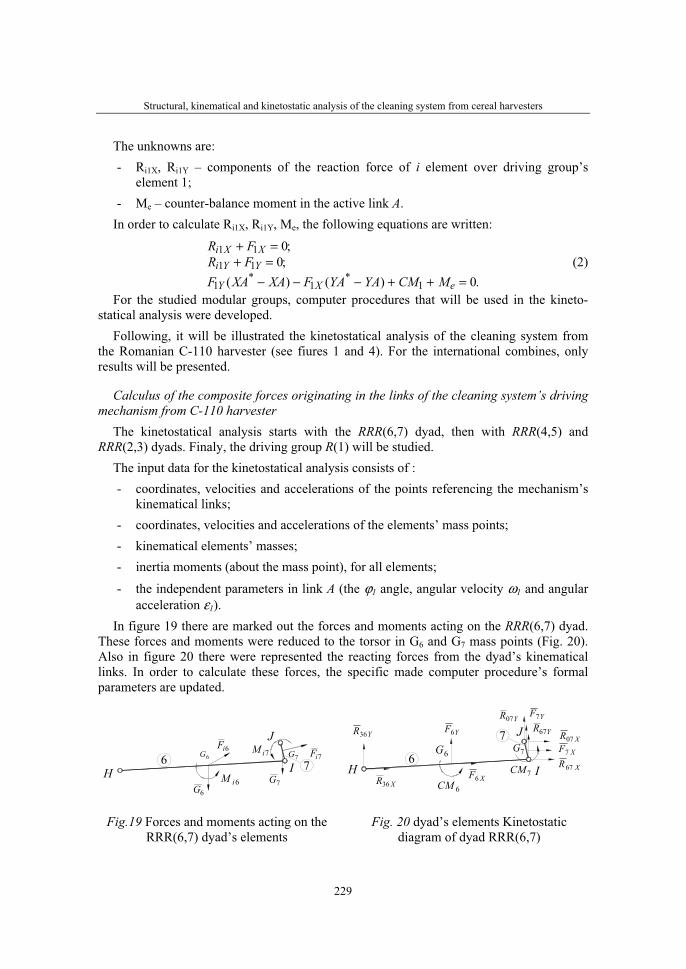
Structural, kinematical and kinetostatic analysis of the cleaning system from cereal harvesters
229
The unknowns are: - Ri1X, Ri1Y – components of the reaction force of i element over driving group’s
element 1; - Me – counter-balance moment in the active link A.
In order to calculate Ri1X, Ri1Y, Me, the following equations are written:
R FR FF XA XA F YA YA CM M
i X Xi Y Y
Y X e
1 11 1
1 1 1
00
0
+ =+ =
− − − + + =
;;
( ) ( ) .* * (2)
For the studied modular groups, computer procedures that will be used in the kineto-statical analysis were developed.
Following, it will be illustrated the kinetostatical analysis of the cleaning system from the Romanian C-110 harvester (see fiures 1 and 4). For the international combines, only results will be presented.
Calculus of the composite forces originating in the links of the cleaning system’s driving mechanism from C-110 harvester
The kinetostatical analysis starts with the RRR(6,7) dyad, then with RRR(4,5) and RRR(2,3) dyads. Finaly, the driving group R(1) will be studied.
The input data for the kinetostatical analysis consists of : - coordinates, velocities and accelerations of the points referencing the mechanism’s
kinematical links; - coordinates, velocities and accelerations of the elements’ mass points; - kinematical elements’ masses; - inertia moments (about the mass point), for all elements;
- the independent parameters in link A (the ϕ1 angle, angular velocity ω1 and angular acceleration ε1).
In figure 19 there are marked out the forces and moments acting on the RRR(6,7) dyad. These forces and moments were reduced to the torsor in G6 and G7 mass points (Fig. 20). Also in figure 20 there were represented the reacting forces from the dyad’s kinematical links. In order to calculate these forces, the specific made computer procedure’s formal parameters are updated.
J
IH6 7
6iM
6iF7iM
7G
7G 7iF
6G
6G
H
7
6
J
I XR67
YR67
XF6
YF7
YF6
XF7
YR36
XR36
XR07
YR07
6G 7G
7CM
6CM
Fig.19 Forces and moments acting on the RRR(6,7) dyad’s elements
Fig. 20 dyad’s elements Kinetostatic diagram of dyad RRR(6,7)
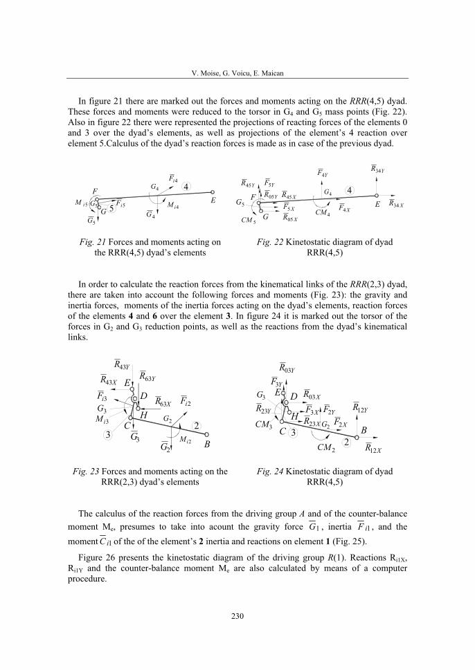
V. Moise, G. Voicu, E. Maican
230
In figure 21 there are marked out the forces and moments acting on the RRR(4,5) dyad. These forces and moments were reduced to the torsor in G4 and G5 mass points (Fig. 22). Also in figure 22 there were represented the projections of reacting forces of the elements 0 and 3 over the dyad’s elements, as well as projections of the element’s 4 reaction over element 5.Calculus of the dyad’s reaction forces is made as in case of the previous dyad.
5
4
4G5iF
4iF
4iM5G
4G
EF
G5iM
5G
XR34YR05
5CM
YR45
5G
YF5
4CMXF5 XF4
XR05
XR45
YF4YR34
4E
G
F 4G
Fig. 21 Forces and moments acting onthe RRR(4,5) dyad’s elements
Fig. 22 Kinetostatic diagram of dyad RRR(4,5)
In order to calculate the reaction forces from the kinematical links of the RRR(2,3) dyad, there are taken into account the following forces and moments (Fig. 23): the gravity and inertia forces, moments of the inertia forces acting on the dyad’s elements, reaction forces of the elements 4 and 6 over the element 3. In figure 24 it is marked out the torsor of the forces in G2 and G3 reduction points, as well as the reactions from the dyad’s kinematical links.
3G
3iF2iF
2iM
3G2G3iM
YR43
XR43 YR63
B
C
DE
23
HXR63
2G
YR12
XR03
YR03
YR23
XR23
XR12
YF3
YF2XF3
XF23CM
2CM
3G
BC
DE
23
H2G
Fig. 23 Forces and moments acting on the RRR(2,3) dyad’s elements
Fig. 24 Kinetostatic diagram of dyad RRR(4,5)
The calculus of the reaction forces from the driving group A and of the counter-balance moment Me, presumes to take into acount the gravity force 1G , inertia 1iF , and the moment 1iC of the of the element’s 2 inertia and reactions on element 1 (Fig. 25).
Figure 26 presents the kinetostatic diagram of the driving group R(1). Reactions Ri1X,Ri1Y and the counter-balance moment Me are also calculated by means of a computer procedure.
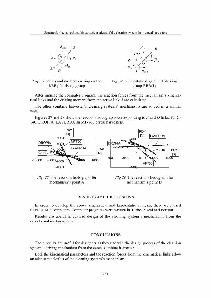
Structural, kinematical and kinetostatic analysis of the cleaning system from cereal harvesters
231
1G
1iM1G
BXR21
YR21
A
11iF
YF1
XF1
XR01
YR01
1CM
A
B
1
1GeM
Fig. 25 Forces and moments acting on the RRR(1) driving group
Fig. 26 Kinetostatic diagram of driving group RRR(1)
After running the computer program, the reaction forces from the mechanism’s kinema-tical links and the driving moment from the active link A are calculated.
The other combine harvester’s cleaning systems’ mechanisms are solved in a similar way.
Figures 27 and 28 show the reactions hodographs corresponding to A and D links, for C-140, DROPIA, LAVERDA an MF-760 cereal harvesters.
-4000
-2000
0
2000
4000
6000
-10000 -5000 0 5000 10000
C140
DROPIA
LAVERDA
MF760
RAY [N]
RAX [N]
-4000
0
4000
-6000 -3000 0 3000 6000
C140
DROPIA
LAVERDA
MF760
RDY [N]
RDX [N]
Fig. 27 The reactions hodograph for mechanism’s point A
Fig.28 The reactions hodograph for mechanism’s point D
RESULTS AND DISCUSSIONS
In order to develop the above kinematical and kinetostatic analysis, there were used PENTIUM 2 computers. Computer programs were written in Turbo-Pascal and Fortran.
Results are useful in advised design of the cleaning system’s mechanisms from the cereal combine harvesters.
CONCLUSIONS
These results are useful for designers as they underlie the design process of the cleaning system’s driving mechanism from the cereal combine harvesters.
Both the kinematical parameters and the reaction forces from the kinematical links allow an adequate calculus of the cleaning system’s mechanism.

V. Moise, G. Voicu, E. Maican
232
REFERENCES
1. Moise, V., Maican, E., Moise, Şt.I., Metode numerice (Teorie şi aplicaţii). Editura Printech, Bucureşti, 2004
2. Moise, V., Simionescu, I., Ene, M., Neacşa, M., Tabără, I., Mecanisme Aplicate, Editura Bren, Bucureşti, 2005
3. Pelecudi, Chr., Simionescu, I., Ene, M., Moise, V., Candrea, A, Probleme de mecanisme, Editura didactică şi pedagogică, Bucuresti, 1982
4. Simionescu, I., Moise,V., Mecanisme, Editura Tehnică, Bucureşti, 1999
5. Voicu, Gh., Cercetări privind mişcarea materialului pe site sub influenţa curentului de aer la sistemele de curăţire ale combinelor de cereale, Teză de doctorat, Universitatea Politehnica Bucureşti, 1996
36. Symposium "Actual Tasks on Agricultural Engineering", Opatija, Croatia, 2008.
233
36.
SIMPOZIJAKTUALNI ZADACIMEHANIZACIJE POLJOPRIVREDE
UDK631.354:633”324”
Stručni radExpert paper
GUBICI ZRNA PRI ŽETVI OZIMOG JEČMA I PŠENICE NA ŽITNOM KOMBAJNU DEUTZ FAHR POWERLINER
4035 H RAJKO BERNIK, FILIP VUČAJNK
Univerzitet u Ljubljani, Biotehhnički fakultet, Odjel za agronomiju, Katedra za poljoprivrednu tehniku, Jamnikarjeva 101, 1000 Ljubljana, Slovenija
SAŽETAK
Kod žetve žita s samohodnim žitnim kombajnom dolazi do određenih gubitaka zrna, koja ne smiju biti veća od 1%. Svrha djela je bila utvrditi stvarne gubitke zrna pri različitim radnim brzinama (4, 6, 8 km/h) kombajna Deutz Fahr Powerliner 4035 H na nagnutom terenu. Za mjerenje gubitka na slamotresih i na uređajima za čiščenje zrna smo koristili mjernu napravu proizvođača Feiffer consult. Za ozimi ječam, pri brzini 4 i 6 km/h, su gubici zrna iznosili oko 1 %, dok su pri brzini 8 km/h gubici iznosili čak 1,9%. Kod sve tri brzine je bilo najviše gubitaka na ozimom ječmu (2−3,4 %) zbog slomljenih klasova, koja su već ležala na tlu. Takođe i kod ozime pšenice su se gubici zrna povećavali s brzinom, od 0,3% pri 4 km/h do 0,9% pri 8 km/h. Tako pri ozimom ječmu kao i pri pšenici su se s povećanjem radne brzine povećali gubici zbog polomljenih i napuklih zrna (kod ječma od 0,6 % do 0,9 %; kod pšenice od 0,6% do 1,2%). Rezultati ukazuju, da je na nagnutom terenu najprimjerenija radna brzina u žetvi između 4 i 6 km/h. Kod brzine 8 km/h su gubici zrna preveliki.
Ključne riječi: kombajn za žito, gubici zrna, slamotresi, uređaj za čišćenjezrna.
UVOD
Razlozi koji utjeću na gubitke zrna pri žetvi su biološko-klimatski, tehničko-tehnološki i organizacijski. Među biološko klimatske spadaju vrsta i stanje usjeva, te klimatski uvjeti u vrijeme žetve. Tipovi kombajna, konstrukcijske karakteristike radnih dijelova i opremlje-nost kombajna s elektroničkim mjernim uređajima predstavljaju jedan dio tehničko-tehnoloških razloga. U zadnju skupinu spadaju organizacija žetve i prijevoza te obučenostljudi koji sudjeluju pri žetvi. Gubici i oštećenja zrna takođe nastaju pri prijevozu, skladiš-tenju i pretovaru (Brkić i sur., 2002)
R. Bernik, F. Vučajnk
234
U Njemačkoj, u zadnjim godinama, iznose ukupni gubici zrna oko 11%. 10% gubici predstavljaju za Njemačku gubitak od oko 1 milijarde €. Čak 16 faktora utjeće na te gubitke i to, slomljeni i podrezani klasovi, istrešena zrna, neovršena zrna, gubici na slamotresu i uređaju za čišćenje zrna, gubici pri sušenju i skladištenju, i još neki faktori. S najboljom organizacijom možemo gubitke smanjiti na 3%, inače na oko 5% (Feiffer, 2003).
Gubici zrna, koji nastaju na kombajnu pri žetvi su direktni tj. kvantitativni i indirektni tj. kvalitativni. Među direktne gubitke spadaju gubici na žetelici i posebno na bubnju vršalice, gornjem i donjem situ i na slamotresima. Indirektni gubici nastaju zbog mehaničkihoštećenja zrna. Među gubitke na žetelici spadaju istrešena zrna, slomljeni klasovi, polegle biljke. Kod poleglog žita na povećanje gubitaka zrna utjeće takođe i pravac žetve u odnosu na poleglo žito. Neovršeni klasići u slami i u pljevi predstavljaju gubitke na bubnju za vršidbu. Zrna u slami su gubici na slamotresih i zrna u pljevi su gubici na sitima (Brkić in sur., 2002).
U pojedinim državama su različite tolerantne granice glede gubitaka zrna i ti standardi tolerantnih gubitaka se više snizuju. Kao primjer, gubici zrna pri žetvi pšenice su se smanjili iz 2,35 % na 2 %. Dozvoljena granica na žetelici je 1,5 %, na slamotresima 0,5 %, na sitima 0,3 % i 0,05 % na bubnju vršalice (Brkić in sur., 2002).
Feifferova (2003) navodi neke gornje tolerantne granice za gubitke zrna. Dva slomljena odnosno podrezana klasa na m2 znače 0,7 % gubitak i 46 kg/ha pri prinosu 65 dt/ha i gustoći od 500 klasova na m2. Pored toga 10 istrešenih zrna na ¼ m2 znači gubitak od 0,27 % i 18,1 kg/ha. 220 zrna na ¼ m2 u mjernoj posudi znači 1 % gubitak zrna na slamotresima i uređaju za čišćenje zrna što znači 65 kg/ha. U koliko nađemo u plasti 50 ovršenih klasova 5 zrna, to predstavlja 0,34 % gubitka tj. 22 kg/ha. 1 zdrobljeno zrno u spremniku za sjeme i 1 zdrobljeno zrno u plastu znači 1,3 % gubitaka tj. 20 kg/ha (Feiffer, 2003).
Ista autorica navodi, da su još uvijek tolerantni gubici na slamotresima i uređaju za čišćenje zrna od 1%. Ukoliko ti gubici iznose 1,5 % ili više, to su već visoki gubici. Brkić i ostali navode (2003), da se na njihajućim slamotresima pri malom protoku biljne mase (0,52 kg/s) oko 60 % zrna očisti na početnom djelu slamotresa. Pri povećanom protoku biljne mase (2,49 kg/s) se 80 % zrna očisti na ¾ dužine slamotresa. Kombajni su opremljeni s elektroničkim uređajima, koji detektiraju gubitke na slamotresima i uređaju za čišćenjezrna, ali jih je potrebno podesiti. Zbog toga je razvijena posebna mjerna posuda, s kojom određujemo gubitke zrna i kasnije podešavamo elektroničke uređaje (Feiffer, 2003).
MATERIJAL I METODE
Pokus smo izvodili na srednje teškim tlima u Šmarju pri Jelšah pri ozimom ječmu i ozimoj pšenici. Uzgoj obiju biljnih vrsta nije bio intenzivan. Žetva ozimog ječma je bila izvedena 26.6. 2007 i žetva ozime pšenice 15.7.2007. Upotrijebili smo žitni kombajn DEUTZ FAHR POWERLINER 4035 H. Riječ je o tangentnom kombajnu sa dva bubanja vršalice i 5 sekcijskih slamotresa. Bubanj vršalice ima promjer 600 mm i širinu 1270 mm. Ventilator je aksijalni. Kapacitet spremnika zrna iznosi 5.200 litara. Motor ima zračnohlađenje, s 6 cilindara i snage 103 kW. Kombajn je opremljen centralnim informacijskim sistemom i optičkim i akustičkim sustavom nadzora za nadzor važnih funkcija. Težina kombajna bez žetelice iznosi 7.025 kg.
Gubici zrna pri žetvi ozimog ječma i pšenice na žitnom kombajnu DEUTZ FAHR POWERLINER 4035 H
235
Mjerili smo gubitke zrna pri brzini gibanja kombajna 4,6 i 8 km/h na nagnutom teretu nagiba 10o. Pri tome su bila sita na kombajnu postavljena u vodoravan položaj. Pokus je postavljen po metodi slučajnog bloknog rasporeda u tri ponavljanja. Dužina pojedine parcele je iznosila 70 m i širina 3,6 m. Najprije smo kombajn optimalno podesili i kasnije počeli s pokusom. Gubitke na slamotresima i uređaju za čišćenje zrna smo izmjerili s mjernom posudom proizvođača Feiffer Consult. Dužina mjerne posude iznosi 100 cm i njena širina 25 cm. Posudu smo postavili na sredinu parcele, tako da je kombajn vozio preko nje i posudu nije oštetio. Slamu iz posude smo odstranili i zrna smo smjestili u pretince na posudi. 1 puni pretinac znači 0,5 % gubitaka (mali gubici), 2 puna 1 % gubitaka (još uvijek prihvatljivo) i 3 tri puna pretinca 1,5% gubitaka (visoki gubici). Jer slama nije bila sasjećena, smo zrna postavili u pretince na lijevoj strani mjerne posude. Pored toga smo odredili i gubitke zbog slomljenih odnosno odrezanih klasova, koji su već ležali na tlu prije žetve. Ozimi ječam se je naime u određenim dijelovima polegao. Željeli smo utvrditi gubitke zbog vršidbe i izbrojati preostala zrna u plasti od 50 klasova slame, ali su bili klasovi potpuno zdrobljeni. Utvrđivali smo takođe gubitke zbog napuknutih i polomljenih zrna. Iz spremnika za zrna smo slučajno uzeli uzorke i izbrojali nakupnuta i polomljena zrna, od 100 zrna.
Utvrdili smo gustoću i visinu biljaka, urod i vlažnost slame, urod i vlažnost zrna. Težinu uroda smo izmjerili. Vlažnost zrna smo utvrdili s mjernom napravom WILLE 55, dok smo vlažnost slame utvrdili s mjernom napravom WILLE 35. Isto tako smo mjerili vrijeme vr-šidbe potrebno za razdaljinu od 70 m, tako da smo dobili stvarnu brzinu gibanja kombajna.
Statističnu analizu podataka smo napravili u programu Statgraph. Upotrijebili smo analizu varijance i Duncanov multipli test rangova (α=0,05) po uvjetima, koji vrijede za slučajne blokove. Ako nisu bili ispunjeni uvijeti o jednakosti varijance, podatke smo transformirali.
REZULTATI
Ozimi ječamSlika 1 prikazuje, da su gubici na slamotresih i uređaju za čiščenje zrna rasli s poveća-
njem brzine gibanja. Gubici zrna pri brzini 8 km/h su bili statistički značajno veći nego pri brzini 4 i 6 km/h. Pri brzini 8 km/h su gubici iznosili 1,9 %, što već predstavlja visoke gubitke. Pri brzini 4 i 6 km/h su bili gubici još prihvatljivi (0,8 tj. 1,1 %). Takođe, su gubici zbog zdrobljenih zrna narasli pri povećanoj brzini gibanja. Pri brzini 6 i 8 km/h su bili gubici zbog zdrobljenih zrna statistički značajno veći nego pri brzini 4 km/h. Ukupni gubici su premašili 4,5 %, što je mnogo više nego što je tolerantni standard, te više nego navode Feiffer (2003) i Brkić sa sur. (2002). Najviše su tome pridonjeli već slomljeni klasovi u vrijeme prije žetve, i to od 2 do 3,5 %.
Broj slomljenih klasova, u sva tri tretitanja, jako nadmašuje tolerantnu vrijednost od 3 klasa na 1 m2. Na taj faktor ne utjeće brzina gibanja (kombajniranja), jer je tako stanje bilo na pokusnoj parceli već prije žetve. To se je dogodilo, zbog velikog broja polegnutih biljaka, a pored toga su već bile i veoma zrele (tablica 1).

R. Bernik, F. Vučajnk
236
Povećana brzina kombajniranja je utjecala i na veći udio zdrobljenih zrna i s tim takođena više gubitke. Pri brzini 6 i 8 km/h su gubici prekoračili udio, koji iznosi 2 %.Rezultati ukazuju da je uzimajući u obzir taj faktor, najprimjerenija brzina žetve manja od 6 km/h (tablica 1).
0,0
1,0
2,0
3,0
4,0
5,0
6,0
7,0
8,0
4 km/h 6 km/h 8 km/h 4 km/h 6 km/h 8 km/h 4 km/h 6 km/h 8 km/h 4 km/h 6 km/h 8 km/h
SLAMOTRESI I UREĐAJ
ZA ČIŠĆENJE ZRNA
ZDROBLJENA ZRNA SLOMLJENI KLASOVI UKUPNO
Gub
ici z
rna
(%)
aa
b
ab b
aa
a
a a a
Slika 1 Gubici zrna kod žetve ozimog ječma pri različitim brzinama. Različita slova značestatistički značajne razlike. Intervali crta označavaju standardno odstupanje
Tablica 1 Broj polomljenih te podrezanih klasova na 1 m2 i broj zdrobljenih zrna od 100 zrna pri žetvi ozimog ječma (Duncanov test α=0,05)
Brzina gibanja(km/h) Broj polomljenih klasova na 1 m2 Broj zdrobljenih zrna od 100 zrna
4 10,3 a 1,3 a
6 10 a 2,7 b
8 6,3 a 3,0 b
U tablici 2 su prikazane neke osobine usjeva ozimog ječma (tablica 2). Gustoća biljaka je iznosila između 150 i 170 b/m2 i visina između 90 i 95 cm. Urod slame se je kretao oko 4.000 kg/ha, a urod zrna između 3.900 i 4.200 kg/ha. S povećanjem brzine gibanja se je statistički značajno povećao protok slame i zrna te posljedično protok ukupne mase. To je bilo očekivano. Odnos između zrna i slame je iznosio oko 1 : 1. Vlaga u zrnu i slami je bila veoma niska, što ukazuje, da je bio ozimi ječam već veoma zreo. Predviđamo, da je zbog toga i došlo do visokog udjela gubitaka zbog polomljenih klasova i zdrobljenih zrna.
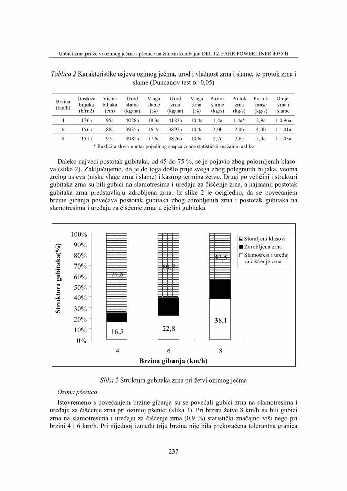
Gubici zrna pri žetvi ozimog ječma i pšenice na žitnom kombajnu DEUTZ FAHR POWERLINER 4035 H
237
Tablica 2 Karakteristike usjeva ozimog ječma, urod i vlažnost zrna i slame, te protok zrna i slame (Duncanov test α=0,05)
Brzina(km/h)
Gustoćabiljaka(b/m2)
Visinabiljaka(cm)
Urodslame
(kg/ha)
Vlagaslame(%)
Urodzrna
(kg/ha)
Vlagazrna(%)
Protokslame(kg/s)
Protokzrna
(kg/s)
Protokmase(kg/s)
Omjerzrna i slame
4 176a 95a 4028a 18,3a 4183a 10,4a 1,4a 1,4a* 2,9a 1:0,96a
6 156a 88a 3935a 16,7a 3892a 10,4a 2,0b 2,0b 4,0b 1:1,01a
8 151a 97a 3982a 17,6a 3876a 10,6a 2,7c 2,6c 5,4c 1:1,03a * Različita slova unutar pojedinog stupca znače statistički značajne razlike
Daleko najveći postotak gubitaka, od 45 do 75 %, se je pojavio zbog polomljenih klaso-va (slika 2). Zaključujemo, da je do toga došlo prije svega zbog polegnutih biljaka, veoma zrelog usjeva (niske vlage zrna i slame) i kasnog termina žetve. Drugi po veličini i strukturi gubitaka zrna su bili gubici na slamotresima i uređaju za čišćenje zrna, a najmanji postotak gubitaka zrna predstavljaju zdrobljena zrna. Iz slike 2 je očigledno, da se povećanjembrzine gibanja povećava postotak gubitaka zbog zdrobljenih zrna i postotak gubitaka na slamotresima i uređaju za čišćenje zrna, u cjelini gubitaka.
16,5 22,838,18,6
16,6
18,4
74,860,7
43,5
0%10%20%30%40%50%60%70%80%90%
100%
4 6 8Brzina gibanja (km/h)
Stru
ktur
a gu
bita
ka(%
)
Slomljeni klasoviZdrobljena zrnaSlamotresi i uređajza čišćenje zrna
Slika 2 Struktura gubitaka zrna pri žetvi ozimog ječma
Ozima pšenica Istovremeno s povećanjem brzine gibanja su se povećali gubici zrna na slamotresima i
uređaju za čišćenje zrna pri ozimoj pšenici (slika 3). Pri brzini žetve 8 km/h su bili gubici zrna na slamotresima i uređaju za čišćenje zrna (0,9 %) statistički značajno viši nego pri brzini 4 i 6 km/h. Pri nijednoj između triju brzina nije bila prekoračena tolerantna granica
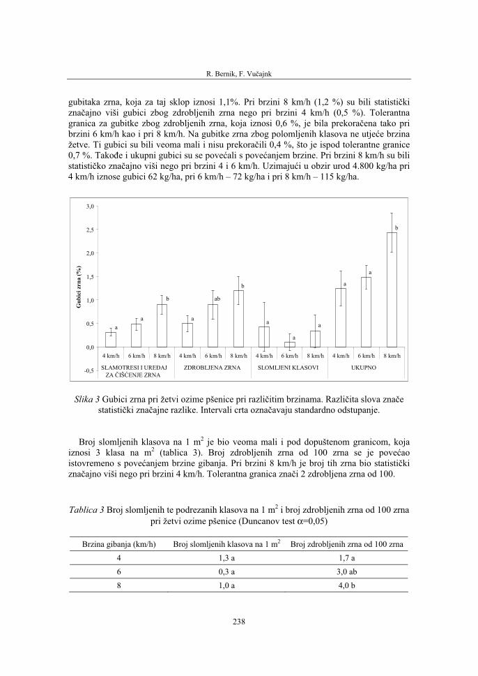
R. Bernik, F. Vučajnk
238
gubitaka zrna, koja za taj sklop iznosi 1,1%. Pri brzini 8 km/h (1,2 %) su bili statističkiznačajno viši gubici zbog zdrobljenih zrna nego pri brzini 4 km/h (0,5 %). Tolerantna granica za gubitke zbog zdrobljenih zrna, koja iznosi 0,6 %, je bila prekoračena tako pri brzini 6 km/h kao i pri 8 km/h. Na gubitke zrna zbog polomljenih klasova ne utjeće brzina žetve. Ti gubici su bili veoma mali i nisu prekoračili 0,4 %, što je ispod tolerantne granice 0,7 %. Takođe i ukupni gubici su se povećali s povećanjem brzine. Pri brzini 8 km/h su bili statističko značajno viši nego pri brzini 4 i 6 km/h. Uzimajući u obzir urod 4.800 kg/ha pri 4 km/h iznose gubici 62 kg/ha, pri 6 km/h – 72 kg/ha i pri 8 km/h – 115 kg/ha.
-0,5
0,0
0,5
1,0
1,5
2,0
2,5
3,0
4 km/h 6 km/h 8 km/h 4 km/h 6 km/h 8 km/h 4 km/h 6 km/h 8 km/h 4 km/h 6 km/h 8 km/h
SLAMOTRESI I UREĐAJ ZA ČIŠĆENJE ZRNA
ZDROBLJENA ZRNA SLOMLJENI KLASOVI UKUPNO
Gub
ici z
rna
(%)
aa
b
a
ab
b
a
a
a
a
a
b
Slika 3 Gubici zrna pri žetvi ozime pšenice pri različitim brzinama. Različita slova značestatistički značajne razlike. Intervali crta označavaju standardno odstupanje.
Broj slomljenih klasova na 1 m2 je bio veoma mali i pod dopuštenom granicom, koja iznosi 3 klasa na m2 (tablica 3). Broj zdrobljenih zrna od 100 zrna se je povećaoistovremeno s povećanjem brzine gibanja. Pri brzini 8 km/h je broj tih zrna bio statističkiznačajno viši nego pri brzini 4 km/h. Tolerantna granica znači 2 zdrobljena zrna od 100.
Tablica 3 Broj slomljenih te podrezanih klasova na 1 m2 i broj zdrobljenih zrna od 100 zrna pri žetvi ozime pšenice (Duncanov test α=0,05)
Brzina gibanja (km/h) Broj slomljenih klasova na 1 m2 Broj zdrobljenih zrna od 100 zrna
4 1,3 a 1,7 a
6 0,3 a 3,0 ab
8 1,0 a 4,0 b

Gubici zrna pri žetvi ozimog ječma i pšenice na žitnom kombajnu DEUTZ FAHR POWERLINER 4035 H
239
Gustoća biljaka je iznosila između 260 i 280 biljaka na 1 m2, visina pa između 66 i 71 cm (tablica 4). Urod slame je iznosio oko 4.200 kg/ha, urod zrna pa oko 4.800 kg/ha. To ukazuje, da su oba uroda bila niska, jer se radilo o manje intenzivnom uzgoju. Vlažnost zrna je bila oko 12 %. Pri povećanoj brzini žetve se je statistički povećao protok slame i zrna, te cjelokupni protok mase. To je bilo očekivano. Omjer između zrna i slame je iznosio oko 1 : 0,90.
Tablica 4 Karakteristike usjeva ozime pšenice, urod i vlažnost zrna i slame, protok zrna i slame
Brzina(km/h)
Gustoćabiljaka(b/m2)
Visinabiljaka(cm)
Urodslame
(kg/ha)
Vlagaslame(%)
Urodzrna
(kg/ha)
Vlagazrna(%)
Protokslame(kg/s)
Protokzrna
(kg/s)
Protokmase(kg/s)
Omjerzrna i slame
4 260a 71a 4259a 31,0a 4886a 11,7a 1,5a* 1,7a 3,2a 1:0,87a
6 280a 67a 4259a 27,7a 4669a 12,5a 2,2b 2,4b 4,5b 1:0,92a
8 272a 66a 4167a 30,1a 4841a 12,0a 2,7b 3,1c 5,8c 1:0,86a * Različita slova unutar pojedinog stupca znače statistički značajne razlike.
Na slici 4 je prikazana struktura gubitaka zrna pri ozimoj pšenici. Gubici zbog slomlje-nih zrna su predstavljali najveći postotak među gubicima, i to od 40 do 60 %. Gubici na slamotresima i uređaju za čišćenje zrna su iznosili od 25 do 30 % u ukupnim gubicima. Najmanji postotak od svih su predstavljali gubici zbog slomljenih klasova. S povećanjembrzine gibanja se je povećao postotak gubitaka na slamotresima i uređaju za čišćenje zrna u ukupnim gubicima.
25,332,6 37,0
40,0
60,7 49,3
34,7
6,713,7
0%
10%
20%
30%
40%
50%
60%
70%
80%
90%
100%
4 6 8Brzina gibanja (km/h)
Stru
ktur
a gu
bita
ka (%
)
Slomljeni klasoviZdrobljena zrnaSlamotresi i uređaj za čišćenje zrna
Slika 4 Struktura gubitaka zrna pri ozimoj pšenici (%)
R. Bernik, F. Vučajnk
240
ZAKLJUČAK
Na osnovi mjerenja gubitaka zrna pri ozimom ječmu na nagnutom terenu, došli smo do sljedećih zaključaka:
• Najviše gubitaka se je pojavilo zbog slomljenih klasova već pred žetvom, jer su bile biljke polegnute. Ti gubici su u ukupnoj strukturi premašili 50 %.
• S povećanjem brzine gibanja su se povećali gubici na slamotresima i uređaju za čišćenje zrna te gubici zbog zdrobljenih zrna.
• Pri žetvi polegnutog ozimog ječma je bila najprimjerenija brzina žetve 4 km/h.
• Protok slame, zrna i ukupni protok se je povećao linearno s povećanjem brzine gibanja.
• Cjelokupni gubici su iznosili čak 4,5 %, što je bitno više nego što je tolerantna granica (oko 2 %).
Na osnovi mjerenja gubitaka zrna pri ozimoj pšenici na nagnutom terenu smo došli do sljedećih zaključaka:
• S povećanjem brzine gibanja su se povećali gubici na slamotresima i uređaju za čišćenje zrna, te gubici zbog zdrobljenih zrna. Najveći gubici su bili pri brzini 8 km/h.
• Cjelokupni gubici su samo pri brzini 8 km/h premašili 2 %.
• Najveći postotak među cjelokupnim gubicima je bio zbog zdrobljenih zrna.
• Protok slame, zrna i ukupni protok se je povećao linearno s povećanjem brzine gibanja.
• Pri žetvi ozime pšenice je obzirom na gubitke i protok mase, bila najprimjerenija brzina žetve 6 km/h.
LITERATURA
1. Brkić, D.Vujčić, M., Šumanovac, L.: Strojevi za žetvu i berbu zrnatih plodina, Poljoprivredni fakulktet u Osijeku, Osijek, 2002, 238 str.
2. Feiffer, A.: Mähdrusch bei Ernteerschwernissen, Fachverlag Feiffer, Sondershausen, 2003, 57 str.
3. Feiffer, A.: Sonnenstrategie im Drusch, Internationaler Fachverlag für Umweltsysteme, Sonders-hausen, 2003, 33 str.
4. Feiffer, A.: Kosten sparen beim Mähdrusch, Rationalisierungs-Kuratorium für Landwirtschaft (RKL), Rensburg, 2003, str. 669−675

Gubici zrna pri žetvi ozimog ječma i pšenice na žitnom kombajnu DEUTZ FAHR POWERLINER 4035 H
241
GRAIN LOSSES DURING HARVESTING OF WINTER BARLEY AND WINTER WHEAT WITH THE
HARVESTER DEUTZ FAHR POWERLINER 4035 H
SUMMARY
During grain harvesting with self propelled harvesters grain losses can appear, but they should not exceed 1 %. The aim of our work was to establish actual grain losses by different working speeds (4, 6, 8 km/h) of the harvester Deutz Fahr Powerliner 4035 H on sloping ground. The measuring vessel from the manufacturer Feiffer consult was used to determine grain losses on straw walkers and cleaning unit. By winter barley the grain losses were about 1 % at 4 and 6 km/h, while at 8 km/h they reached 1,9 %. The greatest part of grain losses by winter barley was due to broken ears, which lied on the ground already before harvest at all three speeds (2−3,4 %). The grain losses increased with increasing speed also by winter wheat from 0,3 % at 4 km/h to 0,9 % at 8 km/h. Just like by winter barley as by winter wheat the grain losses on account of broken and cracked grains increased by increasing speed. By winter barley they extended from 0,6 (4 km/h ) to 0,9 % (8 km/h) and by winter wheat from 0,6 % (4 km/h) to 1,2 % (8 km/h). The results show that working speeds between 4 and 6 km/h are the most suitable for harvesting on sloping ground. At 8 km/h the grain losses are too high.
Key words: grain harvester, grain losses, straw walkers, cleaning unit

36. Symposium "Actual Tasks on Agricultural Engineering", Opatija, Croatia, 2008.
243
36.
SIMPOZIJAKTUALNI ZADACIMEHANIZACIJE POLJOPRIVREDE
UDC620.179:631.67
Stručni radExpert paper
TOP SOIL PROPERTIES ACQUISITION BY A NOVEL FUSION OF SENSORS
C. JANTSCHKE1, S. PHUPAICHITKUN2, K. KOELLER1
1 University of Hohenheim, Institute of Agricultural Engineering, Process Engineering in Plant Production, Garbenstrasse 9, DE-70599 Stuttgart,
e-mail: [email protected] University of Hohenheim, Institute of Agricultural Engineering in the Tropics and
Subtropics, Garbenstrasse 9, DE-70599 Stuttgart
SUMMARY
The arrangement of defined irrigation events reveals a challenging issue to farmers all over the world, whereas the lack of instant top soil characterization simultaneously displays a major reason for this. Due to a consequent spatial heterogeneity of water contents, moving irrigation can scarcly be adjusted evenly in a proper relation to prevailing top soil water contents. For that a number of water content evaluation methods have been established to customise the previously calculated irrigation amounts according to the spatial variation of prevailing water contents on field. The most prominent method to detect a present state of water content is the translation of prevailing suction pressure within different soil depths into water contents. A second method is the Time Domain Reflectometry (TDR) which reveals volumetric water contents using a mathem-atic runtime translation from transmitted electromagnetic pulses (Topp et al., 1980; Roth et al., 1992). Crux of the matter is where to allocate the stationary equipment on farm in order to derive a proper information of an all over field valid information on water content by selecting few and right spots hence to cost and maintenance of the abovementioned detecting devices.
The latest design of a dynamic moving TDR reveals water contents in 3 depths using one solid probe body, moving in the top soil. But the produced shallow strap of information solitarily qualifies to display machine tracks of the moving irrigation cart. The translation into working breadth has been acquired using visually processed thermographic patterns. This resulted in a proper identific-ation of moistened surfaces to a depth of -2 cm, even though an ocularly rating was not feasible. Moreover, the approach reveals current top soil evaporation, indicating changing zones of topsoil properties, which is indispensable to draw a clear image of actual irrigation needs within deeper layers of the root zone.
C. Jantschke, S. Phupaichitkun, K. Koeller
244
Key words: Information management, irrigation, IR-thermography, mobile TDR, sensor-fusion
INTRODUCTION
An instant definition of top soil properties forms one of the most challenging issues of current agricultural research. The lack of instant top soil characterization simultaneously displays a gap of information within the structure of precision agriculture (PA). Computer based decision tools are widespread within PA, whereas the spatial heterogeneity of predominant top soil properties can barely taken into account for essential preservative steps of agricultural activity. For that a number of methods are prevalent determining top soil conditions on the go. Recent developments have brought up FDR and TDR techniques into a dynamic water content acquisition (Laboski et al., 2001; Jantschke et al., 2006; Schulze Lammers et al., 2007), where electrical conductivity mapping has already been established years ago (Bronson et al., 2005; Domsch et al., 2004). But sensor fusion of simple environmental baseline data acquisition holds a greater potential to customise the previously considered data sets. Crux of the matter is at what period and plant stage to move sensors on top of the field and due to which individual production step. The major task is to generate broad field valid information on the spatial distribution of top soil conditions, which are skilled to result in proper drainage information caused by water content measurements of the very surface. Draft force detection creates a further index contemplating clay content proportion.
Appropriate supply of irrigation water is essential to increase the overall water use efficiency and the momentary soil-water availability to the plant. Providing high potential water availability to the root zone is a prerequisite for a high productivity in terms of crop quantity and quality. Different atmospheric, plant-related and soil moisture measurement methods have been used to manage irrigation, specifically, the timing of water application and consequent water quantities. Ambience measurements provide information regarding the current water demand or plant-water status, respectively. However, these data do not provide information whether the plant-water-stress is temporary, nor the sources of the currently recorded stress are publicized. Crop yields are more closely related to soil water availability than to any other soil or meteorological variable (de Jong and Bootsma, 1996). Therefore, frequent measurement of water status in the root zone provides the essential information whether the current water content will supply the potential water requirements of the plant or whether the plant will alternatively have to adapt itself to permanent moisture reduction by partial closure of its stomata. Such conditions distress plant development and eventually yield. Moisture content measurements can also be translated to irrigation timing and degree.
In order to quantify the water dynamics in the soil–plant–atmospheric continuum and its consequent availability to the plant, the sequential and spatial variation of water content in the soil profile is crucial. Soil water content, θ, is a central state variable that influences the apparent hydraulic properties of the soil, which should be known prior to mathematical model’s application for water flow and nutrient transport quantification. The most recogni-zed hydraulic properties are the θ - h relationship (known as the soil retention curve) and K - θ relationship, but several proportions are important as well (diffusivity, dispersivity,
Top soil properties acquisition by a novel fusion of sensors
245
e.g.). Numerical models for soil water dynamics are complex tools for irrigation-design under a clear increase of the overall water use efficiency. The combination of mathematical models and a relative small number of in-situ recorded data describes the ultimate tool for optimal irrigation. It feeds the basis to maximize yield expectations at simultaneous conservation of the environment, saving water as a resource by quantity and pollution grade (deep percolation, pollution of vadose zone).
The importance of frequent water content measurement in the soil profile has been recognized since the early days of modern hydrology and irrigation. The main problem appeared to be the time consumption for direct measurement of moisture content at low output efficiency. A continuous measurement of moisture content at field scale was unrealistic and alternative methods estimating soil moisture content have been altered. The most common indirect method is to measure the soil water potential with tensiometers or gypsum blocks (Armstrong et al., 1985; Lowery et al., 1986) and transfer the appearing water potential to proportional moisture contents using presumptive considered specific retention curves. The problem with this method is that: measurement of retention curve in the laboratory requires extensive test series and the measured curve emerge valid for a single spot of sampling. Field properties are spatially variable, so the determination basis of prevailing moisture content varies due to different locations with many local retention curves. Even bordering spots are not uniform. Concluding field variance of moisture patterns is strikingly high, even within homogenously characterized plots.
FOCUS
The overall focus of the current research is to identify significant measuring spots on field, which are relevant for plant related information on soil water status of depletion or saturation. Comparative measurement approaches are set up on the baseline analysis of soil mapping by sampling and ECa measurements (via EM 38 electrical conductivity detection). The emerging maps are to translate the relative distribution over entire machine tracks using horizontal transects on plot or field scale by means of the newly developed dTDR-method. Another intended sensing device is based on microwave transmitters, measuring the average moisture content along the soil profile at a maximum measurement penetration depth (-30 to -40cm). But still stationary spots are to be revealed in order to verify the field distribution of moisture patterns. For that thermographic soil surface evidence has been established, revealing moist and dry topsoil conditions due to evaporative behaviour of the surface properties given.
The major objective of this study is to make the first needed steps toward developing a plot or field scale criteria for optimal field reality imaging. These steps include:
• To verify the recently developed dTDR by measuring the moisture content at disc-rete points along the transect by the gravimetric and TDR method. The prototype setup will be tested stationary in the soil laboratory of Agricultural Engineering of Hohenheim University. Subsequent to a progress of distinct combined stationary data readings, first trials will be conducted in the soil bin (46 x 5 m of sandy clay, under a glass roof cover).
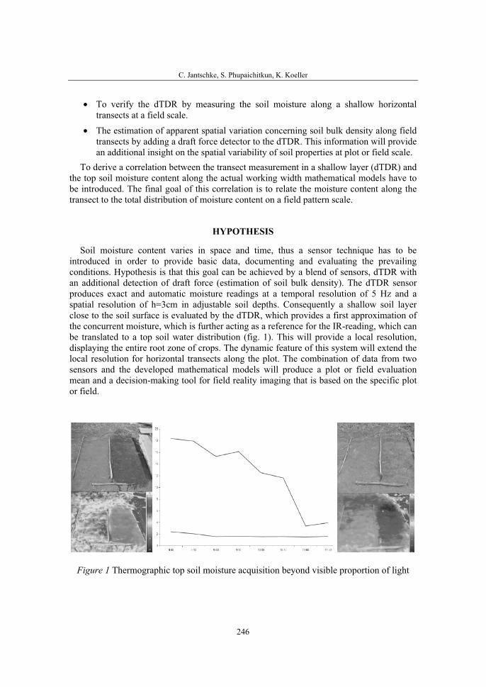
C. Jantschke, S. Phupaichitkun, K. Koeller
246
• To verify the dTDR by measuring the soil moisture along a shallow horizontal transects at a field scale.
• The estimation of apparent spatial variation concerning soil bulk density along field transects by adding a draft force detector to the dTDR. This information will provide an additional insight on the spatial variability of soil properties at plot or field scale.
To derive a correlation between the transect measurement in a shallow layer (dTDR) and the top soil moisture content along the actual working width mathematical models have to be introduced. The final goal of this correlation is to relate the moisture content along the transect to the total distribution of moisture content on a field pattern scale.
HYPOTHESIS
Soil moisture content varies in space and time, thus a sensor technique has to be introduced in order to provide basic data, documenting and evaluating the prevailing conditions. Hypothesis is that this goal can be achieved by a blend of sensors, dTDR with an additional detection of draft force (estimation of soil bulk density). The dTDR sensor produces exact and automatic moisture readings at a temporal resolution of 5 Hz and a spatial resolution of h=3cm in adjustable soil depths. Consequently a shallow soil layer close to the soil surface is evaluated by the dTDR, which provides a first approximation of the concurrent moisture, which is further acting as a reference for the IR-reading, which can be translated to a top soil water distribution (fig. 1). This will provide a local resolution, displaying the entire root zone of crops. The dynamic feature of this system will extend the local resolution for horizontal transects along the plot. The combination of data from two sensors and the developed mathematical models will produce a plot or field evaluation mean and a decision-making tool for field reality imaging that is based on the specific plot or field.
Figure 1 Thermographic top soil moisture acquisition beyond visible proportion of light
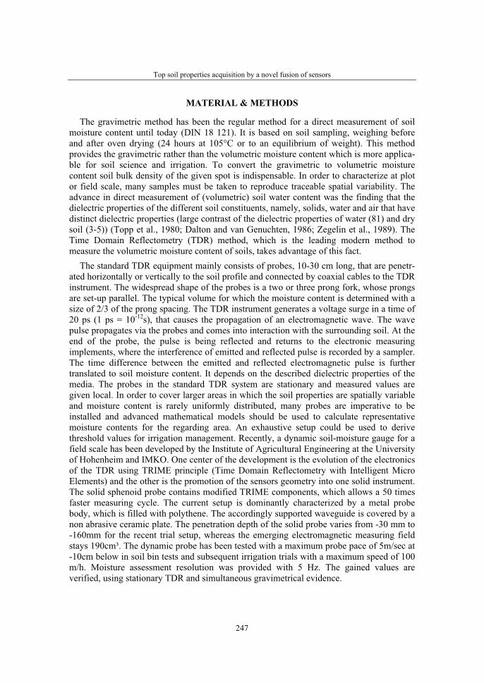
Top soil properties acquisition by a novel fusion of sensors
247
MATERIAL & METHODS
The gravimetric method has been the regular method for a direct measurement of soil moisture content until today (DIN 18 121). It is based on soil sampling, weighing before and after oven drying (24 hours at 105°C or to an equilibrium of weight). This method provides the gravimetric rather than the volumetric moisture content which is more applica-ble for soil science and irrigation. To convert the gravimetric to volumetric moisture content soil bulk density of the given spot is indispensable. In order to characterize at plot or field scale, many samples must be taken to reproduce traceable spatial variability. The advance in direct measurement of (volumetric) soil water content was the finding that the dielectric properties of the different soil constituents, namely, solids, water and air that have distinct dielectric properties (large contrast of the dielectric properties of water (81) and dry soil (3-5)) (Topp et al., 1980; Dalton and van Genuchten, 1986; Zegelin et al., 1989). The Time Domain Reflectometry (TDR) method, which is the leading modern method to measure the volumetric moisture content of soils, takes advantage of this fact.
The standard TDR equipment mainly consists of probes, 10-30 cm long, that are penetr-ated horizontally or vertically to the soil profile and connected by coaxial cables to the TDR instrument. The widespread shape of the probes is a two or three prong fork, whose prongs are set-up parallel. The typical volume for which the moisture content is determined with a size of 2/3 of the prong spacing. The TDR instrument generates a voltage surge in a time of 20 ps (1 ps = 10-12s), that causes the propagation of an electromagnetic wave. The wave pulse propagates via the probes and comes into interaction with the surrounding soil. At the end of the probe, the pulse is being reflected and returns to the electronic measuring implements, where the interference of emitted and reflected pulse is recorded by a sampler. The time difference between the emitted and reflected electromagnetic pulse is further translated to soil moisture content. It depends on the described dielectric properties of the media. The probes in the standard TDR system are stationary and measured values are given local. In order to cover larger areas in which the soil properties are spatially variable and moisture content is rarely uniformly distributed, many probes are imperative to be installed and advanced mathematical models should be used to calculate representative moisture contents for the regarding area. An exhaustive setup could be used to derive threshold values for irrigation management. Recently, a dynamic soil-moisture gauge for a field scale has been developed by the Institute of Agricultural Engineering at the University of Hohenheim and IMKO. One center of the development is the evolution of the electronics of the TDR using TRIME principle (Time Domain Reflectometry with Intelligent Micro Elements) and the other is the promotion of the sensors geometry into one solid instrument. The solid sphenoid probe contains modified TRIME components, which allows a 50 times faster measuring cycle. The current setup is dominantly characterized by a metal probe body, which is filled with polythene. The accordingly supported waveguide is covered by a non abrasive ceramic plate. The penetration depth of the solid probe varies from -30 mm to -160mm for the recent trial setup, whereas the emerging electromagnetic measuring field stays 190cm³. The dynamic probe has been tested with a maximum probe pace of 5m/sec at -10cm below in soil bin tests and subsequent irrigation trials with a maximum speed of 100 m/h. Moisture assessment resolution was provided with 5 Hz. The gained values are verified, using stationary TDR and simultaneous gravimetrical evidence.
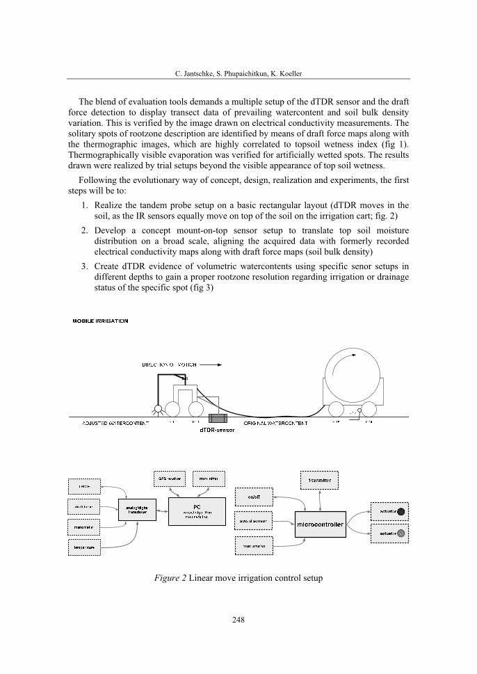
C. Jantschke, S. Phupaichitkun, K. Koeller
248
The blend of evaluation tools demands a multiple setup of the dTDR sensor and the draft force detection to display transect data of prevailing watercontent and soil bulk density variation. This is verified by the image drawn on electrical conductivity measurements. The solitary spots of rootzone description are identified by means of draft force maps along with the thermographic images, which are highly correlated to topsoil wetness index (fig 1). Thermographically visible evaporation was verified for artificially wetted spots. The results drawn were realized by trial setups beyond the visible appearance of top soil wetness.
Following the evolutionary way of concept, design, realization and experiments, the first steps will be to:
1. Realize the tandem probe setup on a basic rectangular layout (dTDR moves in the soil, as the IR sensors equally move on top of the soil on the irrigation cart; fig. 2)
2. Develop a concept mount-on-top sensor setup to translate top soil moisture distribution on a broad scale, aligning the acquired data with formerly recorded electrical conductivity maps along with draft force maps (soil bulk density)
3. Create dTDR evidence of volumetric watercontents using specific senor setups in different depths to gain a proper rootzone resolution regarding irrigation or drainage status of the specific spot (fig 3)
Figure 2 Linear move irrigation control setup
Top soil properties acquisition by a novel fusion of sensors
249
Figure 3 Rootzone displaying – Evolution of dTDR arrangements
DATA & RESULTS
Dry soils reveal higher temperatures due to non- or low-evaporative surfaces along with identical soil surface roughness index and consequent solar radiation grade. The differences in surface wetness are non detectable by the visual part of reflection.
The grade of evaporative surface cooling could be related properly to the grade of surface roughness. Verifications were drawn by gravimetrical evidence (DIN 18121). Furthermore initial results of thermographic data acquisition on various sites showed a high potential, detecting the present top soil moisture in changing top soils. The combination of actual draft force or penetration force along with definite water content in known depths reveals much more than the standalone evaporation rate of bare soil. Various dTDR setups have been realized to promote adequate data to create a state of the field reality, which enables a numerical approximation of top soil water content distribution by means of IR detection.
DISCUSSION
Momentary translation of thermographic evidence needs further side-data to derive highly defined water content information of top soils: Surface roughness and climatic constraints give first hints, resulting in suitable data acquisitions of soil types known. Further automatic field reality imaging functions on a basis of mathematical lateral extrapolation relative to the working width and travel direction given. The dTDR measurements are conducted at each working step on field in order to derive the key data for further extrapolation on field-scale. Shallow penetration of the dTDR measuring field is backed up by the combination of sensors within one setup (rootzone displaying; fig. 3).
C. Jantschke, S. Phupaichitkun, K. Koeller
250
CONCLUSIONS
Supplementary research on an upcoming prototype intends to blend visual sensors, thermographic sensors, climatic baseline information and surface scans by a high resolution laser, which will generate the required information to gain reliable field characterizing data on the basis of defined surface roughness.
The novel system shows a high potential in revealing top soil properties. Application fields are flashy for precision irrigation purposes. Field reality imaging displays an individual tool for high frequency automation of any kind. The equipment’s attendance to various individual production steps accumulates a highly defined spatial knowledge of soil properties.
REFERENCES
1. Armstrong, C. F., Ligon, J. T. and Thomson, S. J. (1985): Calibration of Watermark model 200 soil moisture sensor. ASAE Paper 85, p. 2077.
2. Bronson, K.F., Booker, J.D., Officer, S.J., Lascano, R.J., Maas, S.J., Searcy, S.W., Booker, J. (2005): Apparent electrical conductivity, soil properties and spatial covariance in the U.S. Southern High Plains. Precision Agriculture 6 (3), pp. 297-311.
3. Dalton, F. N. and van Genuchten, M. T. (1986): The time-domain reflectometry method for measuring soil water content and salinity. Geoderma 38, pp. 237–250.
4. de Jong, R. and Bootsma, A. (1996): Review of recent developments in soil water simulation models. Can. J. Soil Sci. 76, pp. 263–273.
5. DIN 18121 Teil 1 (1998): Baugrund; Untersuchung von Bodenproben: Wassergehalt – Bestimmung durch Ofentrocknung. (04).
6. DIN 18121 Teil 2 (2001): Baugrund; Untersuchung von Bodenproben: Wassergehalt – Bestimmung durch Schnellverfahren. (08).
7. Domsch, H., Giebel, A. (2004): Estimation of soil textural features from soil electrical conductivity recorded using the EM38. Precision Agriculture 5 (4), pp. 389-409.
8. Laboski, C.A.M., Lamb, J.A., Dowdy, R.H., Baker, J.M., Wright, J. (2001): Irrigation scheduling for a sandy soil using mobile frequency domain reflectometry with a checkbook method. Journal of Soil and Water Conservation 56 (2), pp. 97-100
9. Lowery, B., Datiri, B. C. and Andraski, B. J. (1986): An electrical readout system for tensiometers. Soil Sci. Soc. Am. J. 50, pp. 494–496.
10. Jantschke, C., Starcevic N., Wallach R., Becker R., Koeller K. (2006): Dynamic Online Moisture Detection to Enhance Irrigation Efficiency. Proceedings of the CIGR Agricultural Engineering World Congress, Bonn, pp. 55-56.
11. Roth, C. H., M. A. Malicki u. R. Plagge (1992): Empirical evaluation of the relationship between soil dielectric constant and volumetric watercontent as the basis for calibrating soil moisture measurements by TDR. J Soil Sci.. 43. pp. 1-13.
12. Topp, G. C., Davis, J. L. and Annan, A. P. (1980): Electromagnetic determination of soil water content: measurements in coaxial transmission lines. Water Resour.Res.16, pp. 574–582.

Top soil properties acquisition by a novel fusion of sensors
251
13. Schulze Lammers, P., Y. Sun and D. Ma (2007): Einsatz eines Kombinationssensors zur Kartierung des Bodenwiderstandes und Bodenwassergehaltes. Landtechnik 62 (5). pp. 330-331.
14. Zegelin, S. J., White, I. and Jenkins, D. R. (1989): Improved field probes for soil water content and electrical conductivity measurement using time domain reflectometry. Water Resour. Res. 25, pp. 2367–2376.

36. Symposium "Actual Tasks on Agricultural Engineering", Opatija, Croatia, 2008.
253
36.
SIMPOZIJAKTUALNI ZADACIMEHANIZACIJE POLJOPRIVREDE
UDC621.384.8
Stručni radExpert paper
STUDY ON QUANTITATIVE METHODS IN NEAR INFRARED SPECTROSCOPY ANALYSIS
JINGZHU WU1*, CUILING LIU1, YAN CHEN1, SHUXIA SUI1, LEI FENG2
1College of Information Engineering, Beijing Technology & Business University, Beijing, China, 100037
2College of Information and Electrical Engineering, China Agricultural University, Beijing, China, 100083
E-mail:[email protected]
SUMMARY
This paper discussed three types of quantitative methods used to build NIR models: PLS (Partial Least Square), BP (Back Propagation Neural Network) and SVM (Support Vectors Machines). One hundred and thirty two unit wheat samples were used as experimental materials. The result indicates that SVM has good performance. There also discussed SVM parameters: the penalty parameter (c) and the kernel parameters (γ) of RBF (Radial Base Function) kernel, which strongly affect prediction ability of the SVM model. The result indicates that c affects the self-prediction ability of SVM model and γ affects the prediction ability of SVM model when the other parameters are fixed.
Key words: NIR, PLS, BP, SVM, quantitative methods
INTRODUCTION
There are two typical quantitative methods used to build NIR (near infrared spectro-scopy) models: PLS (Partial Least Square) and BP (Back Propagation Neural Network). PLS algorithm is the most common used linear method in NIR analysis. While building calibration model by PLS method, the most difficult thing is how to choose the number of principle component (f). BP method has good ability of anti-jamming and nonlinear transformation ability. But it is not used very much because the training is very difficult and complex. In recent years Support Vector Machines (SVM) as a new technology is gradually used in NIR quantitative and qualitative analysis. SVM is a new machine-learning algorithm based on Vapnik-Chervonenkis (VC) Dimension and Structural Risk Minimiza-
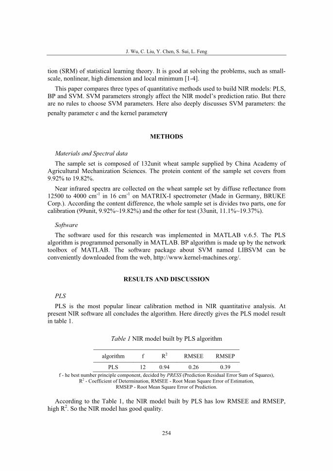
J. Wu, C. Liu, Y. Chen, S. Sui, L. Feng
254
tion (SRM) of statistical learning theory. It is good at solving the problems, such as small-scale, nonlinear, high dimension and local minimum [1-4].
This paper compares three types of quantitative methods used to build NIR models: PLS, BP and SVM. SVM parameters strongly affect the NIR model’s prediction ratio. But there are no rules to choose SVM parameters. Here also deeply discusses SVM parameters: the penalty parameter c and the kernel parameter�
METHODS
Materials and Spectral data The sample set is composed of 132unit wheat sample supplied by China Academy of
Agricultural Mechanization Sciences. The protein content of the sample set covers from 9.92% to 19.82%.
Near infrared spectra are collected on the wheat sample set by diffuse reflectance from 12500 to 4000 cm-1 in 16 cm-1 on MATRIX-I spectrometer (Made in Germany, BRUKE Corp.). According the content difference, the whole sample set is divides two parts, one for calibration (99unit, 9.92%~19.82%) and the other for test (33unit, 11.1%~19.37%).
SoftwareThe software used for this research was implemented in MATLAB v.6.5. The PLS
algorithm is programmed personally in MATLAB. BP algorithm is made up by the network toolbox of MATLAB. The software package about SVM named LIBSVM can be conveniently downloaded from the web, http://www.kernel-machines.org/.
RESULTS AND DISCUSSION
PLSPLS is the most popular linear calibration method in NIR quantitative analysis. At
present NIR software all concludes the algorithm. Here directly gives the PLS model result in table 1.
Table 1 NIR model built by PLS algorithm
algorithm f R2 RMSEE RMSEP
PLS 12 0.94 0.26 0.39 f - he best number principle component, decided by PRESS (Prediction Residual Error Sum of Squares),
R2 - Coefficient of Determination, RMSEE - Root Mean Square Error of Estimation,RMSEP - Root Mean Square Error of Prediction.
According to the Table 1, the NIR model built by PLS has low RMSEE and RMSEP, high R2. So the NIR model has good quality.
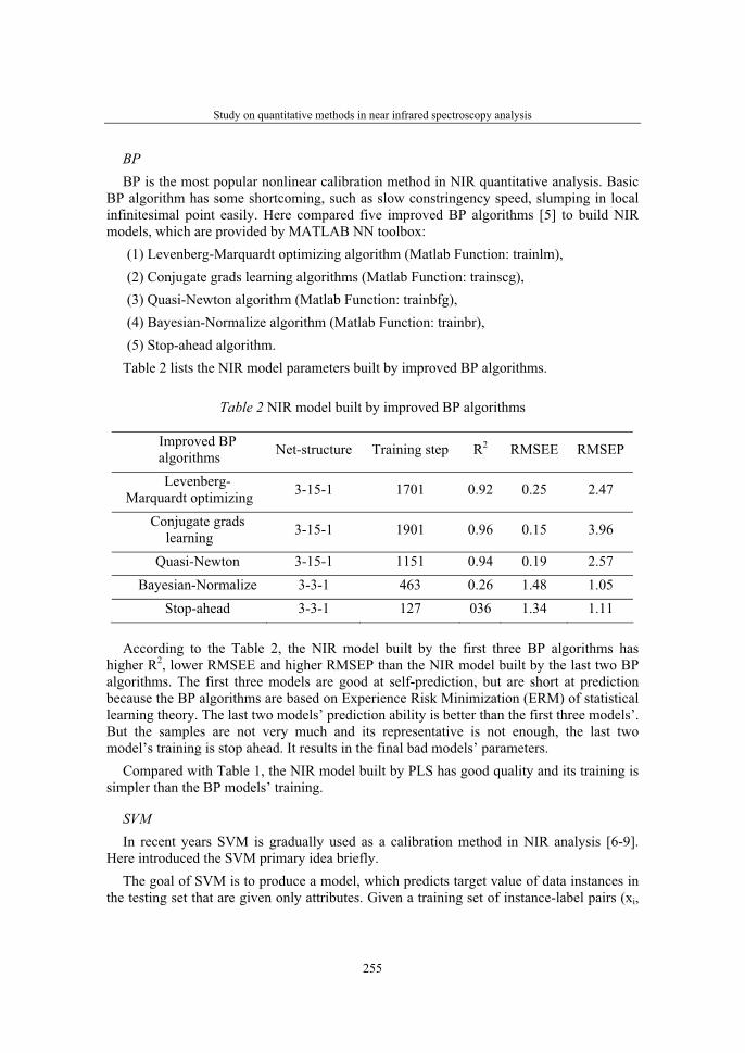
Study on quantitative methods in near infrared spectroscopy analysis
255
BPBP is the most popular nonlinear calibration method in NIR quantitative analysis. Basic
BP algorithm has some shortcoming, such as slow constringency speed, slumping in local infinitesimal point easily. Here compared five improved BP algorithms [5] to build NIR models, which are provided by MATLAB NN toolbox:
(1) Levenberg-Marquardt optimizing algorithm (Matlab Function: trainlm), (2) Conjugate grads learning algorithms (Matlab Function: trainscg), (3) Quasi-Newton algorithm (Matlab Function: trainbfg), (4) Bayesian-Normalize algorithm (Matlab Function: trainbr), (5) Stop-ahead algorithm.
Table 2 lists the NIR model parameters built by improved BP algorithms.
Table 2 NIR model built by improved BP algorithms
Improved BP algorithms Net-structure Training step R2 RMSEE RMSEP
Levenberg-Marquardt optimizing 3-15-1 1701 0.92 0.25 2.47
Conjugate grads learning 3-15-1 1901 0.96 0.15 3.96
Quasi-Newton 3-15-1 1151 0.94 0.19 2.57 Bayesian-Normalize 3-3-1 463 0.26 1.48 1.05
Stop-ahead 3-3-1 127 036 1.34 1.11
According to the Table 2, the NIR model built by the first three BP algorithms has higher R2, lower RMSEE and higher RMSEP than the NIR model built by the last two BP algorithms. The first three models are good at self-prediction, but are short at prediction because the BP algorithms are based on Experience Risk Minimization (ERM) of statistical learning theory. The last two models’ prediction ability is better than the first three models’. But the samples are not very much and its representative is not enough, the last two model’s training is stop ahead. It results in the final bad models’ parameters.
Compared with Table 1, the NIR model built by PLS has good quality and its training is simpler than the BP models’ training.
SVMIn recent years SVM is gradually used as a calibration method in NIR analysis [6-9].
Here introduced the SVM primary idea briefly. The goal of SVM is to produce a model, which predicts target value of data instances in
the testing set that are given only attributes. Given a training set of instance-label pairs (xi,
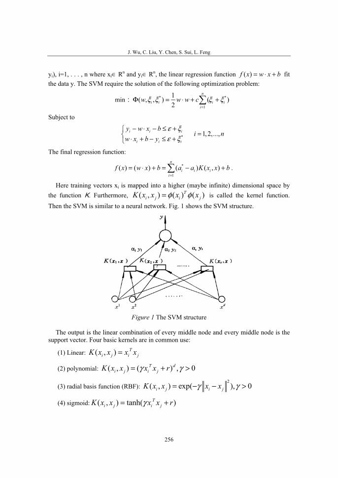
J. Wu, C. Liu, Y. Chen, S. Sui, L. Feng
256
yi), i=1, . . . , n where xi� Rn and yi� Rn, the linear regression function ( )f x w x b= ⋅ + fit the data y. The SVM require the solution of the following optimization problem:
min� * *
1
1( , , ) ( )2
n
i i i ii
w w w cξ ξ ξ ξ=
Φ = ⋅ + +∑
Subject to
* 1,2,...,i i i
i i i
y w x bi n
w x b yε ξε ξ
− ⋅ − ≤ +⎧
=⎨ ⋅ + − ≤ +⎩
The final regression function:
*
1( ) ( ) ( ) ( , )
n
i i ii
f x w x b a a K x x b=
= ⋅ + = − +∑ .
Here training vectors xi is mapped into a higher (maybe infinite) dimensional space by the function �. Furthermore, ( , ) ( ) ( )T
i j i jK x x x xφ φ= is called the kernel function. Then the SVM is similar to a neural network. Fig. 1 shows the SVM structure.
Figure 1 The SVM structure
The output is the linear combination of every middle node and every middle node is the support vector. Four basic kernels are in common use:
(1) Linear: ( , ) Ti j i jK x x x x=
(2) polynomial: ( , ) ( ) , 0T di j i jK x x x x rγ γ= + >
(3) radial basis function (RBF): 2
( , ) exp( ), 0i j i jK x x x xγ γ= − − >
(4) sigmoid: ( , ) tanh( )Ti j i jK x x x x rγ= +
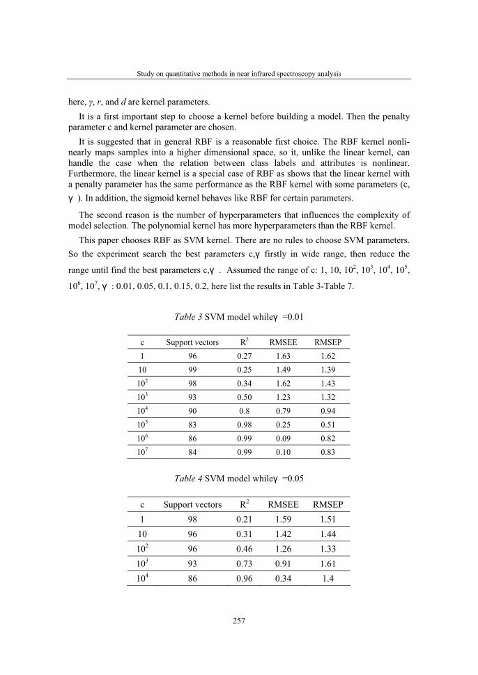
Study on quantitative methods in near infrared spectroscopy analysis
257
here, γ, r, and d are kernel parameters. It is a first important step to choose a kernel before building a model. Then the penalty
parameter c and kernel parameter are chosen.It is suggested that in general RBF is a reasonable first choice. The RBF kernel nonli-
nearly maps samples into a higher dimensional space, so it, unlike the linear kernel, can handle the case when the relation between class labels and attributes is nonlinear. Furthermore, the linear kernel is a special case of RBF as shows that the linear kernel with a penalty parameter has the same performance as the RBF kernel with some parameters (c, � ). In addition, the sigmoid kernel behaves like RBF for certain parameters.
The second reason is the number of hyperparameters that influences the complexity of model selection. The polynomial kernel has more hyperparameters than the RBF kernel.
This paper chooses RBF as SVM kernel. There are no rules to choose SVM parameters. So the experiment search the best parameters c,� firstly in wide range, then reduce the
range until find the best parameters c,� � Assumed the range of c: 1, 10, 102, 103, 104, 105,
106, 107, � : 0.01, 0.05, 0.1, 0.15, 0.2, here list the results in Table 3-Table 7.
Table 3 SVM model while� =0.01
c Support vectors R2 RMSEE RMSEP
1 96 0.27 1.63 1.62
10 99 0.25 1.49 1.39
102 98 0.34 1.62 1.43
103 93 0.50 1.23 1.32
104 90 0.8 0.79 0.94
105 83 0.98 0.25 0.51
106 86 0.99 0.09 0.82
107 84 0.99 0.10 0.83
Table 4 SVM model while� =0.05
c Support vectors R2 RMSEE RMSEP 1 98 0.21 1.59 1.51
10 96 0.31 1.42 1.44 102 96 0.46 1.26 1.33 103 93 0.73 0.91 1.61 104 86 0.96 0.34 1.4

J. Wu, C. Liu, Y. Chen, S. Sui, L. Feng
258
105 85 0.99 0.10 1.35 106 87 0.99 0.09 1.32 107 87 0.99 0.09 1.32
Table 5 SVM model while� =0.1
c Support vectors R2 RMSEE RMSEP 1 92 0.14 1.69 1.71
10 96 0.17 1.63 1.62 102 99 0.29 1.50 1.4 103 98 0.34 1.40 1.39 104 91 0.48 1.23 1.37 105 90 0.78 0.83 0.93 106 81 0.97 0.30 0.52 107 97 0.79 1.02 1.27
Table 6 SVM model while� =0.15
c Support vectors R2 RMSEE RMSEP 1 97 0.25 1.50 1.52
10 94 0.4 1.33 1.38 102 95 0.63 1.05 1.8 103 96 0.88 0.63 2.08 104 91 0.99 0.16 2.03 105 85 0.99 0.10 1.87 106 85 0.99 0.10 1.87 107 85 0.99 0.10 1.87
Table 7 SVM model while� =0.2
c Support vectors R2 RMSEC RMSEP 1 98 0.28 1.47 1.51
10 95 0.44 1.3 1.32 102 93 0.67 0.98 1.72 103 95 0.91 0.55 1.34

Study on quantitative methods in near infrared spectroscopy analysis
259
104 91 0.99 0.13 2.29 105 93 0.99 0.10 2.15 106 93 0.99 0.10 2.15 107 93 0.99 0.10 2.15
According to Table 3-Table 7, here can draw the curves, figure2and figure 3.
�
���
���
���
���
�
���
���
���
���
� � � � � �
lg(c)
RMSE
E
γ=0.01 γ=0.05 γ=0.10 γ=0.15 γ=0.20
Figure 2 lg(c)-RMSEE
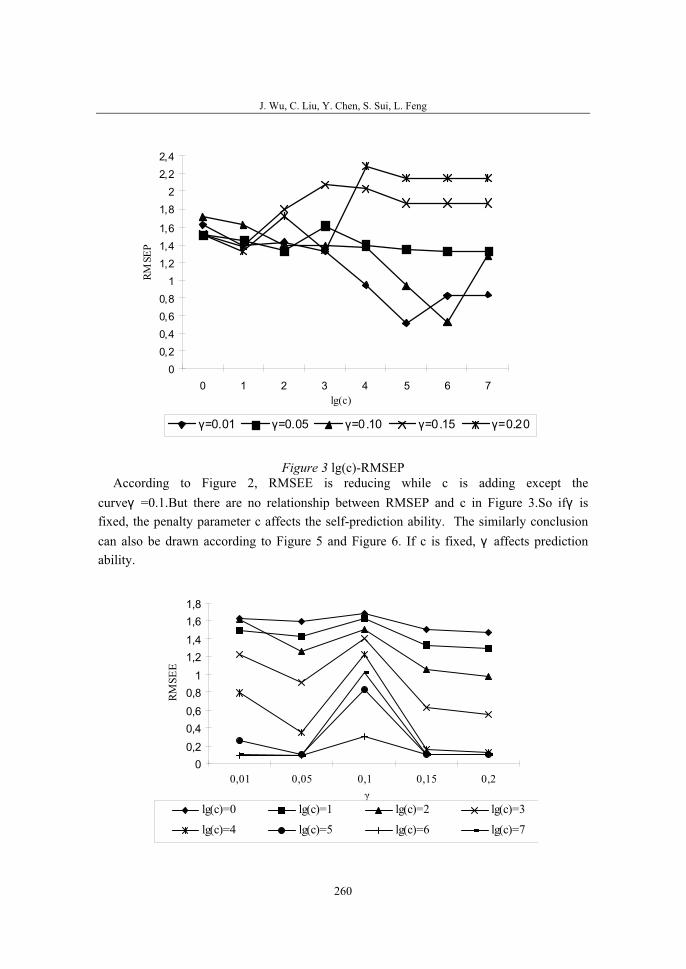
J. Wu, C. Liu, Y. Chen, S. Sui, L. Feng
260
�
���
���
���
���
�
���
���
���
���
�
���
���
� � � � � �
lg(c)
RMSE
P
γ=0.01 γ=0.05 γ=0.10 γ=0.15 γ=0.20
Figure 3 lg(c)-RMSEP According to Figure 2, RMSEE is reducing while c is adding except the
curve� =0.1.But there are no relationship between RMSEP and c in Figure 3.So if� isfixed, the penalty parameter c affects the self-prediction ability. The similarly conclusion can also be drawn according to Figure 5 and Figure 6. If c is fixed, � affects prediction ability.
�
���
���
���
���
�
���
���
���
���
0,01 0,05 0,1 0,15 0,2γ
RMSE
E
lg(c)=0 lg(c)=1 lg(c)=2 lg(c)=3
lg(c)=4 lg(c)=5 lg(c)=6 lg(c)=7
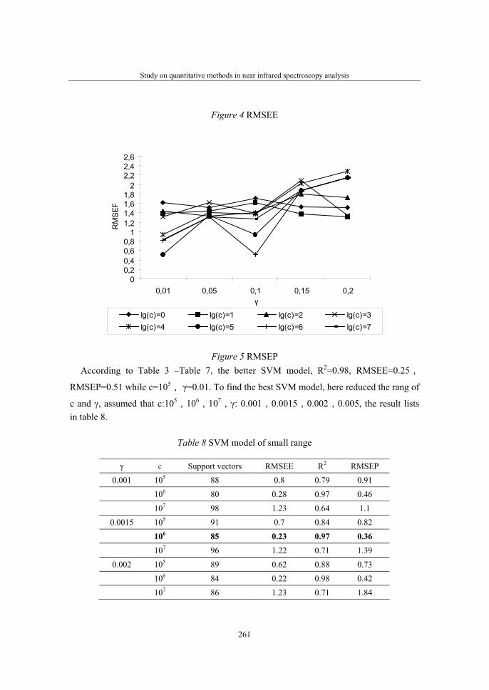
Study on quantitative methods in near infrared spectroscopy analysis
261
Figure 4 RMSEE
�
���
���
���
���
�
���
���
���
���
�
���
���
���
���� ��� ��� ��� ���
γ
�����
�� ��� �� ��� �� ��� �� ���
�� ��� �� �� �� ��� �� ���
Figure 5 RMSEP According to Table 3 –Table 7, the better SVM model, R2=0.98, RMSEE=0.25�
RMSEP=0.51 while c=105� γ=0.01. To find the best SVM model, here reduced the rang of
c and γ, assumed that c:105�106
�107�γ: 0.001�0.0015�0.002�0.005, the result lists
in table 8.
Table 8 SVM model of small range
γ c Support vectors RMSEE R2 RMSEP
0.001 105 88 0.8 0.79 0.91
106 80 0.28 0.97 0.46
107 98 1.23 0.64 1.1
0.0015 105 91 0.7 0.84 0.82
106 85 0.23 0.97 0.36 107 96 1.22 0.71 1.39
0.002 105 89 0.62 0.88 0.73
106 84 0.22 0.98 0.42
107 86 1.23 0.71 1.84
J. Wu, C. Liu, Y. Chen, S. Sui, L. Feng
262
0.005 105 83 0.36 0.96 0.47
106 86 0.14 0.99 0.50
107 85 0.18 0.99 0.57
According to the Table 8, the best SVM model’s index, R2=0.97, RMSEE=0.23, RMSEP=0.36. The indexes are all better than the PLS model.
CONCLUSIONS
Here, this paper can get some conclusions, 1. Compared with the three calibrating procedure, PLS is simple and direct, BP training is
complex, SVM is simpler than BP, but more complex than PLS.2. Compare with the NIR model’s indexes, SVM is better than PLS, PLS is better than BP
in this paper. 3. Compare with the three methods’ foreground in NIR quantitative analysis, PLS,
however, is the first method because it is simple and robust. BP method is complex. Sometimes its result is bad because of its ERM training. But SVM is simple than BP. Sometimes its result is better than PLS because of its SRM training. So the foreground of SVM will be developed better than BP in NIR analysis to build nonlinear quantitative calibration.
4. The penalty parameter (c) and the kernel parameters (γ) of RBF (Radial Base Function) kernel strongly affect prediction ability of the SVM model. The experimental result indicates that c affects the self-prediction ability of SVM model and γ affects the prediction ability of SVM model when the other parameters are fixed.
REFERENCES
1. Zhang Xuegong. (2000). Introduction to Statistical Learning Theory and Support Vector Machines, Acta Automation Sinica26: 32-42
2. Cui Weidong, Zhou Zhihua, and Li Xing. (2001). Research of Support Vector Machines, Computer Engineering and Applications 37:58-61
3. Nello Cristianini, and John Shawe-Taylor. (2004). An Introduction to Support Vector Machines and Other Kernel-based Learning Methods. Beijing
4. Jingzhu Wu. (2006).Study on Quality Detection of Agricultural Products Based on Near Infrared Spectroscopy Technology. Doctoral Dissertation, China Agricultural University, China, 2006 (in Chinese).
5. Xu Dong, Wu Zheng. (2002). System Analysis and Design Based on MATLAB 6.x-- Neural Network. Xi An
Study on quantitative methods in near infrared spectroscopy analysis
263
6. Qu Haibin�Liu Xiaoxuan�Cheng Yiyu. (2004)�A Method for Analysis of Extracting Solution of Panax Notog in seng Using Near- infrared Spectroscopy and Support Vector Regress ion�Chemical Journal Of Chinese University, 25(1): 39-43
7. Du Shuxin, Wu Tiejun (2004). Support Vector Machines for a NIR Spectroscopy Gasoline Octane Number Analyzer�Chinese Journal of Scientific Instrument, 25(5): 582-586
8. Yao Xiaogang, Dai Liankui, Fang Jun. (2004). Diesel Cetane Number Measurement with NIR Spectroanalysis Using LS-SVM Control and Instruments in Chemical Industry, 31(2): 48-51
9. Zhang Luda, Jing Zecheng, Shen Xiaonan,etc. (2005)�Study on Application of Fourier Transformation Near-Infrared Spectroscopy Analysis with Support Vector Machine (SVM), Spectroscopy and Spectral Analysis, 25(9): 1400-1403

36. Symposium "Actual Tasks on Agricultural Engineering", Opatija, Croatia, 2008.
265
36.
SIMPOZIJAKTUALNI ZADACIMEHANIZACIJE POLJOPRIVREDE
UDC543.42:621.384.8
Stručni radExpert paper
BASIC ACCESS IN ANALYSIS AND IDENTIFICATION ORGANIC BONDS IN FOOD INDUSTRY USE
NIR SPECTROMETRY V. CORLUKA, M. MESIC, Z. VALTER
Faculty of Electrical Engineering, University of Osijek,Croatia, Kneza Trpimira 2, 31000 Osijek
SUMMARY
Spectroscopy is the study of the interaction of electromagnetic radiation with a chemical substance. Each molecule has certain natural vibration frequencies. The nature of the interaction depends upon the properties of the substance. When infrared light is incident on the molecule, the frequency which matches the natural vibration frequency is absorbed by the molecule resulting in molecular vibration. Near infrared Spectroscopy (NIR) is a type of vibration spectroscopy in the wavelength range of 780 to 2500nm. This NIR bands are due overtone and combination bands primarily of OH, CH, NH and CO groups. Applications include water content, measure the percentage of proteins, lipids, carbohydrates in food. The absorption of the radiation at the NIR region is attributed to the low mass of the hydrogen atom. The bonds involving hydrogen vibrate with large amplitude. Therefore, the absorption bands observed at the NIR region arise from overtones of stretching vibrations involving functional groups with hydrogen atom or combination involving stretching and bending mode of vibration of these groups. The overtones (1450nm) and combination (1940nm) water bands in the NIR region, spectral bands related to milk. The lipid CH combination and second overtones related at 2320 and 2350nm. The protein NH absorption band at 2060 and 2170nm can be visualized in the wheat spectrum. This information content has been intensively exploited for qualitative and quantities chemical and physical analytical purposes. Instrument selection must be guided by end application. Modern NIR instruments in terms of the technology employed for wavelengths selection: Filter instruments, Led based instrument, AOTF based instrument, Dispersive optics based instruments and Fourier transform based instruments. Stability, reliability, wavelength accuracy, resistance to vibration and temperature change are all factors that determine the performances of the instruments.
Key words: spectroscopy, NIR, molecular, wavelength, absorption, food
V. Corluka, M. Mesic, Z. Valter
266
INTRODUCTION
The IR spectral region is from the red end of the visible spectrum at 780nm (12 820 cm-
1) to the beginning of the microwave region at a wavelength of 1mm (10 cm-1). This range is further subdivided into the near-infrared (NIR), mid-infrared (MIR), and far-infrared (FIR). The MIR region covers the range of 2,5μm to 25μm (400 - 4000 cm-1). The NIR region covers the range of 780 to 2500nm (12 820 - 4000 cm-1). Near infrared Spectroscopy is the region most familiar to the organic chemist as providing a ‘‘fingerprint’’ characteristic of molecular species. It is this region that includes the rich spectrum of absorptions corresponding to fundamental vibrations of the species being probed. Although MIR absorption positions are almost universally reported in units of wavenumbers (cm-1), it remains the norm for NIR spectra to be reported in wavelength units, generally in nanometers. The wavenumber unit cm-1 is commonly used in infrared spectroscopy. It is the frequency of the radiation divided by the speed of light c. NIR analysis has steadily grown in popularity because of its ability to quickly provide qualitative and quantitative information of many products. The non-invasive and non-destructive features of vibration spectroscopy techniques, such as NIR, make them novel tools for in-line quality assurance. The actual NIR analysis was developed in the 1950’s [1] by a work of a group at USDA (United States Department of Agriculture) (1993). They discovered that the non-destructive NIR spectra of biological samples could be obtained with no sample preparation and in less than a minute. This gave rise to a wide range of uses of NIR in the agricultural industry. Many types of industries have also used NIR for several applications. The petrochemical, pulp and paper, and pharmaceutical industries have taken advantage over characteristics of NIR[2]. Today, more papers are being written about the application of the NIR spectral region to all types of analyses than ever before.
NIR spectroscopy has emerged in recent years as the analytical method of choice in an enormous variety of applications. The clearest advantage is that no specific reagents are required. Automated, repetitive analyses can therefore be carried out at very low cost. The appeal of these factors has spurred the development of a new generation of analytical NIR spectrometers that combine high acquisition speed with superb spectral sensitivity. Powerful chemometric algorithms and software packages have emerged in parallel with the new hardware, and new applications emerge continually. Rather than relying upon reagents to promote color reactions, NIR-based analysis is founded upon the spectrum of NIR colors characteristic of the analyte itself. If a particular component provides an NIR absorption spectrum, and its concentration is high enough that the spectrum contributes meaningfully to the NIR absorption profile, and then it may, in principle, be quantified by using NIR spectroscopy.
Methods based on infrared spectroscopy have the potential to satisfy the demands that chemical analysis does not. Infrared spectroscopy probes the vibrations of the functional groups of molecules by letting infrared light interact with the sample under investigation. This is a non destructive, and possibly non-invasive, method which is, in principle, capable of identifying and quantifying organic molecules. Each organic molecule has a unique infrared spectrum, and the strength of this spectrum is proportional to the concentration of the molecule. This means that simultaneous determination of several trace components from one spectrum is feasible provided that the spectra are sufficiently different in the spectral regions that are accessible. Unfortunately, the water in aqueous solutions absorbs
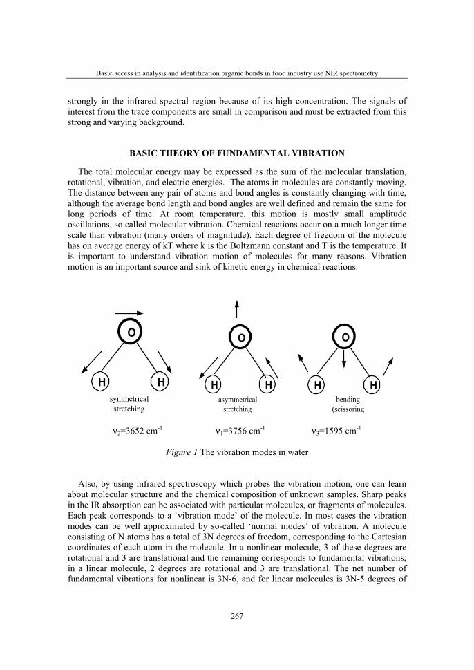
Basic access in analysis and identification organic bonds in food industry use NIR spectrometry
267
strongly in the infrared spectral region because of its high concentration. The signals of interest from the trace components are small in comparison and must be extracted from this strong and varying background.
BASIC THEORY OF FUNDAMENTAL VIBRATION
The total molecular energy may be expressed as the sum of the molecular translation, rotational, vibration, and electric energies. The atoms in molecules are constantly moving. The distance between any pair of atoms and bond angles is constantly changing with time, although the average bond length and bond angles are well defined and remain the same for long periods of time. At room temperature, this motion is mostly small amplitude oscillations, so called molecular vibration. Chemical reactions occur on a much longer time scale than vibration (many orders of magnitude). Each degree of freedom of the molecule has on average energy of kT where k is the Boltzmann constant and T is the temperature. It is important to understand vibration motion of molecules for many reasons. Vibration motion is an important source and sink of kinetic energy in chemical reactions.
H H
O
symmetricalstretching
H H
O
asymmetricalstretching
H H
O
bending(scissoring
ν2=3652 cm-1 ν1=3756 cm-1 ν3=1595 cm-1
Figure 1 The vibration modes in water
Also, by using infrared spectroscopy which probes the vibration motion, one can learn about molecular structure and the chemical composition of unknown samples. Sharp peaks in the IR absorption can be associated with particular molecules, or fragments of molecules. Each peak corresponds to a ‘vibration mode’ of the molecule. In most cases the vibrationmodes can be well approximated by so-called ‘normal modes’ of vibration. A molecule consisting of N atoms has a total of 3N degrees of freedom, corresponding to the Cartesian coordinates of each atom in the molecule. In a nonlinear molecule, 3 of these degrees are rotational and 3 are translational and the remaining corresponds to fundamental vibrations; in a linear molecule, 2 degrees are rotational and 3 are translational. The net number of fundamental vibrations for nonlinear is 3N-6, and for linear molecules is 3N-5 degrees of
V. Corluka, M. Mesic, Z. Valter
268
freedom. Water and carbon dioxide are valuable examples of simple system in which mechanical coupling between two oscillators. Water to be constructed of two O-H oscillators, the individual diatomic systems would be expected to have identical frequencies. When welded together, however, the vibrations of one O-H oscillator interfere with the vibrations of the other O-H oscillator. The coupling interaction is frequency dependent. The closer the frequencies of the two oscillators have the stronger the interaction. When there are identical frequencies and a direct mechanical connection, the coupling effect will be maximized. The three normal modes of H2O also include the symmetric O-H stretch, the asymmetrical stretch, and an H-O-H bends, shown in figure 1. The bending mode has a lower frequency than the others.
The main problem in the description of the vibrations of a polyatomic molecule is the determination of the reduced mass of a specific normal mode. For larger molecules, this becomes an incredibly complicated task. It can, however, in good approximation, partition a molecule into functional groups and neglect the coupling between vibrations of�different�groups if they are spatially separated or if their force constants differ considerably. The introduction of group frequencies allows the identifications of structural elements of a molecule and makes infrared spectroscopy an important tool for the identification of molecular structure and for infrared spectroscopy an important tool for the identification of molecular structure and for quantitative analysis.
SPECTROSCOPY
In absorption spectroscopy, the molecule absorbs energy from the oscillating electric and magnetic field in the electromagnetic wave only if the frequency matches that of the vibration oscillations (such matching of frequencies is called resonance). The energy of the absorbed photon is calculation absorption on formula (1)
Ei = hνi (1)
A polyatomic molecule has more than one normal mode of vibration. Each normal mode has a different frequency and there is, in principle, an absorption peak for each one of the modes. No peak is observed, however, if the normal mode displacements do not lead to a change in the dipole moment of the molecule, where h is Planck’s constant and νi is the frequency. The IR region is active mainly to vibration energy changes of ground electronic state molecules. Generally, only organic molecules can absorb wavelengths in the NIR region. MIR and NIR are based on absorption techniques. The absorption bands are due to molecular vibrations. MIR is associated with fundamental molecular stretching and bending vibration frequency. NIR band are due to overtone and combination bands primarily of OH, CH, NH and CO groups. NIR is currently used in the food industry to measure the percentage of proteins, lipids, carbohydrates and moisture in food. NIR offers the possibility of in-line analysis. NIR Spectra can be collected in two modes: either transmittance (light passing through translucent media) or reflectance (light diffusely reflected from opaque media). Transmittance — log (1/T) — measurements are collected on translucent samples that have low biomass or low light scattering. The use of narrow optical path lengths (less than one millimeter) can improve analyte sensitivity but makes sampling (and cell cleaning) difficult. Diffuse reflectance — log (1/R) — measurements
Basic access in analysis and identification organic bonds in food industry use NIR spectrometry
269
are used to interrogate opaque or strongly light-scattering samples (that is, those with high biomass or high light scattering) suitable NIR spectroscopic models. In MLR, linear relationships are derived between the absorption of NIR energy at discrete wavelengths and the reference analytical chemistry for specific constituents. The primary wavelength is for the analyte of interest, and subsequent wavelengths are included to compensate for overlapping, interfering absorption bands from other broth components or from changes in light scattering intensity.
Infrared spectroscopy is based on the Beer’s-Lambert law, where absorbance is directly proportional contents. Sample is enough thickness, so the transmition is equal zero and suppose is to happen only reflection. From reflection of two wavelengths is calculation absorption on formula (2)
A=log10(R0/R (2)
A – Absorbance R0 – Reflection from referent wavelength or from standard sample Ru – Reflection from sample Molecules that absorb NIR energy vibrate in two fundamental modes: stretching and
bending. Stretching is a continuous change in the inter-atomic distance along the axis between two atoms and it occurs at lower wavelengths than bending vibrations. A bending vibration is a change in the bond angle between diatomic molecules. The NIR bands are mainly overtones and combinations of fundamental vibrations in the mid-infrared. The most often observed bands in the NIR include combination bands, second and third overtones all attributed to information from the mid-IR. Usually, for a solid sample, the reflected light is the parameter measured in NIR. The NIR is convenient to subdivide further this span into natural subregions. The 2000–2500nm range includes the most intense absorptions and thus is the region most commonly exploited for analytical purposes. Absorptions in this region correspond to ‘‘combination bands’’, combining X-H (where X = C, N, O) stretches with other fundamental vibrations, whereas practically all of the higher energy transitions correspond to vibration first (1400–1800 nm), second (950–1250 nm), and third overtones (Table 1). The diversity of transitions in the NIR region has interesting practical consequences. For aqueous solutions, the 2000–2500nm region is best explored by using a transmission cell with an optical path length of 0.5–2.5 mm. The optimal path length to observe the first overtone transitions is longer – of the order of 5–10mm – whereas observation of the second overtones requires a path length of several centimeters. Where sample volume is a consideration, a relatively short path length is a necessity and the combination region is therefore preferred. Another outgrowth of this trend is that tissue is relatively transparent at shorter NIR wavelengths.
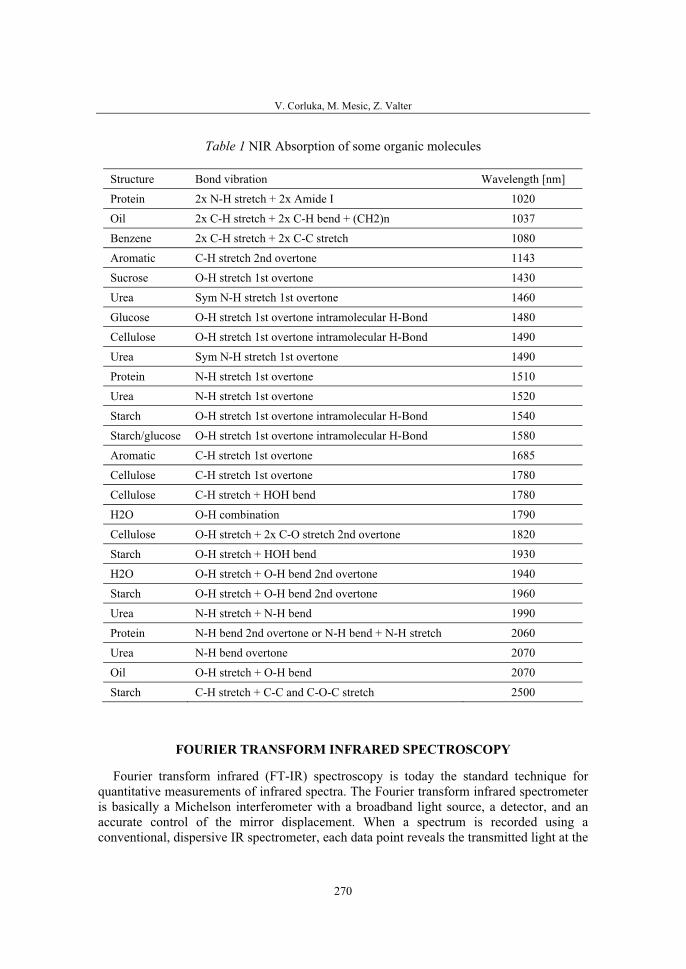
V. Corluka, M. Mesic, Z. Valter
270
Table 1 NIR Absorption of some organic molecules
Structure Bond vibration Wavelength [nm]
Protein 2x N-H stretch + 2x Amide I 1020
Oil 2x C-H stretch + 2x C-H bend + (CH2)n 1037
Benzene 2x C-H stretch + 2x C-C stretch 1080
Aromatic C-H stretch 2nd overtone 1143
Sucrose O-H stretch 1st overtone 1430
Urea Sym N-H stretch 1st overtone 1460
Glucose O-H stretch 1st overtone intramolecular H-Bond 1480
Cellulose O-H stretch 1st overtone intramolecular H-Bond 1490
Urea Sym N-H stretch 1st overtone 1490
Protein N-H stretch 1st overtone 1510
Urea N-H stretch 1st overtone 1520
Starch O-H stretch 1st overtone intramolecular H-Bond 1540
Starch/glucose O-H stretch 1st overtone intramolecular H-Bond 1580
Aromatic C-H stretch 1st overtone 1685
Cellulose C-H stretch 1st overtone 1780
Cellulose C-H stretch + HOH bend 1780
H2O O-H combination 1790
Cellulose O-H stretch + 2x C-O stretch 2nd overtone 1820
Starch O-H stretch + HOH bend 1930
H2O O-H stretch + O-H bend 2nd overtone 1940
Starch O-H stretch + O-H bend 2nd overtone 1960
Urea N-H stretch + N-H bend 1990
Protein N-H bend 2nd overtone or N-H bend + N-H stretch 2060
Urea N-H bend overtone 2070
Oil O-H stretch + O-H bend 2070
Starch C-H stretch + C-C and C-O-C stretch 2500
FOURIER TRANSFORM INFRARED SPECTROSCOPY
Fourier transform infrared (FT-IR) spectroscopy is today the standard technique for quantitative measurements of infrared spectra. The Fourier transform infrared spectrometer is basically a Michelson interferometer with a broadband light source, a detector, and an accurate control of the mirror displacement. When a spectrum is recorded using a conventional, dispersive IR spectrometer, each data point reveals the transmitted light at the
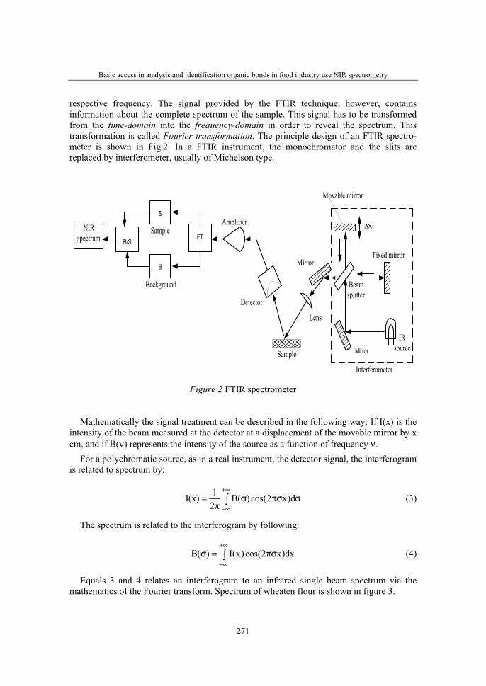
Basic access in analysis and identification organic bonds in food industry use NIR spectrometry
271
respective frequency. The signal provided by the FTIR technique, however, contains information about the complete spectrum of the sample. This signal has to be transformed from the time-domain into the frequency-domain in order to reveal the spectrum. This transformation is called Fourier transformation. The principle design of an FTIR spectro-meter is shown in Fig.2. In a FTIR instrument, the monochromator and the slits are replaced by interferometer, usually of Michelson type.
NIRspectrum B/S
S
FTXΔ
Movable mirror
Fixed mirror
IRsource
Beamsplitter
Mirror
Mirror
Lens
Sample
Detector
Amplifier
B
Sample
Background
Interferometer
Figure 2 FTIR spectrometer
Mathematically the signal treatment can be described in the following way: If I(x) is the intensity of the beam measured at the detector at a displacement of the movable mirror by x cm, and if B(ν) represents the intensity of the source as a function of frequency ν.
For a polychromatic source, as in a real instrument, the detector signal, the interferogram is related to spectrum by:
1I(x) B( )cos(2 x)d2π
+∞
−∞= σ πσ σ∫ (3)
The spectrum is related to the interferogram by following:
B( ) I(x)cos(2 x)dx+∞
−∞σ = πσ∫ (4)
Equals 3 and 4 relates an interferogram to an infrared single beam spectrum via the mathematics of the Fourier transform. Spectrum of wheaten flour is shown in figure 3.
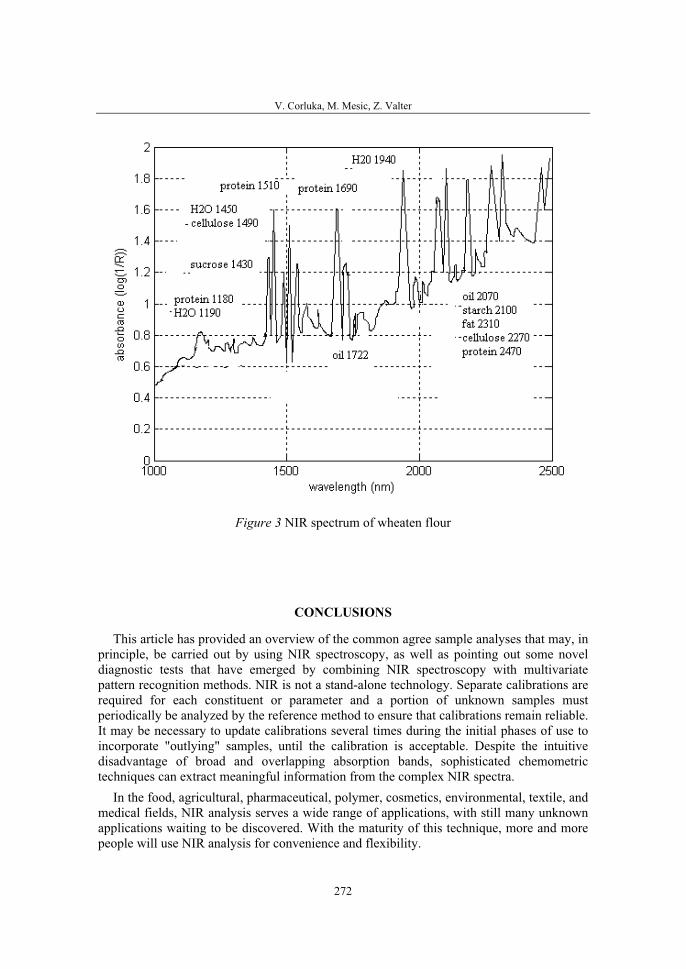
V. Corluka, M. Mesic, Z. Valter
272
Figure 3 NIR spectrum of wheaten flour
CONCLUSIONS
This article has provided an overview of the common agree sample analyses that may, in principle, be carried out by using NIR spectroscopy, as well as pointing out some novel diagnostic tests that have emerged by combining NIR spectroscopy with multivariate pattern recognition methods. NIR is not a stand-alone technology. Separate calibrations are required for each constituent or parameter and a portion of unknown samples must periodically be analyzed by the reference method to ensure that calibrations remain reliable. It may be necessary to update calibrations several times during the initial phases of use to incorporate "outlying" samples, until the calibration is acceptable. Despite the intuitive disadvantage of broad and overlapping absorption bands, sophisticated chemometric techniques can extract meaningful information from the complex NIR spectra.
In the food, agricultural, pharmaceutical, polymer, cosmetics, environmental, textile, and medical fields, NIR analysis serves a wide range of applications, with still many unknown applications waiting to be discovered. With the maturity of this technique, more and more people will use NIR analysis for convenience and flexibility.
Basic access in analysis and identification organic bonds in food industry use NIR spectrometry
273
The simplest form of ‘‘preprocessing’’ is the selection of appropriate wavelengths in MLR (Multiple Linear Regression) model development; the analogy in PLS (Partial Least Square) and PCR (Principal Component Regression) is the selection of a limited spectral region (or regions). The most common procedures are mean centring, variance scaling, and derivation. Mean centring simply subtracts the average of the calibration spectra from each of the individual spectra. Variance scaling involves first evaluating the standard deviation among spectra for the intensity at each wavelength. All spectra are then divided by the pseudospectrum of standard deviations, and hence scaled so that the variance is unity at all wavelengths.
REFERENCES
1. W. Kaye, ‘Near-infrared Spectroscopy I. Spectral Identification and Analytical Applications’, Spectrochim. Acta, 6, 257–287 (1954).
2. K.H. Norris, ‘History of NIR’, J. Near Infrared Spectrosc., 4, 31–37 (1996).
3. P.C. Williams, ‘Application of Near Infrared Reflectance Spectroscopy to Analysis of Cereal Grains and Oilseeds’, Cereal Chem., 52, 561–576 (1975).
4. R.A. Shaw, S. Kotowich, H.H. Mantsch, M. Leroux, ‘Quantitation of Protein, Creatinine, and Urea in Urine by Near-infrared Spectroscopy’, Clin. Biochem., 29, 11–19 (1996).
5. D.E. Honigs, J.M. Freelin, G.M. Hieftje, T.B. Hirschfeld, ‘Near-infrared Reflectance Analysis by Gauss–Jordan Linear Algebra’, Appl. Spectrosc., 37, 491–497 (1983).
6. A. Nikulin, B. Dolenko, T. Bezebah, R.L. Somorjai, ‘Near-optimal Region Selection for Feature Space Reduction: Novel Preprocessing Methods for Classifying MR Spectra’, NMR Biomed., 11,209–216 (1998).
7. P.M. Fredericks, J.B. Lee, P.R. Osborn, D.A.J. Swinkels, ‘Materials Characterization using Factor Analysis of FTIR Spectra. Part 1: Results’, Appl. Spectrosc., 39, 303–310 (1985).
8. P.M. Fredericks, J.B. Lee, P.R. Osborn, D.A.J. Swinkels, ‘Materials Characterization using Factor Analysis of FT-IR Spectra. Part 2: Mathematical and Statistical Considerations’, Appl. Spectrosc.,39, 311–316 (1985).
9. D.A. Haaland, E.V. Thomas, ‘Partial Least-squares Methods for Spectral Analysis. 1. Relation to Other Quantitative Calibration Methods and the Extraction of Qualitative Information’, Anal. Chem., 60, 1193–1203 (1988).

36. Symposium "Actual Tasks on Agricultural Engineering", Opatija, Croatia, 2008.
275
36.
SIMPOZIJAKTUALNI ZADACIMEHANIZACIJE POLJOPRIVREDE
UDC004.021:510.5:631.3
Izvorni znanstveni radOriginal scientific paper
CONSIDERATIONS ABOUT THE RELIABILITY' S STUDY OF THE AGRICULTURAL SYSTEMS USING
BAYES THEOREMS FLORIN MARIAŞIU, BOGDAN VARGA, DORU BALDEAN
The Technical University of Cluj-Napoca, Faculty of Mechanic, [email protected], +040264 401 609
ABSTRACT
The modern design of the agricultural machinery and systems is a necessary condition to increase the technologically performances and also to increase the productivity in the agriculture. Trough the agricultural systems reliability analyses it can realize future plans of maintenance, which by applying can make important savings and also to increase the life cycle in functioning of the agricultural systems.
The present paper propose trough the agricultural systems reliability process utilization of the Bayes theorems in modeling and simulation. These thing help to run and study a numerous number of different scenarios (each one with different parameters) in a minimum time and without of any materials which are necessary to realize experimental stands. The practical application is made above the plant chemistry treatment machine.
Key words: agricultural machinery reliability, Bayes algorithms, modeling, simulation.
INTRODUCTION
In present days we assist to a continue increase of world population number and in this conditions it is necessary to assure the demanded food resources. As FAO previsions for 2030-2050 years it is necessary to increase the yield productivity in order to obtained the necessary food resources [1]. As well too in the conditions in which at European level exist programs and policies that put more and more the accent on the using of biomass as viable alternative to fossil fuels, we can affirm that it is necessary even from this point of view to make agricultural studies based on new and modern engineering approaches especially those that was developed in the last years.
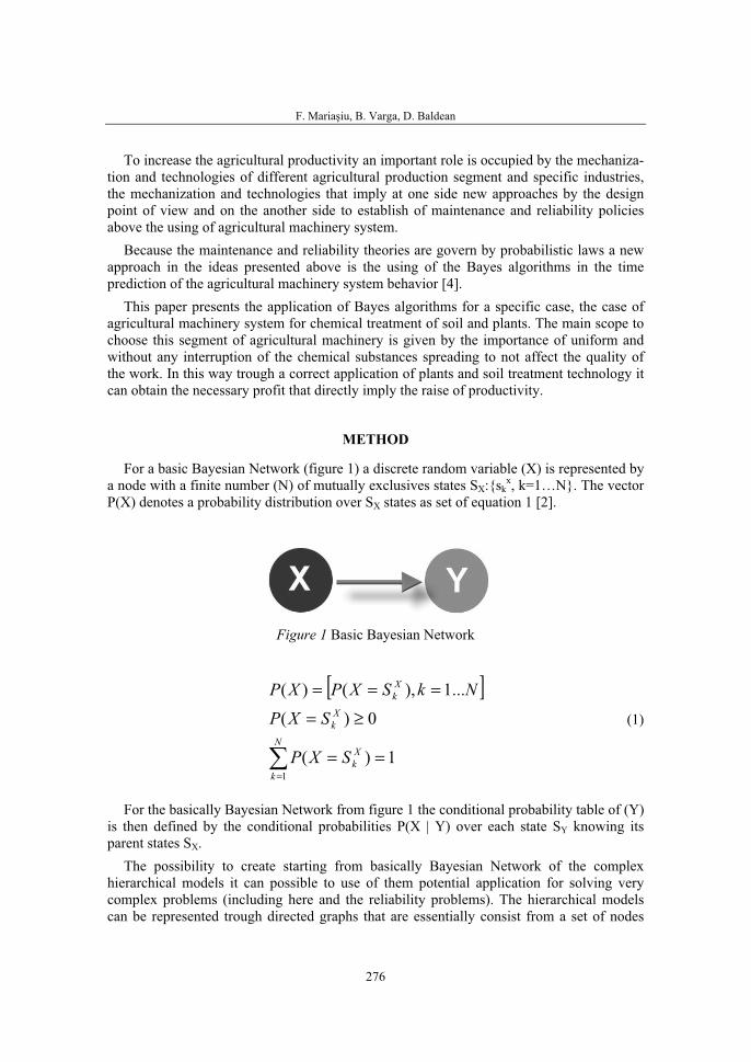
F. Mariaşiu, B. Varga, D. Baldean
276
To increase the agricultural productivity an important role is occupied by the mechaniza-tion and technologies of different agricultural production segment and specific industries, the mechanization and technologies that imply at one side new approaches by the design point of view and on the another side to establish of maintenance and reliability policies above the using of agricultural machinery system.
Because the maintenance and reliability theories are govern by probabilistic laws a new approach in the ideas presented above is the using of the Bayes algorithms in the time prediction of the agricultural machinery system behavior [4].
This paper presents the application of Bayes algorithms for a specific case, the case of agricultural machinery system for chemical treatment of soil and plants. The main scope to choose this segment of agricultural machinery is given by the importance of uniform and without any interruption of the chemical substances spreading to not affect the quality of the work. In this way trough a correct application of plants and soil treatment technology it can obtain the necessary profit that directly imply the raise of productivity.
METHOD
For a basic Bayesian Network (figure 1) a discrete random variable (X) is represented by a node with a finite number (N) of mutually exclusives states SX:{sk
x, k=1…N}. The vector P(X) denotes a probability distribution over SX states as set of equation 1 [2].
Figure 1 Basic Bayesian Network
[ ]
1)(
0)(
...1),()(
1==
≥=
===
∑=
N
k
Xk
Xk
Xk
SXP
SXPNkSXPXP
(1)
For the basically Bayesian Network from figure 1 the conditional probability table of (Y) is then defined by the conditional probabilities P(X | Y) over each state SY knowing its parent states SX.
The possibility to create starting from basically Bayesian Network of the complex hierarchical models it can possible to use of them potential application for solving very complex problems (including here and the reliability problems). The hierarchical models can be represented trough directed graphs that are essentially consist from a set of nodes
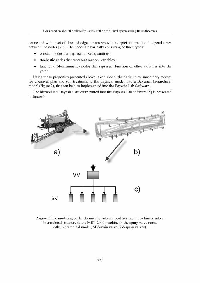
Consideration about the reliability's study of the agricultural systems using Bayes theorems
277
connected with a set of directed edges or arrows which depict informational dependencies between the nodes [2,3]. The nodes are basically consisting of three types:
• constant nodes that represent fixed quantities;
• stochastic nodes that represent random variables;
• functional (deterministic) nodes that represent function of other variables into the graph.
Using those properties presented above it can model the agricultural machinery system for chemical plan and soil treatment to the physical model into a Bayesian hierarchical model (figure 2), that can be also implemented into the Bayesia Lab Software.
The hierarchical Bayesian structure putted into the Bayesia Lab software [5] is presented in figure 3.
Figure 2 The modeling of the chemical plants and soil treatment machinery into a hierarchical structure (a-the MET-2000 machine, b-the spray valve rams,
c-the hierarchical model, MV-main valve, SV-spray valves).
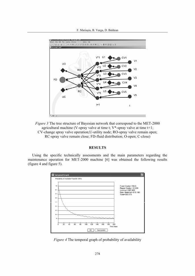
F. Mariaşiu, B. Varga, D. Baldean
278
Figure 3 The tree structure of Bayesian network that correspond to the MET-2000 agricultural machine (V-spray valve at time t; V*-spray valve at time t+1;
CV-change spray valve operation;U-utility node; RO-spray valve remain open;RC-spray valve remain close; FD-fluid distribution; O-open; C-close)
RESULTS
Using the specific technically assessments and the main parameters regarding the maintenance operation for MET-2000 machine [6] was obtained the following results (figure 4 and figure 5).
Figure 4 The temporal graph of probability of availability
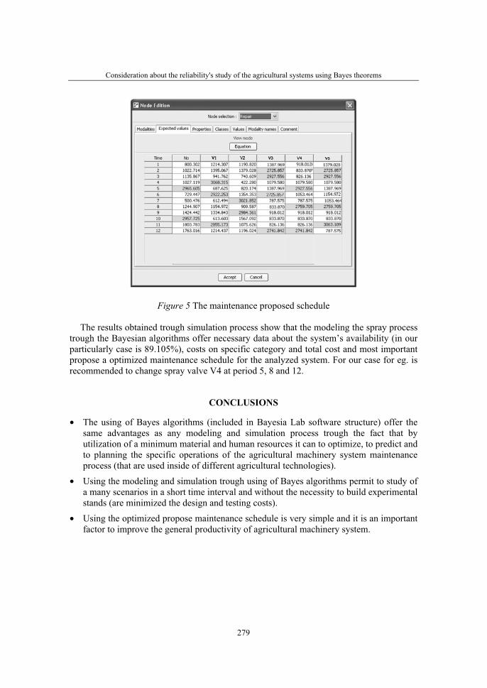
Consideration about the reliability's study of the agricultural systems using Bayes theorems
279
Figure 5 The maintenance proposed schedule
The results obtained trough simulation process show that the modeling the spray process trough the Bayesian algorithms offer necessary data about the system’s availability (in our particularly case is 89.105%), costs on specific category and total cost and most important propose a optimized maintenance schedule for the analyzed system. For our case for eg. is recommended to change spray valve V4 at period 5, 8 and 12.
CONCLUSIONS
• The using of Bayes algorithms (included in Bayesia Lab software structure) offer the same advantages as any modeling and simulation process trough the fact that by utilization of a minimum material and human resources it can to optimize, to predict and to planning the specific operations of the agricultural machinery system maintenance process (that are used inside of different agricultural technologies).
• Using the modeling and simulation trough using of Bayes algorithms permit to study of a many scenarios in a short time interval and without the necessity to build experimental stands (are minimized the design and testing costs).
• Using the optimized propose maintenance schedule is very simple and it is an important factor to improve the general productivity of agricultural machinery system.

F. Mariaşiu, B. Varga, D. Baldean
280
REFERENCES
1. FAO (2003) World agriculture: towards 2015/2030, Rome, Earth scan Publications.
2. Simon, Ch., Weber, Ph., Levat, E. (2007) Bayesian Networks and System Reliability, Journal of Computers, vol.2, no.1, pg.33-43.
3. Robinson, D.G. (2001) A Hierarchical Bayes Approach to System Reliability Analysis, paper SAND 2001-3513, Sandia National Laboratories, Albuquerque, USA.
4. Wilson, S., Taylor, D. (1997) Reliability Assessment from Fatigue Micro-Crack Data, IEEE Transaction on Reliability, vol.46, no.2, pg.165-172
5. www.BayesiaLab.com
6. www.Tehnofavorit.ro The MET-2000 agricultural machine technical book.
36. Symposium "Actual Tasks on Agricultural Engineering", Opatija, Croatia, 2008.
281
36.
SIMPOZIJAKTUALNI ZADACIMEHANIZACIJE POLJOPRIVREDE
UDC621.317.782:631.312.021:631.51
Prethodno priopćenjePreliminary communication
RESEARCHES RAGARDING THE STRESSES DISTRIBUTION DETERMINATION THAT APPEAR ON THE LAMELLAR MOULDBOARD SURFACE WITH A
VIEW TO MODELLING AND OPTIMIZATION OFTHIS ONE
SORIN – TIBERIU BUNGESCU1, SORIN – ŞTEFAN BIRIS2, VALENTIN VLADUT3,GIGEL PARASCHIV3
1Banat’s University of Agricultural Sciences and Veterinary Medicine Timisoara – Department of Agricultural Machines, 119, Calea Aradului Street, Nr. 119, Timisoara –
Romania, Zip code 300645, e-mail: [email protected] 2“POLITEHNICA” University of Bucharest – Romania, 313, Splaiul Independentei Street,
Bucharest – Romania, Zip code 060042, e-mail: [email protected] 3Research and Development National Institute for Agricultural and Food Industry Machines and Implements – INMA Bucharest, 6, Ion Ionescu de la Brad Blvd. Bucharest – Romania,
Zip code 013813, e-mail: [email protected]
SUMMARY
In specialty reference material from our country and in the countries with an advanced agriculture it hasn’t appeared yet a calculation methodology with a view to projection’s optimization of these moldboards and on this line, the current paper, tries to bring a contribution in this field, benefiting by the advantages on which it presents the application of the analysis method with finite elements respectable programme of computer “COSMOS/M”.
By means of “Finite Elements Method” (FEM) respectively of “COSMOS/M” programme it could be performed the stress and deformation state’s modeling in lamellar mouldboard, finally the authors achieving two subprogram’s of cal-culus. On the basis of this subprogram’s, a complete study of the stress and deformation state was effected, using the “Finite Elements Method” (FEM).
The theoretical data were compared with the experimental ones obtained in field conditions using the plough with lamellar mouldboard type Vari - Diamant of Lemken German company.
Key words: lamellar moldboard, stress, deformation
S. – T. Bungescu, S. – Ş. Biris, V. Vladut, G. Paraschiv
282
INTRODUCTION
The ploughs with moldboards recorded a spectacular evolution in the last time. The new types of ploughs possess a different adaptation capacity at the new working technologies of the soil. The adopted technical solutions are capable to offer a high degree of adaptability to: the soil categories, the state of the ground, the covering degree with vegetal remainders, the power base's potential and so on.
A conclusive example represent the ploughs with lamellar moldboards, which in the current stage became prevalent in the farmers' preferences from the countries with advanced agriculture.
The determination of the stresses and deformations on the surface of the lamellar moldboard presents a different significance.
The cognition of the stresses and deformations' distribution on the surface of the lamellar moldboard, in varied conditions from exploitation, can offer an ample experimental and theoretical material to the researchers. On the basis of this material, the researchers can perform a judicious projection of the structure and sizes of the lamellar moldboard.
The estimate of the factors` variation boundaries which influence the strengths at wear it is also permitted.
As part of the Strength of Materials Department from the "Politehnica" University, Timişoara were studied the lamellar moldboard, which equipped the Vari-Diamant plough of Lemken German company and the prototype lamellar moldboard achieved by MAT Craiova Romanian company. The study pursued the determination of the maximum requirement zones, where can appear fissures or even breaks during the working process, using F.E.M. and respectively COSMOS/M programme. For this, there were used: the INTEL PII DESHUTES 350 MHz computer and respectively the COSMOS/M programme achieved by a famous company from Santa Monica, California.
THEORETICAL CONSIDERATIONS REGARDING THE UTILIZATION OF THE FINITE ELEMENT METHOD (F.E.M.) IN THE STRESSES’ DISTRIBUTION’S DETERMINATION ON THE MOLDBOARDS’ SURFACE WITH LAMELLAS
Benefiting by the advantages of the calculation precision which was demonstrated by the utilization of F.E.M. in the ensembles' projection with special spatial configuration and distribution, the authors staff performed researches with a view to definitization of the most suited digitization system that can be applied at the stresses' distribution's determination in the moldboards' lamellas of this type.
It also becomes precise the matrix mathematical expressions which permit the active surface's modeling of the lamellar moldboard.
From the performed thorough studies resulted that for the lamellar moldboard’s surface's digitization, the most suited model for this working mechanism is the variant with triangu-lar elements.
Figure 1,a presents the studied Lemken lamellar moldboard and figure 1,b presents the studied triangular finite element. In figure 2 it presents the manner of digitization with
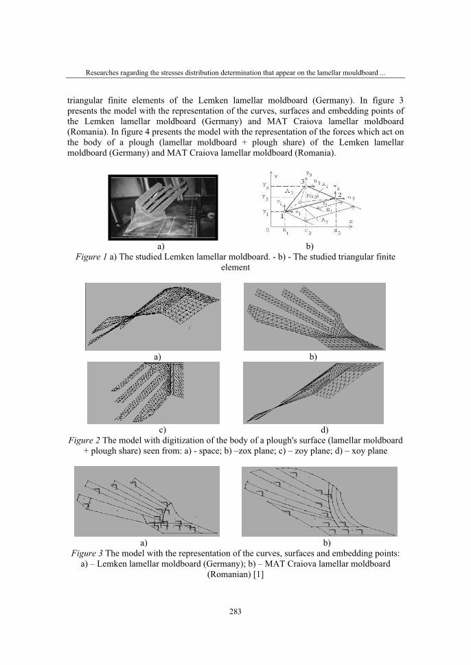
Researches ragarding the stresses distribution determination that appear on the lamellar mouldboard ...
283
triangular finite elements of the Lemken lamellar moldboard (Germany). In figure 3 presents the model with the representation of the curves, surfaces and embedding points of the Lemken lamellar moldboard (Germany) and MAT Craiova lamellar moldboard (Romania). In figure 4 presents the model with the representation of the forces which act on the body of a plough (lamellar moldboard + plough share) of the Lemken lamellar moldboard (Germany) and MAT Craiova lamellar moldboard (Romania).
a) b) Figure 1 a) The studied Lemken lamellar moldboard. - b) - The studied triangular finite
element
a) b)
c) d)
Figure 2 The model with digitization of the body of a plough's surface (lamellar moldboard + plough share) seen from: a) - space; b) –zox plane; c) – zoy plane; d) – xoy plane
a) b) Figure 3 The model with the representation of the curves, surfaces and embedding points:
a) – Lemken lamellar moldboard (Germany); b) – MAT Craiova lamellar moldboard (Romanian) [1]
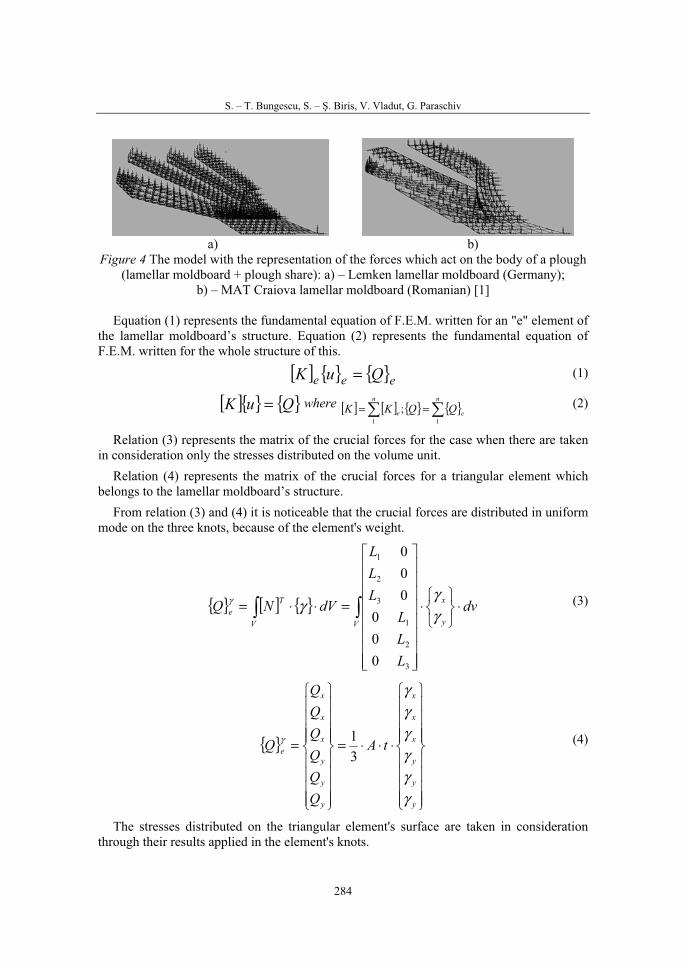
S. – T. Bungescu, S. – Ş. Biris, V. Vladut, G. Paraschiv
284
a) b) Figure 4 The model with the representation of the forces which act on the body of a plough
(lamellar moldboard + plough share): a) – Lemken lamellar moldboard (Germany);b) – MAT Craiova lamellar moldboard (Romanian) [1]
Equation (1) represents the fundamental equation of F.E.M. written for an "e" element of the lamellar moldboard’s structure. Equation (2) represents the fundamental equation of F.E.M. written for the whole structure of this.
[ ] { } { }eee QuK = (1)
[ ]{ } { }QuK = where [ ] [ ] { } { }∑∑ ==n
e
n
e QQKK11
; (2)
Relation (3) represents the matrix of the crucial forces for the case when there are taken in consideration only the stresses distributed on the volume unit.
Relation (4) represents the matrix of the crucial forces for a triangular element which belongs to the lamellar moldboard’s structure.
From relation (3) and (4) it is noticeable that the crucial forces are distributed in uniform mode on the three knots, because of the element's weight.
{ } [ ] { }∫ ∫ ⋅⎭
⎬
⎫
⎩
⎨
⎧
⋅
⎥
⎥
⎥
⎥
⎥
⎥
⎥
⎥
⎦
⎤
⎢
⎢
⎢
⎢
⎢
⎢
⎢
⎢
⎣
⎡
=⋅⋅=V V y
xTe dv
LLL
LLL
dVNQγγ
γγ
3
2
1
3
2
1
000
000
(3)
{ }
⎪
⎪
⎪
⎪
⎭
⎪⎪
⎪
⎪
⎬
⎫
⎪
⎪
⎪
⎪
⎩
⎪⎪
⎪
⎪
⎨
⎧
⋅⋅⋅=
⎪
⎪
⎪
⎪
⎭
⎪⎪
⎪
⎪
⎬
⎫
⎪
⎪
⎪
⎪
⎩
⎪⎪
⎪
⎪
⎨
⎧
=
y
y
y
x
x
x
y
y
y
x
x
x
e tA
QQQQQQ
Q
γγγγγγ
γ
31 (4)
The stresses distributed on the triangular element's surface are taken in consideration through their results applied in the element's knots.
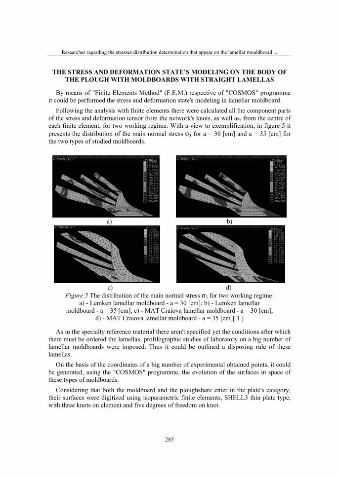
Researches ragarding the stresses distribution determination that appear on the lamellar mouldboard ...
285
THE STRESS AND DEFORMATION STATE’S MODELING ON THE BODY OF THE PLOUGH WITH MOLDBOARDS WITH STRAIGHT LAMELLAS
By means of "Finite Elements Method" (F.E.M.) respective of "COSMOS" programme it could be performed the stress and deformation state's modeling in lamellar moldboard.
Following the analysis with finite elements there were calculated all the component parts of the stress and deformation tensor from the network's knots, as well as, from the centre of each finite element, for two working regime. With a view to exemplification, in figure 5 it presents the distribution of the main normal stress σ3 for a = 30 [cm] and a = 35 [cm] for the two types of studied moldboards.
a) b)
c) d) Figure 5 The distribution of the main normal stress σ3 for two working regime:
a) - Lemken lamellar moldboard - a = 30 [cm]; b) - Lemken lamellarmoldboard - a = 35 [cm]; c) - MAT Craiova lamellar moldboard - a = 30 [cm];
d) - MAT Craiova lamellar moldboard - a = 35 [cm][ 1 ]
As in the specialty reference material there aren't specified yet the conditions after which there must be ordered the lamellas, profilographic studies of laboratory on a big number of lamellar moldboards were imposed. Thus it could be outlined a disposing rule of these lamellas.
On the basis of the coordinates of a big number of experimental obtained points, it could be generated, using the "COSMOS" programme, the evolution of the surfaces in space of these types of moldboards.
Considering that both the moldboard and the ploughshare enter in the plate's category, their surfaces were digitized using isoparametric finite elements, SHELL3 thin plate type, with three knots on element and five degrees of freedom on knot.

S. – T. Bungescu, S. – Ş. Biris, V. Vladut, G. Paraschiv
286
The digitations network had the variable step, fact that encouraged the increase of the number of elements in the fastening zones, or in which appeared section modifications.
As well as real constants, associated to the group of SHELL 3 elements, we introduce thickness as being of 10 mm at the Lemken moldboard and of 7 mm at the MAT Craiova moldboard, and as material properties, the modulus of longitudinal elasticity and modulus of elasticity in shear.
For the calculation of the stresses it considered the situation when, on the ox advan-cement direction (the case when the plough meet in the soil an obstacle) acts a concentrated force in the top ploughshare, and on the body of the ploughshare, the breast of the moldboard and the lamellas it acts a pressure constant distributed, but different as value from a lamella to another respectively from the body of the ploughshare to the breast of the moldboard.
Table 1 The comparative values of the stresses theoretical determined by means of the "COSMOS"programme, in the embedding zones of the LEMKEN lamellar moldboard
(Germany)[1][3]
Fastening/embedding zone's number of the
R.E.T.
Abstatunit
Maximum stress theoretical calculated in the fastening
zones, for a = 30 [ cm ] (Lemken lamellar moldboard).
Maximum stress theoretical calculated in the fastening
zones, for a = 35 [ cm ] (Lemken lamellar moldboard).
1 MPa 15,038 25,163
2 MPa 10,216 17,005
3 MPa 15,038 25,163
4 MPa 10,216 17,005
5 MPa 29,502 33,32
6 MPa 10,216 17,005
7 MPa 15,038 25,163
8 MPa 15,038 25,163
9 MPa 39,145 98,581
10 MPa 53,609 123,05
11 MPa 63,252 90,423
12 MPa 29,502 41,478
13 MPa 53,609 57,793
14 MPa 43,966 49,636
15 MPa 39,145 57,793
16 MPa 39,145 57,793
17 MPa 29,502 57,793
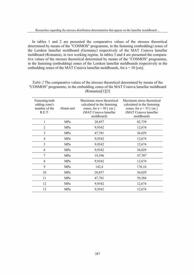
Researches ragarding the stresses distribution determination that appear on the lamellar mouldboard ...
287
In tables 1 and 2 are presented the comparative values of the stresses theoretical determined by means of the "COSMOS" programme, in the fastening (embedding) zones of the Lemken lamellar moldboard (Germany) respectively of the MAT Craiova lamellar moldboard (Romania), in two working regime. In tables 3 and 4 are presented the compara-tive values of the stresses theoretical determined by means of the "COSMOS" programme, in the fastening (embedding) zones of the Lemken lamellar moldboards respectively in the embedding zones of the MAT Craiova lamellar moldboards, for a = 30 [cm].
Table 2 The comparative values of the stresses theoretical determined by means of the "COSMOS" programme, in the embedding zones of the MAT Craiova lamellar moldboard
(Romania)[1][3]
Fastening/embedding zone's number of the
R.E.T.Abstat unit
Maximum stress theoretical calculated in the fastening
zones, for a = 30 [ cm ] (MAT Craiova lamellar
moldboard)
Maximum stress theoretical calculated in the fastening
zones, for a = 35 [ cm ] (MAT Craiova lamellar
moldboard)
1 MPa 28,857 82,739
2 MPa 9,9342 12,674
3 MPa 47,781 36,029
4 MPa 9,9342 12,674
5 MPa 9,9342 12,674
6 MPa 9,9342 36,029
7 MPa 19,396 47,707
8 MPa 9,9342 12,674
9 MPa 142,4 176,16
10 MPa 28,857 36,029
11 MPa 47,781 59,384
12 MPa 9,9342 12,674
13 MPa 9,9342 12,674
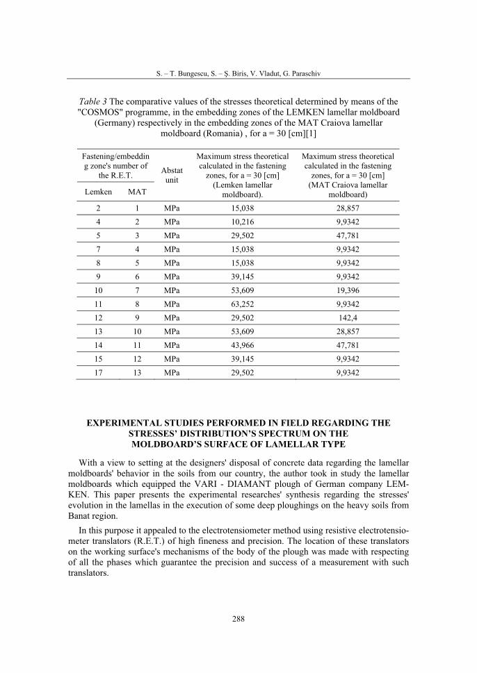
S. – T. Bungescu, S. – Ş. Biris, V. Vladut, G. Paraschiv
288
Table 3 The comparative values of the stresses theoretical determined by means of the "COSMOS" programme, in the embedding zones of the LEMKEN lamellar moldboard
(Germany) respectively in the embedding zones of the MAT Craiova lamellarmoldboard (Romania) , for a = 30 [cm][1]
Fastening/embedding zone's number of
the R.E.T.
Lemken MAT
Abstatunit
Maximum stress theoretical calculated in the fastening
zones, for a = 30 [cm] (Lemken lamellar
moldboard).
Maximum stress theoretical calculated in the fastening
zones, for a = 30 [cm] (MAT Craiova lamellar
moldboard)
2 1 MPa 15,038 28,857
4 2 MPa 10,216 9,9342
5 3 MPa 29,502 47,781
7 4 MPa 15,038 9,9342
8 5 MPa 15,038 9,9342
9 6 MPa 39,145 9,9342
10 7 MPa 53,609 19,396
11 8 MPa 63,252 9,9342
12 9 MPa 29,502 142,4
13 10 MPa 53,609 28,857
14 11 MPa 43,966 47,781
15 12 MPa 39,145 9,9342
17 13 MPa 29,502 9,9342
EXPERIMENTAL STUDIES PERFORMED IN FIELD REGARDING THE STRESSES’ DISTRIBUTION’S SPECTRUM ON THEMOLDBOARD’S SURFACE OF LAMELLAR TYPE
With a view to setting at the designers' disposal of concrete data regarding the lamellar moldboards' behavior in the soils from our country, the author took in study the lamellar moldboards which equipped the VARI - DIAMANT plough of German company LEM-KEN. This paper presents the experimental researches' synthesis regarding the stresses' evolution in the lamellas in the execution of some deep ploughings on the heavy soils from Banat region.
In this purpose it appealed to the electrotensiometer method using resistive electrotensio-meter translators (R.E.T.) of high fineness and precision. The location of these translators on the working surface's mechanisms of the body of the plough was made with respecting of all the phases which guarantee the precision and success of a measurement with such translators.
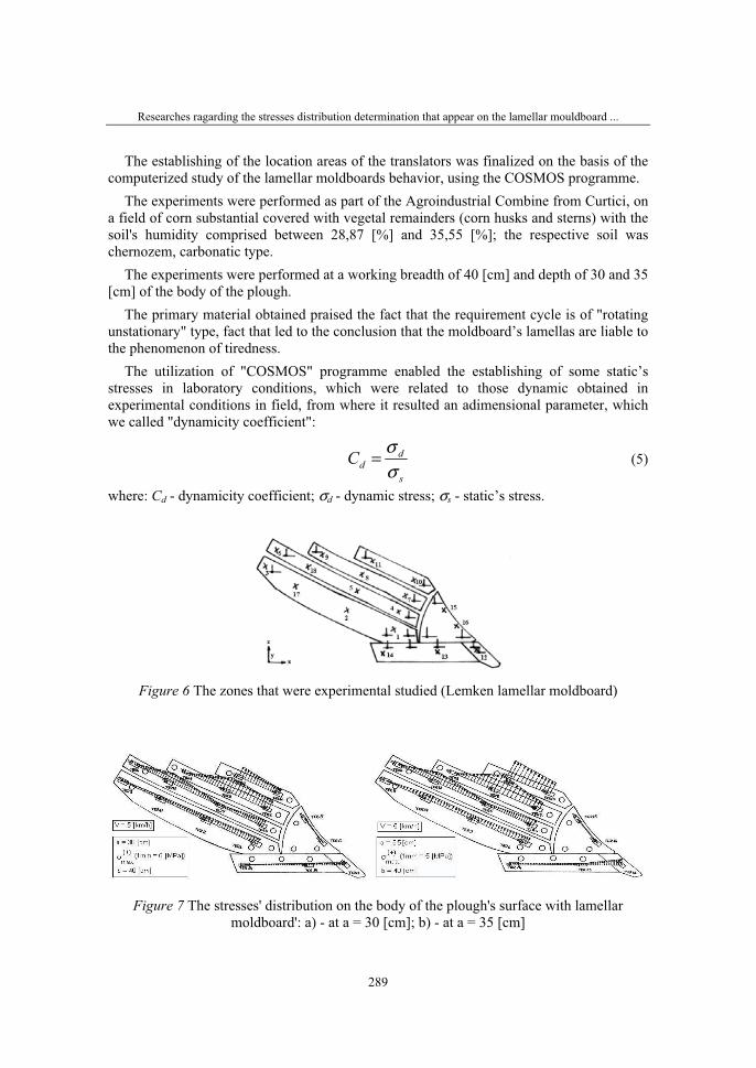
Researches ragarding the stresses distribution determination that appear on the lamellar mouldboard ...
289
The establishing of the location areas of the translators was finalized on the basis of the computerized study of the lamellar moldboards behavior, using the COSMOS programme.
The experiments were performed as part of the Agroindustrial Combine from Curtici, on a field of corn substantial covered with vegetal remainders (corn husks and sterns) with the soil's humidity comprised between 28,87 [%] and 35,55 [%]; the respective soil was chernozem, carbonatic type.
The experiments were performed at a working breadth of 40 [cm] and depth of 30 and 35 [cm] of the body of the plough.
The primary material obtained praised the fact that the requirement cycle is of "rotating unstationary" type, fact that led to the conclusion that the moldboard’s lamellas are liable to the phenomenon of tiredness.
The utilization of "COSMOS" programme enabled the establishing of some static’s stresses in laboratory conditions, which were related to those dynamic obtained in experimental conditions in field, from where it resulted an adimensional parameter, which we called "dynamicity coefficient":
s
ddC
σσ= (5)
where: Cd - dynamicity coefficient; σd - dynamic stress; σs - static’s stress.
Figure 6 The zones that were experimental studied (Lemken lamellar moldboard)
Figure 7 The stresses' distribution on the body of the plough's surface with lamellar moldboard': a) - at a = 30 [cm]; b) - at a = 35 [cm]

S. – T. Bungescu, S. – Ş. Biris, V. Vladut, G. Paraschiv
290
The results obtained in laboratory conditions praised that the calculating stress σs was comprised between 0,57 . . . 90,42 [MPa], and that experimental determined σd was comprised between 1,96 . . . 90,55 [MPa] that is the dynamicity coefficient Cd is comprised between 0,76 . . . 1.15 [MPa], which is in the same order of the magnitude. The compa-rative values of the stresses experimental respectively theoretical determined, for Lemken lamellar moldboard, are presented in table 4.
With a view to exemplification in figure 1 it presents the stresses' distribution on the body of the plough's surface with lamellar moldboard LEMKEN, BS42 type.
Table 4 The comparative values of the stresses theoretical and experimental determined, in the case of the Lemken moldboard with straight lamellas[1][3]
Nr.RET
Workingdepth [cm]
Abstatunit
Maximum stress experimentaldetermined
Maximum stress theoreticalcalculated
Dynamicity coefficient
RET1 30 MPa 28,42 24,681 1,15 RET1 35 MPa 29,4 33,32 0,88 RET2 30 MPa 28,81 24,681 1,16 RET2 35 MPa 25,48 25,163 1,01 RET3 30 MPa 1,96 0,57356 3,41 RET3 35 MPa 1,96 0,69024 2,83 RET4 30 MPa 30,87 29,502 1,04 RET4 35 MPa 28,81 25,163 1,14 RET5 30 MPa 57,62 53,609 1,07 RET5 35 MPa 61,74 57,793 1,06 RET6 30 MPa 1,96 0,57356 3,41 RET6 35 MPa 1,96 0,69024 2,83 RET7 30 MPa 49,39 48,788 1,01 RET7 35 MPa 39,2 41,478 0,94 RET8 30 MPa 72,03 68,073 1,05 RET8 35 MPa 86,24 82,266 1,04 RET9 30 MPa 41,16 39,145 1,05 RET9 35 MPa 11,76 8,8478 1,32 RET10 30 MPa 26,75 24,681 1,08 RET10 35 MPa 61,74 57,793 1,06 RET11 30 MPa 51,45 48,788 1,05 RET11 35 MPa 90,55 90,423 1,001 RET12 30 MPa 11,76 10,216 1,15 RET12 35 MPa 32,92 25,163 1,30 RET13 30 MPa 11,27 10,216 1,10 RET13 35 MPa 9,8 8,8478 1,10 RET14 30 MPa 8,03 10,216 0,78 RET14 35 MPa 9,8 8,8478 1,10 RET15 30 MPa 4,11 5,395 0,76 RET15 35 MPa 7,84 8,8478 0,88 RET16 30 MPa 2,94 0,57356 5,12 RET16 35 MPa 4,11 5,395 0,76 RET17 30 MPa 22,54 15,038 1,49 RET17 35 MPa 37,04 33,32 1,11 RET18 30 MPa 45,27 39,145 1,15 RET18 35 MPa 49,49 49,636 0,99
Researches ragarding the stresses distribution determination that appear on the lamellar mouldboard ...
291
CONCLUSIONS
1. It can be assert that F.E.M., at the level of advanced projection of the agricultural machines, it isn't anymore only a useful instrument, but it is one absolutely necessary.
2. In the context in which the analysis with finite elements praises that in process of dislocation and slide of the furrow on the working mechanisms' surface of the body of the plough, the stresses field varies after a permanent decreasing rule, the optimization of the mechanisms' engineering which constitute this surface would be satisfied if it is taken in consideration that the respective lamella to function like a bar of equal strength.
3. As from constructive point of view, but particularly technological, this thing it isn't established, results that the moldboard’s lamellas must be at least of the thickness of the moldboard’s chest on which it stands out, in the joining zone with the plough share, a stress field more bigger than that from the embedding zone of the lamellas.
4. This paper ranges among the first researches in this field and opens the pathway towards new researches bound of implementation in the modern ploughs' engineering of the lamellar moldboards.
5. By the means of F.E.M. respective of "COSMOS" programme it can be elaborated in an efficient mode the stress and deformation state's modeling from lamellar moldboard, obtaining in this way useful data for the engineering's optimization of this new type of working mechanism of the soil.
6. Following the comparing of the distribution fields of the stresses developed in the lamellar moldboards with those from specialty reference material for full moldboards, it can affirm that the lamellar moldboards which equipped the modern ploughs are liable to much bigger stresses than the classic moldboards which unfold the process in similar working conditions.
7. The stresses fields experimental determined in field and respective theoretical by means of "COSMOS" programme, they complete each other, in the sense that as part of the resulted spectrums through the utilization of "COSMOS" programme, in the embedding zones of the lamellas appear much bigger stresses than in the other zones in which they were experimental determined as a result of the stresses concentrators' appearance typical of any joinings and which couldn't be experimental praised.
8. For the section's projection's optimization of each lamella is necessary and sufficiently to be taken in consideration the stresses established by means of the "COSMOS" programme in the embedding zones, because their values are the biggest in the distribution of the stresses field along the lamellas.
9. In the context of potential's capitalization offered by the COSMOS/M programme in this field, the modeling of the stresses and deformations field became a certainty.
10. The theoretical cognition of the stresses and deformations' distribution is of an unchallenged utility in the evolution's estimate of this process, experimental praised in the ground.
S. – T. Bungescu, S. – Ş. Biris, V. Vladut, G. Paraschiv
292
RERFERENCES
1. Bungescu, S. (2001). Studies and researches regarding the stresses distribution on moldboard’s surface of lamellar type with a view to construction's modeling and optimization, Doctor's degree thesis, Timisoara;
2. Bungescu, S. (2001). The study of the stress and deformation state from the body of a plough with moldboard with straight lamellas, using the Finite Element Method (F.E.M.), Symposium: Simulation and projection watched by the computer in agriculture machinery field - SPCMA, The multiplication center University "Politehnica" Bucharest, pp. 59 - 68;
3. Bungescu, S., Atanas, Z.A., Vladut, V., Biris, S.S., Konstantinovic, M. (2005). The determination of the stresses and deformations which appear on the surface of the lamellar type moldboard of the advantages presented by the “Finite Elements Method”, Anniversary Conference – 60 Years University of Rousse “Anghel Kanchev”, This conference was be organized by: Rousse University, Rousse Union of Scientists, Rousse Municipality, PROCEEDINGS, Volume 44, Book 1, Section: Agricultural Machinery and Technologies, Rousse, pp. 36 – 43;
4. Dumitru, I.; Faur, N. (1997). The Materials' Strength (Theoretical basis in the Materials' Tiredness, Tear’s Mechanic, Composite Materials and Numerical Methods), The multiplication center University "Politehnica" Timişoara;
5. 4.Faur, N.; Dumitru, I. (1997). Finite difference and finite element in the Materials' Strength, Publishing House "Mirton ", Timişoara;
6. Faur, N., Dumitru, I., Popa, M. (1995). About solicitations' modeling which appear in the mouldboard of a plough, Session "Technical and scientifically research in agricultural reorganization and development support", Publishing House "Mirton", Timişoara, pp: 119 - 124;
7. Ştefan, C., Gönczi, A., Iancului, D (1996). Technical progress in agriculture units' domain for soil working, Publishing House "Felix", Arad;
8. Zienkiewicy, O.C., Taylor, R.L. (1991). La methode des éléments finits, AFNOR, Paris;
9. * * * - COSMOS/M, User guide, Santa Monica, Structural Research and Analysis Corporation.
36. Symposium "Actual Tasks on Agricultural Engineering", Opatija, Croatia, 2008.
293
36.
SIMPOZIJAKTUALNI ZADACIMEHANIZACIJE POLJOPRIVREDE
UDC631.354.027
Stručni radExpert paper
STOCHASTIC MODELS FOR SIMULATING SEED SEPARATION PROCESS ON SIEVES
CONSTANTIN TÂRCOLEA, TUDOR CĂSĂNDROIU, GHEORGHE VOICU
„Politehnica” University of Bucharest, Faculty of Biotechnical Systems Engineering Splaiul Independentei, 313, 060032, Bucharest, Romania,
e-mail: [email protected]
ABSTRACT
It is known that the deterministic modelling used for simulating of separation process of seeds at cleaning system sieves of cereal combine harvesters leads to laborious computations, because there are many degrees of freedom and the separation process is very complex.
In this paper, the separation process is modelled by means of stochastic processes, motivated by randomness of the studied phenomena. Therefore, different types of statistic laws of separation intensity distribution on sieve length it is proposed and estimating methods for parameters of the models it is explained.
Each model allows predicting seed losses at the separation on cleaning system sieves and is useful to both the designers and users of combine harvesters.
The main contribution of the paper is to propose a new type of beta distribu-tion with the following density probability function: ( ) ( ) 11)( −− −−= ba xvuxcxffor u ≤ x ≤ v; a > 0, b > 0, c > 0, for the describing variation separation intensity of seeds on sieve length.
The experimental data proved that the new distribution is more adaptive for used in describing of evaluation of grain cleaning and more other processes because this distribution, in function of the parameters, can be symmetric, or left or right asymmetric.
Key words: harvesting combine, cleaning system, seed separation, normal distribution, gamma and beta distributions
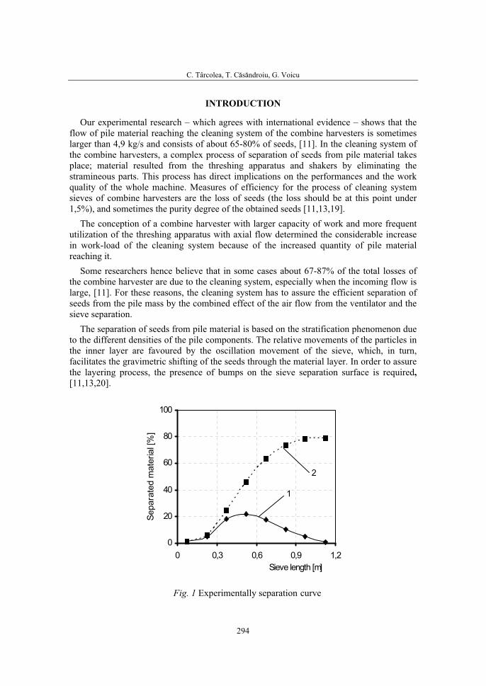
C. Târcolea, T. Căsăndroiu, G. Voicu
294
INTRODUCTION
Our experimental research – which agrees with international evidence – shows that the flow of pile material reaching the cleaning system of the combine harvesters is sometimes larger than 4,9 kg/s and consists of about 65-80% of seeds, [11]. In the cleaning system of the combine harvesters, a complex process of separation of seeds from pile material takesplace; material resulted from the threshing apparatus and shakers by eliminating the stramineous parts. This process has direct implications on the performances and the work quality of the whole machine. Measures of efficiency for the process of cleaning system sieves of combine harvesters are the loss of seeds (the loss should be at this point under 1,5%), and sometimes the purity degree of the obtained seeds [11,13,19].
The conception of a combine harvester with larger capacity of work and more frequent utilization of the threshing apparatus with axial flow determined the considerable increase in work-load of the cleaning system because of the increased quantity of pile material reaching it.
Some researchers hence believe that in some cases about 67-87% of the total losses of the combine harvester are due to the cleaning system, especially when the incoming flow is large, [11]. For these reasons, the cleaning system has to assure the efficient separation of seeds from the pile mass by the combined effect of the air flow from the ventilator and the sieve separation.
The separation of seeds from pile material is based on the stratification phenomenon due to the different densities of the pile components. The relative movements of the particles in the inner layer are favoured by the oscillation movement of the sieve, which, in turn, facilitates the gravimetric shifting of the seeds through the material layer. In order to assure the layering process, the presence of bumps on the sieve separation surface is required,[11,13,20].
Fig. 1 Experimentally separation curve
0
20
40
60
80
100
0 0,3 0,6 0,9 1,2Sieve length [m]
Sepa
rate
d m
ater
ial [
%]
2
1
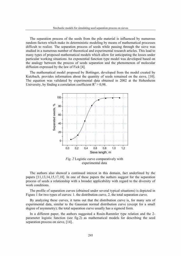
Stochastic models for simulating seed separation process on sieves
295
The separation process of the seeds from the pile material is influenced by numerous random factors which make its deterministic modeling by means of mathematical processes difficult to realize. The separation process of seeds while passing through the sieve was studied in a numerous number of theoretical and experimental research articles. This lead to many types of proposed mathematical models which allow for anticipating the losses under particular working situations An exponential function type model was developed based on the analogy between the process of seeds separation and the phenomenon of moleculardiffusion expressed by the law of Fick [4].
The mathematical model proposed by Bottinger, developed from the model created by Kutzbach, provides information about the quantity of seeds remained on the sieve, [10]. The equation was validated by experimental data obtained in 2002 at the Hohenheim University, by finding a correlation coefficient R2 > 0,98.
The authors also showed a continued interest in this domain, fact underlined by the papers [11,13,14,15,17,18]. In one of these papers the authors suggest for the separation process of seeds a relationship with a broader applicability with regard to the diversity of work conditions.
The profile of separation curves (obtained under several typical situations) is depicted in Figure 1 for two types of curves: 1. the distribution curve, 2. the total separation curve.
By analyzing these curves, it turns out that the distribution curve is, for many sets of experimental data, similar to the Gaussian normal distribution curve (except for a small degree of asymmetry); the total separation curve usually has a sigmoid form.
In a different paper, the authors suggested a Rosin-Rammler type relation and the 2-parameter logistic function (see fig.2) as mathematical models for describing the seed separation process on sieve, [14].
0,0 0,2 0,4 0,6 0,8 1,0 1,2
0
20
40
60
80
100
Sep
arat
ed s
eeds
, %
Sieve length, m
Fig. 2 Logistic curve comparatively with experimental data
C. Târcolea, T. Căsăndroiu, G. Voicu
296
The natural variability, the large number of factors influencing the separation process and their inherent randomness are comprised in the mean value of the two logistic constants.
By confronting the suggested function with the experimental data, a very good fit was obtained, illustrated by a coefficient of correlation R2 = 0.997 and depicted in Figure 2.
A shortcoming of using these relationships is the need to choose values for the respective coefficients, which depend on the concrete work conditions, on the geometry of the cleaning system and on the functional parameters of the latter, [14].
Reflecting the need to increase the precision of describing the separation process, while incorporating the main design and functional parameters of the cleaning system, the authors suggested multiple linear regression functions for the logistic coefficients. A coefficient of correlation R2 = 0.911 was obtained when comparing these models with experimental data, [17].
Along the same line, applying dimensional analysis to the process of separation, the authors suggested a different mathematical model accounting for seven of the main design, functional and characterizing parameters of the material in the cleaning system, [18].
The classical probability theory studies independent random variables. Modern probability theory has dealt with process for which the knowledge of previous outcomes influences predictions for future experiments. A.A. Markov introduced a special class of dependent random variables. The markovian property says that the past history is forgotten and only the present state matters in determining the future behaviour.
The movement and separating of grain particles inside a grain cleaner is stochastic rather than deterministic, [12]. Particle movement is examined as a stochastic process; a distance – transition Markov model for particle movement is proposed, [1, 2].
The main objective of the study is to compare different types of lows, which describe the evaluation of grain cleaning and separating equipment. For comparison the normal, gamma and the beta distributions it is. The authors proposed consequently a new beta distribution on a finite interval [u; v].
DEVELOPMENT OF STOCHASTIC MODELS FOR GRAIN SEPARATION PROCESSES AND ESTIMATION OF PARAMETERS
For a prediction of the separation efficacy on the sieve length it is defined the separation intensity as separable seeds percents quantity on the unit length in a cross section of the sieve [16].
The analysis on experimental data of the separation intensity on the sieve length proved that the empirical curve is an approximate normal distribution but has an asymmetry (fig.1; 1).
Experimental data give good information regarding the distribution of the sample and we extrapolate this information to the distribution of the population. Usually instead of determining a distribution function from experimental data one finds a standard distribution which best fits or represents his observed data, [3, 7, 8, 10].

Stochastic models for simulating seed separation process on sieves
297
The Gaussian model A probability function with many practical applications is the normal distribution. The
density function, [5]:
Rxmxxf ∈−−= },2
)(exp{2
1)(2
2
σπσis known as the normal density with parameters m and σ2 and, symbolically, it is written X~N(m;σ2).
The estimates of the parameters of the normal distribution can be obtain by many methods; in the paper is described the minimum chi-square (χ2) method.
If
∫∫
++
∈−−==11
,1,}2
)(exp{2
1)( 2
2j
j
j
j
x
x
x
xj Jjdxmxdxxfp
σπσ
it is obvious that:
))(;( 2σmpp jj =If the size of the sample is n and the number of the classes is J, we try to minimize the
expression:
∑
=
−=
J
j j
jj
npnpn
1
22 ,
)(χ
where nj is absolute frequency of the class j. If fj is the relative frequency of the class j it results:
jj fnn = .
With these notations χ2 becomes:
∑
=
−=
J
j j
jj
ppf
n1
22 )(
χ .
Using the necessary conditions of extreme values of a function it results the system:
( )
( ) ( )⎪
⎪
⎪
⎩
⎪
⎪
⎪
⎨
⎧
=⎥
⎥
⎦
⎤
⎢
⎢
⎣
⎡
∂
∂−+
∂
∂−−=
∂∂
=⎥
⎥
⎦
⎤
⎢
⎢
⎣
⎡
∂∂−
+∂∂−
−=∂∂
∑∑
∑∑
==
==
02
2)(
02
)(2
122
2
21
2
2
12
2
1
2
J
j
j
j
jjjJ
j j
jj
J
j
j
j
jjjJ
j j
jj
p
p
pfpp
pfn
mp
p
pfmp
ppf
nm
σσσχ
χ
Because ∑
==
n
jjp
11, it obtains ,0=
∂∂∑
mp j 02 =
∂
∂∑σ
jp.

C. Târcolea, T. Căsăndroiu, G. Voicu
298
We can write an approximation of the system:
⎪
⎪
⎩
⎪
⎪
⎨
⎧
=∂
∂−
=∂∂−
∑
∑
=
=
0)(
0)(
21
1
σjJ
j j
jj
jJ
j j
jj
pp
pf
mp
ppf
It derives the functions pj, Jj ,1∈ , with respect to m and σ2:
( )( )
( )⎪
⎪
⎪
⎪
⎩
⎪⎪
⎪
⎪
⎨
⎧
⎥
⎥
⎥
⎦
⎤
⎢
⎢
⎢
⎣
⎡
−+−=∂
∂
−=−=∂∂
∫
∫∫
+
++ −−
12
222
1
2
12
2
)(12
1)(
)(12
1 2
2
j
j
j
j
j
j
x
xj
j
x
x
x
x
mxj
dxxfmxpp
dxxfmxdxemxmp
σσσ
σσπσσ
It follows:
( )⎪
⎪
⎪
⎩
⎪
⎪
⎪
⎨
⎧
=−+−
=⎟
⎟
⎟
⎠
⎞
⎜
⎜
⎜
⎝
⎛
−
∑ ∫
∑ ∫
=
=
+
+
J
j
x
xj
j
J
j
x
xj
j
j
j
j
j
xfmxpf
mdxxxfpf
1
23
12
1
1
0)(11
0)(1
σσ
σ
The solution of this system is:
( )
⎪
⎪
⎪
⎪
⎪
⎪
⎪
⎩
⎪
⎪
⎪
⎪
⎪
⎪
⎪
⎨
⎧
−
=
=
∑
∫
∫
∑
∫
∫
=
=
+
+
+
+
J
jx
x
x
xj
J
jx
x
x
xj
j
j
j
j
j
j
j
j
dxxf
xfmx
f
dxxf
xfx
fm
1
2
2
1
1
1
1
1
)(
)(ˆ
ˆ
)(
)(
ˆ
σ
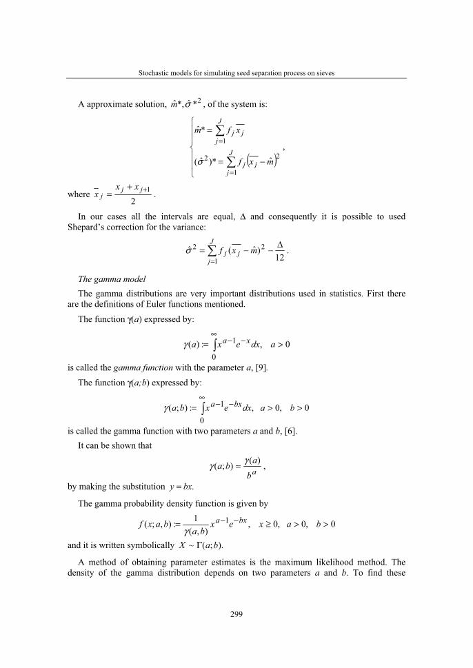
Stochastic models for simulating seed separation process on sieves
299
A approximate solution, 2*ˆ*,ˆ σm , of the system is:
( )⎪
⎪
⎩
⎪
⎪
⎨
⎧
−=
=
∑
∑
=
=J
jjj
J
jjj
mxf
xfm
1
22
1
ˆ)*ˆ(
*ˆ
σ,
where2
1++= jj
jxx
x .
In our cases all the intervals are equal, Δ and consequently it is possible to used Shepard’s correction for the variance:
∑
=
Δ−−=J
jjj mxf
1
2212
)ˆ(σ̂ .
The gamma model The gamma distributions are very important distributions used in statistics. First there
are the definitions of Euler functions mentioned. The function γ(a) expressed by:
∫
∞−− >=
0
1 0,:)( adxexa xaγ
is called the gamma function with the parameter a, [9].The function γ(a;b) expressed by:
∫
∞−− >>=
0
1 0,0,:);( badxexba bxaγ
is called the gamma function with two parameters a and b, [6]. It can be shown that
ab
aba )();( γγ = ,
by making the substitution .bxy =
The gamma probability density function is given by
0,0,0,),(
1:),;( 1 >>≥= −− baxexba
baxf bxaγ
and it is written symbolically ).;(~ baX Γ
A method of obtaining parameter estimates is the maximum likelihood method. The density of the gamma distribution depends on two parameters a and b. To find these

C. Târcolea, T. Căsăndroiu, G. Voicu
300
parameter estimates suppose that a sample x1, x2,…xn of size n is obtained. The distribution of the sample at these values of the variables x1, x2,…xn is the function of the unknown parameters a and b. We take as estimates such values ba ˆ,ˆ of unknown parameters a, bwhich maximize the likelihood function; hence, these are called maximum likelihood estimates. The likelihood function is given as follows
),,;()...,;(),;(),( 21 baxfbaxfbaxfbaL n=where:
bxa exba
baxf −−= 1),(
1),;(γ
is the gamma probability density function. It results:
.))((
),(1
1 1∏=
−−
∑
==n
k
xbakn
ann
kk
exa
bbaLγ
Taking the natural logarithm of L(a;b) does not change the location of its maximum, because the logarithmic base is larger than 1. It obtains:
.)1()](ln[ln),(ln1
∑
=−+−=
n
kkxaanbanbaL γ
Using the necessary maximum conditions we obtain a system defining the maximum likelihood estimates:
⎪
⎪
⎩
⎪
⎪
⎨
⎧
=−=∂
∂
=−+=∂
∂
∑
∑
=
=
0ln
0))((lnlnlnln
1
1n
kk
n
kk
xbna
bL
daadnxbn
aL γ
A solving of the system is the method of successive approximations.
If a ≥ 2, than
)(21
241
21ln))((ln 2
auaada
ad =⎟
⎠
⎞
⎜
⎝
⎛ −+⎟⎠
⎞
⎜
⎝
⎛ −≅−γ .
Thus from the approximation system it results
⎪
⎪
⎪
⎩
⎪⎪
⎪
⎨
⎧
==
=
∏
∑
=
−
=
∑
=n
k
auk
xn
au
n
kk
exeb
xnba
n
kk
1
)(ln1)(
1
ln1
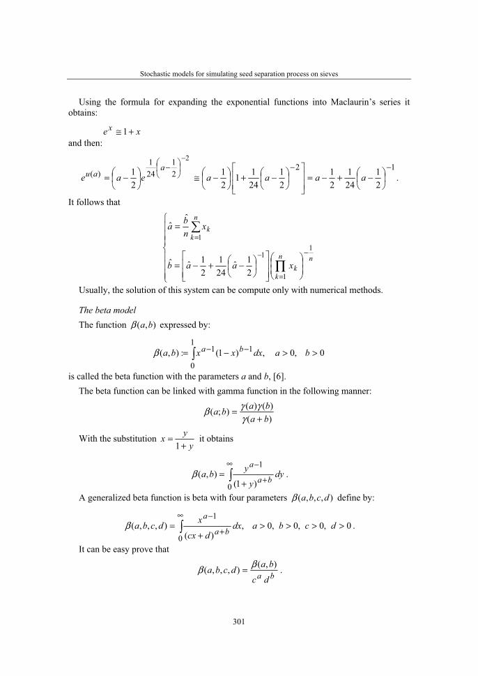
Stochastic models for simulating seed separation process on sieves
301
Using the formula for expanding the exponential functions into Maclaurin’s series it obtains:
xe x +≅ 1and then:
1221
241
)(21
241
21
21
2411
21
21
2−−⎟
⎠
⎞
⎜
⎝
⎛ −⎟
⎠
⎞
⎜
⎝
⎛ −+−=⎥
⎥
⎦
⎤
⎢
⎢
⎣
⎡
⎟
⎠
⎞
⎜
⎝
⎛ −+⎟
⎠
⎞
⎜
⎝
⎛ −≅⎟
⎠
⎞
⎜
⎝
⎛ −=
−
aaaaeaea
au .
It follows that
⎪
⎪
⎪
⎩
⎪⎪
⎪
⎨
⎧
⎟
⎟
⎠
⎞
⎜
⎜
⎝
⎛
⎥
⎥
⎦
⎤
⎢
⎢
⎣
⎡
⎟
⎠
⎞
⎜
⎝
⎛ −+−=
=
−
=
−
=
∏
∑
nn
kk
n
kk
xaab
xnba
1
1
1
1
21ˆ
241
21ˆˆ
ˆˆ
Usually, the solution of this system can be compute only with numerical methods.
The beta model The function ),( baβ expressed by:
∫ >>−= −−1
0
11 0,0,)1(:),( badxxxba baβ
is called the beta function with the parameters a and b, [6]. The beta function can be linked with gamma function in the following manner:
)()()();(
bababa
+=
γγγβ
With the substitution y
yx+
=1
it obtains
∫
∞
+
−
+=
0
1
)1(),( dy
y
yba ba
aβ .
A generalized beta function is beta with four parameters ),,,( dcbaβ define by:
0,0,0,0,)(
),,,(0
1>>>>
+= ∫
∞
+
−dcbadx
dcx
xdcbaba
aβ .
It can be easy prove that
ba dc
badcba ),(),,,( ββ = .

C. Târcolea, T. Căsăndroiu, G. Voicu
302
The beta probability density is given by
0,0,10,)1(),(
1:),;( 11 >>≤≤−= −− baxxxba
baxf baβ
and it is written symbolically );(~ baX Β .
We assume that a sample of size n is given, x1, x2,…xn, for the estimate of the parameters of the population.
The estimates of the parameters of the beta distribution can be more easily obtained by the method of moments. From a given sample, are calculated two sample moments, for example the expectation and variance, and equated to the corresponding theoretical moments of the distribution. The estimates of each parameter are obtained as solutions of the resulting system.
From the sample x1, x2,… xn we find estimates for the expectation and variance:
⎪
⎪
⎩
⎪
⎪
⎨
⎧
−−
=
=
∑
∑
=
=n
ii
n
ii
xxn
s
xn
x
1
22
1
)(1
1
1
The theoretical expectation and variance of the beta distribution are equal to
⎪
⎪
⎩
⎪
⎪
⎨
⎧
⎟
⎠
⎞
⎜
⎝
⎛
+−
++++=
+=
22
))(1()1(
baa
babaaa
baam
σ
We obtain a system
⎪
⎪
⎩
⎪⎪
⎨
⎧
=+++
=+
2)()1(
sbaba
ba
xba
a
from which we find the estimates for a and b.The distribution function of the beta probability function is called the incomplete beta
function and is denoted by );( baI x ,
∫−− −=
xba
x duuuba
baI0
11 )1(),(
1);(β
.
Because the incomplete beta function and cumulative binomial function are related as:
∑
=
−⎟⎟
⎠
⎞
⎜⎜
⎝
⎛
=+−N
kn
nNnp qp
nN
kNkI )1;( ,
Stochastic models for simulating seed separation process on sieves
303
[9], it is possible to evaluate the integral without resorting to numerical approximations.
The new beta distribution We define the function
( ) ( ) ( ) 0,0,0,0,:,,, 11 >>>>−−= −−∫ vubadxxvuxvuba bv
u
aβ .
By making the substitution
uvuxy
−−= ,
it can be shown that:
( ) ( ) ( )bauvvuba ba ,,,, 1 ββ −+−=The focus of the paper is a new type of beta distribution with the following density
probability function ( ) ( ) 11)( −− −−= ba xvuxcxf for u ≤ x ≤ v; a > 0, b > 0, c > 0.
Testing for Goodness-of-fit In statistical applications it is assumed that events occur according to a particular
probability distribution. Testing for goodness-of-fit is a procedure ,which determines if a particular shape for the population frequency curve is consistent with the sample results obtained.
In this section, there are presented chi-square statistic test and the Kolmogorov-Smirnov test for goodness of fit.
The chi-square test. Let x1, x2,…xn be a sample of observations of a random variable X,[6, 7, 8].
From the sample we find estimates of unknown parameters of the distribution law F(x).Then partition the range of the random variable into nonoverlapping J intervals and
determine the number of sample units in each interval, nj, such that ∑=
=J
jj nn
1.
In order to ensure the validity of the chi-square test, the grouping of the sample into classes should be done such that the expected frequency in each interval is not less than five.
Based on the supposed distribution law F(x) the probabilities Jjp j ,1, ∈ of the variable X of following into each interval there are calculated.
Sample value of the test statistic is:
.)(
1
22
∑
=
−=
J
j j
jjs np
npnχ
C. Târcolea, T. Căsăndroiu, G. Voicu
304
Because the random variable j
jj
pn
pnn − has a distribution close to the standard normal
distribution, the chi-square distribution only approximates the true distribution for χ2 as computed above.
If ),1(21
2 −−< − pJs αχχ where p is the number of estimated parameters of F(x), the null-hypothesis does not contradict the sample at a given significance level α.
The Kolmogorov-Smirnov test [3] compares the cumulative sample frequency distributi-on to the theoretical counterpart specified by the null hypothesis. The criterion proposed by Kolmogorov is:
)()(sup xFxSnd −= .Large deviations indicate a poor fit between observed data and what is estimated. An
alternative statistic was by Smirnov and von Mises proposed:
.2
12)(1
22
∑
=⎥
⎦
⎤
⎢
⎣
⎡ −−=n
ii n
ixFw
The Kolmogorov-Smirnov test is more discriminating than the chi-square when the sample size n is small and the distribution is a continuous one; the chi-square test is better when we must estimate parameters.
CONCLUSIONS
The normal distribution is a symmetrical one, but many practical examples illustrate that this case is a particular one.
The main objective of the paper was to proposed different stochastic models which are more adaptive used in describing of evaluation of grain cleaning for working concrete cases. The proposed new beta model has a good significance level in the modelling of the seeds separation process on sieve length.
The proposed distribution is general one and can be adapted for many technical processes and phenomena. In the future we try to solve the problem in time and space based theoretical on a new variant Dirichlet distribution and practical on experimental data.
In this study, the theoretical stochastic models are defined and presented in the second paper the experimentally obtained data are modelled and analyzed based on the proposed theoretical models.
Stochastic models for simulating seed separation process on sieves
305
REFERENCES
1. Balascio, C.C., Misra,M.K., Johnson,H.P., 1987, Particle Movement and Separation Phenomena for a Gravity Separator: I Development of a Markov Probability Model and Estimation of Model Parameters, American Society of Agricultural Engineers, Transactions of the ASAE, pp.1834-1839.
2. Balascio, C.C., Misra, M.K., Johnson, H.P 1987, Particle Movement and Separation Phenomena for a Gravity Separator: II. Experimental Date and Performance of Distance-Transition Markov Models, American Society of Agricultural Engineers, Transactions of the ASAE, pp.1840-1847.
3. Bolotin, V.V., 1969, Statistical methods in structural mechanics, Holden-Day Inc., San Francisco, Cambridge, London, Amsterdam, pp.120-129.
4. Gregory, J.M. and C.B. Fedler. 1987. Mathematical Relationship Predicting Grain Separation in Combines, Transactions of the ASAE. Vol. 30(6): 1600-1604. St. Joseph, MI.
5. Grimmett, G.R., Stirzaker, D.R., 1992, Probability and Random Processes, Oxford University Press Inc., New York, pp.144-160;
6. Heike, H-D, Tarcolea, C., 2000, Grundlagen der Wahrscheinlichkeitsrechnung und Statistik, Oldenbourg Verlag, München, Wien, pp.410-425;
7. Lapin, L.L.,1990, Probability and Statistics for Modern Engineering, PWS-KENT Publishing Company Boston, pp.320-328;
8. Lipson, C., Sheth,N.J., 1973, Statistical Design and Analysis of Engineering Experiments”, McGraw-Hill Inc., pp.172-180;
9. Maksoudian, Y.L., 1969, Probability and Statistics with Applications”, International Textbook Company, Scranton, Pennsylvania, pp.182-209;
10. Schreiber, M., Kutzbach, H.D., Modelling Separation Characteristics in Combine Cleaning Shoes, Landtechnik, nr.4/2003, pag.236 – 237;
11. Segarceanu, M., Casandroiu,T., Manole,C., David,L, Voicu,Gh., Dilea,T., 1986, Experimentarea combinei de cereale cu trei sisteme diferite de curatire C-146/2 (C-140), Raport ştiinţific, Catedra de Masini agricole, I.P.B.
12. Song A., Chung D.S., Nassar R., 1990, A Stochastic Compartmental Model Simulating a Grain Cleaning Process, American Society of Agricultural Engineers, vol. 33(3), pp.877-884;
13. Voicu, Gh., Căsăndroiu, T., 1998, Aprecierea gradului de separare pe lungimea sitei, la sistemele de curatire de la combinele de cereale, Conferinţa TransAgraTech’98, Universitatea Tehnica Cluj-Napoca, Vol.I, pag.183-188, Secţia “Construcţii de maşini. Materiale”;
14. Voicu, Gh., Căsăndroiu, T., 2004, Analiza comparativă a modelelor matematice utilizate la descrierea procesului de separare a seminţelor pe sitele sistemului de curăţare de la combinele de cereale, Revista Construcţia de maşini, nr.11-12/2004;
15. Voicu, Gh., Casandroiu, T., Toma, L., 2005, Adequate statistical models for distribution appreciation of seeds separation by the cleaning system sieves of the combines, International Symposium,”Integrated Systems for Agri-Food Production SIPA ‘05”, Timisoara, Editura Orizonturi Universitare, pp. 185-192;
16. Baumgarten J., 1987, Laboruntersuchungen zur Auslegung und Fuhrung des Separationsprozesses in einer Mahdrescherreinigung – seinrichtung, Agrartechnick, nr.4, pp.165-168;
C. Târcolea, T. Căsăndroiu, G. Voicu
306
17. Voicu, Gh., Căsăndroiu, T., Toma, L.,2006, A multiple logistic regresion statistical model to estimate grain losses on sieve cleaning system from combine, Rev. citată ISI Proceedings ”Actual tasks on agricultural engineering”, Proceedings of the 34th International Symposium on agricultural engineering, 21 – 24 februarie 2006, Opatija, Croaţia, pp.481-491;
18. Voicu, Gh., Căsăndroiu, T., Stan, G., 2007, Using the dimensional analysis for a mathematical model to predict the seeds losses at the cleaning system of the cereals harvester combines, U.P.B Sci.Bull, Series D: Mechanical Engineering, Vol.69, No.4;
19. Wang,Y.S., Chung,D.S., Spillman, C.K, Eckhoff, S.R., Rhee, C., Converse, H.H., 1994, Evaluation of Laboratory Grain Cleaning and Separating Equipment, Part I, American Society of Agricultural Engineers, Transactions of the ASAE, vol 37(2), pp.507-513;
20. Zaika P.M., 1975, Parametri granicinih rejimov vibroseparatii zernovah smesei, Meh. i electrif.s.h., nr.8.
36. Symposium "Actual Tasks on Agricultural Engineering", Opatija, Croatia, 2008.
307
36.
SIMPOZIJAKTUALNI ZADACIMEHANIZACIJE POLJOPRIVREDE
UDC631.353.7.02
Prethodno priopćenjePreliminary communication
NUMERICAL CALCULUS OF THE MAXIMUM DISPLACEMENT BETWEEN THE REEL’S AXES AND THE CUTTER BAR FROM COMBINE HARVESTERS
EDMOND MAICAN, VICTOR MOISE, SORIN-ŞTEFAN BIRIŞ
„Politehnica” University of Bucharest, Faculty of Biotechnical Systems Engineering Splaiul Independentei, no.313, 060032, Bucharest, Romania
SUMMARY
The first phase of the precision agriculture implementation is the numerical modeling of the involved agricultural processes. These mathematical algorithms represent the basis for the subsequent development of computer programs, written for microprocessors controlling the modern agricultural machines’ working processes. This paper solves analytically one of many adjustment and design problems from combine harvesters’ reels: the maximum displacement of the reel’s axes in front of the cutter bar. Until now, a method used to identify a solution for this problem was a graphical one, which is inadequate for the above mentioned purpose. The system of two complex equations found in this study is numerically solved by means of the Newton-Raphson method, which has the advantage of a smaller number of iterations in comparison with other iterative methods.
Key words: reel, cutter bar, numerical method, Newton-Raphson, cereal harvester.
INTRODUCTION
The good operation of a cereal harvester is very much influenced by its subassemblies’ adjustments which, until recently, where dependent on de skills of the operator. Nevert-heless, the human factor has its limitations, so the development of automation systems was very much to the point. However, mathematical algorithms that control the operation of these systems have to be developed first.
The first agricultural combine’s operating part that comes into contact with plants is the reel. Its basic adjustments are related to the physical properties of the crop: height of plants, minimum impact speed that induces seeds detachment from ears, field density, mean
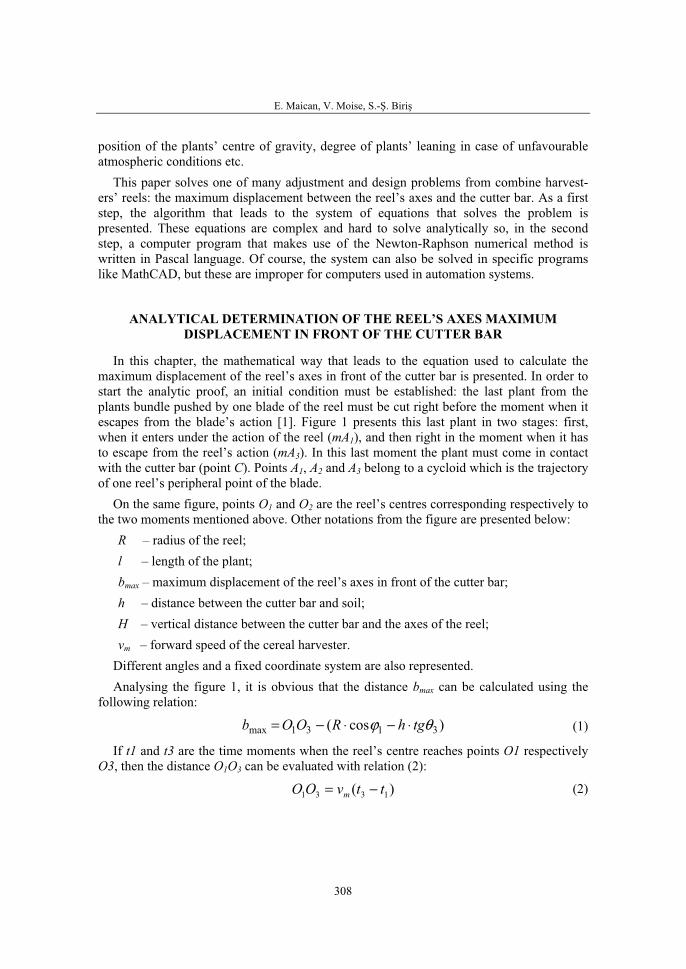
E. Maican, V. Moise, S.-Ş. Biriş
308
position of the plants’ centre of gravity, degree of plants’ leaning in case of unfavourable atmospheric conditions etc.
This paper solves one of many adjustment and design problems from combine harvest-ers’ reels: the maximum displacement between the reel’s axes and the cutter bar. As a first step, the algorithm that leads to the system of equations that solves the problem is presented. These equations are complex and hard to solve analytically so, in the second step, a computer program that makes use of the Newton-Raphson numerical method is written in Pascal language. Of course, the system can also be solved in specific programs like MathCAD, but these are improper for computers used in automation systems.
ANALYTICAL DETERMINATION OF THE REEL’S AXES MAXIMUM DISPLACEMENT IN FRONT OF THE CUTTER BAR
In this chapter, the mathematical way that leads to the equation used to calculate the maximum displacement of the reel’s axes in front of the cutter bar is presented. In order to start the analytic proof, an initial condition must be established: the last plant from the plants bundle pushed by one blade of the reel must be cut right before the moment when it escapes from the blade’s action [1]. Figure 1 presents this last plant in two stages: first, when it enters under the action of the reel (mA1), and then right in the moment when it has to escape from the reel’s action (mA3). In this last moment the plant must come in contact with the cutter bar (point C). Points A1, A2 and A3 belong to a cycloid which is the trajectory of one reel’s peripheral point of the blade.
On the same figure, points O1 and O2 are the reel’s centres corresponding respectively to the two moments mentioned above. Other notations from the figure are presented below:
R – radius of the reel; l – length of the plant; bmax – maximum displacement of the reel’s axes in front of the cutter bar; h – distance between the cutter bar and soil; H – vertical distance between the cutter bar and the axes of the reel; vm – forward speed of the cereal harvester.
Different angles and a fixed coordinate system are also represented. Analysing the figure 1, it is obvious that the distance bmax can be calculated using the
following relation:
)cos( 3131max θϕ tghROOb ⋅−⋅−= (1)
If t1 and t3 are the time moments when the reel’s centre reaches points O1 respectivelyO3, then the distance O1O3 can be evaluated with relation (2):
)( 1331 ttvOO m −= (2)
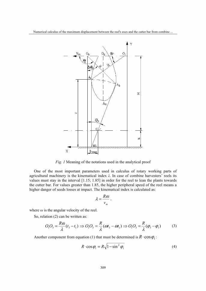
Numerical calculus of the maximum displacement between the reel's axes and the cutter bar from combine ...
309
Fig. 1 Meaning of the notations used in the analytical proof
One of the most important parameters used in calculus of rotary working parts of agricultural machinery is the kinematical index λ. In case of combine harvesters’ reels its values must stay in the interval [1.15; 1.85] in order for the reel to lean the plants towards the cutter bar. For values greater than 1.85, the higher peripheral speed of the reel means a higher danger of seeds losses at impact. The kinematical index is calculated as:
mvRωλ = ,
where ω is the angular velocity of the reel. So, relation (2) can be written as:
)( 1331 ttROO −=λω )( 1331 ttROO ωω
λ−=⇒ )( 1331 ϕϕ
λ−=⇒
ROO (3)
Another component from equation (1) that must be determined is 1cosϕ⋅R :
12
1 sin1cos ϕϕ −=⋅ RR (4)

E. Maican, V. Moise, S.-Ş. Biriş
310
As the reel’s blade must not induce seeds detachment from the ears, the horizontal component vx of the blade when it first touches the plants (point A1) must be zero:
0sin0 1 =−⇒= ϕωRvv mx ωϕ
Rvm=⇒ 1sin
λϕ 1sin 1 =⇒ (5)
Going with relation (5) in (4):
1cos 21 −=⋅ λ
λϕ RR (6)
Also, if equations (4) and (6) are now inserted into (1), bmax becomes:
⎟
⎠
⎞
⎜
⎝
⎛ ⋅−−−−= 32
13max 1)( θλλ
ϕϕλ
tghRRb , or ( ) 32
13max 1 θλϕϕλ
tghRb ⋅+−−−= (7)
If the coordinates of A1 and A3 are (x1, y1), respectively (x3, y3), than (see fig.1): 22
3123 )( lxxy =−+ (8)
The A1 point’s abscissa (x1) is:
111 cosϕ⋅+⋅= Rtvx m
However:
111 ϕλλ
ω RtRtvm ==⋅ (9)
From equations (9) and (6) results:
1211 −+= λ
λϕ
λRRx , or ( )12
11 −+= λϕλRx
The angle φ1 can be evaluated from relation (5):
⎟
⎠
⎞
⎜
⎝
⎛=λ
ϕ 1arcsin1 (10)
So, abscissa x1 becomes:
⎟⎟
⎠
⎞
⎜⎜
⎝
⎛ −+⎟⎠
⎞
⎜
⎝
⎛= 11arcsin 21 λ
λλRx (11)
The A3 point’s abscissa (x3) is:
333 cosϕ⋅+⋅= Rtvx m (12)
But:
333 ϕλλ
ω RtRtvm ==⋅
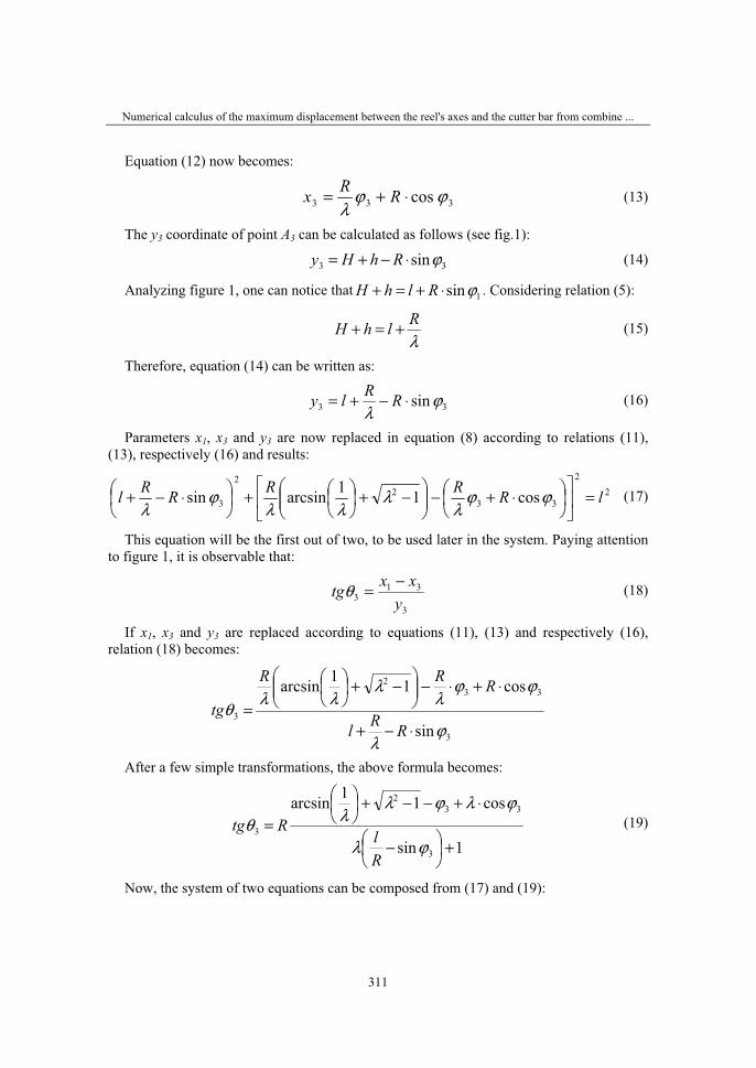
Numerical calculus of the maximum displacement between the reel's axes and the cutter bar from combine ...
311
Equation (12) now becomes:
333 cos ϕϕλ
⋅+= RRx (13)
The y3 coordinate of point A3 can be calculated as follows (see fig.1):
33 sinϕ⋅−+= RhHy (14)
Analyzing figure 1, one can notice that 1sinϕ⋅+=+ RlhH . Considering relation (5):
λRlhH +=+ (15)
Therefore, equation (14) can be written as:
33 sinϕλ
⋅−+= RRly (16)
Parameters x1, x3 and y3 are now replaced in equation (8) according to relations (11), (13), respectively (16) and results:
22
332
2
3 cos11arcsinsin lRRRRRl =⎥
⎦
⎤
⎢
⎣
⎡
⎟
⎠
⎞
⎜
⎝
⎛ ⋅+−⎟⎟
⎠
⎞
⎜⎜
⎝
⎛ −+⎟⎠
⎞
⎜
⎝
⎛+⎟
⎠
⎞
⎜
⎝
⎛ ⋅−+ ϕϕλ
λλλ
ϕλ
(17)
This equation will be the first out of two, to be used later in the system. Paying attention to figure 1, it is observable that:
3
313 y
xxtg −=θ (18)
If x1, x3 and y3 are replaced according to equations (11), (13) and respectively (16), relation (18) becomes:
3
332
3
sin
cos11arcsin
ϕλ
ϕϕλ
λλλθ
⋅−+
⋅+⋅−⎟⎟
⎠
⎞
⎜⎜
⎝
⎛ −+⎟⎠
⎞
⎜
⎝
⎛
=RRl
RRR
tg
After a few simple transformations, the above formula becomes:
1sin
cos11arcsin
3
332
3
+⎟⎠
⎞
⎜
⎝
⎛ −
⋅+−−+⎟⎠
⎞
⎜
⎝
⎛
=ϕλ
ϕλϕλλθ
Rl
Rtg (19)
Now, the system of two equations can be composed from (17) and (19):
E. Maican, V. Moise, S.-Ş. Biriş
312
⎪
⎪
⎪
⎪
⎩
⎪⎪
⎪
⎪
⎨
⎧
=−+⎟
⎠
⎞
⎜
⎝
⎛ −
⋅+−−+⎟⎠
⎞
⎜
⎝
⎛
=⎥
⎦
⎤
⎢
⎣
⎡
⎟
⎠
⎞
⎜
⎝
⎛ ⋅+−⎟⎟
⎠
⎞
⎜⎜
⎝
⎛ −+⎟⎠
⎞
⎜
⎝
⎛+⎟
⎠
⎞
⎜
⎝
⎛ ⋅−+
01sin
cos11arcsin
cos11arcsinsin
3
3
332
22
332
2
3
θϕλ
ϕλϕλλ
ϕϕλ
λλλ
ϕλ
tg
Rl
R
lRRRRRl
This system will be solved by means of numerical methods, using Newton-Raphson method. The unknowns are φ3 and tg(θ3) and their calculated values will be then used to find the maximum displacement between the reel’s axes and the cutter bar bmax, as follows:
RhRb ⋅+⎟⎟
⎠
⎞
⎜⎜
⎝
⎛ −−⎟⎠
⎞
⎜
⎝
⎛−= 11arcsin 23max λ
λϕ
λ (20)
The above formula is based on equations (7) and (10).
COMPUTER PROGRAM FOR NUMERICAL CALCULUS OF THE DISTANCE BETWEEN THE REEL’S AXES AND THE CUTTER BAR
The intricate system of two equations presented above can be solved by means of iterative numerical approach. There are two mostly used numerical approaches: Gradient method and Newton-Raphson method. The equations should be first transformed into functions. Initial guesses for each root are required by each method.
Both methods employ the partial derivatives of each function, so four partial derivatives are necessary in this case. The Gradient method is always convergent, however with a very slow rate of convergence. On the other hand, the Newton-Raphson method lead to significant faster convergence, but it also allows the possibility that the solution may diverge. It is well known that divergence can occur if the initial guesses are insufficiently close to the true roots [2,3]. It is not the case with the problem presented in this paper, as the initial guesses can be efficiently predicted by means of a simple scaled drawing of figure 1.
Values for the following parameters must be defined in the program:
• R (which is distinctive for each model of cereal harvester);
• height of plants l (which, in the real case, can be permanently measured by means of modern data acquisition systems, for example based on laser beam and photoelectric cells);
• kinematical index λ (modern combine harvesters have automatic systems that calcu-late and maintain the kinematical index between 1.15 and 1.85);
• distance between the cutter bar and soil h (which also can be easily automatically determined in real case and stays approximately constant during the entire harve-sting process).

Numerical calculus of the maximum displacement between the reel's axes and the cutter bar from combine ...
313
The program is presented below with test values for the above mentioned parameters, according to the real situations that can be found in the field.
PROGRAM Maximum_displacement; USES CRT,METODNUM; {$M 65520,0,655360} VAR X:VECTOR1; {Array with 200 elements, Unit Metodnum} b_max,Lbd,L,hc,H,EPS,EPS2:REAL; {------------------------------------------ b_max- maximum displacement Lbd - lambda L - height of plants hc - distance between soil and cutter bar ------------------------------------------} I,N,KOD,ITER:INTEGER; CONST R:Real=0.5; {Radius of the reel} {$F+} PROCEDURE FUNCT(N:INTEGER;X:VECTOR1;VAR F:VECTOR1;VAR KOD:INTEGER); BEGIN KOD:=0; F[1]:=sqr(L+R/Lbd-R*sin(x[1]))+sqr(R/Lbd*(arcsin(1/Lbd)+ sqrt(Lbd*Lbd-1))-(R/Lbd*x[1]+R*cos(x[1])))-L*L; F[2]:=R*(arcsin(1/Lbd)-x[2]+sqrt(Lbd*Lbd-1) +Lbd*cos(x[1]))/(Lbd*(L/R-sin(x[1]))+1)-x[2]; END; {$F-} PROCEDURE NewtRaphs(NUME:PROC6;MF:PROC7;N,ITER:INTEGER; H,EPS:REAL;VAR X:VECTOR1;VAR KOD:INTEGER); VAR I,J,JESF,N1:INTEGER; W,W1,DX,F:VECTOR1; BEGIN KOD:=0; N1:=N+1; I:=1; REPEAT MF(NUME,X,N,H,F,W,KOD); INVMAT(W,N,1.E-15,W1,KOD); IF KOD > 0 THEN BEGIN WRITELN(' KOD= ',KOD); READLN;
EXIT; END
ELSE PRODMAT(W1,F,N,N,1,DX); JESF:=0; J:=1; REPEAT IF ABS(DX[J]) < EPS THEN J:=J+1 ELSE BEGIN J:=N1; JESF:=1; END;

E. Maican, V. Moise, S.-Ş. Biriş
314
UNTIL J > N; IF JESF = 0 THEN EXIT; FOR J:=1 TO N DO X[J]:=X[J]-DX[J]; WRITELN(' ITERATION ',I); FOR J:=1 TO N DO WRITELN('X[',J,']= ',X[J]); I:=I+1; UNTIL I > ITER; WRITELN(' ERROR! '); EXIT; END; {________________Main Program_________________} BEGIN CLRSCR; Lbd:=1.5; L:=0.6 {m}; hc:=0.15 {m}; N:=2; {number of equations} H:=0.015; EPS:=1.E-5;{precision of calculus} ITER:=30;{maximum number of iterations} {---------------------} {Initial guesses} X[1]:=2.1; {fi3} X[2]:=0.36;{tan(teta3)} {---------------------} NewtRaphs(FUNCT,MF,N,ITER,H,EPS,X,KOD); WRITELN(^J^M,' ROOTS OF THE SYSTEM:'); FOR I:=1 TO N DO WRITELN(' X[',I,']= ',X[I]:10:4); b_max:=R/Lbd*(x[1]-arcsin(1/Lbd)-sqrt(Lbd*Lbd-1))+hc*x[2]; Writeln(' b_max=',b_max*100:6:1,' cm'); Readln; END.
In this program, the Metodnum unit is a library of useful mathematical functions and procedures made by authors [4]. NewtRaphs procedure calls on INVMAT and PRODMATprocedures, which are used for calculating the inverse matrix and product of two matrixes respectively. Also, the partial derivatives are solved numerically instead of analytical, by means of the MF procedure. All three of them are defined in the Metodnum unit. The Arcsin function is also defined by the authors [5] and included in the Metodnum unit, together with other trigonometric functions.
In the definition line of NewtRaphs procedure, PROC6 and PROC7 are procedure type parameters, defined in the Metodnum unit as follows: PROC6=PROCEDURE(N:INTEGER;X:VECTOR1;VAR F:VECTOR1;VAR KOD:INTEGER); PROC7=PROCEDURE(PROC:PROC6;X:VECTOR1;N:INTEGER;EPS:REAL;
VAR F,W:VECTOR1;VAR KOD:INTEGER);
The following input values were used in the program in order to test it: R = 0.5 m, l = 0.6 m, h = 0.15 m and λ = 1.5. Two initial guess values were given for φ3 and tg(θ3) (denoted respectively with x[1] and x[2] in the program): φ3 = 2.1 rad (about 1200) and tg(θ3) = 0.57 (for an initial value of θ3 of π/6). After the computation, the following results were obtained:
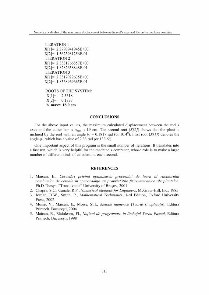
Numerical calculus of the maximum displacement between the reel's axes and the cutter bar from combine ...
315
ITERATION 1 X[1]= 2.3790941945E+00 X[2]= 1.5623981256E-01 ITERATION 2 X[1]= 2.3331766857E+00 X[2]= 1.8282658848E-01 ITERATION 3 X[1]= 2.3317922635E+00 X[2]= 1.8368969665E-01
ROOTS OF THE SYSTEM: X[1]= 2.3318 X[2]= 0.1837 b_max= 18.9 cm
CONCLUSIONS
For the above input values, the maximum calculated displacement between the reel’s axes and the cutter bar is bmax ≈ 19 cm. The second root (X[2]) shows that the plant is inclined by the reel with an angle θ3 = 0.1817 rad (or 10.40). First root (X[1]) denotes the angle φ3, which has a value of 2.33 rad (or 133.60).
One important aspect of this program is the small number of iterations. It translates into a fast run, which is very helpful for the machine’s computer, whose role is to make a large number of different kinds of calculations each second.
REFERENCES
1. Maican, E., Cercetări privind optimizarea procesului de lucru al rabatorului combinelor de cereale în concordanţă cu proprietăţile fizico-mecanice ale plantelor,Ph.D Thesys, “Transilvania” University of Braşov, 2001
2. Chapra, S.C., Canale, R.P., Numerical Methods for Engineers, McGraw-Hill, Inc., 1985 3. Jordan, D.W., Smith, P., Mathematical Techniques, 3-rd Edition, Oxford University
Press, 2002 4. Moise, V., Maican, E., Moise, Şt.I., Metode numerice (Teorie şi aplicaţii). Editura
Printech, Bucureşti, 2004 5. Maican, E., Rădulescu, Fl., Noţiuni de programare în limbajul Turbo Pascal, Editura
Printech, Bucureşti, 1998

36. Symposium "Actual Tasks on Agricultural Engineering", Opatija, Croatia, 2008.
317
36.
SIMPOZIJAKTUALNI ZADACIMEHANIZACIJE POLJOPRIVREDE
UDC631.362.63:635.21
Izvorni znanstveni radOriginal scientific paper
CAD METHODOLOGY OF THE BULB AND POTATO IMPURITIES CLEANING SISTEMS COMPOSED OF
SUCCESSIVE ROLLING CONVEYORS SAFTA VICTOR VIOREL
“Politehnica” University of Bucharest, Faculty of Biotechnical Systems Engineering,313, Splaiul Independenţei, 060032, Bucharest, Romania
SUMMARY
In this paper is presented a CAD methodology which aloud the determination of the optimal parameters, geometrical and functional, of the bulb and tubercles impurities cleaning system composed of successive rolling conveyors, fitted with elliptical profile shaking roles, intended for the equipment of the bulb or tubercles harvesters or conditioning lines. The CAD methodology is composed of specialized soft-wares which can determine the optimal dimensions of the elliptical profile of the shaking roles and their emplacement mode along the rolling conveyor active surfaces and the optimal relative position between the successive conveyors, in the conditions of shaking regimes with maximum intensity imposed to mixture of useful products and impurities, processed on the impurities cleaning system, but without producing damages to the useful products.
Key words: bulb and tubercles harvesters, bulb and tubercle conditioning lines, impurities cleaning system, computer simulation and optimization.
INTRODUCTION
The bulb, tubercle or certain root vegetables harvesters and conditioning lines are fitted with impurities cleaning systems of the useful products digged out from the soil bed wherein they are developed, respectively the useful product brought to the conditioning in order to be garnered. These devices, particulary important and needful to the working process of these equipments, occupe the most of their working active surfaces determining in great measure their general configuration. To the mechanical harvesting, the separation of the useful products from the soil bed, comminuted after the digging, is a dificult process especially because the great quantity of impurities which must be taken off, frequently
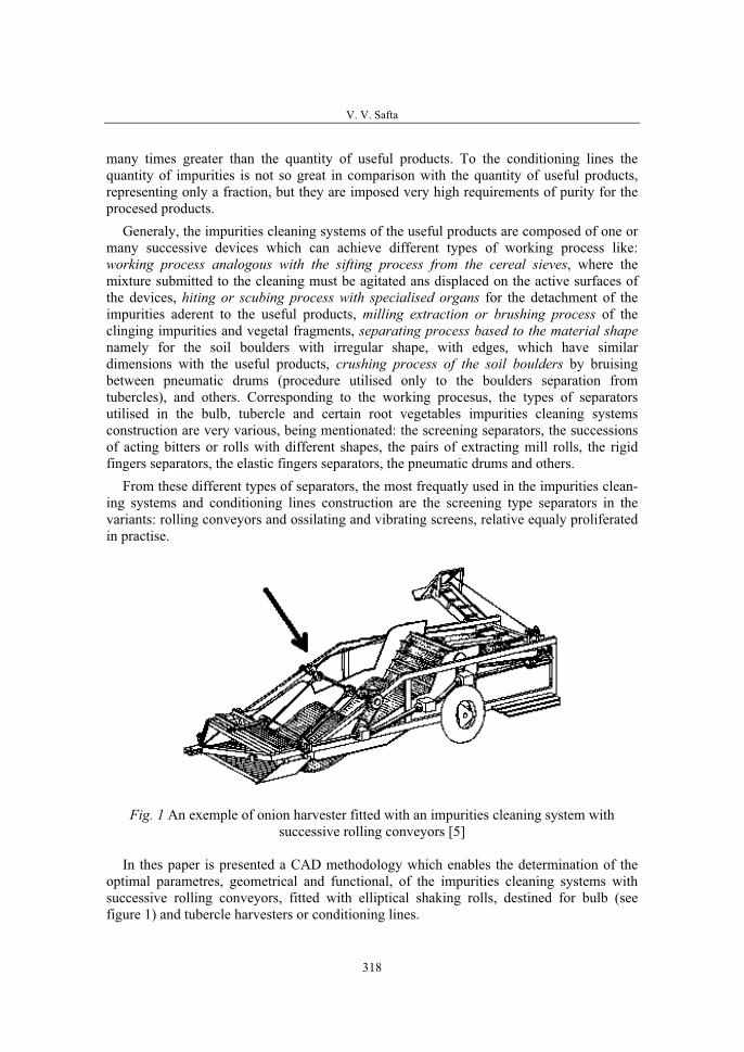
V. V. Safta
318
many times greater than the quantity of useful products. To the conditioning lines the quantity of impurities is not so great in comparison with the quantity of useful products, representing only a fraction, but they are imposed very high requirements of purity for the procesed products.
Generaly, the impurities cleaning systems of the useful products are composed of one or many successive devices which can achieve different types of working process like: working process analogous with the sifting process from the cereal sieves, where the mixture submitted to the cleaning must be agitated ans displaced on the active surfaces of the devices, hiting or scubing process with specialised organs for the detachment of the impurities aderent to the useful products, milling extraction or brushing process of the clinging impurities and vegetal fragments, separating process based to the material shapenamely for the soil boulders with irregular shape, with edges, which have similar dimensions with the useful products, crushing process of the soil boulders by bruising between pneumatic drums (procedure utilised only to the boulders separation from tubercles), and others. Corresponding to the working procesus, the types of separators utilised in the bulb, tubercle and certain root vegetables impurities cleaning systems construction are very various, being mentionated: the screening separators, the successions of acting bitters or rolls with different shapes, the pairs of extracting mill rolls, the rigid fingers separators, the elastic fingers separators, the pneumatic drums and others.
From these different types of separators, the most frequatly used in the impurities clean-ing systems and conditioning lines construction are the screening type separators in the variants: rolling conveyors and ossilating and vibrating screens, relative equaly proliferated in practise.
Fig. 1 An exemple of onion harvester fitted with an impurities cleaning system with successive rolling conveyors [5]
In thes paper is presented a CAD methodology which enables the determination of the optimal parametres, geometrical and functional, of the impurities cleaning systems with successive rolling conveyors, fitted with elliptical shaking rolls, destined for bulb (see figure 1) and tubercle harvesters or conditioning lines.
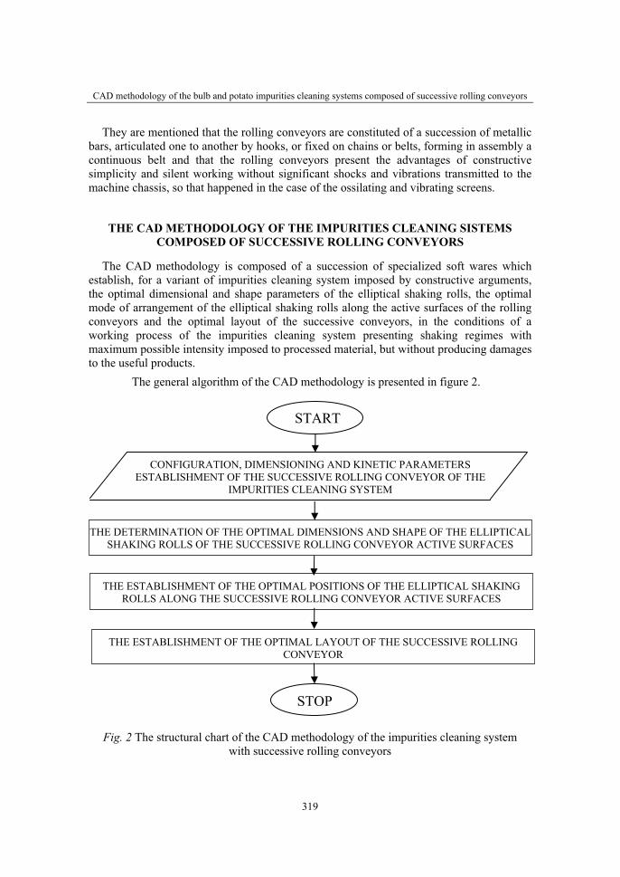
CAD methodology of the bulb and potato impurities cleaning systems composed of successive rolling conveyors
319
They are mentioned that the rolling conveyors are constituted of a succession of metallic bars, articulated one to another by hooks, or fixed on chains or belts, forming in assembly a continuous belt and that the rolling conveyors present the advantages of constructive simplicity and silent working without significant shocks and vibrations transmitted to the machine chassis, so that happened in the case of the ossilating and vibrating screens.
THE CAD METHODOLOGY OF THE IMPURITIES CLEANING SISTEMS COMPOSED OF SUCCESSIVE ROLLING CONVEYORS
The CAD methodology is composed of a succession of specialized soft wares which establish, for a variant of impurities cleaning system imposed by constructive arguments, the optimal dimensional and shape parameters of the elliptical shaking rolls, the optimal mode of arrangement of the elliptical shaking rolls along the active surfaces of the rolling conveyors and the optimal layout of the successive conveyors, in the conditions of a working process of the impurities cleaning system presenting shaking regimes with maximum possible intensity imposed to processed material, but without producing damages to the useful products.
The general algorithm of the CAD methodology is presented in figure 2.
Fig. 2 The structural chart of the CAD methodology of the impurities cleaning system with successive rolling conveyors
START
CONFIGURATION, DIMENSIONING AND KINETIC PARAMETERS ESTABLISHMENT OF THE SUCCESSIVE ROLLING CONVEYOR OF THE
IMPURITIES CLEANING SYSTEM
THE DETERMINATION OF THE OPTIMAL DIMENSIONS AND SHAPE OF THE ELLIPTICAL SHAKING ROLLS OF THE SUCCESSIVE ROLLING CONVEYOR ACTIVE SURFACES
THE ESTABLISHMENT OF THE OPTIMAL POSITIONS OF THE ELLIPTICAL SHAKING ROLLS ALONG THE SUCCESSIVE ROLLING CONVEYOR ACTIVE SURFACES
THE ESTABLISHMENT OF THE OPTIMAL LAYOUT OF THE SUCCESSIVE ROLLING CONVEYOR
STOP

V. V. Safta
320
The input data neccesary for the methodology application are in relation with the concrete configuration of the equipment wherein is used the impurities cleaning system with successive rolling conveyors and are refering to the shapes and the dimensions of all the constitutive parts of the rolling conveyors, namely: belts or chains, bars, driving and returning drums, ranges of adequate dimensions and eccentricity of the eliptical roles, range of the adequate inclination angles towards the horizontal of the active surfaces of the successive rolling conveyors, ranges of adequate speeds of the successive conveyors belts, the positions of the feeding zones of the succesive conveyors active surfaces. Based on these parametres they result the contours of the successive conveyor belts surfaces.
As it can be observed from the structural chart of the methodology, the first step of the algorithm is the determination of the optimal dimensions and shape of the elliptical shaking rolls of the successive rolling conveyor active surfaces which is done with specialized software [1, 2]. The structural chart of this specialized software algorithm is presented in the figure 3.
START
INPUT DATA: The ranges of recommended values for: the rolling conveyor belt speed, the inclination angle toward the horizontal of the rolling conveyor belt active surface, the great semi-axe of the shaking elliptical roles, the ratio between great and small semi-axes of the shaking elliptical roles. The critical value of the impact speed with the active surface of the rolling conveyor for a certainvariety of useful product, exceeding a certain mass.
Establishment of the number of intermediary steps whereat they are calculated the values of the great semi-axe of the shaking elliptical roles,
along its recommended range
Calculation of the intermediary values of the great semi-axe of the shaking elliptical roles, along the recommended range
Establishment of the number of intermediary steps whereat they arecalculated the values of the ratio between great and small semi-axes(eccentricity) of the shaking elliptical roles, along its recommended range
Calculation of the intermediary values of the ratio between great and small semi-axes (eccentricity) of the shaking elliptical roles, along the recommended range
Calculation of the resulted intermediary values for the small semi-axe of the shaking elliptical roles
Assessment of a certain value of the rolling conveyor belt speed, from the recommended range
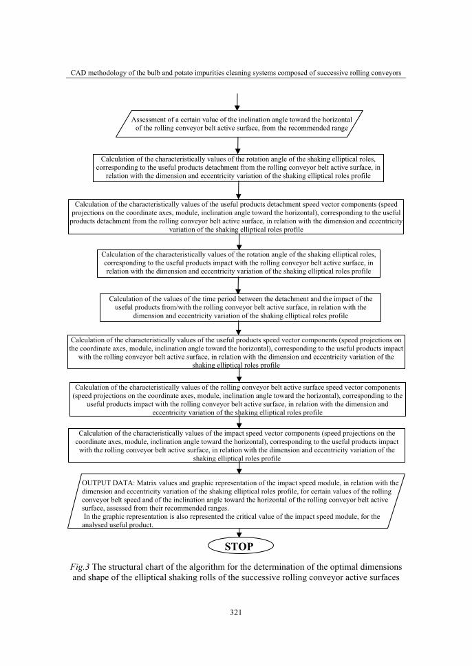
CAD methodology of the bulb and potato impurities cleaning systems composed of successive rolling conveyors
321
Fig.3 The structural chart of the algorithm for the determination of the optimal dimensions and shape of the elliptical shaking rolls of the successive rolling conveyor active surfaces
Calculation of the characteristically values of the rotation angle of the shaking elliptical roles, corresponding to the useful products detachment from the rolling conveyor belt active surface, in
relation with the dimension and eccentricity variation of the shaking elliptical roles profile
Assessment of a certain value of the inclination angle toward the horizontal of the rolling conveyor belt active surface, from the recommended range
Calculation of the characteristically values of the useful products detachment speed vector components (speed projections on the coordinate axes, module, inclination angle toward the horizontal), corresponding to the useful
products detachment from the rolling conveyor belt active surface, in relation with the dimension and eccentricity variation of the shaking elliptical roles profile
STOP
OUTPUT DATA: Matrix values and graphic representation of the impact speed module, in relation with the dimension and eccentricity variation of the shaking elliptical roles profile, for certain values of the rolling conveyor belt speed and of the inclination angle toward the horizontal of the rolling conveyor belt active surface, assessed from their recommended ranges. In the graphic representation is also represented the critical value of the impact speed module, for the analysed useful product.
Calculation of the characteristically values of the useful products speed vector components (speed projections on the coordinate axes, module, inclination angle toward the horizontal), corresponding to the useful products impact
with the rolling conveyor belt active surface, in relation with the dimension and eccentricity variation of the shaking elliptical roles profile
Calculation of the characteristically values of the rolling conveyor belt active surface speed vector components (speed projections on the coordinate axes, module, inclination angle toward the horizontal), corresponding to the
useful products impact with the rolling conveyor belt active surface, in relation with the dimension and eccentricity variation of the shaking elliptical roles profile
Calculation of the characteristically values of the impact speed vector components (speed projections on the coordinate axes, module, inclination angle toward the horizontal), corresponding to the useful products impact
with the rolling conveyor belt active surface, in relation with the dimension and eccentricity variation of the shaking elliptical roles profile
Calculation of the characteristically values of the rotation angle of the shaking elliptical roles, corresponding to the useful products impact with the rolling conveyor belt active surface, in relation with the dimension and eccentricity variation of the shaking elliptical roles profile
Calculation of the values of the time period between the detachment and the impact of the useful products from/with the rolling conveyor belt active surface, in relation with the
dimension and eccentricity variation of the shaking elliptical roles profile

V. V. Safta
322
Considering that under the shaking rolls action the material from the active surfaces of the rolling conveyors executes jumps, the optimizing procedure is based on the comparison between the effective values of the impact speed of the useful products with the active surfaces of the conveyors, determined with a specialized software in the case of the variation of the values of the elliptical shaking roles dimension and eccentricity in their adequate ranges of values and the critical impact speed, which if is exceeded they appear damages of the useful products. The value of the critical impact speed is characteristic for a certain variety of useful products (bulbs, tubercles, roots) which exceed a certain mass value.
The input data of the software are the imposed values of the conveyors belt speeds and of the inclination angles towards the horizontal of the conveyors active surfaces, chosen from the recommended range of values, the ranges of variation of the dimensions and eccentricity of the elliptical shaking rolls and the value of the critical impact speed for the analyzed useful product.
The output data of the software are matrix of values and variation graphics of the impact speed of the useful products with the rolling conveyor active surface in relation with the dimensions and eccentricity of the elliptical shaking rolls, for certain imposed values of the conveyor belt speed and inclination angle of the conveyor active surface.
They were be elaborated two variants of soft wares, a variant for the case of rolling conveyor which have an elastic belt (see figure 4) whereat its undulatory movement, induced by the elliptical shaking rolls to the active surface, is amortized after a short distance after the passage of the belt over the shaking rolls, and a variant for the case of rolling conveyor which have a rigid active surface (see figure 5) whereat all the points of the active surface have the same undulatory movement like that from the acting zone of the elliptical shaking rolls.
Fig.4 The variation of the effective impact Fig.5 The variation of the effective impact speed in the case of elastic active surfaces speed in the case of rigid active surfaces
If they are analyzed the graphics resulted after the running of the software, it can be remarked that the variation of the effective impact speed appear like a curved surface while the critical impact speed appear like a plane parallel with the horizontal plane, which intersect the effective impact speed surface (see figures 4 and 5). The zones of the effective impact speed surface which are above the critical impact speed plane correspond to those
vc vccr, vc vccr,
CAD methodology of the bulb and potato impurities cleaning systems composed of successive rolling conveyors
323
working process with a very energetically shaking whereat the useful products are damaged, while the zones of the effective impact speed surface which are under the critical impact speed plane correspond to those working process with a low shaking whereat the separation of the impurities from the useful products is improperly.
The optimal working process of the rolling conveyor correspond to the point of the intersection curve between the effective impact speed surface and the critical impact speed plane, wherefore they are obtained the most energetically shaking but without damages of the useful products.
So every point of the intersection curve correspond to a pair of optimal values of the dimensions and eccentricity of the elliptic rolls profile for certain imposed values of the conveyor belt speed and of the inclination of the conveyor active surface.
It can be mentioned that the optimizing procedure must be applied independently for each of the successive conveyors.
The next step of the methodology algorithm is the establishment of the optimal positions of the elliptical shaking rolls along the successive rolling conveyor active surfaces which is done with specialized software whose structural chart is presented in the figure 6.
The optimizing procedure is applied to the conveyors with elastic belt whereat the undulatory movement of the belt active surface, induced by the elliptical shaking rolls, is amortized at a certain distance after the passage of the belt over the shaking rolls, and become o pure translation, in which case the separation of the impurities is very much reduced or annulated. Using the specialized software it can be determined the distance, measured along the active surfaces of the conveyors, from an anterior pair of shaking rolls to the place where the ondulatory movement is completely amortized and where it must be located a new pairs of shaking rolls. Thus, locating shaking rolls in optimal positions all-over the rolling conveyors active surfaces, it will be insured an intense and constant agitation of the processed material.
The input data of the software are: the rolling conveyor belt speed, the width of the rolling conveyor active surface, the conveyor feeding flow with material, separation coefficient along the active surface of the conveyor, the distance between the feeding zone and the acting zone of the first pair of elliptical shaking rolls, the length of the elliptical shaking rolls acting zone, expressions of the movement, velocity and acceleration of the conveyor active surface in the acting zone of the elliptical shaking rolls, the elastic constant of the conveyor belt, the amortization coefficient of the conveyor belt, the value for the oscillations amplitude wherefore the conveyor belt oscillation becomes insignificant.
The output data of the software are the optimal distances for the elliptical shaking rolls layout.
It can be mentioned that also this optimizing procedure must be applied independently for each of the successive conveyors.
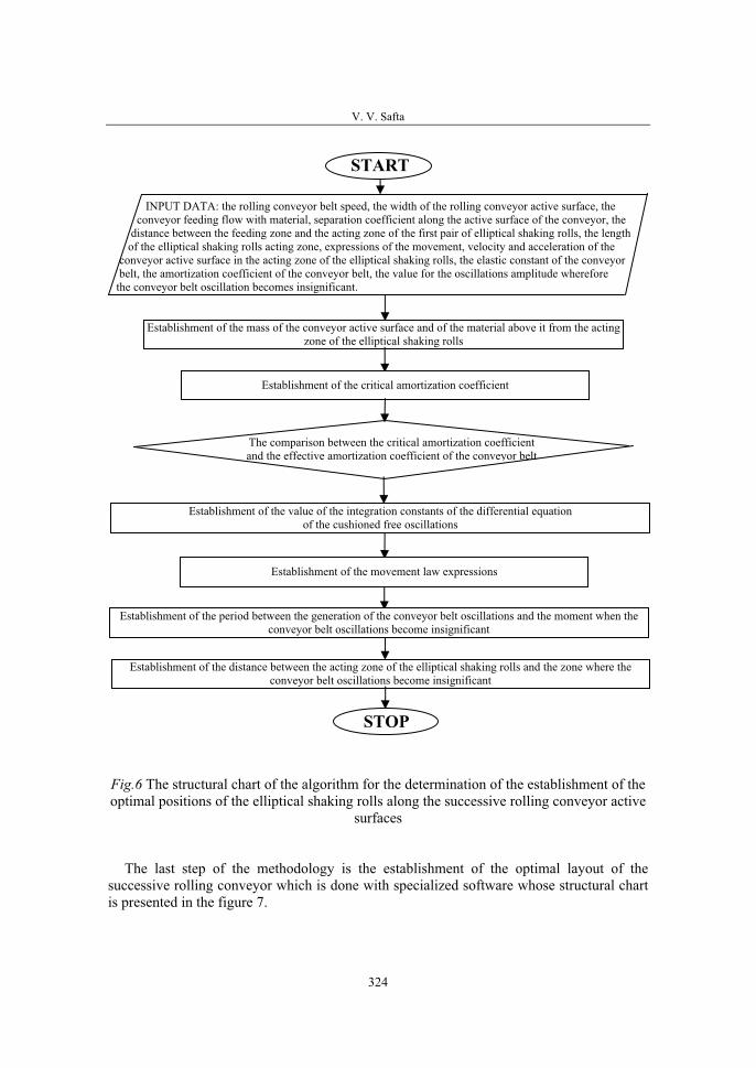
V. V. Safta
324
Fig.6 The structural chart of the algorithm for the determination of the establishment of the optimal positions of the elliptical shaking rolls along the successive rolling conveyor active
surfaces
The last step of the methodology is the establishment of the optimal layout of the successive rolling conveyor which is done with specialized software whose structural chart is presented in the figure 7.
INPUT DATA: the rolling conveyor belt speed, the width of the rolling conveyor active surface, the conveyor feeding flow with material, separation coefficient along the active surface of the conveyor, the distance between the feeding zone and the acting zone of the first pair of elliptical shaking rolls, the length of the elliptical shaking rolls acting zone, expressions of the movement, velocity and acceleration of the conveyor active surface in the acting zone of the elliptical shaking rolls, the elastic constant of the conveyor belt, the amortization coefficient of the conveyor belt, the value for the oscillations amplitude wherefore the conveyor belt oscillation becomes insignificant.
Establishment of the mass of the conveyor active surface and of the material above it from the acting zone of the elliptical shaking rolls
The comparison between the critical amortization coefficient and the effective amortization coefficient of the conveyor belt
Establishment of the value of the integration constants of the differential equationof the cushioned free oscillations
Establishment of the critical amortization coefficient
Establishment of the movement law expressions
Establishment of the period between the generation of the conveyor belt oscillations and the moment when the conveyor belt oscillations become insignificant
Establishment of the distance between the acting zone of the elliptical shaking rolls and the zone where the conveyor belt oscillations become insignificant
STOP
START
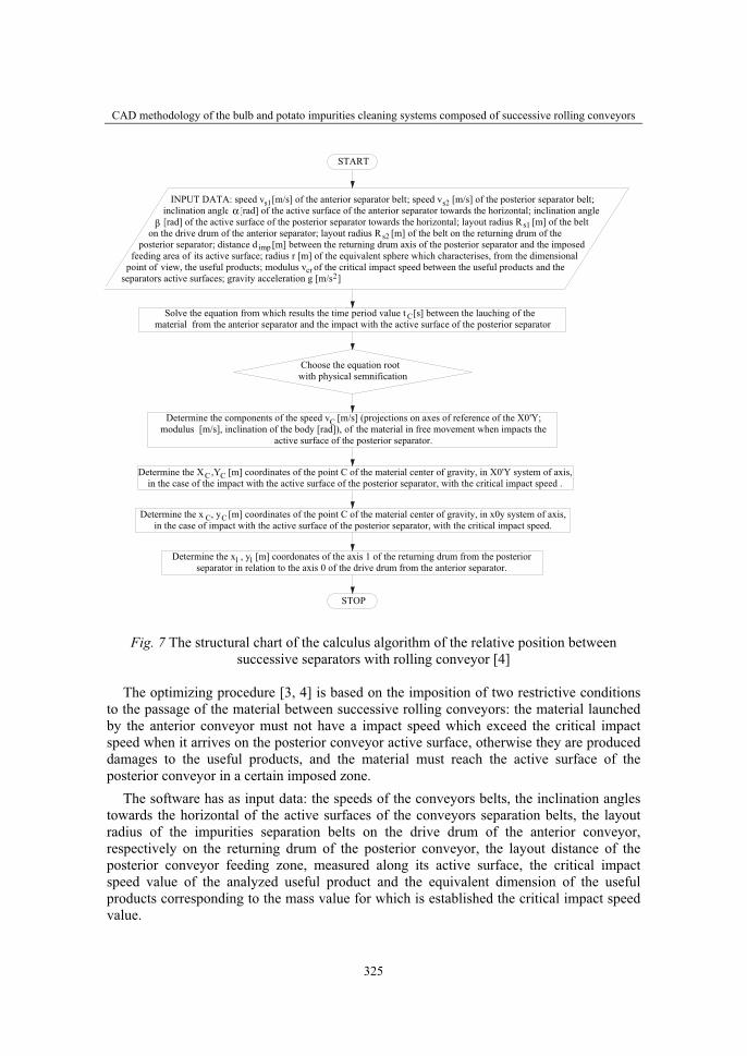
CAD methodology of the bulb and potato impurities cleaning systems composed of successive rolling conveyors
325
STOP
Determine the x , y [m] coordonates of the axis 1 of the returning drum from the posterior separator in relation to the axis 0 of the drive drum from the anterior separator.
Determine the components of the speed v [m/s] (projections on axes of reference of the X0'Y; modulus [m/s], inclination of the body [rad]), of the material in free movement when impacts the
active surface of the posterior separator.
Choose the equation root with physical semnification
Solve the equation from which results the time period value t [s] between the lauching of the material from the anterior separator and the impact with the active surface of the posterior separator
START
1
C C
C
C
s1 s2
C C
1
INPUT DATA: speed v [m/s] of the anterior separator belt; speed v [m/s] of the posterior separator belt; inclination angle a [rad] of the active surface of the anterior separator towards the horizontal; inclination angle
ί [rad] of the active surface of the posterior separator towards the horizontal; layout radius R [m] of the belt on the drive drum of the anterior separator; layout radius R [m] of the belt on the returning drum of the posterior separator; distance d [m] between the returning drum axis of the posterior separator and the imposed feeding area of its active surface; radius r [m] of the equivalent sphere which characterises, from the dimensional point of view, the useful products; modulus v of the critical impact speed between the useful products and the separators active surfaces; gravity acceleration g [m/s ]
s1s2
imp
cr2
Determine the X ,Y [m] coordinates of the point C of the material center of gravity, in X0'Y system of axis,in the case of the impact with the active surface of the posterior separator, with the critical impact speed .
Determine the x , y [m] coordinates of the point C of the material center of gravity, in x0y system of axis,in the case of impact with the active surface of the posterior separator, with the critical impact speed.
Fig. 7 The structural chart of the calculus algorithm of the relative position between successive separators with rolling conveyor [4]
The optimizing procedure [3, 4] is based on the imposition of two restrictive conditions to the passage of the material between successive rolling conveyors: the material launched by the anterior conveyor must not have a impact speed which exceed the critical impact speed when it arrives on the posterior conveyor active surface, otherwise they are produced damages to the useful products, and the material must reach the active surface of the posterior conveyor in a certain imposed zone.
The software has as input data: the speeds of the conveyors belts, the inclination angles towards the horizontal of the active surfaces of the conveyors separation belts, the layout radius of the impurities separation belts on the drive drum of the anterior conveyor, respectively on the returning drum of the posterior conveyor, the layout distance of the posterior conveyor feeding zone, measured along its active surface, the critical impact speed value of the analyzed useful product and the equivalent dimension of the useful products corresponding to the mass value for which is established the critical impact speed value.
αβ

V. V. Safta
326
The output data of the software are the layout coordinates of the returning drum axis of the posterior conveyor in relation with the drive drum axis of the anterior conveyor.
It must be mentioned that after the determination of the optimal layout coordinates between the successive conveyors, it is necessary a verification if they appears geometrical interferences between the two separators, and if it is so, it will be tried new alternatives by modifying the input data regarding the separators characteristics until it will be obtained the appropriate positioning parameters.
CONCLUSIONS
In this paper is presented a CAD methodology which enables the determination of the optimal parametres, geometrical and functional, of the impurities cleaning systems with successive rolling conveyors, fitted with elliptical shaking rolls, destined for bulb and tubercle harvesters or conditioning lines.
The CAD methodology is composed of a succession of specialized soft wares which establish, for a variant of impurities cleaning system imposed by constructive arguments, the optimal dimensional and shape parameters of the elliptical shaking rolls, the optimal mode of arrangement of the elliptical shaking rolls along the active surfaces of the rolling conveyors and the optimal layout of the successive conveyors, in the conditions of a working process of the impurities cleaning system presenting shaking regimes with maximum possible intensity imposed to processed material, but without producing damages to the useful products.
The soft wares are interactive, easy to use and permit to the researcher to modify, depending to the situation, the values of all the input parameters, and obtaining rapidly a multitude of optimized constructive variants of the impurities cleaning system with successive rolling conveyors, from which, after an analysis is chosen the most convenient variant.
CAD methodology of the bulb and potato impurities cleaning systems composed of successive rolling conveyors
327
REFERENCES
Safta V.V. - Main Parameters Optimization of the Shaken Belt Conveyors from the Impurities Cleaning Systems of the Bulb or Tubercle Harvesters – Buletinul Institutului Politehnic din Iaşi,Tomul LII (LVI), Fascicula. 6C, Secţia Construcţii de Maşini, ISSN-1011-2855,Universitatea Tehnică „Gh. Asachi“ din Iaşi, România, 2006, pag.313-321
Safta V.V. – Mathematic Modeling and Simulation of the Displacement of the Material on Oscillating Impurities Cleaning Systems from Bulb and Potato Harvesters – The 35-th International Symposium "Actual Tasks on Agricultural Engineering", ISSN 1333-2651, Opatija, Croatia, 19-23. February 2007, pg. 281-293
Safta V.V. – Mathematical Model of the Material Passage on Successive Cleaning Devices with Rolling Conveyors from the Impurities Cleaning Systems of the Bulb and Tubercle Harvesters – The 1st International Conference "Research People And Actual Tasks On Multidisciplinary Sciences", ISBN 978-954-91147-3-7, Lozenec, Bulgaria, 6 – 8 june 2007, pg.89-93.
Safta V.V, Toma Magdalena-Laura – The Layout of the Successive Impurities Cleaning Devices from the Bulb and Tubercle Harvesters – Buletin Ştiinţific, Volumul 69, Numărul 4/2007, Seria D: Inginerie Mecanică, ISSN 1454-2358, Universitatea „POLITEHNICA” din Bucureşti, România, 2007, pag.67-76.
*** - Prospect of the onion harvester TSJ-3-71, EXCELSIOR, Holland.

36. Symposium "Actual Tasks on Agricultural Engineering", Opatija, Croatia, 2008.
329
36.
SIMPOZIJAKTUALNI ZADACIMEHANIZACIJE POLJOPRIVREDE
UDC004.42:528.93:632.51:635.21
Izvorni znanstveni radOriginal scientific paper
MAPPING OF WEED OCCURRENCE – AN IMPORTANT PART OF PRECISION FARMING SYSTEM
JAROSLAV ČEPL
Potato Research Institute, Czech Republic, [email protected]
SUMMARY
Field trials performed during 2004 – 2007 were focused on the study of weed distribution on selected plots with growing of potatoes. In the period of potato emergence, coordinates were determined for each point in the grid of 20x20 m using of GPS kit GPSMap 276 and values of distribution of all present weed species (g green mass/m2) were assigned to the coordinates. From obtained values aggregate maps of weed distribution and also of individual weed species were separately constructed. GPS data were primary processed using of MapSource 5.4 software and maps of weeds were constructed using of mapping software Surfer 8.04 (data interpolation was done by kriging).Results were derived of critical amount of present weed species per area unit in relation to yield reduction. Based on these findings and maps of weed distribution on a concrete field plot data for map construction of treatments (spraying) were designed. The principle consists in determination of critical amount of weed that varies for individual weed species. Over the critical level the treatment is recommended, under the level it is rejected. The map of distribution consists of all “positive” decisions. The treatment is recommended on all points, on that critical amount was exceeded at least in one weed species. The results are maps of recommendation of herbicide application. It was found that it is possible to reduce herbicide usage by 40 % on a plot with generally lower weed distribution with this measure. This procedure has the highest effect in application against locally distributed weeds such as Cirsium arvense and Sonchus arvensis.
Key words: precision farming, potato, weeds, GPS, mapping, herbicides
INTRODUCTION
In intensive agricultural production application of pesticides is inevitable. Within the rules of sustainable agriculture and good agricultural practice, target applications of pesticides are necessary. There are many mechanisms, how to make pesticide applications
J. Čepl
330
more effective and how to reduce application rates. For fungicides, prediction models could be used that based on meteorological data identify an appropriate first term of application against fungal diseases, in case of insecticides critical level of pest occurrences is taken into account, which signalizes a necessity of a treatment. However, herbicide applications are overall done, often without actual knowledge of weed infestation intensity and occurrence of individual weed species. Consumption of herbicides is at least 50 percent and more from the consumption of all pesticides.
Development of application techniques, possibility of GPS signal use for navigation and rapid advance in electronics opened a way for local pesticide application in dependence on concrete conditions.
The philosophy of precision farming is the individual management of field segments, not field as a whole. The precision farming is currently used especially in fertilizer application and cereal growing technology. It depends on availability of required machinery and the whole technologies based on this principle. In the research field another elements are verified that are in accordance with principles of precision farming. Weed management is one of them.
Herbicides constitute the largest part of pesticide inputs into agriculture at present. In this area noticeable savings could be provided. A series of scientific studies (Werner et Garde, 1998, Clay et al., 1999, Nordmeyer et Häusler, 2000, ref. Balík, 2005) indicate that occurrence of weeds is very uneven also within one plot. Local specific weed management based on principle of precision farming supposes that in sites, where weed occurrence is absent or below the threshold, application of product will be not done and in treated parts the rate will be adjusted according to degree of weed infestation. However, use of principle of local specific weed management supposes that weed infestation of the plot is mapped on sufficiently detailed level. Creating information about distribution of individual species and their aggregation it is necessary to near as much as possible to the reality and simultaneously to keep time consumption on low level. Most frequently, the mapping has been done with direct evaluation of the crop, but it is time consuming. Several literature resources (Krohman et al., 2002, Werner et Garde, 1998, ref. Balík, 2005) indicate that time consumption could be partly reduced by using of maps from previous years, since range of species and weed frequency does not markedly differ due to certain site stability within one year. In recent years, it is also possible to record efforts in using of sensors for automatic weed detection.
To apply precision farming in the technology of potato growing is so far difficult. Application maps based on soil analyses, soil characteristics or pest and disease occurrence are not comparable to yielding maps in a higher degree. The reasons are technical problems associated with obtaining the data for creation of yielding maps. The harvester of cereals has a mounted flow sensor; in potatoes it is difficult to record a definite yield in certain time, on a certain place. It is due to the conditions of potato harvest (surface non-roughness, great shocks) and amounts of admixtures. Systems based on optical scanning using CCD camera (in addition to weight, tuber size and shape is recorded) and a mechanical system with a bounce plate and a loading cell (Molema and Hofstee, 2002, Ehlert, 2002) have been developed.
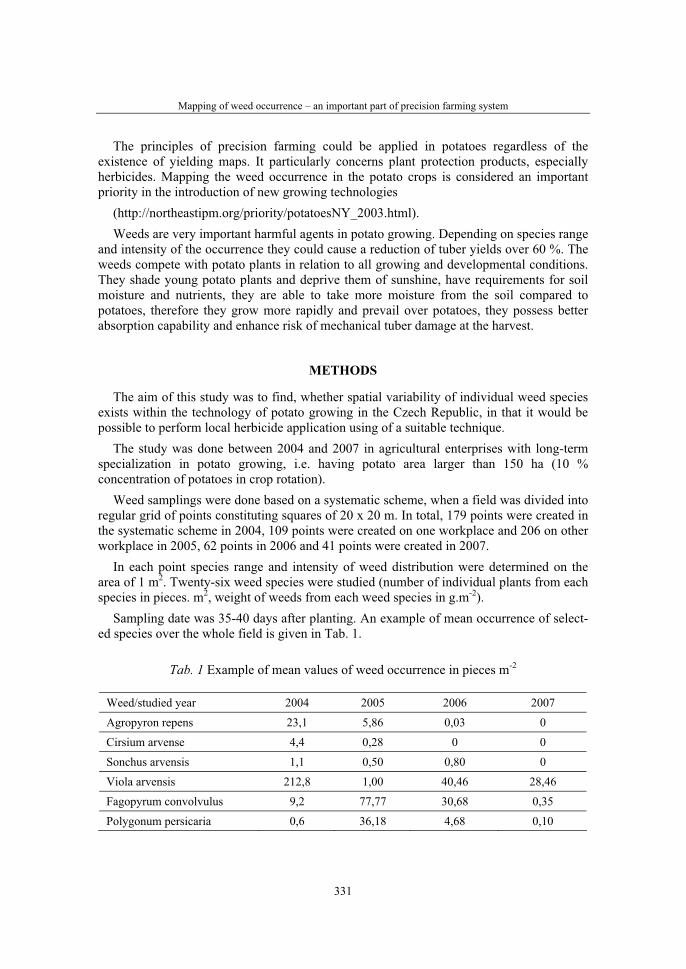
Mapping of weed occurrence – an important part of precision farming system
331
The principles of precision farming could be applied in potatoes regardless of the existence of yielding maps. It particularly concerns plant protection products, especially herbicides. Mapping the weed occurrence in the potato crops is considered an important priority in the introduction of new growing technologies
(http://northeastipm.org/priority/potatoesNY_2003.html).Weeds are very important harmful agents in potato growing. Depending on species range
and intensity of the occurrence they could cause a reduction of tuber yields over 60 %. The weeds compete with potato plants in relation to all growing and developmental conditions. They shade young potato plants and deprive them of sunshine, have requirements for soil moisture and nutrients, they are able to take more moisture from the soil compared to potatoes, therefore they grow more rapidly and prevail over potatoes, they possess better absorption capability and enhance risk of mechanical tuber damage at the harvest.
METHODS
The aim of this study was to find, whether spatial variability of individual weed species exists within the technology of potato growing in the Czech Republic, in that it would be possible to perform local herbicide application using of a suitable technique.
The study was done between 2004 and 2007 in agricultural enterprises with long-term specialization in potato growing, i.e. having potato area larger than 150 ha (10 % concentration of potatoes in crop rotation).
Weed samplings were done based on a systematic scheme, when a field was divided into regular grid of points constituting squares of 20 x 20 m. In total, 179 points were created in the systematic scheme in 2004, 109 points were created on one workplace and 206 on other workplace in 2005, 62 points in 2006 and 41 points were created in 2007.
In each point species range and intensity of weed distribution were determined on the area of 1 m2. Twenty-six weed species were studied (number of individual plants from each species in pieces. m2, weight of weeds from each weed species in g.m-2).
Sampling date was 35-40 days after planting. An example of mean occurrence of select-ed species over the whole field is given in Tab. 1.
Tab. 1 Example of mean values of weed occurrence in pieces m-2
Weed/studied year 2004 2005 2006 2007
Agropyron repens 23,1 5,86 0,03 0
Cirsium arvense 4,4 0,28 0 0
Sonchus arvensis 1,1 0,50 0,80 0
Viola arvensis 212,8 1,00 40,46 28,46
Fagopyrum convolvulus 9,2 77,77 30,68 0,35
Polygonum persicaria 0,6 36,18 4,68 0,10
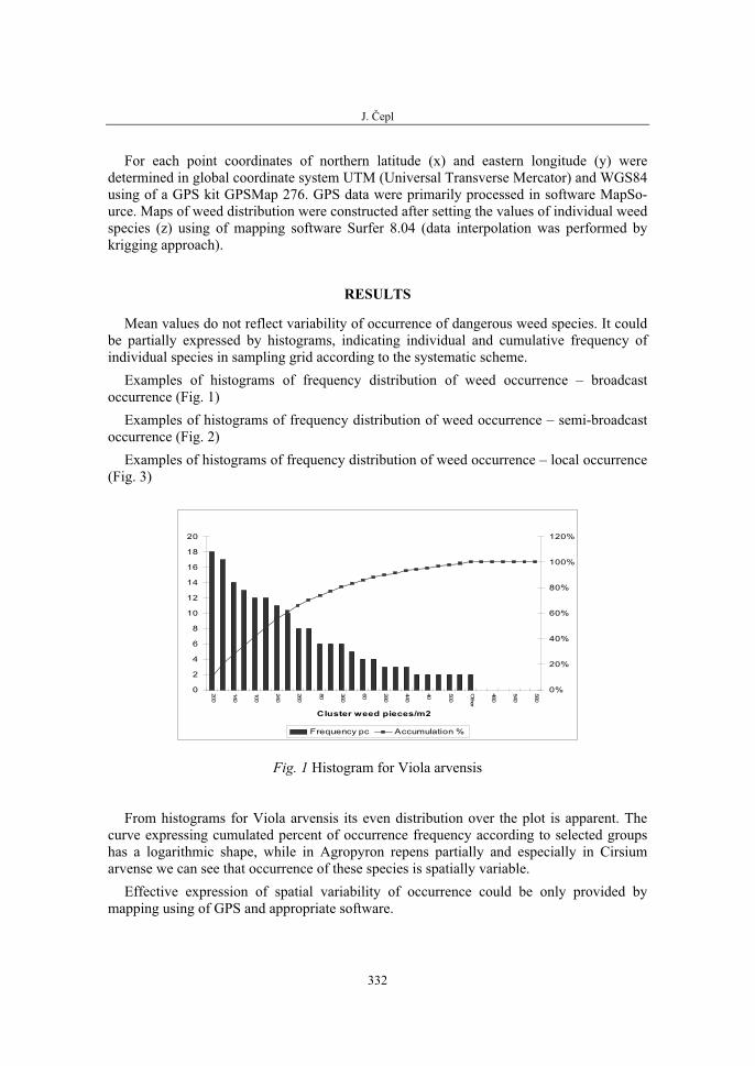
J. Čepl
332
For each point coordinates of northern latitude (x) and eastern longitude (y) were determined in global coordinate system UTM (Universal Transverse Mercator) and WGS84 using of a GPS kit GPSMap 276. GPS data were primarily processed in software MapSo-urce. Maps of weed distribution were constructed after setting the values of individual weed species (z) using of mapping software Surfer 8.04 (data interpolation was performed by krigging approach).
RESULTS
Mean values do not reflect variability of occurrence of dangerous weed species. It could be partially expressed by histograms, indicating individual and cumulative frequency of individual species in sampling grid according to the systematic scheme.
Examples of histograms of frequency distribution of weed occurrence – broadcast occurrence (Fig. 1)
Examples of histograms of frequency distribution of weed occurrence – semi-broadcast occurrence (Fig. 2)
Examples of histograms of frequency distribution of weed occurrence – local occurrence (Fig. 3)
0
2
4
6
8
10
12
14
16
18
20200
140
100
240
260
80 360
60 280
440
40 500
Other
480
540
580
Cluster weed pieces/m2
0%
20%
40%
60%
80%
100%
120%
Frequency pc Accumulation %
Fig. 1 Histogram for Viola arvensis
From histograms for Viola arvensis its even distribution over the plot is apparent. The curve expressing cumulated percent of occurrence frequency according to selected groups has a logarithmic shape, while in Agropyron repens partially and especially in Cirsium arvense we can see that occurrence of these species is spatially variable.
Effective expression of spatial variability of occurrence could be only provided by mapping using of GPS and appropriate software.
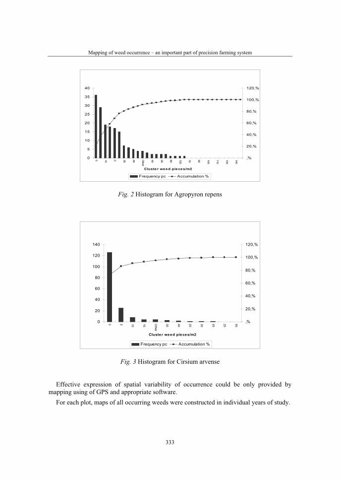
Mapping of weed occurrence – an important part of precision farming system
333
0
5
10
15
20
25
30
35
40
5 15 0 35 45 Other
40 55 60 120
70 90 100
110
125
140
Cluster weed pieces/m2
,%
20,%
40,%
60,%
80,%
100,%
120,%
Frequency pc Accumulation %
Fig. 2 Histogram for Agropyron repens
0
20
40
60
80
100
120
140
0 5 10 15 Other
35 40 20 30 45 25 50
Cluster weed pieces/m2
,%
20,%
40,%
60,%
80,%
100,%
120,%
Frequency pc Accumulation %
Fig. 3 Histogram for Cirsium arvense
Effective expression of spatial variability of occurrence could be only provided by mapping using of GPS and appropriate software.
For each plot, maps of all occurring weeds were constructed in individual years of study.
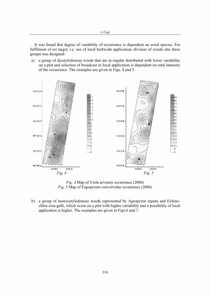
J. Čepl
334
It was found that degree of variability of occurrence is dependent on weed species. For fulfilment of set target, i.e. use of local herbicide application, division of weeds into three groups was designed: a) a group of dicotyledonous weeds that are in regular distributed with lower variability
on a plot and selection of broadcast or local application is dependent on total intensity of the occurrence. The examples are given in Figs. 4 and 5.
Fig. 4 Fig. 5
Fig. 4 Map of Viola arvensis occurrence (2006) Fig. 5 Map of Fagopyrum convolvulus occurrence (2006)
b) a group of monocotyledonous weeds represented by Agropyron repens and Echino-chloa crus-galli, which occur on a plot with higher variability and a possibility of local application is higher. The examples are given in Figs.6 and 7.

Mapping of weed occurrence – an important part of precision farming system
335
Fig. 6 Fig. 7
Fig. 6 Map of Agropyron repens occurrence (2005) Fig. 7 Map of Echinochloa crus-galli occurrence (2007)
c) a group of dicotyledonous weeds, which are represented by Sonchus arvensis and Cirsium arvense with very high variability of their occurrence on a plot (often also after first overall treatment with a herbicide) and local application can be done almost every time. The examples are given in Figs. 8 and 9.
The efficiency of a treatment is decided by occurrence of a weed in comparison to threshold critical amount. Critical amount is such a value of occurrence per area unit, in which cultivated crop is endangered due to weed competition ability. We determined critical amounts of weeds in parallel established trials. Hitherto results indicate that e.g. five plants per 1 m2 are critical amount in Agropyron repens, 2 plants in Galim aparine, Sonchus arvensis and Chenopodium album and only 1 plant in volunteer rape and Cirsium arvense.
This critical number is taken away from concrete value of the occurrence in a studied point. If the sum of all results in all weeds is more than 1, the value YES (1) is assigned to the point, if the sum is nil, value NO (0) is assigned to the point.
Fig. 10 illustrates an application map from the year 2005 in the enterprise Olešná, where 47 % of herbicide could be saved, Fig. 11 presents an application map from the enterprise Borová with a saving of 57 % of herbicide. On contrary, saving in the enterprise Olešná would not be substantial in the year 2006 (Fig. 12). In 2007 44 % of herbicide could be saved according to an application map in the enterprise Okrouhlice (Fig. 13).

J. Čepl
336
Fig. 8 Fig. 9
Fig. 8 Map of Cirsium arvense occurrence (2005) Fig. 9 Map of Sonchus arvensis occurrence (2007)
Fig. 10 Fig. 11
Fig. 10 Application map of Olešná 2005 Fig. 11 Application map of Borová 2005
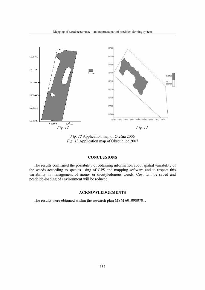
Mapping of weed occurrence – an important part of precision farming system
337
Fig. 12 Fig. 13
Fig. 12 Application map of Olešná 2006 Fig. 13 Application map of Okrouhlice 2007
CONCLUSIONS
The results confirmed the possibility of obtaining information about spatial variability of the weeds according to species using of GPS and mapping software and to respect this variability in management of mono- or dicotyledonous weeds. Cost will be saved and pesticide-loading of environment will be reduced.
ACKNOWLEDGEMENTS
The results were obtained within the research plan MSM 6010980701.

J. Čepl
338
REFERENCES
1. Balík J. (2005). Precizní zemědělství, In: Závěrečná zpráva Vědeckého výboru fytosanitární a životní prostředí. (http://www.phytosanitary.org/pdf/zprava_2005.pdf)
2. Ehlert D. (2002). Bounce plate for yield mapping of potatoes in precision farming, In: Potatoes today and tomorrow, Abstract of papers, 15. triennial conference of EAPR, Hamburg, pp 67
3. Hamouz P., Soukup J., Holec J., Jursík M. (2004). Field-scale variability of weediness on arable land. Plant Soil Environ 50: 134-140
4. Molema G. J., Hofstee J.W. (2002). Machine vision based potato yield mapping, In: Potatoes today and tomorrow, Abstract of papers, 15. triennial conference of EAPR, Hamburg, pp 66
5. New York State Potato Industry Priorities
6. http://northeastipm.org/priority/potatoesNY_2003.html
36. Symposium "Actual Tasks on Agricultural Engineering", Opatija, Croatia, 2008.
339
36.
SIMPOZIJAKTUALNI ZADACIMEHANIZACIJE POLJOPRIVREDE
UDC621.317.799:631.171Prethodno priopćenje
Preliminary communication
AN ACCESSORIAL NAVIGATION AND SURVEILLANCE SYSTEM USED IN AGRICULTURE
ZHOU JIANJUN1, ZHANG MAN1, LI SU2, WANG MAOHUA1, LI S IYU1
1College of Information and Electrical Engineering, China Agricultural University, Beijing, China, 100083, e-mail:[email protected], [email protected]
2Computer College, Beijing Technology and Business University, Beijing, China, 100037
SUMMARY
Automatic navigation of farm machinery is an essential technique to realize positioning prescription agriculture and collecting positioning information. It advances the development of precision agriculture greatly. This paper presents an accessorial navigation and surveillance system. The system has the function of reading prescription map for variable rate application, indicating the position of tractor and helping agriculture machine navigate. The vehicle equips DGPS, electronic compass and angle transducer. In the system, light bar is realized by software and it can indicate the cross track error of tractor. Using an accumulator vehicle as the experimental platform, a simple automatic navigation prototype system is developed.
Key words: automatic navigation; positioning; precision agriculture; GPS
INTRODUCTION
Automatic navigation of farm machinery is an essential technique to realize positioning prescription agriculture and collecting positioning information. It advances the development of precision agriculture greatly. At the same time, it will improve the working efficiency and working precision in farmland, which will lower the working cost and reduce the working strength (Reid, J.F., Qin Zhang et al., 2000). As an important branch of precision agricultural, the farm machinery intelligent navigation technology is receiving more and more attention. It has two main advantages. Firstly, it may liberate the farm machinery pilot from the monotonous repetition work. Second it may increase the precision of work (S. Han, Q. Zhang, H. Noh, B. Shin, 2004).
The research and development of field computer always pays little attention in china, but there is some pertinent research in the other countries. According to the research trend from
J. Zhou, M. Zhang, S. Li, M. Wang, S I. Li
340
the other country, this kind of system not only has its predominance, but also accords with the development trend of agriculture mechanization in precision agriculture. The field computer benefits the progress of agriculture machine navigation equipment (Guo Linsong, He Yong, Zhang Qin et al., 2002).
The accessorial navigation and surveillance system applied in agriculture is a kind of field computer system which is installed on agriculture machine. It has the function of help-ing agriculture machine navigate, reading prescription map for variable rate application, performing variable rate application.
This paper mainly studies positioning and control of automatic navigation based on GPS and posture sensors. An accessorial navigation and surveillance system applied in agricu-lture is developed. A prototype vehicle with automatic navigation function is realized.
RESEARCH PLATFORM
Experiment deviceThe experiment platform is a storage battery car. The car includes steering controller,
posture information acquiring sensors and GPS receiver. Figure 1 shows the storage battery car. The posture information acquiring sensors include angle transducer, accelerometer and digital compass. The angle transducer transforms the angle mechanical rotation to the electrical signal. It can measure the change of the angle-displacement. The angle transducer is equipped in the axis of front wheel of the car and used for measuring turning angle of the front wheel. Figure2 shows the angle transducer, whose type is WYT-AT-1.�
The type of the digital compass is LP3300. There are three orthogonal magnetic field sensors and two axle inclination angle sensors in this digital compass. Figure 3 shows the shape of the digital compass. LP3300 outputs data through the RS-232 and the configu-ration of RS232 is "9600, n, 8, 1". Each frame outputs 20 bytes hexadecimal number.
Field computerField computer is integrated by a single board computer and a USB_CAN card. The type
of the single board computer is PPC-3712GS. Figure 4 shows the computer. It is the product of IEI Company. Table 1 shows the specification of PPC-3712GS.
Table 1 specification of PPC-3712GS
Item Description I/O 4 x COM (1 inside for Touch Screen), 4 x USB,
1 x CF socket Multi-mounting functions: Panel, Wall, Rack and VESA Standard ARM
mounting support Ethernet 1x Gigabit Ethernet support Memory 1G
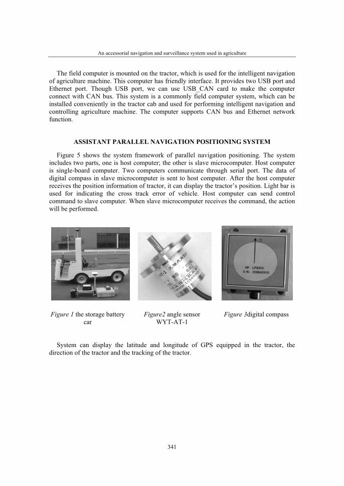
An accessorial navigation and surveillance system used in agriculture
341
The field computer is mounted on the tractor, which is used for the intelligent navigation of agriculture machine. This computer has friendly interface. It provides two USB port and Ethernet port. Though USB port, we can use USB_CAN card to make the computer connect with CAN bus. This system is a commonly field computer system, which can be installed conveniently in the tractor cab and used for performing intelligent navigation and controlling agriculture machine. The computer supports CAN bus and Ethernet network function.
ASSISTANT PARALLEL NAVIGATION POSITIONING SYSTEM
Figure 5 shows the system framework of parallel navigation positioning. The system includes two parts, one is host computer; the other is slave microcomputer. Host computer is single-board computer. Two computers communicate through serial port. The data of digital compass in slave microcomputer is sent to host computer. After the host computer receives the position information of tractor, it can display the tractor’s position. Light bar is used for indicating the cross track error of vehicle. Host computer can send control command to slave computer. When slave microcomputer receives the command, the action will be performed.
Figure 1 the storage battery car
Figure2 angle sensor WYT-AT-1
Figure 3digital compass
System can display the latitude and longitude of GPS equipped in the tractor, the direction of the tractor and the tracking of the tractor.
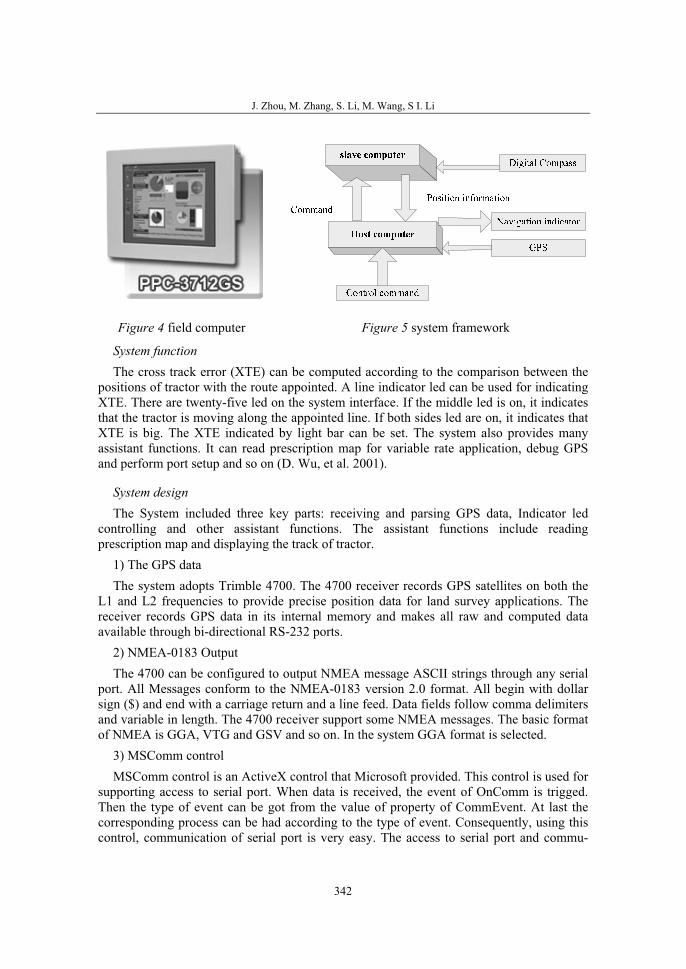
J. Zhou, M. Zhang, S. Li, M. Wang, S I. Li
342
�������
Figure 4 field computer Figure 5 system framework
System function The cross track error (XTE) can be computed according to the comparison between the
positions of tractor with the route appointed. A line indicator led can be used for indicating XTE. There are twenty-five led on the system interface. If the middle led is on, it indicates that the tractor is moving along the appointed line. If both sides led are on, it indicates that XTE is big. The XTE indicated by light bar can be set. The system also provides many assistant functions. It can read prescription map for variable rate application, debug GPS and perform port setup and so on (D. Wu, et al. 2001).
System designThe System included three key parts: receiving and parsing GPS data, Indicator led
controlling and other assistant functions. The assistant functions include reading prescription map and displaying the track of tractor.
1) The GPS data The system adopts Trimble 4700. The 4700 receiver records GPS satellites on both the
L1 and L2 frequencies to provide precise position data for land survey applications. The receiver records GPS data in its internal memory and makes all raw and computed data available through bi-directional RS-232 ports.
2) NMEA-0183 Output The 4700 can be configured to output NMEA message ASCII strings through any serial
port. All Messages conform to the NMEA-0183 version 2.0 format. All begin with dollar sign ($) and end with a carriage return and a line feed. Data fields follow comma delimiters and variable in length. The 4700 receiver support some NMEA messages. The basic format of NMEA is GGA, VTG and GSV and so on. In the system GGA format is selected.
3) MSComm control MSComm control is an ActiveX control that Microsoft provided. This control is used for
supporting access to serial port. When data is received, the event of OnComm is trigged. Then the type of event can be got from the value of property of CommEvent. At last the corresponding process can be had according to the type of event. Consequently, using this control, communication of serial port is very easy. The access to serial port and commu-
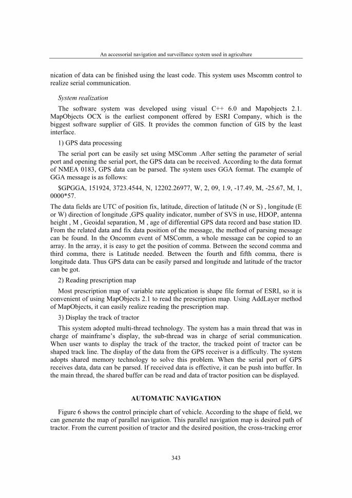
An accessorial navigation and surveillance system used in agriculture
343
nication of data can be finished using the least code. This system uses Mscomm control to realize serial communication.
System realization The software system was developed using visual C++ 6.0 and Mapobjects 2.1.
MapObjects OCX is the earliest component offered by ESRI Company, which is the biggest software supplier of GIS. It provides the common function of GIS by the least interface.
1) GPS data processing The serial port can be easily set using MSComm .After setting the parameter of serial
port and opening the serial port, the GPS data can be received. According to the data format of NMEA 0183, GPS data can be parsed. The system uses GGA format. The example of GGA message is as follows:
$GPGGA, 151924, 3723.4544, N, 12202.26977, W, 2, 09, 1.9, -17.49, M, -25.67, M, 1, 0000*57.The data fields are UTC of position fix, latitude, direction of latitude (N or S) , longitude (E or W) direction of longitude ,GPS quality indicator, number of SVS in use, HDOP, antenna height , M , Geoidal separation, M , age of differential GPS data record and base station ID. From the related data and fix data position of the message, the method of parsing message can be found. In the Oncomm event of MSComm, a whole message can be copied to an array. In the array, it is easy to get the position of comma. Between the second comma and third comma, there is Latitude needed. Between the fourth and fifth comma, there is longitude data. Thus GPS data can be easily parsed and longitude and latitude of the tractor can be got.
2) Reading prescription mapMost prescription map of variable rate application is shape file format of ESRI, so it is
convenient of using MapObjects 2.1 to read the prescription map. Using AddLayer method of MapObjects, it can easily realize reading the prescription map.
3) Display the track of tractor This system adopted multi-thread technology. The system has a main thread that was in
charge of mainframe’s display, the sub-thread was in charge of serial communication. When user wants to display the track of the tractor, the tracked point of tractor can be shaped track line. The display of the data from the GPS receiver is a difficulty. The system adopts shared memory technology to solve this problem. When the serial port of GPS receives data, data can be parsed. If received data is effective, it can be push into buffer. In the main thread, the shared buffer can be read and data of tractor position can be displayed.
AUTOMATIC NAVIGATION
Figure 6 shows the control principle chart of vehicle. According to the shape of field, we can generate the map of parallel navigation. This parallel navigation map is desired path of tractor. From the current position of tractor and the desired position, the cross-tracking error
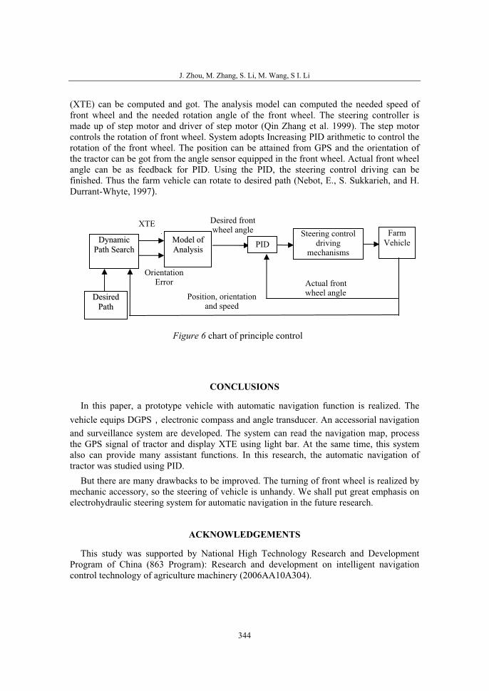
J. Zhou, M. Zhang, S. Li, M. Wang, S I. Li
344
(XTE) can be computed and got. The analysis model can computed the needed speed of front wheel and the needed rotation angle of the front wheel. The steering controller is made up of step motor and driver of step motor (Qin Zhang et al. 1999). The step motor controls the rotation of front wheel. System adopts Increasing PID arithmetic to control the rotation of the front wheel. The position can be attained from GPS and the orientation of the tractor can be got from the angle sensor equipped in the front wheel. Actual front wheel angle can be as feedback for PID. Using the PID, the steering control driving can be finished. Thus the farm vehicle can rotate to desired path (Nebot, E., S. Sukkarieh, and H. Durrant-Whyte, 1997).
CONCLUSIONS
In this paper, a prototype vehicle with automatic navigation function is realized. The vehicle equips DGPS�electronic compass and angle transducer. An accessorial navigation and surveillance system are developed. The system can read the navigation map, process the GPS signal of tractor and display XTE using light bar. At the same time, this system also can provide many assistant functions. In this research, the automatic navigation of tractor was studied using PID.
But there are many drawbacks to be improved. The turning of front wheel is realized by mechanic accessory, so the steering of vehicle is unhandy. We shall put great emphasis on electrohydraulic steering system for automatic navigation in the future research.
ACKNOWLEDGEMENTS
This study was supported by National High Technology Research and Development Program of China (863 Program): Research and development on intelligent navigation control technology of agriculture machinery (2006AA10A304).
Desired frontwheel angle
MMooddeell ooffAAnnaallyyssiiss
Steering control driving
mechanisms
FarmVehicle DDyynnaammiicc
PPaatthh SSeeaarrcchh
OrientationError
DDeessiirreeddPPaatthh
PID
Actual front wheel angle Position, orientation
and speed
XTE
Figure 6 chart of principle control
An accessorial navigation and surveillance system used in agriculture
345
REFERENCES
1. S. Han, Q. Zhang, H. Noh, B. Shin. (2004). A dynamic performance evaluation method for DGPS receivers under linear parallel-tracking applications. Transactions of the ASAE, Vol. 47(1): 321-329.
2. Guo Linsong, He Yong, Zhang Qin et al. (2002). Real-Time Tractor Position Estimation System Using a Kalman Filter. Transactions of the CSAE,Vol.18 (5):96-98.
3. D. Wu, Q. Zhang and J. F. Reid, (2001). Adaptive steering controller using a Kalman estimator for wheel-type agricultural tractors. Robotica, volume 19, pp.527-533.
4. Qin Zhang, John F. Reid, Noboru Noguchi.(1999). Automated Guidance Control for Agricultural Tractor Using Redundant Sensors. Journal of Commercial Vehicles, 108:27-31.
5. Nebot, E., S. Sukkarieh, and H. Durrant-Whyte, 1997. Inertial navigation aided with GPS information, Proceedings of Fourth Annual Conference on Mechatronics and Machine Vision in Practice, pp.169–174, Toowoomba, Qld., Australia.
6. Reid, J.F., Qin Zhang, Noboru Noguchi and Monte Dickson, 2000. Agricultural automatic guidance research in North America, Computers and Electronics in Agriculture, 25(1-2):155-167.

36. Symposium "Actual Tasks on Agricultural Engineering", Opatija, Croatia, 2008.
347
36.
SIMPOZIJAKTUALNI ZADACIMEHANIZACIJE POLJOPRIVREDE
UDC004.89:628.356
Prethodno priopćenjePreliminary communication
PATH PLANNING FOR A SLUDGE PROCESSING ROBOT BY MEANS OF TRAJECTORY SIMULATION
NIKICA STARČEVIĆ1), CHRISTIAN THULLNER1), MARKUS BUX2),JOACHIM MÜLLER1)
1) Universität Hohenheim, Institute of Agricultural Engineering (440e), Garbenstrasse 9, 70599 Stuttgart, Germany, e-mail: [email protected]
2) Thermo-System Industrie- und Trocknungstechnik GmbH,70794 Filderstadt-Bernhausen, Germany
SUMMARY
The Universität Hohenheim and Thermo-System GmbH have developed six motion strategies for a Cartesian 4-DOF mixing and transporting greenhouse robot. Each of the corresponding trajectories consists of more than 1,300 three-dimensional coordinate points. The general approach of motion strategy assessment was done according to the guideline VDI-4446. The total cycle times range between 84,328 s and 114,099 s. The covered distances stot range between 33 km and 44 km per day. By doubling maximum velocity to 60 m/min in x-direction and to 20 m/min in y-direction the total cycle times would be reduced by maximum 20%.
Key words: Path, trajectory, motion, strategy, simulation, robot, solar, drying, biomass
INTRODUCTION
The Universität Hohenheim and Thermo-System GmbH have developed a Cartesian 4-DOF mixing and transporting robot for solar drying of moist biomass (Starcevic et al.,2006; Starcevic et al., 2007). In the next step, a control system had to be developed in order to enable autonomous mixing and transport of the sludge within the dryer. Furthermore, charging and discharging of the solar dryer had to be performed automatically. Therefore, motion paths for the robot had to be developed. The corresponding motion strategies had to be evaluated regarding cycle time, productive and unproductive phases in order to exclusively select the best one for being embedded into the control system.
At present, in literature basically two different possibilities for controlling trajectories of Cartesian robots are reported. The first possibility is a “point-to-point” control. The second
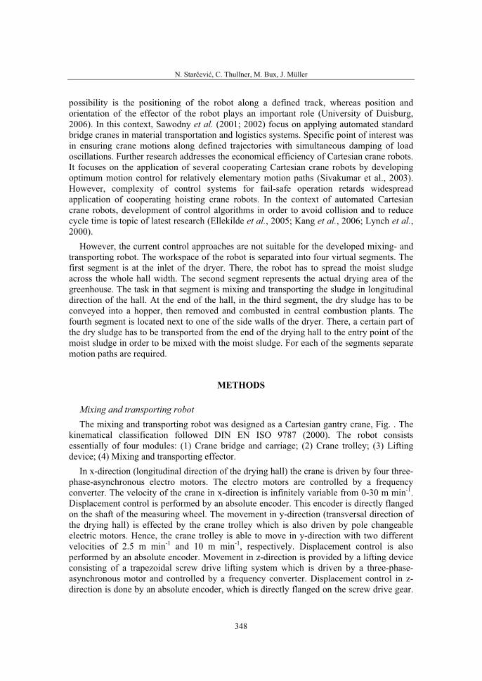
N. Starčević, C. Thullner, M. Bux, J. Müller
348
possibility is the positioning of the robot along a defined track, whereas position and orientation of the effector of the robot plays an important role (University of Duisburg, 2006). In this context, Sawodny et al. (2001; 2002) focus on applying automated standard bridge cranes in material transportation and logistics systems. Specific point of interest was in ensuring crane motions along defined trajectories with simultaneous damping of load oscillations. Further research addresses the economical efficiency of Cartesian crane robots. It focuses on the application of several cooperating Cartesian crane robots by developing optimum motion control for relatively elementary motion paths (Sivakumar et al., 2003). However, complexity of control systems for fail-safe operation retards widespread application of cooperating hoisting crane robots. In the context of automated Cartesian crane robots, development of control algorithms in order to avoid collision and to reduce cycle time is topic of latest research (Ellekilde et al., 2005; Kang et al., 2006; Lynch et al.,2000).
However, the current control approaches are not suitable for the developed mixing- and transporting robot. The workspace of the robot is separated into four virtual segments. The first segment is at the inlet of the dryer. There, the robot has to spread the moist sludge across the whole hall width. The second segment represents the actual drying area of the greenhouse. The task in that segment is mixing and transporting the sludge in longitudinal direction of the hall. At the end of the hall, in the third segment, the dry sludge has to be conveyed into a hopper, then removed and combusted in central combustion plants. The fourth segment is located next to one of the side walls of the dryer. There, a certain part of the dry sludge has to be transported from the end of the drying hall to the entry point of the moist sludge in order to be mixed with the moist sludge. For each of the segments separate motion paths are required.
METHODS
Mixing and transporting robot The mixing and transporting robot was designed as a Cartesian gantry crane, Fig. . The
kinematical classification followed DIN EN ISO 9787 (2000). The robot consists essentially of four modules: (1) Crane bridge and carriage; (2) Crane trolley; (3) Lifting device; (4) Mixing and transporting effector.
In x-direction (longitudinal direction of the drying hall) the crane is driven by four three-phase-asynchronous electro motors. The electro motors are controlled by a frequency converter. The velocity of the crane in x-direction is infinitely variable from 0-30 m min-1.Displacement control is performed by an absolute encoder. This encoder is directly flanged on the shaft of the measuring wheel. The movement in y-direction (transversal direction of the drying hall) is effected by the crane trolley which is also driven by pole changeable electric motors. Hence, the crane trolley is able to move in y-direction with two different velocities of 2.5 m min-1 and 10 m min-1, respectively. Displacement control is also performed by an absolute encoder. Movement in z-direction is provided by a lifting device consisting of a trapezoidal screw drive lifting system which is driven by a three-phase-asynchronous motor and controlled by a frequency converter. Displacement control in z-direction is done by an absolute encoder, which is directly flanged on the screw drive gear.
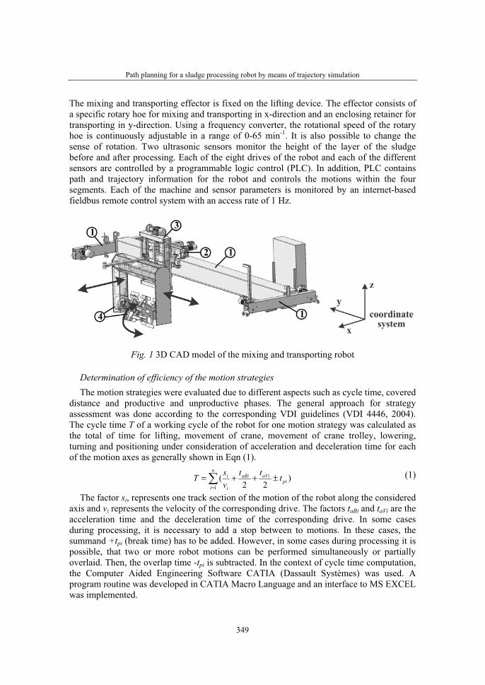
Path planning for a sludge processing robot by means of trajectory simulation
349
The mixing and transporting effector is fixed on the lifting device. The effector consists of a specific rotary hoe for mixing and transporting in x-direction and an enclosing retainer for transporting in y-direction. Using a frequency converter, the rotational speed of the rotary hoe is continuously adjustable in a range of 0-65 min-1. It is also possible to change the sense of rotation. Two ultrasonic sensors monitor the height of the layer of the sludge before and after processing. Each of the eight drives of the robot and each of the different sensors are controlled by a programmable logic control (PLC). In addition, PLC contains path and trajectory information for the robot and controls the motions within the four segments. Each of the machine and sensor parameters is monitored by an internet-based fieldbus remote control system with an access rate of 1 Hz.
Fig. 1 3D CAD model of the mixing and transporting robot
Determination of efficiency of the motion strategies The motion strategies were evaluated due to different aspects such as cycle time, covered
distance and productive and unproductive phases. The general approach for strategy assessment was done according to the corresponding VDI guidelines (VDI 4446, 2004). The cycle time T of a working cycle of the robot for one motion strategy was calculated as the total of time for lifting, movement of crane, movement of crane trolley, lowering, turning and positioning under consideration of acceleration and deceleration time for each of the motion axes as generally shown in Eqn (1).
)22
(1
piaViaBi
n
i i
i tttvsT ±++=∑
=
(1)
The factor si, represents one track section of the motion of the robot along the considered axis and vi represents the velocity of the corresponding drive. The factors taBi and taVi are the acceleration time and the deceleration time of the corresponding drive. In some cases during processing, it is necessary to add a stop between to motions. In these cases, the summand +tpi (break time) has to be added. However, in some cases during processing it is possible, that two or more robot motions can be performed simultaneously or partially overlaid. Then, the overlap time -tpi is subtracted. In the context of cycle time computation, the Computer Aided Engineering Software CATIA (Dassault Systèmes) was used. A program routine was developed in CATIA Macro Language and an interface to MS EXCEL was implemented.
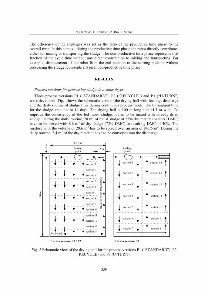
N. Starčević, C. Thullner, M. Bux, J. Müller
350
The efficiency of the strategies was set as the ratio of the productive time phase to the overall time. In this context, during the productive time phase the robot directly contributes either for mixing or transporting the sludge. The non-productive time phase represents that fraction of the cycle time without any direct contribution to mixing and transporting. For example, displacement of the robot from the end position to the starting position without processing the sludge represents a typical non-productive time phase.
RESULTS
Process versions for processing sludge in a solar dryer Three process versions P1 (“STANDARD”), P2 (“RECYCLE”) and P3 (“U-TURN”)
were developed. Fig. shows the schematic view of the drying hall with feeding, discharge and the daily routine of sludge flow during continuous process mode. The throughput time for the sludge amounts to 14 days. The drying hall is 100 m long and 14.5 m wide. To improve the consistency of the fed moist sludge, it has to be mixed with already dried sludge. During the daily routine, 20 m3 of moist sludge at 25% dry matter contents (DMC) have to be mixed with 8.6 m3 of dry sludge (75% DMC) to resulting DMC of 40%. The mixture with the volume of 28.6 m3 has to be spread over an area of 84.75 m2. During the daily routine, 2.4 m3 of the dry material have to be conveyed into the discharge.
14.5 m
100 m
3 m
2 m
section 1
feeding
point
discharge
Process version P1 / P2
section 2
section 3
section 4
section 5
section 6
section 7
section 8
section 9
section 10
section 11
section 12
section 13
section 14
feeding
point
discharge
section 1
section 2
section 3
section 4
section 5
section 6
section 7
section 14
section 13
section 12
section 11
section 10
section 9
section 8
track for return transporting
Process version P3
Fig. 2 Schematic view of the drying hall for the process versions P1 (“STANDARD”), P2 (RECYCLE) and P3 (U-TURN).
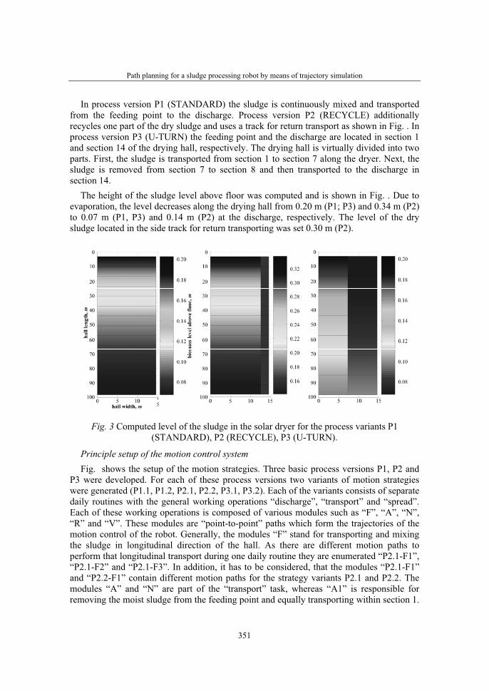
Path planning for a sludge processing robot by means of trajectory simulation
351
In process version P1 (STANDARD) the sludge is continuously mixed and transported from the feeding point to the discharge. Process version P2 (RECYCLE) additionally recycles one part of the dry sludge and uses a track for return transport as shown in Fig. . In process version P3 (U-TURN) the feeding point and the discharge are located in section 1 and section 14 of the drying hall, respectively. The drying hall is virtually divided into two parts. First, the sludge is transported from section 1 to section 7 along the dryer. Next, the sludge is removed from section 7 to section 8 and then transported to the discharge in section 14.
The height of the sludge level above floor was computed and is shown in Fig. . Due to evaporation, the level decreases along the drying hall from 0.20 m (P1; P3) and 0.34 m (P2) to 0.07 m (P1, P3) and 0.14 m (P2) at the discharge, respectively. The level of the dry sludge located in the side track for return transporting was set 0.30 m (P2).
Fig. 3 Computed level of the sludge in the solar dryer for the process variants P1 (STANDARD), P2 (RECYCLE), P3 (U-TURN).
Principle setup of the motion control system Fig. shows the setup of the motion strategies. Three basic process versions P1, P2 and
P3 were developed. For each of these process versions two variants of motion strategies were generated (P1.1, P1.2, P2.1, P2.2, P3.1, P3.2). Each of the variants consists of separate daily routines with the general working operations “discharge”, “transport” and “spread”. Each of these working operations is composed of various modules such as “F”, “A”, “N”, “R” and “V”. These modules are “point-to-point” paths which form the trajectories of the motion control of the robot. Generally, the modules “F” stand for transporting and mixing the sludge in longitudinal direction of the hall. As there are different motion paths to perform that longitudinal transport during one daily routine they are enumerated “P2.1-F1”, “P2.1-F2” and “P2.1-F3”. In addition, it has to be considered, that the modules “P2.1-F1” and “P2.2-F1” contain different motion paths for the strategy variants P2.1 and P2.2. The modules “A” and “N” are part of the “transport” task, whereas “A1” is responsible for removing the moist sludge from the feeding point and equally transporting within section 1.
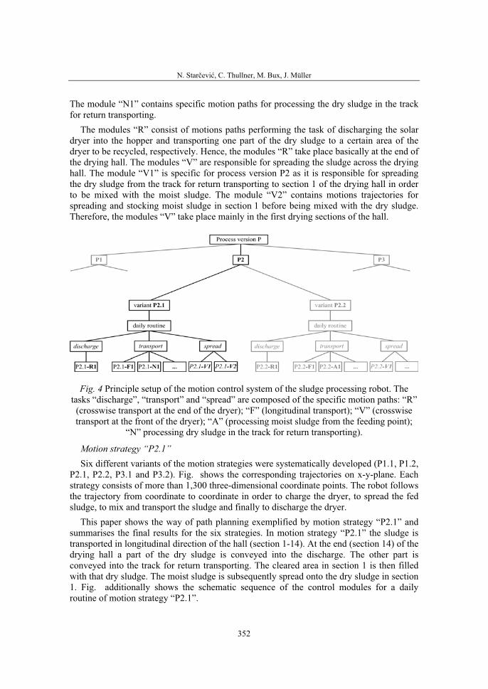
N. Starčević, C. Thullner, M. Bux, J. Müller
352
The module “N1” contains specific motion paths for processing the dry sludge in the track for return transporting.
The modules “R” consist of motions paths performing the task of discharging the solar dryer into the hopper and transporting one part of the dry sludge to a certain area of the dryer to be recycled, respectively. Hence, the modules “R” take place basically at the end of the drying hall. The modules “V” are responsible for spreading the sludge across the drying hall. The module “V1” is specific for process version P2 as it is responsible for spreading the dry sludge from the track for return transporting to section 1 of the drying hall in order to be mixed with the moist sludge. The module “V2” contains motions trajectories for spreading and stocking moist sludge in section 1 before being mixed with the dry sludge. Therefore, the modules “V” take place mainly in the first drying sections of the hall.
Fig. 4 Principle setup of the motion control system of the sludge processing robot. The tasks “discharge”, “transport” and “spread” are composed of the specific motion paths: “R”
(crosswise transport at the end of the dryer); “F” (longitudinal transport); “V” (crosswise transport at the front of the dryer); “A” (processing moist sludge from the feeding point);
“N” processing dry sludge in the track for return transporting).
Motion strategy “P2.1” Six different variants of the motion strategies were systematically developed (P1.1, P1.2,
P2.1, P2.2, P3.1 and P3.2). Fig. shows the corresponding trajectories on x-y-plane. Each strategy consists of more than 1,300 three-dimensional coordinate points. The robot follows the trajectory from coordinate to coordinate in order to charge the dryer, to spread the fed sludge, to mix and transport the sludge and finally to discharge the dryer.
This paper shows the way of path planning exemplified by motion strategy “P2.1” and summarises the final results for the six strategies. In motion strategy “P2.1” the sludge is transported in longitudinal direction of the hall (section 1-14). At the end (section 14) of the drying hall a part of the dry sludge is conveyed into the discharge. The other part is conveyed into the track for return transporting. The cleared area in section 1 is then filled with that dry sludge. The moist sludge is subsequently spread onto the dry sludge in section 1. Fig. additionally shows the schematic sequence of the control modules for a daily routine of motion strategy “P2.1”.
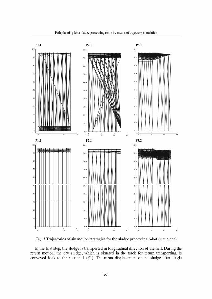
Path planning for a sludge processing robot by means of trajectory simulation
353
Fig. 5 Trajectories of six motion strategies for the sludge processing robot (x-y-plane)
In the first step, the sludge is transported in longitudinal direction of the hall. During the return motion, the dry sludge, which is situated in the track for return transporting, is conveyed back to the section 1 (F1). The mean displacement of the sludge after single
N. Starčević, C. Thullner, M. Bux, J. Müller
354
processing amounts in the drying area to 0.38 m and in the track for return transporting to 0.11-0.19 m. After the first transporting cycle a part of the dry sewage sludge is unloaded into the discharge in section 14 and a part of it into the track for return transporting (R1). Due to time restrictions, exclusively the last 1-m-wide track of section 14 is discharged. In the course of operation, always after three times transporting in longitudinal direction (F1, F2, F3) each, conveying into the discharge and into the area of return transportation is repeated (R1). Next, two cycles for the transporting of the sludge in longitudinal direction of the hall inclusive return transportation of the dry sludge (F1) must be performed. Now the sludge is displaced about 1 m along the drying area after the first three cycles (F1). As result, in section 1 a 1-m-wide area becomes clear. Dry sewage sludge from the track for return transporting has then to be conveyed on this area of section 1 (V1). However, merely half the required volume of 1.25 m³ is up to now available in the track for return transporting. Hence, the transportation in longitudinal direction of the hall must take place once more with concurrent return transportation of dry sludge after the first spreading of the dry sludge (F1). Finally, the remaining required dry sludge is pushed on the 1-m-wide area of section 1 and is afterwards levelled on a height of 0.1 m (V1). As up to now three transporting processes in longitudinal directed passed, a part of the dry sewage sludge is unloaded into the discharge in section 14 and a part of it into the track for return transporting (R1). Up to now, in the track of the return transportation the dry sludge was transported 5 m to the front of the drying hall. However, in section 14 the dry sludge was pushed only 1 m to the front of the drying hall. Therefore, a gap without any sludge has arisen in the track of return transportation within a length of 4 m. In order to close this gap, the dry sludge is transported in the track of the return transportation exclusively in the area of the gap (F2). The dry sludge is transported to front of the hall during the return runs. The cleared area in section 1 is filled, as already described, with dry sewage sludge again (V1).
This operating sequence recurs until the sludge is transported along the drying area for 4.18 m and the area is filled with dry sludge (F1, V1, R1, F2, F2, V1, F1, V1, R1, F3, V1). Then, feeding the dryer with moist sludge starts for the first time during the daily routine. During this time, the sludge is transported again 0.38 m in longitudinal direction of the hall (F1) and dry sludge is spread in section 1 (V1). Then the fed sewage sludge is spread on a surface of 12.5×2.0 m (V2). The dumping height is 0.25 m (0.1 m of dry sludge +0.15 m of humid sludge). After spreading the sludge is transported in longitudinal direction of the hall (F1). Then the newly fed sludge is spread and stacked again (V2). Between section 1 and section 2 a gap of 1.0 m emerged caused by transporting in longitudinal direction of the hall. This free space is filled with dry sludge (0.10 m) (V1) and afterwards with moist sludge (0.24 m) with a total height of the sludge level of 0.34 m (A1). In the course of further operation, the sludge is transported alternately in longitudinal direction of the hall (F3 and F1, respectively) and the newly fed sludge is spread and stacked (V2). Here, the gap between section 1 and 2 increases again. This gap is filled with dry sludge during the transporting in longitudinal direction of the hall and during the spreading or stacking of humid sludge (V1). After the 18th and therefore the last cycle for transporting in longitudinal direction (F1), the dry sludge is spread into the gap with a dumping height of 0.1 m (V1). Subsequently, the fed sludge is spread and stacked (V2). Next, the stacked sludge is spread on the dry sewage sludge and levelled in section 1 (A1). The height of the sludge level is hence 0.34 m. If the sludge is transported in longitudinal direction of the hall the next day, dry and moist sludge are mixed together. As during previous discharging, the
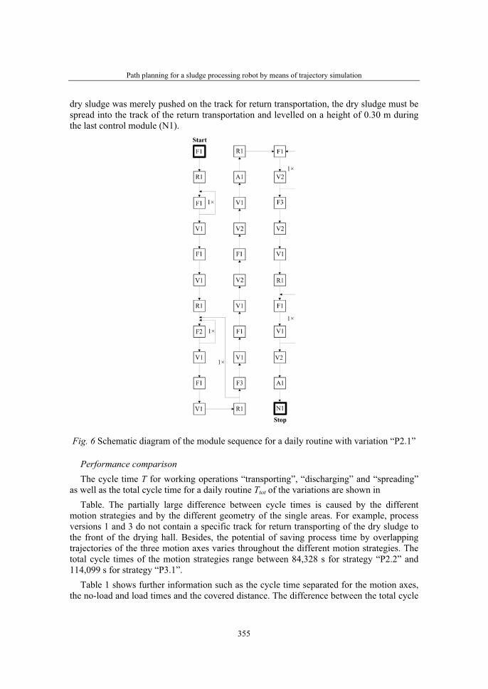
Path planning for a sludge processing robot by means of trajectory simulation
355
dry sludge was merely pushed on the track for return transportation, the dry sludge must be spread into the track of the return transportation and levelled on a height of 0.30 m during the last control module (N1).
Fig. 6 Schematic diagram of the module sequence for a daily routine with variation “P2.1”
Performance comparison The cycle time T for working operations “transporting”, “discharging” and “spreading”
as well as the total cycle time for a daily routine Ttot of the variations are shown inTable. The partially large difference between cycle times is caused by the different
motion strategies and by the different geometry of the single areas. For example, process versions 1 and 3 do not contain a specific track for return transporting of the dry sludge to the front of the drying hall. Besides, the potential of saving process time by overlapping trajectories of the three motion axes varies throughout the different motion strategies. The total cycle times of the motion strategies range between 84,328 s for strategy “P2.2” and 114,099 s for strategy “P3.1”.
Table 1 shows further information such as the cycle time separated for the motion axes, the no-load and load times and the covered distance. The difference between the total cycle
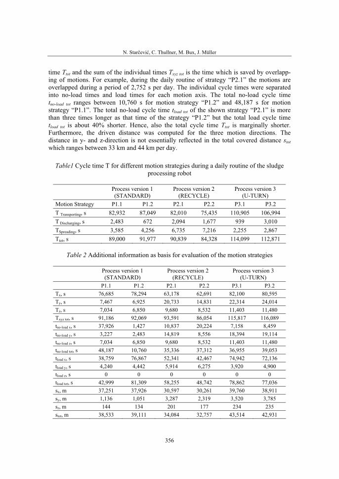
N. Starčević, C. Thullner, M. Bux, J. Müller
356
time Ttot and the sum of the individual times Txyz tot is the time which is saved by overlapp-ing of motions. For example, during the daily routine of strategy “P2.1” the motions are overlapped during a period of 2,752 s per day. The individual cycle times were separated into no-load times and load times for each motion axis. The total no-load cycle time tno-load tot ranges between 10,760 s for motion strategy “P1.2” and 48,187 s for motion strategy “P1.1”. The total no-load cycle time tload tot of the shown strategy “P2.1” is more than three times longer as that time of the strategy “P1.2” but the total load cycle time tload tot is about 40% shorter. Hence, also the total cycle time Ttot is marginally shorter. Furthermore, the driven distance was computed for the three motion directions. The distance in y- and z-direction is not essentially reflected in the total covered distance stotwhich ranges between 33 km and 44 km per day.
Table1 Cycle time T for different motion strategies during a daily routine of the sludge processing robot
Process version 1 (STANDARD)
Process version 2 (RECYCLE)
Process version 3 (U-TURN)
Motion Strategy P1.1 P1.2 P2.1 P2.2 P3.1 P3.2 T Transporting, s 82,932 87,049 82,010 75,435 110,905 106,994 T Discharging, s 2,483 672 2,094 1,677 939 3,010 TSpreading, s 3,585 4,256 6,735 7,216 2,255 2,867 Ttot, s 89,000 91,977 90,839 84,328 114,099 112,871
Table 2 Additional information as basis for evaluation of the motion strategies
Process version 1 (STANDARD)
Process version 2 (RECYCLE)
Process version 3 (U-TURN)
P1.1 P1.2 P2.1 P2.2 P3.1 P3.2 Tx, s 76,685 78,294 63,178 62,691 82,100 80,595 Ty, s 7,467 6,925 20,733 14,831 22,314 24,014 Tz, s 7,034 6,850 9,680 8,532 11,403 11,480 Txyz tot, s 91,186 92,069 93,591 86,054 115,817 116,089 tno-load x, s 37,926 1,427 10,837 20,224 7,158 8,459 tno-load y, s 3,227 2,483 14,819 8,556 18,394 19,114 tno-load z, s 7,034 6,850 9,680 8,532 11,403 11,480 tno-load tot, s 48,187 10,760 35,336 37,312 36,955 39,053 tload x, s 38,759 76,867 52,341 42,467 74,942 72,136 tload y, s 4,240 4,442 5,914 6,275 3,920 4,900 tload z, s 0 0 0 0 0 0 tload tot, s 42,999 81,309 58,255 48,742 78,862 77,036 sx, m 37,251 37,926 30,597 30,261 39,760 38,911 sy, m 1,136 1,051 3,287 2,319 3,520 3,785 sz, m 144 134 201 177 234 235 stot, m 38,533 39,111 34,084 32,757 43,514 42,931
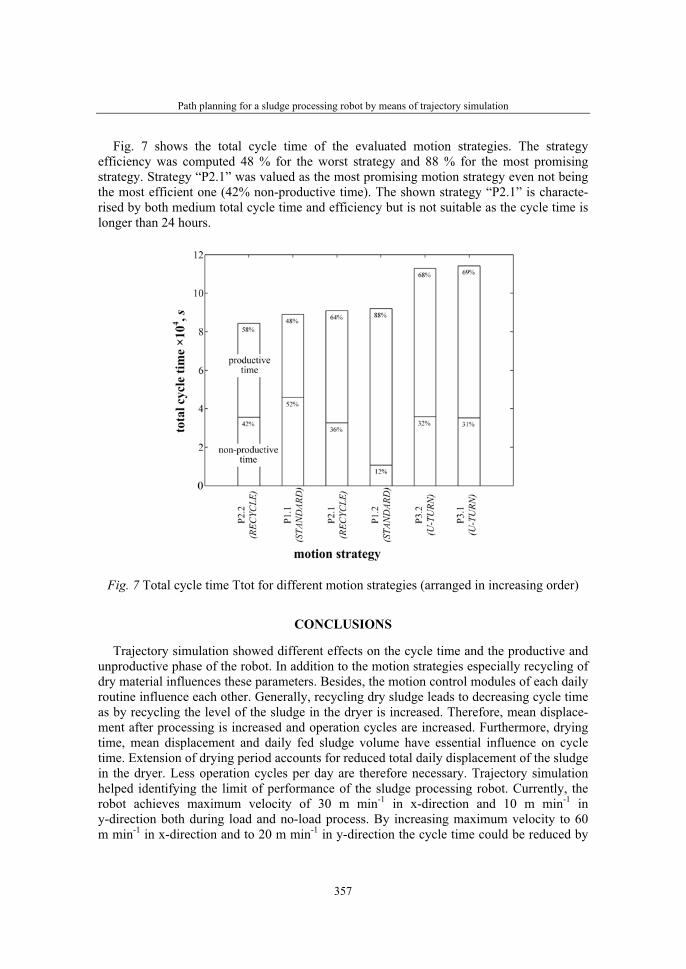
Path planning for a sludge processing robot by means of trajectory simulation
357
Fig. 7 shows the total cycle time of the evaluated motion strategies. The strategy efficiency was computed 48 % for the worst strategy and 88 % for the most promising strategy. Strategy “P2.1” was valued as the most promising motion strategy even not being the most efficient one (42% non-productive time). The shown strategy “P2.1” is characte-rised by both medium total cycle time and efficiency but is not suitable as the cycle time is longer than 24 hours.
Fig. 7 Total cycle time Ttot for different motion strategies (arranged in increasing order)
CONCLUSIONS
Trajectory simulation showed different effects on the cycle time and the productive and unproductive phase of the robot. In addition to the motion strategies especially recycling of dry material influences these parameters. Besides, the motion control modules of each daily routine influence each other. Generally, recycling dry sludge leads to decreasing cycle time as by recycling the level of the sludge in the dryer is increased. Therefore, mean displace-ment after processing is increased and operation cycles are increased. Furthermore, drying time, mean displacement and daily fed sludge volume have essential influence on cycle time. Extension of drying period accounts for reduced total daily displacement of the sludge in the dryer. Less operation cycles per day are therefore necessary. Trajectory simulation helped identifying the limit of performance of the sludge processing robot. Currently, the robot achieves maximum velocity of 30 m min-1 in x-direction and 10 m min-1 in y-direction both during load and no-load process. By increasing maximum velocity to 60 m min-1 in x-direction and to 20 m min-1 in y-direction the cycle time could be reduced by
N. Starčević, C. Thullner, M. Bux, J. Müller
358
maximum 20%. Another solution to reduce cycle time and to avoid needless runs is to adjust hall width to the width of the robot effector. At present, the width of the robot effector is 1.5 m and the hall width is 14.5 m. Hence, the last track is merely 1 m wide. If the hall width would be exactly a multiple of the tool width, the working width of the tool would be used in an optimum way. In that case, overlapping of the tracks would not be necessary. However, cycle time should be more reduced in order to create additional free time for maintenance and repair.
REFERENCES
1. DIN EN ISO 9787 (2000). Industrieroboter, Koordinatensysteme und Bewegungsnomenklaturen. Berlin, Deutsches Institut für Normung e.V.
2. Ellekilde L P; Perram J W (2005). Tool Center Trajectory Planning for Industrial Robot Manipulators Using Dynamical Systems. International Journal of Robotics Research, 24(5), S. 385-396
3. Kang S; Miranda E (2006). Planning and visualization for automated robotic crane erection processes in construction. Automation in construction, 15, S. 398-414
4. Lynch K M; Shiroma N; Arai H; Tanie K (2000). Collision-Free Trajectory Planning for a 3-DOF Robot with a Passive Joint. International Journal of Robotics Research, 19(12), S. 1171-1184
5. Sawodny O; Aschemann H; Bulach A; Hofer E P (2001). Online generation of Trajectories Considering Kinematic Constraints. Proceedings of the 7th IEEE International Conference on Methods & Models in Automation & Robotics, Miedzyzdroje, 28-31 August, S. 713-718
6. Sawodny O; Aschemann H; Lahres S (2002). An automated gantry crane as a large workspace robot. Control Engineering Practice, 10(12), S. 1323-1338
7. Sivakumar P L; Varghese K; Ramesh Babu N (2003). Automated path planning of kooperative crane lifts using heuristic search. Journal of computing in civil engineering, 17(3), S. 197-207
8. Starcevic N., Bux, M., Müller, J. (2006). Systematic Design of a Mixing and Transporting Robot for Solar Drying of Biogenous Residuals. Proceedings of “5. Int. Conf. ORBIT 2006 Biological Waste Management”, pp. 947-957, Weimar, Germany.
9. Starcevic, N., Bux, M., Rohr, T., Lutz, K., Kostadinov, M., Ritterbusch, S., Müller, J. (2007). Development of a Robot for Biomass Handling in a Solar Greenhouse Dryer. Agricultural Engineering International: the CIGR Ejournal of Scientific Research and Development. Manuscript PM 07 010. Vol. IX. March, Website: http://cigr-ejournal.tamu.edu/.
10. University of Duisburg (2006). Einführung in die Robotik 1. Universität Duisburg. http://www.mechatronik.uni-duisburg.de/multimedia/robotik1/robo_61.html (23.08.2006).
11. VDI 4446 (2004). VDI-Richtlinie - Spielzeitenermittlung von Krananlagen. Düsseldorf, VDI-Verlag.
36. Symposium "Actual Tasks on Agricultural Engineering", Opatija, Croatia, 2008.
359
36.
SIMPOZIJAKTUALNI ZADACIMEHANIZACIJE POLJOPRIVREDE
UDC631.362:634.41
Prethodno priopćenjePreliminary communication
A SEGMENTATION ALGORITHM FOR APPLE FRUIT RECOGNITION USING ARTIFICIAL NEURAL
NETWORKZHANG YAJING, LI MINZAN, QIAO JUN, LIU GANG
Key Laboratory of Modern Precision Agriculture System Integration Research, Ministry of Education, China Agricultural University,
Beijing 100083, China, e-mail: [email protected]
SUMMARY
Fruit recognition is an important step in the apple fruit harvesting. Artificial Neural Network algorithm is applied in automatic recognition of apple fruits on the tree. The recognition system is composed of a CCD camera and a personal computer. The camera is used to capture apple images, and the personal computer is used to recognize and locate the fruit based on the fruit images. Because the outdoor environment is not steady, the luminance of the fruit images is different. Thus it is needed to develop a robust recognition algorithm. R/B ratio and texture features are used in the classification procedure since the mean gray level of the object fruit on the red and blue band is different from the background. The texture features: contrast, entropy, correlation, and energy of gray value are calculated by the gray level co-occurrence matrix (GLCM) to each image. A back-propagation neural network (BPNN) classifier is employed to recognize the fruit and the background. The BPNN classifier consists of three layers: the input layer, the hidden layer, and the output layer. The input layer has three nodes, ratio of R and B, contrast, and correlation. The number of nodes in hidden layer is calculated according to an empirical formula. The result of the output layer is a numerical value used to determine what the image is, fruit or background. It is classified into fruit and background based on a certain threshold value. The results of the segmentation show that the success rate is over 87.6%, and the error rate is about 13% for the images with the back lighting condition. It is feasible to use the algorithm in practical recognition of apple fruit.
Key words: fruit recognition, detection algorithms, GLCM, BPNN.
Y. Zhang, M. Li, J. Qiao, G. Liu
360
INTRODUCTION
Apple is one of the major agriculture products in China. It is widely planted in many provinces, like Shandong, Shanxi etc. However, the harvesting of apples still depends on manual work today. It is a higher labor cost task. Therefore, it is necessary to studymechanization of fruit harvesting.
Many studies (D.L.Peterson, 2005; B. Sivaraman, T. F., 2005; S.Laykin et al., 2002; D.Stajnko et al., 2004) have focused on the robotics in agriculture application, especially for harvesting operations. Several kinds of harvesting robots of fruits have been developed.
The major tasks of an intelligent harvesting robot are fruit detecting, picking, holding, and placing (Peter P.Ling et al., 2004). Recognizing the fruit on the tree is the first task for a harvesting robot. After a fruit is located, the harvesting robot can approach and pick it. This work is accomplished by a visual system. The visual system for a harvesting robot is similar to the eyes for human being. First, the visual system obtains apple images by sensors, such as camera, laser etc (G.Polder et al., 2000; Mitsuji Monta et al., 2004). Then, it begins to analysis the image to get the useful parameters like centric point etc, which is used to guide the robotic hand towards the fruit. In the whole image processing, segmentation is an important step to separate the interested fruit from the background. The background includes all the things like the branches, leaves except the fruits. Many methods have been developed for the image segmentation (Lei F.Tian & David C.Slaughter, 1998; Soo Beom Park et al, 2004). Color and texture features were often used for analyzing the image. Kuo-Yi Huang (Kuo-Yi Huang, 2007) used an Artificial Neural Network (ANN) for detecting phalaenopsis seedlings diseases using color and texture features. Guyer and Yand (Guyer & Yand, 2000) employed ANN and spectral imaging to detect defects of cherries.
The objectives of this paper are: (1) to choose the proper texture features for the algorithm; (2) to develop an algorithm for automatic recognition of fruit.
MATERIALS AND METHODS
Image Acquisition��The variety of apple tested in this study was Molise. The color of the apple fruits was
mixed with red and green. The images were acquired using a CMOS (Complementary Met-al Oxide Semiconductor) color camera (DH-HV3103UC, Daheng, China) and a personal computer (AMD processor 1.81GHz). The resolution of the RGB images was 512×512 pixels and in BMP format. Image processing was performed using MATLAB v6.5 and Visual C++6.0 programming.
The apple trees were randomly selected in the middle of October, the harvesting season, from an apple orchard located in the suburb of Beijing. Image samples were used in devel-oping recognition algorithm. One image sample was a part of a whole image. If more than half pixels of a sample image belonged to a fruit, this sample was taken as fruit; otherwise, it was taken as background. Eighty image samples were used to train the network. Forty of them were fruit samples and the others were background samples.
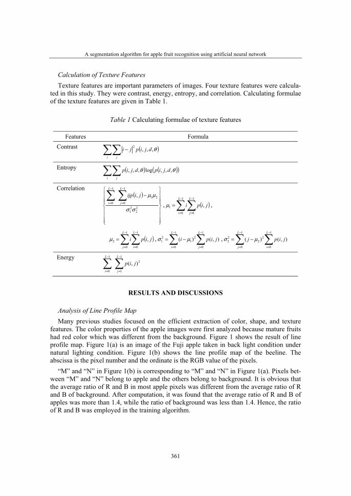
A segmentation algorithm for apple fruit recognition using artificial neural network
361
Calculation of Texture FeaturesTexture features are important parameters of images. Four texture features were calcula-
ted in this study. They were contrast, energy, entropy, and correlation. Calculating formulae of the texture features are given in Table 1.
Table 1 Calculating formulae of texture features
Features Formula
Contrast ( )θ,,,2 djipjiji
−∑∑
Entropy ( ) ( )( )θθ ,,,log,,, djipdjipji∑∑
Correlation( )
⎪
⎪
⎪
⎭
⎪⎪
⎪
⎬
⎫
⎪
⎪
⎪
⎩
⎪⎪
⎪
⎨
⎧
−∑∑
−
=
−
=22
21
1
0
21
1
0
,
σσ
μμL
j
L
i
jiijp
, ( )∑∑
−
=
−
=
=1
0
1
0
1 ,L
j
L
i
jipiμ ,
( )∑∑
−
=
−
=
=1
0
1
0
2 ,L
i
L
j
jipiμ , ∑∑
−
=
−
=
−=1
0
1
0
21
21 ),()(
L
j
L
i
jipi μσ , ∑∑
−
=
−
=
−=1
0
1
0
22
22 ),()(
L
i
L
j
jipj μσ
Energy∑∑
−
=
−
=
1
1
21
0
),(L
j
L
i
jip
RESULTS AND DISCUSSIONS
Analysis of Line Profile Map Many previous studies focused on the efficient extraction of color, shape, and texture
features. The color properties of the apple images were first analyzed because mature fruits had red color which was different from the background. Figure 1 shows the result of line profile map. Figure 1(a) is an image of the Fuji apple taken in back light condition under natural lighting condition. Figure 1(b) shows the line profile map of the beeline. The abscissa is the pixel number and the ordinate is the RGB value of the pixels.
“M” and “N” in Figure 1(b) is corresponding to “M” and “N” in Figure 1(a). Pixels bet-ween “M” and “N” belong to apple and the others belong to background. It is obvious that the average ratio of R and B in most apple pixels was different from the average ratio of R and B of background. After computation, it was found that the average ratio of R and B of apples was more than 1.4, while the ratio of background was less than 1.4. Hence, the ratio of R and B was employed in the training algorithm.
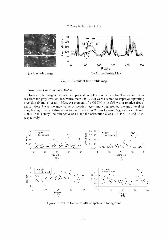
Y. Zhang, M. Li, J. Qiao, G. Liu
362
(a) A Whole Image (b) A Line Profile Map
Figure 1 Result of line profile map
Gray Level Co-occurrence Matrix However, the image could not be separated completely only by color. The texture featu-
res from the gray level co-occurrence matrix (GLCM) were adapted to improve separating precision (Haralick et al., 1973). An element of a GLCM, p(i,j,d,θ) was a relative frequ-ency, where i was the gray value at location (x,y), and j represented the gray level of neighboring pixel at a distance d and an orientation θ from location (x,y) (Kuo-Yi Huang, 2007). In this study, the distance d was 1 and the orientation θ was 0°, 45°, 90° and 135°, respectively.
(a) (b)
(c) (d)
Figure 2 Texture feature results of apple and background
M N
�
��
���
���
���
���
� ��� ��� ��� ��� ���
�� ��� �
���������� G R
B
M N
0
0.3
0.6
0.9
1.2
0 10 20 30 40Samples
Cont
rast
applebackground
0.E+00
2.E+06
4.E+06
6.E+06
8.E+06
0 10 20 30 40Samples
Cor
rela
tion applebackground
0
1
2
3
4
0 10 20 30 40Samples
Entro
py
applebackground
00.20.40.60.8
1
0 10 20 30 40Samples
Ener
gy
applebackground
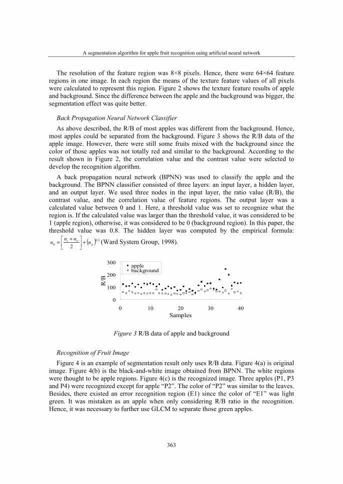
A segmentation algorithm for apple fruit recognition using artificial neural network
363
The resolution of the feature region was 8×8 pixels. Hence, there were 64×64 feature regions in one image. In each region the means of the texture feature values of all pixels were calculated to represent this region. Figure 2 shows the texture feature results of apple and background. Since the difference between the apple and the background was bigger, the segmentation effect was quite better.
Back Propagation Neural Network Classifier As above described, the R/B of most apples was different from the background. Hence,
most apples could be separated from the background. Figure 3 shows the R/B data of the apple image. However, there were still some fruits mixed with the background since the color of those apples was not totally red and similar to the background. According to the result shown in Figure 2, the correlation value and the contrast value were selected to develop the recognition algorithm.
A back propagation neural network (BPNN) was used to classify the apple and the background. The BPNN classifier consisted of three layers: an input layer, a hidden layer, and an output layer. We used three nodes in the input layer, the ratio value (R/B), the contrast value, and the correlation value of feature regions. The output layer was a calculated value between 0 and 1. Here, a threshold value was set to recognize what the region is. If the calculated value was larger than the threshold value, it was considered to be 1 (apple region), otherwise, it was considered to be 0 (background region). In this paper, the threshold value was 0.8. The hidden layer was computed by the empirical formula:
( ) 5.0
2 poi
h nnnn +⎥
⎦
⎤
⎢
⎣
⎡ += (Ward System Group, 1998).
0
100
200
300
0 10 20 30 40Samples
R/B
applebackground
Figure 3 R/B data of apple and background
Recognition of Fruit Image Figure 4 is an example of segmentation result only uses R/B data. Figure 4(a) is original
image. Figure 4(b) is the black-and-white image obtained from BPNN. The white regions were thought to be apple regions. Figure 4(c) is the recognized image. Three apples (P1, P3 and P4) were recognized except for apple “P2”. The color of “P2” was similar to the leaves. Besides, there existed an error recognition region (E1) since the color of “E1” was light green. It was mistaken as an apple when only considering R/B ratio in the recognition. Hence, it was necessary to further use GLCM to separate those green apples.
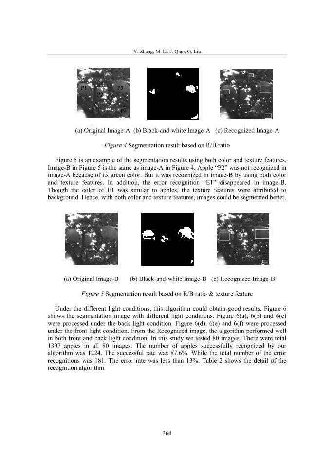
Y. Zhang, M. Li, J. Qiao, G. Liu
364
(a) Original Image-A (b) Black-and-white Image-A (c) Recognized Image-A
Figure 4 Segmentation result based on R/B ratio
Figure 5 is an example of the segmentation results using both color and texture features. Image-B in Figure 5 is the same as image-A in Figure 4. Apple “P2” was not recognized in image-A because of its green color. But it was recognized in image-B by using both color and texture features. In addition, the error recognition “E1” disappeared in image-B. Though the color of E1 was similar to apples, the texture features were attributed to background. Hence, with both color and texture features, images could be segmented better.
(a) Original Image-B (b) Black-and-white Image-B (c) Recognized Image-B
Figure 5 Segmentation result based on R/B ratio & texture feature
Under the different light conditions, this algorithm could obtain good results. Figure 6 shows the segmentation image with different light conditions. Figure 6(a), 6(b) and 6(c) were processed under the back light condition. Figure 6(d), 6(e) and 6(f) were processed under the front light condition. From the Recognized image, the algorithm performed well in both front and back light condition. In this study we tested 80 images. There were total 1397 apples in all 80 images. The number of apples successfully recognized by our algorithm was 1224. The successful rate was 87.6%. While the total number of the error recognitions was 181. The error rate was less than 13%. Table 2 shows the detail of the recognition algorithm.
P1P2
P3
P4
E1

A segmentation algorithm for apple fruit recognition using artificial neural network
365
CONCLUSIONS
We proposed an algorithm to automatically recognize the apple fruit for a machine vision system used to guide a robotic harvesting. We created a neural network classifier with the input of both color and texture features to segment the apple image. It is better than the algorithms only use color features. This algorithm also performs well in both back and front light condition. Future work will focus on developing the better features in order to classify more effectively.
ACKNOWLEDGEMENTS
This study was supported by National High Technology Research and Development Program of China (863 Program): Digital Agriculture (2006AA10Z255).
Table 2 Result of apple fruit recognition
No M S E No M S E No M S E No M S E
1 16 14 2 21 15 13 3 41 15 15 1 61 17 14 4 2 28 24 3 22 10 7 4 42 18 14 2 62 22 17 2 3 31 27 2 23 12 12 1 43 16 14 3 63 18 15 4 4 15 14 3 24 11 11 2 44 18 15 2 64 16 16 2 5 19 17 4 25 27 25 2 45 21 18 2 65 21 17 1 6 12 12 1 26 15 13 2 46 19 18 1 66 23 20 2 7 13 12 2 27 13 11 3 47 15 13 3 67 14 13 1 8 6 6 0 28 27 23 2 48 17 16 1 68 19 17 2 9 15 11 3 29 21 18 1 49 22 21 3 69 21 17 3
10 23 20 2 30 12 10 3 50 18 16 2 70 18 16 1 11 17 15 2 31 12 11 2 51 13 13 1 71 17 14 3 12 16 14 3 32 16 14 4 52 26 24 3 72 20 18 4 13 18 17 1 33 14 11 4 53 14 12 2 73 14 13 2 14 17 16 2 34 15 14 1 54 17 16 2 74 24 21 1 15 9 8 2 35 18 15 3 55 24 21 4 75 17 16 3 16 12 10 2 36 17 12 5 56 21 17 2 76 22 21 1 17 18 16 3 37 16 15 3 57 19 15 3 77 19 16 1 18 14 13 1 38 12 9 2 58 22 18 3 78 24 21 2 19 12 11 2 39 14 11 1 59 14 12 2 79 21 18 2 20 23 19 3 40 17 16 3 60 19 17 3 80 14 12 1
No: Image Number
M: Number of apple fruit per image measured manually
S: Successful number of apple fruit per image measured by algorithm
E: Error number of apple fruit per image measured by algorithm
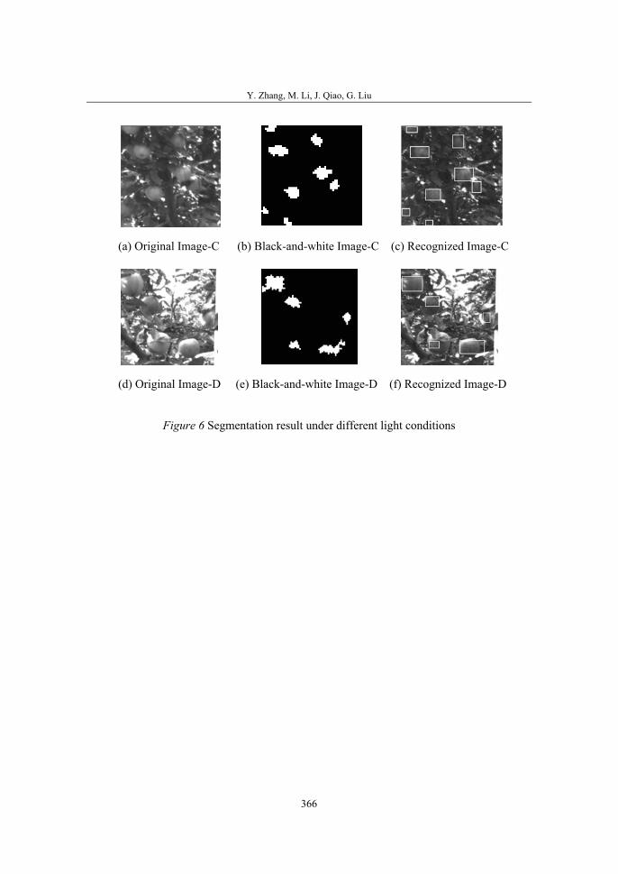
Y. Zhang, M. Li, J. Qiao, G. Liu
366
(a) Original Image-C (b) Black-and-white Image-C (c) Recognized Image-C
(d) Original Image-D (e) Black-and-white Image-D (f) Recognized Image-D
Figure 6 Segmentation result under different light conditions
A segmentation algorithm for apple fruit recognition using artificial neural network
367
REFERENCES
1. B. Sivaraman, T. F. (2005). Primary geometric performance indices for analysis and synthesis of a fruit harvesting robot arm. ASABE meeting Paper No. 053116. Tampa, USA.
2. D.L.Peterson. (2005). Development of a harvest aid for narrow-inclined-trellised tree-fruit canopies. Applied Engineering in Agriculture. 21(5), 803-806.
3. Guyer,D., Yand,X. (2000). Use of genetic artificial neural networks and spectral imaging for defect detection on cherries. Comput. Electron. Agric. 29,179-194.
4. G.Polder, G.W.A.M.van der Heijden, I.T.Young (2000). Spectral image analysis for measuring ripeness of tomatoes, Trans. ASAE. 45(4), 1155-1161.
5. Haralick,R.M., Shanmugam,K., Dinstein,I. (1973). Textual features for image classification. IEEE Trans.Syst.Man Cybernet.3 (6), 610-621.
6. Jain,R., Kasturi,R., Schunck,B.G. (1995). Machine Vision. ISBN 0-07-032018-7, 234-248.
7. Kuo-Yi Huang (2007). Application of artificial neural network for detecting Phalaenopsis seedling diseases using color and texture features. Comput. Electron. Agric. 57(2007), 3-11.
8. Lei F.Tian, David C.Slaughter (1998). Environmentally adaptive segmentation algorithm for outdoor image segmentation. Comput. Electron. Agric. 21(1998), 153-168.
9. Mitsuji Monta, Kazuhiko Namba, Naoshi Kondo. (2004). Three dimensional sensing system using laser scanner. The Canadian Society for Engineering in Agricultural, Food, and Biological systems, paper No.041158.
10. Peter P.Ling, Reza Ehsani, K.C.Ting, et al. (2004). Sensing and End-Effector for a Robotic Tomato harvester. The Canadian Society for Engineering in Agricultural, Food, and Biological systems, paper No.043088.
11. Soo Beom Park, Jae Won Lee, Sang Kyoon Kim (2004). Content-based image classification using a neural network. Pattern Recognition Letters, 25(2004), 287-300.
12. S.Laykin, V.Alchanatis, E.Fallik, Y.Edan (2002). Image-Processing algorithms for tomato classification. Trans.ASAE, 45(3), 851-858.
13. D.Stajnko, M.Lakita, M.Hocevar. (2004) Estimation of number and diameter of apple fruits in an orchard during the growing season by thermal imaging. Comput.electron.agric., 42(2004),31-42.
14. Ward System Group (1998). NeuroShell 2, Version 4. Frederick, MD.

36. Symposium "Actual Tasks on Agricultural Engineering", Opatija, Croatia, 2008.
369
36.
SIMPOZIJAKTUALNI ZADACIMEHANIZACIJE POLJOPRIVREDE
UDC541.123.2:631.362:633.18
Tehnička bilješkaTecnical note
RECOGNITION OF CONJOINT GRAINS OF RICE IN BINARY IMAGES
MING SUN1, SHUHUAI ZHANG2, DONG AN1, YAOGUANG WEI1, YIMING WANG1
1College of information and Electrical Engineering, China Agricultural University,P.O. Box 63, No.17 Qinghua Dong Road, Haidian District, Beijing, 100083 China,
[email protected] of Agriculture and Life Science, Hirosaki University,
Hirosaki, Aomori, 036-8561 Japan
SUMMARY
In this paper, a new watershed algorithm based on prior knowledge is presented for the recognition of binary images of conjoint grains of rice by machine vision. First, an algorithm for component labeling is used to find whole components of the conjoint grains of rice in each binary image. After the components of all the single grains are removed from each binary image according to their area threshold (AT), only the components of the conjoint grains remain, which are marked by MS. The watershed algorithm then separates the remaining components of the conjoint grains from each other where the threshold (ET) of the efficient erosion times is set, and MC. Finally marks the corresponding segmented components, the union of MS and MC is considered as the result of recognition of conjoint grains in the binary images. Over 95% of connected rice particles are correctly segmented, which indicates that the proposed method is valid and efficient.
Key words: Machine Vision, Image Processing, Rice, Conjoint grains, Water-shed Algorithm
INTRODUCTION
In general, human graders who rely on their intuition and empirical knowledge essent-ially determine rice quality. Hence, most of the evaluation results are uncertain. Therefore, digital image processing (Chen and Sun, 2004; Cui, 2000) and machine vision (Jain, et al., 2003) is introduced as a key step toward realizing speed detection of rice quality. Most of the rice images reveal the presence of conjoint grains. If these were not separated from each other, it would hamper further analysis of rice grains (Sun, et al., 2002).

M. Sun, S. Zhang, D. An, Y. Wei, Y. Wang
370
Studies on conjoint objects have been undertaken. In 1995, Shatadal et al. carried out separation experiments on images of five kinds of wheat with conjoint grains by combining limitary erosion with conditional dilation. The segmentation accuracy for the five kinds of wheat was 95%, 95%, 94%, 79%, and 89%, respectively. The segmentation boundary of a few components of grains was not well determined. In 1997, Shashidhar et al. used a method of equivalent ellipse fitting to attempt segmentation of conjoint grains in images and obtained good segmentation results. However, the method was only suited for images with a few connected grains. In 1998, our team proposed a binary image processing method (Sun et al., 1998), which combines distance transformation with the expansion technique, and applied it to separating conjoint apples in images. The separation accuracy was 89%. However, this method was not found to be suitable for conjoint grains of rice either. In 2001, Visen et al. separated conjoint grains of rice by employing a combination of elliptically equivalent regions, the curvature of the boundary of rice grains, and the lease neighbors. The separation results were 99% for only two or three conjoint grains of rice; this implies that the method could not resolve the problem of segmentation of large numbers of conjoint grains of rice.
The paper proposed a new watershed algorithm based on prior knowledge. The results revealed that the proposed algorithm could effectively separate the conjoint grains of rice.
WATERSHED ALGORITHM
Basic concepts of watershed algorithm The basic concept of watershed transformation (Cui, 2000; Roerdink and Meijster, 2001;
Wang et al., 2002) involves an image as a topographic surface. The gray level for every pixel represents the altitude at its position. The different components are termed as the watershed or catchment’s basin. The limit lines formed between the components are termed watershed lines or divide lines. When applied to image segmentation, watershed transformation will change an original image to a tag image where the points belonging to the same watershed are marked with the same tag and those located at the watershed line are marked with a special label. The concrete meanings of these concepts are illustrated in Figure 1.
� � �� � � � � �
Figure 1 Diagrams of watershed concepts: 3D watershed algorithm, 2D watershed algorithm and 1D watershed algorithm; 1. water line, 2. watershed, 3. minimum regions
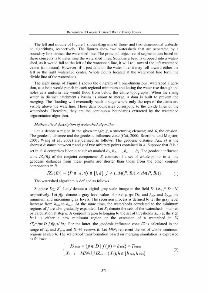
Recognition of Conjoint Grains of Rice in Binary Images
371
The left and middle of Figure 1 shows diagrams of three- and two-dimensional watersh-ed algorithms, respectively. The figures show two watersheds that are separated by a boundary line termed the watershed line. The principal objective of segmentation based on these concepts is to determine the watershed lines. Suppose a bead is dropped into a water-shed, as it would fall to the left of the watershed line, it will roll toward the left watershed center (minimum). However, if it just falls on the water line, it may roll toward either the left or the right watershed center. Whole points located at the watershed line form the divide line of the watersheds.
The right image of Figure 1 shows the diagram of a one-dimensional watershed algori-thm, as a hole would punch in each regional minimum and letting the water rise through the holes at a uniform rate would flood from below the entire topography. When the rising water in distinct catchment’s basins is about to merge, a dam is built to prevent the merging. The flooding will eventually reach a stage where only the tops of the dams are visible above the waterline. These dam boundaries correspond to the divide lines of the watersheds. Therefore, they are the continuous boundaries extracted by the watershed segmentation algorithm.
Mathematical description of watershed algorithm Let A denote a region in the given image; g, a structuring element; and θ, the erosion.
The geodesic distance and the geodesic influence zone (Cui, 2000; Roerdink and Meijster, 2001; Wang et al., 2002) are defined as follows. The geodesic distance dA(x, y) is the shortest distance between x and y of two arbitrary points contained in A. Suppose that B is a set in A. B comprises k conjoint subset marked B1, B2,��, Bi,��, Bk. The geodesic influence zone IZA(Bi) of the conjoint components Bi consists of a set of whole points in A; the geodesic distances from these points are shorter than those from the other conjoint components in B.
)},(),(,],,[,{)( jAiAiA BPdBPdijkijAPBIZ <≠∈∀∈= (1)
The watershed algorithm is defined as follows.
Suppose D⊆ Z2. Let f denote a digital gray-scale image in the field D, i.e., f: D� N,respectively. Let f(p) denote a gray level value of pixel p (p∈D); and hmin and hmax, the minimum and maximum gray levels. The recursion process is defined to let the gray level increase from hmin to hmax. At the same time, the watersheds correlated to the minimum regions of f are also gradually expanded. Let Xh denote the sets of the watersheds obtained by calculation at step h. A conjoint region belonging to the set of thresholds Xh+1 at the step h+1 is either a new minimum region or the extension of a watershed in Xh
(Th={p∈D�f(p)� h}). For the latter, the geodesic influence zone IZ is calculated in the range of Xh and Xh+1, and Xh+1 renews it. Let MINh represent the set of whole minimum regions at step h. The watershed transformation based on merging simulation is expressed as follows:
�
⎩
⎨
⎧
∈===∈=
++ ],[),(})(|{
maxmin11
minminmax
hhhXIZMINXThpfDpX
hThhh
hh
∪� �(2)�
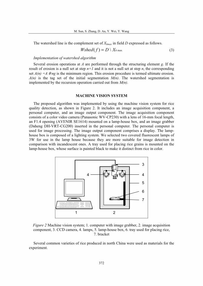
M. Sun, S. Zhang, D. An, Y. Wei, Y. Wang
372
The watershed line is the complement set of Xhmax in field D expressed as follows.
� max\)( hXDfWshed = � (3)�
Implementation of watershed algorithm Several erosion operations at A are performed through the structuring element g. If the
result of erosion is a null set at step n+1 and it is not a null set at step n, the corresponding set A(n) =A θ ng is the minimum region. This erosion procedure is termed ultimate erosion. A(n) is the tag set of the initial segmentation M(n). The watershed segmentation is implemented by the recursion operation carried out from M(n).
MACHINE VISION SYSTEM
The proposed algorithm was implemented by using the machine vision system for rice quality detection, as shown in Figure 2. It includes an image acquisition component, a personal computer, and an image output component. The image acquisition component consists of a color video camera (Panasonic WV-CP230) with a lens of 16-mm focal length, an F1.4 opening (AVENIR SE1614) mounted on a lamp-house box, and an image grabber (Daheng DH-VRT-CG200) inserted in the personal computer. The personal computer is used for image processing. The image output component comprises a display. The lamp-house box is composed of a lighting system. We selected two covered fluorescent lamps of 3W for use in the lamp house because they are more suitable for image detection in comparison with incandescent ones. A tray used for placing rice grains is mounted on the lamp-house box, whose surface is painted black to make it distinct from rice in color.
� �
�
� �
�
�
�
Figure 2 Machine vision system; 1. computer with image grabber, 2. image acquisition component, 3. CCD camera, 4. lamps, 5. lamp-house box, 6. tray used for placing rice,
7. bracket
Several common varieties of rice produced in north China were used as materials for the experiment.
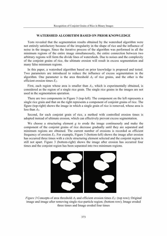
Recognition of Conjoint Grains of Rice in Binary Images
373
WATERSHED ALGORITHM BASED ON PRIOR KNOWLEDGE
Tests revealed that the segmentation results obtained by the watershed algorithm were not entirely satisfactory because of the irregularity in the shape of rice and the influence of noise in the images. Since the iterative process of the algorithm was performed in all the minimum regions of the entire image simultaneously, the entire connection between two arbitrary regions will form the divide lines of watersheds. Due to noises and the complexity of the conjoint grains of rice, the ultimate erosion will result in excess segmentation and many false minimum regions.
In this paper, a watershed algorithm based on prior knowledge is proposed and tested. Two parameters are introduced to reduce the influence of excess segmentation in the algorithm. One parameter is the area threshold AT of rice grains, and the other is the efficient erosion times ET.
First, each region whose area is smaller than AT, which is experimentally obtained, is considered as the region of a single rice grain. The single rice grains in the images are not used in the segmentation operation.
There are two components in Figure 3 (top-left). The component on the left represents a single rice grain and that on the right represents a component of conjoint grains of rice. The figure (top-right) shows the image in which a single grain of rice is removed, whose area is less than AT.
Second, for each conjoint grain of rice, a method with controlled erosion times is adopted instead of ultimate erosion, which can effectively prevent excess segmentation.
We choose a structuring element g to erode the image continuously and make the component of the conjoint grains of rice decrease gradually until they are separated and minimum regions are obtained. The current number of erosions is recorded as efficient frequency of erosion ET. For example, Figure 3 (bottom-left) shows the image after erosion has occurred three times with a circle structuring element selected and the conjoint region is still not apart. Figure 3 (bottom-right) shows the image after erosion has occurred four times and the conjoint region has been separated into two minimum regions.
Figure 3 Concepts of area threshold AT and efficient erosion times ET: (top row); Original image and image after removing single rice-particle region; (bottom row); Image eroded
three times and Image eroded four times
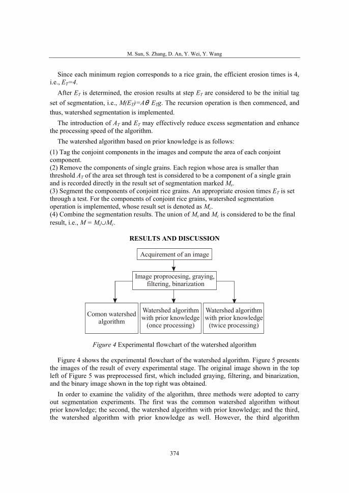
M. Sun, S. Zhang, D. An, Y. Wei, Y. Wang
374
Since each minimum region corresponds to a rice grain, the efficient erosion times is 4, i.e., ET=4.
After ET is determined, the erosion results at step ET are considered to be the initial tag set of segmentation, i.e., M(ET)=A� ETg. The recursion operation is then commenced, and thus, watershed segmentation is implemented.
The introduction of AT and ET may effectively reduce excess segmentation and enhance the processing speed of the algorithm.
The watershed algorithm based on prior knowledge is as follows: (1) Tag the conjoint components in the images and compute the area of each conjoint component.(2) Remove the components of single grains. Each region whose area is smaller than threshold AT of the area set through test is considered to be a component of a single grain and is recorded directly in the result set of segmentation marked Ms.(3) Segment the components of conjoint rice grains. An appropriate erosion times ET is set through a test. For the components of conjoint rice grains, watershed segmentation operation is implemented, whose result set is denoted as Mc.(4) Combine the segmentation results. The union of Ms and Mc is considered to be the final result, i.e., M = Ms∪Mc.
RESULTS AND DISCUSSION
Image proprocesing, graying, filtering, binarization
Acquirement of an image
Comon watershedalgorithm
Watershed algorithmwith prior knowledge
(once processing)
Watershed algorithmwith prior knowledge
(twice processing)
Figure 4 Experimental flowchart of the watershed algorithm
Figure 4 shows the experimental flowchart of the watershed algorithm. Figure 5 presents the images of the result of every experimental stage. The original image shown in the top left of Figure 5 was preprocessed first, which included graying, filtering, and binarization, and the binary image shown in the top right was obtained.
In order to examine the validity of the algorithm, three methods were adopted to carry out segmentation experiments. The first was the common watershed algorithm without prior knowledge; the second, the watershed algorithm with prior knowledge; and the third, the watershed algorithm with prior knowledge as well. However, the third algorithm
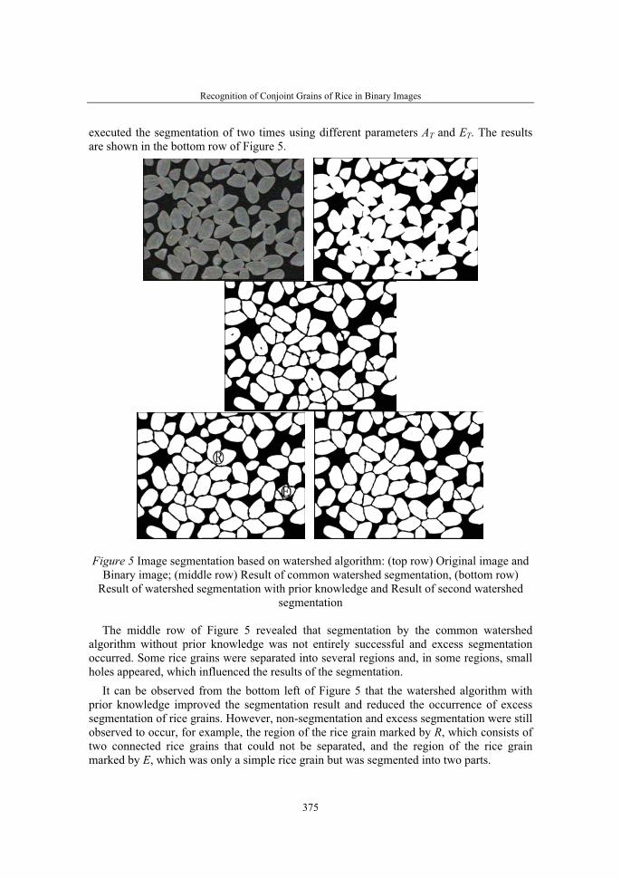
Recognition of Conjoint Grains of Rice in Binary Images
375
executed the segmentation of two times using different parameters AT and ET. The results are shown in the bottom row of Figure 5.
Figure 5 Image segmentation based on watershed algorithm: (top row) Original image and Binary image; (middle row) Result of common watershed segmentation, (bottom row)
Result of watershed segmentation with prior knowledge and Result of second watershed segmentation
The middle row of Figure 5 revealed that segmentation by the common watershed algorithm without prior knowledge was not entirely successful and excess segmentation occurred. Some rice grains were separated into several regions and, in some regions, small holes appeared, which influenced the results of the segmentation.
It can be observed from the bottom left of Figure 5 that the watershed algorithm with prior knowledge improved the segmentation result and reduced the occurrence of excess segmentation of rice grains. However, non-segmentation and excess segmentation were still observed to occur, for example, the region of the rice grain marked by R, which consists of two connected rice grains that could not be separated, and the region of the rice grain marked by E, which was only a simple rice grain but was segmented into two parts.

M. Sun, S. Zhang, D. An, Y. Wei, Y. Wang
376
The error in the region R is due to the small value of ET, which resulted in insufficient erosion times. Since the two rice grains overlapped considerably, they could not be separa-ted into two minimum regions if the erosion times were few. Therefore, for such regions, it might be possible to increase the efficient erosion times ET and perform the second watershed segmentation. During the second watershed segmentation, a proper threshold may be set to ensure that the rice grains, which had been successfully segmented, do not undergo the second watershed segmentation. In this manner, although the watershed segmentation was implemented two times, the rice grains to be processed the second time were fewer in number and would not lead to an much increase in the time consumed. The bottom right of Figure 5 shows the result of the second segmentation. It may be observed that the region R was separated successfully.
The error in region E occurred due to a considerable and complicated overlapping of rice grains; thus, frequent erosions excessively segmented the region. It was found through experiments that this case was not common.
CONCLUSIONS
In this paper, the proposed watershed algorithm based on prior knowledge effectively segmented the conjoint grains of rice in the binary images. The results of segmentation experiments on 100 images with conjoint grains revealed that 95.4% of the grains were accurately separated based on eyeballing judgment.
ACKNOWLEDGEMENTS
The authors would like to express their sincere thanks to Chinese Ministry of Education for financial support in the form of a start-up fund for students who ever studied abroad.
Recognition of Conjoint Grains of Rice in Binary Images
377
REFERENCES
1. Chen B., Sun. M. (2004). Visual C++ practical image processing. Tsinghua University Press, Beijing (in Chinese)
2. Cui Y. (2000). Image processing and analysis—Methods and applications of mathematical morphology. Beijing: China Science Press (in Chinese)
3. Jain R., Kasturi R., Schunck B. G. (2003). Machine vision. China Machine Press, Beijing
4. Roerdink J. B., Meijster A. (2001). The watershed transform: Definitions, algorithms, and parallelization strategies. Fundamental Information. 41: 187–228
5. Shashidhar N. S., Jayas D. S., Crowe T. G., et al. (1997). Processing of digital images of touching kernels by ellipse fitting. Canadian Agricultural Engineering. 39: 139–142
6. Shatadal P., Jayas D. S., Bulley N. R. (1995). Digital image analysis for software separation and classification of touching grains: 2 Classification. Transaction of the ASAE. 382: 645–649
7. Sun M., Takahashi T., Zhang S., et al. (1998). Apple discrimination based on image processing at apple harvest. Part 3 - Development of network model of color image processing and methods of binary image processing. Journal of the Japanese Society of Agricultural Machinery. 60: 79–87 (in Japanese)
8. Sun M., Ling Y., Wang Y. (2002). Computer vision based rice chalkiness detection using MATLAB. Journal of Chinese Agricultural Engineering. 18: 146–149 (in Chinese)
9. Visen N. S., Shashidhar N. S., Paliwal J., et al. (2001). Identification and segmentation of occluding groups of grain kernels in a grain sample image. J. Agric. Engng Res. 79: 159–166
10. Wang J, Liu W., Lu Y. (2002). Application of watershed algorithm to the segmentation of cell images. Journal of Xinan Traffic University. 37: 290–294 (in Chinese)


36. Symposium "Actual Tasks on Agricultural Engineering", Opatija, Croatia, 2008.
379
36.
SIMPOZIJAKTUALNI ZADACIMEHANIZACIJE POLJOPRIVREDE
UDC628.88:631.227.2.014Prethodno priopćenje
Preliminary communication
INVESTIGATION OF THE TEMERATURE FIELD IN A BROILER FARM WITH WINTER VENTILATION
BORIS EVSTATIEV, NICOLAY MIHAILOV
“Angel Kanchev” University of Rousse, 8 Studentska Str., 7017-Rousse, Bulgaria, [email protected], [email protected].
ABSTRACT
A study has been carried out in order to investigate the temperature field in a poultry farm with fans and air inlets, situated on the long walls of the building. The organization of the experiment has been described, as well as the scheme, of the electronic system for measurements. Digital sensors DS18S20 with serial data exchange has been used, installed in 5 columns of 4 sensors each. They are all connected to a personal computer, which is storing the information into a database, through a 1-wire network. The humidity variation in height is also being investigated in this study, with the use of 2 humidity sensors DOL 14. Additionally, the temperature and humidity of the environment are also taken into consideration.
Key words: broiler farm, temperature field, winter ventilation, humidity.
INTRODUCTION
The distribution of the temperature field is of main importance for modeling of the microclimatic processes in a broiler farm. The goal of the microclimate control is to maintain appropriate parameters of the microclimate in the habitation area. The temperature field in the building influences the energy exchange through the walls and the ceiling. The air exchange is one of the factors that greatly influence the temperature field. This analysis shows that the temperature field in a broiler farm depends on a number of factors: temperature and humidity of the air, shape of the building, thermodynamic parameters of the building, air streams etc. These characteristics are a prerequisite for the creation of a mathematical model, which can determine the dynamics of the microclimate parameters variation in the habitation area of the animals, as well as the energy expenses for breeding.
The goal of this study is to determine the temperature variations in height and width of a broiler farm with winter ventilation.
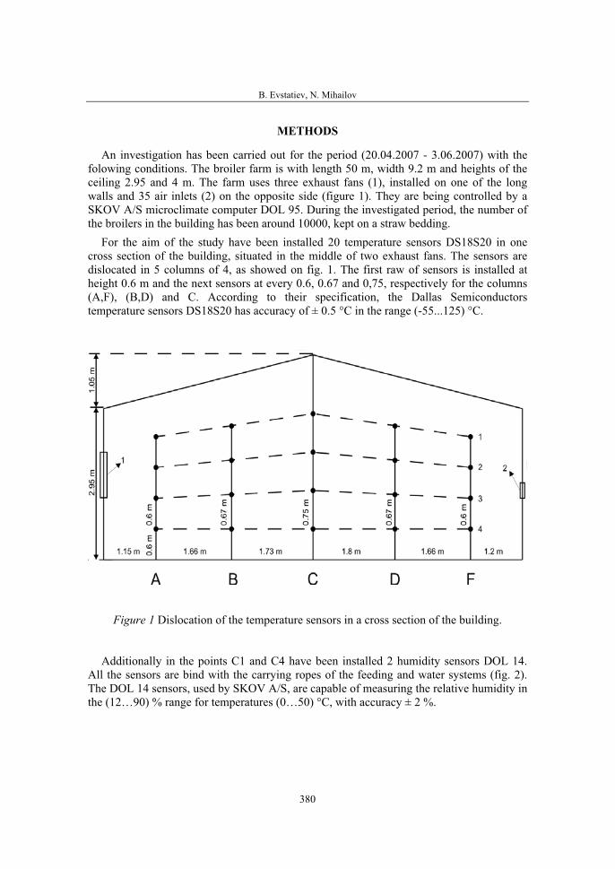
B. Evstatiev, N. Mihailov
380
METHODS
An investigation has been carried out for the period (20.04.2007 - 3.06.2007) with the folowing conditions. The broiler farm is with length 50 m, width 9.2 m and heights of the ceiling 2.95 and 4 m. The farm uses three exhaust fans (1), installed on one of the long walls and 35 air inlets (2) on the opposite side (figure 1). They are being controlled by a SKOV A/S microclimate computer DOL 95. During the investigated period, the number of the broilers in the building has been around 10000, kept on a straw bedding.
For the aim of the study have been installed 20 temperature sensors DS18S20 in one cross section of the building, situated in the middle of two exhaust fans. The sensors are dislocated in 5 columns of 4, as showed on fig. 1. The first raw of sensors is installed at height 0.6 m and the next sensors at every 0.6, 0.67 and 0,75, respectively for the columns (A,F), (B,D) and C. According to their specification, the Dallas Semiconductors temperature sensors DS18S20 has accuracy of ± 0.5 °C in the range (-55...125) °C.
Figure 1 Dislocation of the temperature sensors in a cross section of the building.
Additionally in the points C1 and C4 have been installed 2 humidity sensors DOL 14. All the sensors are bind with the carrying ropes of the feeding and water systems (fig. 2). The DOL 14 sensors, used by SKOV A/S, are capable of measuring the relative humidity in the (12…90) % range for temperatures (0…50) °C, with accuracy ± 2 %.
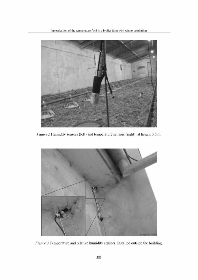
Investigation of the temperature field in a broiler farm wirh winter ventilation
381
Figure 2 Humidity sensors (left) and temperature sensors (right), at height 0.6 m.
Figure 3 Temperature and relative humidity sensors, installed outside the building.
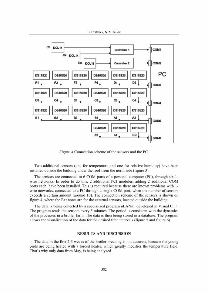
B. Evstatiev, N. Mihailov
382
Figure 4 Connection scheme of the sensors and the PC.
Two additional sensors (one for temperature and one for relative humidity) have been installed outside the building under the roof from the north side (figure 3).
The sensors are connected to 6 COM ports of a personal computer (PC), through six 1-wire networks. In order to do this, 2 additional PCI modules, adding 2 additional COM ports each, have been installed. This is required because there are known problems with 1-wire networks, connected to a PC through a single COM port, when the number of sensors exceeds a certain amount (around 10). The connection scheme of the sensors is shown on figure 4, where the Ext notes are for the external sensors, located outside the building.
The data is being collected by a specialized program uLANm, developed in Visual C++. The program reads the sensors every 5 minutes. The period is consistent with the dynamics of the processes in a broiler farm. The data is then being stored in a database. The program allows the visualization of the data for the desired time intervals (figure 5 and figure 6).
RESULTS AND DISCUSSION
The data in the first 2-3 weeks of the broiler breeding is not accurate, because the young birds are being heated with a forced heater, which greatly modifies the temperature field. That’s why only data from May, is being analyzed.
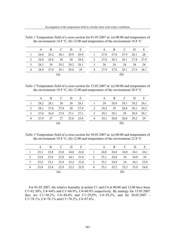
Investigation of the temperature field in a broiler farm wirh winter ventilation
383
Table 1 Temperature field of a cross section for 01.05.2007 at: (a) 00:00 and temperature of the environment 14.8 °C; (b) 12:00 and temperature of the environment 18.8 °C
A B C D E
1 28.8 29.2 30.1 29.9 29.9
2 28.8 28.8 30 30 29.8
3 28.2 29 29.2 29.2 29.1
4 28.9 27.8 29.1 29.8 29 (а)
A B C D E
1 27.8 27.8 27.9 28.1 28
2 27.8 28.2 28.1 27.8 27.9
3 28 28 28 28 28
4 27.9 27.8 28.1 27.9 28.1 (b)
Table 2 Temperature field of a cross section for 15.05.2007 at: (a) 00:00 and temperature of the environment 19.9 °C; (b) 12:00 and temperature of the environment 28.9 °C
A B C D E
1 28,2 28,1 28 28 28,1
2 28,1 27,8 27,9 28 27,9
3 27,8 26,9 27,9 27,1 27,1
4 27,9 27 27 25,8 25,8 (а)
A B C D E
1 29 28,9 29,1 29,2 29,1
2 29,2 29 28,8 29,1 29,2
3 29,1 29,1 29 28,9 29,1
4 29,1 28,8 28,8 29,2 29 (b)
Table 3 Temperature field of a cross section for 30.05.2007 at: (a) 00:00 and temperature of the environment 19.8 °C; (b) 12:00 and temperature of the environment 23.8 °C
A B C D E
1 23,1 23,8 23,8 24,8 22,8
2 23,8 23,9 23,8 24,1 21,9
3 23,2 23,1 22,9 23,2 21,8
4 23,8 22,8 22,9 22,2 22,9 (а)
A B C D E
1 24,8 24,8 24,8 24,1 24,1
2 25,1 24,8 24 24,8 24
3 25,1 24,9 24 24,1 23,9
4 25,1 25,2 25,2 23,9 24,8 (b)
For 01.05.2007, the relative humidity at points C1 and C4 at 00:00 and 12:00 have been C1=62.30%, C4=64% and C1=60.9%, C4=60.9% respectively. By analogy for 15.05.2007 they are C1=50.2%, C4=49,4% and C1=29,9%, C4=29,2%, and for 30.05.2007 - C1=78.1%, C4=76.1% and C1=70.2%, C4=67.6%.
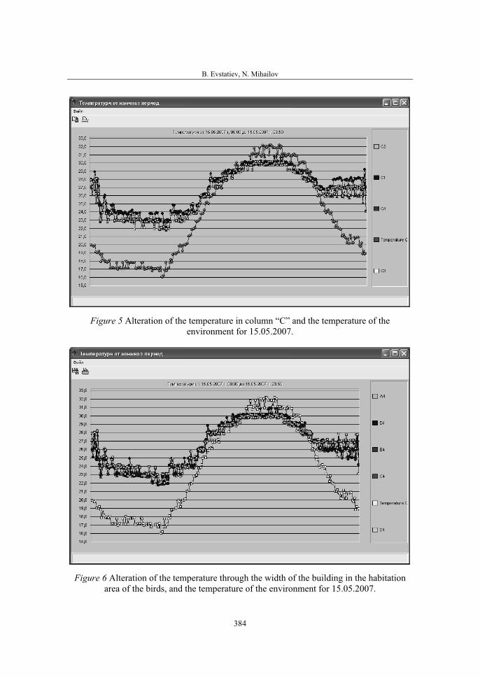
B. Evstatiev, N. Mihailov
384
Figure 5 Alteration of the temperature in column “C” and the temperature of the environment for 15.05.2007.
Figure 6 Alteration of the temperature through the width of the building in the habitation area of the birds, and the temperature of the environment for 15.05.2007.
Investigation of the temperature field in a broiler farm wirh winter ventilation
385
As seen on figures 5 and 6, if the temperature of the environment is higher or close to the required temperature inside the building, the temperature field is homogenous in both width and height. This is caused by the fact that the fans are constantly turned on and the air inlets are open. On the other hand, if the temperature of the environment is lower then the required microclimate one, a period of homogenous field is followed by a period of non homogenous one, depending on whether the exhaust fans are turned on and the air inlets open. When the field is not homogenous the temperature difference in height is from 0 to about 1 °C, depending on the column, and it is lower at the habitation area and higher near the ceiling. The temperature difference in the habitation area of the animals gets up to 1-2 °C, but there is no regularity. Sometimes it’s lower at the side of the exhaust fans and sometimes – from the side of the air inlets. This is most likely caused by the angle, at which the air is being let in (the angle of the air inlets).
According to this, the data in tables 1a, 1b, 2b and 3b represent a homogenous period of the temperature field, while table 2a – a period when the temperature field is not homogenous. On tables 2a and 3a the temperature difference in width and height of the building is from 0 to 2 °C, depending on the column/raw.
CONCLUSIONS
As a result of the experimental study, can be made the conclusion that the homogeneity of the temperature field in a broiler farm with winter ventilation, depends on whether the exhaust fans are turned on and respectively the air inlets – open, and if the environmental temperature is close or higher than the required microclimatic one. When this condition is met, the temperature field inside the building can be considered homogenous. On the other hand, when the environmental temperature is lower than the required one inside the building, the temperature field could be either homogenous, when the exhaust fans and air inlets are closed, or non homogenous, when air is being let inside. The temperature difference in width and height gets up to 2 °C, for non homogenous field.
The difference between the humidity of the air in the habitation area and near the ceiling, commensurate with the accuracy of the sensors could be considered as insignificant.
REFERENCES
1. CIGR, 2002 Climatization of Animal Houses; Working Group Report on: Heat and Moisture Production at Animal and House Level. Published by Research Centre Bygholm, Denmark.
2. Mihailov N., Stoyanov V. Evstatiev B. (2006). Computer system for investigation of the temperature field in a broiler farm. Energy Forum 2006. June 14-17. Sv. Sv. Konstantin I Elena. Bulgaria, pp 185-188.
3. Xin H. et all. (2001). Heat and moisture production of poultry and their housing systems: Broilers. Transactions of the ASAE 44: 1851-1857.
4. Xin, H., J. Sell, and D. Ahn. (1996). Effects of light and darkness on heat and moisture production of broilers. Transactions of the ASAE 39:2255-2258.

36. Symposium "Actual Tasks on Agricultural Engineering", Opatija, Croatia, 2008.
387
36.
SIMPOZIJAKTUALNI ZADACIMEHANIZACIJE POLJOPRIVREDE
UDC628.8:631.22:636.2.083
Izvorni znanstveni radOriginal scientific paper
WATER VAPOUR PRODUCTION OF COWSHED BRONIUS KAVOLELIS, ALGIS JASINSKAS
Lithuanian University of Agriculture, Institute of Agricultural Engineering LT-54132 Raudondvaris, Kaunas reg., LITHUANIA,
E-mail: [email protected], [email protected]
SUMMARY
When designing a barn ventilation system and outside partitions important criteria are flows of animal heat and water vapour. There is data in scientific and standard literature on the amount of water vapour produced by animals and the room. But this data is typical of warm barns in which air temperature ranges from 0 to 35 oC. In recent decades intensive construction of uninsulated cowshed was started. The average temperatures in uninsulated cowshed of East Europe during the coldest season are about minus 10 oC.
The work objective is to establish the emission of water vapour in an uninsulated cowshed. A simple method to establish water vapour emission in a cattle house under production conditions was substantiated. The research was made in an uninsulated cowshed with boxes. During the research the indoor and outdoor temperature and relative humidity were measured as well as CO2concentration in the indoor and outdoor air. According to the measured values specific water vapour emission (amount of water vapour produced by animals and room per animal total heat unit) was calculated, and regression equation relating the flow of water vapour emission with the indoor air temperature was drawn. When temperature is minus 10 oC, specific intensity of water vapour emission is 0.054 g/kJ and at plus 10 oC it is 0.135 g/kJ. Having analysed the data of water vapour emission in cowsheds with temperatures above zero presented by other authors it can be stated that the regression equation drawn reflects the regularity of water vapour emission well.
When the specific intensity of water vapour emission is known, the necessary ventilation intensity and the ventilation system parameters can be calculated.
Key words: water vapour, emission, cowshed, temperature below zero, regre-ssion equation
B. Kavolelis, A. Jasinskas
388
INTRODUCTION
When designing a barn ventilation system and outside partitions important criteria are flows of animal heat and water vapour. Water vapour is produced by animals breathing and sweating. It also evaporates from excrements, water-troughs and from feeding troughs when moist or liquid feed is used. There is data in scientific and standard literature on the amount of water vapour produced by animals and the room. Comprehensive research in water vapour emission in cattle houses and pigsties under natural production conditions was carried out 40 years ago (Jurgenson 1976). The barns were insulated, the inside temperature was above zero. The cattle were kept in a tied-up system. Comprehensive standard data on the amount of water vapour produced was presented (Albrigt 1990). The amounts of water vapour breathed out by an animal and emitted by excrements are given separately. The latter source of water vapour accounts for 13% of the water vapour amount breathed out by an animal. However, the results are given for a situation when the animals are kept in the temperature above -1 oC. An in-depth analysis of different research results on the flows of total, sensible and latent heat of the animal which are directly related with the emission of water vapour were carried out by Pedersen et al. (1998). According to the generalized data the humidity emitted in cattle houses reduces the flow of sensible heat by 10-20%, i.e. the humidity produced in the house accounts for 10-20% of the amount of water vapour produced by animals breathing and sweating. This data is typical of warm barns in which air temperature ranges from 0 to 35 oC.
The amount of heat and water vapour produced by animals is established by using a calorimeter (Chepete et al. 2001) or directly in a room where animals are housed (Jurgenson 1976). The first method provides a more accurate measurement of heat and water vapour produced by an animal and the second method measures the amount of water vapour emitted in the room.
The work objective is to establish the emission of water vapour in an uninsulated cowshed.
METHODS
The majority of researchers have established that CO2 emission production in animal housing premises is directly proportional to the total heat production of animals and on average it is 0,185 m3/kWh (Blanes et al., 2005), i.e. 51 cm3/kJ. There are works proving that the amount of water vapour produced by animals and the room is also proportional to the amount of the total animal heat. It is also proved by the analysis of standard data (Albright, 1990). Therefore, in this work it is accepted that water vapour production is proportional to animal total heat production. Having solved the equations of water vapour and carbon dioxide balances is drawn
e=oi
ooii
CCdd
−− )(51 ϕϕ
(1)
here: e – specific intensity of water vapour emission (amount of water vapour produced by animals and room per animal total heat unit), g/kJ;

Water vapour production of cowshed
389
51– specific intensity of CO2 emission, cm3/kJ;di, do – at the most content of water vapour in the indoor and outdoor air, g/m3;φi,φo – indoor and outdoor air relative humidity, in parts of unit; Ci, Co – carbon dioxide concentration in the inside and outside air, ppm. It can be seen from equation (1) that in order to find the value of water vapour emission
in a room it is enough to measure the indoor and outdoor temperature, relative humidity and carbon dioxide concentration in the inside and outside air.
The research was made in an uninsulated cowshed with boxes. The boxes were covered with rubber mats without bedding. The floor of walking alleys was made of concrete. Manure is removed by a cable scrapper. The average mass of a cow was about 600 kg, the daily milk yield was about 19 kg. The main feed of the cows is maize silage. The width of the cowshed is 22 m. The capacity is 200 cows. The average heat transfer coefficient of walls was 4.5 W/(m2.K), and roof – 5.0 W/(m2.K).
During the research the indoor and outdoor temperature and relative humidity were measured as well as CO2 concentration in the inside and outside air. According to the measured values specific water vapour emission was calculated.
RESULTS AND DISCUSSION
During the research the outdoor air temperature varied from +4,8 to -16,0 oC and the indoor air temperature varied from +11,2 to -9,4 oC. In the latter case the manure in walking alleys was frozen. Water-troughs were functioning in the ordinary way.
The analysis of the results investigation suggests that the greatest influence on the specific emission rate of water vapour intensity is made by the indoor air temperature (Fig. 1). The following exponential was achieved
e=0,085×100.02ti. R=0.94 (2)
0,04
0,06
0,08
0,1
0,12
0,14
0,16
-10 -8 -6 -4 -2 0 2 4 6 8 10 12
Temperature, oC
Em
issi
on r
ate,
g/k
J
0.16
0.14
0.12
0.08
0.040.06
0.10
e = 0.085x10 0.02tie = 0.085x100.02t i
Fig. 1 The dependence specifical emission rate of water vapour on indoor temperature
B. Kavolelis, A. Jasinskas
390
A simple method to establish water vapour emission in a cowshed was substantiated. By using this method under the conditions of natural function in the stall cowshed it was established how water vapour emission depended on the inside air temperature; when it varies from minus 9,4 oC to plus 11,2 oC this dependency is expressed as an exponential.
When comparing the results with the data of other authors achieved at plus temperatures it can be stated that the results achieved within the range of plus temperatures reliably coincide with the data of other authors (Jurgenson 1976) achieved under production conditions. The latter are also expressed by the exponential (e=0,0839×100,0214t
i ) regression coefficients of which unreliably differ from the regression equation drawn in this work.
According to the data of Pedersen et al., when cattle are fed by the feeds in which dry matter accounts for more than 30% and the floor is damp, the calculated specific values of water vapour emission, when the inside temperature is 0oC, are by 1,5 times higher than the results achieved. However, as the air temperature rises this difference decreases down to an insignificant one. According to the standard data ( Albright 1990 ) the calculated values differ from the achieved results even less and at 0oC air temperature this different equals to 20%. As the temperature rises the difference also decreases down to an insignificant one.
When e value is known, it is possible to calculate ratio ε of sensible and total animal heat which assesses the humidity produced by animals and the room, i.e. ε = 1-2.5 e.
When the ratio of sensible and total animal heat is known, the optimum ventilation intensity and the ventilation system parameters can be calculated, i.e.
∑∑
∑ ρ=ρ=⎥⎦
⎤
⎢⎣
⎡ −η+ε= 2211Δ
AvAvxt
IxcQ
G iooo (3)
here: G – optimum intensity of ventilation, kg/s;
∑Qo – total heat production of animals, kW; c – specific heat capacity of air, kJ/(kg·K); xo , x – total and partial module of heat losses through building partitions, 1/K; η =β/αo – coefficient that evaluates solar irradiance, m2
·K/W (β – sun energy absorption coefficient of partition outer surface; αo – heat transfer coefficient of partition outer surface, W/(m2
·K));Δt – permissible difference between inside and outside air temperatures, oC;I – mean density of sun energy flow on total surface of outer partitions, W/m2;
ρi, ρo – inside and outside air density, kg/m3;v1, v2 – air velocity in inlets and outlets, m/s;
∑A1 , ∑A2 – total areas of air inlets and outlets, m2.

Water vapour production of cowshed
391
Total heat loss module xo=( ΣUA+ ψ P)}/ ∑Qo, 1/K, and partial heat loss module x=ΣUA/∑Qo, 1/K. [here: U – heat transfer coefficient of partitions (walls and roof), W/(m2⋅K);A – partition area, m2; ψ – specific heat losses through floors and foundations, W/(m⋅K),(when foundations and floors are insulated, ψ = 0,9, and when they are uninsulated – ψ = 1,5 W/(m⋅K) (Albrigt 1990); P –perimeter of foundations, m; ∑Qo – total heat production of animals, W ].
CONCLUSIONS
1. The literature analysis suggests that there is no data on water vapour emission in a cowshed with minus temperature.
2. A method to determine water vapour emission in a barn was substantiated. 3. The research was carried out in an uninsulated cowshed and a regression equation
relating water vapour emission with the inside air temperature was drawn. 4. Having compared research results with the results by other researchers achieved in
insulated cowsheds it can be stated, that the exponential relating the values of specific water vapour emission with the inside air temperature reflects the process of water vapour emission in a cowshed well.
REFERENCES
1. Albright L.D. (1990). Environment control for animals and plants. American Society of Agricultural Engineers, ASAE Textbook N4.
2. Blanes V., Pedersen S. (2005). Ventilation flow in pig houses measured and calculated by carbon dioxide, moisture, and heat balance equations. Biosystems Engineering. 92(4): 483-493.
3. Chepete H.J.,Xin, H. (2001). Heat and moisture production of poultry and their housing systems – a literature review. In: Livestock Environment VI. Proceedings of the 6th International Symposium (21–23 May 2001, Louisville, Kentucky, USA). ASAE Publication Number 701PO2001, pp 319-335.
4. Jurgenson L.(1976). Stallklimaberechnung unter Berucksichtigung feuchter Flachen. Luft-und Kaltetechnik, 2: 82-85.
5. Pedersen S., Takai H., Johnsen J.H., et al.(1998). A comparison of three balance methods for calculating ventilation rates in livestock buildings. Journal of Agricultural Engineering Research. 70: 25-37.

36. Symposium "Actual Tasks on Agricultural Engineering", Opatija, Croatia, 2008.
393
36.
SIMPOZIJAKTUALNI ZADACIMEHANIZACIJE POLJOPRIVREDE
UDC631.86:636.5
Izvorni znanstveni radOriginal scientific paper
EFFECT OF INITIAL MOISTURE CONTENT ON AEROBIC COMPOSTING OF POULTRY MANURE
WITH WHEAT STRAW IVAN PETRIC1,*, ALMIR ŠESTAN2 AND INDIRA ALIBAŠIĆ2
1Department of Process Engineering, Faculty of Technology, University of Tuzla, Univerzitetska 8, 75000 Tuzla, Bosnia and Herzegovina
2Department of Chemistry, Faculty of Science, University of Tuzla Univerzitetska 4, 75000 Tuzla, Bosnia and Herzegovina
*Corresponding author (e-mail: [email protected])
SUMMARY
Moisture content is one of the most important factors for successfully comp-osting. The objective of this work was to evaluate the effect of initial moisture content in the mixture of poultry manure and wheat straw on degradation rate of organic matter. The experiments were carried out in closed thermally laboratory reactors (1 L) under adiabatic conditions for 13, 14 and 11 days. Different moisture contents were used for monitoring the changes of the substrate tempe-rature, carbon dioxide mass, ammonia mass and organic matter content. The experimental results showed that optimum initial moisture content was 69.11% (even more).
Key words: aerobic composting, poultry manure, wheat straw, moisture content, reactor.
INTRODUCTION
Poultry and wheat are two important agricultural industries in Bosnia and Herzegovina, generating large amount of manure and straw. Serious environmental pollution has been caused due to lack of cost-effective technologies and inappropriate disposal. It is imperative to find effective approaches to reuse and minimize pollution associated with them. Composting poultry manure with wheat straw is one of options and could offer many environmental and economic benefits for the country like Bosnia and Herzegovina where both poultry manure and wheat straw are available. In addition, composting of poultry manure with wheat straw is also a good approach from the standpoint of process enginee-
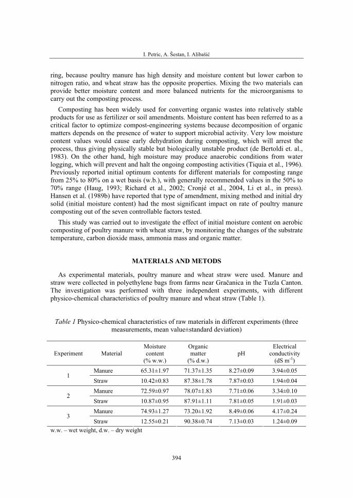
I. Petric, A. Šestan, I. Alibašić
394
ring, because poultry manure has high density and moisture content but lower carbon to nitrogen ratio, and wheat straw has the opposite properties. Mixing the two materials can provide better moisture content and more balanced nutrients for the microorganisms to carry out the composting process.
Composting has been widely used for converting organic wastes into relatively stable products for use as fertilizer or soil amendments. Moisture content has been referred to as a critical factor to optimize compost-engineering systems because decomposition of organic matters depends on the presence of water to support microbial activity. Very low moisture content values would cause early dehydration during composting, which will arrest the process, thus giving physically stable but biologically unstable product (de Bertoldi et. al., 1983). On the other hand, high moisture may produce anaerobic conditions from water logging, which will prevent and halt the ongoing composting activities (Tiquia et al., 1996). Previously reported initial optimum contents for different materials for composting range from 25% to 80% on a wet basis (w.b.), with generally recommended values in the 50% to 70% range (Haug, 1993; Richard et al., 2002; Cronjé et al., 2004, Li et al., in press). Hansen et al. (1989b) have reported that type of amendment, mixing method and initial dry solid (initial moisture content) had the most significant impact on rate of poultry manure composting out of the seven controllable factors tested.
This study was carried out to investigate the effect of initial moisture content on aerobic composting of poultry manure with wheat straw, by monitoring the changes of the substrate temperature, carbon dioxide mass, ammonia mass and organic matter.
MATERIALS AND METODS
As experimental materials, poultry manure and wheat straw were used. Manure and straw were collected in polyethylene bags from farms near Gračanica in the Tuzla Canton. The investigation was performed with three independent experiments, with different physico-chemical characteristics of poultry manure and wheat straw (Table 1).
Table 1 Physico-chemical characteristics of raw materials in different experiments (three measurements, mean value±standard deviation)
Experiment Material Moisturecontent
(% w.w.)
Organicmatter
(% d.w.) pH
Electricalconductivity
(dS m-1)
Manure 65.31±1.97 71.37±1.35 8.27±0.09 3.94±0.05 1
Straw 10.42±0.83 87.38±1.78 7.87±0.03 1.94±0.04
Manure 72.59±0.97 78.07±1.83 7.71±0.06 3.34±0.10 2
Straw 10.87±0.95 87.91±1.11 7.81±0.05 1.91±0.03
Manure 74.93±1.27 73.20±1.92 8.49±0.06 4.17±0.24 3
Straw 12.55±0.21 90.38±0.74 7.13±0.03 1.24±0.09 w.w. – wet weight, d.w. – dry weight
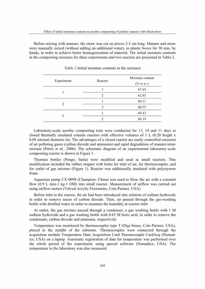
Effect of initial moisture content on aerobic composting of polutry manure with wheat straw
395
Before mixing with manure, the straw was cut on pieces 2.5 cm long. Manure and straw were manually mixed (without adding an additional water), in plastic boxes for 30 min, by hands, in order to achieve better homogenization of material. The initial moisture contents in the composting mixtures for three experiments and two reactors are presented in Table 2.
Table 2 Initial moisture contents in the mixtures
Experiment Reactor Moisture content
(% w.w.)
1 67.65 1
2 62.85
1 69.11 2
2 60.55
1 69.43 3
2 66.19
Laboratory-scale aerobic composting tests were conducted for 13, 14 and 11 days in closed thermally insulated column reactors with effective volumes of 1 L (0.20 height x 0.08 internal diameter m). The advantages of a closed reactor are easily controlled emission of air polluting gases (carbon dioxide and ammonia) and rapid degradation of manure/straw mixture (Petric et al., 2006). The schematic diagram of an experimental laboratory-scale composting reactor is shown in Figure 1.
Thermos bottles (Pengo, Italia) were modified and used as small reactors. This modification included the rubber stopper with holes for inlet of air, for thermocouples, and for outlet of gas mixture (Figure 1). Reactor was additionally insulated with polystyrene foam.
Aquarium pump CX-0098 (Champion, China) was used to blow the air with a constant flow (0.9 L min-1 kg-1 OM) into small reactor. Measurement of airflow was carried out using airflow meters (Valved Acrylic Flowmeter, Cole-Parmer, USA).
Before inlet to the reactor, the air had been introduced into solution of sodium hydroxide in order to remove traces of carbon dioxide. Then, air passed through the gas-washing bottle with distilled water in order to maintain the humidity at reactor inlet.
At outlet, the gas mixture passed through a condenser, a gas washing bottle with 1 M sodium hydroxide and a gas washing bottle with 0.65 M boric acid, in order to remove the condensate, carbon dioxide and ammonia, respectively.
Temperature was monitored by thermocouples type T (Digi-Sense, Cole-Parmer, USA), placed in the middle of the substrate. Thermocouples were connected through the acquisition module Temperature Data Acquisition Card Thermocouple CardAcq (Nomad-ics, USA) on a laptop. Automatic registration of data for temperature was performed over the whole period of the experiment, using special software (Nomadics, USA). The temperature in the laboratory was also measured.

I. Petric, A. Šestan, I. Alibašić
396
Figure 1 Schematic diagram of laboratory reactor system (1. aquarium pump,2. airflow meter, 3. gas washing bottle with solution of sodium hydroxide,
4. gas washing bottle with distilled waster, 5. small reactor, 6. thermocouple,7. condenser, 8. graduated cylinder, 9. gas washing bottle with solution of sodium
hydroxide, 10. gas washing bottle with solution of boric acid, 11. laptop)
For determination of carbon dioxide content, an aliquot volume of sodium hydroxide solution (used as a „trap“), with the indicator of phenolphthalein, was titrated by standard solution of 1 M hydrochloric acid. The difference in titration between blank and sampled probes was used for calculation of the mass of the “trapped” carbon dioxide.
For determination of ammonia content, an aliquot volume of boric acid solution (used as a „trap“), with the indicator of bromcresol green-methyl, was titrated by standard solution of 1 M hydrochloric acid. The difference in titration between sampled and blank probes was used for calculation of mass of the „trapped“ ammonia.
The gas washing bottles were changed daily for determination of produced gases. Moisture content in the substrate was calculated from the difference between the masses
before and after drying of samples in a dry oven at 105°C for 24 h (APHA, 1995). After cooling in a desiccator (30 min), the samples were incinerated at 550°C for 6 h, and then cooled again in a desiccator. The difference in the masses between dried and incinerated samples represents the mass of organic matter (APHA, 1995).
The loss of organic matter k is calculated from the initial and final organic matter contents, according to the Equation (1) (Haug, 1993; Diaz et al., 2003):
[ ][ ](%)OM100(%)OM
100(%)OM(%)OMk
pm
pm
−⋅⋅−
= (1)
where OMm is the organic matter content at the beginning of the process; and OMp is the organic matter content at the end of the process.
Effect of initial moisture content on aerobic composting of polutry manure with wheat straw
397
Each analysis was done in triplicate with calculation of the mean value. Each experiment was done in duplicate in order to reduce the experimental error.
The additional water wasn’t added to composting material during the process because the composting mixture did not dry up. The air passed through the gas-washing bottle with distilled water in order to maintain the humidity at reactor inlet.
The k (loss of organic matter) characteristics of compost and its raw materials were subjected to ANOVA one-way analysis of variance to test differences. The Multiple Range Test was used to establish the significance of differences among treatments. The tempera-ture, carbon dioxide and ammonia patterns were also tested for significant difference over time. All analysis were performed using STATGRAPHICS statistical package (STATGRA-PHICS, 1996).
RESULTS AND DISCUSSION
The temperature regimes of the composting reactors containing different mixtures in three experiments are illustrated in Figure 2. The lag period on temperature curves was not recorded because the original substrate was rich in microorganisms. Thus, after several hours the temperature in the composting mass started to rise due to intense biodegradation. The moisture content of the compost material had a significant effect on the microbial activity and temperature. The initial moisture level of mixture of 69.43% in experiment 3 (Figure 2c) resulted in a cooling effect. Such high water content could also influence gaseous exchange by limiting diffusion and thus restricting oxygen utilisation by microor-ganisms, resulting in decreased microbial activity. In all three experiments the higher temperature profiles were achieved in the reactor 1 than in the reactor 2. It should be noted that reactor 1 had higher initial moisture content in all experiments (Table 2). In the experiment 1 (Figure 1a), the composting process reached the maximum temperature of 56.5°C after 1.2 days in reactor 1, whereas reactor 2 reached lower maximum temperatures (52.5°C after 1.2 days). In the experiment 2 (Figure 2b), the composting process reached the maximum temperature of 64.6°C after 1.3 days in reactor 1, whereas reactor 2 reached lower maximum temperatures (51.0°C after 1 day). In the experiment 3 (Figure 2c), the composting process reached the maximum temperature of 59.5°C after 1.2 days in reactor 1, whereas reactor 2 reached lower maximum temperatures (50.0°C after 1.2 days). There were statistically significant differences in temperature regime between reactors 1 and 2 in all three experiments (experiment 1 – from first to tenth day; experiment 2 – from first to fourth day; experiment 3 – from first to fourth day) (P < 0.05). The temperature in reactor 1 in the experiment 2 was maintained above 55°C for 2 days, which should be sufficient to maximize sanitation (Stentiford, 1996). According to Strauch and Ballarini (1994) only the thermophilic range of 55°C is sufficient to destroy pathogens. Reactor 1 in experiment 1 and 3, and reactor 2 in all three experiment did not provide conditions for full sanitation and destroying of pathogens. Adding water absorbent is a good method to adjust the initial moisture content of compost, because it achieved the longest durations of thermophilic stage and inhibitive temperature stage at the bottom (Luo et al., in press). VanderGheynst et al. (1997) found that maximum rates of oxygen consumption and maximum temperatures increase with increasing moisture content.
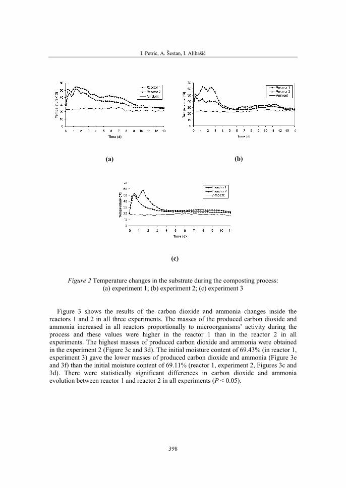
I. Petric, A. Šestan, I. Alibašić
398
(a) (b)
(c)
Figure 2 Temperature changes in the substrate during the composting process:(a) experiment 1; (b) experiment 2; (c) experiment 3
Figure 3 shows the results of the carbon dioxide and ammonia changes inside the reactors 1 and 2 in all three experiments. The masses of the produced carbon dioxide and ammonia increased in all reactors proportionally to microorganisms’ activity during the process and these values were higher in the reactor 1 than in the reactor 2 in all experiments. The highest masses of produced carbon dioxide and ammonia were obtained in the experiment 2 (Figure 3c and 3d). The initial moisture content of 69.43% (in reactor 1, experiment 3) gave the lower masses of produced carbon dioxide and ammonia (Figure 3e and 3f) than the initial moisture content of 69.11% (reactor 1, experiment 2, Figures 3c and 3d). There were statistically significant differences in carbon dioxide and ammonia evolution between reactor 1 and reactor 2 in all experiments (P < 0.05).
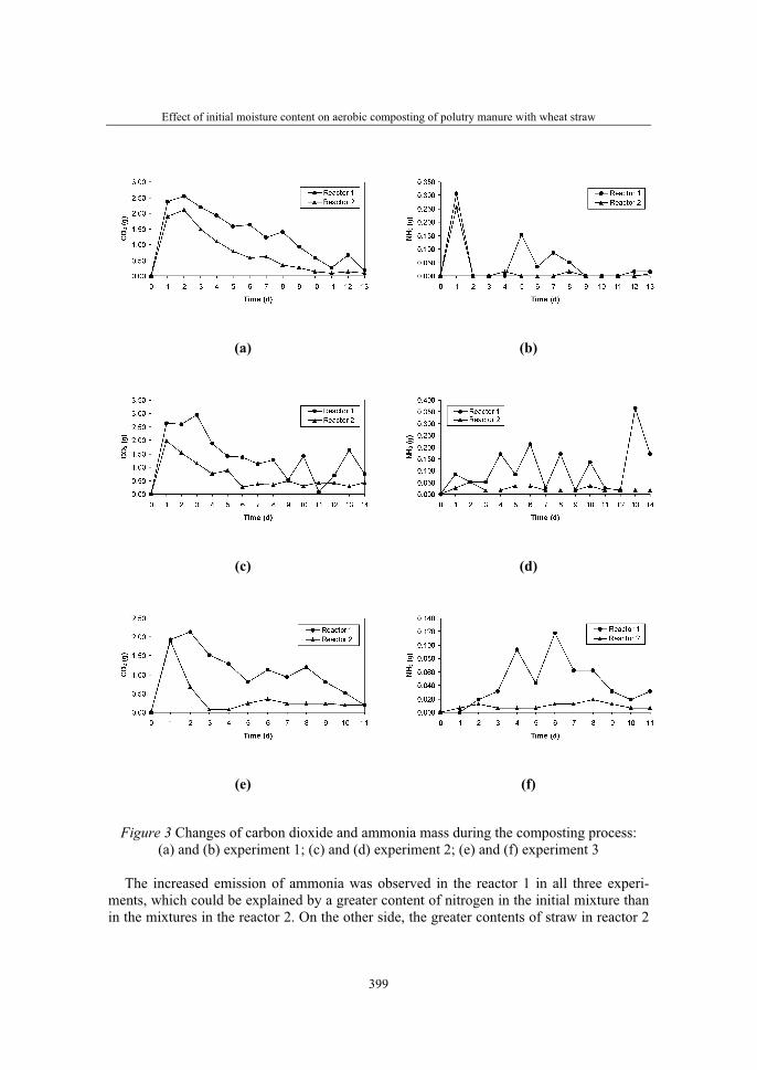
Effect of initial moisture content on aerobic composting of polutry manure with wheat straw
399
(a) (b)
(c) (d)
(e) (f)
Figure 3 Changes of carbon dioxide and ammonia mass during the composting process:(a) and (b) experiment 1; (c) and (d) experiment 2; (e) and (f) experiment 3
The increased emission of ammonia was observed in the reactor 1 in all three experi-ments, which could be explained by a greater content of nitrogen in the initial mixture than in the mixtures in the reactor 2. On the other side, the greater contents of straw in reactor 2
I. Petric, A. Šestan, I. Alibašić
400
(comparing to reactor 1) decreased the moisture content of the mixtures. The smaller straw addition in reactor 1 than in reactor 2 led to lower carbon to nitrogen ratio. For poultry waste, a low carbon to nitrogen ration contributes to large ammonia losses (Gray et al., 1971). Ammonia represents even 98% of emission of nitrogen from composting material (Beck-Friis et al., 2001). The losses of nitrogen often reach up to 33% during the composting of poultry manure (Hansen et al., 1989b). The other important factors for nitrogen loss, in the form of ammonia, are: temperature, mixing, and pH value of composting material (Martins and Dewes 1992), as well as particle size (Hansen et al., 1989a). The temperature controlled the ammonia vapour pressure, so if there was temperature decrease the ammonia remained more dissolved in the water solution of the composting material. The pH value influenced the ammonia concentration in compost air space by controlling the distribution of ammonia and ammonium concentration in the aqueous phase. It has been reported that ammonia volatilisation occurs when water content of the material is close to its water-holding capacity (Cabrera and Chiang, 1994). The high moisture content led to increased loss of NH4+-N content.
The degradation of organic matter was related to the loss of organic matter, which was, in turn, directly related to the microbial respiration (Paredes et al., 2002). The organic matter content of the materials decreased in both reactors during the process, but this reduction was greater in reactor 1 than in reactor 2 in all three experiments (Table 3). This suggested that the higher moisture content probably enhanced the biodegradation of the composting material, which could be further verified by the higher temperature attained and more production of carbon dioxide and ammonia in material with higher moisture content (69.11%). Relatively high moisture content was better for reaching a higher temperature and longer retention time of the high temperature. This conclusion is according with results of Li et al. (in press) with of composting of dairy manure and rice straw. There were statistically significant differences between k values for reactors 1 and 2 in all three experiments (P < 0.05).
Table 3 Conversion of organic matter (k) at the end of the composting process
Experiment 1 Experiment 2 Experiment 3
Reactor 1 2 1 2 1 2
k (%) 38.44 35.21 41.36 26.58 26.66 20.66
The term optimum moisture content represents a trade-off between moisture require-ments of microorganisms and their simultaneous need for an adequate oxygen supply (Haug, 1993). Too high moisture content, of more than 75% inhibits a quick start to the composting process. However, Jeris et al. (1973) have reported that optimum moisture content even range from 75% to 80% for farmyard manure in straw. Fernandes et al. (1994) have reported that successful composting of poultry manure mixed with peat or chopped straw has been obtained at high initial moisture levels (73-80%) but in a passive static-pile. According to the experimental results of Kalyuzhnyi et al. (1999), the optimum initial content of the composting mixture (solid fraction of hen manure supplemented with straw)
Effect of initial moisture content on aerobic composting of polutry manure with wheat straw
401
was found to be 65-70%. Ahn et al. (in press) found that optimum moisture content for beef manure and wheat straw is 68% and 74%, respectively. Liang et al. (2003) have found that a range of 60-70% moisture content provided maximum microbial activity for composting of biosolids and pine sawdust. These authors concluded that moisture content effects are more influential than temperature. With validated model for aerobic composting of mixture of poultry manure and wheat straw, Petric and Selimbašić (in press) have determined the optimum value of initial moisture content of 70% which is in agreement with the results of this research. Simulations also showed that composting process was impossible when moisture content was bellow 31% or above 78%. The fact is that there is no universally applicable optimum moisture content for composting materials. This is because each material has unique physical, chemical and biological characteristics, and these affect the relationship between moisture content and its corollary factors water availability, particle size, porosity, and permeability.
CONCLUSIONS
The initial moisture content of the mixture of poultry manure and wheat straw had a significant effect on aerobic composting process described by the changes of the substrate temperature, carbon dioxide mass, ammonia mass and organic matter content. The optimum initial moisture content was 69.11% or even more, but less than 70%. This suggested that the higher moisture content probably enhanced the biodegradation of the composting material, which could be further verified by the higher temperature attained and more production of carbon dioxide and ammonia in material with moisture content of 69.11%. Based on the results, it could be seen that for aerobic composting of poultry manure and wheat straw, relatively high moisture content was better for reaching a higher temperature and longer retention time of the high temperature. On the other side, the high moisture content led to increased loss of ammonia. Therefore, future work will be focused on control of ammonia emission.
ACKNOWLEDGEMENTS
This research was financially supported by the Federal Ministry of Education and Science of Bosnia and Herzegovina. The authors would like to thank Pejo Pejić for his help in preparation of experimental reactor system.

I. Petric, A. Šestan, I. Alibašić
402
REFERENCES
1. Ahn H.K., Richard T.L., Glanville T.D. (in press). Optimum moisture levels for biodegradation of mortality composting envelope materials. Waste Manage, doi: 10.1016/j.wasman.2007.05.022
2. American Public Health Association (APHA) (1995). Standard Methods for the Examination of Water and Wastewater. APHA, Washington, DC.
3. Beck-Friis B., Smårs S., Jönsson H., Kirchmann H. (2001). Gaseous Emissions of Carbon dioxide, Ammonia and Nitrous Oxide from Organic Household Waste in a Compost Reactor under Different Temperature Regimes. J Agric Engng Res 78(4): 423-430
4. Cabrera, M.L., Chiang S.C. (1994). Water content effect on denitrification and ammonia volatilisation in poultry litter. Soil Sci Soc Am J 58: 811-816
5. Cronjé A.L., Turner C., Williams A.G., Barker A.J., Guy S. (2004). The Respiration Rate of Composting Pig Manure. Compost Sci Util 12(2): 119-129
6. De Bertoldi M., Vallini G., Pera A. (1983). The biology of composting: a review. Waste Manage Res 1: 157-176
7. Diaz M.J., Madejon E., Lopez F., Lopez R., Cabrera F. (2002). Optimization of the rate vinasse/grape marc for co-composting process. Process Biochem 37: 1143-1150
8. Fernandes L., Zhan, W., Patni N.K., Yjui P. (1994). Temperature distribution and variation in passively aerated static compost piles. Biores Technol 48: 257-263
9. Gray K.R., Sherman K., Biddlestone A.J. (1971). Review of Composting - Part 1. Process Biochem 6(6): 32-36
10. Hansen R.C., Keener H.M., Hoitink H.A.J. (1989a). Poultry manure composting: design guidelines for ammonia. Presented at Quebec, PQ, Canada, June. ASAE Paper No. 89-4075. St. Joseph, MI.: American Society of Agricultural Engineers.
11. Hansen R.C., Keener H.M., Hoitink H.A.J. (1989b). Poultry manure composting: an exploratory study. Transactions of the ASAE 32(6): 2151-2158
12. Haug R.T. (1993). The practical handbook of compost engineering. Lewis Publishers, Boca Raton
13. Jeris J.S., Regan R.W. (1973). Controlling Environmental Parameters For Optimum Composting. Part II: Moisture, Free Air Space And Recycle. Compost Sci Util 14(2): 8-15
14. Kalyuzhnyi S., Sklyar V., Fedorovich V., Kovalev A., Nozhevnikova A., Klapwijk A. (1999). The Development of Biological Methods for Utilization and Treatment of Diluted Manure Streams. Wat Sci Tech 40(1): 223-229
15. Li X., Zhang R., Pang Y. (in press). Characteristics of dairy manure composting with rice straw. Biores Technol, doi: 10.1016/j.biortech.2006.12.009
16. Liang C., Das K.C., McClendon R.W. (2003). The influence of temperature and moisture contents regimes on the aerobic microbial activity of a biosolids composting blend. Biores Technol 86:131-137
17. Luo W., Chen T.B., Zheng G.D., Gao D., Zhang Y.A., Gao W. (in press). Effect of moisture adjustments on vertical temperature distribution during forced-aeration static-pile composting of sewage sludge. Resource Conserv Recycl, doi: 10.1016/j.resconrec.2007.08.004
Effect of initial moisture content on aerobic composting of polutry manure with wheat straw
403
18. Martins O., Dewes T. (1992). Loss of Nitrogeneous Composunds during Composting of Animal Wastes. Biores Technol 42: 103-111
19. Paredes C., Bernal M.P., Cegarra J., Roig A. (2002). Bio-degradation of olive mill wastewater sludge by its co-composting with agricultural wastes. Biores Technol 85: 1-8.
20. Petric I., Selimbašić V., Bijedić M. (2006). Optimum ratio of chicken manure and wheat straw for composting process with forced aeration. Proceedings of the 34. International Symposium on Agricultural Engineering, Opatija, Croatia, 21.-24. February 2006, pp 557-563
21. Petric I., Selimbašić V. (in press). Development and validation of mathematical model for aerobic composting process. Chem Eng J, doi: 10.1016/j.cej.2007.08.017
22. Richard T.L., Hamelers H.V.M., Veeken A., Silva, T. (2002). Moisture Relations in Composting Processes. Compost Sci Util 10(4): 286-302
23. STATGRAPHICS (1996). Version 2.1 Statistical Graphics Corporation
24. Stentiford E.T. (1996). Composting control: Principles and practice: In: DeBertoldi, M., Sequi, P., Lemmes, B., Papi, T. (Eds.), The Science of Composting. Chapman & Hall, pp 49-59
25. Strauch D., Ballarini G. (1994). Hygienic aspects of production and agricultural use of animal wastes. J. Vet Med 41: 176-228
26. Tiquia S.M., Tam N.F.Y., Hodgkiss I.J. (1996). Microbial activities during composting of spent pig-manure sawdust litter at different moisture contents. Biores Technol 55: 201-206
27. VanderGheynst J.S., Gossett J.M., Walker L.P. (1997). High-solids aerobic decomposition: pilot-scale reactor development and experimentation. Process Biochem 32(5): 361-375
UTJECAJ POČETNOG SADRŽAJA VLAGE NA AEROBNO KOMPOSTIRANJE PERADARSKOG GNOJA
I PŠENIČNE SLAME
SAŽETAK
Sadržaj vlage je jedan od najvažnijih faktora za uspješno kompostiranje. Cilj ovog rada bio je određivanje utjecaja početnog sadržaja vlage u smjesi peradarskog gnoja i pšenične slame na razgradnju organskih tvari. Eksperimenti su izvedeni u zatvorenim toplinski izoliranim laboratorijskim reaktorima (1 litra) pod adijabatskim uvjetima u trajanju od po 13, 14 i 11 dana. Različiti sadržaji vlage su iskorišteni za praćenje promjena temperature supstrata, mase ugljikovog dioksida, mase amonijaka i sadržaja organskih tvari. Eksperimentalni rezultati su pokazali da je optimalni početni sadržaj vlage bio 69.11% (čak i malo više).
Ključne riječi: aerobno kompostiranje, peradarski gnoj, pšenična slama, sadržaj vlage, reaktor.


36. Symposium "Actual Tasks on Agricultural Engineering", Opatija, Croatia, 2008.
405
36.
SIMPOZIJAKTUALNI ZADACIMEHANIZACIJE POLJOPRIVREDE
UDC631.358:633.521
Stručni radExpert paper
DETERMINATION OF CUTTING PROPERTIES OF COTTON STALK
REFIK POLAT, FERDA KAPLAN
Faculty of Agriculture, Department of Agricultural Machinery, University of Harran,63040 Sanliurfa, Turkey, e-mail: [email protected]
ABSTRACT
In this research, it was aimed to determine the physical and mechanical prop-erties of cotton stalks that remain at fields and concerned with mechanization. The mechanics of cutting on rigid surfaces was investigated by applying cutting tests to cotton stalks. After harvesting, length, diameter and stalk intensity of cotton stalks, the maximum cutting force and cutting stress were examined. In addition, the effects of the stalk moisture content and stalk region from the bottom to the top on cutting properties were researched. At the end of the research, the maximum cutting force was measured between 26,7 N and 95,25 N. The cutting stress was obtained between 0,45 N/mm2 and 0,74 N/mm2. After harvesting, average length, stalk intensity and diameter of cotton stalks were measured as 79,36 cm, 10,6 number/m2 and 14.12 mm (at 0-10 cm of stalk) , respectively.
Key words : Cotton stalk, Physical-mechanical properties, cutting force
INTRODUCTION
Negative changes take place in the chemical and physical structures of agriculture lands due to time, erosion and field traffic. Studies made for protecting the current situations of agriculture lands have gained importance. In these studies that are related to land protection, various techniques and methods are being used. Studies about reuniting the plant wastes that remain on the surface of the land back with the soil are the leading studies that are being made to protect the chemical and physical structure of the soil.
It is declared by most researchers that reuniting the plant wastes with the soil reduce the erosion risk. The more the surface waste is left on the surface, the more the soil gets resistant to surface flows and erosion. Plant wastes on the land surface is the most important component of most erosion control applications and the necessary amount of
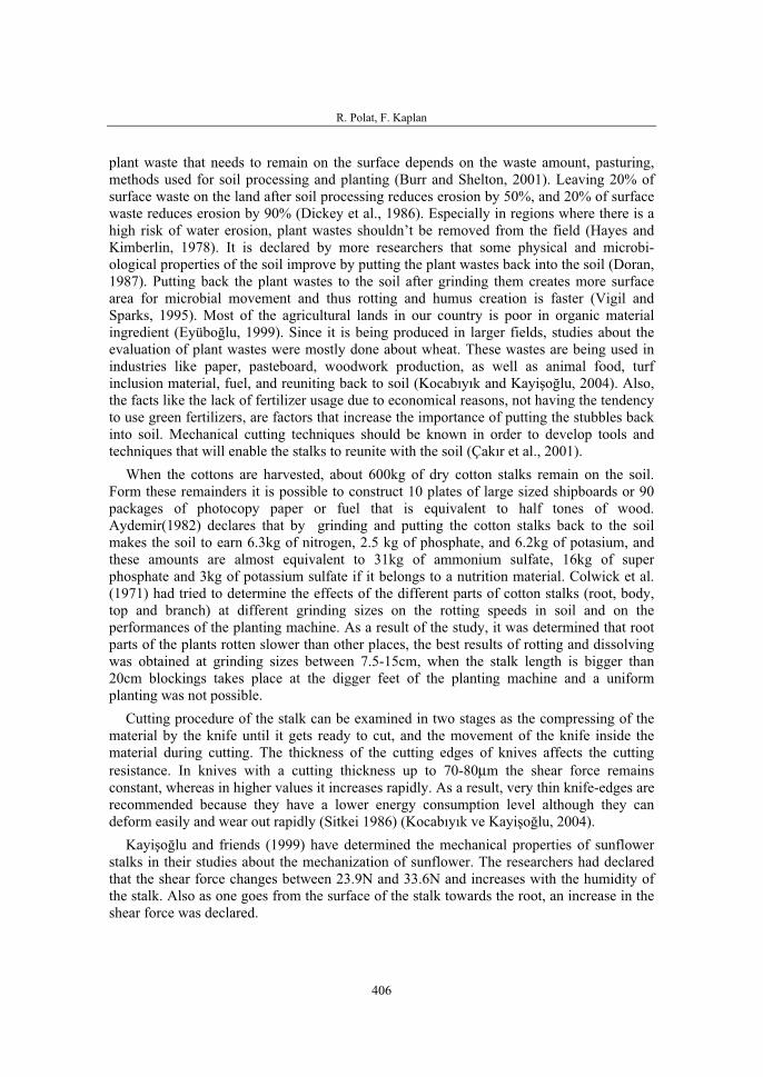
R. Polat, F. Kaplan
406
plant waste that needs to remain on the surface depends on the waste amount, pasturing, methods used for soil processing and planting (Burr and Shelton, 2001). Leaving 20% of surface waste on the land after soil processing reduces erosion by 50%, and 20% of surface waste reduces erosion by 90% (Dickey et al., 1986). Especially in regions where there is a high risk of water erosion, plant wastes shouldn’t be removed from the field (Hayes and Kimberlin, 1978). It is declared by more researchers that some physical and microbi-ological properties of the soil improve by putting the plant wastes back into the soil (Doran, 1987). Putting back the plant wastes to the soil after grinding them creates more surface area for microbial movement and thus rotting and humus creation is faster (Vigil and Sparks, 1995). Most of the agricultural lands in our country is poor in organic material ingredient (Eyüboğlu, 1999). Since it is being produced in larger fields, studies about the evaluation of plant wastes were mostly done about wheat. These wastes are being used in industries like paper, pasteboard, woodwork production, as well as animal food, turf inclusion material, fuel, and reuniting back to soil (Kocabıyık and Kayişoğlu, 2004). Also, the facts like the lack of fertilizer usage due to economical reasons, not having the tendency to use green fertilizers, are factors that increase the importance of putting the stubbles back into soil. Mechanical cutting techniques should be known in order to develop tools and techniques that will enable the stalks to reunite with the soil (Çakır et al., 2001).
When the cottons are harvested, about 600kg of dry cotton stalks remain on the soil. Form these remainders it is possible to construct 10 plates of large sized shipboards or 90 packages of photocopy paper or fuel that is equivalent to half tones of wood. Aydemir(1982) declares that by grinding and putting the cotton stalks back to the soil makes the soil to earn 6.3kg of nitrogen, 2.5 kg of phosphate, and 6.2kg of potasium, and these amounts are almost equivalent to 31kg of ammonium sulfate, 16kg of super phosphate and 3kg of potassium sulfate if it belongs to a nutrition material. Colwick et al. (1971) had tried to determine the effects of the different parts of cotton stalks (root, body, top and branch) at different grinding sizes on the rotting speeds in soil and on the performances of the planting machine. As a result of the study, it was determined that root parts of the plants rotten slower than other places, the best results of rotting and dissolving was obtained at grinding sizes between 7.5-15cm, when the stalk length is bigger than 20cm blockings takes place at the digger feet of the planting machine and a uniform planting was not possible.
Cutting procedure of the stalk can be examined in two stages as the compressing of the material by the knife until it gets ready to cut, and the movement of the knife inside the material during cutting. The thickness of the cutting edges of knives affects the cutting resistance. In knives with a cutting thickness up to 70-80μm the shear force remains constant, whereas in higher values it increases rapidly. As a result, very thin knife-edges are recommended because they have a lower energy consumption level although they can deform easily and wear out rapidly (Sitkei 1986) (Kocabıyık ve Kayişoğlu, 2004).
Kayişoğlu and friends (1999) have determined the mechanical properties of sunflower stalks in their studies about the mechanization of sunflower. The researchers had declared that the shear force changes between 23.9N and 33.6N and increases with the humidity of the stalk. Also as one goes from the surface of the stalk towards the root, an increase in the shear force was declared.

Determination of cutting properties of cotton stalk
407
In this study, it was aimed to determine the dimension properties, stalk densities and cutting properties of the cotton stalks, which will be cutted into parts in order to add to soil in the Southeastern Anatolia Region of Turkey where there are massive amounts of cotton production.
MATERIAL AND METHOD
In this study Stonville-453 type cotton was used which is being produced widely after the irrigation of Şanlıurfa-Harran plain which is a part of GAP. Some of the physical properties of the stalks of this plant is given in Table 1. Experiments made to determine the physical properties of the cotton stalk were carried out in the Harran University Higher Vocational School Mechanics Department's laboratory and Faculty of Agriculture, Department of Agriculture Machines workshops. The trial cottons were harvested by hand in the September and October 2006, in two terms. Trials were done immediately after completing the harvest by hand.
The cotton stalk samples collected from trail field at different times were separated into different section as shown in Figure 1, and regional mechanical properties like shear forces and shear stresses were determined (Kocabıyık, 2003). In order to determine the humidity levels of the cotton stalks, the samples were kept at 103 oC until they reach a stable weight (Kashani Nejad et.al. 2005).
Figure 1 Regions of the cotton stalk on which measurements were made
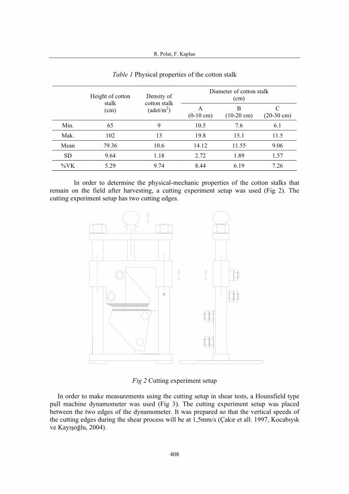
R. Polat, F. Kaplan
408
Table 1 Physical properties of the cotton stalk
Diameter of cotton stalk (cm)Height of cotton
stalk(cm)
Density of cotton stalk (adet/m2) A
(0-10 cm) B
(10-20 cm) C
(20-30 cm)
Min. 65 9 10.5 7.6 6.1
Mak. 102 13 19.8 15.1 11.5
Mean 79.36 10.6 14.12 11.55 9.06
SD 9.64 1.18 2.72 1.89 1.57
%VK 5.29 9.74 8.44 6.19 7.26
In order to determine the physical-mechanic properties of the cotton stalks that remain on the field after harvesting, a cutting experiment setup was used (Fig 2). The cutting experiment setup has two cutting edges.
Fig 2 Cutting experiment setup
In order to make measurements using the cutting setup in shear tests, a Hounsfield type pull machine dynamometer was used (Fig 3). The cutting experiment setup was placed between the two edges of the dynamometer. It was prepared so that the vertical speeds of the cutting edges during the shear process will be at 1,5mm/s (Çakır et all. 1997, Kocabıyık ve Kayışoğlu, 2004).
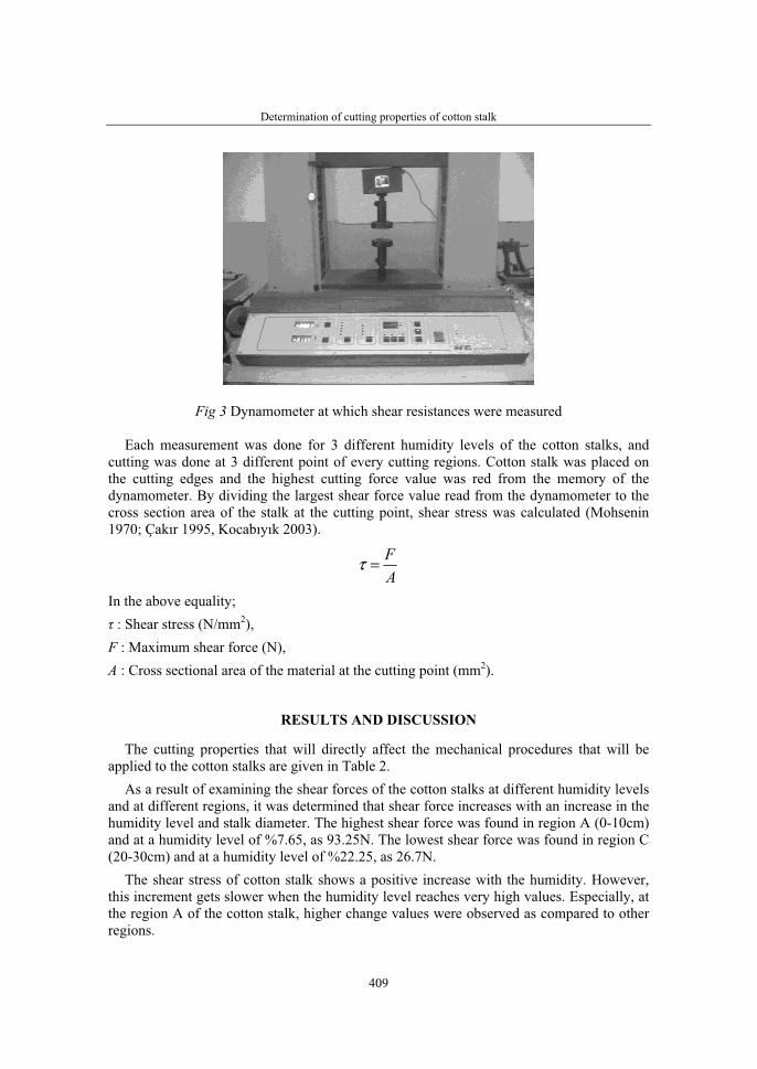
Determination of cutting properties of cotton stalk
409
Fig 3 Dynamometer at which shear resistances were measured
Each measurement was done for 3 different humidity levels of the cotton stalks, and cutting was done at 3 different point of every cutting regions. Cotton stalk was placed on the cutting edges and the highest cutting force value was red from the memory of the dynamometer. By dividing the largest shear force value read from the dynamometer to the cross section area of the stalk at the cutting point, shear stress was calculated (Mohsenin 1970; Çakır 1995, Kocabıyık 2003).
FA
τ =
In the above equality; τ : Shear stress (N/mm2),F : Maximum shear force (N), A : Cross sectional area of the material at the cutting point (mm2).
RESULTS AND DISCUSSION
The cutting properties that will directly affect the mechanical procedures that will be applied to the cotton stalks are given in Table 2.
As a result of examining the shear forces of the cotton stalks at different humidity levels and at different regions, it was determined that shear force increases with an increase in the humidity level and stalk diameter. The highest shear force was found in region A (0-10cm) and at a humidity level of %7.65, as 93.25N. The lowest shear force was found in region C (20-30cm) and at a humidity level of %22.25, as 26.7N.
The shear stress of cotton stalk shows a positive increase with the humidity. However, this increment gets slower when the humidity level reaches very high values. Especially, at the region A of the cotton stalk, higher change values were observed as compared to other regions.

R. Polat, F. Kaplan
410
Table 2 Cutting properties of cotton stalk at different regions
Measuring areas of cotton stalk
A B C
MoistureContent (%) 7.65 13.07 22.25 7.65 13.07 22.25 7.65 13.07 22.25
Min. 89.5 63.0 41.3 80.2 56.1 29.8 67.3 46.4 20.3
Max 99.2 78.3 51.4 89.1 65.6 38.6 76.4 54.6 30.4
Mean 95.25a 71.85c 46.35e 84.95b 60.55d 33.80f 71.60c 48.95e 26.7f
SD 2.81 3.93 3.36 2.99 2.91 3.18 2.37 2.72 2.49
%VK 45.2 53.65 68.42 49.33 62.80 83.21 61.55 72.49 86.48
CuttingForce(N)
AÖF (P<0.05)=10.73
Min. 0.57 0,60 0,66 0,51 0,54 0,53 0,43 0,44 0,42
Max 0,63 0,75 0,82 0,57 0,63 0,71 0,48 0,52 0,55
Mean 0,59b 0,69a 0,74a 0,54a 0,58b 0,62b 0,45b 0,47b 0,49b
SD 0,021 0,047 0,074 0,018 0,029 0,067 0,018 0,026 0,069
% VK 46,30 22,38 45,52 35,65 28,66 45,41 32,71 17,08 48,85
CuttingStress
(N/mm2)
AÖF (P<0.05)= 0.06
As moved from the deep region, the region closest to the soil (region A), towards the upper regions, the cutting properties of the cotton stalk decreases. Janusz et al. (1978), Çakır (1995) and Kocabıyık and Kayışoğlu (2004) have found similar results on their studies concerning sunflower plant stalks. The maximum shear forces and the total shear stress values have decreased in all three regions. This change is due to the fact that the stalk has a harder and wood-like character near the soil.
CONCLUSION
In this study, it was aimed to determine the mechanical properties for mechanization of cotton stalks wastes that remain on the field surface after cotton production which is widely produced in Turkey, especially in the GAP region, and for this purpose shear tests were applied to three different regions of cotton stalk at different humidity levels and the following results were obtained regarding the shear properties of the stalks.
For the three cutting regions of cotton stalks, the maximum shear force was found as 95.25 N in average and shear stress as was found as 0.74 N/mm2 in average. At the end of shear testes, it was determined that mechanical properties like maximum shear force and shear stress exhibit differences depending on the different regions of the stalk and different structural properties. In addition, the humidity ratio of the material is also important on these mechanical properties.
Determination of cutting properties of cotton stalk
411
ACKNOWLEDGEMENTS
This study was partly supported by the Scientific Research Administration Unit of Harran University, Sanliurfa, Turkey.
REFERENCES
1. Aydemir, M., 1982. Pamuk ıslahı, Yetiştirme Tekniği ve Lif Özellikleri, T.K.B. Nazilli Pamuk Araştırma Enstitüsü Yayınları No.3, 233-343s. (In Turkish)
2. Burr, C.A. ve D.P. Shelton, 2001. Winter Weathering Influences on Percent Soybean Residue Cover. Applied Engineering in Agriculture, Vol. 17(2)-159-164.
3. Colwick, R.F., Jones, J.W. and Fulgham, F., 1971. Crop residue disposal-tillage-planting relationships, Transactions of the ASAE, 14(1):114-120pp.
4. Dickey, E.C., P.J. Jasa, D.P. Shelton, 1986. Estimating Residue Cover.. In: Cooperative Extension. University of Nebraska, NebGuide G86-793, Lincoln, USA
5. Doran, J. W., 1987. Microbial biomass and minerilizable nitrogen distribution in no-tillage and plowed soils. Biol. Fertil. Soils 5:68-78.
6. Çakir, E., 1995 The Mechanics of Cutting Plant Residue on a Rigit and Soil Surface. Ph.D. Dissertation. Auburn University. Auburn, AL.
7. Çakir, E., C. E. Johnson, R. L. Raper, R. L. Schafer, 1997. Bitki artıklarının toprak zeminde kesilmesinin mekaniği. Tarımsal Mekanizasyon 17. Ulusal Kongresi, 17-19 Eylül, Tokat. s.966-974. (In Turkish)
8. Çakir, E., C. E. Johnson, R. L. Raper, R. L. Schafer, 2001. The mechanics of cutting plant residue on a rigit and soil surface. SAAED Southern Cooperative Series Bulletin, SCSB-392.
9. Eyüpoğlu, F., 1999. Türkiye Topraklarının Verimlilik Durumu. T.C. Başbakanlık Köy Hizmetleri Genel Müdürlüğü Toprak ve Gübre Araştırma Enstitüsü Yayınları. Genel Yayın No:220. Teknik Yayın No: T-67. Ankara. (In Turkish)
10. Hayes, A.W. and L. W. Kimberlin. 1978. A Guide for Determining Crop Residue for Water Erosion Control. Crop Residue Management System. American Society of Agronomy, Special Publication Number 31. Madison, WI.
11. Janusz, H., B. Szot, J. Korejtko, S. Grundas. 1978. Static cutting resistance and energy of stalk of winter wheat and rye. International Conference on Physical Properties of Plant Materials and Their Influences on Technological Processes. p. 191-199.
12. Kashaninejad M. A. Mortazavi, A. Safekordi and L.G. Tabil. 2005, Some physical properties of pistachio (pistacia vera l.) nut and its kernel. J. of Food Eng. 72 (1), 30-38.
13. Kocabiyik, H. 2003. Ayçiçeği Anızının Parçalanması, Anız Parçalamada Kullanılacak Prototip Bir Makinanın Tasarımı ve İmalatı Üzerine Bir Araştırma. T.Ü. Fen Bilimleri Enstitüsü, Tarım Makinaları Anabilim Dalı, Doktora Tezi, Tekirdağ. (In Turkish)
14. Kocabiyik,H., B., Kayişoğlu. 2004. Ayçiçeği Sapının Kesilme Özelliklerinin Belirlenmesi, Tarım Bilimleri Dergisi.10(3) 263-267. (In Turkish)
15. Mohsenin, N. N., 1970. Physical Properties of Plant and Animal Materials. Gordon and Breach Science Publishers, Library and Congress Catalog Card No: 78-97180, USA.

R. Polat, F. Kaplan
412
16. Sitkei, G., 1986. Mechanics of Agricultural Materials. Elsevier Sciences Publishing, New York.
17. Vigil, M. F. and D. Sparks. 1995. Factors affecting the rate of crop residue decomposition under field conditions. USDA-NRCS/ARS. Conservation Tillage Fact Sheet#3-95, USDA-ARS, Akron, CO.
36. Symposium "Actual Tasks on Agricultural Engineering", Opatija, Croatia, 2008.
413
36.
SIMPOZIJAKTUALNI ZADACIMEHANIZACIJE POLJOPRIVREDE
UDC631.81:633.854.78
Izvorni znanstveni radOriginal scientific paper
THE EFFECT OF MOISTURE CONTENT ON THE THERMAL PROPERTIES OF SUNFLOWER SEEDS
(Helianthus annuus L.)T. AKTAS
Department of Agricultural Machinery, Agricultural Faculty, Namik Kemal University, Tekirdag, Turkey; [email protected]
SUMMARY
Heat transfer in oil seeds is an important issue during production and in handling and processing. Since oil seeds are heat-sensitive due to their comp-osition, their quality may suffer if they are exposed to excessive heat. In some cases heat transfer is also accompanied by mass transfer such as drying or dehydration.
In this research in addition to thermal properties namely thermal conductivity, thermal resistance, specific heat capacity, enthalpy, thermal diffusivity values; some physical properties such as dimensional properties, geometric mean diameter, sphericity, bulk density and 1000 seeds weight were determined experi-mentally. Also water activity values were measured by using a water activity measurement device. All measurements were performed for three different moisture level namely 5.78, 16.18, and 24.2 % (w.b.). The thermal conductivity and thermal resistance were measured by KD2 device that is working according to the transient technique using a line heat source. The specific heat capacity was measured by a calorimeter. Thermal diffusivity was calculated by using obtained data. Enthalpy and water activity values were measured by using a special apparatus that works with Testo 650 data logger. Except thermal resistance all thermal properties increased as the moisture content increased.
Key words: sunflower seeds, thermal properties, moisture content
INTRODUCTION
Sunflower seed (Helianthus annuus L.) is an important oilseed crop because it contains a large quantity of highly nutritious oil (Shulka et al., 1992). It is one of the world’s leading oilseed crops , second only to soybean for total oil production.

T. Aktas
414
The thermal properties of food are its ability to conduct, store, and lose heat. These properties are inherent to today’s food processing and preservation practices. Thermal properties are important for modeling processes (microwave heating, extrusion, freezing, etc.), engineering design of processing equipment, calculating energy demand, and develo-pment of sterilization. Besides processing and preservation, thermal properties also affect sensory quality of foods as well as energy saving from processing (Fontana et al., 2001).
Information on thermal properties of sunflower seed and their dependency on moisture content are useful for the design of various processing equipments that are used in its post harvest processes such as drying, storage, dehulling, oil extraction etc. Thermal conductiv-ity, thermal diffusivity and specific heat capacity are three important engineering properties of a material related to heat transfer characteristics. These parameters are essential in studying heating, drying, oil extraction and cooling processes for sunflower seeds. Thermal properties of many agricultural products have been reported in the literature but the thermal property data of oil seeds are not, however, available in the literature.
Hence, the objective of our investigation was to study on the some physical and thermal properties namely specific heat, thermal conductivity, thermal resistance, enthalpy and thermal diffusivity of sunflower seeds with reference to moisture dependence.
MATERIAL AND METHODS
Sample preparation The samples of the desired moisture contents were prepared by adding the amount of
distilled water (Q) as calculated from the following relation related to initial weight (Wi),initial moisture content (Mi) and final moisture content (Mf) (Coskun et al., 2006):
�
)100()(
f
ifi
MMMW
Q−
−= �� �����
The samples were then kept in polyethylene bags separately and these bags sealed tightly. The samples were kept at 5°C in a refrigerator to enable the moisture to distribute uniformly throughout the sample. During this period, samples were mixed at regular intervals. Before starting a test, the required quantity of the seed was taken out of the refrigerator and allowed to equilibrate to the room temperature for about 2 h (Isik and Unal, 2007).
The sunflower crop is ready for harvest when moisture in seed is 20 % and it can be stored safely when seed contains 10% moisture (http://pnbkrishi.com/sunflower.html). Therefore, all the physical properties and thermal properties of the sunflower seeds were determined at 3 moisture contents in the range of 5.78, 16.18, and 24.2 % (w.b.) with 50 replications for physical properties and 5 repetition for thermal properties at each moisture content. Moisture content values of the sunflower seed samples were determined by oven drying at 130°C to reach constant weight (3 h) with 10 g samples (ASAE, 2003).
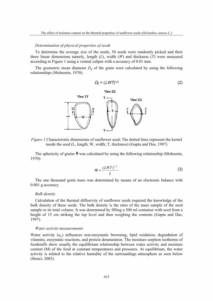
The effect of moisture content on the thermal properties of sunflower seeds (Helianthus annuus L.)
415
Determination of physical properties of seeds To determine the average size of the seeds, 50 seeds were randomly picked and their
three linear dimensions namely, length (L), width (W) and thickness (T) were measured according to Figure 1 using a vernial caliper with a accuracy of 0.01 mm.
The geometric mean diameter Dg of the grain were calculated by using the following relationships (Mohsenin, 1970).
� �������������� �����
Figure 1 Characteristic dimensions of sunflower seed; The dotted lines represent the kernel inside the seed (L, length; W, width; T, thickness) (Gupta and Dos, 1997)
The sphericity of grains was calculated by using the following relationship (Mohsenin, 1970):
�
LLWT 3/1)(=Φ � �����
The one thousand grain mass was determined by means of an electronic balance with 0.001 g accuracy.
Bulk densityCalculation of the thermal diffusivity of sunflower seeds required the knowledge of the
bulk density of these seeds. The bulk density is the ratio of the mass sample of the seed sample to its total volume. It was determined by filling a 500 ml container with seed from a height of 15 cm striking the top level and then weighing the contents (Gupta and Das, 1997).
Water activity measurements Water activity (aw) influences non-enzymatic browning, lipid oxidation, degradation of vitamins, enzymatic reactions, and protein denaturation. The moisture sorption isotherms of foodstuffs show usually the equilibrium relationship between water activity and moisture content (M) of the food at constant temperatures and pressures. At equilibrium, the water activity is related to the relative humidity of the surroundings atmosphere as seen below (Stenci, 2003).
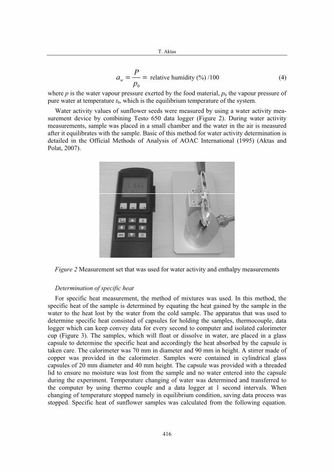
T. Aktas
416
==0p
Paw relative humidity (%) /100 (4)
where p is the water vapour pressure exerted by the food material, p0 the vapour pressure of pure water at temperature t0, which is the equilibrium temperature of the system.
Water activity values of sunflower seeds were measured by using a water activity mea-surement device by combining Testo 650 data logger (Figure 2). During water activity measurements, sample was placed in a small chamber and the water in the air is measured after it equilibrates with the sample. Basic of this method for water activity determination is detailed in the Official Methods of Analysis of AOAC International (1995) (Aktas and Polat, 2007).
Figure 2 Measurement set that was used for water activity and enthalpy measurements
Determination of specific heat For specific heat measurement, the method of mixtures was used. In this method, the
specific heat of the sample is determined by equating the heat gained by the sample in the water to the heat lost by the water from the cold sample. The apparatus that was used to determine specific heat consisted of capsules for holding the samples, thermocouple, data logger which can keep convey data for every second to computer and isolated calorimeter cup (Figure 3). The samples, which will float or dissolve in water, are placed in a glass capsule to determine the specific heat and accordingly the heat absorbed by the capsule is taken care. The calorimeter was 70 mm in diameter and 90 mm in height. A stirrer made of copper was provided in the calorimeter. Samples were contained in cylindrical glass capsules of 20 mm diameter and 40 mm height. The capsule was provided with a threaded lid to ensure no moisture was lost from the sample and no water entered into the capsule during the experiment. Temperature changing of water was determined and transferred to the computer by using thermo couple and a data logger at 1 second intervals. When changing of temperature stopped namely in equilibrium condition, saving data process was stopped. Specific heat of sunflower samples was calculated from the following equation.
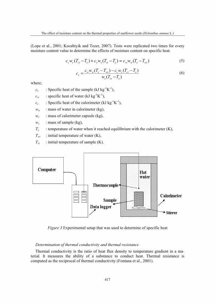
The effect of moisture content on the thermal properties of sunflower seeds (Helianthus annuus L.)
417
(Lope et al., 2001; Kocabiyik and Tezer, 2007). Tests were replicated two times for every moisture content value to determine the effects of moisture content on specific heat.
)()()( wiewwesissecicc TTwcTTwcTTwc −=−+− (5)
)()()(
esis
eciccwiewws TTw
TTwcTTwcc−
−−−= (6)
where; cs : Specific heat of the sample (kJ kg-1K-1),cw : specific heat of water (kJ kg-1K-1),cc : Specific heat of the calorimeter (kJ kg-1K-1),ww : mass of water in calorimeter (kg), wc : mass of calorimeter capsule (kg), ws : mass of sample (kg), Te : temperature of water when it reached equilibrium with the calorimeter (K), Twi : initial temperature of water (K), Tsi : initial temperature of sample (K).
Figure 3 Experimental setup that was used to determine of specific heat
Determination of thermal conductivity and thermal resistance Thermal conductivity is the ratio of heat flux density to temperature gradient in a ma-
terial. It measures the ability of a substance to conduct heat. Thermal resistance is computed as the reciprocal of thermal conductivity (Fontana et al., 2001).
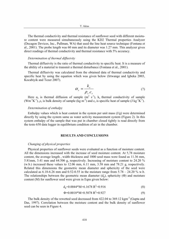
T. Aktas
418
The thermal conductivity and thermal resistance of sunflower seed with different moistu-re content were measured simultaneously using the KD2 Thermal properties Analyzer (Decagon Devices, Inc., Pullman, WA) that used the line heat source technique (Fontana et al., 2001). The probe length was 60 mm and its diameter was 1.27 mm. This analyzer gives direct readings of thermal conductivity and thermal resistance with 5% accuracy.
Determination of thermal diffusivity Thermal diffusivity is the ratio of thermal conductivity to specific heat. It is a measure of
the ability of a material to transmit a thermal disturbance (Fontana et al., 2001). Thermal diffusivity was calculated from the obtained data of thermal conductivity and
specific heat by using the equation which was given below (Irtwange and Igbeka 2003, Kocabiyik and Tezer 2007).
ss
ss c
k.ρ
α = (7)
Here αs is thermal diffusion of sample (m2 s-1), ks thermal conductivity of sample (Wm-1K-1), ρs is bulk density of sample (kg m-3) and cs is specific heat of sample (J kg-1K-1).
Determination of enthalpy Enthalpy values which is heat content in the system per unit mass (J/g) were determined
directly by using the system same as water activity measurement system (Figure 2). In this system enthalpy of the sample that was put in chamber closed tightly is read directly from the testo 650 data logger in equilibrium condition of air in the chamber.
RESULTS AND CONCLUSIONS
Changing of physical properties Physical properties of sunflower seeds were evaluated as a function of moisture content.
All the dimensions increased with the increase of seed moisture content. At 5,78 moisture content, the average length , width thickness and 1000 seed mass were found as 11.36 mm, 5.81mm, 3.41 mm and 64.506 g, respectively. Increasing of moisture content to 24.20 % (w.b.) increased these values to 12.06 mm, 6.11 mm, 3.58 mm and 78.21 g, respectively. Related this dimensions the geometric mean diameter and sphericity of the seed were calculated as 6.18-6.26 mm and 0.52-0.55 in the moisture range from 5.78 – 24.20 % w.b. The relationships between the geometric mean diameter (dg), sphericity (Φ) and moisture content (M) for sunflower seed were given in Eqns given below:
dg=0.0044*M+6.1678 R2=0.916 (8)
Φ=0.0018*M+0.5078 R2=0.927 (9)
The bulk density of the rewetted seed decreased from 422.04 to 369.12 kgm-3 (Gupta and Das, 1997). Correlation between the moisture content and the bulk density of sunflower seed can be seen in Figure 4.
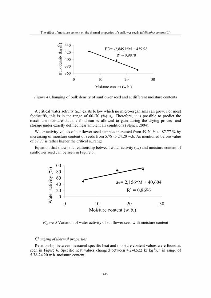
The effect of moisture content on the thermal properties of sunflower seeds (Helianthus annuus L.)
419
BD= -2,8493*M + 439,98R2 = 0,9878
360
380
400
420
440
0 10 20 30
Moisture content (w.b.)
Bul
k de
nsity
(kg
m-3)
Figure 4 Changing of bulk density of sunflower seed and at different moisture contents
A critical water activity (aw) exists below which no micro-organisms can grow. For most foodstuffs, this is in the range of 60–70 (%) aw. Therefore, it is possible to predict the maximum moisture that the food can be allowed to gain during the drying process and storage under exactly defined near ambient air conditions (Stenci, 2004).
Water activity values of sunflower seed samples increased from 49.20 % to 87.77 % by increasing of moisture content of seeds from 5.78 to 24.20 w.b. As mentioned before value of 87.77 is rather higher the critical aw range.
Equation that shows the relationship between water activity (aw) and moisture content of sunflower seed can be seen in Figure 5.
aw= 2,156*M + 40,604
R2 = 0,86960
20406080
100
0 10 20 30Moisture content (w.b.)
Wat
er a
ctiv
ity (%
)
Figure 5 Variation of water activity of sunflower seed with moisture content
Changing of thermal propertiesRelationship between measured specific heat and moisture content values were found as
seen in Figure 6. Specific heat values changed between 4.2-4.522 kJ kg-1K-1 in range of 5.78-24.20 w.b. moisture content.
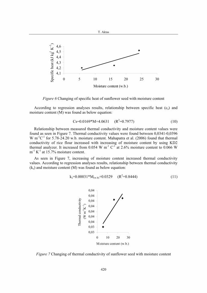
T. Aktas
420
4,14,24,34,44,54,6
0 5 10 15 20 25 30
Moisture content (w.b.)
Spec
ific
heat
(kJ k
g-1 K
-1)
Figure 6 Changing of specific heat of sunflower seed with moisture content
According to regression analyses results, relationship between specific heat (cs) and moisture content (M) was found as below equation:
Cs=0.0169*M+4.0631 (R2=0.7977) (10)
Relationship between measured thermal conductivity and moisture content values were found as seen in Figure 7. Thermal conductivity values were found between 0,0341-0,0396 W m-1C-1 for 5.78-24.20 w.b. moisture content. Mahapatra et al. (2006) found that thermal conductivity of rice flour increased with increasing of moisture content by using KD2 thermal analyzer. It increased from 0.054 W m-1 C-1 at 2.6% moisture content to 0.066 W m-1 K-1 at 15.7% moisture content.
As seen in Figure 7, increasing of moisture content increased thermal conductivity values. According to regression analyses results, relationship between thermal conductivity (ks) and moisture content (M) was found as below equation:
ks=0.00031*M(w.b)+0.0329 (R2=0.8444) (11)
0,030,030,040,040,040,040,040,040,04
0 10 20 30
Moisture content (w.b.)
Ther
mal
con
duct
ivity
(W
m-1
K-1
)
Figure 7 Changing of thermal conductivity of sunflower seed with moisture content
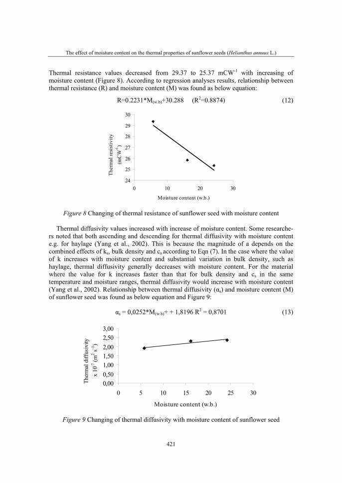
The effect of moisture content on the thermal properties of sunflower seeds (Helianthus annuus L.)
421
Thermal resistance values decreased from 29.37 to 25.37 mCW-1 with increasing of moisture content (Figure 8). According to regression analyses results, relationship between thermal resistance (R) and moisture content (M) was found as below equation:
R=0.2231*M(w.b)+30.288 (R2=0.8874) (12)
24
25
26
27
28
29
30
0 10 20 30
Moisture content (w.b.)
Ther
mal
resi
stiv
ity (m
CW
-1)
Figure 8 Changing of thermal resistance of sunflower seed with moisture content
Thermal diffusivity values increased with increase of moisture content. Some researche-rs noted that both ascending and descending for thermal diffusivity with moisture content e.g. for haylage (Yang et al., 2002). This is because the magnitude of a depends on the combined effects of ks, bulk density and cs according to Eqn (7). In the case where the value of k increases with moisture content and substantial variation in bulk density, such as haylage, thermal diffusivity generally decreases with moisture content. For the material where the value for k increases faster than that for bulk density and cs in the same temperature and moisture ranges, thermal diffusivity would increase with moisture content (Yang et al., 2002). Relationship between thermal diffusivity (αs) and moisture content (M) of sunflower seed was found as below equation and Figure 9:
αs = 0,0252*M(w.b)+ + 1,8196 R2 = 0,8701 (13)
0,000,501,001,502,002,503,00
0 5 10 15 20 25 30
Moisture content (w.b.)
Ther
mal
diff
usiv
ity
x 10
-7 (m
2 s-1
)
Figure 9 Changing of thermal diffusivity with moisture content of sunflower seed
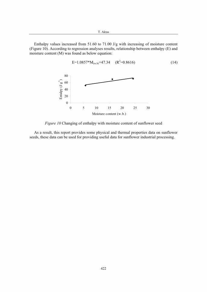
T. Aktas
422
Enthalpy values increased from 51.60 to 71.00 J/g with increasing of moisture content (Figure 10). According to regression analyses results, relationship between enthalpy (E) and moisture content (M) was found as below equation:
E=1.0857*M(w.b)+47.34 (R2=0.8616) (14)
0
20
40
60
80
0 5 10 15 20 25 30
Moisture content (w.b.)
Enta
lpy
(J g
-1)
Figure 10 Changing of enthalpy with moisture content of sunflower seed
As a result, this report provides some physical and thermal properties data on sunflower seeds, these data can be used for providing useful data for sunflower industrial processing.

The effect of moisture content on the thermal properties of sunflower seeds (Helianthus annuus L.)
423
REFERENCES
1. Aktas T., Polat R. (2007).Changes in the drying characteristics and water activity values of selected pistachio cultivars during hot air drying. Journal of Food Process Engineering 30 (5): 607-624.
2. ASAE (2003). ASAE S352.2 FEB03. Moisture Measurement-Unground Grain and Seeds.
3. Coskun M.B., Yalcin I., Ozarslan C. (2006). Physical properties of sweet corn seed (Zea mays saccharata Sturt.), Journal of Food Engineering 74 (4): 523–528.
4. Fontana A.J., Wacker B., Campbell C.S., Campbell G.S. (2001). Simultaneous thermal conductivity, thermal resistance, and thermal diffusivity measurement of selected foods and soil. ASAE Annual International Meeting. California, USA. July 30-August 1. Paper Number 016101.
5. Gupta R.K., Das S.K. (1997). Physical properties of sunflower seeds. J. Agric. Eng. Res. 66: 1–8.
6. Irtwange, S. V., Igbeka, J. C. (2003). Influence of moisture content on thermal diffusivity and specific heat of African yam bean (Sphenostylis stenocarpa). Transactions of the ASAE 46(6):1633-1636.
7. Isik E., Unal H. (2007). Moisture-dependent physical properties of white speckled red kidney bean grains. Journal of Food Engineering .82(2): 209-216.
8. Kocabiyik H., Tezer D. (2007). Determination of thermal properties of rapeseed. Journal of Tekirdag Agricultural Faculty 4 (1): 65-70.
9. Lope G. T., Marshall V., Hong Q., (2001). Thermal properties of sugar beets. ASAE Annual International Meeting. Paper No. 016141.
10. Mahapatra A. K., Lan Y., Nguyen C. (2006). Thermal properties of rice flours. ASABE Annual International Meeting. Portland, Oregon 9 - 12 July. Paper Number: 066112.
11. Mohsenin N.N. (1970). Physical properties of plant and animal materials, Gordon and Breach, New York.
12. Shulka B.D., Srivastava P.K., Gupta R.K. (1992). Oilseed processing technology. CIAE, India .
13. Stencl J. (2004). Modelling the water sorption isotherms of yoghurt powder spray. Mathematics and Computers in Simulation. 65:157-164.
14. Yang W., Sokhansanj S., Tang J., Winter P. (2002).Determination of thermal conductivity, specific heat and thermal diffusivity of borage seeds. Biosystems Engineering 82 (2):169–176.

36. Symposium "Actual Tasks on Agricultural Engineering", Opatija, Croatia, 2008.
425
36.
SIMPOZIJAKTUALNI ZADACIMEHANIZACIJE POLJOPRIVREDE
UDK664.844
Stručni radExpert paper
FIZIČKO – KEMIJSKI POKAZATELJI KVALITETE SUŠENOG POVRĆA IZ A.D. „SEMBERKA“, JANJA,
BOSNA I HERCEGOVINA HUSEJIN KERAN1, NUSRETA ĐONLAGIĆ1, MIRSAD SALKIĆ1,
NIHADA AHEMTOVIĆ2,3, SELMA MULAHALILOVIĆ4
1 – Tehnološki fakultet, Univerzitet u Tuzli, Univerzitetska 8, 75000 Tuzla, BiH 2 – Zavod za javno zdravstvo Tuzlanskog kantona, 75000 Tuzla, BiH
3 – Medicinski fakultet, Univerzitet u Tuzli, Univerzitetska 1, 75000 Tuzla, BiH 4 – A.D. „Semberka“, Janja, BiH
SAŽETAK
Proizvodnja poljoprivrednih kultura u zemljama u tranziciji predstavlja veliki problem iz razloga, što se primjenjuju različite vrste zaštitnih sredstava i gnojiva. Semberija je regija u sjeveroistočnoj Bosni i Hercegovini, te predstavlja ravničarski dio u kojem se najviše uzgajaju poljoprivredne kulture, koje dalje služe za prodaju ili za preradu u fabrici A.D. „Semberka“ iz Janje. Stara poljoprivredna mehanizacija, nedovoljno financijskih sredstava, needuciranost poljoprivrednih proizvođača samo su neki od problema sa kojima se svakodnevno susreće proizvodnja poljoprivrednih kultura. Međutim, iako postoje brojni problemi u poljoprivrednoj proizvodnji, analiza fizičko – kemijskih sastojaka sušenog i prerađenog povrća pokazuje visok nivo kvaliteta. Ovaj rad ima namjeru da ukaže na probleme sa kojima se susreću poljoprivredni proizvođači s jedne strane, a da s druge strane pokaže da je sirovina za preradu sa ovog područja sigurna sa aspekta zdravstvene ispravnosti i da je pod stalnim nadzorom stručnih službi. Kemijske analize teških metala kao što su kadmij, olovo, arsen i živa su uvijek ispod dozvoljenih granica, odnosno manje od 0,1 mg/kg što je propisano važećim pravilnikom o sadržaju teških metala u poljoprivrednim kulturama i proizvodima.
Ključne riječi: teški metali, fizičko – kemijska analiza, poljoprivredne kulture, povrće

H. Keran, N. Đonlagić, M. Salkić, N. Ahemtović, S. Mulahalilović
426
UVOD
Nivo teških metala u okolišu je u zadnjim desetljećima izrazito povećan, kao posljedica djelovanja ljudskih aktivnosti. Kako je toksičnost teških metala vezana za njihove postojećevrste, specijacija istih zauzima posebno mjesto kod njihova proučavanja(1). Zbog toga postoji potreba za veoma brzim i preciznim određivanjem koncentracije teških metala u proizvodima, a posebno onih za koje se smatra da su veoma toksični(3,9).
Najdostupnije metode koriste skupu opremu ili je određivanje sadržaja metala u proizvodima veoma dugotrajno, što za rezultat ima potrebu za brzim terenskim metodama, posebno ako se ima u vidu da razni faktori utiču na sadržaj teških metala na i u biljkama, kao što su klima, njihov sadržaj u tlu, te priroda tla na kome biljka raste i stupanj dozrijevanja biljki u vrijeme njihove žetve(4).
Obzirom da su teški metali veoma toksični i da su u povrću prisutni u niskim koncentracijama, a činjenica je da se povrće najčešće konzumira kao svježe, njihov dnevni unos treba biti pod stalnim nadzorom(11). Potreba za stalnim nadzorom nad unosom teških metala leži i u činjenici da se na tržištu nalaze različite vrste hrane koje nisu adekvatno kontrolirane, a dodatno se i dalje svakodnevno potpisuju novi ugovori koji omogućavajuslobodnu trgovinu roba(5). Imajući u vidu gore sve navedeno, dobavljači sirovina za proces sušenja i proizvodnju sušenih proizvoda na bazi povrća u A.D. “Semberka” Janja su pod stalnim nadzorom kako od strane stručne ovlaštene institucije, tako isto i od agronoma zaposlenika. Zahtjevi koji su propisani za svježe povrće koje ide na proces sušenja od strane A.D. “Semberka” iz Janje su bazirani na važećem pravilniku(6) za navedenu proizvodnju, te se kao takvi moraju poštovati od strane svih onih koji su ocjenjeni kao dobavljači svježih sirovina.
Svježe povrće koje se uzima sa parcela iz Semberije, se obrađuje sa zastarjelom poljoprivrednom mehanizacijom, koja je u prosjeku stara i preko dvadesetak godina. Dodatne probleme u obradi zemljišta stvaraju kako needuciranost stanovništva na ovom području, tako isto i nedostatak financijskih sredstava, potrebnih za angažman stručnogosoblja kod proizvodnje svježeg povrća.
Needuciranost proizvođača povrća i primjena neadekvatnih agrotehničkih mjera u njegovom uzgoju glavna su prepreka za dobivanje zdravstveno sigurne sirovine, a time i gotovog proizvoda(8). Teški metali su kontaminanti koji u povrće mogu da dospiju iz različitih izvora, kao što su tlo, zaštitna sredstva, i dr. a kao takvi uzrokuju velike probleme po zdravlje potrošača(10). Zbog toga rad ima za cilj da prikaže kvalitetu sirovine i gotovog proizvoda, koji su najviše zastupljeni u preradi firme A.D. “ Semberka”, Janja, pri tome se osvrćući na probleme koji su posljedica nedostatka zakonske regulative i pravilnika iz ove oblasti(6,7).
MATERIJAL I METODE
Radi dobre procjene kod upotrebe sušenih proizvoda na bazi povrća, u određenimproizvodima izvršene su kemijske analize koje su imale za cilj utvrđivanje sadržaja teških metala u sušenim proizvodima. Proizvodi, kao što su sušeni paštrnjak, sušene mrkvine
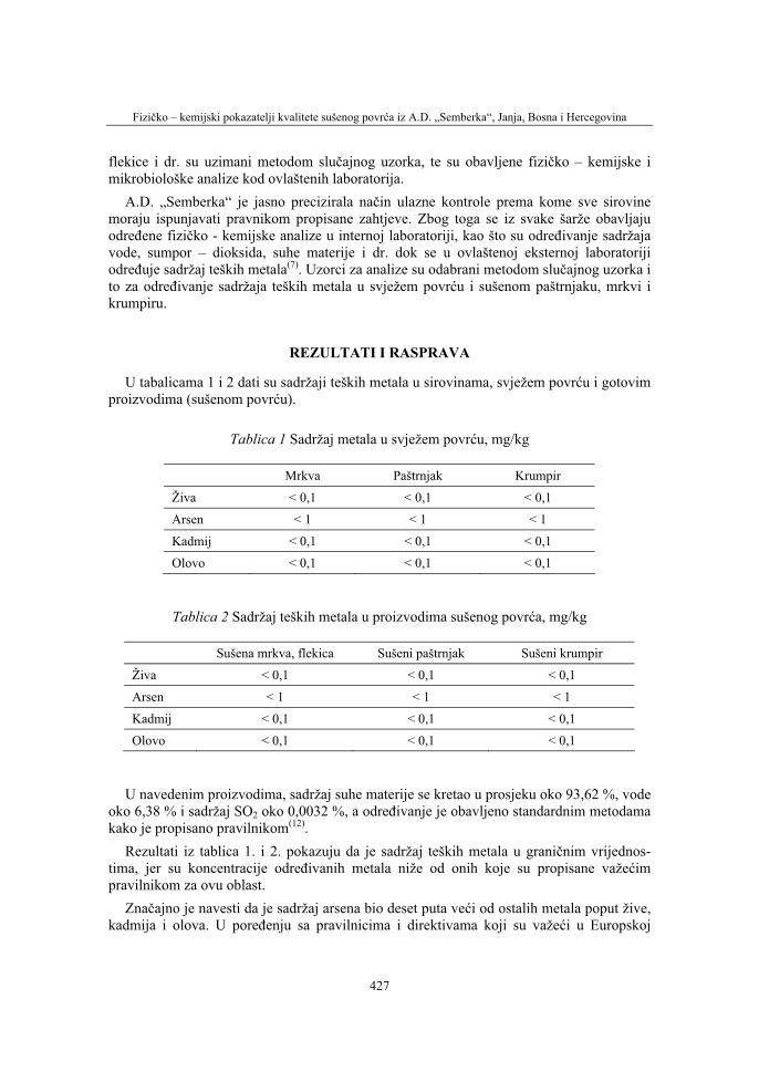
Fizičko – kemijski pokazatelji kvalitete sušenog povrća iz A.D. „Semberka“, Janja, Bosna i Hercegovina
427
flekice i dr. su uzimani metodom slučajnog uzorka, te su obavljene fizičko – kemijske i mikrobiološke analize kod ovlaštenih laboratorija.
A.D. „Semberka“ je jasno precizirala način ulazne kontrole prema kome sve sirovine moraju ispunjavati pravnikom propisane zahtjeve. Zbog toga se iz svake šarže obavljaju određene fizičko - kemijske analize u internoj laboratoriji, kao što su određivanje sadržaja vode, sumpor – dioksida, suhe materije i dr. dok se u ovlaštenoj eksternoj laboratoriji određuje sadržaj teških metala(7). Uzorci za analize su odabrani metodom slučajnog uzorka i to za određivanje sadržaja teških metala u svježem povrću i sušenom paštrnjaku, mrkvi i krumpiru.
REZULTATI I RASPRAVA
U tabalicama 1 i 2 dati su sadržaji teških metala u sirovinama, svježem povrću i gotovim proizvodima (sušenom povrću).
Tablica 1 Sadržaj metala u svježem povrću, mg/kg
Mrkva Paštrnjak Krumpir
Živa < 0,1 < 0,1 < 0,1
Arsen < 1 < 1 < 1
Kadmij < 0,1 < 0,1 < 0,1
Olovo < 0,1 < 0,1 < 0,1
Tablica 2 Sadržaj teških metala u proizvodima sušenog povrća, mg/kg
Sušena mrkva, flekica Sušeni paštrnjak Sušeni krumpir
Živa < 0,1 < 0,1 < 0,1
Arsen < 1 < 1 < 1
Kadmij < 0,1 < 0,1 < 0,1
Olovo < 0,1 < 0,1 < 0,1
U navedenim proizvodima, sadržaj suhe materije se kretao u prosjeku oko 93,62 %, vode oko 6,38 % i sadržaj SO2 oko 0,0032 %, a određivanje je obavljeno standardnim metodama kako je propisano pravilnikom(12).
Rezultati iz tablica 1. i 2. pokazuju da je sadržaj teških metala u graničnim vrijednos-tima, jer su koncentracije određivanih metala niže od onih koje su propisane važećimpravilnikom za ovu oblast.
Značajno je navesti da je sadržaj arsena bio deset puta veći od ostalih metala poput žive, kadmija i olova. U poređenju sa pravilnicima i direktivama koji su važeći u Europskoj

H. Keran, N. Đonlagić, M. Salkić, N. Ahemtović, S. Mulahalilović
428
Uniji, sadržaj nekih teških metala u proizvodima od povrća je drugačije definiran, jer su granične vrijednosti postavljene tako da je maksimalno dozvoljena koncentracija olova, 0,1 mg/kg, kadmija 0,05(2) mg/kg svježeg povrća, što je deset puta manje, za olovo i dvadeset puta manje, kadmij, od maksimalno dozvoljene koncentracije u povrću koja je definirana važećim pravilnikom u BiH. Veliki nedostatak kod važećih pravilnika(6,7) koji se primjenjuju za određivanje teških metala u povrću je taj što se točno ne navodi sadržaj i kao takav predstavlja u zvaničnim analizama. Prikazivanje sadržaja teških metala, kako je prikazano u tablici 1 je neadekvatno jer nije moguće iznositi zaključak o sadržaju kontaminanata u hrani.
Radi usporedbe sadržaja teških metala u svježem i konzerviranom povrću, tj. sušenim proizvodima, prikazan je sadržaj i u sirovini i u gotovom proizvodu. Međutim, nije lako komentirati navedene rezultate, zbog toga što se u laboratorijskim izvješćima ne navode točne vrijednosti sadržaja teških metala. U laboratorijskim izvješćima se navode samo manje ili veće vrijednosti od onih koje su propisane važećim pravilnikom. Institucije koje se bave određivanjem sadržaja teških metala u proizvodima ili nisu dovoljno opremljene da daju precizne rezultate ili takvi rezultati nisu u skladu sa važećim pravilnicima, pri čemu se stvara velika sumnja u njihovu točnost.
Povrće nakon sušenja sadržavalo je 6 do 8 % vode, što je također propisano pravilni-kom(12), a kad su u pitanju proizvodi koji su analizirani, sadržaj vode je u dozvoljenim granicama jer je njegova prosječna vrijednsot bila 6,38 %. Sadražj sumpor dioksida, tako-đer je u graničnim vrijednostima koje su propisane pravilnikom za ovu vrstu proizvoda(12).
Tablica 3 Rezultati mikrobiološke analize proizvoda od sušenog povrća
Rednibroj Vrsta mikroorganizama Veličina Jedinica Rezultat
1. Salmonela vrste u 25,0 g/ml negativan 2. Koagulaza pozitivni
stafilokoki u 0,01 g/ml negativan
3. Sulforedukujućeklostridije u 0,01 g/ml negativan
4. Escherichia coli u 0,001 g/ml negativan 5. Proteus vrste u 0,001 g/ml negativan 6. Ukupan broj bakterija u 1,0 g/ml zadovoljava 7. Broj kvasaca i plijesni u 1,0 g/ml zadovoljava
Rezultati mikrobioloških analiza pokazuju da prisustvo mikroorganizama zadovoljava pravilnikom propisane granične vrijednosti, tj. da je ukupan broj mikroorganizama, plijesni i kvasca u sušenoj mrkvi, sušenom paštrnjaku i sušenom krumpiru manji od onoga koji je propisan važećim pravilnikom(10).
Fizičko – kemijski pokazatelji kvalitete sušenog povrća iz A.D. „Semberka“, Janja, Bosna i Hercegovina
429
ZAKLJUČCI
Na bazi provedenih analiza moguće je zaključiti sljedeće:
• Proizvodi koji su analizirani od strane ovlaštenih laboratorija zadovoljavaju pravilni-kom propisane vrijednosti za teške metale, ali su dobiveni rezultati nepouzdani tako da se može stvarati sumnja u kvalitetu gotovog proizvoda;
• Uspostava nadzora nad dobavljačima osigurava da sadržaj teških metala u gotovim proizvodima bude u graničnim vrijednostima;
• Neprikazivanje točnih rezultata analiza, odnosno komentari u smislu zadovoljava ili ne zadovoljava, zahtjeva brzu reformu ovlaštenih institucija za kontrolu kvalitete hrane, a posebno kada su pitanju toksični metali, rezidue pesticide i dr.;
• Usklađenost pravilnika iz navedene oblasti sa EU direktivama je od izuzetne važnosti, jer su teški metali neprijatelj broj jedan za zdravlje potrošača prehrambenih proizvoda.
LITERATURA
1. Bin Li, Qiuquan Wang, Benli Huang, Shuping Li.(2001). Evaluation of results from a Quasi-Tessier’s sequential extraction procedure for heavy metal speciation in soils and sediment by ICP-MS”. Analytical Sciences, Vol. 17 supplement.
2. European Commission. Commission Regulation (EC) No 466/2001 of 8 March 2001 Setting Maximum Levels for Certain Contaminants in Foodsuffs. Official Journal of the European Communities L77:1-13,
3. Haeng-Shin Lee, Yang-Hee Cho, Seon-Oh Park, Seung-Hee Kye, Bok-Hee Kim, Tae-Shik Hahm, Meehye Kim, Jong Ok Lee, Cho-il Kim.(2006). Dietary exposure of the Korean population to arsenic, cadmium, lead and mercury, Journal of Food Composition and Analysis 19, S31–S37,
4. Meissner, K., Lippert, T., Wokaun, A., Guenther, D. (2004). Analysis of trace metals in comparison of laser-induced breakdown spectroscopy with LA-ICP-MS”, Elsevier 316-322.
5. McLaughlin M. J., Parker D. R, Clarke J. M. (1999). Metals and Micronutrients- Food Safety Issues. Field Crops Research 60, 43-163,
6. PRAVILNIK o količinama, pesticida i drugih otrovnih materija, antibiotika i mikotoksina koji se mogu nalaziti u životnim namirnicama, Sl. list SFRJ br. 59/83 i 79/87.
7. PRAVILNIK o metodi obavljanja analiza i superanaliza za određivanje količine teških metala (olova, bakra, željeza i nikla) u životnim namirnicama – uljima, mastima i margarinu, Sl. list SFRJ 1984.
8. Scott, D., Keoghan, J.M., Allan, B.E. (1996). Native and low-input grasses a New Zealand high country perspective. N. Z. J. Agric. Res. 39, 499–512.
9. Voutsa, D., Grimanis, A., Samara, C. (1996) Trace elements in vegetables grown in an industrial area in relation to soil and air particulate matter. Environ. Pollut. 94, 325–335.
10. Pravilnik o uslovima u pogledu mikrobiološke ispravnosti kojima moraju odgovarati životne namirnice u prometu, Sl. list SFRJ br. 45/83 i 43/89.

H. Keran, N. Đonlagić, M. Salkić, N. Ahemtović, S. Mulahalilović
430
11. Xilong, W., Sato, T., Baoshan, X., Tao, S. (2005). Health risks of heavy metals to the general public in Tianjin, China via consumption of vegetables and fish, Science of the Total Environment339, 153– 166.
12. Pravilnik o kvalitetu proizvoda od voća, povrća, pečurki i pektinskih proizvoda. Sl. list SFRJ br. 1/79 i 20/82.
PHYSICAL – CHEMICAL PARAMETERS OF QUALITY OF DREID VEGETABLES FROM “SEMBERKA”, JANJA,
BOSNIA AND HERZEGOVINA
SUMMARY
Agricultural production in transitional countries presents a big problem because a different nutrients and pesticides have been used. Semberija is a part of North – east Bosnia and Herzegovina, and it is a flat, where many agricultural plants have been grown, which are than used for selling or processing factory ”Semberka” from Janja. An old agricultural machinery, deficit of financial resources, non-educated agricultural producers are only some of present probl-ems in this production. Although, there are many problems in agricultural production, physical – chemical parameters of raw and dried vegetables show a high level of quality. This work is aimed to show what problems are present with agricultural producers and processors. On the other hand, it is also intended to show the quality of raw materials regarding to heavy metals, as well as to emphasize the presence of permanent monitoring by doing chemical analyses of toxic metals such as Cd, Hg, As, Pb. Analyses showed that the content of toxic metals is lower than the limit predicted by regulation, e.g. less than 0,1 mg/kg of fresh weight.
Key words: heavy metals, physical – chemical analyses, agricultural plants, vegetables

36. Symposium "Actual Tasks on Agricultural Engineering", Opatija, Croatia, 2008.
431
36.
SIMPOZIJAKTUALNI ZADACIMEHANIZACIJE POLJOPRIVREDE
UDK66.02:663.815
Stručni radExpert paper
UTJECAJ VRSTE I KONCENTRACIJE ADITIVA NA SENZORNA SVOJSTVA VOĆNOG ŽELEA
SLAVICA GRUJIĆ*, KARMELA PLAVŠIĆ*,MIDHAT JAŠIĆ**, SINIŠA BLAGOJEVIĆ**
*Tehnološki fakultet Univerziteta u Banjoj Luci, S. Stepanovića 73., Banja Luka,Bosna i Hercegovina, e-mail: [email protected]
**Tehnološki fakultet Univerziteta u Tuzli, Tuzla, Bosna i Hercegovina,e-mail: [email protected]
SAŽETAK
Voćni žele je proizvod koji se dobija ukuvavanjem voćnog soka uz dodatak šećera i aditiva, kako bi se postigla pihtijasta konzistencija. Važećim propisima definisani su uslovi kvaliteta koje proizvod mora zadovoljiti. Cilj ovog rada je bila izrada voćnog želea sa reverzibilnim svojstvima želiranja, koji se može koristiti direktno iz ambalaže. Ovi proizvodi namijenjeni su za izradu preliva ili nadjeva za kolače i pekarske proizvode.
Uzorci želea su proizvedeni od koncentrovanih voćnih sokova jabuke (SM 70%) i višnje (SM 65%) i različite količine aditiva, sredstva za želiranje proizvođača DANISCO CULTOR (2 uzorka) i OBIPEKTIN (3 uzorka), sredstva za vezivanje (CaCl2; E 509), regulatora kiselosti (trinatrijun citrat dihidrat, E 331) i limunska kiselina (E 330). Kvalitet proizvedenih uzoraka želea ocijenjivan je senzornim metodama analize, deskriptivnom metodom bodovanja i metodom rangiranja, kako bi se utvrdila revezibilna sposobnost formiranja gela i postojanost nakon zagrijavanja (na temperaturi od 45-50°C), primjene na proizvod i hlađenja 24 i 48 sati (na temperaturi od 4 - 8°C).
Od 23 uzorka voćnog želea (13 od jabuke i 10 od višnje), izdvojeni su uzorci najprihvatljivijeg kvaliteta. Ovi uzorci su i nakon ponovnog zagrijavanja i hlađenja bili dobro želirani, imali su umjereno čvrstu konzistenciju, sjajnu površinu i presjek, kristalnu bistrinu i bili su umjerenog stepena slasti i boje, ukusa i mirisa karakterističnih za voće od kojeg su proizvedeni.
Ključne riječi: voćni žele, razvoj proizvoda
S. Grujić, K. Plavšić, M. Jašić, S. Blagojević
432
UVOD
U savremenoj nauci o ishrani ljudi smatra se da među namirnicama voće i proizvodi od voća trebaju imati jedno od važnijih mjesta [1]. U Bosni i Hercegovini kvalitet voćnog želea definisan je Pravilnikom o kvalitetu proizvoda od voća, povrća, pečurki i pektinskih preparata [2]. Voćni žele je proizvod koji se može proizvoditi ukuvavanjem voćnog soka malina, jagoda, višnje, citrus plodova i dr., uz dodatak šećera i aditiva, kako bi se postigla pihtijasta konzistencija. U proizvodnji voćnih želea radi zadovoljenja posebnih zahtjeva i očekivanja potrošača i postizanja specifičnih svojstava proizvoda najčešće se koriste prehrambeni aditivi: sredstva za želiranje, stabilizatori, regulatori kiselosti, učvršćivači,kiseline i konzervansi [2, 3, 4]. Prilikom utvrđivanja i definisanja kvaliteta prehrambenih proizvoda, kao i kod razvoja novih proizvoda, senzorna analiza ima značajnu ulogu [5, 6, 7, 8, 9].
Cilj ovog rada je bila izrada voćnog želea jabuke i voćnog želea višnje sa reverzibilnim svojstvima želiranja, namijenjenih za izradu preliva ili nadjeva za kolače i pekarske proizvode.
MATERIJAL I METODE
Uzorci želea proizvedeni su od: koncentrovanog voćnog soka jabuke (SM 70%) ili koncentrovanog voćnog soka višnje (SM 65%); šećera (saharoze); sredstva za želiranje proizvođača: DANISCO CULTOR (Grinsted Pectin GZ 955 i Grinsted Pectin LC 710) i OBIPEKTIN (Pektin Purple Ribbon D-0,75 A; Pektin Purple Ribbon D-0,75 AH i Pektin Purple Ribbon pure); sredstva za vezivanje (CaCl2; E 509); regulatora kiselosti (trinatrijun citrat dihidrat, E 331); limunske kiseline (E 330) i vode.
Proces proizvodnje voćnog želea u laboratorijskim uslovima sastoji se od: mjerenja potrebne količine sastojaka, prema recepturi; pripreme rastvora sredstva za želiranje, šećerai vode; pripreme rastvora sredstva za vezivanje, gdje je potrebno, a nakon toga izrade voćnog želea provođenjem postupaka homogenizovanja i zagrijavanja potrebne količinešećera, vode, koncentrovanog voćnog soka i rastvora sredstava za želiranje; dodavanja sredstva za vezivanje, gdje je potrebno; provjere suve materije (refraktometrom), kiselosti (titracijom) i pH vrijednosti (pH-metrom); korekcije kiselosti proizvoda na zadanu vrijednost dodavanjem limunske kiseline; punjenja gotovog proizvoda u zagrijanu staklenu ambalažu i zatvaranja (temp. proizvoda prilikom punjenja minimalno 80°C).
Proizvodnja uzoraka vršena je u dvije faze, a uzorci su se razlikovali u vrsti sredstva za želiranje, sadržaju suve materije, u količini upotrebljenog sredstva za vezivanje i regulatora kiselosti. Kvalitet pripremljenih uzoraka želea ocjenjivan je u staklenoj ambalaži najmanje 10 dana nakon proizvodnje, kao i ponovo želiranih uzoraka nakon zagrijavanja, razlijevanja u kalupe i skladištenja 24h i 48h na temperaturi +4 do +8°C. Nakon senzorne ocjene kvaliteta uzoraka voćnog želea i rangiranja na osnovu ocjene % od maksimalno mogućegkvaliteta, odabrani su uzorci na kojima treba pokušati postići određena poboljšanja kvaliteta. Recepture za izradu ovih uzoraka su korigovane u cilju primjene što manje količine aditiva.
Utjecaj vrste i koncentracije aditiva na senzorna svojstva voćnog želea
433
Senzornom analizom, primjenom metoda bodovanja (skala sa 5 bodova i odgovarajućimkoeficjentima važnosti) i rangiranja, ispitivani su pokazatelji kvaliteta proizvoda: konzistencija, spoljni izgled, boja, ukus i miris, stepen slasti (Tablica 1). Senzorna analiza proizvoda vršena je komisijski (5 članova, stručnjaka u oblasti proizvodnje i kontrole kvaliteta namirnica), koji su upoznati sa ciljem ispitivanja, zahtjevima kvaliteta proizvoda i terminologijom korištenom za izradu ocjenjivačkih listova. Tokom senzorne analize, članovi komisije su svaki dostavljeni uzorak pojedinačno ispitivali, a zatim zajedno prodiskutovali i utvrdili ocjene za odgovarajuće pokazatelje kvaliteta (Tablica 1). Konačnaocjena je unošena u ocjenjivački list.
REZULTATI I DISKUSIJA
Recepture za izradu voćnog želea prilagođene su propisanim uslovima kvaliteta [2].Važećim propisima o kvalitetu definisano je da sadržaj suve materije u voćnim želeima mora biti minimalno 67%, s tim da je udio suve materije iz voća minimalno 6%. Niskokalorični proizvodi od voća moraju imati najmanje 20% niži sadržaj suve materije od predviđene za klasične proizvode, što se postiže umanjenjem sadržaja šećera.
Od voćnog želea se očekuje da nakon zagrijavanja i aplikacije na proizvod zadrži svoja karakteristična senzorna svojstva. Žele treba da bude bistrog izgleda, svjetlucav ili opalescentan, u zavisnosti od vrste upotrebljenog voćnog soka, boje, ukusa i mirisa karakterističnih za sirovinu od koje je proizveden, umjereno čvrste konzistencije gela. Kada se siječe, ako je čvrste konzistencije, treba da ima takvu čvrstinu da se dobije glatka svjetlucava površina.
U prvoj fazi eksperimenta prema odgovarajućim recepturama proizvedeno je 9 uzoraka voćnog želea od jabuke (Tablica 2) i 9 uzoraka voćnog želea od višnje (Tablica 3), od kojih su nakon senzorne ocjene kvaliteta i rangiranja, odabrana po 3 uzorka najprihvatljivijih senzornih svojstava (Tablica 4). Recepture u kojima je korišten koncentrovani sok višnje za izradu voćnog želea, identične su kao i odgovarajuće recepture sa koncentrovanim sokom jabuke. Od uzoraka voćnog želea od jabuke kao najbolji su odabrani uzorak 3.1.1. sa 91% od max. mogućeg kvaliteta, zatim uzorak 5.1.1. sa 81% i uzorak 4.1.1. sa 78% od max. mogućeg kvaliteta (Tablica 4; Slika 1). Od uzoraka voćnog želea od višnje kao najbolji su odabrani uzorak 3.2.1. sa 91% od max. mogućeg kvaliteta i uzorak 4.2.1. sa 77% od max. mogućeg kvaliteta (Tablica 4; Slika 1).
Za drugu fazu eksperimenta odabrano je nekoliko uzoraka, na kojima su se pokušala postići određena poboljšanja kvaliteta, a čija bi proizvodnja bila ekonomski opravdana. Modifikovane su recepture za izradu uzoraka oznake 1.1.4., 3.1.1. 4.1.1. i 5.1.1. (Tablica 5). Sva četiri uzorka su proizvedena sa sniženim ukupnim sadržajem suve materije proizvoda, radi smanjenja slasti proizvoda. Poznato je da se za izradu proizvoda sa smanjenim sadržajem šećera i niskoesterifikovanim pektinima za uspješno želiranje mora obezbjediti prisustvo kalcijumovih jona (Ca++). Uzorak 3.1.1.a je proizveden sa dodatkom sredstva za vezivanje (CaCl2), za razliku od uzorka 3.1.1. za čiju izradu nije korišteno. Uzorak 1.1.4.a (Tablica 5) proizveden je sa većom količinom CaCl2 u odnosu na uzorak 1.1.4. (Tablica 2). Rezultati ovih promjena u recepturi negativno su utjecali na kvalitet svakog od ispitivanih uzoraka, te su odbačeni kao neprihvatljivi.
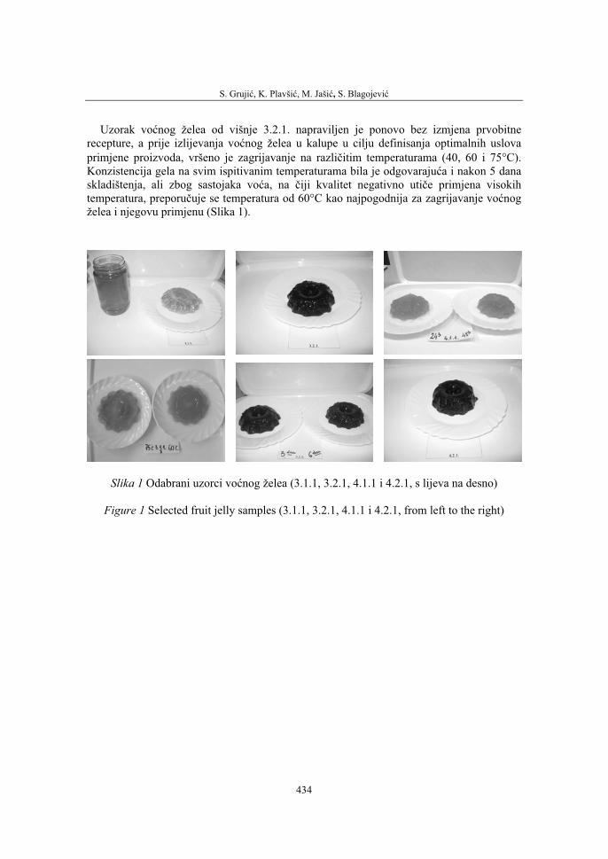
S. Grujić, K. Plavšić, M. Jašić, S. Blagojević
434
Uzorak voćnog želea od višnje 3.2.1. napraviljen je ponovo bez izmjena prvobitne recepture, a prije izlijevanja voćnog želea u kalupe u cilju definisanja optimalnih uslova primjene proizvoda, vršeno je zagrijavanje na različitim temperaturama (40, 60 i 75°C).Konzistencija gela na svim ispitivanim temperaturama bila je odgovarajuća i nakon 5 dana skladištenja, ali zbog sastojaka voća, na čiji kvalitet negativno utiče primjena visokih temperatura, preporučuje se temperatura od 60°C kao najpogodnija za zagrijavanje voćnogželea i njegovu primjenu (Slika 1).
Slika 1 Odabrani uzorci voćnog želea (3.1.1, 3.2.1, 4.1.1 i 4.2.1, s lijeva na desno)
Figure 1 Selected fruit jelly samples (3.1.1, 3.2.1, 4.1.1 i 4.2.1, from left to the right)
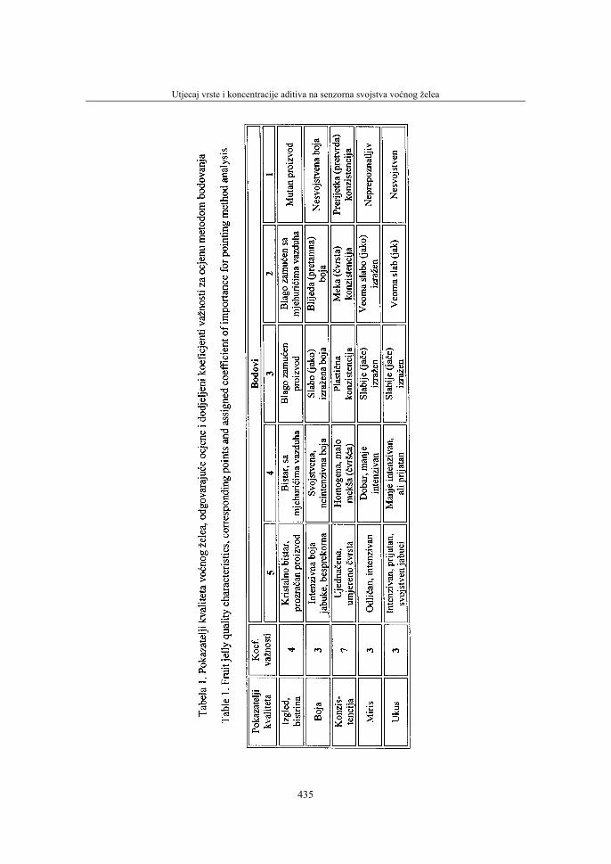
Utjecaj vrste i koncentracije aditiva na senzorna svojstva voćnog želea
435
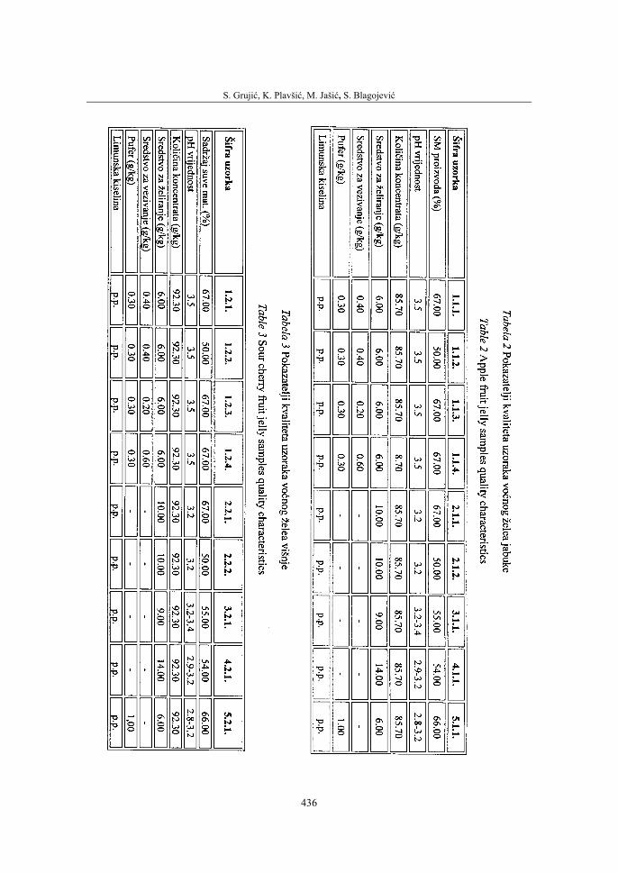
S. Grujić, K. Plavšić, M. Jašić, S. Blagojević
436
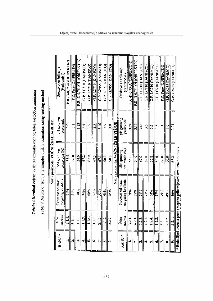
Utjecaj vrste i koncentracije aditiva na senzorna svojstva voćnog želea
437
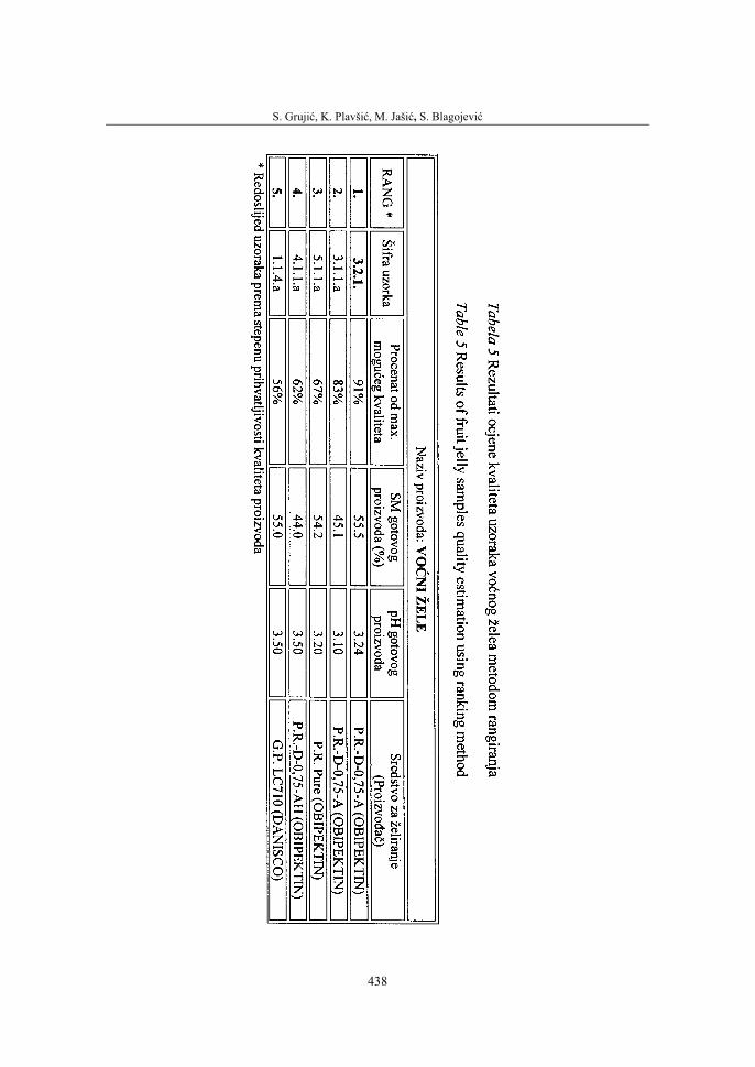
S. Grujić, K. Plavšić, M. Jašić, S. Blagojević
438
Utjecaj vrste i koncentracije aditiva na senzorna svojstva voćnog želea
439
ZAKLJUČCI
Voćni žele namijenjen za izradu preliva i nadjeva za kolače i pekarske proizvode mora zadovoljiti određene uslove kvaliteta. Žele treba da bude bistrog izgleda, svjetlucav ili opalescentan, u zavisnosti od vrste upotrebljenog voćnog soka, boje, ukusa i mirisa karakterističnih za sirovinu od koje je proizveden i umjereno čvrste konzistencije gela. Nije poželjno da se odvaja od proizvoda nakon primjene. Žele pakovan u staklene tegle pri nakretanju treba da zadrži oblik, bez izdvajanja tečnog dijela. U proizvodu, u toku skladištenja u teglama, ne smije doći do kristalizacije šećera ni izdvajanja tečnosti(sinereze).
Od 23 uzorka voćnog želea (13 od jabuke i 10 od višnje), odabrani su uzorci voćnogželea od jabuke i voćnog želea višnje koji su ocijenjeni kao uzorci najprihvatljivijeg kvaliteta. Kao uzorci očekivanog kvaliteta odabrani su voćni žela od jabuke oznake 3.1.1. i voćni žele od višnje oznake 3.2.1. Ovi uzorci su i nakon ponovnog zagrijavanja i hlađenjabili dobro želirani, imali su umjereno čvrstu konzistenciju, sjajnu površinu i presjek, kristalnu bistrinu i bili su umjerenog stepena slasti i boje, ukusa i mirisa karakterističnih za voće od kojeg su proizvedeni.
Na kraju rada izdvojeni su uzorci voćnog želea od jabuke oznake 4.1.1. i voćnog želea od višnje oznake 4.2.1 kao proizvodi sa prijatnom osvježavajućom aromom voća i krupnozrnastom konzistencijom gela, za koje se predlaže upotreba prilikom izrade nadjeva za različite pekarske ili konditorske proizvode, koji se ne podvrgavaju toplotnom tretmanu.
REFERENCE
1. Grujić R., „Nauka o ishrani čovjeka“, Tehnološki fakultet, Banja Luka BiH, 2000.
2. „Pravilnik o kvalitetu proizvoda od voća, povrća i pečurki i pektinskih preparata“, Sl.list SFRJ br. 1/79, 20/82, 74/90.
3. May D.C., „Industrial pectins: Sources, production and applications“, Journal of Science Direct Vol. 12, No.1., 2003, pp 79-99.
4. Grujić S., „Prehrambeni aditivi-funkcionalna svojstva i primjena“, Tehnološki fakultet, Banja Luka BiH, 2005.
5. Meilgaard M., Civille G.V. and Carr. B.T., „Sensory Evaluation Techniques“, CRC Press, 3rd Edition USA, 1999.
6. Dairou V. and Sieffermann M., „A comparison of fourteen jams characterized by conventional profiling and a quick orginal method, the flash profile“, Massy, France. 2000, www.confex.com
7. Radovanović R. i Popov-Raljić J., „Senzorna anliza prehrambenih proizvoda“, Poljoprivredni fakultet, Beograd i Tehnološki fakultet, Novi Sad SRJ, 2000/2001.
8. Marketo Ch. and Moskowitz H., „Sensory optimization and reverse engineering using JAR scales in Workshop Summary: Data Analysis Workshop: getting the most out of just-about-right data“, Food Quality and Preference, Vol.15, 2004, pp 891-899. www.elsevier.com
9. Vigneau E., Qannari M. and Courcoux Ph., „Analysis of just-about-right data: segmentation of the panel of consumer in Workshop Summary: Data Analysis Workshop: getting the most out of just-about-right data“, Food Quality and Preference Vol.15, 2004, pp 891-899. www.elsevier.com
S. Grujić, K. Plavšić, M. Jašić, S. Blagojević
440
INFLUENCE OF ADDITIVE TYPE AND CONCENTRATION ON FRUIT JELLY
SENSORY QUALITY
ABSTRACT
Fruit jelly is product made from fruit juice, sugar and food additives in order to achieve gelatinous consistency. Food law in force define quality conditions which product must fulfill. Purpose of this paper was producing of fruit jelly with reversible gelling characteristics which could be used directly from container. That jelly could be easy used for cookies, biscuits or bakery products glazing or filling.
Jelly samples are produced from apple (DM 70%) and sour cherry (DM 65%) concentrated fruit juice, DANISCO CULTOR (2 samples) and OBIPEKTIN (3 samples) gelling agent, firming agent (CaCl2; E 509), acidity regulator (trisodium citrate, E 331) and citric acid (E 330). Sensory analysis descriptive method of pointing and ranking method were applied in order to analyse quality of produced fruit jelly and its stability after heating (on temperature 45-50°C), product glazing and cooling (on temperature 4 - 8°C).
After sensory analysis, samples with the best characteristics were selected from 23 fruit jelly samples (13 pcs. from apple and 10 pcs. from sour cherry) produced during experimental work. These samples had medium strong consistency, gloss surface, crystal transparence, moderately sweetness and characteristic fruit color, taste and aroma.
Key words: fruit jelly, product development
36. Symposium "Actual Tasks on Agricultural Engineering", Opatija, Croatia, 2008.
441
36.
SIMPOZIJAKTUALNI ZADACIMEHANIZACIJE POLJOPRIVREDE
UDC66.094.38:663.25
Izvorni znanstveni radOriginal scientific paper
THE AGEING INFLUENCE ON THE CHROMATIC AND ANTIOXIDANT CHARACTERISTICS OF RED WINES
MARIANA-ATENA POIANA, DIANA MOIGRADEAN, DIANA RABA,IOSIF GERGEN
Faculty of Food Processing Technology, Banat′s University of Agricultural Sciences and Veterinary Medicine, Calea Aradului no 119, RO-300645, Timisoara, Romania,
e-mail: [email protected]
SUMMARY
In this paper were characterised in relation to the chromatic and antioxidant characteristics the young and aged red wines Sangiovese. During the ageing in bottle, for 4 and 12 months, the colour intensity decreased, the tonality increased, the red pigments contribution to the red wine colour decreased and the yellow pigments contribution increased. By ageing, the stabilisation colour is different depending on the wine type: for three wines from five, the colour obtained by ageing is red-brown. In the ageing course for 12 months, the monomeric anthocyanins content decreased with 20-30%, the fraction of color due to polymeric pigment increased and the percent of colour due to monomeric and copigmented anthocyanins decreased. The values of indices on the basis was quantified the “chemical age” of red wines were modified during the ageing in bottle due to colour stabilisation. The antioxidant properties expressed as antioxidant capacity and polyphenols content were decreased depending on ageing time. Total antioxidant capacity was determined by FRAP method expressed as mM Fe2+/L and the polyphenols content was determined by Folin-Ciocalteu method expressed such as mM acid gallic/L. For the young red wines Sangiovese were registered the biggest values for antioxidant capacity determinated by FRAP method.
Keywords: red wines, chromatic structure, ageing, polyphenols, total antioxi-dant capacity
INTRODUCTION
The chromatic properties of red wines are very important because these characteristics have a important role about the wines quality ant tipicity.
M.-A. Poiana, D. Moigradean, D. Raba, I. Gergen
442
The structure of phenolic compounds varies very much during wine’s maturation and aging because the polymerisation, condensation, polycondensation and oxidation reactions between phenolic compounds from wine (leucoanthocyanidins, anthocyanidins, tannins, substances from flavones group) and other compounds extracted from the stave of the cask, represented especially by hydrolyzable tannins (pirogalolic). The content of polyphenols is developed through polymerisation and condensation of tannins with anthocyanins [2, 8, 12].
Through wines ageing in the bottle, due to oxidation and condensation processes, it was diminished the monomer polyphenols content; during the time of wine storage in bottle take place the structural changes, and one of the most studied of those changes concern red wine colour evolution, called wine ageing. During aging, it has been demonstrated that initially present grape pigments slowly turn into new more stable red pigments. This phenomenon goes on for weeks, months and years [9, 14, 15].
Copigmented anthocyanins are the complexes that result by reaction between anthocyanins and copigments molecules or co-factors. The association of the co-factor with the anthocyanin causes a hyperchromic effect and a bathochromic shift. The hyperchromic effect is an increase in color intensity and the bathochromic effect is an increase of the wavelength of maximum absorbance. Co-factors are colorless compounds that when added to a solution containing anthocyanins will act to enhance the color of the solution. The most important copigments in wine are expected to be the flavan-3-ols and flavanols, hydroxycinnamic acids and even the antocyanins molecules. This phenomenon causes a hyperchromic effect and a bathochromic shift [3, 6, 7, 10-12].
Co-pigmentation permits greater extractability of anthocyanins and cofactors from the grape skins. There is an equilibrium that exists between the grape, the free anthocyanins and cofactors, and the co-pigmented stacks. As the cofactors and the anthocyanins associate to form co-pigmented stacks, the equilibrium of grape and free is shifted to favor extraction of both free anthocyanins and free cofactors. As wine ages the free anthocyanins react to form polymeric pigments, this shifts the equilibrium to replenish free anthocyanins by releasing them from the co-pigmented stacks. So therefore, as wine ages the stacks tend to break-up and co-pigmentation decreases as a result of this equilibrium [3, 6, 13].
Anthocyanins are present in solution in several different forms. These forms exist in an equilibrium that is pH dependent. The red flavylium ion form dominates at low pH, and this form is what provides the red color to solution. As the pH of the solution increases the colorless pseudobase begins to dominate, and the blue quinoidal base begins to appear. The pseudobase interconverts with the open-ring colorless chalcone form. Sulfur dioxide is also participates in this equilibrium because it is able to bind with free anthocyanins, which forms a colorless compound. The bleaching by sulfur dioxide is moderated by the presence of other compounds like acetaldehyde. Acetaldehyde is able to bind sulfur dioxide, and therefore prevent it from binding and bleaching the anthocyanin. Red wine is a complex solution and although its colour can be meaningfully measured rather easily by spectral techniques, the composition of the wine colour is more difficult to determine. Based on an understanding of the pH equilibrium and the different bleaching effect of SO2 on monomeric and polymeric anthocyanins, as well as the preferential binding of SO2 with acetaldehyde rather than anthocyanins, it was developed a set of spectral measures to determine the fraction of color due to each pigments: monomeric, polymeric and
The ageing influence on the chromatic and antioxidant characteristics of red wines
443
copigmented anthocyanins, the chemical age of the wine and the degree of pigment coloration [17].
METHODS
The sample for analysis. In the present research three wine categories were investiga-ted: young red wines (0) and aged in bottle for 4 and 12 months, respectively (1) and (2).
These wines were processed of Italy, from Sangiovese grapes variety harvested in 2005 year from Romagna region (Sangiovese di Romagna Brumale, Sangiovese di Romagna La Rocca–Bernardi, Sangiovese di Romagna Ostro, Sangiovese di Romagna Vecchie Cantine Rove) and from Marche region – the red wine Marche Sangiovese.
Reagent and equipment. All chemicals and reagents were analytical grade or pure quality purchased from Merck, Fluka, Sigma and Chimopar. Absorbance determination for colour analysis were made using Spectrophotometer Specord 205 by Analytik Jena.
Total monomeric anthocyanin content was determined by the pH-differential method [4]. The colored oxonium form predominates at pH 1.0 and the colorless hemiketal form at pH 4.5. Monomeric anthocyanins pigments (mg/L) were calculated as cyanidin-3-gluco-side.
Chromatic parameters: color intensity (IC), tonality (T) and contribution of yellow, red and blue pigments to the wine color were established by Glories method [5].
The analysis of red wine color was effectuated in accord with Somers and Evans method [17]. Somers & Evans developed a set of spectral measures to evaluate red wines and determine the fraction of color due to monomeric, polymeric and copigmented anthocyanins and the ”chemical age” of the wine.
The wines “chemical age” is quantified by two indices that give a measure of the extent to which polymeric pigments have replaced monomer anthocyanins during of wine evolution.
The first index, I1 represent the ratio between color due to polymeric anthocyanins and colour due to total anthocyanins and the second index I2 - the ratio between colour due to polymeric anthocyanins and colour due to monomeric anthocyanins. The degree of pigment coloration (α) gives a measure of the amounts of monomeric anthocyanins in the coloured form [17].
Total antioxidant capacity was determinated by FRAP assay [1]. The total antioxidant capacity in wine samples in mM Fe2+/L was calculated. For antioxidant capacity analysis the dilution was 1/50. Correlation coefficient (r2) for calibration curve was 0.998.
Total polyphenolic content was determined by modified method Folin-Ciocalteu [9] and was expressed in (mM gallic acid /L) [16]. For polyphenols analysis the dilution was 1/25. Correlation coefficient (r2) for calibration curve was 0.995.
M.-A. Poiana, D. Moigradean, D. Raba, I. Gergen
444
RESULTS AND DISCUSSIONS
The data from the table 1 show the chromatic structure obtained by Glories method. By this method application, it was determined the percent with that each pigment category (yellow, red and blue) contribute to the total wine colour. On the base of each pigments category contribution to the wine colour it can be appreciated the wine shade. From obtained data it was observed that the pigments structure reflects exactly the chromatic features of investigated red wines. In general case, for wine with red shade, the red pigment class takes part with biggest percent (more than 40%) to underline the wine colour. In the case of young red wines, the red pigment class participates with 50-52%, the yellow pigments 37-39% and the blue pigments with 9-12% to the total wine colour. The tonality present values in the range 0.74-0.78 for young red wines Sangiovese.
By ageing for 4 month, for all wine types, the colour intensity decreased and the tonality increased; red pigments class participates with 45-47%, the yellow pigments 40-43% and the blue pigments with 10-13% to the total wine colour. By ageing for 12 month, for Sangiovese Brumale and Ostro the shade continues to be red and for wines Sangiovese La Rocca–Bernardi, Marche and Vecchie Cantine Rove, the shade was changes in red-brown. The wine processing technology, specified for each wine making centers, leaded to differences between chromatic parameters. The highest values for IC it was registered for Sangiovese di Romagna Ostro (7.44-7.69) while the smallest values it was registered for Sangivese di Romagna La Rocca – Bernardi (5.34-5.71). The colour stabilisation can be attributed the diminishing of anthocyanins content and formation of combinations between tannin and anthocyanins, polymeric compounds, and intermolecular associations which have the red colour.
From the data showed in the table 2 it can be observed that by ageing the chromatic structure was modified, because the red wines are in the stabilisation course.
It can be observe that for all analysed young and aged red wines the majority colour is due to polymeric pigment class (in the range 59-73% for young wines, 73-90% after 4 month for ageing and 84-93% after 12 month for ageing).
The class of monomeric pigment participates with 14-21% to the young red wine colour and 2-7% in the case of red wine aged for 12 months.
The copigmented anthocyanins participate to the total colour of young red wines Sangiovese with a percent between 10-19% and after 12 months for ageing the participation percent to the wine colour was 4-8%.
The polymeric pigments, that are prevalents, are the stable colour compounds in wine. From these value results that the wine colour is in the course of stabilisation. The small value of copigmented anthocyanins is due the specifics of Sangiovese grapes variety that contain a litle amount of cofactor (especially flavan-3-ols and flavanols). As wine ages the free anthocyanins react to form polymeric pigments, this shifts the equilibrium to replenish free anthocyanins by releasing them from the co-pigmented stacks.
The co-pigmented stacks also act as a reservoir for free flavylium ion, and we see a decrease in the contribution of co-pigmentation to colour over time. So therefore, as wine ages the stacks tend to break-up and co-pigmentation decreases as a result of this equilibrium [2, 5].
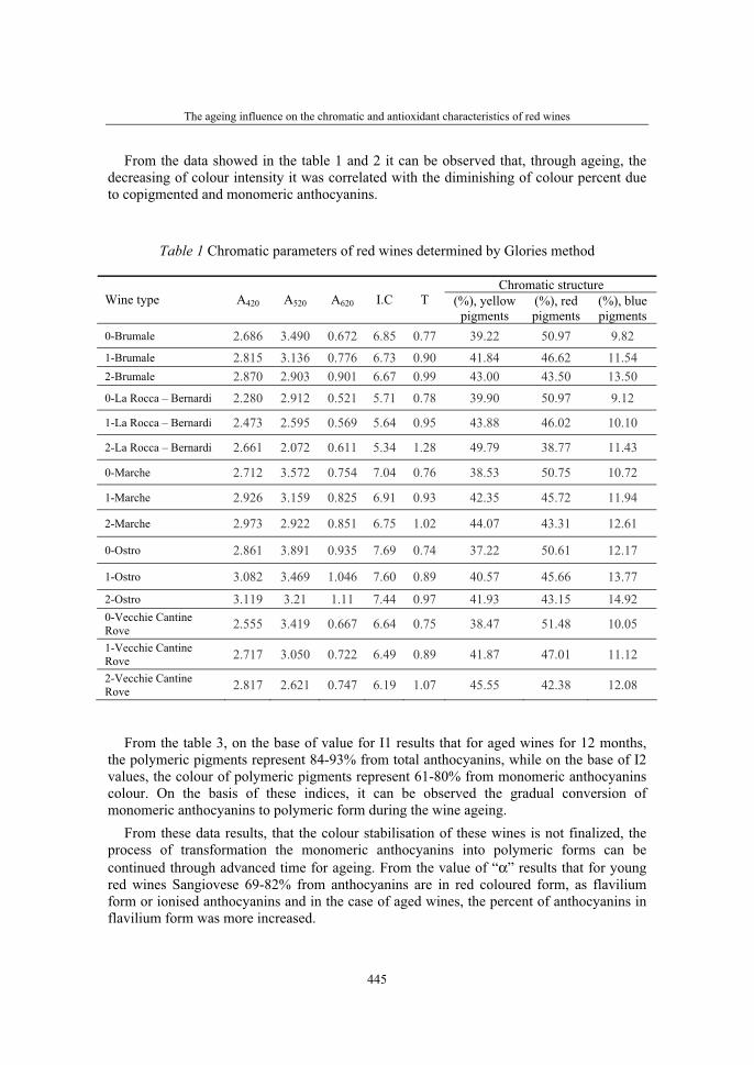
The ageing influence on the chromatic and antioxidant characteristics of red wines
445
From the data showed in the table 1 and 2 it can be observed that, through ageing, the decreasing of colour intensity it was correlated with the diminishing of colour percent due to copigmented and monomeric anthocyanins.
Table 1 Chromatic parameters of red wines determined by Glories method
Chromatic structure Wine type A420 A520 A620 I.C T (%), yellow
pigments(%), redpigments
(%), bluepigments
0-Brumale 2.686 3.490 0.672 6.85 0.77 39.22 50.97 9.82 1-Brumale 2.815 3.136 0.776 6.73 0.90 41.84 46.62 11.54 2-Brumale 2.870 2.903 0.901 6.67 0.99 43.00 43.50 13.50 0-La Rocca – Bernardi 2.280 2.912 0.521 5.71 0.78 39.90 50.97 9.12
1-La Rocca – Bernardi 2.473 2.595 0.569 5.64 0.95 43.88 46.02 10.10
2-La Rocca – Bernardi 2.661 2.072 0.611 5.34 1.28 49.79 38.77 11.43
0-Marche 2.712 3.572 0.754 7.04 0.76 38.53 50.75 10.72
1-Marche 2.926 3.159 0.825 6.91 0.93 42.35 45.72 11.94
2-Marche 2.973 2.922 0.851 6.75 1.02 44.07 43.31 12.61
0-Ostro 2.861 3.891 0.935 7.69 0.74 37.22 50.61 12.17
1-Ostro 3.082 3.469 1.046 7.60 0.89 40.57 45.66 13.77
2-Ostro 3.119 3.21 1.11 7.44 0.97 41.93 43.15 14.92 0-Vecchie Cantine Rove 2.555 3.419 0.667 6.64 0.75 38.47 51.48 10.05
1-Vecchie Cantine Rove 2.717 3.050 0.722 6.49 0.89 41.87 47.01 11.12
2-Vecchie Cantine Rove 2.817 2.621 0.747 6.19 1.07 45.55 42.38 12.08
From the table 3, on the base of value for I1 results that for aged wines for 12 months, the polymeric pigments represent 84-93% from total anthocyanins, while on the base of I2 values, the colour of polymeric pigments represent 61-80% from monomeric anthocyanins colour. On the basis of these indices, it can be observed the gradual conversion of monomeric anthocyanins to polymeric form during the wine ageing.
From these data results, that the colour stabilisation of these wines is not finalized, the process of transformation the monomeric anthocyanins into polymeric forms can be continued through advanced time for ageing. From the value of “α” results that for young red wines Sangiovese 69-82% from anthocyanins are in red coloured form, as flavilium form or ionised anthocyanins and in the case of aged wines, the percent of anthocyanins in flavilium form was more increased.
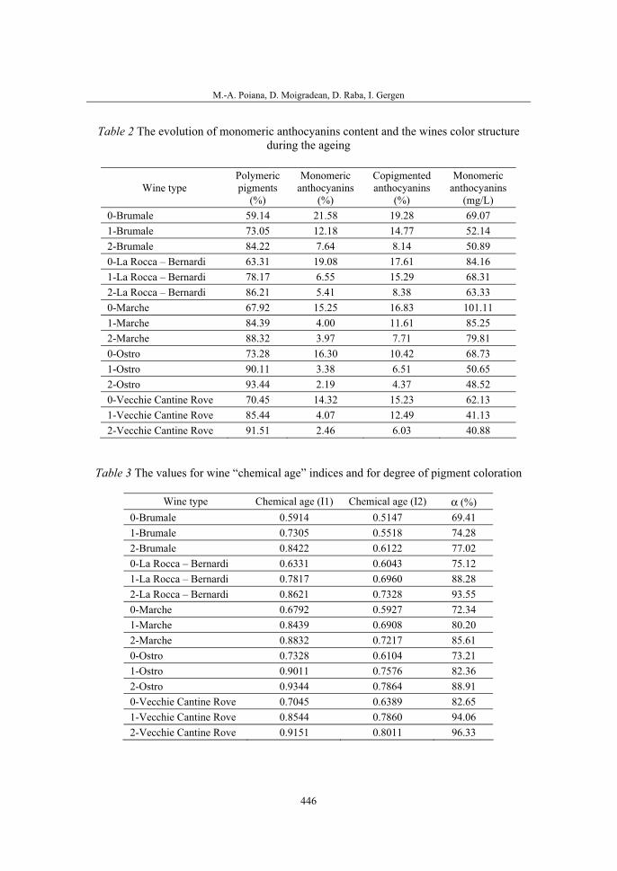
M.-A. Poiana, D. Moigradean, D. Raba, I. Gergen
446
Table 2 The evolution of monomeric anthocyanins content and the wines color structure during the ageing
Table 3 The values for wine “chemical age” indices and for degree of pigment coloration
Wine type Chemical age (I1) Chemical age (I2) α (%) 0-Brumale 0.5914 0.5147 69.41 1-Brumale 0.7305 0.5518 74.28 2-Brumale 0.8422 0.6122 77.02 0-La Rocca – Bernardi 0.6331 0.6043 75.12 1-La Rocca – Bernardi 0.7817 0.6960 88.28 2-La Rocca – Bernardi 0.8621 0.7328 93.55 0-Marche 0.6792 0.5927 72.34 1-Marche 0.8439 0.6908 80.20 2-Marche 0.8832 0.7217 85.61 0-Ostro 0.7328 0.6104 73.21 1-Ostro 0.9011 0.7576 82.36 2-Ostro 0.9344 0.7864 88.91 0-Vecchie Cantine Rove 0.7045 0.6389 82.65 1-Vecchie Cantine Rove 0.8544 0.7860 94.06 2-Vecchie Cantine Rove 0.9151 0.8011 96.33
Wine type Polymericpigments
(%)
Monomericanthocyanins
(%)
Copigmentedanthocyanins
(%)
Monomericanthocyanins
(mg/L)0-Brumale 59.14 21.58 19.28 69.07 1-Brumale 73.05 12.18 14.77 52.14 2-Brumale 84.22 7.64 8.14 50.89 0-La Rocca – Bernardi 63.31 19.08 17.61 84.16 1-La Rocca – Bernardi 78.17 6.55 15.29 68.31 2-La Rocca – Bernardi 86.21 5.41 8.38 63.33 0-Marche 67.92 15.25 16.83 101.11 1-Marche 84.39 4.00 11.61 85.25 2-Marche 88.32 3.97 7.71 79.81 0-Ostro 73.28 16.30 10.42 68.73 1-Ostro 90.11 3.38 6.51 50.65 2-Ostro 93.44 2.19 4.37 48.52 0-Vecchie Cantine Rove 70.45 14.32 15.23 62.13 1-Vecchie Cantine Rove 85.44 4.07 12.49 41.13 2-Vecchie Cantine Rove 91.51 2.46 6.03 40.88

The ageing influence on the chromatic and antioxidant characteristics of red wines
447
From the data showed in the table 4 results that antioxidant capacity and polyphenol content decreased by ageing in bottle for 1 year. The young red wines Sangiovese were registered the biggest values for antioxidant capacity and the aged wines have the smallest values for this parameter. The biggest values for antioxidant capacity and polyphenols content in all situations (0, 1, 2) were obtained for red wine Sangiovese Vecchie Cantine Rove. In opposition, the lowest values for these parameters were registered for red wine Sangiovese Brumale.
Table 4 The values of polyphenols and total antioxidant capacity for investigated wines
Wine type Total polyphenolic content (mM gallic acid /L)
Total antioxidant capacity (mM Fe2+/L)
0-Brumale 10.38 14.10 1-Brumale 9.02 12.23 2-Brumale 7.66 9.37 0-La Rocca – Bernardi 12.51 15.45 1-La Rocca – Bernardi 11.72 12.84 2-La Rocca – Bernardi 10.13 10.12 0-Marche 12.18 15.15 1-Marche 10.94 13.83 2-Marche 8.21 11.33 0-Ostro 12.15 15.00 1-Ostro 11.32 14.01 2-Ostro 9.44 11.97 0-Vecchie Cantine Rove 13.05 16.01 1-Vecchie Cantine Rove 12.18 14.24 2-Vecchie Cantine Rove 10.54 12.37
CONCLUSIONS
The ageing time affects the chromatic properties and the colour structure of red wines. For young red wines, the red pigments class participates with 50-52%, the yellow pigments 37-39% and the blue pigments with 9-12% to the total wine colour.
By ageing, the color intensity decreased and the tonality increased. The highest values for colour intensity it was registered for red wine Sangiovese di Romagna Ostro (7.44-7.69) while the smallest values it was registered for Sangiovese di Romagna La Rocca – Bernardi (5.34-5.71).
For all analysed young and aged red wines the most colour is due to polymeric pigment class (in the range 59-73% for young wines, and 84-93% after 12 month for ageing). The class of monomeric pigment participates with 14-21% to the young red wine color and 2-7% in the case of red wine aged for 12 months.
M.-A. Poiana, D. Moigradean, D. Raba, I. Gergen
448
The copigmented anthocyanins participate to the total colour of young red wines Sangiovese with a percent between 15-19% and after 12 months for ageing the participation percent to the wine colour was 4-8%.
On the basis of indices I1 and I2 it can be observed the gradual conversion of monomeric anthocyanins into polymeric form during the wine ageing.
The young red wines Sangiovese were registered the biggest values for antioxidant capacity evaluated by FRAP method and the aged wines have the smallest values for this parameter.
The biggest values for antioxidant capacity and polyphenols content were obtained for red wine Sangiovese Vecchie Cantine Rove and the lowest values for Brumale wine.
REFERENCES
1. Benzie I.F.F., Strain L. (1996). Ferric reducing ability of plasma (FRAP) as a measure of antioxidant power: The FRAP assay. Analytical Biochemistry. 239: 70-76
2. Berke B., Vauzour D., Castagnino, C., Arnaudinaud V., Nay B., Cheze C., Vercauteren, J. (2003). Vin et santé: découvertes récentes. Journal de Pharmacie de Belgique. 58(3): 57-74
3. Boulton R. (1996). A method for the assessment of copigmentation in red wines. Am. J. Enol. Vitic. 47: 346
4. Giusti Monica, Wrolstad R.E. (2000). Current Protocols in Food Analytical Chemistry
5. Glories Y. (1984). La couler des vins rouges. Connaisance Vigne Vin. 18(4) : 253-271
6. Levengood J. (1996). A survey of copigmentation in Cabernet Sauvignon. Master of Science Thesis. University of California
7. Liao H., Cai Y., Haslam E. (1992). Polyphenol interactions. Anthocyanins: co-pigmentation and colour changes in red wines. J. Sci. Food Agric. 59: 299-305
8. Mazza G., Brouillard R. (1987). Recent developments in the stabilization of anthocyanins in food products. Food Chemistry. 25: 207-225
9. Mazza G., Brouillard R. (1989). The mechanism of co-pigmentation of anthocyanins in aqueous solutions. Phytochemistry. 29: 1097-1102
10. Mazza G. (1995). Anthocyanins in Grapes and Grape Products. Science and Nutrition. 35(4): 341-371
11. Mazza G., Fukumoto, L., Delaquis, P., Girard, B., Ewert, B.V. (1999). Anthocyanins, phenolics, and color of Cabernet Franc, Merlot, and Pinot Noir wines from British Columbia. J. Agric. Food Chem. 47(10): 4009-1017
12. Miniati E., Damiani P. (1992). Copigmentation and self-association of anthocyanins in food model systems. Ital. J. Food Sci. 2: 109-116
13. Mirabel M., Saucier C. (1999). Copigmentation in model wine solutions: Occurrence and relation to wine aging. Am. J. Enol. Vitic. 50: 211-218

The ageing influence on the chromatic and antioxidant characteristics of red wines
449
14. Monagas M., Martín-Álvarez P.J., Bartolomé B., Gómez-Cordovés C. (2006). Statistical interpretation of the color parameters of red wines in function of their phenolic composition during ageing in bottle, Eur. Food Res. Tech. 222(5-6): 702-710
15. Pascu L., (2005). Red wine quality establishing on the basis of chromatic properties. Rev. chim. 56(7): 703-707
16. Singleton V. L., Rossi J. A. (1965). Colorimetry of total phenolics with phosphomolybdic-phosphotungstic acid reagents. Am. J. Enol. Vitic. 16: 1644-1658
17. Somers T.C., Evans M.E. (1974). Wine quality: Correlations with colour density and anthocyanin equilibria in a group of young red wines. J. Sci. Food. Agric. 25: 1369-1379

36. Symposium "Actual Tasks on Agricultural Engineering", Opatija, Croatia, 2008.
451
36.
SIMPOZIJAKTUALNI ZADACIMEHANIZACIJE POLJOPRIVREDE
UDK547.475.2:543.4
Stručni radExpert paper
ODREĐIVANJE L-ASKORBINSKE KISELINE IZRAVNOM ULTRALJUBIČASTOM
SPEKTROFOTOMETRIJOMMIRSAD SALKIĆ, MIDHAT JAŠIĆ, HUSEJIN KERAN, HATIDŽA PAŠALIĆ
Tehnološki fakultet, Univerzitet u Tuzli, Univerzitetska 8, 75 000 Tuzla,Bosna i Hercegovina
SAŽETAK
Razvijena je brza i točna metoda za izravno spektrofotometrijsko određivanjeL-askorbinske kiseline. Za stabilizaciju L-askorbinske kiseline u vodenoj sredini korišćena je etilendiamintetraoctena kiselina (6,45x10⁻⁴ mol/dm3) u acetatnom puferu. Mjerenja apsorbancije su vršena na 256 nm. Određivanje L-askorbinske kiseline je moguće u linearnom opsegu od 2,36x10⁻⁶ do 1,09x10⁻⁴ mol/dm3, sa molarnom apsorptivnošću od 8,94x10³ dm3 mol-1 cm-1. Granica dokazivanja iznosi 7,08x10⁻⁷ mol/dm3, a relativno standardno odstupanje 0,54% za 6,79x10⁻⁵
mol/dm3 L-askorbinske kiseline (n = 7). Kationi, anioni, organske kiseline, šećeri i aminokiseline obično prisutne u
proizvodima vitamina C ne predstavljaju smetnju određivanju L-askorbinske kiseline, dok željezo(II), drugi vitamini i benzoat smetaju. Predložena metoda je uspješno primijenjena za određivanje L-askorbinske kiseline u tabletama vitamina C. Rezultati dobijeni primjenom predložene metode slažu se sa rezultatima titrimetrijske metode s jodom kao titrantom.
Ključne riječi: L-askorbinska kiselina, stabilizator, spektrofotometrija, etilen-diamintetraoctena kiselina
UVOD
L-Askorbinska kiselina (2-okso-L-treo-heksono-1,4-lakton-2,3-endiol) se zbog odgova-rajućih fizioloških i fizičko-hemijskih osobina široko primjenjuje u prehrambenoj industriji, te je mnogi proizvodi sadrže i kao dodatu. Dodaje se u cilju povećanja sadržaja vitamina C, održivosti boje, arome i opće postojanosti prehrambenih proizvoda. U literaturi je opisan veliki broj analitičkih metoda za određivanje L-askorbinske kiseline, kao što su kromatografija (Iwase 2003), spektrofotometrija (Janghel i sur. 2007, Özyürek i sur. 2007,
M. Salkić, M. Jašić, H. Keran, H. Pašalić
452
Lau i sur. 1987), fluorimetrija (Wu i sur. 2003), kapilarna elektroforeza (Wang i Wu 2006), titrimetrija (Fritz i Schenk 1987), hemiluminiscencijske (Kato i sur. 2005) i elektro-kemijske metode (Li i sur. 2006). Glavni problem kod određivanja L-askorbinske kiseline je njena brza oksidacija u dehidro-L-askorbinsku kiselinu, te prisustvo pratećih tvari u realnim uzorcima, naročito reducirajućih agensa.
Cilj ovog rada je bio da se odabere pogodan stabilizator koji će inhibirati oksidaciju L-askorbinske kiseline u vodenim otopinama i time omogućiti njeno kvantitativno određi-vanje u proizvodima vitamina C. Za ovu svrhu predložena je primjena etilendiamintetraoc-tene kiseline (EDTA) u acetatnom puferu. U ovom radu je također ispitan utjecaj nekih metalnih iona, aniona, organskih kiselina, aminokiselina i šećera na izravno spektrofoto-metrijsko određivanje vitamina C u prisustvu odabranog stabilizatora i pufera.
MATERIJALI I METODE
Za pripravljanje otopina korišćeni su reagensi analitičkog stupnja čistoće.Otopina smjese octene kiseline (0,035 mol/dm3), natrijeva acetata (9,77x10⁻³ mol/dm3) i
EDTA (6,45x10⁻⁴ mol/dm3) pripravljena je razblaživanjem 2 cm3 glacijalne octene kiseline (J. T. Baker) i otapanjem 1,33 g CH3COONa·3H2O (Merck) i 0,24 g C10H14N2Na2O8·2H2O(Fluka) u destiliranoj vodi i razblaživanjem vodom do 1 dm3.
Otopina L-askorbinske kiseline koncentracije 1,13x10⁻³ mol/dm3 pripravljena je otapanjem 0,05 g L-askorbinske kiseline (Riedel-de Haën) u 250 cm3 otopine stabilizatora.
Otopine metalnih iona, aniona, organskih kiselina, šećera, aminokiselina i vitamina pripravljene su otapanjem poznatih količina ovih tvari u otopini stabilizatora.
Za mjerenje apsorbancija korišćen je spektrofotometar Cecil 2021. Izmjerena količina praška dobijenog mrvljenjem nekoliko tableta otopi se u otopini
stabilizatora i smjesa razblaži istom otopinom do 50 ili 100 cm3. Ukoliko je potrebno, otopina se filtrira i prvih nekoliko cm3 filtrata se odbace. Alikvot otopine ili filtrata se prenese u odmjernu tikvicu od 50 cm3 i razblaži otopinom stabilizatora do oznake.
Alikvotni dio otopine uzorka koji sadrži 5,68x10⁻⁷ – 2,72x10⁻⁶ mola L-askorbinske kiseline prenese se u volumetrijsku tikvicu od 25 cm3 i razblaži otopinom stabilizatora do oznake. Apsorbancija ovako pripravljene otopine se mjeri na 256 nm prema otopini stabilizatora kao slijepoj probi. Za određivanje količine L-askorbinske kiseline u uzorku koristi se prethodno izvedeni baždarni pravac.
REZULTATI I RASPRAVA
Postojanost L-askorbinske kiseline L-Askorbinska kiselina je u vodenoj sredini vrlo osjetljiva prema djelovanju topline,
alkalija, kisika i svjetlosti. Mnogi metalni ioni, naročito Cu(II) i Fe(III) prisutni i u tragovima, kataliziraju njenu oksidaciju molekularnim kisikom u dehidro-L-askorbinsku kiselinu. Stoga je glavni problem pri analizi L-askorbinske kiseline u realnim uzorcima
Određivanje L-askorbinske kiseline izravnom ultraljubičastom spektrofotometrijom
453
sprječavanje degradacije ovog vitamina. U ovom radu je za stabilizaciju L-askorbinske kiseline u vodenim otopinama korišćena etilendiamintetraoctena kiselina koncentracije 6,45x10⁻⁴ mol/dm3 u acetatnom puferu. Prisustvo pufera je bilo poželjno zbog činjenice da položaj apsorpcijskog maksimuma za L-askorbinsku kiselinu ovisi o pH vijednosti vodene sredine (Eitenmiller i Landen 1999, Francis 2000). U otopinama koje su sadržavale EDTA i komponente acetatnog pufera, L-askorbinska kiselina je bila postojana najmanje pet sati nakon priprave otopina, što pokazuje da odabrani stabilizator učinkovito inhibira oksidaciju ovog vitamina u vodenoj sredini.
Analitičke karakteristike Baždarni pravac, dobijen metodom najmanjih kvadrata, linearan je do koncentracije L-
askorbinske kiseline od 1,09x10⁻⁴ mol/dm3. Molarna apsorptivnost (ε), granica dokazivanja i ostale analitičke karakteristike predložene metode date su u Tablici 1. Vrijednost koeficijenta korelacije (r) ukazuje na jaku linearnu vezu između koncentracije L-askorbinske kiseline i apsorbancije pri 256 nm. Preciznost metode je provjerena analizom otopine L-askorbinske kiseline koncentracije 6,79x10⁻⁵ mol/dm3 i izračunavanjemrelativnog standardnog odstupanja (n = 7).
Tablica 1 Analitičke karakteristike predložene metode
Nagib baždarnog pravca 8943,16
Odsječak baždarnog pravca 0,0042
Standardna pogreška nagiba 28,52
Standardna pogreška odsječka 0,0021
Koeficijent korelacije (r) 0,999985
Granica dokazivanja 7,08x10⁻⁷ mol/dm3
Granica određivanja 2,36x10⁻⁶ mol/dm3
Linearni opseg 2,36x10⁻⁶ – 1,09x10⁻⁴ mol/dm3
Molarna apsorptivnost 8,94x10³ dm3 mol-1 cm-1
Relativno standardno odstupanje 0,54 %
Utjecaj koegzistirajućih tvari Selektivnost predložene metode je provjerena ispitivanjem utjecaja nekih kationa,
aniona, šećera, organskih kiselina, aminokiselina i vitamina na određivanje 6,81x10⁻⁵
mol/dm3 L-askorbinske kiseline. Usvojeno je da koegzistirajuća tvar u dodanoj količini ne predstavlja ozbiljnu smetnju predloženoj metodi ukoliko pri određivanju L-askorbinske kiseline ne uzrokuje relativnu pogrešku veću od ±5,0 %.
Od kationa, ispitan je utjecaj Ca(II), Mg(II), Cu(II), Zn(II), Mn(II), Fe(II) i P(V), koji su česti pratioci L-askorbinske kiseline u prirodnim i komercijalnim proizvodima. Rezultati ispitivanja utjecaja ovih tvari na određivanje L-askorbinske kiseline predloženom metodom prikazani su u Tablici 2. Bakar(II), željezo(II) i mangan(II) ioni u obliku sulfata i Ca(II)
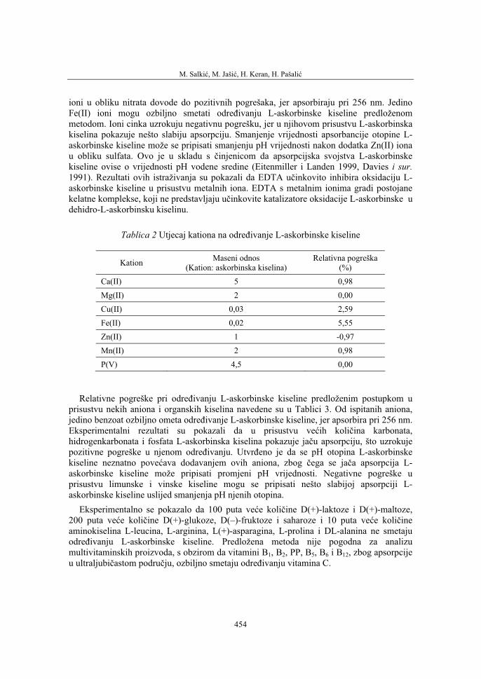
M. Salkić, M. Jašić, H. Keran, H. Pašalić
454
ioni u obliku nitrata dovode do pozitivnih pogrešaka, jer apsorbiraju pri 256 nm. Jedino Fe(II) ioni mogu ozbiljno smetati određivanju L-askorbinske kiseline predloženom metodom. Ioni cinka uzrokuju negativnu pogrešku, jer u njihovom prisustvu L-askorbinska kiselina pokazuje nešto slabiju apsorpciju. Smanjenje vrijednosti apsorbancije otopine L-askorbinske kiseline može se pripisati smanjenju pH vrijednosti nakon dodatka Zn(II) iona u obliku sulfata. Ovo je u skladu s činjenicom da apsorpcijska svojstva L-askorbinske kiseline ovise o vrijednosti pH vodene sredine (Eitenmiller i Landen 1999, Davies i sur.1991). Rezultati ovih istraživanja su pokazali da EDTA učinkovito inhibira oksidaciju L-askorbinske kiseline u prisustvu metalnih iona. EDTA s metalnim ionima gradi postojane kelatne komplekse, koji ne predstavljaju učinkovite katalizatore oksidacije L-askorbinske u dehidro-L-askorbinsku kiselinu.
Tablica 2 Utjecaj kationa na određivanje L-askorbinske kiseline
Kation Maseni odnos(Kation: askorbinska kiselina)
Relativna pogreška (%)
Ca(II) 5 0,98
Mg(II) 2 0,00
Cu(II) 0,03 2,59
Fe(II) 0,02 5,55
Zn(II) 1 -0,97
Mn(II) 2 0,98
P(V) 4,5 0,00
Relativne pogreške pri određivanju L-askorbinske kiseline predloženim postupkom u prisustvu nekih aniona i organskih kiselina navedene su u Tablici 3. Od ispitanih aniona, jedino benzoat ozbiljno ometa određivanje L-askorbinske kiseline, jer apsorbira pri 256 nm. Eksperimentalni rezultati su pokazali da u prisustvu većih količina karbonata, hidrogenkarbonata i fosfata L-askorbinska kiselina pokazuje jaču apsorpciju, što uzrokuje pozitivne pogreške u njenom određivanju. Utvrđeno je da se pH otopina L-askorbinske kiseline neznatno povećava dodavanjem ovih aniona, zbog čega se jača apsorpcija L-askorbinske kiseline može pripisati promjeni pH vrijednosti. Negativne pogreške u prisustvu limunske i vinske kiseline mogu se pripisati nešto slabijoj apsorpciji L-askorbinske kiseline uslijed smanjenja pH njenih otopina.
Eksperimentalno se pokazalo da 100 puta veće količine D(+)-laktoze i D(+)-maltoze, 200 puta veće količine D(+)-glukoze, D(–)-fruktoze i saharoze i 10 puta veće količineaminokiselina L-leucina, L-arginina, L(+)-asparagina, L-prolina i DL-alanina ne smetaju određivanju L-askorbinske kiseline. Predložena metoda nije pogodna za analizu multivitaminskih proizvoda, s obzirom da vitamini B1, B2, PP, B5, B6 i B12, zbog apsorpcije u ultraljubičastom području, ozbiljno smetaju određivanju vitamina C.

Određivanje L-askorbinske kiseline izravnom ultraljubičastom spektrofotometrijom
455
Tablica 3 Utjecaj aniona i organskih kiselina na određivanje L-askorbinske kiseline
Koegzistirajuća tvar Maseni odnos(Tvar: askorbinska kiselina)
Relativna pogreška (%)
SO42⎯ 10 0,00
Cl⎯ 10 0,00
NO3⎯ 2 0,00
H2PO4⎯ 14 0,00
HCO3⎯ 10 2,75
CO32⎯ 5 3,76
PO43⎯ 5 1,92
Tartarat 5 0,00
Benzoat 2 > 5,00
Limunska kiselina 24 -1,76
Vinska kiselina 5 -0,35
Primjena predložene metode Predložena spektrofotometrijska metoda je uspješno primijenjena za određivanje L-
askorbinske kiseline u nekim tabletama vitamina C (Tablica 4).
Tablica 4 Određivanje L-askorbinske kiseline u tabletama
Koncentracija L-askorbinske kiseline (mg/tableta) Naziv proizvoda Deklarirana
na proizvodu Titrimetrijska
metodaaPredložena
metodaaF b t c
Plivit C (Pliva) 500 498,33 ± 5,12 505,12 ± 6,40 1,56 2,29
Cevitbos(Bosnalijek) 500 490,89 ± 4,81 486,85 ± 3,69 1,69 1,84
Upsavit(LaboratoiresUPSA)
1000 994,82 ± 8,51 1003,53 ± 8,02 1,12 2,06
CalciumvitaC(Krka) 500 490,67 ± 5,59 495,96 ± 3,71 2,26 2,18
a 95% Granice pouzdanosti za srednju vrijednost (n = 5) b Teorijska vrijednost za F = 6,39 (95%-tna razina vjerojatnosti) c Teorijska vrijednost za t = 2,306 (95%-tna razina vjerojatnosti)
Titrimetrijska metoda s jodom kao titrantom korišćena je kao referentna metoda (Fritz i Schenk 1987). Rezultati analize tableta vitamina C dobijeni primjenom predložene metode slažu se sa rezultatima dobijenim titrimetrijskom metodom i s količinama deklariranim na

M. Salkić, M. Jašić, H. Keran, H. Pašalić
456
proizvodima. Preciznost i točnost predložene metode provjerene su primjenom F i t-testa na rezultate dobijene referentnom i predloženom metodom. Rezultati pokazuju da predloženi postupak ima zadovoljavajuću preciznost i točnost, s obzirom da su eksperimentalno dobijene F i t vrijednosti u svim slučajevima manje od teorijskih pri 95%-tnoj razini vjerojatnosti. Točnost predložene metode provjerena je i analizom realnih uzoraka uz dodatak standardne L-askorbinske kiseline (1,36x10⁻⁵ mol/dm3), a određivanje je vršeno prije i nakon dodatka standarda. Konačni rezultati analiza dobijeni su oduzimanjem koncentracije L-askorbinske kiseline u samom uzorku od koncentracije u smjesi uzorka i standarda, dijeljenjem ove razlike s koncentracijom dodanog standarda te množenjem sa 100%. Dobijeni rezultati su se kretali u području od 99 do 102%, što pokazuje da tvari prisutne u matrici analiziranih uzoraka nisu smetale određivanju vitamina C predloženom metodom.
ZAKLJUČCI
EDTA u acetatnom puferu učinkovito stabilizira L-askorbinsku kiselinu u vodenim otopinama i omogućuje njeno izravno spektrofotometrijsko određivanje. Mnoge tvari obično prisutne u komercijalnim produktima ne smetaju određivanju L-askorbinske kiseline predloženom metodom. Ozbiljnu smetnju predstavljaju drugi vitamini, Fe(II) ioni i benzoat. Predložena metoda sa EDTA kao stabilizatorom je brza, jednostavna, precizna i točna i može se primijeniti za kvantitativno određivanje L-askorbinske kiseline u proizvodima vitamina C.
Određivanje L-askorbinske kiseline izravnom ultraljubičastom spektrofotometrijom
457
LITERATURA
1. Davies M. B., Austin J., Partridge D. A. (1991). Vitamin C: Its chemistry and Biochemistry. Royal Society of Chemistry, London
2. Eitenmiller R. R., Landen W. O. (1999). Vitamin Analysis for the Health and Food Sciences. CRC Press, USA
3. Francis F. J. (2000). Encyclopedia of Food Science and Technology. John Wiley & Sons, USA
4. Fritz J. S., Schenk G. H. (1987). Quantitative Analytical Chemistry. Prentice Hall, New Jersey
5. Iwase H. (2003). Routine high-performance liquid chromatographic determination of ascorbic acid in foods using L-methionine for the pre-analysis sample stabilization. Talanta 60:1011-1021
6. Janghel E. K., Gupta V. K., Rai M. K., Rai J. K. (2007). Micro determination of ascorbic acid using methyl viologen. Talanta 72:1013-1016
7. Kato T., Ohno O., Nagoshi T., Ichinose Y., Igarashi S. (2005). Determination of small amounts of L-ascorbic acid using the chemiluminescence of an iron-chlorophyllin complex. Analytical Sciences 21:579-581
8. Lau O. W., Luk S. F., Wong K. S. (1987). Determination of ascorbic acid in pharmaceuticals using direct ultraviolet spectrophotometry. Analyst 112: 1023-1025
9. Li C. X., Zeng Y. L., Liu Y. J., Tang C. R. (2006). Simultaneous electrochemical determination of uric acid and ascorbic acid on a glassy carbon electrode modified with cobalt(II) tetrakisphenylporphyrin. Analytical Sciences 22:393-397
10. Özyürek M., Güclü K., Bektasoglu B., Apak R. (2007). Spectrophotometric determination of ascorbic acid by the modified CUPRAC method with extractive separation of flavonoids-La(III) complexes. Analytica Chimica Acta 588:88-95
11. Wang C. C., Wu S. M. (2006). Simultaneous determination of L-ascorbic acid, ascorbic acid-2-phosphate magnesium salt, and ascorbic acid-6-palmitate in commercial cosmetics by micellar electrokinetic capillary electrophoresis. Analytica Chimica Acta 576:124-129
12. Wu X., Diao Y., Sun C., Yang J., Wang Y., Sun S. (2003). Fluorimetric determination of ascorbic acid with o-phenylenediamine. Talanta 59:95-99
M. Salkić, M. Jašić, H. Keran, H. Pašalić
458
DETERMINATION OF L-ASCORBIC ACID USING DIRECT ULTRAVIOLET SPECTROPHOTOMETRY
SUMMARY
A rapid and accurate method was developed for the direct spectrophotometric determination of L-ascorbic acid. Ethylenediaminetetraacetic acid (6.45x10⁻⁴
mol/dm3) in acetate buffer was used to stabilize L-ascorbic acid in aqueous medium. The absorbance measurements were made at 256 nm. The ascorbic acid determination is possible with a linear range of 2.36x10—6 – 1.09x10⁻⁴ mol/dm3
with a molar absorptivity of 8.94x10³ dm3 mol-1 cm-1. The detection limit was 7.08x10⁻⁷ mol/dm3 and the relative standard deviation 0.54% for the determination of 6.79x10⁻⁵ mol/dm3 ascorbic acid (n = 7).
Metal cations, anions, organic acids, sugars and amino acids commonly present in vitamin C products do not interfere with the determination of L-ascorbic acid. Iron(II), other vitamins and benzoate interfere with the determination. The proposed method was applied successfully to the determination of L-ascorbic acid in vitamin C tablets. The results obtained by the proposed method agree with those obtained by the titrimetric method using iodine as titrant.
Key words: L-ascorbic acid, stabilizer, spectrophotometry, ethylenediaminete-traacetic acid

36. Symposium "Actual Tasks on Agricultural Engineering", Opatija, Croatia, 2008.
459
36.
SIMPOZIJAKTUALNI ZADACIMEHANIZACIJE POLJOPRIVREDE
UDK634.11
Izvorni znanstveni radOriginal scientific paper
SPRJEČAVANJE DEGRADACIJE FENOLNIH TVARI U NEKIM KULTIVIRANIM I AUTOHTONIM
SORTAMA JABUKA DIJANA MILIČEVIĆ1, VLASTA PILIŽOTA2, HATIDŽA PAŠALIĆ1, NELA NEDIĆ2,
ASIMA BEGIĆ-AKAGIĆ3, MIRNA ALJIĆ4, MARIZELA ŠABANOVIĆ5
1 Tehnološki fakultet Tuzla, Univerzitet u Tuzli, [email protected] 2 Prehrambeno tehnološki fakultet Sveučilišta J.J.Strossmayer, Osijek
3 Poljoprivredno-prehrambeni fakultet Sarajevo, Univerzitet u Sarajevu4 Univerzitetski klinički centar Tuzla
5 Farmaceutski fakultet Tuzla, Univerzitet u Tuzli
SAŽETAK
Proizvodi na bazi voća vrlo su traženi na tržištu zbog specifičnih senzornih svojstava (okusa, arome, boje) i prehrambene vrijednosti.
Neka istraživanja su pokazala da fenolne tvari, koje se nalaze u voću, imaju znakovitu ulogu u sprječavanju nekih bolesti, npr. nekih vrsti raka, kardio-vaskulrnih bolesti. Budući fenolne tvari imaju i antioksidacijska svojstva pomažu u uklanjanju slobodnih radikala.
Međutim, neki fenolni spojevi u voću, u prisustvu enzima polifenol oksidaze (PPO) i molekularnog kisika, nakon mehaničkog oštećenja voćnog tkiva, oksi-diraju do spojeva tipa o-kinona, u reakciji poznatoj kao enzimsko posmeđivanje,koja je u većini slučajeva nepoželjna u proizvodima od voća i povrća.
Velika pažnja se, zbog toga, posvećuje istraživanjima u području razvoja novih sredstava i metoda za sprječavanje enzimskog posmeđivanja.
Cilj ovog rada je bio da se odredi ukupni sadržaj fenolnih tvari u jabukama (kultiviranih sorti, Idared, Jonagold i Zlatni delišes, i autohtonih, Srebrenička,Prijedorčanka, Čelićka, Zelenika i Bijeli bukci).
Kao inhibitori posmeđivanja soka, ispitivanog voća, upotrijebljeni su kalij sorbat i natrij benzaoat.
U svrhu sprječavanja enzimskog posmeđivanja provedena je i toplinska obrada voćnih sokova.
D. Miličević, V. Piližota, H. Pašalić, N. Nedić, A. Begić-Akagić, M. Aljić, M. Šabanović
460
Količina fenolnih spojeva se je u soku jabuke kretala od 0.8064 g/L, u kultiviranoj sorti jabuke Jonagold do 1.6878 g/L, u autohtonoj sorti jabuke Čelićka. U soku jabuke autohtone sorte Čelićka se nalazilo najviše fenolnih spojeva (1.6878 g/L).
Dobri rezultati, u sprječavanju posmeđivanja, su postignuti dodatkom 3 mM otopine kalij sorbata i 2 mM natrij benzoata u sok jabuka autohtonih sorti i dodatkom 4 mM kalij sorbata u sok kultiviranih sorti jabuka.
Ovi rezultati bi se mogli koristiti u preradi voća radi sprječavanja posme-đivanja i stabilizacije boje različitih proizvoda na bazi voća.
Ključne riječi: fenolni spojevi, jabuka, enzimsko posmeđivanje, kalij sorbat, natrij benzoat.
UVOD
Fenolne tvari predstavljaju veliku grupu spojeva, sekundarnih metabolita, koji utječu na organoleptička svojstva i nutritivnu kvalitetu voća i povrća. Oni sadrže jedan ili više aromatskih benzenovih prstenova sa jednom ili više hidroksilnih grupa. Također, fenolne tvari mogu imati molekulu šećera, jednu ili više, i onda se zovu glukozidi, ako je u pitanju glukoza, ili glikozidi ako je u pitanju neki drugi šećer. Oksidativne reakcije kojima podliježu fenolni spojevi mogu dovesti do promjene kvalitete svježeg ili prerađenog voća i povrća. Enzimsko posmeđivanje je jedna od najčešćih pojava koja može dovesti do razvoja neželjene boje, arome i nekada gubitka nutritivne vrijednosti. Fenolni spojevi se mogu podijeliti na različite načine. Jedna od podjela je na:
• bioflavonoidne polifenole – auroni, lutein, karotenoidi,
• ne-bio-flavonoidne polifenole – derivati organskih kiselina (benzojeve i cimetne), ksantoni, kumarini, naftokinoni, cijanidini, antocijanidini.
Fenolni spojevi se mogu podijeliti i prema slijedeće tri osobine:1. stupanj hidroksilacije2. stupanj polimerizacije3. stupanj konjugacije sa ugljikohidratima ili drugim molekulama
Bio-flavonoidi imaju vrlo važna biokemijska djelovanja, koja su jako bitna za ljudsko zdravlje, a najvažnija su: antioksidativno – vežu slobodne radikale i metale u vidu helatnih spojeva (kvercetin i katehin); inhibicija lipooksigenaze (kvercetin, fisetin, rutin, morin, kempferol i silimarin); inhibicija ATP-aze ovisne o kalciju (kvercetin, fisetin, rutin, morin, kempferol i silimarin); inhibicija eAMP-fosfodiesteraze (kvercetin, fisetin, rutin, morin, kempferol i silimarin); inhibicija proteinkinaze-C (kvercetin, fisetin i luteolin); inhibicija reduktaze aldoze.
Prema mnogobrojnim istraživanjima najzastupljeniji fenolni spoj iz grupe fenolnih kiselina u jabukama je klorogenska kiselina. Klorogenska kiselina je, inače, značajnoprisutna u mnogobrojnim biljnim vrstama. Tako je, recimo, osim u jabuci dosta ima i u kruškama, te u krumpiru i u zelenom zrnu kave, koja predstavlja najbolji izvor klorogenske kiseline, što se hrane tiče. Osim klorogenske kiseline u jabuci su zastupljeni i katehin i
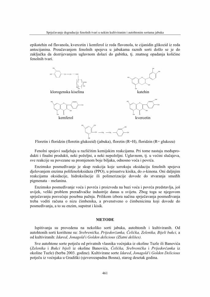
Sprječavanje degradacije fenolnih tvari u nekim kultiviranim i autohtonim sortama jabuka
461
epikatehin od flavanola, kvercetin i kemferol iz reda flavonola, te cijanidin glikozid iz reda antocijanina. Proučavanjem fenolnih spojeva u jabukama raznih sorti došlo se je do zaključka da dozrijevanjem uglavnom dolazi do gubitka, tj. znatnog opadanja količinefenolnih tvari.
CH CH COO
OHOH
COOH
OH
HO
HO
O
OH
OH
OH
OH
HO
klorogenska kiselina katehin
OHO
OH
OH
OH
O
OHO
OH
OH
OH
O
OH
kemferol kvercetin
HO OH
OR
CO CH2 CH2
OH
OH
Floretin i floridzin (floretin glukozid) (jabuka), floretin (R=H), floridzin (R= glukoza)
Fenolni spojevi sudjeluju u različitim kemijskim reakcijama. Pri tome nastaju međupro-dukti i finalni produkti, neki poželjni, a neki nepoželjni. Uglavnom, tj. u većini slučajeva,sve reakcije su povezane sa promjenom boje biljaka, odnosno voća i povrća.
Enzimsko posmeđivanje je skup reakcija koje uzrokuju oksidaciju fenolnih spojeva djelovanjem enzima polifenoloksidaza (PPO), u prisustvu kisika, do o-kinona. Oni daljnjim reakcijama oksidacije, hidroksilacije ili polimerizacije dovode do stvaranja smeđihpigmenata – melanina.
Enzimsko posmeđivanje voća i povrća i proizvoda na bazi voća i povrća predstavlja, još uvijek, veliki problem prerađivačke industrije danas u svijetu. Zbog toga se njegovom sprječavanju posvećuje posebna pažnja. Prilikom izbora načina sprječavanja posmeđivanjatreba voditi računa o nizu čimbenika, a prvenstveno o čimbenicima koji dovode do posmeđivanja, a to su enzim, supstrat i kisik.
METODE
Ispitivanja su provedena na nekoliko sorti jabuka, autohtonih i kultiviranih. Od autohtonih sorti korištene su: Srebrenička, Prijedorčanka, Čelićka, Zelenika, Bijeli bukci, aod kultiviranih: Idared, Jonagold i Golden delicious (Zlatni delišes).
Sve autohtone sorte potječu od privatnih vlasnika voćnjaka iz okoline Tuzle ili Banovića(Zelenika i Bukci bijeli iz okoline Banovića, Čelićka, Srebrenička i Prijedorčanka iz okoline Tuzle) (berba 2003. godine). Kultivirane sorte Idared, Jonagold i Golden Deliciouspotječu iz voćnjaka u Gradiški (sjeverozapadna Bosna), starog desetak godina.
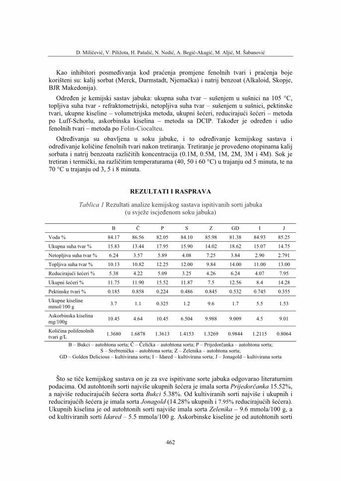
D. Miličević, V. Piližota, H. Pašalić, N. Nedić, A. Begić-Akagić, M. Aljić, M. Šabanović
462
Kao inhibitori posmeđivanja kod praćenja promjene fenolnih tvari i praćenja boje korišteni su: kalij sorbat (Merck, Darmstadt, Njemačka) i natrij benzoat (Alkaloid, Skopje, BJR Makedonija).
Određen je kemijski sastav jabuka: ukupna suha tvar – sušenjem u sušnici na 105 °C, topljiva suha tvar - refraktometrijski, netopljiva suha tvar – sušenjem u sušnici, pektinske tvari, ukupne kiseline – volumetrijska metoda, ukupni šećeri, reducirajući šećeri – metoda po Luff-Schorlu, askorbinska kiselina – metoda sa DCIP. Također je određen i udio fenolnih tvari – metoda po Folin-Ciocalteu.
Određivanja su obavljena u soku jabuke, i to određivanje kemijskog sastava i određivanje količine fenolnih tvari nakon tretiranja. Tretiranje je provedeno otopinama kalij sorbata i natrij benzoata različitih koncentracija (0.1M, 0.5M, 1M, 2M, 3M i 4M). Sok je tretiran i termički, na različitim temperaturama (40, 50 i 60 °C) u trajanju od 5 minuta, te na 70 °C u trajanju od 3, 5 i 8 minuta.
REZULTATI I RASPRAVA
Tablica 1 Rezultati analize kemijskog sastava ispitivanih sorti jabuka(u svježe iscjeđenom soku jabuka)
B Č P S Z GD I J
Voda % 84.17 86.56 82.05 84.10 85.98 81.38 84.93 85.25
Ukupna suha tvar % 15.83 13.44 17.95 15.90 14.02 18.62 15.07 14.75
Netopljiva suha tvar % 6.24 3.57 5.89 4.08 7.25 3.84 2.90 2.791
Topljiva suha tvar % 10.13 10.82 12.25 12.00 9.84 14.00 11.00 13.00
Reducirajući šećeri % 5.38 4.22 5.09 3.25 4.26 6.24 4.07 7.95
Ukupni šećeri % 11.75 11.90 15.52 11.87 7.5 12.56 8.4 14.28
Pektinske tvari % 0.185 0.858 0.224 0.486 0.845 0.532 0.745 0.355
Ukupne kiseline mmol/100 g 3.7 1.1 0.325 1.2 9.6 1.7 5.5 1.53
Askorbinska kiselina mg/100g 10.45 4.64 10.45 6.504 9.988 9.009 4.5 9.01
Količina polifenolnih tvari g/L 1.3680 1.6878 1.3613 1.4153 1.3269 0.9844 1.2115 0.8064
B – Bukci – autohtona sorta; Č – Čelićka – autohtona sorta; P – Prijedorčanka – autohtona sorta;S – Srebrenička – autohtona sorta; Z – Zelenika – autohtona sorta;
GD – Golden Delicious – kultivirana sorta; I – Idared – kultivirana sorta; J – Jonagold – kultivirana sorta
Što se tiče kemijskog sastava on je za sve ispitivane sorte jabuka odgovarao literaturnim podacima. Od autohtonih sorti najviše ukupnih šećera je imala sorta Prijedorčanka 15.52%, a najviše reducirajućih šećera sorta Bukci 5.38%. Od kultiviranih sorti najviše i ukupnih i reducirajućih šećera je imala sorta Jonagold (14.28% ukupnih i 7.95% reducirajućih šećera).Ukupnih kiselina je od autohtonih sorti najviše imala sorta Zelenika – 9.6 mmola/100 g, a od kultiviranih sorti Idared – 5.5 mmola/100 g. Askorbinske kiseline je od autohtonih sorti
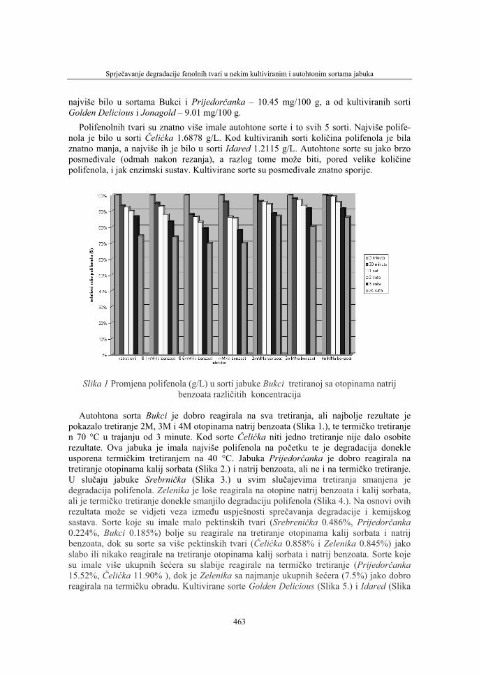
Sprječavanje degradacije fenolnih tvari u nekim kultiviranim i autohtonim sortama jabuka
463
najviše bilo u sortama Bukci i Prijedorčanka – 10.45 mg/100 g, a od kultiviranih sorti Golden Delicious i Jonagold – 9.01 mg/100 g.
Polifenolnih tvari su znatno više imale autohtone sorte i to svih 5 sorti. Najviše polife-nola je bilo u sorti Čelićka 1.6878 g/L. Kod kultiviranih sorti količina polifenola je bila znatno manja, a najviše ih je bilo u sorti Idared 1.2115 g/L. Autohtone sorte su jako brzo posmeđivale (odmah nakon rezanja), a razlog tome može biti, pored velike količinepolifenola, i jak enzimski sustav. Kultivirane sorte su posmeđivale znatno sporije.
Slika 1 Promjena polifenola (g/L) u sorti jabuke Bukci tretiranoj sa otopinama natrij benzoata različitih koncentracija
Autohtona sorta Bukci je dobro reagirala na sva tretiranja, ali najbolje rezultate je pokazalo tretiranje 2M, 3M i 4M otopinama natrij benzoata (Slika 1.), te termičko tretiranje n 70 °C u trajanju od 3 minute. Kod sorte Čelićka niti jedno tretiranje nije dalo osobite rezultate. Ova jabuka je imala najviše polifenola na početku te je degradacija donekle usporena termičkim tretiranjem na 40 °C. Jabuka Prijedorčanka je dobro reagirala na tretiranje otopinama kalij sorbata (Slika 2.) i natrij benzoata, ali ne i na termičko tretiranje. U slučaju jabuke Srebrnička (Slika 3.) u svim slučajevima tretiranja smanjena je degradacija polifenola. Zelenika je loše reagirala na otopine natrij benzoata i kalij sorbata, ali je termičko tretiranje donekle smanjilo degradaciju polifenola (Slika 4.). Na osnovi ovih rezultata može se vidjeti veza između uspješnosti sprečavanja degradacije i kemijskog sastava. Sorte koje su imale malo pektinskih tvari (Srebrenička 0.486%, Prijedorčanka0.224%, Bukci 0.185%) bolje su reagirale na tretiranje otopinama kalij sorbata i natrij benzoata, dok su sorte sa više pektinskih tvari (Čelićka 0.858% i Zelenika 0.845%) jako slabo ili nikako reagirale na tretiranje otopinama kalij sorbata i natrij benzoata. Sorte koje su imale više ukupnih šećera su slabije reagirale na termičko tretiranje (Prijedorčanka15.52%, Čelićka 11.90% ), dok je Zelenika sa najmanje ukupnih šećera (7.5%) jako dobro reagirala na termičku obradu. Kultivirane sorte Golden Delicious (Slika 5.) i Idared (Slika
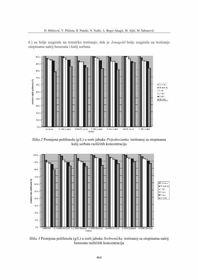
D. Miličević, V. Piližota, H. Pašalić, N. Nedić, A. Begić-Akagić, M. Aljić, M. Šabanović
464
6.) su bolje reagirale na termičko tretiranje, dok je Jonagold bolje reagirala na tretiranje otopinama natrij benzoata i kalij sorbata.
Slika 2 Promjena polifenola (g/L) u sorti jabuke Prijedorčanka tretiranoj sa otopinama kalij sorbata različitih koncentracija
Slika 3 Promjena polifenola (g/L) u sorti jabuke Srebrenička tretiranoj sa otopinama natrij benzoata različitih koncentracija
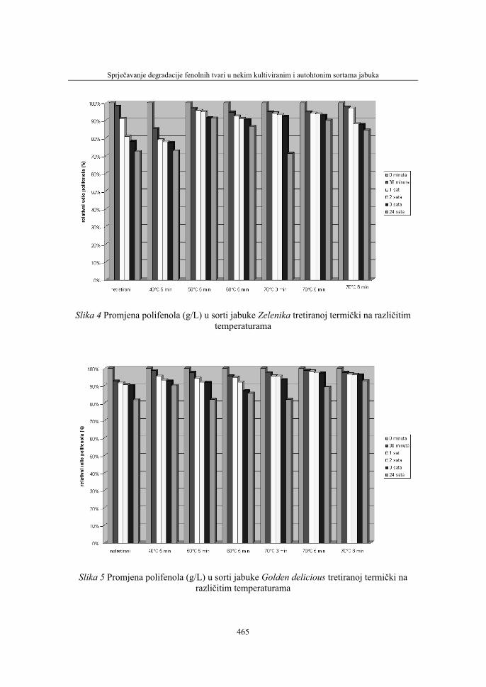
Sprječavanje degradacije fenolnih tvari u nekim kultiviranim i autohtonim sortama jabuka
465
Slika 4 Promjena polifenola (g/L) u sorti jabuke Zelenika tretiranoj termički na različitimtemperaturama
Slika 5 Promjena polifenola (g/L) u sorti jabuke Golden delicious tretiranoj termički na različitim temperaturama
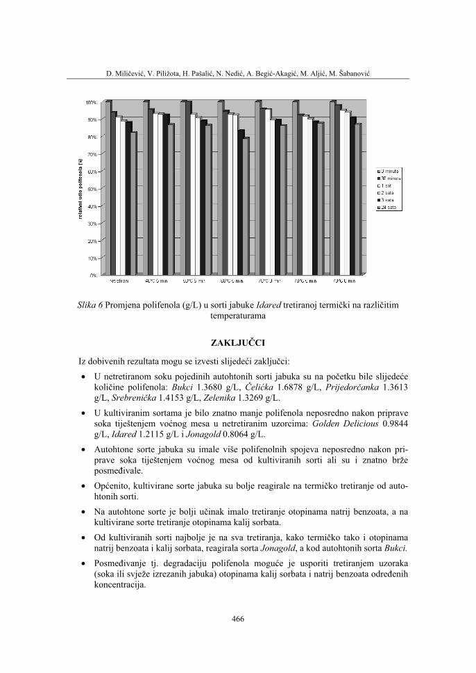
D. Miličević, V. Piližota, H. Pašalić, N. Nedić, A. Begić-Akagić, M. Aljić, M. Šabanović
466
Slika 6 Promjena polifenola (g/L) u sorti jabuke Idared tretiranoj termički na različitimtemperaturama
ZAKLJUČCI
Iz dobivenih rezultata mogu se izvesti slijedeći zaključci:
• U netretiranom soku pojedinih autohtonih sorti jabuka su na početku bile slijedećekoličine polifenola: Bukci 1.3680 g/L, Čelićka 1.6878 g/L, Prijedorčanka 1.3613 g/L, Srebrenička 1.4153 g/L, Zelenika 1.3269 g/L.
• U kultiviranim sortama je bilo znatno manje polifenola neposredno nakon priprave soka tiještenjem voćnog mesa u netretiranim uzorcima: Golden Delicious 0.9844 g/L, Idared 1.2115 g/L i Jonagold 0.8064 g/L.
• Autohtone sorte jabuka su imale više polifenolnih spojeva neposredno nakon pri-prave soka tiještenjem voćnog mesa od kultiviranih sorti ali su i znatno brže posmeđivale.
• Općenito, kultivirane sorte jabuka su bolje reagirale na termičko tretiranje od auto-htonih sorti.
• Na autohtone sorte je bolji učinak imalo tretiranje otopinama natrij benzoata, a na kultivirane sorte tretiranje otopinama kalij sorbata.
• Od kultiviranih sorti najbolje je na sva tretiranja, kako termičko tako i otopinama natrij benzoata i kalij sorbata, reagirala sorta Jonagold, a kod autohtonih sorta Bukci.
• Posmeđivanje tj. degradaciju polifenola moguće je usporiti tretiranjem uzoraka (soka ili svježe izrezanih jabuka) otopinama kalij sorbata i natrij benzoata određenihkoncentracija.
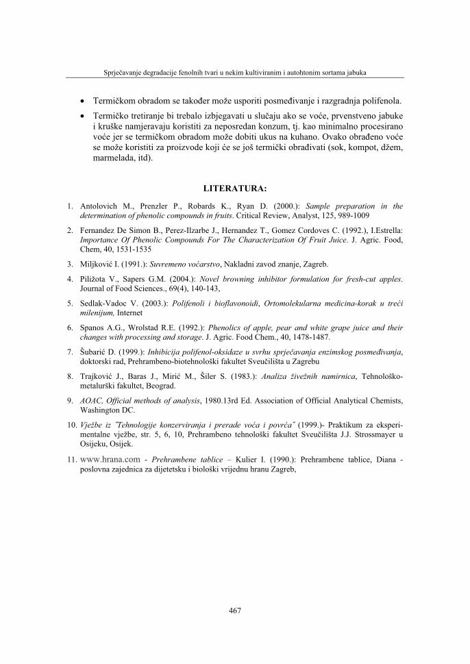
Sprječavanje degradacije fenolnih tvari u nekim kultiviranim i autohtonim sortama jabuka
467
• Termičkom obradom se također može usporiti posmeđivanje i razgradnja polifenola.
• Termičko tretiranje bi trebalo izbjegavati u slučaju ako se voće, prvenstveno jabuke i kruške namjeravaju koristiti za neposredan konzum, tj. kao minimalno procesirano voće jer se termičkom obradom može dobiti ukus na kuhano. Ovako obrađeno voćese može koristiti za proizvode koji će se još termički obrađivati (sok, kompot, džem, marmelada, itd).
LITERATURA:
1. Antolovich M., Prenzler P., Robards K., Ryan D. (2000.): Sample preparation in the determination of phenolic compounds in fruits. Critical Review, Analyst, 125, 989-1009
2. Fernandez De Simon B., Perez-Ilzarbe J., Hernandez T., Gomez Cordoves C. (1992.), I.Estrella: Importance Of Phenolic Compounds For The Characterization Of Fruit Juice. J. Agric. Food, Chem, 40, 1531-1535
3. Miljković I. (1991.): Suvremeno voćarstvo, Nakladni zavod znanje, Zagreb.
4. Piližota V., Sapers G.M. (2004.): Novel browning inhibitor formulation for fresh-cut apples.Journal of Food Sciences., 69(4), 140-143,
5. Sedlak-Vadoc V. (2003.): Polifenoli i bioflavonoidi, Ortomolekularna medicina-korak u trećimilenijum, Internet
6. Spanos A.G., Wrolstad R.E. (1992.): Phenolics of apple, pear and white grape juice and their changes with processing and storage. J. Agric. Food Chem., 40, 1478-1487.
7. Šubarić D. (1999.): Inhibicija polifenol-oksidaze u svrhu sprječavanja enzimskog posmeđivanja,doktorski rad, Prehrambeno-biotehnološki fakultet Sveučilišta u Zagrebu
8. Trajković J., Baras J., Mirić M., Šiler S. (1983.): Analiza živežnih namirnica, Tehnološko-metalurški fakultet, Beograd.
9. AOAC, Official methods of analysis, 1980.13rd Ed. Association of Official Analytical Chemists, Washington DC.
10. Vježbe iz ˝Tehnologije konzerviranja i prerade voća i povrća˝ (1999.)- Praktikum za eksperi-mentalne vježbe, str. 5, 6, 10, Prehrambeno tehnološki fakultet Sveučilišta J.J. Strossmayer u Osijeku, Osijek.
11. www.hrana.com - Prehrambene tablice – Kulier I. (1990.): Prehrambene tablice, Diana - poslovna zajednica za dijetetsku i biološki vrijednu hranu Zagreb,
D. Miličević, V. Piližota, H. Pašalić, N. Nedić, A. Begić-Akagić, M. Aljić, M. Šabanović
468
PREVENTION OF DEGRADATION OF PHENOLIC COMPOUNDS IN SOME KIND OF ANCIENT AND
CULTIVATED VARIETIES OF APPLES
SUMMARY
The fruit based products are highly demanded on the market due to their sensoric properties (taste, aroma, colour) and nutritive values.
Some researches are shown that phenolic compounds in fruit have a protective role in development of certain forms of ilness such as cancer. Being phenolic compounds have antioxidant properties it help to remove free radicals.
However, in spite of the large attention concerning health promotion, phenolic compounds in fruits, in the presence of enzyme polyphenol oxidase (PPO) and molecular oxygen, after plant tissuees physical injury, oxidize to o-quinones, reaction known as an enzymatic browning, which is, in most cases undesirable.
A great emphasis is put on reseach to develop new agents and methods to prevent enzymatic browning.
The aim of this work was to determine total amount of phenolic compounds in apples (cultivated varieties, Idared, Jonagold, and Golden Delicious, as well as ancient varieties originated in Bosnia, Srebrenička, Prijedorčanka, Čelićka,Zalenika, Bijeli bukci), as well as to prevent browning.
As an browning inhibitors potasium sorbate (0.1 mM, 0.5 mM, 1 mM, 2 mM, 3 mM i 4 mM) and sodium benzoate (0.1 mM, 0.5 mM, 1 mM, 2 mM, 3mM, 4 mM) were used.
For the inhibition of the browning a thermal treatment was performed as well. The phenolic compounds in apple juice ranged from 0.8064 g/L in cultivated
apple variety Jonagold to 1.6878 g/L in autocton apple variety Čelićka. The most of the phenolic compound was in juice ancient apple variety Čelićka (1.6878 g/L).
The good results in inhibition of enzymatic browning was performed with addition of 3 mM of potasium sorbate and 2 mM sodium benzoate in apple juice of anciente varieties and 4 mM potasium sorbate in apple juice of cultivated varities.
This results can be used in processing of the fruit under study due to prevent enzimatic browning and stability of colour of different fruit products.
Key words: phenolic compounds, juice, apples, enzymatic browning, potasium sorbate, sodium benzoate.
36. Symposium "Actual Tasks on Agricultural Engineering", Opatija, Croatia, 2008.
469
36.
SIMPOZIJAKTUALNI ZADACIMEHANIZACIJE POLJOPRIVREDE
UDC632.15:633.853.483
Izvorni znanstveni radOriginal scientific paper
RESEARCHES REGARDING THE INFLUENCE OF HEAVY METALS HYPERACCUMULATION ON THE
BRASSICA NIGRA SINIGRIN-MYROSINASESYSTEM ACTIVITY
DANIELA STOIN1, FLORINA RADU1, DIANA DOGARU1, PARSAN PAUL2
Banat’s University of Agricultural Sciences and Veterinary Medicine, 1Faculty of Food Processing Technology,
2Faculty of Agricultural, Calea Aradului, 119, Timisoara, Romania e-mail: [email protected]
SUMMARY
The phenomenon of metal hyperaccumulation in plants has attracted particular interest in the last years, because plants that combine high metal tolerance with an extraordinary ability for metal uptake may be useful for phytoextraction technologies.
Previous research suggest that in species of Brassicaceae family, the heavy metals might represent an ecological advantage by protecting the soils from metal contamination.
One of the plants that seems to play an important role in soils „phytoremedy” with metal ions, is the mustard.
The influence of some transitive metals on the sinigrin-myrosinase system activity from Brassica nigra, was indirectly determined by quantification of glucose resulted from sinigrin hydrolysis. the glucose amount analysed was obtained from mustard samples samples and samples previously treated with a solution of heavy metals salts of above mentioned metals.
Analysis of sinigrin-myrosinase activity as accomplished by use of the following methods: UV-VIS spectrophotometry and RP-HPLC technique.
The obtained experimental data showed that metals constitutes an important factor that determines modifications in myrosinase enzyme behavior.
Thus, the study of transitional metals influence on myrosinase activity, accomplished with two modern techniques has established a better protocol for the RP-HPLC analysis of myrosinase activity.
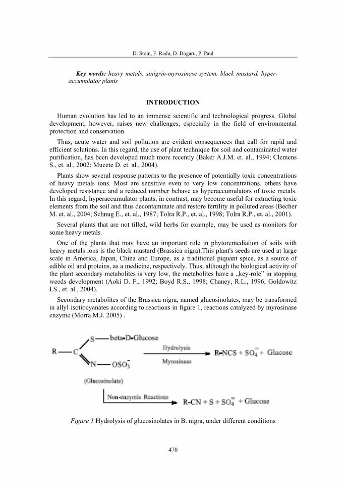
D. Stoin, F. Radu, D. Dogaru, P. Paul
470
Key words: heavy metals, sinigrin-myrosinase system, black mustard, hyper-accumulator plants
INTRODUCTION
Human evolution has led to an immense scientific and technological progress. Global development, however, raises new challenges, especially in the field of environmental protection and conservation.
Thus, acute water and soil pollution are evident consequences that call for rapid and efficient solutions. In this regard, the use of plant technique for soil and contaminated water purification, has been developed much more recently (Baker A.J.M. et. al., 1994; Clemens S., et. al., 2002; Mucete D. et. al., 2004).
Plants show several response patterns to the presence of potentially toxic concentrations of heavy metals ions. Most are sensitive even to very low concentrations, others have developed resistance and a reduced number behave as hyperaccumulators of toxic metals. In this regard, hyperaccumulator plants, in contrast, may become useful for extracting toxic elements from the soil and thus decontaminate and restore fertility in polluted areas (Becher M. et. al., 2004; Schnug E., et. al., 1987; Tolra R.P., et. al., 1998; Tolra R.P., et. al., 2001).
Several plants that are not tilled, wild herbs for example, may be used as monitors for some heavy metals.
One of the plants that may have an important role in phytoremediation of soils with heavy metals ions is the black mustard (Brassica nigra).This plant's seeds are used at large scale in America, Japan, China and Europe, as a traditional piquant spice, as a source of edible oil and proteins, as a medicine, respectively. Thus, although the biological activity of the plant secondary metabolites is very low, the metabolites have a „key-role” in stopping weeds development (Aoki D. F., 1992; Boyd R.S., 1998; Chaney, R.L., 1996; Goldowitz I.S., et. al., 2004).
Secondary metabolites of the Brassica nigra, named glucosinolates, may be transformed in allyl-isotiocyanates according to reactions in figure 1, reactions catalyzed by myrosinase enzyme (Morra M.J. 2005) .
Figure 1 Hydrolysis of glucosinolates in B. nigra, under different conditions
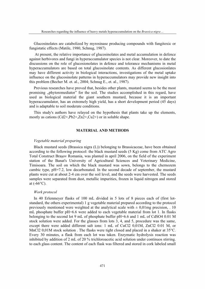
Researches regarding the influence of heavy metals hyperaccumulation on the Brassica nigra ...
471
Glucosinolates are catabolized by myrosinase producing compounds with fungitoxic or fungistatic effects (Matile, 1980, Schnug, 1987).
At present, the relative importance of glucosinolates and metal accumulation in defence against herbivores and fungi in hyperaccumulator species is not clear. Moreover, to date the discussions on the role of glucosionolates in defence and tolerance mechanisms in metal hyperaccumulators are based on total glucosinolate contents. As different glucosionlates may have different activity in biological interactions, investigations of the metal uptake influence on the glucosinolate patterns in hyperaccumulators may provide new insight into this problem (Becher M. et. al., 2004; Schnug E., et. al., 1987).
Previous researches have proved that, besides other plants, mustard seems to be the most promising „phytoremediator” for the soil. The studies accomplished in this regard, have used as biological material the giant southern mustard, because it is an important hyperaccumulator, has an extremely high yield, has a short development period (45 days) and is adaptable to soil moderate conditions.
This study's authors have relayed on the hypothesis that plants take up the elements, mostly as cations (Cd2+,Pb2+,Zn2+,Cu2+) or in soluble shape.
MATERIAL AND METHODS
Vegetable material preparing Black mustard seeds (Brassica nigra (L)) belonging to Brassicaceae, have been obtained
according to the following protocol: the black mustard seeds (5 Kg) come from ATC Agro Total Construct Braşov Romania, was planted in april 2006, on the field of the experiment station of the Banat's University of Agricultural Sciences and Veterinary Medicine, Timisoara. The soil on which the black mustard was sown, belongs to the chernozem cambic type, pH=7.2, low decarbonated. In the second decade of september, the mustard plants were cut at about 2-4 cm over the soil level, and the seeds were harvested. The seeds samples were separated from dust, metallic impurities, frozen in liquid nitrogen and stored at (-66°C).
Work protocol In 40 Erlenmeyer flasks of 100 mL divided in 5 lots of 8 pieces each of (first lot-
standard, the others experimental) 1 g vegetable material prepared according to the protocol previously mentioned were weighted at the analytical scale with ± 0,01mg precision, . 10 mL phosphate buffer pH=6.6 were added to each vegetable material from lot 1. In flasks belonging to the second lot 9 mL of phosphate buffer pH=6.6 and 1 mL of CdSO4 0.01 M stock solution were added. For the glasses from lots 3, 4, and 5, procedure was the same, except there were added different salt ions: 1 mL of CuCl2 0,01M, ZnCl2 0.01 M, or MnCl2 0,01M stock solution . The flasks were tight closed and placed in a shaker at 35°C. Every 30 minutes, a flask from each lot was taken. Enzymatic hydrolysis reaction was inhibited by addition of 2 mL of 20 % trichloroacetic acid solution under continuos stirring. to each glass content. The content of each flask was filtered and stored in cork labeled small
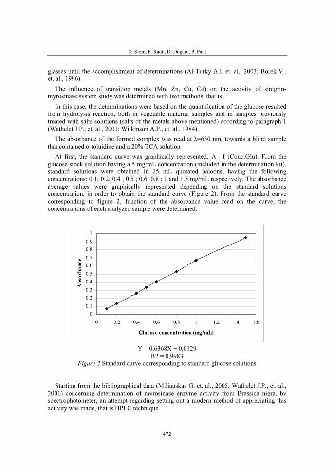
D. Stoin, F. Radu, D. Dogaru, P. Paul
472
glasses until the accomplishment of determinations (Al-Turky A.I. et. al., 2003; Borek V., et. al., 1996).
The influence of transition metals (Mn, Zn, Cu, Cd) on the activity of sinigrin-myrosinase system study was determined with two methods, that is:
In this case, the determinations were based on the quantification of the glucose resulted from hydrolysis reaction, both in vegetable material samples and in samples previously treated with salts solutions (salts of the metals above mentioned) according to paragraph 1 (Wathelet J.P., et. al., 2001; Wilkinson A.P., et. al., 1984).
The absorbance of the formed complex was read at λ=630 nm, towards a blind sample that contained o-toluidine and a 20% TCA solution
At first, the standard curve was graphically represented: A= f (Conc:Glu). From the glucose stock solution having a 5 mg/mL concentration (included in the determination kit), standard solutions were obtained in 25 mL quotated baloons, having the following concentrations: 0.1; 0.2; 0.4 ; 0.5 ; 0.6; 0.8 ; 1 and 1.5 mg/mL respectively. The absorbance average values were graphically represented depending on the standard solutions concentration, in order to obtain the standard curve (Figure 2). From the standard curve corresponding to figure 2, function of the absorbance value read on the curve, the concentrations of each analyzed sample were determined.
00.10.20.30.40.50.60.70.80.9
1
0 0.2 0.4 0.6 0.8 1 1.2 1.4 1.6
Glucose concentration (mg/mL)
Abs
orba
nce
Y = 0,6368X + 0,0129 R2 = 0,9983
Figure 2 Standard curve corresponding to standard glucose solutions
Starting from the bibliographical data (Miliauskas G. et. al., 2005; Wathelet J.P., et. al., 2001) concerning determination of myrosinase enzyme activity from Brassica nigra, by spectrophotometer, an attempt regarding setting out a modern method of appreciating this activity was made, that is HPLC technique.

Researches regarding the influence of heavy metals hyperaccumulation on the Brassica nigra ...
473
In this case, myrosinase activity was determined by measuring the decreasing speed of the sinigrin concentration in black mustard extracts, obtained according to paragraph 1.
HPLC conditions: Agillent HP 100 system NUCLEOSIL column C18; volume: 20 mL; sample flow: 1mL/min; mobile phase: methanol; phosphate buffer solution pH=7, (99:1); column temperature: 35°C; wavelength: 229 nm; eluating mode: isocratic.
Average values of the obtained areas the standard solutions concentration in order to obtain the standard curve (Figure 3).
On the basis of the obtained areas, the sinigrin concentration at equilibrium from the black mustard extracts was determined, and with the help of this concentration the quantity of sinigrin consumed in the reaction of enzymatic hydrolysis, was calculated, so:
CSinCons = CI - Ci
where: CSinCons – Sinigin quantity consumed (mg/mL); CI –sinigrin concentration from the inactivated sample (black mustard), (mg/mL); Ci – sinigrin concentration at equilibrium (mg/mL).
020000400006000080000
100000120000140000160000180000
0 1 2 3 4 5
Sinigrin concentration (mg/mL)
Are
a
Y = 33049,97X + 439,39 R2 = 0,9999
Figure 3 Standard curve corresponding for sinigrin standard solutions
RESULTS AND DISCUSSION
In order to determine the influence of some metals on the hydrolytic activity of myro-sinase, the effect of Mn, Zn, Cl cations as clorurate and Cd as a sulphate, respectively, was studied. Among the tested cations by Schung (1987, 2000) [14, 15], generally speaking, alkaline and sallow-alkaline are promotors of the enzymatic hydrolysis reaction, while transition heavy metals (Pb, Cd, Ni and Cr) are inhibitors of the enzymatic reaction. In exchange, the study of the influence of cations above mentioned, become the aim of some researches that were only at the beggining (Becher M., 2004; Clemens S., et. al., 2002; Mucete D. et. al., 2004). The mustard species taken into study, seems to be a natural metals
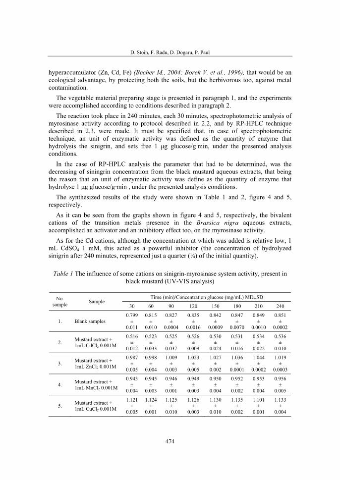
D. Stoin, F. Radu, D. Dogaru, P. Paul
474
hyperaccumulator (Zn, Cd, Fe) (Becher M., 2004; Borek V. et al., 1996), that would be an ecological advantage, by protecting both the soils, but the herbivorous too, against metal contamination.
The vegetable material preparing stage is presented in paragraph 1, and the experiments were accomplished according to conditions described in paragraph 2.
The reaction took place in 240 minutes, each 30 minutes, spectrophotometric analysis of myrosinase activity according to protocol described in 2.2, and by RP-HPLC technique described in 2.3, were made. It must be specified that, in case of spectrophotometric technique, an unit of enzymatic activity was defined as the quantity of enzyme that hydrolysis the sinigrin, and sets free 1 μg glucose/g·min, under the presented analysis conditions.
In the case of RP-HPLC analysis the parameter that had to be determined, was the decreasing of siningrin concentration from the black mustard aqueous extracts, that being the reason that an unit of enzymatic activity was define as the quantity of enzyme that hydrolyse 1 μg glucose/g·min , under the presented analysis conditions.
The synthesized results of the study were shown in Table 1 and 2, figure 4 and 5, respectively.
As it can be seen from the graphs shown in figure 4 and 5, respectively, the bivalent cations of the transition metals presence in the Brassica nigra aqueous extracts, accomplished an activator and an inhibitory effect too, on the myrosinase activity.
As for the Cd cations, although the concentration at which was added is relative low, 1 mL CdSO4 1 mM, this acted as a powerful inhibitor (the concentration of hydrolyzed sinigrin after 240 minutes, represented just a quarter (¼) of the initial quantity).
Table 1 The influence of some cations on sinigrin-myrosinase system activity, present in black mustard (UV-VIS analysis)
Time (min)/Concentration glucose (mg/mL) MD±SD No.sample Sample
30 60 90 120 150 180 210 240
1. Blank samples 0.799
±0.011
0.815±
0.010
0.827±
0.0004
0.835±
0.0016
0.842±
0.0009
0.847±
0.0070
0.849±
0.0010
0.851±
0.0002
2. Mustard extract + 1mL CdCl2 0.001M
0.516±
0.012
0.523±
0.033
0.525±
0.037
0.526±
0.009
0.530±
0.024
0.531±
0.016
0.534±
0.022
0.536±
0.010
3. Mustard extract + 1mL ZnCl2 0.001M
0.987±
0.005
0.998±
0.004
1.009±
0.003
1.023±
0.005
1.027±
0.002
1.036±
0.0001
1.044±
0.0002
1.019±
0.0003
4. Mustard extract + 1mL MnCl2 0.001M
0.943±
0.004
0.945±
0.003
0.946±
0.001
0.949±
0.003
0.950±
0.004
0.952±
0.002
0.953±
0.004
0.956±
0.005
5. Mustard extract + 1mL CuCl2 0.001M
1.121±
0.005
1.124±
0.001
1.125±
0.010
1.126±
0.003
1.130±
0.010
1.135±
0.002
1.101±
0.001
1.133±
0.004
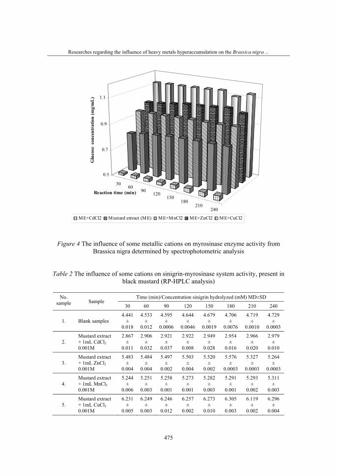
Researches regarding the influence of heavy metals hyperaccumulation on the Brassica nigra ...
475
3060
90120
150180
210240
0.5
0.7
0.9
1.1 G
luco
se c
once
ntra
tion
(mg/
mL
)
Reaction time (min)
ME+CdCl2 Mustard extract (ME) ME+MnCl2 ME+ZnCl2 ME+CuCl2
Figure 4 The influence of some metallic cations on myrosinase enzyme activity from Brassica nigra determined by spectrophotometric analysis
Table 2 The influence of some cations on sinigrin-myrosinase system activity, present in black mustard (RP-HPLC analysis)
Time (min)/Concentration sinigrin hydrolyzed (mM) MD±SD No.sample Sample
30 60 90 120 150 180 210 240
1. Blank samples 4.441
±0.018
4.533±
0.012
4.595±
0.0006
4.644±
0.0046
4.679±
0.0019
4.706±
0.0076
4.719±
0.0010
4.729±
0.0003
2.Mustard extract + 1mL CdCl20.001M
2.867±
0.011
2.906±
0.032
2.921±
0.037
2.922±
0.008
2.949±
0.028
2.954±
0.016
2.966±
0.020
2.979±
0.010
3.Mustard extract + 1mL ZnCl20.001M
5.483±
0.004
5.484±
0.004
5.497±
0.002
5.503±
0.004
5.520±
0.002
5.576±
0.0003
5.327±
0.0003
5.264±
0.0003
4.Mustard extract + 1mL MnCl20.001M
5.244±
0.006
5.251±
0.003
5.258±
0.001
5.273±
0.001
5.282±
0.003
5.291±
0.001
5.293±
0.002
5.311±
0.003
5.Mustard extract + 1mL CuCl20.001M
6.231±
0.005
6.249±
0.003
6.246±
0.012
6.257±
0.002
6.273±
0.010
6.305±
0.003
6.119±
0.002
6.296±
0.004
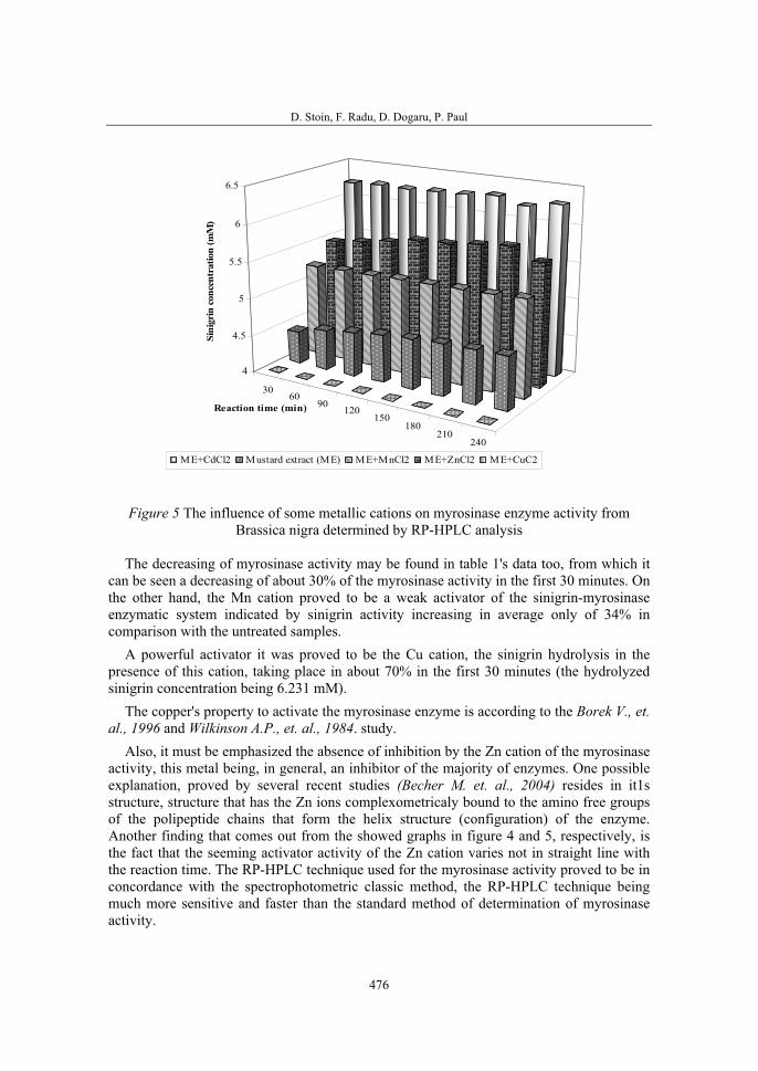
D. Stoin, F. Radu, D. Dogaru, P. Paul
476
3060
90120
150180
210240
4
4.5
5
5.5
6
6.5
Sin
igri
n co
ncen
trat
ion
(mM
)
Reaction time (min)
ME+CdCl2 Mustard extract (ME) ME+MnCl2 ME+ZnCl2 ME+CuC2
Figure 5 The influence of some metallic cations on myrosinase enzyme activity from Brassica nigra determined by RP-HPLC analysis
The decreasing of myrosinase activity may be found in table 1's data too, from which it can be seen a decreasing of about 30% of the myrosinase activity in the first 30 minutes. On the other hand, the Mn cation proved to be a weak activator of the sinigrin-myrosinase enzymatic system indicated by sinigrin activity increasing in average only of 34% in comparison with the untreated samples.
A powerful activator it was proved to be the Cu cation, the sinigrin hydrolysis in the presence of this cation, taking place in about 70% in the first 30 minutes (the hydrolyzed sinigrin concentration being 6.231 mM).
The copper's property to activate the myrosinase enzyme is according to the Borek V., et. al., 1996 and Wilkinson A.P., et. al., 1984. study.
Also, it must be emphasized the absence of inhibition by the Zn cation of the myrosinase activity, this metal being, in general, an inhibitor of the majority of enzymes. One possible explanation, proved by several recent studies (Becher M. et. al., 2004) resides in it1s structure, structure that has the Zn ions complexometricaly bound to the amino free groups of the polipeptide chains that form the helix structure (configuration) of the enzyme. Another finding that comes out from the showed graphs in figure 4 and 5, respectively, is the fact that the seeming activator activity of the Zn cation varies not in straight line with the reaction time. The RP-HPLC technique used for the myrosinase activity proved to be in concordance with the spectrophotometric classic method, the RP-HPLC technique being much more sensitive and faster than the standard method of determination of myrosinase activity.
Researches regarding the influence of heavy metals hyperaccumulation on the Brassica nigra ...
477
CONCLUSIONS
• The study of myrosinase activity from the mustard seeds (Brassica nigra) led to the finding that, sinigrin-myrosinase system is influenced also by different environmental factors (pH, temperature, transitional metal presence in the vegetable material composition, an the incubation time, too);
• The transition metals presence is a factor that determines changes in myrosinase behavior; for example Cd is a powerful inhibitor of enzymatic activity, while Cu contributes to activating sinigrin-myrosinase system, leading to shortening the reaction time and at the same time to increasing with over 70% of enzymatic activity in the first 30 minutes in comparison to untreated samples;
• The atypical behavior of Zn cation was noticed, cation that in this case acted as activator agent, contributing to significant decrease of the sinigrin concentrations in the reaction medium. Regarding this, it is recommended to continue the experimental researches as from the point of view of elucidating the chemical structure of myrosinase, and the mechanism that this metal uses to significantly encourage the hydrolysis process;
• Atypical activator agent behavior of the Zn cation, in comparison with the other two metals (Mn, Cu, respectively) was noticed through not straight variation in time of the enzymatic activity in the case of black mustard extracts, variation caused by Zn hyperaccumulator property of this plant ;
• The study of transition metals presence on myrosinase activity, study accomplished with the help of two modern techniques (UV-VIS spectrophotometry, high performance liquid chromatography HPLC respectively) led to formulating a protocol for the myrosinase activity analysis, much more favorable, both from the point of view of shortening the necessary time to the sample preparing stage, and the experimental data reproducibility, too.
REFERENCES
1. Al-Turky A.I., Dick W.A. (2003) Myrosinase Activity in Soil, Soil Science Society of America Journal, 67, 139-145
2. Aoki, D.F. (1992). The uptake of arsenic and cadmium in mine tailings by poplar trees. M.S. Thesis, University of Iowa, Iowa City, IA.
3. Baker A.J.M., McGrath S.P., Sidoli C.M.D., Reeves R.D. (1994) The possibility of in situ heavy metal decontamination of polluted soils using crops of metal-accumulating plants, Resources, Conservation Recycling, 11:41-49
4. Boyd R.S. (1998) hyperaccumulation as a plant defence strategy. In: Brooks RR, ed. Plants that hyperaccumulate heavy metals: their role in phytoremediation, microbiology, archaeology, mineral exploration and phytomining, Wallingford, UK: CAB International, 181-201
5. Becher Martina, Talke Ina, Krall L., Kramer U. (2004) Cross-species microarray transcript profiling reveals high constitutive expression of metal homeostasis genes in shoots of the zinc hyperaccumulator Arabidopsis halleri, The Plant Journal, 37, 251-268

D. Stoin, F. Radu, D. Dogaru, P. Paul
478
6. Borek V., Morra M.J., McCaffrey J.P. (1996) Myrosinase activity in soil extracts, Soil Sci. Soc. Am. J. 60:1792–1797
7. Clemens S., Palmgren M.G., Kramer U. (2002) A long way ahead: understanding and engineering plant metal accumulation, Trends Plant Sci., 7, 309-315
8. Chaney, R.L. (1996), Phytoremediation of Zn and Cd contaminated soils using metal hyperaccumulator plants: Progress in technology developments. International Phytoremediation Conference, May 8-10, 1996, Arlington, VA. International Business Communications, Southborough, MA.
9. Goldowitz I. S., Goldowitz J., (2004), Phytoremediation of Lead Contaminated Soils in the Urban Residential Environment using Seed Mustard, The 20th Annual International Conference on soils, sediments and water, October 18-21, 2004 University of Massachusetts, Amherst, MA, USA
10. Matile P., 1980, "Die senfölbombe": Zur Kompartimentierung des Myrosinase systems Biochem. Physiol. Pflanz, 175, 722-731
11. Miliauskas G., van Beek T.A., de Waard P., Venskutonis R.P., Sudholter E.J. (2005) Comparison of analytical and semi-preparative columns for high-performance liquid chromatography-solid-phase extraction-nuclear magnetic resonance, J. Chromatogr. A., 1112, 2, 276-84
12. Morra M.J. (2005) Chemical Characterization and Release Efficiency of Defatted Mustard Meals, National Renewable Energy Laboratory, SR-510-36208, 1-18
13. Mucete Daniela, Radu Florina, Bordean Despina, Poiană Mariana, Gergen I. (2004) Influence of some trace metals accumulated in the black mustard (Brassica nigra), seeds, on the myrosinase-sinigrin system activity, Macro and Trace Elements, Mengen und Spurenelemente, Agricultural, Biological, Environmental, Nutritional and Medical Importance of Macro, Trace and Ultra Trace Elements, 22 Workshop, Main Building of the Friedrich Schiller University Jena, ISBN 3-929526-61-1, ISSN 1430-9637, 991-997
14. Schnug E., Haneklaus S. (1987) Röntgenfluoreszenzanalytische Bestimmung des Gesamtglucosinolatgehaltes in Rapssamen und Rapsextraktionsschrot, VDLUFA-Schriftenreihe, 23, 883-898
15. Schnug E., Haneklaus S., Schimmel H., Linsinger T., Mabon N., Marlier M., Wathelet J.P. (2000) Standard reference materials for total sulfur and glucosinolates, Sulfur Nutrition and Sulfur Assimilation in Higher Plants, Edited by C. brunold et al., Paul Haupt, Bern, Switzerland, 251-253
16. Tolra R.P., Gomis M., Barcelo J., Poschenrieder Ch. (1998) Influence of metal hyper-accumulation on glucosinolate content. In: Proceedings VII National-III Iberrian Symposium Plant Mineral Nutrition, Madrid, Spain: Autonomus University Press, 471-476
17. Tolra R.P., Poschenrieder C., Alonso R., Barcelo D., Barcelo J. (2001) Influence of zinc hyperaccumulation on glucosinolates in Thlaspi caerulescens, New Phytologist, 151: 621-626
18. Wathelet J.P., Iori R., Mabon N., Palmieri S., Leoni O., Rollin P., Marlier M. (2001) Determination of the response factors of several desulfo-glucosinolates used for quantitative analysis of Brassicaceae, Réunions techniques du GCIRC, Poznan, Pologne
19. Wilkinson A.P., Rhodes J.C., Fenwik R.G. (1984) Determination of myrosinase (Thioglucoside Glucohydrolase) activity by a spectrophotometric coupled enzyme assay, Anal. Biochem., 139, 284–291
36. Symposium "Actual Tasks on Agricultural Engineering", Opatija, Croatia, 2008.
479
36.
SIMPOZIJAKTUALNI ZADACIMEHANIZACIJE POLJOPRIVREDE
UDC621.317.38:631.563.2:582.998.2:635.72
Izvorni znanstveni radOriginal scientific paper
PRACTICE ORIENTED INVESTIGATION OF CHAMOMILE AND PEPPERMINT DRYING IN
BATCH DRYERS M. MARTINOV1, D. ADAMOVIC2, B. VESELINOV1, M. MATAVULY3, S. BOJIC1,
I. MUJIC4
1Faculty of Technical Sciences, Novi Sad, Serbia, [email protected] 2Institute for Field and Vegetable Crops, Novi Sad, Serbia
3Milan Matavuly, Faculty of Natural Sciences, Novi Sad, Serbia 4Biotechnical Faculty, Department for Food Technology, Bihac, Bosnia and Herzegovina
SUMMARYSmall and medium scale producers of medicinal plants in most cases perform
it in batch dryers, which offers optimal investment/output rate. Disadvantages of this dryer type are: higher drying energy and slower through-heating of upper layers, with the resulting increase of microbial count. It is also frequently followed by higher losses of essential oils.
This paper presents results of investigation of chamomile and peppermint drying characteristics in batch dryer expressed by: essential oil losses, microbial count changes and specific drying energy. Following parameters were measured: fuel consumption, change of material temperature and moisture content in levels 10 cm above grate and 10 cm below surface for three heights of fresh material layer, content of essential oils and microbial count. The drying regime was applied in three different phases, and different material batch heights. The following parameters were calculated: drying duration (related to the material mass), specific consumption of primary energy for drying, temperature course in material layers, change of microbial count and reduction of essential oil content.
The results showed that the essential oil losses are acceptable. Microbial count has increased in the upper layer during drying process, while the temperature was below 45° C for a long period. However, during the final drying phase in this layer, the temperature was also over 45° C, and the final microbial count was almost the same for upper and lower levels. The energy input was higher for the lower layer of fresh material. Final results are instructions, procedure, for drying of chamomile and peppermint.
Key words: Drying, Chamomile, Peppermint, Essential oil losses, Microbial count, Energy
M. Martinov, D. Adamovic, B. Veselinov, M. Matavuly, S. Bojic, I. Mujic
480
INTRODUCTION
The safety and quality demands for medicinal and aromatic plants from year to year are higher. Due to risks that occur by natural drying many buyers accept only technically dried products. Compliance with the microbial count limits, based on European Pharmacopoeia (Anonym, 2002) is mandatory in many countries. In the developing countries, the use of batch dryers presents a compromise between investments and effects. The control of drying process is very poor in conventional batch dryers, which results in lower quality and higher input of energy. New development of control equipment enables control in batch dryers, which is not only satisfactory but is almost comparable to that in big band dryers.
Quick evaporation of physically bond moisture takes place at the beginning of the drying process. For the removal of moisture located inside of material, beside the energy for evaporation, requires the energy for moisture transport to the surface (Bruin and Luyben, 1980, Mühlbauer, 1989). This process largely depends on material structure and it differs, e.g. for leaves and stems. Essential oils are active ingredients of many medicinal and aromatic plants, and their thermal sensitivity is a limiting factor for setting up of drying temperature (Mimica-Dukic et al., 2003). Influence of agent temperature on essential oils losses has been reported in many papers. Sometimes authors tend to disregard the difference between material and agent temperature in different phases (Bushbeck et al., 1967, Stakic et al., 1994), which results in low temperature limits being set up. Müller (1992, 2004) has clearly documented that the influence of high temperature on essential oils losses is high in the final phase, especially if material is over-dried. Drying temperature has impact on specific drying energy, the higher the temperature the lower the specific drying energy (Müller, 2002). Rise of temperature over 45° C results in considerable reduction of microbial count, due to their elimination. Contemporary procedures for reduction of microbial count, treatment with steam or microwaves, are used only in big band dryers (Heindl, 2005). In summation, too high temperatures cause losses of essential oils, while too low increase the microbial count. Due to this contradictory requirement the range of favorable drying agent temperatures is very narrow, especially for the final drying phase, e.g. for moisture content range from 18-20% to the final ones, e.g. 11%. The upper limit, due to essential oil losses is about 50° C, while the lower limit, due to desired reduction of microbial count, is 45° C. Temperature control can be performed relatively easy in contemporary band dryers (Müller, 2004, Martinov et al., 2007b), as opposed to batch dryers. The through-heating of whole material layer, upper levels, is very slow, causing increase of microbial count (Graf et al., 2002, Martinov et al., 2006a).
Monitoring of material moisture content during drying process is a serious problem for producers. In the case of multiphase drying, the moisture content should be measured, while the drying parameters should be changed by reaching the preset level. NIR and microwave moisture content measuring techniques are already used, but, due to high purchasing costs only in big plants, i.e. band dryers (Heindl and Heindl, 1998, Martinov et al., 2007b). Simple and inexpensive quick measuring of moisture content can be done using household microwave ovens. The tests of 15 to 30 minutes of drying and calculating of moisture content showed good results, applicable in practice (Martinov et al., 2007a).
The objective of investigation was to test effects of multiphase drying of medicinal plants on essential oil losses, microbial count, energy inputs and drying time reduction. The
Practice oriented investigation of chamomile and pepermint drying in batch dryers
481
final result should be recommendation for better drying practice. Results of first testing of peppermint drying have been already published (Martinov et al., 2006a, Martinov et al., 2006b), and recommendation for further improvements has been accepted and included in the procedures for here presented investigation. Nearby peppermint, tested in 2005, in the tests in 2006 chamomile drying has been also included.
MATERIALS AND METHODS
MaterialsChamomilla recutita (L.) Rauch cultivar Tetraploidna was harvested using virtual comb
type of rotated harvester in June 2006. The flowers were selected using 22 mm openings sieve. The drying was performed in different fresh material batch heights: flowers in 15 and 25 cm, and not separated material (mixture of flowers, stalks and leaves) in 40 cm. Six tests were made, two for each fresh material layer height.
Cultivar of Mentha x piperita L. Danica in first year of vegetation, first and second harvest, August and October 2006, was used. Whole plant, i.e. herb, was dried in two heights of fresh material batch: 80, and 100 cm (according to the previous tests the layer height of 40 and 60 cm showed inferior results). The tests without turning and with turning of material layer, after finishing of second drying phase, were performed. Material was weighted by integrated balance, accuracy ± 0.2 kg. Material samples for determination of moisture content, essential oil content, and microbial count were taken before drying. In the course of drying, changes of moisture content in the upper and lower levels, 10 cm above the grate and 10 cm below surface were taken for analysis of moisture content and microbial count. Eight tests were made.
MethodsThe experimental batch dryer, SD–16 MGA, produced by Termoplin, Mladenovac is
presented in Fig. 1. It is same as described in Martinov et al. (2006a, 2006b), but for the experiments in 2006 and 2007 placed on the frame carrier –17 and four weighing SG sensors, position –18. This enables continuous measuring of dried material weight with accuracy 2 N. The burner capacity was 15 kW, and ventilator engine 0.78 kW.
The drying agent flow through material layer was adjusted to 0.2 m/s, and measuring was performed with anemometer at overpressure vents opening. The surface of drying grate was 1.6 m2.
During the course of drying, three working regimes, combination of maximum tempe-rature and working mode – open or circulated – were programmed. In comparison with preliminary testing, Martinov et al. (2006a, 2006b), where the time of changing the phase was predicted, integrated balance enables change of drying regime according to measured material mass and calculated moisture content. The dominant process was:
1. Phase – open mode, drying temperature 55° C (for the first test was 50° C). Phase finished when the moisture content of dried material reach 40 do 45%.
M. Martinov, D. Adamovic, B. Veselinov, M. Matavuly, S. Bojic, I. Mujic
482
2. Phase – drying temperature adjusted to 50° C (for the first test was 48° C), automatic change of mode, switching of open mode at the relative humidity of drying agent at 40% for chamomile and 55% for peppermint. Duration of phase up to reduction of dried material moisture content 20 to 25%.
3. Phase – drying temperature adjusted to 48° C (for the first test was 46° C), automatic change of mode, switching to the open mode at the relative humidity of drying agent at 25% for chamomile and 45% for peppermint. Drying down to about 11% of moisture content.
Relative humidity of air after passing through material layer was calculated based on temperatures measured by "wet"–9 and "dry" –10 bulbs. The change from open to circulating mode was performed, after reaching the programmed upper value of the relative humidity of the agent, by opening side flaps –4 and closing circulation opening flap –8 using a servo-motors. For the drying agent temperature was used thermostat of the burner and automatic control of drying mode, switching from circulating to open mode was used common PLC for tobacco dryers.
Fuel consumption was measured by a weighing oil tank before and after drying, and mass converted into liters dividing by 0.86.
Material temperature was measured by Ni–CrNi thermocouples in four points at different levels. Chamomile 15 cm height only one level, at middle, 25 cm height two levels, 5 cm above grate (lower) and 5 cm under the material surface (upper), for 40 cm height 10 cm above grate and 10 cm under surface of fresh material. For all peppermint layer height was always measured the temperature at 10 cm above the grate and 10 cm below material layer surface in fresh material. The accuracy of temperature measurement was ± 1 K. For temperature recording, data acquisition device Acurex Autodata Nine was used. Specially developed software was used for data processing.
Samples from the upper level, 10 cm below surface, and lower level, 10 cm above the grate, were taken every two hours and used for moisture content determination. Microwave oven was used for quick determination of moisture content. According to the previously provided testing and comparison with the common method, the accuracy was assessed to be ± 2% (Martinov et al., 2007a).
Determination of essential oil. Samples of fresh material – control samples – were taken for essential oil determination before the drying. Sampled material was dried at ambient temperature in ventilated room. At the end of drying, samples of dried material in both upper and lower levels were taken. Essential oil content was determined according to Ph. Jug. V (Anonym, 2000).
Losses of essential oil were calculated in percentages based on the difference in essential oil content between control sample and samples taken from material dried in batch dryer.
Determination of microbial count. Samples for determination of microbial count were taken from the fresh material before drying and by changing of drying phase, from lower and upper level. The microbial count was determined by methods and in accordance with national regulations.
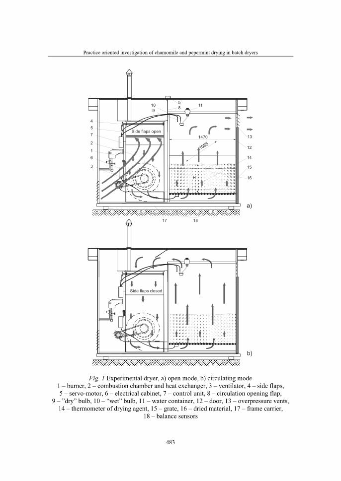
Practice oriented investigation of chamomile and pepermint drying in batch dryers
483
2
1
3
54
7
6
109
5 11
13
12
14
15
16
1470
1085
H
a)
b)
17 18
Side flaps open
Side flaps closed
8
Fig. 1 Experimental dryer, a) open mode, b) circulating mode 1 – burner, 2 – combustion chamber and heat exchanger, 3 – ventilator, 4 – side flaps,5 – servo-motor, 6 – electrical cabinet, 7 – control unit, 8 – circulation opening flap,
9 – ”dry” bulb, 10 – “wet” bulb, 11 – water container, 12 – door, 13 – overpressure vents, 14 – thermometer of drying agent, 15 – grate, 16 – dried material, 17 – frame carrier,
18 – balance sensors
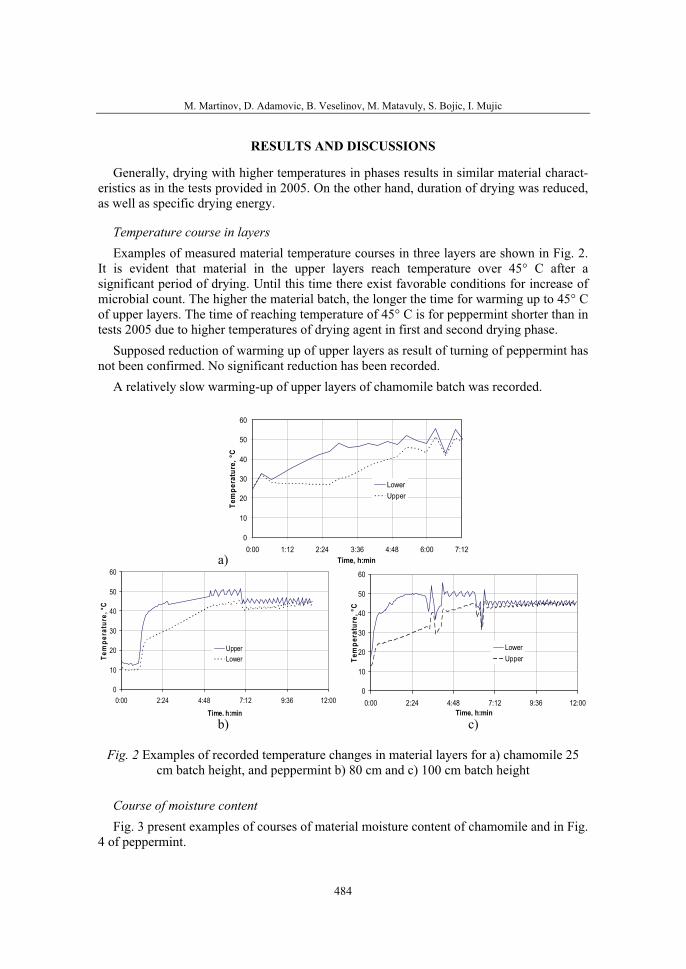
M. Martinov, D. Adamovic, B. Veselinov, M. Matavuly, S. Bojic, I. Mujic
484
RESULTS AND DISCUSSIONS
Generally, drying with higher temperatures in phases results in similar material charact-eristics as in the tests provided in 2005. On the other hand, duration of drying was reduced, as well as specific drying energy.
Temperature course in layers Examples of measured material temperature courses in three layers are shown in Fig. 2.
It is evident that material in the upper layers reach temperature over 45° C after a significant period of drying. Until this time there exist favorable conditions for increase of microbial count. The higher the material batch, the longer the time for warming up to 45° C of upper layers. The time of reaching temperature of 45° C is for peppermint shorter than in tests 2005 due to higher temperatures of drying agent in first and second drying phase.
Supposed reduction of warming up of upper layers as result of turning of peppermint has not been confirmed. No significant reduction has been recorded.
A relatively slow warming-up of upper layers of chamomile batch was recorded.
a)
0
10
20
30
40
50
60
0:00 1:12 2:24 3:36 4:48 6:00 7:12Time, h:min
Tem
pera
ture
, °C
LowerUpper
0
10
20
30
40
50
60
0:00 2:24 4:48 7:12 9:36 12:00
Time, h:min
Tem
pera
ture
, °C
UpperLower
0
10
20
30
40
50
60
0:00 2:24 4:48 7:12 9:36 12:00Time, h:min
Tem
pera
ture
, °C
LowerUpper
b) c)
Fig. 2 Examples of recorded temperature changes in material layers for a) chamomile 25 cm batch height, and peppermint b) 80 cm and c) 100 cm batch height
Course of moisture content Fig. 3 present examples of courses of material moisture content of chamomile and in Fig.
4 of peppermint.
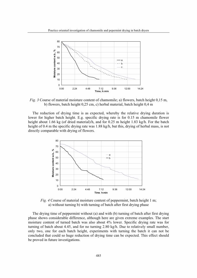
Practice oriented investigation of chamomile and pepermint drying in batch dryers
485
0
10
20
30
40
50
60
70
80
0:00 2:24 4:48 7:12 9:36 12:00 14:24Time, h:min
Moi
stur
e co
nten
t w.b
., %
abc
Fig. 3 Course of material moisture content of chamomile; a) flowers, batch height 0,15 m, b) flowers, batch height 0,25 cm, c) herbal material, batch height 0,4 m
The reduction of drying time is as expected, whereby the relative drying duration is lower for higher batch height. E.g. specific drying rate is for 0.15 m chamomile flower height about 1.66 kg (of dried material)/h, and for 0.25 m height 1.83 kg/h. For the batch height of 0.4 m the specific drying rate was 1.88 kg/h, but this, drying of herbal mass, is not directly comparable with drying of flowers.
0
10
20
30
40
50
60
70
80
0:00 2:24 4:48 7:12 9:36 12:00 14:24Time, h:min
Moi
stur
e co
nten
t w.b
., %
ab
Fig. 4 Course of material moisture content of peppermint, batch height 1 m;a) without turning b) with turning of batch after first drying phase
The drying time of peppermint without (a) and with (b) turning of batch after first drying phase shows considerable difference, although here are given extreme examples. The start moisture content of turned batch was also about 4% lower. Specific drying rate was for turning of batch about 4.45, and for no turning 2.80 kg/h. Due to relatively small number, only two, one for each batch height, experiments with turning the batch it can not be concluded that could so huge reduction of drying time can be expected. This effect should be proved in future investigations.
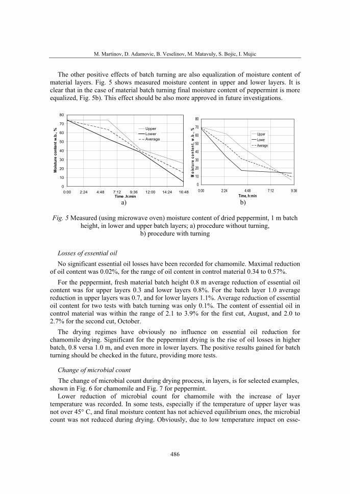
M. Martinov, D. Adamovic, B. Veselinov, M. Matavuly, S. Bojic, I. Mujic
486
The other positive effects of batch turning are also equalization of moisture content of material layers. Fig. 5 shows measured moisture content in upper and lower layers. It is clear that in the case of material batch turning final moisture content of peppermint is more equalized, Fig. 5b). This effect should be also more approved in future investigations.
0
10
20
30
40
50
60
70
80
0:00 2:24 4:48 7:12 9:36 12:00 14:24 16:48Time ,h:min
Moi
stur
e co
nten
t w.b
., % Upper
LowerAverage
0
10
20
30
40
50
60
70
80
0:00 2:24 4:48 7:12 9:36Time, h:min
Moi
stur
e co
nten
t, w
.b.,
%
UpperLowerAverage
a) b)
Fig. 5 Measured (using microwave oven) moisture content of dried peppermint, 1 m batch height, in lower and upper batch layers; a) procedure without turning,
b) procedure with turning
Losses of essential oil No significant essential oil losses have been recorded for chamomile. Maximal reduction
of oil content was 0.02%, for the range of oil content in control material 0.34 to 0.57%. For the peppermint, fresh material batch height 0.8 m average reduction of essential oil
content was for upper layers 0.3 and lower layers 0.8%. For the batch layer 1.0 average reduction in upper layers was 0.7, and for lower layers 1.1%. Average reduction of essential oil content for two tests with batch turning was only 0.1%. The content of essential oil in control material was within the range of 2.1 to 3.9% for the first cut, August, and 2.0 to 2.7% for the second cut, October.
The drying regimes have obviously no influence on essential oil reduction for chamomile drying. Significant for the peppermint drying is the rise of oil losses in higher batch, 0.8 versa 1.0 m, and even more in lower layers. The positive results gained for batch turning should be checked in the future, providing more tests.
Change of microbial count The change of microbial count during drying process, in layers, is for selected examples,
shown in Fig. 6 for chamomile and Fig. 7 for peppermint.Lower reduction of microbial count for chamomile with the increase of layer
temperature was recorded. In some tests, especially if the temperature of upper layer was not over 45° C, and final moisture content has not achieved equilibrium ones, the microbial count was not reduced during drying. Obviously, due to low temperature impact on esse-
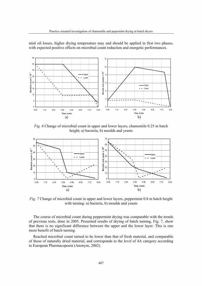
Practice oriented investigation of chamomile and pepermint drying in batch dryers
487
ntial oil losses, higher drying temperature may and should be applied in first two phases, with expected positive effects on microbial count reduction and energetic performances.
0
5
10
15
20
25
30
35
40
0:00 1:12 2:24 3:36 4:48 6:00 7:12 8:24
Time, h:min
Bact
eria
cou
nt x
10
5
UpperLower
0
2
4
6
8
10
12
0:00 1:12 2:24 3:36 4:48 6:00 7:12 8:24
Time, h:min
Mou
lds
and
yeas
ts x
105
UpperLower
a) b)
Fig. 6 Change of microbial count in upper and lower layers, chamomile 0.25 m batch height; a) bacteria, b) moulds and yeasts
0
10
20
30
40
50
60
0:00 1:12 2:24 3:36 4:48 6:00 7:12 8:24
Time, h:min
Bact
eria
cou
nt x
10
5
UpperLower
0
10
20
30
40
50
60
70
0:00 1:12 2:24 3:36 4:48 6:00 7:12 8:24
Time, h:min
Mou
lds
and
yest
s x
105
UpperLower
a) b)
Fig. 7 Change of microbial count in upper and lower layers, peppermint 0.8 m batch height with turning: a) bacteria, b) moulds and yeasts
The course of microbial count during peppermint drying was comparable with the trends of previous tests, done in 2005. Presented results of drying of batch turning, Fig. 7, show that there is no significant difference between the upper and the lower layer. This is one more benefit of batch turning.
Reached microbial count turned to be lower than that of fresh material, and comparable of those of naturally dried material, and corresponds to the level of 4A category according to European Pharmacopoeia (Anonym, 2002).
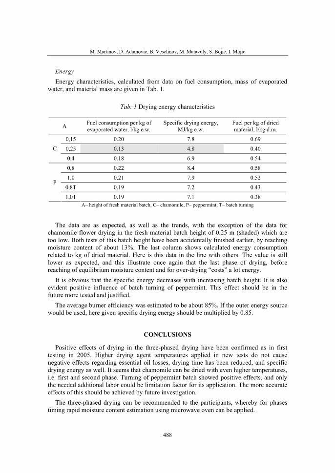
M. Martinov, D. Adamovic, B. Veselinov, M. Matavuly, S. Bojic, I. Mujic
488
EnergyEnergy characteristics, calculated from data on fuel consumption, mass of evaporated
water, and material mass are given in Tab. 1.
Tab. 1 Drying energy characteristics
A Fuel consumption per kg of evaporated water, l/kg e.w.
Specific drying energy, MJ/kg e.w.
Fuel per kg of dried material, l/kg d.m.
0,15 0.20 7.8 0.69
0,25 0.13 4.8 0.40 C
0,4 0.18 6.9 0.54
0,8 0.22 8.4 0.58
1,0 0.21 7.9 0.52
0,8T 0.19 7.2 0.43 P
1,0T 0.19 7.1 0.38 A– height of fresh material batch, C– chamomile, P– peppermint, T– batch turning
The data are as expected, as well as the trends, with the exception of the data for chamomile flower drying in the fresh material batch height of 0.25 m (shaded) which are too low. Both tests of this batch height have been accidentally finished earlier, by reaching moisture content of about 13%. The last column shows calculated energy consumption related to kg of dried material. Here is this data in the line with others. The value is still lower as expected, and this illustrate once again that the last phase of drying, before reaching of equilibrium moisture content and for over-drying “costs” a lot energy.
It is obvious that the specific energy decreases with increasing batch height. It is also evident positive influence of batch turning of peppermint. This effect should be in the future more tested and justified.
The average burner efficiency was estimated to be about 85%. If the outer energy source would be used, here given specific drying energy should be multiplied by 0.85.
CONCLUSIONS
Positive effects of drying in the three-phased drying have been confirmed as in first testing in 2005. Higher drying agent temperatures applied in new tests do not cause negative effects regarding essential oil losses, drying time has been reduced, and specific drying energy as well. It seems that chamomile can be dried with even higher temperatures, i.e. first and second phase. Turning of peppermint batch showed positive effects, and only the needed additional labor could be limitation factor for its application. The more accurate effects of this should be achieved by future investigation.
The three-phased drying can be recommended to the participants, whereby for phases timing rapid moisture content estimation using microwave oven can be applied.
Practice oriented investigation of chamomile and pepermint drying in batch dryers
489
Future investigations should also be directed towards testing the first phase, in order to check possibility for energy reduction. Starting of drying without heating, use of ambient air, will contribute to energy saving, but this will cause prolongation of the drying time.
ACKNOWLEDGEMENT
This investigation was supported by Ministry of Science of the Republic of Serbia, and company Termoplin.
REFERENCES
1. Bruin S., Luyben KChAM. (1980). Drying of Food Materials: A Review of Recent Developments. In: Advances in Drying, Volume:1, Ed.: Mujumdar AS. Hemisphere Publishing Corporation in corporation with Mc Graw-Hill International Book Company, New York
2. Buschbeck E., Keiner E., Klinner, J. (1967). Physical and Thermal Properties Effecting Drying Characteristics of Peppermint. Archiv für Landtechnik 2, 163-200
3. Graf C., Schubert E., Thile K., Müller J. (2002). Hypericum perforatum L.: Veränderung des mikrobiologischen Status während Ernte, Transport und Trocknung. Z.Arzn.Gew.Pfl. 7: 31-37
4. Heindl A., Hendl Th. (1998). Kontinuerliche Feuchtemessung zur Regelung von Bandtrocknern. Z.Arzn.Gew.Pfl. 3: 146-154
5. Heindl A. (2005). Möglichkeiten der Keimreduzierung bei Arznei- und Gewürzpflanzen vor, waehrend und nach der Trocknung mittels Dampf- und Mikrowellenapplikation. Z.Arzn.Gew.Pfl. 10:100-105
6. Martinov M., Adamovic D., Ruzic D., Abrel D. (2006a). Investigation of medicinal plants drying in batch dryers – Quality and energy characteristics. Proc EE&AE 2006 – International Scientific Conference, Rousse, Bulgaria, pp 542-549
7. Martinov M., Veselinov B., Adamovic D., Matavulj M. (2006b). Rezultati preliminarnog ispitivanja sušenja pitome nane u šaržnoj sušari. Bilten za hemlj, sirak i lekovito bilje 38: 37-48
8. Martinov M., Vujanov A., Dujlovic N. (2007a). Brzo utvrđivanje sadržaja vlage biljnog materijala. Revija agronomska saznanja 16: 18-19
9. Martinov M., Oztekin S., Müller, J. (2007b). Drying. In: Medicinal and Aromatic Crops, Harvesting, Drying and Processing (S Oztekin, M Martinov eds), Haworth Food and Agricultural Products Press, New York: 85-129
10. Mimica-Dukic N., Bozin B., Sokovic M., Mihajlovic B., Matavulj M. (2003). Antimicrobial and Antioxidant Activities of Three Mentha Species Essential Oils. Planta Medica 69:413-419
11. Mühlbauer W. (1989). Grain Drying. In: Drying Technique. Band 3. Springer Verlag, Berlin, 64-93
12. Müller J. (1992). Trocknung von Arzneipflanzen mit Solarenergie. (Dissertation), Ulmer Verlag, Stuttgart
13. Müller J. (2004). Drying of MAP. Teaching material. University Stuttgart-Hohenheim, Institute for Agricultural Engineering, Stuttgart

M. Martinov, D. Adamovic, B. Veselinov, M. Matavuly, S. Bojic, I. Mujic
490
14. Stakic M., Maric M., Mimica-Dukic Neda. (1994). Uticaj temperature agensa sušenja na sadržaj etarskih ulja u listovima mente. Medicinal Plant Report 1, 84-88
15. Anonym. (2000). Pharmacopoea jugoslavica 2000. Editio quinta, vol.1, vol. 3. Savezni zavod za zaštitu i unapređenje zdravlja, Beograd
16. Anonym. 2002. Europaeisches Arzneibuch. Amtliche deutsche Ausgabe. 4. Ausgabe. Deutscher Apotheker Verlag/Govi Verlag, Stuttgart/Eschborn
36. Symposium "Actual Tasks on Agricultural Engineering", Opatija, Croatia, 2008.
491
36.
SIMPOZIJAKTUALNI ZADACIMEHANIZACIJE POLJOPRIVREDE
UDC664.8.037.1Stručni rad
Expert paper
SOME APPLICATIONS OF LYOPHILIZATION IN AGRICULTURE
DUMITRU MNERIE, GABRIELA VICTORIA ANGHEL
POLITEHNICA University of Timisoara, Mechanical Engineering Faculty, Bd. Mihai Viteazul, No.1, 300222 Timisoara, Tel. 0040-745-521711, Fax 0040-256-403589,
SUMMARY
The lyophilization is a good method of freeze-drying for make some experiments with many kind of cereals, for the improvement that in food production, in general for a lot of agro-food product. The lyophilization process is depended by a serial of technological factories which are in inter-dependence with the lyophilization systems performances intended for agri-foods products. The paper shows some results of experiments and considerations for development applying lyophilization technology in different domains of agriculture (ex. study of corn oil extract, the maltodextrin from corn, modified cornstarch, spice extracts, soy sauce, hydrolyzed wheat gluten, partially hydrogenated soybean and cottonseed oil etc.). Also it is presents some special equipment and the principal advantages compared to other drying and preserving techniques, some important mechanical engineering elements and one technical solution good for many studies of lyophilization process of freeze-dried food. That is very porous, since it occupies the same volume as the original and so rehydrates rapidly. There is less loss of flavor and texture than with most other methods of drying.
Key words: lyophilization, freeze-drying, cereals, agriculture, heat transfer, agri-food engineering.
INTRODUCTION
The gaining in agriculture signifies: a good natural resources capitalization, a good agro-food product quality, and many profitable businesses. For agriculture the lyophilization (or freeze drying) technology can be very helpful.
The technology of lyophilization appear as a relatively simple process but as the practitioner soon learns the process is deceptively complex and, as a result, is often treated as an art rather than a science. Lyophilization is carried out using sublimation (transition of
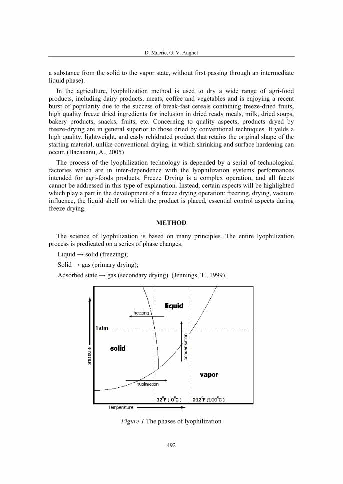
D. Mnerie, G. V. Anghel
492
a substance from the solid to the vapor state, without first passing through an intermediate liquid phase).
In the agriculture, lyophilization method is used to dry a wide range of agri-food products, including dairy products, meats, coffee and vegetables and is enjoying a recent burst of popularity due to the success of break-fast cereals containing freeze-dried fruits, high quality freeze dried ingredients for inclusion in dried ready meals, milk, dried soups, bakery products, snacks, fruits, etc. Concerning to quality aspects, products dryed by freeze-drying are in general superior to those dried by conventional techniques. It yelds a high quality, lightweight, and easly rehidrated product that retains the original shape of the starting material, unlike conventional drying, in which shrinking and surface hardening can occur. (Bacauanu, A., 2005)
The process of the lyophilization technology is depended by a serial of technological factories which are in inter-dependence with the lyophilization systems performances intended for agri-foods products. Freeze Drying is a complex operation, and all facets cannot be addressed in this type of explanation. Instead, certain aspects will be highlighted which play a part in the development of a freeze drying operation: freezing, drying, vacuum influence, the liquid shelf on which the product is placed, essential control aspects during freeze drying.
METHOD
The science of lyophilization is based on many principles. The entire lyophilization process is predicated on a series of phase changes: Liquid → solid (freezing); Solid → gas (primary drying); Adsorbed state → gas (secondary drying). (Jennings, T., 1999).
Figure 1 The phases of lyophilization

Some applications of lyophilization in agriculture
493
There are two major factors that determine what phase (solid, liquid or gas) a substance will take: heat and atmospheric pressure. For a substance to take any particular phase, the temperature and pressure must be within a certain range. Without these conditions, that phase of the substance can't exist. The chart below shows the necessary pressure and temperature values of different phases of water.
In figure 1, (Brain, M., 2007), it is the chart that water can take a liquid form at sea level (where pressure is equal to 1 atm) if the temperature is in between the sea level freezing point (32 degrees Fahrenheit or 0 degrees Celsius) and the sea level boiling point (212 F or 100 C). But if you increase the temperature above 32 F while keeping the atmospheric pressure below .06 atmospheres (ATM), the water is warm enough to thaw, but there isn't enough pressure for a liquid to form. It becomes a gas. This is exactly what a freeze-drying machine does. A typical machine consists of a freeze-drying chamber with several shelves attached to heating units, a freezing coil connected to a refrigerator compressor, and a vacuum pump. With most machines, you place the material to be preserved onto the shelves when it is still unfrozen. When you seal the chamber and begin the process, the machine runs the compressors to lower the temperature in the chamber. The material is frozen solid, which separates the water from everything around it, on a molecular level, even though the water is still present. Next, the machine turns on the vacuum pump to force air out of the chamber, lowering the atmospheric pressure below .06 ATM. The heating units apply a small amount of heat to the shelves, causing the ice to change phase. Since the pressure is so low, the ice turns directly into water vapor. The water vapor flows out of the freeze-drying chamber, past the freezing coil. The water vapor condenses onto the freezing coil in solid ice form, in the same way water condenses as frost on a cold day.
Because the process parameters of lyophilization treatment alternate in type function of agri-food product, there is the opinion that lyophilization plant constructions are different. Exists two category of lyofilization plant: - destined for food product liquids or viscous (milk, cream etc.); - destined for food products with texture (meat, fish etc.). For liquid food products on utilize separate freeze, crumbling continuation in small equipment; that is food product one short period de time.
For food products with texture on utilize continuous or discontinuous equipment. Continuous plant has in the structure one tunnel that contains one standard lyophilization unit, coupled in line or in U form. Discontinuous plant can be like an internal freeze and condenser; internal freeze and external condenser; external freeze and condenser.
For experiments it was used an instalation with the lyophilizer Crist Alpha 1-4, (figure 2.). Freeze dried agri-food when blended with the gel compositions of the invention can be a tasty treat for many meal prepared with some lyophilized components. For example, it was study: maltodextrin (from corn), modified cornstarch, mushrooms, nonfat dry milk, corn oil extract, spice extract, wheat flour, dried whey, cottonseed oil, onion powder, vegetable protein (soybean and wheat), monosodium glutamate (a flavor enhancer), garlic powder, paprika, tomato powder, calcium caseinate, etc.
The cereals are a very good vegetarian resource for eating, with important nutrients like vitamin B12-(fortified soy milk and cereals), iron-fortified cereals and breads, especially whole-wheat, zinc from whole grains (especially the germ and bran), whole-wheat bread. Also, the cereals are the most important source of dietary fiber in many countries. For
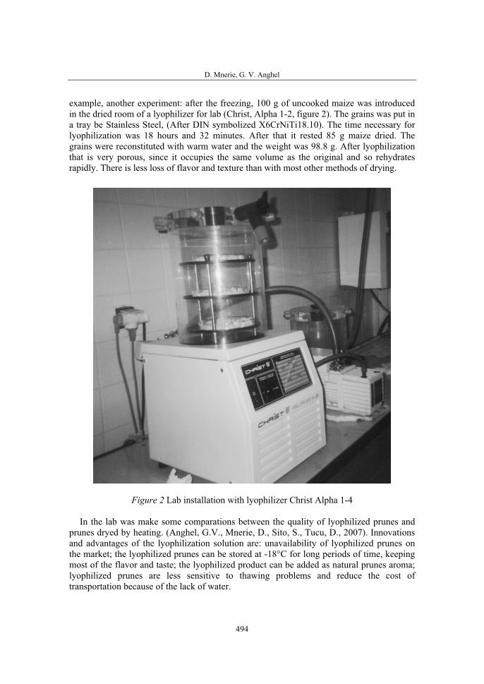
D. Mnerie, G. V. Anghel
494
example, another experiment: after the freezing, 100 g of uncooked maize was introduced in the dried room of a lyophilizer for lab (Christ, Alpha 1-2, figure 2). The grains was put in a tray be Stainless Steel, (After DIN symbolized X6CrNiTi18.10). The time necessary for lyophilization was 18 hours and 32 minutes. After that it rested 85 g maize dried. The grains were reconstituted with warm water and the weight was 98.8 g. After lyophilization that is very porous, since it occupies the same volume as the original and so rehydrates rapidly. There is less loss of flavor and texture than with most other methods of drying.
Figure 2 Lab installation with lyophilizer Christ Alpha 1-4
In the lab was make some comparations between the quality of lyophilized prunes and prunes dryed by heating. (Anghel, G.V., Mnerie, D., Sito, S., Tucu, D., 2007). Innovations and advantages of the lyophilization solution are: unavailability of lyophilized prunes on the market; the lyophilized prunes can be stored at -18°C for long periods of time, keeping most of the flavor and taste; the lyophilized product can be added as natural prunes aroma; lyophilized prunes are less sensitive to thawing problems and reduce the cost of transportation because of the lack of water.
Some applications of lyophilization in agriculture
495
RESULTS AND DISCUSSION
That experiments confirms many research about another applications. Very interesting is the study about the effects of lyophilization on the functional properties of acid modified and autoclaved corn starch preparations were investigated. RS contents and pasting properties of these starch preparations were also determined (Koksel, H., Masatcioglu, T., Kahraman, K., Ozturk, S., Basman, A., 2007). Significant increases in solubility were observed as the hydrolysis level of the lyophilized samples increased. Acid modification seems to be a prerequisite to achieve improving effect of lyophilization.
Another study from Faculty of Agriculture, Alexandria University (FAAU), is about thebehavior of high yield of biomass in fermentation and some strains in the lyophilization conditions, (Ayad, E.H.E., Nashat, S., El-Sadek, N., Metwaly, H., El-Soda, 2004).
Also, some aspects about metal contaminants promote degradation of lipid/DNA complexes during lyophilization, (Marion D.C. Molina, M., Anchordoquy, T.J., 2007), or the investigation of Lactobacilli Strains during Lyophilization (Rumian, N., Tsvetkov, T.D., Angelov, M., 1993), are very important for development of lyophilization application, and for agri-food products safety for healthy.
For the evaluating rennet for cheese making, (Tavaria, F.K., Sousa, M.J., Malcata, X., 2001), the clotting and proteolytic activities are important parameters. Both these activities were determined for extracts of the plant Cynara cardunculus in fresh form and after lyophilization followed by reconstitution, either in water or in citrate buffer (pH 5.4) and stored for up to 4 weeks at 40C. The patterns of degradation of ovine and goats caseins were followed by urea polyacrylamide gel electrophoresis in attempts to qualitatively differentiate the activity of the enzyme extracts as storage time elapsed. Storage at 40Csignificantly decreased the clotting power of the extracts but lyophilization retarded this decrease; β- and α -casein breakdown generally increased with storage time, via patterns that depend on caseinate type and extract used, but lyophilized extracts reconstituted in citrate buffer were significantly less proteolytic than the other extracts. Therefore, it is suggested that lyophilized extracts (reconstituted with citrate buffer) of flowers of C. cardunculus be used rather than fresh extracts.
CONCLUSIONS
The lyophilization applications in agriculture are now in a very important period for research development. In all applications it results an important conclusion in relation with the transmission of energy to the product, that needs to be carefully controlled for three important considerations: 1. - to avoid transferring too much heat and passing the safe primary drying temperature; 2. - to avoid supplying insufficient heat, hence prolonging the sublimation period; 3. - to achieve a homogeneous temperature in the total batch, as the lyophilization cycle will be determined by the temperature of the “coldest” product area. Also, the higher the sublimation temperature, the faster the drying cycle. The conditions of low temperature and high vacuum, can have, if they are unnecessarily prolonged, an effect on living organisms, which form the great bulk of freeze dried products.
D. Mnerie, G. V. Anghel
496
REFERENCES
1. Allemann, E., (2001), Freeze-drying/Lyophilization of Pharmaceutical and Biological products: L. Rey and J. May (Eds), Marcel Dekker, Inc., New York, ISBN 0-8247-1983-2, European Journal of Pharmaceutics and Biopharmaceutics Volume 51, Issue 2, , March 2001, Page 163.
2. Anghel, G.V., Mnerie, D., Sito, S., Tucu, D., (2007), Some aspects about the prunes lyophilization, Proceedings from International Conference Integrated Systems for Agri-food Production - durable development, Editura Orizonturi Universitare Timişoara,ISBN 978-973-348-9, pg. 39-42.
3. Ayad, E.H.E., Nashat, S., El-Sadek, N., Metwaly, H., El-Soda, Selection of wild lactic acid bacteria isolated from traditional Egyptian dairy products according to production and technological criteria, Food Microbiology, Volume 21, Issue 6, December 2004, Pages 715-725
4. Băcăoanu, A., Picoş, M.S., (2005), Rev. Roum. Chim., 50, 435-443
5. Bender, A.E., Bender, D.A., A Dictionary of Food and Nutrition, Oxford University Press, © 1995.
6. Brain, M., (2007), How Refrigerators Work, http://home.howstuffworks.com/refrigerator.htm,
7. Broadbent, J.R., Lin, C., (1999), Effect of Heat Shock or Cold Shock Treatment on the Resistance of Lactococcus lactis to Freezing and Lyophilization, CryobiologyVolume 39, Issue 1, , August 1999, Pages 88-102.
8. Jennings, T.A., “Lyophilization - Introduction and Basic Principles”, Interpharm Press, Buffalo Grove, IL 1999.
9. Koksel, H., Masatcioglu, T., Kahraman, K., Ozturk, S., Basman, A., (2007), Improving effect of lyophilization on functional properties of resistant starch preparations formed by acid hydrolysis and heat treatment, Journal of Cereal ScienceIn Press, Corrected Proof, , Available online 22 May 2007.
1. 10 Molina, M.D.C., Anchordoquy, T.J., (2007), Metal contaminants promote degradation of lipid/DNA complexes during lyophilization, Biochimica et Biophysica Acta (BBA) - BiomembranesVolume 1768, Issue 3, , March 2007, Pages 669-677.
10. Rumian, N., Tsvetkov, T.D., Angelov, M., (1993), Investigation of Lactobacilli Strains during Lyophilization, CryobiologyVolume 30, Issue 5, , October 1993, Pages 536-540.
11. Tavaria, F.K., Sousa, M.J., Malcata, X., (2001), Storage and lyophilization effects of extracts of Cynara cardunculus on the degradation of ovine and goats caseins, Food ChemistryVolume 72, Issue 1, , January 2001, Pages 79-88.
12. http://www.indiamart.com/lyogroup
36. Symposium "Actual Tasks on Agricultural Engineering", Opatija, Croatia, 2008.
497
36.
SIMPOZIJAKTUALNI ZADACIMEHANIZACIJE POLJOPRIVREDE
UDC621.317.38:631.344.5:635.64
Prethodno priopćenjePreliminary communication
ENERGY EFFICIENCY OF TOMATO PRODUCTION IN HEATED AND NON-HEATED GREENHOUSE
M. DJEVIC1, A. DIMITRIJEVIC1, S. BLAZIN2
1 Department for Agricultural Engineering , Faculty of Agriculture Belgrade, Belgrade University, Serbia [email protected], [email protected] 2 Agricultural High School “Josif Pancic” Pancevo, Serbia, [email protected]
SUMMARY
Greenhouse production is still among the most energy-consuming branches of agriculture. Producers are faced with high cost of the operations involved in greenhouse production processes (climate control, fertilizing, irrigation, etc). This is the reason why an optimal combination of energy inputs that will make this production more energy efficient needs to be found.
This paper gives the methodology of estimating energy consumption based on all energy inputs in greenhouse production. Energy analysis is based on estim-ating energy inputs (direct and indirect), using their amount and equivalents, in referent plant production. According to energy output (yield per m2) parameters for estimating greenhouse energy efficiency were calculated (energy input per kg of product, energy out/in ratio and energy productivity). Energy consumption was calculated for tomato production in heated and non heated greenhouse and the aim was do determine energy efficiency and to show its dependence on production technology.
Key words: energy, greenhouse, tomato, energy input, energy output, effic-iency
INTRODUCTION
Greenhouse production, if compared with other parts of agricultural production, is still among the most energy consuming branch. When energy consumption is compared with obtained production and its energy value, it can be also seen (Table 1) that greenhouse production has a very low energy ratio and this parameter is very important in evaluating energy efficiency of production system. Even with knowledge of these facts, there is, still, a great interest in this production technology. The reason lies in benefits that can be obtained
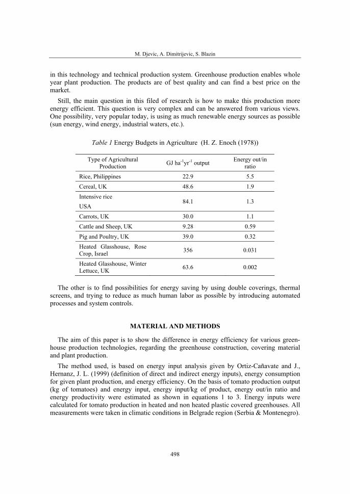
M. Djevic, A. Dimitrijevic, S. Blazin
498
in this technology and technical production system. Greenhouse production enables whole year plant production. The products are of best quality and can find a best price on the market.
Still, the main question in this filed of research is how to make this production more energy efficient. This question is very complex and can be answered from various views. One possibility, very popular today, is using as much renewable energy sources as possible (sun energy, wind energy, industrial waters, etc.).
Table 1 Energy Budgets in Agriculture (H. Z. Enoch (1978))
Type of Agricultural Production GJ ha-1yr-1 output Energy out/in
ratio
Rice, Philippines 22.9 5.5
Cereal, UK 48.6 1.9
Intensive rice USA
84.1 1.3
Carrots, UK 30.0 1.1
Cattle and Sheep, UK 9.28 0.59
Pig and Poultry, UK 39.0 0.32
Heated Glasshouse, Rose Crop, Israel 356 0.031
Heated Glasshouse, Winter Lettuce, UK 63.6 0.002
The other is to find possibilities for energy saving by using double coverings, thermal screens, and trying to reduce as much human labor as possible by introducing automated processes and system controls.
MATERIAL AND METHODS
The aim of this paper is to show the difference in energy efficiency for various green-house production technologies, regarding the greenhouse construction, covering material and plant production.
The method used, is based on energy input analysis given by Ortiz-Cañavate and J., Hernanz, J. L. (1999) (definition of direct and indirect energy inputs), energy consumption for given plant production, and energy efficiency. On the basis of tomato production output (kg of tomatoes) and energy input, energy input/kg of product, energy out/in ratio and energy productivity were estimated as shown in equations 1 to 3. Energy inputs were calculated for tomato production in heated and non heated plastic covered greenhouses. All measurements were taken in climatic conditions in Belgrade region (Serbia & Montenegro).
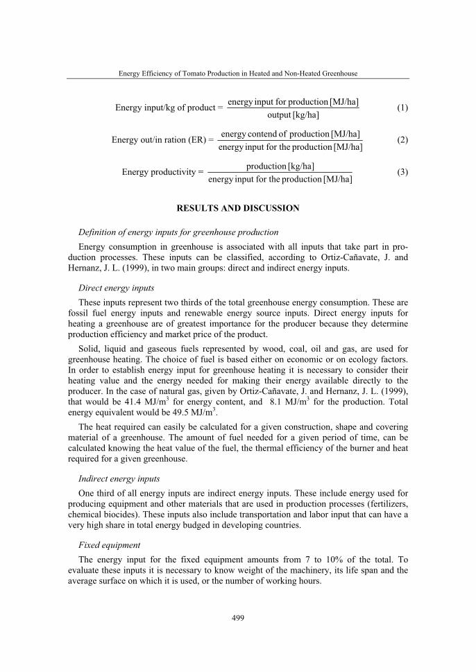
Energy Efficiency of Tomato Production in Heated and Non-Heated Greenhouse
499
Energy input/kg of product = [kg/ha]output
[MJ/ha]productionforinputenergy (1)
Energy out/in ration (ER) = [MJ/ha]productionfor theinputenergy
[MJ/ha]productionofcontendenergy (2)
Energy productivity = [MJ/ha]productionfor theinputenergy
[kg/ha]production (3)
RESULTS AND DISCUSSION
Definition of energy inputs for greenhouse production Energy consumption in greenhouse is associated with all inputs that take part in pro-
duction processes. These inputs can be classified, according to Ortiz-Cañavate, J. and Hernanz, J. L. (1999), in two main groups: direct and indirect energy inputs.
Direct energy inputsThese inputs represent two thirds of the total greenhouse energy consumption. These are
fossil fuel energy inputs and renewable energy source inputs. Direct energy inputs for heating a greenhouse are of greatest importance for the producer because they determine production efficiency and market price of the product.
Solid, liquid and gaseous fuels represented by wood, coal, oil and gas, are used for greenhouse heating. The choice of fuel is based either on economic or on ecology factors. In order to establish energy input for greenhouse heating it is necessary to consider their heating value and the energy needed for making their energy available directly to the producer. In the case of natural gas, given by Ortiz-Cañavate, J. and Hernanz, J. L. (1999), that would be 41.4 MJ/m3 for energy content, and 8.1 MJ/m3 for the production. Total energy equivalent would be 49.5 MJ/m3.
The heat required can easily be calculated for a given construction, shape and covering material of a greenhouse. The amount of fuel needed for a given period of time, can be calculated knowing the heat value of the fuel, the thermal efficiency of the burner and heat required for a given greenhouse.
Indirect energy inputsOne third of all energy inputs are indirect energy inputs. These include energy used for
producing equipment and other materials that are used in production processes (fertilizers, chemical biocides). These inputs also include transportation and labor input that can have a very high share in total energy budged in developing countries.
Fixed equipment The energy input for the fixed equipment amounts from 7 to 10% of the total. To
evaluate these inputs it is necessary to know weight of the machinery, its life span and the average surface on which it is used, or the number of working hours.

M. Djevic, A. Dimitrijevic, S. Blazin
500
Average energy consumption per year and machine weight is given in table 2.
Table 2 Energy incorporated in farm machinery refered to the unit of mass (kg) and per year (a)
Equipemnt Energy, MJ/kg,a
Tractor and self-propelled machines 9-10
Stationary equipemnt 8-10
Agricultural machinery and implements 6-8
FertilizersIn greenhouse production twelve main elements must be supplied during production
process, six macro and six microelements. The most important of all is nitrogen. Average values for energy intensities for most important fertilizers are given in table 3. Overall energy includes production, packaging, transportation and application.
Table 3 Energy content in main mineral fertilizer (Mudahar M. S., T. P. Hignett (1987))
Energy [MJ/kg]
Fertilizer Production PTAA Total N 69.5 8.6 78.1
P2O5 7.6 9.8 17.4
K2O 6.4 7.3 13.7
The possibility for optimization for this type of energy inputs lies in their precise and controlled application, together with watering, that involves some type of agricultural computerized control systems.
Chemical biocides Microclimatic conditions in greenhouses (temperature, relative humidity) if not regulated
on the proper way, create such environment that is ideal for emerging of pests and diseases. Aside from the damage done to the crop, the presence of insects and diseases on the final product is not a pleasant view for the consumer.
The energy embodied in active ingredient production includes production, formulation and packaging. For example, energy input for 1 kg of Malathion would be 229 MJ. Possible ways for reducing the use of chemical biocides would be applying an IPM method (Integra-ted Pest Management) that present an integration of chemical, biological and mechanical control measurements with solarization, pasteurization and sanitation technologies. Insect screens showed great results in decreasing the number of insect, especially white flies, and their varieties, reducing the need for pesticide application and counteracting insect resist-ance to pesticide.
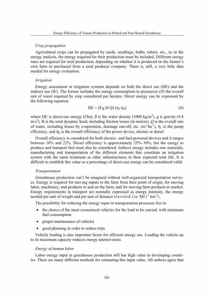
Energy Efficiency of Tomato Production in Heated and Non-Heated Greenhouse
501
Crop propagation Agricultural crops can be propagated by seeds, seedlings, bulbs, tubers, etc., so in the
energy analysis, the energy required for their production must be included. Different energy rates are required for seed production, depending on whether it is produced on the farmer’s own farm or purchased from a seed producer company. There is, still, a very little data needed for energy evaluation.
IrrigationEnergy assessment in irrigation systems depends on both the direct use (DE) and the
indirect use (IE). The former includes the energy consumption to pressurize (H) the overall rate of water required by crop considered per hectare. Direct energy can be expressed by the following equation: DE = (δ g H Q) (η1 η0) (4)
where DE is direct-use energy (J/ha), δ is the water density (1000 kg/m3), g is gravity (9.8 m/s2), H is the total dynamic head, including friction losses (in meters), Q is the overall rate of water, including losses by evaporation, drainage run-off, etc. (m3/ha-1), η1 is the pump efficiency, and η0 is the overall efficiency of the power device, electric or diesel.
Overall efficiency is considered for both electric- and fuel-powered devices and it ranges between 18% and 22%. Diesel efficiency is approximately 25%–30%, but the energy to produce and transport fuel must also be considered. Indirect energy includes raw materials, manufacturing and transportation of the different elements that constitute an irrigation system with the same treatment as other infrastructures in their expected total life. It is difficult to establish this value so a percentage of direct-use energy can be considered valid.
TransportationGreenhouse production can’t be imagined without well-organized transportation servic-
es. Energy is required for moving inputs to the farm from their point of origin, for moving labor, machinery, and products to and on the farm, and for moving farm products to market. Energy requirements in transport are normally expressed as energy intensity, the energy needed per unit of weight and per unit of distance t raveled ( in MJ t-1 km-1) .
The possibility for reducing the energy input in transportation processes lies in: • the choice of the most economical vehicles for the load to be carried, with minimum
fuel consumption
• proper maintenance of vehicles • good planning in order to reduce trips
Vehicle loading is also important factor for efficient energy use. Loading the vehicle up to its maximum capacity reduces energy intensiveness.
Energy of human labor Labor energy input in greenhouse production still has high value in developing countr-
ies. There are many different methods for estimating this input value. All authors agree that
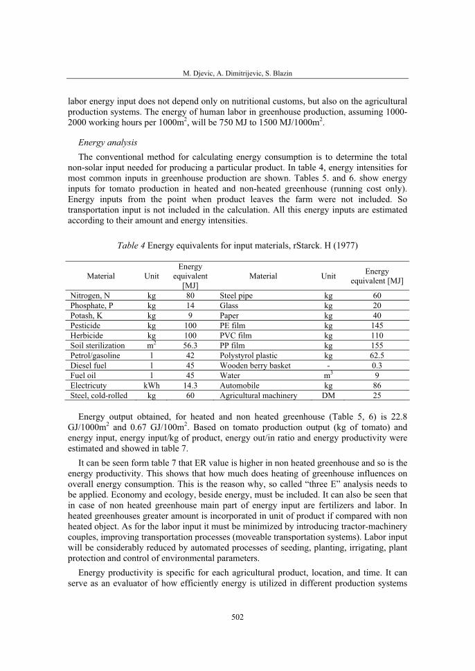
M. Djevic, A. Dimitrijevic, S. Blazin
502
labor energy input does not depend only on nutritional customs, but also on the agricultural production systems. The energy of human labor in greenhouse production, assuming 1000-2000 working hours per 1000m2, will be 750 MJ to 1500 MJ/1000m2.
Energy analysis The conventional method for calculating energy consumption is to determine the total
non-solar input needed for producing a particular product. In table 4, energy intensities for most common inputs in greenhouse production are shown. Tables 5. and 6. show energy inputs for tomato production in heated and non-heated greenhouse (running cost only). Energy inputs from the point when product leaves the farm were not included. So transportation input is not included in the calculation. All this energy inputs are estimated according to their amount and energy intensities.
Table 4 Energy equivalents for input materials, rStarck. H (1977)
Material Unit Energy
equivalent[MJ]
Material Unit Energyequivalent [MJ]
Nitrogen, N kg 80 Steel pipe kg 60 Phosphate, P kg 14 Glass kg 20 Potash, K kg 9 Paper kg 40 Pesticide kg 100 PE film kg 145 Herbicide kg 100 PVC film kg 110 Soil sterilization m2 56.3 PP film kg 155 Petrol/gasoline l 42 Polystyrol plastic kg 62.5 Diesel fuel l 45 Wooden berry basket - 0.3 Fuel oil l 45 Water m3 9 Electricuty kWh 14.3 Automobile kg 86 Steel, cold-rolled kg 60 Agricultural machinery DM 25
Energy output obtained, for heated and non heated greenhouse (Table 5, 6) is 22.8 GJ/1000m2 and 0.67 GJ/100m2. Based on tomato production output (kg of tomato) and energy input, energy input/kg of product, energy out/in ratio and energy productivity were estimated and showed in table 7.
It can be seen form table 7 that ER value is higher in non heated greenhouse and so is the energy productivity. This shows that how much does heating of greenhouse influences on overall energy consumption. This is the reason why, so called “three E” analysis needs to be applied. Economy and ecology, beside energy, must be included. It can also be seen that in case of non heated greenhouse main part of energy input are fertilizers and labor. In heated greenhouses greater amount is incorporated in unit of product if compared with non heated object. As for the labor input it must be minimized by introducing tractor-machinery couples, improving transportation processes (moveable transportation systems). Labor input will be considerably reduced by automated processes of seeding, planting, irrigating, plant protection and control of environmental parameters.
Energy productivity is specific for each agricultural product, location, and time. It can serve as an evaluator of how efficiently energy is utilized in different production systems
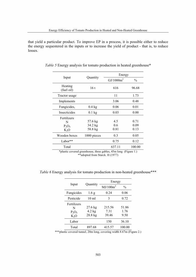
Energy Efficiency of Tomato Production in Heated and Non-Heated Greenhouse
503
that yield a particular product. To improve EP in a process, it is possible either to reduce the energy sequestered in the inputs or to increase the yield of product - that is, to reduce losses.
Table 5 Energy analysis for tomato production in heated greenhouse*
EnergyInput Quantity
GJ/1000m2 %
Heating(fuel oil) 16 t 616 96.68
Tractor usage 11 1.73
Implements 3.06 0.48
Fungicides, 0.4 kg 0.06 0.01
Insecticides 0.1 kg 0.03 0.00
FertilizersN
P2O5K2O
57.6 kg 34.2 kg 58.8 kg
4.50.60.81
0.710.090.13
Wooden boxes 1000 pieces 0.3 0.05
Labor** 0.75 0.12
Total 637.11 100.00 *plastic covered greenhouse, three gables, 45m long (Figure 1.)
**adopted from Starck. H (1977)
Table 6 Energy analysis for tomato production in non-heated greenhouse***
EnergyInput Quantity
MJ/100m2 %
Fungicides 1.6 g 0.24 0.06
Pesticide 10 ml 3 0.72
FertilizersN
P2O5K2O
27.6 kg 4.2 kg 28.8 kg
215.567.3139.46
51.861.769.50
Labor 150 36.10
Total 897.68 415.57 100.00 ***plastic covered tunnel, 20m long, covering width 8.67m (Figure 2.)
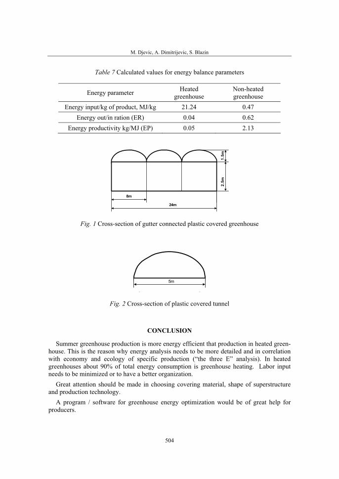
M. Djevic, A. Dimitrijevic, S. Blazin
504
Table 7 Calculated values for energy balance parameters
Energy parameter Heatedgreenhouse
Non-heatedgreenhouse
Energy input/kg of product, MJ/kg 21.24 0.47 Energy out/in ration (ER) 0.04 0.62
Energy productivity kg/MJ (EP) 0.05 2.13
2.5m
24m
8m
1.5m
Fig. 1 Cross-section of gutter connected plastic covered greenhouse
5m
Fig. 2 Cross-section of plastic covered tunnel
CONCLUSION
Summer greenhouse production is more energy efficient that production in heated green-house. This is the reason why energy analysis needs to be more detailed and in correlation with economy and ecology of specific production (“the three E” analysis). In heated greenhouses about 90% of total energy consumption is greenhouse heating. Labor input needs to be minimized or to have a better organization.
Great attention should be made in choosing covering material, shape of superstructure and production technology.
A program / software for greenhouse energy optimization would be of great help for producers.

Energy Efficiency of Tomato Production in Heated and Non-Heated Greenhouse
505
REFERENCES
1. Hanan, J. Joe, 1998. Greenhouses. Advanced Technology for Protected Cultivation, CRC Press
2. Mudahar M. S., T. P. Hignett, 1987. Energy requirements, technology and resources in fertilizer sector,. Energy in Plant Nutrition and Pest Control. Energy in World Agriculture, Vol. 2, ed. Helsel, Z. R., pp. 25–61.
3. Nelson V. Paul, 2003: Greenhouse Operation and Management, Sixth edition, Prentice Hall
4. Ortiz-Cañavate, J., Hernanz, J. L., 1999. Energy Analysis and Saving, In CIGR Handbook of Agricultural Engineering, Volume V, Energy and Biomass Engineering
5. Starck. H., 1977. Towards an Economic of Energy in Horticulture, Symposium on More Profitable use of Energy in Protected Cultivation, Sweden.
6. von Zabelic, Chr. Energy substitution, 1989., Energy Savings in Protected Cultivation, Acta Horticulturae, 245.


36. Symposium "Actual Tasks on Agricultural Engineering", Opatija, Croatia, 2008.
507
36.
SIMPOZIJAKTUALNI ZADACIMEHANIZACIJE POLJOPRIVREDE
UDC004.45:523.98
Izvorni znanstveni radOriginal scientific paper
SOLAR RADIATION MONITORING SYSTEM MUGUR BALAN, MIHAI DAMIAN, LORENTZ JANTSCHI
Technical University of Cluj NapocaB-dul. Muncii 103-105; 400641 Cluj Napoca; Romania,
[email protected]; [email protected]; [email protected]
ABSTRACT
The paper is presenting a solar radiation monitoring system, based on two scientific pyranometers and an on-line computer data acquisition system. The values of total and diffuse solar radiation are stored on a server, in a mysql database, using high precision, original data acquisition equipment and different original software applications. A flexible web based interface, was developed to interrogate the database and to extract relevant data, based on different user selected periods. Average values for the solar radiation components are computed, together with total solar radiant heat for the user selected periods. The results are presented in the form of relevant and suggestive tables. The paper presents also relevant results, discussions and conclusions concerning an important and useful tool, to evaluate the local solar energy potential.
Key words: Solar, Radiation, Monitoring, Data Acquisition, Software, Data-base, Heat
INTRODUCTION
In the context of our day’s relatively acute energy crisis, the scientific world is reconsid-ering the approach through all types of renewable energies. Between those, the solar energy is representing one with the highest potential, all over the world, because for a very long period of time, the Sun can be considered a huge free source of free energy, being also the unique energy source able to entertain the life on Earth. The life of the Sun is estimated at the following 4-5 billions of years.
The incoming solar radiant energy, per square meter, at the outside limit of the earth atmosphere, is named solar constant, being determined by satellite technologies measure-ments, at the value of 1350…1366W/m2. From the outside limit of the atmosphere, until the Earth surface, the intensity of the solar radiation is decreased by several known effects
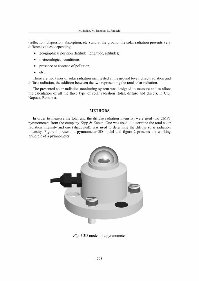
M. Balan, M. Damian, L. Jantschi
508
(reflection, dispersion, absorption, etc.) and at the ground, the solar radiation presents very different values, depending:
• geographical position (latitude, longitude, altitude);
• meteorological conditions;
• presence or absence of pollution;
• etc.There are two types of solar radiation manifested at the ground level: direct radiation and
diffuse radiation, the addition between the two representing the total solar radiation. The presented solar radiation monitoring system was designed to measure and to allow
the calculation of all the three type of solar radiation (total, diffuse and direct), in Cluj Napoca, Romania.
METHODS
In order to measure the total and the diffuse radiation intensity, were used two CMP3 pyranometers from the company Kipp & Zonen. One was used to determine the total solar radiation intensity and one (shadowed), was used to determine the diffuse solar radiation intensity. Figure 1 presents a pyranometer 3D model and figure 2 presents the working principle of a pyranometer.
Fig. 1 3D model of a pyranometer

Solar radiation monitoring system
509
Fig. 2 Working principle scheme of a pyranometer 1 – printed circuit board; 2 – solar radiation sensor; 3 – glass dome; 4 – body; 5 – electrical cable connector;
6 – electrical cable; 7 – screw for horizontal level fixing; 8 – fixings; 9 – accessfor cable connection; 10 – screwed electrical connector; 11 – water babble.
Some used pyranometers specifications are presented in table 1.
Table 1 Specifications of the used pyranometers
Specification Value
Response time (95%) 18s
Zero offsets - thermal radiation (200W/m2) - temperature change (5K)
±15W/m2
±5W/m2
Non stability change / year ±1%
Non linearity (0…1000W/m2) ±2.5%
Directional error (at 80° with 1000W/m2) ±20W/m2
Temperature dependence of sensitivity ±5% (-10…+40°C)
Tilt error at 1000W/m2 ±2%
Sensitivity 5…15µV/W/m2
Operating temperature -40…+80°C
Spectral range 310…2800nm
Maximum irradiance 2000W/m2
Expected daily accuracy ±10%
The scheme of the original data acquisition and solar radiation monitoring system, deve-loped at the Technical University of Cluj Napoca, is presented in figure 3.
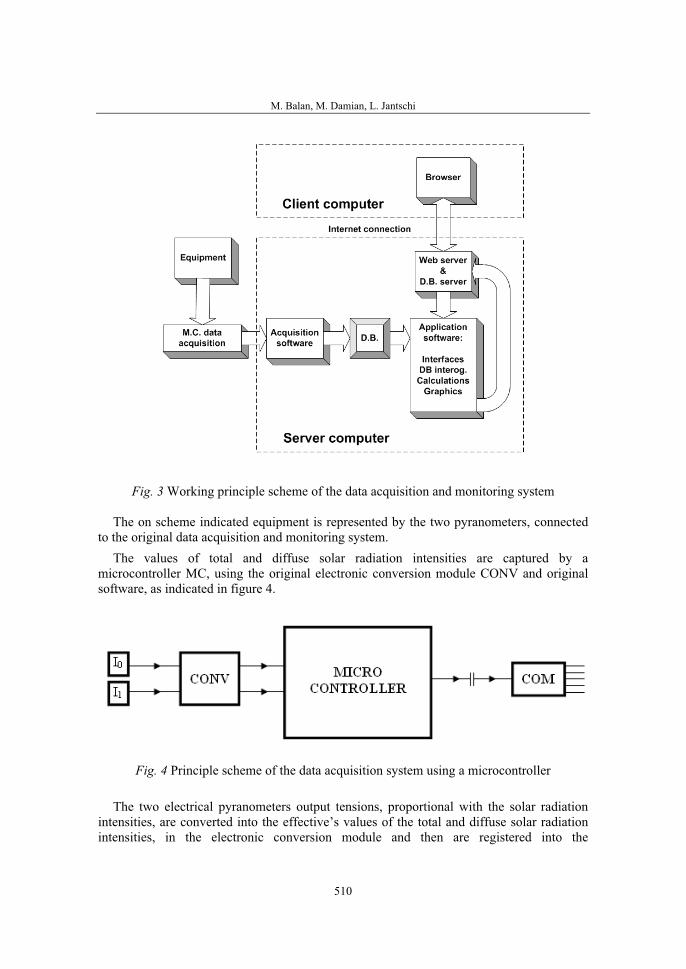
M. Balan, M. Damian, L. Jantschi
510
Fig. 3 Working principle scheme of the data acquisition and monitoring system
The on scheme indicated equipment is represented by the two pyranometers, connected to the original data acquisition and monitoring system.
The values of total and diffuse solar radiation intensities are captured by a microcontroller MC, using the original electronic conversion module CONV and original software, as indicated in figure 4.
Fig. 4 Principle scheme of the data acquisition system using a microcontroller
The two electrical pyranometers output tensions, proportional with the solar radiation intensities, are converted into the effective’s values of the total and diffuse solar radiation intensities, in the electronic conversion module and then are registered into the
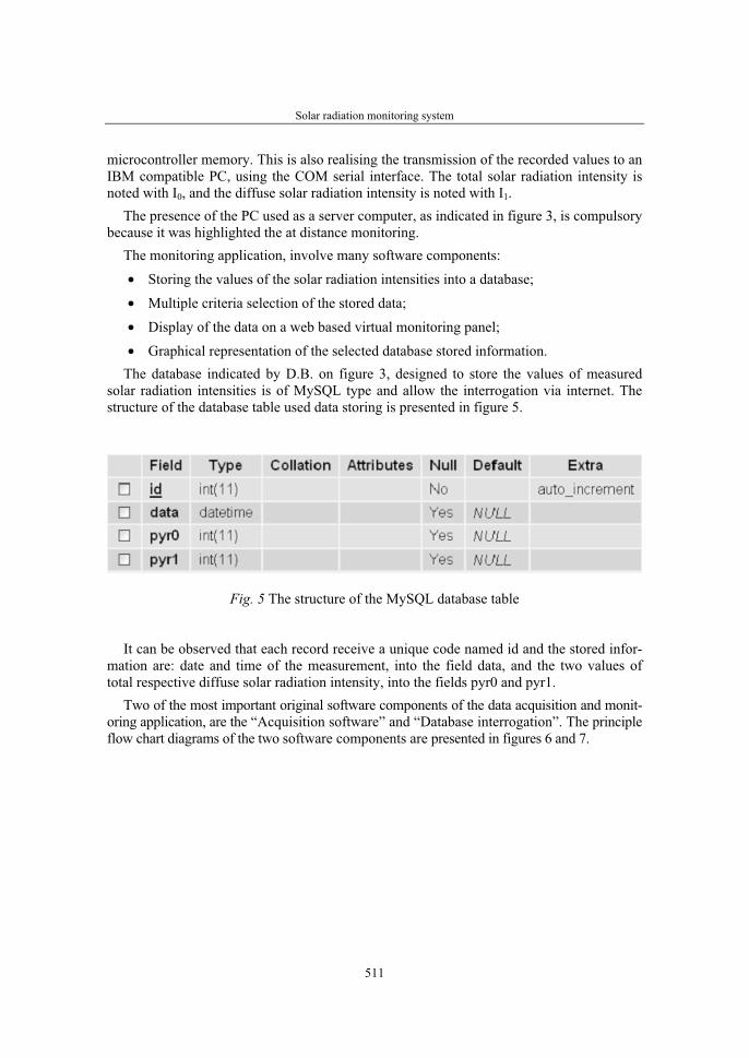
Solar radiation monitoring system
511
microcontroller memory. This is also realising the transmission of the recorded values to an IBM compatible PC, using the COM serial interface. The total solar radiation intensity is noted with I0, and the diffuse solar radiation intensity is noted with I1.
The presence of the PC used as a server computer, as indicated in figure 3, is compulsory because it was highlighted the at distance monitoring.
The monitoring application, involve many software components:
• Storing the values of the solar radiation intensities into a database;
• Multiple criteria selection of the stored data;
• Display of the data on a web based virtual monitoring panel;
• Graphical representation of the selected database stored information. The database indicated by D.B. on figure 3, designed to store the values of measured
solar radiation intensities is of MySQL type and allow the interrogation via internet. The structure of the database table used data storing is presented in figure 5.
Fig. 5 The structure of the MySQL database table
It can be observed that each record receive a unique code named id and the stored infor-mation are: date and time of the measurement, into the field data, and the two values of total respective diffuse solar radiation intensity, into the fields pyr0 and pyr1.
Two of the most important original software components of the data acquisition and monit-oring application, are the “Acquisition software” and “Database interrogation”. The principle flow chart diagrams of the two software components are presented in figures 6 and 7.
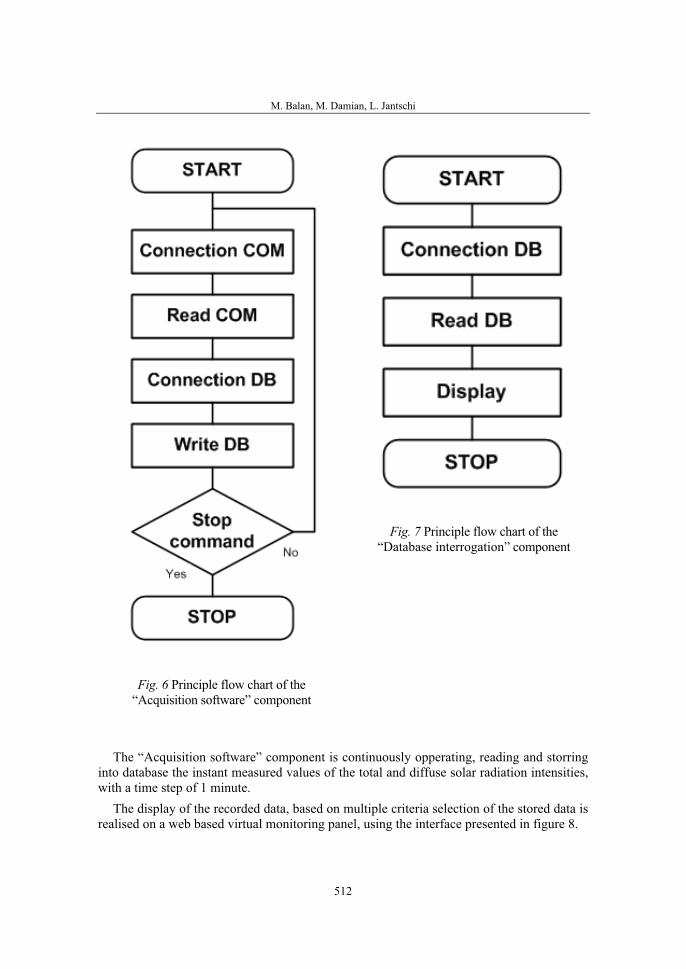
M. Balan, M. Damian, L. Jantschi
512
Fig. 6 Principle flow chart of the“Acquisition software” component
Fig. 7 Principle flow chart of the“Database interrogation” component
The “Acquisition software” component is continuously opperating, reading and storring into database the instant measured values of the total and diffuse solar radiation intensities, with a time step of 1 minute.
The display of the recorded data, based on multiple criteria selection of the stored data is realised on a web based virtual monitoring panel, using the interface presented in figure 8.
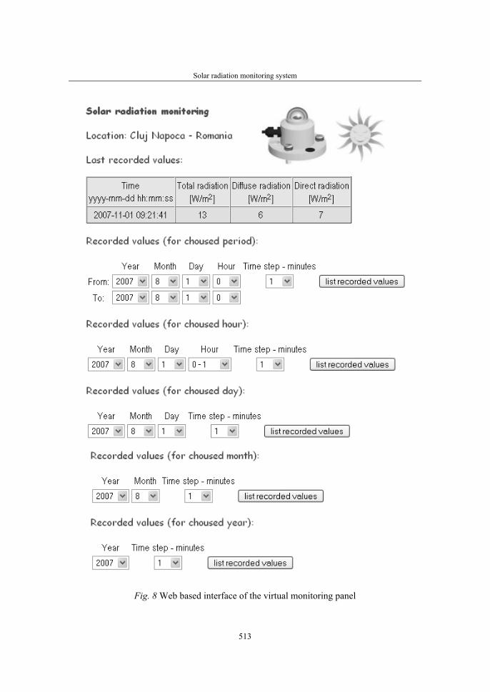
Solar radiation monitoring system
513
Fig. 8 Web based interface of the virtual monitoring panel

M. Balan, M. Damian, L. Jantschi
514
The web based interface, presented in figure 8, cad be displayed on any internet connected computer, indicated as “Client computer” on figure 3. The interface will be displayed in the web browser of that computer. This element suggests that the presented solar radiation monitoring system was designed and realized into client-server architecture.
The interface present the last recorded values of the solar total, diffuse and calculated direct radiation intensities and offer the following selection criteria option, for the recorded data:
• Recorded values for a free chosen period, indicated by: year, month, date and hour of the beginning and ending time for the selected period;
• Recorded values for a free chosen hour, indicated by: year, month, date and the selected time interval, for the selected period;
• Recorded values for a free chosen day, indicated by: year, month and date;
• Recorded values for a free chosen month, indicated by: year and the selected month;
• Recorded values for a free chosen year, indicated by the selected year; For each option, it can be selected also the time step, in minutes, for witch the database
stored date to be displayed. The possible values for the time step, depending of the selected criteria are: 1, 5, 10, 15, 20, 30, 60 minutes.
Each selection criteria can be activated by pressing one of the buttons marked bt “list recorded values”.
Additional to the selected data following each criteria, the activated software compone-nts will also dysplay the following computed values:
• Direct solar radiation intensity, calculated as difference between the total and the diffuse solar radiation intensities;
• Average values for the solar radiation intensities (total, diffuse and direct), for the whole selected period of time;
• Average values for the solar radiation intensities (total, diffuse and direct), for the day time periods (with Sun on the sky) in the whole selected period of time;
• Total values of radiant solar heat (total, diffuse and direct).
RESULTS AND DISCUSSION
Some results, displayed by the different software component of the solar radiation moni-toring system, are indicated as examples.
Figure 9 presents the values of the solar radiation intensities, recorded in august 17, 2007, between 14…15 hours, with a time step of 10 minutes. It was a completely sunny day, the sky was practically clear the whole day, and it can be observed that the recorded values are higher than 800W/m2.
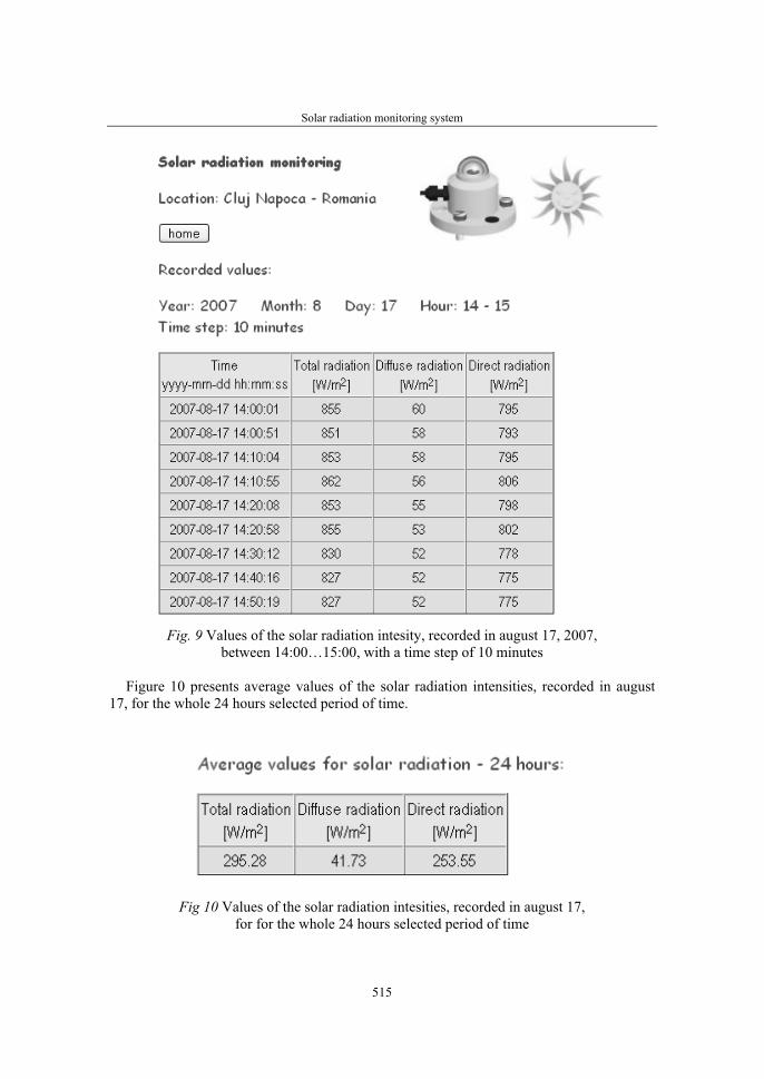
Solar radiation monitoring system
515
Fig. 9 Values of the solar radiation intesity, recorded in august 17, 2007,between 14:00…15:00, with a time step of 10 minutes
Figure 10 presents average values of the solar radiation intensities, recorded in august 17, for the whole 24 hours selected period of time.
Fig 10 Values of the solar radiation intesities, recorded in august 17,for for the whole 24 hours selected period of time
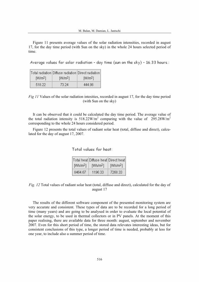
M. Balan, M. Damian, L. Jantschi
516
Figure 11 presents average values of the solar radiation intensities, recorded in august 17, for the day time period (with Sun on the sky) in the whole 24 hours selected period of time.
Fig 11 Values of the solar radiation intesities, recorded in august 17, for the day time period (with Sun on the sky)
It can be observed that it could be calculated the day time period. The average value of the total radiation intensity is 518.22W/m2 comparing with the value of 295.28W/m2
corresponding to the whole 24 hours considered period. Figure 12 presents the total values of radiant solar heat (total, diffuse and direct), calcu-
lated for the day of august 17, 2007.
Fig. 12 Total values of radiant solar heat (total, diffuse and direct), calculated for the day of august 17
The results of the different software component of the presented monitoring system are very accurate and consistent. These types of data are to be recorded for a long period of time (many years) and are going to be analysed in order to evaluate the local potential of the solar energy, to be used in thermal collectors or in PV panels. At the moment of this paper realising, there are available data for three month: august, september and november 2007. Even for this short period of time, the stored data relevates interesting ideas, but for consistent conclusions of this type, a longer period of time is needed, probably at less for one year, to include also a summer period of time.
Solar radiation monitoring system
517
CONCLUSIONS
The presented solar monitoring system is representing an original, complex and usefull hardware and software tool, able to offer all the needed information, to evaluate the local potential of the solar energy, to be used in thermal collectors or in PV panels.
REFERENCES
1. Jain,P. (1988) - Estimation of monthly hourly global and diffuse radiation. Solar and Wind Technology 5, nov. 1, 1988, pg. 7-14.
2. Miroslav,T., Eitzinger, J., Kapler,P., Dubrovsky,M., Semeradova,D., Zalud,V., Formayer, H. (2007) - Effect of Estimated Daily Global Solar Radiation Data on the Results of Crop Growth Models, Sensors 2007, 7, pg. 2330-2362.
3. Balan,M., Damian,M. (2006) - Software aplication for monitoring a small air conditioning unit, IEEE International Conference on Automation, Quality and Testing, Robotics, Cluj Napoca, May 25-28, pg. 183-186.
4. Balan,M., Damian,M., Ion,I. (2007) - Considerations about the potential use of the geotermal energy for domestic heating in romania, International congress Automotive, Environment and Farm Machinery. AMMA, Cluj-Napoca, October 11-13 2007, Romania, pg. 219-224.
5. Hofierka,J., Sury,M. (2002) - The solar radiation model for Open Source GIS: implementation and applications – Open Source GIS – GRASS users conference 2002, Trento, Italy, September 11-13, 2002.
6. Jäntschi,L., Balan,M., Podar,E., Bolboaca,S. (2007) - Thermal Energy Efficiency Analysis for Residential Buildings, IEEE Region 8 Eurocon 2007 Conference, Warsaw, Poland September 9-12, pg. 2009-2014.
7. Kaplanis,S., Kaplani,E. (2005) - The effect of statistical fluctuations of solar radiation to PV system sizing” EuroPES 2005, Conference, 16 June 2005, Spain.
8. Zhaoyan,L., McGill,M., Yongxiang,H., Hostetler,C. Vaughan,M. Winker,D. - Validating lidar depolarization calibration using solar radiation scattered by ice clouds. Geoscience and Remote Sensing Letters, IEEE, July 2004, pg. 157- 161
9. Kreith,F., Kreider,J.F. (1978) - Principles of solar Engineering, Mc Graw – Hill, New York (1978).

36. Symposium "Actual Tasks on Agricultural Engineering", Opatija, Croatia, 2008.
519
36.
SIMPOZIJAKTUALNI ZADACIMEHANIZACIJE POLJOPRIVREDE
UDC620.95:661.9
Stručni radExpert paper
KONSTRUKCIJA ZA PROIZVODNJO BIOPLINA BOGOMIR MURŠEC, PETER VINDIŠ, MIRAN LAKOTA, DENIS STAJNKO,
MATJAŽ SAGADIN
Univerza v Mariboru, Fakulteta za kmetijstvo, Vrbanska 30, 2000 Maribor, Slovenija
POVZETEK
V prispevku je obravnavana konstrukcija za proizvodnjo bioplina v laboratoriju. Konstrukcija je sestavljena iz dvanajstih steklenih plinskih cevi (eudiometrov), dvanajstih fermentorjev, črpalke in grelca s termostatom, termometra, barometra in osnovne konstrukcije. Konstrukcija oziroma mini digestor zajema dvanajst enot, vsaka je sestavljena iz eudiometra ter fermentorja v katerem je substrat. Kot substrat za proizvodnjo bioplina (metana) se uporabljajo energetske rastline ter blato iz čistilnih naprav. Za optimalni potek fermentacije morajo biti fermentorji v vodni kopeli s konstantno temperaturo. Osnovna konstrukcija je varjena iz nerjavnega jekla dolžine 2500 mm, višine 1000 mm in širine 350 mm. Na najvišjem delu konstrukcije je polica z zunanjimi posodami za odvečno tekočino. Spodaj je korito 200 x 200 mm, ki smo ga izolirali s stiroporom zaradi preprečevanja toplotnih izgub in lažjega vzdrževanja konstantne temperature. V koritu za konstantno temperaturo in kroženje vode skrbi še grelna črpalka s termostatom. Korito je pokrito s pokrovom, saj morajo za pravilen potek poskusa substrati biti v temi. Na sredinsko prečko konstrukcije so s prižemami pritrjeni eudiometri. Prižeme so obložene s pluto, kar preprečipoškodbe na steklu. Eudiometer je enostransko zaprta plinska cev s skalo iz katere odčitamo proizvodnjo bioplina. Eudiometri so preko gumijastih cevi povezani z zunanjimi posodami za odvečno tekočino, ki onemogočajo uhajanje plina v okolje. Na levi strani konstrukcije je pritrjen termometer in barometer. S termometrom merimo temperaturo vodne kopeli in temperaturo zraka okolice. Z barometrom merimo tlak v prostoru. Meritve so potrebne za kasnejšo korekcijo rezultatov, saj ima plin glede na plinsko enačbo pri različni temperaturi in različnem tlaku različen volumen. Proizvodnjo bioplina odčitavamo dnevno, sestavo plinov pa merimo z plinskim detektorjem.
Ključne besede: bioplin, mini digestor, fermentor, eudiometer
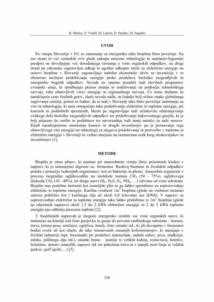
B. Muršec, P. Vindiš, M. Lakota, D. Stajnko, M. Sagadin
520
UVOD
Po vstopu Slovenije v EU se zanimanje za energetsko rabo bioplina hitro povečuje. Na eni strani ni več carinskih ovir glede nakupa ustrezne tehnologije in sanitarno-higienski predpisi ne dovoljujejo več dosedanjega ravnanja z vrsto organskih odpadkov, na drugi strani pa zakonsko zagotovljen odkup in ugodne odkupne tarife za električno energijo na osnovi bioplina v Sloveniji zagotavljajo stabilen ekonomski okvir za investicije v to obetavno možnost pridobivanja energije preko predelave biološko razgradljivih in energetsko bogatih odpadkov. Seveda ne smemo pozabiti tudi številnih programov evropske unije, ki spodbujajo prenos znanja in sodelovanje na področju tehnološkega razvoja, rabe obnovljivih virov energije in regionalnega razvoja. Če temu dodamo še naraščajoče cene fosilnih goriv, zlasti seveda nafte, in čedalje bolj očitne znake globalnega segrevanja ozračja, potem ni čudno, da se tudi v Sloveniji tako hitro povečuje zanimanje za vire in tehnologije, ki nam omogočajo tako pridobivanje električne in toplotne energije, pri katerem ni podnebnih sprememb, hkrati pa zagotavljajo tudi učinkovito odstranjevanje velikega dela biološko razgradljivih odpadkov ter pridobivanje kakovostnega gnojila, ki je bolj prijazno do rastlin in podtalnice ter navsezadnje tudi manj moteče za naše nosove. Kljub naraščajočemu zanimanju kmetov in drugih investitorjev pa je poznavanje tega obnovljivega vira energije ter tehnologij za njegovo pridobivanje in pretvorbo v toplotno in električno energijo v Sloveniji še vedno omejeno na razmeroma ozek krog strokovnjakov in investitorjev [1].
METODE
Bioplin je zmes plinov, ki nastane pri anaerobnem vrenju (brez prisotnosti kisika) v napravi, ki jo imenujemo digestor oz. fermentor. Razkroj biomase in živalskih odpadkov poteka s pomočjo razkrojnih organizmov, kot so bakterije in plesni. Anaerobni organizmi v procesu razgradijo ogljikovodike na molekule metana CH4 (50 - 75%), ogljikovega dioksida CO2 (10 - 40%), ter druge snovi (H2, H2S, N2, NH4, …) odvisno od vrste substrata. Bioplin ima podobne lastnosti kot zemeljski plin in ga lahko uporabimo za soproizvodnjo električne in toplotne energije. Kurilna vrednost 1m3 bioplina (glede na vsebnost metana) ustreza približno 0,6 l kurilnega olja ali okoli 6,0 kilovatne ure (kWh). V napravi za soproizvodnjo električne in toplotne energije tako lahko pridobimo iz 1m3 bioplina (glede na izkoristek naprave) okoli 1,5 do 2 kWh električne energije in 2 do 3 kWh toplotne energije (po odštetju procesne toplote) [2].
V bioplinskih napravah je mogoče energetsko izrabiti vse vrste organskih snovi, ki nastanejo na kmetiji (od čiste gnojevke in gnoja do povsem rastlinskega substrata – koruza, trava, krmna pesa, sončnice, ogrščica, hmelj, žitni ostanki itd., ki jih dovajamo v fermentor bodisi sveže ali kot silažo, do tako imenovanih zunanjih kofermentorjev, ki nastajajo v živilski industriji (npr. bioostanki pri predelavi marmelade, sadnih sokov, piva, sladkorja, mleka, jedilnega olja itd.), ostanki hrane – pomije iz velikih kuhinj, restavracij, hotelov, bolnišnic, domov ostarelih, zaporov itd. ter pokošena trava in v manjši meri listje iz velikih parkov, golf igrišč,…) [3].
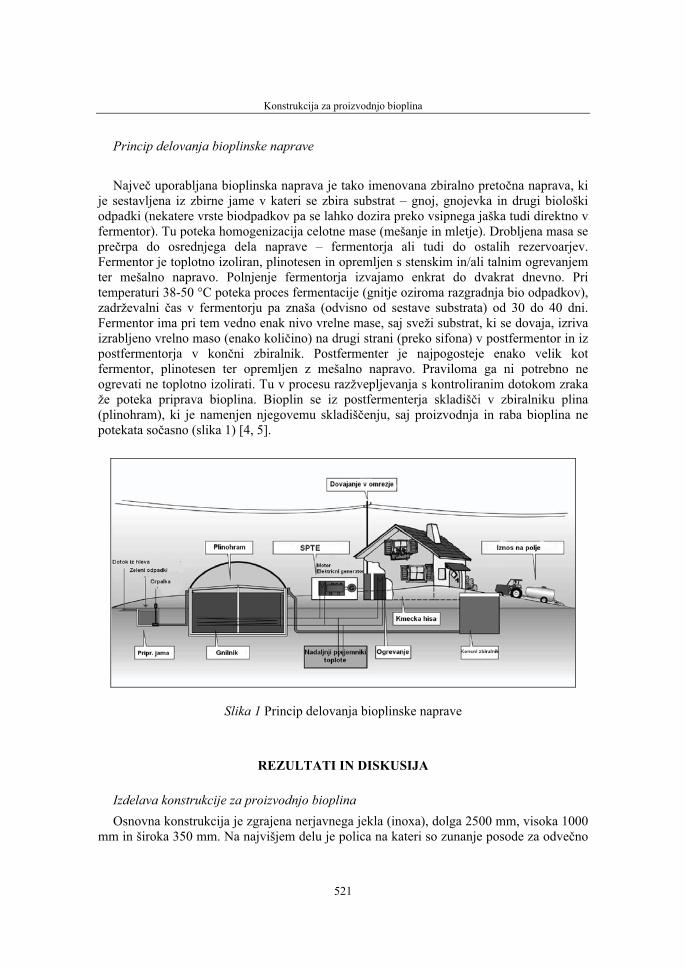
Konstrukcija za proizvodnjo bioplina
521
Princip delovanja bioplinske naprave
Največ uporabljana bioplinska naprava je tako imenovana zbiralno pretočna naprava, ki je sestavljena iz zbirne jame v kateri se zbira substrat – gnoj, gnojevka in drugi biološki odpadki (nekatere vrste biodpadkov pa se lahko dozira preko vsipnega jaška tudi direktno v fermentor). Tu poteka homogenizacija celotne mase (mešanje in mletje). Drobljena masa se prečrpa do osrednjega dela naprave – fermentorja ali tudi do ostalih rezervoarjev. Fermentor je toplotno izoliran, plinotesen in opremljen s stenskim in/ali talnim ogrevanjem ter mešalno napravo. Polnjenje fermentorja izvajamo enkrat do dvakrat dnevno. Pri temperaturi 38-50 °C poteka proces fermentacije (gnitje oziroma razgradnja bio odpadkov), zadrževalni čas v fermentorju pa znaša (odvisno od sestave substrata) od 30 do 40 dni. Fermentor ima pri tem vedno enak nivo vrelne mase, saj sveži substrat, ki se dovaja, izriva izrabljeno vrelno maso (enako količino) na drugi strani (preko sifona) v postfermentor in iz postfermentorja v končni zbiralnik. Postfermenter je najpogosteje enako velik kot fermentor, plinotesen ter opremljen z mešalno napravo. Praviloma ga ni potrebno ne ogrevati ne toplotno izolirati. Tu v procesu razžvepljevanja s kontroliranim dotokom zraka že poteka priprava bioplina. Bioplin se iz postfermenterja skladišči v zbiralniku plina (plinohram), ki je namenjen njegovemu skladiščenju, saj proizvodnja in raba bioplina ne potekata sočasno (slika 1) [4, 5].
Slika 1 Princip delovanja bioplinske naprave
REZULTATI IN DISKUSIJA
Izdelava konstrukcije za proizvodnjo bioplina Osnovna konstrukcija je zgrajena nerjavnega jekla (inoxa), dolga 2500 mm, visoka 1000
mm in široka 350 mm. Na najvišjem delu je polica na kateri so zunanje posode za odvečno
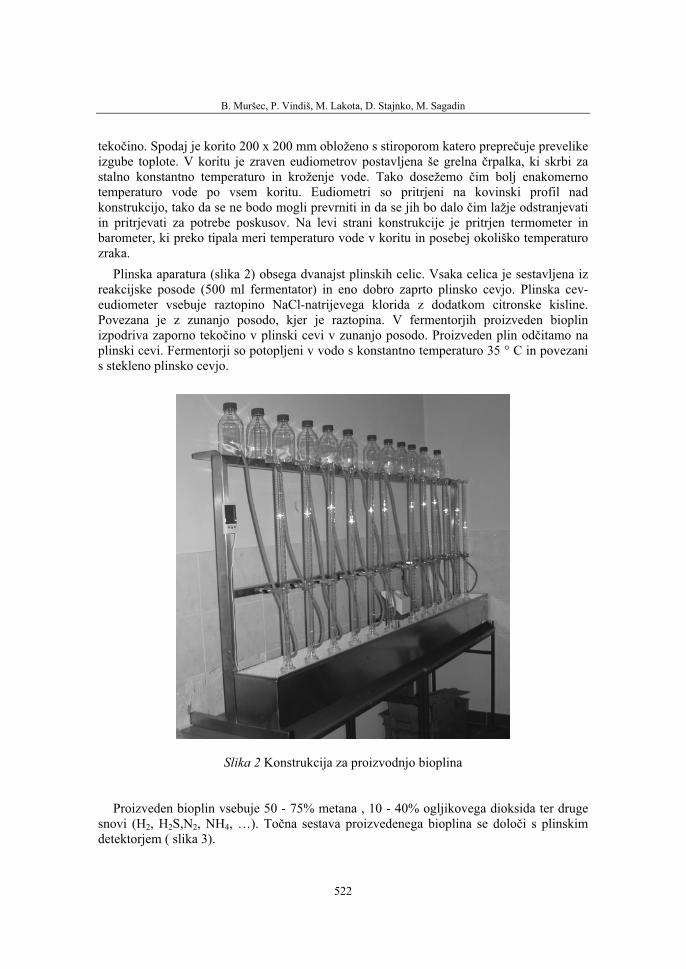
B. Muršec, P. Vindiš, M. Lakota, D. Stajnko, M. Sagadin
522
tekočino. Spodaj je korito 200 x 200 mm obloženo s stiroporom katero preprečuje prevelike izgube toplote. V koritu je zraven eudiometrov postavljena še grelna črpalka, ki skrbi za stalno konstantno temperaturo in kroženje vode. Tako dosežemo čim bolj enakomerno temperaturo vode po vsem koritu. Eudiometri so pritrjeni na kovinski profil nad konstrukcijo, tako da se ne bodo mogli prevrniti in da se jih bo dalo čim lažje odstranjevati in pritrjevati za potrebe poskusov. Na levi strani konstrukcije je pritrjen termometer in barometer, ki preko tipala meri temperaturo vode v koritu in posebej okoliško temperaturo zraka.
Plinska aparatura (slika 2) obsega dvanajst plinskih celic. Vsaka celica je sestavljena iz reakcijske posode (500 ml fermentator) in eno dobro zaprto plinsko cevjo. Plinska cev-eudiometer vsebuje raztopino NaCl-natrijevega klorida z dodatkom citronske kisline. Povezana je z zunanjo posodo, kjer je raztopina. V fermentorjih proizveden bioplin izpodriva zaporno tekočino v plinski cevi v zunanjo posodo. Proizveden plin odčitamo na plinski cevi. Fermentorji so potopljeni v vodo s konstantno temperaturo 35 ° C in povezani s stekleno plinsko cevjo.
Slika 2 Konstrukcija za proizvodnjo bioplina
Proizveden bioplin vsebuje 50 - 75% metana , 10 - 40% ogljikovega dioksida ter druge snovi (H2, H2S,N2, NH4, …). Točna sestava proizvedenega bioplina se določi s plinskim detektorjem ( slika 3).

Konstrukcija za proizvodnjo bioplina
523
Slika 3 Plinski detektor
Potrebni elementi Najpomembnejši člen za pridobivanje bioplina je “eudiometer”. Eudiometer je
enostransko zaprta plinska cev s skalo. Sestavljen je iz dveh delov in to tako, da se steklena zgornja cev direktno priklopi na posodo s fermenterjem, kar bistveno olajša delo, saj ni potrebnih nobenih cevi, ki bi posebej povezovale fermentersko posodo in eudiometer. Držalo eudiometra (prižema) smo pritrdili na sredinsko prečko konstrukcije in s tem bistveno izboljšali stabilnost eudiometrov. Nosilci so obloženi s pluto kar zmanjša poškodbe na steklu. Posode so postavljene na polico na vrhu celotne konstrukcije in služijo za od plina izpodrinjeno tekočino. Z eudiometrom so povezane preko gumijaste cevi.
Z grelno črpalko (slika 4) se meša voda v koritu in hkrati uravnava temperatura vodne kopeli. Zaradi dolžine korita je zelo pomembna postavitev grelne črpalke. Idealna postavitev je na sredino korita, kjer smo z „Y“ razvodnikom razdelili izstopno odprtino črpalke na dva dela. Oba dela smo postavili na nasprotna konca korita, s čimer smo še dodatno pospešili mešanje vode, saj ogreta voda na straneh potiskala vodo proti sredini korita in s tem proti črpalki. S tem dosežemo zelo dobro kroženje vode po koritu in optimalno temperaturo vodne kopeli, kar je pogoj za optimalni potek fermentacije.
Slika 4 Grelna črpalka s termostatom
B. Muršec, P. Vindiš, M. Lakota, D. Stajnko, M. Sagadin
524
Termometer je digitalni z razločnimi velikimi števili. Preko termometra spremljamo temperaturo vode v koritu in jo nato preko grelne črpalke ustrezno uravnavamo. S tem dosežemo idealne pogoje za fermentacijo. S termometrom merimo tudi temperaturo okolja. Temperatura in tlak okolja nam služita za kasnejšo korekcijo rezultatov.
Fermentorji so potopljeni v vodno kopel s konstantno temperaturo 38 ° C in povezani s stekleno plinsko cevjo - eudiometrom. Konstantna temperatura je potrebna za optimalni potek fermentacije. Vodna kopel je obložena s izolacijskim materialom stiroporom ter pokrita s pokrovom, kar omogoča lažje vzdrževanje konstantne temperature.
SKLEPI
Minidigestor služi za potrebe poskusov proizvodnje bioplina iz različnih energetskih rastlin (koruza, sirek, ščiri itd.) ter drugih organskih odpadkov. Osnovna konstrukcija je varjena iz nerjavnega jekla (inox) dolžine 2500 mm, višine 1000 mm in širine 350 mm. Minidigestor je iz dvanajstih enot, kar omogoča opravljanje treh poskusov hkrati s tremi ponovitvami, medtem ko tri enote služijo kot kontrola. To nam daje natančne in raznolike podatke. Vsaka enota je sestavljena iz eudiometra ter fermentorja v katerem je substrat. Ostali elementi ki skrbijo za pravilno delovanje minidigestorja so črpalka in grelec s termostatom, termometer, barometer, prižeme eudiometrov ter gumijaste cevi, ki povezujejo posamezne elemente. Količina plina se odčitava dnevno, sama proizvodnja je odvisna od razmer in vrste substrata. Končna analiza proizvedenega bioplina se izvede s plinskim detektorjem.
LITERATURA
1. www.ljudmila.org/sef/stara/Bioplin05.htm
2. http://www.ape.si/RES%20marekt%20ove%20in%20ure/bioplin.htm
3. Berglund M., Börjesson M. (2006). Assessment of energy performance in the life-cycle of biogas production. Biomass and Bioenergy 30: 254-266
4. Klemenc A. Osnove sodobne soproizvodnje toplotne in električne energije na osnovi anaerobnega gnitja organskih snovi
5. Weiland P. (2006). Biomass Digestion in Agriculture: A Successful Pathway for the Energy Production and Waste Treatment in Germany. Engineering in Life Sciences 6: 302-309
Konstrukcija za proizvodnjo bioplina
525
CONSTRUCTION FOR BIOGAS PRODUCTION
SUMMARY
The paper presents construction of mini digestor for biogas production in laboratory. Construction is made of twelve glass gas tubes (eudiometers), twelve fermentors, pump and boiler with thermostat, thermometer, barometer and basic support. Construction of mini digestor is made of twelve units, each is from eudiometer with fermentor and substrate. As substrate for biogas (methane) production we use different silage plants and sludge. For optimal fermentation the fermentors must be in the water bath with constant temperature. The basic support of mini digestor is from nonrust steel length 2500 mm, height 1000 mm and width 350 mm. On the maximal part of the construction there is a terrace with bottles for unnecessary liquid. The manger, size 200 X 200 mm, is isolated for frustrate temperature loss and to maintain the constant temperature. In the manger there is also heater pump with thermostat to maintain the constant temperature and for circulation of water. The manger is cover because for the right process of the experiment the substrats must be in the dark. On the medium part of the construction the eudiometers are hitch. Hitch elements are garnish with the cork what frustrates damages on the glass. Eudiometer is one side closed gas tube in which we observe the amount of biogas production. Eudiometers are with gummy tubes connected with bottles for unnecessary liquid, which frustrate the escape of gas in the environment. On the left side of the construction is thermometer and barometer. Thermometer gives us information’s about temperature of water bath and temperature of environment. With barometer we measure the pressure in the room. The measurement of temperature and pressure are necessary for calculation of results because gas has according gas equation in different temperature and different pressure different volume. We measure biogas production every day. The combination of biogas we measure with gas detector.
Key words: biogas, mini digestor, fermentor, eudiometer

36. Symposium "Actual Tasks on Agricultural Engineering", Opatija, Croatia, 2008.
527
36.
SIMPOZIJAKTUALNI ZADACIMEHANIZACIJE POLJOPRIVREDE
UDK636.085.522.55:661.9Prethodno priopćenje
Preliminary communication
OPTIMIZIRANJE SMJESE KUKURUZNE SILAŽE PRI DOBIVANJU BIOPLINA
RAJKO BERNIK, ALEŠ ZVER
Biotehnički fakultet, Odjel za agronomiju, Jamnikarjeva 101, SI-1001 Ljubljana
SAŽETAK
Prije nekoliko godina smo počeli, prije svega u Prekomurju sijati na njivama kulture za proizvodnju biogoriva. U međuvremenu se je povećala konkurencija – potreba za hranom i energijom. Danas se to odražava na cijeni poljoprivrednih kultura, prije svega kukuruza, pšenice i konačno svih biljaka uzgajanih na njivama. Zbog toga što pojedini objekti za proizvodnju bioplina postoje i njihova je tehnologija zasnovana na kukuruznoj silaži, potrebno je silažu optimalno pripremiti da bi iskorištenost fermentacije bila najveća. U našem pokusnom reaktoru se odvija fermentacija jednako kao u velikom ekonomičnom, samo u manjem opsegu pritjecanja dnevne količine, što znači, da je ulazna količinajednako obrađena u pokusnom reaktoru kao i u ekonomičnom. U pokusu smo koristili kukuruznu silažu. Istu sortu i pobranu (požetu) u istom danu. Pri tome smo silaži A dodali dodatke za siliranje namijenjene optimiziranju silaže u svrhu proizvodnje bioplina, silaži B nismo dodali nijedan dodatak. Pridobili smo dvadeset postotaka više bioplina, kada smo dodali dodatak za siliranje, uz jednake uvjete djelovanja reaktora.
Ključne riječi: energija, obnovljivi izvori energije, bioplin, kukuruz, silaža
UVOD
Smanjenje vrijednosti CO2 u atmosferi je globalni cilj (UNFCCC, 1997). Države uklju-čene u EZ, imaju jasnu uputu, da do 2010 godine nadomijeste postojeću fosilnu energiju iz obnovljivih izvora energije do vrijednosti 12 % potrošene bruto enegije. To znači trostruko povećanje pridobivanja energije iz postojećih obnovljivih izvora energije u EZ.
U Sloveniji postoje i grade se nove bioplinare. Bioplinare znatno utjeću na smanjivanje emisija stakleničkih plinova i istovremeno doprinose određen udio obnovljive energije. Što više budemo imali bioplinara, veći će biti učinci pokusnih reaktora s kojima optimiziramo djelovanje bioplinara i provjeravamo nove supstrate (Zver, 2005).
R. Bernik, A. Zver
528
Za osiguranje optimalne proizvodnje bioplina je više važnih čimbenika i u grubo ih možemo podijeliti u tri skupine, i to:
• fizikalni: toplota, mješavina, gustoća, struktura supstrata,
• kemijski: omjer C:N, pH, sadržaj makro i mikro elemenata, otrova, teških metala,
• biološki: vrste mikroorganizama, njihova kvantiteta i kvalitetaPronalaženje i optimiziranje mješavine različitih supstrata u pokusnom reaktoru je
svrhovito, jer na takav način osiguravamo optimalno iskorištenje supstrata za proizvodnju bioplina, i te rezultate istraživanja prenosimo u ekonomične uređaje.
Tvrtka KG Rakičan EKOTEH d.o.o., koja je član Grupe Panvita, raspolaže s bioplina-rom snage 1,3 MW i gradi novu bioplinaru manje snage.
Postojeće bioplinare, koje su tako bazirane, da se osnovnom supstratu gnojovke dodaje kukuruzna silaža ne možemo baš tako zatvoriti, iako se je pojavila kriza zbog preskupog energenta - kukuruzne silaže. Imamo tu mogućnost, da kukuruznu silažu siliramo sa dodacima za siliranje i s time povećamo njenu kvalitetu, te posljedično utjećemo na većuiskorištenost bioplina.
PREGLED OBJAVA
Već pred više od dvadeset godina su stručnjaci s područja bivše Jugoslavije počeli raz-mišljati o bioplinu i proizvodili su ga. Iz godine u godinu su utvrdili nešto novo i zajedno su došli do sljedeće spoznaje. U tom razdoblju su sličnu tematiku istraživali znanstvenici sa zapada i sjevera Evrope. Svi zajedno su došli do sljedećeg zaključka kojeg svi ponavljamo.
U bioplinarama je moguće energetsko iskoristiti sve vrste biomase, od čiste gnojovke do posve biljnog supstrata (Bernik, 1982; Nekrep 1983; Gačeša 1985). Organsku biomasu je moguće iskorištavati cijelu godinu bilo sviježu ili kao silažu (Đulbič, 1986;). Iskorištenje bioplina iznosi kod trava i kukuruzne silaže između 350 i 450 litara na kilogram suhe tvari, što je dvostruko toliko, koliko ga je moguće proizvesti samo s gnojovkom i sa stajskim gnojem. Razgradnja mješavine supstrata i s time iskorištenje bioplina, je ovisno od supstra-ta i njegovih sastojaka. Dobro se razgrađuju masnoće, ugljikovi hidrati i proteini, manje vlaknine, kao npr. odrvenjeli ili stariji dijelovi biljaka (Amon 2002).
Od biomase najveću važnost ima kukuruz. U bioplinarama ga upotrebljavamo svježeg ili siliranog. Većinom se upotrebljava siliran. Kukuruz žanjemo i siliramo u fazi optimalne zrelosti i na taj način osiguravamo jedako kvalitetnu sirovinu za cijelu godinu. Optimalnu zrelost ne možemo osiguravati uz dodavanje svježih biljaka, jer se iz dana u dan mjenja kvaliteta kukuruza, raste udio vlaknina, koje se manje razgrađuju (Verbič, 1994).
Da bi silaža bila kroz cijelu godinu jednako kvalitetna moramo je dobro pripremiti. Posljedica slabog siliranja je slabo sačuvana silaža. Silaže s niskom trajnosti opstanka su silaže u kojima su vrenje preuzele enterobakterije ili klostridij ili oba. U tu skupinu ne ubrajamo silaže, koje se počinju kvariti kada dolaze u dodir sa zrakom, jer je to aerobno kvarenje. Slabo očuvane silaže nastaju iz premokrih biljaka ili iz biljaka koje ne sadrže dovoljno u vodi topivih ugljiko hidrata. Mogući uzrok je takođe u premalom broju mlije-čno-kiselinskih bakterija na biljkama namjenjenih siliranju (Stekar, 1993).
Optimiziranje smjese kukuruzne silaže pri pridobivanju bioplina
529
Za bolje siliranje se upotrebljavaju dodaci za siliranje. Dodaci za siliranje su sastavljeni i djeluju u dva osnovna segmenta, prvi ubrzavaju mliječno-kiselinsko vrenje, drugi sva vrenja spriječavaju ili ograničavaju. U prvoj skupini su selekcionirane mlječno-kiselinskebakterije, zatim encimi koji razgrađuju u vodi netopive ugljiko hidrate i s tim povećavaju količinu šećera u siliranoj organskoj masi. Šećeri su hrana mliječno-kiselinskih bakterija. Kada mliječno-kiselinske bakterije prevladaju, stvaraju toliko mliječne kiseline, da se djelovanje drugih mikroorganizama zaustavi ili prekine (Stekar, 1993).
Zbog toga što smo se u članku usredotočili na iskorištenje bioplina iz kukuruzne silaže, na kratko ćemo predstaviti rezultate prethodnih istraživača.
Tablica 1 Iskorištenje bioplina kukuruzne silaže prema različitim autorima
SupstratAutor
Opseg proizvodnje bioplina (l/kg suhe tvari)
Prosječna proizvodnja bioplina(l/kg suhe tvari)
Kukuruzna silaža Beck, 1997 340 – 550 450
KukuruzMedved in Novak, 2000 300 – 400 350
Kukuruzna silaža Đulbić, 1986
380 – 460 420
Kukuruzna silaža Gobec, 2005 170 – 200 185
SupstratAutor
Opseg proizvodnje bioplina (l/kg organske tvari)
Prosječna proizvodnja bioplina(l/kg organske tvari)
Kukuruzna slama Beck, 1997 350 – 480 410
MATERIALI I METODE
Pokusni bioplinski reaktor Rezultat sudjelovanja između Grupe Panvita Ekoteh d.o.o. i Biotehničkog fakulteta
Ljubljana je izgradnja pilot bioplinskog reaktora. Opseg pilot reaktora je 2.500 litara, od toga je 2.000 litara radni opseg, 500 litara pa plinohrama (spremnika za plinove). Reaktor omogućava:
• potpuno umješavanje pri testiranju suhih ili tekućih supstrata
• djelovanje u svim temperaturnim područjima
• jednokratno punjenje i kontinuirani način punjenja i pražnjenja reaktora
• ručno i računalno bilježenje ▫ stanja u reaktoru (temperatura, pH),
R. Bernik, A. Zver
530
▫ količine i kvalitete nastalog bioplina (CH4, CO2, O2, H2S),
• uzimanje uzoraka za analizu sadržaja, na različitim dubinama.
Kukuruzna silaža A silaža: silaža iz kukuruza Pioneer PR37M4B silaža: silaža iz kukuruza Pioneer PR37M4 sa dodatkom za siliranje Dodatak za siliranje Pioneer 11C33: po navodu proizvođača sadržava 1,1×10¹¹/g
različitih sojeva mliječno-kiselinskih bakterija vrste Lactobacillus buchneri, Lactobacillus plantarum i Enterococcus faecium. Heterofermentativne bakterije mliječne kiseline vrste Lactobacillus buchneri u anaerobnim uvjetima pretvaraju mliječnu kiselinu u ocatnu kiselinu i 1,2-propandiol. Zbog povećane koncentracije ocatne kiseline možemo očekivatikod obrađene silaže s dodacima manje teškoća s aerobnim kvarenjem kod uzimanja iz silosa (Verbič, 2005).
Pokretanje reaktora na djelimično prečišćenoj svinjskoj gnojovki Odlučili smo se za upotrebu djelomično prečišćene gnojovke s količinom suhom tvari
između 0,75% i 1,5%, s čime smo osigurali homogenost i izbjegli tehničke poteškoćezačepljenja. Ta gnojovka je imala veoma specifičan sastav, jer je u prosjeku sadržavala 41% pepela u suhoj tvari. U reaktoru smo namjestili temperaturno područje od 37,5 °C sa odstupanjem ±1,5 °C, i s mješanjem u intervalima osigurali potpuno premješanje sadržaja reaktora. Pokrenuli smo ga s mješavinom mezofilnih bakterija uzetih iz anaerobnog dijela uređaja za čišćenje ili stare bioplinare.
Zbog izbora prečišćene gnojovke, koja će ubuduće biti osnovni medij u rektoru, smo morali vrednovati njen energetski potencijal pri određenom vremenu zadržavanja. Odlučilismo se za 30 dnevno vrijeme zadržavanja. Prečišćena gnojovka je imala 50 % pepela u ST (suhoj tvari). Tako smo po više mjesečnom vrednovanju prečišćene gnojevke došli do željenih podataka za tu gnojovku, iskorištenja bioplina na kg ST (suhe tvari) i iskorištenja bioplina na kg OST (organske suhe tvari). Nismo tražili nerazgrađene OST.
Morali smo utvrditi maksimalno opterećenje reaktora. Za to smo upotrijebili kukuruznu silažu, jer o njoj dosta znamo iz literature. Maksimalno opterećenje smo odredili na osnovi kemijske analize supstrata i kemijske analize mješavine supstrata u reaktoru.
Analiza komine:1. Odredili smo količinu hlapivih masnih kiselina, s time smo provjerili raspoloživost
hrane dostupne metanogenim organizmima. 2. Kemijski smo odredili broj mikroorganizama u komini.
Ukoliko je bilo hlapivih masnih kiselina previše, se je sadržaj reaktora zakiselio i narastao je udio CO2 u bioplinu, ukoliko je bilo hrane premalo je bilo posljedično premalo mikroorganizama, što je rezultiralo u manjoj produkciji bioplina standardne kvalitete.
Odlučili smo se za 12 kilograma dodataka za siliranje dnevno, iako to nije maksimalno opterećenje reaktora. Tako smo postigli 31 dnevno vrijeme zadržavanja. Punjenje reaktora sa 12 kg silaže i 52 litra gnojovke nam je u usporedbi s mješavinom kukuruza i gnojovke dalo rezultate usporedive s literaturom.
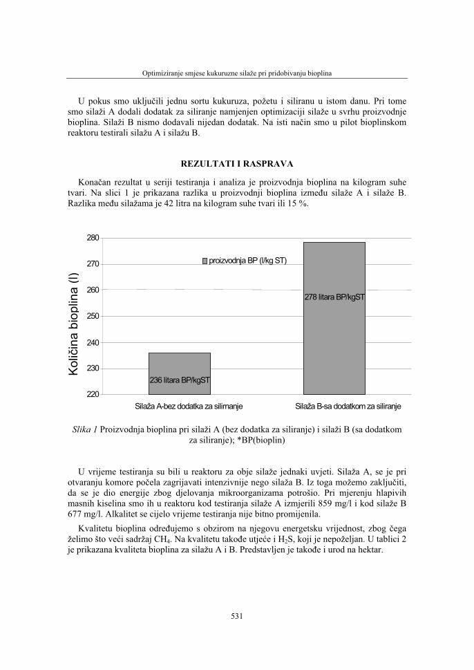
Optimiziranje smjese kukuruzne silaže pri pridobivanju bioplina
531
U pokus smo uključili jednu sortu kukuruza, požetu i siliranu u istom danu. Pri tome smo silaži A dodali dodatak za siliranje namjenjen optimizaciji silaže u svrhu proizvodnje bioplina. Silaži B nismo dodavali nijedan dodatak. Na isti način smo u pilot bioplinskom reaktoru testirali silažu A i silažu B.
REZULTATI I RASPRAVA
Konačan rezultat u seriji testiranja i analiza je proizvodnja bioplina na kilogram suhe tvari. Na slici 1 je prikazana razlika u proizvodnji bioplina između silaže A i silaže B. Razlika među silažama je 42 litra na kilogram suhe tvari ili 15 %.
278 litara BP/kgST
236 litara BP/kgST
220
230
240
250
260
270
280
Silaža A-bez dodatka za silirnanje Silaža B-sa dodatkom za siliranje
Kol
ičin
a bi
oplin
a (l)
proizvodnja BP (l/kg ST)
Slika 1 Proizvodnja bioplina pri silaži A (bez dodatka za siliranje) i silaži B (sa dodatkom za siliranje); *BP(bioplin)
U vrijeme testiranja su bili u reaktoru za obje silaže jednaki uvjeti. Silaža A, se je pri otvaranju komore počela zagrijavati intenzivnije nego silaža B. Iz toga možemo zaključiti,da se je dio energije zbog djelovanja mikroorganizama potrošio. Pri mjerenju hlapivih masnih kiselina smo ih u reaktoru kod testiranja silaže A izmjerili 859 mg/l i kod silaže B 677 mg/l. Alkalitet se cijelo vrijeme testiranja nije bitno promijenila.
Kvalitetu bioplina određujemo s obzirom na njegovu energetsku vrijednost, zbog čega želimo što veći sadržaj CH4. Na kvalitetu takođe utjeće i H2S, koji je nepoželjan. U tablici 2 je prikazana kvaliteta bioplina za silažu A i B. Predstavljen je takođe i urod na hektar.
R. Bernik, A. Zver
532
Tablica 2 Prikaz kvalitete djelomično prečišćene svinjske gnojovke i iskorištenje bioplina iz nje
SUPSTRAT CH4%
CO2%
H2Sppm
Urod ST (kg/ha)
Proizvodnja BP (l/kg ST)
Proizvodnja BP (m3/ha)
Silaža A 54 46 350 12.369 235,8956267 2.918
Silaža B 56 44 700 12.369 278,4516008 3.444 *ST (suha tvar), *BP(bioplin)
LITERATURA
1. Amon T. 2002. Biogas-Strom aus Gülle und Biomasse: Technik, Management, Pendite. Münster – Hiltrup, Landwirtschaftsverlag: 120 str.
2. Beck J. 1997. Anaerobic treatment. V: Manure managment. Treatment strategies for sustainable agriculture. Burton C.H. (ed.). Bia, Silsoe Research Institute: 79–88
3. Đulbić M. 1986. Biogas: dobijanje korišćenje i gradnja uređaja. Beograd, Tehnička knjiga: 171 str.
4. Gobec I. 2005. (So)substrati pri proizvodnji bioplina. Društvo za energetsko ekonomiko in ekologijo.
5. http://www.ljudmila.org/sef/stara/bioplin05/predstavitve_in_fotografije/predstavitve/postojna/so)substrati%20pri%20proizvodnji%20bioplina%20postojna.pdf (7.nov. 2007)
6. Gaćeša S., Vrbaški L., Baras J., Knežić L., Kašnja M., Zidanski F. 1985. Biogas-proizvodnja i primena. Novi Sad, Tehnološki fakultet: 233 str.
7. Medved S., Novak P. 2000. Biomasa. V: Varstvo okolja in obnovljivi viri energije. Ljubljana, Fakulteta za strojništvo: 231 str.
8. Steklar J. 1993. Kdaj uporabiti silirni dodatek. V: Kmečki glas št. 19, s 19.
9. Verbič J. Babnik, D. in Puhan, J. 1994. Hranilna vrednost in siliranje koruze, ki jo je prizadela suša. V. Biotehniške fak., Univ. v Ljubljani, Kmetijstvo. Zootehnika, 64(1994), s. 33-44.
10. Verbič J. 2005. Vpliv zrelosti koruze na kvarjenje silaž. V: Kmečki glas, priloga Sodobno kmetijstvo, l 38, št. 3, s 3.
11. Zver A. 2005. Obnovljivi viri energije, rastlina kot energija in rastlina kot hrana. Diplomsko delo. Ljubljana. Biotehniška fakulteta, Odd. za zootehniko: 67 str.
Optimiziranje smjese kukuruzne silaže pri pridobivanju bioplina
533
OPTIMISATION OF THE CORN SILAGE MIXTURE IN THE GENERATION OF BIOGAS
ABSTRACT
Some years ago, we began the cultivation of crops for the biofuel production purposes. The majority of fields where the experiment took place were located in the Prekmurje region (in the SE of Slovenia). In the course of time there has been a large increase in competitiveness and food and energy demand, which today reflects in the prices of field crops, especially corn, wheat and, finally, all the field-produced plants. With the existence of biogas generation facilities whose technology is based on corn silage, silage must be optimally prepared in order to maximise the recovery of fermentation. The process of fermentation in the pilot reactor equals to the fermentation process in the economical reactor. They merely differ in the volume of the daily mass inflow, meaning that the input mass is equally processed both in the pilot and the economical reactors. Corn silage of the same cultivar harvested on the same day was included in the trial. Silage additive was added to Silage A to optimise it for the biogas production purposes. Silage B, on the other hand, contained no such additives. The use of silage additives under the same conditions of reactor operation increased the generation of biogas by 20 per cent.
Key words: renewable energy, biogass, plants, corn, silage, fermentation

36. Symposium "Actual Tasks on Agricultural Engineering", Opatija, Croatia, 2008.
535
36.
SIMPOZIJAKTUALNI ZADACIMEHANIZACIJE POLJOPRIVREDE
UDC004.42:621.65
Stručni radExpert paper
STUDY CONCERNING THE INFLUENCE OF SOME WORKING CONDITIONS, ON THE HEAT PUMPS
PERFORMANCESMUGUR BALAN*, MIHAI DAMIAN*, LORENTZ JANTSCHI*, ION ION**
*Technical University of Cluj Napoca B-dul. Muncii 103-105; 400641 Cluj Napoca; Romania
[email protected]; [email protected]; [email protected] ** “Dunarea de Jos” University, Str. Domneasca 111, 800201 Galati; Romania
ABSTRACT
The paper presents relevant information about the working principle of the geothermal heat pumps and a study, based on an original computer simulation, analysing the influences of the working conditions on the heat pump performa-nces. After presenting some basic considerations about the geothermal energy and about the heat pumps working principle, there are included some relevant considerations about the environmental conditions of Romania and the potential of the geothermal energy, as important renewable energy, to be used in the field of domestic heating with heat pumps. In domestic heating applications, the only available type of equipment able to use the geothermal energy is the heat pumps. Only these type of equipment can increase the temperature level of the at the Earth surface available geothermal energy, to the needed temperature level of the useful thermal energy. The original software used to analyse the influence of some working conditions, on the heat pumps performances, was written in Engineering Equation Solver language, using an academic licence available at the Technical University of Cluj Napoca. This software environment allows creating software adapted for the evaluation of the influence of many important parameters on the heat pumps performances. Between the relevant studied parameters can be mentioned: heat pump location, heat pump type, quality of the house insulation, type of heat pump application.
Key words: Heat Pump, Geothermal Energy, Renewable Energy, Heating, Simulation, Software, Study
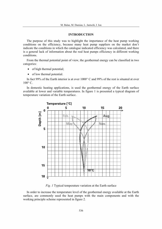
M. Balan, M. Damian, L. Jantschi, I. Ion
536
INTRODUCTION
The purpose of this study was to highlight the importance of the heat pump working conditions on the efficiency, because many heat pump suppliers on the market don’t indicate the conditions in which the catalogue indicated efficiency was calculated, and there is a general lack of information about the real heat pumps efficiency in different working conditions.
From the thermal potential point of view, the geothermal energy can be classified in two categories:
• of high thermal potential;
• of low thermal potential. In fact 99% of the Earth interior is at over 1000° C and 99% of the rest is situated at over
100° C. In domestic heating applications, is used the geothermal energy of the Earth surface
available at lower and variable temperatures. In figure 1 is presented a typical diagram of temperature variation of the Earth surface.
Fig. 1 Typical temperature variation at the Earth surface
In order to increase the temperature level of the geothermal energy available at the Earth surface, are commonly used the heat pumps with the main components and with the working principle scheme represented in figure 2.
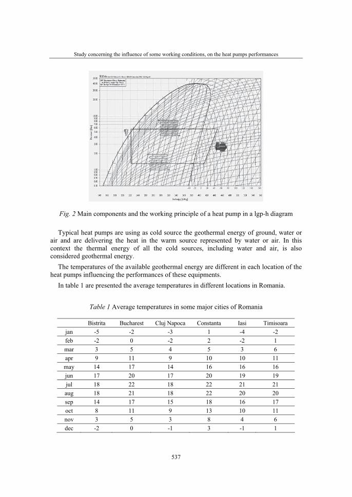
Study concerning the influence of some working conditions, on the heat pumps performances
537
Fig. 2 Main components and the working principle of a heat pump in a lgp-h diagram
Typical heat pumps are using as cold source the geothermal energy of ground, water or air and are delivering the heat in the warm source represented by water or air. In this context the thermal energy of all the cold sources, including water and air, is also considered geothermal energy.
The temperatures of the available geothermal energy are different in each location of the heat pumps influencing the performances of these equipments.
In table 1 are presented the average temperatures in different locations in Romania.
Table 1 Average temperatures in some major cities of Romania
Bistrita Bucharest Cluj Napoca Constanta Iasi Timisoara jan -5 -2 -3 1 -4 -2 feb -2 0 -2 2 -2 1 mar 3 5 4 5 3 6 apr 9 11 9 10 10 11 may 14 17 14 16 16 16 jun 17 20 17 20 19 19 jul 18 22 18 22 21 21 aug 18 21 18 22 20 20 sep 14 17 15 18 16 17 oct 8 11 9 13 10 11 nov 3 5 3 8 4 6 dec -2 0 -1 3 -1 1
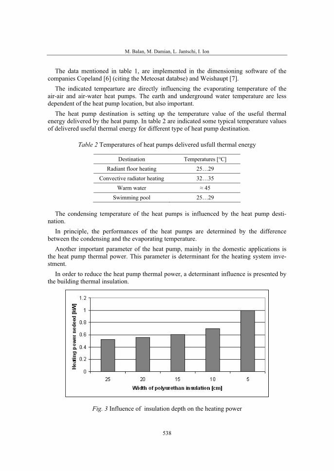
M. Balan, M. Damian, L. Jantschi, I. Ion
538
The data mentioned in table 1, are implemented in the dimensioning software of the companies Copeland [6] (citing the Meteosat databse) and Weishaupt [7].
The indicated tempearture are directly influencing the evaporating temperature of the air-air and air-water heat pumps. The earth and underground water temperature are less dependent of the heat pump location, but also important.
The heat pump destination is setting up the temperature value of the useful thermal energy delivered by the heat pump. In table 2 are indicated some typical temperature values of delivered useful thermal energy for different type of heat pump destination.
Table 2 Temperatures of heat pumps delivered usfull thermal energy
Destination Temperatures [°C]
Radiant floor heating 25…29
Convective radiator heating 32…35
Warm water ≈ 45
Swimming pool 25…29
The condensing temperature of the heat pumps is influenced by the heat pump desti-nation.
In principle, the performances of the heat pumps are determined by the difference between the condensing and the evaporating temperature.
Another important parameter of the heat pump, mainly in the domestic applications is the heat pump thermal power. This parameter is determinant for the heating system inve-stment.
In order to reduce the heat pump thermal power, a determinant influence is presented by the building thermal insulation.
Fig. 3 Influence of insulation depth on the heating power
Study concerning the influence of some working conditions, on the heat pumps performances
539
Figure 3 presents only the results obtained in the case of a typical 150m2 residence realized from Sandwich panels of different width between 5…25cm.
The main characteristics of the considered residence are presented in table 3.
Table 3 Main characteristics of the residence
Parameter Value Inside temperature 25°C Outside temperature -5°C No. of persons 4 Period of time for hot water preparation 8hLength 10m Width 6m Height 7.5m Base surface 80m2
Windows surface 36m2
Windows type Float-Float
METHODS
In order to study the influence of some important parameters, on the heat pump performances, an original software tool was written using Engineering Equation Solver (EES), dedicated and world leader software for thermal calculations.
The main functions realised by the original software are:
• Selection of the heat pump information
• Destination
• Type
• Location
• Calculations
• Heat pump working cycle
• Heat pump efficiency It was studied the influence of the following parameters:
• heat pump type;
• heat pump destination;
• refrigerant.It was considered the following heat pump types:
• ground-water with horizontal collectors;
• ground-water with vertical collectors;
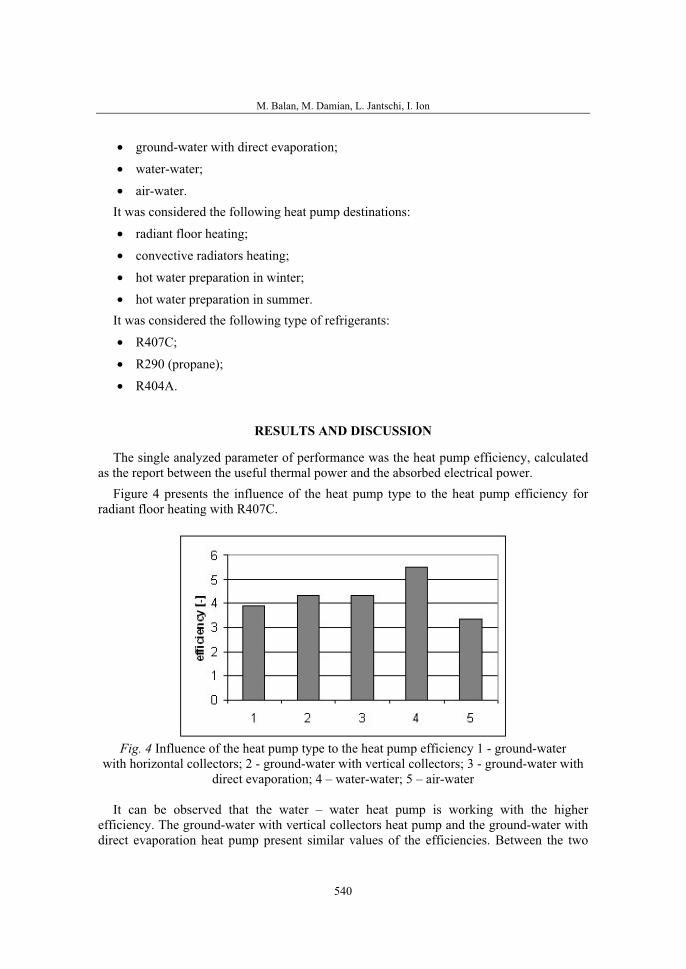
M. Balan, M. Damian, L. Jantschi, I. Ion
540
• ground-water with direct evaporation;
• water-water;
• air-water.It was considered the following heat pump destinations:
• radiant floor heating;
• convective radiators heating;
• hot water preparation in winter;
• hot water preparation in summer. It was considered the following type of refrigerants:
• R407C;
• R290 (propane);
• R404A.
RESULTS AND DISCUSSION
The single analyzed parameter of performance was the heat pump efficiency, calculated as the report between the useful thermal power and the absorbed electrical power.
Figure 4 presents the influence of the heat pump type to the heat pump efficiency for radiant floor heating with R407C.
Fig. 4 Influence of the heat pump type to the heat pump efficiency 1 - ground-waterwith horizontal collectors; 2 - ground-water with vertical collectors; 3 - ground-water with
direct evaporation; 4 – water-water; 5 – air-water
It can be observed that the water – water heat pump is working with the higher efficiency. The ground-water with vertical collectors heat pump and the ground-water with direct evaporation heat pump present similar values of the efficiencies. Between the two
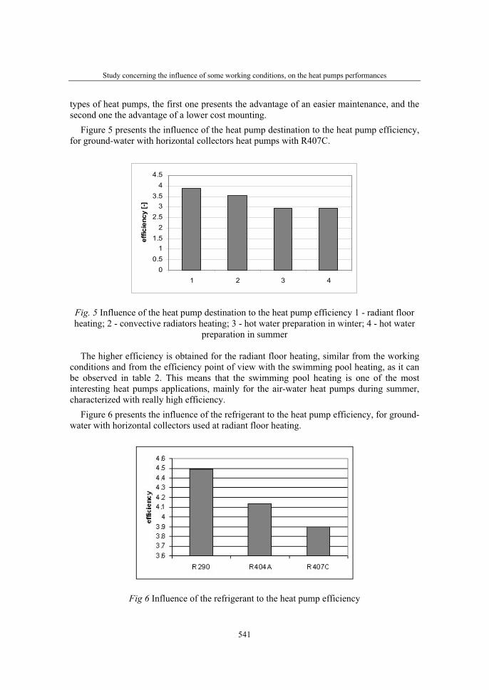
Study concerning the influence of some working conditions, on the heat pumps performances
541
types of heat pumps, the first one presents the advantage of an easier maintenance, and the second one the advantage of a lower cost mounting.
Figure 5 presents the influence of the heat pump destination to the heat pump efficiency, for ground-water with horizontal collectors heat pumps with R407C.
00.5
11.5
22.5
33.5
44.5
1 2 3 4
effic
ienc
y [-]
Fig. 5 Influence of the heat pump destination to the heat pump efficiency 1 - radiant floor heating; 2 - convective radiators heating; 3 - hot water preparation in winter; 4 - hot water
preparation in summer
The higher efficiency is obtained for the radiant floor heating, similar from the working conditions and from the efficiency point of view with the swimming pool heating, as it can be observed in table 2. This means that the swimming pool heating is one of the most interesting heat pumps applications, mainly for the air-water heat pumps during summer, characterized with really high efficiency.
Figure 6 presents the influence of the refrigerant to the heat pump efficiency, for ground-water with horizontal collectors used at radiant floor heating.
Fig 6 Influence of the refrigerant to the heat pump efficiency
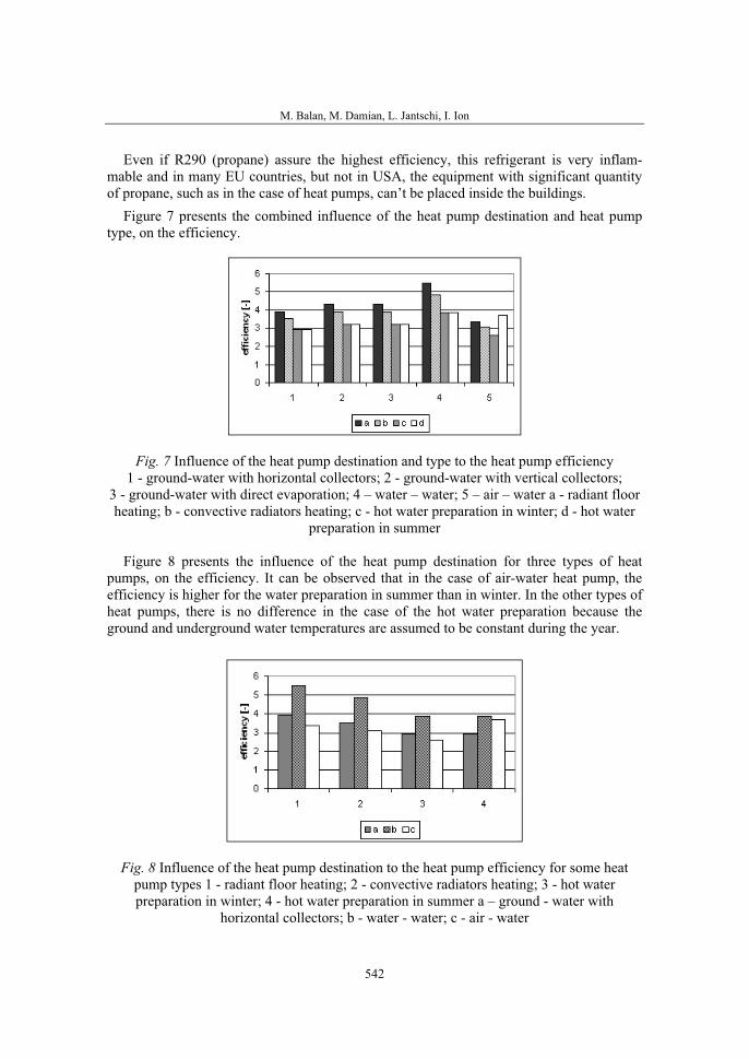
M. Balan, M. Damian, L. Jantschi, I. Ion
542
Even if R290 (propane) assure the highest efficiency, this refrigerant is very inflam-mable and in many EU countries, but not in USA, the equipment with significant quantity of propane, such as in the case of heat pumps, can’t be placed inside the buildings.
Figure 7 presents the combined influence of the heat pump destination and heat pump type, on the efficiency.
Fig. 7 Influence of the heat pump destination and type to the heat pump efficiency1 - ground-water with horizontal collectors; 2 - ground-water with vertical collectors;
3 - ground-water with direct evaporation; 4 – water – water; 5 – air – water a - radiant floor heating; b - convective radiators heating; c - hot water preparation in winter; d - hot water
preparation in summer
Figure 8 presents the influence of the heat pump destination for three types of heat pumps, on the efficiency. It can be observed that in the case of air-water heat pump, the efficiency is higher for the water preparation in summer than in winter. In the other types of heat pumps, there is no difference in the case of the hot water preparation because the ground and underground water temperatures are assumed to be constant during the year.
Fig. 8 Influence of the heat pump destination to the heat pump efficiency for some heat pump types 1 - radiant floor heating; 2 - convective radiators heating; 3 - hot water preparation in winter; 4 - hot water preparation in summer a – ground - water with
horizontal collectors; b - water - water; c - air - water
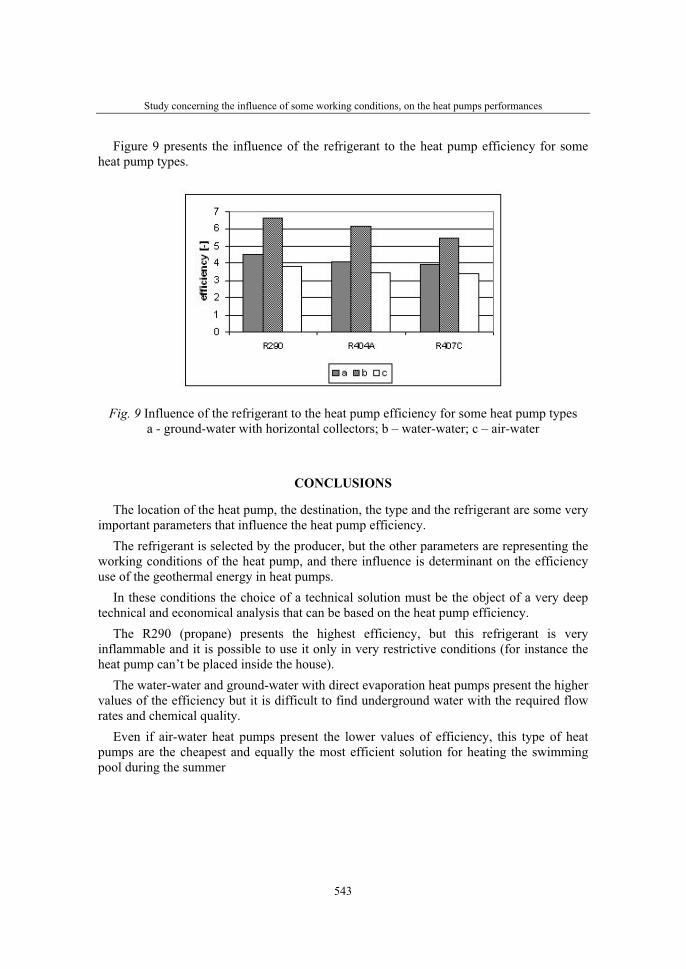
Study concerning the influence of some working conditions, on the heat pumps performances
543
Figure 9 presents the influence of the refrigerant to the heat pump efficiency for some heat pump types.
Fig. 9 Influence of the refrigerant to the heat pump efficiency for some heat pump typesa - ground-water with horizontal collectors; b – water-water; c – air-water
CONCLUSIONS
The location of the heat pump, the destination, the type and the refrigerant are some very important parameters that influence the heat pump efficiency.
The refrigerant is selected by the producer, but the other parameters are representing the working conditions of the heat pump, and there influence is determinant on the efficiency use of the geothermal energy in heat pumps.
In these conditions the choice of a technical solution must be the object of a very deep technical and economical analysis that can be based on the heat pump efficiency.
The R290 (propane) presents the highest efficiency, but this refrigerant is very inflammable and it is possible to use it only in very restrictive conditions (for instance the heat pump can’t be placed inside the house).
The water-water and ground-water with direct evaporation heat pumps present the higher values of the efficiency but it is difficult to find underground water with the required flow rates and chemical quality.
Even if air-water heat pumps present the lower values of efficiency, this type of heat pumps are the cheapest and equally the most efficient solution for heating the swimming pool during the summer
M. Balan, M. Damian, L. Jantschi, I. Ion
544
REFERENCES
1. Balan,M., Damian,M. (2006) - Software aplication for monitoring a small air conditioning unit, IEEE International Conference on Automation, Quality and Testing, Robotics, Cluj Napoca, May 25-28, pg. 183-186.
2. Balan,M., Damian,M., Ion,I. (2007) - Considerations about the potential use of the geotermal energy for domestic heating in romania, International congress Automotive, Environment and Farm Machinery. AMMA, Cluj-Napoca, October 11-13 2007, Romania, pg. 219-224.
3. Jäntschi,L., Balan,M., Podar,E., Bolboaca,S. (2007) - Thermal Energy Efficiency Analysis for Residential Buildings, IEEE Region 8 Eurocon 2007 Conference, Warsaw, Poland September9-12, pg. 2009-2014.
4. Page,D. (2002) – Geothermal Energy. A renewable option. Geothermal Education Office, Tiburon, USA.
5. Porneala,S., Balan,M. (2003) - Utilizarea frigului artificial, Ed. Todesco, Cluj Napoca.
6. *** Copeland Selection Software
7. *** Weishaupt Solarberater Software
36. Symposium "Actual Tasks on Agricultural Engineering", Opatija, Croatia, 2008.
545
36.
SIMPOZIJAKTUALNI ZADACIMEHANIZACIJE POLJOPRIVREDE
UDC620.91:66.067.3:665.334
Stručni radExpert paper
THE STUDY CONCERNING THE BIOFUELS AND THE ELASTOMER SEALING ELEMENTS OF THE OIL
FILTER COMPATIBILITY FLORIN MARIAŞIU1, NICOLAE BURNETE
1The Technical University of Cluj-Napoca, Faculty of Mechanic, [email protected], +040264 401 609
ABSTRACT
The present tendency to use in the near future the biofuels as fuels for compression ignition engines by introducing a 5% in 2008 and till 20% in 2010 parts of biofuels in diesel fuel, necessitate to perform and realize the studies concerning the plastic molding compound materials compatibility (that are used in the manufacture of engine and fuel systems) with biofuels.
The present paper present the results of an experimental study that concerning the fuel filter elements and biofuels used in compression ignition engines compatibility. The experiment was realized taking account of functionally condition of compression ignition engine, especially those that are linked about the maximum value of temperatures that can be reached by the feed system parts and components (50o…80oC) [2].
The mixing formulas of biofuels were realized in conformity with the existent standards and the basic vegetable oil was Rapeseed oil. The fuel filter was the same that it is common used in the standard equipment of Romanian tractors.
Key words: compatibility, biofuels, plastic materials, fuel filter rubber sealing element.
INTRODUCTION
The renewable energy sources, that include the biofuels class, can be the right and immediate answers to the questions about the long term energetic security of European Community. Even those above presented idea is represented as efficient solution for Romanian agriculture in the context of large oil price fluctuation, the using of biofuels as alternative fuel for tractors can improve the benefits that can be obtained from agricultural production [3].
F. Mariaşiu, N. Burnete
546
Through the obtained experimental results we can say that these types of alternative fuels offer the same energetic performance as fossil fuels but with immediate benefits given by:
• very good reducing of noxes;
• the development of agricultural field of activity;
• social impact through develop of new jobs). The development of vegetable oils (and the monoesters derivates) as alternative diesel
fuels present some advantages based on:
• a viable alternative to replace the fossil fuels;
• the monoesters-diesel fuel mixture has appropriate properties with diesel fuel;
• strong reduction of carbon oxide and smoke;
• the vegetable oils are ecologically;
• there are no need particularly modifications on fuel storage and distribution system. Till 70’s the engines, which used biofuels were experimented, researched and studied in
real and laboratory functional conditions [1,5]. The researches were conducted starting to:
• monocylinder engines to multiplecylinders engines (12cylinders);
• indirect injection process (IDI) to direct injection process (DI);
• using the diesel fuels-vegetal oil mixture (the part of vegetable oil varies between 2% and 100%);
• using the various classes of additives (to improve the different physical and chemi-cal properties of vegetable oils).
The period of testing of the engines that run with biofuels was between 10 and 5000 hours and some vehicles and stationary engines was supervising at the long period of 14 years of functioning with biofuels [5].
There are a lot of studies and researches concerning the engine parts and biofuels compa-tibility that was realized by engines manufacturers (Cummings), tractors manufacturers (John Deer, Ford, Mitsubishi), autovehicles manufacturers (Mercedes Benz, Ford , Dodge), automotive spare and supply parts (Foseen Manufacturing and Developing Company, Parker, Wilden Chemical, 3M, e-Funda), universities and governmental agency all over the world.
Also it is very important to use renewable materials in construction of autovehicle components, such as polypropylene for a future ecologically autovehicle industry.
METHOD
The experimental study was conducted to analyze the effect of the biofuels solvent properties on the Romanian tractors filter system (Figure 1). It’s important to mention that in the period when the Romanian tractors (and tractors engine accessories) were designed

The study concerning the biofuels and the elastomer sealing elements of the oil flter compatibility
547
and produced, the only fuel that was take in consideration to use in engine feed was only the diesel fuel and a number of 110,000 are considered to be in function.
The present study tries to show the effect of using the biofuels based on Rapeseed oil on the fuel filter system particularly on the rubber seals that are contained by the filter system. The physically and mechanical properties of rubber seal material are presented in Table 1.
Table 1 Physical and mechanical properties of rubber seal material [4]
Plastic molding compound
Range of application[oC]
Tensile strength[N/mm2]
Shored A hardness [kJ/m2]
Rubber seal NBR -30…+120 10…25 35…100
The physical and chemical properties of Rapeseed oil (that was used as biofuels in this experiment) are presented in Table 2.
Table 2 Physical and chemical properties of rapeseed oil
Properties Rapeseed oil
Density at 15oC
[kg/dm3]
0,92
Caloric power
[MJ/kg]
37,6
Cinematic viscosity at 20oC [mm2/s] 74
Cetane number 40
Pour point
[oC]
-15…-18
Flash point
[oC]
317
Iodine index 94-118
The experiment was realized taking account of functionally condition of compression ignition engine D-118 (that was used in a large number of Romanian tractors), especially those that are linked about the maximum value of temperatures that can be reached by the feed system parts and components (50o…80oC). The mixing formulas of biofuels were realized in conformity with the existent standards and the basic vegetable oil was Rapeseed oil.
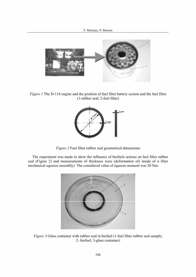
F. Mariaşiu, N. Burnete
548
Figure 1 The D-118 engine and the position of fuel filter battery system and the fuel filter (1-rubber seal; 2-fuel filter)
Figure 2 Fuel filter rubber seal geometrical dimensions
The experiment was made to show the influence of biofuels actions on fuel filter rubber seal (Figure 2) and measurements of thickness were (deformation of) inside of a filter mechanical squeeze assembly). The considered value of squeeze moment was 20 Nm.
Figure 3 Glass container with rubber seal in biofuel (1-fuel filter rubber seal sample;2- biofuel; 3-glass container)
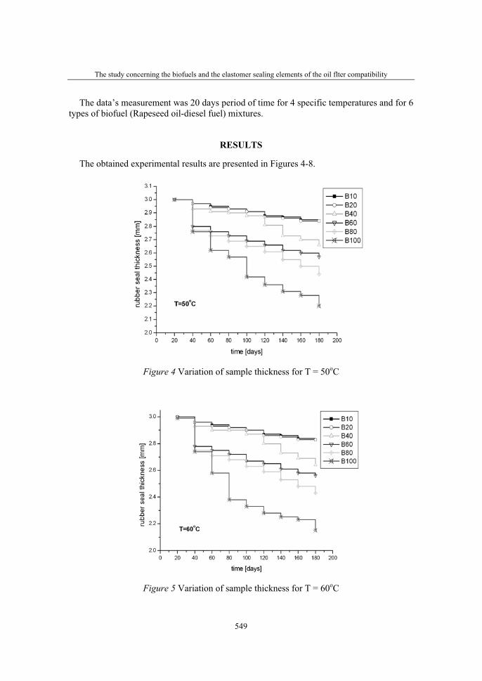
The study concerning the biofuels and the elastomer sealing elements of the oil flter compatibility
549
The data’s measurement was 20 days period of time for 4 specific temperatures and for 6 types of biofuel (Rapeseed oil-diesel fuel) mixtures.
RESULTS
The obtained experimental results are presented in Figures 4-8.
Figure 4 Variation of sample thickness for T = 50oC
Figure 5 Variation of sample thickness for T = 60oC
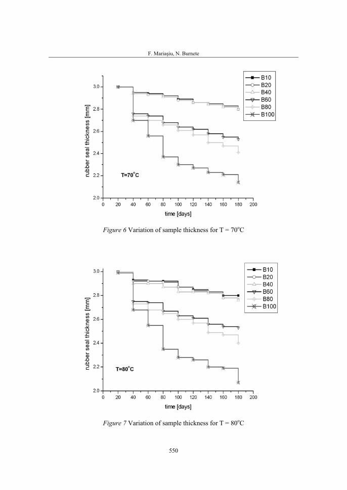
F. Mariaşiu, N. Burnete
550
Figure 6 Variation of sample thickness for T = 70oC
Figure 7 Variation of sample thickness for T = 80oC

The study concerning the biofuels and the elastomer sealing elements of the oil flter compatibility
551
Figure 8 Variation of sample thickness for pure Rapeseed oil (B100)
CONCLUSIONS
• It can be seen that the amplification of natural solvent biofuels property once to increase of the temperature and also with the increasing of concentration level of vegetable oil in biofuel mixture: - 3.3-26% variation in thickness (from initial conditions) for B10 to B100 biofuel type
at 50oC . - 3.4-28% variation in thickness (from initial conditions) for B10 to B100 biofuel type
at 60oC . - 3.4-30.6% variation in thickness (from initial conditions) for B10 to B100 biofuel
type at 70oC . - 4.2-31.2 variation in thickness (from initial conditions) for B10 to B100 biofuel type
at 80oC .
• There are not major treats in using rubber as sealing fuel filter element as components or spare parts for biofuels that contain till 20% Rapeseed oil in volume of mixture (the variation of thickness remain approximately constant at 4%) for the period of time that was considered in this experiment. It can say that for biofuels that contain more that 20% Rapeseed oil in volume can be some sealing problems due to the apparition of great deformation of geometrical shape of rubber seal fuel filter element. Are necessary future studies for a longer period of time and obtain the proper information from users about the fuel filter sealing element structural comportment in conditions of using biofuel for feeding the tractors engines.
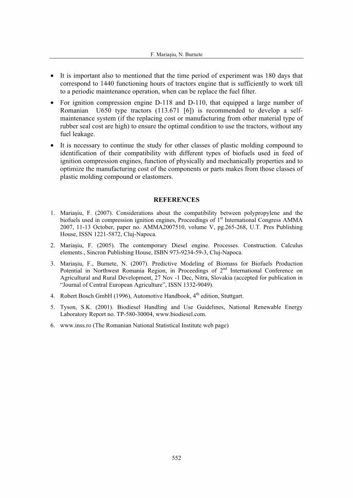
F. Mariaşiu, N. Burnete
552
• It is important also to mentioned that the time period of experiment was 180 days that correspond to 1440 functioning hours of tractors engine that is sufficiently to work till to a periodic maintenance operation, when can be replace the fuel filter.
• For ignition compression engine D-118 and D-110, that equipped a large number of Romanian U650 type tractors (113.671 [6]) is recommended to develop a self-maintenance system (if the replacing cost or manufacturing from other material type of rubber seal cost are high) to ensure the optimal condition to use the tractors, without any fuel leakage.
• It is necessary to continue the study for other classes of plastic molding compound to identification of their compatibility with different types of biofuels used in feed of ignition compression engines, function of physically and mechanically properties and to optimize the manufacturing cost of the components or parts makes from those classes of plastic molding compound or elastomers.
REFERENCES
1. Mariaşiu, F. (2007). Considerations about the compatibility between polypropylene and the biofuels used in compression ignition engines, Proceedings of 1st International Congress AMMA 2007, 11-13 October, paper no. AMMA2007510, volume V, pg.265-268, U.T. Pres Publishing House, ISSN 1221-5872, Cluj-Napoca.
2. Mariaşiu, F. (2005). The contemporary Diesel engine. Processes. Construction. Calculus elements., Sincron Publishing House, ISBN 973-9234-59-3, Cluj-Napoca.
3. Mariaşiu, F., Burnete, N. (2007). Predictive Modeling of Biomass for Biofuels Production Potential in Northwest Romania Region, in Proceedings of 2nd International Conference on Agricultural and Rural Development, 27 Nov -1 Dec, Nitra, Slovakia (accepted for publication in “Journal of Central European Agriculture”, ISSN 1332-9049).
4. Robert Bosch GmbH (1996), Automotive Handbook, 4th edition, Stuttgart.
5. Tyson, S.K. (2001). Biodiesel Handling and Use Guidelines, National Renewable Energy Laboratory Report no. TP-580-30004, www.biodiesel.com.
6. www.inss.ro (The Romanian National Statistical Institute web page)

36. Symposium "Actual Tasks on Agricultural Engineering", Opatija, Croatia, 2008.
553
36.
SIMPOZIJAKTUALNI ZADACIMEHANIZACIJE POLJOPRIVREDE
UDC631.153.46Stručni rad
Expert paper
DETERMINATION OF FARM SIZE LIMIT OF REASONABLE MECHANISATION
BY MODELLING LÁSZLÓ MAGÓ
Hungarian Institute of Agricultural Engineering, Gödöllő,H-2100, Gödöllő, Tessedik s. u. 4
Tel: +36-28-511-689, E-mail: [email protected]
INTRODUCTION
The diversified property structure of agricultural enterprises is not always coupled with efficient power and working machine system. In case of small size farming units the up-to-date, means and cost sparing solutions are rarely to be found and even the medium size farms do not necessarily own the cost efficient machine systems with all the technical-technological advantages of the present era furthering improvingly effective farming.
To solve the present problems of agricultural mechanization (changed farm structure, extended machine selection etc.), the optimal machine utilization and its construction can be approached from a new point of view. Extra emphasis has been laid on the level of utilization of the power machines, enabling hereby the optimum level of machine utilization cost.
Fixed costs represent a considerable rate in the utilization costs of modern power machines with more expensive purchasing price. These cost types can be moderated by the rise of level of utilization. The applied tools are coupled on actual operation cost to each work task. This enables the observation of the influence of the completed operational hours on the expenses.
Taking into consideration the current partitioned structure of the farms the goal was established to determine that in the case of the different branches of plant production on small and middle-sized farms which combination of fleet of machinery can be used effectively.
Key words: mechanisation of small and medium sized farms, machine fleet planning, machine utilisation, low cost machine fleet, machine investment and usage cost
L. Magó
554
THE METHOD
Testing of the mechanised processes of agricultural harvesting was carried out using models. In the model a crop rotation plan was adopted which mirrors the Hungarian production characteristics using wheat and oil plants. Depending on the size of the farm the proportion of the sewed area of each plant was established keeping in mind the agronomical and production technological conditions.
At the basic level the experiments were focused on the lowest investment cost power machinery range of products in Hungary. With this machinery because of the low investment cost the amortisation cost is less and thus the cost of utilisation is low. The determination of the basic data of the costs of machine utilisation has been carried out, based on the database of the Hungarian Institute of Agricultural Engineering [2].
The model calculations involved the key plant size data of the formation of machinery systems in the range of plant size ranging from 5 to 1000 hectares. On the basis of these data, statements can be made regarding a larger segment of the estate structure, and conclusions may be drawn regarding cost of machinery utilisation and investment.
RESULTS
Conclusions drawn regarding the composition of the power machinery system and the performance of hours run, based on the results of the model calculations
The composition of machine systems of minimal utilisation cost broken down in catego-ries of power machinery depending on the sizes of plants
In the course of carrying out our survey the universal power machinery was categorised according to engine performance, as well as taking into consideration the function of being a cereal harvesting machine. The composition of the power machinery systems rendered to a particular area was determined on the criteria of power machinery categories. Taking into consideration the crop structure, growing technology, conditions of mechanised work typical of the Hungarian particularities and the composition of categories of cost effective power machinery systems which are formed on the criterion of plant size, regular interrelations can be established.
The surveyed power machinery system that can be rendered to the smallest plant size, in the case of tractors, consists of machines of 40 kW, a performance that is the minimum requirement for the quality performance of soil work. If the size of the area is higher, then first the performance of the machinery making up the fleet (from the size of 30 hectares tractors with 60 kW performance are required), next the number of tractors increases. Thus, tractors of 40 and 80 kW performance are mentioned together in a machinery system for plant size of 100 hectares or upwards. From the plant size of 300 hectares the function of power machinery mentioned above is filled by tractors of 60 and 120 kW performance, which have sufficient capacity for the increased workload. For the plant size of 500 hectares or upwards the number of tractors increases in proportion to the growth of requirement for capacity.
Determination of farm size limit of reasonable mechanisation by modelling
555
It is necessary to note that, in the case of large plant size, the cost level of machinery utilisation may be further decreased by increasing the number of performance-based categories and optimising the distribution of work among machinery connections of various performance levels. (Magó 2002). [5]
In order to increase utilisation, transportation tasks should also be realised by the means of tractor-trailer connections.
The utilisation of an own, low capacity cereal harvester may be justified above the plant size of 100 hectares. In the case of a plant size exceeding 500 hectares, the large extent of the specialised mechanised work requires the utilisation of harvesters with larger delivery value. According to the calculations, a 1000-hectare farm requires the utilisation of at least two combine harvesters.
Optimal mechanisation levels concerning tractors, depending on plant size The number of tractors required by plants of various sizes is as follows: 1) In the case of a plant size not exceeding one hundred hectares, we calculated with
one tractor.2) In the case of a plant size ranging from one to five hundred hectares, two tractors of
different performance levels are required. 3) In the case of a plant size exceeding five hundred hectares, two tractors are required
from both performance categories in order to carry out the work operations in time and in good quality.
When analysing the number of own power machines per area unit it can be stated that, in the case of a power machinery system of minimal utilisation costs, the coverage on farms of over 50 hectares is favourable. The economically most favourable value can be calculated over 200 hectares, in this case a maximum of one power machine is sufficient for the cultivation of 100 hectares of land.
The specific performance of engines per hectare decreases substantially in the function of plant size. While on small plant sizes 2-8 kW/Ha engine performance is required for every hectare, in the case of medium sized plants this value falls within the range of 1-2 kW/Ha. In plants of large size the work operation may be carried out with a requirement of 0.7 kW/Ha.
The ranges of plant sizes of the “activation” of the power machinery categories The individual power machinery categories are “activated” when they first appear in the
power machinery system developing in the function of the growing plant size. For the “activation” of each power machinery category this is a specific range of plant size. (For example: 80 kW performance category: directly from 100 hectares and upwards, 120 kW performance category: from 300 hectares and upwards. The attachment of a new category also influences the costs of investment on the level of machinery systems. (see Figure 2 and 3).
In connection to the above, up to the plant size of 100 hectares, the system of machinery is formed on the basis of power machines belonging to each of the performance categories. In the range of plant size not exceeding 30 hectares, if we aim to utilise our own machines,
L. Magó
556
in order to decrease the fixed costs, it is reasonable to utilise machines of the lowestperformance level and purchase cost, which are still capable of performing the required workload. If the plant size and number of work tasks grow, the solution is the increase of the level of performance rather than the number of machines. Thus, the category of 60-kW tractors becomes a part of the optimal machinery system from 30 hectares upward. 80-kW tractors are part of the system from 100, whereas 120-kW tractors are part of the system from 300 hectares upward. It is necessary to point out that size in itself does not guarantee the fulfilment of the appropriate number of work hours and favourable utilisation.
The use of own harvester – depending on performance and delivery value – is economi-cally justified over the plant size of 100 hectares.
It can be stated that the following issues must be consequently taken into consideration prior to the “activation” of a new machine:
- is it not possible to perform the tasks by the means of internal redeployment rather than by making a new purchase;
- can the missing capacity be covered by machine rental or other external service;- is it possible to utilise the surplus capacity resulting from the new purchase (eg.
lease work);
The number of performed hours run in the function of plant size With differing plant sizes the number of performable hours run has influence on the
composition of categories of the power machinery system;
• In the case of the examined smallest plant size (up to 50 hectares) low exploitagemay be achieved with tractors: maximum 400-500 hours run per year.
• In the case of medium size plant (50 to 300 hectares) this quantity is larger, 800-1400 hours run per year.
• With large size plants (above 300 hectares) the various categories of tractors achieve significant performance (1000-1800 hours run per year).
A cereal harvester with well-chosen capacity can achieve good exploitage at 300 hours run per year in the case of plant size above 300 hectares, by which the cost of operation becomes reasonable.
The number of hours run projected on a unit of area decreases with the increase of plant size. In small plant sizes 10-15 hours run per year is realised. In the range of 30 to 300 hectares this value is 8-10 hours run per year, and, above this range, a value of 6 hours run per hectare can be observed when realising the efficient work plan.
It can be observed that both in the number of machines and with regards to the performed hours run, the most exploited tractor belongs to the category of 120 kW. The performance of this significant labour time is achieved by the power machine of the given category, when both soil work and transportation tasks are carried out. (See Figure 1)

Determination of farm size limit of reasonable mechanisation by modelling
557
510 20 30 50 100 200 300 500 1000
40 kW tractor60 kW tractor
80 kW tractor120 kW tractor
harvester0
20
40
60
80
100
%
plant size [ha]
Figure 1 The extent of exploitation with the various categories of power machines in the case of the examined plant sizes
The costs of purchase and use of machines The specifications of the function of investment and operation costs of machines projec-
ted on the size of plant
0
1000
2000
3000
4000
5000
6000
0 100 200 300 400 500 600 700 800 900 1000ha
spec
ific
cost
s of
mac
hine
in
vest
men
t (E
UR
/ha)
Figure 2 Specific costs of machine investment in the function of plant size
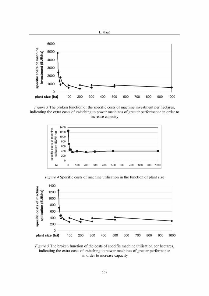
L. Magó
558
0
1000
2000
3000
4000
5000
6000
0 100 200 300 400 500 600 700 800 900 1000plant size [ha]
spec
ific
cost
s of
mac
hine
in
vest
men
t (EU
R/h
a)
Figure 3 The broken function of the specific costs of machine investment per hectares, indicating the extra costs of switching to power machines of greater performance in order to
increase capacity
0
200
400
600
800
1000
1200
1400
0 100 200 300 400 500 600 700 800 900 1000ha
spec
ific
cost
s of
mac
hine
ut
ilisat
ion
(EU
R/
ha)
Figure 4 Specific costs of machine utilisation in the function of plant size
0
200
400
600
800
1000
1200
1400
0 100 200 300 400 500 600 700 800 900 1000plant size [ha]
spec
ific
cost
s of
mac
hine
ut
ilisa
tion
(EU
R/h
a)
Figure 5 The broken function of the costs of specific machine utilisation per hectares, indicating the extra costs of switching to power machines of greater performance
in order to increase capacity
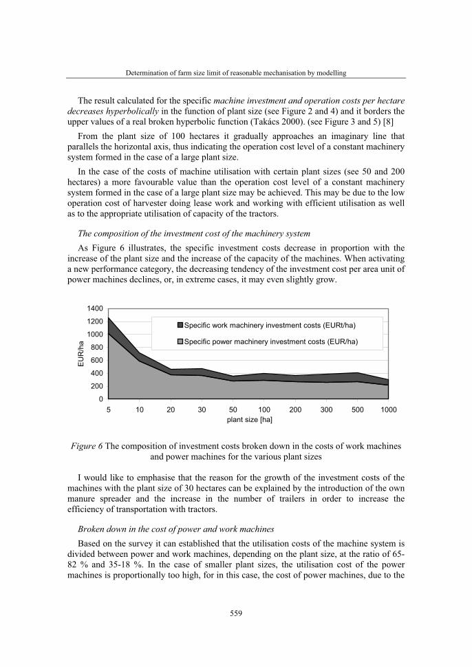
Determination of farm size limit of reasonable mechanisation by modelling
559
The result calculated for the specific machine investment and operation costs per hectare decreases hyperbolically in the function of plant size (see Figure 2 and 4) and it borders the upper values of a real broken hyperbolic function (Takács 2000). (see Figure 3 and 5) [8]
From the plant size of 100 hectares it gradually approaches an imaginary line that parallels the horizontal axis, thus indicating the operation cost level of a constant machinery system formed in the case of a large plant size.
In the case of the costs of machine utilisation with certain plant sizes (see 50 and 200 hectares) a more favourable value than the operation cost level of a constant machinery system formed in the case of a large plant size may be achieved. This may be due to the low operation cost of harvester doing lease work and working with efficient utilisation as well as to the appropriate utilisation of capacity of the tractors.
The composition of the investment cost of the machinery system As Figure 6 illustrates, the specific investment costs decrease in proportion with the
increase of the plant size and the increase of the capacity of the machines. When activating a new performance category, the decreasing tendency of the investment cost per area unit of power machines declines, or, in extreme cases, it may even slightly grow.
0
200
400
600
800
1000
1200
1400
5 10 20 30 50 100 200 300 500 1000plant size [ha]
EU
R/h
a
Specific work machinery investment costs (EURt/ha)
Specific power machinery investment costs (EUR/ha)
Figure 6 The composition of investment costs broken down in the costs of work machines and power machines for the various plant sizes
I would like to emphasise that the reason for the growth of the investment costs of the machines with the plant size of 30 hectares can be explained by the introduction of the own manure spreader and the increase in the number of trailers in order to increase the efficiency of transportation with tractors.
Broken down in the cost of power and work machines Based on the survey it can established that the utilisation costs of the machine system is
divided between power and work machines, depending on the plant size, at the ratio of 65-82 % and 35-18 %. In the case of smaller plant sizes, the utilisation cost of the power machines is proportionally too high, for in this case, the cost of power machines, due to the
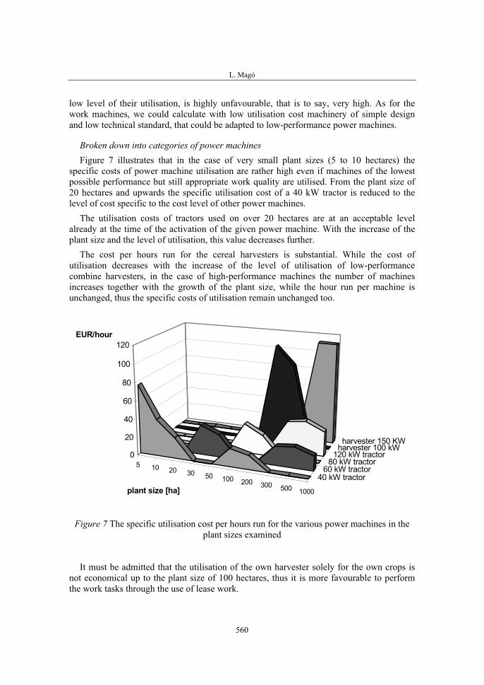
L. Magó
560
low level of their utilisation, is highly unfavourable, that is to say, very high. As for the work machines, we could calculate with low utilisation cost machinery of simple design and low technical standard, that could be adapted to low-performance power machines.
Broken down into categories of power machines Figure 7 illustrates that in the case of very small plant sizes (5 to 10 hectares) the
specific costs of power machine utilisation are rather high even if machines of the lowest possible performance but still appropriate work quality are utilised. From the plant size of 20 hectares and upwards the specific utilisation cost of a 40 kW tractor is reduced to the level of cost specific to the cost level of other power machines.
The utilisation costs of tractors used on over 20 hectares are at an acceptable level already at the time of the activation of the given power machine. With the increase of the plant size and the level of utilisation, this value decreases further.
The cost per hours run for the cereal harvesters is substantial. While the cost of utilisation decreases with the increase of the level of utilisation of low-performance combine harvesters, in the case of high-performance machines the number of machines increases together with the growth of the plant size, while the hour run per machine is unchanged, thus the specific costs of utilisation remain unchanged too.
5 10 20 30 50 100 200 300 500 1000
40 kW tractor60 kW tractor
80 kW tractor120 kW tractor
harvester 100 kWharvester 150 KW
0
20
40
60
80
100
120EUR/hour
plant size [ha]
Figure 7 The specific utilisation cost per hours run for the various power machines in the plant sizes examined
It must be admitted that the utilisation of the own harvester solely for the own crops is not economical up to the plant size of 100 hectares, thus it is more favourable to perform the work tasks through the use of lease work.
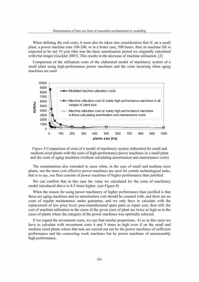
Determination of farm size limit of reasonable mechanisation by modelling
561
When defining the real costs, it must also be taken into consideration that if, on a small plant, a power machine runs 100-200, or in a better case, 500 hours, then its machine life is expected to be not 10 year (this was the basic amortisation period we originally calculated with) but longer (Gockler 2007). This results in the decrease of machine utilisation. [2]
Comparison of the utilisation costs of the elaborated model of machinery system of a small plant using high-performance power machines and the costs incurring when aging machines are used
0100020003000400050006000700080009000
10000
0 100 200 300 400 500 600 700 800 900 1000plants size [ha]
EUR
/ha
Modelled machine utilisation costs
Machine utilisation cost of solely high performance machines in allranges of plant size
Machine utilisation cost of solely high performance machinesw ithout calculating amortisation and maintenance costs
Figure 8 Comparison of costs of a model of machinery system elaborated for small and medium sized plants with the costs of high-performance power machines in a small plant and the costs of aging machines (without calculating amortisation and maintenance costs)
The examinations also extended to cases when, in the case of small and medium sizes plants, not the most cost effective power machines are used for certain technological tasks, that is to say, our fleet consists of power machines of higher performance than justified.
We can confirm that in this case the value we calculated for the costs of machinery model introduced above is 4-5 times higher. (see Figure 8)
When the reason for using power machinery of higher performance than justified is that these are aging machines and no amortisation cost should be counted with, and there are no costs of regular maintenance under guarantee, and we only have to calculate with the replacement of low price level, post-manufactured spare parts as repair cost, then still, the cost of machine utilisation in the cases of the given sizes of plant are twice as high as in the cases of plants where the category of the power machines was optimally selected.
If we regard the investment costs, we can find similar proportions. Al so in this cases we have to calculate with investment costs 4 and 5 times as high even if on the small and medium sized plants where that task are carried out not by the power machines of sufficient performance and the connecting work machines but by power machines of unreasonably high performance.
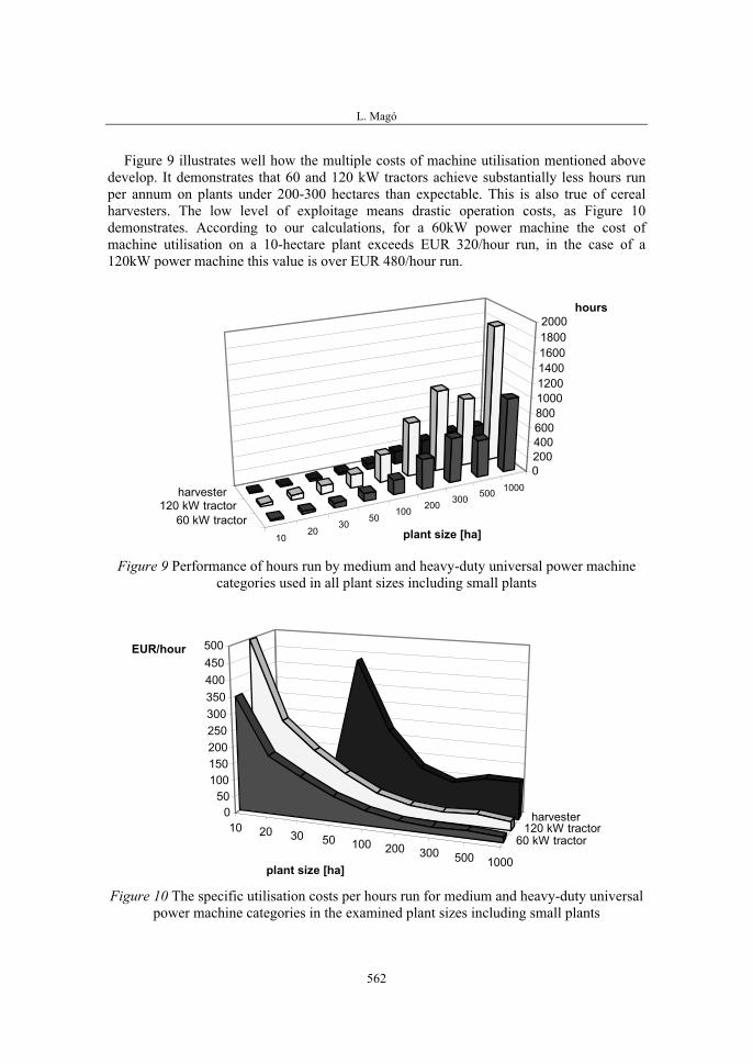
L. Magó
562
Figure 9 illustrates well how the multiple costs of machine utilisation mentioned above develop. It demonstrates that 60 and 120 kW tractors achieve substantially less hours run per annum on plants under 200-300 hectares than expectable. This is also true of cereal harvesters. The low level of exploitage means drastic operation costs, as Figure 10 demonstrates. According to our calculations, for a 60kW power machine the cost of machine utilisation on a 10-hectare plant exceeds EUR 320/hour run, in the case of a 120kW power machine this value is over EUR 480/hour run.
1020
3050
100 200 300 500 1000
60 kW tractor120 kW tractor
harvester
0200400600800100012001400160018002000
hours
plant size [ha]
Figure 9 Performance of hours run by medium and heavy-duty universal power machine categories used in all plant sizes including small plants
10 20 30 50 100 200 300 500 1000
60 kW tractor120 kW tractor
harvester050
100150200250300350400450500EUR/hour
plant size [ha]
Figure 10 The specific utilisation costs per hours run for medium and heavy-duty universal power machine categories in the examined plant sizes including small plants
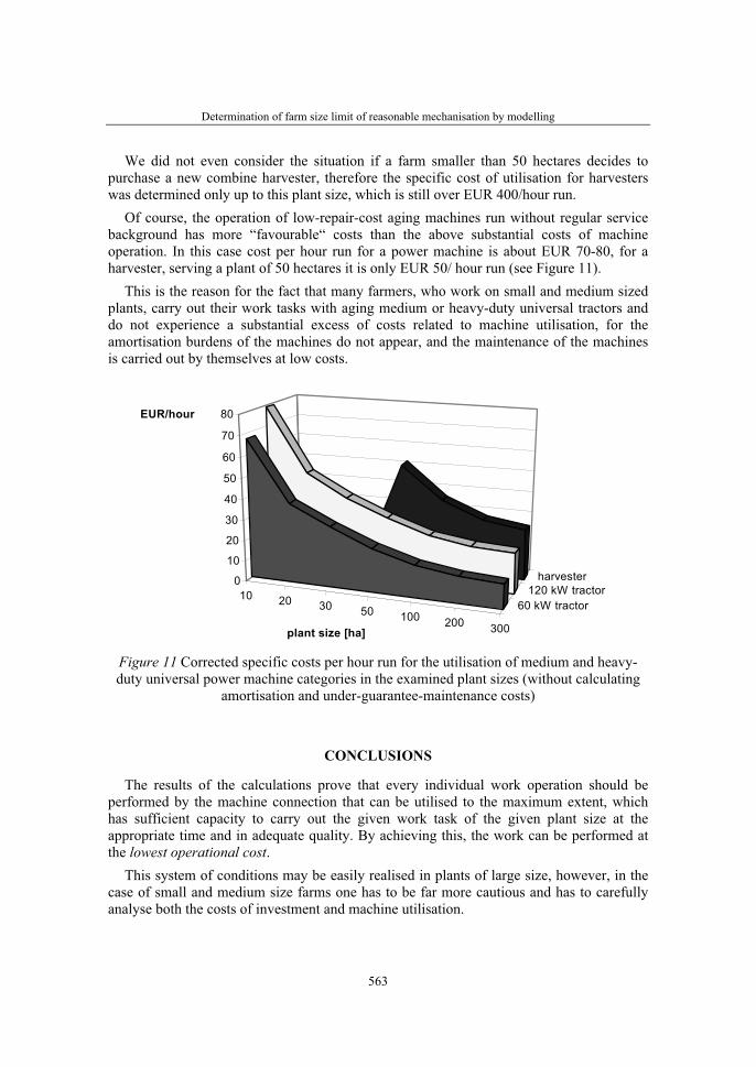
Determination of farm size limit of reasonable mechanisation by modelling
563
We did not even consider the situation if a farm smaller than 50 hectares decides to purchase a new combine harvester, therefore the specific cost of utilisation for harvesters was determined only up to this plant size, which is still over EUR 400/hour run.
Of course, the operation of low-repair-cost aging machines run without regular service background has more “favourable“ costs than the above substantial costs of machine operation. In this case cost per hour run for a power machine is about EUR 70-80, for a harvester, serving a plant of 50 hectares it is only EUR 50/ hour run (see Figure 11).
This is the reason for the fact that many farmers, who work on small and medium sized plants, carry out their work tasks with aging medium or heavy-duty universal tractors and do not experience a substantial excess of costs related to machine utilisation, for the amortisation burdens of the machines do not appear, and the maintenance of the machines is carried out by themselves at low costs.
10 20 30 50 100 200 300
60 kW tractor120 kW tractor
harvester0
10
20
30
40
50
60
70
80EUR/hour
plant size [ha]
Figure 11 Corrected specific costs per hour run for the utilisation of medium and heavy-duty universal power machine categories in the examined plant sizes (without calculating
amortisation and under-guarantee-maintenance costs)
CONCLUSIONS
The results of the calculations prove that every individual work operation should be performed by the machine connection that can be utilised to the maximum extent, which has sufficient capacity to carry out the given work task of the given plant size at the appropriate time and in adequate quality. By achieving this, the work can be performed at the lowest operational cost.
This system of conditions may be easily realised in plants of large size, however, in the case of small and medium size farms one has to be far more cautious and has to carefully analyse both the costs of investment and machine utilisation.
L. Magó
564
In the case of farms between 5-10 hectares it must be decided whether the work tasks should be performed by the own unutilised fleet of machines or low-cost lease work, which makes the management of the farm more vulnerable.
Our calculations proved that the mechanisation of small plants requires multiple costs. While the value of assets used for the mechanisation of a plant over the size of 50 hectares is EUR 840-880/hectare, the same value for a farm of a few hectares is over EUR 4800/hectare, even if the tasks of sowing and harvesting are usually performed by the use of lease work on these small areas.
With regards to machine utilisation, these values are the following: whereas on plants over 20 hectares, on the basis of the model calculations, a machine utilisation cost of EUR 400-480/hectare may be realised, on the small plants this cost may triplicate and exceed EUR 1200/hectare due to the low level of exploitage, even if part of the tasks are performed by lease work.
These figures were calculated presuming the best possible level of machine utilisation among the given conditions, and low technical level of machines.
In the case of small plants the power machines perform less than 500 hours run per annum. With efficient work organisation, professional, and sometimes tight arrangement of work order, on a medium sized plant one power machine may perform a substantial number of hours run. In this case, in our calculations, 1000 hours run per annum per power machine may be realised.
In the case of large size plants, the utilisation of a heavy-duty universal power machineperforming mostly tillage tasks is favourable in the range of 1000-1800 hours run per annum, whereas the utilisation of a secondary tractor performing the tasks of sowing, nutrient supply and plant protection becomes acceptable in the range of 500-1000 hours run per annum.
On the basis of earlier national plant surveys it can be stated that in the small and medium sized plants the power and work machines that could be regarded as new investments are in line with the system of machines modelled in the function of plant size introduced above.
The farmers working on small plants mostly rely on one 40-60 kW power machine in their work, whereas power machines of the medium sized plants are in line with the machine system modelled in the course of the calculations, however, in order to meet the requirements of the production technology and the requirement of performance of the employed work machines, we can often see a primary tractor of higher performance or the number of secondary tractors is higher (Magó 2007). [6]
ACKNOWLEDGEMENT
The author would like to express his gratitude to the OTKA Fund for the financial support (F 60210).
Determination of farm size limit of reasonable mechanisation by modelling
565
REFERENCES
1. Fenyvesi L., Gockler L., Hajdú J., Husti I..: (2003) A mezőgazdaság műszaki fejlesztésének lehetséges megoldásai. Gazdálkodás, No. 5. 1-15 p.
2. Gockler L: (2007) The Purchase Price and Running Costs of Agricultural Machines in 2007, Mezőgazdasági Gépüzemeltetés 2007. No.1., FVM Mezőgazdasági Gépesítési Intézet. Gödöllő.
3. Hajdú J., Magó L.: (2004) Characterization of the Mechanization of the Agriculture Following the Years of the Economical Change on the Basic of Hungarian Experiences, Proceedings of the 32nd International Symposium “Actual Tasks on Agricultural Engineering”, Opatija, Croatia, 23-27. February 2004. Proc. p. 175-182.
4. Husti I.: (2004) Why is the Mechanisation of Hungarian Small and Medium Size Farms so Difficult, Hungarian Agricultural Engineering. No. 17. p.: 74-75.
5. Magó L.: (2002) Economically Reasonable Using of Different Power Machines According to the Farm Sizes, Hungarian Agricultural Engineering, Periodical of the Committee of Agricultural Engineering of the Hungarian Academy of Sciences, Vol. 15/2002. p. 79-82.
6. Magó L.: (2007) Survey of the Present Mechanization of Small and Medium Size Plant Production Farms, Proceedings of the 35th International Symposium “Actual Tasks on Agricultural Engineering”, Opatija, Croatia, 19-23. February 2007. Proc. p. 497-506.
7. Nagy I.: (1998) Költségkímélő, közös géphasználati és gazdálkodássegítő formák. Gazdálkodók kézikönyve. L 34. RAABE Klett könyvkiadó Kft. 24 p.
8. Takács I.: (2000) Elemzés. Egyetemi jegyzet. SZIE, GTK. Gödöllő.

36. Symposium "Actual Tasks on Agricultural Engineering", Opatija, Croatia, 2008.
567
36.
SIMPOZIJAKTUALNI ZADACIMEHANIZACIJE POLJOPRIVREDE
UDC631.17 (439)
Stručni radExpert paper
MECHANIZATION OF THE HUNGARIAN AGRICULTURE IN PRESENT DAYS
JÓZSEF HAJDÚ, LÁSZLÓ MAGÓ
Hungarian Institute of Agricultural Engineering, GödöllőHungary - 2100 Gödöllő, Tessedik S. u. 4.,
Tel: 36 28 511 605, E-mail: [email protected]
SUMMARY
According to KSH (Central Statistical Office) data the number of farming units decreased by 26,1 % and the average property size increased by 37,9% which means an average rate of 10,4 ha/farming unit considering the total area of arable land according to the computational methodology of KSH during the last five years from 2000 till 2005. Correlated to the number of farming units resorting land-based subsidy (SAPS) the average property size shows a more favourable figure 33,91 ha/farming unit which is also in European comparison nearer to that of the countries with highly developed agriculture.
The number of the private farms has decreased more dramatically than that of the economic organizations while the number of farms producing for the market among the private ones has doubled. Among private farms as well as economic organizations the proportion of crop growing plants has increased substantially and that of animal breeding and mixed farming ones has intensely decreased. The number of cattle breeding private farms has decreased by the half and that of pig breeding ones has reduced by one third. The reduction of livestock has been less significant. All the above are first of all consequences of the profitability of animal breeding. The endeavour of the agricultural government to prevent the suppression of animal breeding and to turn back the process is accordingly remarkable. The strengthening of specialisation can be observed among the farms. In the case of those dealing with animal breeding the concentration of livestock can be experienced.
Key words: farm mechanisation, machine investment, power machine stock, statistic
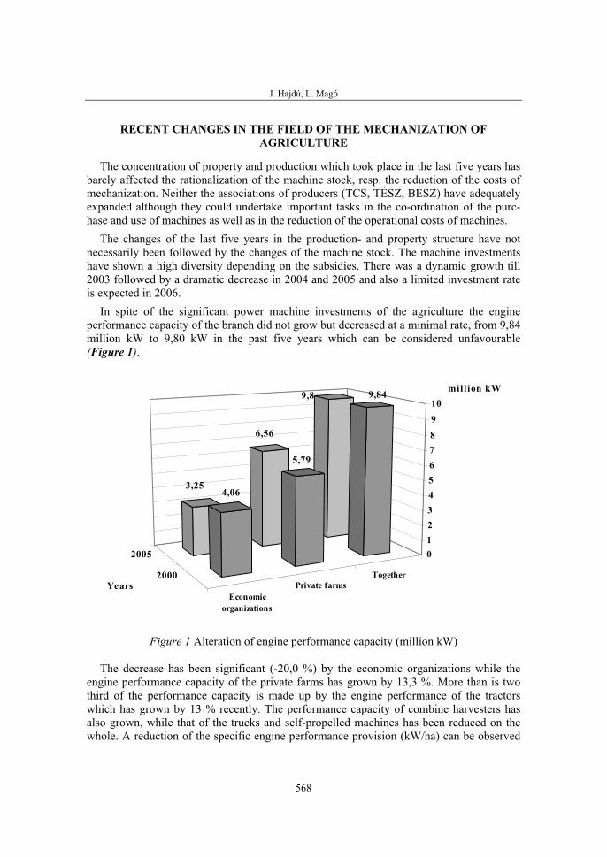
J. Hajdú, L. Magó
568
RECENT CHANGES IN THE FIELD OF THE MECHANIZATION OF AGRICULTURE
The concentration of property and production which took place in the last five years has barely affected the rationalization of the machine stock, resp. the reduction of the costs of mechanization. Neither the associations of producers (TCS, TÉSZ, BÉSZ) have adequately expanded although they could undertake important tasks in the co-ordination of the purc-hase and use of machines as well as in the reduction of the operational costs of machines.
The changes of the last five years in the production- and property structure have not necessarily been followed by the changes of the machine stock. The machine investments have shown a high diversity depending on the subsidies. There was a dynamic growth till 2003 followed by a dramatic decrease in 2004 and 2005 and also a limited investment rate is expected in 2006.
In spite of the significant power machine investments of the agriculture the engine performance capacity of the branch did not grow but decreased at a minimal rate, from 9,84 million kW to 9,80 kW in the past five years which can be considered unfavourable (Figure 1).
Economicorganizations
Private farmsTogether2000
2005
9,8
6,56
3,25
9,84
5,79
4,06
012345678910
million kW
Years
Figure 1 Alteration of engine performance capacity (million kW)
The decrease has been significant (-20,0 %) by the economic organizations while the engine performance capacity of the private farms has grown by 13,3 %. More than is two third of the performance capacity is made up by the engine performance of the tractors which has grown by 13 % recently. The performance capacity of combine harvesters has also grown, while that of the trucks and self-propelled machines has been reduced on the whole. A reduction of the specific engine performance provision (kW/ha) can be observed
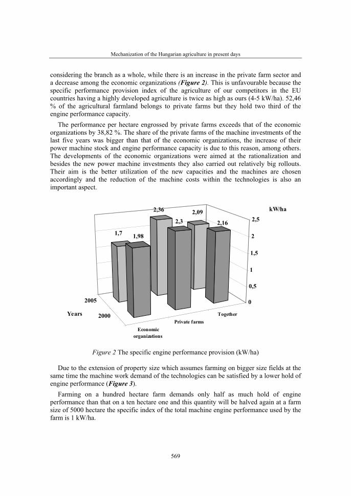
Mechanization of the Hungarian agriculture in present days
569
considering the branch as a whole, while there is an increase in the private farm sector and a decrease among the economic organizations (Figure 2). This is unfavourable because the specific performance provision index of the agriculture of our competitors in the EU countries having a highly developed agriculture is twice as high as ours (4-5 kW/ha). 52,46 % of the agricultural farmland belongs to private farms but they hold two third of the engine performance capacity.
The performance per hectare engrossed by private farms exceeds that of the economic organizations by 38,82 %. The share of the private farms of the machine investments of the last five years was bigger than that of the economic organizations, the increase of their power machine stock and engine performance capacity is due to this reason, among others. The developments of the economic organizations were aimed at the rationalization and besides the new power machine investments they also carried out relatively big rollouts. Their aim is the better utilization of the new capacities and the machines are chosen accordingly and the reduction of the machine costs within the technologies is also an important aspect.
Economicorganizations
Private farmsTogether2000
2005
2,092,36
1,7
2,162,3
1,98
0
0,5
1
1,5
2
2,5
kW/ha
Years
Figure 2 The specific engine performance provision (kW/ha)
Due to the extension of property size which assumes farming on bigger size fields at the same time the machine work demand of the technologies can be satisfied by a lower hold of engine performance (Figure 3).
Farming on a hundred hectare farm demands only half as much hold of engine performance than that on a ten hectare one and this quantity will be halved again at a farm size of 5000 hectare the specific index of the total machine engine performance used by the farm is 1 kW/ha.

J. Hajdú, L. Magó
570
0
1 000
2 000
3 000
4 000
5 000
6 000
0,1-1 1,1-10 10,1-50 50,1-100
100,1-500
500,1-1000
1000,1-5000
>5000
In case of property with own farmland (ha)
kW/1
000
ha
Tractors
Trucks
Combine-harvesters
Other self-propelled machines
Power machines together
Figure 3 The specific quantity of power machine stock by booster branches according to GSZÖ 2005
Economicorganizations
Private farmsTogether2000
2005
120479
96922
23557
113306
87107
26190
0
20000
40000
60000
80000
100000
120000
140000
pieces
Years
Figure 4 The alteration of tractor stock (pc)
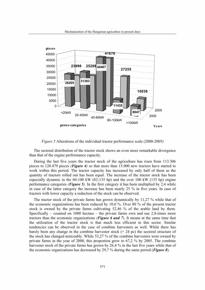
Mechanization of the Hungarian agriculture in present days
571
<20kW20-40kW
40-60kW60-100kW
>100kW
2000
2005
23998 25288
41676
27255
10036
28205 31383
44467
11435
8047
05000
10000
15000
20000
25000
30000
35000
40000
45000
pieces
power-categories Years
Figure 5 Alterations of the individual tractor performance scale (2000-2005)
The sectoral distribution of the tractor stock shows an even more remarkable divergence than that of the engine performance capacity.
During the last five years the tractor stock of the agriculture has risen from 113.306 pieces to 120.479 pieces (Figure 4) so that more than 15.000 new tractors have started to work within this period. The tractor capacity has increased by only half of them as the quantity of tractors rolled out has been equal. The increase of the tractor stock has been especially dynamic in the 60-100 kW (82-135 hp) and the over 100 kW (135 hp) engine performance categories (Figure 5). In the first category it has been multiplied by 2,4 while in case of the latter category the increase has been nearly 25 % in five years. In case of tractors with lower capacity a reduction of the stock can be observed.
The tractor stock of the private farms has grown dynamically by 11,27 % while that of the economic organizations has been reduced by 10,0 %. Over 80 % of the present tractor stock is owned by the private farms cultivating 52,46 % of the arable land by them. Specifically – counted on 1000 hectare – the private farms own and use 2,8-times more tractors than the economic organizations (Figure 6 and 7). It means at the same time that the utilization of the tractor stock is that much less efficient in this sector. Similar tendencies can be observed in the case of combine harvesters as well. While there has barely been any change in the combine harvester stock (+ 24 pc) the sectoral structure of the stock has changed noticeably. While 53,27 % of the combine harvesters were owned by private farms in the year of 2000, this proportion grew to 67,2 % by 2005. The combine harvester stock of the private farms has grown by 26,4 % in the last five years while that of the economic organizations has decreased by 29,7 % during the same period (Figure 8).
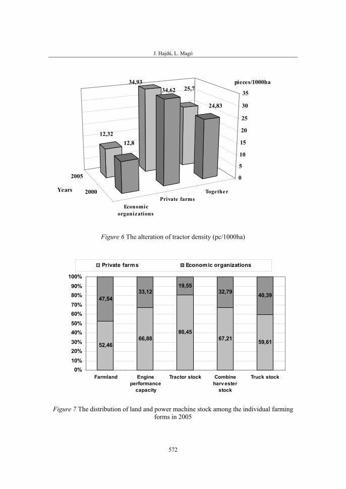
J. Hajdú, L. Magó
572
Economicorganizations
Private farmsTogether2000
2005
25,734,93
12,32
24,83
34,62
12,8
0
5
10
15
20
25
30
35
pieces/1000ha
Years
Figure 6 The alteration of tractor density (pc/1000ha)
52,4666,88
80,4567,21 59,61
47,5433,12
19,5532,79 40,39
0%10%20%30%40%50%60%70%80%90%
100%
Farmland Engineperformance
capacity
Tractor stock Combineharv ester
stock
Truck stock
Private farms Economic organizations
Figure 7 The distribution of land and power machine stock among the individual farming forms in 2005

Mechanization of the Hungarian agriculture in present days
573
Economicorganizations
Private farmsTogether2000
2005
12137
8157
3980
12113
6453
5660
0
2000
4000
6000
8000
10000
12000
14000
pieces
Years
Figure 8 The alteration of combine harvester stock (pc)
It must be taken into consideration by the changes that the higher performance combine harvesters have represented a dominating proportion in the machine investments of the economic organizations while by the private farms preference has been given to the small and medium performance combines matching their territorial aptitudes.
In case of tractors there is also a difference in the performance to be observed between private farms and economic organizations. The average tractor engine performance has risen from 51,9 kW/pc. (70,6 hp) to 55,1 kW/pc. (74,9 hp) which means a 6,15 % increase.
In the tractor stock of private farms the average tractor engine performance increase has been 9,25 % while in case of economic organizations a more moderate growth is to be observed.
The engine performance of the average tractor used by the economic organizations having a bigger average property size (443,6 ha) is 78,1 kW (106,2 hp) nowadays, while the engine performance of the average tractor of the private farms is 49,6 kW (67,5 hp) (Figure9).
With the higher performance tractors the economic organizations are able to carry out the machine works more efficiently and the bigger field sizes also contribute to this.
Considering tractor scale property sizes differentiate. By the 10 hectare farms the tractors with a performance of 20-40 kW (27-55 hp) prevail, by the 50 hectare ones that of 40-60 kW (55-82 hp) performance and by the ones between 100 and 500 hectare the majority of the tractors have an engine performance of 60 to 100 kW (82-135 hp) resp. of

J. Hajdú, L. Magó
574
over 100 kW (135 hp) while in case of properties over 1000 hectare the engine performance of most of the tractors is over 100 kW (135 hp) (Husti 2006), (Magó 2007). [4, 6]
Economicorganizations
Private farmsTogether2000
2005
55,1
49,6
78,1
51,9
45,4
73,6
0
10
20
30
40
50
60
70
80
kW/pieces
Years
Figure 9 The alteration of average tractor engine performance (kW/pc)
According to the property scales registrated by the KSH there are even more remarkable disproportions in the field of engine performance blocking and tractor utilization. In case of property sizes between 1000 and 5000 hectare 660 kW tractor engine performance per 1000 hectare resp. 1188 kW total power machine performance serves the production, while in case of property sizes between 1 and 10 hectare these engine performance values mean 3681 kW tractor resp. 4687 kW total power machine performance per 1000 hectare.
On the basis of the above figures a quadruple-quintuple difference between the specific engine performance blocking of the two property sizes can be demonstrated.
CONCLUSIONS
One of the most important conditions of economical and cost-sparing machine utilization is an appropriate future property concentration which enables the machines to work more efficiently.
Several solutions of property concentration can be taken into consideration, the purchase of property parts, association of economic organizations, or virtually created concentrations of production.
Mechanization of the Hungarian agriculture in present days
575
The European Agricultural Found for Rural Development – EAFRD application structure starting now should also advance that machine investments serve the purpose of modernization, increasing efficiency, structural reform and the increasing competitiveness of production.
REFERENCES
1. Baranyai Zs., Takács I.: (2007) Change of Efficiency of Assets and Equipment in the Hungarian Agriculture (1972-2005), 31st Conference on R&D in Agricultural Engineering, Gödöllő, 2007. January. 23. Proceedings Vol. 3. p. 28-32.
2. Hajdú J., Gockler L. (2005): Relationship between Farm Size and Mechanisation, Hungarian Agricultural Engineering, Periodical of the Committee of Agricultural Engineering of the Hungarian Academy of Sciences, Vol. 18/2005. p. 50-54.
3. Husti I. (2000): Technological development and sustainability in the Hungarian Agriculture. Bulletin of the Szent István University, Gödöllő, 1997 - 2000. p. 241-255.
4. Husti I.: (2006) Problems and Tasks in the Mechanisation of Small and Medium-Size Farms in Hungary, Proceedings of the 34th International Symposium “Actual Tasks on Agricultural Engineering”, Opatija, Croatia, 21-24. February 2006. Proc. p. 445-455.
5. Magó L.: (2004) Farm Machinery Fleet Planning Concerning Machinery Utilization, Proceedings of the 62nd International Conference Agricultural Engineering “Innovation and Integration”, Technical University Dresden, Germany, 07-08. October 2004. VDI Berichte 1855. Düsseldorf: VDI-Verlag, p. 265-273.
6. Magó L.: (2007) Survey of the Present Mechanization of Small and Medium Size Plant Production Farms, Proceedings of the 35th International Symposium “Actual Tasks on Agricultural Engineering”, Opatija, Croatia, 19-23. February 2007. Proc. p. 497-506.

36. Symposium "Actual Tasks on Agricultural Engineering", Opatija, Croatia, 2008.
577
36.
SIMPOZIJAKTUALNI ZADACIMEHANIZACIJE POLJOPRIVREDE
UDC65.011.4:633.1:633.85
Stručni radExpert paper
RATIONALIZATION OF CEREAL AND OIL CROPS DELIVERY PROCESS BY MEANS OF
QUEUING MODELS GORDANA DUKIĆ1, DAVORIN TURKALJ2
1ABACUS Tuition, Research and Business Consultancy, Mosorska 8, 31000 Osijek, Croatia
2University of Josip Juraj Strossmayer in Osijek, Faculty of Agriculture, Department of Agroeconomics, Trg Sv. Trojstva 3, 31000 Osijek, Croatia
SUMMARY
Improved organization and management could save significant financial resources and time in a number of farmer activities. The process of cereal and oil crops delivery into the crop purchase system after harvesting is certainly one of these situations. As a rule, in this period there are long lines of trucks and tractors with trailers at delivery spots, forming queues. By keeping agricultural machinery too long at crop delivery spots, harvesting and other activities are put on hold. Because of such delays, there is a risk of bad weather having a negative impact on the harvest as well. The irritating aspect of waiting is a particular problem. All these issues have necessitated the rationalization of delivery in the crop purchase system. With this aim in mind, this paper presents theoretically and on a hypothetical example the procedure of designing and solving the queuing model with multiple phase system. Its application presupposes that the arrival distribution of vehicles used for cereal and oil crops transport follows the Poisson distribution. It is further assumed that the random variable representing service time has the exponential distribution. The problem under scrutiny here is formulated as a model consisting of several consecutive and independent queuing models, and each of them can have one or more servers. Although the obtained results are of a descriptive character, they will enable managers to comprehend more clearly the queuing problem and take steps that will improve the process of crop delivery and purchase after harvesting. The proposed model is component of decision support system in cereal and oil crops delivery process.
Key words: queuing models, process of crop delivery, rationalization, decision support system
G. Dukić, D. Turkalj
578
INTRODUCTION
Agricultural works carried out within cereal production are subject to natural course of particular development phases of plant crops, and have to be finalized within a relatively short time span. Their realization is greatly influenced by weather conditions, frequently limiting the time during which a certain activity needs to be carried out. In such circumstances, it is desirable to make optimum use of the time at our disposal. To do that, efforts should be made to achieve good planning and organization of agricultural machinery and processes where it is used. In this way, significant financial means can be saved, and unnecessary time wasting can be shortened.
The process of cereal and oil crops delivery, i.e. crop purchase after harvesting is certa-inly one of the areas where queuing problems are particularly prominent. As a rule, in this period there are long lines of trucks and tractors with trailers at delivery spots, forming queues, especially in those parts of Croatia with favourable natural conditions for growing plant crops. By keeping people and machinery too long at crop delivery spots, harvesting and other activities are put on hold. Because of such delays, there is a risk of bad weather having a negative impact on the harvest as well. The irritating aspect of waiting is a particular problem.
By using adequate queuing models it is possible to achieve significant rationalization of delivery in the crop purchase system. Since this system consists of several phases, this paper presents theoretically and on a hypothetical example the procedure of designing and solving the queuing model with multiple phase system. The first phase is the arrival to the check-in booth where adequate forms are filled in and samples are taken for control. Weighing of loaded vehicles is performed in the second phase. After that, their freight is unloaded at a designated unloading spot. The whole process is finished by weighing of an empty vehicle in order to determine the weight of the delivered crops. In each of the above phases, there is a waiting line in front of the server. The longest line of vehicles is formed in front of the check-in booth, and during busiest times it can be several kilometres long. The waiting line for weighing of loaded tractors with trailers and trucks consists of only several vehicles, depending on the available space. The unloading phase can consist of only one server and a single queue, which is characteristic for small-scale crop purchasing units, or alternatively, there can be multiple servers. If there are multiple unloading spots, it is possible to separately accept and categorize cereal and oil crops by type and adequate criteria, such as moisture content and purity. In this phase, the queue length again depends on the space designated for waiting, but also on the unloading process itself. If unloading time is for some reason prolonged, full vehicles will be kept longer at weighing spots, as well as in front of check-in booths. In general, there is no significant waiting in the last phase, which is weighing of empty vehicles.
Managing the cereal and oil crops delivery system after harvesting is the responsibility of service provider, i.e. a business operator in charge of crop purchasing. It is in their best interest to undertake all the necessary activities to improve the system. Namely, poor organization of the server process does not only increase direct operation costs for a particular business unit, but reflects also on increased opportunity costs. They occur when potential customers give up the delivery of their harvest at a particular place because the waiting is too long, and go with their cereal and oil crops to another purchasing unit. It
Rationalization of cereal and oil crops delivery process by means of queuing models
579
follows from the above that the analysis of queues, which appear in the crop purchasing system, is important from the standpoint of farmers as service users, but also from the standpoint of business operators as service providers.
METHODS
With the aim of improving the process of crops delivery after harvesting, this paper has assumed the queuing model with multiple phase system. Its specific feature is combining several consecutive and independent queuing models with one or multiple servers. Key parameters of the queuing model represent the expected values of adequate probability distributions. For this reason, the model analyzed here belongs to the group of stochastic models. Since the determined parameters are not changed during determination process for one set of solutions, such models are also viewed as static. The model presented in this paper is component of decision support system in cereal and oil crops delivery process.
CHARACTERISTICS AND ELEMENTS OF THE QUEUING MODEL
Queuing models represent a quantitative management support. The main characteristic of such models is that their solution does not actually yield an optimum solution for the problem under scrutiny; rather, they describe the expected system behaviour through estimated parameters. Thus, possible solutions are arrived at by examining the effect of changes in input parameters, such as mean arrival rate and mean service rate. Ultimately, the manager has to decide which solution should be implemented in a particular situation.
Here are the basic elements of a queuing system: calling source, customer arrivals, wait-ing line, processing order, service and leaving the system. Calling source is represented by all the potential users of a specific service at the analyzed service spot. If there are no restrictions regarding the new customer access, we speak about an infinite source. If there are such restrictions, the calling source is defined as finite. Customer arrivals, i.e. farmers who want to receive a certain service, is the next element of the queuing system. The arrival rate variability often follows a Poisson distribution. Its parameter λ designates the mean arrival rate. If the arrivals distribution does not have the features of the stated theoretical distribution, it is necessary to use an adequate non-Poisson model or a simulation model in the analysis. The waiting line in front of the service spot depends on the customer arrival rate and the speed of service. The expected number of customers in line and the mean waiting time are the solutions of the analyzed issue. Queue length and time of waiting can be influenced by the number of servers. However, a significant improvement in the perception of waiting can be achieved by certain activities aimed at grabbing the attention of customers waiting in line. Processing order is the activity directly preceding the service itself. The processing order can be decided along various principles. Thus, for example, customers can be served according to the sequence of arrival (general discipline), or according to priority principle. Service is the fifth element in the queuing system. Queues can have one or more servers, and service can consist of a single or multiple phases or steps. It is generally assumed that service time follows an exponential distribution. In this

G. Dukić, D. Turkalj
580
case, parameter μ designates the mean service rate. After leaving the system a customer can return to the calling source or abandon it permanently.
The shape of arrivals and service time distributions, the number of parallel servers, the service discipline, the maximum number allowed in the system and the size of calling source are the criteria for the classification of queuing models. Taking into account the stated features, and aiming at simplicity and good overview, queuing models are designated by Kendall notation, whose basic form is (a/b/c):(d/e/f). The symbols are interpreted in the following way:
a - arrivals distributions (M if Poisson)b - service t ime distribution (M if exponential) c - number of parallel servers d - service discipline (GD if general discipline) e - maximum number allowed in system f - size of calling source
The basic parameters of queuing models are the mean arrival rate λ and mean service rate μ.. In addition, several other parameters need to be defined when posing the problem, such as the number of servers, the number of customers giving up the service and the available waiting places. By solving the model, we arrive at the expected number of customers in the queue and in the system, and the expected waiting time in the queue and in the system. If necessary, we can also calculate the probability of n units in the system, the probability that an arrival will have no wait for service, the probability that there will be no more than n customers in the line, etc.
QUEUING MODEL WITH MULTIPLE PHASE SYSTEM
A queuing system with two or more consecutive phases of service is called a serial system. To receive a service in such a system, a customer has to go through all the phases before leaving the system. This is exactly characteristic of the cereal and oil crops delivery process after harvesting. In the queuing model presented in this paper, which will indicate how the process could be rationalized, it will be assumed that the arrival rate follows a Poisson distribution, whereas service time follows an exponential distribution.
The model with a series of k service phases can also be understood as several consecutive and independent queuing models with one (M/M/1):(GD/∞/∞) or several (M/M/c):(GD/∞/∞) servers.
ARRIVALS Service phase 1 Service phase 2 Service phase k EXIT
(M /M /1):(GD/1 1
(M /M /c ):(GD/1 1 1
∞ ∞/ )or
∞ ∞/ )
(M /M /1):(GD/2 2
(M /M /c ):(GD/2 2 2
∞ ∞/ )or
∞ ∞/ )
(M /M /1):(GD/k k
(M /M /c ):(GD/k k k
∞ ∞/ )or
∞ ∞/ )
...
Figure 1 Queuing model with a series of k service phases
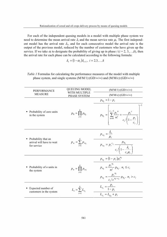
Rationalization of cereal and oil crops delivery process by means of queuing models
581
For each of the independent queuing models in a model with multiple phase system we need to determine the mean arrival rate λi and the mean service rate μi. The first independ-ent model has the arrival rate λ1, and for each consecutive model the arrival rate is the output of the previous model, reduced by the number of customers who have given up the service. If we take αi to designate the probability of giving up in phase i (i = 2, 3,…,k), then the arrival rate for each phase can be calculated according to the following formula:
( ) 11 −−= iii λαλ , k,,,i …32=
Table 1 Formulas for calculating the performance measures of the model with multiple phase system, and single systems (M/M/1):(GD/∞/∞) and (M/M/c):(GD/∞/∞)
(M/M/1):(GD/∞/∞)PERFORMANCEMEASURE
QUEUING MODEL WITH MULTIPLEPHASE SYSTEM (M/M/c):(GD/∞/∞)
ii pp −= 10
� Probability of zero units in the system ∏
==
k
iipp
100
1
1
00
1
−
−
=
⎥
⎥
⎥
⎥
⎥
⎦
⎤
⎢
⎢
⎢
⎢
⎢
⎣
⎡
⎟⎟
⎠
⎞
⎜⎜
⎝
⎛
−+= ∑
ic
n
i
ii
ci
ni
i
cp
!c
p!n
pp
i
iiwp
μλ
=� Probability that an
arrival will have to wait for service
∑
==
k
iiww pp
1
⎟⎟
⎠
⎞
⎜⎜
⎝
⎛
−=
ii
ii
iiciiw
c!c
ppp
μλ
1
0
( ) iniiin ppp −= 1
� Probability of n units in the system ∏
==
k
iinn pp
1
iii
ini
in cn,p!n
pp ≤= 0
iiiicini
ini
in cn,pc!cp
p >= − 0
i
is p
pLi −
=1� Expected number of
customers in the system ∑
==
k
iss i
LL1
iiqs pLLi
+=
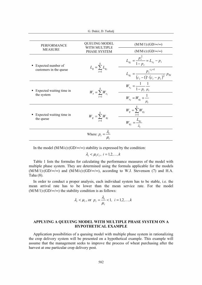
G. Dukić, D. Turkalj
582
(M/M/1):(GD/∞/∞)PERFORMANCEMEASURE
QUEUING MODEL WITH MULTIPLE PHASE SYSTEM (M/M/c):(GD/∞/∞)
iisi
iiq pL
pp
L −=−
=1
2
� Expected number of customers in the queue ∑
==
k
iqq i
LL1
( ) ( ) iiii
ici
iq ppc!c
pL 02
1
1 −⋅−=
+
iis
μpW
i
11
1−
=� Expected waiting time in
the system ∑
==
k
iss i
WW1
iiqis
μ
WW 1+=
∑
==
k
iiqq WW
1� Expected waiting time in
the queue ∑
==
k
iiqq WW
1
i
iqiq
λ
LW =
Where:i
iip
μλ=
In the model (M/M/c):(GD/∞/∞) stability is expressed by the condition:
iii cμλ < , k,,,i …21=
Table 1 lists the formulas for calculating the performance measures of the model with multiple phase system. They are determined using the formula applicable for the models (M/M/1):(GD/∞/∞) and (M/M/c):(GD/∞/∞), according to W.J. Stevenson (7) and H.A. Taha (8).
In order to conduct a proper analysis, each individual system has to be stable, i.e. the mean arrival rate has to be lower than the mean service rate. For the model (M/M/1):(GD/∞/∞) the stability condition is as follows:
ii μλ < , or ,pi
ii 1<=
μλ
k,,,i …21=
APPLYING A QUEUING MODEL WITH MULTIPLE PHASE SYSTEM ON A HYPOTHETICAL EXAMPLE
Application possibilities of a queuing model with multiple phase system in rationalizing the crop delivery system will be presented on a hypothetical example. This example will assume that the management seeks to improve the process of wheat purchasing after the harvest at one particular crop delivery post.
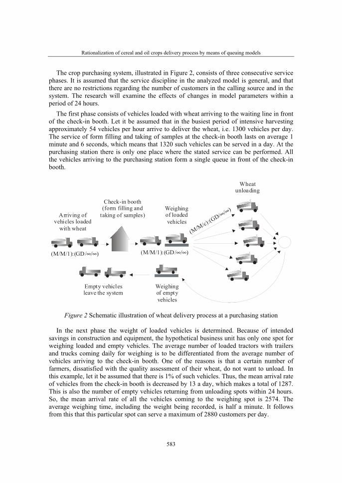
Rationalization of cereal and oil crops delivery process by means of queuing models
583
The crop purchasing system, illustrated in Figure 2, consists of three consecutive service phases. It is assumed that the service discipline in the analyzed model is general, and that there are no restrictions regarding the number of customers in the calling source and in the system. The research will examine the effects of changes in model parameters within a period of 24 hours.
The first phase consists of vehicles loaded with wheat arriving to the waiting line in front of the check-in booth. Let it be assumed that in the busiest period of intensive harvesting approximately 54 vehicles per hour arrive to deliver the wheat, i.e. 1300 vehicles per day. The service of form filling and taking of samples at the check-in booth lasts on average 1 minute and 6 seconds, which means that 1320 such vehicles can be served in a day. At the purchasing station there is only one place where the stated service can be performed. All the vehicles arriving to the purchasing station form a single queue in front of the check-in booth.
Arriving of vehicles loaded
with wheat
Empty vehiclesleave the system
Check-in booth(form filling and
taking of samples)Weighing of loadedvehicles
Wheat unloading
Weighingof emptyvehicles
(M/M/1):(GD/∞ ∞)/
(M/M/c):(GD/∞ ∞)/
(M/M/1):(GD/∞ ∞)/
Figure 2 Schematic illustration of wheat delivery process at a purchasing station
In the next phase the weight of loaded vehicles is determined. Because of intended savings in construction and equipment, the hypothetical business unit has only one spot for weighing loaded and empty vehicles. The average number of loaded tractors with trailers and trucks coming daily for weighing is to be differentiated from the average number of vehicles arriving to the check-in booth. One of the reasons is that a certain number of farmers, dissatisfied with the quality assessment of their wheat, do not want to unload. In this example, let it be assumed that there is 1% of such vehicles. Thus, the mean arrival rate of vehicles from the check-in booth is decreased by 13 a day, which makes a total of 1287. This is also the number of empty vehicles returning from unloading spots within 24 hours. So, the mean arrival rate of all the vehicles coming to the weighing spot is 2574. The average weighing time, including the weight being recorded, is half a minute. It follows from this that this particular spot can serve a maximum of 2880 customers per day.
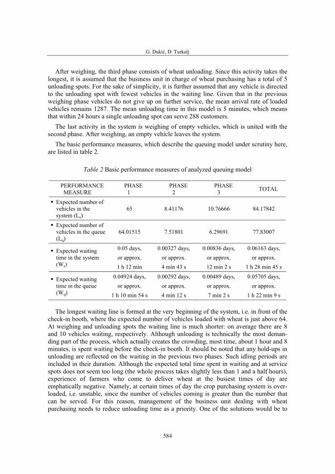
G. Dukić, D. Turkalj
584
After weighing, the third phase consists of wheat unloading. Since this activity takes the longest, it is assumed that the business unit in charge of wheat purchasing has a total of 5 unloading spots. For the sake of simplicity, it is further assumed that any vehicle is directed to the unloading spot with fewest vehicles in the waiting line. Given that in the previous weighing phase vehicles do not give up on further service, the mean arrival rate of loaded vehicles remains 1287. The mean unloading time in this model is 5 minutes, which means that within 24 hours a single unloading spot can serve 288 customers.
The last activity in the system is weighing of empty vehicles, which is united with the second phase. After weighing, an empty vehicle leaves the system.
The basic performance measures, which describe the queuing model under scrutiny here, are listed in table 2.
Table 2 Basic performance measures of analyzed queuing model
PERFORMANCEMEASURE
PHASE1
PHASE2
PHASE3 TOTAL
� Expected number of vehicles in the system (Ls)
65 8.41176 10.76666 84.17842
� Expected number of vehicles in the queue (Lq)
64.01515 7.51801 6.29691 77.83007
� Expected waiting time in the system (Ws)
0.05 days,or approx. 1 h 12 min
0.00327 days,or approx. 4 min 43 s
0.00836 days,or approx. 12 min 2 s
0.06163 days,or approx.
1 h 28 min 45 s
� Expected waiting time in the queue (Wq)
0.04924 days,or approx.
1 h 10 min 54 s
0.00292 days,or approx. 4 min 12 s
0.00489 days,or approx. 7 min 2 s
0.05705 days,or approx.
1 h 22 min 9 s
The longest waiting line is formed at the very beginning of the system, i.e. in front of the check-in booth, where the expected number of vehicles loaded with wheat is just above 64. At weighing and unloading spots the waiting line is much shorter: on average there are 8 and 10 vehicles waiting, respectively. Although unloading is technically the most deman-ding part of the process, which actually creates the crowding, most time, about 1 hour and 8 minutes, is spent waiting before the check-in booth. It should be noted that any hold-ups in unloading are reflected on the waiting in the previous two phases. Such idling periods are included in their duration. Although the expected total time spent in waiting and at service spots does not seem too long (the whole process takes slightly less than 1 and a half hours), experience of farmers who come to deliver wheat at the busiest times of day are emphatically negative. Namely, at certain times of day the crop purchasing system is over-loaded, i.e. unstable, since the number of vehicles coming is greater than the number that can be served. For this reason, management of the business unit dealing with wheat purchasing needs to reduce unloading time as a priority. One of the solutions would be to
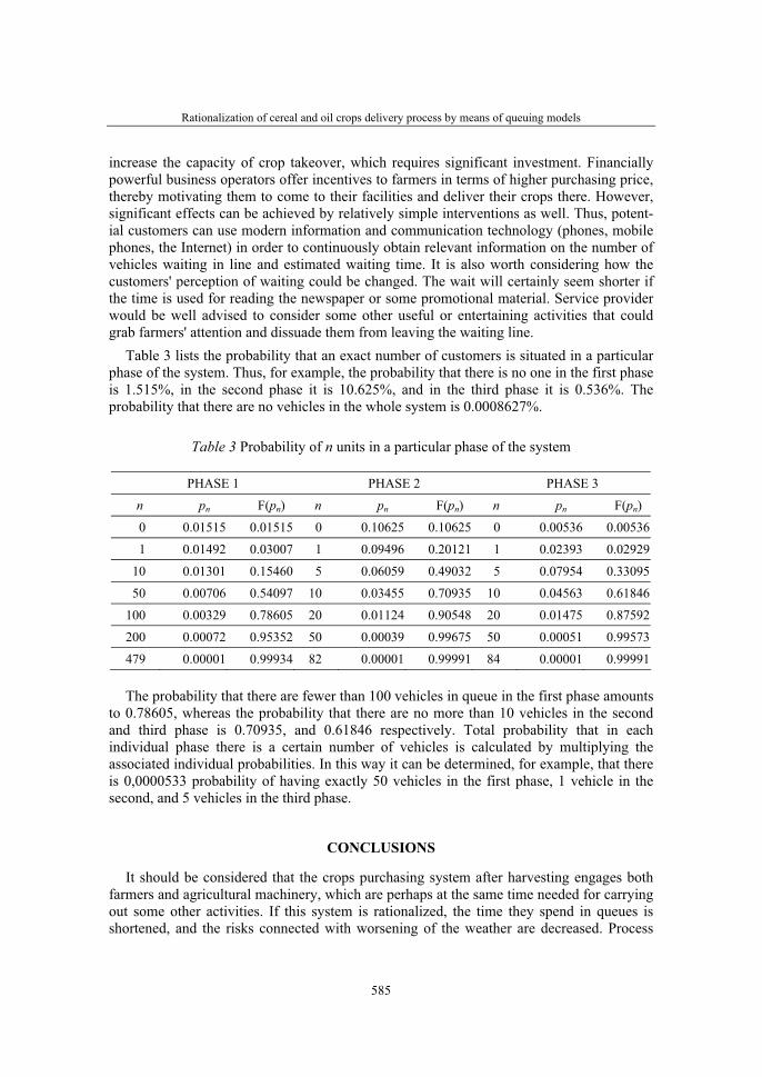
Rationalization of cereal and oil crops delivery process by means of queuing models
585
increase the capacity of crop takeover, which requires significant investment. Financially powerful business operators offer incentives to farmers in terms of higher purchasing price, thereby motivating them to come to their facilities and deliver their crops there. However, significant effects can be achieved by relatively simple interventions as well. Thus, potent-ial customers can use modern information and communication technology (phones, mobile phones, the Internet) in order to continuously obtain relevant information on the number of vehicles waiting in line and estimated waiting time. It is also worth considering how the customers' perception of waiting could be changed. The wait will certainly seem shorter if the time is used for reading the newspaper or some promotional material. Service provider would be well advised to consider some other useful or entertaining activities that could grab farmers' attention and dissuade them from leaving the waiting line.
Table 3 lists the probability that an exact number of customers is situated in a particular phase of the system. Thus, for example, the probability that there is no one in the first phase is 1.515%, in the second phase it is 10.625%, and in the third phase it is 0.536%. The probability that there are no vehicles in the whole system is 0.0008627%.
Table 3 Probability of n units in a particular phase of the system
PHASE 1 PHASE 2 PHASE 3
n pn F(pn) n pn F(pn) n pn F(pn)
0 0.01515 0.01515 0 0.10625 0.10625 0 0.00536 0.00536
1 0.01492 0.03007 1 0.09496 0.20121 1 0.02393 0.02929
10 0.01301 0.15460 5 0.06059 0.49032 5 0.07954 0.33095
50 0.00706 0.54097 10 0.03455 0.70935 10 0.04563 0.61846
100 0.00329 0.78605 20 0.01124 0.90548 20 0.01475 0.87592
200 0.00072 0.95352 50 0.00039 0.99675 50 0.00051 0.99573
479 0.00001 0.99934 82 0.00001 0.99991 84 0.00001 0.99991
The probability that there are fewer than 100 vehicles in queue in the first phase amounts to 0.78605, whereas the probability that there are no more than 10 vehicles in the second and third phase is 0.70935, and 0.61846 respectively. Total probability that in each individual phase there is a certain number of vehicles is calculated by multiplying the associated individual probabilities. In this way it can be determined, for example, that there is 0,0000533 probability of having exactly 50 vehicles in the first phase, 1 vehicle in the second, and 5 vehicles in the third phase.
CONCLUSIONS
It should be considered that the crops purchasing system after harvesting engages both farmers and agricultural machinery, which are perhaps at the same time needed for carrying out some other activities. If this system is rationalized, the time they spend in queues is shortened, and the risks connected with worsening of the weather are decreased. Process

G. Dukić, D. Turkalj
586
improvement can also have a significant impact on the performance of business units involved in crop purchasing. Inadequate organization of the whole system will have a direct effect on the growth of their operating costs, but also on the growth of opportunity costs, which arise when potential customers give up on delivering their cereal and oil crops because the wait is too long, and take their harvest to another purchasing facility.
The process of crop delivery after harvesting can be significantly improved by implementing adequate queuing models, which represent quantitative management support. With this aim in mind, the paper has presented and proposed a queuing model with multiple phase system, whose specific feature is the combination of several consecutive and independent queuing models with one or multiple servers. Although the obtained results are of a descriptive character, they will allow managers to comprehend more clearly the queuing problem and to estimate correctly the effects of changes in particular key parameters.
REFERENCES
1. Anderson D.R., Sweeney D.J., Williams T.A. (2003). An Introduction to Management Science: Quantitative Approaches to Decision Making, 10th Edition, West Publishing Co., St. Paul
2. Baron M. (2007). Probability and Statistics for Computer Scientists, Chapman & Hall/CRC, Boca Raton
3. Bonini C.P., Hausman W.H., Bierman H.Jr. (1997). Quantitative Analysis for Management, Ninth Edition, Irwin/McGraw-Hill, Boston
4. Ching W.K. (2001). Iterative Methods for Queuing and Manufacturing Systems (Springer Monographs in Mathematics), Springer-Verlag, London
5. Dukić G., Dukić D., Alerić I. (2006). Applying Queuing Models in the Rationalization of Usage of the Road Traffic Corridor Vc. In: Mašek A. (ed) Proceedings of 3rd International Scientific Symposium “Corridor Vc as Euro-Regional Connection on the Traffic Rout Baltic Sea - Central Europe - Adriatic Sea”, University of J.J. Strossmayer in Osijek - Faculty of Economics in Osijek, Osijek, pp 134-144
6. Meredith J.R. (1992). The Management of Operations - A Conceptual Emphasis, Fourth Edition, John Wiley & Sons, New York
7. Stevenson W.J. (1992). Introduction to Management Science, Second Edition, Irwin, Homewood
8. Taha H.A. (2003). Operations Research - An Introduction, Seventh Edition, Prentice-Hall, New York
9. Trivedi K.S. (2002). Probability and Statistics with Reliability, Queueing, and Computer Science Applications, Second Edition, John Wiley & Sons, Inc., New York
36. Symposium "Actual Tasks on Agricultural Engineering", Opatija, Croatia, 2008.
587
36.
SIMPOZIJAKTUALNI ZADACIMEHANIZACIJE POLJOPRIVREDE
UDC004.4:631.153.46
Stručni radEXpert paper
COMPUTER OPTIMIZATION OF AGRICULTURAL MACHINERY ASSIGNMENT
DARKO DUKIĆ1, IVANA ALERIĆ2
1ABACUS Tuition, Research and Business Consultancy, Mosorska 8, 31000 Osijek, Croatia
2 University of Josip Juraj Strossmayer in Osijek, Faculty of Economics, Gajev trg 7, 31000 Osijek, Croatia
SUMMARY
With a view to increasing efficiency and effectiveness, different quantitative methods and models can be applied in solving the problems related with agricultural machinery utilization. In spite of availability of state-of-the-art information and communication technologies that have made their usage much simpler and faster, decision-making based on this approach is still in its infancy in our country. This is especially noticeable with small farmers; however, the situation is far from satisfactory even with big business operators who have abundant agricultural machinery and large arable areas. In such circumstances, it is possible to significantly reduce the costs arising from different phases of land cultivation simply by proper assignment of machinery. This paper aims to present the design procedure for an agricultural machinery assignment model, which is based on computer optimization. There are numerous advantages of a model formulated in this way. In this model, the elements of efficiency matrix, which are the expected benefits from assigning a machine for a particular activity, are obtained by scoring according to set criteria. If it proves necessary, it is further possible to emphasize a factor's importance through adequate weighing. Several techniques have been developed for solving the assignment problem. Given the variety of program applications, the model presented here was defined and resolved as a linear programming problem.
Key words: computer optimization, assignment model, increasing efficiency and effectiveness, decision-making
D. Dukić, I. Alerić
588
INTRODUCTION
The assignment problem appears in performing different business activities. As their volume and complexity increase, the process of establishing the optimum schedule of engaging human and technical resources becomes increasingly challenging, and the effectiveness of using an intuitive approach to these tasks goes down dramatically. In farm production, the issue of adequate assignment of agricultural machinery acquires a special dimension. In addition to the characteristics of available human and technical resources, farming requires people to take into account a number of other relevant factors. First of all, farmers have a limited time span within which they have to complete different operations related to cultivation of certain field crops. Delays in any of the farming jobs such as fertilization, ploughing, sowing, plant protection (from diseases, pests, and weeds), cultivation, dressing, harvesting, crop transport, can all significantly decrease the yields, and thus farmers' income. Unfavourable weather conditions can make it even more difficult to plan particular activities. In addition, when composing an optimum assignment set, one must take into account soil characteristics, field size and distance from the place where agricultural machinery is situated. Given these complex conditions, having adequate knowledge and skills, availability of necessary information and ability to grasp the problems are the basic prerequisites for making proper and timely decisions.
In trying to solve the assignment problem one can receive significant help from adequate quantitative methods and models. In spite of wide availability of advanced information and communication technologies that have simplified and speeded up the use of such methods, this type of decision-making is still insufficiently used in our country. This is especially true of smaller producers, i.e. family farms, whose owners lack the required knowledge, whereas their extension services do not provide them with necessary information and support for implementing such models. The situation in business operators that own sufficient agricultural machinery and large areas of arable land is also far from satisfactory. A correct scheme of machinery usage in different phases of field work on these big farms would certainly contribute to increased efficiency and effectiveness of their operation.
Decisions on agricultural machinery assignment based on intuitive approach can be justified only when solving very simple, routine tasks and problems. If the number of machines and jobs where they have to be used is considerable, an adequate assignment model needs to be applied. This paper presents the theoretical background, and takes a hypothetical example to explain the procedure of constructing and solving the agricultural machinery assignment model based on computer optimization. The advantages of implementing a computer assignment model are multiple. First of all, it enables the management to reduce the time required for model construction and deciding on a solution. If the results prove to be unsatisfactory, within computer models it is very simple to make the necessary changes of variables, parameters and relations, and to generate new solutions. An important feature of modern computer programs is that the problem to be solved is entered very simply, thus making them easy to use even for decision makers who do not have sophisticated computer knowledge. In order to popularize the usage of computer models, the paper presents the basic features of QSopt program package.

Computer optimization of a agricultural machinery assignment
589
METHODS
The assignment model, which belongs to the group if quantitative models, is the theoretical background for solving the problem of agricultural machinery assignment when carrying out the tasks in crop husbandry. In its basic form, the aim of solving the assignment model is to develop a set of assignments that will result in minimum total costs. If necessary, it is possible to analyze some specific cases within the assignment model, such as multiple optimal solutions, unequal numbers of machines and tasks, undesirable and not allowed matches, and maximization problem. Since the proposed model defines the efficiency matrix, the goal of model solution is to determine an assignment set with maximum total effects of assigning particular machines to particular tasks. The elements of efficiency matrix actually represent the expected benefits arising from the assignment of each individual machine to certain agricultural activities. They are the result of scoring carried out according to the criteria established by the decision maker. When determining these elements, it is possible to give particular weight and thus stress the importance of particular factors included in the model.
Several techniques can be used for solving the assignment problem. In this paper, the analyzed issue of agricultural machinery assignment is defined as a linear programming model. A number of computer applications have been developed as support in solving these models, and one of them being the program package QSopt. Qsopt was used to solve the problem posed in our hypothetical example. Starting with the advantages of using such programs and modern information and communication technologies, the paper emphasizes the usage value of the concept of computer optimization of the assignment problem.
ASSIGNMENT PROBLEM FORMULATION
In the assignment model it is assumed that it is necessary to achieve optimum pairing of units from one group with units from another group. The condition is that each unit from one group can be paired with only one unit from another group. A typical example would be assigning m machines to n jobs. The aim is to devise an assignment plan that will result in minimum total losses or maximum total efficiency. This is why it is necessary to determine the amount of unit losses, i.e. unit efficiencies for each assignment. On the basis of such data it is possible to formulate a table of losses, i.e. efficiency, table 1.
A machine i does the job j at a unit loss (cost), i.e. at a unit efficiency cij. To solve the problem, we must have m=n. If m>n, we need to add a fictitious column, or columns. In case of m<n, we add a fictitious row, or rows into the model. Unit losses, i.e. unit efficiencies of fictitious rows and columns have the value of 0. This means that e.g. the machine to which a fictitious column was assigned will remain idle. Since each machine can be assigned only one job, the sums of all rows and all columns must be equal to 1.
A set of assignments that results in minimum total losses, i.e. maximum total efficiency can be determined in the following way: first all possible pairs are determined, and then those pairs are singled out for which the defined goal has been achieved. This procedure, however, requires us to determine the assignments for each possible solution set. As there are n! of such sets, this would be a huge task. An illustrative example is the case of analyzing the problem of assigning 10 machines to 10 jobs: in this particular case there are
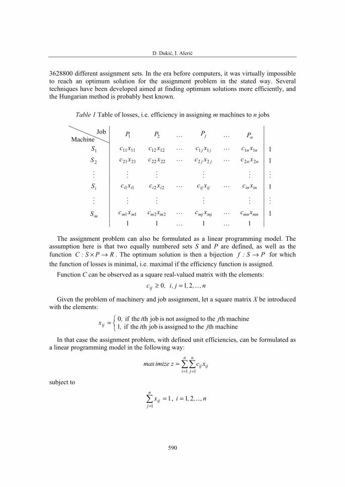
D. Dukić, I. Alerić
590
3628800 different assignment sets. In the era before computers, it was virtually impossible to reach an optimum solution for the assignment problem in the stated way. Several techniques have been developed aimed at finding optimum solutions more efficiently, and the Hungarian method is probably best known.
Table 1 Table of losses, i.e. efficiency in assigning m machines to n jobs
JobMachine 1P 2P … jP … nP
1S 1111xc 1212 xc … jj xc 11 … nn xc 11 1
2S 2121xc 2222 xc … jj xc 22 … nn xc 22 1...
......
. .. . ..
... iS 11 ii xc 22 ii xc … ijij xc … inin xc 1
......
... . ..
. .....
mS 11 mm xc 22 mm xc … mjmj xc … mnmnxc 1 1 1 … 1 … 1
The assignment problem can also be formulated as a linear programming model. The assumption here is that two equally numbered sets S and P are defined, as well as the function RPS:C →× . The optimum solution is then a bijection PS:f → for which the function of losses is minimal, i.e. maximal if the efficiency function is assigned.
Function C can be observed as a square real-valued matrix with the elements: ,cij 0≥ n...,,,j,i 21=
Given the problem of machinery and job assignment, let a square matrix X be introduced with the elements:
⎩
⎨
⎧= machineth the toassignedisjobth theif1machineth the toassignednotisjobth theif0
ji,ji,xij
In that case the assignment problem, with defined unit efficiencies, can be formulated as a linear programming model in the following way:
∑∑
= ==
n
i
n
jijij xczimizemax
1 1
subject to
∑
==
n
jijx
11, n,,,i ...21=

Computer optimization of a agricultural machinery assignment
591
∑
==
n
iijx
11 , n,,,j ...21=
}{ ,,xij 10∈ n,,,j,i ...21=
If for any reason a particular machine cannot be assigned to do a particular job, then the variable representing such assignment is not introduced in the linear programming model.
THE PROCEDURE OF DETERMINING THE EFFICIENCY MATRIX IN THE MODEL OF AGRICULTURAL MACHINERY ASSIGNMENT
When formulating the problem of agricultural machinery assignment, it is necessary to assess the effects of assigning each particular machine to each identified job. The values obtained in this way represent the efficiency matrix elements. Since their determination is very specific, the procedure will be explained in detail below.
Let it be assumed that an agricultural business unit has n tractors which have to assign to n plough-fields. For each of the tractor systems, consisting of a tractor with its plough, the value of following indicators should be determined among other things:
• Engine power (kW) • No. of revolutions at max. power (min-1)• Specific energy (kWh/ha) • Drawbar pull (kN) • Power pull (kW) • Working width (cm)• Ploughing depth (cm) • Driving speed (km/h) • Slip of wheels (%) • Productivity (ha/h) • Fuel consumption hourly (l/h) • Specific energy (l/ha) • Fuel degree efficacy (%) • Coefficient of advantageous
Each plough-field also has a specific set of features, the following being more promi-nent:
• Size of the field (ha) • Distance of the field (km) • Soil type
D. Dukić, I. Alerić
592
• Clay content (%) • Sand content (%) • Soil moisture content (%) • Soil density (g/cm3)• Specific resistant soil (N/cm2)
When solving a concrete problem, it is necessary to include all the relevant factors in the model. After they have been established, the efficiency of assignments is determined. This is done by giving scores to each characteristic of the tractor system and the field. Thus, for example, a maximum score will be given to the tractor system with the highest produc-tivity. In contrast, a minimum score will be given to the efficiency of a tractor system with small length clutch on a very large plough-field. The total score of the assignment is finally obtained by summing up all these individual scores.
If this proves necessary, a decision maker can apply adequate weighting to emphasize the importance of a particular factor. For example, because of fuel price increase, the variable representing fuel consumption can be assigned a higher weight in the assessment process.
The efficiency matrix C is determined on the basis of the established score values of all the assignments:
⎥
⎥
⎥
⎥
⎥
⎥
⎥
⎦
⎤
⎢
⎢
⎢
⎢
⎢
⎢
⎢
⎣
⎡
=
nnnjnn
inijii
nj
nj
cccc
cccc
cccccccc
C
21
21
222221
111211
……
����
……
����
……
……
Thus, the element cij represents the efficiency of the tractor system i when carrying out the activity of ploughing on the plough-field j. In the linear programming model, the elements of the efficiency matrix represent parameters of the objective function.
AN EXAMPLE OF COMPUTER OPTIMIZATION OF AGRICULTURAL MACHINERY ASSIGNMENT
Ploughing is a crucial agro-technical activity in which significant energy values are consumed. For this reason, the management objective is to determine a set of assignments that would result in maximum overall effects. This means primarily achieving the best quality of ploughing accompanied by highest productivity and minimum achievable fuel consumption.
The procedure of computer optimization of agricultural machinery assignment will now be presented on a hypothetical example. Let it be assumed that an agricultural business unit owns five tractor systems that should be assigned to five non-adjacent plough-fields. By comparing the characteristics of tractors and plough-fields we determined the score values
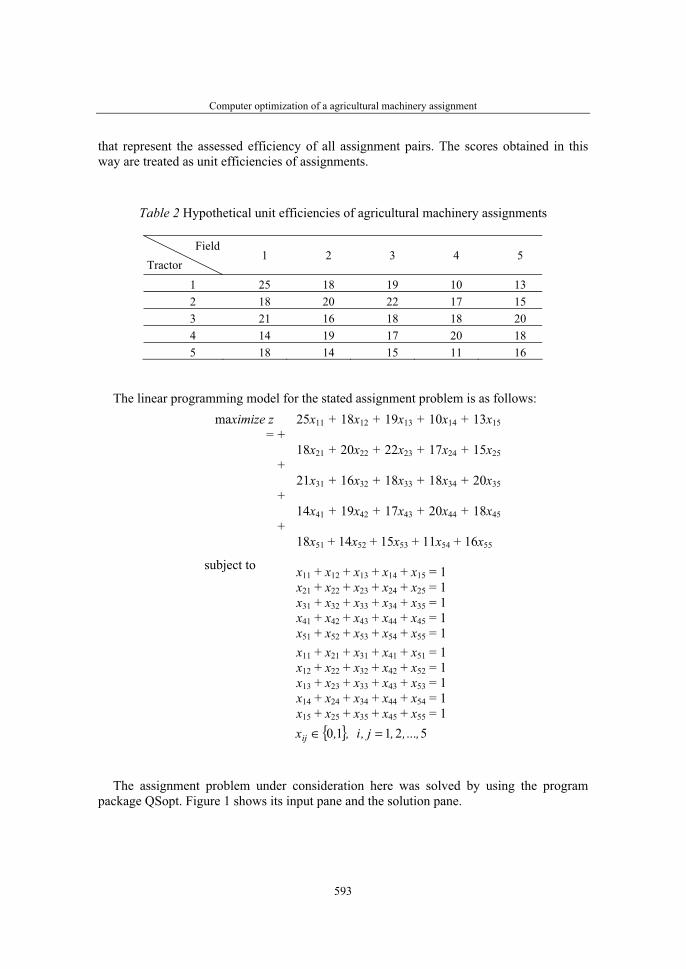
Computer optimization of a agricultural machinery assignment
593
that represent the assessed efficiency of all assignment pairs. The scores obtained in this way are treated as unit efficiencies of assignments.
Table 2 Hypothetical unit efficiencies of agricultural machinery assignments
FieldTractor
1 2 3 4 5
1 25 18 19 10 132 18 20 22 17 153 21 16 18 18 204 14 19 17 20 185 18 14 15 11 16
The linear programming model for the stated assignment problem is as follows: maximize z
=25x11 + 18x12 + 19x13 + 10x14 + 13x15
+18x21 + 20x22 + 22x23 + 17x24 + 15x25
+21x31 + 16x32 + 18x33 + 18x34 + 20x35
+14x41 + 19x42 + 17x43 + 20x44 + 18x45
+18x51 + 14x52 + 15x53 + 11x54 + 16x55
subject to x11 + x12 + x13 + x14 + x15 = 1 x21 + x22 + x23 + x24 + x25 = 1 x31 + x32 + x33 + x34 + x35 = 1 x41 + x42 + x43 + x44 + x45 = 1 x51 + x52 + x53 + x54 + x55 = 1 x11 + x21 + x31 + x41 + x51 = 1 x12 + x22 + x32 + x42 + x52 = 1 x13 + x23 + x33 + x43 + x53 = 1 x14 + x24 + x34 + x44 + x54 = 1 x15 + x25 + x35 + x45 + x55 = 1
}{ ,,xij 10∈ 5...21 ,,,j,i =
The assignment problem under consideration here was solved by using the program package QSopt. Figure 1 shows its input pane and the solution pane.
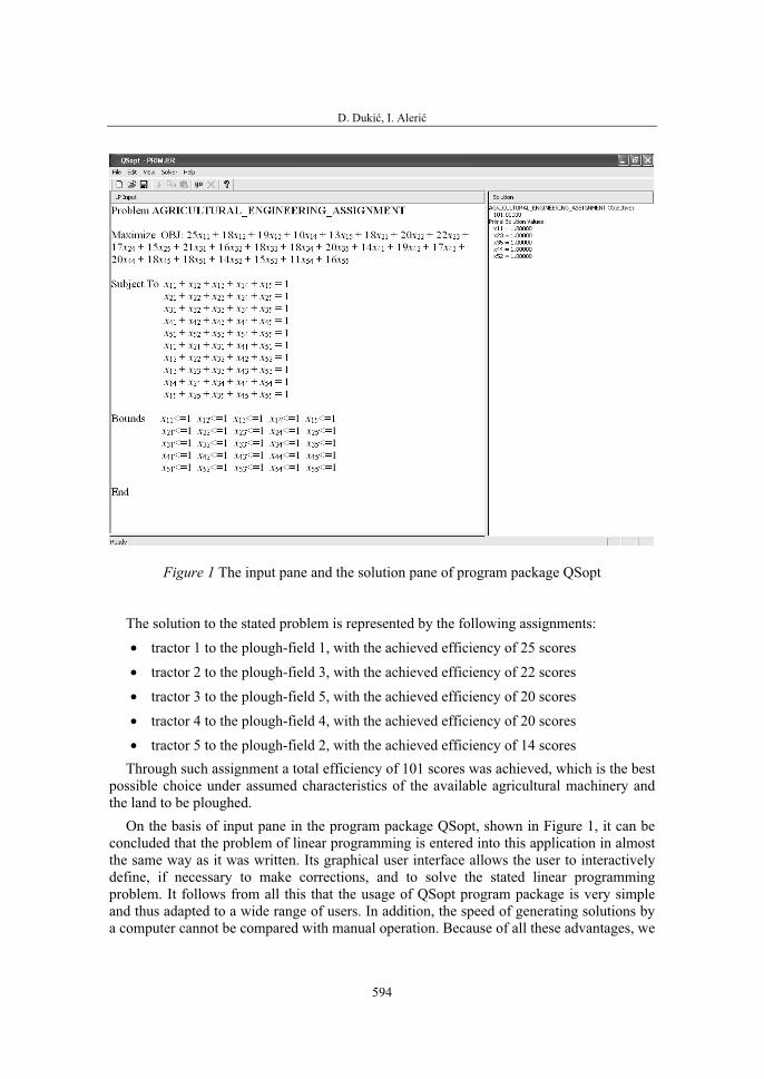
D. Dukić, I. Alerić
594
Figure 1 The input pane and the solution pane of program package QSopt
The solution to the stated problem is represented by the following assignments: • tractor 1 to the plough-field 1, with the achieved efficiency of 25 scores • tractor 2 to the plough-field 3, with the achieved efficiency of 22 scores • tractor 3 to the plough-field 5, with the achieved efficiency of 20 scores • tractor 4 to the plough-field 4, with the achieved efficiency of 20 scores • tractor 5 to the plough-field 2, with the achieved efficiency of 14 scores
Through such assignment a total efficiency of 101 scores was achieved, which is the best possible choice under assumed characteristics of the available agricultural machinery and the land to be ploughed.
On the basis of input pane in the program package QSopt, shown in Figure 1, it can be concluded that the problem of linear programming is entered into this application in almost the same way as it was written. Its graphical user interface allows the user to interactively define, if necessary to make corrections, and to solve the stated linear programming problem. It follows from all this that the usage of QSopt program package is very simple and thus adapted to a wide range of users. In addition, the speed of generating solutions by a computer cannot be compared with manual operation. Because of all these advantages, we
Computer optimization of a agricultural machinery assignment
595
should promote the usage of quantitative methods and computer models in solving various problems involved in performing agricultural activities.
CONCLUSIONS
The assignment model can be applied in numerous decision-making situations. One of these areas is solving the problems related to the usage of agricultural machinery in field crop production. The issue of adequate assignment of different farm machinery is especially prominent in this particular area. In addition to the characteristics of available human and technical resources, the characteristics of arable land where certain activities are to be performed, there are also deadlines and uncertain weather conditions to consider when solving the problem of agricultural machinery assignment. Through adequate assignment of available machinery we can significantly increase the efficiency and effectiveness of business operations, and minimize the possibility of problems arising from delays in performing any of the agricultural jobs.
Quantitative methods and models represent an important management support in solving various management problems, including those related to agricultural machinery assignment. Unfortunately, the usage of such methods is very limited in Croatia. By explaining the procedure of constructing and solving the model of agricultural machinery assignment based on computer optimization, we have attempted in this paper to promote the usage of this approach. In our analysis we have emphasized in particular numerous advantages of computer implementation. The proposed model was first considered from a theoretical point of view, which was followed by a hypothetical example. In this model it is very important to determine the efficiency matrix, whose elements represent the expected benefits arising from assigning each particular machine to carrying out a particular agricultural activity, i.e. job. These elements are the result of scoring which is performed according to predetermined criteria. Because program applications are so wide-spread, the presented assignment model was defined and solved as a linear programming problem.
D. Dukić, I. Alerić
596
REFERENCES
1. Enns R.H., McGuire G.C. (2007). Computer Algebra Recipes: An Advanced Guide to Scientific Modeling, Springer Science + Business Media, LLC, New York
2. Hillier F.S., Lieberman G. J. (2005). Introduction to Operations Research, Eighth Edition, McGraw-Hill, New York
3. Koutsoukis N.S., Mitra G. (2003). Decision Modelling and Information Systems: The Information Value Chain (Operations Research/Computer Science Interfaces Series), Kluwer Academic Publishers, Norwell
4. Mileusnić Z., Đević M., Miodragović R. (2007). Radni parametri traktorsko-mašinskih agregata u obradi zemljišta, Savremena poljoprivredna tehnika, god. 33, br. 1-2: 157-164
5. Stevenson W.J. (1992). Introduction to Management Science, Second Edition, Irwin, Homewood
6. Taha H.A. (2003). Operations Research - An Introduction, Seventh Edition, Prentice-Hall, New York
7. Vanderbei R.J. (2001). Linear Programming: Foundations and Extensions (International Series in Operations Research and Management Science), Second Edition, Springer Science + Business Media, Inc., New York
8. Williams H.P. (1999). Model Building in Mathematical Programming, Fourth Edition, John Wiley & Sons Ltd., Chichester
36. Symposium "Actual Tasks on Agricultural Engineering", Opatija, Croatia, 2008.
597
36.
SIMPOZIJAKTUALNI ZADACIMEHANIZACIJE POLJOPRIVREDE
UDC631.17 (439)
Stručni radExpert paper
ACTUAL TASKS AND POSSIBILITIES IN THE HUNGARIAN AGRICULTURAL INNOVATION
ISTVÁN HUSTI
Systems Engineering and Management Institute; Szent Istvan University Gödöllő,Hungary H-2103 Gödöllő, P.O.B. 303., E-mail: [email protected]
SUMMARY
The role of small and medium-size enterprises has increased in the Hungarian agriculture after the transition. In connection with the general problems, most of the Hungarian small and medium-size enterprises (SME’s) agricultural enterp-rises have serious problems in the field of innovation.
I prepared and used some models to examine the exact possibilities of innovation and to determine what needs to be developed. In this publication I am going to present three of them. • The simplified model of agricultural innovation serves as a theoretical basis
for agricultural developments. This model clearly demonstrates the related and dependent works to be done. It shows that the innovation part-works can be systematized into two integrating umbrellas. These are marketing and knowledge. Marketing is important as the success of innovation is decided in the market. The whole innovation process should be guided by the endeavour for market success. Knowledge combines earlier experience and recent information in the entire process.
• The model of the components of technical development shows that technical development serving agricultural production has got a particular bridging role between the production and the previous innovation phases; it integrates several factors at the same time.
• These models that were successful in the past, would be useful today as well, but the small and medium-size enterprises do not have suitable possibilities for applying them. Unfortunately the conditions of cooperation between the actors are missing as well. In our current situation if an enterprise wants to innovate, it has to develop itself with state support. The adaptive innovation can be a possible solution too. This model is going to be presented later. Key words: agricultural innovation, models of innovation, agricultural techn-
ical development, adaptive innovation
I. Husti
598
INTRODUCTION
We used to say as a slogan: „Innovation is the engine of the development”. It’s true int he „well-developed” world where the innovative efforts have got more and more important role in the national economy. The situation is absolutely different in our country. There is a serious gap between our innovative practice and the world-level innovative results.
We ought to have much more innovative ideas for developing the competitiveness of our economy, especially int he agricultural small and medium-size enterprises. (In Hungary: small enterprise is which has max 50 employees and max 10 million euros revenue per year. The same indicators of medium-size enterprise are: 250 employees and 50 million euros.)
The main objective of the research and this publication is to systemise the present innovation tasks of the Hungarian agriculture, especially focusing on the SMS’s.
METHOD
Several times during the research I had to create models that represent the typical phenomena of a process or a solution. By doing this I wanted to illustrate the situation as well as to capture the most important characteristics of an innovation related problem, its internal and external relations and to describe the area in which they could be used in. In terms of these I used the possibilities offered by the classical system theory. Including this I could not undertake to come up with customized suggestions which could serve as a base for agricultural enterprises to adopt their own technical development solutions. This is impossible because in practice the combination of the developmental components show such diversity that their overall introduction is impossible and would make no sense.
RESULTS AND DISCUSSION
The present situation and the model of agriculture There is almost no area in the domestic innovation practice in which we could be
compared in an international level. Unfortunately the general observations apply to agriculture as well, which is offending because the sector once being successful has a slight chance to fall into line with Europe.
In the previous decades the Hungarian agriculture has proved several times that it is a favourable area for the innovation efforts.
We can say that innovation made the Hungarian agriculture known and recognized internationally. Between 1960 and 1980 the Hungarian agriculture significantly differed from the sectors of the industry with its own values and system approach. This paradigm brought a dynamic development among countries within the same political systems.
Unfortunately the initial excellent results of the agricultural paradigm striving for priority were accompanied by the deteriorating economical conditions and expenditures exceeding the local optimum, then the Hungarian economy got into crisis blocking the
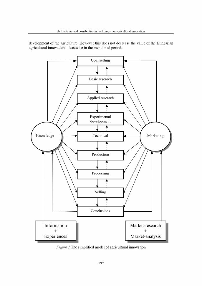
Actual tasks and possibilities in the Hungarian agricultural innovation
599
development of the agriculture. However this does not decrease the value of the Hungarian agricultural innovation – leastwise in the mentioned period.
Figure 1 The simplified model of agricultural innovation
Goal setting
Basic research
Applied research
Experimentaldevelopment
Technical
Production
Processing
Selling
Conclusions
Knowledge Marketing
Information+
Experiences
Market-research+
Market-analysis
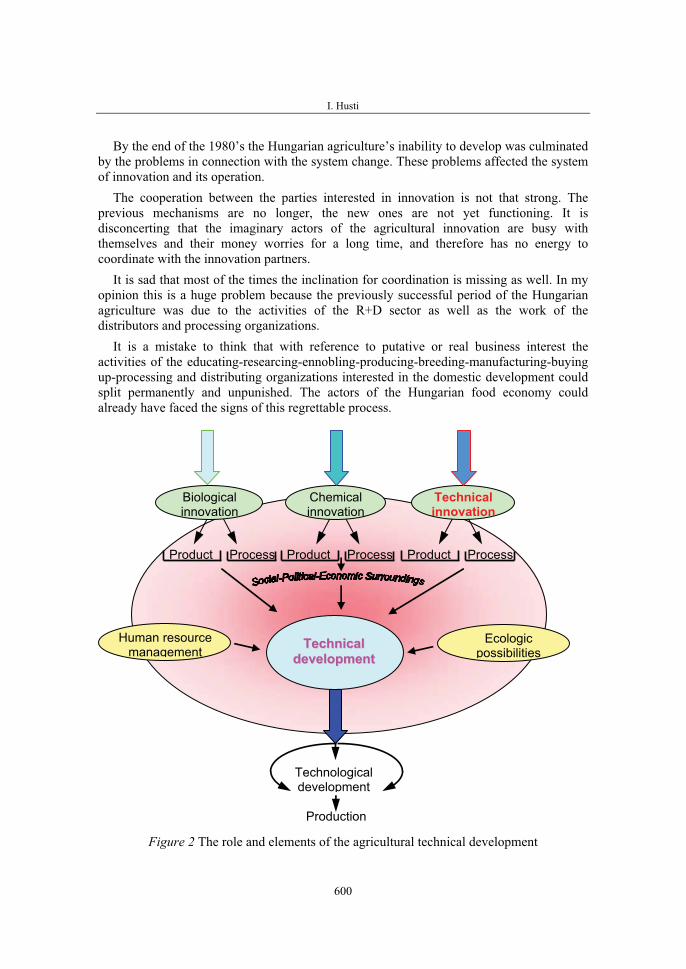
I. Husti
600
By the end of the 1980’s the Hungarian agriculture’s inability to develop was culminated by the problems in connection with the system change. These problems affected the system of innovation and its operation.
The cooperation between the parties interested in innovation is not that strong. The previous mechanisms are no longer, the new ones are not yet functioning. It is disconcerting that the imaginary actors of the agricultural innovation are busy with themselves and their money worries for a long time, and therefore has no energy to coordinate with the innovation partners.
It is sad that most of the times the inclination for coordination is missing as well. In my opinion this is a huge problem because the previously successful period of the Hungarian agriculture was due to the activities of the R+D sector as well as the work of the distributors and processing organizations.
It is a mistake to think that with reference to putative or real business interest the activities of the educating-researcing-ennobling-producing-breeding-manufacturing-buyingup-processing and distributing organizations interested in the domestic development could split permanently and unpunished. The actors of the Hungarian food economy could already have faced the signs of this regrettable process.
Figure 2 The role and elements of the agricultural technical development
TTeecchhnniiccaallddeevveellooppmmeenntt
Human resource management
Ecologicpossibilities
Technologicaldevelopment
Production
Product Process Product Process Product Process
Biologicalinnovation
Chemicalinnovation
Technicalinnovation
Actual tasks and possibilities in the Hungarian agricultural innovation
601
I prepared and used the general model of agricultural innovation (Figure 1.). This model clearly demonstrates related and dependent works to be done. It shows that the innovation part-works can be systematized into two integrating umbrellas. These are marketing and knowledge. Marketing is important as the success of innovation is decided in the market. The whole innovation process should be guided by the endeavour for market success. Knowledge alloys earlier experience and recent information in the entire process.
The functional model is a proper instrument for
• The review of the systematisation of the processes of agricultural innovation
• The introduction of the relation between the part processes
• The analysis of the status of the agricultural innovation
• Defining what to do in the area of development We can say that the Hungarian agriculture was successful till the innovators could do
their activities in a harmonized way as represented by the model. The situation has changed significantly by now. In theory the old practice would be successful, but the SME’s do not have the necessary conditions to be able to follow the model. The other problem is that the conditions of a harmonized cooperation between the actors has changed.
The agricultural innovation, the agricultural research and the technical development should be set on new basis in order to improve the competency of the agriculture. It has to be decided which sector should enjoy priority in respect of the sector’s competency. We are no longer able to develop every area since our current financial possibilities do not cover it.
Technical development, as a phase of agricultural innovation The model about the substance of technical development (Figure 2.) shows that
technical development serving agricultural production has got a particular bridging role between the production and the previous innovation phases by integrating several factors at the same time. It is important that the marked biological, chemical, human and ecological factors should be in harmony, because otherwise the balance breaks effective factor being in relative minimum as per the minimum-law.
The adaptive innovation and it’s model There are a couple of ways for dividing the innovative solutions. One of them
differentiates the original and the adaptive innovation. The original innovation is a result of the organization’s own investment, R+D activities and the activities of the co-workers, while the adaptive innovation is built on results already developed by others. (The subject of this takeover can be an idea, an invention, a know-how, a plan documentation etc..)
The revival of the agricultural innovation was the initial intention of my present publication. In accordance with this my attention focused on the adaptive innovation because I do think that the role of the previously ignored SME’s should be reconsidered in the whole domestic innovation strategy.
We should not have the illusion that these organizations could finance the R+D’s in the long run. Instead their adaptive skills should be improved which is not easy even in the short term. Success requires new challenges in the area of education, consultancy and research.

I. Husti
602
There are numerous factors influencing the processes of adaptive innovation. In my model I highlighted two of them. (Figure 3.). ’External support’ includes all the effects externally influencing the enterprise. The social-political-economical changes could strengthen innovation but could weaken it as well. The pressure of competition could result in mobilizing such dormant energy which would stimulate a sort of ’forward escape’.
The technological push is sensed by producer-distributor organizations interested in agricultural development since their living depends on how well they could force their products and services upon the users/costumers. In this aspect supply push is dominant in our country. The ’demand suck’ represents the demands and desires of the buyers, costumers and processors of agricultural products. In case of manufacturers, satisfying these needs is an evident precondition for competition.
The adventure can be influenced by many factors. The main question is the personality of the entrepreneur, its sensibility to the new and the awareness that development is important otherwise the organization will get to periphery and get off on a slope and do not stop.
Figure 3 The adaptive innovation model
It is important to be motivated enough, should it be internal or externally forced. Entrepreneurial knowledge and experience can help a lot. Think of the role of knowledge
= Adaptive processf l t
START
Getting information
-
+
Utilisation
END
+
Theoretical model
- ±
Aimed inquire
- ±
+
-
Experimental development
+
±
STOP
+ Entrepreneur’sinclination
• Motivation
• Knowledge, experiences
• Information
• Possibilities
External support
• S-P-E effects
• Competition-compulsion
• Technology push
• Demand pull
Actual tasks and possibilities in the Hungarian agricultural innovation
603
on Figure 1, which is the integrating component of the main model. In our dynamic world we may frequently encounter the confusion of information-redundancy. It can be crucial for the entrepreneurs to get the relevant information in the right time and in optimal quantity and quality.
One of the old problems of our consulting system is that the Agricultural Knowledge and Information System (AKIS) is still not operating at an appropriate professional standard.
This operation would be the precondition of a consulting system serving professional objectives.
The enterprise for innovation is also influenced by the capability of an organization.In case of agricultural enterprises the ecological environment is significantly important
as it determines the classical potential of agriculture. Besides these the technological background, production culture, financial status and networks of the enterprise are also relevant.
The enterprise with due external support could start the adaptation process which would then lead to the complete or partial renewal of a product or a process following the principle of the ’considered progress’.
The model illustrates the steps of the adaptation process in a systemized order. Essential is the first phase, to acquire knowledge, whereby the entrepreneur can be
affected by such stimulating impulses that can start the adaptive innovation. Just like in the other phases of the process, the entrepreneur has to consider and evaluate if the new cognition acquired is worth dealing with. If the idea is worth to be improved, then comes the „aimed orientation”, whilst additional information and professional details are obtained and discussed. In this phase the idea still can be rejected.
The generally important time factor in the innovation processes appears here as well, the too much speculation is disadvantageous rather than favourable. In case of a positive outcome the next step is to create a ’mental model’ in reference to the conception. During this phase the entrepreneur mentally assembles and ’plays’ the imagined innovation.
Following the tactics of small steps the next phase is the ’small sample’ which is the practical test of the imagination as an experiment or development.
During this- despite of the preparations- problems can arise resulting in the rejection of the imagination. If in this phase our experiences are favourable, the next step could be the complete takeover that is the substantive adaptation, the application of the solutions developed somewhere else.
I. Husti
604
CONCLUSIONS
The Hungarian domestic system of the agricultural innovation does not make it possible to follow the model of innovation based on the traditional R+D. Not to mention that the cooperation between the actors of the innovation system in the sector ceased to exist. In this situation it seems to be reasonable to follow the model of adaptive innovation which would be useful especially for the SME’s.
In order to make the adaptive innovation faster the external conditions should be improved, and the enterprise enhanced. It would also be important to set up a professional Agricultural Knowledge and Information System (AKIS) which would function accordingly.
REFERENCES
1. EDQUIST, C. (ed.) (1997): Systems of Innovation Technologies, Institutions and Organizations. London: Pinter, Casell Academic.
2. Hajdú J., Magó L.: (2003) Alternatives of the Domestic Agricultural Machinery Market, Hungarian Agricultural Engineering, Periodical of the Committee of Agricultural Engineering of the Hungarian Academy of Sciences, Vol. 16/2003. p. 41-43.
3. HALL, A.J., L. MYTZELKA, and B. OYEYINKA (2004): Innovation Systems: Concepts and Implications for Agricultural Research Policy and Practice. Maastricht: United Nations University.
4. HUSTI, I. (2004): Logistics Problems in Hungarian Agribusiness. =LogInfo. Special Edition for EUROLOG 2004. Vol. 14. No. 3. 2004 May - June. p. 20-21.
5. HUSTI, I. (2007): Gondolatok az agrárinnováció néhány kritikus területéről. =MAG Kutatás,fejlesztés és környezet, Vol. XXI (6.), No 2, 2007 may, p.: 5-11.
6. Magó L.: (2007) Survey of the Present Mechanization of Small and Medium Size Plant Production Farms, Proceedings of the 35th International Symposium “Actual Tasks on Agricultural Engineering”, Opatija, Croatia, 19-23. February 2007. Proc. p. 497-506.
7. SPIELMAN D.J. (2005): Innovation Systems Perspectives on Developing-country Agriculture: A Critical Review. ISNAR Discussion Paper 2. Washington DC: International Food Policy Research Institute (IFPRI).
36. Symposium "Actual Tasks on Agricultural Engineering", Opatija, Croatia, 2008.
605
36.
SIMPOZIJAKTUALNI ZADACIMEHANIZACIJE POLJOPRIVREDE
UDC519.2:631.16/.17
Izvorni znanstveni radOriginal scientific paper
ANALYSIS OF FARMERS' OPINIONS IN OSIJEK-BARANJA COUNTY REGARDING AGRICULTURAL
ENGINEERINGMATE SESAR
University of Josip Juraj Strossmayer in Osijek, Faculty of Agriculture in Osijek, Department of Agroeconomics, Trg Sv. Trojstva 3, 31000 Osijek, Croatia
ABSTRACT
Although there have been certain positive changes over the past few years regarding the existence and technological level of equipment used for farming, Croatian agriculture is still significantly lagging behind this sector in developed countries of the world. Such a situation has a bearing on reduced efficiency and productivity, decreasing the effects of activities implemented in agriculture. Lagging behind in terms of agricultural engineering can partly be explained by the problems inherited from the socialist era, as well as by those emerging in the process of abandoning this management concept and transition to market economy. Negative trends were certainly made worse by the war destruction suffered by the Republic of Croatia in the early 1990s. Nevertheless, the slowed-down development of agricultural engineering was caused also by a number of inadequate measures of economic and agricultural policy, and by omissions in their implementation. A special aspect of the problem is disregard of the views of professional and scientific community, and also of farmers' opinions. Taking into account the views of the people directly involved in agriculture and understanding the problems they are facing could certainly improve the measures taken by agricultural policy decision-makers. This paper will present the research aimed at establishing the basic factors of farmers' perceptions regarding agricultural engineering. By the survey conducted on a sample of respondents residing in the Osijek-Baranja County, we attempted to determine the main reasons for insufficient investment in modernization, as well as possible differences in farmers' opinions regarding the defined aspects. In the analysis of the stated issues different statistical methods were used.
Key words: farmers’ opinions, modernization, agricultural engineering, eco-nomic and agricultural policy, statistical methods
M. Sesar
606
INTRODUCTION
Croatian agriculture has been facing numerous problems for many years. One of the major issues is inadequate equipment and low technological level of engineering used in a variety of agricultural jobs. As Croatia is drawing nearer to full EU membership, these problems become increasingly important. Namely, obsolete farm machinery has a direct impact on decreasing competitiveness of Croatian agriculture on the dynamic European and world markets of agricultural products. Given the sustained liberalization of these markets and decreasing subsidies for agricultural production, there will be grave and far-reaching consequences if Croatia continues to lag behind in modernization.
Investment into agricultural engineering is a basic prerequisite for increasing cost-effectiveness and productivity, since the effects of most activities in agricultural production are reduced unless adequate technical support is provided. Although there have been certain positive changes over the past few years regarding the existence and technological level of equipment used for farming, Croatian agriculture is still significantly lagging behind this sector in developed countries of the world. This situation can partly be explained by the problems inherited from the socialist era, as well as by those emerging in the process of abandoning this management concept and transition to market economy. Understandably, the war destruction suffered by the Republic of Croatia in the early 1990s had a negative effect on the whole economy. Nevertheless, the slowed-down development of Croatian agriculture was caused also by a number of inadequate measures of economic and agricultural policy, and by omissions in their implementation. If policy-makers had taken into account the views of professional and scientific community, and also farmers' opinions, many erroneous decisions might have been avoided.
This paper will present the research aimed at establishing the views of people engaged in agriculture, and the problems they encounter in their work. In it, we tried to determine the basic factors of individual farmers' perceptions regarding agricultural engineering. Within this analysis, special emphasis was given to identifying the main reasons for insufficient investment in modernization, as well as possible differences in farmers' opinions regarding the defined features (gender, age, education level, estimated value of their own agricultural machinery).
The paper examines only a few aspects of this particular topic. In this way, we have set the framework for further research that should be conducted by competent authorities and institutions, with the aim of encouraging investment into agricultural engineering. It should be noted that the sample, i.e. the number of respondents, would have to be much larger and new variables should be introduced into the analysis.
METHODS
The farmers' opinion survey regarding the issue of agricultural engineering was conducted during September and October 2007 on a sample of farmers residing in the Osijek-Baranja County. For this anonymous survey a written questionnaire was used. The purpose of the research and instructions how to fill in the questionnaire were explained individually to every respondent.
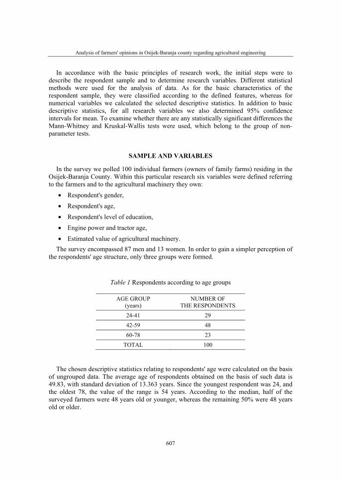
Analysis of farmers' opinions in Osijek-Baranja county regarding agricultural engineering
607
In accordance with the basic principles of research work, the initial steps were to describe the respondent sample and to determine research variables. Different statistical methods were used for the analysis of data. As for the basic characteristics of the respondent sample, they were classified according to the defined features, whereas for numerical variables we calculated the selected descriptive statistics. In addition to basic descriptive statistics, for all research variables we also determined 95% confidence intervals for mean. To examine whether there are any statistically significant differences the Mann-Whitney and Kruskal-Wallis tests were used, which belong to the group of non-parameter tests.
SAMPLE AND VARIABLES
In the survey we polled 100 individual farmers (owners of family farms) residing in the Osijek-Baranja County. Within this particular research six variables were defined referring to the farmers and to the agricultural machinery they own:
• Respondent's gender,
• Respondent's age,
• Respondent's level of education,
• Engine power and tractor age,
• Estimated value of agricultural machinery. The survey encompassed 87 men and 13 women. In order to gain a simpler perception of
the respondents' age structure, only three groups were formed.
Table 1 Respondents according to age groups
AGE GROUP(years)
NUMBER OFTHE RESPONDENTS
24-41 29
42-59 48
60-78 23
TOTAL 100
The chosen descriptive statistics relating to respondents' age were calculated on the basis of ungrouped data. The average age of respondents obtained on the basis of such data is 49.83, with standard deviation of 13.363 years. Since the youngest respondent was 24, and the oldest 78, the value of the range is 54 years. According to the median, half of the surveyed farmers were 48 years old or younger, whereas the remaining 50% were 48 years old or older.
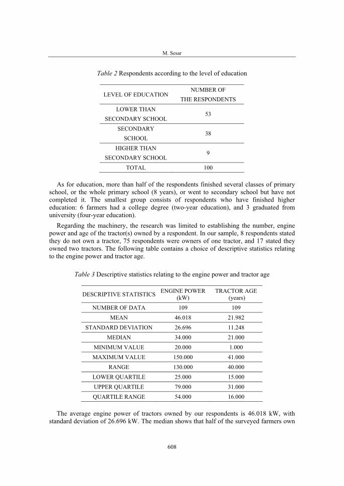
M. Sesar
608
Table 2 Respondents according to the level of education
LEVEL OF EDUCATION NUMBER OF
THE RESPONDENTS
LOWER THAN SECONDARY SCHOOL
53
SECONDARYSCHOOL
38
HIGHER THAN SECONDARY SCHOOL
9
TOTAL 100
As for education, more than half of the respondents finished several classes of primary school, or the whole primary school (8 years), or went to secondary school but have not completed it. The smallest group consists of respondents who have finished higher education: 6 farmers had a college degree (two-year education), and 3 graduated from university (four-year education).
Regarding the machinery, the research was limited to establishing the number, engine power and age of the tractor(s) owned by a respondent. In our sample, 8 respondents stated they do not own a tractor, 75 respondents were owners of one tractor, and 17 stated they owned two tractors. The following table contains a choice of descriptive statistics relating to the engine power and tractor age.
Table 3 Descriptive statistics relating to the engine power and tractor age
DESCRIPTIVE STATISTICS ENGINE POWER(kW)
TRACTOR AGE (years)
NUMBER OF DATA 109 109
MEAN 46.018 21.982
STANDARD DEVIATION 26.696 11.248
MEDIAN 34.000 21.000
MINIMUM VALUE 20.000 1.000
MAXIMUM VALUE 150.000 41.000
RANGE 130.000 40.000
LOWER QUARTILE 25.000 15.000
UPPER QUARTILE 79.000 31.000
QUARTILE RANGE 54.000 16.000
The average engine power of tractors owned by our respondents is 46.018 kW, with standard deviation of 26.696 kW. The median shows that half of the surveyed farmers own
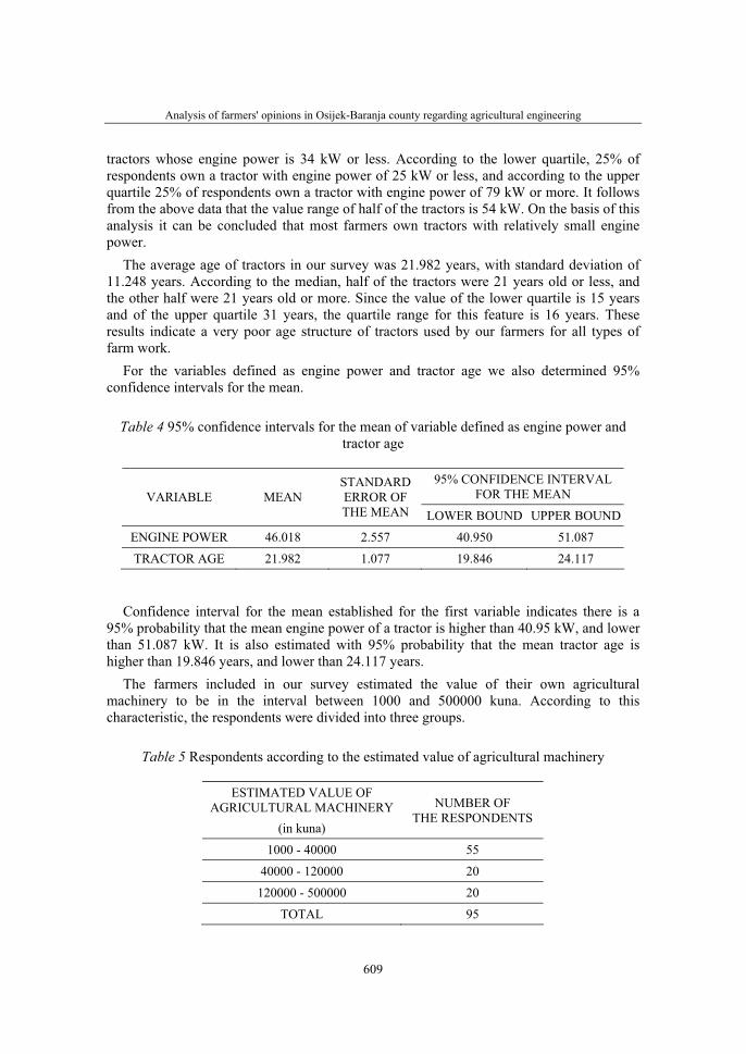
Analysis of farmers' opinions in Osijek-Baranja county regarding agricultural engineering
609
tractors whose engine power is 34 kW or less. According to the lower quartile, 25% of respondents own a tractor with engine power of 25 kW or less, and according to the upper quartile 25% of respondents own a tractor with engine power of 79 kW or more. It follows from the above data that the value range of half of the tractors is 54 kW. On the basis of this analysis it can be concluded that most farmers own tractors with relatively small engine power.
The average age of tractors in our survey was 21.982 years, with standard deviation of 11.248 years. According to the median, half of the tractors were 21 years old or less, and the other half were 21 years old or more. Since the value of the lower quartile is 15 years and of the upper quartile 31 years, the quartile range for this feature is 16 years. These results indicate a very poor age structure of tractors used by our farmers for all types of farm work.
For the variables defined as engine power and tractor age we also determined 95% confidence intervals for the mean.
Table 4 95% confidence intervals for the mean of variable defined as engine power and tractor age
95% CONFIDENCE INTERVAL FOR THE MEAN VARIABLE MEAN
STANDARDERROR OF THE MEAN LOWER BOUND UPPER BOUND
ENGINE POWER 46.018 2.557 40.950 51.087
TRACTOR AGE 21.982 1.077 19.846 24.117
Confidence interval for the mean established for the first variable indicates there is a 95% probability that the mean engine power of a tractor is higher than 40.95 kW, and lower than 51.087 kW. It is also estimated with 95% probability that the mean tractor age is higher than 19.846 years, and lower than 24.117 years.
The farmers included in our survey estimated the value of their own agricultural machinery to be in the interval between 1000 and 500000 kuna. According to this characteristic, the respondents were divided into three groups.
Table 5 Respondents according to the estimated value of agricultural machinery
ESTIMATED VALUE OF AGRICULTURAL MACHINERY
(in kuna)
NUMBER OFTHE RESPONDENTS
1000 - 40000 55
40000 - 120000 20
120000 - 500000 20
TOTAL 95
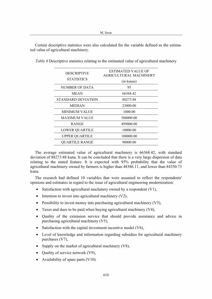
M. Sesar
610
Certain descriptive statistics were also calculated for the variable defined as the estima-ted value of agricultural machinery.
Table 6 Descriptive statistics relating to the estimated value of agricultural machinery
DESCRIPTIVE STATISTICS
ESTIMATED VALUE OF AGRICULTURAL MACHINERY
(in kunas)
NUMBER OF DATA 95
MEAN 66368.42
STANDARD DEVIATION 88273.88
MEDIAN 23000.00
MINIMUM VALUE 1000.00
MAXIMUM VALUE 500000.00
RANGE 499000.00
LOWER QUARTILE 10000.00
UPPER QUARTILE 100000.00
QUARTILE RANGE 90000.00
The average estimated value of agricultural machinery is 66368.42, with standard deviation of 88273.88 kuna. It can be concluded that there is a very large dispersion of data relating to the stated feature. It is expected with 95% probability that the value of agricultural machinery owned by farmers is higher than 48386.11, and lower than 84350.73 kuna.
The research had defined 10 variables that were assumed to reflect the respondents' opinions and estimates in regard to the issue of agricultural engineering modernization:
• Satisfaction with agricultural machinery owned by a respondent (V1),
• Intention to invest into agricultural machinery (V2),
• Possibility to invest money into purchasing agricultural machinery (V3),
• Taxes and dues to be paid when buying agricultural machinery (V4),
• Quality of the extension service that should provide assistance and advice in purchasing agricultural machinery (V5),
• Satisfaction with the capital investment incentive model (V6),
• Level of knowledge and information regarding subsidies for agricultural machinery purchases (V7),
• Supply on the market of agricultural machinery (V8),
• Quality of service network (V9),
• Availability of spare parts (V10).
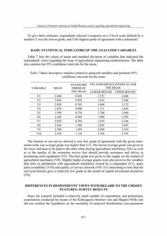
Analysis of farmers' opinions in Osijek-Baranja county regarding agricultural engineering
611
To give their estimates, respondents selected a response on a 5-level scale defined by a number (1 was the lowest grade, and 5 the highest grade of agreement with a statement).
BASIC STATISTICAL INDICATORS OF THE ANALYZED VARIABLES
Table 7 lists the values of mean and standard deviation of variables that indicated the respondents' views regarding the issue of agricultural engineering modernization. The table also contains the 95% confidence intervals for the mean.
Table 7 Basic descriptive statistics related to analyzed variables and pertinent 95% confidence intervals for the mean
95% CONFIDENCE INTERVAL FOR THE MEAN VARIABLE MEAN
STANDARDERROR OF THE MEAN LOWER BOUND UPPER BOUND
V1 2.440 0.845 2.272 2.608 V2 2.050 0.999 1.852 2.248 V3 2.020 0.765 1.868 2.172 V4 1.870 0.800 1.711 2.029 V5 1.930 0.756 1.780 2.080 V6 2.100 0.969 1.908 2.292 V7 2.030 0.784 1.874 2.186 V8 2.560 1.388 2.285 2.835 V9 2.300 1.059 2.090 2.510 V10 2.330 1.138 2.104 2.556
The farmers in our survey showed a very low grade of agreement with the given state-ments (only one average grade was higher than 2.5). The lowest average grade was given to the taxes and dues to be paid to the state when buying agricultural machinery (V4), as well as to the quality of the extension service that should provide assistance and advice in purchasing such equipment (V5). The best grade was given to the supply on the market of agricultural machinery (V8). Slightly higher average grades were also given to the variables that refer to satisfaction with agricultural machinery owned by a respondent (V1), spare parts availability (V10) and quality of service network (V9). It is interesting to note that the surveyed farmers gave a relatively low grade to the model of capital investment incentives (V6).
DIFFERENCES IN RESPONDENTS' VIEWS WITH REGARD TO THE CHOSEN FEATURES: SURVEY RESULTS
Since the research included a relatively small number of respondents, and preliminary examination conducted by means of the Kolmogorov-Smirnov test and Shapiro-Wilks test did not confirm the hypothesis on the normality of analyzed distributions, non-parameter
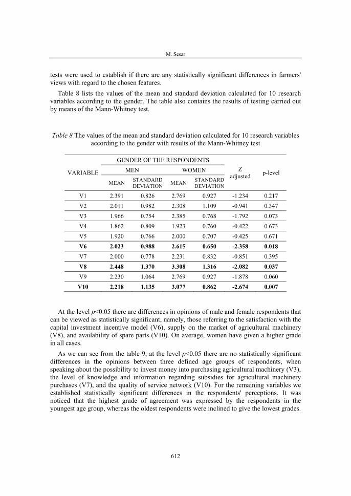
M. Sesar
612
tests were used to establish if there are any statistically significant differences in farmers' views with regard to the chosen features.
Table 8 lists the values of the mean and standard deviation calculated for 10 research variables according to the gender. The table also contains the results of testing carried out by means of the Mann-Whitney test.
Table 8 The values of the mean and standard deviation calculated for 10 research variables according to the gender with results of the Mann-Whitney test
GENDER OF THE RESPONDENTS
MEN WOMEN VARIABLEMEAN STANDARD
DEVIATION MEAN STANDARDDEVIATION
Zadjusted p-level
V1 2.391 0.826 2.769 0.927 -1.234 0.217
V2 2.011 0.982 2.308 1.109 -0.941 0.347
V3 1.966 0.754 2.385 0.768 -1.792 0.073
V4 1.862 0.809 1.923 0.760 -0.422 0.673
V5 1.920 0.766 2.000 0.707 -0.425 0.671
V6 2.023 0.988 2.615 0.650 -2.358 0.018 V7 2.000 0.778 2.231 0.832 -0.851 0.395
V8 2.448 1.370 3.308 1.316 -2.082 0.037 V9 2.230 1.064 2.769 0.927 -1.878 0.060
V10 2.218 1.135 3.077 0.862 -2.674 0.007
At the level p<0.05 there are differences in opinions of male and female respondents that can be viewed as statistically significant, namely, those referring to the satisfaction with the capital investment incentive model (V6), supply on the market of agricultural machinery (V8), and availability of spare parts (V10). On average, women have given a higher grade in all cases.
As we can see from the table 9, at the level p<0.05 there are no statistically significant differences in the opinions between three defined age groups of respondents, when speaking about the possibility to invest money into purchasing agricultural machinery (V3), the level of knowledge and information regarding subsidies for agricultural machinery purchases (V7), and the quality of service network (V10). For the remaining variables we established statistically significant differences in the respondents' perceptions. It was noticed that the highest grade of agreement was expressed by the respondents in the youngest age group, whereas the oldest respondents were inclined to give the lowest grades.
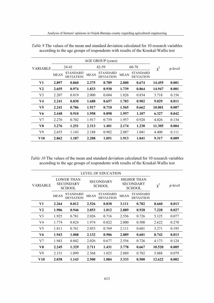
Analysis of farmers' opinions in Osijek-Baranja county regarding agricultural engineering
613
Table 9 The values of the mean and standard deviation calculated for 10 research variables according to the age groups of respondents with results of the Kruskal-Wallis test
AGE GROUP (years)
24-41 42-59 60-78 VARIABLEMEAN STANDARD
DEVIATION MEAN STANDARDDEVIATION MEAN STANDARD
DEVIATION
χ2 p-level
V1 2.897 0.860 2.375 0.789 2.000 0.674 14.455 0.001 V2 2.655 0.974 1.833 0.930 1.739 0.864 14.947 0.001 V3 2.207 0.819 2.000 0.684 1.826 0.834 3.718 0.156
V4 2.241 0.830 1.688 0.657 1.783 0.902 9.029 0.011 V5 2.241 0.786 1.917 0.710 1.565 0.662 10.001 0.007 V6 2.448 0.910 1.958 0.898 1.957 1.107 6.327 0.042 V7 2.276 0.702 1.917 0.739 1.957 0.928 4.026 0.134
V8 3.276 1.251 2.313 1.401 2.174 1.230 11.305 0.004 V9 2.655 1.143 2.188 0.982 2.087 1.041 4.400 0.111
V10 2.862 1.187 2.208 1.051 1.913 1.041 9.317 0.009
Table 10 The values of the mean and standard deviation calculated for 10 research variables according to the age groups of respondents with results of the Kruskal-Wallis test
LEVEL OF EDUCATION
LOWER THAN SECONDARY
SCHOOL
SECONDARYSCHOOL
HIGHER THAN SECONDARY
SCHOOLVARIABLE
MEAN STANDARDDEVIATION MEAN STANDARD
DEVIATION MEAN STANDARDDEVIATION
χ2 p-level
V1 2.264 0.812 2.526 0.830 3.111 0.782 8.660 0.013 V2 1.906 0.946 2.053 1.012 2.889 0.928 7.228 0.027 V3 1.925 0.781 2.026 0.716 2.556 0.726 5.125 0.077
V4 1.774 0.824 1.974 0.822 2.000 0.500 2.622 0.270
V5 1.811 0.761 2.053 0.769 2.111 0.601 3.271 0.195
V6 1.943 1.008 2.132 0.906 2.889 0.601 8.742 0.013 V7 1.943 0.842 2.026 0.677 2.556 0.726 4.173 0.124
V8 2.245 1.329 2.711 1.431 3.778 0.667 10.520 0.005 V9 2.151 1.099 2.368 1.025 2.889 0.782 5.088 0.079
V10 2.038 1.143 2.500 1.084 3.333 0.500 12.622 0.002

M. Sesar
614
With regard to the level of education, at the determined level of significance it was confirmed that there exist statistically significant differences in the respondents' opinions and estimates relating to the satisfaction with agricultural machinery they own (V1), intention to invest into agricultural machinery (V2), satisfaction with the capital investment incentive model (V6), supply on the market of agricultural machinery (V8) and spare parts availability (V10). These variables were given the highest grades by the respondents whose level of education is higher than secondary school, and the lowest grades by the respondents whose level of education is lower than secondary school.
Table 11 The values of the mean and standard deviation calculated for 10 research variables according to the estimated value of agricultural machinery with results of the
Kruskal-Wallis test
ESTIMATED VALUE OF AGRICULTURAL MACHINERY (in kuna)
1000 - 40000 40000 - 120000 120000 - 500000VARIABLE
MEAN STANDARDDEVIATION MEAN STANDARD
DEVIATION MEAN STANDARDDEVIATION
χ2 p-level
V1 2.182 0.696 2.550 0.887 3.150 0.875 16.284 0.000 V2 1.618 0.707 2.300 0.923 3.150 0.875 32.760 0.000 V3 1.982 0.782 1.950 0.887 2.300 0.470 4.057 0.132
V4 1.582 0.686 2.400 0.821 2.250 0.639 21.714 0.000 V5 1.727 0.757 2.150 0.587 2.300 0.801 10.002 0.007 V6 1.818 0.863 2.200 0.894 3.000 0.795 21.243 0.000 V7 1.836 0.739 2.100 0.788 2.600 0.681 12.631 0.002 V8 1.800 0.970 3.100 1.373 4.100 0.852 40.914 0.000 V9 1.745 0.751 2.750 1.020 3.300 0.979 34.517 0.000
V10 1.800 0.890 2.700 1.174 3.450 0.759 32.255 0.000
At the level of p<0.05, there are no statistically significant differences only in the opinions of the three determined groups that refer to the possibility to invest money into purchasing agricultural machinery (V3). The highest grades, with the exception of variable V4, were given to the statements by the respondents in the group of owners of high-value agricultural machinery. On the other hand, opposite grades were given by the respondents in the group that owned equipment with the lowest estimated value.
CONCLUSIONS
The paper presents the research results relating to the farmers' opinions on the issue of agricultural engineering modernization, which was carried out on a sample of respondents residing in the Osijek-Baranja County. Most of the farmers selected into the sample were owners of one tractor with relatively low engine power. The results also indicate a very
Analysis of farmers' opinions in Osijek-Baranja county regarding agricultural engineering
615
poor age structure of tractors that our farmers use for all kinds of farm work. Only 20% of surveyed farmers estimated the value of their agricultural machinery at more than 120000 kuna.
In particular, the paper tries to establish the main reasons for insufficient investments into modernization, as well as possible differences in farmers' opinions in view of the defined features. On the basis of our results it can be concluded that the surveyed farmers expressed a very low level of agreement with all the statements given in the questionnaire, i.e. they were very critical of the current state and possibilities for modernization in the Croatian agriculture. The lowest average grades were given to the taxes and dues to be paid when buying agricultural machinery and the quality of the extension service that should provide assistance and advice in purchasing agricultural machinery. The highest average grade went to the supply on the market of agricultural machinery. In general, the variables indicating the government's involvement and concern regarding agricultural engineering received very low average grades.
On average, female respondents were more optimistic in their assessments of all the research variables. Respondents belonging to the youngest age group, and those with post-secondary education expressed the highest degree of agreement with the given statements, whereas lowest grades were given by the oldest respondents and those with lower-than-secondary education. The highest number of statistically significant differences in farmers' opinions was determined according to the feature representing the estimated value of their own agricultural machinery.

M. Sesar
616
REFERENCES
1. Dukić G., Dukić D., Alerić I. (2007). Computer Supported Model of Statistical Analysis of the Influence of Education Level on the Perception of Economic and Social Issues. In: Barković D., Runzheimer B. (eds) Proceedings of Third Interdisciplinary Symposium “Interdisciplinary Management Research”, University of J.J. Strossmayer in Osijek - Faculty of Economics in Osijek / Pforzheim University of Applied Science - Pforzheim Graduate School
2. Hanke J.E., Reitsch A.G. (1991). Understanding Business Statistics, Irwin, Homewood
3. Mansfield E. (1987). Statistics for Business and Economics - Methods and Application, Third Edition, W.W. Norton & Company, New York
4. McClave J.T., Benson P.G. (1988). Statistics for Business and Economics, Fourth Edition, Dellen Publishing Company/Collier Macmillan Publishers, San Francisco
5. Petz B. (2004). Osnovne statističke metode za nematematičare, V. izdanje, Naklada Slap, Jastrebarsko
6. Spiegel M.R., Stephens L.R. (1999). Statistics, Third Edition, McGraw-Hill, New York
7. Šošić I. (2004). Primijenjena statistika, Školska knjiga, Zagreb
8. Šošić I., Serdar V. (1995). Uvod u statistiku, Deveto izdanje, Školska knjiga, Zagreb
9. Žužul J., Branica M.(1998). Statistika, Treće dopunjeno izdanje, Informator, Zagreb

36. Symposium "Actual Tasks on Agricultural Engineering", Opatija, Croatia, 2008.
617
36.
SIMPOZIJAKTUALNI ZADACIMEHANIZACIJE POLJOPRIVREDE
UDC338.43:631.16
Stručni radExpert paper
STUDY ABOUT INTEGRATION CAPACITY OF SYSTEMS FOR AGRO-FOOD PRODUCTION
DUMITRU MNERIE, DUMITRU TUCU, GABRIELA VICTORIA ANGHEL,TITUS SLAVICI
POLITEHNICA University of Timisoara, Mechanical Engineering Faculty, Bd. Mihai Viteazul, No.1, 300222 Timisoara, Tel. 0040-745-521711, Fax 0040-256-403589,
SUMMARY
The integrated systems are in fact agro-industrial units, being constituted on the bases of a started action of usual a private initiative with a view to obtain a favorable material result. That is defined as the production of high quality products, giving priority to ecologically safer methods, minimizing undesirable side-effects. The constituents of an integrated system for production are: conception, design, manufacturing, distribution to costumers, utilization, re-cycling, re-conception etc. It is very important to apply one managerial program for obtain the maximum profit and a good perspective to development. It showed a variant of managerial simulation for a generalized integrated system for production with some directions and elements general valid, a real guide for news enterprising. In general, the integrated systems in the agro-food production, are mostly used in the private domain, they are in fact industrial units, being constituted on the bases of a started action of a private initiative with a view to obtain a favorable material result.
The paper shows some situations of agro-food production system with different integration capacity, in the context of agriculture integration in European Union. Also, it is presents some experiences of some Small and Medium Sized Private Enterprises from Romania, with agriculture that basis activities, managerial, and special, strategic aspects.
Key words: integration capacity, systems, agro-food production, management
INTRODUCTION
An integrated system for production presumes a primary base, which became the start point for developing circles. The main piece of system is elimination of financial, law,

D. Mnerie, D. Tucu, G. V. Anghel, T. Slavici
618
economical barrier that can be found in usually, commercial, industrial, business. The stages in conception and planning integrated for a production system are: analyses of available personal resources; choose business; establish the main objectives for integrated system; create the strategy; financial and budget plan; elements for evaluation and monitoring the system. Each technologic flux has a high complexity but it’s very important to see the system like a whole unit. It’s really necessary an unit vision, with the possibility to preview all causes for block the system, then we must remark the zone with high-risk possibilities It’s preferable to use an integrated system, where can use minimum an available element (raw material source, the personal land, equipment for processing, personal network marketing, other). (Mnerie, D., 1999)
For agro-food production development can be used a lot of kinds of managerial systems, but after the integration capacity that system can be: integrant, integrated, integrator and one with all of these characteristics. That is very important for internal aspects also for relations with external factors.
An integrated system for agro-food production (ISAP) is a managerial way for business-man who wants to invest in agriculture, special for farmers who want to work and want to gain from agriculture.
Figure 1 Principle of Integrated system for agro-food production
Always, in the production system the most important is quality management. For ISAP is more important that aspect, and for a good efficiency of foods production system is opportune to have an efficacy quality management system. Now European construction, include Romania, an original one, with proper features, and the steps of European integration, beginning period) supposes major economic, financial tools, social and political

Study about integration capacity of systems for agro-food production
619
changes, each steps participating to a qualitative amelioration of process and mechanisms of each participant nation supposing in fact a dynamism of compositeness.
The effect, in institutional, economic, social framework, supposed by Romanian integra-tion in European Union implies a whole global process, in each components schedule, for quality administration. In the European Union the development of agro-food is going to be the primary objective since the only form of living in small settlements is agriculture separation of convectional farming from the other forms of tilling can be observed in the foreign literature during the last 20 years. The growing technology variables were estimated on the basis of soil and plant condition examinations. As the result of different tilling systems the quantity of crop and the production costs differed. Because of the stricter requirement, the agro-food producers have to accept the fact that they can be competitive in the market if they produce extra quality foods. It must examine small and large farms in Romania. It was found that small farms produced lower quality foods than large farms. Small farms could improve foods quality only with the help of government subsidies. But, in the first time, is very important to find the optimal management systems of quality in the all activities from agro-foods firms.
For a competitive food industry the conception and design of technical systems is a periodical activity with decisively role for product quality in rapport with consumer requirements.
The evolution of mechanical manufacturing enterprises in Romania needs the introduction and certificate of quality assurance systems, according to European Union standards, so that the efforts must be well distributed in the next business. All managers must adopt these problems as complex situations, their optimization, as combining mathematical methods with real situation will make a necessity. In the literature there are many prescriptions and norms about quality management principles on which the quality management system standards of the revised ISO 9000:2000 series are based. Senior management as a framework to guide their organizations towards improved performance can use these principles. The principles are derived from the collective experience and knowledge of the international experts who participate in ISO Technical Committee ISO/TC 176, Quality management and quality assurance, which is responsible for develo-ping and maintaining the ISO 9000 standards. The eight quality management principles are defined in ISO 9000:2000, Quality management systems Fundamentals and vocabulary, and in ISO 9004:2000, Quality management systems Guidelines for performance improve-ments.
The standardized descriptions of the principles appear in ISO 9000:2000 and ISO 9004:2000 can help the managers of food industry systems. In addition, can be provides many examples of the benefits derived from their use and of actions that managers typically take in applying the principles to improve their organizations' performance.
METHODS
For ISAP one important characteristic is integration capacity, in the local, regional, national and the European economic system. The integration capacity represents the inter-connections level of ISAP in according with all the inter-dependence factors for a good

D. Mnerie, D. Tucu, G. V. Anghel, T. Slavici
620
function. In fact the integrated systems are as agro-industrial units, being constituted on the bases of a started action of usual a private initiative with a view to obtain a favorable material result. That is defined as the production of high quality foodstuff products, giving priority to ecologically safer methods, minimizing undesirable side-effects. The constituents of an integrated system for production are: conception, design, manufacturing, distribution to costumers, utilization, re-cycling, re-conception etc. It is very important to apply one managerial program for obtain the maximum profit and a good perspective to development through re-investing the profit in one or/and a lot of ISAP components.
After establishing the hierarchy of ISAP influences factors, it can to realize managerial simulation for a generalized integrated system for production with some directions and elements general valid, a real guide for news enterprising. In general, the integrated systems in the agro-food production, are mostly used in the private domain, they are in fact industrial units, being constituted on the bases of a started action of a private initiative with a view to obtain a favorable material result.
It must that ISAP to be a good internal integration capacity, also an important integration capacity of external integration capacity, in good relations with economic system from European/national/regional/local level, but also with professional associations and with firms from specializing domain (Figure 2).
Figure 2 ISAP’s inter-dependences
Also, considering figure 1, the significance of agile manufacturing and supply chain management, in general, for firms can to improve their performance. It must to analyze both agile manufacturing and supply chain management with the objective of developing a framework for responsive supply chain. If it compare their characteristics and objectives, review the selected literature, and analyze some case experiences on agile manufacturing and supply chain management, and develop an integrated framework for a responsive supply chain. The proposed framework can be employed as a competitive strategy in a networked economy in which customized products/services are produced with virtual organizations and exchanged using e-commerce. (Gunasekaran, A., K., Edwin Cheng, T.C., 2008).
Study about integration capacity of systems for agro-food production
621
The potential contribution of integrated farming systems to the development of a more sustainable agriculture has been largely ignored within social science and by policy analysts. The goals of integrated farming systems are to sustain agricultural production, maintain farm incomes, safeguard the environment and respond to consumer concerns about food quality issues. Integrated farming systems can be conceptualized as a ‘third way’ or middle course for agriculture between conventional and organic farming. (Morris, C., Winter, M., 1999),
Instruments that measure the performance of both quality management and production quality were identified and evaluated on the basis of the defined criteria. The criteria for the performance of production quality were 6 quality dimensions, i. e., product quality, availability, costs, flexibility, reliability, and service. The criteria for performance of quality management were analyses of the relationships between quality management, context of the organization, and production quality, a normative procedure, validation, applicability, classification, and a process approach. (Spiegel, M., Luning, P.A., Ziggers, G.W., Jongen, W.M.F., 2004)
Supplier selection is a multi-criteria problem which includes both tangible and intangible factors. In these problems if suppliers have capacity or other different constraints two problems will exist: which suppliers are the best and how much should be purchased from each selected supplier? In this paper an integrated approach of analytic network process and multi-objective mixed integer linear programming is proposed. This integrated approach considers both tangible and intangible factors in choosing the best suppliers and defines the optimum quantities among selected suppliers to maximize the total value of purchasing, and to minimize the total cost and total defect rate and to balance the total cost among periods. (Ustun, O., Demırtas, E.A., 2008)
RESULTS AND DISCUSSION
The model of integrated system for agro-food production shown was applied and verified in a lot of firms which function after that model, and it was tracked down three situations:
1. ISAP-s with low integration capacity level have many problems with state administration, a profit near of 0, a slow rhythm of development;
2. ISAP-s with medium integration capacity level, are in a economic period of stagnation, a low increasing market rate,
3. ISAP with high integration capacity level are agreed by European Union, an important profit value, a great competitively.
In majority ISAP are in Small and Medium Sized Private Enterprises category.The ISAP management issues are much more complex than often assumed and that it
requires a specific research approach. It is argued that management deals with dynamic and complex systems for agro-food production and people systems involved in realizing foodstuff quality. A conceptual agro-food product quality relationship is developed, assuming that foodstuff quality is a function of both food and human behavior and their interaction, and that reflects food quality is dependent on both dynamic properties of the
D. Mnerie, D. Tucu, G. V. Anghel, T. Slavici
622
food product, as related to applied technological conditions, and dynamic properties of people, as related to applied administrative conditions.
CONCLUSIONS
A techno-managerial approach to research food quality management issues is derived, which involves the integrated analysis of theories from technological and managerial sciences. (Luning, P.A., Marcelis, W.J., 2006).
For ISAP the integration capacity in macro-system can be compare with the deve-lopments in Southeast Asia situation. Thus, concerning newly-emerging relationships between the nation-state and a globally-oriented corporation, using an integrated corporate-commodity systems analysis, it examines the nature of the agro-food production and the company most responsible for the vertical integration of production, first in Romania and subsequently elsewhere in the region. It can argue with globally, with the some offers of particularly significant example of the consequences that agro-food restructuring and the intensification of agriculture capitalization with the possibilities for the participatory control of social resources. (Goss, J., Burch, D., Rickson, R.E., 2000).
Some conclusions on management of quality assurance system at agro-foods products systems there were examined aspects of designing of quality assurance system, the aim of quality management, implementation of management system according to European conditions.
REFERENCES
1. Goss, J., Burch, D., Rickson, R.E., (2000), Agri-Food Restructuring and Third World Transnational: Thailand, the CP Group and the Global Shrimp Industry, World Development, Volume 28, Issue 3, March, Pages 513-530
2. Gunasekaran, A., K., Edwin Cheng, T.C., (2008), Responsive supply chain: A competitive strategy in a networked economy, Omega, Volume 36, Issue 4, August, Pages 549-564 Special Issue on Logistics: New Perspectives and Challenges
3. Luning, P.A., Marcelis, W.J., (2006), A techno-managerial approach in food quality management research, Trends in Food Science & Technology, Volume 17, Issue 7, July, Pages 378-385
4. Mnerie, D., (1999), The integrated systems for agro-food production sources for nourishment, Simpozion international “SIPA’99”, 12-13 noi.1999, Timişoara, Opportunities of Integrated Systems for Agrofood Production, Ed. Orizonturi Universitare,’99,ISBN 973–9400–80–9;pg.17-20.
5. Morris, C., Winter, M., (1999), Integrated farming systems: the third way for European agriculture? Land Use Policy, Volume 16, Issue 4, October, Pages 193-205
6. Spiegel, M., Luning, P.A., Ziggers, G.W., Jongen, W.M.F., (2004), Evaluation of performance measurement instruments on their use for food quality systems, Critical Reviews in Food Science and Nutrition, Volume 44, Issues 7-8, Pages 501-512
7. Ustun, O., Demırtas, E.A., (2008), An integrated multi-objective decision-making process for multi-period lot-sizing with supplier selection, Omega, Volume 36, Issue 4, August, Pages 509-521, Special Issue on Logistics: New Perspectives and Challenges
36. Symposium "Actual Tasks on Agricultural Engineering", Opatija, Croatia, 2008.
623
36.
SIMPOZIJAKTUALNI ZADACIMEHANIZACIJE POLJOPRIVREDE
UDK338.5:631.24:633:634
Pregledni radReview paper
KOLEBLJIVOST CIJENA VOĆA I ŽITA I EKONOMSKA OPRAVDANOST INFRASTRUKTURNIH OBJEKATA ZA
ČUVANJE I HLAĐENJE: PRO ET CONTRA MIROSLAV TRATNIK, IVO GRGIĆ, RAMONA FRANIĆ,
Agronomski fakultet Sveučilišta u Zagrebu, Zavod za ekonomiku poljoprivrede i ruralnu sociologiju
SAŽETAK
Sezonalnost je pojava vrlo svojstvena biološkim gospodarskim granama pa tako i poljoprivredi. Ne može se izbjeći, pa izaziva stanovite proizvodno-tržišne dileme oko prisvajanja i načina redistribucije značajne dobiti među sudionicima u navedenom lancu. Spomenuta dobit je posljedica sezonski uvjetovanog rasta cijena, koja se zbog nepostojanja odgovarajuće infrastrukture za čuvanje i hlađenje pri proizvođačima „prelijeva“ u distributivnu sferu.
To potvrđuje i vrlo visoki sumarni indeksi sezonskog utjecaja na porast cijene jabuka (96,5 %), krušaka (111,25 %) i ukupno žita ( 128,11 %) odnosno pšenice (27,63 %).
Bez obzira na troškove čuvanja i hlađenja, ovako visoka cjenovna sezonalnost nekih proizvoda, ekonomski opravdava potrebu za izgradnjom infrastrukture čuvanja i hlađenja pri proizvođačima. Time dilema- pro et contra, svakako je na strani pro-za
Ključne riječi: kolebljivost cijena, indeks sezonalnosti, mjesečne cijene, infrastruktura hlađenja i čuvanja, voće i žita.
UVOD
Skladištenje i čuvanje poljoprivrednih proizvoda je u nas, makroekonomski gledano, najčešće vezano za sektor distribucije i tržište a manje za sektor proizvodnje i proizvođača.S jedne bi se strane moglo ustvrditi kako je to racionalno rješenje, budući distributivna mreža kolektira manje proizvodne količine i tako stvara potrebnu količinu za racionalno čuvanje i hlađenje kvarljivih proizvoda (Tratnik, Grgić, Pliestić, 2006). Ovakva tvrdnja je apsolutni odgovor na pitanje iz naslova „pro“ infrastrukture za čuvanje i hlađenje poljopri-vrednih proizvoda različitih razina konfekcioniranja.
M. Tratnik, I. Grgić, R. Franić
624
No, drugi dio neposrednog odgovora bio bi ipak „contra“ budući da se kolektiranje proizvodnje kroz otkup i prodaju od strane distribucijske mreže obavlja sezonski pri tržišno najnižoj cijeni i čuvanjem kroz iduće mjesece, kroz rast cijena prelijeva i dobar dio dohotka proizvođača i proizvodnje u sferu distribucije odnosno trgovine (Par, Tratnik, 1997). To indirektno umanjuje potencijalni dohodak i na dulje vrijeme slabi ekonomsku snagu sektora proizvodnje i njegovu razvojnu snagu. Kolektiranje većeg broja, količinom manjih proizvodnji nije dovoljan razlog za sadašnju praksu vezivanja čuvanja i hlađenja za sektor distribucije. To bi se isto tako dobro moglo organizirati i od strane većeg broja manjih proizvođača. Pri tome bi se infrastruktura čuvanja i hlađenja, makro-organizacijski i vlasnički (zadružno) trebala locira pri proizvođačima te kroz sezonsku kolebljivost cijena proizvoda zadrži dohodak na njegovom „ishodištu“-proizvodnji i proizvođačima.
METODE ISTRAŽIVANJA
Sezonska kolebljivost cijena ili sezonalnost cijena je periodična pojava promjene cijena nekog proizvoda uvjetovana sezonskim utjecajima na cijenu u trajanju od jedne kalendarske ili tehnološke godine (Grgić, 2000).
U poslovnoj kao i opće gospodarskoj politici grane i pojedinih proizvodnji potrebno je imati brojčane pokazatelje putem kojih se daju prikazati različiti stupnjevi sezonskih utjecaja na cijene analiziranih proizvoda.
U našim smo se izračunima koristili podacima o prosječnim mjesečnim otkupnim cijenama žita (pšenica, kukuruz, raž, ječam, sjemenska pšenica, ječam pivarski, zob) i voća (Šljiva,jabuka, jabuka za preradu, kruška, trešnja, višnja, breskva, orasi, jagode, maline, naranča, limun, smokve i bademi) u Hrvatskoj, iskazanih kroz tekuće cijene. Analizirano je razdoblje od 1995.-2007. godine [5, 6, 7]. Zbog metodoloških zahtjeva o nužnosti cjelovite kalendarske godine (dispozicija od dvanaest mjeseci), šestomjesečni podaci o cijenama iz 2007. godine nisu uključeni u analizu. U metodološkom smislu, sezonske se pojave mogu predstaviti uz pomoć općeg modela aditivnog ili multiplikativnog tipa, zasnovanih na standardnoj dekompoziciji vremenskih pojava.
U izračunima sezonskih utjecaja na ekonomske pojave, empirijski se boljim pokazao multiplikativni model u analizi vremenskih pojava. Iz spomenutog razloga i mi smo se koristili spomenutim općim multiplikativnim modelom za najviše N=152 člana niza.
gdje su Yt frekvencije vremenske serije, Tt su trend vrijednosti, ISt sezonski indeksi a Iεt
indeksi rezidualnih odstupanja. Navedena opća relacija važeća je samo onda ukoliko se ne razdvaja trend komponenta
od ciklične komponente. Za izračun sezonskih indeksa kao i trend i Hendersove krivulje koristili smo se StatSoft
paketom verzije 7.1. odnosno njezinim modulom Basic Statistics/Table i Advanced Linear/Non linear Models.
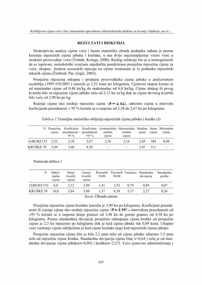
Kolebljivost cijena voća i žita i ekonomska opravdanost infrastrukturnih objekata za čuvanje i hlađenje: pro et ...
625
REZULTATI I DISKUSIJA
Deskriptivna analiza cijena voća i bazna statistička obrada podataka rađena je prema kretanju mjesečnih cijena jabuka i krušaka, u nas dvije najzastupljenije voćne vrste u strukturi proizvodnje voća (Tratnik, Kolega, 2000). Razlog selekcije bio je u nemogućnostida se ispravno, metodološki izračuna zajednička ponderirana prosječna mjesečna cijena za voće, ukupno. Analiza sezonskih utjecaja na cijene izračunata je iz podataka mjesečnihtekućih cijena (Žimbrek, Par, Grgić, 2002).
Prosječna mjesečna otkupna i prodajna proizvođačka cijena jabuke u analiziranom razdoblju (1995-VII/2007.) iznosila je 2,52 kune po kilogramu. Cjenovni raspon kretao se od minimalne cijene od 0,48 kn/kg do maksimalne od 6,8 kn/kg. Cijene donjeg ili prvog kvartila bile su mjesečne cijene jabuke niže od 2,12 kn za kg dok su cijene devetog kvartila bile veće od 2,90 kn po kg.
Rojenje cijena oko srednje mjesečne cijene , odnosno cijena u intervalu koeficijenta pouzdanosti ± 95 % kretala se u rasponu od 2,38 do 2,67 kn po kilogramu.
Tablica 1 Temeljna statistička obilježja mjesečnih cijena jabuke i kruške (I)
N Prosječnacijena
Koeficijentpouzdanosti -
95 %
Koeficijentpouzdanosti
+95 %
Geometrijskasredinacijena
Harmonijskasredinacijena
Medijancijene
Sumacijena
Minimalnacijena
JABUKE152 2,52 2,38 2,67 2,36 2,16 2,49 384 0,48
KRUŠKE 78 3,99 3,48 4,50 - - 3,47 311 -
Nastavak tablice 1
N Maksi-malnacijena
Donjikvartilicijena
Gornjikvartilicijena
Percentili10,00
Percentili90,00
Varijanca Standardnadevijacija
Standardnagreška
JABUKE152 6,8 2,12 2,90 1,41 3,52 0,79 0,89 0,07
KRUŠKE 78 10,8 2,64 5,08 1,37 6,58 5,17 2,27 0,26 Izvor: Obrada autora
Prosječna mjesečna cijena krušaka iznosila je 3,99 kn po kilogramu. Koeficijent pouzda-nosti ili rojenje cijena oko srednje mjesečne cijene s intervalom pouzdanosti od ±95 % kretala se u rasponu donje granice od 3,48 kn do gornje granice od 4,50 kn po kilogramu. Prema standardnoj devijaciji prosječno odstupanje cijena kruške od prosječnecijene je 2,3 kn mjesečno po kilogramu dok je kod cijena jabuke tek 0,89 kuna. Ukupno veće variranje cijena zabilježeno je kod cijene krušaka nego kod mjesečnih cijena jabuke.
Prosječne mjesečna cijena žita je bila 2,2 puta niža od cijene jabuke odnosno 3,5 puta niža od mjesečne cijene kruška. Standardna devijacija cijena žita( σ=0,64 ) niža je od stan-dardne devijacije cijena jabuke(σ=0,89) i kruške(σ=2,27). Veće cjenovno administriranje i
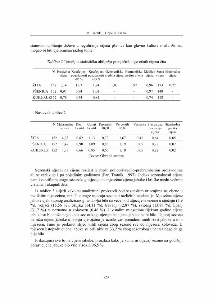
M. Tratnik, I. Grgić, R. Franić
626
stanovito uplitanje države u reguliranje cijena pšenice kao glavne kulture među žitima, mogao bi biti djelomičan razlog tome.
Tablica 2 Temeljna statistička obilježja prosječnih mjesečnih cijena žita
N Prosječnacijena
Koeficijentpouzdanosti
-95 %
Koeficijentpouzdanosti
+95 %
Geometrijskasredina cijena
Harmonijskasredina cijena
Medijancijena
Sumacijena
Minimalnacijena
ŽITA 152 1,14 1,03 1,24 1,03 0,97 0,96 173 0,27
PŠENICA 152 0,97 0,94 1,01 - - 0,97 148 -
KUKURUZ152 0,78 0,74 0,81 - - 0,74 118 -
Nastavak tablice 2
N Maksimalnacijena
Donjikvartil
Gornjikvartil
Percentili10,00
Percentili90,00
Varijanca Standardnadevijacija
cijena
Standardnagreškacijena
ŽITA 152 4,23 0,82 1,13 0,72 1,67 0,41 0,64 0,05
PŠENICA 152 1,42 0,90 1,09 0,83 1,19 0,05 0,22 0,02
KUKURUZ 152 1,33 0,66 0,85 0,60 1,10 0,05 0,22 0,02 Izvor: Obrada autora
Sezonski utjecaj na cijene različit je među poljoprivredno-prehrambenim proizvodima ali se razlikuje i po pojedinim godinama (Par, Tratnik, 1997). Indeks sezonalnosti cijena nam kvantificira snagu sezonskog utjecaja na mjesečne cijene jabuke i kruške među voćnimvrstama i ukupnih žita.
Iz tablice 3 slijedi kako su analizirani proizvodi pod sezonskim utjecajima na cijene u različitim mjesecima, različite snage utjecaja sezone i različitih tendencija. Mjesečne cijene jabuke cjelokupnog analiziranog razdoblja bile su veće pod utjecajem sezone u siječnju (7,9 %), veljači (15,56 %), ožujku (14,11 %), travanj (12,87 %), svibanj (13,89 %), lipanj (31,71%) te neznatno u kolovozu (0,46 %). U ostalim mjesecima tijekom godine cijene jabuke su bile niže nego kada sezonskog utjecaja na cijene jabuke ne bi bilo. Utjecaj sezone na nižu cijenu jabuke u srpnju vjerojatno je uzrokovan ponudom ranih sorti jabuke u tom mjesecu, čime je prekinut slijed viših cijena zbog sezone sve do mjeseca kolovoza. U mjesecu listopadu cijene jabuke su bile niže za 33,2 % zbog sezonskog utjecaja nego da ga nije bilo.
Prikazujući sve to na cijeni jabuke, proizlazi kako je sumarni utjecaj sezone na godišnji porast cijene jabuke bio vrlo visokih 96,5 %.
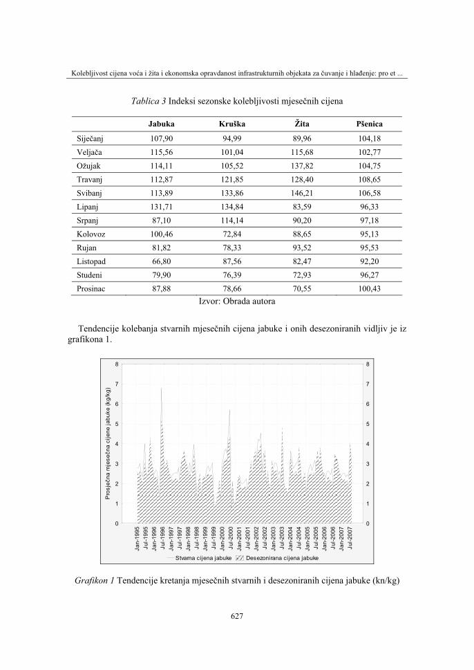
Kolebljivost cijena voća i žita i ekonomska opravdanost infrastrukturnih objekata za čuvanje i hlađenje: pro et ...
627
Tablica 3 Indeksi sezonske kolebljivosti mjesečnih cijena
Jabuka Kruška Žita Pšenica
Siječanj 107,90 94,99 89,96 104,18
Veljača 115,56 101,04 115,68 102,77
Ožujak 114,11 105,52 137,82 104,75
Travanj 112,87 121,85 128,40 108,65
Svibanj 113,89 133,86 146,21 106,58
Lipanj 131,71 134,84 83,59 96,33
Srpanj 87,10 114,14 90,20 97,18
Kolovoz 100,46 72,84 88,65 95,13
Rujan 81,82 78,33 93,52 95,53
Listopad 66,80 87,56 82,47 92,20
Studeni 79,90 76,39 72,93 96,27
Prosinac 87,88 78,66 70,55 100,43 Izvor: Obrada autora
Tendencije kolebanja stvarnih mjesečnih cijena jabuke i onih desezoniranih vidljiv je iz grafikona 1.
Jan-
1995
Jul-1
995
Jan-
1996
Jul-1
996
Jan-
1997
Jul-1
997
Jan-
1998
Jul-1
998
Jan-
1999
Jul-1
999
Jan-
2000
Jul-2
000
Jan-
2001
Jul-2
001
Jan-
2002
Jul-2
002
Jan-
2003
Jul-2
003
Jan-
2004
Jul-2
004
Jan-
2005
Jul-2
005
Jan-
2006
Jul-2
006
Jan-
2007
Jul-2
007
Stvarna cijena jabuke Desezonirana cijena jabuke
0
1
2
3
4
5
6
7
8
Pro
sječ
na m
jese
čna
cije
ne ja
buke
(kg/
kg)
0
1
2
3
4
5
6
7
8
Grafikon 1 Tendencije kretanja mjesečnih stvarnih i desezoniranih cijena jabuke (kn/kg)
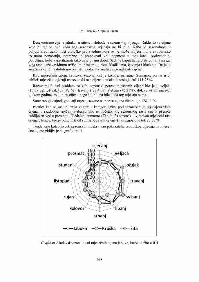
M. Tratnik, I. Grgić, R. Franić
628
Desezonirane cijene jabuka su cijene oslobođene sezonskog utjecaja. Dakle, to su cijene koje bi realno bile kada tog sezonskog utjecaja ne bi bilo. Kako je sezonalnost u poljoprivredi zakonitost biološke proizvodnje koja se ne može izbjeći niti u ekonomsko tržišnom ponašanju, potrebno je prepoznati koji segment u tom lancu proizvodnja-potrošnja, treba kapitalizirati tako uvjetovanu dobit. Sada je kapitalizira distributivna mreža koja raspolaže zavidnom tržišnom infrastrukturom skladištenja, čuvanja i hlađenje. Da je to značajna veličina dobiti govore nam podaci iz analize sezonalnosti cijena.
Kod mjesečnih cijena krušaka, sezonalnost je također prisutna. Sumarno, prema istoj tablici, mjesečni utjecaji na sezonski rast cijena krušaka iznosio je čak 111,25 %.
Razmatrajući isti problem za žita, sezonski porast mjesečnih cijena bio je u veljači(15,67 %), ožujak (37, 82 %), travanj ( 28,4 %), svibanj (46,21%), dok su ostali mjeseci tijekom godine imali nižu cijenu nego što bi ona bila kada tog utjecaja nema.
Sumarno gledajući, godišnji utjecaj sezone na porast cijena žita bio je 128,11 %. Pšenica kao najzastupljenija kultura u kategoriji žita, pod sezonskim je utjecajem viših
cijena, u razdoblju siječanj-svibanj, iako je početak tog sezonskog rasta cijena pšenice zabilježen već u prosincu. Gledajući sumarno (Tablici 3) sezonski uvjetovan mjesečni rast cijena pšenice, bio je puno niži od sumarnog rasta cijene žita i iznosio je tek 27,63 %.
Tendencije kolebljivosti sezonskih indeksa kao pokazatelja sezonskog utjecaja na mjese-čne cijene vidljiv je na grafikonu 1.
Grafikon 2 Indeksi sezonalnosti mjesečnih cijena jabuke, kruške i žita u RH
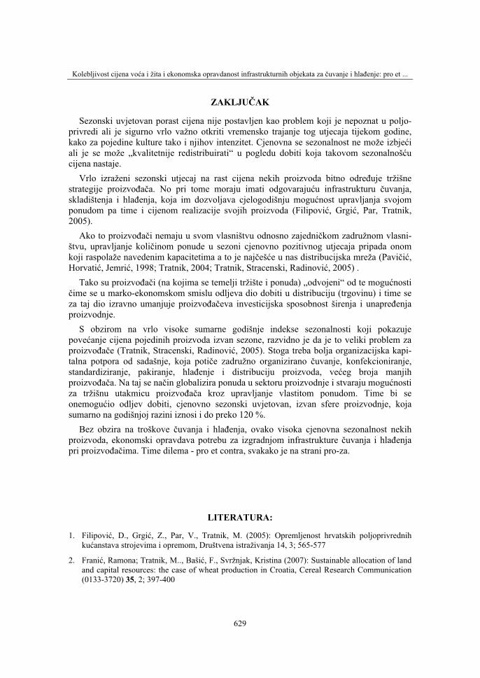
Kolebljivost cijena voća i žita i ekonomska opravdanost infrastrukturnih objekata za čuvanje i hlađenje: pro et ...
629
ZAKLJUČAK
Sezonski uvjetovan porast cijena nije postavljen kao problem koji je nepoznat u poljo-privredi ali je sigurno vrlo važno otkriti vremensko trajanje tog utjecaja tijekom godine, kako za pojedine kulture tako i njihov intenzitet. Cjenovna se sezonalnost ne može izbjećiali je se može „kvalitetnije redistribuirati“ u pogledu dobiti koja takovom sezonalnošćucijena nastaje.
Vrlo izraženi sezonski utjecaj na rast cijena nekih proizvoda bitno određuje tržišne strategije proizvođača. No pri tome moraju imati odgovarajuću infrastrukturu čuvanja,skladištenja i hlađenja, koja im dozvoljava cjelogodišnju mogućnost upravljanja svojom ponudom pa time i cijenom realizacije svojih proizvoda (Filipović, Grgić, Par, Tratnik, 2005).
Ako to proizvođači nemaju u svom vlasništvu odnosno zajedničkom zadružnom vlasni-štvu, upravljanje količinom ponude u sezoni cjenovno pozitivnog utjecaja pripada onom koji raspolaže navedenim kapacitetima a to je najčešće u nas distribucijska mreža (Pavičić,Horvatić, Jemrić, 1998; Tratnik, 2004; Tratnik, Stracenski, Radinović, 2005) .
Tako su proizvođači (na kojima se temelji tržište i ponuda) „odvojeni“ od te mogućnostičime se u marko-ekonomskom smislu odljeva dio dobiti u distribuciju (trgovinu) i time se za taj dio izravno umanjuje proizvođačeva investicijska sposobnost širenja i unapređenja proizvodnje.
S obzirom na vrlo visoke sumarne godišnje indekse sezonalnosti koji pokazuje povećanje cijena pojedinih proizvoda izvan sezone, razvidno je da je to veliki problem za proizvođače (Tratnik, Stracenski, Radinović, 2005). Stoga treba bolja organizacijska kapi-talna potpora od sadašnje, koja potiče zadružno organizirano čuvanje, konfekcioniranje, standardiziranje, pakiranje, hlađenje i distribuciju proizvoda, većeg broja manjih proizvođača. Na taj se način globalizira ponuda u sektoru proizvodnje i stvaraju mogućnostiza tržišnu utakmicu proizvođača kroz upravljanje vlastitom ponudom. Time bi se onemogućio odljev dobiti, cjenovno sezonski uvjetovan, izvan sfere proizvodnje, koja sumarno na godišnjoj razini iznosi i do preko 120 %.
Bez obzira na troškove čuvanja i hlađenja, ovako visoka cjenovna sezonalnost nekih proizvoda, ekonomski opravdava potrebu za izgradnjom infrastrukture čuvanja i hlađenjapri proizvođačima. Time dilema - pro et contra, svakako je na strani pro-za.
LITERATURA:
1. Filipović, D., Grgić, Z., Par, V., Tratnik, M. (2005): Opremljenost hrvatskih poljoprivrednih kućanstava strojevima i opremom, Društvena istraživanja 14, 3; 565-577
2. Franić, Ramona; Tratnik, M.., Bašić, F., Svržnjak, Kristina (2007): Sustainable allocation of land and capital resources: the case of wheat production in Croatia, Cereal Research Communication (0133-3720) 35, 2; 397-400
M. Tratnik, I. Grgić, R. Franić
630
3. Grgić, I. (2000): Promjenjivost proizvođačkih cijena glavnih poljoprivrednih proizvoda u Hrvatskoj, doktorska disertacija, Agronomski fakultet, Sveučilište u Zagrebu
4. Grgić, Z. (1999): Organizacijsko-ekonomske pretpostavke hladnjače voća u obiteljskim gospodarstvima, 15. Hrvatsko savjetovanje tehnologa sušenja i skladištenja s međunarodnimučešćem/S. Pliestić (ur.) Zagreb: Agronomski fakultet, 87.
5. http://www.dzs.hr/Hrv/poljoprivreda/Popis2003.htm
6. http://www.dzs.hr/ljetopis/LjFrameH.htm
7. http://www.dzs.hr/hrv/priopcenja/PrFrameH.htm
8. Kolega, A., Radman, Marija (1999): Primjeri povezivanja obiteljskih gospodarstava na tržištu poljodjelskih proizvoda, Gospodarske smjernice razvitka hrvatskog poljodjelstva, zbornik priopćenja i sažetaka/Kolega, Ante (ur.).-Zagreb, Hrvatsko agronomsko društvo, 136-136.
9. Njavro, M., Par, V. (2004): Utjecaj promjenjivosti prinosa i cijena na upravljanje poljoprivrednim gospodarstvom, Priopćenja s XXXIX. znanstvenog skupa hrvatskih agronoma/Žimbrek, Tito (ur.).-Zagreb, Agronomski fakultet, 101-103.
10. Par, V., Tratnik, M. (1997): O skladišnim kapacitetima kao činiteljima razvoja poljodjelskih gospodarstava, XIII. Međunarodno savjetovanje tehnologa sušenja i skladištenja/Pliestić, Stjepan (ur.).-Zagreb, Agronomski fakultet, Zavod za poljoprivrednu tehnologiju, 133-141.
11. Pavičić, N., Horvatić, R., Jemrić, T. (1998): Modeli skladištenja voća sa obiteljskih gospodarstava, Zbornik radova sa 14. međunarodnog savjetovanja tehnologa sušenja i skladištenja/Stjepan Pliestić (ur.).-Zagreb, Agronomski fakultet, 230-245.
12. Tratnik, M., Grgić, I., Pliestić, S. (2006): Organizacijsko-ekonomski koncept zadružne mreže hladnjača za voće i povrće s obiteljskih gospodarstava u Hrvatskoj, Actual tasks on agricultural engineering / Silvio Košutić (ur.). - Zagreb: Zavod za mehanizaciju poljoprivrede, Agronomski fakultet Sveučilišta u Zagrebu, 457-466.
13. Tratnik, M. (2004): Modeliranje i optimizacija mreže hladnjača za voće i povrće pri obiteljskim poljoprivrednim gospodarstvima, MPŠ RH
14. Tratnik, M., Hrsto, D. (2001): Analiza sezonalnosti cijena povrća na hrvatskom tržištu, Agronomski glasnik 63, 4-5; 205-213
15. Tratnik, M., Kolega, A. (2000): Kolebljivost cijena voća na hrvatskom tržištu, Zbornik plenarnih izlaganja i sažetaka/Brkić, Srećko (ur.).-Zagreb, Hrvatsko agroekonomsko društvo, 168-169.
16. Tratnik, M., Stracenski, Maja; Radinović, S. (2005): Zadrugarstvo: čimbenik stabilnosti, kompetitivnosti i konkurentnosti malih poljoprivrednih gospodarstava, Sociologija sela 43, 167; 195-213
17. Žimbrek, T., Par, V., Grgić, I. (2002): Production and Economic Characteristics of Fruit Sector in Croatia, Proc. of the XXXVIth International Horticultural Congress & Exhibition,Toronto, Canada

Kolebljivost cijena voća i žita i ekonomska opravdanost infrastrukturnih objekata za čuvanje i hlađenje: pro et ...
631
FRUIT AND VEGETABLE PRICE FLUCTUATIONS AND ECONOMIC JUSTIFIABILITY OF INFRASTRUCTURAL
FACILITIES FOR STORAGE AND COOLING:PRO ET CONTRA
TRATNIK MIROSLAV, GRGIĆ IVO, RAMONA FRANIĆ
1Faculty of Agriculture of the University of Zagreb, Department of Agricultural Economics and Rural Sociology
SUMMARY
Seasonality is a phenomenon characteristic for biological economic branches, so for agriculture as well. It can not be avoided, so it causes a certain production and market dilemmas regarding the appropriation and redistribution of a considerable profit between stakeholders in the production-market chain. The mentioned profit is a result of seasonally conditioned price growth, which, due to a lack of adequate producers' storage and cooling facilities, "flows over" into the distribution sphere.
This is proved by a very high aggregate indices of seasonal impact on the price growth of apples (96.5%), pears (111.25%) and total cereals (128.11%), and particularly for wheat (27.63%).
No matter the costs of storage and cooling, such high price seasonality for some products justifies economically the need for construction of the storage and cooling facilities by the producers. Such the dilemma – pro et contra – is definitely on the 'pro' side.
Key words: price fluctuations, seasonality index, monthly prices, cooling and storage facilities, fruits, cereals

36. Symposium "Actual Tasks on Agricultural Engineering", Opatija, Croatia, 2008.
633
36.
SIMPOZIJAKTUALNI ZADACIMEHANIZACIJE POLJOPRIVREDE
UDC631.51.022:635.132
Stručni radEXpert paper
PRODUCING ON MINI BARS AS A CONDITION FOR GETTING REGULAR SHAPE OF CARROT ROOT
MILENA JANČIĆ
Faculty of Agriculture, 21000 Novi Sad, Trg Dositeja Obradovića 8
SUMMARY
One of conditions for breeding carrot for fresh use, is producing regulary, mechanicly not damaged and uniform roots.
When is wished to get these roots, breeding carrots was on mini bars. As a proof, that breeding carrots on mini bars is better than breeding on flat surface, we measured values of soil density and volume mass. Based on the results the soil density was lower after getting mini bars and the carrot roots had better conditions for getting regulary shape. After the harvest, roots were measured in theirs length, diameters and mass. Also are measured the sphericity of root, density and volume. That was important for demands of market. The results were positive and carrot was great positioned in markets. In this paper is shown technology of packing the carrot root.
Key words: carrot root, mini bars, postharvest root quality.
INTRODUCTION
Carrot – Daucus carota, fam. Apiaceae, belong to root vegetable group. Carrot is biennial dicotyledon plant, which is breeding for tasty thick (massy) root, which can be yellow, orange or red colored. Carrot root is used in fresh use over all year, as cooked, spice, dehydrated, marinated, frosted and like baby food.
Traditional carrot breeding, in Vojvodina area, was on flat surface. This breeding method has been for a long time in use, because the machines for carrot breeding were same as for crops breeding.
However, carrot consumers have had high requirements about root shape. The root have to be long, straight and uniform shape. When is wished to get these roots, the idea was to breed carrot on mini bars. That breeding method gave better soil conditions for growing carrot, and the shape was not branched, or ununiform in mass, volume and lenght.
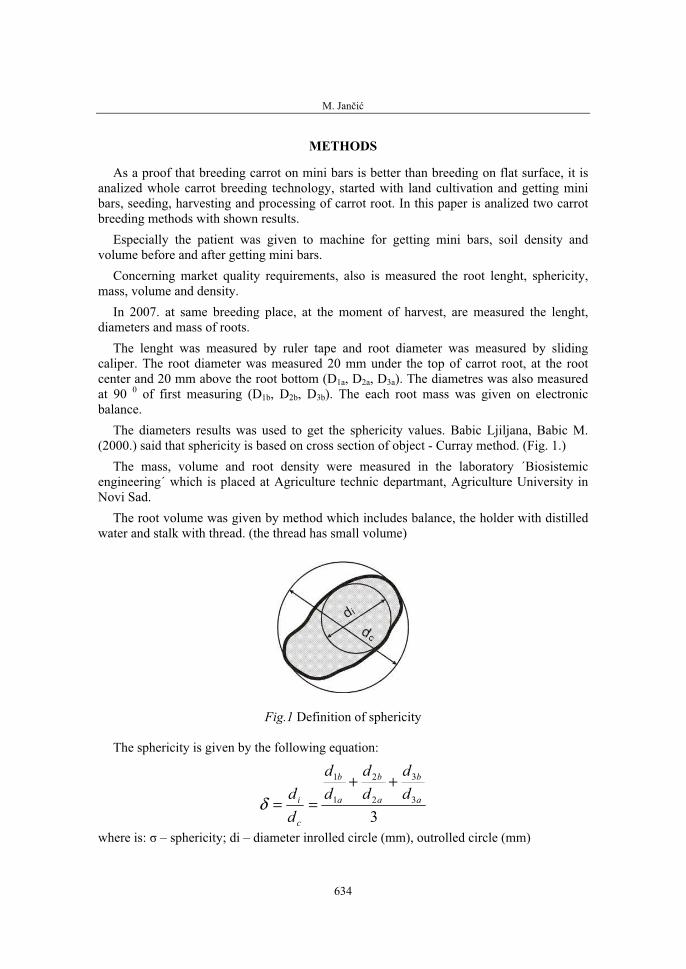
M. Jančić
634
METHODS
As a proof that breeding carrot on mini bars is better than breeding on flat surface, it is analized whole carrot breeding technology, started with land cultivation and getting mini bars, seeding, harvesting and processing of carrot root. In this paper is analized two carrot breeding methods with shown results.
Especially the patient was given to machine for getting mini bars, soil density and volume before and after getting mini bars.
Concerning market quality requirements, also is measured the root lenght, sphericity, mass, volume and density.
In 2007. at same breeding place, at the moment of harvest, are measured the lenght, diameters and mass of roots.
The lenght was measured by ruler tape and root diameter was measured by sliding caliper. The root diameter was measured 20 mm under the top of carrot root, at the root center and 20 mm above the root bottom (D1a, D2a, D3a). The diametres was also measured at 90 0 of first measuring (D1b, D2b, D3b). The each root mass was given on electronic balance.
The diameters results was used to get the sphericity values. Babic Ljiljana, Babic M. (2000.) said that sphericity is based on cross section of object - Curray method. (Fig. 1.)
The mass, volume and root density were measured in the laboratory ´Biosistemic engineering´ which is placed at Agriculture technic departmant, Agriculture University in Novi Sad.
The root volume was given by method which includes balance, the holder with distilled water and stalk with thread. (the thread has small volume)
Fig.1 Definition of sphericity
The sphericity is given by the following equation:
33
3
2
2
1
1
a
b
a
b
a
b
c
i dd
dd
dd
dd
++==δ
where is: σ – sphericity; di – diameter inrolled circle (mm), outrolled circle (mm)
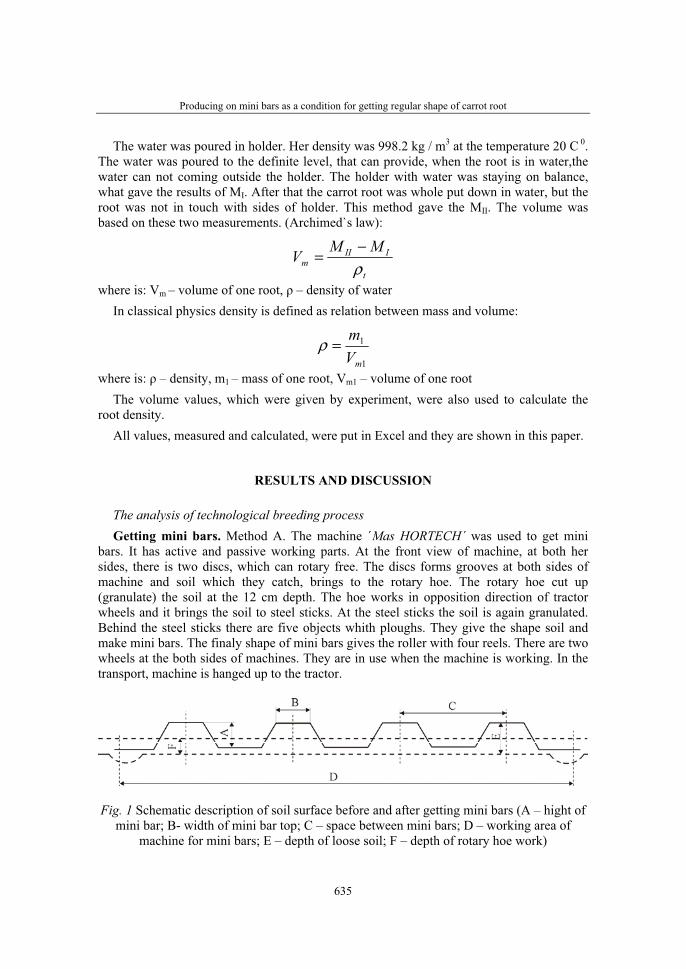
Producing on mini bars as a condition for getting regular shape of carrot root
635
The water was poured in holder. Her density was 998.2 kg / m3 at the temperature 20 C 0.The water was poured to the definite level, that can provide, when the root is in water,the water can not coming outside the holder. The holder with water was staying on balance, what gave the results of MI. After that the carrot root was whole put down in water, but the root was not in touch with sides of holder. This method gave the MII. The volume was based on these two measurements. (Archimed`s law):
t
IIIm
MMVρ−
=
where is: Vm – volume of one root, ρ – density of water In classical physics density is defined as relation between mass and volume:
1
1
mVm
=ρ
where is: ρ – density, m1 – mass of one root, Vm1 – volume of one root The volume values, which were given by experiment, were also used to calculate the
root density. All values, measured and calculated, were put in Excel and they are shown in this paper.
RESULTS AND DISCUSSION
The analysis of technological breeding process Getting mini bars. Method A. The machine ´Mas HORTECH´ was used to get mini
bars. It has active and passive working parts. At the front view of machine, at both her sides, there is two discs, which can rotary free. The discs forms grooves at both sides of machine and soil which they catch, brings to the rotary hoe. The rotary hoe cut up (granulate) the soil at the 12 cm depth. The hoe works in opposition direction of tractor wheels and it brings the soil to steel sticks. At the steel sticks the soil is again granulated. Behind the steel sticks there are five objects whith ploughs. They give the shape soil and make mini bars. The finaly shape of mini bars gives the roller with four reels. There are two wheels at the both sides of machines. They are in use when the machine is working. In the transport, machine is hanged up to the tractor.
Fig. 1 Schematic description of soil surface before and after getting mini bars (A – hight of mini bar; B- width of mini bar top; C – space between mini bars; D – working area of
machine for mini bars; E – depth of loose soil; F – depth of rotary hoe work)
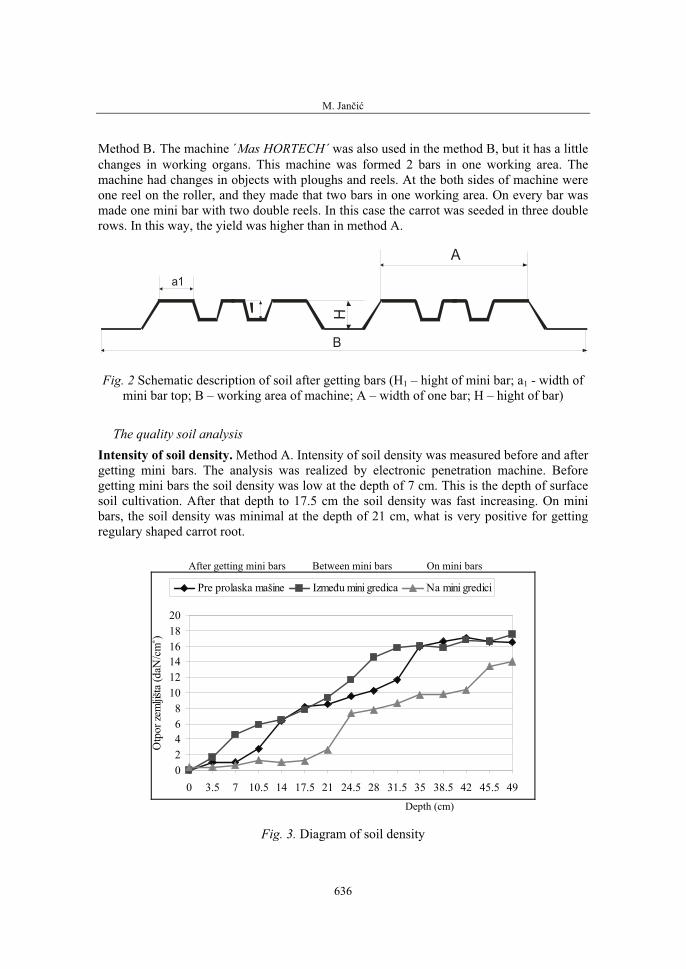
M. Jančić
636
Method B. The machine ´Mas HORTECH´ was also used in the method B, but it has a little changes in working organs. This machine was formed 2 bars in one working area. The machine had changes in objects with ploughs and reels. At the both sides of machine were one reel on the roller, and they made that two bars in one working area. On every bar was made one mini bar with two double reels. In this case the carrot was seeded in three double rows. In this way, the yield was higher than in method A.
A
a1
HB
Fig. 2 Schematic description of soil after getting bars (H1 – hight of mini bar; a1 - width of mini bar top; B – working area of machine; A – width of one bar; H – hight of bar)
The quality soil analysis Intensity of soil density. Method A. Intensity of soil density was measured before and after getting mini bars. The analysis was realized by electronic penetration machine. Before getting mini bars the soil density was low at the depth of 7 cm. This is the depth of surface soil cultivation. After that depth to 17.5 cm the soil density was fast increasing. On mini bars, the soil density was minimal at the depth of 21 cm, what is very positive for getting regulary shaped carrot root.
After getting mini bars Between mini bars On mini bars
02468
101214161820
0 3.5 7 10.5 14 17.5 21 24.5 28 31.5 35 38.5 42 45.5 49
Otp
or ze
mljiš
ta (d
aN/c
m2 )
Pre prolaska mašine Između mini gredica Na mini gredici
Depth (cm)
Fig. 3. Diagram of soil density
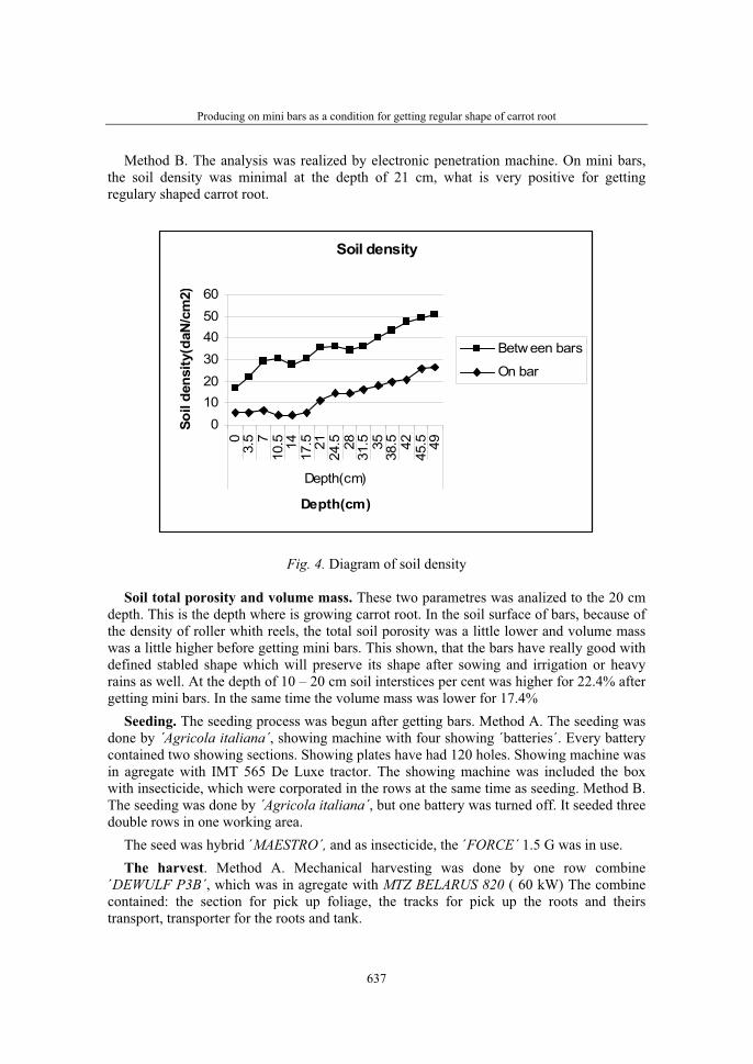
Producing on mini bars as a condition for getting regular shape of carrot root
637
Method B. The analysis was realized by electronic penetration machine. On mini bars, the soil density was minimal at the depth of 21 cm, what is very positive for getting regulary shaped carrot root.
Soil density
0102030405060
03.
5 710
.5 1417
.5 2124
.5 2831
.5 3538
.5 4245
.5 49
Depth(cm)
Depth(cm)
Soil
dens
ity(d
aN/c
m2)
Betw een bars
On bar
Fig. 4. Diagram of soil density
Soil total porosity and volume mass. These two parametres was analized to the 20 cm depth. This is the depth where is growing carrot root. In the soil surface of bars, because of the density of roller whith reels, the total soil porosity was a little lower and volume mass was a little higher before getting mini bars. This shown, that the bars have really good with defined stabled shape which will preserve its shape after sowing and irrigation or heavy rains as well. At the depth of 10 – 20 cm soil interstices per cent was higher for 22.4% after getting mini bars. In the same time the volume mass was lower for 17.4%
Seeding. The seeding process was begun after getting bars. Method A. The seeding was done by ´Agricola italiana´, showing machine with four showing ´batteries´. Every battery contained two showing sections. Showing plates have had 120 holes. Showing machine was in agregate with IMT 565 De Luxe tractor. The showing machine was included the box with insecticide, which were corporated in the rows at the same time as seeding. Method B. The seeding was done by ´Agricola italiana´, but one battery was turned off. It seeded three double rows in one working area.
The seed was hybrid ´MAESTRO´, and as insecticide, the ´FORCE´ 1.5 G was in use. The harvest. Method A. Mechanical harvesting was done by one row combine
´DEWULF P3B´, which was in agregate with MTZ BELARUS 820 ( 60 kW) The combine contained: the section for pick up foliage, the tracks for pick up the roots and theirs transport, transporter for the roots and tank.
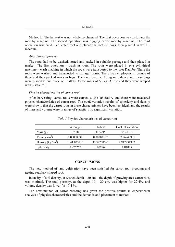
M. Jančić
638
Method B. The harvest was not whole mechanized. The first operation was disfoliage the root by machine. The second operation was digging carrot root by machine. The third operation was hand – collected root and placed the roots in bags, then place it in wash – machine.
After harvest process The roots had to be washed, sorted and packed in suitable package and then placed in
market. The first operation – washing roots. The roots were placed in one cylindrical machine – wash machine in which the roots were transported to the river Danube. There the roots were washed and transported to storage rooms. There was employers in groups of three and they packed roots in bags. The each bag had 10 kg on balance and these bags were placed at one place on ´pallets´ to the mass of 50 kg. At the end they were wraped with plastic foil.
Physics characteristics of carrot root After harvesting, carrot roots were carried to the laboratory and there were measured
physics characteristics of carrot root. The coef. variation results of sphericity and density were shown, that the carrot roots in these characterisitcs have been just ideal, and the results of mass and volume were in range of statistic´s no significant variation.
Tab. 1 Physics characteristics of carrot root
Average Stadeva Coef. of variation
Mass (g) 87.08 31.5296 36.20763
Volume (m3) 0.00008391 0.00003127 37.26745931
Density (kg / m3) 1041.025215 30.32230567 2.912734987
Sphericity 0.976267 0.009868 1.01075
CONCLUSIONS
The new method of land cultivation have been satisfied for carrot root breeding and getting regulary shaped root.
Intensity of soil density, at wished depth – 20 cm – the depth of growing area carrot root, was minimal. The total porosity, at the depth 10 – 20 cm, was higher for 22.4%, and volume density was lower for 17.4 %.
The new method of carrot breeding has given the positive results in experimental analysis of physics characteristics and the demands and placement at market.

Producing on mini bars as a condition for getting regular shape of carrot root
639
REFERENCES
1. Babic Lj. Babic M. Drying and storage, Faculty of agriculture, Novi Sad
2. Babić M. Physical characteristic of agriculture material, Faculty of agriculture, Novi Sad
3. Bajkin A. (1994).The machines in vegetable breeding. University of Novi Sad, Faculty of agriculture, Novi Sad
4. Bajkin A. Jancic M. Ponjican O. (2006). Mechanical harvesting root crop, potato and bulbed vegetables. In: VII Congr Vegetable breeding today Vol 7. Novi Sad, Serbia, pp 36 – 41.
5. Bajkin A. Ponjičan O. Orlović S. Somer D. (2005).The machines in horticulture breeding., University of Novi Sad, Faculty of agriculture, Novi Sad
6. Hadžić V. Belić M. Nešić Lj. (2004). Pedology. Faculty of agriculture, Novi Sad
7. Lazić B. Đurovka M. Marković V. Ilin Ž. (1998).The vegetables. University of Novi Sad, Faculty of agriculture, Novi Sad
8. Todorović J. Lazić B. Komljenović I. (2003). Crops and vegetables guidebook, Grafo – Mark, Laktaši
9. www.agricolaitaliana.com
10. www.dewulf.be
11. www.masitaly.com

Related Documents


![Engi 5035fa05[Assignment6solution]](https://static.cupdf.com/doc/110x72/563db840550346aa9a91fabf/engi-5035fa05assignment6solution.jpg)