Acoustics and Sustainability: How should acoustics adapt to meet future

Acoustics 2008 1

Acoustics 2008 Geelong, Victoria, Australia 24 to 26 November 2008

Acoustics and Sustainability:

How should acoustics adapt to meet future demands?

Scanning laser vibrometer for non-contact three-dimensional displacement and strain measurements

Ben Cazzolato (1), Stuart Wildy (1), John Codrington (1), Andrei Kotousov (1) and Matthias Schuessler (2)

(1) School of Mechanical Engineering, University of Adelaide, SA, Australia

(2) Polytec GmbH, Polytec-Platz 1-7, 76337 Waldbronn, Germany

ABSTRACT

The recent advent of three-dimensional scanning laser vibrometers has enabled extremely accurate non-contact meas-

urement of the three-dimensional displacements of structures. This paper looks at the feasibility of using a scanning

laser vibrometer for the non-contact measurement of dynamic strain fields across the surface of a planar structure. Is-

sues such as laser head alignment and choice of finite-difference scheme are discussed. Finally, experimental results

of a test specimen are presented which clearly demonstrate the significant potential of this new experimental tech-

nique.

INTRODUCTION

The measurement of displacement, strain and stress fields is

important in many fields of applied mechanics and engineer-

ing. Such measurements are most commonly conducted by

contact techniques using strain gauges, brittle surfaces or

piezo-electric sensors, or non-contact methods such as photo-

elasticity (Asundi, 1996), x-ray diffraction (Gilfrich 1998)

and holographic interferometry (Colchero et al. 2002).

Recent improvements in laser measurement systems have

stimulated the application of scanning laser vibrometers to

measure the out-of-plane displacement in plate- or shell-like

structures, from which the curvature, bending strain and

stresses may be estimated via a double spatial derivative

(Miles et al. 1994, Moccio et al. 1996, Xu et al. 1996). It

should be noted that all previous publications involving the

application of laser vibrometers to measure kinematic vari-

ables have been restricted to single laser Doppler vibrometry

able to measure only bending deformations. Due to poor

transducer quality, early applications of the laser vibrometer

technique required extensive spatial filtering to improve the

quality of the strain estimates, at the expense of spatial reso-

lution.

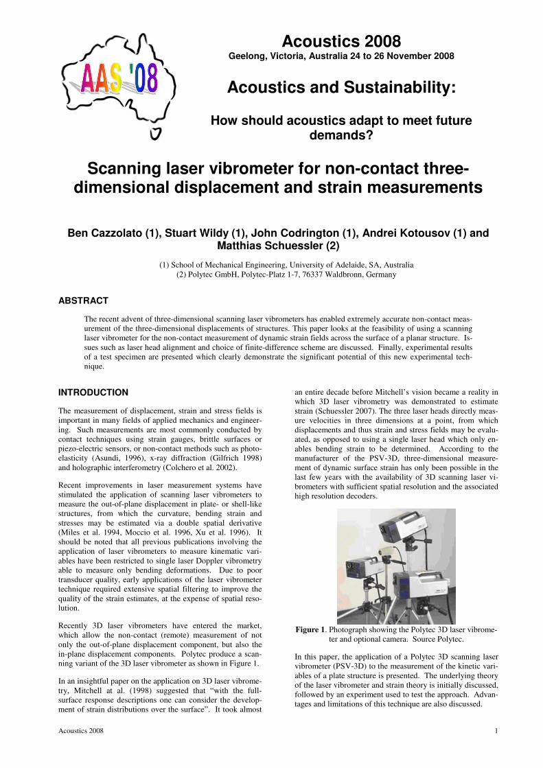
Recently 3D laser vibrometers have entered the market,

which allow the non-contact (remote) measurement of not

only the out-of-plane displacement component, but also the

in-plane displacement components. Polytec produce a scan-

ning variant of the 3D laser vibrometer as shown in Figure 1.

In an insightful paper on the application on 3D laser vibrome-

try, Mitchell at al. (1998) suggested that “with the full-

surface response descriptions one can consider the develop-

ment of strain distributions over the surface”. It took almost

an entire decade before Mitchell’s vision became a reality in

which 3D laser vibrometry was demonstrated to estimate

strain (Schuessler 2007). The three laser heads directly meas-

ure velocities in three dimensions at a point, from which

displacements and thus strain and stress fields may be evalu-

ated, as opposed to using a single laser head which only en-

ables bending strain to be determined. According to the

manufacturer of the PSV-3D, three-dimensional measure-

ment of dynamic surface strain has only been possible in the

last few years with the availability of 3D scanning laser vi-

brometers with sufficient spatial resolution and the associated

high resolution decoders.

Figure 1. Photograph showing the Polytec 3D laser vibrome-

ter and optional camera. Source Polytec.

In this paper, the application of a Polytec 3D scanning laser

vibrometer (PSV-3D) to the measurement of the kinetic vari-

ables of a plate structure is presented. The underlying theory

of the laser vibrometer and strain theory is initially discussed,

followed by an experiment used to test the approach. Advan-

tages and limitations of this technique are also discussed.

24-26 November 2008, Geelong, Australia Proceedings of ACOUSTICS 2008

2 Acoustics 2008

STRAIN ESTIMATION VIA DISPLACEMENT MEASUREMENTS

The approach used for estimating the strain from the dis-

placement field obtained from the lasers is the same as that

used in Finite Element (FE) modelling. The strain finite

element shape functions will now be derived following the

technique presented in Fagan (1992). The analysis presented

here is for planar structures; however the analysis could be

easily extended to three-dimensional structures.

3-noded element

Consider the 3-noded triangular element (shown in Figure 2)

with interpolation function yxyx 321),( αααφ ++= , where

x and y are the coordinates of a point within the element.

This function represents how a value (such as the displace-

ment, u or v ) varies across the element.

y

x

12

3

u1

v1

u2

v2

u3

v3

12

3

u1

v4

u2

v2

u3

v3u44

v1

Figure 2. Two-dimensional 3-noded linear and 4-noded bi-

linear elements.

The real weights iα are a function of the values of φ at each

of the three nodes ( 321 ,, φφφ ) and are given by

( )( )( )3322112

13

33221121

2

33221121

1

φφφα

φφφα

φφφα

ccc

bbb

aaa

A

A

A

++=

++=

++=

A , the area of the triangular element, is given by

( )23123113322121

33

22

11

21

1

1

1

yxyxyxyxyxyx

yx

yx

yx

A −−−++==

where

12321312213

31213231132

23132123321

xxcyybyxyxa

xxcyybyxyxa

xxcyybyxyxa

−=−=−=

−=−=−=

−=−=−=

This can be rewritten more compactly in matrix form of the

following

Φ= ),(),( yxyx Nφ

where N is the FE shape function vector

[ ]),(),(),( 321 yxNyxNyxN=N , such that

( )ycxbayxN iiiAi ++= 21),( .

The interpolation function vector is given by

[ ]T321 φφφ=Φ , where [ ]T is the matrix transpose.

Now consider the displacement [ ]Tvu, at an arbitrary loca-

tion [ ]Tyx, . This is given by the product of shape function

equations at the location and the vector containing the dis-

placements at the nodes,

UN ),(),(

),(yx

yxv

yxu=

where the shape function matrix is (dropping the spatial de-

pendence [ ]Tyx, ) given by

=

321

321

000

000

NNN

NNNN and the column vector

of nodal displacements is given by

=

3

3

2

2

1

1

v

u

v

u

v

u

U .

Differentiating the displacement vector we can obtain the 2-

dimensional strains

x

v

y

u

y

v

x

uxyyx

∂

∂+

∂

∂=

∂

∂=

∂

∂= γεε

To give the strain-nodal displacement matrix relation:

BU=

xy

y

x

γ

ε

ε

where B is the strain matrix given by

=

332211

321

321

000

000

2

1

bcbcbc

ccc

bbb

AB

It should be noted that the strains across linear triangular

elements are therefore uniform, and hence it is known as the

constant strain element.

4-noded element

A similar approach may be taken to define the strain vector

for the 4-noded rectangular bilinear element shown in Figure

2. The formulation presented here is for a rectangular ele-

ment. For a more general treatment of quadrilateral plate

element see Wang et al. (2004) or Kardestuncer (1987).

The displacement field within the element may be interpo-

lated using

UN ),(),(

),(yx

yxv

yxu=

where the displacements at the nodes is given by

Proceedings of ACOUSTICS 2008 24-26 November 2008, Geelong, Australia

Acoustics 2008 3

=

4

4

3

3

2

2

1

1

v

u

v

u

v

u

v

u

U

and the shape function matrix is

=

4321

4321

0000

0000

NNNN

NNNNN where the

individual (bilinear) shape functions as a function of the natu-

ral (normalised) coordinates ξ and η are given by

( )( ) ( )( )( )( ) ( )( ).1111

1111

41

441

2

41

341

1

ηξηξ

ηξηξ

+−=−+=

++=−−=

NN

NN

For rectangular elements the natural (normalised) coordinates

are12

122

xx

xxx

−

+−=ξ and

12

122

yy

yyy

−

+−=η .

By spatially differentiating the displacement field, the strain

field of a 4-node quadrilateral element is obtained

BU=

xy

y

x

γ

ε

ε

where

+−

−

−−−

++

++

−+−

+−

−

−−

−−

−−

−−

=

ab

ba

ab

ba

ab

ba

ab

ba

T

ηξ

ξη

ηξ

ξη

ηξ

ξη

ηξ

ξη

110

10

1

110

10

1

110

10

1

110

10

1

B ,

342

1122

1 xxxxa −=−= and 232

1142

1 yyyyb −=−= .

POLYTEC PSV-3D SCANNING LASER VIBROMETER

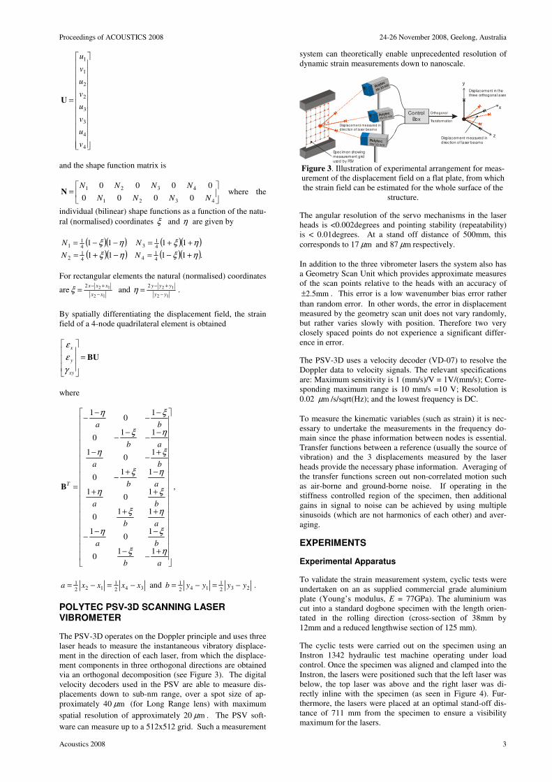
The PSV-3D operates on the Doppler principle and uses three

laser heads to measure the instantaneous vibratory displace-

ment in the direction of each laser, from which the displace-

ment components in three orthogonal directions are obtained

via an orthogonal decomposition (see Figure 3). The digital

velocity decoders used in the PSV are able to measure dis-

placements down to sub-nm range, over a spot size of ap-

proximately 40 mµ (for Long Range lens) with maximum

spatial resolution of approximately 20 mµ . The PSV soft-

ware can measure up to a 512x512 grid. Such a measurement

system can theoretically enable unprecedented resolution of

dynamic strain measurements down to nanoscale.

Polytec

PSV 3D-400

Polytec

PSV-3D 400

Specimen showingmeasurement grid

used by PSV

PolytecPSV-3D 400

Displacement measured indirection of laser beams

x

y

z

Orthogonal

Transformation

Displacement in thethree orthogonal axes

Control

BoxDisplacement measured in

direc tion of laser beams

Figure 3. Illustration of experimental arrangement for meas-

urement of the displacement field on a flat plate, from which

the strain field can be estimated for the whole surface of the

structure.

The angular resolution of the servo mechanisms in the laser

heads is <0.002degrees and pointing stability (repeatability)

is < 0.01degrees. At a stand off distance of 500mm, this

corresponds to 17 mµ and 87 mµ respectively.

In addition to the three vibrometer lasers the system also has

a Geometry Scan Unit which provides approximate measures

of the scan points relative to the heads with an accuracy of

mm5.2± . This error is a low wavenumber bias error rather

than random error. In other words, the error in displacement

measured by the geometry scan unit does not vary randomly,

but rather varies slowly with position. Therefore two very

closely spaced points do not experience a significant differ-

ence in error.

The PSV-3D uses a velocity decoder (VD-07) to resolve the

Doppler data to velocity signals. The relevant specifications

are: Maximum sensitivity is 1 (mm/s)/V = 1V/(mm/s); Corre-

sponding maximum range is 10 mm/s =10 V; Resolution is

0.02 mµ /s/sqrt(Hz); and the lowest frequency is DC.

To measure the kinematic variables (such as strain) it is nec-

essary to undertake the measurements in the frequency do-

main since the phase information between nodes is essential.

Transfer functions between a reference (usually the source of

vibration) and the 3 displacements measured by the laser

heads provide the necessary phase information. Averaging of

the transfer functions screen out non-correlated motion such

as air-borne and ground-borne noise. If operating in the

stiffness controlled region of the specimen, then additional

gains in signal to noise can be achieved by using multiple

sinusoids (which are not harmonics of each other) and aver-

aging.

EXPERIMENTS

Experimental Apparatus

To validate the strain measurement system, cyclic tests were

undertaken on an as supplied commercial grade aluminium

plate (Young’s modulus, E = 77GPa). The aluminium was

cut into a standard dogbone specimen with the length orien-

tated in the rolling direction (cross-section of 38mm by

12mm and a reduced lengthwise section of 125 mm).

The cyclic tests were carried out on the specimen using an

Instron 1342 hydraulic test machine operating under load

control. Once the specimen was aligned and clamped into the

Instron, the lasers were positioned such that the left laser was

below, the top laser was above and the right laser was di-

rectly inline with the specimen (as seen in Figure 4). Fur-

thermore, the lasers were placed at an optimal stand-off dis-

tance of 711 mm from the specimen to ensure a visibility

maximum for the lasers.


4 Acoustics 2008

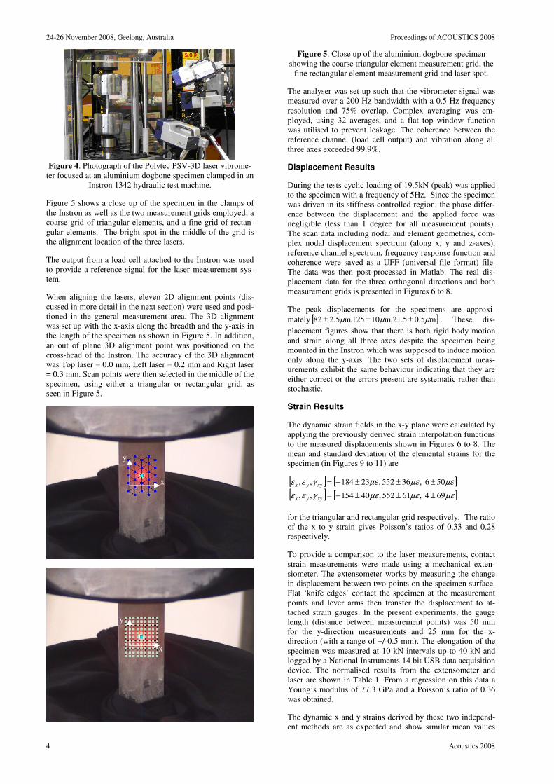
Figure 4. Photograph of the Polytec PSV-3D laser vibrome-

ter focused at an aluminium dogbone specimen clamped in an

Instron 1342 hydraulic test machine.

Figure 5 shows a close up of the specimen in the clamps of

the Instron as well as the two measurement grids employed; a

coarse grid of triangular elements, and a fine grid of rectan-

gular elements. The bright spot in the middle of the grid is

the alignment location of the three lasers.

The output from a load cell attached to the Instron was used

to provide a reference signal for the laser measurement sys-

tem.

When aligning the lasers, eleven 2D alignment points (dis-

cussed in more detail in the next section) were used and posi-

tioned in the general measurement area. The 3D alignment

was set up with the x-axis along the breadth and the y-axis in

the length of the specimen as shown in Figure 5. In addition,

an out of plane 3D alignment point was positioned on the

cross-head of the Instron. The accuracy of the 3D alignment

was Top laser = 0.0 mm, Left laser = 0.2 mm and Right laser

= 0.3 mm. Scan points were then selected in the middle of the

specimen, using either a triangular or rectangular grid, as

seen in Figure 5.

Figure 5. Close up of the aluminium dogbone specimen

showing the coarse triangular element measurement grid, the

fine rectangular element measurement grid and laser spot.

The analyser was set up such that the vibrometer signal was

measured over a 200 Hz bandwidth with a 0.5 Hz frequency

resolution and 75% overlap. Complex averaging was em-

ployed, using 32 averages, and a flat top window function

was utilised to prevent leakage. The coherence between the

reference channel (load cell output) and vibration along all

three axes exceeded 99.9%.

Displacement Results

During the tests cyclic loading of 19.5kN (peak) was applied

to the specimen with a frequency of 5Hz. Since the specimen

was driven in its stiffness controlled region, the phase differ-

ence between the displacement and the applied force was

negligible (less than 1 degree for all measurement points).

The scan data including nodal and element geometries, com-

plex nodal displacement spectrum (along x, y and z-axes),

reference channel spectrum, frequency response function and

coherence were saved as a UFF (universal file format) file.

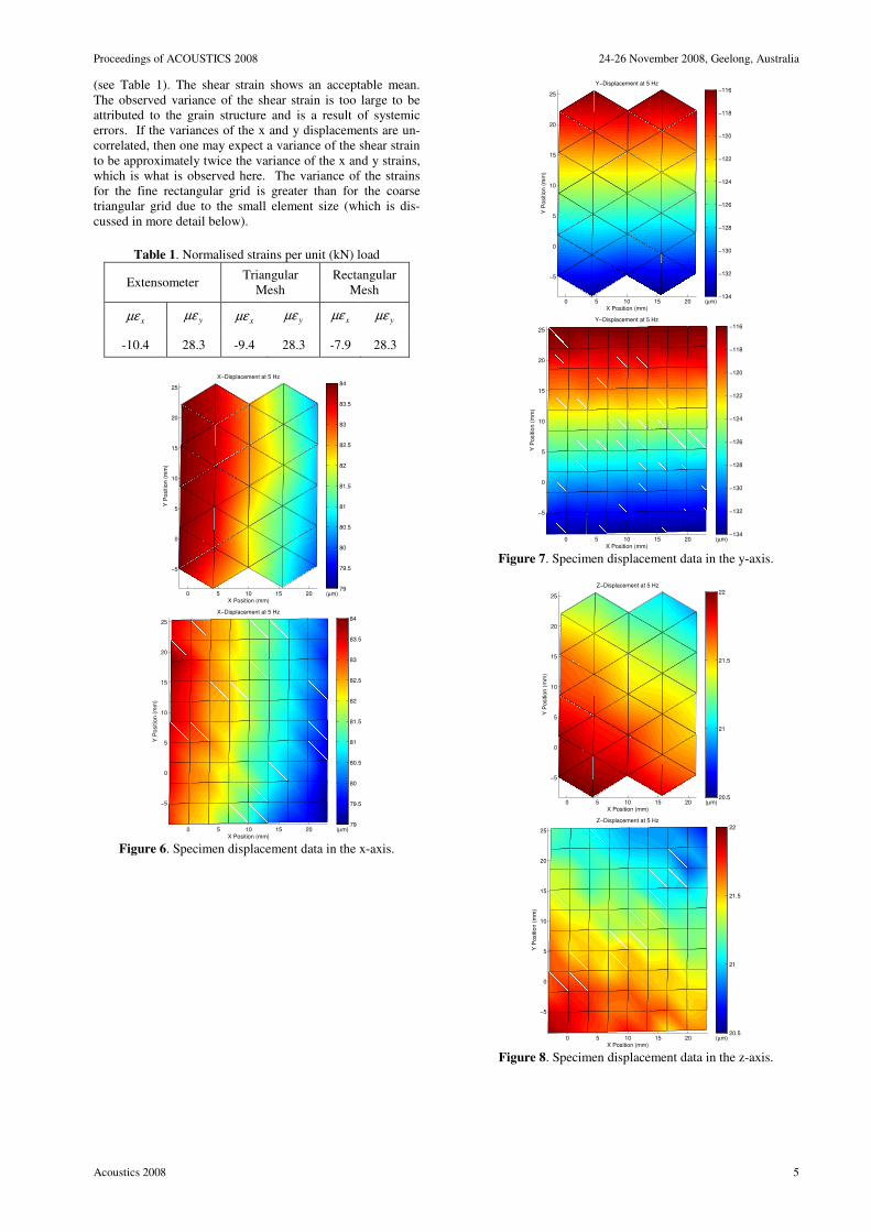
The data was then post-processed in Matlab. The real dis-

placement data for the three orthogonal directions and both

measurement grids is presented in Figures 6 to 8.

The peak displacements for the specimens are approxi-

mately [ ]m5.05.21m,10125m,5.282 µµµ ±±± . These dis-

placement figures show that there is both rigid body motion

and strain along all three axes despite the specimen being

mounted in the Instron which was supposed to induce motion

only along the y-axis. The two sets of displacement meas-

urements exhibit the same behaviour indicating that they are

either correct or the errors present are systematic rather than

stochastic.

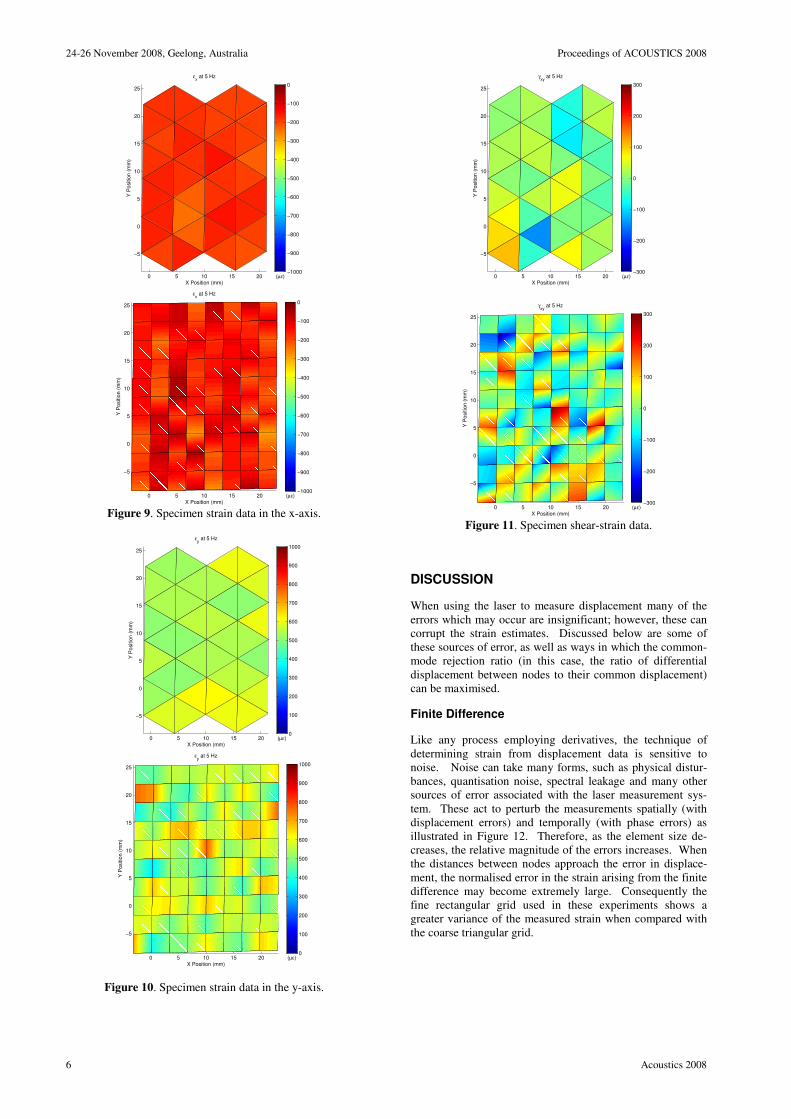
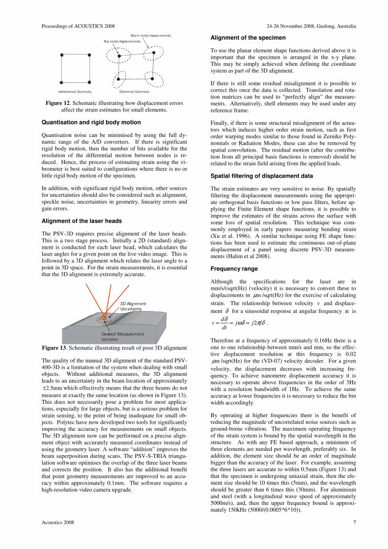
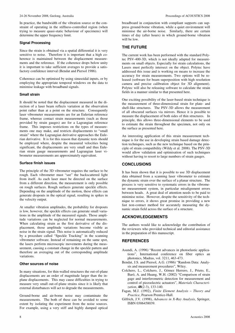
Strain Results

The dynamic strain fields in the x-y plane were calculated by

applying the previously derived strain interpolation functions

to the measured displacements shown in Figures 6 to 8. The

mean and standard deviation of the elemental strains for the

specimen (in Figures 9 to 11) are

[ ] [ ][ ] [ ]µεµεµεγεε

µεµεµεγεε

694 ,61525 ,40154,,

506 ,36525 ,23184,,

±±±−=

±±±−=

xyyx

xyyx

for the triangular and rectangular grid respectively. The ratio

of the x to y strain gives Poisson’s ratios of 0.33 and 0.28

respectively.

To provide a comparison to the laser measurements, contact

strain measurements were made using a mechanical exten-

siometer. The extensometer works by measuring the change

in displacement between two points on the specimen surface.

Flat ‘knife edges’ contact the specimen at the measurement

points and lever arms then transfer the displacement to at-

tached strain gauges. In the present experiments, the gauge

length (distance between measurement points) was 50 mm

for the y-direction measurements and 25 mm for the x-

direction (with a range of +/-0.5 mm). The elongation of the

specimen was measured at 10 kN intervals up to 40 kN and

logged by a National Instruments 14 bit USB data acquisition

device. The normalised results from the extensometer and

laser are shown in Table 1. From a regression on this data a

Young’s modulus of 77.3 GPa and a Poisson’s ratio of 0.36

was obtained.

The dynamic x and y strains derived by these two independ-

ent methods are as expected and show similar mean values

x

y

x

y


Acoustics 2008 5

(see Table 1). The shear strain shows an acceptable mean.

The observed variance of the shear strain is too large to be

attributed to the grain structure and is a result of systemic

errors. If the variances of the x and y displacements are un-

correlated, then one may expect a variance of the shear strain

to be approximately twice the variance of the x and y strains,

which is what is observed here. The variance of the strains

for the fine rectangular grid is greater than for the coarse

triangular grid due to the small element size (which is dis-

cussed in more detail below).

Table 1. Normalised strains per unit (kN) load

Extensometer Triangular

Mesh

Rectangular

Mesh

xµε yµε xµε yµε xµε yµε

-10.4 28.3 -9.4 28.3 -7.9 28.3

0 5 10 15 20

−5

0

5

10

15

20

25

X−Displacement at 5 Hz

X Position (mm)

Y P

ositio

n (

mm

)

(µm)79

79.5

80

80.5

81

81.5

82

82.5

83

83.5

84

0 5 10 15 20

−5

0

5

10

15

20

25

X−Displacement at 5 Hz

X Position (mm)

Y P

ositio

n (

mm

)

(µm)79

79.5

80

80.5

81

81.5

82

82.5

83

83.5

84

Figure 6. Specimen displacement data in the x-axis.

0 5 10 15 20

−5

0

5

10

15

20

25

Y−Displacement at 5 Hz

X Position (mm)

Y P

ositio

n (

mm

)

(µm)−134

−132

−130

−128

−126

−124

−122

−120

−118

−116

0 5 10 15 20

−5

0

5

10

15

20

25

Y−Displacement at 5 Hz

X Position (mm)

Y

Positio

n (

mm

)

(µm)−134

−132

−130

−128

−126

−124

−122

−120

−118

−116

Figure 7. Specimen displacement data in the y-axis.

0 5 10 15 20

−5

0

5

10

15

20

25

Z−Displacement at 5 Hz

X Position (mm)

Y P

ositio

n (

mm

)

(µm)20.5

21

21.5

22

0 5 10 15 20

−5

0

5

10

15

20

25

Z−Displacement at 5 Hz

X Position (mm)

Y P

ositio

n (

mm

)

(µm)20.5

21

21.5

22

Figure 8. Specimen displacement data in the z-axis.


6 Acoustics 2008

0 5 10 15 20

−5

0

5

10

15

20

25

εx at 5 Hz

X Position (mm)

Y P

ositio

n (

mm

)

(µε)−1000

−900

−800

−700

−600

−500

−400

−300

−200

−100

0

0 5 10 15 20

−5

0

5

10

15

20

25

εx at 5 Hz

X Position (mm)

Y P

ositio

n (

mm

)

(µε)−1000

−900

−800

−700

−600

−500

−400

−300

−200

−100

0

Figure 9. Specimen strain data in the x-axis.

0 5 10 15 20

−5

0

5

10

15

20

25

εy at 5 Hz

X Position (mm)

Y P

ositio

n (

mm

)

(µε)0

100

200

300

400

500

600

700

800

900

1000

0 5 10 15 20

−5

0

5

10

15

20

25

εy at 5 Hz

X Position (mm)

Y P

ositio

n (

mm

)

(µε)0

100

200

300

400

500

600

700

800

900

1000

Figure 10. Specimen strain data in the y-axis.

0 5 10 15 20

−5

0

5

10

15

20

25

γxy

at 5 Hz

X Position (mm)

Y P

ositio

n (

mm

)

(µε)−300

−200

−100

0

100

200

300

0 5 10 15 20

−5

0

5

10

15

20

25

γxy

at 5 Hz

X Position (mm)

Y P

ositio

n (

mm

)

(µε)−300

−200

−100

0

100

200

300

Figure 11. Specimen shear-strain data.

DISCUSSION

When using the laser to measure displacement many of the

errors which may occur are insignificant; however, these can

corrupt the strain estimates. Discussed below are some of

these sources of error, as well as ways in which the common-

mode rejection ratio (in this case, the ratio of differential

displacement between nodes to their common displacement)

can be maximised.

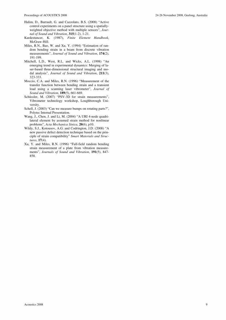
Finite Difference

Like any process employing derivatives, the technique of

determining strain from displacement data is sensitive to

noise. Noise can take many forms, such as physical distur-

bances, quantisation noise, spectral leakage and many other

sources of error associated with the laser measurement sys-

tem. These act to perturb the measurements spatially (with

displacement errors) and temporally (with phase errors) as

illustrated in Figure 12. Therefore, as the element size de-

creases, the relative magnitude of the errors increases. When

the distances between nodes approach the error in displace-

ment, the normalised error in the strain arising from the finite

difference may become extremely large. Consequently the

fine rectangular grid used in these experiments shows a

greater variance of the measured strain when compared with

the coarse triangular grid.


Acoustics 2008 7

True nodal displacements

Undeformed Geometry Deformed Geometry

Error in nodal displacements

Figure 12. Schematic illustrating how displacement errors

affect the strain estimates for small elements.

Quantisation and rigid body motion

Quantisation noise can be minimised by using the full dy-

namic range of the A/D converters. If there is significant

rigid body motion, then the number of bits available for the

resolution of the differential motion between nodes is re-

duced. Hence, the process of estimating strain using the vi-

brometer is best suited to configurations where there is no or

little rigid body motion of the specimen.

In addition, with significant rigid body motion, other sources

for uncertainties should also be considered such as alignment,

speckle noise, uncertainties in geometry, linearity errors and

gain errors.

Alignment of the laser heads

The PSV-3D requires precise alignment of the laser heads.

This is a two stage process. Initially a 2D (standard) align-

ment is conducted for each laser head, which calculates the

laser angles for a given point on the live video image. This is

followed by a 3D alignment which relates the laser angle to a

point in 3D space. For the strain measurements, it is essential

that the 3D alignment is extremely accurate.

Desired Measurement

Location

3D Alignment

Uncertainty

Figure 13. Schematic illustrating result of poor 3D alignment

The quality of the manual 3D alignment of the standard PSV-

400-3D is a limitation of the system when dealing with small

objects. Without additional measures, the 3D alignment

leads to an uncertainty in the beam location of approximately

mm5.2± which effectively means that the three beams do not

measure at exactly the same location (as shown in Figure 13).

This does not necessarily pose a problem for most applica-

tions, especially for large objects, but is a serious problem for

strain sensing, to the point of being inadequate for small ob-

jects. Polytec have now developed two tools for significantly

improving the accuracy for measurements on small objects.

The 3D alignment now can be performed on a precise align-

ment object with accurately measured coordinates instead of

using the geometry laser. A software “addition” improves the

beam superposition during scans. The PSV-S-TRIA triangu-

lation software optimises the overlap of the three laser beams

and corrects the position. It also has the additional benefit

that point geometry measurements are improved to an accu-

racy within approximately 0.1mm. The software requires a

high-resolution video camera upgrade.

Alignment of the specimen

To use the planar element shape functions derived above it is

important that the specimen is arranged in the x-y plane.

This may be simply achieved when defining the coordinate

system as part of the 3D alignment.

If there is still some residual misalignment it is possible to

correct this once the data is collected. Translation and rota-

tion matrices can be used to “perfectly align” the measure-

ments. Alternatively, shell elements may be used under any

reference frame.

Finally, if there is some structural misalignment of the actua-

tors which induces higher order strain motion, such as first

order warping modes similar to those found in Zernike Poly-

nomials or Radiation Modes, these can also be removed by

spatial convolution. The residual motion (after the contribu-

tion from all principal basis functions is removed) should be

related to the strain field arising from the applied loads.

Spatial filtering of displacement data

The strain estimates are very sensitive to noise. By spatially

filtering the displacement measurements using the appropri-

ate orthogonal basis functions or low pass filters, before ap-

plying the Finite Element shape functions, it is possible to

improve the estimates of the strains across the surface with

some loss of spatial resolution. This technique was com-

monly employed in early papers measuring bending strain

(Xu et al. 1996). A similar technique using FE shape func-

tions has been used to estimate the continuous out-of-plane

displacement of a panel using discrete PSV-3D measure-

ments (Halim et al 2008).

Frequency range

Although the specifications for the laser are in

mm/s/(sqrt(Hz) (velocity) it is necessary to convert these to

displacements in mµ /sqrt(Hz) for the exercise of calculating

strain. The relationship between velocity v and displace-

ment δ for a sinusoidal response at angular frequency ω is

δπωδδ

fjjdt

dv 2=== .

Therefore at a frequency of approximately 0.16Hz there is a

one to one relationship between mm/s and mm, so the effec-

tive displacement resolution at this frequency is 0.02

mµ /sqrt(Hz) for the (VD-07) velocity decoder. For a given

velocity, the displacement decreases with increasing fre-

quency. To achieve nanometre displacement accuracy it is

necessary to operate above frequencies in the order of 3Hz

with a resolution bandwidth of 1Hz. To achieve the same

accuracy at lower frequencies it is necessary to reduce the bin

width accordingly.

By operating at higher frequencies there is the benefit of

reducing the magnitude of uncorrelated noise sources such as

ground-borne vibration. The maximum operating frequency

of the strain system is bound by the spatial wavelength in the

structure. As with any FE based approach, a minimum of

three elements are needed per wavelength, preferably six. In

addition, the element size should be an order of magnitude

bigger than the accuracy of the laser. For example, assuming

the three lasers are accurate to within 0.5mm (Figure 13) and

that the specimen is undergoing uniaxial strain, then the ele-

ment size should be 10 times this (5mm), and the wavelength

should be greater than 6 times this (30mm). For aluminium

and steel (with a longitudinal wave speed of approximately

5000m/s), and, then the upper frequency bound is approxi-

mately 150kHz (5000/(0.0005*6*10)).


8 Acoustics 2008

In practice, the bandwidth of the vibration source or the con-

straint of operating in the stiffness-controlled region (when

trying to measure quasi-static behaviour of specimens) will

determine the upper frequency limit.

Signal Processing

Since the strain is obtained via a spatial differential it is very

sensitive to noise. Therefore it is important that a high co-

herence is maintained between the displacement measure-

ments and the reference. If the coherence drops below unity

it is important to take sufficient averages to provide a satis-

factory confidence interval (Bendat and Piersol 1986).

Coherence can be optimised by using sinusoidal inputs, or by

employing the appropriate temporal windows on the data to

minimise leakage with broadband signals.

Small strain

It should be noted that the displacement measured in the di-

rection of a laser beam reflects variation at the observation

point rather than at a point on the structure. Consequently

laser vibrometer measurements are for an Eulerian reference

frame, whereas contact strain measurements (such as those

provided by strain gauges) are for a Lagrangian reference

frame. This imposes restrictions on the types of measure-

ments one may make, and restricts displacements to “small

strain” where the Lagrangian derivative approaches the Eule-

rian derivative. It is for this reason that dynamic tests should

be employed where, despite the measured velocities being

significant, the displacements are very small and thus Eule-

rian strain gauge measurements and Lagrangian laser vi-

brometer measurements are approximately equivalent.

Surface finish issues

The principle of the 3D vibrometer requires the surface to be

rough. Each vibrometer must “see” the backscattered light

from itself. As each laser must be directed on the surface

from a different direction, the measurement is only possible

on rough surfaces. Rough surfaces generate speckle effects.

Depending on the amplitude of the motion, these effects can

generate dropouts in the optical signal, resulting in spikes in

the velocity output.

At smaller vibration amplitudes, the probability for dropouts

is low, however, the speckle effects can generate small varia-

tions in the amplitude of the measured signals. Those ampli-

tude variations can be neglected for normal measurements.

When calculating strain as the first derivative of the dis-

placement, those amplitude variations become visible as

noise in the strain signal. This noise is automatically reduced

by a procedure called “Speckle Tracking” in the scanning

vibrometer software. Instead of remaining on the same spot,

the lasers perform microscopic movements during the meas-

urement, causing a constant change in the speckle pattern and

therefore an averaging out of the corresponding amplitude

variations.

Other sources of noise

In many situations, for thin-walled structures the out-of-plane

displacements are an order of magnitude larger than the in-

plane displacements. This may cause difficulties in trying to

measure very small out-of-plane strains since it is likely that

external disturbances will act to degrade the measurements.

Ground-borne and air-borne noise may contaminate the

measurements. The both of these can be avoided to some

extent by isolating the experiment from the noise sources.

For example, using a very stiff and highly damped optical

breadboard in conjunction with compliant supports can sup-

press ground-borne vibration, while a quiet environment will

minimise the air-borne noise. Similarly, there are certain

times of day (after hours) in which ground-borne vibration

will be low.

THE FUTURE

The current work has been performed with the standard Poly-

tec PSV-400-3D, which is not ideally adapted for measure-

ments on small objects. Especially for strain calculations, the

Lasers must perfectly intersect on the object. Polytec have

addressed this issue and is working on means to increase the

accuracy for strain measurements. Two options will be re-

leased (software for beam superposition with high resolution

camera and precise calibration object for 3D alignment).

Polytec will also be releasing software to calculate the strain

fields in a manner similar to that presented here.

One exciting possibility of the laser-based strain technique is

the measurement of three-dimensional strain for plate- and

shell-like structures. The PSV-3D allows the measurement

of all obscured surfaces via mirrors. Hence it is possible to

measure the displacement of both sides of thin structures. In

principle, this allows three-dimensional elements to be used

to estimate the strain throughout the specimen, not only on

the surface as presented here.

An interesting application of this strain measurement tech-

nique is for the use in developing strain based damage detec-

tion techniques, such as the new technique based on the prin-

ciple of strain compatibility (Wildy et al. 2008). The PSV-3D

would allow validation and optimisation of such techniques

without having to resort to large numbers of strain gauges.

CONCLUSIONS

It has been shown that it is possible to use 3D displacement

data obtained from a scanning laser vibrometer to estimate

the dynamic strain over the surface of a planar structure. The

process is very sensitive to systematic errors in the vibrome-

ter measurement system, in particular misalignment errors

between heads. A great deal of attention needs to be paid to

minimise noise. However, despite the sensitivity of the tech-

nique to errors, it shows great promise in providing a new

fast non-contact method for accurately measuring the dy-

namic strain field across the surface of a structure.

ACKNOWLEDGEMENTS

The authors would like to acknowledge the contribution of

the reviewers who provided technical and editorial assistance

in the preparation of this manuscript.

REFERENCES

Asundi, A. (1996) “Recent advances in photoelastic applica-

tions”, International conference on fiber optics an

photonics, Madras, vol. 3211, 463-473.

Bendat, J.S. and Piersol, A.G. (1986) “Random Data: Analy-

sis and measurement procedures”, Wiley.

Colchero, L., Colchero, J., Gómez Herrero, J., Prieto, E.,

Baró, A. and Huang, W.H. (2002) “Comparison of strain

gage and interferometric detection for measurement and

control of piezoelectric actuators”, Materials Characteri-

zation, 48(2-3), 133-140.

Fagan, M.J. (1992), Finite Element Analysis – Theory and

Practice, Pearson Prentice-Hall.

Gilfrich, J.V. (1998), Advances in X-Ray Analysis, Springer,

ISBN 0306458039.


Acoustics 2008 9

Halim, D., Barrault, G. and Cazzolato, B.S. (2008) “Active

control experiments on a panel structure using a spatially-

weighted objective method with multiple sensors”, Jour-

nal of Sound and Vibration, 315(1-2), 1-21.

Kardestuncer, K. (1987), Finite Element Handbook,

McGraw-Hill.

Miles, R.N., Bao, W. and Xu, Y. (1994) “Estimation of ran-

dom bending strain in a beam from discrete vibration

measurements”, Journal of Sound and Vibration, 174(2),

191-199.

Mitchell, L.D., West, R.L. and Wicks, A.L. (1998) “An

emerging trend in experimental dynamics: Merging of la-

ser-based three-dimensional structural imaging and mo-

dal analysis”, Journal of Sound and Vibration, 211(3),

323-333.

Moccio, C.A. and Miles, R.N. (1996) “Measurement of the

transfer function between bending strain and a transient

load using a scanning laser vibrometer”, Journal of

Sound and Vibration, 189(5), 661-669.

Schüssler, M. (2007) “PSV-3D for strain measurements”,

Vibrometer technology workshop, Loughborough Uni-

versity.

Schell, J. (2003) “Can we measure bumps on rotating parts?”,

Polytec Internal Presentation.

Wang, J., Chen, J. and Li, M. (2004) “A URI 4-node quadri-

lateral element by assumed strain method for nonlinear

problems”, Acta Mechanica Sinica, 20(6), p10.

Wildy, S.J., Kotousov, A.G. and Codrington, J.D. (2008) “A

new passive defect detection technique based on the prin-

ciple of strain compatibility” Smart Materials and Struc-

tures, 17(4).

Xu, Y. and Miles, R.N. (1996) “Full-field random bending

strain measurement of a plate from vibration measure-

ments”, Journals of Sound and Vibration, 191(5), 847-

858.

Acoustics and Sustainability: How should acoustics adapt to meet future

Documents