Accepted Manuscript - Cranfield University

Accepted Manuscript

Study of Jet Precession, Recirculation and Vortex Breakdown in Turbulent

Swirling Jets Using LES

K.K.J. Ranga Dinesh, M.P. Kirkpatrick

PII: S0045-7930(08)00231-4

DOI: 10.1016/j.compfluid.2008.11.015

Reference: CAF 1114

To appear in: Computers & Fluids

Received Date: 10 July 2008

Revised Date: 24 November 2008

Accepted Date: 25 November 2008

Breakdown in Turbulent Swirling Jets Using LES, Computers & Fluids (2008), doi: 10.1016/j.compfluid.

2008.11.015

This is a PDF file of an unedited manuscript that has been accepted for publication. As a service to our customers

we are providing this early version of the manuscript. The manuscript will undergo copyediting, typesetting, and

review of the resulting proof before it is published in its final form. Please note that during the production process

errors may be discovered which could affect the content, and all legal disclaimers that apply to the journal pertain.

Please cite this article as: Dinesh, K.K.J.R., Kirkpatrick, M.P., Study of Jet Precession, Recirculation and Vortex

http://dx.doi.org/10.1016/j.compfluid.2008.11.015



li2106

Text Box

Computers & Fluids, Volume 38, Issue 6, June 2009, Pages 1232-1242

ACCEPTED MANUSCRIPT

1

Study of Jet Precession, Recirculation and Vortex Breakdown in

Turbulent Swirling Jets Using LES

K.K.J.Ranga Dinesh 1 , M.P.Kirkpatrick 2

1. School of Engineering, Cranfield University, Cranfield, Bedford, MK43 0AL,

UK.

2. School of Aerospace, Mechanical and Mechatronic Engineering, The

University of Sydney, NSW 2006, Australia.

Corresponding author: K.K.J.Ranga Dinesh

Email address: [email protected]

Postal Address: School of Engineering, Cranfield University, Cranfield, Bedford,

MK43 0AL, UK.

Telephone number: +44 (0) 1234750111 ext 5350

Fax number: +44 1234750195

Revised Manuscript prepared for the Journal of Computers and Fluids

24th November 2008

ACCEPTED MANUSCRIPT

2

Study of Jet Precession, Recirculation and Vortex Breakdown in

Turbulent Swirling Jets Using LES

K.K.J.Ranga Dinesh 1 , M.P.Kirkpatrick 2

ABSTRACT

Large eddy simulations (LES) are used to investigate turbulent isothermal swirling

flows with a strong emphasis on vortex breakdown, recirculation and instability

behavior. The Sydney swirl burner configuration is used for all simulated test cases

from low to high swirl and Reynolds numbers. The governing equations for continuity

and momentum are solved on a structured Cartesian grid, and a Smagorinsky eddy

viscosity model with the localised dynamic procedure is used as the subgrid scale

turbulence model. The LES successfully predicts both the upstream first recirculation

zone generated by the bluff body and the downstream vortex breakdown bubble. The

frequency spectrum indicates the presence of low frequency oscillations and the

existence of a central jet precession as observed in experiments. The LES calculations

well captured the distinct precession frequencies. The results also highlight the

precession mode of instability in the centre jet and the oscillations of the central jet

precession, which forms a precessing vortex core. The study further highlights the

predictive capabilities of LES on unsteady oscillations of turbulent swirling flow

fields and provides a good framework for complex instability investigations.

Key words: Swirl, Recirculation, Vortex breakdown, Precessing vortex core, Strouhal

number, Large eddy simulation

ACCEPTED MANUSCRIPT

3

I. INTRODUCTION

Swirling flows are frequently found in nature and also occur in a wide range of

practical applications, such as gas turbine combustors, agricultural spraying machines,

whirlpools, cyclone separators and vortex shedding from aircraft wings. Since the

majority of swirling flows operate in a turbulent environment, it is necessary to

consider the unsteady flow oscillations during the flow evolution. Investigation of

precession, recirculation, vortex breakdown and instabilities have received much

attention [1-5] and recently several groups have studied the jet precession, oscillation

mechanisms and the role of precessing vortex core (PVC) in which the centre of the

vortex precesses around the central axis of symmetry [6-7]. In combustion systems,

these phenomena promote the coupling between combustion, flow dynamics and

acoustics [7].

Several groups have identified various forms of precession motion and instability

modes in both reactive and non-reactive swirling flow fields [8-9]. Experimental

evidence has shown that, configurations, the existence of a PVC depends on the

occurrence of vortex breakdown and on having a swirl number greater than its critical

value [10]. However, PVC also occurs at low values of swirl number where a swirling

jet is released into a large expansion. Dellenback et al. [11] observed several

precession mechanisms in experiments involving swirling pipe flow over a range of

high swirl numbers. Alternatively, Sozou and Switenbank [12] carried out an

analytical calculation using an inviscid model for PVC phenomena and found a

reasonable agreement with the data of Chanaud [10] and Cassidy et al. [13].

Averamenko et al. [14] carried out further investigations and found that the PVC

frequency is linearly dependent on both the mean inlet velocity and is a weak function

ACCEPTED MANUSCRIPT

4

of viscosity. Sato et.al. [15] carried out the first computational modelling work using

the Reynolds averaged Navier-Stokes (RANS) technique for the PVC phenomena and

deduced a number of oscillation mechanisms. Guo et al. [16] carried out a RANS

simulation for a turbulent swirl flow passing into a sudden expansion, and found a

large PVC structure and a particular combination of precession and flapping

oscillations for zero swirl strength. However, RANS based methods are only

successful for flows with non-gradient transport and therefore do not provide the level

of accuracy required for the prediction of a large scale highly unsteady PVC.

Large eddy simulation (LES) has been widely accepted as a promising numerical tool

for solving the large-scale unsteady behavior of complex turbulent flows.

Encouraging results have been reported in recent literature and demonstrate the ability

of LES to capture the swirling flow instability and the energy containing coherent

motion of the PVC. For example, Wegner et al. [17] carried out LES calculations for

isothermal swirling flow fields and captured the PVC phenomena with a good degree

of success. Roux et al. [18] performed an LES of an isothermal flow field in a gas

turbine combustor and accurately predicted both the major PVC oscillation frequency

and a strong second acoustic mode. This example, further demonstrates the capability

of LES to capture the strong coupling between the acoustics and the swirling flow

dynamics. Selle et al. [19] also carried out LES of an industrial gas turbine burner and

captured the entire PVC structure of the isothermal flow field. Wang et al. [20]

detected the low frequency oscillations and precession for their LES calculations of

confined isothermal swirl flows. Recently, Wang et al. [21] conducted LES

calculations of flow dynamics for an operational aero engine combustor and found

encouraging results for the PVC phenomena.

ACCEPTED MANUSCRIPT

5

Despite extensive reviews, the investigation of unsteady flow oscillations such as

vortex shedding and the occurrence of the PVC in swirl stabilized systems remains a

challenge. Interactions between different instability modes can cause considerable

noise fluctuations as a result of the oscillating pressure field. Further investigations

are necessary to identify the link between the oscillation mechanisms and the jet

precession in swirl stabilized jets [4][9].

The present work focuses on a series of LES calculations for isothermal flow fields

based on the Sydney swirl burner configuration and demonstrates the features of jet

precession (often starting at moderate swirl number) as well as the existence of PVC

associated with a bluff body [22-24]. The Sydney swirl burner configuration has also

been extensively investigated as a target model problem for computations in the

Proceedings of Turbulent Non-Premixed Flames (TNF) group meetings [25].

The swirl configuration used in this work features unconfined swirling flow fields

generated by an upstream recirculation zone and a second downstream recirculation

zone induced by swirl, which greatly improves the mixing process. In addition, the

swirling flow fields generate central jet precession and a PVC structure close to the

burner exit. The ultimate goal of this paper is to present the correlations between

axial, swirl and vortex breakdown instabilities associated with central jet precession

and analysis the occurrence of PVC using the Strouhal number and geometric swirl

number.

ACCEPTED MANUSCRIPT

6

In our earlier studies, we have shown that LES accurately predicts different

isothermal swirling flow fields of the Sydney swirl flame series [26], and later have

extended the work to reacting cases [27-28]. The current work is a continuation of our

investigations of flow recirculation, vortex breakdown, oscillations and instabilities

associated with the isothermal swirling flow fields. Results will be presented for the

power spectra, Strouhal and swirl numbers.

The layout of this paper is as follows. Section II presents the details of Sydney swirl

burner configuration. In Section III we will present the computational method

including the governing equations, discretisation methods and boundary conditions.

Results from the simulations and comparison with experimental data will be discussed

in Section IV. Finally, a short summary in Section V will conclude the main findings

of this paper.

II. THE SYDNEY SWIRL BURNER

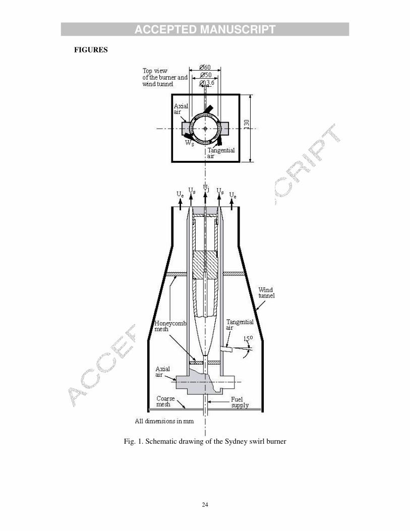
A schematic of the Sydney swirl burner configuration used in this work is shown in

Fig. 1. It has a 60mm diameter annulus for a primary swirling air stream surrounding

the circular bluff body of diameter D=50mm with a 3.6mm diameter central fuel jet.

The jet fluid for isothermal cases is air. The burner is housed in a secondary co-flow

wind tunnel with a square cross section of 130mm sides. Swirl is introduced

aerodynamically into the primary annulus air stream 300mm upstream of the burner

exit plane and inclined 15 degrees upward to the horizontal plane. The swirl number

can be varied by changing the relative magnitude of tangential and axial flow rates.

Velocity measurements were made at the University of Sydney [22-24]. The literature

already includes the details flow conditions such as flow types, their velocities, swirl

ACCEPTED MANUSCRIPT

7

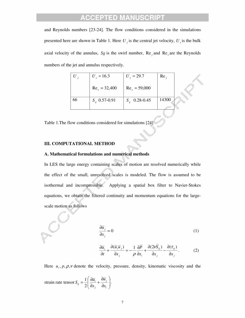
and Reynolds numbers [23-24]. The flow conditions considered in the simulations

presented here are shown in Table 1. Here jU is the central jet velocity, sU is the bulk

axial velocity of the annulus, Sg is the swirl number, jRe and sRe are the Reynolds

numbers of the jet and annulus respectively.

jU 3.16=sU

400,32Re =s

7.29=sU

000,59Re =s

jRe

66 gS 0.57-0.91 gS 0.28-0.45 14300

Table 1.The flow conditions considered for simulations [24]

III. COMPUTATIONAL METHOD

A. Mathematical formulations and numerical methods

In LES the large energy containing scales of motion are resolved numerically while

the effect of the small, unresolved scales is modeled. The flow is assumed to be

isothermal and incompressible. Applying a spatial box filter to Navier-Stokes

equations, we obtain the filtered continuity and momentum equations for the large-

scale motion as follows

0=∂∂

j

j

x

u (1)

j

ij

j

ij

ij

jii

xx

S

xP

x

uu

tu

∂∂

−∂

∂+

∂∂−=

∂∂

+∂

∂ )()2(1)( τνρ

. (2)

Here νρ,,, pui denote the velocity, pressure, density, kinematic viscosity and the

strain rate tensor��

�

�

��

�

�

∂∂

+∂∂=

i

j

j

iij x

u

xu

S21

.

ACCEPTED MANUSCRIPT

8

The last term in equation (2) is the divergence of the SGS stress tensor, which

represents the sub-grid scale (SGS) contribution to the momentum. Hence, subsequent

modelling is required for ( )jijiij uuuu −=τ to close the system of equations. The

Smagorinsky eddy viscosity model [29] is used here to model the SGS stress tensor as

1

23

ijij ij kk sgs Sτ δ τ ν− = − . (3)

Here the eddy viscosity sgsν is a function of the filter size and strain rate

2

sgs sC Sν = ∆ , (4)

Where sC is a Smagorinsky model parameter [29], ∆ is the filter width

and 21

)2(|| ijij SSS = . The localized dynamic procedure of Piomelli and Liu [30] was

used to obtained the model parameter sC , which appears in equation (4) as a part of

the SGS turbulence modelling. This model uses information in the resolved flow

fields to determine the model parameter dynamically. As such, the parameter varies in

both time and space based on local flow conditions.

The governing equations are discretised on a non-uniform, three dimensional,

staggered Cartesian grid by using the LES code PUFFIN originally developed by

Kirkpatrick [31] and later extended by Ranga Dinesh. [32]. PUFFIN calculates the

temporal development of large-scale flow structures by solving the filtered LES

equations for mass and momentum (Eq. 1 and 2). The LES equations are discretised

in space using a finite volume method. A second order central difference scheme is

used for the spatial discretisation of momentum equations and pressure correction

equation. First, the momentum equations are integrated using a third order hybrid

Adam-Bashforth/ Adam-Moulton scheme to give an approximate solution for the

ACCEPTED MANUSCRIPT

9

velocity field. Mass conservation is enforced through a pressure correction step in

which the approximate velocity field is projected onto a subspace of divergence free

velocity fields. The pressure correction method of Van Kan [33] and Bell et al. [34]

was used in the present calculations. The solution is advanced with a time step

corresponding to Courant number less than 0.6. The equations, discretised as

described above, are solved using a linear equation solver. Here a Bi-Conjugate

Gradient Stabilized (BiCGStab) solver with a Modified Strongly Implicit (MSI)

preconditioner is used. The momentum residual error is typically of the order 510− per

time step and the mass conservation error is of the order of 810− . Further details of the

numerical methods used can be found in Kirkpatrick et al. [35-37]

C. Boundary conditions

This section describes the boundary conditions used for the simulations. The mean

velocity distributions for the jet and annulus flows were specified using power law

velocity profiles [26-28]. The mean profiles for both axial and swirl velocities are

specified by a power law of the form

7/1

1218.1 ��

��

�−>=<

δy

UU j , (5)

Where jU is the bulk velocity, y the radial distance from the jet centre line and

jR01.1=δ , where jR is the fuel jet radius of 1.8 mm. The factor 1.01 is added to

ensure that velocity gradients are finite at the walls. The same equation is used for the

swirling air stream with jU replaced by the bulk axial velocity sU and bulk

tangential velocity sW , y the radial distance from the centre of the annulus and

01.1=δ h/2, where h is the width of the annulus. Turbulence at the inlets is modelled

by superimposing fluctuations on the mean velocity profiles generated from a

ACCEPTED MANUSCRIPT

10

Gaussian distribution such that the inflow has the correct turbulence kinetic energy

levels obtained in the experimental data. At solid walls a free slip condition is applied.

At the outlet, a convection boundary condition is used.

D. Domain size, grid and statistics

The computations were performed on non-uniform Cartesian grid in a domain with

dimensions300 300 250mm× × . The grid has 100 100 100× × cells in the x, y and z

directions respectively giving a total of one million cells. Grid lines in the x and y

directions use an expansion ratio of ( ) ( 1) 1.08xy x i x iγ = ∆ ∆ − = and an expansion ratio

of 07.1=zγ is used in the z-direction. A grid sensitivity analysis for a high swirl case

(swirl number 1.59) published in our earlier work [26] indicated that reasonable grid

independence is achieved for the mean velocity fields and Reynolds stresses with this

grid. All simulations were carried out for the total time period of ms300 and two non-

consecutive sampling periods yielded similar results indicating that the statistics were

well converged.

IV. RESULTS AND DISCUSSION

The Sydney swirl burner is designed to study reacting and non-reacting swirling flows

for a range of swirl numbers and Reynolds numbers. This section discusses the LES

results focussing on features of the swirling flow fields such as recirculation, vortex

breakdown, central jet oscillation and PVC structures for various flow conditions.

First the occurrence of vortex breakdown, recirculation and its relationship with the

swirl number will be discussed. Results will then be presented to demonstrate the

central jet precession and PVC structures for different flow conditions. Finally, a

comparison plot for a Strouhal number will be discussed. The results obtained from

ACCEPTED MANUSCRIPT

11

the LES calculations will be discussed in two cases. Case I involves flow features for

moderate swirl numbers at the primary annulus axial velocity of 7.29=sU m/s, while

Case II involves high swirl numbers at the primary annulus axial velocity of

3.16=sU m/s.

Case I: Analysis of recirculation, vortex breakdown, precession frequencies,

precessing vortex core (PVC) and Strouhal number for 7.29=sU m/s at swirl

numbers 45.0,40.0,34.0,28.0=gS .

A. Recirculation and vortex breakdown

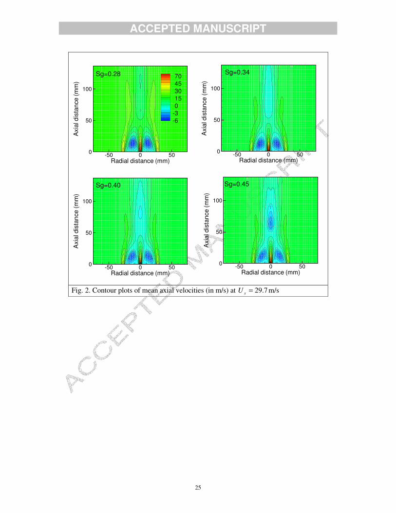
Fig. 2 shows four contour plots of mean axial velocity and clearly shows the upstream

recirculation zone and downstream vortex breakdown. For swirl numbers 0.28, 0.34,

no negative velocities are observed on the centreline and hence no vortex bubble

formed. For swirl numbers, 0.40, 0.45, the mean axial velocity becomes negative on

the centreline, which indicates the occurrence of a vortex breakdown bubble (VBB).

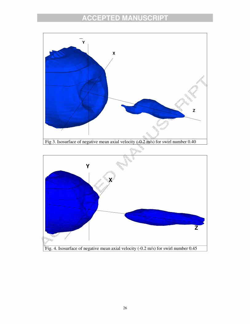
Increasing the swirl number also increases the axial extent of the vortex bubble. Figs.

3 and 4 show isosurfaces of the negative mean axial velocity at a value of 2.0− m/s

for swirl numbers 0.40 and 0.45 respectively. The plots reveal that the expansion of

the upstream recirculation zone is similar; however the growth of the downstream

vortex bubble differs slightly. We have also found that the increased swirl velocity

has a minor impact on the formation of VBB in the downstream region and that the

VBB promotes the shear layer instability in the downstream recirculation zone.

ACCEPTED MANUSCRIPT

12

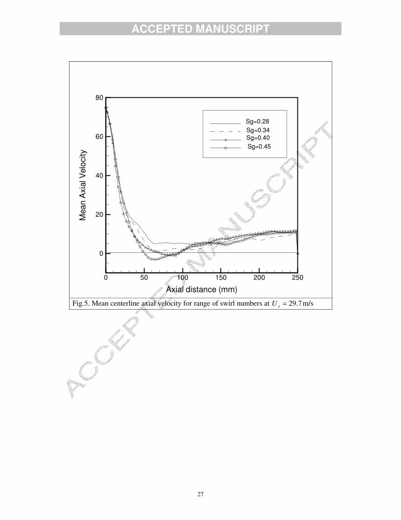
Fig. 5 shows the calculated centerline mean axial velocity for a range of swirl

numbers 45.0,40.0,34.0,28.0=gS . The calculations of centerline negative mean axial

velocity indicates a flow reversal. For the cases with swirl numbers 0.40 and 0.45, the

greatest negative axial velocities of 7.2− m/s and 5.4− m/s occur at approximately

x=80mm and x=65mm respectively. For these two cases, the mean axial velocity is

negative within the range of x=70 – 95mm and x=47 – 90mm respectively. The jet

velocity decays in a similar manner in the downstream section for all cases.

B. Precession frequencies and precessing vortex core (PVC)

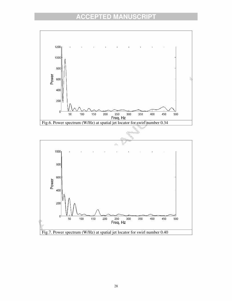
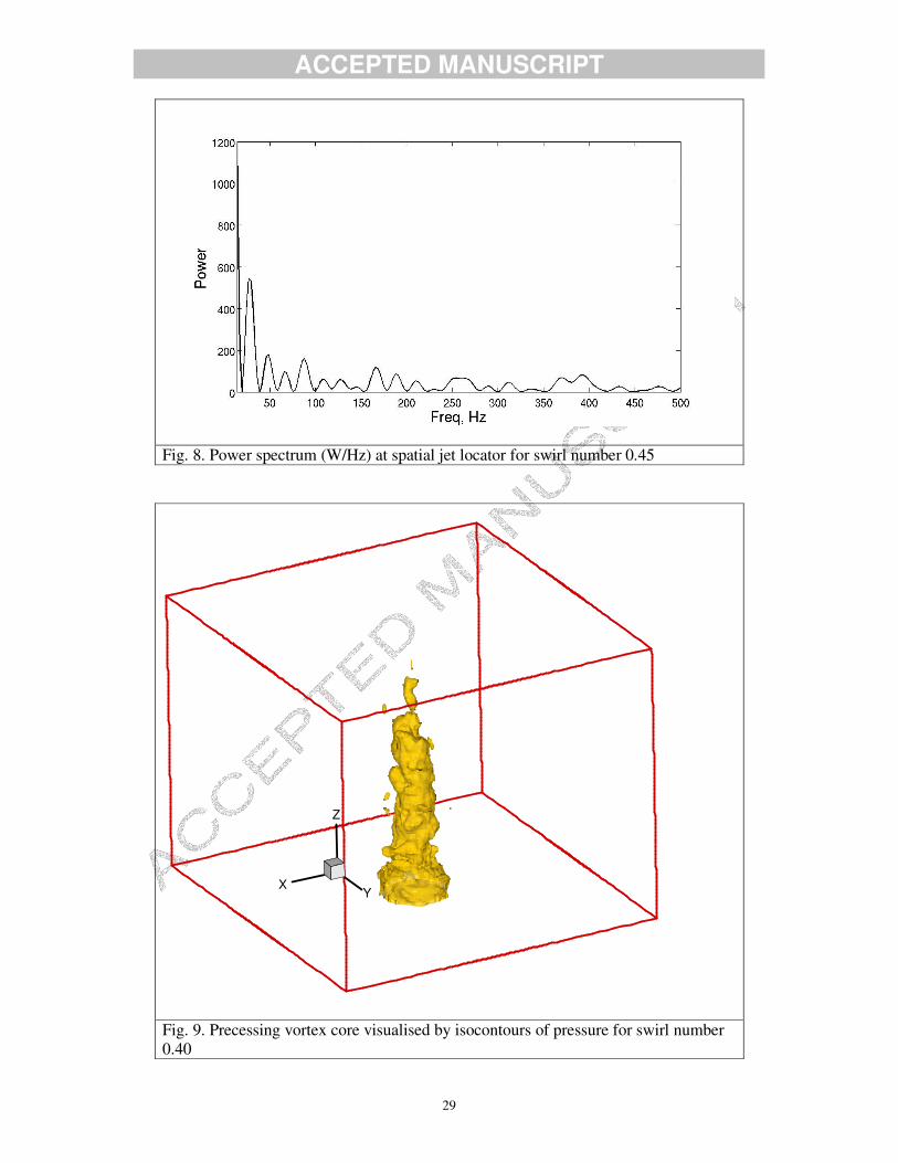
Figs. 6-8 show the power spectra for swirl numbers 0.34, 0.40 and 0.45 at the spatial

jet locator. The spatial jet locator is positioned just off the burner centerline at

x=12.3mm (axial location) and r=2.3mm (radial location) similar to the experimental

investigation. A pair of monitoring points are used on either side of the centre jet [22-

24].

The power spectrum is constructed by applying the Fast Fourier Transform (FFT) to

the instantaneous axial velocity at the jet locator point. The power spectrum for the

case 34.0=gS has a distinct peak at a frequency of ~24 Hz, which indicates the

occurrence of precession. The power spectrum for 40.0=gS has a number of peaks

at low frequency with the highest at approximately 24Hz, which is slightly lower to

than that found in the experimental observation (26Hz) [24]. The spectrum for

40.0=gS also has smaller peaks at 50Hz and 75Hz. These may be attributed to the

critical swirl number for downstream VBB, where the VBB start to disappear. The

power spectrum for 45.0=gS has the highest peak at ~26Hz. All distinct precession

ACCEPTED MANUSCRIPT

13

frequencies obtained from the present simulations are very close to the experimentally

observed values [24].

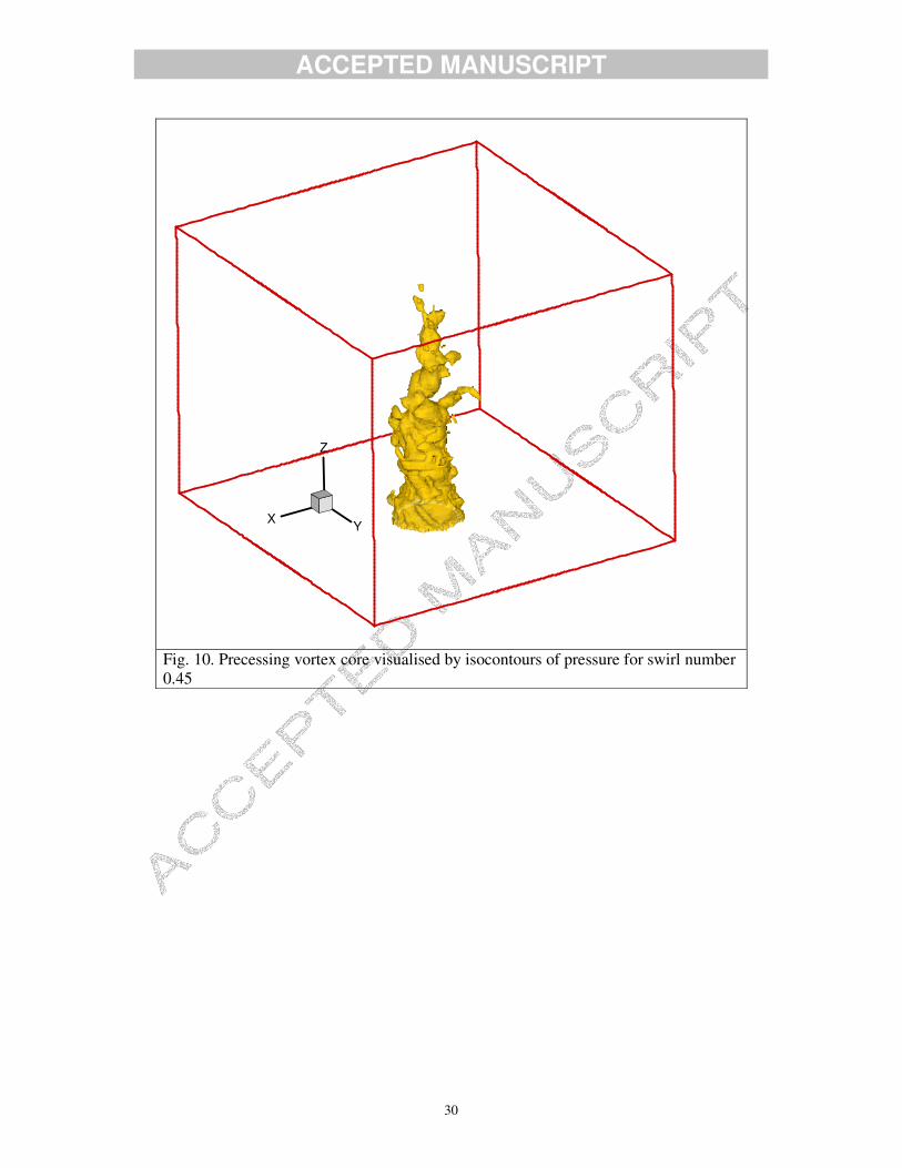
Figs. 9 and 10 show instantaneous isosurfaces of static pressure at 45.0,40.0=gS

and demonstrate the PVC structure outlined by a pressure value of p= -85Pa. In the

low swirl case ( 40.0=gS ) the PVC structure is more coherent than in the high swirl

case ( 45.0=gS ) and both PVC structures occur at same central jet precession

frequency value. For both cases, the low-pressure core aligns with the centerline. The

upstream extent of the vortex bubble is much larger for the case 45.0=gS than for

0.40, which changes the downstream PVC structure as shown in Fig. 10.

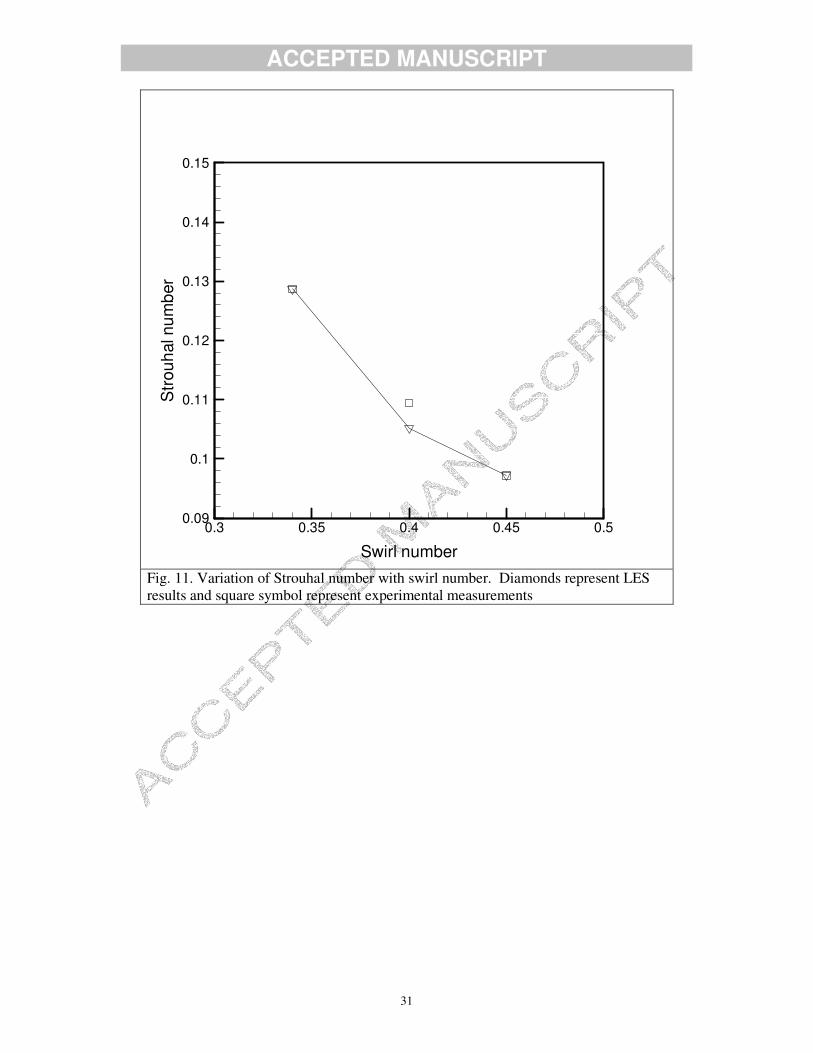
C. Strouhal number

The Strouhal number plays a vital role in detecting precession motion and provides a

basis for precession analysis in both isothermal and reacting swirl flow applications.

Conventionally, the Strouhal number can be defined as QfDe3 , where f is the

frequency, De is the exhaust diameter of the swirl burner and Q is the volumetric

flow rate [9]. For this study, the Strouhal number is calculated as ss WfrSt 2= ,

which is consistent with the experimental definition [24]. Here again, f is a

precession frequency, sr is the radius of the bluff body and sW is the tangential

velocity of the primary annulus. Fig. 11 shows good agreement between predicted and

measured values of Strouhal number for detected precession frequencies. The only

discrepancy appears for the case 40.0=gS for which the LES underestimates the

precession frequency.

ACCEPTED MANUSCRIPT

14

Case II: Analysis of recirculation, vortex breakdown, precession frequencies,

precessing vortex core (PVC) and Strouhal number for 3.16=sU m/s at swirl

numbers 91.0,68.0,57.0=gS .

A. Recirculation and vortex breakdown

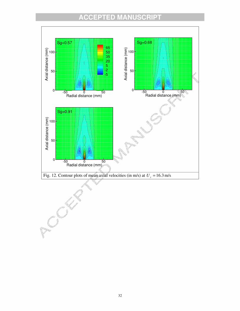
Fig. 12 contains contour plots of the mean axial velocity showing the upstream

recirculation zone and the downstream VBB at the three swirl numbers. The

downstream vortex bubble is only formed for swirl numbers 0.57 and 0.68. Despite

having the highest swirl number, no vortex bubble is formed for the case 91.0=gS .

Therefore the downstream flow reversal disappears at some intermediate swirl

number between 68.0=gS and 0.91. Similar behaviour has been observed by the

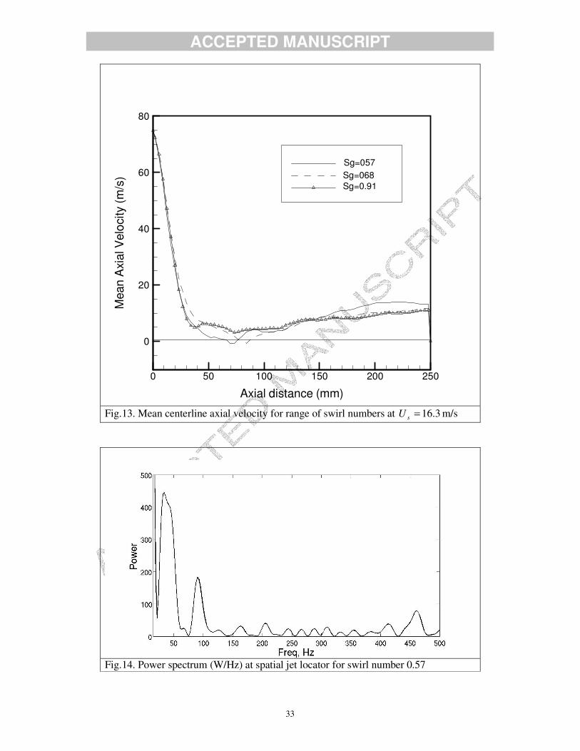
experimental investigation [24]. Fig. 13 shows the predicted centerline mean axial

velocity for the three test cases. A small vortex bubble is formed only for the swirl

number 68.0,57.0=gS . The stagnation point occurs at mmx 70= for 57.0=gS and

at mmx 82= for 68.0=gS . The jet velocity decays in a similar manner in the

upstream section and varies slightly in the range mmx 10040 −= as a result of the

downstream recirculation zone. In case II, the flow conditions are different and hence

size of the downstream VBB is significantly smaller than that found in case I.

B. Precession frequencies and precessing vortex core (PVC)

The power spectra at a spatial jet locator are shown in Figs. 14-16. Fig. 14 shows the

power spectrum for a case 57.0=gS . The LES calculates a precession frequency

value of 30Hz, which is slightly greater than the experimental value (28Hz) [24]. The

ACCEPTED MANUSCRIPT

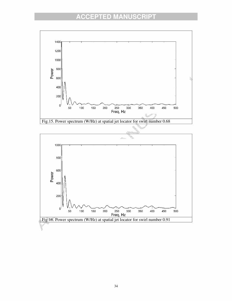
15

power spectrum for 68.0=gS accurately predicts the precession frequency value of

28Hz in comparison to the experimental value (see Fig. 15).

As shown in Fig. 16, for 91.0=gS the LES gives a precession frequency value of

26Hz and contains high peaks in the low frequency range. The cases 68.0=gS and

0.91 have more distinct peaks at the precession frequency than 57.0=gS and the

calculated precession frequency values are much closer to the experimental values

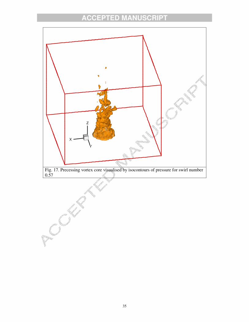
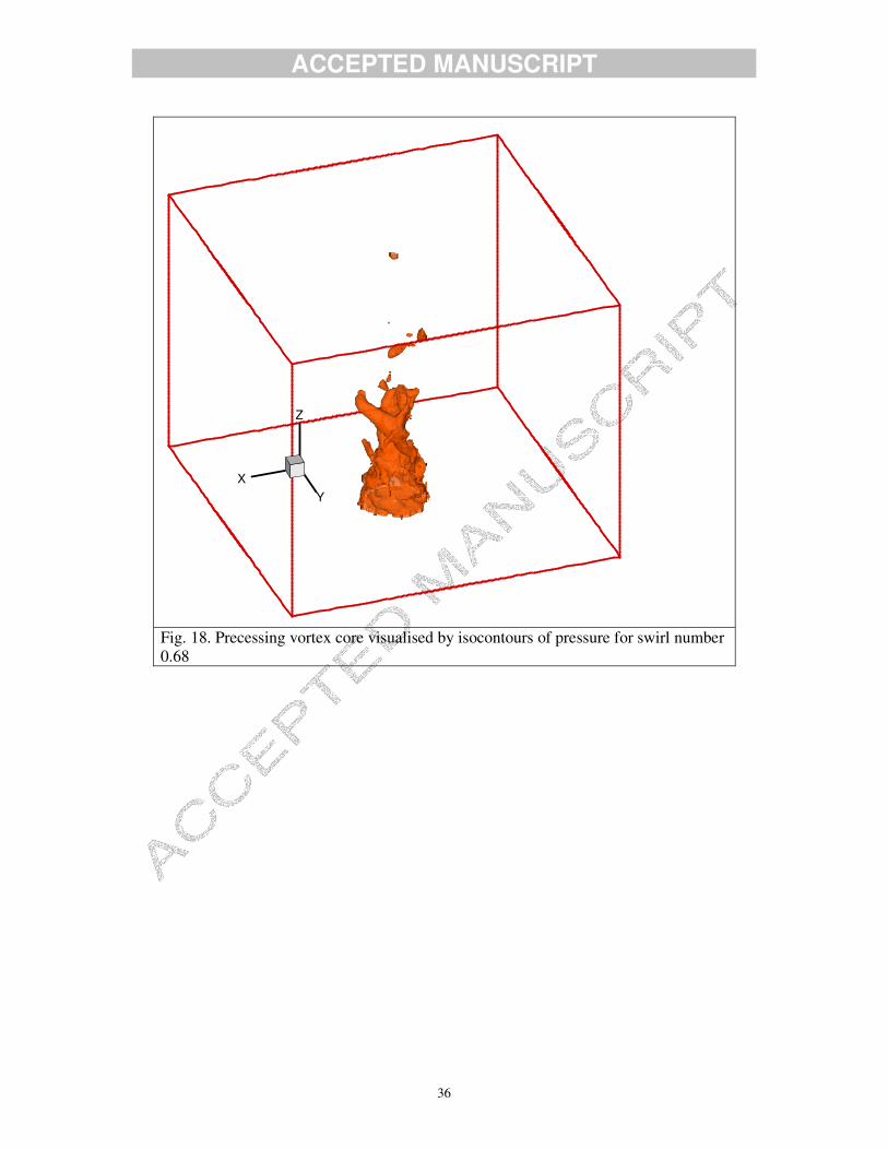
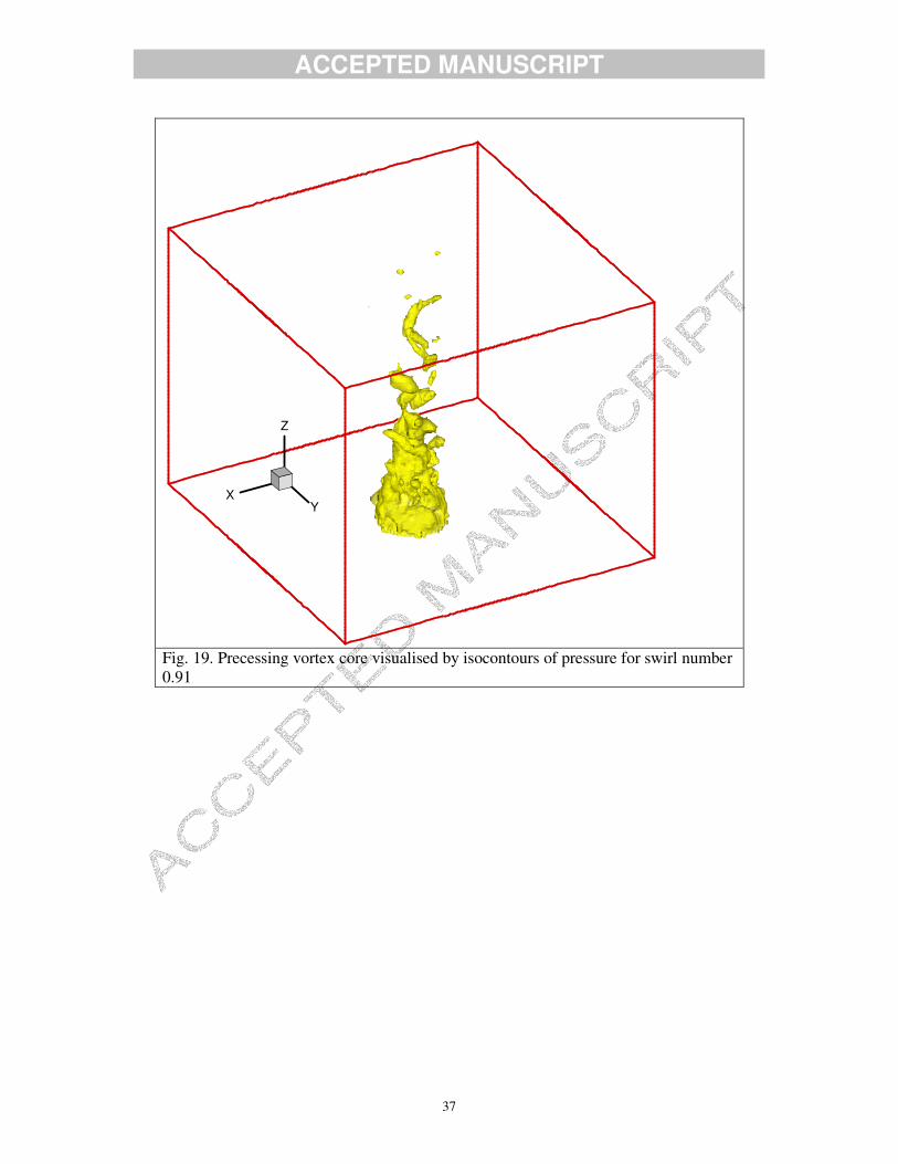
[24]. Fig. 17-19 show instantaneous isosurfaces of static pressure for swirl numbers

91.0,68.0,57.0=gS respectively. As with the PVC for the lower swirl numbers

shown in Figs. 9 and 10, it can be seen that the complexity of the PVC increases as

the swirl number increases.

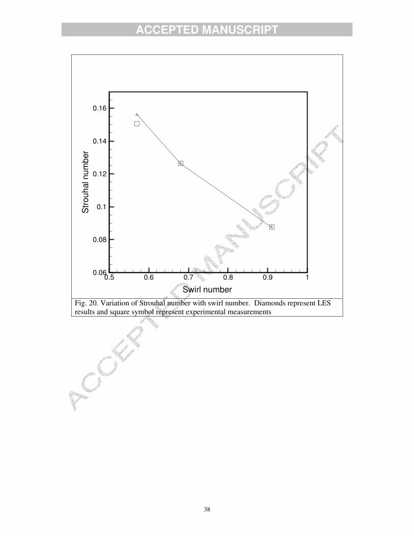
C. Strouhal number

Fig. 20 shows the agreement between the predicted and measured values of Strouhal

number based onthe precession frequency. The only discrepancy with the

experimental value appears at 57.0=gS where the LES slightly overestimates the

precession frequency. This further demonstrates the possibility of using LES to study

the jet precession and oscillation mechanisms in turbulent swirling flows.

V. CONCLUSIONS

In this paper we have reported results for large eddy simulations of isothermal

swirling flows based on the Sydney swirl burner, which was experimentally

investigated by Al-Abdeli and Masri [23-25]. Two major test cases based on different

primary annulus axial velocity have been considered. The two major cases were

ACCEPTED MANUSCRIPT

16

further divided into seven different test cases based on different swirl numbers in

order to study the influence of swirl number on recirculation, vortex breakdown,

precessing vortex core and precession frequencies.

The LES successfully simulated the recirculation zones, vortex breakdown bubbles

and precessing vortex cores for all test cases. In particular, the precession frequencies

for the central jet precession have been captured and are in excellent agreement with

the experimental measurements as seen through a comparison of the Strouhal

numbers [24]. There appears to be a relation between the central jet precessions and

the axial extent of the vortex bubble, however, further investigation is required to

explore the relationship between the central jet precession and the downstream vortex

bubble. The results of this study show that LES seems to be suitable for investigating

instabilities in swirling jets. This is an important finding, since there is a need for

more fundamental LES investigations on the mechanisms of instability modes and

PVC in combustion systems. Further work on coupling mechanisims between

instability and combustion would certainly help to improve the knowledge of

combustion instabilities in swirl combustion systems and we intend to extend our

work for the instability analysis of swirl combustion systems.

ACCEPTED MANUSCRIPT

17

REFERENCES

[1] Sarpkaya T. On stationary and traveling vortex breakdowns. J. Fluid Mech 1971;

45: 545-559

[2] Escudier M, Zehinder N. Vortex-flow regimes. J. Fluid Mech 1982; 115: 105-121

[3] Escudier M. Vortex breakdown: observations and explanations. Prog. Aero. Sci

1988; 25: 189-229

[4] Lucca-Negro O, O’Doherty TO. Vortex breakdown: a review. Prog. Ener. Comb.

Sci 2001; 27: 431-481

[5] Gupta AK, Lilley DJ, Syred N. Swirl flows. Tunbridge Wells, UK: Abacus Press

1984

[6] Froud D, O’Doherty T, Syred N. Phase averaging of the precessing vortex core in

a swirl burner under piloted and premixed combustion conditions. Combust. Flame

1995; 100: 407-417

[7] Syred N, Fick W, O’Doherty T, Griffiths AJ. The effect of the precessing vortex

core on combustion in swirl burner. Combust. Sci. Tech 1997; 125: 139-157

[8] Syred N, Beer JM. Combustion in swirling flows: a review. Combust. Flame

1974; 23: 143-201

ACCEPTED MANUSCRIPT

18

[9] Syred N. A review of oscillation mechanisms and the role of the precessing vortex

core (PVC) in swirl combustion systems. Prog. Energy. Combust. Sci 2006; 32: 93-

161

[10] Chanaud RC. Observations of oscillatory motion in certain swirling flows. J.

Fluid. Mech 1965; 21(1): 111-121

[11] Dellenback PA, Metzger D, Neitzel G. Measurements in turbulent swirling flow

through an abrupt axisymmetric expansion. AIAA Journal 1998; 26(6): 669-680

[12] Sozou C, Swithenbank J. Adiabatic transverse waves in a rotation fluid. J. Fluid.

Mech 1963; 38(4): 657-671

[13] Cassidy J, Falvey H. Observations of unsteady flow arising after vortex

breakdown. J. Fluid Mech 1965; 21(1): 11-22

[14] Averamenko A, Bowen P, Kobzar S, Syred N, Khalatov A, Griffiths A.

Analytical analysis of three dimensional instabilities existing in industrial swirl

generators. ASME Fluid Eng. Div. summer meeting 1997; June 22-26

[15] Sato K, O’Doherty T, Biffin M, Syred N. Analysis of strong swirling flows in a

swirl burner/furnaces. Proceedings of the international symposium on combustion and

emission control, Institute of Energy 1993; 243-247

ACCEPTED MANUSCRIPT

19

[16] Guo B, Langrish T, Fletcher D. CFD simulation of precession in sudden pipe

expansion flows with inlet swirl. Applied Mathe. Model 2002; 26: 1-10

[17] Wenger B, Maltsev A, Schneider C, Sadiki A, Dreizler A, Janicka J.

Assessment of unsteady RANS in predicting swirl flow instability based on LES and

experiments. Int. J. Heat Fluid Flow 2004; 25: 28-36

[18] Roux S, Lartigue G, Poinsot T, Meier U, Berat C. Studies of mean and

unsteady flow in s a swirled combustor using experiments, acoustic analysis and large

eddy simulations. Combust. Flame 2005; 141: 40-54

[19] Selle L, Lartigue G, Poinsot T, Koch R, Schildmacher K, Krebs W, et al.

Compressible large eddy simulation of turbulent combustion in complex geometry on

unstructured meshes. Combust. Flame 2004; 137: 489-505

[20] Wang P, Bai X, Wessman M, Klingmann J. Large eddy simulation and

experimental studies of a confined turbulent swirling flow. Phy. Fluids 2004; 16:

3306-3324

[21] Wang S, Yang V, Hsiao G, Hsieh S, Mongia H. Large eddy simulations of gas

turbine swirl injector flow dynamics. J. Fluid. Mech 2007; 583: 99-122

[22] Al-Abdeli Y. Experiments in Turbulent swirling non-premixed flame and

isothermal flows. PhD Thesis, School of Aero. Mech. Mecha. Eng., University of

Sydney, Australia 2003

ACCEPTED MANUSCRIPT

20

[23] Al-Abdeli Y, Masri AR. Recirculation and flow field regimes of unconfined non-

reacting swirling flow. Exp. Therm. Fluid Sci 2003; 23: 655-665

[24] Al-Abdeli Y, Masri AR. Precession and recirculation in turbulent swirling

isothermal jets. Combust. Sci. Tech 2004; 176: 645-665

[25] Barlow RS. Turbulent non-premixed swirling flames. Proceedings of the 8th

International workshop on Turbulent Non-premixed Flames 2006; Germany

[26] Malalasekera W, Ranga Dinesh KKJ, Ibrahim SS, Kirkpatrick MP. Large eddy

simulation of isothermal turbulent swirling jets. Combust. Sci. Tech 2007; 179: 1481-

1525

[27] Malalsekera W, Ranga Dinesh KKJ, Ibrahim SS, Masri AR. LES of recirculation

and vortex breakdown in swirling flames. Combust. Sci. Tech 2008; 180: 809-832

[28] Kempf, A, Malalasekera, W, Ranga Dinesh KKJ, Stein O. Large eddy simulation

with swirling non-premixed flames with flamelet model: A comparison of numerical

methods. Flow Turb. Combust 2008; Online first

[29] Smagorinsky, J. General circulation experiments with the primitive equations. M.

Weather Review. 1963; 91: 99-164

[30] Piomelli, U. and Liu, J. Large eddy simulation of channel flows using a localized

dynamic model. Phy. Fluids 1995; 7: 839-848.

ACCEPTED MANUSCRIPT

21

[31] Kirkpatrick MP. Large eddy simulation code for industrial and environmental

flows. PhD Thesis, University of Sydney, Australia. 2002

[32] Ranga Dinesh KKJ. Large eddy simulation of turbulent swirling flames. PhD

Thesis, Loughborough University, UK. 2007

[33] Van Kan J. Second order accurate pressure correction scheme for viscous

incompressible flow. SIAM J Sci. Stat Comput 1986; 7: 870-891

[34] Bell J, Colella P, Glaz H. A second order projection method for the

incompressible Navier-Stokes equations. J. Comp. Phys 1989; 85: 257-283

[35] Kirkpatrick MP, Armfield SW, Kent JH. A representation of curved boundaries

for the solutions of the Navier-Stokes equations on a staggered three dimensional

Cartesian grid. J. Comput. Phy 2003; 104: 1-36

[36] Kirpatrick MP, Armfield SW, Kent JH, Dixon TF. Simulation of vortex shedding

flows using high-order fractional step methods. ANZIAM J 2000; 43 (e): 856-876

[37] Kirkpatrick, MP, Armfield. On the stability and performance of the projection-3

method for the time integration of the Navier-Stokes equations. ANIZIAM J 2008;

49:559-575

ACCEPTED MANUSCRIPT

22

FIGURE CAPTIONS

Fig. 1: Schematic drawing of the Sydney swirl burner

Fig. 2: Contour plots of mean axial velocities (in m/s) at 7.29=sU m/s

Fig. 3: Isosurface of negative mean axial velocity (-0.2 m/s) for swirl number 0.40

Fig. 4: Isosurface of negative mean axial velocity (-0.2 m/s) for swirl number 0.45

Fig. 5: Mean centerline axial velocity for range of swirl numbers at 7.29=sU m/s

Fig. 6: Power spectrum (W/Hz) at spatial jet locator for swirl number 0.34



Fig. 9: Precessing vortex core visualised by isocontours of pressure for swirl number

0.40


0.45

ACCEPTED MANUSCRIPT

23

Fig. 11: Variation of Strouhal number with swirl number. Diamonds represent LES

results and square symbol represent experimental measurements

Fig.12: Contour plots of mean axial velocities (in m/s) at 3.16=sU m/s

Fig. 13: Mean centerline axial velocity for range of swirl numbers at 3.16=sU m/s





0.57


0.68


0.91

Fig. 20: Variation of Strouhal number with swirl number. Diamonds represent LES

results and square symbol represent experimental measurements

ACCEPTED MANUSCRIPT

24

FIGURES

Fig. 1. Schematic drawing of the Sydney swirl burner

ACCEPTED MANUSCRIPT

25

Radial distance (mm)

Axi

aldi

stan

ce(m

m)

-50 0 500

50

100

Sg=0.34


Axi

aldi

stan

ce(m

m)

-50 0 500

50

100

704530150

-3-6

Sg=0.28


Axi

aldi

stan

ce(m

m)

-50 0 500

50

100

Sg=0.40


Axi

aldi

stan

ce(m

m)

-50 0 500

50

100

Sg=0.45

Fig. 2. Contour plots of mean axial velocities (in m/s) at 7.29=sU m/s

ACCEPTED MANUSCRIPT

26

Z

X

Y

Fig 3. Isosurface of negative mean axial velocity (-0.2 m/s) for swirl number 0.40

Z

X

Y

Fig. 4. Isosurface of negative mean axial velocity (-0.2 m/s) for swirl number 0.45

ACCEPTED MANUSCRIPT

27

Axial distance (mm)

Mea

nA

xial

Vel

ocity

0 50 100 150 200 250

0

20

40

60

80

Sg=0.28Sg=0.34Sg=0.40Sg=0.45

Fig.5. Mean centerline axial velocity for range of swirl numbers at 7.29=sU m/s

ACCEPTED MANUSCRIPT

28

Fig.6. Power spectrum (W/Hz) at spatial jet locator for swirl number 0.34


ACCEPTED MANUSCRIPT

29

Fig. 8. Power spectrum (W/Hz) at spatial jet locator for swirl number 0.45

XY

Z

Fig. 9. Precessing vortex core visualised by isocontours of pressure for swirl number 0.40

ACCEPTED MANUSCRIPT

30

X Y

Z


ACCEPTED MANUSCRIPT

31

Swirl number

Str

ouha

lnum

ber

0.3 0.35 0.4 0.45 0.50.09

0.1

0.11

0.12

0.13

0.14

0.15

Fig. 11. Variation of Strouhal number with swirl number. Diamonds represent LES results and square symbol represent experimental measurements

ACCEPTED MANUSCRIPT

32


Axi

aldi

stan

ce(m

m)

-50 0 500

50

100655035205

-2-5

Sg=0.57


Axi

aldi

stan

ce(m

m)

-50 0 500

50

100

Sg=0.68


Axi

aldi

stan

ce(m

m)

-50 0 500

50

100

Sg=0.91

Fig. 12. Contour plots of mean axial velocities (in m/s) at 3.16=sU m/s

ACCEPTED MANUSCRIPT

33

Axial distance (mm)

Mea

nA

xial

Vel

ocity

(m/s

)

0 50 100 150 200 250

0

20

40

60

80

Sg=057Sg=068Sg=0.91

Fig.13. Mean centerline axial velocity for range of swirl numbers at 3.16=sU m/s


ACCEPTED MANUSCRIPT

34



ACCEPTED MANUSCRIPT

35

X

Y

Z


ACCEPTED MANUSCRIPT

36

XY

Z


ACCEPTED MANUSCRIPT

37

XY

Z


ACCEPTED MANUSCRIPT

38

Swirl number

Str

ouha

lnum

ber

0.5 0.6 0.7 0.8 0.9 10.06

0.08

0.1

0.12

0.14

0.16

Fig. 20. Variation of Strouhal number with swirl number. Diamonds represent LES results and square symbol represent experimental measurements

Accepted Manuscript - Cranfield University

Documents