Accepted Manuscript - ORBi

Accepted Manuscript

A FE2 modelling approach to hydromechanical coupling incracking-induced localization problems

A.P. van den Eijnden, P. Besuelle, R. Chambon, F. Collin

PII: S0020-7683(16)30155-XDOI: 10.1016/j.ijsolstr.2016.07.002Reference: SAS 9219

To appear in: International Journal of Solids and Structures

Received date: 17 December 2015Revised date: 17 June 2016Accepted date: 2 July 2016

Please cite this article as: A.P. van den Eijnden, P. Besuelle, R. Chambon, F. Collin, A FE2 modellingapproach to hydromechanical coupling in cracking-induced localization problems, International Journalof Solids and Structures (2016), doi: 10.1016/j.ijsolstr.2016.07.002

This is a PDF file of an unedited manuscript that has been accepted for publication. As a serviceto our customers we are providing this early version of the manuscript. The manuscript will undergocopyediting, typesetting, and review of the resulting proof before it is published in its final form. Pleasenote that during the production process errors may be discovered which could affect the content, andall legal disclaimers that apply to the journal pertain.

http://dx.doi.org/10.1016/j.ijsolstr.2016.07.002

http://dx.doi.org/10.1016/j.ijsolstr.2016.07.002

ACCEPTED MANUSCRIPT

ACCEPTED MANUSCRIP

T

A FE2 modelling approach to hydromechanical coupling in

cracking-induced localization problems

A.P. van den Eijndena,b,d, P. Besuellec,b, R. Chambonb, F. Collind

aAndra, 1/7 rue Jean Monnet, 92298 Chatenay-Malabry, FrancebUniv. Grenoble Alpes, 3SR, 38000, Grenoble, France

cCNRS, 3SR, 38000 Grenoble, FrancedArGEnCo dept, Univ. of Liege, 4000 Liege, Belgium

Abstract

An approach to multiscale modelling of the hydro-mechanical behaviour of geomaterials

in the framework of computational homogenization is presented. At the micro level a repre-

sentative elementary volume (REV) is used to model the material behaviour based on the

interaction between a solid skeleton and a pore fluid to provide the global material responses

and associated stiffness matrices. Computational homogenization is used to retrieve these

stiffness matrices from the micro level. The global response to deformation of the REV serves

as an implicit constitutive law for the macroscale. On the macroscale, a poro-mechanical

continuum is defined with coupled hydro-mechanical behaviour, relying on the constitutive

relations obtained from the modelling at the microscale. This double scale approach is ap-

plied in the simulation of a biaxial deformation tests and the response at the macro level

is related to the micro-mechanical behaviour. Hydromechanical coupling is studied as well

as material anisotropy. To be able to study localization of strain, the doublescale approach

is coupled with a local second gradient paradigm to maintain mesh objectivity when shear

bands develop.

Keywords:

multiscale modelling, FE2, computational homogenization, hydromechanical coupling, local

second gradient model, cracking-induced strain localization

Preprint submitted to International Journal of Solids and Structures July 4, 2016

ACCEPTED MANUSCRIPT

ACCEPTED MANUSCRIP

T

1. Introduction1

The classical approach to modelling hydromechanical coupling in materials is the porome-2

chanical description, founded on the pioneering work of Biot (1941), in which a solid and a3

fluid continuum exist at the same material point and the behaviour of both continua and4

their interaction are modelled by phenomenological relations (for details, developments and5

a review see Coussy (1995) and Schanz (2009)). The phenomenological relations of the6

poromechanical description are supposed to correctly represent the interaction between the7

solid skeleton and the pore fluid, that could be identified at a microscopic scale. These8

relations are readily available for cases in which material properties are constant, but for9

more complex behaviour, the formulation of constitutive relations and their implementation10

in numerical methods becomes more and more complex. An alternative approach to de-11

riving the macroscale constitutive relations is to start from the underlying microstructural12

description, for which the different components of the material can be modelled explicitly13

and the interaction of the constituents can be defined based on physical considerations.14

In this work, the framework of computational homogenization is used in the finite element15

squared (FE2) method. On a microscale level, the microstructure of the material is modelled16

in a representative elementary volume (REV), of which the homogenized response serves17

as a numerical constitutive relations in the macroscale continuum. This framework was18

initially introduced for the modelling of microstructural solids of different nature ( Terada19

and Kikuchi (1995); Feyel and Chaboche (2000); Kouznetsova et al. (2001); Miehe and Koch20

(2002), see also Schroder (2014) for an extensive overview) and later extended to multiphysics21

couplings, starting with thermomechanical coupling by Ozdemir et al. (2008b,a). Aspects22

of hydromechanical coupling were studied using computational homogenization by Massart23

(Massart and Selvadurai, 2012, 2014), and doublescale computations with computational24

homogenization of hydromechanical coupled behaviour were studied in Mercatoris et al.25

(2014) and Janicke et al. (2015).26

These methods all describe first-order computational homogenization schemes, taking27

into account only the first gradient of the kinematics fields, which allows the full incor-28

2

ACCEPTED MANUSCRIPT

ACCEPTED MANUSCRIP

T

poration of the separation of scales. This means that the length scale of the kinematical29

gradients at the macroscale is much larger than the microstructural REV, such that the REV30

represents the material point behaviour. The result of the separation of scales is that no31

macroscopic length scale can be taken into account and the method is limited to the classical32

continuum mechanics theory (Geers et al., 2010). As a result, a continuum approach has to33

be maintained at the macroscale throughout the computation. To overcome these limitations34

of the classical continuum theory, the method was extended to second-order computational35

homogenization (Kouznetsova et al., 2004; Feyel, 2003), deriving the classical part of the36

constitutive behaviour as well as the higher gradient part, thereby directly linking the length37

scales between micro and macroscale. With these enrichments, objectivity of the solutions38

with respect to the mesh was restored at the cost of losing the separation of scales.39

Additional approaches were presented for micromorphic continua (Janicke et al., 2009),40

while others have abandoned the macroscale continuum formulation and introduced discon-41

tinuous modes of deformation (Mercatoris and Massart, 2011; Coenen et al., 2011a; Nguyen42

et al., 2011; Toro et al., 2014). However, the application of these discontinuous modes of43

deformation at the macroscale could lead to complications in case of multiphase couplings44

and the restriction to a macroscale continuum is therefore preferred in this work.45

At the macroscale, difficulties arise in the classical formulation when softening response46

is to be considered, and the well-known mesh-sensitivity appears with the loss of ellip-47

ticity of the equilibrium equations (Pijaudier-Chabot and Bazant, 1987). To restore the48

well-posedness of the macroscale problem, an enrichment of the kinematical constraints is49

required. This enrichment has to allow the use of any classical constitutive relation, both50

for the mechanical and the hydraulic behaviour and its coupling, since the computational51

homogenization will provide a constitutive relation in the most general form.52

In this work a computational homogenization approach is introduced for the homogeniza-53

tion of microscale solid-fluid interaction to obtain a macroscale poromechanical description.54

The microscale model is based on the work of Frey et al. (2012). It describes the interac-55

tion between the solid skeleton and pore fluid in a REV, without relying on phenomeno-56

logical coupling relations at the microscale. For upscaling the hydromechanical coupled57

3

ACCEPTED MANUSCRIPT

ACCEPTED MANUSCRIP

T

response to kinematic loading of the REV, the framework of computational homogenization58

(Kouznetsova et al., 2001) is extended to take into account the hydromechanical coupled59

behaviour. The resulting numerical constitutive relation is coupled with a local second gra-60

dient paradigm for hydromechanical coupling (Collin et al., 2006). With the decomposition61

assumption between first and second gradient parts of the constitutive equations (Chambon62

et al., 2001), the continuum can be combined with any classical constitutive relation for63

hydromechanical coupling.64

The paper is structured as follows; Section 2 presents the macroscale formulation of the65

poromechanical continuum with the local second gradient model. Section 3 introduces the66

framework for the REV derived from the assumption of local periodicity and introduces67

the micromechanical model. Section 4 provides the formulation of the computational ho-68

mogenization for hydromechanical coupling based on the Hill-Mandel macro-homogeneity69

principle to derive the definitions of homogenized macro response. An example of the ap-70

plication of the model is given in Section 5 on the modelling of biaxial compression under71

transient conditions. The paper closes with some concluding remarks in Section 6.72

2. Macroscale formulation of the saturated poromechanical continuum in finite73

deformation74

As it is the ambition to apply the method on localization problems with material soften-75

ing, an enhancement of the macroscale continuum is required to maintain the objectivity of76

the macroscale formulation in the softening domain. Many regularization methods were pro-77

posed for this purpose, either based on a nonlocal averaging (Pijaudier-Chabot and Bazant,78

1987), gradient plasticity theories (Aifantis, 1984) or based on micromorphic media (Ger-79

main, 1973) of which many specific cases can be derived. The most famous of these cases is80

the micropolar continuum, better known as the Cosserat medium (Cosserat and Cosserat,81

1909). Here, the local second gradient paradigm (Germain, 1973; Chambon and Caillerie,82

1999; Matsushima et al., 2002) is chosen, which is a specific case of micromorphic medium in83

which the microkinematic gradient νij is constrained to be equal to the macro displacement84

gradient ∂ui/∂xj. The weak form balance equation can be written with Lagrange multipliers85

4

ACCEPTED MANUSCRIPT

ACCEPTED MANUSCRIP

T

to avoid the use of C1 shape functions for the displacement fields (Chambon et al., 2001):86

∫

Ωt

(σtij

∂u?i∂xtk

+ Σtijk

∂v?ij∂xtk

)dΩ−

∫

Ωtλij

(∂u?i∂xtj− v?ij

)dΩ− W ?

e = 0 (1)

with W ?e the external virtual work as an effect of the boundary traction t and the boundary87

double traction T . Superscripts t and ? denote quantities at time t and virtual quantities88

respectively; σtij are the components of the Cauchy stress tensor, Σtijk are the components89

of the double stress tensor. In addition, the constraint on the microkinematical tensor ν,90

with components νij, requires the additional balance equation with respect to the Lagrange91

multiplier fields λij:92 ∫

Ωt

λ?ij

(∂uti∂xtj− νtij

)dΩt = 0 (2)

The balance equation for the fluid part of the problem is formulated without the gradient93

enhancement. In absence of sink terms and neglecting gravitational influences, this gives:94

∫

Ωt

(M tp? −mt

i

∂p?

∂xti

)dΩ− R?

e = 0 (3)

where mti are the components of the fluid mass flux. The external virtual work R?

e is the95

combined effort of the boundary fluid mass flux mt = mini (ni being the components of96

the boundary normal outward vector ~n) and possible sink terms Qt. M is the specific mass97

of the fluid phase with M its time derivative and p is the pore pressure. The iterative98

search to a configuration Ωt for which (1) to (3) hold entails looking for a configuration Ωτ299

that corrects for the residual terms W τ1res, T

τ1res and Rτ1

res corresponding to (1), (2) and (3)100

respectively from a preceding test solution of configuration Ωτ1, using a full Newton-Raphson101

procedure. Development of the iterative procedure in an updated lagrangian formulation102

(with respect to configuration τ1), leads to the following combined expression of iterative103

update dΩ between Ωτ1 and Ωτ2 (see Matsushima et al. (2002) and Collin et al. (2006) for104

full details):105 ∫

Ωτ1[U?,τ1

(x,y)][Eτ1][dU τ1

(x,y)]dΩ = −W τ1res − T τ1

res −Rτ1res (4)

The column vector [dU τ1] contains subsequently the terms∂duτ1i∂xτ1j

, ∂dpτ1

∂xτ1j, dpτ1,

∂dντ1ij∂xτ1k

, dντ1ij106

and dλτ1ij , with d[.]τ1 the difference between subsequent iterative test solutions [.]τ1 and [.]τ2.107

5

ACCEPTED MANUSCRIPT

ACCEPTED MANUSCRIP

T

The 23× 23 matrix [Eτ1] can written as108

[Eτ1] =

E1τ1(4×4) KWM,τ1

(4×3) 0(4×8) 0(4×4) −I(4×4)

KMW,τ1(3×4) KWW,τ1

(3×3) 0(3×8) 0(3×4) 0(3×4)

E2τ1(8×4) 0(8×3) Dτ1

(8×8) 0(4×4) 0(8×4)

E3τ1(4×4) 0(4×3) 0(4×8) 0(4×4) I(4×4)

E4τ1(4×4) 0(4×3) 0(4×8) −I(4×4) 0(4×4)

(5)

with [I(4×4)] the identity matrix. Matrix [D(8×8)] contains the relation between the double109

stress Σijk and the gradient of microkinematics ∂νlm/∂xn, for which a linear isotropic relation110

is formulated in line with the initial work of Mindlin (1965), written for the Jaumann rate111

of double stressΣ:112

Σijk = Dijklmn∂νlm/∂xn (6)

See Besuelle et al. (2006) or Collin et al. (2006) for the full matrix D(8×8) representing the113

6th order tensor with components Dijklmn independent of the material state. The matrices114

[E1], [KWM ], [KMW ] and [KWW ] describe the relation between the classical components115

of the hydromechanical coupled relations. They contain both geometrical and rheological116

terms, the former of which can be found in Matsushima et al. (2002) and Collin et al. (2006).117

The rheological terms are the consistent linearizations of the constitutive relations. In the118

following, they will be written as follows:119

Cijkl Aijl Bij

Eikl Fil Gi

Hkl Ji L

∂δuMk /∂xl

∂δpM/∂xl

δpM

=

δσMij

δmMi

δMM

(7)

or summarized as [Aτ1(7×7)]δU τ1

(7) = δSτ1(7), with U(7) the column vector of the 7 (in a120

two-dimensional problem) first order kinematical degrees of freedom ∇~uM , ∇pM and pM at121

the macroscale material point and S(7) their dual response terms σM , ~mM and M . Spatial122

discretization of field equation (4) is done by means of 8-noded quadrilateral elements with 4123

integration points, using the finite element program Lagamine (University of Liege, Charlier124

(1987)). Quadratic shape functions are used for interpolation of the displacement fields,125

6

ACCEPTED MANUSCRIPT

ACCEPTED MANUSCRIP

T

whereas linear shape functions are used for the fluid problem. An additional 9th node is126

introduced at the center of the element to take into account the Lagrange multipliers λij,127

which are assumed constant over the element. The reader is referred to Collin et al. (2006)128

for more details on the specific element used at the macroscale.129

3. Microscale model for hydromechanical solid-fluid interaction130

On the microscale, the microstructure of the material is defined by grains, separated by131

cohesive interfaces. Fluid can percolate in the pore network that is formed by these interfaces132

and fluid pressure acts statically on the (impermeable) grains. This model was introduced by133

Frey et al. (2012) in large strain formulation and used to constitute a REV. The homogenized134

response to kinematic loading of this REV was used to provide the macroscopic material135

point behaviour. However, this model does not comply with the Hill-Mandel condition of136

macro homogeneity (Hill, 1965; Mandel, 1972), which requires the work at the microscale137

to be equal to the work at the macroscale.138

For the consistent homogenization of the response, the microscale model by Frey et al.139

(2012) needed modifications to avoid non-symmetries in the stress tensors as some inconsis-140

tencies with respect to large deformations prevented the direct application of computational141

homogenization of the microscale model. In addition, the periodic conditions in the presence142

of fluid pressure gradients and the definition of a stress tensor in the interface cohesive zone143

under large deformation required modifications of the microscale model to restore consis-144

tency. For these reasons, the following modifications were made;145

• the total microscale fluid pressure in any point inside the REV is approximated by146

the macroscale fluid pressure pM under the assumption of separation of scales. This147

assumption is required for the consistent application of fluid-to-solid interaction within148

the periodic frame. As a result of this, a fictitious term p defined as pm = pM + p is149

used to capture any deviation from the macroscopic pressure as a result of both the150

macroscopic pressure gradient ∇pM over the REV and the microscale spatial variation151

of the pore pressure as an effect of the periodic heterogeneities. More details are given152

7

ACCEPTED MANUSCRIPT

ACCEPTED MANUSCRIP

T

in Section 3.3;153

• a small strain formulation is adopted for the description of the microstructural REV.154

A decomposition of the macroscale deformation gradient tensor into a stretch and a155

rotation component is used to be able to take into account possible large rotations at156

the macroscale.157

To couple the behaviour of the micro and the macroscale, the macroscale kinematics158

needs to be enforced on the REV through the boundary conditions. It is well-known that159

for the problems with elliptic equations underlying the REV boundary value problem (BVP),160

the periodic boundary conditions are the most efficient way to enforce the global kinematics161

on the REV (K. Terada, 2000; O. van der Sluis, 2000). Ellipticity of the equations can be162

lost when microscale damage or softening behaviour becomes dominant in the homogenized163

REV behaviour. The microscale kinematics then looses its periodicity and the homogenized164

response becomes dependent on the size of the REV as demonstrated by Bilbie et al. (2008)165

for the model under consideration.166

The use of periodic boundary conditions beyond the point of loss of ellipticity leads167

to a material response in which the periodic frame is an inherent part of the homogenized168

response, first of all by defining an artificial internal length with respect to spatial repetitions169

of the micromechanical fracture pattern and secondly by the orientation-dependency of this170

internal length. Early developments of enhancement of the boundary conditions to deal with171

the loss of periodicity were suggested in literature, see for example Coenen et al. (2011b,a);172

Nguyen and Noels (2014); Toro et al. (2014). In this work, no further enhancement is made173

to deal with the loss of periodicity. As a result, the periodic conditions are present in174

the homogenized response and as such introduce an REV size dependency in macroscopic175

softening behaviour. Further development of the boundary conditions, including consistency176

with respect to hydromechanical coupling, remains an unresolved problem.177

The hydraulic problem at the microscale is formulated under steady-state conditions.178

Steady-state conditions are consistent with the separation of scales because the characteristic179

time of the fluid flow at the microscale is much smaller that the characteristic time of fluid180

8

ACCEPTED MANUSCRIPT

ACCEPTED MANUSCRIP

T

flow at the macroscale. This assumption could be discussed if several characteristic times181

at the small scale would coexist, like for a double porosity model or a time dependent182

mechanical behavior.183

3.1. Formulation of the REV periodic BVP184

Two types of kinematics fields are used; those on the macroscale (uMi , pM) and those185

on the microscale (umi , pm). The macroscale kinematics fields are considered continuous,186

whereas the micromechanical displacement fields umi is generally discontinuous and should187

therefore be treated as piecewise differentiable. Discontinuities in the displacement fields are188

restricted to the grain interfaces, such that N continuous subdomains Ωn can be identified.189

These subdomains are separated by interfaces, defining surface domain Γ and the boundaries190

of these subdomains are either the external domain boundaries ∂Ω or internal boundaries191

∂Ωint, spatially coinciding with Γ. With these definitions, divergence theorem leads to192

∑

n=1..N

∫

Ωn

∂umi∂xj

dv =

∫

∂Ωint

umi njds+

∫

∂Ω

umi njds (8)

with ~n the outward normal vector either to the grain boundary ∂Ωint or to the REV boundary193

∂Ω .194

Subdividing the internal boundaries into upper and lower parts of the interface walls ∂Ω+int195

and ∂Ω−int with corresponding displacements u+

i and u−i between which the discontinuity can196

be defined as ∆ui = u+i −u−i allows rewriting (8) into (9) with domain Γ and ~n defined along197

∂Ω−int, Ωc the domain of continuous solids as an assembly of the domains Ωn and Ω = Ωc∪Γ.198

∇~uM =1

Ω

∫

Ωc

∇~umdV +

∫

Γ

∆~um ⊗ ~n−dS

=1

Ω

∫

∂Ω

~um ⊗ ~ndS (9)

with n−i the normal outward vector of ∂Ω−

int and Γ the surface domain of the grain interfaces,199

which is one-dimensional in the 2D computations in this work.200

9

ACCEPTED MANUSCRIPT

ACCEPTED MANUSCRIP

T

For microscale hydraulic pressures pm, no discontinuities exist and the following can be201

written:202

∇pM =1

Ω

∫

Ω

∇pmdv =1

Ω

∫

∂Ω

pm~ndS (10)

In the doublescale framework, ∇~uM , ∇pM and pM , will be used as the macroscopic constraint203

on the global state of the REV and therefore are equal to ∇~uM,τ1, ∇pM,τ1 and pM,τ1. These204

kinematic variables are part of the macroscale kinematic state vector U τ1 in (4) for assessing205

the equilibrium of trial solution [.]τ1. This means that the boundary conditions will be206

consistent with the implicit formulation of the Newton-Raphson iterative scheme for solving207

the macroscale BVP of Section 2.208

The coupling between the two domains is obtained by means of the assumption of local209

periodicity of both the microstructure and the kinematics. Homologous points on the REV210

boundary are found at a distance ~y and periodicity of kinematics prescribes an identical211

behaviour of these points. Introducing lead points xL and follow points xF as the homologous212

points on opposite sides of the REV (see Figure A.1), their kinematics can be related to213

meet (9) and (10):214

~um(xF ) = ~um(xL) +∇~uM · ~y (11)215

pm(xF ) = pm(xL) +∇pM · ~y (12)

with ~nL = −~nF . This leads to216

∇~uM =1

Ω

∫

∂ΩF

(∇~uM · ~y

)⊗ ~nFdS (13)

217

∇pM =1

Ω

∫

∂ΩF

(∇pM · ~y

)⊗ ~nFdS (14)

[Figure 1 about here.]218

The periodic REV implies the continuation of the material in a repetitive way, such that219

a continuity of both strain (or relative displacement in case of interfaces) and stress is220

guaranteed. As a consequence, the REV boundary traction ~t and boundary fluid fluxes221

10

ACCEPTED MANUSCRIPT

ACCEPTED MANUSCRIP

T

q = ~m · ~n are antiperiodic, as to provide a combined equilibrium:222

~tF + ~tL = ~0 (15)223

qF + qL = 0 (16)

The definition of the periodic conditions for hydraulic fluxes requires a steady-state assump-224

tion of the microscale problem. This assumption is in line with the separation of scales.225


3.2. The microscale mechanical problem227

The continuous subdomains introduced above are used to model the granular skeleton228

of the material. The grains are assumed to be elastic and characterized by an isotropic,229

linear elastic constitutive relation. Their internal balance equation (∇ · σ = ~0) is solved230

by means of a finite element discretization using 4-node isoparametric quadrilateral finite231

elements, which need no further discussion. The interface between two grains is modelled232

by means of interface elements to take into account the cohesive traction ~T acting normally233

and tangentially between the grains. 4-node interface elements with initially zero thickness234

are used (see Figure A.4). Normal and tangential cohesive forces are defined independently,235

using a simplistic damage law dependent on parameters Tmaxt/n (the maximum cohesive force236

tangential (t) or normal (n) to the grain boundary), 0 < Dt/n ≤ 1 (the relative degradation237

of the interface) and δct/n (the relative interface displacement for complete degradation of238

the cohesive forces). Interface state parameters Dt and Dn take into account the history of239

the relative displacement between the opposite sides of the interface:240

Dtt = max

τ=0...t

(D0t , |∆uτt |/δct

)(17)

Dtn = max

τ=0...t

(D0n, ∆uτn/δ

cn

)(18)

where D0t and D0

n are two model parameters defining the state of initial degradation and

thereby the initial interface stiffness. The state variables Dtt and Dt

n at time t for the

11

ACCEPTED MANUSCRIPT

ACCEPTED MANUSCRIP

T

normal and tangential components individually allows writing the equations for the interface

cohesion (see also Figure A.3):

T tt = Tmaxt (1−Dtt)

∆uttDttδct

(19)

T tn = Tmaxn (1−Dtn)

∆utnDtnδ

cn

if ∆utn >= 0 (20)

= Tmaxn (1−Dtn)

∆utnDtnδ

cn

− χ∆utn2

if ∆utn < 0

This model is equivalent to the linear softening models used for cohesive zones in for example241

Geubelle and Baylor (1998). For Dn, Dt → 0 this model converges to the linear softening242

model by Camacho and Ortiz (1996). It should be noted that the presented model does243

not take into account any relation between normal and tangential components. As a result,244

frictional effects are not accounted for at the grain interfaces and damage can take place245

in each component individually. Nevertheless, mean stress dependency of strength can be246

found as an effect of the imbrication of the grains. This first-version model of the interface247

cohesive forces, consistent with formulations in Frey et al. (2012); Marinelli et al. (2016),248

can be changed for physically more meaningful constitutive relations without affecting the249

modelling framework.250


The additional term −χ∆utn2

for ∆utn < 0 is used to take into account normal contact of252

grains by means of penalization. The penalization term χ should be taken large to obtain253

physically relevant contacts with a minimum of interpenetration of grains, but not too large254

so to maintain the numerical accuracy of the system of equations to be solved.255

Numerical integration and taking into account the fluid pressure acting normally on the256

grain boundaries allows deriving the element equivalent nodal forces and assembling the257

element stiffness matrices. This leads to the global system of equations for the mechanical258

part of the microscale model:259

[Kmm(n×n)]δu(n) = δf(n) (21)

12

ACCEPTED MANUSCRIPT

ACCEPTED MANUSCRIP

T

This system of equations is used as the auxiliary system of equations [Kmm,ζ1]duζ1 ≈260

−df ζ1 to iteratively update the configuration uζ1 by iterative increment duζ1 =261

uζ2 − uζ1. The updated state uζ2 aime to correct for out-of-balance forces df ζ1.262

Note that the variation of the hydraulic normal forces on the grain interfaces is not taken263

into account in this auxiliary system of equations. As an effect of the separation of scales,264

the microscale fluid pressure pm is approximated by the macroscale fluid pressure pM,τ1265

(see Section 3.3). This means that the hydraulics-to-mechanics coupling is enforced on the266

microscale in a direct way and the microscale granular configuration can be computed in-267

dependent from the hydraulic problem, while maintaining the implicit formulation of the268

framework.269


3.3. The microscale fluid problem271

As introduced above, the microscale pressure is split into two parts to take into account272

variations in pressure gradients and variations in absolute pressure independently at the273

microscale:274

pm = pM + p (22)

Under the assumption of separation of scales the two right hand terms will be of different275

orders of magnitude. This implies that pM can be used for all (variations of) the total value276

of pm, whereas p can be used whenever gradients of pm are considered, either enforced by277

the macroscale gradient ∇pM or due to microstructural heterogeneity.278

The pore channel network formed by the grain interfaces allows fluid to be transported as279

a reaction to a pressure gradient. For defining a relation between the interface configuration280

and the pressure gradient on one hand and the fluid mass flux on the other, the assumption281

on the channel shape and the type of flow is required. As the model is developed in 2D,282

an assumption of steady state laminar flow between smooth parallel plates is made. As a283

function of the fluid viscosity µ, the well-known cubic relation between fluid mass flux in284

the channel $, the interface opening ∆uh and the pressure gradient dp/ds can be derived285

13

ACCEPTED MANUSCRIPT

ACCEPTED MANUSCRIP

T

at a certain position s in the channel:286

$ = −ρwκ(s)dp

ds, κ(s) =

12

µ∆uh

3 (23)

The coupling term κ is here given as a function of ∆uh, which is defined by the normal

opening of the interface ∆un and contains a small correction to avoid negative-thickness or

zero-thickness interface openings as this would lead to non-physical interface flow properties

or numerical instabilities respectively. The translation from ∆un to ∆uh is performed as

follows:

∆uh(s) = ∆uminh −∆utransn + ∆un(s) if ∆un > ∆utrans (24)

= ∆uminh if ∆un <= ∆utrans

Two control parameters ∆uminh and ∆utransn are introduced in this way, controlling indirectly287

the initial and minimum permeability of the material by guaranteeing continuous flow paths288

even in case of closed interfaces from a mechanical point of view (Figure A.5). The minimum289

permeability is a simplistic way to take into account the bulk permeability of undamaged290

material of low permeability, in which flow can take place through some permeable solid291

components. In this case, the homogenized permeability of the REV cannot be smaller than292

the bulk permeability of the intact material.293


Fluid compressibility is taken into account, although the spatial variation of fluid density295

within the REV can be neglected because of the separation of scales. This means that the296

fluid density is a function of the macroscale pressure pM,τ1:297

ρw = ρw0 exp

(pM

kw

)(25)

where ρw0 is the fluid density at zero fluid pressure and kw the fluid bulk modulus. With the298

fluid density constant over the channel and mass conservation in the channel (d$/ds = 0)299

taken into account, (23) can be integrated over the length of an interface element (between300

14

ACCEPTED MANUSCRIPT

ACCEPTED MANUSCRIP

T

l1 and l2, see Figure A.4), leading to the301

$l = ρw

l2∫

l1

1

κ(s)ds

−1

(pl2 − pl1

)(26)

the first part of the right hand side (26) is captured in a singe term φl to characterize the302

fluid transport in channel l, containing both fluid density and channel conductivity:303

φl(pl2 − pl1) = $l (27)

With the fluid mass balance taken into account in each interface element, the domain fluid304

mass balance can be completed for the full domain by considering the nodal fluid mass305

balance q, with the nodes positioned on the intersection of interface channels. Defining the306

element system of equations as307

q

l1

ql2

=

−φ

l 0

0 φl

p

l1

pl2

(28)

allows assembling the global system of equations to solve the hydraulic system of equations308

[Khh(m×m)]p(m) = q(m) (29)

where the nodal mass balance of each node i under steady state conditions requires q(i) = 0.309

Enforcing the REV boundary conditions (11),(12) and (15),(16) to (29) allows solving the310

hydraulic system of equations directly. This gives the relative pore pressure distribution311

field pτ1, from which the fluid mass fluxes can be determined using the fluid density based312

on pMτ1. The microscale hydraulic system for macroscale test solution τ1 is hereby solved313

corresponding to microscale mechanical configuration based on um,τ1.314

4. Computational homogenization for hydromechanical coupling315

4.1. Homogenized response316

Hill-Mandel principle of macro-homogeneity (Hill, 1965; Mandel, 1972) serves as the317

starting point of the coupling between the micro and macroscale. It states that the work318

15

ACCEPTED MANUSCRIPT

ACCEPTED MANUSCRIP

T

performed at the macroscale is equal to the average work of the microscale:319

WM =1

ΩREV

∫

Ω

WmdV (30)

With the assumption of decoupling between first and second gradient parts (Chambon et al.,320

2001), WM considers the work of the first gradient part. The work of the second gradient part321

is accounted for by the second gradient constitutive relation (see (1)). It is straightforward322

to write the virtual work of the first gradient part at the macroscale corresponding to a323

virtual displacement field u?i :324

WM = σMij∂u?Mi∂xj

(31)

Given an equilibrated microscale configuration (∇·σ = 0), with the microscale displacement325

field umi piecewise differentiable and using the previously introduced definitions of domains326

and boundaries, the internal and external virtual work can be written for the subdomains327

as (see Section 3.1):328

W ?m =

∫

Ωc

σmij∂u?i∂xj

dΩ +

∫

Γ

(Ti − pMni)∆u?mi ds

=

∫

∂Ω

tiu?mi ds (32)

=

∫

∂ΩF

ti∂u?Mi∂xj

yjds (33)

Note that for meeting the requirement of macro homogeneity, the small strain assumption329

was adopted to overcome the definition problems of stress and strain states in and around330

the interfaces at the microscale. For (30) to hold, this means that the macroscale stress331

tensor σM is defined as follows:332

σMij =1

ΩREV

∫

∂ΩF

tiyjds (34)

A similar derivative of transport problems leads to the definition of a homogenized response333

of microscale diffusive flow or the combination of diffusive and pore channel flow; see for334

example Ozdemir et al. (2008b,a) for thermal flux or Massart and Selvadurai (2012, 2014)335

16

ACCEPTED MANUSCRIPT

ACCEPTED MANUSCRIP

T

for fluid flux. In this work, only interface channel flow is considered, although a combination336

of interface channel flow and diffusive flow in the grains could be taken into account in the337

exact same formulation (van den Eijnden, 2015). Similar to (30) for the mechanical part of338

the work, the macroscale virtual work term R?M related to the variation of pressure gradients339

has to be equal to its microscale equivalent:340

R?M = R?m (35)

with341

R?M = mMi

∂p?M

∂xi(36)

On the microscale, the residual of the field equations over the REV domain ΩREV is expressed342

as:343

R?m =1

ΩREV

∫

Ωc

mi∂p?

∂xidV +

∫

Γ

$∂p?

∂sds (37)

=1

ΩREV

∫

∂Ω

minip?ds+

∑

∂Γ

$p? (38)

where the first term on the right hand side exists in case of diffusive flow in the grains and344

where∑

∂Γ$ the sum of the fluid flux imbalance in the interfaces, which is non-zero where345

interface channels join the REV boundaries. This expression can be further simplified using346

the antiperiodicity of the fluid fluxes:347

R?m =1

ΩREV

∫

∂ΩF

mjnjyids+∑

∂ΓF

$yi

∂p?M

∂xi(39)

Restriction to a microscale model with impervious grains allows defining the macroscale flux348

from the macro homogeneity condition as:349

mMi =

1

ΩREV

∑

∂ΓF

$yi (40)

Finally, the specific fluid mass M is defined using spatially constant fluid density ρw:350

M =1

Ωρw∫

Γ

∆uhds (41)

17

ACCEPTED MANUSCRIPT

ACCEPTED MANUSCRIP

T

4.2. Tangent stiffness matrix by computational homogenization351

A general formulation of the variation of nodal response (δfi, δq) to a variation of nodal352

kinematics (δui, δp) at the microscale can be formulated for the discretized microstructure,353

without considering the REV boundary value problem:354

K

mm(n×n) Kmh

(n×m)

Khm(m×n) Khh

(m×m)

δu(n)

δp(m)

=

δf(n)

δq(m)

(42)

n and m are here the number of mechanical and hydraulic degrees of freedom respectively.355

Although in general, all terms in the matrices of (42) can be non-zero, it is easily verified that356

in the case of the micromechanical model presented above, [Kmh(n×m)] = [0(n×m)]. The matrices357

[Kmm(n×n)] and [Khh

(m×m)] are provided by the systems of equations used to solve respectively358

the mechanical and hydraulic microscale balance equations. Matrix [Khm(m×n)] contains the359

coupling terms, which were not required for solving the microscale field equations, but can360

be derived from the partial derivatives of the coupling term κ (23) from which the variation361

of fluid mass flux with respect to a variation of nodal positions (i.e. ∂κ/∂unodei ) is used to362

assemble this matrix for the coupling from mechanics to hydraulics.363

To take into account the variation of the macroscopic fluid pressure pM (which is constant364

while solving the microscale problem) the variation of the microscale pressure is split into365

two parts:366

δpm = δpM + δp (43)

with δpM the variation of the macroscale local fluid pressure and δp the variation due to367

the macroscale fluid pressure gradient (enforced by the boundary conditions of (12)) and368

the microkinematic fluctuation field pf . This means that the variation δpM and δp are369

independent.370

For including the boundary conditions of the REV boundary value problem, 7 additional371

degrees of freedom for the macroscale boundary conditions (δ∇~u, δ∇p, δp) can be added to372

18

ACCEPTED MANUSCRIPT

ACCEPTED MANUSCRIP

T

the system described in (42).373

[Kext]

∂δuMi /∂xj(4)

∂δpM/∂xj(2)

δpM(1)

δu(n)

δp(m)

=

0(4)

0(2)

δM(1)

δf(n)

δq(m)

(44)

where the extended matrix [Kext] has the following form:374

0(4×4) 0(4×2) 0(4×1) 0(4×n) 0(4×m)

0(2×4) 0(2×2) 0(2×1) 0(2×n) 0(2×m)

0(1×4) 0(1×2) KMP(1×1) KMm

(1×n) 0(1×m)

0(n×4) 0(n×2) KmP(n×1) Kmm

(n×n) 0(n×m)

0(m×4) 0(m×2) KhP(m×1) Khm

(m×n) Khh(m×m)

(45)

Matrices [KMP(1×1)], and [KMm

(1×n)] form the linearization of the relation between M , pM and375

the microscale configuration characterized by u(n) around the current state, as defined in376

(41). As part of this linearization, [KMP(1×1)] is fully defined by the current pore volume and377

the derivative of (25) with respect to pM . The boundary condition with respect to the total378

macroscopic pressure is hereby taken into account in (45).379

The boundary conditions for ∇~uM and ∇pM have not yet been taken into account in this380

expression. To do so, the periodic boundary conditions are used to reduce the dependent381

degrees of freedom δuF and δpF through substitution by the periodic boundary condi-382

tions of (11) and (12). This entails a column operation in the matrix of (44), redistributing383

the columns related to the follow degrees of freedom over the lead degrees of freedom and384

the macro degrees of freedom. This means that the first 6 columns of the matrix are filled.385

The substitution of the follow degrees of freedom by the periodicity equations reduces the386

number of variables in the system of equations to 7 + ni + mi, with ni and mi the num-387

ber of mechanical and hydraulic independent (those not on the follow boundary) degrees of388

freedom respectively.389

19

ACCEPTED MANUSCRIPT

ACCEPTED MANUSCRIP

T

For the reduction of the number of equations, the equations for antiperiodic traction390

(15) and (16) are used to evaluate the combined nodal balance of the degrees of freedom391

on homologous nodes. At the same time, the equations of the homogenized response (34)392

and (40) are used to provide the dual terms for the variation of strain and pressure gradient393

in the upper six equations. The result is a reduced system of equations with independent394

mechanical and hydraulic degrees of freedom:395

K∗MM(7×7) K∗Mm

(7×7) K∗Mh(7×7)

K∗mM(ni×7) K∗mm

(ni×ni) 0(ni×mi)

K∗hM(mi×7) K∗hm

(mi×ni) K∗hh(mi×mi)

δU(7)

δu(ni)

δp(mi)

=

δS(7)

δf ∗(ni)

δq∗(mi)

(46)

with396

δU(7) =

∂δuM1∂x1

∂δuM1∂x2

∂δuM2∂x1

∂δuM2∂x2

∂δpM

∂x1

∂δpM

∂x2

δpM

(47)

and397

δS(7) =

δσ11

δσ12

δσ21

δσ22

δm1

δm2

δM

(48)

As the system of equations is build for an equilibrated configuration of the microstructure,398

the nodal residuals f ∗i and q∗ are approximately zero. These nodal residuals include the com-399

bined nodal balance of homologous points. This allows to condense the system of equations400

20

ACCEPTED MANUSCRIPT

ACCEPTED MANUSCRIP

T

in (46) by static condensation on the remaining 7 macro degrees of freedom:401

[A∗]δU = δS (49)

with402

[A∗] =[K∗MM

]−[K∗Mm K∗Mh

]K

∗mm 0

K∗hm K∗hh

−1 K

∗mM

K∗hM

(50)

A final transformation is needed to change from a formulation of [A∗] for variation of403

fluid mass δM to a formulation [A] for variation of the rate of change of the fluid mass δM .404

For the incremental time step ∆t in the macroscale BVP, M is computed as405

M t =M t −M t−∆t

∆t(51)

This leads to the expression of δM406

δM =δM t

∆t(52)

The transformation of [A∗] into [A] therefore comprises dividing the seventh row of [A∗]407

by ∆t. As a result, matrix [A] contains all tangent operator terms in (7) and thereby fully408

characterizes the classical part of the constitutive relations for the poromechanical continuum409

presented in Section 2. In this form, the classical part of the constitutive relations shows410

similarities with the formulation of Biot theory. Section 5.5 contains a further discussion on411

this topic.412

The microscale routine for deriving the macroscopic response and consistent tangent413

operators for a given macroscale configuration as presented above is summarized in Figure414

A.6.415


4.3. Small stretch / large rotation417

In order to meet the requirements of the continuity of stress at the microscale, which418

is compromised by the cohesive zone models at the grain interfaces in case of large defor-419

mations, a small strain assumption is used on the microscale. To meet the large strain420

21

ACCEPTED MANUSCRIPT

ACCEPTED MANUSCRIP

T

formulation of the macroscale as well as possible, the principle of frame-invariance is used to421

be able to take into account possible large macro rotations. This is done by decomposing the422

macroscale deformation gradient tensor FM into a rotational componentR and a symmetric423

stretch component U :424

FMij = RM

ikUREVkj (53)

The rotation is equally applied to the transition of the macroscale pressure gradient:425

∇Mi p = RM

ij ∇REVj p (54)

Macroscale stretch tensor UREV (assumed approximately identical to the identity matrix)426

and ∇REV p are used for describing the boundary conditions of the REV ((11) and (12)),427

after which the homogenized response is rotated back to the macroscale using rotation tensor428

RM . The back-rotation in the upscaling is applied on both REV stress response σREV and429

fluid mass flux response ~mREV :430

σMij = RMik σ

REVkl RM

jl (55)431

mMi = RM

ij mREVj (56)

The rotation of the consistent tangent stiffness matrices are not frame-objective and432

require a more extensive operations, which can be found in Appendix A. This procedure433

can be considered as a separate operation between the macro and microscale and will not434

be mentioned explicitly hereafter.435

5. Application in doublescale modelling of biaxial compression tests436

5.1. Microstructure modelling437

Based on Voronoı tesselation of random periodically repeated sites, a periodic microstruc-438

ture is generated (Fritzen et al., 2009).439

Voronoi diagrams were proposed to represent brittle rocks such as granite (Massart and440

Selvadurai, 2012), shale (Yao et al., 2016), marble (Alonso-Marroquın et al., 2005) and also441

clay rock (van den Eijnden, 2015), although the Voronoi diagram does not always match442

the geometry of the microstructural pattern perfectly. The main objective of generating the443

22

ACCEPTED MANUSCRIPT

ACCEPTED MANUSCRIP

T

microstructure from Voronoi diagrams is to have user-objective realizations of unstructured444

grain assemblies, versatile enough to control the orientation distribution. In future applica-445

tions, Voronoi tessellation can be replaced by more advanced algorithms to reproduce the446

specific material microstructure under consideration, see for example Sonon et al. (2012).447

By stretching and rotating the distance functions of the tessellation, a bedding can be448

simulated through the grain shape with parameters βbed for the orientation of the bedding449

plane with respect to the horizontal and ξ for the average elongation index of the individual450

grains. In addition, a shape correction is applied to avoid Voronoı diagrams with very451

short grain boundary sections. This correction is based on the optimization of the position452

of vertices that form the connections of the grain boundary sections with respect to the453

minimum of the sum of the diagram section lengths. Given the set of N section lengths ln454

with n = 1..N , defined by M vertices with coordinates xmi and m = 1..M , the quadratic455

sum L of diagram sections is defined;456

L =N∑

n=1

(ln)2 (57)

The coordinates of the vertices corresponding to a minimum of L (referred to as ~xmin) are457

solved for to smoothen the shape of the grains and allow a better spatial discretization by458

means of finite elements. This minimum is found by solving the 2M equations:459

∂L

∂xmi= 0 (58)

Once the optimized solution ~xmin is found, a linear combination between the original Voronoı460

vertices ~x0 and the optimized vertices ~xmin is taken by means of a parameter 0 ≤ η ≤ 1:461

~xvertexn = (1− η)~x0n + η~xminn (59)

A rotation angle θREV is introduced to define the orientation of the REV with respect462

to the macroscale sample (see Figure A.7). This rotation allows studying the structural463

response of samples with different orientations of the anisotropy, which itself is a material464

property inherently linked to the microstructure under consideration.465

23

ACCEPTED MANUSCRIPT

ACCEPTED MANUSCRIP

T


The representativeness of the microstructure is an argument for a high number of grains467

to be taken into account in the REV, in line with the classical definition of the REV. Argu-468

ments for smaller REVs come from the computational load that comes with the evaluation469

of larger REVs; the time required for solving the microscale BVP scales quadratically with470

the number of degrees of freedom in its discretization. This requires a compromise between471

representativeness of the REV and the computational load to be accepted. However, local-472

ized damage patterns that develop in the softening regime can introduce a specific number of473

localization paths per REV, the spacing of which is in direct relation with the choice of the474

number of grains. Therefore, this choice influences the softening response of the REV. In a475

first attempt, a relatively simple REV with 16 grains is used and no attempt is made to de-476

termine its representativeness. The influence on the softening response is thereby considered477

as part of the constitutive behaviour.478

The stiffness of the grains is homogeneous over the REV with Lame parameters µ = 3.0479

GPa and λ = 2.0 GPa. Identical parameters are used for the normal and tangential compo-480

nents of the interface cohesion and all interfaces have the same cohesive relations. This means481

that any anisotropy in the macroscale response is due to the geometry of the microstructure482

and the orientation of the boundary conditions rather than a phenomenological expression483

in the microscale constitutive relations.A horizontal elongation of 67% (i.e. ξ = 1.67 and484

βbed = 0). Grain shape correction is applied with η = 0.20 to avoid a highly irregular distri-485

bution of grain boundary section lengths. For guaranteeing a well-posed hydraulic system of486

equations and a minimum permeability of the material, the coupling between the interface487

hydraulic opening is characterized by ∆uminh = 2 × 10−5 mm and ∆utransn = −2 × 10−5488

mm according to (24). For the given microstructure at θREV = 0, this corresponds to the489

following initial permeability tensor;490

k0 =

2.652 0.062

0.062 1.233

× 10−20m2 (60)

The parameters for used to characterize the microscale components of the material are491

24

ACCEPTED MANUSCRIPT

ACCEPTED MANUSCRIP

T

summarized in Table A.1.492

[Table 1 about here.]493


5.2. Macroscale configuration and boundary conditions495

A biaxial compression test of a fully saturated sample of dimensions 38 × 76 mm is496

simulated. Drainage is applied on the top and the bottom of the sample, the sample sides are497

impervious. A deformation-controlled loading rate of εa = 1× 10−8 s−1 is applied, which for498

the initial permeability of the material corresponds to transient conditions. The sample ends499

are considered to be perfectly smooth to simulate a biaxial compression test without friction500

between the end platens and the sample (see Figure A.8). No lateral confinement is applied501

and the initial total stress and fluid pressure are zero. The macroscale domain is discretized502

by a regular mesh of 10 × 20 square quadrilateral elements. Defects are introduced on the503

macroscale mesh by reducing the maximum cohesion terms Tmaxn and Tmaxt by 5% for the504

microstructures in elements of the lower left and right corners. As there is no uniqueness505

of solution when strain localization starts (Chambon and Moullet, 2004; Besuelle et al.,506

2006), the weakened elements constitute an attractor towards one of the possible localized507

solutions. Defects in both lower corners has been prefered to a single defect in one of the508

lower corners, to keep the symmetry with respect to the vertical axis of the specimen; the509

material anisotropy itself introduces a dissymmetry of the specimen and is expected to be510

influenced by either one of the two defects.511

5.3. Mesh objectivity and second gradient model calibration512

Regularization of the solution is through the local second gradient model for porome-513

chanical problems (Collin et al., 2006), providing mesh-objective solutions. As a special514

case of the more general form initially introduced by Mindlin (1964), sixth-order tensor D515

in (6) is here fully characterized by a linear elasticity parameter D [N ]. This parameter516

implicitly scales the width w of the shear band as w ∝√D/C, where C is the determinant517

25

ACCEPTED MANUSCRIPT

ACCEPTED MANUSCRIP

T

of the acoustic tensor and therefore depends on the first gradient operator C in (7) and the518

orientation of the band (Chambon et al., 1998; Besuelle et al., 2006; Kotronis et al., 2008).519

With an evolving and anisotropic first gradient operator C, the width of the localization520

band and the effectiveness of regularization is difficult to predict accurately. The parameter521

D is therefore determined iteratively in a series of calibration computations. As a result of522

this, D = 1.0 kN is found to give mesh-objective results in case of strain localization for the523

mesh density used in the examples below.524

It has to be emphasized that the local second gradient model is here deployed purely as a525

regularization technique and the double stress does not represent the microstructural effects526

in the way it does in the formalism of micromorphic continua. In analogy with this, the527

width of the macroscale shear bands has no physical connection with the microstructural528

length scales. Notes that the constitutive parameters could be adjusted to reproduce the true529

band thickness of the material (El Moustapha, 2014). However, the bands can be very thin530

with respect to the size of the problem and would need some very thin elements, increasing531

dramatically the number of elements. As a result of the phenomenological formulation532

of the second gradient model, the macroscale shear band has to be seen as a continuous,533

homogenized representation of of a localization of micro-cracks or a fault.534

To demonstrate the mesh objective results obtained through regularization by the second535

gradient model, a series of biaxial compression tests is performed. This series corresponds to536

the BVP introduced in Figure A.8 for microstructure orientation θREV = 60. In addition537

to the 10×20 reference mesh in later computations, a coarser mesh (5×10 elements), a finer538

mesh (20× 40 elements) and an unstructured mesh (247 elements) are used. The deformed539

mesh with the corresponding VM equivalent strain fields are presented in Figures A.9b),540

A.9a), A.9e) and A.9c) respectively. The white lines indicate the cross-section of the shear541

band as it developed in the 10× 20 mesh. Length and position of the line are kept the same542

for the four subfigures to properly compare the width and location of the shear bands in543

the different meshes. It can be concluded that from the consistent width of the shear band544

and the general agreement of strain localization patterns, the model is mesh objective at545

least for the 10× 20 and 20× 40 meshes. The 5× 10 mesh in A.9a) shows a small deviation546

26

ACCEPTED MANUSCRIPT

ACCEPTED MANUSCRIP

T

from the other meshes and might suffer from some minor mesh dependency, particularly547

around the reflection of the shear band at the lower sample boundary. Some artifacts from548

extrapolation and smoothing in plotting the strain field are visible in A.9c). Nevertheless,549

the general pattern of strain localization is consistent between the four meshes with equal550

parameters D, demonstrating the mesh-objectivity of the model.551

Figures A.9d) and A.9f) show the deformed meshes of computations with parameter552

D = 250 N and D = 4000 kN respectively. Comparison with the deformed meshes for553

D = 1000 N demonstrates the relation between parameter D and the length scale of554

macroscale response (the width of the shear bands). To facilitate a more fair comparison of555

the shear bands, deformed meshes are shows for different levels of nominal axial strain but556

approximately equal state of local deformation inside the shear bands. For D = 250 N in557

A.9d) this means to a nominal axial strain of εa ≈ 0.4%, whereas the nominal axial strain in558

A.9f) reaches εa = 0.7%. With the width of the bands in A.9d) and A.9f) being respectively559

two times as small and two times as large as width of the shearband in A.9e), the relation560

between D and shearband width w is demonstrated at least in an approximated way.561


5.4. Simulation results563

Simulations are conducted with different orientations of the microstructure by means of564

different REV orientations θREV . Figure A.10 shows the global reaction force to deforma-565

tion loading in four of such simulations. The responses for different values of θREV show566

orientation-dependency of the initial material stiffness, the material strength (peak response)567

and the softening behaviour.568


Figure A.11 contains the deformed meshes at the macroscale with Von Mises equivalent570

(VM) strains and relative fluid fluxes, together with a deformed microstructural REV corre-571

sponding to an integration point inside the zone of localized strain. The deformation pattern572

at the macroscale shows localization of the deformation in shear bands.573

27

ACCEPTED MANUSCRIPT

ACCEPTED MANUSCRIP

T

Inspection of the fluid flux field as the response to the biaxial compression shows the574

general trend of fluid transport towards the active localization bands. This behaviour is in575

line with the positive pore volume rate due to the separation of the grains at the interfaces.576

This causes an under pressure and therefore an influx of pore fluid in the zones of localized.577


The lower part of Figure A.11 shows the deformed microstructures of an integration point579

inside the shear band of each of the simulations, indicated in the deformed mesh by the points580

A. It is important to observe here that the orientations of the patterns of interface softening581

at the microscale do not necessarily align with the the shear bands at the macroscale.582

To demonstrate the coupling between the deformation and the fluid transport properties,583

a point that shows strong evolution of permeability is investigated during the simulation584

with θREV = 30 (Point C in Figure A.11). A reference point far away from the zone585

of localized deformation is studied as a reference point (Point D in Figure A.11). The586

deformed microstructures for these points at the end of the simulations are given in Figure587

A.12. They show a different mode of deformation than observed at point A in Figure A.11588

because different loading paths are followed as soon as the homogeneous deformation of589

the sample is lost; a more continuous network of opened interfaces has developed in point590

C, leading locally to a significant increase in permeability (2 orders of magnitude). The591

principal components of the permeability tensor k1 and k2 for points C and D are followed592

during the simulation and their evolutions are given in Figure A.13. It can be observed593

that the evolution at points C and D are identical until εa ≈ −0.006, at which a softening594

response starts (see Figure A.10). At higher states of axial shortening of the sample, the595

localized deformation forms zones with strongly increasing permeability (point C), as more596

continuous fluid percolation paths appear with the opening of interfaces. However, due to597

the two-dimensionality of the model, the evolution of permeability is restricted compared to598

three dimensional model, as the required contacts between grains under compressive loading599

prevents the development of fully continuous flow paths.600


28

ACCEPTED MANUSCRIPT

ACCEPTED MANUSCRIP

T


5.5. Closing remarks603

The macroscale formulation in Section 2 is the formulation of a general poromechanical604

continuum under saturated conditions. Therefore a comparison with the formulation of Biot605

theory can be made. Marinelli et al. (2016) modelled oedometric compression tests under606

poroelastic conditions with an adapted version of the model by Frey et al. (2012). The607

comparison with the analytical solution of the Biot theory demonstrates that the model608

is capable of reproducing consolidation processes. Although a different homogenization609

approach was used, the same tangent operators as given in (7) were derived in Marinelli610

et al. (2016) to make a comparison with Biot coefficients (Biot, 1941). Biot coefficient b is611

demonstrated to be strongly influenced by the relative stiffness of the interfaces with respect612

to the grain stiffness. As a result, b tends to be close to 1 in most cases of microstructure613

characterization. This value decreases with an increasing stiffness of the interface relative to614

the grains. Also, anisotropy and the dependency of the current state of the microstructure615

are present in the homogenized response. This leads to deviations from the classical Biot616

theory, in which parameters are generally constant and isotropic. With the given examples617

in this work and the results of Marinelli et al. (2016) it can be concluded that the model618

can be applied in the simulation of granular solids and capture consolidation processes at619

least for values b close to 1.620

In the given examples, dimensions of the REV were not specified explicitly. This is consis-621

tent with the doublescale framework from a mechanical point of view since all microstructure622

dimensions can be expressed relative to the REV. This means that the mechanical part of623

the model can be applied independent from the grain size. However, the translation from in-624

terface openings to hydraulic conductivity (Equations (23),(24)) defines a hydraulic interface625

opening relative to the fluid viscosity, which introduces the a length scale in the formula-626

tion of the hydraulic system. This indirectly introduces REV dimensions. In the presented627

examples, the REV dimensions were defined as 1 mm× 1 mm. Although the validity of the628

separation of scales in this example could be argued, the only point in which the definition629

29

ACCEPTED MANUSCRIPT

ACCEPTED MANUSCRIP

T

of the REV size has a significant influence, apart from the conceptual consistency, is in the630

(evolution of) the permeability. In case of future applications in which dimensions of grain631

size and interface cohesion parameters are both defined in an absolute sense, the dimensions632

of the REV have to be defined explicitly and the separation of scales has to be verified for633

conceptual consistency of the modelling approach.634

The computation time for the presented doublescale examples is mainly determined by635

the total loading steps required for applying the desired loading path. With the computation636

time for a single macroscale iteration in the order of 1 minute, the total computation time637

for the presented simulations, performed with a single CPU, was between 10 hours and 1 day638

as many small loading steps were required to obtain proper convergence of the NR iterative639

scheme in the post-peak domain.640

6. Conclusions641

In this paper a FE2 approach for the modelling of hydromechanical coupling was pre-642

sented. The behaviour of a poromechanical continuum at the macroscale is derived from643

the modelling of the underlying interaction between a solid granular microstructure and644

the pore fluid. The extension of the framework of computational homogenization to hy-645

dromechanical coupling was derived from the macro homogeneity condition for the work of646

the first gradient part of the model. For the modelling of softening behaviour, the multi-647

scale model was combined with a local second gradient paradigm to avoid the well-known648

mesh dependency of the classical finite element while maintaining decoupled from the (local)649

constitutive relations of the first gradient part.650

The application of the doublescale model for hydromechanical coupling in combination651

with a local second gradient model is demonstrated to be suitable for the modelling of lo-652

calization problems with hydromechanical coupling in a transient domain. The results are a653

good prospective on obtaining a general way of modelling material anisotropy, hydromechan-654

ical coupling and a full history dependency, based on simple micromechanical constitutive655

relations with consideration of the material microstructure.656

30

ACCEPTED MANUSCRIPT

ACCEPTED MANUSCRIP

T

Acknowledgments657

The first author thanks the French national radioactive waste management agency (An-658

dra) for financial support. Denis Caillerie is thanked for his contribution to Section 3. The659

laboratory 3SR is part of the LabEx Tec 21 (Investissements d’Avenir - grant agreement660

nANR-11-LABX-0030).661

References662

Aifantis, E., 1984. On the microstructural origin of certain inelastic models. ASME. J. Eng. Matr. Technol.663

106(4), 326–330.664

Alonso-Marroquın, F., Luding, S., Herrmann, H. J., Vardoulakis, I., May 2005. Role of anisotropy in the665

elastoplastic response of a polygonal packing. Phys. Rev. E 71, 051304.666

Besuelle, P., Chambon, R., Collin, F., 2006. Switching deformation modes in post-localization solutions with667

a quasibrittle material. J. Mech. Mat. Str. 1, 1115 – 1134.668

Bilbie, G., Dascalu, C., Chambon, R., Caillerie, D., 2008. Micro-fracture instabilities in granular solids. Acta669

Geotechnica 3 (1), 25–35.670

Biot, M., 1941. General theory of three-dimensional consolidation. Journal of Applied Physics 12 (2), 155–671

164.672

Camacho, G., Ortiz, M., 1996. Computational modelling of impact damage in brittle materials. International673

Journal of Solids and Structures 33 (20 - 22), 2899 – 2938.674

Chambon, R., Caillerie, D., 1999. Existence and uniqueness theorems for boundary value problems involving675

incrementally non linear models. International Journal of Solids and Structures 36 (33), 5089 – 5099.676

Chambon, R., Caillerie, D., Hassan, N. E., 1998. One-dimensional localisation studied with a second grade677

model. European Journal of Mechanics - A/Solids 17 (4), 637 – 656.678

Chambon, R., Caillerie, D., Matsuchima, T., 2001. Plastic continuum with microstructure, local second679

gradient theories for geomaterials: localization studies. International Journal of Solids and Structures680

38 (46–47), 8503 – 8527.681

Chambon, R., Moullet, J., 2004. Uniqueness studies in boundary value problems involving some second682

gradient models. Computer Methods in Applied Mechanics and Engineering 193 (27 - 29), 2771 – 2796.683

Charlier, R., 1987. Approche unifiee de quelques problemes non lineaires de mecanique des milieux conti-684

nus par la methode des elements finis (grandes deformations des metaux et des sols, contact unilateral685

de solides, conduction thermique et ecoulements en milieu poreux). Ph.D. thesis, Universite de Liege,686

Belgium.687

31

ACCEPTED MANUSCRIPT

ACCEPTED MANUSCRIP

T

Coenen, E., Kouznetsova, V., Geers, M., 2011a. Enabling microstructure-based damage and localization688

analyses and upscaling. Modelling Simul. Mater. Sci. Eng. 19, 1 – 15.689

Coenen, E., Kouznetsova, V., Geers, M., 2011b. Novel boundary conditions for strain localization analyses690

in microstructural volume elements. Int. J. for Num. Meth. in Eng. 90, 1 – 21.691

Collin, F., Chambon, R., Charlier, R., 2006. A finite element method for poro mechanical modelling of692

geotechnical problems using local second gradient models. International Journal for Numerical Methods693

in Engineering 65 (11), 1749–1772.694

Cosserat, E., Cosserat, F., 1909. Theorie des corps deformables. Librairie scientifique A. Hermann et fils,695

Paris, France.696

Coussy, O., 1995. Mechanics of Porous Continua. Wiley.697

El Moustapha, K., 2014. Identification d’une loi de comportement enrichie pour les geomateriaux en presence698

d’une localisation de la deformation. Ph.D. thesis, Universite de Grenoble.699

Feyel, F., 2003. A multilevel finite element method (FE2) to describe the response of highly non-linear struc-700

tures using generalized continua. Computer Methods in Applied Mechanics and Engineering 192 (28/30),701

3233 – 3244, multiscale Computational Mechanics for Materials and Structures.702

Feyel, F., Chaboche, J.-L., 2000. FE2 multiscale approach for modelling the elastoviscoplastic behaviour of703

long fibre sic/ti composite materials. Computer Methods in Applied Mechanics and Engineering 183 (3-4),704

309 – 330.705

Frey, J., Dascalu, C., Chambon, R., 2012. A two-scale poromechanical model for cohesive rocks. Acta706

Geotechnica 7, 1–18.707

Fritzen, F., Bohlke, T., Schnack, E., 2009. Periodic three-dimensional mesh generation for crystalline aggre-708

gates based on Voronoi tessellations. Computational Mechanics 43 (5), 701–713.709

Geers, M., Kouznetsova, V., Brekelmans, W., 2010. Multi-scale computational homogenization: Trends and710

challenges. Journal of Computational and Applied Mathematics 234 (7), 2175 – 2182.711

Germain, P., 1973. La methode des puissances virtuelles en mecanique des milieux continus. J. Mecanique712

12, 235–274.713

Geubelle, P., Baylor, J., 1998. Impact-induced delamination of composites: a 2d simulation. Composites714

Part B: Engineering 29 (5), 589 – 602.715

Hill, R., 1965. A self-consistent mechanics of composite materials. Journal of the Mechanics and Physics of716

Solids 13, 213 – 222.717

Janicke, R., Diebels, S., Sehlhorst, H.-G., Duster, A., 2009. Two-scale modelling of micromorphic continua.718

Continuum Mechanics and Thermodynamics 21 (4), 297–315.719

Janicke, R., Quintal, B., Steeb, H., 2015. Numerical homogenization of mesoscopic loss in poroelastic media.720

European Journal of Mechanics - A/Solids 49 (0), 382 – 395.721

32

ACCEPTED MANUSCRIPT

ACCEPTED MANUSCRIP

T

K. Terada, M. Hori, T. K. N. K., 2000. Simulation of the multi-scale convergence in computational homog-722

enization approaches. International Journal of Solids and Structures 37, 2285–2311.723

Kotronis, P., Al Holo, S., Besuelle, P., Chambon, R., 2008. Shear softening and localization: Modelling the724

evolution of the width of the shear zone. Acta geotechnica 3 (2), 85–97.725

Kouznetsova, V., Brekelmans, W. A. M., Baaijens, F. P. T., 2001. An approach to micro-macro modeling726

of heterogeneous materials. Computational Mechanics 27 (1), 37–48.727

Kouznetsova, V., Geers, M., Brekelmans, W., 2004. Multi-scale second-order computational homogenization728

of multi-phase materials: a nested finite element strategy. Comp. Methode Appl. Mech. Engg 193, 5525–729

5550.730

Mandel, J., 1972. Plasticite classique et viscoplasticite. CISM lecture notes 97.731

Marinelli, F., van den Eijnden, A., Sieffert, Y., Chambon, R., Collin, F., 2016. Modeling of granular solids732

with computational homogenization: Comparison with biot's theory. Finite Elements in Analysis and733

Design 119, 45 – 62.734

Massart, T., Selvadurai, A., 2012. Stress-induced permeability evolution in a quasi-brittle geomaterial.735

Journal of Geophysical Research 117, 1–15.736

Massart, T., Selvadurai, A., 2014. Computational modelling of crack-induced permeability evolution in737

granite dilatant cracks. International Journal of Rock Mechanics and Mining Sciences 70, 593–604.738

Matsushima, T., Chambon, R., Caillerie, D., 2002. Large strain finite element analysis of a local second739

gradient model: application to localization. Int. J. for Num. Meth. in Eng. 54, 499–521.740

Mercatoris, B., Massart, T., Sluys, L., 2014. A multi-scale computational scheme for anisotropic hydro-741

mechanical couplings in saturated heterogeneous porous media. In: J.G.M. Van Mier, G. Ruiz, C. An-742

drade, R.C. Yu and X.X. Zhang (Eds). Proceedings of the VIIIth International Conference on Fracture743

Mechanics of Concrete and Concrete Structures - FraMCoS-8.744

Mercatoris, B. C. N., Massart, T. J., 2011. A coupled two-scale computational scheme for the failure of745

periodic quasi-brittle thin planar shells and its application to masonry. International Journal for Numerical746

Methods in Engineering 85 (9), 1177–1206.747

Miehe, C., Koch, A., 2002. Computational micro-to-macro transitions of discretized microstructures under-748

going small strain. Archive of Applied Mechanics 72, 300–317.749

Mindlin, R., 1964. Micro-structure in linear elasticity. Archive for Rational Mechnaics and Analysis 16,750

51–78.751

Mindlin, R., 1965. Second gradient of strain and surface-tension in linear elasticity. Int. J. of Solids and752

Structures 1, 417–438.753

Nguyen, V., Lloberas-Valls, O., Stroeven, M., Sluys, L., 2011. Homogenization-based multiscale crack mod-754

elling: From micro-diffusive damage to macro-cracks. Comput. Methods Appl. Mech. Engrg. 200, 1220 –755

33

ACCEPTED MANUSCRIPT

ACCEPTED MANUSCRIP

T

1236.756

Nguyen, V.-D., Noels, L., 2014. Computational homogenization of cellular materials. International Journal757

of Solids and Structures 51 (11-12), 2183 – 2203.758

O. van der Sluis, P. Schreurs, W. B. H. M., 2000. Overall behaviour of heterogeneous elastoviscoplastic759

materials: effect of microstructural modelling. Mechanics of Materials 32, 449–462.760

Ozdemir, I., Brekelmans, W., Geers, M., 2008a. FE2 computational homogenization for the thermo-761

mechanical analysis of heterogeneous solids. Comput. Methods Appl. Mech. Engrg. 198, 602–613.762

Ozdemir, I., Brekelmans, W. A. M., Geers, M. G. D., 2008b. Computational homogenization for heat763

conduction in heterogeneous solids. International Journal for Numerical Methods in Engineering 73 (2),764

185–204.765

Pijaudier-Chabot, G., Bazant, Z., 1987. Nonlocal damage theory. J. Eng. Mech. 113, 1512 – 1533.766

Schanz, M., 2009. Poroelastodynamics: Linear models, analytical solutions, and numerical methods 62 (3).767

Schroder, J., 2014. A numerical two-scale homogenization scheme: the FE2–method. In: Plasticity and768

Beyond. Vol. 550. Springer, pp. 1–64.769

Sonon, B., Francois, B., Massart, T., 2012. A unified level set based methodology for fast generation of770

complex microstructural multi-phase RVEs. Computer Methods in Applied Mechanics and Engineering771

223-224 (0), 103 – 122.772

Terada, K., Kikuchi, N., 1995. Nonlinear homogenization method for practical applications. ASME applied773

mechanics division-publications-AMD, 1–16.774

Toro, S., Sı¿œnchez, P., Huespe, A., Giusti, S., Blanco, P., Feijı¿œo, R., 2014. A two-scale failure model775

for heterogeneous materials: numerical implementation based on the finite element method. International776

Journal for Numerical Methods in Engineering 97 (5), 313–351.777

van den Eijnden, B., 2015. Multiscale modelling of the hydromechanical behaviour of argillaceous rocks.778

Ph.D. thesis, Universite Grenoble Alpes.779

Yao, C., Jiang, Q., Shao, J., Zhou, C., 2016. A discrete approach for modeling damage and failure in780

anisotropic cohesive brittle materials. Engineering Fracture Mechanics.781

Appendix A. Rotation of the consistent tangent operators782

The 7×7 consistent tangent operator introduced in (7) is repeated here without reference783

to coordinate system []M or []REV .784

Cijkl Aijl Bij

Eikl Fil Gi

Hkl Ji L

∂δuk/∂xl

∂δp/∂xl

δp

=

δσij

δmi

δM

(A.1)

34

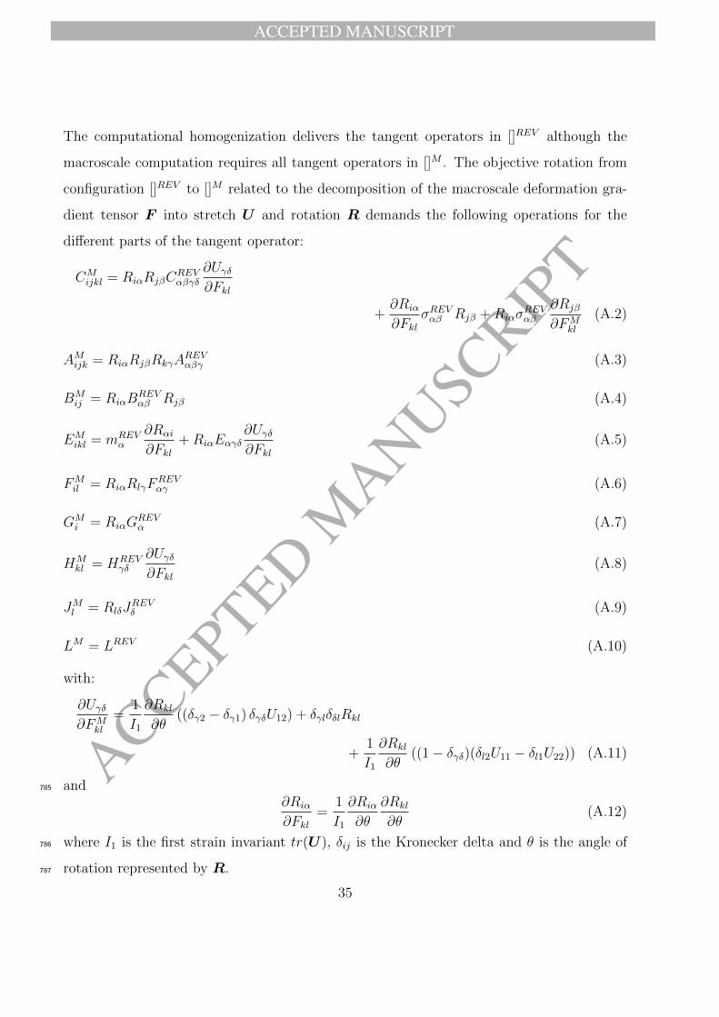
ACCEPTED MANUSCRIPT

ACCEPTED MANUSCRIP

T

The computational homogenization delivers the tangent operators in []REV although the

macroscale computation requires all tangent operators in []M . The objective rotation from

configuration []REV to []M related to the decomposition of the macroscale deformation gra-

dient tensor F into stretch U and rotation R demands the following operations for the

different parts of the tangent operator:

CMijkl = RiαRjβC

REVαβγδ

∂Uγδ∂Fkl

+∂Riα

∂FklσREVαβ Rjβ +Riασ

REVαβ

∂Rjβ

∂FMkl

(A.2)

AMijk = RiαRjβRkγAREVαβγ (A.3)

BMij = RiαB

REVαβ Rjβ (A.4)

EMikl = mREV

α

∂Rαi

∂Fkl+RiαEαγδ

∂Uγδ∂Fkl

(A.5)

FMil = RiαRlγF

REVαγ (A.6)

GMi = RiαG

REVα (A.7)

HMkl = HREV

γδ

∂Uγδ∂Fkl

(A.8)

JMl = RlδJREVδ (A.9)

LM = LREV (A.10)

with:

∂Uγδ∂FM

kl

=1

I1

∂Rkl

∂θ((δγ2 − δγ1) δγδU12) + δγlδδlRkl

+1

I1

∂Rkl

∂θ((1− δγδ)(δl2U11 − δl1U22)) (A.11)

and785

∂Riα

∂Fkl=

1

I1

∂Riα

∂θ

∂Rkl

∂θ(A.12)

where I1 is the first strain invariant tr(U), δij is the Kronecker delta and θ is the angle of786

rotation represented by R.787

35

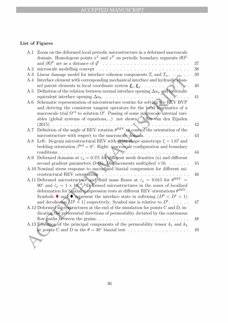
ACCEPTED MANUSCRIPT

ACCEPTED MANUSCRIP

T

List of Figures

A.1 Zoom on the deformed local periodic microstructure in a deformed macroscaledomain. Homologous points xL and xF on periodic boundary segments ∂ΩL

and ∂ΩF are as a distance of ~yt . . . . . . . . . . . . . . . . . . . . . . . . . 37A.2 microscale modelling concept . . . . . . . . . . . . . . . . . . . . . . . . . . . 38A.3 Linear damage model for interface cohesion components Tt and Tn. . . . . . 39A.4 Interface element with corresponding mechanical interface and hydraulic chan-

nel parent elements in local coordinate system ξ1, ξ2. . . . . . . . . . . . . . 40A.5 Definition of the relation between normal interface opening ∆un and hydraulic

equivalent interface opening ∆uh . . . . . . . . . . . . . . . . . . . . . . . . 41A.6 Schematic representation of microstructure routine for solving the REV BVP

and deriving the consistent tangent operators for the local kinematics of amacroscale trial Ωτ2 to solution Ωt. Passing of some microscale internal vari-ables (global systems of equations,...) not shown. After van den Eijnden(2015) . . . . . . . . . . . . . . . . . . . . . . . . . . . . . . . . . . . . . . . 42

A.7 Definition of the angle of REV rotation θREV to control the orientation of themicrostructure with respect to the macroscale domain. . . . . . . . . . . . . 43

A.8 Left: 16-grain microstructural REV with grain shape anisotropy ξ = 1.67 andbedding orientation βbed = 0. Right: macroscale configuration and boundaryconditions. . . . . . . . . . . . . . . . . . . . . . . . . . . . . . . . . . . . . . 44

A.9 Deformed domains at εa = 0.5% for different mesh densities (a) and differentsecond gradient parameters D (b). Displacements multiplied ×10. . . . . . . 45

A.10 Nominal stress response to unconfined biaxial compression for different mi-crostructural REV orientations . . . . . . . . . . . . . . . . . . . . . . . . . 46

A.11 Deformed microstructure and fluid mass fluxes at εa = 0.015 for θREV =90 and εa = 1 × 10−8. Deformed microstructures in the zones of localizeddeformation for biaxial compression tests at different REV orientations θREV .Symbols ♦ and ♦ represent the interface state in softening (D0 < Dt < 1)and decohesion (Dt = 1) respectively. Symbol size is relative to Dt. . . . . . 47

A.12 Deformed microstructures at the end of the simulation for points C and D, in-dicating the preferential directions of permeability dictated by the continuousflow paths between the grains. . . . . . . . . . . . . . . . . . . . . . . . . . . 48

A.13 Evolution of the principal components of the permeability tensor k1 and k2

at points C and D in the θ = 30 biaxial test . . . . . . . . . . . . . . . . . . 49

36

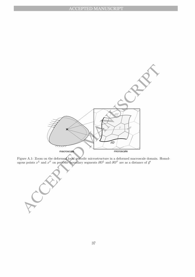
ACCEPTED MANUSCRIPT

ACCEPTED MANUSCRIP

T

+ aL

ayt xFaxL

macroscale microscale

∂ΩL

∂ΩF

Figure A.1: Zoom on the deformed local periodic microstructure in a deformed macroscale domain. Homol-ogous points xL and xF on periodic boundary segments ∂ΩL and ∂ΩF are as a distance of ~yt

37

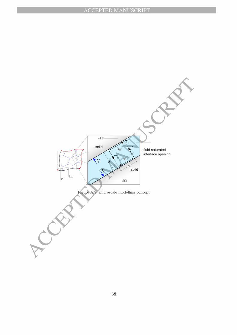
ACCEPTED MANUSCRIPT

ACCEPTED MANUSCRIP

T

solid

∂Ω+

∂Ω-

fp+

fp-

fluid-saturatedinterface opening

Δn

n+

T+t

T+n

T-n

T-t

solidΔ t

n-

ΓΩn

Figure A.2: microscale modelling concept

38

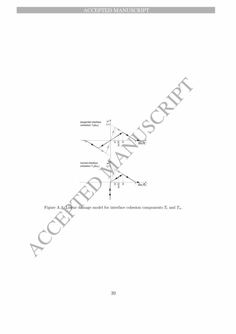
ACCEPTED MANUSCRIPT

ACCEPTED MANUSCRIP

T

Ttmax

Dt0

Dtt

1-1

Δu t

t /δtc

Tt

Tnmax

Dn0

Dnt

1 Δun/δnc

Δu n

t /δnc

Tn

Δut/δtc

tangential interface cohestion Tt(Δut)

normal interface cohestion Tn(Δun)

Figure A.3: Linear damage model for interface cohesion components Tt and Tn.

39

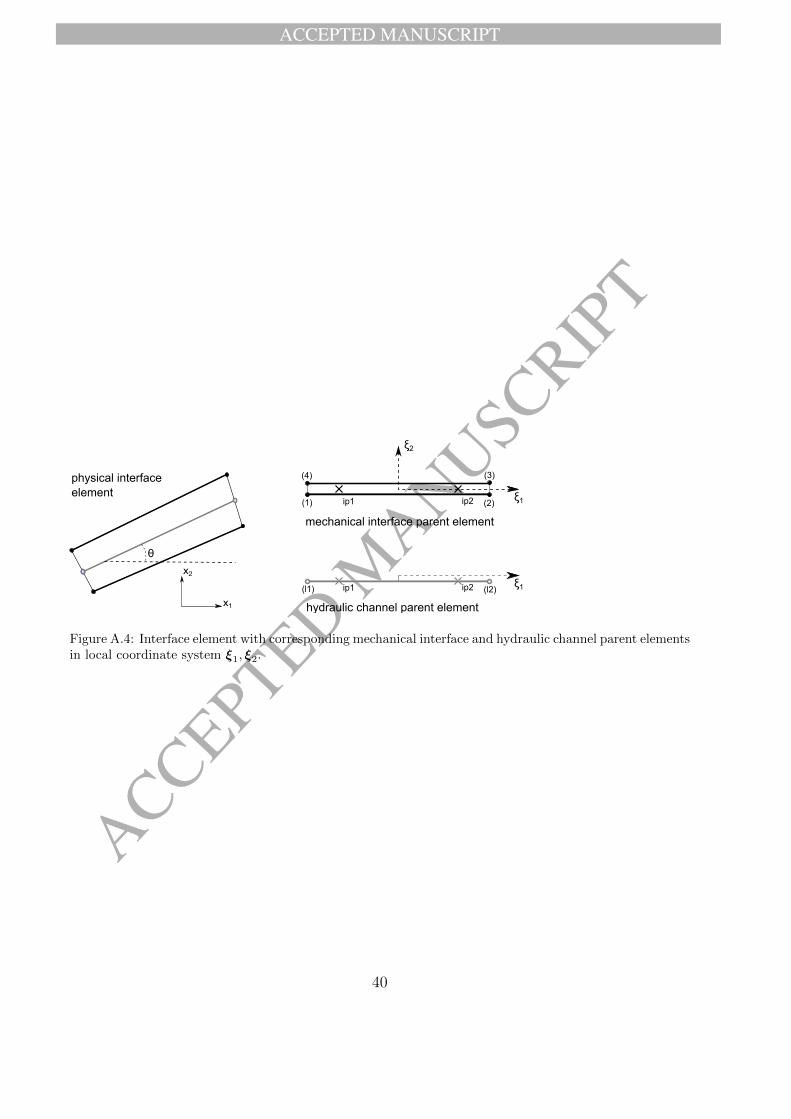
ACCEPTED MANUSCRIPT

ACCEPTED MANUSCRIP

Tx2

x1

(1) (2)

(3)(4)

ip1 ip2

ξ2

ξ1

θ

(l1) (l2)ip1 ip2

mechanical interface parent element

ξ1

hydraulic channel parent element

physical interface element

Figure A.4: Interface element with corresponding mechanical interface and hydraulic channel parent elementsin local coordinate system ξ1, ξ2.

40

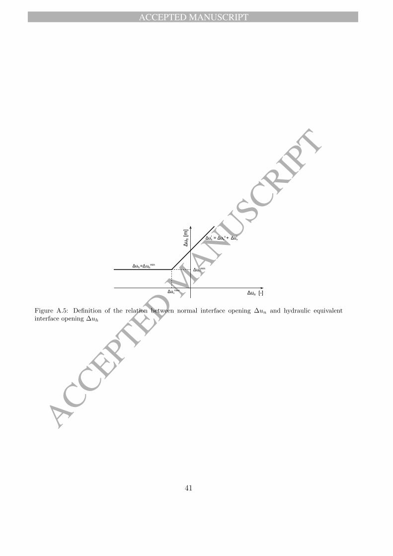
ACCEPTED MANUSCRIPT

ACCEPTED MANUSCRIP

TΔuh

min

Δu h

[m]

Δun [-]

Δuh

Δuh = Δuh0 + Δun

=Δuhmin

Δuntrans

t t

Figure A.5: Definition of the relation between normal interface opening ∆un and hydraulic equivalentinterface opening ∆uh

41

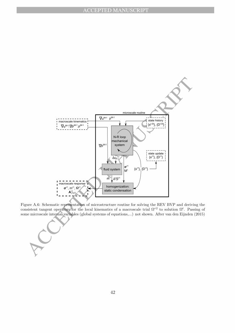
ACCEPTED MANUSCRIPT

ACCEPTED MANUSCRIP

T

macroscale kinematics

uMτ1 , pMτ1,pMτ1Δ

N-R loopmechanical

system

fluid system

Δuhτ1

pMτ1Δ

mτ1

pMτ1

στ1

Mτ2

homogenization:static condensation

στ1, mτ1, Mτ1

Aτ1

macroscale response

(7x7)

xτ1, Dτ1

microscale routine

state update xτ1, Dτ1

Δepτ1

ΔuMτ1

Δstate history

xt-Δt, Dt-Δt

.

Figure A.6: Schematic representation of microstructure routine for solving the REV BVP and deriving theconsistent tangent operators for the local kinematics of a macroscale trial Ωτ2 to solution Ωt. Passing ofsome microscale internal variables (global systems of equations,...) not shown. After van den Eijnden (2015)

42

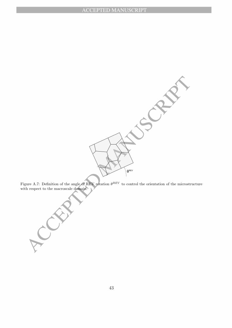
ACCEPTED MANUSCRIPT

ACCEPTED MANUSCRIP

TθREV

Figure A.7: Definition of the angle of REV rotation θREV to control the orientation of the microstructurewith respect to the macroscale domain.

43

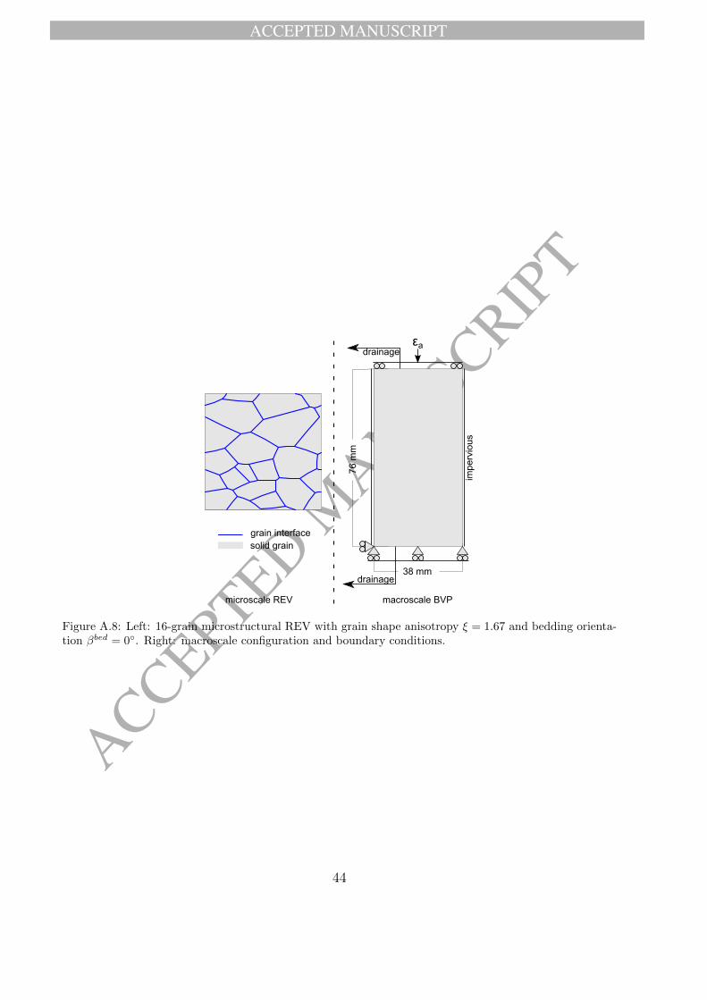
ACCEPTED MANUSCRIPT

ACCEPTED MANUSCRIP

T

76 m

m

38 mm

impe

rvio

us

εa

microscale REV macroscale BVP

drainage

drainage

grain interface solid grain

Figure A.8: Left: 16-grain microstructural REV with grain shape anisotropy ξ = 1.67 and bedding orienta-tion βbed = 0. Right: macroscale configuration and boundary conditions.

44

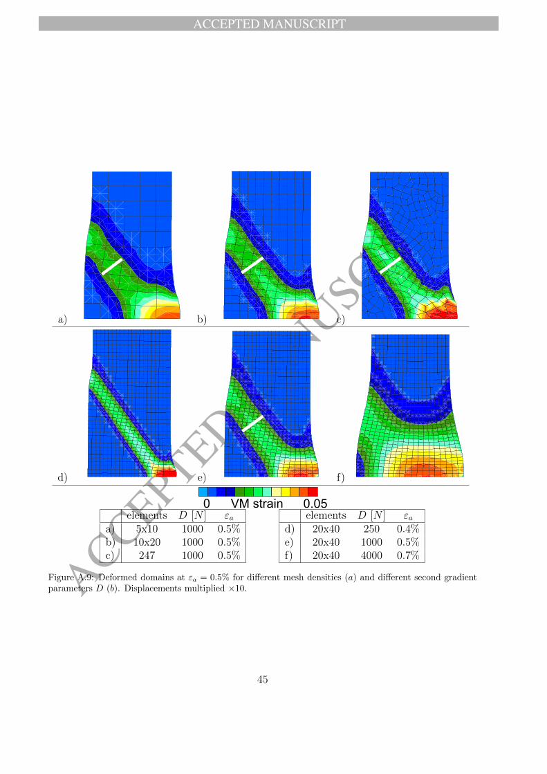
ACCEPTED MANUSCRIPT

ACCEPTED MANUSCRIP

T

a)X

Y<M 0

41

M 83

M 125

M 167

M 209

M 251

M 293

M 335

M 377

M 419

>M 461

)M1.000E/04

ULgM 5x10M

COURBEMDEME/EQTIMEM DMULCUMM5.000EV05M 0.500M

DELT=M0.420E/02M

XM 0.100EV05

TMIN=M 0.00M

TMAX=M4.388E/02

DANSMSTRUCTUREMDEFORMEE:MITYPF=1

PDEPL=M 10.0M (

VUEMENMPLANMXMY

MINM MAX

XM 0.000M 0.047

YM 0.000M 0.072

ZM 0.000M 0.000

SELECTIONMDESMELEMENTS

TOUS

DESFINM 9.4M05/06/2016b)X

Y<M 0

41

M 83

M 125

M 167

M 209

M 251

M 293

M 335

M 377

M 419

>M 461

)M1.000E/04

ULgM 10x20M


DELT=M0.420E/02M

XM 0.100EV05

TMIN=M 0.00M

TMAX=M4.772E/02


PDEPL=M 10.0M (

VUEMENMPLANMXMY

MINM MAX

XM 0.000M 0.047

YM 0.000M 0.074

ZM 0.000M 0.000


TOUS

DESFINM 9.4M05/06/2016c)X

Y<R )

4V

R 8/

R VZ5

R V67

R Z)9

R Z5V

R Z9/

R //5

R /77

R 4V9

>R 46V

ARVP)))E:)4

99 ULgR meshR:RCopyR

COURBERDERE:EQTIMER DMULCUMR4P995ES)5R )P5))R

DELT=R)P4Z)E:)ZR

XR )PV))ES)5

TMIN=RVP58ZE:)/

TMAX=R5P455E:)Z

DANSRSTRUCTURERDEFORMEE:RITYPF=V

=DEPL=R V)P)R N

VUERENRPLANRXRY

MINR MAX

XR )P)))R )P)47

YR )P)))R )P)75

ZR )P)))R )P)))

SELECTIONRDESRELEMENTS

TOUS

DESFINR 9P4R)5()6(Z)V6

d)X

Y<M 0

41

M 83

M 125

M 167

M 209

M 251

M 293

M 335

M 377

M 419

>M 461

)M1.000E/04

ULgM 20x40M/M250M


DELT=M0.420E/02M

XM 0.100EV05

TMIN=M 0.00M

TMAX=M6.019E/02


PDEPL=M 10.0M (

VUEMENMPLANMXMY

MINM MAX

XM 0.000M 0.044

YM 0.000M 0.075

ZM 0.000M 0.000


TOUS

DESFINM 9.4M05/06/2016e)X

Y<M 0

41

M 83

M 125

M 167

M 209

M 251

M 293

M 335

M 377

M 419

>M 461

)M1.000E/04

ULgM 20x40M


DELT=M0.420E/02M

XM 0.100EV05

TMIN=M 0.00M

TMAX=M4.831E/02


PDEPL=M 10.0M (

VUEMENMPLANMXMY

MINM MAX

XM 0.000M 0.047

YM 0.000M 0.075

ZM 0.000M 0.000


TOUS

DESFINM 9.4M06/06/2016f)X

Y< 0

41

83

125

167

209

251

293

335

377

419

> 461

* 1.000E-04

ULg 20x40 - 4000

COURBE DE E-EQTIME DMULCUM 7.219E+05 0.722

DELT= 0.420E-02

X 0.100E+05

TMIN= 0.00

TMAX= 4.643E-02

DANS STRUCTURE DEFORMEE: ITYPF=1

(DEPL= 10.0 )

VUE EN PLAN X Y

MIN MAX

X 0.000 0.054

Y 0.000 0.075

Z 0.000 0.000

SELECTION DES ELEMENTS

TOUS

DESFIN 9.4 08/06/2016

0 VM strain 0.05elements D [N ] εa

a) 5x10 1000 0.5%b) 10x20 1000 0.5%c) 247 1000 0.5%

elements D [N ] εad) 20x40 250 0.4%e) 20x40 1000 0.5%f) 20x40 4000 0.7%

Figure A.9: Deformed domains at εa = 0.5% for different mesh densities (a) and different second gradientparameters D (b). Displacements multiplied ×10.

45

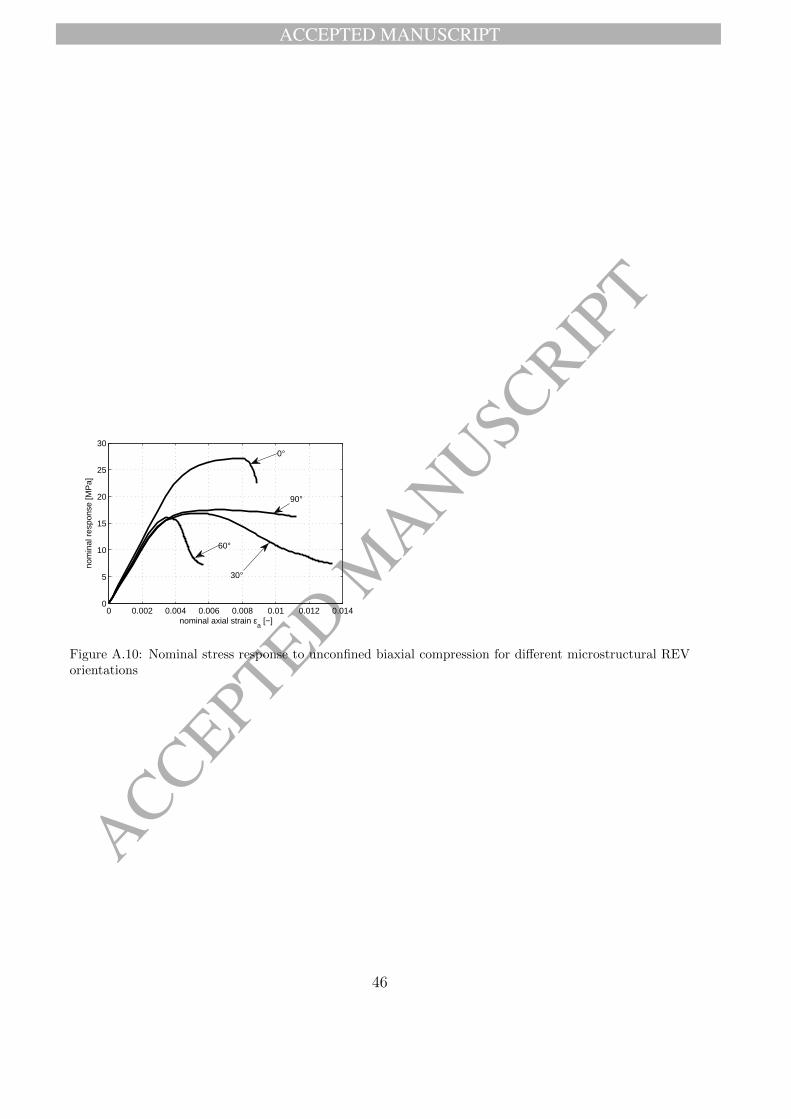
ACCEPTED MANUSCRIPT

ACCEPTED MANUSCRIP

T0 0.002 0.004 0.006 0.008 0.01 0.012 0.014

0

5

10

15

20

25

30

nominal axial strain εa [−]

nom

inal

res

pons

e [M

Pa]

0°

90°

60°

30°

Figure A.10: Nominal stress response to unconfined biaxial compression for different microstructural REVorientations

46

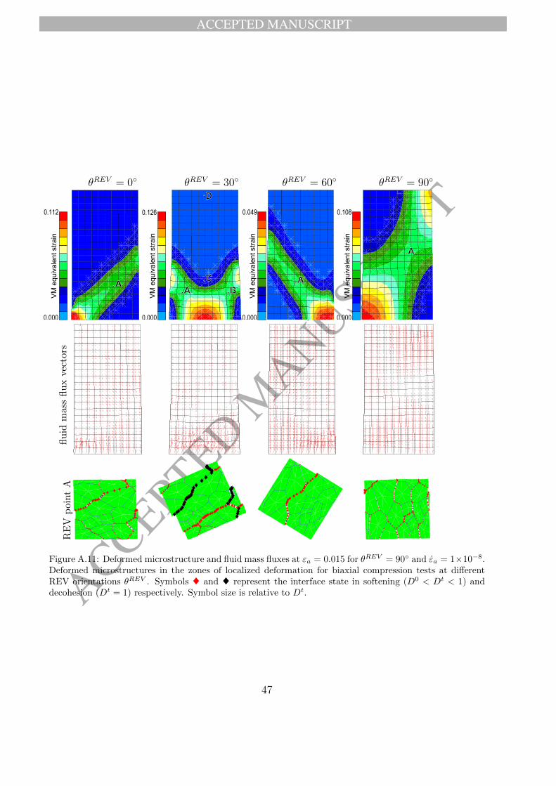
ACCEPTED MANUSCRIPT

ACCEPTED MANUSCRIP

T

θREV = 0 θREV = 30 θREV = 60 θREV = 90

0.112

0.000

VM

equ

ival

ent s

trai

n

A

0.126

AC

B

D

0.049

0.000

VM

equ

ival

ent s

trai

n

A

0.108

0.000

VM

equ

ival

ent s

trai

n

A

flu

idm

ass

flu

xve

ctor

sR

EV

poi

nt

A Element 57, I.P. 1

Element 42, I.P. 2

Element 55, I.P. 2

Element 97, I.P. 3

Figure A.11: Deformed microstructure and fluid mass fluxes at εa = 0.015 for θREV = 90 and εa = 1×10−8.Deformed microstructures in the zones of localized deformation for biaxial compression tests at differentREV orientations θREV . Symbols ♦ and ♦ represent the interface state in softening (D0 < Dt < 1) anddecohesion (Dt = 1) respectively. Symbol size is relative to Dt.

47

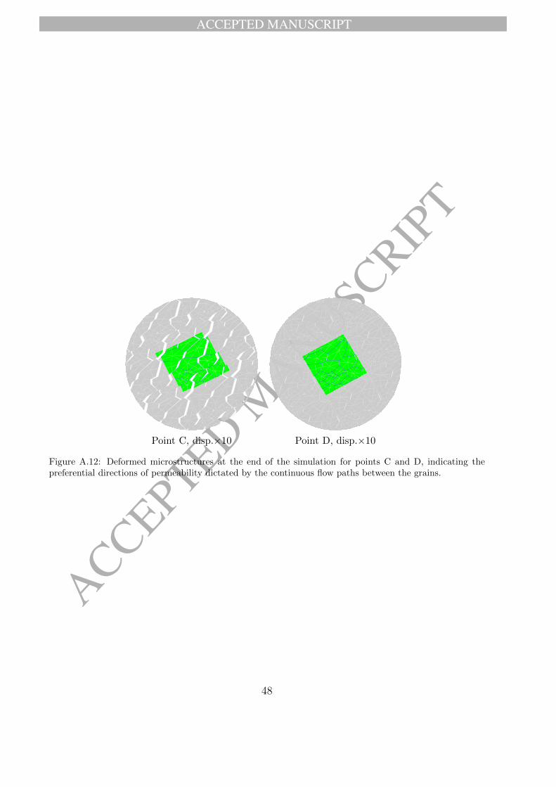
ACCEPTED MANUSCRIPT

ACCEPTED MANUSCRIP

TPoint C, disp.×10 Point D, disp.×10

Figure A.12: Deformed microstructures at the end of the simulation for points C and D, indicating thepreferential directions of permeability dictated by the continuous flow paths between the grains.

48

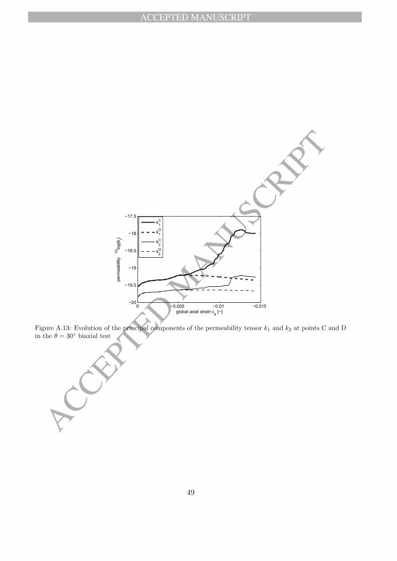
ACCEPTED MANUSCRIPT

ACCEPTED MANUSCRIP

T−0.015−0.01−0.0050

−20

−19.5

−19

−18.5

−18

−17.5

perm

eabi

lity

10lo

g(k i)

global axial strain εa

[−]

k1C

k

2Ck

1D

k2D

Figure A.13: Evolution of the principal components of the permeability tensor k1 and k2 at points C and Din the θ = 30 biaxial test

49

ACCEPTED MANUSCRIPT

ACCEPTED MANUSCRIP

T

List of Tables

A.1 Microscale constitutive properties for the microstructural REV in Figure A.8. 51

50

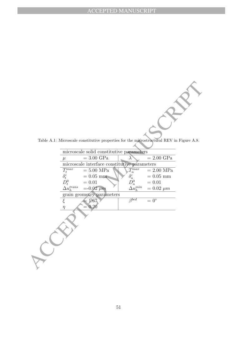
ACCEPTED MANUSCRIPT

ACCEPTED MANUSCRIP

T

Table A.1: Microscale constitutive properties for the microstructural REV in Figure A.8.

microscale solid constitutive parametersµ = 3.00 GPa λ = 2.00 GPamicroscale interface constitutive parametersTmaxt = 5.00 MPa Tmaxn = 2.00 MPaδct = 0.05 mm δcn = 0.05 mmD0t = 0.01 D0

n = 0.01∆utransh =-0.02 µm ∆uminh = 0.02 µmgrain geometry parametersξ = 1.67 βbed = 0

η = 0.20

51

Accepted Manuscript - ORBi

Documents