Copyright is owned by the Author of the thesis. Permission is given for a copy to be downloaded by an individual for the purpose of research and private study only. The thesis may not be reproduced elsewhere without the permission of the Author.

Welcome message from author
This document is posted to help you gain knowledge. Please leave a comment to let me know what you think about it! Share it to your friends and learn new things together.
Transcript

Copyright is owned by the Author of the thesis. Permission is given for a copy to be downloaded by an individual for the purpose of research and private study only. The thesis may not be reproduced elsewhere without the permission of the Author.

Acceptance Sampling for Food QualityAssurance
Edgar Santos-Fernández
Supervisor: Dr. K. GovindarajuDr. Geoff Jones
Institute of Fundamental Sciences
Massey University
This dissertation is submitted for the degree of
Doctor of Philosophy in Statistics
March 2017


Dedicated to my mother, Carmen Fernández Ferrer
A ti madre querida, por ser ejemplo de dedicacion y amor.

iv
“In God we trust, all others bring data.1”
1Attributed to W. Edwards Deming.

Declaration
I hereby declare that except where specific reference is made to the work of others, the contents
of this dissertation are original and have not been submitted in whole or in part for consideration
for any other degree or qualification in this, or any other university. This dissertation is my
own work and contains nothing which is the outcome of work done in collaboration with others,
except as specified in the text and Acknowledgements. This dissertation contains fewer than
65,000 words including appendices, bibliography, footnotes, tables and equations and has fewer
than 150 figures.
Edgar Santos-Fernández
March 2017


Acknowledgements
This thesis is the result of the combined effort of several people for over three years. First,
I would like to thank my supervisor Dr. K. Govindaraju. I will always be grateful for this
opportunity and for the guidance, advice and support. My deepest gratitude to my co-supervisor
Associate Professor Geoff Jones, for his valuable lessons and for encouraging me. Thanks to the
members of the Statistics and Bioinformatics Group and especially to Professor Martin Hazelton.
I would like to acknowledge the absolute support provided by the Institute of Fundamental
Sciences, Massey University.
I am immensely grateful to the Primary Growth Partnership (PGP), which was funded by
Fonterra Co-operative Group Limited and the New Zealand Government, for the financial support.
I would like to show my gratitude to Roger Kissling from Fonterra, for his help and advice
during execution of this project, for his constructive feedbacks and ideas, and for providing the
data. Thanks to Steve Holroyd for reading several of these manuscripts in different stages and
for his valuable suggestions. I also would like to thank other members of Fonterra Co-operative
Group Limited involved in this work.
My gratitude extends to several Editors and anonymous referees for carefully reading the six
works here exposed. Their suggestions and feedback allowed us to substantially improve this
thesis.
Thanks to the present and past postgrad students and colleagues I had the pleasure of working
with for over three years. Thanks to my colleague Nadeeka Premarathna.
Last but not the least, I am thankful to my family for the support and the encouragement.
Gracias a mi madre por tantos años de excepcional educación. Por educarme en el caminohacia la ciencia y el descubrimiento. A mi hermana Laura, por estar siempre a mi lado y portoda la ayuda que me ha brindado a lo largo de los años. Agradezco ademas a mis hermanos, yal resto de mi familia.
Thanks to everyone that contributed to this project.
Palmerston North. December, 2016


Abstract
Acceptance sampling plays a crucial role in food quality assurance. However, safety inspection
represents a substantial economic burden due to the testing costs and the number of quality
characteristics involved. This thesis presents six pieces of work on the design of attribute and
variables sampling inspection plans for food safety and quality. Several sampling plans are
introduced with the aims of providing a better protection for the consumers and reducing the
sample sizes. The effect of factors such as the spatial distribution of microorganisms and the
analytical unit amount is discussed. The quality in accepted batches has also been studied,
which is relevant for assessing the impact of the product in the public health system. Optimum
design of sampling plans for bulk materials is considered and different scenarios in terms of
mixing efficiency are evaluated. Single and two-stage sampling plans based on compressed
limits are introduced. Other issues such as the effect of imperfect testing and the robustness
of the plan have been also discussed. The use of the techniques is illustrated with practical
examples. We considered numerous probability models for fitting aerobic plate counts and
presence-absence data from milk powder samples. The suggested techniques have been found to
provide a substantial sampling economy, reducing the sample size by a factor between 20 and 80%
(when compared to plans recommended by the International Commission on Microbiological
Specification for Food (ICMSF) and the CODEX Alimentarius). Free software and apps have
been published, allowing practitioners to design more stringent sampling plans.
Keywords:
Bulk material, Composite samples, Compressed limit, Consumer Protection, Double sampling
plan, Food safety, Measurement errors, Microbiological testing, Sampling inspection plan.

x
Recommended citation
Santos-Fernández, Edgar (2016) Acceptance Sampling for Food Quality Assurance. PhDdissertation. Massey University.
BIBTEX� �
@PhdThesis{SantosFernandezPhD2016,title = {Acceptance Sampling for Food Quality Assurance},
author = {Santos Fern\ andez, Edgar},school = {Massey University},year = {2016},note = {{PhD} dissertation}}
�� �
EndNote� �
%0 Book%T Acceptance Sampling for Food Quality Assurance%A Santos Fern ndez, Edgar%D 2016%I Massey University%Z PhD dissertation
�� �
Declaration
This thesis complies with the ‘Guidelines for Doctoral Thesis by Publications’ and with the
requirements from the Handbook for Doctoral Study by the Doctoral Research Committee
(DRC), Massey University. January 2011. Version 7.
Disclaimer
The opinions, findings and conclusions in this thesis are solely those of the author(s). Under
no circumstances will the author(s) be responsible for any loss or damage of any kind resulted
from the use of these techniques. The software codes and the apps produced by this research are
licensed under GPL� 2.0 and it comes without warranty of any kind.

Table of contents
List of figures xv
List of tables xxi
1 Introduction 11.1 Food safety and assurance . . . . . . . . . . . . . . . . . . . . . . . . . . . . 1
1.2 Acceptance sampling . . . . . . . . . . . . . . . . . . . . . . . . . . . . . . . 2
1.3 Microbiological sampling plans . . . . . . . . . . . . . . . . . . . . . . . . . 5
1.4 Scientific problem and research objectives . . . . . . . . . . . . . . . . . . . . 6
1.5 List of publications/manuscripts . . . . . . . . . . . . . . . . . . . . . . . . . 8
2 Quantity-Based Microbiological Sampling Plans and Quality after Inspection 92.1 Abstract . . . . . . . . . . . . . . . . . . . . . . . . . . . . . . . . . . . . . . 9
2.2 Introduction . . . . . . . . . . . . . . . . . . . . . . . . . . . . . . . . . . . . 9
2.3 Concentration-based sampling plan . . . . . . . . . . . . . . . . . . . . . . . 11
2.3.1 Single batch microbial risk assessment. . . . . . . . . . . . . . . . . . 11
2.3.2 Average quality in accepted batches . . . . . . . . . . . . . . . . . . . 18
2.4 Variables sampling plan . . . . . . . . . . . . . . . . . . . . . . . . . . . . . 25
2.4.1 Sampling plan design . . . . . . . . . . . . . . . . . . . . . . . . . . 25
2.4.2 Average quality in accepted batches using variables plan . . . . . . . . 26
2.5 Discussion and conclusions . . . . . . . . . . . . . . . . . . . . . . . . . . . . 26
Appendix 2.A Table of symbols . . . . . . . . . . . . . . . . . . . . . . . . . . . . 29
Appendix 2.B The convolution theory . . . . . . . . . . . . . . . . . . . . . . . . 29
3 Compressed Limit Sampling Inspection Plans for Food Safety 313.1 Abstract . . . . . . . . . . . . . . . . . . . . . . . . . . . . . . . . . . . . . . 31
3.2 Introduction . . . . . . . . . . . . . . . . . . . . . . . . . . . . . . . . . . . . 32
3.3 Good Manufacturing Practices (GMP) limits . . . . . . . . . . . . . . . . . . . 33
3.4 Two-class compressed limit attribute plans for known σ . . . . . . . . . . . . . 34
3.5 Three-class compressed limit attribute plan . . . . . . . . . . . . . . . . . . . 38
3.6 Numerical results . . . . . . . . . . . . . . . . . . . . . . . . . . . . . . . . . 42
3.7 Economic evaluation . . . . . . . . . . . . . . . . . . . . . . . . . . . . . . . 44
3.8 Robustness and nonnormal-based compressed limit plans . . . . . . . . . . . . 45

xii Table of contents
3.9 Summary and conclusions . . . . . . . . . . . . . . . . . . . . . . . . . . . . 48
Appendix 3.A Glossary of symbols and definitions. . . . . . . . . . . . . . . . . . 50
Appendix 3.B R Software code . . . . . . . . . . . . . . . . . . . . . . . . . . . . 50
Appendix 3.C Optimum compression constants (t), sample size (nt), acceptance
number (ct) and the corresponding quantile (qt) for given two points of the OC
curve . . . . . . . . . . . . . . . . . . . . . . . . . . . . . . . . . . . . . . . 53
Appendix 3.D Optimum compression constant (t1), (t2), sample size (nt) and accep-
tance numbers (ctM) and (ctm) for three-class compressed limit plan. . . . . . . 54
4 New two-stage sampling inspection plans for bacterial cell counts 574.1 Abstract . . . . . . . . . . . . . . . . . . . . . . . . . . . . . . . . . . . . . . 57
4.2 Introduction . . . . . . . . . . . . . . . . . . . . . . . . . . . . . . . . . . . . 58
4.3 Materials and methods . . . . . . . . . . . . . . . . . . . . . . . . . . . . . . 59
4.3.1 Statistical models . . . . . . . . . . . . . . . . . . . . . . . . . . . . . 59
4.3.2 Compressed limit plans . . . . . . . . . . . . . . . . . . . . . . . . . . 60
4.3.3 Double sampling plans . . . . . . . . . . . . . . . . . . . . . . . . . . 61
4.3.4 Two-stage sampling plan based on compressed limit. . . . . . . . . . . 61
4.4 Evaluation of double sampling plan with compressed limit in the first stage . . 64
4.4.1 The homogeneous case . . . . . . . . . . . . . . . . . . . . . . . . . . 64
4.4.2 The heterogeneous case modelled with the PLN distribution . . . . . . 66
4.4.3 The heterogeneous case modelled with the PG distribution . . . . . . . 67
4.4.4 Iterative algorithm to obtain the optimum sampling plan . . . . . . . . 67
4.4.5 Comparison with the single compressed limit plan . . . . . . . . . . . 69
4.4.6 Assessing the robustness of the plans . . . . . . . . . . . . . . . . . . 69
4.5 Practical results . . . . . . . . . . . . . . . . . . . . . . . . . . . . . . . . . . 71
4.6 A web-based application . . . . . . . . . . . . . . . . . . . . . . . . . . . . . 73
4.7 Discussion and conclusions . . . . . . . . . . . . . . . . . . . . . . . . . . . . 73
Appendix 4.A Markov chain Monte Carlo (MCMC) method . . . . . . . . . . . . . 75
Appendix 4.B codes used for the simulations . . . . . . . . . . . . . . 76
4.B.1 Negative binomial . . . . . . . . . . . . . . . . . . . . . . . . . . . . 76
4.B.2 Poisson-lognormal . . . . . . . . . . . . . . . . . . . . . . . . . . . . 76
4.B.3 Poisson . . . . . . . . . . . . . . . . . . . . . . . . . . . . . . . . . . 77
5 Effects of imperfect testing on presence-absence sampling plans 795.1 Abstract . . . . . . . . . . . . . . . . . . . . . . . . . . . . . . . . . . . . . . 79
5.2 Introduction . . . . . . . . . . . . . . . . . . . . . . . . . . . . . . . . . . . . 80
5.3 Materials and methods . . . . . . . . . . . . . . . . . . . . . . . . . . . . . . 82
5.3.1 Discretization and the analytical unit . . . . . . . . . . . . . . . . . . . 82
5.3.2 The sampling distribution . . . . . . . . . . . . . . . . . . . . . . . . 83
5.3.3 Statistical sample size (n) . . . . . . . . . . . . . . . . . . . . . . . . 83
5.3.4 The population of microorganisms . . . . . . . . . . . . . . . . . . . . 84

Table of contents xiii
5.3.5 The sampling method . . . . . . . . . . . . . . . . . . . . . . . . . . . 85
5.3.6 Testing pooled or composite units . . . . . . . . . . . . . . . . . . . . 86
5.4 Single (isolated) batch risk assessment . . . . . . . . . . . . . . . . . . . . . . 87
5.4.1 Building a hierarchical model based on p . . . . . . . . . . . . . . . . 87
5.4.2 Hierarchical model based on the rate λ . . . . . . . . . . . . . . . . . 89
5.4.3 Hierarchical model for semi-continuous data based on the zero inflated
lognormal (ZILN) distribution . . . . . . . . . . . . . . . . . . . . . . 90
5.5 Bayesian data analysis . . . . . . . . . . . . . . . . . . . . . . . . . . . . . . 90
5.5.1 One sample of 300g vs. 30 samples of 10g each . . . . . . . . . . . . . 92
5.6 Cost analysis . . . . . . . . . . . . . . . . . . . . . . . . . . . . . . . . . . . 94
5.7 Discussion and conclusions . . . . . . . . . . . . . . . . . . . . . . . . . . . . 96
Appendix 5.A Glossary of symbols and definitions . . . . . . . . . . . . . . . . . . 98
Appendix 5.B Reported values of sensitivity and specificity. . . . . . . . . . . . . . 99
Appendix 5.C Models in JAGS for the numerical integration . . . . . . . . . . . . 100
5.C.1 R codes to obtain the Pa using numerical integration . . . . . . . . . . 100
5.C.2 R codes to obtain the Pa using numerical integration using ni composite
samples . . . . . . . . . . . . . . . . . . . . . . . . . . . . . . . . . . 100
5.C.3 R codes to obtain the Pa, p and pe in the accepted batches using MCMC 100
5.C.4 R codes to obtain the Pa using numerical integration based on μ and σ . 100
5.C.5 R codes to obtain the Pa using numerical integration based on the zero
inflated Poisson-lognormal distribution with μ and σ . . . . . . . . . . 101
5.C.6 R codes used for the MCMC simulation (Scenario 1) . . . . . . . . . . 101
Appendix 5.D Shiny app to estimate the risk for presence-absence tests . . . . . . . 101
6 A New Variables Acceptance Sampling Plan for Food Safety 1036.1 Abstract . . . . . . . . . . . . . . . . . . . . . . . . . . . . . . . . . . . . . . 103
6.2 Introduction . . . . . . . . . . . . . . . . . . . . . . . . . . . . . . . . . . . . 103
6.3 Material and methods . . . . . . . . . . . . . . . . . . . . . . . . . . . . . . . 105
6.3.1 The Operating Characteristic (OC) curve . . . . . . . . . . . . . . . . 105
6.3.2 Variables plans for food safety . . . . . . . . . . . . . . . . . . . . . . 105
6.3.3 New plans based on the sinh-arcsinh transformation . . . . . . . . . . 106
6.3.4 Simulation algorithm . . . . . . . . . . . . . . . . . . . . . . . . . . . 106
6.4 Results . . . . . . . . . . . . . . . . . . . . . . . . . . . . . . . . . . . . . . . 107
6.5 The misclassification error . . . . . . . . . . . . . . . . . . . . . . . . . . . . 109
6.6 Example . . . . . . . . . . . . . . . . . . . . . . . . . . . . . . . . . . . . . . 109
6.7 Assessment of robustness . . . . . . . . . . . . . . . . . . . . . . . . . . . . . 111
6.8 Discussion . . . . . . . . . . . . . . . . . . . . . . . . . . . . . . . . . . . . . 113
6.9 Conclusions . . . . . . . . . . . . . . . . . . . . . . . . . . . . . . . . . . . . 113
Appendix 6.A Effect of the parameters in the sampling performance . . . . . . . . 115
Appendix 6.B Tabulated critical distances . . . . . . . . . . . . . . . . . . . . . . 118
Appendix 6.C Software code . . . . . . . . . . . . . . . . . . . . . . . . . . . . . 118
xiv Table of contents
Appendix 6.D Step-by-step guide . . . . . . . . . . . . . . . . . . . . . . . . . . . 119
Appendix 6.E Symbols and definitions. . . . . . . . . . . . . . . . . . . . . . . . . 121
Appendix 6.F Justification of chosen constant for sinh-arcsinh transformation. . . . 121
7 Variables Sampling Plans using Composite Samples for Food Quality Assurance 1237.1 Abstract . . . . . . . . . . . . . . . . . . . . . . . . . . . . . . . . . . . . . . 123
7.2 Introduction . . . . . . . . . . . . . . . . . . . . . . . . . . . . . . . . . . . . 123
7.3 Food safety and composite samples . . . . . . . . . . . . . . . . . . . . . . . 126
7.4 Imperfect mixing . . . . . . . . . . . . . . . . . . . . . . . . . . . . . . . . . 127
7.5 Variables plan for composite samples . . . . . . . . . . . . . . . . . . . . . . . 129
7.6 Design of the variables sampling plan based on composite samples. . . . . . . 131
7.7 Three-class variables plan . . . . . . . . . . . . . . . . . . . . . . . . . . . . . 136
7.8 Conclusions . . . . . . . . . . . . . . . . . . . . . . . . . . . . . . . . . . . . 137
Appendix 7.A Glossary of symbols and definitions . . . . . . . . . . . . . . . . . . 141
Appendix 7.B Sampling plan design . . . . . . . . . . . . . . . . . . . . . . . . . 142
Appendix 7.C Sampling plan guide . . . . . . . . . . . . . . . . . . . . . . . . . . 142
8 General conclusions and future perspectives. 1438.1 Future plan of work . . . . . . . . . . . . . . . . . . . . . . . . . . . . . . . . 144
References 145
Appendix A Contributions to publications 157
Index 163
List of figures
1.1 Types of acceptance sampling schemes . . . . . . . . . . . . . . . . . . . . . . 3
2.1 OC contour plots of two-class concentration-based sampling plans with n = 10
and 30. The batch probability of acceptance is obtained from the Poisson-
lognormal distribution. . . . . . . . . . . . . . . . . . . . . . . . . . . . . . . 14
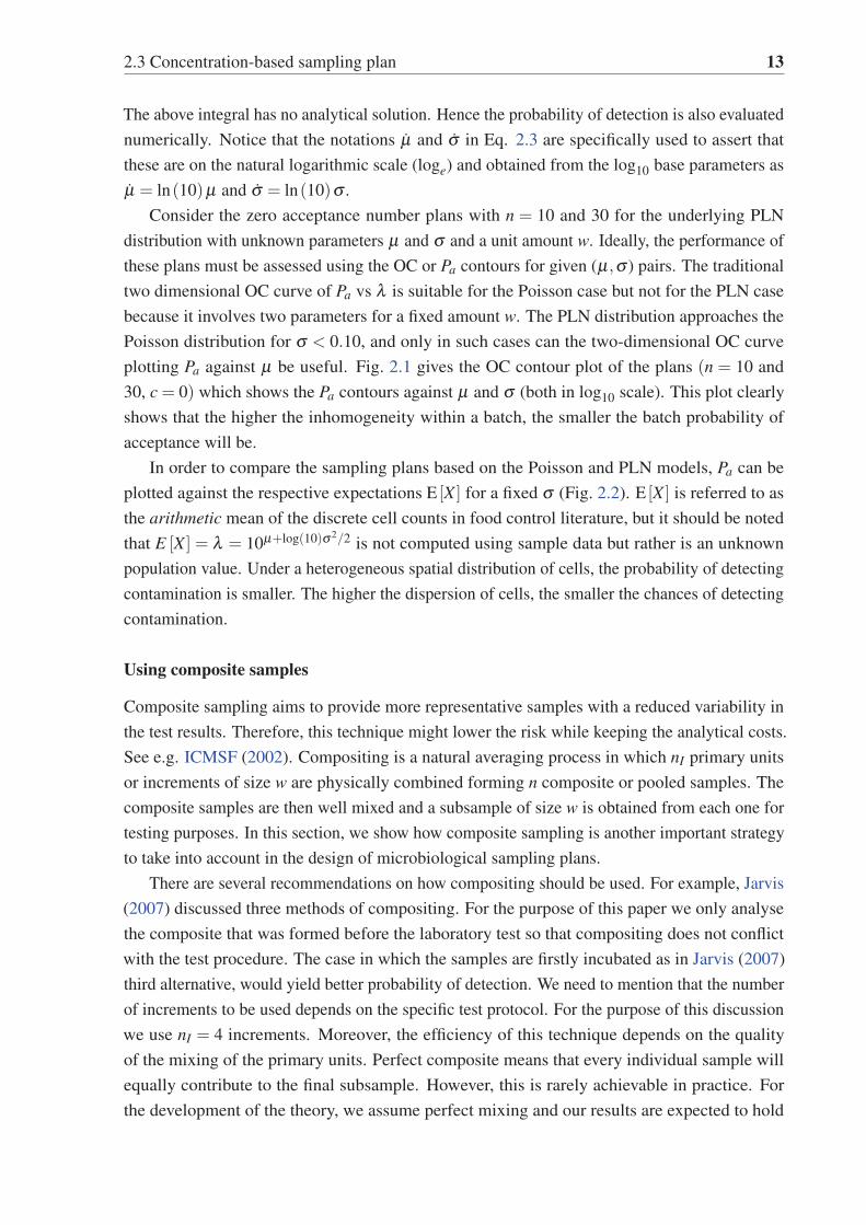
2.2 Effect of batch inhomogeneity on the OC curve (n = 10, c = 0). Cases 1 and 2
refer to homogenous and inhomogeneous contamination respectively. . . . . . 15
2.3 Effect of using composite samples with nI = 4 increments using the plan (n = 10,
c = 0) for the cases of homogeneity and inhomogeneity. . . . . . . . . . . . . . 16
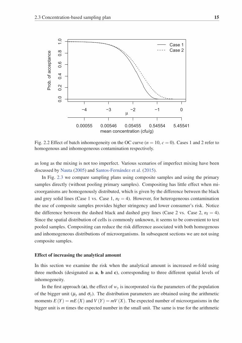
2.4 (a) Incoming concentration (λ ) is represented by the solid line. The mean
concentration after the inspection for Cases 3 and 4 are shown as dashed and
dotdashed lines. (b) Estimates of prevalence in the incoming and in the accepted
batches. (c) Probability of acceptance for the homogeneous and inhomogeneous
batches, before and after inspection. . . . . . . . . . . . . . . . . . . . . . . . 22
2.5 Increased analytical unit amount w = 25g. (a) Incoming concentration (λ ) is
represented by the solid line. The mean concentrations after inspection for Cases
3 and 4 are shown as dashed and dotdashed lines. (b) Estimate of the prevalence
of the contamination in the incoming and in the accepted batches. (c) Probability
of acceptance for the homogeneous and inhomogeneous batches, before and
after inspection. . . . . . . . . . . . . . . . . . . . . . . . . . . . . . . . . . . 24
2.6 OC curve of the variables plan with n = 10 and σw = 0.8 for w = 5 and 25g. This
figure shows that an increased analytical unit amount reduces the consumer’s risk. 26
2.7 (a) Incoming concentration of the contamination (represented by the solid line)
in relation to μ . The concentration after the inspection is given by the dashed
line. (b) It compares the batch probability of acceptance for a single batch and
for the series of batches. . . . . . . . . . . . . . . . . . . . . . . . . . . . . . 27
3.1 Illustration of the GMP limit (m) in relation to the regulatory limit (M) for the
normal distribution. . . . . . . . . . . . . . . . . . . . . . . . . . . . . . . . . 33
3.2 Illustration of the compressed limit approach in the normal distribution. . . . . 35
3.3 Illustration of the three-class compressed limit approach for the normal distribution. 40
3.4 OC contour plot of the three-class compressed limit approach. . . . . . . . . . 42

xvi List of figures
3.5 Compressed limit OC curves for Case 12 plan of the ICMSF. The dark solid OC
curve represents attribute plan with n = 20,c = 0. . . . . . . . . . . . . . . . . 44
3.6 Lognormal, gamma and Weibull (a) probability density functions and (b) cumu-
lative distribution functions matched by the mode and the density. . . . . . . . 46
3.7 Compressed limit OC curves equivalent to the ICMSF (2002) Case 12 (n =
20,c = 0) for known σ (a) and unknown (b). The assumed distribution is
lognormal when the true underlying model is lognormal, gamma and Weibull. . 47
4.1 Operation of the proposed two-stage sampling plan: first approach . . . . . . . 63
4.2 Operation of the proposed two-stage sampling plan: approach two. . . . . . . . 63
4.3 Operating Characteristic (OC) curve of the reference single plan n = 5, c = 0
(solid line). The dashed and dotdash line gives the double plan with compressed
limit in Stage 1. . . . . . . . . . . . . . . . . . . . . . . . . . . . . . . . . . 65
4.4 Average sample number (ASN) of the plans n = 5, c = 0, n1 = 3, n2 = 2, a1 = 0,
r1 = 2, r2 = 2 and n1 = 2, n2 = 5, a1 = 0, r1 = 2, r1m = 1, r2 = 2. . . . . . . . 65
4.5 Average Inspection Time (AIT) of the plans n = 5, c = 0, n1 = 3, n2 = 2, a1 = 0,
r1 = 2, r2 = 2 and n1 = 2, n2 = 5, a1 = 0, r1 = 2, r1m = 1, r2 = 2. . . . . . . . 66
4.6 Operating Characteristic (OC) curve of the reference single plan n = 5, c = 0
(solid line) assuming heterogeneity, with σ = 0.8. The dashed and dotdash lines
give double plans with compressed limit in Stage 1. . . . . . . . . . . . . . . . 67
4.7 Operating Characteristic (OC) curve of the reference single plan n = 5, c = 0
(solid line) assuming heterogeneity, modelled with the Poisson-gamma distri-
bution with dispersion parameter K = 0.25. The dashed and dotdash lines give
double plans with compressed limit in Stage 1. . . . . . . . . . . . . . . . . . 68
4.8 Operating Characteristic (OC) curve of the reference single plan (n = 5, c = 0 ,
m = 50) (in solid line). The dashed line gives the double plan with compressed
limit in Stage 1 while the dotdash line represents the single compressed limit
plan (n = 4, c = 1, m = 50, t = 44). . . . . . . . . . . . . . . . . . . . . . . . 69
4.9 Average sample number (ASN) of the plans n = 5, c = 0; n1 = 2, n2 = 3, a1 = 0,
r1 = 2, r2 = 2, CL = 41 and n = 4, c = 1, CL = 44. . . . . . . . . . . . . . . . 70
4.10 Operating Characteristic (OC) curve of the reference single sampling plan n = 5,
c = 0, m = 50 modelled with the negative binomial distribution with K = 2.17.
The dashed line represents the double plan n1 = 3, n2 = 3, a1 = 0, r1 = 2, r2 = 2,
m = 50, CL = 28. The dotdash line represents the plan n1 = 3, n2 = 3, a1 = 0,
r1 = 2, r1m = 0, r2 = 2, m = 50, CL = 33. . . . . . . . . . . . . . . . . . . . . 72
4.11 Screenshot of the online app for matching single concentration-based sampling
plan and double sampling plans based on compressed limit in stage 1. Online at:
https://edgarsantosfdez.shinyapps.io/Double . . . . . . . . . . . . . . . . . 74
4.12 Posterior densities of the fit to the negative binomial distribution. The parameter
R is the reciprocal of the dispersion parameter K (R = 1/K.) . . . . . . . . . . 76

List of figures xvii
5.1 Mindmap of the structure of the article (clockwise) . . . . . . . . . . . . . . . 81
5.2 Effect of the grid size in the standard deviations and the proportion nonconform-
ing. The grids split the batch into 1 g (a) units and 4 g (b) units respectively. . 82
5.3 Operating Characteristic (OC) curves of the plans n = 10, c = 0 and n = 9, c = 0,
se = sp = 0.95. . . . . . . . . . . . . . . . . . . . . . . . . . . . . . . . . . . 84
5.4 Process of forming a composite sample (Y1) by subsampling a big composite
(J1) composed by several primary units (X1.). . . . . . . . . . . . . . . . . . . 86
5.5 Marginal posterior densities of the proportion nonconforming for the batches
where the pathogen was not detected (p0) and detected (p1). . . . . . . . . . . 92
5.6 (a) Marginal posterior density of every chain of the sensitivity (se). The red solid
line represents the density of the prior beta distribution, Beta(a = 99,b = 1). (b)
Marginal posterior density of every chain of the specificity (sp). The red solid
line represents the density of the prior beta distribution, Beta(a = 99,b = 1). . . 92
5.7 Operating Characteristic (OC) curves of the plans n = 1, c = 0, w = 300g and
n = 30, c = 0, w = 10g. The OC curve of the proposed plans n = 3, c = 0
with w = 100g and w = 300g are also shown. The contamination is assumed
heterogeneous and it is described using the Poisson-lognormal distribution. . . 93
5.8 Sampling cost function of the plans n= 1, n= 3 and n= 30 assuming se= 0.995
and sp = 0.996. . . . . . . . . . . . . . . . . . . . . . . . . . . . . . . . . . 95
5.9 Sampling cost function vs the log10 concentration of the contamination in 10mL
assuming se = 0.995 and sp = 0.996. The black solid line represents the plan
n = 1, c = 0, w = 300 and the dashed line gives the n = 30, c = 0, w = 10. The
proposed plan n = 3, c = 0, w = 300 is also shown. . . . . . . . . . . . . . . . 96
6.1 Comparison of Operating Characteristic (OC) curves for n = 10, AQL = 0.1%
and different values of producer’s risk. The OC curves of the log and sinh-arcsinh transformations are shown in solid and dashed lines respectively. The
new approach offers better consumer protection by lowering the consumer’s risk
at poor quality levels. . . . . . . . . . . . . . . . . . . . . . . . . . . . . . . . 108
6.2 Comparison of Operating Characteristic (OC) curves at a false positive misclas-
sification error of 1% for n = 10, AQL = 0.1% and different values of producer’s
risk. The OC curves of the log and sinh-arcsinh transformations are shown in
heavy solid and dashed lines respectively. . . . . . . . . . . . . . . . . . . . . 110
6.3 Effect in the OC curves when the true distribution is gamma (displayed in thicker
line width). The difference in the LQL at a β risk for the Z2 statistic is much
smaller than that of Z1. . . . . . . . . . . . . . . . . . . . . . . . . . . . . . . 112
6.4 Effect in the OC curves when the true distribution is contaminated lognormal
(displayed in thicker line width). The Z2 statistic shows a much smaller reduction
in LQL than Z1. . . . . . . . . . . . . . . . . . . . . . . . . . . . . . . . . . . 114

xviii List of figures
6.5 Comparison of OC curves at a producer’s risk (α) of 0.01 for different combina-
tions of sample size and AQL. The common cause situation is assumed to be the
lognormal distribution with μ = 0 and σ = 1, both in log scale. . . . . . . . . . 116
6.6 Comparison of OC curves at a producer’s risk (α) of 0.05 for different combina-
tions of sample size and AQL. The common cause situation was modelled in the
lognormal distribution using μ = 0 and σ = 1, both in log scale. . . . . . . . . 117
6.7 Lognormal probability density function with μ = 0 and σ = 1 in solid line
matched with the gamma (c = 1.5,b = 0.75) and Weibull (κ = 1.3,λ = 1.14)
distributions through the mode and the density. The gamma and Weibull distri-
bution are in dashed and dotdashed line. . . . . . . . . . . . . . . . . . . . . . 120
6.8 LQL reduction level plot based on δ and ε . The blue zone is where the plan
based on sinh-arcsinh reduces the LQL. . . . . . . . . . . . . . . . . . . . . . 122
7.1 Illustration of the Operating Characteristic (OC) curve. . . . . . . . . . . . . . 125
7.2 Formation of nc composite samples each one by mixing nI primary samples. . . 127
7.3 Comparison of the OC curves for nc = 20, α = 0.01, AQL = 0.01 with nI =
1, 4 and 8. The thin solid line gives the OC curve when the units are tested
individually (nI = 1) and the heavy solid line shows the case in which the
composite samples are formed under perfect mixing. The other OC curves are
associated with imperfect composites described using a Dirichlet distribution
with a = 0.1 (dotted), a = 1 (dashed), and a = 10 (dotdash). Pa is the probability
of acceptance. . . . . . . . . . . . . . . . . . . . . . . . . . . . . . . . . . . 132
7.4 Comparison of the OC curves for nc = 20, α = 0.01, AQL = 0.01 with nI =
1, 4 and 8. The thin solid line gives the OC curve when the units are tested
individually (nI = 1) and the heavy solid line shows the case in which the
composite samples are formed under perfect mixing. The other OC curves refer
to imperfect mixing with weights described using multivariate central (dashed)
and noncentral hypergeometric distribution (dotted and dotdashed). . . . . . . . 133
7.5 Comparison of the OC curves for nc = 20, α = 0.01, AQL = 0.01 with nI =
1, 4 and 8. The thin solid line gives the OC curve when the units are tested
individually (nI = 1) and the heavy solid line shows the case in which the
composite samples are formed under perfect mixing. The other OC curves are
associated with imperfect mixing described by negative binomial distribution
with shape (d) and scale (b). . . . . . . . . . . . . . . . . . . . . . . . . . . . 134
7.6 Illustration of the three-class plan using a lognormal distribution with two micro-
biological limits. . . . . . . . . . . . . . . . . . . . . . . . . . . . . . . . . . 136
7.7 (a) OC contour plot and (b) OC surface of the three-class variables plans using
nc = 10 primary samples, AQL1 = 0.001, AQL2 = 0.01 and α = 0.01. . . . . . 138
7.8 OC contour plot of the three-class variables plans using composite samples
assuming a perfect mixing with nI = 4, nc = 10, AQL1 = 0.001, AQL2 = 0.01
and α = 0.01. . . . . . . . . . . . . . . . . . . . . . . . . . . . . . . . . . . . 139

List of figures xix
7.9 OC contour plot of the three-class variables plans using composite samples
assuming the mixing as imperfect with a = 0.1, nI = 4, nc = 10, AQL1 = 0.001,
AQL2 = 0.01 and α = 0.01. . . . . . . . . . . . . . . . . . . . . . . . . . . . . 139
7.10 OC contour plot of the three-class variables plans using composite samples
assuming the mixing as imperfect with a = 1, nI = 4, nc = 10, AQL1 = 0.001,
AQL2 = 0.01 and α = 0.01. . . . . . . . . . . . . . . . . . . . . . . . . . . . 140
7.11 OC contour plot of the three-class variables plans using composite samples
assuming the mixing as imperfect with a = 5, nI = 4, nc = 10, AQL1 = 0.001,
AQL2 = 0.01 and α = 0.01. . . . . . . . . . . . . . . . . . . . . . . . . . . . 140


List of tables
2.1 Detection probability according to different methods for σ = 0.8. . . . . . . . . 17
2.2 Number of analytical samples (n) to be tested when the contamination is mod-
elled by the Poisson-lognormal distribution for a desired probability of detection
given μ , σ and analytical portion (in g). . . . . . . . . . . . . . . . . . . . . . 18
2.3 Number of analytical samples to be tested n and the critical distance k given μ ,
σw and w values. T = w×n represents the total amount to be tested. . . . . . . 25
3.1 Compressed limit alternatives for σ known and unknown matching AQL and
LQL of two-class ICMSF plans. . . . . . . . . . . . . . . . . . . . . . . . . . 43
3.2 Zero acceptance number compressed limit alternatives to the two-class ICMSF
plans for the known σ case. . . . . . . . . . . . . . . . . . . . . . . . . . . . . 43
4.1 Comparison in terms of LQL between the proposed plans, the regular single
sampling plan and the single compressed limit plan. The quality is expressed in
terms of log10 (λ ) . . . . . . . . . . . . . . . . . . . . . . . . . . . . . . . . . 70
4.2 Estimated parameters and fitting metrics for the Poisson, PLN and PG distribu-
tions. . . . . . . . . . . . . . . . . . . . . . . . . . . . . . . . . . . . . . . . 71
4.3 Results of applying the double sampling plans to the APC dataset. The compari-
son is done in relation to the decision using the reference single sampling plan
with (n = 5, c = 0). . . . . . . . . . . . . . . . . . . . . . . . . . . . . . . . . 73
5.1 Batch probability of acceptance (Pa), proportion nonconforming (p) and apparent
proportion nonconforming (pe). . . . . . . . . . . . . . . . . . . . . . . . . . 89
5.2 Means of the batch probability of acceptance (Pa), proportion nonconforming
(p), apparent proportion nonconforming (pe) and rate (λ ) as a function of μ and σ . 90
5.3 Means of the batch probability of acceptance (Pa), proportion nonconforming
(p), apparent proportion nonconforming (pe) and rate (λ ) as a function of θ , μand σ . . . . . . . . . . . . . . . . . . . . . . . . . . . . . . . . . . . . . . . . 90
6.1 Calculated estimates of the critical distance factor (k) for two values of pro-
ducer’s risk, an AQL = 0.001 and σ = 1. . . . . . . . . . . . . . . . . . . . . . 107

xxii List of tables
6.2 Result of five samples in aerobic colony count in poultry from ICMSF (2002).
The second and third row express the count using log10 and sinh-arcsinh trans-
formations respectively. . . . . . . . . . . . . . . . . . . . . . . . . . . . . . 109
6.3 Monte Carlo estimates of the critical distance factor (k) for three values of
producer’s risk and AQL = 0.01. . . . . . . . . . . . . . . . . . . . . . . . . . 118
6.4 Calculated estimates of the critical distance factor (k) for three values of pro-
ducer’s risk and AQL = 0.0001. . . . . . . . . . . . . . . . . . . . . . . . . . . 118
6.5 Glossary of symbols and definitions. . . . . . . . . . . . . . . . . . . . . . . . 121
7.1 Estimates of the required sample size and the critical distance for the lognormal
distribution using individual units and composite samples with nI = 4. The
contribution for an imperfect mixing is modelled using the Dirichlet distribution. 135
7.2 Estimates of the required sample size and the critical distance for the lognormal
distribution using individual units and composite samples with nI = 8. The
contribution for an imperfect mixing is modelled using the Dirichlet distribution. 142

Chapter 1
Introduction
1.1 Food safety and assurance
The food industry comprises the activities of farming, manufacturing, preserving and distribution
of foods and beverages. According to the World Bank, there are more people involved in
agricultural and food production than in any other primary activity and this sector accounts for
4% of the global GDP.
The major challenge is not only to produce enough food to feed more than seven billion
people, but also to ensure that food is essentially safe. From the food microbiology perspective,
the term ‘safe’ refers to the near absence of harmful microorganisms or toxins. As stated by
European Commission (2005), “foodstuffs should not contain microorganisms or their toxins or
metabolites in quantities that present an unacceptable risk for human health”.
The consumption of contaminated food with bacteria or viruses causes foodborne illness,
burdening the public health and individuals. Food Safety as a discipline refers to the activities
carried out during the food production chain to prevent foodborne diseases (Motarjemi et al.,
2014)
Disease-causing microorganisms are generally referred to as pathogens. Some of the most
concerning pathogens in food are Salmonella, Cronobacter spp. (formerly Enterobacter sakaza-
kii), Listeria monocytogenes and E.coli. These are generally known as safety quality char-
acteristics and they cause outright rejection of the product when detected in food samples.
Microbiological methods for pathogens aim to determine their presence or absence status rather
than enumeration. Traditional pathogen identification techniques are generally known as cultur-
ing tests, which normally involve enrichment, allowing the multiplication of cells so that colonies
becomes visible and identifiable. These tests are time-consuming; requiring from several hours
to a few days for a result.
Another important group of microorganisms is the sanitary/hygiene ‘indicators’. Indicator
organisms generally refer to non-pathogenic bacteria whose excessive presence might indicate
pathogens contamination. They are primarily used to reflect the sanitary and hygienic conditions
of the food production plants. Generally, tests for indicator organisms are aimed at a group
or family of microorganisms e.g. aerobic plate counts (APC) and Enterobacteriaceae. These

2 Introduction
microorganisms do not cause harm when they are present in small concentrations and therefore
the acceptability of a batch is based on a non-zero microbiological specification limit. Tests
for safety quality characteristics are based on the enumeration or count of colony forming units
(CFUs).
The occurrence of pathogens in foodstuffs is considered stochastic and it may happen at any
stage of the food production chain. The risk is expressed by the probability of occurrence and
it cannot be completely eliminated but can be minimized with Good Manufacturing Practices
(GMP) and the Hazard Analysis and Critical Control Point system (HACCP). These systems
involve programs and principles designed to reduce risks and prevent hazards.
International bodies such as the Codex Alimentarius, the Food and Agriculture Organization
of the United Nations (FAO), the International Commission on Microbiological Specification
for Foods (ICMSF) provide standards, recommendations and good practices in relation to food
safety and consumer protection. The New Zealand Food Safety Authority (NZFSA) within the
Ministry for Primary Industries (MPI) is the body responsible for issues related to food safety in
New Zealand (Lee and Hathaway, 2000).
1.2 Acceptance sampling
Acceptance sampling is one of the main areas of statistical quality control. Sampling inspection
plans are used to assess the “fitness for use” of batches of products. This technique provides
protection to the consumers and motivates producers to keep processes free of special causes.
The most commonly used single sampling plan consists of a sample of size (n) and an acceptance
criterion. The decision of acceptance or rejection is made based on the information obtained
from the sample. Sampling plans are used when 100% inspection is impossible due to technical
limitations, the destructive nature of some testing methods, the costs associated with the measur-
ing, workload, etc. The weak point of acceptance sampling is the risk that batches of acceptable
quality may be rejected and lots of bad quality may be accepted. Hence, sampling plans are
designed in such a way that batches with poor (good) quality will have a low (high) probability
of being accepted.
By increasing the sample size, the risk of accepting or rejecting a batch erroneously is
reduced, but at the same time, it raises the costs. Consequently, acceptance sampling is a
trade-off between risks and costs. Inspection plans allow producers to assess whether batches
satisfy the specifications and to verify that only common causes of variation are acting in the
manufacturing process. For a theoretical justification of acceptance sampling, see Wiel and
Vardeman (1994).
The formal development of sampling inspection plans can be traced back to the creation of
the inspection department at Bell Telephone Laboratories in the 1920s. This department was
integrated among others by Walter A. Shewhart and Harold F. Dodge. The publication of the
inspection tables for single and double plans by attributes (Dodge and Romig, 1941) marked a
milestone in acceptance sampling. Other significant contributions were the publication of the
1.2 Acceptance sampling 3
principles of the sequential sampling (Wald, 1945), the introduction of the approach of variables
plan for the normal distribution given two points in the OC curve by Wallis (1947) and the design
of the variables plan for the proportion nonconforming by Lieberman and Resnikoff (1955).
Since then, a considerable amount of literature has been published in this field.
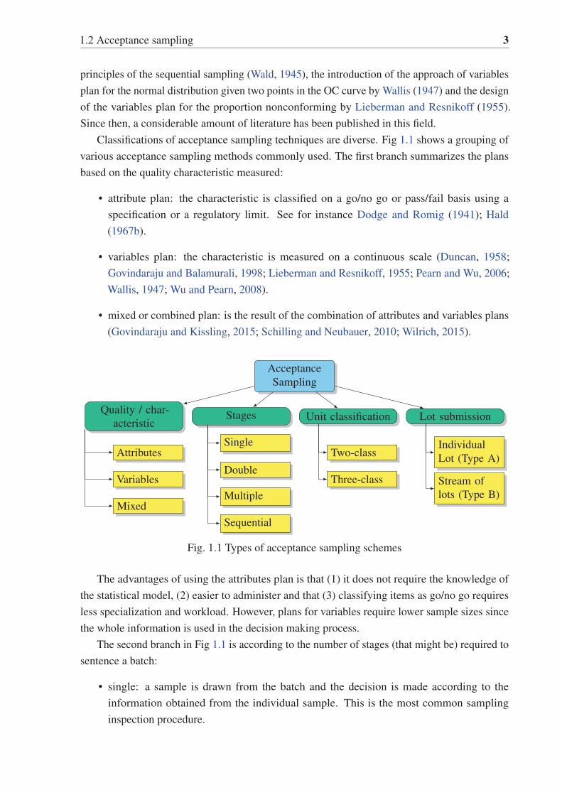
Classifications of acceptance sampling techniques are diverse. Fig 1.1 shows a grouping of
various acceptance sampling methods commonly used. The first branch summarizes the plans
based on the quality characteristic measured:
• attribute plan: the characteristic is classified on a go/no go or pass/fail basis using a
specification or a regulatory limit. See for instance Dodge and Romig (1941); Hald
(1967b).
• variables plan: the characteristic is measured on a continuous scale (Duncan, 1958;
Govindaraju and Balamurali, 1998; Lieberman and Resnikoff, 1955; Pearn and Wu, 2006;
Wallis, 1947; Wu and Pearn, 2008).
• mixed or combined plan: is the result of the combination of attributes and variables plans
(Govindaraju and Kissling, 2015; Schilling and Neubauer, 2010; Wilrich, 2015).
Acceptance
Sampling
Quality / char-
acteristicStages Unit classification Lot submission
Attributes
Variables
Mixed
Single
Double
Multiple
Sequential
Two-class
Three-class
Individual
Lot (Type A)
Stream of
lots (Type B)
Fig. 1.1 Types of acceptance sampling schemes
The advantages of using the attributes plan is that (1) it does not require the knowledge of
the statistical model, (2) easier to administer and that (3) classifying items as go/no go requires
less specialization and workload. However, plans for variables require lower sample sizes since
the whole information is used in the decision making process.
The second branch in Fig 1.1 is according to the number of stages (that might be) required to
sentence a batch:
• single: a sample is drawn from the batch and the decision is made according to the
information obtained from the individual sample. This is the most common sampling
inspection procedure.

4 Introduction
• double: after taking the first sample, the batch might be disposed (accepted or rejected) or
a second sample is taken and combined with the initial one to make the final decision.
• multiple: more than two samples may be drawn from the batch.
• sequential: the units are drawn one-by-one until the decision is made.
Moreover, primary units can be classified into two or more categories:
• two-class plan: when using attributes plans each sample is classified as pass/fail (two
categories), while in variables plan only one upper (lower) specification limit is used e.g.
U = 100 CFU/g.
• three-class plan: for the attributes plan each sample is classified as good, marginal or
bad (three categories), using two limits (Bray et al., 1973b). For a plan of inspection
by variables two limits are required and the decision criterion involves two restrictions,
(Newcombe and Allen, 1988).
The application of the plans may be by lot-by-lot (isolated lot) or focused on controlling the
risks in the stream of batches. Skip-lot and chain sampling schemes are cost-effective inspection
procedures that are applied to the stream of batches (Dodge, 1955a,b; Perry, 1973).
Several alternatives arise from combining characteristics from the branches of Fig 1.1. The
options substantially increase when different statistical distributions are considered e.g. binomial,
lognormal, exponential distribution. Lot-by-lot, single, two-class attributes and variables plan
are the most widely used inspection procedures. The other procedures are known as ‘special
purpose’ plans (Dodge, 1969), which are intended for specific applications. This thesis focuses
on special purpose plans for food control. Most of the categories from Fig 1.1 apart from mixed,
multiple and sequential sampling plans are studied in this thesis. Several statistical distributions
that have been used to describe the frequencies of microorganisms will be considered in the
design of sampling plans, e.g.: binomial, Poisson, normal, lognormal, Weibull, gamma, negative
binomial, Poisson-lognormal, Poisson-gamma, Dirichlet and multivariate hypergeometric.
Hamaker (1960) summarized the most important objectives when designing sampling plans /
schemes. However, he pointed out that it is not possible to accomplish all of them.
1. ‘To strike a proper balance between the consumer’s requirements, the producer’s capabili-
ties and the inspector’s capacity.’
2. ‘To separate bad lots from good.’
3. ‘Simplicity of procedures and administration.’
4. ‘Economy in number of observations.’
5. ‘To reduce the risk of wrong decisions with increasing lot size.’
6. ‘To use accumulated sample data as a valuable source of information.’

1.3 Microbiological sampling plans 5
7. ‘To exert pressure on the producer or supplier when the quality of the lots received is
unreliable or not up to standard.’
8. ‘To reduce sampling when the quality is reliable and satisfactory.’
1.3 Microbiological sampling plans
In food safety and food microbiology, acceptance sampling techniques are commonly used for
quality assurance purposes. Some of the first sampling plans for microbiological applications
were suggested by Kilsby and Baird-Parker (1983); Kilsby et al. (1979). Kilsby et al. (1979)
seminal paper suggested the use of variables plans for bacterial log counts. The design in this
plan is basically obtained from fixing the consumer’s risk point and the sample size. Malcolm
(1984) showed later that Kilsby et al. (1979) approximate method gives an imprecise batch
probability of acceptance and suggested the computation of the risk based on the non-central
t-distribution. Later on, Smelt and Quadt (1990) studied variables plans for the cases in which
the standard deviation is calculated using historical data.
Since 1980s the International Commission on Microbiological Specifications for Foods
(ICMSF) has been publishing regularly recommendations and guidelines on microbiological
sampling plan. Some of the most relevant are ICMSF (1986, 2002, 2011). Simultaneously,
guidelines, policies, recommendations and standards on food safety and particularly on the use
of inspection plans for food trade have been given by the Codex Alimentarius. See for instance
CAC (1997, 2004).
The Food and Agriculture Organization of the United Nations (FAO) and the World Health
Organization (WHO) regularly promote joint experts meeting and publish recommendations
on sampling plans for different microorganisms of interest e.g. FAO/WHO (2006, 2007, 2012,
2014).
Several special purpose sampling plans have been suggested for safety problems. A crucial
advance was the development of the three-class attributes plan theory, firstly proposed by Bray
et al. (1973b). Other important contributions to the applications of these plans to food safety
issues were made by Dahms and Hildebrandt (1998); Hildebrandt et al. (1995); Wilrich and
Weiss (2009). Today three-class attributes plan are widely-used for the inspection of different
commodities and especially for sanitary quality characteristics. See for instance European
Commission (2005); Food Standards Australia New Zealand (2001); ICMSF (2002).
Legan et al. (2001) suggested the use of plans in which the batch probability of acceptance is
based on the concentration of microorganisms rather than the traditional proportion nonconform-
ing. This approach was later on enhanced by Van Schothorst et al. (2009). They suggested the
use of the Poisson-lognormal distribution to describe the frequencies of microorganisms.
More recently numerous authors have studied a range of statistical models to describe the
frequencies of microorganisms. Several methods that allow a better characterization of the risk
for the consumers have been suggested and several recommendations on the design of sampling

6 Introduction
plans have been given. See for instance Gonzales-Barron and Butler (2011a,b); Gonzales-Barron
et al. (2010a, 2013); Hoelzer and Pouillot (2013); Jarvis (2007, 2008); Jongenburger (2012a,b);
Jongenburger et al. (2012a,b, 2011a,b, 2012c); Kiermeier et al. (2011); Mussida et al. (2013a,b);
Powell (2014); Whiting et al. (2006); Zwietering (2009).
Composite sampling
For bulk materials, testing composite or pooled samples is possible but not for discrete items.
Composite sampling is employed in a wide range of disciplines e.g.: mining, food microbiology.
Compositing is defined as “the physical mix of individual sample units or a batch of unblended
individual sample units that are tested as a group”(Patil, 2006). This technique is basically a
physical averaging process, which allows the use of more representative samples for testing and
hence achieves sampling economy.
Silliker and Gabis (1973) and Gabis and Silliker (1974) are among the first authors that
showed the potential of composite sampling in food microbiology. They found that a smaller
number of samples was equally effective to detect pathogens if they contained a larger analytical
amount. Jarvis (2007) discussed the effectiveness and demerits of several pooling alternatives
for pathogen detection. Ross et al. (2011) examined several factors which need to be considered
when compositing, such as the number of increments, the limit of detection and the growing rate.
A fundamental limitation of pooling is the risk of dilution. This has motivated authors like
Jongenburger (2012b) to recommend testing primary units instead of composite samples. So far,
the use of pooled samples in food safety remains contradictory.
1.4 Scientific problem and research objectives
The use of inspection techniques in food safety is restricted by the nature and characteristics of
microbiological testing. Food safety testing is:
1. destructive: the portion of material cannot be reused. Often the whole item or product has
to be sent to the laboratory.
2. costly: the test requires several operations and time in the laboratory, which result in a
substantial expense. For example, a test for parasite identification might cost 180 USD
(7 CFR, 2000) in the United States and 30 analytical tests might be required for every
pathogen in order to sentence a batch.
3. mandatory: testing to determine the acceptability of the batch is compulsory.
4. several quality characteristics are simultaneously measured.
5. focused totally on consumer’s protection.
6. batch is rejected when at least one pathogen cell is found in the sample(s).

1.4 Scientific problem and research objectives 7
7. often the frequencies of microorganisms does not often fit traditional statistical models e.g.
normal.
8. heterogeneity and localized contamination.
9. the concentration of bacteria generally increase over the time.
10. time-consuming test (mainly for culture-based test), but also time-constrained (the decision
need to be made in few days). These makes continuous and sequential plans inappropriate.
11. pathogens appear in small concentrations, yet this might cause serious outbreaks.
12. the target microorganisms might be present but below the limit of detection (LOD).
13. numerous sources of errors including imperfect sensitivity and specificity.
14. simplicity in the sampling procedure is required since inspection is mostly carried out by
food safety professionals and microbiologists.
One of the main challenges in food safety is that the actual inspection procedures cannot
produce the desired and the required levels of protection. For example, 1% of the analytical
units containing target pathogens would have massive consequences in the public heath system.
Detecting this level of bacterial contamination using a single attributes plan under homogeneity
will require a sample size of 230 units, which is far higher than any of the sampling plans used
in the industry. Fortunately, a 1% contamination is a rarity in manufactured food products, and
hence small sample sizes are considered adequate.
This research aims to design special purpose sampling plans for microbiological applications
with better performance in terms of sampling economy, consumer’s protection and robustness.
The specific objectives are:
1. To investigate plans that provide better consumer’s protection and require smaller sample
sizes.
2. To propose optimum plans for bulk materials using composite samples under different
sampling alternatives.
3. To design plans with a robust performance when the underlying statistical distribution
departs from the assumed model.
4. To provide a better characterization of the risk for the consumers using frequentist and
Bayesian methods, considering measurement errors.
The study investigates the use of more effective sampling plan techniques in food microbi-
ology allowing food producers, regulatory agencies, food importers and consumers to reduce
the inspection costs, increase the effectiveness of the sampling procedures and provide higher
protection and assurance. The research will produce online applications to design sampling
inspection plans and to estimate the risks.
8 Introduction
1.5 List of publications/manuscripts
The forthcoming chapters contain the research outputs (papers) in peer-reviewed international
journals of this research, in a non-chronological order. The chapters dealing with attributes and
concentration based sampling plans are firstly presented (Chapters 2-5). The last two chapters (6
and 7) discuss variables plans.
• Chapter 2: Santos-Fernández, E., Govindaraju, K., and Jones, G. (2016a). Quantity-based
microbiological sampling plans and quality after inspection. Food Control, 63:83–92.
• Chapter 3: Santos-Fernández, E., Kondaswamy, G., and Jones, G. (2016c). Compressed
limit sampling inspection plans for food safety. Applied Stochastic Models in Businessand Industry, 32(4):469–484.
• Chapter 4: Santos-Fernández, E., Govindaraju, K., Jones, G., and Kissling, R. (2016b).
New two-stage sampling inspection plans for bacterial cell counts. Food Control. In Press.
• Chapter 5: Santos-Fernández, E., Govindaraju, K., and Jones, G. (Submitted). Effects of
imperfect testing on presence-absence sampling plans. Quality and Reliability EngineeringInternational.
• Chapter 6: Santos-Fernández, E., Govindaraju, K., and Jones, G. (2014). A new variables
acceptance sampling plan for food safety. Food Control, 44:249–257.
• Chapter 7: Santos-Fernández, E., Govindaraju, K., and Jones, G. (2015). Variables
sampling plans using composite samples for food quality assurance. Food Control, 50:530–
538.

Chapter 2
Quantity-Based Microbiological SamplingPlans and Quality after Inspection
Edgar Santos-Fernández, K. Govindaraju, Geoff Jones
Food Control, 2016, 63:83–92
http://www.sciencedirect.com/science/article/pii/S0956713515303005
2.1 Abstract
Sampling inspection plans are principally used to determine whether a batch of food is contam-
inated or not. In this theoretical research, we study the effect of increasing the analytical unit
amount on the performance of microbiological sampling plans, and on the resulting quality after
inspection. We discuss several scenarios of homogeneous and inhomogeneous contamination for
assessing the consumer’s risk. Several statistical approaches to describe the effect of an increase
in analytical amount are studied. We provided a procedure for designing of the sampling plan
for a given consumer’s risk and according to different dispersion parameters and contamination
levels.
Keywords
analytical unit amount; composite samples; heterogeneity; Poisson-lognormal; quality after
inspection; safety sampling plan
2.2 Introduction
Sampling inspection plans for microbiological characteristics seldom allow the acceptance of a
batch when test samples fail on a safety parameter. Even for sanitary characteristics, only one
or two test samples are allowed to fail. The performance of microbiological inspection plans

10 Quantity-Based Microbiological Sampling Plans and Quality after Inspection
largely depends on the number of test samples (n). The adequacy of n can be assessed using
the Operating Characteristic (OC) curve of the plan to ensure that batches of unsafe or limiting
concentration levels are mostly rejected. In addition to ensuring the rejection of unsafe/poor
quality batches, focus must also be placed on the (outgoing) concentration levels in accepted
batches. The amount of material to be tested, called the analytical unit amount (w) in FAO/WHO
(2014) and expressed in weight/volume/area, is an important factor that affects the operating
characteristics of the plan and hence the concentration levels in a series of accepted batches.
When sampling plans are used by regulatory authorities, they deal with many suppliers
whose submitted quality can vary from batch to batch. Regulatory risk assessment cannot ignore
possible batch to batch variation in microbiological concentration levels. Because of sampling
inspection, the overall quality in the accepted batches is expected to be improved because poor
quality batches are mostly rejected. Moderate quality batches may still be accepted and hence
the concentration levels in a series of accepted batches are of interest, for example for evaluating
the expected number of individuals contracting food poisoning.
The analytical unit amount w is an important leverage factor when a higher level of protection
is desired without increasing the number of tests. Even though the size of w is restricted by the
capacity of the analytical method, a small w may lead to a misleading conclusion regarding the
distribution of cells, see the warning given by Jarvis (2008, pp.63). It is reasonable to assume
that the sampled material w is sufficient to capture the local distribution of cells. That is, the size
of the cluster of microorganisms is generally smaller than w.
In this paper, we mainly study the effect of increasing w on the probability of detection and
batch acceptance under a sampling plan. Protection against a poor quality individual batch as
well as the overall concentration level in a series of batches are important. An individual or
isolated batch needs not necessarily be homogeneous which will also affect the protection to the
consumer. Hence we discuss the following four cases:
• Case 1: Contamination within a batch is homogenous (i.e. case of an individual but
homogeneous batch).
• Case 2: Contamination within a batch is inhomogeneous (i.e. case of an individual but
inhomogeneous batch).
• Case 3: Contamination in a series of batches which are homogenous within the batch but
the concentration level fluctuates from batch to batch.
• Case 4: Contamination in a series of batches which are inhomogeneous within as well as
the concentration level fluctuates from batch to batch.
Throughout this paper, C is the observed concentration of microorganisms per gram. The
random variable X represents the number of microorganisms in w. The notations E [X ], Var [X ]
and S [X ] are used to refer to the within batch mean concentration (or expected value), the
variance and standard deviation of the concentration respectively. Notations of μ and σ are

2.3 Concentration-based sampling plan 11
specifically used for the parameters of the lognormal distribution on the base 10 logarithmic
(log10) scale. The log notation without a subscript refers to the natural logarithm (loge or ln). A
summary of the symbols used is presented in the Appendix.
The paper is structured in the following way. We start the discussion with concentration-based
sampling plans in section 2.3. Cases 1 and 2 are studied in subsection 2.3.1 focusing on the
quality assurance of on every batch intended for individual buyers and importers (who in turn
represent the ultimate consumers). The sampling plan design issues are discussed in subsection
2.3.1. In subsection 2.3.2, we consider Cases 3 and 4 which are important for regulatory purposes
wherein the focus is on a broader population dealing with issues such as the rate of cases of
food-borne disease. Finally, a variables version of the inspection plan is studied in section 2.4.
2.3 Concentration-based sampling plan
2.3.1 Single batch microbial risk assessment.
In this section we focus the analysis on presence-absence tests and particularly for safety
characteristics. Safety inspection is carried out when microorganisms pose a significant risk
for human health even when these are unknowingly consumed in minute quantity. Ideally all
accepted batches must be free of pathogens. Safety inspection results are often qualitative
because the batch disposition is based on whether the target microorganism is present in any of
analytical samples or not.
Inspection of a homogeneous batch (Case 1)
In a homogeneous batch , the concentration of pathogen will not differ within it. In other words,
if the batch is split into sublots, no sublot is expected to contain either high or low concentration
when compared to any other sublot. Homogeneity is often assumed in well-mixed bulk materials.
The Poisson distribution is commonly used to model the count (X) of pathogens found in random
samples drawn from a homogeneous batch. For the Poisson distribution, E [X ] and Var [X ] are
equal to λ , the underlying concentration rate in a fixed amount (mass) such as w = 5g of material.
The Poisson function
P(x|λ ) = λ xe−λ
x!(2.1)
gives the probability of obtaining x cells for a given λ . While the concentration C gives the
actual contamination level, λ is a measure of the risk of contamination. The parameter λ must
be defined for a fixed constant mass or amount, and without loss of generality λ can be assumed
to be associated with smallest amount that can be tested (such as 5g). Suppose that the analytical
method is also capable of analysing an amount larger than the unit amount of material, say
wy = 25g. Let m = wy/w. Let the random variable Y represents the number of microorganisms
in wy. The rate parameter λy for the larger amount wy will then be λy = λwy/w = λm. In
12 Quantity-Based Microbiological Sampling Plans and Quality after Inspection
presence-absence tests, an analytical sample is declared as positive when at least one target
microorganism is found. Hence the probability of detection Pd(λ |w) in a single analytical sample
is given by P(x > 0) = 1−P(x = 0) = 1− e−λ for the size w. The probability of detection is
greater for the analytical sample of size wy because P(y > 0) = 1− e−λy = 1− e−λwy/w. This
means that an increase in the analytical amount will always lead to a higher the probability of
detection. We assume that the analytical test has perfect sensitivity and specificity and thereby
avoid the complications of false positives and/or false negatives.
Let n be the number of analytical samples tested. For the inspection of a homogeneous
batch, FAO/WHO (2014) provided sets of amount w and n fixing the total T = nw. For a zero
acceptance number (c = 0) plan, the OC function giving the batch probability of acceptance
is Pa(λ |n,w) = (1−Pd)n =
(e−λ
)nwhich is the probability of n analytical samples failing to
detect any pathogen. For a homogeneous batch, Pa = e−T λ depends on the underlying rate
parameter λ , and the total amount tested T (because T = nw), see FAO/WHO (2014). For
example, for a fixed total amount of material of 50g, testing 10 samples of 5g is similar to testing
2 samples of 25g each. In this case, the second alternative is preferable since it would involve
less testing.
Inspection of an inhomogeneous batch (Case 2)
Microorganisms grow in colonies, clusters or clumps resulting in batch inhomogeneity for the
cell counts. It is well established in food control literature that the Poisson law fails to apply
when pathogen counts are over dispersed (Var [X ] > E [X ]). The family of Poisson mixture
distributions , which combines the Poisson distribution with another continuous distribution to
account for varying λ , is adopted for modelling over-dispersed cell counts. Consider-
P(λ ,x) =∫ ∞
0
λ xe−λ
x!f (λ )dλ (2.2)
where f (λ ) is the mixing distribution. Popular Poisson mixture distributions are the Poisson-
gamma (Anscombe, 1950) and the Poisson-lognormal (Bulmer, 1974a). Both models have been
used extensively in the food safety literature, e.g. Toft et al. (2006), Teunis et al. (2008), Jarvis
(2008), Van Schothorst et al. (2009), Zwietering (2009), Gonzales-Barron and Butler (2011b),
Gonzales-Barron and Butler (2011a), Jongenburger et al. (2012b), Jongenburger et al. (2012c),
Williams and Ebel (2012), Gonzales-Barron et al. (2013), Mussida et al. (2013a) and Haas et al.
(2014).
We particularly focus on the Poisson-lognormal (PLN) distribution because it is common to
study the effect of the amount w using this mixture distribution. The PLN arises as a Poisson
process in which the rate parameter λ is lognormally distributed (with parameters μ and σ ) with
probability density function:
P(x|μ, σ) =∫ ∞
0
λ xe−λ
x!
1
λσ√
2πe
(− (ln(λ )−μ)2
2σ2
)dλ (2.3)
2.3 Concentration-based sampling plan 13
The above integral has no analytical solution. Hence the probability of detection is also evaluated
numerically. Notice that the notations μ and σ in Eq. 2.3 are specifically used to assert that
these are on the natural logarithmic scale (loge) and obtained from the log10 base parameters as
μ = ln(10)μ and σ = ln(10)σ .
Consider the zero acceptance number plans with n = 10 and 30 for the underlying PLN
distribution with unknown parameters μ and σ and a unit amount w. Ideally, the performance of
these plans must be assessed using the OC or Pa contours for given (μ,σ ) pairs. The traditional
two dimensional OC curve of Pa vs λ is suitable for the Poisson case but not for the PLN case
because it involves two parameters for a fixed amount w. The PLN distribution approaches the
Poisson distribution for σ < 0.10, and only in such cases can the two-dimensional OC curve
plotting Pa against μ be useful. Fig. 2.1 gives the OC contour plot of the plans (n = 10 and
30, c = 0) which shows the Pa contours against μ and σ (both in log10 scale). This plot clearly
shows that the higher the inhomogeneity within a batch, the smaller the batch probability of
acceptance will be.
In order to compare the sampling plans based on the Poisson and PLN models, Pa can be
plotted against the respective expectations E [X ] for a fixed σ (Fig. 2.2). E [X ] is referred to as
the arithmetic mean of the discrete cell counts in food control literature, but it should be noted
that E [X ] = λ = 10μ+log(10)σ2/2 is not computed using sample data but rather is an unknown
population value. Under a heterogeneous spatial distribution of cells, the probability of detecting
contamination is smaller. The higher the dispersion of cells, the smaller the chances of detecting
contamination.
Using composite samples
Composite sampling aims to provide more representative samples with a reduced variability in
the test results. Therefore, this technique might lower the risk while keeping the analytical costs.
See e.g. ICMSF (2002). Compositing is a natural averaging process in which nI primary units
or increments of size w are physically combined forming n composite or pooled samples. The
composite samples are then well mixed and a subsample of size w is obtained from each one for
testing purposes. In this section, we show how composite sampling is another important strategy
to take into account in the design of microbiological sampling plans.
There are several recommendations on how compositing should be used. For example, Jarvis
(2007) discussed three methods of compositing. For the purpose of this paper we only analyse
the composite that was formed before the laboratory test so that compositing does not conflict
with the test procedure. The case in which the samples are firstly incubated as in Jarvis (2007)
third alternative, would yield better probability of detection. We need to mention that the number
of increments to be used depends on the specific test protocol. For the purpose of this discussion
we use nI = 4 increments. Moreover, the efficiency of this technique depends on the quality
of the mixing of the primary units. Perfect composite means that every individual sample will
equally contribute to the final subsample. However, this is rarely achievable in practice. For
the development of the theory, we assume perfect mixing and our results are expected to hold

14 Quantity-Based Microbiological Sampling Plans and Quality after Inspection
n = 10
Probability of acceptance contour levels
μ
σ
0.5
1.0
1.5
−3.0 −2.5 −2.0 −1.50.0
0.2
0.4
0.6
0.8
1.0
n = 30
Probability of acceptance contour levels
μ
σ
0.5
1.0
1.5
−3.0 −2.5 −2.0 −1.50.0
0.2
0.4
0.6
0.8
1.0
Fig. 2.1 OC contour plots of two-class concentration-based sampling plans with n = 10 and 30.
The batch probability of acceptance is obtained from the Poisson-lognormal distribution.
2.3 Concentration-based sampling plan 15
−4 −3 −2 −1 0
0.0
0.2
0.4
0.6
0.8
1.0
Pro
b. o
f acc
epta
nce
Case 1Case 2
0.00055 0.00546 0.05455 0.54554 5.45541
μ
mean concentration (cfu/g)
Fig. 2.2 Effect of batch inhomogeneity on the OC curve (n = 10, c = 0). Cases 1 and 2 refer to
homogenous and inhomogeneous contamination respectively.
as long as the mixing is not too imperfect. Various scenarios of imperfect mixing have been
discussed by Nauta (2005) and Santos-Fernández et al. (2015).
In Fig. 2.3 we compare sampling plans using composite samples and using the primary
samples directly (without pooling primary samples). Compositing has little effect when mi-
croorganisms are homogenously distributed, which is given by the difference between the black
and grey solid lines (Case 1 vs. Case 1, nI = 4). However, for heterogeneous contamination
the use of composite samples provides higher stringency and lower consumer’s risk. Notice
the difference between the dashed black and dashed grey lines (Case 2 vs. Case 2, nI = 4).
Since the spatial distribution of cells is commonly unknown, it seems to be convenient to test
pooled samples. Compositing can reduce the risk difference associated with both homogenous
and inhomogeneous distributions of microorganisms. In subsequent sections we are not using
composite samples.
Effect of increasing the analytical amount
In this section we examine the risk when the analytical amount is increased m-fold using
three methods (designated as a, b and c), corresponding to three different spatial levels of
inhomogeneity.
In the first approach (a), the effect of wy is incorporated via the parameters of the population
of the bigger unit (μy and σy). The distribution parameters are obtained using the arithmetic
moments E (Y ) = mE (X) and V (Y ) = mV (X). The expected number of microorganisms in the
bigger unit is m times the expected number in the small unit. The same is true for the arithmetic

16 Quantity-Based Microbiological Sampling Plans and Quality after Inspection
−4 −3 −2 −1 0
0.0
0.2
0.4
0.6
0.8
1.0
Pro
b. o
f acc
epta
nce
0.00055 0.00546 0.05455 0.54554 5.45541
μ
mean concentration (cfu/g)
Case 1Case 2Case 1 , nI = 4Case 2 , nI = 4
Fig. 2.3 Effect of using composite samples with nI = 4 increments using the plan (n = 10, c = 0)
for the cases of homogeneity and inhomogeneity.
variance. These relationships are based on the assumption that there is no spatial correlation
in the (contamination) rate. Using this method, Mussida et al. (2013b) recently demonstrated
how an increase in w leads to a reduction in the risks. This approach, known as convolution, is
briefed in 2.B.
The second method (b) is obtained using the probability mass function given by Haas et al.
(2014, pp.193) for a given m value.
P(x|μ, σ ,m) =∫ ∞
0
(λm)x e−λm
x!
1
λσ√
2πe
(− (ln(λ )−μ)2
2σ2
)dλ (2.4)
This method assumes that λ is locally constant, equivalently that there is a high spatial
correlation locally. That is, adjacent small units in the batch are assumed to have similar
numbers of cells. Since Eq.2.4 depends on m, this form of the distribution is different from the
usual two-parameter PLN distribution based on a fixed w. This equation clearly shows that maffects the probability of detection Pd = P(0|μ,σ ,m) and hence batch probability of acceptance
Pa(μ,σ |m) = (1−Pd)n for the c = 0 plan. For fixed μ and σ , an increase in w will decrease Pa.
The degree of spatial correlation in the contamination is commonly unknown. Our third
method (c) represents the scenario in which the contamination is most likely to be present in one
cluster. The Pd in this alternative is obtained via Monte Carlo simulations using the following
algorithm:
• Step 0. Define the parameters μx, σx in the small analytical unit X of size wx.

2.3 Concentration-based sampling plan 17
• Step 1. Set the increased analytical unit wy and obtain m.
• Step 2. Set the number of iterations I. Using I = 50,000 gives a good estimate.
• Step 3. Generate the number of microorganisms in wx using random numbers from the
PLN(μ , σ ), creating a two dimensional grid Ni j with I rows and m columns.
• Step 4. Sort (ascending) Ni j so that the contaminated small units form a unique cluster in
one extreme of the grid.
• Step 5. Sum by rows (∑mj=1 Ni j) to obtain the number of microorganisms in the bigger unit
Y .
• Step 6. Obtain the Pd as the proportion of Y units with one or more microorganisms.
This contamination is likely to occur when a highly contaminated external source enters to
the stream of product. ICMSF (2002, pp.193) describes this type of contamination as “comet
like”. Other examples of this type contamination can be found in the literature. See for example
the study of the contamination of beef with E. coli O157 by Kiermeier et al. (2011). This case is
also described by Jongenburger et al. (2011b) as localized contamination .
In Table 2.1 we compare the detection probabilities for Case 2 using the three types of
clustering described above. The scale parameter is fixed (σ = 0.8) and different values of μ and
w are considered.
Table 2.1 Detection probability according to different methods for σ = 0.8.
E (X) V (X) μ m Case 2a Case 2b Case 2c
0.055 0.37 -2 2 0.08 0.07 0.04
0.055 0.37 -2 5 0.18 0.14 0.04
0.055 0.37 -2 10 0.32 0.21 0.04
0.546 3.01 -1 2 0.35 0.31 0.22
0.546 3.01 -1 5 0.62 0.47 0.22
0.546 3.01 -1 10 0.83 0.59 0.22
Case 2a of no clustering gives the highest probability of detection being therefore the most
optimistic scenario. The most conservative approach is Case 2c because it gives the lowest Pd .
This is the worst case scenario increasing the consumer’s risk because there is a high correlation
between the contaminated units, and hence the contaminated units form a large cluster with the
rest of the batch cluster free of pathogens. Hence, it may be appropriate to design microbial
sampling plans based on this conservative supposition for some product types relying on the
empirical knowledge on the frequency of large contaminated clusters to improve consumer
protection. This, however, will undoubtedly require higher sample effort involving additional
testing costs.

18 Quantity-Based Microbiological Sampling Plans and Quality after Inspection
Sampling plan design
In this section we provide the required sample size for a given μ , σ , Pd and w for Cases 2a and
2b. We consider that the typical unit amount tested is lognormally distributed with σ = 0.8.
From Table 2.2, it should be noted that for small μ , say -3 log10 cfu/g, using a small unit amount
of 5g is simply not viable since it requires an enormous sample size. Testing 107 samples of 10g
provides the same level of protection as 43 samples of 25g each for Case 2a. Case 2b requires
higher sample sizes because this alternative lowers the probability of detection.
Table 2.2 Number of analytical samples (n) to be tested when the contamination is modelled
by the Poisson-lognormal distribution for a desired probability of detection given μ , σ and
analytical portion (in g).
Case 2a Case 2b Case 2cσ = 0.8 σ = 0.8 σ = 0.8
m w Pd μ=-3 μ=-2 μ=-1 μ=-3 μ=-2 μ=-1 μ=-3 μ=-2 μ=-1
1 5 0.67 213 27 5 213 27 5 213 27 5
1 5 0.90 446 55 10 446 55 10 446 55 10
1 5 0.95 580 72 13 580 72 13 580 72 13
1 5 0.99 891 110 20 891 110 20 891 110 20
σ = 0.5 σ = 0.5 σ = 0.5μ=-1.56 μ=-0.56 μ=0.44 μ=-1.56 μ=-0.56 μ=0.44 μ=-1.56 μ=-0.56 μ=0.44
2 10 0.67 107 14 3 111 15 3 213 27 5
2 10 0.90 224 29 6 231 32 7 446 55 10
2 10 0.95 291 37 7 301 41 9 580 72 13
2 10 0.99 447 57 11 462 63 13 891 110 20
σ = 0.38 σ = 0.38 σ = 0.38
μ=-1.03 μ=-0.03 μ=0.97 μ=-1.03 μ=-0.03 μ=0.97 μ=-1.03 μ=-0.03 μ=0.97
5 25 0.67 43 6 2 48 8 2 213 27 5
5 25 0.90 90 12 3 101 16 4 446 55 10
5 25 0.95 117 16 4 131 21 5 580 72 13
5 25 0.99 180 24 5 201 31 8 891 110 20
2.3.2 Average quality in accepted batches
Highly contaminated batches are most likely rejected by the inspection process. Similarly good
quality batches are likely to be accepted and cleared to the consumers. As a result, the overall
quality in the population (or series) of accepted batches is expected to be superior when compared
to the quality in the submitted or uninspected batches. This property is clearly established in the
literature for physically discrete units, mainly when screening for defective units and correcting
them are possible. In bulk materials, the quality after inspection is more complex to derive
compared to the traditional inspection of units in parts manufacturing. In the microbial risk
assessment context, several authors have shown the need for models accounting for variability
from batch-to-batch. See e.g. Paoli and Hartnett (2006), Zwietering (2009), Gonzales-Barron
et al. (2013), Mussida et al. (2013b).

2.3 Concentration-based sampling plan 19
The impact of pathogenic microorganisms in public health is often assessed for a single batch.
Given that the probability of illness is a function of the intake dose (number of microorganisms),
the computation of metrics like the expected annual number of illnesses is a function of the
quality of the accepted batches. For example, FAO/WHO (2007) provides a web-based tool
for risk assessment for Enterobacter sakazakii in powdered infant formula. This tool gives the
quality after inspection for a given log concentration. It considers within batch heterogeneity as
well as between batch variability. The main limitation of this tool is that it requires knowledge of
the incoming log concentration, which is generally unknown. Moreover, the computation of the
risk for increasing the analytical amount is obtained from Eq.2.4 (Haas et al., 2014). Mussida
et al. (2013b) instead used the convolution approach that gives the most optimistic scenario.
However, both methods underestimate the risk when the contamination is localized in a specific
part of a batch (Case 4c).
In the next subsection, we discuss the measurement of a limit for the average quality after
inspection . This limit gives the peak average level of contamination in accepted batches and
portrays realistic picture of the quality received by the consumer. We also discuss the scenario of
a series of homogenous batches with variation in the contamination rate from batch to batch.
Simulation algorithm
We opted for Monte Carlo simulation in this section since the analytical solution is intractable
when batch to batch variability is additionally involved. The following algorithm allows the
computation of the outgoing concentration levels in accepted batches for Cases 3 and 4:
• Step 0. Set a sample size (n) and an analytical unit amount (w), e.g. n = 10 and w = 5.
• Step 1. Homogeneity within the batch is modelled with the Poisson distribution with
rate λ . We first assumed that the batch is homogenous, but allow the contamination
rate to vary from batch to batch. The inhomogeneous case is then modelled with the
Poisson-lognormal distribution with parameters μ and within batch standard deviation σw.
Similarly, μ changes from batch to batch.
For a given contamination level, the parameters under batch homogeneity and inhomogene-
ity are matched using the mean of the original counts E [X ] = λ = 10μ+log(10)σ2/2. Notice
that if we use the mean log concentration, the risk is underestimated. Define the within
and between batch standard deviations, say σw = 0.8 (Legan et al., 2001) and σb = 0.8
(Mussida et al., 2013b).
• Step 2. Set the number of batches N to be simulated. For instance, N = 50,000 gives a
good estimate.
• Step 3. Suppose that μi changes from batch to batch and that the normal distribution with
standard deviation (σb) is suitable to describe it. Generate N values μi with mean μ and
standard deviation σb. Compute the corresponding λi = 10μi+log(10)σ2/2.
20 Quantity-Based Microbiological Sampling Plans and Quality after Inspection
• Step 4. For each μi (inhomogeneous case) and the matching λi (homogenous case), obtain
the probability of detecting contamination and batch probability of acceptance Pa.
• Step 5. Determine the concentration of microorganisms after inspection as the weighted
arithmetic mean of λi using the batch Pa as weights.
• Step 6. For the incoming and accepted batches, estimate the population prevalence (p) for
the homogeneous and inhomogeneous scenarios. The prevalence p is the proportion of
analytical units in the population with at least one microorganism. The prevalence before
inspection is p = ∑Ni=1 Pdi/N. For accepted batches, it becomes p = ∑N
i=1 Pdi ×Pai/∑Ni=1 Pai .
• Step 7. Compute the proportion of accepted batches out of N.
• Step 8. Repeat Steps 1-7 for various μ in the interval −7 � μ � 0. The bigger the μ value,
the lower the proportion of accepted batches would be.
We considered that every batch is inspected only once and no resampling is carried out when
a nonconforming batch is found. The concentration of microorganisms and the associated
prevalence are treated as measures of quality for the incoming and accepted batches and calculated
in the above steps.
Results
Fig. 2.4 compares several metrics for the submitted as well as the accepted batches using
the sampling plan n = 10, c = 0, w = 5g, σw = σb = 0.8. In Fig. 2.4(a), we compare the
contamination levels of the incoming batches with those in accepted batches. The average
concentration is substantially lower in the accepted batches when compared to the concentration
before inspection. The concentration in Case 4 is higher when compared with Case 3, since
batches with high and localized contamination are more difficult to detect.
Fig. 2.4(b) shows the prevalence before and after inspection. Notice that Case 2 presents
a lower prevalence than Case 1 for the same concentration rate. However, the prevalence is
similar in accepted batches irrespective of whether the submitted batches are homogeneous or
not. For the range of μ we studied, the prevalence was found to be monotonically increasing
with μ . The prevalence after inspection does not decrease (see the right-hand part of this graph)
because a contaminated batch cannot be replaced with a batch guaranteed to be completely free
of contamination (which can occur in screening a batch of discrete units with non-destructive
testing). A newly produced batch is subjected to inspection and upon acceptance; it can take the
place of a rejected batch to form part of the series of batches released to the consumers. Fig. 2.4
(a) represents the contamination for hygiene characteristics, where the conformance depends
on the level of the contamination. While (b) is more relevant for safety characteristics, where
non-conformance as well as noncompliance is caused by the presence of a single cell or more in
the sample.
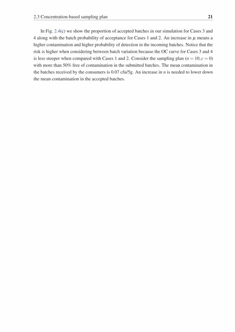
2.3 Concentration-based sampling plan 21
In Fig. 2.4(c) we show the proportion of accepted batches in our simulation for Cases 3 and
4 along with the batch probability of acceptance for Cases 1 and 2. An increase in μ means a
higher contamination and higher probability of detection in the incoming batches. Notice that the
risk is higher when considering between batch variation because the OC curve for Cases 3 and 4
is less steeper when compared with Cases 1 and 2. Consider the sampling plan (n = 10,c = 0)
with more than 50% free of contamination in the submitted batches. The mean contamination in
the batches received by the consumers is 0.07 cfu/5g. An increase in n is needed to lower down
the mean contamination in the accepted batches.

22 Quantity-Based Microbiological Sampling Plans and Quality after Inspection
−4 −3 −2 −1 0
0.0
0.2
0.4
0.6
0.8
1.0
(a) w = 5 , n = 10 , σw = 0.8 , σb = 0.8
μ
cfu/
g
incoming concentrationconc. after insp. (Case 3)conc. after insp. (Case 4)
−4 −3 −2 −1 0
0.0
0.2
0.4
0.6
0.8
1.0
(b) w = 5 , n = 10 , σw = 0.8 , σb = 0.8
μ
p
incoming prevalence (Case 1)incoming prevalence (Case 2)prev. after inspection (Case 3)prev. after inspection (Case 4)
−4 −3 −2 −1 0
0.0
0.2
0.4
0.6
0.8
1.0
(c) w = 5 , n = 10 , σw = 0.8 , σb = 0.8
Pro
b. o
f acc
epta
nce
Case 1Case 2Case 3Case 4
0.00055 0.00546 0.05455 0.54554 5.45541
μ
mean concentration
Fig. 2.4 (a) Incoming concentration (λ ) is represented by the solid line. The mean concentration
after the inspection for Cases 3 and 4 are shown as dashed and dotdashed lines. (b) Estimates of
prevalence in the incoming and in the accepted batches. (c) Probability of acceptance for the
homogeneous and inhomogeneous batches, before and after inspection.

2.3 Concentration-based sampling plan 23
Effect of increasing the analytical amount
Assume that the analytical amount w is increased five-fold (from 5 to 25 g). The probability of
detection for the heterogeneous case in Step 4 is obtained using the three methods described in
the last section. The simulation results shown in Fig. 2.5 reveal the following:
1. the concentration after inspection in the bigger analytical unit is more than the concentra-
tion in the smaller unit (E [Y ]> E [X ]). However, the relative concentration (at the same
w) is smaller for the bigger analytical unit because E [Y ]< E [X ]×w. Consequently, the
overall contamination is reduced in the accepted batches when using a bigger w.
2. the prevalence in the bigger analytical unit increases, since the probability of observing
at least one cell is increased. However, the relative prevalence (at the same w) is smaller
since py < px ×w.
3. the proportion of accepted batches is reduced because of the increased probability of
detection for the analytical sample.
4. as expected the Case 4 becomes closer to Case 3 with increased analytical unit amount.

24 Quantity-Based Microbiological Sampling Plans and Quality after Inspection
−4 −3 −2 −1 0
0.0
0.5
1.0
1.5
2.0
(a) w = 25 , n = 10 , σw = 0.8 , σb = 0.8
μ
cfu/
g
incoming conc.conc. after insp. (Case 3)conc. after insp. (Case 4a)conc. after insp. (Case 4b)conc. after insp. (Case 4c)
−4 −3 −2 −1 0
0.0
0.2
0.4
0.6
0.8
1.0
(b) w = 25 , n = 10 , σw = 0.8 , σb = 0.8
μ
p
incoming prevalence (Case 1)incoming prevalence (Case 2)prev. after insp. (Case 3)prev. after insp. (Case 4a)prev. after insp. (Case 4b)prev. after insp. (Case 4c)
−4 −3 −2 −1 0
0.0
0.2
0.4
0.6
0.8
1.0
(c) w = 25 , n = 10 , σw = 0.8 , σb = 0.8
Pro
b. o
f acc
epta
nce
Case 1Case 2Case 3Case 4aCase 4bCase 4c
0.00055 0.00546 0.05455 0.54554 5.45541
μ
mean concentration
Fig. 2.5 Increased analytical unit amount w = 25g. (a) Incoming concentration (λ ) is represented
by the solid line. The mean concentrations after inspection for Cases 3 and 4 are shown as dashed
and dotdashed lines. (b) Estimate of the prevalence of the contamination in the incoming and in
the accepted batches. (c) Probability of acceptance for the homogeneous and inhomogeneous
batches, before and after inspection.

2.4 Variables sampling plan 25
2.4 Variables sampling plan
Variables plan are mainly employed for hygienic indicators where the background concentra-
tion level is low but not necessarily absent, e.g. Enterobacteriaceae in meat. The lognormal
distribution is the de facto model for estimating the risk in this case. This distribution is easily
transformed to normal after applying log10 and the traditional variables plan is then used. Let
V = log10(X) and mv = log10 (m). The batch is accepted if v+ kσv � mv, otherwise rejected,
where v = ∑ni=1 vi/n is the mean of the log10-transformed count, σv is the known standard devi-
ation of V and k is the critical distance. If the left part in the acceptance criterion (v+ kσv) is
large, the prevalence is higher than expected and hence the batch should be rejected.
Effect of increasing the analytical amount
In this plan, increasing the analytical amount also increases the chances of finding contamination
and therefore it also increases the probability of rejecting poor quality. The effect of w on the
performance of the variables plan is not reported in the literature. Consider the following example.
Suppose that the contamination in the small analytical unit X of 5g is lognormally distributed
with σw = 0.8, X ∼ LN (μ,σw = 0.8). Consider a microbiological limit m = 2.5 log10 cfu/5g.
Consider that the analytical method is also capable of analysing a greater amount, wy = 25g. In
order to obtain the parameters of the bigger unit (μy and σy), we used the convolution approach
previously described. In Fig. 2.6 we show the OC curve of the plan n = 10 for w = 5 & 25. We
notice the substantial reduction in the limiting quality level when increasing w.
2.4.1 Sampling plan design
In Table 2.3 we show the required sample size for given values of w, μ , σw for the case of an
individual batch. From this table, it can be noted that the sample size is significantly reduced
with a higher analytical amount. For example, using 30 samples of 5g each is equivalent in terms
of consumers protection to using 11 samples of 25g each.
Table 2.3 Number of analytical samples to be tested n and the critical distance k given μ , σw and
w values. T = w×n represents the total amount to be tested.
m w n T μ σw LQL k1 5 10 50 0.00 0.80 1.6 1.89
2 10 6 60 0.44 0.72 1.6 1.47
5 25 3 75 1.02 0.60 1.6 0.84
1 5 20 100 0.00 0.80 1.2 2.19
2 10 15 150 0.44 0.72 1.2 1.85
5 25 6 150 1.02 0.60 1.2 1.20
1 5 30 150 0.00 0.80 1.0 2.31
2 10 24 240 0.44 0.72 1.0 2.02
5 25 11 275 1.02 0.60 1.0 1.46

26 Quantity-Based Microbiological Sampling Plans and Quality after Inspection
−0.5 0.0 0.5 1.0 1.5 2.0
0.0
0.2
0.4
0.6
0.8
1.0
n = 10 , σw = 0.8P
rob.
of a
ccep
tanc
ew = 5w = 25
μ
1.73 5.46 17.25 54.55 172.52 545.54mean concentration
Fig. 2.6 OC curve of the variables plan with n = 10 and σw = 0.8 for w = 5 and 25g. This figure
shows that an increased analytical unit amount reduces the consumer’s risk.
2.4.2 Average quality in accepted batches using variables plan
In this section, we explore the microbiological quality in accepted batches when the inspection is
based on a variables plan. In the population of accepted batches, the distributional parameters
of the contamination cannot be obtained analytically. We resorted to the simulation procedure
previously discussed to obtain the probability of acceptance.
In Fig. 2.7 (a), we compare the concentration in the submitted as well as in the accepted
batches for the sampling plan n = 10, w = 5g when σw = σb = 0.8. A substantial reduction in
the concentration is achieved after sampling inspection. In Fig. 2.7 (b), we show the probability
of acceptance for a single batch and for a series of batches allowing for batch to batch variation.
The OC curve becomes less stringent after allowing for variability between the batches. For
example, at a limiting concentration level μ = 1.5, the consumer’s risk of accepting a single
poor quality batch is only half of the risk when batch to batch variation of the order σb = 0.8 is
present even though the average concentration level for these batches is also at μ = 1.5.
2.5 Discussion and conclusions
Microbiological sampling plans under a wide range of scenarios including concentration-based
and variables plans are discussed in earlier sections. We provided a broad range of factors which
can affect quality including the spatial distribution of microorganisms, the use of composite

2.5 Discussion and conclusions 27
−0.5 0.0 0.5 1.0 1.5 2.0
020
040
060
080
0
(a) w = 5 , n = 10 , σw = 0.8 , σb = 0.8
μ
cfu/
g
incoming concentrationconc. after insp.
−0.5 0.0 0.5 1.0 1.5 2.0
0.0
0.2
0.4
0.6
0.8
1.0
(b) w = 5 , n = 10 , σw = 0.8 , σb = 0.8
Pro
b. o
f acc
epta
nce
single lotseries of lots
1.73 5.46 17.25 54.55 172.52 545.54
μ
mean concentration
Fig. 2.7 (a) Incoming concentration of the contamination (represented by the solid line) in
relation to μ . The concentration after the inspection is given by the dashed line. (b) It compares
the batch probability of acceptance for a single batch and for the series of batches.
samples, the amount of material used for testing purposes and then assessed quality after
inspection in a series of batches. We listed the merits and limitations of methods found in the
bibliography (e.g. FAO/WHO, 2007; Mussida et al., 2013b) which incorporate the analytical
unit amount in the computation of the consumer’s risk. In both, concentration-based and
variables inspection plans, the contamination in the accepted batches is considerably smaller
when compared with the contamination in the batches submitted for inspection. This means a
reduction of the risk of contamination is achieved by sampling inspection, and therefore assures
quality received by the consumers.
In the convolution approach, the analytical test units are considered to be uncorrelated. There-
fore, the aggregated unit is assumed to be the sum of independent and identically distributed
random variables. Increasing the unit analytical amount, allows undoubtedly a higher proba-
28 Quantity-Based Microbiological Sampling Plans and Quality after Inspection
bility of detection. However, this strategy should be employed with caution. It brings further
complications because correct parameter estimation for the bigger unit is difficult. The size of
the contamination is often bigger than the size of the analytical unit resulting in non-ignorable
spatial correlation. In this scenario, the current methods may fail to provide a good estimate of
the probability of detection. However, the convolution theory used by Mussida et al. (2013b)
has proven to be satisfactory under certain conditions, for example, when considering a small
increase in w and for a limited range of standard deviations. The results of this study indicate
that highly localized contamination (Case 4c) warrants further increased sampling in the absence
of empirical knowledge on the spatial nature of potential contamination.
We should mention that the main limitation of compositing is the risk of dilution. For
example, suppose that one of the increments contains the pathogen. If we mix this increment
with other non-contaminated samples, then the concentration will be reduced. This would yield a
negative result for concentration values below the limit of detection. Hence, the sensitivity might
be affected; see the comments of Jarvis (2007). Also, the extra laboratory manipulation while
preparing and mixing the composite might increase the risk of cross-contamination. Therefore,
the risk of false positives might be increased, affecting the test specificity. However, this is factor
is often considered as less relevant and is assumed to be negligible.
Finally, statistical models accounting for spatial distribution, such as Log-Gaussian Cox
Process model, should be investigated in order to provide a better characterization of the risk in
the food safety area.

2.A Table of symbols 29
Appendix 2.A Table of symbols
n sample size or the number of analytical samples tested
w analytical unit amount
C concentration of microorganisms
λ rate parameter in the Poisson distribution
Pa probability of acceptance
Pd probability of detection
p prevalence
nI number of primary samples or increments that are combined to form a composite sample
LN lognormal distribution
PLN Poisson-lognormal distribution
μ location parameter (mean log) of the LN and PLN distributions on the log10 scale
σw within-batch scale (standard deviation) of the LN and PLN distributions on the log10 scale
σb between batches scale (standard deviation) on the log10 scale
LQL Limiting Quality Level
β consumer’s risk
X number of microorganisms in the small unit
Y = ∑X number of microorganisms in the bigger unit
E [X ] expected value
Var [X ] variance in the arithmetic scale
S [X ] standard deviation in the arithmetic scale
Case 1 individual but homogeneous batch
Case 2 individual but heterogeneous batch
Case 3 series of homogenous batches
Case 4 series of heterogeneous batches
a convolution method
b Haas et al. (2014) Eq.2.4 method
c simulation method for the case of one cluster
Appendix 2.B The convolution theory
If the cell cluster size is expected to be small compared to analytical unit amount for low
contamination levels, the spatial correlation between the analytical units can be considered
negligible. In other words, the analytical amounts can be treated as independent. Suppose
that the analytical method is also capable of analysing a greater amount of material. For the
bigger amount, the process of aggregation of the small analytical samples can be treated as the
convolution or sum operation done on random variables. The sum of independent log-normally
distributed random variables does not have a closed-form solution, but it can be approximated
by another lognormal distribution under certain conditions, (Johnson et al., 1994, pp. 217).
That is, if Y be the sum of independent and identically distributed (i.i.d.) lognormal random
variables X , then the approximate distribution of Y is LN(μy,σy) where E (Y ) = mE (X) and
V (Y ) = mV (X). The mean and variance for the larger amount is obviously bigger when several
small amounts are aggregated. This approach of approximating the sum of lognormals is known
as the Fenton-Wilkinson (Fenton, 1960) method. In the log10 scale, the parameters μy and σy of
the population using a bigger unit Y become

30 Quantity-Based Microbiological Sampling Plans and Quality after Inspection
μy = log10 (E [Y ])− log(10)σ2y /2 (2.5)
σy =
√√√√log10
(1+
Var [Y ]−E [Y ]
(E [Y ])2
)/log(10) (2.6)

Chapter 3
Compressed Limit Sampling InspectionPlans for Food Safety
Edgar Santos-Fernández, K. Govindaraju, Geoff Jones
Applied Stochastic Models in Business and Industry, 2016
http://onlinelibrary.wiley.com/doi/10.1002/asmb.2170/full
3.1 Abstract
The design of attribute sampling inspection plans based on compressed or narrow limits for food
safety applications is covered. Artificially compressed limits allow a significant reduction in the
number of analytical tests to be done while maintaining the risks at predefined levels. The design
of optimal sampling plans is discussed for two given points on the Operating Characteristic
curve and especially for the zero acceptance number case. Compressed limit plans matching
the attribute plans of the International Commission on Microbiological Specifications for Foods
are also given. The case of unknown batch standard deviation is also discussed. Three-class
attribute plans with optimal positions for given microbiological limit M and Good Manufacturing
Practices limit m are derived. The proposed plans are illustrated through examples. R software
codes to obtain sampling plans are also given.
Keywords
attribute inspection; compressed limits; GMP limit; microbiological sampling plan; three-class
plan
32 Compressed Limit Sampling Inspection Plans for Food Safety
3.2 Introduction
Microbiological assurance of food quality is commonly carried out using sampling inspection
plans. The sampling procedure comprises the number of samples (n) to be drawn and the lot
acceptance criterion includes the upper microbiological limits. Section 3.A lists further symbols
and definitions employed in the paper.
Microbiological attribute plans are divided into two groups FAO/WHO (2014):
1. plans for presence-absence response, intended for microorganisms that in small quantities
represent a serious risk for the human health;
2. plans for concentration response, which are mainly used for hygiene characteristics. In
this case, every analytical sample is classified as conforming if the concentration is below
the set microbiological limit.
This paper deals with compressed limit plans for concentration and/or hygiene characteristic
type responses such as the Aerobic Plate Count (APC). Compressed specification limits cannot
be set to safety characteristics because the specification limit is generally equal to zero and
this limit cannot be compressed. Microbiological risk assessment is commonly based on a
one-sided specification such as an upper regulatory limit or food safety criterion e.g. m = 100
colony forming units per gram (CFU/g) of Listeria monocytogenes in “ready-to-eat foods other
than those intended for infants and for special medical purposes” European Commission (2005).
Microbiological limits included in the microbiological criteria could be either established by
food safety authorities, defined by food operators or are the result of best practices.
The performance of a sampling plan is revealed by its Operating Characteristic (OC) curve .
The OC curve gives the batch probability of acceptance for a given proportion nonconforming.
The vertical axis of the OC curve gives the consumer’s risk (β ) for a given Limiting Quality
Level (LQL). The OC curve also shows the probability of acceptance at a given Acceptance
Quality Limit (AQL) from which the producer’s risk (α) of rejecting AQL quality batches can be
found. High analytical testing costs may force the use of smaller sample sizes, which can lead to
lower protection for the consumer. The aim of this paper is to discuss the use of compressed
specification limits in order to provide better consumer protection even with smaller sample
sizes.
The paper is organized in the following way. An overview of the Good Manufacturing
Practices (GMP) limits is given in Section 3.3. Section 3.4 discusses the use of two-class
compressed limit plans when the standard deviation is known as well as unknown. Section
3.5 introduces a new compressed limit (CL) approach for three-class plans and Section 3.6
presents some numerical results including a discussion on the optimum two-class plans of the
International Commission on Microbiological Specifications for Foods (ICMSF), ICMSF (2002,
2011). Finally, the last part discusses the case in which the underlying concentration distribution
is other than lognormal.
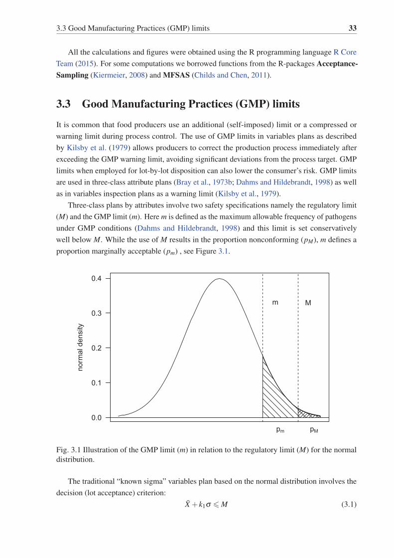
3.3 Good Manufacturing Practices (GMP) limits 33
All the calculations and figures were obtained using the R programming language R Core
Team (2015). For some computations we borrowed functions from the R-packages Acceptance-Sampling (Kiermeier, 2008) and MFSAS (Childs and Chen, 2011).
3.3 Good Manufacturing Practices (GMP) limits
It is common that food producers use an additional (self-imposed) limit or a compressed or
warning limit during process control. The use of GMP limits in variables plans as described
by Kilsby et al. (1979) allows producers to correct the production process immediately after
exceeding the GMP warning limit, avoiding significant deviations from the process target. GMP
limits when employed for lot-by-lot disposition can also lower the consumer’s risk. GMP limits
are used in three-class attribute plans (Bray et al., 1973b; Dahms and Hildebrandt, 1998) as well
as in variables inspection plans as a warning limit (Kilsby et al., 1979).
Three-class plans by attributes involve two safety specifications namely the regulatory limit
(M) and the GMP limit (m). Here m is defined as the maximum allowable frequency of pathogens
under GMP conditions (Dahms and Hildebrandt, 1998) and this limit is set conservatively
well below M. While the use of M results in the proportion nonconforming (pM), m defines a
proportion marginally acceptable (pm) , see Figure 3.1.
0.0
0.1
0.2
0.3
0.4
norm
al d
ensi
ty
Mm
pm pM
Fig. 3.1 Illustration of the GMP limit (m) in relation to the regulatory limit (M) for the normal
distribution.
The traditional “known sigma” variables plan based on the normal distribution involves the
decision (lot acceptance) criterion:
X + k1σ � M (3.1)
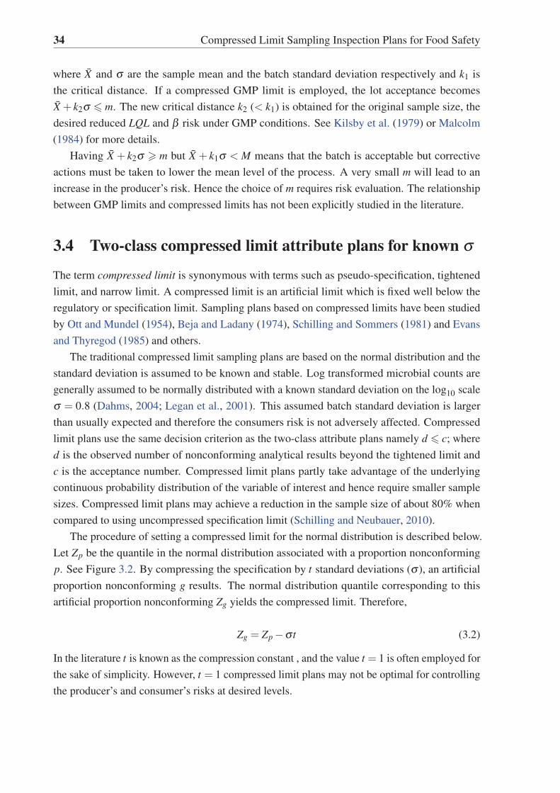
34 Compressed Limit Sampling Inspection Plans for Food Safety
where X and σ are the sample mean and the batch standard deviation respectively and k1 is
the critical distance. If a compressed GMP limit is employed, the lot acceptance becomes
X + k2σ � m. The new critical distance k2 (< k1) is obtained for the original sample size, the
desired reduced LQL and β risk under GMP conditions. See Kilsby et al. (1979) or Malcolm
(1984) for more details.
Having X + k2σ � m but X + k1σ < M means that the batch is acceptable but corrective
actions must be taken to lower the mean level of the process. A very small m will lead to an
increase in the producer’s risk. Hence the choice of m requires risk evaluation. The relationship
between GMP limits and compressed limits has not been explicitly studied in the literature.
3.4 Two-class compressed limit attribute plans for known σ
The term compressed limit is synonymous with terms such as pseudo-specification, tightened
limit, and narrow limit. A compressed limit is an artificial limit which is fixed well below the
regulatory or specification limit. Sampling plans based on compressed limits have been studied
by Ott and Mundel (1954), Beja and Ladany (1974), Schilling and Sommers (1981) and Evans
and Thyregod (1985) and others.
The traditional compressed limit sampling plans are based on the normal distribution and the
standard deviation is assumed to be known and stable. Log transformed microbial counts are
generally assumed to be normally distributed with a known standard deviation on the log10 scale
σ = 0.8 (Dahms, 2004; Legan et al., 2001). This assumed batch standard deviation is larger
than usually expected and therefore the consumers risk is not adversely affected. Compressed
limit plans use the same decision criterion as the two-class attribute plans namely d � c; where
d is the observed number of nonconforming analytical results beyond the tightened limit and
c is the acceptance number. Compressed limit plans partly take advantage of the underlying
continuous probability distribution of the variable of interest and hence require smaller sample
sizes. Compressed limit plans may achieve a reduction in the sample size of about 80% when
compared to using uncompressed specification limit (Schilling and Neubauer, 2010).
The procedure of setting a compressed limit for the normal distribution is described below.
Let Zp be the quantile in the normal distribution associated with a proportion nonconforming
p. See Figure 3.2. By compressing the specification by t standard deviations (σ ), an artificial
proportion nonconforming g results. The normal distribution quantile corresponding to this
artificial proportion nonconforming Zg yields the compressed limit. Therefore,
Zg = Zp −σt (3.2)
In the literature t is known as the compression constant , and the value t = 1 is often employed for
the sake of simplicity. However, t = 1 compressed limit plans may not be optimal for controlling
the producer’s and consumer’s risks at desired levels.

3.4 Two-class compressed limit attribute plans for known σ 35
0.0
0.1
0.2
0.3
0.4
norm
al d
ensi
tymCL
μ
Zg σ
Zp σ
t σ
g p
Fig. 3.2 Illustration of the compressed limit approach in the normal distribution.
For determination of the optimum t value, Ladany (1976) proposed an iterative graphical
method based on the nomograph of the cumulative binomial distribution given by Larson (1966).
An approximate heuristic approach was later proposed by Schilling and Sommers (1981) who
provided the following formulae for the compressed limit plan parameters:
nt = 1.5nv
t = k
ct = 0.75nv −0.67
(3.3)
where nv is the sample size of the variables plan and k the critical distance obtained for the tradi-
tional variables plan, see Duncan (1986); Schilling and Neubauer (2010). Another approximate
optimal solution was suggested by Evans and Thyregod (1985). This method is based on the
normal approximation to the binomial distribution and yields better results. The formulae for the
design of compressed limit plans are
nt =π2
(Zα +Zβ
ZAQL −ZLQL
)2
t = k =ZαZLQL +Zβ ZAQL
Zα +Zβ
ct = (nt −1)/2
(3.4)

36 Compressed Limit Sampling Inspection Plans for Food Safety
Sampling plans published in Schilling and Sommers (1981) are not exact since the risks were
relaxed by allowing tolerances α +0.005 and β +0.005 which leads to smaller sample sizes.
Other approaches obtained by approximation to the binomial model lead to slightly different
results. Hence we provide below a new algorithm to obtain the exact optimal compressed limit
plans.
1. Given two points (AQL,α) and (LQL,β ), compute the corresponding standard normal
quantiles ZAQL and ZLQL.
2. For the sequence of t = 0(0.01)4, calculate the normal quantiles Zg1= ZAQL − t and
Zg2= ZLQL − t.
3. Obtain the artificial proportions nonconforming pg1and pg2
as the right tail areas of the
standard normal distribution corresponding to Zg1and Zg2
.
4. For given pair of points (pg1,α) and (pg2
,β )of the OC curve, obtain nt and ct by solving
the binomial inequalities:
1−α′=
c
∑d=0
(nd
)pd
g1
(1− pg1
)n−d � 1−α
β′=
c
∑d=0
(nd
)pd
g2
(1− pg2
)n−d � β(3.5)
where(n
d
)= n!/(d!(n−d) !) is the binomial coefficient, ! is the factorial and n, c and
d are nonnegative integers. α and β are the predefined producer’s and consumer’s risks
and α ′and β ′
are the achieved producer’s and consumer’s risks. Note that Eq.3.5 implies
α ′ � α and β ′ � β . Guenther (1969), for instance, provides an algorithm to solve these
inequalities.
5. Select the t value that minimizes the sample size.
6. When more than one sampling plan exists, a second optimality criterion has to be em-
ployed. We propose the criterion 1 of the maximum absolute risk difference (MARD)
max[∣∣∣α −α ′
∣∣∣+ ∣∣∣β −β ′∣∣∣]. The MARD criterion provides a slightly tighter OC curve than
desired when α > α ′and β > β ′
, and hence the designed plan is more stringent .
Other alternatives to the MARD criterion are available in the literature, for instance, the
minimum absolute risk difference (MIRD) min[∣∣∣α −α ′
∣∣∣+ ∣∣∣β −β ′∣∣∣] Schilling and Sommers
(1981). The method proposed in Schilling and Sommers (1981) does not impose the conditions
α > α ′and β > β ′
and hence it gives the closest OC curve to the points (AQL,α) and (LQL,β ).
Evans and Thyregod (1985) suggested the use of the midpoint between all the possible t values.
Appendix 3.C gives the compressed limit plans based on two points on the OC curve. The
sampling design is also given for the MIRD criterion. The LQL values correspond to the selected
1If the MARD solution is not found to be unique, the plan with the smaller t can be chosen.

3.4 Two-class compressed limit attribute plans for known σ 37
operating ratios R = LQL/AQL equal to 20 and 40. For very small AQL values, t tends to be
large which may cause a conflict with the specification limit. 3.B contains the R codes to obtain
the optimal sampling design for other combinations of risks. We have also built an easy-to-use
web application (app) using the R package shiny (Chang et al., 2015) for those practitioners
unfamiliar with R. This tool is available at https://edgarsantosfdez.shinyapps.io/compress. As
seen in Appendix 3.C, when both AQL and LQL are very low, the usual uncompressed attribute
plans require large sample sizes such as n = 313. We show that a substantial reduction in the
sample size can be achieved using the optimum compressed limit.
The following step-by-step guide illustrates the design and operation of the compressed limit
attribute plan:
1. Assess the fit to a normal distribution and the stability of the variance using control charts.
2. Using two points (AQL,α) and (LQL,β ), obtain the number of samples to be drawn (nt),
the acceptance number (ct) and the quantile (qt) from 3.C. For other quality levels and/or
risks, use the R codes given in 3.B.
3. Obtain the artificial limit CL as the qt quantile of the normal distribution.
4. Inspect the nt items and determine the number of artificially nonconforming items (dt) for
the CL limit.
5. If dt � ct , accept the batch; otherwise reject.
Zero acceptance number sampling plans
Zero acceptance number (c = 0) inspection plans are desired in several industrial applications.
In food safety, the plans are generally designed using one point in the OC curve (LQL, β )
plus the restriction c = 0. Here, the producer’s point (AQL, α) is not relevant because for
food safety assurance the batch is expected to be free of pathogens. In the inspection of
pathogenic microorganisms, it is not possible to release a lot when one of the samples fails the
microbiological limit. Therefore the compressed limit plans introduced earlier should be limited
to ct = 0. The algorithm to find the compressed limit zero acceptance number plan for the known
σ case is described below.
1. Given the point (LQL,β ) and ct = 0 compute the standard normal quantile ZLQL.
2. Select a reasonable value for t, say t = 1 and obtain the normal quantile Zg2= ZLQL − t.
3. Obtain the artificial proportion nonconforming pg2corresponding to Zg2
(right tail area of
the standard normal distribution).
4. Use pg2and β obtain nt
nt =log(β )
log(1− pg2
) . (3.6)

38 Compressed Limit Sampling Inspection Plans for Food Safety
Two-class compressed limit for unknown σ
For the traditional variables inspection plans, the sample size for the unknown σ case is approx-
imately(1+ k2/2
)times the sample size of the known σ plan, see Wallis (1947) or Schilling
and Neubauer (2010). The compressed limit attribute plan is also expected to be sensitive to
the uncertainty of the population variance. However, the design of compressed limit attribute
plans when the condition of known σ is not satisfied needs to be considered. We developed the
following Monte Carlo simulation procedure to obtain the optimal compressed attribute plans for
unknown σ .
1. For the normal distribution, there exists a one-to-one relationship between AQL and m.
That is, for given producer’s point (AQL,α), obtain the specification limit as the (1−AQL)-
quantile of the standard normal distribution.
2. Generate a random sample of size n from the standard normal distribution (μ = 0,σ = 1).
3. Obtain the compressed limit CL as m− t.
4. Obtain the number of artificial nonconforming items (d) as the number of observations of
the sample greater than CL.
5. Obtain empirically the probability of acceptance as the proportion of cases in which d � cusing at least 5000 iterations.
6. Consider select μ > 0 values. Obtain the probability of acceptance Pa for a range of μvalues.
7. To determine whether a given combination of n, c and t produces an OC curve restricted to
the given two points, the following conditions need to be satisfied: Pa � 1−α and Pa � βat AQL and LQL respectively.
8. The optimum plan is the one that minimizes the sample size and satisfies the two point
restrictions.
9. When more than one sampling design exists obtain the plan applying MARD or MIRD
criterion.
The sampling plans designed for common combinations of quality levels are also shown
in Appendix 3.C (matched with other sampling plans). The operation of this sampling plan is
similar to the two-class compressed limit plan for known σ discussed earlier.
3.5 Three-class compressed limit attribute plan
For food hygiene variables, analytical test results can be classified in more than two classes
such as good, marginal and bad. The three-class attribute plan of Bray et al. (1973b) is the most

3.5 Three-class compressed limit attribute plan 39
commonly used multi-class plan. Three class variables plans were introduced by Newcombe
and Allen (1988). Three-class plans are convenient compared to two-class alternatives since
they provide a greater protection when the assumptions are violated, for example, when the
underlying distribution departs from the assumed model or the standard deviation is higher than
expected (Wilrich and Weiss, 2009). In three-class attribute plans, both GMP and regulatory
limits (m and M) are used simultaneously for classifying the inspected item as “acceptable”,
“marginally acceptable” or “unacceptable” instead of classifying them as just “conforming” or
“non-conforming” for the two-class attribute plans. The population proportion nonconforming,
pM, is based on the M limit while the proportion marginally acceptable, pm, is the population
fraction of items between the m and M limits. Let dM be the number of nonconforming items
found in the sample. Also let dm be the number of marginally acceptable sample units. Denote
cm and cM as the acceptance numbers for marginally acceptable and nonconforming items found
in the sample. The three-class compressed limit plan accepts the lot when both dm ≤ cm and
dM ≤ cM. If dm > cm and/or dM > cM, the lot is rejected.
Since every trial now has three possible outcomes, the probabilities are obtained from the
trinomial distribution . This model is a particular case of the multinomial distribution (Jarvis,
2008; Johnson et al., 1997). The trinomial distribution is relevant when the batch is considered
sufficiently large. For isolated and small batches, the trivariate hypergeometric distribution
should be employed to obtain the risks. The performance of the three class plan is revealed by a
three-dimensional OC surface or by OC contours.
Three-class microbiological plans are widely used in practice. For instance, it is recom-
mended in ICMSF (2002, pp. 163) as cases 1-9, and regulated by European Commission (2005)
for sampling in food categories such as meats, fishery products, milk and dairy products, vegeta-
bles and fruits. These plans use cM = 0. Dahms and Hildebrandt (1998) and Wilrich and Weiss
(2009) showed that the performance of three-class plans depends on the distance between m and
M. Dahms and Hildebrandt (1998) derived this difference between both limits as:
M−m = Z1−AQLσ (3.7)
This condition cannot be ignored since the performance of three-class plans is significantly
affected when using arbitrary m and M values. If the difference between m and M is very large
or very small, the performance of the three-class plan will clearly approach to a two-class plan.
See Wilrich and Weiss (2009) for more details.
The use of artificial or compressed limits in three-class plans can reduce the sample size
while keeping the risks at the same level. However, the use of artificial limits in multi-class
attribute plans has not been considered in the literature. In this section we discuss the three-class
compressed limit approach for the normal distribution with known σ achieving the maximum
absolute risk difference. This method requires the underlying (or log-transformed) distribution
to be normal with stable and known σ , and the batch size to be sufficiently large.
This approach is not easily extended to the case of unknown σ due to various complex issues
involved. Three-class compressed plans can also be designed for a fixed cM = 0, which is an

40 Compressed Limit Sampling Inspection Plans for Food Safety
extension of the zero acceptance number compressed plan discussed above. This alternative,
however, is not discussed in this research.
Consider the proportion nonconforming pM and the proportion marginally acceptable pm
determined by the limits M and m. Setting two compression constants tM and tm creates an
artificial nonconforming proportion gM and an artificial marginally acceptable proportion gm as
illustrated in Figure 3.3.
ZgM = ZpM − tM
Zgm = Zpm − tm(3.8)
0.0
0.1
0.2
0.3
0.4
norm
al d
ensi
ty
MCLM
μ
ZgM σ
ZpM σ
tM σ
mCLm
Zgm σ
Zpm σ
tm σ
pMgM
pmgm
Fig. 3.3 Illustration of the three-class compressed limit approach for the normal distribution.
For the nonconforming classification, let AQLM and LQLM (with AQLM < LQLM) be the
given AQL and LQL values. Also let the corresponding quality levels for the marginally ac-
ceptable cases be AQLm and LQLm (with AQLm < LQLm, AQLm > AQLM and LQLm > LQLM).
Here AQLM and AQLm are the fractions of nonconforming and marginally acceptable items
respectively that will be accepted with high probability (1−α) while LQLM and LQLm are
the fraction nonconforming and fraction marginally acceptable that will be accepted with low
probability β . The three class plan can be designed using the following procedure which is an
extension of the design procedure discussed in Section 3.4.
1. Given two points in the OC surface (AQLM,AQLm,α) and (LQLM,LQLm,β ), obtain the
quantiles of the standard normal distribution ZAQLM ,ZAQLm ,ZLQLM and ZLQLm .

3.5 Three-class compressed limit attribute plan 41
2. Calculate the quantiles associated with the compressed limits as:
Zg1M = ZAQLM − tM
Zg1m = ZAQLm − tm
Zg2M = ZLQLM − tM
Zg2m = ZLQLm − tm
(3.9)
3. Obtain the artificial proportions nonconforming (pg1M and pg2M ) and proportions marginally
acceptable (pg1m and pg2m) as the right tail areas corresponding to Zg1M , Zg1m , Zg2M and
Zg2m of the normal distribution.
4. Using the pairs (pg1M , pg1m ,α) and (pg2M , pg2m ,β ) obtain nt , cM and cm by solving the
trinomial distribution inequalities:
cM
∑dM=0
cm
∑dm=0
nt
dM!dm!do!pdM
g1Mpdm
g1mpdo
g1o� 1−α
cM
∑dM=0
cm
∑dm=0
nt
dM!dm!do!pdM
g2Mpdm
g2mpdo
g2o� β
(3.10)
where dM, dm, cM and cm are nonnegative integers and do = nt −(dM +dm). The algorithm
described in Guenther (1969) helps to solve these inequalities.
5. The optimum tM and tm are found as a pair in order to minimize nt . If there is more than
one pair for the same sample size, the optimum pair is chosen corresponding to maximize
absolute risk difference. Alternatively, the MIRD criterion can be used instead. However,
for simplicity we only used the MARD criterion.
Optimum sampling plans found for various combinations of risks are shown in 3.D. It can be
noted that a considerable reduction in the sample size can be achieved with optimum artificial
limits.
The design and operation of the compressed three-class plans are given below:
1. Given two points in the OC surface (AQLM,AQLm,α) and (LQLM,LQLm,β ) obtain from
3.D the number of samples to be drawn nt , the acceptance numbers ctM and ctm , and the
quantiles qtM and qtm .
2. Compute the artificial limits CLM and CLm as the qtM and qtm normal quantiles.
3. Obtain the number of artificially nonconforming items dtM and the number of artificially
and marginally conforming items dtm .
4. Accept the batch if dtM ≤ ctM and dtm ≤ ctm; otherwise reject.
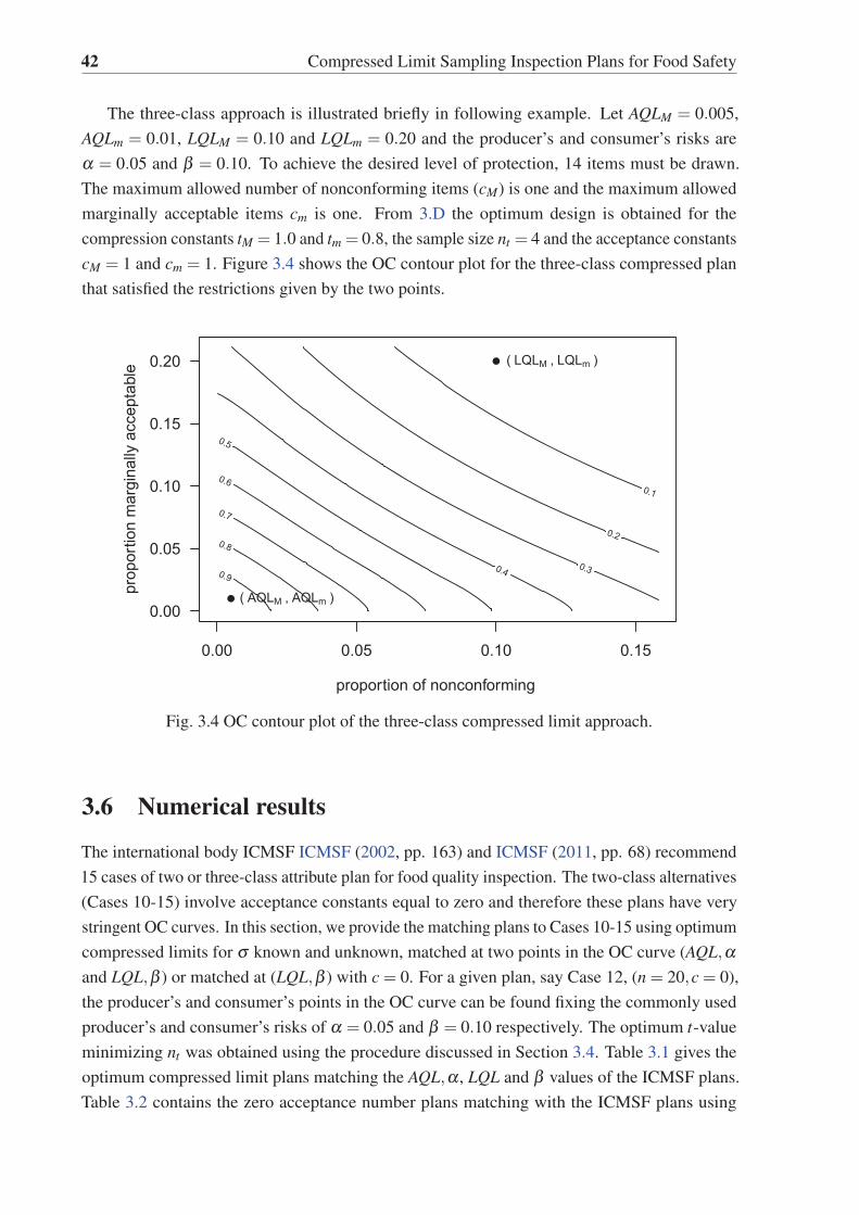
42 Compressed Limit Sampling Inspection Plans for Food Safety
The three-class approach is illustrated briefly in following example. Let AQLM = 0.005,
AQLm = 0.01, LQLM = 0.10 and LQLm = 0.20 and the producer’s and consumer’s risks are
α = 0.05 and β = 0.10. To achieve the desired level of protection, 14 items must be drawn.
The maximum allowed number of nonconforming items (cM) is one and the maximum allowed
marginally acceptable items cm is one. From 3.D the optimum design is obtained for the
compression constants tM = 1.0 and tm = 0.8, the sample size nt = 4 and the acceptance constants
cM = 1 and cm = 1. Figure 3.4 shows the OC contour plot for the three-class compressed plan
that satisfied the restrictions given by the two points.
proportion of nonconforming
prop
ortio
n m
argi
nally
acc
epta
ble
0.1
0.2
0.3 0.4
0.5
0.6
0.7
0.8
0.9
0.00 0.05 0.10 0.15
0.00
0.05
0.10
0.15
0.20
●
●
( AQLM , AQLm )
( LQLM , LQLm )
Fig. 3.4 OC contour plot of the three-class compressed limit approach.
3.6 Numerical results
The international body ICMSF ICMSF (2002, pp. 163) and ICMSF (2011, pp. 68) recommend
15 cases of two or three-class attribute plan for food quality inspection. The two-class alternatives
(Cases 10-15) involve acceptance constants equal to zero and therefore these plans have very
stringent OC curves. In this section, we provide the matching plans to Cases 10-15 using optimum
compressed limits for σ known and unknown, matched at two points in the OC curve (AQL,αand LQL,β ) or matched at (LQL,β ) with c = 0. For a given plan, say Case 12, (n = 20,c = 0),
the producer’s and consumer’s points in the OC curve can be found fixing the commonly used
producer’s and consumer’s risks of α = 0.05 and β = 0.10 respectively. The optimum t-value
minimizing nt was obtained using the procedure discussed in Section 3.4. Table 3.1 gives the
optimum compressed limit plans matching the AQL,α , LQL and β values of the ICMSF plans.
Table 3.2 contains the zero acceptance number plans matching with the ICMSF plans using

3.6 Numerical results 43
compression constant t = 0.5 and 1. These plans are relevant for compliance related applications
where c = 0 is often mandatory. As a result, the control of the producer’s risk α becomes less
critical for these c = 0 plans.
Table 3.1 Compressed limit alternatives for σ known and unknown matching AQL and LQL of
two-class ICMSF plans.
matched compressed plans
ICMSF plan Quality levels and risks σ known σ unknown
na ca AQL LQL α β t nt ct t nt ctCase 10 5 0 0.0102 0.3690 0.05 0.10 1.20 3 1 – – –
Case 11 10 0 0.0051 0.2057 0.05 0.10 1.68 5 2 1.91 9 5
Case 12 20 0 0.0026 0.1087 0.05 0.10 2.18 6 3 1.76 13 5
Case 13 15 0 0.0034 0.1423 0.05 0.10 1.82 5 2 2.55 11 8
Case 14 30 0 0.0017 0.0739 0.05 0.10 2.32 6 3 2.64 15 10
Case 15 60 0 0.0009 0.0376 0.05 0.10 2.56 8 4 2.34 22 10
Table 3.2 Zero acceptance number compressed limit alternatives to the two-class ICMSF plans
for the known σ case.
ICMSF plan matched plans
na ca LQL β t nt ct t nt ctCase 10 5 0 0.3690 0.10 0.50 3 0 1.00 2 0
Case 11 10 0 0.2057 0.10 0.50 5 0 1.00 3 0
Case 12 20 0 0.1087 0.10 0.50 9 0 1.00 5 0
Case 13 15 0 0.1423 0.10 0.50 7 0 1.00 4 0
Case 14 30 0 0.0739 0.10 0.50 13 0 1.00 6 0
Case 15 60 0 0.0376 0.10 0.50 22 0 1.00 10 0
It can be appreciated from Table 3.1 that the number of analytical tests will be reduced
significantly, by a factor of between 40 and 87% for the known σ case. Similarly, the compressed
approach for unknown σ should be used for Cases 12-15 where the sample size is reduced by
27-63%. In the zero acceptance number plans of Table 3.2 the sample size is reduced by 40-83%.
Figure 3.5 shows the OC curve of Case 12 attribute plan of the ICMSF and matching the
optimum compressed limit plan when σ is known and unknown. Notice that the known σcompressed limit plan also reduces the consumer’s risk (lower part of the OC curve) due to
the MARD criterion employed for the design. Figure 3.5 also shows the OC curve of the zero
acceptance number plan is given. This plan does not satisfy the producer’s point restriction and
hence the producer’s risk is increased.

44 Compressed Limit Sampling Inspection Plans for Food Safety
0.00 0.05 0.10 0.15
0.0
0.2
0.4
0.6
0.8
1.0
proportion nonconforming
Pa●
●
( AQL , 1 − α )
( LQL , β )
n = 20 , c = 0t = 2.18 , n = 6 , c = 3t = 1.76 , n = 13 , c = 5t = 1 , n = 5 , c = 0
Fig. 3.5 Compressed limit OC curves for Case 12 plan of the ICMSF. The dark solid OC curve
represents attribute plan with n = 20,c = 0.
3.7 Economic evaluation
From an economic point of view, the decision to apply a plan by variables or attributes is a
trade-off between the sample sizes and costs.
nvCv < naCa (3.11)
where nv and na are the required sample size associated with the variables and the attribute
plan respectively. Cv and Ca are the cost of obtaining a measurement in a continues scale and
classifying as pass or not pass respectively. Commonly Cv >Ca since measurements such as cell
enumeration in food testing requires more time, resources and specialization than just assessing
whether the contamination is below the microbial limit. The same argument applies to the
compressed limit plans. According to Schilling and Sommers (1981) the known σ compressed
plan is preferable when Cv/Ct < 1.5 since nt = 1.5nv while Evans and Thyregod (1985) set this
condition as Cv/Ct < π/2. The MARD criterion requires Cv/Ct < 1.65. This condition is similar
to the one set in Schilling and Sommers (1981).
A full economic design of a sampling inspection plan requires the costs of incorrect decisions
to be considered in addition to the inspection and testing costs. The cost of rejecting a good
quality batch is usually known. However the cost of accepting an unsafe batch is not only very
large for food products but also unknown. For instance, the brand image of a product may be
tarnished due to a single catastrophic incident involving food safety. Due to the difficulty in
estimating the costs of accepted unsafe batches, economical designed microbiological sampling

3.8 Robustness and nonnormal-based compressed limit plans 45
plans are rarely used in practice. International bodies such as ICMSF, FAO and Codex do not
advocate any cost driven sampling inspection plans. A small LQL specification indirectly controls
the cost of unsafe batches reaching the customers. Various preferred small LQL values are set on
empirical grounds by the international bodies depending on the severity of the microbiological
characteristics involved. The compressed limit plans proposed in this paper are matched to the
traditional plans and hence the decision related costs are equal. The main saving achieved is only
in the testing costs.
3.8 Robustness and nonnormal-based compressed limit plans
Compressed limit plans require the knowledge of the underlying probability distribution. De-
parture from this assumption will result in biased estimation of the proportion nonconforming.
Schilling and Sommers (1981) pointed out that this bias increases proportionally to t. It has
been well documented that multiplicative processes such as cell aggregation lead to right-skewed
distributions and particularly lognormal. Empirical evidence suggests that the lognormal dis-
tribution fits satisfactorily the frequencies of microorganisms in foodstuff, see ICMSF (2002);
Jarvis (2008); Kilsby and Baird-Parker (1983). This model is advantageous because the log
transformation leads to a normal distribution.
The robustness of the compressed limit plan for the distributional assumption is discussed
using the following example. Suppose that the CFU per gram of a certain pathogen is assumed
to follow a lognormal distribution with mean μ = 0 and standard deviation σ = 1 (both on the
natural logarithmic scale). The resulting expected value is 1.64 CFU/g and the dispersion is 2.16
CFU/g. The lognormal density and the cumulative distribution function are shown in Figures 3.6
(a) and (b).
The standard procedure is to apply log transformation to the sample measurements. Suppose
that the Case 12 ICMSF attribute plan with n = 20 and c = 0 is used. Form Table 3.1, the
equivalent compressed limit plans are t = 2.18, nt = 6 and ct = 3 for known σ and t = 1.76,
nt = 13 and ct = 5 unknown σ . At α = 0.05 and β = 0.10, the quality levels are AQL = 0.0026
and LQL = 0.1087. Figure 3.7 shows the corresponding OC curves for both cases.
Other right skewed distributions like gamma and Weibull have also been considered to
describe the distribution of pathogens in food e.g. Chen et al. (2003); Corradini et al. (2001);
Jarvis (2008); Jongenburger et al. (2012b,c). The identification of probability distribution such
as lognormal, gamma and Weibull requires large sample sizes (Marshall et al., 2012). However,
microbiological risk assessment is usually done with small sample sizes. To investigate the
robustness of the plans, consider that the true distribution follows a gamma or Weibull model
instead of lognormal. The parameters of the gamma and Weibull distributions matching the
LN (0,1) distribution are obtained so that the modes and their density values are equivalent. The
gamma distribution with shape d = 1.5 and scale b = 0.75; and the Weibull distribution with
shape κ = 1.3 and scale λ = 1.14 match the LN (0,1). Both densities and cumulative distribution
functions are also presented in Figure 3.6. Applying the same plan based on the lognormal

46 Compressed Limit Sampling Inspection Plans for Food Safety
0 1 2 3 4 5 6
0.0
0.1
0.2
0.3
0.4
0.5
0.6
0.7
(a)
x
PD
F LN(0,1)G(1.5,0.75)W(1.3,1.14)
0 2 4 6 8
0.0
0.2
0.4
0.6
0.8
1.0
(b)
x
CD
F LN(0,1)G(1.5,0.75)W(1.3,1.14)
Fig. 3.6 Lognormal, gamma and Weibull (a) probability density functions and (b) cumulative
distribution functions matched by the mode and the density.

3.8 Robustness and nonnormal-based compressed limit plans 47
0.00 0.05 0.10 0.15 0.20
0.0
0.2
0.4
0.6
0.8
1.0
(a)
proportion nonconforming
Pa
LN(0,1)G(1.5,0.75)W(1.3,1.14)
●
●
0.00 0.05 0.10 0.15 0.20
0.0
0.2
0.4
0.6
0.8
1.0
(b)
proportion nonconforming
Pa
LN(0,1)G(1.5,0.75)W(1.3,1.14)
●
●
Fig. 3.7 Compressed limit OC curves equivalent to the ICMSF (2002) Case 12 (n = 20,c = 0) for
known σ (a) and unknown (b). The assumed distribution is lognormal when the true underlying
model is lognormal, gamma and Weibull.

48 Compressed Limit Sampling Inspection Plans for Food Safety
assumption yields the OC curves shown in Figure 3.7. It can be appreciated that the quality levels
at the producer’s and consumer’s risks differ considerably when the true distribution is gamma or
Weibull. This example illustrates that compressed limit plans are not robust to departures from
normality.
When the base-line distribution is known the compressed limit can be recomputed. The
specific compressed limit design for known parameters is obtained by replacing the quantile and
the distribution function of the normal for the true distribution in Steps 1 and 3 of the procedure
given in Section 3.4. The R codes of 3.B also deal with design of the plans for gamma and
Weibull distributions.
3.9 Summary and conclusions
A standard practice in food trade is to use ICMSF attribute sampling plans. By using variables
plans, the number of analytical units tested can be reduced considerably. Nonetheless, the
cost associated with taking a measurement in a continuous scale is generally higher than just
classifying a sample on a go/no-go basis. For lognormally distributed quality characteristics,
variables plans pose problems in administration because the test outcome can be a zero value.
For example, a batch of food product may not be totally free of microorganisms but the observed
number of microorganisms in the samples can be below the limit of detection. This results in
zero counts.
Compressed limit plans combine the features of attribute and variables plans. Therefore,
this approach can achieve the benefits of both alternatives: a reduced sample size and simpler
classification of the tested items as conforming/non-conforming. However, compressed limit
plans also inherit the lack of robustness of variables plans. Previous publications such as Ladany
(1976), Schilling and Sommers (1981) and Evans and Thyregod (1985) are limited to the normal
distribution with known standard deviation. However, in most practical cases the process sigma
is unknown and commonly a conservative (large) standard deviation value is used to protect the
consumer’s interest. For food safety applications, a value of σ = 0.8 is used in the ICMSF plans.
This paper introduces an approach for the normal distribution when σ is unknown and it discusses
compressed limit plans for other right-skewed models such as gamma and Weibull. Three-class
compressed limits are introduced as alternatives to the ICMSF plans. This research as well as
Govindaraju and Kissling (2015) accomplish a reduced sample size, but by different means. The
former uses a compressed limit and assumes knowledge of the underlying distribution, while
the latter consists of a variables plan with an additional restriction. Compressed limit plans are
suitable for pre-shipment inspection by producers, since this method requires the knowledge
of the underlying distribution. From the consumer perspective, compressed limit plans should
be used when the batches come from food suppliers with proven reputation. In this case, the
analytical tests carried out from previous batches must show lognormality for frequencies of
microorganisms. If a departure from the assumed model is suspected, say the lognormality
assumption is not satisfied, a smaller compression constant such as t = 1 may be used. This

3.9 Summary and conclusions 49
approach will increase the required sample size, but can provide increased consumer protection.
In the case of the zero acceptance number compressed plans, using values of t > 1 might
compromise the accuracy of this technique even when the assumptions are marginally violated.
Further research might explore other sampling plan alternatives based on the compressed limits
theory.

50 Compressed Limit Sampling Inspection Plans for Food Safety
Appendix 3.A Glossary of symbols and definitions.
f (x|σ ,μ) = 1
σ√
2πexp
(− (x−μ)2
2σ2
)normal density function
f (d|n, p) =(n
d
)pd (1− p)n−d binomial probability function
f (d1,d2,d3|n; p1, p2, p3) =n
d1!d2!d3! pd11 pd2
2 pd33 trinomial probability function
m microbiological limit in two-class plans or
GMP limit in three-class plans
M second microbiological limit
CL = m− tσ compressed limit
X sample mean
S =
√∑(Xi − X)
2/(n−1) standard deviation
p proportion nonconforming
g artificial proportion nonconforming
α producer’s risk
β consumer’s risk
AQL Acceptance Quality Limit
LQL Limiting Quality Level
na sample size of attribute plan
nv sample size of variables plan
nt sample size of compressed limit plan
k critical distance
d number of observed nonconforming items
c attribute acceptance number
ct acceptance number for compressed limit
t compression constant
MARD = max[∣∣∣α −α ′
∣∣∣+ ∣∣∣β −β ′∣∣∣] maximum absolute risk difference
MIRD = min[∣∣∣α −α ′
∣∣∣+ ∣∣∣β −β ′∣∣∣] minimum absolute risk difference
Appendix 3.B R Software code
The R function given below obtains the optimum compressed limit plans for given two-points
on the OC curve using normal, gamma and Weibull distributions. The function depends on the
R-package AcceptanceSampling Kiermeier (2008) to solve Eq.3.5 by trial and error.
A straightforward shiny app is also developed and made available at
https://internal.shinyapps.io/edgarsantosfdez/compress/ for the practitioners. A reference sam-
pling plan such as (n = 5, c = 0) needs to be input. The app will then return the optimum
matching compressed sampling plan for the specified underlying distribution.

3.B R Software code 51
� �### The R code computes the optimum compressed limit plan.### Edgar Santos Fernandez, K. Govindaraju, Geoff Jones### July/29,2014# AQL # Acceptance Quality Limit# alpha # producer s risk# LQL # Limiting Quality Level# beta # consumer s risk# t # compression constant# dist # statistical distribution (normal, gamma or Weibull)
compress function(AQL = 0.02, LQL = 0.08, alpha = 0.05, beta = 0.10, distr = "normal", ... ){library ("AcceptanceSampling")t = seq(0, 4, 0.01)plan matrix(NA, nrow = length(t), ncol = 3)condition function(code) {tryCatch(code, error = function(c) NA, # Exception handling
warning = function(c) NA, message = function(c) NA)}
if ( distr == "normal"){Zaql qnorm(AQL,lower.tail = 0)Zlql qnorm(LQL,lower.tail = 0)for ( i in 1:length( t )){Zgaql Zaql t [ i ]Zglql Zlql t [ i ]p.gaql pnorm(Zgaql, lower.tail = 0)p. glql pnorm(Zglql, lower. tail = 0)plan[ i ,1] condition(find.plan(PRP=c(p.gaql,1 alpha),CRP=c(p.glql,beta),type="binomial")$n)plan[ i ,2] condition(find.plan(PRP=c(p.gaql,1 alpha),CRP=c(p.glql,beta),type="binomial")$c)plan[ i ,3] 1 p.gaql }}
if ( distr == "gamma"){Zaql qgamma(AQL, shape = shape, scale = scale, lower.tail = 0)Zlql qgamma(LQL, shape = shape, scale = scale, lower.tail = 0)for ( i in 1:length( t )){Zgaql Zaql t [ i ]Zglql Zlql t [ i ]p.gaql pgamma(Zgaql, shape = shape, scale = scale, lower.tail = 0)p. glql pgamma(Zglql, shape = shape, scale = scale, lower.tail = 0)plan[ i ,1] condition(find.plan(PRP=c(p.gaql,1 alpha),CRP=c(p.glql,beta),type="binomial")$n)plan[ i ,2] condition(find.plan(PRP=c(p.gaql,1 alpha),CRP=c(p.glql,beta),type="binomial")$c)plan[ i ,3] 1 p.gaql }}
if ( distr == "Weibull" ){Zaql qweibull(AQL, shape = shape, scale = scale, lower. tail = 0)Zlql qweibull(LQL, shape = shape, scale = scale, lower. tail = 0)for ( i in 1:length( t )){Zgaql Zaql t [ i ]Zglql Zlql t [ i ]p.gaql pweibull(Zgaql,shape=shape,scale=scale,lower.tail = 0)p. glql pweibull(Zglql ,shape=shape,scale=scale,lower.tail = 0)plan[ i ,1] condition(find.plan(PRP=c(p.gaql,1 alpha),CRP=c(p.glql,beta),type="binomial")$n)plan[ i ,2] condition(find.plan(PRP=c(p.gaql,1 alpha),CRP=c(p.glql,beta),type="binomial")$c)plan[ i ,3] 1 p.gaql }}
plan cbind(t,plan); colnames(plan) NULLa plan[which(plan[,2] == min(plan [,2][plan [,2] != 1], na.rm = TRUE)),]fd seq(0, 0.995, 0.0001)madr rep(NA, nrow(a))
for ( j in 1 : nrow(a)){t = a[ j ,1]; n a[j ,2]; c a[j ,3]if ( distr == "normal"){ zp qnorm(fd,lower.tail = 0)zg zp t ; pr pnorm(zg, lower.tail = 0)}

52 Compressed Limit Sampling Inspection Plans for Food Safety
if ( distr == "gamma"){zp qgamma(fd, shape = shape, scale = scale, lower.tail = 0)zg zp t ; pr pgamma(zg, shape = shape, scale = scale, lower.tail = 0)}
if ( distr == "Weibull" ){zp qweibull(fd , shape = shape, scale = scale, lower. tail = 0)zg zp t ; pr pweibull(zg, shape = shape, scale = scale, lower. tail = 0)}
Op cbind(fd, pbinom(q = c, size = n, prob = pr ))madr[j] abs(Op[which(abs((Op[,1] AQL)) == min(abs((Op[,1] AQL)))),2] (1 alpha))+abs(Op[ which(abs((Op[,1] LQL)) == min(abs((Op[,1] LQL)))) ,2] beta)}
opt a[which(madr == max(madr)),]return( list ( t = opt [1], n = opt [2], c = opt [3], q_t = round(opt[4],3) ))
}
# Example 1 normal distributioncompress(AQL=0.01, LQL=0.2, alpha=0.05, beta=0.10, distr="normal")# Example 2 gamma distribution, Case 11 ICMSFshape = 1.50; scale = 0.75compress(AQL=0.0051, LQL=0.2057, alpha=0.05, beta=0.10, distr="gamma",shape=shape, scale=scale)
# Example 3 Weibull distributionshape = 1.30; scale = 1.14compress(AQL=0.02, LQL=0.08, alpha=0.05, beta=0.10, distr="Weibull",shape=shape, scale=scale)
�� �

3.C Optimum compression constants (t), sample size (nt), acceptance number (ct) and the
corresponding quantile (qt) for given two points of the OC curve 53
App
endi
x3.
CO
ptim
umco
mpr
essi
onco
nsta
nts(t),
sam
ple
size
(nt)
,acc
epta
nce
num
ber(c
t)
and
the
corr
espo
ndin
gqu
antil
e(q
t)fo
rgi
ven
two
poin
tsof
the
OC
curv
e
com
pre
ssed
lim
itpla
nσ
know
nco
mpre
ssed
lim
itpla
nσ
unknow
n
Qual
ity
level
san
dri
sks
attr
pla
nusi
ng
MA
RD
usi
ng
MIR
Dusi
ng
MA
RD
usi
ng
MIR
D
AQL
LQL
αβ
nc
tn t
c tq t
tn t
c tq t
tn t
c tq t
tn t
c tq t
0.0
01
0.0
20.0
10.0
5313
22.4
823
11
0.7
29
2.5
923
12
0.6
92
2.3
666
29
0.7
67
2.9
766
45
0.5
48
0.0
01
0.0
20.0
10.1
0265
22.5
619
10
0.7
02
2.2
919
80.7
88
2.6
054
30
0.6
88
2.9
254
37
0.5
67
0.0
01
0.0
20.0
50.0
5236
12.6
516
80.6
70
2.8
116
90.6
10
2.8
547
29
0.5
94
3.4
247
37
0.3
70
0.0
01
0.0
20.0
50.1
0194
12.5
213
60.7
16
2.9
013
80.5
75
2.1
236
12
0.8
34
2.1
236
12
0.8
34
0.0
01
0.0
40.0
10.0
5117
12.4
114
70.7
52
2.0
314
50.8
55
2.1
637
16
0.8
23
3.1
437
29
0.4
80
0.0
01
0.0
40.0
10.1
096
12.3
612
60.7
67
2.7
712
80.6
26
1.9
330
11
0.8
77
2.9
130
22
0.5
70
0.0
01
0.0
40.0
50.0
5117
12.3
010
40.7
85
2.0
310
30.8
55
1.9
330
11
0.8
13
3.3
028
22
0.4
17
0.0
01
0.0
40.0
50.1
096
12.5
38
40.7
12
1.8
58
20.8
93
2.3
022
10
0.7
85
2.4
022
11
0.7
55
0.0
10.2
0.0
10.0
530
21.4
611
50.8
07
1.4
611
50.8
07
1.4
020
90.8
23
0.5
020
30.9
66
0.0
10.2
0.0
10.1
025
21.3
79
40.8
31
1.6
59
50.7
51
1.7
015
90.7
34
1.7
015
90.7
34
0.0
10.2
0.0
50.0
522
11.4
38
30.8
15
2.0
78
50.6
01
0.9
014
30.9
23
0.9
014
30.9
23
0.0
10.2
0.0
50.1
018
11.7
16
30.7
31
1.2
86
20.8
52
1.3
011
40.8
48
1.3
011
40.8
48
0.0
10.4
0.0
10.0
510
11.3
86
30.8
28
0.8
76
20.9
27
1.3
08
40.8
48
1.3
08
40.8
48
0.0
10.4
0.0
10.1
09
11.0
75
20.8
96
0.4
75
10.9
68
3.7
02
10.0
85
3.7
02
10.0
85
0.0
10.4
0.0
50.0
510
10.9
94
10.9
09
1.6
44
20.7
54
1.3
07
30.8
48
2.7
07
60.3
54
0.0
10.4
0.0
50.1
05
01.2
23
10.8
66
1.1
23
10.8
86
3.7
02
10.0
85
3.7
02
10.0
85

54 Compressed Limit Sampling Inspection Plans for Food Safety
App
endi
x3.
DO
ptim
umco
mpr
essi
onco
nsta
nt(t
1),(t
2),
sam
ple
size
(nt)
and
acce
ptan
cenu
m-
bers
(ct M)
and(c
t m)
for
thre
e-cl
assc
ompr
esse
dlim
itpl
an.
Qu
alit
yle
vel
san
dri
sks
thre
e-cl
ass
pla
nth
ree-
clas
sco
mp
ress
edli
mit
pla
n
AQL 1
AQL 2
LQL 1
LQL 2
αβ
nc M
c mt M
t mn t
c tM
c tm
q tM
q tm
0.0
01
0.0
10
.05
0.1
50
.01
0.0
53
31
21
.51
.07
23
0.9
44
0.9
08
0.0
01
0.0
10
.05
0.1
50
.01
0.1
02
91
21
.61
.05
22
0.9
32
0.9
08
0.0
01
0.0
10
.05
0.1
50
.05
0.0
52
10
11
.61
.03
11
0.9
32
0.9
08
0.0
01
0.0
10
.05
0.1
50
.05
0.1
01
70
11
.61
.03
11
0.9
32
0.9
08
0.0
01
0.0
10
.05
0.2
00
.01
0.0
52
61
21
.50
.86
22
0.9
44
0.9
37
0.0
01
0.0
10
.05
0.2
00
.01
0.1
02
21
21
.50
.86
22
0.9
44
0.9
37
0.0
01
0.0
10
.05
0.2
00
.05
0.0
51
70
11
.50
.84
11
0.9
44
0.9
37
0.0
01
0.0
10
.05
0.2
00
.05
0.1
01
40
11
.50
.84
11
0.9
44
0.9
37
0.0
01
0.0
10
.10
0.1
50
.01
0.0
52
61
21
.11
.06
13
0.9
77
0.9
08
0.0
01
0.0
10
.10
0.1
50
.01
0.1
02
21
21
.21
.04
12
0.9
71
0.9
08
0.0
01
0.0
10
.10
0.1
50
.05
0.0
51
60
11
.11
.04
11
0.9
77
0.9
08
0.0
01
0.0
10
.10
0.1
50
.05
0.1
01
30
11
.21
.03
11
0.9
71
0.9
08
0.0
01
0.0
10
.10
0.2
00
.01
0.0
52
21
21
.10
.85
12
0.9
77
0.9
37
0.0
01
0.0
10
.10
0.2
00
.01
0.1
01
41
11
.20
.84
12
0.9
71
0.9
37
0.0
01
0.0
10
.10
0.2
00
.05
0.0
51
30
11
.20
.84
11
0.9
71
0.9
37
0.0
01
0.0
10
.10
0.2
00
.05
0.1
01
10
11
.20
.83
11
0.9
71
0.9
37
0.0
01
0.0
20
.05
0.1
50
.01
0.0
54
01
31
.61
.09
34
0.9
32
0.8
54
0.0
01
0.0
20
.05
0.1
50
.01
0.1
03
51
31
.61
.08
34
0.9
32
0.8
54
0.0
01
0.0
20
.05
0.1
50
.05
0.0
52
70
21
.61
.04
12
0.9
32
0.8
54
0.0
01
0.0
20
.05
0.1
50
.05
0.1
02
20
21
.61
.04
12
0.9
32
0.8
54
0.0
01
0.0
20
.05
0.2
00
.01
0.0
53
11
31
.50
.87
23
0.9
44
0.8
95
0.0
01
0.0
20
.05
0.2
00
.01
0.1
02
21
21
.60
.86
23
0.9
32
0.8
95

3.D Optimum compression constant (t1), (t2), sample size (nt) and acceptance numbers (ctM)and (ctm) for three-class compressed limit plan. 55
...C
on
tin
ued Q
ual
ity
level
san
dri
sks
thre
e-cl
ass
pla
nth
ree-
clas
sco
mp
ress
edli
mit
pla
n
AQL 1
AQL 2
LQL 1
LQL 2
αβ
nc M
c mt M
t mn t
c tM
c tm
q tM
q tm
0.0
01
0.0
20
.05
0.2
00
.05
0.0
52
20
21
.50
.85
12
0.9
44
0.8
95
0.0
01
0.0
20
.05
0.2
00
.05
0.1
01
40
11
.60
.83
11
0.9
32
0.8
95
0.0
01
0.0
20
.10
0.1
50
.01
0.0
53
01
31
.21
.08
24
0.9
71
0.8
54
0.0
01
0.0
20
.10
0.1
50
.01
0.1
02
21
21
.21
.06
23
0.9
71
0.8
54
0.0
01
0.0
20
.10
0.1
50
.05
0.0
51
90
21
.21
.05
12
0.9
71
0.8
54
0.0
01
0.0
20
.10
0.1
50
.05
0.1
01
30
11
.21
.04
12
0.9
71
0.8
54
0.0
01
0.0
20
.10
0.2
00
.01
0.0
52
21
21
.10
.86
13
0.9
77
0.8
95
0.0
01
0.0
20
.10
0.2
00
.01
0.1
01
91
21
.20
.84
12
0.9
71
0.8
95
0.0
01
0.0
20
.10
0.2
00
.05
0.0
51
30
11
.10
.74
11
0.9
77
0.9
12
0.0
01
0.0
20
.10
0.2
00
.05
0.1
01
10
11
.20
.83
11
0.9
71
0.8
95
0.0
05
0.0
10
.05
0.1
50
.01
0.0
53
72
21
.21
.01
34
40
.91
60
.90
8
0.0
05
0.0
10
.05
0.1
50
.01
0.1
03
22
21
.11
.01
13
40
.93
00
.90
8
0.0
05
0.0
10
.05
0.1
50
.05
0.0
52
61
11
.11
.08
22
0.9
30
0.9
08
0.0
05
0.0
10
.05
0.1
50
.05
0.1
02
21
11
.21
.07
22
0.9
16
0.9
08
0.0
05
0.0
10
.05
0.2
00
.01
0.0
52
61
21
.00
.81
13
30
.94
20
.93
7
0.0
05
0.0
10
.05
0.2
00
.01
0.1
02
21
20
.80
.81
02
30
.96
20
.93
7
0.0
05
0.0
10
.05
0.2
00
.05
0.0
52
01
10
.80
.88
12
0.9
62
0.9
37
0.0
05
0.0
10
.05
0.2
00
.05
0.1
01
71
10
.80
.85
11
0.9
62
0.9
37
0.0
05
0.0
10
.10
0.1
50
.01
0.0
52
61
21
.21
.08
33
0.9
16
0.9
08
0.0
05
0.0
10
.10
0.1
50
.01
0.1
02
21
21
.01
.07
23
0.9
42
0.9
08
0.0
05
0.0
10
.10
0.1
50
.05
0.0
52
11
11
.11
.05
12
0.9
30
0.9
08
0.0
05
0.0
10
.10
0.1
50
.05
0.1
01
81
11
.21
.03
11
0.9
16
0.9
08
0.0
05
0.0
10
.10
0.2
00
.01
0.0
52
21
21
.00
.88
23
0.9
42
0.9
37
0.0
05
0.0
10
.10
0.2
00
.01
0.1
01
91
21
.00
.86
22
0.9
42
0.9
37
0.0
05
0.0
10
.10
0.2
00
.05
0.0
51
71
11
.00
.84
11
0.9
42
0.9
37

56 Compressed Limit Sampling Inspection Plans for Food Safety
...C
on
tin
ued Q
ual
ity
level
san
dri
sks
thre
e-cl
ass
pla
nth
ree-
clas
sco
mp
ress
edli
mit
pla
n
AQL 1
AQL 2
LQL 1
LQL 2
αβ
nc M
c mt M
t mn t
c tM
c tm
q tM
q tm
0.0
05
0.0
10
.10
0.2
00
.05
0.1
01
41
11
.00
.84
11
0.9
42
0.9
37
0.0
05
0.0
20
.05
0.1
50
.01
0.0
55
12
41
.51
.01
56
60
.85
90
.85
4
0.0
05
0.0
20
.05
0.1
50
.01
0.1
03
92
31
.51
.01
25
50
.85
90
.85
4
0.0
05
0.0
20
.05
0.1
50
.05
0.0
53
31
21
.51
.08
33
0.8
59
0.8
54
0.0
05
0.0
20
.05
0.1
50
.05
0.1
02
91
21
.51
.08
33
0.8
59
0.8
54
0.0
05
0.0
20
.05
0.2
00
.01
0.0
53
42
31
.30
.81
24
40
.89
90
.89
5
0.0
05
0.0
20
.05
0.2
00
.01
0.1
03
02
31
.30
.81
14
40
.89
90
.89
5
0.0
05
0.0
20
.05
0.2
00
.05
0.0
52
61
21
.30
.88
23
0.8
99
0.8
95
0.0
05
0.0
20
.05
0.2
00
.05
0.1
01
71
11
.20
.87
22
0.9
16
0.8
95
0.0
05
0.0
20
.10
0.1
50
.01
0.0
53
62
31
.21
.09
34
0.9
16
0.8
54
0.0
05
0.0
20
.10
0.1
50
.01
0.1
02
61
31
.21
.09
34
0.9
16
0.8
54
0.0
05
0.0
20
.10
0.1
50
.05
0.0
52
61
21
.11
.06
22
0.9
30
0.8
54
0.0
05
0.0
20
.10
0.1
50
.05
0.1
02
21
21
.21
.04
12
0.9
16
0.8
54
0.0
05
0.0
20
.10
0.2
00
.01
0.0
52
51
31
.20
.88
33
0.9
16
0.8
95
0.0
05
0.0
20
.10
0.2
00
.01
0.1
02
12
21
.00
.87
23
0.9
42
0.8
95
0.0
05
0.0
20
.10
0.2
00
.05
0.0
51
71
11
.20
.86
22
0.9
16
0.8
95
0.0
05
0.0
20
.10
0.2
00
.05
0.1
01
41
11
.20
.84
12
0.9
16
0.8
95

Chapter 4
New two-stage sampling inspection plansfor bacterial cell counts
Edgar Santos-Fernández, K. Govindaraju, Geoff Jones, Roger Kissling
Food Control 1, 2016
http://dx.doi.org/10.1016/j.foodcont.2016.08.042
4.1 Abstract
The inspection of a batch of food generally relies on testing a small number of samples. Yet,
this low rate of testing still results in a significant expenditure for the producer as well as a
substantial laboratory workload due to the large number of safety and sanitary characteristics
involved. A new double sampling methodology employing a compressed limit in the first stage
of inspection is introduced. The proposed double sampling plan provides the same or better
consumer protection with substantially smaller average sample size and hence it reduces the
testing cost and the laboratory workload. This plan is intended for sanitary characteristics where
the bacterial count generally fits a Poisson or a mixed-Poisson distribution, resulting in a high
proportion of zero values. Optimum determination of the compressed limit, which is set well
below the regulatory or specification limit, is addressed. The application of the new plan is
validated using a large empirical dataset of aerobic plate counts observed in milk powder samples.
For this dataset the Poisson-gamma was found to be the best fitting distribution. An interactive
web-based tool (shiny app) that allows the design of the new sampling plan is also provided for
practitioners and food safety professionals.
1An abridged version of this Chapter has been published in Food Control.
58 New two-stage sampling inspection plans for bacterial cell counts
Keywords
double sampling plan; compressed limit; hygiene indicator; consumers protection; Poisson-
gamma distribution
4.2 Introduction
Sampling inspection plans are generally used to assess the acceptability of a batch of foodstuffs
and to determine whether the food safety systems are working free of special causes of variation.
Guidance and regulations on microbiological sampling plans are given by European Commission
(2005); FAO/WHO (2014); Food Standards Australia New Zealand (2001); ICMSF (2002) and
by other country-specific regulatory agencies. The inspection of a batch generally relies on
small sample sizes, typically n = 5 or 10 (Hoelzer and Pouillot, 2013; ICMSF, 2002). Yet, these
testing levels lead to a significant expenditure and a substantial laboratory workload. Several
recent publications have focused on quantitative risk assessment of food products using statistical
models. Their focus is mainly on reducing the consumer’s risk, increasing the sampling plan
stringency and robustness, as well as reducing the testing costs (e.g. Dahms and Hildebrandt,
1998; ICMSF, 2002; Powell, 2014).
Both attribute and variables type inspection plans are recommended in the safety literature e.g.
FAO/WHO (2014). Concentration-based attribute sampling plans are generally used for sanitary
characteristics, where the batch probability of acceptance is expressed as a function of sanitary
quality parameter(s) rather than the proportion nonconforming to specifications; see for instance
FAO/WHO (2014). In the first two alternative plans of FAO/WHO (2014), the test statistic is the
number of individual samples that fail to satisfy the microbiological or the specification limit m.
However, in variables plans the test statistic is obtained from the mean and standard deviation
of the log transformed bacterial count. Variables plans provide similar protection with smaller
sample sizes compared to attribute type concentration-based plans. However, the application of
variables plans is generally limited to the case of high cell counts only because the discontinuity
in large cell counts is not critical. A reduction in sample size can also be achieved using a
compressed limit plan. This technique inherits the benefits of both variables and attribute plans:
a reduced sample size and individual cell counts being classified as pass or fail. However, the
theory of compressed limit plans is limited in the literature, mainly employing this technique to
single inspection plans; see Schilling and Neubauer (2010).
A double sampling plan allows for a second stage of inspection and achieves sampling
economy when compared to taking a single large sample; see Alonzo and Pepe (2003) for an
application of the double sampling approach to inspection. For food product inspection, a two
stage procedure might be convenient because the microorganism indicators are often low (well
below the regulatory limit). The sampling plans as recommended by ICMSF (2002) mostly
involve zero acceptance numbers (c = 0). Under this restriction, a sample size reduction cannot
be achieved by the traditional double sampling plan where the same regulatory limit is employed

4.3 Materials and methods 59
for the assessment of conformance in the two stages of inspection. However, a double sampling
plan with compressed limit in the first stage of inspection will be able to match the performance
of a c = 0 plan. In this research we introduce a new two-stage compressed plan based on
the discrete distributions generally used to describe microbial counts. The proposed plans are
intended for sanitary characteristics with nonzero microbiological limit m > 0 such as an Aerobic
Plate Count (APC). A compressed limit CL < m is used for the first stage, while the regular
specification m is applied in the second stage of sampling. In the common cause situations
(good quality batches), the proposed plans will operate mostly as a single sampling plan but with
lower average sample size. The second stage of sampling will only be reached in special cause
situations. Hence the proposed plan is not expected to cause operational management issues
(such as delaying the batch disposition) under normal circumstances. The plan is not applicable
to safety characteristics because no pathogens can be tolerated for samples in accepted batches:
this regulatory limit of m = 0 cfu obviously cannot be compressed further.
In this paper, the following concepts and abbreviations are used. The parameters μ and σ in
the Poisson-lognormal (PLN) distribution are expressed in the log10 scale. The Poisson-gamma
is abbreviated as PG. The symbols α and β refer to the producer’s and consumer’s risks. The
terms AQL and LQL stand for Acceptance Quality Limit and Limiting Quality Level respectively.
The term Indifference Quality (p0) refers to the point in the x-axis of the Operating Characteristic
(OC) curve corresponding to a probability of acceptance (Pa) of 50%. The indifference quality
zone is the region of the OC curve around this point. By the term ‘matching sampling plans’,
we mean plans having very similar OC curves. Since the OC curves of two plans are seldom
exactly identical, the matching sampling plans are required to satisfy two restrictions such as the
OC curves coinciding well at two points (LQL,β and AQL, α) while differing elsewhere. The
point (AQL, α) is not commonly used in microbial risk assessment but can be used for matching
purposes to compare the performance of sampling plans. An alternative approach to matching
sampling plans is to ensure that the two plans achieve the same indifference quality point p0
and same slope value h0 of the OC at this point. We consider both alternatives in our discussion.
Finally, most of the computations and figures were developed using R (R Core Team, 2015).
4.3 Materials and methods
4.3.1 Statistical models
Consider a random variable X representing the observed number of microorganisms or cfu in a
sample of size w subjected to a limit m. Suppose that the contamination (in cfu/g) is homogenous
in the batch and let λ be the rate of the contamination. Then X follows a Poisson distribution
with probability mass function:
P(X = x|λ ) = λ xe−λ
x!, x = 0,1,2, · · · (4.1)

60 New two-stage sampling inspection plans for bacterial cell counts
Microorganisms tend to form clusters or colonies in certain commodities, in which case
the homogeneity assumption cannot be satisfied. Several models for overdispersed counts
(E [X ] << Var [X ]) have been used for modelling microorganisms in food. For low bacterial
count, compounded Poisson-lognormal (Bulmer, 1974b) and Poisson-gamma (Anscombe, 1950)
models are generally employed. See for example, Van Schothorst et al. (2009), Gonzales-
Barron and Butler (2011b), Gonzales-Barron and Butler (2011a), Jongenburger et al. (2012b),
Jongenburger et al. (2012c), Williams and Ebel (2012), Gonzales-Barron et al. (2013), Mussida
et al. (2013a).
The mixed Poisson-lognormal model is a Poisson process with parameter λ lognormally
distributed with location μ and scale σ (i.e. λ ∼ L N (μ,σ)). The probability mass function
for the PLN case is
P(X = x|μ,σ) =∫ ∞
0
λ xe−λ
x!
1
λσ√
2πe
(− (ln(λ )−μ)2
2σ2
)dλ , x = 0,1,2, · · · (4.2)
where μ and σ are on the natural logarithmic scale (ln or loge), hence obtained from the log10
parameters as μ = ln(10)μ10 and σ = ln(10)σ10.
Poisson-gamma is another popular mixture distribution. The mass function for this case is
parameterized via the mean concentration m = E [X ] and the dispersion parameter K.
P(X = x|K,m) =Γ(K + x)Γ(K)x!
(K
K +m
)K (m
K +m
)x
(4.3)
where Γ is the gamma function.
4.3.2 Compressed limit plans
A compressed or narrow limit is a limit that is set well below the regulatory specification.
Compressed limits are often regarded as good manufacturing practice (GMP) limits. Sampling
plans based on compressed limits are used to achieve a reduction in sample size; see Ott and
Mundel (1954), Beja and Ladany (1974), Schilling and Sommers (1981) and Evans and Thyregod
(1985). Traditional compressed plans are based on a continuous distribution, generally the normal
distribution. The general procedure to obtain a compressed plan is as follows. Let CL = m− t be
the compressed limit where t is the compression constant. Given the points AQL,α and LQL,β ,
obtain the standard normal quantiles ZAQL and ZLQL and then compute the compressed normal
quantiles Zg1= ZAQL − t and Zg2
= ZLQL − t for a given t. Obtain right tail areas of the standard
normal distribution pg1and pg2
associated with Zg1and Zg2
respectively. Using the pairs pg1,α
and pg2,β obtain the required sample size n and the acceptance constant c using the traditional
algorithm suggested by Guenther (1969). For other non-normal models, the assumed non-normal
distribution quantiles are used. Compressed limit plans require knowledge of the underlying
distribution, and the batch proportion nonconforming is incorrectly estimated when the actual

4.3 Materials and methods 61
distribution departs from the assumed model. Schilling and Sommers (1981) demonstrated that
small compression constants are preferred in this case.
4.3.3 Double sampling plans
The double sampling plan (Dodge and Romig, 1959) allows for a second sample to be taken
when the evidence for acceptance or rejection is not conclusive with the inspection of the first
sample. Double sampling plans are in general more complex to administer because they cause
larger decision times and operational costs when compared with a single attribute plan. However
the double sampling approach is advantageous because the average sample number (ASN) is
reduced while maintaining the same producer’s and consumer’s risks. Double sampling plans
are generally chosen to match a given single plan at two designated points on the curve; see
Schilling and Neubauer (2010) for further exposition. The efficiency of double sampling plans
was discussed by Hamaker and Strik (1955) comparing two different plans having the same
indifference point. Hamaker and Strik (1955) further imposed a second constraint involving the
slope of the OC curve measured at the indifference point p0. The quantity h0, defined as the
‘relative’ slope of the OC curve at p0 by Hamaker and Strik (1955), is given by:
h0 =−2pdPa
d p
∣∣∣p=p0
(4.4)
where Pa is the OC function whose first derivative (slope) is evaluated at p = p0. A strong
theoretical argument for using the pair (p0,h0) is given in Wetherill and Kollerstrom (1979).
While a single plan is defined by the pair (n, c), a double plan requires five parameters (n1, n2,
a1, r1, a2 = r2), where n1 and n2 are the sample sizes for the first and second stages of inspection
respectively. The constants a1 and a2 stand for the acceptance numbers while r1 and r2 stand for
the rejection numbers for first and second stages respectively. Let d1 be the observed number of
nonconforming test results in the first stage. The batch is accepted in the first stage when d1 � a1.
Similarly the batch is rejected if d1 � r1. If instead a1 < d1 < r1, a second sample of size n2 is
drawn and d2, the number of nonconforming test results for the second sample, is observed. Let
D = d1 +d2 be the combined or total number of nonconforming test results in both samples (n1
+n2). If D � a2, the batch is accepted; otherwise (D � r2), the batch is rejected.
4.3.4 Two-stage sampling plan based on compressed limit.
The zero acceptance number plan used in the safety area is the most stringent sampling alternative
for a fixed sample size n. The OC of this c = 0 plan drops rapidly close to the vertical axis,
allowing the use of very small values of rejectable or limiting quality level. Using the traditional
matching theory, plans such as double or multiple plans cannot be matched to the c = 0 single
sampling plan: see the tables given in Schilling and Johnson (1980). However, we have
discovered that by using a compressed limit under a two-stage (also multistage) inspection
procedure, the double plan can be matched to the c = 0 plan. In this research, we present two

62 New two-stage sampling inspection plans for bacterial cell counts
variants of this two-stage sampling inspection plan where a compressed limit is used for decision
making in the first stage.
First approach
Our first alternative is a double sampling procedure that uses only the CL in place of m in stage 1.
In this plan we obtain d1 as the artificial number of nonconforming test results in n1 for given CL.
That is, the number of test samples in the first stage of inspection that fail to conform with the
CL. In the second stage, the regular specification limit m will be applied to obtain d2, the number
of test results that exceed m in the second stage of inspection of n2 samples. The operation of the
plan is illustrated in Fig 4.1.
The batch probability of acceptance is equal to the combined probability of acceptance in
stages 1 and 2,
Pa = Pa1+Pa2
(4.5)
where
Pa1= P(d1 � a1) (4.6)
Pa2= P(a1 < d1 < r1 ∩D � a2) . (4.7)
The probabilities Pa1and Pa2
are obtained from the binomial probability function
f (d|n, p) =(
nd
)pd (1− p)n−d (4.8)
where p is the fraction nonconforming or prevalence, which depends on the set limit.
The average sample number (ASN) depends on the probability of proceeding to the second
stage of inspection. The ASN function is obtained as follows:
ASN = n1 +n2 [P(d1 < r1)−P(d1 � a1)] (4.9)
Second approach
We also propose a second alternative that does not allow any test result to be over m in the first
stage of inspection, as shown in Fig 4.2. This alternative uses not only CL but also m in the first
stage. We obtain d1 as the number of samples with count between CL and m. Therefore it gives
the number of marginally acceptable samples, which is different from the first proposed plan.
Also, we obtain d1m as the number of samples with microbiological count over m or the number
of nonconforming samples. The second stage is reached only when none of the sample counts is

4.3 Materials and methods 63
d1 a1 d1 r1
a1 < d1 < r1
d1+d2 a2
Given n1,CL
Given n2,m
RejectAccept
Stage 1
Stage 2d1+d2 r2
Fig. 4.1 Operation of the proposed two-stage sampling plan: first approach
over m (d1m = 0) and a1 < d1 < r1. The batch sentencing in the second stage is similar to the
first approach.
The probability of acceptance Pa2is obtained from the binomial probability distribution. How-
ever, the Pa1is computed using two binomial distributions or by using the trinomial probability
function (Jarvis, 2008; Johnson et al., 1997).
f (d1,d1m,d0|n1; p1, p1m, p0) =n1
d1!d1m!d0!pd1
1 pd1m1m pd0
0 (4.10)
where d0 = n1 −d1 −d1m and p0 = 1− p1 − p1m.
d1 a1 d1m = 0 d1 r1 d1m > 0
a1 < d1 < r1 d1m = 0
d1+d2 a2
Given n1,CL, m
Given n2,m
RejectAccept
Stage 1
Stage 2d1+d2 r2
Fig. 4.2 Operation of the proposed two-stage sampling plan: approach two.
The traditional compressed-limit plans are based on the assumption of normality and the
compression constant is obtained using the standard normal distribution. Since the assumed
distribution is symmetric, the compression constant t (along with n and c) is enough to define
the compressed limit plan. However, for discrete right-skewed distributions used in food control
inspection, the optimum compression constant depends not only on the parameters of the assumed
distribution but on the set specification limit m. Its calculation is considered in the next section.

64 New two-stage sampling inspection plans for bacterial cell counts
4.4 Evaluation of double sampling plan with compressed limitin the first stage
4.4.1 The homogeneous case
Consider for example the zero acceptance number reference plan n = 5, c = 0. For the purpose
of this discussion, let us assume a regulatory limit m = 50 cfu. Fig.4.3 shows the OC curves of
this and the two newly introduced double plans when the count distribution of microorganisms
in a homogenous batch is Poisson.
We now illustrate the use of the compressed limit in the first stage. This plan will require
six parameters: five from the double sampling plan, plus CL. Suppose that we decide n1 = 2
samples are to be taken in the first stage and then employ the set compressed limit of CL = 41
cfu (say). Let us define that a batch is accepted in the first stage when no nonconforming samples
are obtained (a1 = 0), which is a justifiable assumption for food quality problems. Further, that
the batch is going to be rejected when two or more nonconforming samples are observed in stage
one (r1 = 2). We obtain d1 the number of samples failing the compressed limit CL in n1. Notice
that d1 is the number of artificial nonconforming samples since we use CL rather than m. A
second sample of size n2 = 3 will be drawn if d1 = 1. The batch will be rejected in the second
stage when the total number of nonconforming samples (d1 +d2) equals or exceeds two (r2 = 2).
The OC curve of this double compressed plan (Approach 1) is shown in Fig.4.3.
It is also justifiable on grounds of caution to use a plan that does not allow any sample over
m in the first stage (r1m = 1), which is Approach 2. Consider the plan n1 = 2, n2 = 3, a1 = 0,
r1 = 2 , r1m = 1 , r2 = 2 and CL = 42. The OC curve for this plan is also shown in Fig.4.3.
Notice how similar the OC curves of these three sampling plans are. The double plans match
at two points of the OC curve based on α = 0.05 and β = 0.10. Also, both double plans have
slightly higher relative OC slope h0 as well as smaller IQ value p0 when compared with the
reference single sampling plan. This means that the double sampling plans are discriminating
between good and bad quality batches in a slightly better way when compared to the single plan.
In Fig.4.4 we compare the ASN of the single and double plans. It is clear that the two
double plan alternatives will lower the sample sizes on the average for a series of lots. The
metric max(ASN) gives the worst case scenario in terms of the ASN. As a general rule, the
second method tends to provide smaller max(ASN). For larger sample sizes as considered by
the ICMSF, say n = 10 to 60, we found that the reduction in ASN for the double plans is in the
range 22 to 72%.
It is expected that the microbiological quality in some food products may decrease over time.
Therefore, a factor to be considered in food quality assessment is the time frame between the
collection of the samples and the test result being obtained. Our two-stage procedure involves
additional time for testing the second sample and batch disposition. Consider the following
example. Suppose that we are dealing with a quality characteristic for which enumeration
requires the use of the traditional culture method. Let the inspection time of the traditional

4.4 Evaluation of double sampling plan with compressed limit in the first stage 65
1.4 1.5 1.6 1.7 1.8
0.0
0.2
0.4
0.6
0.8
1.0
log10(λ)
Pa●
●
●
h0 = 16.895
●
h0 = 17.552
●
h0 = 17.713
n = 5 , c = 0 , m = 50n1 = 2 , n2 = 3 , a1 = 0 , r1 = 2 , r2 = 2 , m = 50 , CL = 41n1 = 2 , n2 = 3 , a1 = 0 , r1 = 2 , r1m = 1 , r2 = 2 , m = 50 , CL = 42
Fig. 4.3 Operating Characteristic (OC) curve of the reference single plan n = 5, c = 0 (solid line).
The dashed and dotdash line gives the double plan with compressed limit in Stage 1.
1.4 1.5 1.6 1.7 1.8
23
45
6
log10(λ)
AS
N
n = 5 , c = 0 , m = 50n1 = 2 , n2 = 3 , a1 = 0 , r1 = 2 , r2 = 2 , m = 50 , CL = 41n1 = 2 , n2 = 3 , a1 = 0 , r1 = 2 , r1m = 1 , r2 = 2 , m = 50 , CL = 42
Fig. 4.4 Average sample number (ASN) of the plans n = 5, c = 0, n1 = 3, n2 = 2, a1 = 0, r1 = 2,
r2 = 2 and n1 = 2, n2 = 5, a1 = 0, r1 = 2, r1m = 1, r2 = 2.

66 New two-stage sampling inspection plans for bacterial cell counts
sampling plan be 1 (certain known unit length of time). We can then compute the Average
Inspection Time (AIT ) for the two-stage plans as
AIT = 1+[P(d1 < r1)−P(d1 � a1)] (4.11)
In Fig.4.5 we compare the plans’ AIT s. In the worst case scenario, the the first and second
approaches of double sampling will require 1.5 and 1.39 more decision time when compared to
the single plan.
1.4 1.5 1.6 1.7 1.8
0.5
1.0
1.5
2.0
log10(λ)
AIT
n = 5 , c = 0 , m = 50n1 = 2 , n2 = 3 , a1 = 0 , r1 = 2 , r2 = 2 , m = 50 , CL = 41n1 = 2 , n2 = 3 , a1 = 0 , r1 = 2 , r1m = 1 , r2 = 2 , m = 50 , CL = 42
Fig. 4.5 Average Inspection Time (AIT) of the plans n = 5, c = 0, n1 = 3, n2 = 2, a1 = 0, r1 = 2,
r2 = 2 and n1 = 2, n2 = 5, a1 = 0, r1 = 2, r1m = 1, r2 = 2.
4.4.2 The heterogeneous case modelled with the PLN distribution
It is well established in the food safety literature that the probability of detection is smaller in
the presence of a heterogeneous spatial distribution of microorganisms in the batch for a given
average level of contamination. Hence, the consumer’s risk increases when batches are not
completely homogeneous. In this section we match double plans with compressed limits based
on the Poisson-lognormal distribution with σ = 0.8. This value for σ has been found appropriate
in several empirical studies; see for instance Legan et al. (2001). In the presence of heterogeneity,
bigger sample sizes and a tightened CL will be required to match the single sampling plan. We
compare the plans in Fig.4.6. In this graph the probability of acceptance is given as a function of
log10 of the mean concentration and as a function of the parameter μ . The parameters λ and μare connected through the first moment λ = 10μ+log(10)σ2/2.

4.4 Evaluation of double sampling plan with compressed limit in the first stage 67
0.5 1.0 1.5 2.0
0.0
0.2
0.4
0.6
0.8
1.0
log10(λ)
Pa
●
●
●
h0 = 1.204
0 0.5 1 1.5μ
●
h0 = 1.336
●
h0 = 1.292
n = 5 , c = 0 , m = 50n1 = 3 , n2 = 2 , a1 = 0 , r1 = 2 , r2 = 2 , m = 50 , CL = 8n1 = 3 , n2 = 2 , a1 = 0 , r1 = 2 , r1m = 1 , r2 = 2 , m = 50 , CL = 13
Fig. 4.6 Operating Characteristic (OC) curve of the reference single plan n = 5, c = 0 (solid line)
assuming heterogeneity, with σ = 0.8. The dashed and dotdash lines give double plans with
compressed limit in Stage 1.
4.4.3 The heterogeneous case modelled with the PG distribution
In this section we match the OC curves of the concentration based single and the double
sampling plans using the Poisson-gamma distribution. Gonzales-Barron and Butler (2011b)
found dispersion parameters K between 0.044 and 0.401 while fitting the Poisson-gamma
distribution to the plate counts in different datasets. For discussion purposes in this work, we use
K = 0.25. The OC curves of two matching plans are shown in Fig.4.7.
4.4.4 Iterative algorithm to obtain the optimum sampling plan
The two-stage sampling plan studied here involves several parameters. Hence, just two points of
the OC curve are not sufficient to design and fix a unique sampling plan so further optimization
condition involving the ASN is required. In this section we provide an iterative algorithm to
obtain the optimum matching plan to a two-class single plan achieving minimum ASN values.
The proposed procedure slightly differs from the Guenther (1970) method, since the compressed
plan has an extra parameter.
1. Given the single plan (n,c) and the limit m, obtain the points (AQL,1−α) and (LQL,β ),
generally setting α = 0.05 and β = 0.10.
2. Set a1 = 0 since this is a requirement in food safety inspection in particular, and also this
setting involves the minimum sample size. Start with the minimum rejection numbers
r1 = 2 and r2 = 2.

68 New two-stage sampling inspection plans for bacterial cell counts
1.0 1.2 1.4 1.6 1.8
0.0
0.2
0.4
0.6
0.8
1.0
log10(λ)
Pa●
●
●
h0 = 1.971
●
h0 = 1.956
●
h0 = 2
n = 5 , c = 0 , m = 50n1 = 4 , n2 = 2 , a1 = 0 , r1 = 2 , r2 = 2 , m = 50 , CL = 24n1 = 4 , n2 = 2 , a1 = 0 , r1 = 2 , r1m = 1 , r2 = 2 , m = 50 , CL = 33
Fig. 4.7 Operating Characteristic (OC) curve of the reference single plan n = 5, c = 0 (solid
line) assuming heterogeneity, modelled with the Poisson-gamma distribution with dispersion
parameter K = 0.25. The dashed and dotdash lines give double plans with compressed limit in
Stage 1.
3. For the sequence of t = 0(1)m, obtain the compressed limits CL = m− t. Notice that t is a
non-negative integer because the underlying distribution is discrete.
4. Start with n2 = 1. Obtain the largest n1 namely n1L that satisfies Pa (AQL,n1,n2)� 1−α .
5. Check all the combinations 2 � n1 � n1S , 2 � n2 � n−n1 that satisfy the two OC curve
point restrictions.
6. If a plan is not found satisfying the stipulated conditions, then let r1 = r1+1 and r2 = r2+1
and go to Step 4.
7. Repeat Steps 4-7 for every t value.
8. When more than one plan exists at the end of the exhaustive searches, use either of
the following optimality criteria: (i) smaller max(ASN) or (ii) min∫
λ=0 ASN dλ . For
simplicity, we used the first (minimax) optimality criterion throughout the paper. The
second criterion computes the area under the ASN curve which produced very similar
results in the cases we examined.
The above design procedure can be easily modified when the pair (p0,h0) is used for matching
plans.

4.4 Evaluation of double sampling plan with compressed limit in the first stage 69
4.4.5 Comparison with the single compressed limit plan
A compressed limit single plan based on a continuous distribution offers flexibility when finding
a matching plan with a smaller sample size. This is because the compression constant could
theoretically take any positive value. Many combinations of t and c can result in closely matching
OC curves to the single sampling plan. In contrast, when the underlying distribution is discrete,
only a finite and limited number t values can be used. This might limit the ability of the
compressed limit single plan to exactly satisfy the two OC curve point restrictions. On the other
hand, the double plan has more parameters and hence slightly more discriminating plans can be
found. We illustrate this finer matching with an example. In Fig.4.8, the single plan (n = 5,c = 0)
is treated as the reference plan for matching assuming a regulatory limit of m = 50. We found
1.4 1.5 1.6 1.7 1.8
0.0
0.2
0.4
0.6
0.8
1.0
log10(λ)
Pa
●
●
n = 5 , c = 0 , m = 50n1 = 2 , n2 = 3 , a1 = 0 , r1 = 2 , r2 = 2 , m = 50 , CL = 41n1 = 4 , c = 1 , m = 50 , CL = 44
Fig. 4.8 Operating Characteristic (OC) curve of the reference single plan (n = 5, c = 0 , m = 50)
(in solid line). The dashed line gives the double plan with compressed limit in Stage 1 while the
dotdash line represents the single compressed limit plan (n = 4, c = 1, m = 50, t = 44).
that the single compressed limit plan (n = 4, c = 1, CL = 44) equally satisfies the producer’s
and consumer’s points. However, it can be noticed from Fig.4.9 how the double compressed
plan provides a lower ASN. Another advantage of the double compressed limit plan is that the
decision in not solely made based on the compressed limit as in the single alternative. However,
for bigger sample sizes it would be possible to find an approximate single compressed plan, with
lower ASN, relaxing the producer’s point.
4.4.6 Assessing the robustness of the plans
Compressed plans are in general non-robust to departures from the assumed model; see the
warning given in Schilling and Neubauer (2010). In this section we assess the consumers’ risk
when the distribution changes from Poisson to Poisson-lognormal with σ = 0.8. We compare

70 New two-stage sampling inspection plans for bacterial cell counts
1.4 1.5 1.6 1.7 1.8
2.0
2.5
3.0
3.5
4.0
4.5
5.0
5.5
log10(λ)
AS
N
n = 5 , c = 0 , m = 50n1 = 2 , n2 = 3 , a1 = 0 , r1 = 2 , r2 = 2 , m = 50 , CL = 41n1 = 4 , c = 1 , m = 50 , CL = 44
Fig. 4.9 Average sample number (ASN) of the plans n = 5, c = 0; n1 = 2, n2 = 3, a1 = 0, r1 = 2,
r2 = 2, CL = 41 and n = 4, c = 1, CL = 44.
in Table 4.1 the regular single sampling plan (n = 5, c = 0), the single compressed limit plan
(n = 4, c = 1, CL = 44) and the compressed limit double plans discussed earlier. For the Poisson
assumption, we show the LQLP at β = 0.10, expressed in log10 (λ ). Notice that these plans
have similar LQLs as seen in Fig.4.8. We then compute the corresponding values under the
Poisson-lognormal assumption and show the achieved limiting quality levels as LQLPLN . The
single plan gives the lowest LQLPLN , which suggest that the single plan provides slightly better
consumer protection when batches are less homogeneous.
Table 4.1 Comparison in terms of LQL between the proposed plans, the regular single sampling
plan and the single compressed limit plan. The quality is expressed in terms of log10 (λ )
Plan LQLP LQLPLNSingle plan 1.69 2.14
Approach 1 1.69 2.74
Approach 2 1.68 2.74
Single compressed plan 1.68 2.74
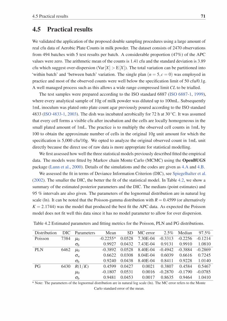
4.5 Practical results 71
4.5 Practical results
We validated the application of the proposed double sampling procedures using a large amount of
real cfu data of Aerobic Plate Counts in milk powder. The dataset consists of 2470 observations
from 494 batches with 5 test results per batch. A considerable proportion (47%) of the APC
values were zero. The arithmetic mean of the counts is 1.41 cfu and the standard deviation is 3.89
cfu which suggest over-dispersion (Var [X ]> E [X ]). The total variation can be partitioned into
‘within batch’ and ‘between batch’ variation. The single plan (n = 5,c = 0) was employed in
practice and most of the observed counts were well below the specification limit of 50 cfu/0.1g.
A well managed process such as this allows a wide range compressed limit CL to be trialled.
The test samples were prepared according to the ISO standard 6887 (ISO 6887-1, 1999),
where every analytical sample of 10g of milk powder was diluted up to 100mL. Subsequently
1mL inoculum was plated onto plate count agar previously poured according to the ISO standard
4833 (ISO 4833-1, 2003). The dish was incubated aerobically for 72 h at 30◦C. It was assumed
that every cell forms a visible cfu after incubation and the cells are locally homogeneous in the
small plated amount of 1mL. The practice is to multiply the observed cell counts in 1mL by
100 to obtain the approximate number of cells in the original 10g unit amount for which the
specification is 5,000 cfu/10g. We opted to analyze the original observed count in 1mL unit
directly because the direct use of raw data is more appropriate for statistical modelling.
We first assessed how well the three statistical models previously described fitted the empirical
data. The models were fitted by Markov chain Monte Carlo (MCMC) using the OpenBUGSpackage (Lunn et al., 2000). Details of the simulations and the codes are given as 4.A and 4.B.
We assessed the fit in terms of Deviance Information Criterion (DIC), see Spiegelhalter et al.
(2002). The smaller the DIC, the better the fit of the statistical model. In Table 4.2, we show a
summary of the estimated posterior parameters and the DIC. The medians (point estimates) and
95 % intervals are also given. The parameters of the lognormal distribution are in natural log
scale (ln). It can be noted that the Poisson-gamma distribution with R = 0.4599 (or alternatively
K = 2.1744) was the model that produced the best fit the APC data. As expected the Poisson
model does not fit well this data since it has no model parameter to allow for over dispersion.
Table 4.2 Estimated parameters and fitting metrics for the Poisson, PLN and PG distributions.
Distribution DIC Parameters Mean SD MC error 2.5% Median 97.5%
Poisson 7384 μ0 -0.2255* 0.0528 7.30E-04 -0.3313 -0.2256 -0.1214
σb 0.9927 0.0432 7.43E-04 0.9131 0.9910 1.0810
PLN 6462 μ0 -0.3892 0.0528 8.40E-04 -0.4942 -0.3884 -0.2869
σw 0.6622 0.0308 8.04E-04 0.6039 0.6616 0.7245
σb 0.9240 0.0438 8.40E-04 0.8411 0.9228 1.0140
PG 6430 R(1/K) 0.4599 0.0427 0.0021 0.3807 0.4584 0.5467
μ0 -0.1807 0.0531 0.0016 -0.2870 -0.1790 -0.0785
σb 0.9481 0.0453 0.0017 0.8635 0.9464 1.0410* Note: The parameters of the lognormal distribution are in natural log scale (ln). The MC error refers to the Monte
Carlo standard error of the mean.

72 New two-stage sampling inspection plans for bacterial cell counts
Using the web-based tool described in Section 4.6, the double plan n1 = 3, n2 = 3, a1 = 0,
r1 = 2, r2 = 2, m = 50, CL = 28 can be found as the Approach 1 plan matching (n = 5,c = 0)
single plan. The matching Approach 2 double plan is with n1 = 3, n2 = 3, a1 = 0, r1 = 2, r1m = 0,
r2 = 2, m = 50, t = 33. This plan also better satisfies the restrictions involving both two points
in the OC curve and the IQ value p0 with relative slope h0.
1.2 1.4 1.6 1.8
0.0
0.2
0.4
0.6
0.8
1.0
log10(λ)
Pa
●
●
●
h0 = 3.406
●
h0 = 3.508
●
h0 = 3.502
n = 5 , c = 0 , m = 50n1 = 3 , n2 = 3 , a1 = 0 , r1 = 2 , r2 = 2 , m = 50 , CL = 28n1 = 3 , n2 = 3 , a1 = 0 , r1 = 2 , r1m = 1 , r2 = 2 , m = 50 , CL = 33
Fig. 4.10 Operating Characteristic (OC) curve of the reference single sampling plan n = 5,
c = 0, m = 50 modelled with the negative binomial distribution with K = 2.17. The dashed line
represents the double plan n1 = 3, n2 = 3, a1 = 0, r1 = 2, r2 = 2, m = 50, CL = 28. The dotdash
line represents the plan n1 = 3, n2 = 3, a1 = 0, r1 = 2, r1m = 0, r2 = 2, m = 50, CL = 33.
Three batches out of 494 were rejected under the traditional sampling plan (n = 5, c = 0),
because at least one observation was over the specification limit m = 50 cfu. In Table 4.3 we
summarize the batch sentencing results for the MCMC simulation of a large series of batches
using the APC dataset we studied. Since the double plans require n1 = 3 in the first stage, three
observations out of five are randomly selected without replacement. By considering all possible
selections we obtain a probability of rejection by the double plans.
A particular batch with sample counts (33, 20, 35, 44, 13) was accepted under the single plan
but this lot will be rejected under Approach 1 with a probability of at least 0.7 mainly because
three of the values are over the CL = 28. Using Approach 2 where CL = 33 the same batch
will be rejected with probability of at least 0.4. This particular batch exhibits marginal sanitary
quality. From Table 4.3 we notice that the total saving when using the double plans is around
40%. In general we found that the second approach performs better than the first one in terms
of the expected number of rejected nonconforming batches. For example, the following three
batches were rejected under the traditional plan: (1) 2, 4, 4, 69, 58, (2) 11, 85, 15, 23, 2 and (3)
0, 0, 1, 0, 56. They will have probabilities of at least 0.9, 0.6 and 0.6 of being rejected by the
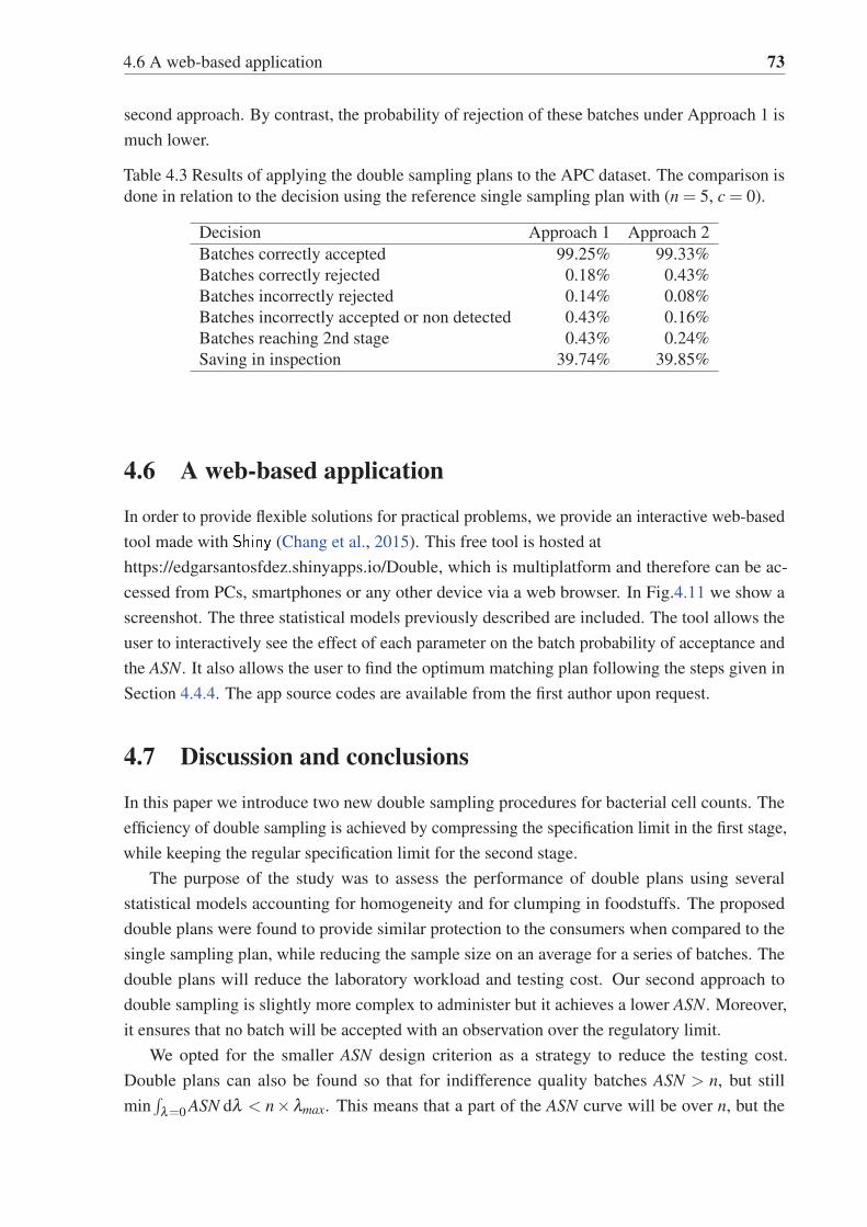
4.6 A web-based application 73
second approach. By contrast, the probability of rejection of these batches under Approach 1 is
much lower.
Table 4.3 Results of applying the double sampling plans to the APC dataset. The comparison is
done in relation to the decision using the reference single sampling plan with (n = 5, c = 0).
Decision Approach 1 Approach 2
Batches correctly accepted 99.25% 99.33%
Batches correctly rejected 0.18% 0.43%
Batches incorrectly rejected 0.14% 0.08%
Batches incorrectly accepted or non detected 0.43% 0.16%
Batches reaching 2nd stage 0.43% 0.24%
Saving in inspection 39.74% 39.85%
4.6 A web-based application
In order to provide flexible solutions for practical problems, we provide an interactive web-based
tool made with (Chang et al., 2015). This free tool is hosted at
https://edgarsantosfdez.shinyapps.io/Double, which is multiplatform and therefore can be ac-
cessed from PCs, smartphones or any other device via a web browser. In Fig.4.11 we show a
screenshot. The three statistical models previously described are included. The tool allows the
user to interactively see the effect of each parameter on the batch probability of acceptance and
the ASN. It also allows the user to find the optimum matching plan following the steps given in
Section 4.4.4. The app source codes are available from the first author upon request.
4.7 Discussion and conclusions
In this paper we introduce two new double sampling procedures for bacterial cell counts. The
efficiency of double sampling is achieved by compressing the specification limit in the first stage,
while keeping the regular specification limit for the second stage.
The purpose of the study was to assess the performance of double plans using several
statistical models accounting for homogeneity and for clumping in foodstuffs. The proposed
double plans were found to provide similar protection to the consumers when compared to the
single sampling plan, while reducing the sample size on an average for a series of batches. The
double plans will reduce the laboratory workload and testing cost. Our second approach to
double sampling is slightly more complex to administer but it achieves a lower ASN. Moreover,
it ensures that no batch will be accepted with an observation over the regulatory limit.
We opted for the smaller ASN design criterion as a strategy to reduce the testing cost.
Double plans can also be found so that for indifference quality batches ASN > n, but still
min∫
λ=0 ASN dλ < n×λmax. This means that a part of the ASN curve will be over n, but the

74 New two-stage sampling inspection plans for bacterial cell counts
Fig. 4.11 Screenshot of the online app for matching single concentration-based sampling plan
and double sampling plans based on compressed limit in stage 1.
Online at: https://edgarsantosfdez.shinyapps.io/Double

4.A Markov chain Monte Carlo (MCMC) method 75
area underneath this curve will be smaller than the area below n. The double plan can also
provide consumer protection against over-dispersed contamination and marginal quality batches
as described in Section 4.5.
Any two-stage sampling plan must be predefined before the actual inspection is carried out.
The proposed plan should not be used as a way of giving another chance to a rejected batch using
a single plan; see the warning given by ICMSF (2002).
Quoting Earl Wiener’s 29th law: “Whenever you solve a problem, you usually create one.You can only hope that the one you created is less critical than the one you eliminated.” The
trade-off in our procedure is the delayed decision time whenever the second stage is reached.
This, however, will not affect the normal operation as long as the process is well maintained
and is kept in a state of statistical control. Under the proposed plan, most poor quality batches
will be sentenced in the first stage of sampling itself. A second stage is mostly required around
the indifference quality levels, which often corresponds to marginal quality batches. The batch
probability of acceptance is more complex to derive for the proposed double plans. However,
this difficulty is overcome using the online app that allows visual matching of sampling plans.
Finally, this technique might be extended to three-class sanitary characteristics based on two
stages, but with obvious detriment to the simplicity of the inspection protocols.
Appendix 4.A Markov chain Monte Carlo (MCMC) method
The fitting of the statistical models was done in OpenBUGS package using MCMC. We simu-
lated three chains each with 10,000 iterations, checked convergence and discarded a ‘burn-in’ of
500 samples. In the Poisson-lognormal case, the within and between standard deviations (σw
and σb) were considered as constant across batches, while μ is a random effect that varies from
batch to batch. Therefore,
λ ∼ L N (μ,σw) (4.12)
where is normally distributed with μ0 and σb.
μ ∼ N (μ0,σb) (4.13)
For priors we used μ0 ∼ N (0,0.01), σw ∼ U (0,10) and σb ∼ U (0,50), which are all
largely uninformative. In the negative binomial (or Poisson-gamma) case, we assumed the
mean concentration m as a random batch effect, while the dispersion parameter or shape K was
considered as constant. For convenience, we used R = 1/K, with prior R ∼ Exp(10−7
)to allow
for the possibility of no over-dispersion (R = 0). For m we used the prior m ∼ L N (μ0,σb).
Finally, in the Poisson distribution case, we assumed that the rate λ changes from batch-to-batch,
lognormally distributed λ ∼ L N (μ0,σb) since it can take only positive values.
The posterior densities of every parameter for the negative binomial distribution case are
shown in Fig.4.12.

76 New two-stage sampling inspection plans for bacterial cell counts
R sample: 00
0.3 0.4 0.5 0.6 0.7P
(R)
0.0
5.0
10.0
sample: 00
-0.2 5.55E-17 0.2-0.6 -0.4
P(
)0.
04.
08.
0
R
sample: 00
0.7 0.8 0.9 1.0 1.1 1.2
P(
)0.
05.
010
.0
Fig. 4.12 Posterior densities of the fit to the negative binomial distribution. The parameter R is
the reciprocal of the dispersion parameter K (R = 1/K.)
Appendix 4.B codes used for the simulations
4.B.1 Negative binomial� �
model{for ( i in 1:2470) {
Count[i] ~ dpois(lambda[i])lambda[i] ~ dgamma(r, b[Batch[i]])
}
for ( j in 1 : 494) {mu[j] ~ dlnorm(mu0,tau0)b[ j ] r / mu[j]
}
tau0 1 / (sig0 * sig0)r 1 / R
#Priors distributions :mu0 ~ dnorm(0,0.01)R ~ dexp(0.0000001)sig0 ~ dunif(0,50)
}
#chain inits :list (mu0 = 0, R = 2, sig0 = 0.01)list (mu0 = 0.2, R = 1, sig0 = 0.05)list (mu0 = 0.2, R = 0.5, sig0 = 0.1)
�� �
4.B.2 Poisson-lognormal� �
model{

4.B codes used for the simulations 77
for ( i in 1 : 2470) {Count[i] ~ dpois(lambda[i])lambda[i] ~ dlnorm(mu[Batch[i]], tau)
}
for ( j in 1 : 494) {mu[j] ~ dnorm(mu0,tau0)
}
tau 1 / (sig * sig)tau0 1 / (sig0 * sig0)
#Priors:mu0 ~ dnorm(0,0.01)sig ~ dunif(0,10)sig0 ~ dunif(0,50)
}
#chain inits :list (mu0 = 0, sig = 2, sig0 = 0.1)list (mu0 = 1, sig = 0.1, sig0 = 0.5)list (mu0 = 1, sig = 0.5, sig0 = 2)
�� �
4.B.3 Poisson� �
model{for ( i in 1 : 2470) {
Count[i] ~ dpois(mu[Batch[i ]])}
for ( j in 1 : 494) {mu[j] ~ dlnorm(mu0,tau0)
}
tau0 1 / (sig0 * sig0)
#Priors:mu0 ~ dnorm(1,0.01)sig0 ~ dunif(0,50)
}
#chain inits :list (mu0 = 0, sig0 = 0.1)list (mu0 = 0.5, sig0 = 0.5)list (mu0 = 1, sig0 = 2)
�� �


Chapter 5
Effects of imperfect testing onpresence-absence sampling plans
Edgar Santos-Fernández, K. Govindaraju, Geoff Jones
Quality and Reliability Engineering International, Submitted 1
5.1 Abstract
Test performance measures such as sensitivity and specificity are generally ignored in microbi-
ological risk assessment. In this research we examine the impact of imperfect analytical tests
on sampling inspection plans for presence-absence characteristics. We discuss several plausible
scenarios and assess the risk for the consumers. The method is illustrated using collected data
over two years for Cronobacter spp. (formerly Enterobacter sakazakii) in skimmed milk powder.
The probability of contamination and the test sensitivity and specificity, are estimated using
Bayesian inference. We examine the sampling plans proposed by the Codex Alimentarius and by
New Zealand’s Ministry of Primary Industries for this pathogen. A cost analysis is carried out to
show the economic loss due to measurement errors. We describe the strengths and limitations of
these plans under different conditions and propose a plan that could provide better protection to
the consumers as well as to the producers.
Keywords
presence-absence tests; sensitivity; specificity; sampling inspection plan; Bayesian inference;
measurement errors; Cronobacter spp.
1An abridged version of this paper was presented at the European Network for Business and Industrial Statistics
(ENBIS) 2016 Annual Conference in Sheffield, UK. http://www.enbis.org/activities/events/current/424_ENBIS_16_in_Sheffield/programmeitem/2164_Effects_of_Imperfect_Testing_on_Presence_Absence_Sampling_Plans

80 Effects of imperfect testing on presence-absence sampling plans
5.2 Introduction
Binary or presence/absence tests aim to classify items, samples or individuals into two classes,
e.g. positive or negative, pass or fail. The efficacy of these tests is expressed by metrics like
sensitivity (se) and specificity (sp). Sensitivity refers to the test’s ability to detect the true
positives (TP). The sensitivity is computed as the number of true positives divided by the total
number of positives (P). P = TP + FN, where FN is the number of false negatives. By contrast,
the specificity expresses the ability of the test to detect true negatives (TN). It is obtained as the
number of true negatives divided by the number of negatives, where N = TN + FP.
The test sensitivity and specificity are assumed to be independent of the prevalence in
the population. Perfect sensitivity and specificity are desirable but not achievable in practice.
Generally, se and sp over 95% are considered appropriate. See for instance Eijkelkamp et al.
(2009). Commonly, there is a trade-off between sensitivity and specificity, which can be
illustrated in the receiver operating characteristic (ROC) curve. The symbols used in this paper
are listed in 5.A.
In the food safety area
FAO/WHO (2014) defines the probability of detecting a target microorganism for a supposedly
perfect specificity and sensitivity. The ICMSF (2002, pp.9) has pointed out that microbial
testing “often lacks sensitivity and specificity” and that usually the sensitivity is sacrificed to
reduce the laboratory time. In practice, tests are usually assumed to be perfectly sensitive and
specific (Pouillot et al., 2013) and microbial sampling plans are based on that assumption. In
this regard ICMSF (2002, pp.120) suggest that when sensitivity and specificity are known for
a particular microbiological method the computation of the risk should be adjusted. This is
partially possible thanks to the FAO/WHO (2012) tool that incorporates into the model the test
sensitivity. Hoelzer and Pouillot (2013) also studied the impact of imperfect test sensitivity in
microbial risk assessment using low sample sizes.
In the traditional culture methods the specificity is generally high and commonly assumed
100% (Gardner, 2004; Hoelzer and Pouillot, 2013; Powell, 2014).
Empirical studies suggest that perfect specificity is seldom attained, independent of the
detection methods. For instance, the cross-contamination risk cannot be completely eliminated.
5.B shows the reported performance indicators of several detection methods (culture, PCR,
immunological, etc.) for different commodities and type of microorganisms. Iversen et al. (2008)
using the FDA (2002) method for Cronobacter spp. detection in powdered infant formula showed
as low as 52.2% sensitivity and 73.5% specificity. In this research we discuss the effect of
imperfect classifiers on the performance of microbiological presence-absence sampling plans.
Our purpose is to reduce the risks and the costs due to sampling and measurement errors. The
remainder of the paper is summarized in Fig. 5.1.

5.2 Introduction 81
Fig. 5.1 Mindmap of the structure of the article (clockwise)
Presence-
absence
sampling plans
1-
Introduction
Food
safety
2-Materials
and methods
Analytical
unit Sampling
distri-
bution
Statistical
sample
size (n)
Population
of
microor-
ganisms
Sampling
method
Composite
units
3-Single
(isolated)
batch risk
assessment
Model
based
on p
Model
based on
the rate λ
Zero
inflated
Poisson
lognormal
model
4-Bayesian
data
analysis
n = 1,
w = 300g
vs.
n = 30,
w = 10g
5-Cost
analysis
6-
Discussion
and
conclusions
The re-
sampling
dilemma

82 Effects of imperfect testing on presence-absence sampling plans
5.3 Materials and methods
5.3.1 Discretization and the analytical unit
Bulk materials are generally studied by splitting into supposedly ‘discrete units’ for analysis.
These analytical units can be conceptualized by supposing that an imaginary two or three-
dimensional square grid is unfolded over the batch. The size of the grid defines the analytical
unit amount.
Let p be the analytical unit probability of contamination for a perfect classifier. That is, p is
the probability of finding one or more microorganisms in the analytical unit. We should mention
that generally in the inspection of discrete items, p denotes a population parameter, which does
not dependent on sampling. However, in bulk materials p is subject to the grid size used to
discretize the lot and hence it will be conditioned by the sampling method.
Discretization is a complex issue and it is known in some disciplines as the Modifiable
Areal Unit Problem (MAUP). See e.g. Wong (2009). To illustrate how the use of different grid
structures leads to different probability of detection, consider the following hypothetical example.
Fig. 5.2 depicts a section of a batch under two different grids. Suppose that the smaller grid in
(a) splits the material into 1 g units, while the larger into 4 g units. The mean concentration is
independent of the grid, being equal to 1 colony-forming unit per gram (cfu/g). However, the
standard deviations are 1.21 cfu/g and 0 respectively. Also the proportion nonconforming is 0.5
in the first case and 1 in the second one.
(a)
●
●
●
●
●
●
●●
●
●
●●
●
●
●
●
(b)
●
●
●
●
●
●
●●
●
●
●●
●
●
●
●
Fig. 5.2 Effect of the grid size in the standard deviations and the proportion nonconforming. The
grids split the batch into 1 g (a) units and 4 g (b) units respectively.
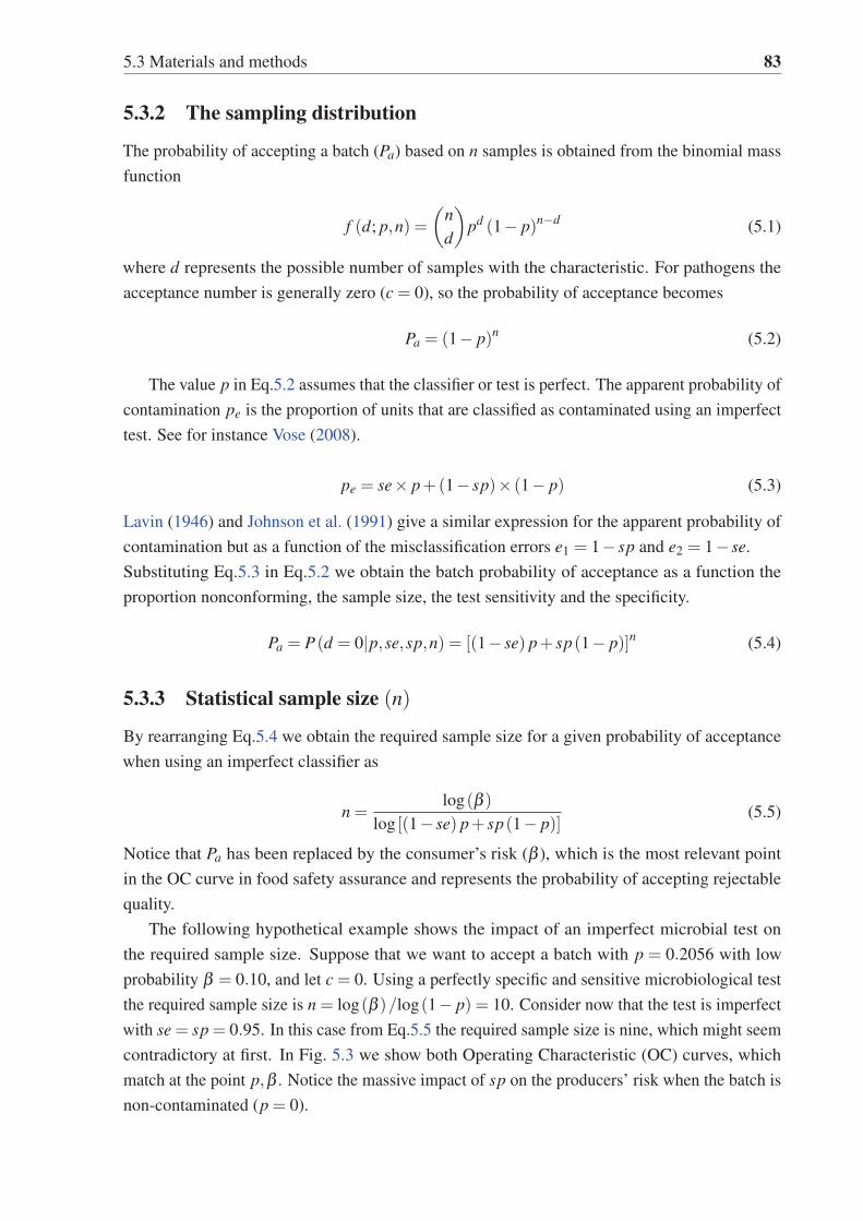
5.3 Materials and methods 83
5.3.2 The sampling distribution
The probability of accepting a batch (Pa) based on n samples is obtained from the binomial mass
function
f (d; p,n) =(
nd
)pd (1− p)n−d (5.1)
where d represents the possible number of samples with the characteristic. For pathogens the
acceptance number is generally zero (c = 0), so the probability of acceptance becomes
Pa = (1− p)n (5.2)
The value p in Eq.5.2 assumes that the classifier or test is perfect. The apparent probability of
contamination pe is the proportion of units that are classified as contaminated using an imperfect
test. See for instance Vose (2008).
pe = se× p+(1− sp)× (1− p) (5.3)
Lavin (1946) and Johnson et al. (1991) give a similar expression for the apparent probability of
contamination but as a function of the misclassification errors e1 = 1− sp and e2 = 1− se.
Substituting Eq.5.3 in Eq.5.2 we obtain the batch probability of acceptance as a function the
proportion nonconforming, the sample size, the test sensitivity and the specificity.
Pa = P(d = 0|p,se,sp,n) = [(1− se) p+ sp(1− p)]n (5.4)
5.3.3 Statistical sample size (n)
By rearranging Eq.5.4 we obtain the required sample size for a given probability of acceptance
when using an imperfect classifier as
n =log(β )
log [(1− se) p+ sp(1− p)](5.5)
Notice that Pa has been replaced by the consumer’s risk (β ), which is the most relevant point
in the OC curve in food safety assurance and represents the probability of accepting rejectable
quality.
The following hypothetical example shows the impact of an imperfect microbial test on
the required sample size. Suppose that we want to accept a batch with p = 0.2056 with low
probability β = 0.10, and let c = 0. Using a perfectly specific and sensitive microbiological test
the required sample size is n = log(β )/log(1− p) = 10. Consider now that the test is imperfect
with se = sp = 0.95. In this case from Eq.5.5 the required sample size is nine, which might seem
contradictory at first. In Fig. 5.3 we show both Operating Characteristic (OC) curves, which
match at the point p,β . Notice the massive impact of sp on the producers’ risk when the batch is
non-contaminated (p = 0).
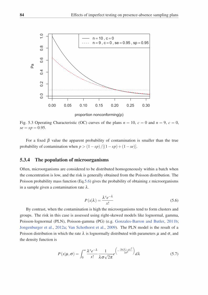
84 Effects of imperfect testing on presence-absence sampling plans
0.00 0.05 0.10 0.15 0.20 0.25 0.30
0.0
0.2
0.4
0.6
0.8
1.0
proportion nonconforming(p)
Pan = 10 , c = 0n = 9 , c = 0 , se = 0.95 , sp = 0.95
Fig. 5.3 Operating Characteristic (OC) curves of the plans n = 10, c = 0 and n = 9, c = 0,
se = sp = 0.95.
For a fixed β value the apparent probability of contamination is smaller than the true
probability of contamination when p > (1− sp)/[(1− sp)+(1− se)].
5.3.4 The population of microorganisms
Often, microorganisms are considered to be distributed homogeneously within a batch when
the concentration is low, and the risk is generally obtained from the Poisson distribution. The
Poisson probability mass function (Eq.5.6) gives the probability of obtaining x microorganisms
in a sample given a contamination rate λ .
P(x|λ ) = λ xe−λ
x!(5.6)
By contrast, when the contamination is high the microorganisms tend to form clusters and
groups. The risk in this case is assessed using right-skewed models like lognormal, gamma,
Poisson-lognormal (PLN), Poisson-gamma (PG) (e.g. Gonzales-Barron and Butler, 2011b;
Jongenburger et al., 2012a; Van Schothorst et al., 2009). The PLN model is the result of a
Poisson distribution in which the rate λ is lognormally distributed with parameters μ and σ , and
the density function is
P(x|μ,σ) =∫ ∞
0
λ xe−λ
x!
1
λσ√
2πe
(− (ln(λ )−μ)2
2σ2
)dλ (5.7)

5.3 Materials and methods 85
Poisson-gamma instead arises when the rate (λ ) follows a gamma distribution. The density
as a function of mean concentration m = E [X ] and the dispersion parameter K is:
P(X = x|K,m) =Γ(K + x)Γ(K)x!
(K
K +m
)K (m
K +m
)x
(5.8)
where Γ is the gamma function.
Another useful mixed distribution is the Conway-Maxwell-Poisson (CMP) distribution
(Shmueli et al., 2005). This model allows both underdispersion and overdispersion by including
an extra parameter (ν).
P(x) =λ x
(x!)ν1
Z (λ ,ν)(5.9)
where λ > 0, ν � 0 and the normalizing constant Z (λ ,ν) is
Z (λ ,ν) =∞
∑j=0
λ j
( j!)ν (5.10)
Other models such as zero-inflated Poisson (ZIP) or zero-inflated negative binomial (ZINB)
can be used as well when the frequency of zero values is very high. See e.g. Lambert (1992) and
Hall (2000). Both models were considered by Gonzales-Barron et al. (2010a) to model E. coliand coliforms counts in beef carcasses.
In Eq.5.7 λ is lognormal distributed and therefore it does not allows for complete absence
of the pathogen in the batch (λ = 0). To solve this issue we propose the use of a zero inflated
Poisson-lognormal distribution. This model comprises two parts. The first one is a binary process
governed by a Bernoulli law defining the proportion of zero values or the inflation probability
(θ ). The second part will contain the realization being Poisson-lognormally distributed. Hence
λ is a semi-continuous variable. The probability mass function is:
Pr(yi = 0) = θ +(1−θ)g(0) ;xi = 0
Pr(yi = xi) = (1−θ)g(xi) ;xi � 1(5.11)
where g is a discrete probability mass function, PLN in this case.
5.3.5 The sampling method
The spatial distribution of the contamination needs to be considered when deciding the sampling
method to be used. Random or systematic sampling will not make any difference in the
probability of detection for a perfectly homogenous contamination. However, under heterogeneity
(specifically under localized contamination) systematic sampling has been found more suitable
to detect pathogens in food. See e.g. Jongenburger et al. (2011b).
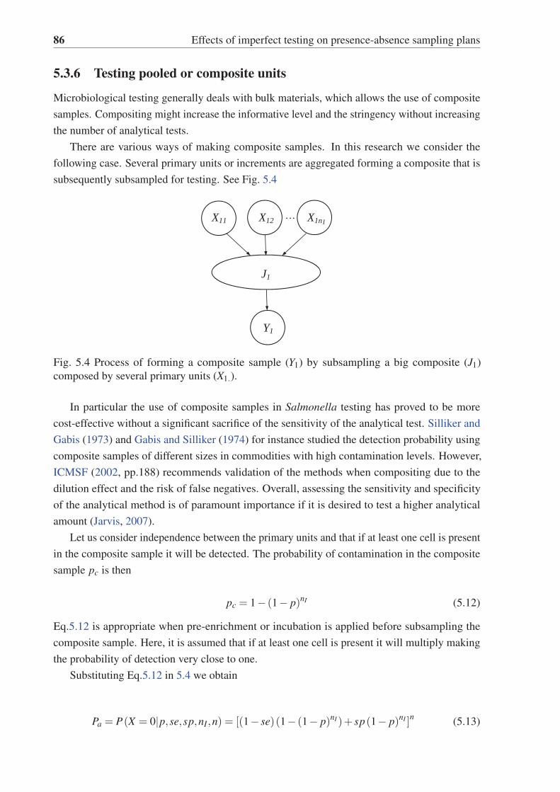
86 Effects of imperfect testing on presence-absence sampling plans
5.3.6 Testing pooled or composite units
Microbiological testing generally deals with bulk materials, which allows the use of composite
samples. Compositing might increase the informative level and the stringency without increasing
the number of analytical tests.
There are various ways of making composite samples. In this research we consider the
following case. Several primary units or increments are aggregated forming a composite that is
subsequently subsampled for testing. See Fig. 5.4
I
Y1
X1nX12 …X11
J1
Fig. 5.4 Process of forming a composite sample (Y1) by subsampling a big composite (J1)
composed by several primary units (X1.).
In particular the use of composite samples in Salmonella testing has proved to be more
cost-effective without a significant sacrifice of the sensitivity of the analytical test. Silliker and
Gabis (1973) and Gabis and Silliker (1974) for instance studied the detection probability using
composite samples of different sizes in commodities with high contamination levels. However,
ICMSF (2002, pp.188) recommends validation of the methods when compositing due to the
dilution effect and the risk of false negatives. Overall, assessing the sensitivity and specificity
of the analytical method is of paramount importance if it is desired to test a higher analytical
amount (Jarvis, 2007).
Let us consider independence between the primary units and that if at least one cell is present
in the composite sample it will be detected. The probability of contamination in the composite
sample pc is then
pc = 1− (1− p)nI (5.12)
Eq.5.12 is appropriate when pre-enrichment or incubation is applied before subsampling the
composite sample. Here, it is assumed that if at least one cell is present it will multiply making
the probability of detection very close to one.
Substituting Eq.5.12 in 5.4 we obtain
Pa = P(X = 0|p,se,sp,nI,n) = [(1− se)(1− (1− p)nI)+ sp(1− p)nI ]n (5.13)
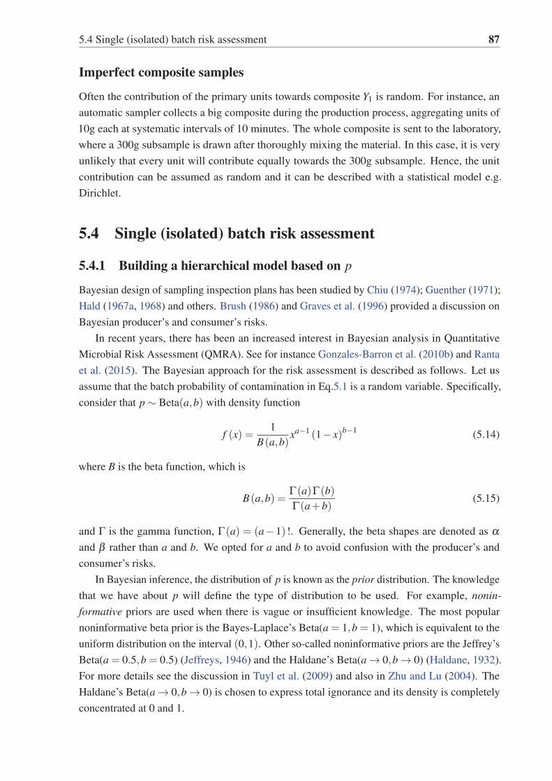
5.4 Single (isolated) batch risk assessment 87
Imperfect composite samples
Often the contribution of the primary units towards composite Y1 is random. For instance, an
automatic sampler collects a big composite during the production process, aggregating units of
10g each at systematic intervals of 10 minutes. The whole composite is sent to the laboratory,
where a 300g subsample is drawn after thoroughly mixing the material. In this case, it is very
unlikely that every unit will contribute equally towards the 300g subsample. Hence, the unit
contribution can be assumed as random and it can be described with a statistical model e.g.
Dirichlet.
5.4 Single (isolated) batch risk assessment
5.4.1 Building a hierarchical model based on p
Bayesian design of sampling inspection plans has been studied by Chiu (1974); Guenther (1971);
Hald (1967a, 1968) and others. Brush (1986) and Graves et al. (1996) provided a discussion on
Bayesian producer’s and consumer’s risks.
In recent years, there has been an increased interest in Bayesian analysis in Quantitative
Microbial Risk Assessment (QMRA). See for instance Gonzales-Barron et al. (2010b) and Ranta
et al. (2015). The Bayesian approach for the risk assessment is described as follows. Let us
assume that the batch probability of contamination in Eq.5.1 is a random variable. Specifically,
consider that p ∼ Beta(a,b) with density function
f (x) =1
B(a,b)xa−1 (1− x)b−1 (5.14)
where B is the beta function, which is
B(a,b) =Γ(a)Γ(b)Γ(a+b)
(5.15)
and Γ is the gamma function, Γ(a) = (a−1) !. Generally, the beta shapes are denoted as αand β rather than a and b. We opted for a and b to avoid confusion with the producer’s and
consumer’s risks.
In Bayesian inference, the distribution of p is known as the prior distribution. The knowledge
that we have about p will define the type of distribution to be used. For example, nonin-formative priors are used when there is vague or insufficient knowledge. The most popular
noninformative beta prior is the Bayes-Laplace’s Beta(a = 1,b = 1), which is equivalent to the
uniform distribution on the interval (0,1). Other so-called noninformative priors are the Jeffrey’s
Beta(a = 0.5,b = 0.5) (Jeffreys, 1946) and the Haldane’s Beta(a → 0,b → 0) (Haldane, 1932).
For more details see the discussion in Tuyl et al. (2009) and also in Zhu and Lu (2004). The
Haldane’s Beta(a → 0,b → 0) is chosen to express total ignorance and its density is completely
concentrated at 0 and 1.

88 Effects of imperfect testing on presence-absence sampling plans
In the Bayesian inference, today’s posterior is tomorrow’s prior. Usually, some relevant
knowledge is available from previous analysis and research. We might consider a priori that
pathogens are rarely present in foodstuffs and that the probability of contamination is very low.
Then we could opt for an informative prior, say a beta distribution with small a and large b. For
example, a = 1, b = 199 yields mean and standard deviation equal to 0.005.
Substituting the prior (Eq.5.14) in the sampling distribution (5.1) we obtain the beta-binomial
distribution
f (d|n,a,b) =(
nd
)B(d +a,n−d +b)
B(a,b)(5.16)
The test’s sensitivity and specificity are generally unknown and they can also be considered
as random variables. In this case, we could describe them with beta distributions as well. Let
us denote the shape parameters for the distribution of the sensitivity as ase and bse. Equally,
we will denote the shapes for the distribution of the specificity as asp and bsp. As seen from
5.B both metrics are generally close to one. Therefore, it seems reasonable to use informative
beta distributions with mass concentrated around one and therefore with values a >> b. If seand sp are included in the model, the probability distribution of Pa is obtained from the triple
integral of Eq.5.13 with respect to p, se and sp. This function has no closed form. See for
instance Rahme et al. (2000). Therefore, we resort to numerical integration to obtain the batch
probability of acceptance. We have developed a shiny application (app), which is available at:
https://edgarsantosfdez.shinyapps.io/PreAbs to obtain the Pa given different priors. In 5.D we
present a screenshot. In 5.C.1 we show the model codes we used.
Let us consider the following four scenarios in order to show how the parameters affect the
probability of acceptance and the risk for the consumers.
• Scenario 1: Beta prior (a = 1, b = 99), high the test sensitivity and specificity (ase = asp =
99,bse = bsp = 1).
• Scenario 2: Beta prior (a = 1, b = 99) , moderate sensitivity and specificity (ase = asp =
19,bse = bsp = 1).
• Scenario 3: Prior distribution of p is Haldane-type (a = b = 0.005), high test sensitivity
(ase = 99,bse = 1) and specificity (asp = 99,bsp = 1).
• Scenario 4: Haldane-type (a = b = 0.001) prior distribution for p, moderate sensitivity
and specificity (ase = asp = 19,bse = bsp = 1).
In Table 5.1 we show the mean of the proportion nonconforming (p), the apparent proportion
nonconforming (pe) and the batch probability of acceptance (Pa), for different sample sizes and
parameters for the prior distributions. This table gives the four scenarios previously described.
We notice that the sp has a major effect on Pa. It can be noticed that the selection of the prior
distribution for p has a critical impact on the risk as well. The se seems much less important that
the other two factors even with a small sample size.
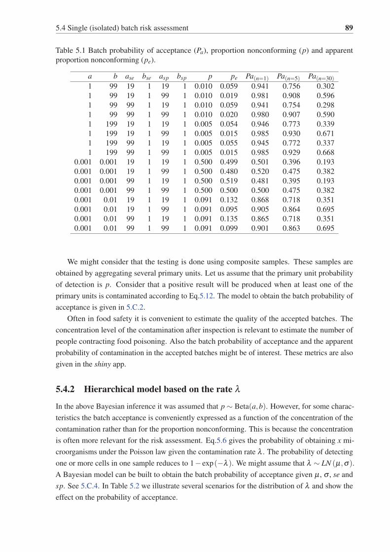
5.4 Single (isolated) batch risk assessment 89
Table 5.1 Batch probability of acceptance (Pa), proportion nonconforming (p) and apparent
proportion nonconforming (pe).
a b ase bse asp bsp p pe Pa(n=1) Pa(n=5) Pa(n=30)
1 99 19 1 19 1 0.010 0.059 0.941 0.756 0.302
1 99 19 1 99 1 0.010 0.019 0.981 0.908 0.596
1 99 99 1 19 1 0.010 0.059 0.941 0.754 0.298
1 99 99 1 99 1 0.010 0.020 0.980 0.907 0.590
1 199 19 1 19 1 0.005 0.054 0.946 0.773 0.339
1 199 19 1 99 1 0.005 0.015 0.985 0.930 0.671
1 199 99 1 19 1 0.005 0.055 0.945 0.772 0.337
1 199 99 1 99 1 0.005 0.015 0.985 0.929 0.668
0.001 0.001 19 1 19 1 0.500 0.499 0.501 0.396 0.193
0.001 0.001 19 1 99 1 0.500 0.480 0.520 0.475 0.382
0.001 0.001 99 1 19 1 0.500 0.519 0.481 0.395 0.193
0.001 0.001 99 1 99 1 0.500 0.500 0.500 0.475 0.382
0.001 0.01 19 1 19 1 0.091 0.132 0.868 0.718 0.351
0.001 0.01 19 1 99 1 0.091 0.095 0.905 0.864 0.695
0.001 0.01 99 1 19 1 0.091 0.135 0.865 0.718 0.351
0.001 0.01 99 1 99 1 0.091 0.099 0.901 0.863 0.695
We might consider that the testing is done using composite samples. These samples are
obtained by aggregating several primary units. Let us assume that the primary unit probability
of detection is p. Consider that a positive result will be produced when at least one of the
primary units is contaminated according to Eq.5.12. The model to obtain the batch probability of
acceptance is given in 5.C.2.
Often in food safety it is convenient to estimate the quality of the accepted batches. The
concentration level of the contamination after inspection is relevant to estimate the number of
people contracting food poisoning. Also the batch probability of acceptance and the apparent
probability of contamination in the accepted batches might be of interest. These metrics are also
given in the shiny app.
5.4.2 Hierarchical model based on the rate λ
In the above Bayesian inference it was assumed that p ∼ Beta(a,b). However, for some charac-
teristics the batch acceptance is conveniently expressed as a function of the concentration of the
contamination rather than for the proportion nonconforming. This is because the concentration
is often more relevant for the risk assessment. Eq.5.6 gives the probability of obtaining x mi-
croorganisms under the Poisson law given the contamination rate λ . The probability of detecting
one or more cells in one sample reduces to 1− exp(−λ ). We might assume that λ ∼ LN (μ,σ).
A Bayesian model can be built to obtain the batch probability of acceptance given μ , σ , se and
sp. See 5.C.4. In Table 5.2 we illustrate several scenarios for the distribution of λ and show the
effect on the probability of acceptance.
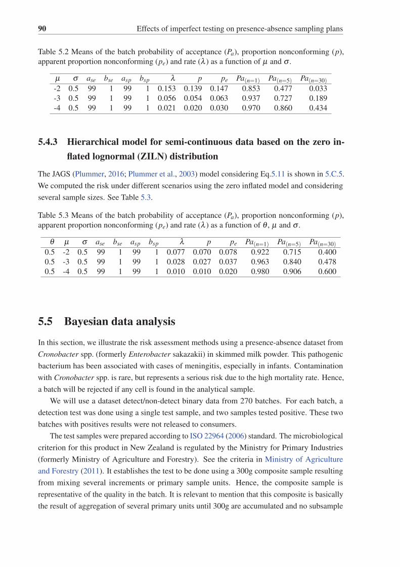
90 Effects of imperfect testing on presence-absence sampling plans
Table 5.2 Means of the batch probability of acceptance (Pa), proportion nonconforming (p),
apparent proportion nonconforming (pe) and rate (λ ) as a function of μ and σ .
μ σ ase bse asp bsp λ p pe Pa(n=1) Pa(n=5) Pa(n=30)
-2 0.5 99 1 99 1 0.153 0.139 0.147 0.853 0.477 0.033
-3 0.5 99 1 99 1 0.056 0.054 0.063 0.937 0.727 0.189
-4 0.5 99 1 99 1 0.021 0.020 0.030 0.970 0.860 0.434
5.4.3 Hierarchical model for semi-continuous data based on the zero in-flated lognormal (ZILN) distribution
The JAGS (Plummer, 2016; Plummer et al., 2003) model considering Eq.5.11 is shown in 5.C.5.
We computed the risk under different scenarios using the zero inflated model and considering
several sample sizes. See Table 5.3.
Table 5.3 Means of the batch probability of acceptance (Pa), proportion nonconforming (p),
apparent proportion nonconforming (pe) and rate (λ ) as a function of θ , μ and σ .
θ μ σ ase bse asp bsp λ p pe Pa(n=1) Pa(n=5) Pa(n=30)
0.5 -2 0.5 99 1 99 1 0.077 0.070 0.078 0.922 0.715 0.400
0.5 -3 0.5 99 1 99 1 0.028 0.027 0.037 0.963 0.840 0.478
0.5 -4 0.5 99 1 99 1 0.010 0.010 0.020 0.980 0.906 0.600
5.5 Bayesian data analysis
In this section, we illustrate the risk assessment methods using a presence-absence dataset from
Cronobacter spp. (formerly Enterobacter sakazakii) in skimmed milk powder. This pathogenic
bacterium has been associated with cases of meningitis, especially in infants. Contamination
with Cronobacter spp. is rare, but represents a serious risk due to the high mortality rate. Hence,
a batch will be rejected if any cell is found in the analytical sample.
We will use a dataset detect/non-detect binary data from 270 batches. For each batch, a
detection test was done using a single test sample, and two samples tested positive. These two
batches with positives results were not released to consumers.
The test samples were prepared according to ISO 22964 (2006) standard. The microbiological
criterion for this product in New Zealand is regulated by the Ministry for Primary Industries
(formerly Ministry of Agriculture and Forestry). See the criteria in Ministry of Agriculture
and Forestry (2011). It establishes the test to be done using a 300g composite sample resulting
from mixing several increments or primary sample units. Hence, the composite sample is
representative of the quality in the batch. It is relevant to mention that this composite is basically
the result of aggregation of several primary units until 300g are accumulated and no subsample

5.5 Bayesian data analysis 91
is done or indicated. We should also point out that the Codex (CAC, 2008), instead, establishes
for powdered infant formula the following criteria: n = 30, c = 0, w = 10g.
We assume that every cell will be recovered and will form a visible colony-forming unit after
incubation. Let us also assume that the competitive micro flora will not affect the growth of
Cronobacter spp.
We used the following Bayesian hierarchical model to describe the contamination. Since the
sample size n = 1, the sampling distribution is Bernoulli, Bern(pe,1− pe). The artificial propor-
tion nonconforming and the proportion nonconforming are related by the following expression
pe = se× p+(1− sp)× (1− p). Let us consider the test sensitivity and specificity as random
variables. The priors for the test sensitivity and specificity are se ∼ Beta(ase = 199,bse = 1) and
sp ∼ Beta(asp = 199,bsp = 1).
The proportion nonconforming p = 1− exp(−mλ ), where λ is the rate of the contamination
in 10g and m = 30. Therefore p is the probability of contamination in 300g. We considered λ as
zero inflated according to Eq.5.11 with θ ∼ Beta(a = 2,b = 20). The positive realization of λ is
lognormally distributed with μ and σw, where σw is the within-batch standard deviation. The
mean μ changes from batch to batch being normally distributed with μ0 and σb. We considered
two scenarios for the within and between-batch standard deviation and for the mean of the
lognormal distribution of contaminated batches:
• Scenario 1: μ0 =−4, σw = 0.8 and σb = 0.8.
• Scenario 2: μ0 =−2, σw = 1 and σb = 1.
The values for σ in the first scenario have been considered among others by FAO/WHO (2006).
The codes of the model for the MCMC simulations (Scenario 1) are shown in 5.C.6. We
obtained the posterior distributions using the package rjags. For plotting densities we adapted
the function diagMCMC from Kruschke (2015). We simulated three chains each with 30,000
iterations and discarded a burn-in of 5,000 samples.
Results of the MCMC simulations for Scenario 1
Based on our prior beliefs about contaminated batches in Scenario 1, the probability that a
batch that tested negative was truly free of the pathogen is estimated as 0.987. Conversely, the
probability that a batch that tested positive was really contaminated is estimated as 0.715. The
mean of the posterior density for the rate in the batches that tested positive is λ = 0.0626. Finally,
the mean of the marginal posterior sensitivity and specificity are 98.9% and 99.6% respectively.
In Fig. 5.5-5.6 we show the posterior densities for the proportion nonconforming in the
batches that tested negative (p0) and positive (p1), and also the posterior densities for se and sp.
We also did MCMC convergence diagnostics. The posterior densities show the highest density
intervals (HDI) in line with our prior beliefs and the values reported in the literature.
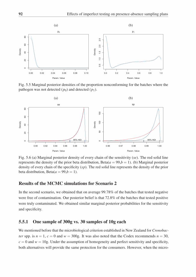
92 Effects of imperfect testing on presence-absence sampling plans
(a)
0.00 0.02 0.04 0.06 0.08 0.10
020
4060
80
p0
Param. Value
Den
sity
(b)
0.0 0.2 0.4 0.6 0.8 1.0
0.5
1.0
1.5
2.0
2.5
p1
Param. Value
Den
sity
Fig. 5.5 Marginal posterior densities of the proportion nonconforming for the batches where the
pathogen was not detected (p0) and detected (p1).
(a)
0.90 0.92 0.94 0.96 0.98 1.00
020
4060
80
se
Param. Value
Den
sity
||| |||95% HDI
(b)
0.96 0.97 0.98 0.99 1.00
050
100
150
sp
Param. Value
Den
sity
||| |||95% HDI
Fig. 5.6 (a) Marginal posterior density of every chain of the sensitivity (se). The red solid line
represents the density of the prior beta distribution, Beta(a = 99,b = 1). (b) Marginal posterior
density of every chain of the specificity (sp). The red solid line represents the density of the prior
beta distribution, Beta(a = 99,b = 1).
Results of the MCMC simulations for Scenario 2
In the second scenario, we obtained that on average 99.78% of the batches that tested negative
were free of contamination. Our posterior belief is that 72.8% of the batches that tested positive
were truly contaminated. We obtained similar marginal posterior probabilities for the sensitivity
and specificity.
5.5.1 One sample of 300g vs. 30 samples of 10g each
We mentioned before that the microbiological criterion established in New Zealand for Cronobac-ter spp. is n = 1, c = 0 and w = 300g. It was also noted that the Codex recommends n = 30,
c = 0 and w = 10g. Under the assumption of homogeneity and perfect sensitivity and specificity,
both alternatives will provide the same protection for the consumers. However, when the micro-
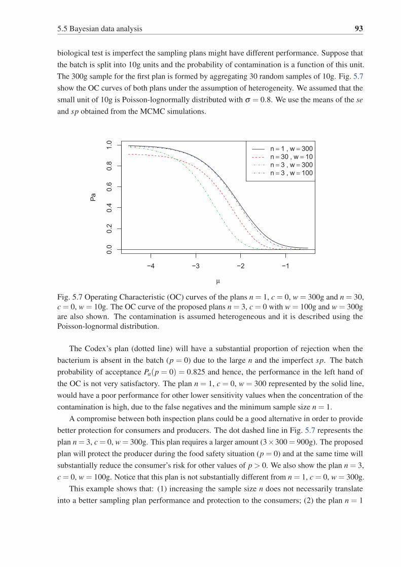
5.5 Bayesian data analysis 93
biological test is imperfect the sampling plans might have different performance. Suppose that
the batch is split into 10g units and the probability of contamination is a function of this unit.
The 300g sample for the first plan is formed by aggregating 30 random samples of 10g. Fig. 5.7
show the OC curves of both plans under the assumption of heterogeneity. We assumed that the
small unit of 10g is Poisson-lognormally distributed with σ = 0.8. We use the means of the seand sp obtained from the MCMC simulations.
−4 −3 −2 −1
0.0
0.2
0.4
0.6
0.8
1.0
μ
Pa
n = 1 , w = 300n = 30 , w = 10n = 3 , w = 300n = 3 , w = 100
Fig. 5.7 Operating Characteristic (OC) curves of the plans n = 1, c = 0, w = 300g and n = 30,
c = 0, w = 10g. The OC curve of the proposed plans n = 3, c = 0 with w = 100g and w = 300g
are also shown. The contamination is assumed heterogeneous and it is described using the
Poisson-lognormal distribution.
The Codex’s plan (dotted line) will have a substantial proportion of rejection when the
bacterium is absent in the batch (p = 0) due to the large n and the imperfect sp. The batch
probability of acceptance Pa(p = 0) = 0.825 and hence, the performance in the left hand of
the OC is not very satisfactory. The plan n = 1, c = 0, w = 300 represented by the solid line,
would have a poor performance for other lower sensitivity values when the concentration of the
contamination is high, due to the false negatives and the minimum sample size n = 1.
A compromise between both inspection plans could be a good alternative in order to provide
better protection for consumers and producers. The dot dashed line in Fig. 5.7 represents the
plan n = 3, c = 0, w = 300g. This plan requires a larger amount (3×300 = 900g). The proposed
plan will protect the producer during the food safety situation (p = 0) and at the same time will
substantially reduce the consumer’s risk for other values of p > 0. We also show the plan n = 3,
c = 0, w = 100g. Notice that this plan is not substantially different from n = 1, c = 0, w = 300g.
This example shows that: (1) increasing the sample size n does not necessarily translate
into a better sampling plan performance and protection to the consumers; (2) the plan n = 1

94 Effects of imperfect testing on presence-absence sampling plans
even under the assumption of perfect composite sampling might not be effective when the test is
subject to false negatives.
Suppose that we use an automatic sampler, which collects a large composite, by combining
hundreds or even thousands of individual units. After thoroughly mixing the composite sample
we take a 300g-subsample for testing. In theory, this alternative might provide higher probability
of detection than taking 300g directly from the batch. The efficiency of compositing increases
proportionally to the quality of the mixing. This alternative also allows for retesting in case a
false positive is suspected.
5.6 Cost analysis
Most of food safety sampling optimization studies fail to consider the effect of the cost constraints
(Powell, 2014; Whiting et al., 2006). Generally, the sampling plan stringency is chosen based on
the severity of the hazard for the consumers rather than optimization of the overall cost function.
Powell (2014), for example, studied the impact of economic constraints in microbiological
sampling plan. In this approach, however, the misclassification errors are considered negligible.
Research in quality control dealing with costs and misclassification errors is diverse. For
instance, Hald (1964, 1968) considered the economical aspect of numerous sampling plans using
prior distributions for p. Ferrell and Chhoker (2002) discussed several alternatives (from 100%
inspection to sampling with/without errors) for continuous quality characteristic. Avinadav and
Perlman (2013) proposed a cost effective plan for stream of batches based on total cost function.
In this section the discussion centers on the producers’ economic burden due to measurement
errors and sampling. The economic loss due to sampling is the result of the sampling cost plus
the loss derived from wrong decisions (Wetherill and Chiu, 1975). The sampling cost is the
analytical test cost (C) times the sample size (n). The sample testing cost is generally high and
is specific to the type of microorganisms, the analytical method, the laboratory, etc. See, for
instance, 7 CFR (2000, 91.37) for detailed list of laboratory fees from the U.S. Code of Federal
Regulations; and New Zealand Parliamentary Counsel Office (2008) for food safety fees and
charges by New Zealand Food Safety Authority.
The loss from making a wrong decision depends on the following probabilities and costs:
• Pr1 [one or more false positives | all samples are free of microorganisms ]
• Pr2 [the test(s) produces false negative and no false positives | one or more samples are
contaminated]
• Cc: the costs associated with a poor quality batch sentenced as acceptable. This includes
the cost of recalling a product from the market, costs associated with food-borne diseases
and compensations, damage to the company’s image, etc. This cost is generally very high.
• Cp: the costs per lot incurred by the producer reprocessing, downgrading, destroying, etc.
a non-contaminated batch due to false positives.

5.6 Cost analysis 95
The total sampling cost function is
T = n×C+Pr1 ×Cp +Pr2 ×Cc (5.17)
where
Pr1 = {1− [(1− p)(1− sp)]n}(1− p)n (5.18)
Pr2 =n
∑d=1
(nd
)(1− se)d pd (1− p)n−d spn−d (5.19)
and d is the observed number of nonconforming samples out of n.
Let us illustrate the impact of imperfect classifiers and sample sizes on the costs using
the following hypothetical example. Consider that the testing cost C = $20/test, that Cp =
20,000$/batch and Cc = 1,000,000$/batch. We consider the se and sp values obtained from the
MCMC simulations. In Fig. 5.8 we show the total cost as a function of p for different sampling
plans. When p → 1 the cost function converges to the testing cost. The larger n, the faster the
convergence. Under the food safety situation where p is very small, opting for high sample sizes
will have a higher overall cost for the producer.
0.0 0.2 0.4 0.6 0.8 1.0
010
0020
0030
0040
0050
00
p
Tota
l cos
t (T)
n = 1n = 30n = 3
Fig. 5.8 Sampling cost function of the plans n = 1, n = 3 and n = 30 assuming se = 0.995 and
sp = 0.996.
Fig. 5.9 illustrates the sampling cost as a function of the log10 concentration of the contami-
nation, log10 (λ ). The proportion nonconforming p is related to concentration λ via the Poisson
distribution. We compare the sampling plans n = 1, c = 0, w = 300, n = 30, c = 0, w = 10 and
n = 3, c = 0, w = 300. Notice that the worst case scenario when using the plan n = 3, c = 0,
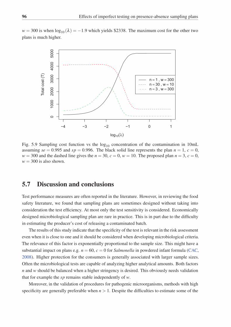
96 Effects of imperfect testing on presence-absence sampling plans
w = 300 is when log10 (λ ) =−1.9 which yields $2338. The maximum cost for the other two
plans is much higher.
−4 −3 −2 −1 0 1
010
0020
0030
0040
0050
00
log10(λ)
Tota
l cos
t (T)
n = 1 , w = 300n = 30 , w = 10n = 3 , w = 300
Fig. 5.9 Sampling cost function vs the log10 concentration of the contamination in 10mL
assuming se = 0.995 and sp = 0.996. The black solid line represents the plan n = 1, c = 0,
w = 300 and the dashed line gives the n = 30, c = 0, w = 10. The proposed plan n = 3, c = 0,
w = 300 is also shown.
5.7 Discussion and conclusions
Test performance measures are often reported in the literature. However, in reviewing the food
safety literature, we found that sampling plans are sometimes designed without taking into
consideration the test efficiency. At most only the test sensitivity is considered. Economically
designed microbiological sampling plan are rare in practice. This is in part due to the difficulty
in estimating the producer’s cost of releasing a contaminated batch.
The results of this study indicate that the specificity of the test is relevant in the risk assessment
even when it is close to one and it should be considered when developing microbiological criteria.
The relevance of this factor is exponentially proportional to the sample size. This might have a
substantial impact on plans e.g. n = 60, c = 0 for Salmonella in powdered infant formula (CAC,
2008). Higher protection for the consumers is generally associated with larger sample sizes.
Often the microbiological tests are capable of analyzing higher analytical amounts. Both factors
n and w should be balanced when a higher stringency is desired. This obviously needs validation
that for example the sp remains stable independently of w.
Moreover, in the validation of procedures for pathogenic microorganisms, methods with high
specificity are generally preferable when n > 1. Despite the difficulties to estimate some of the

5.7 Discussion and conclusions 97
relevant costs, optimization based on costs as discussed here might help food producers and
safety authorities to select nearly optimum inspection plans.
When the inspection is done by producers and historical data is available, an informative
prior for p is recommended. Conversely, a noninformative prior should be selected when the
inspection is done from the consumer’s perspective and the batches come from different sources.
One should keep in mind that some ‘noninformative priors’ can be very informative in zero
inflated problems.
A common assumption in the imperfect classifiers theory is that se and sp are independent
of the prevalence in the population under study. However, this hypothesis has been refuted in
several studies, which have shown variations in se and sp. See for instance Brenner et al. (1997);
Leeflang et al. (2013). This is presumably more complex in food safety due to the nature of the
material under study and the analytical methods. To the best of our knowledge this issue has not
been properly addressed before in microbiological risk assessment.
The resampling dilemma
The dilemma of having false positive and negative samples might lead us to seek for potential
solutions. One of the first things come to mind is to resample those batches where the pathogen
was detected. See the discussion about resampling in ICMSF (2002); Lund (1986). It can
be argued that by sampling and testing again the negative impact of imperfect specificity can
be reduced. A common preference is to opt for larger sample size. Let us consider that we
decide to resample a batch using n = 10 samples, under the same conditions (same analytical
amount, sampling, test, laboratory, etc). If the batch is truly contaminated with low probability
of contamination say p = 0.01 and let se = 0.997 and sp = 0.987, the probability of detecting
contamination in the batch with 10 samples is only 0.12. If we resample this batch after a positive
result is obtained, the conditional probability of detection is just 0.014. This clearly shows that
resampling (under the conditions previously described) could yield the release of a contaminated
batch. The argument that reinspecting will certainly discern between good and poor quality
might be fallacious. Clearly other strategies such as more accurate analytical test can be explored
as well.
Further research might investigate the correlation between the contamination with Cronobac-ter spp. and the level of Enterobacteriaceae in the batch. This last one is a hygienic characteristic
commonly monitored in diary products, which is presumably related to Cronobacter spp.
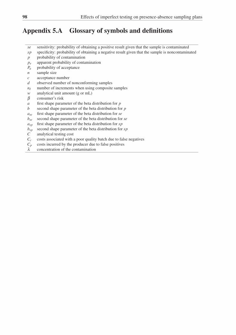
98 Effects of imperfect testing on presence-absence sampling plans
Appendix 5.A Glossary of symbols and definitions
se sensitivity: probability of obtaining a positive result given that the sample is contaminated
sp specificity: probability of obtaining a negative result given that the sample is noncontaminated
p probability of contamination
pe apparent probability of contamination
Pa probability of acceptance
n sample size
c acceptance number
d observed number of nonconforming samples
nI number of increments when using composite samples
w analytical unit amount (g or mL)
β consumer’s risk
a first shape parameter of the beta distribution for pb second shape parameter of the beta distribution for pase first shape parameter of the beta distribution for sebse second shape parameter of the beta distribution for seasp first shape parameter of the beta distribution for spbsp second shape parameter of the beta distribution for spC analytical testing cost
Cc costs associated with a poor quality batch due to false negatives
Cp costs incurred by the producer due to false positives
λ concentration of the contamination

5.B Reported values of sensitivity and specificity. 99
App
endi
x5.
BR
epor
ted
valu
esof
sens
itivi
tyan
dsp
ecifi
city
.
Mic
roorg
anis
mC
lass
if.
Det
ecti
on
met
hod
Food
cate
gory
Sourc
ese
(%)
sp(%
)
Cro
noba
cter
spp
.C
ult
ure
ISO
22
96
4(2
00
6)
PIF
*Iv
erse
net
al.(2
00
8)
10
09
4.2
Cro
noba
cter
spp
.C
ult
ure
CS
BP
IFIv
erse
net
al.
(20
08
)1
00
93
.9
Cro
noba
cter
spp
.C
ult
ure
ISO
22
96
4(2
00
6)
PIF
Zh
uet
al.(2
01
2)
76
**
81
**
Cro
noba
cter
spp
.P
CR
Imp
edan
ceP
IFZ
hu
etal
.(2
01
2)
85
10
0
Cro
noba
cter
spp
.P
CR
Esa
k2
/Esa
k3
PIF
Caw
tho
rnet
al.
(20
08
)8
79
4
Cro
noba
cter
spp
.P
CR
Esa
kf/
Esa
kr
PIF
Caw
tho
rnet
al.
(20
08
)1
00
90
Cro
noba
cter
spp
.C
ult
ure
CE
SP
IFC
awth
orn
etal
.(2
00
8)
10
09
8
Cro
noba
cter
spp
.C
ult
ure
DF
IP
IFC
awth
orn
etal
.(2
00
8)
10
09
8
Salm
onel
lasp
p.
PC
RT
aqM
anM
eat/
Raw
Mil
kM
alo
rny
etal
.(2
00
4)*
**
10
01
00
Salm
onel
lasp
p.
EIA
Ass
ura
nce
EI
®P
ou
ltry
Eij
kel
kam
pet
al.
(20
09
)9
89
6
Salm
onel
lasp
p.
EL
ISA
EL
ISA
VID
AS
®P
ou
ltry
Eij
kel
kam
pet
al.
(20
09
)9
39
6
List
eria
Cu
ltu
reIS
O1
12
90
(19
97
)C
hee
se/M
eat/
Eg
gS
cott
eret
al.(2
00
1)
85
.69
7.4
List
eria
Cu
ltu
rese
lect
ive
pla
tin
gC
hee
seN
ied
erh
ause
ret
al.
(19
93
)6
71
00
List
eria
PC
R(B
)-
Ch
eese
Nie
der
hau
ser
etal
.(1
99
3)
75
10
0
List
eria
PC
RB
AX
®E
nv.
sam
ple
sH
off
man
and
Wie
dm
ann
(20
01
)9
4.7
97
.4
List
eria
PC
RB
AX
®R
awfi
shH
off
man
and
Wie
dm
ann
(20
01
)8
4.8
10
0
Note
:*P
ow
der
edIn
fant
Form
ula
(PIF
),**Z
hu
etal
.(2
012)
linked
the
low
seval
ues
toth
epre
sence
of
com
pet
itiv
em
icro
flora
that
did
not
allo
wth
egro
wth
of
Cro
noba
cter
spp
.d
uri
ng
the
pre
-en
rich
men
tst
age.
**
*M
alo
rny
etal
.(2
00
4)
use
dsm
all
sam
ple
size
s(b
etw
een
20
to4
6).

100 Effects of imperfect testing on presence-absence sampling plans
Appendix 5.C Models in JAGS for the numerical integration
5.C.1 R codes to obtain the Pa using numerical integration� �
model {pe p * se + (1 p) * (1 sp)p ~ dbeta(a,b)se ~ dbeta(a.se, b.se)sp ~ dbeta(a.sp, b.sp)Pa = (1 pe) ^ n
}�� �
5.C.2 R codes to obtain the Pa using numerical integration using ni com-posite samples
� �
model {pe pc * se + (1 pc) * (1 sp)pc 1 (1 p) ^ nip ~ dbeta(a,b)
se ~ dbeta(a.se, b.se)sp ~ dbeta(a.sp, b.sp)Pa = (1 pe) ^ n
}�� �
5.C.3 R codes to obtain the Pa, p and pe in the accepted batches usingMCMC
� �
model {x ~ dbin(p,n)p ~ dbeta(a,b)se ~ dbeta(a.se, b.se)sp ~ dbeta(a.sp, b.sp)pe p * se + (1 p) * (1 sp)Pa = (1 pe) ^ n
}�� �
5.C.4 R codes to obtain the Pa using numerical integration based on μand σ
� �
model {pe p * se + (1 p) * (1 sp)p = 1 exp( lambda)lambda ~ dlnorm(mu , 1 / (sigma ^ 2) )se ~ dbeta(a.se, b.se)

5.D Shiny app to estimate the risk for presence-absence tests 101
sp ~ dbeta(a.sp, b.sp)Pa 1 pe
}�� �
5.C.5 R codes to obtain the Pa using numerical integration based on thezero inflated Poisson-lognormal distribution with μ and σ
� �
model {pa p * se + (1 p) * (1 sp)
p = 1 exp( lambda)lambda = h * xx ~ dlnorm(mu, 1 / (sigma ^ 2) )h ~ dbern(PI)se ~ dbeta(a.se, b.se)sp ~ dbeta(a.sp, b.sp)Pa = (1 pa) ^ n
}�� �
5.C.6 R codes used for the MCMC simulation (Scenario 1)� �
model {for ( i in 1:Ntotal ) {
y[ i ] ~ dbern(pe[i ])pe[ i ] p[i ] * se + (1 p[ i ]) * (1 sp) # apparent prevalencep[ i ] = 1 exp( 30 * lambda[i]) # prev using 30 comp sampleslambda[i] = h[ i ] * x[ i ] # the zero inflated lambdah[ i ] ~ dbern(theta) # prop of non zeroes in the ratex[ i ] ~ dlnorm(mu[i], 1 / (0.8 ^ 2)) # rate is lognormally distributedmu[i] ~ dnorm( 4, 1 / (0.8 ^ 2))} # mu changes from batch to batch
se ~ dbeta(99, 1)sp ~ dbeta(99, 1)lambda0 lambda[1]lambda1 lambda[234]theta ~ dbeta(2,20)}
�� �
Appendix 5.D Shiny app to estimate the risk for presence-absence tests
This interactive shiny tool allows the computation of the batch probability of acceptance given
various beta prior distributions for the proportion nonconforming and the test sensitivity and
specificity. It uses MCMC simulations and considers that no positives results has been found in
a sample of size n. This interactive tool is available at:
https://edgarsantosfdez.shinyapps.io/PreAbs.

102 Effects of imperfect testing on presence-absence sampling plans
Chapter 6
A New Variables Acceptance SamplingPlan for Food Safety
Edgar Santos-Fernández, K. Govindaraju, Geoff Jones
Food Control, 2014, 44:249–257 1
http://www.sciencedirect.com/science/article/pii/S0956713514001765
6.1 Abstract
The variables sampling plans for microbial safety are based on the log transformation of the
observed counts. We propose a new variables plan for lognormal data using the angular transfor-
mation. In a comparison with the classic approach, this new method shows more stringency and
allows the use of a smaller sample size to obtain the same level of consumer protection. This
transformation is robust when the underlying distribution departs from the lognormal distribution
as well as in the presence of contamination. A description of the new plan and the software
codes are provided.
Keywords
food safety; acceptance sampling; lognormal distribution; robust plan; sinh-arcsinh transforma-
tion
6.2 Introduction
Sampling inspection plans are used to assess the “fitness for use” of batches of products providing
protection to the consumers. Sampling inspection cannot be avoided due to the high cost
1Cited in Jarvis, B. (2016). Statistical Aspects of the Microbiological Examination of Foods. Academic Press.
Elsevier/Academic Press
104 A New Variables Acceptance Sampling Plan for Food Safety
associated with laboratory testing and the destructive nature of the microbiological tests makes
100% inspection impossible. A single sample of size n is usually inspected or tested for the
specified microbiological criteria for conformance. The conformance criteria are often regulated
for potentially dangerous pathogens e.g. Regulation (EC) No 2073/2005, (European Commission,
2005). In addition to variables plans, attribute plans are also used for food safety inspection.
In a two-class attribute plans , items are classified as conforming or not while the variables
plans deal with parameters such as the mean concentration. The International Commission on
Microbiological Specification for Foods in ICMSF (2002) as well as the Codex Alimentarius
Commission (CAC) in CAC (2004) recommend both attribute and variables plans for food quality
assessment. The performance of simple attributes plans in the food safety context is widely
studied, see for instance, Hildebrandt et al. (1995), Legan et al. (2001), Dahms (2004), Wilrich
and Weiss (2009). However, the variables plans are preferred because the whole information
from the sample is taken into account in the decision making process so that the same level of
protection can be obtained with small sample sizes. Nonetheless, the application of variables
plans requires the knowledge of the underlying probability distribution of the characteristic of
interest. When the distribution of microorganism departs from the assumed model, the proportion
of the population that does not satisfy the microbiological limit (or the fraction nonconforming)
will be erroneously estimated.
The lognormal model arises as a result of a multiplicative process, particularly in the prolifer-
ation of microbes in the form of clusters or agglomeration. The lognormal distribution is also the
maximum entropy distribution when the mean and standard deviation are fixed. The maximum
entropy property captures the most variation on the positive real line and hence the lognormal
model becomes the conservative model for common cause or baseline situation. Safety plans for
variables as recommended by ICMSF (2002) and CAC (2004) rely on the lognormality. This
distribution has been found suitable empirically to describe frequencies of pathogens in food
(Jongenburger et al., 2012b; Kilsby and Baird-Parker, 1983). The probability density function of
the lognormal distribution is given in Table 6.5 of the Appendix. Since microbial enumeration
is commonly expressed on a logarithmic scale (base 10), the traditional theory of acceptance
sampling for variables based on the normal distribution can be applied.
The common cause or baseline variation pertains to the scenario in which only the usual
sources of variation are acting in the food production chain, e.g. the level of microorganism is
in the acceptable range. By contrast, special causes of variation are the result of a poor food
handling and its identification is vital to avoid foodborne diseases. Often only few units of each
lot are tested because of the budget constraints on laboratory analysis. A small sample size may
fail to detect high levels of fraction nonconforming compromising protection to the consumer.
The paper presents a new decision criterion with a better performance than the classic approach
as well as robust to distributional uncertainties. The proposed variables plan provides the same
level of protection to the producer with fewer units of the batch to be tested, but with a stringent
level of protection to the consumer.
6.3 Material and methods 105
6.3 Material and methods
6.3.1 The Operating Characteristic (OC) curve
The performance of a sampling plan is revealed by its Operating Characteristic (OC) curve, which
is a plot of the probability of acceptance against the process level or the fraction nonconforming
(p). This curve shows how well a sampling inspection plan discriminates between good and
bad quality. If two OC curves are matched to give the same level protection to the producer,
we would then prefer the OC curve which is steeper or more stringent. The ideal OC curve has
probability of acceptance equal to one until the critical fraction nonconforming after which it
drops to zero. See e.g. Montgomery (2005). OC curves are often assessed at given two points
(AQL,α) and (LQL,β ) where AQL and LQL are the acceptance and limiting quality limits
(levels), and α and β the producer’s and consumer’s risk respectively. The AQL is the maximum
fraction nonconforming that is considered acceptable as a process level for the consumer, while
the LQL is the proportion nonconforming that is expected to be accepted with a low probability
for an isolated batch. CAC (2004) recommends for characteristics associated with sanitary risks
to employ low acceptable levels such as 0.1%. On the other hand, the limiting levels are often
fixed lower than the traditional 10% for food safety.
6.3.2 Variables plans for food safety
Suppose that a characteristic of interest (X) such as the cell count follows a lognormal distribution.
The log-concentration (Y ) is then normally distributed with mean μ and standard deviation σ .
At a given microbiological limit (m), the decision criterion results in: Y + kSy < my where kis the acceptability constant for the operation of the variables plan where Y = ∑Yi/n is the
sample mean, Sy =
√∑(Yi − Y )2
/(n−1) is the sample standard deviation and my = log(m)
is the transformed Upper Specification/Safety Limit. This plan will be referred as classical
approach from now on. The following test statistic is obtained by rearranging the last equation.
Z1 =my − Y
Sy(6.1)
The regulatory (specification) limit m is often fixed using base-line or “common-cause”
samples which are free from known food safety issues. The test statistic Z1 expresses the distance
between the specification limit and the sample mean Y in sample standard deviation units. When
this distance is below a critical value k, the resulting proportion nonconforming (p) is greater
than expected. In other words, the lot is accepted whenever Z1 � k, otherwise the lot is rejected.
When the true standard deviation of the process is unknown, the acceptance criterion is then
obtained using the noncentral t-distribution using the consumer’s point (LQL,β ), ICMSF (2002).
Another alternative is when producers use Good Manufacturing Practice (GMP) limits which are
set well below the regulatory limit. In this case, the critical distance can be obtained from Kilsby
et al. (1979).

106 A New Variables Acceptance Sampling Plan for Food Safety
6.3.3 New plans based on the sinh-arcsinh transformation
Suppose that instead of applying logarithm to the cell count the sinh-arcsinh transformation
(Jones and Pewsey, 2009) is used. Hyperbolic functional transformations are commonly applied
to improve the degree of normality of a quality characteristic.
H = sinh[δ sinh−1 (x)− ε
](6.2)
where sinh = (ex − e−x)/2 and sinh−1 = log(
x+√
x2 +1)
are the hyperbolic sine and its
inverse. The hyperbolic functions are the counterpart in the hyperbola of the classic trigonometric
functions. This transformation allows to control the skewness and kurtosis with the parameters
δ and ε . The skewness and kurtosis are measures of the asymmetry and the peakedness of the
distribution respectively. We used a particular combination of parameters, δ = 0.1 and ε = 0.
Let V = H (x) and mv = H (m), then an analogous test statistic to Eq. 6.1 for the new approach
can be defined.
Z2 =mv −V
Sv(6.3)
This plan will be referred as the new method from now on.
6.3.4 Simulation algorithm
The critical values for Z1 and Z2 as well as the probability of acceptance values are obtained by
Monte Carlo simulation since the analytical solution is intractable for the new approach. The
computation and simulations were carried out using R open source software (R Core Team,
2013) using the following algorithm:
• Step 0. Set the point (AQL,α) on the OC curve to protect the producer. This point
represents the aim of the producer that batches with fraction nonconforming AQL should
be accepted with probability 1−α . Let the microbiological common cause situation be
described by the lognormal distribution with log-scale parameter, μ = 0 and shape, σ = 1
taking advantage of the invariance property of the standard normal distribution.
• Step 1. Generate a random sample of data from the lognormal distribution for a given
sample size.
• Step 2. Compute the Z statistic and replicate this random sample generation process (such
as 100,000 simulations) to obtain the vector A.
• Step 3. Obtain the critical distance by dividing the frequency distribution of A in a
proportion of size α , i.e. as the α-quantile; ki = qα (A).
• Step 4. The presence of special causes, leading to food safety concerns, is modelled by a
shift in μ , say from μ0 to μ0 +, where 0 <≤ 2.
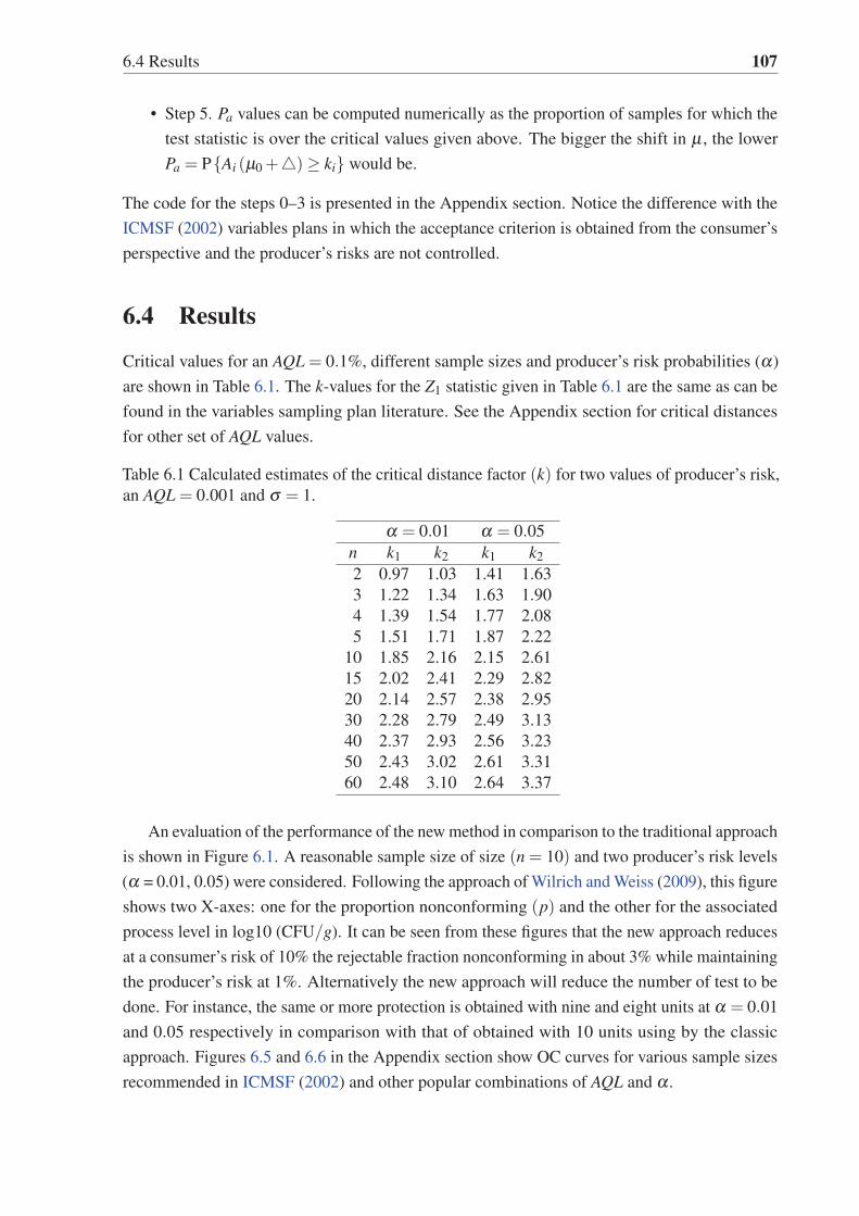
6.4 Results 107
• Step 5. Pa values can be computed numerically as the proportion of samples for which the
test statistic is over the critical values given above. The bigger the shift in μ , the lower
Pa = P{Ai (μ0 +)≥ ki} would be.
The code for the steps 0–3 is presented in the Appendix section. Notice the difference with the
ICMSF (2002) variables plans in which the acceptance criterion is obtained from the consumer’s
perspective and the producer’s risks are not controlled.
6.4 Results
Critical values for an AQL = 0.1%, different sample sizes and producer’s risk probabilities (α)
are shown in Table 6.1. The k-values for the Z1 statistic given in Table 6.1 are the same as can be
found in the variables sampling plan literature. See the Appendix section for critical distances
for other set of AQL values.
Table 6.1 Calculated estimates of the critical distance factor (k) for two values of producer’s risk,
an AQL = 0.001 and σ = 1.
α = 0.01 α = 0.05
n k1 k2 k1 k2
2 0.97 1.03 1.41 1.63
3 1.22 1.34 1.63 1.90
4 1.39 1.54 1.77 2.08
5 1.51 1.71 1.87 2.22
10 1.85 2.16 2.15 2.61
15 2.02 2.41 2.29 2.82
20 2.14 2.57 2.38 2.95
30 2.28 2.79 2.49 3.13
40 2.37 2.93 2.56 3.23
50 2.43 3.02 2.61 3.31
60 2.48 3.10 2.64 3.37
An evaluation of the performance of the new method in comparison to the traditional approach
is shown in Figure 6.1. A reasonable sample size of size (n = 10) and two producer’s risk levels
(α = 0.01, 0.05) were considered. Following the approach of Wilrich and Weiss (2009), this figure
shows two X-axes: one for the proportion nonconforming (p) and the other for the associated
process level in log10 (CFU/g). It can be seen from these figures that the new approach reduces
at a consumer’s risk of 10% the rejectable fraction nonconforming in about 3% while maintaining
the producer’s risk at 1%. Alternatively the new approach will reduce the number of test to be
done. For instance, the same or more protection is obtained with nine and eight units at α = 0.01
and 0.05 respectively in comparison with that of obtained with 10 units using by the classic
approach. Figures 6.5 and 6.6 in the Appendix section show OC curves for various sample sizes
recommended in ICMSF (2002) and other popular combinations of AQL and α .

108 A New Variables Acceptance Sampling Plan for Food Safety
0.00 0.05 0.10 0.15 0.20 0.25
0.0
0.2
0.4
0.6
0.8
1.0
Pa−0.22 0.52 0.67 0.78 0.86 0.93
β
Z1 Z2
Proportion nonconforming
Process level (log10(cfu g))(a) n = 10 , Producer's risk (α) = 0.01
0.00 0.05 0.10 0.15 0.20 0.25
0.0
0.2
0.4
0.6
0.8
1.0
Pa
−0.22 0.52 0.67 0.78 0.86 0.93
β
Proportion nonconforming
Process level (log10(cfu g))(b) n = 10 , Producer's risk (α) = 0.05
Fig. 6.1 Comparison of Operating Characteristic (OC) curves for n = 10, AQL = 0.1% and
different values of producer’s risk. The OC curves of the log and sinh-arcsinh transformations
are shown in solid and dashed lines respectively. The new approach offers better consumer
protection by lowering the consumer’s risk at poor quality levels.

6.5 The misclassification error 109
6.5 The misclassification error
For a given m, the Type I or false positive misclassification error (say, e1) is always involved,
see Lavin (1946) and Govindaraju (2007). This error is very small for regulatory limits, but
necessary for the GMP warning limits which are fixed well below the regulatory limits. The
false negative or Type II misclassification error is not relevant for fixing the m because it arises
only in the presence of special causes having food safety implications. The observed proportion
nonconforming(
p′)
is in fact equivalent to e1 (1− p). For lognormal quality characteristics,
Albin (1990) introduced a variables plan in which the OC curve is constructed for a given ratio of
the means of unacceptable and acceptable quality limits. This procedure also takes into account
the probability of false positive misclassification error. After allowing for the possibility of
a baseline sample showing a false positive result, the probability of acceptance cannot be 1
for p = 0. Consequently, the true probability of acceptance starts at 1− e1 when p = 0; see
Govindaraju (2007) for a discussion on this issue. Zero microbial count in samples tested may
be due to the measurement error. Non-detection is not the same as absence when in fact could be
associated with factors such as the instruments, the measurer or the material preparation. For
this reason, in tests like Aerobic Plate Count (APC) the event of no colonies found is reported as
less than 25 CFU. Consider an e1 value of 1%, the apparent proportion nonconforming result in:
0.99% for an apparent AQL = 0.1%. This affects the performance of the OC curve considerably
as can be seen in Figure 6.2.
6.6 Example
The new approach for lot disposition is illustrated in this section. Table 6.2 gives the aerobic
colony count data obtained in poultry from ICMSF (2002).
Table 6.2 Result of five samples in aerobic colony count in poultry from ICMSF (2002). The
second and third row express the count using log10 and sinh-arcsinh transformations respectively.
APC 40000 69000 81000 200000 350000
log10 (APC) 4.602 4.839 4.908 5.301 5.544
H (APC) 1.385 1.480 1.509 1.679 1.791
For a given microbiological limit equal to 107CFU the test statistics are: Z1 = 5.187 and
Z2 = 6.270. If, for example, a k value related to α = 5% and AQL = 0.1% is used, the following
critical values are obtained: k1 = 1.87 and k2 = 2.22. At this high regulatory limit the batch
is accepted by both methods. Now, consider a lower m value, say 6×10⁵ CFU; the resulting
statistics result in: Z1 = 1.955 and Z2 = 2.053. Thus the batch is rejected at this level by the
new approach, while the traditional method sentences it as acceptable. As the proposed method
tends to have OC curves dropping more steeply, this method provides better consumer protection
against an increase in p or μ . This practical example illustrates how the difference in the OC
curves can lead to different outcomes.

110 A New Variables Acceptance Sampling Plan for Food Safety
0.00 0.05 0.10 0.15 0.20 0.25
0.0
0.2
0.4
0.6
0.8
1.0
Pa−0.22 0.52 0.67 0.78 0.86 0.93
β
Z1Z2
Z1 (under Type I error)Z2 (under Type I error)
Proportion nonconforming
Process level (log10(cfu g))(a) n = 10 , Producer's risk (α) = 0.01
0.00 0.05 0.10 0.15 0.20 0.25
0.0
0.2
0.4
0.6
0.8
1.0
Pa
−0.22 0.52 0.67 0.78 0.86 0.93
β
Proportion nonconforming
Process level (log10(cfu g))(b) n = 10 , Producer's risk (α) = 0.05
Fig. 6.2 Comparison of Operating Characteristic (OC) curves at a false positive misclassification
error of 1% for n = 10, AQL = 0.1% and different values of producer’s risk. The OC curves of
the log and sinh-arcsinh transformations are shown in heavy solid and dashed lines respectively.
6.7 Assessment of robustness 111
6.7 Assessment of robustness
It is well known that the performance of classical variables plans is sensitive to departures from
the assumed model used to describe the cell count, which causes the fraction nonconforming to
be incorrectly estimated. In practice, we would prefer a robust sampling plan whose OC curve
remain stable when the underlying distribution changes and in presence of extreme values. For
instance, the number of pathogens in a baseline study may fit a lognormal model as well as a few
other related distributions such as gamma. Even though the lognormal distribution is justifiable
as a standard distribution for microbial characteristics, it is important to ensure that the plan
based on the lognormal assumption also works satisfactorily when the unknown true model is
gamma. If the OC curve of the plan is forced closer to the vertical axis the protection to the
consumer is improved.
The performance of new and classical procedures is evaluated in three common scenarios:
assuming lognormality when the true distribution is gamma , Weibull and contaminated log-
normal. All these three alternatives also produce right-skewed data. Let us first consider the
gamma, G(c,b) and Weibull, W (κ,λ ) alternatives. The initial parameters of the gamma and
Weibull distributions for the common cause situation can be fixed giving equal values for the
mode, density and overall goodness of fit in relation to LN (0,1). For the gamma distribution, the
following combination of parameters guarantees a match in terms of mode and density: b = 0.75
and c = 1.5. See Figure 6.7 in Appendix. The shape parameter was fixed at this level and a
shift in the scale parameter, equivalent to the modification in the μ parameter of the lognormal,
was introduced to model the special cause situation. This guarantees that for each point the
gamma and the lognormal will have the same mode. The proportion nonconforming was used to
construct the OC curve since the parameters in the lognormal and gamma distributions are not
equivalent. The results obtained are shown in Figure 6.3. When the true distribution is gamma,
the resulting plan is less stringent for both methods but the OC curve for the new method is
rather robust.
Finally, the Weibull distribution is used as the true model, for comparison with the lognormal
OC curve. The starting shape and scale parameters associated with the same mode are κ = 1.3
and λ = 1.14. This combination of parameters also produces a similar shape as can be seen in
Figure 6.7. Fixing the shape and increasing the corresponding scale parameter over 1.14 gives
very similar results as those obtained with the gamma distribution.
The basic idea behind a contaminated or mixture distribution is that the majority of data
comes from a specific distribution f (x), but includes a certain level of contamination with
observations from a different distribution g(x), often the same statistical model but with a greater
mean/variance. If the contamination level is given by p, then the resulting probability density
function is given by: h(x) = (1− p) f (x)+ pg(x). See, for instance Fowlkes (1979). This
technique is often employed to evaluate the robustness of a statistical test procedure. Suppose
that previous experience shows that a microbial count is right skewed justifying the lognormal
assumption. Therefore, a sample will be judged by this hypothesis using the critical distance k

112 A New Variables Acceptance Sampling Plan for Food Safety
0.00 0.05 0.10 0.15 0.20
0.0
0.2
0.4
0.6
0.8
1.0
Proportion nonconforming
Pa
β
Z1Z2
Z1 (under gamma distribution)Z2 (under gamma distribution)
(a) n = 10 , Producer's risk (α) = 0.01
Z1Z2
Z1 (under gamma distribution)Z2 (under gamma distribution)
0.00 0.05 0.10 0.15 0.20
0.0
0.2
0.4
0.6
0.8
1.0
Proportion nonconforming
Pa
β
(b) n = 10 , Producer's risk (α) = 0.05
Fig. 6.3 Effect in the OC curves when the true distribution is gamma (displayed in thicker line
width). The difference in the LQL at a β risk for the Z2 statistic is much smaller than that of Z1.

6.8 Discussion 113
corresponding to the given sample size, the producer’s risk and the AQL. Let the mixed model
be composed of two lognormal distributions with μ = 0 and standard deviations one and two
respectively, and let the degree of contamination be 20%. This leads to a mixed distribution that
is more right-skewed than assumed. The performance of the classic and the new approach is
shown in Figure 6.4. Notice that both approaches tend to reject at lower LQL but the classical
alternative seems to be more affected. The method based on the sinh-arcsinh transformation is
found to be more robust for both α levels. This means that the new approach better preserves its
integrity when the true distribution is contaminated.
6.8 Discussion
As noted in Jongenburger et al. (2012b) and by others, the lognormal distribution is widely
used to describe the number of pathogens in a sample, despite the fact that it is a continuous
distribution. This density is criticized because of the fact that it does not allow zero counts,
whereas discrete distributions such as the negative binomial allow a positive probability for
zero counts. The absence of microorganisms in the sample has a zero probability of occurrence
according to the lognormal density and this can be a drawback when the model is characterized by
an over-dispersion of pathogens. Nevertheless, this issue could be addressed by adequate material
preparation, using composite sampling (which allows a better homogenization) or using the
three-parameter lognormal distribution. In recent years, other distributions have been proposed
as an alternative to lognormal. For instance, Gonzales-Barron et al. (2010a) suggested the use
of heterogeneous Poisson distributions. More recently Gonzales-Barron and Butler (2011b)
and Mussida et al. (2013a) recommended compound distributions such as Poisson-gamma and
Poisson-lognormal. These distributions were found suitable to characterize the colony count
in powdered food products by Jongenburger et al. (2012c). However, we need to recognize
that there is always an inherent distributional uncertainty with small samples. It is, therefore,
important to use a standard distribution but achieve robustness in lot disposition.
OC curves usually start at proportion nonconforming (p) equal to zero. Unavoidable Type I
misclassification error (false positives) results in a non-zero apparent proportion nonconforming(p′)
. This leads to p′= e1 (1− p), a fact not well recognized in the food safety literature. The
proposed procedure incorporates this measurement error for lot disposition and controls the risks
as suggested in Albin (1990) and others. Moreover, a higher degree of consumer protection can
be achieved when compared to the traditional method with the same sample size because the
proposed method achieves a steeper OC curve while maintaining the same producer’s risk.
6.9 Conclusions
The performance of variables sampling plans using log-transformed data was compared with that
obtained using the sinh-arcsinh transformation, for right skewed distributions used for modelling
microbiological counts. This transformation was found to lower the consumer’s risk in all the
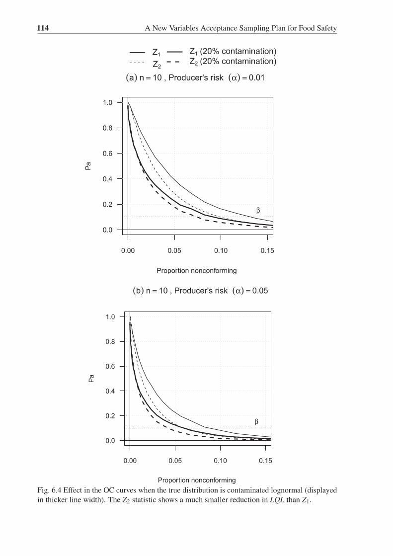
114 A New Variables Acceptance Sampling Plan for Food Safety
0.00 0.05 0.10 0.15
0.0
0.2
0.4
0.6
0.8
1.0
Proportion nonconforming
Pa
β
Z1
Z2
Z1 (20% contamination)Z2 (20% contamination)
(a) n = 10 , Producer's risk (α) = 0.01
0.00 0.05 0.10 0.15
0.0
0.2
0.4
0.6
0.8
1.0
Proportion nonconforming
Pa
β
(b) n = 10 , Producer's risk (α) = 0.05
Fig. 6.4 Effect in the OC curves when the true distribution is contaminated lognormal (displayed
in thicker line width). The Z2 statistic shows a much smaller reduction in LQL than Z1.

6.A Effect of the parameters in the sampling performance 115
scenarios explored. Another important advantage is the greater robustness of the proposed
method. A real life example was given to show how the proposal can offer better consumer
protection than the traditional method.
Appendix 6.A Effect of the parameters in the sampling per-formance
The use of the sinh-arcsinh transformation is beneficial even for small sample sizes under certain
conditions, say n = 2, 3 or 5. Figures 6.5 and 6.6 compare the OC curves of both methods for
different combinations of α , AQL and n. For higher sample sizes, the OC curves drop more
vertically and the reduction in consumer’s risks for the new method is evident. It can also be
noted that small AQL values also achieve similar reduction in consumer’s risks.

116 A New Variables Acceptance Sampling Plan for Food Safety
0.0 0.1 0.2 0.3 0.4 0.5
0.0
0.2
0.4
0.6
0.8
1.0
n = 5 , AQL = 0.01
Proportion nonconforming
Pa
Z1Z2
0.0 0.1 0.2 0.3 0.4
0.0
0.2
0.4
0.6
0.8
1.0
n = 5 , AQL = 0.001
Proportion nonconforming
Pa
0.00 0.05 0.10 0.15 0.20
0.0
0.2
0.4
0.6
0.8
1.0
n = 5 , AQL = 1e−04
Proportion nonconforming
Pa
0.00 0.05 0.10 0.15
0.0
0.2
0.4
0.6
0.8
1.0
n = 20 , AQL = 0.01
Proportion nonconforming
Pa
0.00 0.02 0.04 0.06
0.0
0.2
0.4
0.6
0.8
1.0
n = 20 , AQL = 0.001
Proportion nonconforming
Pa
0.000 0.010 0.020 0.030
0.0
0.2
0.4
0.6
0.8
1.0
n = 20 , AQL = 1e−04
Proportion nonconforming
Pa
0.00 0.02 0.04 0.06
0.0
0.2
0.4
0.6
0.8
1.0
n = 60 , AQL = 0.01
Proportion nonconforming
Pa
0.000 0.005 0.010 0.015 0.020
0.0
0.2
0.4
0.6
0.8
1.0
n = 60 , AQL = 0.001
Proportion nonconforming
Pa
0.000 0.002 0.004 0.006
0.0
0.2
0.4
0.6
0.8
1.0
n = 60 , AQL = 1e−04
Proportion nonconforming
Pa
Fig. 6.5 Comparison of OC curves at a producer’s risk (α) of 0.01 for different combinations of
sample size and AQL. The common cause situation is assumed to be the lognormal distribution
with μ = 0 and σ = 1, both in log scale.

6.A Effect of the parameters in the sampling performance 117
0.0 0.1 0.2 0.3 0.4
0.0
0.2
0.4
0.6
0.8
1.0
n = 5 , AQL = 0.01
Proportion nonconforming
Pa
Z1Z2
0.00 0.10 0.20 0.30
0.0
0.2
0.4
0.6
0.8
1.0
n = 5 , AQL = 0.001
Proportion nonconforming
Pa
0.00 0.05 0.10 0.15 0.20
0.0
0.2
0.4
0.6
0.8
1.0
n = 5 , AQL = 1e−04
Proportion nonconforming
Pa
0.00 0.04 0.08 0.12
0.0
0.2
0.4
0.6
0.8
1.0
n = 20 , AQL = 0.01
Proportion nonconforming
Pa
0.00 0.01 0.02 0.03 0.04 0.05
0.0
0.2
0.4
0.6
0.8
1.0
n = 20 , AQL = 0.001
Proportion nonconforming
Pa
0.000 0.005 0.010 0.015 0.020
0.0
0.2
0.4
0.6
0.8
1.0
n = 20 , AQL = 1e−04
Proportion nonconforming
Pa
0.00 0.01 0.02 0.03 0.04 0.05
0.0
0.2
0.4
0.6
0.8
1.0
n = 60 , AQL = 0.01
Proportion nonconforming
Pa
0.000 0.004 0.008 0.012
0.0
0.2
0.4
0.6
0.8
1.0
n = 60 , AQL = 0.001
Proportion nonconforming
Pa
0.000 0.001 0.002 0.003 0.004
0.0
0.2
0.4
0.6
0.8
1.0
n = 60 , AQL = 1e−04
Proportion nonconforming
Pa
Fig. 6.6 Comparison of OC curves at a producer’s risk (α) of 0.05 for different combinations of
sample size and AQL. The common cause situation was modelled in the lognormal distribution
using μ = 0 and σ = 1, both in log scale.
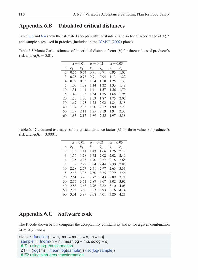
118 A New Variables Acceptance Sampling Plan for Food Safety
Appendix 6.B Tabulated critical distances
Table 6.3 and 6.4 show the estimated acceptability constants k1 and k2 for a larger range of AQLand sample sizes used in practice (included in the ICMSF (2002) plans).
Table 6.3 Monte Carlo estimates of the critical distance factor (k) for three values of producer’s
risk and AQL = 0.01.
α = 0.01 α = 0.02 α = 0.05
n k1 k2 k1 k2 k1 k2
2 0.56 0.54 0.71 0.71 0.95 1.02
3 0.78 0.78 0.91 0.94 1.13 1.22
4 0.92 0.95 1.04 1.10 1.25 1.37
5 1.03 1.08 1.14 1.22 1.33 1.48
10 1.31 1.44 1.41 1.57 1.56 1.79
15 1.46 1.63 1.54 1.75 1.68 1.95
20 1.55 1.76 1.63 1.87 1.75 2.05
30 1.67 1.93 1.73 2.02 1.84 2.18
40 1.74 2.03 1.80 2.12 1.90 2.27
50 1.79 2.11 1.85 2.19 1.94 2.33
60 1.83 2.17 1.89 2.25 1.97 2.38
Table 6.4 Calculated estimates of the critical distance factor (k) for three values of producer’s
risk and AQL = 0.0001.
α = 0.01 α = 0.02 α = 0.05
n k1 k2 k1 k2 k1 k2
2 1.26 1.41 1.43 1.66 1.76 2.13
3 1.56 1.78 1.72 2.02 2.02 2.46
4 1.75 2.03 1.90 2.27 2.18 2.68
5 1.89 2.22 2.04 2.44 2.30 2.85
10 2.28 2.77 2.41 2.97 2.63 3.31
15 2.48 3.06 2.60 3.25 2.79 3.56
20 2.61 3.26 2.72 3.43 2.89 3.71
30 2.77 3.51 2.87 3.67 3.02 3.92
40 2.88 3.68 2.96 3.82 3.10 4.05
50 2.95 3.80 3.03 3.93 3.16 4.14
60 3.01 3.89 3.08 4.01 3.20 4.21
Appendix 6.C Software code
The R code shown below computes the acceptability constants k1 and k2 for a given combination
of α , AQL and n.� �
stats function(n = n, mu = mu, s = s, m = m){sample rlnorm(n = n, meanlog = mu, sdlog = s)# Z1 using log transformationZ1 (log(m) mean(log(sample))) / sd(log(sample))# Z2 using sinh.arcs transformation

6.D Step-by-step guide 119
sinh.arcs function(x, epsilon = 0, delta = 0.1) {sinh(delta *asinh(x) epsilon)}Z2 (sinh.arcs (m) mean(sinh.arcs(sample))) / sd(sinh.arcs(sample))cbind(Z1, Z2)}
# Computation of the acceptance constant (k)n 20 # Sample sizemu 0 # Mean of the lognormal distribution in log scales 1 # Standard deviation of the lognormal distribution in log scalealpha 0.01 # Producer s riskAQL 0.001 # Acceptable Quality Limittrials 1e5 # Number of simulations
m qlnorm(AQL, lower.tail = 0, sdlog = s) # Microbiological limit (m)A mapply(FUN = stats, n = rep(n, trials ), mu = mu, s = s, m = m)k apply(A, 1, f function(x) quantile(x, probs = alpha))
�� �
Appendix 6.D Step-by-step guide
The sampling design for the new approach can be developed by using the following guide:
• Define the producer’s risk (α) and the number of samples to be drawn (n).
• For a given regulatory limit (m), compute the associated AQL as the right tail area in the
lognormal distribution. If m is not established, define an AQL and obtain m as the quantile
of the lognormal distribution.
• Compute the statistic Z2.
• For a given n, AQL and α , obtain k from Table 6.1, 6.3 or 6.4. For other combinations,
obtain k using the R snippet.
• Apply the decision criterion. If Z2 ≥ k accept the lot; otherwise reject.

120 A New Variables Acceptance Sampling Plan for Food Safety
Distribution Matching
Figure 6.7 shows the three distributions matched through their mode and density. The lognormal
distribution is more skewed that the gamma and Weibull models.
0 1 2 3 4
0.0
0.1
0.2
0.3
0.4
0.5
0.6
LN(0,1)G(1.5,0.75)W(1.3,1.14)
●
Mo
Fig. 6.7 Lognormal probability density function with μ = 0 and σ = 1 in solid line matched
with the gamma (c = 1.5,b = 0.75) and Weibull (κ = 1.3,λ = 1.14) distributions through the
mode and the density. The gamma and Weibull distribution are in dashed and dotdashed line.
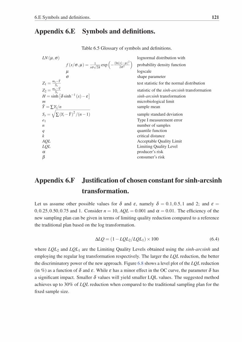
6.E Symbols and definitions. 121
Appendix 6.E Symbols and definitions.
Table 6.5 Glossary of symbols and definitions.
LN (μ,σ) lognormal distribution with
f (x/σ ,μ) = 1
xσ√
2πexp
(− (ln(x)−μ)2
2σ2
)probability density function
μ logscale
σ shape parameter
Z1 =my−Y
Sytest statistic for the normal distribution
Z2 =mv−V
Svstatistic of the sinh-arcsinh transformation
H = sinh[δ sinh−1 (x)− ε
]sinh-arcsinh transformation
m microbiological limit
Y = ∑Yi/n sample mean
Sy =
√∑(Yi − Y )2
/(n−1) sample standard deviation
e1 Type I measurement error
n number of samples
q quantile function
k critical distance
AQL Acceptable Quality Limit
LQL Limiting Quality Level
α producer’s risk
β consumer’s risk
Appendix 6.F Justification of chosen constant for sinh-arcsinhtransformation.
Let us assume other possible values for δ and ε , namely δ = 0.1,0.5,1 and 2; and ε =
0,0.25,0.50,0.75 and 1. Consider n = 10, AQL = 0.001 and α = 0.01. The efficiency of the
new sampling plan can be given in terms of limiting quality reduction compared to a reference
the traditional plan based on the log transformation.
ΔLQ = (1−LQL2/LQL1)×100 (6.4)
where LQL2 and LQL1 are the Limiting Quality Levels obtained using the sinh-arcsinh and
employing the regular log transformation respectively. The larger the LQL reduction, the better
the discriminatory power of the new approach. Figure 6.8 shows a level plot of the LQL reduction
(in %) as a function of δ and ε . While ε has a minor effect in the OC curve, the parameter δ has
a significant impact. Smaller δ values will yield smaller LQL values. The suggested method
achieves up to 30% of LQL reduction when compared to the traditional sampling plan for the
fixed sample size.

122 A New Variables Acceptance Sampling Plan for Food Safety
δ
ε
0.0
0.2
0.4
0.6
0.8
1.0
0.5 1.0 1.5 2.0
−50
−40
−30
−20
−10
0
10
20
30
Fig. 6.8 LQL reduction level plot based on δ and ε . The blue zone is where the plan based on
sinh-arcsinh reduces the LQL.
Chapter 7
Variables Sampling Plans using CompositeSamples for Food Quality Assurance
Edgar Santos-Fernández, K. Govindaraju, Geoff Jones
Food Control, 2015, 50:530–538
http://www.sciencedirect.com/science/article/pii/S0956713514005623
7.1 Abstract
Testing composite samples is a useful strategy to achieve sampling economy. Several studies
have shown the effectiveness of this technique under the assumption of perfect mixing of primary
samples. This paper investigates the effect of imperfect composite sample preparation on the
performance of two and three-class variables sampling inspection plans, and identifies scenarios
in which testing composite samples is not advantageous. The design of sampling plans using
composite samples is discussed and an implementation guide based on two points of the OC
curve for perfect and imperfect mixing is provided.
Keywords
Food safety; Composite samples; Imperfect mixing; Sampling plan
7.2 Introduction
Acceptance sampling methodology is used for disposition of lots of commodities as suitable to
be consumed. Lots are assessed as acceptable or otherwise based on a sample of n test results or
measurements. Sampling inspection plans therefore provide assurance to the consumers on the
quality and safety of accepted lots. Attribute inspection plans are used when an item or a test
sample is classified as conforming or not. Variables inspection plans are used when measurements

124 Variables Sampling Plans using Composite Samples for Food Quality Assurance
are made on a continuous scale. Variables plans are convenient since they require smaller sample
sizes when compared to the attribute plan alternatives. Smaller sample sizes generally mean
lower inspection costs. When attribute plans are employed for food safety, each tested sample
is commonly classified as conforming when the microbial count is under a regulatory limit
e.g. less than 1 CFU 100 kg−1 of salmonella in dried milk. The International Commission
on Microbiological Specifications for Foods, in ICMSF (2002) and the Codex Alimentarius
Commission (CAC) in CAC (2004) provide guidelines on using sampling inspection plans for
food quality/safety assurance. Both protocols recommend inspection plans by attribute and for
variables.
Sampling inspection plans for food safety commonly assume the concentration of microor-
ganisms to be lognormally distributed. Numerous studies reflect that this statistical model is
satisfactory to describe the frequencies of pathogens, see for instance Kilsby and Baird-Parker
(1983). The lognormal model is the maximum entropy distribution when the mean and the
variance are fixed and therefore it is the most conservative statistical model used to describe the
variation due to common or chance causes. The advantage of using the lognormal model is that,
by expressing the cell counts on a logarithmic scale, the variables inspection plans for the normal
distribution can be applied. This methodology is used in the sampling plans discussed by Kilsby
et al. (1979) and Smelt and Quadt (1990).
The performance of a sampling plan is assessed using its Operating Characteristic (OC)
curve. The OC curve gives the probability of acceptance (Pa) for various batch quality levels;
see Fig. 7.1. The batch quality is commonly expressed in proportion nonconforming (fraction of
the population that does not comply to the microbiological limit). The fraction nonconforming
product can be estimated using the sample mean and the standard deviation. The consumer’s point
of interest on the OC curve is typified using the Limiting Quality Level (LQL) and the consumer’s
risk (β ). The producer’s point of interest on the OC curve is typified using the Acceptance Quality
Limit (AQL) and the producer’s risk (α). The AQL is the maximum proportion nonconforming
that is considered acceptable for the consumer, while the LQL is the proportion nonconforming,
that is expected to be rejected with a high probability.
A single sampling plan is designed by either: (1) two points in the OC curve (AQL,α and
LQL,β ) or (2) the sample size (n) plus a restriction. The restriction may be: one point in the
OC curve, the acceptance constant (attribute plans) or the critical distance (variables plans).
The standard practice in quality control is to use the first approach, while the second method is
popular in food quality assurance. For food safety, the focus is on the LQL rather than the AQLbecause the primary objective of inspection is to provide consumer protection. However, the
consumer’s point of interest on the OC curve alone does not uniquely define a sampling plan.
Therefore, the AQL point is additionally used to match the OC curves and for design purposes.
Variables plans for the proportion nonconforming based on two points of the OC curve were
originally introduced by Wallis (1947). For the unknown standard deviation case, approximate
solutions were proposed by Lieberman and Resnikoff (1955) and Owen (1967). Kilsby et al.
(1979) extended the variables inspection plan to include the good manufacturing practice (GMP)
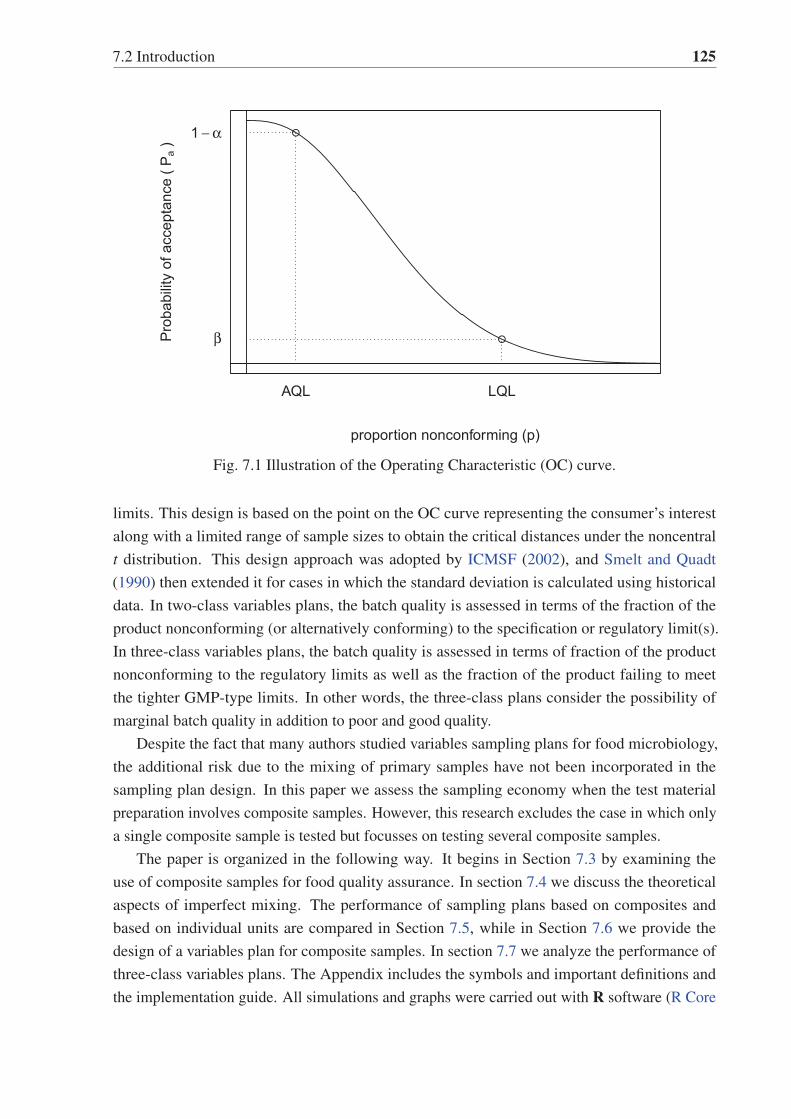
7.2 Introduction 125
proportion nonconforming (p)
Pro
babi
lity
of a
ccep
tanc
e ( P
a )
●
●
AQL LQL
1 − α
β
Fig. 7.1 Illustration of the Operating Characteristic (OC) curve.
limits. This design is based on the point on the OC curve representing the consumer’s interest
along with a limited range of sample sizes to obtain the critical distances under the noncentral
t distribution. This design approach was adopted by ICMSF (2002), and Smelt and Quadt
(1990) then extended it for cases in which the standard deviation is calculated using historical
data. In two-class variables plans, the batch quality is assessed in terms of the fraction of the
product nonconforming (or alternatively conforming) to the specification or regulatory limit(s).
In three-class variables plans, the batch quality is assessed in terms of fraction of the product
nonconforming to the regulatory limits as well as the fraction of the product failing to meet
the tighter GMP-type limits. In other words, the three-class plans consider the possibility of
marginal batch quality in addition to poor and good quality.
Despite the fact that many authors studied variables sampling plans for food microbiology,
the additional risk due to the mixing of primary samples have not been incorporated in the
sampling plan design. In this paper we assess the sampling economy when the test material
preparation involves composite samples. However, this research excludes the case in which only
a single composite sample is tested but focusses on testing several composite samples.
The paper is organized in the following way. It begins in Section 7.3 by examining the
use of composite samples for food quality assurance. In section 7.4 we discuss the theoretical
aspects of imperfect mixing. The performance of sampling plans based on composites and
based on individual units are compared in Section 7.5, while in Section 7.6 we provide the
design of a variables plan for composite samples. In section 7.7 we analyze the performance of
three-class variables plans. The Appendix includes the symbols and important definitions and
the implementation guide. All simulations and graphs were carried out with R software (R Core

126 Variables Sampling Plans using Composite Samples for Food Quality Assurance
Team, 2015). Dirichlet and multivariate hypergeometric random numbers were generated using
the R-packages gtools (Warnes et al., 2013) and BiasedUrn (Fog, 2013), respectively.
7.3 Food safety and composite samples
The use of composite samples becomes a very attractive alternative when the cost of collecting
large number of primary samples is low in relation to the analytical testing costs. A composite
sample can be defined as “the physical mix of individual sample units or a batch of unblended
individual sample units that are tested as a group”(Patil, 2006). Compositing is a physical averag-
ing process. A highly representative composite sample is useful to estimate the population mean
levels. In recent years, there is a growing interest in composite sampling for food safety, (Jarvis,
2007; Ross et al., 2011). However, the use of composite samples remains controversial. As
stated in ICMSF (2002), an “increase in the stringency of examination, without correspondingly
increasing laboratory effort” can be obtained by compositing. On the other hand, CAC (2004)
recommends composite sampling only for economic reasons “given the loss of information on
sample-to-sample variation due to the combination of primary samples”. Jongenburger (2012b)
also favours the use of the individual units instead of composite units due to the dilution effect
independently of the higher workload.
In food microbiology, composite testing is used with the aim of lowering the analytical cost
and reducing the variability in the test result, (Jarvis, 2007; Ross et al., 2011). A composite
sample Yj ( j = 1,2, · · · ,nc) is formed by mixing/blending Xi (i = 1,2, · · · ,nI) individual or
primary units. This process of compositing is often assumed to be perfect for all Yj , e.g.
Van Belle et al. (2001), El-Baz and Nayak (2004), Jonkman et al. (2009), etc. In other words, it
is assumed that
Yj = X j =nI
∑i=1
Xi j/nI (7.1)
implying that each primary sample contributes equally or perfectly to every final composite. The
variance of the composite measurement is then given by σ2y = σ2
x /nI . Fig. 7.2 shows the process
in which nc composite samples are formed each one by mixing nI individual samples. Laboratory
tests are done using the composite samples (Yj’s). Testing a single composite multiple times is
carried out in some situations but this alternative is not considered in this paper. This is because
multiple testing of a single composite only captures the measurement error related variability
and not the variability in the lot or production process. When nI = 1 means that the primary
sample units are tested individually without preparing composites.
In studies involving parameter estimation e.g. El-Baz and Nayak (2004), the number of
primary samples mixed together to form a composite is commonly fixed in the range of two
to 10 (i.e. nI = 2 to 10). Higher values of nI are not considered due to the risk of dilution.
Presence-absence type of attribute testing normally requires higher nI values such as 30, see e.g.
(Jarvis, 2007). This because presence-absence tests involve incubation. If the composite sample
contains one or more cells, the test is likely to yield a positive result. The approach discussed
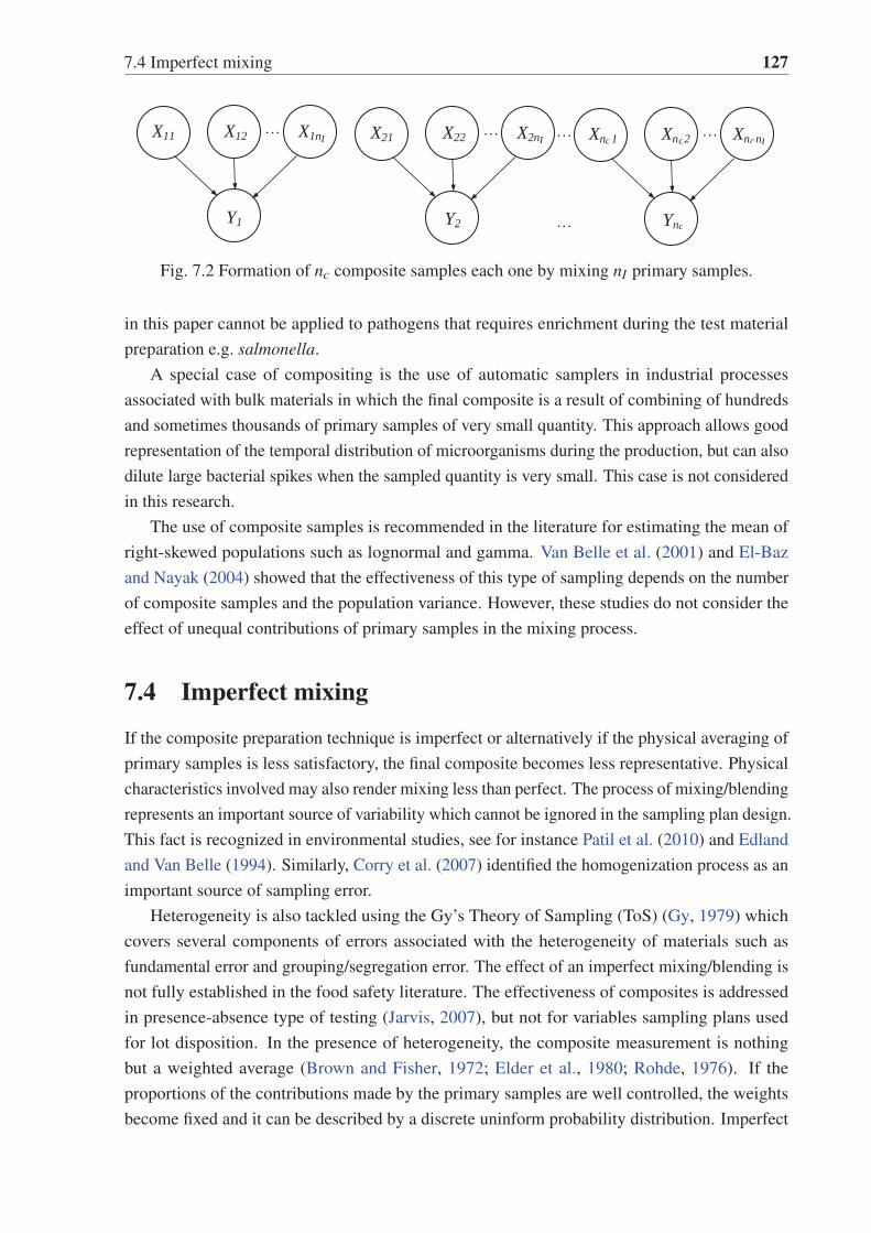
7.4 Imperfect mixing 127
c
c c c
…
… I
Y1
IX1n X12 … X11 I
Y2
IX2n X22 … X21 I
cYn
c IIIXn n cXn 2 … cXn 1
Fig. 7.2 Formation of nc composite samples each one by mixing nI primary samples.
in this paper cannot be applied to pathogens that requires enrichment during the test material
preparation e.g. salmonella.
A special case of compositing is the use of automatic samplers in industrial processes
associated with bulk materials in which the final composite is a result of combining of hundreds
and sometimes thousands of primary samples of very small quantity. This approach allows good
representation of the temporal distribution of microorganisms during the production, but can also
dilute large bacterial spikes when the sampled quantity is very small. This case is not considered
in this research.
The use of composite samples is recommended in the literature for estimating the mean of
right-skewed populations such as lognormal and gamma. Van Belle et al. (2001) and El-Baz
and Nayak (2004) showed that the effectiveness of this type of sampling depends on the number
of composite samples and the population variance. However, these studies do not consider the
effect of unequal contributions of primary samples in the mixing process.
7.4 Imperfect mixing
If the composite preparation technique is imperfect or alternatively if the physical averaging of
primary samples is less satisfactory, the final composite becomes less representative. Physical
characteristics involved may also render mixing less than perfect. The process of mixing/blending
represents an important source of variability which cannot be ignored in the sampling plan design.
This fact is recognized in environmental studies, see for instance Patil et al. (2010) and Edland
and Van Belle (1994). Similarly, Corry et al. (2007) identified the homogenization process as an
important source of sampling error.
Heterogeneity is also tackled using the Gy’s Theory of Sampling (ToS) (Gy, 1979) which
covers several components of errors associated with the heterogeneity of materials such as
fundamental error and grouping/segregation error. The effect of an imperfect mixing/blending is
not fully established in the food safety literature. The effectiveness of composites is addressed
in presence-absence type of testing (Jarvis, 2007), but not for variables sampling plans used
for lot disposition. In the presence of heterogeneity, the composite measurement is nothing
but a weighted average (Brown and Fisher, 1972; Elder et al., 1980; Rohde, 1976). If the
proportions of the contributions made by the primary samples are well controlled, the weights
become fixed and it can be described by a discrete uninform probability distribution. Imperfect

128 Variables Sampling Plans using Composite Samples for Food Quality Assurance
mixing leads to unequal contributions of primary samples towards the composite sample and
hence the weights of such contributions become random and can be described by a non-uniform
probability distribution (Patil et al., 2010). In other words, when the composite is subsampled,
the contribution of each individual unit is different in terms of volume or mass. This means that
the weights will be proportional to the corresponding contribution. Since each contribution is
unknown, the weights are then randomly distributed.
That is, we treat the jth composite sample measurement as
Yj = w1X1 +w2X2 + · · ·+wnI XnI =nI
∑i=1
wiXi (7.2)
where wi are the stochastic weights subject to ∑nIi=1 wi = 1. A matrix algebraic treatment to
describe the composite samples and weights can be found in Lancaster and Keller-McNulty
(1998).
The quality of the mixing of the primary samples during the test material preparation is
specific for every category of food. Since liquids can be easily homogenized, they are often
mixed by manual shaking. However, manual mixing often cannot break the clumps in solid
materials and therefore mechanical mixing is required. Mechanical mixing is commonly carried
out using mixers or stomachers. Some of the sample preparation methods recommended by
Greenfield and Southgate (2003) result in imperfect composite. For instance, the mixing of
solids such as grains, flours and dried milk is carried out in solid state by hand, using spatula and
subsampling after quartering. In solids, the use of diluent significantly improves the degree of
homogenization.
Since the structure of the composite is unknown due to lack of population data, theoretical
models are used in the literature to study various scenarios of sampling variabilities, mixing
strategies and their effect on composite samples. We now consider three non-uniform probability
distributions to describe the weights. Two of them have been used previously, the Dirichlet
distribution (D) in Rohde (1976) and the multivariate hypergeometric distribution (MH) (Brown
and Fisher, 1972; Elder et al., 1980). Each distribution is used to represent different mixing
scenarios. We are not matching the parameters of these distributions so that a wider range of
situations can be covered.
The Dirichlet density function is given by:
f (w1, · · · ,wnI ;a1, · · · ,anI) =Γ(∑nI
i=0 ai)
∏1i=0 Γ(ai)
nI
∏i=1
wai−1i (7.3)
where a = (a1,a2, · · · ,anI) is the vector of concentration parameters and as usual ∑wi = 1. The
concentration parameters determine the contribution of the individual samples. The concentration
parameters are specific to the bulk material and the mixing/blending technique employed. No
empirical information is usually available because their determination requires the full knowledge
of the population variability. Hence we carried out a what-if analysis to assess the impact of a
change in the concentration parameters on the sampling plan. We considered three scenarios of
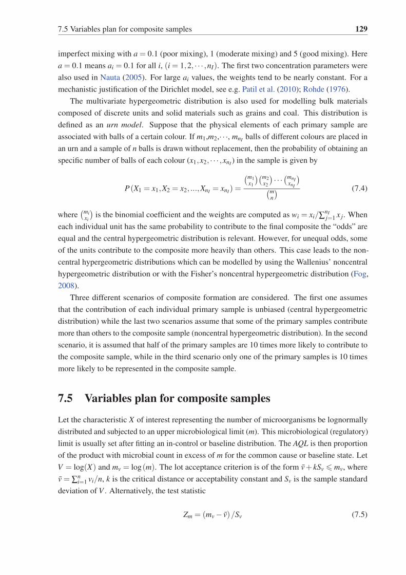
7.5 Variables plan for composite samples 129
imperfect mixing with a = 0.1 (poor mixing), 1 (moderate mixing) and 5 (good mixing). Here
a = 0.1 means ai = 0.1 for all i, (i = 1,2, · · · ,nI). The first two concentration parameters were
also used in Nauta (2005). For large ai values, the weights tend to be nearly constant. For a
mechanistic justification of the Dirichlet model, see e.g. Patil et al. (2010); Rohde (1976).
The multivariate hypergeometric distribution is also used for modelling bulk materials
composed of discrete units and solid materials such as grains and coal. This distribution is
defined as an urn model. Suppose that the physical elements of each primary sample are
associated with balls of a certain colour. If m1,m2,· · ·, mnI balls of different colours are placed in
an urn and a sample of n balls is drawn without replacement, then the probability of obtaining an
specific number of balls of each colour (x1,x2, · · · ,xnI ) in the sample is given by
P(X1 = x1,X2 = x2, ...,XnI = xnI) =
(m1x1
)(m2x2
) · · ·(mnIxnI
)(m
n
) (7.4)
where(mi
xi
)is the binomial coefficient and the weights are computed as wi = xi/∑nI
j=1 x j. When
each individual unit has the same probability to contribute to the final composite the “odds” are
equal and the central hypergeometric distribution is relevant. However, for unequal odds, some
of the units contribute to the composite more heavily than others. This case leads to the non-
central hypergeometric distributions which can be modelled by using the Wallenius’ noncentral
hypergeometric distribution or with the Fisher’s noncentral hypergeometric distribution (Fog,
2008).
Three different scenarios of composite formation are considered. The first one assumes
that the contribution of each individual primary sample is unbiased (central hypergeometric
distribution) while the last two scenarios assume that some of the primary samples contribute
more than others to the composite sample (noncentral hypergeometric distribution). In the second
scenario, it is assumed that half of the primary samples are 10 times more likely to contribute to
the composite sample, while in the third scenario only one of the primary samples is 10 times
more likely to be represented in the composite sample.
7.5 Variables plan for composite samples
Let the characteristic X of interest representing the number of microorganisms be lognormally
distributed and subjected to an upper microbiological limit (m). This microbiological (regulatory)
limit is usually set after fitting an in-control or baseline distribution. The AQL is then proportion
of the product with microbial count in excess of m for the common cause or baseline state. Let
V = log(X) and mv = log(m). The lot acceptance criterion is of the form v+ kSv � mv, where
v = ∑ni=1 vi/n, k is the critical distance or acceptability constant and Sv is the sample standard
deviation of V . Alternatively, the test statistic
Zm = (mv − v)/Sv (7.5)

130 Variables Sampling Plans using Composite Samples for Food Quality Assurance
expresses the allowable distance in standard deviation units between the mean and the specifica-
tion. When the value of Zm is lower than k, the fraction of nonconforming product in the lot is
higher than the AQL and hence the lot is rejected. Under the assumption of normal distribution
for V , the acceptability constant k and the required sample size n can be obtained using formulae,
see Duncan (1986) or Montgomery (2007). The traditional plan design assumes the use of
primary samples.
It is established in the literature that the sum of independent lognormal random variables can
be approximated by a single lognormal distribution (Johnson et al., 1994, pp. 217). Therefore,
the enumeration of cells in the composite samples (Yj) is also assumed to be lognormal. The
analytical test size of Yj is equal to the analytical size in the individual units Xi j for the purpose of
this research. Let U = log(Y ) be the log-count of microorganisms obtained from the composite
samples. The acceptance criterion for the composite samples is then u+ kSu � mv, where
u = ∑ni=1 ui/n, k is the critical distance and Su is the sample standard deviation of U .
Derivation of an analytical expression for the OC function of the variables plan based on the
composite samples is too complex and hence we need to resort to Monte-Carlo simulation to
obtain OC curves. The simulation algorithm for the sampling based on primary units is described
below. The common cause situation is modelled with the lognormal with μ = 0 and σ = 1 both
in log scale. The Zm test statistic is obtained from a vector X generated from the lognormal
distribution. For the purpose of the simulations, the AQL value is used to compute m since there
is a one-to-one relationship between proportion nonconforming and the distribution quantile.
The critical distance k is obtained as the α-quantile of Zm replicated (at least 50,000 times).
Batches under the common cause situation will be accepted with probability 1−α . The special
causes of variation mean a non-random change in the process and they are due to factors such as
temperature misuse, environmental factors and poor handling. Special causes are modelled by
increasing the μ until μ +2 at intervals of 0.05. The probability of acceptance is given for the
proportion of Zm values greater than or equal to the critical distance.
The simulation algorithm for composite samples is slightly different. The Zm test statistic
is obtained from a vector Y resulting from the average (perfect mixing) or weighted average
(imperfect mixing) of the individual sample units (Xi j). The weights for imperfect mixing are
modelled using the three distributions discussed in last section. The OC curves are forced to
match at the producers’ point (AQL,1−α) and then examined whether the consumer’s risk at
other rejectable levels is as small as possible.
To compare the sampling plan performance, let us start with the sampling plan using indi-
vidual units. Let AQL = 0.01, α = 0.01 and consider a reasonable sample size nc = 20. In this
case the analytical tests are done using the individual units. The resulting OC curve is shown in
Fig. 7.3 in thin solid line. Consider than that the 20 tests are carried out over composite samples
each one formed by nI = 4 and 8 individual units. Therefore each alternative require 4 × 20
= 80 and 8 × 20 = 160 primary samples respectively. The OC curves when the mixing of the
individual units is considered as perfect are given in heavy solid line. The thin and the heavy
solid lines give the worst and best case scenarios respectively in terms of consumer’s risk but

7.6 Design of the variables sampling plan based on composite samples. 131
they remain the same in Fig. 7.3–7.5. Suppose that the mixing process is less satisfactory and can
be described using the Dirichlet distribution. Consider the concentration parameters introduced
in the last section to describe three different mixing scenarios. The resulting OC curves are given
in dotted (a = 0.1), dashed (a = 1) and dotdashed (a = 5).
From Fig. 7.3, we note that the use of composite samples achieves a significant reduction in
the LQL at the same β risk (say β = 0.10). The benefit of using composite samples is due to the
natural averaging process as result of the physical mix. However, the composite sample formed
with four primary samples (nI = 4) achieves only a little reduction in the consumer’s risks when
the concentration parameter is small (a = 0.1). The effect of dilution is not compensated by the
improvement in the performance of detecting large fraction nonconforming product levels. As
one would expect, the more evenly the primary samples contribute towards the composite sample,
the steeper the OC curve becomes. In case of uneven contributions, the OC curve becomes less
steeper thereby increasing the consumer’s risks. In other words, the discriminatory power of the
sampling plan (capacity to discriminate between good and poor quality) depends on the standard
deviation of the weights in addition to the number of primary samples used for composite sample
formation.
Now consider the case in which the composite sample formation is modelled by employing
the multivariate hypergeometric distribution. The OC curves obtained using Monte-Carlo
simulation for these scenarios are presented in Fig. 7.4.
Consider the case in which the contributions are derived from the negative binomial distri-
bution , NB(d,b). The resulting OC curves are shown in Fig. 7.5. We particularly note that
compositing does not reduce the consumer’s risk when d = 1 and nI = 4 when compared to
testing nc primary samples.
When mixing is imperfect, the stochastic nature of mixing can be studied only using theoret-
ical models. By employing various probability models, we can examine how the consumer’s
risks are affected and how much efficiency is lost or gained by the use of composite samples.
Figures 7.3 to 7.5 show that testing nc composite samples is a better strategy than testing nc
primary samples, and the consumer’s risks are not affected adversely because of compositing.
The performance of the sampling based on composites requires good mixing for controlling the
risks. We also note that perfectly mixed samples achieve the lowest consumer’s risks in general
for a given nc and nI . In the next section, we use just the Dirichlet distribution for generating
weights since it allows modelling a variety of mixing scenarios with a single parameter.
7.6 Design of the variables sampling plan based on compositesamples.
In this section we examine the number of samples to be tested in order to control the producer’s
and consumer’s risks at desired levels for selected combinations of AQL and LQL values for
nI = 1,4 and 8. Tables 7.1 and 7.2 in the Appendix show the number of samples to be tested

132 Variables Sampling Plans using Composite Samples for Food Quality Assurance
0.00 0.05 0.10 0.15
0.0
0.2
0.4
0.6
0.8
1.0
Proportion nonconforming
Pa
nI = 1nI = 4nI = 4 D(a = 0.1)nI = 4 D(a = 1)nI = 4 D(a = 5)
0.00 0.05 0.10 0.15
0.0
0.2
0.4
0.6
0.8
1.0
Proportion nonconforming
Pa
nI = 1nI = 8nI = 8 D(a = 0.1)nI = 8 D(a = 1)nI = 8 D(a = 5)
Fig. 7.3 Comparison of the OC curves for nc = 20, α = 0.01, AQL = 0.01 with nI = 1, 4 and 8.
The thin solid line gives the OC curve when the units are tested individually (nI = 1) and the
heavy solid line shows the case in which the composite samples are formed under perfect mixing.
The other OC curves are associated with imperfect composites described using a Dirichlet
distribution with a = 0.1 (dotted), a = 1 (dashed), and a = 10 (dotdash). Pa is the probability of
acceptance.

7.6 Design of the variables sampling plan based on composite samples. 133
0.00 0.05 0.10 0.15
0.0
0.2
0.4
0.6
0.8
1.0
Proportion nonconforming
PanI = 1nI = 4nI = 4 MH(eq_odds)nI = 4 MH(dif_odds) 1nI = 4 MH(dif_odds) 2
0.00 0.05 0.10 0.15
0.0
0.2
0.4
0.6
0.8
1.0
Proportion nonconforming
Pa
nI = 1nI = 8nI = 8 MH(eq_odds)nI = 8 MH(dif_odds) 1nI = 8 MH(dif_odds) 2
Fig. 7.4 Comparison of the OC curves for nc = 20, α = 0.01, AQL = 0.01 with nI = 1, 4 and 8.
The thin solid line gives the OC curve when the units are tested individually (nI = 1) and the
heavy solid line shows the case in which the composite samples are formed under perfect mixing.
The other OC curves refer to imperfect mixing with weights described using multivariate central
(dashed) and noncentral hypergeometric distribution (dotted and dotdashed).

134 Variables Sampling Plans using Composite Samples for Food Quality Assurance
0.00 0.05 0.10 0.15
0.0
0.2
0.4
0.6
0.8
1.0
Proportion nonconforming
Pa
nI = 1nI = 4nI = 4 NB(10, 1)nI = 4 NB(2, 2)nI = 4 NB(1, 2)
0.00 0.05 0.10 0.15
0.0
0.2
0.4
0.6
0.8
1.0
Proportion nonconforming
Pa
nI = 1nI = 8nI = 8 NB(10, 1)nI = 8 NB(2, 2)nI = 8 NB(1, 2)
Fig. 7.5 Comparison of the OC curves for nc = 20, α = 0.01, AQL = 0.01 with nI = 1, 4 and 8.
The thin solid line gives the OC curve when the units are tested individually (nI = 1) and the
heavy solid line shows the case in which the composite samples are formed under perfect mixing.
The other OC curves are associated with imperfect mixing described by negative binomial
distribution with shape (d) and scale (b).

7.6 Design of the variables sampling plan based on composite samples. 135
for various scenarios (testing using individual units and testing composite samples with perfect
and different imperfect mixing conditions). The associated acceptability constants k are given
in brackets. The number of samples to be tested n when the units are tested individually follow
from the traditional variables plans discussed in textbooks such as Duncan (1986). The reduction
in the number of samples that are tested is between 30% to 50% for the variables plans based
on composite samples when mixing is assumed to be perfect. However poor mixing does not
reduce the sample sizes nc greatly.
It is well known in the acceptance sampling literature that the closer the quality levels (AQLand LQL) are, higher the required sample size will be. For example, the sample size requirement
for AQL = 0.01, α = 0.01, LQL = 0.10 and β = 0.10 is less than the sample size required for
AQL = 0.05, α = 0.01, LQL = 0.10 and β = 0.10. For safety characteristics, the AQL and LQLvalues cannot be high. But care should be taken to set them apart so that a higher rate of rejection
of poor lots can be achieved using small sample sizes. A step-by-step guide for determining the
sample size and the acceptability constant is presented in the Appendix.
Table 7.1 Estimates of the required sample size and the critical distance for the lognormal
distribution using individual units and composite samples with nI = 4. The contribution for an
imperfect mixing is modelled using the Dirichlet distribution.
AQL LQL α β nc1(k) nc2(k) nc3(k) nc4(k) nc5(k)0.001 0.10 0.01 0.10 13(1.965) 9(2.864) 12(2.092) 10(2.521) 9(2.751)
0.001 0.10 0.05 0.10 10(2.155) 7(3.223) 9(2.298) 8(2.858) 7(3.096)
0.001 0.15 0.01 0.10 9(1.811) 6(2.575) 9(1.950) 7(2.318) 7(2.584)
0.001 0.15 0.05 0.10 7(2.013) 5(3.022) 7(2.199) 6(2.714) 5(2.903)
0.01 0.10 0.01 0.10 30(1.666) 18(2.330) 27(1.760) 22(2.124) 20(2.301)
0.01 0.10 0.05 0.10 21(1.761) 13(2.532) 19(1.876) 16(2.287) 14(2.478)
0.01 0.15 0.01 0.10 18(1.515) 10(2.052) 16(1.593) 13(1.894) 11(2.028)
0.01 0.15 0.05 0.10 13(1.639) 8(2.330) 12(1.745) 9(2.067) 8(2.241)
Note: c1 denotes testing of individual sample units (nI = 1) and c2 denotes testing using composite
samples under perfect mixing conditions (nI = 4). c3, c4 and c5 correspond to the imperfect mixing
(nI = 4) modelled by the Dirichlet distribution with a = 0.1,1 and 5 respectively.
Other statistical models such as the negative binomial (NB) can also be used to describe the
weights. However, this case has not been addressed in the literature before. Let X1, X2,...,XnI be
i.i.d. random variables from the NB distribution with density given by:
f (x) =(
k+ x−1
k
)(1− p)x pk (7.6)
where k and x are the number of successes and failures respectively. As before, define wi =
xi/∑nIj=1 x j. The NB model arises as a mixed Poisson-gamma distribution where the Poisson
parameter (λ ) is distributed as gamma with shape parameter (d) and scale parameter b =
(1− p)/p. Three possible scenarios of weights (from good to poor mixing) being generated by
NB(d = 10,b = 1), NB(d = 2,b = 2) and NB(d = 1,b = 2) were examined.

136 Variables Sampling Plans using Composite Samples for Food Quality Assurance
7.7 Three-class variables plan
The three-class variables plans (Newcombe and Allen, 1988) are an extension of the three-class
attribute plans originally introduced by Bray et al. (1973a). In three-class plans for attributes test
results are classified as acceptable, marginally acceptable and unacceptable. The ICMSF (2002)
considers three-class attributes plans in Cases 1–9. In the three-class variables plans, the lot is
sentenced as acceptable if the observed proportion nonconforming and proportion of marginal
items are lower than some predefined limits. The advantage of the three-class plan for variables
is that it requires a smaller sample size when compared with the three-class plans for attributes
(Newcombe and Allen, 1988). Wilrich and Weiss (2009) proposed the three-class sampling by
variables for safety characteristics and studied the performance when the density departs form
the lognormal model.
Three-class plan for variables involves two microbiological limits m < M (see Fig. 7.6), two
critical distances k2 < k1 and two acceptable quality limits AQL1 < AQL2. Let p1 and p2 be the
0 1 2 3 4 5 6 7
0.0
0.1
0.2
0.3
0.4
0.5
0.6
CFU/g
logn
orm
al d
ensi
ty
Mm
nonconforming
acceptablemarginallyacceptable
Fig. 7.6 Illustration of the three-class plan using a lognormal distribution with two microbiological
limits.
proportion of items exceeding M and m respectively, i.e. the proportion of nonconforming and
marginally acceptable items in the lot respectively. The probability of acceptance is given by
the joint probability function Pr (v+ k1Sv � Mv ∩ v+ k2Sv � mv). The sampling performance is
revealed by the OC surface which is the plot of the proportion nonconforming and marginally
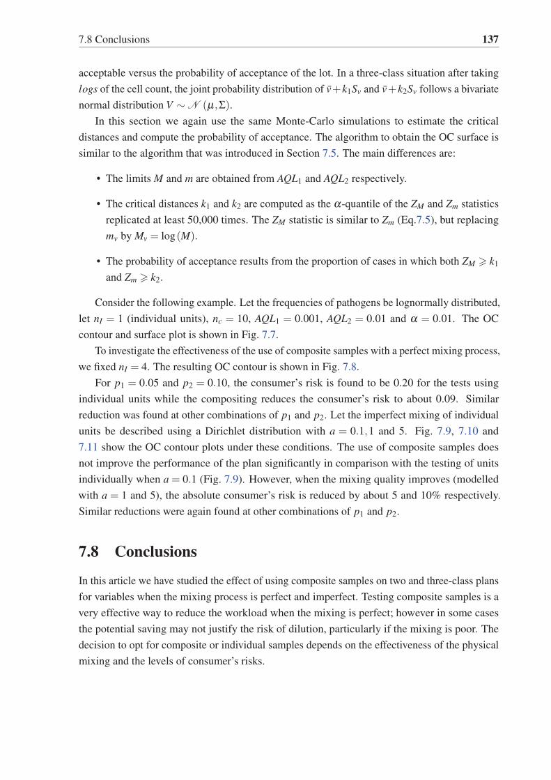
7.8 Conclusions 137
acceptable versus the probability of acceptance of the lot. In a three-class situation after taking
logs of the cell count, the joint probability distribution of v+k1Sv and v+k2Sv follows a bivariate
normal distribution V ∼ N (μ,Σ).In this section we again use the same Monte-Carlo simulations to estimate the critical
distances and compute the probability of acceptance. The algorithm to obtain the OC surface is
similar to the algorithm that was introduced in Section 7.5. The main differences are:
• The limits M and m are obtained from AQL1 and AQL2 respectively.
• The critical distances k1 and k2 are computed as the α-quantile of the ZM and Zm statistics
replicated at least 50,000 times. The ZM statistic is similar to Zm (Eq.7.5), but replacing
mv by Mv = log(M).
• The probability of acceptance results from the proportion of cases in which both ZM � k1
and Zm � k2.
Consider the following example. Let the frequencies of pathogens be lognormally distributed,
let nI = 1 (individual units), nc = 10, AQL1 = 0.001, AQL2 = 0.01 and α = 0.01. The OC
contour and surface plot is shown in Fig. 7.7.
To investigate the effectiveness of the use of composite samples with a perfect mixing process,
we fixed nI = 4. The resulting OC contour is shown in Fig. 7.8.
For p1 = 0.05 and p2 = 0.10, the consumer’s risk is found to be 0.20 for the tests using
individual units while the compositing reduces the consumer’s risk to about 0.09. Similar
reduction was found at other combinations of p1 and p2. Let the imperfect mixing of individual
units be described using a Dirichlet distribution with a = 0.1,1 and 5. Fig. 7.9, 7.10 and
7.11 show the OC contour plots under these conditions. The use of composite samples does
not improve the performance of the plan significantly in comparison with the testing of units
individually when a = 0.1 (Fig. 7.9). However, when the mixing quality improves (modelled
with a = 1 and 5), the absolute consumer’s risk is reduced by about 5 and 10% respectively.
Similar reductions were again found at other combinations of p1 and p2.
7.8 Conclusions
In this article we have studied the effect of using composite samples on two and three-class plans
for variables when the mixing process is perfect and imperfect. Testing composite samples is a
very effective way to reduce the workload when the mixing is perfect; however in some cases
the potential saving may not justify the risk of dilution, particularly if the mixing is poor. The
decision to opt for composite or individual samples depends on the effectiveness of the physical
mixing and the levels of consumer’s risks.

138 Variables Sampling Plans using Composite Samples for Food Quality Assurance
proportion of nonconforming ( p1 )
prop
ortio
n m
argi
nally
acc
epta
ble
( p2 )
0.1
0.2
0.3 0.4
0.5 0.6 0.7 0.8
0.00 0.05 0.10 0.15
0.00
0.05
0.10
0.15
0.20
0.25
●
0.02
0.04
0.06
0.08 0.050.10
0.150.20
0.25
0.2
0.4
0.6
0.8
1.0
p1
p2
Pa
Fig. 7.7 (a) OC contour plot and (b) OC surface of the three-class variables plans using nc = 10
primary samples, AQL1 = 0.001, AQL2 = 0.01 and α = 0.01.

7.8 Conclusions 139
proportion of nonconforming ( p1 )
prop
ortio
n m
argi
nally
acc
epta
ble
( p2 )
0
0.1
0.2 0.3
0.4
0.5
0.6 0.7 0.9
0.00 0.05 0.10 0.15
0.00
0.05
0.10
0.15
0.20
0.25
●
Fig. 7.8 OC contour plot of the three-class variables plans using composite samples assuming a
perfect mixing with nI = 4, nc = 10, AQL1 = 0.001, AQL2 = 0.01 and α = 0.01.
proportion of nonconforming ( p1 )
prop
ortio
n m
argi
nally
acc
epta
ble
( p2 )
0.1
0.2
0.3
0.4
0.5 0.6 0.7
0.8 0.9
0.00 0.05 0.10 0.15
0.00
0.05
0.10
0.15
0.20
0.25
●
Fig. 7.9 OC contour plot of the three-class variables plans using composite samples assuming the
mixing as imperfect with a = 0.1, nI = 4, nc = 10, AQL1 = 0.001, AQL2 = 0.01 and α = 0.01.

140 Variables Sampling Plans using Composite Samples for Food Quality Assurance
proportion of nonconforming ( p1 )
prop
ortio
n m
argi
nally
acc
epta
ble
( p2 )
0.1 0.2
0.3 0.4 0.5
0.6
0.7 0.8
0.00 0.05 0.10 0.15
0.00
0.05
0.10
0.15
0.20
0.25
●
Fig. 7.10 OC contour plot of the three-class variables plans using composite samples assuming
the mixing as imperfect with a = 1, nI = 4, nc = 10, AQL1 = 0.001, AQL2 = 0.01 and α = 0.01.
proportion of nonconforming ( p1 )
prop
ortio
n m
argi
nally
acc
epta
ble
( p2 ) 0
0.1
0.2 0.3
0.4
0.5
0.6
0.7 0.8
0.00 0.05 0.10 0.15
0.00
0.05
0.10
0.15
0.20
0.25
●
Fig. 7.11 OC contour plot of the three-class variables plans using composite samples assuming
the mixing as imperfect with a = 5, nI = 4, nc = 10, AQL1 = 0.001, AQL2 = 0.01 and α = 0.01.
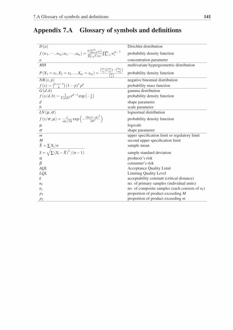
7.A Glossary of symbols and definitions 141
Appendix 7.A Glossary of symbols and definitions
D(a) Dirichlet distribution
f (w1, · · · ,wnI ;a1, · · · ,anI) =Γ(∑
nIi=0 ai)
∏1i=0 Γ(ai)
∏nIi=1 wai−1
i probability density function
a concentration parameter
MH multivariate hypergeometric distribution
P(X1 = x1,X2 = x2, ...,XnI = xnI) =(m1
x1)(m2
x2)···(mnIxnI
)
(mn)
probability density function
NB(x, p) negative binomial distribution
f (x) =(k+x−1
k
)(1− p)x pk probability mass function
G(d,b) gamma distribution
f (x/d,b) = 1Γ(d)bd xd−1 exp
(− xb
)probability density function
d shape parameter
b scale parameter
LN (μ,σ) lognormal distribution
f (x/σ ,μ) = 1
xσ√
2πexp
(− (ln(x)−μ)2
2σ2
)probability density function
μ logscale
σ shape parameter
m upper specification limit or regulatory limit
M second upper specification limit
X = ∑Xi/n sample mean
S =
√∑(Xi − X)
2/(n−1) sample standard deviation
α producer’s risk
β consumer’s risk
AQL Acceptance Quality Limit
LQL Limiting Quality Level
k acceptability constant (critical distance)
nI no. of primary samples (individual units)
nc no. of composite samples (each consists of nI)
p1 proportion of product exceeding Mp2 proportion of product exceeding m

142 Variables Sampling Plans using Composite Samples for Food Quality Assurance
Appendix 7.B Sampling plan design
Table 7.2 Estimates of the required sample size and the critical distance for the lognormal
distribution using individual units and composite samples with nI = 8. The contribution for an
imperfect mixing is modelled using the Dirichlet distribution.
AQL LQL α β nc1(k) nc2(k) nc3(k) nc4(k) nc5(k)0.001 0.10 0.01 0.10 13(1.965) 8(3.698) 12(2.282) 10(3.134) 8(3.461)
0.001 0.10 0.05 0.10 10(2.155) 6(4.143) 9(2.534) 7(3.484) 7(4.043)
0.001 0.15 0.01 0.10 9(1.811) 5(3.235) 8(2.064) 7(2.836) 6(3.209)
0.001 0.15 0.05 0.10 7(2.013) 4(3.801) 6(2.332) 5(3.268) 5(3.796)
0.01 0.10 0.01 0.10 30(1.666) 15(2.969) 26(1.914) 20(2.555) 17(2.851)
0.01 0.10 0.05 0.10 21(1.761) 11(3.242) 18(2.033) 14(2.763) 12(3.107)
0.01 0.15 0.01 0.10 18(1.515) 9(2.650) 15(1.715) 11(2.232) 9(2.468)
0.01 0.15 0.05 0.10 13(1.639) 7(2.997) 11(1.872) 8(2.509) 7(2.826)
Note: c1 denotes testing of individual sample units (nI = 1) and c2 denotes testing using composite
samples under perfect mixing conditions (nI = 8). c3, c4 and c5 correspond to the imperfect mixing
(nI = 8) modelled by the Dirichlet distribution with a = 0.1,1 and 5 respectively.
Appendix 7.C Sampling plan guide
The procedure for the two-class composite sampling design for variables design of the two-class
variables plan based on composite samples is described in the following guide:
1. Fix the consumer’s (LQL,β ) and producer’s (AQL,α) points.
2. From previous experience or according to the mixing process and type of commodity set
the expected concentration parameter (a) in the Dirichlet distribution.
3. Define the number of individual units (nI = 4 or 8). For other nI values, the sampling plan
parameters can be obtained approximately by interpolation.
4. Obtain from Table 7.1 or 7.2 the number of composites to be formed (nc) and the critical
distance (k).
5. Compute the statistic Zm.
6. Accept the lot if Zm ≥ k; otherwise reject it.

Chapter 8
General conclusions and futureperspectives.
This thesis was driven by the needs in the food industry for more efficient sampling plans for
batch inspection. Several sampling plans with application to food microbiological inspection
have been introduced. Issues such as the use of composite samples, compressed limits and
analytical unit amounts have been discussed. The techniques developed in this research allow
producers, food safety authorities and regulatory agencies to (1) reduce the risk for the consumers
(2) utilize smaller sample sizes (3) attain smaller costs and (4) employ easy-to-use free software.
The design of several inspection plans has been discussed and step-by-step guidance has been
given. Both frequentist and Bayesian approaches have been used. Moreover, the computational
codes have been published and several apps have been developed. Some of the chapters contain
data analysis mostly for parameters estimation needed for assessing risks.
More specifically, Chapter 2 studied the risk as a function of the analytical unit amount for
isolated and streams of lots. The effects of heterogeneity are also examined in attributes and
variables plans. Chapter 3 aimed at the application and extension of the compressed limit theory
to food safety problems. This chapter introduced a novel three-class compressed limit plan
and discussed the zero acceptance number sampling plans, both with potential use in the food
industry. A double sampling plan by attributes intended for bacterial counts was introduced in
Chapter 4. This plan that is based on the compressed limit theory is the first double plan (to the
best of our knowledge) that matches the zero acceptance number plan. Measurement error is one
of the main issues in microbial testing. The effects of imperfect testing are studied in Chapter
5. Bayesian inference was used to estimate prevalence jointly with the test’s sensitivity and
specificity. The design of more suitable sampling plans in terms of risk and cost is addressed. A
novel variables sampling plan for lognormally distributed variables was introduced in Chapter 6.
The properties, benefits and demerits of this plan are discussed. Finally, Chapter 7 was dedicated
to studying the use of composite samples in plans by variables. The sampling design is given for
different composite scenarios. It showed the benefits of compositing rather than testing primary
units under certain conditions.

144 General conclusions and future perspectives.
8.1 Future plan of work
Assurance of safety primarily warrants compliance to multiple food safety regulations and con-
sumers specific characteristics. Some bacteria pertain to common families and often association
or correlation can be established. Some microorganism indicators have been linked to high
chances of pathogen contamination. Future studies should explore: (1) these connections and
associations, (2) statistical models to better characterize the risk, (3) the design of more efficient
sampling plans including multivariate alternatives.
Testing for pathogens usually comprises a pre-enrichment stage, which allows the recovery
or resuscitation of the cells. For instance, ISO 22964 (2006) is the standard for the detection of
Enterobacter sakazakii. Decimal dilutions are usually prepared using test portions or analytical
amounts of 10g or 300g for the pre-enrichment stage. Theoretically increasing the analytical
amounts in this stage will yield a higher probability of detecting the target cell if the pathogen is
present in the batch. However, the trade-off is that a higher volume might need higher incubation
time to allow the cell multiply over the limit of detection. See the comments in this regards given
by Ross et al. (2011). This and other issues need further theoretical work and validation.
Much of the risk assessment relies on the correctness of the statistical model. In pathogen
detection, the tests are generally presence/absence, where the positives results are reported as
‘detected’. In the absence of numerical results, it becomes difficult to find suitable statistical
models and appropriate parameters for fitting the frequencies of cells. Moreover, the actual
testing regime does not allow a proper spatial characterization of the occurrence of contamination.
There is a need for studies revealing the spatial contamination in nonconforming and recalled
batches. More effort should be put into making microbiological datasets publicly available. The
sampling inspection plans discussed in this research may have to be tailored differently in future
work for other food industries and processes.
Summing up, the uncountable sources of variation found from sample collection to laboratory
testing and emerging issues in food safety make microbiological acceptance sampling a fertile
territory for future research and development.

References
7 CFR (2000). Code of federal regulation 7: Regulations of the Department of Agriculture.Chapter I - Agricultural marketing service (standards, inspections, marketing practices).
Albin, S. L. (1990). The lognormal distribution for modeling quality data when the mean is nearzero. Journal of Quality Technology, 22:105–110.
Alonzo, T. A. and Pepe, M. S. (2003). Estimating disease prevalence in two-phase studies.Biostatistics, 4(2):313–326.
Anscombe, F. J. (1950). Sampling theory of the negative binomial and logarithmic seriesdistributions. Biometrika, 37(3/4):358–382.
Avinadav, T. and Perlman, Y. (2013). Economic design of offline inspections for a batchproduction process. International Journal of Production Research, 51(11):3372–3384.
Beja, A. and Ladany, S. P. (1974). Efficient sampling by artificial attributes. Technometrics,16(4):601–611.
Bray, D., Lyon, D., and Burr, I. (1973a). Three class attributes plans in acceptance sampling.Technometrics, 15(3):575–585.
Bray, D. F., Lyon, D. A., and Burr, I. W. (1973b). Three class attributes plans in acceptancesampling. Technometrics, 15(3):pp. 575–585.
Brenner, H., Gefeller, O., et al. (1997). Variation of sensitivity, specificity, likelihood ratios andpredictive values with disease prevalence. Statistics in medicine, 16(9):981–991.
Brown, G. and Fisher, N. (1972). Subsampling a mixture of sampled material. Technometrics,14(3):663–668.
Brush, G. G. (1986). A comparison of classical and Bayes producer’s risk. Technometrics,28(1):69–72.
Bulmer, M. (1974a). On fitting the Poisson lognormal distribution to species-abundance data.Biometrics, pages 101–110.
Bulmer, M. G. (1974b). On fitting the Poisson lognormal distribution to species-abundance data.Biometrics, 30(1):101–110.
CAC (1997). Principles for the establishment and application of microbiological criteria forfoods. Codex Alimentarius Commission. Accessed: 2014-04-02.
CAC (2004). General guidelines on sampling. Codex Alimentarius Commission. http://www.codexalimentarius.net/input/download/standards/10141/CXG_050e.pdf. Accessed:2014-04-02.

146 References
CAC (2008). Code of hygienic practice for powdered formulae for infants and young children.Codex Alimentarius Commission. www.codexalimentarius.org/download/standards/11026/CXP_066e.pdf. Accessed:2016-02-24.
Cawthorn, D.-M., Botha, S., and Witthuhn, R. C. (2008). Evaluation of different methods forthe detection and identification of Enterobacter sakazakii isolated from South African infantformula milks and the processing environment. International Journal of Food Microbiology,127(1):129–138.
Chang, W., Cheng, J., Allaire, J., Xie, Y., and McPherson, J. (2015). shiny: Web ApplicationFramework for R. R package version 0.12.2.
Chen, Y., Ross, W. H., Scott, V. N., and Gombas, D. E. (2003). Listeria monocytogenes: lowlevels equal low risk. Journal of Food Protection, 66(4):570–577.
Childs, A. and Chen, Y. (2011). Multilevel fixed and sequential acceptance sampling: The Rpackage MFSAS. Journal of Statistical Software, 43(6):1–20.
Chiu, W. (1974). A new prior distribution for attributes sampling. Technometrics, 16(1):93–102.
Corradini, M., Normand, M., Nussinovitch, A., Horowitz, J., and Peleg, M. (2001). Estimatingthe frequency of high microbial counts in commercial food products using various distributionfunctions. Journal of Food Protection, 64(5):674–681.
Corry, J. E., Jarvis, B., Passmore, S., and Hedges, A. (2007). A critical review of measurementuncertainty in the enumeration of food micro-organisms. Food microbiology, 24(3):230–253.
Dahms, S. (2004). Microbiological sampling plans: Statistical aspects. Mitteilungen ausLebensmitteluntersuchung und Hygiene, 95(1):32–44.
Dahms, S. and Hildebrandt, G. (1998). Some remarks on the design of three-class samplingplans. Journal of Food Protection, 61(6):757–761.
Dodge, H. F. (1955a). Chain sampling inspection plan. Industrial quality control, 11(4):10–13.
Dodge, H. F. (1955b). Skip-lot sampling plan. Industrial Quality Control, 11(5):3–5.
Dodge, H. F. (1969). Notes on the evolution of acceptance sampling plans-part i. Journal ofQuality Technology, 1(2):77–88.
Dodge, H. F. and Romig, H. G. (1941). Single sampling and double sampling inspection tables.Bell System Technical Journal, 20(1):1–61.
Dodge, H. F. and Romig, H. G. (1959). Sampling inspection tables: single and double sampling,volume 6. Wiley New York.
Duncan, A. J. (1958). Design and operation of a double-limit variables sampling plan. Journalof the American Statistical Association, 53(282):543–550.
Duncan, A. J. (1986). Quality Control and Industrial Statistics. Richard D. Irwin Inc.
Edland, S. and Van Belle, G. (1994). Decreased sampling costs and improved accuracy withcomposite sampling. In Cothern, C. R. and Ross, N. P., editors, Environmental statistics,assessment, and forecasting, pages 29–55. CRC Press.
Eijkelkamp, J., Aarts, H., and Van der Fels-Klerx, H. (2009). Suitability of rapid detectionmethods for Salmonella in poultry slaughterhouses. Food Analytical Methods, 2(1):1–13.

References 147
El-Baz, A. and Nayak, T. (2004). Efficiency of composite sampling for estimating a lognormaldistribution. Environmental and Ecological Statistics, 11(3):283–294.
Elder, R. S., Thompson, W. O., and Myers, R. H. (1980). Properties of composite samplingprocedures. Technometrics, 22(2):179–186.
European Commission (2005). Commission regulation (EC) No 2073/2005 of 15 November2005 On microbiological criteria for foodstuffs.
Evans, I. and Thyregod, P. (1985). Approximately optimal narrow limit gauges. Journal ofQuality Technology, 17(2):63–66.
FAO/WHO (2006). Enterobacter sakazakii and Salmonella in powdered infant formula: meetingreport. ftp://ftp.fao.org/docrep/fao/009/a0707e/a0707e00.pdf. Accessed:2016-05-17.
FAO/WHO (2007). Risk assessment for Enterobacter sakazakii in powdered infant formula.FAO/WHO.
FAO/WHO (2012). Microbiological sampling plan analysis tool. http://www.fstools.org/samplingmodel/. Accessed:2015-04-13.
FAO/WHO (2014). Risk manager’s guide to the statistical aspects of microbiological criteriarelated to foods. Accessed:2014-11-19.
FDA (2002). Isolation and enumeration of Enterobacter sakazakii from dehydrated powderedinfant formula. www.fda.gov/Food/FoodScienceResearch/LaboratoryMethods/ucm114665.htm.
Fenton, L. (1960). The sum of log-normal probability distributions in scatter transmissionsystems. IRE Transactions on Communications Systems, 8(1):57–67.
Ferrell, W. G. and Chhoker, A. (2002). Design of economically optimal acceptance samplingplans with inspection error. Computers & Operations Research, 29(10):1283–1300.
Fog, A. (2008). Calculation methods for Wallenius’ noncentral hypergeometric distribution.Communications in Statistics—-Simulation and Computation, 37(2):258–273.
Fog, A. (2013). BiasedUrn: Biased Urn model distributions. R package version 1.06.1.
Food Standards Australia New Zealand (2001). Microbiological limits for food with additionalguideline criteria. https://www.foodstandards.gov.au/code/userguide/documents/Micro_0801.pdf. Accessed:2015-09-22.
Fowlkes, E. B. (1979). Some methods for studying the mixture of two normal (lognormal)distributions. Journal of the American Statistical Association, 74(367):561–575.
Gabis, D. A. and Silliker, J. H. (1974). ICMSF methods studies. II. Comparison of analyticalschemes for detection of salmonella in high-moisture foods. Canadian Journal of Microbiol-ogy, 20(5):663–669.
Gardner, I. A. (2004). An epidemiologic critique of current microbial risk assessment practices:the importance of prevalence and test accuracy data. Journal of Food Protection, 67(9):2000–2007.
Gonzales-Barron, U. and Butler, F. (2011a). Characterisation of within-batch and between-batch variability in microbial counts in foods using Poisson-gamma and Poisson-lognormalregression models. Food Control, 22(8):1268–1278.
148 References
Gonzales-Barron, U. and Butler, F. (2011b). A comparison between the discrete Poisson-gammaand Poisson-lognormal distributions to characterise microbial counts in foods. Food Control,22(8):1279–1286.
Gonzales-Barron, U., Kerr, M., Sheridan, J. J., and Butler, F. (2010a). Count data distributions andtheir zero-modified equivalents as a framework for modelling microbial data with a relativelyhigh occurrence of zero counts. International Journal of Food Microbiology, 136(3):268–277.
Gonzales-Barron, U., Redmond, G., and Butler, F. (2010b). Modeling prevalence and counts frommost probable number in a Bayesian framework: An application to Salmonella typhimuriumin fresh pork sausages. Journal of Food Protection, 73(8):1416–1422.
Gonzales-Barron, U., Zwietering, M. H., and Butler, F. (2013). A novel derivation of a within-batch sampling plan based on a Poisson-gamma model characterising low microbial counts infoods. International Journal of Food Microbiology, 161(2):84–96.
Govindaraju, K. (2007). Inspection error adjustment in the design of single sampling attributesplan. Quality Engineering, 19(3):227–233.
Govindaraju, K. and Balamurali, S. (1998). Chain sampling plan for variables inspection. Journalof Applied Statistics, 25(1):103–109.
Govindaraju, K. and Kissling, R. (2015). A combined attributes-variables plan. AppliedStochastic Models in Business and Industry, 31(5):575–583.
Graves, S. B., Murphy, D. C., and Ringuest, J. L. (1996). Reevaluating producer’s and consumer’srisks in acceptance sampling. Computers & industrial engineering, 30(2):171–184.
Greenfield, H. and Southgate, D. (2003). Food Composition Data. Production, Managementand Use. Rome: Food and Agricultural Organization of the United Nations. Springer, 2. ed.edition.
Guenther, W. C. (1969). Use of the binomial, hypergeometric and Poisson tables to obtainsampling plans. Journal of Quality Technology, 1(2):105–109.
Guenther, W. C. (1970). A procedure for finding double sampling plans for attributes. Journal ofQuality Technology, 2(4):219–225.
Guenther, W. C. (1971). On the determination of single sampling attribute plans based upon alinear cost model and a prior distribution. Technometrics, 13(3):483–498.
Gy, P. (1979). Sampling of Particulate Materials Theory and Practice. Elsevier. Amsterdam.
Haas, C. N., Rose, J. B., and Gerba, C. P. (2014). Quantitative Microbial Risk Assessment. JohnWiley & Sons, New York, NY.
Hald, A. (1964). Bayesian single sampling attribute plans for discrete prior distributions.Technical report, DTIC Document. http://www.dtic.mil/cgi-bin/GetTRDoc?AD=AD0602396.
Hald, A. (1967a). Asymptotic properties of Bayesian single sampling plans. Journal of theRoyal Statistical Society. Series B (Methodological), 29(1):162–173.
Hald, A. (1967b). The determination of single sampling attribute plans with given producer’sand consumer’s risk. Technometrics, 9(3):401–415.
Hald, A. (1968). Bayesian single sampling attribute plans for continuous prior distributions.Technometrics, 10(4):667–683.

References 149
Haldane, J. (1932). A note on inverse probability. Mathematical Proceedings of the CambridgePhilosophical Society, 28(01):55–61.
Hall, D. B. (2000). Zero-inflated Poisson and binomial regression with random effects: a casestudy. Biometrics, 56(4):1030–1039.
Hamaker, H. (1960). Attribute sampling in operation. Bulletin de l’Institut international destatistique (Bulletin of the International Statistical Institute), 37(2):265–281. 1960 Proceedingsof the 32nd session. Tokyo, 1960.
Hamaker, H. and Strik, R. V. (1955). The efficiency of double sampling for attributes. Journal ofthe American Statistical Association, 50(271):830–849.
Hildebrandt, G., Böhmer, L., and Dahms, S. (1995). Three-class attributes plans in micro-biological quality control: A contribution to the discussion. Journal of Food Protection,58(7):784–790.
Hoelzer, K. and Pouillot, R. (2013). Practical considerations for the interpretation of micro-bial testing results based on small numbers of samples. Foodborne pathogens and disease,10(11):907–915.
Hoffman, A. D. and Wiedmann, M. (2001). Comparative evaluation of culture-and BAX poly-merase chain reaction-based detection methods for Listeria spp. and Listeria monocytogenesin environmental and raw fish samples. Journal of Food Protection, 64(10):1521–1526.
ICMSF (1986). Microorganisms in Foods 2. Sampling for microbiological analysis: Principlesand specific applications. Blackwell Scientific Publications.
ICMSF (2002). Microorganisms in Foods 7. Microbiological Testing in Food Safety Man-agement. International Commission on Microbiological Specifications for Foods. KluwerAcademic/Plenum Publishers, New York.
ICMSF (2011). Microorganisms in Foods 8. Use of Data for Assessing Process Control andProduct Acceptance. International Commission on Microbiological Specifications for Foods,volume 8. Springer.
ISO 11290 (1997). Microbiology of the food chain – horizontal method for the detectionand enumeration of Listeria monocytogenes and other Listeria spp. – part 1: Detectionmethod. Technical Report ISO 11290, International Organization for Standardization, Geneva,Switzerland.
ISO 22964 (2006). Milk and milk products — detection of Enterobacter sakazakii. TechnicalReport ISO 22964, International Organization for Standardization, Geneva, Switzerland.
ISO 4833-1 (2003). Microbiology of the food chain – horizontal method for the enumeration ofmicroorganisms – part 1: Colony count at 30 degrees C by the pour plate technique. TechnicalReport ISO 4833-1, International Organization for Standardization, Geneva, Switzerland.
ISO 6887-1 (1999). Microbiology of food and animal feeding stuffs – preparation of test samples,initial suspension and decimal dilutions for microbiological examination–Part 1: Generalrules for the preparation of the initial suspension and decimal dilutions. Technical Report ISO6887-1, International Organization for Standardization, Geneva, Switzerland.
Iversen, C., Druggan, P., Schumacher, S., Lehner, A., Feer, C., Gschwend, K., Joosten, H., andStephan, R. (2008). Development of a novel screening method for the isolation of “Cronobac-ter” spp.(Enterobacter sakazakii). Applied and Environmental Microbiology, 74(8):2550–2553.

150 References
Jarvis, B. (2007). On the compositing of samples for qualitative microbiological testing. Lettersin Applied Microbiology, 45(6):592–598.
Jarvis, B. (2008). Statistical Aspects of the Microbiological Examination of Foods. AcademicPress. Elsevier/Academic Press: Amsterdam, The Netherlands.
Jarvis, B. (2016). Statistical Aspects of the Microbiological Examination of Foods. AcademicPress. Elsevier/Academic Press.
Jeffreys, H. (1946). An invariant form for the prior probability in estimation problems. Proceed-ings of the Royal Society of London A: Mathematical, Physical and Engineering Sciences,186(1007):453–461.
Johnson, N. L., Kotz, S., and Balakrishnan, N. (1994). Continuous univariate distributions, Vol.1. John Wiley & Sons, New York, NY.
Johnson, N. L., Kotz, S., and Balakrishnan, N. (1997). Discrete multivariate distributions. NewYork: John Wiley & Sons.
Johnson, N. L., Kotz, S., and Wu, X.-Z. (1991). Inspection errors for attributes in quality control,volume 44. London: Chapman & Hall.
Jones, M. and Pewsey, A. (2009). Sinh-arcsinh distributions. Biometrika, 96(4):761–780.
Jongenburger, I. (2012a). Distributions of microorganisms in foods and their impact on foodsafety. Wageningen University.
Jongenburger, I. (2012b). Distributions of microorganisms in foods and their impact on foodsafety . PhD thesis, Wageningen University.
Jongenburger, I., Bassett, J., Jackson, T., Gorris, L., Jewell, K., and Zwietering, M. (2012a).Impact of microbial distributions on food safety II. Quantifying impacts on public health andsampling. Food Control, 26(2):546–554.
Jongenburger, I., Bassett, J., Jackson, T., Zwietering, M., and Jewell, K. (2012b). Impactof microbial distributions on food safety I. Factors influencing microbial distributions andmodelling aspects. Food Control, 26(2):601–609.
Jongenburger, I., Reij, M., Boer, E., Gorris, L., and Zwietering, M. (2011a). Actual distributionof Cronobacter spp. in industrial batches of powdered infant formula and consequences forperformance of sampling strategies. International Journal of Food Microbiology, 151(1):62–69.
Jongenburger, I., Reij, M., Boer, E., Gorris, L., and Zwietering, M. (2011b). Random orsystematic sampling to detect a localised microbial contamination within a batch of food.Food Control, 22(8):1448–1455.
Jongenburger, I., Reij, M., Boer, E., Zwietering, M., and Gorris, L. (2012c). Modelling homoge-neous and heterogeneous microbial contaminations in a powdered food product. InternationalJournal of Food Microbiology, 157(1):35–44.
Jonkman, J. N., Gerard, P. D., and Swallow, W. H. (2009). Estimating probabilities under thethree-parameter gamma distribution using composite sampling. Computational Statistics &Data Analysis, 53(4):1099–1109.
Kiermeier, A. (2008). Visualizing and assessing acceptance sampling plans: The R packageAcceptanceSampling. Journal of Statistical Software, 26(6).
References 151
Kiermeier, A., Mellor, G., Barlow, R., and Jenson, I. (2011). Assumptions of acceptance samplingand the implications for lot contamination: Escherichia coli O157 in lots of Australianmanufacturing beef. Journal of Food Protection, 74(4):539–544.
Kilsby, D. and Baird-Parker, A. (1983). Sampling programmes for microbiological analysisof food. In Roberts, T. A. and Skinner, F., editors, Food Microbiology: Advances andprospects, pages 309–315. Society for Applied Bacteriology Symposium Series No. 11.London: Academic Press.
Kilsby, D. C., Aspinall, L. J., and Baird-Parker, A. C. (1979). A system for setting numericalmicrobiological specifications for foods. Journal of Applied Bacteriology, 46(3):591–599.
Kruschke, J. (2015). Doing Bayesian data analysis: A tutorial with R, JAGS, and Stan. AcademicPress, New York, 2. ed. edition.
Ladany, S. P. (1976). Determination of optimal compressed limit gaging sampling plans. Journalof Quality Technology, 8(4):225–231.
Lambert, D. (1992). Zero-inflated Poisson regression, with an application to defects in manufac-turing. Technometrics, 34(1):1–14.
Lancaster, V. A. and Keller-McNulty, S. (1998). A review of composite sampling methods.Journal of the American Statistical Association, 93(443):pp. 1216–1230.
Larson, H. R. (1966). A nomograph of the cumulative binomial distribution. Industrial QualityControl, 23(6):270–278.
Lavin, M. (1946). Inspection efficiency and sampling inspection plans. Journal of the AmericanStatistical Association, 41(236):432–438.
Lee, J. and Hathaway, S. (2000). New Zealand approaches to HACCP systems. Food Control,11(5):373 – 376.
Leeflang, M. M., Rutjes, A. W., Reitsma, J. B., Hooft, L., and Bossuyt, P. M. (2013). Variationof a test’s sensitivity and specificity with disease prevalence. Canadian Medical AssociationJournal, 185(11):E537–E544.
Legan, J., Vandeven, M. H., Dahms, S., and Cole, M. B. (2001). Determining the concentrationof microorganisms controlled by attributes sampling plans. Food Control, 12(3):137–147.
Lieberman, G. J. and Resnikoff, G. J. (1955). Sampling plans for inspection by variables. Journalof the American Statistical Association, 50(270):457–516.
Lund, B. M. (1986). An Evaluation of the Role of Microbiological Criteria for Foods andFood Ingredients: By the National Research Council (US) Food Protection Committee,Subcommittee on Microbiological Criteria. http://www.ncbi.nlm.nih.gov/books/NBK216671/.Accessed:2016-05-05.
Lunn, D. J., Thomas, A., Best, N., and Spiegelhalter, D. (2000). WinBUGS - A Bayesianmodelling framework: concepts, structure, and extensibility. Statistics and Computing,10(4):325–337.
Malcolm, S. (1984). A note on the use of the non-central t-distribution in setting numericalmicrobiological specifications for foods. Journal of Applied Microbiology, 57(1):175–177.
Malorny, B., Paccassoni, E., Fach, P., Bunge, C., Martin, A., and Helmuth, R. (2004). Diagnosticreal-time PCR for detection of Salmonella in food. Applied and Environmental Microbiology,70(12):7046–7052.

152 References
Marshall, A., Meza, J. C., and Olkin, I. (2012). Can data recognize its parent distribution?Journal of Computational and Graphical Statistics, 10(3):555–580.
Ministry of Agriculture and Forestry (2011). Animal products (dairy): Approved criteria forgeneral dairy processing. https://mpi.govt.nz/document-vault/10145. Accessed:2016-02-22.
Montgomery, D. (2005). Introduction to statistical quality control. John Wiley & Sons NewYork, 5 edition.
Montgomery, D. C. (2007). Introduction to statistical quality control. John Wiley & Sons NewYork, 6 edition.
Motarjemi, Y., Moy, G., and Todd, E. (2014). Encyclopedia of food safety. Academic Press,Elsevier Missouri, USA.
Mussida, A., Gonzales-Barron, U., and Butler, F. (2013a). Effectiveness of sampling plans byattributes based on mixture distributions characterising microbial clustering in food. FoodControl, 34(1):50–60.
Mussida, A., Vose, D., and Butler, F. (2013b). Efficiency of the sampling plan for Cronobacterspp. assuming a Poisson lognormal distribution of the bacteria in powder infant formulaand the implications of assuming a fixed within and between-lot variability. Food Control,33(1):174–185.
Nauta, M. J. (2005). Microbiological risk assessment models for partitioning and mixing duringfood handling. International Journal of Food Microbiology, 100(1–3):311–322. The FourthInternational Conference on Predictive Modelling in Foods.
New Zealand Parliamentary Counsel Office (2008). Food (fees and charges) regulations1997. http://www.legislation.govt.nz/regulation/public/1997/0100/latest/DLM232769.html?search=ts_regulation_food_resel&sr=1. Accessed:2016-01-22.
Newcombe, P. and Allen, O. (1988). A three-class procedure for acceptance sampling byvariables. Technometrics, 30(4):415–421.
Niederhauser, C., Höfelein, C., Lüthy, J., Kaufmann, U., Bühler, H.-P., and Candrian, U. (1993).Comparison of “Gen-Probe” DNA probe and PCR for detection of Listeria monocytogenes innaturally contaminated soft cheese and semi-soft cheese. Research in Microbiology, 144(1):47–54.
Ott, E. R. and Mundel, A. B. (1954). Narrow-limit gaging. Industrial Quality Control, 10(5):21–28.
Owen, D. (1967). Variables sampling plans based on the normal distribution. Technometrics,9(3):417–423.
Paoli, M. G. and Hartnett, E. (2006). Overview of a risk assessment model for Enterobactersakazakii in powdered infant formula. Available from The Food and Agriculture Organizationof the United Nations and the World Health Organization, FAO/WHO.
Patil, G. (2006). Composite sampling. In Encyclopedia of Environmetrics, pages 387–391. JohnWiley & Sons, Ltd.
Patil, G., Gore, S., and Taillie, C. (2010). Composite Sampling: A Novel Method to AccomplishObservational Economy in Environmental Studies. Environmental and ecological statistics.Springer.
References 153
Pearn, W. and Wu, C.-W. (2006). Critical acceptance values and sample sizes of a variablessampling plan for very low fraction of defectives. Omega, 34(1):90–101.
Perry, R. L. (1973). Skip-lot sampling plans. Journal of Quality Technology, 5(3):123–130.
Plummer, M. (2016). rjags: Bayesian Graphical Models using MCMC. R package version 4-5.
Plummer, M. et al. (2003). JAGS: A program for analysis of Bayesian graphical models usingGibbs sampling. In Proceedings of the 3rd International workshop on distributed statisticalcomputing, volume 124, page 125. Technische Universit at Wien Wien, Austria.
Pouillot, R., Hoelzer, K., Chen, Y., and Dennis, S. (2013). Estimating probability distributionsof bacterial concentrations in food based on data generated using the most probable number(MPN) method for use in risk assessment. Food Control, 29(2):350 – 357.
Powell, M. R. (2014). Optimal food safety sampling under a budget constraint. Risk Analysis,34(1):93–100.
R Core Team (2013). R: A Language and Environment for Statistical Computing. R Foundationfor Statistical Computing, Vienna, Austria.
R Core Team (2015). R: A Language and Environment for Statistical Computing. R Foundationfor Statistical Computing, Vienna, Austria.
Rahme, E., Joseph, L., and Gyorkos, T. W. (2000). Bayesian sample size determination forestimating binomial parameters from data subject to misclassification. Journal of the RoyalStatistical Society: Series C (Applied Statistics), 49(1):119–128.
Ranta, J., Lindqvist, R., Hansson, I., Tuominen, P., Nauta, M., et al. (2015). A Bayesian approachto the evaluation of risk-based microbiological criteria for Campylobacter in broiler meat. TheAnnals of Applied Statistics, 9(3):1415–1432.
Rohde, C. A. (1976). Composite sampling. Biometrics, pages 273–282.
Ross, T., Fratamico, P., Jaykus, L., and M.H.Zwietering (2011). Statistics of sampling formicrobiological testing of foodborne pathogens. In Hoorfar, J., editor, Rapid Detection,Characterization, and Enumeration of Foodborne Pathogens, pages 103–120. ASM Press.
Santos-Fernández, E., Govindaraju, K., and Jones, G. (2014). A new variables acceptancesampling plan for food safety. Food Control, 44:249–257.
Santos-Fernández, E., Govindaraju, K., and Jones, G. (2015). Variables sampling plans usingcomposite samples for food quality assurance. Food Control, 50:530–538.
Santos-Fernández, E., Govindaraju, K., and Jones, G. (2016a). Quantity-based microbiologicalsampling plans and quality after inspection. Food Control, 63:83–92.
Santos-Fernández, E., Govindaraju, K., and Jones, G. (Submitted). Effects of imperfect testingon presence-absence sampling plans. Quality and Reliability Engineering International.
Santos-Fernández, E., Govindaraju, K., Jones, G., and Kissling, R. (2016b). New two-stagesampling inspection plans for bacterial cell counts. Food Control. In Press.
Santos-Fernández, E., Kondaswamy, G., and Jones, G. (2016c). Compressed limit sampling in-spection plans for food safety. Applied Stochastic Models in Business and Industry, 32(4):469–484.

154 References
Schilling, E. G. and Johnson, L. I. (1980). Tables for the construction of matched single,double, and multiple sampling plans with application to MIL-STD-105D. Journal of QualityTechnology, 12:220–229.
Schilling, E. G. and Neubauer, D. V. (2010). Acceptance sampling in quality control. CRC Press,Boca Raton, FL.
Schilling, E. G. and Sommers, D. J. (1981). Two-point optimal narrow limit plans with applica-tions to MIL-STD-105D. Journal of Quality Technology, 13:83–92.
Scotter, S., Langton, S., Lombard, B., Schulten, S., Nagelkerke, N., Rollier, P., Lahellec, C., et al.(2001). Validation of ISO method 11290 Part 1- detection of Listeria monocytogenes in foods.International Journal of Food Microbiology, 64(3):295–306.
Shmueli, G., Minka, T. P., Kadane, J. B., Borle, S., and Boatwright, P. (2005). A usefuldistribution for fitting discrete data: revival of the Conway-Maxwell-Poisson distribution.Journal of the Royal Statistical Society: Series C (Applied Statistics), 54(1):127–142.
Silliker, J. H. and Gabis, D. A. (1973). ICMSF methods studies.I. Comparison of analyticalschemes for detection of salmonella in dried foods. Canadian Journal of Microbiology,19(4):475–479.
Smelt, J. and Quadt, J. (1990). A proposal for using previous experience in designing microbio-logical sampling plans based on variables. Journal of Applied Bacteriology, 69(4):504–511.
Spiegelhalter, D. J., Best, N. G., Carlin, B. P., and Van Der Linde, A. (2002). Bayesian measuresof model complexity and fit. Journal of the Royal Statistical Society: Series B (StatisticalMethodology), 64(4):583–639.
Teunis, P., Ogden, I., and Strachan, N. (2008). Hierarchical dose response of E.coli O157: H7from human outbreaks incorporating heterogeneity in exposure. Epidemiology and Infection,136(06):761–770.
Toft, N., Innocent, G. T., Mellor, D. J., and Reid, S. W. (2006). The gamma-Poisson model as astatistical method to determine if micro-organisms are randomly distributed in a food matrix.Food microbiology, 23(1):90–94.
Tuyl, F., Gerlach, R., and Mengersen, K. (2009). Posterior predictive arguments in favor ofthe Bayes-Laplace prior as the consensus prior for binomial and multinomial parameters.Bayesian analysis, 4(1):151–158.
Van Belle, G., Griffith, W., and Edland, S. (2001). Contributions to composite sampling.Environmental and Ecological Statistics, 8(2):171–180.
Van Schothorst, M., Zwietering, M., Ross, T., Buchanan, R., and Cole, M. (2009). Relatingmicrobiological criteria to food safety objectives and performance objectives. Food Control,20(11):967–979.
Vose, D. (2008). Risk analysis: A quantitative guide. Wiley, New York.
Wald, A. (1945). Sequential Analysis of Statistical Data. Columbia University Press.
Wallis, W. (1947). Use of variables in acceptance inspection for percent defective. In Selectedtechniques of statistical analysis for scientific and industrial research and production andmanagement engineering, pages 3–93. Columbia University. Statistical Research Group andEisenhart, Churchill and Hastay, Millard W and Wallis, Wilson Allen.

References 155
Warnes, G. R., Bolker, B., and Lumley, T. (2013). gtools: Various R programming tools. Rpackage version 3.1.1.
Wetherill, G. and Chiu, W. (1975). A review of acceptance sampling schemes with emphasison the economic aspect. International Statistical Review/Revue Internationale de Statistique,pages 191–210.
Wetherill, G. B. and Kollerstrom, J. (1979). Sampling inspection simplified. Journal of theRoyal Statistical Society. Series A (General), 142(1):1–32.
Whiting, R., Rainosek, A., Buchanan, R., Miliotis, M., LaBarre, D., Long, W., Ruple, A.,and Schaub, S. (2006). Determining the microbiological criteria for lot rejection from theperformance objective or food safety objective. International Journal of Food Microbiology,110(3):263–267.
Wiel, S. A. V. and Vardeman, S. B. (1994). A discussion of all-or-none inspection policies.Technometrics, 36(1):102–109.
Williams, M. S. and Ebel, E. D. (2012). Methods for fitting the Poisson-lognormal distributionto microbial testing data. Food Control, 27(1):73–80.
Wilrich, P.-T. (2015). Sampling inspection by variables with an additional acceptance criterion.In Knoth, S. and Schmid, W., editors, Frontiers in Statistical Quality Control 11, pages251–269. Springer International Publishing.
Wilrich, P.-T. and Weiss, H. (2009). Are three-class sampling plans better than two-classsampling plans? In World Dairy Summit. Session 7: Analysis/Sampling, Berlin.
Wong, D. (2009). The modifiable areal unit problem (MAUP). In Fotheringham, A. S. andRogerson, P. A., editors, The SAGE handbook of spatial analysis, pages 105–123. SAGEpublications, London.
Wu, C.-W. and Pearn, W. L. (2008). A variables sampling plan based on cpmk for productacceptance determination. European Journal of Operational Research, 184(2):549–560.
Zhu, M. and Lu, A. Y. (2004). The counter-intuitive non-informative prior for the Bernoullifamily. Journal of Statistics Education, 12(2):1–10.
Zhu, S., Schnell, S., and Fischer, M. (2012). Rapid detection of Cronobacter spp. with a methodcombining impedance technology and rRNA based lateral flow assay. International Journalof Food Microbiology, 159(1):54–58.
Zwietering, M. H. (2009). Quantitative risk assessment: Is more complex always better?:Simple is not stupid and complex is not always more correct. International Journal of FoodMicrobiology, 134(1):57–62.


Appendix A
Contributions to publications

158 Contributions to publications

159

160 Contributions to publications

161

162 Contributions to publications

Index
λ , 11
acceptance quality limit (AQL), 105
acceptance sampling, 2
analytical unit amount, 10, 15
arithmetic mean, 13
arithmetic moments, 15
average quality, 18
common cause situation, 104
composite sample, 126
imperfect, 127
perfect, 126
composite sampling, 13, 126
compressed limit, 34
compression constant, 34
concentration-based sampling plan, 11
convolution method, 16, 29
Dirichlet distribution, 128
double sampling plan, 4
food safety, 1
gamma distribution, 45, 111
Good Manufacturing Practices (GMP), 33
homogeneous batch, 11
indicator microorganism, 1
individual sample, 126
inhomogeneous batch, 12
limiting quality level (LQL), 105
localized contamination, 17
lognormal distribution, 104, 124, 129
maximum absolute risk difference (MARD), 36
microbiological attribute plans, 32
minimum absolute risk difference (MIRD), 36
misclassification error, 109
mixing, 126, 128
multivariate hypergeometric distribution, 129
negative binomial distribution, 131
normal distribution, 34
OC contour plot, 14, 138–140
OC surface plot, 138
Operating Characteristic (OC) curve, 32, 105
operating ratio, 37
overdispersion, 12
pathogens, 1
Poisson distribution, 11
Poisson mixture distribution, 12
Poisson-gamma (PG), 12
Poisson-lognormal (PLN), 12
primary samples, 15
proportion marginally acceptable, 33
quality after inspection, 19, 26
R software code, 50, 118
risk, 2
robustness, 111
safety quality characteristic, 1
sampling plan by attributes, 3
sampling plan by variables, 3
sampling plan design, 18, 25, 107, 119, 124
for composite samples, 131, 142
shiny App, 37, 50
164 Index
single sampling plan, 3
sinh-arcsinh transformation, 106
spatial correlation, 16
special causes, 104
three-class attribute plan, 38
three-class compressed limit attribute plan, 38
design and operation, 41
example, 42
three-class plan, 4
three-class variables plan, 39
using composite samples, 136
imperfect mixing, 137
perfect mixing, 137
trinomial distribution, 39
two-class attribute plans, 104
two-class compressed limit attribute plan, 34
c = 0 plan operation, 37
economic evaluation, 44
example, 42
known σ , 34
robustness, 45
unknown σ , 38
operation, 37
two-class plan, 4
variables sampling plan, 25, 104, 105
for composite samples, 129
for the proportion nonconforming, 124
Weibull distribution, 45, 111
Related Documents


![Acceptance Sampling[1]](https://static.cupdf.com/doc/110x72/54cd28584a7959f64d8b459c/acceptance-sampling1.jpg)