USPAS Accelerator Physics June 2013 Accelerator Physics Linear Optics A. Bogacz, G. A. Krafft, and T. Zolkin Jefferson Lab Colorado State University Lecture 3

Welcome message from author
This document is posted to help you gain knowledge. Please leave a comment to let me know what you think about it! Share it to your friends and learn new things together.
Transcript

USPAS Accelerator Physics June 2013
Accelerator PhysicsLinear Optics
A. Bogacz, G. A. Krafft, and T. ZolkinJefferson Lab
Colorado State UniversityLecture 3

USPAS Accelerator Physics June 2013
Linear Beam Optics Outline• Particle Motion in the Linear Approximation• Some Geometry of Ellipses• Ellipse Dimensions in the β-function Description• Area Theorem for Linear Transformations• Phase Advance for a Unimodular Matrix
– Formula for Phase Advance– Matrix Twiss Representation– Invariant Ellipses Generated by a Unimodular Linear
Transformation• Detailed Solution of Hill’s Equation
– General Formula for Phase Advance– Transfer Matrix in Terms of β-function– Periodic Solutions
• Non-periodic Solutions– Formulas for β-function and Phase Advance
• Beam Matching

USPAS Accelerator Physics June 2013
Linear Particle Motion
Fundamental Notion: The Design Orbit is a path in an Earth-fixed reference frame, i.e., a differentiable mapping from [0,1] to points within the frame. As we shall see as we go on, it generally consists of arcs of circles and straight lines.
( ) ( ) ( ) ( )( )3 :[0,1] R
, ,X X Y Z
σ
σ σ σ σ σ
→
→ =r
Fundamental Notion: Path Length
2 2 2dX dY dZds dd d d
σσ σ σ
⎛ ⎞ ⎛ ⎞ ⎛ ⎞= + +⎜ ⎟ ⎜ ⎟ ⎜ ⎟⎝ ⎠ ⎝ ⎠ ⎝ ⎠

USPAS Accelerator Physics June 2013
The Design Trajectory is the path specified in terms of the path length in the Earth-fixed reference frame. For a relativistic accelerator where the particles move at the velocity of light, Ltot=cttot.
( ) ( ) ( ) ( )( )3 :[0, ] R
, ,tots L
s X s X s Y s Z s
→
→ =r
The first step in designing any accelerator, is to specify bending magnet locations that are consistent with the arc portions of the Design Trajectory.

USPAS Accelerator Physics June 2013
Comment on Design Trajectory
The notion of specifying curves in terms of their path length is standard in courses on the vector analysis of curves. A good discussion in a Calculus book is Thomas, Calculus and Analytic Geometry, 4th Edition, Articles 14.3-14.5. Most vector analysis books have a similar, and more advanced discussion under the subject of “Frenet-Serret Equations”. Because all of our design trajectories involve only arcs of circles and straight lines (dipole magnets and the drift regions between them define the orbit), we can concentrate on a simplified set of equations that “only” involve the radius of curvature of the design orbit. It may be worthwhile giving a simple example.

USPAS Accelerator Physics June 2013
4-Fold Symmetric Synchrotron
L
ρ
xz0 0s = 1s
5s
3s
7s 2 / 2s L ρπ= +
4 22s s=
6 23s s=
verticaly
xz

USPAS Accelerator Physics June 2013
Its Design Trajectory
( )( ) ( )( ) ( )( )( )
1
1 1 1 2
0,0, 0
0,0, cos / 1,0,sin /
,0
s s L s
L s s s s s s sρ ρ ρ
ρ
< < =
+ − − − < <
−( ) ( )( )( ) ( )( ) ( )( )( )
( ) ( )( )
2 2 3
3 3 3 4
4
, 1,0,0
,0, sin / ,0,cos / 1
2 ,0, 0,0, 1
L s s s s s
L L s s s s s s s
L L s s
ρ
ρ ρ ρ ρ ρ
ρ
+ + − − < <
− − + + − − − − < <
− − + − −
( ) ( )( ) ( )( )( )( ) ( )( )
( ) ( )( )
4 5
5 5 5 6
6 6 7
7
2 ,0,0 1 cos / ,0, sin /
,0, 1,0,0
,0, sin / ,0,1 cos
s s s
L s s s s s s s
L s s s s s
s s s
ρ ρ ρ ρ
ρ ρ
ρ ρ ρ ρ
< <
− − + − − − − < <
− − − + − < <
− − + − − −( )( )( )7 7 2/ 4s s s sρ < <

USPAS Accelerator Physics June 2013
Betatron Design Trajectory
( ) ( ) ( )( )3 :[0, 2 ] R
cos / , sin / ,0
s R
s X s R s R R s R
π →
→ =r
Use path length s as independent variable instead of t in the dynamical equations.
1
c
d dds R dt
=Ω

USPAS Accelerator Physics June 2013
Betatron Motion in s
( )2
2 22
22
2
1
0
c c
c
d r pn r Rdt p
d z n zdt
δ δ
δ δ
Δ+ − Ω = Ω
+ Ω =
( )2
2 2
2
2 2
1 1
0
nd r prds R R p
d z n zds R
δ δ
δ δ
− Δ+ =
+ =
⇓
USPAS Accelerator Physics June 2013
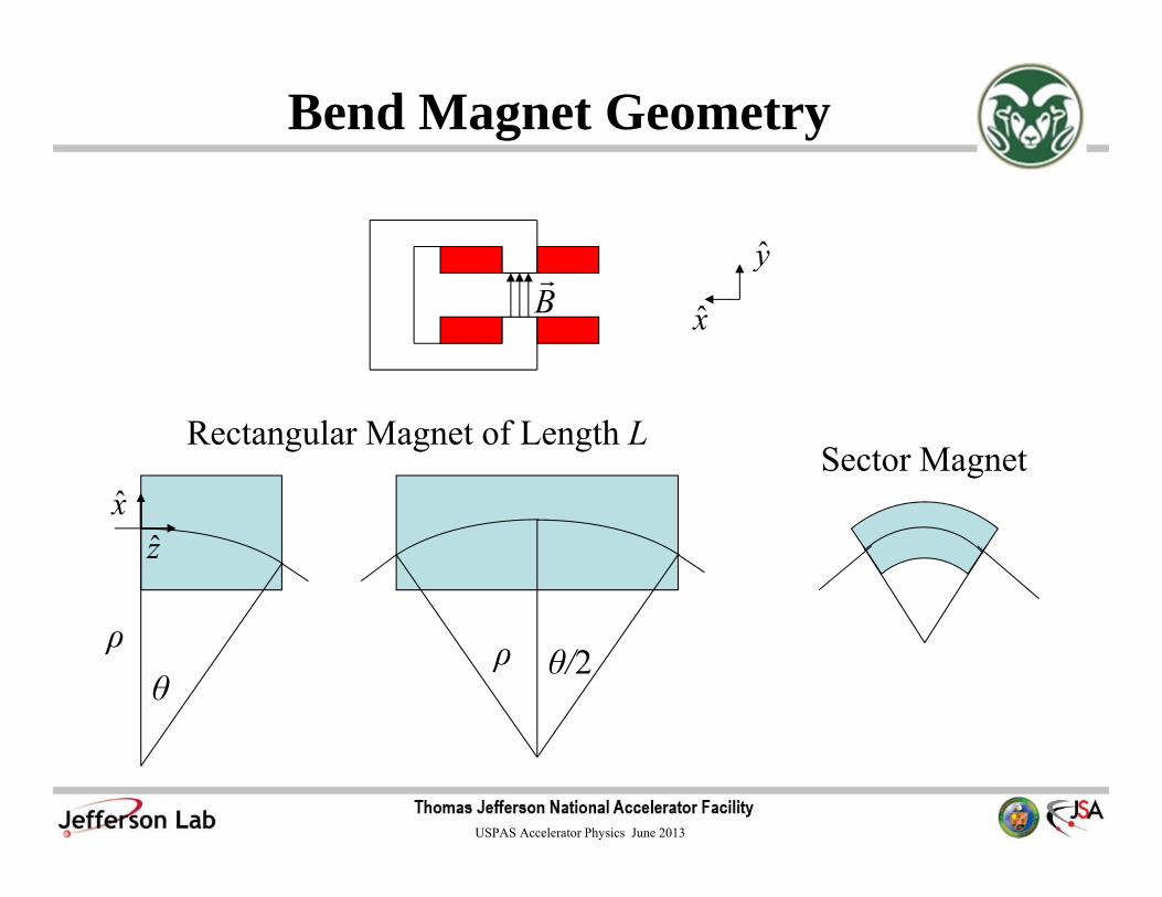
Bend Magnet Geometry
ρ ρ θ/2
Rectangular Magnet of Length LSector Magnet
Br
θ
x
y
xz

USPAS Accelerator Physics June 2013
Bend Magnet TrajectoryFor a uniform magnetic field
( )
( )
( )
xz y
zx y
d mV E V Bdt
d mV qV Bdt
d mV qV Bdt
γ
γ
γ
⎡ ⎤= + ×⎣ ⎦
= −
=
rr r r
22
2 0xc x
d V Vdt
+ Ω =2
22 0z
c zd V Vdt
+ Ω =
For the solution satisfying boundary conditions:
( ) ( )( ) ( )( )cos 1 cos 1 /c c c yy
pX t t t qB mqB
ρ γ= Ω − = Ω − Ω =
( ) ( ) ( )s in s inc cy
pZ t t tq B
ρ= Ω = Ω
( ) ( ) 0 ˆ0 0 0 zX V V z= =r r

USPAS Accelerator Physics June 2013
Magnetic Rigidity
The magnetic rigidity is:
It depends only on the particle momentum and charge, and is a convenient way to characterize the magnetic field. Given magnetic rigidity and the required bend radius, the required bend field is a simple ratio. Note particles of momentum 100 MeV/chave a rigidity of 0.334 T m.
ypB Bq
ρ ρ= =
( )( )2sin / 2BL Bρ θ= ( )sinBL Bρ θ=
Long Dipole MagnetNormal Incidence (or exit)
Dipole Magnet

USPAS Accelerator Physics June 2013
Natural Focusing in Bend Plane
Perturbed Trajectory
Design Trajectory
Can show that for either a displacement perturbation or angular perturbation from the design trajectory
( )2
2 2x
d x xds sρ
= −( )
2
2 2y
d y yds sρ
= −
USPAS Accelerator Physics June 2013
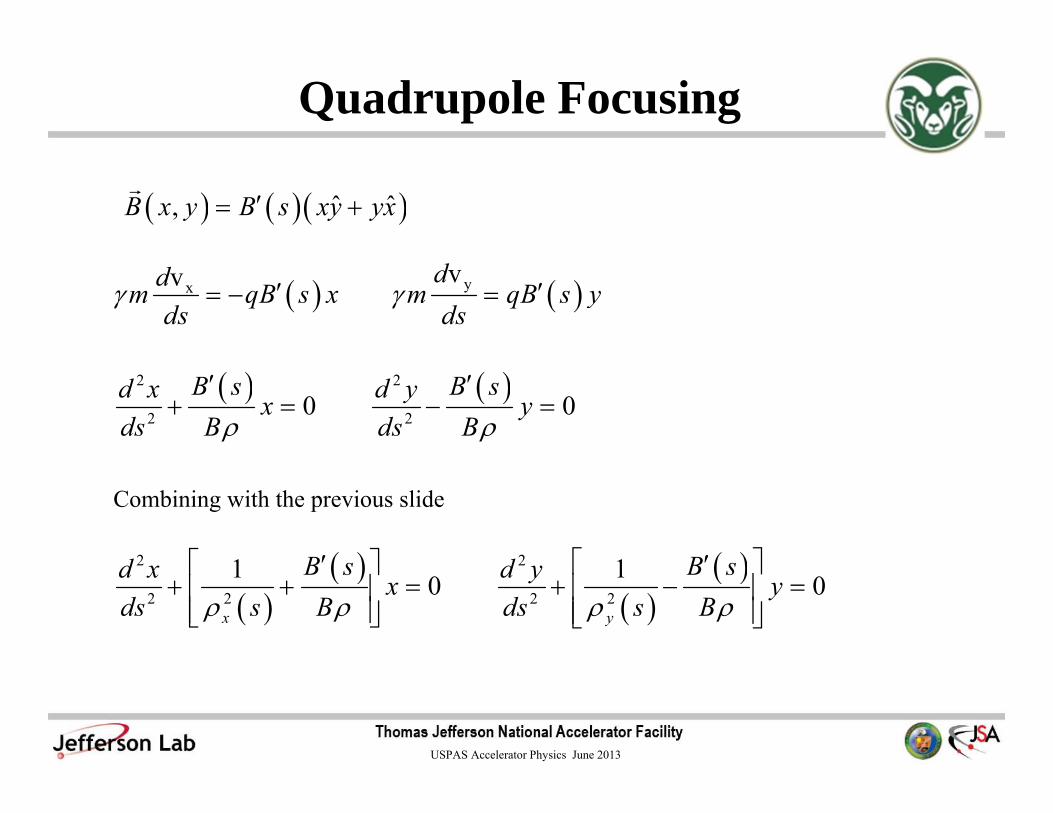
Quadrupole Focusing
( ) ( )( )ˆ ˆ,B x y B s xy yx′= +r
( ) ( )yxvv
ddm qB s x m qB s yds ds
γ γ′ ′= − =
( ) ( )2 2
2 20 0B s B sd x d yx y
ds B ds Bρ ρ′ ′
+ = − =
Combining with the previous slide
( )( )
( )( )2 2
2 2 2 2
1 10 0x y
B s B sd x d yx yds s B ds s Bρ ρ ρ ρ
⎡ ⎤⎡ ⎤′ ′+ + = + − =⎢ ⎥⎢ ⎥⎢ ⎥ ⎢ ⎥⎣ ⎦ ⎣ ⎦

USPAS Accelerator Physics June 2013
Hill’s Equation
Note that this is like the harmonic oscillator, or exponential for constant K, but more general in that the focusing strength, and hence oscillation frequency depends on s
Define focusing strengths (with units of m-2)
( ) ( )2 2
2 20 0x yd x d yk s x k s yds ds
+ = + =
( ) ( )( )
( )( )
2 2
1 1 x yx y
B s B sk s k
s B s Bρ ρ ρ ρ′ ′
= + = −

USPAS Accelerator Physics June 2013
Energy Effects
This solution is not a solution to Hill’s equation directly, but is a solution to the inhomogeneous Hill’s Equations
( )( )
( )
( )( )
( )
2
2 2
2
2 2
1 1
1 1
x x
y y
B sd x pxds s B s p
B sd y pyds s B s p
ρ ρ ρ
ρ ρ ρ
⎡ ⎤′ Δ+ + =⎢ ⎥⎢ ⎥⎣ ⎦⎡ ⎤′ Δ
+ − =⎢ ⎥⎢ ⎥⎣ ⎦
( ) ( )( )1 cos /y
p px s seB p
ρΔΔ = −
ρ
( )1 /p pρ + Δ
USPAS Accelerator Physics June 2013
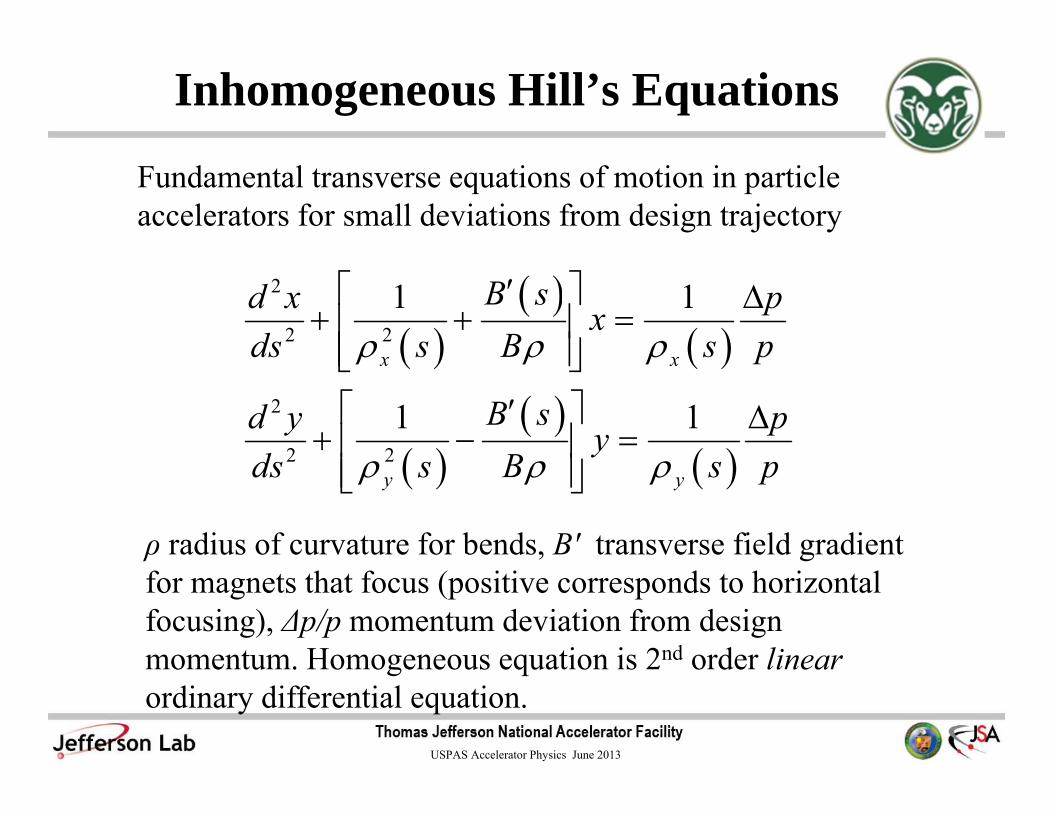
Inhomogeneous Hill’s Equations
Fundamental transverse equations of motion in particle accelerators for small deviations from design trajectory
( )( )
( )
( )( )
( )
2
2 2
2
2 2
1 1
1 1
x x
y y
B sd x pxds s B s p
B sd y pyds s B s p
ρ ρ ρ
ρ ρ ρ
⎡ ⎤′ Δ+ + =⎢ ⎥⎢ ⎥⎣ ⎦⎡ ⎤′ Δ
+ − =⎢ ⎥⎢ ⎥⎣ ⎦
ρ radius of curvature for bends, B' transverse field gradient for magnets that focus (positive corresponds to horizontal focusing), Δp/p momentum deviation from design momentum. Homogeneous equation is 2nd order linear ordinary differential equation.

USPAS Accelerator Physics June 2013
DispersionFrom theory of linear ordinary differential equations, the general solution to the inhomogeneous equation is the sum of any solution to the inhomogeneous equation, called the particular integral, plus two linearly independent solutions to the homogeneous equation, whose amplitudes may be adjusted to account for boundary conditions on the problem.
( ) ( ) ( ) ( ) ( ) ( ) ( ) ( )1 2 1 2= =p x x p y yx s x s A x s B x s y s y s A y s B y s+ + + +
Because the inhomogeneous terms are proportional to Δp/p, the particular solution can generally be written as
( ) ( ) ( ) ( )= =p x p yp px s D s y s D s
p pΔ Δ
where the dispersion functions satisfy
( )( )
( ) ( )( )
( )
22
2 2 2 2
1 1 1 1 yxx y
x x y y
d DB s B sd D D Dds s B s ds s B sρ ρ ρ ρ ρ ρ
⎡ ⎤⎡ ⎤′ ′+ + = + − =⎢ ⎥⎢ ⎥⎢ ⎥ ⎢ ⎥⎣ ⎦ ⎣ ⎦

USPAS Accelerator Physics June 2013
M56In addition to the transverse effects of the dispersion, there are important effects of the dispersion along the direction of motion. The primary effect is to change the time-of-arrival of the off-momentum particle compared to the on-momentum particle which traverses the design trajectory.
( ) ( ) ( )= p dsd z D s
p sρΔ
Δ
( )( )
( )( )
2
1
56
syx
x ys
D sD sM ds
s sρ ρ⎧ ⎫⎪ ⎪= +⎨ ⎬⎪ ⎪⎩ ⎭∫
( )ρ +
ds
Design Trajectory Dispersed Trajectory
( ) pD spΔ
( )ds pz D s dsp
ρρ⎛ ⎞Δ
Δ = + −⎜ ⎟⎝ ⎠

USPAS Accelerator Physics June 2013
Solutions Homogeneous Eqn.Dipole
( )
( )( )( ) ( )( )( )( ) ( )( )
( )
( )cos / sin /
sin / / cos /
ii i
ii i
x s x ss s s sdx dxs ss s s sds ds
ρ ρ ρ
ρ ρ ρ
⎛ ⎞ ⎛ ⎞⎛ ⎞− −⎜ ⎟ ⎜ ⎟⎜ ⎟=⎜ ⎟ ⎜ ⎟⎜ ⎟− − −⎜ ⎟ ⎜ ⎟⎝ ⎠⎝ ⎠ ⎝ ⎠
Drift
( )
( )
( )
( )10 1
ii
i
x s x ss sdx dxs sds ds
⎛ ⎞ ⎛ ⎞−⎛ ⎞⎜ ⎟ ⎜ ⎟= ⎜ ⎟⎜ ⎟ ⎜ ⎟⎝ ⎠⎜ ⎟ ⎜ ⎟⎝ ⎠ ⎝ ⎠

USPAS Accelerator Physics June 2013
Quadrupole in the focusing direction
( )
( )( )( ) ( )( )( )( ) ( )( )
( )
( )cos sin /
sin cos
ii i
ii i
x s x sk s s k s s kdx dxs sk k s s k s sds ds
⎛ ⎞⎛ ⎞ ⎛ ⎞− −⎜ ⎟⎜ ⎟ ⎜ ⎟= ⎜ ⎟⎜ ⎟ ⎜ ⎟⎜ ⎟ ⎜ ⎟⎜ ⎟− − −⎝ ⎠ ⎝ ⎠⎝ ⎠
Thin Focusing Lens (limiting case when argument goes to zero!)
( )
( )
( )
( )1 0
1/ 1
x s x sdx dxfs sds ds
ε ε
ε ε
⎛ ⎞ ⎛ ⎞+ −⎛ ⎞⎜ ⎟ ⎜ ⎟= ⎜ ⎟⎜ ⎟ ⎜ ⎟−+ −⎝ ⎠⎜ ⎟ ⎜ ⎟
⎝ ⎠ ⎝ ⎠
/k B Bρ′=
Thin Defocusing Lens: change sign of f

USPAS Accelerator Physics June 2013
Solutions Homogeneous Eqn.Dipole
( )
( )( )( ) ( )( )( )( ) ( )( )
( )
( )cos / sin /
sin / / cos /
ii i
ii i
x s x ss s s sdx dxs ss s s sds ds
ρ ρ ρ
ρ ρ ρ
⎛ ⎞ ⎛ ⎞⎛ ⎞− −⎜ ⎟ ⎜ ⎟⎜ ⎟=⎜ ⎟ ⎜ ⎟⎜ ⎟− − −⎜ ⎟ ⎜ ⎟⎝ ⎠⎝ ⎠ ⎝ ⎠
Drift
( )
( )
( )
( )10 1
ii
i
x s x ss sdx dxs sds ds
⎛ ⎞ ⎛ ⎞−⎛ ⎞⎜ ⎟ ⎜ ⎟= ⎜ ⎟⎜ ⎟ ⎜ ⎟⎝ ⎠⎜ ⎟ ⎜ ⎟⎝ ⎠ ⎝ ⎠

USPAS Accelerator Physics June 2013
Quadrupole in the focusing direction
( )
( )( )( ) ( )( )( )( ) ( )( )
( )
( )cos sin /
sin cos
ii i
ii i
x s x sk s s k s s kdx dxs sk k s s k s sds ds
⎛ ⎞⎛ ⎞ ⎛ ⎞− −⎜ ⎟⎜ ⎟ ⎜ ⎟= ⎜ ⎟⎜ ⎟ ⎜ ⎟⎜ ⎟ ⎜ ⎟⎜ ⎟− − −⎝ ⎠ ⎝ ⎠⎝ ⎠
/k B Bρ′=
Quadrupole in the defocusing direction
( )
( )( )( ) ( )( )( )( ) ( )( )
( )
( )cosh sinh /
sinh cosh
ii i
ii i
x s x sk s s k s s kdx dxs sk k s s k s sds ds
⎛ ⎞⎛ ⎞ ⎛ ⎞− − − − −⎜ ⎟⎜ ⎟ ⎜ ⎟= ⎜ ⎟⎜ ⎟ ⎜ ⎟⎜ ⎟ ⎜ ⎟⎜ ⎟− − − − −⎝ ⎠ ⎝ ⎠⎝ ⎠
/k B Bρ′=

USPAS Accelerator Physics June 2013
Transfer MatricesDipole with bend Θ (put coordinate of final position in solution)
( )( )
( ) ( )( ) ( )
( )( )
cos sinsin / cos
after before
after before
x s x s
dx dxs sds ds
ρρ
⎛ ⎞ ⎛ ⎞⎛ ⎞Θ Θ⎜ ⎟ ⎜ ⎟= ⎜ ⎟⎜ ⎟ ⎜ ⎟− Θ Θ⎝ ⎠⎜ ⎟ ⎜ ⎟
⎝ ⎠ ⎝ ⎠
Drift
( )( )
( )( )
10 1
after beforedrift
after before
x s x sLdx dxs sds ds
⎛ ⎞ ⎛ ⎞⎛ ⎞⎜ ⎟ ⎜ ⎟= ⎜ ⎟⎜ ⎟ ⎜ ⎟⎝ ⎠⎜ ⎟ ⎜ ⎟
⎝ ⎠ ⎝ ⎠

USPAS Accelerator Physics June 2013
Quadrupole in the defocusing direction length L
( )( )
( ) ( )( ) ( )
( )( )
cosh sinh /
sinh cos
after before
after before
x s x sk L k L kdx dxs sk k L k Lds ds
⎛ ⎞ ⎛ ⎞⎛ ⎞− − −⎜ ⎟ ⎜ ⎟⎜ ⎟=⎜ ⎟ ⎜ ⎟⎜ ⎟⎜ ⎟− − −⎜ ⎟ ⎜ ⎟⎝ ⎠⎝ ⎠ ⎝ ⎠
Quadrupole in the focusing direction length L
( )( )
( ) ( )( ) ( )
( )( )
cos sin /
sin cos
after before
after before
x s x sk L k L kdx dxs sk k L k Lds ds
⎛ ⎞ ⎛ ⎞⎛ ⎞⎜ ⎟ ⎜ ⎟⎜ ⎟=⎜ ⎟ ⎜ ⎟⎜ ⎟⎜ ⎟−⎜ ⎟ ⎜ ⎟⎝ ⎠⎝ ⎠ ⎝ ⎠
Wille: pg. 71

USPAS Accelerator Physics June 2013
Thin Lenses
Thin Focusing Lens (limiting case when argument goes to zero!)
( )
( )
( )
( )1 0
1/ 1
lens lens
lens lens
x s x sdx dxfs sds ds
ε ε
ε ε
⎛ ⎞ ⎛ ⎞+ −⎛ ⎞⎜ ⎟ ⎜ ⎟= ⎜ ⎟⎜ ⎟ ⎜ ⎟−+ −⎝ ⎠⎜ ⎟ ⎜ ⎟
⎝ ⎠ ⎝ ⎠
Thin Defocusing Lens: change sign of f
f –f
USPAS Accelerator Physics June 2013
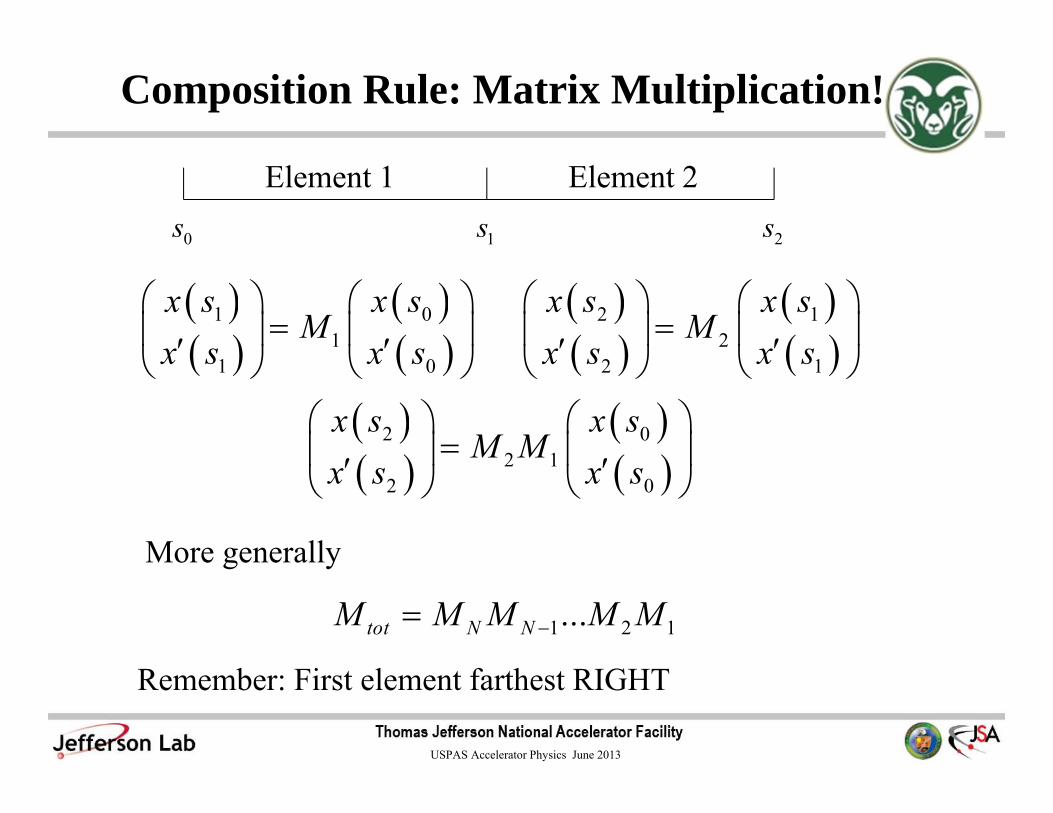
Composition Rule: Matrix Multiplication!
Remember: First element farthest RIGHT
Element 1 Element 2
0s 1s 2s
( )( )
( )( )
1 01
1 0
x s x sM
x s x s⎛ ⎞ ⎛ ⎞
=⎜ ⎟ ⎜ ⎟′ ′⎝ ⎠ ⎝ ⎠
( )( )
( )( )
2 12
2 1
x s x sM
x s x s⎛ ⎞ ⎛ ⎞
=⎜ ⎟ ⎜ ⎟′ ′⎝ ⎠ ⎝ ⎠
( )( )
( )( )
2 02 1
2 0
x s x sM M
x s x s⎛ ⎞ ⎛ ⎞
=⎜ ⎟ ⎜ ⎟′ ′⎝ ⎠ ⎝ ⎠
1 2 1...tot N NM M M M M−=
More generally

USPAS Accelerator Physics June 2013
Some Geometry of Ellipsesy
x
ba
Equation for an upright ellipse
122
=⎟⎠⎞
⎜⎝⎛+⎟
⎠⎞
⎜⎝⎛
by
ax
In beam optics, the equations for ellipses are normalized (by multiplication of the ellipse equation by ab) so that the area of the ellipse divided by π appears on the RHS of the defining equation. For a general ellipse
DCyBxyAx =++ 22 2

USPAS Accelerator Physics June 2013
The area is easily computed to be
2
AreaBAC
D−
=≡ επ
εβαγ =++ 22 2 yxyx
So the equation is equivalently
222 and , ,
BACC
BACB
BACA
−=
−=
−= βαγ
Eqn. (1)

USPAS Accelerator Physics June 2013
Example: the defining equation for the upright ellipse may be rewritten in following suggestive way
ε==+ abybax
ab 22
β = a/b and γ = b/a, note ,max βε== ax γε== bymax
When normalized in this manner, the equation coefficients clearly satisfy
12 =−αβγ

USPAS Accelerator Physics June 2013
General Tilted Ellipse
x
y
b
a
Needs 3 parameters for a completedescription. One way
where s is a slope parameter, a is the maximumextent in the x-direction, and the y-intercept occurs at b, and again ε is the area of the ellipse divided by π
( ) ε==−+ absxybax
ab 22
y=sx
ε==+−⎟⎟⎠
⎞⎜⎜⎝
⎛+ aby
baxy
basx
bas
ab 22
2
22 21
USPAS Accelerator Physics June 2013
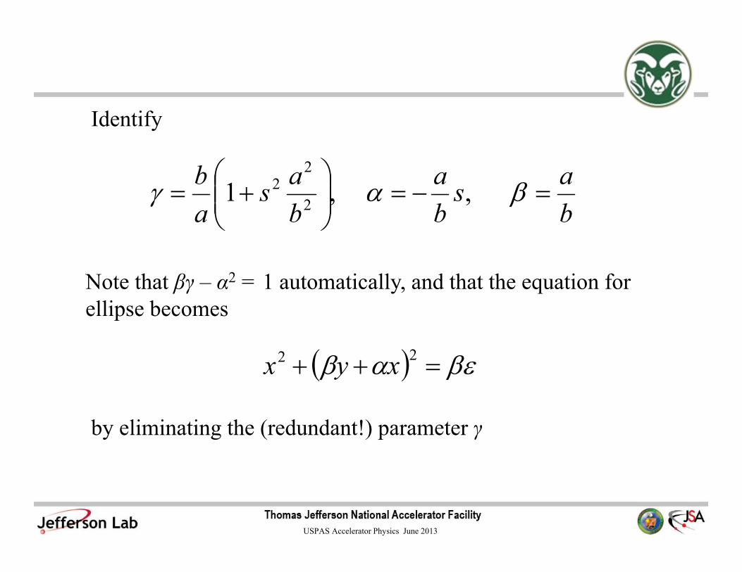
Identify
bas
ba
bas
ab
=−=⎟⎟⎠
⎞⎜⎜⎝
⎛+= βαγ , ,1 2
22
Note that βγ – α2 = 1 automatically, and that the equation for ellipse becomes
( ) βεαβ =++ 22 xyx
by eliminating the (redundant!) parameter γ

USPAS Accelerator Physics June 2013
Ellipse Dimensions in the β-function Description
As for the upright ellipse γε=maxy,max βε=x
x
y=sx=– α x / β
βε=a
βε /=bγε
γε
⎟⎟⎠
⎞⎜⎜⎝
⎛−
βεαβε ,
⎟⎟⎠
⎞⎜⎜⎝
⎛− γε
γεα ,
y
Wille: page 81

USPAS Accelerator Physics June 2013
Area Theorem for Linear OpticsUnder a general linear transformation
an ellipse is transformed into another ellipse. Furthermore, if det (M) = 1, the area of the ellipse after the transformation is the same as that before the transformation.
⎟⎟⎠
⎞⎜⎜⎝
⎛⎟⎟⎠
⎞⎜⎜⎝
⎛=⎟⎟
⎠
⎞⎜⎜⎝
⎛yx
MMMM
yx
2221
1211
''
Pf: Let the initial ellipse, normalized as above, be
02
002
0 2 εβαγ =++ yxyx

USPAS Accelerator Physics June 2013
Because
( ) ( )( ) ( )
1 1
11 12
1 1
21 22
''
M Mx xy yM M
− −
− −
⎛ ⎞⎛ ⎞ ⎛ ⎞⎜ ⎟=⎜ ⎟ ⎜ ⎟⎜ ⎟⎝ ⎠ ⎝ ⎠⎝ ⎠
022 2 εβαγ =++ yxyx
The transformed ellipse is
( ) ( ) ( ) ( )( ) ( ) ( ) ( ) ( ) ( )( ) ( ) ( )
( ) ( ) ( ) ( )
2 21 1 1 10 0 011 11 21 21
1 1 1 1 1 1 1 10 0 011 12 11 22 12 21 21 22
2 21 1 1 10 0 012 12 22 22
2
2
M M M M
M M M M M M M M
M M M M
γ γ α β
α γ α β
β γ α β
− − − −
− − − − − − − −
− − − −
= + +
= + + +
= + +

USPAS Accelerator Physics June 2013
Because (verify!)
( )( ) ( ) ( ) ( ) ( ) ( ) ( ) ( )( )
( )( )
2 20 0 0
2 2 2 21 1 1 1 1 1 1 1
21 12 11 22 11 22 12 21
22 10 0 0
2
det
M M M M M M M M
M
βγ α β γ α
β γ α
− − − − − − − −
−
− = −
× + −
= −
the area of the transformed ellipse (divided by π) is, by Eqn. (1)
|det |det
Area012
000
0 MM
εαγβεε
π=
−==
−

USPAS Accelerator Physics June 2013
Tilted ellipse from the upright ellipseIn the tilted ellipse the y-coordinate is raised by the slope with respect to the un-tilted ellipse
⎟⎟⎠
⎞⎜⎜⎝
⎛⎟⎟⎠
⎞⎜⎜⎝
⎛=⎟⎟
⎠
⎞⎜⎜⎝
⎛yx
syx
101
''
bas
bas
ba
ab
=−=+=∴ βαγ , , 2
( )10 0 0 21
, 0, , b a M sa b
γ α β −= = = = −
Because det (M)=1, the tilted ellipse has the same area as the upright ellipse, i.e., ε = ε0.

USPAS Accelerator Physics June 2013
Phase Advance of a Unimodular MatrixAny two-by-two unimodular (Det (M) = 1) matrix with |Tr M| < 2 can be written in the form
( ) ( )μαγβα
μ sincos1001
⎟⎟⎠
⎞⎜⎜⎝
⎛−−
+⎟⎟⎠
⎞⎜⎜⎝
⎛=M
Pf: The equation for the eigenvalues of M is
The phase advance of the matrix, μ, gives the eigenvalues of the matrix λ = e iμ, and cos μ = (Tr M)/2. Furthermore βγ–α2=1
( ) 0122112 =++− λλ MM
USPAS Accelerator Physics June 2013
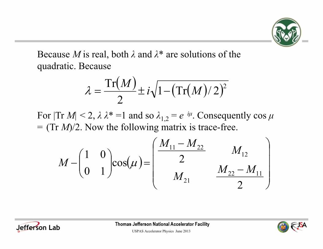
Because M is real, both λ and λ* are solutions of the quadratic. Because
For |Tr M| < 2, λ λ* =1 and so λ1,2 = e iμ. Consequently cos μ = (Tr M)/2. Now the following matrix is trace-free.
( ) ( )( )22/Tr12
Tr MiM−±=λ
( )⎟⎟⎟⎟
⎠
⎞
⎜⎜⎜⎜
⎝
⎛
−
−
=⎟⎟⎠
⎞⎜⎜⎝
⎛−
2
2cos1001
112221
122211
MMM
MMM
M μ

USPAS Accelerator Physics June 2013
Simply choose
μγ
μβ
μα
sin ,
sin ,
sin221122211 MMMM
−==−
=
and the sign of μ to properly match the individual matrix elements with β > 0. It is easily verified that βγ – α2 = 1. Now
( ) ( )μαγβα
μ 2sin2cos10012
⎟⎟⎠
⎞⎜⎜⎝
⎛−−
+⎟⎟⎠
⎞⎜⎜⎝
⎛=M
( ) ( )μαγβα
μ nnM n sincos1001
⎟⎟⎠
⎞⎜⎜⎝
⎛−−
+⎟⎟⎠
⎞⎜⎜⎝
⎛=
and more generally

USPAS Accelerator Physics June 2013
Therefore, because sin and cos are both bounded functions, the matrix elements of any power of M remain bounded as long as |Tr (M)| < 2.
NB, in some beam dynamics literature it is (incorrectly!) stated that the less stringent |Tr (M)| 2 ensures boundedness and/or stability. That equality cannot be allowed can be immediately demonstrated by counterexample. The upper triangular or lower triangular subgroups of the two-by-two unimodular matrices, i.e., matrices of the form
clearly have unbounded powers if |x| is not equal to 0.
⎟⎟⎠
⎞⎜⎜⎝
⎛⎟⎟⎠
⎞⎜⎜⎝
⎛101
or 10
1x
x
≤

USPAS Accelerator Physics June 2013
Significance of matrix parametersAnother way to interpret the parameters α, β, and γ, which represent the unimodular matrix M (these parameters are sometimes called the Twiss parameters or Twiss representation for the matrix) is as the “coordinates” of that specific set of ellipses that are mapped onto each other, or are invariant, under the linear action of the matrix. This result is demonstrated in
Thm: For the unimodular linear transformation
( ) ( )μαγβα
μ sincos1001
⎟⎟⎠
⎞⎜⎜⎝
⎛−−
+⎟⎟⎠
⎞⎜⎜⎝
⎛=M
with |Tr (M)| < 2, the ellipses

USPAS Accelerator Physics June 2013
cyxyx =++ 22 2 βαγare invariant under the linear action of M, where c is any constant. Furthermore, these are the only invariant ellipses. Note that the theorem does not apply to I, because |Tr ( I)| = 2.
Pf: The inverse to M is clearly
( ) ( )μαγβα
μ sincos10011
⎟⎟⎠
⎞⎜⎜⎝
⎛−−
−⎟⎟⎠
⎞⎜⎜⎝
⎛=−M
By the ellipse transformation formulas, for example( ) ( )( ) ( )
( )( ) ββμμ
μβαμβμβααμβ
βμαμαμαμμβγμββ
=+=
++−+=
+++−+=
22
2222222
222
cossin sincossin21sin
sincossincossin2sin'

USPAS Accelerator Physics June 2013
Similar calculations demonstrate that α' = α and γ' = γ. As det (M) = 1, c' = c, and therefore the ellipse is invariant. Conversely, suppose that an ellipse is invariant. By the ellipse transformation formula, the specific ellipse
is invariant under the transformation by M only if
( ) ( )( ) ( )( )( ) ( )( )
( ) ( )( ) ( )
,
sincossinsincos2sinsinsincossin21sinsincos
sinsinsincos2sincos
22
2
22
vTT M
i
i
i
M
i
i
i
i
i
i
r≡
⎟⎟⎟
⎠
⎞
⎜⎜⎜
⎝
⎛≡
⎟⎟⎟
⎠
⎞
⎜⎜⎜
⎝
⎛
⎟⎟⎟⎟
⎠
⎞
⎜⎜⎜⎜
⎝
⎛
++−+−−−
−−=
⎟⎟⎟
⎠
⎞
⎜⎜⎜
⎝
⎛
βαγ
βαγ
μαμμβμαμμβμγμαμμβγμβμαμ
μγμγμαμμαμ
βαγ
εβαγ =++ 22 2 yxyx iii

USPAS Accelerator Physics June 2013
i.e., if the vector is ANY eigenvector of TM with eigenvalue 1.All possible solutions may be obtained by investigating the eigenvalues and eigenvectors of TM. Now
( ) 0Det hen solution w a has =−= ITvvT MM λλ λλrr
( )( )2 22 4cos 1 1 0λ μ λ λ⎡ ⎤+ − + − =⎣ ⎦
i.e.,
Therefore, M generates a transformation matrix TM with at least one eigenvalue equal to 1. For there to be more than one solution with λ = 1,
2 21 2 4cos 1 0, cos 1, or M Iμ μ⎡ ⎤+ − + = = = ±⎣ ⎦
vr

USPAS Accelerator Physics June 2013
cvv i /,11rr ε=
and we note that all ellipses are invariant when M = I. But, these two cases are excluded by hypothesis. Therefore, M generates a transformation matrix TM which always possesses a single nondegenerate eigenvalue 1; the set of eigenvectors corresponding to the eigenvalue 1, all proportional to each other, are the only vectors whose components (γi, αi, βi) yield equations for the invariant ellipses. For concreteness, compute that eigenvector with eigenvalue 1 normalized so βiγi – αi
2 = 1
All other eigenvectors with eigenvalue 1 have , for some value c.
( )⎟⎟⎟
⎠
⎞
⎜⎜⎜
⎝
⎛=
⎟⎟⎟
⎠
⎞
⎜⎜⎜
⎝
⎛−
−=
⎟⎟⎟
⎠
⎞
⎜⎜⎜
⎝
⎛=
βαγ
ββαγ
12/
/
122211
1221
,1 MMMMM
v
i
i
i
ir

USPAS Accelerator Physics June 2013
Because we have enumerated all possible eigenvectors with eigenvalue 1, all ellipses invariant under the action of M, are of the form
Because Det (M) =1, the eigenvector clearly yields the invariant ellipse
.2 22 εβαγ =++ yxyxLikewise, the proportional eigenvector generates the similar ellipse
( ) εβαγε=++ 22 2 yxyx
c
1vr
iv ,1r
cyxyx =++ 22 2 βαγ

USPAS Accelerator Physics June 2013
To summarize, this theorem gives a way to tie the mathematical representation of a unimodular matrix in terms of its α, β, and γ, and its phase advance, to the equations of the ellipses invariant under the matrix transformation. The equations of the invariant ellipses when properly normalized have precisely the same α, β, and γ as in the Twiss representation of the matrix, but varying c.
Finally note that throughout this calculation c acts merely as a scale parameter for the ellipse. All ellipses similar to the starting ellipse, i.e., ellipses whose equations have the same α, β, and γ, but with different c, are also invariant under the action of M. Later, it will be shown that more generally
is an invariant of the equations of transverse motion.
( )( ) βαββαγε /'''2 2222 xxxxxxx ++=++=

USPAS Accelerator Physics June 2013
Applications to transverse beam opticsWhen the motion of particles in transverse phase space is considered, linear optics provides a good first approximation of the transverse particle motion. Beams of particles are represented by ellipses in phase space (i.e. in the (x, x') space). To the extent that the transverse forces are linear in the deviation of the particles from some pre-defined central orbit, the motion may analyzed by applying ellipse transformation techniques.
Transverse Optics Conventions: positions are measured in terms of length and angles are measured by radian measure. The area in phase space divided by π, ε, measured in m-rad, is called the emittance. In such applications, α has no units, β has units m/radian. Codes that calculate β, by widely accepted convention, drop the per radian when reporting results, it is implicit that the units for x' are radians.

USPAS Accelerator Physics June 2013
Linear Transport MatrixWithin a linear optics description of transverse particle motion, the particle transverse coordinates at a location s along the beam line are described by a vector
( )( )⎟
⎟
⎠
⎞
⎜⎜
⎝
⎛
sdsdx
sx
If the differential equation giving the evolution of x is linear, one may define a linear transport matrix Ms',s relating the coordinates at s' to those at s by
( )( )
( )( )⎟
⎟
⎠
⎞
⎜⎜
⎝
⎛=⎟
⎟
⎠
⎞
⎜⎜
⎝
⎛
sdsdx
sxMs
dsdx
sxss ,''
'

USPAS Accelerator Physics June 2013
From the definitions, the concatenation rule Ms'',s = Ms'',s' Ms',s must apply for all s' such that s < s'< s'' where the multiplication is the usual matrix multiplication.
Pf: The equations of motion, linear in x and dx/ds, generate a motion with
( )( )
( )( )
( )( )
( )( )⎟
⎟
⎠
⎞
⎜⎜
⎝
⎛=⎟
⎟
⎠
⎞
⎜⎜
⎝
⎛=⎟
⎟
⎠
⎞
⎜⎜
⎝
⎛=⎟
⎟
⎠
⎞
⎜⎜
⎝
⎛
sdsdx
sxMMs
dsdx
sxMs
dsdx
sx
sdsdx
sxM ssssssss ,'',''','','' '
'
''
''
for all initial conditions (x(s), dx/ds(s)), thus Ms'',s = Ms'',s' Ms',s.
Clearly Ms,s = I. As is shown next, the matrix Ms',s is in general a member of the unimodular subgroup of the general linear group.

USPAS Accelerator Physics June 2013
Ellipse Transformations Generated by Hill’s Equation
The equation governing the linear transverse dynamics in a particle accelerator, without acceleration, is Hill’s equation*
( ) 02
2
=+ xsKds
xd
* Strictly speaking, Hill studied Eqn. (2) with periodic K. It was first applied to circular accelerators which had a periodicity given by the circumference of the machine. It is a now standard in the field of beam optics, to still refer to Eqn. 2 as Hill’s equation, even in cases, as in linear accelerators, where there is no periodicity.
Eqn. (2)
( )( ) ( )
( )( )
( )( )⎟
⎟
⎠
⎞
⎜⎜
⎝
⎛≡⎟
⎟
⎠
⎞
⎜⎜
⎝
⎛
⎟⎟
⎠
⎞
⎜⎜
⎝
⎛
−=⎟
⎟
⎠
⎞
⎜⎜
⎝
⎛
+
++ s
dsdx
sxMs
dsdx
sx
dssK
ds
dssdsdx
dssxsdss ,
1rad rad
1
The transformation matrix taking a solution through an infinitesimal distance ds is

USPAS Accelerator Physics June 2013
Suppose we are given the phase space ellipse
at location s, and we wish to calculate the ellipse parameters, after the motion generated by Hill’s equation, at the location s + ds
( ) ( ) ( ) εβαγ =++ 22 ''2 xsxxsxs
( ) ( ) ( ) '''2 22 εβαγ =+++++ xdssxxdssxdssBecause, to order linear in ds, Det Ms+ds,s = 1, at all locations s, ε' = ε, and thus the phase space area of the ellipse after an infinitesimal displacement must equal the phase space area before the displacement. Because the transformation through a finite interval in s can be written as a series of infinitesimal displacement transformations, all of which preserve the phase space area of the transformed ellipse, we come to two important conclusions:

USPAS Accelerator Physics June 2013
1. The phase space area is preserved after a finite integration of Hill’s equation to obtain Ms',s, the transport matrix which can be used to take an ellipse at s to an ellipse at s'. This conclusion holds generally for all s' and s.
2. Therefore Det Ms',s = 1 for all s' and s, independent of the details of the functional form K(s). (If desired, these two conclusions may be verified more analytically by showing that
( ) ( ) ( ) ( ) ssssdsd
∀=−→=− ,1 0 22 αγβαβγ
may be derived directly from Hill’s equation.)

USPAS Accelerator Physics June 2013
Evolution equations for the α, β functions
The ellipse transformation formulas give, to order linear in ds
( ) ( )sdsdss βαβ +−=+rad
2
( ) ( ) ( ) ( ) rad rad
Kdsssdssdss βαγα ++−=+
So
( ) ( )rad
2 ssdsd αβ
−=
( ) ( ) ( )rad
rad sKssdsd γβα
−=

USPAS Accelerator Physics June 2013
Note that these two formulas are independent of the scale of the starting ellipse ε, and in theory may be integrated directly for β(s) and α(s) given the focusing function K(s). A somewhat easier approach to obtain β(s) is to recall that the maximum extent of an ellipse, xmax, is (εβ)1/2(s), and to solve the differential equation describing its evolution. The above equations may be combined to give the following non-linear equation for xmax(s) = w(s) = (εβ)1/2(s)
( ) ( )22
2 3
/ rad.d w K s w
ds wε
+ =
Such a differential equation describing the evolution of the maximum extent of an ellipse being transformed is known as an envelope equation.

USPAS Accelerator Physics June 2013
The envelope equation may be solved with the correct boundary conditions, to obtain the β-function. α may then be obtained from the derivative of β, and γ by the usual normalization formula. Types of boundary conditions: Class I—periodic boundary conditions suitable for circular machines or periodic focusing lattices, Class II—initial condition boundary conditions suitable for linacs or recirculating machines.
It should be noted, for consistency, that the same β(s) = w2(s)/εis obtained if one starts integrating the ellipse evolution equation from a different, but similar, starting ellipse. That this is so is an exercise.

USPAS Accelerator Physics June 2013
Solution to Hill’s Equation inAmplitude-Phase form
To get a more general expression for the phase advance, consider in more detail the single particle solutions to Hill’s equation
( ) 02
2
=+ xsKds
xd
From the theory of linear ODEs, the general solution of Hill’s equation can be written as the sum of the two linearly independent pseudo-harmonic functions
( ) ( ) ( )sieswsx μ±± =
( ) ( ) ( )sBxsAxsx −+ +=where

USPAS Accelerator Physics June 2013
are two particular solutions to Hill’s equation, provided that
( ) ( ) ( ) , and 23
2
2
2
swcs
dsd
wcwsK
dswd
==+μ
and where A, B, and c are constants (in s)
That specific solution with boundary conditions x(s1) = x1 and dx/ds (s1) = x'1 has
( ) ( ) ( ) ( )
( ) ( )( ) ( ) ( )
( ) ⎟⎟⎠
⎞⎜⎜⎝
⎛
⎟⎟⎟
⎠
⎞
⎜⎜⎜
⎝
⎛
⎥⎦
⎤⎢⎣
⎡−⎥
⎦
⎤⎢⎣
⎡+
=⎟⎟⎠
⎞⎜⎜⎝
⎛−
−
−
1
1
1
11
11
11
''' 11
11
xx
esw
icswesw
icsw
eswesw
BA
sisi
sisi
μμ
μμ
Eqns. (3)

USPAS Accelerator Physics June 2013
Therefore, the unimodular transfer matrix taking the solution at s = s1 to its coordinates at s = s2 is
( )( )
( ) ( ) ( ) ( )
( ) ( )( ) ( ) ( ) ( )
( )( )
( )( )
( )( )
( ) ( ) ⎟⎟⎠
⎞⎜⎜⎝
⎛
⎟⎟⎟⎟⎟⎟⎟⎟
⎠
⎞
⎜⎜⎜⎜⎜⎜⎜⎜
⎝
⎛
Δ+ΔΔ⎥
⎦
⎤⎢⎣
⎡−−
Δ⎥⎦⎤
⎢⎣⎡ +−
ΔΔ−Δ
=⎟⎟⎠
⎞⎜⎜⎝
⎛
1
1
,12
,2
1
,1
2
2
1
,21122
12
,12
,12
,1
2
2
2
'sin'coscos''
sin''1
sinsin'cos
'1212
12
12
121212
xx
cswsw
swsw
swsw
swsw
cswswswsw
swswc
cswsw
cswsw
swsw
xx
ssss
ss
ss
ssssss
μμμ
μ
μμμ
where
( ) ( ) ( )dssw
csss
sss ∫=−=Δ
2
1
12 212, μμμ

USPAS Accelerator Physics June 2013
Case I: K(s) periodic in sSuch boundary conditions, which may be used to describe circular or ring-like accelerators, or periodic focusing lattices, have K(s + L) = K(s). L is either the machine circumference or period length of the focusing lattice.
It is natural to assume that there exists a unique periodic solution w(s) to Eqn. (3a) when K(s) is periodic. Here, we will assume this to be the case. Later, it will be shown how to construct the function explicitly. Clearly for w periodic
( ) ( ) ( )dssw
csssLs
sLL ∫
+
=−= 2 with μμμφ
is also periodic by Eqn. (3b), and μL is independent of s.

USPAS Accelerator Physics June 2013
The transfer matrix for a single period reduces to
( ) ( ) ( )
( )( ) ( ) ( ) ( ) ( ) ( )
( ) ( )LL
LLL
LLL
cswsw
cswswswsw
swc
csw
cswsw
μαγβα
μ
μμμ
μμμ
sincos1001
sin'cossin''1
sinsin'cos
22
2
⎟⎟⎠
⎞⎜⎜⎝
⎛−−
+⎟⎟⎠
⎞⎜⎜⎝
⎛=
⎟⎟⎟⎟
⎠
⎞
⎜⎜⎜⎜
⎝
⎛
+⎥⎦⎤
⎢⎣⎡ +−
−
where the (now periodic!) matrix functions are
( ) ( ) ( ) ( ) ( ) ( ) ( )( )s
ssc
swsc
swswsβαγβα
22 1 , ,' +==−=
By Thm. (2), these are the ellipse parameters of the periodically repeating, i.e., matched ellipses.
USPAS Accelerator Physics June 2013
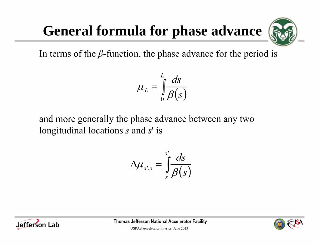
General formula for phase advance
( )∫=L
L sds
0 βμ
In terms of the β-function, the phase advance for the period is
and more generally the phase advance between any two longitudinal locations s and s' is
( )∫=Δ'
,'
s
sss s
dsβ
μ

USPAS Accelerator Physics June 2013
Transfer Matrix in terms of α and β
( )( ) ( )( ) ( ) ( )
( ) ( )( ) ( )( )( ) ( )( )
( )( ) ( )( )⎟⎟
⎟⎟⎟
⎠
⎞
⎜⎜⎜⎜⎜
⎝
⎛
Δ−Δ⎥⎦
⎤⎢⎣
⎡
Δ−+
Δ+−
ΔΔ+Δ=
ssssss
ss
ssssss
ss
sss
ssss
ss
sssss
M
,',','
,'
,',','
,'
sin'cos'cos'
sin'1
'1
sin'sincos'
μαμββ
μααμαα
ββ
μββμαμββ
Also, the unimodular transfer matrix taking the solution from s to s' is
Note that this final transfer matrix and the final expression for the phase advance do not depend on the constant c. This conclusion might have been anticipated because different particular solutions to Hill’s equation exist for all values of c, but from the theory of linear ordinary differential equations, the final motion is unique once x and dx/ds are specified somewhere.

USPAS Accelerator Physics June 2013
Method to compute the β-functionOur previous work has indicated a method to compute the β-function (and thus w) directly, i.e., without solving the differential equation Eqn. (3). At a given location s, determine the one-period transfer map Ms+L,s (s). From this find μL (which is independent of the location chosen!) from cos μL = (M11+M22) / 2, and by choosing the sign of μL so that β(s) = M12(s) / sin μL is positive. Likewise, α(s) = (M11-M22) / 2 sin μL. Repeat this exercise at every location the β-function is desired.
By construction, the beta-function and the alpha-function, and hence w, are periodic because the single-period transfer map is periodic. It is straightforward to show w=(cβ(s))1/2 satisfies the envelope equation.

USPAS Accelerator Physics June 2013
Courant-Snyder Invariant
( )( ) βαββαγε /'''2 2222 xxxxxxx ++=++=
Consider now a single particular solution of the equations of motion generated by Hill’s equation. We’ve seen that once a particle is on an invariant ellipse for a period, it must stay on that ellipse throughout its motion. Because the phase space area of the single period invariant ellipse is preserved by the motion, the quantity that gives the phase space area of the invariant ellipse in terms of the single particle orbit must also be an invariant. This phase space area/π,
is called the Courant-Snyder invariant. It may be verified to be a constant by showing its derivative with respect to s is zero by Hill’s equation, or by explicit substitution of the transfer matrix solution which begins at some initial value s = 0.

USPAS Accelerator Physics June 2013
Pseudoharmonic Solution
( )( )
( )( ) ( )
( )( )( )( )( ) ( ) ( )( ) ⎟
⎟⎟
⎠
⎞
⎜⎜⎜
⎝
⎛
⎟⎟⎟⎟⎟
⎠
⎞
⎜⎜⎜⎜⎜
⎝
⎛
Δ−Δ⎥⎦
⎤⎢⎣
⎡
Δ−+
Δ+−
ΔΔ+Δ
=⎟⎟
⎠
⎞
⎜⎜
⎝
⎛
0
0
0,0,0
0,0
0,0
0
0,00,00,0
sincoscos
sin11
sinsincos
dsdxx
sss
s
s
ss
sdsdx
sx
sss
s
sss
μαμββ
μααμαα
ββ
μββμαμββ
( ) ( ) ( ) ( ) ( )( )( ) ( ) ( )( ) εβαββαβ ≡++=++ 02
000020
22 /'/' xxxssxssxssx
gives
Using the x(s) equation above and the definition of ε, the solution may be written in the standard “pseudoharmonic” form
( ) ( ) ( ) ⎟⎟⎠
⎞⎜⎜⎝
⎛ +=−Δ= −
0
000010,
'tan wherecosx
xxssx sαβδδμεβ
The the origin of the terminology “phase advance” is now obvious.

USPAS Accelerator Physics June 2013
Case II: K(s) not periodicIn a linac or a recirculating linac there is no closed orbit or natural machine periodicity. Designing the transverse optics consists of arranging a focusing lattice that assures the beam particles coming into the front end of the accelerator are accelerated (and sometimes decelerated!) with as small beam loss as is possible. Therefore, it is imperative to know the initial beam phase space injected into the accelerator, in addition to the transfer matrices of all the elements making up the focusing lattice of the machine. An initial ellipse, or a set of initial conditions that somehow bound the phase space of the injected beam, are tracked through the acceleration system element by element to determine the transmission of the beam through the accelerator. The designs are usually made up of well-understood “modules” that yield known and understood transverse beam optical properties.
USPAS Accelerator Physics June 2013
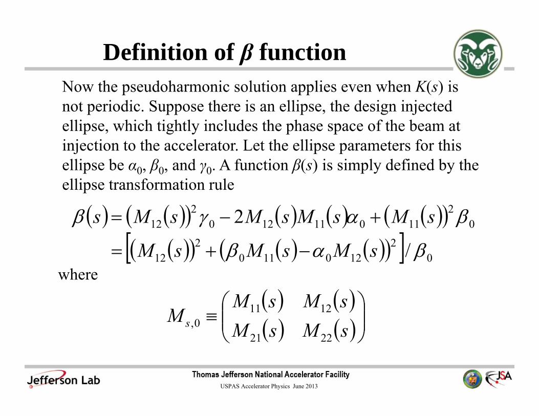
Definition of β function
( ) ( )( ) ( ) ( ) ( )( )( )( ) ( ) ( )( )[ ] 0
2120110
212
02
110111202
12
/
2
βαβ
βαγβ
sMsMsM
sMsMsMsMs
−+=
+−=
where
( ) ( )( ) ( )⎟⎟⎠
⎞⎜⎜⎝
⎛≡
sMsMsMsM
M s2221
12110,
Now the pseudoharmonic solution applies even when K(s) is not periodic. Suppose there is an ellipse, the design injected ellipse, which tightly includes the phase space of the beam at injection to the accelerator. Let the ellipse parameters for this ellipse be α0, β0, and γ0. A function β(s) is simply defined by the ellipse transformation rule

USPAS Accelerator Physics June 2013
One might think to evaluate the phase advance by integrating the beta-function. Generally, it is far easier to evaluate the phase advance using the general formula,
( )( )( ) ( )( )
12,'11,'
12,','tan
ssss
ssss MsMs
Mαβ
μ−
=Δ
where β(s) and α(s) are the ellipse functions at the entrance of the region described by transport matrix Ms',s. Applied to the situation at hand yields
( )( ) ( )sMsM
sMs
120110
120,tan
αβμ
−=Δ

USPAS Accelerator Physics June 2013
Beam MatchingFundamentally, in circular accelerators beam matching is applied in order to guarantee that the beam envelope of the real accelerator beam does not depend on time. This requirement is one part of the definition of having a stable beam. With periodic boundary conditions, this means making beam density contours in phase space align with the invariant ellipses (in particular at the injection location!) given by the ellipse functions. Once the particles are on the invariant ellipses they stay there (in the linear approximation!), and the density is preserved because the single particle motion is around the invariant ellipses. In linacs and recirculating linacs, usually different purposes are to be achieved. If there are regions with periodic focusing lattices within the linacs, matching as above ensures that the beam

USPAS Accelerator Physics June 2013
envelope does not grow going down the lattice. Sometimes it is advantageous to have specific values of the ellipse functions at specific longitudinal locations. Other times, re/matching is done to preserve the beam envelopes of a good beam solution as changes in the lattice are made to achieve other purposes, e.g. changing the dispersion function or changing the chromaticity of regions where there are bends (see the next chapter for definitions). At a minimum, there is usually a matching done in the first parts of the injector, to take the phase space that is generated by the particle source, and change this phase space in a way towards agreement with the nominal transverse focusing design of the rest of the accelerator. The ellipse transformation formulas, solved by computer, are essential for performing this process.

USPAS Accelerator Physics June 2013
Dispersion CalculationBegin with the inhomogeneous Hill’s equation for the dispersion.
Write the general solution to the inhomogeneous equation for the dispersion as before.
Here Dp can be any particular solution. Suppose that the dispersion and it’s derivative are known at the location s1, and we wish to determine their values at s2. x1 and x2, because they are solutions to the homogeneous equations, must be transported by the transfer matrix solution Ms2,s1 already found.
( ) ( )2
2
1d D K s Dds sρ
+ =
( ) ( ) ( ) ( )1 2= pD s D s Ax s Bx s+ +

USPAS Accelerator Physics June 2013
To build up the general solution, choose that particular solution of the inhomogeneous equation with boundary conditions
( ) ( ),0 1 ,0 1 0p pD s D s′= =
( ) ( )( ) ( )
( )( )
11 1 2 1 1
1 1 2 1 1
x s x s D sAx s x s D sB
−⎛ ⎞ ⎛ ⎞⎛ ⎞
= ⎜ ⎟ ⎜ ⎟⎜ ⎟ ′ ′ ′⎝ ⎠ ⎝ ⎠ ⎝ ⎠
Evaluate A and B by the requirement that the dispersion and it’s derivative have the proper value at s1 (x1 and x2 need to be linearly independent!)
( ) ( ) ( ) ( ) ( ) ( )
( ) ( ) ( ) ( ) ( ) ( )2 1 2 1
2 1 2 1
2 ,0 2 1 , 1 , 111 12
2 ,0 2 1 , 1 , 121 22
p s s s s
p s s s s
D s D s s M D s M D s
D s D s s M D s M D s
′= − + +
′ ′ ′= − + +
USPAS Accelerator Physics June 2013
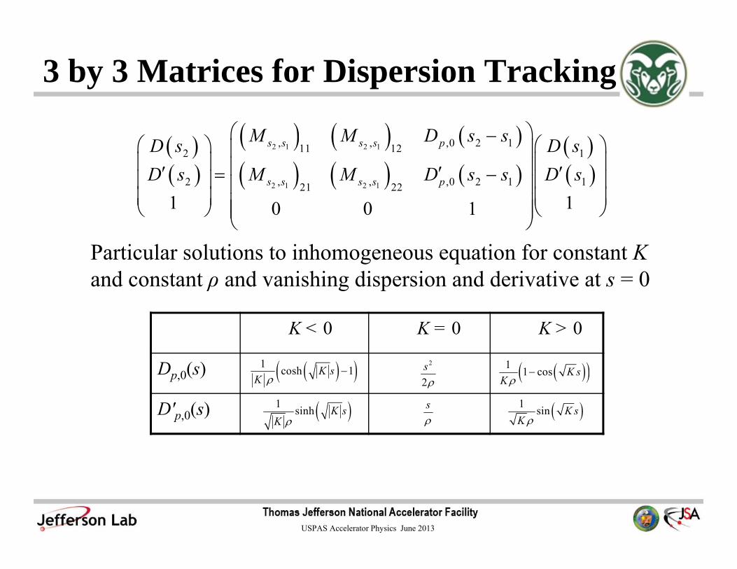
3 by 3 Matrices for Dispersion Tracking
( )( )
( ) ( ) ( )
( ) ( ) ( )( )( )
2 1 2 1
2 1 2 1
, , ,0 2 111 122 1
2 , , ,0 2 1 121 221 10 0 1
s s s s p
s s s s p
M M D s sD s D sD s M M D s s D s
⎛ ⎞−⎛ ⎞ ⎛ ⎞⎜ ⎟⎜ ⎟ ⎜ ⎟⎜ ⎟′ ′ ′= −⎜ ⎟ ⎜ ⎟⎜ ⎟⎜ ⎟ ⎜ ⎟⎜ ⎟⎝ ⎠ ⎝ ⎠⎜ ⎟
⎝ ⎠
Particular solutions to inhomogeneous equation for constant Kand constant ρ and vanishing dispersion and derivative at s = 0
K < 0 K = 0 K > 0
Dp,0(s)
D'p,0(s)
2
2sρ
sρ
( )( )1 1 cos K sKρ
−
( )1 sin K sK ρ( )1 sinh K s
K ρ
( )( )1 cosh 1K sK ρ
−

USPAS Accelerator Physics June 2013
M56In addition to the transverse effects of the dispersion, there are important effects of the dispersion along the direction of motion. The primary effect is to change the time-of-arrival of the off-momentum particle compared to the on-momentum particle which traverses the design trajectory.
( ) ( ) ( )= p dsd z D s
p sρΔ
Δ
( )( )
( )( )
2
1
56
syx
x ys
D sD sM ds
s sρ ρ⎧ ⎫⎪ ⎪= +⎨ ⎬⎪ ⎪⎩ ⎭∫
( )ρ +
ds
Design Trajectory Dispersed Trajectory
( ) pD spΔ
( )ds pz D s dsp
ρρ⎛ ⎞Δ
Δ = + −⎜ ⎟⎝ ⎠

USPAS Accelerator Physics June 2013
Solenoid FocussingCan also have continuous focusing in both transverse directions by applying solenoid magnets:
( )B z
z

USPAS Accelerator Physics June 2013
Busch’s TheoremFor cylindrical symmetry magnetic field described by a vector potential:
Conservation of Canonical Momentum gives Busch’s Theorem:
( ) ( )( )
( ) ( ) ( )
1ˆ, , is nearly constant
0, 0,,
2 2
z
z zr
A A z r B rA z rr r
B r z r B r z rA z r B
θ θ
θ
θ ∂= =
∂′= =
∴ =
r
2
2
for particle with 0 where 0, 0
2 2
z
czLarmor
P mr qrA const
B PqBmr
m
θ θ
θ
γ θ
θ
γ θ ωγ
= + =
= = =Ω
= − = − = −
&
&
&
Beam rotates at the Larmor frequency which implies coupling

USPAS Accelerator Physics June 2013
Radial Equation( ) 2 2
2
2 2
2 2
2 2 22
2
thin lens focal length
1 weak compared to quadrupole for high 4
L z L
L
z
z
z
d mr mr qr B mrdt
kc
e B dz
f m c
γ γ ω θ γ ω
ωβ
γγβ
∞
−∞
− = = −
∴ =
=∫
&&
If go to full ¼ oscillation inside the magnetic field in the “thick” lens case, all particles end up at r = 0! Non-zero emittance spreads out perfect focusing!
x
y

USPAS Accelerator Physics June 2013
Larmor’s TheoremThis result is a special case of a more general result. If go to frame that rotates with the local value of Larmor’s frequency, then the transverse dynamics including the magnetic field are simply those of a harmonic oscillator with frequency equal to the Larmor frequency. Any force from the magnetic field linear in the field strength is “transformed away” in the Larmor frame. And the motion in the two transverse degrees of freedom are now decoupled. Pf: The equations of motion are
( )
( )
( )
2
2
2 2
2
2 2
2
2
2-D Harmonic Oscillator
z
L L z L z
L
d mr mr qr Bdtmr qA cons P
d mr mr mr mr qr B qr Bdtmr P
d mr mr mrdt
mr P
θ θ
θ
θ
γ γ θ θ
γ θ
γ γ θ γ θ ω γ ω θ ω
γ θ
γ γ θ γ ω
γ θ
− =
+ = =
′ ′ ′− + − = −
′ =
⎫′− = − ⎪⎬⎪′ = ⎭
& &&
&
& &&
&
&&
&
Related Documents