ABSTRACT Title of dissertation: WAVELET AND FRAME THEORY: FRAME BOUND GAPS, GENERALIZED SHEARLETS, GRASSMANNIAN FUSION FRAMES, AND P -ADIC WAVELETS Emily Jeannette King, Doctor of Philosophy, 2009 Dissertation directed by: Professor John J. Benedetto and Professor Wojciech Czaja Department of Mathematics The first wavelet system was discovered by Alfr´ ed Haar one hundred years ago. Since then the field has grown enormously. In 1952, Richard Duffin and Albert Schaeffer synthesized the earlier ideas of a number of illustrious mathematicians into a unified theory, the theory of frames. Interest in frames as intriguing objects in their own right arose when wavelet theory began to surge in popularity. Wavelet and frame analysis is found in such diverse fields as data compression, pseudo-differential operator theory and applied statistics. We shall explore five areas of frame and wavelet theory: frame bound gaps, smooth Parseval wavelet frames, generalized shearlets, Grassmannian fusion frames, and p-adic wavlets. The phenomenon of a frame bound gap occurs when certain se- quences of functions, converging in L 2 to a Parseval frame wavelet, generate systems with frame bounds that are uniformly bounded away from 1. In the 90’s, Bin Han proved the existence of Parseval wavelet frames which are smooth and compactly

Welcome message from author
This document is posted to help you gain knowledge. Please leave a comment to let me know what you think about it! Share it to your friends and learn new things together.
Transcript
ABSTRACT
Title of dissertation: WAVELET AND FRAME THEORY:FRAME BOUND GAPS,GENERALIZED SHEARLETS,GRASSMANNIAN FUSION FRAMES, ANDP -ADIC WAVELETS
Emily Jeannette King, Doctor of Philosophy, 2009
Dissertation directed by: Professor John J. Benedetto andProfessor Wojciech CzajaDepartment of Mathematics
The first wavelet system was discovered by Alfred Haar one hundred years
ago. Since then the field has grown enormously. In 1952, Richard Duffin and Albert
Schaeffer synthesized the earlier ideas of a number of illustrious mathematicians into
a unified theory, the theory of frames. Interest in frames as intriguing objects in
their own right arose when wavelet theory began to surge in popularity. Wavelet and
frame analysis is found in such diverse fields as data compression, pseudo-differential
operator theory and applied statistics.
We shall explore five areas of frame and wavelet theory: frame bound gaps,
smooth Parseval wavelet frames, generalized shearlets, Grassmannian fusion frames,
and p-adic wavlets. The phenomenon of a frame bound gap occurs when certain se-
quences of functions, converging in L2 to a Parseval frame wavelet, generate systems
with frame bounds that are uniformly bounded away from 1. In the 90’s, Bin Han
proved the existence of Parseval wavelet frames which are smooth and compactly
supported on the frequency domain and also approximate wavelet set wavelets. We
discuss problems that arise when one attempts to generalize his results to higher
dimensions.
A shearlet system is formed using certain classes of dilations over R2 that yield
directional information about functions in addition to information about scale and
position. We employ representations of the extended metaplectic group to create
shearlet-like transforms in dimensions higher than 2. Grassmannian frames are in
some sense optimal representations of data which will be transmitted over a noisy
channel that may lose some of the transmitted coefficients. Fusion frame theory is
an incredibly new area that has potential to be applied to problems in distributed
sensing and parallel processing. A novel construction of Grassmannian fusion frames
shall be presented. Finally, p-adic analysis is a growing field, and p-adic wavelets are
eigenfunctions of certain pseudo-differential operators. A construction of a 2-adic
wavelet basis using dilations that have not yet been used in p-adic analysis is given.

WAVELET AND FRAME THEORY:FRAME BOUND GAPS, GENERALIZED SHEARLETS,
GRASSMANNIAN FUSION FRAMES, AND P -ADIC WAVELETS
by
Emily Jeannette King
Dissertation submitted to the Faculty of the Graduate School of theUniversity of Maryland, College Park in partial fulfillment
of the requirements for the degree ofDoctor of Philosophy
2009
Advisory Committee:Professor John J. Benedetto, Co-ChairProfessor Wojciech Czaja, Co-ChairProfessor Kasso A. OkoudjouProfessor Johnathan M. RosenbergProfessor Dianne O’Leary

c© Copyright byEmily Jeannette King
2009
Acknowledgments
Many people supported me throughout my graduate career who deserve my
gratitude.
First and foremost, I would like to thank my co-chairs, Professors John J.
Benedetto and Wojciech Czaja. Professor Benedetto has always encouraged my
mathematical explorations, even meeting with me before I took my first class at the
university. He has been quite supportive of me and is always promoting me. It has
been a pleasure to have been mentored by such a kind and intelligent person. I can
always depend on Professor Czaja to be completely honest in his assessments. He
has no problem taking pen to paper and battling a tough concept with me.
Professors Benedetto and Czaja, as well as the other members of my commit-
tee, Professor Kasso A. Okoudjou, Professor Jonathan M. Rosenberg, and Professor
Dianne O’Leary, are also due thanks for carefully reading through my thesis and
offering invaluable recommendations on how to improve it.
I am also grateful to a number of professors who are not faculty at the Uni-
versity of Maryland. Professor David R. Larson, Texas A&M University, was my
undergraduate and Master’s advisor and continued to support me throughout my
graduate career. I took my first analysis course with him, and he also introduced
me to the exciting field of frame and wavelet theory. Professor Keri Kornelson, Uni-
versity of Oklahoma, also helped guide my undergraduate research in finite frame
theory. Professors Sue Geller, Texas A&M University; Jennifer Quinn, University
of Washington, Tacoma; and Konstantina Trivisa, University of Maryland, have
ii

all been excellent mentors as women in mathematics. I gained pedagogical insight
from Amy Austin, Texas A&M University. I would also like to thank Professor
Maria Skopina, Saint Petersburg State University, as well as the anonymous referee
of [11], for suggesting improvements to some of the content of Chapters 6 and 2,
respectively.
I greatly appreciate the mathematical conversations that I have had with my
colleagues, especially Nate Strawn, who also started studying frames and wavelets
under the tutelage of Professor David R. Larson and continues as a student of Pro-
fessor John J. Benedetto. I am indebted to my fellow graduate students with whom
I studied for the qualifying exams and without whom I may have not reached can-
didacy quickly: Jeff Frazier, Joe Galante, Fernando Galaz Garcia, Cecilia Gonzalez-
Tokman, and Sean Rostami. I would also like to thank my roommates and office-
mates: Andy Sanders, Aaron Skinner, Kareem Sorathia, Nate Strawn, Christian
Sykes, and Shelby Wilson. They made doing mathematics fun.
I also owe my gratitude to various staff members in the department for making
my life as a graduate student easier, namely, Patty Woodwell, Linette Berry, Haydee
Hidalgo, Dr. Chris Shaw, Fletch Kinne, and everyone else on the first floor. I am
particularly indebted to Celeste Regalado, who always made time to deal with the
university bureaucracy on my behalf. She went the extra mile for me or any other
graduate student when we asked.
Of course I am grateful for my family and friends back in Texas. My mother
and father helped instill my love of learning. My little sister Renata is one of my
closest friends and confidantes. Janine Rodriguez, Liz Williams, Kris Plummer-
iii

Escobar, Sean Gourley, Nick Welp and Nate Chandler were all just a phone call
away when I needed a break from math.
Finally, I owe my deepest thanks to my fiance Jim. He is my best friend and
the love of my life. His support through out my graduate career has been invaluable.
I should acknowledge the financial support that I received while I completed
my doctorate: GAANN fellowship, Ann G. Wylie dissertation fellowship, Norbert
Wiener Center summer research assistantship, VIGRE travel funds, Kaplan travel
funds, and a Goldhaber travel grant.
I apologize to anyone whom I inadvertently omitted from this list.
iv
Table of Contents
List of Abbreviations vii
1 Introduction 11.1 Background . . . . . . . . . . . . . . . . . . . . . . . . . . . . . . . . 11.2 Preliminaries . . . . . . . . . . . . . . . . . . . . . . . . . . . . . . . 3
2 Smooth Functions Associated with Wavelet Sets on Rd and Frame BoundGaps 82.1 Introduction . . . . . . . . . . . . . . . . . . . . . . . . . . . . . . . . 8
2.1.1 Problem . . . . . . . . . . . . . . . . . . . . . . . . . . . . . . 82.1.2 Preliminaries . . . . . . . . . . . . . . . . . . . . . . . . . . . 92.1.3 Neighborhood mapping construction . . . . . . . . . . . . . . 112.1.4 Outline and results . . . . . . . . . . . . . . . . . . . . . . . . 13
2.2 Frame bounds and approximate identities . . . . . . . . . . . . . . . . 142.2.1 Approximating frame bounds . . . . . . . . . . . . . . . . . . 142.2.2 Approximate Identities . . . . . . . . . . . . . . . . . . . . . . 17
2.3 A canonical example . . . . . . . . . . . . . . . . . . . . . . . . . . . 212.4 A shrinking method to obtain frames . . . . . . . . . . . . . . . . . . 27
2.4.1 The shrinking method . . . . . . . . . . . . . . . . . . . . . . 272.4.2 Oversampling . . . . . . . . . . . . . . . . . . . . . . . . . . . 32
2.5 Frame bound gaps . . . . . . . . . . . . . . . . . . . . . . . . . . . . 35
3 Smooth Parseval frames for L2(R) and generalizations to L2(Rd) 433.1 Introduction . . . . . . . . . . . . . . . . . . . . . . . . . . . . . . . . 43
3.1.1 Motivation . . . . . . . . . . . . . . . . . . . . . . . . . . . . . 433.1.2 Background . . . . . . . . . . . . . . . . . . . . . . . . . . . . 433.1.3 Outline and Results . . . . . . . . . . . . . . . . . . . . . . . . 44
3.2 Schwartz class Parseval frames . . . . . . . . . . . . . . . . . . . . . . 453.2.1 Parseval frames for L2(R) . . . . . . . . . . . . . . . . . . . . 453.2.2 Extensions of Han’s construction . . . . . . . . . . . . . . . . 50
3.3 A construction in higher dimensions . . . . . . . . . . . . . . . . . . . 603.4 Partitions of unity . . . . . . . . . . . . . . . . . . . . . . . . . . . . 613.5 Other Methods . . . . . . . . . . . . . . . . . . . . . . . . . . . . . . 67
3.5.1 MSF smoothing . . . . . . . . . . . . . . . . . . . . . . . . . . 673.5.2 Baggett, Jorgensen, Merrill, and Packer smoothing . . . . . . 673.5.3 Smoothing by time domain convolution . . . . . . . . . . . . . 693.5.4 Operator interpolation . . . . . . . . . . . . . . . . . . . . . . 703.5.5 Stability results and an error in [46] . . . . . . . . . . . . . . . 713.5.6 Conclusion . . . . . . . . . . . . . . . . . . . . . . . . . . . . . 74
v

4 Shearlet Analogues for L2(Rd) 764.1 Introduction . . . . . . . . . . . . . . . . . . . . . . . . . . . . . . . . 76
4.1.1 Problem . . . . . . . . . . . . . . . . . . . . . . . . . . . . . . 764.1.2 Shearlets . . . . . . . . . . . . . . . . . . . . . . . . . . . . . . 774.1.3 Outline and Results . . . . . . . . . . . . . . . . . . . . . . . . 78
4.2 Reproducing subgroups . . . . . . . . . . . . . . . . . . . . . . . . . . 794.2.1 Preliminaries . . . . . . . . . . . . . . . . . . . . . . . . . . . 794.2.2 Lie subgroups of R2 o Sp(1,R) . . . . . . . . . . . . . . . . . 82
4.3 Translation-dilation-shearing group . . . . . . . . . . . . . . . . . . . 834.3.1 Building Reproducing Functions for (TDS)k . . . . . . . . . . 99
4.4 Shearlets and the extended metaplectic group . . . . . . . . . . . . . 1034.5 Conclusion . . . . . . . . . . . . . . . . . . . . . . . . . . . . . . . . . 115
5 Grassmannian fusion frames 1165.1 Introduction . . . . . . . . . . . . . . . . . . . . . . . . . . . . . . . . 1165.2 Hadamard matrices . . . . . . . . . . . . . . . . . . . . . . . . . . . . 1205.3 Construction . . . . . . . . . . . . . . . . . . . . . . . . . . . . . . . 1215.4 Future Work . . . . . . . . . . . . . . . . . . . . . . . . . . . . . . . . 124
6 p-adic wavelets 1256.1 Introduction . . . . . . . . . . . . . . . . . . . . . . . . . . . . . . . . 1256.2 Preliminaries . . . . . . . . . . . . . . . . . . . . . . . . . . . . . . . 126
6.2.1 p-adic numbers . . . . . . . . . . . . . . . . . . . . . . . . . . 1266.2.2 p-adic wavelets . . . . . . . . . . . . . . . . . . . . . . . . . . 129
6.3 MRA construction . . . . . . . . . . . . . . . . . . . . . . . . . . . . 1326.4 Wavelet construction . . . . . . . . . . . . . . . . . . . . . . . . . . . 1406.5 Future work . . . . . . . . . . . . . . . . . . . . . . . . . . . . . . . . 145
Bibliography 147
vi

List of Abbreviations
MRA multiresolution analysisONB orthonormal basisMSF minimally supported frequencyEqn equation
vii

Chapter 1
Introduction
1.1 Background
This dissertation contains five distinct components, which are all unified under
the umbrella of frame and wavelet theory.
Alfred Haar probably did not foresee the impact that the first wavelet system,
which was a seemingly innocuous example presented in an appendix of his 1909 dis-
sertation, would have on the mathematical and scientific communities ([59], [60]).
This set of functions existed many years with out a name or a greater context to
be viewed in. About 70 years later, Jean Morlet and Alex Grossman resurrected
this mathematical concept to analyze geophysical measurements and other physical
phenomena (see, for example [49], [55], and [56]). They named the objects on-
delettes, little waves, which was later translated to wavelets, and started building
the foundation of wavelet theory. Meyer and Mallat then developed the multireso-
lution analysis scheme ([85] and [83]). Since then the field has grown enormously.
Wavelet analysis is used for data compression, pattern recognition, noise reduction
and transient recognition, and wavelet algorithms work in such varied areas as ap-
plied statistics, numerical PDEs and image processing. An excellent resource for
the study of wavelet theory is Daubechies’ book [36]. Heil and Walnut also wrote
an expository paper about wavelet theory that caught a snapshot of the field as it
1
was beginning to expand at lightening speed, [67]. For a thorough collection of fun-
damental papers (or their translations, if necessary) in the field of wavelet theory,
see [66].
In their seminal paper “A class of nonharmonic Fourier series” [45], Richard
Duffin and Albert Schaeffer synthesized the earlier ideas of a number of illustrious
mathematicians, including Ralph Boas Jr ([17], [18]), Raymond Paley and Norbert
Wiener ([88]) into a unified theory, the theory of frames. Interest in frames as
intriguing objects in their own right, apart from their connection to nonharmonic
Fourier series, remained dormant for many years. Frame theory became a subject
of interest when wavelet theory began to surge in popularity. Frames are intricately
connected to sampling theory ([45]) and operator theory ([65]) and have applications
in many fields, including wavelet theory ([36]), pseudodifferential operators ([54]),
signal processing ([75]) and wireless communication ([96]).
We shall explore five areas of frame and wavelet theory: frame bound gaps,
smooth Parseval wavelet frames, generalized shearlets, Grassmannian fusion frames,
and p-adic wavlets. In Chapter 2, we introduce the following: a new method to im-
prove frame bound estimation; a shrinking technique to construct frames; and a
nascent theory concerning frame bound gaps. The phenomenon of a frame bound
gap occurs when certain sequences of functions, converging in L2 to a Parseval frame
wavelet, generate systems with frame bounds that are uniformly bounded away from
1. In [62] and [63], Bin Han proved the existence of Parseval wavelet frames which
are smooth and compactly supported on the frequency domain and also approxi-
mate wavelet set wavelets. In Chapter 3, we discuss problems that arise when one
2

attempts to generalize his results to higher dimensions. Chapters 2 and 3 solely
concern dyadic wavelet systems. A shearlet system is formed using certain classes
of non-dyadic dilations over R2 that yield directional information about functions
in addition to information about scale and position. In Chapter 4, we employ rep-
resentations of the extended metaplectic group to create shearlet-like transforms in
dimensions higher than 2. Grassmannian frames are in some sense optimal repre-
sentations of data which will be transmitted over a noisy channel that may lose
some of the transmitted coefficients. Fusion frame theory is an incredibly new area
that has potential to be applied to problems in distributed sensing and parallel
processing. A novel construction of Grassmannian fusion frames shall be presented
in Chapter 5. Finally, p-adic analysis is a growing field, with applications in such
areas as quantum physics ([73]) and DNA sequencing ([44]). As eigenfunctions of
certain pseudo-differential operators, p-adic wavelets play an important role in these
applications. A construction of a 2-adic wavelet basis using dilations that have not
yet been used in p-adic analysis is in Chapter 6.
1.2 Preliminaries
We now document certain notation, definitions, and conventions that will be
used throughout the thesis.
Definition 1. For
x =
x1
...xd
∈ Cd and y =
y1
...yd
∈ Cd,
3

x · y = 〈x, y〉x1y1 + . . .+ xdyd;
that is, the dot product is conjugate linear in the second entry.
Definition 2. For a function f ∈ L1(Rd), the Fourier transform of f is defined to
be
F(f)(γ) = f(γ) =
∫f(x)e−2πix·γdx.
By Plancherel’s Theorem, F extends from L1 ∩ L2 to a unitary operator L2 → L2.
We denote the inverse Fourier transform of a function g ∈ L2(Rd) as F−1g = g.
Definition 3. For f : Rd → C, y ∈ Rd, ξ ∈ Rd, and A ∈ GL(R, d)\R∗I define the
following operators
Tyf(x) = f(x− y),
Mξf(x) = e2πiξ·xf(x), and
DAf(x) = | detA|1/2f(Ax).
In Chapters 2 and 3, for t ∈ R∗, we shall define
Dtf(x) = 2td/2f(2tx) (1.1)
since dyadic dilations are very commonly used.
These operators are unitaries which satisfy the following commutation rela-
4
tions, which are all easily verified (see, for example [9], [53]) :
MξTy = e2πiξ·yTyMξ
MξDA = DAMA−1ξ
DATy = TA−1yDA
FTy = M−yF
FMξ = TξF and
FDA = DtA−1F ,
where tA denotes the transpose of A. We are now able to define the term wavelet.
Definition 4. Let ψ ∈ L2(Rd)
and define the (dyadic) wavelet system (using the
notation in (1.1),
W (ψ) = {DnTkψ(x) : n ∈ Z, k ∈ Zd} = {2nd/2ψ (2nx− k) : n ∈ Z, k ∈ Zd}.
If W (ψ) is an orthonormal basis for L2(Rd), then ψ is an orthonormal dyadic
wavelet or simply a wavelet for L2(Rd).
We can extend some of these definitions to general fields and dilations.
Definition 5. Let F be a field with valuation | · |. For f : Fd → C, y ∈ Fd, and
A ∈ GL(F, d) define the following operators
Tyf(x) = f(x− y) and
DAf(x) = | detA|1/2f(Ax),
where in Chapters 2 and 3, the dilation is defined as in (1.1). We will also call
{DATyψ(x) : A ∈ A ⊂ GL(F, d), y ∈ Z ⊂ Fd}
5
a wavelet system and ψ a wavelet.
Next, we define the term frame.
Definition 6. A sequence {ej}j∈J in a Hilbert space H is a frame for H if there
exist constants 0 < A ≤ B <∞ such that
∀f ∈ H, A‖f‖2 ≤∑j∈J
|〈f, ej〉|2 ≤ B‖f‖2. (1.2)
The maximal such A and minimal such B are the optimal frame bounds. In this
thesis, the phrase frame bound will always mean the optimal frame bound, where
A is the lower frame bound and B is the upper frame bound. A frame is tight if
A = B, and it is Parseval if A = B = 1. If a frame {ej}j∈J for H has the property
that for all k ∈ J , {ej}j 6=k is not a frame for H, then {ej}j∈J is a Riesz basis for H.
If the second inequality of (1.2) is true, but possibly not the first, then {ej}j∈J is a
Bessel sequence. In this case, we shall still refer to B as the upper frame bound to
simplify statements of certain theorem. We note that it is usually called the Bessel
bound. A frame is normalized if ‖ej‖ = 1 for j ∈ J . A frame is equiangular if for
some α, |〈ej, ei〉| = α for all i 6= j.
Every orthonormal basis is a frame. One may view frames as generaliza-
tions of orthonormal bases which mimic the reconstruction properties (i.e.: ∀x, x =∑〈x, ej〉ej) of orthonormal bases but may have some redundancy. We remark that
{ej} is a tight frame with frame bound A if and only if
∀f ∈ H, Af =∑j∈J
〈f, ej〉ej. (1.3)
6
In Definition 4, we deal with wavelet systems that are orthonormal bases. However,
there is no reason that we should not consider systems W(ψ) which form frames
(respectively, Bessel sequences) for L2(Rd). In this case, ψ is a frame wavelet (re-
spectively, Bessel wavelet).
Definition 7. Let X be a measure space. For any measurable set S ⊆ X, the
characteristic function of S, 1S, is
1S(x) =
1 ; x ∈ S
0 ; else
.
Finally, we note that our definition of support will not be the traditional one.
Definition 8. Let (X,µ) be a measure space and f a complex-valued function de-
fined on X. The support of f , supp f is the following equivalence class of measurable
sets
{S ⊆ X :
∫X\S|f(x)|dµ(x) = 0, and if R ⊂ S and
∫X\R|f(x)|dµ(x) = 0 then µ(S\R) = 0
}.
We shall still speak of the support of a function, just as we refer to a function
in an Lp space. So, supp f ⊆ S means that at least one element in the equivalence
class is a subset of S and f is compactly supported means that supp f ⊆ K, where
K is a compact set.
7
Chapter 2
Smooth Functions Associated with Wavelet Sets on Rd and Frame
Bound Gaps
2.1 Introduction
2.1.1 Problem
Wavelet theory for Rd, d > 1, was historically associated with multiresolution
analysis (MRA), e.g., [86]. In particular, for dyadic wavelets, it is well-known that
2d− 1 wavelets are required to provide a wavelet orthonormal basis (ONB) with an
MRA for L2(Rd), cf., [82], [4], and [95]. In fact, until the mid-1990s, it was assumed
that it would be impossible to construct a single dyadic wavelet ψ generating an
ONB for L2(Rd). This changed with the groundbreaking work of Dai and Larson
[33] and Dai, Larson, and Speegle [34], [35]. The earliest known examples of such
single dyadic wavelets for d > 1 had complicated spectral properties, see [6], [12], [8],
[13], [33], [34], [35], [69], [70], [93], [98]. Further, such wavelets have discontinuous
Fourier transforms. As such it is a natural problem to construct single wavelets
with better temporal decay. Further, even on R, in order to improve the temporal
decay, one must consider systems of frames rather than orthonormal bases [5], [25],
[62], [63] or wavelets which have an MRA structure [69], [70]. We shall address
the problem of smoothing ψ by convolution, where ψ is derived by the so-called
8

neighborhood mapping method; see Section 2.1.3. This method has the advantage
of being general and constructive. Although there are other smoothing techniques
that have been introduced in the area of wavelet theory, e.g., [62] and [63], we choose
to smooth by convolution because of its theoretical simplicity and computational
effectiveness. However, as will be shown later in the thesis, convolutional smoothing
on the frequency domain yields counterintuitive results.
2.1.2 Preliminaries
Recall that in this chapter, Dtf(x) = 2td/2f(2tx). The Haar wavelet is the
function ψ = 1[0,1/2) − 1[1/2,1). The Haar wavelet is well localized in the time do-
main but not in the frequency domain. There are wavelets that are characteristic
functions in the frequency domain and thus are not localized in the time domain. A
classical example of a wavelet which is the inverse Fourier transform of a character-
istic function is the Shannon or Littlewood-Paley wavelet, 1[−1,−1/2)∪[1/2,1). Another
example is the Journe wavelet,
1[− 167,−2)∪[− 1
2,− 2
7)∪[ 27, 12)∪[2, 167 ).
At an AMS special session in 1992, Dai and Larson introduced the term wavelet set,
which generalizes this phenomenon. Their original publications concerning wavelet
sets are [33] and also [34] and [35], which were written with Speegle. Hernandez,
Wang, and Weiss developed a similar theory in [69] and [70], using the terminology
minimally supported frequency (MSF ) wavelets.
Definition 9. If K is a measurable subset of Rd and 1K is a wavelet for L2(Rd),
9
then K is a wavelet set.
We can extend this definition to frames.
Definition 10. If L is a measurable subset of Rd andW(1L) is a frame (respectively,
tight frame or Parseval frame) for L2(Rd), then L is a frame (respectively, tight frame
or Parseval frame) wavelet set.
We need the following definition in order to characterize wavelet sets and
Parseval frame wavelet sets.
Definition 11. Let K and L be two measurable subsets of Rd. A partition of K is
a collection {Kl : l ∈ Z} of subsets of K such that⋃lKl and K differ by a set of
measure 0 and, for all l 6= j, Kl ∩Kj is a set of measure 0. If there exist a partition
{Kl : l ∈ Z} of K and a sequence {kl : l ∈ Z} ⊆ Zd such that {Kl + kl : l ∈ Z} is a
partition of L, then K and L are Zd-translation congruent. Similarly, if there exist a
partition {Kl : l ∈ Z} of K and a sequence {nl : l ∈ Z} ⊆ Z, where {2nlKl : l ∈ Z}
is a partition of L, then K and L are dyadic-dilation congruent.
The following proposition appears in [35].
Proposition 12. Let K ⊆ Rd be measurable. The following are equivalent:
• K is a (Parseval frame) wavelet set.
• K is Zd-translation congruent to (a subset of) [0, 1)d, and K is dyadic-dilation
congruent to [−1, 1)d\[−12, 1
2)d.
•{K + k : k ∈ Zd
}is a partition of (a subset of) Rd and {2nK : n ∈ Z} is a
partition of Rd.
10
2.1.3 Neighborhood mapping construction
An infinite iterative construction of wavelet sets, called the neighborhood map-
ping construction, is given by Leon, Sumetkijakan, and Benedetto in [14], [12], and
[8]. See also [98], [6], and [93]. In dimensions d ≥ 2, the example wavelet sets K
formed by this process are fractal-like but not fractals. Following a question by E.
Weber, the authors proved that the sets (Km\Am) they defined, formed after a finite
number of steps of the neighborhood mapping construction, are actually Parseval
frame wavelet sets.
We shall require the following definition and theorem from [14].
Definition 13. Let K0 be a bounded neighborhood of the origin in Rd. Assume that
K0 is Zd-translation congruent to [0, 1]d. Let S be a measurable map S : Rd → Rd
satisfying the following properties:
• S is a Zd-translated map, i.e.,
∀γ ∈ Rd, ∃kγ ∈ Zd such that S(γ) = γ + kγ;
• S is injective;
• The range of S − I is bounded, where I is the identity map on Rd;
•[∪∞k=1S
k(K0)]∩ [∪∞n=02−nK0] = ∅, where S0 = I and Sk ≡ S ◦ · · · ◦ S︸ ︷︷ ︸
k-fold
.
For each m ∈ N ∪ {0} define
Am = Km ∩ [⋃∞n=1 2−nKm] ,
Km+1 = (Km\Am) ∪ S(Am),
and K = [K0\⋃∞m=0Am] ∪
[⋃∞m=0
(S(Am)\
⋃n>mAn
)].
11

This process is the neighborhood mapping construction. Loosely speaking, K is the
limit of the Km.
Theorem 14. Let K be defined by the neighborhood mapping construction. K is a
wavelet set. Further, for each m ≥ 0, Km\Am is a Parseval frame wavelet set.
These frame wavelet sets are finite unions of convex sets. The delicate, com-
plicated shape of an orthonormal wavelet set K constructed in [14] makes it difficult
to use natural methods with which to smooth it. It is for this reason that we shall
deal with frame wavelets and with the smoothing of 1L, where L is a Km\Am. We
shall use the following collection of sets in Section 2.2.
Example 15. Let
K0 =
[−1
2,1
2
)dand S(γ1, · · · , γd) = (γ1 + 2 sign(γ1), · · · , γd + 2 sign(γd)).
When d = 1, the resulting K is the Journe wavelet set.
It should be mentioned that Merrill [84] has recently found examples of or-
thonormal wavelet sets for d = 2 which may be represented as finite unions of 5
or more convex sets. She uses the generalized scaling set technique from [6]. It
is unknown if the construction can be used for d > 2. Moreover, the question of
existence of orthonormal wavelet sets in Rd for d > 2, which are the finite union
of convex sets, is still an open problem. Furthermore, in [14], it is shown that a
wavelet set in Rd can not be decomposed into a union of d or fewer convex sets. It
is possible that this bound is not sharp for d = 2; that is, it is still not known if
there exists a wavelet set in R2 which may be written as the union of 3 or 4 convex
sets.
12
2.1.4 Outline and results
We shall smooth Parseval wavelet sets L by convolving 1L with auxiliary
functions to obtain ψ and consider the properties of W(ψ). In many cases, the
resulting W(ψ) is a frame. In Section 2.2, we develop methods to estimate the
resulting frame bounds. We apply those methods to a canonical example in Section
2.3. However, we see in Section 2.4 that there exists a Parseval wavelet set L such
that W((1L ∗ m21[− 1
m, 1m
])∨) is not a frame for any m > 0. Later in Section 2.4, we
introduce the shrinking method, with which we modify the preceding example to
obtain a frame. This method may be used to modify Parseval frame wavelets sets
in such a way that they may be smoothed using our techniques or other methods,
like those in [63]. Section 2.5 contains Theorems 44 and 48, which show that frame
bound gaps occur with many wavelet sets. In fact, for certain Parseval frame wavelet
sets L and approximate identities {kλ}, the system W((1L ∗ kλ)∨) does not have
frame bounds that converge to 1 as λ→∞, even though, for all 1 ≤ p <∞,
limλ→∞‖1L ∗ kλ − 1L‖Lp(bRd) = 0.
Furthermore, when we smooth a specific class of Parseval frame wavelet sets Ld ⊆ Rd
with certain approximate identities kλ,d = ⊗di=1kλ, the corresponding upper frame
bounds increase and converge to 2 as d→∞.
13

2.2 Frame bounds and approximate identities
2.2.1 Approximating frame bounds
In this section we give several methods, mostly well-known, to evaluate frame
bounds. Our goal is to manipulate Parseval frame wavelet set wavelets on the
frequency domain in order to construct frames with faster temporal decay than the
original Parseval frames.
Remark 16. The following calculation and ones similar to it are commonly used
to prove facts about frame wavelet bounds. Define Qn = [0, 2−n]d and T = R/Z.
Using the Parseval-Plancherel theorem on both Rd and Td as well as a standard L1
periodization technique, we let ψ ∈ L2(Rd) and have the following calculation:
∀f ∈ L2(R),∑n∈Z
∑k∈Zd|〈f,DnTkψ〉|2 =
∑n∈Z
∑k∈Zd
∣∣∣〈f , D−nM−kψ〉∣∣∣2
14

=∑n∈Z
∑k∈Zd
∣∣∣〈f , DnMkψ〉∣∣∣2
=∑n∈Z
∑k∈Zd
∣∣∣∣∫ f(γ)2dn/2e2πik·2nγψ(2nγ)dγ
∣∣∣∣2
=∑n
2dn∑k
∣∣∣∣∣∫Qn
∑l∈Zd
f(γ + 2−nl)e2πik·2n(γ+2−nl)ψ(2nγ + l)dγ
∣∣∣∣∣2
=∑n
∫Qn
∣∣∣∣∣∑l
f(γ + 2−nl)ψ(2nγ + l)
∣∣∣∣∣2
dγ
=∑n
∫Qn
∑l
∑k∈Zd
f(γ + 2−nl)ψ(2nγ + l)f(γ + 2−nk)ψ(2nγ + k)dγ
=∑n
∫ ∑k
f(γ)f(γ + 2−nk)ψ(2nγ)ψ(2nγ + k)dγ (2.1)
=
∫ ∣∣∣f(γ)∣∣∣2∑
n
∣∣∣ψ(2nγ)∣∣∣2 dγ +
∫ ∑n
∑k 6=0
f(γ)f(γ + 2−nk)ψ(2nγ)ψ(2nγ + k)dγ.
(2.2)
Here, (2.1) and (2.2) are formally computed, but the calculations will be justified
when they are used later in the thesis. To simplify notation, we define
F (f) =
∫ ∣∣∣f(γ)∣∣∣2∑
n
∣∣∣ψ(2nγ)∣∣∣2 dγ+
∫ ∑n
∑k 6=0
f(γ)f(γ + 2−nk)ψ(2nγ)ψ(2nγ+k)dγ.
(2.3)
We would like to find explicit upper and lower bounds of F (f) in terms of ‖f‖2.
Clearly, these bounds correspond to frame bounds for the systemW(ψ). Specifically,
if W(ψ) has frame bounds A, B, then
A = inf‖f‖2=1
F (f) and B = sup‖f‖2=1
F (f).
Consequently, if f ∈ L2(Rd)
has unit norm, then A ≤ F (f) ≤ B.
Calculations such as these play a basic role in proving the following well-known
theorem ([36], [24]) and its variants.
15

Theorem 17. Let ψ ∈ L2(Rd), and let a > 0 be arbitrary. Define
µψ(γ) =∑k∈Zd
∑n∈Z
∣∣∣ψ (2nγ) ψ (2nγ + k)∣∣∣ and
Mψ = esssupγ∈bRd µψ(γ) = esssupa≤‖γ‖≤2a µψ(γ).
If Mψ <∞, then W (ψ) is a Bessel sequence with upper frame bound B, and Mψ ≥
B. Similarly, define
νψ(γ) =∑n∈Z
∣∣∣ψ (2nγ)∣∣∣2 −∑
k 6=0
∑n∈Z
∣∣∣ψ (2nγ) ψ (2nγ + k)∣∣∣ and
Nψ = essinfγ∈bRd νψ(γ) = essinfa≤‖γ‖≤2a νψ(γ).
If Nψ > 0, then W (ψ) is a frame with lower frame bound A ≥ Nψ.
We refer to Mψ and Nψ as the Daubechies-Christensen bounds. Christensen
proved Theorem 17 for functions ψ ∈ L2(R), but his proof extends to L2(Rd) with
only minor modifications. Chui and Shi proved necessary conditions for a wavelet
system in L2(R) to have certain frame bounds, [27]. Jing extended this result to
L2(Rd) for d ≥ 1, [72].
Proposition 18. Define κψ(γ) =∑
n∈Z
∣∣∣ψ (2nγ)∣∣∣2. If W(ψ) is a wavelet frame for
L2(Rd) with bounds A and B, then, for almost all γ ∈ Rd,
A ≤ κψ(γ) ≤ B.
Define Kψ = esssupγ∈bRd κψ(γ) and Kψ = essinfγ∈bRd κψ(γ)
We may combine the previous two results to obtain the following corollary.
Corollary 19. Let ψ ∈ L2(Rd). Let a > 0 be arbitrary. If Mψ < ∞, then W(ψ)
is a Bessel sequence with bound B satisfying Kψ ≤ B ≤ Mψ. If, further, Nψ > 0,
then W(ψ) is a frame with lower frame bound A satisfying Nψ ≤ A ≤ Kψ.
16
Many of the ψ that we mention in this thesis are continuous. In these cases,
we shall simply calculate the supremum and infimum of κψ, rather than the essential
supremum and essential infimum.
2.2.2 Approximate Identities
Definition 20. An approximate identity is a family {k(λ) : λ > 0} ⊆ L1(Rd) of
functions with the following properties:
i. ∀λ > 0,∫k(λ)(x)dx = 1;
ii. ∃K such that ∀λ > 0, ‖k(λ)‖L1(Rd) ≤ K;
iii. ∀η > 0, limλ→∞∫‖x‖≥η |k(λ)(x)|dx = 0.
The following result is well-known, e.g., [9], [48], [94].
Proposition 21. Suppose k ∈ L1(Rd) satisfies∫k(x)dx = 1. Define the family,
{kλ : kλ(x) = λdk(λx), λ > 0},
of dilations. Then, the following assertions hold.
a. {kλ} is an approximate identity;
b. If f ∈ Lp(Rd) for some 1 ≤ p <∞, then limλ→∞ ‖f ∗ kλ − f‖Lp(Rd) = 0;
c. If k is an even function, there exists a subsequence {λm} of {λ} such that
limm→∞
∫f(u)Txkλm(u)du = f(x) a.e. x ∈ Rd.
17
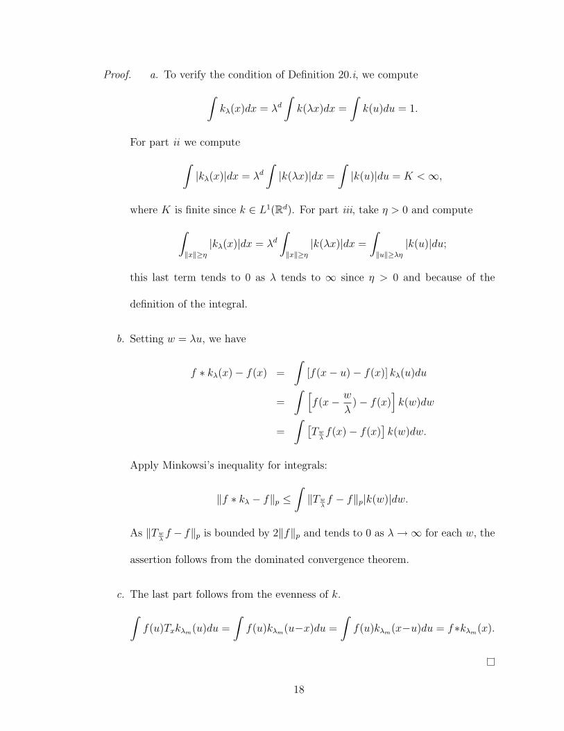
Proof. a. To verify the condition of Definition 20.i, we compute∫kλ(x)dx = λd
∫k(λx)dx =
∫k(u)du = 1.
For part ii we compute∫|kλ(x)|dx = λd
∫|k(λx)|dx =
∫|k(u)|du = K <∞,
where K is finite since k ∈ L1(Rd). For part iii, take η > 0 and compute∫‖x‖≥η
|kλ(x)|dx = λd∫‖x‖≥η
|k(λx)|dx =
∫‖u‖≥λη
|k(u)|du;
this last term tends to 0 as λ tends to ∞ since η > 0 and because of the
definition of the integral.
b. Setting w = λu, we have
f ∗ kλ(x)− f(x) =
∫[f(x− u)− f(x)] kλ(u)du
=
∫ [f(x− w
λ)− f(x)
]k(w)dw
=
∫ [Twλf(x)− f(x)
]k(w)dw.
Apply Minkowsi’s inequality for integrals:
‖f ∗ kλ − f‖p ≤∫‖Tw
λf − f‖p|k(w)|dw.
As ‖Twλf − f‖p is bounded by 2‖f‖p and tends to 0 as λ→∞ for each w, the
assertion follows from the dominated convergence theorem.
c. The last part follows from the evenness of k.∫f(u)Txkλm(u)du =
∫f(u)kλm(u−x)du =
∫f(u)kλm(x−u)du = f∗kλm(x).
18

We shall use approximate identities on Rd. The following notation will stream-
line our arguments.
Proposition 22. Fix a non-negative, compactly supported, bounded, even function
k : Rd → C with the property that∫k(γ)dγ = 1. Then, k ∈ L1 ∩ L2(Rd) and the
results of Proposition 21 hold. For ω ∈ Rd and α > 0, define gλ,α,ω ∈ L2(Rd) by
gλ,α,ω =√αTωkλ. If α = 1, we write gλ,ω = gλ,1,ω. Note that ‖gλ,ω‖2 = 1 for all
λ, ω.
The following 2 propositions may be seen as special cases of Proposition 18.
Our results in this subsection require more hypotheses than the results just ref-
erenced, but the proofs are decidedly less technical, requiring fewer analytic esti-
mates, and they also give greater insight as to why these bounds are valid. Fur-
thermore, methods used later in the thesis which improve the bound estimates
provided by Corollary 19 are inspired by these proofs. Recall the function κψ(γ) =∑n∈Z
∣∣∣ψ(2nγ)∣∣∣2.
Proposition 23. Let ψ ∈ L2(Rd) be a function with non-negative Fourier transform.
Further, assume that κψ(γ) ∈ Lp(Rd) for some 1 ≤ p ≤ ∞. If W(ψ) is a Bessel
sequence with upper frame bound B, then κψ(γ) ∈ L∞(Rd) and B ≥ Kψ.
Proof. We have assumed ψ(γ) ≥ 0 for all γ ∈ Rd. For any f ∈ L2(Rd) with non-
negative Fourier transform, lines (2.1) and (2.2) hold by the Tonelli theorem, and
we have
F (f) ≥∫ ∣∣∣f(γ)
∣∣∣2 κψ(γ)dγ.
19
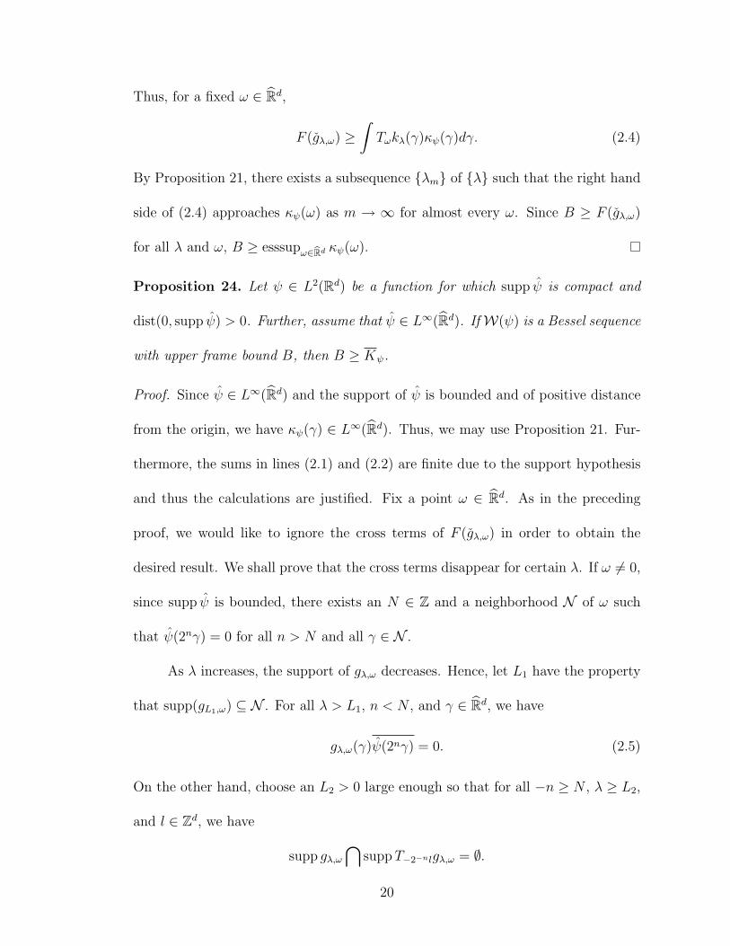
Thus, for a fixed ω ∈ Rd,
F (gλ,ω) ≥∫Tωkλ(γ)κψ(γ)dγ. (2.4)
By Proposition 21, there exists a subsequence {λm} of {λ} such that the right hand
side of (2.4) approaches κψ(ω) as m → ∞ for almost every ω. Since B ≥ F (gλ,ω)
for all λ and ω, B ≥ esssupω∈bRd κψ(ω).
Proposition 24. Let ψ ∈ L2(Rd) be a function for which supp ψ is compact and
dist(0, supp ψ) > 0. Further, assume that ψ ∈ L∞(Rd). IfW(ψ) is a Bessel sequence
with upper frame bound B, then B ≥ Kψ.
Proof. Since ψ ∈ L∞(Rd) and the support of ψ is bounded and of positive distance
from the origin, we have κψ(γ) ∈ L∞(Rd). Thus, we may use Proposition 21. Fur-
thermore, the sums in lines (2.1) and (2.2) are finite due to the support hypothesis
and thus the calculations are justified. Fix a point ω ∈ Rd. As in the preceding
proof, we would like to ignore the cross terms of F (gλ,ω) in order to obtain the
desired result. We shall prove that the cross terms disappear for certain λ. If ω 6= 0,
since supp ψ is bounded, there exists an N ∈ Z and a neighborhood N of ω such
that ψ(2nγ) = 0 for all n > N and all γ ∈ N .
As λ increases, the support of gλ,ω decreases. Hence, let L1 have the property
that supp(gL1,ω) ⊆ N . For all λ > L1, n < N , and γ ∈ Rd, we have
gλ,ω(γ)ψ(2nγ) = 0. (2.5)
On the other hand, choose an L2 > 0 large enough so that for all −n ≥ N , λ ≥ L2,
and l ∈ Zd, we have
supp gλ,ω⋂
suppT−2−nlgλ,ω = ∅.
20

Set L = max{L1, L2}. Then, for any λ > L, n ∈ Z, and γ ∈ Rd,
gλ,ω(γ)gλ,ω(γ + 2−nl)ψ(2nγ)ψ(2nγ + l) = 0.
Thus for λ > L,
F (gλ,ω) =
∫Tωkλ(γ)κψ(γ)dγ.
Letting a certain subsequence of λ get larger, we obtain B ≥ κψ(ω) for almost every
ω. Thus, B ≥ esssupω∈bRd κψ(ω).
2.3 A canonical example
For this section, let L =[−1
2,−1
4
)∪[
14, 1
2
), which is K0\A0 from the 1-d Journe
construction; see Example 15.
Example 25. We shall compute some Bessel bounds.
a. W(1∨L) is a Parseval frame. Smooth 1L by defining ψ = 1L ∗ 81[− 116, 116
]. We
would like to determine if W(ψ) is a Bessel sequence and, if so, to determine
its upper frame bound. We compute Kψ = 1716
. Within the dyadic interval[932, 9
16
)this supremum occurs at 7
16. Also, Mψ = 17
16, where the supremum
occurs at the same point. Thus, by Corollary 19, the upper frame bound of
W(ψ) is 1716
.
b. Similarly, if ψ = 1[− 12, 12
)2\[− 14, 14
)2 ∗ 641[− 116, 116
]2 , then the upper frame bound of
W(ψ) is 305256
.
Example 26. Once again, let ψ = 1L ∗ 81[− 116, 116
].
21

a. We have that Kψ = 920
and Nψ = 29. It now follows from Corollary 19 that
W is a frame with lower frame bound A, satisfying 29≤ A ≤ 9
20. We would
like to tighten these bounds around A. This is a delicate operation. For
this estimate, we shall use functions consisting of multiple spikes, scaled by
positive and negative numbers. We have that Kψ occurs at 2140
within the
dyadic interval[
932, 9
16
). By symmetry, this infimum is also achieved at −21
40.
Further,
supγ
∑n
∑l 6=0
ψ(2nγ)ψ(2nγ + l) =1
4.
This supremum occurs at ±12. In order to compute the lower frame bound, we
need to minimize F (f), defined in (2.3), over all f ∈ L2(Rd). We shall refer
to the summands,
f(γ)f(γ + 2−nk)ψ(2nγ)ψ(2nγ + k),
in F (f) as cross terms. We would like to find an f ∈ L2(Rd) that allows us
to use the cross terms to mitigate the other terms as much as possible. Since
±2140
is close to ±12, one possibility is to set fλ = gλ, 1
2, 12− gλ, 1
2,− 1
2. The centers
of the bumps are chosen to be a distance 1 apart from each other so that the
cross terms do not disappear as λ gets larger, while the negative coefficient
is chosen so that the cross terms cancel out some of the other terms. For
large enough λ, supp(gλ, 12, 12)∩ supp(gλ, 1
2,− 1
2) = ∅. We may always rescale the k
which generates the gλ, 12,± 1
2so that these supports are disjoint for all λ. Thus,
without loss of generality, assume that the supports are disjoint for all λ. We
22
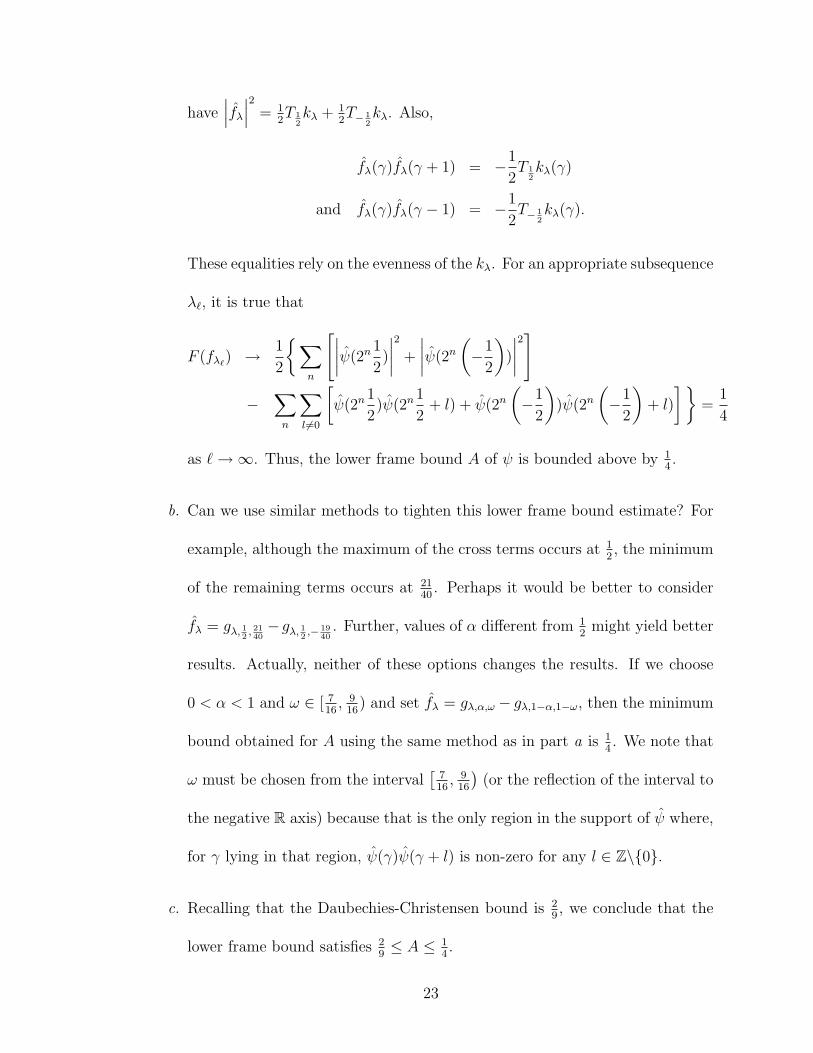
have∣∣∣fλ∣∣∣2 = 1
2T 1
2kλ + 1
2T− 1
2kλ. Also,
fλ(γ)fλ(γ + 1) = −1
2T 1
2kλ(γ)
and fλ(γ)fλ(γ − 1) = −1
2T− 1
2kλ(γ).
These equalities rely on the evenness of the kλ. For an appropriate subsequence
λ`, it is true that
F (fλ`) →1
2
{∑n
[∣∣∣∣ψ(2n1
2)
∣∣∣∣2 +
∣∣∣∣ψ(2n(−1
2
))
∣∣∣∣2]
−∑n
∑l 6=0
[ψ(2n
1
2)ψ(2n
1
2+ l) + ψ(2n
(−1
2
))ψ(2n
(−1
2
)+ l)
]}=
1
4
as `→∞. Thus, the lower frame bound A of ψ is bounded above by 14.
b. Can we use similar methods to tighten this lower frame bound estimate? For
example, although the maximum of the cross terms occurs at 12, the minimum
of the remaining terms occurs at 2140
. Perhaps it would be better to consider
fλ = gλ, 12, 2140−gλ, 1
2,− 19
40. Further, values of α different from 1
2might yield better
results. Actually, neither of these options changes the results. If we choose
0 < α < 1 and ω ∈ [ 716, 9
16) and set fλ = gλ,α,ω − gλ,1−α,1−ω, then the minimum
bound obtained for A using the same method as in part a is 14. We note that
ω must be chosen from the interval[
716, 9
16
)(or the reflection of the interval to
the negative R axis) because that is the only region in the support of ψ where,
for γ lying in that region, ψ(γ)ψ(γ + l) is non-zero for any l ∈ Z\{0}.
c. Recalling that the Daubechies-Christensen bound is 29, we conclude that the
lower frame bound satisfies 29≤ A ≤ 1
4.
23
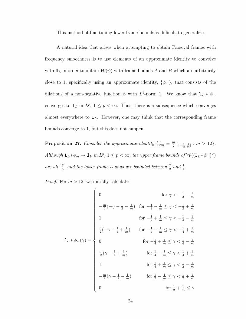
This method of fine tuning lower frame bounds is difficult to generalize.
A natural idea that arises when attempting to obtain Parseval frames with
frequency smoothness is to use elements of an approximate identity to convolve
with 1L in order to obtain W(ψ) with frame bounds A and B which are arbitrarily
close to 1, specifically using an approximate identity, {φm}, that consists of the
dilations of a non-negative function φ with L1-norm 1. We know that 1L ∗ φm
converges to 1L in Lp, 1 ≤ p < ∞. Thus, there is a subsequence which converges
almost everywhere to 1L. However, one may think that the corresponding frame
bounds converge to 1, but this does not happen.
Proposition 27. Consider the approximate identity {φm = m21[− 1
m, 1m
] : m > 12}.
Although 1L ∗φm → 1L in Lp, 1 ≤ p <∞, the upper frame bounds of W((1L ∗φm)∨)
are all 1716
, and the lower frame bounds are bounded between 29
and 14.
Proof. For m > 12, we initially calculate
1L ∗ φm(γ) =
0 for γ < −12− 1
m
−m2
(−γ − 12− 1
m) for −1
2− 1
m≤ γ < −1
2+ 1
m
1 for −12
+ 1m≤ γ < −1
4− 1
m
n2(−γ − 1
4+ 1
m) for −1
4− 1
m≤ γ < −1
4+ 1
m
0 for −14
+ 1m≤ γ < 1
4− 1
m
m2
(γ − 14
+ 1m
) for 14− 1
m≤ γ < 1
4+ 1
m
1 for 14
+ 1m≤ γ < 1
2− 1
m
−m2
(γ − 12− 1
m) for 1
2− 1
m≤ γ < 1
2+ 1
m
0 for 12
+ 1m≤ γ
24

Let ψm = 1L ∗ φm. Just as above, we then calculate κψm(γ). Because of symmetry,
we only need to calculate κψm over the positive dyadic interval[
14
+ 12m, 1
2+ 1
m
].
κψm(γ) =
(m2
4
) (γ2 +
(2m− 1
2
)γ +
(116− 1
2m+ 1
m2
))for 1
4+ 1
2m≤ γ < 1
4+ 1
m
1 for 14
+ 1m≤ γ < 1
2− 2
m(m2
4
) (14γ2 +
(1m− 1
4
)γ +
(116− 1
2m+ 5
m2
))for 1
2− 2
m≤ γ < 1
2− 1
m(m2
4
) (54γ2 −
(54
+ 1m
)γ +
(516
+ 12m
+ 2m2
))for 1
2− 1
m≤ γ < 1
2+ 1
m
The maximum value of g is 1716
and occurs at 12− 1
m. So the upper frame bound of
W(ψm) is at least 1716
. We now calculate (µψm−κψm)(γ) =∑
n
∑l 6=0
∣∣∣ψm(2nγ)ψm(2nγ + l)∣∣∣
over the same interval and obtain
(µψm − κψm)(γ) =
0 for 1
4+ 1
2m≤ γ < 1
2− 1
m(m2
4
) (−γ2 + γ +
(−1
4+ 1
m2
))for 1
4+ 1
2m≤ γ < 1
4+ 1
m
The upper frame bound of W(ψm) is bounded above by Mψm = supγ(κψm(γ) +
(µψm − κψm)(γ)), which is also 1716
. Hence W(ψm) has upper frame bound 1716
for
every m ≥ 12. Now consider
Nψm = infγ
(κψm(γ)− (µψm − κψm)(γ)) =2
9.
By Theorem 17, W(ψm) is a frame with lower frame bound A ≥ 29. If we now
calculate F ((gλ, 12, 12− gλ, 1
2,− 1
2)∨), as in Example 26, we obtain A ≤ 1
4.
One may hope to improve the frame bounds of the smooth frame wavelets,
e.g., by bringing both of the bounds closer to 1, by convolving with a linear spline.
The following proposition shows that, in this case, the resulting upper frame bound
is closer to 1, than for the case of Proposition 27, but that it also constant for large
25

enough m. Further, in the limit, there is a positive gap between upper and lower
frame bounds.
Proposition 28. Consider the approximate identity {φm : m > 12}, where φm(γ) =
max(m(1 − m|γ|), 0), γ ∈ R. Although 1L ∗ φm → 1L pointwise a.e. and in Lp,
1 ≤ p < ∞, the upper frame bounds of W((1L ∗ φm)∨) are all 6564
, and the lower
frame bounds are bounded between 29
and 14.
Proof. Let ψm = 1L ∗φm. By utilizing basic methods of optimization from calculus,
we evaluate
Kψm = Mψm =65
64.
It follows from Corollary 19 that the upper frame bound of W(ψm) is equal to 6564
,
independent of which m > 12 is used.
As in Example 26, set fλ = gλ, 12, 12− gλ, 1
2,− 1
2. Then, we can verify that there
exists a subsequence λ` such that
F (fλ`) →1
2
{∑n
[∣∣∣∣ψ(2n(
1
2
))
∣∣∣∣2 +
∣∣∣∣ψ(2n(−1
2
))
∣∣∣∣2]
−∑n
∑l 6=0
[ψ(2n
(1
2
))ψ(2n
(1
2
)− l) + ψ(2n
(−1
2
))ψ(2n
(−1
2
)− k)
]}=
1
4,
as `→∞. Also, the lower Daubechies-Christensen bound is 29, yielding the desired
bounds on the lower frame bound.
We shall call the phenomenon which occurs in Propositions 27 and 28 a frame
bound gap. The results presented in this section prompt the following questions,
which we address in Sections 2.4 and 2.5.
26

• Do we obtain a frame when we try to smooth K1\A1 from the 1-d Journe
neighborhood mapping construction?
• Can we ever precisely determine the lower frame bound?
• What happens when we smooth K0\A0 from higher dimensional Journe con-
structions?
• Does a frame bound gap occur for other wavelet sets and other approximate
identities?
2.4 A shrinking method to obtain frames
2.4.1 The shrinking method
When we try to smooth 1L for other sets L obtained using the neighborhood
mapping constrution, we do not necessarily obtain a frame.
Example 29. Let
L =
[−9
4,−2
)∪[−1
2,− 9
32
)∪[
9
32,1
2
)∪[2,
9
4
),
which is K1\A1 from the neighborhood mapping construction of the 1-d Journe set
(Example 15). For m ∈ N, define ψm = 1L ∗ m2 1[− 1m, 1m
]. ThenW(ψm) is not a frame
for any m. This can be shown by considering F ((gλ, 12, 12− gλ, 1
2,− 1
2)∨) for arbitrarily
large λ, just as in Example 26. Specifically, a subsequence of F ((gλ, 12, 12− gλ, 1
2,− 1
2)∨)
converges to 0, while each gλ, 12, 12− gλ, 1
2,− 1
2has unit norm. However, for arbitrary
m, W(ψm) is a Bessel sequence, and for any m > 64, the Bessel bound is bounded
27

between 305256
and 118
. Again, we see that the upper frame bound does not converge
to 1.
It seems reasonable to assume that smoothing 1L in Example 29 with a linear
spline may yield a frame; however, the following example shows that this does not
happen.
Example 30. Let
L =
[−9
4,−2
)∪[−1
2,− 9
32
)∪[
9
32,1
2
)∪[2,
9
4
),
and for m > 64, let φm be the linear spline φm(γ) = max(m(1 − m|γ|), 0). Set
ψ = 1L ∗ φm. Then, using Mathematica we obtain
Mψ =41
32≈ 1.28125
Kψ ≈ 1.14833
Kψ ≈ 0.38092
Nψ = 0.
In fact, for some subsequence {λ`},
F ((gλ`, 12 ,12− gλ`, 12 ,− 1
2)∨)→ νψ(2) = 0
If W(ψ) formed a frame, then it would have a lower frame bound 0 = Nψ ≤ A ≤
νψ(2) = 0. Thus W(ψ) is not a frame, but it is a Bessel sequence with upper frame
bound 1.14833 ≤ B ≤ 1.28125.
We would not only like to construct frames, but also to determine the exact
lower frame bound of such a frame rather than a range of possible values. The
following definitions and theorem will help us do that.
28

Definition 31. For any measurable subset L ⊆ Rd define
∆(L) = dist(L,
⋃k∈Zd\{0}
(L+ k)).
Definition 32. If f is a function Rd → R, define f+ = |f |+f2
. For ε ≥ 0, define
suppε f = supp(f(·)− ε)+.
Essentially, suppε f returns the regions over which f takes values greater than
ε. Notice that supp f = supp0 |f |.
Theorem 33. Let ψ ∈ L∞c (Rd) be a non-negative function. If there exists an ε > 0
such that for L = suppε ψ,⋃n∈Z 2nL = Rd up to a set of measure 0, and for
L = supp ψ, ∆(L) > 0, and dist(0, L) > 0. Then, W(ψ) is a frame for L2(Rd). The
frame bounds are essinfγ κψ(γ) and esssupγ κψ(γ).
Remark 34. If the L ⊆ Rd is a Parseval frame wavelet set and the closure L ⊆
(−12, 1
2)d, then ψ = 1L and 0 < ε < 1 satisfy the hypotheses with L = L.
Proof. We first note that since ψ is compactly supported and bounded, it lies in
L2(Rd). Thus ψ ∈ L2(Rd). We now prove that W(ψ) is a frame. Since ∆(L) > 0,
∀γ ∈ Rd∑n∈Z
∑k 6=0
∣∣∣ψ(2nγ)ψ(2nγ + k)∣∣∣ = 0. (2.6)
So
Mψ = Kψ.
By assumption, ψ is bounded. Furthermore, since dist(0, L) > 0 and L is bounded,
for any γ ∈ Rd, ψ(2nγ) is non-zero for only finitely many n ∈ Z. Putting these two
29

facts together, we conclude that
Kψ <∞.
Similarly,
Nψ = Kψ.
Since dyadic dilations of L cover Rd, for almost every γ ∈ Rd, there exists n ∈ Z
such that 2nγ ∈ L, which implies that ψ(2nγ) > ε. Thus essinfγ∈bRd κψ(γ) > 0.
Thus, by Corollary 19, W(ψ) is a frame with bounds A and B which satisfy
A = Kψ
and B = Kψ.
A statement very similar to the preceding theorem appears camouflaged (through
a number of auxiliary functions) as Theorem 8 in [26].
Remark 35. Let ψ ∈ L2(R) satisfy the hypotheses of Theorem 33. Then for
C = max{A−1, B} and almost all γ ∈ R
0 < C−1 ≤ κψ(γ) ≤ C <∞.
Furthermore, it follows from line (2.6) that for almost all γ ∈ R,
ψ (2nγ)ψ (2nγ + 2nk) = 0 ∀k ∈ Z\2Z , k ∈ N ∪ {0}.
Thus, by Proposition 2.2 of [37], if S : L2(R)→ L2(R) is the frame operator defined
as
Sf =∑n∈Z
∑k∈Zd〈f,DnTkψ〉DnTkψ,
then S is translation invariant. That is, for all x ∈ R, STx = TxS as operators.
30

Corollary 36. Let L be a Parseval frame wavelet set from the neighborhood mapping
construction. Let δ = dist(0, L) > 0. Let α > 0 be such that the closure αL ⊆
(−12
+ ε, 12− ε)d, for some 0 < ε < 1
2. Further let φ be an essentially bounded
non-negative function such that suppφ ⊆ min{αδ2, ε} · (−1, 1)d and suppφ contains
a neighborhood about the origin. Then if ψ = 1αL ∗ φ, W(ψ) is a frame for L2(Rd).
Proof. Define L = supp ψ. Since suppφ contains a neighborhood about the origin,
φ is non-negative, and ψ is continuous, there exists an ε > 0 such that
αL ⊆ ψ−1(ε,∞).
Thus, for this ε,
Rd = αRd = α⋃n∈Z
2nL ⊆⋃n∈Z
2n suppε ψ,
up to a set of measure zero. As the convolution of two essentially bounded functions
with compact support, ψ ∈ L∞ immediately. It follows from Theorem 33 thatW(ψ)
is a frame for L2(Rd).
Example 37. Let
L =
[− 9
32,−1
4
)∪[− 1
16,− 9
256
)∪[
9
256,
1
16
)∪[
1
4,
9
32
).
Then L is K1\A1 from the 1-d Journe construction, shrunk by a factor of 8. Further
let ψm = 1L ∗ m21[− 1
m, 1m
]. Then for any m ≥ 384, W(ψm) is frame with bounds 81260
and 305256
. Note that W((18L ∗ m21[− 1
m, 1m
])∨) is not a frame for any m > 0 (Example
29).
Example 38. Let La =[−a,−a
2
)∪[a2, a)
for 0 < a < 12. Then La is
[−1
2,−1
4
)∪[
14, 1
2
)from the 1-d Journe construction, dilated by a factor of 2a < 1. Recall from
31
Proposition 27 that
W((1[− 12,− 1
4)∪[ 14, 12) ∗
m
21[− 1
m, 1m
))∨)
is a frame with upper frame bound 1716
and lower frame bound between 29
and 14.
Define ψm,a = 1La ∗ m2 1[− 1m, 1m
]. For 0 < a < 12
and m ≥ max{ 21−2a
, 6a}, W(ψm,a) is a
frame with with frame bounds 920
and 1716
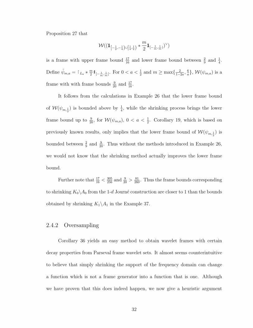
.
It follows from the calculations in Example 26 that the lower frame bound
of W(ψm, 12) is bounded above by 1
4, while the shrinking process brings the lower
frame bound up to 920
, for W(ψm,a), 0 < a < 12. Corollary 19, which is based on
previously known results, only implies that the lower frame bound of W(ψm, 12) is
bounded between 29
and 920
. Thus without the methods introduced in Example 26,
we would not know that the shrinking method actually improves the lower frame
bound.
Further note that 1716< 305
256and 9
20> 81
260. Thus the frame bounds corresponding
to shrinking K0\A0 from the 1-d Journe construction are closer to 1 than the bounds
obtained by shrinking K1\A1 in the Example 37.
2.4.2 Oversampling
Corollary 36 yields an easy method to obtain wavelet frames with certain
decay properties from Parseval frame wavelet sets. It almost seems counterintuitive
to believe that simply shrinking the support of the frequency domain can change
a function which is not a frame generator into a function that is one. Although
we have proven that this does indeed happen, we now give a heuristic argument
32

that this method should work for dyadic-shrinking. If the collection {DnTkψ :
n ∈ Z, k ∈ Zd} ⊆ L2(Rd) is a Bessel sequence, then it is not a frame if and
only if there exists a sequence {fm : ‖fm‖2 = 1,m ∈ Z} ⊆ L2(Rd) such that
limm→∞∑
n∈Z∑
k∈Zd |〈fm, DnTkψ〉|2 = 0. Having a positive lower frame bound is
a stronger condition than being complete. However, if we add more elements to
{DnTkψ : n ∈ Z, k ∈ Zd}, it is more likely that the system will be complete and
thus also more likely that it will have a lower frame bound. We would like to show
that shrinking the support of ψ will add more elements to the system. For α > 0
and ψ ∈ L2(Rd), let ϕ(γ) = ψ(αγ). Then Fϕ = α−d/2Dlog2 αFψ,
⇒ ϕ = F−1Fϕ
= F−1(α−d/2Dlog2 αF)ψ
= F−1(α−d/2FD− log2 α)ψ
= α−d/2D− log2 αψ
⇒ DnTkϕ = α−d/2DnTkD− log2 αψ
= α−d/2Dn−log2 αT kαψ.
Hence, if α = 2N , for N ∈ N,
span{DnTkϕ : n ∈ Z, k ∈ Zd} = span{DnT k
2Nψ : n ∈ Z, k ∈ Zd}.
Thus, dyadic shrinking on the Fourier domain has the effect of increasing the size
of the system generated by dilations and translations by a power of 2. One may
call this an oversampling of the continuous wavelet system {Dlog2 rTsψ : r > 0, s ∈
R}. If L ⊆ Rd is Parseval frame wavelet set and φ ∈ L∞c (Rd), W ((1L ∗ φ)∨) is a
33

Bessel sequence but perhaps not a frame (see Example 37). Hence, dyadic shrinking
increases the likelihood that W ((1L ∗ φ)∨) is complete and thus also the likelihood
that W ((1L ∗ φ)∨) has a positive lower frame bound. In general, shrinking by any
α > 1 has the effect of increasing the number of translations in the original wavelet
system and shifts each of the dilation operators by the same amount. We compare
and contrast our results with the following two oversampling theorems found in [26].
Theorem 39. Let W(ψ) be a frame for L2(R) with frame bounds A and B. Then
for every odd positive integer N , the family
{DnT kNψ : n, k ∈ Z}
is a frame with bounds A and B which satisfy A ≥ NA and B ≤ NB.
Theorem 40. Let ψ ∈ L2(R) decay sufficiently fast and satisfy∫ψ(x)dx = 0. If
W(ψ) forms a frame, then for any positive integer N ,
{DnT kNψ : n, k ∈ Z}
is a frame also.
Remark 41. The specific decay conditions in the hypothesis of Theorem 40 are
described in [26], but are too lengthy to list here. The smoothed frame wavelets
mentioned in this thesis all satisfy the decay conditions.
Only dyadic shrinking corresponds to oversampling in the Chui and Shi sense.
Oversampling may potentially create a frame system from a pre-existing frame sys-
tem, but we see in Example 37 that oversampling may change a non-frame system
34
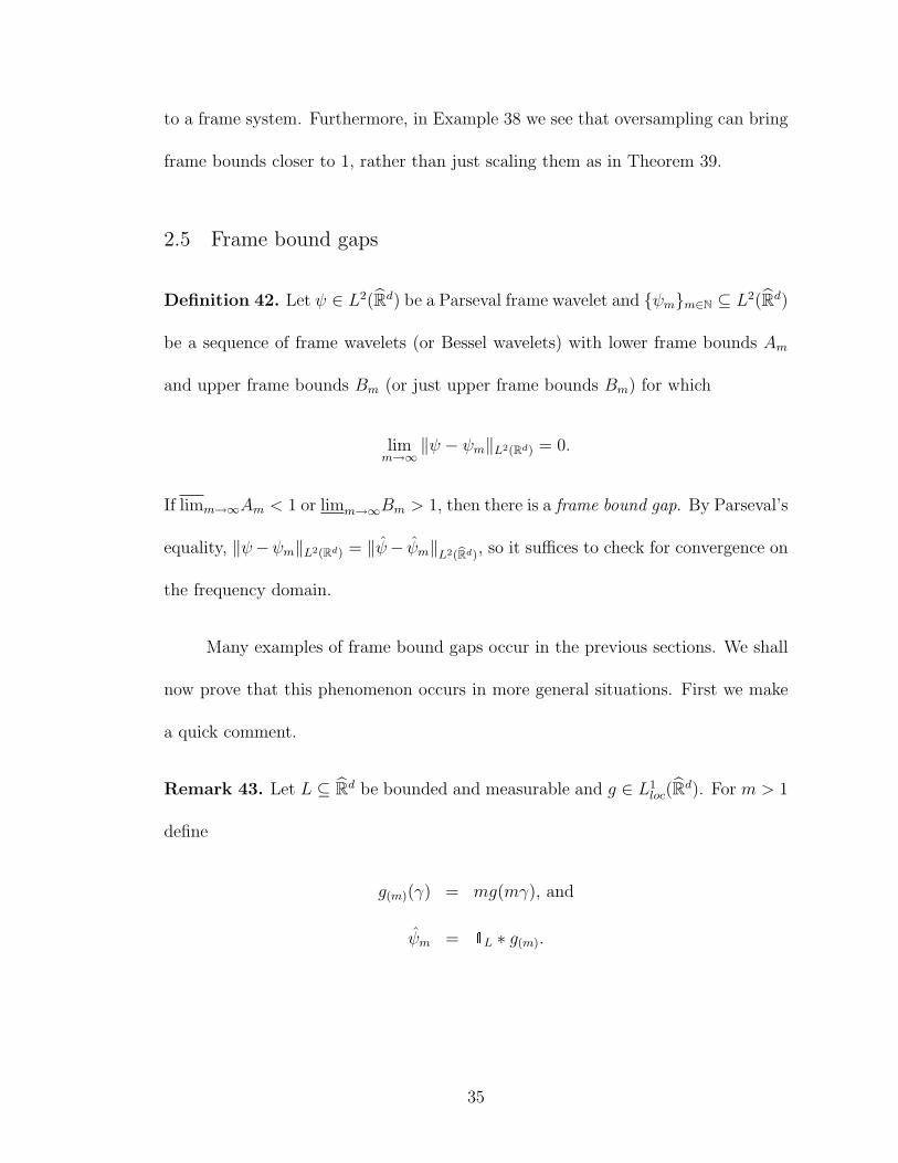
to a frame system. Furthermore, in Example 38 we see that oversampling can bring
frame bounds closer to 1, rather than just scaling them as in Theorem 39.
2.5 Frame bound gaps
Definition 42. Let ψ ∈ L2(Rd) be a Parseval frame wavelet and {ψm}m∈N ⊆ L2(Rd)
be a sequence of frame wavelets (or Bessel wavelets) with lower frame bounds Am
and upper frame bounds Bm (or just upper frame bounds Bm) for which
limm→∞
‖ψ − ψm‖L2(Rd) = 0.
If limm→∞Am < 1 or limm→∞Bm > 1, then there is a frame bound gap. By Parseval’s
equality, ‖ψ−ψm‖L2(Rd) = ‖ψ− ψm‖L2(bRd), so it suffices to check for convergence on
the frequency domain.
Many examples of frame bound gaps occur in the previous sections. We shall
now prove that this phenomenon occurs in more general situations. First we make
a quick comment.
Remark 43. Let L ⊆ Rd be bounded and measurable and g ∈ L1loc(Rd). For m > 1
define
g(m)(γ) = mg(mγ), and
ψm = 1L ∗ g(m).
35
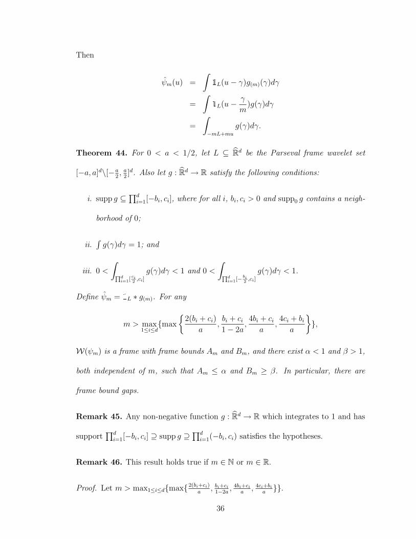
Then
ψm(u) =
∫1L(u− γ)g(m)(γ)dγ
=
∫1L(u− γ
m)g(γ)dγ
=
∫−mL+mu
g(γ)dγ.
Theorem 44. For 0 < a < 1/2, let L ⊆ Rd be the Parseval frame wavelet set
[−a, a]d\[−a2, a
2]d. Also let g : Rd → R satisfy the following conditions:
i. supp g ⊆∏d
i=1[−bi, ci], where for all i, bi, ci > 0 and supp0 g contains a neigh-
borhood of 0;
ii.∫g(γ)dγ = 1; and
iii. 0 <
∫Qdi=1[
ci2,ci]
g(γ)dγ < 1 and 0 <
∫Qdi=1[− bi
2,ci]
g(γ)dγ < 1.
Define ψm = 1L ∗ g(m). For any
m > max1≤i≤d
{max
{2(bi + ci)
a,bi + ci1− 2a
,4bi + ci
a,4ci + bi
a
}},
W(ψm) is a frame with frame bounds Am and Bm, and there exist α < 1 and β > 1,
both independent of m, such that Am ≤ α and Bm ≥ β. In particular, there are
frame bound gaps.
Remark 45. Any non-negative function g : Rd → R which integrates to 1 and has
support∏d
i=1[−bi, ci] ⊇ supp g ⊇∏d
i=1(−bi, ci) satisfies the hypotheses.
Remark 46. This result holds true if m ∈ N or m ∈ R.
Proof. Let m > max1≤i≤d{max{2(bi+ci)a
, bi+ci1−2a
, 4bi+cia
, 4ci+bia}}.
36
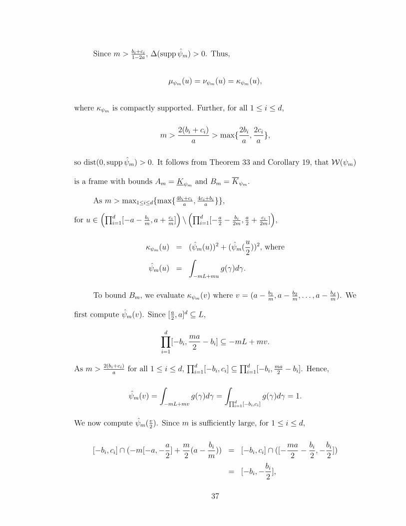
Since m > bi+ci1−2a
, ∆(supp ψm) > 0. Thus,
µψm(u) = νψm(u) = κψm(u),
where κψm is compactly supported. Further, for all 1 ≤ i ≤ d,
m >2(bi + ci)
a> max{2bi
a,2cia},
so dist(0, supp ψm) > 0. It follows from Theorem 33 and Corollary 19, that W(ψm)
is a frame with bounds Am = Kψm and Bm = Kψm .
As m > max1≤i≤d{max{4bi+cia
, 4ci+bia}},
for u ∈(∏d
i=1[−a− bim, a+ ci
m])\(∏d
i=1[−a2− bi
2m, a
2+ ci
2m])
,
κψm(u) = (ψm(u))2 + (ψm(u
2))2, where
ψm(u) =
∫−mL+mu
g(γ)dγ.
To bound Bm, we evaluate κψm(v) where v = (a− b1m, a− b2
m, . . . , a− bd
m). We
first compute ψm(v). Since [a2, a]d ⊆ L,
d∏i=1
[−bi,ma
2− bi] ⊆ −mL+mv.
As m > 2(bi+ci)a
for all 1 ≤ i ≤ d,∏d
i=1[−bi, ci] ⊆∏d
i=1[−bi, ma2 − bi]. Hence,
ψm(v) =
∫−mL+mv
g(γ)dγ =
∫Qdi=1[−bi,ci]
g(γ)dγ = 1.
We now compute ψm(v2). Since m is sufficiently large, for 1 ≤ i ≤ d,
[−bi, ci] ∩ (−m[−a,−a2
] +m
2(a− bi
m)) = [−bi, ci] ∩ ([−ma
2− bi
2,−bi
2])
= [−bi,−bi2
],
37
[−bi, ci] ∩ (−m[−a2,a
2] +
m
2(a− bi
m)) = [−bi, ci] ∩ ([−bi
2,ma− bi
2])
= [−bi2, ci], and
[−bi, ci] ∩ (−m[a
2, a] +
m
2(a− bi
m)) = [−bi, ci] ∩ ([ma− bi
2,3ma
2− bi
2])
= ∅.
It follows that(d∏i=1
[−bi, ci]
)∩(−mL+m(
v
2))
=
(d∏i=1
[−bi, ci]
)\
(d∏i=1
[−bi2, ci]
),
and that
ψm(v
2) =
∫−mL+m( v
2)
g(γ)dγ = 1−∫
Qdi=1[− bi
2,ci]
g(γ)dγ.
Define β = κψm(v) = 1 +(
1−∫Qd
i=1[− bi2,ci]g(γ)dγ
)2
. Then, Bm ≥ κψm(v) = β > 1,
and β is independent of m.
Let ω = (a+ c1m, a+ c2
m, . . . , a+ cd
m). We shall show that κψm(ω) is strictly less
than 1. We compute
−mL+mω =
(d∏i=1
[ci, 2ma+ ci]
)\
(d∏i=1
[ma
2+ ci,
3ma
2+ ci]
)
⇒
(d∏i=1
[−bi, ci]
)∩ (−mL+mω) = ∅.
Thus, ψm(ω) = 0. Furthermore,
−mL+m(ω
2) =
(d∏i=1
[−ma2
+ci2,3ma
2+ci2
]
)\
(d∏i=1
[ci2,ma+
ci2
]
).
It follows from our choice of m that for all 1 ≤ i ≤ d, −ma2
+ ci2< −bi and
ci < ma+ ci2< 3ma
2+ ci
2. Hence,(
d∏i=1
[−bi, ci]
)∩ (−mL+m(
ω
2)) =
(d∏i=1
[−bi, ci]
)\
(d∏i=1
[ci2, ci]
), and
38

ψm(ω
2) = 1−
∫Qdi=1[
ci2,ci]
g(γ)dγ.
We define
α = κψm(ω) =
(1−
∫Qdi=1[
ci2,ci]
g(γ)dγ
)2
.
Consequently, Am ≤ α < 1 for all sufficiently large m.
Corollary 47. For 0 < a < 12, let Ld ⊆ Rd be the wavelet set [−a, a]d\[−a
2, a
2]d.
Also, let g : R→ R satisfy the following conditions:
i. supp g ⊆ [−b, c] for some b, c > 0 and supp0 g contains a neighborhood of 0;
ii.∫g(γ)dγ = 1; and
iii. 0 <∫ cc2g(γ)dγ < 1 and 0 <
∫ c− b
2g(γ)dγ < 1.
Define gd =⊗d
i=1 g : Rd → R. Further define ψm,d = 1Ld ∗ gd(m). Then, for each
m > max{2(b+ c)
a,b+ c
1− 2a,4b+ c
a,4c+ b
a},
and d ≥ 1, W(ψm,d) is a frame with bounds Am,d and Bm,d which satisfy
Am,d ≤
1−
(∫ c
c2
g(γ)dγ
)d2
< 1, and
Bm,d ≥
1−
(∫ c
− b2
g(γ)dγ
)d2
+ 1 > 1.
Also for such m, limd→∞Bm,d = 2.
Proof. All of the hypotheses of Theorem 44 are satisfied, so
Am,d ≤
1−
(∫ c
c2
g(γ)dγ
)d2
< 1, and
Bm,d ≥
1−
(∫ c
− b2
g(γ)dγ
)d2
+ 1 > 1,
39

where
limd→∞
1−
(∫ c
− b2
g(γ)dγ
)d2
+ 1 = 2,
since 0 <∫ c− b
2g(γ)dγ < 1. Furthermore,
Bm,d = supu∈[−a− b
m,a+ c
m]d\[−a
2− b
2m,a2
+ c2m
]dκψm,d(u)
= supu∈[−a− b
m,a+ c
m]d\[−a
2− b
2m,a2
+ c2m
]d(ψm,d(u))2 + (ψm,d(
u
2))2
≤ 2.
Thus, limd→∞Bm,d = 2 for all large enough m.
A similar result holds for a large class of wavelet sets in R.
Theorem 48. Let L =⋃
j∈J⊆Z
[aj, bj], with aj < bj for all j ∈ J , be a Parseval frame
wavelet set. Let g : R → R be a non-negative function satisfying∫g(γ)dγ = 1 and
with support supp g = [−c, d], where c, d > 0 and which contains a neighborhood
of zero. Define ψm = 1L ∗ g(m) for m > c+dbj−aj for all j ∈ J . Then if W(ψm)
forms a Bessel sequence, the upper frame bound satisfies Bm ≥ β > 1, where β is
independent of m. In particular, there is a frame bound gap.
Proof. Set ak = min{aj > 0 : j ∈ J }, and let bi ∈ {bj}j∈J be the unique bj > 0
such that there exists N ∈ N∪ {0} with 2Nak = bi. We wish to bound κψm(bi− cm
).
Since m > c+dbi−ai ,
−mL+m(bi −c
m) ⊇ m[−bi,−ai] +m(bi −
c
m)
= [−c,m(bi − ai)− c]
⊇ [−c, d],
40

implying that
ψm(bi −c
m) =
∫−mL+m(bi− c
m)
g(γ)dγ = 1.
Similarly,
−mL+m(2−N(bi −c
m)) = −mL+mak − 2−Nc
⊇ m[−bk,−ak] +mak − 2−Nc
= [m(ak − bk)− 2−Nc,−2−Nc]
⊇ [−c,−2−Nc].
So
ψm(2−N(bi −c
m)) ≥
∫ −2−N c
−cg(γ)dγ > 0.
Hence,
Bm ≥ κψm(bi −c
m) ≥ 1 +
(∫ −2−N c
−cg(γ)dγ
)2
> 1.
We note that by construction (viii) in Chapter 4 of [33], cantor-like wavelet
sets exist. Thus, Theorem 48 does not apply to all wavelet sets in R.
Corollary 49. Let L =J⋃j=1
[aj, bj] ⊆ (−1
2,1
2), with aj < bj for all j ∈ J , be a
Parseval frame wavelet set. Let g : R → R be a non-negative function satisfying∫g(γ)dγ = 1, with support supp g = [−c, d], where c, d > 0, and which contains a
neighborhood of zero. Define ψm = 1L ∗ g(m) for all m large enough that
m > max
{c+ d
(minj aj)− (maxj bj) + 1,max
j
{ c+ d
bj − aj},
d
dist(0, L),
c
dist(0, L)
}.
Then W(ψm) forms a frame with upper frame bound Bm ≥ β > 1, where β is
independent of m.
41
Proof. Since m > c+d(minj aj)−(maxj bj)+1
, µψm = νψm = κψm . Because supp ψm ) L,
inf κψm > 0. Finally, since m > max{ ddist(0,L)
, cdist(0,L)
} and supp ψm is compact,
supκψm <∞. Hence W(ψm) is a frame.
The remainder of the claim follows from Theorem 48.
In this chapter Parseval frame wavelets are smoothed on the frequency do-
main by elements of successive elements of approximate identities. However, the
corresponding frame bounds do not converge to 1 even though L is a Parseval frame
wavelet set. We contrast these facts to the case of time domain smoothing. In [1],
the Haar wavelet is smoothed using convolution on the time domain with members
of particular approximate identities {kλ}. The smoothed functions generate Riesz
basis wavelets which have frame bounds which approach 1 as λ → ∞. Thus, con-
volutional smoothing affects frame bounds dramatically differently depending on
whether the smoothing is done on the temporal or frequency domains. Further-
more, Theorems 44 and 48 may be used to show that certain smooth functions are
not the result of convolutional smoothing; see Section 3.5 in the next chapter. Fi-
nally, the shrinking method introduced in Section 2.4 may be used to simply modify
non-complete systems in order to obtain frames.
42

Chapter 3
Smooth Parseval frames for L2(R) and generalizations to L2(Rd)
3.1 Introduction
3.1.1 Motivation
As in Chapter 2, we are concerned with finding frame wavelets which are
smoothed approximations of Parseval wavelet set wavelets. We attempt to generalize
Bin Han’s non-constructive proof of the existence of Schwartz class functions which
approximate Parseval wavelet set wavelets in L2(R) arbitrarily well. We show that
the natural approaches to such a generalization fail. Furthermore, we show that
a collection of well-known functions which also approximate wavelet set wavelets
generate frames with upper frame bounds that converge to 1.
3.1.2 Background
Recall that in this chapter, Dtf(x) = 2td/2f(2tx).
Definition 50.
• The space C∞c (Rd) consists of functions f : Rd → C which are infinitely
differentiable and compactly supported.
• Given a multi-index α = (α1, α2, . . . , αd) ∈ (N ∪ {0})d, we write |α| =∑d
i=1 αi,
43

xα =∏d
i=1 xαii , and Dα =
∂α1
∂xα11
∂α2
∂xα22· · · ∂αd
∂xαdd
. An infinitely differentiable func-
tion f : Rd → C is an element of the Schwartz space S (Rd) if
∀n = 0, 1, . . . sup|α|≤n,α∈(N∪{0})d
supx∈Rd
(1 + ‖x‖2
)α |Dαf(x)| <∞.
Clearly S ⊂ L1, so the Fourier transform is well defined on S and is in fact
a topological automorphism. Since C∞c ⊆ S , the (inverse) Fourier transform
of a smooth compactly supported function is smooth.
• We will denote the space {f ∈ L2(R) : supp f ⊆ [0,∞)} as H2(R), as in [63].
We now make note of a now well-known result, which appeared in Bin Han’s
paper [63], as well as many other contemporary papers.
Theorem 51. Let ψ ∈ L2(Rd). Then W(ψ) is a Parseval frame if and only if
∑n∈Z
|ψ(2nγ)|2 = 1 and∞∑n=0
ψ(2nγ)ψ(2n(γ +m)) = 0 (3.1)
with absolute convergence for almost every γ ∈ Rd and for all m ∈ Zd\2Zd.
3.1.3 Outline and Results
In Section 3.2.1, we present the results from [62] and [63] which concern the ex-
istence of smooth Parseval frames which approximate 1-dimensional Parseval frame
wavelet sets. Bin Han’s methods involve auxiliary smooth functions which we try
to generalize to higher dimensions in Section 3.2.2. We show that forming tensor
products or other similarly modified versions of the auxiliary functions from Section
3.2.1 either fails to yield a Parseval frame or fails to yield a smooth wavelet when
44
used to smooth a certain type of wavelet set. However, some Parseval wavelet set
wavelets in Rd can be smoothed using methods inspired by Han’s work, see Section
3.3. In Section 3.4 we construct a class of C∞c functions which form frames with
upper frame bounds converging to 1.
We conclude with Section 3.5 which contains a review of previously known
methods to smooth frame wavelet set wavelets.
3.2 Schwartz class Parseval frames
3.2.1 Parseval frames for L2(R)
In his Master’s thesis, [62], as well as the paper [63], Bin Han proved the
existence of C∞ Parseval frames for H2(R). The following two lemmas and definition
appear in the paper [63].
Lemma 52. There exists a function θ ∈ C∞(R) satisfying θ(x) = 0 when x ≤ −1
and θ(x) = 1 when x ≥ 1 and
θ(x)2 + θ(−x)2 = 1, x ∈ R.
Definition 53. Given a closed interval I = [a, b] and two positive numbers δ1, δ2
such that δ1 + δ2 ≤ b− a, we define
f(I;δ1,δ2)(x) =
θ(x−aδ1
)when x < a+ δ1
1 when a+ δ1 ≤ x ≤ b− δ2
θ(b−xδ2
)when x > b− δ2
Note that supp(f(I;δ1,δ2)) ⊆ [a− δ1, b+ δ2].
45
Lemma 54. For any positive numbers δ1, δ2, δ3 and 0 < a < b < c,
f(I;δ1,δ2)(2nx) = f(2−kI;2−kδ1,2−kδ2)(x)
and
f 2([a,b];δ1,δ2)(x) + f 2
([b,c];δ2,δ3)(x) = f 2([a,c];δ1,δ3)(x).
The preceding lemmas are used to prove
Proposition 55 ([63]). Suppose that a family of disjoint closed intervals Ii = [ai, bi],
1 ≤ i ≤ l in (0,∞) is arranged in a decreasing order, i.e., 0 < bl < bl−1 < . . . < b1
and ∪li=1Ii is dyadic dilation congruent to [1/2, 1) ⊆ R. If ∆(∪li=1Ii) > 0. Then for
any
0 < δ <1
2min{∆(∪li=1Ii), min
1≤i≤l{bi − ai}, min
1≤i<ldist(Ii, Ii+1)},
let
ψδ = f(I1; δ2,δ) +
l∑i=2
f(Ii;2−ki−1δ,2−ki−1δ)
where ki is the unique non-negative integer such that 2kiIi ⊆ [12b1, b1]. We have
ψδ ∈ S (R) and W(ψδ) is a Parseval frame in H2(R).
Bin Han states that a similar proposition holds for L2(R), but does not ex-
plicitly state it nor prove it. However, it is easy to extend the result using similar
methods to his proof of the preceding proposition.
Proposition 56. Suppose that a family of disjoint closed intervals Ii = [ai, bi],
1 ≤ i ≤ l in R is arranged in a decreasing order, i.e., bl < bl−1 < . . . < b1 where
bj < 0 < aj−1 and ∪li=1Ii is dyadic dilation congruent to [−1,−1/2) ∪ [1/2, 1) ⊆ R.
46

If ∆(∪li=1Ii) > 0, then for any
0 < δ <1
2min{∆(∪li=1Ii), min
1≤i≤l{bi − ai}, min
1≤i<ldist(Ii, Ii+1)},
let
ψδ = f(I1; δ2,δ) +
[l−1∑i=2
f(Ii;2−ki−1δ,2−ki−1δ)
]+ f(Il;δ,
δ2
)
where for 2 ≤ i ≤ j − 1, ki is the unique non-negative integer such that 2kiIi ⊆
[12b1, b1] and for j ≤ i ≤ l − 1, ki is the unique non-negative integer such that
2kiIi ⊆ [al,12al]. We have ψδ ∈ S (R) and W(ψδ) is a Parseval frame in L2(R).
Proof. We’d like to make use of Theorem 51. To this end, let
f1 = f(I1; δ2,δ)
fi = f(Ii;2−ki−1δ,2−ki−1δ) for 2 ≤ i ≤ l − 1
fl = f(Il;δ,δ2
)
In order for the fi to be well defined, we need
δ
2+ δ ≤ b1 − a1
2−ki−1δ + 2−ki−1δ ≤ bi − ai for 2 ≤ i ≤ l − 1
δ
2+ δ ≤ bl − al
By our choice of δ, for all 1 ≤ i ≤ l,
δ
2+ δ <
12(bi − ai)
2+
1
2(bi − ai)
=3
4(bi − ai)
< bi − ai.
47
So for i = 1 and i = l the desired inequalities hold. Also because ki ≥ 0 for each
2 ≤ i ≤ l − 1,
2−ki−1δ + 2−ki−1δ = 2−kiδ
< 2−ki(bi − ai
2
)= 2−ki−1(bi − ai)
< bi − ai
So the fi are all well-defined and
supp f1 ⊆ [a1 −δ
2, b1 + δ],
supp fi ⊆ [ai − 2−ki−1δ, bi + 2−ki−1δ] for any 2 ≤ i ≤ l − 1
supp fl ⊆ [al −δ
2, bl + δ].
Hence for any 1 ≤ i ≤ l, supp fi ⊂ [ai − δ, bi + δ]. Since 0 < δ < 12∆(∪li=1),
∆(∪li=1 supp fi) ≥ ∆(∪li=1[ai − δ, bi + δ]) ≥ ∆(∪li=1Ii)− 2δ > 0.
Thus for all 1 ≤ i, k ≤ l, n ∈ N ∪ {0}, m ∈ Z\0,
fi(2nγ)fk(2
n(γ +m)) = 0,
since 2nm ∈ Z\{0}. Hence for any n ∈ N ∪ {0} and m ∈ Z\{0},
ψδ(2nγ)ψδ(2
n(γ +m)) = 0 a.e.
By construction,
1I1 +
(l−1∑i=2
12kiIi
)+ 1Il = 1[al,
12al]∪[ 1
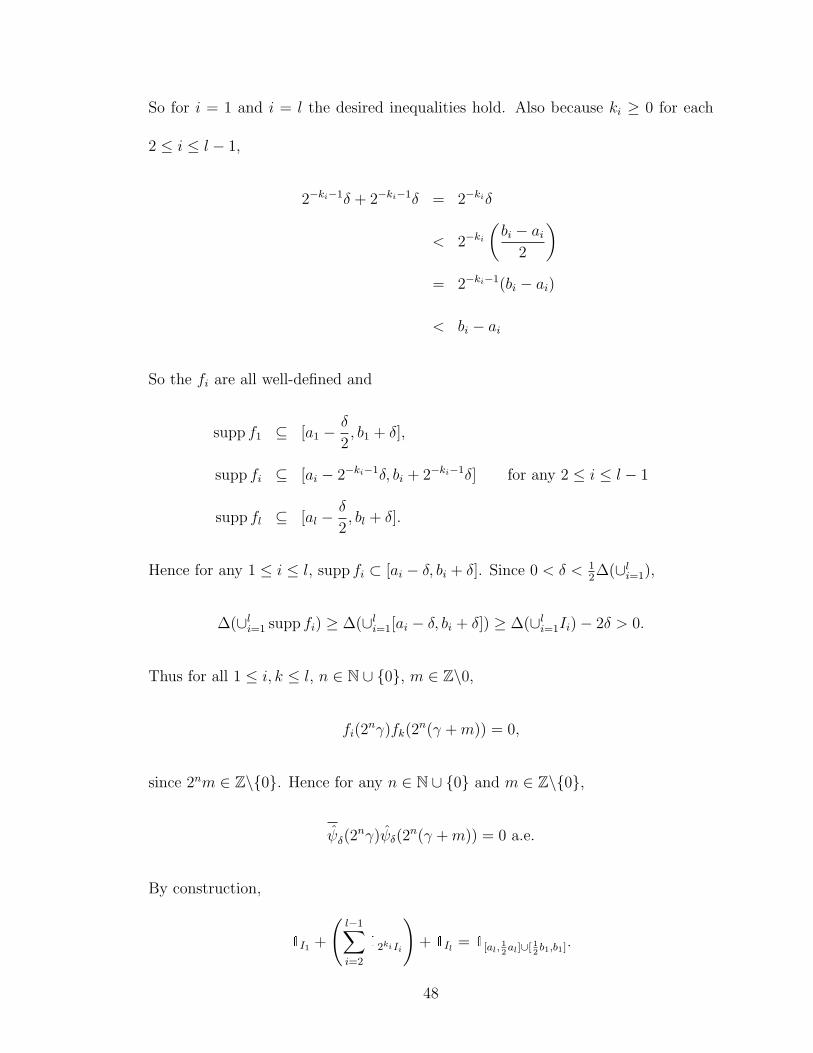
2b1,b1].
48

Using the Lemma 54, we obtain
f 21 (γ) +
j−1∑i=2
f 2i (2−kiγ) = f 2
(I1; δ2,δ)
(γ) +
j−1∑i=2
f 2(Ii;2−ki−1δ,2−ki−1δ)(2
−kiγ)
= f 2(I1; δ
2,δ)
(γ) +
j−1∑i=2
f 2(2kiIi;
12δ, 1
2δ)
(γ)
= f 2([ 1
2b1,b1]; 1
2δ,δ)
(γ).
Similarly,l−1∑i=j
f 2i (2−kiγ) + f 2
l (γ) = f 2([al,
12al];δ,
12δ)
(γ).
So we know that
∑n∈Z
l∑i=1
f 2i (2nγ) =
∑n∈Z
(f 2
([al,12al];δ,
12δ)
(2nγ) + f 2([ 1
2b1,b1]; 1
2δ,δ)
(2nγ))
=∑n∈Z
(f 2
(2−n[al,12al];2−nδ,2−n−1δ)
(γ) + f 2(2−n[ 1
2b1,b1];2−n−1δ,2−nδ)
(γ)).
For any n ∈ Z, we again apply Lemma 54 to get(f 2
(2−n[al,12al];2−nδ,2−n−1δ)
(γ) + f 2(2−n[ 1
2b1,b1];2−n−1δ,2−nδ)
(γ)
)+
(f 2
(2−n−1[al,12al];2−n−1δ,2−n−2δ)
(γ) + f 2(2−n−1[ 1
2b1,b1];2−n−2δ,2−n−1δ)
(γ)
)= f 2
([2−nal,2−n−2al];2−nδ,2−n−2δ)(γ) + f 2([2−n−2b1,2−nb1];2−n−2δ,2−nδ)(γ)
As a result of these 2 equalities,∑l
i=1
∑n∈Z fi(2
nγ) = 1(−∞,∞)(γ), where the con-
vergence is almost everywhere and absolute for 1 ≤ i ≤ l. Since 0 < δ <
12
min1≤i≤l{dist(Ii, Ii+1)}, supp fi ⊆ [ai − δ, bi + δ],
|ψδ(γ)|2 =l∑
i=1
f 2i (γ).
Thus ∑n∈Z
|ψδ(2nγ)|2 =∑n∈Z
l∑i=1
f 2i (2nγ) = 1
49
for almost all γ. Hence ψδ generates a Parseval wavelet frame in L2(R). Clearly
ψδ ∈ S (R) since fi ∈ S (R), 1 ≤ i ≤ l.
In Corollary 36, we shrunk Parseval frame wavelet sets and obtained frame
wavelets with better decay than the original Parseval frame wavelet. We again
employ that idea in order to modify any bounded Parseval frame wavelet set in R
so that we may apply Proposition 56 in order to obtain a smooth Parseval frame
wavelet set.
Corollary 57. Let L ⊆ R be a Parseval frame wavelet set. Let N ∈ Z have the
trait that 2NL ⊆ (−12, 1
2). Then there exists a ψ ∈ S (R) such that ψ ∈ C∞c (R) and
W(ψ) is a Parseval frame and the measure of supp(ψ)\2NL is arbitrarily small.
3.2.2 Extensions of Han’s construction
We would like to extend Han’s results even further in order to create Schwartz
class Parseval frames over L2(Rd) for d > 1. The basic idea of Han’s construction
is to replace each 1[ai,bi](x) with an appropriate C∞c bump function f([ai,bi];δi,δi)(x),
where ∪i[ai, bi] is a Parseval frame wavelet set with ∆(∪i[ai, bi]) > 0. We will attempt
to generalize the smoothing techniques on the class of Parseval frame wavelet sets
{La} = {[−2a, 2a]2\[−a, a]2 : 0 < a <1
4}.
It is easy to see that any such La is indeed a Parseval frame wavelet set since each
tiles the plane under dyadic dilation and ∆(La) > 0 for 0 < a < 14
(Proposition
12). These sets are natural ones to start with because of their simplicity. When
50

a = 2N for N ≤ −3, then La may be obtained by dyadically shrinking the K0\A0
set obtained from the neighborhood mapping construction of the 2-d Journe set,
as in Example 15. We need to define an appropriate family of bump functions to
replace each 1La(x, y). We try the following functions:
h(La;δ, δ2
)(x, y) = f([−2a,2a];δ,δ)(x)f([−2a,2a];δ,δ)(y)− f([−a,a]; δ2, δ2
)(x)f([−a,a]; δ2, δ2
)(y), and
(3.2)
g(La;δ, δ2
)(x, y) =
θ(
2a−|y|δ
)when |x| ∈ [0, 2a− δ] and |y| ∈ [2a− δ, 2a+ δ]
θ(
2a−|y|δ
)θ(
2a−|x|δ
)when |x|, |y| ∈ [2a− δ, 2a+ δ]
θ(
2a−|x|δ
)when |y| ∈ [0, 2a− δ] and |x| ∈ [2a− δ, 2a+ δ]
1 when (|x|, |y|)T ∈ [0, 2a− δ]2\[0, a+ δ2]2
θ(|y|−aδ/2
)when |x| ∈ [0, a− δ
2] and |y| ∈ [a− δ
2, a+ δ
2]
θ(|y|−aδ/2
)θ(|x|−aδ/2
)when |x|, |y| ∈ [a− δ
2, a+ δ
2]
θ(|x|−aδ/2
)when |y| ∈ [0, a− δ
2] and |x| ∈ [a− δ
2, a+ δ
2]
0 otherwise,
(3.3)
where θ is as in Lemma 52. We first note that g is well defined even though the
piecewise domains overlap. In order to form h, we tensor the 1-dimensional interval
bump functions to create 2-dimensional rectangle bump functions and then subtract
such functions corresponding to [−2a, 2a]2 and [−a, a]2. The function g may be seen
as a piecewise tensor product. In fact,
h(La;δ, δ2
)(x, y) = g(La;δ, δ2
)(x, y) for (x, y)T /∈ [−a− δ
2, a+
δ
2]2\[−a+
δ
2, a− δ
2]2
51

and supph(La;δ, δ2
) = supp g(La;δ, δ2
). Although both of these functions seem promising,
neither∑
n∈Z h2(La;δ, δ
2)(2nx, 2ny) nor
∑n∈Z g
2(La;δ, δ
2)(2nx, 2ny) are equal to 1 almost
everywhere. It follows from Theorem 51 that neither W(h) nor W(g) are Parseval
frames.
Proposition 58. Let 0 < a < 14, set L = [−2a, 2a]2\[−a, a]2, and pick a δ such that
0 < δ < 12
min{1−4a, a}. Let h be as in Equation 3.2. Then∑
n∈Z h2(La;δ, δ
2)(2nx, 2ny)
is not equal to 1 a.e.
Proof. We first rewrite h(La;δ, δ2
) in terms of θ (from Lemma 52).
h(La;δ, δ2
)(x, y) =
θ(
2a−|y|δ
)when |x| ∈ [0, 2a− δ] and |y| ∈ [2a− δ, 2a+ δ]
θ(
2a−|y|δ
)θ(
2a−|x|δ
)when |x|, |y| ∈ [2a− δ, 2a+ δ]
θ(
2a−|x|δ
)when |y| ∈ [0, 2a− δ] and |x| ∈ [2a− δ, 2a+ δ]
1 when (|x|, |y|)T ∈ [0, 2a− δ]2\[0, a+ δ2]2
1− θ(a−|y|δ/2
)when |x| ∈ [0, a− δ
2] and |y| ∈ [a− δ
2, a+ δ
2]
1− θ(a−|y|δ/2
)θ(a−|x|δ/2
)when |x|, |y| ∈ [a− δ
2, a+ δ
2]
1− θ(a−|x|δ/2
)when |y| ∈ [0, a− δ
2] and |x| ∈ [a− δ
2, a+ δ
2]
0 otherwise.
We will prove the claim if we show that∑
n∈Z h2(La;δ, δ
2)(2nx, 2ny) < 1 on a set of
positive measure. Note that for (x, y)T ∈ [0, a− δ2]× (a− δ
2, a+ δ
2],
∑n∈Z
h2(La;δ, δ
2)(2nx, 2ny) = h2
(La;δ, δ2
)(x, y) + h2
(La;δ, δ2
)(2x, 2y)
=
(1− θ
(a− yδ/2
))2
+ θ2
(a− yδ/2
)= 1 + 2θ
(a− |y|δ/2
)[θ
(a− |y|δ/2
)− 1
]< 1
52

since 0 < θ(a−|y|δ/2
)< 1 for y > a− δ
2.
Proposition 59. Let 0 < a < 14, set L = [−2a, 2a]2\[−a, a]2, and pick a δ such that
0 < δ < 12
min{1−4a, a}. Let g be as in Equation 3.3. Then∑
n∈Z g2(La;δ, δ
2)(2nx, 2ny)
is not equal to 1 a.e.
Proof. We first compute the following for x, y > 0, making use of Lemma 54:
g2(La;δ, δ
2)(x, y) + g2
(La;δ, δ2
)(2x, 2y)
53
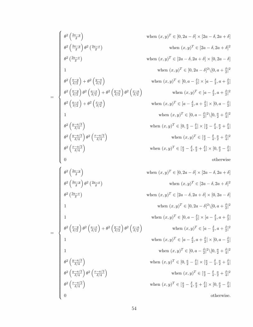
=
θ2(
2a−yδ
)when (x, y)T ∈ [0, 2a− δ]× [2a− δ, 2a+ δ]
θ2(
2a−yδ
)θ2(
2a−xδ
)when (x, y)T ∈ [2a− δ, 2a+ δ]2
θ2(
2a−xδ
)when (x, y)T ∈ [2a− δ, 2a+ δ]× [0, 2a− δ]
1 when (x, y)T ∈ [0, 2a− δ]2\[0, a+ δ2 ]2
θ2(a−yδ/2
)+ θ2
(y−aδ/2
)when (x, y)T ∈ [0, a− δ
2 ]× [a− δ2 , a+ δ
2 ]
θ2(a−yδ/2
)θ2(a−xδ/2
)+ θ2
(y−aδ/2
)θ2(x−aδ/2
)when (x, y)T ∈ [a− δ
2 , a+ δ2 ]2
θ2(a−xδ/2
)+ θ2
(x−aδ/2
)when (x, y)T ∈ [a− δ
2 , a+ δ2 ]× [0, a− δ
2 ]
1 when (x, y)T ∈ [0, a− δ2 ]2\[0, a2 + δ
4 ]2
θ2(y−a/2δ/4
)when (x, y)T ∈ [0, a2 −
δ4 ]× [a2 −
δ4 ,
a2 + δ
4 ]
θ2(y−a/2δ/4
)θ2(x−a/2δ/4
)when (x, y)T ∈ [a2 −
δ4 ,
a2 + δ
4 ]2
θ2(x−a/2δ/4
)when (x, y)T ∈ [a2 −
δ4 ,
a2 + δ
4 ]× [0, a2 −δ4 ]
0 otherwise
=
θ2(
2a−yδ
)when (x, y)T ∈ [0, 2a− δ]× [2a− δ, 2a+ δ]
θ2(
2a−yδ
)θ2(
2a−xδ
)when (x, y)T ∈ [2a− δ, 2a+ δ]2
θ2(
2a−xδ
)when (x, y)T ∈ [2a− δ, 2a+ δ]× [0, 2a− δ]
1 when (x, y)T ∈ [0, 2a− δ]2\[0, a+ δ2 ]2
1 when (x, y)T ∈ [0, a− δ2 ]× [a− δ
2 , a+ δ2 ]
θ2(a−yδ/2
)θ2(a−xδ/2
)+ θ2
(y−aδ/2
)θ2(x−aδ/2
)when (x, y)T ∈ [a− δ
2 , a+ δ2 ]2
1 when (x, y)T ∈ [a− δ2 , a+ δ
2 ]× [0, a− δ2 ]
1 when (x, y)T ∈ [0, a− δ2 ]2\[0, a2 + δ
4 ]2
θ2(y−a/2δ/4
)when (x, y)T ∈ [0, a2 −
δ4 ]× [a2 −
δ4 ,
a2 + δ
4 ]
θ2(y−a/2δ/4
)θ2(x−a/2δ/4
)when (x, y)T ∈ [a2 −
δ4 ,
a2 + δ
4 ]2
θ2(x−a/2δ/4
)when (x, y)T ∈ [a2 −
δ4 ,
a2 + δ
4 ]× [0, a2 −δ4 ]
0 otherwise.
54
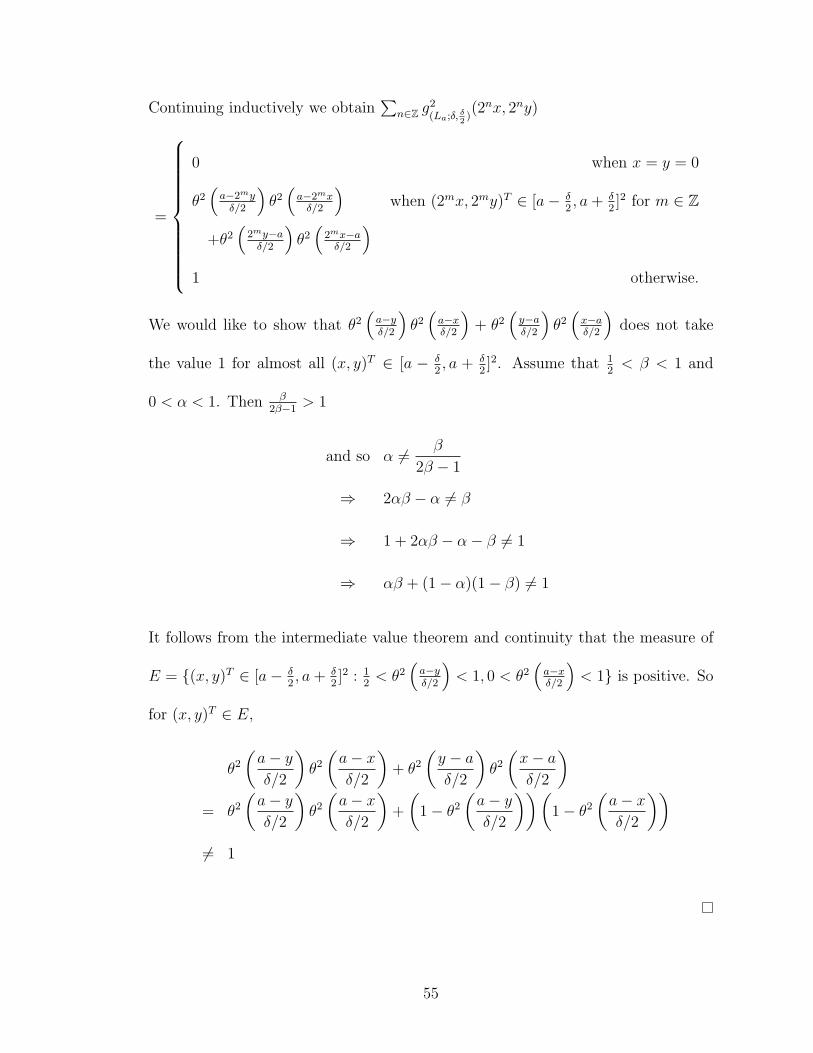
Continuing inductively we obtain∑
n∈Z g2(La;δ, δ
2)(2nx, 2ny)
=
0 when x = y = 0
θ2(a−2myδ/2
)θ2(a−2mxδ/2
)when (2mx, 2my)T ∈ [a− δ
2, a+ δ
2]2 for m ∈ Z
+θ2(
2my−aδ/2
)θ2(
2mx−aδ/2
)1 otherwise.
We would like to show that θ2(a−yδ/2
)θ2(a−xδ/2
)+ θ2
(y−aδ/2
)θ2(x−aδ/2
)does not take
the value 1 for almost all (x, y)T ∈ [a − δ2, a + δ
2]2. Assume that 1
2< β < 1 and
0 < α < 1. Then β2β−1
> 1
and so α 6= β
2β − 1
⇒ 2αβ − α 6= β
⇒ 1 + 2αβ − α− β 6= 1
⇒ αβ + (1− α)(1− β) 6= 1
It follows from the intermediate value theorem and continuity that the measure of
E = {(x, y)T ∈ [a− δ2, a+ δ
2]2 : 1
2< θ2
(a−yδ/2
)< 1, 0 < θ2
(a−xδ/2
)< 1} is positive. So
for (x, y)T ∈ E,
θ2
(a− yδ/2
)θ2
(a− xδ/2
)+ θ2
(y − aδ/2
)θ2
(x− aδ/2
)= θ2
(a− yδ/2
)θ2
(a− xδ/2
)+
(1− θ2
(a− yδ/2
))(1− θ2
(a− xδ/2
))6= 1
55
However, as the calculations above show,∑
n∈Z h2(La;δ, δ
2)(2mx, 2ny) = 1 for all
(|x|, |y|)T /∈ {0} ∪
(⋃m∈Z
2m[a− δ
2, a+
δ
2
]2).
So we adjust h(La;δ, δ2
)(x, y) on C = [a − δ2, a + δ
2]2 ∪ [2a − δ, 2a + δ]2 in hopes of
obtaining a Parseval frame. We do this by setting
f(La;δ, δ2
)(x, y) = h(La;δ, δ2
)(x, y) for (|x|, |y|)T /∈ C
and
f(La;δ, δ2
)(x, y) = f(La;δ, δ2
)(x, y),
for (|x|, |y|)T , (|x|, |y|)T ∈ C, |x|+|y| = |x|+|y|, and |x|+|y| small enough. Explicitly,
f(La;δ, δ2
)(x, y) =
θ(
2a−|y|δ
)when |x| ∈ [0, 2a− δ] and |y| ∈ [2a− δ, 2a+ δ]
θ(
4a−|x|−|y|−δδ
)when |x|, |y| ∈ [2a− δ, 2a+ δ], where 4a− 2δ ≤ |x|+ |y| ≤ 4a
θ(
2a−|x|δ
)when |y| ∈ [0, 2a− δ] and |x| ∈ [2a− δ, 2a+ δ]
1 when (|x|, |y|)T ∈ [0, 2a− δ]2\[0, a+ δ2]2
1 when |x|, |y| ∈ [a− δ2, a+ δ
2] where 2a ≤ |x|+ |y| ≤ 2a+ δ
θ(|y|−aδ/2
)when |x| ∈ [0, a− δ
2] and |y| ∈ [a− δ
2, a+ δ
2]
θ(|x|+|y|−2a+δ/2
δ/2
)when |x|, |y| ∈ [a− δ
2, a+ δ
2] where 2a− δ ≤ |x|+ |y| ≤ 2a
θ(|x|−aδ/2
)when |y| ∈ [0, a− δ
2] and |x| ∈ [a− δ
2, a+ δ
2]
0 otherwise.
Proposition 60. Let 0 < a < 14, set L = [−2a, 2a]2\[−a, a]2, and pick a 0 < δ <
12
min{1− 4a, a}. Let ψδ = f(La;δ, δ2
). For x, y > 0,
ψ2δ (~x) + ψ2
δ (2~x) = f 2([−2a,2a]2\[−a
2,a2
]2;δ, δ4
)(~x).
56

Proof.
ψ2δ (~x) + ψ2
δ (2~x)
=
θ2(
2a−yδ
)when (x, y)T ∈ [0, 2a− δ]× [2a− δ, 2a+ δ]
θ2(
4a−x−y−δδ
)when (x, y)T ∈ [2a− δ, 2a+ δ]2
θ2(
2a−xδ
)when (x, y)T ∈ [2a− δ, 2a+ δ]× [0, 2a− δ]
1 when (x, y)T ∈ [0, 2a− δ]2\[0, a+ δ2 ]2
1 when (x, y)T ∈ [a− δ2 , a+ δ
2 ]2 where 2a ≤ x+ y2a+ δ
θ2(a−yδ/2
)+ θ2
(y−aδ/2
)when (x, y)T ∈ [0, a− δ
2 ]× [a− δ2 , a+ δ
2 ]
θ2(x+y−2a+δ/2
δ/2
)+
θ2(
2a−x−y−δ/2δ/2
)when (x, y)T ∈ [a− δ
2 , a+ δ2 ]2 where 2a− δ ≤ x+ y ≤ 2a
θ2(a−xδ/2
)+ θ2
(x−aδ/2
)when (x, y)T ∈ [a− δ
2 , a+ δ2 ]× [0, a− δ
2 ]
1 when (x, y)T ∈ [0, a− δ2 ]2\[0, a2 + δ
4 ]2
1 when (x, y)T ∈ [a2 −δ4 ,
a2 + δ
4 ]2 where a ≤ x+ ya+ δ2
θ2(y−a/2δ/4
)when (x, y)T ∈ [0, a2 −
δ4 ]× [a2 −
δ4 ,
a2 + δ
4 ]
θ2(x+y−a+δ/4
δ/4
)when (x, y)T ∈ [a2 −
δ4 ,
a2 + δ
4 ]2 where a− δ2 ≤ x+ y ≤ a
θ2(x−a/2δ/4
)when (x, y)T ∈ [a2 −
δ4 ,
a2 + δ
4 ]× [0, a2 −δ4 ]
0 otherwise,
57

=
θ2(
2a−yδ
)when (x, y)T ∈ [0, 2a− δ]× [2a− δ, 2a+ δ]
θ2(
4a−x−y−δδ
)when (x, y)T ∈ [2a− δ, 2a+ δ]2
θ2(
2a−xδ
)when (x, y)T ∈ [2a− δ, 2a+ δ]× [0, 2a− δ]
1 when (x, y)T ∈ [0, 2a− δ]2\[0, a2 + δ4 ]2
1 when (x, y)T ∈ [a2 −δ4 ,
a2 + δ
4 ]2 when a ≤ x+ y ≤ a+ δ2
θ2(y−a/2δ/4
)when (x, y)T ∈ [0, a2 −
δ4 ]× [a2 −
δ4 ,
a2 + δ
4 ]
θ2(x+y−a+δ/4
δ/4
)when (x, y)T ∈ [a2 −
δ4 ,
a2 + δ
4 ]2 where a− δ2 ≤ x+ y ≤ a
θ2(x−a/2δ/4
)when (x, y)T ∈ [a2 −
δ4 ,
a2 + δ
4 ]× [0, a2 −δ4 ]
0 otherwise,
= f2([−2a,2a]2\[−a
2,a2
]2;δ, δ4
)(~x),
as desired.
Proposition 61. Let 0 < a < 14, set L = [−2a, 2a]2\[−a, a]2, and pick a 0 < δ <
12
min{1 − 4a, a}. Let ψδ = f(La;δ, δ2
). Then ψδ ∈ Cc(R2)\C1c (R2) and W(ψδ) is a
Parseval frame for L2(R2).
Proof. Since
supp ψδ ⊆ [−2a− δ, 2a+ δ]2 ⊆(−2a− 1
2(1− 4a), 2a+
1
2(1− 4a)
)2
=
(−1
2,1
2
)2
,
for all n ∈ N ∪ {0} and k ∈ Z2\{0},
ψδ (2n(~x+ k)) ψδ(2n~x) = 0 a.e.,
where ~x = (x, y). In order to utilize Theorem 51, we would like to show that
∑n∈Z
∣∣∣ψδ(2n~x)∣∣∣2 = 1 a.e.
58

We will accomplish this by showing that
ψ2δ (~x) + ψ2
δ (2~x) = f 2([−2a,2a]2\[−a
2,a2
]2;δ, δ4
)(~x).
Then it will follow from iteration that
N∑n=M
∣∣∣ψδ(2n~x)∣∣∣2 = f 2
([−21−Ma,21−Ma]2\[−2−Na,2−Na]2;2−M δ,2−1−N δ)(~x),
which is 1 on [21−Ma + 2−Mδ, 21−Ma − 2−Mδ]2\[2−Na + 2−1−Nδ, 2−Na − 2−1−Nδ]2,
where
21−Ma− 2−Mδ = 2−M(2a− δ)→∞ as M → −∞
and
2−Na− 2−1−Nδ = 2−N(a− δ
2)→ 0 as N →∞
So∑
n∈Z
∣∣∣ψδ(2n~x)∣∣∣2 = 1 a.e. By symmetry, it will suffice to show that
ψ2δ (~x) + ψ2
δ (2~x) = f 2([−2a,2a]2\[−a
2,a2
]2;δ, δ4
)(~x)
for positive x and y. The preceding proposition is a proof of this fact.
Thus,W(ψδ) is a Parseval frame, but ψδ has cusps along {(2a−δ+t, 2a−δ)T :
0 ≤ t ≤ 2δ}, as well as other edges. So ψδ /∈ C1c (R2).
Thus we have found a method to smooth the Parseval frame wavelets 1La for
0 < a < 14, which is analogous to Han’s method, but it does not yield Parseval
frame wavelets with good temporal decay like Schwartz functions. It seems that
this method should generalize to other Parseval frame wavelet sets in R2 which
have piecewise horizontal and vertical boundaries. However, there does not seem
to be an easy way to write an explicit formula that works in general. Furthermore,
59
only a relatively small number of Parseval frame wavelet sets have such a boundary.
Perhaps not all is lost. Instead of trying to smooth 1K for some Parseval frame
wavelet set K resulting from the neighborhood mapping construction, we now try
to build Schwartz class Parseval frames for L2(R2) directly from the C∞c bump
functions over R.
3.3 A construction in higher dimensions
In the preceding work, problems arose around the corners of the boundary
of La = [−2a, 2a]2\[−a, a]2 when we tried to smooth 1La . What if there were no
corners to deal with? For 0 < a < 14, we define
f([a,2a]×S1; δ2,δ)(x, y) = f([a,2a]; δ
2,δ)(√x2 + y2),
where yet again f([a,2a]; δ2,δ)(·) is as in Definition 53.
Proposition 62. Let 0 < a < 14. For any 0 < δ < 1
2min{1 − 4a, a}, define
ψδ : R2 → R by ψδ(x, y) = f([a,2a]; δ2,δ)(√x2 + y2). Then, ψ ∈ S (R2) and W(ψδ) is
a Parseval frame for L2(R2).
Proof. By construction, ψδ ∈ C∞c (R2) ⇒ ψδ ∈ S (R2). Since δ < 12(1 − 4a),
∆(supp ψδ) < 0. So for all n ∈ N ∪ {0} and k ∈ Z\{0},
ψδ(2n(~x+ k))ψ(2n~x) = 0 a.e.
where ~x = (x, y)T . Hence, in order to prove that W(ψδ) is a Parseval frame, it
60
suffices to show that∑
n∈Z
∣∣∣ψδ(2n~x)∣∣∣2 = 1 a.e. We compute
∑n∈Z
∣∣∣ψ(2n~x)∣∣∣2 =
∑n∈Z
∣∣∣f([a,2a]; δ2,δ)
(√(2nx)2 + (2ny)2
)∣∣∣2=
∑n∈Z
∣∣∣f([a,2a]; δ2,δ)(2
nz)∣∣∣2 for z =
√x2 + y2 (3.4)
We know that (3.4) = 1 for almost all non-negative z, specifically for z > 0. So∑n∈Z
∣∣∣ψδ(2nx)∣∣∣2 = 1 for R2 3 ~x 6= 0. ThusW(ψδ) is a Parseval frame for L2(R2).
This result and proof generalize to Rd, d > 2.
Corollary 63. Let 0 < a < 14. For any 0 < δ < 1
2min{1−4a, a}, define ψδ : Rd → R
by ψδ(x) = f([a,2a]; δ2,δ)(‖x‖). Then, ψ ∈ S (Rd) and W(ψδ) is a Parseval frame for
L2(Rd).
Proof. The proof is as above.
We now have Schwartz class Parseval frames for L2(Rd), d > 1 which are
elementary to describe.
3.4 Partitions of unity
C∞ partitions of unity are important tools in analysis and differential topology.
While the topic of C∞ partitions of unity is outside the scope of this thesis, we shall
utilize a class of functions which is commonly used in conjunction with that subject,
e.g.: [81].
Definition 64. Let f : R→ R be the function f(γ) = e−1γ1(0,∞). Also, let b,m > 0
61
be such that b− 1m> 0. Define ϕ ∈ C∞c (R) as
ϕb,m(γ) =f(b+ 1
m− |γ|)
f(b+ 1m− |γ|) + f(|γ| − b+ 1
m).
If a > 4m
is clear from the context, we shall write ϕm = ϕa4,m.
ϕb,m is a smooth function which takes the value 1 on the disk (−b+ 1m, b− 1
m)
and the value 0 outside the disk D(−b − 1m, b + 1
m). We shall now prove that the
function is actually monotonic over the positive reals.
Lemma 65. Fix b − 1m> 0. Then ϕb,m is increasing over (−∞, 0) and decreasing
over (0,∞).
Proof. Let γ > 0. We calculate ϕ′b,m(γ)
=
(f(b+ 1
m − γ) + f(γ − b+ 1m)) (−f ′(b+ 1
m − γ))− f(b+ 1
m − γ)(−f ′(b+ 1
m − γ) + f ′(γ − b+ 1m))(
f(b+ 1m − γ) + f(γ − b+ 1
m))2
=−(f(γ − b+ 1
m))f ′(b+ 1
m− γ) + f(b+ 1
m− γ)f ′(γ − b+ 1
m))(
f(b+ 1m− γ) + f(γ − b+ 1
m))2 .
For all γ ∈ R, f(γ) ≥ 0 and f ′(γ) = 1γ2 e− 1γ1(0,∞) ≥ 0. Hence for γ ≥ 0, ϕ′b,m(γ) ≤ 0.
Since ϕb,m is even, this implies that ϕ′b,m(γ) ≥ 0 for γ ≤ 0.
Theorem 66. Let 0 < α < 12
and m > max{ 6a, 2
1−2a}. Define
ψm = ϕm(γ +3a
4) + ϕm(γ − 3a
4) ∈ C∞c (R).
Then ψm ∈ S(R) and W(ψm) forms a frame with bounds Am and Bm. For all m,
Am ≤ 12, but as m→∞, Bm → 1.
Proof. As m > 4a, ϕm is well-defined, and it follows from the definition of ϕm that
supp ψm = [−a− 1
m,−a
2+
1
m] ∪ [
a
2− 1
m, a+
1
m].
62

Since m > 21−2a
, supp ψm ⊂ (−12, 1
2). By continuity, there exists ε > 0 such that
[−a,−a2) ∪ [a
2, a) ⊆ suppε ψm. Thus, it follows from Theorem 33 that W(ψm) forms
a frame with lower frame bound Am = Kψm and upper frame bound Bm = Kψm . As
ψm is even, it suffices to optimize κψm over any positive dyadic interval. We shall use
[a2
+ 12, a+ 1
m). Since m > 5
a, κψm(γ) = (ψm(γ))2 + (ψm(γ
2))2 for γ ∈ [a
2+ 1
2m, a+ 1
m).
Also m > 6a
implies that a− 2m> a
2+ 1
m. Hence, over [a
2+ 1
2m, a+ 1
m),
κψm = (ψm(γ))2 + (ψm(γ
2))2
=
(ψm(γ))2 + 0 for a2
+ 12m≤ γ < a
2+ 1
m
1 + 0 for a2
+ 1m≤ γ < a− 2
m
1 + (ψm(γ2))2 for a− 2
m≤ γ < a− 1
m
(ψm(γ))2 + (ψm(γ2))2 for a− 1
m≤ γ < a+ 1
m
=
(ϕm(γ − 3a4
))2 for a2
+ 12m≤ γ < a
2+ 1
m
1 for a2
+ 1m≤ γ < a− 2
m
1 + (ϕm(γ2− 3a
4))2 for a− 2
m≤ γ < a− 1
m
(ϕm(γ − 3a4
))2 + (ψ(γ2− 3a
4))2 for a− 1
m≤ γ < a+ 1
m
.
Note that
• γ − 3a4< 0 for a
2+ 1
2m≤ γ < a
2+ 1
msince m > 4
a,
• γ2− 3a
4< 0 for a− 2
m≤ γ < a− 1
m,
• γ − 3a4> 0 for a− 1
m≤ γ < a+ 1
msince m > 4
a, and
• γ2− 3a
4< 0 for a− 1
m≤ γ < a+ 1
msince m > 2
a.
63

Thus, κψm is increasing over a2
+ 12m≤ γ ≤ a − 1
m, but is not monotonic over
a− 1m< γ < a+ 1
m. Hence
mina2
+ 12≤γ≤a− 1
m
κψm(γ) = κψm(a
2+
1
2)
=
(ϕm((
a
2+
1
2m)− 3a
4)
)2
=
(ϕm(−a
4+
1
2m)
)2
=
(e−2m/3
e−2m/3 + e−2m
)2
=
(1
1 + e−4m/3
)2
,
and
maxa2
+ 12≤γ≤a− 1
m
κψm(γ) = κψm(a− 1
m)
= 1 +
(ϕm(
1
2(a− 1
m)− 3a
4)
)2
= 1 +
(e−2m
e−2m + e−2m/3
)2
= 1 +
(1
1 + e4m/3
)2
.
Note that as m→∞,
mina2
+ 12≤γ≤a− 1
m
κψm(γ) → 1
maxa2
+ 12≤γ≤a− 1
m
κψm(γ) → 1
We shall now consider κψm over (a− 1m, a+ 1
m). We start by substituting γ = a+ t
m,
64

t ∈ (−1, 1) and expanding κψm over these values:
κψm(a+t
m) =
(ϕm(a+
t
m− 3a
4)
)2
+
(ϕm(
a
2+
t
2m− 3a
4)
)2
=
(ϕm(
a
4+
t
m)
)2
+
(ϕm(−a
4+
t
2m)
)2
=
(e−m/(1−t)
e−m/(1−t) + e−m/(1+t)
)2
+
(e−2m/(2+t)
e−2m/(2+t) + e−2m/(2−t)
)2
=
(1
1 + e2mt/(1−t2)
)2
+
(1
1 + e−4mt/(4−t2)
)2
At t = 0, κψm takes the value(
12
)2+(
12
)2= 1
2. We claim that for any 0 < δ < 1
2,
κψm(a+ tm
) converges uniformly to 1 over [δ, 1− δ]. Choose an arbitrary 0 < ε < 2.
We claim that for any
m > max
(1− δ2) ln(√
2ε− 1)
δ,(δ2 − 4) ln(1−
√1− ε
2)
4δ
|κψm(a + t
m) − 1| < ε for all t ∈ [δ, 1 − δ]. A routine application of the triangle
inequality yields
|κψm(a+t
m)− 1| =
∣∣∣∣∣(
1
1 + e2mt/(1−t2)
)2
+
(1
1 + e−4mt/(4−t2)
)2
− 1
∣∣∣∣∣≤
∣∣∣∣∣(
1
1 + e2mt/(1−t2)
)2∣∣∣∣∣+
∣∣∣∣∣(
1
1 + e−4mt/(4−t2)
)2
− 1
∣∣∣∣∣ .Since m >
(1−δ2) ln(√
2ε−1)
δ, for all t ∈ [δ, 1− δ],√
2
ε− 1 < e2mδ/(1−δ2) ≤ e2mt/(1−t2)
⇒ 2
ε< (1 + e2mt/(1−t2))2
⇒
∣∣∣∣∣(
1
1 + e2mt/(1−t2)
)2∣∣∣∣∣ < ε
2.
65

Since m >(δ2−4) ln(1−
√1− ε
2)
4δ,
1−√
1− 2
ε> e−4mδ/(4−δ2) ≥ e−4mt/(4−t2)
⇒ (e−4mt/(4−t2))2 − 2(e−4mt/(4−t2)) +ε
2> 0
⇒ |(e−4mt/(4−t2))2 − 2(e−4mt/(4−t2))| < ε
2
⇒ |1− (1 + e−4mt/(4−t2))2| < ε
2
⇒
∣∣∣∣∣1− (1 + e−4mt/(4−t2))2
(1 + e−4mt/(4−t2))2
∣∣∣∣∣ < ε
2
⇒∣∣∣∣ 1
(1 + e−4mt/(4−t2))2− 1
∣∣∣∣ < ε
2.
Thus, |κψm(a+ tm
)−1| < ε for all t ∈ [δ, 1−δ]. It is also true that for any 0 < δ < 12,
κψm(a+ tm
) converges uniformly to 1 over [−1+ δ,−δ]. The proof works in the same
manner, except the triangle inequality is used in the following way
|κψm(a+t
m)− 1| =
∣∣∣∣∣(
1
1 + e2mt/(1−t2)
)2
+
(1
1 + e−4mt/(4−t2)
)2
− 1
∣∣∣∣∣≤
∣∣∣∣∣(
1
1 + e2mt/(1−t2)
)2
− 1
∣∣∣∣∣+
∣∣∣∣∣(
1
1 + e−4mt/(4−t2)
)2∣∣∣∣∣ .
Combining this convergence with our knowledge of the values κψm(0) = 12, κψm(a+
1m
) =(
11+e−4m/3
)2
, and κψm(a− 1m
) = 1 +(
11+e4m/3
)2
, we conclude that
limm→∞
Bm = limm→∞
Kψm = 1.
Since the t1−t2 exponent makes computer calculations nearly impossible, these
smooth frames are interesting, but not usable in applications. As there is no up-
per frame bound gap, it follows from Theorem 48 that these functions which are
commonly used in mathematics are not the result of convolutional smothing.
66
3.5 Other Methods
3.5.1 MSF smoothing
As mentioned above, E. Hernandez, X. Wang, and G. Weiss, [69], created the
theory of MSF wavelets. They characterize wavelets ψ for which ψ has support
in [−83α, 2 − 4
3α], for 0 < α ≤ 1
2, and prove that these are all associated with a
multiresolution analysis (MRA). The authors then smoothed these MSF wavelets
[70]. Their smoothing procedure was accomplished by deforming given low-pass
filters to obtain new filters. This process sometimes results in non-bandlimited
orthonormal wavelets.
This process will not work to improve the frame wavelet set wavelets which
were created in [14] because this process relies heavily on the associated MRA struc-
ture, which requires an orthonormal basis. Further, some of the sets generated in
the neighborhood mapping construction do not have support lying in [−83α, 2− 4
3α],
for some 0 < α ≤ 12. For example, K1\A1 in the construction of the 1-d Journe set
is [−94,−2)∪ [−1
2,− 9
32)∪ [ 9
32, 1
2)∪ [2, 9
4). The support of this set is spread due to the
fact that it is approximating a wavelet set which is not associated with an MRA.
3.5.2 Baggett, Jorgensen, Merrill, and Packer smoothing
A different smoothing idea is employed in [5]. The authors smooth the 1-d
Journe wavelet using a Generalized Multiresolution Analysis. Frame wavelets for
67

L2(R) are constructed which have the same dimension function,
∑k∈Z
∞∑n=1
|ψ (2n (x+ k)) |2,
as the Journe wavelet set but are arbitrarily differentiable and have C∞ Fourier
transforms. As in [70], they do not regularize the members of the frame directly
but rather define auxillary functions which build wavelets sharing certain traits with
the original wavelet. Since they construct Parseval frame wavelets, we know from
Theorem 48 that their functions cannot result from convolutional smoothing on the
frequency domain. They note that if ψ is a frame wavelet contructed using the
methods of [5], then {Tkψ : k ∈ Z} does not form a frame for span{Tkψ : k ∈ Z}.
They reference [13] in their comment. The following theorem from [13] may be used
to prove the same result for frames found using our methods.
Proposition 67. Let ψ ∈ L2(R) and let Ψ(γ) =∑
k∈Z |ψ(γ + k)|2 ∈ L∞(T). The
sequence {Tkψ : k ∈ Z} is a frame for span{Tkψ : k ∈ Z} if and only if there are
positive constants A and B such that
A ≤ Ψ(γ) ≤ B a.e. on T\N,
where N = {γ ∈ T : Ψ(γ) = 0}.
Proposition 68. Let ψ be as in Corollary 36. Then {Tkψ : k ∈ Zd} is not a frame
for spank∈ZdTkψ.
Proof. Since ψ is the result of a convolution, it is continuous. Let 12
denote the
vector in Rd for which every component is 12. Then Ψ(1
2) =
∑k∈Z |ψ(1
2+ k)|2 = 0
68
by the construction of ψ. Since ψ is continuous, for any ε > 0 which is sufficiently
small, there exists a γ ∈ Rd such that ε = Ψ(γ). The conclusion now follows from
Proposition 67.
3.5.3 Smoothing by time domain convolution
In [1], the authors make use of the following two results in order to smooth
the Haar wavelet by means of convolution on the time domain.
Proposition 69 ([50]). Let f be a bounded variation function with total variation
V (f). Assume that supp f ⊆ I, where I is an interval of length less than 1, and∫f(t)dt = 0. Then W(f) is a Bessel sequence, with bound
M = 11‖f‖∞ (V (f) + ‖f‖∞) |I|.
Theorem 70. If {en : n ∈ N} is an orthonormal basis for L2 (R) and {en − fn :
n ∈ N} is a Bessel sequence with bound M < 1, then {fn : n ∈ N} is a Riesz basis
with bounds A and B satisfying A ≥(
1−√M)2
and B ≤(
1 +√M)2
.
The main idea of [1] is to convolve the Haar function ψ = 1[0,1/2) − 1[1/2,1)
with a function φ ∈ W 1,j (R) = {φ ∈ L1 (R) : φ(j) ∈ L1 (R)}. This results in a
C(m) (R) function ψ ∗ φ. If φ has additional properties, then Proposition 69 can be
used to show thatW (ψ − ψ ∗ φ) is a Bessel sequence with bound M < 1. It follows
from Theorem 70 that ψ ∗ φ is a C(m) (R) function which generates a Riesz basis
with bounds(
1−√M)2
and(
1 +√M)2
. Thus, convolutional smoothing on the
temporal domain does not yield frame bound gaps, in contrast to smoothing on the
frequency domain.
69

3.5.4 Operator interpolation
Let K and L be (orthonormal) wavelet sets. By Proposition 12, K and L are
Zd-translation congruent and tile Rd by dyadic dilation. Dai and Larson use these
facts to construct a unitary operator U on L2(Rd) in [33]. If the group generated
by U commutes with the Fourier transformed dilation and translation operators
when applied to 1K , then the wavelet sets admit operator interpolation. This means
that polynomials in U , with coefficients satisfying certain conditions, applied to
1K yield the Fourier transform of a mother wavelet. If K and L satisfy futher
conditions, then this interpolated wavelet may also be continuous in the frequency
domain. In [64], this process is extended to Parseval (sub-) frame wavelet sets. The
“sub-” prefix means that the generated sequence of functions form a Parseval frame
for their span, rather than necessarily for all of L2(Rd). The loosened restrictions
allow for K and L to be Parseval sub-frame wavelet sets which are Zd-translation
congruent. While the sets Km\Am from the neighborhood mapping construction
are Parseval frame wavelets, operator interpolation does not seem to be a viable
method to obtain frame wavelets with good decay from these sets. Initially, if we
fix a neighborhood K0 and map S, then Km1\Am1 and Km2\Am2 will have different
measure if m1 6= m2. Hence, these sets can not be Zd-translation congruent. If
we look to sets created using different neighborhoods K0 and K0 and maps S and
S, we may obtain Parseval frame wavelet sets Km1\Am1 and Km2\Am2 which have
equal measure and thus may potentially be Zd-translation congruent. However,
calculations have not yet yielded any pairs of these equal measure sets which are
70

actually Zd-translation congruent. Hence, we are unable to interpolate between the
corresponding Parseval frame wavelets. Although operator interpoliation is a clever
application of von Neumann algebra theory to regularization of (sub-frame) wavelet
set wavelets, it is not helpful in our endeavor.
3.5.5 Stability results and an error in [46]
While attempting to modify the methods of [1] in order to use them, we
considered a number of various stability results. Stability results give conditions
under which perturbations of a frame or Riesz basis is again a frame or Riesz basis.
Theorem 70 is a very special case of the following stability proven by Chistensen
and Heil for Banach frames [25]. The result as it applies to Hilbert spaces has a
remarkably simple proof which uses the triangle inequality.
Theorem 71. Let {en} be a frame for a Hilbert space H with frame bounds A and
B. Let {fn} ⊆ H. If {en − fn} is a Bessel sequence for H with bound M < A, then
{fn} is a frame with frame bounds A and B satisfying A(
1−√M/A
)2
≤ A and
B ≤ B(
1 +√M/B
)2
.
While the hypothesis for this result is much weaker than many pre-existing
basis-type assumptions and, thus, is more applicable, the use of the triangle in-
equality in its proof means that, in general, the constants in Theorem 71 are not
optimal. In fact, convolving K0\A0 from the 2-d Journe construction with elements
of an approximate identity failed to yield bounds M < 1, meaning that Theorem 71
cannot be applied at all in this case. Fortunately, Corollary 19 provides frame bound
71

estimation that is simple to compute. There are other stability results in [46], but,
unfortunately, one of the major results of the paper is incorrect.
Definition 72. {DjTkφ} is semiorthogonal if for any j 6= m and any k, n ∈ Zd,
〈DjTkφ,DmTnφ〉 = 0.
They write in [46]
Theorem 10: Let Φ be a semiorthogonal sequence in L2(Rd),
and let ψ be any function in the closure of the linear span of
{Tkφ : k ∈ Zd}. If Φ is a wavelet frame (wavelet Riesz basis)
in L2(Rd) with bounds A and B and ‖ψ − φ‖ < A3/2B, then
Ψ = {φj,k = DjTkφ : j, k ∈ Zd} is a semiorthogonal wavelet
frame wavelet (wavelet Riesz basis) in L2(Rd) with bounds([1−
(B
A3/2
)]‖ψ − φ‖
)2A and
([1 +
(B1/2
A
)]‖ψ − φ‖
)2
B.
Obviously, they mean j ∈ Z. Also, there is a typo in the statement of the new
bounds. Since B ≥ A, the bounds as stated would always yield lower frame
bounds ≤ 0. Based on the results that they cited in the proof, they meant to
write(1−
(B
A3/2
)‖ψ − φ‖
)2A and
(1 +
(B1/2
A
)‖ψ − φ‖
)2
B.
Proof: The semiorthogonality is trivial. Let g = φ − ψ, and let
S be the frame operator, i.e.:
Sf =∑j∈Zd
∑k∈Zd〈f, φj,k〉φj,k.
Again the j should lie in Z.
The hypotheses imply that if j 6= 0, then 〈g, φj,k〉 = 0. Thus,
g =∑
m∈Zd amφ0,m(x), for am = 〈S−1g, φ0,m〉.
72

While it is true that g =∑
n
∑m〈S−1g, φn,m〉φn,m, there is no reason for 〈S−1g, φm,n〉 =
0 for all n 6= 0. If the rest of the proof were correct, then this problem would most
likely be fixed by writing g =∑
m∈Zd bmS−1φ0,m, for bm = 〈g, φ0,m〉.
Let {cn,k} be any finite sequence of scalars, then∥∥∥∥∥∑j
∑k
cj,kgj,k
∥∥∥∥∥2
=
∥∥∥∥∥∑j
∑k
∑m∈Zd
amcj,kφm,j+k
∥∥∥∥∥2
≤ B∑j
∑k
∑m
|amcj,k|2
= B∑m
|am|2∑j
∑k
|cj,k|2 .
Initially, there is an error in the indices,∥∥∥∑j
∑k
∑m∈Zd amcj,kφm,j+k
∥∥∥2
should be∥∥∥∑j
∑k
∑m∈Zd amcj,kφj,m+k
∥∥∥2
. More crucially, the authors miss the sub-
tle fact that m and k are taking values all over Zd, so m1+k1 = m2+k2 for numerous
values of mi, ki. Using the substitution n = m+ k, the correct inequality would be∥∥∥∥∥∑j
∑k
∑m∈Zd
amcj,kφj,m+k
∥∥∥∥∥2
=
∥∥∥∥∥∑j
∑n
∑m∈Zd
amcj,n−mφj,n
∥∥∥∥∥2
≤ B∑j
∑n
∣∣∣∣∣∑m
cj,n−mam
∣∣∣∣∣2
.
Since in general |∑
m xm|2 6≤
∑m |xm|
2, their desired result does not follow. Their
proof isn’t repairable, which of course doesn’t mean that the theorem is also incor-
rect; however, calculations using other methods indicate that a class of functions
which satisfy the hypotheses do not form frames. Let Φ =W(1[−1,−1/2)∪[1/2,1)). Φ is
an orthonormal basis and is thus trivially a semiorthogonal Riesz basis with frame
bound 1. Set
ψ = (1
2I − 1
2M2)1[−1,−1,2)∪[1/2,1),
73

then ψ ∈ span{Tk1[−1,−1,2)∪[1/2,1)}. Also,
‖ψ − 1∨[−1,−1/2)∪[1/2,1)‖2 = ‖ψ − 1[−1,−1/2)∪[1/2,1)‖2
=
∥∥∥∥((1
2− 1
2e4πix)− 1
)1[−1,−1/2)∪[1/2,1)(x)
∥∥∥∥2
=
∫ −1/2
−1
1
4(1 + 2 cos 4πix+ 1)dx+
∫ 1
1/2
1
4(1 + 2 cos 4πix+ 1)dx
=1
2(−1
2− (−1) + 1− 1
2)
=1
2
< 1.
Thus, the hypotheses of Theorem 10 in [46] are satisfied. However, ψ is a continuous
function which vanishes at every point γ = ± 12k
. Thus κψ is also a continuous
function which vanishes at every point γ = ± 12k
, and
infγ∈bRκψ(γ) = 0.
It now follows from Proposition 18 that W(ψ) is not a frame.
3.5.6 Conclusion
Theorem 44 in Chapter 2 showed that convolutional smoothing of Parseval
frame wavelet set wavelets on the frequency domain yields systems with upper frame
bounds which increase away from 1 as the dimension increases. This theme of
Chapter 2 and [11] is continued in this chapter. We see in Section 3.2.2 that natural
generalizations of Bin Han’s construction of smooth Parseval wavelets in L2(R) to R2
also fail. Thus, the question remains whether there exist continuous functions ψn for
which W(ψn) has frame bounds converging to 1 and for which ‖1[−a,a]2\[−a/2,a/2]2 −
74

ψn‖L2(bR2) converges to 0 as n→∞ for some a < 1/2. Furthermore, we also explicitly
construct smooth frame wavelets which have upper frame bounds converging to 1
in Section 3.3. This construction, combined with results from Chapter 2 shows
that basic functions used in differential topology are not the result of convolutional
smoothing.
75
Chapter 4
Shearlet Analogues for L2(Rd)
4.1 Introduction
4.1.1 Problem
Typically, multidimensional data has been analyzed using tensor products of
1-dimensional wavelets; however, these methods do not yield any information about
directional components or trends. For example, if one image was a rotation of
another image, we would like the coefficients of the wavelet representation to in-
dicate that. A number of new representations have sprung up in an attempt to
solve this problem. Contourlets ([42]), curvelets and ridgelets ([21]), bandlets ([89]),
wedgelets ([43]), and shearlets ([57] and [80]) are just a few examples. There is a
Fast Shearlet Transform, which makes the shearlets especially desirable. However,
these transforms are for 2-dimensional data sets. It is becoming more common for
higher dimensional data sets to appear, which need to be analyzed. Inspired by the
work of Cordero, DeMari, Nowak, and Tabacco ([28], [28], [39], and [40]), we would
like to exploit the representation theory of the extended metaplectic group in order
to construct analogs of the shearlet transform for L2(Rd), d > 2.
76

4.1.2 Shearlets
Shearlets were introduced by Labate, Guo, Kutyniok and Weiss in [57] and
[80] and are a specific type of composite dilation wavelet ([58]).
Definition 73. Given ψ ∈ L2(R2), the continuous shearlet system is
{TyD(S`Aa)−1ψ = a−3/4ψ(A−1a S−1
` (· − y)) : a > 0, ` ∈ R, y ∈ R2},
where Aa is the parabolic scaling matrix
a 0
0√a
and S` is the shearing matrix
1 `
0 1
.
Shearlet bases and frames are formed by selecting a discrete subcollection of
a continuous shearlet system. The most common subcollection is generated by the
indices
{(a, `, y) = (4j, k2j, Sk2jA4jm) : j, k ∈ Z,m ∈ Z2}.
By the commutation properties of the dilation and translation operators and shear-
ing and parabolic scaling matrices,
TSk2j
A4jmD(S
k2jA
4j)−1 = D(S
k2jA
4j)−1Tm
= D(A4jSk)−1Tm,
which looks exactly like the operators used to generate wavelets in Sections 2 and 3,
with dilation by powers of 2 replaced with dilation by the products of matrix powers
A4jSk.
77
Definition 74. Let B = {Bj}j∈J and C = {Ck}k∈K be subsets of GL(d,R). Let
ψ ∈ L2(Rd). The composite dilation wavelet system corresponding to B and C is
{D(BjCk)−1Tmψ : j ∈ J , k ∈ K,m ∈ Zd}.
A shearlet system is a composite dilation wavelet system with Bj = A4j and
Ck = Sk. Typically, more restraints are put on the sets B and C. For example,
it is common for B to be a collection of invertible matrices with integer entries
and eigenvalues with moduli greater than 1 and for C to be a group of matrices,
each with determinant 1. However, these constraints are not always necessary, see
[58]. Many authors have published results about shearlets and composite dilation
wavelets, which in some sense emulate wavelet theory and applications. To name a
few examples, there is a shearlet multiresolution analysis theory and decomposition
algorithm ([78]), there is an FFT-based method to compute the Continuous Shearlet
Transform ([79]), and there are composite dilation wavelet sets ([16]). Many of these
results should hopefully extend to the higher dimensional shearlets.
4.1.3 Outline and Results
Our goal is to integrate shearlet theory into the theory created by Cordero,
DeMari, Nowak and Tabacco. To this end we also present some of the main results
of Cordero et al. concerning reproducing subgroups of the metaplectic group and
their connection to known function transforms in Section 4.2. In Section 4.3, we
generalize the Translation-Dilation-Shearing group to L2(Rd) for arbitrarily large
d. The Translation-Dilation-Shearing group maps under a certain representation to
78

a group of operators that are related to the operators used in the shearlet trans-
form. We also fit the actual group of shearlet operators into the framework set up
by Cordero et al. in Section 4.4. We conclude with Section 4.5, which contains
references to other generalizations of shearlets and future directions of research.
4.2 Reproducing subgroups
4.2.1 Preliminaries
In a general sense, a reproducing formula is simply an integral representation
of the identity on some function space. Reproducing formulas are used throughout
mathematics and the sciences. The Cauchy integral formula of complex analysis
([51]), reconstruction in computed axial tomography ([87]), and resolutions of the
identity are all examples of such formulas. We shall be particularly interested in the
following types of reproducing formulas, which hold for all f ∈ L2(Rd),
f =
∫H
〈f, µe(h)φ〉µe(h)φdh, (4.1)
where H is a Lie subgroup of a particular Lie group, µe is a particular representation
of that group, φ is a suitable window in L2(Rd), and the integral is interpreted
weakly. Equations which have the form of (4.1) arise in such areas as time-frequency
analysis, wavelet theory, and quantum mechanics ([53], [47]). If such a φ exists, we
shall call H a reproducing subgroup and any function φ which satisfies Eqn (4.1) a
reproducing function for H. We begin by introducing the Heisenberg group(s) and
Schrodinger representation.
79

Definition 75. For d ≥ 1, the Heisenberg (Lie) group Hd is a central extension of
R2d by R, endowed with the manifold structure of R× R2d and the product
(λ, x, ξ) · (λ, x, ξ) = (λ+ λ+1
2(〈x, ξ〉 − 〈x, ξ〉), x+ x, ξ + ξ).
The Schrodinger representation ρ is a unitary representation of the Heisenberg
group. That is, ρ is a strongly continuous group homomorphism from Hd to the
unitary operators on L2(Rd) defined by ρ(λ, x, ξ) = e2πiλeπi〈x,ξ〉TxMξ.
We are now able to be more precise in our description of equation (4.1). We
would like to first clarify of which Lie group H is a subgroup. In order to do this,
we must define the symplectic group.
Definition 76. For d ≥ 1, let J =
0 Id
−Id 0
. The symplectic group Sp(d,R)
is the subgroup of 2d× 2d matrices g ∈ M(2d,R) which satisfy tgJ g = J , where tg
denotes the transpose of g.
We shall make a few quick comments concerning the pertinent representation
theory. A detailed exposition may be found in [53]. Each symplectic matrix in-
duces a unitary representation of the Heisenberg group which, by the Stone-von
Neumann Theorem is equivalent to the Schrodinger representation. By considering
the relationship between each symplectic matrix and the corresponding intertwining
operators, one obtains a projective unitary representation of Sp(d,R). By passing
to the double cover of the Sp(d,R), the metaplectic group Mp(d,R), one obtains
an actual unitary representation µ, the metaplectic representation. Matrix mul-
tiplication defines an action of Sp(d,R) in R2d which in turn induces an action of
80

Mp(d,R) on Hd. The metaplectic representation extends to the extended metaplectic
representation µe on Hd o Mp(d,R). We shall define µe to be
µe(x, ξ, A) = ρ(λ, x, ξ)µ(A), (λ, x, ξ, A) ∈ Hd o Mp(d,R). (4.2)
We use the standard model of the metaplectic representation which is given by the
following formulas:
µ
A 0
0 tA−1
f(x) = DA−1f(x), A ∈ GL(d,R), (4.3)
µ
I 0
C I
f(x) = eiπ〈Cx,x〉f(x), C ∈ M(d,R), C = tC (4.4)
µ(J ) = (−i)d/2F .
Sp(d,R) is generated by finite products of A 0
0 tA−1
: A ∈ GL(d,R)
,
I 0
C I
: C ∈ M(d,R), C = tC
, and J
(see, [47]). It follows from Schur’s Lemma that this definition of µ on generators of
Sp(d,R) is ambiguous up to sign; however, for the H we shall consider, (4.3) and
(4.4) explicitly define a representation.
The H in (4.1) shall be Lie subgroups of Sp(d,R) and µe defined as in (4.2). In
Theorems 89 and 107, we shall prove which φ ∈ L2(Rd) satisfy Eqn (4.1) for given
Lie subgroups H. The H that we shall use are related to the shearlet transform.
81

4.2.2 Lie subgroups of R2 o Sp(1,R)
DeMari and Nowak classified all connected Lie subgroups, up to inner conju-
gation, of HoSp(1,R) and R2oSp(1,R) in [40]. They then analyzed those groups in
[39] and determined which ones were reproducing. It turns out that the reproducing
subgroups correspond to the known transforms of L2(R), namely, the Gabor-Weyl-
Heisenberg, wavelet and chirp transforms. One may hope that by characterizing
the reproducing subgroups of R2d o Sp(d,R), new transforms for L2(Rd) may be
discovered. However, the structure of R2d o Sp(2d,R) is incredibly complicated for
d > 1. For example, the affine (or ax + b) group embeds into R2d o Sp(d,R). The
representation of the affine group over R as the product of translation and dilation
operators splits into only two irreducible representations. However, the analogous
representation for the affine group over Rd, d > 1, is highly reducible ([53]). Also,
in order to characterize the Lie subgroups of R2 o Sp(1,R), DeMari and Nowak
used a characterization of the subgroups of Sp(1,R) that does not exist over higher
dimensions. Thus, it may not be possible to characterize all of the reproducing
subgroups of R2d o Sp(d,R) for d > 1. However, the theory may still be used in
order to find new transformations. In [29] and [30], the authors prove that 2 differ-
ent subgroups of R4 o Sp(2,R) are indeed reproducing. We will generalize one of
those, the Translation-Dilation-Shearing group, to higher dimensions in the follow-
ing section. There are some known dimension bounds for reproducing subgroups in
R2doSp(d,R) for arbitrary d ([28]). The bounds are sharp, but it is still not known
whether reproducing subgroups exist of the intermediate dimensions between the
82
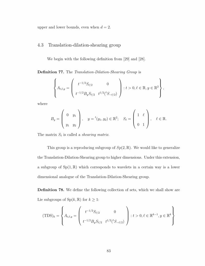
upper and lower bounds, even when d = 2.
4.3 Translation-dilation-shearing group
We begin with the following definition from [29] and [28].
Definition 77. The Translation-Dilation-Shearing Group isAt,`,y =
t−1/2S`/2 0
t−1/2ByS`/2 t1/2(tS−`/2)
: t > 0, ` ∈ R, y ∈ R2
,
where
By =
0 y1
y1 y2
, y = t(y1, y2) ∈ R2; S` =
1 `
0 1
, ` ∈ R.
The matrix S` is called a shearing matrix.
This group is a reproducing subgroup of Sp(2,R). We would like to generalize
the Translation-Dilation-Shearing group to higher dimensions. Under this extension,
a subgroup of Sp(1,R) which corresponds to wavelets in a certain way is a lower
dimensional analogue of the Translation-Dilation-Shearing group.
Definition 78. We define the following collection of sets, which we shall show are
Lie subgroups of Sp(k,R) for k ≥ 1:
(TDS)k =
At,`,y =
t−1/2S`/2 0
t−1/2ByS`/2 t1/2(tS−`/2)
: t > 0, ` ∈ Rk−1, y ∈ Rk
83

where
By =
yk ; i = j = k
yj ; i = k, j < k
yi ; i < k, j = k
0 ; else
i,j
=
0 0 . . . y1
0 0 . . . y2
......
. . ....
y1 y2 . . . yk
, y = t(y1, y2, · · · , yk) ∈ Rk.
For k ≥ 2 and ` = t(`1, `2, . . . `k−1) ∈ Rk−1, S` is the shearing matrix
S` =
1 ; i = j
`j ; 1 ≤ i ≤ k − 1, j = k
0 ; else
i,j
=
1 0 . . . 0 `1
0 1 . . . 0 `2
......
. . ....
0 0 . . . 1 `k−1
0 0 . . . 0 1
For k = 1, we formally define S` for ` ∈ R0 to be simply 1.
Note that when k = 1,
(TDS)1 =
At,y =
t−1/2 0
t−1/2By t1/2
: t > 0, y ∈ R
.
We will use both At,y and the formally defined At,`,y as notation in the case k = 1
while hopefully keeping the exposition clear. Furthermore, when k > 1, as a geo-
metric operator, S` fixes the kth dimension and stretches the first k− 1 coordinates
parallel to the kth coordinate. Mundane computations show that for `, ˜ ∈ Rk−1,
S`S˜ = S`+˜ and for y, y ∈ Rk, By +By = By+y.
Proposition 79. For any k ≥ 1, (TDS)k is a Lie subgroup of Sp(k,R) of dimension
2k.
84
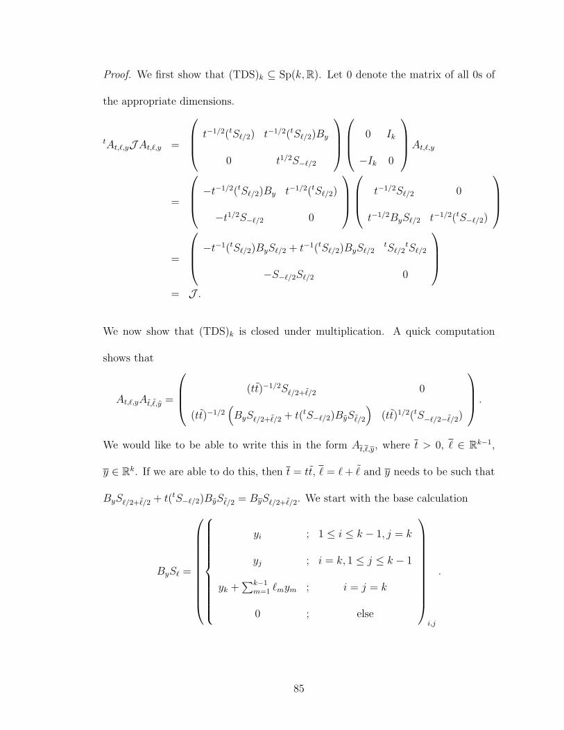
Proof. We first show that (TDS)k ⊆ Sp(k,R). Let 0 denote the matrix of all 0s of
the appropriate dimensions.
tAt,`,yJAt,`,y =
t−1/2(tS`/2) t−1/2(tS`/2)By
0 t1/2S−`/2
0 Ik
−Ik 0
At,`,y
=
−t−1/2(tS`/2)By t−1/2(tS`/2)
−t1/2S−`/2 0
t−1/2S`/2 0
t−1/2ByS`/2 t−1/2(tS−`/2)
=
−t−1(tS`/2)ByS`/2 + t−1(tS`/2)ByS`/2tS`/2
tS`/2
−S−`/2S`/2 0
= J .
We now show that (TDS)k is closed under multiplication. A quick computation
shows that
At,`,yAt,˜,y =
(tt)−1/2S`/2+˜/2 0
(tt)−1/2(ByS`/2+˜/2 + t(tS−`/2)ByS˜/2
)(tt)1/2(tS−`/2−˜/2)
.
We would like to be able to write this in the form At,`,y, where t > 0, ` ∈ Rk−1,
y ∈ Rk. If we are able to do this, then t = tt, ` = `+ ˜ and y needs to be such that
ByS`/2+˜/2 + t(tS−`/2)ByS˜/2 = ByS`/2+˜/2. We start with the base calculation
ByS` =
yi ; 1 ≤ i ≤ k − 1, j = k
yj ; i = k, 1 ≤ j ≤ k − 1
yk +∑k−1
m=1 `mym ; i = j = k
0 ; else
i,j
.
85
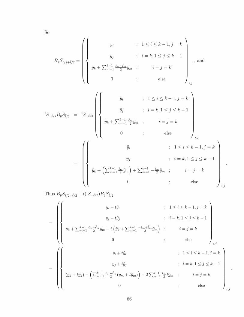
So
ByS`/2+˜/2 =
yi ; 1 ≤ i ≤ k − 1, j = k
yj ; i = k, 1 ≤ j ≤ k − 1
yk +∑k−1
m=1`m+˜
m
2ym ; i = j = k
0 ; else
i,j
, and
tS−`/2ByS˜/2 = tS−`/2
yi ; 1 ≤ i ≤ k − 1, j = k
yj ; i = k, 1 ≤ j ≤ k − 1
yk +∑k−1
m=1
˜m
2ym ; i = j = k
0 ; else
i,j
=
yi ; 1 ≤ i ≤ k − 1, j = k
yj ; i = k, 1 ≤ j ≤ k − 1
yk +(∑k−1
m=1
˜m
2ym
)+∑k−1
m=1−`m2ym ; i = j = k
0 ; else
i,j
.
Thus ByS`/2+˜/2 + t(tS−`/2)ByS˜/2
=
yi + tyi ; 1 ≤ i ≤ k − 1, j = k
yj + tyj ; i = k, 1 ≤ j ≤ k − 1
yk +∑k−1
m=1`m+˜
m2 ym + t
(yk +
∑k−1m=1
−`m+˜m
2 ym
); i = j = k
0 ; else
i,j
=
yi + tyi ; 1 ≤ i ≤ k − 1, j = k
yj + tyj ; i = k, 1 ≤ j ≤ k − 1
(yk + tyk) +(∑k−1
m=1`m+˜
m2 (ym + tym)
)− 2
∑k−1m=1
`m2 tym ; i = j = k
0 ; else
i,j
.
86

If ByS`/2+˜/2 + t(tS−`/2)ByS˜/2 = ByS`/2+˜/2, then
yi = yi + tyi, for 1 ≤ i ≤ k − 1 and
yk +k−1∑m=1
`m + ˜m
2ym = (yk + tyk) +
(k−1∑m=1
`m + ˜m
2(ym + tym)
)− 2
k−1∑m=1
`m2tym
⇒ yk = yk + tym −k−1∑m=1
`mtym.
So each (TDS)k corresponds to a subgroup of Sp(k,R) with a group operation
parameterized by
(t, `, y)(t, ˜, y) = (tt, `+ ˜, t(y1 + ty1, . . . , yk−1 + tyk−1, yk + tyk −k−1∑m=1
`mtym)),
when k > 1 and
(t, y)(t, y) = (tt, y + ty),
when k = 1, with identity the identity matrix corresponding to (1, 0, 0) for any
k ≥ 1. Hence for each k ≥ 1, (TDS)k is a matrix group. In particular, each (TDS)k
is a Lie subgroup of Sp(k,R). Finally, (TDS)k is of dimension 1+(k−1)+k = 2k.
We now define the first of three unitary representations of (TDS)k, the wavelet
representation. This representation is called the wavelet representation because each
element of the Lie group is mapped to a product of a translation and a dilation
operator.
Proposition 80. The mapping ν defined on each (TDS)k by
ν(At,`,y) = TyDt−1(tS`)
is a unitary representation.
87

Proof. Let y, y ∈ Rk, t, t > 0, `, ˜∈ Rk−1. We shall compute (TyDt−1(tS`))(TyDt−1(tS˜)).
For f ∈ L2(Rk),
(TyDt−1(tS`))(TyDt−1(tS˜))f(x) = t−k/2TyDt−1(tS`)f(t−1(tS˜(x− y))
= (tt)−k/2f((tt)−1(tS`+˜(x− (y + ttS−`y))).
We compute
tS−`y =
y1
y2
...
yk −∑k−1
m=1 `mym
y + ttS−`y =
y1 + ty1
y2 + ty2
...
yk + tyk −∑k−1
m=1 `mtym
Hence
(TyDt−1(tS`))(TyDt−1(tS˜)) = TyD(tt)−1(tS`+˜)
,
where yi = yi + tyi for 1 ≤ i ≤ k − 1 and yk = yk + yk −∑k−1
m=1 `mtym. Thus
ν(At,`,y)ν(At,˜,y) = ν(At,`,yAt,˜,y). Strong continuity of the representation follows
from the strong continuity of the translation and dilation operators. It follows that
each ν is a unitary representation.
Thus, the (TDS)k groups generate composite dilation wavelets. The second
representation is derived from the first.
88

Definition 81. Conjugate ν with F to obtain the π representation of each (TDS)k
π(At,y)f(u) = F ◦ ν(At,y) ◦ F−1f(u) = e−2πiyuDtf(u), k = 1
π(At,`,y)f(u) = F ◦ ν(At,`,y) ◦ F−1f(u) = e−2πi〈y,u〉DtS−`f(u), k > 1
The final representation that we consider in this section is the metaplectic
representation. We make use of the factorization
At,`,y = Dt,`Lt,y,` =
t−1/2S`/2 0
0 t1/2(tS−`/2)
I 0
t−1(tS`/2)ByS`/2 I
.
Then for f ∈ L2(Rk) by Eqns (4.3) and (4.4),
µ(At,`,y)f(x) = [µ(Dt,`)µ(Lt,y,`)f ] (x)
= tk/4 [µ(Lt,y,`)f ] (t1/2S−`/2x)
= tk/4e−iπ〈tS`/2Byx,S−`/2x〉f(t1/2S−`/2x)
= tk/4e−iπ〈Byx,x〉f(t1/2S−`/2x).
We record the Haar measures of the (TDS)k for future use.
Proposition 82. The left Haar measures, up to normalization, of the (TDS)k are
dτ = dtt2dy for k = 1 and dτ = dt
tk+1dyd` for k > 1, where dt, dy and d` are the
Lebesgue measures over R+, Rk and Rk−1, respectively.
Proof. Assume that k > 1. Let f be integrable with respect to dτ . We shall use the
89
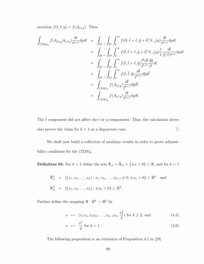
notation f(t, `, y) = f(At,`,y). Then
∫(TDS)k
f(At,˜,yAt,`,y)dt
tk+1dyd` =
∫Rk−1
∫Rk
∫ ∞0
f(tt, ˜+ `, y + t(tS−˜)y)dt
tk+1dyd`
=
∫Rk−1
∫Rk
∫ ∞0
f(t, ˜+ `, y + t(tS−˜)y)1
t
dt
(t/t)k+1dyd`
=
∫Rk−1
∫Rk
∫ ∞0
f(t, ˜+ `, y)tkdt
tk+1
dy
tkd`
=
∫Rk−1
∫Rk
∫ ∞0
f(t, `, y)dt
tk+1
dyd`
=
∫(TDS)k
f(At,`,y)dt
tk+1
dyd`
=
∫(TDS)k
f(At,`,y)dt
tk+1dyd`.
The ` component did not affect the t or y components. Thus, the calculation above
also proves the claim for k = 1 as a degenerate case.
We shall now build a collection of auxiliary results in order to prove admissi-
bility conditions for the (TDS)k.
Definition 83. For k = 1 define the sets R± = R± = {±x > 0} ⊂ R, and for k > 1
Rk± = {(x1, x2, . . . , xk) : x1, x2, . . . , xk−1 6= 0,±xk > 0} ⊂ Rk and
Rk± = {(x1, x2, . . . , xk) : ±xk > 0} ⊂ Rk.
Further define the mapping Ψ : Rk → Rk by
x 7→ (x1xk, x2xk, . . . , xk−1xk,x2k
2) for k ≥ 2, and (4.5)
x 7→ x2
2for k = 1. (4.6)
The following proposition is an extension of Proposition 4.1 in [29].
90

Proposition 84. The mappings defined on lines (4.5) and (4.6) restrict to diffeo-
morphisms Ψ : Rk± → Rk
+ and is such that Ψ(−x) = Ψ(x). Further, they satisfy
a. The Jacobian of Ψ at x = (x1, x2, . . . , xk) ∈ Rk± is JΨ(x) = xkk;
b. The Jacobian of Ψ−1 : Rk+ → Rk
+ at u = (u1, u2, . . . , uk) = Ψ(x1, x2, . . . , xk) is
JΨ−1(u) = (2uk)−k/2 = x−kk ;
c. Ψ−1(t2S2`u) = tS`Ψ−1(u) for every u ∈ Rk
±; and
d. 〈Byx, x〉 = 〈2y,Ψ(x)〉 for every x ∈ Rk± and every y ∈ Rk.
Proof. Clearly, Ψ(−x) = Ψ(x). We calculate the matrices of the partials.
∂Ψ(x)i∂xj
=
xk ; i = j
xi ; j = k
0 ; else
and
∂Ψ−1(u)i∂uj
=
(2uk)
−1/2 ; i = j
−ui(2uk)−3/2 ; j = k, i < k
0 ; else
Hence the Jacobian of Ψ at x is det(∂Ψ(x)i∂xj
)i,j
= xkk, and the Jacobian of Ψ−1 at
u = Ψ(x) is det(∂Ψ−1(u)i
∂uj
)i,j
= (2uk)−k/2 = x−kk . We now prove parts (c) and (d).
Ψ−1(t2S2`u) = Ψ−1(t2(t(u1 + 2`1uk, . . . , uk−1 + 2`k−1uk, uk))
= t(t2(u1 + 2`1uk/√
2t2uk), . . . , t2(uk−1 + 2`k−1uk/
√2t2uk),
√t2uk)
= tt(u1√2uk
+ `1
√2uk, . . . ,
uk−1√2uk
+ `k−1
√2uk,√uk)
= tS`Ψ−1(u).
91

When k = 1, the preceding computation simply consists of the kth coordinate. Also,
〈Byx, x〉 = t(y1xk, . . . , yk−1xk,
k∑i=1
yixi)
=k−1∑i=1
yixixk +k∑i=1
yixixk
= 2
[(k−1∑i=1
yixixk) + yk(1
2x2k)
]= 〈2y,Ψ(x)〉.
Since Ψ and Ψ−1 are smooth, bijective self maps of Rk+ with non-vanishing Jacobians,
they are diffeomorphisms. By considering −Ψ−1, we can see that Ψ : Rk− → Rk
+ is
also a diffeomorphism.
The following function class will be useful in a number of proofs.
Definition 85. Define L2(Rk) to be the collection
{f ∈ L2(Rk) : supp f ⊆ {‖u1, . . . , uk−1‖ < C} × {c < ‖uk‖ < C}, 0 < c < C <∞}.
Lemma 86. Let 1+ = 1Rk+. If h ∈ L2(Rk), then
1+(u)
(2uk)k/2(h(Ψ−1(u)) + h(−Ψ−1(u)) ∈ L1 ∩ L2(Rk).
Proof. We first show that h(Ψ−1(·)) ∈ L2(Rk+):
∫Rk+|h(Ψ−1(u))|2du =
∫Rk+|h(x)|2xkkdx
≤ ‖h‖2L2(Rk) esssupx∈supph |xk|k
< ∞.
92

We examine the support of h(±Ψ−1(·)). For almost all u with uk 6= 0:
h(±Ψ−1(u)) 6= 0 ⇒ ‖ u1√2uk
, . . . ,uk−1√
2uk‖ < C and c <
√2uk < C
⇔
√∑k−1i=1 u
2i
2uk< C and
c2
2< uk <
C2
2
⇔
√√√√k−1∑i=1
u2i < C2 and
c2
2< uk <
C2
2.
Hence, f(u) = 1+(u)[h(Ψ−1(u))+h(−Ψ−1(u))] ∈ L2(Rk) has support in the compact
set
{t(u1, . . . , uk−1) : ‖u1, . . . , uk−1‖ < C2} × {uk :c2
2< ‖uk‖ <
C2
2}.
Thus, if we show that f(u)
(2uk)k/2∈ L2(Rk), we will have proven the claim. We compute∫
Rk
|f(u)|2
(2uk)kdu <
2k
c2k‖f‖L2(Rk) <∞.
The following lemma is a generalization of Lemma 4.4 in [29], which is about
functions in L2(R2). The preceding lemma is neither stated nor proven in [29],
but it is necessary to justify the proof of Lemma 4.4. Also, the hypotheses of the
following lemma in the case that k = 2 are slightly different that than the hypotheses
on Lemma 4.4 in [29]. The hypotheses in [29] allow for possible divergence of the
integrals and make certain lines in the proof purely formal calculations. Other than
those points, the proof of the following lemma closely mimics the proof of Lemma
4.4 in [29].
Lemma 87. Let 1+ = 1Rk+. Let h ∈ L2(Rk). Then∫
Rk
∣∣∣∣∫Rkh(x)e2πi〈y,Ψ(x)〉dx
∣∣∣∣2 dy =
∫Rk+|h(x) + h(−x)|2dx
xkk.
93

Proof. By the properties of Ψ listed in Proposition 84,
∫Rkh(x)e2πi〈y,Ψ(x)〉dx =
(∫Rk+
+
∫Rk−
)h(x)e2πi〈y,Ψ(x)〉dx
=
∫Rk+h(x)e2πi〈y,Ψ(x)〉dx+
∫Rk+h(−x)e2πi〈y,Ψ(−x)〉dx
=
∫Rk+
[h(x) + h(−x)]e2πi〈y,Ψ(x)〉dx
=
∫Rk+
[h(Ψ−1(u)) + h(−Ψ−1(u))]e2πi〈y,u〉 du
(2uk)k/2
=
∫Rk
1+(u)
(2uk)k/2[h(Ψ−1(u)) + h(−Ψ−1(u))]e2πi〈y,u〉du.(4.7)
Since 1+(u)
(2uk)k/2[h(Ψ−1(u))+h(−Ψ−1(u))]e2πi〈y,u〉 ∈ L1∩L2(Rk) by Lemma 86, it follows
from Parseval’s equality that
‖(Eqn 4.7)‖2L2(Rk) =
∫Rk
∣∣∣∣∫Rk
1+(u)
(2uk)k/2[h(Ψ−1(u)) + h(−Ψ−1(u))]e2πi〈y,u〉du
∣∣∣∣2 dy=
∫Rk
∣∣∣∣ 1+(u)
(2uk)k/2[h(Ψ−1(u)) + h(−Ψ−1(u))]
∣∣∣∣2 du=
∫Rk
∣∣h(Ψ−1(u)) + h(−Ψ−1(u))∣∣2 du
(2uk)k/2
=
∫Rk|h(x) + h(−x)|2 x
kkdx
x2kk
=
∫Rk|h(x) + h(−x)|2 dx
xkk.
Proposition 84 can be used to prove the equivalence the wavelet and meta-
plectic representations of the (TDS)k groups.
Theorem 88. Let u ∈ Rk+ and extend the map Qf(u) = |2uk|−k/4f(Ψ−1(u)) as an
even function to Rk\{x1x2 . . . xk = 0}. This is a unitary map of L2even(Rk) onto
itself that intertwines the representations π and µ.
94
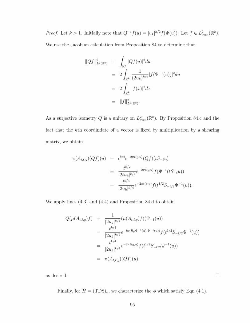
Proof. Let k > 1. Initially note that Q−1f(u) = |uk|k/2f(Ψ(u)). Let f ∈ L2even(Rk).
We use the Jacobian calculation from Proposition 84 to determine that
‖Qf‖2L2(Rk) =
∫Rk|Qf(u)|2du
= 2
∫Rk+
1
(2uk)k/2|f(Ψ−1(u))|2du
= 2
∫Rk+|f(x)|2dx
= ‖f‖2L2(Rk).
As a surjective isometry Q is a unitary on L2even(Rk). By Proposition 84.c and the
fact that the kth coordindate of a vector is fixed by multiplication by a shearing
matrix, we obtain
π(At,`,y)(Qf)(u) = tk/2e−2πi〈y,u〉(Qf)(tS−`u)
=tk/2
|2tuk|k/4e−2πi〈y,u〉f(Ψ−1(tS−`u))
=tk/4
|2uk|k/4e−2πi〈y,u〉f(t1/2S−`/2Ψ−1(u)).
We apply lines (4.3) and (4.4) and Proposition 84.d to obtain
Q(µ(At,`,y)f) =1
|2uk|k/4(µ(At,`,y)f)(Ψ−1(u))
=tk/4
|2uk|k/4e−iπ〈ByΨ−1(u),Ψ−1(u)〉f(t1/2S−`/2Ψ−1(u))
=tk/4
|2uk|k/4e−2πi〈y,u〉f(t1/2S−`/2Ψ−1(u))
= π(At,`,y)(Qf)(u),
as desired.
Finally, for H = (TDS)k, we characterize the φ which satisfy Eqn (4.1).
95
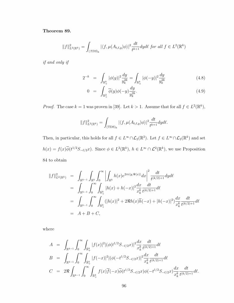
Theorem 89.
‖f‖2L2(Rk) =
∫(TDS)k
|〈f, µ(At,`,y)φ〉|2dt
tk+1dyd` for all f ∈ L2(Rk)
if and only if
2−k =
∫Rk+|φ(y)|2 dy
y2kk
=
∫Rk+|φ(−y)|2 dy
y2kk
(4.8)
0 =
∫R2
+
φ(y)φ(−y)dy
y2kk
. (4.9)
Proof. The case k = 1 was proven in [39]. Let k > 1. Assume that for all f ∈ L2(Rk),
‖f‖2L2(Rk) =
∫(TDS)k
|〈f, µ(At,`,y)φ〉|2dt
tk+1dyd`.
Then, in particular, this holds for all f ∈ L∞∩L2(R2). Let f ∈ L∞∩L2(Rk) and set
h(x) = f(x)φ(t1/2S−`/2x). Since φ ∈ L2(Rk), h ∈ L∞ ∩ L2(Rk), we use Proposition
84 to obtain
‖f‖2L2(Rk) =
∫Rk−1
∫Rk
∫ ∞0
∣∣∣∣∫Rkh(x)e2πi〈y,Ψ(x)〉dx
∣∣∣∣2 dt
t(k/2)+1dyd`
=
∫Rk−1
∫ ∞0
∫Rk+|h(x) + h(−x)|2dx
xkk
dt
t(k/2)+1d`
=
∫Rk−1
∫ ∞0
∫Rk+
(|h(x)|2 + 2<h(x)h(−x) + |h(−x)|2)dx
xkk
dt
t(k/2)+1d`
= A+B + C,
where
A =
∫Rk−1
∫ ∞0
∫Rk+|f(x)|2|(φ(t1/2S−`/2x)|2dx
xkk
dt
t(k/2)+1d`
B =
∫Rk−1
∫ ∞0
∫Rk+|f(−x)|2|(φ(−t1/2S−`/2x)|2dx
xkk
dt
t(k/2)+1d`
C = 2<∫
Rk−1
∫ ∞0
∫Rk+f(x)f(−x)φ(t1/2S−`/2x)φ(−t1/2S−`/2x)
dx
xkk
dt
t(k/2)+1d`.
96
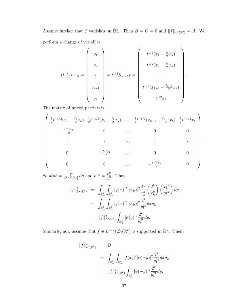
Assume further that f vanishes on Rk−. Then B = C = 0 and ‖f‖L2(Rk) = A. We
perform a change of variables
(t, `) 7→ y =
y1
y2
...
yk−1
yk
= t1/2S−`/2x =
t1/2(x1 − `12xk)
t1/2(x2 − `22xk)
...
t1/2(xk−1 − `k−1
2xk)
t1/2xk
.
The matrix of mixed partials is
12t−1/2(x1 − `1
2xk)
12t−1/2(x2 − `2
2xk) . . . 1
2t−1/2(xk−1 − `k−1
2xk)
12t−1/2xk
− t1/2xk2
0 . . . 0 0
......
. . ....
...
0 − t1/2xk2
. . . 0 0
0 0 . . . − t1/2xk2
0
.
So dtd` = 2k
t(k−2)/2xkkdy and t−k =
x2kk
y2kk. Thus,
‖f‖2L2(Rk) =
∫Rk+
∫Rk+|f(x)|2|φ(y)|2dx
xkk
(2k
xkk
)(x2kk
y2kk
)dy
=
∫Rk+
∫Rk+|f(x)|2|φ(y)|2 2k
y2kk
dxdy
= ‖f‖2L2(Rk)
∫Rk+|φ(y)|2 2k
y2kk
dy.
Similarly, now assume that f ∈ L∞ ∩ L2(Rk) is supported in Rk−. Then,
‖f‖2L2(Rk) = B
=
∫Rk+
∫Rk−|f(x)|2|φ(−y)|2 2k
y2kk
dxdy
= ‖f‖2L2(Rk)
∫Rk+|φ(−y)|2 2k
y2kk
dy.
97

Thus any reproducing function must satisfy (4.8). Now simply assume that f ∈
L∞ ∩ L2(Rk) and assume that φ satisfies (4.8). Then
‖f‖2L2(Rk) = ‖f‖2
L2(Rk+)+ ‖f‖2
L2(Rk−)+ C,
which implies that C = 0. Also
0 = C = 2<∫
Rk+
∫Rk+f(x)f(−x)φ(y)φ(−y)
2k
y2kk
dydx. (4.10)
Assume that∫
Rk+f(x)f(−x)dx 6= 0. If f is also real valued, then (4.10) implies
that <∫
Rk+φ(y)φ(−y) dy
y2kk= 0. If f is purely imaginary, then (4.10) implies that
=∫
Rk+φ(y)φ(−y) dy
y2kk= 0. Hence φ must satisfy (4.9).
Conversely, assume that f ∈ L∞ ∩ L2(Rk). By the preceding arguments,
∫(TDS)k
|〈f, µ(At,`,y)φ〉|2dt
tk+1dyd` =
∫Rk+|f(x)|2dx
∫Rk+|φ(y)|2 2k
y2kk
dy
+
∫Rk−|f(x)|2dx
∫Rk+|φ(−y)|2 2k
y2kk
dy
+2<∫
Rk+f(x)f(−x)dx
∫Rk+φ(y)φ(−y)
2k
y2kk
dy.
If φ satisfies (4.8) and (4.9), then
∫(TDS)k
|〈f, µ(At,`,y)φ〉|2dt
tk+1dyd` =
(∫Rk−
+
∫Rk+
)|f(x)|2dx+ 0 = ‖f‖2
L2(Rk).
Now let f be any arbitrary function in L2(Rk) where φ still satisfies (4.8) and (4.9).
Since L∞ ∩ L2(Rk) is dense in L2(Rk),we can chose a {fn} ⊂ L∞ ∩ L2(Rk) which
converges to f in L2(Rk). For any fn, fm, the difference fn−fm lies in L∞∩L2(Rk).
Hence
‖〈fn, µ((At,`,y)φ〉 − 〈fm, µ((At,`,y)φ〉‖2L2((TDS)k) = ‖fn − fm‖2
L2(Rk) → 0
98
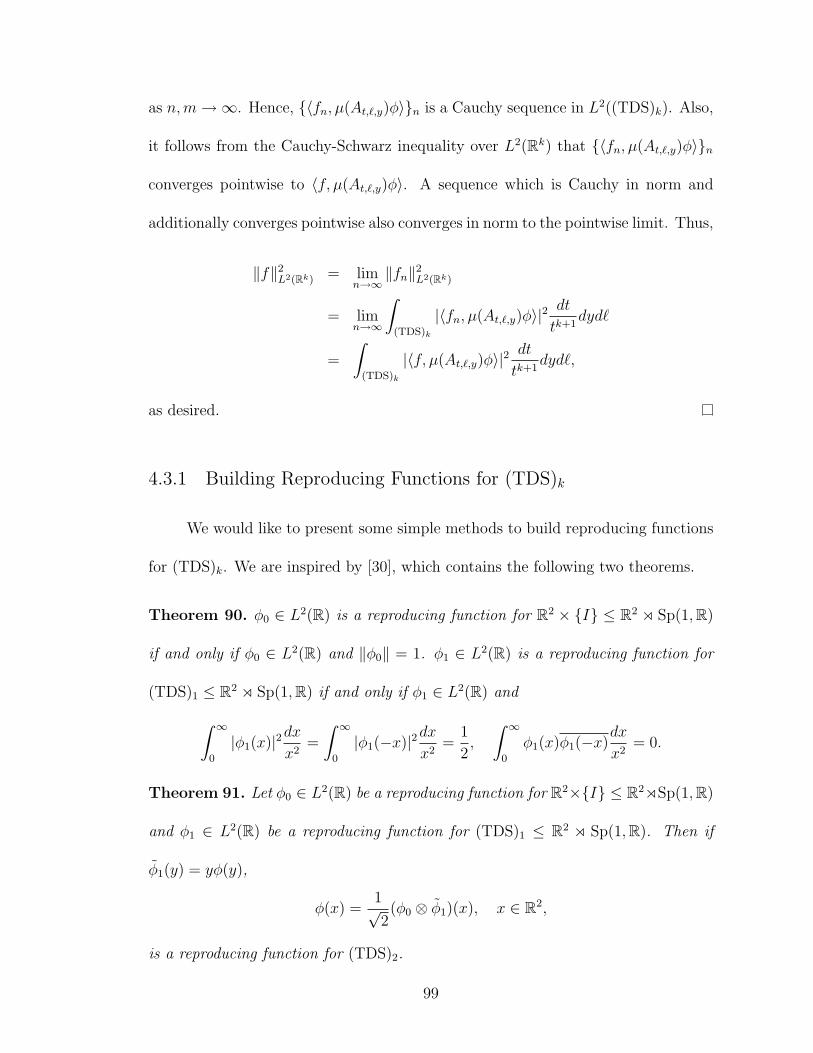
as n,m→∞. Hence, {〈fn, µ(At,`,y)φ〉}n is a Cauchy sequence in L2((TDS)k). Also,
it follows from the Cauchy-Schwarz inequality over L2(Rk) that {〈fn, µ(At,`,y)φ〉}n
converges pointwise to 〈f, µ(At,`,y)φ〉. A sequence which is Cauchy in norm and
additionally converges pointwise also converges in norm to the pointwise limit. Thus,
‖f‖2L2(Rk) = lim
n→∞‖fn‖2
L2(Rk)
= limn→∞
∫(TDS)k
|〈fn, µ(At,`,y)φ〉|2dt
tk+1dyd`
=
∫(TDS)k
|〈f, µ(At,`,y)φ〉|2dt
tk+1dyd`,
as desired.
4.3.1 Building Reproducing Functions for (TDS)k
We would like to present some simple methods to build reproducing functions
for (TDS)k. We are inspired by [30], which contains the following two theorems.
Theorem 90. φ0 ∈ L2(R) is a reproducing function for R2 × {I} ≤ R2 o Sp(1,R)
if and only if φ0 ∈ L2(R) and ‖φ0‖ = 1. φ1 ∈ L2(R) is a reproducing function for
(TDS)1 ≤ R2 o Sp(1,R) if and only if φ1 ∈ L2(R) and∫ ∞0
|φ1(x)|2dxx2
=
∫ ∞0
|φ1(−x)|2dxx2
=1
2,
∫ ∞0
φ1(x)φ1(−x)dx
x2= 0.
Theorem 91. Let φ0 ∈ L2(R) be a reproducing function for R2×{I} ≤ R2oSp(1,R)
and φ1 ∈ L2(R) be a reproducing function for (TDS)1 ≤ R2 o Sp(1,R). Then if
φ1(y) = yφ(y),
φ(x) =1√2
(φ0 ⊗ φ1)(x), x ∈ R2,
is a reproducing function for (TDS)2.
99

We generalize this result to obtain the following theorem.
Theorem 92. Let φ0 ∈ L2(R) be a reproducing function for R2×{I} ≤ R2oSp(1,R)
and let φk−1 ∈ L2(Rk−1) be a reproducing function for (TDS)k−1. Then
φ(x) =xk√
2(φ0 ⊗ φk−1)(x), x ∈ Rk
is a reproducing function for (TDS)k.
Proof. By Theorem 90 φ0 satisfies ‖φ0‖ = 1 and φk−1 satisfies
1 = 2k−1
∫Rk−1
+
|φk−1(x)|2 dx
x2(k−1)k−1
,
1 = 2k−1
∫Rk−1
+
|φk−1(−x)|2 dx
x2(k−1)k−1
, and
0 = 2k−1
∫Rk−1
+
φk−1(x)φk−1(−x)dx
x2(k−1)k−1
.
So
2k∫
Rk+|φ(x)|2 dx
x2kk
= 2k∫
Rk+| xk√
2(φ0 ⊗ φk−1)(x)|2 dx
x2kk
= 2k−1
∫R|φ0(x1)|2dx1
∫Rk−1
+
|φk−1(x)|2 dx
x2(k−1)k−1
= 2k−1 · 1 · 1
2k−1
= 1.
Similarly, 2k∫
Rk+|φ(−x)|2 dx
x2kk
= 1. Finally,∫Rk+φ(x)φ(−x)
dx
x2kk
=1
2
∫Rφ0(x1)φ0(−x1)dx1
∫Rk−1
+
φk−1(x)φk−1(−x)dx
x2(k−1)k−1
=1
2
(∫Rφ0(x1)φ0(−x1)dx1
)· 0
= 0.
100

This leads to the following corollary.
Corollary 93. Let φ0 ∈ L2(R) be a reproducing function for R2 × {I} ≤ R2 o
Sp(1,R) and let φ1 ∈ L2(R) be a reproducing function for (TDS)1. Then
φ(x) =1
2(k−1)/2
((⊗k−1
i=1 φ0)⊗ φ1
)(x), x ∈ Rk,
where φ1(y) = yk−1φ1(y), is a reproducing function for (TDS)k.
We shall now now explicitly construct a class of functions which are reproduc-
ing functions for (TDS)1.
Theorem 94. Let f : R→ R be supported in some interval [0, b], b > 0 and satisfy∫f 2(x)dx = 1
4. For a > 0, define
φ(x) = x (f(x− a)− f(−x+ a+ 2b) + f(x+ a+ b) + f(−x− a− b)) .
Then φ is a reproducing function for (TDS)1.
Proof. By Theorem 90, it suffices to show that
0 =
∫ ∞0
φ(x)φ(−x)dx
x2and
1
2=
∫ ∞0
|φ(x)|2dxx2
=
∫ ∞0
|φ(−x)|2dxx2.
We note that the following shifts have supports contained in
shift supp
f(· − a) [a, a+ b]
f(− ·+a+ 2b) [a+ b, a+ 2b]
f(·+ a+ b) [−a− b,−a]
f(− · −a− b) [−a− 2b,−a− b].
101
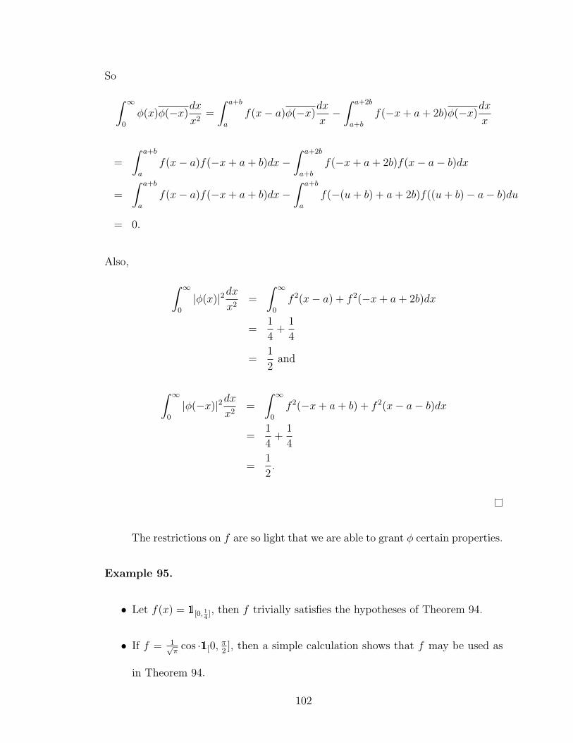
So
∫ ∞0
φ(x)φ(−x)dx
x2=
∫ a+b
a
f(x− a)φ(−x)dx
x−∫ a+2b
a+b
f(−x+ a+ 2b)φ(−x)dx
x
=
∫ a+b
a
f(x− a)f(−x+ a+ b)dx−∫ a+2b
a+b
f(−x+ a+ 2b)f(x− a− b)dx
=
∫ a+b
a
f(x− a)f(−x+ a+ b)dx−∫ a+b
a
f(−(u+ b) + a+ 2b)f((u+ b)− a− b)du
= 0.
Also,
∫ ∞0
|φ(x)|2dxx2
=
∫ ∞0
f 2(x− a) + f 2(−x+ a+ 2b)dx
=1
4+
1
4
=1
2and
∫ ∞0
|φ(−x)|2dxx2
=
∫ ∞0
f 2(−x+ a+ b) + f 2(x− a− b)dx
=1
4+
1
4
=1
2.
The restrictions on f are so light that we are able to grant φ certain properties.
Example 95.
• Let f(x) = 1[0, 14
], then f trivially satisfies the hypotheses of Theorem 94.
• If f = 1√π
cos ·1[0,π2], then a simple calculation shows that f may be used as
in Theorem 94.
102
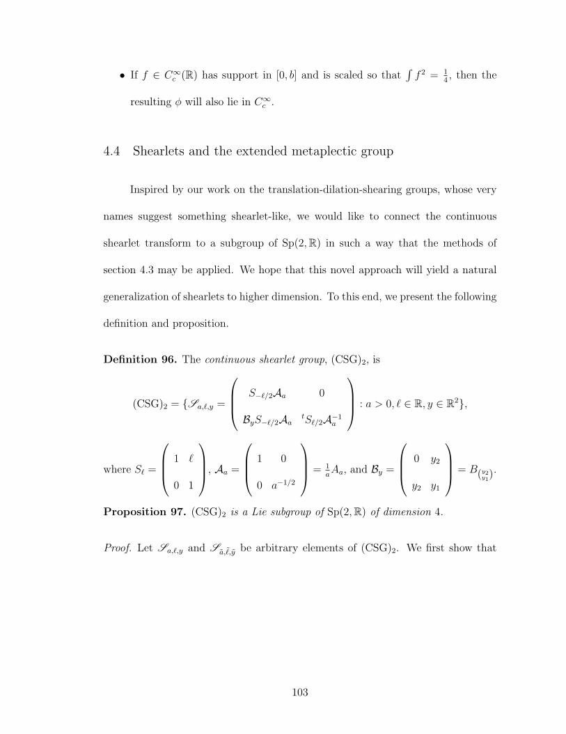
• If f ∈ C∞c (R) has support in [0, b] and is scaled so that∫f 2 = 1
4, then the
resulting φ will also lie in C∞c .
4.4 Shearlets and the extended metaplectic group
Inspired by our work on the translation-dilation-shearing groups, whose very
names suggest something shearlet-like, we would like to connect the continuous
shearlet transform to a subgroup of Sp(2,R) in such a way that the methods of
section 4.3 may be applied. We hope that this novel approach will yield a natural
generalization of shearlets to higher dimension. To this end, we present the following
definition and proposition.
Definition 96. The continuous shearlet group, (CSG)2, is
(CSG)2 = {Sa,`,y =
S−`/2Aa 0
ByS−`/2Aa tS`/2A−1a
: a > 0, ` ∈ R, y ∈ R2},
where S` =
1 `
0 1
, Aa =
1 0
0 a−1/2
= 1aAa, and By =
0 y2
y2 y1
= B(y2y1).
Proposition 97. (CSG)2 is a Lie subgroup of Sp(2,R) of dimension 4.
Proof. Let Sa,`,y and Sa,˜,y be arbitrary elements of (CSG)2. We first show that
103

(CSG)2 ⊂ Sp(2,R).
tSa,`,yJSa,`,y =
AatS−`/2 AatS−`/2By0 tA−1
a S`/2
0 I2
−I2 0
Sa,`,y
=
−AatS−`/2By AatS−`/2−tA−1
a S`/2 0
S−`/2Aa 0
ByS−`/2Aa tS`/2A−1a
=
−AatS−`/2ByS−`/2Aa +AatS−`/2ByS−`/2Aa AatS−`/2tS`/2A−1a
−tA−1a S`/2S−`/2Aa 0
= J .
We now compute
Sa,`,ySa,˜,y =
S−`/2Aa 0
ByS−`/2Aa tS`/2A−1a
S−˜/2Aa 0
ByS−˜/2AatS˜/2A
−1a
=
S−`/2AaS−˜/2Aa 0
ByS−`/2AaS−˜/2Aa + tS`/2A−1a ByS−˜/2Aa
tS`/2A−1a
tS˜/2A−1a
=
S−`/2S−a1/2 ˜/2AaAa 0
(ByS−`/2Aa + tS`/2A−1a By)S−˜/2Aa
tS`/2tSa1/2 ˜/2A−1
a A−1a
,
104

where (ByS−`/2Aa + tS`/2A−1a By)S−˜/2Aa
=
0 a−1/2y2
y2−a−1/2`
2y2 + a−1/2y1
+
0 y2
a1/2y2`2y2 + a1/2y1
1 −a−1/2 ˜
2
0 a−1/2
=
0 a−1/2y2 + y2
y2 + a1/2y2−a−1/2`
2y2 + a−1/2y1 + `
2y2 + a1/2y1
1 −a−1/2 ˜
2
0 a−1/2
=
0 (aa)−1/2(y2 + a1/2y2)
y2 + a1/2y2−(aa)−1/2
2(`+ a1/2 ˜)(y2 + a1/2y2) + (aa)−1/2(y1 + ay1 + a1/2`y2)
= B
(y1+ay1+a1/2`y2
y2+a1/2y2)S−(`+a1/2 ˜)
2
Aaa.
So Sa,`,ySa,˜,y = Sa,`,y, where a = aa, ` = ` + a1/2 ˜ and y =(y1+ay1+a1/2`y2
y2+a1/2y2
). Thus
(CSG)2 is a Lie subgroup of Sp(2,R). The parameterization of (CSG)2 yields the
dimension.
As we did in Section 4.3, we shall again present three representations of
(CSG)2. We shall begin with a “wavelet representation,” which we shall also denote
with a ν.
Definition 98. Define the wavelet representation of (CSG)2 by
ν(Sa,`,y) = TyD(S`Aa)−1 .
Proposition 99. ν is a unitary representation of (CSG)2.
Proof. Each ν(Sa,`,y) is a unitary operator on L2(R2). In the proof of Proposition
97, we showed
Sa,`,ySa,˜,y = Sa,`,y,
105
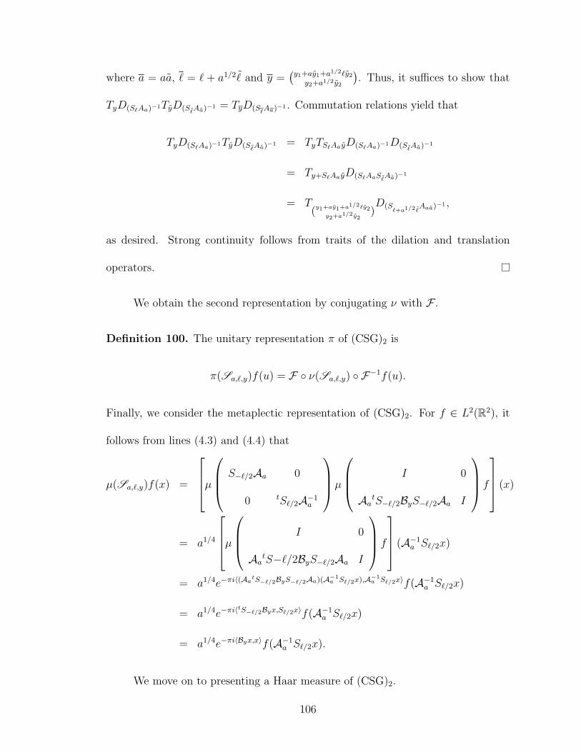
where a = aa, ` = ` + a1/2 ˜ and y =(y1+ay1+a1/2`y2
y2+a1/2y2
). Thus, it suffices to show that
TyD(S`Aa)−1TyD(S˜Aa)−1 = TyD(S`Aa)−1 . Commutation relations yield that
TyD(S`Aa)−1TyD(S˜Aa)−1 = TyTS`AayD(S`Aa)−1D(S˜Aa)−1
= Ty+S`AayD(S`AaS˜Aa)−1
= T(y1+ay1+a1/2`y2
y2+a1/2y2)D(S
`+a1/2 ˜Aaa)−1 ,
as desired. Strong continuity follows from traits of the dilation and translation
operators.
We obtain the second representation by conjugating ν with F .
Definition 100. The unitary representation π of (CSG)2 is
π(Sa,`,y)f(u) = F ◦ ν(Sa,`,y) ◦ F−1f(u).
Finally, we consider the metaplectic representation of (CSG)2. For f ∈ L2(R2), it
follows from lines (4.3) and (4.4) that
µ(Sa,`,y)f(x) =
µ S−`/2Aa 0
0 tS`/2A−1a
µ
I 0
AatS−`/2ByS−`/2Aa I
f
(x)
= a1/4
µ I 0
AatS−`/2ByS−`/2Aa I
f
(A−1a S`/2x)
= a1/4e−πi〈(AatS−`/2ByS−`/2Aa)(A−1
a S`/2x),A−1a S`/2x〉f(A−1
a S`/2x)
= a1/4e−πi〈tS−`/2Byx,S`/2x〉f(A−1
a S`/2x)
= a1/4e−πi〈Byx,x〉f(A−1a S`/2x).
We move on to presenting a Haar measure of (CSG)2.
106
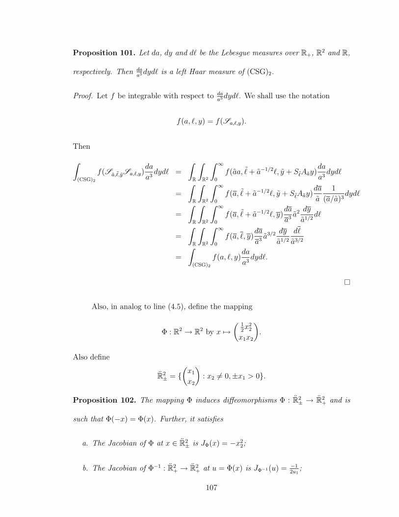
Proposition 101. Let da, dy and d` be the Lebesgue measures over R+, R2 and R,
respectively. Then daa3dyd` is a left Haar measure of (CSG)2.
Proof. Let f be integrable with respect to daa3dyd`. We shall use the notation
f(a, `, y) = f(Sa,`,y).
Then
∫(CSG)2
f(Sa,˜,ySa,`,y)da
a3dyd` =
∫R
∫R2
∫ ∞0
f(aa, ˜+ a−1/2`, y + S˜Aay)da
a3dyd`
=
∫R
∫R2
∫ ∞0
f(a, ˜+ a−1/2`, y + S˜Aay)da
a
1
(a/a)3dyd`
=
∫R
∫R2
∫ ∞0
f(a, ˜+ a−1/2`, y)da
a3 a2 dy
a1/2d`
=
∫R
∫R2
∫ ∞0
f(a, `, y)da
a3 a3/2 dy
a1/2
d`
a3/2
=
∫(CSG)2
f(a, `, y)da
a3dyd`.
Also, in analog to line (4.5), define the mapping
Φ : R2 → R2 by x 7→(
12x2
2
x1x2
).
Also define
R2± = {
(x1
x2
): x2 6= 0,±x1 > 0}.
Proposition 102. The mapping Φ induces diffeomorphisms Φ : R2± → R2
+ and is
such that Φ(−x) = Φ(x). Further, it satisfies
a. The Jacobian of Φ at x ∈ R2± is JΦ(x) = −x2
2;
b. The Jacobian of Φ−1 : R2+ → R2
+ at u = Φ(x) is JΦ−1(u) = −12u1
;
107

c. Φ−1(AatS`u) = A−1
a S`/2Φ−1(u) for every u ∈ R2+; and
d. 〈Byx, x〉 = 2〈y,Φ(x)〉 for every x ∈ R2± and every y ∈ R2.
Proof. By definition, Φ is even. Note that Φ−1(u) =(u2/√
2u1√2u1
). We now calculate
the matrices of the partials:
∂Φ(x)i∂xj
=
x2 ; i = 3− j
x1 ; i = j = 2
0 ; else
and
∂Φ−1(u)i∂uj
=
1(2u1)1/2
; i = 3− j
−2u2
(2u1)3/2; i = j = 2
0 ; else
.
Hence
JΦ(x) = det
(∂Φ(x)i∂xj
)i,j
= −x22 and
JΦ−1(u) = det
(∂Φ−1(u)i∂uj
)i,j
=−1
2u1
.
We now prove parts (c) and (d):
Φ−1(AatS`u) = Φ−1
(au1
a1/2`u1 + a1/2u2
)=
(u1+a1/2u2√2au1√2au1
)=
( `2
√2u1 + u2√
2u1
a1/2√
2u1
)= A−1
a S`/2
( u2√2u1√2u1
)= A−1
a S`/2Φ−1(u),
108

and
〈Byx, x〉 = 〈
0 y2
y2 y1
(x1
x2
),
(x1
x2
)〉
= 〈(
x2y2
x1y2 + x2y1
),
(x1
x2
)〉
= x1x2y2 + x1x2y2 + x22y1
= 2〈(y1
y2
),
(12x2
2
x1x2
)〉
= 2〈y,Φ(x)〉.
We now use these results to show that the wavelet and metaplectic repsenta-
tions of (CSG)2 are equivalent.
Theorem 103. Let u ∈ R2+ and extend the map
Pf(u) =1
|2u1|1/2f(Φ−1(u))
as an even function to R2\{x1x2 = 0}. This is a unitary map of L2even(R2) onto
itself that intertwines the representations π and µ.
Proof. Note that P−1f(x) = x2f(Φ(x)). Let f ∈ L2even(R2). It follows from the
Jacobian calculation in Proposition 102 that
‖Pf‖2L2(R2) =
∫R2
|Pf(u)|2du
= 2
∫R2
+
(1
2u1
)|f(Φ−1(u))|2du
= 2
∫R2
+
|f(x)|2dx
= ‖f‖2L2(R2).
109

P is a unitary operator on L2even(R2) since it is a surjective isometry. By Proposition
102, (4.3), (4.4) and Definition 100
π(Sa,`,y)(Pf)(u) = e−2πi〈y,u〉DAatS`(Pf)(u)
= a3/4e−2πi〈y,u〉(Pf)(AatS`u)
= a3/4e−2πi〈y,u〉 1
|2au1|1/2f(Φ−1(Aa
tS`u))
=a1/4
|2u1|1/2e−2πi〈y,u〉f(A−1
a (tS`/2)Φ−1(u))
=a1/4
|2u1|1/2e−πi(2〈y,Φ(Φ−1(u))〉)f(A−1
a (tS`/2)Φ−1(u))
=a1/4
|2u1|1/2e−πi〈ByΦ−1(u),Φ−1(u)〉f(A−1
a (tS`/2)Φ−1(u))
=1
|2u1|1/2(µ(Sa,`,y)f)(Φ−1(u))
= P(µ(Sa,`,y)f)(u).
Definition 104. Define
L′2(Rk) = {f(x1, x2, . . . , xk) mapping Rk → C : f(x2, . . . , xk, x1) ∈ L2}
The next two lemmas are the workhorses needed to prove that (CSG)2 is
reproducing.
Lemma 105. Let 1+ = 1R2+
. If h ∈ L′2(R2) then
1+(u)
2u1
[h(Φ−1(u)) + h(−Φ−1(u))] ∈ L1 ∩ L2(R2).
Proof. The proof is exactly like the proof of Lemma 86, but with Φ instead of Ψ, x1
and x2 swapped, u1 and u2 swapped, and R2+ instead of R2
+.
110

Lemma 106. Let h ∈ L′2(R2). Then∫R2
∣∣∣∣∫R2
h(x)e2πi〈y,Φ(x)〉dx
∣∣∣∣2 dy =
∫R2
+
|h(x) + h(−x)|2dxx2
2
.
Proof. By Proposition 102∫R2
h(x)e2πi〈y,Φ(x)〉dx = (
∫R2
+
+
∫R2−
)h(x)e2πi〈y,Φ(x)〉dx
=
∫R2
+
h(x)e2πi〈y,Φ(x)〉dx+
∫R2
+
h(−x)e2πi〈y,Φ(−x)〉dx
=
∫R2
+
[h(x) + h(−x)]e2πi〈y,Φ(x)〉dx
=
∫R2
+
[h(Φ−1(u)) + h(−Φ−1(u))]e2πi〈y,u〉 du
2u1
=
∫R2
1+(u)
2u1
[h(Φ−1(u)) + h(−Φ−1(u))]e2πi〈y,u〉du (4.11)
Since the integrand is in L1 ∩ L2(R2), we may apply Parseval’s equality to obtain
‖Eqn(4.11)‖2L2(R2) =
∫R2
∣∣∣∣∫R2
1+(u)
2u1
[h(Φ−1(u)) + h(−Φ−1(u))]e2πi〈y,u〉du
∣∣∣∣2 dy=
∫R2
|1+(u)
2u1
[h(Φ−1(u)) + h(−Φ−1(u))]|2du
=
∫R2
+
|h(Φ−1(u)) + h(−Φ−1(u))|2 du
(2u1)2
=
∫R2
+
|h(x) + h(−x)|2 x22dx
(x22)2
=
∫R2
+
|h(x) + h(−x)|2dxx2
2
.
We show that (CSG)2 is reproducing and characterize the reproducing func-
tions.
Theorem 107. If φ ∈ L2(R2), then
‖f‖2L2(R2) =
∫(CSG)2
|〈f, µ(Sa,`,y)φ〉|2da
a3dyd` for all f ∈ L2(R2)
111
if and only if
1
4=
∫R2
+
|φ(y)|2dyy4
2
=
∫R2
+
|φ(−y)|2dyy4
2
(4.12)
0 =
∫R2
+
φ(y)φ(−y)dy
y42
. (4.13)
Proof. Assume that for all f ∈ L2(R2),
‖f‖2L2(R2) =
∫(CSG)2
|〈f, µ(Sa,`,y)φ〉|2da
a3dyd`.
Then, in particular, this holds for all f ∈ L∞ ∩ L′2(R2). Let f ∈ L∞ ∩ L′2(R2) and
set h(x) = f(x)φ(A−1a S`/2x). Since φ ∈ L2(R2), h ∈ L1 ∩ L′2(R2). Thus, we obtain
‖f‖2L2(R2) =
∫R
∫R2
∫ ∞0
∣∣∣∣∫R2
h(x)e2πi〈y,Φ(x)〉dx
∣∣∣∣2 da
a5/2dyd`
=
∫R
∫ ∞0
∫R2
+
|h(x) + h(−x)|2dxx2
2
da
a5/2d`
=
∫R
∫ ∞0
∫R2
+
(|h(x)|2 + 2<h(x)h(−x) + |h(−x)|2)dx
x22
da
a5/2d`
= A+B + C,
where
A =
∫R
∫ ∞0
∫R2
+
|f(x)|2|(φ(A−1a S`/2x)|2dx
x22
da
a5/2d`
B =
∫R
∫ ∞0
∫R2
+
|f(−x)|2|(φ(−A−1a S`/2x)|2dx
x22
da
a5/2d`
C = 2<∫
R
∫ ∞0
∫R2
+
f(x)f(−x)φ(A−1a S`/2x)φ(−A−1
a S`/2x)dx
x22
da
a5/2d`.
Assume further that f vanishes on R2−. Then B = C = 0 and ‖f‖L2(R2) = A. We
perform a change of variables
(a, `) 7→ y = (y1, y2) = A−1a S`/2x = (x1 +
`
2x2, a
1/2).
112
The matrix of mixed partials is 0 12a−1/2x2
x2
20
.
So dad` = 114a−1/2x2
2dy1dy2 = 4a1/2
x22dy1dy2 and a−2 =
x42
y42. Thus,
‖f‖2L2(R2) =
∫R2
+
∫R2
+
|f(x)|2|φ(y)|2dxx2
2
(4
x22
)(x4
2
y42
)dy
=
∫R2
+
∫R2
+
|f(x)|2|φ(y)|2 4
y42
dxdy
= ‖f‖2L2(R2)
∫R2
+
|φ(y)|2 4
y42
dy.
Similarly, now assume that f ∈ L∞ ∩ L′2(R2) is supported in R2−. Then,
‖f‖2L2(R2) = B
=
∫R2
+
∫R2−
|f(x)|2|φ(−y)|2 4
y42
dxdy
= ‖f‖2L2(R2)
∫R2
+
|φ(−y)|2 4
y42
dy.
Thus any reproducing function must satisfy (4.12). Now simply assume that f ∈
L∞ ∩ L′2(R2) and assume that φ satisfies (4.12). Then
‖f‖2L2(R2) = ‖f‖2
L2(R2+)
+ ‖f‖2L2(R2
−)+ C,
which implies that C = 0. Also
0 = C = 2<∫
R2+
∫R2
+
f(x)f(−x)φ(y)φ(−y)4
y42
dydx. (4.14)
Assume that∫
R2+f(x)f(−x)dx 6= 0. If f is also real valued, then (4.14) implies
that <∫
R2+φ(y)φ(−y)dy
y42= 0. If f is purely imaginary, then (4.14) implies that
=∫
R2+φ(y)φ(−y)dy
y42= 0. Hence φ must satisfy (4.13).
113
Conversely, assume that f ∈ L′2(R2). By the preceding arguments,
∫(CSG)2
|〈f, µ(Sa,`,y)φ〉|2da
a3dyd` =
∫R2
+
|f(x)|2dx∫
R2+
|φ(y)|2 4
y42
dy
+
∫R2−
|f(x)|2dx∫
R2+
|φ(−y)|2 4
y42
dy
+2<∫
R2+
f(x)f(−x)dx
∫R2
+
φ(y)φ(−y)4
y42
dy.
If φ satisfies (4.12) and (4.13), then
∫(CSG)2
|〈f, µ(Sa,`,y)φ〉|2da
a3dyd` =
(∫R2−
+
∫R2
+
)|f(x)|2dx+ 0 = ‖f‖2
L2(R2).
Now let f be any arbitrary function in L2(R2) where φ still satisfies (4.12) and (4.13).
Since L∞ ∩ L′2(R2) is dense in L2(R2), we can chose a {fn} ⊂ L∞ ∩ L′2(R2) which
converges to f in L2(R2). For any fn, fm, the difference fn−fm lies in L∞∩L′2(R2).
Hence
‖〈fn, µ(Sa,`,y)φ〉 − 〈fm, µ(Sa,`,y)φ〉‖2L2((CSG)2) = ‖fn − fm‖2
L2(R2) → 0
as n,m→∞. Hence, {〈fn, µ(Sa,`,y)φ〉}n is a Cauchy sequence in L2((CSG)2). Also,
it follows from the Cauchy-Schwarz inequality over L2(R2) that {〈fn, µ(Sa,`,y)φ〉}n
converges pointwise to 〈f, µ(Sa,`,y)φ〉. A sequence which is Cauchy in norm and
additionally converges pointwise also converges in norm to the pointwise limit. Thus,
‖f‖2L2(R2) = lim
n→∞‖fn‖2
L2(R2)
= limn→∞
∫(CSG)2
|〈fn, µ(Sa,`,y)φ〉|2da
a3dyd`
=
∫(CSG)2
|〈f, µ(Sa,`,y)φ〉|2da
a3dyd`,
as desired.
114

4.5 Conclusion
Dahlke et al. created shearlet analogs for L2(Rd), d > 2 in [31] and [32].
One paper deals with anisotropic dilations, which generalize the parabolic scaling
matrix, and one paper uses isotropic dilations. They work from the perspective of
co-orbit space theory and obtain a different generalization of the shearing matrix. It
is curious because no intuitive generalization of the shearing matrix, other than the
one employed in Section 4.3, yields a reproducing subgroup. We plan on using co-
orbit space theory to analyze each (TDS)k in order to find discrete, implementable
transformations. The generalization of the Translation-Dilation-Shearing group in
Section 4.2 may be used to analyze multidimensional data and images. We are
currently working to find the appropriate definition of (CDS)k for k > 2, generalizing
the results of Section 4.4. Finally, we would like to completely characterize the
dimensions of the reproducing subgroups of R4oSp(2,R). The results of this chapter
successfully integrate shearlet theory into the theory created by Cordero, DeMari,
Nowak and Tabacco and hopefully will lay the foundation of new transforms in
various applied fields.
115

Chapter 5
Grassmannian fusion frames
5.1 Introduction
When data is transmitted over a communication line, the received message
may be corrupted by noise and data loss. As an oversimplified example, if I send
you the message 1729, you could receive the noisy message 1728 or nothing at all.
Representing data in a way that is resilient to such problems is clearly desirable.
Expressing data using a redundant frame provides some protection, but some frames
work better than others. Goyal et al. proved that a normalized frame is optimally
robust against (o.r.a.) noise and one erasure if the frame is tight. Furthermore, a
normalized frame is o.r.a multiple erasures if it is Grassmannian ([96], [7]).
Definition 108. For F = R or C, define
F (N,FM) = {{ei}Ni=1 ⊂ FM : ‖ei‖ = 1 for all 1 ≤ i ≤ N and {ei} is a frame for FM}.
The maximal frame correlation is
M∞({ei}Ni=1) = max1≤i<j≤N
{|〈ei, ej〉|}.
A sequence of unit norm vectors {ui}Ni=1 ⊆ FM is called a Grassmannian frame if it
is a solution to
min{ei}∈F (N,FM )
{M∞({ei}Ni=1)}.
116

If N = M , the Grassmannian frames are precisely the orthonormal bases for
FM . If N = 3 and M = 2, the 2-dimensional vectors representing the cubic roots
of unity are a Grassmannian frame. However, the vectors representing the fourth
roots of unity do not form a Grassmannian frame for N = 4 and M = 2. Since
|〈(1, 0), (−1, 0)〉| = 1, the fourth roots of unity actually have the maximum possible
maximal frame correlation. The following theorem is proven in a number of classical
texts, see [96] for one proof and citations of other methods.
Theorem 109. Let {ei}Ni=1 be a normalized frame for FM . Then
M∞({ei}Ni=1) ≥
√N −MM(N − 1)
(5.1)
Equality holds in (5.1) if and only if {ei} is an equiangular tight frame. How-
ever, equality can only hold for certain N and M . Bodmann and Paulsen proved
a functorial equivalence between real equiangular frames and α-regular 2-graphs,
where α depends on N and M [20]. An α-regular 2-graph is a particular type of
hypergraph. This correspondence can be used to characterize when equiangular
frames exist. Other than the case N = M + 1, there are very few known pairs
(N,M) which yield equiangular frames and, further, there are many pairs (N,M)
for which it has been proven that no equiangular frames exist. When equiangular
frames do not exist, it can be complicated to construct Grassmannian frames.
Definition 110. For 1 ≤ m ≤M , setG(M,m) to be the collection of m dimensional
subspaces of FM . As a manifold, G(M,m) = O(M)/(O(m) × O(M − m)), where
O(M) denotes elements of the R orthogonal group or the C unitary group. G(M,m)
is also an algebraic projective variety.
117

G(M,m) is called a Grassmannian. The Grassmannian packing problem is the
problem of finding N points in G(M,m) so that the minimal distance between any
two of them is as large as possible. Finding Grassmannian frames is equivalent to
solving the Grassmannian packing problem for G(M, 1). It is natural to ask what
analytic structures one obtains by considering the Grassmannian packing problem
for m > 1.
Fusion frames, originally called frames of subspaces, were introduced by Casazza
and Kutyniok in [22]. There are many potentially exciting applications of fusion
frames, in areas such as coding theory [19], distributed sensing [23], and neurology
[91].
Definition 111. A fusion frame for FM is a finite collection of subspaces {Wi}Ni=1
in FM such that there exist 0 < A ≤ B <∞ satisfying
A‖x‖2 ≤N∑i=1
‖Pix‖2 ≤ B‖x‖2,
where Pi is an orthogonal projection onto Wi. If A = B, we say that the fusion
frame is tight.
For two subspaces Wi,Wj ⊂ FM of equal dimension m, define the chordal
distance
dist(Wi,Wj) = [m− tr(PiPj)]1/2,
where Pi is an orthogonal projection onto Wi. A tight fusion frame consisting of
equal dimensional subspaces with equal pairwise chordal distances is an equi-distance
tight fusion frame.
118
Similar to (1.3), a fusion frame is tight with bound A if and only if
N∑i=1
Pi = AIM . (5.2)
Fusion frames may either be viewed as generalizations of frames or special types
of frames. In the former sense, we are merely replacing the projections (modulo a
constant multiples) of vectors x ∈ H (on line (1.2)) onto the subspace spanned by
each frame vector with projections onto spaces of dimensions possibly higher than
1. In the latter sense, we may see a fusion frame as a frame with sub-collections
of frame vectors which group in nice ways. As is common in the literature, nice
is an oversimplification of some very deep properties. In fact, splitting frames into
such sub-collections is related to the (in)famous Feichtinger Conjecture. A fusion
frame is o.r.a. against noise if it is tight ([77]), a tight fusion frame is o.r.a. one
subspace erasure if the dimensions of the subspaces are equal ([19]), and a tight
fusion frame is o.r.a. multiple subspace erasures if the subspaces have equal chordal
distances. An equi-distance tight fusion frame is a solution to the Grassmannian
packing problem ([77]). The following definition does not exist in the literature but
seems quite natural.
Definition 112. A fusion frame {Wi}Ni=1 for RM consisting of d-dimensional sub-
spaces shall be called a Grassmannian fusion frame if it is a solution to the Grass-
mannian packing problem for N points in G(M,m).
We would like to construct such objects. The idea is very simple and makes
use of Hadamard matrices.
119
5.2 Hadamard matrices
The first Hadamard matrices were discovered by Sylvester in 1867 ([97]). In
1893, Hadamard first defined and started to characterize Hadamard matrices, which
have the maximal possible determinant amongst matrices with entries from {±1}
([61]).
Definition 113. A Hadamard Matrix of order n is an n× n matrix H with entries
from {±1} such that H(tH) = nIn.
In the original paper by Hadamard, it was proven that Hadamard matrices
must have order equal to 2 or a multiple of 4. It is still an open conjecture as to
whether Hadamard matrices exist for every dimension divisible by 4. However, there
are many constructions of Hadamard matrices, which use methods from number the-
ory, group cohomology and other areas of math. Horadam’s book [71] is an excellent
resource. One class of Hadamard matrices are formed from Walsh functions.
Definition 114. The Walsh functions ωj : [0, 1]→ {±1} ⊂ R, j ≥ 0, are piecewise
constant functions which have the following properties:
1. ωj(0) = 1 for all j ≥ 0,
2. ωj has precisely j sign changes (zero crossings), and
3. 〈ωj, ωk〉 = δjk.
Walsh functions have been used for over 100 years by communications engi-
120
neers to minimize cross talk. The first four Walsh functions are
ω0 = 1[0,1]
ω1 = 1[0,1/2) − 1[1/2,1]
ω2 = 1[0,1/4) − 1[1/4,3/4) + 1[3/4,1]
ω3 = 1[0,1/4) − 1[1/4,1/2) + 1[1/2,3/4) − 1[3/4,1].
By sampling the first 2n Walsh functions at the points k2n
, one obtains a Hadamard
matrix; that is
Wn =
(ωj
(k
2n
))0≤j,k<2n
is a 2n× 2n Hadamard matrix. There is a speedy algorithm, the Fast Hadamard (or
Walsh) Transform, for multiplying a vector by such a matrix.
5.3 Construction
The idea behind the new construction of the Grassmannian fusion frames is
very simple. We remove the first i rows of a Hadamard matrix H to obtain a
submatrix H ′. The columns of H ′ will then be partitioned into spanning sets for
subspaces. Since the elements of the matrix are ±1, the computations should be
simplified and the resulting (fusion) frame should be easy to implement. It is well-
known (see, for example, [71]) that any Hadamard matrix can be normalized so that
first row consists solely of 1s.
Theorem 115. Let H be a 2n×2n Hadamard matrix indexed by 0, . . . , 2n−1 which
121

has been normalized so that the first row consists solely of 1s. Then
{ek =1√
2n − 1(H(j, k))1≤j≤2n−1 : 0 ≤ k ≤ 2n − 1}
is a Grassmannian frame for F2n−1.
Proof. For any 0 ≤ k1, k2 ≤ 2n − 1,
〈H(j, k1))0≤j≤2n−1, H(j, k2))0≤j≤2n−1〉 = 2nδk1,k2 and
〈H(k1, j))0≤j≤2n−1, H(k2, j))0≤j≤2n−1〉 = 2nδk1,k2 .
Thus 〈ek1 , ek2〉 = 12n−1
(2nδk1,k2 − 1), and the collection is equiangular. We now show
that the ek do indeed form a frame. Let x ∈ F2n−1 be arbitrary. We verify that
(1.3) holds. Let
L =
(1√
2n − 1(H(j, k))
)0≤k≤2n−1,1≤j≤2n−1
.
Then, by the orthogonality of the columns,
2n−1∑k=0
〈x, ek〉ek = ∗LLx =2n
2n − 1x.
We follow it up with the construction of a class of Grassmannian fusion frames.
Theorem 116. Let Wn be the 2n × 2n Walsh-Hadamard matrix indexed by
0, . . . , 2n − 1. Then
{Wk = span
{(Wn(j, k))2≤j≤2n−1, (Wn(j, k + 2n−1))2≤j≤2n−1
}: 0 ≤ k ≤ 2n−1
}is a tight Grassmannian fusion frame for F2n−2.
122
Proof. Since
Wn(0, k) = 1 for 0 ≤ k ≤ 2n − 1
Wn(1, k) =
1 for 0 ≤ k ≤ 2n−1 − 1
−1 for 2n−1 ≤ k ≤ 2n − 1
,
For any 0 ≤ k1, k2 ≤ 2n − 1, 〈Wn(j, k1))2≤j≤2n−1,Wn(j, k2))2≤j≤2n−1〉
=
2n − 2 k1 = k2
−2 for 0 ≤ k1, k2 ≤ 2n−1 − 1 or 2n−1 ≤ k1, k2 ≤ 2n − 1
0 else.
Thus, for each 0 ≤ k ≤ 2n−1,
{1√
2n − 2(Wn(j, k))2≤j≤2n−1,
1√2n − 2
(Wn(j, k + 2n−1))2≤j≤2n−1
}
is an orthonormal basis for Wk, and Pk = ∗LkLk, where
Lk =
(1√
2n − 2(Wn(j, k + i))
)i=0,4,1≤j≤2n−1
.
For 0 ≤ k1, k2 ≤ 2n−1 − 1,
tr(Pk1Pk2) = tr(∗Lk1Lk1(∗Lk2Lk2))
= tr(∗Lk1(−2
2n − 2I2)Lk2)
=−2
2n − 2tr(∗Lk1Lk2)
=−2
2n − 2(−2
2n − 2+−2
2n − 2)
=2
(2n−1 − 1)2.
Thus the Wk have pairwise equal chordal distance. We now show that the Wk do
123
indeed form a frame by verifying that (5.2) holds. Let x ∈ F2n be arbirary. Then,(2n−1−1∑k=0
Pk
)x =
2n−1∑k=0
〈x, 1√2n − 2
(Wn(j, k))2≤j≤2n−1〉1√
2n − 2(Wn(j, k))2≤j≤2n−1
=2n
2n − 2x.
5.4 Future Work
Removing the first 3 rows of a Walsh-Hadamard matrix does not yield an equi-
distance fusion frame. However, there has been recent work done to numerically
find optimal Grassmannian packings ([41]) which works well in some dimensions.
However, in other dimensions the convergence is incredibly slow. The algorithm uses
a random initial configuration. Perhaps by seeding the algorithm with a Hadamard
submatrix, the convergence would accelerate. On the other hand, removing the first
4 rows of a Walsh-Hadamard matrix does yield an equi-distance fusion frame. The
proof is very similar to the proof of Theorem 116 in the preceding section. We
conjecture that removing the first 2k rows from Wn, n > k will always yield an
equi-distance fusion frame. Finally, we would like develop an algorithm for a fast
implementation of the Walsh-Hadamard-generated fusion frames utilizing the Fast
Hadamard Transform.
124
Chapter 6
p-adic wavelets
6.1 Introduction
Kurt Hensel introduced the p-adic numbers Qp, p prime, in 1897 motivated by
the connections between algebraic field theory for numbers and for functions ([68]).
The p-adic numbers still play a big role in algebraic number and function theory
([74]), but there is a growing movement to incorporate p-adic numbers into pure and
applied analysis. The strange topology of Qp seems ideal to model quantum physical
phenomena (see, for example, [73]). There even seems to be a relation between
distance in a p-adic model and genetic code degeneracy ([44]). A good physical
model will contain some sort of differentiation. One cannot define a derivative
on p-adic function spaces, but the p-adics are locally compact abelian groups, so
there exists a Haar measure. Thus, one can define pseudo-differential operators over
the p-adics. It ends up that p-adic wavelets diagonalize certain pseudo-differential
operators ([2], [92]).
Up until now, all p-adic wavelet systems have been formed using dilations by p.
However, there is no reason to believe that other matrix dilations could not be used.
Furthermore, it is well known (see, for example [36]) that a wavelet basis formed
from a real multiresolution analysis (MRA) generated by dilations by a matrix A
contains | detA| − 1 generating wavelets. Thus, we would like to generate an MRA
125
with a p-adic matrix A for which | detA|2 = 2.
6.2 Preliminaries
6.2.1 p-adic numbers
We begin by defining a valuation.
Definition 117. Let F be a field. A valuation | · | is a map | · | : F→ R satisfying :
1. |α| ≥ 0 for a α ∈ F, and |α| = 0 if an only if α = 0,
2. For all α, β ∈ F, |αβ| = |α||β|, and
3. For all α, β ∈ F, |α + β| ≤ |α|+ |β|.
A valuation is called non-Archimedian if it satisfies the strong triangle inequality ;
that is, for all α, β ∈ F
|α + β| ≤ max{|α|, |β|}.
Two valuations | · |1, | · |2 are said to be equivalent if there exists a positive real
number s such that for all α ∈ F, |α|2 = |α|s1.
We now define the p-adic valuation.
Definition 118. Given a prime p, every non-zero rational number r may be written
uniquely as pim/n, where gcd (m,n) = 1 and p - m,n. The p-adic absolute value
|·|p is a valuation on Q defined as
|r|p =
0 if r = 0
p−i if r 6= 0
126

The p-adic numbers Qp are Q analytically completed with respect to the p-adic
absolute value.
The p-adic valuation is non-Archimedian, and, thus, Qp has an interesting
topology. For example, every ball is both topologically closed and open, and any
two balls are either nested or disjoint. Over Q, all of the valuations are known; this
is one of a handful of results in number theory known as Ostrowski’s theorem.
Theorem 119. Every non-trivial valuation of Q is equivalent to either a p-adic
valuation or the Euclidean absolute value.
The proof of Ostrowski’s theorem is quite simple, given certain elementary
facts of valuation theory, which we will not state here.
For every prime p, the additive group of Qp is a locally compact abelian group
which contains the compact open subgroup Zp. The group Zp is the set {α ∈
Qp
∣∣∣|α|p ≤ 1}, the unit ball in Qp. Equivalently, Zp is the subgroup generated by
1. It is well-known ([90]) that since Qp is a locally compact abelian group with a
compact open subgroup, it has a Haar measure normalized so that the measure of
Zp is 1. For simplicity, we shall denote this measure by dx. The metric on Qp is
induced by the valuation.
Every p-adic rational number x may be expanded
x =∞∑k=K
αkpk,
where |x|p = p−K and for all K ≤ k < ∞, αk ∈ {0, 1, . . . , p − 1}. Notice that the
127

series
1
1− p=∞∑k=0
pk
converges. Thus, for each prime p,
−1 =p− 1
1− p=∞∑k=0
(p− 1)pk.
Definition 120. For any x =∑∞
k=K αkpk ∈ Qp, we define the fractional part of x,
{x} =∑−1
k=K αkpk, where the sum is formally 0 if K ≥ 0 and the integer part of x,
[x] =∑∞
k=0 αkpk. We also define the set
Ip = {x ∈ Qp : {x} = x}.
Ip is a set of coset representatives for Qp/Zp. Since Zp is open, Ip is discrete.
This set will be very useful in the work that follows because Qp has no discrete
subgroup. We mention the p-adic valuation of elements of finite algebraic extensions,
which we shall use to analyze eigenvalues.
Definition 121. If α is the root of a monic, irreducible polynomial xn+an−1xn−1 +
. . .+ a0 ∈ Qp[x], we define |α|p = n√|ao|p.
Also, for any k ≥ 1, Qkp is a vector space over Qp. We shall denote the norm
with single bars, rather than double bars, and define it as
Definition 122. For any t(x1, x2, . . . , xk) ∈ Qkp, the norm is
|t(x1, x2, . . . , xk)|p = max1≤i≤k
{|xi|p}.
128

6.2.2 p-adic wavelets
There are two main function theories over the p-adics. One deals with functions
Qp → C and the other with Qp → Qp. We shall only deal with the former theory.
The latter differs dramatically from the former. For example, p-adic valued functions
have no Haar measure, but there is differentiation. For an analytic treatment of both
function theories, see [73].
In 2002, Kozyrev published the first example of a p-adic wavelet ([76])
{DpjTae{p−1kx}
1Zp(x) = p−j/2e{p−1k(pjx−a)}
1Zp(pjx−a) : k = 1, 2, . . . , p−1, j ∈ Z, a ∈ Ip}.
Since Qp does not have a discrete subgroup, he translated by a discrete set of coset
representatives. This approach is typical, not only in p-adic wavelet analysis, but
also in Gabor theory over locally compact abelian groups ([54]). Also notice the
sign of the exponent of the constant that comes out during dilation
Dpf(x) = p−1/2f(px),
in contrast to the real case. This is due to the p-adic valuation.
After Kozyrev’s publication, Shelkovich and Skopina created a p-adic MRA
theory ([92]), and Benedetto and Benedetto introduced p-adic wavelet set theory
([15], [10]). We shall be concerned with p-adic MRA. We now define a p-adic MRA,
generalized for this thesis.
Definition 123. Let A ∈ GL(k,Qp). If the p-adic valuations of the eigenvalues are
all strictly greater than 1 and | detA|p ∈ N then A is an expansive p-adic matrix.
129
Definition 124. Let A ∈ GL(k,Qp) be an expansive p-adic matrix. A collection of
closed spaces Vj ⊂ L2(Qkp) is called a multiresolution analysis (MRA) for L2(Qk
p) if
the following hold:
a. Vj ⊂ Vj+1 for all j ∈ Z,
b.⋃j∈Z Vj is dense in L2(Qp),
c.⋂j∈Z Vj = {0},
d. f(·) ∈ VJ ⇔ f(A·) ∈ Vj+1 for all j ∈ Z, and
e. there exists a function φ ∈ V0, called the scaling function, such that the system
{φ(· − a) : a ∈ Ikp } is an orthonormal basis for V0.
The structure is very similar to an MRA over Rk. Notice that by definition,
the functions {| detA|1/2p φ(Ajx − a) : a ∈ Ikp } form an orthonormal basis for Vj.
Mimicking real MRA, for each j ∈ Z, we define wavelet spaces Wj by
Vj+1 = Vj ⊕Wj.
It then follows from Definition 124.b-d that
L2(Qkp) =
⊕j∈Z
Wj.
Thus, if ψ ∈ W0 is such that {ψ(x − a) : a ∈ Ikp } is an orthonormal basis for W0,
then
{| detA|1/2ψ(Ajx− a) : j ∈ Z, a ∈ Ikp }
130
is an orthonormal (wavelet) basis for L2(Qkp) We call such a ψ a (p-adic) wavelet
function. It follows from Definition 124.a,d that a scaling function φ must satisfy
φ =∑a∈Ikp
αaφ(A · −a)
for some αa ∈ C. We call such a function refinable. Assume that the Ikp translations
of φ ∈ L2(Qkp) form an orthonormal set and that φ is refinable. Then define
Vj = span{φ(A · −a) : a ∈ Ikp }.
Clearly, parts (d) and (e) of Definition 124 are satisfied. In the real case, the
refinability of φ would also give us (a). However, that is not true in the p-adic case
because Ikp does not form a group. In order for (a) to be true, φ(· − b) must be
refinable for each b ∈ Ikp .
The number of wavelet functions needed to create an orthonormal basis cor-
responding to an MRA is equal to | detA| − 1, where the bars represent whichever
valuation one is working with. The only previously known wavelet bases for L2(Q22)
required 3 wavelet generators. We would like to construct an MRA for L2(Q22) using
a matrix A for which | detA|2 = 2. We now have the tools we need to construct
this new MRA. We shall construct the MRA in Section 6.3. We shall also present a
wavelet for this MRA in 6.4. Finally, in Section 6.5, we review future directions for
the research.
131
6.3 MRA construction
Let
A =
1 −1
1 1
−1
=
12
12
−12
12
,
the inverse of the well-known quincunx matrix. In [52], a multiresolution analysis
was presented for L2(R2) which used dilations by the quincunx. Since | detA−1| = 2,
there was only one wavelet generator. However, its support was a fractal, the twin
dragon fractal. In contrast, we shall see that the MRA for L2(Q22) associated to this
matrix corresponds to a wavelet with a simple support, namely, Z22.
The inverse of the quincunx matrix is expansive since the eigenvalues 1±i2
have
2-adic valuation√
2 > 1. Furthermore,
| detA|2 =
∣∣∣∣12∣∣∣∣2
= 2,
so we hope to obtain an MRA with a single generating wavelet. We first prove a
lemma that will be useful in computations which will follow later in the thesis.
Lemma 125. Let x1, x2 ∈ Q2.
• If |x1|2 > |x2|2 then |x1 + x2|2 = |x1 − x2|2 = |x1|2;
• If |x1|2 < |x2|2 then |x1 + x2|2 = |x1 − x2|2 = |x2|2; and
• If |x1|2 = |x2|2 then |x1+x2|2 ≤ 12|x1−x2|2 = 1
4|x1|2 or |x1−x2|2 ≤ 1
2|x1+x2|2 =
14|x1|2.
Proof. Set 2−Ki = |xi|2 for i = 1, 2. There exist αk ∈ {0, 1} and βk ∈ {0, 1} such
132

that
x1 = 2K1 +∞∑
k=K1+1
αk2k and
x2 = 2K2 +∞∑
k=K2+1
βk2k.
Since −1 =∑∞
k=0 2k,
−x2 = 2K2 +∞∑
k=K2+1
(1 +k∑
j=K2+1
βj)2k.
Assume that |x1|2 > |x2|2, then K2 ≥ K1 + 1. So
|x1 + x2|2 =
∣∣∣∣∣2K1 +
K2−1∑k=K1+1
αk2k + (1 + αk)2
K2 +∞∑
k=K2+1
(αk + βk)2k
∣∣∣∣∣2
= |x1|2,
and
|x1 − x2|2 =
∣∣∣∣∣2K1 +
K2−1∑k=K1+1
αk2k + (1 + αk)2
K2 +∞∑
k=K2+1
(αk + (1 +k∑
j=K1+1
βj))2k
∣∣∣∣∣2
= |x1|2.
By symmetry, if |x1|2 < |x2|2 then
|x1 + x2|2 = |x1 − x2|2 = |x2|2.
Now assume that |x1|2 = |x2|2. Then
|x1 + x2|2 =
∣∣∣∣∣(1 + αK1+1 + βK2+1)2K1+1 +∞∑
k=K1+2
(αk + βk)2k
∣∣∣∣∣2
= |x1|22
for αK1+1 = βK2+1
≤ |x1|24
for αK1+1 6= βK2+1.
133
Similarly,
|x1 − x2|2 =
∣∣∣∣∣(2 + αK1+1 + βK2+1)2K1+1 +∞∑
k=K1+2
(αk + 1 +k∑
j=K2+1
βj)2k
∣∣∣∣∣2
= |x1|22
for αK1+1 6= βK2+1
≤ |x1|24
for αK1+1 = βK2+1.
We wish to find a candidate for a scaling function from which we can build an
MRA.
Proposition 126.
Z22 = A−1Z2
2 t(A−1Z2
2 +
(0
1
)),
where t represents disjoint union.
Proof. We decompose Z22 into
Z22 = S1 t S2 t S3 t S4,
where
S1 = {(x1
x2
)∈ Z2
2 : |x1|2 = |x2|2 = 1}
S2 = {(x1
x2
)∈ Z2
2 : |x1|2 = 1, |x2|2 < 1}
S3 = {(x1
x2
)∈ Z2
2 : |x2|2 = 1, |x1|2 < 1} and
S4 = {(x1
x2
)∈ Z2
2 : |x1|2, |x2|2 < 1}.
It follows from simple parity arguments that
A−1S1 t A−1S4 ⊆ S4, A−1S2 t A−1S3 ⊆ S1.
134
Also, S1 +(
01
)= S2 and S4 +
(01
)= S3. We shall now prove that
AS1 ⊆ S2 t S3 and AS4 ⊆ S1 t S4.
Assume that x ∈ S1 then Ax = 12
(x1+x2
−x1+x2
). It follows from Lemma 125 that one of
|12x1 + 1
2x2|2 and | − 1
2x1 + 1
2x2|2 is 1
2|12x1|2 = 1 and one is ≤ 1
4|12x1|2 = 1
2. Either
way, Ax ∈ S2 t S3. Thus , S1 = A−1S2 t A−1S3.
Now assume that x ∈ S4. If either |x1|2, |x2|2 < 12
or if |x1|2 = |x2|2 = 12, then
it follows from Lemma 125 that∣∣∣∣12x1 +1
2x2
∣∣∣∣2
,
∣∣∣∣−1
2x1 +
1
2x2
∣∣∣∣2
< 1.
If instead |x1|2 < |x2|2 = 12
or |x2|2 < |x1|2 = 12
then∣∣∣∣12x1 +1
2x2
∣∣∣∣2
=
∣∣∣∣−1
2x1 +
1
2x2
∣∣∣∣2
= 1.
Thus, AS4 ⊆ S1 t S4, which implies that S4 = A−1S1 t A−1S4. Hence, A−1Z22 =
S1 t S4. Furthermore,
A−1Z22 +
(0
1
)= (S1 t S4) +
(0
1
)= (S1 +
(0
1
)) t (S4 +
(0
1
))
= S2 t S3.
Define
φ(x) = 1Z22(x)
and
Vj = span{φ(Ajx− a) : a ∈ I22} for j ∈ Z. (6.1)
135
We shall show that φ and the Vj form a multiresolution analysis.
Proposition 127. Let Vj be defined as in (6.1). For all j ∈ Z, Vj ⊆ Vj+1.
Proof. The proposition is equivalent to the statement
φ(Ajx− a) ∈ span{φ(Aj+1x− b) : b ∈ I22}
for all j ∈ Z and a ∈ I22 . Further, it suffices to prove this statement for the case
j = 0. The remaining cases will follow from the substitution x 7→ Ajx. It follows
from Proposition 126 that φ satisfies the refinement equation
φ(x) = φ(Ax) + φ(Ax+
(1/2
1/2
)).
Furthermore, φ is Z22-periodic. Let a ∈ I2
2 . Then
φ(x− a) = φ(Ax− Aa) + φ(Ax− Aa+
(1/2
1/2
))
= φ(Ax− {Aa}) + φ(Ax− {Aa−(
1/2
1/2
)}).
We now make note of an important lemma.
Lemma 128. For each x ∈ Q22, there exists N ∈ Z such that
|ANx|2 = 1.
Proof. We first employ a (real) linear algebra trick to compute ANx. Namely, we
view A as a dilation and rotation. We write
A =1√2
cos(π4) sin(π
4)
sin(−π4) cos(π
4)
.
136
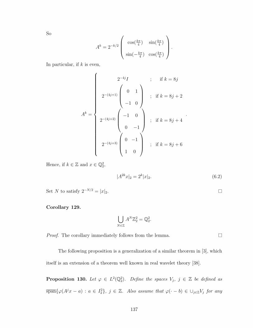
So
Ak = 2−k/2
cos(kπ4
) sin(kπ4
)
sin(−kπ4
) cos(kπ4
)
.
In particular, if k is even,
Ak =
2−4jI ; if k = 8j
2−(4j+1)
0 1
−1 0
; if k = 8j + 2
2−(4j+2)
−1 0
0 −1
; if k = 8j + 4
2−(4j+3)
0 −1
1 0
; if k = 8j + 6
.
Hence, if k ∈ Z and x ∈ Q22,
|A2kx|2 = 2k|x|2. (6.2)
Set N to satisfy 2−N/2 = |x|2.
Corollary 129. ⋃N∈Z
ANZ22 = Q2
2.
Proof. The corollary immediately follows from the lemma.
The following proposition is a generalization of a similar theorem in [3], which
itself is an extension of a theorem well known in real wavelet theory [38].
Proposition 130. Let ϕ ∈ L2(Q22). Define the spaces Vj, j ∈ Z be defined as
span{ϕ(Ajx − a) : a ∈ I22}, j ∈ Z. Also assume that ϕ(· − b) ∈ ∪j∈ZVj for any
137
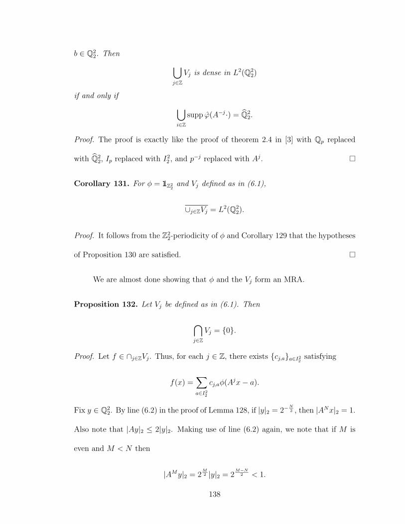
b ∈ Q22. Then ⋃
j∈Z
Vj is dense in L2(Q22)
if and only if ⋃i∈Z
supp ϕ(A−j·) = Q22.
Proof. The proof is exactly like the proof of theorem 2.4 in [3] with Qp replaced
with Q22, Ip replaced with I2
2 , and p−j replaced with Aj.
Corollary 131. For φ = 1Z22
and Vj defined as in (6.1),
∪j∈ZVj = L2(Q22).
Proof. It follows from the Z22-periodicity of φ and Corollary 129 that the hypotheses
of Proposition 130 are satisfied.
We are almost done showing that φ and the Vj form an MRA.
Proposition 132. Let Vj be defined as in (6.1). Then
⋂j∈Z
Vj = {0}.
Proof. Let f ∈ ∩j∈ZVj. Thus, for each j ∈ Z, there exists {cj,a}a∈I22 satisfying
f(x) =∑a∈I22
cj,aφ(Ajx− a).
Fix y ∈ Q22. By line (6.2) in the proof of Lemma 128, if |y|2 = 2−
N2 , then |ANx|2 = 1.
Also note that |Ay|2 ≤ 2|y|2. Making use of line (6.2) again, we note that if M is
even and M < N then
|AMy|2 = 2M2 |y|2 = 2
M−N2 < 1.
138
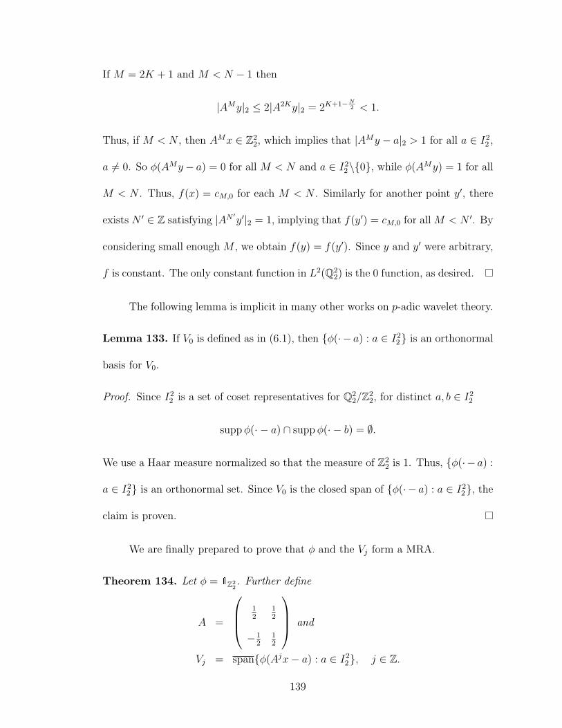
If M = 2K + 1 and M < N − 1 then
|AMy|2 ≤ 2|A2Ky|2 = 2K+1−N2 < 1.
Thus, if M < N , then AMx ∈ Z22, which implies that |AMy − a|2 > 1 for all a ∈ I2
2 ,
a 6= 0. So φ(AMy− a) = 0 for all M < N and a ∈ I22\{0}, while φ(AMy) = 1 for all
M < N . Thus, f(x) = cM,0 for each M < N . Similarly for another point y′, there
exists N ′ ∈ Z satisfying |AN ′y′|2 = 1, implying that f(y′) = cM,0 for all M < N ′. By
considering small enough M , we obtain f(y) = f(y′). Since y and y′ were arbitrary,
f is constant. The only constant function in L2(Q22) is the 0 function, as desired.
The following lemma is implicit in many other works on p-adic wavelet theory.
Lemma 133. If V0 is defined as in (6.1), then {φ(· − a) : a ∈ I22} is an orthonormal
basis for V0.
Proof. Since I22 is a set of coset representatives for Q2
2/Z22, for distinct a, b ∈ I2
2
suppφ(· − a) ∩ suppφ(· − b) = ∅.
We use a Haar measure normalized so that the measure of Z22 is 1. Thus, {φ(· − a) :
a ∈ I22} is an orthonormal set. Since V0 is the closed span of {φ(· − a) : a ∈ I2
2}, the
claim is proven.
We are finally prepared to prove that φ and the Vj form a MRA.
Theorem 134. Let φ = 1Z22. Further define
A =
12
12
−12
12
and
Vj = span{φ(Ajx− a) : a ∈ I22}, j ∈ Z.
139

Then {Vj} is a multiresolution analysis for L2(Q22) and φ is a scaling function for
this MRA.
Proof. Using the lettering from Definition 124, (a) follows from Proposition 127, (b)
follows from Corollary 131, (c) follows from Proposition 132, (d) follows from the
definition of the Vj and (e) follows from Lemma 133.
6.4 Wavelet construction
We define the function ψ(x) = φ(Ax)− φ(Ax−(
1/21/2
)). We would like to show
that ψ is a wavelet corresponding to the MRA in Theorem 134. We make note that
φ(Ax) =1
2(φ(x) + ψ(x)) (6.3)
φ(Ax−(
1/2
1/2
)) =
1
2(φ(x)− ψ(x)). (6.4)
Lemma 135. Let a, b ∈ I22 . If A(b− a) or A(b− a) +
(1/21/2
)is in Z2
2, then a = b.
Proof. If A(b − a) ∈ Z22 then b − a ∈ Z2
2 since A−1Z22 ⊂ Z2
2. As I22 is a set of coset
respresentativies of Q22/Z2
2, a = b. If
A(b− a) +
(1/2
1/2
)= A(b− a+
(1/2
1/2
)) ∈ Z2
2,
then b− a+(
01
)∈ Z2
2 and thus a = b.
We need to prove another lemma before proving the final theorem.
140

Lemma 136. Define
U1 = {Ab ∈ I22 : b ∈ I2
2},
U2 = {Ab+
(0
1
)∈ I2
2 : b ∈ I22},
U3 = {Ab+
(1/2
1/2
)∈ I2
2 : b ∈ I22}, and
U4 = {Ab+
(−1/2
1/2
)∈ I2
2 : b ∈ I22}.
Then I22 = U1 t U2 t U3 t U4.
Proof. We begin by making a comment about notation. For any prime p it is
impossible (see, for example [73]) to define a partial order structure on Qp such that
• 1 ≥ 0 ≥ −1,
• if a, b ≥ 0, then a+ b ≥ 0, and
• if an ≥ 0 for all n ∈ N and limn→∞ an = a, then a ≥ 0
all hold. However, in order to prove this lemma, we shall use the symbols “<”
and “≤.” When those symbols appear, they will be used between 2-adic numbers
which are also non-negative dyadic rational numbers. The symbols should then be
interpreted as coming from the canonical strict total and total orderings placed on
the non-negative dyadic rational numbers as a subset of the real numbers.
Assume that a =(a1
a2
)∈ I2
2 . We analyze when A−1a, A−1(a −(
01
)), A−1(a −(
1/21/2
)) and A−1(a−
(−1/21/2
)) lie in I2
2 .
A−1a =
(a1 − a2
a1 + a2
)
141

lies in I22 if and only if a2 ≤ a1 and 0 ≤ a1 + a2 < 1. Similarly,
A−1(a−(
0
1
)) =
(a1 − a2 + 1
a1 + a2 − 1
)lies in I2
2 if and only if a1 < a2 and 1 ≤ a1 + a2 < 2,
A−1(a−(
1/2
1/2
)) =
(a1 − a2
a1 + a2 − 1
)lies in I2
2 if and only if a2 ≤ a1 and 1 ≤ a1 + a2 < 2, and
A−1(a−(−1/2
1/2
)) =
(a1 − a2 + 1
a1 + a2
)lies in I2
2 if and only if a1 < a2 and 0 ≤ a1 + a2 < 1. Thus,
U1 = {a ∈ I22 : a2 ≤ a1 and 0 ≤ a1 + a2 < 1},
U2 = {a ∈ I22 : a1 < a2 and 1 ≤ a1 + a2 < 2},
U3 = {a ∈ I22 : a2 ≤ a1 and 1 ≤ a1 + a2 < 2}, and
U4 = {a ∈ I22 : a1 < a2 and 0 ≤ a1 + a2 < 1},
which implies that I22 = U1 t U2 t U3 t U4.
We introduce the following notation. Let
U1 = {b ∈ I22 : Ab ∈ U1},
U2 = {b ∈ I22 : Ab+
(0
1
)∈ U2},
U3 = {b ∈ I22 : Ab+
(1/2
1/2
)∈ U3}, and
U4 = {b ∈ I22 : Ab+
(−1/2
1/2
)∈ U4}.
Note that U1 ∩ U2, U3 ∩ U4 = ∅, but the other pairwise intersections are not empty.
Thus, unlike the Ui, the Ui are not disjoint. However,
I22 ⊂ U1 ∪ U2 ⊂ U1 ∪ U2 ∪ U3 ∪ U4. (6.5)
142

Theorem 137. ψ = φ(A·)−φ(A ·−(
1/21/2
)) is a wavelet corresponding to the MRA in
Theorem 134. That is, {ψ(·−a) : a ∈ I22} is an orthonormal basis for W0 = V1V0.
Proof. We first show that {ψ(· − a) : a ∈ I22} is an orthonormal set. We compute
for a, b ∈ I22 , using Z2
2-periodicity of φ,
2〈ψ(x− a), ψ(x− b)〉 = |detA|2〈ψ(x− a), ψ(x− b)〉
= | detA|2〈φ(Ax−Aa)− φ(Ax− (Aa+(
1/21/2
))), φ(Ax−Ab)− φ(Ax− (Ab+
(1/21/2
)))〉
= 〈φ(x−Aa), φ(x−Ab)− φ(x− (Ab+(
1/21/2
)))〉
+〈φ(x− (Aa+(
1/21/2
))),−φ(x−Ab) + φ(x− (Ab+
(1/21/2
)))〉
= 〈φ(x−Aa), φ(x−Ab)− φ(x− (Ab+(
1/21/2
))) + φ(x−Ab)− φ(x− (Ab+
(1/21/2
)))〉
= 2〈φ(x−Aa), φ(x−Ab)− φ(x− (Ab+(
1/21/2
)))〉
= 2〈φ(x), φ(x−A(b− a))− φ(x− (A(b− a) +(
1/21/2
)))〉
=
2 if b = a
0 if b 6= a
by Lemma 135. Hence {ψ(· − a) : a ∈ I22} is an orthonormal set. We now show that
ψ(x− a) ∈ V ⊥0 for each a ∈ I22 . We compute for a, b ∈ I2
2 , using the Z22-periodicity
of φ,
|detA|2〈ψ(x− a), φ(x− b)〉
= |detA|2〈φ(Ax−Aa)− φ(Ax− (Aa+(
1/21/2
))), φ(Ax−Ab) + φ(Ax− (Ab+
(1/21/2
)))〉
= 〈φ(x−Aa), φ(x−Ab) + φ(x− (Ab+(
1/21/2
)))〉
+〈φ(x− (Aa+(
1/21/2
))),−φ(x−Ab)− φ(x− (Ab+
(1/21/2
)))〉
= 〈φ(x−Aa), φ(x−Ab) + φ(x− (Ab+(
1/21/2
)))− φ(x−Ab)− φ(x− (Ab+
(1/21/2
)))〉
= 0,
143
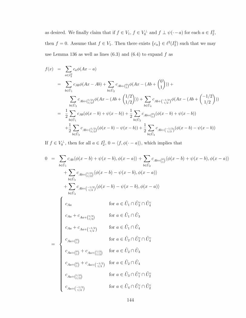
as desired. We finally claim that if f ∈ V1, f ∈ V ⊥0 and f ⊥ ψ(·−a) for each a ∈ I22 ,
then f = 0. Assume that f ∈ V1. Then there exists {ca} ∈ `2(I22 ) such that we may
use Lemma 136 as well as lines (6.3) and (6.4) to expand f as
f(x) =∑a∈I22
caφ(Ax− a)
=∑b∈U1
cAbφ(Ax−Ab) +∑b∈U2
cAb+(01)φ(Ax− (Ab+
(01
))) +
∑b∈U3
cAb+(1/2
1/2)φ(Ax− (Ab+
(1/21/2
))) +
∑b∈U4
cAb+(−1/2
1/2 )φ(Ax− (Ab+(−1/21/2
)))
=12
∑b∈U1
cAb(φ(x− b) + ψ(x− b)) +12
∑b∈U2
cAb+(01)
(φ(x− b) + ψ(x− b))
+12
∑b∈U3
cAb+(1/2
1/2)(φ(x− b)− ψ(x− b)) +
12
∑b∈U4
cAb+(−1/2
1/2 )(φ(x− b)− ψ(x− b))
If f ∈ V ⊥0 , then for all a ∈ I22 , 0 = 〈f, φ(· − a)〉, which implies that
0 =∑b∈U1
cAb〈φ(x− b) + ψ(x− b), φ(x− a)〉+∑b∈U2
cAb+(01)〈φ(x− b) + ψ(x− b), φ(x− a)〉
+∑b∈U3
cAb+(1/2
1/2)〈φ(x− b)− ψ(x− b), φ(x− a)〉
+∑b∈U4
cAb+(−1/2
1/2 )〈φ(x− b)− ψ(x− b), φ(x− a)〉
=
cAa for a ∈ U1 ∩ U c3 ∩ U c
4
cAa + cAa+(1/2
1/2)for a ∈ U1 ∩ U3
cAa + cAa+(−1/2
1/2 ) for a ∈ U1 ∩ U4
cAa+(01)
for a ∈ U2 ∩ U c3 ∩ U c
4
cAa+(01)
+ cAa+(1/2
1/2)for a ∈ U2 ∩ U3
cAa+(01)
+ cAa+(−1/2
1/2 ) for a ∈ U2 ∩ U4
cAa+(1/2
1/2)for a ∈ U3 ∩ U c
1 ∩ U c2
cAa+(−1/2
1/2 ) for a ∈ U4 ∩ U c1 ∩ U c
2
144
By line (6.5), these cases exhaust all of the a ∈ I22 . Hence,
f(x) =∑
b∈U1∩(U3∪U4)
cAbψ(x− b) +∑
b∈U2∩(U3∪U4)
cAb+(01)ψ(x− b).
If further, f ⊥ ψ(· − a) for all a ∈ I22 , then
0 =∑
b∈U1∩(U3∪U4)
cAb〈ψ(x− b), ψ(x− a)〉+∑
b∈U2∩(U3∪U4)
cAb+(01)〈ψ(x− b), ψ(x− a)〉
=
cAa for a ∈ U1 ∩ (U3 ∪ U4)
cAa+(01)
for a ∈ U2 ∩ (U3 ∪ U4)
.
Hence f is identically 0.
Thus, {DAnTaψ : n ∈ Z, a ∈ I22} is an orthonormal basis for L2(Q2
2) generated
by a single wavelet.
6.5 Future work
It has been proven that the Haar MRA is the only MRA that exists for L2(Qp)
under dilation by p ([3]). One possible choice for the scaling function of such an
MRA is 1Zp . The known MRAs for L2(Qkp) are tensor products of the 1-dimensional
systems. It follows from the definition of the Qkp metric that
⊗ki=1 1Zp = 1Zkp , which
for p = 2 and k = 2 was the scaling function used in this thesis. It remains to be
seen if there exists a p-adic MRA for which 1Zkp cannot be a scaling function. We
would like to construct MRAs using different dilations in order to try to answer this
problem.
Benedetto and Bendetto initiated the study of local field wavelet sets, which
included the construction of p-adic wavelet sets ([10], [15]). We are also interested in
145

constructing wavelet sets associated to this new dilation. Unlike in the real setting,
p-adic wavelet set wavelets are already “smooth,” so there is no need to smooth
them as we did in Chapters 2 and 3.
146

Bibliography
[1] H. A. Aimar, A. L. Bernardis, and O. P. Gorosito. Perturbations of the Haarwavelet by convolution. Proc. Amer. Math. Soc., 129(12):3619–3621 (elec-tronic), 2001.
[2] S. Albeverio, Yu Khrennikov, and V.M. Shelkovich. Harmonic analysis in the p-adic Lizorkin spaces: Fractional operators, pseudo-differential equations, p-adicwavelets, Tauberian theorems. Journal of Fourier Analysis and Applications,12(4):393–425, August 2006.
[3] S. Albeverio, S. Evdokimov, and M. Skopina. p-adic multiresolution analysisand wavelet frames. Preprint, 2008.
[4] Pascal Auscher. Solution of two problems on wavelets. J. Geom. Anal.,5(2):181–236, 1995.
[5] Lawrence Baggett, Palle Jorgensen, Kathy Merrill, and Judith Packer. A non-MRA Cr frame wavelet with rapid decay. Acta Appl. Math., 89(1-3):251–270(2006), 2006.
[6] Lawrence W. Baggett, Herbert A. Medina, and Kathy D. Merrill. Generalizedmulti-resolution analyses and a construction procedure for all wavelet sets inRn. J. Fourier Anal. Appl., 5(6):563–573, 1999.
[7] J. J. Benedetto and J. D. Kolesar. Geometric properties of Grassmannianframes for R2 and R3. EURASIP Journal on Applied Signal Processing, (49850),2006.
[8] J. J. Benedetto and M. Leon. The construction of single wavelets in D-dimensions. J. Geom. Anal., 11(1):1–15, 2001.
[9] John J. Benedetto. Harmonic analysis and applications. Studies in AdvancedMathematics. CRC Press, Boca Raton, FL, 1997.
[10] John J. Benedetto and Robert L. Benedetto. A wavelet theory for local fieldsand related groups. J. Geom. Anal., 14(3):423–456, 2004.
[11] John J. Benedetto and Emily J. King. Smooth functions associated with waveletsets on Rd , d ≥ 1, and frame bound gaps. Acta Applicandae Mathematicae:An International Survey Journal on Applying Mathematics and MathematicalApplications, 2009.
[12] John J. Benedetto and Manuel T. Leon. The construction of multiple dyadicminimally supported frequency wavelets on Rd. In The functional and har-monic analysis of wavelets and frames (San Antonio, TX, 1999), volume 247of Contemp. Math., pages 43–74. Amer. Math. Soc., Providence, RI, 1999.
147
[13] John J. Benedetto and Shidong Li. The theory of multiresolution analy-sis frames and applications to filter banks. Appl. Comput. Harmon. Anal.,5(4):389–427, 1998.
[14] John J. Benedetto and Songkiat Sumetkijakan. Tight frames and geometricproperties of wavelet sets. Adv. Comput. Math., 24(1-4):35–56, 2006.
[15] Robert L. Benedetto. Examples of wavelets for local fields. In Wavelets, framesand operator theory, volume 345 of Contemp. Math., pages 27–47. Amer. Math.Soc., Providence, RI, 2004.
[16] Jeffrey Blanchard. Minimally supported frequency composite dilation wavelets.Journal of Fourier Analysis and Applications. Preprint.
[17] R. P. Boas, Jr. A trigonometric moment problem. J. London Math. Soc.,14:242–244, 1939.
[18] R. P. Boas, Jr. Entire functions bounded on a line. Duke Math. J., 6:148–169,1940.
[19] Bernhard G. Bodmann. Optimal linear transmission by loss-insensitive packetencoding. Appl. Comput. Harmon. Anal., 22(3):274–285, 2007.
[20] Bernhard G. Bodmann and Vern I. Paulsen. Frames, graphs and erasures.Linear Algebra Appl., 404:118–146, 2005.
[21] Emmanuel J. Candes and Franck Guo. New multiscale transforms, minimumtotal variation synthesis: applications to edge-preserving image reconstruction.Signal Processing, 82(11):1519 – 1543, 2002.
[22] Peter G. Casazza and Gitta Kutyniok. Frames of subspaces. In Wavelets,frames and operator theory, volume 345 of Contemp. Math., pages 87–113.Amer. Math. Soc., Providence, RI, 2004.
[23] Peter G. Casazza, Gitta Kutyniok, and Shidong Li. Fusion frames and dis-tributed processing. Appl. Comput. Harmon. Anal., 25(1):114–132, 2008.
[24] Ole Christensen. An introduction to frames and Riesz bases. Applied andNumerical Harmonic Analysis. Birkhauser Boston Inc., Boston, MA, 2002.
[25] Ole Christensen and Christopher Heil. Perturbations of Banach frames andatomic decompositions. Math. Nachr., 185:33–47, 1997.
[26] Charles K. Chui and Xian Liang Shi. Bessel sequences and affine frames. Appl.Comput. Harmon. Anal., 1(1):29–49, 1993.
[27] Charles K. Chui and Xian Liang Shi. Inequalities of Littlewood-Paley type forframes and wavelets. SIAM J. Math. Anal., 24(1):263–277, 1993.
148
[28] E. Cordero, F. De Mari, K. Nowak, and A. Tabacco. Dimensional upper boundsfor admissible subgroups for the metaplectic representation. Math. Nach. (toappear).
[29] E. Cordero, F. De Mari, K. Nowak, and A. Tabacco. Reproducing groupsfor the metaplectic representation. In Pseudo-differential operators and relatedtopics, volume 164 of Oper. Theory Adv. Appl., pages 227–244. Birkhauser,Basel, 2006.
[30] Elena Cordero, Filippo De Mari, Krzysztof Nowak, and Anita Tabacco. An-alytic features of reproducing groups for the metaplectic representation. J.Fourier Anal. Appl., 12(2):157–180, 2006.
[31] Stephan Dahlke, Gabriele Steidl, and Gerd Teschke. The continuous shearlettransform in arbitrary space dimensions. In Stephan Dahlke, Ingrid Daubechies,Michal Elad, Gitta Kutyniok, and Gerd Teschke, editors, Structured Decomposi-tions and Efficient Algorithms, number 08492 in Dagstuhl Seminar Proceedings,Dagstuhl, Germany, 2009. Schloss Dagstuhl - Leibniz-Zentrum fuer Informatik,Germany.
[32] Stephan Dahlke and Gerd Teschke. The continuous shearlet transform in higherdimensions: variations of a theme. In Charles W. Danellis, editor, Group The-ory: Classes, Representation and Connections, and Applications, MathematicsResearch Developments. Nova Publishers, 2010.
[33] Xingde Dai and David R. Larson. Wandering vectors for unitary systems andorthogonal wavelets. Mem. Amer. Math. Soc., 134(640):viii+68, 1998.
[34] Xingde Dai, David R. Larson, and Darrin M. Speegle. Wavelet sets in Rn. J.Fourier Anal. Appl., 3(4):451–456, 1997.
[35] Xingde Dai, David R. Larson, and Darrin M. Speegle. Wavelet sets in Rn. II. InWavelets, multiwavelets, and their applications (San Diego, CA, 1997), volume216 of Contemp. Math., pages 15–40. Amer. Math. Soc., Providence, RI, 1998.
[36] Ingrid Daubechies. Ten lectures on wavelets, volume 61 of CBMS-NSF RegionalConference Series in Applied Mathematics. Society for Industrial and AppliedMathematics (SIAM), Philadelphia, PA, 1992.
[37] Ingrid Daubechies and Bin Han. The canonical dual frame of a wavelet frame.Appl. Comput. Harmon. Anal., 12(3):269–285, 2002.
[38] Carl de Boor, Ronald A. DeVore, and Amos Ron. On the construction ofmultivariate (pre)wavelets. Constr. Approx., 9(2-3):123–166, 1993.
[39] Filippo De Mari and Krzysztof Nowak. Analysis of the affine transformationsof the time-frequency plane. Bull. Austral. Math. Soc., 63(2):195–218, 2001.
149

[40] Filippo De Mari and Krzysztof Nowak. Canonical subgroups of H1 o SL(2,R).Boll. Unione Mat. Ital. Sez. B Artic. Ric. Mat. (8), 5(2):405–430, 2002.
[41] I. S. Dhillon, R. W. Heath, Jr., T. Strohmer, and J. A. Tropp. Constructingpackings in Grassmannian manifolds via alternating projection. Experiment.Math., 17(1):9–35, 2008.
[42] Minh N. Do and Martin Vetterli. Contourlets, volume 10 of Studies in Compu-tational Mathematics, pages 1–27. Academic Press/Elsevier Science, San Diego,CA, 2003.
[43] David L. Donoho. Wedgelets: nearly minimax estimation of edges. Ann.Statist., 27(3):859–897, 1999.
[44] B. Dragovich and A. Dragovich. A p-adic model of DNA sequence and geneticcode. eprint arXiv:q-bio/0607018, July 2006.
[45] R. J. Duffin and A. C. Schaeffer. A class of nonharmonic Fourier series. Trans.Amer. Math. Soc., 72:341–366, 1952.
[46] S. J. Favier and R. A. Zalik. On the stability of frames and Riesz bases. Appl.Comput. Harmon. Anal., 2(2):160–173, 1995.
[47] Gerald B. Folland. Harmonic analysis in phase space, volume 122 of Annals ofMathematics Studies. Princeton University Press, Princeton, NJ, 1989.
[48] Gerald B. Folland. Real analysis. Pure and Applied Mathematics (New York).John Wiley & Sons Inc., New York, second edition, 1999. Modern techniquesand their applications, A Wiley-Interscience Publication.
[49] P. Goupillaud, A. Grossmann, and J. Morlet. Cycle-octave and related trans-forms in seismic signal analysis. Geoexploration, 23(1):85 – 102, 1984. SeismicSignal Analysis and Discrimination III.
[50] N. K. Govil and R. A. Zalik. Perturbations of the Haar wavelet. Proc. Amer.Math. Soc., 125(11):3363–3370, 1997.
[51] Robert E. Greene and Steven G. Krantz. Function theory of one complex vari-able, volume 40 of Graduate Studies in Mathematics. American MathematicalSociety, Providence, RI, second edition, 2002.
[52] K. Grochenig and W. R. Madych. Multiresolution analysis, Haar bases, andself-similar tilings of Rn. IEEE Trans. Inform. Theory, 38(2, part 2):556–568,1992.
[53] Karlheinz Grochenig. Foundations of time-frequency analysis. Applied andNumerical Harmonic Analysis. Birkhauser Boston Inc., Boston, MA, 2001.
150

[54] Karlheinz Grochenig and Thomas Strohmer. Pseudodifferential operators onlocally compact abelian groups and Sjostrand’s symbol class. J. Reine Angew.Math., 613:121–146, 2007.
[55] A. Grossmann. Wavelet transforms and edge detection. In Stochastic processesin physics and engineering (Bielefeld, 1986), volume 42 of Math. Appl., pages149–157. Reidel, Dordrecht, 1988.
[56] A. Grossmann, M. Holschneider, R. Kronland-Martinet, and J. Morlet. Detec-tion of abrupt changes in sound signals with the help of wavelet transforms.In Inverse problems: an interdisciplinary study (Montpellier, 1986), Adv. Elec-tron. Electron Phys., Suppl. 19, pages 289–306. Academic Press, London, 1987.
[57] Kanghui Guo, Gitta Kutyniok, and Demetrio Labate. Sparse multidimensionalrepresentations using anisotropic dilation and shear operators. In Wavelets andsplines: Athens 2005, Mod. Methods Math., pages 189–201. Nashboro Press,Brentwood, TN, 2006.
[58] Kanghui Guo, Demetrio Labate, Wang-Q Lim, Guido Weiss, and Edward Wil-son. Wavelets with composite dilations. Electron. Res. Announc. Amer. Math.Soc., 10:78–87 (electronic), 2004.
[59] Alfred Haar. Zur Theorie der orthogonalen Funktionensysteme. PhD thesis,University of Gottingen, 1909.
[60] Alfred Haar. Zur Theorie der orthogonalen Funktionensysteme. Math. Ann.,69(3):331–371, 1910.
[61] J. Hadamard. Resolution d’une question relative aux determinants. Bull Sci-ences Math., 2(17):240–246, 1893.
[62] Bin Han. Wavelets. Master’s thesis, Academy of Sciences, China, 1994.
[63] Bin Han. On dual wavelet tight frames. Appl. Comput. Harmon. Anal.,4(4):380–413, 1997.
[64] Deguang Han. Interpolation operators associated with sub-frame sets. Proc.Amer. Math. Soc., 131(1):275–284 (electronic), 2003.
[65] Deguang Han and David R. Larson. Frames, bases and group representations.Mem. Amer. Math. Soc., 147(697), 2000.
[66] Christopher Heil and David F. Walnut, editors. Fundamental papers in wavelettheory. Princeton University Press, Princeton, NJ, 2006.
[67] Christopher E. Heil and David F. Walnut. Continuous and discrete wavelettransforms. SIAM Rev., 31(4):628–666, 1989.
[68] Kurt Hensel. Uber eine neue Begrundung der Theorie der algebraischen Zahlen.Jahresbericht der Deutschen Mathematiker-Vereinigung, 6(3):83–88, 1897.
151
[69] Eugenio Hernandez, Xihua Wang, and Guido Weiss. Smoothing minimallysupported frequency wavelets. I. J. Fourier Anal. Appl., 2(4):329–340, 1996.
[70] Eugenio Hernandez, Xihua Wang, and Guido Weiss. Smoothing minimallysupported frequency wavelets. II. J. Fourier Anal. Appl., 3(1):23–41, 1997.
[71] K. J. Horadam. Hadamard matrices and their applications. Princeton Univer-sity Press, Princeton, NJ, 2007.
[72] Zhang Jing. On the stability of wavelet and Gabor frames (Riesz bases). J.Fourier Anal. Appl., 5(1):105–125, 1999.
[73] Andrei Khrennikov. p-adic valued distributions in mathematical physics, volume309 of Mathematics and its Applications. Kluwer Academic Publishers Group,Dordrecht, 1994.
[74] Helmut Koch. Number theory, volume 24 of Graduate Studies in Mathematics.American Mathematical Society, Providence, RI, 2000. Algebraic numbers andfunctions, Translated from the 1997 German original by David Kramer.
[75] Jelena Kovecec and Martin Vetterli. Wavelets and Subband Cod-ing. Prentice Hall PTR, 1995. Now available online for free athttp://www.waveletsandsubbandcoding.org/.
[76] S. V. Kozyrev. Wavelet theory as p-adic spectral analysis. Izv. Ross. Akad.Nauk Ser. Mat., 66(2):149–158, 2002.
[77] Gitta Kutyniok, Ali Pezeshki, Robert Calderbank, and Taotao Liu. Robust di-mension reduction, fusion frames, and Grassmannian packings. Appl. Comput.Harmon. Anal., 26(1):64–76, 2009.
[78] Gitta Kutyniok and Tomas Sauer. Adaptive directional subdivisionschemes and shearlet multiresolution analysis, 2007. Accessed athttp://www.citebase.org/abstract?id=oai:arXiv.org:0710.2678.
[79] Gitta Kutyniok and Tomas Sauer. From wavelets to shearlets and back again.In M Neamtu and L.L. Schumaker, editors, Approximation Theory XII: SanAntonio, 2007, 2008.
[80] Demetrio Labate, Wang-Q Lim, Gitta Kutyniok, and Guido Weiss. Sparse mul-tidimensional representation using shearlets. SPIE Proc. 5914, SPIE, Belling-ham, pages 254–262, 2005.
[81] John M. Lee. Introduction to smooth manifolds, volume 218 of Graduate Textsin Mathematics. Springer-Verlag, New York, 2003.
[82] Wally R. Madych. Some elementary properties of multiresolution analyses ofL2(Rn). In Wavelets, volume 2 of Wavelet Anal. Appl., pages 259–294. Aca-demic Press, Boston, MA, 1992.
152
[83] S. Mallat. Multiresolution representation and wavelets. PhD thesis, Universityof Pennsylvania, 1988.
[84] Kathy D. Merrill. Simple wavelet sets for integral dilations in R2. In Palle E.T.Jorgensen, Kathy D. Merrill, and Judith A. Packer, editors, Representations,Wavelets, and Frames: A Celebration of the Mathematical Work of LawrenceW. Baggett, Applied and Numerical Harmonic Analysis. Birkhauser, Boston,MA, 2008.
[85] Y. Meyer. Ondelettes et fonctions splines. In Seminaire sur les equationsaux derivees partielles 1986–1987, pages Exp. No. VI, 18. Ecole Polytech.,Palaiseau, 1987.
[86] Yves Meyer. Ondelettes et operateurs. I - III. Actualites Mathematiques.[Current Mathematical Topics]. Hermann, Paris, 1990.
[87] F. Natterer. The mathematics of computerized tomography, volume 32 of Clas-sics in Applied Mathematics. Society for Industrial and Applied Mathematics(SIAM), Philadelphia, PA, 2001. Reprint of the 1986 original.
[88] Raymond E. A. C. Paley and Norbert Wiener. Fourier transforms in the com-plex domain, volume 19 of American Mathematical Society Colloquium Publi-cations. American Mathematical Society, Providence, RI, 1987. Reprint of the1934 original.
[89] E. Le Pennec and S. Mallat. Bandelet image approximation and compression.SIAM Journal of Multiscale Modeling and Simulation, 4:2005, 2005.
[90] Hans Reiter and Jan D. Stegeman. Classical harmonic analysis and locallycompact groups, volume 22 of London Mathematical Society Monographs. NewSeries. The Clarendon Press Oxford University Press, New York, second edi-tion, 2000.
[91] C.J. Rozell, I.N. Goodman, and D.H. Johnson. Feature-based information pro-cessing with selective attention. In Acoustics, Speech and Signal Processing,2006. ICASSP 2006 Proceedings. 2006 IEEE International Conference on, vol-ume 4. IEEE, 2006.
[92] Vladimir Shelkovich and Maria Skopina. p-adic Haar multiresolution analysisand pseudo-differential operators. Journal of Fourier Analysis and Applications.Preprint.
[93] Paolo M. Soardi and David Weiland. Single wavelets in n-dimensions. J. FourierAnal. Appl., 4(3):299–315, 1998.
[94] Elias M. Stein and Guido Weiss. Introduction to Fourier analysis on Euclideanspaces. Princeton University Press, Princeton, N.J., 1971. Princeton Mathe-matical Series, No. 32.
153
[95] Robert S. Strichartz. How to make wavelets. Amer. Math. Monthly, 100(6):539–556, 1993.
[96] Thomas Strohmer and Robert W. Heath, Jr. Grassmannian frames withapplications to coding and communication. Appl. Comput. Harmon. Anal.,14(3):257–275, 2003.
[97] J.J. Sylvester. Thoughts on inverse orthogonal matrices, simultaneous signsuccessions and tesselated pavements in two or more colors, with applicationto Newton’s rule, ornamental tile work and the theory of numbers. Phil. Mag.,(34):461–475, 1867.
[98] Vladimir Zakharov. Nonseparable multidimensional Littlewood-Paley likewavelet bases. Preprint, 1996.
154
Related Documents