A Variation on the Luenberger Shortage Function

Single-Period Markowitz Portfolio Selection,

Performance Gauging, and Duality: A Variation

on the Luenberger Shortage Function1

W. BRIEC,2 K. KERSTENS,3 AND J. B. LESOURD4

Communicated by D. G. Luenberger

Abstract. The Markowitz portfolio theory (Ref. 1) has stimulated

research into the efficiency of portfolio management. This paper studies

existing nonparametric efficiency measurement approaches for single-

period portfolio selection from a theoretical perspective and generalizes

currently used efficiency measures into the full mean-variance space. We

introduce the efficiency improvement possibility function (a variation on

the shortage function), study its axiomatic properties in the context of

the Markowitz efficient frontier, and establish a link to the indirect

mean-variance utility function. This framework allows distinguishing

between portfolio efficiency and allocative efficiency; furthermore, it

permits retrieving information about the revealed risk aversion of in-

vestors. The efficiency improvement possibility function provides a more

general framework for gauging the efficiency of portfolio management

using nonparametric frontier envelopment methods based on quadratic

optimization.

Key Words. Shortage function, efficient frontier, risk aversion, mean-

variance portfolios.

1. Introduction

Markowitz (Ref. 1) seminal work on modern portfolio theory intro-

duced the idea of a tradeoff between risk and expected return of a portfolio;

1The authors are grateful for comments made by E. Clark, A. Coen, H. Malloch, and an

anonymous referee.2Maıtre de Conferences, JEREM, Universite de Perpignan, Perpignan, France.3Charge de Recherche, CNRS-LABORES, URA 362, IESEG, Lille, France.4Directeur de Recherche, GREQAM-CNRS, UMR 6579, Universite de la Mediterranee,

Aix-Marseille, France.

JOURNAL OF OPTIMIZATION THEORY AND APPLICATIONS: Vol. 120, No. 1, pp. 1–27, January 2004 (g2004)

1

0022-3239=04=0100-0001=0 g 2004 Plenum Publishing Corporation

and defined an efficient frontier concept as a Pareto-optimal subset of port-

folios, that is, portfolios whose expected returns may not increase unless

their variances increase. In addition to its strongly maintained assumptions

on probability distributions and Von Neumann-Morgenstern utility func-

tions, the main problem at the time was the computational cost of solving

quadratic programs. Farrar (Ref. 2) was apparently the first to test empiri-

cally the full-covariance Markowitz model, while computing costs motivated

Sharpe (Ref. 3) to formulate a simplified diagonal model. Later, Sharpe

(Ref. 4) and Lintner (Ref. 5) introduced the capital asset pricing model

(CAPM), an equilibrium model assuming that all agents have similar

expectations about the market. Under these circumstances, it is not necessary

to compute the efficient frontier. Historical surveys of these developments

are e.g. Constantinides and Malliaris (Ref. 6) and Philippatos (Ref. 7). Tools

for gauging portfolio efficiency, such as the Sharpe (Ref. 8) and Treynor

(Ref. 9) ratios and the Jensen (Ref. 10) alpha, have been developed mainly

with reference to these developments (in particular CAPM). Surveys on

measuring the performance of managed portfolios are found in Grinblatt

and Titman (Ref. 11) or Shukla and Trzcinka (Ref. 12).

Despite these enhancements, the static Markowitz model remains the

more general framework. Our contribution integrates an efficiency measure

into this single-period Markowitz model and develops a dual framework for

assessing the degree of satisfaction of the investors preferences, starting from

the seemingly forgotten ideas advanced by Farrar (Ref. 2). This leads to

decomposing the portfolio performance into allocative and portfolio effi-

ciency components. In addition, this duality offers information about the

investors risk aversion via the shadow prices associated with the specific

efficiency measure. This is an issue of great practical significance that, to the

best of our knowledge, is novel. An empirical application is included to

illustrate the potentials of the proposed framework.

There are both theoretical and practical motivations guiding these

developments. Theoretically, this contribution brings portfolio theory in line

with developments in production theory, where distance functions have

proven to be useful tools to derive efficiency measures and to develop dual,

relations with economic (e.g. profit) support functions [Chambers, Chung,

and Fare (Ref. 13)]. From a practical viewpoint, there are the following

advantages. First, the integration of efficiency measures responds to the

needs for portfolio rating tools. Second, instead of tracing the whole efficient

portfolio frontier using a critical line search method, each asset or fund is

projected onto the relevant part of the frontier according to a meaningful

efficiency measure. This may lead to computational gains, depending on

the number of assets or funds to evaluate and the aimed fineness of the port-

folio frontier representation. Third, the possibility of measuring portfolio

2 JOTA: VOL. 120, NO. 1, JANUARY 2004

performance using a dual approach permits not only gauging assets or funds

using given information about risk aversion, but it reveals also the (shadow)

risk aversion minimizing portfolio inefficiency. In these ways, the contribu-

tion enriches the empirical toolbox of practitioners.

A variation of the shortage function is introduced, a distance function

proposed in production theory by Luenberger (Ref. 14) that is dual to

the profit function. This function accomplishes four goals: (i) it gauges port-

folio performance by measuring a distance between a portfolio and an opti-

mal portfolio projection on the Markowitz efficient frontier; (ii) it leads to a

nonparametric estimation of an inner bound of the true but unknown port-

folio frontier; (iii) it judges simultaneously mean-return expansions and risk

contractions and thereby generalizes existing approaches; and (iv) it provides

a new, dual interpretation of our portfolio efficiency distance. Given the in-

vestment context, this efficiency measure is called the efficiency improvement

possibility (EIP) function.

To develop point (iv), the paper establishes a link between the EIP

function and mean-variance utility functions, thereby offering an integrated

framework for assessing portfolio efficiency from the dual standpoint. To

each efficient portfolio, there corresponds a particular utility function, whose

optimal value is the indirect utility function. This approach provides a dual

interpretation of the EIP function through the structure of risk preferences.

Technically, this result is derived easily from Luenberger (Ref. 14–15). Along

this line, a link is established to some kind of Slutsky matrix, defined as a

matrix of derivatives with respect to risk aversion (based on the structure of

the mean-variance utility function).

To situate the results more precisely, it is possible to distinguish between

several approaches for testing portfolio efficiency. It is common to develop

statistical tests based on certain parametric distributional assumptions [e.g.

Jobson and Korkie (Ref. 16), Gourieroux and Jouneau (Ref. 17), Philippatos

(Ref. 7)]. However, from the outset [Markowitz (Ref. 1)], there has been

attention also to simple nonparametric approaches to test for portfolio effi-

ciency. This work is best contrasted with some recent developments in the

nonparametric test tradition which uses economic restrictions [Matzkin

(Ref. 18)]. Varian (Ref. 19) develops nonstatistical tests checking whether the

observed investments are consistent with the expected utility and the mean-

variance models. However, his formulation can infer only whether or not

certain data are consistent with the tested hypothesis, but lacks an indication

about the degree of goodness of fit between data and models.5 Sengupta

(Ref. 20) is probably the first to link the Varian (Ref. 19) portfolio test

5In this respect, it is similar to the early nonparametric test literature on production [Diewert and

Parkan (Ref. 22)] and consumption [Varian (Ref. 23)].

JOTA: VOL. 120, NO. 1, JANUARY 2004 3

approach to the nonparametric efficiency literature by introducing explicitly

an efficiency measure.6 Morey and Morey (Ref. 21) measure investment fund

performance focusing on radial potentials for either risk contraction or

mean-return expansion. By contrast, the approach in this article looks sim-

ultaneously for risk contraction and mean-return augmentation.

Among the advantages of a nonparametric approach to production,7

consumption and investment, one can mention: (i) it avoids postulating

specific functional forms, (ii) it uses revealed preference conditions of some

sort that are finite in nature and that are directly tested on a finite number of

observations, (iii) it determines inner and outer approximations of choice

sets that contain the true but unknown frontier, (iv) these approximations

are based on (most frequently piecewise linear) functions that are spanned

directly by the observations in the sample, (v) the computational cost is low,

often just solving mathematical programming problems [e.g. Matzkin

(Ref. 18), Morey and Morey (Ref. 21), Varian (Ref. 19)].

Section 2 of the article lays down the foundations of the analysis.

Section 3 introduces the EIP function and studies its axiomatic properties.

Section 4 studies the link between the EIP function and the direct and

indirect mean-variance utility functions. Section 5 presents mathematical

programs to compute the efficiency decomposition. A simple empirical illu-

stration using a small sample of 26 investment funds is provided in Section 6.

Conclusions and possible extensions are formulated in Section 7.

2. Efficient Frontier and Portfolio Management

In developing the basic definitions, consider the problem of selecting a

portfolio (or fund of funds) from n financial assets (or funds). Assets are

characterized by an expected return E(Ri), i = 1, . . . , n, since returns of assets

are correlated by a covariance matrix Wi, j =Cov(Ri, Rj), i, j˛{1, . . . , n}. A

portfolio x is composed by a proportion of each of these n financial assets.

Thus, one can define x = (x1, . . . , xn), with �i=1,..., n xi = 1. The condition xi$0

is imposed whenever short sales are excluded.

6Fare and Grosskopf (Ref. 24) link the literature on regularity tests and the efficiency con-

tributions employing distance functions (or their inverses, efficiency measures) as an explicit

(nonstatistical) goodness of the fit indicator.7Aside from the investment context, the estimation of monotone concave boundaries is exten-

sively studied in production. Following Farrell (Ref. 25), nonparametric efficiency methods

estimate an inner bound approximation of the true, unknown production frontier using

piecewise linear envelopments of the data, instead of traditional parametric, econometric esti-

mation methods that suffer from the risk of specification error.


Decision makers face often additional economic constraints [see, e.g.,

Pogue (Ref. 26) or Rudd and Rosenberg (Ref. 27)]. For instance, the pro-

portion of each of the n financial assets composing a portfolio can be mod-

ified by taking into account transaction costs or by imposing upper limits on

any fraction invested. If these constraints are linear functions of the asset

weights, then the set of admissible portfolios is defined as

I = x˛Rn; �i=1... n

xi = 1, Ax#b, x$0

� �, (1)

where A is a m·n matrix and b˛Rm. It is assumed throughout the paper that

I„;.The return of portfolio x is

R(x) = �i=1,..., n

xiRi:

The expected return and its variance can be calculated as follows:

E(R(x))= �i=1,..., n

xiE(Ri), (2)

V (R(x))= �i, j

xixj Cov(Ri, Rj): (3)

It is useful to define the mean-variance representation of the set I of port-

folios. From Markowitz (Ref. 1), it is straightforward to give the following

definition:

@ = {(V (R(x)), E(R(x))); x˛I}: (4)

However, such a representation cannot be used for quadratic programming,

because the subset @ is not convex [see for instance Luenberger (Ref. 28)].

Thus, the above set can be extended by defining a mean-variance (portfolio)

representation set through

< = {@ + (R+ · (–R+))}˙R2+ : (5)

This set can be rewritten as follows:

< = {(V ¢, E¢)˛R2+;9x˛I, ( –V ¢, E¢)# (–V (R(x)), E(R(x)))}: (6)

The addition of the cone is necessary for the definition of a sort of ‘‘free

disposal hull’’ of the mean-variance representation of feasible portfolios.

Clearly, the above definition is compatible with the definition in Markowitz

(Ref. 1). To measure the degree of portfolio efficiency, it is necessary to

isolate a subset of this representation set, generally known as the efficient

frontier. This subset is defined as follows.


Definition 2.1. In the mean-variance space, the weakly efficient frontier

is defined as

¶M(I) = {(V (R(x)), E(R(x)));

x˛I ^ (–V (R(x)), E(R(x)))< ( –V ¢, E¢)�(V ¢, E¢)ˇ<}:

From the above definition, the weakly efficient frontier is the set of

all the mean-variance points that are not strictly dominated in the two-

dimensional space. It is possible also to define a strongly efficient frontier, but

the above formulation simplifies most results in this contribution. Moreover,

the geometric representation of the frontier (see Figure 1) is quite similar,

except for some rather special cases.

The above definition enables us to define the set of weakly efficient

portfolios.

Definition 2.2. The set of the weakly efficient portfolios is defined in

the simplex as

LM(I)= {x˛I; (V (R(x)), E(R(x)))˛¶M(I)}:

Markowitz (Ref. 29) defines an optimization program to determine the

portfolio corresponding to a given degree of risk aversion. This portfolio

maximizes a mean-variance utility function defined by

U(r, m)(x) = mE(R(x)) – rV (R(x)), (7)

where m$0 and r$0. This utility function satisfies positive marginal utility

of expected return and negative marginal utility of risk. The quadratic opti-

mization program may be simply written as follows:

max U(r, m)(x) = mE(R(x)) – rV (R(x)), (8a)

s:t: Ax#b, (8b)

�i=1,... , n

xi = 1, x$0: (8c)

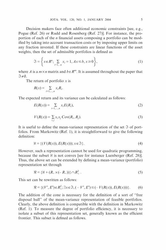
Fig. 1. Finding the optimal portfolio.


Traditionally, the ratio j = r=m [0,+O] represents the degree of absolute

risk aversion.

Setting m = 0 and r= 1 eliminates the return information from this

quadratic mathematical program and yields the efficient portfolio with

minimum risk. Denoting this global minimum-variance portfolio x, it can be

represented in the two-dimensional mean-variance space as (see Figure 1)

(V,R) = (V (R(x)), E(R(x))):

When shorting is allowed or there is a riskless asset with zero variance

and nonzero positive return, then from the two-fund theorem and the one-

fund theorem, the efficient frontier is determined by simple analytical solu-

tions [e.g. Elton, Gruber, and Padberg (Ref. 30), or Luenberger (Ref. 28)].

Though the computational burden of the more general quadratic program-

ming approach remains substantial, when building realistic portfolio models

it is hard to avoid. The approach developed in Section 3 adheres to this

quadratic programming tradition to maintain generality. To extend the well-

known Markowitz approach, Section 3 introduces the EIP function of a

portfolio as an indicator of its performance. This EIP function is similar to

the shortage function [see Luenberger (Ref. 14)].

3. Efficiency Improvement Possibility Function and the Frontier of Efficient

Portfolios

Intuitively stated, the shortage function in production theory measures

the distance between some point of the production set and the Pareto fron-

tier. Before introducing this function formally in a portfolio context, it is of

interest to focus on the basic properties of the subset < on which the shortage

function is defined below.

Proposition 3.1. The subset < satisfies the following properties:

(i) < is a convex set.

(ii) < is a closed set.

(iii) 8(V, E )˛<,(–V ¢, E ¢ )$0 and (–V ¢, E ¢ )# (–V, E )� (V ¢, E ¢) ˛<.

Proof.

(i) From equation (6), one obtains immediately

< = {(V ¢, E¢)˛R2+;9x˛I, (–V ¢, E¢)# (–V (R(x)), E(R(x)))}:

Assume that (V1, E1) and (V2, E2)˛<. Thus, one can deduce that there exists

x1, x2˛I such that

(–V1, E1)# (–V (R(x1)), E(R(x1)))


and

(–V2, E2)# (–V (R(x2)), E(R(x2)))˛<:

Let us show that

q(V1, E1) + (1 – q)(V2, E2)˛<, 8q [0, 1]:

Since V(R(.)) is a convex function, one gets immediately the inequality

qV1 + (1 – q)V2$q(V (R(x1))) + (1 – q)(V (R(x2)))$V (R(qx1 + (1 – q)x2)):

Moreover, we have

qE1 + (1 – q)E2#E(R(qx1 + (1 – q)x2)):

Thus, since

{x˛Rn;Ax#b, �i=1,..., n

xi = 1, xi$0}

is a convex set, there exists

x= qx1 + (1 – q)x2˛I

such that

(–V (R(x)), E(R(x)))$q(–V 1, E1) + (1 – q)(–V 2, E2):

From the expression (6), this implies

q(–V 1, E1) + (1 – q)(–V 2, E2)˛<

and (i) is proven.

(ii) The functions V(R(.)) and E(R(.)) are continuous with respect to

x; thus, @ is a closed set. Using the result in Briec and Lesourd (Ref. 31), we

get that {@ + (R+· ( –R+))} is closed and obviously (ii) holds.

(iii) From equation (6), the fact that

8(V , E)˛@, (–V ¢, E¢)# (–V , E)� (V ¢, E¢)˛<

and (iii) can be deduced. u

From the above properties of the representation set, it is possible now to

define the notion of an efficiency measure in the specific context of the

Markowitz portfolio theory. Before introducing our own approach, existing

efficiency measures in the context of portfolio benchmarking are briefly

reviewed.

The first measure, introduced by Morey and Morey (Ref. 21), computes

the maximum expansion of the mean return while the risk is fixed at its

current level [this also seems the approach taken by Sengupta (Ref. 20)].


From our definition of the representation set, this mean-return expansion

function is defined by

DMRE(x) = sup{q ; (V (R(x)), qE(R(x)))˛<}: (9)

In a similar vein, the same authors define a risk contraction function as

follows:

DRC(x) = inf{l; (lV (R(x)), E(R(x)))˛<}: (10)

This function measures the maximum proportionate reduction of risk while

fixing the mean-return level. These authors apply these functions to measure

investment fund performance.

Now, the shortage function [Luenberger (Ref. 14)] is introduced and its

properties are studied in the context of the Markowitz portfolio theory. It is

shown below (see Proposition 3.2) that it encompasses the functions (9) and

(10) as special cases. To achieve this objective, we introduce the efficiency

improvement possibility (EIP) function defined as follows.

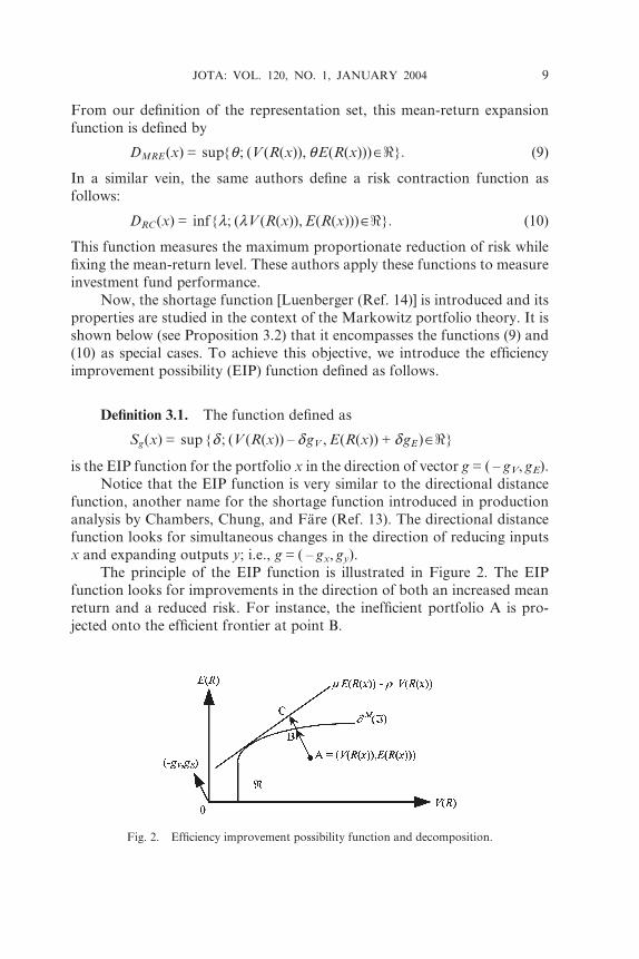
Definition 3.1. The function defined as

Sg(x) = sup {d ; (V (R(x)) – dgV , E(R(x))+ dgE)˛<}

is the EIP function for the portfolio x in the direction of vector g = ( – gV, gE).

Notice that the EIP function is very similar to the directional distance

function, another name for the shortage function introduced in production

analysis by Chambers, Chung, and Fare (Ref. 13). The directional distance

function looks for simultaneous changes in the direction of reducing inputs

x and expanding outputs y; i.e., g = ( – gx, gy).

The principle of the EIP function is illustrated in Figure 2. The EIP

function looks for improvements in the direction of both an increased mean

return and a reduced risk. For instance, the inefficient portfolio A is pro-

jected onto the efficient frontier at point B.

Fig. 2. Efficiency improvement possibility function and decomposition.


The pertinence of the EIP function as a portfolio management efficiency

indicator results from some of its elementary properties, as summarized in

the following proposition.

Proposition 3.2. Let Sg be the EIP function defined on I. Sg has the

following properties:

(i) x˛I�Sg(x)< +O.

(ii) If (gV, gE) >0, then Sg(x) = 0�x˛¶M(I) (weak efficiency).

(iii) 8x, y˛I, (–V(R(y)), E(R(y)))# (–V(R(x)), E(R(x)))�Sg(x)#Sg(y)

(weak monotonicity on @).

(iv) Sg is continuous on I.

(v) If gV = –V(R(x)) and gR = 0, then DRC (x) = 1 – Sg(x).

(vi) If (gV, gE) >0 and gR = E(R(x)), then DMRE (x)= 1 + Sg(x).

Proof.

(i) From the definition of the representation set, if x˛I, then the

subset

C(x) = {(V ¢, E¢)˛<; (V ¢, – E¢)# (V (R(x)), – E(R(x)))}

is bounded. It follows trivially that Sg(x)<+O.

(ii) Assume that xˇLM(I). In such a case, there exists some

(V ¢, E ¢)˛< such that

(–V ¢, E¢)$ (–V (R(x)), E(R(x))):

But, from Definition 3.1, it follows immediately that

Sg(x)>0:

Consequently, it can be deduced that

Sg(x) = 0�x˛LM(I):

To prove the converse, let

(V (R(x)) – Sg(x)gV , E(R(x))+ Sg(x)gE):

Assume that Sg(x) >0. Since (gV, gE) >0, we get

(–V (R(x)) + Sg(x)gV , E(R(x)) + Sg(x)gE)> (–V (R(x)), E(R(x))):

It can be deduced immediately that xˇLM(I) and (ii) holds.

(iii) This follows from Luenberger (Ref. 14).

(iv) Let the function T: <fiR+ be defined by

T(V , E) = sup {d ; (V – dgV , E + dgE)˛<}:


Since < is convex and satisfies the free disposal rule, it is easy to show

the continuity of T. Moreover, since mean and variance are continuous

functions with respect to x, (iv) holds.

(v) and (vi) result from making some obvious changes [see e.g.

Chambers, Chung, and Fare (Ref. 13)]. u

Briefly commenting on these properties, the use of the EIP function

guarantees only weak efficiency. It does not exclude projections on vertical

parts of the frontier allowing for an additional expansion in terms of the

expected return. Furthermore, portfolios with weakly dominated risk and

return characteristics are classified only as weakly less efficient. Finally, the

last two parts establish clearly a link with the Morey and Morey (Ref. 21)

single-dimension efficiency measurement orientations in (9) and (10). Im-

plementing some obvious changes, a simple proof for these links is straight-

forwardly derived for instance from Chambers, Chung, and Fare (Ref. 13).

Section 4 studies the EIP function from a duality standpoint.

4. Duality, Shadow Risk Aversion, and Mean-Variance Utility

Markowitz (Ref. 29) conceived portfolio selection as a two-step proce-

dure, whereby the reconstruction of the efficient set of portfolios in a first

step is followed subsequently by picking the optimal portfolio for a given

preference structure. To provide a dual interpretation of the EIP function,

the indirect mean-variance utility function must be defined first [see e.g.

Farrar (Ref. 2) or Philippatos (Ref. 7)].

Definition 4.1. For given parameters (r,m), the function defined as

U*(m, r) = sup mE(R(x)) – rV (R(x)),

s:t: Ax#b,

�i=1,..., n

xi = 1, x$0,

is called the indirect mean-variance utility function.

Therefore, the maximum value function for the decision maker is simply

determined for a given set of parameters (r,m) representing his or her risk

aversion. Knowledge of these parameters allows selecting a unique efficient

portfolio among those on the weakly efficient frontier maximizing the deci-

sion maker direct mean-variance utility function. Furthermore, Farrar

(Ref. 2) suggested to trace the set of efficient portfolios by solving this dual

problem for different sets of parameters (r,m).


More elaborate dual frameworks exist in the literature. For instance,

Varian (Ref. 19) describes nonparametric test procedures verifying whether

or not a suitable mean-variance utility function rationalizes the observed

portfolio choices and asset prices. This contribution adheres to the pre-

viously mentioned tradition and does not depend on asset price information.

To grasp duality in our framework, it is useful to distinguish between

overall, allocative, and portfolio efficiency when evaluating the scope for

improvements in portfolio management. The following definition clearly dis-

tinguishes between these concepts.

Definition 4.2. Let Sg be the EIP function defined on I.

(i) The overall efficiency (OE) index is the quantity

OE(x, r,m)= sup{d ;m(E(R(x))+ dgE) – r(V (R(x)) – dgV )

#U*(r,m)}:

(ii) The allocative efficiency (AE) index is the quantity

AE(x, r,m) =OE(x, r,m) – Sg(x):

(iii) The portfolio efficiency (PE) index is the quantity

PE(x) = Sg(x):

This definition implies immediately

OE(x, r,m) = [U*(r,m) –U(r, m)(x)]=(rgV + mgE): (11)

Thus, overall efficiency (OE) is simply the ratio between (a) the difference

between (maximum) indirect mean-variance utility (Definition 4.1) and the

value of the direct mean-variance utility function for the observation eval-

uated and (b) the normalized value of the direction vector g = ( – gV, gE) for

the given parameters (r,m).

Expanding on the decomposition introduced in Definition 4.2, portfolio

efficiency (PE) guarantees only reaching a point on the portfolio frontier, not

necessarily a point on the frontier maximizing the investor indirect mean-

variance utility function. In this sense, it is similar to the notion of technical

efficiency in production theory. Allocative efficiency (AE), by contrast,

measures the needed portfolio reallocation, along the portfolio frontier, to

achieve the maximum of the indirect mean-variance utility function. This

requires adjusting an eventual portfolio efficient portfolio in function of

relative prices, that is, the parameters of the mean-variance utility function.

Overall efficiency ensures that both these ideals are achieved simultaneously.


Obviously, the following additive decomposition identity holds:

OE(x, r,m)=AE(x, r,m) + PE(x) (12)

Notice that changes in the risk-aversion parameters (r,m) alter the slope

of the indirect utility function. While the amount of PE is invariant to these

changes, the relative importance of AE and OE normally changes.

In Figure 2, this decomposition is illustrated for a portfolio denoted by

point A. For simplicity, assume that

kgk = k(– gV , gE)k = 1,

where k.k is the usual Euclidean metric. In terms of this figure, it is easy to

see that

OE = kC –Ak, PE = kB –Ak, AE = kC – Bk:

The indirect mean-variance utility function turns out to be a useful tool

to characterize the representation set <. In particular, by using duality, one

can state the following property.

Proposition 4.1. The representation set < admits the following dual

characterization:

< = {(V , E)˛R2;mE – rV #U*(r,m)}˙R2+:

Proof. By definition,

< = {@ + (R+ · (–R+))}˙R2+:

However, if (r,m)ˇR+2 , then

sup {U(r,m)(x); (V (R(x)), E(R(x)))˛@+ (R+ · (–R+))} = +O:

Since for any mean-variance vector, we have

(V ,E)˛@+ (R+ · (–R+)),

it can be deduced that

U*(r,m)$mE – rV :

Now, assume that

(V ,E)ˇ<:

From Proposition 3.1, < is convex. From the separation theorem, there

exists (r,m)˛R+2 such that

mE – rV >U*(r,m):


Consequently,

U*(r,m)$mE – rV

implies

(V , E)˛<

and Proposition 4.1 follows. u

Proposition 4.1 prepares the link between the shortage function and the

indirect utility function in Proposition 4.2. In particular, the duality result in

Proposition 4.2 shows that the EIP function can be derived from the indirect

mean-variance utility function, and conversely. It is inspired by Luenberger

(Ref. 14), who established duality between the expenditure function and the

shortage function.

Proposition 4.2. Let Sg be the EIP function defined on I. Sg has the

following properties:

(i) Sg(x) = inf{U*(r,m) –U(r,m)(x); mgE + rgV = 1, m$0, r$0}.

(ii) U*(r,m) = sup{U(r,m)(x) – Sg(x); x˛I}.

Proof. The proof is a straightforward consequence of Luenberger

(Ref. 14). u

This result proves that the EIP function can be computed over the dual

of the mean-variance space. The support function of the representation set

is the indirect utility function U*.

Attention turns now to studying the properties of the EIP function that

presume differentiability at the point where the function is evaluated.

Therefore, the following adjusted risk aversion function is introduced:

(r,m)(x) = argmin{U*(r,m) –U(r,m)(x);mgE + rgV = 1,m$0, r$0}, (13)

that characterizes implicitly the agent risk aversion. It could also be labeled

a shadow indirect mean-variance utility function, since it adopts a reverse

approach by searching for the parameters (r,m) defining a shadow risk

aversion that renders the current portfolio optimal for the investor. For

these, the parameters (r,m) are such that OE = PE, since AE = 0 by defini-

tion. This function is similar to the adjusted price function defined by

Luenberger (Ref. 14) in consumer theory, hence its naming as the adjusted

risk aversion function.


Proposition 4.3. Let Sg be the EIP function defined on I. At the

point where Sg is differentiable, it has the following properties:

(i) ¶Sg(x)=¶x= ¶U(r, m)(x)(x)=¶x= (m(x)I – 2r(x)W)R,

(ii) ¶Sg(x)=¶V (R(x))jE(R(x))=Ct = r(x),

¶Sg(x)=¶E(R(x))jV (R(x))=Ct = – m(x),

where R denotes the vector of expected asset returns and I is a unit

vector of appropriate dimensions.

Proof.

(i) The proof is obtained by the standard envelope theorem. The

relationship

¶Sg(x)=¶x = ¶U(r,m)(x)(x)=¶x

is obvious. Since

¶U(r,m)(x)(x)=¶x = m(x)R – 2r(x)WR,

the result can be deduced.

(ii) The proof for (ii) is obtained in a similar way. u

Result (i) shows that the variations of the shortage function with respect

to x are identical to the variation of the indirect utility function, but calcu-

lated with respect to the adjusted risk aversion function. Moreover, it can be

linked directly to the return of each asset and the covariance matrix. Fur-

thermore, result (ii) shows that the shortage function decreases when the

expected return increases.

As shown below, there is a link between the adjusted risk aversion

function and some kind of Marshallian demand for each asset. First, intro-

duce the matrix of derivatives

[B]i, j =¶r=¶x¶m=¶x

" #i, j

: (14)

Moreover, given a risk aversion vector (r,m), the Marshallian demand for

assets is defined by

m(r,m) = argmax{U(r,m)(x)(x);x˛I}: (15)

This allows the definition of some kind of Slutsky matrix,

[S]i, j = [¶m(r,m)=¶r, ¶m(r,m)=¶m]i, j : (16)

As shown in the next proposition, this Slutsky matrix can be linked to the

matrix B.


Proposition 4.4. Let Sg be the EIP function defined on I. At the

point where Sg is differentiable, it has the following properties:

(i) BS = [1=(rgV + mgE)]I – [1=(rgV + mgE)2]rm

� �· (gV , gE)

� �;

(ii) STBT = [1=(rgV + mgE)]I – [1=(rgV + mgE)2]gV

gE

� �· (r,m)

� �;

(iii) BB+ = I – [1=(rgV + mgE)2]gV

gE

� �· (gV , gE):

Proof.

(i) Consider

( r, m) = (r,m)=(rgV + mgE):

There are the equalities:

¶r=¶r = �k=1,..., n

(¶r=¶xk)(¶mk=¶r)

= 1=(rgV + mgE) – rgV=(rgV + mgE)2,

¶m=¶m = �k=1,..., n

(¶m=¶xk)(¶mk=¶m)

= 1=(rgV + mgE) – mgE=(rgV + mgE)2,

¶r=¶m = �k=1,..., n

(¶r=¶xk)(¶mk=¶r)

= – rgE=(rgV + mgE)2,

¶m=¶r = �k=1,..., n

(¶r=¶xk)(¶mk=¶r)

= – mgV=(rgV + mgE)2:

Now, since

BS =

�k=1,... , n

(¶r=¶xk)(¶mk=¶r) �k=1,... , n

(¶r=¶xk)(¶mk=¶r)

�k=1,... , n

(¶m=¶xk)(¶mk=¶r) �k=1,... , n

(¶m=¶xk)(¶mk=¶m)

0B@

1CA,

the result can be deduced.

(ii) This is obtained by taking the transpose of (i).

(iii) This follows by combining (i) and (ii). u


This proof can also be derived from Luenberger (Ref. 32). This result

states that the Slutsky matrix, characterizing the Marshallian demand for

each asset, is a type of skewed pseudo-inverse of the matrix B.

5. Computational Aspects of the EIP Function

The representation set <, defined by expression (6), can be used directly

to compute the EIP function by using standard quadratic optimization

methods. Assume a sample of m portfolios or investment funds y1, y2, . . . , ym.

Now, consider a specific portfolio yk for k˛{1, . . . , m} whose performance

needs to be gauged. The shortage function for this portfolio yk under eval-

uation is computed by solving the following quadratic program:

(P1) max d ,

s:t: E(R( yk))+ dgE #E(R(x)),

V (R( yk)) – dgV $V (R(x)),

Ax#b,

�i=1,..., n

xi = 1, xi$0, i = 1, . . . , n:

From equations (2) and (3), program (P1) can be rewritten as follows:

(P2) max d ,

s:t: E(R( yk))+ dgE # �i=1,..., n

xiE(Ri),

V (R( yk)) – dgV $ �i, jWi, jxixj ,

Ax#b,

�i=1,..., n

xi = 1, xi$0, i = 1, . . . , n:

To assess its performance, one quadratic program is solved for each port-

folio. To obtain the entire decomposition from Definition 4.2, the only

requirement is to compute the additional quadratic program from Definition

4.1. Then, applying expression (11) and Definition 4.2 itself, the components

OE and AE follow suit.

All of the above programs can be seen as special cases of the following

standard form:

(P3) min cTz,

s:t: Lj(z) = a j, j = 1, . . . , q,

Qk(z)#bk, k = 1, . . . , r,

z˛Rp,


where Lj is a linear map for j = 1, . . . , q and Qk is a positive semidefinite

quadratic form for k = 1, . . . , r. In the case of program (P2), q = 1 and

r = n + 3, the latter because there are n nonnegativity constraints. Program

(P3) is a standard quadratic optimization problem [see Fiacco and Mc-

Cormick (Ref. 33), Luenberger (Ref. 34)].

A novel result of some practical significance is that the adjusted risk

aversion function (13) can be derived from the Kuhn-Tucker multipliers in

program (P2). This is shown in the next proposition.

Proposition 5.1. Let k˛{1, . . . , m} be such that program (P2) has

a regular optimal solution. Let lE$0 and lV$0 be respectively the Kuhn-

Tucker multipliers of the first two constraints in program (P2). If the EIP

function is differentiable at point yk˛I, then this yields

(i) ¶Sg( y)=¶V (R( y))jy=yk

jE(R( y))=E(R( yk))

= lV ,

¶Sg( y)=¶E(R( y))jy=yk

jV (R( y))=V (R( yk))

= – lE:

(ii) The adjusted price function is identical to the Kuhn-Tucker

multipliers:

(r,m)(yk) = (lV , lE):

Proof.

(i) The proof is based on the sensitivity theorem [e.g. Luenberger

(Ref. 34)]. A solution of program (P2) is obtained immediately by solving the

program

(P4) min – d ,

s:t: – �i=1,..., n

xiE(Ri)+ dgE # – E(R( yk)),

�i, jWi, jxixj + dgV #V (R( yk)),

Ax#b,

�i=1,..., n

xi = 1, – xi#0, i = 1, . . . , n:

Remark that all the constraint functions on the left-hand side in the two

first inequalities are convex. Therefore, program (P4) has the standard

form described in Luenberger (Ref. 34).


Now, consider the parametric program

(P5) min – d ,

s:t: – �i=1,..., n

xiE(Ri) + dgE #cE ,

�i, jWi, jxixj + dgV #cV ,

Ax#b,

�i=1,..., n

xi = 1, xi$0, i = 1, . . . , n:

Since program (P2) has a regular optimal solution, the bordered Hessian of

program (P4) at the optimum is nonsingular. Consequently, the sensitivity

theorem applies. Let x*(cV, cE) be the optimal solution of the parametric

program (P5). Let – d*(x*(cV, cE)) denote the corresponding optimal value

function. By definition, the Kuhn-Tucker multipliers of programs (P2) and

(P4) are identical. From the sensitivity theorem, we have

¶(– d*(x*(cV , cE)))=¶cV jcV=V (R( yk)) = – lV ,

¶(– d*(x*(cV , cE)))=¶cE jcE= – E(R( yk)) = – lE :

We deduce immediately that

¶Sg( y)=¶V (R( y))jy=yk

jE(R( y))=E(R( yk))

= – ¶(– d*(x*(cV , cE)))=¶cV jcV=V (R( yk)) = lV :

Moreover,

¶Sg( y)=¶E(R( y))jy=yk

jV (R( y))=V (R( yk))

= – ¶(– d*(x*(cV , – cE)))=¶(– cE)j–cE = E(R( yk))

= ¶(– d*(x*(cV , cE)))=¶cEjcE= – E(R( yk)) = – lE :

This ends the proof of part (i).

(ii) This result is immediate from Proposition 4.3 (ii). u

The interest of this approach based on quadratic programming concerns

not only the original Markowitz model with short sales excluded. Of course,

when short sales are not excluded or when there exists a riskless asset with zero

variance and nonzero positive return, then the efficient frontier is determined

by simpler, analytical solutions without recourse to quadratic optimization

[e.g. Elton, Gruber, and Padberg (Ref. 30)]. However, in general, the quad-

ratic programming approach remains valid. In particular, since quadratic

program (P2) can be derived from (P3), it does not require a positive-definite

covariance matrix. Therefore, the models remain equally valid under these


cases, with practical applications to measuring asset management efficiency

for e.g. regulated funds of futures and unregulated hedge funds.

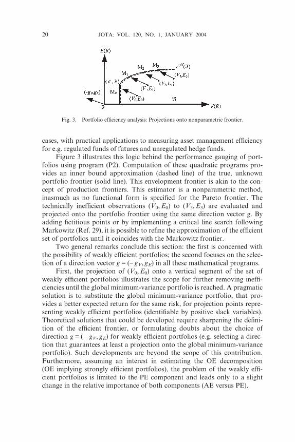
Figure 3 illustrates this logic behind the performance gauging of port-

folios using program (P2). Computation of these quadratic programs pro-

vides an inner bound approximation (dashed line) of the true, unknown

portfolio frontier (solid line). This envelopment frontier is akin to the con-

cept of production frontiers. This estimator is a nonparametric method,

inasmuch as no functional form is specified for the Pareto frontier. The

technically inefficient observations (V0, E0) to (V3, E3) are evaluated and

projected onto the portfolio frontier using the same direction vector g. By

adding fictitious points or by implementing a critical line search following

Markowitz (Ref. 29), it is possible to refine the approximation of the efficient

set of portfolios until it coincides with the Markowitz frontier.

Two general remarks conclude this section: the first is concerned with

the possibility of weakly efficient portfolios; the second focuses on the selec-

tion of a direction vector g = (– gV, gE) in all these mathematical programs.

First, the projection of (V0, E0) onto a vertical segment of the set of

weakly efficient portfolios illustrates the scope for further removing ineffi-

ciencies until the global minimum-variance portfolio is reached. A pragmatic

solution is to substitute the global minimum-variance portfolio, that pro-

vides a better expected return for the same risk, for projection points repre-

senting weakly efficient portfolios (identifiable by positive slack variables).

Theoretical solutions that could be developed require sharpening the defini-

tion of the efficient frontier, or formulating doubts about the choice of

direction g = ( – gV, gE) for weakly efficient portfolios (e.g. selecting a direc-

tion that guarantees at least a projection onto the global minimum-variance

portfolio). Such developments are beyond the scope of this contribution.

Furthermore, assuming an interest in estimating the OE decomposition

(OE implying strongly efficient portfolios), the problem of the weakly effi-

cient portfolios is limited to the PE component and leads only to a slight

change in the relative importance of both components (AE versus PE).

Fig. 3. Portfolio efficiency analysis: Projections onto nonparametric frontier.


Second, some remarks on the choice of the direction vector are useful.

In principle, various alternative directions are possible [e.g. Chambers,

Chung, and Fare (Ref. 13)]. For instance, it is possible to choose a common

direction for all portfolios, as illustrated in Figure 3 above. This has a clear

economic meaning in consumer theory where, for instance, utility may be

measured using a type of distance function with respect to a common basket

of goods [see the benefit function in Luenberger (Ref. 15)]. But the economic

interpretation of a common direction g in production and investment theory

is not evident to us.8

A far more straightforward choice for investment theory is to use the

observation under evaluation itself, i.e.,

g = (–V (R(x)), E(R(x))):

Then, the shortage function measures the maximum percentage of risk

reduction and expected return improvement. The dual formulation of the

shortage function leads to a simpler interpretation,

Sg(x) = inf{U*(r,m) –U(r,m)(x);mgE + rgV = 1,m$0, r$0}

= inf{U*(r,m) –U(r,m)(x); – mE(R(x)) + rV (R(x)) = 1,m$0, r$0}

= inf{U*(r,m) –U(r,m)(x);U(r,m)(x) = 1,m$0, r$0}: (17)

Now, using a simple normalization scheme [see Chambers, Chung, and Fare

(Ref. 13)], this can be written equivalently as

Sg(x) = inf{[U*(r¢,m¢) –U(r¢,m¢)(x)]=U(r¢, m¢)(x);m¢$0, r¢$0}: (18)

Thus, the shortage function is now interpreted as the minimum percentage

improvement in the direction to reach the maximum of the utility function

(i.e., the indirect utility function). Since this is conducted in the mean-

variance space, the shadow risk-aversion minimizing this percentage provides

a general efficiency index.

6. Empirical Illustration: Investment Funds

To show the ease of implementing the basic framework developed in this

contribution, the decomposition of overall efficiency for a small sample

of 26 investment funds, earlier analyzed in Morey and Morey (Ref. 21), is

8One possibility, suggested by P. Vanden Eeckaut, is a common direction minimizing the OE for

all observations. This could prove useful when risk-aversion is unknown, and one would like to

avoid penalizing observations too heavily when fixing a pair of risk-aversion parameters.

Implementing this suggestion involves issues of aggregation of efficiency measures that are

currently underdeveloped.


computed. It concerns the problem of selecting a fund of funds from a set

of funds based upon the tradeoff between the expected return and risk

(formally similar to composing a portfolio from a series of assets).

Return and risk are calculated over a 3-year time horizon between July

1992 and July 1995 (see Tables 1 and 8 of Ref. 21). Computing program (P2)

to obtain TE, the quadratic program in Definition 4.1 for the parameters

m = 1 and r = 2 to obtain the maximum of the indirect mean-variance utility

function, applying the decomposition in Definition 4.2, and using (11), the

results summarized in Table 1 of this paper are obtained. To save space,

portfolio weights and slack variables are not reported. Risk aversion follows

the conventional values for r that often range between 0.5 and 10 [e.g. Uysal,

Trainer, and Reis (Ref. 35)].

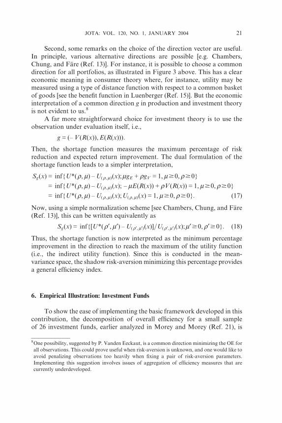
Table 1. Decomposition results for Morey and Morey (1999) sample.

Observations OE PE AE j*

20th Century Ultra Investors 0.718 0.433 0.285 0.095

44 Wall Street Equity 0.398 0.225 0.172 0.166

AIM Aggressive Growth 0.606 0.000 0.606 0.072

AIM Constellation 0.627 0.274 0.353 0.097

Alliance Quasar A 0.616 0.550 0.066 0.205

Delaware Trend A 0.610 0.351 0.259 0.116

Evergreen Aggressive Growth A 0.742 0.538 0.204 0.108

Founders Special 0.589 0.439 0.150 0.152

Fund Manager Aggressive Growth 0.366 0.357 0.009 0.330

IDS Strategy Aggressive B 0.593 0.583 0.011 0.314

Invesco Dynamics 0.543 0.274 0.269 0.122

Keystone Amer Omega A 0.521 0.448 0.073 0.213

Keystone Small Co Growth (S-4) 0.722 0.331 0.391 0.079

Oppenheimer Target A 0.402 0.320 0.082 0.219

Pacific Horizon Aggregate Growth 0.700 0.619 0.081 0.175

PIMCo Advanced Opportunity C 0.742 0.304 0.438 0.000

Putnam Voyager A 0.541 0.323 0.218 0.135

Security Ultra A 0.559 0.503 0.057 0.225

Seligman Capital A 0.573 0.564 0.009 0.319

Smith Barney Aggregate Growth A 0.726 0.485 0.241 0.102

State St. Research Capital C 0.643 0.245 0.399 0.089

SteinRoe Capital Opport 0.588 0.317 0.272 0.116

USAA Aggressive Growth 0.708 0.545 0.162 0.128

Value Line Leveraged Growth Investment 0.481 0.319 0.163 0.161

Value Line Specific Situations 0.687 0.517 0.170 0.129

Winthrop Focus Aggregate Growth 0.026 0.014 0.011 0.332

Mean 0.578 0.380 0.198 0.162

Standard Deviation 0.155 0.159 0.152 0.087

Maximum 0.742 0.619 0.606 0.332

* Absolute risk aversion: computed via shadow prices of the EIP function (Proposition 5.1).


To underline the ease of interpretation of the performance measure, the

decomposition results of a single fund ‘‘44 Wall Street Equity’’ are com-

mented upon. It could improve its OE by 40%, in both terms of improving its

return and reducing its risk. In terms of the decomposition, 22.5% of this

rather poor performance is due to PE, i.e., operating below the portfolio

frontier, while 17% is due to AE, i.e., choosing a wrong mix of return and

risk given the postulated risk attitudes.

The average performance of the investment funds is poor. They could

improve their OE performance by about 58%, with the majority of ineffi-

ciencies being attributed to PE. Looking at the individual results, none of

the investment funds suits perfectly the investors’ preferences. Therefore, all

are to some extent overall inefficient. The last investment fund in the list

comes closest to satisfying the investors needs. Only one investment fund

(number 3) is portfolio efficient and is part of the set of frontier portfolios.

The residual degree of AE, listed in the third column, is small compared

to the amount of PE detected. This relative importance of PE relative to

AE is a common finding in production analysis. Whether or not the same

general tendency holds also in portfolio gauging remains an open question.

Obviously, these efficiency measures can be used easily as a rating tool.

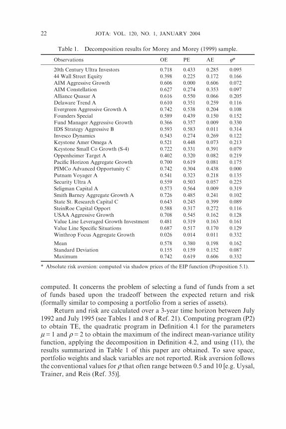
The same results are depicted also on the graph shown in Figure 4. We

plot the return and risk of investment funds in the sample, their projections

onto the portfolio frontier using the shortage function (PE), and the single

point on the frontier maximizing the investors’ preferences (OE).

A potential major issue is the sensitivity of the results, and in particular

the decomposition, to the postulated risk-aversion parameters. Using Pro-

position 5.1, the adjusted risk-aversion function minimizing inefficiency from

the Kuhn-Tucker multipliers in program (P2) can be retrieved easily. These

shadow risk aversions are shown in the last column of Table 1. Note that, for

one fund, the shadow risk aversion is zero, due to positive slack in the risk

dimension. For the sample, the shadow risk aversion is on average 0.162 with

3

2

1

00 5 10 15 20 25 30

Evaluated mutual funds Frontier projections (PE) Optimum (OE)

Ret

urn

Variance

Fig. 4. Portfolio frontier: Observed portfolios and decomposition results.


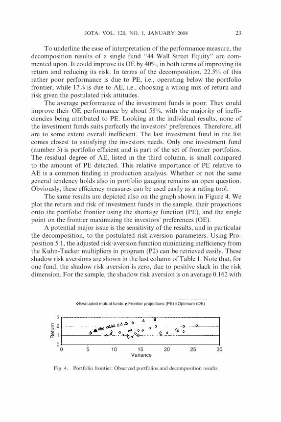
a standard deviation of 0.087. To test the sensitivity of the decomposition

results, the average efficiency components were also computed for the param-

eter m = 1 and a wide range of values for r. The results shown in Figure 5 for

values ranging from almost 0 to 10 and in the detail window for the range

between 0.05 and 1 indicate that the main source of inefficiency remains PE,

except when risk aversion approaches zero. AE is minimized for the value

of the above-mentioned shadow risk-aversion and increases slightly for

deviations on both sides of this minimum.

Two remarks may be made. First, the confrontation between postulated

risk-aversion parameters and shadow risk aversion could be instructive when

assessing whether portfolio management strategies adhere to certain speci-

fied risk profiles. Second, the decomposition depends on a specified risk-

aversion parameter, but if risk aversion is unknown, OE could equally well

be ignored to focus on PE as such.

7. Conclusions

The objective of this paper has been to introduce a general method for

measuring portfolio efficiency. Portfolios are benchmarked by looking

simultaneously for risk contraction and mean-return augmentation using the

shortage function framework [Luenberger (Ref. 14)]. The virtues of this ap-

proach can be summarized as follows: (i) it does not require the complete

estimation of the efficient frontier, but approximates the true frontier by a

nonparametric envelopment method; (ii) its efficiency measure lends itself

Fig. 5. Sensitivity of portfolio efficiency decomposition results for r.


perfectly for performance gauging; (iii) it yields interesting dual interpreta-

tions; (iv) it stays close to the theoretical framework of Markowitz (Ref. 29)

and does not require any simplifying hypotheses. A simple empirical appli-

cation on a limited sample of investment funds has illustrated the computa-

tional feasibility of this general framework.

The general idea of looking for both risk contraction and mean-return

expansion is useful in a wide range of financial models. Just to mention one

theoretical extension, right from the outset, alternative criteria for portfolio

selection based, among others, upon higher-order moments have been

developed [Philippatos (Ref. 36)]. Since the shortage function is a distance

(gauge) function, a perfect representation of multidimensional choice sets,

we conjecture that this framework could well be extended to these multi-

dimensional portfolio selection approaches.

At the philosophical level, the question remains whether any eventual

portfolio inefficiencies reveal judgmental errors of investors or whether these

are simply the result of not accounting for additional constraints inhibiting

full mean-variance efficiency. In the latter case, additional modeling efforts

are required to derive the so-called fitted portfolios [Gourieroux and

Jouneau (Ref. 17)]. However, analogously with similar discussions elsewhere

[Førsund, Lovell, and Schmidt (Ref. 37)], it could be conjectured that even

accounting for additional constraints does not eliminate all inefficiencies.

Therefore, having an unambiguous and general portfolio efficiency measure

like the one proposed remains as useful as ever.

References

1. MARKOWITZ, H., Portfolio Selection, Journal of Finance, Vol. 7, pp. 77–91, 1952.

2. FARRAR, D. E., The Investment Decision under Uncertainty, Prentice Hall,

Englewood Cliffs, New Jersey, 1962.

3. SHARPE, W., A Simplified Model for Portfolio Analysis, Management Science, Vol.

9, pp. 277–293, 1963.

4. SHARPE, W., Capital Asset Prices: A Theory of Market Equilibrium under Condi-

tion of Risk, Journal of Finance, Vol. 19, pp. 425–442, 1964.

5. LINTNER, J., The Valuation of Risk Assets and the Selection of Risky Investment

in Stock Portfolios and Capital Budgets, Review of Economics and Statistics,

Vol. 47, pp. 13–37, 1965.

6. CONSTANTINIDES, G. M., and MALLIARIS, A. G., Portfolio Theory, Handbooks

in OR & MS: Finance, Edited by R. Jarrow, V. Maksimovic, and W. T. Ziemba,

Elsevier, Amsterdam, Holland, Vol. 9, pp. 1–30, 1995.

7. PHILIPPATOS, G. C., Mean-Variance Portfolio Selection Strategies, Handbook

of Financial Economics, Edited by J. L. Bicksler, North-Holland, Amsterdam,

Holland, pp. 309–337, 1979.


8. SHARPE, W., Mutual Fund Performance, Journal of Business, Vol. 39, pp. 119–138,

1966.

9. TREYNOR, J. L., How to Rate Management of Investment Funds, Harvard Business

Review, Vol. 43, 63–75, 1965.

10. JENSEN, M., The Performance of Mutual Funds in the Period 1945–1964, Journal

of Finance, Vol. 23, pp. 389–416, 1968.

11. GRINBLATT, M., and TITMAN, S., Performance Evaluation, Handbooks in OR &

MS: Finance, Edited by R. Jarrow, V. Maksimovic, and W. T. Ziemba, Elsevier,

Amsterdam, Holland, Vol. 9, pp. 581–609, 1995.

12. SHUKLA, R., and TRZCINCA, C., Performance Measurement of Managed Portfolios,

Financial Markets, Institutions, and Instruments, Vol. 1, pp. 1–59, 1992.

13. CHAMBERS, R., CHUNG, Y., and FARE, R., Profit, Directional Distance Function,

and Nerlovian Efficiency, Journal of Optimization Theory and Applications,

Vol. 98, pp. 351–364, 1998.

14. LUENBERGER, D. G., Microeconomic Theory, McGraw Hill, New York, NY, 1995.

15. LUENBERGER, D. G., Benefit Functions and Duality, Journal of Mathematical

Economics, Vol. 21, pp. 461–481, 1992.

16. JOBSON, J. D., and KORKIE, B., A Performance Interpretation of Multivariate Tests

of Asset Set Intersection, Spanning, and Mean-Variance Efficiency, Journal of

Financial and Quantitative Analysis, Vol. 24, pp. 185–204, 1989.

17. GOURIEROUX, C., and JOUNEAV, F., Econometrics of Efficient Fitted Portfolios,

Journal of Empirical Finance, Vol. 6, pp. 87–118, 1999.

18. MATZKIN, R. L., Restrictions of Economic Theory in Nonparametric Methods,

Handbook of Econometrics, Edited by R. F. Engle, and D. L. McFadden,

Elsevier, Amsterdam, Holland, Vol. 4, pp. 2523–2558, 1994.

19. VARIAN, H., Nonparametric Tests of Models of Investment Behavior, Journal of

Financial and Quantitative Analysis, Vol. 18, pp. 269–278, 1983.

20. SENGUPTA, J. K., Nonparametric Tests of Efficiency of Portfolio Investment,

Journal of Economics, Vol. 50, pp. 1–15, 1989.

21. MOREY, M. R., and MOREY, R. C., Mutual Fund Performance Appraisals: A

Multi-Horizon Perspective with Endogenous Benchmarking, Omega, Vol. 27, pp.

241–258, 1999.

22. DIEWERT, W., and PARKAN, C., Linear Programming Test of Regularity Conditions

for Production Functions, Quantitative Studies on Production and Prices, Edited

by W. Eichhorn, K. Neumann, and R. Shephard, Physica-Verlag, Wurzburg,

Germany, pp. 131–158, 1983.

23. VARIAN, H., The Nonparametric Approach to Demand Analysis, Econometrica,

Vol. 50, pp. 945–973, 1983.

24. FARE, R., and GROSSKOPF, S., Nonparametric Tests of Regularity, Farrell Effi-

ciency, and Goodness-of-Fit, Journal of Econometrics, Vol. 69, pp. 415–425, 1995.

25. FARRELL, M., The Measurement of Productive Efficiency, Journal of the Royal

Statistical Society, Vol. 120A, pp. 253–281, 1957.

26. POGUE, G., An Extension of the Markowitz Portfolio Selection Model to Include

Variable Transactions Costs, Short Sales, Leverage Policies, and Taxes, Journal

of Finance, Vol. 25, pp. 1005–1027, 1970.


27. RUDD, A., and ROSENBERG, B., Realistic Portfolio Optimization, Portfolio Theory,

25 Years After, Edited by E. J. Elton and M. J. Gruber, North-Holland,

Amsterdam, Holland, pp. 21–46, 1979.

28. LUENBERGER, D. G., Investment Science, Oxford University Press, New York,

NY, 1998.

29. MARKOWITZ, H., Portfolio Selection: Efficient Diversification of Investments, John

Wiley, New York, NY, 1959.

30. ELTON, E. J., GRUBER, M. J., and PADBERG, M. W., The Selection of Optimal

Portfolios: Some Simple Techniques, Handbook of Financial Economics, Edited

by J. L. Bicksler, North-Holland, Amsterdam, Holland, pp. 339–364, 1979.

31. BRIEC, W., and LESOURD, J. B., Metric Distance Function and Profit: Some Duality

Result, Journal of Optimization Theory and Applications, Vol. 101, pp. 15–33,

1999.

32. LUENBERGER, D. G., Welfare from a Benefit Viewpoint, Economic Theory, Vol. 7,

pp. 463–490, 1996.

33. FIACCO, A. V., and MCCORMICK, G. P., Nonlinear Programming: Sequential

Uncontrained Minimization Techniques, John Wiley, New York, NY, 1968.

34. LUENBERGER, D., Linear and Nonlinear Programming, 2nd Edition, Addison

Wesley, Reading, Massachusetts, 1984.

35. UYSAL, E., TRAINER, F. H., and REIS, J., Revisiting Mean-Variance Optimization

from a Scenario Analysis Perspective, Journal of Portfolio Management, Vol. 27,

pp. 71–81, 2001.

36. PHILIPPATOS, G. C., Alternatives to Mean-Variance for Portfolio Selection, Hand-

book of Financial Economics, Edited by J. L. Bicksler, North-Holland, Amster-

dam, Holland, pp. 365–386, 1979.

37. FØRSUND, F., LOVELL, C. A. K., and SCHMIDT, P., A Survey of Frontier Production

Functions and of Their Relationship to Efficiency Measurement, Journal of

Econometrics, Vol. 13, pp. 5–25, 1980.


A Variation on the Luenberger Shortage Function

Documents