A Unifying Pricing Theory for Insurance and Financial ...risklab.es/es/seminarios/pasados/marzo2002-1.pdf · A Unifying Pricing Theory for Insurance and Financial Risks: Applications

A Unifying Pricing Theory for Insurance and

Financial Risks: Applications for a Unified

Risk Management

Alejandro Balbas1 and Jose Garrido1,2

1Department of Business Administration

University Carlos III of Madrid, Spain2Department of Mathematics and Statistics

Concordia University, Canada

Instituto MEFF

April 24, 2002

1

Overview:

1. Introduction:

1.1 Distortion Operators, Insurance Pricing,

1.2 Choquet Pricing of Assets and Losses.

2. Wang’s Distortion Operator,

3. Applications:

3.1 Asset Pricing,

3.2 Capital Asset Pricing Model,

3.3 Black-Scholes Formula,

3.4 Deviance and Tail Index.

4. Dynamic Coherent Measures.

2

1. Introduction

Insurance and financial risks are becoming more integrated.

The actuarial literature argues for a unified pricing theory linking

both fields [Smith (1986), Cummins (1990, 1991) or Embrechts

(1996), Wang (2000), Cheuk (2001)] .

The price of an insurance risk (excluding other expenses) is called

a risk-adjusted premium. From classical expected utility theory

[Borch (1961), Buhlmann (1980), Goovaerts et al. (1984)] a

dual theory of risk has emerged in the economic literature [Yaari

(1987)].

Similarly, the price of a financial instrument (e.g. options) also

carries risk loads. But the markets and the strategies by which

insurance and financial risks are sold differ substantially.

3

We will discuss Wang’s proposal of a risk-adjustment method

that distorts the survival function of an insurance risk.

Wang (2000) shows that his (one-parameter) distortion operator

reproduces Black-Scholes theory for option pricing and extends

the Capital Asset Pricing Model (CAPM) to insurance pricing.

Major and Venter (1999), Gao and Qiu (2001) and Cheuk (2001)

consider two-parameter Wang transforms. With it Cheuk defines

a generalized Value at Risk (VaR) measure.

We characterize Wang’s transform as a “coherent measure” and

propose a dynamic (stochastic process) version. Also a tail index

for (financial or insurance) risk distributions is derived from it.

4

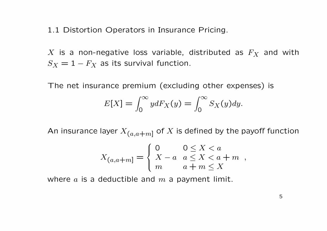
1.1 Distortion Operators in Insurance Pricing.

X is a non-negative loss variable, distributed as FX and with

SX = 1 − FX as its survival function.

The net insurance premium (excluding other expenses) is

E[X] =∫ ∞

0ydFX(y) =

∫ ∞

0SX(y)dy.

An insurance layer X(a,a+m] of X is defined by the payoff function

X(a,a+m] =

0 0 ≤ X < a

X − a a ≤ X < a + m

m a + m ≤ X

,

where a is a deductible and m a payment limit.

5

The survival function of this insurance layer is given by SX as

SX(a,a+m](y) =

{

SX(a + y) 0 ≤ y < m

0 m ≤ y.

It yields a net premium of

E[X(a,a+m]] =

∫ ∞

0SX(a,a+m]

(y)dy =

∫ a+m

aSX(x)dx.

Wang (1996) suggested to introduce the risk loading by first

distorting the survival function before taking expectations.

6

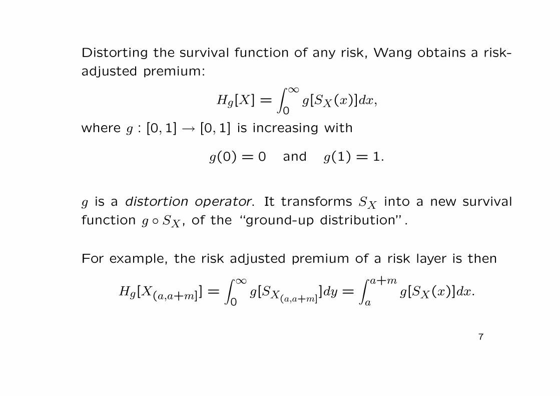
Distorting the survival function of any risk, Wang obtains a risk-

adjusted premium:

Hg[X] =

∫ ∞

0g[SX(x)]dx,

where g : [0,1] → [0,1] is increasing with

g(0) = 0 and g(1) = 1.

g is a distortion operator. It transforms SX into a new survival

function g ◦ SX, of the “ground-up distribution”.

For example, the risk adjusted premium of a risk layer is then

Hg[X(a,a+m]] =

∫ ∞

0g[SX(a,a+m]

]dy =

∫ a+m

ag[SX(x)]dx.

7

For general insurance pricing, g should satisfy:

• 0 < g(u) < 1, g(0) = 0 and g(1) = 1,

• g increasing and concave,

• g′(0) = +∞, where it is defined.

Wang (1996) shows that in a class of one-parameter functions,

only

g(u) = ur, u ∈ [0,1], 0 < r ≤ 1,

satisfies all of the above.

This corresponds to the proportional hazards (PH) transform of

Wang (1995).

8

Despite some desirable properties, Wang’s PH transform suffers

some major drawbacks. The PH transform:

• of a lognormal is not lognormal (Black-Scholes formula for

option pricing),

• lacks flexibility yielding fast increasing risk loadings for high

layers,

• cannot be applied simultaneously to assets and liabilities. It

yields to serious inconsistencies; see the following section.

9

1.2 Choquet Pricing of Assets and Losses

Consider an asset A as a negative loss X = −A. The Choquet

integral with respect to the distortion g is then given by:

Hg[X] =

∫ 0

−∞{g[SX(x)] − 1}dx +

∫ ∞

0g[SX(x)]dx.

It has been proposed as a general pricing method for financial

markets with frictions [Chateauneuf et al. (1996)].

Definition: For any risk X and a real valued h, the payoff Y =

h(X) is a derivative of X. If h is non-decreasing, then Y is called

a comonotone derivative of the underlying X.

10

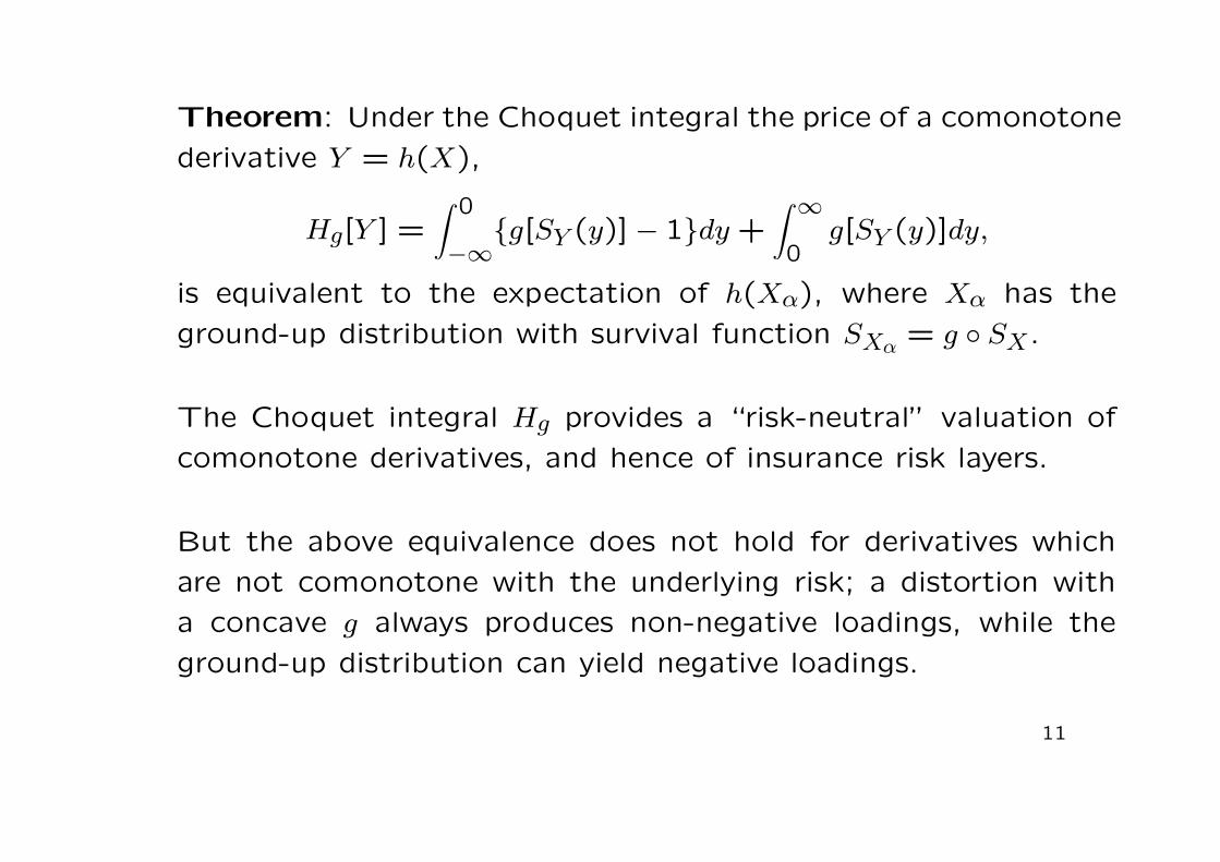
Theorem: Under the Choquet integral the price of a comonotone

derivative Y = h(X),

Hg[Y ] =∫ 0

−∞{g[SY (y)] − 1}dy +

∫ ∞

0g[SY (y)]dy,

is equivalent to the expectation of h(Xα), where Xα has the

ground-up distribution with survival function SXα= g ◦ SX.

The Choquet integral Hg provides a “risk-neutral” valuation of

comonotone derivatives, and hence of insurance risk layers.

But the above equivalence does not hold for derivatives which

are not comonotone with the underlying risk; a distortion with

a concave g always produces non-negative loadings, while the

ground-up distribution can yield negative loadings.

11

Denneberg (1994) shows that for an asset A > 0

Hg[−A] = −Hg∗[A],

where g∗(u) = 1 − g(1 − u) is the dual distortion operator of g.

A loss X distorted by a concave g always yields Hg[X] ≥ E[X].

When g is concave, g∗ is convex and Hg∗[A] ≤ E[A].

For most choices g, the dual g∗ belongs to a different parametric

family. In particular, if the PH transform g(u) = ur is applied to

losses, the dual g∗(u) = 1 − (1 − u)r would apply to assets.

Symmetric treatment of assets and liabilities is possible for a new

class of distortion operators.

12

2. Wang’s Distortion Operator

Wang (2000) suggests a new distortion operator defined as:

gα(u) = Φ[Φ−1(u) + α], u ∈ [0,1],

where α ∈ R and Φ is the standard normal distribution with

density function:

φ(x) =1√2π

e−x2

2 , x ∈ R.

For α > 0, gα satisfies all the desirable properties of a distortion

operator for insurance pricing:

1. 0 < gα(u) < 1 for u ∈ [0,1], with gα(0) = limu→0+

gα(u) = 0 and

gα(1) = limu→1−

gα(u) = 1.

13

2. gα is increasing and for x = Φ−1(u),

g′α(u) =∂gα(u)

∂u=

φ(x + α)

φ(x)= e−αx−x2

2 > 0, u ∈ (0,1).

3. For α > 0, gα is concave and

g′′α(u) =∂2gα(u)

∂u2= −αφ(x + α)

φ(x)2< 0, u ∈ (0,1).

4. For α > 0, g′α(u) becomes unbounded as u approaches 0.

5. The dual operator g∗α(u) = 1 − gα(1 − u) = g−α(u).

6. g∗α is convex when gα is concave, as in 3.

14

For gα the Choquet integral gives

H[X;α] =

∫ 0

−∞{gα[SX(x)] − 1}dx +

∫ ∞

0gα[SX(x)]dx,

which enjoys some very nice properties:

1. H[c;α] = c and H[X + c;α] = H[X;α]+ c, for any constant c.

2. H[bX; α] = bH[X; α] while H[−bX;α] = −bH[X;−α], for any

b > 0. In particular H[−X;α] = −H[X;−α].

3. If X1, X2 are comonotone H[X1+X2;α] = H[X1;α]+H[X2;α].

Since two layers of the same risk are comonotone, then

H[X(a,b];α] + H[X(b,c];α] = H[X(a,c];α],

for any a < b < c.

15

4. For any two variables X1 and X2

H[X1 + X2;α] ≤ H[X1;α] + H[X2;α], forα > 0,

≥ H[X1;α] + H[X2;α], forα < 0,

showing the benefit of diversification.

5. H[X; α] is an increasing function of α, with

min[X] ≤ H[X;α] ≤ max[X].

6. With α > 0 for losses and α < 0 for assets, H[X;α] preserves

1st and 2nd order stochastic dominance [see Rothschild and

Stiglitz (1971)].

7. For α > 0, g′α(u) goes unbounded as u approaches 0. For

example, if X ∼ Bernoulli(θ) then

limθ→0

H[X;α]

E[X]= lim

θ→0

Φ[Φ−1(θ) + α]

θ= g′α(0) = +∞.

16

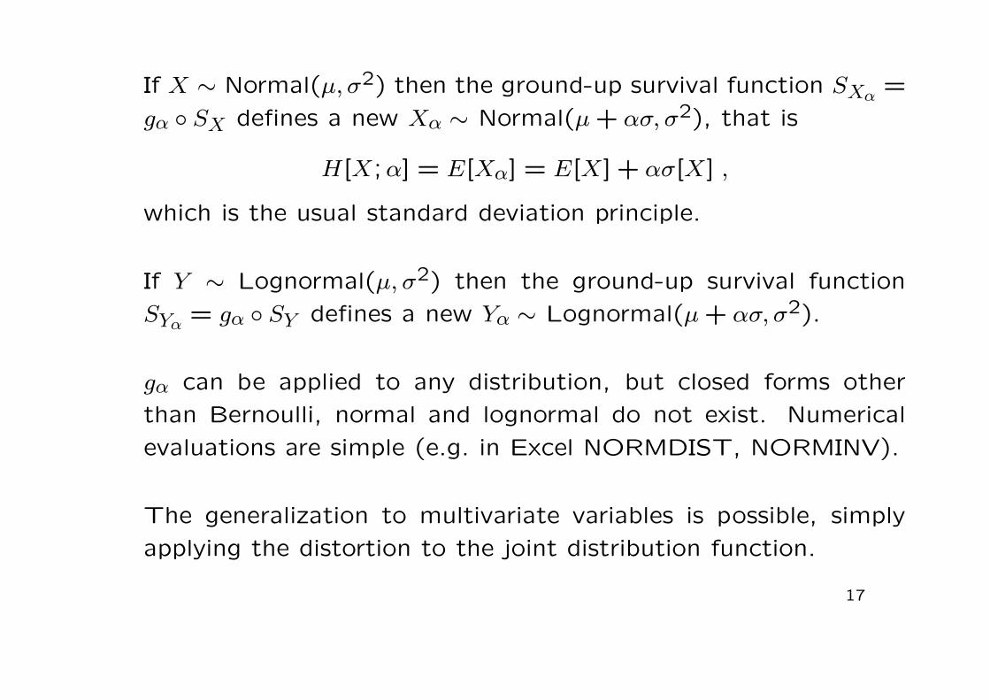
If X ∼ Normal(µ, σ2) then the ground-up survival function SXα=

gα ◦ SX defines a new Xα ∼ Normal(µ + ασ, σ2), that is

H[X;α] = E[Xα] = E[X] + ασ[X] ,

which is the usual standard deviation principle.

If Y ∼ Lognormal(µ, σ2) then the ground-up survival function

SYα= gα ◦ SY defines a new Yα ∼ Lognormal(µ + ασ, σ2).

gα can be applied to any distribution, but closed forms other

than Bernoulli, normal and lognormal do not exist. Numerical

evaluations are simple (e.g. in Excel NORMDIST, NORMINV).

The generalization to multivariate variables is possible, simply

applying the distortion to the joint distribution function.

17

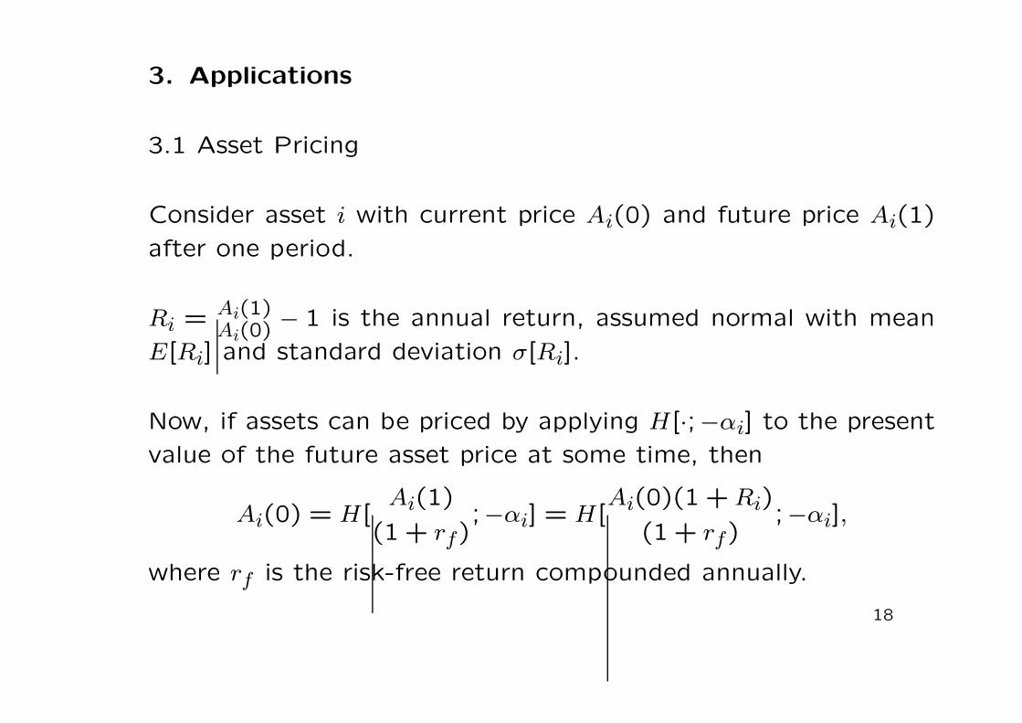
3. Applications

3.1 Asset Pricing

Consider asset i with current price Ai(0) and future price Ai(1)

after one period.

Ri = Ai(1)Ai(0)

− 1 is the annual return, assumed normal with mean

E[Ri] and standard deviation σ[Ri].

Now, if assets can be priced by applying H[·;−αi] to the present

value of the future asset price at some time, then

Ai(0) = H[Ai(1)

(1 + rf);−αi] = H[

Ai(0)(1 + Ri)

(1 + rf);−αi],

where rf is the risk-free return compounded annually.

18

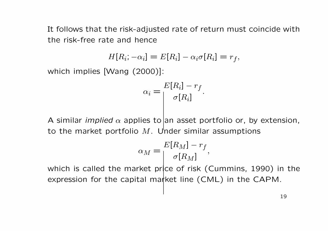
It follows that the risk-adjusted rate of return must coincide with

the risk-free rate and hence

H[Ri;−αi] = E[Ri] − αiσ[Ri] = rf ,

which implies [Wang (2000)]:

αi =E[Ri] − rf

σ[Ri].

A similar implied α applies to an asset portfolio or, by extension,

to the market portfolio M . Under similar assumptions

αM =E[RM ] − rf

σ[RM ],

which is called the market price of risk (Cummins, 1990) in the

expression for the capital market line (CML) in the CAPM.

19

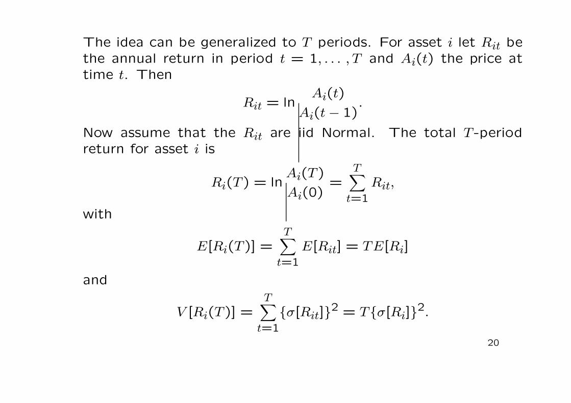
The idea can be generalized to T periods. For asset i let Rit bethe annual return in period t = 1, . . . , T and Ai(t) the price attime t. Then

Rit = lnAi(t)

Ai(t − 1).

Now assume that the Rit are iid Normal. The total T -periodreturn for asset i is

Ri(T ) = lnAi(T )

Ai(0)=

T∑

t=1

Rit,

with

E[Ri(T )] =T

∑

t=1

E[Rit] = TE[Ri]

and

V [Ri(T )] =T

∑

t=1

{σ[Rit]}2 = T{σ[Ri]}2.

20

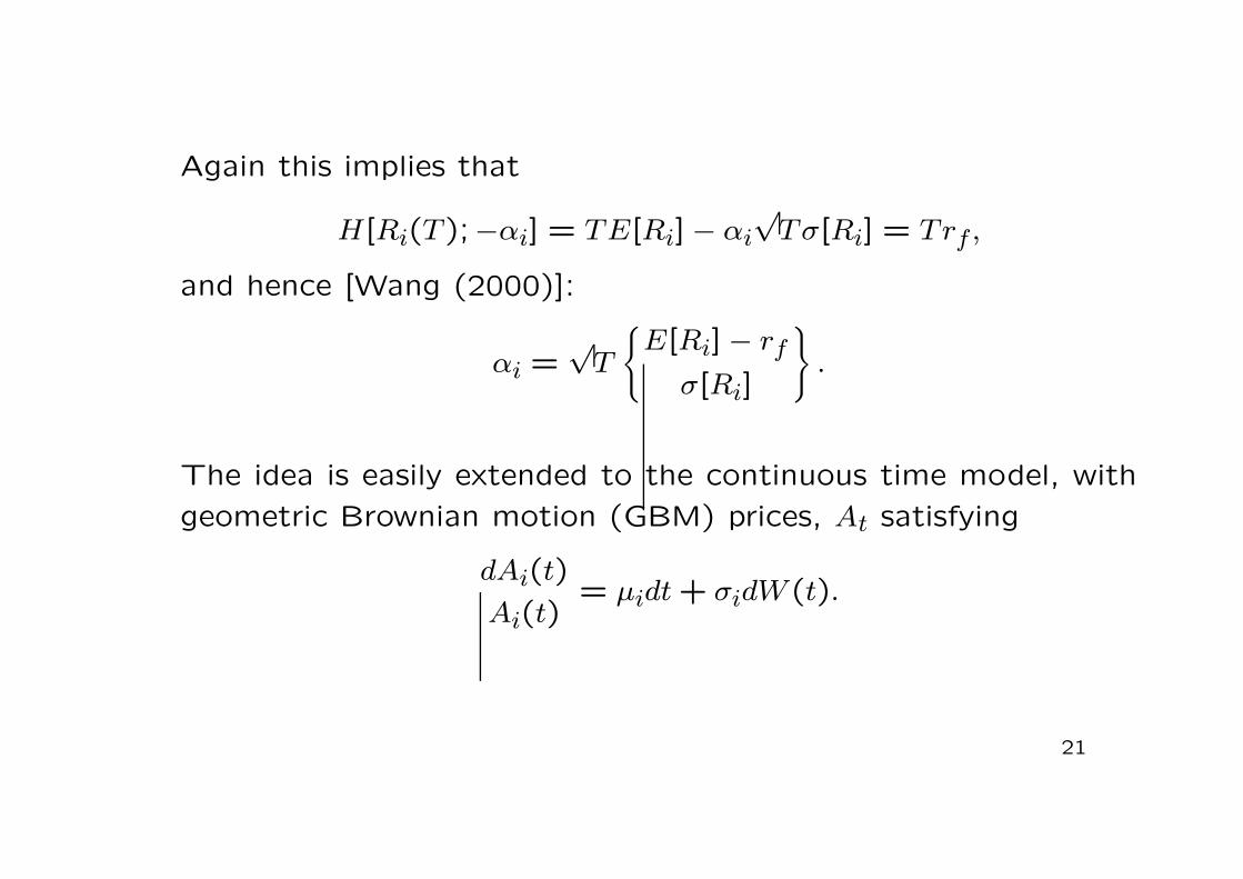
Again this implies that

H[Ri(T );−αi] = TE[Ri] − αi

√Tσ[Ri] = Trf ,

and hence [Wang (2000)]:

αi =√

T

{

E[Ri] − rf

σ[Ri]

}

.

The idea is easily extended to the continuous time model, with

geometric Brownian motion (GBM) prices, At satisfying

dAi(t)

Ai(t)= µidt + σidW (t).

21

Let Ai(0) be the current asset price. At any future date T , the

price Ai(T ) is solution to the above equation and has a lognormal

distribution [Hull (1997)]:

lnAi(T )

Ai(0)∼ Normal[(µ − σ2

2)T, σ2T ].

No-arbitrage with a continuous risk-free return rc implies:

Ai(0) = H[e−rcTAi(T );−αi] = e−rcTH[Ai(T );−αi],

which implies again [Wang (2000)]:

αi =(µi − rc)

√T

σi.

Notice that αi shares many properties with the volatility and is

proportional to the square root of the horizon T .

22

3.2 Capital Asset Pricing Model (CAPM)

As seen, the market price of risk αM in the CML of CAPM links

the systematic risk of X to the portfolio risk.

The CAPM measures a portfolio’s risk under the constraint of

an expected return level in one compounding period and the

assumption of an efficient market.

Mixing a risk-free return rf with an efficient market portfolio,

gives a minimal risk portfolio for a given level of expected return.

Let the expected return and risk of this optimal strategy be

µp and σp, respectively. Then the following capital market line

(CML) relation holds:

µp = rf + αMσp.

23

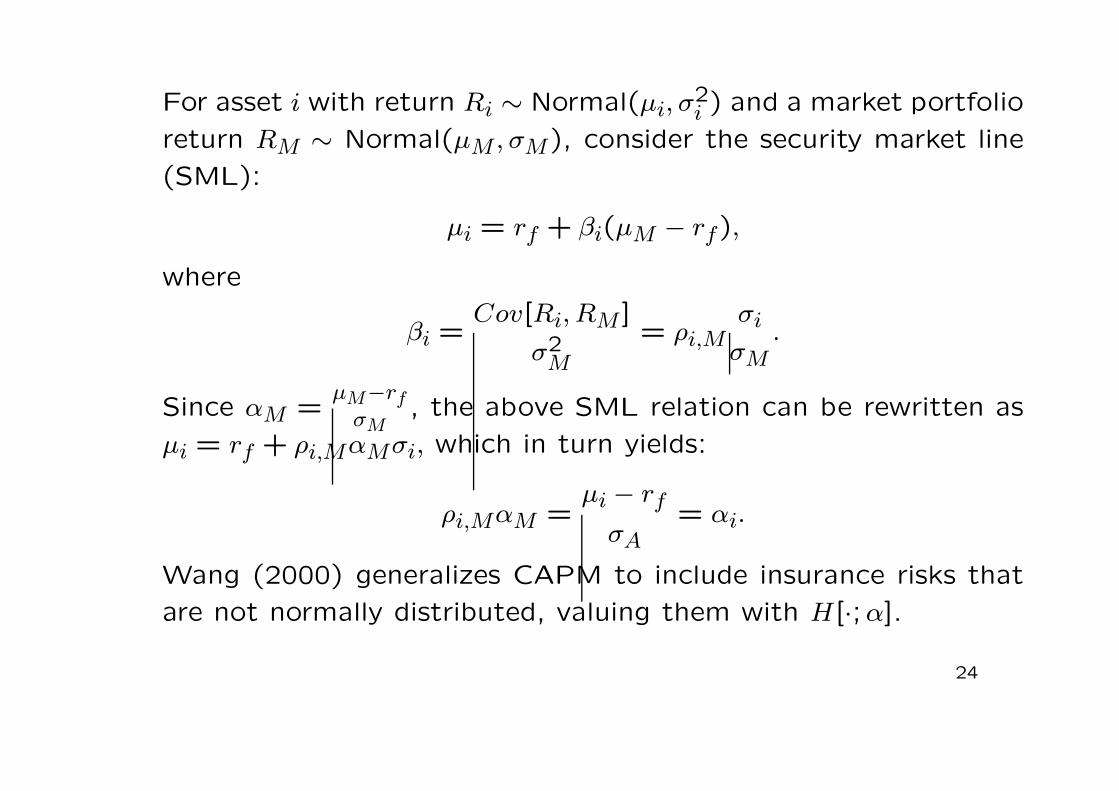
For asset i with return Ri ∼ Normal(µi, σ2i ) and a market portfolio

return RM ∼ Normal(µM , σM), consider the security market line

(SML):

µi = rf + βi(µM − rf),

where

βi =Cov[Ri, RM ]

σ2M

= ρi,Mσi

σM

.

Since αM =µM−rf

σM, the above SML relation can be rewritten as

µi = rf + ρi,MαMσi, which in turn yields:

ρi,MαM =µi − rf

σA

= αi.

Wang (2000) generalizes CAPM to include insurance risks that

are not normally distributed, valuing them with H[·;α].

24

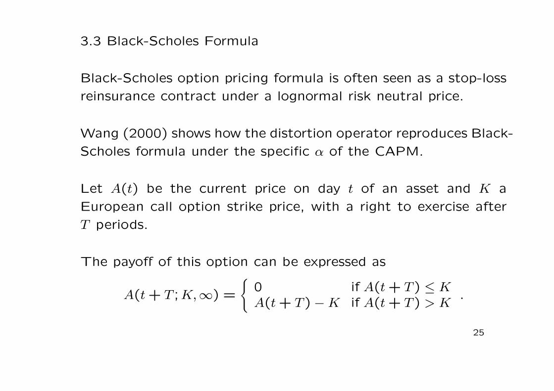
3.3 Black-Scholes Formula

Black-Scholes option pricing formula is often seen as a stop-loss

reinsurance contract under a lognormal risk neutral price.

Wang (2000) shows how the distortion operator reproduces Black-

Scholes formula under the specific α of the CAPM.

Let A(t) be the current price on day t of an asset and K a

European call option strike price, with a right to exercise after

T periods.

The payoff of this option can be expressed as

A(t + T ;K,∞) =

{

0 if A(t + T ) ≤ K

A(t + T ) − K if A(t + T ) > K.

25

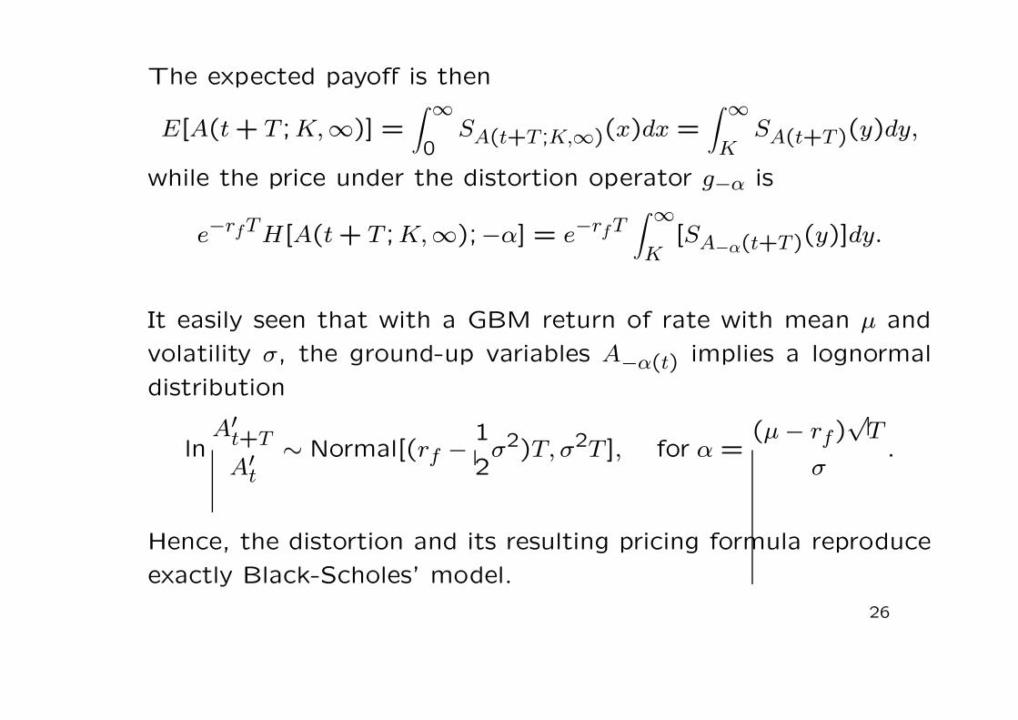
The expected payoff is then

E[A(t + T ;K,∞)] =∫ ∞

0SA(t+T ;K,∞)(x)dx =

∫ ∞

KSA(t+T)(y)dy,

while the price under the distortion operator g−α is

e−rfTH[A(t + T ; K,∞);−α] = e−rfT∫ ∞

K[SA−α(t+T)(y)]dy.

It easily seen that with a GBM return of rate with mean µ and

volatility σ, the ground-up variables A−α(t) implies a lognormal

distribution

lnA′

t+T

A′t

∼ Normal[(rf − 1

2σ2)T, σ2T ], for α =

(µ − rf)√

T

σ.

Hence, the distortion and its resulting pricing formula reproduce

exactly Black-Scholes’ model.

26

3.4 Deviance and Tail Index

Both, insurance and financial analysts, use indexes to measure

and compare “riskyness”, in the form of a volatility measure,

down-side risk, variance, deviance or more generally speaking, a

risk measure.

The distortion operator gα induces a risk loading H[X; α]. It is

natural to think that it can also be used to define a risk measure.

Since min[X] ≤ H[X; α] ≤ max[X], for any α ∈ R, and in particular

H[X; 0] = E(X) for α = 0, Wang (2000) defines right and left

deviance measures.

27

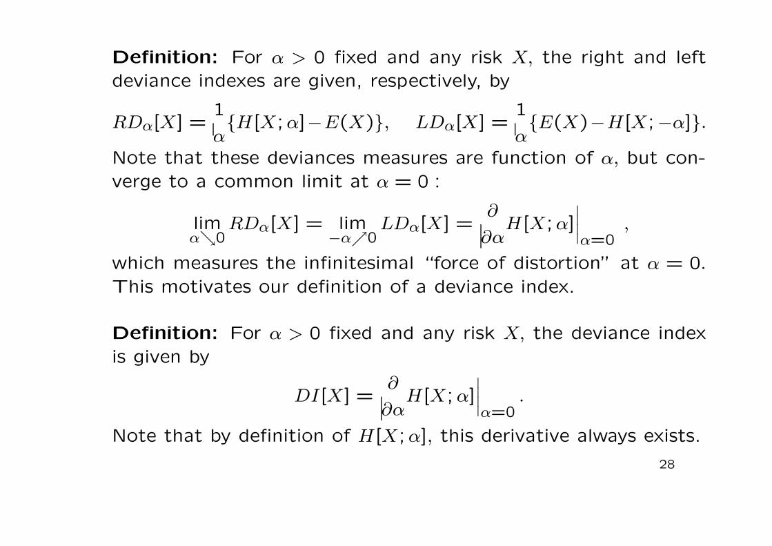
Definition: For α > 0 fixed and any risk X, the right and left

deviance indexes are given, respectively, by

RDα[X] =1

α{H[X;α]−E(X)}, LDα[X] =

1

α{E(X)−H[X;−α]}.

Note that these deviances measures are function of α, but con-

verge to a common limit at α = 0 :

limα↘0

RDα[X] = lim−α↗0

LDα[X] =∂

∂αH[X;α]

∣

∣

∣

∣

α=0,

which measures the infinitesimal “force of distortion” at α = 0.

This motivates our definition of a deviance index.

Definition: For α > 0 fixed and any risk X, the deviance index

is given by

DI[X] =∂

∂αH[X; α]

∣

∣

∣

∣

α=0.

Note that by definition of H[X;α], this derivative always exists.

28

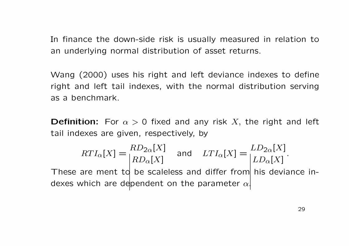
In finance the down-side risk is usually measured in relation to

an underlying normal distribution of asset returns.

Wang (2000) uses his right and left deviance indexes to define

right and left tail indexes, with the normal distribution serving

as a benchmark.

Definition: For α > 0 fixed and any risk X, the right and left

tail indexes are given, respectively, by

RTIα[X] =RD2α[X]

RDα[X]and LTIα[X] =

LD2α[X]

LDα[X].

These are ment to be scaleless and differ from his deviance in-

dexes which are dependent on the parameter α.

29

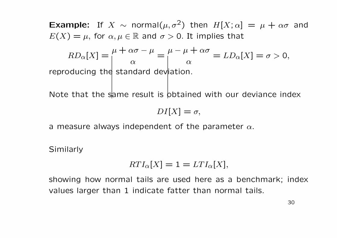
Example: If X ∼ normal(µ, σ2) then H[X;α] = µ + ασ and

E(X) = µ, for α, µ ∈ R and σ > 0. It implies that

RDα[X] =µ + ασ − µ

α=

µ − µ + ασ

α= LDα[X] = σ > 0,

reproducing the standard deviation.

Note that the same result is obtained with our deviance index

DI[X] = σ,

a measure always independent of the parameter α.

Similarly

RTIα[X] = 1 = LTIα[X],

showing how normal tails are used here as a benchmark; index

values larger than 1 indicate fatter than normal tails.

30

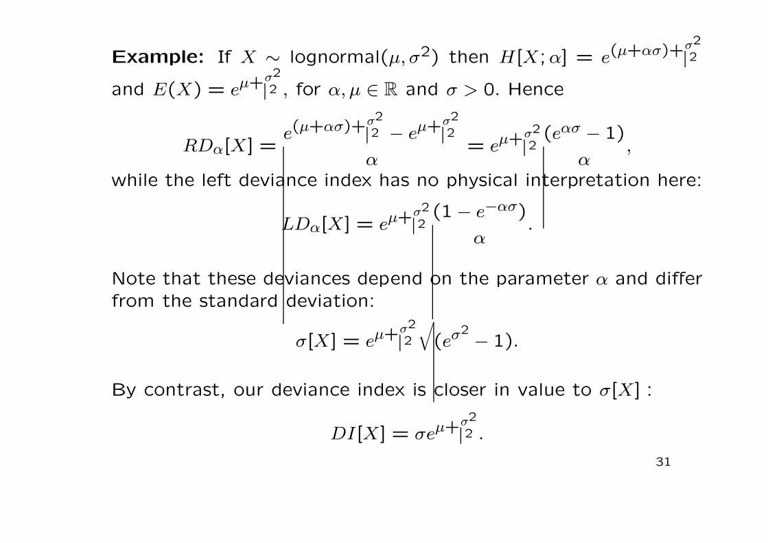
Example: If X ∼ lognormal(µ, σ2) then H[X;α] = e(µ+ασ)+σ2

2

and E(X) = eµ+σ2

2 , for α, µ ∈ R and σ > 0. Hence

RDα[X] =e(µ+ασ)+σ2

2 − eµ+σ2

2

α= eµ+σ2

2(eασ − 1)

α,

while the left deviance index has no physical interpretation here:

LDα[X] = eµ+σ2

2(1 − e−ασ)

α.

Note that these deviances depend on the parameter α and differ

from the standard deviation:

σ[X] = eµ+σ2

2

√

(eσ2 − 1).

By contrast, our deviance index is closer in value to σ[X] :

DI[X] = σeµ+σ2

2 .

31

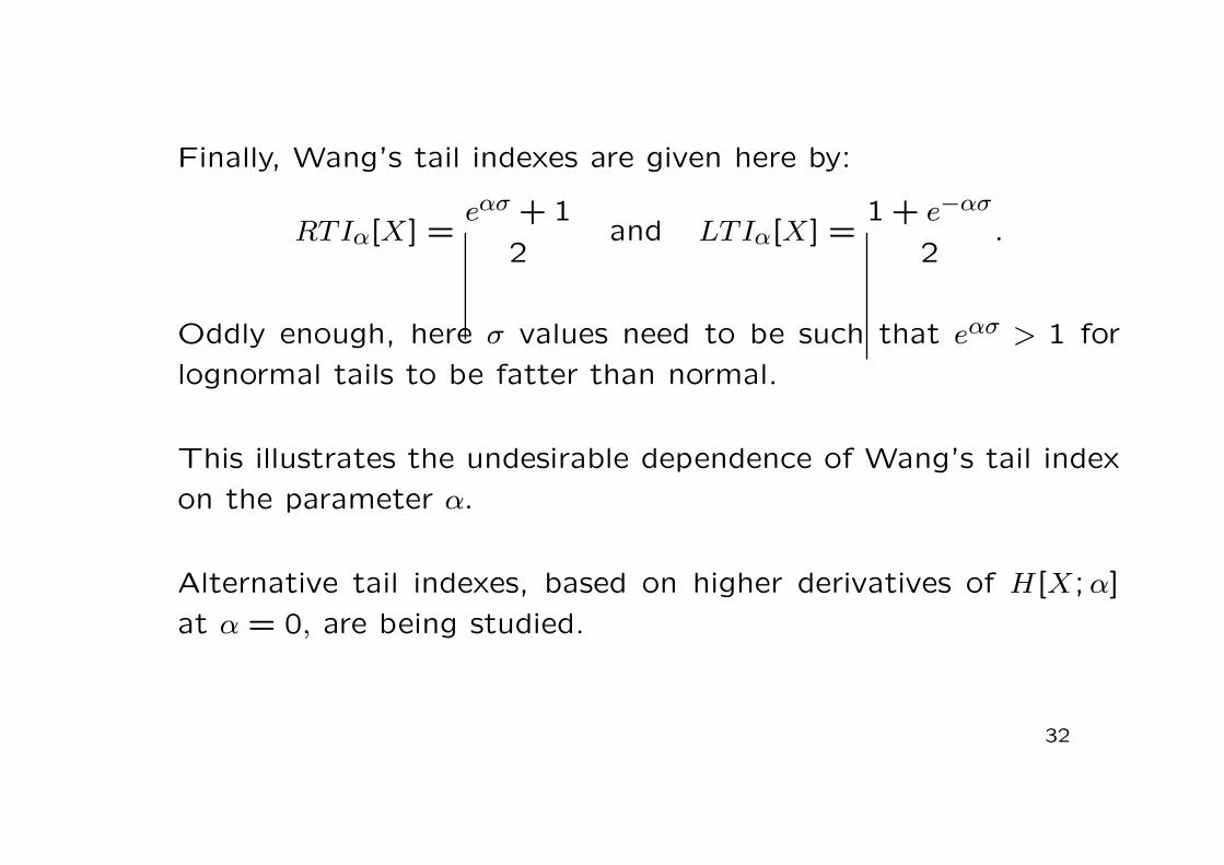
Finally, Wang’s tail indexes are given here by:

RTIα[X] =eασ + 1

2and LTIα[X] =

1 + e−ασ

2.

Oddly enough, here σ values need to be such that eασ > 1 for

lognormal tails to be fatter than normal.

This illustrates the undesirable dependence of Wang’s tail index

on the parameter α.

Alternative tail indexes, based on higher derivatives of H[X;α]

at α = 0, are being studied.

32

Example: For X ∼ Bernoulli(θ0), H[X;α] = θα = Φ[Φ−1(θ0)+α]

and E[X] = θ0, where α ∈ R and 0 ≤ θ0 ≤ 1. Hence

RDα[X] =Φ[Φ−1(θ0) + α] − θ0

α=

θα − θ0

α,

while again, the left deviance index has no physical interpretation:

LDα[X] =θ0 − Φ[Φ−1(θ0) − α]

α=

θ0 − θ−α

α.

These deviance measures also differ from the standard deviation

σ[X] =√

θ0(1 − θ0) and depend on the parameter α.

By contrast, our deviance index is given by:

DI[X] = φ[Φ−1(θ0)] =1√2π

e−[Φ−1(θ0)]2

2 .

33

Finally, Wang’s tail indexes

RTIα[X] =Φ[Φ−1(θ0) + 2α] − θ0

2{Φ[Φ−1(θ0) + α] − θ0}=

θ2α − θ0

2(θα − θ0)

and

LTIα[X] =θ0 − Φ[Φ−1(θ0) − 2α]

2{θ0 − Φ[Φ−1(θ0) − α]}=

θ0 − θ−2α

2(θ0 − θ−α),

depend on α in an intricate way.

34

4. Dynamic Coherent Measures

Wang’s use of distortion operators and Choquet integrals has

been embedded in the framework of coherent risk measures

[Artzner, Delbaen, Eber and Heath (1999)].

In Balbas, Garrido and Mayoral (2002) we assume a dynamic

framework which reflects the stochastic behavior of (insurance)

risks and (financial) pay-offs.

As a special application, we study the extensions of VaR (Value

at Risk) and TCE (Tail Conditional Expectation) to this dynamic

setting.

35

Bibliography:

Borch, K.H. (1961) “The utility concept applied to the theory of insurance”,ASTIN Bulletin, 11, 52-60.

Bulmann, H. (1980) “An economic premium principle”, ASTIN Bulletin, 16,2, 52-60.

Chateauneuf, A., Kast, R. and Lapied, A. (1996) “Choquet pricing for finan-cial markets with frictions”, Mathematical Finance, 6, 145-166.

Cheuk, W.L. (2001) Value at Risk and the Distortion Operator, M.Sc. Thesis,Concordia University, Montreal.

Cummins, J.D. (1990) “Asset pricing models and insurance ratemaking”,ASTIN Bulletin, 20, 2, 125-166.

Cummins, J.D. (1991) “Statistical and financial models of insurance pricing”,J. of Risk and Insurance, 58, 261-302.

Denneberg, D. (1994) Non-Additive Measure and Integral, Kluwer AcademicPublishers, Boston.

36

Embrechts, P. (1996) “Actuarial versus financial pricing of insurance”, Con-ference on Risk Management of Insurance Firms, May 15-17, 1996, The

Wharton School of the University of Pennsylvania.

Gao, J. and Qiu, W. (2001) “An improved distortion operator for pricinginsurance risks”, submitted to North American Actuarial J..

Goovaerts, M.J., De Vylder, F. and Haezendonck, J. (1984) Insurance Pre-

miums: Theory and Applications, North-Holland, Amsterdam.

Hull, J. (1997) Options, Futures and Other Derivatives, 3rd edition, PrenticeHall, New Jersey.

Rothschild, M. and Stiglitz, J.E. (1971) “Increasing risk I: a definition”, J. of

Economic Theory, 2, 225-243.

Smith, C.W., Jr. (1986) “On the convergence of insurance and finance re-search”, J. of Risk and Insurance, 53, 693-717.

Wang, S.S. (1995) “Insurance pricing and increased limits ratemaking byproportional hazards transforms”, Insurance: Mathematics and Economics,17, 43-54.

Wang, S.S. (1996) “Premium calculation by transforming the layer premiumdensity”, ASTIN Bulletin, 26, 1, 71-92.

Yaari, M.E. (1987) “The dual theory of choice under risk”, Econometrica,55, 95-115.

37