A Unifying Approach to the Empirical Evaluation of … · A Unifying Approach to the Empirical Evaluation of Asset Pricing Models ... or Cochrane (2001a) for textbook treatments ...

A Unifying Approach to the Empirical Evaluation of

Asset Pricing Models�

Francisco Peñaranda

SanFI, Paseo Menéndez Pelayo 94-96, E-39006 Santander, Spain.

<[email protected]>

Enrique Sentana

CEMFI, Casado del Alisal 5, E-28014 Madrid, Spain.

<sentana@cem�.es>

First version: July 2010

Revised: May 2014

Abstract

Regression and SDF approaches with centred or uncentred moments and symmetric or

asymmetric normalizations are commonly used to empirically evaluate linear factor pricing

models. We show that unlike two-step or iterated GMM procedures, single-step estimators

such as continuously updated GMM yield numerically identical risk prices, pricing errors

and overidentifying restrictions tests irrespective of the model validity and regardless of the

factors being traded, or the use of excess or gross returns. We illustrate our results with

Lustig and Verdelhan�s (2007) currency returns, propose tests to detect some problematic

cases and provide Monte Carlo evidence on the reliability of asymptotic approximations.

Keywords: CU-GMM, Factor pricing models, Forward premium puzzle, Generalized Em-

pirical Likelihood, Stochastic discount factor.

JEL: G12, G15, C12, C13.�We would like to thank Abhay Abhyankar, Manuel Arellano, Craig Burnside, Antonio Díez de los Ríos,

Prosper Dovonon, Lars Hansen, Raymond Kan, Craig MacKinlay, Cesare Robotti, Rosa Rodríguez, Amir Yaron,participants at the Finance Forum (Elche, 2010), SAEe (Madrid, 2010), ESEM (Oslo, 2011), FMG 25th An-niversary Conference (London, 2012), MFA (New Orleans, 2012), as well as audiences at the Atlanta Fed, Bankof Canada, Banque de France, Duke, Edinburgh, Fuqua, Geneva, Kenan-Flagler, Málaga, Montreal, Princeton,St.Andrews, UPF, Warwick and Wharton for helpful comments, suggestions and discussions. The comments froman associate editor and an anonymous referee have also led to a substantially improved paper. Felipe Carozziand Luca Repetto provided able research assistance for the Monte Carlo simulations. Of course, the usual caveatapplies. Financial support from the Spanish Ministry of Science and Innovation through grants ECO 2008-03066and 2011-25607 (Peñaranda) and ECO 2008-00280 and 2011-26342 (Sentana) is gratefully acknowledged.

1 Introduction

Asset pricing theories are concerned with determining the expected returns of assets whose

payo¤s are risky. Speci�cally, these models analyze the relationship between risk and expected

returns, and address the crucial question of how to value risk. The most popular empirically

oriented asset pricing models e¤ectively assume the existence of a common stochastic discount

factor (SDF) that is linear in some risk factors, which discounts uncertain payo¤s di¤erently

across di¤erent states of the world. Those factors can be either the excess returns on some

traded securities, as in the traditional CAPM of Sharpe (1964), Lintner (1965) and Mossin

(1966) or the so-called Fama and French (1993) model, non-traded economy wide sources of

uncertainty related to macroeconomic variables, like in the Consumption CAPM (CCAPM) of

Breeden (1979), Lucas (1978) or Rubinstein (1976), or a combination of the two, as in the exact

version of Ross�(1976) APT.

There are two main approaches to formally evaluate linear factor pricing models from an

empirical point of view using optimal inference procedures. The traditional method relies on

regressions of excess returns on factors, and exploits the fact that an asset pricing model im-

poses certain testable constraints on the relationship between slopes and intercepts. More recent

methods rely on the SDF representation of the model instead, and exploit the fact that the cor-

responding pricing errors should be zero. There are in fact two variants of the SDF method, one

that demeans the factors (the �centred�version) and another one that does not (the �uncen-

tred�one), and one can envisage analogous variants of the regression approach, although only

the �centred�one has been used so far in empirical work.

The initial asset pricing tests tended to make the assumption that asset returns and factors

were independently and identically distributed as a multivariate normal vector. Nowadays,

empirical researchers rely on the generalized method of moments (GMM) of Hansen (1982),

which has the advantage of yielding asymptotically valid inferences even if the assumptions

of serial independence, conditional homoskedasticity or normality are not totally realistic in

practice (see Campbell, Lo and MacKinlay (1996) or Cochrane (2001a) for textbook treatments).

Unfortunately, though, each approach (and their multiple variants) typically yields di¤erent

estimates of prices of risk and pricing errors, and di¤erent values for the overidentifying restric-

tions test. This begs the question of which approach is best, and there has been some controversy

surrounding the answer. For example, Kan and Zhou (1999) advocated the use of the regression

method over the uncentred SDF method because the former provides more reliable risk pre-

mia estimators and more powerful pricing tests than the latter. However, Cochrane (2001b) and

Jagannathan and Wang (2002) criticized their conclusions on the grounds that they did not con-

1

sider the estimation of factor means and variances. Speci�cally, Jagannathan and Wang (2002)

showed that if the excess returns and the factor are jointly distributed as an iid multivariate

normal random vector, in which case the regression approach is optimal, the (uncentred) SDF

approach is asymptotically equivalent under the null. Kan and Zhou (2002) acknowledged this

equivalence result, and extended it to compatible sequences of local alternatives under weaker

distributional assumptions.

More recently, Burnside (2012) and Kan and Robotti (2008) have also pointed out that

in certain cases there may be dramatic di¤erences between the results obtained by applying

standard two-step or iterated GMM procedures to the centred and uncentred versions of the SDF

approach. Moreover, Kan and Robotti (2008, footnote 3) e¤ectively exploit the invariance to

coe¢ cient normalizations of the continuously updated GMM estimator (CU-GMM) of Hansen,

Heaton and Yaron (1996) to prove the numerical equivalence of the overidenti�cation tests

associated to the centred and uncentred versions of the SDF approach. As is well known,

CU-GMM is a single-step method that integrates the heteroskedasticity and autocorrelation

consistent (HAC) estimator of the long-run covariance matrix in the objective function.

In this context, the main contribution of our paper is to show the more subtle result that in

�nite samples the application to both the regression and SDF approaches of single-step GMM

methods, including CU-GMM, gives rise to numerically identical estimates of prices of risk,

pricing errors and overidentifying restrictions tests irrespective of the validity of the asset pricing

model and regardless of whether one uses centred or uncentred moments and symmetric or

asymmetric normalizations. We also show that the empirical evidence in favour or against a

pricing model is not a¤ected by the addition of an asset with non-zero cost that pins down

the scale of the SDF if one uses single step methods, unlike what may happen with multistep

methods.

Therefore, one could argue that in e¤ect, there is only one optimal GMM procedure to

empirically evaluate asset-pricing models. Although the rationale for our results is the well-

known functional invariance of maximum likelihood estimators, their validity does not depend

on any distributional assumption, the number of assets, the speci�c combination of traded and

non-traded factors, and remain true regardless of whether or not the researcher works with excess

returns or gross returns. For ease of exposition, we centre most of our discussion on models with

a single priced factor. Nevertheless, our numerical equivalence results do not depend in any

way on this simpli�cation. In fact, the proofs of our main results explicitly consider the general

multifactor case.

Another relevant issue that arises with asset pricing tests is that the moment conditions are

2

sometimes compatible with SDFs which are a¢ ne functions of risk factors that are uncorrelated

or orthogonal to the vector of excess returns. To detect such cases, which are unattractive

from an economic point of view, we provide a battery of distance metric tests that empirical

researchers should systematically report in addition to the J test.

We would like to emphasize that our results apply to optimal GMM inference procedures. In

particular, we do not consider sequential GMMmethods that �x the factor means to their sample

counterparts. We do not consider either procedures that use alternative weighting matrices

such as the uncentred second moment of returns chosen by Hansen and Jagannathan (1997)

or the popular two-pass regressions. Those generally suboptimal GMM estimators fall outside

the realm of single-step methods, and therefore they would typically give rise to numerically

di¤erent statistics.

While single-step methods are not widespread in empirical �nance applications, this situation

is likely to change in the future, as the recent papers by Almeida and Garcia (2012), Bansal, Kiku

and Yaron (2012), Campbell, Gilgio and Polk (2012) or Julliard and Gosh (2012) attest. There

are several reasons for their increasing popularity. First, like traditional likelihood methods,

these modern GMM variants substantially reduce the leeway of the empirical researcher to

choose among the surprisingly large number of di¤erent ways of writing, parameterizing and

normalizing the asset pricing moment conditions, which also avoids problematic cases.

More importantly, single step GMM implementations often yield more reliable inferences in

�nite samples than two step or iterated methods (see Hansen, Heaton and Yaron (1996)). Such

Monte Carlo evidence is con�rmed by Newey and Smith (2004), who highlight the �nite sample

advantages of CU and other generalized empirical likelihood estimators over two-step GMM by

going beyond the usual �rst-order asymptotic equivalence results. As we shall see below, our

own simulation evidence reinforces those conclusions.

However, the CU-GMM estimator and other single-step, generalized empirical likelihood

(GEL) estimators, such as empirical likelihood or exponentially-tilted methods, are often more

di¢ cult to compute than two-step estimators, particularly in linear models, and they may some-

times give rise to multiple local minima and extreme results. Although we explain in Peñaranda

and Sentana (2012) how to compute CU-GMM estimators by means of a sequence of OLS re-

gressions, here we derive simple, intuitive consistent parameter estimators that can be used to

obtain good initial values, and which will be e¢ cient for elliptically distributed returns and

factors. Interestingly, we can also show that these consistent estimators coincide with the GMM

estimators recommended by Hansen and Jagannathan (1997), which use the second moment of

returns as weighting matrix. In addition, we suggest the imposition of good deal restrictions

3

(see Cochrane and Saa-Requejo (2000)) that rule out implausible results.

We illustrate our results by using the currency portfolios constructed by Lustig and Verdelhan

(2007) to assess some popular linear factor pricing models: the CAPM and linearized versions

of the Consumption CAPM, including the Epstein and Zin (1989) model in appendix A. Our

�ndings con�rm that the con�ict among criteria for testing asset pricing models that we have

previously mentioned is not only a theoretical possibility, but a hard reality. Nevertheless,

such a con�ict disappears when one uses single-step methods. At the same time, our results

con�rm Burnside�s (2011) �ndings that US consumption growth seems to be poorly correlated

to currency returns. This fact could explain the discrepancies between the di¤erent two-step and

iterated procedures that we �nd because non-traded factors that are uncorrelated with excess

returns will automatically price those returns with a SDF whose mean is 0. Such a SDF is not

very satisfactory, but strictly speaking, the vector of risk premia and the covariances between

excess returns and factors belong to the same one-dimensional linear space. On the other hand,

lack of correlation between factors and returns is not an issue when all the factors are traded,

as long as they are part of the set of returns to be priced. In this sense, our empirical results

indicate that the rejection of the CAPM that we �nd disappears when we do not attempt to

price the market.

The rest of the paper is organized as follows. Section 2 provides the theoretical background

for the centred and uncentred variants of the SDF and regression approaches that only consider

excess returns. We then study in more detail SDFs with traded and non-traded factors in sections

3 and 4, respectively. We report the results of the empirical application to currency returns in

section 5 and the simulation evidence in section 6. Finally, we summarize our conclusions and

discuss some avenues for further research in section 7. Extensions to situations in which the SDF

combines both traded and non-traded factors, or a gross return is added to the data at hand,

are relegated to appendix A, while appendix B contains the proofs of our main results. We also

include a supplemental appendix that discusses a model with an orthogonal factor, describes

the Monte Carlo design, and contains a brief description of multifactor models and CU-GMM,

together with some additional results.

2 Theoretical background

2.1 The SDF approach

Let r be an n � 1 vector of excess returns, whose means we assume are not all equal to

zero. Standard arguments such as lack of arbitrage opportunities or the �rst order conditions

4

of a representative investor imply that

E (mr) = 0

for some random variable m called SDF, which discounts uncertain payo¤s in such a way that

their expected discounted value equals their cost.

The standard approach in empirical �nance is to model m as an a¢ ne transformation of

some risk factors, even though this ignores that m must be positive with probability 1 to avoid

arbitrage opportunities (see Hansen and Jagannathan (1991)). With a single risky factor f , we

can express the pricing equation as

E [(a+ bf) r] = 0 (1)

for some real numbers (a; b), which we can refer to as the intercept and slope of the a¢ ne SDF

a+ bf . For each asset i, the corresponding equation

E [(a+ bf) ri] = 0; (i = 1; : : : ; n)

de�nes a straight line in (a; b) space. If asset markets were completely segmented, in the sense

that the same source of risk is priced di¤erently for di¤erent assets (see e.g. Stulz (1995)),

those straight lines would be asset speci�c, and the only solution to the homogenous system of

equations (1) would be the trivial one (a; b) = (0; 0), as illustrated in Figure 1a.

(FIGURE 1)

On the other hand, if there is complete market integration, all those n lines will coincide,

as in Figure 1b. In that case, though, we can at best identify a direction in (a; b) space, which

leaves both the scale and sign of the SDF undetermined, unless we add an asset whose price is

di¤erent from 0, as in appendix A. As forcefully argued by Hillier (1990) for single equation

IV models, this suggests that we should concentrate our e¤orts in estimating the identi�ed

direction, which can be easily achieved by using the polar coordinates a = sin and b = cos

for 2 [��=2; �=2). However, empirical researchers often prefer to estimate points rather than

directions, and for that reason they typically focus on some asymmetric scale normalization, such

as (1; b=a), although (a=b; 1) would also work. Figure 2a illustrates how di¤erent normalizations

pin down di¤erent points along the identi�ed direction. As we shall see below, this seemingly

innocuous choice may have important empirical consequences.

5

(FIGURE 2)

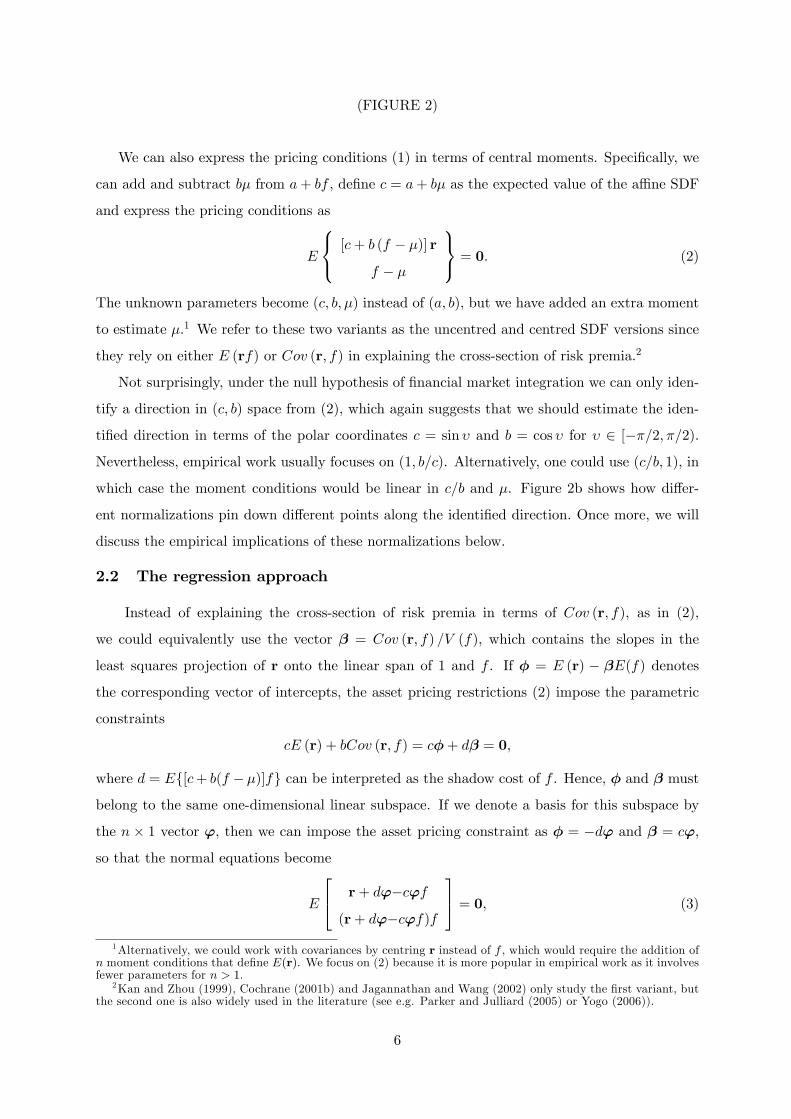
We can also express the pricing conditions (1) in terms of central moments. Speci�cally, we

can add and subtract b� from a+ bf , de�ne c = a+ b� as the expected value of the a¢ ne SDF

and express the pricing conditions as

E

8<: [c+ b (f � �)] r

f � �

9=; = 0: (2)

The unknown parameters become (c; b; �) instead of (a; b), but we have added an extra moment

to estimate �.1 We refer to these two variants as the uncentred and centred SDF versions since

they rely on either E (rf) or Cov (r; f) in explaining the cross-section of risk premia.2

Not surprisingly, under the null hypothesis of �nancial market integration we can only iden-

tify a direction in (c; b) space from (2), which again suggests that we should estimate the iden-

ti�ed direction in terms of the polar coordinates c = sin � and b = cos � for � 2 [��=2; �=2).

Nevertheless, empirical work usually focuses on (1; b=c). Alternatively, one could use (c=b; 1), in

which case the moment conditions would be linear in c=b and �. Figure 2b shows how di¤er-

ent normalizations pin down di¤erent points along the identi�ed direction. Once more, we will

discuss the empirical implications of these normalizations below.

2.2 The regression approach

Instead of explaining the cross-section of risk premia in terms of Cov (r; f), as in (2),

we could equivalently use the vector � = Cov (r; f) =V (f), which contains the slopes in the

least squares projection of r onto the linear span of 1 and f . If � = E (r) � �E(f) denotes

the corresponding vector of intercepts, the asset pricing restrictions (2) impose the parametric

constraints

cE (r) + bCov (r; f) = c�+ d� = 0;

where d = Ef[c+ b(f ��)]fg can be interpreted as the shadow cost of f . Hence, � and � must

belong to the same one-dimensional linear subspace. If we denote a basis for this subspace by

the n � 1 vector ', then we can impose the asset pricing constraint as � = �d' and � = c',

so that the normal equations become

E

24 r+ d'�c'f

(r+ d'�c'f)f

35 = 0; (3)

1Alternatively, we could work with covariances by centring r instead of f , which would require the addition ofn moment conditions that de�ne E(r). We focus on (2) because it is more popular in empirical work as it involvesfewer parameters for n > 1.

2Kan and Zhou (1999), Cochrane (2001b) and Jagannathan and Wang (2002) only study the �rst variant, butthe second one is also widely used in the literature (see e.g. Parker and Julliard (2005) or Yogo (2006)).

6

where (c; d;') are the new parameters to estimate.3 As in the previous section, we can only

identify a direction in (c; d) space. Once again, the usual asymmetric normalization in empirical

work sets (1; d=c), but we could also set (c=d; 1) or indeed estimate the identi�ed direction in

terms of the polar coordinates c = sin# and d = cos# for # 2 [��=2; �=2).

Alternatively, we could start from the uncentred variant of the SDF approach in (1), which

explains the cross-section of risk premia in terms of E(fr), and re-write the �nancial market

integration restrictions using the vector � = E(fr)=E(f2), which de�nes the regression slopes

of the least squares projection of r onto the linear span of f only. Speci�cally, if � = E (r)���

denotes the mean of the uncentred projection errors, the asset pricing restrictions (1) impose

the parametric constraint

aE (r) + bE (rf) = a�+ d� = 0;

since d = E [(a+ bf) f ]. Hence, � and � must also belong to the same one dimensional subspace.

If we denote a basis for this subspace by the n� 1 vector %, then we can impose this constraint

as � = �d% and � = a%, so that the appropriate moment conditions would be

E

24 r+ %d� a%f(r� a%f) f

35 = 0; (4)

with (a; d;%) as the parameters to estimate. Once again, we can only identify a direction in

(a; d) space, and the obvious asymmetric normalization would be (1; d=a).

Given that (3) relies on covariances and (4) on second moments, we refer to these moment

conditions as the centred and uncentred versions of the regression approach, respectively. How-

ever, since we are not aware of any empirical study based on (4), we shall not consider these

moments conditions henceforth.

3 Traded factors

3.1 Moment conditions and parameters

Let us assume that the pricing factor f is itself the excess return on another asset, such as

the market portfolio in the CAPM.4 As forcefully argued by Shanken (1992), Farnsworth et al.

(2002) and Lewellen, Nagel and Shanken (2010) among others, the pricing model applies to f

too, which means that

E [(a+ bf) f ] = 0: (5)

3An alternative, equivalent version of the second group of moment conditions in (3) would be E[(r + d' �c')(f ��)] = 0, which would require the addition of the moment condition E(f ��) = 0 to de�ne �. Theoreticaland Monte Carlo results for these alternative moments are available on request.

4 It is important to mention that our assets could include managed portfolios. Similary, the factor could alsobe a scaled version of a primitive excess return to accommodate conditioning information; see the discussion inchapter 8 of Cochrane (2001a).

7

The uncentred SDF approach relies on the n+1 moment conditions (1) and (5) once we choose

a normalization for (a; b). As we mentioned before, the normalization could be asymmetric

or symmetric. The latter relies on the directional coordinate , while the former is typically

implemented by factoring a out of the pricing conditions, leaving � = �b=a as the only unknown

parameter. Given moment condition (5), we will have that

� = � cot = �

; (6)

where is the second moment of f , which allows us to interpret � as a �price of risk� for the

factor.

Similarly, the centred SDF approach works with the n+ 2 moment conditions (2) and

Ef[c+ b (f � �)]fg = 0: (7)

Again, the normalization could be asymmetric or symmetric. The latter will make use of the

polar coordinate �, while the former is typically implemented by factoring c out of the pricing

conditions, leaving � = �b=c and � as the only unknown parameters. Either way, we can use

moment condition (7) to show that:

� = � cot � = �

�2; (8)

where �2 = � �2 denotes the variance of f , which means that � also has a �price of risk�

interpretation.

When the risk factor coincides with the excess returns on a traded asset, its shadow cost

d must coincide with its actual cost, which is 0. If we impose this constraint in the moment

conditions (3), then the centred regression approach reduces to the 2n overidenti�ed moment

conditions

E

24 r� �f

(r� �f) f

35 = 0; (9)

where the n unknown parameters are the elements of � because the regression intercepts must

be 0 (see MacKinlay and Richardson (1991)).5 As a result, the slope coe¢ cients coincide with

both Cov(r;f)=V (f) and E(rf)=E(f2) when (1) and (5) hold, so that the uncentred and centred

variants of the regression (or beta) approach are identical in this case. The regression method

identi�es � with the expected excess return of a portfolio whose �beta� is equal to 1. Thus,

this parameter represents a �factor risk premium�when f is traded. To estimate it, we can add

f � � to (9), as in (2), and simultaneously estimate � and �.5These moment conditions con�rm the result in Chamberlain (1983b) that says that a+ bf will constitute an

admissible SDF if and only if f lies on the mean-variance frontier generated by f and r. Then, the well-knownproperties of mean-variance frontiers imply that the least squares projection of r onto the linear span generatedby a constant and f should be proportional to f .

8

Under standard regularity conditions (more on this in section 4.4), all three overidentifying

restrictions (J) tests will follow an asymptotic chi-square distribution with n degrees of freedom

when the corresponding moments are correctly speci�ed.

The overidenti�cation tests are regularly complemented by three standard evaluation mea-

sures. Speci�cally, we can de�ne Jensen�s alphas as E (r)��E (f) for the regression method, as

well as the �pricing errors�associated to the uncentred SDF representation, E (r)�E (rf) �, and

the centred SDF representation, E (r)�E[r (f � �)]� . In population terms, these three pricing

errors coincide. In particular, they should be simultaneously 0 under the null hypothesis.

3.2 Numerical equivalence results

As we mentioned in the introduction, Kan and Zhou (1999, 2002), Cochrane (2001b), Ja-

gannathan and Wang (2002), Burnside (2012) and Kan and Robotti (2008) compare some of

the aforementioned approaches when researchers rely on traditional, two-step or iterated GMM

procedures. In contrast, we show that all the methods coincide if one uses instead single-step

procedures such as CU-GMM, which we describe in appendix F. More formally:

Proposition 1 If we apply single-step procedures to the uncentred SDF method based on themoment conditions (1) and (5), the centred SDF method based on the moment conditions (2)and (7), and the regression method based on the moment conditions (9), then for a commonspeci�cation of the characteristics of the HAC weighting matrix the following numerical equiva-lences hold for any �nite sample size:1) The overidenti�cation restrictions (J) tests regardless of the normalization used.2) The direct estimates of (a; b) from (1) and (5), their indirect estimates from (2) and (7) thatexploit the relationship c = a+ b�, and the indirect estimates from (9) extended to include (�; )which exploit the relationship a�+ b = 0 when we use symmetric normalizations or compatibleasymmetric ones. Analogous results apply to (c; b) and �.3) The estimates of Jensen�s alphas E (r)��E (f) obtained by replacing E (�) by an unrestrictedsample average and the elements of � by their direct estimates obtained from the regressionmethod, and the indirect estimates obtained from SDF methods with symmetric normalizationsand compatible asymmetric ones extended to include �. Analogous results apply to the alternativepricing errors of the uncentred and centred SDF representations.

Importantly, these numerical equivalence results do not depend in any sense on the number

of assets or indeed the number of factors, and remain true regardless of the validity of the asset

pricing restrictions. In order to provide some intuition, imagine that for estimation purposes

we assumed that the joint distribution of r and f is i:i:d: multivariate normal. In that context,

we could test the mean-variance e¢ ciency of f by means of a likelihood ratio (LR) test. We

could then factorize the joint log-likelihood function of r and f as the marginal log-likelihood

of f , whose parameters � and �2 would be unrestricted, and the conditional log-likelihood of

r given f . As a result, the LR version of the original Gibbons, Ross and Shanken (1989) test

would be numerically identical to the LR test in the joint system irrespective of the chosen

parameterization. The CU-GMM overidenti�cation test, which implicitly uses the Gaussian

9

scores as in�uence functions, inherits the invariance of the LR test. The advantage, though,

is that we can make it robust to departures from normality, serial independence or conditional

homoskedasticity.

From a formal point of view, the equivalence between the two SDF approaches is a direct con-

sequence of the fact that single-step procedures are numerically invariant to normalization, while

the additional, less immediate results relating the regression and SDF approaches in proposition

1 follow from the fact that those GMM procedures are also invariant to reparameterizations and

parameter dependent linear transformations of the moment conditions (see again appendix F).6

3.3 Starting values and other implementation details

One drawback of CU-GMM and other GEL estimators is that they involve a non-linear

optimization procedure even if the moment conditions are linear in parameters, which may

result in multiple local minima. In this sense, the uncentred SDF method has a non-trivial

computational advantage because it contains a single unknown parameter.7 At the same time,

one can also exploit the numerical equivalence of the di¤erent approaches covered in proposition

1 to check that a global minimum has been reached. Likewise, one could also exploit the

numerical equivalence of the Euclidean empirical likelihood and CU-GMM estimators of the

model parameters (see Antoine, Bonnal and Renault (2006)). A much weaker convergence test

is the fact that the value of the criterion function at the CU-GMM estimators cannot be larger

than at the iterated GMM estimators, which do not generally coincide (see Hansen, Heaton and

Yaron (1996)).

In any case, it is convenient to have good initial parameter values. For that reason, we

propose to use as starting value a computationally simple intuitive estimator that is always

consistent, but which would become e¢ cient for i:i:d: elliptical returns, a popular assumption

in �nance because it guarantees the compatibility of mean-variance preferences with expected

utility maximization regardless of investors� preferences (see Chamberlain (1983a) and Owen

and Rabinovitch (1983)):

Lemma 1 If (rt; ft) is an i.i.d. elliptical random vector with bounded fourth moments and thenull hypothesis of linear factor pricing holds, then the most e¢ cient GMM estimator of � = �b=aobtained from (1) and (5) will be given by

_�T =

PTt=1 ftPTt=1 f

2t

: (10)

6Empirical researchers sometimes report the cross-sectional (squared) correlation between the actual and modelimplied risk premia. Proposition 1 trivially implies that they would also obtain a single number for each of thethree approaches if they used single-step GMM.

7This advantage becomes more relevant as the number of factors k increases because the centred SDF methodrequires the additional estimation of k factor means and the regression method the estimation of n � k factorloadings.

10

Intuitively, this means that in those circumstances (5), which is the moment involving f ,

exactly identi�es the parameter �, while (1), which are the moments corresponding to r, provide

the n overidenti�cation restrictions to test. Although the elliptical family is rather broad (see

Fang, Kotz and Ng (1990)), and includes the multivariate normal and Student t distribution as

special cases, it is important to stress that _�T will remain consistent under linear factor pricing

even if the assumptions of serial independence and ellipticity are not totally realistic in practice.8

A rather di¤erent justi�cation for (10) is that it coincides with the GMM estimator of � that

we would obtain from (1) and (5) if we used as weighting matrix the second moment of the

vector of excess returns x = (f; r0)0. Speci�cally, (10) minimizes the sample counterpart to the

Hansen and Jagannathan (1997) distance

E [(1� �f)x]0�E�xx0���1

E [(1� �f)x]

irrespective of the distribution of returns and the validity of the asset pricing model.

Hansen, Heaton and Yaron (1996) also indicate that CU-GMM occasionally generates ex-

treme estimators that lead to large pricing errors with even larger variances. In those circum-

stances, we would suggest the imposition of good deal restrictions (see Cochrane and Saa-Requejo

(2000)) to rule out implausible results.9

4 Non-traded factors

4.1 Moment conditions and parameters

Let us now consider situations in which f is either a scalar non-traded factor, such as the

growth rate of per capita consumption, or the empirical researcher ignores that it is traded. The

main di¤erence with the analysis in section 3 is that the pricing equations (5) and (7) are no

longer imposed, so that the SDF is de�ned by (1) or (2) only. Similarly, the regression approach

relies on (3) or (4) without the additional parametric constraint d = 0 implied by a traded

factor. Obviously, the resulting reduction in the number of moment conditions or constraints

yields a reduction in the degree of overidenti�cation, which becomes n� 1.8We can also prove that we obtain an estimator of � that is asymptotically equivalent to (10) if we follow

Spanos (1991) in assuming that the so-called Haavelmo distribution, which is the joint distribution of the T (n+1)observed random vector (r1; f1; : : : ; rt; ft; : : : ; rT ; fT ), is an a¢ ne transformation of a scale mixture of normals,and therefore elliptical. Intuitively, the reason is that a single sample realization of such a Haavelmo distributionis indistinguishible from a realization of size T of an i:i:d: multivariate normal distribution for (rt; ft).

9Speci�cally, given that we know from Hansen and Jagannathan (1991) that

S2 � E2(m)=V (m) = R2;

where S is the maximum attainable Sharpe ratio of any portfolio of the assets under consideration, and R2 is thecoe¢ cient of determination in the (theoretical) regression of f on a constant and the tradeable assets, one couldestimate the linear factor pricing model subject to implicit restrictions that guarantee that the values of S or thecoe¢ cient of variation of m computed under the null should remain within some loose but empirically plausiblebounds. In the case of traded factors both these bounds should coincide because R2 = 1.

11

Nevertheless, we can still provide a �price of risk� interpretation to some parameters, but

this time in terms of factor mimicking portfolios. In particular, (6) is replaced by

� = � cot = E(r+)

E(r+2); (11)

where

r+ = E(fr0)E�1(rr0)r (12)

is the uncentred least squares projection of f on r. Similarly, (8) becomes

� = � cot � = E(r++)

V (r++); (13)

where

r++ = Cov(f; r0)V �1(r)r

is the centred least squares projection of f on r.

In turn, given that the standard implementation of the centred regression uses the asym-

metric normalization (1; d=c) in the 2n overidenti�ed moment restrictions (3), and estimates the

n+1 parameters { = �d=c and � = 'c (see Campbell, Lo and MacKinlay (1996, chap. 5)), we

can interpret � = { + � as the �factor risk premium�: the expected excess return of a portfolio

whose �beta�is equal to 1.10

Finally, the expressions for the centred and uncentred SDF pricing errors at the end of section

3 continue to be valid, while Jensen�s alphas are now de�ned as E (r)� ��.

4.2 Numerical equivalence results

As in the case of traded factors, we can show that all the approaches discussed in the

previous subsection coincide if one uses single-step methods. More formally

Proposition 2 If we apply single-step procedures to the uncentred SDF method based on themoment conditions (1), the centred SDF method based on the moment conditions (2), and thecentred regression method based on the moment conditions (3), then for a common speci�cationof the characteristics of the HAC weighting matrix the following numerical equivalences hold forany �nite sample size:1) The overidenti�cation restrictions (J) tests regardless of the normalization used.2) The direct estimates of (a; b) from (1), their indirect estimates from (2) that exploit therelationship c = a + b�, and the indirect estimates from (3) extended to include (�; ) thatexploit the relationships c = a+ b� and d = a�+ b when we use symmetric normalizations orcompatible asymmetric ones. Analogous results apply to (c; b) and (c; d).3) The estimates of Jensen�s alphas E (r) � �� obtained by replacing E (�) by an unrestrictedsample average and the elements of �� by their direct estimates obtained from the regressionmethod, and the indirect estimates obtained from SDF methods with symmetric normalizationsand compatible asymmetric ones extended to include �, and �. Analogous results apply to thealternative pricing errors of the uncentred and centred SDF representations.

10Jagannathan and Wang (2002) use ��� instead of {, and add the in�uence functions f�� and (f � �)2��2to estimate � and �2 too. The addition of these moments is irrelevant for the estimation of { and the J testbecause they exactly identify � and �2 (see e.g. pp. 196�197 in Arellano (2003) for a proof of the irrelevance ofunrestricted moments).

12

Once again, we can gain some intuition by assuming that the joint distribution of r and f is

i:i:d: multivariate normal. In that context, we could test the validity of the model by means of a

LR test that compares the restricted and unrestricted criterion functions, as in Gibbons (1982).

We could then factorize the joint log-likelihood function of r and f as the marginal log-likelihood

of f , whose parameters � and �2 would be unrestricted, and the conditional log-likelihood of

r given f , which would have an a¢ ne mean and a constant variance. As a result, the LR

version of the linear factor pricing test would be numerically identical to the LR test in the

joint system irrespective of the chosen parameterization. The CU-GMM overidenti�cation test,

which implicitly uses the Gaussian scores as in�uence functions, inherits the invariance of the LR

test. The advantage, though, is that we can make it robust to departures from normality, serial

independence or conditional homoskedasticity.11 As we shall see in section 4.4, though, we can

encounter situations in which some of the popular asymmetric normalizations are incompatible

the estimates obtained with the symmetric ones.

It is important to distinguish proposition 2 from the results in Jagannathan and Wang (2002)

and Kan and Zhou (2002). These authors showed that the centred regression and uncentred SDF

approaches lead to asymptotically equivalent inferences under the null and compatible sequences

of local alternatives in single factor models. In contrast, proposition 2 shows that in fact both

SDF approaches and the regression method yield numerically identical conclusions if we work

with single-step GMM procedures. Since our equivalence result is numerical, it holds regardless

of the validity of the pricing model and irrespective of n or the number of factors.12

4.3 Starting values and other implementation details

The numerical equivalence of the di¤erent approaches gives once more a non-trivial com-

putational advantage to the uncentred SDF method, which only contains a single unknown

parameter. At the same time, one can also exploit the fact that the approaches discussed in

proposition 2 coincide to check that a global minimum has been obtained.

11Kan and Robotti (2008) also show that CU-GMM versions of the SDF approach are numerically invariant toa¢ ne transformations of the factors with known coe¢ cients, which is not necessarily true of two-step or iteratedGMM methods. Not surprisingly, it is easy to adapt the proof of Proposition 2 to show that the regressionapproach is also numerically invariant to such transformations.12We could also consider a nonlinear SDF such as m = f� , with � unknown, so that the moments would become

E(rf�) = 0:

In this context, we can easily show that a single-step overidentifying restrictions test would be numericallyequivalent to the one obtained from the �regression�-based moment conditions

E

2664(r� �m(f� � m=�m))(r� �m(f� � m=�m)))f�

f� � �mf2� � m

3775 = 0;whose unkown parameters are (�;�m; �m; m).

13

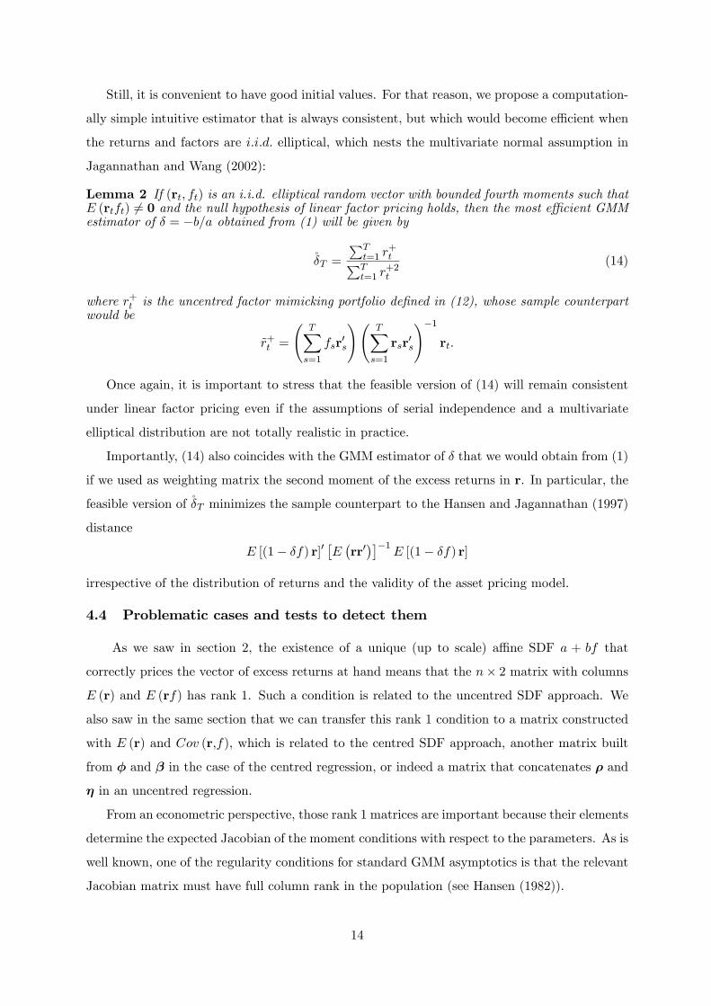
Still, it is convenient to have good initial values. For that reason, we propose a computation-

ally simple intuitive estimator that is always consistent, but which would become e¢ cient when

the returns and factors are i:i:d: elliptical, which nests the multivariate normal assumption in

Jagannathan and Wang (2002):

Lemma 2 If (rt; ft) is an i.i.d. elliptical random vector with bounded fourth moments such thatE (rtft) 6= 0 and the null hypothesis of linear factor pricing holds, then the most e¢ cient GMMestimator of � = �b=a obtained from (1) will be given by

��T =

PTt=1 r

+tPT

t=1 r+2t

(14)

where r+t is the uncentred factor mimicking portfolio de�ned in (12), whose sample counterpartwould be

~r+t =

TXs=1

fsr0s

! TXs=1

rsr0s

!�1rt:

Once again, it is important to stress that the feasible version of (14) will remain consistent

under linear factor pricing even if the assumptions of serial independence and a multivariate

elliptical distribution are not totally realistic in practice.

Importantly, (14) also coincides with the GMM estimator of � that we would obtain from (1)

if we used as weighting matrix the second moment of the excess returns in r. In particular, the

feasible version of��T minimizes the sample counterpart to the Hansen and Jagannathan (1997)

distance

E [(1� �f) r]0�E�rr0���1

E [(1� �f) r]

irrespective of the distribution of returns and the validity of the asset pricing model.

4.4 Problematic cases and tests to detect them

As we saw in section 2, the existence of a unique (up to scale) a¢ ne SDF a + bf that

correctly prices the vector of excess returns at hand means that the n� 2 matrix with columns

E (r) and E (rf) has rank 1. Such a condition is related to the uncentred SDF approach. We

also saw in the same section that we can transfer this rank 1 condition to a matrix constructed

with E (r) and Cov (r;f), which is related to the centred SDF approach, another matrix built

from � and � in the case of the centred regression, or indeed a matrix that concatenates � and

� in an uncentred regression.

From an econometric perspective, those rank 1 matrices are important because their elements

determine the expected Jacobian of the moment conditions with respect to the parameters. As is

well known, one of the regularity conditions for standard GMM asymptotics is that the relevant

Jacobian matrix must have full column rank in the population (see Hansen (1982)).

14

When the pricing factor is traded, we should add to these matrices a row whose second

element is always di¤erent from 0. This additional row ensures that all the Jacobians have full

rank when risk premia are not all simultaneously zero (see lemma G1 in appendix G).

When the pricing factor is non-traded, or treated as if it were so, all the symmetrically

normalized moment conditions also have a full column rank Jacobian as long as risk premia are

not zero (see lemma G2 in appendix G). As a result, if the additional GMM regularity conditions

are satis�ed, the unique single step overidenti�cation test associated to all of them will be

asymptotically distributed as �2n�1 under the null.13 Moreover, the multistep overidenti�cation

tests will also share this asymptotic distribution.

In contrast, there are some special cases in which the population Jacobians of some of the

asymmetrically normalized moment conditions do not have full rank.14 Next, we study in detail

the case of an uncorrelated factor, which is the most relevant one in empirical work.

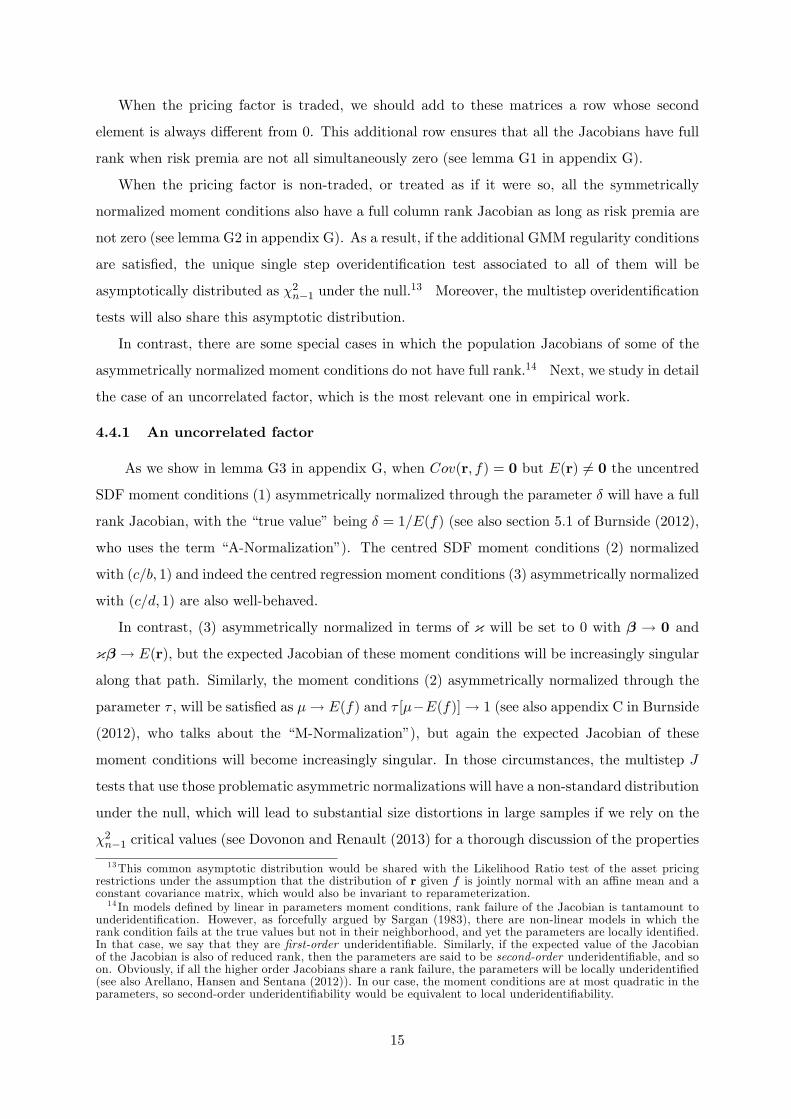
4.4.1 An uncorrelated factor

As we show in lemma G3 in appendix G, when Cov(r; f) = 0 but E(r) 6= 0 the uncentred

SDF moment conditions (1) asymmetrically normalized through the parameter � will have a full

rank Jacobian, with the �true value�being � = 1=E(f) (see also section 5.1 of Burnside (2012),

who uses the term �A-Normalization�). The centred SDF moment conditions (2) normalized

with (c=b; 1) and indeed the centred regression moment conditions (3) asymmetrically normalized

with (c=d; 1) are also well-behaved.

In contrast, (3) asymmetrically normalized in terms of { will be set to 0 with � ! 0 and

{� ! E(r), but the expected Jacobian of these moment conditions will be increasingly singular

along that path. Similarly, the moment conditions (2) asymmetrically normalized through the

parameter � , will be satis�ed as �! E(f) and � [��E(f)]! 1 (see also appendix C in Burnside

(2012), who talks about the �M-Normalization�), but again the expected Jacobian of these

moment conditions will become increasingly singular. In those circumstances, the multistep J

tests that use those problematic asymmetric normalizations will have a non-standard distribution

under the null, which will lead to substantial size distortions in large samples if we rely on the

�2n�1 critical values (see Dovonon and Renault (2013) for a thorough discussion of the properties

13This common asymptotic distribution would be shared with the Likelihood Ratio test of the asset pricingrestrictions under the assumption that the distribution of r given f is jointly normal with an a¢ ne mean and aconstant covariance matrix, which would also be invariant to reparameterization.14 In models de�ned by linear in parameters moment conditions, rank failure of the Jacobian is tantamount to

underidenti�cation. However, as forcefully argued by Sargan (1983), there are non-linear models in which therank condition fails at the true values but not in their neighborhood, and yet the parameters are locally identi�ed.In that case, we say that they are �rst-order underidenti�able. Similarly, if the expected value of the Jacobianof the Jacobian is also of reduced rank, then the parameters are said to be second-order underidenti�able, and soon. Obviously, if all the higher order Jacobians share a rank failure, the parameters will be locally underidenti�ed(see also Arellano, Hansen and Sentana (2012)). In our case, the moment conditions are at most quadratic in theparameters, so second-order underidenti�ability would be equivalent to local underidenti�ability.

15

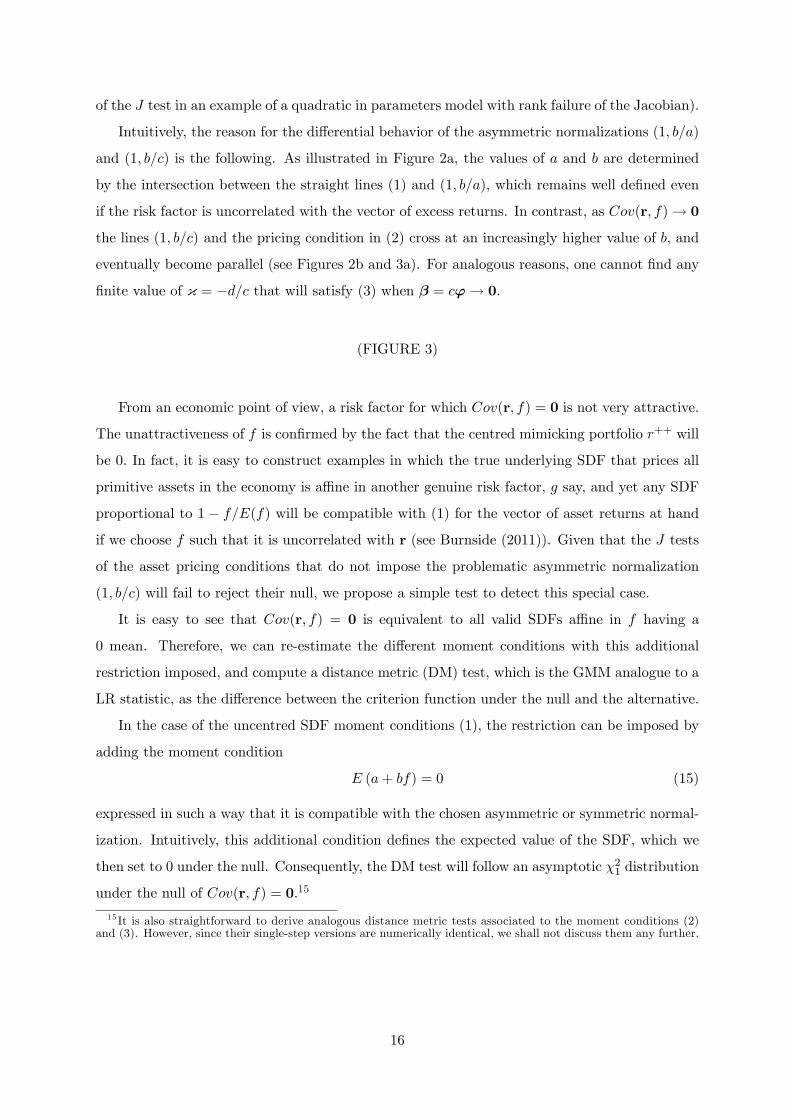
of the J test in an example of a quadratic in parameters model with rank failure of the Jacobian).

Intuitively, the reason for the di¤erential behavior of the asymmetric normalizations (1; b=a)

and (1; b=c) is the following. As illustrated in Figure 2a, the values of a and b are determined

by the intersection between the straight lines (1) and (1; b=a), which remains well de�ned even

if the risk factor is uncorrelated with the vector of excess returns. In contrast, as Cov(r; f)! 0

the lines (1; b=c) and the pricing condition in (2) cross at an increasingly higher value of b, and

eventually become parallel (see Figures 2b and 3a). For analogous reasons, one cannot �nd any

�nite value of { = �d=c that will satisfy (3) when � = c'! 0.

(FIGURE 3)

From an economic point of view, a risk factor for which Cov(r; f) = 0 is not very attractive.

The unattractiveness of f is con�rmed by the fact that the centred mimicking portfolio r++ will

be 0. In fact, it is easy to construct examples in which the true underlying SDF that prices all

primitive assets in the economy is a¢ ne in another genuine risk factor, g say, and yet any SDF

proportional to 1 � f=E(f) will be compatible with (1) for the vector of asset returns at hand

if we choose f such that it is uncorrelated with r (see Burnside (2011)). Given that the J tests

of the asset pricing conditions that do not impose the problematic asymmetric normalization

(1; b=c) will fail to reject their null, we propose a simple test to detect this special case.

It is easy to see that Cov(r; f) = 0 is equivalent to all valid SDFs a¢ ne in f having a

0 mean. Therefore, we can re-estimate the di¤erent moment conditions with this additional

restriction imposed, and compute a distance metric (DM) test, which is the GMM analogue to a

LR statistic, as the di¤erence between the criterion function under the null and the alternative.

In the case of the uncentred SDF moment conditions (1), the restriction can be imposed by

adding the moment condition

E (a+ bf) = 0 (15)

expressed in such a way that it is compatible with the chosen asymmetric or symmetric normal-

ization. Intuitively, this additional condition de�nes the expected value of the SDF, which we

then set to 0 under the null. Consequently, the DM test will follow an asymptotic �21 distribution

under the null of Cov(r; f) = 0.15

15 It is also straightforward to derive analogous distance metric tests associated to the moment conditions (2)and (3). However, since their single-step versions are numerically identical, we shall not discuss them any further.

16

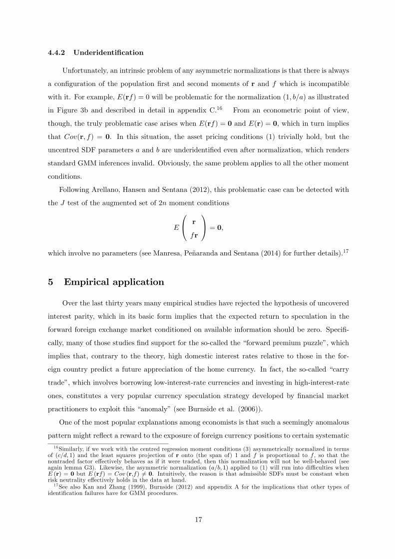
4.4.2 Underidenti�cation

Unfortunately, an intrinsic problem of any asymmetric normalizations is that there is always

a con�guration of the population �rst and second moments of r and f which is incompatible

with it. For example, E(rf) = 0 will be problematic for the normalization (1; b=a) as illustrated

in Figure 3b and described in detail in appendix C.16 From an econometric point of view,

though, the truly problematic case arises when E(rf) = 0 and E(r) = 0, which in turn implies

that Cov(r; f) = 0. In this situation, the asset pricing conditions (1) trivially hold, but the

uncentred SDF parameters a and b are underidenti�ed even after normalization, which renders

standard GMM inferences invalid. Obviously, the same problem applies to all the other moment

conditions.

Following Arellano, Hansen and Sentana (2012), this problematic case can be detected with

the J test of the augmented set of 2n moment conditions

E

0@ r

fr

1A = 0;

which involve no parameters (see Manresa, Peñaranda and Sentana (2014) for further details).17

5 Empirical application

Over the last thirty years many empirical studies have rejected the hypothesis of uncovered

interest parity, which in its basic form implies that the expected return to speculation in the

forward foreign exchange market conditioned on available information should be zero. Speci�-

cally, many of those studies �nd support for the so-called the �forward premium puzzle�, which

implies that, contrary to the theory, high domestic interest rates relative to those in the for-

eign country predict a future appreciation of the home currency. In fact, the so-called �carry

trade�, which involves borrowing low-interest-rate currencies and investing in high-interest-rate

ones, constitutes a very popular currency speculation strategy developed by �nancial market

practitioners to exploit this �anomaly�(see Burnside et al. (2006)).

One of the most popular explanations among economists is that such a seemingly anomalous

pattern might re�ect a reward to the exposure of foreign currency positions to certain systematic

16Similarly, if we work with the centred regression moment conditions (3) asymmetrically normalized in termsof (c=d; 1) and the least squares projection of r onto (the span of) 1 and f is proportional to f , so that thenontraded factor e¤ectively behaves as if it were traded, then this normalization will not be well-behaved (seeagain lemma G3). Likewise, the asymmetric normalization (a=b; 1) applied to (1) will run into di¢ culties whenE (r) = 0 but E (rf) = Cov (r;f) 6= 0. Intuitively, the reason is that admissible SDFs must be constant whenrisk neutrality e¤ectively holds in the data at hand.17See also Kan and Zhang (1999), Burnside (2012) and appendix A for the implications that other types of

identi�cation failures have for GMM procedures.

17

risk factors. To study this possibility, Lustig and Verdelhan (2007) constructed eight portfolios

of currencies sorted at the end of the previous year by their nominal interest rate di¤erential

to the US dollar, creating in this way annual excess returns (in real terms) on foreign T-Bill

investments for a US investor over the period 1953-2002. Interestingly, the broadly monotonic

relationship between the level of interest rates di¤erentials and risk premia for those portfolios

captured in Figure 1 of their paper provides informal evidence on the failure of uncovered interest

rate parity.

Lusting and Verdelhan (2007) used two-pass regressions to test if some popular empirical

asset pricing models that rely on certain domestic US risk factors were able to explain the cross-

section of risk premia. In what follows, we use their data to estimate the parameters and assess

the asset pricing restrictions of the di¤erent sets of moments conditions described in previous

sections by means of two-step, iterated and CU-GMM.18 In all cases, we estimate the asymptotic

covariance matrix of the relevant in�uence functions by means of its sample counterpart, as in

Hansen, Heaton and Yaron (1996). As for the �rst-step estimators, we use the identity matrix

as initial weighting matrix given the prevalence of this practice in empirical work. Finally,

we implicitly choose the leverage of the carry trades whose payo¤s are the excess returns by

systematically expressing all returns and factors as pure numbers. This scaling does not a¤ect

CU or iterated GMM, but it a¤ects some of the two-step GMM procedures.19

5.1 Traded factor

Given that for pedagogical reasons we have only considered a single traded factor in our

theoretical analysis, we focus on the CAPM. Following Lustig and Verdelhan (2007), we take

the pricing factor to be the US market portfolio, which we also identify with the CRSP value-

weighted excess return. Table 1 contains the results of applying the di¤erent inference procedures

previously discussed to this model. Importantly, Figure G1a in appendix G, which plots the

CU-GMM criterion as a function of �, con�rms that we have obtained a global minimum.

The �rst thing to note is that the value of the CU-GMM overidenti�cation restriction statistic

is the same across �ve di¤erent variants covered by proposition 1. In contrast, there are marked

numerical di¤erences between the corresponding two-step versions of the J test. In particular,

an asymmetrically normalized version of the centred SDF approach yields a substantially higher

value, while the two symmetric SDFs and the regression variants have p-values above 50%.

These numerical di¤erences are reduced but not eliminated as we update the weighting matrix.

18We have also considered other single step procedures such as empirical likelihood and exponentially-tiltedmethods, but since they yield J tests, parameter estimates and standard errors similar to their CU/Euclideanempirical likelihood counterparts, we do not report them in the interest of space.19 In contrast, the scale of the data does not a¤ect those two-step GMM procedures that use (10) or (14) as

�rst-step estimators instead of relying on the identity matrix.

18

In particular, iterated GMM applied to symmetric centred SDF gives a test statistic similar to

CU, while its asymmetric version is still much higher.

(TABLE 1)

Table G1 in appendix G also con�rms the numerical equality of the CU-GMM estimators of

prices of risk (�, � and �) and pricing errors regardless of the approach used to estimate them, as

stated in points 2 and 3 of proposition 1. In contrast, two-step and iterated GMM yield di¤erent

results, which explains the three di¤erent columns required for each of them.20 In addition, the

magnitudes of the two-step, iterated and CU-GMM estimates of � and � are broadly the same,

while the CU-GMM estimate of � is noticeably higher than its multistep counterparts.

In any case, most tests reject the null hypothesis of linear factor pricing. Interestingly, these

rejections do not seem to be due to poor �nite sample properties of the J statistics in this

context since the F version of the Gibbons, Ross and Shanken (1989) regression test, which

remains asymptotically valid in the case of conditional homoskedasticity, also yields a p-value

of 0.3%.

The J tests reported in Table 1 can also be interpreted as DM tests of the null hypothesis of

zero pricing errors in the eight currency returns only. The rationale is as follows. If we saturate

(1) by adding n pricing errors, then the joint system of moment conditions becomes exactly

identi�ed, which in turn implies that the optimal criterion function under the alternative will

be zero.

We can also consider the DM test of the null hypothesis of zero pricing error for the traded

factor. Once again, the criterion function under the null takes the value reported in Table 1.

Under the alternative, though, we need to conduct a new estimation. Speci�cally, if we saturate

the moment condition (5) corresponding to the traded factor by adding a single pricing error,

then the exact identi�ability of this modi�ed moment condition means that the joint system

of moment conditions e¤ectively becomes equivalent to another system that relies on (1) only.

Treating the excess return on the US stock market as a nontraded factor delivers a CU-GMM

J test of 6:87 (p-value 0:44). Hence, the CAPM restrictions are not rejected when we do not

force this model to price the market, although the estimated � is negative. In contrast, the DM

test of zero pricing error for the traded factor, which is equal to the di¤erence between this J

20The implied estimate of � from the uncentred SDF approach also di¤ers between two-step and iter-ated GMM (0.139 vs. 0.150), which are in turn di¤erent from the sample mean of f . The reason isthat GMM equates to zero the average of the sample analogue of the orthogonalized in�uence function(f � �) � E [(f � �)mr]

�E�m2rr0

���1(mr), (assuming i:i:d: observations) where m = 1 � �f , rather than the

average of f � �. This residual depends on the estimate of �, which di¤ers between two-step and iterated GMM(4.455 vs. 4.534).

19

statistic and the one reported in Table 1, is 12:09, with a tiny p-value. Therefore, the failure of

the CAPM to price the US stock market portfolio provides the clearest source of model rejection,

thereby con�rming the relevance of the recommendation in Shanken (1992), Farnsworth et al.

(2002) and Lewellen, Nagel and Shanken (2010).

Importantly, these DM tests avoid the problems that result from the degenerate nature of the

joint asymptotic distribution of the pricing error estimates recently highlighted by Gospodinov,

Kan and Robotti (2012). This would be particularly relevant in the elliptical case because the

moment condition (5) coincides with the optimal one in view of lemma 1.

5.2 Non-traded factor

Let us now explore a linearized version of the CCAPM, which de�nes the US per capita

consumption growth of nondurables as the only pricing factor. Table 2 displays the results from

the application of the di¤erent inference procedures previously discussed for the purposes of

testing this model. Once again, Figure G1b in appendix G, which plots the CU-GMM criterion

as a function of �, con�rms that we have obtained a global minimum.

In this case, the common CU-GMM J test (5:66, p-value 58%) does not reject the null

hypothesis implicit in (1), (2) or (3), which is in agreement with the empirical results in Lustig

and Verdelhan (2007). This conclusion is con�rmed by a p-value of 83.9% for the test of the same

null hypothesis computed from the regression using the expressions in Beatty, LaFrance and Yang

(2005). Their F -type test is asymptotically valid in the case of conditional homoskedasticity,

and may lead to more reliable inferences in �nite samples.

In contrast, there are important numerical di¤erences between the standard two-step GMM

implementation of the �ve approaches, which lead to diverging conclusions at conventional sig-

ni�cance levels. Speci�cally, while the asymmetric centred SDF approach rejects the null hy-

pothesis, its symmetric version does not, with p-values of almost zero and 47%, respectively.

These numerical di¤erences are attenuated when we use iterated GMM procedures, but the

contradicting conclusions remain.

(TABLE 2)

In contrast, when we look at the uncentred SDF (both symmetric and asymmetric variants)

and regression approaches, the multistep GMM procedures yield results closer to CU-GMM. In

particular, the two-step and iterated versions of the J test of the centred regression are closer

to its uncentred SDF counterpart than to the centred SDF one. The reason is that in (3) we do

not need to rescale the in�uence functions when we switch from the asymmetric normalization

20

(1; d=c) to (c=d; 1). Therefore, both normalizations are numerically equivalent not only with

CU-GMM but also with two-step and iterated GMM. In contrast, in the centred SDF moments

(2) we rescale the in�uence functions as we switch from the asymmetric normalization (1; b=c)

to (c=b; 1).

Table G2 in appendix G also con�rms the numerical equality of the CU-GMM estimators of

prices of risk (�, � and �) and pricing errors regardless of the approach used to estimate them,

as expected from points 2 and 3 of proposition 2. In contrast, two-step and iterated GMM yield

di¤erent results. In this case, all the estimates of � and � are fairly close, but the CU-GMM

estimate of � is much higher than its multistep counterparts. However, the directional estimates

based on � in the symmetric variant of the centred SDF approach behave very similarly across

the di¤erent GMM implementations. Therefore, we can conclude that a very important driver

of the di¤erences between test statistics and parameter estimates is the normalization chosen,

possibly even more than the use of centred or uncentred moments, or indeed the use of CU or

iterated GMM.

The discrepancies that we observe suggest that we may have encountered one of the prob-

lematic situations described in section 4.4. The hypothesis of zero risk premia is clearly rejected

with a J statistic of 39:97, whose p-value is e¤ectively 0. Therefore, there are statistically

signi�cant risk premia in search of pricing factors to explain them. Similarly, the hypothesis

of underidenti�cation in section 4.4.2 is also rejected with a statistic of 53:04 and a negligible

p-value, which con�rms that the parameters appearing in (1), (2) and (3) are point identi�ed

after normalization.

Nevertheless, there is little evidence against the hypothesis of a zero mean SDF. Speci�cally,

the DM test introduced in section 4.4.1 yields 2:73 and a p-value of almost 10%. The relevance

of this p-value is reinforced by the �ndings of a Monte Carlo experiment reported in the next

section, which suggest that this test tends to overreject.

It is worth noting that CU-GMM proves once again useful in unifying the empirical results

in this context because the joint overidenti�cation test of (1) and (15), which trivially coincides

with the sum of the DM test of a SDF with zero mean and the J test of the CCAPM pricing

restrictions, is numerically equivalent to a test of the null that all the betas are 0, whose p-value

is 36%. For analogous reasons, we obtain the same J test whether we regress r on f or f on r.

This lack of correlation does not seem to be due to excessive reliance on asymptotic distributions,

because it is corroborated by a p-value of 81.7% for the F test of the second univariate regression,

which like the corresponding LR test, is also invariant to exchanging regressand and regressors.

As explained by Savin (1983) using results from Sche¤é (1953), the joint test of an uncorrelated

21

factor is e¤ectively testing that any portfolio formed from the eight currency portfolios has

zero correlation with US consumption growth (see also Gibbons, Ross and Shanken (1989) for a

closely related argument). Obviously, if we computed t-tests between every conceivable portfolio

and consumption growth, a non-negligible fraction of them will be statistically signi�cant, so the

usual trade o¤ between power and size applies (see Lustig and Verdelhan (2011) and Burnside

(2011) for further discussion of this point). In any case, the number of portfolios must be strictly

larger than the number of pricing factors for (1) to have testable implications.

In summary, the fact that we cannot reject the asset pricing restrictions implicit in (1), (2)

or (3) must be interpreted with some care. In this sense, the CCAPM results are very similar to

the ones described at the end of the previous subsection when we treated the market portfolio

as non-traded. This is not very surprising given that the correlations between the eight currency

portfolios and the excess returns on the US market portfolio and consumption growth are of

similar order.

6 Monte Carlo

In this section we report the results of some simulation experiments based on a linear factor

pricing model with a nontraded factor. In this way we assess the reliability of the empirical

evidence on the CCAPM we have obtained in section 5.2. Given that the number of mean,

variance and correlation parameters for eight arbitrage portfolios and a risk factor is rather

large, we have simpli�ed the data generating process (DGP) as much as possible, so that in the

end we only had to select a handful of parameters with simple interpretation; see appendix D

for details.

We consider two di¤erent sample sizes: T = 50 and T = 500 and three designs (plus a fourth

one in appendix C). In the �rst two, there is a valid SDF a¢ ne in the candidate risk factor, which

gives rise to a 0 Hansen-Jagannathan distance, while in the third one, a second risk factor would

be needed. In the interest of space, we only report results for the combination of normalizations,

moments and initial conditions that we have analyzed in the empirical application. In view

of the discussion of Table 2 in section 5, in the case of the multistep regression estimators

we systematically computed the two asymmetric normalizations (1; d=c) and (c=d; 1) mentioned

in section 2, and kept the results that provided the lower J statistic. We did so because the

regression criterion function very often fails to converge in the neighborhood of � = 0 (or � = 0)

even when the population values of those parameters are far away.

Although we are particularly interested in the �nite sample rejection rates of the di¤erent

versions of the overidenti�cation test of the asset pricing restrictions and DM tests of the prob-

22

lematic cases, we also look at the distribution of the estimators of the di¤erent prices of risk.

To do so, we have created �bicorne plots�, which combine a kernel density estimate on top of a

box plot. We use vertical lines to describe the median and the �rst and third quartiles, while

the length of the tails is one interquartile range. The common vertical line, if any, indicates the

true parameter value.

6.1 Baseline design

We set the mean of the risk factor to 1 in order to distinguish between centred and uncentred

second moments in our experiment. We also set its standard deviation to 1 without loss of

generality. Finally, we set the maximum Sharpe ratio achievable with excess returns to 0.5 and

choose the R2 of the regression of the factor on the excess returns to be 0.1. As in Burnside�s

(2012) related simulation exercise, all the underlying random variables are independent and

identically distributed over time as multivariate Gaussian vectors.

We report the rejection rates of the di¤erent overidenti�cation tests that rely on the critical

values of a chi-square with 7 degrees of freedom in Tables 3 (T = 50) and G3 (T = 500). Given

that the performance of two-step and iterated GMM is broadly similar, we will focus most of

our comments on their di¤erences with CU.

(TABLE 3)

The most striking feature of those tables is the high rejection rates of the multistep J tests

of the centred SDF moment conditions (2) asymmetrically normalized in terms of � . These

substantial overrejections are surprising since in this design the population Jacobians have full

rank by construction. As expected, the size distortions are mitigated when T = 500, but the

di¤erences with the other tests still stand out. The Monte Carlo results in Burnside (2012)

indicate a lower degree of over-rejection for the same moment conditions, which is probably due

to the use of a sequential GMM procedure that �xes the factor mean to its sample counterpart.

His implementation is widely used in the literature because of its linearity in � when combined

with multiple step GMM (see e.g. section 13.2 in Cochrane (2001a)), although Parker and

Julliard (2005) and Yogo (2006) use optimal GMM in this context.

In contrast, the behavior of the multistep implementations of the J test of the centred SDF

moment conditions (2) with a symmetric normalization is similar to the uncentred SDF and

regression tests.

Tables 3 and G3 also report DM tests of the null hypothesis of an uncorrelated factor that

we derived in section 4.4.1. As expected, we �nd high rejection rates, especially for T = 500.

23

As for the parameter estimators, the bicorne plots for the prices of risk in Figures 4 indicate

that the three GMM estimators of � and � are rather similar for T = 50. In contrast, the CU

estimates of � are more disperse than their multistep counterparts, which on the other hand

show substantial biases.

(FIGURE 4)

When the sample size increases to T = 500, CU and the other GMM implementations behave

very similarly except for � (see Figure G2).

6.2 Uncorrelated factor

In this case, we reduce the R2 of the regression of the pricing factor on the excess returns

all the way to 0, but leave the other DGP characteristics unchanged.

Tables 4 and G4 report the rejection rates for this design. Once again the most striking

feature is the high rejection rates of the multistep J tests of the centred SDF moment conditions

(2) asymmetrically normalized in terms of � . Unlike what happens in the baseline design, though,

those rejection rates do not converge to the nominal values for T = 500, which is not surprising

given the failure of the GMM regularity conditions discussed in section 4.4.1 (see also Burnside

(2012) for related evidence). In contrast, CU tends to underreject slightly for T = 50 but the

distortion disappears with T = 500. As for the other J tests, they usually have rejection rates

higher than size, especially the asymmetric uncentred SDF version.

(TABLE 4)

Table 4 also reports the DM test of the null hypothesis of an uncorrelated factor, which is

true in this design. We �nd that the rejection rates are too high in the case of the zero SDF

mean null when T = 50, but they converge to the nominal size for T = 500 in Table G4. We

leave for further research the use of bootstrap methods to improve the �nite sample properties

of the DM tests.

The bicorne plots for the prices of risk shown in Figures 5 and G3 clearly indicate that the

biggest di¤erence across the GMM implementations corresponds to � . In this sense, the sampling

distribution of the CU estimator seems to re�ect much better the lack of a �nite true parameter

value. In contrast, both two-step and iterated GMM may give the misleading impression that

there is a �nite true value when T = 50, and they still generate a bimodal bicorne plot with a

24

substantially lower dispersion when the sample size increases to T = 500 (see Hillier (1990) for

related evidence in the case of single equation IV). In addition, all the estimators of � show clear

bimodality, which again re�ects that this parameter does not have a �nite true value either.

(FIGURE 5)

On the other hand, the three GMM estimators of � behave reasonably well. Regarding

and �, the CU estimators are more disperse, but once again they avoid the biases that plague

the multistep estimators.

6.3 A missing risk factor

So far we have seen that GMM asymptotic theory provides a reliable guide for the CU version

of the J test when the moment conditions hold, and the same applies to the CU parameter

estimator when there exists a �nite true value. In contrast, standard asymptotics seems to o¤er a

poor guide to the �nite sample rejection rates of the tests that rely on two step and iterated GMM

applied to asymmetric normalizations, even in non-problematic cases. In addition, the sampling

distributions of the multistep parameter estimators fail to properly re�ect the inexistence of a

�nite parameter value in problematic cases, unlike what happens with single step estimators.

But it is also of interest to analyze the behavior of the di¤erent testing procedures when in

e¤ect the true SDF that prices all primitive assets in the economy depends on a second factor

that the econometrician does not consider. To capture this situation, we simply change the

baseline design by setting the Hansen-Jagannathan distance to 0.2.

Table 5 reports the rejection rates of the versions of the J tests that we have considered

all along in this third design. Given the size distortions documented for the baseline case, it

is not surprising that the CU test has lower rejection rates than the multistep tests, with the

asymmetric centred SDF versions standing out again. However, the rejection rates become very

similar once we adjust them for their nominal sizes under the null.

(TABLE 5)

Although those size-adjusted rates suggest low power, this is mostly due to the rather small

value of the Hansen-Jagannathan distance we have chosen and the small sample size. For the

same Hansen-Jagannathan distance, the rejection rates become very high when T = 500 (see

Table G5). Moreover, the raw rejection rates of the di¤erent tests are similar for T = 500, which

re�ects the smaller size distortions in large samples.

25

7 Conclusions

There are two main approaches to evaluate linear factor pricing models in empirical �nance.

The oldest method relies on regressions of excess returns on factors, while the other more recent

method relies instead on the SDF representation of the model. In turn, there are two variants

of each approach, one that uses centred moments and another one which does not. In addition,

an empirical researcher has to choose a speci�c normalization, and she can also transform her

moment conditions to improve their interpretation or eliminate some exactly identi�ed parame-

ters. Given that such an unexpectedly large number of di¤erent procedures may lead to di¤erent

empirical conclusions, it is perhaps not surprising that there has been some controversy about

which approach is most adequate.

In this context, our paper shows that if we use single step methods such as CU-GMM instead

of standard two-step or iterated GMM procedures, then all these procedures provide the same

estimates of prices of risk, overidentifying restrictions tests, and pricing errors irrespective of

the validity of the model, and regardless of the number asset payo¤s and the sample size. In

this way, we eliminate the possibility that di¤erent researches report potentially contradictory

results with the same data set.

Our numerical equivalence results hold for any combination of traded and non-traded factors.

We also show that if one uses single step methods, the empirical evidence in favour or against a

particular valuation model is not a¤ected by the addition of an asset with non-zero cost for the

purposes of pinning down the scale of the SDF. Thus, we would argue that in e¤ect there is a

single optimal GMM procedure to empirically evaluate asset-pricing models.

For the bene�t of practitioners, we also develop simple, intuitive consistent parameter esti-

mators that can be used to obtain good initial conditions for single step methods, and which

will be e¢ cient for elliptically distributed returns and factors. Interestingly, these consistent

estimators also coincide with the GMM estimators recommended by Hansen and Jagannathan

(1997), which use as weighting matrix the second moment of returns.

Importantly, we propose several distance metric tests that empirical researchers should sys-

tematically report in addition to the J test to detect those situations in which the moment

conditions are compatible with SDFs that are unattractive from an economic point of view.

In particular, we propose tests of the null hypotheses that the mean of the SDF is 0, which

corresponds to a risk factor uncorrelated with the vector of excess returns, and the intercept of

the SDF is 0, which arises with orthogonal factors.

We illustrate our results with the currency portfolios constructed by Lustig and Verdelhan

(2007). We consider some popular linear factor pricing models: the CAPM and linearized

26

versions of the Consumption CAPM, including the Epstein and Zin (1989) model in appendix

A. Our �ndings clearly point out that the con�ict among criteria for testing asset pricing

models that we have previously mentioned is not only a theoretical possibility, but a hard

reality. Nevertheless, such a con�ict disappears when one uses single step methods.

A di¤erent issue, though, is the interpretation of the restrictions that are e¤ectively tested.

In this sense, our results con�rm Burnside�s (2011) suggestion that the discrepancies between

traditional estimators are due to the fact that the US domestic risk factors seem poorly correlated

with currency returns. In this regard, we �nd that if we force the CAPM to price the market

portfolio, then we reject the asset pricing restrictions.

Nevertheless, the numerical coincidence of the di¤erent procedures does not necessarily imply

that single step inferences are more reliable than their multistep counterparts. For that reason,

we also conduct a detailed simulation experiment which shows that GMM asymptotic theory

provides a reliable guide for the CU version of the J test when the moment conditions hold, and

the same applies to the CU parameter estimator when there exists a �nite true value. In fact,

the same is true of all GMM implementations based on symmetric normalizations. In contrast,

standard asymptotics seem to o¤er a poor guide to the �nite sample rejection rates of those tests

that rely on two-step and iterated GMM applied to asymmetric normalizations, even in non-

problematic cases. In addition, the sampling distributions of the multistep parameter estimators

fail to properly re�ect the inexistence of a �nite parameter value in problematic cases, unlike

what happens with single step estimators.

From the econometric point of view, it would be useful to study in more detail possible ways

of detecting the identi�cation failures in asset pricing models with multiple factors discussed

by Kan and Zhang (1999) and many others. In a follow up project (Manresa, Peñaranda and

Sentana (2014)), we are currently exploring the application to linear factor pricing models of

the underidenti�cation tests recently proposed by Arellano, Hansen and Sentana (2012).

From the empirical point of view, an alternative application of our numerical equivalence

results would be the performance evaluation of mutual and hedge funds. This literature can also

be divided between papers that rely on regression methods, such as Kosowski et al. (2006), and

papers that rely on SDF methods, such as Dahlquist and Soderlind (1999) and Farnsworth et

al. (2002).

Undoubtedly, both these topics constitute interesting avenues for further research.

27

References

Almeida, C. and R. Garcia, �Assessing misspeci�ed asset pricing models with empirical

likelihood estimators�, Journal of Econometrics 170 (2012), 519�537.

Antoine, A., H. Bonnal and E. Renault, �On the e¢ cient use of the informational content

of estimating equations: Implied probabilities and Euclidean empirical likelihood�, Journal of

Econometrics 138 (2007), 461�487.

Arellano, M., Panel Data Econometrics (Oxford: Oxford University Press, 2003).

Arellano, M., L.P. Hansen and E. Sentana, �Underidenti�cation?�, Journal of Econometrics

170 (2012), 256�280.

Bansal, R., D. Kiku and A. Yaron, �Risks for the long run: Estimation with time aggrega-

tion�, mimeo, College of Business at Illinois (2012).

Beatty, T.K., J.T. LaFrance and M. Yang, �A simple Lagrange multiplier F-test for multi-

variate regression models�, University of California, Berkeley, Department of Agricultural and

Resource Economics CUDARE Working Paper 996 (2005).

Breeden, D.T., �An intertemporal asset pricing model with stochastic consumption and

investment opportunities�, Journal of Financial Economics 7 (1979), 265�296.

Burnside, C., M. Eichenbaum, I. Kleshchelski and S. Rebelo, �The returns to currency

speculation�, NBER Working Paper 12489 (2006).

Burnside, C., �The cross-section of foreign currency risk premia and consumption growth

risk: Comment�, American Economic Review 101 (2011), 3456�3476.

Burnside, C., �Identi�cation and inference in linear stochastic discount factor models�,

mimeo, Duke University (2012).

Campbell, J.Y., S. Gilgio, and C. Polk, �Hard times�, forthcoming in the Review of Asset

Pricing Studies (2012).

Campbell, J.Y., A.W. Lo and A.C. MacKinlay, The Econometrics of Financial Markets

(Princeton: Princeton University Press, 1997).

Chamberlain, G., �A characterization of the distributions that imply mean-variance utility

functions�, Journal of Economic Theory 29 (1983a), 185�201.

Chamberlain, G., �Funds, factors, and diversi�cation in arbitrage pricing models�, Econo-

metrica 51 (1983b), 1305�1323.

Cochrane, J.H., Asset Pricing, (Princeton: Princeton University Press, 2001a).

Cochrane, J.H., �A rehabilitation of stochastic discount factor methodology�, mimeo, GSB

University of Chicago (2001b).

28

Cochrane, J. H., and J. Saa-Requejo, �Beyond arbitrage: good-deal asset price bounds in

incomplete markets�, Journal of Political Economy 108 (2000), 79�119.

Dahlquist, M. and P. Söderlind, �Evaluating portfolio performance with stochastic discount

factors�, Journal of Business 72 (1999), 347�83.

de Jong, R.M. and J. Davidson, �Consistency of kernel estimators of heteroskedasticity and

autocorrelation covariance matrices�, Econometrica 68 (2000), 407�423.

Dovonon, P. and Renault, E., �Testing for common GARCH factors�, Econometrica 81

(2013), 2561�2586.

Epstein, L.G. and S.E. Zin, �Substitution, risk aversion, and the temporal behavior of con-

sumption and asset returns: A theoretical framework�, Journal of Political Economy 57 (1989),

937�969.

Fama, E.F. and K.R. French, �Common risk factors in the returns on stock and bonds�,

Journal of Financial Economics 33 (1993), 3�56.

Fang, K.-T., S. Kotz and K.-W. Ng, Symmetric Multivariate and Related Distributions,

(London: Chapman and Hall, 1990).

Farnsworth, H., W. Ferson, D. Jackson, and S. Todd, �Performance evaluation with stochas-

tic discount factors�, Journal of Business 75 (2002), 473�503.

Gibbons, M., �Multivariate tests of �nancial models: a new approach�, Journal of Financial

Economics 10 (1982), 3�27.

Gibbons, M.R., S.A. Ross and J. Shanken, �A test of the e¢ ciency of a given portfolio�,

Econometrica 57 (1989), 1121�1152.

Gospodinov, N., R. Kan and C. Robotti, �Further results on the limiting distribution of

GMM sample moment conditions�, Journal of Business and Economic Statistics 30 (2012),

494�504.

Hansen, L.P., �Large sample properties of generalized method of moments estimators�,

Econometrica 50 (1982), 1029�1054.

Hansen, L.P., J. Heaton and A. Yaron, �Finite sample properties of some alternative GMM

estimators�, Journal of Business and Economic Statistics 14 (1996), 262�280.

Hansen, L.P. and R. Jagannathan, �Implications of security market data for models of dy-

namic economies�, Journal of Political Economy 99 (1991), 225�262.

Hansen, L.P. and R. Jagannathan, �Assessing speci�cation errors in stochastic discount

factor models�, Journal of Finance 52 (1997), 557�590.

Hillier, G.H., �On the normalization of structural equations: properties of direct estimators�,

Econometrica 58 (1990), 1181�1194.

29

Hodrick, R. J. and Zhang, X., �Evaluating the speci�cation errors of asset pricing models�,

Journal of Financial Economics 62 (2001), 327�376.

Householder, A.S., The Theory of Matrices in Numerical Analysis, (London: Blaisdell Pub-

lishing Co., 1964).

Jagannathan, R. and Z. Wang, �Empirical evaluation of asset-pricing models: a comparison

of the SDF and beta methods�, Journal of Finance 57 (2002), 2337�2367.

Julliard, C. and A. Ghosh, �Can rare events explain the equity premium puzzle?�, Review

of Financial Studies 25 (2012), 3037�3076.

Kan, R. and C. Robotti, �Speci�cation tests of asset pricing models using excess returns�,

Journal of Empirical Finance 15 (2008), 816�38.

Kan, R. and C. Zhang, �GMM tests of stochastic discount factor models with useless factors�,

Journal of Financial Economics 54 (1999), 103�127.

Kan, R. and G. Zhou, �A critique of the stochastic discount factor methodology�, Journal

of Finance 54 (1999), 1221�1248.

Kan, R. and G. Zhou, �Empirical asset pricing: the beta method versus the stochastic

discount factor method�, mimeo, University of Toronto (2002).

Kosowski, R., A. Timmermann , R. Wermers, and H. White, �Can mutual fund stars really

pick stocks? New evidence from a bootstrap analysis�, Journal of Finance 61 (2006), 2551�2595.

Lewellen J., S. Nagel and J. Shanken, �A skeptical appraisal of asset-pricing tests, Journal

of Financial Economics 96 (2010), 175�194.

Lintner, J., �The valuation of risk assets and the selection of risky investments in stock

portfolios and capital budgets�, Review of Economics and Statistics 47 (1965), 13�37.

Lucas, R.E., �Asset prices in an exchange economy�, Econometrica 46 (1978), 1429�1446.

Lustig, H. and A. Verdelhan, �The cross-section of foreign currency risk premia and con-

sumption growth risk�, American Economic Review 97 (2007), 89�17.

Lustig, H. and A. Verdelhan, �The cross-section of foreign currency risk premia and con-

sumption growth risk: Reply�, American Economic Review 101 (2011), 3477�3500.

MacKinlay, A.C. and M.P. Richardson, �Using generalized method of moments to test mean-

variance e¢ ciency�, Journal of Finance 46 (1991), 511�527.

Magnus, J.R. and H. Neudecker, Matrix Di¤erential Calculus with Applications to Econo-

metrics (West Sussex: Wiley, 1988).

Manresa, E., Peñaranda, F. and Sentana, E., �Empirical evaluation of underidenti�ed asset

pricing models�, work in progress, CEMFI (2014).

Mossin, J., �Equilibrium in a capital asset market�, Econometrica 34 (1966), 768�783.

30

Newey, W.K. and D.L. McFadden, �Large sample estimation and hypothesis testing�, in R.F.

Engle and D.L. McFadden, eds., Handbook of Econometrics vol. IV, 2111�2245 (Amsterdam:

Elsevier, 1994).

Newey, W.K. and R.J. Smith, �Higher order properties of GMM and generalized empirical

likelihood estimators�, Econometrica 72 (2004), 219�255.

Owen, J. and R. Rabinovitch, �On the class of elliptical distributions and their applications

to the theory of portfolio choice�, Journal of Finance 58 (1983), 745�752.

Parker, J.A. and C. Julliard, �Consumption risk and the cross-section of expected returns�,

Journal of Political Economy 113 (2005), 185�222.

Peñaranda, F. and E. Sentana, �Spanning tests in portfolio and stochastic discount factor

mean-variance frontiers: a unifying approach�, Journal of Econometrics 170 (2012), 303�324.

Rubinstein, M., �The valuation of uncertain income streams and the pricing of options�,

Bell Journal of Economics 7 (1976), 407�425.

Ross, S.A., �The arbitrage theory of capital asset pricing�, Journal of Economic Theory 13

(1976), 341�360.

Sargan, J.D., �Identi�cation and lack of identi�cation�Econometrica 51 (1983), 1605�1634.

Savin, N.E., �Multiple hypothesis testing�, in Z. Griliches and M.D. Intrilligator, eds., Hand-

book of Econometrics vol. II, 827�879 (Amsterdam: North Holland, 1984).

Sche¤e, H., �A method of judging all contrasts in the analysis of variance�, Biometrika 40

(1953), 87�104.

Shanken, J., �On the estimation of beta pricing models�, Review of Financial Studies 5

(1992), 1�33.

Sharpe, W.F., �Capital asset prices: a theory of market equilibrium under conditions of

risk�, Journal of Finance 19 (1964), 425�442.

Spanos, A., �A parametric model to dynamic heteroskedasticity: the Student�s t and related

models�, mimeo, Virginia Polytechnic Institute and State University (1991).

Stulz, R., �International asset pricing: An integrative survey,�in R. Jarrow, M. Maximovich

and W. Ziemba, eds. Handbook of Modern Finance (Amsterdam: North Holland, 1995).

Yogo, M., �A consumption-based explanation of expected stock returns�, Journal of Finance

61 (2006), 539�580:

31

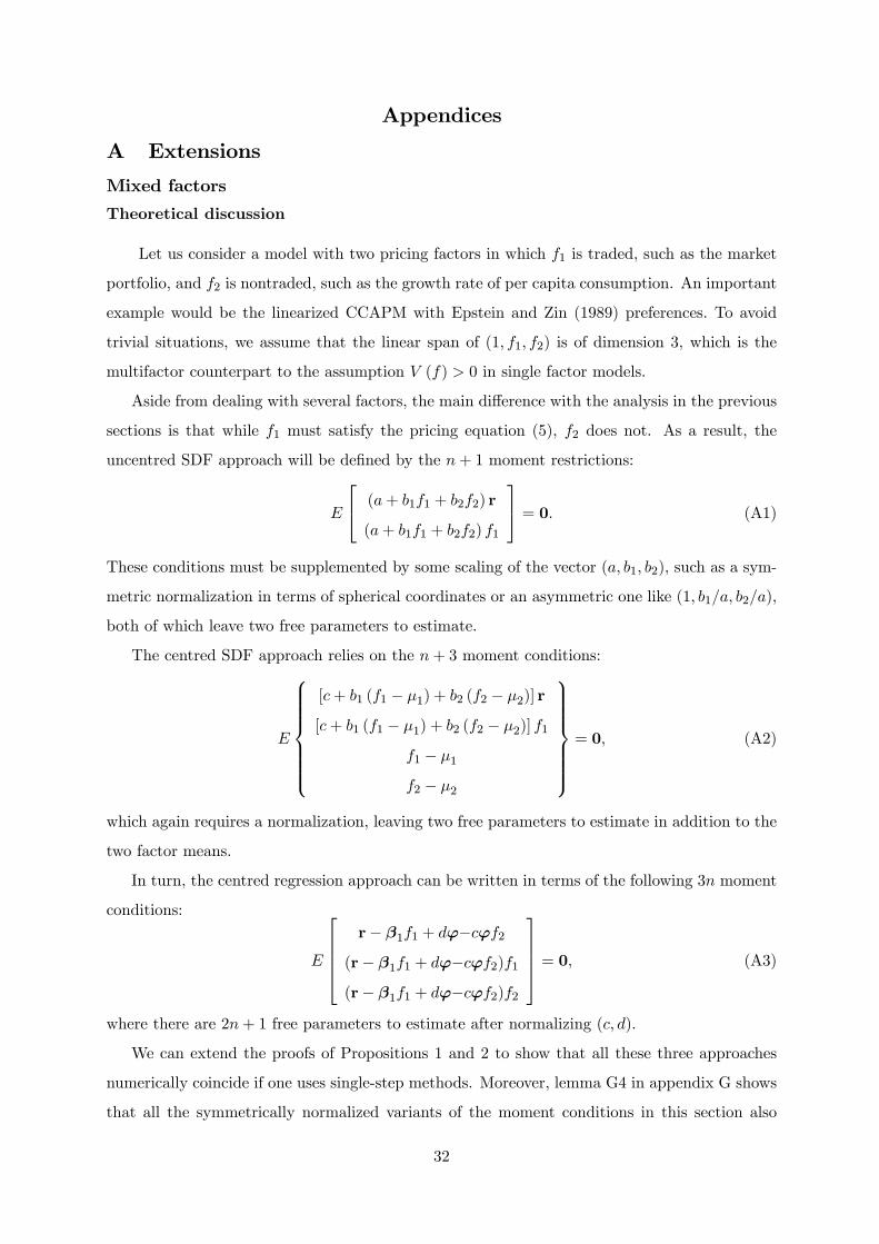
Appendices

A Extensions

Mixed factors

Theoretical discussion

Let us consider a model with two pricing factors in which f1 is traded, such as the market

portfolio, and f2 is nontraded, such as the growth rate of per capita consumption. An important

example would be the linearized CCAPM with Epstein and Zin (1989) preferences. To avoid

trivial situations, we assume that the linear span of (1; f1; f2) is of dimension 3, which is the

multifactor counterpart to the assumption V (f) > 0 in single factor models.

Aside from dealing with several factors, the main di¤erence with the analysis in the previous

sections is that while f1 must satisfy the pricing equation (5), f2 does not. As a result, the

uncentred SDF approach will be de�ned by the n+ 1 moment restrictions:

E

24 (a+ b1f1 + b2f2) r

(a+ b1f1 + b2f2) f1

35 = 0: (A1)

These conditions must be supplemented by some scaling of the vector (a; b1; b2), such as a sym-

metric normalization in terms of spherical coordinates or an asymmetric one like (1; b1=a; b2=a),

both of which leave two free parameters to estimate.

The centred SDF approach relies on the n+ 3 moment conditions:

E

8>>>>>><>>>>>>:

[c+ b1 (f1 � �1) + b2 (f2 � �2)] r

[c+ b1 (f1 � �1) + b2 (f2 � �2)] f1f1 � �1f2 � �2

9>>>>>>=>>>>>>;= 0; (A2)

which again requires a normalization, leaving two free parameters to estimate in addition to the

two factor means.

In turn, the centred regression approach can be written in terms of the following 3n moment

conditions:

E

26664r� �1f1 + d'�c'f2

(r� �1f1 + d'�c'f2)f1(r� �1f1 + d'�c'f2)f2

37775 = 0; (A3)

where there are 2n+ 1 free parameters to estimate after normalizing (c; d).

We can extend the proofs of Propositions 1 and 2 to show that all these three approaches

numerically coincide if one uses single-step methods. Moreover, lemma G4 in appendix G shows

that all the symmetrically normalized variants of the moment conditions in this section also

32

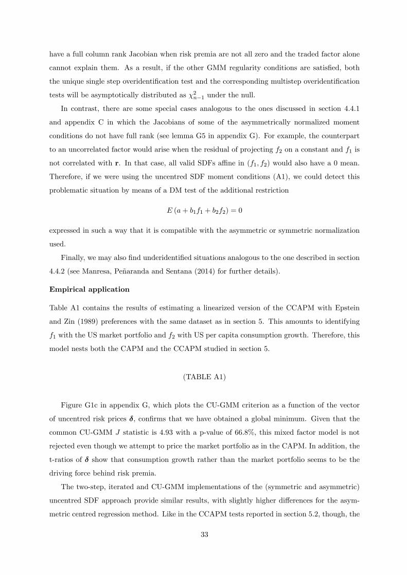
have a full column rank Jacobian when risk premia are not all zero and the traded factor alone

cannot explain them. As a result, if the other GMM regularity conditions are satis�ed, both

the unique single step overidenti�cation test and the corresponding multistep overidenti�cation

tests will be asymptotically distributed as �2n�1 under the null.

In contrast, there are some special cases analogous to the ones discussed in section 4.4.1

and appendix C in which the Jacobians of some of the asymmetrically normalized moment

conditions do not have full rank (see lemma G5 in appendix G). For example, the counterpart

to an uncorrelated factor would arise when the residual of projecting f2 on a constant and f1 is

not correlated with r. In that case, all valid SDFs a¢ ne in (f1; f2) would also have a 0 mean.

Therefore, if we were using the uncentred SDF moment conditions (A1), we could detect this

problematic situation by means of a DM test of the additional restriction

E (a+ b1f1 + b2f2) = 0

expressed in such a way that it is compatible with the asymmetric or symmetric normalization

used.

Finally, we may also �nd underidenti�ed situations analogous to the one described in section

4.4.2 (see Manresa, Peñaranda and Sentana (2014) for further details).

Empirical application

Table A1 contains the results of estimating a linearized version of the CCAPM with Epstein

and Zin (1989) preferences with the same dataset as in section 5. This amounts to identifying

f1 with the US market portfolio and f2 with US per capita consumption growth. Therefore, this

model nests both the CAPM and the CCAPM studied in section 5.

(TABLE A1)

Figure G1c in appendix G, which plots the CU-GMM criterion as a function of the vector

of uncentred risk prices �, con�rms that we have obtained a global minimum. Given that the

common CU-GMM J statistic is 4:93 with a p-value of 66:8%, this mixed factor model is not

rejected even though we attempt to price the market portfolio as in the CAPM. In addition, the

t-ratios of � show that consumption growth rather than the market portfolio seems to be the

driving force behind risk premia.

The two-step, iterated and CU-GMM implementations of the (symmetric and asymmetric)

uncentred SDF approach provide similar results, with slightly higher di¤erences for the asym-

metric centred regression method. Like in the CCAPM tests reported in section 5.2, though, the

33

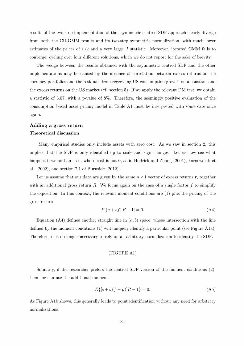
results of the two-step implementation of the asymmetric centred SDF approach clearly diverge

from both the CU-GMM results and its two-step symmetric normalization, with much lower

estimates of the prices of risk and a very large J statistic. Moreover, iterated GMM fails to

converge, cycling over four di¤erent solutions, which we do not report for the sake of brevity.

The wedge between the results obtained with the asymmetric centred SDF and the other

implementations may be caused by the absence of correlation between excess returns on the

currency portfolios and the residuals from regressing US consumption growth on a constant and

the excess returns on the US market (cf. section 5). If we apply the relevant DM test, we obtain

a statistic of 3:07, with a p-value of 8%. Therefore, the seemingly positive evaluation of the

consumption based asset pricing model in Table A1 must be interpreted with some care once

again.

Adding a gross return

Theoretical discussion

Many empirical studies only include assets with zero cost. As we saw in section 2, this

implies that the SDF is only identi�ed up to scale and sign changes. Let us now see what

happens if we add an asset whose cost is not 0, as in Hodrick and Zhang (2001), Farnsworth et

al. (2002), and section 7.1 of Burnside (2012).

Let us assume that our data are given by the same n� 1 vector of excess returns r, together

with an additional gross return R. We focus again on the case of a single factor f to simplify

the exposition. In this context, the relevant moment conditions are (1) plus the pricing of the

gross return

E[(a+ bf)R� 1] = 0: (A4)

Equation (A4) de�nes another straight line in (a; b) space, whose intersection with the line

de�ned by the moment conditions (1) will uniquely identify a particular point (see Figure A1a).

Therefore, it is no longer necessary to rely on an arbitrary normalization to identify the SDF.

(FIGURE A1)

Similarly, if the researcher prefers the centred SDF version of the moment conditions (2),

then she can use the additional moment

Ef[c+ b (f � �)]R� 1g = 0: (A5)

As Figure A1b shows, this generally leads to point identi�cation without any need for arbitrary

normalizations.

34

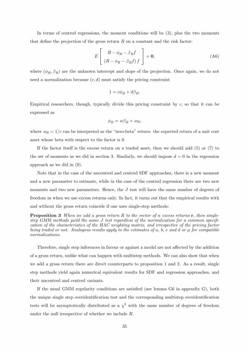
In terms of centred regressions, the moment conditions will be (3), plus the two moments

that de�ne the projection of the gross return R on a constant and the risk factor:

E

24 R� �R � �Rf

(R� �R � �Rf) f

35 = 0; (A6)

where (�R; �R) are the unknown intercept and slope of the projection. Once again, we do not

need a normalization because (c; d) must satisfy the pricing constraint

1 = c�R + d�R:

Empirical researchers, though, typically divide this pricing constraint by c, so that it can be

expressed as

�R = {�R + {R;

where {R = 1=c can be interpreted as the �zero-beta�return: the expected return of a unit cost

asset whose beta with respect to the factor is 0.

If the factor itself is the excess return on a traded asset, then we should add (5) or (7) to

the set of moments as we did in section 3. Similarly, we should impose d = 0 in the regression

approach as we did in (9).

Note that in the case of the uncentred and centred SDF approaches, there is a new moment

and a new parameter to estimate, while in the case of the centred regression there are two new

moments and two new parameters. Hence, the J test will have the same number of degrees of

freedom as when we use excess returns only. In fact, it turns out that the empirical results with

and without the gross return coincide if one uses single-step methods:

Proposition 3 When we add a gross return R to the vector of n excess returns r, then single-step GMM methods yield the same J test regardless of the normalization for a common speci�-cation of the characteristics of the HAC weighting matrix, and irrespective of the pricing factorbeing traded or not. Analogous results apply to the estimates of a, b, c and d or � for compatiblenormalizations.

Therefore, single step inferences in favour or against a model are not a¤ected by the addition

of a gross return, unlike what can happen with multistep methods. We can also show that when

we add a gross return there are direct counterparts to proposition 1 and 2. As a result, single

step methods yield again numerical equivalent results for SDF and regression approaches, and

their uncentred and centred variants.

If the usual GMM regularity conditions are satis�ed (see lemma G6 in appendix G), both

the unique single step overidenti�cation test and the corresponding multistep overidenti�cation

tests will be asymptotically distributed as a �2 with the same number of degrees of freedom

under the null irrespective of whether we include R.

35

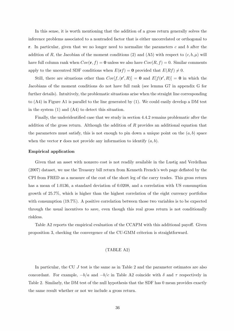
In this sense, it is worth mentioning that the addition of a gross return generally solves the

inference problems associated to a nontraded factor that is either uncorrelated or orthogonal to

r. In particular, given that we no longer need to normalize the parameters c and b after the

addition of R, the Jacobian of the moment conditions (2) and (A5) with respect to (c; b; �) will

have full column rank when Cov(r; f) = 0 unless we also have Cov(R; f) = 0. Similar comments

apply to the uncentred SDF conditions when E(rf) = 0 provided that E(Rf) 6= 0.

Still, there are situations other than Cov[f; (r0; R)] = 0 and E[f(r0; R)] = 0 in which the

Jacobians of the moment conditions do not have full rank (see lemma G7 in appendix G for

further details). Intuitively, the problematic situations arise when the straight line corresponding

to (A4) in Figure A1 is parallel to the line generated by (1). We could easily develop a DM test

in the system (1) and (A4) to detect this situation.

Finally, the underidenti�ed case that we study in section 4.4.2 remains problematic after the

addition of the gross return. Although the addition of R provides an additional equation that

the parameters must satisfy, this is not enough to pin down a unique point on the (a; b) space

when the vector r does not provide any information to identify (a; b).

Empirical application

Given that an asset with nonzero cost is not readily available in the Lustig and Verdelhan

(2007) dataset, we use the Treasury bill return from Kenneth French�s web page de�ated by the

CPI from FRED as a measure of the cost of the short leg of the carry trades. This gross return

has a mean of 1.0136, a standard deviation of 0.0208, and a correlation with US consumption

growth of 25.7%, which is higher than the highest correlation of the eight currency portfolios

with consumption (19.7%). A positive correlation between those two variables is to be expected

through the usual incentives to save, even though this real gross return is not conditionally

riskless.

Table A2 reports the empirical evaluation of the CCAPM with this additional payo¤. Given

proposition 3, checking the convergence of the CU-GMM criterion is straightforward.

(TABLE A2)

In particular, the CU J test is the same as in Table 2 and the parameter estimates are also

concordant. For example, �b=a and �b=c in Table A2 coincide with � and � respectively in

Table 2. Similarly, the DM test of the null hypothesis that the SDF has 0 mean provides exactly

the same result whether or not we include a gross return.

36

However, the uncentred and centred SDF approaches, which become numerically equivalent

to each other once we add a gross return, reject the model in their multistep GMM implementa-

tions. In particular, the p-value of the asymmetric uncentred SDF decreases from around 57%

in Table 2 to less than 5% in Table A2. Therefore, a naive researcher looking at these results

may conclude that the excess return data on their own did not have enough power to reject the

model, but the addition of the gross return was decisive.

Finally, given that proposition 3 also applies to a traded factor model, we have repeated the

same exercise replacing consumption growth with the excess returns on the US stock market

portfolio. As expected, the CU J statistic is still the same, unlike what happens with multistep

GMM.

B Proofs

All proofs consider the multifactor context of appendix E instead of the simplifying single

factor set up in the main text. In addition, the proofs of proposition 1, 2 and 3 do not rely on

any particular normalization since they are irrelevant for single-step methods, although some

of the asymmetric normalizations might be ill-de�ned for some problematic con�gurations, as

illustrated in section 4.4. Nevertheless, the overidenti�cation tests are always well de�ned.

In what follows we represent a set of k factors by the vector f , but maintain the assumption

that the number of assets exceeds the number of factors (n > k). We also replace the vectors �

and ' in section 2 by the n� k matrices

B =��1 � � � �k

�; P =

�'1 � � � 'k

�;

respectively.

Proposition 1:

In order to show that single-step methods yield numerical equivalent parameter estimators

and tests, we prove that we can write hR (r; f ;B) in (E12) and hU (r; f ; a;b) in (E10) as pa-

rameter dependent linear transformation of each other after a suitable reparameterization and

an augmentation with unrestricted moments, so that the associated criterion functions will be

numerically identical for any compatible set of parameter values. Speci�cally, let us de�ne an

extended regression system that adds the estimation of (�;�) to hR (r; f ;B):

hR (r; f ;B;�;vech (�)) =

26664hR (r; f ;B)

f � �

vech�� 0 � �

�37775 =

26666664r�Bf

vec ((r�Bf) f 0)

f � �

vech�� 0 � �

�

37777775 :

37

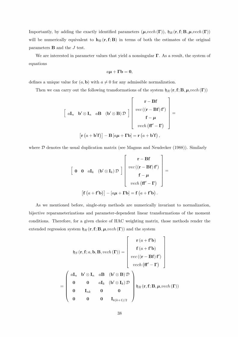
Importantly, by adding the exactly identi�ed parameters (�;vech (�)), hR (r; f ;B;�;vech (�))

will be numerically equivalent to hR (r; f ;B) in terms of both the estimates of the original

parameters B and the J test.

We are interested in parameter values that yield a nonsingular �. As a result, the system of

equations

a�+ �b = 0;

de�nes a unique value for (a;b) with a 6= 0 for any admissible normalization.

Then we can carry out the following transformations of the system hR (r; f ;B;�;vech (�))

haIn b0 In aB (b0 B)D

i26666664

r�Bf

vec ((r�Bf) f 0)

f � �

vech�� 0 � �

�

37777775 =�r�a+ b0f

���B [a�+ �b] = r

�a+ b0f

�;

where D denotes the usual duplication matrix (see Magnus and Neudecker (1988)). Similarly

h0 0 aIk (b0 Ik)D

i26666664

r�Bf

vec ((r�Bf) f 0)

f � �

vech�� 0 � �

�

37777775 =�f�a+ f 0b

��� [a�+ �b] = f

�a+ f 0b

�:

As we mentioned before, single-step methods are numerically invariant to normalization,

bijective reparameterizations and parameter-dependent linear transformations of the moment

conditions. Therefore, for a given choice of HAC weighting matrix, those methods render the

extended regression system hR (r; f ;B;�;vech (�)) and the system

hS (r; f ; a;b;B; vech (�)) =

26666664r (a+ f 0b)

f (a+ f 0b)

vec ((r�Bf) f 0)

vech�� 0 � �

�

37777775

=

0BBBBBB@aIn b0 In aB (b0 B)D

0 0 aIk (b0 Ik)D

0 Ink 0 0

0 0 0 Ik(k+1)=2

1CCCCCCA hR (r; f ;B;�;vech (�))

38

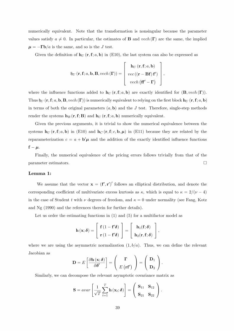
numerically equivalent. Note that the transformation is nonsingular because the parameter

values satisfy a 6= 0. In particular, the estimates of B and vech (�) are the same, the implied

� = ��b=a is the same, and so is the J test.

Given the de�nition of hU (r; f ; a;b) in (E10), the last system can also be expressed as

hU (r; f ; a;b;B; vech (�)) =

26664hU (r; f ; a;b)

vec ((r�Bf) f 0)

vech�� 0 � �

�37775 ;

where the in�uence functions added to hU (r; f ; a;b) are exactly identi�ed for (B; vech (�)).

Thus hU (r; f ; a;b;B; vech (�)) is numerically equivalent to relying on the �rst block hU (r; f ; a;b)

in terms of both the original parameters (a;b) and the J test. Therefore, single-step methods

render the systems hR (r; f ;B) and hU (r; f ; a;b) numerically equivalent.

Given the previous arguments, it is trivial to show the numerical equivalence between the

systems hU (r; f ; a;b) in (E10) and hC (r; f ; c;b;�) in (E11) because they are related by the

reparameterization c = a + b0� and the addition of the exactly identi�ed in�uence functions

f � �.

Finally, the numerical equivalence of the pricing errors follows trivially from that of the

parameter estimators. �

Lemma 1:

We assume that the vector x = (f 0; r0)0 follows an elliptical distribution, and denote the

corresponding coe¢ cient of multivariate excess kurtosis as �, which is equal to � = 2=(� � 4)

in the case of Student t with � degrees of freedom, and � = 0 under normality (see Fang, Kotz

and Ng (1990) and the references therein for further details).

Let us order the estimating functions in (1) and (5) for a multifactor model as

h (x; �) =

24 f (1� f 0�)r (1� f 0�)

35 =24 h1(f ; �)

h2(r; f ; �)

35 ;where we are using the asymmetric normalization (1; b=a). Thus, we can de�ne the relevant

Jacobian as

D = E

�@h (x; �)

@�0

�=

0@ �

E�rf 0�1A =

0@ D1

D2

1A :

Similarly, we can decompose the relevant asymptotic covariance matrix as

S = avar

"1pT

TXt=1

h (xt; �)

#=

0@ S11 S12

S21 S22

1A :

39

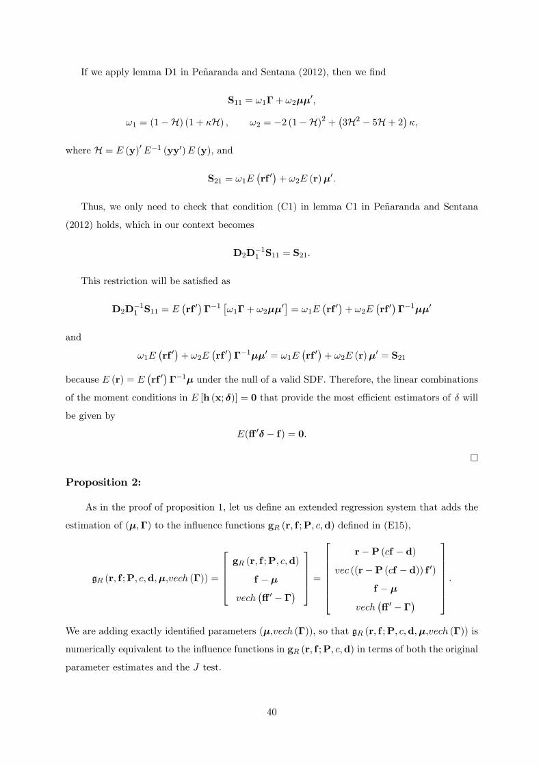
If we apply lemma D1 in Peñaranda and Sentana (2012), then we �nd

S11 = !1�+ !2��0;

!1 = (1�H) (1 + �H) ; !2 = �2 (1�H)2 +�3H2 � 5H+ 2

��;

where H = E (y)0E�1 (yy0)E (y), and

S21 = !1E�rf 0�+ !2E (r)�

0:

Thus, we only need to check that condition (C1) in lemma C1 in Peñaranda and Sentana

(2012) holds, which in our context becomes

D2D�11 S11 = S21:

This restriction will be satis�ed as

D2D�11 S11 = E

�rf 0���1

�!1�+ !2��

0� = !1E�rf 0�+ !2E

�rf 0���1��0

and

!1E�rf 0�+ !2E

�rf 0���1��0 = !1E

�rf 0�+ !2E (r)�

0 = S21

because E (r) = E�rf 0���1� under the null of a valid SDF. Therefore, the linear combinations

of the moment conditions in E [h (x; �)] = 0 that provide the most e¢ cient estimators of � will

be given by

E(� 0� � f) = 0:

�

Proposition 2:

As in the proof of proposition 1, let us de�ne an extended regression system that adds the

estimation of (�;�) to the in�uence functions gR (r; f ;P; c;d) de�ned in (E15),

gR (r; f ;P; c;d;�;vech (�)) =

26664gR (r; f ;P; c;d)

f � �

vech�� 0 � �

�37775 =

26666664r�P (cf � d)

vec ((r�P (cf � d)) f 0)

f � �

vech�� 0 � �

�

37777775 :

We are adding exactly identi�ed parameters (�;vech (�)), so that gR (r; f ;P; c;d;�;vech (�)) is

numerically equivalent to the in�uence functions in gR (r; f ;P; c;d) in terms of both the original

parameter estimates and the J test.

40

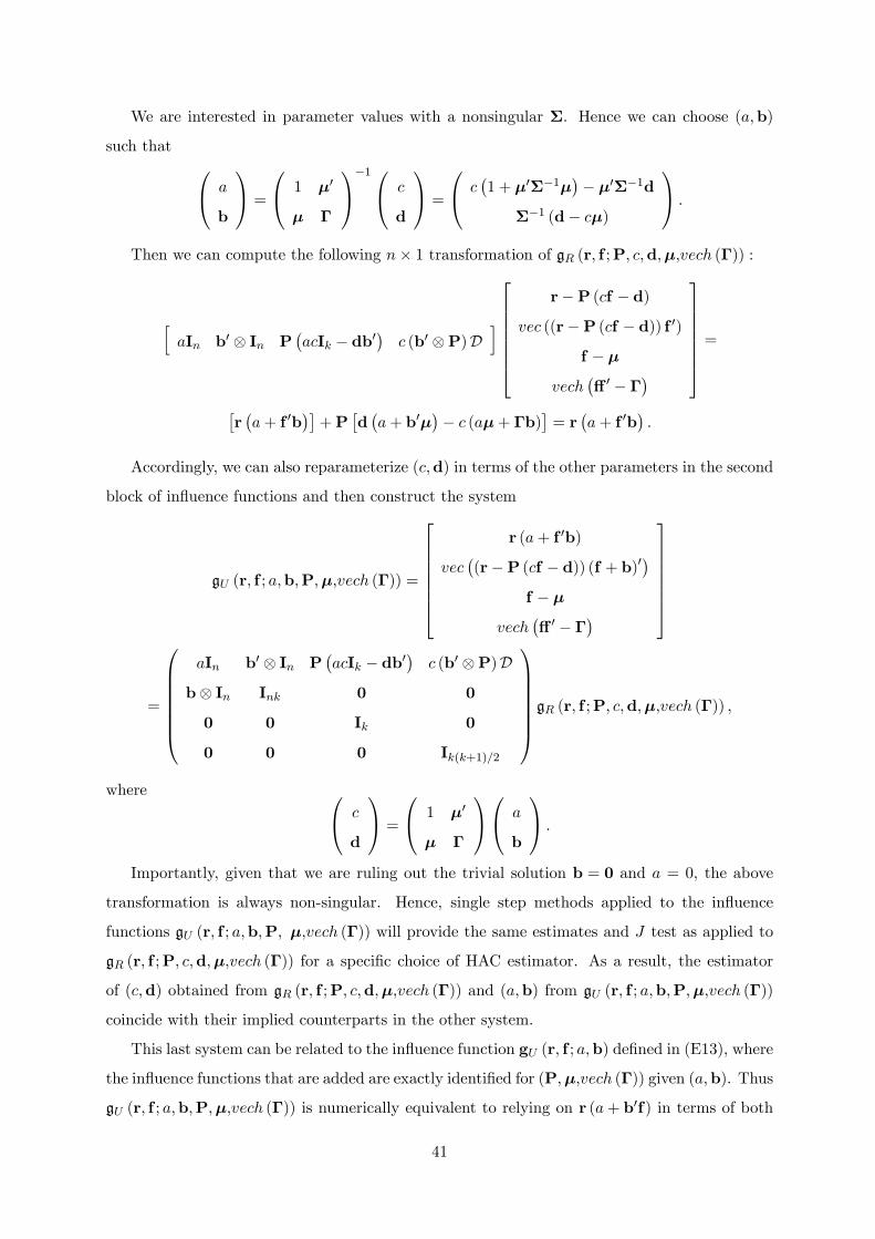
We are interested in parameter values with a nonsingular �. Hence we can choose (a;b)

such that 0@ a

b

1A =

0@ 1 �0

� �

1A�10@ c

d

1A =

0@ c�1 + �0��1�

�� �0��1d

��1 (d� c�)

1A :

Then we can compute the following n� 1 transformation of gR (r; f ;P; c;d;�;vech (�)) :

haIn b0 In P

�acIk � db0

�c (b0 P)D

i26666664

r�P (cf � d)

vec ((r�P (cf � d)) f 0)

f � �

vech�� 0 � �

�

37777775 =�r�a+ f 0b

��+P

�d�a+ b0�

�� c (a�+ �b)

�= r

�a+ f 0b

�:

Accordingly, we can also reparameterize (c;d) in terms of the other parameters in the second

block of in�uence functions and then construct the system

gU (r; f ; a;b;P;�;vech (�)) =

26666664r (a+ f 0b)

vec�(r�P (cf � d)) (f + b)0

�f � �

vech�� 0 � �

�

37777775

=

0BBBBBB@aIn b0 In P

�acIk � db0

�c (b0 P)D

b In Ink 0 0

0 0 Ik 0

0 0 0 Ik(k+1)=2

1CCCCCCA gR (r; f ;P; c;d;�;vech (�)) ;

where 0@ c

d

1A =

0@ 1 �0

� �

1A0@ a

b

1A :

Importantly, given that we are ruling out the trivial solution b = 0 and a = 0, the above

transformation is always non-singular. Hence, single step methods applied to the in�uence

functions gU (r; f ; a;b;P; �;vech (�)) will provide the same estimates and J test as applied to

gR (r; f ;P; c;d;�;vech (�)) for a speci�c choice of HAC estimator. As a result, the estimator

of (c;d) obtained from gR (r; f ;P; c;d;�;vech (�)) and (a;b) from gU (r; f ; a;b;P;�;vech (�))

coincide with their implied counterparts in the other system.

This last system can be related to the in�uence function gU (r; f ; a;b) de�ned in (E13), where

the in�uence functions that are added are exactly identi�ed for (P;�;vech (�)) given (a;b). Thus

gU (r; f ; a;b;P;�;vech (�)) is numerically equivalent to relying on r (a+ b0f) in terms of both

41

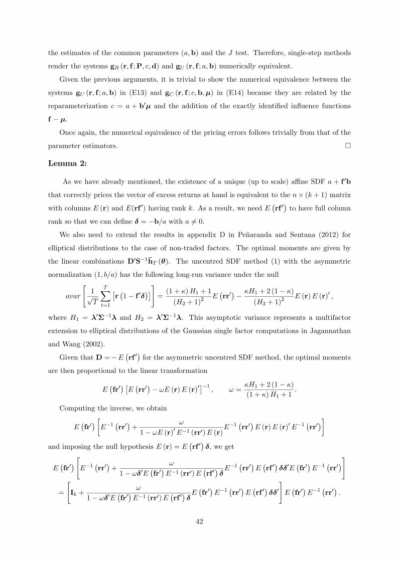
the estimates of the common parameters (a;b) and the J test. Therefore, single-step methods

render the systems gR (r; f ;P; c;d) and gU (r; f ; a;b) numerically equivalent.

Given the previous arguments, it is trivial to show the numerical equivalence between the

systems gU (r; f ; a;b) in (E13) and gC (r; f ; c;b;�) in (E14) because they are related by the

reparameterization c = a + b0� and the addition of the exactly identi�ed in�uence functions

f � �.

Once again, the numerical equivalence of the pricing errors follows trivially from that of the

parameter estimators. �

Lemma 2:

As we have already mentioned, the existence of a unique (up to scale) a¢ ne SDF a + f 0b

that correctly prices the vector of excess returns at hand is equivalent to the n� (k + 1) matrix

with columns E (r) and E(rf 0) having rank k. As a result, we need E�rf 0�to have full column

rank so that we can de�ne � = �b=a with a 6= 0.

We also need to extend the results in appendix D in Peñaranda and Sentana (2012) for

elliptical distributions to the case of non-traded factors. The optimal moments are given by

the linear combinations D0S�1�hT (�). The uncentred SDF method (1) with the asymmetric

normalization (1; b=a) has the following long-run variance under the null

avar

"1pT

TXt=1

�r�1� f 0�

��#=(1 + �)H1 + 1

(H2 + 1)2 E

�rr0�� �H1 + 2 (1� �)

(H2 + 1)2 E (r)E (r)0 ;

where H1 = �0��1� and H2 = �0��1�. This asymptotic variance represents a multifactor

extension to elliptical distributions of the Gaussian single factor computations in Jagannathan

and Wang (2002).

Given that D =�E�rf 0�for the asymmetric uncentred SDF method, the optimal moments

are then proportional to the linear transformation

E�fr0� �E�rr0�� !E (r)E (r)0

��1; ! =

�H1 + 2 (1� �)(1 + �)H1 + 1

:

Computing the inverse, we obtain

E�fr0� �E�1

�rr0�+

!

1� !E (r)0E�1 (rr0)E (r)E�1

�rr0�E (r)E (r)0E�1

�rr0��

and imposing the null hypothesis E (r) = E�rf 0��, we get

E�fr0� "E�1

�rr0�+

!

1� !�0E�fr0�E�1 (rr0)E

�rf 0��E�1

�rr0�E�rf 0���0E

�fr0�E�1

�rr0�#

=

"Ik +

!

1� !�0E�fr0�E�1 (rr0)E

�rf 0��E�fr0�E�1

�rr0�E�rf 0���0

#E�fr0�E�1

�rr0�:

42

Since the k� k matrix in brackets has full rank, we can conclude that the optimal estimator

of � solves the sample moments

1

T

TXt=1

�r+t�1� f 0t�T

��= 0;

with

r+t = E�fr0�E�1

�rr0�rt:

Finally, note that to implement this optimal estimator in practice, we need consistent estimators

of E�fr0�and E (rr0), which we can easily obtain from their unrestricted sample counterparts.

�

Proposition 3:

When we add a gross return to the uncentred SDF in�uence functions (E10) or (E13) but

we retain the same normalization for a and b, there is an additional in�uence function

�a+ b0f

�R� q (B7)

and a new parameter q that captures the scale of the SDF (a=q)+(b0=q) f . Similarly, the centred

SDF in�uence functions become (E11) or (E14) plus

[c+ b0 (f � �)]R� q: (B8)

In contrast, the centred regression method adds to (E12) or (E15) the k + 1 new in�uence

functions 24 R� �R � �0Rf

vec��R� �R � �0Rf

�f 0�35 ;

which depend on the k + 1 new parameters (�R;�R) because q is given by c�R + d0�R, so

that it collapses to q = c�R when f represents excess returns on traded factors. Given that we

are adding unrestricted moments in all three instances, the original parameter estimators will

be una¤ected, and the optimal criterion function will remain the same. But since single-step

methods are invariant to reparameterizations and parameter dependent linear transformations

of the in�uence functions, the same results hold even if we use the q = 1 normalization in (A4),

unlike what happens with multistep methods. �

43

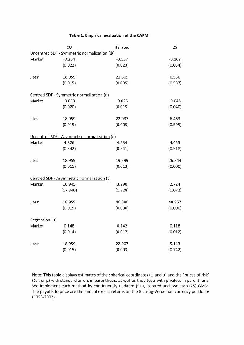
CU Iterated 2S

Uncentred SDF - Symmetric normalization (ψ)

Market -0.204 -0.157 -0.168

(0.022) (0.023) (0.034)

J test 18.959 21.809 6.536

(0.015) (0.005) (0.587)

Centred SDF - Symmetric normalization (υ)

Market -0.059 -0.025 -0.048

(0.020) (0.015) (0.040)

J test 18.959 22.037 6.463

(0.015) (0.005) (0.595)

Uncentred SDF - Asymmetric normalization (δ)

Market 4.826 4.534 4.455

(0.542) (0.541) (0.518)

J test 18.959 19.299 26.844

(0.015) (0.013) (0.000)

Centred SDF - Asymmetric normalization (τ)

Market 16.945 3.290 2.724

(17.340) (1.228) (1.072)

J test 18.959 46.880 48.957

(0.015) (0.000) (0.000)

Regression (μ)

Market 0.148 0.142 0.118

(0.014) (0.017) (0.012)

J test 18.959 22.907 5.143

(0.015) (0.003) (0.742)

Table 1: Empirical evaluation of the CAPM

Note: This table displays estimates of the spherical coordinates (ψ and υ) and the "prices of risk"

(δ, τ or μ) with standard errors in parenthesis, as well as the J tests with p-values in parenthesis.

We implement each method by continuously updated (CU), iterated and two-step (2S) GMM.

The payoffs to price are the annual excess returns on the 8 Lustig-Verdelhan currency portfolios

(1953-2002).

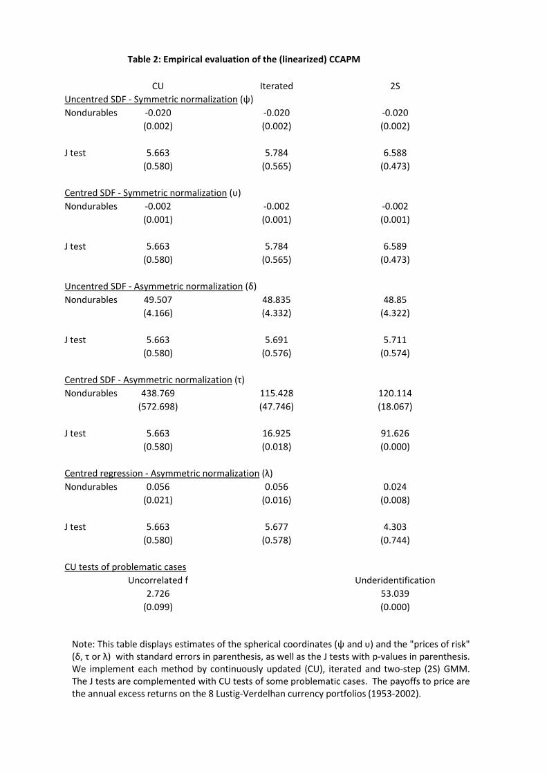
CU Iterated 2S

Uncentred SDF - Symmetric normalization (ψ)

Nondurables -0.020 -0.020 -0.020

(0.002) (0.002) (0.002)

J test 5.663 5.784 6.588

(0.580) (0.565) (0.473)

Centred SDF - Symmetric normalization (υ)

Nondurables -0.002 -0.002 -0.002

(0.001) (0.001) (0.001)

J test 5.663 5.784 6.589

(0.580) (0.565) (0.473)

Uncentred SDF - Asymmetric normalization (δ)

Nondurables 49.507 48.835 48.85

(4.166) (4.332) (4.322)

J test 5.663 5.691 5.711

(0.580) (0.576) (0.574)

Centred SDF - Asymmetric normalization (τ)

Nondurables 438.769 115.428 120.114

(572.698) (47.746) (18.067)

J test 5.663 16.925 91.626

(0.580) (0.018) (0.000)

Centred regression - Asymmetric normalization (λ)

Nondurables 0.056 0.056 0.024

(0.021) (0.016) (0.008)

J test 5.663 5.677 4.303

(0.580) (0.578) (0.744)

CU tests of problematic cases

Uncorrelated f Underidentification

2.726 53.039

(0.099) (0.000)

Table 2: Empirical evaluation of the (linearized) CCAPM

Note: This table displays estimates of the spherical coordinates (ψ and υ) and the "prices of risk"

(δ, τ or λ) with standard errors in parenthesis, as well as the J tests with p-values in parenthesis.

We implement each method by continuously updated (CU), iterated and two-step (2S) GMM.

The J tests are complemented with CU tests of some problematic cases. The payoffs to price are

the annual excess returns on the 8 Lustig-Verdelhan currency portfolios (1953-2002).

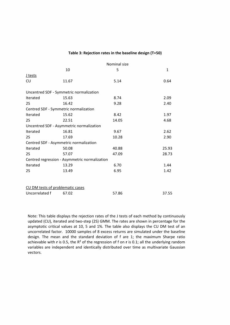
10 5 1

J tests

CU 11.67 5.14 0.64

Uncentred SDF - Symmetric normalization

Iterated 15.63 8.74 2.09

2S 16.42 9.28 2.40

Centred SDF - Symmetric normalization

Iterated 15.62 8.42 1.97

2S 22.51 14.05 4.68

Uncentred SDF - Asymmetric normalization

Iterated 16.81 9.67 2.62

2S 17.69 10.28 2.90

Centred SDF - Asymmetric normalization

Iterated 50.08 40.88 25.93

2S 57.07 47.09 28.73

Centred regression - Asymmetric normalization

Iterated 13.29 6.70 1.44

2S 13.49 6.95 1.42

CU DM tests of problematic cases

Uncorrelated f 67.02 57.86 37.55

Nominal size

Table 3: Rejection rates in the baseline design (T=50)

Note: This table displays the rejection rates of the J tests of each method by continuously

updated (CU), iterated and two-step (2S) GMM. The rates are shown in percentage for the

asymptotic critical values at 10, 5 and 1%. The table also displays the CU DM test of an

uncorrelated factor. 10000 samples of 8 excess returns are simulated under the baseline

design. The mean and the standard deviation of f are 1; the maximum Sharpe ratio

achievable with r is 0.5, the R² of the regression of f on r is 0.1; all the underlying random

variables are independent and identically distributed over time as multivariate Gaussian

vectors.

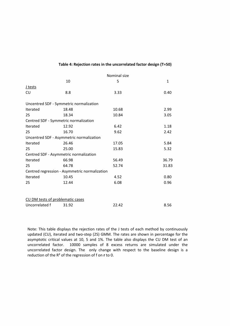
10 5 1

J tests

CU 8.8 3.33 0.40

Uncentred SDF - Symmetric normalization

Iterated 18.48 10.68 2.99

2S 18.34 10.84 3.05

Centred SDF - Symmetric normalization

Iterated 12.92 6.42 1.18

2S 16.70 9.62 2.42

Uncentred SDF - Asymmetric normalization

Iterated 26.46 17.05 5.84

2S 25.00 15.83 5.32

Centred SDF - Asymmetric normalization

Iterated 66.98 56.49 36.79

2S 64.78 52.74 31.83

Centred regression - Asymmetric normalization

Iterated 10.45 4.52 0.80

2S 12.44 6.08 0.96

CU DM tests of problematic cases

Uncorrelated f 31.92 22.42 8.56

Nominal size

Table 4: Rejection rates in the uncorrelated factor design (T=50)

Note: This table displays the rejection rates of the J tests of each method by continuously

updated (CU), iterated and two-step (2S) GMM. The rates are shown in percentage for the

asymptotic critical values at 10, 5 and 1%. The table also displays the CU DM test of an

uncorrelated factor. 10000 samples of 8 excess returns are simulated under the

uncorrelated factor design. The only change with respect to the baseline design is a

reduction of the R² of the regression of f on r to 0.

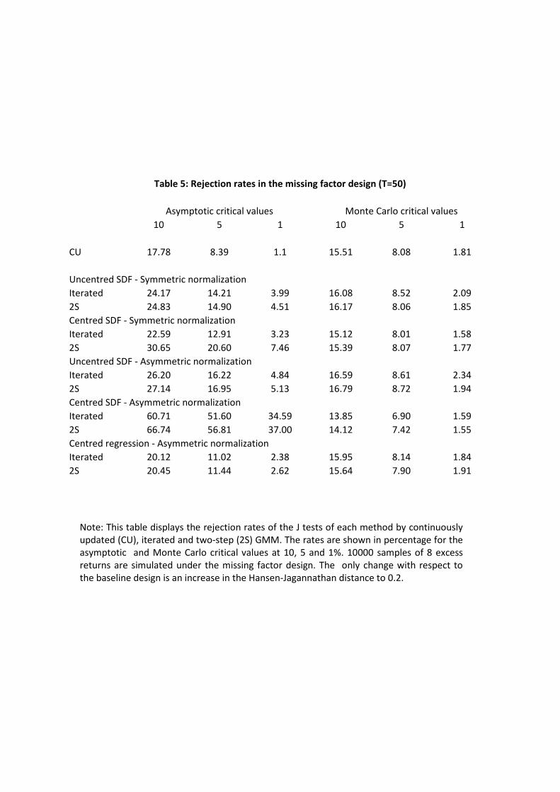
10 5 1 10 5 1

CU 17.78 8.39 1.1 15.51 8.08 1.81

Uncentred SDF - Symmetric normalization

Iterated 24.17 14.21 3.99 16.08 8.52 2.09

2S 24.83 14.90 4.51 16.17 8.06 1.85

Centred SDF - Symmetric normalization

Iterated 22.59 12.91 3.23 15.12 8.01 1.58

2S 30.65 20.60 7.46 15.39 8.07 1.77

Uncentred SDF - Asymmetric normalization

Iterated 26.20 16.22 4.84 16.59 8.61 2.34

2S 27.14 16.95 5.13 16.79 8.72 1.94

Centred SDF - Asymmetric normalization

Iterated 60.71 51.60 34.59 13.85 6.90 1.59

2S 66.74 56.81 37.00 14.12 7.42 1.55

Centred regression - Asymmetric normalization

Iterated 20.12 11.02 2.38 15.95 8.14 1.84

2S 20.45 11.44 2.62 15.64 7.90 1.91

Asymptotic critical values Monte Carlo critical values

Table 5: Rejection rates in the missing factor design (T=50)

Note: This table displays the rejection rates of the J tests of each method by continuously

updated (CU), iterated and two-step (2S) GMM. The rates are shown in percentage for the

asymptotic and Monte Carlo critical values at 10, 5 and 1%. 10000 samples of 8 excess

returns are simulated under the missing factor design. The only change with respect to

the baseline design is an increase in the Hansen-Jagannathan distance to 0.2.

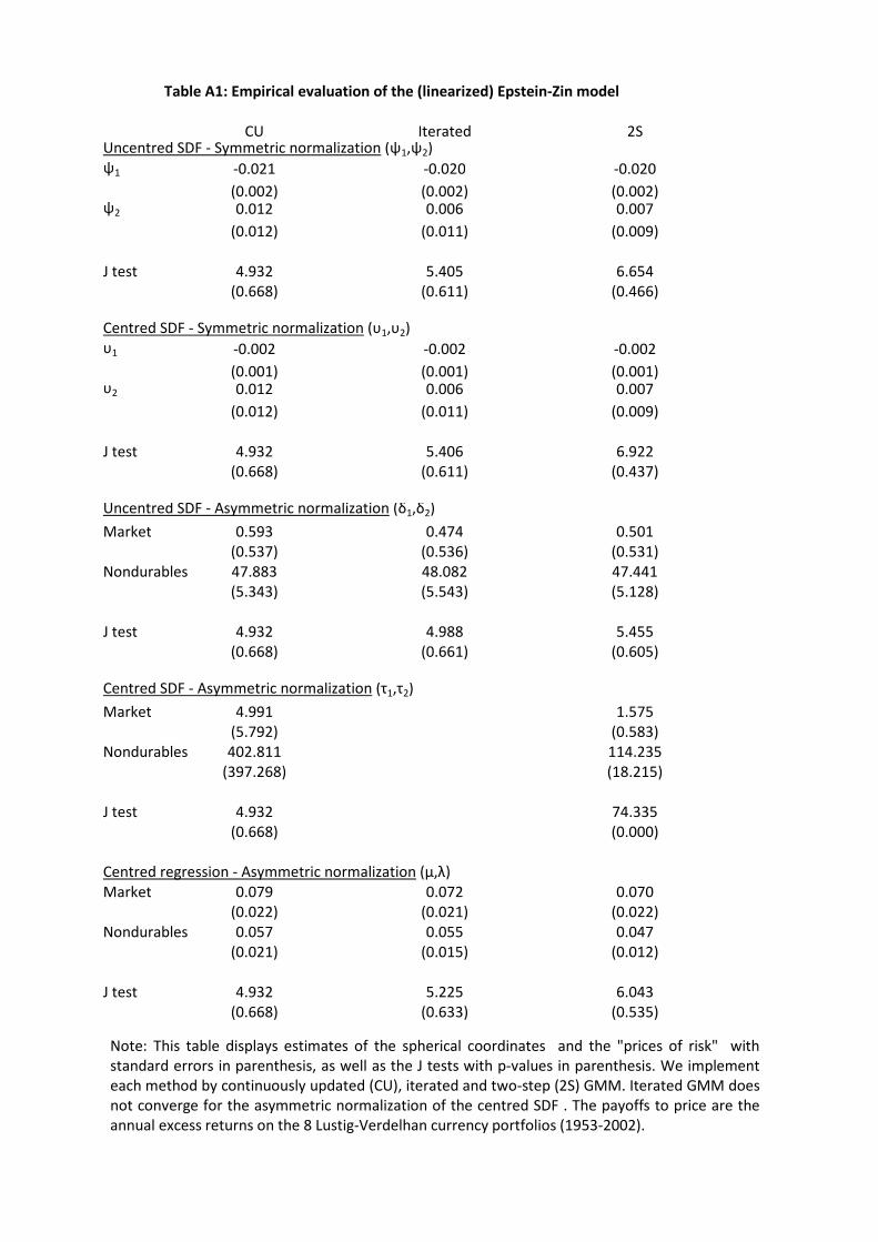
CU Iterated 2SUncentred SDF - Symmetric normalization (ψ1,ψ2)

ψ1 -0.021 -0.020 -0.020

(0.002) (0.002) (0.002)ψ2 0.012 0.006 0.007

(0.012) (0.011) (0.009)

J test 4.932 5.405 6.654

(0.668) (0.611) (0.466)

Centred SDF - Symmetric normalization (υ1,υ2)

υ1 -0.002 -0.002 -0.002

(0.001) (0.001) (0.001)υ2 0.012 0.006 0.007

(0.012) (0.011) (0.009)

J test 4.932 5.406 6.922

(0.668) (0.611) (0.437)

Uncentred SDF - Asymmetric normalization (δ1,δ2)

Market 0.593 0.474 0.501

(0.537) (0.536) (0.531)

Nondurables 47.883 48.082 47.441

(5.343) (5.543) (5.128)

J test 4.932 4.988 5.455

(0.668) (0.661) (0.605)

Centred SDF - Asymmetric normalization (τ1,τ2)

Market 4.991 1.575

(5.792) (0.583)

Nondurables 402.811 114.235

(397.268) (18.215)

J test 4.932 74.335

(0.668) (0.000)

Centred regression - Asymmetric normalization (μ,λ)

Market 0.079 0.072 0.070

(0.022) (0.021) (0.022)

Nondurables 0.057 0.055 0.047

(0.021) (0.015) (0.012)

J test 4.932 5.225 6.043

(0.668) (0.633) (0.535)

Table A1: Empirical evaluation of the (linearized) Epstein-Zin model

Note: This table displays estimates of the spherical coordinates and the "prices of risk" with

standard errors in parenthesis, as well as the J tests with p-values in parenthesis. We implement

each method by continuously updated (CU), iterated and two-step (2S) GMM. Iterated GMM does

not converge for the asymmetric normalization of the centred SDF . The payoffs to price are the

annual excess returns on the 8 Lustig-Verdelhan currency portfolios (1953-2002).

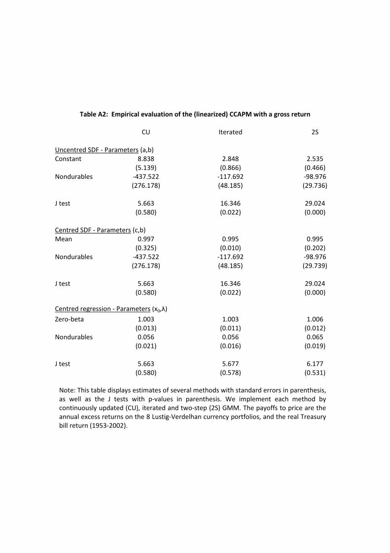
CU Iterated 2S

Uncentred SDF - Parameters (a,b)

Constant 8.838 2.848 2.535

(5.139) (0.866) (0.466)

Nondurables -437.522 -117.692 -98.976

(276.178) (48.185) (29.736)

J test 5.663 16.346 29.024

(0.580) (0.022) (0.000)

Centred SDF - Parameters (c,b)

Mean 0.997 0.995 0.995

(0.325) (0.010) (0.202)

Nondurables -437.522 -117.692 -98.976

(276.178) (48.185) (29.739)

J test 5.663 16.346 29.024

(0.580) (0.022) (0.000)

Centred regression - Parameters (х0,λ)

Zero-beta 1.003 1.003 1.006

(0.013) (0.011) (0.012)

Nondurables 0.056 0.056 0.065

(0.021) (0.016) (0.019)

J test 5.663 5.677 6.177

(0.580) (0.578) (0.531)

Table A2: Empirical evaluation of the (linearized) CCAPM with a gross return

Note: This table displays estimates of several methods with standard errors in parenthesis,

as well as the J tests with p-values in parenthesis. We implement each method by

continuously updated (CU), iterated and two-step (2S) GMM. The payoffs to price are the

annual excess returns on the 8 Lustig-Verdelhan currency portfolios, and the real Treasury

bill return (1953-2002).

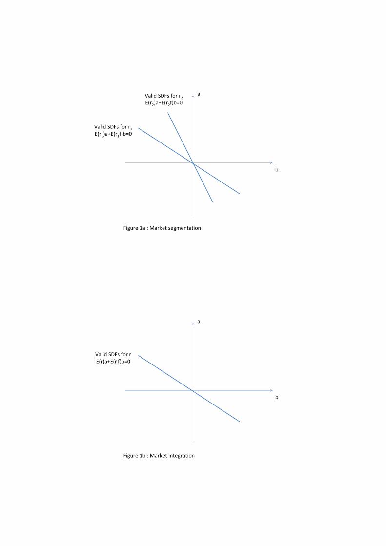
a

b

Valid SDFs for r1E(r1)a+E(r1f)b=0

Valid SDFs for r2E(r2)a+E(r2f)b=0

Figure 1a : Market segmentation  

a

b

Valid SDFs for rE(r)a+E(r f)b=0

Figure 1b : Market integration  

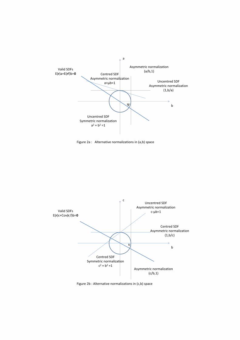
a

b

Valid SDFsE(r)a+E(rf)b=0

Uncentred SDFAsymmetric normalization

(1,b/a)

Uncentred SDFSymmetric normalization

a2 + b2 =1

Centred SDFAsymmetric normalization

a+µb=1

Figure 2a :   Alternative normalizations in (a,b) space

ψ

Asymmetric normalization(a/b,1)

c

b

Valid SDFsE(r)c+Cov(r,f)b=0

Centred SDFAsymmetric normalization

(1,b/c)

Centred SDFSymmetric normalization

c2 + b2 =1

Uncentred SDFAsymmetric normalization

c‐µb=1

Figure 2b : Alternative normalizations in (c,b) space

υ

Asymmetric normalization(c/b,1)

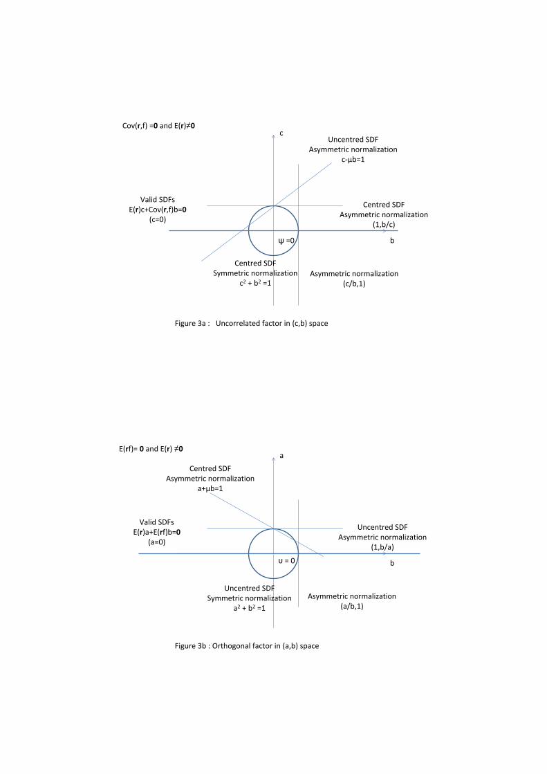
c

b

Valid SDFsE(r)c+Cov(r,f)b=0

(c=0)

Centred SDFAsymmetric normalization

(1,b/c)

Centred SDFSymmetric normalization

c2 + b2 =1

Uncentred SDFAsymmetric normalization

c‐µb=1

Cov(r,f) =0 and E(r)≠0

Figure 3a :   Uncorrelated factor in (c,b) space

ψ =0

Asymmetric normalization(c/b,1)

a

b

Valid SDFsE(r)a+E(rf)b=0

(a=0)

Uncentred SDFAsymmetric normalization

(1,b/a)

Uncentred SDFSymmetric normalization

a2 + b2 =1

Centred SDFAsymmetric normalization

a+µb=1

E(rf)= 0 and E(r) ≠0

Figure 3b : Orthogonal factor in (a,b) space

υ = 0

Asymmetric normalization(a/b,1)

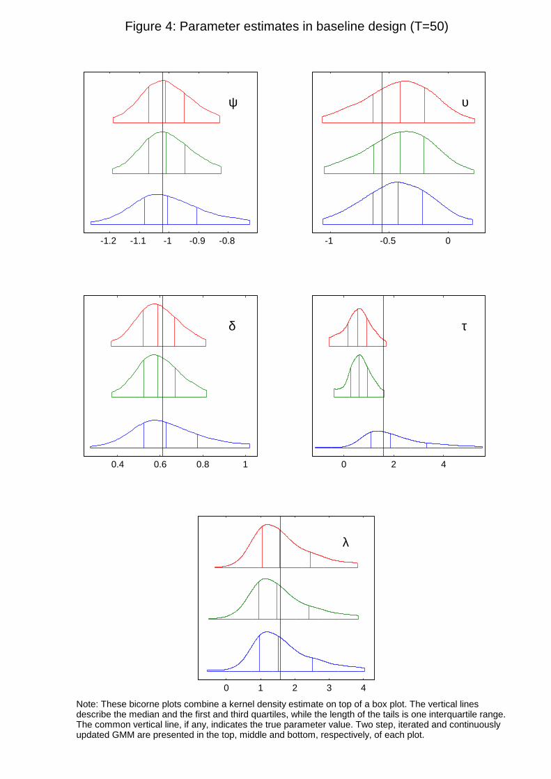
-1.2 -1.1 -1 -0.9 -0.8 -1 -0.5 0

0.4 0.6 0.8 1 0 2 4

0 1 2 3 4

τ

υψ

δ

λ

Figure 4: Parameter estimates in baseline design (T=50)

Note: These bicorne plots combine a kernel density estimate on top of a box plot. The vertical lines describe the median and the first and third quartiles, while the length of the tails is one interquartile range. The common vertical line, if any, indicates the true parameter value. Two step, iterated and continuouslyupdated GMM are presented in the top, middle and bottom, respectively, of each plot.

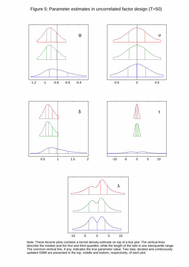
-1.2 -1 -0.8 -0.6 -0.4 -0.5 0 0.5

0.5 1 1.5 2 -10 -5 0 5 10

-10 -5 0 5 10

τ

υψ

δ

λ

Figure 5: Parameter estimates in uncorrelated factor design (T=50)

Note: These bicorne plots combine a kernel density estimate on top of a box plot. The vertical lines describe the median and the first and third quartiles, while the length of the tails is one interquartile range. The common vertical line, if any, indicates the true parameter value. Two step, iterated and continuouslyupdated GMM are presented in the top, middle and bottom, respectively, of each plot.

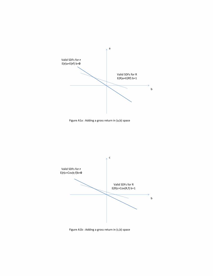
a

b

Valid SDFs for rE(r)a+E(rf) b=0

Valid SDFs for RE(R)a+E(Rf) b=1

Figure A1a : Adding a gross return in (a,b) space

c

b

Valid SDFs for rE(r)c+Cov(r,f)b=0

Valid SDFs for RE(R)c+Cov(R,f) b=1

Figure A1b : Adding a gross return in (c,b) space