A Survey on Solution Methods for Integral Equations · A Survey on Solution Methods for Integral Equations⁄ Ilias S. Kotsireasy June 2008 1 Introduction Integral Equations arise

A Survey on Solution Methods for Integral Equations∗

Ilias S. Kotsireas†

June 2008

1 Introduction

Integral Equations arise naturally in applications, in many areas of Mathematics, Science andTechnology and have been studied extensively both at the theoretical and practical level. Itis noteworthy that a MathSciNet keyword search on Integral Equations returns more thaneleven thousand items. In this survey we plan to describe several solution methods for IntegralEquations, illustrated with a number of fully worked out examples. In addition, we provide abibliography, for the reader who would be interested in learning more about various theoreticaland computational aspects of Integral Equations.

Our interest in Integral Equations stems from the fact that understanding and implementingsolution methods for Integral Equations is of vital importance in designing efficient param-eterization algorithms for algebraic curves, surfaces and hypersurfaces. This is because theimplicitization algorithm for algebraic curves, surfaces and hypersurfaces based on a nullvectorcomputation, can be inverted to yield a parameterization algorithm.

Integral Equations are inextricably related with other areas of Mathematics, such as IntegralTransforms, Functional Analysis and so forth. In view of this fact, and because we made aconscious effort to limit the length in under 50 pages, it was inevitable that the present workis not self-contained.

∗We thank ENTER. This project is implemented in the framework of Measure 8.3 of the programme ”Com-petitiveness”, 3rd European Union Support Framework, and is funded as follows: 75% of public funding from theEuropean Union, Social Fund, 25% of public funding from the Greek State, Ministry of Development, Generalsecretariat of research and technology, and from the private sector.

†We thank Professor Ioannis Z. Emiris, University of Athens, Athens, Greece, for the warm hospitality inhis Laboratory of Geometric & Algebraic Algorithms, ERGA.

1

2 Linear Integral Equations

2.1 General Form

The most general form of a linear integral equation is

h(x)u(x) = f(x) +

∫ b(x)

a

K(x, t)u(t) dt (1)

The type of an integral equation can be determined via the following conditions:f(x) = 0 Homogeneous. . .f(x) 6= 0 Nonhomogeneous. . .b(x) = x . . . Volterra integral equation. . .b(x) = b . . . Fredholm integral equation. . .h(x) = 0 . . . of the 1st kind.h(x) = 1 . . . of the 2nd kind.

For example, Abel’s problem:

−√

2gf(x) =

∫ x

0

φ(t)√x− t

dt (2)

is a nonhomogeneous Volterra equation of the 1st kind.

2.2 Linearity of Solutions

If u1(x) and u2(x) are both solutions to the integral equation, then c1u1(x) + c2u2(x) is also asolution.

2.3 The Kernel

K(x, t) is called the kernel of the integral equation. The equation is called singular if:

• the range of integration is infinite

• the kernel becomes infinite in the range of integration

2.3.1 Difference Kernels

If K(x, t) = K(x−t) (i.e. the kernel depends only on x−t), then the kernel is called a differencekernel. Volterra equations with difference kernels may be solved using either Laplace or Fouriertransforms, depending on the limits of integration.

2

2.3.2 Resolvent Kernels

2.4 Relations to Differential Equations

Differential equations and integral equations are equivalent and may be converted back andforth:

dy

dx= F (x) ⇒ y(x) =

∫ x

a

∫ s

a

F (t) dt ds + c1x + c2

2.4.1 Reduction to One Integration

In most cases, the resulting integral may be reduced to an integration in one variable:

∫ x

a

∫ s

a

F (t) dt ds =

∫ x

a

F (t)

∫ x

t

ds dt =

∫ x

a

(x− t)F (t) dt

Or, in general:

∫ x

a

∫ x1

a

. . .

∫ xn−1

a

F (xn) dxn dxn−1 . . . dx1 =

1

(n−1)!

∫ x

a

(x− x1)n−1F (x) dx1

2.4.2 Generalized Leibnitz formula

The Leibnitz formula may be useful in converting and solving some types of equations.

d

dx

∫ β(x)

α(x)

F (x, y) dy =

∫ β(x)

α(x)

∂F

∂x(x, y) dy + F (x, β(x))

dβ

dx(x)− F (x, α(x))

dα

dx(x)

3 Transforms

3.1 Laplace Transform

The Laplace transform is an integral transform of a function f(x) defined on (0,∞). Thegeneral formula is:

F (s) ≡ L{f} =

∫ ∞

0

e−sxf(x) dx (3)

3

The Laplace transform happens to be a Fredholm integral equation of the 1st kind with kernelK(s, x) = e−sx.

3.1.1 Inverse

The inverse Laplace transform involves complex integration, so tables of transform pairs arenormally used to find both the Laplace transform of a function and its inverse.

3.1.2 Convolution Product

When F1(s) ≡ L{f1} and F2(s) ≡ L{f2} then the convolution product is L{f1 ∗ f2} ≡F1(s)F2(s), where f1 ∗ f2 =

∫ x

0f1(x − t)f2(t) dt. f1(x − t) is a difference kernel and f2(t)

is a solution to the integral equation. Volterra integral equations with difference kernels wherethe integration is performed on the interval (0,∞) may be solved using this method.

3.1.3 Commutativity

The Laplace transform is commutative. That is:

f1 ∗ f2 =

∫ x

0

f1(x− t)f2(t) dt =

∫ x

0

f2(x− t)f1(t) dt = f2 ∗ f1

3.1.4 Example

Find the inverse Laplace transform of F (s) = 1s2+9

+ 1s(s+1)

using a table of transform pairs:

f(x) = L−1

{1

s2 + 9+

1

s(s + 1)

}

= L−1

{1

s2 + 9

}+ L−1

{1

s(s + 1)

}

=1

3sin 3x + L−1

{1

s− 1

s + 1

}

=1

3sin 3x + L−1

{1

s

}− L−1

{1

s + 1

}

=1

3sin 3x + 1− e−x

4

3.2 Fourier Transform

The Fourier exponential transform is an integral transform of a function f(x) defined on(−∞,∞). The general formula is:

F (λ) ≡ F{f} =

∫ ∞

−∞e−iλxf(x) dx (4)

The Fourier transform happens to be a Fredholm equation of the 1st kind with kernel K(λ, x) =e−iλx.

3.2.1 Inverse

The inverse Fourier transform is given by:

f(x) ≡ F−1{F} =1

2π

∫ ∞

−∞eiλxF (λ) dλ (5)

It is sometimes difficult to determine the inverse, so tables of transform pairs are normally usedto find both the Fourier transform of a function and its inverse.

3.2.2 Convolution Product

When F1(λ) ≡ F{f1} and F2(λ) ≡ F{f2} then the convolution product is F{f1 ∗ f2} ≡F1(λ)F2(λ), where f1 ∗ f2 =

∫∞−∞ f1(x − t)f2(t) dt. f1(x − t) is a difference kernel and f2(t)

is a solution to the integral equation. Volterra integral equations with difference kernels wherethe integration is performed on the interval (−∞,∞) may be solved using this method.

3.2.3 Commutativity

The Fourier transform is commutative. That is:

f1 ∗ f2 =

∫ ∞

−∞f1(x− t)f2(t) dt =

∫ ∞

−∞f2(x− t)f1(t) dt = f2 ∗ f1

3.2.4 Example

Find the Fourier transform of g(x) = sin axx

using a table of integral transforms:The inverse transform of sin aλ

λis

f(x) =

{12, |x| ≤ a

0, |x| > a

5

but since the Fourier transform is symmetrical, we know that

F{F (x)} = 2πf(−λ).

Therefore, let

F (x) =sin ax

x

and

f(λ) =

{12, |x| ≤ a

0, |x| > a

so that

F

{sin ax

x

}= 2πf(−λ) =

{π, |λ| ≤ a0, |λ| > a

.

3.3 Mellin Transform

The Mellin transform is an integral transform of a function f(x) defined on (0,∞). The generalformula is:

F (λ) ≡ M{f} =

∫ ∞

0

xλ−1f(x) dx (6)

If x = e−t and f(x) ≡ 0 for x < 0 then the Mellin transform is reduced to a Laplace transform:

∫ ∞

0

(e−t)λ−1f(e−t)(−e−t) dt = −∫ ∞

0

e−λtf(e−t) dt.

3.3.1 Inverse

Like the inverse Laplace transform, the inverse Mellin transform involves complex integration,so tables of transform pairs are normally used to find both the Mellin transform of a functionand its inverse.

3.3.2 Convolution Product

When F1(λ) ≡ M{f1} and F2(λ) ≡ M{f2} then the convolution product is M{f1 ∗ f2} ≡F1(λ)F2(λ), where f1 ∗ f2 =

∫∞0

f1(t)f2(xt)

tdt. Volterra integral equations with kernels of the

form K(xt) where the integration is performed on the interval (0,∞) may be solved using this

method.

6

3.3.3 Example

Find the Mellin transform of e−ax, a > 0. By definition:

F (λ) =

∫ ∞

0

xλ−1e−ax dx.

Let ax = z, so that:

F (λ) = a−λ

∫ ∞

0

e−zzλ−1 dz.

From the definition of the gamma function Γ(ν)

Γ(ν) =

∫ ∞

0

xν−1e−x dx

the result is

F (λ) =Γ(λ)

aλ.

4 Numerical Integration

General Equation:

u(x) = f(x) +

∫ b

a

K(x, t)u(t) dt

Let Sn(x) =∑n

k=0 K(x, tk)u(tk)∆kt.Let u(xi) = f(xi) +

∑nk=0 K(xi, tk)u(tk)∆kt, i = 0, 1, 2, . . . , n.

If equal increments are used, ∴ ∆x = b−an

.

4.1 Midpoint Rule

∫ b

a

f(x) dx ≈ b− a

n

n∑i=1

f

(xi−1 + xi

2

)

4.2 Trapezoid Rule

∫ b

a

f(x) dx ≈ b− a

n

[1

2f(x0) +

n−1∑i=1

f(xi) +1

2f(xn)

]

7

4.3 Simpson’s Rule

∫ b

a

f(x) dx ≈ b− a

3n[f(x0) + 4f(x1) + 2f(x2) + 4f(x3) + · · ·+ 4f(xn−1) + f(xn)]

5 Volterra Equations

Volterra integral equations are a type of linear integral equation (1) where b(x) = x:

h(x)u(x) = f(x) +

∫ x

a

K(x, t)u(t) dt (7)

The equation is said to be the first kind when h(x) = 0,

−f(x) =

∫ x

a

K(x, t)u(t) dt (8)

and the second kind when h(x) = 1,

u(x) = f(x) +

∫ x

a

K(x, t)u(t) dt (9)

5.1 Relation to Initial Value Problems

A general initial value problem is given by:

d2y

dx2+ A(x)

dy

dx+ B(x)y(x) = g(x) (10)

y(a) = c1, y′(a) = c2

∴ y(x) = f(x) +

∫ x

a

K(x, t)y(t) dt

where

f(x) =

∫ x

a

(x− t)g(t) dt + (x− a)[c1A(a) + c2] + c1

andK(x, t) = (t− x)[B(t)− A′(t)]− A(t)

8

5.2 Solving 2nd-Kind Volterra Equations

5.2.1 Neumann Series

The resolvent kernel for this method is:

Γ(x, t; λ) =∞∑

n=0

λnKn+1(x, t)

where

Kn+1(x, t) =

∫ x

t

K(x, y)Kn(y, t) dy

andK1(x, t) = K(x, t)

The series form of u(x) is

u(x) = u0(x) + λu1(x) + λ2u2(x) + · · ·

and since u(x) is a Volterra equation,

u(x) = f(x) + λ

∫ x

a

K(x, t)u(t) dt

so

u0(x) + λu1(x) + λ2u2(x) + · · · =f(x) + λ

∫ x

a

K(x, t)u0(t) dt + λ2

∫ x

a

K(x, t)u1(t) dt + · · ·

Now, by equating like coefficients:

u0(x) = f(x)

u1(x) =

∫ x

a

K(x, t)u0(t) dt

u2(x) =

∫ x

a

K(x, t)u1(t) dt

......

un(x) =

∫ x

a

K(x, t)un−1(t) dt

9

Substituting u0(x) = f(x):

u1(x) =

∫ x

a

K(x, t)f(t) dt

Substituting this for u1(x):

u2(x) =

∫ x

a

K(x, t)

∫ s

a

K(s, t)f(t) dt ds

=

∫ x

a

f(t)

[∫ x

t

K(x, s)K(s, t) ds

]dt

=

∫ x

a

f(t)K2(x, t) dt

Continue substituting recursively for u3, u4, . . . to determine the resolvent kernel. Sometimesthe resolvent kernel becomes recognizable after a few iterations as a Maclaurin or Taylor seriesand can be replaced by the function represented by that series. Otherwise numerical methodsmust be used to solve the equation.

Example: Use the Neumann series method to solve the Volterra integral equation of the2nd kind:

u(x) = f(x) + λ

∫ x

0

ex−tu(t) dt (11)

In this example, K1(x, t) ≡ K(x, t) = ex−t, so K2(x, t) is found by:

K2(x, t) =

∫ x

t

K(x, s)K1(s, t) ds

=

∫ x

t

ex−ses−t ds

=

∫ x

t

ex−t ds

= (x− t)ex−t

and K3(x, t) is found by:

K3(x, t) =

∫ x

t

K(x, s)K2(s, t) ds

=

∫ x

t

ex−s(s− t)es−t ds

10

=

∫ x

t

(s− t)ex−t ds

= ex−t

∫ x

t

(s− t) ds

= ex−t

[s2

2− ts

]x

t

= ex−t

[x2 − t2

2− t(x− t)

]

=(x− t)2

2ex−t

so by repeating this process the general equation for Kn+1(x, t) is

Kn+1(x, t) =(x− t)n

n!ex−t.

Therefore, the resolvent kernel for eq. (11) is

Γ(x, t; λ) = K1(x, t) + λK2(x, t) + λ2K3(x, t) + · · ·= ex−t + λ(x− t)ex−t + λ2 (x− t)2

2ex−t + · · ·

= ex−t

[1 + λ(x− t) + λ2 (x− t)2

2+ · · ·

].

The series in brackets, 1 + λ(x − t) + λ2 (x−t)2

2+ · · ·, is the Maclaurin series of eλ(x−t), so the

resolvent kernel isΓ(x, t; λ) = ex−teλ(x−t) = e(λ+1)(x−t)

and the solution to eq. (11) is

u(x) = f(x) + λ

∫ x

0

e(λ+1)(x−t)f(t) dt.

5.2.2 Successive Approximations

1. make a reasonable 0th approximation, u0(x)

2. let i = 1

3. ui = f(x) +∫ x

0K(x, t)ui−1(t) dt

11

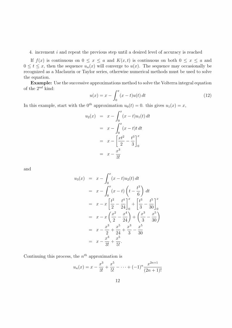
4. increment i and repeat the previous step until a desired level of accuracy is reached

If f(x) is continuous on 0 ≤ x ≤ a and K(x, t) is continuous on both 0 ≤ x ≤ a and0 ≤ t ≤ x, then the sequence un(x) will converge to u(x). The sequence may occasionally berecognized as a Maclaurin or Taylor series, otherwise numerical methods must be used to solvethe equation.

Example: Use the successive approximations method to solve the Volterra integral equationof the 2nd kind:

u(x) = x−∫ x

0

(x− t)u(t) dt (12)

In this example, start with the 0th approximation u0(t) = 0. this gives u1(x) = x,

u2(x) = x−∫ x

0

(x− t)u1(t) dt

= x−∫ x

0

(x− t)t dt

= x−[xt2

2− t3

3

]x

0

= x− x3

3!

and

u3(x) = x−∫ x

0

(x− t)u2(t) dt

= x−∫ x

0

(x− t)

(t− t3

6

)dt

= x− x

[t2

2− t4

24

]x

0

+

[t3

3− t5

30

]x

0

= x− x

(x2

2− x4

24

)+

(x3

3− x5

30

)

= x− x3

2+

x5

24+

x3

3− x5

30

= x− x3

3!+

x5

5!.

Continuing this process, the nth approximation is

un(x) = x− x3

3!+

x5

5!− · · ·+ (−1)n x2n+1

(2n + 1)!

12

which is clearly the Maclaurin series of sin x. Therefore the solution to eq. (12) is

u(x) = sin x.

5.2.3 Laplace Transform

If the kernel depends only on x− t, then it is called a difference kernel and denoted by K(x− t).Now the equation becomes:

u(x) = f(x) + λ

∫ x

0

K(x− t)u(t) dt,

which is the convolution product∫ x

0

K(x− t)u(t) dt = K ∗ u

Define the Laplace transform pairs U(s) ∼ u(x), F (s) ∼ f(x), and K(s) ∼ K(x).Now, since

L{K ∗ u} = KU,

then performing the Laplace transform to the integral equations results in

U(s) = F (s) + λK(s)U(s)

U(s) =F (s)

1− λK(s), λK(s) 6= 1,

and performing the inverse Laplace transform:

u(x) = L−1

{F (S)

1− λK(s)

}, λK(s) 6= 1.

Example: Use the Laplace transform method to solve eq. (11):

u(x) = f(x) + λ

∫ x

0

ex−tu(t) dt.

Let K(s) = L{ex} = 1s−1

and

U(s) =F (s)

1− λs−1

= F (s)s− 1

s− 1− λ

13

= F (s)s− 1− λ + λ

s− 1− λ

= F (s) + λF (s)

s− 1− λ

= F (s) + λF (s)

s− (λ + 1).

The solution u(x) is the inverse Laplace transform of U(s):

u(x) = L−1

{F (s) + λ

F (s)

s− (λ + 1)

}

= L−1{F (s)}+ λL−1

{F (s)

s− (λ + 1)

}

= f(x) + λL−1

{1

s− (λ + 1)F (s)

}

= f(x) + λe(λ+1)x ∗ f(x)

= f(x) + λ

∫ x

0

e(λ+1)(x−t)f(t) dt

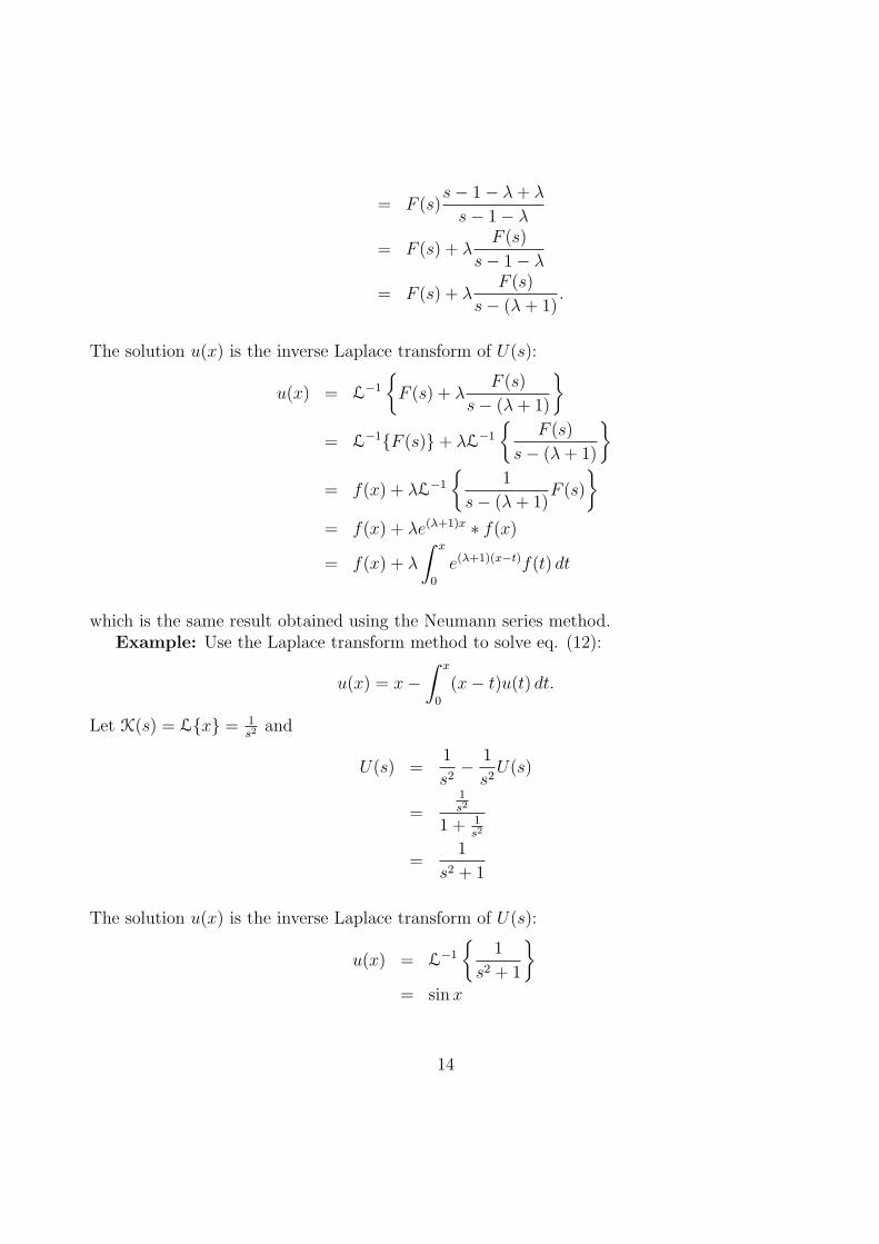
which is the same result obtained using the Neumann series method.Example: Use the Laplace transform method to solve eq. (12):

u(x) = x−∫ x

0

(x− t)u(t) dt.

Let K(s) = L{x} = 1s2 and

U(s) =1

s2− 1

s2U(s)

=1s2

1 + 1s2

=1

s2 + 1

The solution u(x) is the inverse Laplace transform of U(s):

u(x) = L−1

{1

s2 + 1

}

= sin x

14

which is the same result obtained using the successive approximations method.

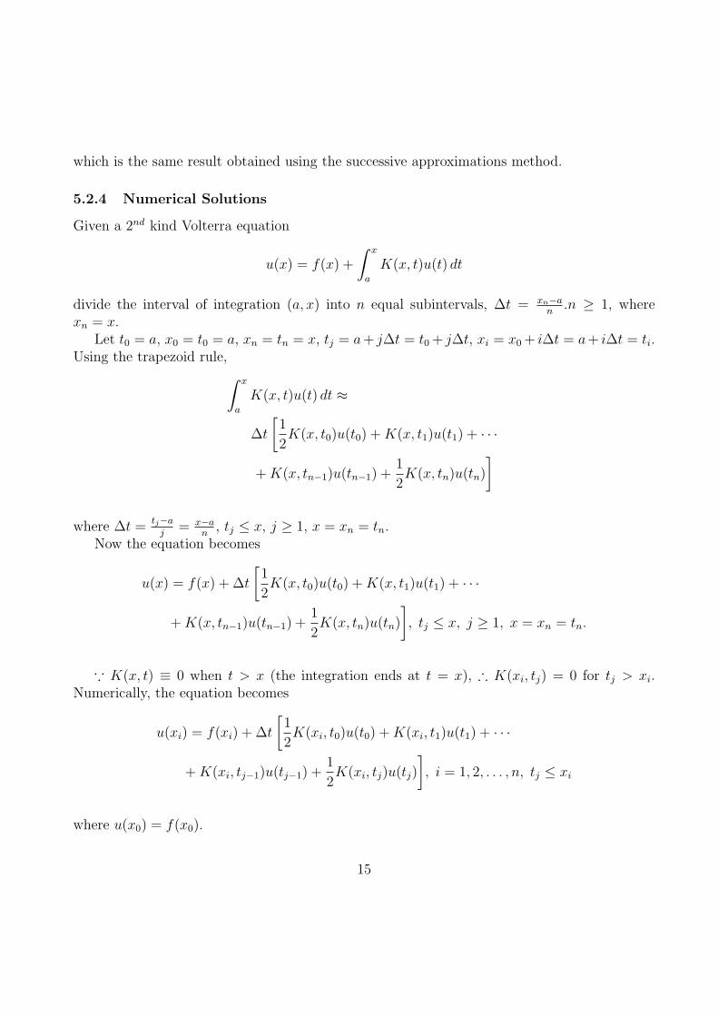
5.2.4 Numerical Solutions

Given a 2nd kind Volterra equation

u(x) = f(x) +

∫ x

a

K(x, t)u(t) dt

divide the interval of integration (a, x) into n equal subintervals, ∆t = xn−an

.n ≥ 1, wherexn = x.

Let t0 = a, x0 = t0 = a, xn = tn = x, tj = a+ j∆t = t0 + j∆t, xi = x0 + i∆t = a+ i∆t = ti.Using the trapezoid rule,

∫ x

a

K(x, t)u(t) dt ≈

∆t

[1

2K(x, t0)u(t0) + K(x, t1)u(t1) + · · ·

+ K(x, tn−1)u(tn−1) +1

2K(x, tn)u(tn)

]

where ∆t =tj−a

j= x−a

n, tj ≤ x, j ≥ 1, x = xn = tn.

Now the equation becomes

u(x) = f(x) + ∆t

[1

2K(x, t0)u(t0) + K(x, t1)u(t1) + · · ·

+ K(x, tn−1)u(tn−1) +1

2K(x, tn)u(tn)

], tj ≤ x, j ≥ 1, x = xn = tn.

∵ K(x, t) ≡ 0 when t > x (the integration ends at t = x), ∴ K(xi, tj) = 0 for tj > xi.Numerically, the equation becomes

u(xi) = f(xi) + ∆t

[1

2K(xi, t0)u(t0) + K(xi, t1)u(t1) + · · ·

+ K(xi, tj−1)u(tj−1) +1

2K(xi, tj)u(tj)

], i = 1, 2, . . . , n, tj ≤ xi

where u(x0) = f(x0).

15

Denote ui ≡ u(ti), fi ≡ f(xi), Kij ≡ K(xi, tj), so the numeric equation can be written in acondensed form as

u0 = f0, ui = fi + ∆t

[1

2Ki0u0 + Ki1u1 + · · ·

+ Ki(j−1)uj−1 +1

2Kijuj

], i = 1, 2, . . . , n, j ≤ i

∴ there are n + 1 equations

u0 = f0

u1 = f1 + ∆t

[1

2K10u0 +

1

2K11u1

]

u2 = f2 + ∆t

[1

2K20u0 + K21u1 +

1

2K22u2

]

......

un = fn + ∆t

[1

2Kn0u0 + Kn1u1 + · · ·+ Kn(n−1)un−1 +

1

2Knnun

]

where a general relation can be rewritten as

ui =fi + ∆t

[12Ki0u0 + Ki1u1 + · · ·+ Ki(i−1)ui−1

]

1− ∆t2

Kii

and can be evaluated by substituting u0, u1, . . . , ui−1 recursively from previous calculations.

5.3 Solving 1st-Kind Volterra Equations

5.3.1 Reduction to 2nd-Kind

f(x) = λ

∫ x

0

K(x, t)u(t) dt

If K(x, x) 6= 0, then:

df

dx= λ

∫ x

0

∂K(x, t)

∂xµ(t) dt + λK(x, x)u(x)

⇒ u(x) =1

λK(x, x)

df

dx−

∫ x

0

1

K(x, x)

∂K(x, t)

∂xu(t) dt

16

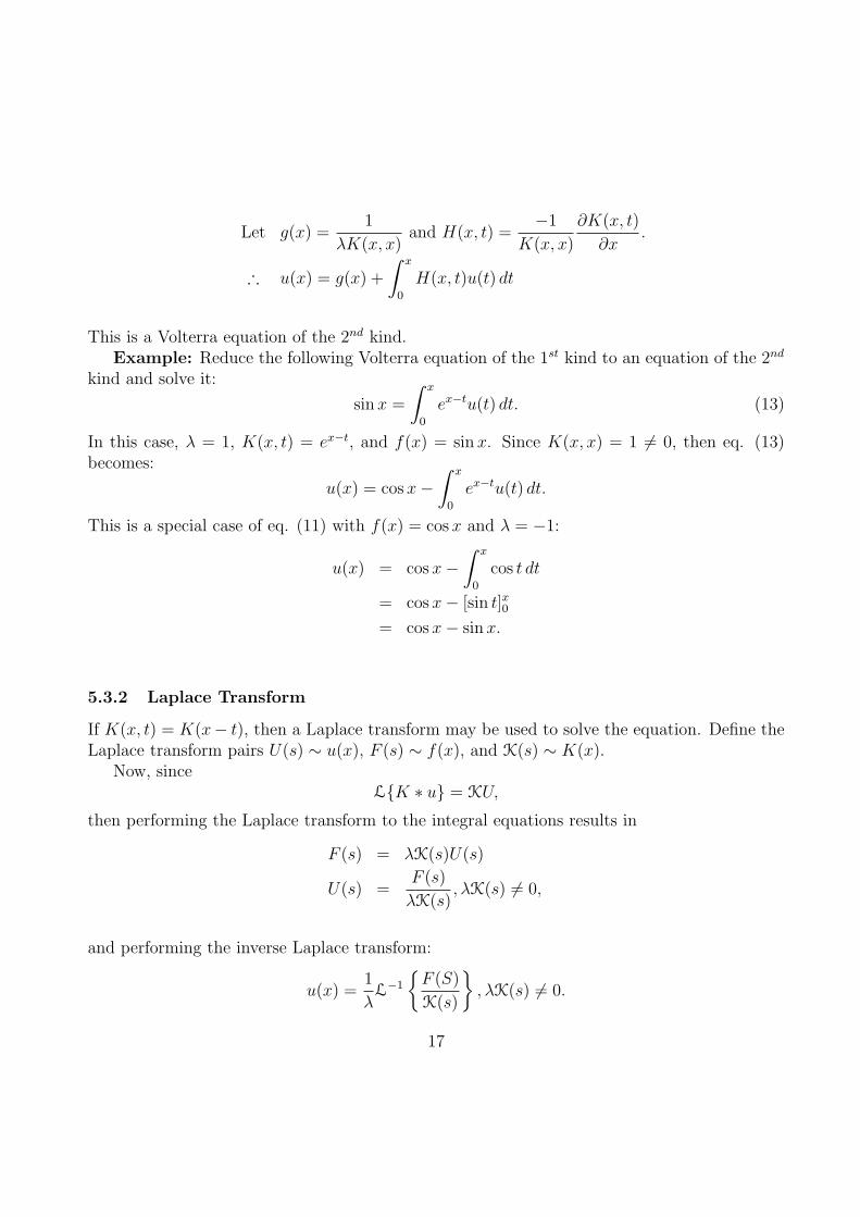
Let g(x) =1

λK(x, x)and H(x, t) =

−1

K(x, x)

∂K(x, t)

∂x.

∴ u(x) = g(x) +

∫ x

0

H(x, t)u(t) dt

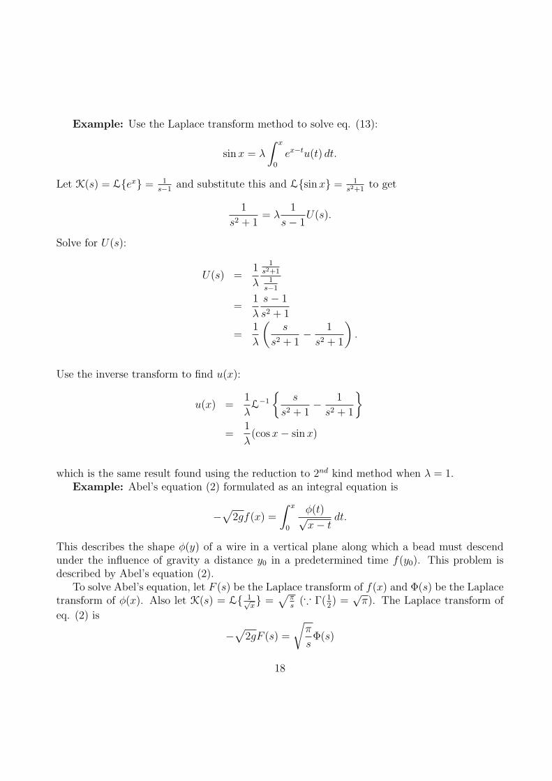
This is a Volterra equation of the 2nd kind.Example: Reduce the following Volterra equation of the 1st kind to an equation of the 2nd

kind and solve it:

sin x =

∫ x

0

ex−tu(t) dt. (13)

In this case, λ = 1, K(x, t) = ex−t, and f(x) = sin x. Since K(x, x) = 1 6= 0, then eq. (13)becomes:

u(x) = cos x−∫ x

0

ex−tu(t) dt.

This is a special case of eq. (11) with f(x) = cos x and λ = −1:

u(x) = cos x−∫ x

0

cos t dt

= cos x− [sin t]x0= cos x− sin x.

5.3.2 Laplace Transform

If K(x, t) = K(x− t), then a Laplace transform may be used to solve the equation. Define theLaplace transform pairs U(s) ∼ u(x), F (s) ∼ f(x), and K(s) ∼ K(x).

Now, sinceL{K ∗ u} = KU,

then performing the Laplace transform to the integral equations results in

F (s) = λK(s)U(s)

U(s) =F (s)

λK(s), λK(s) 6= 0,

and performing the inverse Laplace transform:

u(x) =1

λL−1

{F (S)

K(s)

}, λK(s) 6= 0.

17

Example: Use the Laplace transform method to solve eq. (13):

sin x = λ

∫ x

0

ex−tu(t) dt.

Let K(s) = L{ex} = 1s−1

and substitute this and L{sin x} = 1s2+1

to get

1

s2 + 1= λ

1

s− 1U(s).

Solve for U(s):

U(s) =1

λ

1s2+1

1s−1

=1

λ

s− 1

s2 + 1

=1

λ

(s

s2 + 1− 1

s2 + 1

).

Use the inverse transform to find u(x):

u(x) =1

λL−1

{s

s2 + 1− 1

s2 + 1

}

=1

λ(cos x− sin x)

which is the same result found using the reduction to 2nd kind method when λ = 1.Example: Abel’s equation (2) formulated as an integral equation is

−√

2gf(x) =

∫ x

0

φ(t)√x− t

dt.

This describes the shape φ(y) of a wire in a vertical plane along which a bead must descendunder the influence of gravity a distance y0 in a predetermined time f(y0). This problem isdescribed by Abel’s equation (2).

To solve Abel’s equation, let F (s) be the Laplace transform of f(x) and Φ(s) be the Laplacetransform of φ(x). Also let K(s) = L{ 1√

x} =

√πs

(∵ Γ(12) =

√π). The Laplace transform of

eq. (2) is

−√

2gF (s) =

√π

sΦ(s)

18

or, solving for Φ(s):

Φ(s) = −√

2g

π

√sF (s).

So φ(x) is given by:

φ(x) = −√

2g

πL−1{√sF (s)}.

Since L−1{√s} does not exist, the convolution theorem cannot be used directly to solve for

φ(x). However, by introducing H(s) ≡ F (s)√s

the equation may be rewritten as:

φ(x) = −√

2g

πsH(s).

Now

h(x) = L−1{H(s)}= L−1

{1√sF (s)

}

=1√π

∫ x

0

f(t)√x− t

dt

and since h(0) = 0,

dh

dx= L−1{sH(s)− h(0)}= L−1{sH(s)}

Finally, use dhdx

to find φ(x) using the inverse Laplace transform:

φ(x) = −√

2g

π

d

dx

[1√π

∫ x

0

f(t)√x− t

dt

]

=−√2g

π

d

dx

∫ x

0

f(t)√x− t

dt

which is the solution to Abel’s equation (2).

19

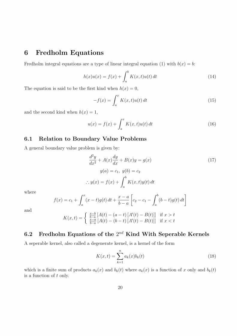
6 Fredholm Equations

Fredholm integral equations are a type of linear integral equation (1) with b(x) = b:

h(x)u(x) = f(x) +

∫ b

a

K(x, t)u(t) dt (14)

The equation is said to be the first kind when h(x) = 0,

−f(x) =

∫ x

a

K(x, t)u(t) dt (15)

and the second kind when h(x) = 1,

u(x) = f(x) +

∫ x

a

K(x, t)u(t) dt (16)

6.1 Relation to Boundary Value Problems

A general boundary value problem is given by:

d2y

dx2+ A(x)

dy

dx+ B(x)y = g(x) (17)

y(a) = c1, y(b) = c2

∴ y(x) = f(x) +

∫ b

a

K(x, t)y(t) dt

where

f(x) = c1 +

∫ x

a

(x− t)g(t) dt +x− a

b− a

[c2 − c1 −

∫ b

a

(b− t)g(t) dt

]

and

K(x, t) =

{x−bb−a

[A(t)− (a− t) [A′(t)−B(t)]] if x > tx−ab−a

[A(t)− (b− t) [A′(t)−B(t)]] if x < t

6.2 Fredholm Equations of the 2nd Kind With Seperable Kernels

A seperable kernel, also called a degenerate kernel, is a kernel of the form

K(x, t) =n∑

k=1

ak(x)bk(t) (18)

which is a finite sum of products ak(x) and bk(t) where ak(x) is a function of x only and bk(t)is a function of t only.

20

6.2.1 Nonhomogeneous Equations

Given the kernel in eq. (18), the general nonhomogeneous second kind Fredholm equation,

u(x) = f(x) + λ

∫ b

a

K(x, t)u(t) dt (19)

becomes

u(x) = f(x) + λ

∫ b

a

n∑

k=1

ak(x)bk(t)u(t) dt

= f(x) + λ

n∑

k=1

ak(x)

∫ b

a

bk(t)u(t) dt

Define ck as

ck =

∫ b

a

bk(t)u(t) dt

(i.e. the integral portion). Multiply both sides by bm(x), m = 1, 2, . . . , n

bm(x)u(x) = bm(x)f(x) + λ

n∑

k=1

ckbm(x)ak(x)

then integrate both sides from a to b

∫ b

a

bm(x)u(x) dx =

∫ b

a

bm(x)f(x) dx + λ

n∑

k=1

ck

∫ b

a

bm(x)ak(x) dx

Define fm and amk as

fm =

∫ b

a

bm(x)f(x) dx

amk =

∫ b

a

bm(x)ak(x) dx

so finally the equation becomes

cm = fm + λ

n∑

k=1

amkck, m = 1, 2, . . . , n.

That is, it is a nonhomogeneous system of n linear equations in c1, c2, . . . , cn. fm and amk areknown since bm(x), f(x), and ak(x) are all given.

21

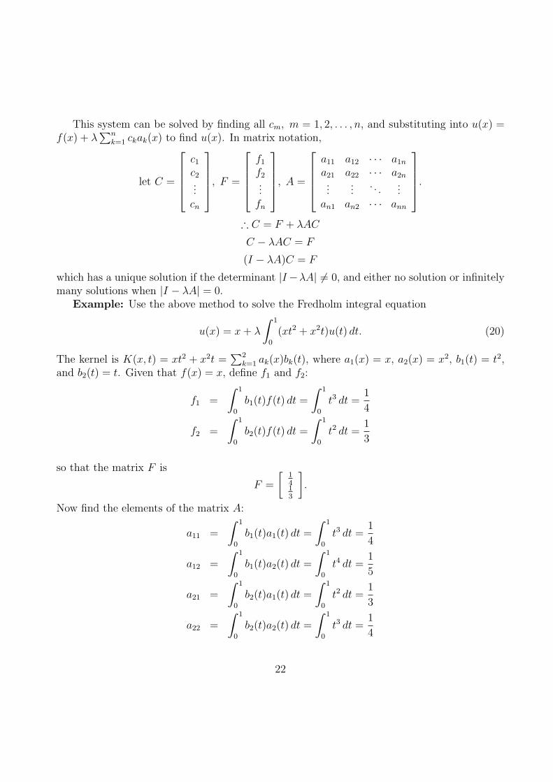
This system can be solved by finding all cm, m = 1, 2, . . . , n, and substituting into u(x) =f(x) + λ

∑nk=1 ckak(x) to find u(x). In matrix notation,

let C =

c1

c2...cn

, F =

f1

f2...

fn

, A =

a11 a12 · · · a1n

a21 a22 · · · a2n...

.... . .

...an1 an2 · · · ann

.

∴ C = F + λAC

C − λAC = F

(I − λA)C = F

which has a unique solution if the determinant |I−λA| 6= 0, and either no solution or infinitelymany solutions when |I − λA| = 0.

Example: Use the above method to solve the Fredholm integral equation

u(x) = x + λ

∫ 1

0

(xt2 + x2t)u(t) dt. (20)

The kernel is K(x, t) = xt2 + x2t =∑2

k=1 ak(x)bk(t), where a1(x) = x, a2(x) = x2, b1(t) = t2,and b2(t) = t. Given that f(x) = x, define f1 and f2:

f1 =

∫ 1

0

b1(t)f(t) dt =

∫ 1

0

t3 dt =1

4

f2 =

∫ 1

0

b2(t)f(t) dt =

∫ 1

0

t2 dt =1

3

so that the matrix F is

F =

[1413

].

Now find the elements of the matrix A:

a11 =

∫ 1

0

b1(t)a1(t) dt =

∫ 1

0

t3 dt =1

4

a12 =

∫ 1

0

b1(t)a2(t) dt =

∫ 1

0

t4 dt =1

5

a21 =

∫ 1

0

b2(t)a1(t) dt =

∫ 1

0

t2 dt =1

3

a22 =

∫ 1

0

b2(t)a2(t) dt =

∫ 1

0

t3 dt =1

4

22

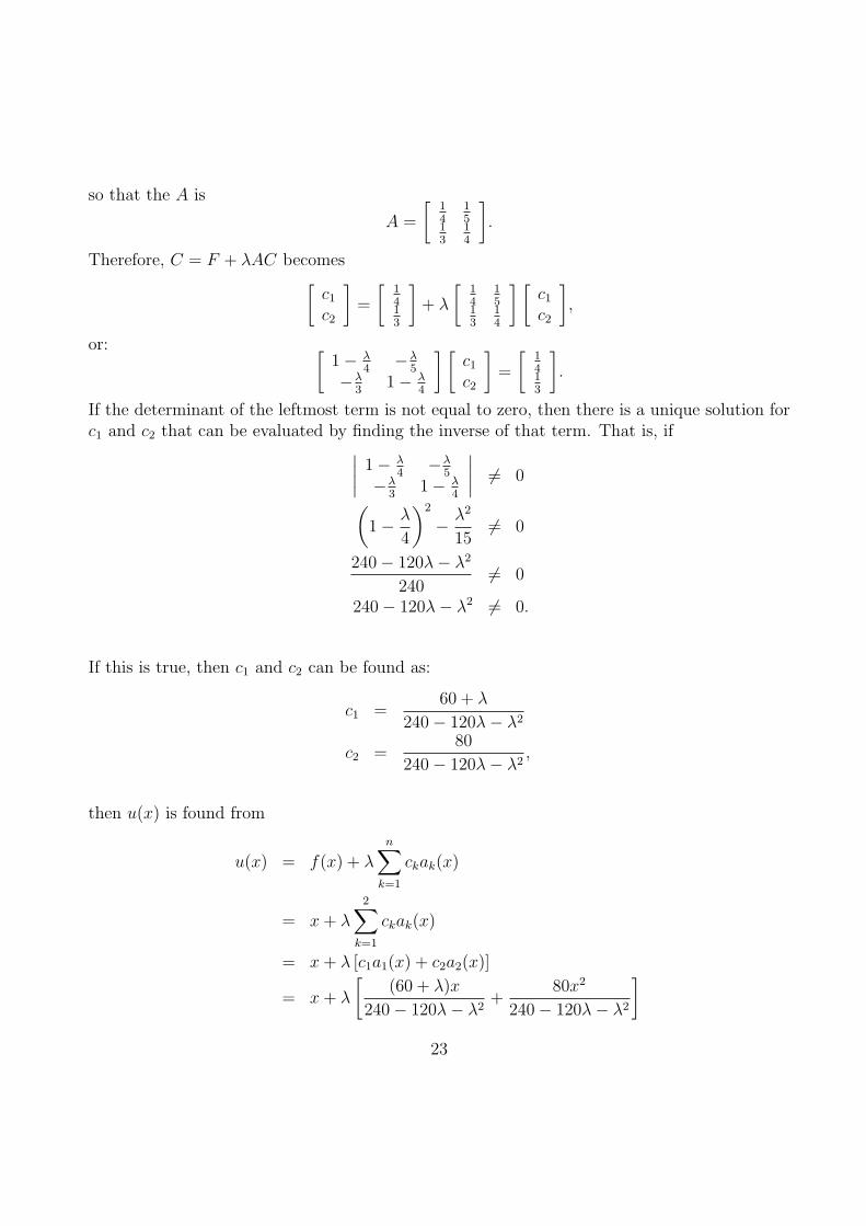
so that the A is

A =

[14

15

13

14

].

Therefore, C = F + λAC becomes[

c1

c2

]=

[1413

]+ λ

[14

15

13

14

] [c1

c2

],

or: [1− λ

4−λ

5

−λ3

1− λ4

] [c1

c2

]=

[1413

].

If the determinant of the leftmost term is not equal to zero, then there is a unique solution forc1 and c2 that can be evaluated by finding the inverse of that term. That is, if

∣∣∣∣1− λ

4−λ

5

−λ3

1− λ4

∣∣∣∣ 6= 0

(1− λ

4

)2

− λ2

156= 0

240− 120λ− λ2

2406= 0

240− 120λ− λ2 6= 0.

If this is true, then c1 and c2 can be found as:

c1 =60 + λ

240− 120λ− λ2

c2 =80

240− 120λ− λ2,

then u(x) is found from

u(x) = f(x) + λ

n∑

k=1

ckak(x)

= x + λ

2∑

k=1

ckak(x)

= x + λ [c1a1(x) + c2a2(x)]

= x + λ

[(60 + λ)x

240− 120λ− λ2+

80x2

240− 120λ− λ2

]

23

=(240− 60λ)x + 80λx2

240− 120λ− λ2, 240− 120λ− λ2 6= 0.

6.2.2 Homogeneous Equations

Given the kernel defined in eq. (18), the general homogeneous second kind Fredholm equation,

u(x) = λ

∫ b

a

K(x, t)u(t) dt (21)

becomes

u(x) = λ

∫ b

a

n∑

k=1

ak(x)bk(t)u(t) dt

= λ

n∑

k=1

ak(x)

∫ b

a

bk(t)u(t) dt

Define ck, multiply and integrate, then define amk as in the previous section so finally theequation becomes

cm = λ

n∑

k=1

amkck, m = 1, 2, . . . , n.

That is, it is a homogeneous system of n linear equations in c1, c2, . . . , cn. Again, the systemcan be solved by finding all cm, m = 1, 2, . . . , n, and substituting into u(x) = λ

∑nk=1 ckak(x)

to find u(x). Using the same matrices defined earlier, the equation can be written as

C = λAC

C − λAC = 0

(I − λA)C = 0.

Because this is a homogeneous system of equations, when the determinant |I − λA| 6= 0 thenthe trivial solution C = 0 is the only solution, and the solution to the integral equation isu(x) = 0. Otherwise, if |I −λA| = 0 then there may be zero or infinitely many solutions whoseeigenfunctions correspond to solutions u1(x), u2(x), . . . , un(x) of the Fredholm equation.

Example: Use the above method to solve the Fredholm integral equation

u(x) = λ

∫ π

0

(cos2 x cos 2t + cos 3x cos3 t)u(t) dt. (22)

24

The kernel is K(x, t) = cos2 x cos 2t + cos 3x cos3 t =∑

k=1 2ak(x)bk(t) where a1(x) = cos2 x,a2(x) = cos 3x, b1(t) = cos 2t, and b2(t) = cos3 t. Now find the elements of the matrix A:

a11 =

∫ π

0

b1(t)a1(t) dt =

∫ π

0

cos 2t cos2 t dt =π

4

a12 =

∫ π

0

b1(t)a2(t) dt =

∫ π

0

cos 2t cos 3t dt = 0

a21 =

∫ π

0

b2(t)a1(t) dt =

∫ π

0

cos3 t cos2 t dt = 0

a22 =

∫ π

0

b2(t)a2(t) dt =

∫ π

0

cos3 t cos 3t dt =π

8

and follow the method of the previous example to find c1 and c2:[1− λπ

40

0 1− λπ8

]= 0

(1− λ

π

4

)= 0

(1− λ

π

8

)= 0

For c1 and c2 to not be the trivial solution, the determinant must be zero. That is,∣∣∣∣

1− λπ4

00 1− λπ

8

∣∣∣∣ =(1− λ

π

4

)(1− λ

π

8

)= 0,

which has solutions λ1 = 4π

and λ2 = 8π

which are the eigenvalues of eq. (22). There are twocorresponding eigenfunctions u1(x) and u2(x) that are solutions to eq. (22). For λ1 = 4

π, c1 = c1

(i.e. it is a parameter), and c2 = 0. Therefore u1(x) is

u1(x) =4

πc1 cos2 x.

To form a specific solution (which can be used to find a general solution, since eq. (22) islinear), let c1 = π

4, so that

u1(x) = cos2 x.

Similarly, for λ2 = 8π, c1 = 0 and c2 = c2, so u2(x) is

u2(x) =8

πc2 cos 3x.

To form a specific solution, let c2 = π8, so that

u2(x) = cos 3x.

25

6.2.3 Fredholm Alternative

The homogeneous Fredholm equation (21),

u(x) = λ

∫ b

a

K(x, t)u(t) dt

has the corresponding nonhomogeneous equation (19),

u(x) = f(x) + λ

∫ b

a

K(x, t)u(t) dt.

If the homogeneous equation has only the trivial solution u(x) = 0, then the nonhomogeneousequation has exactly one solution. Otherwise, if the homogeneous equation has nontrivialsolutions, then the nonhomogeneous equation has either no solutions or infinitely many solutionsdepending on the term f(x). If f(x) is orthogonal to every solution ui(x) of the homogeneousequation, then the associated nonhomogeneous equation will have a solution. The two functionsf(x) and ui(x) are orthogonal if

∫ b

af(x)ui(x) dx = 0.

6.2.4 Approximate Kernels

Often a nonseperable kernel may have a Taylor or other series expansion that is separable.This approximate kernel is denoted by M(x, t) ≈ K(x, t) and the corresponding approximatesolution for u(x) is v(x). So the approximate solution to eq. (19) is given by

v(x) = f(x) + λ

∫ b

a

M(x, t)v(t) dt.

The error involved is ε = |u(x)− v(x)| and can be estimated in some cases.Example: Use an approximating kernel to find an approximate solution to

u(x) = sin x +

∫ 1

0

(1− x cos xt)u(t) dt. (23)

The kernel K(x, t) = 1 − x cos xt is not seperable, but a finite number of terms from itsMaclaurin series expansion

1− x

(1− x2t2

2!+

x4t4

4!− · · ·

)= 1− x +

x3t2

2!− x5t4

4!+ · · ·

is seperable in x and t. Therefore consider the first three terms of this series as the approximatekernel

M(x, t) = 1− x +x3t2

2!.

26

The associated approximate integral equation in v(x) is

v(x) = sin x +

∫ 1

0

(1− x +

x3t2

2!

)v(t) dt. (24)

Now use the previous method for solving Fredholm equations with seperable kernels to solveeq. (24):

M(x, t) =2∑

k=1

ak(x)bk(t)

where a1(x) = (1 − x), a2(x) = x3, b1(t) = 1, b2(t) = t2

2. Given that f(x) = sin x, find f1 and

f2:

f1 =

∫ 1

0

b1(t)f(t) dt =

∫ 1

0

sin t dt = 1− cos 1

f2 =

∫ 1

0

b2(t)f(t) dt =

∫ 1

0

t2

2sin t dt =

1

2cos 1 + sin 1− 1.

Now find the elements of the matrix A:

a11 =

∫ 1

0

b1(t)a1(t) dt =

∫ 1

0

(1− t) dt =1

2

a12 =

∫ 1

0

b1(t)a2(t) dt =

∫ 1

0

t3 dt =1

4

a21 =

∫ 1

0

b2(t)a1(t) dt =

∫ 1

0

t2

2(1− t) dt =

1

24

a22 =

∫ 1

0

b2(t)a2(t) dt =

∫ 1

0

t5

2dt =

1

12.

Therefore, C = F + λAC becomes

[c1

c2

]=

[1− cos 1

12cos 1 + sin 1− 1

]+ 1

[12

14

124

112

] [c1

c2

],

or [1− 1

2−1

4

− 124

1− 112

] [c1

c2

]=

[1− cos 1

12cos 1 + sin 1− 1

].

27

The determinant is∣∣∣∣

1− 12

−14

− 124

1− 112

∣∣∣∣ =1

2· 11

12− 1

4· 1

24

=43

96

which is non-zero, so there is a unique solution for C:

c1 = −76

43cos 1 +

64

43+

24

43sin 1 ≈ 1.0031

c2 =20

43cos 1− 44

43+

48

43sin 1 ≈ 0.1674.

Therefore, the solution to eq. (24) is

v(x) = sin x + c1a1(x) + c2a2(x)

≈ sin x + 1.0031(1− x) + 0.1674x3

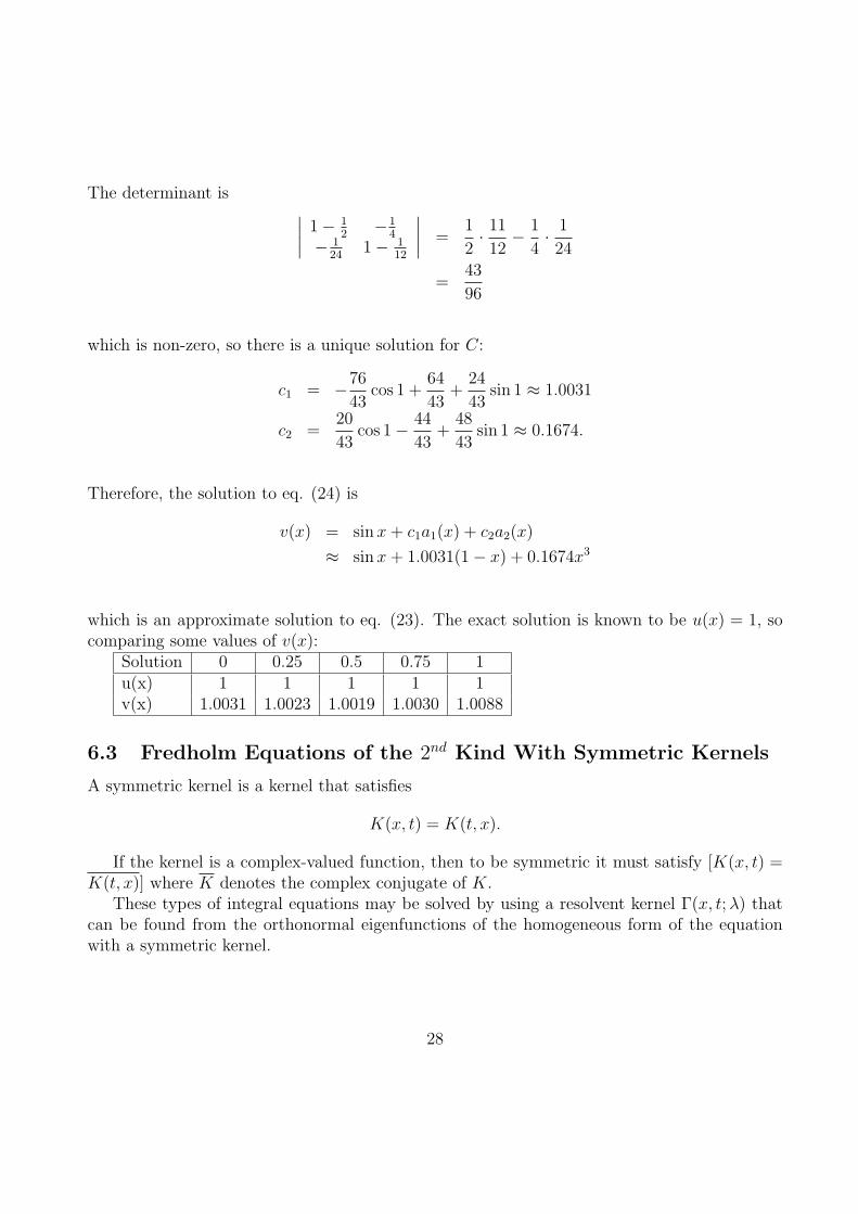
which is an approximate solution to eq. (23). The exact solution is known to be u(x) = 1, socomparing some values of v(x):

Solution 0 0.25 0.5 0.75 1u(x) 1 1 1 1 1v(x) 1.0031 1.0023 1.0019 1.0030 1.0088

6.3 Fredholm Equations of the 2nd Kind With Symmetric Kernels

A symmetric kernel is a kernel that satisfies

K(x, t) = K(t, x).

If the kernel is a complex-valued function, then to be symmetric it must satisfy [K(x, t) =K(t, x)] where K denotes the complex conjugate of K.

These types of integral equations may be solved by using a resolvent kernel Γ(x, t; λ) thatcan be found from the orthonormal eigenfunctions of the homogeneous form of the equationwith a symmetric kernel.

28

6.3.1 Homogeneous Equations

The eigenfunctions of a homogeneous Fredholm equation with a symmetric kernel are functionsun(x) that satisfy

un(x) = λn

∫ b

a

K(x, t)un(t) dt.

It can be shown that the eigenvalues of the symmetric kernel are real, and that the eigen-functions un(x) and um(x) corresponding to two of the eigenvalues λn and λm where λn 6= λm

are orthogonal (see earlier section on the Fredholm Alternative). It can also be shown thatthere is a finite number of eigenfunctions corresponding to each eigenvalue of a kernel if thekernel is square integrable on {(x, t)|a ≤ x ≤ b, a ≤ t ≤ b}, that is:

∫ b

a

∫ b

a

K2(x, t) dx dt = B2 < ∞.

Once the orthonormal eigenfunctions φ1(x), φ2(x), . . . of the homogeneous form of the equa-tions are found, the resolvent kernel can be expressed as an infinite series:

Γ(x, t; λ) =∞∑

k=1

φk(x)φk(t)

λ− λk

, λ 6= λk

so the solution of the 2nd-order Fredholm equation is

u(x) = f(x) + λ

∞∑

k=1

akφk(x)

λk − λ

where

ak =

∫ b

a

f(x)φk(x) dx.

6.4 Fredholm Equations of the 2nd Kind With General Kernels

6.4.1 Fredholm Resolvent Kernel

Evaluate the Fredholm Resolvent Kernel Γ(x, t; λ) in

u(x) = f(x) + λ

∫ b

a

Γ(x, t; λ)f(t) dt (25)

Γ(x, t; λ) =D(x, t; λ)

D(λ)

29

where D(x, t; λ) is called the Fredholm minor and D(λ) is called the Fredholm determinant.The minor is defined as

D(x, t; λ) = K(x, t) +∞∑

n=1

(−λ)n

n!Bn(x, t)

where

Bn(x, t) = CnK(x, t)− n

∫ b

a

K(x, s)Bn−1(s, t) ds, B0(x, t) = K(x, t)

and

Cn =

∫ b

a

Bn−1(t, t) dt, n = 1, 2, . . . , C0 = 1

and the determinant is defined as

D(λ) =∞∑

n=0

(−λ)n

n!Cn, C0 = 1.

Bn(x, t) and Cn may each be expressed as a repeated integral where the integrand is adeterminant:

Bn(x, t) =

∫ b

a

∫ b

a

· · ·∫ b

a

∣∣∣∣∣∣∣∣∣

K(x, t) K(x, t1) · · · K(x, tn)K(t1, t) K(t1, t1) · · · K(t1, tn)

......

. . ....

K(tn, t) K(tn, t1) · · · K(tn, tn)

∣∣∣∣∣∣∣∣∣dt1 dt2 . . . dtn

Cn =

∫ b

a

∫ b

a

· · ·∫ b

a

∣∣∣∣∣∣∣∣∣

K(t1, t1) K(t1, t2) · · · K(t1, tn)K(t2, t1) K(t2, t2) · · · K(t2, tn)

......

. . ....

K(tn, t1) K(tn, t2) · · · K(tn, tn)

∣∣∣∣∣∣∣∣∣dt1 dt2 . . . dtn

6.4.2 Iterated Kernels

Define the iterated kernel Ki(x, t) as

Ki(x, y) ≡∫ b

a

K(x, t)Ki−1(t, y) dt, K1(x, t) ≡ K(x, t)

so

φi(x) ≡∫ b

a

Ki(x, y)f(y) dy

30

and

un(x) = f(x) + λφ1(x) + λ2φ2(x) + · · ·+ λnφn(x)

= f(x) +n∑

i=1

λiφi(x)

un(x) converges to u(x) when |λB| < 1 and

B =

√∫ b

a

∫ b

a

K2(x, t) dx dt.

6.4.3 Neumann Series

The Neumann series

u(x) = f(x) +∞∑i=1

λiφi(x)

is convergent, and substituting for φi(x) as in the previous section it can be rewritten as

u(x) = f(x) +∞∑i=1

λi

∫ b

a

Ki(x, t)f(t) dt

= f(x) +

∫ b

a

[ ∞∑i=1

λiKi(x, t)

]f(t) dt

= f(x) + λ

∫ b

a

Γ(x, t; λ)f(t) dt.

Therefore the Neumann resolvent kernel for the general nonhomogeneous Fredholm integralequation of the second kind is

Γ(x, t; λ) =∞∑i=1

λi−1Ki(x, t).

6.5 Approximate Solutions To Fredholm Equations of the 2nd Kind

The solution of the general nonhomogeneous Fredholm integral equation of the second kind eq.(19), u(x), can be approximated by the partial sum

SN(x) =N∑

k=1

ckφk(x) (26)

31

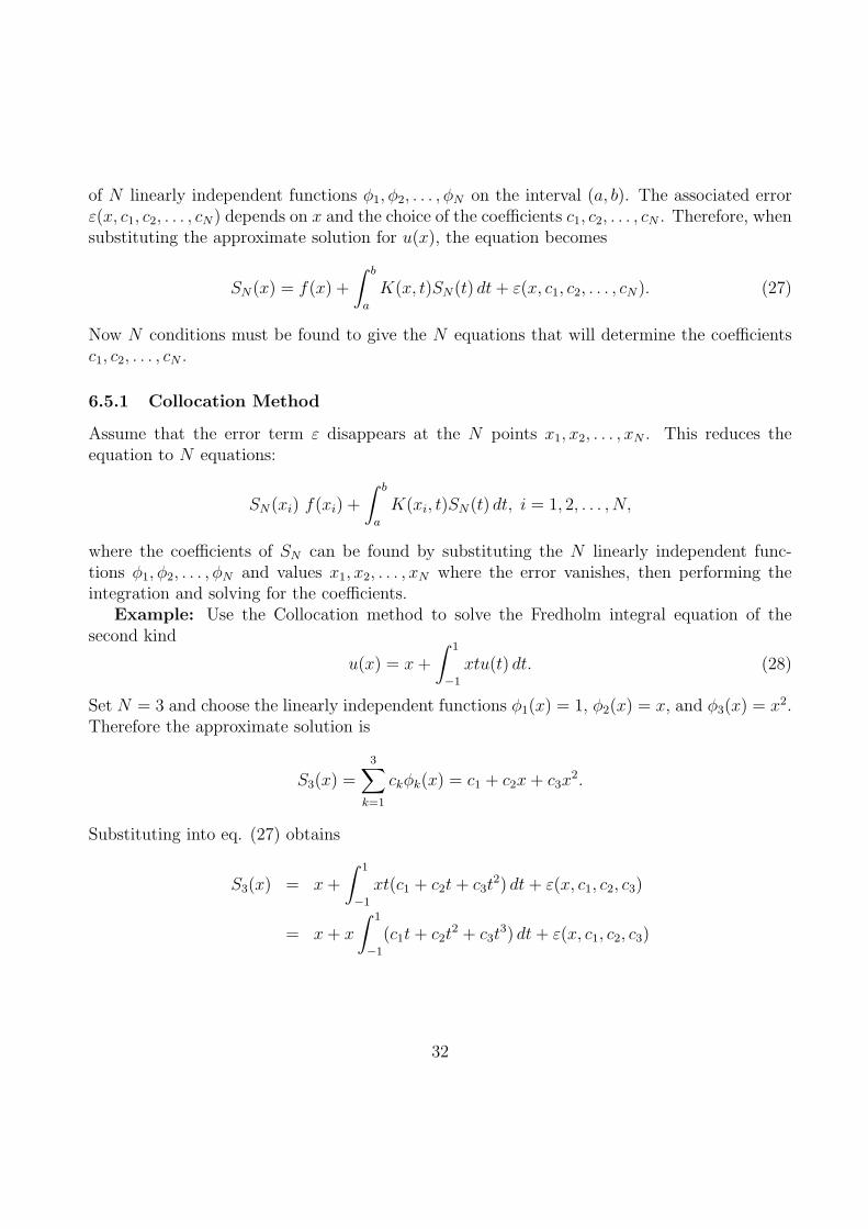
of N linearly independent functions φ1, φ2, . . . , φN on the interval (a, b). The associated errorε(x, c1, c2, . . . , cN) depends on x and the choice of the coefficients c1, c2, . . . , cN . Therefore, whensubstituting the approximate solution for u(x), the equation becomes

SN(x) = f(x) +

∫ b

a

K(x, t)SN(t) dt + ε(x, c1, c2, . . . , cN). (27)

Now N conditions must be found to give the N equations that will determine the coefficientsc1, c2, . . . , cN .

6.5.1 Collocation Method

Assume that the error term ε disappears at the N points x1, x2, . . . , xN . This reduces theequation to N equations:

SN(xi) f(xi) +

∫ b

a

K(xi, t)SN(t) dt, i = 1, 2, . . . , N,

where the coefficients of SN can be found by substituting the N linearly independent func-tions φ1, φ2, . . . , φN and values x1, x2, . . . , xN where the error vanishes, then performing theintegration and solving for the coefficients.

Example: Use the Collocation method to solve the Fredholm integral equation of thesecond kind

u(x) = x +

∫ 1

−1

xtu(t) dt. (28)

Set N = 3 and choose the linearly independent functions φ1(x) = 1, φ2(x) = x, and φ3(x) = x2.Therefore the approximate solution is

S3(x) =3∑

k=1

ckφk(x) = c1 + c2x + c3x2.

Substituting into eq. (27) obtains

S3(x) = x +

∫ 1

−1

xt(c1 + c2t + c3t2) dt + ε(x, c1, c2, c3)

= x + x

∫ 1

−1

(c1t + c2t2 + c3t

3) dt + ε(x, c1, c2, c3)

32

and performing the integration results in

∫ 1

−1

(c1t + c2t2 + c3t

3) dt =

[c1t

2

2+

c2t3

3+

c3t4

4

]1

−1

=c1

2+

c2

3+

c3

4−

(c1

2− c2

3+

c3

4

)

=c1 − c1

2+

c2 + c2

3+

c3 − c3

4

=2

3c2

so eq. (27) becomes

c1 + c2x + c3x2 = x + x

(2

3c2

)+ ε(x, c1, c2, c3)

= x

(1 +

2

3c2

)+ ε(x, c1, c2, c3).

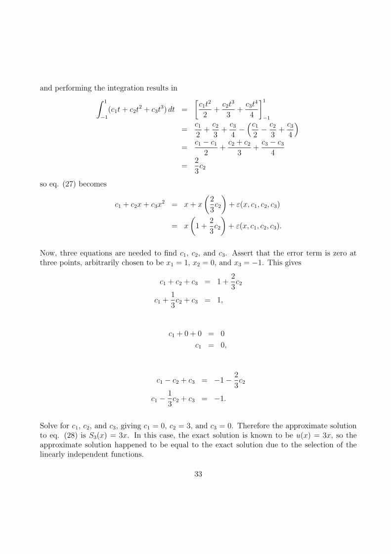
Now, three equations are needed to find c1, c2, and c3. Assert that the error term is zero atthree points, arbitrarily chosen to be x1 = 1, x2 = 0, and x3 = −1. This gives

c1 + c2 + c3 = 1 +2

3c2

c1 +1

3c2 + c3 = 1,

c1 + 0 + 0 = 0

c1 = 0,

c1 − c2 + c3 = −1− 2

3c2

c1 − 1

3c2 + c3 = −1.

Solve for c1, c2, and c3, giving c1 = 0, c2 = 3, and c3 = 0. Therefore the approximate solutionto eq. (28) is S3(x) = 3x. In this case, the exact solution is known to be u(x) = 3x, so theapproximate solution happened to be equal to the exact solution due to the selection of thelinearly independent functions.

33

6.5.2 Galerkin Method

Assume that the error term ε is orthogonal to N given linearly independent functions ψ1, ψ2, . . . , ψN

of x on the interval (a, b). The N conditions therefore become

∫ b

a

ψj(x)ε(x, c1, c2, . . . , cN) dx

=

∫ b

a

ψj(x)

[SN(x)− f(x)−

∫ b

a

K(x, t)SN(t) dt

]dx

= 0, j = 1, 2, . . . , N

which can be rewritten as either

∫ b

a

ψj(x)

[SN(x)−

∫ b

a

K(x, t)SN(t) dt

]dx

=

∫ b

a

ψj(x)f(x) dx, j = 1, 2, . . . , N

or

∫ b

a

ψj(x)

{N∑

k=1

ckφk(x)−∫ b

a

K(x, t)

[N∑

k=1

ckφk(t)

]dt

}dx

=

∫ b

a

ψj(x)f(x) dx, j = 1, 2, . . . , N

after substituting for SN(x) as before. In general the first set of linearly independent func-tions φj(x) are different from the second set ψj(x), but the same functions may be used forconvenience.

Example: Use the Galerkin method to solve the Fredholm integral equation in eq. (28),

u(x) = x +

∫ 1

−1

xtu(t) dt

using the same linearly independent functions φ1(x) = 1, φ2(x) = x, and φ3(x) = x2 giving theapproximate solution

S3(x) = c1 + c2x + c3x2.

34

Substituting into eq. (27) results in the error term being

ε(x, c1, c2, c3) = c1 + c2x + c3x2 − x−

∫ 1

−1

xt(c1 + c2t + c3t2) dt.

The error must be orthogonal to three linearly independent functions, chosen to be ψ1(x) = 1,ψ2(x) = x, and ψ3(x) = x2:

∫ 1

−1

1

[c1 + c2x + c3x

2 −∫ 1

−1

xt(c1 + c2t + c3t2) dt

]dx =

∫ 1

−1

x dx

∫ 1

−1

[c1 + c2x + c3x

2 − x

∫ 1

−1

(c1t + c2t2 + c3t

3) dt

]dx =

x2

2

∣∣∣∣1

−1∫ 1

−1

[c1 + c2x + c3x

2 − x

[c1t

2

2+

c2t3

3+

c3t4

4

]1

−1

]dx =

1

2− 1

2∫ 1

−1

(c1 − 1

3c2x + c3x

2

)dx = 0

[c1x +

c2x2

6+

c3x3

3

]1

−1

= 0

2c1 +2

3c3 = 0,

∫ 1

−1

x

[c1 + c2x + c3x

2 −∫ 1

−1

xt(c1 + c2t + c3t2) dt

]dx =

∫ 1

−1

x2 dx

∫ 1

−1

x

(c1 − 1

3c2x + c3x

2

)dx =

x3

3

∣∣∣∣1

−1∫ 1

−1

(c1x− 1

3c2x

2 + c3x3

)dx =

1

3+

1

3[c1x

2

2+

c2x3

9+

c3x4

4

]1

−1

=2

3

2

9c2 =

2

3c2 = 3,

∫ 1

−1

x2

[c1 + c2x + c3x

2 −∫ 1

−1

xt(c1 + c2t + c3t2) dt

]dx =

∫ 1

−1

x3 dx

35

∫ 1

−1

x2

(c1 − 1

3c2x + c3x

2

)dx =

x4

4

∣∣∣∣1

−1∫ 1

−1

(c1x

2 − 1

3c2x

3 + c3x4

)dx =

1

4− 1

4[c1x

3

3+

c2x4

12+

c3x5

5

]1

−1

= 0

2

3c1 +

2

5c3 = 0.

Solving for c1, c2, and c3 gives c1 = 0, c2 = 3, and c3 = 0, resulting in the approximate solutionbeing S3(x) = 3x. This is the same result obtained using the collocation method, and alsohappens to be the exact solution to eq. (27) due to the selection of the linearly independentfunctions.

6.6 Numerical Solutions To Fredholm Equations

A numerical solution to a general Fredholm integral equation can be found by approximatingthe integral by a finite sum (using the trapezoid rule) and solving the resulting simultaneousequations.

6.6.1 Nonhomogeneous Equations of the 2nd Kind

In the general Fredholm Equation of the second kind in eq. (19),

u(x) = f(x) +

∫ b

a

K(x, t)u(t) dt,

the interval (a, b) can be subdivided into n equal intervals of width ∆t = b−an

. Let t0 = a,tj = a + j∆t = t0 + j∆t, and since the variable is either t or x, let x0 = t0 = a, xn = tn = b,and xi = x0 + i∆t (i.e. xi = ti). Also denote u(xi) as ui, f(xi) as fi, and K(xi, tj) as Kij. Nowif the trapezoid rule is used to approximate the given equation, then:

u(x) = f(x) +

∫ b

a

K(x, t)u(t) dt ≈ f(x) + ∆t

[1

2K(x, t0)u(t0)

+K(x, t1)u(t1) + · · ·+ K(x, tn−1)u(tn−1) +1

2K(x, tn)u(tn)

]

36

or, more tersely:

u(x) ≈ f(x) + ∆t

[1

2K(x, t0)u0 + K(x, t1)u1 + · · ·+ 1

2K(x, tn)un

].

There are n + 1 values of ui, as i = 0, 1, 2, . . . , n. Therefore the equation becomes a set ofn + 1 equations in ui:

ui = fi + ∆t

[1

2Ki0u0 + Ki1u1 + · · ·+ Ki(n−1)un−1

+1

2Kinun

], i = 0, 1, 2, . . . , n

that give the approximate solution to u(x) at x = xi. The terms involving u may be moved tothe left side of the equations, resulting in n + 1 equations in u0, u1, u2, . . . , un:

(1− ∆t

2K00

)u0 −∆tK01u1 −∆tK02u2 − · · · − ∆t

2K0nun = f0

−∆t

2K10u0 + (1−∆tK11) u1 −∆tK12u2 − · · · − ∆t

2K1nun = f1

......

−∆t

2Kn0u0 −∆tKn1u1 −∆tKn2u2 − · · ·+

(1− ∆t

2Knn

)un = fn.

This may also be written in matrix form:

KU = F,

where K is the matrix of coefficients

K =

1− ∆t2

K00 −∆tK01 · · · −∆t2

K0n

−∆t2

K10 1−∆tK11 · · · −∆t2

K1n...

.... . .

...−∆t

2Kn0 −∆tKn1 · · · 1− ∆t

2Knn

,

U is the matrix of solutions

U =

u0

u1...

un

c

,

37

and F is the matrix of the nonhomogeneous part

F =

f0

f1...

fn

.

Clearly there is a unique solution to this system of linear equations when |K| 6= 0, and eitherinfinite or zero solutions when |K| = 0.

Example: Use the trapezoid rule to find a numeric solution to the integral equation in eq.(23):

u(x) = sin x +

∫ 1

0

(1− x cos xt)u(t) dt

at x = 0, 12, and 1. Choose n = 2 and ∆t = 1−0

2= 1

2, so ti = i∆t = i

2= xi. Using the trapezoid

rule results in

ui = fi +1

2

(1

2Ki0u0 + Ki1u1 +

1

2Ki2u2

), i = 0, 1, 2,

or in matrix form:

1− 14K00 −1

2K01 −1

4K02

−14K10 1− 1

2K11 −1

4K12

−14K20 −1

2K21 1− 1

4K22

u0

u1

u2

=

sin 0sin 1

2

sin 1

.

Substituting fi = f(xi) = sin i2

and Kij = K(xi, tj) = 1− i2cos ij

4into the matrix obtains

1− 14(1− 0) −1

2(1− 0) −1

4(1− 0)

−14

(1− 1

2

)1− 1

2

(1− 1

2cos 1

4

) −14

(1− 1

2cos 1

2

)−1

4(1− 1) −1

2

(1− cos 1

2

)1− 1

4(1− cos 1)

u0

u1

u2

=

sin 0sin 1

2

sin 1

34

−12

−14

−18

12

+ 14cos 1

4−1

4+ 1

8cos 1

2

0 −12

+ 12cos 1

234

+ 14cos 1

u0

u1

u2

=

sin 0sin 1

2

sin 1

0.75 −0.5 −0.25−0.125 0.7422 −0.1403

0 −0.0612 0.8851

u0

u1

u2

≈

00.47940.8415

,

which can be solved to give u0 ≈ 1.0132, u1 ≈ 1.0095, and u2 ≈ 1.0205. The exact solution ofeq. (23) is known to be u(x) = 1, which compares very well with these approximate values.

38

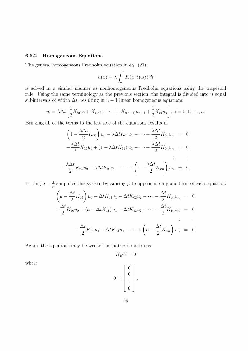
6.6.2 Homogeneous Equations

The general homogeneous Fredholm equation in eq. (21),

u(x) = λ

∫ b

a

K(x, t)u(t) dt

is solved in a similar manner as nonhomogeneous Fredholm equations using the trapezoidrule. Using the same terminology as the previous section, the integral is divided into n equalsubintervals of width ∆t, resulting in n + 1 linear homogeneous equations

ui = λ∆t

[1

2Ki0u0 + Ki1u1 + · · ·+ Ki(n−1)un−1 +

1

2Kinun

], i = 0, 1, . . . , n.

Bringing all of the terms to the left side of the equations results in(

1− λ∆t

2K00

)u0 − λ∆tK01u1 − · · · − λ∆t

2K0nun = 0

−λ∆t

2K10u0 + (1− λ∆tK11) u1 − · · · − λ∆t

2K1nun = 0

......

−λ∆t

2Kn0u0 − λ∆tKn1u1 − · · ·+

(1− λ∆t

2Knn

)un = 0.

Letting λ = 1µ

simplifies this system by causing µ to appear in only one term of each equation:(

µ− ∆t

2K00

)u0 −∆tK01u1 −∆tK02u2 − · · · − ∆t

2K0nun = 0

−∆t

2K10u0 + (µ−∆tK11) u1 −∆tK12u2 − · · · − ∆t

2K1nun = 0

......

−∆t

2Kn0u0 −∆tKn1u1 − · · ·+

(µ− ∆t

2Knn

)un = 0.

Again, the equations may be written in matrix notation as

KHU = 0

where

0 =

00...0

,

39

U is the same as the nonhomogeneous case:

U =

u0

u1...

un

,

and KH is the coefficient matrix for the homogeneous equations

KH =

µ− ∆t2

K00 −∆tK01 · · · −∆t2

K0n

−∆t2

K10 µ−∆tK11 · · · −∆t2

K1n...

.... . .

...−∆t

2Kn0 −∆tKn1 · · · µ− ∆t

2Knn

.

An infinite number of nontrivial solutions exist iff |KH | = 0. This condition can be used to findthe eigenvalues λ of the system by finding µ = 1

λas the zeros of |KH | = 0.

Example: Use the trapezoid rule to find a numeric solution to the homogeneous Fredholmequation

u(x) = λ

∫ 1

0

K(x, t)u(t) dt (29)

with the symmetric kernel

K(x, t) =

{x(1− t), 0 ≤ x ≤ tt(1− x), t ≤ x ≤ 1

at x = 0, x = 12, and x = 1. Therefore n = 2 and ∆t = 1

2, and

Kij = K

(i

2,j

2

), i, j = 0, 1, 2.

The resulting matrix is

µ 0 00 µ− 1

80

0 0 µ

.

For the system of homogeneous equations obtained to have a nontrivial solution, the determi-nant must be equal to zero:

∣∣∣∣∣∣

µ 0 00 µ− 1

80

0 0 µ

= µ2

(µ− 1

8

)= 0,

40

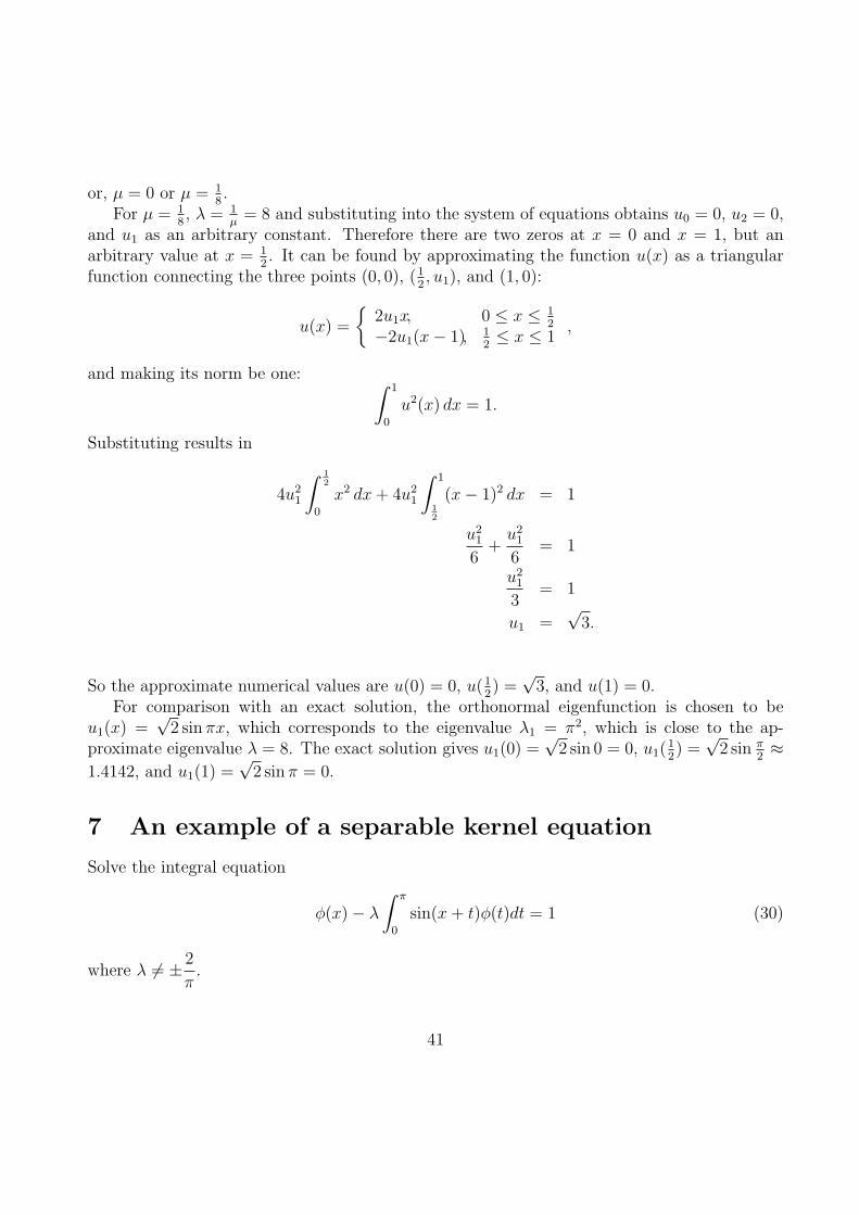
or, µ = 0 or µ = 18.

For µ = 18, λ = 1

µ= 8 and substituting into the system of equations obtains u0 = 0, u2 = 0,

and u1 as an arbitrary constant. Therefore there are two zeros at x = 0 and x = 1, but anarbitrary value at x = 1

2. It can be found by approximating the function u(x) as a triangular

function connecting the three points (0, 0), (12, u1), and (1, 0):

u(x) =

{2u1x, 0 ≤ x ≤ 1

2

−2u1(x− 1), 12≤ x ≤ 1

,

and making its norm be one: ∫ 1

0

u2(x) dx = 1.

Substituting results in

4u21

∫ 12

0

x2 dx + 4u21

∫ 1

12

(x− 1)2 dx = 1

u21

6+

u21

6= 1

u21

3= 1

u1 =√

3.

So the approximate numerical values are u(0) = 0, u(12) =

√3, and u(1) = 0.

For comparison with an exact solution, the orthonormal eigenfunction is chosen to beu1(x) =

√2 sin πx, which corresponds to the eigenvalue λ1 = π2, which is close to the ap-

proximate eigenvalue λ = 8. The exact solution gives u1(0) =√

2 sin 0 = 0, u1(12) =

√2 sin π

2≈

1.4142, and u1(1) =√

2 sin π = 0.

7 An example of a separable kernel equation

Solve the integral equation

φ(x)− λ

∫ π

0

sin(x + t)φ(t)dt = 1 (30)

where λ 6= ± 2

π.

41

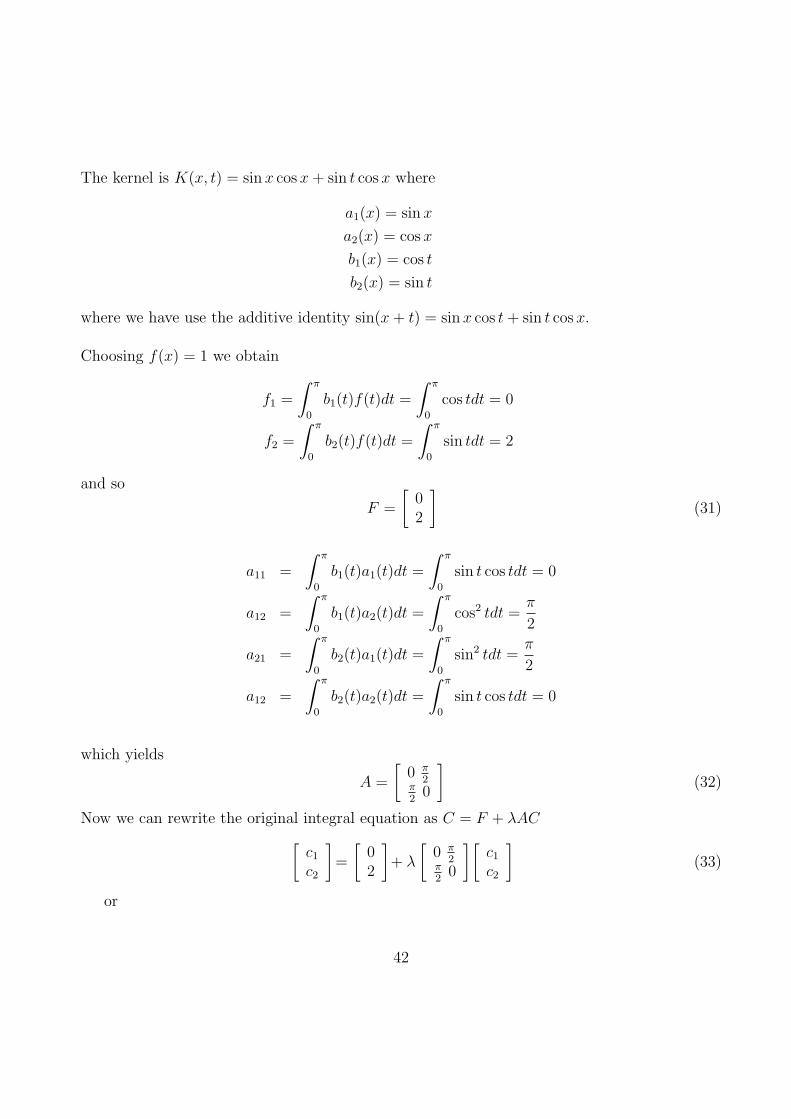
The kernel is K(x, t) = sin x cos x + sin t cos x where

a1(x) = sin x

a2(x) = cos x

b1(x) = cos t

b2(x) = sin t

where we have use the additive identity sin(x + t) = sin x cos t + sin t cos x.

Choosing f(x) = 1 we obtain

f1 =

∫ π

0

b1(t)f(t)dt =

∫ π

0

cos tdt = 0

f2 =

∫ π

0

b2(t)f(t)dt =

∫ π

0

sin tdt = 2

and so

F =

[02

](31)

a11 =

∫ π

0

b1(t)a1(t)dt =

∫ π

0

sin t cos tdt = 0

a12 =

∫ π

0

b1(t)a2(t)dt =

∫ π

0

cos2 tdt =π

2

a21 =

∫ π

0

b2(t)a1(t)dt =

∫ π

0

sin2 tdt =π

2

a12 =

∫ π

0

b2(t)a2(t)dt =

∫ π

0

sin t cos tdt = 0

which yields

A =

[0 π

2π2

0

](32)

Now we can rewrite the original integral equation as C = F + λAC

[c1

c2

]=

[02

]+ λ

[0 π

2π2

0

][c1

c2

](33)

or

42

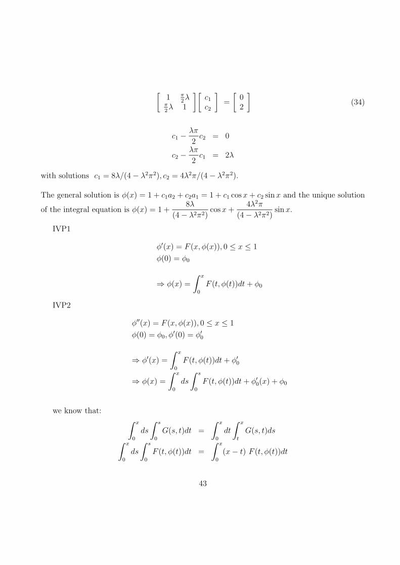
[1 π

2λ

π2λ 1

][c1

c2

]=

[02

](34)

c1 − λπ

2c2 = 0

c2 − λπ

2c1 = 2λ

with solutions c1 = 8λ/(4− λ2π2), c2 = 4λ2π/(4− λ2π2).

The general solution is φ(x) = 1 + c1a2 + c2a1 = 1 + c1 cos x + c2 sin x and the unique solution

of the integral equation is φ(x) = 1 +8λ

(4− λ2π2)cos x +

4λ2π

(4− λ2π2)sin x.

IVP1

φ′(x) = F (x, φ(x)), 0 ≤ x ≤ 1

φ(0) = φ0

⇒ φ(x) =

∫ x

0

F (t, φ(t))dt + φ0

IVP2

φ′′(x) = F (x, φ(x)), 0 ≤ x ≤ 1

φ(0) = φ0, φ′(0) = φ′0

⇒ φ′(x) =

∫ x

0

F (t, φ(t))dt + φ′0

⇒ φ(x) =

∫ x

0

ds

∫ s

0

F (t, φ(t))dt + φ′0(x) + φ0

we know that:∫ x

0

ds

∫ s

0

G(s, t)dt =

∫ x

0

dt

∫ x

t

G(s, t)ds

∫ x

0

ds

∫ s

0

F (t, φ(t))dt =

∫ x

0

(x− t) F (t, φ(t))dt

43

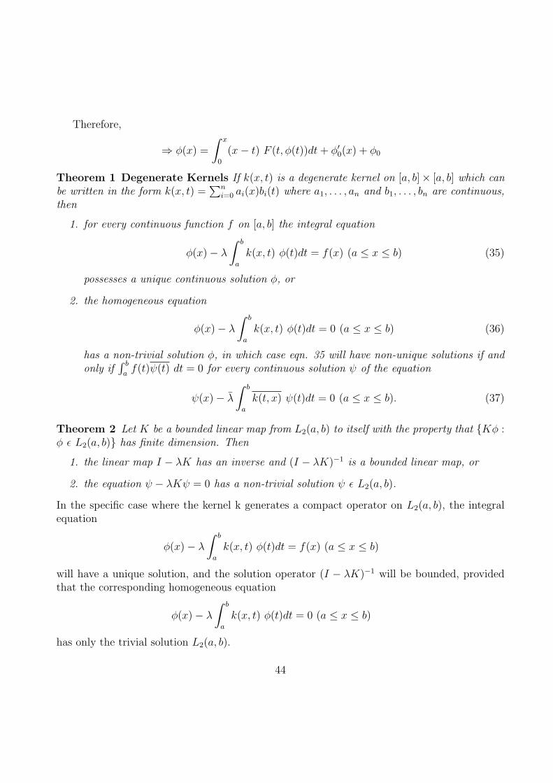
Therefore,

⇒ φ(x) =

∫ x

0

(x− t) F (t, φ(t))dt + φ′0(x) + φ0

Theorem 1 Degenerate Kernels If k(x, t) is a degenerate kernel on [a, b]× [a, b] which canbe written in the form k(x, t) =

∑ni=0 ai(x)bi(t) where a1, . . . , an and b1, . . . , bn are continuous,

then

1. for every continuous function f on [a, b] the integral equation

φ(x)− λ

∫ b

a

k(x, t) φ(t)dt = f(x) (a ≤ x ≤ b) (35)

possesses a unique continuous solution φ, or

2. the homogeneous equation

φ(x)− λ

∫ b

a

k(x, t) φ(t)dt = 0 (a ≤ x ≤ b) (36)

has a non-trivial solution φ, in which case eqn. 35 will have non-unique solutions if andonly if

∫ b

af(t)ψ(t) dt = 0 for every continuous solution ψ of the equation

ψ(x)− λ

∫ b

a

k(t, x) ψ(t)dt = 0 (a ≤ x ≤ b). (37)

Theorem 2 Let K be a bounded linear map from L2(a, b) to itself with the property that {Kφ :φ ε L2(a, b)} has finite dimension. Then

1. the linear map I − λK has an inverse and (I − λK)−1 is a bounded linear map, or

2. the equation ψ − λKψ = 0 has a non-trivial solution ψ ε L2(a, b).

In the specific case where the kernel k generates a compact operator on L2(a, b), the integralequation

φ(x)− λ

∫ b

a

k(x, t) φ(t)dt = f(x) (a ≤ x ≤ b)

will have a unique solution, and the solution operator (I − λK)−1 will be bounded, providedthat the corresponding homogeneous equation

φ(x)− λ

∫ b

a

k(x, t) φ(t)dt = 0 (a ≤ x ≤ b)

has only the trivial solution L2(a, b).

44

8 Bibliographical Comments

In this last section we provide a list of bibliographical references that we found useful in writ-ing this survey and that can also be used for further studying Integral Equations. The listcontains mainly textbooks and research monographs and do not claim by any means that itis complete or exhaustive. It merely reflects our own personal interests in the vast subject ofIntegral Equations. The books are presented using the alphabetical order of the first author.

The book [Cor91] presents the theory of Volterra integral equations and their applications,convolution equations, a historical account of the theory of integral equations, fixed point theo-rems, operators on function spaces, Hammerstein equations and Volterra equations in abstractBanach spaces, applications in coagulation processes, optimal control of processes governed byVolterra equations, and stability of nuclear reactors.

The book [Hac95] starts with an introductory chapter gathering basic facts from analysis,functional analysis, and numerical mathematics. Then the book discusses Volterra integralequations, Fredholm integral equations of the second kind, discretizations, kernel approxima-tion, the collocation method, the Galerkin method, the Nystrom method, multi-grid methodsfor solving systems arising from integral equations of the second kind, Abel’s integral equation,Cauchy’s integral equation, analytical properties of the boundary integral equation method,numerical integration and the panel clustering method and the boundary element method.

The book [Hoc89] discusses the contraction mapping principle, the theory of compact operators,the Fredholm alternative, ordinary differential operators and their study via compact integraloperators, as well as the necessary background in linear algebra and Hilbert space theory.Some applications to boundary value problems are also discussed. It also contains a completetreatment of numerous transform techniques such as Fourier, Laplace, Mellin and Hankel, adiscussion of the projection method, the classical Fredholm techniques, integral operators withpositive kernels and the Schauder fixed-point theorem.

The book [Jer99] contains a large number of worked out examples, which include the approxi-mate numerical solutions of Volterra and Fredholm, integral equations of the first and secondkinds, population dynamics, of mortality of equipment, the tautochrone problem, the reductionof initial value problems to Volterra equations and the reduction of boundary value problemsfor ordinary differential equations and the Schrodinger equation in three dimensions to Fred-holm equations. It also deals with the solution of Volterra equations by using the resolventkernel, by iteration and by Laplace transforms, Green’s function in one and two dimensions andwith Sturm-Liouville operators and their role in formulating integral equations, the Fredholmequation, linear integral equations with a degenerate kernel, equations with symmetric kernelsand the Hilbert-Schmidt theorem. The book ends with the Banach fixed point in a metricspace and its application to the solution of linear and nonlinear integral equations and the use

45

of higher quadrature rules for the approximate solution of linear integral equations.

The book [KK74] discusses the numerical solution of Integral Equations via the method ofinvariant imbedding. The integral equation is converted into a system of differential equations.For general kernels, resolvents and numerical quadratures are being employed.

The book [Kon91] presents a unified general theory of integral equations, attempting to unifythe theories of Picard, Volterra, Fredholm, and Hilbert-Schmidt. It also features applicationsfrom a wide variety of different areas. It contains a classification of integral equations, a de-scription of methods of solution of integral equations, theories of special integral equations,symmetric kernels, singular integral equations, singular kernels and nonlinear integral equa-tions.

The book [Moi77] is an introductory text on integral equations. It describes the classification ofintegral equations, the connection with differential equations, integral equations of convolutiontype, the method of successive approximation, singular kernels, the resolvent, Fredholm theory,Hilbert-Schmidt theory and the necessary background from Hilbert spaces.

The handbook [PM08] contains over 2500 tabulated linear and nonlinear integral equations andtheir exact solutions, outlines exact, approximate analytical, and numerical methods for solvingintegral equations and illustrates the application of the methods with numerous examples. Itdiscusses equations that arise in elasticity, plasticity, heat and mass transfer, hydrodynamics,chemical engineering, and other areas. This is the second edition of the original handbookpublished in 1998.

The book [PS90] contains a treatment of a classification and examples of integral equations,second order ordinary differential equations and integral equations, integral equations of thesecond kind, compact operators, spectra of compact self-adjoint operators, positive operators,approximation methods for eigenvalues and eigenvectors of self-adjoint operators, approxima-tion methods for inhomogeneous integral equations, and singular integral equations.

The book [Smi58] features a carefully chosen selection of topics on Integral Equations us-ing complex-valued functions of a real variable and notations of operator theory. The usualtreatment of Neumann series and the analogue of the Hilbert-Schmidt expansion theorem aregeneralized. Kernels of finite rank, or degenerate kernels, are discussed. Using the method ofpolynomial approximation for two variables, the author writes the general kernel as a sum of akernel of finite rank and a kernel of small norm. The usual results of orthogonalization of thesquare integrable functions of one and two variables are given, with a treatment of the Riesz-Fischer theorem, as a preparation for the classical theory and the application to the Hermitiankernels.

The book [Tri85] contains a study of Volterra equations, with applications to differential equa-

46

tions, an exposition of classical Fredholm and Hilbert-Schmidt theory, a discussion of orthonor-mal sequences and the Hilbert-Schmidt theory for symmetric kernels, a description of the Ritzmethod, a discussion of positive kernels and Mercer’s theorem, the application of integral equa-tions to Sturm-Liouville theory, a presentation of singular integral equations and non-linearintegral equations.

References

[Cor91] C. Corduneanu. Integral equations and applications. Cambridge University Press,Cambridge, 1991.

[Hac95] W. Hackbusch. Integral equations, volume 120 of International Series of Numeri-cal Mathematics. Birkhauser Verlag, Basel, 1995. Theory and numerical treatment,Translated and revised by the author from the 1989 German original.

[Hoc89] H. Hochstadt. Integral equations. Wiley Classics Library. John Wiley & Sons Inc.,New York, 1989. Reprint of the 1973 original, A Wiley-Interscience Publication.

[Jer99] A. J. Jerri. Introduction to integral equations with applications. Wiley-Interscience,New York, second edition, 1999.

[KK74] H. H. Kagiwada and R. Kalaba. Integral equations via imbedding methods. Addison-Wesley Publishing Co., Reading, Mass.-London-Amsterdam, 1974. Applied Mathe-matics and Computation, No. 6.

[Kon91] J. Kondo. Integral equations. Oxford Applied Mathematics and Computing ScienceSeries. The Clarendon Press Oxford University Press, New York, 1991.

[Moi77] B. L. Moiseiwitsch. Integral equations. Longman, London, 1977. Longman Mathemat-ical Texts.

[PM08] A. D. Polyanin and A. V. Manzhirov. Handbook of integral equations. Chapman &Hall/CRC, Boca Raton, FL, second edition, 2008.

[PS90] D. Porter and D. S. G. Stirling. Integral equations. Cambridge Texts in AppliedMathematics. Cambridge University Press, Cambridge, 1990. A practical treatment,from spectral theory to applications.

[Smi58] F. Smithies. Integral equations. Cambridge Tracts in Mathematics and MathematicalPhysics, no. 49. Cambridge University Press, New York, 1958.

[Tri85] F. G. Tricomi. Integral equations. Dover Publications Inc., New York, 1985. Reprintof the 1957 original.

47