A STOCHASTIC PHASE-FIELD MODEL DETERMINED …szepessy/md_pde-1.pdf · Introduction to Phase-Field Models The phase- eld model for a liquid ... (macroscopic) scale; the molecular dynamics

A STOCHASTIC PHASE-FIELD MODEL DETERMINED FROM MOLECULARDYNAMICS

ERIK VON SCHWERIN AND ANDERS SZEPESSY

Abstract. The dynamics of dendritic growth of a crystal in an undercooled melt is determined by macro-

scopic diffusion-convection of heat and by capillary forces acting on the nanometer scale of the solid–liquidinterface width. Its modeling is useful for instance in processing techniques based on casting. The phase-field

method is widely used to study evolution of such microstructural phase transformations on a continuum level;

it couples the energy equation to a phenomenological Allen-Cahn/Ginzburg-Landau equation modeling thedynamics of an order parameter determining the solid and liquid phases, including also stochastic fluctua-

tions to obtain the qualitatively correct result of dendritic side branching. This work presents a method to

determine stochastic phase-field models from atomistic formulations by coarse-graining molecular dynamics.It has three steps: (1) a precise quantitative atomistic definition of the phase-field variable, based on the

local potential energy; (2) derivation of its coarse-grained dynamics model, from microscopic Smoluchowski

molecular dynamics (that is Brownian or over damped Langevin dynamics); and (3) numerical computationof the coarse-grained model functions. The coarse-grained model approximates Gibbs ensemble averages of

the atomistic phase-field, by choosing coarse-grained drift and diffusion functions that minimize the approx-imation error of observables in this ensemble average.

Contents

1. Introduction to Phase-Field Models 12. Quantitative Atomistic Definition of the Phase-Field Variable 33. An Atomistic Smoluchowski Dynamics Model 54. Coarse-Grained Phase-Field Dynamics 74.1. The Ito Formula for the Phase-Field 84.2. The Error Representation 104.3. Computation of Averages in Cross Sections 104.4. Computed Coarse-Grained Phase-Field 125. The Computational Method 135.1. Discrete Smoluchowski System Simulated at Constant Volume 145.2. Computation of the Coarse-Grained Model Functions 156. Conclusions 17References 18

1. Introduction to Phase-Field Models

The phase-field model for a liquid–solid phase transformation is an Allen-Cahn/Ginzburg-Landau equationcoupled to the energy equation

k0∂tφ = div(k1∇φ)− k2

(f ′(φ) + k3g

′(φ)(T − TM ))︸︷︷︸

∂φF(φ,T )

+noise

∂t(cvT + k4g(φ)

)= div(k5∇T )

(1.1)

1

2 ERIK VON SCHWERIN AND ANDERS SZEPESSY

with a double well potential f having local minima at ±1, smoothed step function g, temperature T , meltingtemperature TM , specific heat cv and latent heat k4g(φ), cf. [34], [4]; the unknown variables to determine areφ and T while the other quantities are given data. Using the phase-field variable φ : R3 × [0,∞) → [−1, 1],the solid and liquid phases are interpreted as the domains {x ∈ R3 : φ(x) > 0} and {x ∈ R3 : φ(x) < 0}respectively. To have such an implicit definition of the phases, as in the level set method, is a computationaladvantage compared to a sharp interface model, where the necessary direct tracking of the interface introducecomputational drawbacks. This phenomenological phase-field model, with free energy potentials F motivatedby thermodynamics, has therefore become a popular and effective computational method to solve problemswith complicated structures of dendrite and eutectic growth, cf. [1], [4]. The evolution of the phase interfacedepends on the orientation of the solid crystal; this is modeled by an anisotropic matrix k1. Added noise tosystem (1.1) is also important, e.g. to model nucleation phenomena, when a crystal initiates in an under-cooled liquid and starts to grow, and to obtain sidebranching dendrites [18]. The phase-field model hasmathematical wellposedness [5] and convergence to sharp interface results [36]. The sharp interface limit isa consistency issue showing that, when the ratio of the diffusion term and the reaction term becomes smallin the phase-field equation, the phase-field solution tends to the solution with the sharp interface of a Stefanproblem. We have the situation of an almost sharp interface here since we formulate the phase-field equationin a bounded microscopic scale x, which is related to the macroscopic scale y by x = ε−1y with a smallparameter ε� 1, and

∂2xφ

f(φ)= ε2

∂2yφ

f(φ).

The aim of this work is to present a computational method to determine the data for the phase-fieldequation (1.1), including the noise term, from more fundamental molecular dynamics. We call the phase-fieldequation (1.1) a macroscopic model, since its variables varies on a large (macroscopic) scale; the moleculardynamics model is called a microscopic model here, since the particle positions variables X : [0,∞) → R3N

of N � 1 particles vary on a small (microscopic) scale. Phase changes can be modeled on an atomisticlevel by molecular dynamics or kinetic Monte Carlo methods (i.e. stochastic interacting particle models ona lattice as in the Ising model). To derive stochastic differential equations approximating kinetic MonteCarlo dynamics is a classical problem, studied e.g. in [7], [25], [38]. The work [20] derived coarse-grainedstochastic differential equations from a kinetic Monte Carlo method with a technique related to the studyhere on molecular dynamics. Molecular dynamics is in some sense more attractive than kinetic Monte Carlodynamics as a starting point for coarse-graining, since fewer parameters need to be set (none with ab initiomolecular dynamics). Assuming that the reaction term in the Allen-Cahn equation takes a given form, forexample with the common choice

f(φ) = (1− φ2)2,

g(φ) =1516

(15φ5 − 2

3φ3 + φ) +

12,

(1.2)

the scalar parameters k2, k3, k4, scalar functions k0 = k0(∇φ), k5 = k5(φ), and matrix function k1 = k1(∇φ) inthe phase-field model have been determined from atomistic molecular simulations, using the Gibbs-Thomsoncondition for the temperature of a moving solid-liquid interface as a function of curvature, normal velocity,latent heat, melting temperature, the excess interface free energy, and a kinetic coefficient, cf. the reviewarticles [15] [2]: the excess interface free energy can be determined from molecular dynamics by introducinga ”cleaving” potential to reversibly transform a solid and a liquid system to a solid-liquid system, or fromposition fluctuations related to interfacial stiffness; the kinetic coefficient can be determined from moleculardynamics by setting the temperature and measuring the induced velocity of an interface, or by studying thefluctuation of the number of ”solid” particles. An alternative choice of phase-field functions (1.2) in [1] usesa steeper step function g to easily derive consistency with sharp interface models.

A STOCHASTIC PHASE-FIELD MODEL DETERMINED FROM MOLECULAR DYNAMICS 3

This work presents a different method to determine data for a stochastic phase-field equation by coarse-graining appropriate molecular dynamics – the new ingredient here is a method to determine the noise andalso the actual functions in the right hand side of the phase-field equation, and not only the parameters ki.This is made in three steps in Sections 2 to 4:

(1) a precise quantitative atomistic definition of the phase-field variable m(x,X), based on the localpotential energy of particle positions X;

(2) derivation of its coarse-grained for dynamics model φ(x, t) ≈ m(X(t)

), from microscopic Smolu-

chowski molecular dynamics (i.e. Brownian dynamics) of the particle positions X; and(3) numerical computation of the coarse-grained model functions.

We call the approximation φ(x, t) ≈ m(x,X(t)

)coarse-graining, since the microscopic molecular description

m : R3 × R3N → R is of much higher dimension 3N + 3 � 3 than the macroscopic approximation φ :R3 × [0,∞) → R. One may ask if the Smoluchowski (i.e. the over damped Langevin) dynamics is a goodchoice as the microscopic molecular dynamics model – our answer is that the Smoluchowski dynamics sampleGibbs ensemble averages, it generates a coarse-grained model which is a stochastic reaction-diffusion equationof the phase-field type (1.1), and Gibbs ensemble averages of the atomistic phase-field is well approximatedby the coarse-grained model (in some sense optimally as explained in Section 4).

To determine the drift in the stochastic phase-field equation we use the setting of a traveling wave: theshape of the traveling wave, computed from molecular dynamics, determines the reaction term balancing thediffusion; since the total drift becomes zero, the reaction and diffusion terms in the phase-field equation arethen determined up to a multiplicative constant – this multiplicative constant is chosen to match equilibriumfluctuations of the phase-field. The diffusion coefficient for the noise in the stochastic phase-field is determinedfrom an optimization problem, where the diffusion is chosen to minimize the error of observables in the Gibbsensemble.

This alternative method to determine the phase-field model from atomistic simulations comes with somenew ideas, e.g. handling the noise, but it would need further verification and comparison by others to reachsimilar maturity as the established methods in [2] for atomistic verification of phase-field parameters.

We present computational results for an example based on Lennard-Jones type molecular dynamics in anequilibrium simulation with constant number of particles, volume, and temperature and with periodic bound-ary conditions; we compute both the noise function and the free energy function at the melting temperature,i.e. F(φ, TM ), for some orientations of the solid–liquid interface with respect to the crystal. To determinethe free energy function above and below the melting temperature is also important; that requires a differentmolecular dynamics simulation in a non periodic setting following a moving interface; see Remark 5.1. Otherrelevant extensions for the future would be to include constant pressure and hybrid simulations, see Remarks5.1 and 5.2.

2. Quantitative Atomistic Definition of the Phase-Field Variable

The aim is to give a unique definition of the phase-field variable, so that it can be determined preciselyfrom atomistic simulations. The usual interpretation is to measure interatomic distances or to use radialdistribution functions (cf. Figure 4) to measure where the phase is solid and where it is liquid, which thenimplicitly defines the phase-field variable [4]. Here we instead use the energy equation for a quantitative andexplicit definition of the phase-field variable. The macroscopic energy equation with a phase transformationand heat conduction is

(2.1) ∂t(cvT +m) = div(k∇T )

where m corresponds to the latent heat release. In (1.1) the latent heat determines the parameter k2, since φis defined to jump from 1 to −1 in the phase transformation. We will instead use this latent heat to directlydefine the phase-field function, and not only the parameter k2. The latent heat is the change in enthalpy ofa phase transformation at constant pressure, see [22, 24, 28]. We will study molecular dynamics at constant


volume, instead of pressure; then the latent heat is the change in the potential energy. The total energy,cvT +m, can be defined from molecular dynamics of N particles with position Xi, velocity vi, and mass µ ina potential V ,

(2.2) cvT +m =N∑i=1

µ|vi|2

2+ V (X1, . . . , XN ),

see [16], [14]. We assume for simplicity that the potential is defined from pair interactions

(2.3) V (X) =12

N∑i=1

∑j 6=i

Φ(Xi −Xj),

where Φ : R3 → R is a molecular dynamics pair potential, e.g. a Lennard-Jones potential

Φ(x) = z1

( σ|x|

)12

− z2

( σ|x|

)6

;

in this work we use the exponential-6 pair potential (modeling Argon at high pressure), which is almost thesame as the Lennard-Jones potential, see [32]. In the macroscopic setting the jump of m in a phase change iscalled the latent heat, which depends on the thermodynamic variables kept constant: with constant N,T , andvolume it is called the internal energy and with constant pressure instead of volume it is called enthalpy. Herewe study the ensemble with constant volume; Remark 5.1 comments on the constant pressure ensemble, whichis more common in applications. For a molecular system in equilibrium with constant volume, the mean of thekinetic energy,

∑i µ|vi|2/2, is N times the temperature. It is therefore natural to let the phase-field variable

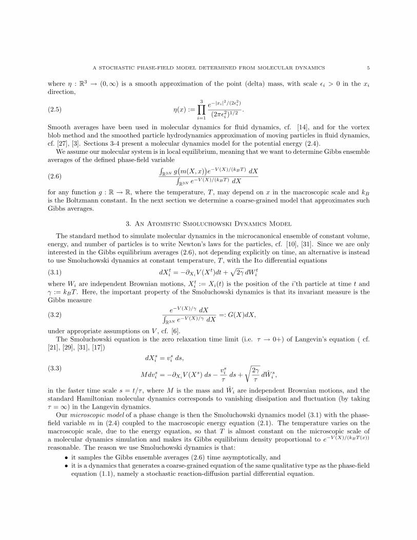
be determined by the potential energy V (X), which typically has a jump at the melting temperature that weidentify with the latent heat; see Figure 1. In a point-wise setting the potential energy can be represented by

TM

Latent heat, L

Subcooled Liquid Liquid

Solid Superheated Solidm

m

T

Figure 1. Schematic picture of m(T ) for a pure liquid (top curve) and a pure solid (bottomcurve) and the latent heat as the jump in m at a phase transition.

the distribution12

N∑i=1

∑j 6=i

Φ(Xi −Xj)δ(x−Xi)

where δ is the point mass at the origin [16]. We seek an averaged variant and we will study a microscopicphase change model where the interface is almost planar in the microscopic scale with normal in the x1

direction. Therefore we take a smooth average and define the phase-field variable by

(2.4) m(X,x) :=12

N∑i=1

∑j 6=i

Φ(Xi −Xj)︸︷︷︸mi(X)

η(x−Xi)


where η : R3 → (0,∞) is a smooth approximation of the point (delta) mass, with scale εi > 0 in the xidirection,

(2.5) η(x) :=3∏i=1

e−|xi|2/(2ε2i )

(2πε2i )1/2.

Smooth averages have been used in molecular dynamics for fluid dynamics, cf. [14], and for the vortexblob method and the smoothed particle hydrodynamics approximation of moving particles in fluid dynamics,cf. [27], [3]. Sections 3-4 present a molecular dynamics model for the potential energy (2.4).

We assume our molecular system is in local equilibrium, meaning that we want to determine Gibbs ensembleaverages of the defined phase-field variable

(2.6)

∫R3N g

(m(X,x)

)e−V (X)/(kBT ) dX∫

R3N e−V (X)/(kBT ) dX

for any function g : R → R, where the temperature, T , may depend on x in the macroscopic scale and kBis the Boltzmann constant. In the next section we determine a coarse-grained model that approximates suchGibbs averages.

3. An Atomistic Smoluchowski Dynamics Model

The standard method to simulate molecular dynamics in the microcanonical ensemble of constant volume,energy, and number of particles is to write Newton’s laws for the particles, cf. [10], [31]. Since we are onlyinterested in the Gibbs equilibrium averages (2.6), not depending explicitly on time, an alternative is insteadto use Smoluchowski dynamics at constant temperature, T , with the Ito differential equations

(3.1) dXti = −∂XiV (Xt)dt+

√2γ dW t

i

where Wi are independent Brownian motions, Xti := Xi(t) is the position of the i’th particle at time t and

γ := kBT . Here, the important property of the Smoluchowski dynamics is that its invariant measure is theGibbs measure

(3.2)e−V (X)/γ dX∫

R3N e−V (X)/γ dX=: G(X)dX,

under appropriate assumptions on V , cf. [6].The Smoluchowski equation is the zero relaxation time limit (i.e. τ → 0+) of Langevin’s equation ( cf.

[21], [29], [31], [17])

dXsi = vsi ds,

Mdvsi = −∂XiV (Xs) ds− vsiτds+

√2γτdW s

i ,(3.3)

in the faster time scale s = t/τ , where M is the mass and Wi are independent Brownian motions, and thestandard Hamiltonian molecular dynamics corresponds to vanishing dissipation and fluctuation (by takingτ =∞) in the Langevin dynamics.

Our microscopic model of a phase change is then the Smoluchowski dynamics model (3.1) with the phase-field variable m in (2.4) coupled to the macroscopic energy equation (2.1). The temperature varies on themacroscopic scale, due to the energy equation, so that T is almost constant on the microscopic scale ofa molecular dynamics simulation and makes its Gibbs equilibrium density proportional to e−V (X)/(kBT (x))

reasonable. The reason we use Smoluchowski dynamics is that:• it samples the Gibbs ensemble averages (2.6) time asymptotically, and• it is a dynamics that generates a coarse-grained equation of the same qualitative type as the phase-field

equation (1.1), namely a stochastic reaction-diffusion partial differential equation.


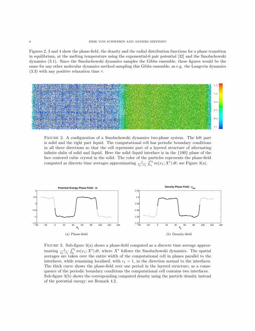
Figures 2, 3 and 4 show the phase-field, the density and the radial distribution functions for a phase transitionin equilibrium, at the melting temperature using the exponential-6 pair potential [32] and the Smoluchowskidynamics (3.1). Since the Smoluchowski dynamics samples the Gibbs ensemble, these figures would be thesame for any other molecular dynamics method sampling this Gibbs ensemble, as e.g. the Langevin dynamics(3.3) with any positive relaxation time τ .

Figure 2. A configuration of a Smoluchowski dynamics two-phase system. The left partis solid and the right part liquid. The computational cell has periodic boundary conditionsin all three directions so that the cell represents part of a layered structure of alternatinginfinite slabs of solid and liquid. Here the solid–liquid interface is in the {100} plane of theface centered cubic crystal in the solid. The color of the particles represents the phase-fieldcomputed as discrete time averages approximating 1

t2−t1

∫ t2t1m(x1;Xt) dt; see Figure 3(a).

−40 −20 0 20 40 60 80 100 120 140−1.5

−1

−0.5

0

0.5

1

x1

Potential Energy Phase Field : m

(a) Phase-field

−40 −20 0 20 40 60 80 100 120 1401.22

1.24

1.26

1.28

1.3

1.32

x1

Density Phase Field : ρloc

(b) Density-field

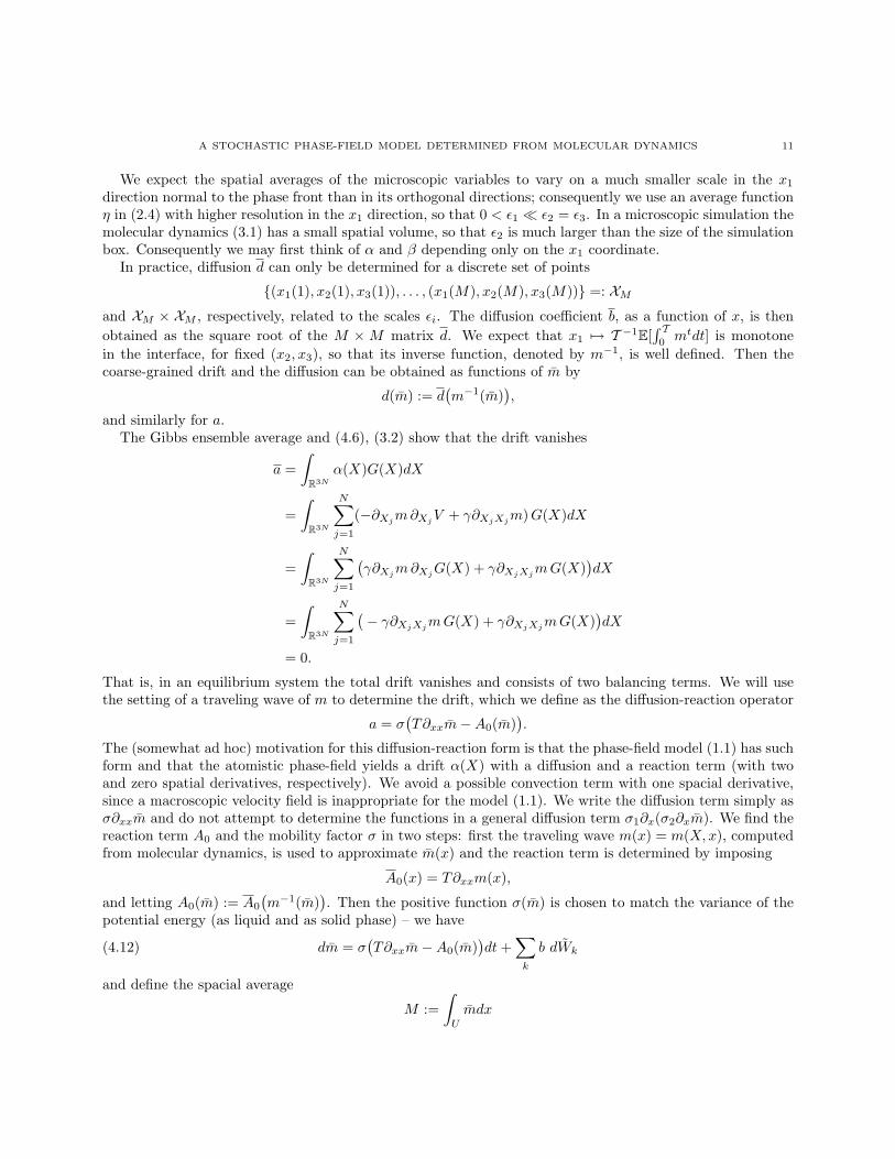
Figure 3. Sub-figure 3(a) shows a phase-field computed as a discrete time average approx-imating 1

t2−t1

∫ t2t1m(x1;Xt) dt, where Xt follows the Smoluchowski dynamics. The spatial

averages are taken over the entire width of the computational cell in planes parallel to theinterfaces, while remaining localised, with ε1 = 1, in the direction normal to the interfaces.The thick curve shows the phase-field over one period in the layered structure; as a conse-quence of the periodic boundary conditions the computational cell contains two interfaces.Sub-figure 3(b) shows the corresponding computed density using the particle density insteadof the potential energy; see Remark 4.2.


4. Coarse-Grained Phase-Field Dynamics

We want to determine a mean drift function a(m) and a diffusion function b(m) so that the coarse-grainedapproximation mt, solving the coarse-grained equation

dmt = a(mt)dt+M∑k=1

bk(mt)dW tk,(4.1)

optimally approximates the Gibbs ensemble averages (2.6), of the phase-field m(Xt, ·) defined in (2.4) with Xt

solving the Smoluchowski dynamics (3.1). The Brownian motions Wk, k = 1, . . . ,M are mutually independentand also independent of all Wi. To obtain an optimal approximation, we seek the minimal error of the Gibbsensemble average

(4.2) mina,b

limT→∞

T −1

∫ T0

E[g(m(XT , ·)

)]− E

[g(mT )

]dT

for any given function g : R → R, with the same initial value m0 = m(X0, ·). Such minimizing functions, aand b, lead (by ergodicity) to our objective - to approximate the Gibbs average defined in (2.6)

limT→∞

T −1

∫ T0

E[g(m(XT , ·)

)]dT =

∫R3N g

(m(X,x)

)e−V (X)/(kBT ) dX∫

R3N e−V (X)/(kBT ) dX.

0 0.5 1 1.5 2 2.5 3 3.50

0.5

1

1.5

2

2.5

3

3.5

r

Radial Distribution Function, g(r)

Pure solid phaseSolid in two phase system

(a) FCC

0 0.5 1 1.5 2 2.5 3 3.50

0.5

1

1.5

2

2.5

3

3.5

r

Radial Distribution Function, g(r)

Pure liquid phase Liquid in two phase system

(b) Liquid

Figure 4. The radial distribution function, g(r), computed from several configurations,separated in time, in the process of setting up one of the two-phase systems. The solid curveshows g(r) computed as an average over all particles in the computational cell used while pre-simulating the solid and the liquid part, in sub-figure (a) and (b) respectively. The dashedcurves show g(r) computed as an average over particles in two slices of the computational cellof the two-phase system; sub-figure (a) shows g(r) obtained from a slice inside the solid phase,and sub-figure (b) shows g(r) from a slice inside the liquid phase. The radial distributionfunctions show good agreement between the single phase systems and the corresponding solidand liquid subdomains away from the interface.


We perform this optimal control way of coarse-graining in three steps, described below. Note that there maybe other microscopic dynamics with different coarse-graining functions that lead to smaller approximationerror - our optimality concerns coarse-grained drift and diffusion functions a and b for the given microscopicSmoluchowski dynamics (3.1).

The first idea in the coarse-graining procedure, in Section 4.1, is that Ito’s formula and the Smoluchowskidynamics (3.1) determine functions α and β, depending on the microscopic state X, so that

(4.3) dm(Xt, ·) = α(Xt)dt+N∑j=1

βj(Xt)dW tj .

The next step, in Section 4.2, is to estimate the error, using the Kolmogorov equations for m and (4.3),similar to [37, 20], which leads to

E[g(m(XT , ·)

)− g(mT )

]= E[

∫ T0

〈u′, α− a〉+ 〈u′′,N∑j=1

βj ⊗ βj −M∑k=1

bk ⊗ bk〉dt],

where 〈u′, ·〉 is the L2(R3) scalar product (corresponding to the variable x ∈ R3) with u′, which is theGateaux derivative (i.e. functional derivative) of the functional E[g(mT ) | mt = n] with respect to n; andsimilarly 〈u′′, ·〉 is the L2(R3 × R3) scalar product with the second Gateaux derivative u′′ of the functionalE[g(mT ) | mt = n] with respect to n. The notation bk ⊗ bk(x, x′) := bk(x)bk(x′) is the tensor product.

The final step, in Section 4.3, is to use molecular dynamics simulations for a planar interface two phaseproblem and compute averages in cross sections parallel to the interface, where u′, u′′, a, and

∑k bk ⊗ bk are

m-independent, to evaluate approximations to the functions a and∑k bk ⊗ bk by

a = limT→∞

1T

E[ ∫ T

0

αdt],

∑k

bk ⊗ bk = limT→∞

1T

E[ ∫ T

0

N∑j=1

βj ⊗ βjdt].(4.4)

Ergodicity implies that the approximations can be written as the Gibbs ensemble averages

a(x) =∫

R3Nα(x;X)G(X)dX∑

k

bk ⊗ bk(x, y) =∫

R3Nβj ⊗ βj(x, y;X)G(X)dX,

(4.5)

with the Gibbs density G defined in (3.2).

4.1. The Ito Formula for the Phase-Field. The Ito formula (cf. [11]) implies

(4.6) dm(Xt, x) =N∑j=1

(−∂Xjm∂XjV + γ∂XjXjm)︸︷︷︸α(Xt)

dt+N∑j=1

√2γ∂Xjm︸︷︷︸βj(Xt)

dWj .

The definition in (2.4),

m(Xt, x) =∑i

mi(X)η(x−Xti ),

yields∂Xjm =

∑i

∂Xjmiη(x−Xi) +mj∂Xjη(x−Xj).


In (4.6) we will use (2.5) to evaluate the last derivative as

∂Xjη(x−Xj) = −∂xη(x−Xj), in dt terms,

∂Xjη(x−Xj) = −η(x−Xj)( (x−Xj)1

ε21,

(x−Xj)2

ε22,

(x−Xj)3

ε23

), in dWj terms,

in order to avoid spatial derivatives on the diffusion coefficient, while including them in the drift. Since

mi =12

∑k 6=i

Φ(Xi −Xk)

and

V (X) =12

∑i

∑j 6=i

Φ(Xi −Xj)

there holds

∂Xjmi =12

∑k 6=i

Φ′(Xi −Xk)δij −12

Φ′(Xi −Xj)(1− δij),

∂XjV (X) =∑k 6=j

Φ′(Xj −Xk),

where

δij :=

{1 i = j,

0 i 6= j,

is the Kronecker symbol. The second derivatives are

∂XjXjm =∑i

∂XjXjmiη(x−Xi)− 2∂Xjmj∂xη(x−Xj) +mj∂xxη(x−Xj),

with

∂XjXjmi =12

∑k 6=i

Φ′′(Xi −Xk)δij +12

Φ′′(Xi −Xj)(1− δij)

and all terms in (4.6) are now expressed in terms of Φ, its gradient Φ′ and Hessian Φ′′. We note that thedrift, α, has the form

α = ∂xxA2 + ∂xA1 +A0 :=

= γ∂xxm(Xt, x) + ∂x

( N∑i=1

n1i(Xt)η(x−Xti ))

+N∑i=1

n0i(Xt)η(x−Xti )

(4.7)

of conservative and non conservative reaction terms. Similarly the diffusion, βj , takes the form

N∑i=1

n3ji(Xt)η(x−Xti ) + n4j(Xt)η(x−Xt

j)(x−Xtj).


4.2. The Error Representation. The conditioned expected value

(4.8) u(n, t) := E[g(mT ) | mt = n]

satisfies the Kolmogorov equation (cf. [37, 20])

∂tu+ 〈u′, a〉+ 〈u′′,M∑k=1

bk ⊗ bk〉 = 0,

u(·, T ) = g.

(4.9)

Let mt := m(Xt, ·). The final condition in (4.9) and the definition (4.8) show that

E[g(m(XT , ·)

)− g(mT )

]= E[u(mT , T )]− u(m0, 0) = E[

∫ T0

du(mt, t)].

Use the Ito formula and (4.6) to evaluate du(mt, t) and then Kolmogorov’s equation (4.9) to replace ∂tu inthis right hand side to obtain the error representation

E[g(m(XT , ·)

)− g(mT )

]= E

[ ∫ T0

〈u′, α〉+ 〈u′′,N∑j=1

βj ⊗ βj〉+ ∂tu dt]

= E[ ∫ T

0

〈u′, α− a〉+ 〈u′′,N∑j=1


bk ⊗ bk〉 dt].

Remark 4.1 (Energy fluctuation). If we integrate the noise term over all x1, i.e. take ε1 very large, andlet g(m) = m2, then the error we are studying E

[g(m(XT , ·)

)− g(mT )

]is the usual fluctuation of energy

E[V 2 − E[V ]2] (proportional to the specific heat [17]), provided we set m = E[V ].

4.3. Computation of Averages in Cross Sections. The optimal choice of the function b⊗b is to minimizeE[∫ T

0〈u′′, β ⊗ β − b ⊗ b〉dt], which seems hard to determine exactly, since u′′

(m(Xt, ·), t

)depends on Xt.

However, the function u′′(m(Xt, ·), t

)depends only on the coarse-grained m(Xt, ·) and not directly on Xt

and not on t for T → ∞. A possible approximation is to neglect the fluctuations of m(Xt, ·) and setm(Xt, x) = m(x) in the ε-neighbourhood of x and write

E[∫ T

0

〈u′′(m(Xt, x), t

), β ⊗ β(x)− b⊗ b

(m(x)

)〉dt] ≈ 〈u′′

(m(x), T

),E[∫ T

0

β ⊗ β(x)− b⊗ b(m(x)

)dt]〉

which leads to the minimizing condition

limT→∞

T −1E[∫ T

0

β ⊗ β(x)− b⊗ b(m(x)

)dt] = 0,

and means that the diffusion matrix d(x, x′) := b⊗ b(m(·, x)

)is

(4.10) d(x, x′) = limT→∞

1T

E[ ∫ T

0

N∑j=1

βj(x)⊗ βj(x′)dt],

and similarly the drift a(x) := a(m(·, x)) is

(4.11) a(x) = limT→∞

1T

E[ ∫ T

0

α(x)dt].

In other words, it is useful to think of an expansion of u′ in α − a and determine a by the leading orderconditions (4.11) and (4.10).


We expect the spatial averages of the microscopic variables to vary on a much smaller scale in the x1

direction normal to the phase front than in its orthogonal directions; consequently we use an average functionη in (2.4) with higher resolution in the x1 direction, so that 0 < ε1 � ε2 = ε3. In a microscopic simulation themolecular dynamics (3.1) has a small spatial volume, so that ε2 is much larger than the size of the simulationbox. Consequently we may first think of α and β depending only on the x1 coordinate.

In practice, diffusion d can only be determined for a discrete set of points

{(x1(1), x2(1), x3(1)), . . . , (x1(M), x2(M), x3(M))} =: XMand XM × XM , respectively, related to the scales εi. The diffusion coefficient b, as a function of x, is thenobtained as the square root of the M ×M matrix d. We expect that x1 7→ T −1E[

∫ T0mtdt] is monotone

in the interface, for fixed (x2, x3), so that its inverse function, denoted by m−1, is well defined. Then thecoarse-grained drift and the diffusion can be obtained as functions of m by

d(m) := d(m−1(m)

),

and similarly for a.The Gibbs ensemble average and (4.6), (3.2) show that the drift vanishes

a =∫

R3Nα(X)G(X)dX

=∫

R3N

N∑j=1

(−∂Xjm∂XjV + γ∂XjXjm)G(X)dX

=∫

R3N

N∑j=1

(γ∂Xjm∂XjG(X) + γ∂XjXjmG(X)

)dX

=∫

R3N

N∑j=1

(− γ∂XjXjmG(X) + γ∂XjXjmG(X)

)dX

= 0.

That is, in an equilibrium system the total drift vanishes and consists of two balancing terms. We will usethe setting of a traveling wave of m to determine the drift, which we define as the diffusion-reaction operator

a = σ(T∂xxm−A0(m)

).

The (somewhat ad hoc) motivation for this diffusion-reaction form is that the phase-field model (1.1) has suchform and that the atomistic phase-field yields a drift α(X) with a diffusion and a reaction term (with twoand zero spatial derivatives, respectively). We avoid a possible convection term with one spacial derivative,since a macroscopic velocity field is inappropriate for the model (1.1). We write the diffusion term simply asσ∂xxm and do not attempt to determine the functions in a general diffusion term σ1∂x(σ2∂xm). We find thereaction term A0 and the mobility factor σ in two steps: first the traveling wave m(x) = m(X,x), computedfrom molecular dynamics, is used to approximate m(x) and the reaction term is determined by imposing

A0(x) = T∂xxm(x),

and letting A0(m) := A0

(m−1(m)

). Then the positive function σ(m) is chosen to match the variance of the

potential energy (as liquid and as solid phase) – we have

(4.12) dm = σ(T∂xxm−A0(m)

)dt+

∑k

b dWk

and define the spacial average

M :=∫U

mdx


to obtain (from integration, linearization, and periodic boundary conditions) the Ornstein-Uhlenbeck process

dM = −σ(m)A′0(m)Mdt+∫U

∑k

b(m) dWkdx.

The function σ(m) can be determined (for the liquid and solid state) by equating the variance of M andthe variance of the spatial average of the atomistic phase-field

∫Um(x;X)dx. Figure 5(b) shows that the

potential k2f , defined by k2f′(m) = A0(m), is convex in a neighborhood of the equilibrium points (where

A′0(m) = 0), so that A′0(m) > 0 and the invariant distribution of M is a normal distribution with mean zeroand variance proportional to 1/(σA′0).

Remark 4.2. [Density dynamics] A similar derivation with Ito’s formula shows that the density, ρ(x) :=∑i η(x−Xi), satisfies

dρ = γ∂xxρ dt− ∂xN∑i=1

η(x−Xi)(− V ′(X) dt+

√2γ dWi

).

The expression for the coarse-grained values (4.4) implies that the drift for the density satisfies

γ∂xx

∫R3N

∑i

η(x−Xi)G(X)dX︸︷︷︸=:ρ

−∂x∫

R3N

N∑i=1

η(x−Xi)(− V ′(X)

)G(X)︸︷︷︸

γ∂XG(X)

dX

= γ∂xxρ− γ∂xx∫

R3N

N∑i=1

η(x−Xi)G(X)dX = 0

which leads to a stochastic reaction diffusion equation of the same qualitative form as for the phase-field m.

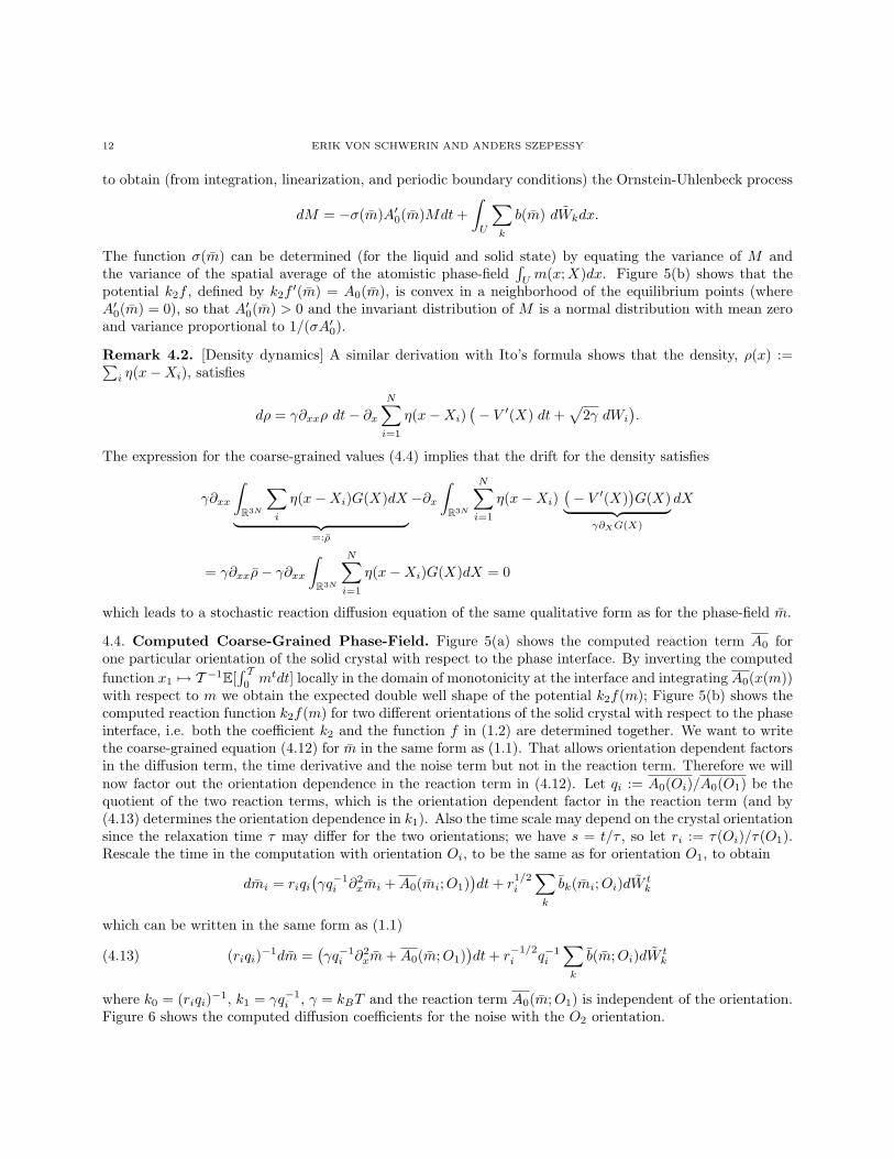
4.4. Computed Coarse-Grained Phase-Field. Figure 5(a) shows the computed reaction term A0 forone particular orientation of the solid crystal with respect to the phase interface. By inverting the computedfunction x1 7→ T −1E[

∫ T0mtdt] locally in the domain of monotonicity at the interface and integrating A0(x(m))

with respect to m we obtain the expected double well shape of the potential k2f(m); Figure 5(b) shows thecomputed reaction function k2f(m) for two different orientations of the solid crystal with respect to the phaseinterface, i.e. both the coefficient k2 and the function f in (1.2) are determined together. We want to writethe coarse-grained equation (4.12) for m in the same form as (1.1). That allows orientation dependent factorsin the diffusion term, the time derivative and the noise term but not in the reaction term. Therefore we willnow factor out the orientation dependence in the reaction term in (4.12). Let qi := A0(Oi)/A0(O1) be thequotient of the two reaction terms, which is the orientation dependent factor in the reaction term (and by(4.13) determines the orientation dependence in k1). Also the time scale may depend on the crystal orientationsince the relaxation time τ may differ for the two orientations; we have s = t/τ , so let ri := τ(Oi)/τ(O1).Rescale the time in the computation with orientation Oi, to be the same as for orientation O1, to obtain

dmi = riqi(γq−1i ∂2

xmi +A0(mi;O1))dt+ r

1/2i

∑k

bk(mi;Oi)dW tk

which can be written in the same form as (1.1)

(4.13) (riqi)−1dm =(γq−1i ∂2

xm+A0(m;O1))dt+ r

−1/2i q−1

i

∑k

b(m;Oi)dW tk

where k0 = (riqi)−1, k1 = γq−1i , γ = kBT and the reaction term A0(m;O1) is independent of the orientation.

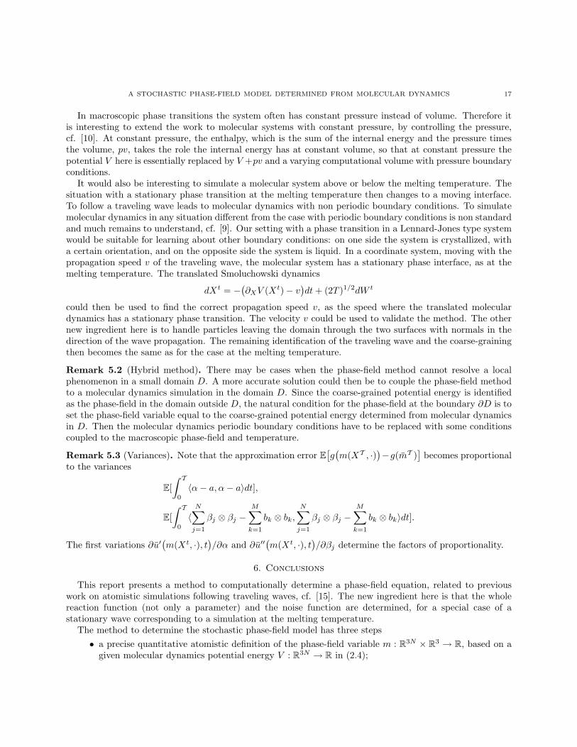
Figure 6 shows the computed diffusion coefficients for the noise with the O2 orientation.


−40 −20 0 20 40 60 80 100 120 140−0.8

−0.6

−0.4

−0.2

0

0.2

0.4

0.6

x1

Drift component kB

T d2m/dx12

(a) −A0(x) = γ∂2xm(x)

−1 −0.5 0 0.5

0

0.1

0.2

0.3

0.4f(m)

m

Orientation 1Orientation 2

(b) k2f(m) =R m

m0−A0(x(m)) dm

Figure 5. Sub-figure 5(a) shows an example of a computed reaction term −A0(x) over theperiodic computational cell containing two interfaces. Inverting the computed phase-fieldfunction inside the interfaces and integrating with respect to m gives the double-well typepotentials shown in Sub-figure 5(b) for two different orientations of the solid–liquid interfacewith respect to the face centered cubic crystal structure in the solid; in Orientation 1, O1,the interface is along the {100} plane in the crystal and in Orientation 2, O2, it is alongthe {111} plane. The two curves with the same orientation correspond to the two phasetransitions in the computational domain, explained in Figure 3. Note that the potentials areindeed qualitative similar to the function φ 7→ k2(1 − φ2)2 in (1.2) if we rescale to have theequilibrium points in m = ±1 and we restrict the domain to φ ∈ [−1, 1] where the phase-fieldhas it values.

5. The Computational Method

This section describes the numerical implementation for computing the drift and diffusion functions, defin-ing the coarse-grained phase-field dynamics (4.1), from two-phase Smoluchowski dynamics simulations atconstant volume and temperature. The procedure computes time averaged quantities like the time averagedpotential energy phase-field

limT→∞

T −1E[∫ T

0

mtdt]


0

50

100

0

50

1000

10

20

30

x1

y1

0

5

10

15

20

25

30

35

Figure 6. Computed values of the diffusion matrix using the same configurations from theO2-simulation that gave the reaction term in 5(a).

and the corresponding coarse-grained drift and diffusion coefficient functions (4.11) and (4.10). A moredetailed description of the numerical method and the computational results is in [32].

5.1. Discrete Smoluchowski System Simulated at Constant Volume. The discrete time approxima-tions Xn of Xtn , were computed using the explicit Euler-Maruyama scheme

Xn = Xn−1 − ∂XV (Xn−1) ∆tn +√

2kBT ∆Wn,(5.1)

where ∆tn = tn − tn−1 is a time increment and ∆Wn = W (tn) − W (tn−1) is an increment in the 3N -dimensional Wiener process. Each run was performed using constant time step size.

The particles are contained in a computational cell, shaped like a rectangular box, of fixed dimensions andthe boundary conditions are periodic in all directions. Hence the volume, V , and the number of particles, N ,are fixed. In standard Hamiltonian molecular dynamics the temperature is determined by the kinetic energydue to velocity fluctuations; in Smoluchowski dynamics the temperature, T , enters directly in the dynamics.The temperature parameter is held fixed, which can be viewed as a kind of thermostat built into the dynamicssimulating the canonical ensemble with constant number of particles, volume, and temperature. Since thevolume of the computational cell is constant the overall density of the system remains constant over time,which allows for stationary two-phase configurations where part of the domain is solid and part is liquid.

The initial configurations for the Smoluchowski dynamics simulations were set up to obtain a two-phasesystem at temperature T = 2.90 with approximately equal volumes of solid and liquid and with stationaryinterfaces; see Figure 2. Simulation O1 used 64131 particles in a computational cell of dimensions 93.17 ×23.29 × 23.29, while simulation O2 used 78911 particles in a cell of dimensions 100.86 × 24.71 × 24.96. Thevalues above are given in reduced Lennard-Jones units.

An effect of the finite size of the computational cell is that periodic boundary conditions may interactwith the solid and affect the results; here the computational cell was chosen to match the FCC structure in aspecific orientation with respect to the box and thus stabilised the structure and orientation. It is important toknow that the density in the FCC part (and hence the box cross section) is consistent with constant pressuresimulations close to the melting point. A related question is whether the length of the computational box is


large enough for properties around the interfaces in the infinitely layered structure to be good approximationsof those near an interface between a solid and liquid on the macroscopic scale.

5.2. Computation of the Coarse-Grained Model Functions. The drift and diffusion coefficient func-tions in the stochastic differential equation (4.1) for the coarse-grained phase-field are defined in terms of thetime averaged expected values (4.11) and (4.10) on the form

1T

E

[∫ T0

ψ(·;Xt)∣∣∣∣ X0 = X0

],

where the initial configuration X0 is a configuration of a stationary two-phase system. By setting up X0 andsimulating discrete sample trajectories using the Euler-Maruyama method (5.1), a sequence of configurations{Xk}Kk=1 approximating the sequence {Xtk}Kk=1 for some times 0 < t1 < · · · < tK = T is obtained. In a postprocessing step a set of configurations S ⊆ {Xk}Kk=1 is selected and averages

AS (ψ) =∑X∈S

ψ(·;X )wX ,

consistently weighted with weights wX , are computed as approximations of the corresponding expected valuesin the continuous time model. It is usually more efficient not to include every configuration in the averages;see [32].

As described in Section 4.3, the averages are functions of the coordinate direction x1, normal to the planarinterface, since the mollifier in the definition (2.4) of the microscale phase-field, m, is chosen to take uniformaverages in the planes parallel to the interface. The mollifier used in the computations is

η(x) = η(x1) = c exp(−1

2

(x1

ε

)2)1|x1|<Rc ,(5.2)

where c is a normalising constant, ε is a smoothing parameter, and Rc is a cut-off. The smoothing parameteris on the order of typical nearest neighbour distances, ε = 1, and Rc = 6ε which gives η(Rc) ≈ 1.5 · 10−8η(0).

An explicit derivation of expressions for the drift and the diffusion is given in the appendix of [32]. Sepa-rating the drift in terms containing two, one, and zero derivatives of the mollifier, the right hand side of (4.11)is approximated by

kBT∂2

∂x21

AS (m) +∂

∂x1AS (a1) +AS (a0),

where

a1(x;X ) =N∑j=1

(kBT −mj(X ))[Fj(X )]1η(x−Xj)(5.3)

and

a0(x;X ) = −N∑j=1

(kBT∂Xj · Fj(X ) +

12||Fj(X )||2

)η(x−Xj)

− 12

N∑j=1

N∑i 6=j,i=1

fij(X ) · Fj(X )η(x−Xi).(5.4)


Here Fj is the total force acting on particle j, [Fj(X )]1 is the x1-component of the force, and fij are thecontributions from individual pairs,

Fj(X ) = −∂XjV (X ) =N∑

i 6=j,i=1

Φ′(||Xi −Xj ||)Xi −Xj

||Xi −Xj ||=

N∑i6=j,i=1

fij(X ).

The right hand side in equation (4.10), for the coarse-grained diffusion, is approximated by

B(·, ·) = AS

2kBT

N∑j=1

(pj(·, ·;X) + qj(·, ·;X)

),(5.5)

where

pj(x, y;X ) =(mj(X )ε2

)2 [x−Xj

]1

[y −Xj

]1η(x−Xj)η(y −Xj)

− mj(X )2ε2

[x−Xj ]1η(x−Xj)(

[Fj(X )]1η(y −Xj) +N∑

i 6=j,i=1

[fij(X )]1η(y −Xi))

− mj(X )2ε2

[y −Xj ]1η(y −Xj)(

[Fj(X )]1η(x−Xj) +N∑

i 6=j,i=1

[fij(X )]1η(x−Xi))

and

qj(x, y;X ) =14

(Fj(X )η(x−Xj) +

N∑i6=j,i=1

fij(X )η(x−Xi))

·(Fj(X )η(y −Xj) +

N∑i 6=j,i=1

fij(X )η(y −Xi)).

The functions AS (ψ) are computed in a discrete set of points DK = {xi1}Ki=1 along the x1 axis of themolecular dynamics domain. This makes the computed components, AS (m), AS (a1), and AS (a0), of thedrift coefficient function K-vectors and the computed B a K-by-K matrix. The individual diffusion coefficientfunctions bj are obtained by taking the square root of the computed diffusion matrix, B = B

1/2(B

1/2)T, and

letting the j:th column of B1/2

define bj .With one Wiener process Wj in the coarse-grained stochastic differential equation (4.1) per evaluation

point, K = M , the component vectors, bj , of the diffusion in the coarse-grained equation can be defined asthe column vectors of the matrix B, to obtain

M∑j=1

bjbT

j ≈ B.

If two grid points, x1 and y1, are further apart than twice the sum of the cut-off in the potential and thecut-off in the mollifier, then pj(x, y; ·) and qj(x, y; ·) are zero; hence a natural ordering x1

1 < x21 < · · · < xK1 of

the grid points makes B a band matrix. Using the square root of B is a way that preserves the connectionbetween grid points and diffusion functions and hence the dominating terms in a tabulated vector bj are thoseof nearby grid points.

Remark 5.1 (Extensions). We have computed coarse-grained approximations for a pair potential molecularequilibrium system in the canonical ensemble (with constant number of particles, volume and temperature)using periodic boundary conditions.


In macroscopic phase transitions the system often has constant pressure instead of volume. Therefore itis interesting to extend the work to molecular systems with constant pressure, by controlling the pressure,cf. [10]. At constant pressure, the enthalpy, which is the sum of the internal energy and the pressure timesthe volume, pv, takes the role the internal energy has at constant volume, so that at constant pressure thepotential V here is essentially replaced by V +pv and a varying computational volume with pressure boundaryconditions.

It would also be interesting to simulate a molecular system above or below the melting temperature. Thesituation with a stationary phase transition at the melting temperature then changes to a moving interface.To follow a traveling wave leads to molecular dynamics with non periodic boundary conditions. To simulatemolecular dynamics in any situation different from the case with periodic boundary conditions is non standardand much remains to understand, cf. [9]. Our setting with a phase transition in a Lennard-Jones type systemwould be suitable for learning about other boundary conditions: on one side the system is crystallized, witha certain orientation, and on the opposite side the system is liquid. In a coordinate system, moving with thepropagation speed v of the traveling wave, the molecular system has a stationary phase interface, as at themelting temperature. The translated Smoluchowski dynamics

dXt = −(∂XV (Xt)− v

)dt+ (2T )1/2dW t

could then be used to find the correct propagation speed v, as the speed where the translated moleculardynamics has a stationary phase transition. The velocity v could be used to validate the method. The othernew ingredient here is to handle particles leaving the domain through the two surfaces with normals in thedirection of the wave propagation. The remaining identification of the traveling wave and the coarse-grainingthen becomes the same as for the case at the melting temperature.

Remark 5.2 (Hybrid method). There may be cases when the phase-field method cannot resolve a localphenomenon in a small domain D. A more accurate solution could then be to couple the phase-field methodto a molecular dynamics simulation in the domain D. Since the coarse-grained potential energy is identifiedas the phase-field in the domain outside D, the natural condition for the phase-field at the boundary ∂D is toset the phase-field variable equal to the coarse-grained potential energy determined from molecular dynamicsin D. Then the molecular dynamics periodic boundary conditions have to be replaced with some conditionscoupled to the macroscopic phase-field and temperature.

Remark 5.3 (Variances). Note that the approximation error E[g(m(XT , ·)

)−g(mT )

]becomes proportional

to the variances

E[∫ T

0

〈α− a, α− a〉dt],

E[∫ T

0

〈N∑j=1


bk ⊗ bk,N∑j=1


bk ⊗ bk〉dt].

The first variations ∂u′(m(Xt, ·), t

)/∂α and ∂u′′

(m(Xt, ·), t

)/∂βj determine the factors of proportionality.

6. Conclusions

This report presents a method to computationally determine a phase-field equation, related to previouswork on atomistic simulations following traveling waves, cf. [15]. The new ingredient here is that the wholereaction function (not only a parameter) and the noise function are determined, for a special case of astationary wave corresponding to a simulation at the melting temperature.

The method to determine the stochastic phase-field model has three steps• a precise quantitative atomistic definition of the phase-field variable m : R3N × R3 → R, based on a

given molecular dynamics potential energy V : R3N → R in (2.4);


• derivation of a macroscopic coarse-grained dynamics, i.e. the phase-field model (4.13)

(rq)−1dm =(kBTq

−1∂2xm+A0(m)

)dt+ r−1/2q−1

∑k

bk(m)dW tk,

for m(x, t) approximating m(Xt, x) in (4.1) - (4.4), using the microscopic Smoluchowski moleculardynamics

dXti = −∂XiV (Xt)dt+

√2kBT dW t

i ,

for particle positions X : [0,∞)→ R3N and standard Brownian motions Wk and Wi;• numerical molecular dynamics computation to evaluate m and b in the phase transition by ensemble

averages based on (4.4); the phase-field variable m then determines the functions A0 and q from atraveling wave: the shape of the traveling wave, computed from molecular dynamics, determines thereaction term balancing the diffusion (since the total drift becomes zero in our case of a stationarywave), the reaction and diffusion terms in the phase-field equation are then determined up to amultiplicative constant – this multiplicative constant is chosen to match equilibrium fluctuations ofthe phase-field; the diffusion coefficient b is determined from an optimization problem, where thediffusion is chosen to minimize the error of observables in the Gibbs ensemble.

The coarse-grained model approximates Gibbs ensemble averages of the atomistic phase-field, by choosingcoarse-grained drift and diffusion functions that minimize the approximation error of observables in thisensemble average.

The quotient of reaction terms q = qi := A0(Oi)/A0(O1) depends on the crystal orientation Oi relativeto the phase interface and the reaction term A0 forms a double well potential shown in Figure 5. Thediffusion coefficient b is determined from the square root of the diffusion matrix of the noise in Figure 6.The function r = ri is the quotient of relaxation times: the time scale τ used Smoluchowski dynamics maydepend on the crystal orientation, since the relaxation time τ may differ for two orientations Oi, and wedefine ri := τ(Oi)/τ(O1) for the reference orientation O1. Langevin dynamics

dXsi = vsi ds,

Mdvsi = −∂XiV (Xs) ds− vsiτds+

√2γτdW s

i ,

defines the relaxation time. The relaxation time τ is related to the shear viscosity η by τ(Oi)/τ(O1) =η(O1)/η(Oi). The function r can therefore be determined similarly as the function m(x), replacing theSmoluchowski dynamics with Langevin dynamics (or Hamiltonian dynamics corresponding to τ = ∞) andusing a standard molecular dynamics expression for the viscosity, cf. [10].

The computational results with a Lennard-Jones type molecular potential shows that the determinedphase-field equation has the right qualitative behavior, with a double well potential and orientation dependentcoefficients. Further numerical studies would be needed to validate the method for realistic materials.

References

[1] Amberg G., Semi sharp phase-field method for quantitative phase change simulations, Phys. Rev. Lett. 91 (2003), 265505–

265509.[2] Asta M., Beckermann C. , Karma A., Kurz W., Napolitano R., Plapp M., Purdy G., Rappaz M.,Trivedi R., Solidification

microstructures and solid-state parallels: Recent developments, future directions, Acta Materialia, available online December2008.

[3] Beale J.T., Majda A.J., Vortex methods. I. Convergence in three dimensions. Math. Comp. 39 (1982), 1–27.

[4] Boettinger W.J., Warren J.A., Beckermann C., Karma A., Phase field simulation of solidification, Ann. Rev. Mater. Res.

32 (2002), 163–194.[5] Burman E., Rappaz J., Existence of solutions to an anisotropic phase-field model, Math. Methods Appl. Sci. 26 (2003),

no. 13, 1137–1160.[6] Cances E., Legoll F., Stolz G., Theoretical and numerical comparison of some sampling methods for molecular dynamics,

Math. Model. Num. Anal., 41 (2007) 351-389.


[7] De Masi A., Orlandi E., Presutti E., Triolo L., Glauber evolution with the Kac potentials. I. Mesoscopic and macroscopic

limits, interface dynamics, Nonlinearity 7 (1994), 633–696.

[8] Dirr N., Luckhaus S., Mesoscopic limit for non-isothermal phase transition, Markov Processes and Related Fields 7 (2001),355 - 381.

[9] E W., Ren W., Heterogeneous multiscale method for the modeling of complex fluids and micro-fluidics. J. Comput. Phys.,

vol. 204, no. 1, pp. 1-26, 2005.[10] Frenkel D., Smit B., Understanding Molecular Simulation, Academic Press, 2002.

[11] Gooodman J., Moon K.-S., Szepessy A., Tempone R., Zouraris G., Stochastic and partial differential equations with adapted

numerics, http://www.math.kth.se/∼szepessy/sdepde.pdf[12] Gouyet J.F., Plapp M., Dietrich W., Maass P., Description of far-from-equilibrium process by mean-field lattice gas models,

Advances in Physics 52 (2003), 523–638.

[13] Groot R.D., Warren P.B., Dissipative particle dynamics: bridging the gap between atomistic and mesoscopic simulation, J.Chem. Phys. 107 (1997), 4423–4435.

[14] Hardy R.J., Formulas for determining local properties in molecular dynamics: shock waves, J. Chem. Phys. 76 (1982),622-628.

[15] Hoyt J. J., Asta M., Karma A., Atomistic and continuum modeling of dendritic solidification, Materials Science Engineering

R-Reports 41 (2003), 121–163.[16] Irving J.H, Kirkwood J.G, The statistical mechanics of transport processes: IV the equations of hydrodynamics, J. Chem.

Phys. 18 (1950), 817–829.

[17] Kadanoff L.P., Statistical physics : statics, dynamics and renormalization, World Scientific, 2000.[18] Karma A., Rappel W.J., Phase-field model of dendritic side branching with thermal noise, Phys Rev. E. 60 (1999),

3614–3625.

[19] Katsoulakis M.A., Majda A.J., Vlachos D.G., Coarse-grained stochastic processes and Monte Carlo simulations in latticesystems, J. Comput. Phys. 186 (2003), 250–278.

[20] Katsoulakis M., Szepessy A. Stochastic hydrodynamical limits of particle systems, Comm. Math. Sciences 4, (2006).

[21] Kramer P.R., Majda A.J., Stochastic mode reduction for particle-based simulation methods for complex microfluid systems,SIAM J. Appl. Math. 64 (2003), 401–422.

[22] Kroemer H. and Kittel C., Thermal Physics, W. H. Freeman Company, 1980.[23] Kurtz T.G., A limit theorem for perturbed operator semigroups with applications to random evolutions, J. Func. Anal. 12

(1973), 55–67.

[24] Landau L.D. and Lifshitz E.M., Statistical Physics Part 1, Pergamon Press, 1980.[25] Liggett T.M., Interacting particle systems, Springer-Verlag, Berlin, 2005.

[26] Majda A.,J., Timofeyev I., Vanden Eijnden E., A mathematical framework for stochastic climate models, Comm. Pure Appl.

Math. 54 (2001), 891–974.[27] Mas-Gallic S., Raviart P.-A., A particle method for first-order symmetric systems. Numer. Math. 51 (1987), 323–352.

[28] Morandi G., Napoli F. and Ercolessi E., Statistical Mechanics: An Intermediate Course, World Scientific Publishing, 2001.

[29] Nelson E., Dynamical Theories of Brownian Motion, Princeton University Press, 1967.[30] Olla S., Varadhan S. R. S., Yau H.-T., Hydrodynamical limit for a Hamiltonian system with weak noise. Comm. Math.

Phys. 155 (1993), 523–560.

[31] Schlick T., Molecular modeling and simulation, Springer Verlag 2002.[32] von Schwerin E., A Stochastic Phase-Field Model Computed From Coarse-Grained Molecular Dynamics, arXiv:0908.1367,

included in [33].[33] von Schwerin E., Adaptivity for Stochastic and Partial Differential Equations with Applications th Phase Transformations,

PhD thesis, KTH (Royal Institute of Technology, Stockholm) 2007. ISBN 978-91-7178-744-6.

[34] Pavlik S.G, Sekerka R.J., Forces due to fluctuations in the anisotropic phase-field model of solidification, Physica A 268(1999), 283-290.

[35] Shardlow T., Splitting for dissipative particle dynamics, SIAM J. Sci. Comput. 24 (2003), 1267–1282.[36] Soner H.M., Convergence of the phase-field equations to the Mullins-Sekerka Problem with kinetic undercooling, Arch. Rat.

Mech. Anal. 131 (1995), 139–197.

[37] Szepessy A., Tempone R., Zouraris G., Adaptive weak approximation of stochastic differential equations, Comm. Pure

Appl. Math, 54 (2001), 1169-1214.[38] van Kampen N.G., Stochastic Processes in Physics and Chemistry, North-Holland, 1981.

A STOCHASTIC PHASE-FIELD MODEL DETERMINED …szepessy/md_pde-1.pdf · Introduction to Phase-Field Models The phase- eld model for a liquid ... (macroscopic) scale; the molecular dynamics

Documents