Foundations and Trends R in Computer Graphics and Vision Vol. 2, No. 4 (2006) 259–362 c 2007 S.-C. Zhu and D. Mumford DOI: 10.1561/0600000018 A Stochastic Grammar of Images Song-Chun Zhu 1,∗ and David Mumford 2 1 University of California, Los Angeles USA, [email protected] 2 Brown University, USA, David [email protected] Abstract This exploratory paper quests for a stochastic and context sensitive grammar of images. The grammar should achieve the following four objectives and thus serves as a unified framework of representation, learning, and recognition for a large number of object categories. (i) The grammar represents both the hierarchical decompositions from scenes, to objects, parts, primitives and pixels by terminal and non-terminal nodes and the contexts for spatial and functional relations by horizon- tal links between the nodes. It formulates each object category as the set of all possible valid configurations produced by the grammar. (ii) The grammar is embodied in a simple And–Or graph representation where each Or-node points to alternative sub-configurations and an And-node is decomposed into a number of components. This represen- tation supports recursive top-down/bottom-up procedures for image parsing under the Bayesian framework and make it convenient to scale up in complexity. Given an input image, the image parsing task con- structs a most probable parse graph on-the-fly as the output interpre- tation and this parse graph is a subgraph of the And–Or graph after * Song-Chun Zhu is also affiliated with the Lotus Hill Research Institute, China.

Welcome message from author
This document is posted to help you gain knowledge. Please leave a comment to let me know what you think about it! Share it to your friends and learn new things together.
Transcript

Foundations and TrendsR© inComputer Graphics and VisionVol. 2, No. 4 (2006) 259–362c© 2007 S.-C. Zhu and D. MumfordDOI: 10.1561/0600000018
A Stochastic Grammar of Images
Song-Chun Zhu1,∗ and David Mumford2
1 University of California, Los Angeles USA, [email protected] Brown University, USA, David [email protected]
Abstract
This exploratory paper quests for a stochastic and context sensitivegrammar of images. The grammar should achieve the following fourobjectives and thus serves as a unified framework of representation,learning, and recognition for a large number of object categories. (i) Thegrammar represents both the hierarchical decompositions from scenes,to objects, parts, primitives and pixels by terminal and non-terminalnodes and the contexts for spatial and functional relations by horizon-tal links between the nodes. It formulates each object category as theset of all possible valid configurations produced by the grammar. (ii)The grammar is embodied in a simple And–Or graph representationwhere each Or-node points to alternative sub-configurations and anAnd-node is decomposed into a number of components. This represen-tation supports recursive top-down/bottom-up procedures for imageparsing under the Bayesian framework and make it convenient to scaleup in complexity. Given an input image, the image parsing task con-structs a most probable parse graph on-the-fly as the output interpre-tation and this parse graph is a subgraph of the And–Or graph after
* Song-Chun Zhu is also affiliated with the Lotus Hill Research Institute, China.

making choice on the Or-nodes. (iii) A probabilistic model is definedon this And–Or graph representation to account for the natural occur-rence frequency of objects and parts as well as their relations. Thismodel is learned from a relatively small training set per category andthen sampled to synthesize a large number of configurations to covernovel object instances in the test set. This generalization capabilityis mostly missing in discriminative machine learning methods and canlargely improve recognition performance in experiments. (iv) To fill thewell-known semantic gap between symbols and raw signals, the gram-mar includes a series of visual dictionaries and organizes them throughgraph composition. At the bottom-level the dictionary is a set of imageprimitives each having a number of anchor points with open bonds tolink with other primitives. These primitives can be combined to formlarger and larger graph structures for parts and objects. The ambigu-ities in inferring local primitives shall be resolved through top-downcomputation using larger structures. Finally these primitives forms aprimal sketch representation which will generate the input image withevery pixels explained. The proposal grammar integrates three promi-nent representations in the literature: stochastic grammars for compo-sition, Markov (or graphical) models for contexts, and sparse codingwith primitives (wavelets). It also combines the structure-based andappearance based methods in the vision literature. Finally the paperpresents three case studies to illustrate the proposed grammar.

1Introduction
1.1 The Hibernation and Resurgence of Image Grammars
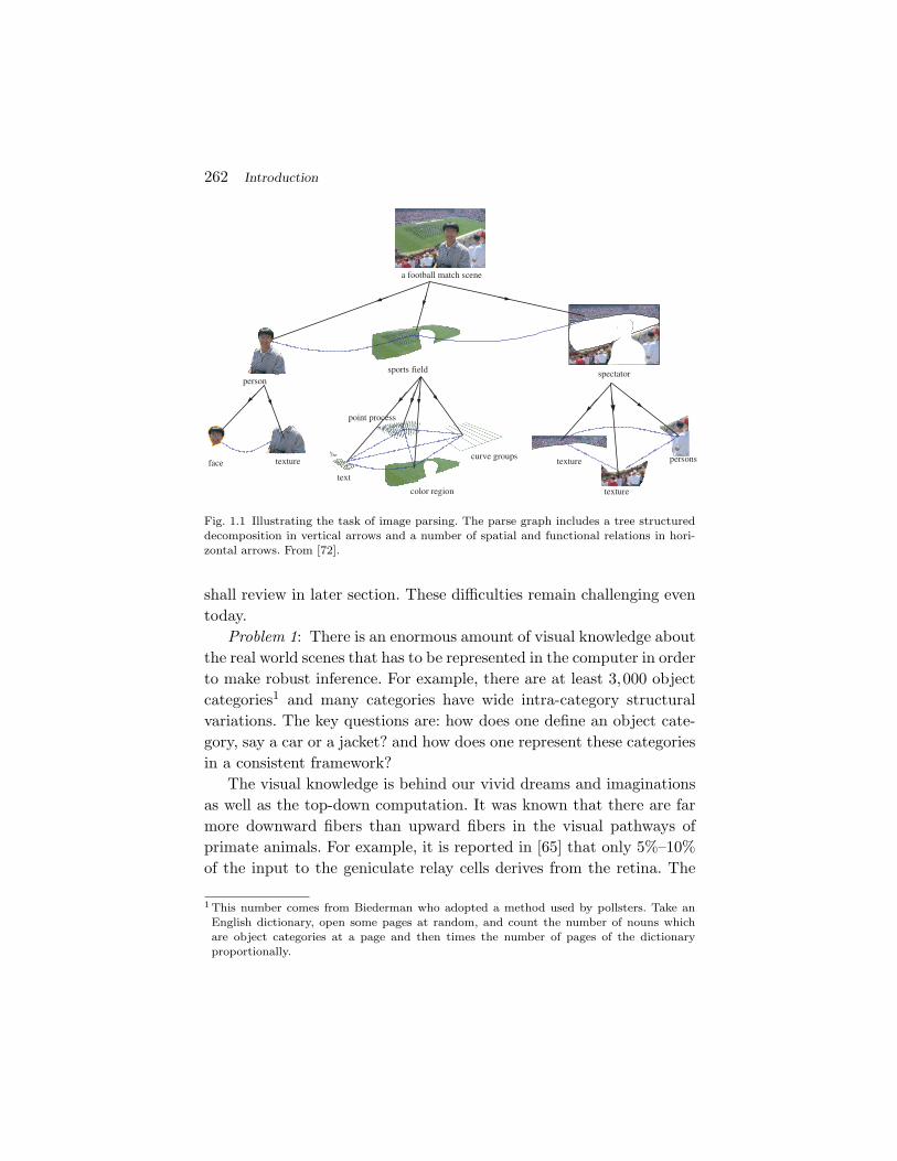
Understanding the contents of images has always been the core prob-lem in computer vision with early work dated back to Fu [22], Riseman[33], Ohta and Kanade [54, 55] in the 1960–1970s. By analogy to naturallanguage understanding, the task of image parsing [72], as Figure 1.1illustrates, is to compute a parse graph as the most probable inter-pretation of an input image. This parse graph includes a tree struc-tured decomposition for the contents of the scene, from scene labels, toobjects, parts, primitives, so that all pixels are explained, and a num-ber of spatial and functional relations between nodes for contexts at alllevels of the hierarchy.
People who worked on image parsing in the 1960–1970s were, obvi-ously, ahead of their time. In Kanade’s own words, they had only 64Kmemory to work with at that time. Indeed, his paper with Ohta [55]was merely 4-page long! The image parsing efforts and structured meth-ods encountered overwhelming difficulties in the 1970s and since thenentered a hibernation state for a quarter of a century. The syntacticand grammar work have been mostly studied in the backstage as we
261
262 Introduction
a football match scene
texture
text
face
person
color region
curve groupstexture
sports field spectator
texture
persons
point process
Fig. 1.1 Illustrating the task of image parsing. The parse graph includes a tree structureddecomposition in vertical arrows and a number of spatial and functional relations in hori-zontal arrows. From [72].
shall review in later section. These difficulties remain challenging eventoday.
Problem 1: There is an enormous amount of visual knowledge aboutthe real world scenes that has to be represented in the computer in orderto make robust inference. For example, there are at least 3,000 objectcategories1 and many categories have wide intra-category structuralvariations. The key questions are: how does one define an object cate-gory, say a car or a jacket? and how does one represent these categoriesin a consistent framework?
The visual knowledge is behind our vivid dreams and imaginationsas well as the top-down computation. It was known that there are farmore downward fibers than upward fibers in the visual pathways ofprimate animals. For example, it is reported in [65] that only 5%–10%of the input to the geniculate relay cells derives from the retina. The
1 This number comes from Biederman who adopted a method used by pollsters. Take anEnglish dictionary, open some pages at random, and count the number of nouns whichare object categories at a page and then times the number of pages of the dictionaryproportionally.

1.1 The Hibernation and Resurgence of Image Grammars 263
rest derives from local inhibitory inputs and descending inputs fromlayer 6 of the visual cortex. The weakness in knowledge representationand top-down inference is, in our opinion, the main obstacle in the roadtoward robust and large scale vision systems.
Problem 2: The computational complexity is huge.2 A simple glanceof Figure 1.1 reveals that an input image may contain a large numberof objects. Human vision is known [70] to simultaneously activate thecomputation at all levels from scene classification to edge detection —all occurs in a very short time ≤400 ms, and to adopt multiple visualroutines [76] to achieve robust computation. In contrast, most pat-tern recognition or machine learning algorithms are feedforward andcomputer vision systems rarely possess enough visual knowledge forreasoning.
The key questions are: how does one achieve robust computationthat can be scaled to thousands of categories? and how does one coor-dinate these bottom-up and top-down procedures? To achieve scalablecomputation, the vision algorithm must be based on simple proceduresand structures that are common to all categories.
Problem 3: The most obvious reason that sent the image parsingwork to dormant status was the so-called semantic gap between theraw pixels and the symbolic token representation in early syntactic andstructured methods. That is, one cannot reliably compute the symbolsfrom raw images. This has motivated the shift of focus to appearancebased methods in the past 20 years, such as PCA [75], AAM [12], andappearance based recognition [51], image pyramids [69] and wavelets[15], and machine learning methods [21, 63, 78] in the past decade.
Though the appearance based methods and machine learning algo-rithms have made remarkable progress, they have intrinsic problemsthat could be complemented by structure based methods. For example,they require too many training examples due to the lack the compo-sitional and generative structures. They are often over-fit to specifictraining set and can hardly generalize to novel instances or configura-tions especially for categories that have large intra-class variations.
2 The NP-completeness is no longer an appropriate measure of complexity, because evenmany simplified vision problems are known to be NP-hard.

264 Introduction
After all these developments, the recent vision literature hasobserved a pleasing trend for returning to the grammatical and com-positional methods, for example, the work in the groups of Ahuja [71],Geman [27, 36], Dickinson [14, 40], Pollak [79], Buhmann [57] and Zhu[9, 32, 44, 59, 72, 74, 85, 86]. The return of grammar is in response tothe limitations of the appearance based and machine learning methodswhen they are scaled up.
The return of grammar is powered by progresses in several aspects,which were not available in the 1970s. (i) A consistent mathemati-cal and statistical framework to integrate various image models, suchas Markov (graphical) models [90], sparse coding [56], and stochas-tic context free grammar [10]. (ii) More realistic appearance modelsfor the image primitives to connect the symbols to pixels. (iii) Morepowerful algorithms including discriminative classification and gener-ative methods, such as the Data-Driven Markov China Monte Carlo(DDMCMC) [73]. (iv) Huge number of realistic training and testingimages [87].
1.2 Objectives
This exploratory paper will review the issues and recent progress indeveloping image grammars, and introduce a stochastic and contextsensitive grammar as a unified framework for representation, learning,and recognition. This framework integrates many existing models andalgorithms in the literature and addresses the problems raised in theprevious subsection. This image grammar should achieve the followingfour objectives.
Objective 1: A common framework for visual knowledge representa-tion and object categorization. Grammars, studied mostly in language[1, 26], are known for their expressive power in generating a very largeset of configurations or instances, i.e., their language, by composinga relatively much smaller set of words, i.e., shared and reusable ele-ments, using production rules. Hierarchic and structural compositionis the key concept behind grammars in contrast to enumerating allpossible configurations.

1.2 Objectives 265
In this paper, we embody the image grammar in an And–Orgraph representation3 where each Or-node points to alternative sub-configurations and an And-node is decomposed into a number ofcomponents. This And–Or graph represents both the hierarchicaldecompositions from scenes, to objects, parts, primitives and pixelsby terminal and non-terminal nodes and the contexts for spatial andfunctional relations by horizontal links between the nodes. It is an alter-nate way of representing production rules and it contains all possibleparse trees. Then we will define a probabilistic model for the And–Orgraph which can be learned from examples using maximum likelihoodestimation. Therefore, all the structural and contextual informationare represented in the And–Or graph (and equivalently the grammar).This also resolve the object categorization problem. We can define eachobject category as the set of all valid configurations which are producedby the grammar, with its probability learned to reproduce natural fre-quency of instances occurring in the observed ensemble.
As we will show in later section, this probability model integratespopular generative models, such as sparse coding (wavelet coding) andstochastic context free grammars (SCFG), with descriptive models,such as Markov random fields and graphical models. The former rep-resents the generative hierarchy for reconfigurability while the lattermodels context.
Objective 2: Scalable and recursive top-down/bottom-up computa-tion. The And–Or graph representation has recursive structures withtwo types of nodes. It can be easily scalable up in the number of nodesand object categories. For example, suppose an Or-node represents anobject, say car, it then has a number of children nodes for differentviews (front, side, back etc.) of cars. By adding a new child node, wecan augment to new views. This representation supports recursive top-down/bottom-up procedures for image parsing and make it convenientto scale up in complexity.
Figure 1.2 shows a parsing graph under construction at a time step.This simple grammar is one of our case study in later section uses one
3 The And–Or graph was previously used by Pearl in [58] for heuristic searches. In our work,we use it in a very different purpose and should not be confused with Pearl’s work.

266 Introduction
top-downproposals
bottom-upproposals
mesh ruler3
cube ruler6
nest ruler4
A CB
Sscene
objects
rectangularsurfaces
configurationC
imageI
parse graphG
edge map
Fig. 1.2 Illustrating the recursive bottom-up/top-down computation processes in imageparsing. The detection of rectangles (in red) instantiates some non-terminal nodes shown asupward arrows. They in turn activate graph grammar rules for grouping larger structuresin nodes A,B, and C, respectively. These rules generate top-down prediction of rectan-gles (in blue). The predictions are validated from the image under the Bayesian posteriorprobability. Modified from [59].

1.2 Objectives 267
primitive: rectangular surfaces projected onto the image plane. Thegrammar rules represents various organization, such as alignments ofthe rectangles in mesh, linear, nesting, cubic structures. In the kitchenscene, the four rectangles (in red) accepted through bottom-up processand they activate the production rules represented by the non-terminalnodes A, B, and C, respectively. Which then predict a number of can-didates (in blue) in top-down search. The solid upward arrows showthe bottom-up binding, while the downward arrows show the top-downprediction. As the ROC curves in Figure 9.5 shows in later section, thetop-down prediction largely improves the recognition rate of the rect-angles, as certain rectangles can only be hallucinated through top-downprocess due to occlusion and severe image degradation.
Given an input image, the image parsing task constructs a mostprobable parse graph on-the-fly as the output interpretation and thisparse graph is a subgraph of the And–Or graph after making choiceson the Or-nodes.
As we shall discuss in later section, the computational algorithmmaintains the same data structures for each of the And-nodes andOr-nodes in the And–Or graph and adopt the same computationalprocedure: (i) bottom-up detecting and binding using a cascade of fea-tures; and (ii) top-down on-line template composition and matching.To implement the system, we only need to write one common class (inC++ programming) for all the nodes, and different objects and partsare realized as instances of this class. These nodes use different bottom-up features/tests and the top-down templates during the computationalprocess. The features and templates are learned off-line through train-ing images and loaded into the instances of the C++ class during thecomputational process. This recursive algorithm has the potential tobe implemented in a massively parallel machine where each unit hasthe same data structures and functions described above.
Objective 3: Small sample learning and generalization. The prob-abilistic model defined on this And–Or graph representation can belearned from a relatively small training set per category and then sam-pled through Monte Carlo simulation to synthesize a large number ofconfigurations. This is in fact an extension to the traditional texturesynthesis experiment by the minimax entropy principle [90], where new

268 Introduction
texture samples are synthesized which are different from the observedtexture but are perceptually equivalent to the observed texture. Theminimax entropy learning scheme is extended to the And–Or graphmodels in [59], which can generate novel configurations through com-position to cover unforeseen object instances in the test set. This gener-alization capability is mostly missed in discriminative machine learningmethods.
In the experiments reported in [44, 59], they seek for the mini-mum number of distinct training samples needed for each category,usually in the range of 20–50. They prune some redundant exam-ples which can be derived through other examples by composition.Then they found that the generated samples can largely improve theobject recognition performance. For example, a 15% recognition rate isreported in [44].
Objective 4: Mapping the visual vocabulary to fill the semantic gap.To fill the well-known semantic gap between symbols and pixels, thegrammar includes a series of visual dictionaries for visual concepts atall levels. There are two key observations for these dictionaries.
1. The elements of the dictionaries are organized through graphcomposition. At the bottom-level the dictionary is a set ofimage primitives each having a number of anchor points in asmall graph with open bonds to link with other primitives.These primitives can be combined to form larger and largergraph structures for parts and objects, in a way similar toLego pieces that kids play with.4
2. Vision is distinct from other sensors, like speech in the aspectthat objects can appear at arbitrary scales. As a result, theinstances of each node can occur at any sizes. The non-terminal nodes at all levels of the And–Or graph can termi-nate directly as image primitives. Thus one has to accountfor the transitions between instances of the same node overscales. This is the topics studied in the perceptual scale spacetheory [80].
4 Note that Lego pieces are well designed to have standardized teeth to fit each other, thisis not true in the image primitives. The latter are more flexible.

1.3 Overview of the Image Grammar 269
Though there are variations in the literature for what the low levelprimitives should be, the differences are really minor between whatpeople called textons, texels, primitives, patches, and fragments. Theambiguities in inferring these local primitives shall be resolved throughtop-down computation using larger structures.
Finally the primitives are connected to form a primal sketch graphrepresentation [31] which will generate the input image with every pix-els explained. This closes the semantic gap.
1.3 Overview of the Image Grammar
In this subsection, we overview the basic concepts in the image gram-mar. We divided it into two parts: (i) representation and data struc-tures, (ii) Image annotation dataset to learn the grammar, and thelearning and computing issues.
1.3.1 Overview of the Representational Conceptsand Data Structures
We use Figure 1.3 as an example to review the representational conceptsin the following:
1. An And–Or graph. Figure 1.3(a) shows a simple example ofan And–Or graph. An And–Or graph includes three typesof nodes: And-nodes (solid circles), Or-nodes (dashed cir-cles), and terminal nodes (squares). An And-node representsa decomposition of an entity into its parts. It corresponds tothe grammar rules, for example,
A → BCD, H → NO.
The horizontal links between the children of an And-noderepresent relations and constraints. The Or-nodes act as“switches” for alternative sub-structures, and stands forlabels of classification at various levels, such as scene cat-egory, object classes, and parts etc. It corresponds to pro-duction rules like,
B → E | F, C → G | H | I.

270 Introduction
A
B
KJI
P
GFE
DC
NL
T
H
SRQ
O
1 8765432 11109
and-node
or-node
leaf node
M
6
8
1 10
<B,C>
<C,D>
<C,D>
<B,C>
<N
,O>
U
<B,C><L
,M>
2
4
9'
9
<C,D
>(a) And-Or graph (b) parse graph 1 (c) parse graph 2
A
B
JE
DC
N
H
S
O
1 86 10
U
(d) configuration 1 (e) configuration 2
A
B
I
P
DC
R
42 9'
I
9
F
L M
Fig. 1.3 Illustrating the And–Or graph representation. (a) An And–Or graph embodies thegrammar productions rules and contexts. It contains many parse graphs, one of which isshown in bold arrows. (b) and (c) are two distinct parse graphs by selecting the switches atrelated Or-nodes. (d) and (e) are two graphical configurations produced by the two parsegraphs, respectively. The links of these configurations are inherited from the And–Or graphrelations. Modified from [59].
Due to this recursive definition, one may merge the And–Or graphs for many objects or scene categories into a largergraph. In theory, all scene and object categories can be repre-sented by one huge And–Or graph, as it is the case for naturallanguage. The nodes in an And–Or graph may share commonparts, for example, both cars and trucks have rubber wheelsas parts, and both clock and pictures have frames.
2. A parse graph, as shown in Figure 1.1, is a hierarchic gen-erative interpretation of a specific image. A parse graph isaugmented from a parse tree, mostly used in natural or pro-gramming language by adding a number of relations, shownas side links, among the nodes. A parse graph is derivedfrom the And–Or graph by selecting the switches or classifi-cation labels at related Or-nodes. Figures 1.3(b) and 1.3(c)

1.3 Overview of the Image Grammar 271
are two instances of the parse graph from the And–Or graphin Figure 1.3(a). The part shared by two node may have dif-ferent instances, for example, node I is a child of both nodesC and D. Thus we have two instances for node 9.
3. A configuration is a planar attribute graph formed by link-ing the open bonds of the primitives in the image plane.Figures 1.3(d) and 1.3(e) are two configurations producedby the parse graphs in Figures 1.3(b) and 1.3(c), respec-tively. Intuitively, when the parse graph collapses, it pro-duces a planar configuration. A configuration inherits therelations from its ancestor nodes, and can be viewed as aMarkov networks (or deformable templates [19]) with recon-figurable neighborhood. We introduce a mixed random fieldmodel [20] to represent the configurations. The mixed ran-dom field extends conventional Markov random field modelsby allowing address variables and handles non-local connec-tions caused by occlusions. In this generative model, a con-figuration corresponds to a primal sketch graph [31].
4. The visual vocabulary. Due to scaling property, the termi-nal nodes could appear at all levels of the And–Or graph.Each terminal node takes instances from certain set. The setis called a dictionary and contains image patches of variouscomplexities. The elements in the set may be indexed byvariables such as its type, geometric transformations, defor-mations, appearance changes etc. Each patch is augmentedwith anchor points and open bond to connect with otherpatches.
5. The language of a grammar is the set of all possible validconfigurations produced by the grammar. In stochastic gram-mar, each configuration is associated with a probability. Asthe And–Or graph is directed and recursive, the sub-graphunderneath any node A can be considered a sub-grammar forthe concept represented by node A. Thus a sub-language fornode A is the set of all valid configurations produced by theAnd–Or graph rooted at A. For example, if A is an object cat-egory, say a car, then this sub-language defines all the valid

272 Introduction
configurations of car. In an exiting case, the sub-language ofa terminal node contains only the atomic configurations andthus is called a dictionary.
In comparison, an element in a dictionary is an atomic structure andan element in a language is a composite structure (or configuration)made of a number of atomic structures. A configuration of node A inzoomed-out view loses its resolution and details, and becomes an atomicelement in the dictionary of node A. For example, a car viewed in closedistance is a configuration consisting of many parts and primitives.But in far distance, a car is represented by a small image patch as awhole and is not decomposable. This is a special property of the imagegrammar. The perceptual transition over scales is studied in [80, 84].
1.3.2 Overview of the Dataset and Learning
Now we briefly overview the learning and computing issues withstochastic image grammars.
A foremost question that one may ask is: how do you build thisgrammar and where is the dataset? Collecting the dataset for learningand training is perhaps more challenging than the learning task itself.
Although fully automated learning is most ideal, for example, leta computer program watch Disney cartoon or Hollywood movies andhope it figures out all the object categories and relations. But purelyunsupervised learning is less practical for learning the structured com-positional models at present for two reasons. (i) Visual learning must beguided by objectives and purposes of vision, not purely based on statis-tical information. Ideally one has to integrate this automatic learningprocess with autonomous robot and AI reasoning at the higher level.Before the robotics and AI systems are ready, we should guide thelearning process with some human supervision. For example, what areimportant structures and what are decorative stuff. (ii) In almost allthe unsupervised learning methods, the trainers still have to select theirdata carefully to contrast the involved concepts. For example, to learnthe concept that a car has doors, we must select images of cars withdoors both open and closed. Otherwise the concept of door cannot belearned.

1.3 Overview of the Image Grammar 273
We propose to learn the image grammar in a semi-automatic way.We shall start with a supervised learning with manually annotatedimages and objects to produce the parse graphs. We use this datasetto initiate the process and then shift to weakly supervised learning.This initial dataset is still very large if we target thousands of objectcategories.
To make the large scale grammar learning framework practical, thefirst author founded an independent non-profit research institute whichstarted to operate in the summer of 2005.5 It has a full time annotationteam for parsing the image structures and a development team for theannotation tools and database construction. Each image or object isparsed, semi-automatically, into a parse graph where the relations arespecified and objects are names using the wordnet standard. Figure 1.4lists an inventory of the current ground truth dataset parsed at LHI.It has now over 500,000 images (or video frames) parsed, covering 280object categories. Figure 1.5 shows two examples — the parse treesof cat and car. For clarity we only show the parse trees with namingof the nodes. Beyond the object parsing, there are many scene imagesannotated with the objects and their spatial relations labeled. As statedin a report [87], this ground truth annotation is aimed at broader scopeand more hierarchic structures than other datasets collected in variousgroups, such as Berkeley [4, 50], Caltech [16, 29], and MIT [62].
With this annotated dataset, we can construct the And–Or graphfor object and scene categories and learn the probability model on theAnd–Or graphs. These learning steps are guided by a minimax entropylearning scheme [90] and maximum likelihood estimation. It is dividedinto three parts:
1. Learning the probabilities at the Or-node so that the con-figurations generated account for the natural co-occurrencefrequency. This is typical in stochastic context free gram-mars [10].
2. Learning and pursuing the Markov models on the horizontallinks and relations to account for the spatial relations, as well
5 It is called the Lotus Hill Research Institute (LHI) in China (www.lotushill.org).

274 Introduction
land
scap
e
seas
hore
scen
ege
neri
cob
ject
othe
rs
attr
ibut
ecu
rve
natu
ral
man
mad
e
land
mam
mal
pig
cat
hors
eti
ger
catt
lebe
arpa
nda
kang
aroo
oran
guta
ng
zebr
a...
bird
robi
n
eagl
ecr
ane
ibis
parr
otfl
amin
goow
lpi
geon
duck
hen
...
mar
ine
shar
kba
ss
dolp
intr
out
gold
fish
shri
mp
octo
pus
...
inse
rt
butt
erfl
yan
t
cock
roac
hdr
agon
fly
may
fly
scor
pion
tick ...
othe
r
turt
lecr
ocod
ile
forg
crab
snak
...
anim
alot
her
mou
ntai
n/hi
ll
plan
tfl
ower
frui
t
body
ofw
ater
...
chai
rta
ble
bed
benc
hco
uch
...
furn
itur
e
tele
visi
onla
mp
mic
row
ave
air-
cond
itio
n
ceili
ngfa
n
...ambu
lanc
ete
lepn
one
mp3
cell
phon
e
cam
era
elec
tron
ic
helic
opte
r
batt
lesh
ipca
nnon
rifl
eta
nk
swor
d...
wea
pon
food
cont
aine
rco
mpu
ter
flag tool
sm
usic
inst
rum
ent
stat
ione
ry...othe
r
airp
lane
car
bus
bicy
cle
mot
orcy
cle
...ambu
lanc
e
truc
kSU
V
crui
sesh
ip
vehi
cle
bath
room
bedr
oom
corr
idor
hall
kitc
hen
livin
groo
mof
fice
indo
or
stre
et
city
view
harb
orhi
ghw
ay
park
ing
rura
l
fore
st
outd
oor
Dat
abas
e63
6,74
8im
ages
3,92
7,13
0P
Os
4,79
8im
ages
156,
665
PO
s58
7,39
1fr
ames
3,12
1,79
8PO
svi
deo
surv
eilla
nce
vide
ocl
ips
1,85
4im
ages
46,4
19P
Os
chin
ese
engl
ish
text
1,27
1im
ages
14,7
84P
Os
face ag
epo
seex
pres
sion
25,4
49im
ages
146,
835
PO
s1,
625
imag
es11
7,21
5P
Os
14,3
60im
ages
323,
414
PO
s mee
ting
shop
ping
spor
ts
dinn
erle
ctur
e
acti
vity
grap
hlet
...
busi
ness
park
ing
airp
ort
resi
dent
ial
indu
stry
inte
rsec
tion
mar
ina
scho
ol
aeri
alim
age
wea
kbo
und
ary
low
-mid
dle
leve
lvis
ion
cart
oon
mov
iecl
ips
Inve
ntor
yof
the
anno
tate
dim
age
data
base
byN
ov.0
6P
Om
eans
apa
rsed
obje
ctno
dein
the
data
base
Fig
.1.
4In
vent
ory
ofth
ecu
rren
thu
man
anno
tate
dim
age
data
base
from
Lot
usH
illR
esea
rch
Inst
itut
efo
rle
arni
ngan
dte
stin
g.Fr
om[8
7].
Ala
rge
set
ofhu
man
anno
tate
dim
ages
and
vide
ogr
ound
trut
his
avai
labl
eat
the
web
site
ww
w.im
agep
arsi
ng.c
om.

1.3 Overview of the Image Grammar 275
Fig. 1.5 Two examples of the parse trees (cat and car) in the Lotus Hill Research Instituteimage corpus. From [87].

276 Introduction
as consistency of appearance between nodes in the And–Orgraphs. This is similar to the learning of Markov randomfields [90], except that we are dealing with a dynamic graph-ical configuration instead of a fixed neighborhood.
3. Learning the And–Or graph structures and dictionaries. Theterminal nodes are learned through clustering and the non-terminal nodes are learned through binding. We only brieflydiscuss this issue in this paper as the current literature hasnot made significant progress in this part.
The proposed stochastic context sensitive grammar (SCSG) com-bines the reconfigurability of SCFG with the contextual constraints ofgraphical (MRF) models, and has the following properties: (a) Com-positional power for representing large intra-class structural variations.The grammar can generate a huge number of configurations (i.e., itslanguage) for scenes and objects by composing a relatively much smallervocabulary. All are represented in graphical configurations. The lan-guage of the grammar is the set of all valid configurations of a cat-egory, such as furniture, clothes, vehicles, etc. Thus it has enormousexpressive power. (b) Recursive structures for scalable computing. Thegrammar is embodied into an And–Or graph which has recursive struc-ture. The latter is easy to scale in terms of increasing the number ofobject categories or augmenting more levels (e.g., scene nodes). Con-sequently the inference algorithms is also recursively defined. We onlyneed to write general top-down and bottom-up functions for a com-mon And–Or node, and re-use the code for all nodes in the And–Orgraph. (c) Small sample for effective learning. Due to explicit composi-tion and part-sharing between categories, the state spaces for all objectcategories are decomposed into products of subspaces of lower dimen-sions for the vocabulary and relations. Thus we need relatively smallernumber of training examples (20–100 instances) for each category. Inrecent experiments (see Figure 2.6), we can sample the learned objectmodel to generate novel object configurations for generalization, andobserve remarkable (over 15% improvement in object category) recog-nition tasks.

1.3 Overview of the Image Grammar 277
The rest of the paper is organized in the following way. We first dis-cuss in Chapter 2 the background of stochastic grammar, its formula-tion, the new issues of image grammar in contrast to language grammar,and previous work on image grammar. Then we present the grammarand And–Or graph representation in Chapters 3–6 sequentially: thevisual grammar, the relations and configurations, the parse graphs,and finally the And–Or graph. The learning algorithm and results arediscussed in Chapter 7, which is followed by the top-down/bottom-upinference algorithm in Chapter 8, and three case studies in Chapter 9.Finally, we raise a number of unsolved problems in Chapter 10 to con-clude the paper.

2Background
2.1 The Origin of Grammars
The origin of grammar in real-world signals, either language or vision,is that certain parts of a signal s tend to occur together more fre-quently than by chance. Such co-occurring elements can be groupedtogether forming a higher order part of the signal and this process canbe repeated to form increasingly larger parts. Because of their higherprobability, these parts are found to re-occur in other similar signals,so they form a vocabulary of “reusable” parts. A basic statistical mea-sure, which indicates whether something is a good part, is a quantitywhich measures, in bits, the strength of binding of two parts s|A ands|B of the signal s:
log2
(p(s|A∪B)
(p(s|A) · p(s|B)
). (2.1)
Two parts of a signal are bound if the probability of their co-occurrenceis significantly greater than the probability if their occurence wasindependent. The classic example which goes back to Laplace is thesequence of 14 letters “CONSTANTINOPLE”: these occur much morefrequently in normal text than in random sequences of the 26 letters
278

2.1 The Origin of Grammars 279
S
A B
S
AB
(a) (b)
Fig. 2.1 (a) Two parallel lines form a reusable part containing as its constituents the twolines, (b) A T-junction is another reusable part formed from two lines.
in which the letters are chosen independently, even with their standardfrequencies. In this example, the composite part is a word, its con-stituents are letters. A more elaborate example from vision is shownin Figure 2.1. On the left, this illustrates how nearby lines tend to beparallel more often than at other mutual orientations, hence a pair ofparallel lines forms a reusable part. On the right, we see how anotherfrequent configuration is when the two lines are roughly perpendicularand touch forming a “T-junction.”
The set of reusable parts that one identifies in some class of signals,e.g., in images, is called the vocabulary for this class of signals. Eachsuch reusable part has a name or label. In language, a noun phrase,whose label is “NP” is a common reusable part, an element of thelinguistic vocabulary. In vision, a face is a clear candidate for such a veryhigh-level reusable part. The set of such parts which one encounters inanalyzing statistically a specific signal is called the parse graph of thesignal. Abstractly, one first associates to a signal s : D → I the set ofsubsets Ai of D such that s|Ai is a reusable part. Then these subsetsare made into the vertices or nodes 〈Ai〉 of the parse graph. In thegraph, the proper inclusion of one subset in another, Ai Aj , is shownby a “vertical” directed edge 〈Aj〉 → 〈Ai〉. For simplicity, we pruneredundant edges in this graph, adding edges only when Ai Aj andthere is no Ak such that Ai Ak Aj .
In the ideal situation, the parse graph is a tree with the whole signalat the top and the domain D (the letters of the text or the pixels of theimage) at the bottom. Moreover, each node 〈Ai〉 should be the disjointunion of its children, the parts Aj |Aj Ai. This is the case for the

280 Background
simple parse trees of Figure 2.1 or in most sentences, such as the onesshown below in Figure 2.6.
2.2 The Traditional Formulation of Grammar
The formal idea of grammars goes back to Panini’s Sanskit grammar inthe first millenium BCE, but its modern formalization can be attributedto Chomsky [11]. Here one finds the definition making a grammar intoa 4-tuple G = (VN ,VT ,R,S), where VN is a finite set of non-terminalnodes, VT a finite set of terminal nodes, S ∈ VN is a start symbol atthe root, and R is a set of production rules,
R = γ : α → β. (2.2)
One requires that α,β ∈ (VN ∪ VT )+ are strings of terminal or non-terminal symbols, with α including at least a non-terminal symbol.1
Chomsky classified languages into four types according to the form oftheir production rules. A type 3 grammar has rules A → aB or A → a,where a ∈ VT and A,B ∈ VN . It is also called a finite state or regulargrammar. A type 2 grammar has rules A → β and is called a contextfree grammar. A type 1 grammar is context sensitive with rules ξAη →ξβη where a non-terminal node A is rewritten by β in the context oftwo strings ξ and η. The type 0 grammar is called a phrase structureor free grammar with no constraint on α and β.
The set of all possible strings of terminals ω derived from a grammarG is called its language, denoted by
L(G) =
ω : SR∗=⇒ ω, ω ∈ V ∗
T
. (2.3)
R∗ means a sequence of production rules deriving ω from S, i.e.,
Sγ1,γ2,...,γn(ω)
=⇒ ω (2.4)
If the grammar is of type 1, 2, or 3, then given a sequence of rules gen-erating the terminal string ω, we obtain a parse tree for ω, denoted by
pt(ω) = (γ1,γ2, . . . ,γn(ω)), (2.5)
1 V ∗ means a string consisting of n ≥ 0 symbols from V , and V + means a string with n ≥ 1symbols from V .

2.2 The Traditional Formulation of Grammar 281
if each production rule creates one node labeled by its head A anda set of vertical arrows between A and each symbol in the string β.To relate this to the general setup of the previous section, note thateach node has a set of ultimate descendents in the string ω. This is tobe a reusable part. If we give this part the label A ∈ VN , we see thatthe tree can equally well be generated by taking these parts as nodesand putting in vertical arrows when one part contains another withno intermediate part. Thus the standard Chomskian formulation is aspecial case of our general setup.
As is illustrated in Figure 2.4, the virtue of the grammar lies in itsexpressive power of generating a very large set of valid sentences (orstrings), i.e., its language, through a relatively much smaller vocabu-lary VT ,VN and production rules R. Generally speaking, the followinginequality is often true in practice,
|L(G)| |Vn|, |VT |, |R|. (2.6)
In images, VT can be pixels, but here we will find it more convenientto make it correspond to a simple set of local structures in the image,textons, and other image primitives [30, 31]. Then VN will be reusableparts and objects in the image, and a production rule A → β is a tem-plate which enables you to expand A. Then the L(G) will be the setof all valid object configurations, i.e., scenes. The grammar rules repre-sent both structural regularity and flexibility. The structural regularityis enforced by the template which decomposes an entity A, such asobject into certain elements in β. The structural flexibility is reflectedby the fact that each structure A has many alternative decompositions.
In this paper, we will find it convenient to describe the entiregrammar by one universal And–Or tree, which contains all parsingsas subtrees. In this tree, the Or-nodes are labeled by VN ∪ VT andthe And-nodes are labeled by production rules R. We generate thistree recursively, starting by taking start symbol as a root which is anOr-node. We proceed as follows: wherever we have an Or-node withnon-terminal label A, we consider all rules which have A on the leftand create children which are And-nodes labeled by the correspondingrules. These in turn expand to a set of Or-nodes labeled by the symbolson the right of the rule. An Or-node labeled by a non-terminal does

282 Background
S
r1 r2
ba S
r2r1
a S b
and
or
leaf
And−Or tree
A parsing tree pt(abb)
Fig. 2.2 A very simple grammar, its universal And–Or tree and a specific parse tree inshadow.
not expand further. Clearly, all specific parse trees will be containedin the universal And–Or tree by selecting specific children for each Or-node reached when descending the tree. This tree is often infinite. Anexample is shown in Figure 2.2.
A vision example of an And–Or tree, using the reusable parts inFigure 2.1, is shown in Figure 2.3. A,B,C are non-terminal nodes and
A
B C
a c cb
Or-node
And-node
leaf-node
Fig. 2.3 An example of binding elements a,b,c into a larger structures A in two alternativeways, represented by an And–Or tree.

2.2 The Traditional Formulation of Grammar 283
a,b,c are terminal or leaf nodes. B,C are the two ambiguous ways tointerpret A. B represents an occlusion configuration with two layerswhile C represents a butting/alignment configuration at one layer. Thenode A in Figure 2.3 is a frequently observed local structure in naturalimages when a long bar (e.g., a tree trunk) occludes a surface boundary(e.g., a fence).
The expressive power of an And–Or tree is illustrated in Figure 2.4.On the left is an And-node A which has two components B and C.Both B and C are Or-nodes with three alternatives shown by the sixleaf nodes. The 6 leaf nodes can compose a set of configurations fornode A, which is called the “language” of A – denoted by L(A). Someof the valid configurations are shown at the bottom. The power of com-position is crucial for representing visual concepts which have varyingstructures, for example, if A is an object category, such as car or chair,then L(A) is a set of valid designs of cars or chairs. The expressivepower of the And–Or tree rooted at A is reflected in the ratio of thetotal number of configurations that it can compose over the number ofnodes in the And–Or tree. For example, Figure 2.4(b) shows two lev-els of And-nodes and two levels of Or-nodes. Both have branch factor
Or-node
And-node
leaf-node
B C
a fcb
A
L(A) = ...
d e
(a) (b)
Fig. 2.4 (a) An And-node A is composed of two Or-nodes B and C, each of which includesthree alternative leaf nodes. The 6 leaf nodes can compose a set of configurations for node A,which is called the “language” of A. (b) An And–Or tree (5-level branch number = 3)with 10 And-nodes, 30 Or-nodes, and 81 leaf nodes, can produce 312 = 531,441 possibleconfigurations.

284 Background
b = 3. This tree has a total of 10 And-nodes, 30 Or-nodes, and 81 leafnodes, the number of possible structures is (3 × 33)3 = 531,441, thoughsome structures may be repeated.
In Section 2.6, we shall discuss three major differences betweenvision grammars and language grammars.
2.3 Overlapping Reusable Parts
As mentioned, in good cases, there are no overlapping reusable parts inthe base signal and each part is the disjoint union of its children. Butthis need not be the case. If two reusable parts do overlap, typicallythis leads to parse structures with a diamond in them, Figure 2.5 isan example. Many sentences, for example, are ambiguous and admittwo reasonable parses. If there exists a string ω ∈ L(G) that has morethan one parse tree, then G is said to be an ambiguous grammar.For example, Figure 2.6 shows two parse trees for a classic ambiguoussentence (discussed in [26]). Note that in the first parse, the reusablepart “saw the man” is singled out as a verb phrase or VP; in thesecond, one finds instead the noun phrase (NP) “the man with thetelescope.” Thus the base sentence has two distinct reusable partswhich overlap in “the man.” Fixing a specific parse eliminates thiscomplication. In context, the sentence is always spoken with only oneof these meanings, so one parse is right, one is wrong, one reusablepart is accepted, one is rejected. If we reject one, the remainingparts do not overlap.
A
a b c
CB
Fig. 2.5 Parts sharing and the diamond structure in And–Or graphs.

2.3 Overlapping Reusable Parts 285
S
NP VP
VP PP
NPNP
Det
PV
N
I saw the man with the telescope
Det N
S
NP VP
NP
PP
NP
NP
Det
P
V
N
I saw the man with the telescope
Det N
Fig. 2.6 An example of ambiguous sentence with two parse trees. The non-terminal nodesS, V, NP, VP denotes sentence, verbal, noun phrase, and verbal phrase, respectively. Notethat if the two parses are merged, we obtain a graph, not a tree, with a “diamond” in it asabove.
The above is, however, only the simplest case where reusable partsoverlap. Taking vision, there seem to occur an overlap in four ways.
1. Ambiguous scenes where distinct parses suggest themselves.2. High level patterns which incorporate multiple partial
patterns.3. “Joints” between two high level parts where some sharing of
pixels or edges occurs.4. Occlusion where a background object is completed behind a
foreground object, so the two objects overlap.
A common cause of ambiguity in images is when there is an acciden-tal match of color across the edge of an object. An example is shown inFigure 2.7(a): the man’s face has similar color to the background and,in fact, the segmenter decided the man had a pinnocio-like nose. Thetrue background and the false head with large nose overlap. As in thelinguistic examples, there is only “true” parse and the large nose partshould be rejected.
An example of the second is given by a square (or by many alpha-numeric characters). A square may be broken up into two pairs ofparallel lines. A pair of parallel lines is a common reusable part in itsown right, so we may parse the square as having two child nodes, each

286 Background
(a) (b)
(c) (d)
Fig. 2.7 Four types of images in which “reusable parts” overlap. (a) The pinnocio noseis a part of the background whose gray level is close to the face, so it can be groupedwith the face or the background. This algorithm chose the wrong parse. (b) The squarecan be parsed in two different ways depending on which partial patterns are singled out.Neither parse is wrong but the mid-level units overlap. (c) The two halves of a butt jointhave a common small edge. (d) The reconstructed complete sky, trees and field overlapwith the face.
such a pair. But the square is also built up from 4 line pairs meet-ing in a right angle. Such pairs of lines also form common reusableparts. The two resulting parses are shown in Figure 2.7(b). One “solu-tion” to this issue is to choose, once and for all, one of these asthe preferred parse for a square. In analyzing the image, both parsesmay occur but, in order to give the whole the “square” label, oneparse is chosen and the other parts representing partial structures arerejected.
“Joints” will be studied below: often two parts of the image arecombined in characteristic geometric ways. For example, two thin rect-angles may butt against each other and then form a compound part.But clearly, they share a small line segment which is common to both

2.4 Stochastic Grammar 287
their boundaries: see Figure 2.7(c). If the parsing begins at the pixellevel, such sharing between adjacent parts is almost inevitable. Thesimplest way to restore the tree-like nature of the parse seems to be toduplicate the overlapping part. For example, an edge is often part ofthe structure on each side and it seems very natural to allocate to theedge two nodes — the edge attached to side 1 and the edge attachedto side 2.
The most vision-specific case of overlap is caused by occlusion.Occlusion is seen in virtually every image. It can be modeled by whatthe second author has called the 2.1D sketch. Mentally, humans (andpresumably other visual animals) are quite aware that two completeobjects exist in space but that certain parts of the two objects projectto the same image pixels, with only one being visible. Here we con-sciously form duplicate image planes carrying the two objects: this iscrucial when we actually want to use our priors to reconstruct as muchas possible of the occluded object. It seems clear that the right parsefor such objects should add extra leaves at the bottom to representthe occluded object. The new leaves carry colors, textures etc. extrap-olated from the visible parts of the object. Their occluded boundarieswere what the gestalt school called amodal contours. The gestalt schooldemonstrated that people often make very precise predictions for suchamodal contours.
Below we will assume that the reusable parts do not overlap so thatinclusion gives us a tree-like parse structure. This simplifies immenselythe computational algorithms. Future work may require dealing withdiamonds more carefully (REF Geman).
2.4 Stochastic Grammar
To connect with real-world signals, we must augment grammars with aset of probabilities P as a fifth component. For example, in a stochasticcontext free grammar (SCFG) — the most common stochastic grammarin the literature, suppose A ∈ VN has a number of alternative rewritingrules,
A → β1 |β2 | · · · |βn(A), γi : A → βi. (2.7)
288 Background
Each production rule is associated with a probability p(γi) = p(A → βi)such that:
n(A)∑i=1
p(A → βi) = 1. (2.8)
This corresponds to what is called a random branching process in statis-tics [2]. Similarly a stochastic regular grammar corresponds to a Markovchain process.
The probability of a parse tree is defined as the product,
p(pt(ω)) =n(ω)∏j=1
p(γj). (2.9)
The probability for a string (in language) or configuration (in image)ω ∈ L(G) sums over the probabilities of all its possible parse trees.
p(ω) =∑pt(ω)
p(pt(ω)). (2.10)
Therefore a stochastic grammar G = (VN ,VT ,R,S,P) produces a prob-ability distribution on its language
L(G) =
(ω,p(ω)) : SR∗=⇒ ω, ω ∈ V ∗
T
. (2.11)
A stochastic grammar is said to be consistent if∑
ω∈L(G) p(ω) = 1. Thisis not necessarily true even when Equation (2.8) is satisfied for eachnon-terminal node A ∈ VN . The complication is caused by cases whenthere is a positive probability that the parse tree may not end in afinite number of steps. For example, if we have a production rule thatexpands A to AA or terminates to a, respectively,
A → AA |a with prob. ρ |(1 − ρ)
If ρ > 12 , then node A expands faster than it terminates, and it keeps
replicating. This poses some constraints for designing the set of prob-abilities P.
The set of probabilities P can be learned in a supervised wayfrom a set of observed parse trees ptm,m = 1,2, . . . ,M by maximum

2.5 Stochastic Grammar with Context 289
likelihood estimation,
P∗ = argmaxM∏
m=1
p(pti). (2.12)
The solution is quite intuitive: the probability for each non-terminalnode A in (2.7) is
p(A → βi) =#(A → βi)∑n(A)
j=1 #(A → βj). (2.13)
In the above equation, #(A → βi) is the number of times a rule A → βi
is used in all the M parse trees. In an unsupervised learning case, whenthe observation is a set of strings without parse trees, one can stillfollow the ML-estimation above with an EM-algorithm. It was shownin [10] that the ML-estimation of P can rule out infinite expansion andproduce a consistent grammar.
In Figure 2.3, one can augment the two parses by probabilities ρ
and 1 − ρ, respectively. We write this as a stochastic production rule:
A → a · b |c · c; ρ|(1 − ρ). (2.14)
Here “|” means an alternative choice and is represented by an “Or-node.” “·” means composition and is represented by an “And-node”with an arc underneath. One may guess that the interpretation B hasa higher probability than C, i.e., ρ > 1 − ρ in natural images.
2.5 Stochastic Grammar with Context
In the rest of this paper, we shall use an And–Or tree defined by astochastic grammar but we will augment it to an And–Or graph byadding relations and contexts as horizontal links. The resulting proba-bilistic models are defined on the And–Or graph to represent a stochas-tic context sensitive grammar for images.
A simple example of this in language, due to Mark, Miller andGrenander augments the stochastic grammar models with word co-occurrence probabilities. Let ω = (ω1,ω2, . . . ,ωn) be a sentence with n
words, then bi-gram statistics counts the frequency h(ωi, ωi+1) and all

290 Background
word pairs, and therefore leads to a simple Markov chain model for thestring ω:
p(ω) = h(ω1)n−1∏i=1
h(ωi+1|ωi). (2.15)
In [48], a probabilistic model was proposed to integrate parse tree modelin (2.9) and the bi-gram model in (2.15) for the terminal string, byadding factors h∗(ωi,ωi+1) and re-normalizing the probability:
p(pt(ω)) =1Z
h∗(ω1)n−1∏i=1
h∗(ωi+1, ωi) ·n(ω)∏j=1
p(γj). (2.16)
The factors are chosen so that the marginal probability on word pairsmatches the given bi-gram model. Note that one can always rewrite theprobability in a Gibbs form for the whole parse tree and strings,
p(pt(ω);Θ) =1Z
exp
−
n(ω)∑j=1
λ(γj) −n−1∑i=1
λ(ωi+1, ωi)
, (2.17)
where λ(γj) = − logp(γj) and λ(ωi+1|ωi) = − logh∗(ωi+1|ωi) are para-meters included in Θ. Thus the existence of the h∗ is a con-sequence of the existence of exponential models matching givenexpectations.
However, the left-to-right sequence of words may not express thestrongest contextual effects. There are non-local relations as the arrowsin Figure 2.8 show. First interjections mess up phrases in language. Theitalicized words in the sentence split the text flow. Thus the “next”relation in the bi-gram is not deterministically decided by the wordorder but has to be inferred. Second the word “what” is both the objectof the verb “said” and the subject of the verb “is.” It connects the
What I just said, though I cannot be completely sure, is perhaps real.
Fig. 2.8 An English sentence with non-local “next” relations shown by the arrows and theword “what” is a joint to link two clauses.

2.6 Three New Issues in Image Grammars in Contrast to Language 291
two clauses together. Quite generally, all pronouns indicate long rangedependencies, link two reusable parts and carry context from one partof an utterance or text to another. In images one shall see many differenttypes of joints that combine parts of objects, such as butting, hinge,and various alignments that similarly link two reusable parts. As weshall discuss in a later section, each node may have many types ofrelations in the way it interacts with other nodes. These relations areoften hidden or cannot be deterministically decided and thus we shallrepresent these potential connections through some “address variables”associated with each node. The value of an address variable in a node ωi
is an index toward another node ωj , and the node pair (ωi, ωj) observesa certain relation. These address variables have to be computed alongwith the parse tree in inference.
In vision, these non-local relations occur much more frequently.These relationships represent the spatial context at all levels of visionfrom pixels and primitives to parts, objects and scenes, and lead to var-ious graphical models, such as Markov random fields. Gestalt organiza-tions are popular examples in the middle level and low-level vision. Forexample, whenever a foreground object occludes part of a backgroundobject, with this background object being visible on both sides of theforeground one, these two visible parts of the background object con-strain each other. Other non-local connections may reflect functionalrelations, such as object X is “supporting” object Y.
2.6 Three New Issues in Image Grammars in Contrastto Language
As we have seen already, an image grammar should include two aspects:(i) The hierarchic structures (the grammar G) which generate a largeset of valid image configurations (i.e., the language L(G)). This is espe-cially important for modeling object categories with large intra-classstructural variabilities. (ii) And the context information which makessure that the components in a configuration observe good spatial rela-tionships between object parts, for example, relative positions, ratio ofsizes, and consistency of colors. Both aspects encode important partsof our visual knowledge.

292 Background
Going from 1D language grammars to 2D image grammars is non-trivial and requires a major leap in technology. Perhaps more importantthan anything else, one faces enormous complexity, although the prin-ciples are still simple. The following section summarizes three majordifferences (and difficulties) between the language grammars and imagegrammars.
The first huge problem is the loss of the left-to-right ordering inlanguage. In language, every production rule A → β is assumed to gen-erate a linearly ordered sequence of nodes β and following this downto the leaves, we get a linearly ordered sequence of terminal words.In vision, we have to replace the implicit links of words to their leftand right neighbors by the edges of a more complex “region adjacencygraph” or RAG. To make this precise, let the domain D of an image Ihave a decomposition D = ∪k∈SRk into disjoint regions. Then we makean RAG with nodes 〈Ri〉 and edges 〈Rk〉 — 〈Rl〉 whenever Rk and Rl
are adjacent. This means we must explicitly add horizontal edges to ourparse tree to represent adjacency. In a production rule A → β, we nolonger assume the nodes of β are linearly ordered. Instead, we shouldmake β into a configuration, that is, a set of nodes from VN ∪ VT plushorizontal edges representing adjacency. We shall make this precisebelow.
Ideas to deal with the loss of left-to-right ordering have been pro-posed by the K. S. Fu school of “syntactic pattern recognition” underthe names “web grammars” and “plex grammars” [22], by Grenanderin his pattern theory [28], and more recently by graph grammars fordiagram interpretation in computer science [60]. These ideas have notreceived enough attention in vision. We need to study the much richerspatial relations for how object and parts are connected. Making mat-ters more complex, due to occlusions and other non-local groupings,non-adjacent spatial relations often have to be added in the course ofparsing.
One immediate consequence of the lack of natural ordering is thata region has very ambiguous production rules. Let A be a region and a
an atomic region, and let the production rules be A → aA |a. A linearregion ω = (a,a,a, . . . ,a) has a unique parse graph in left-to-right order-ing. With the order removed, it has a combinatorial number of parse
2.6 Three New Issues in Image Grammars in Contrast to Language 293
a a aaaa
(a) (b)
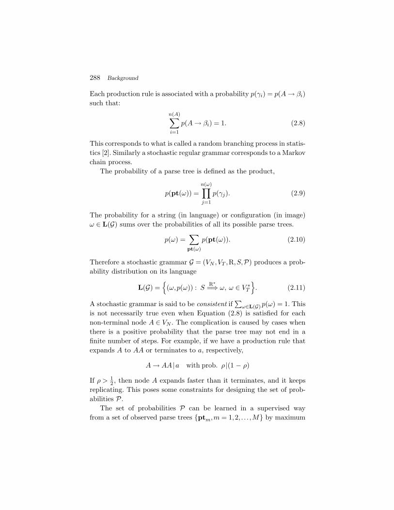
Fig. 2.9 A cheetah and the background after local segmentation: both can be described byan RAG. Without the left-to-right order, if the regions are to be merged one at a time, theyhave a combinatorially explosive number of parse trees.
trees. Figure 2.9 shows an example of parsing an image with a cheetah.It becomes infeasible to estimate the probability p(ω) by summing overall these parse trees in (2.10).
Therefore we must avoid these recursively defined grammar rulesA → aA, and treat the grouping of atomic regions into one large regionA as a single computational step, such as the grouping and partitioningin a graph space [3]. Thus the probability p(ω) is assigned to each objectas a whole instead of the production rules. In the literature, there are anumber of hierarchic representations by an adaptive image pyramid, forexample, the work by Rosenfeld and Hong in the early 80s [34], and themulti-scale segmentation by Galun et al. [23]. Though generic elementsare grouped in these works, there are no explicit grammar rules. Weshall distinguish such multi-scale pyramid representation from parsetrees.
The second issue, unseen in language grammar, is the issue of imagescaling [45, 80, 82]. It is a unique property of vision that objects appearat arbitrary scales in an image when the 3D object lies nearer or far-ther from the camera. You cannot hear or read an English sentenceat multiple scales, but the image grammar must be a multi-resolution

294 Background
images sketches primitives
Fig. 2.10 A face appears at three resolutions is represented by graph configurations in threescales. The right column shows the primitives used at the three levels.
representation. This implies that the parse tree can terminate immedi-ately at any node because no more detail is visible.
Figure 2.10 shows a human face in three levels from [85]. The left col-umn shows face images at three resolutions, the middle column showsthree configurations (graphs) of increasing detail, and the right columnshows the dictionaries (terminals) used at each resolution, respectively.At a low resolution, a face is represented by patches as a whole (forexample, by principle component analysis), at a middle resolution, it isrepresented by a number of parts, and at a higher resolution, the faceis represented by a sketch graph using smaller image primitives. Thesketch graphs shown in the middle of Figure 2.10 expands with increas-ing resolution. One can account for this by adding some terminationrules to each non-terminal node, e.g., each non-terminal node may exitthe production for a low resolution case.
∀A ∈ VN , A → β1 | · · · |βn(A) | t1 | t2 |, (2.18)

2.7 Previous Work in Image Grammars 295
where t1, t2,∈ VT are image primitives or image templates for A at cer-tain scales. For example, if A is a car, then t1, t2 are typical views (smallpatches) of the car at low resolution. As they are in low resolution, theparts of the cars are not very distinguishable and thus are not rep-resented separately. The decompositions βi, i = 1,2, . . . ,n(A) representthe production rules for higher resolutions, so this new issue does notcomplicate the grammar design, except that one must learn the imageprimitives at multiple scales in developing the visual vocabulary.
The third issue with image grammars is that natural images con-tain a much wider spectrum of quite irregular local patterns than inspeech signals. Images not only have very regular and highly struc-tured objects which could be composed by production rules, they alsocontain very stochastic patterns, such as clutter and texture which arebetter represented by Markov random field models. In fact, the spec-trum is continuous. The structured and textured patterns can transferfrom one to the other through continuous scaling [80, 84]. The two cat-egories of models ought to be integrated more intimately and meldedinto a common model. This raises numerous challenges in modeling andlearning at all levels of vision. For example, how do we decide when weshould develop a image primitive (texton) for a specific element or usea texture description (for example, a Markov Random Field)? How dowe decide when we should group objects in a scene by a productionrule or by a Markov random field for context?
2.7 Previous Work in Image Grammars
There are four streams of research on image grammars in the visionliterature.
The first stream is syntactic pattern recognition by K. S. Fu and hisschool in the late 1970s to early 1980s [22]. Fu depicted an ambitiousprogram for scene understanding using grammars. A block world exam-ple is illustrated in Figure 2.11. Similar image understanding systemswere also studied in the 1970–1980s [33, 54] The hierarchical represen-tation on the right is exactly the sort of parse graph that we are pur-suing today. The vertical arrows show the decomposition of the sceneand objects, and the horizontal arrows display some relations, such as

296 Background
Scene A
wall N
floor M
object D
object E
L
T
Z
YX
relation 1: support = (M,D), (M,E) relation 2: adjacency = (L,T), (X,Y), (Y,Z), (Z,X), (M,N)
scene A
D
background Cobjects B
E NM
ZYXTL
1
1
2
2
22
2
Fig. 2.11 A parser tree for a block world from [22]. The ellipses represents non-terminalnodes and the squares are for terminal nodes. The parse tree is augmented into a parsegraph with horizontal connections for relations, such as one object supporting the other, ortwo adjacent objects sharing a boundary.
support and adjacency. Fu and collaborators applied stochastic gram-mars to simple objects (such as diagrams) and shape contours (such asoutline of a chromosome). Most of the work remained in 1D structures,although the ideas of web grammars and plex grammars were also stud-ied. This stream was disrupted in the 1980s and suffered from the lackof an image vocabulary that is realistic enough to express real-worldobjects and scenes, and reliably detectable from images. This remainsa challenge today, though much progress has been made recently inappearance based methods, such as PCAs, image primitives, [31], codebooks [17], fragments and patches [38, 77]. It is worth mentioning thatmany of these works on patches and fragments do not provide a for-malism for composition and that they lack the bond structures studiedin this paper.
The second stream are the medial axis techniques for analyzing2D shapes. For animate objects represented by simple closed contours,Blum argued in 1973 [8] that medial axes are an intuitive and effectiverepresentation of a shape, in contrast to boundary fragments. Leytonproposed a process grammar approach to these in 1988 [43]. He arguedthat any shape is a record of motion history, and developed a gram-mar for the procedure for how a shape grows from a simple object, saya small circle. A shape grammar for shape matching and recognitionvia medial axes was then developed by Zhu and Yuille in 1996 [91].

2.7 Previous Work in Image Grammars 297
S
714
1798
631013
1615
11 12 2 14 5
7
14 17
98
6
3
10 1316
15
11 12
2 1
4 5S
(a) (b) (c)
Fig. 2.12 (a) A dog and its decomposition into parts using the medial axis algorithm of[91]. (b) The shock graph of a goat with its shock tree in (c) adopted from [68]. The rootof the tree is the node at the “hip” of the goat marked by a square.
An example is shown on the left in Figure 2.12. The dog should beread as a node A in the parse tree and the fragments below it as thechild nodes for a production rule that expands the dog into its limbs,trunk, head, and tail. The circles are the maximal circles on which themedial axis is based and allow one to create horizontal arrows betweenthe parts, so that the production yields not merely a set of parts but aconfiguration.
A formal shock graph was studied by Zucker’s school including Dick-inson [40], Kimia [67], Siddiqi et al. [41, 64, 68]. They reverse Leyton’sgrowth process by collapsing the shape using the distance transform.The singularities in the process create “shocks,” for example, whentwo sides of the leg of a dog collapse into an axis. Thus different sec-tions of their skeleton are characterized by the types of singularityand record the temporal record of the shape’s collapse. Figure 2.12shows on the right the shock graph of a goat from [68]. The verticalarrows in their shock tree are very different from those in the parsetree. In the shock tree the child nodes are a younger generation thatgrow from the parent nodes, thus the two graphs have quite differentinterpretations.
The third stream can be seen as a number of works branching outfrom the school of pattern theory. Grenander [28] defined a regular pat-tern on a set of graphs which are made from some primitives which he

298 Background
called “generators.” Each generator is like a terminal element and hasa number of attributes and “bonds” to connect with other generators.Geman and collaborators [6, 27, 36] proposed a more ambitious for-mulation for compositionality which is quite similar to that developedin this paper. Moreover, they seek to create not only computer visionsystems but models of cortical vision mechanisms in animals. In sharpcontrast to our approach, they make the overlapping of their reusableparts into a central element of their formalism. This overlapping is usedto allow parts to compute their “binding strength” depending on anyand all features of this overlap. It is also the key, in their system, tosynchronizing the activity of the neurons expressing the higher orderparts. As a proof of concept, they applied the compositional system tohandwritten upper case letter recognition and to licence plate reading[36]. The work in this paper belongs to this approach, cf. an attributegrammar to parse images of the man-made world [32], and a contextsensitive grammar for representing and recognizing human clothes [9].These will be reviewed in later sections.
Finally, the sparse image coding model can be viewed as an attributeSCFG. In sparse coding [56, 69], an image is made of a number of n
independent image bases, and there are a few types of image bases,such as Gabor cosine, Gabor sine, and Laplacian of Gaussian etc. Thesebases have attributes θ = (x,y,τ,σ,α) for locations, orientations, scalesand contrasts, respectively. This can be expressed as an SCFG. Let S
denote a scene, A an image base, and a,b,c the different bases.
S → An, n ∼ p(n) ∝ e−λon,
A → a(θ) |b(θ) |c(θ), θ ∼ p(θ) ∝ e−λ|α|,
where p(θ) is uniform for location, orientation and scale. Crouse et al.[13] introduce a Markov tree hierarchy for the image bases and thisproduces an SCFG.

3Visual Vocabulary
3.1 The Hierarchic Visual Vocabulary — The “Lego Land”
In English dictionaries, a word not only has a few attributes, such asmeanings, number, tense, and part of speech, but also a number ofways to connect with other words in a context. Sometimes the con-nections are so strong that compound words are created, for example,the word “apple” can be bound with “pine” or “Fuji” to the left, or“pie” and “cart” to the right. For slightly weaker connections, phrasesare used, for instance, the work “make” can be connected with “some-thing” using the prepositions “of” or “from,” or connected with “some-body” through the prepositions “at” or “against.” Figure 3.1 illustratesa word with attributes and a number of “bonds” to connect with otherwords. Thus a word is very much like a piece of Legos for building toyobjects.
The bonds exist more explicitly and are much more necessaryin the 2D image domain. We define the visual vocabulary in thefollowing.
299

300 Visual Vocabulary
MakeAttributes
meaningpluraltensepart of speech
nounverbadverb
...
. from sth
. of sth
. at sb
. against sb
applepine
Fuji cart
pie
(a) (b)
Fig. 3.1 In an English dictionary, each word has a number of attributes and some con-ventional ways to connect to other words. In the first example, the word “make” can beconnected to “something” or “somebody.” The word “apple” has strong bonds with otherwords to make compound words “pine-apple,” “Fuji-apple,” “apple-pie,” “apple-cart.”
Definition 3.1 Visual vocabulary. The visual vocabulary is a set ofpairs, each consisting of an image function Φi(x,y;αi) and a set of d(i)bonds (i.e., its degree), to be eventually connected with other elements,which are denoted by a vector βi = (βi,1, . . . ,βi,d(i)). We think of βi,k
as an address variable or pointer. αi is a vector of attributes for (a) ageometric transformation, e.g., the central position, scale, orientationand plastic deformation, and (b) appearance, such as intensity con-trast, profile or surface albedo. In particular, αi determines a domainΛi(αi) and Φi is then defined for (x,y) ∈ Λi with values in R (a gray-valued template) or R3 (a color template). Often each βi,k is associatedwith a subset of the boundary of Λi(αi). The whole vocabulary is thusa set:
∆ = (Φi(x,y;αi),βi) : (x,y) ∈ Λi(αi) ⊂ Λ, (3.1)
where i indexes the type of the primitives.
The conventional wavelets, Gabor image bases, image patches, andimage fragments are possible examples of this visual vocabulary exceptthat they do not have bonds. As an image grammar must adopt amulti-resolution representation, the elements in its vocabulary repre-sent visual concepts at all levels of abstraction and complexity. In the

3.2 Image Primitives 301
following, we introduce some examples of the visual vocabulary at thelow, middle, and high levels, respectively.
3.2 Image Primitives
In the 1960s–1970s, Julesz conjectured that textons (blobs, bars, ter-minators, crosses) are the atomic elements in the early stage of visualperception for local structures [37]. He found in texture discriminationexperiments that the human visual system seem to detect these ele-ments with a parallel computing mechanism. Marr extended Julesz’stexton concept to image primitives which he called “symbolic tokens” inhis primal sketch representation [49]. An essential criterion in selectinga dictionary in low level vision is to ensure that they are parsimoniousand sufficient in representing real-world images, and more importantlythey should have the necessary structures to allow composition intohigher level parts. In this subsection, we review a dictionary of imageprimitives proposed in Guo et al. [31] as a formal mathematical modelof the primal sketch. Many other studies have come up with similarlists, including studies which are based on the statistical analysis ofsmall image patches from large databases [35, 42, 66].
Illustrated in Figure 3.2(a), an image primitive is a small imagepatch with a degree d connections or bonds which are illustrated bythe half circles. The primitives are called blobs, terminators, edgesor ridges, “L”-junctions, “T”-junctions, and cross junctions for d =0,1,2,3,4, respectively. Each primitive has a number of attributes for itsgeometry and appearance. The geometric attributes include position,orientation, scale, and relative positions of the bonds with respect tothe center. The appearance is described by the intensity profiles aroundthe center and along the directions perpendicular to the line-segmentconnecting the center and the bonds. For instance, a d = 2 primitivecould be called a step edge, a ridge/bar, or double edge dependingon its intensity profile. Each bond of the primitive is like an arm orhand. When the bonds of two primitives are joined by matching thetwo half circles, we say they are connected. Figure 3.2(b) illustrateshow a “T”-shape is composed through 3 terminators, 3 bars, and 1“T”-junction.

302 Visual Vocabulary
(a) (b)
Fig. 3.2 Low level visual vocabulary — image primitives. (a) Some examples of imageprimitives: blobs, terminators, edges, ridges, “L”-junctions, “T”-junction, and cross junctionetc. These primitives are the elements for composing a bigger graph structure at the upperlevel of the hierarchy. (b) is an example of composing a big “T”-shape image using 7primitives. From [30].
In the following, we show how these primitives can be used to rep-resent images. We start with a toy image in Figure 3.3 to illustrate themodel and a real image in Figure 3.4.
In Figure 3.3, the boundaries of the two rectangles are covered by4 “T”-junctions, 8 “L”-junctions, and 20 step edges. We denote thedomain covered by an image primitive Φsk
i by Λsk,i, and the pixelscovered by these primitives, which are called the “sketchable part” in[31], are denoted by
Λsk =nsk⋃i=1
Λsk,i. (3.2)
The image I on Λsk is denoted by Isk and is modeled by the imageprimitives through their intensity profiles. Let ε be the residualnoise.
Isk(x,y) = Φski (x,y;αi,βi) + ε(x,y), (x,y) ∈ Λsk,i, i = 1,2, . . . ,nsk.
(3.3)

3.2 Image Primitives 303
(a) (b)
B
A
B
A
Fig. 3.3 An illustrative example for composing primitives into a graph configuration. (a)is a simple image, and (b) is a number of primitives represented by rectangles which coverthe structured parts of the image. The remaining part of the image can be reconstructedthrough simple heat diffusion.
(a) input image (b) sketch graph configuration (c) pixels covered by primitives
(d) remaining texture pixels (e) texture pixels clustered (f) reconstructed image
Fig. 3.4 An example of the primal sketch model. (a) An input image I. (b) The sketchgraph – configuration computed from the image I. (c) The pixels in the sketchable partΛsk. (d) The remaining non-sketchable portion are textures, which are segmented into asmall number of homogeneous regions in (e). (f) The final synthesized image integratingseamlessly the structures and textures. From [31].

304 Visual Vocabulary
The remaining pixels are flat or stochastic texture areas, called non-sketchable, and are clustered into a few homogeneous texture areas
Λnsk = Λ\Λsk =nnsk⋃j=1
Λnsk,j . (3.4)
They can be reconstructed through Markov random field models con-ditional on Isk,
Insk,j |Isk ∼ p(Insk |Isk;Θj). (3.5)
Θj is a vector-valued parameter for the Gibbs model, for example, theFRAME model [90].
Figure 3.4 shows a real example of the primal sketch model usingprimitives. The input image has 300 × 240 pixels, of which 18,185 pix-els (around 25%) are considered sketchable. The sketch graph has 275edges/ridges (primitives with degree d = 2) and 152 other primitives for“vertices” of the graph. Their attributes are coded by 1,421 bytes. Thenon-sketchable pixels are represented by 455 parameters or less. Theparameters are 5 filters for 7 texture regions and each pools a 1D his-togram of filter responses into 13 bins. Together with the codes for theregion boundaries, total coding length for the textures is 1,628 bytes.The total coding length for the synthesized image in Figure 3.4(f) is3,049 bytes or 0.04 byte per pixel. It should be noted that the codinglength is roughly computed here by treating the primitives as beingindependent. If one accounts for the dependence in the graph andapplies some arithmetic compression schemes, a higher compressionrate can be achieved.
To summarize, we have demonstrated that image primitives cancompose a planar attribute graph configuration to generate the struc-tured part of the image. These primitives are transformed, warped,and aligned to each other to have a tight fit. Adjacent primitives areconnected through their bonds. The explicit use of bonds distinguishesthe image primitives from other basic image representations, such aswavelets and sparse image coding [47, 56] mentioned before, and otherimage patches and fragments in the recent vision literature [77]. Thebonds encode the topological information, in addition to the geometry

3.3 Basic Geometric Groupings 305
and appearance, and enable the composition of bigger and bigger struc-tures in the hierarchy.
3.3 Basic Geometric Groupings
If by analogy, image primitives are like English letters or phonemes,then one wonders what are the visual words and visual phrases. This isthe central question addressed by the gestalt school of psychophysicists[39, 88]. One may summarize their work by saying that the geometricrelations of alignment, parallelism and symmetry, especially as createdby occlusions, are the driving forces behind the grouping of lower levelparts into larger parts. A set of these composite parts is shown inFigure 3.5 and briefly described in the caption.
It is important to realize that these groupings occur at every scale.Many of them occur in local groupings containing as few as 2–8 imageprimitives as in the previous section. We will call these “graphlets” [83].But extended curves, parallels and symmetric structures may span thewhole image. Notably, symmetry is always a larger scale feature butone occurring very often in nature (e.g., in faces) and which is highlydetectable by people even in cluttered scenes. Parallel lines also occur
(a)
(c)
(b)
(d)
(e)
(g)
(f)
(h)
(i)
(k)
(j)
Fig. 3.5 Middle level visual vocabulary: common groupings found in images. (a) extendedcurves, (b) curves with breaks and imperfect alignment, (c) parallel curves, (d) parallelscontinuing past corners, (e) ends of bars formed by parallels and corners, (f) curves continu-ing across paired T-junctions (the most frequent indication of occlusion), (g) a bar occludedby some edge, (h) a square, (i) a curve created by repetition of discrete similar elements,(j) symmetric curves, and (k) parallel lines ending at terminators forming a curve.

306 Visual Vocabulary
(a) (b)
Fig. 3.6 An example of graphlets in natural image. The graphlets are highlighted in theprimal sketch. These graphlets can be viewed as larger pieces of lego. From [24].
frequently in nature, e.g., in tree trunks. The occlusion clue shown inFigure 3.5 is especially important because it is not only common butis the strongest clue in a static 2D image to the 3D structure of thescene. Moreover, it implies the existence of an “amodal” or occludedcontour representing the continuation of the left and right edges behindthe central bar. This necessitates a special purpose algorithm to bediscussed below. Figure 3.6 shows an image with its primal sketch onthe right side with its graphlets shown in dark line segments.
These graphlets are learned through clustering and binding theimage primitives in a way discussed in Equation (2.1). Each cluster inthis space is an equivalence class subject to an affine transform, somedeformation, as well as minor topological editing. These graphlets aregeneric 2D patterns, and some of them could be interpreted as objectparts.
3.4 Parts and Objects
If one is only interested in certain object categories segmented from thebackground, such as bicycles, cars, ipods, chairs, clothes, the dictionarywill be object parts. Although these object parts are significant withineach category or reusable by a few categories, their overall frequency

3.4 Parts and Objects 307
g2
g1
11β
12β13β
β
β β
21β
33β32β
31β23β
22
g3
2425
Fig. 3.7 High level visual vocabulary — the objects and parts. We show an example ofupper body clothes made of three parts: a collar, a left and a right short sleeves. Eachpart is again represented by a graph with bonds. A vocabulary of part for human clothesis shown in Figure 3.8. From [9].
is low and they are often rare events in a big database of real-worldimages. Thus the object parts are less significant as contributors tolowering image entropy than the graphlets presented above, and thelatter are, in turn, less entropically significant than the image primitivesat the low level.
We take one complex object category — clothes as an example.Figure 3.7 shows how a shirt is composed of three parts: a collar, aleft, and a right short sleeves. In this figure, each part is represented byan attribute graph with open bonds, like the graphlets. For example,the collar part has 5 bonds, and the two short sleaves have 3 bonds tobe connected with the arms and collar. By decomposing a number ofinstances in the clothes category together with upper body and shoes,one can obtain a dictionary of parts. Figure 3.8 shows some examplesfor each category.
Thus we denote the dictionary by
∆cloth = (Φclothi (x,y;αi),βi) : ∀i,αi,βi. (3.6)

308 Visual Vocabulary
a
b
c
d
e
f
gh
g
Fig. 3.8 The dictionary of object parts for cloth and body components. Each element is asmall graph composed of primitives and graphlets and has open-bonds for collecting withother parts. Modified from [9].
As before, Φclothi is an image patch defined in a domain Λcloth
i whichdoes not have to be compact or connected. αi controls the geometricand photometric attributes, and βi = (βi1,βi2, . . . ,βid(i)) is a set of openbonds. These bonds shall be represented as address variables that pointto other bonds. Some upper-cloth examples that are synthesized bythese parts are shown in Figure 9.7.
In fact, the object parts defined above are not so much different fromthe dictionaries of image primitives or graphlets, except that they arebigger and more structured. Indeed they form a continuous spectrumfor the vision vocabulary from low to high levels of vision.
By analogy, each part is like a class in object oriented program-ming, such as C++. The inner structures of the class are encapsulated,only the bonds are visible to other classes. These bonds are used forcommunication between different object instances.
In the literature, Biederman [5] proposes a set of “geons” as 3Dobject elements, which are generalized cylinders for representing 3Dman-made objects. In practice, it is very difficult to compute thesegeneralized cylinders from images. In comparison, we adopt a viewbased representation for the primitives, graphlets, and parts which canbe inferred relatively reliably.

4Relations and Configurations
While the hierarchical visual vocabulary represents the vertical compo-sitional structures, the relations in this section represent the horizontallinks for contextual information between nodes in the hierarchy at alllevels. The vocabulary and relations are the ingredients for constructinga large number of image configurations at various level of abstractions.The set of valid configurations constitutes the language of an imagegrammar.
4.1 Relations
We start with a set of nodes V = Ai : i = 1,2, . . . ,n where Ai =(Φi(x,y;αi),βi) ∈ ∆ is an entity representing an image primitive,a grouping, or an object part as defined in the previous section. A num-ber of spatial and functional relations must be defined between thenodes in V to form a graph with colored edges where the color indexesthe type of relation.
Definition 4.1 Attributed Relation. A binary relation defined onan arbitrary set S is a subset of the product set S × S
(s, t) ⊂ S × S. (4.1)
309

310 Relations and Configurations
An attributed binary relation is augmented with a vector of attributesγ and ρ,
E = (s, t;γ,ρ) : s, t ∈ S, (4.2)
where γ = γ(s, t) represents the structure that binds s and t, andρ = ρ(s, t) is a real number measuring the compatibility between s
and t. Then 〈S,E〉 is a graph expressing the relation E on S. A k-wayattributed relation is defined in a similar way as a subset of Sk.
There are three types of relations of increasing abstraction for thehorizontal links and context. The first type is the bond type that con-nects image primitives into bigger and bigger graphs. The second typeincludes various joints and grouping rules for organizing the parts andobjects in a planar layout. The third type is the functional and semanticrelation between objects in a scene.
Relation type 1: Bonds and connections. For a set of nodes V =Ai : i = 1,2, . . . ,n defined above, each node Ai ∈ V has a numberof open bonds βij : j = 1,2, . . . ,n(i) shown by the half disks in theprevious section. We collect all these bonds as a set,
Sbond = βij : i = 1,2, . . . ,n, j = 1,2, . . . ,n(i). (4.3)
Two bonds βij and βkl are said to be connected if they are alignedin position and orientation. Therefore the bonding relation is a set ofpairs of bonds with attributes:
Ebond(S) = (βij ,βkl ; γ,ρ), (4.4)
where γ = (x,y,θ) denote the position and orientation of the bond.The latter is the tangent direction at the bond for the two connectedprimitives. ρ is a function to check the consistency of intensity profileor color between two connected primitives.
The trivial example is the image lattice. The primitives Ai,
i = 1, . . . , |Λ| are the pixels. Each pixel has 4 bonds βij , j = 1,2,3,4.Then Ebond(S) is the set of 4-nearest neighbor connections. In thiscase, γ = nil is empty, and ρ is a pair-clique function for the intensitiesat pixels i and j. Figures 3.5 and 3.7 show more examples of bondsfor composing graphlets from primitives, and composing clothes from

4.1 Relations 311
parts. Very often people use graphical models, such as templates, withfixed structures where the bonds are decided deterministically and thusbecome transparent. In the next subsection, we shall define the bondsas random variables to reconfigure the graph structures.
Relation type 2: Joints and junctions. When image primitives areconnected into larger parts, some spatial and functional relations mustbe found. Besides its open bonds to connect with others, usually itsimmediate neighbors, a part may be bound with other parts in vari-ous ways. The gestalt groupings discussed in the previous section arethe best examples: parts can be linked over possibly large distancesby being collinear, parallel, or symmetric. To identify this groupings,connections must be created flagging this non-accidental relationship.Figure 4.1 displays some typical relations of this type between objectparts.
Some of these relations also contribute to 3D interpretations. Forexample, an ellipse is a part that has multiple possible compositions.If it is recognized as a bike wheel, its center can function as an axisand thus can be connected to the tip of a bar (see the rightmost ofFigure 4.1). It could also be the rim of a tea cup, and then the twoends of its long axis will be joined to a pair of parallel lines to forma cylinder. In Figure 2.8, we discussed a phenomenon occurred in lan-guage where the word “what” is shared by two clauses. Similarly wehave many such joints in images, such as hinge joints, and buttingjoints.
Hinged Butting Concentric Attached Colinear Parallel Radial Bar-circle
Fig. 4.1 Examples of spatial relations for binding object parts. The red dots or lines are theattributes γ(s, t) of joint relation (s, t) which form the “glue” in this relation. From [59].

312 Relations and Configurations
As Figure 4.1 shows, two parts can be hinged at a point. For exam-ple, two hands of a clock have a common axis. For a set of parts in animage S = V , the hinge relation is a set
Ehinge(S) = (Ai,Aj ; γ(Ai,Aj),ρ(Ai,Aj)). (4.5)
Here γ is the hinge point and ρ = nil. In a butting relation, γ(Ai,Aj)represents the line segment(s) shared by the two parts. The line segmentis shown in red in Figure 4.1. Sometimes, two parts may share two linesegments. For example the handle of a teapot or cup share two linesegments with the body.
Relation type 3: Object interactions and semantics. When lettersare grouped into words, semantic meanings emerge. When parts aregrouped into objects, semantic relations are created for their interac-tions. Very often these relations are directed. For example, the occlud-ing relation is a viewpoint dependent binary relation between objector surfaces, and it is important for figure-ground segregation. A viewpoint independent relation is a supporting relation. A simple exampleis shown in Figure 2.11. Let S = V be a set of objects,
Esupp = 〈M,D〉,〈M,E〉,
Eoccld = 〈D,M〉,〈E,M〉,〈D,N〉,〈E,N〉.(4.6)
The 〈 〉 represents directed relation and the attributes γ,ρ are omit-ted. There are other functional relations among objects in a scene. Forexample, a person A is eating an apple BEedible(S) = 〈A,B〉, anda person is riding a bike Eride(S) = 〈A,C〉. These directed relationsusually are partially ordered.
It is worth mentioning that the relations are dense at low level, suchas the bonds, in the sense that the size |E(S)| is in the order of |S|,and that they become very sparse (or rare) and diverse at high level. Atthe high level, we may find many interesting relations but each relationmay only have a few occurrences in the image.
4.2 Configurations
So far, we have introduced the visual dictionaries and relations at vari-ous levels of abstractions. The two components are integrated into whatwe call the visual configuration in the following.

4.2 Configurations 313
Definition 4.2 Configuration. A configuration C is a spatial layoutof entities in a scene at certain level of abstraction. It is a one layergraph, often flattened from hierarchic representation,
C = 〈V,E〉. (4.7)
V = Ai, i = 1,2, . . . ,n is a set of attributed image structures at thesame semantic level, such as primitives, parts, or objects and E is arelation. If V is a set of sketches and E = Ebonds, then C is a primalsketch configuration. If E is a union of several relations E = Er1 ∪ ·· · ∪Erk
, which often occurs at the object level, then C is called a “mixedconfiguration.” For a generative model, the image on a lattice is theultimate “terminal configuration,” and its primal sketch is called the“pre-terminal configuration.” Note that E will close some of the bondsin V and leave others open; thus we may speak of the open bonds in aconfiguration.
We briefly present examples of configurations at three levels.First, for early vision, the scene configuration C is a primal sketch
graph where V is a set of image primitives with bonds and E = Ebonds
is the bond relation. For example, Figure 3.3(b) illustrates a configu-ration for a simple image in Figures 3.3(a), and 3.4(b) is a configura-tion for the image in Figure 3.4(a). These configurations are attributedgraphs because each primitive vi is associated with variables αi for itsgeometric properties and photometric appearance. The primal sketchgraph is a parsimonious “token” representation in Marr’s words [49],and thus it is a crucial stage connecting the raw image signal and thesymbolic representation above it. It can reconstruct the original imagewith perceptually equivalent texture appearance.
Second, for the parts to object level, Figure 9.7 displays three possi-ble upper body configurations composed of a number of clothes’ partsshown in Figure 3.8. In these examples, each configuration C is a graphwith vertices being 6–7 parts and E = Ebond is a set of bonds connect-ing the parts, as it was shown in Figure 3.7.
Third, Figures 4.2(a) and 4.2(b) illustrate a scene configuration atthe highest level of abstraction. V is a set of objects, and E included

314 Relations and Configurations
(a) image (b) layer 1 configuration (c) layer 2 configuration
sky
body
head
field
sky
body
upperhead
field
occludedsky
occludedfield 2
occludedfield 1
lowerhead
Fig. 4.2 An illustration of scene configuration. (a) is a scene of a man in a field.(b) is the graph for the highest level configuration C = 〈V,E〉, V is the set of 4 objectssky, field, head, body and E = Eadj ∪ Eocclude includes two relations: “adjacency” (solidlines) and“occlusion” (dotted arrows). (c) is the configuration at an intermediate level inwhich the occlusion relation is unpacked: now the dotted arrows indicate two identical setsof pixels but on separate layers.
two relations an “adjacency” relation in solid lines
Eadj = (sky,field),(head,body), (4.8)
and a directed “occlusion” relation in dotted arrows,
Econtain = 〈head,sky〉,〈head,field〉,〈body,field〉. (4.9)
In summary, the image grammar which shall be presented in thenext section is also called a “layered grammar.” That is, it can generateconfigurations as its “language” at different levels of detail.
4.3 The Reconfigurable Graphs
In vision, the configurations are inferred from images. For example, ina Bayesian framework, the graph C = 〈V,E〉 will not be pre-determinedbut reconfigurable on-the-fly. That is, the set of vertices may change,so does the set of edges (relations). Therefore, the configurations mustbe made flexible to meet the demand of various visual tasks. Figure 4.3shows such an example.
On the left of the figure is a primal sketch configuration Csk forthe simple image shown in Figure 3.3. This is a planar graph with 4“T”-junctions. In this configuration two adjacent primitives are con-nected by the bond relation Ebond. The four “T”-junctions are then

4.3 The Reconfigurable Graphs 315
B
A
a1
a3 a4
b1
b5
b3
b6b4 b4
b1 b3b2
a4a3
b5
a1
b6
a2
(a) (b)
a2
b2
t3
t1 t2
t4
Fig. 4.3 (a) A primal sketch configuration for a simple image. It has four primitives for“T”-junctions — t1, t2, t3, t4. It is a planar graph formed by bonding the adjacent prim-itives. (b) A layered (2.1D sketch) representation with two occluding surfaces. The four“T”-junctions are broken. The bonds are reorganized. a1 is bonded with a3, and a2 isbonded with a4.
broken in the right configuration, which is called the 2.1D sketch [53]and denoted by C2.1sk. The bonds are reorganized with a1 being con-nected with a3 and a2 with a4. C2.1sk includes two disjoint subgraphsfor the two rectangles in two layers. From this example, we can seethat both the vertices and the bonds must be treated as random vari-ables. Figure 4.4 shows a real application of this sort of reconfigurationin computing a 2.1D sketch from a 2D primal sketch. This exampleis from [25]. It decomposes an input image in Figure 4.4(a) into threelayers in Figures 4.4(d)–(f), found after reconfiguring the bonds by com-pleting the contours (red line segments in Figures 4.4(b) and 4.4(c))behind and filling-in the occluded areas using the Markov random fieldregion descriptor in the primal sketch model. From the point of view ofparse structures, we need to add new nodes to represent the extra lay-ers present behind the observed surfaces together with “occluded by”relations. This is illustrated in Figure 4.2(c). This is a configurationwhich has duplicated three regions to represent missing parts of thebackground layer.
A mathematical model for the reconfigurable graph is called themixed Markov model in [20]. In a mixed Markov model, the bondsare treated as nodes. Therefore, the vertex set V of a configuration

316 Relations and Configurations
(a) input image (b) curve completion at layer 2 (c) curve completion at layer 3
(d) layer 1 (e) layer 2 after fill-in (f) layer 3 after fill-in
Fig. 4.4 From a 2D sketch to a 2.1D layered representation by reconfiguring the bondrelations. (a) is an input image from which a 2D sketch is computed. This is transferred toa 2.1D sketch representations with three layers shown in (d), (e), and (f), respectively. Theinference process reconfigures the bonds of the image primitives shown in red in (b) and(c). From [25].
has two type of nodes — V = Vx ∪ Va. Vx include the usual nodes forimage entities, and Va is a set of address nodes, for example, the bonds.The latter are like the pointers in the C language. These address nodesreconfigure the graphical structure and realize non-local relations. Itwas shown that a probability model defined on such reconfigurablegraphs still observes a suitable form of he Hammersley-Clifford theoremand can be simulated by Gibbs sampler.
By analogy to language, the bonds in this example correspond tothe arrows in the English sentence discussed in Figure 2.8 for non-local context. As there are many possible (bond, joint, functional, andsemantic) relations, each image entity (primitives, parts, objects) mayhave many random variables as the “pointers.” Many of them could beempty, and will be instantiated in the inference process. This is similarto the words “apple” and “make” in Figure 3.1.

5Parse Graph for Objects and Scenes
In this chapter, we define parse graphs as image interpretations. Thenwe will show in the next chapter that these parse graphs are generatedas instances by an And–Or graph. The latter is a general representationthat embeds the image grammar.
Recall that in Section 2.2 a language grammar is a 4-tuple G =(VN ,VT ,R,S), and that a sentence ω is derived (or generated) by asequence of production rules from a starting symbol S,
Sγ1,γ2,...,γn(ω)
=⇒ ω. (5.1)
These production rules form a parse tree for ω,
pt(ω) = (γ1,γ2, . . . ,γn(ω)). (5.2)
For example, Figure 2.6 shows two possible parse trees for a sentence“I saw the man with the telescope.”
This grammar is a generative model, and the inference is an inverseprocess that computes a parse tree for a given sentence as its interpre-tation or one of its best interpretations. Back to image grammars, aconfiguration C is a flat attributed graph corresponding to a sentence ω,and a parse tree pt is augmented to a parse graph pg by adding hor-izontal links for various relations. In previous chapter, Figure 2.11(b)
317

318 Parse Graph for Objects and Scenes
has shown a parse graph for a block work scene, and Figure 1.1 hasshown a parse graph for a football match scene.
In the following, we define a parse graph as an interpretation ofimage.
Definition 5.1 Parse graph. A parse graph pg consists of a hierar-chic parse tree (defining “vertical” edges) and a number of relations E
(defining “horizontal edges”):
pg = (pt,E). (5.3)
The parse tree pt is also an And-tree whose non-terminal nodes areall And-nodes. The decomposition of each And-node A into its partsis given by a production rule which now produces not a string but aconfiguration:
γ : A → C = 〈V,E〉. (5.4)
A production should also associate the open bonds of A with openbonds in C. The whole parse tree is a sequence of production rules
pt(ω) = (γ1,γ2, . . . ,γn). (5.5)
The horizontal links E consists of a number of directed or undirectedrelations among the terminal or non-terminal nodes, such as bonds,junctions, functional and semantic relations,
E = Er1 ∪ Er2 ∪ ·· · ∪ Erk. (5.6)
A parse graph pg, when collapsed, produces a series of flat configura-tions at each level of abstraction/detail,
pg =⇒ C. (5.7)
Depending on the type of relation, there may be special rules for pro-ducing relations at a lower level from higher level relations in the col-lapsing process. The finest configuration is the image itself in whichevery pixel is explained by the parse graph. The next finest configura-tion is the primal sketch graph.

319
... ...
(a) (b)
Fig. 5.1 Two parse graph examples for clocks which are generated from the And–Or-graphin Figure 6.1. From [86].
The parse graph, augmented with spatial context and possiblefunctional relations, is a comprehensive interpretation of the observedimage I. The task of image parsing is to compute the parse graph frominput image(s). In the Bayesian framework, this is to either maximizethe posterior probability for an optimal solution,
pg∗ = argmaxp(pg|I), (5.8)
or sampling the posterior probability for a set of distinct solutions,
pgi : i = 1,2, . . . ,K ∼ p(pg|I). (5.9)
Object instances in the same category may have very different con-figurations and thus distinct parse graphs. Figure 5.1 displays two parsegraphs for two clock instances. It has three levels and the componentsare connected through three types of relations: the hinge joint to con-nect clock hands, a co-centric relation to align the frames, and a radialrelation to align the numbers.
As it was mentioned in Section 2.6, objects appear at arbitraryscales in images. As shown in Figure 2.10, a face can be decomposedinto facial elements at higher resolution, and it may terminate as awhole face for low resolution. Therefore, one remarkable property thatdistinguishes an image parse graph is that a parse graph may stopat any level of abstraction, while the the parse tree in language muststop at the word level. This is the reason for defining visual vocabularyat multiple levels of resolution, and defining the image grammar as alayered grammar.

6Knowledge Representation with And–Or Graph
This chapter addresses the central theme of the paper — developinga consistent representation framework for the vast amount of visualknowledge at all levels of abstraction. The proposed representation isthe And–Or graph embedding image grammars. The And–Or graphrepresentation was first explicitly used in [9] for representing and rec-ognizing a complex object category of clothes.
6.1 And–Or Graph
While a parse graph is an interpretation of a specific image, an And–Orgraph embeds the whole image grammar and contains all the valid parsegraphs. Before introducing the And–Or graph, we revisit the origin ofgrammar and its Chomsky formulation in Sections 2.1 and 2.2.
First, we know each production rule in the SCFG can be written as
A → β1 |β2 · · · |βn(A), with A ∈ VN, β ∈ (VN ∪ VT)+. (6.1)
Therefore each non-terminal node A can be represented by an Or-node with n(A) alternative structures, each of which is an And-nodecomposed of a number of substructures. For example, the following rule
320

6.1 And–Or Graph 321
is represented by a two level And–Or tree in Figure 2.3.
A → a · b |c · c; ρ|(1 − ρ). (6.2)
The two alternatives branches at the Or-node are assigned probabilities(ρ,1 − ρ). Thus an SCFG can be understood as an And–Or tree.
Second, we have shown in Figure 2.4 that a small And–Or tree canproduce a combinatorial number of configurations — called its lan-guage. To represent contextual information in the following, we aug-ment the And–Or tree into an And–Or graph producing a context sen-sitive image grammar.
In a previous survey paper [89], the first author showed that anyvisual pattern can be conceptualized as a statistical ensemble thatobserves a certain statistical description. For a complex object pat-tern, its statistical ensemble must include a large number of distinctconfigurations. Thus our objective is to define an And–Or graph, thusits image grammar, such that its language, i.e., the set of valid config-urations that it produces, reproduces the ensemble of instances for thevisual pattern.
An And–Or graph augments an And–Or tree with two new features.
1. Horizontal lines are indicate to show relations, bonds, junc-tions, and semantic relations.
2. Relations at all levels are augmented on the And–Orgraph to represent hard (compatibility) or soft (statistical)constraints.
3. The children of an Or-node may share Or-node children. Itrepresents a reusable part shared by several production rules.The sharing of nodes reduces the complexity of the represen-tation and thus the size of dictionary. Other possible sharingsmay be useful: see, for example, Section 2.3.
In Chapter 1, Figure 1.3(a) has shown a simple example of an And–Or graph. An And–Or graph includes three types of nodes: And-nodes(solid circles), Or-nodes (dashed circles), and terminal nodes (squares).The Or-nodes have labels for classification at various levels, such as

322 Knowledge Representation with And–Or Graph
scene category, object classes, and parts etc. Due to this recursivedefinition, one may merge the And–Or graphs for many objects orscene categories into a larger graph. In theory, the whole natural imageensemble can be represented by a huge And–Or graph, as it is forlanguage.
By assigning values to these labels on the Or-node, one obtains anAnd-graph — i.e., a parse graph. The bold arrows and shaded nodesin Figure 1.3(a) constitute a parse graph pg embedded in the And–Or graph. This parse graph is shown in Figure 1.3(b) and produces aconfiguration shown in Figure 1.3(d). It has four terminal nodes (forprimitives, parts, or objects): 1,6,8,10 and the edges are inherited fromtheir parent relations. Both nodes 8 and 10 have a common ancestornode C. Therefore the relation 〈B,C〉 is propagated to 〈1,6〉 and 〈1,8〉.For example, if 〈B,C〉 includes three bonds, two bonds may be inheritedby 〈1,8〉 and one by 〈1,6〉. Similarly the links 〈6,10〉 and 〈8,10〉 areinherited from 〈C,D〉.
Figure 1.3(c) is a second parse graph and it produces a configurationin Figure 1.3(e). It has 4 terminal nodes 2,4,9,9′. The node 9 is areusable part shared by nodes C and D. It is worth mentioning that ashared node may appear as multiple instances.
Definition 6.1 And–Or Graph. An And–Or graph is a 6-tuple forrepresenting an image grammar G.
Gand−or = 〈S,VN , VT , R, Σ,P〉. (6.3)
S is a root node for a scene or object category, VN = V and ∪ V or isa set of non-terminal nodes including an And-node set V and and anOr-node set V or. The And-nodes plus the graph formed by their chil-dren are the productions and the Or-nodes are the vocabulary items.VT is a set of terminal nodes for primitives, parts, and objects (notethat an object at low resolution may terminate without decomposi-tion directly), R is a number of relations between the nodes, Σ isthe set of all valid configurations derivable from the grammar, i.e.,its language, and P is the probability model defined on the And–Orgraph.

6.1 And–Or Graph 323
The following is more detailed explanation of the components in theAnd–Or graph.
1. The Non-terminal nodes include both And-nodes and Or-nodes VN = V and ∪ V or,
V and = u1, . . . ,um(u), V or = v1, . . . ,vm(v). (6.4)
An Or-node v ∈ V or is a switch pointing to a number of pos-sible And-nodes, the productions whose head is v.
v → u1 |u2 · · · |un(v), u1, . . . ,un ∈ V and. (6.5)
We define a switch variable ω(v) for v ∈ V , that takes aninteger value to index the child node.
ω(v) ∈ ∅,1,2, . . . ,n(v). (6.6)
By choosing the switch variables in the Or-nodes, one obtainsa parse graph from the And–Or graph. The switch vari-able is set to empty ω(v) = ∅ if v is not part of the parsegraph. In fact the assignments of Or-nodes at various lev-els of the And–Or graph corresponds to scene classificationand object recognition. In practice, when an Or-node has alarge n(v), i.e., too fat, one may replace it by a small Or-treethat has n(v) leaves. We omit the discussion of such cases forclarity.
An And-node u ∈ V and either terminates as a templatet ∈ VT or it can be decomposed into a set of Or-nodes. In thelatter case, the relations between these child nodes are spec-ified by some relations r1, . . . , rk(u) ∈ R shown by the dashedhorizontal lines in Figure 1.3. We adopt the symbol :: for rep-resenting the relations associated with the production rule orthe And-node.
u → t ∈ VT ; or
u → C = (v1, . . . ,vn(v)) :: (r1, . . . , rk(v)), vi ∈ V, rj ∈ R.
The termination rule reflects the multi-scale representation.That is, the node u may be instantiated by a template at arelatively lower image resolution.

324 Knowledge Representation with And–Or Graph
2. The Terminal node set VT = t1, . . . , tm(T ) is a set ofinstances from the image dictionary ∆. Usually it is agraphical template (Φ(x,y;α),β) with attributes α and openbonds β. Usually, each t ∈ VT is a sketch graph, such as theimage primitives.
3. The Configurations which are produced from the root nodeS are the language of the grammar: Gand−or,
L(Gand−or) = Σ =
Ck : SGand−or=⇒ Ck k = 1,2, . . . ,N
. (6.7)
Each configuration C ∈ Σ is a composite template, for exam-ple, the cloth shown in Figure 3.7. The And–Or graph inFigure 1.3(a) contains a combinatorial number of valid con-figurations, e.g.,
Σ = (1,6,8,10),(2,4,9,9),(1,5,11),(2,4,6,7,9), . . .. (6.8)
The first two configurations are shown on the right side ofFigure 1.3.
4. The relation set R pools over all the relations between nodesat all levels.
R =⋃m
Em = est = (vs,vt;γst,ρst). (6.9)
These relations become the pair-cliques in the compositegraphical template. When a node vs is split later, the linkest may be split as well or may descend to specific pairs ofchildren. For example, in Figure 1.3 node C is split into twoleaf nodes 6 and 8, then the relation (B,C) is split into twosubsets between (1,6) and (1,8).
5. P is a probability model defined on the And–Or graph. Itincludes many local probabilities - one at each Or-node toaccount for the relative frequency of each alternative, andlocal energies associated with each link e ∈ R. The formeris like the SCFG and the latter is like the Markov randomfields or graphical models. We will discuss the probabilitycomponent in the next subsection.

6.1 And–Or Graph 325
hands
and-node
or-node
frames numbers
clock
3 hands 2 hands Arabic Roman
hourhand
minutehand
secondhand
a1 a12
nonumber
...
1 12...
r1 r12...
I XII...
leaf-node
... ...
noframe
nohand ...... ...
outerring
innerring
centralring
no ring
Fig. 6.1 An And–Or graph example for the object category — clock. It has two parse graphsshown in Figure 5.1, one of which is illustrated in dark arrows. Some leaf nodes are omittedfrom the graph for clarity. From [86].
Before concluding this section, we show an And–Or graph for a clockcategory [86] in Figure 6.1. Figure 6.1 has shown two parse graphs asinstances of this And–Or graph. The dark bold arrows in Figure 6.1are the parse tree shown in Figure 5.1(a).
Another And–Or example is shown in Figure 9.6. It is a subgraphextracted, for reason of clarity, from a big And–Or graph for the upperbody of human figure [9]. Figure 9.7 displays three cloth configurationsproduced by this And–Or graph.
In summary, an And–Or graph Gand−or defines a context sensi-tive graph grammar with VT being its vocabulary, VN the productionrules, Σ its language, R the contexts. Gand−or contains all the pos-sible parse graphs which in turn produce a combinatorial number ofconfigurations. Again, the number of configurations is far larger than

326 Knowledge Representation with And–Or Graph
the vocabulary, i.e.,
|VN ∪ VT | |Σ|. (6.10)
This is a crucial aspect for representing the large intra-category struc-tural variations.
Our next task is to define a probability model on Gand−or to makeit a stochastic grammar.
6.2 Stochastic Models on the And–Or Graph
The probability model for the And–Or graph Gand−or must inte-grate the Markov tree model (SCFG) for the Or-nodes and thegraphical (Markov) models for the And-nodes. Together a proba-bility model is defined on the parse graphs. The objective of thisprobability model is to match the frequency of parse graphs in anobserved training set (supervised learning will be discussed in the nextsection).
Just as the language model in Equation (2.17) defined probabilitieson each parse tree pt(ω) of each sentence ω, the new model shoulddefine probabilities on each parse graphs pg. As pg produces a finalconfiguration C deterministically when it is collapsed, thus p(pg;Θ)produces a marginal probability on the final configurations with Θbeing its parameters. A configuration C is assumed to be directlyobservable, i.e., the input, and parse graph pg are hidden variablesand have to be inferred.
By definition IV, a parse graph pg is a parse tree pt augmentedwith relations E,
pg = (pt,E). (6.11)
For notational convenience, we denote the following components in pg.
• T (pg) = t1, . . . , tn(pg) is the set of leaf nodes in pg. Forexample, T (pg) = 1,6,8,10 for the parse graph shown bythe dark arrows in Figure 1.3. In applications, T (pg) is oftenthe pre-terminal nodes with each t ∈ T (pg) being an imageprimitive in the primal sketch.

6.2 Stochastic Models on the And–Or Graph 327
• V or(pg) is the set of non-empty Or-nodes (switches) thatare used pg. For instance, V or(pg) = B,C,D,N,O. Theseswitch variables selected the path to decide the parse treept = (γ1,γ2, . . . ,γn).
• E(pg) is the set of links in pg.
The probability for pg is of the following Gibbs form, similar to Equa-tion (2.17),
p(pg;Θ,R,∆) =1
Z(Θ)exp−E(pg), (6.12)
where E(pg) is the total energy,
E(pg) =∑
v∈V or(pg)
λv(ω(v)) +∑
t∈T (pg)∪V and(pg)
λt(α(t))
+∑
(i,j)∈E(pg)
λij(vi,vj ,γij ,ρij). (6.13)
The model is specified by a number of parameters Θ, the relations setR, and the vocabulary ∆. The first term in the energy is the sameas the SCFG. It assigns different weights λv() to the switch variablesω(v) at the or-nodes v. The weight should account for how frequentlya child node appears. Removing the 2nd and 3rd terms, this reduces toan SCFG in Equation (2.9). The second and third terms are typical sin-gleton and pair-clique energy for graphical models. The second term isdefined on the geometric and appearance attributes of the image prim-itives. The third term models the compatibility constraint, such as thespatial and appearance constraint between the primitives, graphlets,parts, and objects.
This model can be derived from a maximum entropy principle undertwo types of constraints on the statistics of training image ensembles.One is to match the frequency at each Or-node, just like the SCFG, andthe other is to match the statistics, such as histograms or co-occurrencefrequency as in standard graphical models. Θ is the set of parametersin the energy,
Θ = λv(),λt(),λij(); ∀v ∈ V or,∀t ∈ VT ,∀(i, j) ∈ R. (6.14)

328 Knowledge Representation with And–Or Graph
Each λ() above is a potential function, not a scalar, and is representedby a vector through discretizing the function in a non-parametric way,as it was done in the FRAME model for texture [90]. ∆ is the vocab-ulary for the generative model. The partition function is summed overall parse graph in the And–Or graph Gand−or or the grammar G.
Z = Z(Θ) =∑pg
exp−E(pg). (6.15)

7Learning and Estimation with And–Or Graph
Suppose we have a training set sampled from an underlying distributionf governing the objects.
Dobs = (Iobsi ,pgobs
i ) : i = 1,2, . . . ,N ∼ f(I,pg). (7.1)
The parse graphs pgobsi are from the groundtruth database [87] or con-
sidered missing in unsupervised case. The objective is to learn a modelp which approaches f by minimizing a Kullback–Leibler divergence,
p∗ = argminKL(f ||p)
= argmin∑
pg∈Ωpg
∫ΩI
f(I,pg) logf(I,pg)
p(I,pg;Θ,R,∆)dI. (7.2)
This is equivalent to the ML estimate for the optimal vocabulary ∆,relation R, and parameter Θ, as it was formulated in [59]
(∆,R,Θ)∗ = argmaxN∑
i=1
logp(Iobsi ,pgobs
i ;Θ,R,∆) − (VT ,VN ,N),
(7.3)where (VT ,VN ,N) is a term that shall balance the model complexityw.r.t. sample size N but also account for the semantic significance of
329

330 Learning and Estimation with And–Or Graph
each elements for the vision purpose (human guided here). The latter isoften reflected by utility or cost functions in Bayesian decision theory.
Learning the probability model includes three phases and all threephases follow the same principle above [59].
1. Estimating the parameters Θ from training date Dobs forgiven R and ∆,
2. Learning and pursuing the relation set R for nodes in Ggiven ∆,
3. Discovering and binding the vocabulary ∆ and hierarchicAnd–Or tree automatically.
In the following we briefly discuss the first two phases. There is nosignificant work done for the third phase yet.
7.1 Maximum Likelihood Learning of Θ
For a given And–Or graph hierarchy and relations, the esti-mation of Θ follows the MLE learning process. Let L(Θ) =∑N
i=1 logp(Iobsi ,pgobs
i ;Θ,R,∆) be the log-likelihood, by setting ∂L(Θ)∂Θ =
0, we have the following three learning steps.
1. Learning the λv at each Or-node v ∈ V or accounts for thefrequency of each alternative choice. The switch variable atv has n(v) choices ω(v) ∈ ∅,1,2, . . . ,n(v) and it is ∅ whenv is not included in the pg. We compute the histogram,
hobsv (ω(v) = i) =
#(ω(v) = i)∑n(v)j=1 #(ω(v) = j)
, i = 1,2, . . . ,n(v).
(7.4)#(ω(v) = i) is the number of times that node v appears withω(v) = i in all the parse graphs in Ωobs
pg . Thus,
λv(ω(v) = i) = − loghobsv (ω(v) = i), ∀v ∈ V or. (7.5)
2. Learning the potential function λt() at the terminal nodet ∈ VT . ∂(Θ)
∂λt= 0 leads to the statistical constraints,
Ep(pg;Θ,R,∆)[h(α(t)] = hobst , ∀t ∈ VT . (7.6)

7.2 Learning and Pursuing the Relation Set 331
In the above equation, α(t) are the attributes of t and h(α(t))is a statistical measure of the attributes, such as the his-togram. hobs
t is the observed histogram pooled over all theoccurrences of t in Ωobs
pg .
hobst (z) =
1#t
∑t
1(z − ε
2< α(t) ≤ z +
ε
2
). (7.7)
#t is the total number of times, a terminal node t appearsin the data Ωobs
pg . z indexes the bins in the histogram and ε
is the length of a bin.3. Learning the potential function λij() for each pair relation
(i, j) ∈ R. ∂(Θ)∂λij
= 0 leads to the following implicit function,
Ep(pg;Θ,R,∆)[h(vi,vj)] = hobsij , ∀(i, j) ∈ R. (7.8)
Again, h(vi,vj) is a statistic on vi,vj , for example, a his-togram on the relative size, position, and orientation, appear-ance etc. hobs
ij is the histogram summed over all the occur-rence of (vi,vj) in Dobs.
The equations (7.5), (7.6), and (7.8) are the constraints for derivingthe Gibbs model p(pg;Θ,R,∆) in Equation (6.12) through the maxi-mum entropy principle.
Due to the coupling of the energy terms, both Equations (7.6) and(7.8) are solved iteratively through a gradient method. In a generalcase, we follow the stochastic gradient method adopted in learning theFRAME model [90], which approximates the expectations Ep[h(α(t))]in Equation (7.6) and Ep[h(vi,vj)] in (7.8) by sample means from a setof synthesized examples. This is the method of analysis-by-synthesisadopted in our texture modeling paper [90]. At the end of this chap-ter, we show the sampling and synthesis experiments on two objectcategories — clock and bike in Figures 7.1 and 7.2.
7.2 Learning and Pursuing the Relation Set
Besides the learning of parameters Θ, we can also augment the rela-tion sets R in an And–Or Graph, and thus pursue the energy terms

332 Learning and Estimation with And–Or Graph
(a)
(b)
(c)
(d)
(e)
Fig. 7.1 Learning the And–Or graph parameters for the clock category. (a) Sampled clockexamples (synthesis) based on SCFG (Markov tree) that accounts for the frequency ofoccurrence. (b–e) Synthesis examples at four incremental stages of the minimax entropypursuit process. (b) Matching the relation positions between parts, (c) further matching therelative scales, (d) further pursuing the hinge relation, (e) further matching the containingrelation. From [59].
in∑
(i,j)∈E(pg)λij(vi,vj) in the same way as pursuing the filters andstatistics in texture modeling by the minimax entropy principle [90].
Suppose we start with an empty relation set R = ∅ and thus p =p(pg;λ,∅,∆) is an SCFG model. The learning procedure is a greedypursuit. In each step, we add a relation e+ to R and thus augmentmodel p(pg;Θ,R,∆) to p+(pg;Θ,R+,∆), where R+ = R ∪ e+.
e+ is selected from a large pool ∆R so as to maximally reduce KL-divergence,
e+ = argmaxKL(f ||p) − KL(f ||p+) = argmaxKL(p+||p), (7.9)
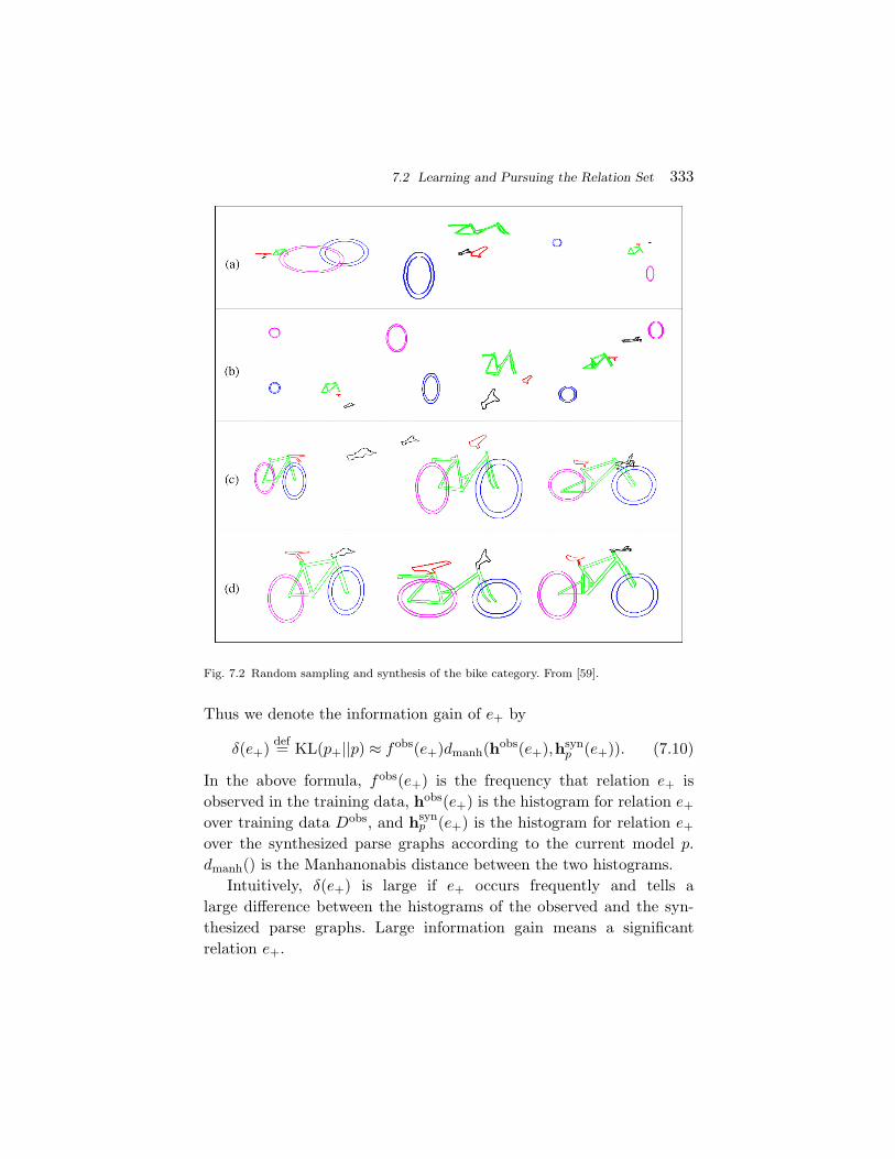
7.2 Learning and Pursuing the Relation Set 333
Fig. 7.2 Random sampling and synthesis of the bike category. From [59].
Thus we denote the information gain of e+ by
δ(e+) def= KL(p+||p) ≈ fobs(e+)dmanh(hobs(e+),hsynp (e+)). (7.10)
In the above formula, fobs(e+) is the frequency that relation e+ isobserved in the training data, hobs(e+) is the histogram for relation e+
over training data Dobs, and hsynp (e+) is the histogram for relation e+
over the synthesized parse graphs according to the current model p.dmanh() is the Manhanonabis distance between the two histograms.
Intuitively, δ(e+) is large if e+ occurs frequently and tells alarge difference between the histograms of the observed and the syn-thesized parse graphs. Large information gain means a significantrelation e+.

334 Learning and Estimation with And–Or Graph
Algorithm 7.1. Learning Θ by Stochastic Gradients
Input: Dobs = pgobsi ; i = 1,2, . . . ,M.
1. Compute histograms hobsv ,hobs
t ,hobsij from Dobs for all fea-
ture/relations.2. Learn the parameters λv at the Or-nodes by Equation (7.5).3. Repeat (outer loop)4. Sample a set of parse graphs from the current model
p(pg;Θ,R,∆) Dsyn = pgsyni ; i = 1,2, ...,M ′
5. Compute histograms hsynt ,hsyn
ij from Dsyn for all feature/relations
6. Select a feature/relation that maximizes the difference betweenobs. vs syn. histograms.
7. Set λ = 0 for the newly selected feature/relation.8. Repeat (inner loop)9. Update the parameters with stepsize η
δλt = ηt (hsynt − hobs
t ), ∀t ∈ VT ,
δλij = ηij (hsynij − hobs
ij ), ∀(i, j) ∈ R.
Sample a set of parse graphs and update the histograms.10. Until |hsyn
t − hobst | ≤ ε and |hsyn
ij − hobsij | ≤ ε for the selected fea-
ture/relations.11. Until |hsyn
t − hobst | ≤ ε and |hsyn
ij − hobsij | ≤ ε for all features and
relations.
Equations (7.6) and (7.8) are then satisfied to certain precision.
7.3 Summary of the Learning Algorithm
In summary, the learning algorithm starts with an SCFG (Markov tree)and a number of observed parse graphs for training Dobs. It first learnsthe SCFG model by counting the occurrence frequency at the Or-nodes.Then by sampling this SCFG, it synthesizes a set of instances Dsyn. Thesampled instances in Dsyn will have the proper components but oftenhave wrong spatial relations among the parts as there are no relations

7.4 Experiments on Learning and Sampling 335
specified in SCFG. Then the algorithm chooses a relation that has themost different statistics (histogram) over some measurement betweenthe sets Dobs and Dsyn. The model is then learned to reproduce theobserved statistics over the chosen relation. A new set of synthesizedinstances is sampled. This iterative process continues until no moresignificant differences are observed between the observed and synthe-sized sets.
Remark 1. At the initial step, the synthesized parse graphs willmatch the frequency counts on all Or-nodes first, but the synthesizedparse graphs and their configurations will not look realistic. Parts ofthe objects will be in wrong positions and have wrong relations. Theiterative steps will make improvements. Ideally, if the features and sta-tistical constraints selected in Equations (7.6) and (7.8) are sufficient,then the synthesized configurations
ΩsynC = Csyn
i : pgsyni −→ Cobs
i , i = 1,2, . . . ,M ′. (7.11)
should resemble the observed configurations. This is what people didin texture synthesis.
Remark 2. Note that in the above learning process, a parse graphpgobs
i contributes to some parameters only when the correspondingnodes and relations are present in pgobs
i .
7.4 Experiments on Learning and Sampling
In [89], the first author showed a range of image synthesis experimentsby sampling the image model (ensembles) for various visual patterns,such as textures, texton processes, shape contours, face etc. to verify thelearned model in the spirit of analysis-by-synthesis. In this subsection,we show synthesis results in sampling the probabilistic ensemble (orthe language) defined by the grammar, i.e., sampling the typical con-figurations from the probabilistic model defined on the And–Or graph.
C ∼ L(Gand−or) =
(Ck,p(Ck)) : SGand−or=⇒ Ck
. (7.12)
This is equivalent to first sampling the parse graphs,
pg;∼ p(pg;Θ,∆), (7.13)
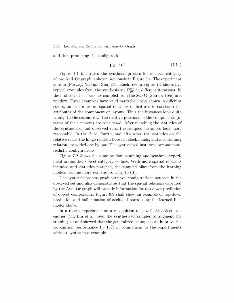
336 Learning and Estimation with And–Or Graph
and then producing the configurations,
pg → C. (7.14)
Figure 7.1 illustrates the synthesis process for a clock categorywhose And–Or graph is shown previously in Figure 6.1. The experimentis from (Porway, Yao and Zhu) [59]. Each row in Figure 7.1 shows fivetypical examples from the synthesis set Ωsyn
pg in different iterations. Inthe first row, the clocks are sampled from the SCFG (Markov tree) in awindow. These examples have valid parts for clocks shown in differentcolors, but there are no spatial relations or features to constrain theattributes of the component or layouts. Thus the instances look quitewrong. In the second row, the relative positions of the components (interms of their centers) are considered. After matching the statistics ofthe synthesized and observed sets, the sampled instances look morereasonable. In the third, fourth, and fifth rows, the statistics on therelative scale, the hinge relation between clock hands, and a containingrelation are added one by one. The synthesized instances become morerealistic configurations.
Figure 7.2 shows the same random sampling and synthesis experi-ment on another object category — bike. With more spatial relationsincluded and statistics matched, the sampled bikes from the learningmodels become more realistic from (a) to (d).
The synthesis process produces novel configurations not seen in theobserved set and also demonstrates that the spatial relations capturedby the And–Or graph will provide information for top-down predictionof object components. Figure 9.9 shall show an example of top-downprediction and hallucination of occluded parts using the learned bikemodel above.
In a recent experiment on a recognition task with 33 object cat-egories [44], Lin et al. used the synthesized samples to augment thetraining set and showed that the generalized examples can improve therecognition performance by 15% in comparison to the expertimentswithout synthesized examples.

8Recursive Top-Down/Bottom-Up Algorithm
for Image Parsing
This chapter briefly reviews an inference algorithm with three casestudies of image parsing using grammars by the author and collabora-tors. The first case is a generic grammar for man-made world scenes.The compositional objects include buildings (indoor or outdoor) andfurniture [32]. The second is a more restrictive grammar for humanclothes and upper body [9]. The third case [86] applies the grammarfor recognizing five object categories — clock, bike, computer (screenand keyboard), cup/bowl, teapot. In both cases, the inference is per-formed under the Bayesian framework. Given an input image I as theterminal configuration, we compute a parse graph pg that maximizesa posterior probability
pg∗ = arg maxpg
p(I|pg;∆sk)p(pg;Θ,∆). (8.1)
The likelihood model is based on the primal sketch in Section 3.2, andthe prior is defined by the grammar model in Equation (6.12).
In the following, we briefly review the computing procedures, andrefer to the original papers [32] and [9] for more details.
The And–Or graph is defined recursively, as is the inferencealgorithm. This recursive property largely simplifies the algorithm
337

338 Recursive Top-Down/Bottom-Up Algorithm for Image Parsing
design and makes it easily scalable to arbitrarily large number of objectcategories.
Consider an arbitrary And-node A in an And–Or graph. A maycorrespond to an object or a part. Without loss of generality, we assumeit can be either terminated into one of n leaves at low resolution ordecomposed into n(A) = 3 parts,
A → A1 · A2 · A3 | t1 | · · · | tn. (8.2)
This recursive unit is shown in Figure 8.1.In this figure, each such unit is associated with data structures which
are widely used in heuristic searches in artificial intelligence [58].
• An Open List stores a number of weighted particles (orhypotheses) which are computed in bottom-up process forthe instances of A in the input image.
• A Closed List stores a number of instances for A which areaccepted in the top-down process. These instances are nodesin the current parse graph pg.
Thus the inference algorithm consists of two basic processes thatcompute and maintain the Open and Closed lists for each unit A.
The bottom-up process creates the particles in the Open lists in twomethods.
(i) Generating hypotheses for A directly from images. Suchbottom-up processes include detection algorithms such as
t1 t2 tn
A
A1 A2 A3
At1 t2 tn
A A1 A2 A3. .
open list (weighted particles for hypotheses)
closed list (accepted instances)
Fig. 8.1 Data structure for the recursive inference algorithm on the And–Or graph. See textfor interpretation.

339
Adaboosting [21, 78], Hough transform etc. for detecting thevarious terminals t1, . . . , tn without identifying the parts. Thedetection process tests some image features. These particlesare shown in Figure 8.1 by single circles with bottom-uparrows. The weight of a detected hypothesis (indexed by i)is the logarithm of some local marginal posterior probabilityratio given a small image patch Λi,
ωiA = log
p(Ai|Iλi)p(Ai|Iλi)
≈ logp(Ai|F (Iλi))p(Ai|F (Iλi))
= ωiA.
A means competitive hypothesis. For computational effec-tiveness, the posterior probability ratio is approximated byposterior probabilities using local features F (Iλi) rather thanthe image Iλi . For example, in face detection by Adaboosting[78], the strong classifier can be reformulated as a posteriorprobability ratio of face vs. non-face [21, 63].
(ii) Generating hypotheses for A by binding a number of k
(1 ≤ K ≤ n(A)) parts from the existing Open and Closedlists of its children A1,A2, . . . ,An(A). The binding process willtest the relationships between these child nodes for compat-ibility and quickly rule out the obviously incompatible com-positions. In Figure 8.1, these hypotheses are illustrated by abig ellipse containing n(A) = 3 small circles for its children.The upward arrows show existing parts in the Open or Closedlists of the child nodes, and the downward arrows show themissing parts that need to be validated in the top-down pro-cess. The weight of a bound hypothesis (indexed by i) isthe logarithm of some local conditional posterior probabilityratio. Suppose a particle Ai is bound from two existing partsAi
1 and Ai2 with Ai
3 missing, and Λi is the domain containingthe hypothesized A. Then the weight will be
ωiA = log
p(Ai|Ai1,A
i2,IΛi)
p(Ai|Ai1,A
i2,IΛi)
= logp(Ai
1,Ai2,IΛi |Ai)p(Ai)
p(Ai1,A
i2,IΛi |Ai)p(Ai)
≈ logp(Ai
1,Ai2|Ai)p(Ai)
p(Ai1,A
i2|Ai)p(Ai)
= ωiA,
340 Recursive Top-Down/Bottom-Up Algorithm for Image Parsing
where A means competitive hypothesis. p(Ai1,A
i2|Ai) is
reduced to tests of compatibility between Ai1 and Ai
2 for com-putational efficiency. It leaves the computation of searchingfor Ai
3 as well as fitting the image area IΛAto the top-down
process.
The top-down process validates the bottom-up hypotheses in all theOpen lists, following the Bayesian posterior probability. It also needsto maintain the weights of the Open lists.
(i) Given a hypothesis Ai with weight ωiA, the top-down process
validates it by computing the true posterior probability ratioωi
A stated above. If Ai is accepted into the Closed list of A.This corresponds to a move from the current parse graphpg to a new parse graph pg+. The latter includes a newnode Ai – either as a leaf node or as a non-terminal nodewith children Ai
1, . . . ,Ain(A). The criterion of the acceptance
is discussed below. In a reverse process, the top-down processmay also select a node A in the Closed list, and then eitherdeletes it (putting it back to the Open list) or disassemblesit into independent parts.
(ii) Maintaining the weights of the particles in the OPEN Listsafter adding (or removing) a node Ai from the parse graph.It is clear that the weight of each particle depends on thecompeting hypothesis. Thus for two competing hypotheses A
and A′ which overlap in a domain Λo, accepting one hypoth-esis will lower the weight of the other. Therefore, wheneverwe add or delete a node A in the parse graph, all the otherhypotheses whose domains overlap with that of A will haveto update their weights.
The acceptance of a node can be done by a greedy algorithm thatmaximizes the posterior probability. Each time it selects the particlewhose weight is the largest among all Open lists and then accepts ituntil the largest weight is below a threshold.
Otherwise, one may use a stochastic algorithm with reversiblejumps. According to the terminology of data driven Markov chain

341
Monte Carlo (DDMCMC) [73, 74], one may view the approximativeweight ωi
A as a logarithm of the proposal probability ratio. The accep-tance probability, in the Metropolis–Hastings method [46], is thus
a(pg → pg+) = min(
1,q(pg+ → pg)q(pg → pg+)
· p(pg+|I)p(pg|I)
)
= min(
1,q+(Ai)q(Ai)
expωiA − ωi
A)
,
where q+(Ai) (or q(Ai)) is the proposal probability for selecting Ai tobe disassembled from pg+ (to be added to pg).
For the stochastic algorithm, its initial stage is often deterministicwhen the particle weights are very large and the acceptance probabilityis always 1.
We summarize the inference algorithm in the following:
Algorithm 8.1. Image Parsing by Top-down/Bottom-upInference
Input: an image I and an And–Or graph.Output: a parse graph pg with initial pg = ∅.
1. Repeat2. Schedule the next visit note A
3. Call the Bottom — Up(A) process to update A’s Open lists4. (i) Detecting terminal instances for A from images5. (ii) Binding non-terminal instances for A from its children’s
Open or Closed lists.6. Call the Top — Down(A) process to update A’s Closed and Open
lists7. (i) Accept hypotheses from A’s Open list to its Closed list.8. (ii) Remove (or disassemble) hypotheses from A’s closed lists.9. (iii) Update the Open lists for particles that overlap with current
node.10. Until a certain number of iteration or the largest particle weight
is below a threshold.

342 Recursive Top-Down/Bottom-Up Algorithm for Image Parsing
The key issue of the inference algorithm is to order the particles inthe Open and Closed lists. In other words, the algorithm must schedulethe bottom-up and top-down processes to achieve computational effi-ciency. For some visual patterns, like human faces in Figure 2.10, itis perhaps more effective to detect the whole face and then locate thefacial components. For other visual patterns, like the cheetah image inFigure 2.9, it is more effective to work in a bottom-up fashion. Moreobjects, like the two examples in the following two subsections, need toalternate between the bottom-up and top-down processes.
The optimal schedule between bottom-up and top-down is a longstanding problem in vision. A greedy way for scheduling is to measurethe information gain of each step, either a bottom-up testing/binding ora top-down validation, divided by its computational complexity (CPUcycles). Then one may order these steps by the gain/cost ratio. A specialcase is studied in [7] for coarse-to-fine testing. Many popular algorithmsin AI heuristic search [58] or the matching pursuit [47] can be considereddeterministic versions of the above algorithm. In DDMCMC [73, 92],the algorithm always performs all the necessary bottom-up tests beforerunning the top-down process. As does the feedforward neural networks[61]. This may not be the optimal schedule.

9Three Case Studies of Image Grammar
9.1 Case Study I: Parsing the Perspective Man-MadeWorld by Han and Zhu
In this case, the grammar has one class of primitives as the terminalnodes (i.e., VT ), which are 3D planar rectangles projected on images.Obviously rectangles are the most common elements in man-madescenes, such as buildings, hallways, kitchens, living rooms, etc. Eachrectangle a ∈ VT is made of two pairs of parallel line segments in 3Dspace, which may intersect at two vanishing points through projection.The grammar has only two types of non-terminal nodes (i.e., VN ) —the root node S for the scene and a node A for any composite objects.The grammar has six production rules as shown in Figure 9.1. Thescene node S generates m independent objects (rule r1). An objectnode A can be instantiated (assigned) to a rectangle (rule r5), or beused recursively by the other four production rules: r2 — the line pro-duction rule that aligns a number of rectangles in one row, r3 — themesh production rule that arranges a number of rectangles in a matrix,r4 — the nesting production rule that has one rectangle containing theother, and r6 — the cube production rule that aligns three rectangle
343
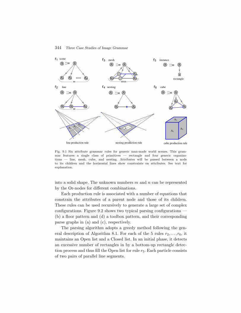
344 Three Case Studies of Image Grammar
r1S ::= S
m
r2
::=A A
A1m
scene
line
r3
::=A A
A11
mxn
mesh
AmA2
r4
::=A A
A1
nesting
A2
r6
::=A A
cube
A1
A2A3
r5
::=A
instance
A
A1A2
A3
line production rule
A1 A2
nesting production rule
A1A2
A3
cube production rule
rectangleA1 A2 Am A1m
A2m a
Fig. 9.1 Six attribute grammar rules for generic man-made world scenes. This gram-mar features a single class of primitives — rectangle and four generic organiza-tions — line, mesh, cube, and nesting. Attributes will be passed between a nodeto its children and the horizontal lines show constraints on attributes. See text forexplanation.
into a solid shape. The unknown numbers m and n can be representedby the Or-nodes for different combinations.
Each production rule is associated with a number of equations thatconstrain the attributes of a parent node and those of its children.These rules can be used recursively to generate a large set of complexconfigurations. Figure 9.2 shows two typical parsing configurations —(b) a floor pattern and (d) a toolbox pattern, and their correspondingparse graphs in (a) and (c), respectively.
The parsing algorithm adopts a greedy method following the gen-eral description of Algorithm 8.1. For each of the 5 rules r2, . . . , r6, itmaintains an Open list and a Closed list. In an initial phase, it detectsan excessive number of rectangles in by a bottom-up rectangle detec-tion process and thus fill the Open list for rule r5. Each particle consistsof two pairs of parallel line segments.

9.1 Case Study I: Parsing the Perspective Man-Made World by Han and Zhu 345
a b c ed
ab c
d er2
r4 r4
r4
a
bc
d
r2
r4r4
r6
abc de
e
f
f
g
g
(a) (d)(c)(b)
Fig. 9.2 Two examples of rectangle object configurations (b) and (d) and their correspond-ing parse graphs (a) and (c). The production rules are shown as non-terminal nodes.
The top-down and bottom-up computation has been illustrated inFigure 1.2 for a kitchen scene. Figure 1.2 shows a parse graph underconstruction at a time step, the four rectangles (in red) are the acceptedrectangles in the Closed list for r5. They activated a number of candi-dates for larger groups using the production rules r3, r4, r6, respectively,and three of these candidates are then accepted as non-terminal nodesA, B, and C, respectively. The solid upward arrows show the bottom-upbinding, while the downward arrows show the top-down prediction.
Figure 9.3 shows the five Open lists for the candidate sets of thefive rules. At each step the parsing algorithm will choose the candidatewith the largest weight from the five particle sets and add a new non-terminal node to the parse graph. If the particle is in the r5 Open list,it means accepting a new rectangle. Otherwise the algorithm creates anon-terminal node and inserts the missing children in this particle intotheir respective Open lists for future tests.
r2
r6
r4
r3
r5
Fig. 9.3 Illustration for the open lists of the five rules.

346 Three Case Studies of Image Grammar
Fig. 9.4 Some experimental results. The first row shows the input images. The second rowshows the computed rectangle configurations. From [32].
Figure 9.4 shows three examples of the inference algorithm. Thecomputed configuration C for each image consists of a number of rect-angles arranged in generic structures. More discussions and experimentsare referred to [32].
Figure 9.5 shows two ROC curves for performance comparisonin detecting the rectangles in 25 images against human annotatedgroundtruth. One curve shows the detection rate (vertical axis) overthe number of false alarms per image (horizontal axis) for pure bottom-up method. The other curve is for the methods integrating bottom-up and top-down. From these ROC curves, we can clearly see thedramatic improvement by using top-down mechanism over the tradi-tionally bottom-up mechanism only. Intuitively, some rectangles arenearly impossible to detect using the bottom-up methods and canonly be recovered through the context information using the grammarrules.
9.2 Case Study II: Human Cloth Modeling and Inferenceby Chen, Xu, and Zhu
The second example, taken from [9], represents and computes clothes byAnd–Or graph. Unlike the rigid rectangle objects in the first example,

9.2 Case Study II: Human Cloth Modeling and Inference by Chen, Xu, and Zhu 347
Fig. 9.5 ROC curves for the rectangle detection results by using bottom-up only and, usingboth bottom-up and top-down. From [32].
human clothes are very flexible objects with large intra-category struc-tural variations.
The authors in [9] took 50 training images of college students sittingin a high chair with good light conditions and uniform background toreduce occlusion and control illumination. An artist was asked to drawsketches as consistent as possible on these images. From the sketches,they manually separate a layer of sketches corresponding to shadingfolds and textures (e.g., shoe lace, text printed on T-shirt), and thendecompose the remaining structures into a number of parts: hair, face,collar, shoulder, upper and lower arms, cuff, hands, pants, shoes, andpockets. Some of the examples are shown in Figure 3.8. The largest twocategories are hands and shoes. The hands have many possible config-urations — separate or held/crossed. The 50 pairs of hands collectedare not necessarily exhaustive. However, an interesting observation inthe experiment is that human vision is not very sensitive to the precise

348 Three Case Studies of Image Grammar
BB
D F
C C E E
... ... ... ... ... ... ...
Arms
Fig. 9.6 The And–Or graph for arms as a part of the overall And–Or graph.
hand gesture/poses. If a test image has a hand configuration outside ofour training category, the algorithm will find a closest match and sim-ply paste the part at the hand position without noticeable difference.Therefore complex parts, such as hands and shoes, can be treated lessprecisely.
With these categories, an And–Or graph is constructed manuallyto account for the variability of configurations. A portion of the And–Or graph for arms and hands is shown in Figure 9.6. Intuitively, thisAnd–Or graph is like a “mother template” and it can produce a largeset of configurations including configurations not seen in the trainingset. Figure 9.7 displays three configurations produced by this And–Orgraph.
This And–Or graph is then used for drawing clothes from imagesusing a version of algorithm II. The algorithm makes use of the bottom-up process for detecting parts that are most discriminable, such as face,skin color, shoulder. Then it activates top-down searches for predictedparts based on the context information encoded in the And–Or graph.Figure 9.8 shows three results of the computed configurations. Thesegraphical sketches are quite nice for they are generated by rearrangingthe artist’s parts. Such results have potential applications in digitalarts and cartoon animations.

9.3 Case Study III: Recognition on Object Categories by Xu, Lin, and Zhu 349
g1 g1
g2 g2g3 g3
g4 g4g5 g5
g6 g7 g6
g7
g1
g2 g3
g4 g5
g7g6
Fig. 9.7 Three novel configurations composed of 6,5,7 sub-templates in the categories,respectively. The bonds are shown by the red dots.
Fig. 9.8 Experiment on inferring upper body with clothes from images. From [9].
9.3 Case Study III: Recognition on Object Categoriesby Xu, Lin, and Zhu
The third example, taken from [86], applies the top-down/bottom-upinference to five object categories — clock, bike, computer (screen and

350 Three Case Studies of Image Grammar
keyboard), cup/bowl, and teapot. The five categories are selected froma large scale ground truth database from the Lotus Hill Institute. Thedatabase includes more than 500,000 objects over 200 categories parsedin And–Or graphs [87]. The probabilistic models are learned for theseAnd–Or graphs using the MLE learning presented in the previous sec-tion. The clock and bike sampling results were shown in Figures 7.1and 7.2.
The And–Or graphs together with their probabilistic models repre-sent the prior knowledge above the five categories for top-down infer-ence. Figure 9.9 shows an example of inferring a partially occludedbicycle from clutter.
In Figure 9.9, the first row shows the input image, an edge map,and bottom-up detection of the two wheels using Hough transform. The
input image edge map bottom up detection
top-down predict 1 top-down predict 3top-down predict 2
match 1 match 2 match 3
imagine 1 imagine 2 imagine 3
Fig. 9.9 The top-down influence in inferring a partially occluded bike from clutter.From [86].

9.3 Case Study III: Recognition on Object Categories by Xu, Lin, and Zhu 351
Hough transform method is adopted to detect parts like circles, ellipses,and triangles. The second row shows some top-down predictions of bikeframe based on the two wheels. The transform parameters of the bikeframe are sampled from the learned MRF model. As we cannot tell thefront wheel from the rear at this moment, the frames are sampled forboth directions. We only show three samples for clarification. The thirdrow shows the template matching process that matching the predictedframes (in red) to the edges (in blue) in the image. The one with min-imum matching cost is selected. The fourth row shows the top-downhallucinations (imaginations) for the seat and handlebar (in green). Asthese two parts are occluded. The three sets of hallucinated parts arerandomly sampled from the And–Or graph model, in the same way asrandom sampling of the whole bike.
Finally, we show a few recognition examples in Figure 10.1 for thefive categories. For each input image, the image on its right-side showsthe recognized parts from the image in different colors. It should bementioned that the recognition algorithm is distinct from most of theclassification algorithms in the literature. It interprets the image by aparse graph which includes the classification of categories and parts onthe Or-nodes, and matches the leaf templates to images, and halluci-nates occluded parts.

10Summary and Discussion
This exploratory paper is concerned with representing large scale visualknowledge in a consistent modeling, learning, and computing frame-work. Specifically two huge problems must be solved before a robustvision system is feasible: (i) large number (hundreds) of object andscene categories; and (ii) large intra-category structural variation. Theframework proposed to tame these two problems is a stochastic graphgrammar embedded in an And–Or graph, which can be learned from alarge annotated dataset.
First, to represent intra-category variation, the grammar can cre-ate a large number of configurations from a relatively much smallervocabulary. The And–Or graph acts like a reconfigurable mother tem-plate, and assembles novel configurations on-the-fly to interpret novelinstances unseen before.
Second, to scale up to hundreds of categories, the And–Or graph isrecursively designed. Thus one can integrate, without much overhead,all categories into one big And–Or graph. The learning and inferencealgorithms are designed recursively as well. This permits large scaleparallel computing.
352

353
Fig. 10.1 Recognition experiments on five object categories. From [86].
There are two open issues for further study.
(i) Learning and discovering the And–Or graph. As it was pro-posed in a series of recent works [17, 52, 59, 81, 86], theobjective is to map the visual vocabulary including dictio-naries at all levels of abstraction and all visual aspects. Thistask can be formulated in theory under a common learn-ing principle, that is to put the dictionary ∆ into the max-imum likelihood learning process. The various informationcriteria, such as the binding strength, mutual information,

354 Summary and Discussion
minimax entropy, will come naturally out of this learningprocess.
However, the ultimate visual vocabulary is unlikely to belearned fully automatically from statistical principles, as thedetermination of the vocabulary must take the purposes ofvision into account. This argues for a semi-automatic methodwhich is being carried out at the Lotus Hill Institute. Humanusers, guided by real life experience, psychology and visiontasks, define most of the structures, and leaving the estima-tion of parameters and adaptation to computers. The com-puters, at a more sophisticated stage, should be able to findand pursue the addition of novel elements in their dictionar-ies. So far, And–Or graphs have been constructed for over200 object and scene categories, including aerial images, atthe Lotus Hill Institute [87].
(ii) Scheduling and ordering of top-down and bottom-up pro-cesses. When we have a big And–Or graph with thousands ofnodes organized hierarchically, we can imagine that the com-puting process is like a many-story factory with thousandsof assembly lines. Intuitively, each assembly line correspondsto the Open and Closed lists of a node in the And–Or graph.With all these assembly lines sharing only one CPU (or evenmultiple CPUs), it is crucial to optimize the schedule to maxi-mize the total throughput of the factory. Traditionally, visionalgorithms always start with bottom-up processes to feedthe assembly lines with raw materials (proposing weightedhypothesis), for example, the DDMCMC [73, 92], and feed-forward neural networks [61]. Due to the multi-resolutionproperty, each node in the And–Or graph can be terminatedimmediately and thus the raw material can be sent to theassembly lines at all stories of the factory directly, insteadof going up story-by-story. This strategy is supported byhuman vision experiments [18, 70] that show humans candetect scene and object categories as fast as we detect thelow level textons and primitives.

355
There has been a long standing debate over the roles of top-downand bottom-up processes [76]. We believe that this debate can only beanswered numerically not verbally. That is to say, we need to compute,numerically, the information gain of each operator, either top-down orbottom-up, over the ensemble of real-world images.

Acknowledgments
The authors thank Drs. Stuart Geman, Yingnian Wu, Harry Shum,Alan Yuille, and Joachim Buhmann for their extensive discussions andhelpful comments. The first author also thanks many students at UCLA(Hong Chen, Jake Porway, Kent Shi, Zijian Xu) and the Lotus HillInstitute (Liang Lin, Zhenyu Yao, Tianfu Wu, Xiong Yang, et al.) fortheir assistance. The work is supported by a NSF grant IIS-0413214 andan ONR grant N00014-05-01-0543. The work at the Lotus Hill Instituteis supported by a Chinese National 863 grant 2006AA01Z121.
356

References
[1] S. P. Abney, “Stochastic attribute-value grammars,” Computational Linguis-tics, vol. 23, no. 4, pp. 597–618, 1997.
[2] K. Athreya and A.Vidyashankar, Branching Processes. Springer-Verlag, 1972.[3] A. Barbu and S. C. Zhu, “Generalizing Swendsen-Wang to sampling arbitrary
posterior probabilities,” IEEE Transactions on PAMI, vol. 27, no. 8, pp. 1239–1253, 2005.
[4] K. Barnard et al., “Evaluation of localized semantics: Data methodology, andexperiments,” Tech. Report, CS, U. Arizona, 2005.
[5] I. Biederman, “Recognition-by-components: A theory of human image under-standing,” Psychological Review, vol. 94, pp. 115–147, 1987.
[6] E. Bienenstock, S. Geman, and D. Potter, “Compositionality, MDL priors, andobject Recognition,” in Advances in Neural Information Processing Systems 9,(M. Mozer, M. Jordan, and T. Petsche, eds.), MIT Press, 1998.
[7] G. Blanchard and D. Geman, “Sequential testing designs for pattern recogni-tion,” Annals of Statistics, vol. 33, pp. 1155–1202, June 2005.
[8] H. Blum, “Biological shape and visual science,” Journal of Theoretical Biology,vol. 38, pp. 207–285, 1973.
[9] H. Chen, Z. J. Xu, Z. Q. Liu, and S. C. Zhu, “Composite templates for clothmodeling and sketching,” in Proceedings of IEEE Conference on Pattern Recog-nition and Computer Vision, New York, June 2006.
[10] Z. Y. Chi and S. Geman, “Estimation of probabilistic context free grammar,”Computational Linguistics, vol. 24, no. 2, pp. 299–305, 1998.
[11] N. Chomsky, Syntactic Structures. Mouton: The Hague, 1957.
357

358 References
[12] T. F. Cootes, C. J. Taylor, D. Cooper, and J. Graham, “Active appearancemodels–their training and applications,” Computer Vision and Image Under-standing, vol. 61, no. 1, pp. 38–59, 1995.
[13] M. Crouse, R. Nowak, and R. Baraniuk, “Wavelet based statistical signal pro-cessing using hidden Markov models,” IEEE Transactions on Signal Processing,vol. 46, pp. 886–902, 1998.
[14] S. J. Dickinson, A. P. Pentland, and A. Rosenfeld, “From volumes to views:An approach to 3D object recognition,” CVGIP: Image Understanding, vol. 55,no. 2, pp. 130–154, 1992.
[15] D. L. Donoho, M. Vetterli, R. A. DeVore, and I. Daubechie, “Data compressionand harmonic analysis,” IEEE Transactions on Information Theory, vol. 6,pp. 2435–2476, 1998.
[16] L. Fei-Fei, R. Fergus, and P. Perona, “Learning generative visual models fromfew training examples: An incremental Bayesian approach tested on 100 objectcategories,” Workshop on Generative Model Based Vision, 2004.
[17] L. Fei-Fei, R. Fergus, and P. Perona, “One-Shot learning of object categories,”IEEE Transactions on PAMI, vol. 28, no. 4, pp. 594–611, 2006.
[18] L. Fei-Fei, A. Iyer, C. Koch, and P. Perona, “What do we perceive in a glanceof a real-world scene?,” Journal of Vision, vol. 7, no. 1, pp. 1–29, 2007.
[19] M. Fischler and R. Elschlager, “The representation and matching of pictorialstructures,” IEEE Transactions on Computer, vol. C-22, pp. 67–92, 1973.
[20] A. Fridman, “Mixed markov models,” Proceedings of Natural Academy of Sci-ence USA, vol. 100, pp. 8092–8096, 2003.
[21] J. Friedman, T. Hastie, and R. Tibshirani, “Additive logistic regression: A sta-tistical view of boosting,” Annals of Statistics, vol. 38, no. 2, pp. 337–374,2000.
[22] K. S. Fu, Syntactic Pattern Recognition and Applications. Prentice-Hall, 1982.[23] M. Galun, E. Sharon, R. Basri, and A. Brandt, “Texture segmentation by
multiscale aggregation of filter responses and shape elements,” Proceedings ofICCV, Nice, pp. 716–723, 2003.
[24] R. X. Gao, T. F. Wu, N. Sang, and S. C. Zhu, “Bayesian inference for layeredrepresentation with mixed Markov random field,” in Proceedings of the 6thInternational Conference on EMMCVPR, Ezhou, China, August 2007.
[25] R. X. Gao and S. C. Zhu, “From primal sketch to 2.1D sketch,” TechnicalReport, Lotus Hill Institute, 2006.
[26] S. Geman and M. Johnson, “Probability and statistics in computational lin-guistics, a brief review,” in Int’l Encyc. of the Social and Behavioral Sciences,(N. J. Smelser and P. B. Baltes, eds.), pp. 12075–12082, Pergamon: Oxford,2002.
[27] S. Geman, D. Potter, and Z. Chi, “Composition systems,” Quarterly of AppliedMathematics, vol. 60, pp. 707–736, 2002.
[28] U. Grenander, General Pattern Theory. Oxford University Press, 1993.[29] G. Griffin, A. Holub, and P. Perona, “The Caltech 256,” Technical Report,
2006.[30] C. E. Guo, S. C. Zhu, and Y. N. Wu, “Modeling visual patterns by integrating
descriptive and generative models,” IJCV, vol. 53, no. 1, pp. 5–29, 2003.

References 359
[31] C. E. Guo, S. C. Zhu, and Y. N. Wu, “Primal sketch: Integrating texture andstructure,” in Proceedings of International Conference on Computer Vision,2003.
[32] F. Han and S. C. Zhu, “Bottom-up/top-down image parsing by attribute graphgrammar”. Proceedings of International Conference on Computer Vision, Bei-jing, China, 2005. (A long version is under review by PAMI).
[33] A. Hanson and E. Riseman, “Visions: A computer system for interpretingscenes,” in Computer Vision Systems, 1978.
[34] T. Hong and A. Rosenfeld, “Compact region extraction using weightedpixel linking in a pyramid,” IEEE Transactions on PAMI, vol. 6, pp. 222–229,1984.
[35] J. Huang, PhD Thesis, Division of Applied Math, Brown University.[36] Y. Jin and S. Geman, “Context and hierarchy in a probabilistic image model,”
in Proceedings of IEEE Conference on Computer Vision and Pattern Recogni-tion, New York, June 2006.
[37] B. Julesz, “Textons, the elements of eexture perception, and their interactions,”Nature, vol. 290, pp. 91–97, 1981.
[38] T. Kadir and M. Brady, “Saliency, scale and image description,” InternationalJournal of Computer Vision, 2001.
[39] G. Kanisza, Organization in Vision. New York: Praeger, 1979.[40] Y. Keselman and S. Dickinson, “Generic model abstraction from examples,”
CVPR, 2001.[41] B. Kimia, A. Tannenbaum, and S. Zucker, “Shapes, shocks and deformations I,”
Interantional Journal of Computer Vision, vol. 15, pp. 189–224, 1995.[42] A. B. Lee, K. S. Pedersen, and D. Mumford, “The nonlinear statistics of
high-contrast patches in natural images,” IJCV, vol. 54, no. 1/2, pp. 83–103,2003.
[43] M. Leyton, “A process grammar for shape,” Artificial Intelligence, vol. 34,pp. 213–247, 1988.
[44] L. Lin, S. W. Peng, and S. C. Zhu, “An empirical study of object categoryrecognition: Sequential testing with generalized samples,” in Proceedings ofInternational Conference on Computer Vision, Rio de Janeiro, Brazil, Octo-ber 2007.
[45] T. Lindeberg, Scale-Space Theory in Computer Vision. Netherlands: KluwerAcademic Publishers, 1994.
[46] J. S. Liu, Monte Carlo Strategies in Scientific Computing. NY: Springer-Verlag,p. 134, 2001.
[47] S. Mallat and Z. Zhang, “Matching pursuit in a time-frequency dictionary,”IEEE Transactions on Signal Processing, vol. 41, pp. 3397–3415, 1993.
[48] K. Mark, M. Miller, and U. Grenander, “Constrained stochastic language mod-els,” in Image Models (and Their Speech Model cousins), (S. Levinson andL. Shepp, eds.), IMA Volumes in Mathematics and its Applications, 1994.
[49] D. Marr, Vision. Freeman Publisher, 1983.[50] D. Martin, C. Fowlkes, D. Tal, and J. Malik, “A database of human segmented
natural images and its application to evaluating segmentation algorithms,”ICCV, 2001.

360 References
[51] H. Murase and S. K. Nayar, “Visual learning and recognition of 3-D objectsfrom appearance,” International Journal of Computer Vision, vol. 14, pp. 5–24,1995.
[52] K. Murphy, A. Torralba, and W. T. Freeman, “Graphical model for recognizingscenes and objects,” Proceedings of NIPS, 2003.
[53] M. Nitzberg, D. Mumford, and T. Shiota, “Filtering, segmentation and depth,”Springer Lecture Notes in Computer Science, vol. 662, 1993.
[54] Y. Ohta, Knowledge-Based Interpretation of Outdoor Natural Color Scenes.Pitman, 1985.
[55] Y. Ohta, T. Kanade, and T. Sakai, “An analysis system for scenes containingobjects with substructures,” in Proceedings of 4th International Joint Confer-ence on Pattern Recognition, (Kyoto), pp. 752–754, 1978.
[56] B. A. Olshausen and D. J. Field, “Emergence of simple-cell receptive fieldproperties by learning a sparse code for natural images,” Nature, vol. 381,pp. 607–609, 1996.
[57] B. Ommer and J. M. Buhmann, “Learning compositional categorizationmethod,” in Proceedings of European Conference on Computer Vision, 2006.
[58] J. Pearl, Heuristics: Intelligent Search Strategies for Computer Problem Solving.Addison-Wesley, 1984.
[59] J. Porway, Z. Y. Yao, and S. C. Zhu, “Learning an And–Or graph for modelingand recognizing object categories,” Technical Report, Department of Statistics,2007.
[60] J. Rekers and A. Schurr, “A parsing algorithm for context sensitive graphgrammars,” TR-95–05, Leiden University, 1995.
[61] M. Riesenhuber and T. Poggio, “Neural mechanisms of object recognition,”Current Opinion in Neurobiology, vol. 12, pp. 162–168, 2002.
[62] B. Russel, A. Torralba, K. Murphy, and W. Freeman, “LabelMe: A databaseand web-based tool for image annotation,” MIT AI Lab Memo AIM-2005-025,September 2005.
[63] R. E. Schapire, “The boosting approach to machine learning: An overview,”MSRI Workshop on nonlinear Estimation and Classification, 2002.
[64] T. B. Sebastian, P. N. Klein, and B. B. Kimia, “Recognition of shapes by editingtheir shock graphs,” IEEE Transactions on PAMI, vol. 26, no. 5, pp. 550–571,2004.
[65] S. M. Sherman and R. W. Guillery, “The role of thalamus in the flow of informa-tion to cortex,” Philosophical Transactions of Royal Society London (Biology),vol. 357, pp. 1695–1708, 2002.
[66] K. Shi and S. C. Zhu, “Visual learning with implicit and explicit manifolds,”IEEE Conference on CVPR, June 2007.
[67] K. Siddiqi and B. B. Kimia, “Parts of visual form: Computational aspects,”IEEE Transactions on PAMI, vol. 17, no. 3, pp. 239–251, 1995.
[68] K. Siddiqi, A. Shokoufandeh, S. J. Dickinson, and S. W. Zucker, “Shock graphsand shape matching,” IJCV, vol. 35, no. 1, pp. 13–32, 1999.
[69] E. P. Simoncelli, W. T. Freeman, E. H. Adelson, and D. J. Heeger, “Shiftablemulti-scale transforms,” IEEE Transactions on Information Theory, vol. 38,no. 2, pp. 587–607, 1992.

References 361
[70] S. Thorpe, D. Fize, and C. Marlot, “Speed of processing in the human visualsystem,” Nature, vol. 381, pp. 520–522, 1996.
[71] S. Todorovic and N. Ahuja, “Extracting subimages of an unknown categoryfrom a set of images,” CVPR, 2006.
[72] Z. W. Tu, X. R. Chen, A. L. Yuille, and S. C. Zhu, “Image parsing: Unifyingsegmentation, detection, and recognition,” International Journal of ComputerVision, vol. 63, no. 2, pp. 113–140, 2005.
[73] Z. W. Tu and S. C. Zhu, “Image segmentation by data-driven Markov chainMonte Carlo,” IEEE Transactions on PAMI, May 2002.
[74] Z. W. Tu and S. C. Zhu, “Parsing images into regions, curves and curve groups,”International Journal of Computer Vision, vol. 69, no. 2, pp. 223–249, 2006.
[75] M. Turk and A. Pentland, “Eigenfaces for recognition,” Journal of CognitiveNeuroscience, vol. 3, p. 1, 1991.
[76] S. Ullman, “Visual routine,” Cognition, vol. 18, pp. 97–157, 1984.[77] S. Ullman, E. Sali, and M. Vidal-Naquet, “A fragment-based approach to object
representation and classification,” in Proceedings of 4th International Workshopon Visual Form, Capri, Italy, 2001.
[78] P. Viola and M. Jones, “Rapid object detection using a boosted cascade ofsimple features,” CVPR, pp. 511–518, 2001.
[79] W. Wang, I. Pollak, T.-S. Wong, C. A. Bouman, M. P. Harper, and J. M.Siskind, “Hierarchical stochastic image grammars for classification and segmen-tation,” IEEE Transactions on Image Processing, vol. 15, no. 10, pp. 3033–3052,2006.
[80] Y. Z. Wang, S. Bahrami, and S. C. Zhu, “Perceptual scale space and it applica-tions,” in International Conference on Computer Vision, Beijing, China, 2005.
[81] M. Weber, M. Welling, and P. Perona, “Towards automatic discovery of objectcategories,” IEEE Conference on CVPR, 2000.
[82] A. P. Witkin, “Scale space filtering,” International Joint Conference on AI.Palo Alto: Kaufman, 1983.
[83] T. F. Wu, G. S. Xia, and S. C. Zhu, “Compositional boosting for computinghierarchical image structures,” IEEE Conference on CVPR, June 2007.
[84] Y. N. Wu, S. C. Zhu, and C. E. Guo, “From information scaling laws of naturalimages to regimes of statistical models,” Quarterly of Applied Mathematics,2007 (To appear).
[85] Z. J. Xu, H. Chen, and S. C. Zhu, “A high resolution grammatical model for facerepresentation and sketching,” in Proceedings of IEEE Conference on CVPR,San Diego, June 2005.
[86] Z. J. Xu, L. Lin, T. F. Wu, and S. C. Zhu, “Recursive top-down/bottom-up algorithm for object recognition,” Technical Report, Lotus Hill ResearchInstitute, 2007.
[87] Z. Y. Yao, X. Yang, and S. C. Zhu, “Introduction to a large scale general pur-pose groundtruth database: Methodology, annotation tools, and benchmarks,”in 6th International Conference on EMMCVPR, Ezhou, China, 2007.
[88] S. C. Zhu, “Embedding Gestalt laws in Markov random fields,” IEEE Trans-actions on PAMI, vol. 21, no. 11, 1999.

362 References
[89] S. C. Zhu, “Statistical modeling and conceptualization of visual patterns,”IEEE Transactions on PAMI, vol. 25, no. 6, pp. 691–712, 2003.
[90] S. C. Zhu, Y. N. Wu, and D. B. Mumford, “Minimax entropy principle and itsapplications to texture modeling,” Neural Computation, vol. 9, no. 8, pp. 1627–1660, November 1997.
[91] S. C. Zhu and A. L. Yuille, “Forms: A flexible object recognition and model-ing system,” Interantional Journal of Computer Vision, vol. 20, pp. 187–212,1996.
[92] S. C. Zhu, R. Zhang, and Z. W. Tu, “Integrating top-down/bottom-up forobject recognition by data-driven Markov chain Monte Carlo,” CVPR, 2000.
Related Documents


![homepages.inf.ed.ac.ukhomepages.inf.ed.ac.uk/rbf/BOOKS/BANDB/LIB/bandb6_123.pdf · Grammars with such rules are termed stochastic [Fu 1974]. There is no unique grammar for a given](https://static.cupdf.com/doc/110x72/5e922a79fb4bd55b7d093319/grammars-with-such-rules-are-termed-stochastic-fu-1974-there-is-no-unique-grammar.jpg)