A Stochastic Differential Equation SIS Epidemic Model

!∀!∀ ! #! ∃%∃ & ∋∀

∋ ∃%&& !∋!∀() &&∗(+,−

!

∀#!∃ %

% & &

∋ #

(!

A Stochastic Differential Equation SIS

Epidemic Model

A. Gray1, D. Greenhalgh1, L. Hu2, X. Mao1,∗, J. Pan1

1 Department of Mathematics and Statistics,University of Strathclyde, Glasgow G1 1XH, U.K.

2 Department of Applied Mathematics,Donghua University, Shanghai 201620, China.

Abstract

In this paper we extend the classical SIS epidemic model from a deterministicframework to a stochastic one, and formulate it as a stochastic differential equation(SDE) for the number of infectious individuals I(t). We then prove that this SDEhas a unique global positive solution I(t) and establish conditions for extinctionand persistence of I(t). We discuss perturbation by stochastic noise. In the case ofpersistence we show the existence of a stationary distribution and derive expressionsfor its mean and variance. The results are illustrated by computer simulations,including two examples based on real life diseases.

Key words: SIS model, Brownian motion, stochastic differential equations, ex-tinction, persistence, basic reproduction number, stationary distribution, gonorrhea,pneumococcus.

1 Introduction

Epidemics are commonly modelled by using deterministic compartmental models wherethe population amongst whom the disease is spreading is divided into several classes,such as susceptible, infected and removed individuals. The classical Kermack-McKendrickmodel [15] is sometimes used for modelling common childhood diseases where a typicalindividual starts off susceptible, at some stage catches the disease and after a short infec-tious period becomes permanently immune. This is sometimes called the SIR (susceptible-infected-removed) model.

However some diseases, in particular some sexually transmitted and bacterial diseases,do not have permanent immunity. For these diseases individuals start off susceptible, atsome stage catch the disease and after a short infectious period become susceptible again.There is no protective immunity. For these diseases SIS (susceptible-infected-susceptible)models are appropriate [14]. If S(t) denotes the number of susceptibles and I(t) the

∗Corresponding author and e-mail: [email protected]

1

number of infecteds at time t, then the differential equations which describe the spreadof the disease are:

dS(t)dt

= µN − βS(t)I(t) + γI(t)− µS(t),dI(t)dt

= βS(t)I(t)− (µ+ γ)I(t),(1.1)

with initial values S0 + I0 = N . N is the total size of the population amongst whomthe disease is spreading. Here µ is the per capita death rate, and γ is the rate at whichinfected individuals become cured, so 1/γ is the average infectious period. β is the diseasetransmission coefficient, so that β = λ/N where λ is the per capita disease contact rate. λis the average number of adequate contacts of an infective per day. An adequate contactis one which is sufficient for the transmission of an infection if it is between a susceptibleand an infected individual. This is one of the simplest possible epidemic models andbecause it is so simple it and its variants are commonly studied. For example, SIS modelsare discussed by Brauer et al. [2]. There are many other examples of SIS epidemic modelsin the literature.

In their excellent monograph Hethcote and Yorke [14] outline several mathematicalmodels for gonorrhea with increasing levels of complexity. The simplest of these is theabove model (1.1) with µ set to zero (i.e. no demography). As S + I = N , the totalpopulation is constant, the two models with and without demographics are equivalent; justreplace γ in the model with no demography by µ+ γ to get the model with demography.

This is a very simple model for gonorrhea. It assumes that the population is homoge-neous (so is more suitable for a homosexual than a heterosexual population) and mixingis homogeneous, whereas in practice sexual mixing is extremely heterogeneous. It alsoignores the small but non-zero disease incubation period and assumes that contact ratesremain constant and do not vary seasonally. Lajmanovich and Yorke [17] and Nold [28]discuss heterogeneously mixing SIS epidemic models for the spread of gonorrhea. Themodel (1.1) also ignores screening. Hethcote and Yorke define the contact number to beσ = λ/γ, so in our model σ = βN/(µ+ γ).

If I = I/N is the fraction of the population infected at time t then they show that inour notation the solution is

I(t) =

[

β

βN−µ−γ(1− e−(βN−µ−γ)t) + 1

I0e−(βN−µ−γ)t

]−1

, if βN

µ+γ6= 1,

[

βt+ 1I0

]−1

, if βN

µ+γ= 1.

(1.2)

It is straightforward to show that σ has the usual interpretation as the basic repro-duction number R0. This is the expected number of secondary cases produced by a singlenewly infected individual entering a disease-free population at equilibrium. In such asituation each newly infected individual remains infectious for time 1/(µ+ γ) and duringthis period infects βN of the N susceptibles present. Hence

R0 = σ =βN

µ+ γ. (1.3)

From now on we denote this R0 by RD0 to emphasise that it is R0 for the deterministic

model. It is a straightforward consequence of equations (1.2) that [14]:

2

• If RD0 ≤ 1, limt→∞ I(t) = 0.

• If RD0 > 1, limt→∞ I(t) = N

(

1− 1RD

0

)

.

Another disease for which it is possible to use an SIS model is pneumococcal carriage.Streptococcus pneumoniae (S.pneumoniae) is a bacterium commonly found in the throatof young children. When an individual carries pneumococcus the infectious carriage nor-mally lasts around 7 weeks [30] and at the end of this carriage period the individual issusceptible again. R0 for pneumococcal carriage and transmission is 1.8-2.2 [32]. Lipsitch[20] discusses mathematical models for the transmission of S.pneumoniae with multipleserotypes and vaccination. Lamb, Greenhalgh and Robertson [18] discuss a mathematicalmodel for the transmission of a single serotype of S.pneumoniae with vaccination. Ifwe have only a single serotype and no vaccination then the disease can be modelled byequations (1.1). Other bacterial diseases, for example tuberculosis, can be modelled bySIS models [9].

Allen [1] discusses a stochastic model of the above SIS epidemic model. Howeverthis is done by constructing a stochastic differential equation (SDE) approximation to thecontinuous time Markov Chain model. The latter is obtained by assuming that events oc-curring at a constant rate in the deterministic model occur according to a Poisson processwith the same rate. McCormack and Allen [27] construct a similar SDE approximationto an SIS multihost epidemic model and explore the stochastic and deterministic modelsnumerically. However this is not the only way to introduce stochasticity into the model,and in this paper we explore an alternative, namely parameter perturbation.

We have previously used the technique of parameter perturbation to examine theeffect of environmental stochasticity in a model of AIDS and condom use [5]. We foundthat the introduction of stochastic noise changes the basic reproduction number of thedisease and can stabilise an otherwise unstable system. Ding, Xu and Hu [6] apply asimilar technique to a simpler model of HIV/AIDS transmission. Other previous work onparameter perturbation in epidemic models seems to have concentrated on the SIR model.Tornatore, Buccellato and Vetro [29] discuss an SDE SIR system with and without delaywith a similar parameter perturbation as we shall discuss here. The system for the SDESIR model with no delay is

dS(t) = [µ− βS(t)I(t)− µS(t)]dt− σS(t)I(t)dB(t),

dI(t) = [βS(t)I(t)− (µ+ γ)I(t)]dt+ σS(t)I(t)dB(t),

dR(t) = γI(t)− µR(t),

(1.4)

where B(t) is a Brownian motion. Here S, I and R denote respectively the susceptible,infected and removed fractions of the population, rather than absolute numbers, so thatβ in this model corresponds to βN in (1.1). They study the stability of the disease-freeequilibrium (DFE). They find that

0 < β < min

γ + µ−σ2

2, 2µ

is a sufficient condition for the asymptotic stability of the DFE. Their computer simu-lations for the SDE SIR model agree well with the analytical results and show that the

3

introduction of noise into the system raises the threshold to µ+ γ + (σ2/2), so if

min

µ+ γ −σ2

2, 2µ

< β < γ + µ+σ2

2

then the DFE E0 = (S(0), I(0), R(0)) = (1, 0, 0) is stable and the disease does not occur,whereas if β > γ+µ+(σ2/2) then the DFE is unstable. These results are similar to thoseof [5]. Chen and Li [4] study an SDE version of the SIR model both with and withoutdelay, but introduce stochastic noise in a different way than we and Tornatore, Buccellatoand Vetro [29] do. Lu [22] studies an SIRS (susceptible-infected-removed-susceptible)model which generalises the model of [29] by allowing removed individuals to becomesusceptible again. He extends their results by including the possibility that immunity isonly temporary and improving the analytical bound on the sufficient condition for thestability of the DFE to β < µ+ γ − (σ2/2).

In summary the deterministic SIS epidemic model is one of the simplest possible epi-demic models, which has applications to transmission of real-life diseases, such as pneu-mococcus, gonorrhea and tuberculosis. It is important to include the effect of uncertaintyin estimation of parameters such as the disease transmission coefficient. Whilst severalpapers study the effect of stochastic parameter perturbation on SIR and SIRS epidemicmodels, we are not aware of any literature addressing this issue in SIS epidemic models.This paper is an attempt to fill this gap.

2 Stochastic Differential Equation SIS Model

Throughout this paper, we let (Ω,F , Ftt≥0,P) be a complete probability space with afiltration Ftt≥0 satisfying the usual conditions (i.e. it is increasing and right continuouswhile F0 contains all P-null sets) and we let B(t) be a scalar Brownian motion defined onthe probability space. We use a ∨ b to denote max(a, b), a ∧ b to denote min(a, b), anda.s. to mean almost surely. We will denote the indicator function of a set G by IG.

Let us now consider the second equation of (1.1). To establish the stochastic dif-ferential equation (SDE) model, we naturally re-write this equation in the differentialform

dI(t) = [βS(t)I(t)− (µ+ γ)I(t)]dt. (2.1)

Here [t, t+dt) is a small time interval and we use the notation d· for the small changein any quantity over this time interval when we intend to consider it as an infinitesimalchange, for example dI(t) = I(t + dt) − I(t) and the change dI(t) is described by (2.1).Consider the disease transmission coefficient β in the deterministic model. This can bethought of as the rate at which each infectious individual makes potentially infectiouscontacts with each other individual, where a potentially infectious contact will transmitthe disease if the contact is made by an infectious individual with a susceptible individual.Thus the total number of new infections in the small time interval [t, t+ dt) is

βS(t)I(t)dt

and a single infected individual makes

4

βdt

potentially infectious contacts with each other individual in the small time interval [t, t+dt).

Now suppose that some stochastic environmental factor acts simultaneously on eachindividual in the population. In this case β changes to a random variable β. Moreprecisely each infected individual makes

βdt = βdt+ σdB(t)

potentially infectious contacts with each other individual in [t, t+dt). Here dB(t) = B(t+dt)−B(t) is the increment of a standard Brownian motion. Thus the number of potentiallyinfectious contacts that a single infected individual makes with another individual in[t, t+ dt) is normally distributed with mean βdt and variance σ2dt. Hence E(βdt) = βdtand var(βdt) = σ2dt. As var(βdt) → 0 as dt → 0 this is a biologically reasonable model.Indeed this is a well-established way of introducing stochastic environmental noise intobiologically realistic population dynamic models. See [7, 10, 11, 12, 19, 22, 29] and manyother references.

To motivate our assumption we argue as follows. Suppose that the number of po-tentially infectious contacts between an infectious individual and another individual insuccessive time intervals [t, t+ T ), [t+ T, t+ 2T ), . . . , [t+ (n− 1)T, t+ nT ) are indepen-dent, identically distributed random variables and n is very large. Then by the CentralLimit Theorem the total number of potentially infectious contacts made in [t, t + nT )has approximately a normal distribution with mean nµ0 and variance nσ2

0, where µ0 andσ20 are respectively the mean and variance of the underlying distribution in each of the

separate time intervals of length T . Thus it is reasonable to assume that the total numberof potentially infectious contacts has a normal distribution whose mean and variance scaleas the total length of the time interval as in our assumptions.

Therefore we replace βdt in equation (2.1) by βdt = βdt+ σdB(t) to get

dI(t) = S(t)I(t)(βdt+ σdB(t))− (µ+ γ)I(t)dt. (2.2)

Note that βdt now denotes the mean of the stochastic number of potentially infectiouscontacts that an infected individual makes with another individual in the infinitesimallysmall time interval [t, t+ dt). Similarly, the first equation of (1.1) becomes another SDE.That is, the deterministic SIS model (1.1) becomes the Ito SDE

dS(t) = [µN − βS(t)I(t) + γI(t)− µS(t)]dt− σS(t)I(t)dB(t),dI(t) = [βS(t)I(t)− (µ+ γ)I(t)]dt+ σS(t)I(t)dB(t).

(2.3)

This SDE is called an SDE SIS model.

Given that S(t) + I(t) = N , it is sufficient to study the SDE for I(t)

dI(t) = I(t)(

[βN − µ− γ − βI(t)]dt+ σ(N − I(t))dB(t))

(2.4)

with initial value I(0) = I0 ∈ (0, N). In the following sections we will concentrate on thisSDE only.

5

3 Existence of Unique Positive Solution

The SDE SIS model (2.4) is a special SDE. In order for the model to make sense, we needto show at least that this SDE SIS model does not only have a unique global solution butalso the solution will remain within (0, N) whenever it starts from there. The existinggeneral existence-and-uniqueness theorem on SDEs (see e.g. [23, 24, 25]) is not applicableto this special SDE in order to guarantee these properties. It is therefore necessary toestablish such a new theory.

Theorem 3.1 For any given initial value I(0) = I0 ∈ (0, N), the SDE (2.4) has a uniqueglobal positive solution I(t) ∈ (0, N) for all t ≥ 0 with probability one, namely

PI(t) ∈ (0, N) for all t ≥ 0 = 1.

Proof. Regarding equation (2.4) as an SDE on R, we see that its coefficients are locallyLipschitz continuous. It is known (see e.g. [23, 24, 25]) that for any given initial valueS0 ∈ (0, N) there is a unique maximal local solution I(t) on t ∈ [0, τe), where τe is theexplosion time. Let k0 > 0 be sufficiently large for 1/k0 < I0 < N − (1/k0). For eachinteger k ≥ k0, define the stopping time

τk = inft ∈ [0, τe) : I(t) 6∈ (1/k, N − (1/k)),

where throughout this paper we set inf ∅ = ∞ (as usual, ∅ = the empty set). Clearly, τkis increasing as k → ∞. Set τ∞ = limk→∞ τk, whence τ∞ ≤ τe a.s. If we can show thatτ∞ = ∞ a.s., then τe = ∞ a.s. and I(t) ∈ (0, N) a.s. for all t ≥ 0. In other words, tocomplete the proof all we need to show is that τ∞ = ∞ a.s. If this statement is false, thenthere is a pair of constants T > 0 and ε ∈ (0, 1) such that

Pτ∞ ≤ T > ε.

Hence there is an integer k1 ≥ k0 such that

Pτk ≤ T ≥ ε for all k ≥ k1. (3.1)

Define a function V : (0, N) → R+ by

V (x) =1

x+

1

N − x.

By the Ito formula (see e.g. [25]), we have, for any t ∈ [0, T ] and k ≥ k1,

EV (I(t ∧ τk)) = V (I0) + E

∫ t∧τk

0

LV (I(s))ds, (3.2)

where LV : (0, N) → R is defined by

LV (x) = x

(

−1

x2+

1

(N − x)2

)

[βN − µ− γ − βx]

+ σ2x2(N − x)2(

1

x3+

1

(N − x)3

)

. (3.3)

6

It is easy to show that

LV (x) ≤µ+ γ

x+

βN

N − x+ σ2N2

(

1

x+

1

N − x

)

≤ CV (x), (3.4)

where C = (µ+ γ) ∨ (βN) + σ2N2. Substituting this into (3.2) we get

EV (I(t ∧ τk)) ≤ V (I0) + E

∫ t∧τk

0

CV (I(s))ds ≤ V (I0) + C

∫ t

0

EV (I(s ∧ τk))ds.

The Gronwall inequality yields that

EV (I(T ∧ τk)) ≤ V (I0)eCT . (3.5)

Set Ωk = τk ≤ T for k ≥ k1 and, by (3.1), P(Ωk) ≥ ε. Note that for every ω ∈ Ωk,I(τk, ω) equals either 1/k or N − (1/k), and hence

V (I(τk, ω)) ≥ k.

It then follows from (3.5) that

V (I0)eCT ≥ E

[

IΩk(ω)V (I(τk, ω))

]

≥ k P(Ωk) ≥ εk.

Letting k → ∞ leads to the contradiction

∞ > V (I0)eCT = ∞,

so we must therefore have τ∞ = ∞ a.s., whence the proof is complete.

4 Extinction

In the study of population systems, extinction and persistence are two of most importantissues. We will discuss the extinction of the SDE SIS model (2.4) in this section but leaveits persistence to the next section.

Theorem 4.1 If

RS0 := RD

0 −σ2N2

2(µ+ γ)=

βN

µ+ γ−

σ2N2

2(µ+ γ)< 1 and σ2 ≤

β

N, (4.1)

then for any given initial value I(0) = I0 ∈ (0, N), the solution of the SDE (2.4) obeys

lim supt→∞

1

tlog(I(t)) ≤ βN − µ− γ − 0.5σ2N2 < 0 a.s., (4.2)

namely, I(t) tends to zero exponentially almost surely. In other words, the disease diesout with probability one.

7

Proof. By the Ito formula, we have

log(I(t)) = log(I0) +

∫ t

0

f(I(s))ds+

∫ t

0

σ(N − I(s))dB(s), (4.3)

where f : R → R is defined by

f(x) = βN − µ− γ − βx− 0.5σ2(N − x)2. (4.4)

However, under condition (4.1), we have

f(I(s)) = βN − µ− γ − 0.5σ2N2 − (β − σ2N)I(s)− 0.5σ2I2(s),

≤ βN − µ− γ − 0.5σ2N2,

for I(s) ∈ (0, N). It then follows from (4.3) that

log(I(t)) ≤ log(I0) + (βN − µ− γ − 0.5σ2N2)t+

∫ t

0

σ(N − I(s))dB(s). (4.5)

This implies

lim supt→∞

1

tlog(I(t)) ≤ βN −µ−γ−0.5σ2N2+lim sup

t→∞

1

t

∫ t

0

σ(N − I(s))dB(s) a.s. (4.6)

But by the large number theorem for martingales (see e.g. [25]), we have

lim supt→∞

1

t

∫ t

0

σ(N − I(s))dB(s) = 0 a.s.

We therefore obtain the desired assertion (4.2) from (4.6).

It is useful to observe that in the classical deterministic SIS model (1.1), I(t) tendsto 0 if and only if RD

0 ≤ 1; while in the SDE SIS model (2.3), I(t) tends to 0 if RS0 =

RD0 − 0.5σ2N2/(µ + γ) < 1 and σ2 ≤ β/N . In other words, the conditions for I(t) to

become extinct in the SDE SIS model are weaker than in the classical deterministic SISmodel. The following example illustrates this result more explicitly:

Example 4.2 Throughout the paper we shall assume that the unit of time is one dayand the population sizes are measured in units of 1 million, unless otherwise stated. Withthese units assume that the system parameters are given by

β = 0.5, N = 100, µ = 20, γ = 25, σ = 0.035.

So the SDE SIS model (2.4) becomes

dI(t) = I(t)(

[5− 0.5I(t)]dt+ 0.035(100− I(t))dB(t))

. (4.7)

Noting that

RS0 =

βN

µ+ γ−

σ2N2

2(µ+ γ)=

50

45−

12.25

90= 1.111− 0.136 < 1,

and σ2 = 0.001225 ≤β

N= 0.005,

8

we can therefore conclude, by Theorem 4.1, that for any initial value I(0) = I0 ∈ (0, 100),the solution of (4.7) obeys

lim supt→∞

1

tlog(I(t)) ≤ −1.125 a.s.

That is, I(t) will tend to zero exponentially with probability one.

On the other hand, the corresponding deterministic SIS model (1.1) becomes

dI(t)

dt= I(t)(5− 0.5I(t)). (4.8)

For RD0 > 1, it is known that, for any initial value I(0) = I0 ∈ (0, 100), this solution has

the property

limt→∞

I(t) = N

(

1−1

RD0

)

= 10 (see section 1).

The computer simulations in Figure 4.1, using the Euler Maruyama (EM) method (seee.g. [16, 25, 26]), support these results clearly, illustrating extinction of the disease.

0 2 4 6 8 10

020

4060

80

t

I(t)

StochasticDeterministic

(a)

0 2 4 6 8 10

05

1015

2025

t

I(t)

StochasticDeterministic

(b)

Figure 4.1: Computer simulation of the path I(t) for the SDE SIS model (4.7) and its

corresponding deterministic SIS model (4.8), using the EM method with step size ∆ = 0.001,

using initial values (a) I(0) = 90 and (b) I(0) = 1.

In Theorem 4.1 we require the noise intensity σ2 ≤ β/N . The following theoremcovers the case when σ2 > β/N :

Theorem 4.3 If

σ2 >β

N∨

β2

2(µ+ γ), (4.9)

then for any given initial value I(0) = I0 ∈ (0, N), the solution of the SDE SIS model(2.4) obeys

lim supt→∞

1

tlog(I(t)) ≤ −µ− γ +

β2

2σ2< 0 a.s., (4.10)

9

namely, I(t) tends to zero exponentially almost surely. In other words, the disease diesout with probability one.

Proof. We use the same notation as in the proof of Theorem 4.1. It is easy to see thatthe quadratic function f : R → R defined by (4.4) takes its maximum value f(x) at

x = x :=σ2N − β

σ2.

By condition (4.9), it is easy to see that x ∈ (0, N). Compute

f(x) = βN − µ− γ − 0.5σ2N2 +(σ2N − β)2

2σ2= −µ− γ +

β2

2σ2,

which is negative by condition (4.9). It therefore follows from (4.3) that

log(I(t)) ≤ log(I0) + f(x)t+

∫ t

0

σ(N − I(s))dB(s).

This implies, in the same way as in the proof of Theorem 4.1, that

lim supt→∞

1

tlog(I(t)) ≤ f(x) a.s.,

as required. The proof is hence complete.

Note that condition (4.9) implies that RS0 ≤ 1.

Example 4.4 We keep the system parameters the same as in Example 4.2 but let σ =0.08, so the SDE SIS model (2.4) becomes

dI(t) = I(t)(

[5− 0.5I(t)]dt+ 0.08(100− I(t))dB(t))

. (4.11)

It is easy to verify that the system parameters obey condition (4.9). We can thereforeconclude, by Theorem 4.3, that for any initial value I(0) = I0 ∈ (0, 100), the solution of(4.11) obeys

lim supt→∞

1

tlog(I(t)) ≤ −45 +

0.52

2× 0.082= −25.4688 a.s.

That is, I(t) will tend to zero exponentially with probability one. The computer simula-tions shown in Figure 4.2 support these results clearly.

5 Persistence

Theorem 5.1 If

RS0 :=

βN

µ+ γ−

σ2N2

2(µ+ γ)> 1 (5.1)

10

0 2 4 6 8 10

020

4060

80

t

I(t)

StochasticDeterministic

(a)

0 2 4 6 8 10

05

1015

2025

t

I(t)

StochasticDeterministic

(b)

Figure 4.2: Computer simulation of the path I(t) for the SDE SIS model (4.11) and itscorresponding deterministic SIS model (4.8), using the EM method with step size ∆ = 0.001,

with initial values (a) I(0) = 90 and (b) I(0) = 1.

then for any given initial value I(0) = I0 ∈ (0, N), the solution of the SDE SIS model(2.4) obeys

lim supt→∞

I(t) ≥ ξ a.s. (5.2)

andlim inft→∞

I(t) ≤ ξ a.s. (5.3)

where

ξ =1

σ2

(

√

β2 − 2σ2(µ+ γ)− (β − σ2N))

(5.4)

which is the unique root in (0, N) of

βN − µ− γ − βξ − 0.5σ2(N − ξ)2 = 0. (5.5)

That is, I(t) will rise to or above the level ξ infinitely often with probability one.

Proof. Recall the definition (4.4) of function f : R → R. By condition (5.1), it is easy tosee that equation f(x) = 0 has a positive root and a negative root. The positive one is

1

σ2

(

√

(β − σ2N)2 + 2σ2(βN − µ− γ − 0.5σ2N2)− (β − σ2N))

=1

σ2

(

√

β2 − 2σ2(µ+ γ)− (β − σ2N))

= ξ.

Noting that

f(0) = βN − µ− γ − 0.5σ2N2 > 0 and f(N) = −µ− γ < 0,

we see that ξ ∈ (0, N) and

f(x) > 0 is strictly increasing on x ∈ (0, 0 ∨ x), (5.6)

11

f(x) > 0 is strictly decreasing on x ∈ (0 ∨ x, ξ), (5.7)

whilef(x) < 0 is strictly decreasing on x ∈ (ξ,N). (5.8)

We now begin to prove assertion (5.2). If it is not true, then there is a sufficientlysmall ε ∈ (0, 1) such that

P(Ω1) > ε, (5.9)

where Ω1 = lim supt→∞ I(t) ≤ ξ−2ε. Hence, for every ω ∈ Ω1, there is a T = T (ω) > 0such that

I(t, ω) ≤ ξ − ε whenever t ≥ T (ω). (5.10)

Clearly we may choose ε so small (if necessary reduce it) that f(0) > f(ξ−ε). It thereforefollows from (5.6), (5.7) and (5.10) that

f(I(t, ω)) ≥ f(ξ − ε) whenever t ≥ T (ω). (5.11)

Moreover, by the large number theorem for martingales, there is a Ω2 ⊂ Ω with P(Ω2) = 1such that for every ω ∈ Ω2,

limt→∞

1

t

∫ t

0

σ(N − I(s, ω))dB(s, ω) = 0. (5.12)

Now, fix any ω ∈ Ω1 ∩ Ω2. It then follows from (4.3) and (5.11) that, for t ≥ T (ω),

log(I(t, ω)) ≥ log(I0) +

∫ T (ω)

0

f(I(s, ω))ds+ f(ξ − ε)(t− T (ω))

+

∫ t

0

σ(N − I(s, ω))dB(s, ω). (5.13)

This yields

lim inft→∞

1

tlog(I(t, ω)) ≥ f(ξ − ε) > 0,

whencelimt→∞

I(t, ω) = ∞.

But this contradicts (5.10). We therefore must have the desired assertion (5.2).

Let us now prove assertion (5.3). If it were not true, then there is a sufficiently smallδ ∈ (0, 1) such that

P(Ω3) > δ, (5.14)

where Ω3 = lim inft→∞ I(t) ≥ ξ + 2δ. Hence, for every ω ∈ Ω3, there is a τ = τ(ω) > 0such that

I(t, ω) ≥ ξ + δ whenever t ≥ τ(ω). (5.15)

Now, fix any ω ∈ Ω3 ∩ Ω2. It then follows from (4.3) and (5.8) that, for t ≥ τ(ω),

log(I(t, ω)) ≤ log(I0) +

∫ τ(ω)

0

f(I(s, ω))ds+ f(ξ + δ)(t− τ(ω))

+

∫ t

0

σ(N − I(s, ω))dB(s, ω). (5.16)

12

This, together with (5.12), yields

lim supt→∞

1

tlog(I(t, ω)) ≤ f(ξ + δ) < 0,

whencelimt→∞

I(t, ω) = 0.

But this contradicts (5.15). We therefore must have the desired assertion (5.3). The proofis therefore complete.

Example 5.2 Assume that the system parameters are given by

β = 0.5, N = 100, µ = 20, γ = 25, σ = 0.03.

That is, we keep all the system parameters the same as in Example 4.2 except σ is reducedto 0.03 from 0.035. So the SDE SIS model (2.4) becomes

dI(t) = I(t)(

[5− 0.5I(t)]dt+ 0.03(100− I(t))dB(t))

. (5.17)

Noting that

RS0 =

βN

µ+ γ−

σ2N2

2(µ+ γ)=

50

45− 0.1 > 1,

we compute

ξ =1

σ2

(

√

β2 − 2σ2(µ+ γ)− (β − σ2N))

= 1.2179.

We can therefore conclude, by Theorem 5.1, that for any initial value I(0) = I0 ∈ (0, 100),the solution of (5.17) obeys

lim inft→∞

I(t) ≤ 1.2179 ≤ lim supt→∞

I(t) a.s.

In comparison, we recall that the solution of the corresponding deterministic SIS model(1.2) has the property

limt→∞

I(t) = N

(

1−1

RD0

)

= 10.

The computer simulations in Figure 5.1 support these results clearly, showing fluctuationaround the level 1.2179.

Example 5.3 To further illustrate the effect of the noise intensity σ on the SDE SISmodel, we keep all the parameters in Example 5.2 unchanged but reduce σ to σ = 0.01,namely we have

β = 0.5, N = 100, µ = 20, γ = 25, σ = 0.01.

So the SDE SIS model (2.4) now becomes

dI(t) = I(t)(

[5− 0.5I(t)]dt+ 0.01(100− I(t))dB(t))

. (5.18)

13

0 2 4 6 8 10

020

4060

80

t

I(t)

StochasticDeterministicxi

(a)

0 2 4 6 8 10

010

2030

40

t

I(t)

StochasticDeterministicxi

(b)

Figure 5.1: Computer simulation of the path I(t) for the SDE SIS model (5.17) and itscorresponding deterministic SIS model (4.8), using the EM method with step size ∆ = 0.001

and initial values (a) I(0) = 90 and (b) I(0) = 1.

Noting that

RS0 =

βN

µ+ γ−

σ2N2

2(µ+ γ)=

50

45− 0.011 > 1,

we compute

ξ =1

σ2

(

√

β2 − 2σ2(µ+ γ)− (β − σ2N))

= 9.1751.

We can therefore conclude, by Theorem 5.1, that for any initial value I(0) = I0 ∈ (0, 100),the solution of (5.18) obeys

lim inft→∞

I(t) ≤ 9.1751 ≤ lim supt→∞

I(t) a.s.

The computer simulations in Figure 5.2 support these results clearly, illustrating persis-tence and that the effect of reducing the standard deviation σ is to increase the level ξ,which becomes closer to the limiting value of the corresponding deterministic SIS model.

These computer simulations indicate strongly that ξ will increase to N(1− (1/RD0 )),

which is the equilibrium state of the deterministic SIS model (1.1), as the noise intensityσ decreases to zero. This is of course not surprising. The following proposition describesthis situation rigorously:

Proposition 5.4 Assume that RS0 > 1 and regard ξ defined by (5.4) as a function of σ

for

0 < σ <

√

2(βN − µ− γ)

N:= σ.

Then ξ is strictly decreasing and

limσ→0

ξ = N

(

1−1

RD0

)

and limσ→σ

ξ =

0, if 1 ≤ RD0 ≤ 2,

N(

RD

0−2

RD

0−1

)

, if RD0 > 2.

14

0 2 4 6 8 10

2040

6080

t

I(t)

StochasticDeterministicxi

(a)

0 2 4 6 8 10

510

1520

t

I(t)

StochasticDeterministicxi

(b)

Figure 5.2: Computer simulation of the path I(t) for the SDE SIS model (5.18) and itscorresponding deterministic SIS model (4.8), using the EM method with step size ∆ = 0.001

and initial values (a) I(0) = 90 and (b) I(0) = 1.

Proof. Compute

dξ

dσ=

1

2

(β2

σ4−

2(µ+ γ)

σ2

)− 1

2

(

−4β2

σ5+

4(µ+ γ)

σ3

)

+2β

σ3,

=−2β2 + 2σ2(µ+ γ) + 2β

√

β2 − 2σ2(µ+ γ)

σ3√

β2 − 2σ2(µ+ γ),

=−(

√

β2 − 2σ2(µ+ γ)− β)2

σ3√

β2 − 2σ2(µ+ γ).

Since σ > 0 we have√

β2 − 2σ2(µ+ γ) − β 6= 0. We therefore have that dξ

dσ< 0

which implies that ξ is strictly decreasing as σ increases. Moreover, by the well-knownL’Hopital’s rule,

limσ→0

ξ = limσ→0

[−(β2 − 2σ2(µ+ γ))−1

2 (µ+ γ) +N ] = −µ+ γ

β+N = N

(

1−1

RD0

)

as desired. Furthermore, it is obvious that

limσ→σ

ξ =

√

β2 − 2σ2(µ+ γ)− β + σ2N

σ2.

The numerator equals|βN − 2(µ+ γ)|

N+

βN − 2(µ+ γ)

N,

so if 1 ≤ RD0 ≤ 2 we have limσ→σ ξ = 0, but if RD

0 > 2 we have limσ→σ ξ = N(

RD

0−2

RD

0−1

)

.

The proof is complete.

15

Note that Proposition 5.4 implies that for RS0 > 1, ξ lies between the deterministic

equilibrium value (and limiting value)

N

(

1−1

RD0

)

for I(t) and

max

(

0, N

(

1−1

RD0 − 1

))

.

If RD0 is large then ξ will be close to but beneath the deterministic equilibrium value for

I(t).

Example 5.5 The computer simulations of the solution to the SDE SIS model in thepersistent case also suggest for higher σ that the distribution of the solution is skewed, asthere are larger oscillations above ξ than below ξ, while for lower σ the oscillations aboutξ appear to be more symmetrically distributed. This is confirmed by the histograms inFigure 5.3, showing the distribution of I(t) in the case of β = 0.5, N = 100, µ = 20, γ = 25,and σ= 0.03, 0.02, 0.01, 0.005 and 0.001, respectively. The simulations were run for100,000 iterations with step size ∆ = 0.001, i.e. for 100 time steps, and the first 90,000iterations were discarded to allow for I(t) to reach its recurrent level. The distribution ispositively skewed for σ = 0.03 and 0.02, but as σ reduces it becomes more symmetric aboutξ, so that the distribution appears closer to a normal distribution. The correspondingsample skewness coefficients are 4.8774, 0.9319, 0.1692, 0.1798, and −0.2106.

Testing these data for normality, all tests used were highly significant, conclusivelyrejecting normality in all cases. This is not surprising in view of the very large samplesizes (10,000), as even moderate deviations from the tested distribution will be significant,however the normal QQ plots in Figure 5.4 suggest that these data are not far from beingnormally distributed for smaller values of σ.

6 Stationary Distribution

In the previous section we showed that I(t) will fluctuate around the level ξ ∈ (0, N) withprobability 1 when RS

0 > 1. The computer simulations also strongly indicate that theSDE SIS model (2.4) has a stationary distribution. To be more precise, let PI0,t(·) denotethe probability measure induced by I(t) with initial value I(0) = I0, that is

PI0,t(A) = P(I(t) ∈ A), A ∈ B(0, N),

where B(0, N) is the σ-algebra of all the Borel sets A ⊂ (0, N). If there is a probabilitymeasure P∞(·) on the measurable space ((0, N),B(0, N)) such that

PI0,t(·) → P∞(·) in distribution for any I0 ∈ (0, N),

we then say that the SDE (2.4) has a stationary distribution P∞(·) (see e.g. [13, 26]).To show the existence of a stationary distribution, let us first cite a known result fromHas’minskii [13, pp.118–123] as a lemma.

16

I(t): sigma=0.03

dens

ity

0 5 10 15 20 25 30 35

0.0

0.1

0.2

0.3

I(t): sigma=0.02

dens

ity

0 5 10 15 20 25 30

0.00

0.02

0.04

0.06

0.08

I(t): sigma=0.01

dens

ity

5 10 15

0.00

0.05

0.10

0.15

I(t): sigma=0.005

dens

ity

6 8 10 12 14

0.00

0.05

0.10

0.15

0.20

I(t): sigma=0.001

dens

ity

9.0 9.5 10.0 10.5

0.0

0.2

0.4

0.6

0.8

1.0

1.2

1.4

Figure 5.3: Histograms of the values of the path I(t) for the recurrent SDE SIS model (2.4),for parameter values β = 0.5, N = 100, µ = 20, γ = 25, I(0) = 90, and differing values of σ=

0.03, 0.02, 0.01, 0.005 and 0.001.

Lemma 6.1 The SDE SIS model (2.4) has a unique stationary distribution if there is astrictly proper sub-interval (a, b) of (0, N) such that E(τ) < ∞ for all I0 ∈ (0, a] ∪ [b,N),where

τ = inft ≥ 0 : I(t) ∈ (a, b),

17

−4 −2 0 2 4

510

15

Theoretical Quantiles

Samp

le Qu

antile

s: si

gma=

0.01

−4 −2 0 2 4

68

1012

14

Theoretical Quantiles

Samp

le Qu

antile

s: si

gma=

0.005

−4 −2 0 2 4

9.09.5

10.0

10.5

Theoretical Quantiles

Samp

le Qu

antile

s: si

gma=

0.001

Figure 5.4: Normal quantile-quantile plots of the values of the path I(t) for the recurrent SDESIS model (2.4), for parameter values β = 0.5, N = 100, µ = 20, γ = 25, and differing values of

σ=0.01, 0.005 and 0.001, corresponding to the last three histograms in Figure 5.3.

and, moreover,

supI0∈[a,b]

E(τ) < ∞ for every interval [a, b] ⊂ (0, N).

It should be pointed out that in the original Has’minskii theorem, there is one morecondition which states that the square of the diffusion coefficient of the SDE (2.4), namelyσ2I2(N − I)2, is bounded away from zero for I ∈ (a, b). But this is obvious for the SDE,hence there is no point to state.

Theorem 6.2 If RS0 > 1, then the SDE SIS model (2.4) has a unique stationary distri-

bution.

Proof. We will use the same notation as used in the proofs of Theorems 4.1 and 5.1. Fixany 0 < a < ξ < b < N . We observe from (5.6)–(5.8) that

f(x) ≥ f(0) ∧ f(a) > 0 if 0 < x ≤ a and f(x) ≤ f(b) < 0 if b ≤ x < N. (6.1)

Define τ as in Lemma 6.1. For any I0 ∈ (0, a), it then follows from (4.3) and (6.1) that

log(a) ≥ E(log(I(τ ∧ t)) ≥ log(I0) + (f(0) ∧ f(a))E(τ ∧ t), ∀t ≥ 0.

18

Letting t → ∞ yields

E(τ) ≤log(a/I0)

f(0) ∧ f(a), ∀I0 ∈ (0, a). (6.2)

Similarly, for any I0 ∈ (b,N),

log(b) ≤ E(log(I(τ ∧ t)) ≤ log(I0)− |f(b)|E(τ ∧ t), ∀t ≥ 0.

Letting t → ∞ yields

E(τ) ≤log(N/b)

|f(b)|, ∀I0 ∈ (b,N). (6.3)

The conditions in Lemma 6.1 follow clearly from (6.2) and (6.3). Hence the SDE SISmodel (2.4) has a unique stationary distribution. The proof is complete.

The following theorem gives the mean and variance of the stationary distribution.Such explicit formulae are particularly useful in the test of computer simulations.

Theorem 6.3 Assume that RS0 > 1. Let m and v denote the mean and variance of the

stationary distribution of the SDE SIS model (2.4). Then

m =2β(RS

0 − 1)(µ+ γ)

2β(β − σ2N) + σ2(βN − µ− γ)(6.4)

and

v =m(βN − µ− γ)

β−m2. (6.5)

Proof. Fix any I0 ∈ (0, N). It follows from (2.4) that

I(t) = I0 +

∫ t

0

I(s)[βN − µ− γ − βI(s)]ds+

∫ t

0

σ(N − I(s))dB(s).

Dividing both sides by t, letting t → ∞ and applying the ergodic property of the stationarydistribution (see e.g. [13, 21]) and the large number theorem for martingales (see e.g. [25]),we obtain

0 = (βN − µ− γ)m− βm2, (6.6)

where m2 denotes the second moment of the stationary distribution. Similarly, dividingboth sides of (4.3) by t and letting t → ∞ we get

limt→∞

log(I(t))

t= βN − µ− γ − 0.5σ2N2 − (β − σ2N)m− 0.5σ2m2 a.s. (6.7)

This, together with Theorem 5.1, implies

limt→∞

log(I(t))

t= 0 a.s.

Writing βN − µ− γ − 0.5σ2N2 = (RS0 − 1)(µ+ γ), we then have

0 = (RS0 − 1)(µ+ γ)− (β − σ2N)m− 0.5σ2m2. (6.8)

19

Substituting (6.6) into (6.8) yields

0 = (RS0 − 1)(µ+ γ)− (β − σ2N)m−

σ2(βN − µ− γ)m

2β.

This implies assertion (6.4). Moreover, it follows from (6.6) that

m2 =m(βN − µ− γ)

β.

Hence

v = m2 −m2 =m(βN − µ− γ)

β−m2,

which is the other assertion (6.5). The proof is therefore complete.

Example 6.4 We now use the same parameter values β = 0.5, N = 100, µ = 20 andγ = 25 for both σ = 0.02 and 0.001 and show the results of running 1,000 simulationsof the path I(t) for the recurrent SDE SIS model, for a longer run of 200,000 iterationswith step size ∆ = 0.001, but storing only the last of these I(t) values in each case.Figure 6.1 shows the histogram of the last 10,000 samples from a single run of 200,000iterations, beside the histogram of the last I(t) values from each of the 1,000 simulations,and also the corresponding two empirical cumulative distribution functions (ecdfs), forcomparison, for both values of σ. In each of the two cases, the corresponding histogramsare similar and the ecdfs are close to each other.

The similarity of these distributions in each case of σ may be taken as an illustra-tion of the existence of the stationary distribution of I(t), and that in the simulationsthe probability distribution of I(t) has more or less reached this stationary distribution.From (6.4) and (6.5), for these parameter values the mean and variance of the stationarydistribution are 6.493506 and 22.76944 respectively when σ = 0.02, compared to the twosample means of 7.306251 and 6.557697 and the corresponding unbiased sample variancesof 19.50794 and 23.18525, for the first and second histograms respectively. For σ = 0.001,the mean and variance of the stationary distribution are 9.991898 and 0.08094976, com-pared to the two sample means of 10.01330 and 9.98392 and unbiased sample variancesof 0.06149254 and 0.07802619 respectively for the lower two histograms in Figure 6.1.

7 Two More Realistic Examples

As slightly more realistic examples to illustrate our theory, we suggest two SIS epidemicmodels with parameters estimated from actual disease situations. In this section the unitof time is still one day, but the population values are not scaled as previously:

Model A Gonorrhea amongst homosexuals [14].

In this model, the parameters are given by N = 10, 000, RD0 = 1.4, µ = (1/(40 ×

365.25))/day = 6.84463 × 10−5/day (average sexually active lifetime), γ = (1/55)/day =0.018182/day (based on Yorke et al. [31]). Benenson [3] says that the infectious period

20

I(t): sigma=0.02

de

nsity

0 5 10 15 20 25

0.0

00

.02

0.0

40

.06

0.0

80

.10

I(t): sigma=0.02, 1000 runs

de

nsity

0 5 10 20 30

0.0

00

.02

0.0

40

.06

0.0

8

0 5 10 15 20 25

0.0

0.2

0.4

0.6

0.8

1.0

Empirical cdf plot

I(t) value, sigma= 0.02

ecd

f

I(t): sigma=0.001

de

nsity

9.5 10.0 10.5

0.0

0.5

1.0

1.5

I(t): sigma=0.001, 1000 runs

de

nsity

9.0 9.5 10.0 10.5

0.0

0.2

0.4

0.6

0.8

1.0

1.2

9.5 10.0 10.5 11.0

0.0

0.2

0.4

0.6

0.8

1.0

Empirical cdf plot

I(t) value, sigma= 0.001

ecd

f

Figure 6.1: Histograms of the values of the path I(t) for the recurrent SDE SIS model (2.4) forthe last 10,000 samples of a single run of 200,000 iterations (left plot in each row) and also forthe last iteration from each of 1,000 such runs (middle plot in each row), and the empirical

cumulative distribution plot of each of these (right plot in each row; the black line correspondsto the first histogram and the blue line to the second one), for parameter values

β = 0.5, N = 100, µ = 20, γ = 25, and σ = 0.02 (top row) and σ = 0.001 (bottom row).

21

0 500 1000 1500 2000 2500 3000

10

00

15

00

20

00

25

00

30

00

35

00

t

I(t)

StochasticDeterministicxi

(a)

0 1000 2000 3000 4000 5000 6000

01

00

03

00

05

00

07

00

0

t

I(t)

StochasticDeterministicxi

(b)

0 1000 2000 3000 4000 5000 6000

02

00

04

00

06

00

08

00

0

t

I(t)

StochasticDeterministic

(c)

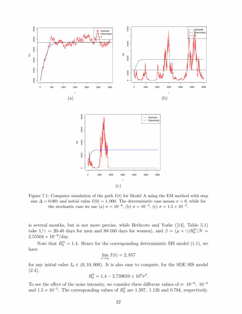
Figure 7.1: Computer simulation of the path I(t) for Model A using the EM method with stepsize ∆ = 0.001 and initial value I(0) = 1, 000. The deterministic case means σ = 0, while for

the stochastic case we use (a) σ = 10−6, (b) σ = 10−5, (c) σ = 1.5× 10−5.

is several months, but is not more precise, while Hethcote and Yorke ([14], Table 5.1)take 1/γ = 20-40 days for men and 80-160 days for women), and β = (µ + γ)RD

0 /N =2.55504× 10−6/day.

Note that RD0 = 1.4. Hence for the corresponding deterministic SIS model (1.1), we

havelimt→∞

I(t) = 2, 857

for any initial value I0 ∈ (0, 10, 000). It is also easy to compute, for the SDE SIS model(2.4),

RS0 = 1.4− 2.739659× 109σ2.

To see the effect of the noise intensity, we consider three different values of σ: 10−6, 10−5

and 1.5× 10−5. The corresponding values of RS0 are 1.397, 1.126 and 0.784, respectively.

22

By Theorem 5.1 we see that the SDE SIS model is persistent in the first two cases.However, in the last case, verifying σ2 = 2.25 × 10−10 < β/N = 2.55504 × 10−10 weconclude by Theorem 4.1 that the SDE SIS model is extinctive. The computer simulationsshown in Figure 7.1 support these results clearly. Figure 7.2 shows the level ξ and thevalue of the mean m in (6.4) as a function of σ in the range given by Proposition 5.4.

0.0e+00 2.0e−06 4.0e−06 6.0e−06 8.0e−06 1.0e−05 1.2e−05

050

010

0015

0020

0025

00

Model A

sigma

level

ximean m

Figure 7.2: Plot of level of ξ (solid curve) and the mean m in (6.4) (dotted curve) against thevalue of σ in the range given in Proposition 5.4, for model A. The horizontal dotted lines show

the levels 0 and N(

1− 1RD

0

)

as limiting values for ξ.

Figure 7.3 shows histograms of the approximate stationary distribution of the twopersistent cases (a) and (b) in Figure 7.1, resulting from the last 2 million iterations (last2,000 days) for case (a) and the last 4 million iterations (4,000 days) for case (b). Bothappear skewed to the right. The sample mean and unbiased sample variance are 2,901.894and 31,045.18 respectively for case (a), compared to the theoretical mean and variance ofthe stationary distribution of 2,847.062 and 28,522.01 from (6.4) and (6.5). For case (b)the sample mean and unbiased sample variance are 1,051.77 and 2,125,489, compared to1,354.592 and 2,035,258 from (6.4) and (6.5).

Model B Pneumococcus amongst children under 2 years in Scotland (Lamb, Greenhalghand Robertson [18]).

In this model, the parameters are given byN = 150,000, γ = 1/(7.1 wk) = 0.02011/day(Weir [30]), µ = 1/(104 wk) = 1.3736 ×10−3/day, and β = 2.0055 ×10−6/wk = 2.8650×10−7/day (Zhang et al. [32]). (Farrington [8] has RD

0 = 1.5, which gives β = 2.1486×10−7/day.)

23

I(t): sigma=1e−06

dens

ity

2600 2800 3000 3200 3400

0.000

00.0

005

0.001

00.0

015

0.002

00.0

025

I(t): sigma=1e−05

dens

ity

0 2000 4000 6000

0e+0

01e

−04

2e−0

43e

−04

4e−0

45e

−04

6e−0

47e

−04

Figure 7.3: Histograms of the values of the path I(t) for model A for Figure 7.1(a) and 7.1(b),using the last 2 million iterations (2,000 days) for case (a) and the last 4 million iterations

(4,000 days) for case (b).

It is easy to compute RD0 = 2. Hence for the corresponding deterministic SIS model

(1.1), we havelimt→∞

I(t) = 75, 000

for any initial value I0 ∈ (0, 150, 000). It is also easy to compute, for the SDE SIS model(2.4),

RS0 = 2− 5.23655× 1011σ2.

To see the effect of the noise intensity, we consider three different values of σ: 10−6, 1.3×10−6 and 1.5 × 10−6. The corresponding values of RS

0 are 1.476, 1.115 and 0.822, re-spectively. By Theorem 5.1 we see that the SDE SIS model is persistent in the first twocases. However, in the last case, verifying σ2 = 2.25× 10−12 > (β/N) ∨ (β2/2(µ + γ)) =1.910347× 10−12 we conclude by Theorem 4.3 that the SDE SIS model is extinctive. Thecomputer simulations shown in Figure 7.4 support these results clearly. In Figure 7.4(c)the deterministic simulation goes off the scale but is the same as in the other two simu-lations. Figure 7.5 shows the level ξ and the value of the mean m in (6.4) as a functionof σ in the range given by Proposition 5.4.

Figure 7.6 shows histograms of the approximate stationary distribution of the twopersistent cases (a) and (b) in Figure 7.4, resulting from the last 2 million iterations(the last 2,000 days). The first appears symmetric, the second positively skewed. Thesample mean and unbiased sample variance are 61,448.49 and 647,526,916 respectivelyfor case (a), compared to the theoretical mean and variance of the stationary distributionof 58,856.32 and 950,958,848 from (6.4) and (6.5). For case (b) the sample mean andunbiased sample variance are 45,633.17 and 1,494,311,814, compared to 25,718.33 and1,267,792,373 from (6.4) and (6.5).

24

0 500 1000 1500 2000 2500 3000

02

00

00

60

00

01

00

00

0

t

I(t)

StochasticDeterministicxi

(a)

0 500 1000 1500 2000 2500 3000

02

00

00

60

00

01

00

00

0

t

I(t)

StochasticDeterministicxi

(b)

0 500 1000 1500 2000 2500 3000

05

00

01

00

00

15

00

0

t

I(t)

StochasticDeterministic

(c)

Figure 7.4: Computer simulation of the path I(t) for Model B using the EM method with stepsize ∆ = 0.001 and initial value I(0) = 50, 000. The deterministic case means σ = 0, while for

the stochastic case we use (a) σ = 10−6, (b) σ = 1.3× 10−6, (c) σ = 1.5× 10−6.

8 Discussion

Consider the stochastic SIS epidemic model in a neighbourhood of the DFE (I = 0).Then equation (2.4) becomes approximately

dI = [βN − (µ+ γ)]Idt+ σNIdB(t),

with solution

I(t) = I0 exp

[(

βN − (µ+ γ)−1

2σ2N2

)

t+ σNB(t)

]

.

Hence as limt→∞ |B(t)|/t = 0 [25] we expect that if

25

0.0e+00 2.0e−07 4.0e−07 6.0e−07 8.0e−07 1.0e−06 1.2e−06 1.4e−06

020

000

4000

060

000

Model B

sigma

level

ximean m

Figure 7.5: Plot of level of ξ (solid curve) and the mean m in (6.4) (dotted curve) against thevalue of σ in the range given in Proposition 5.4, for model B. The horizontal dotted lines show

the levels 0 and N(

1− 1RD

0

)

as limiting values for ξ.

I(t): sigma=1e−06

dens

ity

0 20000 60000 100000

0.0e+

005.0

e−06

1.0e−

051.5

e−05

I(t): sigma=1.3e−06

dens

ity

0 20000 60000 100000

0e+0

01e

−05

2e−0

53e

−05

4e−0

5

Figure 7.6: Histograms of the values of the path I(t) for model B for Figure 7.4(a) and 7.4(b),using the last 2 million iterations (2,000 days) in each case.

RS0 =

βN

µ+ γ−

σ2N2

2(µ+ γ)< 1,

26

then the approximate solution will die out, but if RS0 > 1 then the approximate solution

will diverge from the DFE. Thus in this sense RS0 is the natural interpretation of R0 in

the SDE SIS model (2.4), although it is negative unless σ2 < 2β/N .

This is almost what we have shown. Theorems 4.1 and 4.3 show that if either

(i) RS0 < 1 and σ2 ≤

β

Nor (ii) σ2 >

β

N∨

β2

2(µ+ γ),

the disease will die out, whereas Theorem 5.1 shows that if RS0 > 1 then the disease will

persist. It is natural to make the following conjecture:

Conjecture 8.1 If

RS0 < 1 and

β2

2(µ+ γ)≥ σ2 >

β

N, (8.1)

then the disease will die out with probability 1.

While we have not so far been able to prove this, Example 8.2 provides an illustration ofit.

Example 8.2 We now use the system parameters

β = 0.5, N = 100, µ = 10, γ = 8,

and now let σ = 0.0825, so that condition (8.1) is satisfied, and so the SDE SIS model(2.4) becomes

dI(t) = I(t)(

[32− 0.5I(t)]dt+ 0.0825(100− I(t))dB(t))

. (8.2)

Figure 8.1 shows two simulations of the path I(t), both becoming extinctive quickly. InFigure 8.2(b) the deterministic trajectory is as in Figure 8.2(a) although off the scale.

An alternative approach to including environmental stochasticity outlined by Allen [1]is to model the per capita disease transmission coefficient as a time dependent stochasticprocess β(t). The problem is discretised with a small timestep ∆t so that β(n∆t) follows arandom walk with state-dependent transition probabilities. These transition probabilitiesinclude both a diffusion term which causes the random walk to diverge and a mean-reverting term which drives the process back to a given mean value, say β0. Under theseassumptions the limiting process as ∆t → 0, β(t), follows an Ornstein-Uhlenbeck SDE

dβ = γ(β0 − β)dt+ σdB(t).

This differential equation can be solved exactly and for large times the disease transmissioncoefficient is approximately normally distributed with mean β0 and variance σ2/2γ [1].

In our method of including environmental stochasticity the total number of poten-tially infectious contacts between an infected individual and another individual in theinfinitesimally small time interval [t, t+ dt) is given by

27

0 5 10 15 20

02

04

06

08

0

t

I(t)

StochasticDeterministic

(a)

0 5 10 15 20

05

10

15

20

25

t

I(t)

StochasticDeterministic

(b)

Figure 8.1: Computer simulation of the path I(t) for the SDE SIS model (8.2) and its

corresponding deterministic SIS model (4.8), using the EM method with step size ∆ = 0.001,

using initial values (a) I(0) = 90 and (b) I(0) = 1.

βdt = β0dt+ σdB(t)

(where β is as in Section 2 and β0 is the given value as above) which implies that

∫ t

0

βdt = β0t+ σB(t)

i.e. the total number of potentially infectious contacts between them in [0, t) has a normaldistribution with mean β0t and variance σ2t. This is a well-established method [7, 10, 11,12, 19, 22, 29], although both methods are biologically reasonable.

In this paper we have looked at an SDE version of the classical SIS epidemic model,with noise introduced in the disease transmission term. We showed that the SDE had aunique positive global solution and established conditions for extinction and persistenceof disease. A key parameter was the basic reproduction number RS

0 , which was less thanthe corresponding deterministic version RD

0 . Theorems 4.1 and 4.3 show that if RS0 ≤ 1,

under mild extra conditions the disease would die out. Theorem 5.1 shows that if RS0 > 1

then the disease will persist. We also showed (Theorem 6.2) that if RS0 > 1 then the

model has a unique stationary distribution and derived expressions for its mean andvariance (Theorem 6.3). We made a conjecture about the disease behaviour if RS

0 ≤ 1and the conditions of Theorems 4.1 and 4.3 are not satisfied. Throughout the paperwe have illustrated our theoretical results with computer simulations, including two setswith realistic parameter values for gonorrhea amongst homosexuals and pneumococcusamongst young children.

28

Acknowledgements

The authors would like to thank the referees and the editor for their very helpful commentsand suggestions. The authors would also like to thank the Scottish Government, theBritish Council Shanghai and the Chinese Scholarship Council for their financial support.

References

[1] Allen, E., Modelling with Ito Stochastic Differential Equations, Springer-Verlag, 2007.

[2] Brauer, F., Allen, L.J.S., Van den Driessche, P. and Wu, J. Mathematical Epidemi-ology Lecture Notes in Mathematics, No. 1945, Mathematical Biosciences Subseries,2008.

[3] Benenson, A.S., Control of Communicable Diseases in Man, Fifteenth Edition, Amer-ican Public Health Association, 1990.

[4] Chen, G. and Li, T., Stability of a stochastic delayed SIR model, Stochastics andDynamics, 9(2), 231-252, 2009.

[5] Dalal, N., Greenhalgh, D. and Mao, X., A stochastic model of AIDS and condomuse, Journal of Mathematical Analysis and Applications, 325, 36-53, 2007.

[6] Ding, Y., Xu, M. and Hu, L., Asymptotic behaviour and stability of a stochasticmodel for AIDS transmission, Applied Mathematics and Computation, 204, 99-108,2008.

[7] Engen, S. and Lande, R., Population dynamic models generating the lognormalspecies abundance distribution, Mathematical Biosciences, 132, 169-183, 1996.

[8] Farrington, P., What is the reproduction number for pneumococcal infection, anddoes it matter? In: 4th International Symposium on Pneumococci and PneumococcalDiseases, May 9-13, 2004 at Marina Congress Center, Helsinki, Finland, 2004.

[9] Feng, Z., Huang, W. and Castillo-Chavez, C., Global behaviour of a multi-groupSIS epidemic model with age-structure, Journal of Differential Equations, 218(2),292-324, 2005.

[10] Foley, P., Predicting extinction times from environmental stochasticity and carryingcapacity, Conservation Biology, 8(1), 124-137, 1994.

[11] Gard, T.C., Introduction to Stochastic Differential Equations, Marcel Dekker Inc.,1988.

[12] Grafton, R.Q., Kampas, T. and Lindenmayer, D., Marine reserves with ecologicaluncertainty, Bulletin of Mathematical Biology, 67, 957-971, 2005.

[13] Has’minskii, R.Z., Stochastic Stability of Differential Equations, Sijthoff and Noord-hoff, 1980.

29

[14] Hethcote, H.W. and Yorke, J.A., Gonorrhea Transmission Dynamics and Control,Lecture Notes in Biomathematics 56, Springer-Verlag, 1994.

[15] Kermack, W.O. and McKendrick, A.G. Contributions to the mathematical theory ofepidemics. Part I. Proceedings of the Royal Society Series A, 115, 700-721, 1927.

[16] Kloeden, P. E. and Platen, E., Numerical Solution of Stochastic Differential Equa-tions, Springer, 1992.

[17] Lajmanovich, A. and Yorke, J.A. A deterministic model for gonorrhea in a nonho-mogeneous population, Mathematical Biosciences, 28, 221-236, 1976.

[18] Lamb, K.E., Greenhalgh, D. and Robertson, C., A simple mathematical model forgenetic effects in pneumococcal carriage and transmission, Journal of Computationaland Applied Mathematics, 235, 1812-1818, 2011.

[19] Lande, R., Engen, S. and Saether, B.-E., Spatial scale of population synchrony:Environmental correlation versus dispersal and density regulation, The AmericanNaturalist, 154(3), 271-281, 1999.

[20] Lipsitch, M., Vaccination against colonizing bacteria with multiple serotypes, Pro-ceedings of the National Academy of Sciences, 94, 6571-6576, 1997.

[21] Loeve, M., Probability Theory, D. Van Nostrand Company Inc., 1963.

[22] Lu, Q., Stability of SIRS system with random perturbations, Physica A, 388, 3677-3686, 2009.

[23] Mao, X., Stability of Stochastic Differential Equations with Respect to Semimartin-gales, Longman Scientific and Technical, 1991.

[24] Mao, X., Exponential Stability of Stochastic Differential Equations, Marcel Dekker,1994.

[25] Mao, X., Stochastic Differential Equations and Applications, 2nd Edition, Horwood,Chichester, UK, 2007.

[26] Mao, X. and Yuan, C., Stochastic Differential Equations with Markovian Switching,Imperial College Press, 2006.

[27] McCormack, R.K. and Allen, L.J.S., Stochastic SIS and SIR multihost epidemicmodels. Proceedings of the Conference on Differential and Difference Equations andApplications, R.P. Agarwal and K. Perera, Eds., Hindawi Publishing Corporation,pp.775-786, 2006.

[28] Nold, A., Heterogeneity in disease transmission modelling, Mathematical Biosciences,52, 227-240, 1980.

[29] Tornatore, E., Buccellato, S.M. and Vetro, P., Stability of a stochastic SIR system,Physica A, 354, 111-126, 2005.

30

[30] Weir, A. Modelling the impact of vaccination and competition on pneumococcal car-riage and disease in Scotland, Unpublished Ph.D. Thesis, University of Strathclyde,Glasgow, Scotland, 2009.

[31] Yorke, J.A., Hethcote, H.W. and Nold A. Dynamics and control of the transmissionof gonorrhea, Sexually Transmitted Diseases, 5, 51-56, 1978.

[32] Zhang, Q., Arnaoutakis, K., Murdoch, C., Lakshman, R., Race, G., Burkinshaw,R. and Finn, A. Mucosal immune responses to capsular pneumococcal polysaccha-rides in immunized preschool children and controls with similar nasal pneumococcalcolonization rates, Pediatric Infectious Diseases Journal, 23, 307-313, 2004.

31