International Journal of Computer Networks & Communications (IJCNC) Vol.5, No.5, September 2013 DOI: 10.5121/ijcnc.2013.5512 161 A GENERAL STOCHASTIC INFORMATION DIFFUSION MODEL IN SOCIAL NETWORKS BASED ON EPIDEMIC DISEASES Hamidreza Sotoodeh 1 , Farshad Safaei 2,3 , Arghavan Sanei 3 and Elahe Daei 1 1 Department of Computer Engineering, Qazvin Islamic Azad University, Qazvin, IRAN {hr.sotoodeh, e.daei}@qiau.ac.ir 2 School of Computer Science, Institute for Research in Fundamental Sciences (IPM), P.o.Box 19395-5746, Tehran, IRAN [email protected] 3 Faculty of ECE, Shahid Beheshti University G.C., Evin 1983963113, Tehran, IRAN [email protected], [email protected] ABSTRACT Social networks are an important infrastructure for information, viruses and innovations propagation. Since users’ behavior has influenced by other users’ activity, some groups of people would be made regard to similarity of users’ interests. On the other hand, dealing with many events in real worlds, can be justified in social networks; spreading disease is one instance of them. People’s manner and infection severity are more important parameters in dissemination of diseases. Both of these reasons derive, whether the diffusion leads to an epidemic or not. SIRS is a hybrid model of SIR and SIS disease models to spread contamination. A person in this model can be returned to susceptible state after it removed. According to communities which are established on the social network, we use the compartmental type of SIRS model. During this paper, a general compartmental information diffusion model would be proposed and extracted some of the beneficial parameters to analyze our model. To adapt our model to realistic behaviors, we use Markovian model, which would be helpful to create a stochastic manner of the proposed model. In the case of random model, we can calculate probabilities of transaction between states and predicting value of each state. The comparison between two mode of the model shows that, the prediction of population would be verified in each state. KEYWORDS Information diffusion, Social Network, epidemic disease, DTMC Markov model, SIRS epidemic model 1. INTRODUCTION In recent decades, networks provide an infrastructure that economic, social and other essential revenues are depending on. They can form the physical backbones such as: transportation networks (convey vehicle flows from sources to destinations), construction and logistic ones (provide transforming the row material and presenting the ultimate products), electricity and power grid ones (consign required fuels) and Internet ones [1] (provides global public accesses and communications). These structures lead to thousands of jobs, social, politics, economics, and other activities. Moreover, complex physical networks are also established such networks, like financial, social and knowledge networks, and those ones are under development as smart grid [2]. Social network has declared as a structure, that its entities can communicate with each other through various ways. These entities denote as users [3]. So, users play the main role in construction of social networks. Since, the social networks are abstraction of a real world; many social phenomena can be modeled at the level of social networks [4]. Dealing with all kind of diseases among population of a

Welcome message from author
This document is posted to help you gain knowledge. Please leave a comment to let me know what you think about it! Share it to your friends and learn new things together.
Transcript

International Journal of Computer Networks & Communications (IJCNC) Vol.5, No.5, September 2013
DOI: 10.5121/ijcnc.2013.5512 161
A GENERAL STOCHASTIC INFORMATION
DIFFUSION MODEL IN SOCIAL NETWORKS
BASED ON EPIDEMIC DISEASES
Hamidreza Sotoodeh1, Farshad Safaei
2,3, Arghavan Sanei
3 and Elahe Daei
1 1 Department of Computer Engineering, Qazvin Islamic Azad University, Qazvin, IRAN
{hr.sotoodeh, e.daei}@qiau.ac.ir 2
School of Computer Science, Institute for Research in Fundamental Sciences (IPM),
P.o.Box 19395-5746, Tehran, IRAN [email protected]
3 Faculty of ECE, Shahid Beheshti University G.C., Evin 1983963113, Tehran, IRAN
[email protected], [email protected]
ABSTRACT
Social networks are an important infrastructure for information, viruses and innovations propagation. Since users’
behavior has influenced by other users’ activity, some groups of people would be made regard to similarity of users’
interests. On the other hand, dealing with many events in real worlds, can be justified in social networks; spreading
disease is one instance of them. People’s manner and infection severity are more important parameters in
dissemination of diseases. Both of these reasons derive, whether the diffusion leads to an epidemic or not. SIRS is a
hybrid model of SIR and SIS disease models to spread contamination. A person in this model can be returned to
susceptible state after it removed. According to communities which are established on the social network, we use the
compartmental type of SIRS model. During this paper, a general compartmental information diffusion model would
be proposed and extracted some of the beneficial parameters to analyze our model. To adapt our model to realistic
behaviors, we use Markovian model, which would be helpful to create a stochastic manner of the proposed model.
In the case of random model, we can calculate probabilities of transaction between states and predicting value of
each state. The comparison between two mode of the model shows that, the prediction of population would be
verified in each state.
KEYWORDS
Information diffusion, Social Network, epidemic disease, DTMC Markov model, SIRS epidemic model
1. INTRODUCTION
In recent decades, networks provide an infrastructure that economic, social and other essential revenues
are depending on. They can form the physical backbones such as: transportation networks (convey
vehicle flows from sources to destinations), construction and logistic ones (provide transforming the row
material and presenting the ultimate products), electricity and power grid ones (consign required fuels)
and Internet ones [1] (provides global public accesses and communications). These structures lead to
thousands of jobs, social, politics, economics, and other activities. Moreover, complex physical networks
are also established such networks, like financial, social and knowledge networks, and those ones are
under development as smart grid [2].
Social network has declared as a structure, that its entities can communicate with each other through
various ways. These entities denote as users [3]. So, users play the main role in construction of social
networks. Since, the social networks are abstraction of a real world; many social phenomena can be
modeled at the level of social networks [4]. Dealing with all kind of diseases among population of a

International Journal of Computer Networks & Communications (IJCNC) Vol.5, No.5, September 2013
162
society, could be one major issue of them. Communication between infectious and susceptible users
makes dissemination of these diseases. Outbreak of a disease and also, how people behave in the face of
contagious can be the reason of modeling information diffusion in social networks [5].
Information diffusion is a general concept and is defined as all process of propagation, which doesn’t
rely on the nature of things to publish. Recently, the diffusion of innovations and diseases over social
networks has been considered [6]. These models assume users in a social network are influenced by the
others, in other words, they model processes of information cascades [7]. This process makes an overlay
network on the social or information network. Context network and power of data influence effect on,
how data spreads over the network [7, 8].
Many mathematical studies have been done on disease diffusion, assuming population in a society has
totally homogeneous structure (i.e., individuals behave exactly the same as each other) [9, 10]. This
assumption allows writing easier the nonlinear differential equations, which describe the individual’s
behavior. But, this assumption is not realistic; because, the structures and features of individuals are not
the same as each one [11]. For example, they don’t have the same capability of transferring and caching
diseases. Therefore, population can be divided into some groups, that individuals in each community have
similar abilities and structures; however, they have different capabilities in comparison with the other
communities. This model refers to the compartmental epidemic models, which treat nearly real treatments
[12]. By the thanks of difference equations, we can obtain the number of infected individual as a function
of time. Also, it can be obtained the size of diffusion and be discussed about, whether the epidemic has
occurred or not?
Furthermore, epidemic behavior usually declares via a transition phase, which takes place whenever it
can be jumped from epidemicless state to a condition which contains that. Basic reproduction number ( 0R
) is a trivial concept in epidemic disease and determines this mutation from these two states [10]. This
parameter has been defined as a threshold, which if 0R 1> , then the spreading of the contamination can be
occurred through the infected individual. On the other hand, if 0R 1< , then contamination cannot outbreak
among all population, disease will be disappeared. So, the epidemic doesn’t occur [13].
Generally, epidemic models divided into two deterministic and stochastic categories [14]. The most
important concern of deterministic models is their simplicity, which proposed in communities for large
population. Usually in these models, we can find some questions as [15]:
• Will the entrance of a disease lead to an epidemic manner? Or when does a disease go into the
epidemic?
• How many people are affected? Or what is the influence of immunization (vaccination) to the
part of a community that has been incurred?
• ...
However, as mentioned earlier, the oblivious fact is people are in different level of infections. If a
group of people connected to one infected person, all those population could be affected. By grouping of
individuals with their capacity, there are still some questions [15]:
• What is the probability, that individuals get the infection per each group?
• Or sometimes, the situations may arise that, how we can predict the probability of disease
dissemination in a large population?
Stochastic methods are usually suitable to response these questions. However, these ones have more
complication than deterministic methods. Better solution is presenting a stochastic model based on
deterministic one. Three approaches have been proposed of these methods [16], two of them are related to
DTMC1 and CTMC
2 Markovian models and the third one suggests using SDE
3 methods.
1 Discrete Time Markovian Chain. 2 Continuous Time Markovian Chain.

International Journal of Computer Networks & Communications (IJCNC) Vol.5, No.5, September 2013
163
In this paper, our goal is present a general model of information diffusion, which is based on epidemic
diseases. In fact, this model actually is a result of developing SIRS deterministic model and including
compartmental assumption. We aim to adapt our proposed deterministic model to stochastic one by using
discrete-time Markovian model. It should be expressed that, the graph structure impacts to process of
diffusion definitely; however, in this paper this affection is not be considered and assumed all structures
have the same affection. The outline of the paper is as follows: we first introduce information diffusion
models and related work of them especially about epidemic models in section 2; then, propose a general
model to diffusion based on SIRS deterministic epidemic model in section 3; moreover, we get into the
analytical model description and obtaining important threshold measurement for our model during this
section. Another major aim of this section is leading our deterministic model to a stochastic one by the
help of DTMC model. Finally, in section 4, we bring experimental results, in this section we are going to
validate our measures that have gotten from our model.
2. RELATED WORK
Researchers usually consider two approaches to model information diffusion, dependent and independent
of graphs. Graph-based approaches focus on topology and graph structure to investigate of their impact on
spreading processes. Two of the most important diffusion models in this class are Linear Threshold (LT)
[8] and Independent Cascade(IC) [17] models. These are based on a directed graph, where each node can
be activated or inactivated (i.e., informed or uninformed). The IC model needs probability to be assigned
to each edge, whereas the LT needs an influence degree to be declared on each edge and an influence
threshold for each node. Both of the models do the diffusion process iteratively in a synchronous way
along a discrete-time, starting from a set of initially activated nodes. In the IC, newly activated nodes try
to activate their neighbors with the probability defined on their edges. This activity has been done for per
iteration. On the other hand, in LT, the active nodes join to activate sets by their activated neighbors when
the sum of the influence degrees goes over their own influence threshold. This event is done at per
iteration of this process. Successful activations are effective at the next iteration. In both models, the
diffusion end while there is no neighboring node can be contacted. These two models rely on two
different perspectives: IC refers to sender-centric and LT is receiver-centric approach. With the sake of
both these models have the inconvenience to proceed in a synchronous way along a discrete time, which
doesn’t suitable in real social networks. In order to establish more consistency on real networks, can
referred to ASIC and ASLT models [18], which are asynchronous extension of these models. These
mechanisms use continues time approach and for this, each edge would be equipped a time-delay
parameter.
In the case of independent graph models, there isn’t any assumption about graph structure and
topology impaction on the diffusion. These models have been mainly developed to model epidemic
processes. Nodes are organized to various classes (i.e. states) and focused on evaluation of proportion of
nodes in each state. SIR and SIS are two famous instant of these models [9, 19]. Acronyms “S” is for
susceptible state, “I” declare infectious (informed person) state. In both models, nodes in class “S” can
exchange their state to “I” with a constant rate (e.g.α ). Then, in SIS model nodes can make a transition to
“S” state again with the constant rate (e.g. β ). In case of SIR model nodes, can switch to “R” (stand for
Removed/Recovery) situation permanently. The percent proportion of population determine by the help
of difference equations. Both models assume that every node has the same probability to be connected to
another; thus connections inside the population are made at random. But, the topology of the nodes
relations is very important in social network; as a result, the assumptions made by these models are
unrealistic.
A good survey regarding to analysis, developing, vaccination and difference equations of populations
growth has been done in [20], and this research is based on SIR and SIS, two famous epidemic models.
3 Stochastic Differential Equation.

International Journal of Computer Networks & Communications (IJCNC) Vol.5, No.5, September 2013
164
But, as mentioned earlier, in these models assume, whole the network as a homogeneous and all the
individuals is in equal statuses (i.e. similar node degree distributions, equal infection probability and …).
In case of these models, each person has the same relation to another one and contagion rate is determined
by density of infected peoples, which mean dependent to the number of infected individuals.
The virus propagation on homogeneous networks with epidemic models has been analyzed by
Kephart and Wiht [13]. One of the important things that could be obvious is real networks including
social networks; router and AS4 networks follow a power low structure instead. One study has done on
non-homogeneous models and in there population divided into separate communities with each own
features [13]. These models are part of compartmental models. The result can be deduced from [13], is
using one important theorem, which declares the relation between threshold parameter and individual
relationships as matrix Eigenvalues.
Following the work of [20], many epidemic models have developed till now, which each one can be
useful as their applications. A good reference that surveyed these models could be found in [21]. The
compartmental models have been developed as a good manner in [22]; the authors’ work is based on SIR
model and susceptible individuals decomposed to different groups with the same properties. In this model
immunized people will permanently vaccinate and would not return to population. This proposed model,
have been developed afterwards and been created a new differential model, which immunized people
after a time can join to susceptible group [23]. Moreover, there are two time periods, first one, latent time
period to appearance symptoms of disease that a person infected, and the second one is to start of
transmission. Then, they present the extended SEIRS model for virus propagation on computer networks.
Given the deterministic models represent the equations of population changes as well, but random
behavior of users in real social networks, cause deterministic models to stochastic ones.
One of the rich study have focused on three methods to obtain stochastic models, according to
deterministic models [16]. Two of them related to DTMC and CTMC Markovian models and the third one
is suggested to use SDE methods for this aim. Epidemic threshold is one of the important parameters,
which get considered in all studies. A survey has been investigated on this parameter as their major
applications [24]. Pastor-Satrras and Vespignani [25] have studied virus propagation on stochastic
networks with power low distribution structure. In such networks, have been showed that, threshold has a
trivial value meaning; that even an agent with extremely low infectivity could be propagated and stayed
on them. “Mean-field” approach is used by them, where all graphs should have similar behavior in terms
of viral propagation in recent work; Castellano and Pastor-Satorras [26] empirically argue that, some
special family of random power-low graphs have a non-vanishing threshold in SIR model over the
limitation of infinite size, but provide no theoretical justification. Newman [10, 27] studied threshold for
multiple competing viruses on special random graphs, accordingly mapping SIR model to a percolation
problem on a network. The threshold for SIS model on arbitrary undirected networks has been given by
Chakrabarti et al. [28] and Ganesh et al.; finally, Parkash et al. [29], focuses on the arbitrary virus
propagation models on arbitrary, real graphs.
3. THE PROPOSED DIFFUSION MODEL
The model, which we will propose for information diffusion in a social network, inspired of SIRS
deterministic model of epidemic disease [30]. The person who is susceptible (i.e. waiting to get
information) denoted by “S”, and the person who gets a new information will run into active, “A” state.
Finally, rest of the population belongs to deactivate state would be appeared with “D”. Deactivated users
may return to networks after period of a time. A person who has returned, count for a susceptible one,
since it can be influenced another reason and transfers to the same or different infection states. According
to the nature of users’ behavior in social networks, the proposed model inclined toward a compartmental
model. This means that, each state can be divided into several groups regarding to users’ features. All of
4 Autonomous Systems
International Journal of Computer Networks & Communications (IJCNC) Vol.5, No.5, September 2013
165
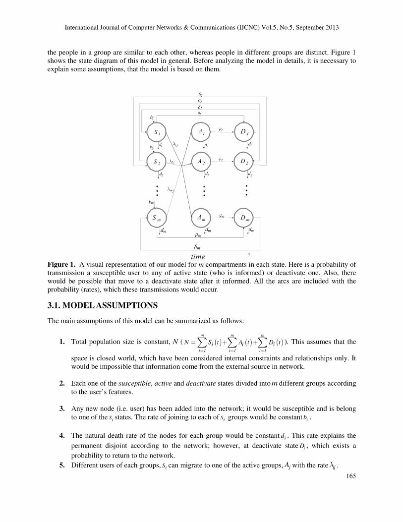
the people in a group are similar to each other, whereas people in different groups are distinct. Figure 1
shows the state diagram of this model in general. Before analyzing the model in details, it is necessary to
explain some assumptions, that the model is based on them.
Figure 1. A visual representation of our model for m compartments in each state. Here is a probability of
transmission a susceptible user to any of active state (who is informed) or deactivate one. Also, there
would be possible that move to a deactivate state after it informed. All the arcs are included with the
probability (rates), which these transmissions would occur.
3.1. MODEL ASSUMPTIONS
The main assumptions of this model can be summarized as follows:
1. Total population size is constant, N ( ( ) ( ) ( )m m m
i 1 i 1 i 1
i i iN S t A t D t
= = =
= + +∑ ∑ ∑ ). This assumes that the
space is closed world, which have been considered internal constraints and relationships only. It
would be impossible that information come from the external source in network.
2. Each one of the susceptible, active and deactivate states divided into m different groups according
to the user’s features.
3. Any new node (i.e. user) has been added into the network; it would be susceptible and is belong
to one of the iS states. The rate of joining to each of iS groups would be constant ib .
4. The natural death rate of the nodes for each group would be constant id . This rate explains the
permanent disjoint according to the network; however, at deactivate state iD , which exists a
probability to return to the network.
5. Different users of each groups, iS can migrate to one of the active groups, jA with the rate ijλ .

International Journal of Computer Networks & Communications (IJCNC) Vol.5, No.5, September 2013
166
ijλ stands for transfer rate from iS to jA state ( i S 1 i m , j A 1 j m∈ ∋ ≤ ≤ ∈ ∋ ≤ ≤ ).
6. Infectious period for each user of each iA group is constant.
7. Transferring, between susceptible iS and deactivate groups is done with rate iρ . Note that,
deactivate state is equal for all population, but people can return to the same state that they had
activated before. So, dividing this state to m groups, allow the transmission to analogous
susceptible groups.
8. Each users of iA can inactivate themselves for Different reasons. This change can be done with
rate, iϕ for any iA state to iD .
9. Users which have gone to inactive state after return to the network would be in susceptible state
again. While users were being deactivated, they are away from new information and don’t get any
information. So, as they return from the deactivate state, cannot join to active groups and should
return to the status, as they had been inactivated before ( iS ). This migration is done with rate i
δ .
Most mathematical models, which have developed in this area, are based on above assumptions [9, 10,
12, 15, 22, and 23].
3.2 Problem of Interest
Before we get into the detail of our approach, it is useful to notify some criteria and metrics, that we are
eager to derive from the proposed model and is used in whole of the paper. One of the important measures
per epidemic diffusion processes is a threshold value, which is a criterion for determining, whether the
epidemic take place or not. Based on the diffusion type, this parameter can give distinct value with
different parameters. Firstly, we can calculate this measure for our model and determine when an
epidemic can occur following this model. Then, specify how this value effects on diffusion process. To
better adaption the model to reality, we use DTMC Markovian model, since this model explains better
random users’ behavior. Calculating probability transition and then expected number of users in each
state of epidemic can be attractive. Also, once information (beneficial or no beneficial) extinct in network,
determining the end of diffusion process, “when does it happen?” would be another motivation of this
paper. In the following, we investigate to calculate these parameters; but, before we will consider an
analytical description of the proposed model.
3.3. Analytical Description of the Proposed Model
In this section, we’ll investigate mathematical description for our proposed model. User’s treatment can
be modeled by difference equations, which made on getting information. According to assumptions in
section 3.1, following equations could be deduced.

International Journal of Computer Networks & Communications (IJCNC) Vol.5, No.5, September 2013
167
λ ρ δ
λ ϕ
ϕ ρ δ
= =
= − − + +
= − +
= + − +
∑
∑
1
1
'
'
'
( ) ( ) ( ) ( ) ( )
( ) ( ) ( )A ( )
( ) ( ) ( ) ( )D ( )
m
ij
m
j
ij i i i i i i
ij i i i i
i i i i i i i
S t b S t d S t ti
t S t d ti
t t S t d ti
D
A
D A
(1)
Based on above equations, ' ( )iS t , '
( )itA and '
( )itD denote variations of susceptible of information,
informed users and removed ones, respectively. Also, the number of susceptible, informed person and
removed users is according to time. Once one user gets information, it can move from its own state.
Entrance and exit of its state is determined with sign (+) and (–), respectively.
Regarding to Assumption 5 of the model ijλ is stand for the rate between iS and jA states. However, this
parameter relates to two other measures: susceptibility of each user in per groups of susceptible iε and
infectiousness of each user in any infection groups jγ .
Also, as mentioned earlier, another important measure, that impact to this parameter is network
structures. This measure denotes relationship between users in a network. Certainly, different graphs have
distinct affect. We have to impact this measure as α. In other words, capability of getting data (infection)
relates to rate of the relationships and number of the infected users, who is involved in relationships.
As a result, ijλ should be defined as how that three mentioned measures, iε , jγ and α can be effective
to calculate it. Values of these parameters, determine as random, which was assigned to each their groups.
For calculatingα , relations between users in a network should be considered. However, in this paper we
ignore this influence and just have used a random value for this parameter. As a mathematically form, we
can use Equation (2) to calculate ijλ :
(2)
whereA j
N, denotes the percent of informed users of group j to the total users in network. In other words,
it explains the fraction of users with transmission strength jγ , can inform susceptible users of group i with
susceptibility iε .According to user’s behavior, one of them can disjoin from the network and would return
again. So, the parameterα should be updated based onϕi, δiand
ib parameters. This action can be done
with considering the least values of them ( )i ii bmin , ,δϕ .
Regarding to movement of users, changes can accrue in the system; so whenever system is at stable
state, there would be no more changes in the states ( ∼( ), ( ), ( ) 0' ' 'S t A t D ti i i ). Since, the population of these
states would be based on information, whether gets epidemic or not. So, the threshold parameter 0R plays
an important role on population size of each group. These sizes can be deduced in stable state from
Equation (3).
jij i j
A
N,λ αε γ=

International Journal of Computer Networks & Communications (IJCNC) Vol.5, No.5, September 2013
168
δ ρ
δ ρ δ ρ
δϕ
< ⇒
= =→∞
+ +
+ + + +
> > ⇒
= =→∞
+−
ɶ ɶ
ɶ ɶ ɶ
0
0
(1) 1* *lim ( ( ), ( ), ( )) ( ( ),0, ( ))
( )( ,0, ),( ) ( )
(2) 1, 0
* * *lim ( ( ), ( ), ( )) ( ( ), ( ), ( ))
(
(
i i i
i
i i i
R
S t A t D t S t D ti it
b d b di i i i i id d d di i i i i i i i
R A
S t A t D t S t A t D ti i it
di i b Ai i idi
δδ
ϕ ρ
ρ δ δϕ ρ δϕ δ
λ
+ ++
+ + ++ + ++ + +
∑=
)
, , ).( )( )
( )
1
di id bi i id A Si i i i i
d dd di i i i ii i i i idi i i mAij j
j
(3)
• Case 1: occurs when new information on network doesn’t get epidemic in stable state, or we are
in disease-free equilibrium ( iA 0→ ).
• Case 2: whenever happen that propagated information on network is pervasive, or we are in
endemic equilibrium ( iA 0> ).
In case 2, the value of *iA is calculated in parametric form. But, for *iS due to lake of space, we
ignore to write the parametric value, as well as for calculating *iD . In the following, we calculate the
threshold parameter to our proposed model. However, before that, we are going to define this parameter
in detail and introduce how to get it in compartmental models briefly.
3.3.1. Threshold Parameter to determine the Extent of the Epidemic Dissemination of
Information
One of the most important concerns about any infectious disease is its ability to invade a population.
Many epidemiological models have a disease free equilibrium (DFE) at which, the population remains in
the absence of disease. These models usually have a threshold parameter, known as the basic reproduction
number 0R ; such that, if <
01R , then the DFE is locally asymptotically stable, and the disease cannot
invade the population; because, on average an infected individual produces less than one, new infected
individual over the course of its infectious period. Conversely, if >01R then each infected individual
produces, on average more than one new infection, and the disease can invade the population. So, the
DFE is unstable [22]. A definition for this threshold can be defined, as below.
Definition 1 [31]: The basic reproduction number denoted by 0R is ‘the expected number of secondary
cases produces, in a completely susceptible population, by a typical infective individual.
In the case of a single infected compartment, 0R is simply the product of the infection rate and the
mean duration of the infection. However, for more complicated models with several infected
compartments this simple heuristic definition of 0R is insufficient. Further, the general basic reproduction
number can be defined as the number of new infectious produced by a typical infective individual in a
population at a DFE.
There exist different approaches to calculate this parameter. Table 1 shows these methods with their
references. According to the proposed model belongs to compartmental models; the next generation
matrix is a suitable method to obtain threshold value.

International Journal of Computer Networks & Communications (IJCNC) Vol.5, No.5, September 2013
169
Table 1. Different Methods to calculate threshold parameter, 0R in the literatures.
Reference Methods
[32-34] Next-generation Operator
[19, 39-45] Local stability of disease-free equilibrium
[40,41] Existence of an endemic equilibrium
[42-44] Multiple criteria
3.3.1.1. A general Compartmental Model
Let consider a heterogeneous population, that individuals are not distinguishable from each other;
according to age, behavior, spectral position and … So, this population can be grouped to n
subpopulation. In this section, it would be explained one general epidemic model for this population,
which presented by van den Driessche and Watmough [31]. Although these models are based on a
continuous-time model, we focus on the discrete –time of that and later will adapt it to our model.
Consider a population vector ( )1 nx x ,..., x= | ix 0≥ , that defines the number of individuals in each of n
compartment and let the first m of these compartments correspond to infected conditions. To calculate the
value of 0R , determining a new infection is more important than other changes in the same population.
Assume ( )i xF is the rate of appearance of new infections in compartment i, ( )xi+
V represent the rate of
movement of individuals into compartment i by means of other infection; ( )i x−
V is the rate of removal of
individuals from compartment i by any means. Note that, distinction between terms included in ( )i xF and
( )i x+
V is not mathematical, but biological; this distinction impacts the computation of 0R .
We can formulate a difference equation model of this process as follows:
( ) ( ) ( ) ( )( )i
'i i i i i
x
x f x x x x ,+ −
−
= = + −�������
V
F V V (4)
The only restrictions placed on the form of the functions, are given by the following assumptions.
These hypotheses don’t effect on the behavior of functions though these are biological assumptions,
which impact on the model treatments.
1. Since that, each function determines the direction of individual transmission, all of them is
nonnegative. Or ( ) ( ) ( ) { }i i i
if x 0, then x , x , x 0 , i 1,...,n .+ −
> ≥ ∈F V V
2. If one of the subpopulation is empty, there will be impossible to transmit any of them. Or
( ) ( ) { }i i iif x 0 then x 0 and x 0 ,i 1,..,m .
+= = = ∈F V
3. Outbreak and spread of disease from the non-infected subpopulation could be impossible and equal
to zero. Or
( )i
x 0 for i m.= >F
4. People cannot get out of the subpopulation over than its capacity .Or
( ) iix x .
−≤V

International Journal of Computer Networks & Communications (IJCNC) Vol.5, No.5, September 2013
170
As mentioned in previous sections, if the basic reproduction number 0R is less than one, then the
DFE is locally asymptotically stable, and also the disease cannot spread easily. However, whenever a
population vector(x) can be called as DFE, the first m compartments of x are zero (i.e.,
{ }ix 0 | x 0,i 1,..,m≥ = = ).
While all of the Eigenvalues of the Jacobian matrix of the function at the equilibrium x ( ( )J D x= − V
), have modulus less than one, we can say the disease free population dynamics is locally stable. This
condition is based on the derivation of f near (or at) a DFE. For our purpose, we define a DFE of (4) to
be a stable equilibrium solution of disease free model. Note that, it is not necessary assume the model has
a unique DFE. Consider a population near the DFE 0x . If the population remains near the DFE (i.e. if the
introduction of a few infective individuals does not result in an epidemic) then the population will return
into the DFE, according to the linearized system of
( )( )'0 0x Df x x x ,= − (5)
where, ( )0Df x is the Jacobian matrix (i.e. i
j
f
x
δ
δ
that evaluated at the DFE, 0x ). In stability analysis,
can be used the Eigenvalues of the Jacobian matrix evaluated at an equilibrium point, to determine the
nature of that equilibrium. If all of the Eigenvalues are negative, the equilibrium is stable. Because, we restrict our
attention to systems in the absence of new infection, so, the stability of DFE determined by the
Eigenvalues of ( )J D x .= − V
3.3.1.2 CALCULATING THE THRESHOLD PARAMETER IN THE PROPOSED MODEL
Before going into details of calculating this parameter in our model, first we explain a theorem to obtain
this parameter for compartmental model, which come its description earlier. The proof of this theorem
can be found in [31, 45].
Theorem 1 [45]: Let x be a DFE and define the m m× matrices { }ijF f= and { }ijV v= as:
{ }i iij x ij x
j j
d df | ,v | i, j 1,..,m ,
dx dx= = ∈F V
(6)
the next-generation matrix is given by 1K FV −= , so ( )10R FVρ −= , where ρ denote the spectral
radius of matrix K. The DFE x is locally asymptotically stable if and only if the spectral radius of the
Jacobian, ( )I F Vρ + − , is less than 1, which in turn occurs if and only if is 0R less than 1.
To interpret the entries of 1FV − and develop a meaningful definition of 0R , consider the fate of an
infected individual into compartment k of a disease free population. The ( )j ,k entry of 1V − is the average
period of time this individual spends in compartment j during its lifetime. Assuming that the population
remains near the DFE and barring reinfection. The ( )i , j entry of F is the rate of which infected
individuals in compartment j produce new infections in compartment i. Hence, the ( )i ,k entry of the
product 1FV − is the expected number of new infectious in compartment i produced by the infected
individual originally introduces into compartment k. Following Diekmann et al. [32], we call the next
generation matrix for the model and set ( )10R FVρ −= .
Now, we would like to calculate 0R by decomposing the system of ordinary differential equation into
the new information and transfer of user as below.

International Journal of Computer Networks & Communications (IJCNC) Vol.5, No.5, September 2013
171
(7)
Further, with calculating the Jacobian at DFE we have:
( ) ( )
( ) ( )
( )
( ) ( )
( ) ( )( )
0 0
0
0 0
i j
* *x x1 111 1m*
x ,i ijij* *x xm mm1 mm
1 1 11 1 1 1m
.i i ij
m m m m mmm1
and
S S
F S
S S
d d
V d
d d
λ λ
λ
λ λ
ϕ φ ϕ φ
ϕ φ
ϕ φ ϕ φ
= =
+ +
= = +
+ +
…
⋮ ⋱ ⋮
⋯
…
⋮ ⋱ ⋮
⋯
(8)
Where in the above equations *
iS come from the system at the DFE, which we calculated in Equation
(3). We can rewrite stable condition as δ ρ
δ ρ δ ρ
+ +
+ + + +
( )( ,0, )( ) ( )
b d b di i i i i i
d d d di i i i i i i i
.Also, about ijφ , we have:
.ij
0 if i j
1 if i jφ
≠=
= (9)
Thus, we can calculate next generation matrix regard to its spectral radius as a reproduction number:
( )
( )( )0
*i0ij1 1
iji i
,
x SFV R FV
d
λρ
ϕ
− −
= ⇒ =+
(10)
if we choose i jij ω ηλ = × [46], which the next generation matrix has rank one, we can write 0R as:
( ) ( )
( )
*m0 0 ii i
0
i ii 1
x x S,
dR
ω η
ϕ=
+=∑ (11)
( ) ( )
( ) ( ) ( ) ( ) ( )
( ) ( )
( ) ( ) ( ) ( )
i i
i i
i i
,
.
m
ij i
j 1
m
i ij i i i i
j 1
i
i i i i i
x t
x t d t t
d t
t t d t
0
S
0
b S S D
A
A S D
F
V
ρ
ϕ
δ
λ
λ δ
ϕ ρ
=
=
+
+
+
= − + + − = − + +
∑
∑

International Journal of Computer Networks & Communications (IJCNC) Vol.5, No.5, September 2013
172
where iω and jη are constant. In this situation, spectral radiance can be calculated by summation diagonal
of ( )1FV− matrix.
3.4. The Transaction Probability Calculation
The model that we present for information diffusion in section 3.2 is based on deterministic model. It
should be noticed that, modeling and analyzing deterministic modes would be easier than stochastic ones.
However, these cases are away from the reality. So, we are going to use DTMC [47], to justify our model
to a stochastic manner, since it adapts to real user’s behavior more than deterministic case.
To calculate probability transactions with the help of Markovian model, we should put on some
hypothesizes before using Markovian model.
1. Markov property [47]: this means, to predict the future state we just consider present state and
ignore the previous states. We can show this property at mathematical format as:
if ( ){ }X t ,t 0≥ denotes a set of stochastic variables, where ( )X t is based-on a Markov process, then
for all values of1 2 m m 1t t ... t t +< < < < , we can define following equation:
( ) ( ) ( ) ( ){ }( ) ( ){ }
m mm 1 1 1 2 2
m mm 1 .
P X t x | X t x ,X t x ,....,X t x
P X t x | X t x
+
+
≤ = = =
= ≤ = (12)
2. We define three stochastic variables to determine the number of users in susceptible, active and
deactivate states at time t.
( ) ( ) ( ) { }
( ) ( ) ( )
i j k
m m m
k i j
k 1 i 1 j 1
t , t , t 0,1,2,....,N ,i, j,k 1..m
t N t t ,i, j,k 1..m
= = =
∈ = = − + =∑ ∑ ∑
S A D
D S A (13)
3. Time in DTMC model should be divided into small time units, that one event occur only per epoch
{ }( )t 0, t ,2 t ,...∈ ∆ ∆ [16].
According to Assumption 2, we can consider two stochastic variables,i i( t ), ( t )S A , the random variable
i( t )D can be calculated as ( ) ( ) ( )m m m
k i j
k 1 i 1 j 1
t N t t ,i, j ,k 1..m
= = =
= − + =∑ ∑ ∑D S A . So, we don’t have to consider
it in the computations. As a result, bivariate process ( ) ( )( ){ } t 0i j,t t∞=S A , has a joint probability function
given by:
( ) ( ) ( ) ( )( ){ }i j
i i j js ,ap t Pr ob t s , t a= = =S A (14)
This bivariate process has the Markov property and is time-homogeneous. Transition probabilities can
be defined based on the assumptions of the deterministic formulation. First, assume that, ∆t can be chosen

International Journal of Computer Networks & Communications (IJCNC) Vol.5, No.5, September 2013
173
small sufficiently, that at most one change in state occurs during the time interval ∆t. The transition
probabilities are denoted as follows:
( ) ( ) ( ) ( ) ( ) ( )( ){ }
( ) ( )
i j i ji j i j i j,
i i i
s k ,a l s ,aPr ob , ( k , l ) | , ( s ,a .
i , j 1..m ,
p t t t
t t t
+ +∆ ∆ = =
= ∆ = −
∆ =
+∆
S A S A
S S S
(15)
Hence,
( ) ( )( )
( ) ( )
( ) ( )
( ) ( ) ( )
( ) ( ) ( )
( ) ( )
j
m
ij i 1
j 1
j i 2
3
4
1 2 3 4 5
b 0is k ,a l , s ,ai i j
j
i i j
i i i
p t
s t k ,l 1,1
a ( d ) t k ,l 0, 1
N s a t k ,l 1,0
s t k ,l 1,0
1 ( ) k ,l 0,0
0 Otherwise
d
λ θ
ϕ θ
δ θ
θ
θ θ θ θ θ
ρ
=
=+ +∆ =
∆ = = − + ∆ = = − − − ∆ = = ∆ = = − − + + + = =
+
∑ (16)
According to Equation (16), probability of transitions calculated per time step, ∆t. in this time, just
one movement can be taken between states because ∆t is sufficiently, small which only one event can take
place. For example, the probability of ( ) ( )k,l 1,1= − means that, for each state i, only one person can
migrate from state s i toj
a . This probability has calculated as a specific state i, so we can transfer to one
of j state from a states (i.e.m
ij i
j 1
s tλ
=
∆∑ , which equals to 1θ symbol). All probabilities have been calculated
similar to this one. Moreover, in Equation (16) assumed that, birth rates at each susceptible states, are
zero and sum of the all probabilities lead to one, so this avoids additional computations. The time step ∆t must be chosen sufficiently small, such that each of the transition probabilities lie in
the interval [0, 1]. The sake of these states is now ordered pairs, the transition matrix become more
complex and its form depends on, how the states( )i js ,a are ordered; moreover, this matrix is a Trier
dimension. The column of this matrix declares as( )i js ,a and the rows define( )i js k,a l+ + pairs. Third
dimension would be applied for ( ),i j pair, which1 , .i j m≤ ≤ so, we have avoided showing this matrix
here. However, applying the Markov property, the difference equation satisfied by the probability
( )( )i js ,a
t tP +∆ and can be expressed in terms of the transition probabilities.
( ) ( ) ( ) ( ) ( ) ( ) ( )( )
( ) ( ) ( )( )
( ) ( )( ) ( )
( ) ( )( )
1
, 1, 1 , 11
1,
1,
5,
1
1 1 ( )
1i i
j
i j i j i j
i j
i j
i j
ma
ij i j i js a s a s aj
i i js a
is a
s a
p t t p t p t t
p t N s a t
p t d t
p t t
s t a d
s
δ
ρ
θ
λ ϕ−
+ − +=
−
+
+ ∆ = + ∆ +
− − ∆ +
+ ∆ +
∆
+ ∆ + +
−
+
∑
(17)
If we obtain the transition matrix as a diagonal 3D-matrix, we can show that Equation (17) as an inner
product, ( ) ( ) ( )0p t P t p∆ = ∆ , where ( )P t∆ is as a transition matrix and also ( )0p explains initial

International Journal of Computer Networks & Communications (IJCNC) Vol.5, No.5, September 2013
174
probability vector ( ) ( ) ( ) ( ) ( ) ( ) ( ) ( ) ( )( )1, 1 , 1 1, ,1,0 , 0 , 0 , , 0
i j i j i j i ji js a s a s a s as a
p p pp p+ − + − +
. Therefore, Equation
(17) can be expressed in matrix and vector notation as:
( ) ( ) ( ) ( )1. 0
np t t P t p t P p
++ ∆ = ∆ = , where .t n t= ∆ (18)
Moreover, we can derive the mean values of each susceptible iS and informed jA , according to Equation
(17). We can define them as below:
( )( ) ( )( )
( )( ) ( )( )
i
j
j
i
i
j 0 s 0
a
j
i 0 a 0
sm
s,a
m
s ,a
t sp t
t ap t
E
E
= =
= =
=
=
∑∑
∑∑
S
A
(19)
3.5. The Variable Population Size
So far, all of the assumptions are based on a constant size of population. But, we can investigate to
variation population size in calculations. To do this, it is possible to relate both rates of birth and death of
population size, N. For this reason, we would use logistic equation, which it is proposed about population
growth by Verhast [48]. This equation redefines as following:
( ) ( )dN N
b N d N N 1dt K
ρ= − = −
(20)
Equation (20) has shown the relation between birth, death rates and population size, N. Instead of
using fix values of birth and death rated in Equation (1), we define these variables
( )2
NN
dK
b( N ) N andρ
ρ == and then recalculate all our calculations.
In Equation (20), K and � play important roles to increase and decrees of population size, whereas
growth of K, lead to increase of death rate and the amount of people will be reduced, and vice versa. Also,
we can have similar deduction for parameter �.
4. EXPERIMENTAL RESULTS
In order to evaluate our parameters, which were extracted from the proposed model, the assumptions of
the evaluated parameters should be presented at first. All assumptions to these evaluations are the same as
those mentioned earlier in section 3.1. Following steps illustrate our simulation process:
Step 1: Deliberation of user’s deterministic behaviors.
Step 2: Compare between users behavior in the case of deterministic model and stochastic DTMC
model.
Step 3: Deliberation of threshold value affection in the extinction of information from a
population.
Step 4: Deliberation of model, according to variable size of the population.

International Journal of Computer Networks & Communications (IJCNC) Vol.5, No.5, September 2013
175
4.1 The Simulation Method
Classical epidemic models have been surveyed as many literatures. The researchers of them considered
those models from different views as mentioned in related work. Almost their simulator can be found in
resources, which we have study most of them. However, we propose a new model of information
diffusion, that is based on epidemic spreading, especially SIRS model. Moreover, we extract some
parameters, that their calculation is different to related models. So, we have to implement this method by
ourselves. This model is implemented with MATLAB simulator.
First step of this simulation belongs to solve of differential equations with initial value parameters,
which is given in table 2. After that, there are used a discrete-time method to simulate users behavior
according to the proposed model and all the transitions are based on the rates that defined between states.
All these predefined values are brought in table 2. To determine transition probability, first we should
calculate these probabilities at a ∆t (sufficiently small) epoch, which is based on the define probabilities
(rates) on move direction on the model; then we use these probabilities to conclude the probability at t+∆t
time. Growth of Mean values of infected and susceptible users in comparison of deterministic mode,
would be verified our approach. All other initial values and assumptions, that applied to the simulation
summarized in table2, where bring below:
Table 2. Initial values of the parameters during the simulation
Parameter Description Value
N Number of population 100
ib Birth rate at each group i 0.01
id death rate at each group i 0.01
m Number of predefined clusters 2
iρ Migration rate from iS to iD 0.2
iδ Migration rate from iD to iS 0.03
iϕ Migration rate from iA to iD 0.03
iε Susceptibility of user in each iS groups 1 20.4, 0.6ε ε= =
jγ Capability of transfer information for each jA groups 1 20.4, 0.7γ γ= =
0iA Initial values of each active groups iA 0 0
1 2A A20 8= =,
0iS Initial values of each susceptible groups iS 0 0
1 2S S30 42= =,
0iD Initial values of each deactivate groups iD 0
4.2. Stochastic vs. Deterministic Model
This section evaluates deterministic and stochastic behaviors of the proposed model. Result of
deterministic manner can be derived from the solution of differential equations, which would be
considered in section 3.2. Also, as be shown in section 3.3, we could derive probabilistic transactions
between states regarding to DTMC model. Then we calculate the expected number of population size at
each state. To compare and verify two modes of model, we show their behavior at different time steps
with0
R 1.4= .This adaption will be seen in Figure 2. This figure shows the number of infected, susceptible
and deactivates users of two compartments, according to time; as can be seen, all this charts have three
regions, at first since the measures have been gotten in each ∆t=8 msec, all six charts be linear until 10
msec (it would be like warm up phase). According to charts (a) and (b), between 10 to 20 msec we
observe that activated users are increasing; because, entrance rates to these states are more than exits of it
as predefined values (Table 2). After that, the trends of these charts dramatically decreased; since that, it

International Journal of Computer Networks & Communications (IJCNC) Vol.5, No.5, September 2013
176
is going to DFE state (i.e. final of epidemic); thus, the stable state would be occurred and continued.
Charts (c) and (d) show behavior of susceptible users, who acts in opposite of activated users; during
activated number have growth, susceptible goes down; these charts are following initial values, which
have brought in Table 2; and then enter to stable state as same as previous charts. Moreover, we observe
that, deactivated users grow incrementally; because, entrance rates, which initiated from active and
susceptible sates, are more than exits that relates to death rate and migration to susceptible rate (see Table
2). After 40 msec, their behavior reaches to stable state, similar to other charts. Stochastic results show as
same as the deterministic trend; however, in the case of stochastic mode, we observe some distortions
during its progress. These deviations are happened; because, time grows with discrete form of
{ }t = ∆t, 2∆t, ... and at each time spaces; one event occur only, which due to calculate mean values. Before
calculating these mean values, we should solve Equation (17). For this purpose, we use Equation (18), to
calculate from matrix form. n in this equation depends on the expected time, t and epoch time ∆t, which
only one event can occur during this time. One drawback of this solution is whatever population size
raise, the time and spectral complexity get higher. The major result of this complexity goes to calculation.
Therefore, we should find a better solution to make less complexity. On choice is using prediction
mechanism via Data mining tools. With the help of these mechanisms, such as: regression, decision tree
and etc., we can forecast the end of the epidemic with amount of partial knowledge of it. One of the best
benefits of these methods is their less complexity and higher speed computation in a large population size
[49]. However, here we consider the epidemic model and some of the most important metrics.
(b)
(a)
(d)
(c)

International Journal of Computer Networks & Communications (IJCNC) Vol.5, No.5, September 2013
177
(f)
(e)
(a), (b) the comparison between two active groups 1 and 2.
(c) ,(d) the comparison between two susceptible groups 1 and 2.
(e), (f) the comparison between two deactivate groups 1 and 2.
Figure 2. The comparison between Deterministic (Equation (1)) and Stochastic (DTMC) behavior
between susceptible, active and deactivate groups with 0R 1.4= . In all charts, deterministic behavior has
be shown by (dashed curve) and in stochastic has been shown by (solid curve).
4.3. The Impaction of on the Information Diffusion on Extinction Time
As mentioned earlier 0R plays a key role on contagion. Therefore, this parameter has a significant impact on
information persistence. When this value goes higher, more users get that information and take longer time
to extinct. In contrast, if 0R is being in low value, less users augment spreading of information and it loses
its importance sooner. We get started our experiment with assign initial values to active users, according to
table 2. The model is performed for variable population, 0-90. For each size of population, model has been
continued until activated users go to zero. Also, by the assumption, we have two groups of activated users,
so we should wait to sum of the both activated number get near zero. The time of this event stands for
extinction time or the time no new information exists among the people. Impaction of parameter 0R on
extinction time, whole over the system is shown in Figure 3. Easily can be seen, whatever 0R get increase,
extinction time would be rise, too. In the case of 0R 2.3= , approximately near 40msec would be our extinct
time, which it has been reached to stability; because, after this time, activated number gets almost to zero.
This can be observed more oblivious in Figure 2 (a) and (b). Also, for 0R 4.9= , we have the same trend;
however, time, which related to this value of threshold, appears in higher value, makes more
interconnection between users. As a result, importance of information takes longer time to disappear.

International Journal of Computer Networks & Communications (IJCNC) Vol.5, No.5, September 2013
178
Figure 3. Affection of 0R
on the mean extinction time in whole of the system.
4.4. The Variable Population Size
In a social network, population dynamicity is a major feature, where can impact user behaviors’. As
mentions in section 3.4, the logistic equation can model this dynamicity well. This section emphasizes on
impact of parameter K on the individual growth of active groups. Figure 4, shows the variation number of
activated users, according to time duration. Impaction of the parameter, K calculates in two active groups,
whenever this parameter is more, as a result the number of active users also raise more. The sake of this
behavior refers to reduction of death rate (Equation (20)), and as follows increment of individuals in
groups. This claim is justifiable in Figure 4. Also, we can see at the same value of the time, for example
20msec, number of active persons in group2
A , is more than1
A . This state come from, that susceptible
user number of group2
A , is more than1
A ; whose their susceptibility is in a higher place. After this time,
the numbers of all activated persons get down near to zero; because, the DFE state would be started and
epidemic run over among population. This state is called stable state in the system.
Figure 4. Impaction of K on the activated user rate in groups 1 and 2. 0R 1.4, 1.0ρ= = .
Behavior with k = 100 is shown with (solid curve) and with k = 200 are shown by (dashed curve).
5. CONCLUSIONS AND FUTURE WORKS

International Journal of Computer Networks & Communications (IJCNC) Vol.5, No.5, September 2013
179
In this paper, by the help of epidemic diseases, we proposed a general information diffusion model in
social networks. Since, we grouped the users with different property, this model belongs to a
compartmental model, all of users in a compartment have the same feature; but, distinct with other
groups. At the first step, we have extracted a deterministic behavior of the model as a chunk differential
equations, future with thank of DTMC model; stochastic behavior of the model has been deduced
according to deterministic mode of the proposed model. To adaption of deterministic manner to stochastic
one, we used Markovian property to calculate transition probability at a small piece of time. Then, apply
this probability to obtain the mean value of population per each group. One of the important measures that
we have used in this paper is a threshold measure to determine when information diffusion runs over. We
extract this parameter for our model at DFE state. Moreover, the variable population size has been studied
in this paper and has shown what its impaction on the number of informed users is. Also, mean of
extinction time was another parameter, which extract during simulation. Relation between this parameter
and threshold was depicted as a chart as well. In future work, we decide to measure the impaction of
network topology on this information diffusion model and will study some important networks to show
this effectiveness. As mentioned earlier, calculation related to probability of expected number, which is
contained infection and susceptible users, would be more complex and has high computational order.
Therefore, another study, that has worth to do, is a prediction of the number of informed users, whenever
we just have initial states of users. For this reason, we can consider the growth of population as a
branching process and do our calculations on this dynamic population.
EFERENCES
[1] A. Vázquez, R. P.Satorras and A. Vespignani, “Large-scale topological and dynamical properties of Internet,” Phys. Rev. E
65, 066130-066130-12, Vol. 65, Issue 6, June 2002.
[2] A. Nagurneya and Q. Qiang, “Fragile networks: identifying vulnerabilities and synergies in an uncertain age,” Wiley Intl.
Trans. in Op. Res., Vol.19, Issue 1, March, 2010, pp.123-160.
[3] M. Gjoka, measurement of online social networks dissertation, Doctor of Philosophy Thesis, Computer science
Department, University of California, Irvine, 2010.
[4] Z. Shen, K.l. Ma and T. Eliassi-Rad, “Visual Analysis of Large Heterogeneous Social Networks by Semantic and Structural
Abstraction,” Visualization and Computer Graphics, Vol. 12, Issue 6, 2006, pp.1427-1439.
[5] E.Fee and D. M. Fox, AIDS: The making of chronic disease, university of California press, First edition, Berkeley, Los
Angles 1992.
[6] A.Guille and H.Hacid, “A predictive model for the temporal dynamics of information diffusion in online social networks,”
WWW '12 Companion Proceedings of the 21st international, pp.1145-1152, 2012, Lyon, France.
[7] E.Sadikov, M.Medina, J.Leskovec and H.Garcia-Molina, “Correcting for missing data information cascades,” WSDM '11
Proceedings of the fourth ACM international conference on Web search and data mining, pp. 55-64, 2011, New York,
USA.
[8] D.Kempe, J.Kleinberg and E.Tardos, “Maximizing the Spread of Influence through a Social Network,” KDD '03
Proceedings of the ninth ACM SIGKDD international conference on Knowledge discovery and data mining, pp.137-146,
2003, Washington, USA.
[9] H.W. Hethcote, “The mathematics of infectious diseases,” SIAM Review, Vol. 42, No. 4, 2000, pp. 599-653.
[10] M.E.J. Newman, “The spread of epidemic disease on networks,” Phys. Rev. E 66, 016128, Vol. 66, Issue 1, 2002.
[11] S.Bansal, B.T. Grenfell and L.A. Meyers, “When individual behavior matters: homogeneous and network models in
epidemiology,” Journal of the Royal Society Interface, Vol. 4 No. 16, October, 2007, pp. 879-891.
[12] H.W. Hethcote and H.R. Thieme, “Stability of the endemic equilibrium in epidemic models with subpopulations,”
Mathematical Biosciences, Vol.75, Issue 2, August, 1985, pp. 205-227.
[13] J. M. Hyman and J. Li, “Differential Susceptibility and Infectivity Epidemic Models,” Mathematical Biosciences and
Engineering, Vol. 3, No. 1, January, 2006, pp. 89-100.
[14] X. Wang, “Review of Classical Epidemic Models,” Statistical and Applied Mathematical Sciences Institute,
Undergraduate, Workshop, spring, 2010.
[15] T. Britton, “Stochastic Epidemic Models: A survey”, Mathematical Biosciences, Vol. 225, Issue 1, May, 2010, pp. 24-35.
[16] J.S. Allen, An Introduction to Stochastic Processes with Biology Applications, First edition, Prentice Hall, 2003.

International Journal of Computer Networks & Communications (IJCNC) Vol.5, No.5, September 2013
180
[17] J.Goldenberg, B.Libai and E.Muller, “Talk of the network: A complex systems look at the underlying process of word-of-
mouth,” Marketing Letters, springer, Vol.12, Issue 3, August 2001, pp. 211-223.
[18] K.Satio, M.Kimura, K.Ohara, and H.Motoda, “Selecting information diffusion models over social networks for behavior
analysis,” Machine Learning and Knowledge Discovery in Databases, springer, Vol. 6323, 2010, pp.180-195.
[19] M.E.J. Newman, “The structure and function of complex networks,” Society for Industrial and Applied Mathematics, SIAM
Review, Vol. 45, No. 2, 2003, pp. 167-256.
[20] D. Easley, J. Kleinberg, Networks, Crowds, and Markets, first edition, Cambridge University Press, Cambridge, 2010.
[21] E. Vynnycky and R.White , An Introduction to Infectious Disease Modeling, Oxford University Press, First edition, Oxford,
2010.
[22] J.M. Hyman and J. Li, “Differential Susceptibility Epidemic Models,” Journal of Mathematical Biology, springer, Vol. 50,
Issue 6, June, 2005, pp. 626-644.
[23] Mishra, B.K and Ansari G.M., “Differential Epidemic Model of Virus and Worms in Computer Network,” International
Journal of Network Security, Vol. 14, No. 3, May 2012, pp. 149-155.
[24] J.M Heffernan, R.J Smith and L.M Wahl, “Perspectives on the basic reproductive ratio,” J.R.Soc Interface, Vol.2, No.4,
September, 2005, pp.281-293.
[25] R. Pastor-Santorrass and A. Vespignani, “Epidemic Spreading in scale-free networks,” Phys.Rev.Lett, Vol. 86, No. 14,
2001, pp. 3200-3203.
[26] C.Castellano and R.Pastor-Satorras, “Threshold for epidemic spreading in networks,” Phys.Rev.Let 105, 218701, Vol.105,
Issue 21, 2010.
[27] M.E.J. Newman, “Threshold Effects for Two Pathogens Spreading on a Network,” Phys. Rev. Let.95, 108701, Vol. 95,
Issue 10, 2005.
[28] D. Chakrabarti, Y.Wang, C.Wang, J. Leskovec, and C.Faloutsos, “Epidemic thresholds in real networks,” ACM
Transactions on Information and System Security (TISSEC), Vol. 10, No.1, Issue 4, January 2008.
[29] B.A. Parkash, D. Chakrabarti, M.Faloutsos, N. Valler and C.Faloutsos, “Threshold Conditions for Arbitrary cascade
models on Arbitrary Networks,” Knowledge and Information Systems, Springer, Vol. 33, Issue. 3, December, 2012, pp.
549-575.
[30] J.A. Jacquez and P. O’Neil,“Reproduction numbers and thresholds in stochastic epidemic models. I. Homogeneous
populations,” Mathematic Bioscience, Vol.107, Issue 2, December, 1991, pp. 161-186.
[31] P. Van Den Driessche and J.Watmough, “Reproduction numbers and sub-threshold endemic equilibrium for compartmental
models of disease transmission”, Mathematic Bioscience, Vol.180, Issue 1-2, November-December 2002, pp.29-48.
[32] O.Diekmann, J.A.P. Heesterbeek and J.A.J. Metz, “On the Definition and the Computation of the Basic Reproduction Ratio
R0 in Models for Infectious Diseases,” Journal of Mathematical Biology, Vol. 28, No. 4, 1990, pp. 365–382.
[33] G.R.Fulford, M.G.Roberts and J.A.P. Heesterbeek, “The metapopulation dynamics of an infectious disease: Tuberculosis in
possums,” Theoretical Population Biology, Vol. 61, Issue 1, February, 2002, pp. 15–29.
[34] C.Fraser, S.Riley, R.Anderson and N.M. Ferguson, “Factors that make an infectious disease outbreak controllable,”
proceeding the national academy of sciences of the united states of america, Vol. 101, 2004, pp. 6146–6151.
[35] M.Boguna and R.Pastor-Satorras, “Epidemic spreading in correlated complex networks,” Phys Rev E 66, 047104, Vol.66,
Issue 4, 2002.
[36] A.N.Hill and I.M. Longini, “The critical vaccination fraction for heterogeneous epidemic models,” Mathematic Bioscience,
Vol.181, Issue 1, January, 2003, pp.85-106.
[37] Y. Wang, D.Chakrabarti, C.Wang and C.Faloutsos, “Epidemic spreading in real networks: An eigenvalue viewpoint,”
Reliable Distributed Systems Proceedings 22nd International Symposium, pp. 25–34, October, 2003, Florence, Italy.
[38] M.E.Alexander and S.M.Moghadas, “Bifurcation analysis of an SIRS epidemic model with generalized incidence,” SIAM
Journal on Applied Mathematics, Vol. 65, Issue 5, 2005, pp. 1794–1816.
[39] I.Z.Kiss, D.M.Green and R.R. Kao, “The effect of contact heterogeneity and multiple routes of transmission on final
epidemic size,” Mathematic Bioscience, Vol. 203, 2006, pp. 124–136.
[40] R. Anderson and R.M. May, Infectious Diseases of Humans: Dynamics and Control, Oxford University Press, Oxford, 1991.
[41] N. Masuda and N. Konno, “Multi-state epidemic processes on complex networks,” Journal of Theoretical Biology, Vol.
243, Issue 1, November 2006, pp. 64–75.
[42] K. B. Blyuss and Y.N. Kyrychko, “On a basic model of a two-disease epidemic,” Applied Mathematics and Computation,
Vol. 160, Issue 1, January, 2005, pp. 177–187.
[43] J.A. Hyman and J. Li, “The reproductive number for an HIV model with differential infectivity and staged progression,”
Linear Algebra and its Application, Vol. 398, March, 2005, pp.101–116.

International Journal of Computer Networks & Communications (IJCNC) Vol.5, No.5, September 2013
181
[44] M. Salmani and P.van den Driessche, “A model for disease transmission in a patchy environment,” Discrete Continuous
Dynamical Systems Series B, Vol. 6, No. 1, 2006, pp. 185–202.
[45] L. Zager, “Thresholds infection processes on networks with structural uncertainly,” Ph.D Thesis, EECS Dept.,
Massachusetts institute of technology, 2008.
[46] D.S. Bernstein, Matrix Mathematics: Theory, Facts, and Formulas, second edition, Princeton University, New Jersey,
2009.
[47] W.K. Ching and M.K. Ng, Markov Chains: Models, Algorithms and Applications, First edition, France, Springer, 2006.
[48] N. Bacaer, A Short History of Mathematical Population Dynamics, First edition, London, Springer, 2011.
[49] A.Nagar, L.Denoyer and P.Gallinari, “Predicting Information Diffusion on Social Networks with Partial Knowledge,”
WWW 2012 Companion, pp. 16-20, April, 2012, Lyon, France.
Related Documents