A sensor-data-based denoising framework for hyperspectral images

A sensor-data-based denoisingframework for hyperspectral images

Ferdinand Deger, 1,2,∗ Alamin Mansouri,1 Marius Pedersen,2 Jon Y.Hardeberg2 and Yvon Voisin1

1Le2i – Universite de Bourgogne, Auxerre, France2Norwegian Colour and Visual Computing Laboratory – Gjøvik University College, Gjøvik,

Norway∗ [email protected]

Abstract: Many denoising approaches extend image processing to ahyperspectral cube structure, but do not take into account a sensor modelnor the format of the recording. We propose a denoising framework forhyperspectral images that uses sensor data to convert an acquisition toa representation facilitating the noise-estimation, namely the photon-corrected image. This photon corrected image format accounts for themost common noise contributions and is spatially proportional to spectralradiance values. The subsequent denoising is based on an extended varia-tional denoising model, which is suited for a Poisson distributed noise. Aspatially and spectrally adaptive total variation regularisation term accountsthe structural proposition of a hyperspectral image cube. We evaluate theapproach on a synthetic dataset that guarantees a noise-free ground truth,and the best results are achieved when the dark current is taken into account.

© 2015 Optical Society of America

OCIS codes: (100.2980) Image enhancement; (110.4280) Noise in imaging systems;(110.4234) Multispectral and hyperspectral imaging.

References and links1. H. Li and L. Zhang, “A hybrid automatic endmember extraction algorithm based on a local window,” IEEE

Trans. Geosci. Remote Sens. 49, 4223–4238 (2011).2. X. Liu, S. Bourennane, and C. Fossati, “Denoising of hyperspectral images using the PARAFAC model and

statistical performance analysis,” IEEE Trans. Geosci. Remote Sens. 50, 3717–3724 (2012).3. H. Othman and S.-E. Qian, “Noise reduction of hyperspectral imagery using hybrid spatial-spectral derivative-

domain wavelet shrinkage,” IEEE Trans. Geosci. Remote Sens. 44, 397–408 (2006).4. J. Martın-Herrero, “Anisotropic diffusion in the hypercube,” IEEE Trans. Geosci. Remote Sens. 45, 1386–1398

(2007).5. D. Letexier and S. Bourennane, “Noise removal from hyperspectral images by multidimensional filtering,” IEEE

Trans. Geosci. Remote Sens. 46, 2061–2069 (2008).6. Q. Yuan, L. Zhang, and H. Shen, “Hyperspectral image denoising employing a spectral spatial adaptive total

variation model,” IEEE Trans. Geosci. Remote Sens. 50, 3660–3677 (2012).7. J. Yang and Y. Zhao, “Poisson-Gaussian mixed noise removing for hyperspectral image via spatial-spectral struc-

ture similarity,” in “32nd Chinese Control Conf.” (Xi’an, 2013), pp. 3715–3720.8. X. Gong, B. Lai, and Z. Xiang, “A L0 sparse analysis prior for blind poissonian image deconvolution,” Opt.

Express 22, 370–375 (2014).9. F. Deger, A. Mansouri, M. Pedersen, J. Y. Hardeberg, and Y. Voisin, “A variational approach for denoising

hyperspectral images corrupted by Poisson distributed noise,” in Image Signal Process (Springer, 2014), pp.106–114.

10. H. Zhang, W. He, L. Zhang, H. Shen, and Q. Yuan, “Hyperspectral image restoration using low-rank matrixrecovery,” IEEE Trans. Geosci. Remote Sens. 52, 4729–4743 (2014).

#224335 - $15.00 USD Received 7 Oct 2014; revised 11 Dec 2014; accepted 8 Jan 2015; published 26 Jan 2015 (C) 2015 OSA 9 Feb 2015 | Vol. 23, No. 3 | DOI:10.1364/OE.23.001938 | OPTICS EXPRESS 1938

11. T. Skauli, “Sensor noise informed representation of hyperspectral data, with benefits for image storage and pro-cessing.” Opt. Express 19, 13031–13046 (2011).

12. L. Rudin, S. Osher, and E. Fatemi, “Nonlinear total variation based noise removal algorithms,” Phys. D 60,259–268 (1992).

13. S. Osher and T. Goldstein, “The Split Bregman method for L1 regularized problems,” SIAM J. Imaging Sci. 2,323–343 (2009).

14. E. L. Dereniak and G. D. Boreman, Infrared Detectors and Systems (Wiley, 1996).15. T. Skauli, “An upper-bound metric for characterizing spectral and spatial coregistration errors in spectral imag-

ing.” Opt. Express 20, 918–933 (2012).16. (HySpex / Norsk Elektro Optikk AS), “Imaging spectrometer (user manual),” Tech. Rep. (2013).17. T. Le, R. Chartrand, and T. J. Asaki, “A variational approach to reconstructing images corrupted by Poisson

noise,” J. Math. Imaging Vis. 27, 257–263 (2007).18. P. Getreuer, “Rudin-Osher-Fatemi total variation denoising using Split Bregman,” Image Process. Line (2012).19. R. Zanella, P. Boccacci, L. Zanni, and M. Bertero, “Efficient gradient projection methods for edge-preserving

removal of Poisson noise,” Inverse Probl. 25, 1–24 (2009).20. M. D. Fairchild and G. M. Johnson, “Metacow: a public-domain, high-extended-dynamic-range, spectral test

target for imaging system analysis and simulation,” in “Color Imaging Conf.”, (IS&T, 2004), pp. 239–245.21. J. Padfield, “Library of illumination spectral power distributions,”

http://research.ng-london.org.uk/scientific/spd/. Accessed: 2014-12-10.22. R. Shrestha, R. Pillay, S. George, and J. Y. Hardeberg, “Quality evaluation in spectral imaging–quality factors

and metrics,” JAIC-Journal of the International Colour Association 12 (2014).23. Z. Wang, A. C. Bovik, H. R. Sheikh, and E. P. Simoncelli, “Image quality assessment: from error visibility to

structural similarity.” IEEE Trans. Image Process. 13, 600–612 (2004).24. J. Romero, A. Garcıa-Beltran, and J. Hernandez-Andres, “Linear bases for representation of natural and artificial

illuminants,” J. Opt. Soc. Am. A 14, 1007–1014 (1997).

1. Introduction

Hyperspectral imaging (HSI) is affected by noise, which impacts the precision of all furtherprocessing steps, such as unmixing [1] or classification [2]. Noise is inevitable during theacquisition, and caused at different stages in both the optics and the photodetector. An on-going research challenge is to find appropriate image processing methods that reduce the in-fluence of noise in a post-processing step. Most approaches adapt techniques from grey-levelimage processing and extend them to the needs of HSI. Othman and Qian [3] extended waveletshrinkage denoising to a hybrid spatial-spectral wavelet shrinkage, Martın-Herrero [4] adjustedanisotropic diffusion for the HSI cube, Letexier and Bourennane [5] adapted a Wiener filter toHSI and Liu et al. [2] used a higher order generalization of singular value decomposition. Yuanet al. [6] extended a variational denoising model to HSI using a spectral-spatial adaptive totalvariation (TV) semi-norm.

State of the art approaches do not only take the structural cube properties into account, butalso adapt to the type of noise. In nowadays hyperspectral scanners, the most relevant noisesource is photon noise, also known as shot noise. Yang and Zao [7] propose a Poisson-Gaussianmixed model for HSI using a multistep approach including principal component analysis trans-formation. Gong et al. [8] use a blind deconvolution to smooth HSI contaminated by Poissonnoise. We recently proposed a variational approach for denoising HSI corrupted by Poissondistributed noise [9]. Zhang et al. [10] employed a low-rank matrix recovery, which can simul-taneously remove Gaussian noise, impulse noise, dead pixels or lines, and stripes.

These current denoising approaches adapt for the type of noise and the structural properties ofthe image cube, but remain rather vague about the parameterisation, and do not clarify whetherthe HSI should be stored as a radiometric calibrated radiance values or raw sensor output. Thesetwo questions are closely linked, as noise is a random process that can be well characterisedusing the knowledge of the sensor characteristics. Skauli [11] analysed different image formatslike the raw sensor response or calibrated spectral radiance (with the unit Wsr−1m−2nm−1),and proposed a representation that facilitates the use of physical noise-estimates. The formataccounts for the most important noise contributions, such as the random arrival of the photons


PhotonCorrected

Image

Spectral Radiance

Image

Spectral Radiance

Image

Raw Sensor

Parameter Estimation

Spatially -spectrally

adaptive TV Denoising

DenoisingSensor Data Knowledge

Fig. 1. Different stages of the proposed denoising framework for HSI. Knowl-edge of the sensor characteristics allows the conversion to a photon correctedimage (presented in Section 3). This is a better representation to find an ap-propriate noise model and to estimate the corresponding parameters.

and the contribution of the dark current, but neglects less relevant details, such as the non-uniformity of the sensor elements.

The proposed denoising framework for HSI (see Fig. 1) uses sensor data to transform theimage to a photon corrected representation. This format is similar to the one proposed in [11],but accounts for the contribution of the dark current and does not use a constant weightingfactor. In this format, the noise is mathematically described by a Poisson distribution, and thestandard deviation can be directly estimated. For the denoising, we use a Rudin-Osher-Fatemi(ROF) [12] variational model and a Split Bregman optimisation [13]. The data term is adaptedto a Poisson distributed noise, and the TV regularisation accounts for the structural propertiesof the HSI cube. Knowledge of the noise variance allows estimating a good parameterisationthat weights the contribution of the data fidelity and regularisation term. We convert the outputto device independent spectral radiance values. The approach is evaluated deliberately only ona synthetic dataset. In contrast to a real acquisition, this ensures a noise free ground truth.

The remaining paper is structured as following: In Section 2, we introduce a basic signalmodel and derive important noise contributions. Section 3 presents the transformation to a pho-ton corrected image format, which is the foundation for the denoising process. Two formatsare presented: One is accounting the contribution of the dark current and a second one is sim-pler and does not account for it. In Section 4 the spatially and spectrally adaptive variationalROF model is described that we have previously presented in [9]. The evaluation in Section 5uses a sensor model, and a realistic parameterisation to evaluate the proposed denoising frame-work and to analyse the influence of the dark current. We conclude and propose future work inSection 7.

2. Hyperspectral noise model

HSI is affected by different noise sources, such as the random arrival of photons, the contri-bution of the dark current, readout noise, and rounding errors. A basic signal model [11, 14]can be applied to pushbroom- and whiskbroom-scanning sensors, and helps to identify differ-ent noise contributions. Considering the spectral radiance values L[i, j] of a scene at a spatiallocation i and a spectral band j, the acquisition sensor will receive Nph[i, j] photons, which canbe calculated as


Nph[i, j] = L[i, j] t AΩΔλλ [ j]hc

, (1)

where t is the acquisition time, A the sensor aperture, Ω the solid angle of a single pixel, Δλthe spectral sampling, λ the respective wavelength and h the Planck’s constant and c the speedof light. These photons will excite the following number of photoelectrons

N[i, j] = η [i, j]Nph[i, j]+ Id [i, j] t +δN, (2)

where η [i, j] describes the quantum efficiency depending on the spatial and spectral location. Itincludes non-uniformities of the sensor and all signal losses in both the optics and the detector.Id [i, j] is the dark current and δN describes the read-out noise. The photoelectrons are multipliedby a constant gain factor g f and discretized to the raw sensor values

Draw[i, j] = round(g f N[i, j]), (3)

This signal model implies a couple of assumptions. The light samples are supposed to bewithin the capacity of the photodetector. In Eq. (1), the dense spectral sampling is simplifiedto a constant energy at the centre of every band λ [ j], and the spectral sampling Δλ is assumedto be constant in the acquisition range. The model is therefore only suited for devices thatsample the spectral information densely. The following noise sources can be described withinthis sensor model.

Photon noise , or shot noise is a fundamental physical limit, and the dominating noise contri-bution in current hyperspectral sensors. It is caused by the random arrival of the photonsas well as the random absorption at the photodetector, and can be described by a Poissondistribution of photoelectrons (Eq. 2). The standard deviation is σpn =

√N[i, j].

Readout noise accounts for the variability in the transfer and amplification of the photoelec-tron signal. In Eq. (2) it is characterised as an additive Gaussian distribution with zeromean and the standard deviation δN.

The noise contribution of the dark current is characterised by Id [i, j] t in Eq. (2), as δNhas zero mean. In many cases it is small compared to the actual photoelectron countη [i, j]Nph[i, j]. However, for acquisitions in dark environments such as in astronomy, thedark current is more dominant.

Digitization noise occurs, when N[i, j] is multiplied by a gf and converted to an integer valuein Eq. (3).

This model is not treating optical co-registration errors, such as keystone and smile distor-tions. Such distortions are better described and compensated separately [15]. This paper focuseson the effects of the photon noise.

3. Photon corrected image

HSI are conventionally converted to radiance values. This format has the advantage of beingdevice independent, and can be interpreted and processed without any prior sensor knowledge.An estimation of the spectral radiance Ln[i, j] can be calculated by applying Eqs. (1) – (3) inreverse order

Ln[i, j] =

(Draw

g f− Id [i, j] t

)hc

η [i, j] t AΩΔλ λ. (4)


The estimated radiance Ln[i, j] is similar to the original sample L[i, j], but corrupted by noise.Although a noise description for Ln[i, j] is possible [11], the noise characteristics in the radi-ance format does not only depend on the signal intensity, but also the spatial location i and thespectral band j. A denoising model would become unnecessarily complicated and computa-tionally expensive. Therefore, Skauli [11] proposed a corrected raw data frc, especially suitedfor low-level operations, such as denoising. It hides uninteresting details, while allowing toaccess important sensor properties. In contrast to the raw sensor data, it reduces the quantumefficiency to its spectral domain

η [ j] =1M

M

∑i=1

η [i, j], (5)

where i is the spatial location along a line, and M is the number of pixels in a single line. Thiscan be justified, as the spectral variation of the quantum efficiency is much more significantthan the spatial nonuniformity. In this format, the dark current is not accounted. The correctedraw data frc[i, j] is spatially proportional to the radiance at any location i, described by

frc[i, j] = Ln[i, j]k[ j]−1,

k[ j] =hc

sdw η [ j] t AΩΔλ [ j]λ,

(6)

where sdw is a constant weighting factor to increase the numerical precision during the digiti-zation. The corrected raw data frc can be efficiently estimated from raw sensor values, and thecommercial push-broom scanner line HySpex has an option to save directly in this format [16].The photon corrected image fpc, that we use for the denoising process is an extension that ac-counts the contribution of the dark current. To remain spatially proportional to radiance values,we add an average of the dark current

fc[i, j] =frc[i, j]

sdw+ Id t, (7)

where Id is the mean value of the dark current. Readout noise, as described in Eq. (2) is notaccounted as the Gaussian distribution is assumed to have a zero mean value. We compensatethe weighting factor sdw, because we do not apply a digitization and correct magnitude allows astraightforward parameter estimation. In many acquisitions the contribution of the dark currentseems insignificant. A simplified corrected photon image fcs only corrects the scaling

fcs[i, j] = frc[i, j]/sdw. (8)

All calculation for the corrected images frc, fc and fcs are fully reversible. Radiance valuescan be estimated from fc by subtracting an offset (Eq. 7) and multiplying a location invariantscaling factor k[ j] Eq. (6). The corrected images include all relevant noise contributions, whichcan be characterised by a single Poisson distribution. The noise contribution is independent ofthe location and the standard deviation depends only on the signal value

σn[i, j] =√

fc[i, j]≈√

fcs[i, j], (9)

at every location. The corrected raw data frc[i, j] can be used alternatively as an input for thedenoising framework, just the noise variance, Eq. (9), must be scaled accordingly.


4. Denoising

4.1. Total variation denoising

The measurement fc is corrupted by a Poisson distributed noise. Let u be the noise free imagethat we want to reconstruct. This reconstruction benefits from the spatial and spectral relation-ship of neighboring locations. Instead of analyzing a single point, as in the previous sections,we now assume a HSI cube. A push-broom scanner is required to acquire multiple lines. Both,fc and u are of dimensions M1 ×M2 ×B, in which M1 and M2 are the spatial dimensions ofthe image, and B represents the spectral band-number. Noise corruption is an ill-posed prob-lem and a reconstruction is often based on a regularisation approach. The presented denoisingapproach [9] is based on ROF models [12] that are successful at denoising. Traditionally thesemodels assume Gaussian white noise, but they have been adapted to Poisson distributed noiseby Le et al. [17]. A reconstructed image u can be described as

u = arg minu

‖u‖TV (H) +β∫

H(u(x)− fc(x) logu(x))dx, (10)

where H = M1 ×M2 ×B is the image domain of the HSI. The first term ‖ · ‖TV (H) is the TVsemi-norm that serves as a regularisation term. The second term is the data fidelity, in which thelogarithmic component accounts for the Poisson distributed noise in fc, as described in [9, 17].Both components are balanced by the regularisation parameter β . The TV semi-norm permitsa stronger denoising in smooth areas, while preserves edges and structures. A spatial-spectraladaptive TV semi-norm (SSATV) performs best for HSI [6, 9]

‖u‖SSATV =M1M2

∑i

WiGi, (11)

where Gi is the gradients of all bands at a single location i

Gi =

√√√√B

∑j(∇xu)2

i, j +(∇yu)2i, j, (12)

with ∇x and ∇y being the discrete horizontal and vertical derivation in the image plane M1×M2.This means that Gi discourages a large oscillation in the reconstructed image. A weightingfactor Wi in Eq. (11) helps to preserve structure. It allows a stronger denoising in comparablysmooth regions, and lower denoising for sharp edges

Wi =(1+Gi)

−1

1M1M2

∑M1M2k (1+Gk)−1

. (13)

A discrete ROF model of Eq. (10) is used for variational denoising approach that preserves thestructure of a HSI and accounts the appropriate Poisson distributed noise. It is denoted as

u = arg minu

M1M2

∑i

WiGi +βM1M2

∑i

B

∑j

(ui, j − fi, j logui, j

). (14)

To efficiently solve this minimization, a Split-Bregman Optimisation [13,18] can be applied.The unconstrained minimization is split into constrained problems that can be solved moreeasily. The complexity is hereby reduced to O(M2), M being the number of voxels in the HSIcube.


4.2. Parameter estimation

An appropriate parameterisation is important for a good denoising result. When β in Eq. (14)is zero, only the regularisation gets accounted, and the result is over-smoothed. In the case ofa too large β , the data term is too strong, and the resulting image remains similar to the noisyimage fc. The parameterisation depends on both the noise level, and the image. Even withthe knowledge of the standard deviation, there is no closed form to estimate β , and a meta-optimisation has to be applied. In Gaussian noise corrupted images, the discrepancy principleis applied [17–19]. The principle states that the mean-squared error between the reconstructionand the noisy data should be equal to the variance of the noise. A proposed adaptation to Poissonnoise uses the error of the data term, and optimizes it to match the mean variance of the image[17, 18].

arg minu

‖u‖TV (H) subject to∫

H(u(x)− fc(x) logu(x))dx = mean(σ [i, j]2) (15)

5. Experimental evaluation

Many existing denoising approaches have been evaluated on real HSIs as a ground truth (GT),in which Gaussian noise of different intensity is added [3, 6, 7]. Such an evaluation does notnecessarily reflect a realistic noise contribution. Furthermore, the GT itself cannot be assumedto be noise free. Therefore, we decided to evaluate the framework only on synthetic datasets,based on the sensor model described in Section 2. To be as realistic as possible, we use a non-uniform quantum efficiency, and dark current from a real pushbroom HSI scanning device. Thespectral variation of the quantum efficiency and illumination automatically lead to differentnoise levels in different spectral bands. We include readout noise and digitization noise. Thefirst aim of this evaluation is to quantify the denoising potency of the proposed framework.We also investigated the influence of the dark current on the two image formats fc, Eq. (7)compared to fcs, Eq. (8).

5.1. Generating synthetic datasets

The computer generated Metacow image [20] has its origins in the field of colour imaging. Theimage is a noiseless, high contrast HSI. It shows 24 cows with different spectral surfaces, and isfreely available. We used an image size of 600 px×400 px and 70 spectral bands from 415nmto 760nm with Δλ = 5nm. The reflectance values are scaled between 0 and 1, and multipliedby different, spatially uniform illuminants, see Fig. 2(a). For simplicity, the spectral irradianceis directly interpreted as spectral radiance values. The resulting image L is shown in Fig. 2(b).

We simulate a pushbroom scanner according to our sensor model. To be as realistic as possi-ble, we use the parameterisation from a real pushbroom scanner, the HySpex VNIR 1600 [16],and adapted the dimensions accordingly. We assumed an aperture of A = 0.0008m2, and an in-tegration time t = 0.08s. The solid angle is the same for all pixels Ω = 7.03×10−8 (obviouslywith different orientations). The quantum efficiency η [i, j] is shown in Fig. 3(a), and includeseffects of the optics and the photodetector. The dark current Id [i, j] t is shown in Fig. 3(b), andhas a variance of Var(Id [i, j] t) = 6.5. The constant offset is measured in a laboratory environ-ment at room temperature and averaged over 200 measurements. In Eq. (2) we added readoutnoise with zero mean and the same variance as the fixed pattern dark current. This ensures thatonly few locations become negative due to the readout noise. Negative values require a trunca-tion to zero, which is a further anomaly. A Poisson distributed noise is then applied to the resultof Eq. (2). This noise distribution has no parameterisation, and depends only on the magnitudeof each value. The gain factor in Eq. (3) is gf = 0.1024, which is applied before the digitization.

Different synthetic illuminants are used to generate different spectral characteristics. The


400 450 500 550 600 650 700 750 800

Wavelength [nm]

0.0000

0.0002

0.0004

0.0006

0.0008

0.0010

0.0012

0.0014

0.0016

Intensity[W/m

2]

Illuminant

CIE D65

CIE A

GE 4100K

(a)

(b)

Fig. 2. Spectral power distributions (SPDs) of the applied illuminants andradiance values of the synthetic dataset. a) CIE D65 and CIE A are stan-dardized SPDs, while GE 4100K is measured by [21]. b) Spectral radiancevalues L of the synthetic data set [20]. The image width is 600 px and everycow is 100 px × 100 px. In total there are 24 cows in different colors. Forthis visualization, the bands 40,30,9 are assigned to the red, green and bluechannel.

synthetic CIE D65 is a standardized daylight illumination with a color temperature of approx-imately 6500 K and the CIE illuminant A represents a standardized tungsten filament lamp.Additionally we used a spectral power distribution (SPD) of the GE FC8T9/CW lamp with4100K that is online available [21].

Further datasets were generated by weighting the contribution of the dark current. We didnot modify the dark current as these values are device and temperature dependent, nor did weincrease the acquisition time. Instead, we multiplied each illuminant by a constant factor gl .A brighter illumination leads to a larger number of photoelectrons, and the contribution of theacquisition becomes larger compared to the contribution of the dark current. This simulationdoes not include a saturation limit for the sensor, and along with the illumination increases thesignal-to-noise ratio. In total we generated nine datasets, based on three different illuminantshaving three different intensities.


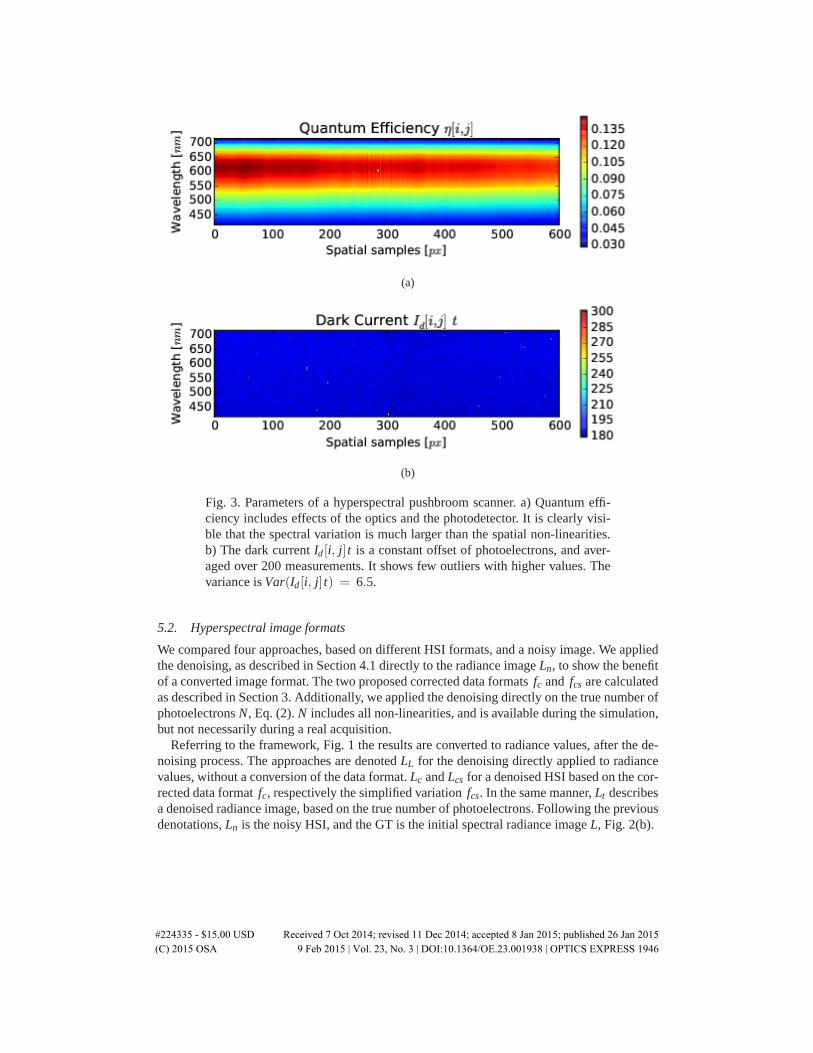
(a)

(b)

Fig. 3. Parameters of a hyperspectral pushbroom scanner. a) Quantum effi-ciency includes effects of the optics and the photodetector. It is clearly visi-ble that the spectral variation is much larger than the spatial non-linearities.b) The dark current Id [i, j] t is a constant offset of photoelectrons, and aver-aged over 200 measurements. It shows few outliers with higher values. Thevariance is Var(Id [i, j] t) = 6.5.

5.2. Hyperspectral image formats

We compared four approaches, based on different HSI formats, and a noisy image. We appliedthe denoising, as described in Section 4.1 directly to the radiance image Ln, to show the benefitof a converted image format. The two proposed corrected data formats fc and fcs are calculatedas described in Section 3. Additionally, we applied the denoising directly on the true number ofphotoelectrons N, Eq. (2). N includes all non-linearities, and is available during the simulation,but not necessarily during a real acquisition.

Referring to the framework, Fig. 1 the results are converted to radiance values, after the de-noising process. The approaches are denoted LL for the denoising directly applied to radiancevalues, without a conversion of the data format. Lc and Lcs for a denoised HSI based on the cor-rected data format fc, respectively the simplified variation fcs. In the same manner, Lt describesa denoised radiance image, based on the true number of photoelectrons. Following the previousdenotations, Ln is the noisy HSI, and the GT is the initial spectral radiance image L, Fig. 2(b).


5.3. Evaluation metrics

Different metrics for a quality evaluation of HSI have been proposed [22]. To evaluate thedenoising framework, we use the following three metrics. The peak signal to noise ratio (PSNR)between the GT and an estimation L indicates how well the signal is reconstructed

PSNR(L, L) = 10log10

(max(L)

MSE

), MSE =

1M1M2B

M1M2B

∑i

(Li − Li)2, RMSE =

√MSE.

(16)Additionally, we use the structural similarity (SSIM) index [23] to evaluate for visual artifacts

that might have been introduced in the course of the denoising. It is calculated

SSIM(L, L) =(2μLμL + c1)(2σL,L + c2)

(μ2L +μ2

L+ c1)(σ2

L +σ2L+ c2)

, (17)

where μ is the average and σ2 is the variance, both in a local neighborhood (We use 5×5 pixel).The constants c1 and c2 stabilize the division with weak denominator and are set to fixed ratioof the maximum image value. PSNR is well defined on an image and a HSI cube, while SSIMis calculated band-wise and averaged for a global value.

For hyperspectral images, the spectral feature is very important. The goodness of fit coeffi-cient (GFC) [24] describes how well a single spectral curve is preserved

GFC(p, p) =|∑ j p j p j|

|∑ j(p j)2|−1/2|∑ j( p j)2|−1/2, (18)

where p is the radiance value of a single pixel in the HSI cube. Analyzing several locationsallow a statistical evaluation of different approaches.

6. Results and discussion

The denoising was applied with the best parameterization on the datasets described in Section5.1. The different HSI formats that are described in Section 5.2 are compared to each other.The results for PSNR are denoted in Table 1. The three illuminants have a different noise leveland the PSNR increases with the intensity factor gl . The proposed photon corrected format Lc,and the true photoelectron count Lt show quit similar results. Both take the dark current intoaccount and are notably more effective than the simplified Lcs. In most cases there is a marginaladvantage for Lc. A reason for this is the conversion to radiance values for the evaluation.The proposed format fc is spatially proportional to spectral radiance. Therefore, the denoisingresults from the spatial adaptive TV denoising model are preserved in Lc.

In Table 2, we observe that the results of PSNR and SSIM are in agreement for differentilluminants and intensities. The denoising improves both the structure and the PSNR of an HSIfor all formats. In lower light intensities the LL format shows only a poor performance. ThisHSI format applies the SSATV denoising directly to the radiance values and a conversion tothe photon corrected image format is skipped. The mathematical denoising model assumes aPoisson distributed noise, but this assumption does not hold true in LL, due to the radianceformat and the different noise contributions.

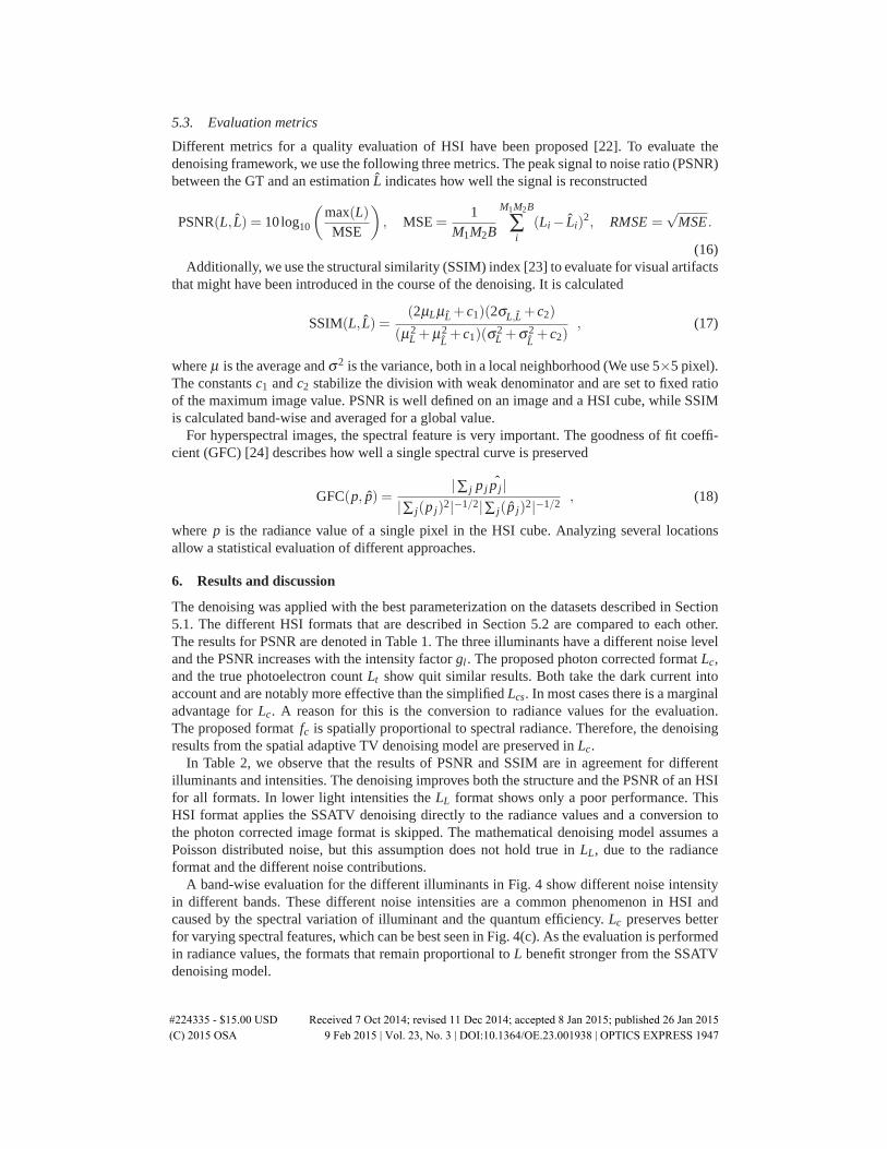
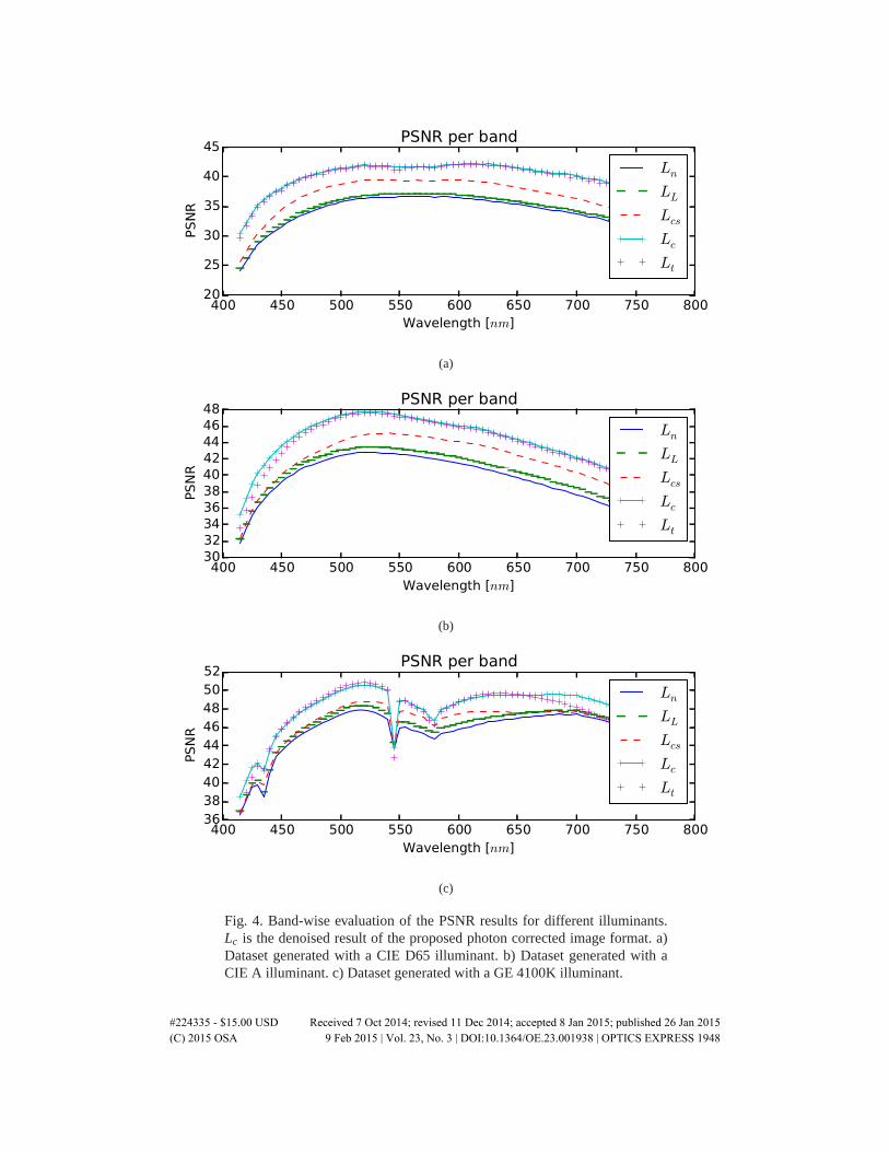
A band-wise evaluation for the different illuminants in Fig. 4 show different noise intensityin different bands. These different noise intensities are a common phenomenon in HSI andcaused by the spectral variation of illuminant and the quantum efficiency. Lc preserves betterfor varying spectral features, which can be best seen in Fig. 4(c). As the evaluation is performedin radiance values, the formats that remain proportional to L benefit stronger from the SSATVdenoising model.


(a)

(b)

(c)

Fig. 4. Band-wise evaluation of the PSNR results for different illuminants.Lc is the denoised result of the proposed photon corrected image format. a)Dataset generated with a CIE D65 illuminant. b) Dataset generated with aCIE A illuminant. c) Dataset generated with a GE 4100K illuminant.


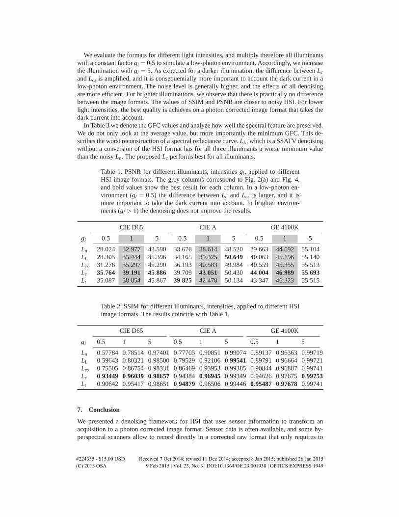
We evaluate the formats for different light intensities, and multiply therefore all illuminantswith a constant factor gl = 0.5 to simulate a low-photon environment. Accordingly, we increasethe illumination with gl = 5. As expected for a darker illumination, the difference between Lc

and Lcs is amplified, and it is consequentially more important to account the dark current in alow-photon environment. The noise level is generally higher, and the effects of all denoisingare more efficient. For brighter illuminations, we observe that there is practically no differencebetween the image formats. The values of SSIM and PSNR are closer to noisy HSI. For lowerlight intensities, the best quality is achieves on a photon corrected image format that takes thedark current into account.

In Table 3 we denote the GFC values and analyze how well the spectral feature are preserved.We do not only look at the average value, but more importantly the minimum GFC. This de-scribes the worst reconstruction of a spectral reflectance curve. LL, which is a SSATV denoisingwithout a conversion of the HSI format has for all three illuminants a worse minimum valuethan the noisy Ln. The proposed Lc performs best for all illuminants.

Table 1. PSNR for different illuminants, intensities gl , applied to differentHSI image formats. The grey columns correspond to Fig. 2(a) and Fig. 4,and bold values show the best result for each column. In a low-photon en-vironment (gl = 0.5) the difference between Lc and Lcs is larger, and it ismore important to take the dark current into account. In brighter environ-ments (gl > 1) the denoising does not improve the results.

CIE D65 CIE A GE 4100K

gl 0.5 1 5 0.5 1 5 0.5 1 5

Ln 28.024 32.977 43.590 33.676 38.614 48.520 39.663 44.692 55.104LL 28.305 33.444 45.396 34.165 39.325 50.649 40.063 45.196 55.140Lcs 31.276 35.297 45.290 36.193 40.583 49.984 40.559 45.355 55.513Lc 35.764 39.191 45.886 39.709 43.051 50.430 44.004 46.989 55.693Lt 35.087 38.854 45.867 39.825 42.478 50.134 43.347 46.323 55.515

Table 2. SSIM for different illuminants, intensities, applied to different HSIimage formats. The results coincide with Table 1.


gl 0.5 1 5 0.5 1 5 0.5 1 5

Ln 0.57784 0.78514 0.97401 0.77705 0.90851 0.99074 0.89137 0.96363 0.99719LL 0.59643 0.80321 0.98500 0.79529 0.92106 0.99541 0.89791 0.96664 0.99721Lcs 0.75505 0.86754 0.98331 0.86469 0.93953 0.99385 0.90844 0.96807 0.99741Lc 0.93449 0.96039 0.98657 0.94384 0.96945 0.99349 0.94626 0.97675 0.99753Lt 0.90642 0.95417 0.98651 0.94879 0.96506 0.99446 0.95487 0.97678 0.99741

7. Conclusion

We presented a denoising framework for HSI that uses sensor information to transform anacquisition to a photon corrected image format. Sensor data is often available, and some hy-perspectral scanners allow to record directly in a corrected raw format that only requires to


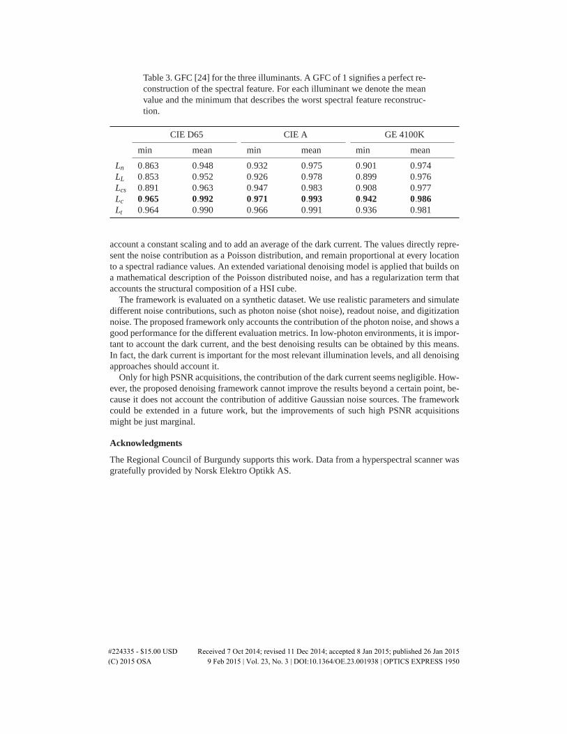
Table 3. GFC [24] for the three illuminants. A GFC of 1 signifies a perfect re-construction of the spectral feature. For each illuminant we denote the meanvalue and the minimum that describes the worst spectral feature reconstruc-tion.


min mean min mean min mean

Ln 0.863 0.948 0.932 0.975 0.901 0.974LL 0.853 0.952 0.926 0.978 0.899 0.976Lcs 0.891 0.963 0.947 0.983 0.908 0.977Lc 0.965 0.992 0.971 0.993 0.942 0.986Lt 0.964 0.990 0.966 0.991 0.936 0.981

account a constant scaling and to add an average of the dark current. The values directly repre-sent the noise contribution as a Poisson distribution, and remain proportional at every locationto a spectral radiance values. An extended variational denoising model is applied that builds ona mathematical description of the Poisson distributed noise, and has a regularization term thataccounts the structural composition of a HSI cube.

The framework is evaluated on a synthetic dataset. We use realistic parameters and simulatedifferent noise contributions, such as photon noise (shot noise), readout noise, and digitizationnoise. The proposed framework only accounts the contribution of the photon noise, and shows agood performance for the different evaluation metrics. In low-photon environments, it is impor-tant to account the dark current, and the best denoising results can be obtained by this means.In fact, the dark current is important for the most relevant illumination levels, and all denoisingapproaches should account it.

Only for high PSNR acquisitions, the contribution of the dark current seems negligible. How-ever, the proposed denoising framework cannot improve the results beyond a certain point, be-cause it does not account the contribution of additive Gaussian noise sources. The frameworkcould be extended in a future work, but the improvements of such high PSNR acquisitionsmight be just marginal.

Acknowledgments

The Regional Council of Burgundy supports this work. Data from a hyperspectral scanner wasgratefully provided by Norsk Elektro Optikk AS.


A sensor-data-based denoising framework for hyperspectral images

Documents