A Sensitivity Analysis of Quality of Life Indices Across Countries

A Sensitivity Analysis of Quality of Life Indices Across Countries

Tauhidur Rahman Ron C. Mittelhammer Philip Wandschneider

Department of Agricultural and Resource Economics Washington State University

Pullman, WA 99163

Paper prepared for presentation at the American Agricultural Economics Association Annual Meeting, Montreal, Canada, July 27-30, 2003

Copyright 2003 by [authors]. All rights reserved. Readers may make verbatim copies of this document for non-commercial purposes by any means, provided that this copyright notice appears on all such copies.

1

A Sensitivity Analysis of Quality of Life Indices Across Countries

Tauhidur Rahman Ron C. Mittelhammer Philip Wandschneider

Abstract

This paper attempts to provide a comprehensive analysis of interrelationships among the determinants of the Quality of Life (QOL). We show that various measures of well-being are highly sensitive to domains of QOL that are considered in the construction of comparative indices, and how measurable inputs into the well-being indicators are aggregated and weighted to arrive at composite measures of QOL. We present a picture of conditions among the 43 countries of the world with respect to such interrelated domains of QOL as the relationship with family and friends, emotional well-being, health, work and productivity, material well-being, feeling part of one�s community, personal safety, and the quality of environment. On the basis of Borda Rule and the principal components approach, we search for factor-indices that may function as QOL indices comparatively across countries. Such indices can be useful in making QOL comparisons and evaluations with reference to both time and place. Comparing and analyzing well-being conditions among countries in this way are aimed at facilitating the discovery of extant of problems with government policies impacting QOL. Key Words: quality of life, domains, Borda rule, principal components, and rankings JEL classification: I31, D60, D63

I. Introduction

Given that improving the quality of life (QOL) is now a common aim of

international development, the long-term future of humanity lies in a better understanding

of factors that may have had or will have an impact on the QOL. For a better

understanding and the long term survivability of humanity during coming the coming

millennia, the following seven distinct issues must be addressed: first, what do we mean

by the term �quality of life�; second, how to measure QOL; third, what are the domains

of well-being that should be included in the measurement; fourth, at what scale to

measure the QOL; fifth, how various domains of well-being are related; sixth, how these

factors affect various subgroups of populations; and seventh, how to provide outcomes

that have practical policy implications by allowing comparisons across countries,

individuals, groups, and over a period of time.

2

In the presence of overwhelming consensus that per capita income or related

measures of income are substantially insufficient measures of well-being, the emphasis

has now shifted to the identification of alternative measures. Quality of life (QOL), social

indicators and basic needs are new approaches that are being discussed.1 All these

approaches are related to the concept of the standard of living. Sen (1985, 1987) has

made a thorough investigation of the concept of standard of living. Improving QOL is

now a common aim of international development. However, identifying robust QOL

indicators, or providing a coherent and robust definition of the concept, remain

problematic (Bloom, David E. et al, 2001).

Historically, life expectancy, literacy rates, per capita income, mortality and

morbidity statistics have been widely employed to construct various indices of well-

being. Probably the best-known composite indices of well-being are the Human

Development Index (HDI), developed by the United Nations Development Program

(UNDP), and the Physical Quality of Life Index (PQLI), developed by Morris (1979).

These new approaches are recognized improvements in terms of capturing various

dimensions of QOL, but they are still substantially limited by their inability to capture

diverse domains of QOL, arbitrary assignment of weights, data used not being subjected

to empirical testing, arbitrary selection of variables, non-comparability of measures over

time and space, measurement errors in variables, and estimation biases due to omission of

feedback effects with various indicators as environmental quality and political and civil

liberties.

1 See for example, Hicks and Streeten (1979), Hicks (1979), Drenowski (1974), Morris (1979), Sen. (1973), Streeten (1979), Dasgupta (1990b), Dasgupta and Weale (1992), Kakwani (1993), Ram (1982), Slottje (1991).

3

In this paper, we make an attempt to provide a comprehensive analysis of

interrelationships among the determinants of QOL. We show that the various measures of

well-being are highly sensitive to domains of QOL that are considered in the construction

of comparative indices, and how measurable inputs into the well-being indicators are

aggregated and weighted to arrive at composite measures of well-being. We also

reexamine some policy relevant questions that have been addressed previously in the

growth economics literature in light of the sensitivity findings.

We present an assessment of conditions among 43 countries of the world with

respect to such interrelated domains of QOL as the relationship with family and friends,

emotional well-being, health, work and productive activity, material well-being, feeling

part of one�s community, personal safety, and the quality of environment. We make an

attempt to measure the various domains of QOL as comprehensively as possible given

the constraint of non-availability of comparable and reliable data on a large set of

countries for our present exercise. Empirical results are illustrated on the basis of data

collected on well-being indicators from various sources, including Human Development

Reports (UNDP) and World Development Indicators (the World Bank) for the year 1999

for 43 countries of the world (Annex A & B).

This paper is organized as follows: Section II briefly reviews the literature on

well-being indices. In section III we discuss on our conceptual framework and the data to

be used in the analysis of sensitivity of well-being measures with respect to the various

domains of QOL and with respect to alternative aggregation rules to arrive at composite

measures of well-being. Section IV describes three alternative aggregation rules to

compute a QOL index. In particular, we derive the rankings of countries on the bases of

4

the Borda Rule, and the principal components approach, and compare these results with

the rankings of Human Development Index (UNDP, 1999). The results are discussed in

Section IV. We provide concluding remarks in section V.

II. Literature Review

Traditionally, per capita gross domestic product (GDP) was considered as the sole

and reliable measure of well-being and economic development. However, in the presence

of overwhelming consensus that as the GDP increases, well-being does not necessarily

increase along with it, there is agreement among economists that per capita GDP or

related measures of income are substantially insufficient measures of well-being. Thus,

the emphasis now has shifted to the identification of alternative measures. Quality of

Life, social indicators and basic needs are new approaches that are being discussed (see

Hicks 1979, Morris, 1979, Sen 1973, Dasgupta and Weale 1992). As early as the year

1967, Adelman and Morris examined numerous indicators of socio-economic and

political change. Morris (1979) proposed the Physical Quality of Life Index (PQLI) as an

alternative to per capita GDP for measuring the well-being of people. The PQLI is a

function of life expectancy at age one, infant mortality rate, and literacy rate. Dasgupta

and Weale (1992) constructed a measure of QOL that included per capita income, life

expectancy at birth, adult literacy rate, and indices of political rights and civil liberties.

However, probably the best known and the most controversial measure of well-being (the

Human Development Index) has been published by UNDP in their Human Development

Reports since 1990 to date. The human development index is based on the assumption

that economic development does not necessarily equate to human development or

5

improvement in well-being. The HDI is based on three indicators: life expectancy at

birth, educational attainment and real GDP per capita.

The HDI is obtained by a procedure where each individual country is first placed

on a scale of 0 to 100 (0 representing the worst performance and 100 the best) with

respect to any indicator; and then it is obtained by a simple arithmetic average of the

scale indicators.

More recently, Lars Obsberg and Andrew Sharpe have developed the Index of

Economic Well-Being (IEWB) (see Osberg and Sharpe, 1998, 1999, and 2000). Their

index is based on the view that the economic well-being of society depends on the level

of consumption flows, accumulation of productive stocks, and inequality in the

distribution of income and insecurity in the anticipation of future incomes. The weights

attached to each of their IEWB component varies depending on the values of different

observers. They argue that the public debate would be improved if there is an explicit

consideration of the aspects of economic well-being obscured by average income trends

and if weights attached to these aspects were explicitly open for discussion.

The American Demographic Index (ADI) of well-being for the United States from

February 1996 to December 1998 was published by American Demographics. It is a

monthly composite of five indicators developed, maintained, and reported by Elia

Kacapyr. He selected the items on the basis of an economist�s perception of well-being,

free of any paradigm or QOL theory.

These new approaches are recognized improvements in terms of capturing various

dimensions of QOL, but they are still substantially limited by their inability to capture

diverse domains of QOL, arbitrary weights, data used not being subjected to empirical

6

testing and arbitrary selection of variables. One weakness (among others) with indices of

general well-being currently in use in such institutions as the World Bank and the United

Nations Development Program (e.g., UNDP, 1990) is that they are restricted to the

socioeconomic aspects of life; the political and civil aspects are for the part kept separate.

When the latter are mentioned at all, they are dealt with perfunctorily (Dasgupta and

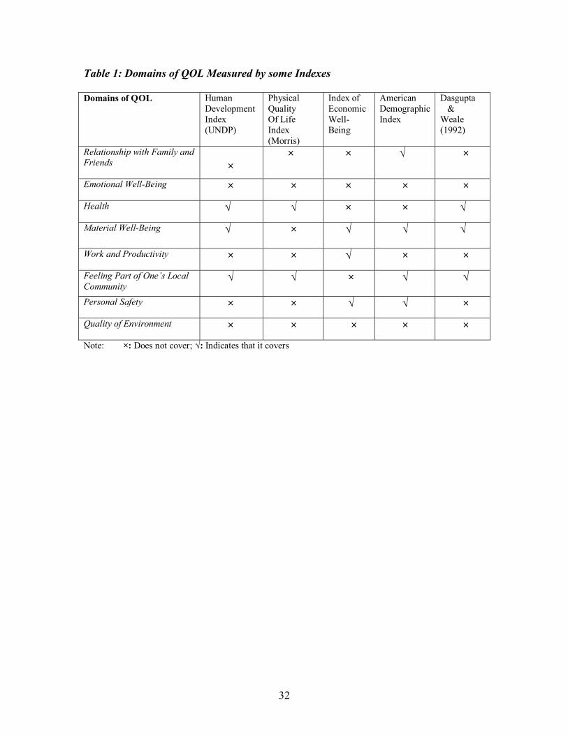
Weale, 1992). Table 1 shows an overview of the various domains of QOL that are

measured or captured by the various well-being indices discussed in the preceding

review. From Table 1, we can easily notice that existing indices of well-being are

severely limited by their inability to capture the multidimensional nature of QOL. The

HDI, which is the most well-known and widely used index of well-being, captures only

three domains of the QOL. It is quite remarkable that the HDI ignores the domains of

relationship with family and friends, emotional well-being, work and productivity,

personal safety, and the quality of environment. In fact, none of the indices of current

well-being captures the domain of the quality of environment; despite the fact that it is

well documented that the environmental quality has direct effect on the QOL.2

Consequently, different indices of well-being give different rankings of countries, and

can lead to potentially misleading policy recommendations.

In the next section, we discuss the conceptual framework and data sources of the indicators of the QOL employed to compute the QOL rankings of countries in our study. III. Conceptual Framework for the QOL

In the behavioral sciences it is generally assumed that individuals� behavior is

guided by the goal of seeking a higher level of the quality of life and that actual behavior

2 For more discussion on this, see Charles Perrings (1998), �Income, Consumption and Human Development: Environmental Linkages�, Background papers, Human Development Report, 1998.

7

should be seen as the reflection of that. However, economists often use the concept of

utility instead of quality of life, while psychologists use the term satisfaction or

happiness. Here we shall use the terms quality of life, standard of living, human well-

being, and welfare interchangeably.

In consumer theory the utility function )(xu , defined on the commodity space X,

is a device to describe a preference ordering among commodity bundles. Indifference

curves are described by the equation kxu =)( where k is constant. The function

)(xu can never be completely identified, but it may be estimated by observing consumer

choice behavior, i.e. via revealed preferences. In principle any monotonic transformation

))(( xug will describe the same indifference curves and the maximization of ))(( xug will

result in the same choice behavior as the maximization of )(xu . This is the idea of

viewing utility as an ordinal concept, describing a preference ordering only.3 If

individuals or public policy makers on the behalf of people are driven by the achievement

of a higher standard of living, understanding and analyzing the determinants of QOL over

a population, society or a country seems a necessary condition to understand human

behavior. In order to accomplish comparisons, achievements of different societies or

population would have to be interpersonally comparable, and societies producing similar

results need to enjoy similar standard of living. Is this plausible? The answer is yes in

light of arguments that satisfaction levels or the level of standard of living are predictive

in the sense that individuals or societies will not choose to continue activities which

produce low satisfaction levels or the low levels of the standards of living.4

3 See for example Pareto (1904), Robbins (1932), Samuelson (1945), and Debreu (1959). 4 See for detailed arguments and justification Kahneman et al., (1993), Clark (1998), and Frijters (2000).

8

Life expectancy, literacy rates, mortality and the like are usually considered as

�indicators� of QOL of people and these statistics have been used by many researchers

over the years to construct various indices of well-being. It is now well recognized that

none of these indicators is singly adequate to measure the QOL (see Sen, 1981). The

QOL is, in fact, a composite variable, which is determined by the interactions of several

dimensions of well-being. Changes in the income level of people, their living conditions,

health status, environment, safety, stress, leisure, and the satisfaction with family life,

social contacts, and many other such variables interact in complex ways and determine

the QOL and its changes.

In the present study, we interpret the QOL of people as an �abstract conceptual

variable�, which cannot be directly measured, but is jointly determined by changes in

several (exogenously determined) causal variables. The causal variables are supposed to

be measured with a reasonable degree of accuracy. In this paper, we focus on factors that

may affect the QOL by identifying the following eight domains of QOL that have been

emphasized at different times by different researchers depending on what were

considered to be the major elements of well-being5:

• Relationship with family and friends,

• Emotional well-being,

• Health,

• Work and productive activity,

• Material well-being,

5 These eight domains of QOL have been identified based on our review of current and historical literature on well-being indices. However, we note that these eight domains are not mutually exclusive of each other, as we don�t expect zero correlation among them. Many readers might question our classification of domains, but we emphasize that it is not an ad hoc classification, as we will provide justifications in the subsequent discussions.

9

• Feeling part of one�s local community,

• Personal safety, and

• Quality of environment

The QOL is a multidimensional concept, which has many distinct domains. Therefore,

besides a composite measure of the QOL, we may distinguish also specific domains such

as the eight domains mentioned above. We speak of domains of the QOL, 1D ,�,

JD where J stands for the number of different domains. Then the QOL must be a

composite of the various domains, say

),....( 1 JDDQOLQOL = , where J =8 (1)

Moreover, each domain J has its own indicators, which are observable, say a

vector of observable indicators ),....,( 1j

Kjj xxx = , (where j = 1� 8), will determine the

achievements in the respective domains. Hence, our basic conceptualization of QOL will

be:

))(),.....,((( 11

JJ xDxDQOLQOL = (2)

In this paper our aim is to compute a composite QOL index (say, QOLI) based on

the general conceptualization in equation (2). If the QOL could be numerically measured

and related to the causal variables (indicator variables in each domain), it would be

straight forward to determine, say, a least squares regression of QOL on the causal

variables. In that case, the partial derivative of QOL with respect to the one of the causal

variables would measure the marginal rate of change of QOL for a small change in the

causal variable, holding other causal variables fixed; and an estimator of QOL would be

obtained as the estimator of the mean of the conditional distribution of QOL when causal

10

variables are held fixed. Since QOL is not directly observable, some rules are needed to

aggregate its various domains (in the present case eight) and corresponding indicators to

arrive at a composite measure of the QOL, and that we discuss in the next section.

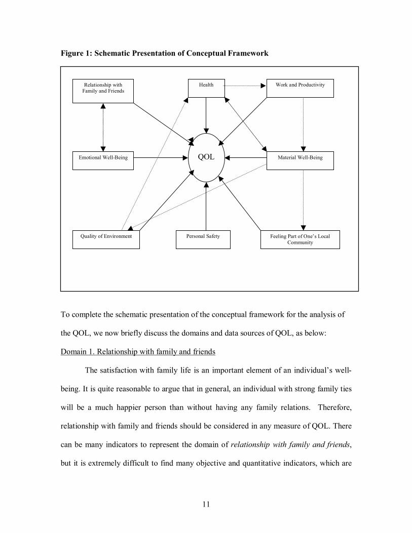
Figure 1 contains the schematic presentation of the conceptual framework

relating to domains of QOL. Here we attempt to draw as broad a picture as possible of

QOL. Some links are direct and easy to understand, but indirect links can also have a

substantial effect. Policy makers often neglect indirect effects, where they need to be

aware of both unanticipated consequences and positive feedback when they assess the

actual effects of changes in any components of QOL. Figure 1 shows both direct and

indirect links between the QOL and its various domains. As can be seen, the QOL has

direct links with its eight domains, which are indicated by bold arrows. In addition, it

indicates the links between domains of QOL, and shows possible indirect effects,

represented by the dotted arrows. These eight domains of QOL have therefore driven the

choice of indicators in the present study for the 43 countries of the world for which

comparable data on various indicators of the QOL are available.

11

Figure 1: Schematic Presentation of Conceptual Framework

To complete the schematic presentation of the conceptual framework for the analysis of

the QOL, we now briefly discuss the domains and data sources of QOL, as below:

Domain 1. Relationship with family and friends

The satisfaction with family life is an important element of an individual�s well-

being. It is quite reasonable to argue that in general, an individual with strong family ties

will be a much happier person than without having any family relations. Therefore,

relationship with family and friends should be considered in any measure of QOL. There

can be many indicators to represent the domain of relationship with family and friends,

but it is extremely difficult to find many objective and quantitative indicators, which are

QOL

Relationship with Family and Friends

Emotional Well-Being

Health Work and Productivity

Material Well-Being

Feeling Part of One�s Local Community

Quality of Environment Personal Safety

12

necessary for cross-country comparisons. Therefore due to the limitation of data

availability, we consider one indicator to focus the first domain, viz., incidence of divorce

rates. Increasing divorce rate is an indication of failing marriages and eroded relationship

with family and relatives.6 The data for this variable has been obtained from Gulnar and

Nugman of the Heritage Foundation. The data is for the year 1999, or the nearest

available date. The divorce rate is reported as the number of divorces per thousand

people.

Domain 2. Emotional Well-Being

Although measures such as crime statistics, health status, and indicators of wealth

are surely related to QOL, these indicators cannot capture what it means to be �happy�.

How happy an individual is, not only depends on his/her income, and consumption, but it

is also affected by intensity of stress, depression, and psychology. Emotional well-being,

like physical health, can be judged on a variety of dimensions. Yet, in both realms, it is

difficult to say which of these dimensions are essential for overall well-being. We use

estimates of both male and female suicide rates to focus on emotional well-being.

Teenage suicide rates were used in the construction of the index of social health (ISH) by

Miringoff of the Fordham Institute for Innovation in Social Policy (1996, 1999). We have

obtained data for both male and female suicide rates from the Mental Health Data of the

6 It can be argued that the incidence of divorce rate is not a good indicator of relationship with family and friends. One can dispute it on the ground that a marriage not ending in divorce does not mean that people in the marriage are happy. For instance, many researchers have argued it that low rate of divorce in countries like India and Islamic countries can be partly explained by the low status of women in the society where women are traditionally supposed to be playing the role of homemaker. However, we strongly emphasize that in these countries people attach higher importance to joint family system, social status, and marriage is considered as a social value rather than a contract, and divorce is viewed as the social taboo. Thus, we argue that low divorce rates in these countries are not only a result of the low status of women in the society, but also it is a reflection of a strong joint family system and relationship with family and friends.

13

World Health Organization (WHO). We assume that a higher incidence of suicide rates

by either gender is an indication of weaker emotional well-being.

Domain 3. Health

Good health should result in a better QOL. Health has both direct and indirect

positive effects on QOL. Improvement in health has an immediate impact on a person�s

QOL, but may also indirectly increase it by acting on other variables that in turn also

have a beneficial effect. One of the most studied relationships is between health and

income. Higher income leads to better health, but better health also leads to higher

income because of better productivity and labor force participation.7 To focus on the

domain of health a balance has to be struck among various components of a healthy

society: demography, longevity, mortality, morbidity, and health infrastructure. Thus, we

use population growth rate (representing demographic pressure); life expectancy at birth

(longevity); infant mortality rate (mortality); the number of AIDS cases and tuberculosis

cases (representing morbidity); government expenditure on health as a percentage of

GDP, and doctor/population ratio (representing health facilities) to capture the domain of

health in our measure of the QOL. The data on these indicators have been obtained from

HDR, 1999.

Domain 4. Material well-being

The elements of material well-being have both direct and indirect positive and

negative impact on a person�s QOL. For instance, rising national income due to

industrialization raises QOL on the one hand, but on the other hand decreases it for those

living in polluted areas. The latter may suffer further indirect effects if increased

7 See for example Lee (1982), Ettner (1996), Pritchett and Summers (1996), Luft (1975), Grossman and Benham (1980), Bloom and Malaney (1998), Bloom and Sachs (1998), Bloom and Williamson (1998), Bloom and Canning (1999).

14

pollution raises the incidence of disease and chronic illness. Aspects of material well-

being have been most widely used to construct various indices of well-being. One of the

main reasons for its use is the availability of good data on various indicators.

Traditionally measures of income or related measures of material well-being were

considered adequate indicators of standards of living. To capture the extent of material

well-being in our QOL we use per capita GDP (at purchasing power parity), daily per

capita supply of calories, the commercial use of energy, and telephone lines per thousand

people (both representing infrastructure).8 The data for these indicators have been

obtained from the HDR, 1999.

Domain 5. Feeling part of one�s local community

Feeling part of one�s local community and society in general depend on the

factors like educational attainments, political rights, and civil liberties, among others.

Many people in different countries of the world are systematically denied political liberty

and basic civil rights. It is sometimes claimed that the denial of these rights helps to

stimulate economic growth and is �good� for rapid economic development. However,

comprehensive intercountry comparisons have not provided any confirmation of this

thesis, and there is little evidence that authoritarian politics actually helps economic

growth. As Sen. (1999) argued:

�-----political liberty and civil freedoms are directly important on their own, and do not have to be justified indirectly

in terms of their effects on economy. Even when people without political liberty or civil rights do not lack adequate

economic security (and happen to enjoy favorable economic circumstances), they are deprived of important freedoms

in leading their lives and denied the opportunity to take part in crucial decisions regarding public affairs. These

8 Since daily per capita supply of calorie is much influenced by income; one can argue we will be counting income twice. However, we note that the quality of consumption does not only depend on the level of income, but also how income is being used by the individual, which in turn depends on his/her level of education. Moreover, it is an easy matter to redo all our computations by deleting data on either of our material well-being indices.

15

deprivations restrict social and political lives, and must be seen as repressive even without their leading to other

afflictions. Since political and civil freedoms are constitutive elements of human freedom, their denial is a handicap in

itself.� (Sen. (1999, p. 16-17))

Concurrent with this realization, economists who previously assumed that

measures of income are the sole and reliable indicators of human well-being finally have

begun to understand that political liberties and civil freedoms are as important elements

of QOL as any other elements of QOL. Thus we emphasize that any measure of current

well-being that does not include political and civil spheres of life, will be incomplete and

misleading for intercountry comparisons of QOL. Here we use indices of political and

civil liberties along with both male and female adult literacy rates to capture this domain

of QOL. The indices of political rights and civil liberties are taken from Gastil, R. D. -

Freedom in the World: Political and Civil Liberties (For definition see Taylor and Jodice

1983). It is also available from various human development reports of UNDP. Rights to

political liberty measures citizens right to play a part in determining their government,

and what laws are and will be. Countries are ranked with scores ranging from one

(highest degree of liberty) to seven (lowest degree of liberty). On the other hand, the

index of civil liberties measures the extent of people�s access to an impartial judiciary,

access to free press, and liberty to express their opinion. Countries are ranked with scores

ranging from one (highest civil liberty) to seven (lowest degree civil liberty).

Domain 6. Work and productive activity

The estimates of unemployment rate; combined first, second, and third level

school gross enrollment ratio; and female economic activity rate are used to capture the

�extent of work and productive activity� that exists in countries included in our sample.

At any point of time, citizens of a country can be productively engaged either in work

16

employment, or be engaged in the process of learning in school. The female economic

activity rate is used to capture the intensity of gender equality in productive activity.

Domain 7. Personal safety

For the well-being of people personal safety is as important as any other domains

of the QOL. In a society where incidence of crimes is less, people can enjoy their living

much better than in a society where criminal offences are high and very common. This is

very important because an individual derives utility not only from the commodity bundles

in her/his consumption basket, but it very much depends on her/his ability to walk, and

live free of crimes on streets, material theft, good law and order situations in the

neighborhoods. To capture these domains of well-being, we use two different indicators,

viz., the total number of offences contained in the national crime statistics, and

expenditure on military as percentage of GDP. This total number of offences includes

cases of murder, sex offences, serious assaults, theft, fraud, counterfeit currency offences,

and drug offences. We believe that the higher is the total number of offences; the lower

will be the well-being of people. Similarly, we argue that the expenditure on military is

an unproductive expenditure, and therefore it has indirect adverse effect on the QOL. We

have obtained data on total offences from the International Crime Statistics of the

Interpol. The data refers to the year 1997. Data on military expenditures were obtained

from HDR, 1999.

Domain 8. Quality of Environment

Most indices of human well-being have ignored the interrelationships between the

QOL and environmental changes. Quality of environment has direct and indirect long-

term effects on the health status of the citizens, and consequently it affects the quality of

17

life of people in the region. As we can see from Figure 1, the elements of material well-

being have impact on quality of environment; the quality of environment has direct and

an immediate effect on QOL, and an indirect effect on QOL through its effect on health.

To capture the extent of the quality of environment, we use a measure of greenhouse gas

emissions- carbon dioxide (CO2); a measure of water pollution-access to safe water

supplies (ACH2O); and a measure of the depletion of environmental resources-

deforestation. Emissions of CO2 are primarily a by-product of industrialization, and

attract more attention in middle and upper-income countries. Deforestation and depletion

of local water supplies attract the most attention in low-income countries. Water pollution

is of the major concern because of its immediate effects on human health and

productivity. Deforestation is important because it affects the hydrological cycle, and it is

linked with the depletion and pollution of water supplies. We have obtained data on these

variables from the World Development Indicators, 1999; and HDR, 1999.

Our aim here is to conduct a number of simple exercises with data on eight

domains of the quality of life. The present method is to select and test out domains (in the

present case, eight), which may function as the QOL indices. In the next section, we

describe three aggregation methods to arrive at a composite measure of the QOL index.

First, we briefly describe the computation of QOL based on the principal component

approach. Second, we make use of the well-known Borda Rule as the aggregator of set of

variables in each domain of the QOL. Third, UNDP�s approach to Human Development

Index (HDI).

18

IV. Computation of Quality of Life Index (QOLI)

We postulate a latent variable model where the QOL is linearly determined by a

set of observable indicators (or a set of causal variables) plus a disturbance term

capturing error.

Let the general model in equation (2) can be written as:

εβββα +++++= )(......)()( 888

222

111 xDxDxDQOL (3)

where 1D ,�, 8D are set of indicators in each domain of the QOL that are used to

capture the �quality of life index�, and 81 ,......,ββ are the corresponding vectors of

parameters in each domain. Thus the total variation in the QOL is composed of: a) the

variation due to sets of indicators, and b) the variation due to error. If the model (3) is

well specified, including an adequate number of indicators in each domain, so that the

mean of the probability distribution of ε is zero, ( 0)( =εE ), and error variance is small

relative to the total variance of the latent variable QOL, we can reasonably assume that

the total variation in QOL is largely explained by the variation in the indicator variables

in each domain included for the computation of this composite index.

Since the number of indicators variables included in the model (3) may be large

and the indicator variables may be mutually linearly related, we propose to replace the set

of indicators by an adequate number of their principal components (PC). The principal

components are normalized linear functions of the indicator variables and they are

mutually orthogonal. The first principal component accounts for the largest proportion of

total variation (trace of the covariance matrix) of all indicator variables. The second

principal component accounts for the second largest proportion and so on. In practice, it

is adequate to replace the whole set of indicator variables by only the first few

19

components, which account for a substantial proportion of the total variation in all

indicator variables. However, if the number of causal variables is not very large, we may,

as well, compute as many principal components so that 100% of the variation in

indicators is accounted for by their PCs (see Anderson, 1984). To compute PCs, we

proceed as follows:

Step 1: Transform the indicators into their standardized form i.e.

Xk = ( )

k k

k

X Xstd X

−

Step 2: Then solve the determinental equation

R−λΙ=0 for λ

where R is a K×K correlation matrix of the standardized vector of indicator variables;

this provides Kth degree polynomial equation in λ and hence K roots. These roots are

called the eigenvalues of R. Now let us arrange λ in the descending order of magnitude,

as

λ1>λ2>…>λk

Step 3: Corresponding to each value of λ, we solve the matrix equation

( ) 0R λ α− Ι = For the K×1 eigenvectorsα, subject to the condition that ' 1α α = .

Let us write the characteristic vectors as

α1=

11 1

1

. .,............, ,. .

. .

k

k

k kk

α α

α

α α

=

which

correspond to 1 ,............ κλ λ λ= respectively.

20

Step 4: The principal components are obtained as

1 11 1 1

2 21 1 2

1 1

........

..........

........

α α

α α

α α

Κ Κ

Κ Κ

Κ Κ ΚΚ Κ

Ρ = Χ + + Χ

Ρ = Χ + + Χ

Ρ = Χ + + Χ

Thus we compute all these principal components using elements of successive

eigenvectors corresponding to respective eigenvalues.

Step 5: We define the weighted average of the principal components as an estimator of

the quality of life index (QLI), thus:9

QOLI = 1 1 2 2

1 2

...........

λ λ λλ λ λ

Κ Κ

Κ

Ρ + Ρ + + Ρ+ + +

where the weights are 1,.........,λ λΚ are variances of successive principal components. We

assign the largest weight λ1 to the first principal component, as it accounts for the largest

proportion of variation in all causal variables. Similarly, the second principal component

has the second largest weight and so on.

Step 6: Finally, we normalize the QOLI value by the following procedure,

)()(

)(ii

iii

QOLIMinimumQOLIMaximumQOLIMinimumQOLQOLI

−−=

where i = 1, 2 �n (=43, countries of the world). Then on the basis of estimated value of

QOLI we rank 43 countries of the world where the value of 0 indicates worst performing

country and therefore it gets the rank of 43. Similarly, the value of 1 indicates the best

performing country, and hence it is assigned the rank of 1 (highest rank).

9 This methodology was originally proposed by Nagar, A. L., and Tauhidur Rahman (1999), has been subsequently used by many researchers including Nagar, and Basu (2001 a, b and 2002).

21

Advantages of the above procedure are the following: First, it minimizes the

problem of assigning arbitrary weights since weights are based on information contained

in the date set. That is, we assign weights to successive principal components based on

their relative contribution in accounting the total variation in all indicator variables.

Second, it overcomes the difficulties associated with the maximum likelihood method for

the estimation of Multiple Indicators and Multiple Causes (MIMIC) model. For instance,

the maximum likelihood method requires that the number of causal variables to be

included in the model does not exceed the number of observations and none of the causal

variables is linearly related with others. In fact, the method requires that the matrix of

sum of squares and products of observations on causal variables is non-singular (see

Goldberger, 1974; Joreskog and Goldberger, 1975). Thus, the usefulness of the principal

component approach lies in its simplicity and its wide scope in providing flexibility for

exploratory statistical analyses to be conducted on various domains of the quality of life.

Of the many alternative aggregation methods, the most well known and most

studied is the Borda Rule. This rule provides a method of rank-order score, the procedure

being to award each alternative (say, a country) points equal to its rank in each criterion

of ranking (the criteria being per capita income, life expectancy, and the like), adding

each alternative�s scores to obtain its aggregate score, and then ranking alternatives on

the basis of their aggregate scores. To illustrate, suppose a country has the ranks i, j, k, l,

and m, respectively, for the five criteria. Then it�s Borda score is i + j + k + l + m. The

rule invariably yields a complete ordering of alternatives. We note that the Borda Rule

suffers from various limitations (Goodman and Markowitz (1952) and Fine and Fine

(1974) have investigated the strengths and limitations of the Borda rule). The fact that

22

Borda rule is simple, and its strengths and weaknesses are transparent, provides a good

justification for using it (Dasgupta and Weale, 1992). Moreover, it provides a very simple

tool to analyze the sensitivity of quality of life ranking across countries contingent on

inclusion or exclusion of a particular domain of the quality of life.

United Nations Development Program (UNDP) in its first Human Development

Report (1990) introduced a new way of measuring well-being by combining indicators of

life expectancy, educational attainment and income into a composite human development

index (HDI). Although, over the years some changes have been made in the construction

of HDIs, the methodology has remained the same. The HDI is based on three indicators:

(a) longevity, as measured by life expectancy at birth; (b) educational attainment,

measured as a weighted average of (i) adult literacy rate with two-third weight, and (ii)

combined gross primary, secondary and tertiary enrolment with one-third weight; (c)

standard of living, as measured by real gross domestic product (GDP) per capita (PPPS).

The HDI sets a minimum and maximum for each dimension and then shows where each

country stands in relation to this scales-expressed as value between 0 and 1. Since the

minimum adult literacy rate is 0% and the maximum is 100%, the literacy component of

knowledge for a country where literacy rate is 75% would be 0.75. Similarly, HDI uses

the minimum of life expectancy as 25 years and the maximum of 85 years, so the

longevity component for a country where life expectancy is 55 years would be 0.50. For

income, the minimum is $100 (PPP) and the maximum is $40,000 (PPP). Then the scores

for the three dimensions are averaged in an overall index.

23

IV. Discussion of Results

We consider 43 countries of the world for which comparable data on eight

domains of QOL and corresponding indicators were available in the year 1999. Our set of

countries includes both developed and developing economies of the world. In total we

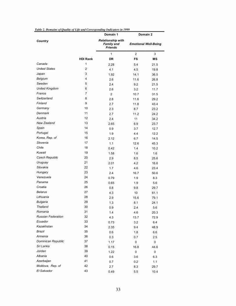
make use of 26 indicators of the QOL. Table 2 summarizes the data. The first column of

the table 2 represents the domain 1, the relationships with family and friends. Its indicator

is the divorce rate (DR). Columns 2 & 3 represent domain 2, emotional well-being. Its

two indicators are Female suicide rate (FS) and male suicide rate (MS). Columns 4 to 10

represent domain 3, health. It has in total seven indicators: population growth rate (PGR),

infant mortality rate (IMR), life expectancy at birth (LE), cases of AIDS (AIDS), cases of

tuberculosis (TC), health expenditure by the government as the percentage of GDP (HE),

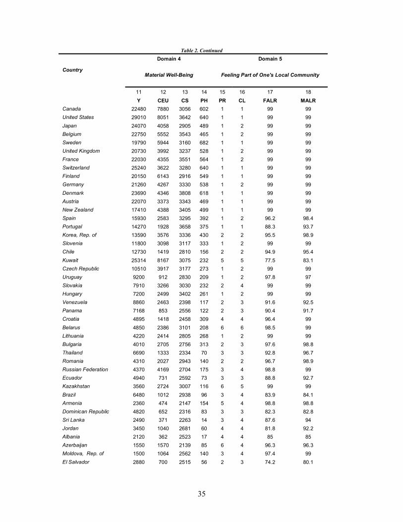
and doctor population ratio (DPR). Columns 11 to 14 represent domain 4, material well-

being. It includes per capita GDP (at PPP), Commercial energy use (CEU), daily per

capita supplies of calories (CS), and Phone lines available per 1000 population (PH).

Columns 15 to 18 describe domain 5, feeling parts of one�s local community: political

rights index (PR), civil liberties index (CL), female adult literacy rate (FALR), and the

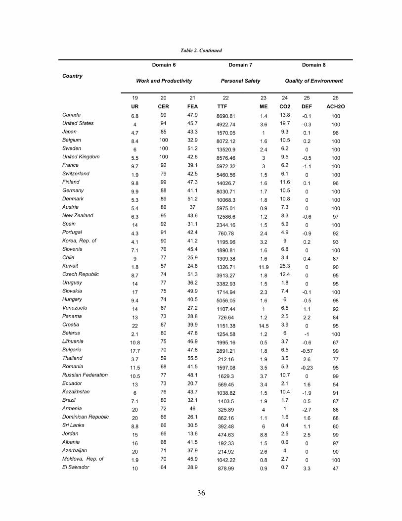
male adult literacy rate (MALR). Columns 19 to 21 represent domain 6, work and

productive activity, where unemployment rate (UR), combined enrollment ratio in school

(CER), and female economic activity rates (FEA) are its indicators. Columns 22 and 23

show domain 6, in which the total number of offenses (TTF), and expenditure on military

as a percent of GDP (ME) are its two indicators. Finally, columns 24 to 26 represent the

domain of the quality of environment. Its three indicators are emissions of carbon dioxide

(CO2), rate of deforestation (DEF), and the access to safe water (ACH20).

24

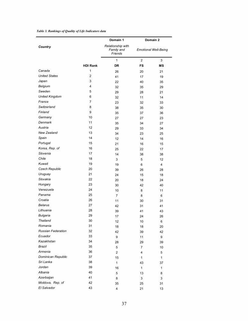
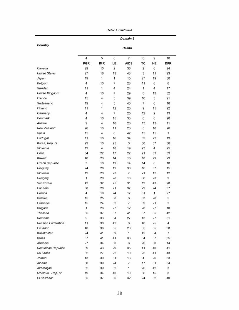
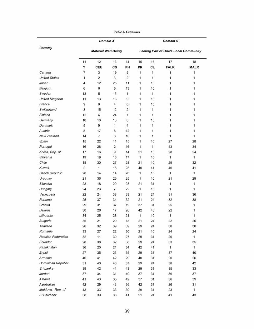
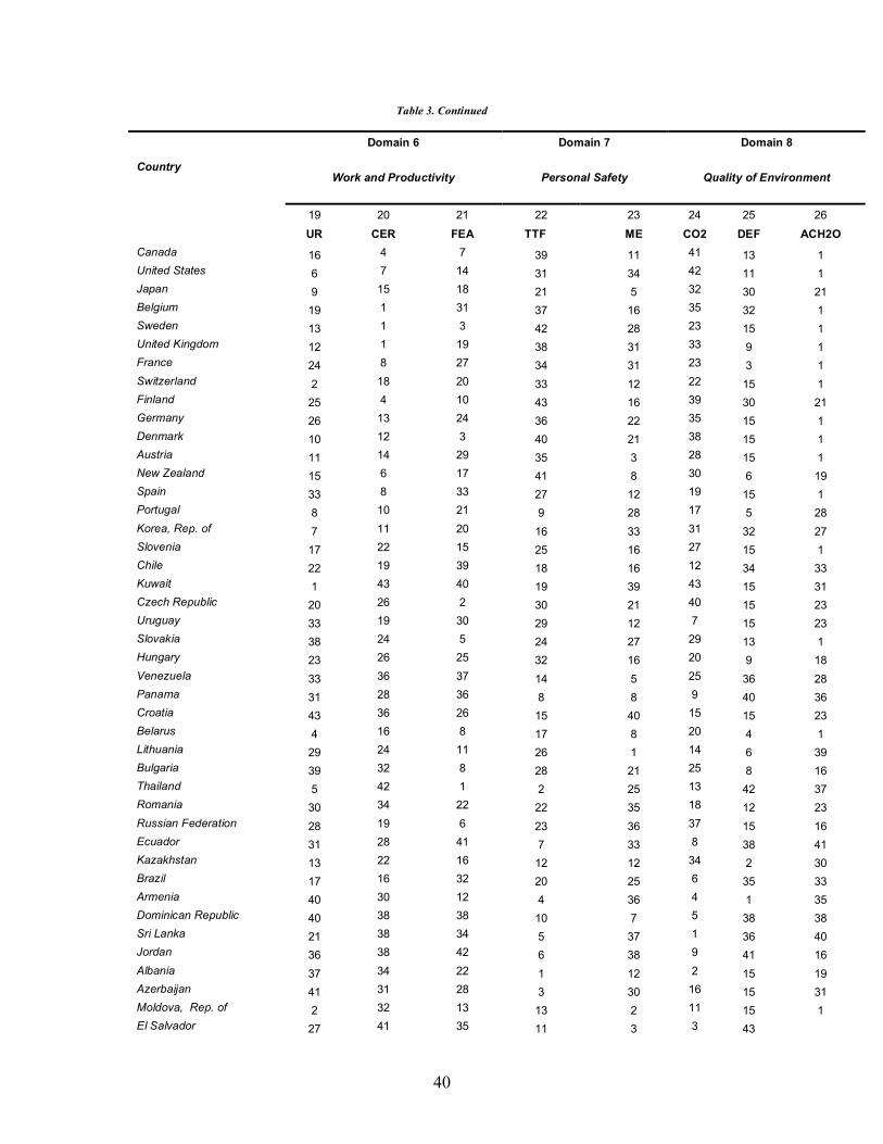
Table 3 presents the rankings of quality of life indicators data. The HDI rank is

the rankings of countries provided by human development report, 1999, and the rankings

of the countries have been re-assigned in accordance with countries in our set. We note

that rank of 1 represents the best performing country, and the rank of 43 represents the

worst performing country. Even a glance at these rankings in Table 3 tells us that well-

being rankings are highly sensitive to its� domain and corresponding indicators. Also

rankings of eight domains indicate that they do not quite follow the rankings provided by

HDI, which uses different weighting criterion, and very limited numbers of QOL

indicators. Thus, rankings in Table 3 suggest that not only the measures of well-being are

sensitive to its coverage of the various domains, but also how different well-being inputs

are aggregated to arrive at a composite measure of the QOL. Developed countries like

Canada, USA, Japan, and Sweden perform the best in the domains of material well-being,

and feeling part of one�s local community, but they do not perform as good in the

domains of personal safety, and the quality of environment, relationships with family and

friends, and emotional well-being. On the other low ranked countries on the basis of HDI,

do better in the domains of relationships with family and friends, emotional well-being,

and personal safety. These exploratory and tentative results may be an indicative of

differences between advanced industrial societies with nucleus family, and developing

countries with traditional societies and strong family ties.

Table 4 presents a comparison of quality of life indices based on each of eight

domains, an overall QOLI* based on both Borda Rule and Principal Components

approach, and the HDI ranks. Let�s look at the best five performing countries on the basis

of both HDI and QOLI* (Borda Rule). The best five HDI countries are: Canada, USA,

25

Japan, Belgium, and Sweden. On the other hand, the best five countries on the basis of

QOLI* (Borda Rule) are: Spain, Austria, Sweden, Switzerland, and Canada. That is, there

are only two countries, Canada, and Sweden, which figure in these two schemes of

aggregation. Similarly, we look at five worst performing countries on the basis of both

HDI and QOLI* (Borda) rankings. The five worst performing countries on the HDI

rankings are: El Salvador (43), Moldova (42), Azerbaijan (41), Albania (40), and Jordan

(39). On the other hand, the worst five countries on the basis of QOLI* (Borda) rankings

are: Russia (43), Sri Lanka (42), Ecuador (40), Kazakhstan (40), and South Korea (39). It

is quite chilling to note that there is not even single country common between two sets of

five worst performing countries based on HDI and QOLI*. Now let us look at the

rankings based on the QOLI* (Borda Rule) and QOLI* (principal components (PC)

approach). We can clearly note from the table 4 that these two methods of weighting of

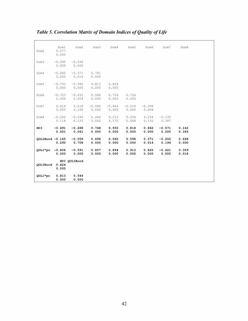
well-being indicators do not produce quite similar rankings. From table 5, we observe

that the rank correlation coefficient between HDI and QOLI*(Borda) is 0.624, between

HDI and QOLI*(PC) is 0.813, and between QOLI*(Borda) and QOLI* (PC) is 0.544.

Thus we can say that the rankings based on the principal component approach follows

more closely with the HDI rankings than with the rankings based on the Borda Rule.

Since these two rankings are based on all eight domains of QOL, we conclude that there

is sufficient evidence that the well-being rankings are sensitive to aggregation rules.

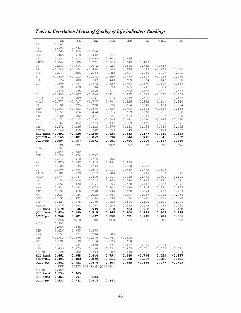
Table 5 presents rank correlation matrix of indices of QOL domains, the HDI, and

QOLI* itself. First, let us look at the correlation coefficients between QOLI*(Borda) and

its eights domains. We notice that QOLI* has statistically significant correlation with

only five domains of the QOL: health (0.696), material well-being (0.560), feeling parts

26

of one�s local community (0.598), work and productive activity (0.371), and the quality

of environment (0.668). QOLI* has the highest correlation (0.696) with the domain of

health. We were not expecting this. We did not have any reason to expect that health

would be the closest to our measure of the quality of life. Nevertheless, our findings

support the results obtained by Dasgupta and Weale (1992) where they found that life

expectancy (an indicator of health) was closest to the measure of the QOL. Thus, if we

had to choose a single ordinal domain of aggregate well-being, the domain of health

would seem to be the best if the aggregation method is the Borda Rule. Moreover, if we

really had to choose one indicator instead of a domain, it would be most appropriate to

choose the life expectancy at birth as the indicator of the quality of life. This is also

corroborated from the correlation between QOLI*(Borda) and LE, which is (0.745) from

Table 6. The QOLI*(Borda) has the second highest correlation with the domain of the

quality of environment. This supports our postulation that the quality of environment is

very important for human well-being, and it has direct and positive impact on the QOL.

Since QOLI* is highly correlated with quality of environment, any alternative index of

well-being in the development literature that ignores the domain of the quality of

environment, would give misleading rankings of countries and consequently misleading

policy recommendations.

Moreover, QOLI*(Borda) has statistically insignificant correlation with the

domains of relationship with family and friends, emotional well-being, and the personal

safety. The statistically insignificant correlation of QOLI*(Borda) with the domains of

relationship with family and friends, emotional well-being, and the personal safety, might

mislead readers that these domains are not critical to any measures of the QOL. But we

27

caution readers that this is not the case at all. First, these domains have statistically

significant correlations with the QOLI*(PC). Second, as we mentioned in the previous

section that the divorce rate is a crude indicator of relationship with family and friends,

and therefore it cannot singly and adequately capture the domain of relationship with

family and friends. Similarly, emotional well-being is much more diverse domain than it

is being captured by suicides rates. Due to the non-availability of data we limited

ourselves to the choice of divorce statistics.10 Thus we emphasize the exploratory nature

of our inquiry only because the matter is a sensitive one, and there is a great deal

remaining to be done and examined in this field. The correlation coefficient of 0.824

between the domains of material well-being and feeling parts of one�s local well-being

mean that the claim that the circumstances which cause poverty are also those which

make it necessary for government to deny citizens their political and civil liberties is

simply false. There are countries in the sample which are low-income countries and

which enjoy relatively high levels of civil and political liberties.

V. Concluding Remarks

This paper introduced a multidimensional approach to measuring the quality of

life across countries. We operationalized Sen�s concept that other factors besides

measures of per capita income and mortality rates should be included into any analysis of

quality of life. Using information on eight domains of the quality of life we showed that

the various measures of well-being are highly sensitive to domains of QOL that are

considered in the construction of comparative indices, and how measurable inputs into

10 Some can argue that emotional well-being and relationship with family and friends are subjective domains of the QOL, and therefore it would be difficult to find many indicators in these domains, which will be reliable enough to perform intercountry comparisons. However, we note that people always attach higher weights to emotional well-being and relationships with family and friends in direct surveys when they are asked to rank the elements of their well-being.

28

the well-being indicators are aggregated and weighted to arrive at composite measures of

QOL. We presented a picture of conditions among the 43 countries of the world with

respect to such interrelated domains of QOL as the relationship with family and friends,

emotional well-being, health, work and productivity, material well-being, feeling part of

one�s community, personal safety, and the quality of environment. On the basis of Borda

Rule and the principal components approach, we searched for factor-indices that may

function as QOL indices comparatively across countries. Our results suggest that the

well-being rankings are not robust to the various aggregation methods and the domains of

the QOL. Therefore, further research is needed to find an optimal and robust aggregation

methods to derive appropriate weights for the well-being attributes.

29

References

[1] Adelman, I., and C. T. Morris (1967), �Society, Politics and Economic Development�, Johns Hopkins University Press, Baltimore, MD. [2] Bloom, David E., Patricia H. Craig, and Pia N. Malaney (2001), �The Quality of Life in Rural Asia�, Oxford University Press, Hong Kong. [3] Bloom, David E., and Pia N. Malaney (1998), �Macroeconomic Consequences of the Russian Mortality Crisis�, World Development, 26 (11): 2073-2085. [4] Bloom, David E., and Jeffrey Sachs (1998), �Geography, Demography, and Economic Growth in Africa�, Brookings Papers on Economic Activity 2: 207-295. [5] Bloom, David E., and Jeffrey Williamson (1998), �Demographic Transitions and Economic Miracles in Emerging Asia�, World Bank Economic Review 12 (3): 419-455. [6] Bloom, David E., and David Canning (2000), �The Health and Wealth of Nations�, Science 287: 1207-1209. [7] Cark, A.E. (1998), �Comparison-Concave utility and following behavior in Social and Economic setting�, Journal of Public Economics, 70(1): 133-155. [8] Dasgupta, P. (1990), �Well-being and the Extent of its Realization in Poor Countries�, Economic Journal, Vol. 100, Supplement: 1-32. [9] Dasgupta, P., and Martin Weale (1992), �On Measuring the Quality of Life�, World Development, Vol. 20, No. 1: 119-131. [10] Debreu, G. (1959), �Theory of Value�, Yale University Press, New Haven. [11] Drenowski, J. (1974), �On Measuring and Planning the Quality of Life�, Institute of Social Studies, The Hague. [12] Ettner, Susan L. (1996), �New Evidence on the Relationship between Income and Health�, Journal of Health Economics, 15: 67-85. [13] Fine, B., and K. Fine (1974), �Social Choice and Individual Rankings, I and II�, Review of Economic Studies, Vol. 44, No. 3 and 4: 303-322, and 459-476. [14] Frijters, P. (2000), � Do Individuals try to Maximize General Satisfaction?� Journal of Economic Psychology, 21(3): 281-304. [15] Goodman, L.A., and H. Markowitz (1952), �Social Welfare Functions based on Individual Rankings�, American Journal of Sociology, Vol. 58.

30

[16] Grossman, M., and Lee Benham (1980), �Health Hours and Wages�, In The Economics of Health and Medical Care: An Introduction, edited by Philip Jacobs, Baltimore: University Park Press. [17] Hicks, N. (1979), �Growth vs. Basic Needs: Is there a trade-off?� World Development, Vol.7: 985-994. [18] Hicks, N., and Paul Streeten (1979), �Indicators of Development: The Search for a Basic need Yardstick�, World Development, Vol. 7. [19] Kahneman, D., Fredrickson, B.L., Schreiber, C.A., and Redelmeier, D.A. (1993), � When more Pain is preferred to less: Adding a better end�, Psychological Science, Vol. 4:401-405. [20] Kakwani, N. (1993), �Performance in Living Standards: An International Comparison�, Journal of Development Economics, Vol. 41: 307-336. [21] Kacapyre, Elia (1996), �Are we having fun yet?� American Demographics (October): 28-29. [22] Lee, Lung-Fei. (1982), �Health and Wage: A Simultaneous Equation Model with Multiple Discrete Indicators�, International Economic Review 23: 199-219. [23] Luft, Harold S. (1975), �Impact of Poor Health on Earnings�, Review of Economics and Statistics, Vol. 75: 43-57. [24] Miringoff, Marc L., and Marque L. Miringoff (1999), �The Social Health of the Nation: How America is Really Doing�, New York: Oxford University Press. [25] Morris, David. (1979), �Measuring the Conditions of the World Poor, the Physical Quality of Life Index�, Pergaman Press, New York. [26] Osberg, L., and Andrew Sharpe (1998), �An Index of Economic Well-being for Canada�, Research Paper R-99-3E, Applied Research Branch, Human Resources Development, Canada, Ottawa, Ontario. [27]-------------------------------------------- (1999), �An Index of Economic Well-being for Canada and the United States�, paper presented at the annual meeting of the American Economic Association, New York, January. [28]-------------------------------------------- (2000), �International Comparisons of Trends in Economic Well-being�, paper presented at the annual meeting of the American Economic Association, Boston, MA. January.

31

[29] Perrings, Charles. (1998), �Income, Consumption and Human Development: Environmental Linkages�, In Background Papers, Human Development Report, 1998: 151-212. [30] Pritchett, L., and Lawrence H. Summers (1996), �Wealthier is Healthier�, Journal of Human Resources, 31(4): 841-868. [31] Ram, R. (1982), �Composite Indices of Physical Quality of Life, Basic Needs Fulfillment, Income: A Principal Component Representation�, Journal of Development Economics, Vol. 11: 227-247. [32] Robbins, L. (1932), �An Essay on Nature and Significance of Economic Science�, Macmillan, London. [33] Samuelson, P.A. (1945), � Foundations of Economic Analysis�, Harvard University Press, Cambridge MA. [34] Sen., A. K. (1999), �Development as Freedom�, Alfred A. Knopf, New York. [35] Sen., A. K. (1987), �Standard of Living�, Cambridge University Press, New York. [36] Sen., A.K. (1985), �Commodities and Capabilities�, North-Holland, Amsterdam. [37] Sen., A.K. (1981), �Public Action and the Quality of Life in Developing Countries�, Oxford Bulletin of Economics and Statistics, Vol. 43. [38] Sen., A.K. (1973), �On the Development of Basic economic Indicators to Supplement GNP Measures�, United Nations Bulletin for Asia and the Far East, Vol. 24. [39] Slottje, Daniel. (1991), �Measuring the Quality of Life across Countries�, the Review of Economics and Statistics, Vol. 73: 684-693. [40] Taylor, C. L., and D.A. Jodice (1983), �World Handbook of Political and Social Indicators, Vol. 1, Yale University Press, New Haven, CT.

32

Table 1: Domains of QOL Measured by some Indexes Domains of QOL Human

Development Index (UNDP)

Physical Quality Of Life Index (Morris)

Index of Economic Well-Being

American Demographic Index

Dasgupta & Weale (1992)

Relationship with Family and Friends

×

× × √ ×

Emotional Well-Being

× × × × ×

Health

√ √ × × √

Material Well-Being

√

× √ √ √

Work and Productivity

× × √ × ×

Feeling Part of One�s Local Community

√

√ × √ √

Personal Safety

× × √ √ ×

Quality of Environment

× × × × ×

Note: ×: Does not cover; √: Indicates that it covers

33

Table 2. Domains of Quality of Life and Corresponding Indicators in 1999 Domain 1 Domain 2

Country

Relationship with Family and

Friends Emotional Well-Being

1 2 3 HDI Rank DR FS MS Canada 1 2.28 5.4 21.5 United States 2 4.1 4.5 19.8 Japan 3 1.92 14.1 36.5 Belgium 4 2.6 11.6 26.8 Sweden 5 2.4 9.2 21.5 United Kingdom 6 2.6 3.2 11.7 France 7 2 10.7 31.5 Switzerland 8 2.8 11.6 29.2 Finland 9 2.7 11.8 43.4 Germany 10 2.3 8.7 23.2 Denmark 11 2.7 11.2 24.2 Austria 12 2.4 11 34.2 New Zealand 13 2.65 6.9 23.7 Spain 14 0.9 3.7 12.7 Portugal 15 1.9 4.4 12.2 Korea, Rep. of 16 2.12 6.7 14.5 Slovenia 17 1.1 12.6 45.3 Chile 18 0.42 1.4 10.2 Kuwait 19 1.58 1.6 1.6 Czech Republic 20 2.9 8.5 25.6 Uruguay 21 2.01 4.2 16.6 Slovakia 22 1.7 4.6 23.4 Hungary 23 2.4 16.7 50.6 Venezuela 24 0.79 1.9 8.3 Panama 25 0.65 1.9 5.6 Croatia 26 0.8 9.8 29.7 Belarus 27 4.3 10 61.1 Lithuania 28 2.9 15.6 79.1 Bulgaria 29 1.3 8.1 24.1 Thailand 30 0.9 2.4 5.6 Romania 31 1.4 4.6 20.3 Russian Federation 32 4.3 13.7 72.9 Ecuador 33 0.73 3.2 6.4 Kazakhstan 34 2.35 9.4 48.9 Brazil 35 0.6 1.8 6.6 Armenia 36 0.3 0.7 2.5 Dominican Republic 37 1.17 0 0 Sri Lanka 38 0.15 16.8 44.6 Jordan 39 1.22 0 0 Albania 40 0.6 3.6 6.3 Azerbaijan 41 0.7 0.2 1.1 Moldova, Rep. of 42 2.7 8.3 29.7 El Salvador 43 0.49 5.5 10.4

34

Table 2. Continued Domain 3

Country Health

4 5 6 7 8 9 10 PGR IMR LE AIDS TC HE DPR Canada 1.2 6 79 50.4 6.5 6.9 221 United States 1 7 76.7 225.3 7.9 6.5 245 Japan 0.6 4 80 1.2 33.5 5.6 177 Belgium 0.2 6 77.2 23.7 13.3 6.9 365 Sweden 0.4 4 78.5 17.6 5.6 7.1 299 United Kingdom 0.2 6 77.2 25.9 10.7 5.9 164 France 0.5 5 78.1 81 13.1 8 280 Switzerland 0.6 5 78.6 83.8 10.6 6.9 301 Finland 0.4 4 76.8 5.2 12.6 5.8 269 Germany 0.2 5 77.2 20.7 14.4 8.1 319 Denmark 0.2 6 75.7 40.1 9.2 6.9 283 Austria 0.3 5 77 21.7 17.1 5.9 327 New Zealand 0.9 7 76.9 17.1 8.7 5.7 210 Spain 0.5 5 78 123.3 21 5.8 400 Portugal 0.4 7 75.3 48 53.2 5 291 Korea, Rep. of 1.2 6 72.4 0.2 68.7 1.9 127 Slovenia 0.6 5 74.4 3.2 28.2 7.1 219 Chile 1.6 11 74.9 13.4 28 2.3 108 Kuwait 2.5 12 75.9 1.4 23.7 3.5 178 Czech Republic 0.1 6 73.9 1.1 19.1 6.9 293 Uruguay 0.7 18 73.9 28.7 21.6 1.9 309 Slovakia 0.6 10 73 0.3 28 6.1 325 Hungary -0.2 10 70.9 2.8 43.2 4.9 337 Venezuela 2.7 21 72.4 30.4 25 1 194 Panama 2.1 18 73.6 52.5 41.1 4.7 119 Croatia 0.2 8 72.6 2.6 48.4 8.5 201 Belarus 0.5 14 68 0.2 53.9 5.3 379 Lithuania 0.5 13 69.9 0.3 70.2 5.1 399 Bulgaria -0.2 16 71.1 0.6 36.8 3.6 333 Thailand 1.7 31 68.8 101.1 67.4 2 24 Romania 0.3 22 69.9 22.8 106.9 3.6 176 Russian Federation 0.4 20 66.6 0.2 75.1 4.3 380 Ecuador 2.5 30 69.5 5.2 54.1 2 111 Kazakhstan 0.7 37 67.6 0.1 84.8 2.2 360 Brazil 1.9 37 66.8 69.4 54 1.9 134 Armenia 1 25 70.5 0.2 26 3.1 312 Dominican Republic 2.2 44 70.6 48.7 75.4 1.8 77 Sri Lanka 1.4 17 73.1 0.4 30.1 1.4 23 Jordan 4 20 70.1 0.9 8 3.7 158 Albania 1.2 34 72.8 0.3 23.4 2.5 141 Azerbaijan 1.4 34 69.9 0.1 32.6 1.1 390 Moldova, Rep. of 0.6 25 67.5 0.4 66.8 5.8 356 El Salvador 1.7 31 69.1 34.1 29.1 2.4 91

35

Table 2. Continued Domain 4 Domain 5

Country Material Well-Being Feeling Part of One's Local Community

11 12 13 14 15 16 17 18 Y CEU CS PH PR CL FALR MALR Canada 22480 7880 3056 602 1 1 99 99 United States 29010 8051 3642 640 1 1 99 99 Japan 24070 4058 2905 489 1 2 99 99 Belgium 22750 5552 3543 465 1 2 99 99 Sweden 19790 5944 3160 682 1 1 99 99 United Kingdom 20730 3992 3237 528 1 2 99 99 France 22030 4355 3551 564 1 2 99 99 Switzerland 25240 3622 3280 640 1 1 99 99 Finland 20150 6143 2916 549 1 1 99 99 Germany 21260 4267 3330 538 1 2 99 99 Denmark 23690 4346 3808 618 1 1 99 99 Austria 22070 3373 3343 469 1 1 99 99 New Zealand 17410 4388 3405 499 1 1 99 99 Spain 15930 2583 3295 392 1 2 96.2 98.4 Portugal 14270 1928 3658 375 1 1 88.3 93.7 Korea, Rep. of 13590 3576 3336 430 2 2 95.5 98.9 Slovenia 11800 3098 3117 333 1 2 99 99 Chile 12730 1419 2810 156 2 2 94.9 95.4 Kuwait 25314 8167 3075 232 5 5 77.5 83.1 Czech Republic 10510 3917 3177 273 1 2 99 99 Uruguay 9200 912 2830 209 1 2 97.8 97 Slovakia 7910 3266 3030 232 2 4 99 99 Hungary 7200 2499 3402 261 1 2 99 99 Venezuela 8860 2463 2398 117 2 3 91.6 92.5 Panama 7168 853 2556 122 2 3 90.4 91.7 Croatia 4895 1418 2458 309 4 4 96.4 99 Belarus 4850 2386 3101 208 6 6 98.5 99 Lithuania 4220 2414 2805 268 1 2 99 99 Bulgaria 4010 2705 2756 313 2 3 97.6 98.8 Thailand 6690 1333 2334 70 3 3 92.8 96.7 Romania 4310 2027 2943 140 2 2 96.7 98.9 Russian Federation 4370 4169 2704 175 3 4 98.8 99 Ecuador 4940 731 2592 73 3 3 88.8 92.7 Kazakhstan 3560 2724 3007 116 6 5 99 99 Brazil 6480 1012 2938 96 3 4 83.9 84.1 Armenia 2360 474 2147 154 5 4 98.8 98.8 Dominican Republic 4820 652 2316 83 3 3 82.3 82.8 Sri Lanka 2490 371 2263 14 3 4 87.6 94 Jordan 3450 1040 2681 60 4 4 81.8 92.2 Albania 2120 362 2523 17 4 4 85 85 Azerbaijan 1550 1570 2139 85 6 4 96.3 96.3 Moldova, Rep. of 1500 1064 2562 140 3 4 97.4 99 El Salvador 2880 700 2515 56 2 3 74.2 80.1

36

Table 2. Continued

Domain 6 Domain 7 Domain 8

Country Work and Productivity Personal Safety Quality of Environment

19 20 21 22 23 24 25 26 UR CER FEA TTF ME CO2 DEF ACH2O Canada 6.8 99 47.9 8690.81 1.4 13.8 -0.1 100 United States 4 94 45.7 4922.74 3.6 19.7 -0.3 100 Japan 4.7 85 43.3 1570.05 1 9.3 0.1 96 Belgium 8.4 100 32.9 8072.12 1.6 10.5 0.2 100 Sweden 6 100 51.2 13520.9 2.4 6.2 0 100 United Kingdom 5.5 100 42.6 8576.46 3 9.5 -0.5 100 France 9.7 92 39.1 5972.32 3 6.2 -1.1 100 Switzerland 1.9 79 42.5 5460.56 1.5 6.1 0 100 Finland 9.8 99 47.3 14026.7 1.6 11.6 0.1 96 Germany 9.9 88 41.1 8030.71 1.7 10.5 0 100 Denmark 5.3 89 51.2 10068.3 1.8 10.8 0 100 Austria 5.4 86 37 5975.01 0.9 7.3 0 100 New Zealand 6.3 95 43.6 12586.6 1.2 8.3 -0.6 97 Spain 14 92 31.1 2344.16 1.5 5.9 0 100 Portugal 4.3 91 42.4 760.78 2.4 4.9 -0.9 92 Korea, Rep. of 4.1 90 41.2 1195.96 3.2 9 0.2 93 Slovenia 7.1 76 45.4 1890.81 1.6 6.8 0 100 Chile 9 77 25.9 1309.38 1.6 3.4 0.4 87 Kuwait 1.8 57 24.8 1326.71 11.9 25.3 0 90 Czech Republic 8.7 74 51.3 3913.27 1.8 12.4 0 95 Uruguay 14 77 36.2 3382.93 1.5 1.8 0 95 Slovakia 17 75 49.9 1714.94 2.3 7.4 -0.1 100 Hungary 9.4 74 40.5 5056.05 1.6 6 -0.5 98 Venezuela 14 67 27.2 1107.44 1 6.5 1.1 92 Panama 13 73 28.8 726.64 1.2 2.5 2.2 84 Croatia 22 67 39.9 1151.38 14.5 3.9 0 95 Belarus 2.1 80 47.8 1254.58 1.2 6 -1 100 Lithuania 10.8 75 46.9 1995.16 0.5 3.7 -0.6 67 Bulgaria 17.7 70 47.8 2891.21 1.8 6.5 -0.57 99 Thailand 3.7 59 55.5 212.16 1.9 3.5 2.6 77 Romania 11.5 68 41.5 1597.08 3.5 5.3 -0.23 95 Russian Federation 10.5 77 48.1 1629.3 3.7 10.7 0 99 Ecuador 13 73 20.7 569.45 3.4 2.1 1.6 54 Kazakhstan 6 76 43.7 1038.82 1.5 10.4 -1.9 91 Brazil 7.1 80 32.1 1403.5 1.9 1.7 0.5 87 Armenia 20 72 46 325.89 4 1 -2.7 86 Dominican Republic 20 66 26.1 862.16 1.1 1.6 1.6 68 Sri Lanka 8.8 66 30.5 392.48 6 0.4 1.1 60 Jordan 15 66 13.6 474.63 8.8 2.5 2.5 99 Albania 16 68 41.5 192.33 1.5 0.6 0 97 Azerbaijan 20 71 37.9 214.92 2.6 4 0 90 Moldova, Rep. of 1.9 70 45.9 1042.22 0.8 2.7 0 100 El Salvador 10 64 28.9 878.99 0.9 0.7 3.3 47

37

Table 3. Rankings of Quality of Life Indicators data

Domain 1 Domain 2

Country

Relationship with Family and

Friends Emotional Well-Being

1 2 3 HDI Rank DR FS MS Canada 1 26 20 21 United States 2 41 17 19 Japan 3 22 40 35 Belgium 4 32 35 29 Sweden 5 29 28 21 United Kingdom 6 32 11 14 France 7 23 32 33 Switzerland 8 38 35 30 Finland 9 35 37 36 Germany 10 27 27 23 Denmark 11 35 34 27 Austria 12 29 33 34 New Zealand 13 34 23 25 Spain 14 12 14 16 Portugal 15 21 16 15 Korea, Rep. of 16 25 22 17 Slovenia 17 14 38 38 Chile 18 3 5 12 Kuwait 19 19 6 4 Czech Republic 20 39 26 28 Uruguay 21 24 15 18 Slovakia 22 20 18 24 Hungary 23 30 42 40 Venezuela 24 10 8 11 Panama 25 7 8 6 Croatia 26 11 30 31 Belarus 27 42 31 41 Lithuania 28 39 41 43 Bulgaria 29 17 24 26 Thailand 30 12 10 6 Romania 31 18 18 20 Russian Federation 32 42 39 42 Ecuador 33 9 11 9 Kazakhstan 34 28 29 39 Brazil 35 5 7 10 Armenia 36 2 4 5 Dominican Republic 37 15 1 1 Sri Lanka 38 1 43 37 Jordan 39 16 1 1 Albania 40 5 13 8 Azerbaijan 41 8 3 3 Moldova, Rep. of 42 35 25 31 El Salvador 43 4 21 13

38

Table 3. Continued Domain 3

Country Health

4 5 6 7 8 9 10 PGR IMR LE AIDS TC HE DPR Canada 29 10 2 36 2 6 24 United States 27 16 13 43 3 11 23 Japan 19 1 1 15 27 19 30 Belgium 4 10 7 28 11 6 6 Sweden 11 1 4 24 1 4 17 United Kingdom 4 10 7 29 8 13 32 France 15 4 5 39 10 3 21 Switzerland 19 4 3 40 7 6 16 Finland 11 1 12 20 9 15 22 Germany 4 4 7 25 12 2 13 Denmark 4 10 15 33 6 6 20 Austria 9 4 10 26 13 13 11 New Zealand 26 16 11 23 5 18 26 Spain 15 4 6 42 15 15 1 Portugal 11 16 16 34 32 22 19 Korea, Rep. of 29 10 25 3 38 37 36 Slovenia 19 4 18 19 23 4 25 Chile 34 22 17 22 21 33 39 Kuwait 40 23 14 16 18 29 29 Czech Republic 3 10 19 14 14 6 18 Uruguay 24 28 19 30 16 37 15 Slovakia 19 20 23 7 21 12 12 Hungary 1 20 28 18 30 23 9 Venezuela 42 32 25 31 19 43 28 Panama 38 28 21 37 29 24 37 Croatia 4 19 24 17 31 1 27 Belarus 15 25 38 3 33 20 5 Lithuania 15 24 32 7 39 21 2 Bulgaria 1 26 27 12 28 27 10 Thailand 35 37 37 41 37 35 42 Romania 9 33 34 27 43 27 31 Russian Federation 11 30 42 3 40 25 4 Ecuador 40 36 35 20 35 35 38 Kazakhstan 24 41 39 1 42 34 7 Brazil 37 41 41 38 34 37 35 Armenia 27 34 30 3 20 30 14 Dominican Republic 39 43 29 35 41 40 41 Sri Lanka 32 27 22 10 25 41 43 Jordan 43 30 31 13 4 26 33 Albania 30 39 24 7 17 31 34 Azerbaijan 32 39 32 1 26 42 3 Moldova, Rep. of 19 34 40 10 36 15 8 El Salvador 35 37 36 32 24 32 40

39

Table 3. Continued

Domain 4 Domain 5

Country Material Well-Being Feeling Part of One's Local Community

11 12 13 14 15 16 17 18 Y CEU CS PH PR CL FALR MALR Canada 7 3 19 5 1 1 1 1 United States 1 2 3 2 1 1 1 1 Japan 4 12 25 11 1 10 1 1 Belgium 6 6 5 13 1 10 1 1 Sweden 13 5 15 1 1 1 1 1 United Kingdom 11 13 13 9 1 10 1 1 France 9 8 4 6 1 10 1 1 Switzerland 3 15 12 2 1 1 1 1 Finland 12 4 24 7 1 1 1 1 Germany 10 10 10 8 1 10 1 1 Denmark 5 9 1 4 1 1 1 1 Austria 8 17 8 12 1 1 1 1 New Zealand 14 7 6 10 1 1 1 1 Spain 15 22 11 15 1 10 27 28 Portugal 16 28 2 16 1 1 43 34 Korea, Rep. of 17 16 9 14 21 10 28 24 Slovenia 19 19 16 17 1 10 1 1 Chile 18 30 27 28 21 10 29 32 Kuwait 2 1 18 23 40 41 40 41 Czech Republic 20 14 14 20 1 10 1 1 Uruguay 21 36 26 25 1 10 21 29 Slovakia 23 18 20 23 21 31 1 1 Hungary 24 23 7 22 1 10 1 1 Venezuela 22 24 38 33 21 24 31 36 Panama 25 37 34 32 21 24 32 38 Croatia 29 31 37 19 37 31 25 1 Belarus 30 26 17 26 42 43 22 1 Lithuania 34 25 28 21 1 10 1 1 Bulgaria 35 21 29 18 21 24 22 26 Thailand 26 32 39 39 29 24 30 30 Romania 33 27 22 30 21 10 24 24 Russian Federation 32 11 30 27 29 31 20 1 Ecuador 28 38 32 38 29 24 33 35 Kazakhstan 36 20 21 34 42 41 1 1 Brazil 27 35 23 35 29 31 37 40 Armenia 40 41 42 29 40 31 20 26 Dominican Republic 31 40 40 37 29 24 38 42 Sri Lanka 39 42 41 43 29 31 35 33 Jordan 37 34 31 40 37 31 39 37 Albania 41 43 35 42 37 31 36 39 Azerbaijan 42 29 43 36 42 31 26 31 Moldova, Rep. of 43 33 33 30 29 31 23 1 El Salvador 38 39 36 41 21 24 41 43

40

Table 3. Continued

Domain 6 Domain 7 Domain 8

Country Work and Productivity Personal Safety Quality of Environment

19 20 21 22 23 24 25 26 UR CER FEA TTF ME CO2 DEF ACH2O Canada 16 4 7 39 11 41 13 1 United States 6 7 14 31 34 42 11 1 Japan 9 15 18 21 5 32 30 21 Belgium 19 1 31 37 16 35 32 1 Sweden 13 1 3 42 28 23 15 1 United Kingdom 12 1 19 38 31 33 9 1 France 24 8 27 34 31 23 3 1 Switzerland 2 18 20 33 12 22 15 1 Finland 25 4 10 43 16 39 30 21 Germany 26 13 24 36 22 35 15 1 Denmark 10 12 3 40 21 38 15 1 Austria 11 14 29 35 3 28 15 1 New Zealand 15 6 17 41 8 30 6 19 Spain 33 8 33 27 12 19 15 1 Portugal 8 10 21 9 28 17 5 28 Korea, Rep. of 7 11 20 16 33 31 32 27 Slovenia 17 22 15 25 16 27 15 1 Chile 22 19 39 18 16 12 34 33 Kuwait 1 43 40 19 39 43 15 31 Czech Republic 20 26 2 30 21 40 15 23 Uruguay 33 19 30 29 12 7 15 23 Slovakia 38 24 5 24 27 29 13 1 Hungary 23 26 25 32 16 20 9 18 Venezuela 33 36 37 14 5 25 36 28 Panama 31 28 36 8 8 9 40 36 Croatia 43 36 26 15 40 15 15 23 Belarus 4 16 8 17 8 20 4 1 Lithuania 29 24 11 26 1 14 6 39 Bulgaria 39 32 8 28 21 25 8 16 Thailand 5 42 1 2 25 13 42 37 Romania 30 34 22 22 35 18 12 23 Russian Federation 28 19 6 23 36 37 15 16 Ecuador 31 28 41 7 33 8 38 41 Kazakhstan 13 22 16 12 12 34 2 30 Brazil 17 16 32 20 25 6 35 33 Armenia 40 30 12 4 36 4 1 35 Dominican Republic 40 38 38 10 7 5 38 38 Sri Lanka 21 38 34 5 37 1 36 40 Jordan 36 38 42 6 38 9 41 16 Albania 37 34 22 1 12 2 15 19 Azerbaijan 41 31 28 3 30 16 15 31 Moldova, Rep. of 2 32 13 13 2 11 15 1 El Salvador 27 41 35 11 3 3 43

41

Table 4. A Comparison of Quality of Life Indices

Country Dom1 Dom2 Dom3 Dom4 Dom5 Dom6 Dom7 Dom8 HDI QOLI* QOLI* Rank Borda PC Based Canada 26 21 12 6 1 3 29 22 1 5 6 USA 41 18 20 1 1 3 40 20 2 18 1 Japan 22 38 13 14 9 12 9 35 3 17 17 Belgium 32 31 3 4 9 16 32 28 4 16 5 Sweden 29 24 1 6 1 1 43 7 5 3 3 U.K. 32 13 11 12 9 6 42 9 6 10 12 France 23 32 9 3 9 21 40 2 7 6 8 Switzerland 38 32 8 5 1 11 23 6 8 4 7 Finland 35 37 6 13 1 9 37 41 9 30 4 Germany 27 25 2 9 9 22 35 17 10 8 9 Denmark 35 29 7 2 1 2 39 20 11 13 2 Austria 29 34 5 11 1 19 15 12 12 2 10 New Zealand 34 23 17 8 1 7 26 22 13 12 11 Spain 12 14 10 17 20 26 16 4 14 1 20 Portugal 21 15 23 16 21 9 14 16 15 9 21 Korea, S 25 20 30 15 24 7 26 41 16 39 23 Slovenia 14 39 13 19 9 19 19 9 17 7 19 Chile 3 8 33 24 27 29 13 33 18 18 32 Kuwait 19 5 27 10 43 32 35 39 19 35 30 Czech Rep. 39 27 4 18 9 14 30 32 20 26 15 Uruguay 24 16 27 26 19 30 19 13 21 20 28 Slovakia 20 22 15 21 18 25 30 9 22 14 24 Hungary 30 42 18 20 9 26 25 14 23 25 16 Venezuela 10 10 38 31 31 41 6 39 24 28 35 Panama 7 6 37 33 33 36 4 36 25 24 36 Croatia 11 29 16 30 29 40 33 18 26 29 29 Belarus 42 36 21 22 30 5 8 1 27 27 14 Lithuania 39 43 22 26 9 23 10 24 28 31 18 Bulgaria 17 25 19 24 28 28 26 15 29 21 26 Thailand 12 7 42 34 32 14 10 43 30 38 34 Romania 18 19 36 29 21 33 34 18 31 32 27 Russian 42 41 24 23 23 18 37 28 32 43 13 Ecuador 9 11 40 34 35 37 17 37 33 40 40 Kazakhstan 28 35 33 28 26 16 7 26 34 40 22 Brazil 5 8 41 32 40 24 23 30 35 37 37 Armenia 2 4 25 40 34 30 17 8 36 11 31 Dominican Rep. 15 1 43 38 39 42 5 34 37 32 42 Sri Lanka 1 40 35 43 36 34 21 31 38 42 38 Jordan 16 1 31 37 42 42 22 26 39 32 41 Albania 5 12 32 42 41 34 1 5 40 15 39 Azerbaijan 8 3 29 39 38 37 12 25 41 21 33 Moldova, Rep. of 35 28 26 36 25 13 3 2 42 23 25 El Salvador 4 17 39 41 37 39 2 38 43 35 43

Note: Dom1: Relationship with family and friends, Dom2: Emotional Well-being, Dom3: Health, Dom4: Material Well-being, Dom5: Feeling part of one�s local community, Dom6: Work and productivity, Dom7: Personal safety, Dom8: Quality of environment.

42

Table 5. Correlation Matrix of Domain Indices of Quality of Life Dom1 Dom2 Dom3 Dom4 Dom5 Dom6 Dom7 Dom8 Dom2 0.577 0.000 Dom3 -0.595 -0.530 0.000 0.000 Dom4 -0.660 -0.371 0.781 0.000 0.014 0.000 Dom5 -0.701 -0.585 0.813 0.824 0.000 0.000 0.000 0.000 Dom6 -0.723 -0.431 0.584 0.726 0.726 0.000 0.004 0.000 0.000 0.000 Dom7 0.419 0.218 -0.584 -0.664 -0.518 -0.398 0.005 0.160 0.000 0.000 0.000 0.008 Dom8 -0.242 -0.240 0.466 0.212 0.304 0.234 -0.135 0.118 0.122 0.002 0.172 0.048 0.132 0.387 HDI -0.491 -0.288 0.748 0.930 0.818 0.662 -0.571 0.142 0.001 0.061 0.000 0.000 0.000 0.000 0.000 0.365 QOLIBord -0.165 -0.059 0.696 0.560 0.598 0.371 -0.202 0.668 0.290 0.708 0.000 0.000 0.000 0.014 0.194 0.000 QOLI*pc -0.806 -0.591 0.857 0.894 0.913 0.820 -0.621 0.359 0.000 0.000 0.000 0.000 0.000 0.000 0.000 0.018 HDI QOLIBord QOLIBord 0.624 0.000 QOLI*pc 0.813 0.544 0.000 0.000

43

Table 6. Correlation Matrix of Quality of Life Indicators Rankings DR FS MS PGR IMR LE AIDS TC FS 0.541 MS 0.601 0.941 PGR -0.569 -0.638 -0.644 IMR -0.465 -0.518 -0.432 0.564 LE -0.224 -0.213 -0.098 0.301 0.846 AIDS -0.044 -0.185 -0.271 0.066 -0.243 -0.433 TC -0.218 -0.014 0.072 0.125 0.598 0.752 -0.349 HE -0.543 -0.494 -0.466 0.665 0.773 0.609 -0.228 0.536 DPR -0.544 -0.385 -0.504 0.583 0.231 0.039 0.297 0.055 Y -0.426 -0.213 -0.132 0.260 0.793 0.829 -0.536 0.596 CEU -0.676 -0.400 -0.382 0.443 0.729 0.624 -0.142 0.520 CS -0.609 -0.367 -0.352 0.529 0.706 0.570 -0.318 0.433 PH -0.628 -0.438 -0.394 0.599 0.885 0.781 -0.309 0.586 PR -0.476 -0.445 -0.359 0.514 0.782 0.725 -0.511 0.517 CL -0.395 -0.307 -0.200 0.414 0.727 0.699 -0.522 0.508 FALR -0.670 -0.609 -0.631 0.613 0.659 0.512 -0.011 0.437 MALR -0.777 -0.717 -0.777 0.704 0.626 0.362 0.118 0.280 UR -0.500 -0.295 -0.270 0.090 0.364 0.247 -0.188 0.124 CER -0.541 -0.321 -0.330 0.455 0.708 0.624 -0.265 0.488 FEA -0.557 -0.416 -0.454 0.515 0.269 0.020 0.211 0.058 TTF 0.660 0.482 0.471 -0.624 -0.754 -0.647 0.312 -0.590 ME -0.173 -0.197 -0.235 -0.006 0.041 0.080 -0.146 -0.020 CO2 0.662 0.352 0.374 -0.437 -0.609 -0.475 0.016 -0.376 DEF -0.472 -0.286 -0.423 0.579 0.251 0.166 0.240 0.125 ACH2O -0.563 -0.350 -0.382 0.559 0.649 0.526 -0.170 0.563 HDI Rank -0.491 -0.326 -0.269 0.424 0.883 0.877 -0.441 0.619 QOLI*Bor -0.165 -0.081 -0.057 0.390 0.644 0.745 -0.341 0.652 QOLI*pc -0.806 -0.597 -0.591 0.681 0.786 0.610 -0.167 0.510 HE DPR Y CEU CS PH PR CL DPR 0.361 Y 0.566 0.020 CEU 0.628 0.334 0.782 CS 0.613 0.310 0.746 0.705 PH 0.779 0.347 0.818 0.831 0.769 PR 0.603 0.195 0.704 0.564 0.688 0.767 CL 0.506 0.054 0.679 0.511 0.639 0.752 0.916 FALR 0.702 0.479 0.517 0.700 0.567 0.737 0.652 0.549 MALR 0.774 0.547 0.410 0.666 0.538 0.703 0.506 0.401 UR 0.253 -0.018 0.523 0.465 0.540 0.407 0.272 0.271 CER 0.552 0.330 0.661 0.655 0.738 0.793 0.687 0.671 FEA 0.428 0.391 0.078 0.404 0.220 0.416 0.228 0.204 TTF -0.694 -0.360 -0.708 -0.798 -0.720 -0.854 -0.792 -0.709 ME 0.024 0.184 0.028 -0.061 0.007 0.027 0.292 0.189 CO2 -0.531 -0.331 -0.686 -0.933 -0.626 -0.701 -0.435 -0.373 DEF 0.424 0.675 0.100 0.358 0.436 0.458 0.195 0.136 ACH2O 0.776 0.482 0.507 0.605 0.638 0.694 0.483 0.386 HDI Rank 0.670 0.146 0.939 0.810 0.754 0.912 0.791 0.762 QOLI*Bor 0.639 0.340 0.515 0.366 0.508 0.662 0.606 0.585 QOLI*pc 0.768 0.521 0.697 0.852 0.771 0.905 0.704 0.656 FALR MALR UR CER FEA TTF ME CO2 MALR 0.905 UR 0.259 0.346 CER 0.626 0.583 0.368 FEA 0.557 0.631 0.284 0.306 TTF -0.782 -0.696 -0.280 -0.743 -0.354 ME 0.198 0.130 0.114 0.095 0.018 -0.155 CO2 -0.647 -0.634 -0.428 -0.531 -0.437 0.669 0.068 DEF 0.495 0.550 0.108 0.332 0.495 -0.371 -0.056 -0.341 ACH2O 0.620 0.682 0.303 0.602 0.378 -0.661 0.071 -0.524 HDI Rank 0.662 0.568 0.444 0.798 0.240 -0.786 0.053 -0.697 QOLI*Bor 0.496 0.383 0.099 0.566 0.188 -0.517 0.221 -0.221 QOLI*pc 0.842 0.851 0.474 0.808 0.565 -0.856 0.079 -0.759 DEF ACH2O HDI Rank QOLI*Bor ACH2O 0.459 HDI Rank 0.239 0.603 QOLI*Bor 0.464 0.691 0.624 QOLI*pc 0.531 0.741 0.813 0.544

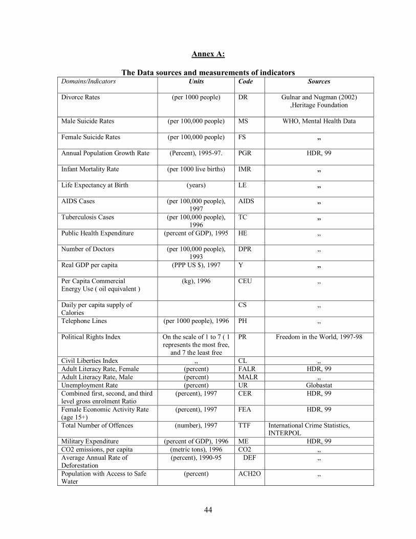
44

Annex A:

The Data sources and measurements of indicators Domains/Indicators

Units Code Sources

Divorce Rates

(per 1000 people)

DR

Gulnar and Nugman (2002) ,Heritage Foundation

Male Suicide Rates

(per 100,000 people) MS WHO, Mental Health Data

Female Suicide Rates

(per 100,000 people) FS ,,

Annual Population Growth Rate

(Percent), 1995-97. PGR HDR, 99

Infant Mortality Rate

(per 1000 live births) IMR ,,

Life Expectancy at Birth

(years) LE ,,

AIDS Cases (per 100,000 people), 1997

AIDS ,,

Tuberculosis Cases (per 100,000 people), 1996

TC ,,

Public Health Expenditure

(percent of GDP), 1995 HE ,,

Number of Doctors (per 100,000 people), 1993

DPR ,,

Real GDP per capita

(PPP US $), 1997 Y ,,

Per Capita Commercial Energy Use ( oil equivalent )

(kg), 1996 CEU ,,

Daily per capita supply of Calories

CS ,,

Telephone Lines

(per 1000 people), 1996 PH ,,

Political Rights Index On the scale of 1 to 7 ( 1 represents the most free,

and 7 the least free

PR Freedom in the World, 1997-98

Civil Liberties Index ,, CL ,, Adult Literacy Rate, Female (percent) FALR HDR, 99 Adult Literacy Rate, Male (percent) MALR ,, Unemployment Rate (percent) UR Globastat Combined first, second, and third level gross enrolment Ratio

(percent), 1997 CER HDR, 99

Female Economic Activity Rate (age 15+)

(percent), 1997 FEA HDR, 99

Total Number of Offences (number), 1997 TTF International Crime Statistics, INTERPOL

Military Expenditure (percent of GDP), 1996 ME HDR, 99 CO2 emissions, per capita (metric tons), 1996 CO2 ,, Average Annual Rate of Deforestation

(percent), 1990-95 DEF ,,

Population with Access to Safe Water

(percent) ACH2O ,,

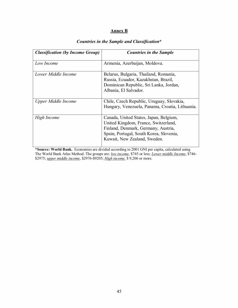
45

Annex B

Countries in the Sample and Classification*

Classification (by Income Group)

Countries in the Sample

Low Income Armenia, Azerbaijan, Moldova.

Lower Middle Income Belarus, Bulgaria, Thailand, Romania, Russia, Ecuador, Kazakhstan, Brazil, Dominican Republic, Sri Lanka, Jordan, Albania, El Salvador.

Upper Middle Income Chile, Czech Republic, Uruguay, Slovakia,

Hungary, Venezuela, Panama, Croatia, Lithuania.

High Income Canada, United States, Japan, Belgium, United Kingdom, France, Switzerland, Finland, Denmark, Germany, Austria, Spain, Portugal, South Korea, Slovenia, Kuwait, New Zealand, Sweden.

*Source: World Bank. Economies are divided according to 2001 GNI per capita, calculated using The World Bank Atlas Method. The groups are: low income, $745 or less; Lower middle Income, $746- $2975; upper middle income, $2976-$9205; High income, $ 9,206 or more.