A Rational Approach to the Design of Propulsors behind Axisymmetric Bodies by .. Mesut GUNER A Thesis submitted for the degree of Doctor of Philosophy Marine Technology .,. The University of Newcastle upon Tyne 1994 NEWCASTLE UNIVERSITY LIBRARY ---------------------------- 093 52190 0 ----------------------------

Welcome message from author
This document is posted to help you gain knowledge. Please leave a comment to let me know what you think about it! Share it to your friends and learn new things together.
Transcript

A Rational Approach to the Design of Propulsors behind Axisymmetric Bodies
by
.. Mesut GUNER
A Thesis submitted for the degree of
Doctor of Philosophy
Marine Technology .,.
The University of Newcastle upon Tyne
1994
NEWCASTLE UNIVERSITY LIBRARY ----------------------------
093 52190 0 ----------------------------

Abstract
In the context of "Lifting Line Methodology", this thesis presents a rational
approach to Marine Screw Propeller design and its applications in combination
with a "Stator" device for further performance improvement.
The rational nature of the approach is relative to the Classical Lifting Line
procedure and this is claimed by more realistic representation of the propeller
slipstream tube which contracts in radial direction along the tube at downstream.
Therefore, in accordance with the Lifting Line Methodology, the design procedure
presented in this thesis involves the representation of the slipstream shape by a
trailing vortex system. The deformation of this system is considered by means of
the so-called "Free Slipstream Analysis Method" in which the slipstream tube is
allowed to deform and to align with the direction of local velocity which is the
sum of the inflow velocity and induced velocities due ,to the trailing vortices. This
deformation is neglected in the Classical Lifting Lin~ approach.
The necessary flow field data or the wake for the design is predicted by using
a three-dimensional "Panel Method" for the outer potential flow, whilst a "Thin
Shear Layer Method" is used for the inner boundary layer flow. The theoretical
procedures in both methods neglect the effect of the free surface and therefore
the implemented software for the flow prediction caters only for deeply submerged

Abstract 111
bodies. However, the overall design software is general and applicable to surface
ships with an external feedback on the wake.
Since the realistic information on the slipstream shape is one of the key pa
rameter in the design of performance improvement devices, the proposed design
methodology has been combined with a stator device behind the propeller and
the hydrodynamic performance of the combined system has been analysed. The
design analysis involved the torque balancing characteristics of the system and the
effects of systematic variations of the key design parameters on the performance
of torpedo shape bodies and surface ships at varying loading conditions.
The ·overall conclusions from the thesis indicate that a more realistic represen
tation of the slipstream shape presents a higher efficiency in comparison to the
regular slipstream shape assumption, in particular for heavily loaded propellers.
Moreover, this representation is essential for sound design of the stator devices as
it will determine the radius of the stator. From the investigation on the stator it
was found that the undesirable effect of the unbalanced propeller torque can be
avoided by the stator. The efficiency of the system will increase with the increase in
the number of stator blades and the distance between the stator and the propeller
over a practical range of the design parameters.
It is believed that the procedure and software tool provided in this thesis
could provide the designer with capability for more sound propeller and the stator
design for, partly, surface ships and for submerged ships in particular torpedos,
Autonomous Underwater Vehicles (AUV) and submarines.
Although the improvement gained by the present procedure will be accompa-

Abstract IV
nied by an increase in computer time, this is not expected to be a major problem
considering the enormous power of existing computers. In fact, this has been the
major source of encouragement for the recommendation in this thesis to improve
the present procedure by using the "Lifting Surface Methodology" as the natural
extension of the Lifting Line Methodology.
Copyright © 1994 by Mesut GUNER
The copyright of this thesis rests with the author. No quotation from it should
be published without Mesut GUNER 's prior written consent and information
derived from it should be acknowledged.

Acknowledgements
This work has been carried out under the supervision of Dr. E.J. Glover in the
Department of Marine Technology, University of Newcastle upon Tyne. I would
like to express my deep gratitude to Dr. E.J. Glover for his direction, continuous
encouragement, very valuable stimulating discussions and guidance throughout
this research.
My thanks are also extended to the staff of the Department of Marine Tech
nology and in particular, Dr. Mehmet Atlar and Mr. G.H.G Mitchell for their
help and advice in every respect.
The extra resources, which were necessary in the development and running of
the programs, provided by the Computing Laboratory is greatly appreciated.
I also wish to thanks to my colleagues and in particular Dazheng Wang for his
many helpful discussions.
Financial assistance from the Education Ministry of Turkey is also gratefully
acknowledged.
Finally, I would like to thank my parents and friends for their encouragement
and support which they have given me over this period of my life.

Notations and Symbols Vl
Notations and Symbols
Most of the symbols are defined explicitly when they first appear in the text.
The principal symbols used in the present work are as follows:
A: Area
C: Chord length
CD: Drag coefficient
C L: Lift coefficient
D: Propeller diameter, Drag force
D6: Stator diameter
dD: Elementary drag of blade section
dL: Elementary lift of blade section
F: Rate of flow
G: Non-dimensional bound circulation
g: Non-dimensional vortex intensity
H: Shape parameter
I: Induction factor
J: Advance coefficient
KT: Thrust coefficient

Notations and Symbols
KQ: Torque coefficient
L: Lift force
m: Strength of source
n: Propeller rate of rotation
P: Pressure
PE: Engine brake power
PD: Delivered power
Pi: Pitch at itk section of propeller
Q: The rate of fluid mass, torque
R: Propeller radius
Rs: Stator radius
r: Distance between two points, radius of propeller section
T: Thrust
t: Maximum thickness of blade section
U: Inflow velocity
VA: Advance speed
VR: Resultant velocity
VB: Ship speed
Vll

Notations and Symbols V111
Ua : Non-dimensional axial inflow
U: Non-dimensional induced velocity
U e : External velocity
U apm : Axial mean induced velocity by propeller
Utpm: Tangential mean induced velocity by propeller
WQ: Torque identity wake fraction
x: Non-dimensional radius
Y: Axial distance downstream
Z: Number of prvpeller bades
Zs: Number of stator blades
a: Slope of the vortex line
/3: Angle of advance
/3i: Hydrodynamic pitch angle
r: Circulation
-y: Vortex intensity
6: Boundary layer thickness
8*: Displacement thickness
c: Vortex pitch angle in ultimate wake

Notations and Symbols lX
1]: Efficiency
(): Momentum thickness, the rate of fluid flow
p: Density
u: Source of strength
</J: Velocity potential, angular coordinate
w: Angular velocity of the propeller
Subscripts:
a, t, r: Axial, tangential and radial components of the inductions factors or
velocities.

Contents
Contents
Abstract ........ .
Acknowledgements
1 Introduction "
1.1
1.2
General
Objectives and Layout
2 Review of Literature
2.1
2.2
2.3
2.4
General
Propeller
Propeller/Stator Combination
Potential Flow and Boundary Layer
3 Flow around and in the Wake of a Body
3.1
3.2
3.3
Introduction
Potential Flow
3.2.1
3.2.2
3.2.3
3.2.4
3.2.5
3.2.6
Introduction
Fundamental Concepts
Flow Governing Equation
Boundary Conditions
Method of Solution ,-
Discretization
Boundary Layer "
3.3.1 General
3.3.2 Laminar and Turbulent Flow
x
• , • • • • •• 11
v
1
1
4
6
6
6
11
13
16
16
17
17
18
19
23
25
27
30
30
31
3.3.3 Boundary Layer Characteristics 32
3.3.4 Determination of the B.L. Characteristics 34

Contents Xl
3.4 Interactions ........................... . 35
4 The Conventional Lifting Line Model of Propeller Action 38
4.1
4.2
4.3
4.4
Introduction
Momentum Theory
Blade Element Theory
Circulation Theory
38
39
41
44
4.5 Lifting Line Design Method with Regular Helical Slipstream 46
4.5.1 Design Variables . . . 46
4.5.2 Mathematical Model 48
4.5.3
4.5.4
4.5.5
Determination of Bound Circulation
Calculation of the Mean Induced Velocities
Effect of the Bound Vortices
5 Advanced Lifting Line Model
5.1
5.2
5.3
5.4
5.5
5.6
5.7
5.8
5.9
5.10
Introduction
Design Considerations
Mathematical Formulation of the Model
Calculation of the Induced Velocities ..
Location of Field and Reference Vortices
Determination of the Mid-Zone Effect
Local Wake Velocities in the Slipst~eam
Deformation of the Slipstream ..
Convergence of Slipstream Shape
Circumferential Mean Velocities by Trailing Vortices
6 Propeller/Stator Combination
6.1 Introduction
55
57
61
63
63
63
64
70
72
74
79
80
81
82
85
85

Contents
6.2
6.3
6.4
6.5
6.6
6.7
Propeller with Downstream or Upstream Stator
Hydrodynamic Modelling of the Stator . . .
Design Consideration of Downstream Stator
Determination of Bound Vortices of the Stator
Stator Torque and Thrust ...
Design Procedure of Propulsors
7 Application ..... .
7.1 Introduction
7.2
7.3
7.4
Flow Analysis
Propeller Design
7.3.1 Design Methodology
7.3.2 lllustrative Examples
7.3.3 Design Calculations for DATA2
7.3.4 Discussion........
Propeller with Downstream Stator
8 General Conclusion
9 References
A Propeller Characteristics
B Body Input Points
C Slipstream Characteristics for DATAl
D Propellers and Stator Design Outputs
Xll
86
86
92
94
95
97
100
100
101
109
109
114
122
126
136
156
164
170
172
178
187

LIST OF FIGURES
3.1: The Flow around a Submerged Body .................... 16
3.2: Boundary Layer along a Plane Surface ............. ....... 31
3.3: Displacement Body Outline ........................... 35
3.4: Flow Chart for Interaction between the Flows ................ 37
4.1: Regular Helical Slipstream 39
4.2: Momentum Theory . 41
4.3: Propeller Blade Definition .................... . ....... 42
4.4: Blade Element Theory . 43
4.5: Combined Momentum and Blade Element Theories .44
4.6: The Replacement of the Blade Section by a Single Vortex .46
4.7: Regular Helical Slipstream ................. 53
4.8: Elementary Vortex System . . . . . . . . . . . . . . . . . . . . . ....... 58
4.9: Bound Vortex Line 62
5.1: Irregular Helical Slipstream . 66
5.2: Model of Slipstream shape ............................ 72

List of Figures
5.3: Field and Reference Vortices
6.1: Stator Modelling by Non-deformed Vortex Lines ....
6.2: Stator Modelling by Deformed Vortex Lines
6.3: Downstream Stator .............. .
6.4: Forces at Section of the Propeller and Downstream Stator
7.1: The Geometry of the Body
7.2: Discretisation of the Body
7.3: The velocity on the Body surface
7.4: Boundary Layer Thickness on the Body
7.5: Axial Velocity Distribution at 50 knots
7.6: Axial Velocity Distribution at 15 knots
7.7: Radial Velocity Distribution at 50 knots
7.8: Radial Velocity Distribution at 15 knots
7.9: Propeller Design Procedure .................. .
7.10: Variation of Axial Induced Velocity at x=O.61 for DATAl
7.11: Variation of Tangential Induced Velocity at x=0.6l for
DATAl
XlV
· 73
· 87
· 91
· 93
· 96
102
104
105
105
107
108
108
109
111
118
118
7.12: Variation of Radial Induced Velocity at x=0.61 for DATAl.. . . . 119
7.13: Variation of Radius at x=0.61 for DATAl 119
7.14: Vortex Pitch Variation at x=0.61 for DATAl 120
7.15: Circulation Distribution (DATAl) 120

Lis t of Figures xv
7.16: Hydrodynamic Pitch Angle (DATAl) 121
7.17: Lift-Length Coefficient (DATAl) .............. . 121
7.18: Slipstream Shape by Present Method for DATAl ..... 123
7.19: Slipstream Shape by Koumbis' Method for DATAl .... 124
7.20: Variation of Axial Induced Velocity at x=0.61 for DATA2 .. . . . . . 127
7.21: Variation of Tangential Induced Velocity at x=0.61 for
DATA2 127
7.22: Variation of Radial Induced Velocity at x=0.61 for DATA2 .. . . . . . 128
7.23: Variation of Radius at x=0.61 for DATA2 128
7.24: Vortex Pitch Variation at x=0.61 for DATAl 129
7.25: Circulation Distribution (DATA2) 129
7.26: Hydrodynamic Pitch Angle (DATA2) 130
7.27: Lift-Length Coefficient (DATA2) .............. . 130
7.28: Slipstream Shape by Present Method for DATA2 ..... 131
7.29: Flow behind the Body for DATAl 132
7.30: Flow behind the Body for DATA2 133
7.31: Axial Induced Velocities at Y /R=0.5 for DATAl ..... 140
7.32: Tangential Induced Velocities at Y /R=0.5 for DATAl .. 141
7.33: Radial Induced Velocities at Y/R=O.5 for DATAl 142
7.34: Axial Induced Velocities at Y /R=O.5 for DATA2 143
7.35: Tangential Induced Velocities at Y /R=O.5 for DATA2 .. 144

List of Figures XVl
7.36: Radial Induced Velocities at Y jR=0.5 for DATA2 145
7.37: Variation of Stator Blades for DATAl ..... 148
7.38: Gain after Balancing the Torque for DATAl '" 149
7.39: Variation of Stator Blades for DATA2 .. · . · ... . . . ... · .. 149
7.40: Gain after Balancing the Torque for DATA2 · ... · . · .. 150
7.41: Variation of Stator Blades for DATA3 . . · . · ...... · . · . · .. 150
7.42: Gain after Balancing the Torque for DATA3 · ...... · . · . · .. 151
7.43: Variation of Stator Blades for DATA4 . . . · . · ...... · ... · .. 151
7.44: Gain after Balancing the Torque for DATA4 · ...... · . · . · .. 152
7.45: Variation of Stator Blades for DATA5 . . . · . · ...... · . · . · .. 152
7.46: Gain after Balancing the Torque for DATA5 ........ .. . . . . . 153
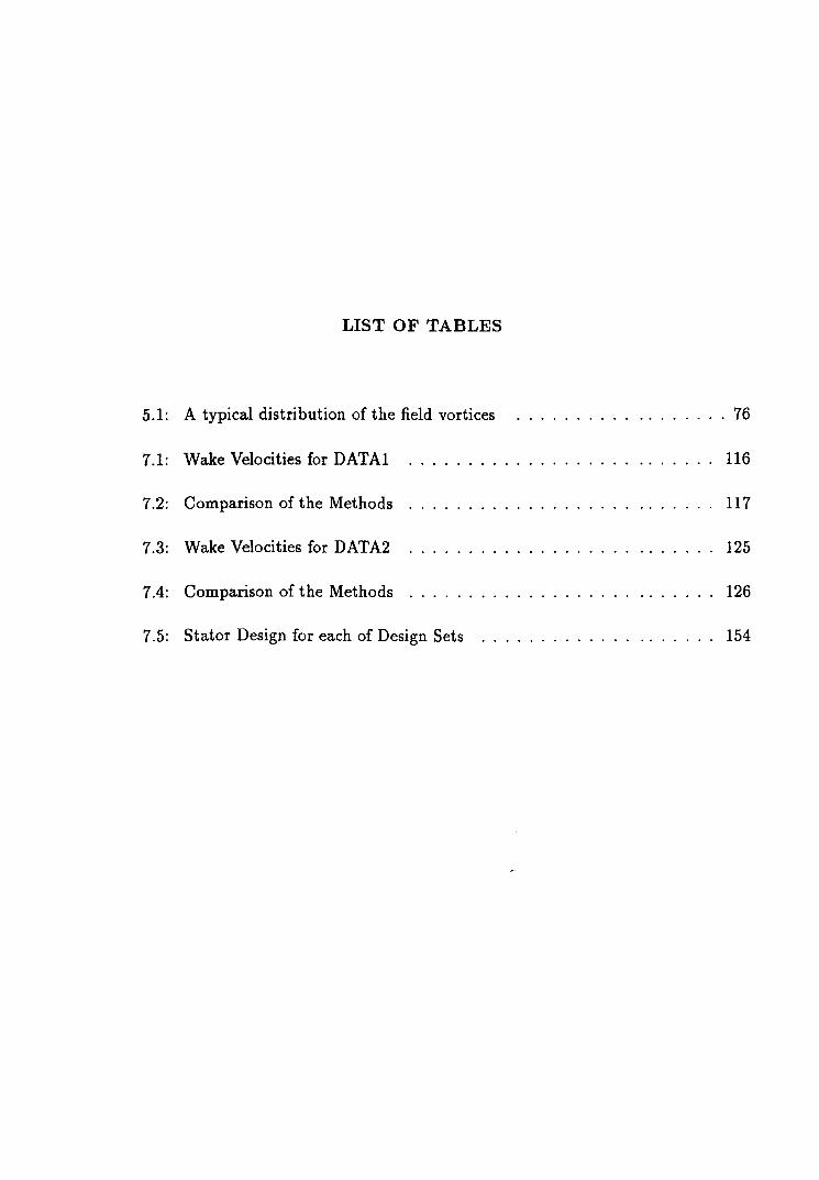
LIST OF TABLES
5.1: A typical distribution of the field vortices . 76
7.1: Wake Velocities for DATAl 116
7.2: Comparison of the Methods 117
7.3: Wake Velocities for DATA2 125
7.4: Comparison of the Methods 126
7.5: Stator Design for each of Design Sets 154
Chapter I
Introd uction
1.1 General
Screw propellers are the most common form of marine propulsion device. They
are used to supply the thrust needed to overcome the resistance experienced by a
moving marine vehicle. Such propellers produce thrust through the production of
lift and drag on their rotating blades.
The design of marine propellers has traditionally been performed on the basis
of open water experimental systematic series. Such procedures have served, and
continue to serve, propeller designers well for the design of typical ship propellers,
but do not readily allow for the analysis of less traditional propulsor alternatives,
such as a rotor/stator combination. The use of series data also does not allow the
designer to properly tailor the propulsor to the wake and physical arrangement of
a particular ship.
Over the past decades analytical procedures for the design of marine propellers
have become well established. These procedures are based on computer models of
propellers varying from a simplified representation of the propeller hydrodynamics
(e.g. lifting line method) to more complex representations (e.g. lifting surface
method). In the historical development of these procedures, the hydrodynamic
design of a propeller is accomplished on two levels. First, a lifting line model is
used to determine the basic propeller geometry and operating conditions as well as

Introduction 2
to determine a radial distribution of circulation over the blades that will provide
the total thrust and, usually, maximum efficiency. In the second step the final
shape of the blade is determined using a lifting surface analysis procedure.
The lifting line model of the propeller, where the blades of the propeller are
considered to be sufficiently thin and narrow and substituted by a single bound vor
tex line, is used to estimate propeller forces and determine the radial distribution
of bound circulation.
Since the lifting line theory alone cannot accurately represent the effect of the
actual blade geometry, more elaborate representations of the propeller are required.
For this purpose lifting surface methods, where the blades are modelled as sheet
of singularities, are usually employed. More sophisticated lifting surface or surface
panel representations of the propeller can then be used to analyse the performance
of the resulting blade geometry. Consideration of the unsteady forces or cavitation
predicted by these methods might then lead back to new design constraints at the
lifting line level.
Within the context of the widely recognised design procedures the major steps
for the design and analysis of propeller can be listed as
• Determination of diameter, blade surface area and thickness of a basic propeller
to satisfy the given conditions.
• Using lifting line design procedure to achieve wake adaptation of the propeller.
• Generating blade sections using simple blade section design methods.
• U sing lifting surface theory to predict the performance of the blade and to

Introduction 3
investigate the effects of changes in blade geometry. (Glover, [47])
In developing propeller theories, hydrodynamic modelling of the trailing vortex
lines behind the propeller is an essential part of accurate representation. In the
past the vortex lines downstream of the propeller were assumed to have constant
pitch and lie on cylinders of constant radius. In the actual propeller, the trailing
vortices leave the trailing edge of the propeller blade and flow into the slipstream
with the local velocity at that position. Therefore, the velocity distribution behind
the propeller should be known in order to establish the realistic model of the
trailing vortex lines. Within this context, the methods used to obtain the velocity
distribution can be experimental or theoretical. The analysis of the velocities in
the slipstream by model experiment is expensive, difficult and also time consuming.
On the other hand the use of computer software, based on treoretical methods,
provides a solution of complex analysis calculations in a short time and also many
variations of the design can be done. But it still needs experimental work to
validate and sometimes verify the calculation.
In order to achieve the goal of an improved propulsive efficiency some alterna-
tive propulsors have been proposed, the aim of which is to reduce the energy losses
associated with the action of the propeller. These losses are due mainly to the
transfer of energy to the water in the slipstream of the propeller, the axial energy ~
loss arising from the acceleration of the water necessary to create thrust and the
rotational energy loss from the transfer of torque from the propeller to the water.
There is also a viscous drag loss due to the movement of the blades through the
water.
Recovery of the rotational energy loss and significant gains in efficiency can

Introduction 4
be achieved from the use of contrarotating propellers. At the moment there is
renewed interest in the use of these propulsors on large ocean going ships but their
widespread use is inhibited by the mechanical complexities of the transmission
system and costs.
A cheaper and less complicated alternative to contrarotation is the use of fixed
guide vanes placed upstream or downstream of the propeller, the penalty being
a smaller gain in propulsor efficiency due to the drag of the fixed vanes. The
combination of propeller and guide vanes is now referred to as a propeller/stator
propulsor.
1.2 Objectives and Layout
The main objective of this thesis is the further improvement of the lifting
line procedure with an emphasis on more realistic representation of the slipstream
deformation. As this deformation is one of the key parameters in the design of
performance improvement devices, the secondary objective of the thesis is to design
a stator behind the propeller and analyse the performance characteristics of the
combined propulsor system.
In achieving the above objectives, in the present chapter of the thesis a.n intro
ductory section is given together with the objectives' and the layout. The second
chapter of the thesis includes a review of the three key issues involved in the pro
peller design as well as in the objectives of the thesis. These issues are the propeller
design procedures, propeller/stator combination and flow around a torpedo body
and propeller. The main reason of selecting the torpedo body is to reduce the
complexity of the procedure, since it is a submerged body of revolution and there-

Introduction 5
fore some effects such as free surface effect need not be taken into account. The
selection of a torpedo body also has some practical significance. Glover, in unpub
lished work on the design of rotor/stator propulsors for torpedoes, demonstrated
the difficulty of defining the true flow in the slipstream of the propulsor with the
two components at different positions on a steep conical after body. This defined
a requirement for a flow model of the combined body and propulsor.
In Chapter 3 the flow around a slender body is analysed. This effort provides
a set of wake data which is important in designing a propeller. The interactions
between the flow and propeller are also studied by introducing the idea of effective
wake.
In Chapter 4, a review is given of traditional propeller design methods. Having
explained these methods, a new propeller design procedure, which is based on
lifting line theory, will be presented in Chapter 5. This is a more advanced lifting
line method than others and it covers the realistic hydrodynamic model of propeller
as much as possible.
In Chapter 6 a design procedure for the stator will be described. The theoret
ical formulations are derived to calculate the stator circulation and consequently
the velocities induced by the stator. In Chapter 7, some numerical examples will
be given. Finally general remarks and conclusion will be shown in Chapter 8.
Chapter II
Review of Literature
2.1 General
In this review the main emphasis is placed on propeller and propulsor design.
In order to establish a realistic modelling of the propeller, the flow around and
behind the propeller should also be investigated. As will be appreciated, modelling
of the flow is a very wide and general subject and cannot be covered in such a short
space. Therefore a very short summary of the review of this subject is presented.
2.2 Propeller
The development of the theory of propeller action stems from both the axial
momentum theory and the blade element theory. The first theory of propeller
action was introduced by Rankine [11] and was further developed by R.E. Froude
[12]. Although the momentum theory leads to a number of important conclusions
regarding the action of the propeller, it gives no indication of the propeller geometry
necessary to produce the required forces. A differeI}t theory concerned with the
blade geometry was developed by W. Froude [38] and it is called the blade element
theory. The use of the blade element theory is based on the assumption that the
elements act independently of each other and that the flow across the blade is
entirely in the direction of the chords of the sections.
These two theories were well developed but they did not completely overcome

Review of Literature 7
the lack of understanding of the effects of the blade number and of choice of
appropriate lift and drag values for the blade elements. The problems encountered
were not solved until the advent ofthe vortex theory ofthe wing which was initiated
by Lanchester [13].
In 1919 Prandtl [14] showed that the effect of the free vortices shed at the ends
of an aerofoil of finite span is to induce a downwash velocity on it and hence reduce
its effective angle of incidence. Furthermore, the energy loss in the slipstream can
be considered as an induced drag the magnitude of which is minimum when the
spanwise circulation of the foil is elliptical.
The introduction of the vortex theory for the analysis and design of marine
propeller requires some assumptions to be made in its application. The first is
related to the representation of the blade. Based on the assumption that the blade
section is sufficiently thin, it may be replaced by a distribution of vortices along
its mean line. Hence the whole blade is represented by a thin bound vortex sheet,
referred to as a lifting surface. Considerable simplification of the model, and in
particular the numerical techniques for its solution, are achieved if the blades are
assumed to be narrow enough for them to be represented by a lifting line. The
second refers to the shape of the free vortices in the slipstream. The combined
rotation and translation of the blades causes free vortices which trail downstream
along helical paths.
A method, providing the performance analysis of marine propellers where the
effect of the above assumptions is allowed, was developed by Burrill [8]. This
method is based on the combination of the momentum theory and the blade el
ement theory together with aspects of the vortex theory. In this method the

Review of Literature 8
slipstream contraction and downstream increase in vortex line pitch are taken into
consideration in an approximate manner. The effect of the finite number of blades
on the magnitude of the induced velocities is considered by the use of correction
factors. These are due to Goldstein and are derived on the basis of a theoretical
examination of the flow past a number of helicoidal surfaces of infinite length. The
finite width and thickness of the blades in Burrill's method are taken into account
by a modification of the lift curve slope and no lift angle derived from Gutsche's
cascade data. A similar correction derived from N ACA data is applied for the
effects of viscosity.
In 1955 a wake adapted design method was introduced by Burrill [9]. The
Burrill wake adapted design method makes use of the expressions established in
the analysis process together with a minimum energy loss condition.
Propeller design methods based on the lifting line theory can be divided into
two groups: the approximate and rigorous or induction factor methods. The former
has been used by Eckhart and Morgan [15]. In this the condition of normality is
used and the axial and tangential induced velocities are expressed in terms of
simple trigonometric relationships that contain the Goldstein factors. The effect
of the radial induced velocities is ignored.
The use of induction factors gives more reliable 'and accurate results. This is
due to the fact that a more accurate representation of the slipstream is considered.
An analytical method, developed by Lerbs [16], determines the axial and tangential
factors. Another method, based on the concept of the induction factor, was devel
oped by Strscheletzky [7]. Unlike Lerbs' method this is based on the calculation
of the incremental induction factor by the Biot-Savart Law. This method provides
Review of Literature 9
the equations for the determination of the induction factors. These induction fac
tors are used to calculate velocities induced by the propeller in axial, tangential
and radial directions. Consequently by calculating the induced velocities in the
slipstream the slipstream deformation can be determined.
In 1973 Glover [2] proposed a new lifting line theory for heavily loaded pro
pellers based on Burrill's minimum energy loss condition applying induction factors
for the calculation of induced velocities. This method allows the extension of the
lifting line model of the propeller to take into account slipstream deformation.
The downstream contraction of the cylinder radius and increase in vortex pitch
downstream are calculated using the obtained induced velocities and the results
provide the new shape of the slipstream for the next input data.
In 1976, the lifting line theory was used for calculating the characteristics of a
supercavitating propeller by Anderson [49]. Some correction factors were developed
for the improvement of the numerical results by comparison with model tests.
Van Gent and Van Oossanen [24] introduced their lifting line design method
for the wake adapted propeller based on the precalculated hydrodynamic pitch
using the Van Manen [25] criterion and induced velocities calculated using Lerbs'
induction factors.
Koumbis [6] extended Glover's approach to obtain the final balanced slipstream
shape using a successive iteration process. The bound circulation distribution and
the slipstream geometry are continuously changed and interact freely in order to
form a new shape during the iteration process while satisfying Burrill's minimum
energy loss condition. He also introduced a concentrated tip vortex of finite core

Review of Literature 10
radius in order to improve the results. He suggested that the tip vortex core
extends from z = 0.96 to 1.00 and that the resulting induced velocity at the tip
is equal to that induced at x = 0.95 multiplied by a coefficient HTip. He further
suggested that the induced axial velocity is zero outside of the tip vortex.
A different representation of the propeller wake [48J, is based on the assumption
that, after a short distance downstream, the free vortices shed at the center of
the lifting line move outwards to wrap around the strong tip and boss vortices.
This, commonly referred to as roll-up vortex wake model, basically consists of
two concentrated helical vortices which carry the whole of the lifting line bound
circulation downstream.
Cummings [26J showed that the ultimate tip vortex radius is approximately
85% of the propeller radius for various types of propellers and loading conditions,
and insists that Glover's procedure will result in a rolled up geometry providing
that successive computation is made, but this claim turns out to be untrue as a
consequence of Koumbis' work.
Greeley and Kerwin [27] revised the former slipstream model by including the
slipstream alignment procedure in which the trailing vortex lines in the transition
slipstream region are located corresponding to the local flow. This revised slip
stream model recognises partly the importance of vortex pitch and partly takes
account of experimental results showing that the tip vortex was not completely
rolled up. Again this procedure requires slipstream shape defining parameters.
Recently Hoshino [28] took an important step towards a better understanding
of the trailing vortex problem by combining theoretical and experimental methods.

Review of Literature 11
Using experimental results he defined polynomal expressions for the variation of
slipstream contraction and pitch of the tip vortex. He then used these expressions
in his propeller method and obtained results which are in good agreement with
experimental data.
2.3 Propeller/Stator Combination
The propeller/stator combination is now gaining recognition as a propulsive
device for the reduction of energy losses. Recently there has been considerable
interest in this subject and a summary of the published works is given below.
In 1988 Kerwin et al. [22] presented a theoretical method for determining
optimum circulation distributions for propeller/stator propulsor. This work in
cluded cavitation tunnel measurements for a given propeller running behind an
axisymmetric and non-axisymmetric stator. In this study a 6% gain was predicted
theoretically and confirmed experimentally. In the same year Mautner et al. [29]
introduced a new design method for a stator upstream of the propeller by taking
zero r.p.m for the forward propeller of the contrarotating propeller system. They
demonstrated that the increase in efficiency is greater than 50% of that achieved
by the contrarotating propeller. A propulsor designed using this method has been
manufactured and tested on an axisymmetric, underwater vehicle. The test results
showed a good agreement with the design predictions.
A theoretical method was developed to model a ducted propeller with stator by
Hughes et al. [30]. Using this method a duct and a range of stators were designed
to operate efficiently with an existing propeller. Experiments were carried out on
the ducted propeller and stator combination and a good agreement between the

Review of Literature 12
theoretical and experimental results was obtained.
Iketaha [33] developed a method for theoretical calculation of propulsive per
formance of the propeller/stator combination. In this combination a stator was
located behind the propeller and covered with a ring. It was theoretically shown
that a 5%-7% percent gain was performed by the application of the method.
In a recent paper Patience [23] presents a very useful current state of the
art in Marine Propellers with emphasis upon developments over the last 20 years
and moving market direction. In this review work, he categorised the stator as a
reaction device and indicates its greater advantages compared to other propeller
and flow devices. He draws attention to the flow controlling capability of an
upstream stator and conjectures that in a properly designed system, the stator
device could evolve into the basic propulsor to be expected for the future possibility
with the added component of a duct.
In 1992, Gaafary and Mosaad [31] predicted the gain in propulsor efficiency
due to the presence of an upstream stator using linearised lifting surface theory.
They found that a 6% increase in propeller efficiency and the results showed a
good agreement with those obtained by theoretical and experimental work at MIT
[22].
Coney [32] has extended the work described in [22] and developed a new design
method for determining the optimum circulation distribution for both single and
multiple stage propulsors. The lifting line model was used for the design. A good
result was obtained from the application of the method. An attempt was also made
in the same year by Chen [34] to develop a design method for postswirl propulsors.
Review of Literature 13
A description of the lifting line procedure for the design of upstream and down
stream stator was given by Glover [3]. In his work, the influence of the number
of stator blades, variations in stator load factor and axial separation of the pro
peller and stator were investigated. This work showed that the combination of the
propeller and a downstream stator was more efficient than the combination of the
propeller and an upstream stator for the same number of stator blades. The gain
was about 3.5%-4.5% for the propeller/upstream propulsors and 4.5%-6% for the
propeller / downstream propulsors.
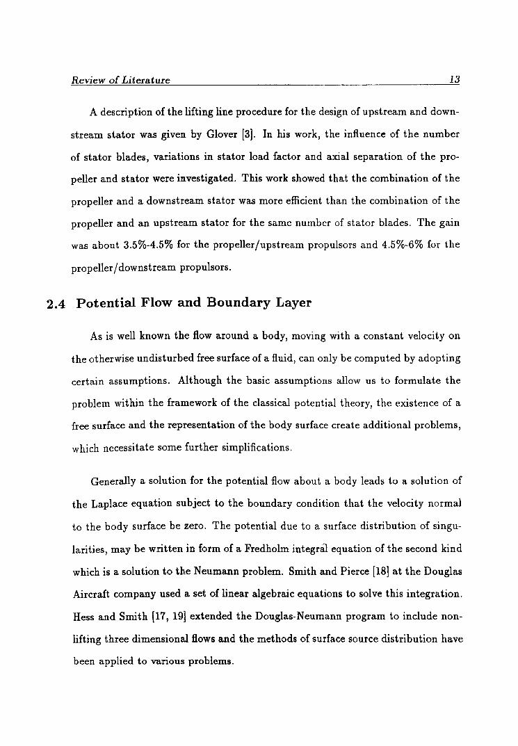
2.4 Potential Flow and Boundary Layer
As is well known the flow around a body, moving with a constant velocity on
the otherwise undisturbed free surface of a fluid, can only be computed by adopting
certain assumptions. Although the basic assumptions allow us to formulate the
problem within the framework of the classical potential theory, the existence of a
free surface and the representation of the body surface create additional problems,
which necessitate some further simplifications.
Generally a solution for the potential flow about a body leads to a solution of
the Laplace equation subject to the boundary condition that the velocity normal
to the body surface be zero. The potential due to a surface distribution of singu
larities, may be written in form of a Fredholm integraJ. equation of the second kind
which is a solution to the Neumann problem. Smith and Pierce [18] at the Douglas
Aircraft company used a set of linear algebraic equations to solve this integration.
Hess and Smith [17, 19] extended the Douglas-Neumann program to include non
lifting three dimensional flows and the methods of surface source distribution have
been applied to various problems.

Review of Literature 14
The original approach by Hess and Smith does not include the free surface
effect and hence gives the solution of the Neumann problem for a given form and
its image, (i.e. Double model in a infinite fluid). In order to improve the accuracy
of the result obtained from the Neumann problem, Brard [35], and many others
studied the Neumann-Kelvin problem which again takes the exact body surface in
its linearised form.
In most of the source distribution methods, the body surface is replaced by
quadrilateral elements or facets. One of the major drawbacks of this approximation
is that the planes formed by all four corners of each element do not necessarily
match the real body surface hence, either a discontinuity will occur on the source
surface or the centroids of each element will form a different body shape than
the original one. This statement becomes particularly significant at highly curved
regions. In order to avoid such errors it is possible to
• increase the number of elements and hence reduce the element sizes,
• employ curved surface elements with variable source density as is investigated
by Hess [21],
• use triangular surface elements, Webster [36].
As is expected any increase in the number of surface elements will increase the
computer time. The second alternative, the use of higher-order surface elements,
has also its own drawbacks. Having considered these alternatives it was decided
that the body surface should be discretised by using quadrilateral fiat elements and
that more elements should be introduced in regions of high body surface curvature.
Therefore the Hess-Smith method is chosen to define the velocities around the body.

Review of Literature 15
The potential flow solution gives the velocity and pressure distribution around
the body, together with the characteristics related to body geometry, i.e. coor
dinates of the control points, areas, components of the unit normal vectors etc.
The results from the potential flow solution can be used for the boundary layer
calculation.
Available methods for calculating boundary layer equations may be divided
into two groups; integral methods and differential methods. In the integral meth
ods the main interest lies in the determination of the global properties of the
shear layer and hence the momentum transport equations are integrated in the
normal direction thus reducing the number of unknowns by one. Distribution of
the properties across the shear layer are determined by means of empirical ex
pressions derived from the experimental data. Differential methods on the other
hand deal with the spatial variation of the properties by solving the momentum
transport equations for a thin shear layer (TSL) together with some additional
equations. These additional equations are introduced to model the transport of
Reynolds stress and to achieve the closure, that is to make the uumber of variables
equal to the number of equations. In the present work thin shear equations have
been used to predict the flow around the body. The method, given by Cebeci [39],
is chosen to obtain the solution of these equations. A description of the method
will be given in the next chapter.

Chapter III
Flow around and in the Wake of a Body
3 .1 Introduction
Knowledge of the fl owfield into, around and behind a m arine propeller is es
senti al and important from the point view of propeller design and analysi s. Th e
flow into t he propeller and in it s slipstream depends 011 t he form of the body be-
hind which the propeller operates . Accurate determination of t he flow around and
behind t he body is t herefore of prime importance. An effi cient way of compu ting
the flow around a body is t o di vide the flow into different regions, applying in
each region the most effici ent met hod available. Int eractions between the r.;gions,
including the influence of the operating propeller, h n.v t.o be considered .
TransiLion Point
Laminar B.1. --/ Po LenLia l Flow
TurbulenL 13.L
------ ---- ---------~>----\---
Wak e
Figure 3.1 - The Flow around a Submerged Body

Flow around and in the Wake of a Body 17
A fundamental picture of the flow around a deeply submerged body is shown
in Figure 3.1. Two main regions may be distinguished: One adjacent to the body
surface, extending backwards, and one outside this region. The former is usually
referred to as the boundary layer, while the latter is called the potential flow.
There is one major difference between the two: viscosity may be neglected in the
potential flow, while it has a strong effect on the boundary layer.
For the evaluation of the flow characteristics, it is necessary to start with
the potential flow solution so that the velocity distribution on the body can be
calculated. These results are then used as a basis of determining the viscous
flow around the body, which is in general, much different from the potential flow.
Although the interest is confined to the flow into the propeller plane and slipstream
of a body of revolution, the methods used are general enough to be utilised for
other aims.
3.2 Potential Flow
3.2.1 Introduction
The method used to define the potential flow around a submerged body is the
Hess-Smith method, [17, 19], which uses a source density distribution on the body
surface and determines the distribution necessary to ~ake the normal velocity zero
on the boundary. In order to approximate the body surface a number of quadrilat
eral source panels are used. Having solved for the unknown source densities, the
flow velocities at the points on and off the body surface can be calculated. In the
following section the procedure will be described briefly, the detailed procedure of
the formulation can be found in [17].

Flow around and in the Wake of a Body 18
3.2.2 Fundamental Concepts
A fluid is generally defined as a substance which continues to deform in the
presence of any shearing stress. The laws of fluid motion are applicable to flows
of any medium so long as the same properties are involved. Fluids possess a sub
microscopic molecular structure in which elementary particles are in continuous
motion through relatively large expanses of empty space. The details of such
motion are often of primary importance, particularly if the scale of the motion is
very small or the pressure very low. In most studies of fluid flows, however, neither
the molecular structure nor molecular movement as such is of specific interest, and
a greatly simplified yet highly useful picture can then be obtained by assuming
that the fluid under study is continuous even to the infinitesimal limit. Under
the assumed conditions, not only the fluid properties but such characteristics as
velocity and pressure can be regarded as continuously variable throughout the
region of flow, and can be defined mathematically at any particular point. This
approach is taken not only for the resultant simplicity of analysis, but also because
the behaviour of the individual molecules whose properties are varying. Therefore
the average properties of the molecules in a small parcel of fluid are used as the
properties of the continuous material.
In the potential flow problem, it is assumed that there exists a scalar function
that satisfies Laplace's equation in the fluid domain. The fluid characteristics, such
as the velocity and pressure, at any point in the fluid can be explicitly described
in terms of this function. In order for such a scalar function to exist the following
assumptions should be made

Flow around and in the Wake of a Body 19
• The fluid is incompressible
V.V = 0 (3.1)
where V is the flow velocity
• The fluid is irrotational
VxV=o (3.2)
• The fluid is inviscid and homogeneous.
3.2.3 Flow Governing Equation
From the law of mass and momentum conservation, the velocity V and the
pressure P must be obtained simultaneously. However, the pressure P is taken to
be the required independent variable. Thus the problem is obtaining the velocity
V under the given pressure field.
The law of conservation of mass forms the basis of what is called the principle
of continuity. This principle states that the rate of increase of the fluid mass
contained within a given space must be equal to the difference between the rates
of influx into and efflux out of the space. The assumption of a continuous fluid
medium then permits this principle to be expressed in differential form.
If the velocity of flow of a fluid in three dimensions is denoted by V, and the
mass density of the fluid at a point by p(~, y, z), then the vector Q = p V has the
same direction as the flow and has a magnitude Q numerically equal to the rate
of the flow of the fluid mass through the unit area perpendicular to the direction
of the flow. The differential rate of the flow through a directed element of surface
area dA = ndA is then given by A.dA = Q.ndA, this quantity being positive if the

Flow around and in the Wake of a Body 20
projection of Q on the vector n is positive. In particular, if dA is an element of a
closed surface then Q .dA is positive if the flow is outward from the surface. The
components of Q are
(3.3)
Taking a small closed differential element of volume which consists of rectangles
with one vertex at [z, y, z] and with edges dz, dy, dz parallel to the coordinate axes,
the left-hand face is then represented by the differential surface vector, jdzdz, and
the differential rate of the flow through this face is given by
Q.( -jdzdz) = -Qydzdz (3.4)
the negative sign indicating that if Qy is positive, the direction of flow through this
face is into the volume element. Similarly, the differential rate of the flow through
the right-hand face is given by
(3.4)
If the remaining four faces are treated in the same manner, the resulting dif-
ferential rate of the flow outward from the volume element dT = dxdydz is given
by
dF = (8Qz + 8Qy 8QZ )dzdydz Bx By Bz
(3.5)
or
dF = (V7 .Q)dT (3.6)

Flow around and in the Wake of a Body 21
Thus, the divergence of Q at point [x, y, z] can be said to represent the rate
of the fluid flow, per unit volume, outward from a differential volume associated
with the point [x, y, z], or to be the rate of decrease of the mass per unit volume
in the neighbourhood of the point. If no mass is added to or subtracted from the
element dT, the following relation is obtained,
\l.Q = -: (3.7)
where p denotes the mass density of the fluid.
For an incompressible fluid p = constant, hence
\l.Q = p\l.V = 0 (3.8)
It has been assumed here that no mass is introduced into, or taken from the
system, that is, there are no points in the element dT where the fluid is added
to or withdrawn from the system. If such points are assumed to be present, a
vector V with non-zero divergence can be considered as a velocity vector of an
incompressible fluid in a region. Points at which fluid is added to or taken from
the system are referred to as source and sinks respectively.
If V is continuously differentiable in a simply connected region R and if \l x V =
o at all points in R, then a scalar function 4> exists such that d¢ = V dr. In other
words, if \l x V = 0 in a region, then V is the gradient of a scalar function ¢ in
that region.
(3.9)

Flow around and in the Wake of a Body 22
where, 4> is called velocity potential. Flows derived from ¢ are referred to
as potential flow. An important observation pertaining to Equation 3.9 is that a
vector function V may be exchanged for a single scalar function ¢, if the motion
is irrotational. In general, a vector function contains three scalar functions which
are the components of the vector, so substitution of \7 ¢ for V should simplify the
equations of motion. If the fluid is incompressible and there is no distribution of
sources or sinks in the region, we have
3.10
Combining Equations 3.9 and 3.10,
(3.11)
That is, in the flow of an incompressible irrotational fluid without distributed
sources and sinks, the velocity vector is the gradient of a potential ¢ which satisfies
the Laplace equation,
or (3.11)
This equation will be solved with the appropriate boundary conditions for some
particular problem.
If sources and sinks exist in an irrotational flow of incompressible ideal fluid
one obtains Poisson's equation,
(3.12)

Flow around and in the Wake of a Body 23
where m the strength of the source or sink. The particular solution of this equation
IS
</J(p) = - 1 m(q) dV(q) r(p, q) 47l"
where </J(p) is the potential at a point p generated by a source or sink.
(3.13)
If boundaries are represented with source or sinks, the disturbance in the flow
field due to these singularities will be the sum of the contribution from each sin-
gularity. In the flow domain (outside the distributed singularities), however, the
Laplace equation still holds as there are no singularities present in that regime.
3.2.4 Boundary Conditions
The behaviour of quantities on the existing boundaries is determined usually
from physical reasoning such as the vanishing normal velocity condition on a solid
boundary when there is a relative velocity between the body and the surrounding
fluid. This is possible when the nature of the field and the boundary concerned
are of simple character but if either or both of them are not simple, it may not be
easy to decide by physical insight what conditions must be applied. The partial
differential equation representing a field is frequently common in form in many
physical situations and for a given field an identical form governs it regardless of
some important physical parameters involved such as boundary shape or initial
state. These physical parameters, the so called boundary conditions, make an
individual problem unique and choose "the solution" out of arbitrary functions of
some argument or an infinite number of possible solutions of the field equation.
The distribution of the field quantity inside the domain is constrained to some
extent by that along the boundaries. In other words, it adjusts itself to be com-

Flow around and in the Wake of a Body 24
patible with the given environment. It is therefore of great interest to expound the
manner by which the field quantity adjusts itself at the boundary and its effect on
the rest of the field in the expectation that the same principles would hold for any
problem under the same circumstances. In this connection, the type of boundary
conditions are:
• Cauchy boundary condition specifies both field value and normal gradients on
the boundary.
• Dirichlet boundary condition specifies only the field value, if it were zero ev
erywhere on the boundary the condition would be homogeneous, otherwise
inhomogeneous.
• Neumann boundary condition specifies only the normal gradient, and agam
homogeneous and inhomogeneous Neumann conditions are defined in the same
way as above.
• Mixed boundary condition specifies a linear combination of field value and
normal gradient homogeneously or inhomogeneously.
The application of a particular type of boundary condition has a different effect
on the solution depending on the type of the field equation.
When a flow field is governed by the Laplace equation of velocity potential
the relevant boundary condition is usually the homogeneous Neumann condition
stating that there is no flux of fluid across a solid boundary. That is, at each
control point of the source panels, the normal component of the induced velocity
potential satisfies the tangential velocity condition.
Flow around and in the Wake of a Body 25
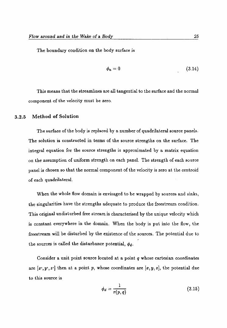
The boundary condition on the body surface is
(3.14)
This means that the streamlines are all tangential to the surface and the normal
component of the velocity must be zero.
3.2.5 Method of Solution
The surface of the body is replaced by a number of quadrilateral source panels.
The solution is constructed in terms of the source strengths on the surface. The
integral equation for the source strengths is approximated by a matrix equation
on the assumption of uniform strength on each panel. The strength of each source
panel is chosen so that the normal component of the velocity is zero at the centroid
of each quadrilateral.
When the whole flow domain is envisaged to be wrapped by sources and sinks,
the singularities have the strengths adequate to produce the freest ream condition.
This original undisturbed free stream is characterised by the unique velocity which
is constant everywhere in the domain. When the body is put into the flow, the
freestream will be disturbed by the existence of the sources. The potential due to
the sources is called the disturbance potential, <Pd.
Consider a unit point source located at a point q whose cartesian coordinates
are [x',Y',z'] then at a point p, whose coordinates are [x,y,z], the potential due
to this source is
1 <Pd = -r(p-,-q) (3.15)

Flow around and in the Wake of a Body 26
where r(p,q) is the distance between p and q,
If the local intensity of the distribution is denoted by u(q), where the source
point q now denotes a general point of the surface A, then the potential of the
distribution is
<Pd = r cr( q) dA( q) JA r(p, q)
(3.16)
The flow can be described then as sum of a freestream flow at infinity plus a
flow induced by source surface.
(3.17)
where <Poo is freest ream potential.
Then the velocity must satisfy the normal velocity boundary condition on the
surface A.
1 p-q = n(p).Uoo + n(p) 3( ) u(q)dA(q)
A r p,q (3.18)
=0
where the n(p) is the unit outward normal vector at point p due to the unit source
at the point q.
When q approaches p along the local normal direction, the principal part
27ru(p) must be extracted in this case,
1 p-q n(p).Uoo + 27ru(p) + n(p) 3( )u(q)dA(q) = 0
A r p,q (3.19)

Flow around and in the Wake of a Body 27
3.2.6 Discretization
The rather arbitrary shape of the boundary surfaces prevents the construction
of a simple functional expression to represent them, which in turn, makes it im-
practical to express the source strengths in an explicit functional form. Therefore,
an attempt is made to express the continuous variation of source strengths on the
surfaces by a set of numerical values at a finite number of points representing the
surface.
The body surface is replaced by a number of plane elements, the dimensions
of which are small in comparison with the body. The value of the source density
over each of the panels is assumed to be constant. The total disturbance potential
can be found from the equation below,
N 1 </>(p) = L O'j L. ( ) dA(q)
j=l J r p, q (3.20)
Where N is the number of panels on the body surface, Aj is the area of jth
panel and O'j is the source strength of jth panel.
A set of simultaneous equation can be constructed in terms of N unknown
source strengths. The N simultaneous equations can be set up by applying the
boundary conditions on each of the panels, more specifically at each control point
of the panels.
Because of the singular behaviour, the induced velocity at a control point on
the source panel itself is 27!'0'. Thus the disturbance velocity will be

Flow around and in the Wake of a Body 28
(3.21 )
Let us define matrices u(i,j), v(i,j) and w(i,j) as follow
When j I- i
(3.22)
w(i,j) = j z~(- Z~dA(q) Ai r p, q
when j = i u(i,j) = 27rnz i
v( i, j) = 27rnyi (3.23)
w(i,j) = 27rnz i
where nzi, nyi and nzi are the components of n along the x, y and z directions
respectively. These matrices U, V and Ware the components of the induced
velocity at the ith control points by the /h source panel of unit strength and will
be called the induced velocity matrices. Equation 3.21 can be written in terms of
the induced velocity matrices.
N
Vi = I:[u(i,j)i + v(i,j)j + w(i,j)kjUj j=1
(3.23)
When the body surface boundary condition is applied on the ith panel for

Flow around and in the Wake of a Body
instance, the following equation is obtained.
N
+ E[n:Z:iu(i,j) + nyiv(i,j) + nziw(i,j)]O'j j=l
=0
If the induced normal velocity matrix, A( i, j), is defined as
A(i,j) = n:z:iu(i,j) + nyiv(i,j) + nziw(i,j)
the following equation is obtained.
N
L A(i,j)O'j = -(nxiUoo + nyiVoo + nziWoo) j=l
29
(3.24)
(3.25)
(3.25)
When applied to all of the N panels this equation will yield N simultaneous
equation for N unknown values of O"s. In the matrix form this system of simulta-
neous equation is
A(l,l)
A(2, 1)
A(1,2)
A(2,2)
A(N,l) A(N,2)
A(l,N)
A(2,N)
A(N,N)
n:z:lUoo + nyl Voo + nzl Woo
n:z:2Uoo + ny2Voo + nz2Woo
Flow around and in the Wake of a Body 30
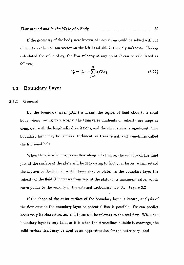
If the geometry of the body were known, the equations could be solved without
difficulty as the column vector on the left hand side is the only unknown. Having
calculated the value of tTj, the flow velocity at any point P can be calculated as
follows;
3.3 Boundary Layer
3.3.1 General
N
Vp = Voo + L tTjV'<Pd ;=1
(3.27)
By the boundary layer (B.L.) is meant the region of fluid close to a solid
body where, owing to viscosity, the transverse gradients of velocity are large as
compared with the longitudinal variations, and the shear stress is significant. The
boundary layer may be laminar, turbulent, or transitional, and sometimes called
the frictional belt.
When there is a homogeneous flow along a flat plate, the velocity of the fluid
just at the surface of the plate will be zero owing to frictional forces, which retard
the motion of the fluid in a thin layer near to plate. In the boundary layer the
velocity of the fluid U increases from zero at the plate to its maximum value, which
corresponds to the velocity in the external frictionless flow Uoo , Figure 3.2
If the shape of the outer surface of the boundary layer is known, analysis of
the flow outside the boundary layer as potential flow is possible. We can predict
accurately its characteristics and these will be relevant to the real flow. When the
boundary layer is very thin, as it is when the streamlines outside it converge, the
solid surface itself may be used as an approximation for the outer edge, and

Flow around and in the Wake of a Body 31
y
----- - --.-~---.-
~----~----
x
Figure 3.2 - Boundary Layer along a Plane Surface
the potential flow analysed before the thickness of the boundary layer is known.
Boundary layer theory also provide qualitative explanations for the aspects of
the flow, such as separation and form drag, which are not entirely amenable to
calculation. The crux of the matter is that the boundary layer is thin. Only then
is it valid to divide the whole region of the flow into two parts: the boundary layer
and the potential flow outside it.
3.3.2 Laminar and Turbulent Flow
In a laminar flow a fluid moves in laminas or layers. The layers do not mIX
transversely but slide over one another at relative speeds, which varies across the
flow.
In turbulent flow the fluid's velocity components have random fluctuations.
The flow is broken down and the fluid is mixed transversely in eddying motion.

Flow around and in the Wake of a Body 32
The flow is broken down and the fluid is mixed transversely in eddying motion.
The velocity of the flow has to be considered as the mean value of velocities of the
particles.
Factors that determine whether a flow is laminar or turbulent are the fluid, the
velocity, the form and the size of the body placed in the flow, the depth of water
and if the flow is in a channel, the channel configuration and size. Both laminar
and turbulent flows occur in nature, but turbulent form is the more common.
As the velocity increases, the flow will change from laminar to turbulent, passing
through a transition regime. The transition takes place at a Reynolds number
Rn = 105 - 106 . Thus in model experiments the flow over an unknown area of the
model can be laminar, which means that the experiment's accuracy is often not as
600d as is wanted. The effects of viscosity are present in turbulent flow, but they
'lre usually masked by the dominant turbulent shear stresses.
3.3.3 Boundary Layer Characteristics
The main effect of a boundary layer on the external flow is to displace the
streamlines away from the surface in the direction of the surface normal. This
occurs because the fluid near the surface is slowed down by viscous effects. In a
two dimensional flow, the rate at which fluid mass passes the plane :r:=constant
between y = 0 and y = h, where h is slightly larger 'than the boundary thickness,
6, is
3.28
per unit distance in the z (spanwise) direction, where p is the density of and u is
an internal stream of velocity. In the absence of a boundary layer, u will be equal

Flow around and in the Wake of a Body 33
to the external stream velocity, U e and P = pe. Therefore, the reduction in mass
flow rate per unit span between y = 0 and y = h caused by the presence of the
boundary layer is
3.29
The thickness in the y direction of a layer of external stream fluid carrying this
mass flow per unit span in constant density flow is
lak U
6* = (1 - -)dy o U e
3.30
This is the distance by which the external-flow streamlines are displaced in the
y direction by the presence of the boundary layer and is called the displacement
thickness.
The thickness of a layer of external stream fluid carrying a momentum flow
rate equal to the reduction in momentum flow rate is defined as the momentum
thickness, () and can be expressed as follows:
lak U U
() = -(1 - -)dy o U e U e
(3.31)
The velocity inside of the boundary layer is calculated by the power-law as-
sumption: 2
n = -:-----,-(H -1)
1 (3.32) ----
(n + 1)
u(6) = (y(6))1/7 U e 6
where H is the shape parameter.

Flow around and in the Wake of a Body 34
3.3.4 Determination of the B.L. Characteristics
Solving shear layer equations or simply using empirical formulas provides the
characteristics of the boundary layer, e.g. displacement thickness, momentum
thickness and skin friction.
In this work the thin-shear-Iayer (TSL) approximation for two dimensional flow
is used since it is a simplified form of the N avier-Stokes equations. TSL equations
are valid when the ratio of the shear layer thickness, 0, to the streamwise length
of the flow, 1, is very small. These equations are written for two dimensional
incompressible flows with eddy viscosity concept:
ou {}u 1 {}p 1 0 ou , , u- + v- = --- + --[IL- - puv 1 ox oy p ox p oy oy
{}u {}v -+-=0 8z {}y
{}p = 0 {}y
where JL is the viscosity, and p is pressure.
(3.33)
A numerical procedure for the solution of the TSL equations and its source
program are given in [39]. This program has been modified for the present use. The
laminar and turbulent boundary layer are calculated 9Y starting the calculations at
the forward stagnation point of the body with a given external velocity distribution
and a given transition point where the turbulent flow starts. Having run the
program, 0*, () and H are obtained. Using Equation 3.32 the boundary layer
thickness and velocities inside of the boundary layer are calculated.

Flow around and in the Wake of a Body 35
3.4 Interactions
Interaction Between the Boundary Layer and Potential Flow
The boundary layer moves the streamlines away from the body surface and a
new body geomet ry is generated by adding the loca.l displacement thickness to the
original body geometry. This body will be called the displacement body, Figure
3.3 .
Figure 3.3 - Displacement Body Outline
The outline of the displacement body can be found by an iteration as follows :
1. Calculate the inviscid flow around the body by potenti al flow theory.
2.Using the external velocity obtained from step 1 , calculate the displacement
thickness by TSL method.

Flow around and in the Wake of a Body 36
3. Add 6* , obtained from step 2, to the body shape to form a new displacement
surface and recalculate the potential flow. Repeat steps 2 and 3 until the results
converge.
Interaction Between the Propeller and Body
The flow for a body with an operating propeller can be described as the sum
of the freestream flow plus the flow induced by propeller and panels. The total
potential velocity can be written by
(3.34)
where cPpr is the potential due to the propeller.
In order to find the value of the source strengths and consequently the velocities
around the body, the Neumann boundary condition should be employed in order
to cancel the normal velocities at each quadrilateral.
or
84>Total = Vn = 0 8n
N
Vn = Uoo • n + [L: lTj\7cPd]' n + unpr
j=l
where unpr is normal velocity induced by the propeller on each panel.
(3.35)
The solution of the above equation gives the new value of the source strengths.
The total velocity then becomes
N
V = Voo + Vpr + L: lTjV'cPd ;=1
(3.36)
Flow around and in the lVake of a Body 37
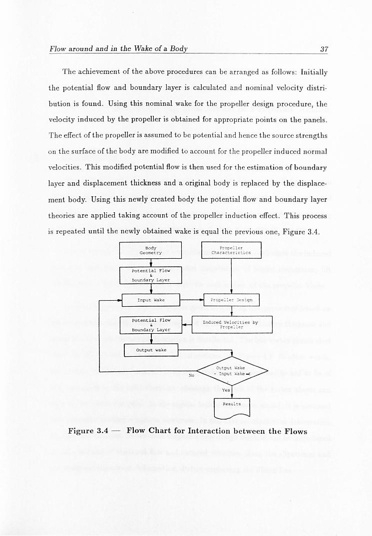
T he achievement of the above procedures can be arranged as follows: Initially
the potential flow and boundary layer is calcula ted and nominal velocity distri
bution is found . Using this nominal wake for the propeller design procedure, the
velocity induced by the propeller is obtained for appropriate points on the panels.
T he effect of the propeller is assumed to be potential and hence th e source strength s
on the surface of the body are modified to account for t he propeller indu ced normal
velocities. This modified potential flow is then used for the estimation of bound ary
layer and displacement thickness and a original body is replaced by the displ ace
ment body. Using this newly created body the potential flow and boundary layer
theories are applied taking account of the propeller induction effect . This process
is repeated until the newly obtained wake is equal the previous one, Figure 3.4.
:-10
I nd~ced Vel oc: ti e s by ? ~ope : :e c
Figure 3.4 - Flow Chart for Interaction between the Flows

Chapter IV
The Conventional Lifting Line Model of Propeller Action
4.1 Introduction
The design of the marine propeller is a subject that has received the attention
of many researchers during the last century as evidenced from the large numbers of
papers and reports in the technical literature. One of these methods called lifting
line theory is widely used in propeller design [1, 2, 5, 6, 23, 37, 40, 44, 45].
In the theory one of the major computational tasks is to calculate the induced
velocities and hence determine the radial distribution of bound circulation, lift
coefficient and hydrodynamic pitch angle for each section of the propeller blade.
In this chapter a description will be given of a lifting line procedure based on
the assumption that the blades are replaced by lifting lines with zero thickness and
width along which the bound circulation is distributed. The free vortex sheets shed
from the lifting lines lie on regular helical surfaces, see Figure 4.1. In other words,
the trailing vortices are assumed to lie on cylinders of constant radius and to be of
constant pitch in the axial direction, although the pitch of the vortex sheets can
vary in the radial direction. In the regular helical slipstream model, it is assumed
that propeller loading is light or moderate. In this case no slipstream deformation
is taken into account. In the next chapter a new design method will be introduced
to take account of the local flow and induced velocities along the slipstream and
the resultant slipstream deformation. Before explaining the lifting line

The Conventional Lifting Line Model of Propeller Action 39
Figure 4.1 - Regular Helical Slipstream
procedure, it is better to give some explanation of the basic theories such as momen
tum theory, blade element theory and circulation theory which have been building
bricks in the later development of the advanced propeller theories.
4.2 Momentum Theory
The first rational theory of propeller action was developed by Rankine and
R.E Froude [11, 12]. The theory is based on the concept that the hydrodynamic
forces on the propeller blades are due to momentum changes which occur in the
region of the fluid acted upon by the propeller. This region of fluid forms a circular
column which is acted upon by a disc representing the propeller and which forms
what is termed the "slipstream" of the propeller. The slipstream has both an
axial and angular motion; in the simple momentum theory only the axial motion
The Conventional Lifting Line Model of Propeller Action 40
is considered, while in the extended momentum theory the angular motion also is
taken into account. The following assumptions are made in this theory:
• The fluid is assumed to be non-viscous,
• The propeller has an infinite number of blades, i.e. it is replaced by the so-called
"actuator disc" .
• The propeller is assumed to be capable of imparting a sternward axial thrust
without causing rotation in the slipstream.
• The thrust is assumed to be uniformly distributed over the disk area.
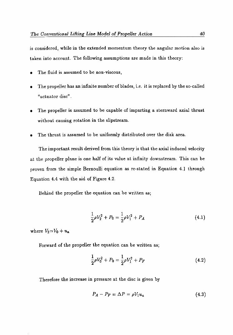
The important result derived from this theory is that the axial induced velocity
at the propeller plane is one half of its value at infinity downstream. This can be
proven from the simple Bernoulli equation as re-stated in Equation 4.1 through
Equation 4.4 with the aid of Figure 4.2.
Behind the propeller the equation can be written as;
( 4.1)
Forward of the propeller the equation can he written as;
(4.2)
Therefore the increase in pressure at the disc is given by
(4.3)

The Conventional Lifting Line Model of Propeller Action 41
Having combined above equations, the following statement can be obtained
(4.4 )
.\J"T \;1
I 'OI{W,t\!{1) ~ .....
l~ V2 P A
Pr I~ Vo .....
....... DISC
Figure 4.2 - Momentum Theory
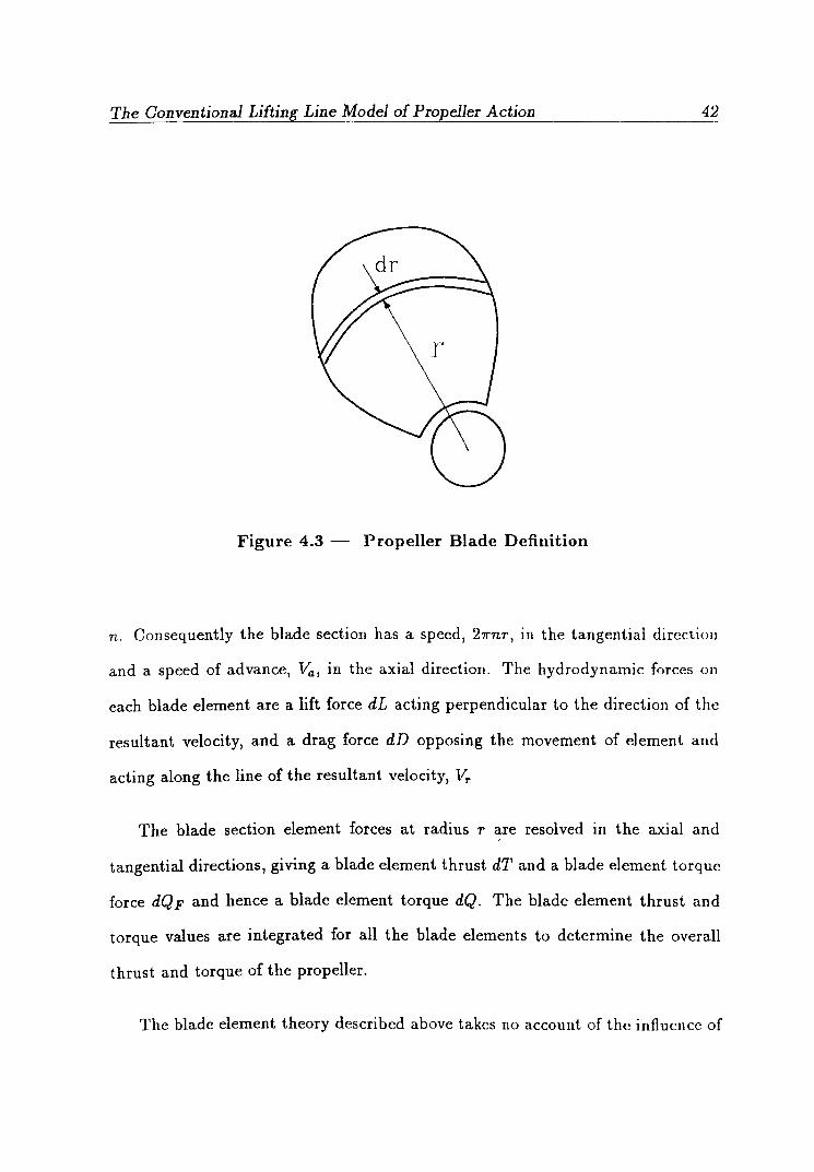
4.3 Blade Element Theory
In the blade element theory, which is based on the early work by W. Froude
[38] and others, each blade of the propeller is divide~ into a number of chordwise
elements each of which is assumed to operate as if it were part of a hydrofoil,
Figure 4.3.
As seen in Figure 4.4 the velocity of fluid relative to each blade element is the
resultant of the axial and angular velocities. A torque Q is applied to the propeller
by the driving shaft, and the propeller and shaft rotate at the rotational speed
The Conventional Lifting Line Model of Propeller Action 42
Figure 4.3 - Propeller Blade Definition
n. Consequently the blade section has a speed, 27rnr, in the tangential directiol\
and a speed of advance, Va, in the axial direction. The hydrodynamic forces 011
each blade element are a lift force dL acting perpendicular to the direction of the
resultant velocity, and a drag force dD opposing the movement of element and
acting along the line of the resultant velocity, Vr
The blade section element forces at radius r are resolved in the axial and
tangential directions, giving a blade element thrust dT and a blade element torque
force dQp and hence a blade element torque dQ. The blade element thrust and
torque values are integrated for all the blade elements to determine the overall
thrust and torque of the propeller.
The blade element theory described above takes no account of the influence of

The Conventional Lifting Line Model of Propeller Action 43
Va
(t)r
dD
Figure 4.4 - Blade Element Theory
the propeller on the flow. This can be accounted for by int.roducing the axial and
rotational induced velocity components, the existence of which is explained by the
momentum theory, Figure 4.5. The direction of the resultant flow is modified by
the presence of the induced velocities and now lies on a helical line defined by the
hydrodynamic pitch angle, {k
However, the expressions for the induced velocities derived from the momentum
theory relate to the actuator disc which is virtually an infinitely bladed propeller.
The problem of accounting for the fact that the propeller has a finite number
of blades is overcome by the introduction of the circulation or vortex theory of
propeller action.

The Conventional Lifting Line Model of Propeller Action 44
Vi).
dQr ------~~~~~-------.------------~
dD
Figure 4.5 - Combined Momentum and Blade Element Theories
4.4 Circulation Theory
The circulation theory is based on a concept due to Lanchcs ter [13] whi ch sta.tes
that the lift developed by the propeller blades is caused by th circulatory fl \V
which is set up around the blades. This causes an increased local velocity across
the back of the blade, and a reduced local velocity across the face of th blade .
The fluid velocities relative to a blade element around which th re is a circul a t ry
flow in a non-viscous fluid can be specified by a translation velocity Vr together
with a circulation velocity Ve · The circulation, fr, around the element is d fin d
as the line integral of the circulation velocity, V e , around any path which encloses
the element . Thus, for a given circulation, the circulation velocity diminishes with
distance from the element.

The Conventional Lifting Line Model of Propeller Action 45
For two dimensional flow the lift force dL on the element of chord length
C and width dr is related to the translation velocity and the circulation by the
Kutta-Joukowski equation
(4.5)
In applying the circulation theory to the flow conditions of a propeller, each
blade is first assumed to be replaced by a vortex line which extends from the
propeller axis to blade tip and around which there is a circulation flow. This
vortex line, which is termed a bound vortex line, is terminated at the propeller
axis and blade tip by two trailing vortex lines. The axial vortex line follows a path
along the propeller axis and the tip vortex line follows a helical path which traces
out the boundary of the slipstream. If the circulation is constant from the propeller
axis to the tip then the circulation of each trailing vortex line will be equal to that
of the bound vortex line. If the circulation varies radially, as in the propeller case,
then a system of trailing vortex lines of similar form to the tip vortex line is shed
along the radial length of the blade, and the single bound vortex line is replaced
by a series of bound vortex lines all extending from the propeller axis but each
terminating at, and of circulation equal to, one of trailing vortex lines. This system
of trailing vortex lines forms a helicoidal sheet associated with which is an induced
velocity. If the slipstream contraction is neglected and if it is assumed that pitch
of the vortex sheets is radially uniform it can be shown that the direction of the
induced velocity is normal to the vortex sheet. However, in the more general case
of non-uniform vortex sheet pitch, this "condition of normality" is not fulfilled.
These induced velocities can be resolved into components in the axial, tangential
and radial directions.
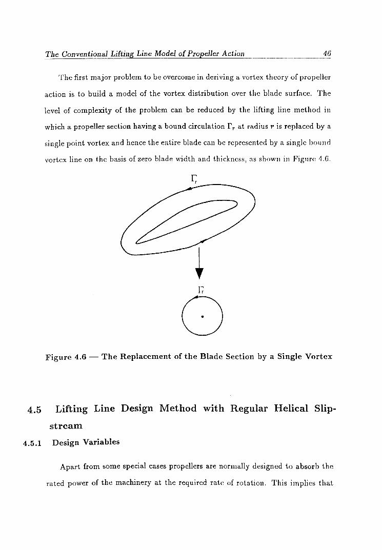
The Conventional Lifting Line Model of Propeller Action 46 ----
The first major problem to be overcome in deriving a vortex theory of propeller
action is to build a model of the vortex distribution over the blade surface. The
level of complexity of the problem can be reduced by the lifting line method in
which a propeller section having a bound circulation r T at radius r is replaced by a
single point vortex and hence the entire blade can be represcntcd by a single bound
vortex line on the basis of zero blade width and t.hickness, as showlI ill Figure ~ .G.
r;
o Figure 4.6 - The Replacement of the Blade Section by a Single Vortex
4.5 Lifting Line Design Method with Regular Helical Slip-
stream
4.5.1 Design Variables
Apart from some special cases propellers are normally designed to absorb the
rated power of the machinery at the required rate of rotation. This implies that

The Conventional Lifting Line Model of Propeller Action 47
two of the input design parameters are associated with the engine, while the other
parameters are listed as follows:
• Engine brake power, PB kw
• Shaft efficiency, 1]8
• Delivered power, PD = PB X 1]8
• Propeller rate of rotation, N
• Ship speed, Vs
• Torque identity wake fraction, wQ
• Number of blades, Z
U sing these data and an appropriate Bp - 6 diagram the optimum diameter, D,
and the mean face pitch ratio of a "basic" propeller to satisfy the design condition
can be determined.
The blade surface area required to minimise the risk of cavitation can be deter
mined using a cavitation diagram, such as that due to Burrill [8]. The distribution
of this area on an appropriate blade outline gives the blade chord widths at the
design radii.
A simple stressing calculation can be used to calculate the blade section thick
ness and drag coefficients determined as function of the section thickness ratios.
The wake-adaptation of the design, i.e. optimisation with respect to the radial
wake distribution in which the propeller is assumed to work, is then carried out

The Conventional Lifting Line Model of Propeller Action 48
using the lifting line procedure.
In this procedure the above design conditions are represented by the require
ment that the propeller should achieve a torque coefficient, KQ, given by
(4.6)
Optimisation of the design, i.e. the determination of the radial loading distri-
bution corresponding to maximum efficiency, is achieved by introducing a minimum
energy loss condition into the solution of the lifting line model. In this work the
condition derived by Burrill [9] is used, in which the vortex sheets on the ultimate
wake are assumed to have uniform pitch radially, i.e. :
:Vi'K tan ei = constant (4.7)
where :Vi = rd R is the non-dimensional form of the ith section radius, R is the
propeller radius and ei is the pitch angle of helical vortex sheets at infinity.
4.5.2 Mathematical Model
In the development of the mathematical model of the propeller, a satisfactory
formulation of the induced velocities is essential. In general there are two ways of
obtaining the velocities induced on the lifting line by a regular helical vortex line.
The first involves the solution of Laplace's differential equation whilst the second
method is based on the use of the Biot-Savart Law to calculate the incremental
velocity induced by a vortex element at any point. Then the total induced velocity
at the point is calculated by numerically integrating the individual effects of the

The Conventional Lifting Line Model of Propeller Action 49
elements constituting the vortex line.
The induced velocities calculated by either method are finite except for the case
where the reference point lies on the vortex and especially, the leading end where
the velocity components become infinite. The induction factors are introduced to
overcome this difficulty. An induction factor is defined as the ratio of the velocity
induced at a point by a semi-infinite helical vortex line to that induced by a semi-
infinite straight vortex line of the same strength. They can be evaluated either by
the solution of a partial differential equation subject to boundary conditions [16]
or by the Biot-Savart method.
Based on the assumption that the circulation of the lifting line, or bound
circulation, is assumed to go continuously to zero at both the tip and the boss,
the associated expression for the circulation can be defined by a Fourier sine series
and written in non-dimensional form as follows
r. 00
Q. - --'- - LAn' sinn<pi , - 7rDVs - n=l
( 4.8)
Where r i is the bound circulation at :l:i and An is the bound circulation coefficient
whose value is to be determined.
The angular coordinate, (Pi, is defined in terms the radial coordinate, :l:i, as
follows,
(4.9)
Where :l:h is the non-dimensional hub radius and <Pi varies from 0 at the hub to 7r
at the tip.
The problem is now the determination of the unknown An's. Once these values

The Conventional Lifting Line Model of Propeller Action 50
are calculated, the axial, tangential and radial induced velocities at any point of
the lifting line can be estimated and finally the hydrodynamic pitch angle, lift
coefficient and torque, thrust coefficient can be calculated.
At the xith radial lifting line location, a free vortex will be shed of strength
(dG dx) dx i
(4.1O)
and circulation at the Xi+dz th radial location is
( 4.11)
The total velocity induced at a point at radius Xi by helical lines starting at
points Xk can be given in terms of the induction factors as follows
1
u - /1 dG dXk a,t,T - a,t,T (d ) 2( )
x k Xi - xk Zh
(4.12)
where I represents induction factors which depend only on the geometry of
slipstream and can be calculated by the two methods mentioned earlier. The
subscript a, t and r denote axial, tangential and radial components respectively.
For the induction factors Lerbs, [16], expressed analytical formulations as fol-
lows:
For the internal field (Xi> Xk)
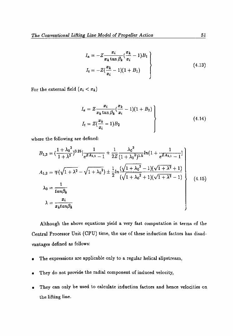
The Conventional Lifting Line Model of Propeller Action
X' xk Ia = -Z t (- - 1)Bl
Xk tanf3k Xi
It = _Z(Xk - 1)(1 + B 1) Xi
For the external field (Xi < Xk)
where the following are defined:
_ 1 + A02 O.25[ 1 ± ~ A02 In 1 1 BI ,2 - ( 1 + A2 ) eZA2 ,1 - 1 2Z (1 + A02)1.5 ( + eZA2 ,1 _ 1l
Al 2 = ~(J 1 + A 2 _ J 1 + AO 2) ± !In ( J 1 + AO 2
- 1)( VI + A 2
+ 1) , 2 ( J 1 + AO 2 + 1) ( V 1 + A 2 - I)
1 AO=--
tanf3k
51
(4.13)
(4.14)
( 4.15)
Although the above equations yield a very fast computation in terms of the
Central Processor Unit (CPU) time, the use of these induction factors has disad-
vantages defined as follows:
• The expressions are applicable only to a regular helical slipstream,
• They do not provide the radial component of induced velocity,
• They can only be used to calculate induction factors and hence velocities on
the lifting line.
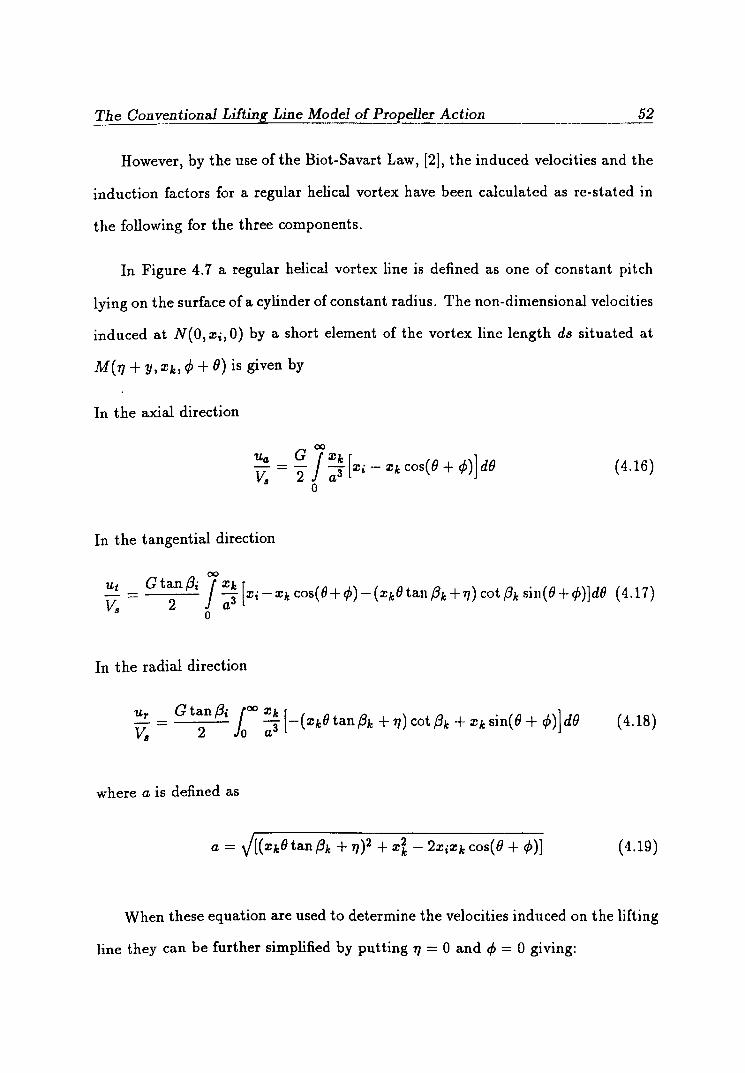
The Conventional Lifting Line Model of Propeller Action 52
However, by the use ofthe Biot-Savart Law, [2], the induced velocities and the
induction factors for a regular helical vortex have been calculated as re-stated in
the following for the three components.
In Figure 4.7 a regular helical vortex line is defined as one of constant pitch
lying on the surface of a cylinder of constant radius. The non-dimensional velocities
induced at N{O, Xi, 0) by a short element of the vortex line length ds situated at
In the axial direction
( 4.16)
In the tangential direction
In the radial direction
(4.18)
where a is defined as
(4.19)
When these equation are used to determine the velocities induced on the lifting
line they can be further simplified by putting 1'/ = 0 and 4> = 0 giving:

The Conventional Lifting Line Model of Propeller Action 53
Z , T'
7)
y
Figure 4.7 - Regular Helical Slipstream

The Conventional Lifting Line Model of Propeller Action 54
( 4.20)
00
Ut Gtanf3i J xlc [ - = 2 3" Xi - xlc cos () - XIc sin ()]dB Va a
o
(4.21)
( 4.22)
( 4.23)
The velocities calculated using these equations are finite except when XIc = Xi
and () approaches zero under which circumstances the integrands become infinite.
In order to overcome this difficulty the concept of the induction factor is introduced.
The induced velocities at any point Xi is divided by the velocity induced at Xi by
a starting semi-infinite vortex line of circulation G starting at Xlo i.e.
U
V"
G
The equations for the induction factors then became
00
10. = (Xi - XIc) J :; [XIc - Xi cos ())] d(J
o
00
It = (Xi - XIc) tanf31c J :; [Xi - xlc cos (J - XIe(J sin (J]d(J
o
( 4.24)
(4.25)
( 4.26)
Tbe Conventional Lifting Line Model of Propeller Action
00
IT = (Xi - Xk) tan.Bk J :: [-XkO cos 0 + Xk sinO]dO o
55
( 4.27)
It can be seen from the equations for la, It, IT that the induction factors are
completely independent of the circulation. They depend entirely upon the pitch
of the free vortex line and the relative position of the point of inception and the
point where the velocities are being calculated. It can be shown that the induction
factor factors remain finite for all values of the variables and that when Xk = Xi
they assume limiting values as below:
( 4.28)
4.5.3 Determination of Bound Circulation
The solution of the lifting line design problem involves determination of the
value of the unknown bound circulation coefficient, An, in Equation 4.8. In order
to obtain a tractable solution, the infinite series is truncated to a small number of
terms. It is convenient if the number of terms is equal to the number of blade sec-
tion considered. Generally the blade can be adequately represented by 11 sections
including the hub and tip, typical values being
Xh ,0.25 , 030 , 0.40 ,0.50 ,0.60 ,0.70 ,080 ,0.90 ,0.95 , 1.0
However, since the circulation is zero at the hub and at the tip, it is sufficient
to consider a 9-term series to be solved in relation to reference points between the
hub and tip.
In Equation 4.12, Xk is replaced by the angular coordinate, 4>, and Xi by a
The Conventional Lifting Line Model of Propeller Action 56
similar angular coordinate, 'I/J, then the equation for the induced velocities becomes
where
Ui = J'lr Ia,t,T[A1 cos <I> + 2A2 cos 24> + ... + 9A9 cos 94>1 d4> a,t," 2£( cos <I> - cos 1/J )
o
£ = 1- Xh
2
(4.29)
In the above integral expression, the integration is carried out numerically such
that for each of nine values of Xi, the nine term of equations for the induced velocity
components are set up in terms of the unknown An's.
In order to optimise the radial loading distribution of the wake-adapted pro-
peller Burrill's minimum energy loss condition is used as given by Equation 4.7.
For the 9 reference points, the tangential and axial induced velocities in terms of
the 9 unknown Fourier coefficients are substituted into Equation 4.7. Finally a
system of nine simultaneous equations is formed as follows:
( 4.30)
Where J6 = !b is advance coefficient and Wi is the local wake fraction at the
blade section radius Xi·
These equations can be solved by commonly used matrix methods to give the
circulation coefficients. Having established the circulation, the final parameters as-
sociated with the propeller may be investigated by the equations given in Appendix
A.

The Conventional Lifting Line Model of Propeller Action 57
4.5.4 Calculation of the Mean Induced Velocities
In the solution of the lifting line model, it is only necessary to calculate the
velocities induced on the line itself by the helical free vortex lines in the slipstream.
Since the free vortex system rotates with the propeller, the induced velocities on
the lifting line do not vary with time.
In the case of a compound propulsor with a fixed component, such as a duct
or stator, the velocities induced by the propeller on the component will vary with
time at blade frequency. Normally these fluctuations in induced velocities can not
be accounted for in designing the fixed component and it is necessary to have the
means of calculating the mean velocities induced by the propeller at a fixed point
in the fluid, i.e. a field point.
The mean velocities can be calculated by applying the Biot-Savart method to a
number of points over the blade phase angle and integrating the induced velocities
at these points to find the time. This approach is very expensive in terms of CPU
time. In the case of the regular helical slipstream the mean induced velocities call
be calculated more economically by assuming that the helical vortex lines can be
replaced by a vortex cylinder comprising a semi-infinite tube of ring vortices and
an infinite number of horse-shoe vortices, consisting of bound vortices and straight
vortices, Figure 4.8.
When considering a system of Z helical vortex lines of constant pitch Pi, radius
Ti and strength (~dr)i' the circulation due to this helical vortex can be written
-Z(frdr)i, [41]. Also the circulation due to a continuous distribution of ring
vortices of constant strength is ((riPi dr ), where "'(ri the vortex intensity of the ring

Tbe Conventional Lifting Line Model of Propeller Action 58
r
1 dri
ooooooooo°tl
r
y
0 1° ~ .. 0 Z
I.
0 0
0 0
0 0
0 0
r
I I I I I I ,
I '" /
-_.- ,-_. _.
ring vortic s
I I
\ \ \ \ ,
straight vortices
bound vortices
Figure 4.8 - E lementary Vortex System
y
:.;

The Conventional Lifting Line Model of Propeller Action 59
vortices.
Equating these expressions
(4.31)
This can be expressed in its non-dimensional form as follows:
(4.32)
Similarly the non-dimensional vortex intensity of the straight vortex lines can
be shown to be
9 . _ Z(~~)i ... -
:Vi ( 4.33)
As indicated by Equations 4.32 and 4.33, a system of Z equispaced regular he
lical vortices can be substituted by an infinite number of ring and straight vortices
with constant vorticity downstream. The mean velocities induced by this vortex
cylinder at any field point can be calculated by a piecewise integration along its
length. However, it has been shown in [46] that the velocity induced by a semi-
infinite vortex cylinder of unit strength can be expressed in terms of complete
elliptic integrals of the first, second and third kind.

The Conventional Lifting Line Model of Propeller Action 60
The total induced velocity can be found by the integration of the effect of the
free vortices from the boss to the tip as follows:
:Z:t Z(dG). - J~ ""ili'd Ua,t,r - - (}Ua,t,r {3 x x·tan . :Z:h "
(4.34)
or in terms of the angular coordinate
11' ~ 00
Z J uUa,t,r L A U a tr = - (3 nncosnt/Jidt/J , , x·tan .
0' , n=l
( 4.35)
where OUa,t,r are the incremental axial, tangential and radial induced velocities due
to each cylinder which can be calculated using following equations:
Mean axial induced velocity component
1 Y (r - 1) 2 SUa = -2 [A + J 2 [K(k) - ( )II(a ,k)1J
7r y2 + (r + 1) r + 1
Where
A = 7r if r2 < 1, A = a if r2 > 1
Mean tangential induced velocity component
Where
1 ~ (r - 1) 2 SUt = -2 [B + J [K(k) + ( )IT(a ,k)]]
7r y2 + (r + 1) 2 r + 1
B = a if r2 < 1, B = ~ if r2 > 1 r
( 4.36)
( 4.37)

The Conventional Lifting Line Model of Propeller Action
Mean radial induced velocity component
1 2 k2
OUr = k2 J [E(k) - (1 - -)K(k)] ?r y2 + (r + 1)2 2
where
Yi Y=-, Xi
Xo r=-,
xi
k = 4r y2 + (x2 + 1)2'
Xi : Radius of the vortex cylinder
Xo : Radius of field point
4r a=---(r + 1)2
Yi : Axial distance of the field point from the propeller axis
61
( 4.38)
The symbols K( k), E( k) and II( a 2 , k) denote complete elliptical integrals of
the first, second and third kind respectively.
4.5.5 Effect of the Bound Vortices
The equations for the calculation of the induced velocities due to bound vortices
can be derived from the use of the Biot-Savart's Law. In terms of cylindrical polar
coordinates the velocities induced at P(y, ro, B) by a vortex element Or located at
(0, r, ¢), Figure 4.9, will, when reduced to non-dimensional terms, be given by
dUa
= G Xo sin(~ - ¢) dx 2 a
( 4.39)
dUt = - ~ y cos~ - ¢) dx ( 4.40)
dUr
= _ G y sin( {} - ¢) dx 2 a3 (4.41 )

The Conventional Lifting Line Model of Propeller Actio~ ______ . ____ . ____ . __________ .!~
r-----------------~p
<\.0
y y
Figure 4.9 - Bound Vortex Line
where
( 4.42)
The total velocities induced at P a system Z equally spaced lifting lines arc
therefore given by
z:l!t •
d - '" J G Xo sm( e - ¢) U a - L..J - 3 dx
1 2 a :l!h
( 4.43)
(4.44 )
(4.45 )
Chapter V
Advanced Lifting Line Model
5.1 Introduction
In this Chapter a description is given of the development of a lifting line de
sign procedure in which the body wake flow velocities are taken into account in
addition to the velocities induced by the propeller. The major characteristic of
the procedure compared to that described in Chapter 4 is that account is taken of
the true shape of the slipstream. The slipstream is assumed to comprise deformed
helical vortex sheets, the shape of which is a function of the velocities induced in
the slipstream by the propeller and the body wake velocities.
5.2 Design Considerations
The aim of the design is the solution of the vortex model of the propeller and
in particular the determination of the distribution of the bound circulation on the
lifting line such that it absorbs a given power at a specified rate of rotation. The
design input parameters, derived from the standard series diagrams, are the same
as those for the regular helical slipstream design, only the local wake velocities in
the slipstream are extra input parameters.
As before, the solution of the lifting line model requires the introduction of
a condition for minimum energy loss and hence the specification of the optimum
radial distribution of the bound circulation. In previous Chapter the condition

Advanced Lifting Line Model 64
proposed by Burrill was used. For the case of the irregular slipstream, this condi
tion was defined as "1rZoo tan e = constant", [1]. In this expression Zoo refers to
the contracted radius of a slipstream line starting at radius Zo on the lifting line
and the ultimate pitch angle, e, is given by
_ _1[(1 - Wnoo ) + 2uaij e - tan -'---'I["-:Z: -~--
~ - 2U ti J'Il'
(5.1 )
where W noo is the wake at infinity downstream, uai and u~ axial and tangential
induced velocity at ith. section of the lifting line.
In the present method W noo approaches to zero and Zoo becomes much smaller
than Zo. Therefore the solution for the bound circulation by using Equation 5.1
presents unrealistic values. Therefore it was decided to use the wake values (W n)
and radius (zo) on the lifting line rather than Wnoo and Zoo. For the initial value
of X1r tan e is assumed and entered to the design program.
5.3 Mathematical Formulation of the Model
The major numerical calculations mainly involve the determination of the in
duction factors. In order to obtain the induction factors for an irregular helix
Glover [1] suggests that the helix should be split up into a number of finite regular
helical elements. The length of these elements should be small in areas where the
pitch and diameter of the irregular helix change most. Furthermore, their pitch
and diameter should be equal to the arithmetic mean of the irregular element they
represent.
In this present work, however, a different procedure will be used. Initially the
Biot-Savart Law is introduced to find the equation for the calculation of the induc-

Advanced Lifting Line Model 65
tion factors and induced velocities. Having obtained the equations, the induction
factors and induced velocities are calculated by a direct numerical integration.
The incremental velocity induced by a vortex element length ds at the point
N, Figure 5.1, according to the Biot-Savart Law is
dil = ~ ds xii 471" a3
(5.2)
or
-J
1 (5.3)
where
(5.4)
r = Strength of vortex line
ds = Length of vortex element
ii = Distance from d"S to the point where the velocity induced by the vortex
line.
ri = radius of the reference point
rkj = radius of the vortex element
Okj = rotational distance of the vortex elemeni from the lifting line

Advanced Lifting Line Model 66
~ ~---------------- Xi--------------~
y
Figure 5.1 -- Irregular Helical Slips tream
Advanced Lifting Line Model 67
Ykj = axial distance from the axes of the reference point
).. - 21\'"(n-l). bl d I h - 1 2 3 Z 'f'z - Z 15 a e ang e were n - , , , ... ,
13kj = the hydrodynamic pitch angle of the vortex element
The hydrodynamic pitch angle of the vortex lines can be calculated in a manner
such that the local velocities are taken into account;
(5.5)
Where Uo,kj' U tkj are the axial and tangential local wake velocities respectively.
On the lifting line the non~dimensional radius is Xk and the hydrodynamic
pitch angle is 13k, however at the jth downstream location these will be referred as
Xkj and 13kj respectively. Accordingly the axial distance from the lifting line can
be represented in terms of 13kj, Xkj and Okj.
or
and y'
J dy e kj = J -::2:-:-k -. ---
o ~Xk tan 13kj
(5.6)
(5.7)
(5.8)
The induction factors in the axial, tangential and radial directions can be
obtained from the Equation 5.3 and summing up the effect of all blades they are
written in non~dimensional quantities as follows:

Advanced Lifting Line Model 68
The induction factor in axial direction
(5.9)
The induction factor in tangential direction
The induction factor in radial direction
These equations form the major part of the numerical calculation leading to the
determination of the velocity induced by the Z vortex lines at Xi on the reference
blade.
The induction factors calculated using these equation are finite except when
Xi = Xkj and f)kj -+ 0 at the point Ykj = 0 in which case the integrals approach
infinity. By examining the behaviour of the equation for small values of f)kj it has
been shown in [1] that the integrals can be analytically determined. When ()kj is
small and lies within the range 0 to 1/; it can be assumed that
()2 cos () = 1 - - and sin () = ()
2 (5.12)
The deformed vortex in this location can be replaced by one of constant pitch and
diameter as follows:
Advanced Lifting Line Model
The hydrodynamic pitch angle
The radius of the vortex line
and
The integration between 0 and .,p gives
c _ xm Om -
Xi
69
(5.13)
(5.14)
[.,p ~
ala ~ (1 - 8k) (1 _ 8m
)J.,p2(02 tan2 f3m + 8m
) + (1 _ 8m
)2 - -2(-8""-2 t-a-n2=-f3-m-+-8-m':"':)1-=-.5
/.,p2(8'!ntan2f3m + 8m )(1 - Om)2 + '1/1/82 tan2 f3m + 8m (In 11 - 8m l
_ /'1/1 2 ( 82 tan
2 f3m + 8m) ) Om
~ tan2 f3m + 8m) + (1- 8m? 1 (5.15 )
As Xkj - Xi the above equation approach the indefinite value, according to
the rule of de L 'Hospital the result has been found, as in [1], to be
ala = - cos f3i (5.16)
Similarly for the tangential induction factor
[.,p 8m
D.lt ~ (1 - 8d (1 _ 8m)/.,p2(82 tan2 f3m + 8m) + (1 _ 8m)2 - 2(82 tan2 f3m + 8m)1.5
/'I/12(8'!ntan2f3m + Om)(1- 8m)2 + '1/1/02 tan2 f3m + Om (in 11 - oml
J.,p2( 02 tan2 f3m + Om) - )]Omtan.Bm
/'1/1 2 ( 02 tan2 .Bm + Om) + (1 - Om? ( 5.17)

~A_d_v:_a_n_ce_d_L_ifi_tl_·n ..... g,--L_in_e_M_o_d_e_l _____________________ 7_0
At the limit Dm - 1
tl.1t = sin f3i (5.18)
For the radial induction factor
(5.19)
and at the limit Dm - 1
(5.20)
These equations will be used for the first element of the first blade to calculate
the induction factors. The rest of the induction factors can be easily determined
from the Equations 5.9, 5.10 and 5.11.
If 1 is the axial, radial and tangential induction factor due to helical vortex
shed at Zk, the the total velocity induced at Zi can be written as
(5.21)
5.4 Calculation of the Induced Velocities
The calculation of induced velocities due to the trailing vortex sheet at points
on the lifting line and in the slipstream involves evaluation of the induction factors
defined by Equation 5.9 to 5.11. The integration of these equation from f) = 0 to
f) = 00 is impracticable and it is therefore truncated to an upper limit (i.e 107r)
with a compromise between accuracy and computational time.
Advanced Lifting Line Model 71
The calculation of the induced velocities on the lifting line is carried out for
a small number of reference points distributed between the hub and the tip. A
helical free vortex line starts at each reference point and these vortex lines will be
referred to as reference vortices. The induced velocities in the slipstream will be
calculated at a number of control points distributed along the reference vortices.
The total induced velocities at any reference point or control point are derived
by integrating Equation 5.21 numerically for a large number of field vortices dis
tributed on either side of the reference point and reference vortex. The induction
factors corresponding to the field vortices being calculated from Equation 5.9 to
5.11.
The induction factor at a slipstream control point representing the velocity
induced by a field vortex will be that due to a finite length of the field vortex
lying between the control point and the lifting line (i.e. the Left Hand Side Effect,
L.H.S) and that due to the semi-infinite line lying downstream from the point (the
Right Hand Side Effect, R.H.S), Figure 5.2. As far as the tangential and axial
induction factors are concerned the effects of these two vortex system are additive
but in the case of the radial component the opposite applies. The total induction
factor at a point in the slipstream are then calculated as follows:
in the tangential and axial components
I = IR.H.S + h.H.s (5.22)
in the radial component
I = IR.H.S - h.H.s (5.23)

Advanced Lifting Line Model 72
L.H.S 1~.ll.S ------.... --_._---------
Lifting Line Point
Figure 5.2 - Model of Slipstream shape
5.5 Location of Field and Reference Vortices
The number and location of the field and reference vortices have an important
effect on the length of the calculation and the accuracy of the results. The reference
points will be situated at the blade design sections and form part of the input
data. According to these values, the field points can be spaced on either side of
each reference point in a special manner that more points have to be taken where
the maximum changes are expected. Therefore it is essential to concentrate the
points at the end of lifting line within the general rule of discretisation.
A field vortex is assumed to be shed on both sides of each reference helix and
the space between two field vortices is referred to as the mid-zone. If £0 is the
width of the mid-zone and £ f the approximate spacing of the field vortices, Figure
5.3, then the location of them relative to a reference poiut at <Pi can be set up as

Advanced Lifting Line Model 73
------r---------------~
-----~------~~----------~--~
X i,
I
X · t
------- fi eld vortex
- - - - - - r ferellce vortex
Figure 5.3 -- Field and Reference Vortices
Advanced Lifting Line Model 74
follows:
• Two field vortices are assumed to be shed at the location of <Pi + ~ and <Pi - ~
• Between the two reference vortices (<PI, <P2) the number of field vortices can be
estimated as below:
(5.24)
If (2 > (1 then the number of the field vortices between the reference points
becomes /J..Np = Nl + 1, otherwise /J..Np = N2 + 1.
The number of reference vortices and the values of eo and e f will be input
parameters to the design program. It was pointed out by Glover, [1], that 11
reference vortices with eO = 60 and e f = 40 - 50 give maximum accuracy and
minimum execution time. A typical example is given when the width of the mid
zone is 6° and the spacing of the field vortices 4°.
5.6 Determination of the Mid-Zone Effect
As was shown previously (Equation 5.21) the total induced velocities at a point
are given by
(5.25)

Adva.nced Lifting Line Model 75
Reference Vortex No. of the Field Vortex Radius 4>0
11 40 1.0000 180.0000
39 0.9991 176.3150
38 0.9966 172.6250
37 0.9926 168.9301
36 0.9824 162.9301
35 0.9721 158.4875
34 0.9597 154.0450
10 0.9500 151.0449
33 0.9394 148.0450
32 0.9269 144.8177
31 0.9134 141.5904
9 0.9000 138.5904
30 0.8857 135.5904
29 0.8645 131.3936
28 0.8418 127.1968
27 0.8179 123.0000
8 0.8000 120.0000
26 0.7816 117.0000
25 0.7514 112.2388
24 0.7201 107.4775
7 0.7000 104.4775
23 0.6796 101.4775
22 0.6504 97.2388
21 0.6209 93.0000
6 0.6000 90.0000
20 0.5791 87.0000

Advanced Lifting Line Model 76
Reference Vortex No. of the Field Vortex Radius 4>0
19 0.5496 82.7613
18 0.5204 78.5225
5 0.5000 75.5225
17 0.4799 72.5225
16 0.4486 67.7612
15 0.4184 63.0000
4 0.4000 60.0000
14 0.3821 57.0000
13 0.3582 52.8032
12 0.3355 48.6064
11 0.3143 44.4096
3 0.3000 41.4096
10 0.2866 38.4096
9 0.2731 35.1823
8 0.2606 31.9550
2 0.2500 28.9550
7 0.2403 25.9550
6 0.2278 21.5124
5 0.2176 17.0704
4 0.2074 11.0702
3 0.2023 7.3801
2 0.2008 3.6900
1 1 0.2000 0.0000
Table 5.1 - A typical distribution of the field vortices
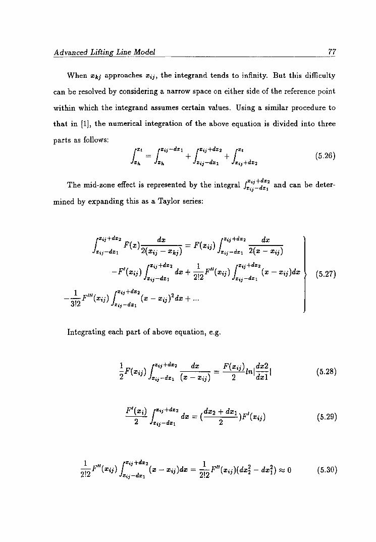
Advanced Lifting Line Model 77
When ~ki approaches Xij, the integrand tends to infinity. But this difficulty
can be resolved by considering a narrow space on either side of the reference point
within which the integrand assumes certain values. Using a similar procedure to
that in [1], the numerical integration of the above equation is divided into three
parts as follows:
(5.26)
The mid-zone effect is represented by the integral J:i; ~::12 and can be deter
mined by expanding this as a Taylor series:
(5.27)
1 lzoo+dz2
", '1 2 - -,- F ( ~ij ) (x - ~ij) d~ + ...
3.2 Zij-dzl
Integrating each part of above equation, e.g.
(5.28)
(5.29)
(5.30)
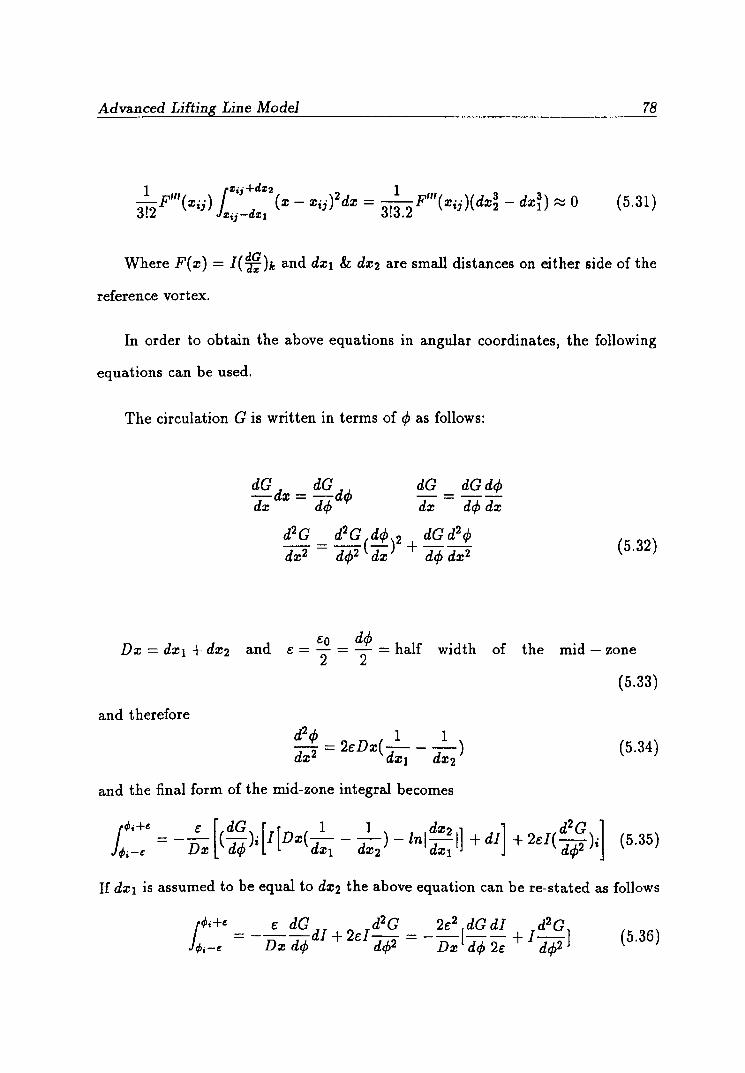
Advanced Lifting Line Model 78
1 l zi;+dz2 1 -,-F"'(Xij) (x - Xij)2dx = 3'3 2F"'(Xij)(dx~ - dx~) ~ 0 3.2 Zij-dzl ..
(5.31)
Where F( x) = J( ~)k and dXl & dX2 are small distances on either side of the
reference vortex.
In order to obtain the above equations in angular coordinates, the following
equations can be used.
The circulation G is written in terms of cp as follows:
dG d = dG dcp dG dG dcp dx x dcp dx dcp dx
d2G d2G dcp 2 dG d2cp dx2 = dcp2 (dx) + dcp dx 2 (5.32)
co dcp Dx = dXl + dX2 and e = - = - = half width of the mid - zone
2 2 (5.33)
and therefore d2cp 1 1 dx 2 = 2cDx( dXl - dX2) (5.34)
and the final form of the mid-zone integral becomes
If dXl is assumed to be equal to dX2 the above equation can be re-stated as follows
(5.36)

Advanced Lifting Line Model 79
The above equation can be simplified using the expressions of 2£ = d¢ and 'it =
l-,;Zb sin ~i and finally it becomes
(5.37)
This is the resulting equation obtained as in [1] and accordingly the velocity in
duced at the lh downstream of the ith reference vortex by the kth field vortex can
be represented as follows.
5.7 Local Wake Velocities in the Slipstream
Detailed knowledge of the local wake velocity distribution in the slipstream
is necessary for the establishment of a realistic model of the part of the trailing
vortices which have a significant effect on the propeller design and final slipstream
shape. This is the major difference between the present method and other conven-
tionallifting line methods. In these conventional methods the radial wake velocity
distribution at the propeller plane is assumed to be constant along the slipstream.
But in reality this is not true, therefore it is essential to take account of the wake
velocities behind the propeller for modelling the true shape of the slipstream.
In this procedure the wake velocities in the slipstream are calculated at a num
ber of control points using the methods described in Chapter 3. The choice of the
number of control points to be considered is a compromise between numerical ac-
curacy and computing time. In the present work, 21 control points are distributed
axially along each of 12 lines placed at various radial locations.

Advanced Lifting Line Model 80
Ofthe radial control points, 11 are situated at the propeller design section radii
and an extra point is placed below the propeller hub radius to allow the calculation
of the wake velocities within the contracted propeller slipstream. The axial control
points are placed at the following non-dimensional distances, Y / R, downstream of
the propeller plane:
Y R = 0.0, 0.06, ,0.20, 0.40, 0.60, 0.80, 1.0, 1.2, 1.4, 1.6
1.8, 2.0, 4.0, 6.0, 8.0, 10.0, 12.0, 14.0, 16.0, 18.0, 20.0
The local wake velocities at the 252 control points are calculated and stored for
later use in calculating the deformation of the slipstream. In the later calculation,
the wake velocities at control points on the vortex lines are derived by linear
interpolation within the stored values.
5.8 Deformation of the Slipstream
At a point :i)ij a distance Yij downstream from the lifting line, the slope of the
vortex line is given by
(5.39)
where Uai;, Uri; are the local wake velocities in the axial and radial directions
and 'Uai;' 'Urij propeller induced velocities in the axial and radial directions.
The radius of the vortex line can be then determined from the following equa-
tion: {Y"
:i)ij = :i)i + Jo
'3 tan a'ida, (5.40)

Advanced Lifting Line Model 81
The hydrodynamic pitch angle of the trailing vortices in the slipstream becomes
1 [ Ua .. + U a ·· ] f3ii = tan - '3 'J
7r~ijnD - Utij (5.41)
As can be seen from Equations 5.39 and 5.41, the deformed slipstream shape de-
pends on the total velocity on the vortex lines. The total velocity can be defined as
the sum of velocities induced at the point by the trailing vortices in the slipstream,
bound vortices at the lifting line and the local wake velocities. As long as the total
velocity at the point is calculated correctly, the true shape of the slipstream can
be obtained.
The components of the induced velocities or the local wake velocities can be
calculated using previously mentioned procedures, except for the velocities induced
by the trailing vortices at the hub and tip where the induction factors approach
infinity. In order to overcome this difficulty the hub and tip radii are redefined as
~hu.b = ~h + 0.012, ~tip = ~t - 0.012. These sections are treated as the hub and
tip radii within the all design calculations.
5.9 Convergence of Slipstream Shape
One of the main objectives of this section is to show how the helical slipstream
shape gradually converges to a final stable form. In order to achieve this objective,
the total velocities are calculated at each of the control points located on the
reference vortex lines. Their location with respect to the lifting line is given as
follows:
7r 8= 0, 8'
7r 4'
7r
2' 37r 4' 2.57r

Advanced Lifting Line Model 82
Hence, 231 control points are used for the representation of the slipstream. }or
the initial numerical calculation to define the trailing vortex shape, the local wake
velocities only are used since the induced velocities are still unknown. Using this
slipstream shape the bound circulation can be defined and provides the means for
the calculation of the induced velocities. Having calculated the induced velocities
related to the previously established bound circulation, a new slipstream shape is
obtained. According to the new deformed helical slipstream shape, the induction
factors and the bound circulation are redefined and consequently the velocities
induced at control points are recalculated. This procedure are carried out until
a satisfactory result is obtained with the aim of modelling a final stable irregular
helical slipstream shape. The design also satisfies the power absorption condition.
This convergence can be achieved by 3 or 4 iterations. At least 3 iterations are
essential to ensure the accuracy of the results.
In the process of deriving the new slipstream shape, an over correction of the
radii of the helices results in a fluctuation of the induced velocities when using
Equation 5.40. Therefore, it is necessary to use a new approximation which is the
arithmetic mean of the existing radius and that calculated by Equation 5.40. This
procedure supplies a smooth change from an original form to deformed one.
5.10 Circumferential Mean Velocities by Trailing Vortices
In the regular helical slipstream case, the mean induced velocities due to trail
ing vortices can be calculated using elliptic integrals, whereas in the deformed
helical slipstream case the use of elliptic integrals is impossible. Therefore, the
most straight forward procedure for the calculation of mean velocities is to use the
equations from the Biot-Savart's Law. The angle between the blades is divided

Advanced Lifting Line Model 83
into a number of parts and velocities induced at these points are calculated. These
velocities are then integrated numerically and divided by the blade angle to obtain
the circumferential mean induced velocities. In this study the angle between the
blades is divided into six parts resulting in seven points. On each point, the in
duction factors are calculated from a slightly different form of Equation 5.9, 5.10,
5.11 as stated below:
where
¢ _ 27r(K - 1) f - Z(N -1) K = 1,2, ... ,N
N: The number of the points between the blades
Z: The number of the blades.
(5.42)
(5.45)
The bound vortices also contribute to the circumferential mean induced ve-
locities. Using a formal application of Biot-Savart's Law, one can show that the
mean velocities induced by the bound vortices of the propeller are only tangential.
Thus, the circumferential mean induced velocities include:

Advanced Lifting Line Model 84
• Axial, tangential, radial circumferential mean velocities induced by trailing
vortices.
• Tangential circumferential mean velocity induced by bound vortices.

Chapter VI
Propeller /Stator Combination
6.1 Introduction
Current design procedures, including optimisation of radial loading on the
basis of the lifting line model, result in conventional propellers with the highest
achievable efficiency. In recent years shipowners' requirements for improved fuel
economy have led to the development and application of propulsive devices other
than the conventional propeller.
Contrarotating propellers provide an effective means of reducing the rotational
energy in the slipstream and will also remove the unbalanced torque reaction as
sociated with the conventional propeller. However, their application involves in
creased capital cost and mechanical complications related to gear box and shafting.
Largely for these reasons contrarotating propellers have not gained widespread use
on commercial vessels and their use has been limited to torpedoes, where torque
balance is essential.
Some of the benefits of contrarotation can be achieved at less cost and with
reduced mechanical complication by the use of fixed guide vanes, i.e. stators, placed
either upstream or downstream of the propeller. The stator can be designed to
remove the unbalanced torque reaction and to reduce the rotational energy loss, but
the gain in propulsor efficiency will be less than that achieved with contrarotation
because of the increased drag of the stator.

Propeller-Stator Combination 86
As with other energy saving propulsors, the use of a stator is only worthwhile
where the energy losses in the slipstream are significant i.e. the propeller loading
is moderate to high. Where the propeller loading is light, as in the case of torpedo,
the use of a stator may result in reduced propulsor efficiency, but they provide a
cheap and effective means of removing the unbalanced torque.
6.2 Propeller with Downstream or Upstream Stator
Both downstream and upstream stators are designed such that the tangential
velocities which they induce in the slipstream cancel those induced by the propeller,
but the source of the efficiency gain is different in each case.
The downstream stator has a negligible effect on the propeller forces but,
for appropriate propulsor loading, the stator produces a net positive thrust and
the propulsor efficiency becomes greater than that of the equivalent conventional
propeller.
On the other hand, the upstream stator produces a net negative thrust but
modifies the flow to the propeller in such way that the propeller thrust is increased
and, again in the right conditions, the propeller efficiency is increased.
Previous studies have shown, [3], that the use of a downstream stator is more
effective than that of an upstream stator. Therefore the propeller with a down
stream stator will be investigated more fully in the following sections.
6.3 Hydrodynamic Modelling of the Stator
The stator can be modelled by a system of lifting lines. The path of the trailing
vortices behind the stator is different than that of the propeller. In the stator case,
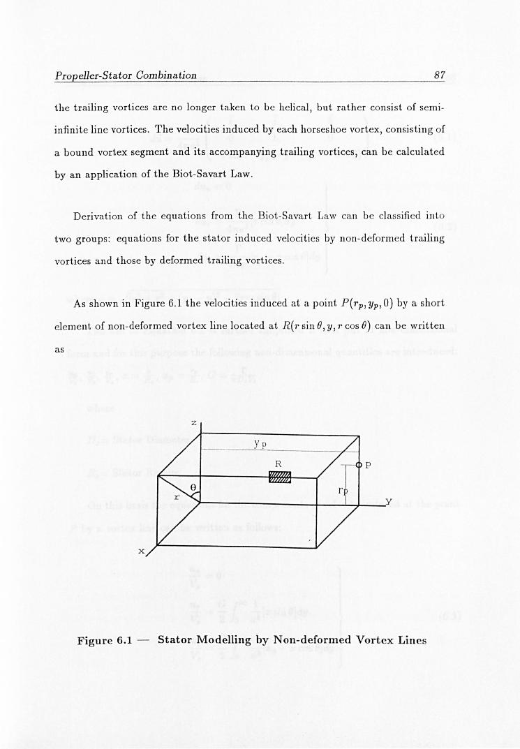
Propeller-Stator Combination 87
the trailing vortices are no longer taken to be helical, but rather consist of semi
infinite line vortices. The velocities induced by each horseshoe vortex, consisting of
a bound vortex segment and its accompanying trailing vortices, can be calculated
by an application of the Biot-Savart Law.
Derivation of the equations from the Biot -Savart Law can be cl ass ified into
two groups: equations for the stator induced velocities by non-deformed trailing
vortices and those by deformed trailing vortices.
As shown in Figure 6.1 the velocities induced at a point. P(rp, YP' 0) by a short
element of non-deformed vortex line located a t R(r sin B, y , r cos B) can be written
as
z
yp
R
x
Figure 6.1 - Stator Modelling by Non-deformed Vortex Lines

Propeller-Stator Combination
--J ( ; d -- r '1£=-- 0
47ra3 -r sinO
1
yp -y
k ) (rp - ~ cos 0)
or
r . dUr = --3 [r sm Oldy
471'a
r dUt = --3 [rp - r cos OJdy
471'a
where a = J[r2 + r; + (yP - y)2 - 2rrp sin OJ
BB
(6.1)
(6.2)
The use of Equation 6.2 is further simplified if it is put in non-dimensional
form and for this purpose the following non-dimensional quantities are introduced:
1!A 1'4- ~ a::-..L a:: -!.L G- r V.' V.' v.' -R.' p-R.' -1rD.V.
where
D" = Stator Diameter
R,,= Stator Radius
On this basis the equations for the components of velocity induced at the point
P by a vortex line can be written as follows:
Ua. = 0 V"
'1£ G 1000 1 ....!.=- -[a::sinB]dy
Va 2 0 a3
Ut G 1000 1 - = - -[a:: - a:: cos Ojdy Va 2 0 a3 p
(6.3)

Propeller-Stator Combination 89
where
For a stator having Z, equally spaced blades, Za free vortex lines will start
from the points on the blades corresponding to the radius r, the angular position
of these lines in relation to the reference blade being given by
<Pz = 27r(n - 1) Z,
(6.4)
where n = 1,2,3, ... Z, Then the total induced velocities can be determined by the
simple summation of the individual velocities induced by the Z, vortex lines from
the hub (Zh) to tip (Zt) as follows:
U a = 0 Va
U Z, G l Zt 1000 1
v.T
= L - 3"[z sin{B + <Pz)]dydz a 1 2 Zh 0 a
Ut Z, G l Zt 1000 1 V.
= L - 3"[zp - Z cos(B + <Pz)]dydz , 1 2 Zh 0 a
(6.5)
The above equations only give the effect of the vortices between y = 0 and
y = 00 and named as R.H.S. effect (explained in section 5.4). If a point is located
between y = 0 and y = YP' in addition to the R.H.S, the L.H.S effect is also
calculated by integrating effect of the vortices between the y = 0 and y = YP as
follows:
Propeller-Stator Combination 90
U Z, G l Zt 101lP 1 v.
T = ~ -2 3"[:Z: sin(O + tPz)]dyd:z:
s 1 zh 0 a (6.6)
Ut Z, G l Zt loYP 1 - = ~ - 3"[:Z:P -:z: cos(O + cPz)]dyd:z: ~ 1 2 Zh 0 a
The total induced velocities at the point P from the lifting line can be obtained
by the summation of the effect of R.H.S and L.H.S for the tangential and axial
induced velocities and the subtraction of the effect L.H.S and R.H.S for the radial
induced velocities.
With a finite number of stator blades, the self-induced velocities around the
circle at any radius of the stator will fluctuate cyclically. To design the stator it is
necessary to use the mean values of these fluctuations. These mean velocities can
easily be calculated in terms of the elliptic integrals of the first, second and third
kind and written with the effect of the free vortices placed from the boss and the
ti p as follows: Zt Z (8G). - J c s 8z 'd Ua t T - - UU(a t r)· :z: t, "$ z.
Zh t
(6.7)
When x is replaced by the angular coordinate tP , the above equation becomes
(6.8)
where U(a,t,T)i are the axial, tangential and radial mean induced velocity compo
nents given by Equation 4.37 to 4.39.
The equation for the velocities induced at the point P(O, yp, rp), Figure 6.2, by
a deformed trailing vortex located at a general point (r sin 0, y, r cos 0) can be

Propeller-Stator Combination
z
p
~-----------------+----~~---y
x
Figure 6.2 - Stator Modelling by Deformed Vortex Lines
formulated as follows:
or
dil = ~ ( - taniasine - tan a cos 0 k ) 47ra
- r sinO (rp - r cos 0)
dUa = ~[(rp - r cos 0) tan a sine + tan a cos o· r sin 0Jdy 47ra
dUr = ~[-(yp - y)tanasinO + rsinOJdy 47ra
r dut = --3 [Tp - T cos () + (yP - y) tan a cos ()Jdy
47ra
91
(6.9)
(6.10)
When integration of the trailing vortices downstream from the lifting line and
from the hub to the tip for each blade are considered) the following equations are

Propeller-Stator Combination 92
obtained in non-dimensional form:
z. G l Xt 1000 1
U a = L - 3"[(zp - z cos(O + ¢z)) tan a sin(8 + ¢z)+ 1 2 Zh 0 a
tanacos(B + ¢z)' zsin(O + ¢z)]dydz
z. G l Zt 1000 1
Ut = L - 3[zP - Z cos(O + ¢>z) + (yp - y) tan a cos(B + ¢z)]dydz 1 2 Xh 0 a
(6.11)
6.4 Design Consideration of Downstream Stator
The design variables for the stator are the number of blades and the axial
separation of the propeller and stator. It is desirable to keep the tip of the stator
within the propeller slipstream and for that reason the tip radius of the stator is
set equal to the radius of the contracted propeller slipstream at the plane of the
stator, as shown in Figure 6.3.
The following assumptions are also made in designing a downstream stator:
• The blades of the stator are considered to have an equal angular spacing.
• The stator is assumed to have zero skew and rake.
• The blades are represented by straight, radial lifting lines.
Having established the stator hub and tip radii from the propeller slipstream
shape, 37 field points are distributed between the hub and tip with 5° spacing
between the points in angular coordinate. As in the case of the propeller, this
spacing was found to give good accuracy and acceptable computation time. The

Propeller-Stator Combination 93
Axial Distance (AXD)
Propeller Stator
Figure 6.3 - Downstream Stator
locations of the field points are determined by following equation,
(6.12)
where ()i = :S(N - 1) (N = 1,2,3, ___ ,37)
Since there are no rotational induced velocities downstream of the stator) the
free vortex lines shed by the stator are directed axially downstream on the sur-
faces of cylinders which contract with the propulsor slipstream. On each of the
trailing vortex lines shed from the stator 30 vortex elements and control points are
considered and the non-dimensional axial location of these points is determined as
below:
(6.13)

Propeller-Stator Combination 94
where 8i = :0 N N=1,2,3, ... ,30
Having done this, 1110 points are obtained to model the slipstream shape
behind the stator. The next step is to determine the bound vortices of the stator
in order to achieve the design of the stator. Once the bound circulation of the
stator is established, the velocity induced by the stator can be calculated in axial,
radial and tangential directions using Equation 6.11.
6.5 Determination of Bound Vortices of the Stator
In order to determine the induced velocities, first the circulation of the stator
must be calculated. As stated earlier, the principle of the downstream stator
design was to balance out the tangential velocities in the slipstream. Therefore
the mean tangential velocities induced by the propeller should be cancelled out by
those of the stator at infinity downstream where the trailing vortices shed from
the propeller or the stator have significant effect while the bound vortices do not
have any effect. The tangential velocities induced by the stator can be written in
terms of the unknown circulation coefficients, An's as follows
~107r ~ A . ,1,.1000 [xp - xcos(8 + rPz) + (yP - y)tanacos(8 + rPz)Jd
dA. Ut = ~ ~ n·SIll n.,..i Y If'
1 0 n=l 0 2[x2+x~+(Yp-y)2-2xxpsin(8+rPz)]3/2 (6.14)
In order to calculate the mean tangential induced velocity at any radial location,
the blade angle is divided into five parts and the above equation is applied at the
resulting six points. The induced velocities are calculated and integrated at these
points, then divided by the blade angle to give the mean induced velocity at that
radial location.
The total mean tangential velocities induced by propeller are calculated on

Propeller-Stator Combination 95
each of 9 radii at infinity and those by stator are also determined at the same
locations in terms of the unknown An's. Then a system of nine simultaneous
equations is formed. The solution of this resulting matrix gives the unknown bound
circulation coefficients of the stator. Having established the bound circulation, the
induced velocities are calculated using Equation 6.11. An earlier experiment with
the method indicated that the induced velocities in axial and radial directions are
very small and they are ignored in this work.
6.6 Stator Torque and Thrust
As can be seen from Figure 6.4, the thrust and torque can be formulated for
each blade section as below:
dT = dL cos f3i - dD sin f3i (6.15)
dQ = (dL sin f3i + dD cos f3i) r (6.16)
where f3i = ~tI+UtlP"" uapm and Utpm are the axial and tangential mean velocities tp"'-Ut.
induced by the propeller, Uta is the tangential velocity induced by the stator and
Ua is the local wake velocity.
The resultant velocity, lift coefficient, drag coefficient, and lift-length coefficient
can also be expressed as below respectively:
v,. = uapm + Ua
sin f3i

Propeller-Stator Combination
Uo
2rc nr
Propell er
Uapm
Ua
Slalor
Figure 6.4 - Forces at Section of the Propeller and Downstream
Stator
96

Propeller-Stator Combination
CL = dL IpCdrV.2 2 T
CD = dD IpCdrV.2 2 T
ceL 27rG sin f3i
DIJ uapm + Ua
97
( 6.17)
For each section of the stator blade, the thrust and torque can be obtained by
making use of above Equations 6.15 to 6.17 as follows:
(6.18)
(6.19)
When the velocity in knots, diameter in metre and p = 1025.9kg/m3 the thrust
and torque can be expressed as below:
e ZIJ DIJ[uapm + Ua12[~ - CD] dT = 67.87 . (.l , dx
SInfJi (6.20)
(6.21)
6.7 Design Procedure of Propulsors
The design procedure in designing propeller & downstream stator combination
can be summarised as follows:
• The propeller is designed by the method given in Chapter 5. The tangential
mean velocities induced by the propeller are also calculated at infinity in the
slipstream.

Propeller-Stator Combination 98
• The stator diameter is established as the diameter of the slipstream at the given
axial distance.
• The stator bound circulation is calculated such that the stator induced tangen-
tial velocities cancel those due to the propeller. Consequently the thrust and
torque are calculated using the stator characteristics. The calculations of the
stator geometry, which are adopted from [3], are carried out as follows:
The initial width of the stator blade is taken as 25 % of the propeller diameter.
The thickness of the blades section tapers linearly from b = 0.20 at the hub to
t = 0.003Ds at the tip and the thickness, ti, of the section at Xi becomes
t. - (0.20Ch - 0.003D,)(:Z:t - :Z:i) D , - ( ) + 0.003 , :Z:t - Xh
(6.22)
where Ch is the chord width at the hub, D, the stator diameter, Xh the hub radius
and Xt the tip radius.
The section drag coefficient can be written in terms of the blade thickness and
chord length as below:
CD. = 2(1 + 2Cti
)[1.89 + 1.621og( Ci 6 )r2•5
, i 30 x 10-(6.23)
Using the initial values of the stator geometry the stator design is made for the
cancellation of the rotational velocity due to the propeller. Since it is unlikely that
the stator blades will experience cavitation, the only limit which need be placed on
the lift developed by the blade sections is that they should not have excessive form
drag. On completion of the initial stator design calculations the section chords are
adjusted to give lift coefficient values between 0.55 and 0.65, while at the same time
maintaining a fair blade outline. The section thicknesses and drag coefficients are

Propeller-Stator Combination 99
given new values appropriate to the new chord lengths. The design of the stator
is repeated with these new values and the process continued until convergence. In
this way, cancellation of the rotational induced velocities is achieved with minimum
stator drag.

Chapter VII
Application
7.1 Introduction
The purpose of this chapter is to illustrate the numerical application of the
theoretical procedures given in the earlier sections and to discuss the results of the
application. For the most appropriate application of the procedures, the calcula
tions were carried out for a torpedo shaped body which was assumed to be deeply
submerged.
Initially, the flow analysis around the body were carried out for the body
without an operating propeller, for which the flow was assumed to consist of two
parts: potential flow and boundary layer flow. The free surface effect was not taken
into account since the body was assumed to be deeply submerged. The theoretical
procedures described earlier were used to calculate the potential and boundary
layer flows around the body and, in particular, to produce the nominal velocity
distribution in the plane of the propeller.
The next step was the achievement of the propeller design using the newly
obtained nominal velocity distribution. When the body was investigated with an
operating propeller, essential interactions between the body and propeller had to
be taken into account and simultaneously the propeller design should be redone.
This procedure could provide the effective wake. Due to the slender body and the
complexity of the mathematical modelling of the wake, the interaction between

Application 101
the body&the propeller and the propeller&the boundary layer are ignored, as will
be explained in a later section. Therefore the nominal velocities were used in all
calculations. The use of the nominal wake would also provide the possibility of
comparing the results for the propeller design.
Having obtained the final design of the propeller with a balanced slipstream
shape, a stator device was placed downstream of the propeller. Based upon the
assumption that the stator had no effect on the body, the performance of this
combination was investigated for the variation in the number of the blades of the
stator and for the variation in the axial distance between the stator and propeller.
In order to perform the above computations miscellaneous computer programs
were written in Fortran 77 programming language for the propeller and stator
design and some of the existing softwares were modified for flow calculations. These
programs were set up to be run on an unix based Sun workstation.
7.2 Flow Analysis
In order to analyse the flow around the body, the potential flow calculation
was carried out using Hess-Smith method [17]. The existing computer program
based on this method was enhanced and used for computing the flow velocities
around the torpedo shape body.
The input data file to the program contained the necessary information to
control the flow of the computations, geometry of the body surface and off-body
points. The body surface was defined by offset points in three dimensional space.
The coordinate system, which these points were referred to, was designated as
the reference coordinate system. The offset input had to be distributed in such a

Application 102
way that an efficient representation of the body in terms of minimum CPU time
could be achieved. In particular, the input points were increased in regi ons where
the curvature of the body surface was large and the flow velocity was expected to
change rapidly, while the input points were distributed sparsely in regions where
neither the body geomet ry nor the th e fl ow properties were varying sign ifi cantl y.
5.3 m
.533- . - . - . -
1.031 ~-------------------~ I
Figure 7.1 - The Geometry of the Body
The body surface was approximated by joining t he input offset points which
formed a set of plane quadrilateral panels . It was easy to organise the input offset
points in such a way that the body was divided by rows and columns so that these
points could easily be entered either in row direction or in column direction. The
body, whose geometric characteristics as shown in Figure 7.1, was initially defined
by 3952 input points. Nevertheless, this number was found to be hi gh as it required

Application 103
very large amount of CPU time. Therefore a set of preliminary calculations was
carried out to find the optimum number of of input points for the same accuracy
and consequently the number of input points was reduced to 1000. Although the
body was approximated by 1000 input points, only 250 of them were entered to the
computer program because of the axisymmetric nature of the body geometry. The
details of the offset points are given in Appendix B for information. The density
of the offset of points was increased at the aft and fore part of the body where the
surface curvature was high as shown in Figure 7.2.
Using this input data the potential flow computation was carried out for unit
inflow in direction of the body axis and, the non-dimensional flow velocity distri
bution was obtained in the fluid domain. The result for the distribution of the
external flow velocity on the body surface is shown in Figure 7.3. This computed
external velocity distribution was used to calculate the displacement thickness in
combination with the earlier described the TSL equations. In making this cal
culation it was assumed that a transition point, at which the flow changes from
laminar to turbulent, occurs at the junction of the curved forward portion and the
parallel body. This seems a reasonable assumption to make because of the sudden
change in body curvature which occurs at that point. Based upon this assumption
the boundary layer calculation was performed. The resulting displacement and
boundary layer (B.L.) thicknesses normal to the body surface are shown in Figure
7.4 at speeds of 50 and 15 knots. These speeds were considered as the design speed
of the propellers as corresponding to lightly and heavily loaded operation condi
tions respectively. It can be seen from this figure that the change in speed does
not result in much change in displacement thickness, but in a significant change in
boundary layer thickness.

Application 104
Figure 7.2 - Discretisation of the Body
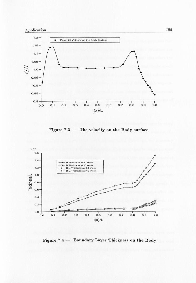
Application
1 .2
1.15
1 . 1
1.05
<: X 1 .0
'> 0 .95
0 .9
0 .85
0.8
0 .0
·10"
1.6
1.4
1 .2
-I 1 .0 -(J) (J) Q) c: 0 .8 .:.:: CJ :c t-- 0.6
0.4
0 .2
0.0
0 .0
_ Pote ntia l V e locity o n the Body S urface
0 .1 0.2 0 .3 0.4 0.5
I(x)/L
0 .6 0 .7 0 .8 0.9 1 .0
Figure 7.3 - The velocity on the Body surface
0 . 1
-e- D .Thlckness a t 5 0 knols --[9-- D .Thlckness a t 15 kno t s _ B .L. Thickness a t 50 k n o ts
-- 0 -- B .L. Thickness a t 15 kno t s
0 .2 0 .3 0.4 0 .5
I(x)/L
0 .6
. .0-------00
0 .7 0 .8
.p
.~ ," .; ,i
," ,'" ,0
,pi'
0 .9 1 .0
Figure 7.4 - Boundary Layer Thickness on the Body
105

Application 106
In simplified terms, the hydrodynamic interaction between the potential flow
and the BL flow can be taken into account by the change in the flow velocities due
to the displacement effect of the flow field. In order to implement this effect the
same potential flow calculation was carried out for the displacement body which
was defined as the actual body plus the displacement thickness. This calculation
resulted in a change in the external velocities of the order of 0.7%, which was con
sidered to be insignificant. This follows from the small values of the displacement
thickness shown in Figure 7.4, which can be attributed to the slender geometry of
the body.
The next stage was to calculate the velocities inside the boundary layer by using
Equation 3.32. Having performed the calculation of the local flow velocities at the
control points of the slipstream in the axial and radial directions, the necessary
input data for the wake distribution became ready for the propeller design process.
As noticed, the local tangential velocities were not taken into account because of
the slender shape of the body and the assumption of the potential flow, which does
not create a tangential velocity. The computed axial flow velocities downstream
from the propeller plane are shown in Figure 7.5 and 7.6 for two design speeds. It
can be seen from these figures that the axial velocity distribution approaches the
uniform onset flow value at Y / R = 2.0 In comparing the two design speeds, the
axial velocities for 50 knots are higher than those for 15 knots due to the greater
thickness of the boundary layer at low speed.
The radial components of the flow at points within the boundary layer were
calculated on the assumption that the ratio of the radial components to the axial
components (Ur/Ua) derived from the potential flow calculation remained constant

Application 107
and could be applied to the axial velocities derived from the boundary layer cal-
culation. Although it could be argued that this effect should be calcula ted on a
more sound basis, the assumption was considered to be satisfactory in relation
to the flow associated with the slender torpedo body. The radial velocities hav
small values at the propeller plane and approach zero rapidly in the downstream
direction.
1.0
0.9
0.8
0.7
<: X 0.6 '-"
::> 0.5
0.4
0.3
0.2 0.0
They are shown in Figure 7.7 and Figure 7.8 for the two design sp eds.
0.5 1.0 1.5
-t9- r/R=O.37
-€t- r/R=O.409
-A-- r/R=O.449
-+ r/R=O.528 ""* r/R=O.606 -e- r/R=O.685
~ r/R=O.764
-$- r/R=O.842
- r/R=O.921
-¥- r/R=O.961
-- r/R=1.000
2.0
Axial Distance (Y/R)
2.5
Figure 7.5 - Axial Velocity Distribution at 50 knots

Application
<: x ----::::>
S ::::>
1 .0
0 .9
0 .8
0.7
0 .6
0 .5
0 .4
0 .3
0.2 0 .0
0 .0
-0.05
-0.1
-0.15
-0 .2
-0 .25
-0.3
-0.35
-0.4
0 .5
-EI- r/R_ O.37
-e- r/R_ O.40B
-6- r/R- O.449 -e- r/R_ O.S26
~ r/R - O.S06 -e- r/R- O.S6S -*- r/ R . O.764 -$- r/R- O.642 -- r/R _ O.92l -¥- r/R_ O.9G l
- r/A- l .OOO
1.0 1 .5
Axial Distance (Y fR)
2 .0 2 .5
Figure 7.6 - Axial Velocity Distribution at 15 knots
--6- r/ A - O.37 -e- r/ A . OA09 -6- r/R- 0.44 9 ~ r/R . O.526 ~ r/R- O.60S -e- r/R- O.66 5 --*- r/R_ O.764 --$- r/R - O.B42
-- r/R- O.92l -¥- r/R- O.96l
- r/R - LOOO
0 .0 0 .5 1 .0 1 .5
Axial Distance (Y fR)
2.0 2.5
Figure 7.7 - Radial Velocity Distribution at 50 knots
108
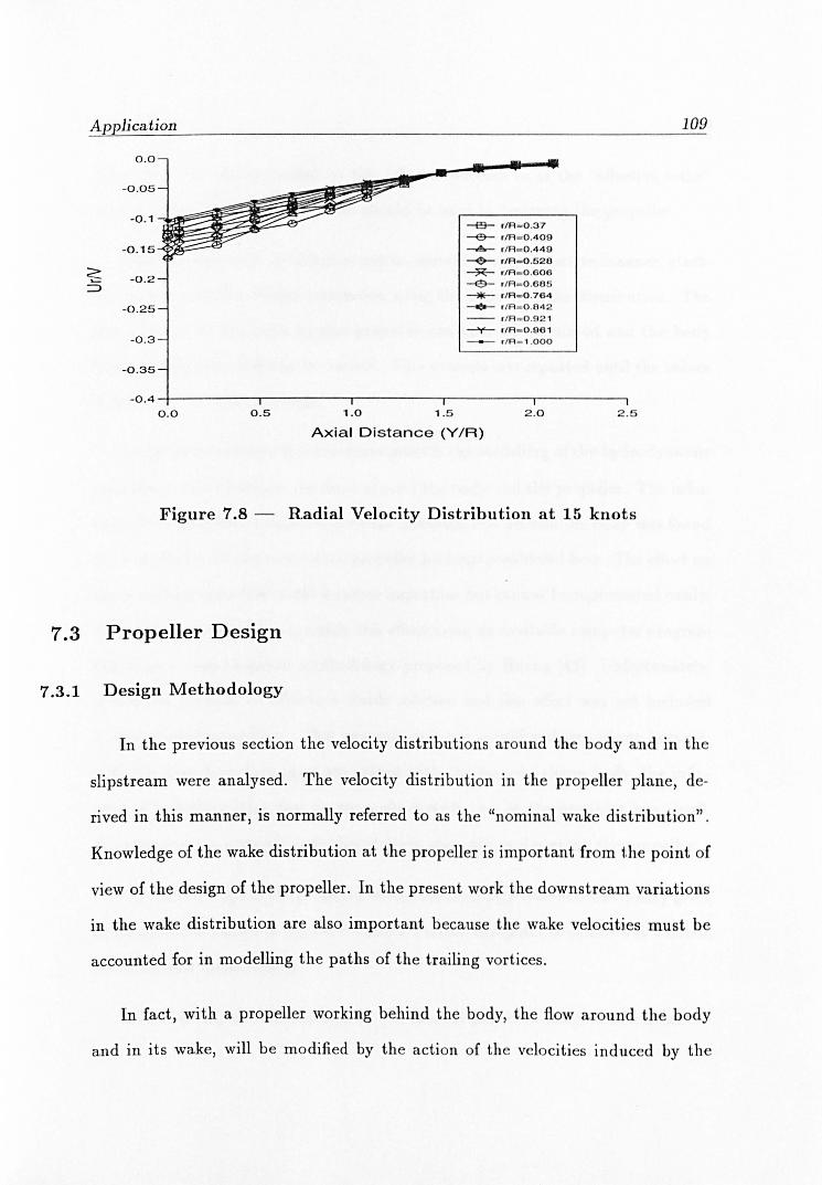
Application
0.0
-0.05
-0.1
-0. 15
~ -0 .2 ~
-0.25
-0 . 3
-0 .35
-0.4
0 .0 0 .5 1.0 1.5
-e3- r/A - O.37 -e- r/A - O.409 -.!!I.- r /A _ O.44 9
-e- r/A - O.528 ~ r /A- O.SOS -e- r / A _ O.S8S ~ r /A_ O.7S4 --$- r /A . O.84 2 -- r / A . O.92 1 ->y<- r/A. O.9S 1
r /R - 1 .000
2. 0
Axial Distance (VIR)
2.5
Figure 7.8 - Radial Velocity Distribution at 15 knots
7.3 Propeller Design
7.3.1 Design Methodology
109
In the previous section the velocity distributions around the body and in the
slipstream were analysed. The velocity distribution in the propeller plane, de-
rived in this manner, is normally referred to as the "nominal wake distribution".
Knowledge of the wake distribution at the propeller is important from the point of
view of the design of the propeller. In the present work the downstream variations
in the wake distribution are also important because the wake velocities must be
accounted for in modelling the paths of the trailing vortices.
In fact, with a propeller working behind the body, the flow around the body
and in its wake, will be modified by the action of th e velocities induced by the

Application 110
propeller. The wake modified by this effect is referred to as the "effective wake"
and the effective wake distribution should be used in designing the propeller.
The effective wake distribution can be derived in an interactive manner, start
ing with a propeller design calculation using the nominal wake distribution. The
flow induced on the body by this propeller can then be calculated and the body
flow and effective wake can be derived. This procedure is repeated until the values
of the effective wake converge.
In the above process the important point is the modelling of the hydrodynamic
interaction effect between the flows around the body and the propeller. The influ
ence of the propeller induced flow on the potential flow around the body was found
to be negligible for the most of the propeller loadings considered here. The effect on
the boundary layer flow could be more important but cannot be represented easily.
The author attempted to quantify this effect using an available computer program
based on a semi-empirical methodology proposed by Huang [43]. Unfortunately,
it was not possible to achieve a stable solution and this effect was not included
in the present procedure. This omission was not considered important because,
with the thin boundary layer associated with the torpedo shape body, the influ
ence of boundary layer flow on the wake distribution at the propeller was small.
In summary, the nominal wake distribution was used in designing the propeller.
The major steps of the propeller design methodology based on the theory given
in Chapter 5 is shown in Figure 7.9 and a Fortran computer program was written,
based on this methodology.
The basic input data required by the present propeller design method can be

Application
Calculation of Induced
veloc ities
Results
Prope ll r Input D ta
Assump ion of x. 1(. a m:
~ i = ( ~+C)/2
Calculation 0 Indu c ion F t
r constant
Yes
Solu tion of An '
Calculation of Bound ircula ion
Calcula i n of I n duc d v 1
a nd De orma ion
No
Figure 7.9 - Propeller Design Procedure
111

~A~p~p=li~·c=a=tl=·o~n~ ________________________________________________ ~112
listed as follows:
Design Variables
• Body speed
• Delivered power
• Shaft speed
Geometric Design Parameters
• N umber of propeller blades
• Propeller diameter
• Ser:tion chord widths and thicknesses
Environmental Parameters
• Body wake velocities at propeller plane and downstream
Having defined the input data above, the design condition became to achieve
the required torque coefficient KQ at the advance coefficient Jv" where KQ and
Jv , are defined as follows:
K _ 33.55PD Q - ['if]3 D2
Jv, = V. ND
(7.1 )
(7.2)
In order to calculate the induction factors using Equations 5.9 to 5.11, the
initial value of the vortex pitch angle of the trailing vortices should be determined.
The advance angle {3y at the propeller plane and downstream is calculated from

Application 113
the rotational speed of the propeller, N, and the wake velocities. An initial value
of Xl!' tan €, the pitch ratio of the vortex sheets in the ultimate wake is assumed
and the initial values of the vortex pitch angles are derived from
(7.3)
Using these values the initial slipstream geometry is defined and the induc-
tion factors are calculated to determine expressions for the velocities induced by
the propeller vortex system at 9 radial points on the lifting line, in terms of the
unknown Fourier coefficients. These expressions are introduced to the minimum
energy 1055 condition Xl!' tan € = constant and a system of nine simultaneous equa
tion is formed. The solution of these equations gives the circulation coefficients
An and hence the bound circulation r.
Having calculated the bound circulation the induced velocities in the slipstream
are calculated. Using these calculated induced velocities and the wake velocities, a
deformed slipstream shape is obtained. Based on this deformed slipstream shape,
the calculation of the induction factors is carried out. Keeping the bound circu-
lation constant, the induced velocities and consequently the deformation of the
slipstream are re-calculated. This is the completion of the first iteration. Hav
ing completed the first iteration, the next iteration starts using that deformed
slipstream to calculate the bound circulation. The expressions for the induced
velocities at the lifting line are determined and the resulting equations are solved
as before to give the new circulation. This procedure is continued until the slip
stream shape is converged. It was found by early experiments with the method
that at least 3 iterations would be necessary for the convergence of the slipstream

Application 114
shape and to achieve the required torque coefficient. During each iteration the
elementary torque coefficients dfLQ for eleven sections are calculated, the values
at the hub and tip being set equal to zero. Integration of these coefficients gives
the calculated torque coefficient, KQo' If IKQ() - KQI < 0.0001 and the slipstream
shape is properly converged, the design is considered to be completed. The final
propeller characteristics such as hydrodynamic pitch angle, (3i, the lift-length co
efficient *, the lift coefficient CL, and the elementary thrust coefficient d!kT are
then calculated for each nine sections.
7.3.2 lllustrative Examples
In this section a propeller design based upon the above methodology was per-
formed for verification and comparison with results of other methods. Since the
slipstream deformation was expected to be a function of load coefficient CT, it was
decided to select two types of loading condition: lightly and heavily loaded cases
with the same propeller geometric characteristics at different advance speeds and
rates of rotation. Details of the design data which are referred to as DATAl for
the lightly loaded case are as follows:
Design Characteristics for DATAl
Delivered Power, PD= 260 KW
Design Speed, V = 50 Knots
Rate of Rotation, N = 3000 rpm
Propeller Diameter, D= 0.490 metre
Number of Blades, Z= 3

Application 115
Radius 0.37 0.409 0.449 0.528 0.606 0.685 0.764 0.842 0.921 0.961 1.0
C (m) 0.1725 0.1800 0.1925 0.2080 0.2122 0.2045 0.1840 0.1420 0.1050 0
CD 0.0095 0.0093 0.0092 0.0091 0.0090 0.0089 0.0088 0.0087 0.0086
The input wake velocities (U(x)jV) computed from the previous procedure is
shown in Table 7.1
Radius 0.37 0.409 0.449 0.528 0.606 0.685 0.764 0.842 0.921 0.961 1.0 YIR
0.00 0.455 0.649 0.740 0.841 0.904 0.912 0.920 0.927 0.933 0.936 0.938
0.06 0.588 0.691 0.763 0.851 0.904 0.913 0.920 0.927 0.933 0.936 0.938
0.26 0.716 0.775 0.819 0.885 0.906 0.914 0.922 0.928 0.934 0.937 0.939
0.46 0.790 0.830 0.864 0.900 0.909 0.917 0.924 0.930 0.936 0.938 0.940
0.67 0.836 0.867 0.893 0.904 0.913 0.921 0.927 0.933 0.938 0.940 0.943
0.87 0.888 0.895 0.900 0.910 0.919 0.926 0.932 0.937 0.942 0.944 0.946
1.08 0.900 0.905 0.910 0.919 0.926 0.932 0.937 0.942 0.946 0.948 0.949
1.28 0.914 0.918 0.922 0.929 0.934 0.939 0.943 0.947 0.950 0.952 0.954
1.48 0.930 0.933 0.935 0.939 0.943 0.947 0.950 0.953 0.956 0.957 0.958
1.69 0.944 0.946 0.947 0.949 0.952 0.954 0.956 0.959 0.960 0.961 0.962
1.89 0.955 0.955 0.956 0.958 0.959 0.961 0.962 0.964 0.965 0.966 0.967
2.10 0.962 0.963 0.963 0.964 0.965 0.966 0.967 0.968 0.969 0.970 0.970
4.14 0.988 0.988 0.988 0.988 0.988 0.988 0.988 0.989 0.989 0.989 0.989
6.18 0.994 0.994 0.994 0.994 0.994 0.994 0.994 0.994 0.994 0.994 0.994
8.22 0.996 0.996 0.996 0.996 0.996 0.996 0.996 0.996 0.996 0.996 0.996
10.26 0.997 0.997 0.997 0.997 0.997 0.997 0.997 0.997 0.997 0.997 0.997
12.30 0.998 0.998 0.998 0.998 0.998 0.998 0.998 0.998 0.998 0.998 0.998
14.34 0.998 0.998 0.998 0.998 0.998 0.998 0.998 0.998 0.998 0.998 0.999
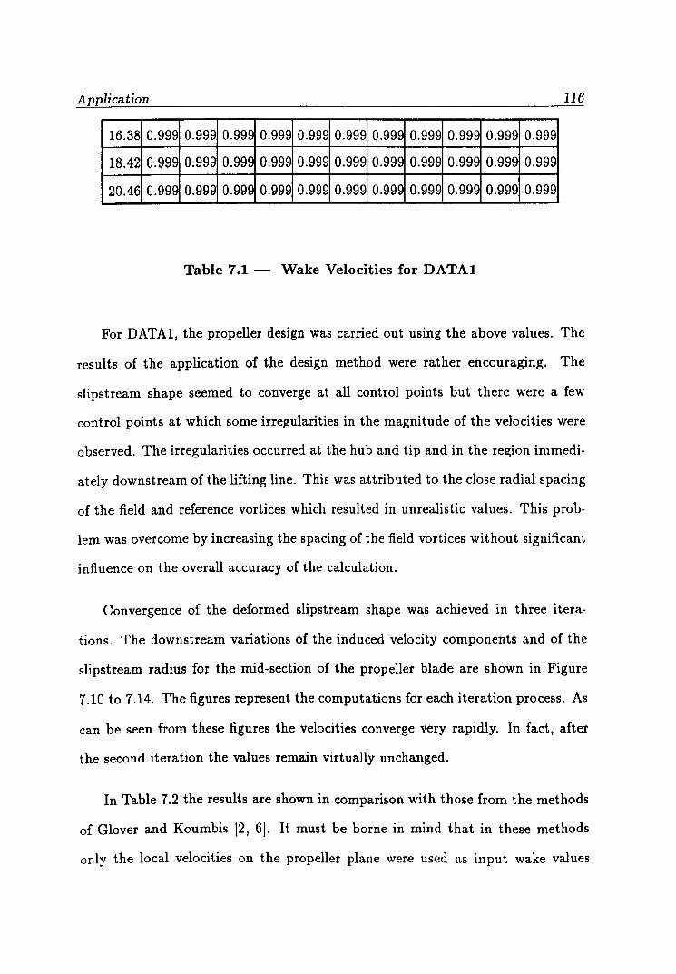
~A~p~p=h~'c=a=tl='o=n~ ________________________________________________ -=116
16.38 0.999 0.999 0.999 0.999 0.999 0.999 0.999 0.999 0.999 0.999 0.999
18.42 0.999 0.999 0.999 0.999 0.999 0.999 0.99~ 0.999 0.999 0.999 0.999
20.46 0.999 0.999 0.999 0.999 0.999 0.999 0.999 0.999 0.999 0.999 0.999
Table 7.1 -- Wake Velocities for DATAl
For DATAl, the propeller design was carried out using the above values. The
results of the application of the design method were rather encouraging. The
slipstream shape seemed to converge at all control points but there were a few
control points at which some irregularities in the magnitude of the velocities were
observed. The irregularities occurred at the hub and tip and in the region immedi
ately downstream of the lifting line. This was attributed to the close radial spacing
of the field and reference vortices which resulted in unrealistic values. This prob
lem was overcome by increasing the spacing of the field vortices without significant
influence on the overall accuracy of the calculation.
Convergence of the deformed slipstream shape was achieved in three itera
tions. The downstream variations of the induced velocity components and of the
slipstream radius for the mid-section of the propeller blade are shown in Figure
7.10 to 7.14. The figures represent the computations for each iteration process. As
can be seen from these figures the velocities converge very rapidly. In fact, after
the second iteration the values remain virtually unchanged.
In Table 7.2 the results are shown in comparison with those from the methods
of Glover and Koumbis [2, 6]. It must be borne in mind that in these methods
only the local velocities on the propeller plane were used as input wake values

Application 117
whereas in the present method the variation of the flow velocities in the slipstream
was taken into account. In Glover's method the non-deformed helical slipstream
shape is used for the hydrodynamic modelling of the propeller, while a deformed
slipstream shape is considered in Koumbis' method.
Lightly Loaded Case (DATAl)
Glover's Method Koumbis' Method Pro Method
KQ 0.1143 0.01143 0.1143
KT 0.0502 0.0503 0.0500
TJ 0.647 0.648 0.646
GT 0.149 0.149 0.148
Table 7.2 - Comparison of the Methods
As can be seen from Table 7.2, there is not much difference between the calcu
lated results. This may suggest that for this design case (i.e. loading) the effect of
the variation in flow velocities in the slipstream does not have a significant effect
on the propeller design.
The calculated bound circulation, hydrodynamic pitch angle, lift-length coef
ficient are shown in Figures 7.15 to 7.17 respectively in comparison with other
methods (i.e Glover's method and Koumbis' method).
The results for the reference helices shed at the characteristic non-dimensional
radii of the lifting line with variation of axial distance downstream and iterations

Application
0 . 1 2
en
~ 0 . 1
=> .t::- 0 . 0 8 ·0 0
Q5 >- 0 .0 6 -0 ill <...> ~ -0 0 .04 E <i::i ·x c:x:: 0 .0 2
0 .0
0 2 3 456 7 a Axia l Dis t a nce Y I R
9
118
1 0 1 1 1 2
Figure 7.10 - Variation of Axial Induced Velocity a t x=0.6l for
0 .0
en $
-0 .02 :=> .t::-·0 0
Q5 -0 .0 4 >--0 ill <...> ~ -0 -0 .06 E .~ C ill
-0 .0 8 0> c co I-
-0 . 1
0 2 3
DATAl
45678
Axia l Di s t a n ce Y/R
9 1 0 1 1 12
Figure 7.11 - Variation of Ta ngential Induced Velocity at x = 0.61 for
DATAl

Application 119
U)
~ :=> Z;-·0 0
Q) > -0 Q) u ::::;J
-0 C
co '6 co a:
0 .0
-0.005
-0 .01
-0.015
-0 .02~--~---'----r---.---.----r--~---'----r---~--'---~
o 2 3 4 5 6 7 8 9 10 " ' 2
Axial Distance Y fR
Figure 7.12 - Variation of Radial Induced Velocity at x = O.6l for
1 .0
0 .9
0
~ 0.8
(/) ::J '6 0.7 ro a: E 0 .6 ro jg en .9- 0 .5 en
0.4
0 .3 0 2 3
DATAl
4 5 6 7 8
Axial Distance Y fR
9 10 11 1 2
Figure 7.13 - Variation of Radius at x=O.61 for DATAl

Application
5 0
45
40 <l> en c 35 4:
.s=-u
3 0 ~ X <l> 25 t:: -e- Itorallon 1 0 >
2 0
---e--- Ito ra tion 2 -....- ltoraUon 3
15
10 0 2 3 4 5 6 7 8 9 10 1 1 12
Axia l Dista nce Y/R
Figure 7.14 - Vortex Pit ch Variation at x==O.61 for DATAl
·1 0 "
1 .2
§: 1 .0 c .2 co -S 0 .8 u '-(3 (ij 0 .6 c 0 Ow C <l> 0 .4 E (5 C
0 .2 0 Z
0 .0 0 .3 0 .4 0 .5 0 .6
-e3- Presen t M e thod ... (!) ... Glove ~s M e thod -- 01!!.-- K oumbl s ' M ethod
0 .7 0 .8
Non- Dime nsiona l R a dii (X)
0 .9 1 .0
Figure 7.15 - Circulation Distribu t ion (DATAl)
120

Application
35
Q)
c;, 30 c « ~
.B c: .~ 25 cO c ~ e -g. 20 I
-E:J- Present M e thod ... (9 ... Glover's M ethod
··A·· Koumbis ' M e thod
15~------~-------'--------'-------'-------~------'-------~
0 .3
0 .05
0- 0 .04 ::::J (.) .s. -c Q) 0 .03 '0 :E Q) 0
<-) 0 .02
~ 0, C Q) ~
~ 0.01 ::J
0 .0
0.4 0 .5 0 .6 0 .7 0 .8 0 .9 1 .0
Non-Dimensiona l Radii (X)
Figure 7.16 - Hydrodynamic Pitch Angle (DATAl)
0 .3 0.4
-E:J- Presont M e ll10d .. . (9 ... G lo vor' s M e thod
- -6- - Koumbls 'mothod
0 .5 0 .6 0 .7 0 .8 0 .9
Non-Dimensiona l Radii (X)
1 .0
Figure 7.17 - Lift-Length Coefficient (DATAl)
121

Application 122
are shown in Appendix C to demonstrate the changes in the hydrodynamic pitch
angle, radius and induced velocities along the slipstream.
The variation of the slipstream radius along the downstream are also plotted
in Figure 7.18. The results obtained from Koumbis' method [6J is also shown in
Figure 7.19 for the same data. The comparison of the two figures indicates that
the slipstream radii calculated by the present method are smaller than those by
the Koumbis method. This was because the local velocities in the slipstream would
have a significant effect on the shape of the trailing vortices as in the real slipstream
case and this effect was neglected in Koumbis' work.
7.3.3 Design Calculations for DATA2
The set of design data for the heavily loaded case is referred to as DATA2 and
corresponding design characteristics are given as follows:
Design Characteristics for DATA2
Delivered Power, PD= 260 KW
Design Speed, V = 15 Knots
Rate of Rotation, N = 2000 rpm
Propeller Diameter, D= 0.490 metre
Number of Blades, Z= 3
The chord widths and thicknesses of the propeller blade corresponding to each
of the section radii are taken the same as DATAL The wake velocities at the
propeller plane and downstream are given in Table 7.3:

Application 123
0 N
co ...-
NmmOOgo.nti!iN ~~OO
~~~~ ffi,....~~~~ lflflflflflflflflflflf
CD x x x x ~ x x x x x x
~~~t+++~<ptt ...-
""'" ...-
a: --N >-...-Cl) U C
0 CU ...- ...... (/)
0
co CU >< «
CD
o
o
Figure 7.18 - Slipstream Shape by Present Method for DATAl

Application 124
~ 8 m ~ ~ ~ ~ N ~ - ~ ~..,.::;j:S'j :Zr-QI;Sl~Ol 9, 9, 9, 9, ?, 9, 9, 9, 9, ?, 9, K X ~ X ~ X ~ X X ~ X
C\J
$~+t+++*~i- * ..-
..-
..-
0 ..-
())
ex:> a: >==
I"- m u c
<.0 co ....... en 0
l.(') co
~ -.:;t
o ,..... c:i
Figure 7.19 - Slipstream Shape by Koumbis' M ethod for DATAl

Application 125
Radius 0.37 00409 0.449 0.528 0.606 0.685 0.764 0.842 0.921 0.961 1.0 Y/R
0.00 00405 0.603 0.697 0.805 0.875 0.913 0.920 0.927 0.933 0.936 0.939
0.06 0.512 0.647 0.722 0.817 0.881 0.913 0.921 0.927 0.933 0.936 0.939
0.26 0.678 0.740 0.788 0.852 0.906 0.915 0.922 0.928 0.934 0.937 0.939
0046 O.77e 0.808 0.841 0.899 0.909 0.917 0.924 0.930 0.935 0.938 0.940
0.67 0.810 0.840 0.867 0.903 0.912 0.920 0.927 0.933 0.938 0.940 0.942
0.87 0.833 0.860 0.885 0.909 0.918 0.925 0.931 0.936 0.941 0.943 0.945
1.08 0.856 0.880 0.908 0.917 0.925 0.931 0.936 0.941 0.945 0.947 0.949
1.28 0.911 0.916 0.920 0.927 0.933 0.938 0.942 0.946 0.950 0.951 0.953
1048 0.928 0.931 0.933 0.938 0.942 0.946 0.949 0.952 0.955 0.956 0.957
1.69 0.943 0.944 0.946 0.948 0.951 0.953 0.956 0.958 0.960 0.961 0.962
1.89 0.954 0.954 0.955 0.957 0.958 0.960 0.961 0.963 0.965 0.965 0.966
2.10 0.961 0.962 0.962 0.963 0.964 0.965 0.966 0.968 0.969 0.969 0.970
4.14 0.988 0.988 0.988 0.988 0.988 0.988 0.988 0.988 0.988 0.989 0.989
6.18 0.994 0.994 0.994 0.994 0.994 0.994 0.994 0.994 0.994 0.994 0.994
8.22 0.996 0.996 0.996 0.996 0.996 0.996 0.996 0.996 0.996 0.996 0.996
10.26 0.997 0.997 0.997 0.997 0.997 0.997 0.997 0.997 0.997 0.997 0.997
12.30 0.998 0.998 0.998 0.998 0.998 0.998 0.998 0.998 0.998 0.998 0.998
14.34 0.998 0.998 0.998 0.998 0.998 0.998 0.998 0.998 0.998 0.998 0.998
16.38 0.999 0.999 0.999 0.999 0.999 0.999 0.999 0.999 0.999 0.999 0.999
18.42 0.999 0.999 0.999 0.999 0.999 0.999 0.999 0.999 0.999 0.999 0.999
20.46 0.999 0.999 0.999 0.999 0.999 0.999 0.999 0.999 0.999 0.999 0.999
Table 7.3 - Wake Velocities for DATA2

Application 126
The design calculations were carried out as for the previous lightly loaded
case, the similar results are shown in Table 7.4 and in Figures from 7.20 to 7.27.
As shown in Table 7.4 the present method with this set of data (DATA2) indi
cates slightly higher efficiency value in comparison with the methods of Glover
and Koumbis. The comparison of the lightly and heavily loaded design cases are
discussed in the following section.
Heavily Loaded Case (DATA2)
Glover's Method Koumbis' Method Pro Method
KQ 0.03858 0.03858 0.03858
KT 0.2636 0.2706 0.2754
11 0.448 0.458 0.466
CT 3.94 4.05 4.11
Table 7.4 - Comparison of the Methods
7.3.4 Discussion
In the previous sections, it was shown the influence of the helical slipstream
upon itself with the local velocities results in change in the slipstream so that it
gradually converges to a fixed deformed form. The slipstream deformations for
each of flow cases, such as potential flow, wake flow without a propeller and wake
flow with a propeller, are shown in Figures 7.29 and 7.30 for DATAl and DATA2
respectively.

Application
1 .2
(fJ
~ 1 .0
=:> Z- 0 .8 'u 0
Q) >- 0 .6 -0 Q) <..> ::l -0 0 .4 .E co 'x « 0.2
0 .0 0 2 4 6 8
Axial Dis t a nce Y IR
127
1 0 1 2 14
Figure 7.20 - Variation of Axial Induced Velocity at x = O.61 for
DATA2
0 .0
- 0 .5
- 1 .0
- 1 .5
o 2 4 6 8 10 12 1 4
Axia l Dis t a n ce Y/R
Figure 7.21 - Variat ion of Tangential Induced Velocity a t x=0.61 for
DATA2

Application
0 .0
en ~ -0.02
:::> .z-·0 0 -0 .0 4
W >--0 Q) (.)
=> - 0 .0 6 -0 c:
<U 'i5 - 0 .08 <U a:
- 0 . 1
0 2 4 6 8 10
Axial Distance Y fR
~ 1I0 rll 1 Io" 1
---e-- Ito r lion 2 -A- HaraHon 3
1 2 1 4
128
Figure 7.22 - Variation of Radial Induced Velocity at x = O.61 for
1 .0
0 .9
o ~ 0 .8
en .::! -0 0 .7 <U a: E <U 0 .6 ~ U) .9- 0 .5 en
0 .4
DATA2
0 . 3~-----'.------r-----.------.------.------'------.---
o 2 4 6 8 1 0 1 2 1 4
Axial Dista nce Y/R
Figure 7.23 - Variation of Radius a t x = O.61 for DATA2

Application
50
45
4 0 Q)
""6> c 35 « .c .B 3 0 0:::: x Q) 25 "t:: 0 >
20
15
10 0 2 4 6 8 10
Axial Dista nce Y/R
-e- Ifo ra llo n 1 __ lto ra tion 2
--.0.- ltora tion::J
12 14
Figure 7.24 - Vortex Pitch Variation at x=O.6l for DATAl
0 .12
§: C 0 .1 0
~ ~
E 0 .0 8 G "@ c 0 .0 6 0 ·w c Q)
E 0 .0 4
is C: 0 0 .0 2 Z
0 .0 0 .3 0.4 0. 5 0 .6
... (!) ..
....
-e:r Present Mothod ... (!) ... Glo ver's M o tho d
- ~A-- K o umbls' M e tho d
0 .7 0 .8
Non-Dime n siona l R a d ii (X)
0 .9 1 .0
Figure 7.25 - Circulation Distribution (DATA2)
129

Application
35
Cl)
0> 30 c « .c .8 0:::: .~ 25
cO c >
"'0 e ~ 20 :I:
-e:t- Present Method ... (9 ... G lovor's M o thod --6 - - Koumbls' Mothod
15~-------.-------r------.-------'-------'-------~--~~
0 .3 0.4 0 .5 0.6 0 .7 0 .8 0 .9 1 .0
Non-Dimensional Radii (X)
Figure 7.26 - Hydrodynamic Pitch Angle (DATA2)
0 ,2
0- 0 .18 ::::J 0 ..s. 0 .16 ....... c <l> '(3 0 .14 ~ Cl> 0 0 .12 0 .c ....... 0> 0 .1 c: Cl> --l ~ :.::::i
0 .08
0 .06
0 .3 0.4
.. .(9 .. ::.--- __ _
-e:t- Present M e thod ... (!)- .. Glover's Method
--b- Koumbls' m e thod
0 .5 0 .6 0 .7 0 .8
Non-Dimensional Radii (X)
0 ,9
Figure 7.27 - Lift-Length Coefficient (DATA2)
1 .0
130

Application
No)C')CO~
~~~Cj<o dddcic:i II II II II II
>< >< >< >< ><
:i3;'b~Nq;~ <'o"""CX)OlmOl 000000 II II II II II II >< >< >< >< >< ><
o
o ('f)
0 N
L{) .,..-
0 .,..-
L{)
o
131
a: >= (]) U C ro ....... en
0 ro >< «
Figure 7.28 - Slipstream Shape by Present Method for DATA2

Application 132
j ... .. .. .. ... :11 :0 :0 :0 · 0 0
·0 0
:0 : 0 · 0
.9! 0
;: : 0 g Q; Qj · 0
ro Cl. :0
~ 2 ~ :0 Cl. Cl. 0 0
i '5 2 0 Cl. 0 0
£ .c ·0 0 « "0 .~ .j I 0: l- V) 0 o· « Q) V) '" 0 0: Q) Q)
0 .<; .<; .<; 0 o· E E E ·0
'" "' '" 0 ~ ~ ~ 0 in iJi iJi 0
0 I I
I 0 I I I I I , ,
I I
I I
Figure 7.29 - Flow behind the Body for DATAl

Application 133
.I ,
:0 :0 :0 :0
:0 l , :0 , :0
l , :I ,
l :0 J :0 J :0 l :0 J :0 J :0 J :0
;: .Si l :0 2 0; .Si
, :0
1§ 0- , :0 0 0; , :0
C C. 0- , :0 0> '5 e :0 :0
N 8. 0 0-:0 :0 « :; '" :0 :0 "0 . ~ ~ !;t: '" :0 :0
0> '" '" :0 :0
0 .s 0> 0> :0 .s .s
E E E :1: '" '" '" ~ : ~ ~ ~ ~ jj) jj) jj) .,'
o·
Figure 7.30 - Flow behind the Body for DATA2

Application 134
The ratio of the slipstream contraction is a function of the thrust load coef-
ficient. In classical methods, in which the wake velocities are assumed to remain
constant along the slipstream, more contraction of the slipstream could be seen for
the heavily loaded propellers in comparison with that for lightly loaded propellers.
However in the present work the contraction of the lightly loaded propeller (Fig
ure 7.18) far downstream was found to be higher than that of the heavily loaded
propeller (Figure 7.28). This is because the downstream variation of the wake
velocities is taken into account. The wake velocities increase along the slipstream
and approach the onset velocity at infinity downstream. It can be seen from fol
lowing equation that when the total velocity in the axial direction increases, the
slope of the trailing vortex lines or slipstream decreases.
Uf ·· + U f ·· tan elij = 'J 'J
UBi; + UBi;
In the heavily loaded case the axial velocity components of each vortex were much
bigger than those in the lightly case, while there is no significant change on the
other components of the velocities for both loading cases. Therefore, the above
formulation results in small values for the heavily loaded case.
When the induced velocities at the lifting line Uo and at infinity U oo down-
stream were compared, it was found that the convergence in magnitude from Uo
to U oo took place at a very short distance in the downstream as seen from Figure
7.10, 7.11, 7.12, 7.20, 7.21 and 7.22. According to the classical lifting line theory
the magnitude of the induced velocities at the blade sections (uo) are half of the
velocities at the far downstream. This is valid for the axial and tangential velocity
components whilst the radial components becomes zero as can be seen from Figure
7.12 and 7.22 for two different design cases.

Application 135
If one investigates the behaviour of the axial and tangential induced velocity
components, it can be seen that, the rate of convergence of the induced velocity
magnitude (uo) to the velocity magnitude at the far downstream (uoo ) is relatively
high as shown in Figures 7.10, 7.11 ,7.20 and 7.21. In other words, the change in
magnitude from (uo) to (uoo ) takes place at very short distance from the blade
section along the downstream.
Another interesting aspect of the behaviour of these induced velocities is that
the ratio of the magnitude of the induced velocities far downstream to that at the
lifting line (~ ) does not equal 2.0 as expected from the simple theory and varies
dependent upon the loading conditions. As can be seen from Figures 7.10 and 7.11
for the lightly loaded case, ~ equals to 1.74 for the axial induced velocity and
2.48 for the tangential induced velocity. A similar trend is also observed for the
heavily loaded case, as seen from Figure 7.20 and 7.21, for which the associated
velocity ratios take values of 1.62 and 2.76 respectively for the axial and tangential
components. The differences in the velocity ratio with respect to the classical
lifting line theory value (i.e. ~ = 2.0 ) is due to the effect of the trailing vortex
lines defined as follows.
Let an "External Field" vortex be defined as a vortex line located at a point
above that at which the induced velocities are to be calculated and similarly let
an "Internal Field" vortex be defined as the one below that point. With a non
deformed helical slipstream shape, which is used in the classical lifting line theory,
the behaviour of the vortex line does not change along the slipstream, so that it
remains in the external or the internal field in relation to reference point.
However, when the slipstream deformation is accounted for, a vortex line,

Application 136
which is initially in the External Field in relation to a particular reference point,
contracts and moves into Internal Field at some distance downstream from the
lifting line. This results in a reduction in the axial velocity induced by the vortex
line at the reference point and an increase in the tangential velocity.
7.4 Propeller with Downstream Stator
In this section the results of design calculations for propulsors comprising a
propeller and a downstream stator will be described.
The theoretical basis of the stator design method was described in Chapter 6.
Based on this theory, an appropriate software module which contained a group of
subroutines was written and combined with the main propeller design program.
The input data to the stator design program consists of the number of the
blades, the chord lengths, the axial distance between the propeller and the sta
tor and the axial distance along the slipstream at which the tangential velocities
induced by the propeller are to be cancelled out. This location was taken as
Y/R = 15.0.
Designs were made for 5 sets of data. As stated in the Introduction, a major
motivation for the present work was to develop a design method for propeller/stator
propulsors driving torpedo shape bodies. DATAl represents a typical set of torpedo
propulsor design data and DATA2 represents a fictional heavily-loaded version of
the same propulsor. Propeller/stator propulsors were designed for both these sets
of data.
In Reference 3, Glover presented results from the application of a propeller/stator
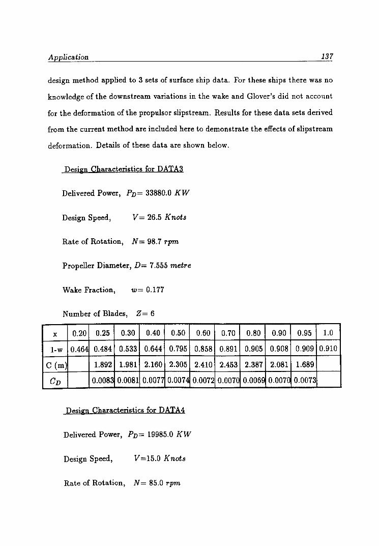
Application 137
design method applied to 3 sets of surface ship data. For these ships there was no
knowledge of the downstream variations in the wake and Glover's did not account
for the deformation of the propulsor slipstream. Results for these data sets derived
from the current method are included here to demonstrate the effects of slipstream
deformation. Details of these data are shown below.
Design Characteristics for DATA3
Delivered Power, PD= 33880.0 KW
Design Speed, V = 26.5 Knots
Rate of Rotation, N= 98.7 rpm
Propeller Diameter, D= 7.555 metre
Wake Fraction, w= 0.177
N umber of Blades, Z = 6
x 0.20 0.25 0.30 0.40 0.50 0.60 0.70 0.80 0.90 0.95 1.0
l-w 0.464 0.484 0.533 0.644 0.795 0.858 0.891 0.905 0.908 0.909 0.910
C (m) 1.892 1.981 2.160 2.305 2.410 2.453 2.387 2.081 1.689
CD 0.008~ 0.0081 0.0077 0.0074 0.0072 0.0070 0.0069 0.007C 0.0073
Design Characteristics for DATA4
Delivered Power, PD= 19985.0 KW
Design Speed, V=15.0 Knots
Rate of Rotation, N = 85.0 rpm

Application 138
Propeller Diameter, D= 8.340 metre
Wake Fraction, W= 0.443
Number of Blades, Z= 4
x 0.20 0.25 0.30 0.40 0.50 0.60 0.70 0.80 0.90 0.95 1.0
1-w 0.308 0.332 0.363 0.435 0.561 0.715 0.792 0.847 0.869 0.874 0.878
C (m) 2.002 2.103 2.285 2.439 2.550 2.596 2.526 2.202 1.787
CD - 0.008~ 0.0085 0.008e 0.0076 0.0074 0.0072 0.0070 0.0071 0.0073 -
Design Characteristics for DATA5
Delivered Power, PD= 28540.0 KW
Design Speed, V =19.6 Knots
Rate of Rotation, N = 105.0 rpm
Propeller Diameter, D= 7.56 metre
Wake Fraction, W= 0.390
Number of Blades, Z= 5
x 0.20 0.25 0.30 0.40 0.50 0.60 0.70 0.80 0.90 0.95 1.0
1-w 0.627 0.595 0.547 0.462 0.400 0.386 0.501 0.657 0.822 0.891 0.947
C (m) 2.342 2.460 2.674 2.853 2.984 3.037 2.955 2.576 2.090
CD 0.0079 0.0077 0.0073 0.0071 0.0069 0.0067 0.0067 0.0067 0.0069
In investigating the performance characteristics of the propeller/stator combi
nation, two parameters were considered to be important and were therefore sys
tematically varied. These parameters were the number of stator blades and the

Application 139
axial distance between the propeller and the stator.
In order to investigate the effect of the number of stator blades, the stator
blade number was varied from 3 to 15 in steps of 3 for all data, except for DATA4
which involved a 4 bladed propeller and for which the number of stator blades was
varied from 4 to 14 in steps of 2. In varying the number of blades, the objective
was to determine the blade number beyond which the gain in performance becomes
practically insignificant.
The axial distance (AXD) between the lifting line of the propeller and the stator
results in changes in the stator diameter and the propeller induced velocities. For
each set of design data the axial spacing was varied from Y/ R=0.2 to 0.8 in steps
of 0.2, where Y/ R is the ratio of axial distance to the propeller radius.
Calculation of the mean velocities induced by the propeller, at the stator and
in the slipstream, is essential for the design of the stator. These calculations were
carried out using Equations 5.42 - 5.44 and results from DATAl & DATA2 are
shown in Figures 7.31 to 7.36 for the axial, tangential and radial components, re
spectively. The axes of these figures are self explanatory and each figure represents
the variations during one revolution of the propeller of the velocities induced on a
stator blade, which in this case was situated a distance Y/ R = 0.5 downstream of
the propeller.
The main objective of the application of propeller/stator propulsors to torpedos
is the cancellation of the unbalanced torque reaction. Design of the stator to cancel
the rotational velocities in the slipstream results in a stator torque which is less
than that of the propeller because of the smaller frictional drag of the stator. This

Application
a a
o If) o l-
S f\ /D\\
I • I •
W I!') ~ :::;: :!. t- 0 C') <D (» N > > 0 v, v, ~ t- t- <D I!') "'" "'" 0> o .-m ~ ~ ~
DOt] I
140
Figure 7.31 - Axial Induced Velocities at Y /R=O.5 for DATAl

Application 141
0 \p.
U\ S\l\~\J'6 N
\
S f\ /"\\\ C') <0 (\J CX) C') CX)
~ 0 LO 0 <0
I ~ ~ ~ C}l C}l CO( CO( u;> u;> <? <? 0 0 0 0
T"""
X 0 0 0 0 0 0 0 0 0 0
W <0 (\J IX) C') IX) ~ 0 lC'l 0 <0 3: > ~ C}l C}l CO( CO( "'1 u;> u;> <? <? 0
0 0 ...J ro W
~ ro
DO I
Figure 7.32 - Tangential Induced Velocities at Y /R=O.5 for DATAl

Application 142
C'J 0 0 "'r ~ "<I" co N ,.... N CD 0 lI) I
0 -;- -;- ~ ~ c:> c:> "'r "'r ,--x
0 0 0
w "'r ~ "<I" co N ,.... N CD 0 lI) ~ > -;- -;- ~ ~ c:> c:> "'r "'r 0 0
...J CD W « CD
DDLJ I I I
Figure 7.33 - Radial Induced Velocities at Y /R=O.5 for DATAl

Application 143
cry 0 0 10 8 10 0 10 0 10 0 10 0
'0 " ~ C') <D C') 0> <D C\I 0> 10 C\I
" " " <D <D 10 10 U") V V V ,.-
, , , , , , , , , w ~8~~ 10 g ~ ~ U") ~ ~ > 0> U")
0 " " <0 <D 10 10 10 v v v 0
-J co w « co
DOG] I I
Figure 7.34 - Axial Induced Velocities at Y /R=O.5 for DATA2
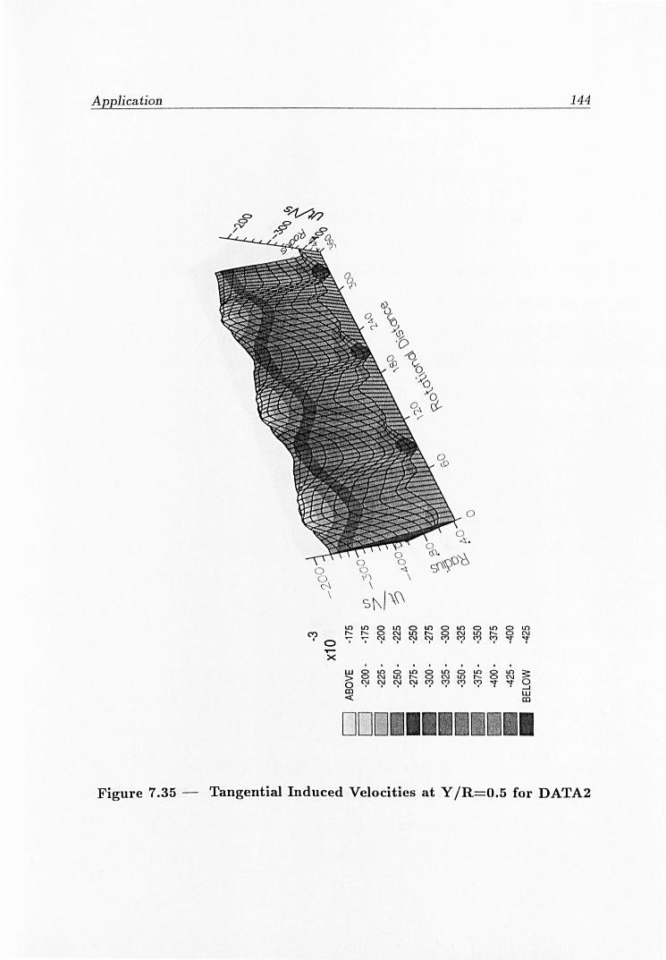
Application 144
0 0 0
I")
C'\ \ \ S\\!\\\
tl) tl) e tl) 0 LO 0 LO 0 to 8 LO
CO( I'- I'- e ~
to I"-~
N ~ ~
N
0 '7 ~ ~ ~ ~ <'? "'f "'f . ...-x .
w 8 to 0 LO 8 to ~ to 8 LO ~ > C\J to l"- N l"- N
0 ~ ~ ~ ~ <'? <'? <'? <'? "'f "'f 0 ....J
CD W « CD
DDD I I I
Figure 7.35 - Tangential Induced Velocities at Y /R=O.5 for DATA2

Application 145
\
s ~1 }\\ (") a a l/) a l/) a l/) a l/) a l/) a '0 Ll( <0
~ r-- ~ ~ ~ ~ ~ ~ ~ ~ ,....... , ,
X
. . . w l/) a l/) a l/)
~ ~ a l/) lil :0; > Ll( ~ <0 N r-- '<T Ol
0 "7 ~ ~ ~ co;> "r "r Ll( 0 . -I III W « III
DOD I I
Figure 7.36 - Radial Induced Velocities at Y /R=O.5 for DATA2
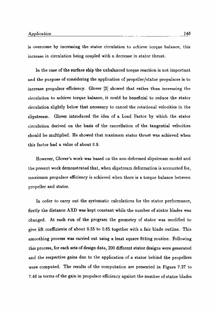
Application 146
is overcome by increasing the stator circulation to achieve torque balance, this
increase in circulation being coupled with a decrease in stator thrust.
In the case of the surface ship the unbalanced torque reaction is not important
and the purpose of considering the application of propeller/stator propulsors is to
increase propulsor efficiency. Glover [3] showed that rather than increasing the
circulation to achieve torque balance, it could be beneficial to reduce the stator
circulation slightly below that necessary to cancel the rotational velocities in the
slipstream. Glover introduced the idea of a Load Factor by which the stator
circulation derived on the basis of the cancellation of the tangential velocities
should be multiplied. He showed that maximum stator thrust was achieved when
this factor had a value of about 0.9.
However, Glover's work was based on the non-deformed slipstream model and
the present work demonstrated that, when slipstream deformation is accounted for,
maximum proPulsor efficiency is achieved when there is a torque balance between
propeller and stator.
In order to carry out the systematic calculations for the stator performance,
firstly the distance AXD was kept constant while the number of stator blades was
changed. At each run of the program the geometry of stator was modified to
give lift coefficients of about 0.55 to 0.65 together with a fair blade outline. This
smoothing process was carried out using a least square fitting routine. Following
this process, for each sets of design data, 200 different stator designs were generated
and the respective gains due to the application of a stator behind the propellers
were computed. The results of the computation are presented in Figure 7.37 to
7.46 in terms of the gain in propulsor efficiency against the number of stator blades

Application 147
for varying AXD.
As can be seen seen from Figure 7.37 to 7.46, the general trend of the results in
such that as the number of stator blades increases the efficiency increases at a high
rate for a practical number of blades (about 9-10) and converges to a maximum
value. Moreover, as AXD increases the gain also increases. This trend is valid for
all the design data except for the lightly loaded case (DATAl) which displayed no
dramatic gain with the varying number of blades. If one compares the effect of the
number of the stator blades on the heavily loaded (i.e. Figures 7.39-40) and lightly
loaded (Figures 7.37-38) cases respectively two distinct trends can be observed: the
first one is such that the gain for the heavily loaded case is much more than for
lightly loaded case. Secondly, in general, the gain decreases as the number of stator
blades increases for the lightly load case while the trend is opposite for the heavily
loaded case. The reason behind the above defined trends can be partly explained
by investigating the following thrust equation of the stator blade element:
According to the above equation the negligible gain in the lightly loaded case
can be attributed to the negative thrust generated by the stator partly due to small
lift relative large drag forces on the stator. In the lightly loaded case the value
of [t:nL,si - CD] becomes less than zero for some blade sections. Therefore these
blade sections produce a negative thrust which results in a decrease in propulsor
efficiency. For the second trend it is difficult to analyse the contribution of each
parameters (i.e. CL, C,/3i, etc.) in above equation. Even if one could investigate
the effect of each parameter, to draw a conclusion for an entire stator would be

Application 148
difficult due to the large number of parameters to be investigated. Therefore it is
author's belief that the second trend is also the direct result of thi s equation.
As mentioned earlier, since the maximum gain is reached with a practical
number of stator blades, there will be no point in further increasing the number of
blades which is also a handicap from the manufacturing point of view (i .e. labour,
material etc.)
0.4
0.2
0 .0
-0 .2
c -0.4 'co (!)
-0 .6
-E9- AXD- O.2 -e- A X D - O.4 --6- AXD- O.6 --t- AXD _ O.O
-0.8-r---r---r---'---'---.---.---.---.---.---.--~r-~ 3 4 5 6 7 8 9 10 11 12 13 1 4 1 5
Number of Stator Blades
Figure 7.37 - Variation of Stator Blades for DATAl
Similarly, as the axial separation was increased the gain also increased at a
high rate for practical value ofAXD and this rate became smaller for the large
AXD values. This also suggested that, from the design point of view, there will be
no point in locating the stator far behind the propeller for high efficiency values.
On the other hand, hased upon the non-deformed slipstream assumption , Glover

Application 149
0.4
-f9- AXD- O.2
0 .2 -e- A XD_O.4 -.!!!.- AXD- O.G --t- AXD- O.B
-0 .6
-0.8-r---.--_,r_--r_--._--_r---.--~r_--r_--._--_r--_.--~
3 4 5 6 7 8 9 10 11 12 13 14 15
Number of Stator Blades
Figure 7.38 - Gain after Balancing the Torque for DATAl
8
6
~ ~
4 >-<..)
C CD 0(3
2 :E UJ -€3- AXD_ O.2 £ -e- AXD. O.4 c 0 -.!r- AXD_ O.G ·co
CD --t- AXD- O.B
-2
-4 -r--_.----r_--.---,_---r---,----r---~--,_--~--_,r___,
3 4 5 6 7 8 9 10 11 12 13 14 15
Number of Stator Blades
Figure 7.39 - Variation of Stator Blades for DATA2

A pplication 150
--e:r- AXD_ O.2 -E9-- AXD_ O.4
--..!!r- A XD- O.6 --t- AXD_ O.B
3 4 5 6 7 8 9 10 11 12 1 3 14 1 5
Number of Stator Bla d es
Figure 7.40 - Gain after Balancing the Torque for DATA2
6
5
~ e...... 4
>-C,,)
c: 3 Q) ' (3
:E UJ 2 ,~ c
'~
(.!) --e:r- A XD_ O.2
-e- AXD- O.4 -.<!!o.- A XD_ O.6
0 --t- A XD- O.8
-1
3 4 5 6 7 8 9 10 11 1 2 1 3 14 1 5
Number of Stator Bla d es
Figure 7.41 - Variation of Stator Blad es for DATA3

Application 151
6
5
~ ~
4
>-c..> c::: 3 Q)
-(3
:E W 2 -~ c::: -~ C) -€9- A XD- O.2
-e- A XD- O.4 -6- A XD- O.B
0 -+-- A XD- O.B
- 1
3 4 5 6 7 8 9 10 11 12 13 14 1 5
Number of Stator Blades
Figure 7.42 - Gain after Balancing the Torque for DATA3
6
-€9- A XD. O.2 -e- A XD_ O.4 -6- A XD- O.6 -+-- A XD_ O.B
O~----~---'-----r----'---~-----r----.---~-----r---.
4 5 6 7 8 9 10 11 1 2 13 14
Number of Stator Blades
Figure 7.43 - Variation of Stator Blades for DATA4
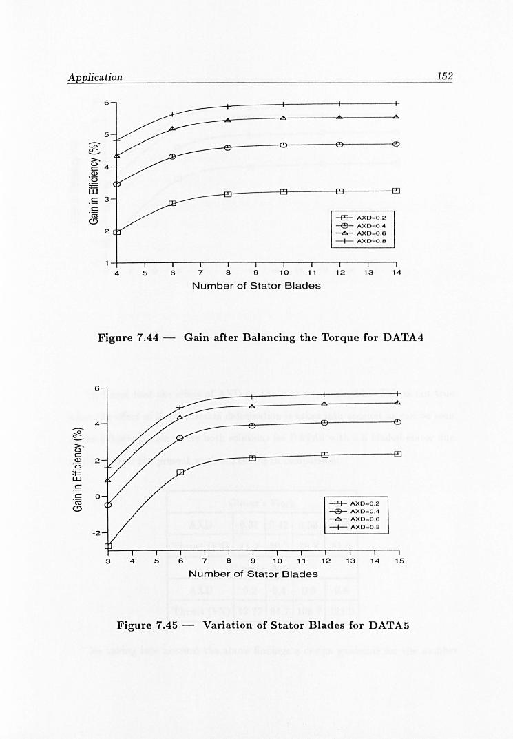
Application
6
-f9- AXD_ O.2
--6- AXD-D .4 ---.!!.- AXD_O.6 -+-- A XD- O.O
1~----~---.-----r----r----.----.-----r----.----.----.
4 5 6 7 8 9 10 11 12 13 14
Number of Stator Blades
Figure 7.44 - Gain after Balancing the Torque for DATA4
>-. <..> c
6
4
CD 2 0(3
:E UJ c c 0 0ctj
<D
-2
3 4 5
-f9- AXD- O.2 --6- AXD_ OA ---.!!.- AXD - O.6 -+-- AXD. O.O
6 7 8 9 10 11 12 13
Number of Stator Blades
14 1 5
Figure 7.45 - Variation of Stator Blades for DATA5
152

Application
c c
.ct:j
6
5
CD 0
- 1
3 4 5 6
__ --~r_------~9---------0
-£9- A X D _ O.2
-e- A XD- O.4 -6- A X D - O.6 -f- A XD_ O.B
7 8 9 10 11 1 2 13 14 1 5
Number of Stator Blade s
Figure 7.46 - Gain after Balancing the Torque for DATA5
153
[3] found that the effect ofAXD on the gain was negligible. Thi s is not t.rue
when the effect of the slipstream deformation is t aken into account as can be seen
in the following table where both solutions for DATA3 with a 6 bladed stator due
to Glover and the present work are shown in comparison:
Glover's Work
AXD 0.31 0.42 0.53 0.66
Thrust (kN) 81.2 80.7 79.8 81.4
Present Work
AXD 0.2 0.4 0.6 0.8
Thrust (kN) 43.77 84.7 108.7 121.9
By taking into account the above findings a design guideline for the number
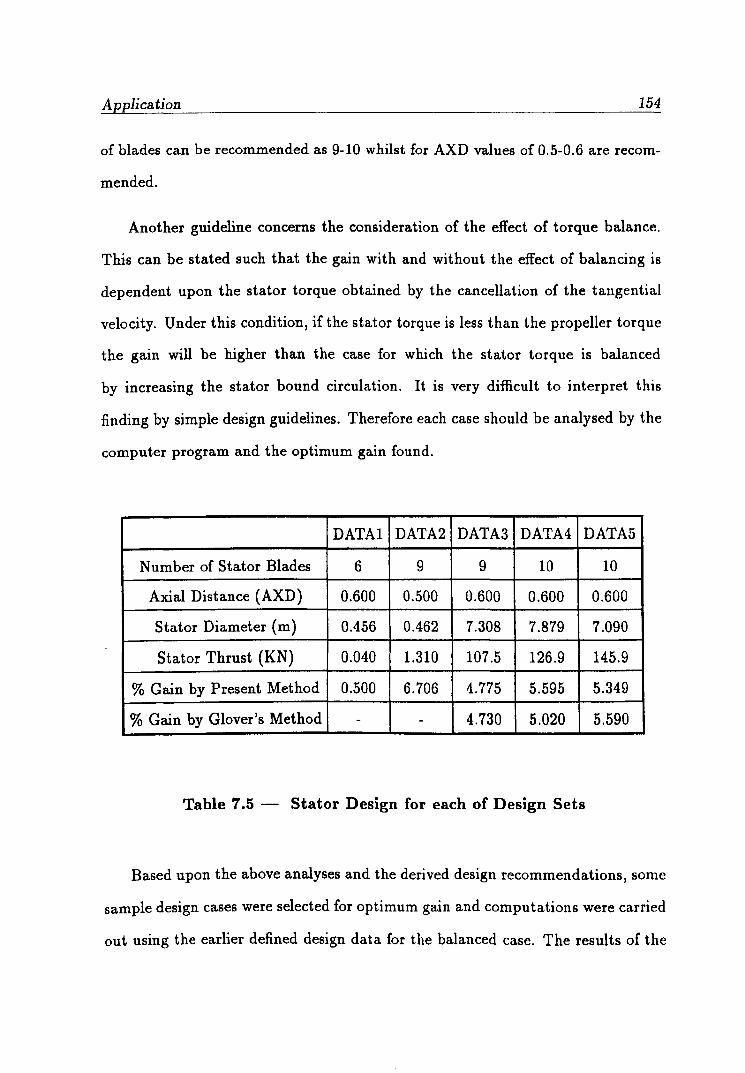
Application 154
of blades can be recommended as 9-10 whilst for AXD values of 0.5-0.6 are recom
mended.
Another guideline concerns the consideration of the effect of torque balance.
This can be stated such that the gain with and without the effect of balancing is
dependent upon the stator torque obtained by the cancellation of the tangential
velocity. Under this condition, if the stator torque is less than the propeller torque
the gain will be higher than the case for which the stator torque is balanced
by increasing the stator bound circulation. It is very difficult to interpret this
finding by simple design guidelines. Therefore each case should be analysed by the
computer program and the optimum gain found.
DATAl DATA2 DATA3 DATA4 DATA5
Number of Stator Blades 6 9 9 10 10
Axial Distance (AXD) 0.600 0.500 0.600 0.600 0.600
Stator Diameter (m) 0.456 0.462 7.308 7.879 7.090
Stator Thrust (KN) 0.040 1.310 107.5 126.9 145.9
% Gain by Present Method 0.500 6.706 4.775 5.595 5.349
% Gain by Glover's Method - - 4.730 5.020 5.590
Table 7.5 - Stator Design for each of Design Sets
Based upon the above analyses and the derived design recommendations, some
sample design cases were selected for optimum gain and computations were carried
out using the earlier defined design data for the balanced case. The results of the

Application 155
computations are presented in Table 7.5 in comparison with the Glover data [3].
The full details of the computation for the propellers and stators are included in
Appendix D for further information.

Chapter VIII
General Conclusion
One of the most significant advances in propeller design has been the great
increase in the use of computer. As computer technology has advanced, the com
putational procedures for propeller design have been improved to take advantage
of this new technology. The simple Momentum Theory has evolved into today's
Lifting Surface Theory.
During the evolution of the design procedures between the above mentioned
two extremes, the lifting line design procedure has occupied the screw propeller
designers more than any other method. Therefore today lifting line methods still
have the most respected place amongst the others. This is not only because they are
modest in terms ofthe computational demands, but also they have the advantage of
being widely used and well established procedure due to their long service history.
From the above point of view, it could be well justified to seek for the fur
ther improvements in the present lifting line procedures. Indeed if one investigates
the earlier lifting line models, it is found that a number of simplifying. assump
tions were necessary in order to derive a solution with the available computational
tools. One of these assumptions is that the propeller is moderately loaded and
that the downstream variation in induced velocities and the resulting slipstream
deformation can be neglected. Later development of the lifting line methods has
tackled the slipstream deformation by taking into account the self induced veloci-

General Conclusion 157
ties. But none of these methods included the effect of the local inflow velocities in
the slipstream which would contribute to the deformation of the slipstream.
Therefore it was thought that the objective of this thesis should be the further
improvement of the lifting line procedure with an emphasis on more realistic rep
resentation of the slipstream deformation. As this deformation is one of the key
parameters in the design of the performance improvement devices, the secondary
objective of the thesis has been set to design a stator behind the propeller and
analyse the performance characteristics of the combined propulsor system.
In order to justify the above objectives, in the first chapter of the thesis an
introductory section has been included and objectives and the layout of the thesis
also presented. The second chapter of the thesis involved the review of the three
key issues involved in the propeller design as well as in the objectives of the thesis.
These issues were the propeller design procedures, propeller/stator combination
and flow around the body and propeller. Based upon this review work, in the third
chapter of the thesis, the flow prediction around a slender body was presented by
using a "Three-dimensional Panel Technique" for the potential flow and the "Thin
Shear Layer Equations" for viscous flow. This provided the necessary wake data to
develop the propeller design theory. In the fourth chapter, a description was given
of the basic theory which led to the development of the Classical Lifting Line theory
which assumes a regular helical slipstream downstream of the propeller. The fifth
chapter described the development of the Advanced Lifting Line method in which
the deformed nature of the trailing vortex system was determined using the "Free
Slipstream Analysis Method".
In this method the slipstream geometry was allowed to deform and to align

General Conclusion 158
with the local velocity field which comprised the inflow velocities and the velocities
induced by the trailing vortices. In the sixth chapter this design procedure was
combined with that of a stator device placed behind the propeller. Therefore the
necessary formulation for the induced velocities of the stator was presented. The
seventh chapter involved the illustration of the numerical application of the design
procedure and discussion of the results deducted from this application for different
loading cases. Finally in the present chapter, overall conclusions drawn from the
work are discussed and recommendations for future work are given.
During the computational implementation of the above methodology a set of
computer programs was used. Some of them were developed by the author and
some were modified or enhanced versions of software available in the department.
Tht- software can be classified into three major groupSj flow calculation, propeller
design and stator design software. The first group of software was available in the
department and was further enhanced .for the present use, the rest of software was
developed by the author during the course of the work.
Based upon the work carried out in this thesis the following overall conclusions
can be drawn:
• In spite of the advances in numerical methods and computers, the lifting line
based propeller design procedures still play an important role in propeller design
methodology and there is still room to further improve these procedures.
• One of the simplifying assumptions of the conventional lifting line method is
that the propeller is moderately loaded and that the resulting slipstream shape
is regular. This may not be true, particularly, for the heavily loaded propeller

General Conclusion 159
due to the effect of the inflow velocities and the induced velocities of the trailing
vortices on themselves which would result in a contracted slipstream tube and
a downstream increase in vortex pitch.
• Rational design of the stator device requires accurate information on the slip
stream geometry for determining the stator diameter. This can be provided by
the improved procedure presented in this thesis.
• In determining the slipstream shape geometry an iterative solution was im
plemented such that the bound circulation obtained from first iteration of the
lifting line solution remained constant and the form of the trailing vortex lines
was modified corresponding to the local inflow velocities and the induced ve
locities due to trailing vortex system. This procedure was employed until a
balanced slipstream shape was obtained. In this iterative process it was found
that the slipstream form was stabilised well within a distance of 3.5R down
stream of the propeller.
• The analysis of the slipstream deformation indicated that the rate of contrac
tion was very high in the above specified region and the contribution due to
the local inflow velocities played a significant role in this contraction.
• As a result of more realistic slipstream shape, the hydrodynamic pitch angle
({3i) increased very rapidly downstream of the propeller and the hydrodynamic
pitch angle on the lifting line were found to be smaller than those obtained by
the regular helical slipstream model (i.e. conventional lifting line model) for
heavily loaded propeller.
• Effort put in to this thesis for the improvement of the actual slipstream repre-

General Conclusion 160
sentation indicated that the classical lifting line methods would underestimate
the propeller efficiency for the heavily loaded propeller about 4% whilst for the
lightly loaded propeller the use of the regular slipstream assumption can be
justified.
• The improved design methodology presented in this thesis would provide more
sound design for the performance improvement devices, e.g stator, contraro
tating propellers, Grim vane wheels etc, due to more realistic representation of
the slipstream details.
• The performance analysis of the propeller combined with the stator located
behind the propeller indicated that the undesirable effect of the propeller torque
can be avoided by the use ofthe stator. This is an important design requirement
for the directional stability of the high speed submerged bodies like submarines,
torpedos, Autonomous Underwater Vehicles (AUV's).
• It is a known fact that the number of the blades is one of the important pa
rameters in the design of the stator devices. The parametric analysis of the
number of blades of the stator indicated as the number of blade increased,
the efficiency increased at a high rate over a practical number of blades and
converges to a maximum value. Therefore there will be no point in further
increasing the number of blades beyond certain number which will increase the
manufacturing costs.
• Another important design parameter of the stator device was its longitudinal
separation from the propeller. The systematic investigation of this design pa
rameter indicated that the gain would increase at high rate for practical values

General Oonclusion 161
of this separation whilst it would be negligible beyond a certain range.
• By taking into account the above two findings, a design guideline for the number
of blades was recommended as 9-10 whilst for the stator separation a value of
0.5 or 0.6R was recommended.
• The gain obtained by the application of the stator device was dependent upon
the load case and the torque balance of the propeller. In general the maximum
gain which was about 6.5% was obtained for the heavily loaded case.
• It was found that the absolute torque balance and the maximum gain cannot
be achieved simultaneously. Therefore the stator designer should make a design
decision depending upon his design objectives or should search for a compromise
design solution by using the stator design software.
The majority of the above conclusions were drawn from the computation car
ried out by using the earlier mentioned design software developed during this re
search work. The theoretical procedure and the associated software for the flow
prediction neglects the effect of the free surface. Therefore, the implemented soft
ware for the flow prediction can cater only for the wake values of deeply submerged
bodies. However overall design software is general and also applicable to surface
ships provided that the wake data are available.
• Within the above limitations it is believed that the procedure and the associated
software provided in this thesis would provide the designers with the capability
for more sound propeller and stator design in particular for submerged ships
like submarines, torpedos and AUV's.
Apart from the immediate application to the naval submerged bodies {i.e. tor-
General Conclusion 162
pedo, submarines), today one of the major applications of the present work could
be to AUV's which have considerable promise as a major tool for gathering scien
tific data in the deep ocean. Their use in combination with more efficient remote
sensing techniques for the determination of sea floor characteristics and local water
column properties has been a major attraction for the underwater technologists.
The accuracy of the sensor performance and maintenance of the intended trajecto
ries is very much dependent on the superior motion performance of the vehicle, in
particular its stability. Moreover, they require efficient propulsion systems due to
long data gathering time spent under water with limited fuel/battery space in their
bodies. Within this context, the existing design tool would be very appropriate as
it could be used for balancing the torque as well as improving propulsive efficiency.
Another potential application area for the present design tool would be the
Small Water Area Twin Hull (SWATH) ships. These vessels have slender sub
merged hulls which are ideal for the application of the performance improvement
devices. They suffer from higher frictional drag due to a large wetted surface area
and they are payload limited due to large structural weight. Therefore energy effi
cient systems like propeller/stator combination would be very much appropriate.
• However the improvement gained by the present procedure will be offset by the
increase in the computer time, the ratio of the CPU of the present propeller
design method in comparison with that of the classical lifting line method
is about 30. This is not expected to be a major problem considering the
enormous power of existing computers. In fact this has been the major source
of encouragement for the recommendation to improve the present procedure by
using the "Lifting Surface Method" as a natural extension of the Lifting Line

General Conclusion 163
Methods.
• It should be borne in mind that throughout this work no consideration has be
given to cavitation and noise. Generally, due to its low speed, there should
be no danger of cavitation occurring on the stator blades but the influence of
propeller cavitation on the stator performance may need to be considered.
• The flow prediction module of the existing design software neglects the effect
of the free surface. As a result the present software has restricted application
to surface ships if the wake data is not available. Therefore it is recommended
to combine this effect in the present wake prediction software by using state of
the art methods.
• Because of the novelty of the system there is not much detailed data on the
performance characteristics of the stators. Therefore it would be useful to
perform model propeller testing to verify and validate the present design tool.

References
1. Glover, E.J. " Slipstream Deformation and its Influence on Marine propeller
Design", Ph.D. Thesis, University of Newcastle upon Tyne, 1970
2. Glover, E.J. " A Design Method For the Heavily Loaded Marine Propellers",
Trans.RINA, Vol.116, pp.111, 124, 1973
3. Glover, E.J. " Roto!" jStator Propulsors - Parametric Studies, " Hydronav'91,
Gdansk, 1991
4. Glover, E.J. " Free Slipstream Analysis of Propeller Slipstream Deformation, "
International Symposium on Hydro and Aerodynamics in Marine En9ineering,
HADMAR'91, Volume.1, 28 October-1 November, Varna Bulgaria, 1991
5. Koumbis, A. " An Improved Mathematical Model of The Action of Open
Propellers and Ducted Thrusters," PhD Thesis, University of Newcastle upon
Tyne, 1981
6. Koumbis, A. " On the Effect of the Slipstream on the Representation of Open
Propellers", Trans-RINA, 1983
7. Strscheletzky, M. " Hydrodynamische Grundlagen zur Berechnung der Schiff
schrauben ", G. Braun, Karlsruhe, 1950

References 165
8. Burrill, L.C. " Calculation of Marine Propeller Performance Characteristics, "
Trans. N.E.C.l.E.S. Vol. 60, 1949-44
9. Burrill, L.C. "The Optimum Diameter of Marine Propellers," Trans. N.E.C.I.E.S.
Vol. 72, 1955-56
10. Ryan P.G. and Glover, E.J. " A Ducted Propeller Design Method: A new
Approach Using Surface Vorticity Distribution Techniques and Lifting Line
Theory", Trans-RINA 1972, pp.545,569
11. Rankine, W.J.M. " On the Mechanical Principles of the Action of Propellers",
Trans. l.N.A., Vol. 6, 1865
12. Froude, R.E. " On the Part Played in the Operation of Propulsion by Differ
ences in Fluid Pressure", Trans. I.N.A., Vol. 90, 1889
13. Lanchester, F.W. " Aerodynamics" Constable & Co., London, 1907
14. Prandtl, L. and Betz, A. " Vier Abhandlungen zur Hydro-und Aerodynamik",
Gottingen, 1927
15. Eckhart, M.K. and Morgan W.B., " A Propeller Design Method" Trans.
SNAME, Vol. 69, 1955
16. Lerbs, H.W," Moderately Loaded Propellers with a Finite Numbers of Blades
and an Arbitrary Distribution of Circulation", Trans SNAME, vol.60, 1952
17. Hess, J.L. and Smith, A.M.O. "Calculation of Non-Lifting Potential Flow
about Arbitrary Three-Dimensional Bodies," Douglas Aircraft Company Inc,
Report No:ES40622 , 1962

References
18. Smith, A. M. 0 and Pierce, J. " Exact Solution of the Neumann Problem,
Calculation of Non-Circulatory Plane and Axially Symmetric Flow About or
Within Arbitrary Boundaries," Douglas Aircraft Co. Report ES-269881 1958
19. Hess, J.L. and Smith, A.M.O. "Calculation of Potential Flow about Arbitrary
Bodies ," Pergamen Press Series l Progress in Aeronautical Science I Vol. 81
1966
20. Hess, J.L. and Smith, A.M.O. "Calculation of Potential Flow about Arbi
trary Three-Dimensional Lifting Bodies," Douglas Aircraft Company Inc , Re
port No:MDC J5679-011 Oct.1972
21. Hess, J.L. " Status of a Higher-Order Panel method for Non-Lifting Three Di
mensional Potential Flow," Douglas Aircraft Company Inc , Report No:NACS-
76118-301 1977
22. Kerwin, J.E., Coney, W.B. and Hsin, C.Y. " Hydrodynamic Aspects of Pro
peller/Stator Design", Propeller'88 Symposium) Virginia, Paper No.31 1.988
23. Patience, G. " Developments in Marine Propellers," Stone Manganese Marine
Limited, Technical Paper No.221 January 1991
24. Van Gent W. and Van Oossanen P. " Influence of Wake on Propeller Loading
and Cavitation", [SPI p.279-3211 1973
25. Van Manen, J. D. et al. "The Design of Wake~adapted Screws and Their
Behaviour Behind the Ship'" [SP ) Vol. 2 No:7) 1955.
26. Cummings, D.E. " The Effect of Propeller Wake Deformation on Propeller
Design", ISP, July, 1976
References 167
27. Greeley, D. C. and Kerwin J. E. "Numerical Methods For Propeller Design
and Analysis in Steady-Flow" Trans SNAME ,Vol.90, 1982, p.415-459
28. Hoshino, T. " A Surface Panel Methods with a Deformed Wake Model to An
alyze Hydrodynamic Characteristics of Propellers in Steady Flow," MTB195,
April, 1991
29. Mautner, T.S., Nelson, D.M. and Gillcrist, M.C. " Investigation of the SISUP
(Swirl Including Stator Upstream of Propeller) Concept for Marine Propul
sion", SNAME, Propellers'88 Symposium, Paper No.2, Virginia,1988
30. Hughes, J. M. and Kinnas, S.A " A analysis Method for a ducted Propeller
with Pre-Swirl Stator Blades", SNAME, Propellers/Shafting '91 Symposium,
Virginia, 1991
31. Gaafary, M.M. and Mosaad, M.A. " Pre-Swirl Stator and Propeller/Stator
Efficiency", SN AME Propellers/Shafting '91 symposium, Virginia, USA, 1991
32. Coney, W.B. " Optimum Circulation Distributions for a Class of Marine
Propulsors ," Journal of Ship Research, Vol.36 No.3, 1992
33. Ikehata M and Chanda S. " Theoretical Calculation of Propulsive Perfor
mances of Stator-Propeller in Uniform Flow by Vortex Lattice Method", Jour
nalof The Society of Naval Architects of Japan, Vol. 166, 1989
34. Chen, B.Y.H. " Postswirl Propulsors - A Design Method and an Application ,"
International Symposium on Propulsors and Cavitation, Hamburg, Germany,
June, 1992
35. Brard, R. " The Representation of a Given Ship Form by Singularity Distribu-

~R~e~k~r~en~ce=s~ ________________________________________________ --=168
tions when the Boundary Condition on the Free Surface is Linearised," Journal
of Ship Research, Vol. 16, 1972
36. Webster, W. C. "The Flow about Arbitrary Three-Dimensional Smooth Bod
ies," Journal of Ship Research, Vol. 19, No.4, Dec. 1975, pp. 206-218.
37. Gomez, G.P., Linares, F.G and Briones LB. " Some Improvements of Tradi
tional Lifting Line Theory For Ship Propellers", [SP, 1989, pp.154,175
38. Froude, W. " On the Elementary Relation between Pitch, Slip and Propulsive
Efficiency", Trans. I.N.A., Vol. 19, 1878
39. Cebeci, T. and Bradshaw, P. "Momentum Transfer in Boundary layers," Me Graw
Hill Book Co.,lne.,New York, 1977
40. Caracostas N. " Off-Design Performance Analysis of Ducted Propellers", SNAME
Propellers'78, Vir:ginia, paper:9, pp.3.1-3.18
41. Dyne, G. "A Method for the Design of Ducted Propellers in a Uniform Flow,"
Publication of the Swedish State Shipbuilding Experimental Tank, No. 62, 1967.
42. McCormick, B. M., Eisenhuth J. J. and Lynn, J. E. " A Study of Torpedo
Propellers -Part I ," Ordnance Research Lab., Pennsylvania State Univ., Rept.
No: 16597-5 , March 1956.
43. Huang, T. T., Wang, H. T., Santelli, W. and Groves, N. C "Propeller/Stern/Boundary
Layer Interaction on Axisymmetric Bodies: Theory and Experiment," DTNSRDC
Report 76-0119, David W. Taylor Naval Ship Research and Development Cen-
tre J Bethasda, Md., 1976.

References
44. Koronowicz, T. " A Theoretical Model of the Propeller and its Slipstream
taking into account the deformation of the Free vortex System," Proceedings of
the symposium on Advances in Propeller Research and Design, Gdansk, 1981
45. Loukakis, T.A. " On the Design of Highly Skewed Propellers, " Proceedings of
the symposium on Advances in Propeller Research and Design, Gdansk, 1981
46. Gibson, 1.S and Lewis, R.I " Ducted Propeller Analysis by Surface Vorticity
and Actuator Disc theory," Symposium on Ducted Propellers, RINA, 197!i
47. Glover, E.J. "Lifting Surface Analysis of High Speed Propeller Performance,"
Symposium on High Speed Marine Vehicles, Naples Castel del'Ovo, Italy, 14-15
February 1991, Italy
48. Loukakis, T.A. " A New Theory for the Wake of Marine Prop.'!llers," Ph.D
Thesis, M.I. T. Report No. 71-1 May 1971
49. Anderson, P. " Lifting Line Theory and Calculation For supercavitating Pro
pellers", ISP, 1976
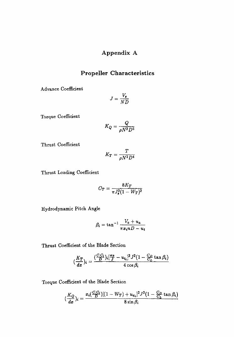
Appendix A
Propeller Characteristics
Advance Coefficient
Torque Coefficient
Thrust Coefficient
J= V, ND
K - Q Q - pN2D5
Thrust Loading Coefficient
CT = 8KT 7rJ](l - WT)2
Hydrodynamic Pitch Angle
{3 t -1 Va + U a
i = an 7rxinD - Ut
Thrust Coefficient of the Blade Section
Torque Coefficient of the Blade Section
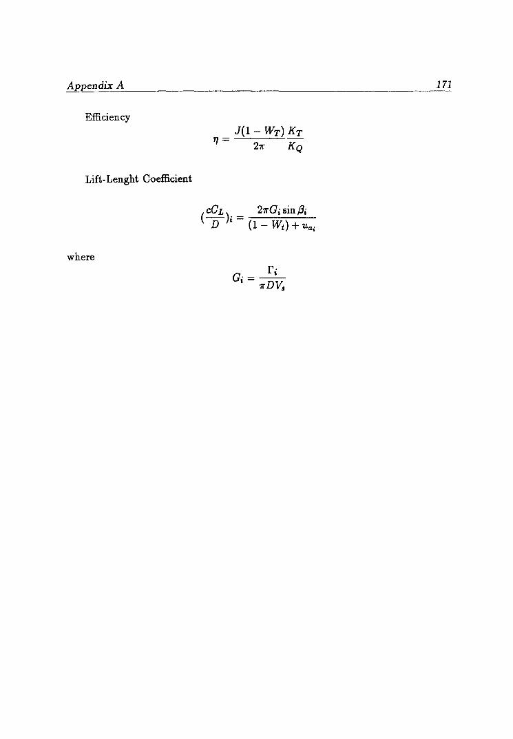
Appendix A
Efficiency
Lift-Lenght Coefficient
where r· G. - __ I-
I - 7rDV,
171

Appendix B
Body Input Points
Body Input Points Coordinates x(m) y(m) z(m) x(m) y{m) z{m)
0.00000 0.000000 0.053300 0.00000 0.009255 0.052490 0.00000 0.018230 0.050086 0.00000 0.026650 0.046159 0.00000 0.034261 0.040830 0.00000 0.040830 0.034261 0.00000 0.046159 0.026650 0.00000 0.050086 0.018230 0.00000 0.052490 0.009255 0.00000 0.053300 0.000000 0.00000 0.000000 0.106600 0.00000 0.018511 0.104980 0.00000 0.036459 0.100171 0.00000 0.053300 0.092318 0.00000 0.068521 0.081660 0.00000 0.081660 0.068521 0.00000 0.092318 0.053300 0.00000 0.100171 0.036459 0.00000 0.104980 0.018511 0.00000 0.106600 0.000000 0.00000 0.000000 0.159900 0.00000 0.027766 0.157471 0.00000 0.054689 0.150257 0.00000 0.079950 0.138477 0.00000 0.102782 0.122490 0.00000 0.122490 0.102782 0.00000 0.138477 0.079950 0.00000 0.150257 0.054689 0.00000 0.157471 0.027766 0.00000 0.159900 0.000000 0.00000 0.000000 0.213200 0.00000 0.037022 0.209961 0.00000 0.072919 0.200342 0.00000 0.106600 0.184637 0.00000 0.137042 0.163321 0.00000 0.163321 0.137042 0.00000 0.184637 0.106600 0.00000 0.200342 0.072919 0.00000 0.209961 0.037022 0.00000 0.213200 0.000000 0.00500 0.000000 0.266500 0.00500 0.046277 0.262451 0.00500 0.091148 0.250428 0.00500 0.133250 0.230796 0.00500 0.171303 0.204151 0.00500 0.204151 0.171303 0.00500 0.230796 0.133250 0.00500 0.250428 0.091148 0.00500 0.262451 0.046277 0.00500 0.266500 0.000000 0.42500 0.000000 0.266500 0.42500 0.046277 0.262451 0.42500 0.091148 0.250428 0.42500 0.133250 0.230796 0.42500 0.171303 0.204151 0.42500 0.204151 0.171303 0.42500 0.230796 0.133250 0.42500 0.250428 0.091148 0.42500 0.262451 0.046277 0.42500 0.266500 0.000000 0.85000 0.000000 0.266500 0.85000 0.046277 0.262451 0.85000 0.091148 0.250428 0.85000 0.133250 0.230796 0.85000 0.171303 0.204151 0.85000 0.204151 0.171303 0.85000 0.230796 0.133250 0.85000 0.250428 0.091148 0.85000 0.262451 0.046277 0.85000 0.266500 0.000000 1.27500 0.000000 0.266500 1.27500 0.046277 0.262451 1.27500 0.091148 0.250428 1.27500 0.133250 0.230796 1.27500 0.171303 0.204151 1.27500 0.204151 0.171303 1.27500 0.230796 0.133250 1.27500 0.250428 0.091148 1.27500 0.262451 0.046277 1.27500 0.266500 0.000000 1.70000 0.000000 0.266500 1.70000 0.046277 0.262451
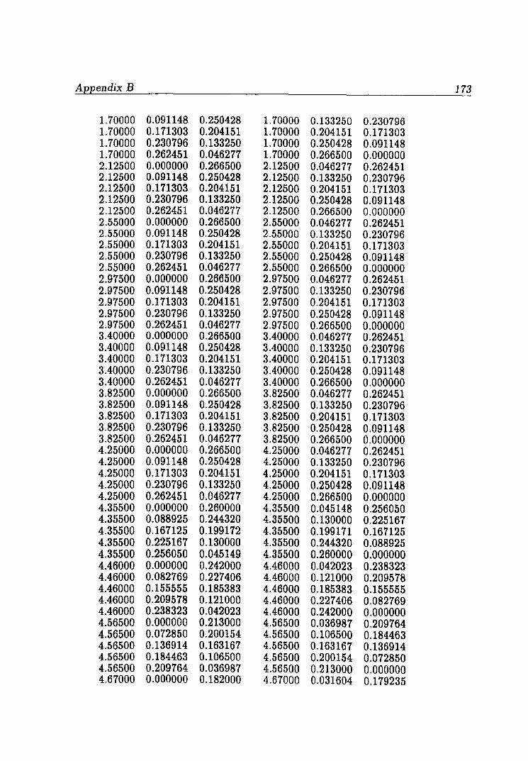
Appendix B 173
1.70000 0.091148 0.250428 1.70000 0.133250 0.230796 1.70000 0.171303 0.204151 1.70000 0.204151 0.171303 1.70000 0.230796 0.133250 1.70000 0.250428 0.091148 1.70000 0.262451 0.046277 1.70000 0.266500 0.000000 2.12500 0.000000 0.266500 2.12500 0.046277 0.262451 2.12500 0.091148 0.250428 2.12500 0.133250 0.230796 2.12500 0.171303 0.204151 2.12500 0.204151 0.171303 2.12500 0.230796 0.133250 2.12500 0.250428 0.091148 2.12500 0.262451 0.046277 2.12500 0.266500 0.000000 2.55000 0.000000 0.266500 2.55000 0.046277 0.262451 2.55000 0.091148 0.250428 2.55000 0.133250 0.230796 2.55000 0.171303 0.204151 2.55000 0.204151 0.171303 2.55000 0.230796 0.133250 2.55000 0.250428 0.091148 2.55000 0.262451 0.046277 2.55000 0.266500 0.000000 2.97500 0.000000 0.266500 2.97500 0.046277 0.262451 2.97500 0.091148 0.250428 2.97500 0.133250 0.230796 2.97500 0.171303 0.204151 2.97500 0.204151 0.171303 2.97500 0.230796 0.133250 2.97500 0.250428 0.091148 2.97500 0.262451 0.046277 2.97500 0.266500 0.000000 3.40000 0.000000 0.266500 3.40000 0.046277 0.262451 3.40000 0.091148 0.250428 3.40000 0.133250 0.230796 3.40000 0.171303 0.204151 3.40000 0.204151 0.171303 3.40000 0.230796 0.133250 3.40000 0.250428 0.091148 3.40000 0.262451 0.046277 3.40000 0.266500 0.000000 3.82500 0.000000 0.266500 3.82500 0.046277 0.262451 3.82500 0.091148 0.250428 3.82500 0.133250 0.230796 3.82500 0.171303 0.204151 3.82500 0.204151 0.171303 3.82500 0.230796 0.133250 3.82500 0.250428 0.091148 3.82500 0.262451 0.046277 3.82500 0.266500 0.000000 4.25000 0.000000 0.266500 4.25000 0.046277 0.262451 4.25000 0.091148 0.250428 4.25000 0.133250 0.230796 4.25000 0.171303 0.204151 4.25000 0.204151 0.171303 4.25000 0.230796 0.133250 4.25000 0.250428 0.091148 4.25000 0.262451 0.046277 4.25000 0.266500 0.000000 4.35500 0.000000 0.260000 4.35500 0.045148 0.256050 4.35500 0.088925 0.244320 4.35500 0.130000 0.225167 4.35500 0.167125 0.199172 4.35500 0.199171 0.167125 4.35500 0.225167 0.130000 4.35500 0.244320 0.088925 4.35500 0.256050 0.045149 4.35500 0.260000 0.000000 4.46000 0.000000 0.242000 4.46000 0.042023 0.238323 4.46000 0.082769 0.227406 4.46000 0.121000 0.209578 4.46000 0.155555 0.185383 4.46000 0.185383 0.155555 4.46000 0.209578 0.121000 4.46000 0.227406 0.082769 4.46000 0.238323 0.042023 4.46000 0.242000 0.000000 4.56500 0.000000 0.213000 4.56500 0.036987 0.209764 4.56500 0.072850 0.200154 4.56500 0.106500 0.184463 4.56500 0.136914 0.163167 4.56500 0.163167 0.136914 4.56500 0.184463 0.106500 4.56500 0.200154 0.072850 4.56500 0.209764 0.036987 4.56500 0.213000 0.000000 4.67000 0.000000 0.182000 4.67000 0.031604 0.179235
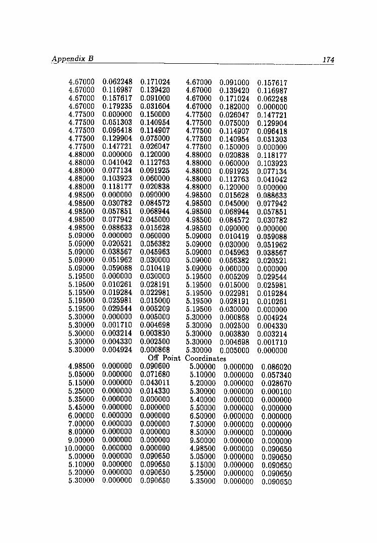
Appendix B 174
4.67000 0.062248 0.171024 4.67000 0.091000 0.157617 4.67000 0.116987 0.139420 4.67000 0.139420 0.116987 4.67000 0.157617 0.091000 4.67000 0.171024 0.062248 4.67000 0.179235 0.031604 4.67000 0.182000 0.000000 4.77500 0.000000 0.150000 4.77500 0.026047 0.147721 4.77500 0.051303 0.140954 4.77500 0.075000 0.129904 4.77500 0.096418 0.114907 4.77500 0.114907 0.096418 4.77500 0.129904 0.075000 4.77500 0.140954 0.051303 4.77500 0.147721 0.026047 4.77500 0.150000 0.000000 4.88000 0.000000 0.120000 4.88000 0.020838 0.118177 4.88000 0.041042 0.112763 4.88000 0.060000 0.103923 4.88000 0.077134 0.091925 4.88000 0.091925 0.077134 4.88000 0.103923 0.060000 4.88000 0.112763 0.041042 4.88000 0.118177 0.020838 4.88000 0.120000 0.000000 4.98500 0.000000 0.090000 4.98500 0.015628 0.088633 4.98500 0.030782 0.084572 4.98500 0.045000 0.077942 4.98500 0.057851 0.068944 4.98500 0.068944 0.057851 4.98500 0.077942 0.045000 4.98500 0.084572 0.030782 4.98500 0.088633 0.015628 4.98500 0.090000 0.000000 5.09000 0.000000 0.060000 5.09000 0.010419 0.059088 5.09000 0.020521 0.056382 5.09000 0.030000 0.051962 5.09000 0.038567 0.045963 5.09000 0.045963 0.038567 5.09000 0.051962 0.030000 5.09000 0.056382 0.020521 5.09000 0.059088 0.010419 5.09000 0.060000 0.000000 5.19500 0.000000 0.030000 5.19500 0.005209 0.029544 5.19500 0.010261 0.028191 5.19500 0.015000 0.025981 5.19500 0.019284 0.022981 5.19500 0.022981 0.019284 5.19500 0.025981 0.015000 5.19500 0.028191 0.010261 5.19500 0.029544 0.005209 5.19500 0.030000 0.000000 5.30000 0.000000 0.005000 5.30000 0.000868 0.004924 5.30000 0.001710 0.004698 5.30000 0.002500 0.004330 5.30000 0.003214 0.003830 5.30000 0.003830 0.003214 5.30000 0.004330 0.002500 5.30000 0.004698 0.001710 5.30000 0.004924 0.000868 5.30000 0.005000 0.000000
Off Point Coordinates 4.98500 0.000000 0.090600 5.00000 0.000000 0.086020 5.05000 0.000000 0.071680 5.10000 0.000000 0.057340 5.15000 0.000000 0.043011 5.20000 0.000000 0.028670 5.25000 0.000000 0.014330 5.30000 0.000000 0.000100 5.35000 0.000000 0.000000 5.40000 0.000000 0.000000 5.45000 0.000000 0.000000 5.50000 0.000000 0.000000 6.00000 0.000000 0.000000 6.50000 0.000000 0.000000 7.00000 0.000000 0.000000 7.50000 0.000000 0.000000 8.00000 0.000000 0.000000 8.50000 0.000000 0.000000 9.00000 0.000000 0.000000 9.50000 0.000000 0.000000
10.00000 0.000000 0.000000 4.98500 0.000000 0.090650 5.00000 0.000000 0.090650 5.05000 0.000000 0.090650 5.10000 0.000000 0.090650 5.15000 0.000000 0.090650 5.20000 0.000000 0.090650 5.25000 0.000000 0.090650 5.30000 0.000000 0.090650 5.35000 0.000000 0.090650
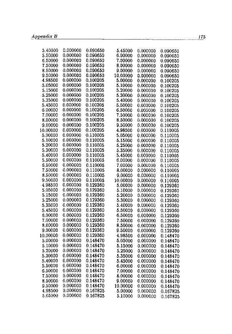
Appendix B 175 -.-.--.---.~- -~-----.
5.40000 0.000000 0.090650 5.45000 0.000000 0.090650 5.50000 0.000000 0.090650 6.00000 0.000000 0.090650 6.50000 0.000000 0.090650 7.00000 0.000000 0.090650 7.50000 0.000000 0.090650 8.00000 0.000000 0.090650 8.50000 0.000000 0.090650 9.00000 0.000000 0.090650 9.50000 0.000000 0.090650 10.00000 0.000000 0.090650 4.98500 0.000000 0.100205 5.00000 0.000000 0.100205 5.05000 0.000000 0.100205 5.10000 0.000000 0.100205 5.15000 0.000000 0.100205 5.20000 0.000000 0.100205 5.25000 0.000000 0.100205 5.30000 0.000000 0.100205 5.35000 0.000000 0.100205 5.40000 0.000000 0.100205 5.45000 0.000000 0.100205 5.50000 0.000000 0.100205 6.00000 0.000000 0.100205 6.50000 0.000000 0.100205 7.00000 0.000000 0.100205 7.50000 0.000000 0.100205 8.00000 0.000000 0.100205 8.50000 0.000000 0.100205 9.00000 0.000000 0.100205 9.50000 0.000000 0.100205
10.00000 0.000000 0.100205 4.98500 0.000000 0.110005 5.00000 0.000000 0.110005 5.05000 0.000000 0.110005 5.10000 0.000000 0.110005 5.15000 0.000000 0.110005 5.20000 0.000000 0.110005 5.25000 0.000000 0.110005 5.30000 0.000000 0.110005 5.35000 0.000000 0.110005 5.40000 0.000000 0.110005 5.45000 0.000000 0.110005 5.50000 0.000000 0.110005 6.00000 0.000000 0.110005 6.50000 0.000000 0.110005 7.00000 0.000000 0.110005 7.50000 0.000000 0.110005 8.00000 0.000000 0.110005 8.50000 0.000000 0.110005 9.00000 0.000000 0.110005 9.50000 0.000000 0.110005 10.00000 0.000000 0.110005 4.98500 0.000000 0.129360 5.00000 0.000000 0.129360 5.05000 0.000000 0.129360 5.10000 0.000000 0.129360 5.15000 0.000000 0.129360 5.20000 0.000000 0.129360 5.25000 0.000000 0.129360 5.30000 0.000000 0.129360 5.35000 0.000000 0.129360 5.40000 0.000000 0.129360 5.45000 0.000000 0.129360 5.50000 0.000000 0.129360 6.00000 0.000000 0.129360 6.50000 0.000000 0.129360 7.00000 0.000000 0.129360 7.50000 0.000000 0.129360 8.00000 0.000000 0.129360 8.50000 0.000000 0.129360 9.00000 0.000000 0.129360 9.50000 0.000000 0.129360
10.00000 0.000000 0.129360 4.98500 0.000000 0.148470 5.00000 0.000000 0.148470 5.05000 0.000000 0.148470 5.10000 0.000000 0.148470 5.15000 0.000000 0.148470 5.20000 0.000000 0.148470 5.25000 0.000000 0.148470 5.30000 0.000000 0.148470 5.35000 0.000000 0.148470 5.40000 0.000000 0.148470 5.45000 0.000000 0.148470 5.50000 0.000000 0.148470 6.00000 0.000000 0.148470 6.50000 0.000000 0.148470 7.00000 0.000000 0.148470 7.50000 0.000000 0.148470 8.00000 0.000000 0.148470 8.50000 0.000000 0.148470 9.00000 0.000000 0.148470 9.50000 0.000000 0.148470 10.00000 0.000000 0.148470 4.98500 0.000000 0.167825 5.00000 0.000000 0.167825 5.05000 0.000000 0.167825 5.10000 0.000000 0.167825
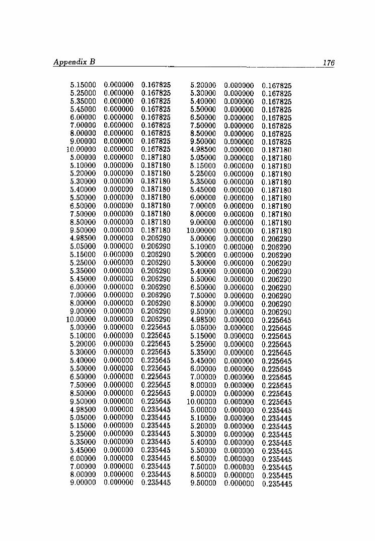
Appendix B 176
5.15000 0.000000 0.167825 5.20000 0.000000 0.167825 5.25000 0.000000 0.167825 5.30000 0.000000 0.167825 5.35000 0.000000 0.167825 5.40000 0.000000 0.167825 5.45000 0.000000 0.167825 5.50000 0.000000 0.167825 6.00000 0.000000 0.167825 6.50000 0.000000 0.167825 7.00000 0.000000 0.167825 7.50000 0.000000 0.167825 8.00000 0.000000 0.167825 8.50000 0.000000 0.167825 9.00000 0.000000 0.167825 9.50000 0.000000 0.167825
10.00000 0.000000 0.167825 4.98500 0.000000 0.187180 5.00000 0.000000 0.187180 5.05000 0.000000 0.187180 5.10000 0.000000 0.187180 5.15000 0.000000 0.187180 5.20000 0.000000 0.187180 5.25000 0.000000 0.187180 5.30000 0.000000 0.187180 5.35000 0.000000 0.187180 5.40000 0.000000 0.187180 5.45000 0.000000 0.187180 5.50000 0.000000 0.187180 6.00000 0.000000 0.187180 6.50000 0.000000 0.187180 7.00000 0.000000 0.187180 7.50000 0.000000 0.187180 8.00000 0.000000 0.187180 8.50000 0.000000 0.187180 9.00000 0.000000 0.187180 9.50000 0.000000 0.187180 10.00000 0.000000 0.187180 4.98500 0.000000 0.206290 5.00000 0.000000 0.206290 5.05000 0.000000 0.206290 5.10000 0.000000 0.206290 5.15000 0.000000 0.206290 5.20000 0.000000 0.206290 5.25000 0.000000 0.206290 5.30000 0.000000 0.206290 5.35000 0.000000 0.206290 5.40000 0.000000 0.206290 5.45000 0.000000 0.206290 5.50000 0.000000 0.206290 6.00000 0.000000 0.206290 6.50000 0.000000 0.206290 7.00000 0.000000 0.206290 7.50000 0.000000 0.206290 8.00000 0.000000 0.206290 8.50000 0.000000 0.206290 9.00000 0.000000 0.206290 9.50000 0.000000 0.206290
10.00000 0.000000 0.206290 4.98500 0.000000 0.225645 5.00000 0.000000 0.225645 5.05000 0.000000 0.225645 5.10000 0.000000 0.225645 5.15000 0.000000 0.225645 5.20000 0.000000 0.225645 5.25000 0.000000 0.225645 5.30000 0.000000 0.225645 5.35000 0.000000 0.225645 5.40000 0.000000 0.225645 5.45000 0.000000 0.225645 5.50000 0.000000 0.225645 6.00000 0.000000 0.225645 6.50000 0.000000 0.225645 7.00000 0.000000 0.225645 7.50000 0.000000 0.225645 8.00000 0.000000 0.225645 8.50000 0.000000 0.225645 9.00000 0.000000 0.225645 9.50000 0.000000 0.225645 10.00000 0.000000 0.225645 4.98500 0.000000 0.235445 5.00000 0.000000 0.235445 5.05000 0.000000 0.235445 5.10000 0.000000 0.235445 5.15000 0.000000 0.235445 5.20000 0.000000 0.235445 5.25000 0.000000 0.235445 5.30000 0.000000 0.235445 5.35000 0.000000 0.235445 5.40000 0.000000 0.235445 5.45000 0.000000 0.235445 5.50000 0.000000 0.235445 6.00000 0.000000 0.235445 6.50000 0.000000 0.235445 7.00000 0.000000 0.235445 7.50000 0.000000 0.235445 8.00000 0.000000 0.235445 8.50000 0.000000 0.235445 9.00000 0.000000 0.235445 9.50000 0.000000 0.235445

Appendix B 177
10.00000 0.000000 0.235445 4.98500 0.000000 0.245000 5.00000 0.000000 0.245000 5.05000 0.000000 0.245000 5.10000 0.000000 0.245000 5.15000 0.000000 0.245000 5.20000 0.000000 0.245000 5.25000 0.000000 0.245000 5.30000 0.000000 0.245000 5.35000 0.000000 0.245000 5.40000 0.000000 0.245000 5.45000 0.000000 0.245000 5.50000 0.000000 0.245000 6.00000 0.000000 0.245000 6.50000 0.000000 0.245000 7.00000 0.000000 0.245000 7.50000 0.000000 0.245000 8.00000 0.000000 0.245000 8.50000 0.000000 0.245000 9.00000 0.000000 0.245000 9.50000 0.000000 0.245000 10.00000 0.000000 0.245000

Appendix C
Slipstream Characteristics for DATAl
REF DATAl
ADVS 1. 0506 CT 0 .147 ITNO 3
AXIAL DISTANCE DOvJNSTREAN (Y / R I
0.000 0.000 0.000 0.053 0.053 0 .052 0.124 0.124 0. 1 22 0.259 0.251 0.242 0 .4 11 0.390 0 .372 0.56 8 0.530 0.499 0 . 9 11 0.826 0 . 76 4 1. 289 1. 1 59 1.068 1.683 1.539 1 .45 9 2.095 1.946 1.926 2.515 2.350 2.421 2.940 2.756 2.918 3 . 797 3. 585 3.943 4.662 4 . 423 4.983 5.532 5.265 6.029 6.405 6. 110 7.080 7 .2 79 6.957 8.13 4 8.1 54 7.805 9.190 9.907 9.503 11.305
11.662 1 1 .204 13.424 16 . 931 1 .315 19.794
AXIAL INDUCED VELOCITY (UA / VSI
0 . 1 26 0.110 0.11 2 0 .244 0.214 0.197 0.183 0.172 0 . 149 0.139
0 .235 0.24 0 . 201 0 . 206 0. 18 0 0.185 0 .16 0 0.169 0.142 0. 1 47 0. 1 20 0. 1 08 0. 110 0. 0 99
0. 1 33 0 .107 0.098 0 .12 4 0.099 0.085 0 .1 18 0.0 99 0 . 085 0.117 0.099 0.085 0.116 0.100 0 . 085 0.ll5 0.115 0.114 0.114 0.114 0 . 114 0 .114 0.114
0.099 0.099 0 . 099 0.099 0.099 0.099 0.099 0 .099
0.084 0.084 0.084 0.084 0.084 0 . 083 0.083 0.083
AXIAL DISTANCE DONNSTREAM (Y / R)
0.000 0 . 000 0 .000 0 . 062 0.061 0.061 0 .13 4 0 .13 3 0. 1 32 0 . 279 0 . 275 0 . 27 0
PROPELLER DESIGN (ADVANCED LTFTHIG HODELI
X 0 .37
HYDRODYNAlll C PITCH ( BETA1 I
29.480 28.53 7 28 . 554 41. 335 40.830 41 . 1 79 42.143 41.155 41 .357 45 .22 1 44 .01 1 44 . 220 47 .3 17 45.697 46.127 49.199 47 . 370 4 7.96~
53. 541 53.184 52 . 877 57.535 60.178 61.019 61 .505 66. 497 69.686 63.401 70.67 2 76.712 63.471 7 2 . 493 78.207 63.974 7 2 . 827 78.554 6 4 .455 7 3 .4 72 79.14 5 64.764 7 3 .756 79 . 36 3 6 4 . 905 73.865 79 . 441 65 . 007 73.96 5 79.507 65 . 067 74.014 79.5 38 65. 106 74 . 050 79.560 65.164 74.09 6 79.582 65.194 74.125 79 .598 6 5 .260 74 . 176 79 . 648
TANGENTIJI.L INDUCED VELOC ITY (UT / VS I
- 0 .079 - 0. 06 7 -0.0 5 -0 .19 0 - 0. 162 - 0 . 1 84 -0.192 -0 . 17 8 - 0.178 - 0.194 -0.175 - 0.174 - 0.198 -0 . 171 -0 . 173 - 0.196 -0.166 -0. 17 2 -0.189 -0. 1 67 - 0 . 15 9 -0.184 -0 .1 64 -0 . 162 - 0.184 -0.177 -0 . 1 90 -0. 178 - 0 . 184 -0.214 -0. 16 3 -0. 186 -0.2 14 - 0. 1 64 - 0.1 86 - 0 . 215 -0. 1 69 -0.190 - 0 .218 -0.168 -0.190 -0.218 -0. 1 68 -0.190 -0.218 - 0. 1 68 -0.190 - 0 .2 18 -0. 168 - 0.191 -0.218 -0. 1 68 - 0.191 -0.219 -0.168 -0 . 191 - 0 .2 19 - 0 . 168 -0. 191 -0.219 -0.169 -0 . 191 -0.2 19
x ; 0 . 41
HYDRODYNAI-lIC PITCH ( BETAI)
34.279 3 4 . 170 34. 2 55 40.6 4 3 40 .4 3 4 40.49 2 41.687 41 .2 ~4 41 .2 1 1 44.275 43.639 43 .69
S LIPSTRP.AJ.! 11AIIUS ( X/ XO I
1 . 0 0 00 1 . 0000 1 . 0000 0 . 98 01 O. 7 e o. 724 0 . 9606 0 . 9 4 69 0.9437 0 . 921 3 0 . 0941 0 . 80 94 0 . A8 12 0 . 8400 0 . 83 41 0 . 842 0 . 78 2 0 . 7 79 4 0 . 7 98 O. 80" O.G 77 0 . 710] 0 . 58 0 0 . ~ ~8
0 . 6 71 0 . 5 137 0 . 4613 O. 4 32 0 . 4 58 0 . 4044 0 . 6346 0 . 627 2 O. 2 4 O. 20 O. 192
0 . 3 901 O . 0 9 O. 82 J
.3 79 4 0 . 3 787
0.6 183 0. 4 O. 7 81 0 . 617 8 0 . 4 55 4 0 .3 778
0 . 4 ,, 1 0 . 377 0.4 47 0 . 3773 0. 4 54 5 0 . 3 77J 0. 4 541 0 .37 7 0
RJ,DIA L IN DUCED VI, LOC I 'I'Y (U HI VS I
- 0 .00" - 0 . 00 5 - 0 . 00 5 - 0 . 00 5 -0. 00 5 - 0 . 00 4 - 0 . 0 0 5 - 0 . 00 - 0 . 00 5 - 0 . 0 5 - O . O O~ - o . oo~
- 0 . 00 5 - 0 . 00 5 - o . oo ~
- 0 . 00 - 0 . 00 - 0 . 00 " - 0 . 004 - 0 . 004 - O . OO ~
- 0 . 00 2 - 0.00 3 - 0 .0 04 - 0.001 - 0.002 - 0 . 002 - 0.001 - 0 . 001 - 0 . 00 1 0.000 0 . 00 0 0 . 000 0 . 000 0 . 000 0 . 000 0 . 000 0 . 00 0 0 . 000 0.000 0 . 000
0 . 000 0 . 000 0 . 000 0.000 0. 0 00 0 . 000 0.000 0 . 000 0 . 000 0 . 000 0 . 000
0 . 000 CI . OOO 0 . 000 0 . 000 0 . 000 0.000 0.000 0 . 000 0 . 000 0 . 000 0 . 000
S LIPSTRE~1 RADlUS (X/ XOI
1 . 0000 1.00 00 1 . 000 0 0 .9 84 5 0 . 979 8 0 .9 787 0. 9692 0. 9591 0 . 9 ' 0 0 . 9 3 8 0 . 91 8 0 . 91 17
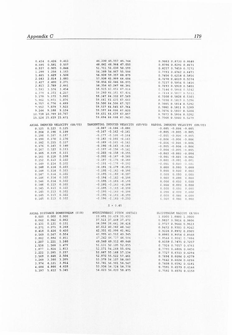
Appendix C
0.434 0. 426 0.4 13 0. 595 0. 581 0 . 5 57 0.937 0.905 0 .84 8 1.298 1 . 258 1 .163 1 .665 1.629 1 . 50 8 2.043 2. 014 1.883 2.427 2.400 2 . 2 71 2. 813 2. 7 89 2.661 3 . 593 3. 576 3.454 4. 379 4.373 4.257 5 . 170 5 . 17 2 5. 0 65 5.962 5 . 973 5 . 876 6.757 6. 7 76 6.689 7.552 7 . 57 9 7. 503 9.1 44 9. 188 9 .134
10.738 10 .799 10. 7 67 15 . 524 15 . 639 1 5.67 1
AXIAL INDUCED VELOCITY ( UA/VS )
0 . 125 0. 1 23 0 .1 25 0.2 04 0. 198 0. 199 0 . 19 8 0.187 0.187 0 . 190 0.170 0.1 7 0 0.182 0.155 0.157 0.176 0. 14 3 0. 14 0 0. 167 0.1 23 0.113 0 . 165 0. 119 0.1 11 0. 161 0 .11 8 0 .1 08 0 . 15 2 0. 113 0 . 102 0. 149 0. 114 0 . 102 0 . 148 0. 114 0 . 103 0.148 0 .114 0.103 0. 147 0. 114 0.102 0.146 0. 11 4 0.102 0. 146 0.114 0.102 0 . 146 0.113 0.102 0.1 45 0. 11 3 0 . 102 0. 145 0 .113 0.102 0.145 0 .113 0.102 0. 145 0.113 0 . 10 2
AXI AL DISTANCE DOWNSTREAM ( Y/R ) 0.000 0 . 00 0 0 .000 0.062 0.062 0. 0 62 0. 131 0 . 13 1 0. 131 0 . 27 1 0.27 1 0.268 0 .41 8 0. 416 0 . 410 0 . 569 0.882 1. 207 1. 538 1.877 2. 222 2.569 3.269 3.97 4 4 .684 5.397
0.567 0.554 0.884 0.851 1. 22 1 1.160 1. 568 1. 479 1. 924 1. 813 2.2 8 5 2. 157 2. 64 8 2 . 504 3. 38 0 4 .12 1 4 .866 5. 612
3 . 205 3. 914 4 . 628 5. 34 5
46.23 0 45.557 45.7 44 48 . 041 46 . 964 47 . 050 51. 71 1 51 . 03 0 50 . 599 54 .38 9 54 .86 7 55.598 56.9 39 59.357 60 . 879 57 . 93 8 61 . 999 64 .60 4 58. 056 62.8 4 6 66. 075 58. 35 6 63 . 247 66 . 38 1 58. 915 63 .65 1 67.016 59.2 60 6~.1 8 1 6 7. 4 3 ~
59.3 47 64 .332 67.569 59.441 6~ . ' 3 5 67.6 0 59.5 00 64 .50 6 67 .727 59.5 37 64.54 5 67 . 7 64 59.597 64. 60 6 67.82 0 59 . 63 1 64 . 639 67.857 59.69 4 64. 688 67.94 5
TANGENTIAL INDUCED VELOCITY (UT/ VS I -0.087 -0.086 - 0 .086 -0. 167 - 0 . 162 - 0 . 161 -0.177 -0 . 166 - 0 . 16 4 - 0.183 -0 . 166 - 0.1 63 -0. 189 -0 .1 65 - 0 . 163 -0. 190 -0.163 - 0.161 -0. 197 -0 . 158 - 0 . 141 - 0.2 03 -0.158 - 0.1 55 -0.202 - 0 . 167 - 0.16 6 -0 .197 -0 .:75 - 0.18 8 -0.19 1 -0.178 -0. 192 -0.19 1 -0.179 - 0 . 193 -0. 195 -0 . 182 - 0.1 96 -0 .195 -0 . 18 2 - 0 . 19 7 -0 .1 94 -0.182 - 0 . 198 -0 . 195 - 0 .1 83 - 0 .j98 -0 . 195 -0.1 83 - 0.1 98 -0 .195 -0 . :63 - 0 . 198 -0 .195 -0 . 183 - 0 . 198 - 0 . 195 -0. 18 3 - 0 . 199 -0. 196 -0 . 18 3 - 0. 200
x = 0 . 4 5
HYDRODYNAI-!I C PITCH ( BETAI )
33.491 33.4 28 33 .43 3 37 . 511 37 . 469 37.47 2 38.598 38.441 38.428 40.61 2 40 . 382 40 . 342 42.351 41. 99 6 41. 90 2 43.9 95 43.512 43 . 34 5 47.242 46.:37 46 . 506 49.5 40 49 .512 49.648 51.13 1 52 .105 52.85 5 52 .1 7 1 54 .268 55 . 694 52.687 55. 16 8 57.134 52.870 55.522 57 . 4 61 53.3 7 9 56 . 107 58 .08 7 53.78 1 56 .50 1 58.547 53 . 93 6 56 . 724 58.77 8 5 4 .023 56. 82 0 58 . 87 5
0 .9 0 83 0 . 87 3 0 0 . 864A 0.8796 0 . 8291 0 . 8171 0.A 25 7 0 . 7 4 59 0 . 7211 0 . 7793 O. 7 2 O. 0 .7 456 0 .62 ' 8 0.72 -'0 0 . 6019 0.7237 O. 956 0 . 719 3 0 . 59 19 0.71 44 0 . ' A64 0 . ', 3 4 2 0.7 1 14 o . ~ 37 0 . " 13 0.7 100 0 .5828 O. 3 0 3 0 .7 090 0.50 L9 o.~ 9 0 .70 8 ' 0 . ~ B 1 4 O. :1 •
0. 7081 0 .~ 811 0 . 528 ' 0.7076 0 .~ 8 07 0 . ~28 4
0 . 7073 0 .5804 0 . ~2B .
0.7068 0 . 58 0 0 0.5279
179
RADIAL I NDUCED VELOC I 'r 'i (U H/VS )
- O.OO~ - 0.0 06 - 0.00 5 - 0.00 5 - 0 . 00 5 - O , OO ~
- 0.005 - 0 . 00 - 0 . 00'> - 0.006 - 0.00 - 0 , 00 - 0 . 0 0 6 - 0 . 00 - 0 . 00 - 0 . 005 - 0 . 006 - 0 . 0 06 - 0.00 4 - 0 .00 - . OO ~
- 0 .003 - 0 . 00 3 - 0 , 004 - 0 .001 - 0.001 - 0.002 - 0 . 001 - 0.001 - O. OOl -0.0 0 0.00 0 0.0 01
0 . 000 0 .0 0 0 0. 000 0 . 0 00 0 . 000 0.000 0 .0 0 0 0.0 0 0 0.000 0.0 0 0 0 . 000 C. OOO 0 . 00 0 0.000 0.000 0 . 000 0 . 000
. 0 00 0.000 0.000 0 . 000
0 . 000 0.000 0. 000 0. 000 0 . 000 0.000 0.000 0 . 000 0. 00 0
SLI?S1'RElIl'l RJ\ l US ( X/XO )
1 . 0000 1.000 0 1 .0000 0.9857 0.98 1 0 . 9 0 0 . 97 2 7 0 . 9644 0.962 0 .9 47 2 0. 93 0 3 0.9262 0 .92 28 0 .89 7 2 0 .6909 0 .899 3 0 . 86 4 0 . 8 H O. 854~ 0.R 04 2 0.7R9 4 0.8159 0 . 7 47 5 0.72~7 0.7924 0 .7 0 57 0.67 J 0 .7795 O. 806 0.64 5 0 . 7727 0.67 13 0 .62 94 0 . 7 694 0.6684 0 . 627 0.7642 0 .7 608 0 . 7591 0 .7 5 Rl
0.662 4 0 . 659 0 . 65 -' 9 0 .6570
0.6 2 1 0.6181 0 .61 0 .6 15
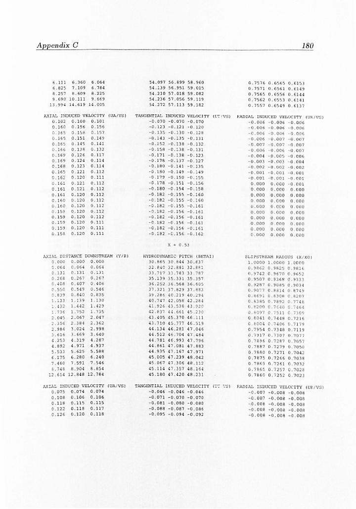
Appendix C
6. 111 6.360 6.064 6.825 7.109 6. 784 8.257 8.609 8.225 9 . 69 0 10.111 9 . 669
13 . 994 14.619 14.005
AXIAL INDUCED VELOCITY (UA /VS ) 0.102 0.100 0.101 0 . 160 0. 156 0.156 0 .165 0.158 0.157 0 .1 65 0 .151 0.165 0 .14 5 0 . 166 0.138 0 .1 69 0.126 0. 169 0.124 0. 16 8 0.123 0. 165 0. 121 0. 162 0 . 120 0 .161 0 .121 0. 161 0.1 21 0 .161 0.120 0 .1 60 0. 120 0 . 160 0.120 0 . 159 0. 120
0.14 9 0 .14 1 0.132 0 . 117 0.114 0.114 0 . 112 0 . 111 0.112 0.112 0.112 0. 11 2 0. 11 2 0.112
0.159 0.120 0 . 11 2 0.159 0.120 0 . 111 0. 15 9 0.120 0. 11 1 0. 15 8 0.120 0.111
;.xI;'L DISTANC=: DONNSTREAH (Y/R) 0 .000 0 . 00 0 0.000 O. 06 ~ 0.06 4 0.064 0 .131 0. 131 0.13 1 0. 268 0.267 0.267 0 .408 0 . 407 0.406 0 .550 0 .54 9 0 .54 6 0 .839 0.840 0 . 835 1. 133 1.1 39 1 .130 : . ~ 3 2 1 .44 2 1.4 29 1. 73 6 1. 752 1.735 2. 045 2.067 2.047 2 .356 2 .384 2 . 362 2.9 84 3.024 2.9 98 3 .6 1 6 3.669 3.640 4 .253 4 . 319 4 . 287 4.89 2 4.971 4 . 937 5.533 5.625 5 . 588 6. 17 5 6.280 6.240 7 .46 0 7 .59 1 7 . 546 S .748 8.904 8.854
12 . 614 12.S48 12.784
AX!;'L INDUCED VELOC ITY (UA / VS) 0. 07 5 0 . 074 0.074 0. 108 0. 10 6 0.106 0 .118 0. 115 0.115 0 .12 2 0.118 0 . 117 0. 126 0. 120 0.118
54.097 56.899 58 . 960 54.139 56.951 59.015 54.2 10 57.018 59 . 082 54 .2 36 57 . 056 59 . 119 54.272 57.113 59.18 2
0 . 7576 0 . 7 571. 0.756 0.7562 O. 0 . 7557 O.
180
0 . 6 1 ~
O. 14 9 O. J 4 4 O. 141 0 . 6137
TANGENTIAL INDUCED VELOC1TY \ T / VS I RADIAL INDUCED VELOCITY \UH/VS I -0.070 - 0 .070 - 0.070 - 0 . 00 - 0 . 00 - 0 . 006 -0.123 - 0.121 -0 . 120 -0 . 135 -0.130 - 0. 128 -0.143 -0.135 -0 .1 31 -0. 152 - 0.138 - 0 .1 32 -0.158 -0.138 -0. 131 - 0.171 -0.138 - 0 . 123 -0. 178 - 0.1 37 - 0 . 127 - 0 . lS 0 - 0 . 141 -0 . 135 - 0 .1 80 -0.149 - 0 .1 49 - 0 .179 -0. 150 - 0 .155 -0. 178 - 0 . 151 - 0 . 156 -0 . 180 -0 . 154 -0.158 - 0.18 2 - 0.155 -0 . 160 - 0 . 182 -0.1 55 - 0 . 160 -0 .18 2 -0 .1 55 - 0.161 -0.182 -0. 156 - 0.1 1 -0 . 18 2 - 0.156 - 0.161 -0 . 18 2 - 0 . 156 - 0 .16 J -0. 18 2 - 0.156 -0.161 -0.182 -0 .15 6 - 0 . 16 2
x = 0. 53
HYDRODYNAHIC PITCH ( BET/,ll 30 . 865 30 . 844 30.8 37 32 . 840 32.88 1 32.ee l 33.7 17 33 .78 3 33 . 787 35. 13 9 35.3 31 35 . 357 36 . 252 36. 568 3 6.605 37 . 32 1 37.829 37. 883 39.286 ( 0 . 219 40.294 40.7 47 42.0 58 42 . 28 4 41 . 92 43.538 4 3. 9 ~ 0
42.837 '4 .66 1 45 .2 30 43. 405 d5.370 46 .11 1 43. 710 45 . 777 46.519 44 . 134 46.2 81 47 .0 46 44 .5 12 46.7 04 47.484 44.781 46. 993 47.796 44 .861 47. 081 47.883 44 . 935 47.167 4 7.971 45 005 47.2 39 48 .042 45 067 47 .3 06 48 .112 45.114 47.3 57 48 . 164 45 . 180 47 . 420 48 .231
TANGENTIAL INDUCED VELOCITY W7 ·:S ) - 0.046 -0.04 6 - 0.04 6 -0. 071 -0 . 070 - 0 .070 - 0.081 -0. 080 - 0 . 080 -0. 088 -0 . 087 -0.086 -0.095 -0.094 -0.092
- 0 . 00 - 0 . 00 - 0 . 00 - 0 . 00 - 0 . 00 - 0 . 00 - 0 . 006 - 0 . 007 - 0 . 007 - 0 . 007 - 0 . 007 - 0 . 00 7 - 0 . 006 - 0 . 00 - 0 . 007 - 0 . 004 - O.OO~ - 0 . 00 - 0 . 00 3 - 0 . 00 - 0 . 04 - 0 . 00 2 - 0 . 00 2 - O . OO ~
- 0 . 001 - 0 . 00 1 - 0 . 001 - 0 . 001
0 . 000 0 . 000 0 . 000 0 . 000 0.000 0.000
- 0 . 00 1 0 . 000 0 . 000 0 . 000 0 . 00 0 0 . 0 00 0 . 000
- 0 . 00 1 - 0 . 001
0 . 000 0 . 000 0 . 000 0 . 000 0 . 000
0 .000 0 . 000 0 . 000 0.000 0 . 000 0 . 000 0 . 000 0 . 000 0 . 0 a 0 . 000 0 . 00 0 0 . 000
SLII'STREAN R/,DIUS (X / XC) 1 .0000 1.0000 1 . 0 00 O. 862 0 .98 5 0 . 9Hl 1 . 7420 . 97 0 .9 ,2 0 . 9~07 0.9 3 B 0 . • 333 O. 287 0.9085 0.903~ 0 . 90 77 0 . 8 14 0 874 0 . 869 0 . 8 08 0 . R207 0 . 638 5 0 . 7 92 0. 77 48 0 . 820 0 0. 7 G ~0 0 . • • t, 0 .809 1 0 .7 5 11 . 7309 0 . 80 41 0.7448 0.7 1 O. 00 4 O . 7~0 0. 7179 0 . 79 4 0.?348 0 . 7119 0 . 7917 .7] 07 0 . 707 7 0 .7 896 0 . 7 ~ 87 0 . 70' 7 0 .7 887 0 . 7 279 0 . 70 0 0.7 880 0 . 72 71 0.704 2 0 . 7 875 0 . 7 2 6 0 . 70 8 0 . 7 A69 0 . 7261 0 . 701 2 0 . 7 8 5 0 . 7 57 0.70 8 0 . 786 0 0 .7252 0. 70 23
RAD1AL Jl.JDUCED VELO ITY (URIVS ) - 0. 007 -0.008 - 0 . 00 8 - 0.007 - 0 . 008 - 0 . 00 8 - 0 .008 - 0.008 - 0 . 00 8 - 0.008 - 0 . 008 - O. OO A - 0 . 00 8 -0. 00 8 - O. OO R
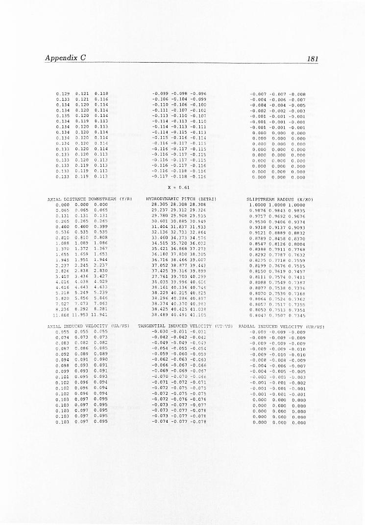
Appendix C
0.129 0.121 0. 1 18 0. 13 3 0.121 0. 116 0. 1 3~ 0. 120 0.114 0.134 0.1 20 0.114 0 .135 0.120 0 . 114 0 . 134 0.119 0.113 0 . 134 0.120 0. 1 13 0.134 0. 134 O. ]34 0.133 0. 13 3 0.133 0.133 0.133 0.133
0.120 0. 120 0. 12 0 0.120 0. 120 0 .1 20 0. 119 0 .11 9
0. 11 9
0 . 11 4
0 . 11 4 O. 1l~
0 . 114 0.113 0.113 0. 11 3 0. 11 3 0.113
AXIAL DI STr~CE DOI'INSTREAN (Y I RI 0.000 0.000 0.000 0.065 0.131 0.265 0.400 0.536 0.8 10
.088 1.370 1.655 1.945 2.2 37 2.826 3. 41 9 ':. 016 4.616 5.2 1 8
0.065 0.131 0 .265 0.400 0. 53 5 0.8 10 1 . 089 1.372 1.659 1.951 2 .245 2.838 3.436 4.038 4.643 5.249
0.065 0.131 0.265 0 .3 99 0.535 0.808 1.086 1.367 1.653 1.944 2.237 2.830 3 .42 7 4 .029 4.633 5.239
5 .820 5.856 5 . 8 , 6 7 .02 7 7.073 7.063 8.236 8 292 8.281
11.868 11.953 11 .g e 1
.' ,.xFL INDUCED VELOCI TY (UA / VSI 0.055 0.055 0.055 0.074 0.073 0.073 0 .08 3 0.082 0 .08 2 0. 087 0.086 0.085 0 .092 0.089 0.089 0.09 4 0 . 091 0.090 0.098 0.093 0 . 091 0.099 0. 093 0 .091 0 .101 0 . 095 0.093 0 . 10 2 0.096 0.094 0.102 0.096 0 . 094 0 .102 0 .096 0.094 0.103 0.097 0.095 0. 103 0.097 0.095 0 .103 0.097 0.095 0 .103 0.097 0.09 5 0. 103 0.097 0.095
- 0.099 -0.098 - 0.096 - 0.106 -0 . 104 - 0.099 -0 . 110 -0.106 -0.100 - 0.111 - 0 . 107 -0.102 -0 .1 13 - 0.1 10 - 0.1 07 -0. 114 -0 . 113 - 0 . 11 0 - 0.114 -0.1 13 - 0 . 11 1 - 0.114 -0 . 115 -0 .11 3 - 0.115 - 0.116 - O.l:C - 0 . 116 -0.117 - 0 . 11 5 -0.116 -0.117 - 0 . 115 - 0.116 - 0.117 - 0 . 11 5 -0 .116 -0 .117 - 0.11 5 -0 . 116 -0. 117 - 0 . 116 -0. 11 6 - 0.118 - 0.11 6 -0. 117 -0.1 18 - 0 . 11 5
x = 0.61
HYDRODYNN1I C PITCH (SETA II 28 . 305 28. 308 28.308 29.237 29 . 31 2 29 .326 29 . 780 29.908 29 . 905 30.60 1 30.885 3 0 .949 31.40 4 31.8 37 31 .933 32 .1 36 32.73 3 32.e6~
33.46 0 34 .373 3 4 . ~ 7 5
34.515 35.720 36.0 ;2 35 . 421 36 .868 37.2 73 36.180 37 . 810 38.305 36 . 716 38 . 466 39. 007 37.052 38.87 7 39. C43 37. 425 39 . 316 39.899 37 . 76 1 39 .7 03 40 .299 38.035 39.996 40 .£ C: 38.161 40.136 40 . 7C5 38.229 4 0 . 215 40. 025 38.296 4 0 . 286 40. 697 38.37 4 40.370 40. 983 38.425 40.425 41 . 038 38.489 40.491 41 .1 05
TANGENTI AL INDUCED VELOCI TY n ':T ' \'S I -0.030 -0.031 -0.031 -0.042 -0.042 - 0.04 2 - 0.049 -0.049 -0. 0 4 9 -0.054 -0.055 -0 . 05C -0 . 059 - 0.0 60 - 0 . 05 9 - 0.062 -0.063 - 0 . 053 - 0 . 066 - 0 . 067 - 0 .066 -0 . 069 -0.069 -0.067 -0 .070 -0 . 070 - 0. 0 50 -0.071 - 0 . 072 - 0. 071 -0 . 07 2 -0 . 075 -0 . 075 -0 .0 72 -0.075 - 0.0 75 -0. 07 2 -0.076 - 0 .076 - 0. 07 3 -0 . 07 7 -0.077 -0. 0 73 -0.077 - 0.07 8 -0.07 3 -0.077 - 0.0 78 -0.074 -0.077 -0.Oi 8
181
- 0 . 007 - 0 . 007 - 0 .00 8 - 0 . 004 - 0.00 - 0 . 007 - 0 . 004 - 0 . 004 - 0 , 00 - 0 . 00 2 - 0 . 002 - 0 . 003 - 0.001 - 0 .001 -0.0 01 - 0.001 - 0.001 - 0 . 001 - 0.001 - 0 . 001 - 0 .0 01
0 . 000 0 .000 0 . 000 0.000 0 . 000 0 . 000 0 .00 0 0 . 000 0 . 000
0.000 0.000 0 . 0 00 0.000 0 . 000 0 . 000 0 .000 0.000 0 . 000
0 .000 0 . 000 0 . 000 0 . 000 O, QOO 0 . 000 0.000 0 . 000 0 . 000
SI..IPSTRElIt1 MDIU S ( X/XO I 1 . 0000 1.0000 1.0000 0.'876 0.98 43 0.9835 0 . 97 . 7 O. 692 0.967 0.9530 0.940 0 . 937 4 0.9318 0. 9137 0. 909 0 . 9121 0 . 8889 0 . 88 2 0 . 8789 0.8458 0.8370 0.8547 0 . 8126 0 . A004 0.8388 0 . 79 11 0 . 7768 0,8292 0, 7787 0 . 7 2 0.82 ~ 5 0 .7 718 0.7~59 0.R19 0 .7 7 0.751 ' 0.8150 0.7 19 0.74"7 0 . 8111 0. 7 74 0. 7 411 0 . 8018 0 . 7549 0 .7 H7 0 . 8077 0 . 7 5 38 0 . 737 0.8070 0,7530 0 .736 0 . 8064 0 .752 4 0 .7 2
.AOS7 0 . 7 17 0. 7 3~5
0 . 8053 0 .75 13 0 . 7 1 0.804 7 0.7 0 7 0 73 4~
RADIAL INDUCED VELOC 1TY ( - 0 . 00 9 - 0 . 009 - 0 . 009 - 0 . 00 - 0.009 - 0 . 009 - 0 . 00 - 0.009 - 0 . 009 - 0.009 - 0 . 009 -0 . 010 - 0.009 - 0.010 - 0. 0 10 - 0.008 - 0.008 - 0.009 - 0 .004 - 0.006 - 0.007 - 0.004 - 0.005 - 0 . 005 - 0 . 0 2 - 0 . 00 3 - 0.00 3 - 0 .0 01 - 0 . 001 - 0 . 00 2 - 0.001 - 0 . 00 1 - 0.0 01 - 0.001 -0 . 001 - 0 . 001 0.000 0 . 000 0 . 000 0.000 0. 000 0.000 0.000 0.000 0 .000 0.000 0 . 000 0 . 000 0.000 0.000 0.000
/ VS I

Appendix C
0. 102 0.097 0.095 0 .102 0 . 097 0 . 095 0.102 0.097 0.095 0. 102 0.097 0.094
AXIAL DISTANCE DOWNSTREAM (Y/R )
0 . 000 0 .000 0.000 0 . 065 0 . 065 0.065 0 .1 32 0 . 13 2 0.132 0 .2 66 0 . 26 6 0.266 0 .401 0.401 0 . 400 0. 537 0 . 537 0.536 0.810 0.810 0.809 1.087 1.087 1 .085 1.3 67 1.367 1.364 1.651 1.651 1.647 1.9 37 1.939 1.934 2 .226 2.229 2.224 2 . 808 2.813 2.808 3 .3 95 3. 401 3. 396 3.984 3 . 994 3.98 8 4. 577 4.589 4.58 3 5. 171 5.185 5.180 5.766 5 .783 5.777 6.958 6.980 6.975 8 . 152 8. 179 8.174
11 .739 11 . 781 11.776
."-.XI.; L INDUCED VELOCITY (UAIVS ) 0.05 4 0 .055 0. 05 5 0.07 3 0 .073 0 .074 0.08 1 0.081 0. 081 0.0 85 0.085 0.085 0. 089 0. 088 0 .088 0 . 092 0. 090 0. 089 0 .096 0. 093 0.092 0 .097 0.0 94 0.093 C.099 0 095 0. 09 4 0. 100 0. 097 0.096 0 .100 0.097 0.095 0 .1 00 0 .0 97 0 . 096 0. 101 0 .098 0.0 96 0. 101 0.OS 8 0.097 0 . 101 0. 098 0.097 0 .101 0 .1 01 0. 101 0. 101 0. 101 0. 101
0.098 0.098 0 .09 8 0.09 8 0 .098 0.0 98
0. 096 0.096 0.096 0. 096 0.096 0.096
;V:IAL DISTANCE DOWNSTREAl1 ( Y /R)
0.000 0.000 0.000 0. 066 0 .066 0 . 066 0 .133 0. 133 0 . 132
-0.074 - 0 . 078 -0. 07R -0.074 -0. 078 -0 078 -0.074 -0.078 -0 . 078 -0.074 - 0 . 07 8 -0. 079
x = 0.6 9
HYDRODYNAnC PITCH (8ETAI) 25.56 5 25 . 579 25.584 26. 376 26.457 6. ~ 78
26.868 27.0 12 27.049 27 . 514 27.7 90 27.860 28.135 28. 539 28 .641 28.667 29. 206 29.3 47 29.67 2 30. 47 8 30 .691 30. 455 31 .461 31.7 44 31.155 32.3 36 32 . 68 4 31.7 52 3] .0 72 33. 47 5 32.190 33 . 597 34.035 32.483 33. 94 5 3(.399 32.813 34.330 34.7 98 33. 108 3, . 67 3 ; 5 . 151 33 .3 52 3' . 939 35 . 42 8 33 . 475 35 .07 6 35 . 564 33.539 35.147 35 . 637 33 . 600 35. 214 35.70 3 33.676 35 . 295 35 .7 86 33.7 22 35. 34 6 35.838 33.784 35. 41 1 35 .904
T,\NGENTIAL I:·;::JUCED VE:'OCITY (UT I VS )
-0.027 -0.027 -0 . C27 -0.C36 - 0. 03 7 -0. 037 -0. 04 2 - 0. 04 2 ·0 .0 42 -0 . 04 6 - 0 .047 -0.0 47 -0.05C -C.051 -0.05 1 - 0.052 - 0 .0 53 -0.053 -0.055 - 0 . 057 -0.05 7 -0.057 - 0.0 59 -0.057 -0.056 -0 .060 -0.0 5 -0 .059 -0. 061 -0. 061 -0.06J -0 . 063 -0.06 4 -0. 060 - 0 .064 -0.06 4 - 0.060 -0.064 -0. 065 -0. 06 1 -0.065 -0.0,6 - 0.061 - 0.066 -0.066 -0.062 -0 . 06 6 -0 .066 -0 .062 - 0 .06 6 -0.067 -0.062 - 0 .066 -0.0 67 -0.062 -C.066 - 0.0 67 - 0.062 -0.066 -0.0 67 - 0 . 062 - 0 .06 6 - 0.0 67
x = 0.76
HYDRODYNJ.j·lIC PITCH (BETAI)
23 . 296 23 . 312 23.3 18 24.045 24 . 114 24.133 24.417 2'.536 24 .567
182
0 . 000 0.000 0 . 000 0 . 000 0 . 000 0 . 000 0.00 0 0.0 00 0 . 000 0.000 0 . 000 0 . 000
S LIPSTREAM RADIU S ( X/ XO) 1 .0000 1 . 0000 1 . 000 0.9aA8 o. 859 O. 8 ,. 0 . 9781 0.9724 0 . 970 0 . 958 0 . 9 47 0 o. 441 0.9 400 0 . 9236 0 . 91 93 0.9 235 0. 90 21 0 . 89 64 0 . 8966 0 . 066 4 0.8578 0 . 877 3 0.840 0 . 8 297 0.6 641 0 . 8230 0.810 5 0.855 7 0 . 81 22 0.798 9 0 . 850 5 0 . 8059 0 . 7 922 0.8471 0 . 8018 0.7879 0.8423 0 .7962 0.7823 0 . 8386 0 .79 18 0 . 77 78 0 . 83 6 0 .789 0.77 2 0.83~2 0 . 78 81 0 . 77 41 0 . 8345 0.7874 0 . 773 3 0.8339 0 . 7867 0.77 27 0.8332 0 .7860 0 . 771 9 0 . 832 8 0.7 855 0 .77 1 0. 8 22 0. 78 50 0 .7 70
~\DIAL IN U ED VELOCITY (U R/VS ) - 0 . 010 - 0 . 01 0 - 0.010 - 0.010 - 0 . 01 0 - 0 . 01 1 -0. 010 - 0 . 010 - 0 . 011 - 0.010 - 0.011 - 0 . 01 1 - 0. 010 - 0 . 01 1 - 0 .011 - 0.008 - 0.009 - 0 . 009 - 0 . 00 5 - 0 .00 - 0 . 007 - 0 . 004 - 0 . 004 - 0 . 005 -0.0 02 - 0 . 00 - 0 . 00 _ - 0 . 00 1 - 0.001 - 0 . 001 - 0 .0 01 - 0 . 001 - 0.001 - 0 . 001 - 0 .0 01 - 0 . 00 1
0 . 000 0 . 000 0 .000 0 . 000 0.000 0. 000 0.000 0.00 0 0 . 00 0 0.000 0 . 000 0.000 0 . 000 0 . 000 0 .000
0.000 0 .000 0 . 000 0 . 000 0 . 000 0.000
0 .000 0 . 000 0 . 000 0.000 0.000 0.000
SLIPSTREAM RADI US ( X/XO )
1 . 0000 1 . 0000 1 . 0000 0 . 9909 0 . 988 5 0 . 987 9 0 . 9822 0 . 9775 0 .9763

Appendix C
a 267 0 .40 2 0.538 0 .812
.088 1.3 67 1.649 1 .93 4 2 . 22 1 ::!.799 3 . 380
0. 267 0 . 267 0 .4 02 0 .402 0.538 0.538 0. 812 0.811 1.088 1.0 86 1 . 36 7 1.365 1. 649 1.646
. 934 1.931
. 22 2 2 . 21 8
.800 2. 7 96
. 383 3 . 379 3.965 . 96 9 3 . 965 ~ . 552 4.5 57 4.55 3 5. 14 1 5.1 48 5 .14 4
.731 739 5.7 35 6 . 913 6 . 923 6. 91 9 8.096 8.10 9 8 . 105
11. 652 11 . 673 11 . 669
,\X E L I NDUCED VELOCITY (UA / VS) 0 .053 0 . 054 0 . 054 0.075 a 07 5 0 .075 0.0 81 0 . 082 0 .08 2 0 .085 a 085 0 .085 o 089 0 06 9 0. 089 0 . 091 0 . 050 0 . 09 0 0 . 095 0 .094 0 .093 0 . 096 0 .0 94 0 . 094 o 097 0 . 095 0.095 O . 0~9 0 . 097 0 . 097 0 .099 0.097 0. 096 0 . 099 0.097 0. 0 97 0.099 0.098 0 . 097 0.100 0 . 098 0 . 09 8 C.1 00 0 G9S 0 . 09 8 0 .100 0.0 98 0. 098 0. 100 0 . 098 0 . 09 8 C. ICO 0 098 0 .098 0 .100 0 .098 0 . 097 C. 100 0.098 0. 097 0 .100 0 . 098 0 . 097
;'~-;:;'.:" DISTANCE DO\vNSTREAl1 (Y / R I
0 . 000 0 . 000 0 . 000 0 .06 6 0.066 0 . 06 6 0 . 133 0 .1 33 0.133 0. 26 8 0 . 26 8 0.2 68 0 . 404 0. 404 0 . 404
. 540 0 . 54 0 0 .54 0 0 .814 0.8 14 0.81 3 1.09 1 1.090 1. 088
.36 9 1. 368 1 . 3 66
. 650 1. 65 0 1 . 647 1 . 934 1. 933 1.930 2 . 220 2 . 21 9 2 . 216 2. 794 2 . 79 4 2.7 90 3.372 3 . 372 3.368
24 . 910 25.1 3 1 25. 188 25.38 3 25.70 2 25.78 5 25. 786 26. 20 5 26 .31 7 2 6 .54 5 27.1 5 4 27.32 0 27.144 27 .892 28. 101 27.688 28.5 57 2 8. 807 28 . 158 29.12 5 29 . 41 0 28 . 513 29 . 544 29.8 ( 9 28 . 760 2 9. 832 30.14 9 29 . 050 30 . 168 30. 49 29 . 307 3 0.4 64 30 .801 29. 522 30 . 698 31.04 5 29.637 30 . 823 31 . 171 29 . 695 30. 889 3 1 . 237 29 . 7 50 30.94 9 3 1 .298 29 . 8 22 31 . 026 31 .375 29.8 653 1 . 0733 1 .42 3 29 . 923 31 . 135 31 . 466
TAlVGENTIAL INDUCED VELOCI TY ( U1'/ \lS I
-0.0 23 - 0.0 24 - 0.024 - 0 . 033 -0. 033 -0 . 033 -0 .037 - 0 . 038 - 0 . 038 -0 . 04 0 -0 . 04 1 - 0.041 - 0.04 3 - 0 . 04 5 -0 . 04 5 - 0.045 - 0 .04 6 -0 . 04 - 0.047 - 0.04 9 -0. 04 9 - 0.049 - 0 . 0 50 -0 . 050 - 0. 050 -0 . 051 -0. 051 - 0. 050 - 0 . 053 -0.053 -0 .051 - 0 . 054 -0 . 055 - 0 .05 2 -0. 0 55 - 0. 055 -0 . 052 - 0 . 055 - 0.0 56 - 0 .053 - 0.05 6 - 0. 057 - 0 .053 -0 . 05 6 - 0. 057 - 0.053 - 0. 057 - 0 . 057 - 0 .053 -0 . 057 -0 . 057 -0.0 53 - 0.057 -0.058 -0 .05 3 - 0. 05 7 -0 . 058 -0 . 05 3 - 0. 0 57 -0.058 -0 . 053 - 0 . 057 - 0. 058
x = 0.84
HYDRODYNAI'1IC P ITCH ( BE1'AI )
21 . 411 21 . 426 21 . 430 22. 155 22.2 06 22.2 1 9 22.426 22.51 7 22.539 22.805 22 . 974 23 .01 6 23 .17 0 23 . 413 23. 475 23 .4 81 23 .79 9 23.883 24.068 24.524 24.648 24.53 8 25. 09 6 25.2 48 24 . 971 25 . 61 6 25.795 25.348 26 . 06 4 26 . 26 7 25 . 638 26.403 26. 62 0 25.847 26 .644 26 . 86 9 2 6 .10 3 26.938 27. 172 26 . 328 27.19 6 27. 438
183
0 . 96 ~ 8 0. 9 ~65 0 .9 5 41 0 . 9508 0 . 937 0 . 9331 0 . 9373 0 . 9 197 0 . 9 150 0 . 91 54 0 . 8910 0 . 88 42 0. 8995 0 . 8701 O.R 16 0 . 888 2 0.0 55 4 0 . 8 457 0 . 880 8 0 . 84 60 0 . 83 57 0 . 8'1 61 0 .A 40J 0 . 8295 0 . 8728 O. R 62 O. A '5 0. 8 83 O.B OH 0 . 01 0 . 86 4 , 0 .. 6' 0 .8 l:>~
0 . 862 4 0 . 8 240 0 . 8130 0 . 8613 0 . A22 0.8 1 1A 0 .8 0 0 . 822 0 0 . 8110 0.R60 1 0 . 82 14 D. AI 03 0 . 8593 0 . 8 206 0 . 8096 0.8 589 0 . 82 01 0 . 80 I 0 . 8584 0 .819J 0 . 808 5
RADIAL 1 NI)UCEO VELOC ITY ( UR / VS 1
- 0. 0 11 - 0 . 011 - 0 . 0 11 - 0. 011 - 0 .011 - 0 .0 11 - 0 . 011 - 0 . 011 - 0. 01 1 - 0 . 01 1 - 0 . 011 - 0 . 01 - 0 . 011 - 0 . 01 1 - 0 . 01 2 - 0 . 009 - 0 . 00 9 - 0.0 10 - 0 . 00 - 0 .00 ' - 0 . 00 - 0 .004 - 0 . 00 4 - 0 . 004 - 0 . 00 2 - 0.003 - 0. 00 3 - 0.001 - 0.0 01 - 0.001 - 0 . 001 - 0 . 00 1 - 0 . 001 - 0.0 01 - 0 . 001 - 0.00 1
0 .000 0 .000 0 . 00 0 0 . 000 0 . 000 0 . 000 0. 000 0. 000 0 . 000 0 . 000 0 . 000 0 .000 0 . 00 0
0 .000 0 . 000 0. 000 0 . 000 0 .000
0 . 000 0 . 000 0 .000 0 .0 00 0 . 000 0.000 0 . 000 0.000 0.000
S LI PSTREAM RADIU IX / XO) 1 . 00 00 1 . 0000 1 . 0000 0.9924 0.9904 0 . 98 99 0 . 98 51 0 . 98 12 0 . 980 2 0 . 971 4 0 . 963 8 0 .96 1 8 0.9589 0 . 947 8 0 . 9 44 9 0.9 47 6 0. 9332 0.92 94 0 . 9293 0.90 94 0 .9039 0 . ~ 1 5 8 0 . 89 19 0. 8852 0 .9 0 61 0.879 4 0 .87 18 0 .8996 0 . 8711 0 .8630 0 .895 2 0 . 86 5 7 0.8 57 3 0 . 892 1 0 .86 19 0 .853 4 0. 8877 0 . 8567 0 . 84AO 0 . 884 3 0 . 8525 0 . 843 8

Appendix C
3 .9 53 3 . 954 3 . 950 4.537 4 .53 9 4.534 5.122 5 . 125 5 . 120 5 . 708 5.711 5.706 6.883 6 .887 6.882 8.059 8.065 8.059
11.593 11.603 11.59 6
.'.xr.lIL INDUCED VELOC I TY (uA f VS) 0.052 0 .052 0.053 0.078 0 .08 3 0.086 0.089
0. 078 0 . 083 0 . 086 0.08 9
0 . 078 0.083 0.086 0.089
0.091 0 . 090 0 . 090 0 .094 0 . 093 0.093 0.095 0. 094 0.094 0.0 9 6 0.095 0.095 0.098 0.097 0.096 0 . 098 0 . 097 0 . 096 0.098 0.097 0.097 o 099 0.098 0 .09 7 0.099 0.09 8 0.098 0.099 0 .098 0.098 0 . 099 0.098 0.098 0 .099 0.098 0. 098 o 099 0 . 098 0.098 o 099 0.098 0. 098 0.099 0 098 0 098 o 099 0 098 0 .098
.".XI."L DISTA."ICE DOWNSTREAH ( Y f R )
0.000 0 . 000 0.000 0.066 0.066 0.066 0 .13 4 0.134 0. 133 o 269 0. 405 0. 541 0.8 15 1. 090 1 . 367 1.647 1 . 929 2.212 2.783 3 . 356 3.933 4.512 5.092 5.674 6.839
0. 269 0 .2 68 0.40 4 0. 403 0.5 40 0.539 0.813 0.811 l. 088 l. 085 1.365 1.361 1. 644 l. 639 1.925 l.91 9 2.20 9 2.202 2. 778 2.770 3.351 3.341 3.928 3.91 6 4.50 7 4.493 5.08 7 5. 071 5. 668 5 . 651 6.832 6.812
8 .005 7.999 7.975 11 . 511 11 . 502 11.469
p.xIAL INDUCED VELOCITY (UA f VS )
0.051 0.052 0.051 0.078 0 . 0 77 0 .07 7 0.081 0.080 0.079
26. 518 27.403 27 . 653 26.623 27.517 27.768 26.676 27.577 27.828 26. 7 27 27 . 632 27 . 884 26. 7 93 27 . 703 27 . 956 26 . 833 27.746 28 . 000 26. 887 27.804 28 . 0 58
TANGENTI AL INDUCED VELOCITY (UT f VS ) -0.02 1 -0. 021 - 0 . 0 21 -0.030 - 0.031 - 0.031 -0 . 034 - 0 . 034 - 0 . 034 - 0.036 - 0.037 - 0.0 37 -0.039 -0.039 - 0 .039 -0 . 040 -0. 041 - 0 .041 -0 . 041 -0. 04 3 - 0.04 3 -0 . 04 3 -0 . 044 - 0.04 3 - 0 .04 4 -0.045 - 0 . 044 - 0 .04 4 - 0.046 -0.046 -0 . 045 - 0 . 047 - 0.048 -0.046 -0 . 048 - 0.048 -0 . 046 - 0.048 - 0.049 -0.046 - 0.049 - 0.049 -0 . 04 6 - 0 .0 49 - 0 . 050 -0 .047 - 0 . 04 9 - 0.050 -0 . 047 -0 . 050 - 0.050 -0.047 -0.050 -0 .05 0 -0.047 - 0 .050 - 0 . 050 -0.047 - 0.050 - 0.0 50 -0. 047 -0.050 -0 . 050
x = 0.92
HYDRODYNAHI C P ITCH ( BETAl) 19 . 794 1 9.805 19.801 20. 48 7 20. 49 7 20. 484 20.6 67 20 . 709 20. 7 03 20.959 21.062 21.074 21 .241 21.399 21.427 21 . 484 21.694 21 . 74 2 21. 94 2 22.250 22 .3 29 22 .31 8 22.696 22 . 797 22.665 23. 106 23.226 22.971 23.464 23.601 23.2 12 23. 741 23.887 23 . 391 23.945 24.09 9 23 . 616 24.201 24 . 362 23.814 24.426 24.592 23 . 982 24 . 608 24 . 78 2 24. 079 2 4 . 713 24 .8 88 24 . 127 24 . 767 24 . 94 2 24 . 174 2 4 . 81 8 24.993 24.236 24.886 25.061 24.272 24.925 25.1 01 24.323 24 . 979 25 . 15 6
TANGENTIAL INDUCED VELOCITY (UTf VS ) - 0 . 019 - 0 . 019 - 0 . 019 -0 . 028 -0.028 -0.027 -0.030 -0 .030 -0.029
184
0.882 J 0 .8 ~01 0 . 841 3 0.88 JO 0. 84 89 0 . 840 1 0 .8 003 0 .8 48 1 0 .A393 0.8 798 0 .8 475 0 . 038 0 . 8790 0 .8 4 7 0.8378 0.8786 0 . 84 2 0 . B373 0 . 8 780 0 . 8 45 0 . 8 3G7
RADI,;L IN DUCED VEt,OCITY (U Rf\'S ) - (l . Oll - 0 . 012 -0. 01 , - 0.012 - 0.01 2 - 0.01 2 - 0 . 012 - 0 . 012 - 0 . 0] 2 - 0. 01 2 - U. 01 2 - 0 . 01 . - 0.012 - 0 . 01 2 - 0 . 01 ~
-0. 00 9 - 0 . 00 - 0.0 10 - 0 . 00 5 - 0 . 005 - 0 . 00 - 0.004 - 0 . 004 - 0.004 - 0 . 002 - 0 . 002 - 0 . 00 3 - 0.00 1 - 0 . 001 - 0.001 -0. 001 - 0. 0 01 - 0 . 001 - 0 . 001 0 . 0 00 - 0 .001 0.000 0.000 0 . 000 0.000 0.0 00 0 . 000 0.000 0.000 0 . 000
0 . 0 00 0 . 00 0 0 . 000 0 . 000 0 . 000 0.0 00 0.000 0 . 000 0 . 000
0 . 000 0. 000 0 . 00 0 0.000 0.000 0.000 0 . 000 0.000 0 . 00 0
SL ] PSTREAl1 MOlUS ( X I XO ) 1.0000 1 . 00 00 1 . 0000 0.99 6 0 .99 19 0 . 99J 5 0.987 4 0.9 75 9 o. 0.9 ' 3 0 . 95 7 0.9 400
O. R33 0 . 967 o. ~ 5 o. 405 O. q ] 1
O . 928 ~ O. 9U8G 0.9032 0 .9200 0 . 8 77 0.891 0.91 41 0.8902 0 .8837 0 . 9100 0.885 0 . 8784 0. 9 071 0.B817 0 . 8747 0. 90 2 o. 995 0.8975 0.8964 0 . 8957
0 . 8766 0.B726 0 . 87 0 2 0 . 8689 o. 68 1
0 . B694 0 . 865 3 0.0 28 0 .8615 0.A60 ?
0 . 895 1 0.8675 0.0 0 1 0.894 4 0.8 67 0 .8 92 0.89 40 0 .86 2 0.8587 0 . 89 34 0 . 8655 0 . 8581
RADIAL INDUCED VELOC ITY (uR f VS ) -0.012 - 0.0 12 - 0 . 012 - 0.012 - 0.012 - 0.012 - 0 . 01 2 -0 .0 12 - 0.012
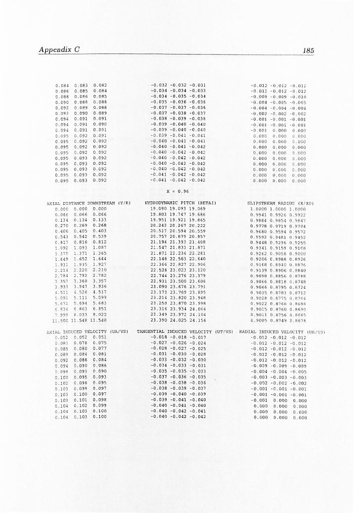
Appendix C
o 08 4 0. 083 0 .082 o 086 0. 0 8 5 0 . 084 o 0 88 0 .086 0.085 0.090 0 . 08 8 0.088 0.092 0. 089 0.088 0.093 0.090 0.089 0.094 0.091 0.091 0 .094 0. 091 0 . 09 0 0. 094 0. 091 0.0 91 0. 095 0 .092 0.091 0.095 0 .09 2 0.092 0 . 095 0. 092 0 . 0 92 0 .095 0 .092 0 . 0 92 0.095 0.093 0.09 2 0 . 095 0. 093 0 . 09 2 0.095 0.093 0.092 0.095 0.093 0 0 92 0. 095 0.093 0.09 2
AXIAL D!STANCE DOWNSTREAl1 (Y / R)
0 . 000 0 .000 0.000 0.06 6 0.066 0.066 0 . 134 0 .134 0 . 133 0.2 7 0 0.2 69 0.268 0. 406 0. 405 0 . 403 0.5 4 3 0.54 2 0 . 539 0.B 17 0 .816 0.812 1 . 09 2 1.093 1.0 87 1 .370 .371 1 .365 1.6 ~ 9 1.6 52 1 .6 4 4 : . 93 1 1 . 935 1.927 2 . 214 2 .220 2.210 2.784 2.792 2. 7 82 3. 35 7 3.368 3.357 3 . 93 3 3.9 47 3.936
. 51 1 ~.52 8 4 . 517 09, 5 .1 11 5.099
5 . 671 5 . 69 4 5. 6 8 3 6.8) , 5 . 863 6 . 851 7. 9 99 B. 033 8 . 022
1 1 .50 0 11. 54 8 11.540
,;.xlAL I NDUCED VELOCITY (UA/VS )
0 . 052 0 .052 0.051 0. 08 3 0 . 085 0 . 089 0 . 092 O . 09 ~
0. 098 0 . 100 0 .102 0 .1 03 0 . 103 0. 103 0 .104 0 .1 04 0 . 104
0.078 0.080 0 .084 0 . 088 0. 090 0 .09 3 0 .095 0. 098 0.0 99 0. 100 0 .101 0.102 0 .103 0 . 103
0 . 075 0.077 0. 081 0.084 0.086 0. 090 0.0 93 0 . 095 0.097 0 .097 0.09 8 0 . 099 0.100 0.100
- 0 .032 - 0 . 0 32 - 0.03 1 -0.034 - 0 . 034 - 0 . 033 - 0 . 034 - 0.035 - 0 . 034 -0.03 5 -0 . 036 - 0 . 03 6 - 0.037 - 0 . 037 - 0 . 036 -0 .037 -0 .03 8 - 0 . 0 37 - 0 .038 - 0 . 0 39 - 0 . 03 8 -0 . 039 -0.040 - 0 .0 40 -0 . 03 9 -0 . 040 - 0 . 04 0 - 0. 039 - 0 . 041 - 0.041 - 0.040 - 0.041 - 0 .0 41 - 0 .040 - 0.041 - 0 . 042 -0. 040 - 0.0 4 2 - 0 . 04 2 - 0.040 - 0 . 042 - 0 . 042 - 0 . 040 - 0 .0 4 2 - 0 . 042 - 0.040 - 0.04 2 - 0.042 -0.0 41 - 0 .0 42 - 0 .042 -0. 041 - 0.042 - 0. 0 42
x = 0 .9 6
HYDRODYNAlHC PITCH ( BETAI)
19 .090 19 .093 19 .0 69 19.803 19 .7 47 19 . 68 6 19 . 9 51 19.921 19 .865 20.242 2 0 . 267 20.222 20 .517 20 . 594 20.559 20 .757 20.879 20 . 857 21. 19 4 21.393 2 1 . 408 21.547 2 1. 833 21 . 871 21 . 871 22. 234 22.28 1 22 . 14 8 22.563 22.640 22 . 36 6 22 . 827 22 . 906 22. 528 23.023 23 . 120 22.7 44 23 . 27 6 23.379 22 .931 23.5 00 23.60 6 23. 090 23 . 676 23.791 2 3 . 17 3 2 3 .7 69 2 3.89 5 23. 214 23 .820 23.9 ~ 8
23.259 23.87 0 23 . 998 23.316 23. 9 34 24 . 0 64 23. 349 2 3 . 97 2 2 4.104 23. 3 90 2 4 . 02 5 2 4 . 154
TANGENTIAL INDUCED VELOCITY (UT / VS I - 0. 018 - 0 . 018 -0 . 017 -0 .027 - 0.02 6 - 0.0 24 -0.028 - 0 . 027 -0.025 - 0.031 - 0 . 030 - 0 . 0 28 -0.033 - 0.032 - 0 . 030 -0.034 - 0 . 033 - 0.0 31 -0. 0 35 -0 . 035 - 0.033 -0. 037 - 0 . 03 6 -0 . 035 -0. 038 - 0 . 038 - 0 .036 - 0 . 038 - 0 . 039 - 0 .037 -0.039 - 0 . 040 - 0 .039 -0. 039 - 0 . 041 -0 . 040 - 0.040 - 0.041 - 0 . 040 -0 . 040 - 0 . 04 2 - 0 . 041 - 0 . 0 40 - 0.042 - 0.04 2
185
- 0 . 0 1 ~ - 0 . 01 2 - 0 . 0] - 0 . 01 2 - 0 . 0] - 0 . 01 2 -0 . 009 - 0 . 009 - 0.010 - 0 . 004 - 0 . 0 0 ' - O . O O ~
- 0 . 004 - 0.00 4 - 0 . 004 - 0. 002 - 0 . 00 2 - 0 . 00 2 - 0 . 001 - 0 . 001 - 0 . 001 - 0 . 001 - 0 . 001 - 0 . 0 1 - 0.001 0 . 0 00 0 . 000
0 .00 0 0. 000 0 . 000 0 . 000 0.000 0. 0 00 0.000 0 . 000 0 . 000 0 . 00 0 0 . 00 0 0.000 0 . 000
0.000 0 . 000 0.000 0. 0 00 0 . 000 0 . 0 00 0 . 0 00
0 . 00 0 0.000 0. 000 0. 00 0 0. 000 0 . 00 0 0 . 00 0
S LIPSTREIIM RAD I US ( X/ XO ) 1 . 0000 1 . 0000 1 .0 000 0 . 99 41 0 . 99 26 O. 2/ 0.9884 O. 54 O. 0 . 9 7 78 0 . 9 71 9 O. 0 . 9680 0 . 9 94 O. ~7 2
0 .9592 0.9481 O. 4!> 2 0 . 9 448 0 . 9296 0 . 925 5 0 . 93 41 0.91 9 0 . 9 108 0 . 926 0 . 90 5 8 O. 0 00 0 . 9 206 0. 89 8 8 0 . 8 2 0 . 9 168 0 . 894 0 0 . R07 0 . 9 139 0 . 8 06 0 .8840 0 . 9098 0 . 885 0 . B7BR 0 . 9066 0 .8018 0 . 8 7 48 O. 0'6 0 . 8795 0 . 67 24 0 . 9035 0 . 87R 0.871 2 0 . 902R 0 . 877 5 0.81 0 4 O. 022 0 . 87 6A O. A 9A O. Ol ~ 0 . A7 a 0 . 86 e
0 . 9011 0.8756 O. R R 0.9005 0.87 4 0 . R67A
RADIAL IN UCED VELO 1 TY (U RI S )
- 0 . 01 2 - 0 . 01 2 - 0 . 0 12 - 0.012 - 0.012 - 0 . 0 12 - 0 . 01 2 - 0 . 01 2 - 0 . 01 2 - 0 . 01 2 - 0 . 01 2 - 0 . 01 2 - 0 . 01 2 - 0 . 01 2 - 0.0 12 - 0 . 009 - 0 . 009 - 0.00 9 - 0.004 - 0 . 004 - .005 - 0 . 003 - 0.00 3 - 0 . 003 - 0 . 002 - 0 . 00 2 - 0 .00 2 - 0 . 00 1 - 0. 001 -0.001 - 0 . 001 -0.00 1 -0 . 001 - 0 . 001 0 . 000 0 . 000 0.000 0 . 000 0 . 00 0 0 . 000 0 . 00 0 0. 000 0.000 0. 000 0 . 000

Appendix C
0.104 0.103 0. 101 0.104 0.103 0.101 0.104 0.103 0.101 0. 104 0.103 0.101 0 . 104 0.103 0.101 0. 103 0.103 0.101
l-J: IA L DI STh NCE oovJNSTRE;'.~1 (Y f E)
0.000 0.000 0.000 0.0 63 0 . 06 3 0 .063 0.127 0.12 7 0. 126 0.255 0 . 253 0 . 25 1 0 .383 0.38 0 0 .377 0 .51 2 0.50 8 0.504 0.770 0.765 0.759 1.029 1.023 1.015 1 . 290 1. 283 1.274 1.552 1.545 1. 534 1.817 1.808 1.796 2 .082 2.074 2 060 2.617 2.608 2.593 3 .155 3 . 14 5 3.1 29 3.696 3.686 3.668 4 . 239 4.229 4.210 4.784 4 . 773 4.754 5.330 5 . 318 5.298 6.424 6.411 6.39 0 7 .520 7.5 05 7 .4 83
10 . 813 10.794 10 769
AXIAL INDUCED VELOCITY (UA/ VSl 0.029 0.031 0 . 02 8 0.032 0 .0 22 0 . 01 6 0 . 030 0 .0 20 0 . 0 14 0 .0 34 0.024 0 .01 7 0.03 7 0 .028 0.0 40 0 . 032 0 .043 0 . 035 o 0 46 0.03 8 o 046 0 . 041 o 049 0.040 o 049 O.OH 0.049 0.045 0 .050 0 . 04 6 0 .051 0.051 0.051 0 . 051 0. 051 0.05 1 0.051 0 .051
0.047 0.048 0.048 0.048 0.048 0.048 0.048 0 .04 8
o 0 20 0 . 021 o 025 0 . 0 32 0.034 0 . 037 0 . 03 8 0.039 0.04 0 0. 041 0 . 041 0.042 0.042 0.042 0.042 0.042 0.043
- 0 . 040 - 0.04 2 -0.04 2 - 0.040 -0.042 -0.042 - 0.040 -0 . 043 - 0.04 2 -0 . 041 -0.043 -0.042 -0 . 041 -0.043 - 0.042 -0 . 040 -0 043 - 0.042
x ; 1. 00
!iYD?ODYN;'J-lIC P l Te l-! ( [lETA T 1
17.984 18 016 17 .973 18 . 117 17 .96 0 17.83 7 18. 175 18 . 035 17.914 18.434 18.3 27 18.21 5 1 8 . 692 18 . 64 1 18 .510 18.908 18 . 92 5 18.707 19 .29 3 19 .33 1 19.17 2 19 . 588 19 . 716 19.661 19.84 3 20 075 20.029 20.128 20 . 32 1 20 . 36 5 20 .329 20.634 20.626 20 . 489 20.8 42 20 .8 40 20.701 21.0 88 21.096 20.8 77 21.300 2 1 . 30 9 21.028 21.477 21.490 21 . 139 2 1. 602 21.63 3 21.178 21.649 21.681 21.2 17 21. 69 5 21.72 8 21.282 21.770 21.80 6 21 . 31 2 21.80 4 21 . 84 4 21 . 367 21.869 21.914
0 . 000 0 . 000 0 . 000 0 . 000 0 . 000 0.000
0 . 000 0 . 000 0 . 000 0 . 0 00 0 . 000 0 . 000
186
0 .00 0 0 . 000 0 . 000 0 . 000 0 . 00 0 0 . 000
SL II'S'I'I1EII11 RAD l u t 1>: 1>:0 1
1 . 0000 1 . 00 0 1 . 0 000 O. 94 " 0 .9932 0 . 992A 0 . 989 2 0 . Y8 ~ O.Y8~9
0 . 9791 0 .9 74 0 0 . '7 27 0. 96 9 O . . 9 0 0 . 9 6 15 0 . 94 0 . 9478 0 . 9 10 0.9 374 O. 211 0 . 9 1 4 0.9294 0 . 9108 0 . 90~4
0 . 9236 0 . 90 33 0.A9 74 0 .9 19 5 0 . 0981 0 . 89 19 0 . 9 1 64 0 .8 43 0 . S~7
0 . 912 2 0 . R89 1 O.BA2 4 0. 90 87 O. A4 0 . A7 HO 0.9064 0 . 88 21 0.8 75 0 0 .3 051 0 . 880 0 .8 734 0 . 9044 0 . 079 8 0 . 87 2 6 0 . 90 38 0 . 8790 0. A7 1 B 0. 9029 0 .878 0 0.870 0. 9025 0.B77 0.870 0 . 9018 0. 87 7 0. 8
TANGSIJ1'!AL I1<DU:::ED VELOC ITY (UT / VS l RADIA L I NDUCED VE1 0C l TY ( F ':5 1 - 0. 009 -0 . 009 - 0.009 -0.012 - 0 . 01 1 -0. 0 11 - 0 .007 - 0 . 004 - 0. 002 - 0.01.2 - . 12 -0. 12 -0 .007 - 0 . 003 -0. 001 - 0.012 - 0 . 01 2 - 0. 01 - 0 .008 -0 . 005 - 0. 002 -0.0 12 -0.012 -0. 01 2 -0. 010 - 0 . 007 - 0. 00 4 -0 . 0 11 -0. 008 -0. 004 - 0.0 12 - 0.0 09 - 0.005 - 0. 0 14 - 0.01 1 -0. 007 - 0 .014 -0. 011 -0.008 -0.015 -0 . 0 11 -0 .010 - 0 .015 - 0.0 13 -0.011 -0.016 -0. 0 1~ -0. 011 -0 . 0 16 -0 . 0 14 -0 . 012 -0.016 - 0 .015 -0.01 2 -0 . 0 1 6 - 0 .015 -0. 01 3 -0.016 -0 . 015 -0 . 013 -0 . 016 -0 . 015 -0.01 3 - 0.016 - 0. 015 - 0.013 -0.016 -0.015 -0.0 13 -0.016 - 0. 015 -0 . 01 3 - 0 .016 - 0 . 015 -0.01 3
- 0 . 01 2 - O.Ol ~ -0 01 - 0.010 - 0.010 0. 010 - 0.005 - 0 . 00 5 - 0.005 - 0 .00 4 - 0.004 Q.OO ~
-0 .OU 3 - 0 .00 ' - 0.0 2 - 0.001 - 0.00] -0. 1I 0 ] - 0 . 001 - 0 . 001 -0. 001 - 0.0 0 1 0 . 00 0 - . 00 1
0 .000 0 .000 0. 000 0 . 0 00 0 . 000 0. 000 0.000 0 . 000 0. 00 0 0 . 000 0. 000
0 .000 0 . 000 0 .00 0 0 .000 0 . 000 0.00 0 0 .000 0.000
0 . 0 00 0. 000 O. 00 0 . 000 0. 000 0.001l 0.000 0 . 000

~ '"I o ~
C'D ....-C'D '"I
tj C'D (fJ .....
aq ~
o ~ M-~ ~ M-
0' '"I
tj
~ f-'
PROPELLER DESIGN I-II TH IRREGULAR HELI CAL SL I PSTREAM
INPUT DATA DHP RPI1 VS I- I'll'
348.6 3000 . 0 50. 00 0.885 RADIUS I-WN THICKNESS
0.37 0.455 0 0.41 0.649 0 0 .000 0.45 0.740 0 0 . 000 0. 53 0.8410 0 .000 0.6 1 0.9042 0 . 000 0 . fi9 0.913 0 0.000 0.76 0.92 06 0 . 000 0 . 84 0.9273 0 . 000 0 . 92 0 . 9334 0.000 0 .96 0 . 9362 0 . 000 1. 00 0.9388
DERIVED DESIGN COtlU I'l'lOll oS KO .JVS
0 . 011 43 RE5lJ l. TS
1 .050
C I PCULAT I OH COEFF1CH;/ITS
(PROGRAN FPST.FOR)
DIAl1ETER BLADES
490 .00 CHORD DRAG COEFl'
172. 500 0 . 00950 180.000 0.00930 195.000 0.00920 208.000 0.00910 212.200 0 . 00900 204 . 50 0 0.00890 18 4. 000 0.00880 142.000 0.00870 105.000 O.OOPSO
0 . 0 10989 1 0.00 245 69 0.0012071 CIRCULATION
0 . 0005494 Ul'/VS
0.0000597 VAiVS
0.0000 6 59 - 0 . ~~DIUS BETA · BETA1 URIVS CC L I D
0.41 27.95 34 .2 6 0.009046 - 0.08544 0 .1 2 5 06 - 0. 005';8 0 . 0 4133 0. 45 28.8 6 33 . 43 0.010761 -0 .069 51 0. 100 56 - 0. 0 0618 0 . 0 4432 0. 53 28. 04 3 0.8 4 0 .011148 - 0. 046 17 0 .074 0 5 - 0 .00767 0 . 0 3924 0 .61 26 . 5 2 28 . 31 0.010~83 - 0 .03 071 0.055 32 - 0 . 00919 0.032 55 0. 69 24 .02 25 . 58 0.00990 3 - 0. 02708 0 .054 82 - 0.010 ';4 0.02 776 0. 76 21. 95 23 . 32 0.009030 - 0.023 91 0.05385 - 0. 01127 0 . 0 23 0 5 0.84 2 0.22 21. 43 0 . 007729 - 0.02 11 6 0-.0 5269 - 0 . 01169 O. 018 11
. 92 18 .72 19 .80 0.00 5809 - 0. 01876 0.0510 - 0.01168 0 . C1 2 55
.96 18 .04 1 9 . 07 0.003999 - 0.01740 0.05 118 - 0.01: 56 0.0083: XTEPSI KC KT r:FFY
. 3512 0 . 011<: 4 0.0 4998 O.5~6
00 341 CL
0.11 74 0 0. 12064 0.098 60 0.076 69 0.06 411 0.05522 0.04822 0.0 4332 0.0388
0 . 000073 4 DKO
0 .00 0 DK'T
0.00833 0. 050 53 0.0 1179 0.06763
70
'"0 "1 0
"0 ro --ro "1 rn ~ ::: 0... en. M-~ Mo-0 "1
U ro rn .... .
aq ::: 0 ~ M-
"0
= M0-rn
;> "0 "0 ro ::: 0... .... . >< U

"t! .., o
"0 I'D --I'D .., t1 I'D r/l aq. ::s o ~ .....
"0 ::: ..... 0' .., o ~ > N
PROPE LL ER DESIGN vliTH I RREGULAR HELICAL SL IPSTREAH (PROGRN! FPST . FOR)
INPUT DATA DHP RPN VS l-'.'1T DIAl·iET SR BLl>. DES
348.6 2000 . 0 15.00 0.873 49 0 . 00 RADIUS 1 - WN TH ICKNESS CHORD DRAG COE FF
0.37 0 .4 0 50 0.41 0. 6030 0.0 00 172. 500 0.00950 0.45 0.69 70 0.000 18 0 . 000 0.00930 0. 53 0.80 50 0.000 195.000 0.00920 0.61 0 .875 0 0.000 208.000 0.00910 0.69 0 . 9134 0.0 00 2 12.200 0.00900 0 . 76 0 . 92 10 0.00 0 204 . 50 0 0 .00890 0.84 0.9276 0.000 18 4 . 000 0.008 80 0.92 0.9337 0 . 000 142.00 0 0.00870 0.96 0.936 5 0 .000 105.000 0.00860 1. 0 0 0 . 9391
DERIVED DESIGN CONDITIONS KQ JVS
0 . 03 8 511 O.~72P.
RESU LTS CIRCULATIOn COEFfICIENTS
.1277742 0 . 001 43 78 0.002674 ? 0.0007 !!! 0. 000199 4 0.00013 911 - 0.000150 1 P.ADIUS BETA BETAl CIRCULA'EO;l U7 / VS "A / VS UR / VS ceLl ::> CL
0.41 12. 5 : 28.61 0.06636 9 - G. 1 2 20~
0. 45 1 ) . 1'; - C. 4353) 0 . 5 3 12 .9 -0.40791
.61 12 . 26 -0.37611 11 .35
0.76 10.2 .8( 9 . '; t . 92 S . E7 . 96 a. J.l 2
X7EPS u;:y
. ~ 1 0 . 27459 C. ~ 5
0 .0000495 -0 .0001035 DKO ::JK-
~
I~ ::l Q...
I ~
;... 00

1:1 ..., o 'tl I'D --I'D ..., tj I'D rJl ....
aq ::s o >= ~
"=' :: ~
~ ...,
t:I
~ c..J
INPUT DATA DIlP RPH VS l-WT
45414. 6 98.7 26. 50 0.833 RADIUS l-\oJN THICKNESS
0.22 0 . 4642 0 . 25 0 . 4840 0.000 0.30 0.533 0 0 . 000 0 . 40 0.644 0 0 . 000 0.50 0.7950 0 . 000 0.60 0.85 80 0.000 0.70 0.891 0 0 . 000 0.80 0 . 9050 0 .000 0.90 0.9080 0.000 0.9 5 0.909 0 0.00 0 1. 00 0 . 91 00
DEP.I VED DESIGN CONDITI ONS KO JVS
0 .04784 1 .0969 RESULTS CIRCULATION COEFFICI ENTS
P? OPELLER DE S IGN WI TH IRREGULAR HELICAL SLIPSTREAI1 (PROGRAH F PST . FOR)
DIAHETER BLADES
75 60.00 6 CHORD DRAG COEFF
1892.000 0.00 830 19 81. 000 0 .008] 0 216 0 . 000 0.00770 2305.000 0.0074 0 2410.000 0 . 00 720 2453.00 0 0.00700 23 87.000 0.00690 2081.000 0.00700 1689. 000 0 .00730
0.92 157 3) 0 . 0004887 0.0014633 - 0.0000992 - 0.000 19 72 - 0.0001 53 7 0 . 0000469 RADIUS BETA BEThI C IRCULi\TI Otl U'i' J"/S UAIVS UR / VS CCL / D CL
XT E?SI O. ~52
26.53 ~l.H
:D .96 2L4 21. 55 25 . 50 : 9 .·:1 2! 03
. (1 2 : . 9S
.O ~ jI 5
::f?Y 35-'-: '1.1 : 9
0.0000268 0.00007 76 KO DK!
O.OS . lH 07 . 21184 .,831 .. . 3519 ~
. ~
;t:. '"i:l '"i:l
~ Q.. ..... ~
t:l
..... ~

"t1 '"1 o
"0 ~ --~ '"1
tj I'D CIl ....
Otl ::!
o c: M-
"0 c: M-
~ '"1
tj
~ > ~
PROPELLER DESIGN WITH IRREGULAR HE LICAL SLIPSTREN1 ( PROGRA~l FPST _ FOR)
INPUT DATA DHP RPM VS 1-\~T DIN'!ETER BLADES
26789.5 85.0 15. 00 0.721 8340. 00 RADI US I-1m THICKNESS CHOR D DRJ\G COEFF
0.20 0 .308 0 0.25 0 .3320 0 .000 2002.000 0 .00 880 0.30 0 .3630 0. 000 210 3 . 000 0 . 008 50 0.40 0 .4350 0.000 228 5 .000 0.00800 0 . 50 0 . 5610 0.000 2439.000 0.00760 0.60 0 .7150 0 . 000 25 50.000 0.00 740 0.70 0 .7920 0 . 000 2596 . 000 0.0 072 0 0.80 0 .84 70 0 . 000 2 526.000 0.0 0700 0 .90 0 .8690 0 . 000 2202.000 0 . 0071 0 0. 95 0. 8740 0 .00 0 1787.000 0.00730 1. 00 0 .8780
DERIVED DES IGN CONDI TIONS KO JVS
0 .02704 0.6535 RESULTS CIRCULAT l orl COEfFICIENTS
0.0491752 0.0040149 RADIUS ' BETA BETA I
0.0019995 CIRCULATI ON
- 0.0004596 UT / VS
- 0 . 0002282 0 . 0001 5 6
0.25 15. 44 32.88 0.3 0 14.13 29.92
12 . 75 25.50 ].14
B.n D.24 2. 42
11 . 36 0 . 53
Fe
0.0287 0 . 037920
:. ~r-: ZTEPSI . 322 0. 0 2695 a. 2~4~' :.595
-0 .27697 -0.27 54 2 - 0.2 4662 - 0.2030 -0.15862
UA / VS UR / VS CCLI D
0.26 592 0.30849
0.04910 0 .164 21 0.Cl3267
89
82 (5 691 15
- O. 12H~
0.0000396 CL
0.0000353 D! KT
00 H 89
~ 't:l 't:l g Q..
><" o
~
(Q c
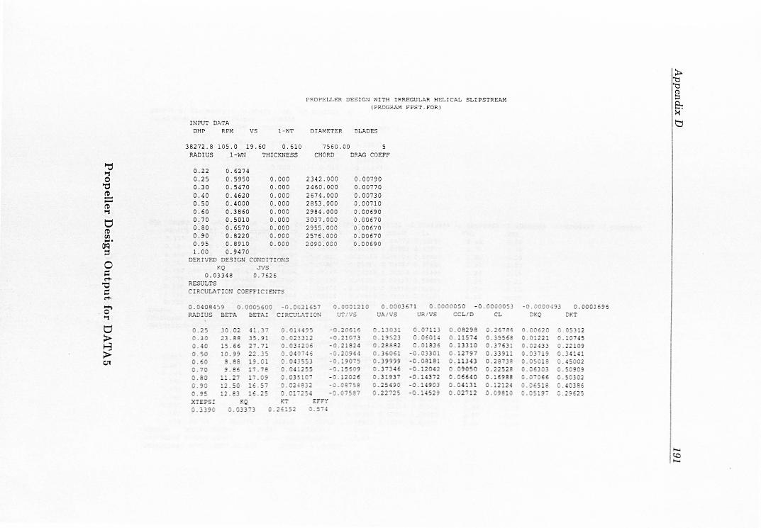
~ .., o ~ t'D --t'D .., tj t'D C/l ~.
::s o -... t+"0 t:: t+-
O' '"l
u ~ > 01
PROPELLER DES IGN WITH IRREGULAR HELIC AL SLIPSTREAM (PROGRAM FPST.FOR)
INPUT DATA DHP RPt1 VS 1-WT DIAMETER BLADES
38272.8 105.0 19.60 0.6 10 7560.00 RADIUS 1 - ~1N THICKNESS CHORD DRAG COEFF
0.22 0.6274 0.25 0.5950 0 . 000 2342.000 0.00790 0.30 0. 5 470 0 . 000 2460.000 0.00770 0 . 40 0.4620 0.000 2674.000 0.007 30 0. 50 0 . 4000 0 .000 2853.000 0 . 00710 0.60 0. 3860 0.000 2984.000 0.00690 0.70 0.5010 0.000 3037.000 0.00670 0.80 0 . 6570 0.000 2955.000 0.00670 0.90 0.8220 0 . 000 2576.000 0 .00670 0 . 95 0.8910 0.000 2090.000 0.00690 1. 00 0.9470
DERIVED DESIGN CONDIT I ONS KQ JVS
0.03348 0.7525 RESULTS CIRCULATION COEFFIC IENTS
0.04084 59 0.0005600 RADIUS BETA BETAl
- 0 . 00 2165 Ci RCULATION
0.0001210 f / VS
0.000 3 671 0.0000050 - 0.00000 53
0 .25 30.02 4 1. 37 .30 23.88 35.91
0.40 15.66 27.71 0. 50 10.99 22 . 35 0.60 S.88 19.01 0.10 9 .8 6 1;.78
11. 27 17. 09 .9!J 12 . 50 16 . 5 .9 5 12.83 15.25
XTE?Sr K
. 3J90 O.03r3
UA / VS
0.O l 44 95 -0.20616
;:1' :;:;:-, 5:52 O.S7 ~
Uil l VS
0.07113 .050 H
0.0183
CC L I D
0.08298 0. 11574 0. 13310
CL - 0.0000493
DK
0.000J695 KT
0.05312 .1074 5 . 22109 .341"
.2962 5
~ "i::l "i::l § ~
>< ' t:l
..... ~ ......

r.n <+ ~ <+ o ""l
tj I'D til
Oij'
= o = <+ '0 = <+
0' ""l
tj > ~ .....
STATOR D. (In Net 8 r) = (l. ~S63 6 NO. o r llLADES= Axial Distance (AXD / R(pr) = 0.6000
RADIUS 1-WN 0.30 0 . 32 0. 6502 0 .37 0 .7554 0.44 0.54 0 . 65 0 . 76 0.86 0.93 0.98 1 .0 0
0 . 8573 0.8972 0.9120 0.9216 0 . 9290 0 . 9342 0.9373
THICKNESS
0 .000 0.000 0 . 00 0 0.000 0.001 0.001 0.001 0.001 0.001
CHORD
0 . 040 0.0 40 0 .039 0 .037 0.033 0.028 0.022 0 .016 0 .01 2
STATOR DESI GN
DRAG COErF
0 . 01575 0.0 1582 0.0 1600 0.01637 0.01711 0.01824 0 . 02029 0.02311 0 . 02698
CIR. COErr. (H) - 0. 00774855 - 0 . 00211062 - 0 . 001 41739 -0.0 00 537 35 -0. 000 42435 RADI US BETAI CIRCULATI ON UTS / VS UTP/ VS UAP/VS CCLID CL 0 . 317 81.14 -0.006016 0.04490 - 0 .1669 5 0.13246 0 .04772 0.5485 8 0.367 83.99 -0.007916 0.05477 - 0 . 14842 0. 13391 0.05562 0.6 377 4 0.444 87.28 -0.008007 0.067 57 - 0.1 1412 0.12360 0.0 5123 0.59644 0. 542 88.78 -0. 007521 0 .05 2 5 8 - 0 . 07 387 0.09866 0.04744 0 . 57 88 6 0 .650 89.23 - 0.00 6473 0.04106 - 0 .05447 0.0 900 9 0 .04058 0.5544 8 0.758 89.31 -0.005 83 8 0.03400 - 0 . 0 462 0 0 . 09078 0. 0 3623 0. 58 42 5 0 . 8 56 89.2 5 - 0.004875 0 . 02647 - 0.03 9 74 0 . 08976 0 . 0 3 006 0. 6351 3 0 . 933 88.64 -0. 003155 0.00993 - 0 .03414 0.08610 0.01943 0. 554 07 0.9 83 88.33 - 0 . 002515 0.00391 - 0.03384 0.08622 0.01 543 0.G070a
STATOR TORQUE (r.NM) = 0.78 TH r:.UST (K!l) = 0.04 PROPELLER TORQl}E (KN~:) = 0 . 83 TH PUST ( iWl = ;'3 PROPULSORS ErrICI ElICY =0.650 GAl ~!(~) = ~.5 S3
STATOR DESIGN ;'I.~E F" a~LNi'=-ir;G T HE TORQU E
- 0.1 '5.5 95 - 0 . - 0 . - oJ. - ;J.
- 0. - .:L C39--! -v.C:; ..; i - " . C;}1 S ~
7:-i?;;sr 0;];) = 7,",:?~5: { tQ; ) = - . 3J
~:"ll: f ! ) = J . 5.JC
- 0.00005820 -0 . 00034659 TKO
0.46 0.79 1.06 1. 24 1. 28 1. 36 1. 2 9 0 .92 0.77
0. ~9
. 8 4 ! . 13 1 . 1 :
..,-; :. . ~ ~ L38
.22
TKT 0.80 0.76 0.22
- 0.07 -0 .15 - 0. 15 - 0 . 13 - 0.0 - 0.05
- Q - ~ ,:
- ' ".1 J -.: . - ::1.)5
0 .00009578 - 0 . 00006360
~ .'i:l 'i:l (b
::l c... ><' tl
'-' \0 t-v
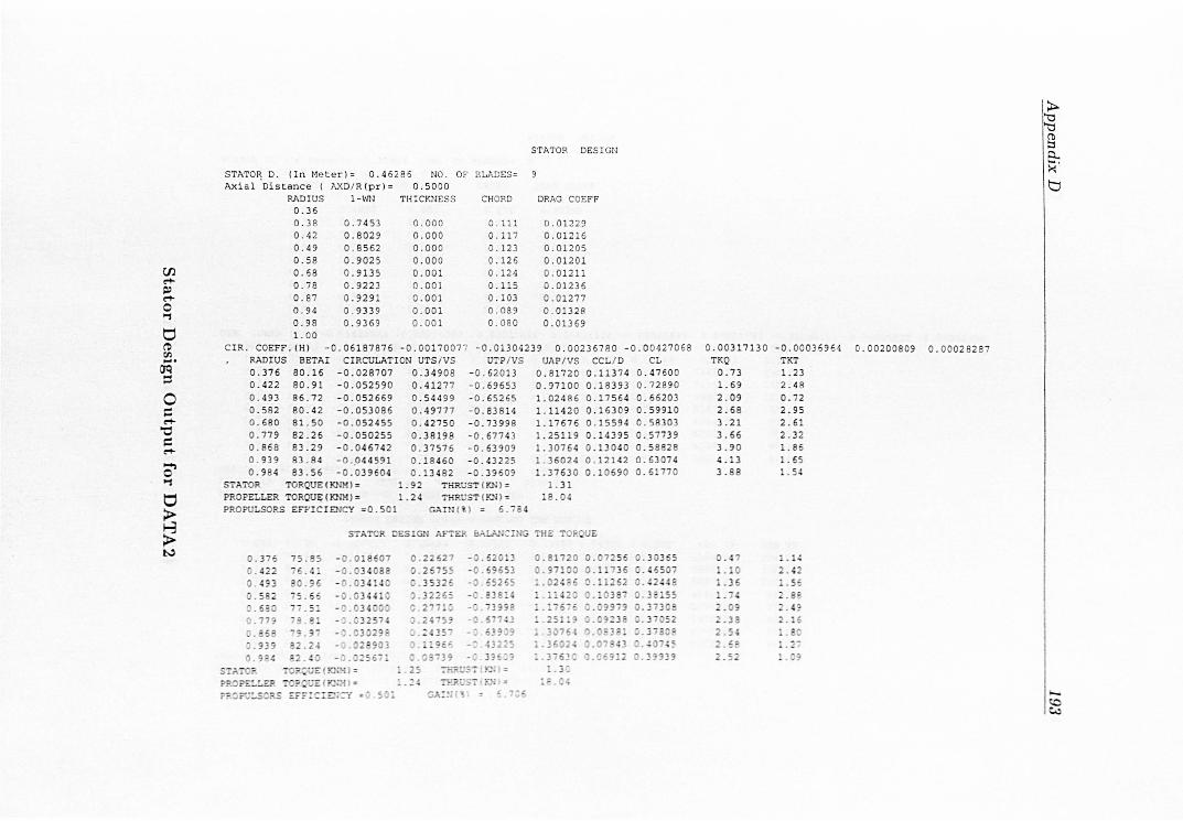
en ..t~ ..to "1
tj ~ en
otj0 ~
o ~ ..t
"0 ~ ..t-
0' "1
t:I
~ ~
STATO~ D. (In Meter) = 0. 4 6286 NO. OF BLADES= Axial Distance (AXD/R( pr) = 0 .5 000
RADIUS 1-WN 0.36 0.38 0 . 7453 0 . 42 0.8029 0.49 0.8562 0. 58 0.9025 0.68 0.78 0 . 87 0.94 0.98 1 .00
0.9 135 0.9223 0.92 9 1 0.9 33 9 0 . 9369
THICKNESS CHORD
0.000 O. III 0 . 000 O. 117 0 . 000 0.123 0 . 000 0.126 0 .001 0.124 0.00] 0.115 0 .00] 0 . 103 0.001 0.089 0 . 00] 0 . 080
STATOR DESIGN
DR1,G COEFF
0 .01229 0.01216 0.01205 0 . 01201 0 . 0 1211 0.01235 0.0 1277 0.01328 0 . 01369
CIR. COEFF. (H) -0.06187 876 - 0.0017007 7 -0.01304239 0.00236780 - 0.00427068 RADIUS BETA I 0. 376 80.16 0. 422 80.91 0. 493 86.72 0.582 80.42
CIRCULATI ON UTS /VS -0.028707 0 . 34 908
UTP IVS - 0.62013
- 0 .0525 90 0.41277 - 0.69653
0.680 0.779 0.868 0.939 0. 98 4
81.50 82.26 83.29 83.84 83. 5 6
- 0.0526 69 -0.053086 - 0.05245 5 - 0.050255 - 0.04674 2 - 0 . . 0 44591 - 0.03960 4
STATOR TORQUECKNM) = PROPELLER TORQ~CKNM) =
PROPULSORS EFPICIENCY =0.501
0 .544 99 0. 4 9777 0. 42750 0. 3 8198 0. 3 7 576 0.18 460 0.13482
- 0.65265 - 0.83814 - 0.73998 - 0.67743 - 0.63909 - 0.43225 - 0.39609
1. 92 1. 24
THRUST ( K!; ) = THRUST CKN J =
GiUtl(% ) = 6 . 7
UAP / VS CCL I D CL 0.81720 0.11374 0 .4760 0 0.97100 0 . 18 39 3 0.72890 1.024 86 0.17 564 0 . 66203 1.11420 0.1630 9 0.599 10 1.17676 0.15594 0 .58303 1.25119 0.1439 5 0 . 57739 1.30764 0.130 40 0.58828 1 .36024 0.12142 0.63074 1.37630 0.10690 0.6177
1 .31 18.04
STATOR DESIGN AFTER S;,!.l,.tICIKG THE TORQU E
0.376 75.85
s·] .:..
J.2 4-S9 ::. ~(!5-
O. 1:9E::
: . 2 :.24
S'J9 : l; ~:?
::";J~:'''S-; ~~: ) = TFj'; t:5T :~: =
G.A : ~; r: :. - ~s
t. ~ G
: E.C
. 30 365
.46501
.42 44 e
. JEiS:'
0.00 31713 0 - 0.00036964 TKQ TKT
0 . 73 1. 23 1. 69 2.48 2.09 0 . 72 2 .68 2 .9 5 3 . 21 2.61 3.66 2. 32 3.90 1. 86 4 .13 1. 65 3.88 1. 54
0.4 LI C 2.~
1.36 L5~
1.14 2.8: 2.09 2.'? 2. ]S 2 . 15 2.5~
2.5£ 1.27 .52 !. O~
0.002 00809 0 . 00028287
~ '"0 ,'"0 ~ 0... .... . ~
t:J
,.... (C ~

r.n .... ~ .... o '1
o ('tI r.Jl
aq' ::= o s:: ~
"e s:: ~
~ '1
tj
~ > ~
STATOR DESI GN
STATOR D. (In t-Ieter): 7.30863 NO. OF BLADES= 9 Axial Distance (AXD / R(pr)= 0.6000
RADIUS 1-WN 0.24 0.26 0.32 0 . 40 0 .5 1 0.6 2 0.74 0.84 0.93 0.98 1. 00
0.4880 0. 5396 0.6293 0.7778 0 .8585 0.89 3 0 0.90 55 0 .9079 0.9090
THICKNESS
0.001 0 . 002 0.005 0 . 008 0.011 0.01 4 0 . 017 0.020 0 . 021
CHORD DRAG COEFF
0.976 0.00780 1 . 034 0.00774 1. 08 6 0.0 077 0 1.1 07 0 .00771 1 . 073 0 . 00781 0 . 971 0.00803 0.835 0.00836 0 . 673 0 . 00887 0.567 0.00932
crR. COEI'F. (H) -0.0 1623 082 - 0.000103 03 -0 . 00221844 0 .00041324 -0.00 06 5649 0.00025794 - 0.000601 02 - 0. 00010238 - 0.00030706 RADIUS BETAI CIRCULATION UTS / VS UTP/ VS
0 . 263 71 . 65 - 0.00 7530 0 .1092 0 -0 .31521 0.3 17 74 . 89 - 0 . 010B07 0 . 139 Bl -0 .34 079 0 .400 80.74 - 0 .014184 0. 16 831 - 0.31 050 0 . 505 85.62 - 0 .014342 0.1 523 7 - 0 .22976 o. G/.? 86.S' - 0 .014375 0. 12552 - n . IA51R 0 .739 87.50 - 0. 014046 0 .110 09 - 0 .15 99 3 0.844 B7.75 - 0 .013004 0.09885 - 0 .14479 0 .928 86.28 -0.01 0989 0.057)4 - 0 .134 13 0.982 85.17 - 0 .008566 0.03353 - 0 .1)330
STATOR TORQUE (YJlM ) = 3432 . 28 THRUST(KN ) = PROPELLER TORQUE (~1) = 3279 . 41 THRUST(KN ) = PROPULSORS EFFICIENCY =0.752 GAI N(%) = 4.705
U,\PIVS CCL / D CL 0.13327 0.072 29 0 .54124 0.20466 0.08808 0.62245 0.24274 0 . 10086 0 .67910 0 .23171 0.08900 0.58739 0.23 14 ry P.0822 9 0.56 048 0.25 029 0 .077 12 0.5803) 0.26498 0 .06976 0. 51041 0.27308 0 . 058) 4 0.63365 0.27286 0 . 045)8 0.58542 105.56
2138 . 23
STATOR DESIGN AF~ER 3ALANCING THE TORQUE
0.263
S-':;"TC R
? ? P:l
- " . 00 0_10434
:-:-:::.uS7 f :~; 1 = 2 : 3; . 23 c;;..n; ( '1 ) : .; . i -; 5
.51592
. 59H6
TKQ 650.91
1345.70 2611 . 97 3858.85 5167.84 6254.91 6773.45 634 9.15 5241.41
522_13 1285.11
TKT 213.93 298.71 270 .55 132.62 93.23 68.90 56.06 95 . 47 99.98
208 .9 9
~ :g ~ Q.. ><.
tl
...... ~ ..::..

en ~
ll.l ~
o .., tJ C'tI til
ciQ" = o == ~
"tl
== ~
~ .., tj
~ .z:...
STATOR DESIGN
STATOR D. (In Me~er )= 7.87960 NO. OF BLADES= 10 Axial Distance (AXD / R(pr)= 0.6000
RADIUS l-WN THICKNESS 0.23 0.25 0 . 30 0. 39 0.50 0.61 0.73 0.84 0.93 0.98 1. 00
0. 3244 0.3 543 0.4109 0.5207 0.6851 0.7867 0.8441 0.8 636 0.8717
0.001 0.002 0.005 0.008 0.012 0.015 0 . 019 0.021 0.0 23
CHORD DRAG COE??
1.726 0.00701 1.730 0 . 00702 1 .708 0.00706 1.629 0.00715 1.494 0.00730 1 . 282 0.00758 1.028 0.00799 0.779 0.00858 0.624 0.00913
ClR. COE?F. (HI - 0.02446066 -0.0031449 8 - 0.00379712 0.00011798 - 0.00131048 -0.00015413 -0 . 00109232 - 0.00021951 - 0.0 003 3132 RADIUS
0.248 0 . 303 0.388 0. 495 0.614 0.734
BETAl 71.58 69 . 87 77.47 82.06 85.31 86.47
0.84 1 87.02 0 .926 85.52 0.981 84.28
CIRCULATI ON UTS / VS -0.0149 39 0 . 23536 -0.019378 0.29439 -0.023436 0.33033 -0.023 33 7 0 . 27493 -0.021213 0.20979 -0.019380 0. 16584 -0.017079 0.13844 -0.014133 0.07981 -0.010915 0.04690
UTP / VS UAP/VS CCL/D CL -0.47653 0.39983 0.12297 0.56148 -0.61066 0.50855 0.13249 0.60353 -0.553 53 0.59344 0.14313 0.66047 - 0.43328 0.61457 0 . 12792 0.61876 - 0 .311 98 0.559 44 0.10674 0.56300 - 0 .24767 0.54034 0.09159 0 . 56296 - 0 .2101 0 0. 53376 0.07778 0.59594 - 0. 18999 0.5 4399 0.06290 0.636 28 - 0. 1889 4 0 .5 4654 0. 0 4812 0.60 77 0
STATOR TORQUE(KNM)= 2563 . 78 PROPELLER TORQUE(~1~) = 2246.28 ?ROPULSORS EFFICI ENCY =0 .62S
TP~UST(KN ) = 121 . 9 8 THRUST (KNI = 2134 . 24
GAIN( ~) = 5.406
?R.'
.2 48
.303
. 3 0. 495
STATOR DESIGN AFTER 3.'ili!'':;CniG THE TORQUE
- 0.0 13089 0.39983 0.10639 0.48 57 7 .508 55 0. 11~44 0.521 31 . 593~~ 0.12 424 0. 57330
. 53969
125. 49 2U~ . H
5
TKQ TKT 632.83 206.88
1194.10 354.00 2150.78 29 7 .05 308 9.35 202.18 3816.68 108.88 4437.94 73.95 4654.88 54.18 4335.60 76.88 3574.99 78.62
555 . 14 202 .92 10 4 7.51 345.48 1885 . 0 '; 308.38 270 8,46 216.33 334 5.55 121.63 3889 . 71 83. 0 2 401 9 . 56 60. 4)
99 .6:- 72.67 llH.13 70. 0
~ :g g c.. ~.
tl
!-.. (Q <:""1
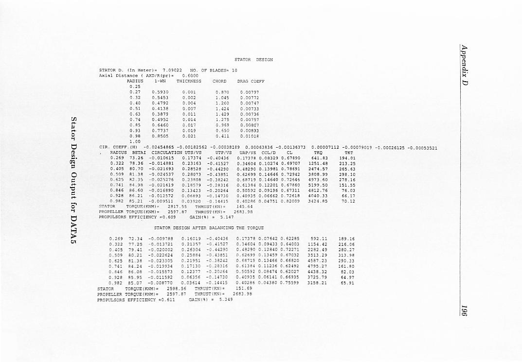
en ~
~ ~
o '"l
o (t)
'" aq' =' o ~ .....
"C ~ ..... 0-'"l
o
~ c:11
STATOR DESIGN
STATOR D. (In Meter)= 7.09022 NO. OF BLADES= 10 Axial Distance (AXD / R(pr)= 0.6000
RADIUS 1-WN THICKNESS CHORD DRAG COEFF 0.25 0 . 27 0.32 0 .40 0 . 51 0 .63 0 . 74 0.8 5 0.93 0.98 1. 00
0 . 593 0 0 . 5453 0.4792 0.4138 0. 3879 0.4952 0.6 46 0 0.7737 0.8505
0 . 00 1 0.002 0.004 0.007 0.011 0.014 0 . 01 7 0 . 0 19 0.021
0.870 1.045 1 .260 1.424 1 . 429 1.275 0.969 0.650 0. 411
0.00797 0.00772 0.00747 0 . 007 33 0.007 36 0.00757 0.0080'7 0.00893 0.01018
crR. COEFF . (H) -0 .02 454865 - 0.00182562 -0 . 000381 89 0.00063836 -0.00136373 RADIUS 0.269 0.322 0.405 0.509 0.62 5 0.7 41 0.8 46 0. 928 0 . 9B2
BETAI CIRCULATION UTS / VS 73.26 78.36 80.70 81. 38 R2 . 35 84.98 86.60 86.21 R5 . 21
- 0. 010615 -0. 014881 - 0.021693 -0 .024537 -0.025276 - 0.021619 -0 .016890 -0 .012572 -0 .009511
0.17374 0.23163 0.28528 0 .2 8073 0.23R08 0 . 1 8 57 9 0.13423 0.0689 3 0 .03920
UTP /VS UAP /VS - 0.40436 0.17378 -0.41527 0.34604 - 0.44290 0.48290 - 0.43851 0.62699 - 0.38242 0 . 68719 - 0 . 2831 6 0 . 61384 - 0.20264 0.50592 - 0 . 1473 0 0 .4 09 35 -0 . 14415 0.402R
STATOR TOROUE (KN1~) = 28 17 . 55 PROPELLER TORQUE(KNM)= 2597 . 8 7 PROPULSORS EFFICIENCY =0 .609
THRUST ( KN)= 145 .64 THRUST(KNI = 26R3.98
GAIN( %) = 5.147
CCLID CL 0.08329 0 .67890 0.10274 0.69707 0 .13 981 0.78691 0.14646 0.72942 0 . 14640 0.72646 0.12201 0.67860 0.09196 0.67311 0.06662 0 . 72618 0.0 4751 0.82009
STATOR DESIGN AFTER BALANCING THE rluUE
0.269 72.34 0.322
57 ( K1r ) = : r.?usr (;::1) = 26
5 . ]~9
0.00007112 -0.000790 19 - 0 .00026125 - 0.00053521 TKO TKT
641. 8 3 1251. 48 2474.57 3 808 .9 9 4973 . 60 5199 . 50 4812.76 4 0 40 . 33 34 2 4 .8 5
3
194.01 213 .25 265.63 298 . 10 278.16 151.55 76. 03 66.17 70 . 12
64 . 9 65 . 9 "
l:g ~ c... ..... >< b
..... (0 C)
Related Documents
![Rational, unirational and stably rational varietiespirutka/survey.pdf · could be rational (resp. stably rational, resp. retract rational) [30, p.282]. Unirational nonrational varieties.](https://static.cupdf.com/doc/110x72/5f8fad2d18211140cf6c6b61/rational-unirational-and-stably-rational-varieties-pirutka-could-be-rational.jpg)