A posteriori error analysis for elliptic PDEs on domains with complicated structures

A POSTERIORI ERROR ANALYSIS FOR ELLIPTICPDES ON DOMAINS WITH COMPLICATED

STRUCTURES

CARSTEN CARSTENSEN AND STEFAN A. SAUTER

Abstract. The discretisation of boundary value problems on com-plicated domains cannot resolve all geometric details such as smallholes or pores. The model problem of this paper consists of a tri-angulated polygonal domain with holes of a size of the mesh-widthat most and mixed boundary conditions for the Poisson equation.Reliable and efficient a posteriori error estimates are presented fora fully numerical discretisation with conforming piecewise affinefinite elements. Emphasis is on technical difficulties with the nu-merical approximation of the domain and their influence on theconstants in the reliability and efficiency estimates.

!!!!!!!!!!!!!!!!!!!!

""""""""""""""""""""

####$$$$

%%%%%%%%%%%%%%%%

&&&&&&&&&&&&

''(()))))))))))))))))))))))))

********************

++++,,,,

---------.........

////////////////

0000000000000000

111111222222333333444444

555555555555555555555555555555

666666666666666666666666666666777

777888888

999999999999999999999999999999999999

::::::::::::::::::::::::::::::::::::;;;

;;;<<<<<<

==============================

>>>>>>>>>>>>>>>>>>>>>>>>>>>>>>

????????????????????????????????????????????????????????

@@@@@@@@@@@@@@@@@@@@@@@@@@@@@@@@@@@@@@@@@@@@@@@@@

AAAAAAAAAAAAAAAAAAAAAAAAAAAAAA

BBBBBBBBBBBBBBBBBBBBBBBBBBBBBB

CCCCCCDDDDEEEEEE

EEEEEEEEEEEEEEEEEEEEEEEE

FFFFFFFFFFFFFFFFFFFFFFFFFFFFFF

GGGGHHHH

IIIIIIIIIIIIIIIIIIIIIIIII

JJJJJJJJJJJJJJJJJJJJJJJJJ

KKKKKKKKKKKKKKKKKKKKKKKKKKKKKKKKKKKK

LLLLLLLLLLLLLLLLLLLLLLLLLLLLLL

MMMMMMMMMMMMMMMMMMMMMMMMMMMMMM

NNNNNNNNNNNNNNNNNNNNNNNNNNNNNN

OOOOOOOOOOOOOOOOOOOOOOOOOOOOOOOOOOOO

PPPPPPPPPPPPPPPPPPPPPPPPPPPPPP

QQQQQQQQQQQQQQQQQQQQQQQQQQQQQQ

RRRRRRRRRRRRRRRRRRRRRRRRR

SSSSSSSSSSSSSSSSSSSSSSSSSSSSSSSSSSSS

TTTTTTTTTTTTTTTTTTTTTTTTTTTTTTTTTTTT

UUUUUUUUUUUUUUUUUUUU

VVVVVVVVVVVVVVVV

WWWWWWWWWWWWWWWWWWWW

XXXXXXXXXXXXXXXX

YYYYYYZZZZZZ[[[[[

[[[[[[[[[[[[[[[[[[[[[[[[[

\\\\\\\\\\\\\\\\\\\\\\\\\\\\\\

]]]]]]]]]]]]]]]]]]]]]]]]]]]]]]

^^^^^^^^^^^^^^^^^^^^^^^^^

____________________________________

````````````````````````````````````

aaaaaaaaaaaaaaaaaaaaaaaaaaaaaa

bbbbbbbbbbbbbbbbbbbbbbbbbbbbbb

cccccccccccccccccccc

dddddddddddddddd

eeeeeeeeeeeeeeeeeeeeeeeee

ffffffffffffffffffff

gggggggggggggggggggg

hhhhhhhhhhhhhhhh

iiiiiiiiiiiiiiiiiiii

jjjjjjjjjjjjjjjjjjjjkkkkkkkkkkkkkkkkkkkkkkkkk

lllllllllllllllllllllllll

mmmmmmmmmmmm

nnnnnnnnnnnn

ooooooooopppppppppqqqqqqrrrrsstt

uuuuvvvvwwwwxxxx

yyz|

~~~~~~~~~~~~~~~~

Figure 1. Intersection of a triangle T with the domainΩ at the boundary.

Date: June 7, 2001.1991 Mathematics Subject Classification. 65N30, 65R20, 73C50.Key words and phrases. finite element method, a posteriori error estimates,

adaptive algorithm, reliability, efficiency.1

2 CARSTEN CARSTENSEN AND STEFAN A. SAUTER

1. Introduction

Porous media or advanced materials with microstructures provide ex-amples for boundary value problems with small geometric details. Typ-ically, those details cannot be completely resolved by the mesh of afinite element discretisation, but have to be involved. This work is de-voted to the mathematical analysis for the Poisson equation on a do-main with holes of a mesoscale: Large holes are resolved by the finiteelement mesh exactly, but holes of the diameter of the mesh-size andsmaller are not, as illustrated in Fig. 1. Efficient and reliable a poste-riori error estimates are derived for a conforming piecewise affine finiteelement scheme on a triangulation which covers a bigger domain Ω?

that includes the domain Ω with holes inside and on the surface.

For elliptic problems on complicated domains, the minimal dimensionof any finite element space is huge since the finite element mesh hasto resolve the geometry. Thus, from the viewpoint of accuracy andbalancing of local errors, we cannot expect that the degrees of freedomof such a finite element space are distributed in a (nearly) optimalway. In [HS1], composite finite element spaces have been introducedwhere the minimal number of unknowns is independent of the sizeand number of geometric details. The combination of composite finiteelement spaces with an a posteriori error estimator (used as an errorindicator) allows to design problem-adapted finite element spaces wherethe adaptation process starts from very coarse levels.

In addition, by using this a posteriori error estimator the finite elementerror can be estimated on discretisation levels where not all geometricdetails are resolved by the mesh (but taking them into account by usingcomposite finite element functions).

Our paper is devoted to the definition and analysis of a reliable andefficient a posteriori error estimator. As a model problem we will studythe Poisson problem −∆u = f with mixed boundary conditions. Wewill consider a Lipschitz domain Ω which arises by removing from apolygonal domain Ω? a possibly huge number of holes. “Holes” aresimple connected domains which are collected in the set of holes C. Wesuppose homogeneous Neumann boundary conditions on the boundaryof holes, e.g., for small bubbles of gas.

The discretisation is based on a conforming triangulation T of theoverlapping domain Ω? with continuous, piecewise affine finite elementsand their restrictions to the domain Ω. In a first phase, a T -piecewiseaffine discrete function U ? is computed on Ω? while the approximationof the continuous solution u is given by U := U ?|Ω.

A POSTERIORI ERROR ANALYSIS FOR COMPLICATED DOMAINS 3

!

"$#

%

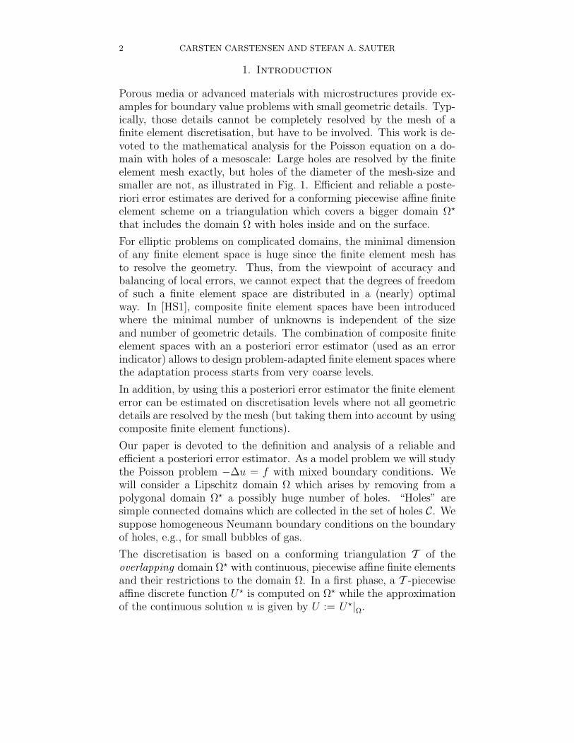
Figure 2. Intersection of a hole ω with ∪E .

Our reliable a posteriori error estimator will be presented in Section 3.Besides error residuals, we obtain, for an interior hole ω ∈ C, the term

η2ω := hω

∫

∂ω

|∂U/∂nω |2 ds

corresponding to ∂u/∂nω = 0 on ∂ω (and modifications for any holewhich touches the boundary).

We carefully study the efficiency of this contribution where difficultiesarise from the fact that ω may be intersected with edges of the trian-gulation T in a quite arbitrary and complicated way; compare Figure 2for an illustration.

Our main result can be stated as follows. Suppose u ∈ H1(Ω) denotesthe exact solution and U = U ?|Ω its discrete approximation. If allintegrals are evaluated exactly (otherwise we obtain inconsistency errorsources ηc), the error in energy norm ‖∇(u − U)‖L2(Ω) is bounded by

η := ‖hT f‖L2(Ω) + ‖h1/2E [∂U?/∂nE ]‖L2(∪E) + (

∑

ω∈C

η2ω)1/2,

where hT (resp. hE , hω) is the local mesh-size (resp. edge-size, hole-size), and [∂U?/∂nE ] is the jump of the normal components of two(T -piecewise) discrete gradients across the edges (and standard modi-fications on the boundary). Theorem 3.1 implies (for exactly matchedDirichlet boundary conditions) the reliability of η in the sense of

‖∇(u − U)‖L2(Ω) ≤ c1 η.


Theorem 6.1 shows efficiency, i.e., the converse inequality

c2 η ≤ ‖∇(u − U)‖L2(Ω) + h.o.t.

In the latter inequality, h.o.t. are known higher order terms and it holdsin a local form. The constants c1 and c2 are independent of mesh-sizesor hole-sizes. They depend on some features of the geometry of holes.For instance, c1 stays uniformly bounded if the holes are circular withdiameter hω ≤ c3 hT for neighbouring elements T of size hT provided aseparation condition is satisfied, namely, two distinct holes ω1 and ω2

have a distance dist(ω1, ω2) with hω1 + hω2 ≤ c4 dist(ω1, ω2). To boundc2 from below, we will assume in addition that hω < c4 dist (ω, Γ?)holds. It is stressed that, then, c1 and c2 are independent of the waythe edges intersect with holes and tiny pieces as well as entire edgesmay lie inside the hole.

As a setting for this, the behaviour of the constants appearing in sometrace estimates and in estimates of norms of appropriate extension op-erators on some geometry parameters will be investigated in Section 4.The reliability of the a posteriori error estimator (stated in Theorem3.1) will be proved in Section 5. The conditions sufficient for the ef-ficiency estimate of Theorem 6.1 may appear technical at first glance.Therefore, included examples illustrate the consequences of Assump-tions 6.1 till 6.8. The proof in Section 7, however, clearly underlinesthat the assumptions posed are natural. The analysis of edge andvolume contributions per se requires minor modifications of standardtechniques [V] while the investigations of the hole contributions aremore involved. We emphasise that, in contrast to [DR], where the ef-fect of approximating the boundary of the domain is incorporated inthe error estimator, our finite element spaces are defined on the truedomain while the construction allows a low-dimensional discretisationeven for very complicated domains.

2. Model problem

As a model problem we consider a domain Ω ⊂ 2 which arises byremoving holes from a polygonal domain. More precisely, let Ω? ⊂ 2

denote a polygonal domain with boundary Γ? = ∂Ω? and let C =ωj : 1 ≤ j ≤ J be a countable set of simply connected Lipschitz do-mains ωj, the ‘holes’, which have a positive distance from each otherand are all (not necessarily compactly) contained in Ω?. The physical

domain Ω := Ω?\⋃ C is supposed to be Lipschitz (as a further assump-tion on the intersections of the hole boundaries ∂ω with Γ?). Mixedboundary conditions are imposed on the boundary Γ := ∂Ω, namely


homogeneous Neumann boundary conditions on γ := Ω? ∩ ∂ (∪C), pre-scribed Neumann data g on ΓN := (Γ∩Γ?)\ΓD, and prescribed Dirichletdata uD on ΓD ⊂ Γ ∩ Γ? of positive length.

Remark 2.1. Note that ΓD∪ΓN = Γ? if Ω? includes all holes compactly.Otherwise, the inclusion ΓD ∪ ΓN ⊂ Γ? can be strict.

The strong formulation of the continuous problem reads: Given f ∈L2(Ω), g ∈ L2 (ΓN), and uD ∈ H1(ΓD), seek u ∈ H1(Ω) satisfying

∆u + f = 0 in Ω, u = uD on ΓD,

∂u/∂n = g on ΓN , ∂u/∂n = 0 on γ.(2.1)

Since the normal derivative of u vanishes at interior boundaries of holes,the weak formulation reads: Seek u ∈ H1(Ω) with u|ΓD

= uD and

(2.2)

∫

Ω

∇u · ∇v dx =

∫

Ω

f v dx +

∫

ΓN

g v ds

for all test functions v ∈ H1D(Ω) := v ∈ H1(Ω) : v|ΓD

= 0.The discretisation of the model problem is based on composite finiteelements which are defined in three steps (i)-(iii) [HS1].

(i) The (overlapping) triangulation. The polygonal domain Ω? ispartitioned exactly by a regular triangulation T into closed trianglesT ∈ T in the sense of Ciarlet [BS, Ci], Ω? = ∪T . Two non-disjointdistinct triangles in T share either a common edge E or a vertex z callednode. The set of all edges resp. nodes is denoted by E resp. N . Edgeson the boundary Γ? (belong to only one triangle and) are collected inthe set EΓ? = ED ∪ EN , where EΓ? is split into edges of Dirichlet- andNeumann type as follows. Let |E ∩ ΓD| and |E ∩ ΓN | denote the one-dimensional measure of the sets E∩ΓD and E∩ΓN , respectively, alongthe edge E ∈ EΓ?; suppose that either |E ∩ ΓD| or |E ∩ ΓN | is positive(but not both of them). Then, set ED := E ∈ EΓ? : |E ∩ΓD| > 0 andEN := EΓ? \ ED, EΩ := E \ EΓ?, and Γ?

N := ∪EN resp. Γ?D := ∪ED.

(ii) The (overlapping) finite element space. Let S? denote thespace of T -piecewise affine finite elements and S?

D its subspace withvanishing traces on Γ?

D, i.e.,

(2.3)S? := V ∈ C(Ω?) : ∀T ∈ T , V |T is affine on T ,S?

D := V ∈ S? : V |Γ?D

= 0.


(iii) The (restricted) composite finite element space. The spacesS and SD are given by

S := S?|Ω := V ∈ C (Ω) : ∃V ? ∈ S?, V = V ?|Ω ,

SD := S?D|Ω.

Remark 2.2. Using ΓD ⊂ Γ? we have

S?D = V ∈ S? : ∀E ∈ ED, V |E = 0 .

Remark 2.3. Throughout the paper we write u, v, for functions lying inthe infinite dimensional space H1 (Ω), H1

D (Ω) and U, V, . . . for functionsin the finite element space S, SD. Functions on the extended domainΩ? have a superscript ?, e.g., u?, U?. Approximations to the right-handsides and the porosity (see below) are denoted with a tilde superscript

as, e.g., f , g, while f ? is the extension of f from Ω to Ω? by zero. If vand v? appear in the same context, we understand v = v?|Ω.

The intersection of an element with the domain and some notationsare illustrated in Fig. 1. Note carefully that domains are open andconnected and that T ∈ T and E ∈ E are closed sets in 2 ; the interiorof T is denoted by int(T ).

To define a fully numerical discretisation, we need to approximateDirichlet data uD ∈ H1 (ΓD) by the trace of some function U ?

D ∈ S?.The finite element scheme requires a stiffness matrix where, for eachelement T ∈ T of area |T |, some constant %|T approximates the ratio%T := |Ω∩T |/|T |, where % ∈ L0(T ) and L0(T ) denotes the T -piecewiseconstants. Furthermore, the computation involves approximate right-hand sides f ? ∈ L2(Ω?) and g? ∈ L2(Γ?

N). Then, the discrete problemreads: Seek U ? ∈ S? and U := U?|Ω satisfying U? = U?

D on Γ?D and, for

all V ? ∈ S?D,

(2.4)

∫

Ω?

%∇U? · ∇V ? dx =

∫

Ω?

f ?V ? dx +

∫

Γ?N

g?V ? ds.

Remark 2.4. Notice that the computational cost for solving the discreteproblem (2.4) are small as the geometry is not resolved in detail (useof Ω?, Γ?

D, Γ?N instead of Ω, ΓD, ΓN) and holes are taken into account

only via an approximate porosity. In the error analysis, those errorsshall be taken into account.

Remark 2.5. The integrals over intersections T∩Ω? should be evaluatedby using a composite quadrature rule employing a hierarchical resolu-tion of the domain (cf., e.g., [HS2, OR]). The efficient implementationof the a posteriori controlled discretisation scheme presented here will


be the topic of a forthcoming paper. Some ideas on the adaptive nu-merical integration will be sketched at the end of Section 3.

3. A posteriori error estimate

Suppose u ∈ H1 (Ω) is the exact solution of (2.2) and let U = U ?|Ω bethe restriction of the discrete solution of (2.4). The ingredients of theerror estimator for the energy error of u−U are the volume residual ηΩ,the edge contributions ηE, the hole errors ηC, the Dirichlet contributionηD, and the consistency term ηc.

Let hT (resp. hE) be a T -piecewise (resp. E-piecewise) constant weightto measure the mesh-size (resp. edge-size) regarded as L∞-functionson Ω? (resp. on ∪E). Then, the volume contribution reads

(3.1) ηΩ := ‖hT f‖L2(Ω) .

For each edge E ∈ E , let nE denote one unit normal on E with fixedorientation (oriented to the exterior if E ∈ EΓ?) and nE ∈ L∞(∪E)denotes their composition, i.e., nE |E := nE. The T -piecewise constantdiscrete gradient ∇U has a jump across each inner edge E ∈ EΩ andthe difference (∇U)|T+ − (∇U)|T−

is denoted as [∇U ] on E; T+ andT− are the two distinct elements which share the edge E such thatnE points into T+. Note that the jump of the normal components[∇U ] · nE =: [∂U/∂nE ]|E is independent of the chosen orientation ofnE. We regard nE and [∂U/∂nE ] as E-piecewise constant functions onthe skeleton ∪E of edges; ∪E is the set of all points x on some boundary∂T of some triangle T ∈ T . Then, the edge contribution reads

(3.2) ηE :=

∥∥∥∥h1/2E

[∂U?

∂nE

]∥∥∥∥L2(∪EΩ)

+

∥∥∥∥h1/2E

(g? − ∂U?

∂n

)∥∥∥∥L2(Γ?

N )

.

Owing to homogeneous Neumann conditions on γ, the analogue to theedge contribution defines the hole contributions,

(3.3) ηC :=

(∑

ω∈C

hω

∫

∂ω\Γ?D

|∂U?/∂nω|2 ds

)1/2

(hω denotes the diameter of ω ∈ C). In case that uD is the restrictionof a smooth function on Γ?

D, the Dirichlet contribution(3.4)

ηD := min‖∇v‖L2(Ω) : v ∈ H1(Ω) such that v = uD − U on ΓD


is of higher order (and then may be neglected). Finally, the abstractconsistency term is given by

(3.5) ηc := supW ?∈S?

D‖W ?‖H1(Ω?)=1

∫

Ω?

(f ? − f ?) W ?dx

+

∫

Γ?N

(g? − g?) W ?ds −∫

Ω?

(% − %)∇U ? · ∇W ?dx

.

Theorem 3.1. There exists an (hT , hE , u, U, f, g)-independent positiveconstant c1 such that

‖∇(u − U) ‖L2(Ω) ≤ c1(ηΩ + ηE + ηC + ηD + ηc).

The constant c1 depends on the domain Ω, ΓD, ΓN , and the shape ofthe elements in T (such as their aspect ratio) but neither on the numberor size of the holes in C nor the way they are hit by ∪E .

Sections 4 and 5 are devoted to the proof of the theorem while efficiencywill be studied in Sections 6 and 7.

A few remarks and examples on the evaluation of the error estimatorwill conclude this section.

The evaluation of the term ηE can be performed as described in [V]since U? is a standard finite element function and EΩ resp. Γ?

N consistsof triangle edges.

The remaining terms in the error estimator concern integrals over theintersections T ∩ Ω resp. T ∩ ∂ω which can be realized by adaptivelysubdividing T ; a triangle T is subdivided regularly by connecting themidpoints of edges.

The triangulation T (T ), which is generated for numerical integrationpurposes only, is the result of “T (T ) := ∅; refine(T, T (T ))”.

procedure refine(T, T ) ;

begin

if T ∩ Ω is a simple domain, i.e., the integrals∫

T∩Ω

. . . dx,

∫

T∩∂ω

. . . ds,

∫

T∩ΓN

. . . ds

can be approximated by standard quadrature formulae,

then T := T ∪ T


else begin

subdivide T regularly to obtain the children Tj4j=1;

for all 1 ≤ j ≤ 4 with int (Tj) ∩ Ω 6= ∅ do refine (Tj, T );

end; end;

By using the subdivisions T (T ), the contribution ηC can be evaluatedby

(3.6) η2C =

∑

ω∈C

hω

∑

T∈TT∩∂ω 6=∅

∑

K∈T (T )

∫

K∩(∂ω\Γ?D)

χ (n · ∇qT )2 ds

where qT := ∇ (U?|T ) and χ : ∂ω → 1/2, 1 is given by

χ (x) :=

1 if there is only one K ∈ T (T ) with x ∈ K,1/2 otherwise.

Since the main focus of this paper is the investigation of the hole con-tributions to the finite element error we discuss the error terms cor-responding to the data approximation ηD and ηc under simplifyingassumptions.

Example 3.1. Suppose that there is a function U ?D ∈ S? with uD =

U?D |ΓD

. Then, the Dirichlet contribution vanishes by making the ansatzU? = U?

D+U?0 and solving for U ?

0 . Note that U?0 vanishes at the Dirichlet

boundary.

Example 3.2. If there exists a continuous u?D : Γ?

D → with uD =u?

D|ΓDwhich is ED-piecewise smooth, i.e., u?

D|E ∈ H2(E) for all E ∈ ED,ηD can be of higher order. Indeed, it is proved in Lemma 4.1 of [CB]that, if U?(z) = u?

D(z) for all nodes z ∈ N ∩ ΓD, then

ηD ≤ c5‖h3/2E ∂2u?

D/∂s2‖L2(Γ?D),

where ∂/∂s denotes the derivative along E.

Example 3.3. Assume that the data f, g are sufficiently smooth. Wemay extend the function f ∈ L2 (Ω) to f ? ∈ L2 (Ω?) and g ∈ L2 (ΓN)to g? ∈ L2 (Γ?

N) by zero. In order to evaluate the integrals, we employthe subdivision T (T ) to obtain∫

Ω?

f ?V ?dx =

∫

Ω

fV dx =∑

T∈T

∫

Ω∩T

fV dx =∑

T∈T

∑

K∈T (T )

∫

Ω∩K

fV dx.

Since we assumed that the integrals over Ω ∩ K can be approximatedsufficiently accurate and f is smooth, the corresponding consistencyterm in ηc can be neglected. In a similar fashion, the integral over


Γ?N reduces to an integral over ΓN and the subdivisions T (T ) can be

employed for numerical integration as in (3.6).

Remark 3.1. By an adaptive resolution of the boundary generated bythe procedure refine, the amount of work for realising our finite ele-ment method is proportional to the number of elements in T plus thenumber of subdivided elements for resolving the curved boundary and,in this way, depends linearly on the number of geometric details.

4. Extension operators, trace theorems, and Poincare

inequalities on complicated domains

The proof of the reliability and the efficiency of the error estimator isbased on estimates of the norm of certain extension and trace operators.In this section, we will show that their norms are moderately boundedfor a broad class of domains which might contain a huge number ofsmall holes.

4.1. Extension operators. Let Ω ⊂ Ω?, ΓD, Γ?D, etc. be as in Sec-

tion 2 and H1D (Ω?) :=

v ∈ H1 (Ω?) : v|Γ?

D= 0

. In this section, we

will define an extension operator D : H1D (Ω) → H1

D (Ω?) so that thesupremum

supv∈H1

D(Ω)\0

‖∇ Dv‖L2(Ω?)/‖∇v‖L2(Ω) =: c6 < ∞.

is moderately bounded for large class of domains, which may containa huge number of geometric details.

Remark 4.1. The constant c1 will depend on c6.

The extension operator D is constructed in three steps. Let u ∈H1

D (Ω). Since Ω is a Lipschitz domain it is well known that thereexists an extension operator Stein : H1

D(Ω) → H1 (Ω?). Put u?1 :=

Steinu ∈ H1 (Ω?) and note that u|ΓD= 0. Next, we employ a function

m : Ω? → [0, 1] satisfying m ≡ 1 on Ω and m = 0 on Γ?D\ΓD to define

u?2 := mu?

1 ∈ H1D (Ω?). Finally, the local Ritz-projections u0

2 of u?2 on

ω ∈ C is subtracted to end up with u? := u?2 − u0

2 =: Du. The detailsof this construction along with illustrating examples will be discussedin this section.

Theorem 4.1 (Stein). Let Ω ⊂ d be a bounded Lipschitz domain.Then, there exists an extension operator Stein : H1

D(Ω) → H1 (Ω?).


d( - 1 , 0 )( 0 , 0 )

( e , e )

e - dw

W

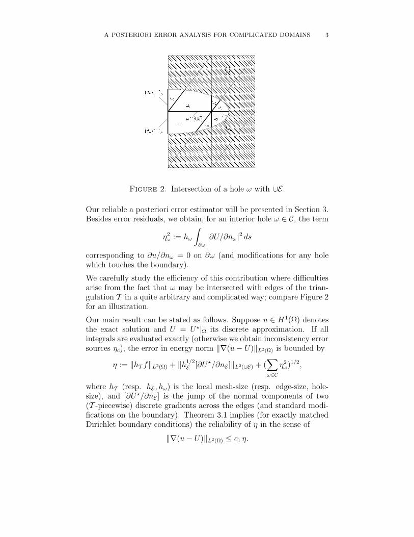
( 1 , 0 )Figure 3. Domain Ω with triangular hole ω and achange of the type of boundary conditions outside ∂Ωto illustrate Assumption 4.1.

For a proof, we refer to [S]. Theorem 4.1 neither implies that theoperator norm of Stein is moderately bounded (the bound might bevery large for domains with a huge number of small geometric details)nor that the H1-seminorm of the extended function can be estimatedby the H1-seminorm of the original function. To fulfil homogeneousDirichlet boundary conditions on Γ?

D, we assume the existence of anappropriate cutoff-function.

Assumption 4.1. There exists a function m : Ω? → [0, 1] such thatm ≡ 1 on Ω while m = 0 on Γ?

D\ΓD and, for all v ∈ H1 (Ω?) with v = 0on ΓD, we have that the product mv belongs to H1

D (Ω?). Set

:v ∈ H1 (Ω?) : v|ΓD

= 0→ H1

D (Ω?) , v 7→ mv.

For holes ω ∈ C, which do not touch the exterior Dirichlet boundaryΓ?

D\ΓD, we may choose m|ω ≡ 1. The following example considers thecharacteristic model situation of Figure 3.

Example 4.1. Let Ω = Ω?\ω where Ω? = (−1, 1) × (0, 1) and

ω := int conv(0, 0), (ε, 0), (ε, ε) for some 0 < ε < 1/2.

(Recall that int and conv denote the interior and convex hull, respec-tively, of a set.) Suppose Γ?

D := [−1, δ]×0 for some 0 < δ < ε, whileΓ?

N := Γ?\Γ?D, ΓD = [−1, 0] × 0. Let (x, y) = r (cos α, sinα). We

define the function m by

m(x, y) :=

1 if x ∈ Ω,χ(x) + (1 − χ(x)) sin (2α) if x ∈ ω,


where χ(x) = 0 for 0 < x < δ and χ(x) = (x− δ)/(ε− δ) for δ ≤ x ≤ ε.It is easy to check that m is continuous in the open set Ω? and m = 0on Γ?

D\ΓD. Given v?1 ∈ H1(Ω?) with v?

1|ΓD= 0, we define v?

2 := mv?1.

The proof of

‖m‖L∞(Ω?) = 1 and |∇m (x)| ≤ 2 +√

2

r (1 − δ/ε)for all x ∈ Ω?

is straightforward. Hence, Hardy’s inequality in the form of Theo-rem 1.4.44 in [G] (where s = 1, p = 2, α = 0) yields

v?

1 ∈ H1(Ω?)and so eventually v?

2 ∈ H1D(Ω?).

In the next step, we introduce the Ritz-projection of functions H1D (Ω?)

in the space V :=v ∈ H1 (Ω?) : v|Ω∪Γ?

D= 0.

Definition 4.1. The Ritz-projection : H1D (Ω?) → V is given for

v?1 ∈ H1

D (Ω?) by v?2 := v?

1 where v?2 ∈ V is the solution of

∫

Ω?

∇v?2 · ∇w =

∫

Ω?

∇v?1 · ∇w dx for all w ∈ V.

Now, we have all ingredients for defining the extension operator D.

Definition 4.2. The extension operator D : H1D (Ω) → H1

D (Ω?) isgiven by the composition

(4.1) D := (I − ) Stein.

Following the ideas in [OSY], it was proved in [SW] that the norm ofthe extension operator D does not depend on the size and numberof holes in the domain provided a certain separation condition (seeSection 1, (4.2), and [SW, (2.8)]) is satisfied.

To reduce technicalities we focus on some characteristic examples andrefer to [SW] for proofs and general considerations.

Example 4.2. Let Ω? ⊂ d denote a Lipschitz domain and Bjj∈N ,N ⊆ , be a family of balls with radius εj which are compactly includedin Ω? and satisfy a separation condition

(4.2) dist (Bj, Bk) ≥ c7 max εj, εk and dist (Bj, Γ?) ≥ c7 εj

for all distinct j, k ∈ N and the global constant c7 > 0. Let Ω :=Ω?\⋃Bj∈N . Choose m ≡ 1 in Ω? (cf. Assumption 4.1) and define D

as in (4.1). Then, the operator norm of D and its seminorm, i.e., theconstant c6, is bounded independently of card(N) or εj.


Example 4.3. For δ > 0, let Ω? = (−1 − δ, 1 + δ)2 and ω = (−1, 1)2.Then, there exists a constant c8 > 0 so that the norm of every extensionoperator : H1(Ω?\ω) → H1(Ω?) can be estimated from below by

c8 δ−1/2 ≤ ‖ ‖ .

The following example shows that the separation condition (4.2) is notnecessary in order to bound the norm of the minimal extension operatorby a moderate constant.

Example 4.4. Let Ω? = (−1, 1)3 and, for j = 1, 2, ωj = Bj × (−1, 1).Here, Bj denotes the disc with radius ε about the points (±2ε, 0) .Then, the norm of the minimal extension operator : H1 (Ω?\ω1 ∪ ω2)→ H1 (Ω?) is bounded uniformly as ε → 0.

Finally, we revisit Example 4.1 and estimate the norm of the extensionoperator.

Example 4.5. Let Ω, Ω?, ω, and the function m be defined as in Example4.1. Then, the norm and the seminorm of the extension operator D

as in (4.1) can be estimated form above by C/ (1 − δ/ε).

This example indicates that the (semi-)norm of the extension operator D behaves critically if the ratio of the length of the Dirichlet portion∂ω ∩ Γ?

D compared to the length of the outer boundary ∂ω ∩ Γ? tendsto one.

4.2. Clement interpolation on complicated domains. The proofof the reliability of the error estimator makes use of the Clement ap-proximation [Cl, V, CF] operator P : H1

D(Ω?) → S?D such that, for all

T ∈ T and u? ∈ H1 (Ω?),

‖u? − Pu?‖L2(T ) + hT |u? − Pu?|H1(T ) ≤ c9hT |u?|H1(ωT ) ,(4.3)∥∥h−1

T (u? − Pu?)∥∥

L2(Ω?)+ |u? − Pu?|H1(Ω?) ≤ c10 |u?|H1(Ω?) .(4.4)

Here, ωT := ∪K ∈ T : T ∩ K 6= ∅. The constants c9 and c10

depend merely on the aspect ratio of the elements. Their quantitativeestimation is given in [CF]. With u? = Du we obtain that the right-hand side in (4.4) can be bounded from above by c11 |u|H1(Ω) where c11

depends on c6 and c10.

4.3. Trace theorems. Traces of H1-functions along edges have to beestimated by their norms on adjacent triangles [Cl, CF]. For shaperegular meshes, we have the local estimate for u ∈ H1(T ) on the edgeE ⊂ ∂T , E ∈ E , T ∈ T ,

‖u‖2L2(E) ≤ c12

(h−1

E ‖u‖2L2(T ) + hE |u|2H1(T )

)


and a global version, for u? ∈ H1 (Ω?),

‖u?‖L2(∪E) ≤ c13

(‖h−1/2

T u?‖L2(Ω?) + ‖h1/2T ∇u?‖L2(Ω?)

).

Non-resolved geometric details require further estimates.

Definition 4.3. Let ω ⊂ 2 denote a Lipschitz domain of area |ω|and let γ ⊂ ω be a Lipschitz curve of length |γ|. The trace constantC(γ, ω) is

(4.5) C(γ, ω) := supv∈H1(ω)\0

‖v‖2L2(γ)

|γ| / |ω| ‖v‖2L2(ω) + |ω| / |γ| |v|2H1(ω)

.

Remark 4.2. Letting v ≡ 1 in (4.5) shows 1 ≤ C(γ, ω).

The trace constant C(γ, ω) is scaling-invariant.

Lemma 4.1. For ω and γ as in Definition 4.3 and ε > 0, defineχε : ω → ωε by χε (x) = εx and ωε = χε (ω), γε = χε (γ). Then,C(γε, ωε) = C(γ, ω).

Proof. Straightforward calculations yield |v|Hk(ω) = εk−1 |v χ−1ε |Hk(ωε),

k = 0, 1, and ‖v‖2L2(γ) = ε−1 ‖v χ−1

ε ‖2L2(γε) for each v ∈ H1(ω) and

|ωε| = ε2|ω| or |γε| = ε|γ| from which we deduce the assertion.

Example 4.6. (a) Let ω be a disc with boundary γ = ∂ω. Then,C(γ, ω) ≤ 3. (b) Let ω be a parallelogram and γ one of its sides.Then, C(γ, ω) ≤ 2.

Proof. For the proof of (a) we refer to [BS, Sec. 1.6] and indicatethe proof of (b) for rectangles (the case of a parallelogram is similar).Suppose ω = (0, a) × (0, b). The mean value theorem guarantees that

f(η) = b−1∫ b

0f(y) dy for f ∈ H1(0, b) and some η ∈ (0, b). The funda-

mental theorem of calculus and Cauchy inequalities then show

(4.6) f(0)2 = (b−1

∫ b

0

f(y) dy −∫ η

0

f ′(y) dy)2

≤ 2b−2‖ f ‖2L1(0,b) + 2‖ f ′ ‖2

L1(0,b) ≤ 2b−1‖ f ‖2L2(0,b) + 2b‖ f ′ ‖2

L2(0,b).

Replacing f(y) in (4.6) by v(x, y) (and prime by ∂/∂y) and integratingwith respect to x over (0, a) we deduce (b).

In the sequel, we will frequently estimate functions on (subsets of) holesand appropriate neighbourhoods thereof.


Notation 4.1. For a set A ⊂ 2 , the Chebyshev ball BA is the minimalball that contains A. The disc with radius 2 diamA about the midpointof BA is denoted by VA.

Lemma 4.2. Let ω ⊂ 2 be a domain with diameter hω and let T bea shape regular triangulation of 2 . Then,

‖v‖2L2(ω∩(∪E)) ≤ 2c14

(h−1

ω ‖v‖2L2(Vω) + hω |v|2H1(Vω)

).

The constant c14 is the number of ω-intersections with edges.

Proof. Let

Eω := ω ∩ E : E ∈ E ∧ |ω ∩ E| > 0 .

For each S ∈ Eω define a rectangle Q(S) with one side S and the otherof length hω. Example 4.6(b) shows

1

2‖ v ‖2

L2(S) ≤ h−1ω ‖ v ‖2

L2(Q(S)) + hω| v |2H1(Q(S)).

By definition, c14 is the number of overlaps of Q(S) ⊂ Vω for all S ∈ Eω.This leads to

1

2‖ v ‖2

L2(∪Eω) ≤ h−1ω

∑

S∈Eω

‖ v ‖2L2(Q(S)) + hω

∑

S∈Eω

| v |2H1(Q(S))

≤ c14h−1ω ‖ v ‖2

L2(Vω) + c14hω| v |2H1(Vω).

4.4. Poincare inequalities. The proof of reliability and efficiency ofthe error estimators requires Poincare inequalities [N, PW].

Theorem 4.2 (Payne and Weinberger). Let ω denote a convex do-main in 2 with diameter hω. Then, for all u ∈ H1 (ω) and uω :=∫

ωu dx/|ω|,

‖u − uω‖L2(ω) ≤ hω/π |u|H1(ω) .

For a nonconvex domain ω, we first extend u to a convex neighbourhoodVω and then deduce

‖u − uω‖L2(ω) ≤ ‖ u − uVω ‖L2(ω) ≤ ‖u − uVω‖L2(Vω)(4.7)

≤ diam(Vω)/π |u|H1(Vω) ≤ c15 hω |u|H1(ω).


U * s o l u t i o n o f ( 2 . 4 )r e s t r i c t i o n

U : = R W U * a p p r o x i m a t i o n o f uu e x a c t s o l u t i o n

e : = u - Ut r a c e l i f t i n gv | G : = ( u D - U ) | GD D

w : = e - v

e * : = E D e

w * : = E D w

e x t e n s i o n

e x t e n s i o nC l é m e n t i n t e r p o l a t i o n W * : = P w *

z * : = w * - W * z : = R W z *r e s t r i c t i o n W : = R W W *

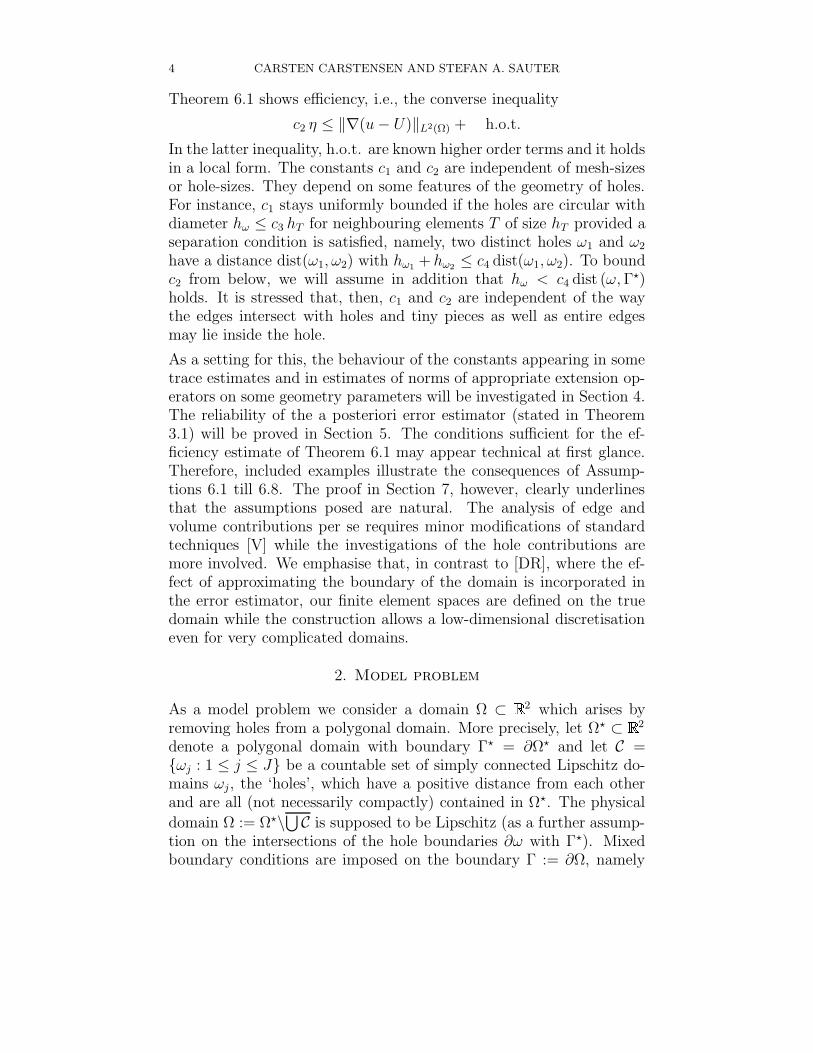
Figure 4. Diagram illustrating the relationship of thefunctions U , U?, u, e, e?, v, w, w?, W ?, W , z?, and z.

5. Proof of Reliability

Throughout the proof we write a b for a ≤ c b, where the multi-plicative constant c > 0 is independent of hT , hE , u, U , f , g and maydepend on Ω, ΓD, ΓN , and on the shape of the elements or their aspectratio. Furthermore, the estimates depend on the numbers

(5.1) maxω∈C

card T ∈ T : T ∩ ω 6= ∅ and supx∈Ω?

card ω ∈ C : x ∈ Vω .

Since emphasis is on many small holes ω with hω hT (others shall beresolved in Ω?) the numbers in (5.1) are moderate.

In the sequel, various functions arise with relationships illustrated inFigure 4. Recall that U ? ∈ S? solves (2.4) and U := RΩU?, whereRΩ is the restriction of a function v : Ω? → to Ω. Split the errore := u − U ∈ H1(Ω) into e − v and v, where v ∈ H1(Ω) satisfiesv = uD − U on ΓD and ηD = ‖∇v‖L2(Ω). Given w := e − v ∈ H1

D(Ω)let w? := Dw ∈ H1

D(Ω?) and let W ? := Pw? denote the Clementapproximation to w?. Define z? := w? − W ? ∈ H1(Ω?) and z := RΩz?,W := RΩW ?. Observe z ∈ H1

D(Ω) and z? = 0 on Γ?D. The H1-norm of

W ? can be estimated by using a Friedrichs inequality for w? ∈ H1D (Ω?),


the approximation properties of the Clement approximation (4.4) andthe continuity of the extension operator D with respect to the H1-seminorm

‖W ?‖H1(Ω?) ≤ ‖W ? − w?‖H1(Ω?) + ‖w?‖H1(Ω?)

|w?|H1(Ω?) |e − v|H1(Ω) .

This, a triangle inequality with |e?|H1(Ω?) |e|H1(Ω), and |U?−v?|H1(Ω?) |e|H1(Ω) at the end yield

(5.2) ‖ h−1T z? ‖L2(Ω?) + ‖ h

−1/2E z? ‖L2(∪E) + | z?|H1(Ω?) + ‖W ?‖H1(Ω?)

|e − v|H1(Ω) |e|H1(Ω) + ηD.

The definition of v implies∫Ω∇v · ∇ϕ dx = 0 for all ϕ ∈ H1

D (Ω). Thechoice ϕ = e − v leads to∫

Ω

∇v · ∇e dx = η2D.

Hence, we obtain with e = z + W + v

(5.3) | e |2H1(Ω) =

∫

Ω

∇e · ∇z dx +

∫

Ω

∇e · ∇Wdx + η2D.

The second term on the right-hand side in (5.3) is split into ∇u · ∇Wand ∇U · ∇W . The concept of the porosity %, the weak formulation(2.2), and (5.2) show (recall that f ? and g? vanish outside Ω and ΓN)

(5.4)

∫

Ω

∇e · ∇W dx =

∫

Ω?

(f ? − f ?) W ? dx +

∫

Γ?N

(g? − g?) W ? ds

−∫

Ω?

(% − %)∇U ? · ∇W ? dx ≤ ‖W ? ‖H1(Ω?) ηc | e |H1(Ω) ηc.

For the first term on the right-hand side in (5.3), an integration by partson each T ∩ Ω is performed. Careful account on the exact boundaryconditions results in

(5.5)

∫

Ω

∇e · ∇z dx =

∫

∪E∩Ω

[∂U/∂nE ] z ds

+

∫

ΓN

(g − ∂U/∂n) z ds +

∫

Ω

f z dx −∫

γ

z ∂U/∂n ds

with jump terms on ∪E ∩Ω := (∪E)∩Ω within Ω. Next, we will derivean appropriate representation of the last integral in (5.5). Figure 2illustrates how edges and boundary pieces might hit a hole ω ∈ C.

Let us consider one hole ω ∈ C with outer normal nω = −nΩ = −n andboundary ∂ω = γω∪γ?

D∪γ?N , where γω := (∂ω)∩γ, γ?

D := (∂ω)∩Γ?D, and


γ?N := (∂ω)∩Γ?

N . The edges cut ω into a finite number of connectivitycomponents ω1, . . . , ωJ illustrated in Fig. 2, ω \ (∪E) = ∪ω1, . . . , ωJ.(Their number J 1 is limited since ω intersects with only a finitenumber of elements, cf. (5.1)). On each ωj, ∇U? is constant and equalto ∇U?|ωj

. The divergence theorem shows

(5.6)

∫

∂ωj

∂U?/∂nωjds = ∇U?|ωj

·∫

∂ωj

nωjds = 0.

Therefore, for any real constant cω, we obtain

∫

∂ωj

z?∂U?/∂nωjds =

∫

∂ωj

(z? − cω) ∂U?/∂nωjds.

Note that ∇U ? is, in general, discontinuous across ∪EΩ. Besides thesituation in Figure 2 it may happen that γω has a positive intersectionwith the skeleton ∪EΩ, |γω ∩ (∪EΩ)| > 0. Even in this case, we have

∂U/∂n = −∂U ?/∂nω − [∂U?/∂nE ] on E ∩ γω, E ∈ EΩ.

Therefore,

∫

γ?N

z? ∂U?/∂nω ds −∫

γω

z ∂U/∂n ds −∫

(∂ω)∩(∪EΩ)

z? [∂U?/∂nE ] ds

=

∫

∂ω

z? ∂U?/∂nω ds

=J∑

j=1

∫

∂ωj

z? ∂U?j /∂nωj

ds +

∫

(∪EΩ)∩ω

z? [∂U?/∂nE ] ds.

We used z? = 0 on γ?D and that the definition of the jumps [∂U ?/∂nE ]

does not depend on the underlying orientation of nE . The combinationof the last four identities shows

(5.7)∫

γω

z ∂U/∂n ds = −∫

(γω∪ω)∩(∪E)

z? [∂U?/∂nE ] ds+

∫

γ?N

z? ∂U?/∂nω ds

+

J∑

j=1

∫

∂ωj

(cω − z?) ∂U?/∂nωjds.


A summation over all holes ω ∈ C and a rearrangement of boundarypieces of ∪∂ωj : j = 1, . . . , J yield

(5.8)

∫

γ

z∂U

∂nds = −

∫

(Ω?\Ω)∩(∪E)

z?

[∂U?

∂nE

]ds +

∫

Γ?N\ΓN

z? ∂U?

∂nds

+∑

ω∈C

(∫

∂ω

(cω − z?)∂U?

∂nωds +

∫

ω∩(∪E)

(cω − z?)

[∂U?

∂nE

]ds

).

Combining this representation with (5.5) leads to(5.9)∫

Ω

∇e · ∇z dx =

∫

∪EΩ

[∂U?/∂nE ] z? ds

+

∫

Γ?N

(g? − ∂U?/∂n) z ds +

∫

Ω?

f ? z? dx

+∑

ω∈C

(∫

∂ω

(z? − cω)∂U?

∂nωds +

∫

ω∩(∪E)

(z? − cω)

[∂U?

∂nE

]ds

).

The first three summands on the right-hand side of (5.9) can be es-timated with standard arguments (e.g., from [V]) utilising (5.2) andCauchy’s inequality. The last contribution of (5.9) is bounded by

(5.10)∑

ω∈C

h−1/2ω ‖ z? − cω ‖L2(ω∩(∪E)) h1/2

ω ‖[∂U?

∂nE

]‖L2(ω∩(∪E)).

The trace inequality (cf. Lemma 4.2), (5.1), and a Poincare inequalitywith proper cω (cf. Subsection 4.4) result in

‖ z? − cω ‖2L2(ω∩(∪E)) h−1

ω ‖z? − cω‖2L2(Vω) + hω |z?|2H1(Vω)

hω |z?|2H1(Vω) .(5.11)

Its combination with (5.10) yields (recall the finite overlap of the neigh-bourhoods Vω from (5.1)) and the boundedness of the extension oper-ator)

∑

ω∈C

∫

ω∩(∪E)

(z? − cω) [∂U?/∂nE ] ds ηE |z?|H1(Ω?) .

For the second last term on the right-hand side of (5.9), we considerfirst the case that |Γ?

D ∩ ∂ω| = 0 and employ analogous arguments toobtain ∑

ω∈C

∫

∂ω

(z? − cω)∂U?

∂nω

ds ηC |z?|H1(Ω?) ,

since ∂ω\Γ?D equals ∂ω up to a set of measure zero (cf. (3.3)). If

|Γ?D ∩ ∂ω| > 0 we set cω = 0. Employing z? = 0 on Γ?

D and the trace


theorem (cf. Section 4.3) yield∫

∂ω

(z? − cω) ∂U?/∂nω ds ‖∂U?/∂n‖L2(∂ω\Γ?D)

×(h−1

ω ‖z?‖2L2(Vω) + hω |z?|2H1(Vω)

)1/2

.

Since |∂ω ∩ Γ?D| > 0 and using again z?|Γ?

D= 0, a Friedrichs’ inequality

leads to ‖z?‖2L2(Vω) hω |z?|2H1(Vω) and

∑

ω∈C

∫

∂ω

(z? − cω)∂U?

∂nωds ηC |z?|H1(Ω?) .

The combination of the above estimates concludes the proof of Theo-rem 3.1.

6. Efficiency: Geometric Preliminaries and Main Result

This section is devoted to the presentation of sufficient assumptions forthe converse (called efficiency) estimate of Theorem 3.1 and so to thesharpness of that (reliability) estimate. For the ease of this discussion,we assume throughout this section that all holes are compactly embed-ded in Ω?. Otherwise, the hole boundaries (∂ω) ∩ Γ?

D and (∂ω) ∩ Γ?N

would require a special treatment, i.e., a modification of the extensionoperator D. The main part of this section is devoted to characterisea class of holes (of quite general geometry) that allows for an efficiencyestimate. The main result is stated in Theorem 6.1 and proved in thesubsequent section.

Assumption 6.1. For any hole ω ∈ C, the neighbourhood Vω fromNotation 4.1 is compactly included in Ω?.

Remark 6.1. The definition of Vω could be generalised by replacing thefactor 2 in Notation 4.1 by any other factor which is larger than oneor even to more generally shaped neighbourhoods Vω, where ∂Vω haspositive distance to ω.

Definition 6.1. For any ball B let ρB be the standard mollifier ρB ∈D(B) with 0 ≤ ρB ≤ 1, i.e., for the ball B around z with radius r > 0,

ρB(x) = exp(1/r + 1/(|x − z|2 − r)) if x ∈ B and ρB(x) = 0 else.

Assumption 6.2. Suppose that, for any edge E ∈ E , there exists aball BE ⊂ Ω? with E ∩ BE = ∅ and

(a) diam(BE) ≈ hE (size control),(b) dist(BE, E) hE (distance control),


(c)∫Ω

ρBEdx ≈ h2

E (porosity control).Let σE denote the union of BE with all triangles T ∈ T with E ⊂ T .

Assumption 6.3. Suppose that, for any element T ∈ T , there existsa ball BT ⊂ Ω? \ (∪E) with

(a) diam(BT ) ≈ hT (size control),(b) dist(BT , T ) hT (distance control),(c)∫Ω

ρBTdx ≈ h2

T (porosity control).Set σT := T ∪ BT .

The local efficiency estimate for the contribution of the hole ω ∈ Crequires a set of additional assumptions.

First, we will mollify and extend the normal n along ∂ω (that pointsinto ω; n = −nω) to a neighbourhood of ∂ω. Some examples in Figure 5illustrate Assumption 6.4.

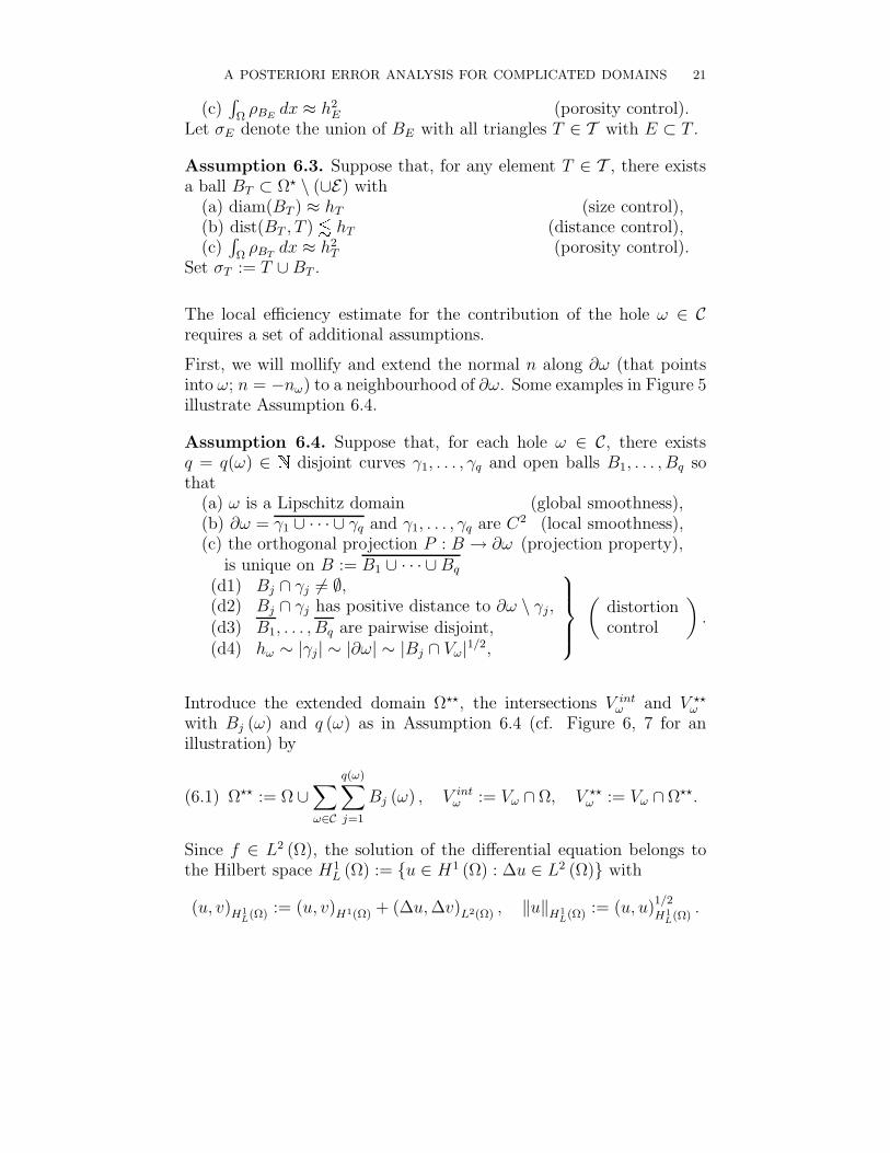
Assumption 6.4. Suppose that, for each hole ω ∈ C, there existsq = q(ω) ∈ disjoint curves γ1, . . . , γq and open balls B1, . . . , Bq sothat

(a) ω is a Lipschitz domain (global smoothness),(b) ∂ω = γ1 ∪ · · · ∪ γq and γ1, . . . , γq are C2 (local smoothness),(c) the orthogonal projection P : B → ∂ω (projection property),

is unique on B := B1 ∪ · · · ∪ Bq

(d1) Bj ∩ γj 6= ∅,(d2) Bj ∩ γj has positive distance to ∂ω \ γj,(d3) B1, . . . , Bq are pairwise disjoint,(d4) hω ∼ |γj| ∼ |∂ω| ∼ |Bj ∩ Vω|1/2,

(distortioncontrol

).

Introduce the extended domain Ω??, the intersections V intω and V ??

ω

with Bj (ω) and q (ω) as in Assumption 6.4 (cf. Figure 6, 7 for anillustration) by

(6.1) Ω?? := Ω ∪∑

ω∈C

q(ω)∑

j=1

Bj (ω) , V intω := Vω ∩ Ω, V ??

ω := Vω ∩ Ω??.

Since f ∈ L2 (Ω), the solution of the differential equation belongs tothe Hilbert space H1

L (Ω) := u ∈ H1 (Ω) : ∆u ∈ L2 (Ω) with

(u, v)H1L(Ω) := (u, v)H1(Ω) + (∆u, ∆v)L2(Ω) , ‖u‖H1

L(Ω) := (u, u)1/2

H1L(Ω)

.


w

B 1

¶ w = g 1

wg j

B j

w

Figure 5. The domains (a) and (b) satisfy Assump-tion 6.4 with moderate constants in the estimates whilethis is not the case for domain (c).

Ww

ww

B i

B i

B i

Figure 6. Domain Ω with holes. The extended domainΩ∗∗ arises by including the shaded half balls to Ω.

The following assumption concerns the existence of an extension oper-ator for a subspace of H1

L (Ω). Let us introduce

W (Ω) :=u ∈ H1

L (Ω) : ∂u/∂n = 0 on γ⊕ S

equipped with the H1L (Ω)-norm.

Assumption 6.5. Adopt Assumption 6.4 and suppose

(a) there exists a continuous extension operator L : W (Ω) →H1

L (Ω??) so that, for all u ∈ W (Ω) and ω ∈ C,

‖ Lu‖H1L(V ??

ω ) ≤ c16 ‖u‖H1L(V int

ω ) .


w

B j¶ V w

V w i n t

Figure 7. Neighborhood Vω of ω with boundary ∂Vω,intersection V int

ω = Vω ∩ Ω and extended intersectionV ∗∗

ω = Vω ∩ Ω∗∗.

(b) If u ∈ W (Ω) and ∆u ∈ H1 (V intω ), then, ∆ Lu ∈ H1 (V ??

ω ) and

‖∆ Lu‖H1(V ??ω ) ≤ c17 ‖∆u‖H1(V int

ω ) ,

(c) if u is affine on some Bj (ω)∩Ω, then, the extension Lu is theaffine extension on Bj (ω).

Remark 6.2. Assumption 6.5 implies that, for all u ∈ W (Ω) and v ∈C∞

0 (Bj (ω)),

(6.2)

∫

Bj(ω)

∇v · ∇ ( Lu) − v∆ ( Lu) dx = 0.

Remark 6.3. Consider Ω = (−1, 0)×(0, 1) and Ω? = (−1, 1)×(0, 1) withthe hole ω = Ω?\Ω and the inner boundary γ := Ω ∩ Ω?. Then, thereexists no extension operator from H1

L (Ω) into H1L (Ω?). The reason is

that all functions w ∈ H1L (Ω?) satisfy w ∈ H2

loc (Ω?) and, hence, w|γ ∈H

3/2loc (γ) , while the trace map tr : H1 (Ω) → H1/2 (γ) is surjective. As

an example, the function u ∈ H1L (Ω) defined by u (x) = rλ sin (λϕ),

where (r, ϕ) are polar coordinates in Ω centred at (0, 1/2) and λ ∈(0, 1), belongs to H1

L (Ω) and cannot be extended to u? ∈ H1L (Ω?).1

The extension operator L is constructed for one typical polygonalhole.

1Thanks are due to M. Costabel for providing us with this Remark.


Example 6.1. Let Ω, Ω?, ω, γ be as in Remark 6.3. Then, there exists anextension operator L : W (Ω) → H1

L (Ω?) which satisfies Assumption6.5. For u ∈ H1

L (Ω), the extended function u? := Lu is given, forx ∈ ω, by

(6.3) u? (x1, x2) := u (−x1, x2) + 2x1∂u

∂x1(0, x2) .

For u ∈ W (Ω) and x ∈ Ω, let

u2 (x) := x1∂u

∂x1(0, x2) .

The definition of W (Ω) implies that ∂u/∂x1 is constant on γ and,hence, u2 ∈ S. The function u1 := u − u2 satisfies ∂u1/∂x1 = 0 on γ.The linearity of L allows to investigate u?

1 := Lu1 and u?2 := Lu2

separately. For u1 and (x1, x2) ∈ ω, the extension operator simplifies tou?

1 (x1, x2) := u1 (−x1, x2). The density of C∞ (Ω) ∩ H1L (Ω) in H1

L (Ω)implies that it is sufficient to investigate the boundedness of Lu1 forfunctions u1 ∈ C∞ (Ω) ∩ W (Ω). Simple calculations result in u?

1 =u1, ∇u?

1 = ∇u1 on γ and ∆ ( Lu1) (x1, x2) = (∆u1) (−x1, x2) on ω.Consequently, for all u?

1 ∈ H1L (Ω), there holds

‖u?1‖H1

L(Ω?) = 2 ‖u1‖H1L(Ω) .

If, in addition, ∆u?1 ∈ H1 (Ω?), then,

‖∆u?1‖H1

L(Ω?) = 2 ‖∆u1‖H1L(Ω) .

The definition (6.3) directly implies that affine functions are extendedanalytically, i.e., “by themselves”. The proof of

‖u?2‖H1

L(Ω?) ‖u2‖H1L(Ω) , ‖∆u?

1‖L2(Ω?) = ‖∆u1‖L2(Ω) = 0

is straightforward. Next,

‖u2‖H1L(Ω) ‖∂u/∂x1‖H−1/2(γ) .

The continuity of the trace operators in H1L (Ω) implies ‖u2‖H1

L(Ω) ‖u‖H1

L(Ω) from which we conclude

‖u?‖H1L(Ω?) ‖u1‖H1

L(Ω) + ‖u2‖H1L(Ω)

≤ ‖u‖H1L(Ω) + 2 ‖u2‖H1

L(Ω) ‖u‖H1L(Ω) .


To mollify and to extend the normal field n to some neighbourhood ofthe hole boundaries we employ the ansatz (recall the definition of Bfrom Assumption 6.4)

(6.4) N =

λn P in B,0 otherwise.

The function λ is a generalization of bubble functions from the a poste-riori error analysis [V] with an integral mean orthogonal to the direction(cos α, sin α).

Assumption 6.6. The function λ = λα ∈ C∞ ( 2) in (6.4) dependscontinuously on α ∈ [−π, π] and satisfies

(a)suppλα ⊆ B and 0 ≤ λα ≤ 1 on ∂ω|λα|L∞( 2) + hω |λα|W 1,∞( 2) 1

(cut-off function),

(b)for any γj there exists a sub-arc γj ⊂ γj

with |γj| ∼ |γj| and λα ≥ 1/2 on γj

(positivity),

(c)∫

V intω

(cos αsinα

)· N dx = 0 (α-orthogonality).

Remark 6.4. The compactness of [−π, π] and the continuous depen-dence of λ on α imply an α-uniform estimate in Assumption 6.6.(a).

We need an abstract assumption on the hole boundaries.

Assumption 6.7. The mollified and extended normal field N is of theform (6.4) where λ satisfies Assumption 6.6 and, for all q ∈ 2 ,

h−1ω ‖q · N‖2

L2(Vω) + hω |q · N |2H1(Vω)(6.5)

‖q · n‖2L2(∂ω)

∫

∂ω

(q · N) (q · n) ds.

We illustrate these abstract assumptions with two typical examples.

Example 6.2. (polygonal hole). Assume that ω is a polygonal holesatisfying Assumption 6.4 with straight lines γj orthogonal to nj. Then,

∫

Vω

|q · N |2 dx =

q∑

j=1

∫

Bj∩Vω

|q · λn P |2 dx

=

q∑

j=1

|q · nj|2∫

Bj∩Vω

λ2dx q∑

j=1

|q · nj|2 |Bj ∩ Vω|

=

q∑

j=1

|Bj ∩ Vω||γj|

∫

γj

|q · nj|2 ds hω

∫

∂ω

|q · n|2 dx.


e

F2 a

r

w

( e , 0 )

Figure 8. Circular hole ω in Example 6.3.

The estimate of the H1-seminorm follows analogously by using∫

Bi∩Vω

‖∇λ‖2 dx 1.

The second inequality in (6.5) follows from∫

∂ω

|q · n|2 dx =

q∑

j=1

|q · nj|2|γj||γj|

∫

γj

1ds

q∑

j=1

|q · nj|2∫

γj

λ ds ≤∫

∂ω

(q · N) (q · n) ds.

Remark 6.5. The estimates in Example 6.2 are based on Assumptions6.4 and 6.6 and so are the multiplicative constants hidden in the nota-tion .

Remark 6.6. The condition (6.5) is partly redundant as ‖q · N‖L2(Vω)

is bounded by diam(Vω)|q · N |H1(Vω) owing to a Friedrichs inequality.

The following example shows that Assumption 6.7 may hold with mod-erate constant for holes with curved boundary (cf. Figure 8).

Example 6.3 (circle). If ∂ω is a circle and F is a sub-arc of ∂ω wefind polar coordinates centred at the midpoint of ω and, without lossof generality, suppose ω = B(0, ε) and F = ε(cos(ϕ, sin ϕ) : −α <ϕ < α for some ε > 0 and 0 < α < π/2. Let λ be a scaled

mollifier with centre at (ε, 0) and support B := B((ε, 0), r) for r :=

ε min1/2,√

2(1 − cos α). then, N(r, ϕ) := %B(r, ϕ) (cos ϕ, sin ϕ) sat-isfies Assumption 6.7. The constant in (6.5) is independent of ε butdegenerates if α is small.

Remark 6.7. The previous two examples illustrate that and how N canbe constructed for a quite large class of piecewise smooth domains:Corners are cut-off. It is also clear that the support Vω of N can be a

A POSTERIORI ERROR ANALYSIS FOR COMPLICATED DOMAINS 27D 1

B 1

w

wD 1

D 1

w

D 1

ww

D 1

D 2D 3

D 4

D 5

D 6

Figure 9. Triangulations covering a hole ω. The ballsof connecting edges are denoted by Dj while the balls foreach smooth component γj are denoted by Bj

subset of an arbitrary small neighbourhood of ∂ω on the expense of alarge constant in (6.5).

The subsequent notions concern the patch around a hole and allow thatholes may intersect arbitrarily with the mesh.

Definition 6.2. Let

Tω := T ∈ T : T ∩ ∂ω 6= ∅ .

A sequence (Tj)Jj=0 of triangles in T is edge-connected if, for j =

1, 2, . . . , J , the triangles Tj−1, Tj share a common edge Ej.

Some characteristic examples illustrating Assumption 6.8 are depictedin Figure 9.

Assumption 6.8. For any hole ω ∈ C and any K ∈ Tω there is asequence of edge-connected triangles (Kj)

Jj=0 in T with J = J (K)

such that, for all edges Ej = Kj−1 ∩ Kj, there exists a ball Dj withradius rj centred at Mj ∈ Ej and(a) rj

hω,

(b) Dj ⊂ Ω??,(c) the endpoints of Ej have positive distance to Dj ∩ Ej.

Remark 6.8. Assumption 6.8 can be generalized by allowing more gen-eral domains Dj for connecting neighbouring triangles with finite over-lap.

Remark 6.9. The definition of the balls Dj in Assumption 6.8 impliesthat, for all U? ∈ S? and U := U?|Ω, there holds U? = LU on Dj.


The constants in the preceding assumptions of this section enter inthe multiplicative constant in the efficiency estimate. Its proof is thecontents of the next section. Recall the definition of σT and σE fromAssumption 6.2 and 6.3.

Theorem 6.1. Under the Assumptions 6.1–6.8 and notation of Sec-tion 2 we have with f ?

L := ∆ Lu

η2Ω + η2

E + η2C ‖∇e‖2

L2(Ω) +∑

E∈EN

hE mingE∈

‖(g − gE)‖2L2(E∩ΓN )

+∑

T∈T

h2T min

fT ∈ ‖ f − fT ‖2

L2(Ω∩σT ) +∑

E∈E

h2E min

fE∈ ‖ f − fE ‖2

L2(Ω∩σE)

+∑

ω∈C

h2ω min

fω∈ ‖f ?

L − fω‖2L2(V ??

ω ) .

Remark 6.10. Theorem 6.1 even holds in a more local form as shownin the proof in Section 7.

Remark 6.11. The third and fourth term are of higher order if theright-hand side f is smooth in the sense that it is the restriction of afunction F in H1(Ω?). Indeed, f = F |Ω yields

minfT∈

‖ f − fT ‖L2(Ω∩σT ) ≤ minFT∈

‖F − FT ‖L2(σT ) hT ‖∇F ‖L2(σT )

according to (4.7) and Assumption 6.3. An analogous estimate holdsfor minfE∈ ‖ f−fE ‖L2(Ω∩σE). If f ∈ H1 (V int

ω ), Assumption 6.5 impliesf ?

L = ∆ Lu ∈ H1L (V ??

ω ) and the last term is of higher order

minfω∈

‖f ?L − fω‖L2(V ??

ω ) hω ‖∆ Lu‖H1(V ??ω ) ≤ c17hω ‖∆u‖H1(V int

ω )

= c17hω ‖f‖H1(V intω ) .

The second term is of higher order if there exists G ∈ H1 (Γ?N) such

that g = G|ΓN. In this case, there holds

∑

E∈EN

hE mingE∈

‖(g − gE)‖2L2(E∩ΓN ) ‖h3/2

E ∂G/∂s‖2L2(Γ?

N ).

7. Proof of Efficiency

The following results provide local estimates summarised in Theo-rem 6.1. The combination of Lemma 7.2, 7.4, 7.5, and 7.6 is the proofof the theorem.


Definition 7.1. For any edge E with ball BE from Assumption 6.2 letβE be the piecewise quadratic product of the two barycentric coordi-nates with βE = λ1 λ2 on T ∈ T with E ⊂ ∂T that vanishes on ∂T \Eand equals s(hE − s)/h2

E on E with respect to the arc-length s. Let

bE := βE − cE ρBEfor cE :=

∫

Ω

βE dx/

∫

Ω

ρBEdx ∈ .

Lemma 7.1. Under the Assumption 6.2, the function bE from Defini-tion 7.1 equals s(hE − s)/h2

E on E with respect to the arc-length s andsatisfies supp bE ⊂ σE,

(7.1)

∫

Ω

bE dx = 0, Lip(bE) 1/hE, and ‖∇bE ‖L2(σE) 1.

Proof. Since E ∩ BE = ∅ in Assumption 6.2, bE = βE on E and∫Ω

bE dx = 0 follows by definition of cE. The functions ρBEand βE

are Lipschitz with Lipschitz constant 1/hE. Hence it remains toverify 0 ≤ cE 1. Assumption 6.2.(c) shows cE 1. The remainingestimate then follows from Assumption 6.2.

Definition 7.2. Let d = 1, 2. For any d-dimensional measurable setV ⊂ 2 , let |ω ∩ V | denote the d-dimensional measure of ω∩V and set

CV := ω ∈ C : |ω ∩ V | > 0.

Lemma 7.2. We have, for all E ∈ EΩ and fE ∈ , E ′ := E\ E,

‖ h1/2E [∂U?/∂nE] ‖2

L2(E) ‖∇e ‖2L2(Ω∩σE) + h2

E ‖ f − fE ‖2L2(Ω∩σE)

+∑

ω∈CσE

hω ‖ ∂U?/∂nω ‖2L2(∂ω) +

∑

ω∈CE

hω ‖[∂U?/∂nE ]‖2L2(ω∩(∪E ′)) .

Proof. Let JE denote the constant [∂U ?/∂nE] and notice that (since bE

reads s(hE − s)/h2E on E)

(7.2) hE ‖ JE ‖2L2(E) = hE/3 JE

∫

E

[∂U?/∂nE] bE ds.


The last integral has a representation as in (5.9) with z? replaced bybE, namely,∫

E

JE bE ds =

∫

Ω

∇e · ∇bE dx −∫

Ω

f bE dx

+∑

ω∈C

(∫

∂ω

(cω − bE)∂U

∂nωds +

∫

ω∩(∪E)

[∂U?

∂nE

](cω − bE) ds

).

(7.3)

For holes ω ∈ C with ω∩E = ∅, the function bE equals zero on ω∩(∪E)and we set in these cases cω = 0. Thus, the sum

∑ω∈C over the last

integral in (7.3) reduces to a sum over all ω ∈ CE, i.e.,

∑

ω∈CE

JE

∫

ω∩E

(cω − bE) ds +∑

ω∈CE

∫

ω∩(∪E ′)

[∂U?

∂nE

](cω − bE) ds.

For the remaining holes ω ∈ CE, we choose the constant cω such that∫ω∩E

(cω − bE) ds vanishes. Then, cω equals bE(ξ) for some ξ in theconvex hull of ω ∩ E and for any x ∈ ω we have |x − ξ| hω. ByLemma 7.1, bE is Lipschitz with Lip(bE) 1/hE. This and a Cauchyinequality for the length |∂ω| show

(7.4)

∫

∂ω

|cω − bE| |∂U?/∂nω| ds ≤ ‖ cω − bE ‖L2(∂ω)‖ ∂U?/∂nω ‖L2(∂ω)

|∂ω|1/2 hω/hE‖ ∂U?/∂nω ‖L2(∂ω).

The sum∑

ω∈C for the second last integral in (7.3) reduces to∑

ω∈CσE.

Note that∑

ω∈CσEh2

ω h2E and, thus,

∑

ω∈C

∫

∂ω

|cω − bE| |∂U?/∂nω| ds ≤

∑

ω∈CσE

hω‖ ∂U?/∂nω ‖2L2(∂ω)

1/2

.

In the same fashion, we obtain by using |ω ∩ (∪E ′)| hω and Cauchy’sinequality the estimate

∑

ω∈CE

∫

ω∩(∪E ′)

∣∣∣∣[∂U?

∂nE

](cω − bE)

∣∣∣∣ ds ≤∑

ω∈CE

hω

hE

∥∥∥∥h1/2ω

[∂U?

∂nE

]∥∥∥∥L2(ω∩(∪E ′))

≤(∑

ω∈CE

∥∥∥∥h1/2ω

[∂U?

∂nE

]∥∥∥∥2

L2(ω∩(∪E ′))

)1/2

.


By construction,∫Ω

bE dx = 0. Hence,∫Ω

f bE dx can be replaced by∫Ω(f − fE) bE dx. Taking into account (7.1) we are led to∫

E

JE bE ds ≤ ‖∇e‖L2(Ω∩σE) + ‖hT (f − fE)‖L2(Ω∩σE)

+

∑

ω∈CσE

‖ ∂U?

∂nω‖2

L2(∂ω)

1/2

+

(∑

ω∈CE

∥∥∥∥h1/2ω

[∂U?

∂nE

]∥∥∥∥2

L2(ω∩(∪E ′))

)1/2

.

This concludes the proof.

Definition 7.3. For any triangle T with ball BT from Assumption 6.3let βT be the cubic bubble function which is the product of the threebarycentric coordinates, βT = λ1 λ2 λ3, on T that vanishes on ∂T . Let

bT := βT − cT ρBTfor cT :=

∫

Ω

βT dx/

∫

Ω

ρBTdx ∈ .

Lemma 7.3. Under the Assumption 6.3, the function bT from Defini-tion 7.3 satisfies supp bT ⊂ σT , and

∫

Ω

bT dx = 0, Lip(bT ) 1/hT , and ‖∇bT ‖L2(σT ) 1.

Proof. The proof is analogous to that of Lemma 7.1 and so omitted.

Lemma 7.4. We have, for all T ∈ T and fT ∈ ,

(7.5) ‖ hT f ‖2L2(Ω∩T ) ‖∇e ‖2

L2(Ω∩σT )

+ h2T ‖ f − fT ‖2

L2(Ω∩σT ) +∑

ω∈CσT

hω ‖ ∂U?/∂nω ‖2L2(∂ω).

Proof. Suppose that fT is the integral mean of f over Ω ∩ σT andcalculate

(7.6) ‖ hTf ‖2L2(Ω∩σT ) − ‖ hT (f − fT ) ‖2

L2(Ω∩σT ) = ‖ hT fT ‖2L2(Ω∩σT ).

Assumption 6.3 implies that |σT | h2T and that (7.6) is bounded by

(7.7) h2T‖ b

1/2T fT ‖2

L2(Ω∩σT ) h2T |fT |

∫

Ω∩σT

bT |fT − f | dx

+ h2T |fT

∫

Ω∩σT

bT f dx|.


This and Cauchy’s and Young’s inequalities lead to

(7.8) ‖ hT f ‖2L2(Ω∩T ) ≤ ‖hT f‖2

L2(Ω∩σT )

‖ hT (f − fT ) ‖2L2(Ω∩σT ) + h2

T

(∫

Ω∩σT

bT f dx)2

.

We focus on the estimate of∫Ω∩σT

bT f dx. By choosing z? = bT in

(5.9), we obtain(7.9)∫

Ω∩σT

f bT dx =

∫

Ω∩σT

∇e · ∇bT dx

−∑

ω∈C

(∫

∂ω

(bT − cω)∂U?

∂nωds +

∫

ω∩(∪E)

(bT − cω)

[∂U?

∂nE

]ds

).

Next, we choose the constants cω in (7.9). For all holes ω ∈ C which arecompactly included in σT , we choose cω :=

∫∂ω

bT ds/ |∂ω| and observe

‖bT − cω‖L2(∂ω) |∂ω|1/2 hω/hT .

For all remaining holes, we choose cω = 0 and, since bT vanish at somepoint of ∂ω in these cases, we get the estimate

‖bT − cω‖L2(∂ω) = ‖bT‖L2(∂ω) |∂ω|1/2 hω/hT .

Thus, the last sum in (7.9) vanishes while the second last sum can beestimated form above by

∑

ω∈C

∫

∂ω

∣∣∣∣(bT − cω)∂U?

∂nω

∣∣∣∣ ds ≤∑

ω∈C

‖bT − cω‖L2(∂ω)

∥∥∥∥∂U?

∂nω

∥∥∥∥L2(∂ω)

∑

ω∈CσE

|∂ω|1/2 hω

hT

∥∥∥∥∂U?

∂nω

∥∥∥∥L2(∂ω)

∑

ω∈CσE

∥∥∥∥h1/2ω

∂U?

∂nω

∥∥∥∥2

L2(∂ω)

1/2

.

The combination of those estimates concludes the proof.

Lemma 7.5. Under Assumptions 6.1, 6.4, 6.5, 6.7, 6.8 we have, forany fω ∈ , f ?

L := ∆ Lu, and V ??ω as in (6.1),

h1/2ω ‖∂U?/∂n‖L2(∂ω) | Le|H1(V ??

ω ) + hω ‖f ?L − fω‖L2(V ??

ω ) .

Proof. Abbreviate qT := ∇U? |T∈ 2 for T ∈ T and obtain(7.10)∫

∂ω

|∂U?/∂n|2 ds =∑

T∈Tω

∫

T∩∂ω

|qT · n|2 ds maxT∈Tω

∫

T∩∂ω

|qT · n|2 ds


from card Tω 1. Let the maximum on the right-hand side of (7.10)be attained for K ∈ T . Hence,

(7.11)

∫

∂ω

|∂U?/∂n|2 ds ∫

∂ω

|qK · n|2 ds.

Let α denote the polar angle of qK ∈ 2 and define λ = λα as inAssumption 6.6. Combining ∂u/∂n = 0 on γ, the last condition inAssumption 6.6, and the divergence theorem we derive, for any fω ∈ ,

‖qK · n‖2L2(∂ω)

∫

∂ω

(qK · N)(qK · n) ds

=

∫

∂ω

(qK · N)((qK −∇u) · n) ds

=

∫

V intω

(∇ (qK · N)) (qK −∇u) + (qK · N) (f − fω) dx.

With Assumption 6.7, we infer

(7.12) ‖qK · n‖2L2(∂ω) ‖(qK · n)‖L2(∂ω)h

−1/2ω ‖qK −∇u‖L2(V int

ω )

+ ‖(qK · n)‖L2(∂ω) h1/2ω ‖f − fω‖L2(V int

ω ) .

The combination of (7.12) with (7.10) yields

h1/2ω ‖∂U?/∂n‖L2(∂ω) ‖qK −∇u‖L2(V int

ω ) + hω ‖f − fω‖L2(V intω ) .

It remains to consider the first term on the right-hand side. Since

(7.13) ‖qK −∇u‖L2(V intω ) ≤ ‖∇e‖L2(V int

ω ∩K) + ‖qK −∇u‖L2(V intω \K)

it is sufficient to investigate the last term in (7.13). Take the sequence

of edge-connected triangles (Kj)Jj=0 as in Assumption 6.8 and recall

the definition of the balls Dj with radii rj therein. Put qj := qKjand

notice that continuity of U ? along Ej implies that qj − qj−1 is parallelto nEj

. Then,

(7.14) |qj − qj−1| =∣∣[∂U?/∂nEj

]∣∣ for j = 1, 2, . . . , J.

Define a bubble function bj supported in Dj with

‖bj‖L∞(Dj)+ rj |bj|W 1,∞(Dj)

1,∫

Dj∩Ej

bjds ≈ rj, and

∫

Dj

bj = 0.

Put u? := Lu, f ?L := −∆u?, and e?

L := u? − U?. Remark 6.9 impliese?

L := Le on Dj. An integration by parts shows, as in the proof of


Lemma 7.2, by using (6.2)

hω

∣∣[∂U?/∂nEj

]∣∣ ≈∣∣∣∣∣

∫

Dj∩Ej

bj

[∂U?/∂nEj

]ds

∣∣∣∣∣(7.15)

=

∣∣∣∣∣

∫

Dj

(∇bj · ∇e? − f ?Lbj)dx

∣∣∣∣∣ |e?

L|H1(Dj)+ hω ‖f ?

L − fω‖L2(Dj).

The combination of (7.14)-(7.15) results in

‖qj − qj−1‖L2(V intω ) hω

∣∣[∂U?/∂nEj

]∣∣(7.16)

|e?L|H1(Dj)

+ hω ‖f ?L − fω‖L2(Dj)

.

Owing to J 1, triangle inequalities lead to

(7.17) ‖qK −∇u‖L2(V intω ∩T ) ≤ |e?

L|H1(V ??ω ) +

J∑

j=1

‖qj − qj−1‖L2(V intω ) .

Utilizing (7.16)-(7.17) and summing the result for all T ∈ T \ K withT ∩ V int

ω 6= ∅ we conclude

‖qK −∇u‖L2(V intω \K) |e?

L|H1(V ??ω ) + hω ‖f ?

L − fω‖L2(V ??ω ) .

The combination with (7.13) concludes the proof.

Lemma 7.6. Under Assumptions 6.1, 6.4, 6.5, 6.7, 6.8 we have, forany fω ∈ , f ?

L := ∆ Lu, and V ?ω as in (6.1),

(7.18) h1/2ω ‖[∂U?/∂nE ]‖L2(ω∩(∪E)) ≤ |e?|H1(V ??

ω ) + hω ‖f ?L − fω‖L2(V ??

ω ) .

Proof. We adopt the notations of the previous proof. Consider anyE ∈ E satisfying |E ∩ ω| > 0. The estimate

hω |[∂U?/∂nE]| |e?|H1(Dj)+ hω ‖f ?

L − fω‖L2(Dj)

is derived as (7.15). By employing√

hω |ω ∩ E|/hω 1 we obtain

(7.19) h1/2ω ‖[∂U?/∂nE]‖L2(ω∩E) |e?|H1(V ??

ω ) + hω ‖f ?L − fω‖L2(V ?

ω ) .

Since, for any hole ω ∈ E , the number of edges E with |E ∩ ω| > 0is bounded by a moderate constant (cf. (5.1)) a summation of (7.19)over all E ∈ E leads to (7.18).


References

[BS] S.C. Brenner, L.R. Scott: The Mathematical Theory of Finite Element

Methods. Texts Appl. Math. 15, Springer, New-York, 1994.[CB] C. Carstensen, S. Bartels: Each averaging technique yields reliable a pos-

teriori error control in FEM on unstructured grids. Part I: Low order con-

forming, nonconforming and Mixed FEM. Math. Comp. (accepted (2001)).Preprint available at http://www.numerik.uni-kiel.de/reports/1999/.

[CF] C. Carstensen, S.A. Funken: Constants in Clement-interpolation error and

residual-based a posteriori error estimates in Finite Element Methods. East-West-Journal of Numerical Analysis 8 (2000) 153-175.

[Ci] P.G. Ciarlet: The finite element method for elliptic problems. North-Holland, Amsterdam 1978.

[Cl] P. Clement: Approximation by finite element functions using local regular-

ization. RAIRO Ser. Rouge Anal. Numer. R-2 (1975) 77-84.[DR] W. Dorfler, M. Rumpf: An adaptive strategy for elliptic problems including

a posteriori controlled boundary approximation. Math. Comp. 67 (1998),1361-1382.

[EEHJ] K. Eriksson, D. Estep, P. Hansbo, C. Johnson: Computational Differential

Equations. Cambridge, Univ. Press, 1996.[G] P. Grisvard: Elliptic problems in nonsmooth domains. Pitman, 1985[HS1] W. Hackbusch, S.A. Sauter: Composite finite elements for the approxima-

tion of PDEs on domains with complicated micro-structures. Numer. Math.75, 1997, 447–472.

[HS2] W. Hackbusch, S.A. Sauter: Composite finite elements for problems con-

taining small geometric details. Part II: Implementation and numerical

results. Comput. Visual. Sci. 1, 1997, 15-25.[N] J. Necas: Let methodes directes en theorie des equations elliptiques.

Academia, Prague, 1967.[OR] M. Ohlberger, M. Rumpf: Hierarchical and adaptive visualization on nested

grids. Computing 59 (1997), 365-385.[OSY] O.A. Oleinik, A.S. Shamaev and G.A. Yosifian: Mathematical problems in

elasticity and homogenization. North-Holland, Amsterdam, 1992.[PW] L.E. Payne, H.F. Weinberger: An optimal Poincare-inequality for convex

domains. Archiv Rat. Mech. Anal. 5 (1960) 286—292[SW] S.A. Sauter, R. Warnke: Extension operators and approximation on do-

mains containing small geometric details. East-West J. Numer. Math. 7(1999) 61-78.

[S] E.M. Stein: Singular integrals and differentiability properties of functions.Princeton, Univ. Press, N.J. 1970.

[V] R. Verfurth: A review of a posteriori error estimation and adaptive

mesh-refinement techniques. Teubner Skripten zur Numerik. B.G. Wiley-Teubner, Stuttgart, 1996.


Mathematisches Seminar, Christian-Albrechts-Universitat zu Kiel, Ludewig-

Meyn-Str. 4, D-24098 Kiel, Germany

E-mail address : [email protected]

Institut fur Mathematik, Universitat Zurich, Winterthurerstr. 190,

CH-8057 Zurich, Switzerland.

E-mail address : [email protected]

A posteriori error analysis for elliptic PDEs on domains with complicated structures

Documents