A POSTERIORI EIGENVALUE ERROR ESTIMATION FOR A … · A POSTERIORI EIGENVALUE ERROR ESTIMATION FOR A SCHRODINGER OPERATOR WITH INVERSE SQUARE POTENTIAL ... elliptic operators with

DISCRETE AND CONTINUOUS doi:10.3934/dcdsb.2015.20.1377DYNAMICAL SYSTEMS SERIES BVolume 20, Number 5, July 2015 pp. 1377–1391

A POSTERIORI EIGENVALUE ERROR ESTIMATION FOR A

SCHRODINGER OPERATOR WITH INVERSE

SQUARE POTENTIAL

Hengguang Li

Department of Mathematics

Wayne State University

Detroit, MI 48202, USA

Jeffrey S. Ovall

Fariborz Maseeh Department of Mathematics & Statistics

Portland State UniversityPortland, OR 97201, USA

Abstract. We develop an a posteriori error estimate of hierarchical type for

Dirichlet eigenvalue problems of the form (−∆ + (c/r)2)ψ = λψ on bounded

domains Ω, where r is the distance to the origin, which is assumed to be in Ω.This error estimate is proven to be asymptotically identical to the eigenvalue

approximation error on a family of geometrically-graded meshes. Numerical

experiments demonstrate this asymptotic exactness in practice.

1. Introduction. We consider the eigenvalue problem

−∆φ+c2

r2φ = λφ, (1)

in a bounded domain Ω ⊂ R2 with the Dirichlet boundary condition φ|∂Ω = 0,where c > 0 and r = |x| is the distance to the origin, which is assumed to be in Ω.This eigenvalue problem is associated with the Schrodinger equation

−∆u+c2

r2u = f, (2)

with the Dirichlet boundary condition u|∂Ω = 0. For simplicity of the theory, weassume that c is constant, and that Ω is a polygon. However, we will also considernon-polygonal domains in the examples as well as in the experiments throughout thepaper, to which our results extend. In fact, our analysis can also deal with certaintype of non-constant functions c possessing multiple inverse-square singularities, asin [15].

The eigenvalue problem (1) with the inverse-square, or centrifugal, potential(c/r)2 is of importance in quantum mechanics (for example cf. [11,12,23,28]). Thispotential presents the same “differential order” as the Laplacian near the origin,as is apparent when the Laplacian is expressed in polar coordinates. The strong

2010 Mathematics Subject Classification. Primary: 65N30, 65N25; Secondary: 65N15, 65N50.Key words and phrases. Eigenvalue problems, Schrodinger operator, finite elements, error es-

timation, asymptotic exactness.H. Li was partially supported by the NSF Grants DMS-1158839 and DMS-1418853. J.S. Ovall

was partially supported by the NSF Grant DMS-1414365.

1377

1378 HENGGUANG LI AND JEFFREY S. OVALL

singularity r−2 in the potential generally causes singular behavior (unbounded gra-dient) in the solution of (2) as well as in some of the eigenfunctions of (1). Inaddition to the singular potential, the geometry (smoothness) of the domain andboundary conditions may also play a critical role in determining the regularity ofthe solution. Therefore, new analytical tools, different from techniques for standardelliptic operators with bounded coefficients, are needed to develop well-posednessand regularity results, as well as effective numerical algorithms for (2) and (1).For Schrodinger operators with similar singular potentials, the analysis is generallycarried out in Sobolev spaces with special weights, instead of in the usual Sobolevspace Hm (for example, see [10,11,15,21,22] and references therein). In particular,based on the weighted estimates, effective finite element methods associated with aclass of graded meshes were proposed in [21] to approximate singular solutions ofthe Schrodinger equation at the optimal rate. An a posteriori error estimate of hier-archical type for these optimal finite element algorithms was developed in [22], andit provides a practical stopping criterion for approximating the solution of (2). Thepresent paper builds on this work, adapting it to eigenvalue problems. We prove,and then numerically demonstrate, that our cheaply-computable error estimate isasymptotically identical to the error in our eigenvalue approximation, independentof singularities present in the eigenfunctions or whether the eigenvalues are degen-erate.

Finite element methods for elliptic eigenvalue problems are nearly as old thosefor the associated boundary value problems, so there is a rich literature, and basicanalysis is well-developed, at least for standard second-order elliptic operators. Wedo not attempt a comprehensive overview of the relevant literature, but merely citetwo classic references for the basic theory, [3, 25], and mention some three recentpapers concerning a posteriori error estimates for lower-order methods which mightbe most readily compared to our own, [6, 7, 24]. In both [24] and [6], eigenvalueerror estimates are developed for standard elliptic operators. These are proven toasymptotically exact under certain assumptions on mesh structure and smoothnessof the eigenfunctions. Non-self-adjoint problems having real eigenvalues are alsoconsidered in [24]. The work [6] employs hierarchical bases for error estimation,in the same manner as we do here, but the effectivity analysis for boundary valueproblems is quite different from ours, as is the theoretical bridge between boundaryvalue problems and eigenvalue problems—which is done here via a key identity(Lemma 3.1). A certain class of non-linear eigenvalue problems, also relevant incertain quantum physical applications, is considered in [7]. Asymptotic exactnessof the eigenvalue errors is not considered in [7], and cannot be achieved for thetype of error estimates used, but the important issue of proving convergence of theassociated adaptive method is addressed.

The rest of the paper is organized as follows. In Section 2, we define the weightedSobolev spaces used in the analysis of [21, 22], state key regularity results, andpresent basic eigenvalue theory for (1). Two examples are presented to provide someintuition about these eigenvalue problems, and one of these is revisited explicitly inthe experiments. In Section 3, we first formulate the finite element approximationof the eigenvalue problem on graded meshes (Definition 3.2). Then, using finiteelement analysis in weighted spaces, we prove the exactness of our a posteriori errorestimate in Theorem 3.4, our main result. In Section 4, we report numerical testsfor different domains with different singular eigenfunctions. These tests confirm ourtheoretical prediction on the effectivity of the a posteriori estimate.

EIGENVALUE ERROR ESTIMATION FOR A SCHRODINGER OPERATOR 1379

2. Basic definitions and results. Throughout, we use the following notation forthe L2-inner-product and norm,

(u, v) =

∫Ω

uv , ‖u‖ =√

(u, u) . (3)

For multi-indices α = (α1, α2) ∈ N20, we employ the standard conventions |α| =

α1 + α2, and for v = v(x1, x2) ∂αv = ∂|α|v∂xα11 ∂x

α22

. Let Q consist of the origin and

the corners of Ω. These are the points at which one might expect an eigenfunctionof (1) to have an unbounded gradient (cf. [1,2,4,8,13,14,16–18,20,27]). For x ∈ Ω,let ρ(x) be the distance between x and Q. We define the following weighted Sobolevspaces and their corresponding norms

Kma = v ∈ L2(Ω) : ρ|α|−a∂αv ∈ L2(Ω) for all |α| ≤ m , (4)

|v|Kma =

∑|α|=m

‖ρm−a∂αv‖21/2

, ‖v‖2Kma =

∑|α|≤m

|v|2Kma

1/2

. (5)

We note that K00 = L2(Ω). Letting

H = v ∈ K11 : v = 0 on ∂Ω in the trace sense , (6)

we define the following bilinear form on H,

B(u, v) =

∫Ω

∇u · ∇v +c2

r2uv , (7)

and note that it is, in fact, an inner-product. We denote the induced norm by ||| · |||.It can be shown (cf. [22]) that

Lemma 2.1. The norms ||| · ||| and ‖ · ‖K11

are equivalent on H.

With these definitions in hand, the variational form of our eigenvalue problem isgiven by

Find (λ, φ) ∈ R+ × (H \ 0) such that B(φ, v) = λ (φ, v) for all v ∈ H . (8)

We will refer to a solution (λ, φ) of (8) as an eigenpair of B on H, with eigenva-lue λ and eigenfunction φ. Before stating a few basic facts about the eigenvalueproblem (8), we introduce a related family of boundary value problems

Given f ∈ L2(Ω) find u(f) ∈ H such that B(u(f), v) = (f, v) for all v ∈ H , (9)

and remark on their well-posedness. Lemma 2.1 leads to the well-posedness of (9)in H by the Riesz Representation Theorem.

A stronger regularity result is proven for the boundary value problem (9) in [21,Theorem 3.3]:

Theorem 2.2. There is a constant η > 0 depending only on Ω and the constantc ≥ 0 in (7) such that, for any f ∈ Km−1

a−1 , where m ∈ N0 and |a| < η, we have

u(f) ∈ Km+1a+1 . More specifically, it holds that

‖u(f)‖Km+1a+1≤ C‖f‖Km−1

a−1, (10)

where C depends on m and a, but not on f .

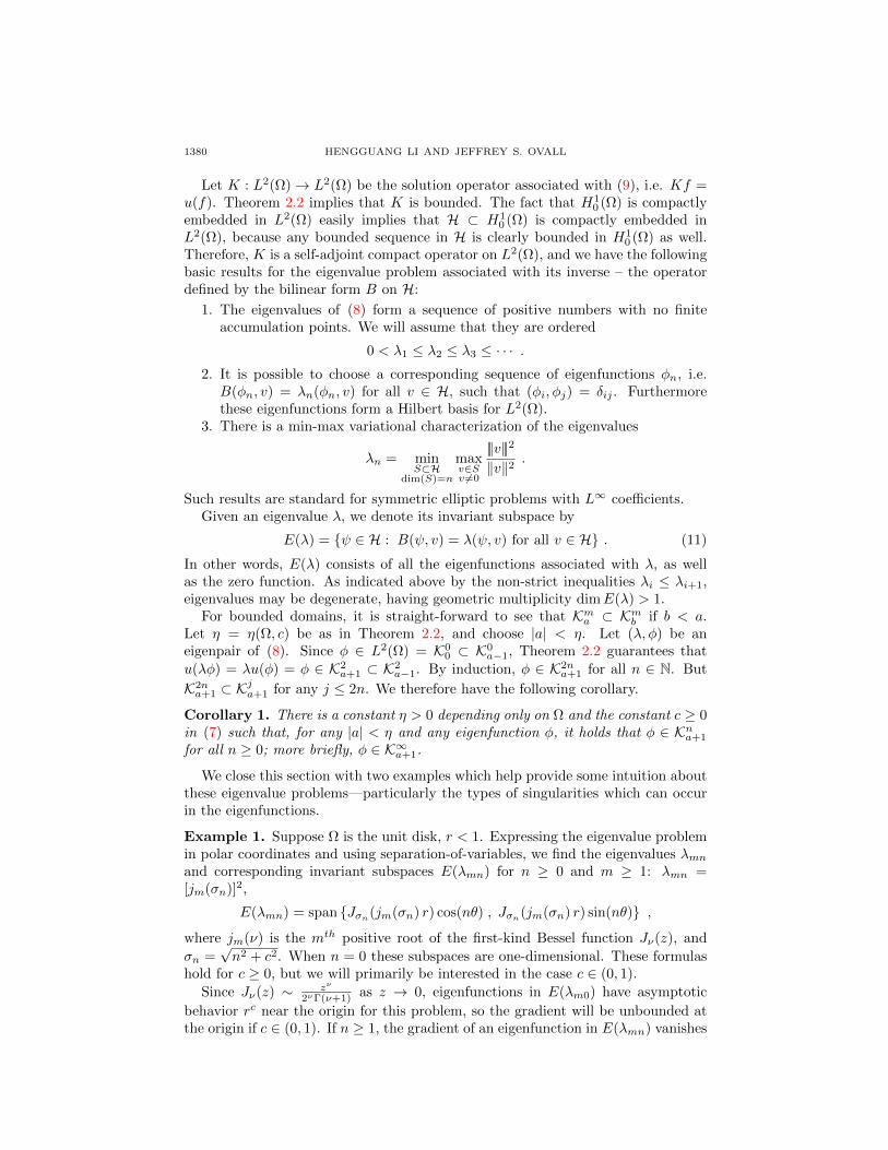
1380 HENGGUANG LI AND JEFFREY S. OVALL

Let K : L2(Ω)→ L2(Ω) be the solution operator associated with (9), i.e. Kf =u(f). Theorem 2.2 implies that K is bounded. The fact that H1

0 (Ω) is compactlyembedded in L2(Ω) easily implies that H ⊂ H1

0 (Ω) is compactly embedded inL2(Ω), because any bounded sequence in H is clearly bounded in H1

0 (Ω) as well.Therefore, K is a self-adjoint compact operator on L2(Ω), and we have the followingbasic results for the eigenvalue problem associated with its inverse – the operatordefined by the bilinear form B on H:

1. The eigenvalues of (8) form a sequence of positive numbers with no finiteaccumulation points. We will assume that they are ordered

0 < λ1 ≤ λ2 ≤ λ3 ≤ · · · .2. It is possible to choose a corresponding sequence of eigenfunctions φn, i.e.B(φn, v) = λn(φn, v) for all v ∈ H, such that (φi, φj) = δij . Furthermorethese eigenfunctions form a Hilbert basis for L2(Ω).

3. There is a min-max variational characterization of the eigenvalues

λn = minS⊂H

dim(S)=n

maxv∈Sv 6=0

|||v|||2

‖v‖2.

Such results are standard for symmetric elliptic problems with L∞ coefficients.Given an eigenvalue λ, we denote its invariant subspace by

E(λ) = ψ ∈ H : B(ψ, v) = λ(ψ, v) for all v ∈ H . (11)

In other words, E(λ) consists of all the eigenfunctions associated with λ, as wellas the zero function. As indicated above by the non-strict inequalities λi ≤ λi+1,eigenvalues may be degenerate, having geometric multiplicity dimE(λ) > 1.

For bounded domains, it is straight-forward to see that Kma ⊂ Kmb if b < a.Let η = η(Ω, c) be as in Theorem 2.2, and choose |a| < η. Let (λ, φ) be aneigenpair of (8). Since φ ∈ L2(Ω) = K0

0 ⊂ K0a−1, Theorem 2.2 guarantees that

u(λφ) = λu(φ) = φ ∈ K2a+1 ⊂ K2

a−1. By induction, φ ∈ K2na+1 for all n ∈ N. But

K2na+1 ⊂ K

ja+1 for any j ≤ 2n. We therefore have the following corollary.

Corollary 1. There is a constant η > 0 depending only on Ω and the constant c ≥ 0in (7) such that, for any |a| < η and any eigenfunction φ, it holds that φ ∈ Kna+1

for all n ≥ 0; more briefly, φ ∈ K∞a+1.

We close this section with two examples which help provide some intuition aboutthese eigenvalue problems—particularly the types of singularities which can occurin the eigenfunctions.

Example 1. Suppose Ω is the unit disk, r < 1. Expressing the eigenvalue problemin polar coordinates and using separation-of-variables, we find the eigenvalues λmnand corresponding invariant subspaces E(λmn) for n ≥ 0 and m ≥ 1: λmn =[jm(σn)]2,

E(λmn) = span Jσn(jm(σn) r) cos(nθ) , Jσn(jm(σn) r) sin(nθ) ,

where jm(ν) is the mth positive root of the first-kind Bessel function Jν(z), and

σn =√n2 + c2. When n = 0 these subspaces are one-dimensional. These formulas

hold for c ≥ 0, but we will primarily be interested in the case c ∈ (0, 1).

Since Jν(z) ∼ zν

2νΓ(ν+1) as z → 0, eigenfunctions in E(λm0) have asymptotic

behavior rc near the origin for this problem, so the gradient will be unbounded atthe origin if c ∈ (0, 1). If n ≥ 1, the gradient of an eigenfunction in E(λmn) vanishes

EIGENVALUE ERROR ESTIMATION FOR A SCHRODINGER OPERATOR 1381

λ n m mult9.8696044010893586188 0 1 115.920513426475879895 1 1 227.181727337203603368 2 1 239.478417604357434475 0 2 141.354888262245568479 3 1 2

λ n m mult11.394747278578650551 0 1 116.823380260414901268 1 1 227.799823099432368260 2 1 241.856135733780468863 3 1 242.644242596364950600 0 2 1

Table 1. The smallest eight eigenvalues for the unit disk problem,Example 1, listed together with their indices and multiplicities:c = 1/2 (top) and c = 2/3.

at the origin. Determining the location in the spectrum of all eigenfunctions havinga specific regularity is untenable as it would require knowledge of the interlacing ofroots of the Bessel functions Jσn . However, a couple of specific instances will shedlight on typical behavior. Table 1 gives the smallest eight eigenvalues (countingmultiplicities) for this problem when c = 1/2 and c = 2/3. These eigenvalues arecorrect in all digits shown, up to rounding in the last digit.

Example 2. Fixing α ≥ 1/2, suppose Ω is the sector of the unit disk, with r < 1and 0 < θ < π/α, where θ is the opening angle of the sector. The limiting caseα = 1/2 represents the unit disk with the positive x-axis removed. As before, we findthe eigenvalues λmn and corresponding invariant subspaces E(λmn) for m,n ≥ 1,

λmn = [jm(σn)]2 , E(λmn) = span Jσn(jm(σn) r) sin(nα θ) ,

where and σn =√

(nα)2 + c2. Again, these formulas hold for c ≥ 0, and the casec = 0 (the Laplace eigenvalue problem) illustrates the type of singularities whichcan occur solely because of re-entrant corners, i.e. α < 1. We provide the first eighteigenvalues for c = 0, with α = 1/2 (slit disk) and α = 2/3 (L-shape) in Table 2.

3. Discretization and error estimation. In this section, we consider the finiteelement approximation of solutions to the eigenvalue problem (8), with focus onthe estimation of error in the computed eigenvalue approximations. Before gettinginto the details of our finite element discretization, we make a few relevant claimswhich hold more generally. We restrict our attention to finite dimensional subspacesV ⊂ H. The natural analogues of (8) and (9) are

Find (λ, φ) ∈ R+ × (V \ 0) such that B(φ, v) = λ (φ, v) for all v ∈ V , (12)

Given f ∈ L2(Ω) find u(f) ∈ V such that B(u(f), v) = (f, v) for all v ∈ V . (13)

As before, we will refer to a solution (λ, φ) of (12) as an eigenpair of B on V ,

with eigenvalue λ and eigenfunction φ. These discrete problems are well-posed bybasic linear algebra and by the coercivity of the bilinear form on V (Lemma 2.1).

1382 HENGGUANG LI AND JEFFREY S. OVALL

λ n m mult9.8696044010893586188 1 1 114.681970642123893257 2 1 120.190728556426629975 3 1 126.374616427163390770 4 1 133.217461914268368860 5 1 139.478417604357434475 1 2 140.706465818200319742 6 1 148.831193643619198878 7 1 1

λ n m mult11.394747278578650551 1 1 118.278538262077375859 2 1 126.374616427163390770 3 1 135.642557845428184984 4 1 142.644242596364950600 1 2 146.052882654426898622 5 1 156.113114813020558488 2 2 157.582940903291124744 6 1 1

Table 2. The smallest eight eigenvalues for the unit sector prob-lem, Example 2, listed together with their indices and multiplicitiesfor c = 0; α = 1/2 (top) and α = 2/3.

More specifically, if v1, v2, . . . , vN is a basis for V , then (12) is equivalent to thegeneralized eigenvalue problem

Ax = λMx , aij = B(vj , vi) , mij = (vj , vi) , (14)

where the matrices A = (aij) and M = (mij). The following analogues from thecontinuous eigenvalue problem apply:

1. There are precisely N = dim(V ) eigenvalues for the system (14), which wetake to be ordered as

0 < λ1 ≤ λ2 ≤ · · · ≤ λN .

2. It is possible to choose corresponding eigenfunctions φn, i.e. B(φn, v) =

λn(φn, v) for all v ∈ V , such that (φi, φj) = δij . These eigenfunctions clearlyform a Hilbert basis for V .

3. There is a min-max variational characterization of the eigenvalues

λn = minS⊂V

dim(S)=n

maxv∈Sv 6=0

|||v|||2

‖v‖2= min

S⊂Rndim(S)=n

maxx∈Sx 6=0

xtAx

xtMx.

This characterization implies that λn ≥ λn for n ≤ N .

Lemma 3.1. Suppose that (λ, φ) is an eigenpair for B on H and (λ, φ) is an

eigenpair for B on V , with ‖φ‖ = ‖φ‖ = 1. Let φ = u(λφ). It holds that

λ− λ = |||φ− φ|||2 + (λ− λ)[(φ− φ, φ) + (φ, φ− φ)

]+ λ(φ− φ, φ− φ) . (15)

EIGENVALUE ERROR ESTIMATION FOR A SCHRODINGER OPERATOR 1383

Proof. Using the fact that ‖φ‖ = ‖φ‖ = 1, we first have the following identities,

|||φ− φ|||2 = B(φ− φ, φ− φ) = λ+ λ− 2λ(φ, φ) ,

λ‖φ− φ‖2 = λ(φ− φ, φ− φ) = λ+ λ− 2λ(φ, φ) .

Subtracting these identities, we obtain the well-known error formula,

λ− λ = |||φ− φ|||2 − λ‖φ− φ‖2 . (16)

Using the fact that B(φ, v) = λ(φ, v) for all v ∈ H, we further manipulate (16),

λ− λ = B(φ− φ, φ− φ)− λ(φ− φ, φ− φ)

= λ(φ, φ− φ)−B(φ, φ− φ)− λ(φ, φ− φ) + λ(φ, φ− φ)

= λ(φ, φ− φ)−B(φ, φ− φ) + (λ− λ)(φ, φ− φ)

= B(φ− φ, φ− φ) + (λ− λ)(φ, φ− φ)

= |||φ− φ|||2 +B(φ− φ, φ− φ) + (λ− λ)(φ, φ− φ)

= |||φ− φ|||2 + λ(φ− φ, φ)− λ(φ− φ, φ) + (λ− λ)(φ, φ− φ) ,

from which (15) follows directly.

Our computed estimate of λ−λ will be based on approximating |||φ−φ|||2, treatingthe rest of the bound in (15) as higher-order terms. To make this more precise, wenow shift to definitions of our finite element spaces, and a few key results.

Given a triangulation T of Ω, let V be the vertex set (the vertices of all triangles),which we assume includes all singular points Q. We define the two spaces

V = V (T ) = H ∩ C(Ω) : v|T ∈ P1, ∀T ∈ T , (17)

W = W (T ) = H ∩ C(Ω) : v|T ∈ P2, ∀T ∈ T and v(z) = 0, ∀z ∈ V. (18)

The space Pk consists of polynomials of total degree k or less. We note that it isnecessary that v(0) = 0 for v ∈ V . We will approximate the solution of (8) in thespace V and assess the error of this approximation in the space W .

Definition 3.2 (Graded Triangulations). Let T be a triangulation of Ω whosevertices include Q, such that no triangle in T has more than one of its vertices inQ. For κ ∈ (0, 1/2], a κ refinement of T , denoted by κ(T ), is obtained by dividingeach edge AB of T in two parts as follows:

• If neither A nor B is in Q, then we divide AB into two equal parts.• Otherwise, if say A is in Q, we divide AB into AC and CB such that |AC| =κ|AB|.

This will divide each triangle of T into four triangles. Figure 1 shows a trianglehaving a singular vertex (the vertex on the top), together with three subsequent κ-refinements, with κ = 1/4. Given an initial triangulation T0, the associated familyof graded triangulations Tn : n ≥ 0 is defined recursively, Tn+1 = κ(Tn).

Remark 1. Although it may be useful in practice to have a different grading ratioκq for each q ∈ Q, which is not difficult to implement, we do not pursue thattheoretical generality here.

Given a family Tn of κ-refined triangulations, we set Vn = V (Tn) and Wn =W (Tn), and un(f) ∈ Vn is the solution of (13) on Vn. We see that dim(Vn) ∼

1384 HENGGUANG LI AND JEFFREY S. OVALL

Figure 1. A triangle and three consecutive κ-refinements towardsthe top vertex, κ = 1/4.

dim(Wn) ∼ 4n, because each refinement increases the number of triangles by pre-cisely a factor of 4. We also define εn(f) ∈Wn by

B(εn(f), v) = (f, v)−B(un(f), v) for all v ∈Wn . (19)

We collect two key results from [21,22].

Theorem 3.3. Let η be as in Theorem 2.2, and for 0 < a < min(η, 1) chooseκ = 2−1/a. There is a constant C which is independent of f and n, such that

|||u(f)− un(f)||| ≤ C2−n‖f‖K0a−1

(20)

|||u(f)− un(f)− εn(f)||| ≤ C2−σn‖f‖K1ξ−1

(21)

where the related numbers σ > 1 and a < ξ < min(2a, η, 1) are also independent off and n.

Although we generally think of f as remaining fixed, these results allow for f tovary with n, and we exploit this fact below. In what follows, we let (λk,n, φk,n) :1 ≤ k ≤ N = dim(Vn), be eigenpairs for B on Vn with (φi,n, φj,n) = δij , as

discussed at the beginning of this section; therefore, λk,n = λk, φk,n = φk andV = Vn, for example.

EIGENVALUE ERROR ESTIMATION FOR A SCHRODINGER OPERATOR 1385

Corollary 2. Setting ψk,n = u(λk,nφk,n) and εk,n = εn(λk,nφk,n), and employingthe assumptions of Theorem 3.3, we have

|||ψk,n − φk,n||| ≤ Cλk,n 2−n , (22)

|||ψk,n − φk,n − εk,n||| ≤ Cλ3/2k,n 2−σn , (23)

where C is independent of k and n.

Proof. Putting (20) in this context, we have

|||ψk,n − φk,n||| ≤ C2−n‖λk,nφk,n‖K0a−1≤ C2−nλk,n‖φk,n‖L2(Ω) ≤ Cλk,n 2−n .

Similarly,

|||ψk,n − φk,n − εk,n||| ≤ C2−σn‖λk,nφk,n‖K1ξ−1≤ C2−σnλk,n|||φk,n||| ≤ Cλ3/2

k,n 2−σn .

This completes the proof.

We emphasize that the computation of εk,n involves solving the problem

B(εk,n, v) = λk,n(φk,n, v)−B(φk,n, v) for all v ∈Wn . (24)

Using the standard bases for Vn and Wn, it is shown in [22, Theorem 3.6] that thecondition number of the matrix associated with (24) is well-conditioned independentof n. In fact, it is spectrally equivalent to its own diagonal. This makes (24) veryinexpensive to solve, particularly when compared with computing solutions to the

eigenvalue problem Ax = λMx on Vn, where the stiffness matrix A is known tohave a condition number which grows like 4n.

Suppose we fix k and consider the sequence of discrete eigenpairs (λk,n, φk,n) :n ≥ 0 for the Schrodinger operator with meshes appropriately graded near theset Q (see Theorem 3.3). We do not rehearse standard finite element convergencetheory for eigenvalue problems (cf. [9, Section 3.3], [3]), but by the approximationproperty given in Theorem 3.3, the following results for our eigenvalue problem canbe derived in a similar fashion:

• The approximate eigenvalues λk,n converge (down) to λk quadratically,

λk ≤ λk,n with λk,n − λk = O(4−n) . (25)

• The distance between φk,n and the invariant subspace E(λk) associated withλk decreases linearly in the energy norm,

minv∈E(λk)

|||v − φk,n||| = O(2−n) . (26)

We emphasize that λk may be a degenerate eigenvalue (repeated in the se-quence of eigenvalues), so E(λk) may have dimension greater than one. Theanalogous statements on Vn hold as well. In light of this, it does not nec-essarily make sense to say that φk,n : n ≥ 0 converges, even up to sign.Nevertheless, we do have convergence in the sense of (26), and we refer to this(loosely) as eigenvector “convergence”. We also remark that, although theeigenfunction v ∈ E(λk) which is nearest to φk,n may not be of unit length,but we do not lose (26) if we add this restriction.

In practice, the eigenvalue convergence is precisely quadratic, and the eigenvector“convergence” is precisely linear on these properly graded meshes.

1386 HENGGUANG LI AND JEFFREY S. OVALL

We now reconsider the various terms in the error identity (15),

λk,n − λk = |||ψk,n − φk,n|||2 + (λk,n − λk) [(ψk,n − φk,n, vk,n) + (φk,n, vk,n − φk,n)]

+ λk,n(ψk,n − φk,n, vk,n − φk,n) .

Here we have taken vk,n = argmin‖v − φk,n‖ : v ∈ E(λk) , ‖v‖ = 1.• We take the simple bound ‖vk,n − φk,n‖ ≤ C|||vk,n − φk,n||| = O(2−n).• Using a duality argument (L2-lifting, or Nitsche’s trick), we see that ‖ψk,n −φk,n‖ = O(4−n).

• Finally, we note that

|||ψk,n − φk,n|||2 − |||εk,n|||2 = (|||ψk,n − φk,n||| − |||εk,n|||)(|||ψk,n − φk,n|||+ |||εk,n|||)

≤ (|||ψk,n − φk,n − εk,n|||)(|||ψk,n − φk,n|||+ |||εk,n|||) = O(2−(1+σ)n) .

Combining these pieces, we arrive at our key eigenvalue error theorem.

Theorem 3.4. Under the assumptions of Theorem 3.3, it holds that

λk,n − λk = |||εk,n|||2 +O(4−τn) , (27)

for some constant τ > 1. The hidden constant in O(4−τn) depends on λk.

4. Numerical experiments. In this section we report the outcome of severalnumerical experiments, to demonstrate how well the theory of previous sections—particularly Theorem 3.4—are realized in practice. The data of interest are theeigenvalue errors λk,n − λk, their computed estimates |||εk,n|||2, and the associatedeffectivities

EFF =λk,n − λk|||εk,n|||2

.

The software package PLTMG [5] was used for these experiments, with suitablemodifications for employing hierarchical basis error estimation and graded meshrefinement, with ARPACK [19] in shift-and-invert mode as the algebraic eigenvaluesolver. In order reduce the width of tables of numerical data, we use the followingabbreviation of scientific notation, a× 10m ↔ am. For example,

1.949× 10−4 ↔ 1.949−4 .

We first revisit the unit disk problem of Example 1, considering case c = 1/2,for which we know that the eigenfunctions associated with λ1 ≈ 9.86960440 andλ6 ≈ 39.4784176 have an r1/2 singularity (see Table 1). The grading ratio κ =0.2 was used for refinement. Note that by Theorem 3.3, the upper bound of thegrading parameter κ near the origin is 2−1/(1/2) = 0.25 to achieve the optimalconvergence rate. Therefore, we have chosen an appropriate grading ratio here.The data for these experiments are in Table 3. The eigenvalue convergence is seento be quadratic, i.e. linear in N = dim(Vn), and the effectivities are very close 1.The top row of data is absent for λ6 because, on this coarse mesh, the approximateeigenvalue 33.2876671 was actually (slightly) nearer to λ4 = λ5 ≈ 27.1817273 thanto λ6. The effectivity of the error estimate when this was taken into account was1.010.

We now consider the degenerate eigenvalue λ = λ2 = λ3 ≈ 15.9205134. Thecorresponding invariant subspace (eigenspace) is spanned by

φ2 = Jσ(√λ r) cos(θ) , φ3 = Jσ(

√λ r) sin(θ) where σ =

√5

2≈ 1.11803 .

EIGENVALUE ERROR ESTIMATION FOR A SCHRODINGER OPERATOR 1387

n N λ1,n − λ1 |||ε1,n|||2 EFF λ6,n − λ6 |||ε6,n|||2 EFF0 48 9.467−1 8.284−1 1.1421 224 2.429−1 1.907−1 1.273 3.892+0 3.395+0 1.1462 961 5.690−2 4.594−2 1.238 9.629−1 8.450−1 1.1393 3968 1.631−2 1.413−2 1.154 2.493−1 2.284−1 1.0914 16129 3.957−3 3.605−3 1.098 6.182−2 5.898−2 1.0485 65025 1.026−3 9.527−4 1.076 1.560−2 1.510−2 1.0336 261121 2.637−4 2.469−4 1.068 3.929−3 3.844−3 1.022

Table 3. Data for the Unit Disk problem, corresponding to ap-proximations of λ1 and λ6 on graded meshes with κ = 0.2, c = 1/2.

Of course the ordering of φ2 and φ3 is arbitrary, as is that particular choice of basisfor this invariant subspace. These functions are smooth enough to be optimallyapproximated on a sequence of uniformly refined meshes, κ = 0.5; for compari-son, grading ratio κ = 0.4 and κ = 0.2 were used as well. On each mesh, twoapproximate eigenvalues and eigenvectors were computed and error estimates forboth were computed. The results indicate that it really is irrelevant which of theapproximate eigenpairs is used to estimate error in the eigenvalue approximation, asindicated by our theory. Since the code (PLTMG+ARPACK) assigns an order tothe approximate eigenpairs, we employ this order as well, (λ2,n, φ2,n), (λ3,n, φ3,n).The computed eigenvalues λ2,n and λ3,n agreed with each other to far more digitsthan they agreed with λ2 = λ3, so the reported errors are identical. It is only theerror estimates, and hence effectivities, which are slightly different. In terms of thegrading, all three grading choices gave optimal order convergence, as the theorypredicts, with uniform refinement (κ = 0.5) yielding the smallest errors and κ = 0.2yielding the largest errors. In terms of effectivities, uniform refinement was theworst, followed in order by κ = 0.4 and κ = 0.2, though all were close to 1. To savespace, only the data for κ = 0.5 and κ = 0.2 are reported in Table 4. In order todemonstrate the “drift” in approximate eigenfunctions associated with degenerateeigenvalues, we provide a sequence of contour plots for φ2,n, n = 1, 2, 3, 4 in Figure2. The contour plots of φ3,n are essentially obtained by rotating the given plotsby 90 degrees. These plots illustrate the assertion in Section 3 that the sequenceφk,n may not converge, though the terms are getting successively closer to E(λk).

Finally, we turn to the L-shape domain Ω = (−1, 3)2 \ [1, 3)2. We consider thecase c = 1/2, for which there will be eigenfunctions having an r1/2-singularity at theorigin and an r2/3-singularity at the point (1, 1). We use the grading ratios κ = 0.2for triangles touching the origin, and κ = 0.3 for triangles touching (1, 1). Table 5contains our approximations and error estimates for the first four eigenvalues. Con-tour plots of the first four eigenfunctions are given in Figure 3. As an interestingcomparison, we also consider the case c = 0, for which no singularity is present atthe origin, and grading is only needed near the point (1, 1). The eigenvalues in thiscase have been obtained elsewhere to very high accuracy [26] using a computationalvery well-suited to the Laplacian, and we report their values here, rescaling themby a factor of four due to the fact that our domain has four times the area of theirs:

λ1 ≈ 2.4099310 , λ2 ≈ 3.7993130 , λ3 =π2

2≈ 4.9348022 , λ4 ≈ 7.3803703 . (28)

1388 HENGGUANG LI AND JEFFREY S. OVALL

n N λ2,n − λ2 |||ε2,n|||2 EFF λ3,n − λ3 |||ε3,n|||2 EFF0 48 1.019+0 9.181−1 1.110 1.019+0 9.181−1 1.1101 224 2.544−1 2.233−1 1.139 2.544−1 2.197−1 1.1582 961 6.371−2 5.498−2 1.158 6.371−2 5.588−2 1.1403 3968 1.596−2 1.424−2 1.121 1.596−2 1.413−2 1.1294 16129 3.997−3 3.562−3 1.122 3.997−3 3.576−3 1.1185 65025 1.001−3 8.987−4 1.114 1.001−3 8.966−4 1.1166 261121 2.506−4 2.250−4 1.113 2.506−4 2.250−4 1.113

n N λ2,n − λ2 |||ε2,n|||2 EFF λ3,n − λ3 |||ε3,n|||2 EFF0 48 2.371+0 2.361+0 1.004 2.371+0 2.361+0 1.0041 224 5.769−1 5.170−1 1.116 5.769−1 5.272−1 1.0932 961 1.433−1 1.299−1 1.103 1.433−1 1.278−1 1.1223 3968 3.576−2 3.311−2 1.080 3.576−2 3.282−2 1.0904 16129 8.938−3 8.406−3 1.063 8.938−3 8.374−3 1.0675 65025 2.234−3 2.117−3 1.055 2.234−3 2.114−3 1.0576 261121 5.586−4 5.312−4 1.052 5.586−4 5.308−4 1.052

Table 4. Data for the Unit Disk problem, corresponding to ap-proximations of λ2 = λ3. Uniform refinement (top) and κ = 0.2graded refinement, c = 1/2.

n N λ1,n |||ε2,n|||2 λ2,n |||ε2,n|||2 λ3,n |||ε3,n|||2 λ4,n |||ε4,n|||20 16 4.416 1.326+0 5.091 1.163+0 8.044 2.135+0 11.00 3.150+0

1 80 3.491 3.064−1 4.212 2.682−1 6.582 5.633−1 8.488 7.348−1

2 353 3.251 7.477−2 4.005 6.746−2 6.128 1.387−1 7.878 1.930−1

3 1472 3.194 2.126−2 3.953 1.730−2 6.024 4.031−2 7.723 5.063−2

4 6017 3.177 5.588−3 3.940 4.361−3 5.992 1.055−2 7.684 1.283−2

5 24321 3.173 1.488−3 3.937 1.094−3 5.984 2.813−3 7.674 3.242−3

6 97793 3.172 3.901−4 3.936 2.737−4 5.982 7.394−4 7.672 8.130−4

7 392192 3.172 1.024−4 3.936 6.855−5 5.982 1.949−4 7.671 2.035−4

Table 5. Data for the L-shape problem, corresponding to ap-proximations of λ1 through λ4, κ = 0.2 and κ = 0.3 for differentsingular points, c = 1/2.

The second eigenfunctions for c = 1/2 and c = 0 are not linearly dependent, nor arefourth eigenfunctions for both c = 1/2 and c = 0. Their contour plots are merelyvery similar, though not identical.

Acknowledgments. We thank the referees for a careful reading of the manuscriptand for offering helpful suggestions.

REFERENCES

[1] T. Apel and S. Nicaise, The finite element method with anisotropic mesh grading for ellipticproblems in domains with corners and edges, Math. Methods Appl. Sci., 21 (1998), 519–549.

EIGENVALUE ERROR ESTIMATION FOR A SCHRODINGER OPERATOR 1389

Figure 2. Contour plots of φ2,n for n = 1, 2 (top) and n = 3, 4for the Unit Disk problem, with κ = 0.4.

[2] I. Babuska, R. B. Kellogg and J. Pitkaranta, Direct and inverse error estimates for finite

elements with mesh refinements, Numer. Math., 33 (1979), 447–471.[3] I. Babuska and J. Osborn, Eigenvalue problems, In Handbook of numerical analysis, Vol. II,

Handb. Numer. Anal., II, pages 641–787. North-Holland, Amsterdam, 1991.[4] C. Bacuta, V. Nistor and L. T. Zikatanov, Improving the rate of convergence of ‘high order

finite elements’ on polygons and domains with cusps, Numer. Math., 100 (2005), 165–184.

[5] R. E. Bank, PLTMG: A software package for solving elliptic partial differential equations.

Users’ Guide 10.0, Technical report, University of California at San Diego, Department ofMathematics, 2007.

[6] R. E. Bank, L. Grubisic and J. S. Ovall, A framework for robust eigenvalue and eigenvectorerror estimation and ritz value convergence enhancement, Applied Numer. Math., 66 (2013),

1–29.

[7] H. Chen, L. He and A. Zhou, Finite element approximations of nonlinear eigenvalue problemsin quantum physics, Comput. Methods Appl. Mech. Engrg., 200 (2011), 1846–1865.

[8] M. Dauge, Elliptic Boundary Value Problems on Corner Domains, volume 1341 of Lecture

Notes in Mathematics, Springer-Verlag, Berlin, 1988.[9] A. Ern and J.-L. Guermond, Theory and Practice of Finite Elements, volume 159 of Applied

Mathematical Sciences, Springer-Verlag, New York, 2004.

[10] V. Felli, A. Ferrero and S. Terracini, Asymptotic behavior of solutions to Schrodinger equa-tions near an isolated singularity of the electromagnetic potential, J. Eur. Math. Soc. (JEMS),

13 (2011), 119–174.

[11] V. Felli, E. Marchini and S. Terracini, On the behavior of solutions to Schrodinger equationswith dipole type potentials near the singularity, Discrete Contin. Dyn. Syst., 21 (2008),

91–119.

1390 HENGGUANG LI AND JEFFREY S. OVALL

Figure 3. Contour plots of φk,5 for k = 1, 2, 3, 4 for the L-shapeproblem. The left column corresponds to c = 0 and the rightcolumn to c = 1/2.

EIGENVALUE ERROR ESTIMATION FOR A SCHRODINGER OPERATOR 1391

[12] S. Fournais, M. Hoffmann-Ostenhof, T. Hoffmann-Ostenhof and T. Østergaard Sørensen,Analytic structure of solutions to multiconfiguration equations, J. Phys. A, 42 (2009), 315208,

11pp.

[13] P. Grisvard, Elliptic Problems in Nonsmooth Domains, volume 24 of Monographs and Studiesin Mathematics, Pitman (Advanced Publishing Program), Boston, MA, 1985.

[14] P. Grisvard, Singularities in Boundary Value Problems, volume 22 of Recherches enMathematiques Appliquees [Research in Applied Mathematics], Masson, Paris, 1992.

[15] E. Hunsicker, H. Li, V. Nistor and U. Ville, Analysis of Schrodinger operators with inverse

square potentials I: Regularity results in 3D, Bull. Math. Soc. Sci. Math. Roumanie (N.S.),55 (2012), 157–178.

[16] V. A. Kondrat′ev, Boundary value problems for elliptic equations in domains with conical or

angular points, Trudy Moskov. Mat. Obsc., 16 (1967), 209–292.[17] V. A. Kozlov, V. G. Maz′ya and J. Rossmann, Elliptic Boundary Value Problems in Domains

with Point Singularities, volume 52 of Mathematical Surveys and Monographs, American

Mathematical Society, Providence, RI, 1997.[18] V. A. Kozlov, V. G. Maz′ya and J. Rossmann, Spectral Problems Associated with Corner

Singularities of Solutions to Elliptic Equations, volume 85 of Mathematical Surveys and

Monographs, American Mathematical Society, Providence, RI, 2001.[19] R. B. Lehoucq, D. C. Sorensen and C. Yang, ARPACK Users’ Guide, volume 6 of Software,

Environments, and Tools, Society for Industrial and Applied Mathematics (SIAM), Philadel-phia, PA, 1998. Solution of large-scale eigenvalue problems with implicitly restarted Arnoldi

methods.

[20] H. Li, A. Mazzucato and V. Nistor, Analysis of the finite element method for transmis-sion/mixed boundary value problems on general polygonal domains, Electron. Trans. Numer.

Anal., 37 (2010), 41–69.

[21] H. Li and V. Nistor, Analysis of a modified Schrodinger operator in 2D: Regularity, index,and FEM, J. Comput. Appl. Math., 224 (2009), 320–338.

[22] H. Li and J. S. Ovall, A posteriori error estimation of hierarchical type for the Schrodinger

operator with inverse square potential, Numer. Math, 128 (2014), 707–740.[23] S. Moroz and R. Schmidt, Nonrelativistic inverse square potential, scale anomaly, and complex

extension, Annals of Physics, 325 (2010), 491–513.

[24] A. Naga and Z. Zhang, Function value recovery and its application in eigenvalue problems,SIAM J. Numer. Anal., 50 (2012), 272–286.

[25] G. Strang and G. J. Fix, An Analysis of the Finite Element Method, Prentice-Hall Inc.,Englewood Cliffs, N. J., 1973. Prentice-Hall Series in Automatic Computation,

[26] L. N. Trefethen and T. Betcke, Computed eigenmodes of planar regions, In Recent advances

in differential equations and mathematical physics, volume 412 of Contemp. Math., pages297–314. Amer. Math. Soc., Providence, RI, 2006.

[27] N. M. Wigley, Asymptotic expansions at a corner of solutions of mixed boundary value prob-

lems, J. Math. Mech., 13 (1964), 549–576.[28] H. Wu and D. W. L. Sprung, Inverse-square potential and the quantum vortex, Phys. Rev.

A, 49 (1994), 4305–4311.

Received August 2013; revised January 2015.

E-mail address: [email protected]

E-mail address: [email protected]