A polynomial algorithm for 2-cyclic robotic scheduling: A non-Euclidean case

Discrete Applied Mathematics 157 (2009) 339–355

Contents lists available at ScienceDirect

Discrete Applied Mathematics

journal homepage: www.elsevier.com/locate/dam

A polynomial algorithm for 2-cyclic robotic scheduling:A non-Euclidean caseVladimir Kats a, Eugene Levner b,∗

a Institute for Industrial Mathematics, Beer-Sheva, P.O. Box 15013, 84105, Israelb Holon Institute of Technology, Holon, P.O. Box 305, 58102, Israel

a r t i c l e i n f o

Article history:Received 27 October 2006Received in revised form 7 February 2008Accepted 9 March 2008Available online 25 April 2008

Keywords:Cyclic schedulingRobotic schedulingPolynomial-time algorithmsComplexityNo-wait conditionEuler formula

a b s t r a c t

In this paper we consider the problem of no-wait cyclic scheduling of identical parts in anm-machine production line in which a robot is responsible for moving each part from amachine to another. The aim is to find the minimum cycle time for the so-called 2-cyclicschedules, in which exactly two parts enter and two parts leave the production line duringeach cycle. The earlier known polynomial-time algorithms for this problem are applicableonly under the additional assumption that the robot travel times satisfy the triangleinequalities. We lift this assumption on robot travel times and present a polynomial-timealgorithm with the same time complexity as in the metric case, O(m5 log m).

© 2008 Elsevier B.V. All rights reserved.

1. Introduction

This paper considers a robotic flowshop cell which consists of m machines M1, . . . ,Mm, an input station M0, an outputstation Mm+1, and a single robot that performs all material handling operations in the cell, i.e., the transportation of partsbetween the machines and the stations, as well as the loading and unloading of parts onto and from the machines andstations. Each part must spend a predetermined amount of processing time on each machine and, once this time is elapsed,it must be immediately transported by the robot to the next machine (or to the output station) in a technological sequence.This condition is called the no-wait condition. In the electrochemical industry, violating this condition may deteriorate theproduct quality and cause a defect product. The paper considers cyclic production of identical parts which means that alloperations in the cell are periodically repeated. The robot repeats its moves periodically, and the corresponding sequence ofrobot moves is called a cyclic sequence. The sequence of robot moves supplied by the start and finish times is called robot’sschedule. A schedule is said to be cyclic if the start and finish times repeat periodically with a constant time T, called the cycletime.

A cyclic schedule in which each processing operation and each robot move appear r times during each cycle is said tobe r-cyclic. During each cycle of the r-cyclic schedule, exactly r parts enter the line and r parts are unloaded at the outputstation; at the end of the cycle the flowshop cell returns to its original state. The mean cycle time is defined as the whole cycletime divided by r. The throughput rate is the inverse of the mean cycle time. An optimization problem for robotic flowshopsasks to specify a cyclic sequence of robot moves so as to maximize the throughput rate of the flowshop, or, equivalently, tominimize the cycle time.

∗ Corresponding author. Fax: +972 35026733.E-mail address: [email protected] (E. Levner).

0166-218X/$ – see front matter © 2008 Elsevier B.V. All rights reserved.doi:10.1016/j.dam.2008.03.025

340 V. Kats, E. Levner / Discrete Applied Mathematics 157 (2009) 339–355

Optimal robotic flowshop schedules have been intensely studied over the past decades — for a thorough description anddiscussion of the model considered in this paper we refer the interested reader to the book by Dawande et al. [11], the surveysby Hall [13], Crama et al. [9] and Dawande et al. [10], and numerous references therein. In general, the multi-cyclic schedulesmay have a better throughput rate than the 1-cyclic ones, as has been reported by many authors (e.g., [25,17,20,16,5,6]).

The literature on the r-cyclic scheduling, for r > 1, is not so vast. To the best of our knowledge, the first work onmulti-cyclic robotic scheduling has appeared in the 1960s in the former Soviet Union: Suprunenko et al. [26], Aizenshtat [2]and Tanayev [27], have proposed concise mathematical descriptions of the r-cyclic processes with transporting automaticdevices and introduced the so-called method of forbidden intervals (MFI) for finding an optimal schedule; however, theseauthors did not study its complexity and did not establish its polynomiality. This method has been further developed andproved to be polynomial for the 1-cyclic case by Levner and Kats [18] and Levner et al. [19], where the upper bound ofO(m3

· log m) has been obtained. However, this result is related to the 1-cyclic schedules only.Sethi et al. [24] proved that for a 2-machine bufferless robotic cell producing identical parts the optimal solution is 1-

cyclic and conjectured that 1-cyclic schedules yield optimal solutions for every multi-machine robotic flowshop. Crama andKlundert [8] established the validity of the conjecture for three machines. However, Brauner and Finke [4] proved that 1-cyclic schedules do not necessarily yield optimal solutions for cells when the number of machines is four or larger. For a2-machine no-wait robotic cell producing identical parts Agnetis [1] showed that the optimal solution is 1-cyclic whereasfor a 3-machine no-wait robotic cell the optimal solution could be 2-cyclic. Akturk et al. [3] proved that the optimal solutionis not necessarily 1-cyclic and could be 2-cyclic for the 2-machine flexible cells, in which the processing of each part consistsof several different operations and the latter operations are to be allocated to the machines.

Special attention of the researchers has been devoted to finding efficient algorithms for the case of multi-machine 2-cyclicscheduling. Based on the above-mentioned method of forbidden intervals (MFI), Levner et al. [20] have proposed a geometricalgorithm solving this class of problems fast in practice and have conjectured that it is of polynomial time. This conjecturehas been proven by Chu [7] for a special case in which the robot transportation times satisfy the triangle inequalities. For thesake of brevity, we refer to this case as “the Euclidean case” although the Euclidean metrics is only a special type of metricssatisfying the triangle inequalities. These authors have proved that, in this case, the complexity of the geometric algorithm isO(m8 log m). Chu [7] has presented a more elaborate analysis of the MFI for the considered problem, which permitted him toimprove the algorithm complexity estimation for the Euclidean case from O(m8 log m) to O(m5 log m). In order to completethe entire picture, we add that for a more general class of r-cyclic schedules, r > 2, Che et al. [5], have shown that for afixed r, the MFI solves the Euclidean case in polynomial time in m with the complexity quickly increasing with the growthof r, approximately as m6r2(m3/r)r(r−1)/2 (if r < m). The complexity for the general non-Euclidean case remained an openquestion, which will be answered in this paper for 2-cyclic schedules.

Thus, we investigate a general, non-Euclidean case, when the robot transportation and traveling times are not required tosatisfy the triangle inequalities. This model may be appropriate in practical situations in which distances are not necessarilyEuclidean, for example, in the case when a mobile robot has to navigate in an area with many obstacles. Here, the methodof forbidden intervals, in its original form, is not applicable because the intervals cannot be simply merged together, as inthe Euclidean case. We suggest a different geometric approach based on the concepts of feasible polygons and singular pointswhich is valid for both of the cases, Euclidean as well as non-Euclidean. Using this approach, we enhance the geometricalscheme suggested by Levner et al. [20] and construct an improved algorithm of complexity O(m5 log m).

This paper is organized as follows. Section 2 gives a formal description of the problem. Section 3 presents the analysisof the problem and restate it as a finite series of linear programming problems. Section 4 introduces the singular pointsand estimates their total number. Based on the concepts of feasible polygons and singular points, Section 5 presents anew polynomial algorithm and estimates its complexity. A numerical example in this section demonstrates that the MFIdeveloped for the Euclidean case is no longer an exact method valid for the non-Euclidean case. Section 6 concludes thepaper. Appendix A contains the proofs. Appendix B introduces the MFI method and gives computational details for theexample from Section 5 whereas Appendix C provides the details of how the present geometrical algorithm solves thisexample to optimality.

2. Problem formulation and notation

In 2-cyclic schedules, exactly two parts enter and two parts leave the line during each cycle of length T. The identical partsare loaded into the line at time . . .−kT,−kT+T1, . . . ,−2T,−2T+T1,−T,−T+T1, 0, T1, T, T+T1, 2T, . . . , kT+T1, (k+1)T, . . . ,where T1 < T. The parts loaded at time kT (respectively, at time kT + T1), k = 0,±1,±2, . . . are called the parts of Class 1(respectively, the parts of Class 2).

Two sequences, U and S, characterize the considered scheduling problem:• a fixed and a priori known sequence U = {0, 1, 2, . . . ,m,m+1}which specifies that each of the (identical) parts is loaded

at the input station M0, processed on the machines in order M1, . . . ,Mm, and then is unloaded at an output station Mm+1;• an a priori unknown sequence S of robot moves, S = {s(1) = 0, s(2), . . . , s(2m + 2)}, which is to be found; it specifies

the order of operations to be performed by the robot in each cycle in the 2-cyclic schedule. After unloading machineMs(2m+2) the robot moves again to station s(1) = M0 and at time T introduces a new part into the process. Without lossof generality (as all the robot moves are cyclically repeated), we assume that robot’s cycle starts at the input station M0,that is, s(1) = 0.

V. Kats, E. Levner / Discrete Applied Mathematics 157 (2009) 339–355 341

The first robot move, s(1), in Sdenotes that the robot starts its cycle by taking a part at the input stationM0, then transportsthe part to the first machine M1 on its technological sequence U and loads the part to M1. The ith robot move in sequence S,denoted by s(i), i = 2, . . . , 2m + 1, consists of the following sequential operations: the robot runs empty to machine Ms(i)

and waits until that machine finishes its processing operation, then unloads a part from machine Ms(i), and, finally, eithertransports the part from Ms(i) to the next machine Ms(i)+1 on its technological sequence U and loads a part there if s(i) 6= m,or transports the part from Ms(i) to the unloading station Mm+1 if s(i) = m. During its (2m+ 2)th move, the robot runs emptyto machine Ms(2m+2) and waits if necessary, then unloads a part from machine Ms(2m+2), transports the part from Ms(2m+2) tothe next machine Ms(2m+2)+1 (or to the unloading station) on its technological sequence U, loads a part there and, finally,runs empty to the input station M0, where it takes the next part and starts the next cycle.

Definition 1 (Cycle Time T). For any instance of the problem, the cycle time T is defined as the total time required by therobot to perform all the 2m+ 2 moves in sequence S.

Notice that the length of a life cycle of each part (that is, the time elapsed between the moment when the part entersinto the line and the moment when it is unloaded to the output station) can be much longer than the cycle time T, which isdependent of S.

To make a formal definition for the problem, we introduce the following parameters:pi The processing time of a part at machine Mi, i = 1, 2, . . . ,m;di The transportation time of a part from machine Mi to Mi+1, i = 0, 1, 2, . . . ,m, where “machine” Mm+1 is the unloading

station and “machine” M0 is the input station; to simplify the presentation, we assume that the transportation timeincludes the durations of the unloading operation at machine Mi and the loading operation at machine Mi+1. We assumethat the transportation times are non-negligible, di > 0;

rij The traveling time of an unloaded robot from machine Mi to machine Mj, i = 1, 2, . . . ,m+ 1; j = 0, 1, 2, . . . ,m;Zi The completion time of the ith processing operation in U performed at machine Mi, which, due to the no-wait condition,

is equal to the start time of robot’s travel to machine Mi+1, Zi =∑

j=1,...,i (dj−1 + pj), i = 1, . . . ,m;Rij Robot’s total traveling time from Mi to Mi+1 then to Mj : Rij = di + ri+1,j, where i, j = 0, 1, 2, . . . ,m. Since all Rij > 0, the

robot cannot do more than one unloading operation at a time.

We start with formulating several natural constraints of the problems. Consider the part introduced into the processat time 0. Due to the no-wait condition, this part must be completed at machine Mi at time Zi = Zi−1 + di−1 + pi, i =1, . . . ,m, Z0 = 0. Correspondingly, the part introduced into the process at time t must be unloaded from machine Mi at timet+Zi. We assume that each processing machine cannot process more then one part simultaneously. This condition prohibitsthe values T1 and T− T1 to be less than pi for any i. As long as the robot is capable of transporting only one part at a time, thevalues T1 and T − T1 must not be smaller than di−1 + pi + di, for any i, otherwise the transportation operations to machineMi and from machine Mi will overlap in time. Thus, we have

T1 ≥ T0 = maxi=1,...,m

(di−1 + pi + di) = maxi=1,...,m

(di + Zi − Zi−1); (1a)

T − T1 ≥ T0 = maxi=1,...,m

(di−1 + pi + di) = maxi=1,...,m

(di + Zi − Zi−1). (1b)

On the other hand, let us define the upper bound T0 for T1 and T − T1 as follows:T0= Zm + dm + rm+1,0.

Obviously, the minimal values of T1 and T−T1 are not larger than T0. Indeed, the schedule with T1 = T−T1 = T0 correspondsto a primitive cyclic robot route S0 = {0, 1, 2, . . . ,m, 0, 1, 2, . . . ,m}, repeating twice the technological order of machines U.Comparing T0 and T0, we obtain:

T0=

∑j=1,...,m

(dj−1 + pj)+ dm + rm+1,0 ≤ mT0 + rm+1,0. (1c)

The process periodicity allows us to restrict its analysis to a single cycle confined within the time interval [0, T). Withinthis interval, exactly two parts are unloaded from each machine Mi: the part which was introduced at time (−kT), wherek = floor(Zi/T), will be unloaded at time Yi = Zi mod T = Zi− kT, whereas the part which was introduced at time (−hT+ T1),where h = floor[(Zi + T1)/T], will be unloaded at time Y ′i = (Zi + T1) mod T = Zi + T1 − hT. The station M0 will be unloadedat time 0 and T1.

Notice that the height ki (and, correspondingly, hi) where ki = floor(Zi/T) (correspondingly, hi = floor[(Zi+T1)/T]) definesthe number of complete cycles that the part has gone through before being completed since its introduction into the process.

Let Y be the set containing all the values Yi = Zi mod T and Y ′i = (Zi+T1) mod T, i = 0, 1, . . . ,m:Y = {Y(∗)1 , Y(∗)

2 , . . . , Y(∗)2m+2},

where symbol Y(∗)i denotes either Yi or Y ′i .

Proposition 1. For the given values T and T1, the periodically repeated robot route can be found by ordering 2m+ 2 numbers inthe set Y in the following order

0 = Y0 = Y(∗)s(1) ≤ Y(∗)

s(2) ≤ · · · ≤ Y(∗)s(2m+2) < T. (2)

342 V. Kats, E. Levner / Discrete Applied Mathematics 157 (2009) 339–355

The sequence of indices S = {s(1) = 0, s(2), . . . , s(2m + 2)} determines the robot route, which is the sequence of robotmoves between the machines in time interval [0, T).

The proof is similar to the 1-cyclic case given, for instance, by Livshits and Mikhailetski [21] and Phillips and Unger [23],and is skipped here. In case we need to indicate that the robot moves a part of Class 2 from a certain machine (that is, themove starts at moment Y ′i ), the corresponding machine number in S will be marked by symbol “′ ”, the notation will be usedin the Example in Section 5 and in Appendix C.

If, for some values T and T1, the relations (2) hold as strict equations for some i and j, for instance, the equation Y(∗)i = Y(∗)

j

takes place, this means that the robot moves from machines Mi and Mj should start simultaneously, which is physicallyimpossible, because all transportation operations are not instantaneous (Ri,j > 0). In the following, we will consider twotypes of points (T, T1) defined by inequalities (2). On the one hand, there are values (T, T1) such that all relations (2) holdas strict inequalities; for any of such pairs (T, T1), Proposition 1 defines the robot route uniquely. On the other hand, we willconsider points (T, T1), such that at least one of inequalities (2) holds as a strict equation, for example Y(∗)

i = Y(∗)j , which means

that in a neighborhood of such a point the robot route changes, namely, instead of moving from machine Mi to machine Mj

when Y(∗)i < Y(∗)

j , it will move from Mj to Mi as long as Y(∗)i > Y(∗)

j .

Definition 2 (Feasible Robot’s Route). Given some values of T and T1, we say that a robot’s route S is feasible, if the time valuesT and T1 are sufficient for the robot moving along route S to carry out all transporting operations within a cycle.

Similarly to the 1-cyclic case (see, for instance, [21,23,14]), a 2-cyclic schedule S = {s(1) = 0, s(2), . . . , s(2m + 2)} isfeasible iff the decision variables (the times) T, T1, and Y(∗) satisfy inequalities (1a)–(1b) and the following inequalities (3)below:

Y(∗)s(k) + Rs(k),s(k+1) ≤ Y(∗)

s(k+1), (3)

where k = 1, 2, . . . , (2m+ 2); Rs(2m+2),s(2m+3) ≡ Rs(2m+2),s(1); Y(∗)s(2m+3) ≡ Y0 + T = T.

Now the 2-cyclic scheduling problem under consideration can be formulated as follows:

Problem P. To find a feasible 2-cyclic robot route S and a variable T1 minimizing the cycle time T (such a route is said to beoptimal).

3. Problem analysis

In this section, we estimate the number of all feasible robot routes. Recall that the robot route remains unchanged aslong as the set of values Y(∗)

s(k) keeps the same order defined by (2). In other words, the robot route changes if and only ifthe order (2) is changed for some pair of values Y(∗)

s(k). If so, in order to study all such changes, we shall examine all possibleintersections between pairs of decision variables Y(∗)

i and Y(∗)j considered as functions of parameters T and T1.

3.1. Types of the intersection lines

The times Yi = Zi mod T = Zi − kiT are piecewise linear functions of a single variable, namely, the cycle time T, whereasthe times Y ′i = (Zi + T1) mod T = Zi + T1 − hiT are piecewise linear functions of two variables, T and T1. At some values ofT and T1 the different functions, say, Y(∗)

i and Y(∗)j intersect which means that at these points the robot changes the order of

serving machines Mi and Mj.The intersections can be of four types, which are written out below; in what follows, without loss of generality, we assume

that j > i.Type 1. Intersections of Yi = Zi mod T and Yj = Zj mod T.The intersections are determined by the equation

Zi − kiT = Zj − kjT

and take place at values

T = Fijk = (Zj − Zi)/k, (4)

where k = kj − ki, that is k = 1, 2, . . . .Note that functions Yi = Zi mod T consist of segments of lines Zi − kiT (ki = 1, 2, . . .), ranging between 0 and

T : 0 ≤ Zi − kiT < T, (see Fig. 1). Therefore, at value T = Fijk, only one pair of segments of lines Yi and Yj intersect, whereasthe infinite number of straight lines Zi − kiT and Zj − kjT, where ki = 0, 1, . . . , kj = ki + k, intersect at T = Fijk.

As we will see below, the number of different k in (4) is, in fact, finite and bounded from above by the number of machinesm, due to the fact that the cycle time T, which we are interested in, cannot be arbitrarily small and is bounded from belowby T0 (see condition (1a)).

Type 2. Intersections of Y ′i = (Zi + T1) mod T and Y ′j = (Zj + T1) mod T.

V. Kats, E. Levner / Discrete Applied Mathematics 157 (2009) 339–355 343

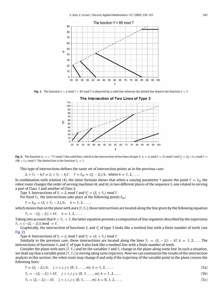
Fig. 1. The function Y = Z mod T = 85 mod T is depicted by a solid line whereas the dotted line depicts the function Y = T.

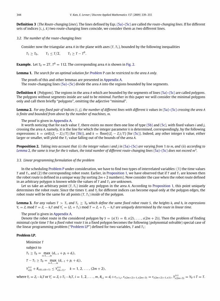
Fig. 2. The function T1 = (−77) mod T (the solid line), which is the intersection of two lines of type 3: Yi = Zi mod T = 21 mod T and Y′j = (Zj+T1) mod T =

(98+ T1) mod T. The dotted line is the function T1 = T.

This type of intersections defines the same set of intersection points as in the previous case:Zi + T1 − hiT = Zj + T1 − hjT; T = Fijk = (Zj − Zi)/k, where k = 1, 2, . . . .

In combination with relation (4), the latter formula shows that when a varying parameter T passes the point T = Fijk therobot route changes the order of serving machines Mi and Mj in two different places of the sequence S, one related to servinga part of Class 1 and another of Class 2.

Type 3. Intersections of Yi = Zi mod T and Y ′j = (Zj + T1) mod T.For fixed T1, the intersections take place at the following points Eijk:

T = Eijk = (Zj + T1 − Zi)/k, k = 1, 2, . . . ,

which means that on the plane with axes (T, T1), those intersections are located along the line given by the following equationT1 = −(Zj − Zi)+ kT, k = 1, 2, . . . .

Taking into account that 0 ≤ T1 < T, the latter equation presents a composition of line segments described by the expressionT1 = [−(Zj − Zi)]mod = T.

Graphically, the intersection of functions Yi and Y ′j of type 3 looks like a toothed line with a finite number of teeth (seeFig. 2).

Type 4. Intersections of Yj = Zj mod T and Y ′i = (Zi + T1) mod T.Similarly to the previous case, those intersections are located along the lines T1 = (Zj − Zi) − kT, k = 1, 2, . . .. The

intersections of functions Yi and Y ′j of type 4 also look like a toothed line with a finite number of teeth.Consider the plane with axes (T, T1) and let the variables T and T1 change in the plane along some line. In such a situation,

we shall say that a variable point (T, T1) is moving along some trajectory. Now we can summarize the results of the intersectionanalysis in this section: the robot route may change if and only if the trajectory of the variable point in the plane crosses thefollowing lines:

T = (Zj − Zi)/k, j > i, i, j ∈ {0, 1, . . . ,m}; k = 1, 2, . . . . (5a)

T1 = −(Zj − Zi)+ kT, j > i, i, j ∈ {0, 1, . . . ,m}; k = 1, 2, . . . . (5b)

T1 = (Zj − Zi)− kT, j > i, i, j ∈ {0, 1, . . . ,m}; k = 0, 1, 2, . . . . (5c)

344 V. Kats, E. Levner / Discrete Applied Mathematics 157 (2009) 339–355

Definition 3 (The Route-changing Lines). The lines defined by Eqs. (5a)–(5c) are called the route-changing lines. If for differentsets of indices (i, j, k) two route-changing lines coincide, we consider them as two different lines.

3.2. The number of the route-changing lines

Consider now the triangular area A in the plane with axes (T, T1), bounded by the following inequalities

T1 ≥ T0, T1 ≤ T/2, T1 ≥ T − T0.

Example. Let T0 = 27, T0= 112. The corresponding area A is shown in Fig. 2.

Lemma 1. The search for an optimal solution for Problem P can be restricted to the area A only.

The proofs of this and other lemmas are presented in Appendix A.The route-changing lines (5a)–(5c) divide the area A into the regions bounded by line segments.

Definition 4 (Polygons). The regions in the area A which are bounded by the segments of lines (5a)–(5c) are called polygons.The polygons without segments inside are said to be minimal. Further in this paper we will consider the minimal polygonsonly and call them briefly “polygons”, omitting the adjective “minimal”.

Lemma 2. For any fixed pair of indices (i, j), the number of different lines with different k values in (5a)–(5c) crossing the area Ais finite and bounded from above by the number of machines, m.

The proof is given in Appendix A.It worth noticing that for each value T, there exists no more then one line of type (5b) and (5c), with fixed values i and j,

crossing the area A, namely, it is the line for which the integer parameter k is determined, correspondingly, by the followingexpressions: k = ceil[(Zj − Zi)/T] (for (5b)), and k = floor[(Zj − Zi)/T] (for (5c)). Indeed, any other integer k value, eitherlarger or smaller, will yield the T1 value falling out of the bounds of the area A.

Proposition 2. Taking into account that (i) the integer values i and j in (5a)–(5c) are varying from 1 to m, and (ii) according toLemma 2, the same is true for the k values, the total number of different route-changing lines (5a)–(5c) does not exceed m3.

3.3. Linear programming formulation of the problem

In the scheduling Problem P under consideration, we have to find two types of interrelated variables: (1) the time valuesT and T1, and (2) the corresponding robot route. Earlier, in Proposition 1, we have observed that if T and T1 are known thenthe robot route is defined in a unique way (by sorting 2m+2 numbers). Now consider the case when the robot route definedin an arbitrary polygon is known while the values of T and T1 are unknown.

Let us take an arbitrary point (T, T1) inside any polygon in the area A. According to Proposition 1, this point uniquelydetermines the robot route. Since the times Yi and Yj for different indices can become equal only at the polygon edges, therobot route will be the same for all points (T, T1) inside of the polygon.

Lemma 3. For any values T > T1 and T1 ≥ T0 which define the same fixed robot route S, the heights ki and hi in expressionsYi = Zi mod T = Zi − kiT and Y

′

i = (Zi + T1) mod T = Zi + T1 − hiT are uniquely determined by the route in linear time.

The proof is given in Appendix A.Denote the robot route in the considered polygon by S = {s(1) = 0, s(2), . . . , s(2m + 2)}. Then the problem of finding

minimal cycle time T for a fixed robot route S in a fixed polygon becomes the following (polynomial solvable) special case ofthe linear programming problem (“Problem LP”) defined for two variables, T and T1:

Problem LP.

Minimize T

subject toT1 ≥ T0 = max

i=1,...,m(di−1 + pi + di),

T − T1 ≥ T0 = maxi=1,...,m

(di−1 + pi + di),

Y(∗)s(k) + Rs(k),s(k+1) ≤ Y(∗)

s(k+1), k = 1, 2, . . . , (2m+ 2),

where Yi = Zi−kiT or Y ′i = Zi+T1−hiT, i = 1, 2, . . . ,m, Ri,j = di+ri+1,j, rs(2m+2)+1,s(2m+3) = rs(2m+2)+1,s(1), Y(∗)s(2m+3) = Y0+T = T.

V. Kats, E. Levner / Discrete Applied Mathematics 157 (2009) 339–355 345

Here all the parameters Zi are known input data, and the heights ki and hi for each Yi and Y ′i are defined prior to thesolution of Problem LP, as indicated in Lemma 3. The total number of constraints, 2m+ 4, is linear in m.

Note that the initial scheduling Problem P is not a standard linear programming problem. Indeed, it turns into Problem LP,a simple problem of two variables, T and T1, as soon as the heights ki and hi for each Yi and Y ′i are known and fixed. However,these values are different for different polygons in the area A and a priori unknown. So, in order to solve P, Problem LP is tobe solved repeatedly in each of polygons. As we will see below, this can be done in strongly polynomial time.

3.4. The number of robot routes. The Euler formula

Let us estimate the total number of polygons in the area A.

Theorem 1. The number of polygons in A is at most O(m5).

Proof. 1. First, let us estimate how many intersection points the lines (5a)–(5c) can have in A. Any line of type (5a),T = Fijk = (Zj − Zi)/k (with i, j, k fixed), may intersect the line T1 = −(Zg − Zf ) + hT (and, respectively T1 = (Zg − Zf ) − hT)inside the area A only if h = ceil[(Zg − Zf )/Fijk] (respectively, h = floor[(Zg − Zf )/Fijk]) (without loss of generality, we assumethat g > f ). It means that a single line T = Fijk = (Zj − Zi)/k (with i, j, k fixed) can cross all other lines of types (5b)–(5c) inat most O(m2) points. Then the total number of such type points, caused by all the intersections of all the lines of type (5a)with all other route-changing lines, is at most O(m5).

Further, the intersection of two lines of the same type, that is, either (a) T1 = −(Zj − Zi)+ k′T with T1 = −(Zg − Zf )+ k′′T,or (b) T1 = (Zj − Zi) − k′T with T1 = (Zg − Zf ) − k′′T, takes place at a point T = Gijf gk = [(Zj − Zi) − (Zg − Zf )]/k,where, without loss of generality, we assume that (Zj − Zi) > (Zg − Zf ), k = 1, 2, . . . ,m. Note that inside the area Aonly one pair of the lines may intersect at this point. In case (a) this pair of lines is determined by the pair of numbersk′ = ceil[(Zj−Zi)/Gijf gk] and k′′ = ceil[(Zg−Zf )/Gijf gk]whereas in case (b), correspondingly, by the pair k′ = floor[(Zj−Zi)/Gijf gk]

and k′′ = floor[(Zg − Zf )/Gijf gk].The intersection of lines of different types, that is, either (a) T1 = −(Zj − Zi) + k′T with T1 = (Zg − Zf ) − k′′T or (b)

T1 = (Zj− Zi)− k′T with T1 = −(Zg− Zf )+ k′′T, takes place at point T = G′ijf gk = [(Zj− Zi)+ (Zg− Zf )]/k. Inside the area A, thereare only points such that [(Zj− Zi)± (Zg− Zf )]/k ≥ 2T0. Since [(Zj− Zi)± (Zg− Zf )] ≤ Zm+ Zm ≤ 2mT0, it immediately followsthat 1 ≤ k ≤ 2mT0/2T0 = m. Hence, the total number of points Gijf gk and G′ijf gk, for all possible i, j, f , g, and k, is O(m5). FromLemma 2 it follows that the total number of lines (5a)–(5c) is O(m3), so the number of intersection points of those lines withthe border of the triangular area A is also at most O(m3). Thus, the total number of intersection points, including those lyingon the border of A, is at most O(m5).

2. Now we can estimate the total number of polygons. Denote the number of polygons in Aby f , the number of intersectionpoints in A by n, and the number of line segments connecting pairs of intersection points in A by e. Let us interpret theintersection points as vertices of a planar graph, the connecting segments as edges and the polygons as faces of a planargraph (not counting the outer infinitely large face). Then we can use the Euler polyhedron formula which claims:

f = e− n+ 1.

For a simple, connected, planar graph with n vertices and e edges, it is well known in graph theory that, for n ≥ 3, it holds:e ≤ 3n− 6, and, therefore, f ≤ 2n− 5. Thus, the total number of the polygons in A is of the same order of magnitude as thenumber of intersection points, that is, it does not exceed O(m5). �

3.5. A straightforward algorithm

Now we can construct a straightforward algorithm on the plane taking into account that all points (T, T1) in any polygondefine just the same robot route, and, therefore, the original scheduling Problem P can be solved by examining all possiblepolygons inside the area A. The algorithm works as follows: First, sequentially examine all the polygons pA in the area A, oneafter another, and in each of them do the following: (i) find the robot’s route determined by the sorting (2), (ii) compute theheights ki and hi for each Yi, and Y ′i , i = 1, . . . ,m, using Lemma 3, and (iii) having the above information, solve Problem LPwith respect to T and T1. Then, among all the found solutions for different polygons, choose the one with the minimum Tvalue.

Let us estimate the complexity of this algorithm. For each polygon, finding a robot route requires O(m log m) operations.After a route is found in a certain polygon, the next route in any neighboring polygon can be obtained in O(1) time, because,as it was shown in Section 3.1, the adjacent robot routes in two neighboring polygons differ only in one or two knowntranspositions of adjacent numbers (machine indices).

Next, the heights ki and hi in expressions Yi = Zi mod T = Zi − kiT and Y′

i = (Zi + T1) mod T = Zi + T1 − hiT, according toLemma 3, are uniquely determined by the route in some initial polygon in linear time and then can be obtained also in O(1)time in any neighboring polygon.

Further, the system of constraints of Problem LP contains only two variables, T and T1, therefore, its solution (ineach polygon) can be found in O(m) operations (see [22,12]). Hence, the total complexity of this algorithm is at mostO(m log m)+O(m5)(O(1)+O(m))+Csub = O(m6)+Csub, where Csub is the computational complexity of a sub-procedure which

346 V. Kats, E. Levner / Discrete Applied Mathematics 157 (2009) 339–355

organizes the enumeration and sequential scanning of the polygons on a plane. Apparently, this can be done in polynomialtime by using the linked data structures; however, a more detailed discussion of this question falls out of the scope of thispaper. In what follows, we propose an enhanced algorithm which does not need the enumeration of the polygons and hasa better complexity, O(m5 log m).

4. Singular points

4.1. Definition of the singular points

Consider an arbitrary polygon pA created by the intersection of the route-changing lines (5a)–(5c) in the area A. Since therobot route S = {s(1) = 0, s(2), . . . , s(2m + 2)} is determined uniquely for all points (T, T1) in pA, we can now re-define thepolygon pA as the set of points in the area A satisfying 2m+2 inequalities (2). Let us re-write the system (2) using explicitly thedecision variables T and T1; then each inequality in chain (2) will be replaced by one of the following inequalities (6a)–(6c):

Zs(l) − ks(l)T ≤ Zs(l+1) − ks(l+1)T, (6a)

or Zs(l) + T1 − ks(l)T ≤ Zs(l+1) − ks(l+1)T, (6b)

or Zs(l) − ks(l)T ≤ Zs(l+1) + T1 − ks(l+1)T, (6c)

where l ∈ {1, 2, . . . , 2m + 1}. For the given robot route S the heights ks(l) and ks(l+1) are uniquely determined by the routeand, according to Lemma 3, are the same for all values T and T1 in the considered polygon pA.

Along with polygons pA, consider now another set of polygons, called polygons of feasible solutions and denoted by pB.Each of polygon pB is located inside a polygon pA and determined by the system of inequalities (1a), (1b), (3) defining thearea of feasible solutions of Problem LP. Replace each inequality in (3) by one of the following inequalities (7a)–(7c) below,using explicitly the variables T and T1:

Zs(l) − ks(l)T + Rs(l),s(l+1) ≤ Zs(l+1) − ks(l+1)T, or (7a)

Zs(l) + T1 − ks(l)T + Rs(l),s(l+1) ≤ Zs(l+1) − ks(l+1)T, or (7b)

Zs(l) − ks(l)T + Rs(l),s(l+1) ≤ Zs(l+1) + T1 − ks(l+1)T, (7c)

where l ∈ {1, 2, . . . , 2m+ 1}. The last inequality in chain (3) could be one of the following:

Zs(2m+2) − ks(2m+2)T + Rs(2m+2),0 ≤ Z0 + T, or (7d)

Zs(2m+2) + T1 − ks(2m+2)T + Rs(2m+2),0 ≤ Z0 + T. (7e)

Denote Zs(2m+3) ≡ Z0 = 0 and ks(2m+3) ≡ −1, for l = 2m + 2 in (7a) and (7b). Then inequality (7d) becomes of the form(7a) and inequality (7e) becomes of the form (7b). Notice that some of the polygons pB, defined by (7a)–(7e), can be empty.Obviously, the heights ks(l) and ks(l+1) in (7a)–(7c) and in (6a)–(6c) are the same as they are defined for the same robot routeS.

If the heights for unknown Yi are found prior to finding T and T1, and ks(l+1) 6= ks(l) the inequalities (7a) can be solved withrespect to T:

T ≥ [Zs(l) − Zs(l+1) + Rs(l),s(l+1)]/(ks(l) − ks(l+1)), if ks(l+1) < ks(l). (8)

or T ≤ [Zs(l+1) − Zs(l) − Rs(l),s(l+1)]/(ks(l+1) − ks(l)), if ks(l+1) > ks(l). (8′)

Similarly, the inequalities (7b) and (7c) can be re-written as follows:

T ≥ [Zs(l) + T1 − Zs(l+1) + Rs(l),s(l+1)]/(ks(l) − ks(l+1)), if ks(l+1) < ks(l), (9)

or T ≤ [Zs(l+1) − Zs(l) − T1 − Rs(l),s(l+1)]/(ks(l+1) − ks(l)), if ks(l+1) > ks(l), (9′)

and, correspondingly,

T ≥ [Zs(l) − Zs(l+1) − T1 + Rs(l),s(l+1)]/(ks(l) − ks(l+1)), if ks(l+1) < ks(l), (10)

or T ≤ [Zs(l+1) + T1 − Zs(l) − Rs(l),s(l+1)]/(ks(l+1) − ks(l)), if ks(l+1) > ks(l). (10′)

In the case when ks(l+1) = ks(l) the inequalities (7a) do not contain any variables:

Zs(l) + Rs(l),s(l+1) ≤ Zs(l+1), (8′′)

while the inequalities (7b)–(7c) depend on variable T1 only:

T1 ≤ Zs(l+1) − Zs(l) − Rs(l),s(l+1), (9′′)Zs(l) − Zs(l+1) + Rs(l),s(l+1) ≤ T1. (10′′)

If the numerical inequalities of type (8′′ ) are inconsistent we will say that the polygon pB is empty.

V. Kats, E. Levner / Discrete Applied Mathematics 157 (2009) 339–355 347

From the theory of linear programming it follows that if the polygon pB is not empty then the minimal value of the cycletime T in pB is always reached at the extreme point (vertex) of the convex polygon, which, in turn, is defined as an intersectionpoint of a pair of lines obtained from (8), (8′), (9)–(9′′) and (10)–(10′′) as exact equations.

Since the considered Problem LP is a minimization linear programming problem, its optimal extreme points willnecessarily belong to one of the lines bounding a halfplane of the types (8)–(10) whereas the lines bounding the halfplanesof the types (8′), (9′)–(9′′) and (10′)–(10′′) can be skipped. Although this fact does not affect the worst-case complexity ofthe forthcoming algorithm, it decreases twice the total number of operations in the algorithm below, which is important inpractical computations.

The relations (8)–(10) regarded as strict equations can be presented as follows:

T = Wjik, or (11a)

T = Wjik + T1/k, or (11b)

T = Wjik − T1/k, (11c)

where Wjik = (Zj − Zi + Rj,i)/k, j > i and j, i ∈ {0, 1, 2, . . . ,m}; k = 1, 2, . . . ,m.The maximal value of k is m because k = |ks(l) − ks(l+1)|, and each of ks(l), according to Lemma 2, is not larger than m.

Definition 5 (Lines of Possible Solutions). The lines defined by the Eqs. (11a)–(11c) are called the lines of possible solutions.

Lemma 4. Any of the constraints of Problem LP of the form (7a)–(7c), when considered on the lines of possible solutions, can bereduced to either an equivalent inequality with one variable T1 only, or a numerical inequality with no variables at all.

The proof is given in Appendix A.

Definition 6 (Singular Points). Consider the points in the area A in which the lines of possible solutions (11a)–(11c) intersectwith the route-changing lines (5a)–(5c). These points are said to be singular. Two singular points lying on the same line ofpossible solutions are said to be neighboring if there is no other singular point lying between them on that line.

Definition 7 (Basic Segments). Consider a piece of a line of the type (11a)–(11c) bounded by (the points of its intersectionwith) the borders of area A. The singular points belonging to it divide it into smaller segments. Each segment lying in betweentwo neighboring singular points is said to be basic and denoted by sA.

If there are two repeated singular points, a segment confined between them is considered to be empty. By the definitionof the route-changing lines, in each of the basic segments the robot route will be the same for all its points (T, T1).

4.2. The number of singular points

Let us estimate the total number of singular points in area A.

4.2.1. Lines of possible solutions T = Eijk = (Zj − Zi + Rj,i)/kThe lines of the type (11a) may intersect only lines of the types (5b) and (5c). Among all the lines (5b), i.e. those of the

form T1 = −(Zg − Zf ) + hT (where here and below g > f ), with the same pair of indices (f , g) and different h, only the linewith h = ceil[(Zg − Zf )/Eijk] may cross line T = Eijk in the area A. Analogously, among all the lines (5c), respectively, of theform T1 = (Zg − Zf )− hT, with the same pair of indices (f , g) and different h, only the line with h = floor[(Zg − Zf )/Eijk]maycross line T = Eijk in the area A. Indeed, any other integer h values, either larger or smaller, will yield the T1 value falling out ofthe bounds of the area A. Thus, the single line T = Eijk may contain at most O(m2) singular points. Therefore, the total numberof singular points capable of changing the robot route and belonging to all the lines of the type (11a) is at most O(m5).

4.2.2. Lines of possible solutions T1 = −(Zj − Zi + Rj,i)+ kT(a) Intersection with lines of the type (5a) T = Ff gh = (Zg − Zf )/h. Among all the lines (11b) with the fixed pair of indices

(i, j) and different k, only the line with k = ceil[(Zj−Zi)/Ff gh]may be crossed by line T = Ff gh in area A. Thus, the total numberof intersection points of lines (11b) with lines (5a) is at most O(m5).

(b) Intersection with lines of the type (5b) T1 = −(Zg − Zf ) + hT. The intersection points are of the form T = Hijf gl =

|(Zj − Zi + Rj,i) − (Zg − Zf )|/l, l = 1, 2, . . . . In area A, at point Hijf gl only one pair of the lines intersect each other, namely,those determined by k = ceil[(Zj − Zi + Rj,i)/Hijf gl] and h = ceil[(Zg − Zf )/Hijf gl]. Thus, the total number of intersection pointsof lines (11b) with lines (5b) is at most O(m5).

(c) Intersection with lines of the type (5c) T1 = (Zg − Zf ) − hT. The intersection points are of the form T = H′ijf gl =[(Zj − Zi + Rj,i) + (Zg − Zf )]/l, l = 1, 2, . . . ; in area A at point H′ijf gl only one pair of lines intersect each other, namely, thosedetermined by k = ceil[(Zj − Zi + Rj,i)/H′ijf gl] and h = floor[(Zg − Zf )/H′ijf gl]. The values i, j, f , and g are all varying between 1and m. The same is true for l as well, because l = k− h, and the values of k and h do not exceed m. Thus, the total number ofintersection points of lines (11b) with lines (5b) is at most O(m5).

348 V. Kats, E. Levner / Discrete Applied Mathematics 157 (2009) 339–355

4.2.3. Lines of possible solutions T1 = (Zj − Zi + Rj,i)− kT

The total number of intersection points of those lines with lines (5a)–(5c) is O(m5). The proof is similar to the previouscase.

To summarize, the total number of all singular points, lying on the lines of possible solutions (11a)–(11c) in area A is atmost O(m5).

5. Algorithm and complexity

Now we can describe the improved algorithm. It is based on the following facts.

A. The optimal solution to the considered problem must be located on one of the lines of possible solutions (11a)–(11c).Due to this, instead of solving the set of two-variable problems LP defined on polygons pA, we can solve a set of simpleone-variable problems determined on corresponding segments sA of lines (11a)–(11c), introduced in Section 4.1. Thecorresponding techniques are described in detail in Theorem 2.

B. The robot routes determined on two adjacent segments sA, s′A (that is, those having a common singular point) of the sameline, will differ in the order of one or two pairs of neighboring machines only. It allows us to obtain the robot route on anycurrent segment s′A just from the previously found robot route on the adjacent segment sA, by transposing the order ofone or two pairs of neighboring machines in the latter route, which, in turn, leads to a considerable computational gain.(A similar situation takes place in the case of 1-cyclic scheduling, see [15]). We explain these techniques in more detailin Appendix C.

Evidently, any two-variable Problem LP defined for variables T and T1 lying on any segment of a line of possible solutionsbounded between two neighboring singular points can be reduced to a single one-variable Problem LP (since there is a strictequation linking the variables). In the algorithm which we present below, we will not examine anymore all the problems LPon polygons pB in A, one after another (as the above algorithm of Section 3 does). Instead, all the basic segments on the linesof feasible solutions are scanned one after another, and an optimal solution to the Problem LP is found separately in each ofthem, or “no solution” is returned. Although this scheme may look straightforward, its complexity is better than that of thealgorithm in Section 3, as the following Theorems 2 and 3 claim.

Theorem 2. (a) The optimal solution to the scheduling Problem P can be achieved by solving a set of one-variable linearprogramming problems determined on the basic segments sA.

(b) The total number of all one-variable problems solved on all the basic segments in the area A does not exceed O(m5).

Proof. (a) The minimal value of the cycle time T in any polygon pB is achieved at a vertex lying on a line of the form (11a)–(11c). Evidently, this optimal solution is located on one of the basic segments. So, the original Problem P can be solved byexamining all the basic segments one after another as follows. Consider an arbitrary segment sA and find the robot route S

in it, together with all corresponding ‘height’ coefficients k and h. For this purpose, calculate the values Y(∗)i in an arbitrary

interior point of the basic segment sA and arrange the obtained numbers Y(∗)i according to relations (2). Notice that the robot

route found will be the same for all the points of the considered segment. Consider now the inequalities (7a)–(7e). Usingthe equation of the line on which the segment sA lies, that is, on one of the Eqs. (11a)–(11c), we can, according to Lemma 4,transform all inequalities (7a)–(7c) defining the Problem LP into either equivalent inequalities with one variable T1 only, ornumerical inequalities with no variables at all. If these inequalities are consistent, then the interval of feasible solutions willbe found in the segment sA, otherwise, no solution exists in this segment. After the above procedure is repeated for all basicsegments on all the lines of feasible solutions, the optimal solution to Problem P is found.

(b) The total number of the one-dimensional problems solved on all the basic segments does not exceed the total numberof singular points, which is, as shown in Section 4.2, does not exceed O(m5). �

As we will see in Theorem 3 below, along any line of possible solutions it is sufficient to solve from scratch only one linearprogramming problem in some initial basic segment sA in O(m) time and, then, in all the following segments the problemsLP can be solved in only O(log m).

The algorithm is presented below. Denote the minimum cycle time T by Topt. Set Topt = ∞. If this initial value of Topt willnot be improved it means that no solution to the problem exists.

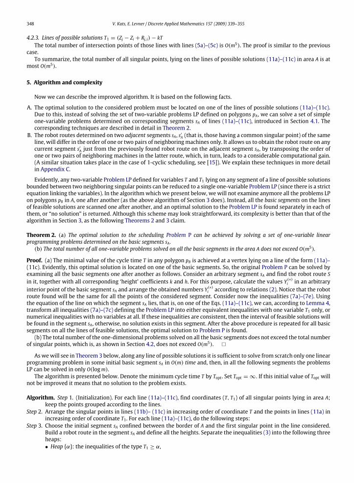
Algorithm. Step 1. (Initialization). For each line (11a)–(11c), find coordinates (T, T1) of all singular points lying in area A;keep the points grouped according to the lines.

Step 2. Arrange the singular points in lines (11b)– (11c) in increasing order of coordinate T and the points in lines (11a) inincreasing order of coordinate T1. For each line (11a)–(11c), do the following steps:

Step 3. Choose the initial segment sA confined between the border of A and the first singular point in the line considered.Build a robot route in the segment sA and define all the heights. Separate the inequalities (3) into the following threeheaps:• Heap {α}: the inequalities of the type T1 ≥ α,

V. Kats, E. Levner / Discrete Applied Mathematics 157 (2009) 339–355 349

• Heap {β}: the inequalities of the type T1 ≤ β,• Heap {γ}: the inequalities of the type γ ≥ 0, where α, β, and γ are the real numbers (see the proof of Lemma 4).In each heap, arrange the numbers α, β and γ in increasing order.

Step 4. If max{α} ≤ min{β} and 0 ≤ min{γ}, that is, the inequalities (3) in the considered segment are consistent, do thefollowing:Step 4.1. For line of the type (11a) take T = Wjik and T1 = max{α}; for line of the type (11b) take T1 = max{α} and

T = Wjik + T1/k; for line of the type (11c) take T1 = min{β} and T = Wjik − T1/k.Step 4.2. If T < Topt then keep the new solution Topt := T together with the corresponding T1.Step 4.3. Choose the next line from among (11a)–(11c) and go to Step 2.Else go to Step 5.

Step 5. If the current segment sA is not the last one in the line considered, then move through the singular point to the nextadjacent segment s′A; adjust the robot route and the heaps of inequalities as described in Appendix C, and return toStep 4. If the current segment sA is the last one in the line considered, take the next line (11a)–(11c) and go to Step2. If the current segment sA is the last one in the last line (11a)–(11c) return Topt with the corresponding T1 and therobot route.If Topt = ∞ return “no solution”.

Notice that the algorithm, along with the coordinates (T, T1) of all singular points, needs to keep the information abouttheir intersection lines, i.e., each singular point is supplied with the following attributes fully determining the lines of possiblesolutions and route-changing line as they were described in Section 4.2:

• Attribute A1: indices (i, j) of the lines of the type (11a)–(11c) and indices (f , g) of the lines of the type (5a)–(5c),• Attribute A2: integers k of lines (11a)–(11c) and h of lines (5a)–(5c), and• Attribute A3: the corresponding line types: “type (5a), (5b) or (5c)” for the route-changing line, and “type (11a), (11b) or

(11c)” for the line of possible solutions.

Theorem 3. The enhanced algorithm solves the initial scheduling problem in O(m5 log m) time.

Proof. There are a total of at most O(m5) singular points. Therefore, Step 1 requires at most O(m5) operations to calculateall of them and group them into O(m3) different groups according to the lines (11a)–(11c). Let nj be the number of singularpoints placed on the same line j of the form (11a)–(11c), where index j represents an individual line and runs over all lines(11a)–(11c). At each its pass, Step 2 requires O(nj log nj) operations to arrange the points in increasing order of coordinate T.All the passes of Step 2 require O(

∑j nj log nj) ≤ O((

∑j nj)(log m5)) ≤ O(m5 log m). At each pass, Step 3 requires O(m log m)

operations, and totally, for all the passes (for all the lines), O(m4 log m). Step 4 requires O(1) operations at each pass. Step5 requires O(1) operations to adjust the robot route and the corresponding ‘height’ coefficients k and h for all Y(∗). Thisstep requires O(log m) operations to adjust heaps {α}, {β}, and {γ}. Steps 4 and 5 can be repeated O(nj) times, when beingperformed for every line (11a)–(11c).

So, the number of all operations made during one pass of Steps 2–5 (i.e., for any individual line of the type (11a)–(11c)) isO(nj log nj)+O(m log m)+(O(1)+O(log m)) ·O(nj) = O(nj log nj)+O(nj) ·O(log m). Thus, the total complexity of the algorithmduring all repetitions of Steps 2-5 is the sum of all the operations over all lines (11a)–(11c),

∑j(nj log nj) +

∑j(nj log m) ≤

(∑

j nj) log(maxj nj)+ (m5 log m) = O(m5 log m). �

Concluding this section, let us show that the method of forbidden intervals (MFI) mentioned in the introduction is invalidfor the non-Euclidean case. The reason is that the MFI uses the so-called extended set of inequalities of type (3) imposed onthe decision variables Yi, but in the general case the latter set is excessive and may lead to the loss of the optimal solution.The following example illustrates this situation.

Example. Let a robotic flowshop cell consist of m = 5 machines M1, . . . ,M5, the input station M0, and the output stationM6. The parameters of the cell are the following:

p1 = 17; p2 = 15; p3 = 21; p4 = 19; p5 = 10; d0 = 4; d1 = d2 = d3 = d4 = 3; d5 = 1.

All traveling times rij = 1, except for r6,0 = 13 and r4,2 = 3. In this cell, the transportation and traveling times do notsatisfy the Euclidean metrics, or the triangle inequality Rij ≤ Rik + Rkj, (i, j, k = 0, 1, . . . ,m).

According to the MFI, the optimal solution (T, T1) will be (118, 50). However, it is not true. Actually, any of the abovealgorithms in Sections 3 and 5 finds the following optimal schedule: the minimum cycle time T = 80, T1 = 30, and the robotroute S = {0, 4, 3′, 5, 1, 0′, 4′, 2, 5′, 1′, 3, 2′} (see Fig. 4). In Appendices B and C, we present details of computations.

350 V. Kats, E. Levner / Discrete Applied Mathematics 157 (2009) 339–355

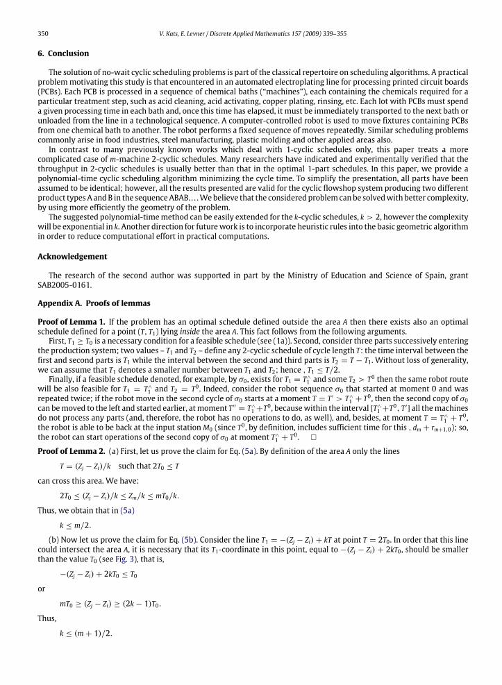
6. Conclusion

The solution of no-wait cyclic scheduling problems is part of the classical repertoire on scheduling algorithms. A practicalproblem motivating this study is that encountered in an automated electroplating line for processing printed circuit boards(PCBs). Each PCB is processed in a sequence of chemical baths (“machines”), each containing the chemicals required for aparticular treatment step, such as acid cleaning, acid activating, copper plating, rinsing, etc. Each lot with PCBs must spenda given processing time in each bath and, once this time has elapsed, it must be immediately transported to the next bath orunloaded from the line in a technological sequence. A computer-controlled robot is used to move fixtures containing PCBsfrom one chemical bath to another. The robot performs a fixed sequence of moves repeatedly. Similar scheduling problemscommonly arise in food industries, steel manufacturing, plastic molding and other applied areas also.

In contrast to many previously known works which deal with 1-cyclic schedules only, this paper treats a morecomplicated case of m-machine 2-cyclic schedules. Many researchers have indicated and experimentally verified that thethroughput in 2-cyclic schedules is usually better than that in the optimal 1-part schedules. In this paper, we provide apolynomial-time cyclic scheduling algorithm minimizing the cycle time. To simplify the presentation, all parts have beenassumed to be identical; however, all the results presented are valid for the cyclic flowshop system producing two differentproduct types A and B in the sequence ABAB. . . . We believe that the considered problem can be solved with better complexity,by using more efficiently the geometry of the problem.

The suggested polynomial-time method can be easily extended for the k-cyclic schedules, k > 2, however the complexitywill be exponential in k. Another direction for future work is to incorporate heuristic rules into the basic geometric algorithmin order to reduce computational effort in practical computations.

Acknowledgement

The research of the second author was supported in part by the Ministry of Education and Science of Spain, grantSAB2005-0161.

Appendix A. Proofs of lemmas

Proof of Lemma 1. If the problem has an optimal schedule defined outside the area A then there exists also an optimalschedule defined for a point (T, T1) lying inside the area A. This fact follows from the following arguments.

First, T1 ≥ T0 is a necessary condition for a feasible schedule (see (1a)). Second, consider three parts successively enteringthe production system; two values – T1 and T2 – define any 2-cyclic schedule of cycle length T: the time interval between thefirst and second parts is T1 while the interval between the second and third parts is T2 = T − T1. Without loss of generality,we can assume that T1 denotes a smaller number between T1 and T2; hence , T1 ≤ T/2.

Finally, if a feasible schedule denoted, for example, by σ0, exists for T1 = T∧1 and some T2 > T0 then the same robot routewill be also feasible for T1 = T∧1 and T2 = T0. Indeed, consider the robot sequence σ0 that started at moment 0 and wasrepeated twice; if the robot move in the second cycle of σ0 starts at a moment T = T ′ > T∧1 + T0, then the second copy of σ0can be moved to the left and started earlier, at moment T ′′ = T∧1 +T0, because within the interval [T∧1 +T0, T ′] all the machinesdo not process any parts (and, therefore, the robot has no operations to do, as well), and, besides, at moment T = T∧1 + T0,the robot is able to be back at the input station M0 (since T0, by definition, includes sufficient time for this , dm + rm+1,0); so,the robot can start operations of the second copy of σ0 at moment T∧1 + T0. �

Proof of Lemma 2. (a) First, let us prove the claim for Eq. (5a). By definition of the area A only the lines

T = (Zj − Zi)/k such that 2T0 ≤ T

can cross this area. We have:

2T0 ≤ (Zj − Zi)/k ≤ Zm/k ≤ mT0/k.

Thus, we obtain that in (5a)

k ≤ m/2.

(b) Now let us prove the claim for Eq. (5b). Consider the line T1 = −(Zj − Zi)+ kT at point T = 2T0. In order that this linecould intersect the area A, it is necessary that its T1-coordinate in this point, equal to −(Zj − Zi) + 2kT0, should be smallerthan the value T0 (see Fig. 3), that is,

−(Zj − Zi)+ 2kT0 ≤ T0

or

mT0 ≥ (Zj − Zi) ≥ (2k− 1)T0.

Thus,

k ≤ (m+ 1)/2.

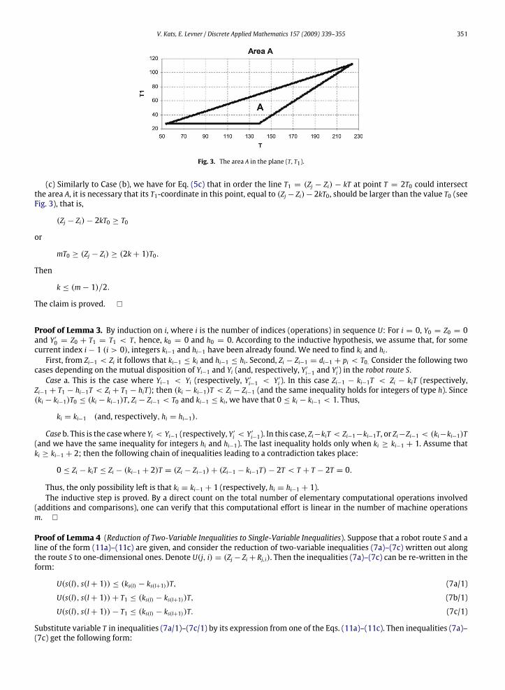
V. Kats, E. Levner / Discrete Applied Mathematics 157 (2009) 339–355 351

Fig. 3. The area A in the plane (T, T1).

(c) Similarly to Case (b), we have for Eq. (5c) that in order the line T1 = (Zj − Zi) − kT at point T = 2T0 could intersectthe area A, it is necessary that its T1-coordinate in this point, equal to (Zj − Zi)− 2kT0, should be larger than the value T0 (seeFig. 3), that is,

(Zj − Zi)− 2kT0 ≥ T0

or

mT0 ≥ (Zj − Zi) ≥ (2k+ 1)T0.

Then

k ≤ (m− 1)/2.

The claim is proved. �

Proof of Lemma 3. By induction on i, where i is the number of indices (operations) in sequence U: For i = 0, Y0 = Z0 = 0and Y ′0 = Z0 + T1 = T1 < T, hence, k0 = 0 and h0 = 0. According to the inductive hypothesis, we assume that, for somecurrent index i− 1 (i > 0), integers ki−1 and hi−1 have been already found. We need to find ki and hi.

First, from Zi−1 < Zi it follows that ki−1 ≤ ki and hi−1 ≤ hi. Second, Zi − Zi−1 = di−1 + pi < T0. Consider the following twocases depending on the mutual disposition of Yi−1 and Yi (and, respectively, Y ′i−1 and Y ′i ) in the robot route S.

Case a. This is the case where Yi−1 < Yi (respectively, Y ′i−1 < Y ′i ). In this case Zi−1 − ki−1T < Zi − kiT (respectively,Zi−1 + T1 − hi−1T < Zi + T1 − hiT); then (ki − ki−1)T < Zi − Zi−1 (and the same inequality holds for integers of type h). Since(ki − ki−1)T0 ≤ (ki − ki−1)T, Zi − Zi−1 < T0 and ki−1 ≤ ki, we have that 0 ≤ ki − ki−1 < 1. Thus,

ki = ki−1 (and, respectively, hi = hi−1).

Case b. This is the case where Yi < Yi−1 (respectively, Y ′i < Y ′i−1). In this case, Zi−kiT < Zi−1−ki−1T, or Zi−Zi−1 < (ki−ki−1)T(and we have the same inequality for integers hi and hi−1). The last inequality holds only when ki ≥ ki−1 + 1. Assume thatki ≥ ki−1 + 2; then the following chain of inequalities leading to a contradiction takes place:

0 ≤ Zi − kiT ≤ Zi − (ki−1 + 2)T = (Zi − Zi−1)+ (Zi−1 − ki−1T)− 2T < T + T − 2T = 0.

Thus, the only possibility left is that ki = ki−1 + 1 (respectively, hi = hi−1 + 1).The inductive step is proved. By a direct count on the total number of elementary computational operations involved

(additions and comparisons), one can verify that this computational effort is linear in the number of machine operationsm. �

Proof of Lemma 4 (Reduction of Two-Variable Inequalities to Single-Variable Inequalities). Suppose that a robot route S and aline of the form (11a)–(11c) are given, and consider the reduction of two-variable inequalities (7a)–(7c) written out alongthe route S to one-dimensional ones. Denote U(j, i) = (Zj − Zi + Rj,i). Then the inequalities (7a)–(7c) can be re-written in theform:

U(s(l), s(l+ 1)) ≤ (ks(l) − ks(l+1))T, (7a/1)

U(s(l), s(l+ 1))+ T1 ≤ (ks(l) − ks(l+1))T, (7b/1)

U(s(l), s(l+ 1))− T1 ≤ (ks(l) − ks(l+1))T. (7c/1)

Substitute variable T in inequalities (7a/1)–(7c/1) by its expression from one of the Eqs. (11a)–(11c). Then inequalities (7a)–(7c) get the following form:

352 V. Kats, E. Levner / Discrete Applied Mathematics 157 (2009) 339–355

1. On lines of the type (11a), T = Wjik, becomes the following:

0 ≤ (ks(l) − ks(l+1))Wjik − U(s(l), s(l+ 1)), (7a/2)

T1 ≤ (ks(l) − ks(l+1))Wjik − U(s(l), s(l+ 1)), (7b/2)

−T1 ≤ (ks(l) − ks(l+1))Wjik − U(s(l), s(l+ 1)). (7c/2)

2. On lines of the type (11b), T = Wjik + T1/k, becomes the following:

U(s(l), s(l+ 1)) ≤ (ks(l) − ks(l+1))(Wjik + T1/k),

or − [(ks(l) − ks(l+1))/k]T1 ≤ (ks(l) − ks(l+1))Wjik − U(s(l), s(l+ 1)), (7a/3)U(s(l), s(l+ 1))+ T1 ≤ (ks(l) − ks(l+1))(Wjik + T1/k),

or [1− (ks(l) − ks(l+1))/k]T1 ≤ (ks(l) − ks(l+1))Wjik − U(s(l), s(l+ 1)), (7b/3)U(s(l), s(l+ 1))− T1 ≤ (ks(l) − ks(l+1))(Wjik + T1/k),

or [−1− (ks(l) − ks(l+1))/k]T1 ≤ (ks(l) − ks(l+1))Wjik − U(s(l), s(l+ 1)). (7c/3)

3. On lines of type (11c), T = Wjik − T1/k, becomes the following:

U(s(l), s(l+ 1)) ≤ (ks(l) − ks(l+1))(Wjik − T1/k),

or [(ks(l) − ks(l+1))/k]T1 ≤ (ks(l) − ks(l+1))Wjik − U(s(l), s(l+ 1)), (7a/4)U(s(l), s(l+ 1))+ T1 ≤ (ks(l) − ks(l+1))(Wjik − T1/k),

or [1+ (ks(l) − ks(l+1))/k]T1 ≤ (ks(l) − ks(l+1))Wjik − U(s(l), s(l+ 1)), (7b/4)U(s(l), s(l+ 1))− T1 ≤ (ks(l) − ks(l+1))(Wjik − T1/k),

or [−1+ (ks(l) − ks(l+1))/k]T1 ≤ (ks(l) − ks(l+1))Wjik − U(s(l), s(l+ 1)), (7c/4)

denote

cs(l) = (ks(l) − ks(l+1))Wjik − U(s(l), s(l+ 1))

as(l) =

0, for line T =Wjik,−[(ks(l) − ks(l+1))/k], for line T =Wjik + T1/k,[(ks(l) − ks(l+1))/k], for line T =Wjik − T1/k.

Then the inequalities (7a)–(7c) become of the form

as(l) · T1 ≤ cs(l), (7a*)

(as(l) + 1) · T1 ≤ cs(l), (7b*)

(as(l) − 1) · T1 ≤ cs(l). (7c*)

which proves the lemma. �

Appendix B. Description of the MFI and example

The method of forbidden intervals MFI [20,16,6] for 2-cyclic scheduling is based on the feasibility condition (FC) forthe robot route, which is presented by inequalities (3) imposed on the decision variables Y(∗)

i . Though the FC requires theinequalities (3) to hold for the pairs of indices (i, j) along the robot route only, the MFI imposes the so-called extended systemof relations (3), in which variables Y(∗)

i , Y(∗)j are to satisfy the following conditions

Y(∗)i + Ri,j ≤ Y(∗)

j , if Y(∗)i ≤ Y(∗)

j (3a*)

Y(∗)i + Ri,j ≤ Y(∗)

j + T, if Y(∗)i > Y(∗)

j , (3b*)

for all possible pairs of indices (i, j). The introduction of the extended system is explained by two reasons: First, the robotroute is a priori unknown and, hence, the sequence of indices along the route is unknown, as well. Second, in the Euclideancase, if variables Y(∗)

i and Y(∗)j satisfy (3) along a route then they also satisfy the extended system of inequalities (which is

not valid in the general case).The MFI works as follows: First, the feasibility conditions for T and T1 presented in the algebraic form (1a), (1b), (3a*),

(3b*) are re-written in terms of the forbidden intervals, as follows:

kT 6∈ I, T1 6∈ I, kT + T1 6∈ I, kT − T1 6∈ I, (3c*)

where k = 1, 2, . . . ,m; I = (−∞, T0) ∪ {⋃m−1

i=0⋃m

j=i+1(−U(i, j),U(j, i))}, and (−U(i, j),U(j, i)) = (Zj − Zi − Ri,j, Zj − Zi + Rj,i).

V. Kats, E. Levner / Discrete Applied Mathematics 157 (2009) 339–355 353

Table 1The Zi and U(j, i) values

i 0 1 2 3 4 5Zi 0 21 39 63 85 98U(0, i) 5 −16 −34 −58 −80 −93U(1, i) 25 4– −14 −38 −60 −73U(2, i) 43 22 4– −20 −42 −55U(3, i) 67 46 30 4 −18 −31U(4, i) 89 68 50 26 4 −9U(5, i) 112 79 61 37 15 2

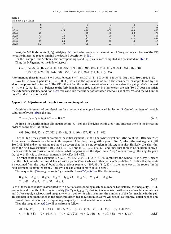
Next, the MFI finds points (T, T1) satisfying (3c*), and selects one with the minimum T. We give only a scheme of the MFIhere; the interested reader can find the detailed description in [6,7].

For the Example from Section 5, the corresponding Zi and U(j, i) values are computed and presented in Table 1:Thus, the MFI generates the following set I:

I = (−∞, 27) ∪ (16, 25) ∪ (34, 43) ∪ (58, 67) ∪ (80, 89) ∪ (93, 112) ∪ (14, 22) ∪ (38, 46) ∪ (60, 68)

∪(73, 79) ∪ (20, 30) ∪ (42, 50) ∪ (55, 61) ∪ (18, 26) ∪ (31, 37) ∪ (9, 15).

After merging these intervals, I will be as follows: I = (−∞, 30) ∪ (31, 50) ∪ (55, 68) ∪ (73, 79) ∪ (80, 89) ∪ (93, 112).Now let us take a pair (T, T1) = (80, 30) which is the optimal solution in the considered example found by the

algorithm presented in Section 5. The MFI will not find this optimal solution because it considers this pair forbidden. Indeed,T + T1 = 110, that is, T + T1 belongs to the forbidden interval (93, 112), or, in other words, the pair (80, 30) does not satisfythe extended feasibility condition (3c*). We conclude that the set of forbidden intervals I is excessive, and the MFI, in thenon-Euclidean case, is invalid.

Appendix C. Adjustment of the robot routes and inequalities

Consider a fragment of our algorithm for a numerical example introduced in Section 5. One of the lines of possiblesolutions of type (11b) is the line

T1 = −(Z4 − Z1 + R4,1)+ T = −68+ T. (A3.1)

At Step 2 the algorithm finds all singular points (T, T1) on this line lying within area A and arranges them in the increasingorder of coordinate T as follows:

(98, 30), (103, 35), (107, 39), (110, 42), (114, 46), (127, 59), (131, 63).

Then at Step 3 the algorithm examines the initial segment sA at this line (whose right end is the point (98, 30)) and at Step4 discovers that there is no solution in this segment. After that, the algorithm goes to Step 5, selects the next segment [(98,30), (103, 35)] and, on returning to Step 4, discovers that there is no solution in this segment also. Similarly, the algorithmscans the next two segments [(103, 35), (107, 39)] and [(107, 39), (110, 42)] and finds that there is no solution in any ofthem, as well. Let us consider in more detail what happens when the algorithm at Step 5 moves through the singular point(T, T1) = (110, 42) to the next segment [(110, 42), (114, 46)].

The robot route in this segment is: S = {0, 4′, 1, 5′, 2, 0′, 3, 1′, 2′, 4, 5, 3′}. Recall that the symbol (′) in S, say s′, meansthat the robot unloads machine Ms loaded with a part of Class 2 while all other parts in S are of Class 1. (Notice that the routeS is obtained from the route S′ found at the previous segment, [(107, 39), (110, 42)], in the same way as the route S′′ in thenext segment is computed from S — this will be explained in more detail below).

The inequalities (3) along the route S given in the form (7a*)–(7c*) will be the following:

0 ≤ 12, 0 ≤ 0, 0 ≤ 5, 0 ≤ 7, T1 ≥ 43, T1 ≤ 58, T1 ≥ 46, 0 ≤ 14,

T1 ≤ 42, 0 ≤ 9, T1 ≥ 37, 0 ≤ 1.(A3.2)

Each of those inequalities is associated with a pair of corresponding machine numbers. For instance, the inequality T1 ≥ 43was obtained from the following inequality (3): Y2 + R2,0 ≤ Y ′0, that is, it is associated with a pair of machine numbers 2and 0′. We supply each obtained inequality with a pointer #s which denotes the number s of the first machine in the pair.This pointer is not mentioned in the algorithm described above because, as we will see, it is a technical detail needed onlyto provide direct access to a corresponding inequality without an additional search.

Then the inequalities (A3.2) will be written as follows:

(0 ≤ 12, #0); (0 ≤ 0, #4′); (0 ≤ 5, #1); (0 ≤ 7, #5′); (T1 ≥ 43, #2); (T1 ≤ 58, #0′);

(T1 ≥ 46, #3); (0 ≤ 14, #1′); (T1 ≤ 42, #2′); (0 ≤ 9, #4); (T1 ≥ 37, #5); (0 ≤ 1, #3′). (A3.3)

354 V. Kats, E. Levner / Discrete Applied Mathematics 157 (2009) 339–355

The inequalities of the form (A3.3) are separated into three heaps and arranged in the increasing order of their right-handsides, as follows:

{α} = {(T1 ≥ 37, #5); (T1 ≥ 43, #2); (T1 ≥ 46, #3)},

{β} = {(T1 ≤ 42, #2′); (T1 ≤ 58, #0′)},{γ} = {(0 ≤ 0, #4′); (0 ≤ 1, #3′); (0 ≤ 5, #1); (0 ≤ 7, #5′); (0 ≤ 9, #4); (0 ≤ 12, #0); (0 ≤ 14, #1′)}.

Now we can explain how the robot route and the inequalities are adjusted at the next iteration. At Step 4 inequalitiesmax{α} = 46 ≤ min{β} = 42 and 0 ≤ min{γ} = 0 are examined, and it is found that the first inequality is inconsistent. Nextthe algorithm at Step 5 verifies that the current segment sA is not the last one in the considered line and moves through thesingular point (T, T1) = (114, 46) to the next adjacent segment s′A = [(114, 46), (127, 59)]. The singular point (114, 46) isthe intersection of our scanned line with the following line of type (5c): T1 = Z4 − Z2 − 0 · T = (85− 39), that is, T1 = 46.

Since Z4 and Z2 define the latter line (5c) it follows that when a varying point (T, T1) passes through this singular point thesequence S is changed by transposing only two neighboring indices, namely, the machine numbers 2′ and 4. Thus, the robotroute within segment s′A becomes S′ = {0, 4′, 1, 5′, 2, 0′, 3, 1′, 4, 2′, 5, 3′}. This results in that the set of inequalities (3) alsochanges: instead of the inequalities defined by the pairs of indices (1′, 2′), (2′, 4) and (4, 5), the inequalities defined by thepairs of indices (1′, 4), (4, 2′) and (2′, 5) appear. To adjust the heaps of inequalities we discard from the available heaps theinequalities marked by the pointers #1′, #2′, and #4, that is, the inequalities (0 ≤ 14, #1′) and: (0 ≤ 9, #4) from {γ}, and(T1 ≤ 42, #2′) from {β}. After that new inequalities are formed: (T1 ≤ 60, #∗1′); (T1 ≥ 50, #4), and (T1 ≤ 55, #2′) and all ofthem are placed into the appropriate heaps.

As a result, the algorithm generates the following heaps:

{α} = {(T1 ≥ 37, #5); (T1 ≥ 43, #2); (T1 ≥ 46, #3); (T1 ≥ 50, #4)},

{β} = {(T1 ≤ 55, #2′); (T1 ≤ 58, #0′); (T1 ≤ 60, #1′)}{γ} = {(0 ≤ 0, #4′); (0 ≤ 1, #3′); (0 ≤ 5, #1); (0 ≤ 7, #5′); (0 ≤ 12, #0)}.

At this point, the current iteration of the algorithm is completed. At the next iteration, the algorithm returns to Step 4 andexamines the new inequalities

max{α} = 50 ≤ min{β} = 55 and 0 ≤ min{γ} = 0.

Now the inequalities are consistent, we have T1 = max{α} = 50, then the cycle time T = 68+ T1 = 68+ 50 = 118. Thus,the algorithm stores a current feasible schedule determined by point (T, T1) = (118, 50), and the scanning of line (A3.1) isfinished.

Then the algorithm returns to Step 2 and repeats the similar operations for each new line. Consider the situation whenthe algorithm scans the following line of type (11b)

T1 = −(Z4 − Z2 + R4,2)+ T = −50+ T,

starting with its initial segment, [(77, 27), (85, 35)].The robot route determined at this segment is: S = {0, 4, 3′, 5, 1, 0′, 4′, 2, 5′, 1′, 3, 2′}. The corresponding inequalities

(3) in this segment are the following:

T1 ≤ 30, T1 ≥ 26, T1 ≤ 31, T1 ≥ 29, T1 ≥ 25, T1 ≤ 30, 0 ≤ 0, 0 ≤ 5, T1 ≥ 29,

T1 ≤ 38, T1 ≥ 30, 0 ≤ 7.

Then the algorithm separates these inequalities into heaps, arranges them in the increasing order of their right-handsides, and, as a result, provides the following:

{α} = {(T1 ≥ 25, #1); (T1 ≥ 26, #4); (T1 ≥ 29, #5); (T1 ≥ 29, #5′); (T1 ≥ 30, #3)},

{β} = {(T1 ≤ 30, #0); (T1 ≤ 30, #0′); (T1 ≤ 31, #3′); (T1 ≤ 38, #1′)},{γ} = {(0 ≤ 0, #4′); (0 ≤ 5, #2); (0 ≤ 7, #2′)}.

Then the algorithm examines the following conditions:

max{α} = 30 ≤ min{β} = 30 and 0 ≤ min{γ} = 0.

Those inequalities are consistent, so we have T1 = max{α} = 30, then the cycle time T = 50+ T1 = 50+30 = 80. Thus, afeasible solution found at this segment and kept by the algorithm is as follows: T = 80, T1 = 30. After the algorithm finishedscanning all the lines (11a)–(11c), it became clear that the latter feasible solution is the best among all. This schedule ispresented in Fig. 4 in Section 5.

V. Kats, E. Levner / Discrete Applied Mathematics 157 (2009) 339–355 355

Fig. 4. The Gantt chart depicting the optimal solution for the example. The thick lines correspond to the processing operations; the dotted line depicts therobot route in time.

References

[1] A. Agnetis, Scheduling no-wait robotic cells with two and three machines, European Journal of Operational Research 123 (2) (2000) 303–314.[2] V.S. Aizenshtat, Multi-operator cyclic processes, Doklady of the Byelorussian Academy of Sciences 7 (4) (1963) 224–227 (in Russian).[3] M.S. Akturk, H. Gultekin, O. Karasan, Robotic cell scheduling with operational flexibility, Discrete Applied Mathematics 145 (3) (2005) 334–348.[4] N. Brauner, G. Finke, Final results on the one-cycle conjecture in robotic cells, Internal report, Laboratoire LEIBNIZ, Institut IMAG, Grenoble, France,

1997.[5] A. Che, C. Chu, F. Chu, Multicyclic hoist scheduling with constant processing times, IEEE Transactions on Robotics and Automation 18 (1) (2002) 69–80.[6] A. Che, C. Chu, E. Levner, A polynomial algorithm for 2-degree cyclic robot scheduling, European Journal of Operational Research 145 (1) (2003) 31–44.[7] C. Chu, A faster polynomial algorithm for 2-cyclic robotic scheduling, Journal of Scheduling 9 (5) (2006) 453–468.[8] Y. Crama, J. Van de Klundert, Cyclic scheduling in 3-machine robotic flow shops, Journal of Scheduling 4 (1999) 35–54.[9] Y. Crama, V. Kats, J. van de Klundert, E. Levner, Cyclic scheduling in robotic flowshop, Annals of Operations Research 96 (1–4) (2000) 97–123.

[10] M.N. Dawande, H.N Geismer, S.P. Sethi, C. Sriskandarajah, Sequencing and scheduling in robotic cells: Recent developments, Journal of Scheduling 8(5) (2005) 387–426.

[11] M.W. Dawande, H.N. Geismer, S.P. Sethi, C. Sriskandarajah, Throughput Optimization in Robotic Cells, Springer, Berlin, 2007.[12] M.E. Dyer, Linear time algorithms for two- and three-variable linear programming, SIAM Journal on Computing 13 (1) (1984) 31–45.[13] N.G. Hall, Operations research techniques for robotic system planning, design, control and analysis, in: S.Y. Nof (Ed.), Handbook of Industrial Robotics,

vol. II, John Wiley, New York, 1999, pp. 543–577.[14] V. Kats, E. Levner, A strongly polynomial algorithm for no-wait cyclic robotic flowshop scheduling, Operations Research Letters 21 (1997) 171–179.[15] V. Kats, E. Levner, Cyclic scheduling in a robotic production line, Journal of Scheduling 5 (2002) 23–41.[16] V. Kats, E. Levner, L. Meyzin, Multiple-part cyclic hoist scheduling using a sieve method, IEEE Transactions on Robotics and Automation 15 (4) (1999)

704–713.[17] L. Lei, T.J. Wang, Determining optimal cyclic hoist schedules in a single-hoist electroplating line, IEE Transactions 26 (2) (1994) 25–33.[18] E. Levner, V. Kats, Efficient algorithms for cyclic robotic flowshop problem, in: R. Storch (Ed.), Proceedings of the International Working Conference

IFIP WG5.7 on Managing Concurrent Manufacturing to Improve Industrial Performance, University of Washington Press, Seattle, 1995, pp. 115–123.[19] E.V. Levner, V. Kats, V. Levit, An improved algorithm for cyclic flowshop scheduling in a robotic cell, European Journal of Operational Research 197

(1997) 500–508.[20] E. Levner, V. Kats, C. Sriskandarajah, A geometric algorithm for finding two-unit cyclic schedules in no-wait robotic flowshop, in: E. Levner (Ed.),

Proceedings of the International Workshop in Intelligent Scheduling of Robots and FMS, WISOR-96, HAIT Press, Holon, Israel, 1996, pp. 101–112.[21] E.M. Livshits, Z.N. Mikhailetsky, E.V Chervyakov, A scheduling problem in an automated flow line with an automated operator, Computational

Mathematics and Computerized Systems 5 (1974) 151–155 (in Russian).[22] N. Megiddo, Linear time algorithms for linear programming in R3 and related problems, SIAM Journal on Computing 12 (4) (1983) 759–776.[23] L.W. Phillips, P.S. Unger, Mathematical programming solution of a hoist scheduling program, AIIE Transactions 8 (2) (1976) 219–225.[24] S.P. Sethi, C. Sriskandarajah, G. Sorger, J. Blazewicz, W. Kubiak, Sequencing of parts and robot moves in a robotic cell, The International Journal of

Flexible Manufacturing Systems 4 (1992) 331–358.[25] W. Song, Z.B. Zabinsky, L. Storch, An algorithm for scheduling a chemical process tank line, Production Planning & Control 4 (1993) 323–332.[26] D.A. Suprunenko, V.S. Aizenshtat, A.S. Metel’sky, Multi-operator transformation processes, Doklady of the Byelorussian Academy of Sciences 6 (9)

(1962) 541–544 (in Russian).[27] V.S. Tanayev, On a single-operator flowshop scheduling problem, Engineering Physical Journal 7 (3) (1964) 111–114 (in Russian).