A Numerical Model for Safety Vacuum Release System (SVRS ...

1

A Numerical Model for Safety Vacuum Release System (SVRS)

An Interim Report Submitted by Dr. Jim C. P. Liou to CPSC (September 29, 2009)

Introduction and Summary Drain suction entrapment is a potential safety hazard in swimming pools, spas, and hot tubs. Safety vacuum release systems (SVRS) are used to mitigate such hazards. The Consumer Products Safety Commission (CPSC) is studying SVRS to understand better the phenomenon involved so that sound standards can be developed to safeguard consumers. In this effort, CPSC has been conducting experiments and has engaged Dr. Jim Liou to develop a numerical model for SVRS. This interim report describes the numerical model and the results obtained so far. Based on the comparisons between model results and CPSC’s physical test data, it is concluded that the model captures the main traits of SVRS and can be used to analyze SVRS behavior under various combinations of flow rate, suction pipe length, pump horsepower, and pump elevation offset. The ability of the model to simulate a dual-drain system is demonstrated with an example. The modeling approach for air vents is described and will be implemented in the remaining portion of the project. Main Traits of Vacuum Development and Vacuum Release

Water is recirculated in pools and spas by pumping. The recirculating system consists of a drain sump, a length of piping that conveys water from the sump to pump suction (suction pipe), a centrifugal pump, and a length of piping (discharge pipe) that directs the pumped flow back into the pool. The mass and velocity of the water in the piping represents the inertia of the flow. When the drain sump is blocked, the inertia tends to pull water away from the blocked sump. Because water cannot be pulled away until vaporization takes place, this pulling causes a local pressure reduction and subsequent vaporization at the sump. The pressure at vaporization is around 14 psi below local atmospheric pressure. The vacuum force developed at a 6-inch sump at 14 psi negative pressure is about 400 lbs, sufficient to cause entrapment.

Vacuum development is just one aspect of the hydraulics of SVRS. As the pressure reduction at the sump is happening, its effect spreads out to the rest of the piping system as pressure and flow waves propagating at a speed on the order of 1000 ft/s. This phenomenon is known as water hammer. As a result of wave propagations and wave reflections from the pool, the water

2

column in the piping slows down and stops. If the pump is tripped (explained below), water will enter the pipe from the pool and flow backward toward the sump. Eventually, water will return to the sump, close the vapor cavity, and eliminate the vacuum.

Immediately after the blockage, the decreasing flow causes an increase in the pressure rise across the pump (an inherent characteristic of centrifugal pumps) and a decrease in the pump discharge pressure (demanded by the fixed pool level and the reduced flow). Consequently, the pressure in the suction pipe must decrease. This action may lead to vaporization in the suction pipe, especially near the pump suction, where the elevation is higher. Although the pump discharge pressure is reduced by the reduced flow, the pump head is still higher than the pool level. Water is prevented from entering the discharge pipe from the pool, despite the low pressure in the suction pipe.

When the pump is tripped, the head that prevents the water from entering the discharge pipe diminishes over time. How fast this head diminishes depends on the pump characteristics and the moment of inertia of the rotating mass (pump, motor and entrained water). When the head is sufficiently diminished, water starts to enter the discharge pipe from the pool. The head differential between the pool and the vapor cavity at the sump accelerates the water column toward the sump. The de-energized pump now impedes the reversed flow as it spins down, reverses, and eventually stops. The characteristics of the pump and moment of inertia of rotating mass influences the timing when the vacuum at the sump is eliminated.

The CPSC’s SVRS Test Facility

The development of the test facility was guided by voluntary standards (ASME 2002, ASTM 2004). A schematic of CPSC’s test facility is shown in Figure 1. A transparent sump is situated at the bottom of a tank. A suction pipe leads the flow from the sump to a centrifugal pump. The length of the suction pipe is 37 ft. This can be increased to 100 ft. if the pipe segment L shown in the lower left corner of the schematic is inserted. There are nine elbows and one valve on the suction pipe. The valve is kept wide open. The discharge pipe has a fixed length of 100 ft. There are 16 elbows and three valves on the discharge pipe. The valves are throttled to obtain the desired steady-state flow prior to each test. All pipes are 2-inch rigid schedule 40 PVC pipes. All valves are 2-inch schedule 80 ball valves. The elevation profile of the piping is indicated in the schematic. The pump is mounted on a platform with an adjustable height. Motor power can be 1/2, 1, 2, and 3 hp.

A mechanical actuator, aligned vertically with the center of the sump, lowers an interrupter element (IE) to the vicinity of the sump and to let the flow suck the IE away toward the opening of the sump and block it fully. The IE is a 3.5-inch thick, 11-inch diameter foam, made of ethyl vinyl acetate (EVA), with a hardness of 35 Shore 00. The IE has a buoyancy of 11 lbs.

3

Figure 1 The schematic of CPSC’s SVRS test facility (Source: Mark Eilbert of CPSC)

Seven channels of pressure data are measured. These are: Designation Location Pu sump Pvis suction pipe Venturi inlet Pvts suction pipe Venturi throat Ps pump suctiom Pd pump discharge Pvid discharge pipe Venturi inlet Pvtd discharge pipe venture throat Additional data include the rotational speed of the pump, the position of the top face of the IE, and the pump trip time. All data were acquired by a computerized data system with sample frequency of 100 kHz. This data rate is more than sufficient to capture the details of transients in the system.

For each test, the behavior of the IE before and after blocking the sump was filmed using a high speed camera. The frame rate was either 250 frames per second or 125 frames per second.

4

Test Matrix Used in Model Development

To date, the following set of tests was used in model development:

Table 1: Test parameters and Steady-state Conditions Case 1 Case 2 Case 3 Case 4 Case 5 Test Date 7/21/09 7/29/09 7/30/09 8/21/09 8/21/09 File name P+F+O-S+T-M- P+F-O-S-T+M- P+F-O+S-T-M+ P-F+O-S-T+M+ P-F+O-S-T+M+ Pump hp 3 3 3 0.5 0.5 Flow (gpm) 68.4 47 45.4 50.9 51.2 Pump offset (in) -36 -36 36 -36 -36 S. pipe len. (ft) 100 100 37 37 37 Block time (s) 0.53 0.735 0.921 0.3578 0.457567 Trip time (s) 1.031 2.297 1.306 0.5590 0.663984 IE mass (lbm) 13 13 51 51 51 IE Buoyancy (lb) 13 11 11 11 11 Trial 2 4 2 1 2 Tank depth (in) 34 34 34 34 34 P at Pu (psia) 16.06 16.06018 16.00619 16.04191 16.08094 P at Pvis (psia) 16.26 17.54962 17.41077 17.02807 17.00426 P at Ps (psia) 8.67 13.20908 10.88634 13.43375 13.45621 P at Pd (psia) 49.38 56.6455 54.45229 19.90823 20.09286 P at Pvid (psia) 28.92 29.20763 29.77307 17.62668 17.52855 Temp (deg F) 72 78 77 78 78 (Source: Mark Eilbert of CPSC) The pressures in the table are taken from the first line of the data files provided by CPSC. They represent the steady-state condition for each test. These pressures are useful in establishing the amount of throttling of the ball valves on the discharge line and in establishing elbow head loss coefficients. The extra digits in the pressure values are not meaningful and could have been rounded off. IE Behavior The behavior of the IE is described with the aid of a sequence of 12 photos takes from Case 2 test (P+F-O-S-T+M-_no4.mpg) by CPSC. The camera is aimed at the center of the suction pipe inlet. The pressure transducer Pu is on the left wall of the sump. The pipe on the right side is blanked off. Images were recorded at 250 frames per second. The time is indicated in the photos. The pressure at the sump and the displacement of the top face of the IE foam are shown in Figure 3.

5

Figure 2-1

The IE blockage is being lowered to the sump just before blockage.

Figure 2-2

The IE has just blocked the sump inlet. The foam is being sucked into the sump. The sucked-in foam is shaped as a portion of a sphere.

Figure 2-3

The IE foam has stopped deforming. This results in pressure being lowered toward vapor pressure. Vapor cavity appears.

6

Figure 2-4

The IE foam remains in place, while the vapor cavity grows over time. The pressure remains at water’s vapor pressure.

Figure 2-5

The vapor cavity volume reaches a maximum.

Figure 2-6

The water column in the piping returns to the sump and splashes on the sump wall. The vapor cavity is being filled by the returning flow.

7

Figure 2-7

The filling continues. The pressure should remain at the vapor pressure as long as the vapor cavity exists.

Figure 2-8

The vapor cavity is just about to disappear. There appears to be no significant change in the size and shape of the sucked-in foam as the cavity is being filled.

Figure 2-9

The vapor cavity has disappeared, and the foam is retracting. The pressure in the sump at this time should be above the vapor pressure. The bubbles visible in the photo are air bubbles.

8

Figure 2-10

This is the moment just before the foam starts to move up and away as a whole. The foam is still visible at the top of the frame. Notice that the underside of the foam has nearly returned to flat surface. Some air bubbles are visible.

Figure 2-11

The foam has moved away because it is no longer visible at the top of the frame. Some air bubbles are still visible.

9

Figure 3 Sump pressure and downward deformation at the center of the top face of the IE foam Due to instrumentation difficulty, the vertical position of the IE foam was measured at the top center instead of the bottom center of the foam. A dry static test was conducted by CPSC to see if the measured displacement of the top center can be regarded as that of the bottom center. In this test, a vacuum was applied to a blocked sump, where the surrounding air was at atmospheric pressure. The center deformations of the foam, both at the top and at the bottom surfaces, were obtained as a function of vacuum pressure in the sump. The top deformation was measured by a cable transducer, while the bottom was measured by sight and scale. The result is shown in Figure 4. It appears that the bottom deflection follows the top deformation as the whole foam block bends. In other words, there is little relative displacement between the top and the bottom faces of the foam as it is deformed. Therefore, the measured changes in the vertical position of the top face of the IE foam can be taken as the position change of the bottom face. There is no further usage of the information in Figure 4 because the effects of water surrounding the IE foam were not accounted for in such a dry, static test.

0 1 2 3 4 5 6 70

5

10

15

20

0

0.5

1

1.5

2pressure (red), deformation (blue)

time in seconds

abso

lute

pre

ssur

e in

psia

foam

def

orm

atio

n in

inch

es

10

Figure 4 The result of a dry test of foam deformation versus vacuum pressure Figures 2 and 3 reveal that: (1) immediately after the blockage, the center displacement of the IE foam is proportional to the absolute pressure in the sump until the vapor pressure of water was reached; (2) the foam stays deformed when the vapor cavity existed; (3) the foam starts to return to its original shape only after the vapor cavity had disappeared; (4) the underside of the foam returns to a flat surface before the foam moves up and away as a whole; (5) free air (i.e., undissolved air) exists in the system; and (6) the demarcation of vapor cavity formation and collapse is smeared by the free air. Modeling the IE Foam The video reveals that as the flow of water is blocked off suddenly, a portion of the IE foam is being sucked into the sump. This foam deformation provides a temporary volume flux across the sump inlet, which softens the effect of the sudden stoppage of water flow. This softening plays a key role in vacuum development and must be quantified. Figure 4 shows the IE foam center displacement as a function of sump absolute pressure for Cases 2, 3, 4, and 5 (such data are not captured for Case 1). The loci of the foam displacement and sump pressure pair form a loop. At the steady-state and prior to lowering the IE, the sump is at about 16 psia. There is a slight deformation and sump pressure reduction just before

0 5 10 150.5

1

1.5

2

2.5bottom (blue), top (red)

vacuum pressure in psia

verti

cal p

ositi

on in

inch

es

11

Figure 4 IE foam center vertical displacement as a function sump absolute pressure based on wet and dynamic tests

the sump blockage. Once blocked, the center portion of the foam is pulled down by the increasing vacuum in the sump. This phase of the deformation (here called loading phase) tracks the lower limb of the loop. The vapor cavity formation and collapse are marked by the upper left corner of the loop. After the vapor cavity collapses, the foam retracts as the vacuum is being diminished by the return flow. This phase of the deformation (the unloading phase) tracks the upper limb of the loop. Notably, there is still about 0.25 inches of foam displacement when the vacuum is released. This is reasonable because the foam is buoyant and tends to move up before full retraction. The sump blocked with the IE foam is modeled as a capacitance element. This is depicted in Figure 5. Both the foam and the free air contribute to the capacitance. There are five unknowns: (1) flow into the suction pipe from the sump Q; (2) volume flux across sump inlet due to foam displacement QB; (3) absolute pressure at the sump P; (4) piezometric head at the inlet of the suction pipe H; and (5) piezometric head at the sump Hs. There are five equations available:

0 2 4 6 8 10 12 14 16 180.5−

0.25−

0

0.25

0.5

0.75

1

1.25

1.5

1.75

2case 2 (green), 3(magenta), 4(red), 5 (blue)

sump absolute pressure in psia

foam

cen

ter d

ispl

acem

ent i

n in

ches

0

0.25

12

Figure 5 The sump model schematic. The left panel indicates the volume flux QB due to foam displacement. The right panel indicates bulk cavity filled with free air and water vapor. Bubbles of air and vapor in water may present at any time.

(1) The equation of state of free air:

𝑃 = 𝑐1𝑠

𝑉𝑜𝑙𝑑 + 𝑑𝑡 (1 − 𝜑)(𝑄𝑜𝑙𝑑 − 𝑄𝐵𝑜𝑙𝑑) + 𝑑𝑡 𝜑 (𝑄 − 𝑄𝐵)

(2) The pressure - head relationship in the sump:

𝑃 = 𝛾(𝐻𝑠 − 𝛽𝑠)

(3) The C- compatibility equation for the suction pipe (Wylie and Streeter 1993):

𝐻 = 𝐶𝑀 + 𝐵𝑀 𝑄

(4) The volume versus pressure for the sump:

[𝜑 𝑄𝐵 + (1 − 𝜑) 𝑄𝐵𝑜𝑙𝑑] 𝑑𝑡 = −𝛾 𝑉𝑠 (𝐻𝑠 − 𝐻𝑠𝑜𝑙𝑑)

𝐾

13

(5) The relationship between the head in the sump and the head at suction pipe inlet:

𝐻𝑠 = 𝐻 + (1 + 𝐾0)𝑄2

2𝑔 𝐴2 𝑖𝑓 𝑄 > 0

𝐻𝑠 = 𝐻 𝑖𝑓 𝑄 ≤ 0

In the above equations, C1s = a constant equal to the product of the initial absolute sump pressure, initial void fraction due to the free air, and the initial sump volume, V = volume of free air and water vapor mixture, dt =time step used in numerical integration, φ = a weighting function in numerical integration (0.75 used throughout), 𝛽 = sum of sump elevation and the vapor pressure head, Vs = sump volume, A = pipe cross-sectional area, K0 = entrance head loss coefficient, and K = an equivalent bulk modulus of the blocked sump that varies with sump pressure and have different values for loading and unloading, CM and BM = suction pipe constants representing pipe impedance and friction (Wylie and Streeter 1993). Subscript old denotes quantities at dt seconds earlier. Subscript s represents quantities at the sump.

The foam displacement versus sump absolute pressure data for Case 2 was used to establish the equivalent bulk modulus (K) for a blocked sump. The volume of the foam inside the sump is assumed to be the lower portion of a sphere. Based on the measured foam center displacement, the sump volume, as a function of the measured sump pressure, is represented by Figure 6. The slope of the curves, shown in Figure 7, is the equivalent bulk modulus.

Figure 6 Sump volume as a function of the absolute sump pressure (based on Case 2 data)

0 500 1 103× 1.5 103× 2 103× 2.5 103×0.18

0.185

0.19

0.195

0.2

0.205loading (red),unloading (blue)

sump pressure in psfa

sum

p vo

lum

e in

cubi

c ft

14

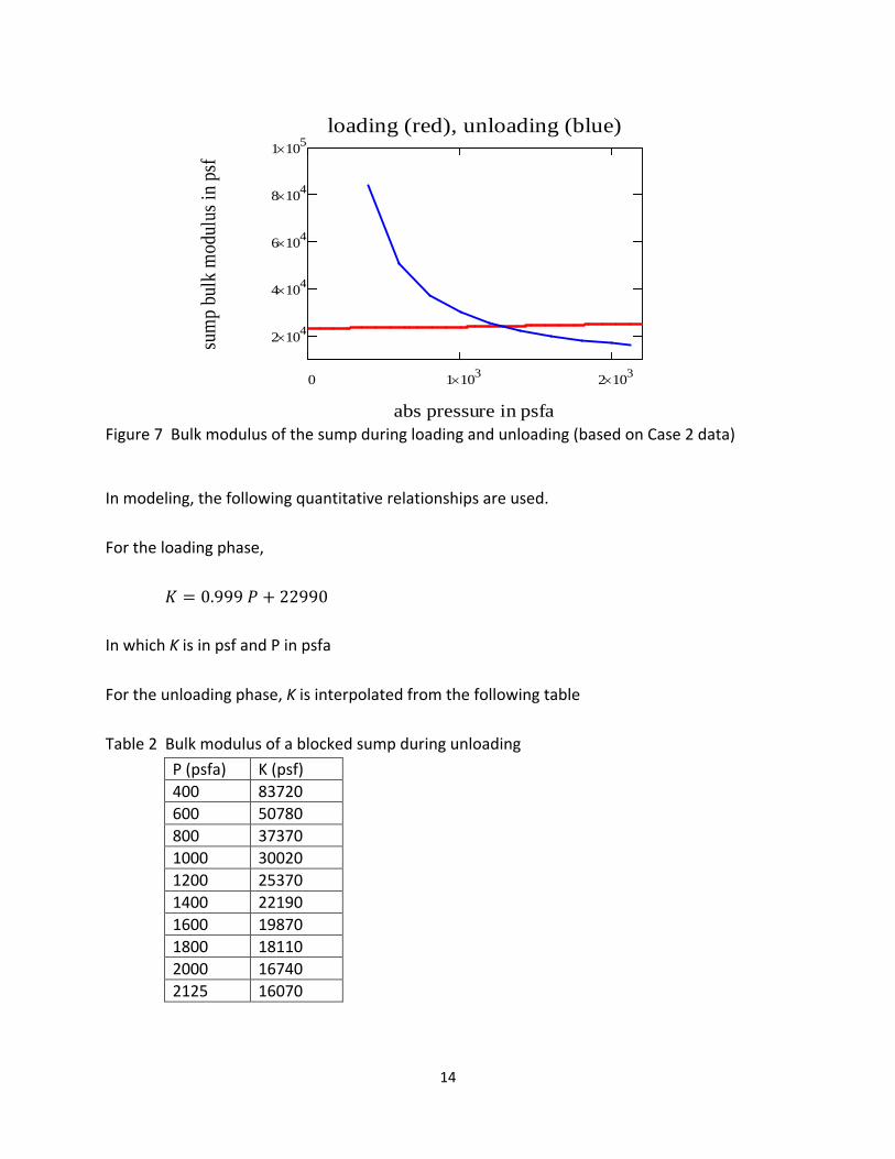
Figure 7 Bulk modulus of the sump during loading and unloading (based on Case 2 data)

In modeling, the following quantitative relationships are used. For the loading phase, 𝐾 = 0.999 𝑃 + 22990 In which K is in psf and P in psfa For the unloading phase, K is interpolated from the following table Table 2 Bulk modulus of a blocked sump during unloading

P (psfa) K (psf) 400 83720 600 50780 800 37370 1000 30020 1200 25370 1400 22190 1600 19870 1800 18110 2000 16740 2125 16070

0 1 103× 2 103×

2 104×

4 104×

6 104×

8 104×

1 105×

loading (red), unloading (blue)

abs pressure in psfa

sum

p bu

lk m

odul

us in

psf

15

It is believed that the test data have captured relevant aspects of the complex dynamics of the water surrounding the IE foam on the pool side. The sump appears to be more rigid (i.e., higher K) in the beginning of the unloading phase because the pool water above the foam has to be accelerated upward and pushed away as the foam retracts. Once the surrounding water is mobilized, the retraction becomes easier, and the sump appears to be softer (lower K).

The timing of vacuum release is of interest. This is handled by keeping track of the volume of foam inside the sump as a result of volume flux QB. 𝑆 = 𝑆𝑜𝑙𝑑 + 𝑑𝑡 [𝜑 𝑄𝐵 + (1 − 𝜑)𝑄𝐵𝑜𝑙𝑑]

S is zero at the very moment when the IE foam first contacts the sump. Its value then increases and decreases as demanded by the system dynamics. The vacuum is considered released when S becomes zero again. Modeling the Centrifugal Pump Pump switch is one of the two means to release the vacuum at the sump. Modeling the dynamics of the pump and its spinning down after tripping is necessary. The pumps used in the test are a 3 hp Pentair Challenger high-head pump and a 1/2 hp Sta-Rite spa pump. The available data is limited to head versus flow curves at 3450 rpm. The rated heads and flows are not indicated on these curves. It appeared that the 3 hp pump was operated near its rated condition prior to stripping. The 1/2 hp pump was operated way out on its performance curve (i.e., higher flow and lower head than the rated values). Other estimated data include the rated torque, the four-quadrant pump performance data, and the moment of inertia of pump and motor. The estimated data for the pumps are shown below. Table 3: Estimated rated Conditions of the Pumps Used in CPSC’s Tests 3 hp pump 1/2 hp pump Rated speed (rpm) 3450 3450 Rated head (ft) 98 30.7 Rated flow (gpm) 80 51 Rated torque (ft-lb) 3.8 0.75 WRR (lb –ft2) 0.066 0.011 The estimated specific speeds are 1277 and 1001, in rpm-gpm-ft units, for the 3 hp and 1/2 hp pumps, respectively. The four-quadrant performance data for a pump with a specific speed of

16

Figure 8 Four quadrant performance curves for a pump with a specific of 1270 in rpm-gpm-ft units (Wylie and Streeter 1993)

1270 in rpm-gpm-ft is available (Wylie and Streeter 1993) and is used for both pumps. These data are shown in Figure 8. The data are more applicable to the 3 hp pump than the 1/2 hp pump. Better four-quadrant performance data and the WRR values should be used, when available. In Figure 8, v = flow scaled by the rated flow, α = speed scaled by the rated speed; WH and WB represent scaled head and torque curves.

17

There are six variables involved in pump modeling: (1) head at pump suction Hs, (2) head at pump discharge Hd, (3) flow through the pump Q, (4) total dynamic head produced by the pump TDH, (5) resistive torque T, and (6) pump rotational speed ω. The available equations are: (1) The scaled pump head versus scaled flow relationship represented by the WH curve (2) The scaled pump torque versus scaled flow relationship represented by the WB curve (3) The energy balance across the pump 𝐻𝑑 − 𝐻𝑠 = 𝑇𝐷𝐻 (4) The C+ compatibility equation from the suction pipe 𝐻𝑠 = 𝐶𝑃 − 𝐵𝑃 𝑄 (5) The C- compatibility equation from the discharge pipe 𝐻𝑑 = 𝐶𝑀 + 𝐵𝑀 𝑄 (6) The relationship between rotational acceleration and the applied resistive torque

𝑇 =−𝑊𝑅𝑅𝑔

𝑑𝜔𝑑𝑡

In the above, CP, BP, CM, and BM are constants representing the characteristic impedance and friction of the suction and discharge pipes. g = gravitational acceleration, and t = time. Modeling the Air Vent (to be implemented) The other means to release vacuum at the sump is to open an air vent near the pump suction. The action and effect of the air vent will be modeled as an air valve. The air entered into the pipe will be lumped at a computational section. The variables involved are: (1) mass flow rate of air mdot; (2) absolute pressure inside pipe and at the computational section P; (3) flow toward the computational section QU; (4) flow moving away from the computational section Q; and (5) head at the computational section H. The available equations are: (1) The mass flow rate through the air valve. There are four possibilities:

18

(a) Subsonic air inflow

𝑚𝑑𝑜𝑡 = 𝐶𝐴𝑖𝑛�7𝑃0𝜌0 ��𝑃𝑃0�1.4286

− �𝑃𝑃0�1.714

� if 𝑃0 > 𝑃 > 0.53 𝑃0

(b) Sonic inflow

𝑚𝑑𝑜𝑡 = 𝐶𝐴𝑖𝑛0.686�𝑅 𝑇0

𝑃0 if 𝑃 ≤ 0.53 𝑃0

(c) Subsonic outflow

𝑚𝑑𝑜𝑡 = −𝐶𝐴𝑜𝑢𝑡�7𝑅 𝑇

��𝑃0𝑃�1.4286

− �𝑃0𝑃�1.714

� if 𝑃00.53

> 𝑃 > 𝑃0

(d) Sonic outflow

𝑚𝑑𝑜𝑡 = −𝐶𝐴𝑜𝑢𝑡0.686√𝑅 𝑇

𝑃 if 𝑃 > 𝑃0

0.53

In the above, CAin = product of discharge coefficient and valve orifice cross-sectional area for inflow, CAout = product of discharge coefficient and valve orifice cross-sectional area for outflow, R = the gas constant of air, T0 = absolute air temperature outside pipe, T = absolute air temperature inside pipe, P0 = absolute pressure outside pipe. Values for CAin and CAout need to be established from air vent vendor or through tests.

(2) The C+ compatibility equation from the pipe segment upstream of the air valve

𝐻 = 𝐶𝑃 − 𝐵𝑃 𝑄𝑈

(3) The C- compatibility equation from the pipe segment downstream from the air valve


(4) The equation of state for the air mass inside pipe

𝑃 �𝑉𝑎𝑜𝑙𝑑 +𝑑𝑡2

[ (𝑄 − 𝑄𝑈) + (𝑄𝑜𝑙𝑑 − 𝑄𝑈𝑜𝑙𝑑]� = �𝑚𝑜𝑙𝑑 +𝑑𝑡2

(𝑚𝑑𝑜𝑡 + 𝑚𝑑𝑖𝑡𝑜𝑙𝑑)� 𝑅 𝑇

(5) The absolute pressure - head relationship at the section

𝑃 = 𝛾(𝐻 − 𝛽)

Modeling the Second Drain

19

An effective way to prevent vacuum from developing is to use dual drains. When the first drain is blocked suddenly, the low pressure induced in the suction pipe will cause an inrush of flow from the second drain, which can release the vacuum at the first drain. The dual-drain configuration indicated in Figure 1 is modeled by adding a “T” junction to the system model and by adding a second drain that remains fully open.

In modeling the “T” junction, head losses at the junction are ignored. There are four variables: (1) junction head H, (2) flow into junction from the first drain Q1, (3) flow into junction from the second drain Q2, and (4) flow leaving the junction Q3. The available equations are

(1) The C+ compatibility equation from the pipe between the first drain and the junction

𝐻 = 𝐶𝑃1 − 𝐵𝑃1 𝑄1

(2) The C+ compatibility equation from the pipe between the fsecond drain and the junction

𝐻 = 𝐶𝑃2 − 𝐵𝑃2 𝑄2

(3) The C- compatibility equation from the suction pipe downstream of the junction

𝐻 = 𝐶𝑀 + 𝐵𝑀 𝑄3

(4) The continuity equation

𝑄1 + 𝑄2 = 𝑄3

The variables for the second drain sump are: (1) head in the drain sump Hs, (2) head in the inlet of the pipe between the drain and the junction H, (3) flow into the pipe Q. The applicable equations are

(1) The C- compatibility equation from the pipe between the drain and the junction


(2) Relationship between pool head and sump head (applicable to both sumps)

𝐻𝑝𝑜𝑜𝑙 = 𝐻𝑠 + (1 + 𝐾0) 𝑄2

2𝑔 𝐴𝑠2 𝑖𝑓 𝑄 > 0

𝐻𝑝𝑜𝑜𝑙 = 𝐻𝑠 𝑖𝑓 𝑄 ≤ 0

(3) Relationship between sump head and suction pipe inlet head (applicable to both sumps)

𝐻𝑠 = 𝐻 + (1 + 𝐾0) 𝑄2

2𝑔 𝐴𝑠2 𝑖𝑓 𝑄 > 0

𝐻𝑠 = 𝐻 𝑖𝑓 𝑄 ≤ 0

20

Modeling Transient Flow in pipes

Because the drain line is a low-head system, it is very likely that the water contains some free air (as opposed to dissolved air in the water). It is also very likely that some free air may be entrapped in piping at the numerous turns and elbows. To allow for the free air, the discrete gas cavity model (Wylie 1984, Liou 2000) is used. In this model, some fixed amount of free air is assumed to exist, and the wave speeds are pressure dependent. In the model, the air mass is lumped at the pipe interior computational sections. The water column between sections are regarded as free of air. This approach allows the well-established method of characteristics with constant wave speed (Wylie and Streeter 1993) to be used. The model allows gaseous vapor cavities to form, grow, and collapse in the pipe interior. It was found to be essential to include free air in modeling SVRS.

In capturing the frictional resistance to flow by the pipes, an absolute roughness of zero was assumed for the PVC pipes. Steady-state friction factors established from the Moody diagram with the applicable Reynolds numbers were used during transients.

There are four variables at the computational section: (1) head at the section; (2) flow toward the section; (3) flow leaving the section; and (4) the absolute pressure at the section. The available equations are:

(1) The C+ compatibility equation from the upstream pipe segment

𝐻 = 𝐶𝑃 − 𝐵𝑃 𝑄𝑈

(2) The C- compatibility equation from the downstream pipe segment


(3) The equation of state for the air mass at the section

𝑃 �𝑉𝑎𝑜𝑙𝑑 +𝑑𝑡2

[ (𝑄 − 𝑄𝑈) + (𝑄𝑜𝑙𝑑 − 𝑄𝑈𝑜𝑙𝑑]� = 𝑚 𝑅 𝑇

(4) The absolute pressure - head relationship at the section

𝑃 = 𝛾(𝐻 − 𝛽)

Modeling the complete System

All the components described above are integrated into an inter-connected system by the C+ and C- compatibility equations. The method of characteristics with a fixed time interval is used. The pipes are divided into computational reaches with equal length of one foot. The time step size is governed by the Courant condition

21

𝑑𝑡 =𝑑𝑥𝑎

in which dx = computational reach length and a is the water hammer wave speed in the system. The wave speed for a 2-inch Schedule 40 PVC pipe containing water free of free air is estimated at 1450 ft/s. The numerous elbows in the system may have made the pipe stronger (i.e., higher wave speed). On the other hand, the presence of free air (as opposed to dissolved air) in the water significantly lowers the wave speed. In low-pressure systems with numerous fittings (valves and elbows), such as the test facility, it is highly likely that free air was present in the system. And it is not possible to quantify the mass and location of such free air in the system. Consequently, the wave speed cannot be determined a priori.

Modeling Results and Comparison with Measurements

The unknown amount and the location of free air, the uncertain pump data, and the slight fluctuations in the steady-state pressure data require that some of the parameters be adjusted for individual Cases. These variables and their adjusted values used are shown in Table 4. Table 4 Parameters adjusted in the simulations Case 1 Case 2 Case 3 Case 4 Case 5 Pipe void fraction

0.0017 0.0008 0.0075 0.00198 0.0.0017

Sump air void fraction

0.005 0.005 0.005 0.005 0.005

WRR, lb-ft2 0.0380 0.297 0.0363 0.02136 0.02136 elbow head loss coefficient

0.750 0.400 0.724 0.590 0.572

The pipe void fraction is the average void fraction of free air in the suction and discharge piping at the standard pressure and temperature. Their values were adjusted so that the simulated period of pressure oscillations in the system after vacuum release best matched those in the measurements. The higher values for Case 3 reflect the fact that the pump was 3 ft above the pool water surface, and thus this case tends to have more free air. The sump air void fraction accounts for free air in the sump. Its value was determined by matching the simulated and the measured sump pressure traces immediately after sump blockage. No variation of this parameter was found to be necessary. The WRR values were adjusted so that the timing of the pump speed reversal in the simulations matched those in the tests. The elbow head loss coefficients were calculated by a head balance in the steady-state using the measured pressures. The values should be the same. The differences are caused by some slight fluctuations in the measured data. In any event, the values are all within the range for elbows

22

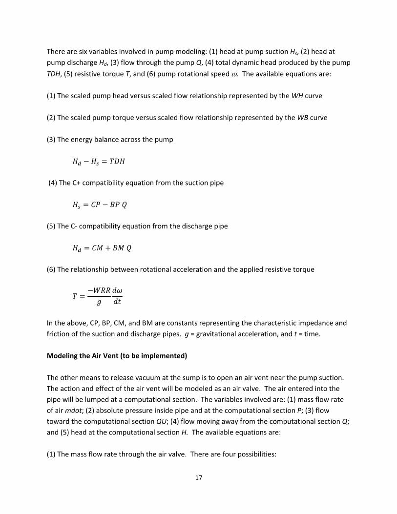
Figure 9 Case 1: Comparison between measurement and simulation

0 1 2 3 4 5 6 70

10

20

30

40

50

60

2− 103×

1− 103×

0

1 103×

2 103×

3 103×

4 103×

measurement

Puj

Pvisj

Psj

Pdj

Pvidj

rpmj

secondsj

0 1 2 3 4 5 6 70

10

20

30

40

50

60

2− 103×

1− 103×

0

1 103×

2 103×

3 103×

4 103×

simulation

PUj

PVISj

PSj

PDj

PVIDj

RPMj

secondsj

23


0 1 2 3 4 5 6 70

10

20

30

40

50

60

2− 103×

1− 103×

0

1 103×

2 103×

3 103×

4 103×

simulation

PUj

PVISj

PSj

PDj

PVIDj

RPMj

secondsj

0 1 2 3 4 5 6 70

10

20

30

40

50

60

2− 103×

1− 103×

0

1 103×

2 103×

3 103×

4 103×

measurement

Puj

Pvisj

Psj

Pdj

Pvidj

rpmj

secondsj

24


0 1 2 3 4 5 60

10

20

30

40

50

60

2− 103×

1− 103×

0

1 103×

2 103×

3 103×

4 103×

measurement

Puj

Pvisj

Psj

Pdj

Pvidj

rpmj

secondsj

0 1 2 3 4 5 6 70

10

20

30

40

50

60

2− 103×

1− 103×

0

1 103×

2 103×

3 103×

4 103×

simulation

PUj

PVISj

PSj

PDj

PVIDj

RPMj

secondsj

25


0 1 2 3 4 5 60

10

20

30

40

50

60

2− 103×

1− 103×

0

1 103×

2 103×

3 103×

4 103×

measurement

Puj

Pvisj

Psj

Pdj

Pvidj

rpmj

secondsj

0 1 2 3 4 5 60

10

20

30

40

50

60

2− 103×

1− 103×

0

1 103×

2 103×

3 103×

4 103×

simulation

PUj

PVISj

PSj

PDj

PVIDj

RPMj

secondsj

26


0 1 2 3 4 5 60

10

20

30

40

50

60

2− 103×

1− 103×

0

1 103×

2 103×

3 103×

4 103×

measurement

Puj

Pvisj

Psj

Pdj

Pvidj

rpmj

secondsj

0 1 2 3 4 5 60

10

20

30

40

50

60

2− 103×

1− 103×

0

1 103×

2 103×

3 103×

4 103×

simulation

PUj

PVISj

PSj

PDj

PVIDj

RPMj

secondsj

27

and do not affect the results. The simulated pressures and pump speed are compared in Figures 9 through 14.

Figures 9 through 13 demonstrate that the main traits of SVRS hydraulics are captured by the model. Uncertainties in the amount and location of free air and in the pump characteristics and its moment of inertia prevented a better match between simulation and measurements.

Of particular interest in the simulated results is the vacuum release time. A comparison is shown in Table 5. At its present stage of development, and despite the uncertainties, the model can predict the vacuum release time reasonably well for different pump horsepower, suction pipe length, steady-state flow rate, and pump elevation offset relative to pool level. Table 5 Vacuum Release Times Case 1 Case 2 Case 3 Case 4 Case 5 Simulated (sec) 3.70 5.20 3.60 2.20 2.20 Measured (sec) 3.70 6.05 3.25 2.38 2.38

Simulating the Effects of Dual Drains

The model was also used to simulate a dual-drain system shown in Figure 1. It was assumed that the two drains are identical. The second drain is identical to the first so that the steady-state flow is equally divided between the two. The measured steady-state flow and pressures for Case 2 were used. The IE foam was assumed to be lowered to the vicinity of the first drain and blocked it suddenly and completely at 0.735 seconds. The pump remained energized at all times. There are no dual-drain tests data to compare. Only the simulated results are discussed below.

Figure 14 shows the pressures at various locations and the pump rpm as before. It is seen that, with the second drain open, the first drain could not remain blocked. The disturbance to the pressures in the system is small and damped out quickly.

28

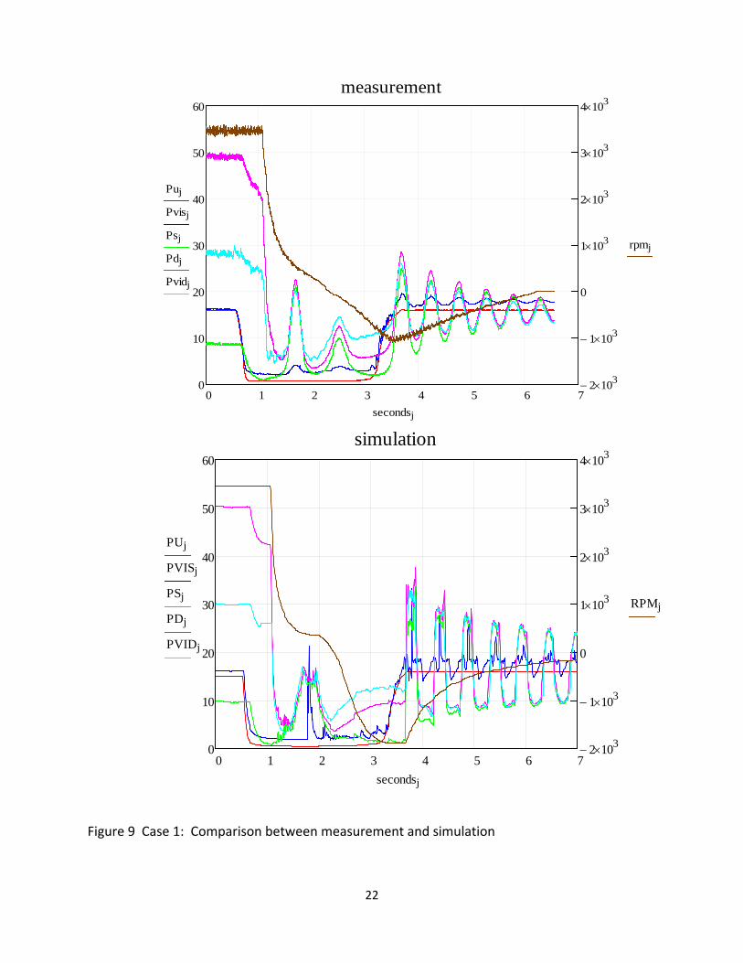
Figure 14 Disturbance produced by momentary blockage of one drain in a dual-drain system Figure 15 explains the dynamics of the blockage and the subsequent release f the IE foam. Q1 represents the flow entering the connector between sump 1 and the “T” junction. It is to be distinguished from the flow from pool into sump 1, which is zero once the drain is blocked. P1 represents the gauge pressure at the first sump. The corresponding quantities for sump 2 are denoted as Q2 and P2. Q3 is the flow entering the suction pipe immediately downstream of the junction. P3 is junction pressure. S represents the foam volume in sump 1 in cubic inches. In Figure 5, the flows are in gpm, and the pressures are in psig. Blocking sump 1 causes different amounts of reductions in P1, P2, and P3 as shown. In the beginning, the flow from sump 1 is decelerated, while the flow from sump 2 is accelerated by these pressure differentials. Q1 is reversed in this process. As Q1 feeds sump 1, P1 starts to recover, and the IE foam starts to retract. The foam is released from sump 1 vacuum at about 0.866 seconds when S becomes zero (see the bottom panel of Figure 15). Thereafter, P1 is at pool pressure, which is higher than the junction pressure P3. As a result, the flow toward sump1 is being slowed down and then turned around. The original steady-state flow is soon reestablished after the momentary blockage.

0 1 2 3 4 5 6 70

10

20

30

40

50

60

2− 103×

1− 103×

0

1 103×

2 103×

3 103×

4 103×

simulation

PUj

PVISj

PSj

PDj

PVIDj

RPMj

secondsj

29

Figure 15 Details explaining the dynamics of dual-drain systems

0.5 0.6 0.7 0.8 0.9 1 1.1 1.2 1.3 1.4 1.530−

20−

10−

0

10

20

30

40

50

60

70

Q1j

Q2j

Q3j

secondsj

0.5 0.6 0.7 0.8 0.9 1 1.1 1.2 1.3 1.4 1.50.5−

0

0.5

1

1.5

2

2.5

3

3.5

Sj

secondsj

0.5 0.6 0.7 0.8 0.9 1 1.1 1.2 1.3 1.4 1.52−

1.5−

1−

0.5−

0

0.5

1

1.5

2

P1j

P2j

P3j

secondsj

30

Conclusion A numerical model for SVRS has been developed with the aid of physical test data and high-speed videos provided by CPSC. Favorable comparisons between model results and test data indicate that the model captures the main traits of SVRS and can be used to analyze SVRS under various conditions. The ability of the model to simulate a dual-drain system is demonstrated. The model explains the complex dynamics involved and is helpful in understanding the dynamics of SVRS. MathCad codes of the model in electronic form are submitted in parallel with the submission of this report. The modeling approach for air vents is described and will be implemented in the remaining portion of the project. References ASME, 2002, “Manufacture Safety Vacuum Release Systems (SVRS) for Residential and Commercial Swimming Pools, Spas, Hot Tubs, and Wading Pool Suction Systems – An American National Standard,” ASME A112.19.17-2002. ASTM, 2004, “Standard Specifications for Manufactured Safety Vacuum Release System (SVRS) for Swimming Pools, Spas, and Hot Tubs,” ASTM Designation: F 2387 – 04. Liou, Jim C. P., 2000, “Numerical Properties of the Discrete Gas Cavity Model for Transients,” ASME Journal of Fluids Engineering, Vol. 122, September, pp. 636-639. Wylie, E. B., 1984, “Simulation of Vaporous and Gaseous Cavitation,” ASME Journal of Fluids Engineering, Vol. 106, September, pp 307-311. Wylie, E. B., and Streeter, V. L., 1993, Fluid Transients in Systems, Prentice Hall, Englewood Cliffs, NJ.

A Numerical Model for Safety Vacuum Release System (SVRS ...

Documents