A numerical model for light interaction with a two-level atom medium

1

A numerical model for light interaction with a two-level atom medium.

T. Colin a and B. Nkonga a

a Mathematiques Appliquees de Bordeaux,Universite Bordeaux 1 et CNRS UMR 5466351, Cours de la Liberation, 33405 Talence,mail: colin, [email protected]

The aim of this work is to study the interaction of a laser pulse with a gas describedby the Bloch equations. The physical model is derived from the Maxwell-Bloch equationsunder the assumption that the polarization and the electric field are both oriented in asingle direction, and under the slowly varying envelope approximation. The Schrodingerequation is formulated for a two-level atom medium under the rotating wave approxi-mation and dipole interaction. A rigorous asymptotic analysis of the simplified systemis performed to point out the different mechanisms associated with the physical model.A numerical approach based on a splitting technique is proposed and successfully per-formed.

Key Words: Nonlinear Optics, Two-level Atom, Asymptotic Analysis, Splitting Scheme,Lasers pulses.

1. Introduction

Many topics of interest in nonlinear optical applications are related to the propagationof light and to the interaction of the electric field with material media (see for example[23,7,18] for numerical study). The regime of the laser sources (small wavelength) displaysquantum mechanical coupling via the optical properties of the medium (see for examplethe classical textbooks [19,8,17]). The density of the material medium is either high [23]or low [16]. Then according to the intensity of the laser beams, we can obtain differentlevels of linear and nonlinear interactions. Modeling and computing those behaviors aredifficult numerical challenges. The full description of the light-matter interaction involvesthe resolution of the Maxwell equation coupled to the atomic wave function which obeysthe Schrodinger equations [8,19]. The numerical approach of this model is only possible forsimplified media with a small number of atoms. The nonlinear Maxwell-Bloch system is amacroscopic model taking into account the quantum mechanical coupling for a large classof media. It contains some essential numerical difficulties. In some cases, the full waveintegration of this system is unavoidable and has been investigated in the finite differencetime-domain (FDTD) context [22,15]. In general the computational time needed for thoseapplications is very expensive (see [7,12,9] for general nonlinearity and [5,4,24,23,20] forMaxwell-Bloch systems). However, we are concerned with the propagation of a quasi-monochromatic optical field in a dilute atomic vapor. Atoms with two energy levels

2

connected by an electric-dipole transition are embedded in the medium. The laser beamfrequency is nearly resonant with the atomic transition and sufficiently intense to removea significant fraction of the population from the atomic ground state to the excited state.

We assume that the envelope of the optical field is slowly varying and that the nonlinearpolarization is a perturbation term. The polarization and the electric field are supposed tobe oriented with the same fixed direction so that they can be treated as scalar quantities.The Schrodinger equation is formulated for a two-level atom medium under the rotatingwave approximation [8] and dipole interaction. In order to obtain an efficient numericalscheme, a nonlinear transformation is introduced to simplify the derived system. Thistransformation is inspired from [13] and is one of the key point of this work. Using a set ofparameters associated to an industrial application, we perform a scaling of the equationsand identify a small parameter. The asymptotic analysis is then performed and leadsto the characterization of the important operators governing the coupling mechanism.According to this characterization, a numerical model, that respects the properties of themain operators, is proposed. This method is applied to a boundary value problem.This paper is organized as follows: in Section 2, the physical model is derived from theMaxwell-Bloch system. In Section 3, rigorous asymptotic expansions are performed. Wepresent the numerical method in Section 4. In Section 5, we give some numerical results.We validate our numerical approach in the asymptotic regimes described in Section 3.Finally, in Section 6, we list some open questions concerning this problem.

2. Physical model

2.1. Statement of the basic equations

We are interested in the isotopic separation of uranium using an ionization by interac-tion with a nearly resonant laser. The uranium atomic gas is composed of U235 (∼ 0.1%)and U238 (∼ 99.9%) isotopes. In order to separate the U235 isotope, the U235 is ionizedbefore going across a Coulomb electric field. The ionization is obtained by an intense laserthat is resonant with the transition frequency of the U235 isotope. However, the transitionfrequency of both isotopes are very close so that a large part of the gas is excited. Theaim here is to propose an efficient numerical approach to compute the laser interactionwith the U238 isotope. Indeed, this interaction involves restrictive numerical constraintsrelated to the finite-difference stability and makes the computations inefficient. For thesake of simplicity, we restrict ourselves to the 2-D case (the unknowns depend only ontwo variables but live in R3). We call (x, z) ∈ R2 the basic coordinates and (ex, ey, ez)the basis of R3.The basic assumptions used for the model are :

• The elements of the dipole matrix and the electric field are singly oriented in thedirection ey : EEE = Eey, B = Bxex + Bzez where E denotes the electric field and B

denotes the magnetic field.

• The matter is composed of two-level atoms.

• The laser is nearly resonant with the medium.

The starting point of our model is the 2D Maxwell-Bloch equations in the transversemagnetic mode:

3

∂tBz + ∂xE = 0,

∂tBx − ∂zE = 0,

∂tE − c2(∂zBx − ∂xBz) = −µ0c2∂tP,

∂tC1 + iω1C1 = iΩC2,

∂tC2 + iω2C2 = iΩC1,

where the Ci’s are the complex representations of the populations, P = Nµ(C1C2 +C1C2)is the physical polarization, N is the density of atoms per unit of volume, µ is the dipole

coupling coefficient, c is the speed of light, µ0 the permeability of free space, Ω =µE~

is

the Rabi frequency and ~ the Planck constant. The frequencies ω1 and ω2 are associatedwith each level. For a two-level atom, it is usual [17] to formulate the Bloch equationswith the variables N = |C1|2 − |C2|2 and Λ = C1C2:

∂tΛ = iω21Λ− iΩN, ∂tN = −2iΩ(Λ− Λ),

where ω21 = ω2 − ω1. Since the laser is only nearly resonant with the medium (that is,its frequency is close to ω21 but not equal to ω21), one expects that the excitation processwill be weak and that |C2| << |C1| for all time (starting with atoms that are all in thefundamental state). Moreover since |C1|2 (resp. |C2|2) is the probability for an atom tobe in the energy level 1 (resp. 2), one has |C1|2 + |C2|2 = 1. Therefore we expect N ∼ 1and we look for N under the form N = 1− N . The Bloch equations then read:

∂tΛ = iω21Λ− iΩ + iΩN ,

∂tN = 2iΩ(Λ− Λ),

or dropping the tildes:

∂tΛ = iω21Λ− iΩ + iΩN,

∂tN = 2iΩ(Λ− Λ),

We now present a dimensionless form of the system formed by the Maxwell equationsand the Bloch equations. Let Tref be a characteristic time of the problem (taken equalto the duration of the pulse), let Lref = cTref the characteristic length in the directionof propagation (Lref is the length of the pulse), and let ρref the characteristic lengthin the transverse direction. The characteristic value of the electric field Eref is given

by the characteristic value of the Rabi frequency ωr =µEref

~which is given. As usual,

we take Bref =Eref

cas the characteristic value of Bx and By. We denote by Λref and

4

Nref the characteristic values of Λ and N that are to be determined later on. Moreoverwe introduce the phase mismatch parameter ∆ = ω − ω21 that measures the differencebetween the frequency of light ω and the characteristic frequency ω21 of the medium. Oneobtains the following system for the dimensionless variables:

∂tBz +cTref

ρref∂xE = 0, (1)

∂tBx − ∂zE = 0, (2)

∂tE −(

∂zBx −cTref

ρref∂xBz

)= −µ0c

2ΛrefNµ

Eref∂t(Λ + Λ), (3)

∂tΛ = i(ω −∆)TrefΛ− iωrTref

Λref

E + iωrTrefNref

Λref

EN, (4)

∂tN = 2iωrTrefLref

NrefE(Λ− Λ). (5)

We now explain how to find Λref and Nref . We consider the linear part of equation (4):

∂tΛ = i(ω −∆)TrefΛ− iωrTref

ΛrefE . (6)

The electric field field will be of the form eiωTref tE(t). Therefore, we look for a solution of(6) of the form Λ = eiωTref tΛ. The equation satisfied by Λ is :

∂tΛ + iωTref Λ = i(ω −∆)Tref Λ− iωrTref

ΛrefE .

One gets

Λ =

∫ t

0

e−i∆Tref (t−s)(−iωrTref

ΛrefE)ds = −i

ωrTref

Λref

∫ t

0

e−i∆Tref (t−s)E(s)ds

since Λ(t = 0) = 0. We perform an integration by part in time and obtain:

Λ = − ωr

∆Λref

([e−i∆Tref (t−s)E)

]t0−∫ t

0

e−i∆Tref (t−s)∂tEds

).

The near resonance hypothesis implies (see below for numerical values) :

ωTref >> ∆Tref >> 1.

5

The dominant term in this expression is therefore:

Λ = − ωr

∆Λref

E + O

(1

∆Tref

).

In order to obtain order O(1) effects on Λ, Λref is set to

Λref =ωr

∆. (7)

As explained before, |C1| ≈ 1 and |C2| << 1, therefore since N = 1 − (|C1|2 − |C2|2) =2|C2|2 (we have used |C1|2 + |C2|2 = 1) and since |Λ| = |C1||C2| ≈ |C2|, it follows that

Nref = 2Λ2ref . (8)

System (1)-(5) now reads:

∂tBz +cTref

ρref

∂xE = 0,

∂tBx − ∂zE = 0,

∂tE − (∂zBx −cTref

ρref

∂xBz) = −iµ0c

2µ2ω21TrefN∆~

(Λ− Λ),

∂tΛ = i(ω −∆)TrefΛ− i∆TrefE + i2ω2

rTref

∆EN,

∂tN = iTref∆E(Λ− Λ).

We now introduce the following parameters:

ε =1

∆Tref, ν =

1

ωTref, ε1 =

ρref

cTref, β =

µ2ω21TrefN2ε0∆~

and α =2Trefω

2r

∆.

The system reads:

∂tBz +1

ε1∂xE = 0,

∂tBx − ∂zE = 0,

∂tE − (∂zBx −1

ε1

∂xBz) = −2iβ(Λ− Λ),

∂tΛ =i

νΛ− i

εΛ− i

εE + iαEN,

∂tN =i

εE(Λ− Λ).

Numerical values: For our particular physical situation, one has Tref = 2.10−8s; thisgives Lref = 6m. We choose ρref = 1cm. The density of polarized atoms is N =5.1018atoms/m3 (this is a very dilute gas). The characteristic value of the Rabi frequency

6

is ωr = 109rad/s. The dipole coupling coefficient is µ = 5.10−31 in usual units, theelectric dipole frequency is ω21 ∼ π1015rad/s and the phase mismatch ∆ ∼ 1010rad/s.The laser frequency is also of order π1015rad/s. We recall the value of the constant:ε0 = 8.85.10−12F/m and ~ = 10−34Js. With these values we obtain:

ε ∼ 5.10−3, ν ∼ 10−8, ε1 ∼ 10−3, β ∼ 1 and α ∼ 1.

We therefore have three small parameters. The aim of the next section is to perform anasymptotic expansion in order to obtain a simplified model. We could make the expansionε, ν and ε1 → 0 and obtain a very simplified model, but doing that we would loose a lotof physical information. In fact, these three parameters have different significations. Theparameters ν and ε1 are related to the form of the pulse and are useful for the paraxialapproximation. More precisely, ν measures the efficiency of the envelope approximation.Indeed the electric field is of the form Eeit/ν with |∂tE| << 1

ν|E|. Since ν is very small,

we will make this approximation here. The parameter ε1 measures the diffraction ef-fects in the transverse direction. If we keep ε1 fixed, we overlook the diffraction effectsthat are of great importance for the propagation. In order to recover the usual paraxialapproximation we will choose:

ε1 =

√ν

2L .

The parameter ε has a completely different status: it is linked to the way that the phasemismatch modifies the propagation of the laser in the gas. We choose to keep it fixed inorder to keep this phenomenon in the final model. The dimensionless system is finally:

∂tBz +

√2L√ν

∂xE = 0, (9)

∂tBx − ∂zE = 0, (10)

∂tE −(

∂zBx −√

2L√ν

∂xBz

)= −2iβ(Λ− Λ), (11)

∂tΛ =i

νΛ− i

εΛ− i

εE + iαEN, (12)

∂tN =i

εE(Λ− Λ). (13)

7

2.2. Derivation of the model.

We now perform an almost standard geometric optics expansion on (9)-(13) as ν → 0.We make the following ansatz:

(Bx, Bz, E) =2∑

j=0

(Bjx, B

jz, E j)νj/2ei (t−z)

ν + c.c.,

where c.c. stands for complex conjugate and

Λ = (Λ0 + ν1/2Λ1 + νΛ2)ei(t−z)

ν ,

because the fields (Bx, Bz, E) are real while Λ is complex. N is non-oscillatory (see [13])and is expanded as

N = N0 + ν1/2N1 + νN2.

We now substitute this ansatz in (9)-(13).

• Terms of order1

ν:

One obtains

iB0z = 0, iB0

x + iE0 = 0, iE0 + iB0x = 0, iΛ0 = iΛ0, 0 = 0,

which gives

B0z = 0 and B0

x = −E0. (14)

E0, Λ0 and N0 are unknown at this level.

• Terms of order1

ν1/2:

iB1z +

√2L∂xE0 = 0,

iB1x + iE1 = 0,

iE1 + iB1x −

√2L∂xB

0z = 0,

iΛ1 = iΛ1

0 = 0

According to (14), B0z = 0 and this last system gives:

B1z = i

√2L∂xE0, (15)

B1x = −E1, (16)

8

where E1, Λ1 and N1 are unknown.

• Terms of order O(1):One gets

iB2z + ∂tB

0z +

√2L∂xE1 = 0, (17)

iB2x + ∂tB

0x + iE2 − ∂zE0 = 0, (18)

iE2 + ∂tE0 − (∂zB0x − iBB2

x −√

2L∂xB1z) = −2iβΛ0, (19)

iΛ2 + ∂tΛ0 = iΛ2 − i

εΛ0 − i

εE0 + iαE0N0, (20)

∂tN0 = − i

εE0Λ0 +

i

εE0Λ0. (21)

We have kept only the resonant terms in these equations and have dropped all othersharmonics.We now subtract (18) from (19) and using (14) we get:

∂tE0 + ∂zE0 +√

2L∂xB1z + ∂tE0 + ∂zE0 = −2iβΛ0

and (15) gives

∂tE0 + ∂zE0 + iL∂2xE0 = −iβΛ0. (22)

Now (20) implies

∂tΛ0 = − i

ε(Λ0 + E0) + iαE0N0 (23)

and (21) gives

∂tN0 =

2

εIm(E0Λ0). (24)

The 3-D extension of the system (22)-(24) reads (∆⊥ = ∂2x + ∂2

y):

(∂t + ∂z + iL∆⊥)E0 = −iβΛ0,

∂tΛ0 +

i

ε(Λ0 + E0) = iαE0N0,

∂tN0 =

2

εIm(E0Λ0).

(25)

9

It is the classical Schrodinger-Bloch system that can be found in textbooks. We haveobtained it formally with our scaling. For justification and extension to the three levelmodel see [6]. The main problem here is that this system is quite stiff since the parameterε is of order 5.10−3. It is especially difficult to make computations directly on (25) because

of the factor1

εin front of the nonlinear term.

2.3. Nonlinear change of variable

In [13], Joly, Metivier and Rauch proposed a generic change of variables in order tohandle systems that satisfy a ”transparency” condition. The main example considered in[13] is the Maxwell-Bloch system. In the two-level case, things are quite simple. Indeed,recall that the dimensional value N ∗ of N satisfies N ∗ = 1 − |C1|2 + |C2|2 but since|C1|2 + |C2|2 = 1, one has N ∗ = 2|C2|2 and |C2|2 = N∗/2. Besides |Λ∗|2 = |C1|2|C2|2 =(1− |C2|2)|C2|2 = (1−N∗/2)N∗/2 and N∗ is a solution of the second order equation

X2 − 2X + 4|Λ∗|2 = 0,

which solutions are

X = 1±√

1− 4|Λ∗|2.Since we expect the process to be weak (N ∗ << 1), we have

N∗ = 1−√

1− 4|Λ∗|2.For the dimensionless variables, we get:

N =1−

√1− 4Λ2

ref |Λ|2

2Λ2ref

But from the definition of Λref and α, one has Λ2ref = αε/2 and

N =1−

√1− 2αε|Λ|2αε

.

It follows that (25) is replaced by

(∂t + ∂z + iL∆⊥) E0 = −iβΛ0,

∂tΛ0 +

i

ε(Λ0 + E0) = iE0 1−

√1− 2αε|Λ0|2

ε,

(26)

which is not stiff anymore. Of course we can directly verify that

∂t

((αεN0 − 1)2 + (1− 2αε|Λ0|2)

)= 0.

For the analysis of the next section, we will simplify the nonlinear term as iα|Λ0|2E0 andwe consider (dropping the 0):

(∂t + ∂z + iL∆⊥)E = −iβΛ,

∂tΛ +i

ε(Λ + E) = iα|Λ|2E .

(27)

10

Moreover ε21 = ν

2L and L ∼ 10−2. We therefore write L = δε with δ = O(1). The finalform of the system is:

(∂t + ∂z + iδε∆⊥)E = −iβΛ,

∂tΛ +i

ε(Λ + E) = iα|Λ|2E .

(28)

This system (28) will be also used in the following form:

∂tU +A∂zU + δεB∆⊥U + CU = S(U) (29)

where

U =

(EΛ

), S(U) =

(0

iαEF(|Λ|2)

),

A =

(1 00 0

), B =

(i 00 0

), C =

(0 iβiε

iε

).

For the simplified system, the nonlinear function is given by F(|Λ|2) = |Λ|2. However, in

the general formulation we have F(|Λ|2) =1−√

1−2αε|Λ|2αε

.For applications of interest, the characteristic propagation distance is Zmax ∼ 100

(about 1km) and the time of propagation is Tmax ∼ 100 (about 2 .10−6s) . The length ofthe domain in the transverse direction is ρref ∼ 10−2 (about 10cm). An other importantremark on this system is that the polarization coefficient β is of order ∼ 1, due to the factthat the gas is diluted (N ∼ 1018 At/m3). Consequently the coupling is not stiff. This hasto be put in contrast with the solid medium (N ∼ 1023 At/m3) where the polarizationstrength is β ∼ 1

ε. The numerical approach we have proposed in [9] for stiff coupling

(β ∼ 1ε) between the polarization and the electric field is inefficient here. In order to

develop an efficient numerical approach we now analyze the asymptotic behavior of themodel (28).

3. Asymptotic behavior

The techniques used here are inspired from the works of Joly, Metivier and Rauch, seefor example [13]. However, it is not a straightforward consequence of [13]. Therefore wepresent the complete analysis of the problem as ε → 0.

3.1. Linear analysis

Let us consider the linear part of (28) where we neglect the ∆⊥ term. We look fortraveling waves in the form:

E = Ewei(wt−ξz) and Λ = Λwei(wt−ξz),

where w, ξ, Ew and Λw are constants. Substituting this ansatz in (28) we find that Ew

and Λw satisfy the linear system

(w − ξ)Ew + βΛw = 0,1

εEw +

(w + 1

ε

)Λw = 0.

11

The existence of nontrivial traveling waves is possible if and only if the matrix associatedwith the system is singular. Therefore, we find that the frequency w should satisfy thefollowing dispersion relation:

w2 +

(1

ε− ξ

)w − β + ξ

ε= 0.

The two roots of this equation, denoted by w1 and w2, can be approximated as follows:

w1 = β + ξ + O(ε) and w2 = −1

ε− β + O(ε).

There are two types of traveling waves, the first one (associated with w1) with a frequencyof order β and a group velocity nearly equal to one; the second one with a frequency oforder −1

ε− β and a group velocity nearly equal to zero. Since β ∼ 1, the frequency − 1

ε

governs the oscillating component of the solution of the linear and consequently, that ofthe nonlinear system.

3.2. Formal expansion and profile equations

According to the structure of the traveling waves for the linear system the oscillatingcomponent of the solution is dominated by the frequency − 1

ε. Therefore the solution of

the nonlinear system expands as follows:

U ' Vε(x, y, z, t, θ) = V0 + εV1 where U = V =

(EΛ

). (30)

The functions V0 and V1 have Fourier series (with respect to the variable θ = −tε):

Vl(x, y, z, t, θ) =∑

j

Vlj(x, y, z, t) eijθ for l ∈ 0, 1.

We assume that the functions Vlj are sufficiently smooth. These profiles are then substi-tuted into system (28) and the terms are collected according to the power of ε.

• At the order ε−1, system (28) gives

−∂θE0 = 0, (31)

−∂θΛ0 + i(Λ0 + E0) = 0. (32)

Using equation (31) we find that E0p = 0 when p 6= 0 and we conclude that E0 = E00.Therefore, we obtain from equation (32) that Λ0p = 0 when p is different from 0 or1. Moreover, the following relation holds: Λ00 = −E00. It follows from this analysisis that the profiles of E0 and Λ0 are given by :

E0 = E00 and Λ0 = −E00 + Λ01 eiθ. (33)

At this stage, E00 and Λ01 are unknown.

12

• At the order ε0 : the equations are

−∂θE1 + (∂t + ∂z)E0 = −iβΛ0, (34)

−∂θΛ1 + i(Λ1 + E1) + ∂tΛ0 = iαE0|Λ0|2. (35)

Using the relations (33), the nonlinear term E0|Λ0|2 is computed by:

E0|Λ0|2 = E00

(|E00|2 − E00Λ01 e−iθ − Λ01E00 eiθ + |Λ01|2

),

= −E200Λ01 e−iθ + E00

(|E00|2 + |Λ01|2

)− |E00|2Λ01 eiθ.

The ( eiθ)0 component of (34)-(35) is:

( eiθ)0

(∂t + ∂z)E00 = iβE00,

i(Λ10 + E10)− ∂tE00 = iαE00(|E00|2 + |Λ01|2). (36)

The first equation gives the evolution of E00.The component of the system associated with ( eiθ)1 is :

( eiθ)1

−iE11 = −iβΛ01,

iE11 + ∂tΛ01 = −iα|E00|2Λ01.

It follows that the evolution of Λ01 is coupled to the evolution of E00 by the followingordinary differential equation:

∂tΛ01 + iβΛ01 = −iα|E00|2Λ01. (37)

Finally, the system associated with ( eiθ)−1 is a single relation:

2Λ1(−1) + E1(−1) = −αE200Λ01.

For the other component of the system, associated with ( eiθ)−p, |p| > 1, we obtainthat

Λ1p = E1p = 0 for |p| > 1.

Therefore, we have Vε = V0 + εV1 with

V0 = V00 + V01 eiθ and V1 = V1(−1) e−iθ + V10 + V11 eiθ, (38)

where

V00 =

(E00

−E00

), V01 =

(0

Λ01

), V1(−1) =

(E1(−1)

−αE200Λ01−E1(−1)

2

),

V10 =

(E10

T10(E00, Λ01)− E10

), V11 =

(βΛ01

Λ11

),

13

where T10(E00, Λ01) = −i∂tE00 + αE00(|E00|2 + |Λ01|2). The variables E00 and Λ01 satisfythe following system:

(∂t + ∂z)E00 = iβE00, (39)

∂tΛ01 + iβΛ01 = −iα|E00|2Λ01. (40)

At this stage, we can assume that the variables E1(−1), E10, and Λ11 are equal to zero sincethey do not play any role in the expansion. Then, it is easy to check as usual that:

∂tV0 +A∂zV0 + δεB∆⊥V0 + CV0 − S(V0) = εRε, (41)

with

A =

(1 00 0

), S(V) =

(0

iαE|Λ|2)

, C =

(0 iβiε

iε

), B =

(i 00 0

)

where Rε is bounded.

3.3. Rigorous results

The aim of this section is to prove the following theorem:

Theorem 1. Let a and b be two functions in Hs(R3) for s large enough.Let (E00(x, y, z, t), Λ01(x, y, z, t)) be the solution of the following Cauchy problem:

(∂t + ∂z)E00 = iβE00

∂tΛ01 + iβΛ01 = −iα|E00|2Λ01with

(E00(x, y, z, 0)Λ01(x, y, z, 0)

)=

(a

b + a

).

Then, there exists T > 0 and a unique solution Uε ∈ C([0, T ]; Hs) of the system (29)

satisfying the initial condition Uε(t = 0) =

(ab

)and such that

|Uε − V0|L∞(0,T ;Hs−2×Hs−2) = O(ε) where V0 =

( E00

−E00 + Λ01 e−i tε

).

Proof: By usual techniques, it is easy to show that there exists a solution Uε(t) of (29),defined for t ∈ [0, Tε]. The first step is to prove that ∃T > 0 such that Tε ≥ T and thatUε is bounded uniformly on [0, T ] independently of ε. We first consider the linear systemin Fourier form:

∂tU = M(ξ)U where M(ξ) = −iξA− C,

and iξ is the symbol of ∂z + iδε∆⊥. We now write explicitly the spectral decompositionof M(ξ) in order to solve (34)-(35). The eigenvalues of M(ξ) are given by

λ± = − i

2ε

(1 + εξ ±

√δ)

, (42)

where δ = δ(ξ, ε) = (1 − εξ)2 + 4εβ is a real positive function. The spectral projectorsΠ+ and Π− are given by:

Π+ =M − λ−λ+ − λ−

and Π− =M − λ+

λ− − λ+.

14

Let us denote by I the identity matrix and define the matrix J by:

J =

εξ − 1

2εβ

11− εξ

2

.

Using these matrices, the projectors Π+ and Π− are given by:

Π+ =1

2I +

1√δJ and Π− =

1

2I − 1√

δJ. (43)

The difficulty here is that δ(ξ, ε) is not bounded from below uniformly in ξ and ε. It istherefore not possible to obtain an uniform bound for the solution Uε of (29), such that

|Uε(., t)| ≤ C|Uε(., 0)|,

with C independent of ε and ξ. Nevertheless, the particular structure of the nonlinearterms of (34)-(35) allows to obtain some bounds.The solution Uε of system (29) satisfies:

Π+Uε(t) = eλ+tΠ+Uε(0) +

∫ t

0

eλ+(t−s)Π+S(Uε(s))ds

and

Π−Uε(t) = eλ−tΠ−Uε(0) +

∫ t

0

eλ−(t−s)Π−S(Uε(s))ds,

where Π± and λ± now denotes the Fourier multipliers which symbols are defined by theequations (43) and (42).

Uε(t) = ( eλ+tΠ+ + eλ−tΠ−)Uε(0) +

∫ t

0

( eλ+(t−s)Π+ + eλ−(t−s)Π−)S(Uε(s))ds. (44)

The proof of Theorem 1 now goes through three lemmas.

Lemma 1. ∃C1 > 0 such that for all g ∈ Hs(R3), we have∣∣∣∣Π±

(0g

)∣∣∣∣Hs

≤ C1|g|Hs.

Proof: Taking the Fourier transform leads to:

Π±

(0g

)= 1

2

(0g

)± 1√

δJ

(0g

),

= 12

(0g

)± εβ√

δ

(g0

)± 1−εξ

2√

δ

(0g

).

Now recall that δ = (1− εξ)2 + 4εβ so thatεβ√

δand

1− εξ

2√

δare uniformly bounded with

respect to ε and ξ. The result follows.

15

Lemma 2. For all ε ≤ 1/2, ∃C2 > 0 such that for all f and g in Hs(R3), with the

support of f and the support of g included in

|ξ| ≤ 1√

ε

, we have

∣∣∣∣Π±

(fg

)∣∣∣∣Hs

≤ C2 (|f |Hs + |g|Hs) .

Proof: Taking the Fourier transform leads to:

Π±

(fg

)= 1

2

(fg

)± 1√

δJ

(fg

),

= 12

(fg

)± εβ√

δ

(g0

)± 1√

δ

(0

f

)± 1−εξ

2√

δ

(−fg

).

(45)

For |ξ| ≤ 1√ε

and ε ≤ 1/2, we have

√δ ≥

√(1−√ε)2 + 4εβ ≥ 1/2.

Moreover,εξ − 1√

δand

εβ√δ

are bounded. Lemma 2 follows.

Lemma 3. ∃C3 > 0 such that for all f and g in Hs(R3), for all ε ≤ 1/2 with the support

of f and the support of g included in

|ξ| ≥ 1√

ε

, we have

∣∣∣∣Π±

(fg

)∣∣∣∣Hs

≤ C3(|f |Hs+1 + |g|Hs+1).

Proof: Using again (45) and writing

√δ =

√(1− εξ)2 + 4εβ ≥

√4β√

ε

we get

∣∣∣∣Π±

(fg

)∣∣∣∣ ≤ C3

(1 +

1√ε

)(|f |+ |g|

)≤ C3

(1 + |ξ|

)(|f |+ |g|

).

The last inequality is satisfied thanks to the condition on the support of f and g. Itfollows that

∣∣∣∣Π±

(fg

)∣∣∣∣Hs

≤ C3

(|f |Hs+1 + |g|Hs+1

).

This ends the proof of Lemma 3.

16

Let us come back to equation (44). We have

|Uε(t)|Hs ≤ |Π+Uε(0)|Hs + |Π−Uε(0)|Hs

+

∫ t

0

(|Π+S(Uε)|Hs + |Π−S(Uε)|Hs) dτ.

Using Lemma 2 and 3 and writing

Uε(0) = Uε(0)1|ξ|≤ 1√ε

+ Uε(0)1|ξ|> 1√ε

,

we obtain

|Π+Uε(0)|Hs + |Π−Uε(0)|Hs ≤ (C2 + C3)|Uε(0)|Hs+1.

Now using Lemma 1, we have

∣∣∣∣Π±

(0

iαEε|Λε|2)∣∣∣∣

Hs

≤ C1|E|Hs|Λ|2Hs ≤ C1|Uε|3Hs,

provided s > d/2. Finally, equation (44) leads to the following estimate

|Uε(t)|Hs ≤ C|Uε(0)|Hs+1 + C

∫ t

0

|Uε|3Hsds.

This implies that there exists T > 0 and C0 such that

Tε ≥ T and |Uε|L∞(0,T ;Hs) ≤ C0.

Now in order to prove Theorem 1, we define U by:

Uε = V0 + εU .

According to equations (29) and (41) satisfied respectively by Uε and Vε, the systemsatisfied by U is

∂tU +A∂zU + δεB∆⊥U + CU = −Rε +S(Uε)− S(V0)

ε= −Rε +

(0iα

)δSε

, (46)

where δS = |Uε,2|2Uε,1 − |V0,2|2V0,1. What we need now is to control δSε

uniformly in ε.We have:

δS =(|Uε,2|2 − |V0,2|2

)Uε,1 + ε|V0,2|2E ,

=(ε(Uε,2 + V0,2)Λ + Uε,2V0,2 − U ε,2V0,2

)Uε,1 + ε|V0,2|2E ,

= ε(Uε,2Λ + V0,2Λ + V0,2Λ− V0,2Λ

)Uε,1 + ε|V0,2|2E ,

= ε((Uε,2Λ + V0,2Λ

)Uε,1 + |V0,2|2E

)= εf(U),

17

where f(U) = δSε

is a linear function in U with uniformly bounded coefficients. Theintegral form of the differential equation (46) is

U =(

eλ+tΠ+ + eλ−tΠ−

)U(0)−

∫ t

0

(eλ+(t−τ)Π+ + eλ−(t−τ)Π−

)Rεdτ

+

∫ t

0

(eλ+(t−τ)Π+ + eλ−(t−τ)Π−

)( 0

iαf(U)

)dτ.

Using Lemma 2 and 3 for the first two terms and Lemma 3 for the last one yields:

|U |Hs ≤ C|U(0)|Hs+1 +

∫ t

0

C|R|Hs+1dτ +

∫ t

0

C|f(U)|Hsdτ.

Now since the function f(U) is linear and since |U |L∞(0,T ;Hs) ≤ C, Gronwall’s lemma

implies that U is bounded in [0, T ], in fact as long as Uε exists. This ends the proof ofTheorem 1.

3.4. Long time expansion

Let us consider the case when Λ01(x, y, z, 0) = 0; then according to equation (37) for alltime Λ01(x, y, z, t) = 0. We introduce the variable τ = εt and we suppress the variable θ:

U ' Vε = V0 + εV1 + ε2V2 with Λ0 = −E0. (47)

At the order ε0, the equations are:

(∂t + ∂z)E0 = −iβΛ0,i(Λ1 + E1) + ∂tΛ0 = iαE0|Λ0|2.

Therefore, we obtain

(∂t + ∂z)E0 = iβE0,∂tE0 − i(Λ1 + E1) = −iαE0|E0|2. (48)

At the order ε1, we obtain:

∂τE0 + (∂t + ∂z)E1 + iδ∆⊥E0 = −iβΛ1,i(Λ2 + E2) + ∂tΛ1 − ∂τE0 = iαE1|Λ0|2 + 2iαE0Re(Λ0Λ1).

(49)

Using the value of (Λ1 + E1), given by the order ε0 expansion, leads to

∂τE0 +(∂t + ∂z − iβ

)E1 + iδ∆⊥E0 = −β

(∂tE0 + iα|E0|2E0

).

In order to avoid secular terms, we have to impose:

(∂t + ∂z − iβ

)E1 = 0

and therefore

∂τE0 + iδ∆⊥E0 = −β(∂tE0 + iα|E0|2E0

)

and we take E1 = 0. Then Λ1 is then given by the second equation of (48) and Λ2 by thesecond equation of (49). We obtain the following proposition.

18

Proposition 1. Let us consider an approximate solution U0 of system (29), defined on[0, T/ε] with the initial condition Λ0(0) = −E0(0). Then E0 satisfies the equations:

(∂t + ∂z)E0 = iβE0, (50)

∂τE0 + iδ∆⊥E0 − β∂zE0 = −iβ2E0 − iαβ|E0|2E0. (51)

The phase associated with equation (50) is β. If we disregard the transverse direction,the phase associated with equation (51) one is −(β2 + βα|E0|2), therefore, the oscillatoryfrequency given by this expansion is ωl ' β − ε(β2 + βα|E0|2). Moreover, it easy to seethanks to equation (50), that |E0| is simply transported. We do not know how to provea convergence result yet, because the estimates of the previous section are not valid on atime interval of the form [0, T/ε]. However, we have:

Proposition 2. Let E0 be the solution of system (50)-(51) with a smooth enough initialdata a. Take s large enough. Then there exists T0 > 0 independent of ε and a uniquesolution U ε of (29) with initial data (a,−a) defined on [0, T0| log(ε)|]. Moreover thereexists K > 0 and A > 0 such that:

|U ε − (V0 + εV1)|Hs ≤ Kε2(eAt − 1) for all t ∈ [0, T0| log(ε)|]

This proposition implies that

|E − E0|Hs ≤ Kε2(eAt − 1) for all t ∈ [0, T0| log(ε)|]

This proposition is a consequence of the work by D. Lannes and J. Rauch [14]. Itimplies that for bounded time this approximation is better than the previous one since itis of order ε2.

4. Numerical Method

In the previous section, we proved that at first order, the electric field moves withvelocity 1 and has time frequency β. It is therefore important that our numerical methodenables us to obtain this behavior. The best way to achieve this is to use a splittingstrategy in three steps. The first step is the resolution of (∂t + ∂z)E = 0 (propagationwith velocity 1). The second step is the computation of the remaining of the linear partof the system, that is:

(∂t + iδε∆⊥)E = −iβΛ,

∂tΛ +i

ε(Λ + E) = 0.

Asymptotically, this gives the right frequency β for E . The last step is the nonlinear one.More precisely: we are concerned with the propagation of localized wave packets (pulses)over a large distance. In order to reduce the computer resources needed to compute theentire region of interest, the system is formulated with the arbitrary Lagrangian Eulerian(ALE) approach. Given a moving window with the velocity uuu the ALE formulation of thesystem is:

∂tU +A∂zU + δεB∆⊥U + CU = S(U), (52)

19

where A is now a function of the velocity uuu:

A =

(1− uuu 0

0 −uuu

).

In the sequel we assume that uuu is constant during a time step. In practice, the windowvelocity is uuu = 0 until the pulse is completely in the computational domain. Then, thewindow velocity is set to uuu = 1 until the end of the computation.

The field equations are discretized in the standard finite-difference staggered grid inconjunction with an explicit time-marching method. In order to simplify the presentationof the numerical approach we assume that the spatial dimension is two. Let us considera Cartesian grid and denote by δz, δx the grid size in the propagation direction and inthe transverse direction respectively and by δt the time step. The discrete variables aredefined by:

Unj,k = U(nδt, jδx, kδz),

for 0 ≤ j ≤ Nx, 0 ≤ k ≤ Nz + 1 and 0 ≤ n ≤ Nt. We denote by Lx = Nxδx andby Lz = Nzδz. In the sequel, we assume, without loss of generality, that the solution isperiodic in the transverse direction. Indeed, the pulse is always localized in the transversedirection. Then if the computational domain is sufficiently large, the solution on thetransverse boundary is always zero and we can assume periodicity.

It is classical in optics applications to use Crank-Nicolson implicit schemes for thenonlinear Schrodinger equation [11,10,1] because of its non-diffusive property. However,this kind of scheme suffers phase errors for large propagation distance [3]. For highfrequency wave propagation over longer distances, the grid requirement (in order to avoidthe phase error) becomes excessive, leading to unreachable processing time and memoryrequirements. This is the most penalizing aspect of the Crank-Nicolson method especiallywhen the space dimension increases. However, our system has a stiff coupling for the linearterms but only a weak coupling with regard to the nonlinearity. Then we can use a splittingtechnique, based on the fact that the (linear) propagation and the linear interaction canbe solved exactly. The numerical resolution consists in three steps: propagation, linearinteraction and nonlinear interaction.

• Propagation step: The system solved in this step is the hyperbolic system definedby ∂tU +A∂zU = 0 where the initial condition, inside the domain, is the solution(Un

j,k) computed at the previous time step. When uuu = 0, we only have to define theelectric amplitude at the left boundary of the computational domain. The incomingwave at the left boundary, is defined by a function I(t, x) where x is the transversecoordinate. Therefore we have:

Enj,0 = I(tn, xj).

The index k = 0 is associated with the left boundary of the vapor when the compu-tational window is fixed (uuu = 0). On the other hand, when uuu = 1, we have to set thevalue of the polarization field or the right boundary of the computational window(associated with the index k = Nz + 1). As the atoms behind the computational

20

window are in the ground state and the electric field is equal to zero, it is naturalto set this polarization to zero on the right boundary: Λn

j,Nz+1 = 0.For 0 ≤ j ≤ Nx and 1 ≤ k ≤ Nz, the propagation is performed as follows:

Un+ 13

j,k − Unj,k +

δt

δz

(−A+Uj,k−1 + |A|Uj,k +A−Uj,k+1

)= 0,

where |A| = A if uuu = 0 and |A| = −A if uuu = 1, A+ = A+|A|2

, A− = A−|A|2

It is easyto see that the stability condition of this numerical scheme is δt ≤ δz and that theamplitude error is optimal when δt = δz (the normalized light speed here is equal toequal one). For all the tests cases, the time step is chosen in order to give a Courantnumber of equal to 1.

• Linear Interaction step: In this section we are concerned with the integration, dur-ing the time step δt, of the system ∂tU +B∆⊥U +CU = 0, with the initial condition

Un+ 13

j,k . We apply the Fourier transform with respect to the transverse direction,to the system for linear interactions and to the initial data. Let us denote by m(m = 1− Nx

2, ...., Nx

2

)the index of the Fourier coefficient and by Mm the matrix

Mm = ξmB − C with ξm = L(

2πmLx

)2

. For 0 ≤ j ≤ Nx and 1 ≤ k ≤ Nz, the linear

interaction step reads:

∂tUm,k −MmUm,k = 0,

Um,k(t = tn) = Un+1/3m,k .

The index k still indicates the position in the propagation direction z. The previous

system is integrated analytically and the predicted solution Un+ 23

m,k is given by:

Un+ 23

m,k = e(Mmδt) Un+ 13

m,k ,

or more explicitly

En+ 23

m,k = −K1(λ1ε + 1) e(iλ1δt) −K2(λ2ε + 1) e(iλ2δt),

Λn+ 2

3m,k = K1 e(iλ1δt) +K2 e(iλ2δt),

where

λ1 =εξm−1−

√(εξm−1)2+4ε(β+ξm)

2ε, K1 =

(ελ2+1)Λn+1

3m,k

+En+13

m,k√(εξm−1)2+4ε(β+ξm)

,

λ2 =εξm−1+

√(εξm−1)2+4ε(β+ξm)

2ε, K2 = − (ελ1+1)Λ

n+ 13

m,k+En+1

3m,k√

(εξm−1)2+4ε(β+ξm).

Since this integration is exact, we are computing accurately the phase of the solution.

• Nonlinear Interaction step: In order to compute the nonlinearity, we apply the

inverse Fourier transform to the coefficients Un+ 23

m,k computed in the previous step.

21

Then we obtain Un+ 23

j,k for 0 ≤ j ≤ Nx and 1 ≤ k ≤ Nz. We solve the system

∂tUj,k = S(Uj,k) with Uj,k(tn) = Un+ 2

3j,k . The solution Un+1

j,k of this system at timet = tn + δt is approximated by:

Un+1j,k = Un+ 2

3j,k + δtS(Un+ 2

3j,k ),

for 0 ≤ j ≤ Nx and 1 ≤ k ≤ Nz.

In the whole the splitting technique for the simplified system is:

Un+1 = Sb Snl(δt) F−1 Sl(δt) F Sp(δt) · Un, (53)

where Sp(δt), Sl(δt) and Snl(δt) are the semi-groups associated to the propagation, to thelinear interaction and to the nonlinear interaction respectively. The boundary conditionsoperator is Sb, and F is the Fourier transform operator. The stability and the accuracyof this splitting technique for linear operators can be found in [21].

5. Applications

The numerical scheme introduced in the previous section is now applied to the propa-gation of a light pulse in a two-level atom medium. At the initial time of the computation(t = 0), the atoms of the medium are in the ground state: CCC1 = 1 and CCC2 = 0. Theincoming electric field at the left boundary (z = 0) is given by:

I(t, ρ) = A0 e−At(t−Tm)2 e−iAc cos (ωc(t−Tm)) e−Aρ(ρ−ρ0)10 ,

where Tm = 80ns and At = ln√

2T 2

l

with Tl = 20ns. Computations are performed for

different values of A0, Ac, ωc. The Gaussian pulses are defined by Ac = 0 and ωc = 0.The phase-modulated Gaussian pulses are defined by Ac 6= 0 and ωc 6= 0. For the 1Dcomputations we have Aρ = 0 and for higher space dimensions Aρ = 2 ln

√2, ρ0 =

max ρ+min ρ2

. For the 2D computations ρ = x and for the 3D computations ρ =√

x2 + y2.From the initial time t = 0 to t = 2Tm, the computations are performed in a fixed

window z ∈ [0, 2Rw] where the radius of the window is Rw = cTm = 24m (Fig. 1 and 2).When the parameter ε is small, the pulse at the time t = 2Tm is centered in the window.Then, for t > 2Tm, the computations are performed in a moving window ξ ∈ [0, 2Rw]where ξ = z − c(t− 2Tm) and the mesh size is δξ = δz.

5.1. Gaussian pulse

We consider the propagation of a Gaussian pulse propagating in a two level-atommedium and assume that the transverse effects are negligible. Therefore, we considera one dimensional problem. At the time t = 3.3µs the moving window is centered at thepoint z = Zm = 984m. The fixed parameters are: β = 0.92, α = 0.5, ||A0|| = 1 andδz = 24mm. For small values ε ≤ 10−5, the pulse is also centered in the moving window.When large values are used for the parameter ε, the pulse moves to the left. The long timeexpansion estimates this drift as being proportional to εβ. Using the results of Figure 3

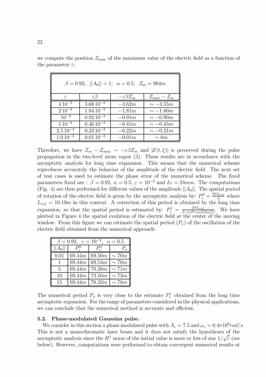
22

we compute the position Zmax of the maximum value of the electric field as a function ofthe parameter ε:

β = 0.92, ||A0|| = 1, α = 0.5, Zm = 984m

ε εβ −εβZm Zmax − Zm

4 10−3 3.68 10−3 −3.62m ∼ −3.55m2 10−3 1.84 10−3 −1.81m ∼ −1.80m10−3 0.92 10−3 −0.91m ∼ −0.90m

5 10−4 0.46 10−3 −0.45m ∼ −0.45m2.5 10−4 0.23 10−3 −0.22m ∼ −0.21m1.0 10−5 0.01 10−3 −0.01m ∼ 0m

Therefore, we have Zm − Zmax ∼ −εβZm and |E(t, ξ)| is preserved during the pulsepropagation in the two-level atom vapor (3). These results are in accordance with theasymptotic analysis for long time expansion. This means that the numerical schemereproduces accurately the behavior of the amplitude of the electric field. The next setof test cases is used to estimate the phase error of the numerical scheme. The fixedparameters fixed are : β = 0.92, α = 0.5, ε = 10−2 and δz = 24mm. The computations(Fig. 4) are then performed for different values of the amplitude ||A0||. The spatial period

of rotation of the electric field is given by the asymptotic analysis by: P 0ε =

2πLref

βwhere

Lref = 10.19m in this context. A correction of this period is obtained by the long time

expansion, so that the spatial period is estimated by: P 1ε =

2πLref

β−ε(β2+αβ||E0||2) . We haveplotted in Figure 4 the spatial evolution of the electric field at the center of the movingwindow. From this figure we can estimate the spatial period (Pν) of the oscillation of theelectric field obtained from the numerical approach:

β = 0.92, ε = 10−2, α = 0.5||A0|| P 0

ε P 1ε Pν

0.01 69.44m 69.50m ∼ 70m1 69.44m 69.54m ∼ 70m5 69.44m 70.38m ∼ 71m10 69.44m 73.16m ∼ 73m15 69.44m 78.32m ∼ 78m

The numerical period Pν is very close to the estimate P 1ε obtained from the long time

asymptotic expansion. For the range of parameters considered in the physical applications,we can conclude that the numerical method is accurate and efficient.

5.2. Phase-modulated Gaussian pulse.

We consider in this section a phase modulated pulse with Ac = 7.5 and ωc = 0.4π109rad/s.This is not a monochromatic laser beam and it does not satisfy the hypotheses of theasymptotic analysis since the H1 norm of the initial value is more or less of size 1/

√ε (see

below). However, computations were performed to obtain convergent numerical results at

23

the limit of the mesh refinement (Fig. 5-8). The temporal profile of the electric amplitudeafter 1km of propagation in the atomic vapor shows an envelope modification of the pulseand of the population densities (Fig. 5-8). The variation of the population densities isvery small (Fig. 7 and 8 ). The local amplitude of the electric field progressively grows toreach saturation after ∼ 2km of vapor (Fig. 9). Then the system goes into an oscillatingregime (Fig. 9). We claim that this behavior of the electric field is only due to the linearinteractions of the different spectral components of the initial pulse. To understand whathappens, let us go back to the model and consider the linear asymptotic behavior for highfrequencies. In the Fourier basis, the simplified linear model for a given frequency m is:

∂tEm = iζmEm − iβΛm,

∂tΛm = −i1εEm − i1

εΛm.

The eigenvalues of this system are given by

λ± = − i

2ε

(1− εζm ±

√(1− εζm)2 + 4ε(β + ζm)

).

For the considered test case (Ac = 7.5 and ωc = 0.4π 109 rad/s), the typical frequency ofthe modulation is

ζm = ωcTref ' 25 ∼ 1√ε.

Thus we assume that ζm = ζ√ε

with ζ of order one. In doing so we shall use the followingexpansion:

√(1− εζm)2 + 4ε(β + ζm) ' 1 +

√εζ + 2βε− 2βε

√εζ + 2βε2

(ζ2 − β

)

−ε2√

ε(2βζ3 − 6β2ζ + 7

8ζ5)

.

Then, we can derive an equation for the longtime linear self-action:

(i∂T + ∂2Z −

√ε∂3

Z)A = 0.

Let us consider a permanent wave with constant amplitude and modulated phase corre-sponding to Ac = 7.5 and wc = 0.4π rad/ns. The phase modulation is periodic and wefocus our investigation on a period. The dynamics of the normalized shape obtained inthis case (Fig. 11) is very close to the behavior that can be locally observed for com-putations performed with the two-level atom model (Fig. 12). It is then clear that thelocal compression observed on the shape of the electric field is essentially related to lin-ear effects on a phase modulated wave. Three dimensional computations have been alsoperformed successfully (Fig. 13). All the numerical results are in accordance with theexpected physical behavior.

6. Conclusion

We have suggested a methodology for the derivation of simplified models for laser beamspropagating in two-level atom material medium. This methodology can be extended

24

to other material media. In order to avoid some difficulties related to the stiffness ofthe model, we introduced a nonlinear change of variable inspired by the conservationproperties of the physical system. A small parameter is associated with the simplifiedmodel. Using the classical ansatz for geometric optics, the stability of the asymptoticexpansion was proved. Moreover, the characteristic component of the model has beenidentified and according to this result, a splitting numerical approximation was proposed.This numerical model has been validated in the hypothesis of asymptotic stability butalso successfully applied in a more general context. However, the strategy proposed cannot be applied to systems where population inversion can arise. A number of points willbe investigated in further works:• The stability of splitting schemes for systems that are singularly perturbed is not clearwhen the perturbation term is not skew symmetric. The symmetric case is treated in [21].See also [2] for Schrodinger-like equations.• The asymptotic behavior for initial data with modulated phase has to be made moreprecise and it is clearly not covered by geometric optics as done in Section 3.• The numerical experiments show that the propagation of the pulse over a long distanceis stable, even in the phase-modulated Gaussian case. Of course the simulation shouldinclude the other isotope U 235 which is not considered in this work. Our purpose was onlyto propose a simple and efficient numerical scheme for a two-level case.

Acknowledgments

This work has been partially supported by the CEA/DEN/DPC/SPAL with the collabo-ration of the CEA/DAM. We want to thank R. Abgrall for fruitful discussions about thiswork and the referees for very precise reports that helped us to improve this paper.

REFERENCES

1. C. Besse and B. Bidegaray, Numerical study of self-focusing solutions to theSchrodinger-Debye system. M2AN Math. Model. Numer. Anal., 1:35–55, 2001.

2. C. Besse, B. Bidegaray, and S. Descombes, Order estimates in time of splitting methodsfor the nonlinear Schrodinger equation. preprint MIP, Universite de Toulouse 3., 2001.

3. Christophe Besse, Relaxation scheme for the nonlinear Schroedinger equation andDavey-Stewartson systems. C. R. Acad. Sci., Paris, Ser. I, Math., 326(12):1427–1432, 1998.

4. B. Bidegaray, A. Bourgeade, D. Reignier and R. Ziolkowski, Multi-level Maxwell-Blochsimulations. In A. Bermudez, D. Gomez, C. Hazard, P. Joly and J.E. Roberts, editors,Mathematical and Numerical aspects of Wave Propagation, pages 221-225, 2000.

5. B. Bidegaray, Contributions a l’electromagnetisme dans le domaine temporel.Modelisation classique et quantique en optique non lineaire. PhD thesis, UniversitePaul Sabatier, October 2001.

6. T. Boucheres, A. Bourgeade, T. Colin, B. Nkonga and B. Texier, Study of a mathe-matical model for stimulated Raman scattering, preprint MAB, Universite Bordeaux1, 2003.

7. A. Bourgeade and E. Freysz, Computational modeling of the second harmonic gener-ation by solving full-wave vector Maxwell equations. JOSA, 17, 226-234, 2000.

8. R. W. Boyd, Nonlinear Optics. Academic Press, 1992.

25

9. T. Colin and B. Nkonga, Computing oscillatory waves of nonlinear hyperbolic systemsusing a phase-amplitude approach. In Proceeding of the Fifth Int. Conf. on Math-ematical and Numerical Aspects of Wave Propagation, page 954, 2000. July 10-14,Santiago de Compostela, Spain.

10. Thierry Colin and Pierre Fabrie. Semidiscretization in time for nonlinearSchroedinger-waves equations. Discrete Contin. Dyn. Syst., 4(4):671–690, 1998.

11. M. Delfour, M. Fortin, and G. Payne, Finite difference solutions of a nonlinearSchrodinger equation. J. Comput. Phys., 44:277–288, 1981.

12. B. Fidel, E. Heyman, R. Kastner, and R.W. Ziolkowski, Hybrid Ray-FDTD movingwindow approach to pulse propagation. J. Comput. Phys., 138(2):480–500, 1997.

13. J.-L. Joly, G. Metivier, and J. Rauch, Transparent nonlinear geometric optics andMaxwell-Bloch equations. J. Differential Equations, 166:175–250, 2000.

14. D. Lannes, J. Rauch, Validity of nonlinear geometric optics with times growing loga-rithmically. Proc. Amer. Math. Soc. 129 (2001), no. 4, 1087–1096.

15. R. M. Joseph and A. Tavlove, FD-TD Maxwell’s equations models for nonlinear elec-trodynamics and optics. IEEE Trans. Antennas and Propagation, 45, 1997.

16. A. Maria, N. M. Ercolani, S. A. Glasgow, and J. V. Moloney, Complete integrability ofthe reduced Maxwell-Bloch equations with permanent dipole. Phys. D, 138(1-2):134–162, 2000.

17. A. C. Newell and J. V. Moloney, Nonlinear Optics. Addison-Wesley PublishingCompagny, 1991.

18. B. Nkonga, A. Bourgeade, N. Seguin, and Bourdalle-Badie, Resolution directe paralleled’impulsions breves dans un milieu non lineaire. Preprint No 99022, MAB, 1999.

19. R. Pantel and H. E. Puthoff, Electronique quantique en vue des applications. Dunod,1973.

20. D. Reignier, Couplage des equations de Maxwell avec les equations de Bloch pourla propagation d’une onde electromagnetique, PhD thesis, Universite Paul Sabatier,March 200.

21. B. Sportisse, An analysis of operator splitting techniques in the stiff case. J. Comput.Phys., 161(1):140–168, 2000.

22. K. S. Yee, Numerical solution of initial boundary value problems involving Maxwell’sequations in isotropic media. IEEE Trans. Antennas and Propagation, 14:302–307,1966.

23. R.W. Ziolkowski, J. M. Arnold, and D. M. Gogny, Ultrafast pulse interactions withtwo-level atoms. Physical Review A, 52(4):3082–3094, 1995.

24. R.W. Ziolkowski, Realization of an all-optical triode and diode with a two-level atomloaded diffraction grating, Appl. Opt., 36:8547-8556, 1997.

26

0 10 20 30 40 500

0.2

0.4

0.6

0.8

1

z (m)

|E||A0|

t = 80 nst = 96 nst = 112 nst = 128 nst = 144 nst = 160 ns

Figure 1. Evolution of the Spatial profile of the normalized amplitude of the electric field.Fixed window during the incoming pulse phase. The computation is performed with theparameters: β = 0.92, |A0| = 2π, ε = 4 10−4 and α = 0.5 .

27

0 10 20 30 40 50−1

−0.5

0

0.5

1

z (m)

<(

E|A0|

)

t = 80 nst = 96 nst = 112 nst = 128 nst = 144 nst = 160 ns

Figure 2. Evolution of the Spatial profile of the normalized real component of the electricfield. Fixed window during the incoming pulse phase. The computation is performedwith: β = 0.92, |A0| = 2π, ε = 4 10−4 and α = 0.5 .

28

10009969929889849809769729680

0.5

1

z (m)

|E||A0|

ε = 10−5

ε = 0.00025ε = 0.0005ε = 10−3

ε = 0.002ε = 0.004

Figure 3. Spatial profile of the normalized amplitude of the electric field at time T = 3.3µs,for different values of ε. For these computations: β = 0.92, |A0| = 1 and α = 0.5.

29

25 45 65 85 105 125 145 165 185−1

−0.5

0

0.5

1

1.5

z (m)

<(E(t(z),z)|A0|

) |A0| = 0.1

|A0| = 1

|A0| = 5

|A0| = 10

|A0| = 15

Figure 4. Rotation of the real component of the electric field at the middle of the movingwindow (t(z) = 2Tm + z−Rw

c), for different values of |A0|. For these computations: β =

0.92, ε = 10−3 and α = 0.5.

30

50 60 70 80 90 100 1100

25

50

75

100

Nz = 5 000Nz = 10 000Nz = 20 000Nz = 30 000Nz = 40 000Nz = 50 000

τ (ns)

|E(τ, Zf)|2

Figure 5. Temporal profile of the norm of the electric field at the point z = Zf = 1km:

τ = t − Zf

c. For these computations: β = 0.92, ε = 10−3, α = 0.5, A0 = 6.93, Aω = 7.5

and wc = 0.4π rad/ns.

31

79 80 81 82 83 84 85−4.5

−3.5

−2.5

−1.5

−0.5

0.5

1.5

2.5

3.5

4.5Nz = 5 000Nz = 10 000Nz = 20 000Nz = 30 000Nz = 40 000Nz = 50 000

τ (ns)

<(E(τ, Zf))

Figure 6. Zoom on the temporal profile of the real component of the electric field at thepoint z = Zf = 1km: τ = t− Zf

c. For these computations: β = 0.92, ε = 4 10−4, α = 0.5

and A0 = 6.93.

32

50 60 70 80 90 100 1100.998

0.999

1

Nz = 5 000Nz = 10 000Nz = 20 000Nz = 30 000Nz = 40 000Nz = 50 000

τ (ns)

|CCC1|2

Figure 7. Temporal profile of the density population |CCC1|2 at the point z = Zf = 1km:

τ = t − Zf

c. For these computations: β = 0.92, ε = 10−3, α = 0.5, A0 = 6.93, Aω = 7.5

and wc = 0.4π rad/ns.

50 60 70 80 90 100 1100

0.001

0.002Nz = 5 000Nz = 10 000Nz = 20 000Nz = 30 000Nz = 40 000Nz = 50 000

τ (ns)

|CCC2|2

Figure 8. Temporal profile of the density population |CCC2|2 at the point z = Zf = 1km:

τ = t − Zf

c. For these computations : β = 0.92, ε = 10−3, α = 0.5, A0 = 6.93, Aω = 7.5

and wc = 0.4π rad/ns.

33

0.0 1.0 2.0 3.0 4.0 5.0 6.0 7.0 8.0 9.0 10.00.0

1.0

2.0

3.0

4.0

z (km)

max(|E||A0|

)Nz = 10000

Nz = 20000

Nz = 30000

Nz = 40000

Nz = 50000

Figure 9. Evolution of the normalized maximum amplitude in the atomic vapor. Forthese computations we have used: β = 0.92, ε = 4 10−4, α = 0.5, A0 = 6.93, Aω = 7.5and wc = 0.4π rad/ns.

34

50 80 1100

1

2

3

450 80 110

0

1

2

3

4

50 80 1100

1

2

3

450 80 110

0

1

2

3

4

50 80 1100

1

2

3

450 80 110

0

1

2

3

4

τ (ns)

z = 1.0km z = 1.5km z = 2.0km

z = 2.5km z = 3.0km z = 3.5km

Figure 10. Temporal profile of the normalized amplitude |E||A0| at the points z = 1km,

z = 1.5km, z = 2km, z = 2.5km, z = 3km and z = 3.5km. For these computations wehave used: β = 0.92, ε = 4 10−4, α = 0.5, A0 = 6.93, Ac = 7.5 and wc = 0.4π rad/ns.

35

0 0.25 0.5 0.75 10

1

2

3

0 0.25 0.5 0.75 10

1

2

3

0 0.25 0.5 0.75 10

1

2

3

0 0.25 0.5 0.75 10

1

2

3

0 0.25 0.5 0.75 10

1

2

3

0 0.25 0.5 0.75 10

1

2

3

Figure 11. Evolution of the temporal profile of the amplitude when solving the equation:(i∂T +∂2

Z +√

ε∂3Z)A = 0. For these computations the initial spatial profile has a constant

amplitude and a modulated phase corresponding to Ac = 7.5 and wc = 0.4π rad/ns.

36

80 82 84 86 880

1

2

3

480 82 84 86 88

0

1

2

3

4

80 82 84 86 880

1

2

3

480 82 84 86 88

0

1

2

3

4

80 82 84 86 880

1

2

3

480 82 84 86 88

0

1

2

3

4

τ (ns)

z = 1.0km z = 1.5km z = 2.0km

z = 2.5km z = 3.0km z = 3.5km

Figure 12. Zoom on the temporal profile of the normalized amplitude |E||A0| at the points

z = 1km, z = 1.5km, z = 2km, z = 2.5km, z = 3km and z = 3.5km. For thesecomputations: β = 0.92, ε = 4 10−4, α = 0.5, A0 = 6.93, Ac = 7.5 and wc = 0.4π rad/ns.

37

Figure 13. Modulated laser pulse propagating in a two-level atom medium: Spatial pro-file of the shape of the Numerical solution after 100m in the atomic vapor. For thesecomputations: L = 10−6, β = 0.92, ε = 4 10−4, α = 0.5, A0 = 6.93, Ac = 7.5 andwc = 0.4π rad/ns.