A NEW VERIFICATION METHOD FOR EMBEDDED SYSTEMS by Robert A. Thacker A dissertation submitted to the faculty of The University of Utah in partial fulfillment of the requirements for the degree of Doctor of Philosophy in Computer Science School of Computing The University of Utah May 2010

Welcome message from author
This document is posted to help you gain knowledge. Please leave a comment to let me know what you think about it! Share it to your friends and learn new things together.
Transcript

A NEW VERIFICATION METHOD FOR
EMBEDDED SYSTEMS
by
Robert A. Thacker
A dissertation submitted to the faculty ofThe University of Utah
in partial fulfillment of the requirements for the degree of
Doctor of Philosophy
in
Computer Science
School of Computing
The University of Utah
May 2010

Copyright c© Robert A. Thacker 2010
All Rights Reserved

THE UNIVERSITY OF UTAH GRADUATE SCHOOL
SUPERVISORY COMMITTEE APPROVAL
of a dissertation submitted by
Robert A. Thacker
This dissertation has been read by each member of the following supervisory committeeand by majority vote has been found to be satisfactory.
Chair: Chris J. Myers
Ganesh Gopalakrishnan
Eric G Mercer
John Regehr
Ken Stevens

THE UNIVERSITY OF UTAH GRADUATE SCHOOL
FINAL READING APPROVAL
To the Graduate Council of the University of Utah:
I have read the dissertation of Robert A. Thacker in its final formand have found that (1) its format, citations, and bibliographic style are consistent andacceptable; (2) its illustrative materials including figures, tables, and charts are in place;and (3) the final manuscript is satisfactory to the Supervisory Committee and is readyfor submission to The Graduate School.
Date Chris J. MyersChair, Supervisory Committee
Approved for the Major Department
Martin BerzinsChair/Dean
Approved for the Graduate Council
Charles A. WightDean of The Graduate School

ABSTRACT
Cyber-physical systems, in which computers control real-world mechanisms, are ever
more pervasive in our society. These complex systems, containing a mixture of software,
digital hardware, and analog circuitry, are often employed in circumstances where their
correct behavior is crucial to the safety of their operators. Therefore, verification of such
systems would be of great value. This dissertation introduces a modeling and verification
methodology sufficiently powerful to manage the complications inherent in this mixed
discipline design space.
Labeled hybrid Petri nets (LHPNs) are a modeling formalism that has been shown
to be useful for modeling analog/mixed signal systems. This dissertation presents an
extended LHPN model capable of modeling complex computer systems. Specifically, this
extended model uses discrete valued variables to represent software variables. In addition,
a rich expression syntax has been added to model the mathematical operations performed
in computer processors.
No formalism is useful if it remains inaccessible to designers. To facilitate the use
of this model, a translation system is presented that enables the compilation of LHPNs
from intermediate descriptions similar to assembly language. Users can create an LHPN
construction language appropriate to each portion of their design.
Once a model is defined, it is necessary to determine the range of behaviors of that
system. Specifically, a determination must be made if the model exhibits any behaviors
that violate the design constraints. To that end, this dissertation describes an efficient
state space exploration method. This method uses state sets to represent the potentially
infinite state spaces of LHPN models.
Complex models often yield intractably large state spaces, resulting in unacceptably
long runtimes and large memory requirements. It is, therefore, often necessary to distill
from a model the information necessary to prove a particular property, while removing
extraneous data. This dissertation presents a number of correctness preserving trans-
formations that depend on simple, easily checked properties to reduce the complexity of
LHPNs. These transformations alleviate the need to model variables, transitions, and

places that do not contribute to correctness of the property under test.
Finally, an in depth case study is used to demonstrate the utility of this method. Each
step in the modeling and analysis process is applied in turn to this example, showing its
progression from initial block diagram to final verified implementation.
v

To new sights, new places, and new opportunities.

CONTENTS
ABSTRACT . . . . . . . . . . . . . . . . . . . . . . . . . . . . . . . . . . . . . . . . . . . . . . . . . . . . . . iv
LIST OF FIGURES . . . . . . . . . . . . . . . . . . . . . . . . . . . . . . . . . . . . . . . . . . . . . . . ix
LIST OF TABLES . . . . . . . . . . . . . . . . . . . . . . . . . . . . . . . . . . . . . . . . . . . . . . . . . xii
LIST OF ALGORITHMS . . . . . . . . . . . . . . . . . . . . . . . . . . . . . . . . . . . . . . . . . . xiii
ACKNOWLEDGEMENTS . . . . . . . . . . . . . . . . . . . . . . . . . . . . . . . . . . . . . . . . . xiv
CHAPTERS
1. INTRODUCTION . . . . . . . . . . . . . . . . . . . . . . . . . . . . . . . . . . . . . . . . . . . . . 1
1.1 Formal Verification . . . . . . . . . . . . . . . . . . . . . . . . . . . . . . . . . . . . . . . . . . . 21.2 Hardware Verification . . . . . . . . . . . . . . . . . . . . . . . . . . . . . . . . . . . . . . . . . 31.3 Software Verification . . . . . . . . . . . . . . . . . . . . . . . . . . . . . . . . . . . . . . . . . . 41.4 System Verification . . . . . . . . . . . . . . . . . . . . . . . . . . . . . . . . . . . . . . . . . . . 51.5 Contributions . . . . . . . . . . . . . . . . . . . . . . . . . . . . . . . . . . . . . . . . . . . . . . . 61.6 Organization . . . . . . . . . . . . . . . . . . . . . . . . . . . . . . . . . . . . . . . . . . . . . . . . 7
2. LABELED HYBRID PETRI NETS . . . . . . . . . . . . . . . . . . . . . . . . . . . . . 8
2.1 Related Work . . . . . . . . . . . . . . . . . . . . . . . . . . . . . . . . . . . . . . . . . . . . . . . 82.2 LHPN Syntax . . . . . . . . . . . . . . . . . . . . . . . . . . . . . . . . . . . . . . . . . . . . . . . 92.3 Semantics for Extended LHPNs . . . . . . . . . . . . . . . . . . . . . . . . . . . . . . . . . 132.4 Summary . . . . . . . . . . . . . . . . . . . . . . . . . . . . . . . . . . . . . . . . . . . . . . . . . . . 15
3. SYSTEMS MODELING . . . . . . . . . . . . . . . . . . . . . . . . . . . . . . . . . . . . . . . . 16
3.1 Language Definition . . . . . . . . . . . . . . . . . . . . . . . . . . . . . . . . . . . . . . . . . . 163.2 Software Modeling . . . . . . . . . . . . . . . . . . . . . . . . . . . . . . . . . . . . . . . . . . . . 223.3 Hardware Modeling . . . . . . . . . . . . . . . . . . . . . . . . . . . . . . . . . . . . . . . . . . . 283.4 Interrupt Modeling . . . . . . . . . . . . . . . . . . . . . . . . . . . . . . . . . . . . . . . . . . . 293.5 Environment Modeling . . . . . . . . . . . . . . . . . . . . . . . . . . . . . . . . . . . . . . . . 333.6 Limitations . . . . . . . . . . . . . . . . . . . . . . . . . . . . . . . . . . . . . . . . . . . . . . . . . 33
4. VERIFICATION . . . . . . . . . . . . . . . . . . . . . . . . . . . . . . . . . . . . . . . . . . . . . . 38
4.1 State Sets . . . . . . . . . . . . . . . . . . . . . . . . . . . . . . . . . . . . . . . . . . . . . . . . . . 384.2 State Space Exploration . . . . . . . . . . . . . . . . . . . . . . . . . . . . . . . . . . . . . . . 414.3 Error Trace Generation . . . . . . . . . . . . . . . . . . . . . . . . . . . . . . . . . . . . . . . . 464.4 Contributions . . . . . . . . . . . . . . . . . . . . . . . . . . . . . . . . . . . . . . . . . . . . . . . 46

5. LHPN TRANSFORMATIONS . . . . . . . . . . . . . . . . . . . . . . . . . . . . . . . . . . 47
5.1 Related Work . . . . . . . . . . . . . . . . . . . . . . . . . . . . . . . . . . . . . . . . . . . . . . . 485.2 Preliminaries . . . . . . . . . . . . . . . . . . . . . . . . . . . . . . . . . . . . . . . . . . . . . . . . 495.3 Remove Arc After Failure Transition . . . . . . . . . . . . . . . . . . . . . . . . . . . . . 515.4 Removing Dead Transitions . . . . . . . . . . . . . . . . . . . . . . . . . . . . . . . . . . . . 525.5 Remove Dangling Places . . . . . . . . . . . . . . . . . . . . . . . . . . . . . . . . . . . . . . . 535.6 Remove Write Before Write . . . . . . . . . . . . . . . . . . . . . . . . . . . . . . . . . . . . 545.7 Substitute Correlated Variables . . . . . . . . . . . . . . . . . . . . . . . . . . . . . . . . . 565.8 Local Assignment Propagation . . . . . . . . . . . . . . . . . . . . . . . . . . . . . . . . . . 575.9 Remove Unread Variables . . . . . . . . . . . . . . . . . . . . . . . . . . . . . . . . . . . . . 595.10 Constant Enabling Conditions . . . . . . . . . . . . . . . . . . . . . . . . . . . . . . . . . . 605.11 Remove Vacuous Transitions . . . . . . . . . . . . . . . . . . . . . . . . . . . . . . . . . . . . 615.12 Remove Dominated Transitions . . . . . . . . . . . . . . . . . . . . . . . . . . . . . . . . . 645.13 Remove Vacuous Loops . . . . . . . . . . . . . . . . . . . . . . . . . . . . . . . . . . . . . . . . 655.14 Timing Bound Normalization . . . . . . . . . . . . . . . . . . . . . . . . . . . . . . . . . . . 675.15 Putting It All Together . . . . . . . . . . . . . . . . . . . . . . . . . . . . . . . . . . . . . . . . 67
6. CASE STUDY . . . . . . . . . . . . . . . . . . . . . . . . . . . . . . . . . . . . . . . . . . . . . . . . 70
6.1 Motivating Example . . . . . . . . . . . . . . . . . . . . . . . . . . . . . . . . . . . . . . . . . . 706.2 Initial Model . . . . . . . . . . . . . . . . . . . . . . . . . . . . . . . . . . . . . . . . . . . . . . . . 716.3 Transformations . . . . . . . . . . . . . . . . . . . . . . . . . . . . . . . . . . . . . . . . . . . . . 786.4 Results . . . . . . . . . . . . . . . . . . . . . . . . . . . . . . . . . . . . . . . . . . . . . . . . . . . . . 906.5 Summary . . . . . . . . . . . . . . . . . . . . . . . . . . . . . . . . . . . . . . . . . . . . . . . . . . . 103
7. CONCLUSIONS AND FUTURE WORK . . . . . . . . . . . . . . . . . . . . . . . . 104
7.1 Dissertation Summary . . . . . . . . . . . . . . . . . . . . . . . . . . . . . . . . . . . . . . . . . 1047.2 Future Work . . . . . . . . . . . . . . . . . . . . . . . . . . . . . . . . . . . . . . . . . . . . . . . . 105
7.2.1 Modeling . . . . . . . . . . . . . . . . . . . . . . . . . . . . . . . . . . . . . . . . . . . . . . . 1057.2.2 Compilation . . . . . . . . . . . . . . . . . . . . . . . . . . . . . . . . . . . . . . . . . . . . 1057.2.3 Analysis . . . . . . . . . . . . . . . . . . . . . . . . . . . . . . . . . . . . . . . . . . . . . . . . 1057.2.4 Abstraction . . . . . . . . . . . . . . . . . . . . . . . . . . . . . . . . . . . . . . . . . . . . . 1057.2.5 Case Studies . . . . . . . . . . . . . . . . . . . . . . . . . . . . . . . . . . . . . . . . . . . . 106
APPENDIX: REACTOR INPUT FILES . . . . . . . . . . . . . . . . . . . . . . . . . . . . 107
REFERENCES . . . . . . . . . . . . . . . . . . . . . . . . . . . . . . . . . . . . . . . . . . . . . . . . . . . 118
viii

LIST OF FIGURES
2.1 Illustrative sample LHPN. . . . . . . . . . . . . . . . . . . . . . . . . . . . . . . . . . . . . . . . 10
3.1 BNF for language definition files . . . . . . . . . . . . . . . . . . . . . . . . . . . . . . . . . . 17
3.2 Typical delimiter set . . . . . . . . . . . . . . . . . . . . . . . . . . . . . . . . . . . . . . . . . . . 18
3.3 Sample LHPN macro definition . . . . . . . . . . . . . . . . . . . . . . . . . . . . . . . . . . . 19
3.4 Sample branch command . . . . . . . . . . . . . . . . . . . . . . . . . . . . . . . . . . . . . . . . 20
3.5 BNF for a process description file. . . . . . . . . . . . . . . . . . . . . . . . . . . . . . . . . 21
3.6 Sample program and resulting LHPN. . . . . . . . . . . . . . . . . . . . . . . . . . . . . . . 21
3.7 Definition of a 6811 Load Accumulator B instruction. . . . . . . . . . . . . . . . . . 24
3.8 Sample branch definitions. . . . . . . . . . . . . . . . . . . . . . . . . . . . . . . . . . . . . . . . 25
3.9 6811 ADCTL write instruction. . . . . . . . . . . . . . . . . . . . . . . . . . . . . . . . . . . . 26
3.10 Sample subroutine call. . . . . . . . . . . . . . . . . . . . . . . . . . . . . . . . . . . . . . . . . . 27
3.11 6811 accumulator model. . . . . . . . . . . . . . . . . . . . . . . . . . . . . . . . . . . . . . . . . 28
3.12 Sample interrupt service mechanism. . . . . . . . . . . . . . . . . . . . . . . . . . . . . . . . 30
3.13 Precise interrupt handling. . . . . . . . . . . . . . . . . . . . . . . . . . . . . . . . . . . . . . . 32
3.14 Sample multibranch structure. . . . . . . . . . . . . . . . . . . . . . . . . . . . . . . . . . . . . 34
3.15 LHPN with concurrency. . . . . . . . . . . . . . . . . . . . . . . . . . . . . . . . . . . . . . . . . 35
3.16 Extended memory model. . . . . . . . . . . . . . . . . . . . . . . . . . . . . . . . . . . . . . . . 36
5.1 Remove arc after failure transition. . . . . . . . . . . . . . . . . . . . . . . . . . . . . . . . . 52
5.2 Removing dead transitions/Removing dangling places. . . . . . . . . . . . . . . . . . 54
5.3 Remove write before write. . . . . . . . . . . . . . . . . . . . . . . . . . . . . . . . . . . . . . . 55
5.4 Substituting correlated variables. . . . . . . . . . . . . . . . . . . . . . . . . . . . . . . . . . 56
5.5 Local assignment propagation. . . . . . . . . . . . . . . . . . . . . . . . . . . . . . . . . . . . . 58
5.6 Removing unread variables. . . . . . . . . . . . . . . . . . . . . . . . . . . . . . . . . . . . . . . 59
5.7 Substituting constant enabling conditions. . . . . . . . . . . . . . . . . . . . . . . . . . . 61
5.8 Deleting unnecessary transitions. . . . . . . . . . . . . . . . . . . . . . . . . . . . . . . . . . . 63
5.9 Transition elimination abstraction. . . . . . . . . . . . . . . . . . . . . . . . . . . . . . . . . 64
5.10 Remove dominated transitions. . . . . . . . . . . . . . . . . . . . . . . . . . . . . . . . . . . . 65
5.11 Remove vacuous loops. . . . . . . . . . . . . . . . . . . . . . . . . . . . . . . . . . . . . . . . . . 66

5.12 Timing bound normalization. . . . . . . . . . . . . . . . . . . . . . . . . . . . . . . . . . . . . 67
6.1 Fault tolerant cooling system for a nuclear reactor. . . . . . . . . . . . . . . . . . . . 71
6.2 Nuclear reactor environment model. . . . . . . . . . . . . . . . . . . . . . . . . . . . . . . . 72
6.3 Part of the ADC circuitry model. . . . . . . . . . . . . . . . . . . . . . . . . . . . . . . . . . 73
6.4 Nuclear reactor software model. . . . . . . . . . . . . . . . . . . . . . . . . . . . . . . . . . . 74
6.5 LHPN representing the nuclear reactor environment and ADC circuitry . . . 75
6.6 LHPN representing the nuclear reactor software initialization loop. . . . . . . . 76
6.7 LHPN representing the nuclear reactor software main loop. . . . . . . . . . . . . . 77
6.8 LHPN representing the nuclear reactor software stall loop. . . . . . . . . . . . . . 78
6.9 System stall loop (a) before and (b) after post failure transition removal. . . 79
6.10 System stall loop after (a) dead transition removal and (b) after danglingplace removal. . . . . . . . . . . . . . . . . . . . . . . . . . . . . . . . . . . . . . . . . . . . . . . . . 80
6.11 Software initialization transitions initial model and after applying Transfor-mation 4 (write before write). . . . . . . . . . . . . . . . . . . . . . . . . . . . . . . . . . . . . 81
6.12 Software model (a) initialization loop and (b) main loop after eliminatingunread assignments. . . . . . . . . . . . . . . . . . . . . . . . . . . . . . . . . . . . . . . . . . . . . 82
6.13 Software initialization transitions before and after applying Transforma-tion 6 (local assignment propagation). . . . . . . . . . . . . . . . . . . . . . . . . . . . . . . 83
6.14 Software initialization transitions after constant expression transformation. 84
6.15 Software model (a) initialization loop and (b) main loop after expressionpropagation . . . . . . . . . . . . . . . . . . . . . . . . . . . . . . . . . . . . . . . . . . . . . . . . . . 85
6.16 Main software loop before and after expression propagation. . . . . . . . . . . . 86
6.17 ADC enabling transition before and after enabling condition transformation. 87
6.18 ADC enabling transition before and after correlated variable substitution . 87
6.19 Environment and ADC processes after correlated variable substitution. . . . . 88
6.20 Software process after correlated variable substitution. . . . . . . . . . . . . . . . . . 89
6.21 Candidate for vacuous transition removal before and after removing vacuoustransitions. . . . . . . . . . . . . . . . . . . . . . . . . . . . . . . . . . . . . . . . . . . . . . . . . . . . 90
6.22 Software process after vacuous transition removal. . . . . . . . . . . . . . . . . . . . . 91
6.23 Simplified environment and ADC processes. . . . . . . . . . . . . . . . . . . . . . . . . . 92
6.24 Normalized environment and ADC processes. . . . . . . . . . . . . . . . . . . . . . . . . 93
6.25 Normalized software process. . . . . . . . . . . . . . . . . . . . . . . . . . . . . . . . . . . . . . 94
6.26 Software process without initialization loop. . . . . . . . . . . . . . . . . . . . . . . . . . 96
6.27 ADC processes with 9-bit ADC. . . . . . . . . . . . . . . . . . . . . . . . . . . . . . . . . . . 97
6.28 ADC processes with 64 clock cycle conversions. . . . . . . . . . . . . . . . . . . . . . . 99
x

6.29 Fast environmental temperature slew. . . . . . . . . . . . . . . . . . . . . . . . . . . . . . . 100
6.30 Fast environmental temperature slew, low precision ADC. . . . . . . . . . . . . . . 101
xi

LIST OF TABLES
6.1 Verification results for the reactor example. . . . . . . . . . . . . . . . . . . . . . . . . . 95
6.2 Changes in abstractions. . . . . . . . . . . . . . . . . . . . . . . . . . . . . . . . . . . . . . . . . 102

LIST OF ALGORITHMS
4.1 Semi-algorithm to find the reachable states. . . . . . . . . . . . . . . . . . . . . . . . . . . . 42
4.2 Algorithm to find possible events. . . . . . . . . . . . . . . . . . . . . . . . . . . . . . . . . . . . 43
4.3 Algorithm to update the state. . . . . . . . . . . . . . . . . . . . . . . . . . . . . . . . . . . . . . 44
4.4 Algorithm to fire a transition. . . . . . . . . . . . . . . . . . . . . . . . . . . . . . . . . . . . . . . 45
4.5 Algorithm for advancing time. . . . . . . . . . . . . . . . . . . . . . . . . . . . . . . . . . . . . . 45
5.1 Algorithm for transforming an LHPN. . . . . . . . . . . . . . . . . . . . . . . . . . . . . . . . 69

ACKNOWLEDGEMENTS
It has been a long trek, and even now it is difficult to believe it is coming to an end.
Or perhaps it is better to say it is time to embark on a new stage of the journey. In either
case, many people have helped me along the way, and deserve to be recognized.
Dr. Chris Myers, my advisor, has earned my undying gratitude. Chris has been a
great adviser and a good friend. I have benefited greatly from his mentorship, endless
support, and (nearly) infinite patience.
The many fellow students who have shared the office/lab with me over the years have
provided invaluable input into my research. We have also had some great conversations
on politics, literature, and a million other topics.
Thanks are due to my committee for their direction in my research. Special mention
should be made of Dr. Eric Mercer, who also falls into the former office mate category.
The Semiconductor Research Corporation has funded most of my graduate career.
Many people there deserve my gratitude, but chief among them is Virginia Wiggins.
Ginny has worked tirelessly to support me. She helped me get extensions when funding
ran dry, and poked and prodded me to get done.
My relationship with the U.S. Army has been ambivalent over the last few years.
It has caused significant delays in my progression, but has also provided much needed
diversion. (Not to mention endless opportunities for creative procrastination.) My fellow
soldiers have cheered me on and supported my family in many difficult situations.
Finally, my wife Kay has been at my side through many tough times. She is the
greatest blessing in my life, and I couldn’t have made it without her. Thank you for
everything.

CHAPTER 1
INTRODUCTION
Cyber-physical systems, or systems in which computers interact with and control real
world mechanisms, are a growing area of research. The subset known as Embedded
systems have been aptly described as any computer your parents would not recognize as
a computer. These small, often self-contained, computer systems pervade our society. For
instance, model year 2001 cars contained between 20 and 80 microprocessors, controlling
everything from running the engine to the brake system to the deployment of airbags [70].
Embedded systems are unavoidable, and increasingly are used in complex, safety-critical
environments, where their failure can lead to serious injury or even death. It is crucial
that such systems be thoroughly understood and function properly every time.
While compact, embedded systems combine a variety of components. Low level
software, digital hardware, and analog components all interact. Historically, these systems
have used small processors and functioned without a complex operating system. Often
their software has been small and written directly in assembly language. Today they
are growing increasingly complex, often including elements such as wireless networking.
Even though embedded software is now often written in C or other high level languages,
access to low-level hardware features often requires embedded assembly code. The effects
of this low-level code need to be taken into account. Furthermore, constructs that appear
atomic at the higher level become multiple distinct steps and introduce risky behavior
once compiled into assembly. Compilers also often do not appropriately treat the low
level constructs critical to the proper behavior of these systems [33].
Embedded systems also interact with external analog sensors and actuators. These
analog components are usually modeled using differential equations and very small time
steps, rather than the Boolean mathematics and large time steps of digital models.
Environmental variables need to be modelled using continuous variables to maintain
enough fidelity. Due to the heterogeneous nature of embedded systems, traditional system
testing is often insufficient

2
1.1 Formal Verification
All computer systems designed today are subjected to a validation process. This is a
directed system aimed at identifying specific faults and demonstrating correct behavior
under specific, limited circumstances. During the design process, a set of test cases
are assembled that are believed to exercise the important elements of system behavior.
Before the system is fabricated, a number of simulation runs are conducted to find design
flaws. All efforts are made to find a reasonable set of test cases that cover the important
conditions under which the system is expected to function. After manufacture, many of
these same or similar test cases are used to ensure that the production system matches
the design to find manufacturing flaws. The shortfall of this method is it can only find
flaws that are exercised by the specific set of test vectors chosen.
Formal verification is the process of mathematically analyzing systems to determine
their properties. This usually takes one of two forms, static analysis or model checking.
Static analysis is the process of studying the structure of a system. Much can be
determined from this process. For instance, this process can often tell that a particular
branch of an if/then/else structure is never going to be taken, or that a particular wire
never takes on a high value.
Model checking [23] is more useful for determining the sequential behavior of a system.
A representative model is created for the system. Since most systems are too large to
analyze in toto, it is often necessary to abstract it. This means reducing it to a simplified
form that is tractable. While abstracting, it is crucial to ensure that the new system
displays all of the behaviors of the original system that are pertinent to the properties
that need to be tested. Note that different properties may require a different abstraction.
For example, trying to prove that a CPU talks to its memory block correctly requires quite
a different model than when trying to prove it does math correctly. It is also possible to
decompose the system into simpler subsystems. Often these smaller blocks are tractable
for complete, exhaustive testing. Once an adder is proven to add correctly, it can be
replaced with a simpler (abstracted) representation for testing of the overall system.
Once an appropriate and tractable model has been developed, state space exploration is
conducted. In a sense, the model is executed, finding all possible paths it can follow and
all possible states it can enter.
There are two general types of properties that can be checked. Safety properties
test that a specific undesired occurrence does not happen. Liveness properties specify

3
that desirable behavior happens eventually. Safety properties can be disproved with finite
traces. Liveness properties are more complex because they require infinite traces to detect
them. This requires detecting that a loop has been closed and that the loop violates the
liveness property.
State space exploration may be performed by either forward exploration or backward
exploration. To conduct forward exploration, the system is first seeded with the initial
state or states of the system. Each possible successor state is then added to the set of
reachable states. This process is repeated until no new states are found. This process
produces the entire reachable state space of the system, which can then be exhaustively
analyzed and compared against a number of properties. Alternatively, if only a single
property is being checked, run time can potentially be shortened by continually testing
new states and stopping as soon as a violating trace has been identified. To conduct
backward exploration, the system is seeded with states violating the needed property,
and all possible predecessor states are determined. This process is repeated until no new
states are encountered or until the initial state is found. If the initial state is encountered,
the system violates the property. If not, the system is known to be safe with respect to
the given property. Backward analysis can only be applied to a single property, so if
multiple properties are to be checked, this is not an appropriate method.
Bounded model checking [18], an alternative version, limits the depth of state space
exploration. Each possible branch is explored to a fixed depth, then the system moves on
to the next branch. The intuition is that if something bad is going to happen, it is likely
to happen quickly. This method is generally only useful for proving safety properties.
1.2 Hardware Verification
Hardware verification has been quite successful [19, 20, 23, 24, 27, 28, 47, 60]. One of
the key areas of focus has been equivalence checking. Intuitively, this is the process
of proving that two different representations of a system are functionally the same.
This comparison is untimed, and looks for the two blocks to compute the same set of
Boolean functions. Most commonly, this method is used to compare two different levels
of synthesis, such as register transfer level (RTL) and layout. This is most useful to
analyze the functional blocks within pipeline stages of a synchronous design.
State machines, which perform processes in a sequential fashion, need to be analyzed
with respect to their behavior over time. Model Checking is generally used to perform this

4
analysis [24, 45, 64]. Properties expressed in linear temporal logic (LTL) or computation
tree logic (CTL) can be used to prove such things as “when a request is made, an
acknowledgment is eventually given.” LTL expresses properties of single linear traces,
while CTL expresses properties of multiple branches of executions. This methodology
has gained a lot of momentum in the industrial realm, and many commercial tools are
available to perform this analysis.
In analyzing some systems, it is not sufficient to simply model what is the next
possible step. These systems require the consideration of complex timing information.
Specifically, many asynchronous systems require this style of analysis to be proven correct.
Timed CTL/LTL variants have been developed to allow specific timing requirements to be
specified. This allows the specification of “when a request is received, an acknowledgement
comes in 3 ms,” rather than just that the response arrives eventually. This methodology
has made very little inroads into industry, and few commercial tools address these issues.
However, a great many academic endeavors have focused on this topic [3, 13].
Many industrial research groups have recently focused their interest on analog/mixed
signal (AMS) circuits. These hybrid systems are difficult to address because of the
distinct nature of their subcomponents. Analog circuits are generally analyzed using
SPICE, executing low level models of current and voltage with very fine time steps. Digital
hardware, on the other hand, tends to be analyzed in large time steps, allowing analog
and transient effects to settle out so they can be discounted. Recent academic work
[51, 35] shows promise in using formal methods to model and analyze these systems.
1.3 Software Verification
Software is more difficult to analyze because of several factors [31]. Software inter-
acts in complex fashions with other software, including increasingly complex operating
systems. Software operating on large data sets can also result in state spaces that are
astronomically complex. Abstract interpretation, the analysis of static properties of a
program by pseudo-evaluation, has been used for some time. In [59], the authors analyzed
Algol programs by propagating types through calculations, ensuring that all operands
are of a valid type for the operations being performed. Cousot and Cousot [25] further
concretized rules for deriving abstract models of computer programs. Clarke and Emerson
[22] proposed applying model checking to synchronization skeletons, i.e. the control flow
graph of a program. In [65], the authors derive an interpreted Petri net representing

5
key elements of the program, which is then subjected to model checking. Holzmann
[38, 39] introduced SPIN, one of the earliest software model checking tools. Interestingly,
some research has indicated that model checking and static analysis are functionally
interchangeable [69, 71].
More recent work has applied a combination of aggressive abstraction with focused
local refinement to analyze more complex models. A good example are the SLAM [12] and
BLAST [36] projects. These systems focus on proving basic properties of device drivers,
i.e. “this line of code is never executed”. Abstraction is taken to the ultimate extreme:
the system starts with only information about decision points and current location in the
program. Counterexample guided abstraction refinement is then used to derive a tighter
abstraction that eliminates false failures as they arise [10, 21, 48].
Another promising avenue has been leveraging simulation tools to perform verification
[54]. In general, the process is to use a simulator to execute for a time period. At the end
of that period, the system may choose to interject an interrupt or continue operation.
As with all state space exploration systems, both paths are explored. The benefit of this
method is that it can use existing technologies and can operate on the actual object code,
not a representation of it.
1.4 System Verification
System verification compounds the issues of hardware and software verification. Much
like in AMS systems, verifying software and hardware together is complicated by the fact
that both are modeled in vastly different ways. Software is usually modeled simply by
tracking the order of events, and it is considered to be correct if key events occur in
the proper order. Issues such as cache misses, disk reads, context swaps, and operating
system calls make trying to model timing nearly impossible. Meshing that with hardware
behavior, and throwing in external stimuli makes things even harder.
Work in this area has generally been focused on hardware-software co-verification, an
offshoot of hardware-software co-design [41]. These efforts focus on proving key temporal
properties of systems where hardware and software are being designed in parallel, with
an emphasis on finding the right balance between the two.
There are a number of interesting projects in this area. In [42] the Uppaal system is
used to check timed automata representing C-like control programs. In [46] the authors
use model checking of executable code to determine the presence of worms. The authors

6
of [52] test C code for sensitivity to input variation. In [9] x86 executables are translated
into a weighted pushdown system, which is then checked for reachability. Concurrent with
our project, the author of [68] used the [mc]square to perform model checking on ELF
format source files, checking them against CTL specifications. In the future, it would be
interesting to do an in depth comparison of the similarities and differences between that
project and our work.
1.5 Contributions
The research embodied in this dissertation makes four significant contributions. The
first contribution is an extended labeled hybrid Petri net (LHPN) model, which has been
formulated to be capable of representing complete embedded systems. The second is
a synthesis method for constructing LHPN models from high-level descriptions. The
third contribution is an automated simplification and abstraction methodology to reduce
complex systems to a minimal representation capable of proving a particular property.
Fourth, a method has been developed that facilitates exploration of the possibly infinite
state spaces of these systems. Finally, an in depth case study is explored to demonstrate
the usefulness of this method.
LHPNs, which were originally developed to model AMS circuits, have been extended
to handle the complexities of embedded computer systems. This dissertation develops a
rich expression syntax, capable of representing the mathematical operations performed
by microprocessors. In addition to Boolean and continuous variables, a new discrete
data type is added, to reflect values found in memories and registers. The syntax and
semantics of the original LHPN language are reformulated to adapt to the complexities of
arbitrary expressions, and some (but not all) of the restrictions of the original language
have been eased.
This dissertation describes an automatic synthesis tool to generate LHPN level repre-
sentations of assembly language programs. This tool is also capable of generating hard-
ware and environmental models from an intermediate representation similar to assembly
language. The user can define a small handful of primitives and leverage them to create
complex LHPNs with just a few lines of code.
This dissertation also presents a state space exploration method that handles the new
complexities of extended LHPNs, including indeterminate values and range mathematics.
This dissertation develops abstraction methods to reduce the size and complexity of

7
systems under analysis. Transforms have been created that reduce the number of variables
under consideration as well as the number of places and transitions in the graph structure
of the LHPN models. These transforms fall into two classes: simplifications that maintain
exact behavior while simplifying the LHPN structure and abstractions that conservatively
approximate the behavior of the original LHPN.
Finally, this set of methods is used to develop, encode, abstract, and analyze a model
for a practical example. A temperature sensing module for a nuclear reactor is examined,
and a set of design parameters is explored.
1.6 Organization
This dissertation is organized as follows. First, Chapter 2 introduces the extended
LHPN model. The syntax of the language is presented, including the complex expression
language now supported. Restrictions are discussed as to when completely arbitrary
expressions are not allowed. Semantics for the execution of an LHPN model are developed
in this chapter.
Chapter 3 presents a method and tool for representing embedded computer systems
using LHPNs. A new intermediate format is presented in which systems can easily be
described and understood. Methods are described to represent environments, analog and
digital hardware, and assembly level software. Finally, the limitations of the system are
discussed.
Chapter 4 presents a method for representing the potentially infinite state spaces of
LHPNs. State sets are defined, as well as the semi-algorithm used for exploring them.
Special attention is given to interval mathematics and the use of intervals to represent
undetermined values.
Chapter 5 discusses an automated abstraction process. The goal is to eliminate
unnecessary state from the system. Two approaches are presented. First, simplifications
are applied to remove redundant information from the LHPNs. Second, conservative
transformations are applied to the graphs to reduce the complexity to only that required
to analyze the desired property.
Chapter 6 presents a case study of a nuclear reactor control system and some verifi-
cation results from this system. Finally, Chapter 7 presents our conclusions and future
plans.

CHAPTER 2
LABELED HYBRID PETRI NETS
The first step in modeling an embedded system is to develop a modeling formalism
sufficiently expressive to represent all elements of the system. LHPNs have been shown
to be useful for modeling AMS circuits [51, 76]. This dissertation expands this formalism
to represent more complex systems. This chapter presents the expanded LHPN model.
Section 2.1 discusses related work and possible alternate modeling approaches are
then discussed. Section 2.2 presents the complete syntax for the new, extended LHPNs.
Section 2.3 gives the semantics of this formalism. Finally, Section 2.4 presents a summary.
2.1 Related Work
In order to apply model checking to embedded systems, it is necessary to develop
a single model that is capable of representing both discrete software and continuous
interface behavior. Automata and Petri nets (PNs) [61, 62] were developed to represent
the behavior of sequential systems. The basic versions merely represent the present state
and the possible next states reachable as a reaction to stimuli (input). Automata are
represented by a set of symbols, a set of states, and a flow relation that indicates what
state changes should be made in response to those symbols.
Automata and PNs are useful, but the class of interesting systems that can be
represented is limited. It is not always sufficient to know that event x leads to event
y. Often it is important to know the temporal relationship between the two. In other
words, how long does it take after x for y to occur? Therefore, the next step is to
introduce clocks into the analysis. Timed automata [2, 6] and time/timed Petri nets [55]
(TPNs) include timing relationships on transitions. These allow complex systems to be
analyzed to determine the timing relationships between events [8, 13, 63, 78, 17, 58, 77].
Timed automata and TPNs require all clock variables to progress at the same rate,
and they do not allow a clock’s progress to be stopped. To address systems with
true continuous quantities, hybrid automata [3, 4, 7, 5] and hybrid Petri nets (HPNs)

9
[11, 26] have been proposed. Hybrid automata are quite expressive, but their use of
invariants to ensure progress is a difficult compilation target, as it is not a natural way
in which such systems are expressed in higher level languages such as VHDL-AMS and
Verilog-AMS. Hybrid Petri nets use separate continuous places and transitions, making
them also a difficult compilation target from high level languages. Recently, the labeled
hybrid Petri net (LHPN) model has been developed and applied to the verification of
analog and mixed-signal circuits [49, 51, 76]. This model is inspired by features found
in both hybrid Petri nets and hybrid automata and includes both Boolean variables
for representing digital circuits and continuous variables for representing analog circuits.
Compilers have been developed from VHDL-AMS as well as SPICE simulation data
[49, 50]. Model checking algorithms have been developed for LHPNs using both explicit
zone-based methods [49, 51] as well as implicit BDD and SMT-based methods [75].
2.2 LHPN Syntax
This dissertation extends LHPNs to accurately model assembly language level embed-
ded software. Namely, discrete integer values are added to represent register and memory
values. An extended expression syntax for enabling conditions and assignments is also
introduced to facilitate the manipulations of variables in the model. An LHPN is a tuple
N = 〈P , T , Tf , B, X, V , ∆, V , F , L, M0, S0, Y0, Q0, R0〉:
• P : is a finite set of places;
• T : is a finite set of transitions;
• Tf ⊆ T : is a finite set of failure transitions;
• B : is a finite set of Boolean variables;
• X : is a finite set of discrete integer variables;
• V : is a finite set of continuous variables;
• ∆ : is a finite set of rate variables;
• V : V → ∆ is the mapping of variables to their rates;
• F ⊆ (P × T ) ∪ (T × P ) is the flow relation;
• L : is a tuple of labels defined below;
• M0 ⊆ P is the set of initially marked places;
• S0 : B → {0, 1,⊥} is the initial value of each Boolean;

10
• Y0 : X → (Z ∪ {−∞}) × (Z ∪ {∞}) is the initial range of values for each discrete
variable;
• Q0 : V → (Q∪{−∞})× (Q∪{∞}) is the initial range of values for each continuous
variable;
• R0 : ∆→ (Q ∪ {−∞})× (Q ∪ {∞}) is the initial range of rates of change for each
continuous variable.
Figure 2.1 illustrates the elements of an LHPN. The places are the circles labeled p0,
p1, and p2. The places p0 and p2 are initially marked, indicated by the token within
the place. The transitions are the boxes labeled t0, t1, and t2. Transition t2 is a failure
transition, as indicated by the dashed box. The flow relation, F , is represented in the
figure by the arcs connecting the places and the transitions. This example has one Boolean
variable, g, which is initially false. This example has one discrete variable, y, with an
initial value of 14. Finally, this example has one continuous variable, x, which has an
initial value of 5 and an initial rate of change of 1.
Initial values:g:=false
x:=5dx/dt:=1
y:=14
p0
t0{x≥9}[0,3]
<g:=true,dx/dt:=-2>
t1{x≤3}[0,3]
<x:=y+2>
p1
p2
t2{x≤-3}[0,0]
<y:=(x*25)/2>
Figure 2.1: Illustrative sample LHPN with three places, three transitions, and twoprocesses.

11
A connected set of places and transitions in an LHPN is referred to as a process. Every
transition t ∈ T has a preset denoted by •t = {p | (p, t) ∈ F} and a postset denoted by
t• = {p | (t, p) ∈ F}. Presets and postsets for places are defined similarly. The functions
•T =⋃t∈T • t and T • =
⋃t∈T t• apply to sets of transitions. The set of all possible
successor transitions reachable from a set of transitions T is defined with the recursive
function post(T ) = (T • •) ∪ (post(T • •)). Similarly, pre(T ) = (• • T ) ∪ (pre(• • T ))
defines the set of all possible predecessor transitions from which T may be reached. The
recursive function proc(T ) = pre(T ) ∪ post(T ) ∪ proc(pre(T ) ∪ post(T )) returns the set
of all transitions that are graphically connected to the elements in T . The LHPN in
Figure 2.1 includes two processes. One consists of transitions t0 and t1, and the other
consists of just transition t2.
Before defining the labels formally, let us first introduce the grammar used by these
labels. The numerical portion of the grammar is defined as follows:
χ ::= ci | ∞ | xi | vi | vi | (χ) | − χ | χ+ χ | χ− χ | χ ∗ χ | χ/χ | χ^χ | χ%χ |
NOT(χ) | OR(χ, χ) | AND(χ, χ) | XOR(χ, χ) | INT(φ)
where ci is a rational constant from Q, xi is a discrete variable, and vi is a continuous
variable. The function vi returns the rate variable associated with the continuous variable
vi. The functions NOT, OR, AND, and XOR are bit-wise logical operations, and they are
only applicable to integers and assume a 2’s complement format with arbitrary precision.
The function INT converts a Boolean true value to an integer 1 and false value to an
integer 0. The set Pχ is defined to be all formulas that can be constructed from the χ
grammar.
The Boolean part of the grammar is as follows:
φ ::= true | false | bi | ¬φ | φ ∧ φ | φ ∨ φ | BIT (χ, χ) |
χ > χ | χ ≥ χ | χ = χ | χ ≤ χ | χ < χ
where bi is a Boolean variable, ¬, ∧, and ∨ are boolean negation, conjunction, and
disjunction, and BIT (α1, α2) extracts bit α2 from α1.1 The usual set of relational
operators (≥, >,=, <, and ≤) are included. The set Pφ is defined to be all formulas
that can be constructed from the φ grammar.
1This is only defined when the expressions α1 and α2 evaluate to integer values.

12
The analysis algorithm requires that enabling conditions be restricted to a subset of
the χ and φ grammars. The numerical part of this restricted grammar, χe, is defined as
follows:
χe ::= ci | xi | (χe) | − χe | χe + χe | χe − χe | χe ∗ χe | χe/χe | χe^χe | χe%χe |
NOT(χe) | OR(χe, χe) | AND(χe, χe) | XOR(χe, χe)
This grammar does not allow continuous variables to be used, nor does it allow Boolean
expressions to be converted into integers. The set Pχe is defined to be all formulas that
can be constructed from the χe grammar. The Boolean part of this restricted grammar,
φe, is defined as follows:
φe ::= true | false | bi | ¬φe | φe ∧ φe | φe ∨ φe | BIT (χe, χe) |
χe > χe | χe ≥ χe | χe = χe | χe ≤ χe | χe < χe | vi ≥ χe | vi ≤ χe |
The set Pφe is defined to be all formulas that can be constructed from the φe grammar.
Intuitively, enabling conditions only allow continuous variables to appear on the left side
of relations of the form vi ≥ χe or vi ≤ χe. This guarantees that the right side of these
relations remains constant between transition firings as time advances.
Each transition in an LHPN is labeled with an enabling condition as well as a set of
assignments. These are formally defined using the tuple L = 〈En, D , BA, XA, VA, RA〉:
• En : T → Pφe labels each transition t ∈ T with an enabling condition.
• D : T → Q+ × (Q+ ∪ {∞}) labels each transition t ∈ T with a lower and upper
delay bound, [dl(t), du(t)].
• BA : T ×B → Pφ labels each transition t ∈ T and Boolean variable b ∈ B with the
Boolean assignment made to b when t fires.
• XA : T ×X → Pχ labels each transition t ∈ T and discrete variable x ∈ X with the
discrete variable assignment that is made to x when t fires.
• VA : T × V → Pχ labels each transition t ∈ T and continuous variable v ∈ V with
the continuous variable assignment that is made to v when t fires.
• RA : T ×∆→ Pχ labels each transition t ∈ T and continuous rate variable v ∈ ∆
with the rate assignment that is made to v when t fires.
For convenience in defining other functions, the set of all assignments, i.e. AA = BA ∪
XA ∪ V A ∪ RA, is defined, as well as the set of all noncontinuous assignments SA =

13
BA∪XA. Note that most assignments are vacuous (i.e. reassign the existing value) and
are therefore not represented in the graphical representation. Formally, vacuous(t, v)⇔
(AA(t, v) = (v)).
Transition t0 from the first process of Figure 2.1 has an enabling condition of {x > 9}.
The delay of this transition varies form 0 to 3 time units. When t0 fires, the rate of
continuous variable x, dx/dt, is assigned to -2. The firing of transition t0 also assigns the
Boolean variable g to true. The firing of transition t1 assigns the continuous variable x to
the value of the expression y+ 2. The firing of t2 results in a discrete variable assignment
to y that sets its value to the value of the expression (x∗25)/2. Note that this assignment
scales a continuous variable and assigns a truncated value to an integer.
2.3 Semantics for Extended LHPNs
The state of an LHPN is defined using a 7-tuple of the form σ = 〈M , S, Y , Q, R, I,
C〉 where:
• M ⊆ P is the set of marked places;
• S : B → {0, 1} is the value of each Boolean variable;
• Y : X → Z is the value of each discrete variable;
• Q : V → Q is the value of each continuous variable;
• R : V → Q is the rate of each continuous variable;
• I : I → {0, 1} is the value of each continuous inequality.
• C : T → Q is the value of each transition clock.
The set of continuous inequalities, I, consists of all subexpressions of the form vi ./ α
where ./ is ≤ or ≥, and α is a member of the set Pχe . In this example, this includes
x ≤ 3, x ≤ −3 and x ≥ 9. These inequalities are treated in a unique way because their
truth values can change due to time advancement. Maintaining this set is not strictly
necessary for the semantics, but it is convenient in several definitions and is used by the
analysis method.
The current state of an LHPN can change either by the firing of an enabled transition
or by time advancement. A transition t ∈ T is enabled when all of the places in its
preset are marked (i.e. •t ⊆ M), and the enabling condition on t evaluates to true
(i.e. Eval(En(t), σ) where the function Eval evaluates an expression for a given state).
The function E(σ) is defined to return the set of enabled transitions for the given state.

14
When a transition t becomes enabled, its clock is initialized to zero. The transition t
can then fire at any time after its clock satisfies its lower delay bound and must fire
before it exceeds its upper delay bound (i.e. dl(t) ≤ C(t) ≤ du(t)) as long as it remains
continuously enabled. A transition is disabled any time one of the places in its preset
becomes unmarked or its enabling condition evaluates to false. This interpretation is
referred to as disabling semantics. From a state σ, a new state σ′ can be reached by firing
a transition t found in E(σ). This new state is determined as follows:
• M ′ = (M − •t) ∪ t•;
• S′(bi) = Eval(BA(t, bi), σ)
• Y ′(xi) = Eval(XA(t, xi), σ)
• Q′(vi) = Eval(V A(t, vi), σ)
• R′(vi) = Eval(RA(t, vi), σ)
• I ′(vi ./ α) = (Q′(vi) ./ Eval(α, σ))
• C ′(ti) =
{0 if ti 6∈ E(σ) ∧ ti ∈ E(σ′)C(ti) otherwise
In other words, the marking is updated, Boolean, discrete, continuous value, and contin-
uous rate assignments associated with transition t are executed, the state of the contin-
uous inequalities are updated, and the clocks associated with newly enabled transitions
are reset to 0. For the assignments that return ranges, a random value is chosen by
Eval(AA(t, v), σ) from within the range of acceptable values as specified by the lower
and upper bound.
In a state σ, time can advance by any value τ that is less than τmax(σ). The value of
τmax(σ) is the largest amount of time that may pass before a transition is forced to fire
(i.e. the clock associated with it exceeds its upper bound) or an inequality changes value
(i.e. for an inequality of the form vi ≥ α, its continuous variable’s value, vi, crosses the
value returned by its expression, α). This is defined as follows:
τmax(σ) = min
{du(ti)− C(ti) ∀ti ∈ E(σ)Eval(α,σ)−Q(vi)
R(vi)∀(vi≥α)∈I.
I(vi≥α)6=(R(vi)≥0)
The new state, σ′, after τ time units have advanced is defined as follows:
• Q′(vi) = Q(vi) + τ ·R(vi)

15
• I ′(vi ./ α) =
{R(vi) ./ 0 if Q′(vi) = Eval(α, σ)I(vi ./ α) otherwise
• C ′(ti) =
{0 if ti 6∈ E(σ) ∧ ti ∈ E(σ′)C(ti) + τ otherwise
To illustrate LHPN semantics, consider a few states for the example in Figure 2.1. In
the initial state, p0 and p2 are marked; g is false; y has a value of 14; x has a value of
5 and is changing at a rate of 1. In this state, no transitions are enabled. Note that t0
is guarded by the Boolean expression {x ≥ 9} and t2 by {x ≤ −3}, neither of which is
satisfied in the initial state. The first event that can occur is advancing time, and the
maximum time advancement τmax = 4. At that point, {x ≥ 9} becomes true. Transition
t0 is now marked and Boolean enabled. Clock C(t0) is set to zero. Because the timing
bounds on transition t0 are [0,3], it is now time enabled, and the next event that can
happen in the system is for t0 to fire. Transition t0 can fire instantly, or in up to three
time units. When transition t0 fires, g is set to true, x is set to a rate of -2, and the
marking is moved from p0 to p1. In this new state, p1 is marked, but not Boolean enabled.
The next possible event is for time to advance. Because x can have a value anywhere
between 9 and 12, It can take anywhere from 3 to 5 time units for {x ≤ 3} to become
true. When that happens, transition t1 fires instantly, setting x to a value of 16. The
right process is a watchdog. If at any time the value of x drops below -3 for five time
units or more, transition t2 fires, terminating execution.
2.4 Summary
This chapter presents an LHPN formalism for analysis of embedded systems. This
model includes integer variables, as well as numerical and Boolean expressions. This
method provides the ability to model all aspects of an embedded system, including
performing the mathematical and logical operations found in modern microcontrollers.
Chapter 3 discusses a compilation system designed to make this formalism accessible to
designers.

CHAPTER 3
SYSTEMS MODELING
Chapter 2 introduced a formalism sufficiently powerful to model a complete embedded
system. This formalism is, however, of little use if designers need an intimate knowledge of
the underlying formalism to create models. It is especially cumbersome to hand generate
models for complex systems. This chapter therefore introduces a compilation system to
generate models from an intermediate form that should be comfortable for designers to
use. This system allows a language to be defined, similar in syntax to assembly language,
to define each part of the design. The formal structure for this language is described in
Section 3.1.
Modeling complete systems is difficult because they are not monolithic entities. Each
subsystem has its own complexities and core properties that are key to properly repre-
senting its behavior. Embedded systems can be thought of as posing three essential
modeling challenges: the software, the hardware (both analog and digital), and the
environment. We have developed methods to represent each of these components us-
ing LHPNs. Section 3.2 describes a suggested modeling schema for assembly language
software. Section 3.3 describes a schema for modeling electronic hardware. Section 3.4
discusses methods for modeling interrupts. Section 3.5 describes a schema for describing
the operating environment for the embedded system.
3.1 Language Definition
The assembly language abstraction is a useful method of describing systems. A simple
command (mnemonic) along with a set of arguments can be used to represent a complex
action. In this way, a simple set of primitive commands can be rapidly formed into
a more elaborate system. Allowing the user to define their own language provides a
highly customizable environment and allows for great precision in the description of the
system. This section explains the format for defining LHPN construction languages.
First, the structure of the language is explained. Example instructions are then shown.

17
The structure of program files is then discussed, followed by the presentation of a sample
program. Finally, a discussion of variable typing is presented.
Figure 3.1 describes the Backus-Naur form (BNF) for language definitions to be used
with this system. Each command defines a parametrized Petri net fragment with a single
initial place. An arbitrary number of transitions can branch from that place. Each
transition can be followed by any number of transition/place pairs. A target must be
designated for each of the hanging transitions. Parameters are prefixed with ’@’ and
are replaced at compile time by user provided arguments. The parameter “@next” is
a reserved word representing the initial place of the following command. The keyword
“@first” is also reserved, indicating the first place in a net definition.
The user may define an arbitrarily complex set of delimiters to separate the arguments
to the commands. Figure 3.2 shows an example set of delimiters used in an assembly
language := delimiters commands
| delimiters MERGE CODE commands
delimiters := CHAR
| delimiters CHAR
commands := OPCODE args decls legs
args := ARG arg rest
| delimiters ARG arg rest
| ARG arg rest delimiters
| delimiters ARG arg rest delimiters
arg rest :=
| arg rest delimiters ARG
decls := type vars
type := ’#i’
| ’#b’
| ’#r’
vars := VAR
| vars VAR
legs := LABEL TARGET transitions
transitions := transition
|transitions transition
transition: = delay bounds ’<’ ’>’
| delay bounds ’<’ assigns ’>’
delay := ’{}’| ’{’ EXPR ’}’
bounds := ’[’ EXPR ’,’ EXPR ’]’
assigns := assign
| assigns assign
assign := assigntype VAR ’:=’ EXPR
assigntype :=
| ’#b’
| ’#r’
Figure 3.1: BNF for language definitions.

18
//delimiters
#,+\t-\ []
//merge code
NO TRANS
Figure 3.2: Typical delimiters used in an assembly definition file.
definition file. The only restriction is that none of the characters chosen as delimiters may
appear in an argument, as this would cause the argument to be split and recognized as
two separate arguments. (The translation tool does not parse or evaluate expressions.) In
order to match at compilation time, the number of arguments must match, as well as the
delimiters used to separate them. Two arguments separated by a comma, for instance,
are not the same as two arguments separated by white space. Again, arguments that are
meant as placeholders must start with “@”. All other arguments are matched literally.
Figure 3.3 shows an example of a command, “set val”, which serves to make a value
assignment to a single LHPN variable. This command takes five arguments and has one
transition. The first argument, “@1”, is the enabling condition for the transition. The
argument “@2” is the variable to be set, and argument “@3” is the expression that it is
to be set to. The arguments “@4” and “@5” are the timing bounds. Note that argument
“@2” is defined to be of type “#i”. This can mean that the variable is either a discrete
or continuous variable.
Figure 3.4 shows an example of a command with more than one transition. Argument
“@1” is the enabling condition for the “BRANCH” transition. Argument “@2” is the label
for the place target that this transition links. Arguments “@3” and “@4” are the timing
bounds for this transition. The “NO BRANCH” transition is enabled by the complement
of “@1”. Arguments “@5” and “@6” are the timing bounds for this transition. Although
not shown, a transition can be followed by an arbitrary number of transitions.
The BNF for a “program” written using such a language is shown in Figure 3.5. Once
the user has identified what language definition is to be used to expand the commands,
they define the system by describing the macros to be used and their relation to each
other. The inspiration for this method was the structure of assembly language programs.
However, descriptions of the environment and hardware may be more appropriately
bethought of as a netlist.

19
set val
// enabling:variable:value:time bounds
@1 @2 @3 @4 @5
#i @2
NO BRANCH
@next
@1
[@4,@5]
<
@2 := @3
>
@next
{@1}[@4, @5]
〈@2 := @3〉
Figure 3.3: Sample macro definition and matching LHPN fragment for an assemblylanguage instruction.
Figure 3.6 shows an example of a simple description using the example.inst file
(see Appendix A) and the resulting LHPN. Note the use of the univ pred command, a
predefined system command that conjuncts its parameter with every enabling condition
in the process. In order to avoid having to declare an excessive variety of commands, an
optional merge code can be included in language definitions. When this value is passed
as the enabling condition parameter to any command, it squashes that command into
the preceding transition. This allows a small number of primitive instructions to describe
a variety of complicated transitions. For instance, the user does not need to define a
separate command to make a continuous variable assignment and one to set the value in
parallel with the rate assignment. Once a command that makes a single assignment is

20
//conditional branch different times
iff
@1 @2 @3 @4 @5 @6
NO BRANCH
@next
{~(@1)}[@3,@4]
<
>
BRANCH
@2
{@1}[@5,@6]
<
>
[@3,@4]
@next
t1
{@1}[@5,@6]
@2
i0
{¬(@1)}t0
Figure 3.4: Sample macro definition and matching LHPN fragment for a branchingcommand.

21
program := library commands
library := ’include’ PATH
commands := OPCODE args
| LABEL OPCODE args
args := ARG arg rest
| delimiters ARG arg rest
| ARG arg rest delimiters
| delimiters ARG arg rest delimiters
arg rest :=
| arg rest delimiters ARG
Figure 3.5: BNF for a process description file.
include <example.inst>
univ pred ~fail
start set val true x 45 10 12
set rate NO TRANS x 2 0 0
set sig x>100 d true 10 20
set val NO TRANS g 7 10 20
link start
〈x := 45, x′dot := 2〉
i0
t1
{¬fail ∧ (x > 100)}[10,20]
〈d := true, g := 7〉
start
{¬fail}t0
[10,12]
Figure 3.6: Sample assembly program and resulting LHPN.

22
defined, it can be merged with one or more others (or copies of itself) to make the more
complex transitions. This construction is demonstrated in Figure 3.6. Transition t0 is
the product of merging the set val and set rate instructions.
Because there is no separate variable declaration section, each command is expected
to take ownership of and declare some portion of the variables it uses. It is acceptable
for variables to be declared more than once in a program, as they are assembled in a
nonduplicating fashion into a final list. The convention that has been followed in the
examples shown in this dissertation is that each instruction declares only the variables
that it assigns. This keeps the declared set of variables at a minimum.
Three types of variables are recognized by the system. Variables declared as type
“#b” are boolean variables. Declaration as type “#i” indicates a numerical variable that
can be either discrete or continuous. In the examples used here, any command that sets a
numerical value will define its parameter in this fashion. If a variable is declared as type
“#r”, it is a continuous variable. In the examples, this is used in rate assignments. This
has the effect of declaring a variable as continuous if and only if it has a rate assignment.
In Figure 3.6 , the set val instruction tags x as a numerical variable, and the set rate
instruction further clarifies that it is a continuous variable. The variable g, which has no
rate assignment, is implicitly declared to be discrete.
3.2 Software Modeling
Modeling straight-line software is relatively simple because it is essentially a sequential
set of instructions. However, there are several issues that arise that require careful analysis
and handling. This section explores these issues in depth. The first topic presented is
the modeling of individual instructions and their composition into LHPNs representing
straight-line code. A method for representing function calls is then presented. Finally,
methods for managing program threads are discussed.
One goal of this work is to be able to annotate assembly language files while keeping
them compilable. In this way, analysis can be conducted on the same files that are
assembled and executed in the live system. In order to accomplish this, it is necessary to
code verification specific commands embedded in assembly language files in such a way
that they do not interfere with the normal compilation process. Most assemblers use
“;” as the comment tag. Therefore, embedded commands are tagged with “;@” so they
can be ignored by the assembler, but executed by the LHPN compiler. The translation

23
system simply strips these leading characters off and processes the line like any other.
Individual instructions can be complex because many instructions have a large side
effect set. Some instructions, in fact, may not even perform the obvious, expected
behavior. In the 6811/12 family, for instance, write instructions to several parts of the
control register set do not change the value, but start a subsystem on a compute cycle.
Some bits are not writable, so although the value changes, it is not exactly the value
written. Some are unusual combinations: the ADC control register has bits that never
change, some that are cleared by a write, regardless of the value written, and any write
starts a new sample cycle, regardless of the current state of the previous cycle.
Simple declarative commands are relatively straightforward. Each instruction directly
affects its operand, in addition to potentially affecting the processor condition codes. The
only complication is ensuring that all of the side effects of the instruction are accounted
for. Figure 3.7 shows an immediate load instruction. This instruction takes a single
argument, which must be preceded by a “#” in order to match this production. That
argument is loaded into the accumulator regB. Note that the BOUND construct is a
method to indicate what the limitations on the operand are. At this point, it is supported
for parsing but has no affect on compilation. This instruction affects the negative (ccrN),
overflow (ccrV ), and zero (ccrZ) condition bits. The three condition codes are declared as
Boolean variables, and the accumulator is declared as a discrete variable. This instruction
has one transition, labeled “NO BRANCH”, which connects to the following instruction
in the program. The delay of this instruction is exactly one clock cycle. The assignment
set assigns the constant value to regB. The condition code ccrN is set if bit 7 of the
constant is set. The condition code ccrV is cleared because a load cannot result in an
overflow. The condition code ccrZ is set if the constant being loaded is zero.
Unconditional branches are modeled the same as declarative statements. Their only
(side) effect is to change control flow and reset the PC. This is modeled by connecting
the graph to the target instruction, rather than directly representing a PC. This saves
the state of an additional 16-bit variable. Conditional branches are only slightly more
complicated. They are represented as two transitions with complementary enabling con-
ditions. The “false” transition links to the following command, and the “true” transition
links to the branch target. Figure 3.8 shows an example of both an unconditional and
a conditional branch. The BRA instruction is an unconditional branch. It takes a single
argument, which is the label of the instruction to branch to. This instruction takes exactly

24
//immediate
LDAB
#@1
@1 BOUND -128 255
#b ccrN ccrV ccrZ
#i regB
NO BRANCH
@next
[1,1]
<
regB:=@1
#b ccrN:=bit(@1,7)
#b ccrZ:=(@1=0)
#b ccrV:=FALSE
>
@next
t0
[1,1]
i0
〈regB := @1, ccrN := bit(@1, 7), ccrV := false, ccrZ := (@1 = 0)〉
Figure 3.7: Definition of a 6811 Load Accumulator B instruction.
3 clock cycles to execute. The BEQ instruction is an unconditional branch. Based on the
value of the ccrZ condition code, it either takes one clock cycle to fall through to the next
instruction or takes three cycles to branch to the location specified by argument “@1”.
As mentioned before, in a microcontroller, not every command has the expected be-
havior. Often writes to system memory locations are used to initiate operations, without
changing the values in the register. The ADCTL register of the 6811 microcontroller is a
good example. As shown in Figure 3.9, a write starts a conversion cycle, and clears bit 7,
which is then asynchronously set to indicate the cycle is complete. Bit 6 is always 0. Bits
5-0 indicate the kind of conversion to be performed, and are written like any other memory
location. A read from this location returns the current values, without any unusual side

25
BRA
@1
BRANCH
@1
{}[3,3]
<
>
BEQ
@1
#b ccrZ
BRANCH
@1
{ccrZ}[3,3]
<
>
NO BRANCH
@next
{~(ccrZ)}[1,1]
<
>
(a)
[3,3]
@1
b2
(b)
t0
[3,3]
@1
b1
t2
{¬(ccrZ)}[1,1]
@next
t1
{ccrZ}
Figure 3.8: Sample definitions for (a) an unconditional branch and (b) a conditionalbranch.

26
@next
adc cd := and(regb, 8), adc mult := and(regb, 16), adc scan := and(regb, 32),ccrN := (and(regB, 128) = 128), ccrV := false, ccrZ := (regB = 0)〉
i0
[3,3]〈adc ca := and(regb, 1), adc cb := and(regb, 2), adc cc := and(regb, 4), adc ccf := false,
Figure 3.9: Sample LHPN for a 6811 ADCTL write instruction. This instruction sets aseries of control bits, rather than a traditional register value.
effects. The compilation system allows a number of different forms of a command, and
specific names always take precedence over placeholders. So, if a STAB @1 command and
a STAB ADCTL command are both defined, a STAB ADCTL assembly instruction
always matches the latter.
One distinguishing feature of software systems is the passing of control between
subroutines. Although there is only one active point of control at any given time, control
can be passed between unconnected portions of the code. This is modeled by passing
control with a handshake using a single Boolean variable. A predicate foo 1 is used to
control the execution of the function foo. The subroutine call sets the variable true, then
waits on it becoming false. The subroutine, on the other hand, waits for the variable
to become true, executes once through, and sets the variable false. The subroutine is
assumed to have a single point of entry. This model is shown in Figure 3.10. Note that
the RTS instruction links back to the top of the subroutine. In the actual system there
is no such branch, because this is a snippet of straight line code, rather than a loop.
Because the system is being represented by a Petri net, the token must be returned to
the initial place if the subroutine is to be executed again.

27
MAIN BSR FOO
...
BRA MAIN
FOO ...
RTS
main
t0[3,3]
<foo_1:=true>
t2[3,3]p0
t1{¬foo_1}[0,0]
...
i0
foo
t3{foo_1}[0,0]
...
i1
t4[0,0]
<foo_1:=false>
Figure 3.10: Sample LHPN construction to service a subroutine call. The left processmodels the main software loop, while the right process models the subroutine.

28
3.3 Hardware Modeling
This section discusses a proposed methodology for representing a microcontroller and
associated electronic hardware, as well as some of the choices made in creating that model.
Part of the challenge of modeling computer hardware is in knowing how much to
represent. It is possible to explicitly model each operational unit, passing values through
an explicit bus. However, the primary purpose is not to prove the functionality of
the microcontroller, so much of its internal behavior can be abstracted. Registers,
accumulators, and memory locations can be represented by discrete variables. The
arithmetic logic unit (ALU) can be implicitly represented by mathematical functions
embedded in variable assignments.
One salient feature of embedded systems is the need to read sensors, which often
deliver their data as an analog voltage. Most microcontrollers contain an ADC, which
converts that voltage to a discrete value. Again, instead of modeling the actual circuitry,
the functionality can be encapsulated in an expression that performs the same calculation.
The ability to combine discrete and continuous variables makes this simple.
Microprocessors also frequently refer to the same piece of memory using different
names. In the 6811/12 family, for instance, there are two 8 bit accumulators, A and B.
These locations also form a 16 bit register, D, as shown in Figure 3.11. This relationship
can be explicitly represented; however, this requires three variables. In addition, the D
register needs to be updated each time the A and B registers are reassigned, and vice
versa. This requires a great deal of excess computation. Intuitively, most of the time the
user is likely to be doing 8-bit computation, with an occasional 16-bit calculation. The
user can therefore choose to use two 8 bit values, and concatenate them together when
the 16 bit value is needed. This is much more efficient. Alternatively, if the user knows
that predominantly they use 16-bit math, the model can be adapted to perform most
calculations on the D register. Values for the A and B registers can then be stripped out
as necessary.
B707
0
0A
D15
Figure 3.11: The 6811 accumulator set consists of two 8-bit accumulators, A and B,which are concatenated together as D when 16-bit values (such as memory addresses) aremanipulated.

29
3.4 Interrupt Modeling
For many reasons, microcontroller based systems may need to switch between func-
tional threads. For example, the system may need to process an asynchronous input
or perform a time sensitive operation. All modern processors have an interrupt method
to manage this process. This section discusses methods of interrupt control and task
switching, as well as managing the effects of interrupts on individual instructions.
In [32], the author discusses several methods of modeling exceptional control flow,
or interrupt handling. The environment used is the Bogor [66] framework, where each
node in the control flow graph represents a complete instruction. The author’s preferred
method is to augment the tool with a “listener” function. After the execution of each
instruction, a helper function decides the next instruction to execute and manipulates
the exploration system to cause the correct behavior. While this provides for efficient
software verification, the Bogor framework is a traditional event-based model checker,
and does not seem to include support for the rich environmental descriptions possible
with LHPNs. Let us therefore consider possible methods of managing interrupts within
the LHPN formalism.
An interrupt service routine (ISR) can be modeled in much the same fashion as
earlier described for subroutines. However, an interrupt can be initiated independent
of the current program flow. Servicing an interrupt can be sandwiched in between any
pair of instructions. Since there is no defined start point, every instruction that has
the capacity to be interrupted has to be guarded by a predicate. To accomplish this,
a predicate is defined for each thread, including each ISR. Each transition in the main
function is predicated on the variable main thr, and the ISR is guarded with ISR i.
If any thread calls a subroutine, a copy of that subroutine must be created that is
guarded by the predicate for that thread. The compilation system contains a pragma,
univ pred, which can be used to conjunct a Boolean term with all existing enabling
conditions. This command indicates that an entire process should be guarded by the
Boolean expression used as its argument, conjuncted with whatever enabling expressions
the individual commands may already have. In this fashion, each thread has a single
variable indicating that control of the processor.
A system with multiple threads, or multiple causes of interrupts, needs a centralized
thread control process. This process needs to receive interrupt causing inputs and decide
which pending interrupt has priority. It passes control between individual threads by

30
performing a handshake, setting and clearing thread predicates. Figure 3.12 shows a
sample main program thread and interrupt service manager designed to manage two
threads. The expression irqi encapsulates all of the conditions necessary to cause an
interrupt to happen, such as an interrupt enabling code and an external input. Once
that expression is satisfied, the control process revokes control from the main thread
by clearing main thr and setting the permission bit for the appropriate ISR. Each ISR
should terminate with a return from interrupt (RTI) command. This is modeled in a
similar fashion to an RTS command. The token is returned to the first instruction,
resetting the ability of the ISR to be executed. In addition, the ISRi predicate is cleared,
returning control to the interrupt control process.
Microcontrollers often include a software interrupt (SWI) instruction. This command
functions similar to a BSR call, except that it takes no argument and allows the interrupt
system to decide what ISR is executed.
There are a variety of models for what happens to the current instruction when an
MAIN ...
BRA MAIN
main
...t1
{main_thr}[3,3]
i0
foo
{irq1}[12,12]
<main_thr:=false,isr_1:=true>
{irq2∧¬irq1}[12,12]
<main_thr:=false,isr_2:=true>
i1
{¬isr_1}[0,0]
<main_thr:=true>
i1
{¬isr_2}[0,0]
<main_thr:=true>
Figure 3.12: Sample interrupt service mechanism. The left process represents the mainthread. The right process models an arbitration system that manages two conflictinginterrupts, irq1 and irq2. Note that irq1 has higher priority. Each of the interruptservice routines would be modeled exactly as the previously shown subroutine.

31
interrupt arrives. Some machines drop the current instruction to start the service routine,
then restart the instruction when they come back. This is managed automatically in the
LHPN methodology. When the enabling for the current instruction is removed by clearing
the thread predicate, it automatically rolls back to the start of that instruction.
Some machines have a slightly different model, and finish the current instruction
and then jump to the service routine. When completed, they return to the following
instruction. The 6811/12 is an example of this. Properly modeling this process requires
adding additional places to each instruction. Each instruction would have to be able
to perform a 4-phase handshake with the interrupt mechanism. This would require two
predicates: interrupt requested and interrupt forbidden. Each instruction would need
at least two transitions. The first would be guarded on the interrupt requested flag, and
could not start if an interrupt is pending. It would also set the interrupt forbidden bit,
preventing an interrupt from initiating during the course of the instruction. The last
transition would clear the interrupt forbidden bit. This creates a small window between
each instruction that allows an interrupt to slip in. The interrupt system would need to
raise the interrupt requested flag, then wait for interrupt forbidden to become false. It
could then execute the interrupt handler code, and finally drop the interrupt requested
bit, allowing the following instruction to execute. An example using this model is shown
in Figure 3.13
This is a heavy burden, and there is a simpler alternative. Because the interrupt
is an asynchronous event, it is probably not important which instruction it follows.
If the disabling semantics are used to model the instruction squashing semantics, the
interrupt system can be allowed to have a delay of [0,8] before clearing the main thr
bit. Because the longest instruction in the 6811/12 instruction set takes 7 cycles, this
allows the interrupt to occur both before and after the current instruction. (Indeed, it
could possibly even occur after one or two more instructions.) This is an encapsulating
behavior: the interrupt occurs in at least the right place. It introduces the possibility
of a false failure if the property under test fails because the interrupt occurred in one
of these other places. It is unlikely that a specification so sensitive it does not succeed
if an asynchronous event is off by one instruction is going to work anyway. However, it
captures all valid failures.

32
MAIN ...
BRA MAIN
main
...
i0
{¬irq_req}[0,0]
<irq_forb:=true>
P5
t1[3,3]
<irq_forb:=false>
foo
{irq1}[0,0]
<irq_req:=true>
{irq2∧¬irq1}[0,0]
<irq_req:=true>
i1
{¬irq_forb}[12,12]
<isr_1:=true>
i1
{¬isr_1}[0,0]
<irq_req:=false>
i1
{¬irq_forb}[12,12]
<isr_2:=true>
i1
{¬isr_2}[0,0]
<irq_req:=false>
Figure 3.13: Precise interrupt handling mechanism. Each instruction of the main threadis prevented from initiating by the irq req signal. The interrupt service mechanism, onthe other hand, cannot initiate an interrupt handler until the irq forb signal has beenreleased.

33
3.5 Environment Modeling
The environment tends to be much more diverse in the kinds of stimulus it can provide.
Often there are a large number of choices that can be made from a given control point.
This can be cumbersome to model with a simple if-then-else structure. The compilation
system does allow the construction of commands that have an arbitrary number of branch
targets, but creating a large body of instructions can be daunting. However, there is an
alternate method. Places in the LHPNs are defined by the labels defined in the system
definition files. If multiple instructions are tagged with the same label, they represent
different control paths starting from the same initial point. This can be done without
defining any kind of branch instruction at all. There is no need to ensure that the
enabling conditions are mutually exclusive. In simulation, an arbitrary choice is made
between overlapping enablings. In a verification run, both options are taken in separate
traces. An example of such a structure is shown in Figure 3.14.
Environmental values that need to be modeled, such as temperature, speed, etc. can
be represented by continuous variables. Although differential equations cannot be used to
define the values of these variables, they can usually be defined in a piecewise fashion. A
net structure is built that defines the circumstances under which the rate of the variable
changes, and the new value it takes on.
3.6 Limitations
This chapter presents a method for compiling LHPNs from high level, easily un-
derstandable descriptions. It also proposes a model for representing embedded systems
using this method. While this system is sufficient for many purposes, it has a number
of limitations. Simplifying assumptions were made as to the type of programs to be
verified. Many of these were derived from [40], where the author lays out guidelines for
acceptable practices for writing safety critical software. This section discusses several of
these limitations, as well as possible ways to overcome many of them.
One drawback of the system at present is that there is no equivalent of the continuous
assignment features of Verilog and VHDL. If a relationship can be reduced to a linear
rate of change, it can be modeled using a continuous variable. Otherwise, a net must be
constructed to represent the circuit model in a piecewise fashion.
As implemented, this system only generates a subset of LHPN behavior. Specifically,
only nets where each transition has a single place in both its preset and postset are

34
e start set rate temp<=2200 temp 2 3 5
dr rod set rate temp>=9800 temp -2 3 5
link e start
dr rod set rate temp>=9800 temp -1 3 5
link e start
[3, 5]< temp′dot := 2 >
dr rod
t1{¬shutdown ∧ (temp >= 9800)}
[3, 5]< temp′dot := −2 >
e start
t2{¬shutdown ∧ (temp >= 9800)}
[3, 5]< temp′dot := −1 >
t0{¬shutdown ∧ (temp <= 2200)}
Figure 3.14: Sample multi-branch structure. Note that all instructions given the samelabel (e.g. dr rod) will initiate from the same LHPN place. This structure allows thecreation of arbitrary branching structures without needlessly complicating the macrodefinition language.

35
created. This impacts the kinds of concurrency that can be described. Consider the
LHPN shown in Figure 3.15(a). The firing of transition t0 marks both places p1 and p2,
allowing transitions t1 and t2 to fire in parallel. This structure cannot be generated by
the compilation system. However, the same behavior can be generated using the structure
in Figure 3.15(b). Note that an additional Boolean variable is required to achieve this.
In developing the software model presented in this chapter, a simplifying assumption
is made that all memory accesses are made to named variables. Any significant system,
however, needs more free form memory access. Computer memories are best modeled
as arrays. Unfortunately, the LEMA system does not support arrays as a data type,
which needs to be corrected in the future. However, a generalized memory model can
be represented by the structure shown in Figure 3.16(a). This process models a system
with two memory locations, but it can be expanded to an arbitrary size. Note that no
matter the size of the memory, only one place and two transitions are required. The set
p0
t0{En(t0)}[0,3]
p1 p2
t1{En(t1)}[0,3]
t2{En(t2)}[0,3]
(a)
p0
t0{En(t0)}[0,3]
<mark_p2:=true>
p1
t1{En(t1)}[0,3]
p2
t2{En(t2)∧mark_p2}
[0,3]<mark_p2:=false>
(b)
Figure 3.15: An example of an LHPN with concurrency (a) in a form not supported bythis modeling formalism and (b) equivalent functionality using Boolean signals.

36
of assignments on the write transition and the number of terms in the read assignment
grow linearly with the size of the memory. Figure 3.16(b) shows a read instruction to read
the contents of memory address foo and store that value in the variable bar. Note that
this method includes explicit address and data buses. Also shown is a write instruction
which stores the value of variable bar to memory address foo.
Another assumption made was that all jumps would be made to predetermined ad-
dresses. This allows the program counter (PC) to be implicitly represented. Register
mem
{mem_w}[0,0]
<mem_w:=false,mem_1:=INT(addr=1)*data+INT(!(addr=1))*mem_1,mem_2:=INT(addr=2)*data+INT(!(addr=2))*mem_2>
{mem_r}[0,0]
<mem_r:=false,data:=INT(addr=1)*mem_1+INT(addr=2)*mem_2>
(a)
read
[0,0]<mem_r:=true,addr:=foo>
{¬mem_r}[3,3]
<bar:=data>
write
[2,2]<mem_w:=true,addr:=foo,data:=bar>
(b)
Figure 3.16: Model for a more general memory architecture including (a) the memorysubsystem and (b) read and write instructions implemented to access it.

37
indexed branching is possible in many processors, so it is necessary to be able to explicitly
represent this control flow. One method for accomplishing this is to have each instruction
update the PC and include the proper value of the PC in each transitions enabling
expression. In addition, the interrupt control process could be made sensitive to the PC
and could use it instead of variables such as main thr and ISR i to transfer control
between threads. This method does require significant extra computation at execution
time, but it provides greater flexibility in the kind of programs that can be analyzed.
This chapter and Chapter 2 explain how to construct an LHPN to model an embedded
system. The next chapter discusses how to perform state space exploration on that LHPN,
in order to prove useful properties of the system.

CHAPTER 4
VERIFICATION
In order to analyze and verify properties of LHPNs, it is necessary to explore the
reachable state space of the system. This process reveals all of the behaviors the system
can exhibit. There are several obstacles to this process, including the fact that the
state space can potentially be infinite. This chapter discusses the details of state space
exploration.
Section 4.1 introduces state sets, along with a discussion of the mathematics of
intervals. A detailed method for exploring LHPN state spaces is presented in Section 4.2.
Section 4.3 discusses an algorithm for finding failure traces. Finally, Section 4.4 discusses
the contributions of this new method.
4.1 State Sets
State space exploration is required to analyze and verify properties of LHPNs. This
exploration is complicated by the fact that LHPNs typically have an infinite number of
states. Therefore, to perform state space exploration on LHPNs, this infinite number of
states must be represented by a finite number of state equivalence classes called state sets.
State sets for extended LHPNs are represented with the tuple ψ = 〈M,S, Y,Q,R, I, Z〉
where:
• M ⊆ P is the set of marked places;
• S : B → {0, 1,⊥} is the value of each Boolean variable;
• Y : X → Z× Z is a range of values for each discrete integer variable;
• Q : V → Q×Q is a range of values for each inactive continuous variable;
• R : V → Q×Q is the current rate of change for each continuous variable;1
1Note that although the rate is defined to be a range, the method requires the rate to be asingle value. This is not a problem as an LHPN with ranges of rates can be transformed into onewith only single valued rates [51].

39
• I : I → {0, 1,⊥} is the value of each continuous inequality;
• Z : (T ∪ V ∪ {c0}) × (T ∪ V ∪ {c0}) → Q is a difference bound matrix (DBM)
[16, 30, 67] composed of active transition clocks, active continuous variables, and
c0 (a reference clock that is always 0).
State sets and states differ in several ways. First, entries in S and I are extended to
be able to take the value of unknown (⊥) to indicate uncertainty in their value. Second,
discrete integer and inactive continuous variables (i.e. R(vi) = 0) are extended to allow
them to take a range of values. Finally, a DBM Z is used to represent the ranges of
values for clocks and active continuous variables. It should be noted that despite the use
of state sets, due to the use of discrete and continuous variables, the state space of an
LHPN may still be infinite making verification undecidable.
The use of state sets requires that the expression evaluation function, Eval(α, ψ), as
well as the enabled transition function, E(ψ), be extended take a state set, to operate on
ranges of values, and to return a range of values. For example, the relational operators
on ranges are defined as follows:
([l1, u1] = [l2, u2]) = if (l1 = l2 = u1 = u2) then 1
elseif ((l1 > u2)|(l2 > u1)) then 0
else ⊥
([l1, u1] > [l2, u2]) = if (l1 > u2) then 1
elseif (l2 ≥ u1) then 0
else ⊥
([l1, u1] ≥ [l2, u2]) = if (l1 ≥ u2) then 1
elseif (l2 > u1) then 0
else ⊥
([l1, u1] < [l2, u2]) = if (u1 < l2) then 1
elseif (u2 ≤ l1) then 0
else ⊥
([l1, u1] ≤ [l2, u2]) = if (u1 ≤ l2) then 1
elseif (u2 < l1) then 0
else ⊥

40
When applying relational operators to ranges, the result may be “⊥” since the relational
operator must be applied to all values in the range. For example, the statement [1, 2] =
[1, 2] returns “⊥” because the comparison is between all pairs of values in the ranges, not
between the two ranges themselves.
Arithmetic on ranges has been well studied [37]. Addition and subtraction is fairly
straightforward, as shown below:
[l1, u1] + [l2, u2] = [l1 + l2, u1 + u2]
[l1, u1]− [l2, u2] = [l1 − u2, u1 − l2]
However, dealing with the sign of the operands makes multiplication and division some-
what more complicated:
[l1, u1] ∗ [l2, u2] = [min(l1 ∗ l2, l1 ∗ u2, u1 ∗ l2, u1 ∗ u2),
max(l1 ∗ l2, l1 ∗ u2, u1 ∗ l2, u1 ∗ u2)]
[l1, u1]/[l2, u2] =
{[l1, u1] ∗ [1/l2, 1/u2] if 0 6∈ [l2, u2][−∞,∞] otherwise
Division by a range that includes 0 is quite involved [37], so for simplicity, a conservative
unbounded range is returned.
The modulo, bitwise, and bit extraction operations on ranges cannot be easily per-
formed exactly and may result in noncontinuous ranges. For example, the operation
[6, 9]%8 generates the results 0, 1, 6, and 7. These can be grouped into the ranges [0, 1]
and [6, 7], but this would require splitting the zone. One method to do this is to use a
multizone DBM approach, as described in [14], which we plan to investigate in the future.
Currently, a more conservative approach is taken, choosing the larger region [0, 7] which
encapsulates all possible values. Therefore, to address this problem, these operations are
performed exactly when the operands are single values (i.e. li = ui), and an approximated
solution is used when any operand is a range. The conservative approximations for these
operations on ranges are the following:
[l1, u1]%[l2, u2] = [min(0,max(−(max(|l2|, |u2|)− 1), l1)),
max(0,min(max(|l2|, |u2|)− 1, u1))]

41
NOT ([l1, u1]) = [−(u1 + 1),−(l1 + 1)]
AND([l1, u1], [l2, u2]) = [min(l1 + l2, 0),max(u1, u2)]
OR([l1, u1], [l2, u2]) = [min(l1, l2),max(u1 + u2,−1)]
XOR([l1, u1], [l2, u2]) = [min(l1 − u2, l2 − u1, 0),
max(u1 + u2,−(l1 + l2),−1)]
BIT ([l1, u1], [l2, u2]) = ⊥
Any time abstraction is used, it is possible to capture invalid behaviors. False negatives
can thus be found. Any error trace derived from an abstracted system must be scrutinized
carefully to determine its validity.
4.2 State Space Exploration
This dissertation extends the state space exploration method for LHPNs described in
[49, 51] that uses zones that are defined using DBMs to represent the continuous portion
of the state space. In particular, this method must be extended to utilize the extended
expression syntax for enabling conditions and assignments.
The DBM based method shown in Algorithm 4.1 uses a depth first search to find
the reachable state space for an extended LHPN. Note that because the state space of
an LHPN may not have a finite representation, this is a semi-algorithm as it may not
terminate. First, this method constructs the initial state set for the extended LHPN and
adds it to the set of reachable state sets, Ψ. The initial state set is 〈M0, S0, Y0, Q0,
R0, I0, Z0〉 where I0 contains the initial value for all continuous inequalities (i.e. I0(vi ./
α) = (Q0(vi) ./ Eval(α,ψ0))), and Z0 includes active continuous variables (i.e. R0(vi) 6=
0) set to their initial value and clocks for enabled transitions set to zero. The set of
encountered state transitions, Γ, is initialized to be empty. Next, the method uses the
findPossibleEvents function to determine all possible events, E, that can result in a
new state set. A single event, e, is arbitrarily chosen from E using the select function.
If after removing e from E, events still remain in E, the remaining events and the current
state set are pushed onto the stack for later exploration. At this point, the current state
set, ψ, is updated to reflect the occurrence of the event, e. If that event is a member of the
failure set, TF , a failure trace is calculated and exploration is terminated. If this new state
set, ψ′, has not been seen before, it is added to the state space, Ψ, a new transition (ψ,ψ′)
is added to Γ, a new set of possible events is calculated, and the exploration continues

42
from this new state. If the state set is not new, a previously explored state set and set
of unexplored events are popped from the stack, and the exploration continues from this
point. Finally, when the stack is found to be empty, the entire reachable state space has
been found, and it is returned. This section now explains each of these steps in more
detail.
Algorithm 4.1: Semi-algorithm to find the reachable states.
reach()1
ψ = ψ0 = initialStateSet()2
Ψ = {ψ}3
Γ = ∅4
E = findPossibleEvents(ψ)5
while(true)6
e = select(E)7
if (E − {e} 6= ∅) then push(E − {e}, ψ)8
ψ′ = updateState(ψ, e)9
if (e ∈ TF ) then10
findFailureTrace (Ψ,Γ, ψ0, ψ′)11
return (ΨF ,ΓF , false)12
if ψ′ 6∈ Ψ then13
Ψ = Ψ ∪ {ψ′}14
Γ = Γ ∪ {(ψ,ψ′)}15
ψ = ψ′16
E = findPossibleEvents(ψ)17
else18
Γ = Γ ∪ {(ψ,ψ′)}19
if(stack not empty) then (E,ψ) = pop()20
else return (Ψ,Γ, true)21
The findPossibleEvents function that is shown in Algorithm 4.2 determines the set
of all possible events from the current state. There are two event types: a transition can
fire or an inequality can change value due to the advancement of time. A transition may
fire at any time after its clock has reached the lower bound of the delay for that transition,
and it must fire before its clock exceeds the upper bound of its delay. Transition clocks
become active when they become enabled, and, as mentioned before, only clocks for
enabled transitions are kept in Z. Therefore, any transition whose clock is in Z (denoted
t ∈ Z) that can reach its lower bound (i.e. ub(Z, t) ≥ dl(t)) may fire. Note that ub(Z, t)
is defined to retrieve the upper bound for t’s clock from Z. An inequality, vi ./ α, may
change value when it is possible for time to advance to the point where the value of the
continuous variable, vi, crosses the value of the expression, α. This is determined by
the ineqCanChange function by examining the current state set, ψ. The ineqCanChange

43
function must be modified from the one described in [51] in that the original version only
allowed the expression α to be a rational constant. The new version must be extended to
evaluate α based on the current state. It is important to note that α must be relatively
constant. Namely, the value of α must only change as a result of transition firings. It
is this requirement that led to the restrictions described in Section 2.2 on the forms
of expressions that can be used in enabling conditions. For each possible event, the
addSetItem function is used to determine if this event can actually be the next to occur.
The event may actually not be able to occur before some event already found in E, and it
would not be added in this case. Alternatively, the event may be possible to occur next,
and it may in turn prevent some other events in E from being next. The details of this
function are the same as the previous version of the algorithm, so the interested reader
should see [51].
Algorithm 4.2: Algorithm to find possible events.
findPossibleEvents(ψ)1
E = ∅2
for t ∈ Z3
if ub(Z, t) ≥ dl(t) then4
E = addSetItem(E, t)5
for (vi ./ α) ∈ I6
if ineqCanChange(ψ, vi, α) then7
E = addSetItem(E, (vi ./ α))8
return E9
The updateState function shown in Algorithm 4.3 determines the new state set that
is reached after the occurrence of an event, e. First, this function calls the restrict
function to modify Z to reflect that time must have advanced to the point necessary for
the event to have occurred (i.e. the clock for the transition firing reaches its lower bound,
or the continuous variable vi reaches the value of its right hand expression α). This
function also must be extended to address the fact that inequalities can now be bounded
by expressions. Next, the recanonicalize function uses Floyd’s all-pairs shortest path
algorithm to restore Z to a canonical form. When the event is an inequality changing
value, the next step simply updates its value in I. When the event is a transition firing,
however, the state update is more involved as shown in Algorithm 4.4, which is described
below. Next, the transitions are checked to see if they have become newly enabled or
disabled. A clock for a transition t not in Z that is enabled must be added to Z while a

44
clock for a transition t in Z that is not enabled must be removed from Z. Here again is
another necessary modification in that determining if a transition is enabled requires the
evaluation of the more complex expressions that are allowed in extended LHPNs. Finally,
time is advanced using Algorithm 4.5 described below, Z is recanonicalized again, and
finally, the new state set is returned.
Algorithm 4.3: Algorithm to update the state.
updateState(ψ, e)1
Z = restrict(ψ, e)2
Z = recanonicalize(Z)3
if e 6∈ T then4
ψ = updateIneq(ψ, e)5
else6
ψ = fireTransition(ψ, e)7
for t ∈ T8
if t 6∈ Z ∧ t ∈ E(ψ) then9
Z = addT(Z, t)10
else if t ∈ Z ∧ t 6∈ E(ψ) then11
Z = rmT(Z, t)12
Z = advanceTime(ψ)13
Z = recanonicalize(Z)14
return ψ15
The fireTransition function shown in Algorithm 4.4 is called by the updateState
function to fire a transition t in state set ψ. This function must first update the marking
by removing the tokens from all places in •t and adding tokens to all places in t•. Next,
the transition t is removed from Z. Then, all assignments labeled on t are performed. This
includes Boolean variable, discrete variable, continuous variable, and rate assignments.
For extended LHPNs, these assignment functions are more involved. While in the basic
LHPNs only constants are assigned, in extended LHPNs these assignments involve more
complex expressions that must be evaluated on the current state. The assignments may
have changed the values of some inequalities, so these must be updated next. The rate
assignments may have activated or deactivated a continuous variable, so all continuous
variables are checked and added or removed from Z as necessary. Finally, Z is warped
using dbmWarp to properly account for any rate changes that may have occurred. The
warping function described in [49, 51] is a technique that allows zones to be used even
when continuous variables evolve at nonunity rates. The warping function does not need
to be changed for extended LHPNs, so the interested reader is referred to [49, 51]. Once

45
again, the warping of zones is an abstraction of the state space that can result in false
negatives. It does not, however, ever produce false positives, and it has been shown to be
a reasonable abstraction allowing for accurate verification of several interesting systems
[51].
Algorithm 4.4: Algorithm to fire a transition.
fireTransition(ψ, t)1
M ′ = (M − •t) ∪ t•2
Z′ = rmT(Z,t)3
S′ = doBoolAsgn(ψ)4
Y ′ = doIntAsgn(ψ)5
(Z′, Q′) = doVarAsgn(ψ)6
R′ = doRateAsgn(ψ)7
I ′ = updateI(S′, Y ′, Q′, R′, I, Z′)8
for v ∈ V9
if v 6∈ Z ∧R′(v) 6= 0 then10
(Z′, Q′) = addV(Z′, Q′, v)11
else if v ∈ Z ∧R′(v) = 0 then12
(Z′, Q′) = rmV(Z′, Q′, v)13
(Z′, R′) = dbmWarp(Z′, R,R′)14
return 〈M ′, S′, Y ′, Q′, R′, I ′, Z′〉15
The updateState function calls the advanceTime function, shown in Algorithm 4.5,
to advance time in Z. The basic idea behind this function is that it allows time to advance
as far as possible without missing an event. To ensure that a transition firing t is not
missed, advanceTime sets the upper bound value for the clock associated with t to the
upper delay bound for t. To ensure that a change in inequality value is not missed on
a variable v, all inequalities involving variable v are checked by the function checkIneq,
and the largest amount of time that can advance before one of these inequalities changes
value is assigned to the upper bound value for v. Note that this function must be modified
to evaluate the expressions now found in these inequalities.
Algorithm 4.5: Algorithm for advancing time.
advanceTime(ψ)1
for t ∈ Z2
ub(Z, t) = du(t)3
for v ∈ Z4
ub(Z, v) = checkIneq(ψ, v)5
return Z6

46
4.3 Error Trace Generation
Once a failure has been identified, it must be reported to the user. To accomplish
this, a failure trace is extracted from the state space. This process starts with the initial
state ψ0. A breadth first search is performed. The successors of each state are extracted
from the state space, and tagged with their depth relative to ψ0. This continues until a
failure state is found. The trace is then constructed by starting with the failure state,
then iteratively selecting a single predecessor state with depth one less, continuing until
a depth of zero is reached. This method results in a minimal length trace exhibiting the
error.
4.4 Contributions
The method presented in this chapter is an extension of that presented in [49, 51].
The primary contribution of this extension lies in the adaptation of the original method
to support more complex operations and the development of methods to reasonably
approximate mathematical operations on ranges of values.
This exploration method becomes intractable if the systems being explored are too
complex. Chapter 5 defines some methods for simplifying LHPNs to enable analysis of
larger designs.

CHAPTER 5
LHPN TRANSFORMATIONS
The overarching goal of this work is the analysis of real world designs. Unfortunately,
the complexity of these systems increases rapidly as the number of subsystems and
environmental effects increases. Especially when descriptions are automatically compiled,
a great deal of extraneous information is introduced. Therefore, most systems are much
too complicated to analyze in their full explicit form. Much of that information is never
used for any purpose. Even more is not useful in analyzing a particular property. It is
useful to eliminate information that does not contribute to the resolution of the question
at hand. At the same time, it is necessary to make sure that the reduced version has
all of the essential features of the original system with respect to the property under
consideration. Because each property has a different support set, the same system may
look strikingly different when abstracted with different target properties. This chapter
introduces several graph transformations that eliminate unnecessary complexity while
maintaining critical data. With each transformation, the intuition for the change is
discussed, as well as a set of sufficient conditions for applying the transformation.
The LHPN transformations introduced in this chapter fall into two general categories.
Simplifications modify the net, but do not make any changes to externally observable
behavior. They can be compared to instruction reordering in compilers. Abstractions
eliminate information that is thought to be unnecessary to model the behavior being
tested. This is done in a conservative fashion, by adding behaviors and including states
that are not part of the original system specification. This can introduce false failures,
by including failure states that are not truly reachable. Such behaviors would then need
to be weeded out by refining the abstraction.
Section 5.1 first presents related work in this area. Then, Section 5.2 presents pre-
liminary topics necessary for these discussions. Sections 5.3 through 5.14 present some
correctness preserving LHPN simplifications. Finally, Section 5.15 presents some conclu-
sions.

48
5.1 Related Work
Petri nets have been used for system modeling for some time, and a great deal of effort
has been devoted to the development of abstraction methodologies in order to allow the
synthesis and analysis of more complex systems. In [72, 73], the authors demonstrate
methods for reducing the complexity of a complex system by replacing subnets by single
transitions. The graph transformations presented in [15] are intended to preserve a
broad class of properties, including unavoidable states, safety, and liveness. The authors
of [44, 56, 57] introduce transformations for Petri nets without conflict. While these
transformations preserve liveness and safety properties, the conflict restriction makes
them unsuitable to PNs modeling state machines. In addition, they apply only to untimed
nets. In [74], the authors significantly reduce the number of preconditions required to
perform correctness preserving transformations. The transformations described in [79] are
defined on timed Petri nets, but apply to networks addressing purely Boolean variables.
An important part of the abstraction process is identifying which behavior can be elim-
inated. There are two paths to this. First, identify the variables that contribute directly
to the behavior in question, then solve backwards to find the minimal set of assignments
necessary to accurately find their value. This is a sort of fixed point calculation. Tracing
back from the actual assignments should eventually reach a point where constants are
assigned and no more values and/or calculations are needed. Alternatively, there may
be a closed loop on a segment of the graph that has already been processed. Once the
set of critical actions has been found, all other value assignments and calculations can
be eliminated. Presumably, all branch control enabling conditions and those assignments
that support them should be part of this critical set. The timing of the reduced places
must be maintained so the overall system behavior does not change. (It should be
possible to combine transitions and places that only mark time.) This approach can
be computationally intensive and difficult to prove correct. The BLAST [36] and SLAM
[12] projects are an extreme example of this method. Both start with an absolutely
minimal set of “important” behaviors, generally just control flow points, and derive locally
important behaviors as part of the abstraction-refinement loop.
The other possibility is to solve it bottom up: search for behavior that is clearly
unnecessary and eliminate it. This approach must be applied in an iterative fashion, as
such transformations may make other behavior superfluous. Much research has been done
on this topic in the compiler world [1], and some of the same concepts can be applied

49
here. Other related work includes reduction techniques for timed and hybrid automata
described in [29, 34, 53]. This chapter introduces some useful net transformations, based
on bottom up analysis of the LHPN.
5.2 Preliminaries
This section defines some basic predicates and functions that are useful in explaining
the transformations presented in this chapter.
A transition t is said to read a variable v if it contains any reference to v other than
its own vacuous assignment. Formally, this is defined below:
reads(t, v) ⇔ (v ∈ sup(En(t))) ∨ (∃v′ ∈ AV.(¬vac(t, v′) ∧ v ∈ sup(AA(t, v′)))).
It is important to note that many of the transformations discussed in this chapter can
only be applied to variables that are local to a given process. Formally, a variable v is
local with respect to the process containing transition t as defined below:
local(t, v) ⇔ ((v ∈ B) ∨ (v ∈ X)) ∧ ∀t′ ∈ (T − proc({t})).vac(t′, v) ∧ ¬reads(t′, v).
Intuitively, this means the variable is neither referenced nor assigned in any other process.
The function sup(e) returns the set of all variables that occur in the expression e. The
function Local(t) = {v ∈ V |local(t, v)} returns the set of all variables that are local to
the process containing t, and the function Global(t) = AV − Local(t) returns the set of
all variables assigned or referenced by any other process.
There is an interesting superset of local variables that are written only by a single
process but possibly referenced elsewhere. References to these variables within this
process can be reshuffled but timing relationships of assignments must be maintained.
Formally, a variable v is locally written with respect to the process containing transition
t as defined below.
lw(t, v) ⇔ ((v ∈ B) ∨ (v ∈ X)) ∧ ∀t′ ∈ (T − proc({t})).vac(t′, v).
The function LW (t) = {v ∈ AV | lw(t, v)} returns the set of all variables that are locally
written with respect to the process containing t.

50
As an artifact of the compilation and simplification process, often expressions are
constructed that have clear solutions or partial solutions. The function simplify(e) applies
the following simplifications to expressions.
simplify(c1 op c2) = eval((c1 op c2), σ0)
simplify(0 + e) = e
simplify(1 ∗ e) = e
simplify(e− 0) = e
simplify(0− e) = −e
simplify(0/e) = 0
simplify(e/1) = e
simplify(true&e) = e
simplify(false&e) = false
simplify(true|e) = true
simplify(false|e) = e
simplify(e|e) = e
simplify(e&e) = e
simplify(e&¬e) = false
simplify(e|¬e) = true
While applying transformations, it is occasionally necessary to substitute an expres-
sion for a variable. The function replace(e, v, e′) substitutes the expression e′ for every
occurrence of the variable v in the expression e. It then applies the function simplify(e)
to the resulting expression. The function replace(t, v, e) performs replace(En(t), v, e) and
replace(AA(t, v′), v, e) for all v′ in AV .
A sequence of transitions ρ = (t0, t1, ..., tn) is defined to be a path if ∀i ∈ {0, 1, ..., n}.((ti ∈
T ) ∧ ((i = n) ∨ (ti+1 ∈ ti • •)). The set of paths Π(N) is the set of all paths ρ defined
by the flow relation within an LHPN. Note that this is not an execution sequence, but a
graphically connected ordered set of transitions.
It is occasionally necessary to evaluate the result of firing a transition. The function
apply(σ, t) returns the new state σ′ generated when the transition t is fired from the state

51
σ. In order to generalize this, the state σ⊥ is defined to be a state where all variables
have unknown values.
It is useful to know if a particular transition t cannot disable an expression e. That
is, the set of assignments in A(t) does not have the potential to drive the truth value of e
to false. To determine this fact exactly is challenging, but a reasonable approximation
is the following:
cannotDisable(t, e) ⇔ (∀v ∈ sup(e).vac(t, v)) ∨ (Eval(e, apply(σ⊥, t)) = true)
In other words, a transition t cannot disable an expression e if it does not assign to any
elements of the support of e or if it assigns a controlling set of values that drive the value
of e to true. In an analogous fashion, an approximate form of cannotEnable can be
defined as follows:
cannotEnable(t, e) ⇔ (∀v ∈ sup(e).vac(t, v)) ∨ (Eval(e, apply(σ⊥, t)) = false)
The LHPN transformations presented in this chapter are assumed to be applied only
to LHPNs in which each process may have choice but not concurrency (i.e. ∀t ∈ T.|t • | =
| • t| = 1). This assumption is reasonable since all LHPNs generated by our compilation
method (described in Chapter 3) satisfy this property. Concurrency is achieved by the
use of communicating processes.
5.3 Remove Arc After Failure Transition
The purpose of conducting state space exploration for verification is to find a coun-
terexample, or prove that none exist. Execution stops once a counterexample has been
located, as indicated by the firing of a failure transition. It is, therefore, possible to
remove the flow relation arc from such a transition without affecting the behavior of the
system. The benefit of this transformation is not immediately obvious. It neither reduces
the state space nor reduces the state vector. However, if it is the only entry point into a
region of the LHPN, those places and transitions reachable only from this transition can
be removed from the LHPN. Because the failure set is constant, this transformation need
only be applied once.
Transformation 1 (Remove arc after failure transition): Consider a transition
t ∈ Tf . The net can be transformed as follows:

52
• F = F − {(t, p) ∈ F | p ∈ t•}.
This transformation is illustrated with the LHPN fragment in Figure 5.1. If transition
t is a member of the failure set Tf , executing it will terminate state space exploration.
The link from t to place p′ can be removed, preventing p′ from being marked by this
transition.
5.4 Removing Dead Transitions
A transition is dead if it can never fire. For example, if the enabling condition of
a transition is a constant false, this transition is dead. While such an enabling term
is unlikely to be specified by a designer, it happens frequently as a result of correlated
variable substitution. Similarly, if there exist no tokens in any predecessor places to a
transition, it is also dead as its preset can never become marked. Again, this is likely
to be the result of the removal of dead upstream transitions rather than a feature of the
original design. Dead transitions can be safely removed from the LHPN. Notice that
〈A(t)〉
p
t
{En(t)}[dl(t), du(t)]
〈A(t)〉
p
t
{En(t)}[dl(t), du(t)]
p′
t′
{En(t′)}[dl(t
′), du(t′)]
〈..., v := AA(t′, v), ...〉
p′
t′
{En(t′)}[dl(t
′), du(t′)]
〈..., v := AA(t′, v), ...〉Figure 5.1: Remove arc after failure transition: Transition t is a failure transition. Thelink connecting it to place p′ can be eliminated, because it will never be taken.

53
this transformation breaks the graph flow, and does not connect the predecessor to the
successor. This is defined formally as follows:
Transformation 2 (Removing dead Transitions): Consider a transition t. If
• (En(t) = false) ∨ (pre(•t) ∩M0) = ∅
then the net can be transformed in the following way:
• T = T − {t}
• F = F − ({(p.t) ∈ F | p ∈ •t} ∪ {(t, p) ∈ F | p ∈ t•}).
This transformation is illustrated with the LHPN fragment in Figure 5.2. If the
enabling condition of transition t is false, or place p cannot be marked, t can be eliminated
from the LHPN. If t is the only transition leading to place p′, transition t′ can be removed
as well.
5.5 Remove Dangling Places
Removing dead transitions often results in places that no longer have any transitions
in their postset. These places serve no purpose, and they can be removed. This is formally
defined as follows:
Transformation 3 (Remove dangling places): Consider a place p. If
• (p•) = ∅
then the net can be transformed in the following way:
• P = P − {p}
• F = F − {(t, p) ∈ F | t ∈ •p}.
This transformation is illustrated with the LHPN fragment in Figure 5.2. After the
application of Transformation 2 to remove transition t, place p can be removed if and
only if t is the sole successor transition to p. Similarly, if t′ is the only successor to p′ and
t′ is removed, t′ can also be eliminated.

54
p
〈..., v := AA(t′, v), ...〉
p′
t′
{En(t′)}[dl(t
′), du(t′)]
〈..., v := AA(t′, v), ...〉
p
t
{En(t)}[dl(t), du(t)]
〈..., v := AA(t, v), ...〉
p′
t′
{En(t′)}[dl(t
′), du(t′)]
Figure 5.2: Removing dead transitions: If the enabling condition En(t) is false, orplace p has no possibility of being marked, t can be removed from the LHPN. If t is theonly transition in •p′, transition t′ can also be eliminated. Removing dangling places: Iftransition t is the only successor to place p, it can be eliminated. Similarly, if transitiont′ is removed, and it is the only successor to place p′, p′ can be removed as well.
5.6 Remove Write Before Write
There are many calculations that microcontrollers perform in the execution of every
instruction. These values are often not used and are immediately recalculated. Removing
these calculations simplifies the process of calculating a new state, reducing run time
without affecting the correctness of the system analysis. It should be noted that this
does not reduce the size of the state vector, but it may conceivably reduce the number
of states. The primary benefit of this transformation, however, is to reduce the number
of assignments and potentially reduce an entire transition to vacuity. This enables the
application of transformations that remove transitions with only vacuous assignments
(Transformations 10 and 11), which are described later in this chapter.
Transformation 4 (Remove write before write:) Consider a transition t and a
variable v. If

55
• ¬vac(t, v),
• local(t, v), and
• ¬∃(t0, t1, ..., tn) ∈ Π(N).((t0 = t) ∧ reads(tn, v) ∧ ∀i ∈ {1, 2, ..., n− 1}.(vac(ti, v)))
then
• AA(t, v) := v.
This transformation is illustrated with the LHPN fragment in Figure 5.3. Transition
t performs a nonvacuous assignment to a variable v, which is local with respect to the
process associated with transition t. All paths starting at t either (a) reach a transition
t′ that assigns a new value to v and does not read v before any other transition references
v or (b) end without ever referencing v. In this situation, the assignment AA(t, v) can be
vacated, i.e. changed to AA(t, v) = v.
t
{En(t)}[dl(t), du(t)]
〈..., v := v, ...〉
{En(t′)}[dl(t
′), du(t′)]
〈..., v := AA(t′, v), ...〉
p′
t′
{En(t′)}[dl(t
′), du(t′)]
〈..., v := AA(t′, v), ...〉
p
t
{En(t)}[dl(t), du(t)]
p′
〈..., v := AA(t, v), ...〉
t′
p
Figure 5.3: Remove write before write: If transition t makes a nonvacuous assignment tovariable v, and all paths starting at t either never reference v or terminate in a transition t′
that assigns a new value to v without reading it, the assignment AA(t, v) can be changedto AA(t, v) = v
.

56
5.7 Substitute Correlated Variables
Occasionally, two or more variables are closely correlated. Every time one of them
is assigned, the other is assigned to a value that is easily derived from the other. That
value may be the same or a clear function of the other. In either case, if they are always
assigned at the same time and have the same relationship to each other every time they
are assigned, it is not necessary to maintain both variables. Deleting these variables
simplifies the state vector. Since the values are always in synchronization, this does
not result in a state space reduction, but it may make detection of constant enabling
expressions (Transformations 8 and 9) easier. This transformation is defined formally as
follows:
Transformation 5 (Substitute correlated variables): Consider the variables v and
v′. If
• ∀t ∈ T.(AA(t, v′) = f(AA(t, v)) ∨ (vac(t, v) ∧ vac(t, v′)))
where f(x) is any clearly defined function of one variable, including the identity function,
then
• ∀t ∈ T.replace(t, v′, f(v)).
As an example, consider the LHPN fragment in Figure 5.4. Assuming v and v′ have
been clearly shown to always have the relationship v′ = f(v), v′ is redundant and can
be eliminated. The reference to v′ in the assignment to v′′ must be replaced with the
appropriate function of v.
[dl(t), du(t)]
〈..., v := AA(t, v), v′ := f(AA(t, v)), v′′ := f ′(v′)...〉
p
t
{En(t)}
〈..., v := AA(t, v), v′′ := f ′(f(v)), ...〉[dl(t), du(t)]
p
t
{En(t)}
Figure 5.4: The variables v and v′ are clearly and consistently assigned to an easilyidentifiable function of each other. v′ can be eliminated, and the use in the assignmentof v′′ changed to the appropriate function of v.

57
5.8 Local Assignment Propagation
Microprocessors and microcontrollers perform calculations in a paced, steady fashion.
In exploring state spaces, it is beneficial to have calculations performed in short bursts.
The timing of local variable assignments is usually unimportant. If, however, a local
variable assignment has a global variable in its support, the timing of that reference to
the global variable must not change. It is otherwise sufficient to maintain the ordering of
assignments with respect to other assignments that depend on their result. It is therefore
possible to push variable assignments forward to perform “just in time” assignment.
Indeed, it is often possible to substitute the expression used to calculate a variable, and to
eliminate the calculation of the separate variable altogether. This can reduce the number
of transitions that perform useful work, enabling the application of Transformation 10. It
also reduces the state space by reducing the number of states in which variables change
values.
It should be noted that this is not an analog to a compiler optimization. Indeed,
it is in many ways a decompilation step. Compilers need to break calculations down
into minimal steps that can be mapped to assembly language instructions. State space
analysis is better served by making a single, complex calculation than by creating several
states to make a series of intermediate calculations. It is even preferable to calculate the
same value several times, if the state where it is calculated separately can be eliminated.
Delaying the assignment of a local variable requires that all transitions immediately
preceding the target transition make exactly the same assignment to the variable, and that
none make changes to the support set of the assignment expression. This transformation
is formally defined as follows:
Transformation 6 (Local assignment propagation): Consider an assignment v :=
AA(t, v) on a transition t. If
• ¬vac(t, v),
• local(t, v),
• ∀v′ ∈ sup(e).lw(t, v′),
• ∀t′′ ∈ (•(t•)).AA(t′′, v) = AA(t, v), and
• ∀t′′ ∈ (•(t•)).(∀v′ ∈ (sup(AA(t, v))− {v}).vac(t′′, v′))

58
then
• ∀t′ ∈ (t • •).replace(t′, v, AA(t, v)), and
• ∀t′′ ∈ (•(t•)), AA(t′′, v) := v.
This transformation is illustrated with the LHPN fragment in Figure 5.5. If AA(t, v) is
a nonvacuous assignment to a variable that is local with respect to the process associated
with transition t, all variables v′ that are in the support of AA(t, v) are locally written,
all transitions in the preset of p′ make the same assignment v, and all variables other
than v in the support of e are not assigned in these transitions, then the assignment to v
on transitions t and t′′ can be made vacuous and all occurrences of v in transition t′ can
be replaced with AA(t, v). Note that if AA(t′, v) was a vacuous assignment, this has the
effect of moving the assignment to t′.
〈..., v′′ := AA(t′, v′′), ...〉
p′
t′
{En(t′)}[dl(t
′), du(t′)]
p1
{En(t1)}t1
[dl(t1), du(t1)]
〈..., v := v, ...〉
{En(t′)}
pn
{En(tn)}tn
[dl(tn), du(tn)]
〈..., v := AA(tn, v), ...〉
p1
{En(t1)}t1
[dl(t1), du(t1)]
〈..., v := AA(t1, v), ...〉
pn
{En(tn)}tn
[dl(tn), du(tn)]
〈..., v := v, ...〉
〈..., v′′ := replace(AA(t′, v′′), v, AA(t, v)), ...〉
p′
t′
[dl(t′), du(t
′)]
Figure 5.5: Local assignment propagation example. The assignment of variable vto expression AA(t, v) on transition t is eliminated, as are all assignments in paralleltransitions t′′. All uses of v in transition t′ are changed to AA(t, v).

59
5.9 Remove Unread Variables
The automatic compilation of an LHPN from a generalized microcontroller descrip-
tion must include every effect and side effect of every instruction. Often, this means
variables are introduced and calculated that never get used. In addition, in the process of
abstraction, the uses of variables are often eliminated, leaving these orphaned variables
unused and unnecessary. Eliminating these variables simplifies the system without losing
any useful information. At a minimum, this reduces the state vector. In addition,
states differentiated solely by these variables are eliminated. This transformation also
potentially enables the application of transformations that remove transitions with only
vacuous assignments (Transformations 10 and 11), which are described later in this
chapter.
When a variable is written but never read, the variable can be removed from the
system with no loss of precision. Note that this includes cases where a variable is used
solely to calculate a new value for itself. This is formally defined as follows:
Transformation 7 (Remove unread variables): Consider variable v. If
• ∀t ∈ T.¬reads(t, v)
then
• AV = AV − {v}.
As an example, consider the LHPN fragment in Figure 5.6. Assuming v has been
proven unused, it can be eliminated from consideration.
[dl(t), du(t)]
〈..., v′ := AA(t, v′), v := AA(t, v), v′′ := AA(t, v′′)...〉
p
t
{En(t)}
〈..., v′ := AA(t, v′), v′′ := AA(t, v′′), ...〉[dl(t), du(t)]
p
t
{En(t)}
Figure 5.6: If the variable v is not ever used, it is removed from the domain of AV ,effectively eliminating all assignments to v.

60
5.10 Constant Enabling Conditions
Automatic instantiation of hardware components often results in LHPNs that contain
descriptions of hardware functionality that is unexercised by a particular application. For
example, a microcontroller subsystem may have eight modes of operation, controlled by
three bits in a control register. If those bits are only ever set one way, seven of the entry
control transitions can never be taken. It is also possible for a path controlling enabling
condition to evaluate to true in the initial state and never to change. These conditions
occur often enough for it to be worthwhile to detect them and to replace the enabling
conditions with their constant truth values. Replacing unsatisfiable conditions with false
enables dead transition removal. Replacing tautological conditions with true results in
simplification of evaluation, reducing runtimes.
If the enabling condition of a transition is false in the initial state and no assignment
made by the LHPN to its support set can make it true, it can be replaced by the constant
false. Conversely, if it is true in the initial condition, and no assignment can negate it,
it can be replaced with true. Note that if any assignment has the possibility of reversing
the condition no simplification can be made. These transformations are formally defined
as follows:
Transformation 8 (Constant false enabling condition): Consider a transition t.
If
• Eval(En(t), σ0) = false), and
• ∀t′ ∈ (T − proc(t)).cannotEnable(t′, En(t))
then
• En(t) := false
Transformation 9 (Constant true enabling condition): Consider a transition t.
If
• (Eval(En(t), σ0) = true), and
• ∀t′ ∈ (T − proc(t)).cannotDisable(t′, En(t))
then
• En(t) := true

61
As an example, consider the LHPN fragment in Figure 5.7. If En(t) can be shown to
always evaluate to false, it can be replaced with the constant false. Similarly, if it can
be shown to always evaluate true, it can be replaced with the constant true.
5.11 Remove Vacuous Transitions
After applying the previously defined transformations, it is frequently the case that
there are transitions that contain only vacuous assignments. This is the result of assign-
ments either being eliminated as unnecessary or moved to a later transition. Many of
these transitions can then be eliminated from the LHPN. When this occurs, the delay
represented by the transition is pushed into the following transitions and the transition
and its following place are folded into the preceding place. This reduces the complexity
of the LHPN, reducing the number of possible markings and, therefore, the number of
reachable states.
For this transformation to occur, all enabling conditions of the transition and all of
its successors transitions must only involve locally written variables. This prevents the
enabling conditions from becoming disabled once they are enabled. This transformation
is formally defined as follows:
Transformation 10 (Remove vacuous transitions 1): Consider a transition t. If
• ∀v ∈ AV.vac(t, v),
• (•t)• = •(t•) = {t},
• ∀t′ ∈ (T − proc(t)).cannotDisable(t′, En(t))
• ∀ti ∈ (t • •).sup(En(ti)) ⊆ LW (t), and
[dl(t), du(t)]
〈A(t)〉
p
t
{false}
〈A(t)〉[dl(t), du(t)]
p
t
{En(t)}
Figure 5.7: If En(t) always evaluates to false, it can be replaces with the constant.

62
• t 6∈ TF .
then
• T = T − t
• P = P − t•
• ∀ti ∈ (t • •).dl(ti) = dl(t) + dl(ti)
• ∀ti ∈ (t • •).du(ti) = du(t) + du(ti)
• ∀ti ∈ (t • •).En(ti) = En(t) ∧ En(tt)
• F = (F −R1)∪R2 where R1 = {(p, t) ∈ F | p ∈ •t}∪{(t, p) ∈ F | p ∈ t•}∪{(p, ti) |
(p ∈ t•) ∧ (ti ∈ t • •)} and R2 = {(p, ti) | (p ∈ •t) ∧ (ti ∈ t • •)}
This transformation is illustrated with the LHPN fragment in Figure 5.8. If transition
t includes only vacuous assignments, the structure of the net is exactly as shown, the
support of the enabling condition of t and its successor transitions include only locally
written variables, and t is not a failure transition, then t can be removed and its delay
can be pushed forward.
Transformation 10 requires that the support set of all enabling conditions be locally
written variables. If this condition is not met, it is possible for transitions to be enabled
and disabled, complicating the timing properties of the newly combined transitions. It is
still possible to remove the vacuous transition, but a different set of conditions must be
assumed and different timing bounds must be applied. Specifically, the restriction on the
enabling conditions of the following transitions is removed as follows:
Transformation 11 (Remove vacuous transitions 2): Consider a transition t. If
• ∀v ∈ AV.vac(t, v),
• (•t)• = •(t•) = {t},
• ∀t′ ∈ (T − proc(t)).cannotDisable(t′, En(t)), and
• t 6∈ TF .
then

63
[dl(tn), du(tn)]
p
tn
{En(t) ∧ En(tn)}
〈A(tn)〉[dl(t) + dl(tn), du(t) + du(tn)]
t1
{En(t) ∧ En(t1)}
〈A(t1)〉[dl(t) + dl(t1), du(t) + du(t1)]
[dl(t1), du(t1)]
tn
{En(tn)}
〈A(tn)〉
{En(t)}[dl(t), du(t)]
p
t
p′
t1
{En(t1)}
〈A(t1)〉Figure 5.8: Deleting unnecessary transitions. The transition t does nothing but marktime. The delay encapsulated in the enabling condition and delay bounds of transition tmust be added to each of its successors ti.
• T = T − t
• P = P − t•
• ∀ti ∈ (t • •).dl(ti) = dl(ti)
• ∀ti ∈ (t • •).du(ti) = du(t) + du(ti)
• ∀ti ∈ (t • •).En(ti) = En(t) ∧ En(ti)
• F = (F −R1)∪R2 where R1 = {(p, t) ∈ F | p ∈ •t}∪{(t, p) ∈ F | p ∈ t•}∪{(p, ti) |
(p ∈ t•) ∧ (ti ∈ t • •)} and R2 = {(p, ti) | (p ∈ •t) ∧ (ti ∈ t • •)}
The difference between Transformations 10 and 11 is that the delay of the new
transitions cannot be guaranteed to be exactly the sum of the pair they replace. Consider
the net fragment in Figure 5.9. Note that the new lower time bound is that of the original
successor transition, while the upper time bound is the sum of the two transitions. En′(ti)
can become disabled by changes in global variables. When it becomes re-enabled, it is
unclear whether this occurs during the time frame originally associated with t or ti. The

64
[dl(tn), du(tn)]
p
tn
{En(t) ∧ En(tn)}
〈A(tn)〉[dl(tn), du(t) + du(tn)]
t1
{En(t) ∧ En(t1)}
〈A(t1)〉[dl(t1), du(t) + du(t1)]
[dl(t1), du(t1)]
tn
{En(tn)}
〈A(tn)〉
{En(t)}[dl(t), du(t)]
p
t
p′
t1
{En(t1)}
〈A(t1)〉Figure 5.9: Transition elimination as an abstraction. Note that the lower bound of eachnew transition remains unchanged, due to the unstable nature of the enabling conditions.
conservative approximation is to assume that it is after t would have fired. This is a safe,
encapsulating approximation.
These transformations are a good example of the difference between a simplification
and an abstraction. As previously explained, simplifications do not change externally
observable behavior. It is often the case, however, that greater reductions in LHPN
complexity can be achieved using broader assumptions. This may introduce behavior
that is not present in the original network. It is therefore preferable to use simplifications
when possible.
5.12 Remove Dominated Transitions
It is often possible to statically determine which of two possible transitions from a
place is fired. This occurs when enabling conditions and timing bounds make it clear that
the upper timing bound of one transition is always reached before the lower bound of
the other can possibly be reached. The dominated transition can be removed completely
from the net. This transformation simplifies the state vector. This is formally defined as
follows:

65
Transformation 12 (Remove dominated transitions): Consider two transitions t
and t′. If
• (•t = •t′)
• (En(t′) =⇒ En(t))
• (du(t) < dl(t′))
then
• T = T − t
• F = F − ({(p.t) ∈ F | p ∈ •t} ∪ {(t, p) ∈ F | p ∈ t•}).
As an example, consider the LHPN fragment in Figure 5.10. If En(t) implies En(t′),
t will always be enabled if t′ is. If dl(t′) is less than du(t), t′ will never be taken, and it
can be removed from the LHPN.
5.13 Remove Vacuous Loops
One way of stopping a program is to insert a self loop that does nothing. In C, this
is represented by something such as “while (1);”. In assembly language, it would be
“self BRA self”. This results in a place with a transition leading back to itself, with no
assignments. This is a simpler version of a more complex situation that can result from
abstraction: a loop that contains a series of transitions that do no useful work. These
can be collapsed into a single transition, and may result in the same structure. For the
purposes of this discussion, removing such a self loop is a safe transformation. It should
〈A(t)〉[dl(t), du(t)]
p
t
{En(t)}
〈A(t)〉[dl(t), du(t)]
p
t′
{En(t′)}
〈A(t′)〉[dl(t
′), du(t′)]
t
{En(t)}
Figure 5.10: If transition t will always be taken before t′, t′ can be removed from thenet.

66
be noted, however, that such a removal masks a behavior known as “livelock.” When
the system reaches a point where no transition can fire, state space exploration ceases.
It is possible for this single transition to repeatedly fire, which the system interprets as
progress being made. If the transition is removed, no forward movement will be possible,
and the system reports a deadlock. It should be noted that this can occur even when the
original LHPN had no livelock condition: this loop might have done something productive
that was abstracted as not germane to the property under consideration. Formally, the
removal of such a self loop is defined as follows:
Transformation 13 (Remove vacuous loops): Consider a transition t. If
• (•t = t•) ∧ (∀v ∈ AV.vacuous(t, v))
then
• T = T − t
• F = F − ({(p.t) ∈ F | p ∈ •t} ∪ {(t, p) ∈ F | p ∈ t•}).
As an example, consider the LHPN fragment in Figure 5.11. Transition t does not
contribute useful information to the state space exploration, but it may fragment the
state space. It can and should therefore be removed from the LHPN.
{En(t)}[dl(t), du(t)]
t′
{En(t′)}
〈A(t′)〉[dl(t
′), du(t′)]
p
t′
{En(t′)}
〈A(t′)〉[dl(t
′), du(t′)]
p
t
Figure 5.11: If transition t does no useful work, it does not contribute to the state spaceexploration and can be removed from the lhpn.

67
5.14 Timing Bound Normalization
As explained in Section 4.2, our state space exploration finds states sets rather than
individual states. Representing irregular sets of states can be difficult. Therefore, it is
advantageous to have timing bounds that encapsulate a range of behaviors. This can
be accomplished using a timing bound normalization in which the delay assignments are
enlarged such that the bounds are a multiple of a given normalization factor k. This,
however, is an abstraction since it introduces new behavior into the reachable state sets.
However, it is safe in that no false positive verification results occur. This transformation
is formally defined as follows:
Transformation 14 (Timing bound normalization): For a normalizing factor k,
adjust the delay assignment for each transition t as follows:
• dl(t) = bdl(t)/kc ∗ k
• du(t) = ddu(t)/ke ∗ k
As an example, consider the LHPN fragment in Figure 5.12. The bounds are expanded
to the nearest multiple of the normalization constant k. Note that if either bound is
already a multiple of k, it will remain unchanged.
5.15 Putting It All Together
State space exploration of complex systems can be prohibitively expensive. This
chapter presents some correctness preserving transformations that can be applied to
LHPNs to reduce their complexity. Such reduced LHPNs are easier to reason about,
[dl(t), du(t)]
〈A(t)〉
p
t
{En(t)}
〈A(t)〉[bdl(t)/kc ∗ k, ddu(t)/ke ∗ k]
p
t
{En(t)}
Figure 5.12: Timing bounds are expanded to the nearest multiple of k, the normalizationconstant.

68
and because of their reduced state spaces can be verified in much smaller memory and
time constraints.
A suggested method for applying these transformations is presented in Algorithm 5.1.
Initially the algorithm is seeded with a version of the LHPN that has been cut at
each of the failure transitions (Transformation 1). This transformation only needs to
be applied once, because new failures are not introduced during the transformation
process. The algorithm then performs a fixed point calculation, iteratively applying
transformations until the graph stops changing. These transformations fall into two
groups: those that change the behavior of transitions, and those that mutate the graph
structure. The first step is to remove all transitions and places that have been ren-
dered dead (Transformations 2 and 3). Deleting these prevents the unneeded work
of performing other transformations on them. Next, calculations that are not used
before being recalculated are vacated (Transformation 4). Correlated variables are then
substituted (Transformation 5). Purely local variable calculations are percolated through
the net, delaying them as much as possible, and folding them into the calculation of
global variables wherever possible (Transformation 6). This sequence should result in
the existence of a number of variables that are never used. These variables are then
removed from the LHPN altogether (Transformation 7). Enabling conditions are then
examined to determine if any have been reduced to constant truth values, which are
substituted where possible (Transformations 8 and 9). Transitions are then analyzed to
determine if they should be removed from the graph. Vacuous transitions are folded into
their successors (Transformations 10 and 11). Dominated transitions are pruned from
the graph (Transformation 12). Finally, any vacuous loops that have been created are
removed (Transformation 13). The graph is then tested to see if it has changed during
the last loop. If it has, the loop repeats until a fixed point has been reached. Finally, the
timing bounds are normalized (Transformation 14). Performing this step only once and
last ensures the tightest normalized bounds possible. In this way false behaviors are kept
to a minimum.
This dissertation has now presented a modeling formalism, established a method of
building a model from high level descriptions, discussed a method for reducing that model
to a manageable size, and explained a method for analyzing that model. The next chapter
presents the application of this complete methodology to some interesting case studies.

69
Algorithm 5.1: Algorithm for transforming an LHPN.
transform(N, k)1
N ′ =RemoveArcAfterFAilureTransitions(N) //Transformation 12
do3
N = N ′4
N ′ =RemoveDeadTransitions(N ′) //Transformation 25
N ′ =RemoveDanglingPlaces(N ′) //Transformation 36
N ′ =RemoveWriteBeforeWrite(N ′) //Transformation 47
N ′ =SubstituteCorrelatedVariables(N ′) //Transformation 58
N ′ =LocalAssignmentPropagation(N ′) //Transformation 69
N ′ =RemoveUnreadVariables(N ′) //Transformation 710
N ′ =ConstantEnablingConditions(N ′) //Transformations 8 and 911
N ′ =RemoveVacuousTransitions1(N ′) //Transformation 1012
N ′ =RemoveVacuousTransitions2(N ′) //Transformation 1113
N ′ =RemoveDominatedTransitions(N ′) //Transformation 1214
N ′ =RemoveVacuousLoops(N ′) //Transformation 1315
while(N ! = N ′)16
N =NormalizeTimeBounds(N ′, k) //Transformation 1417
return (N)18

CHAPTER 6
CASE STUDY
Chapters 2 through 5 present a method for building a model of an embedded system,
transforming that model into an LHPN, simplifying the LHPN, and performing analysis
of the resulting simplified system. In order to demonstrate the utility of this method,
this chapter follows a complete example through that process. We have updated the
LEMA verification tool to support extended LHPNs as described in this dissertation. This
includes an editor to create extended LHPNs, as well as the compiler to create them from
assembly level descriptions. The abstraction methods described in Chapter 5 are also
automated within the tool.
Section 6.1 presents a high level description of the example. Section 6.2 then presents
the assembly level model along with the compilation result. Section 6.3 details the
application of transformations to reduce the model complexity and shows the result-
ing simplified model. Section 6.4 presents verification results for a set of operational
parameters. Finally, section 6.5 presents a summary of this chapter.
6.1 Motivating Example
A traditional hybrid systems example is the cooling system for a nuclear reactor [3, 43].
In this example, the temperature of the nuclear reactor core is monitored, and when the
temperature is too high, one of two control rods is inserted to cool the reactor core. After
a control rod is used, it must be removed for a set period of time before it can be used
again. If the temperature is too high and no control rod is available, the reactor is shut
down. In our modified version of the example, there are two temperature sensors to add
fault tolerance. Namely, each temperature sensor is periodically sampled and if at any
point the temperature difference between them is too large, it is assumed that one of the
temperature sensors has become faulty and the reactor is shut down. A block diagram
for this fault tolerant cooling system for a nuclear reactor is shown in Figure 6.1.

71
Port2
LPF AMPSensor 1Temp.
Rod1
Rod2Shutdown
ADC
Input 2ADC
Input 1
MicroController
LPF AMPSensor 2Temp.
Port0
Port1
Figure 6.1: Fault tolerant cooling system for a nuclear reactor. Each analog sensorinput is fed through an amplifier and a low pass filter (LPF). They are then fed intothe microcontrollers ADC inputs. The software controls three outputs, two cooling rodinsertion signals and a shutdown signal.
This example is interesting because it includes analog components (i.e. the tem-
perature sensors), mixed-signal components (i.e. the analog/digital converters (ADCs)),
digital components (i.e. the microcontroller), and embedded software (i.e. the program
running on the microcontroller).1 The verification problem for this example is to deter-
mine if the reactor can be shut down even when the temperature sensors are operating
correctly. On the surface, this does not appear to be a problem. However, there are a
number of implementation details that make this not so obvious. First, there is typically
only one ADC on a microcontroller that is multiplexed to sample from each ADC input
one at a time. This means that the temperature sensors are not sampled at exactly the
same time. A second problem is that when the software that is checking the results is
examined at the assembly level, it is possible that the results that are compared are not
even from the same sampling cycle.
6.2 Initial Model
Modeling this system requires three processes. The first models the environment,
the second the processor ADC hardware, and the last the software model. To simplify
1It should be noted that the traditional version of this example as a hybrid automata does notconsider the software directly as this is cumbersome to do in that formalism.

72
the presentation, only the portion of the model related to the temperature sensors is
considered.
The environmental model is shown in Figure 6.2. Neglecting the control rods, the
reactor temperature is simply modeled as a triangle wave. The temperature is allowed to
rise at a rate of two temperature units per time unit until reaching a value of 9800. The
temperature then falls at two temperature units per time unit until reaching a value of
2200 again. At this point, the temperature begins to increase again. The analog circuitry
in the model (the low pass filters and amplifiers) are encapsulated in this model, and the
variable temp is provided as the input to the ADC subsystem.
Part of the ADC model is shown in Figure 6.3. The ADC subsystem has three
inputs: V Rh, the high voltage reference, V Rl, the low reference, and eight inputs. This
model provides the temp variable as the input to all eight channels. There are four result
registers, ADR1 through ADR4. The system multiplexes the scaled results of conversions
from the inputs into these results. If the adc mult and adc cc bits are set, a conversion
cycle reads from an0 through an3 and stores the results in the result registers. If the
adc mult bit is set and the adc cc bit is cleared, a conversion cycle reads from an3 through
an7 and stores the results in the result registers. In order to simplify presentation, the
eight other loops have been removed. If the adc mult bit is cleared, the eight bit number
formed by adc cc, adc cb and adc ca selects one of the eight inputs for four successive
reads. These sample loops are similar in construction and would be pruned by the same
simplification steps.
This model requires that several variables be initialized. V Rl and V Rh are system
inputs that are the references that voltages are tested against. The adc start and adc ccf
variables are processor signals used to indicate the status of the system. Much of the
;@ include <example.inst>init_rate temp -2init_val temp 2200
e_start set_rate temp<=2200 temp 2 5 5dr_rod set_rate temp>=9800 temp -2 5 5
link e_startFigure 6.2: Nuclear reactor environment model. This process models the temperatureas a triangle wave oscillating between the values of 2190 and 9810.

73
include <example.inst>init_val VRl 0init_val VRh 10000init_sig adc_start falseinit_sig adc_ccf falseinit_val AN2 undefinit_val AN3 undef
; initiate round robin reading from an0-an3a_start set_sig adc_start&adc_mult&~adc_cc adc_start false 0 0ins0 set_val ~adc_start ADR1 (temp-VRl)*255/(VRh-VRl) 32 32ins1 set_val ~adc_start ADR2 (temp-VRl)*255/(VRh-VRl) 32 32ins2 set_val ~adc_start ADR3 AN2 32 32ins3 set_val ~adc_start ADR4 AN3 32 32
set_sig NO_TRANS adc_ccf true 0 0iff adc_scan ins0 0 0 0 0link a_start
ins0 pause adc_start 0 0link a_start
ins1 pause adc_start 0 0link a_start
ins2 pause adc_start 0 0link a_start
ins3 pause adc_start 0 0link a_start
; initiate round robin reading from an7-an7a_start set_sig adc_start&adc_mult&adc_cc adc_start false 0 0ins4 set_val ~adc_start ADR1 (temp-VRl)*255/(VRh-VRl) 32 32ins5 set_val ~adc_start ADR2 (temp-VRl)*255/(VRh-VRl) 32 32ins6 set_val ~adc_start ADR3 AN2 32 32ins7 set_val ~adc_start ADR4 AN3 32 32
set_sig NO_TRANS adc_ccf true 0 0iff adc_scan ins4 0 0 0 0link a_start
ins4 pause adc_start 0 0link a_start
ins5 pause adc_start 0 0link a_start
ins6 pause adc_start 0 0link a_start
ins7 pause adc_start 0 0link a_start
Figure 6.3: Part of the ADC circuitry model. The full ADC consists of ten possibleconversion loops. For simplicity, only two are shown, one of which is exercised by thesoftware model.

74
complexity of this model arises from the fact that the arrival of an adc start signal at
any time causes the system to start a new conversion cycle.
The software model is shown in Figure 6.4. Notice that LEMA specific commands
have been embedded using the ;@ construct. This model implements the initialization and
redundant temperature sensor check, but does not implement the cooling rod control loop.
Storing 48 to the ADCTL register initiates a sample of an0 through an3. The program
then busy-waits until it receives the adc ccf flag from the ADC subsystem, which shows
up as the high order bit of a read from the ADCTL register. Once a complete cycle has
been finished, the program then repetitively reads the contents of ADR1 and ADR2 and
compares their values. If they are within tolerance, the loop repeats. If not, an error
code is written to PORTB and the program enters a stall loop,
The compiled LHPN for the environment model is shown in Figure 6.5(a), the ADC
subsystem in Figure 6.5(b), and the program code in Figures 6.6-6.8.
;@ include <6811.inst>
main ldab #48stab ADCTL
test ldab ADCTLbpl test
loop ldab ADR1ldaa ADR2sbaadda #7cmpa #14bls loop
;@ fail_setldab #7stab PORTB
term bra term
Figure 6.4: Nuclear reactor software model. This software initiates a continuousconversion cycle, then waits for the first cycle to be complete. It then tests the twosampled temperatures for coherence. Adding 7 to the result of the sba instruction, thentesting for a number less than 14, checks for an absolute difference less than 6. Note thatthe ldab #7 instruction is tagged as a failure, since execution of this instruction indicatesthat the system has encountered an error.

75
e_start
t0{temp≤2200}
[5,5]
<temp'dot:=2>
dr_rod
t1{temp≥9800}
[5,5]
<temp'dot:=-2>
(a)
a_start
t2{adc_start∧adc_mult∧¬adc_cc}
[0,0]
<adc_start:=false>
t13
{adc_start∧adc_mult∧adc_cc}
[0,0]
<adc_start:=false>
ins0
ins4
t3{¬adc_start}
[32,32]
<ADR1:=(temp-VRl)*255/(VRh-VRl)>
ins1 t4
{¬adc_start}
[32,32]
<ADR2:=(temp-VRl)*255/(VRh-VRl)>
ins2 t5
{¬adc_start}
[32,32]
<ADR3:=(temp-VRl)*255/(VRh-VRl)>
ins3
t6{¬adc_start}
[32,32]
<ADR4:=(temp-VRl)*255/(VRh-VRl),adc_ccf:=true>
i0
t7{¬(adc_scan)}
[0,0]
(b)
t8{adc_scan}
[0,0]
t9{adc_start}
[0,0] t10
{adc_start}
[0,0] t11
{adc_start}
[0,0]
t20
{adc_start}
[0,0]
t12
{adc_start}
[0,0]
t21
{adc_start}
[0,0]
t22
{adc_start}
[0,0]
t14
{¬adc_start}
[32,32]
<ADR1:=(temp-VRl)*255/(VRh-VRl)>
ins5
t23
{adc_start}
[0,0]
t15
{¬adc_start}
[32,32]
<ADR2:=(temp-VRl)*255/(VRh-VRl)>
ins6 t16
{¬adc_start}
[32,32]
<ADR3:=(temp-VRl)*255/(VRh-VRl)>
ins7 t17
{¬adc_start}
[32,32]
<ADR4:=(temp-VRl)*255/(VRh-VRl),adc_ccf:=true>
i1
t18
{¬(adc_scan)}
[0,0]
t19
{adc_scan}
[0,0]
Fig
ure
6.5:
LH
PN
repr
esen
ting
the
faul
tto
lera
ntco
olin
gsy
stem
for
the
nucl
ear
reac
tor
(a)
envi
ronm
ent
and
(b)
AD
Cci
rcui
try.

76
main
t24[1,1]
<regB:=48,ccrN:=BIT(48,7),ccrZ:=(48=0),ccrV:=false>
i2
t25[3,3]
<adc_ca:=BIT(regB,0),adc_cb:=BIT(regB,1),adc_cc:=BIT(regB,2),adc_ccf:=false,adc_cd:=BIT(regB,3),
adc_mult:=BIT(regB,4),adc_scan:=BIT(regB,5),adc_start:=true,ccrN:=BIT(regB,7),ccrZ:=(regB=0),ccrV:=false>
test
t26[3,3]
<regB:=(adc_ccf*128)+(adc_scan*32)+(adc_mult*16)+(adc_cd*8)+(adc_cc*4)+(adc_cb*2)+(adc_ca),ccrN:=adc_ccf,ccrZ:=¬adc_ccf∧¬adc_scan∧¬adc_mult∧¬adc_cd∧¬adc_cc∧¬adc_cb∧¬adc_ca,
ccrV:=false>
i3
t27{¬ccrN}[3,3]
t28{ccrN}[1,1]
loop
Figure 6.6: LHPN representing the fault tolerant cooling system for the nuclear reactorsoftware initialization loop.

77
t29[3,3]
<regB:=ADR1,ccrN:=BIT(ADR1,7),ccrZ:=(ADR1=0),ccrV:=false>
i4
t30[3,3]
<regA:=ADR2,ccrN:=BIT(ADR2,7),ccrZ:=(ADR2=0),ccrV:=false>
i5
t31[2,2]
<regA:=(regA-regB),ccrN:=BIT(regA-regB,7),ccrZ:=((regA-regB)=0),ccrC:=(¬BIT(regA,7)∧BIT(regB,7))∨(BIT(regB,7)∧BIT(regA-regB,7))∨(BIT(regA-regB,7)∧¬BIT(regA,7)),ccrV:=(BIT(regA,7)∧¬BIT(regB,7)∧¬BIT(regA-regB,7))∨(¬BIT(regA,7)∧BIT(regB,7)∧BIT(regA-regB,7))>
i6
t32[1,1]
<regA:=(regA+6),ccrN:=BIT(6+regA,7),ccrZ:=((6+regA)=0),ccrC:=(¬BIT(regA,7)∧BIT(6,7))∨(BIT(6,7)∧BIT(regA+6,7))∨(BIT(regA+6,7)∧¬BIT(regA,7)),ccrV:=(BIT(regA,7)∧¬BIT(6,7)∧¬BIT(regA+6,7))∨(¬BIT(regA,7)∧BIT(6,7)∧BIT(regA+6,7))>
i7
t33[1,1]
<ccrN:=BIT(regA-12,7),ccrZ:=((regA-12)=0),ccrC:=(¬BIT(regA,7)∧BIT(12,7))∨(BIT(12,7)∧BIT(regA-12,7))∨(BIT(regA-12,7)∧¬BIT(regA,7)),ccrV:=(BIT(regA,7)∧¬BIT(12,7)∧¬BIT(regA-12,7))∨(¬BIT(regA,7)∧BIT(12,7)∧BIT(regA-12,7))>
i8
t34{(ccrC∨ccrZ)}
[3,3]
t35{(¬ccrC∧¬ccrZ)}
[1,1]
loopi9
Figure 6.7: LHPN representing the fault tolerant cooling system for the nuclear reactorsoftware main loop.

78
i9
t36[1,1]
<regB:=7,ccrN:=BIT(7,7),ccrZ:=(7=0),ccrV:=false>
i10
t37[3,3]
<PORTB:=regB,ccrN:=BIT(regB,7),ccrZ:=(regB=0),ccrV:=false>
term
t38[3,3]
Figure 6.8: LHPN representing the fault tolerant cooling system for the nuclear reactorsoftware stall loop.
6.3 Transformations
This section describes how the LHPN model for the reactor control system shown in
Figures 6.5-6.8 can be simplified and abstracted to make it more tractable for verification.
Consider the LHPN shown in Figure 6.9(a). Transition t36 is a failure transition.
Transition t37 is therefore uninteresting and can be removed by applying Transforma-
tion 1. The resulting LHPN is shown in Figure 6.9(b).
The next step is the removal of graph structure rendered inoperative by Transfor-
mation 1. Consider transitions t37 and t38, shown in Figure 6.9(b). Neither of these
transitions can ever be fired, because there is no way their presets, •t37 and •t38, can
be marked. These transitions can therefore be removed using Transformation 2. The
resulting structure is shown in Figure 6.10(a). Note that places i10 and term are now

79
i8
t34{(ccrC∨ccrZ)}
[3,3]
t35{(¬ccrC∧¬ccrZ)}
[1,1]
i9
t36[1,1]
<regB:=7,ccrN:=BIT(7,7),ccrZ:=(7=0),ccrV:=false>
i10
t37[3,3]
<PORTB:=regB,ccrN:=BIT(regB,7),ccrZ:=(regB=0),ccrV:=false>
term
t38[3,3]
(a)
i8
t34{(ccrC∨ccrZ)}
[3,3]
t35{(¬ccrC∧¬ccrZ)}
[1,1]
i9
t36[1,1]
<regB:=7,ccrN:=BIT(7,7),ccrZ:=(7=0),ccrV:=false>
i10
t37[3,3]
<PORTB:=regB,ccrN:=BIT(regB,7),ccrZ:=(regB=0),ccrV:=false>
term
t38[3,3]
(b)
Figure 6.9: System stall loop (a) before and (b) after post failure transition removal.

80
dangling places. They can be eliminated using Transformation 3, resulting in the graph
shown in Figure 6.10(b).
The first two transitions of the software model are shown in Figure 6.11(a). These rep-
resent the instructions ldab #48 and stab ADCTL. The three condition codes ccrN, ccrV,
and ccrZ are written in both transitions, but not referenced during the firing of t25.
Applying Transformation 4, these assignments can be vacated. The result of applying
that transformation is shown in Figure 6.11(b). The result of applying this transformation
i8
t34{(ccrC∨ccrZ)}
[3,3]
t35{(¬ccrC∧¬ccrZ)}
[1,1]
i9
t36[1,1]
<regB:=7,ccrN:=BIT(7,7),ccrZ:=(7=0),ccrV:=false>
i10
t37[3,3]
<PORTB:=regB,ccrN:=BIT(regB,7),ccrZ:=(regB=0),ccrV:=false>
term
t38[3,3]
(a)
i8
t34{(ccrC∨ccrZ)}
[3,3]
t35{(¬ccrC∧¬ccrZ)}
[1,1]
i9
t36[1,1]
<regB:=7,ccrN:=BIT(7,7),ccrZ:=(7=0),ccrV:=false>
i10
t37[3,3]
<PORTB:=regB,ccrN:=BIT(regB,7),ccrZ:=(regB=0),ccrV:=false>
term
t38[3,3]
(b)
Figure 6.10: System stall loop after (a) dead transition removal and (b) after danglingplace removal.

81
main
t24[1,1]
<regB:=48,ccrN:=BIT(48,7),ccrZ:=(48=0),ccrV:=false>
i2
t25[3,3]
<adc_ca:=BIT(regB,0),adc_cb:=BIT(regB,1),adc_cc:=BIT(regB,2),adc_cd:=BIT(regB,3),adc_mult:=BIT(regB,4),adc_scan:=BIT(regB,5),adc_ccf:=false,adc_start:=true,ccrN:=BIT(regB,7),ccrZ:=(regB=0),ccrV:=false>
(a)
main
t24[1,1]
<regB:=48>
i2
t25[3,3]
<adc_ca:=BIT(regB,0),adc_cb:=BIT(regB,1),adc_cc:=BIT(regB,2),adc_cd:=BIT(regB,3),adc_mult:=BIT(regB,4),adc_scan:=BIT(regB,5),adc_ccf:=false,adc_start:=true,ccrN:=BIT(regB,7),ccrZ:=(regB=0),ccrV:=false>
(b)
Figure 6.11: Software initialization transitions (a) initial model and (b) after applyingTransformation 4 (write before write) to transition t25.
to the complete software model is shown in Figure 6.12.
Figure 6.13(a) shows the new version of these same two transitions. Note that the
assignments to ccrN, ccrV, and ccrZ have now also been removed from t25. Consider then
the application of Transformation 6 to this transition pair. The variable regB is local with
respect to the software process, and references no global variables in this assignment. The
assignment can be propagated forward, and its value pushed into the expressions in t25.

82
main
t24[1,1]
<regB:=48>
i2
t25[3,3]
<adc_ca:=BIT(regB,0),adc_cb:=BIT(regB,1),adc_cc:=BIT(regB,2),adc_ccf:=false,adc_cd:=BIT(regB,3),adc_mult:=BIT(regB,4),
adc_scan:=BIT(regB,5),adc_start:=true>
test
t26[3,3]
<ccrN:=adc_ccf>
i3
t27{¬ccrN}[3,3]
t28{ccrN}[1,1]
loop
(a)
(b) loop
t29[3,3]
<regB:=ADR1>
i4
t30[3,3]
<regA:=ADR2>
i5
t31[2,2]
<regA:=(regA-regB)>
i6
t32[1,1]
<regA:=(regA+6)>
i7
t33[1,1]
<ccrN:=BIT(regA-12,7),ccrZ:=((regA-12)=0),ccrC:=(¬BIT(regA,7)∧BIT(12,7))∨(BIT(12,7)∧BIT(regA-12,7))∨(BIT(regA-12,7)∧¬BIT(regA,7))>
i8
t34{(ccrC∨ccrZ)}
[3,3]
t35{(¬ccrC∧¬ccrZ)}
[1,1]
i9
t36[1,1]
(b)Figure 6.12: Software model (a) initialization loop and (b) main loop after eliminatingunread assignments.

83
The result of applying that transformation is shown in Figure 6.13(b). After simplifying
the expressions, the new LHPN looks like Figure 6.14. Applying these transformations
to the complete system results in the reduced LHPN for the software process shown
in Figure 6.15. Notice that many transitions now do no useful work, and most of the
calculation of condition codes is now performed on the transitions that actually execute
main
t24[1,1]
<regB:=48>
i2
t25[3,3]
<adc_ca:=BIT(regB,0),adc_cb:=BIT(regB,1),adc_cc:=BIT(regB,2),adc_cd:=BIT(regB,3),adc_mult:=BIT(regB,4),adc_scan:=BIT(regB,5),adc_ccf:=false,adc_start:=true>
(a)
main
t24[1,1]
i2
t25[3,3]
<adc_ca:=BIT(48,0),adc_cb:=BIT(48,1),adc_cc:=BIT(48,2),adc_cd:=BIT(48,3),adc_mult:=BIT(48,4),adc_scan:=BIT(48,5),adc_ccf:=false,adc_start:=true>
(b)
Figure 6.13: Software initialization transitions (a) before and (b) after applying Trans-formation 6 (local assignment propagation).

84
t24[1,1]
i0
t25[3,3]
<regB:=48,adc_ca:=false,adc_cb:=false,adc_cc:=false,adc_ccf:=false,adc_cd:=false,adc_mult:=true,adc_scan:=true,
adc_start:=true>
main
Figure 6.14: Software initialization transitions after constant expression transformation.
the branches. Figure 6.16 shows the changes to the main program loop.
Let us now turn to the LHPN for the ADC process and consider transition t13,
shown in Figure 6.17(a). In the initial state, adc start is false while adc mult and adc cc
are undefined. The adc mult and adc cc variables are only assigned once in the entire
LHPN. Namely, transition t25 sets adc start is set true.and adc cc to false. Therefore,
this expression can never take on a true value. Using Transformation 8 this transition
can be changed as shown in Figure 6.17(b).
Consider again the LHPN shown in Figure 6.14. This is the only write to the ADCTL
register, so other than the handshaking signals adc start and adc ccf , the rest of the
ADC control bits are only set here. This makes it clear that they are highly correlated
and that adc ca, adc cb, adc cc, adc cd, adc mult, and adc scan can be reduced to a single
variable. Consider transition t2, shown in Figure 6.18(a). If Transformation 5 is applied
pairwise to these variables, it generates the changes shown in Figure 6.18(b). Namely,
adc ca, adc cb, and adc cd are replaced with adc cc, and adc mult, and adc scan are
replaced with ¬adc cc. The result is that En(t2) = adc start&¬adc cc&¬adc cc, which
simplifies to adc start&¬adc cc.

85
main
t24[1,1]
i2
t25[3,3]
<adc_ca:=false,adc_cb:=false,adc_cc:=false,adc_ccf:=false,adc_cd:=false,adc_mult:=true,
adc_scan:=true,adc_start:=true>
test
t26[3,3]
<ccrN:=adc_ccf>
i3
t27{¬ccrN}
[3,3]
t28{ccrN}
[1,1]
loop
(a)
(fourscore and seven years ago.b) loop
t29[3,3]
<regB:=ADR1>
i4
t30[3,3]
<regA:=ADR2>
i5
t31[2,2]
i6
t32[1,1]
i7
t33[1,1]
i8
t34{((BIT((regA-regB-6),7)∧¬BIT((regA-regB+6),7))∨
((regA-regB-6)=0))}[3,3]
t35{(¬(BIT((regA-regB-6),7)∧¬BIT((regA-regB+6),7))∧
¬((regA-regB-6)=0))}[1,1]
i9
t36[1,1]
(b)Figure 6.15: Software model (a) initialization loop and (b) main loop after expressionpropagation

86
loop
t29
[3,3]
<regB:=ADR1>
t34
{(ccrC∨ccrZ)}
[3,3]
i4
t30
[3,3]
<regA:=ADR2>
i5
t31
[2,2]
<regA:=(regA-regB)>
i6 t32
[1,1]
<regA:=(regA+6)>
i7 t33
[1,1]
<ccrN:=BIT(regA-12,7),ccrZ:=((regA-12)=0),
ccrC:=(¬BIT(regA,7)∧BIT(12,7))∨(BIT(12,7)∧BIT(regA-12,7))∨
(BIT(regA-12,7)∧¬BIT(regA,7))>
i8 t35
{(¬ccrC∧¬ccrZ)}
[1,1]
(a)
loop
t29
[3,3]
<regB:=ADR1>
t34
{((BIT((regA-regB-6),7)∧¬BIT((regA-regB+6),7))∨
((regA-regB-6)=0))}
[3,3]
i4 t30
[3,3]
<regA:=ADR2>
i5 t31
[2,2]
i6 t32
[1,1]
i7 t33
[1,1]
i8
t35
{(¬(BIT((regA-regB-6),7)∧¬BIT((regA-regB+6),7))∧
¬((regA-regB-6)=0))}
[1,1]
(b)
Fig
ure
6.16
:M
ain
soft
war
elo
op(a
)be
fore
and
(a)
afte
rex
pres
sion
prop
agat
ion.

87
a_start
t13{adc_start&adc_mult&adc_cc}
[0,0]<adc_start:=false>
(a)
a_start
t13{false}[0,0]
<adc_start:=false>
(b)
Figure 6.17: ADC enabling transition (a) before and (b) after enabling conditiontransformation.
a_start
t2{adc_start&adc_mult&~adc_cc}
[0,0]<adc_start:=false>
(a)
a_start
t2{adc_start&~adc_cc}
[0,0]<adc_start:=false>
(b)
Figure 6.18: ADC enabling transition (a) before and (b) after correlated variablesubstitution.
Consider transition t5 from the ADC process. This transition assigns ADR3, which
is never read anywhere. This assignment, as well as all other assignments to ADR3 and
ADR4 can be eliminated by applying Transformation 7. The result of applying these
transformations to the complete system is shown in Figure 6.19 and Figure 6.20.
After applying the transformations just described, many transitions are vacuous and
can therefore be removed. Consider transition t24 shown in Figure 6.21(a). This transi-
tion does nothing but mark time, and can be eliminated as shown in Figure 6.21(b). The
result of applying this transform to the software process is shown in Figure 6.22. Note

88
e_start
t0{temp<=2200}
[5,5]
<temp'dot:=2>
dr_rod
a_start
t2{adc_start∧¬adc_cc}
[0,0]
<adc_start:=false>
t13
{false}
[0,0]
<adc_start:=false>
ins0
ins4
t1{temp>=9800}
[5,5]
<temp'dot:=-2>
t3{¬adc_start}
[32,32]
<ADR1:=(temp-VRl)*255/(VRh-VRl)>
ins1 t4
{¬adc_start}
[32,32]
<ADR2:=(temp-VRl)*255/(VRh-VRl)>
ins2 t5
{¬adc_start}
[32,32]
ins3 t6
{¬adc_start}
[32,32]
<adc_ccf:=true>
i0
t7{¬(¬adc_cc)}
[0,0]
t8{¬adc_cc}
[0,0]
t9{adc_start}
[0,0] t10
{adc_start}
[0,0] t11
{adc_start}
[0,0]
t20
{adc_start}
[0,0]
t12
{adc_start}
[0,0]
t21
{adc_start}
[0,0] t22
{adc_start}
[0,0]
t14
{¬adc_start}
[32,32]
<ADR1:=(temp-VRl)*255/(VRh-VRl)>
ins5
t23
{adc_start}
[0,0]
t15
{¬adc_start}
[32,32]
<ADR2:=(temp-VRl)*255/(VRh-VRl)>
ins6 t16
{¬adc_start}
[32,32]
<> ins7 t17
{¬adc_start}
[32,32]
<adc_ccf:=true>
i1
t18
{¬(¬adc_cc)}
[0,0]
t19
{¬adc_cc}
[0,0]
Fig
ure
6.19
:E
nvir
onm
ent
and
AD
Cpr
oces
ses
afte
rco
rrel
ated
vari
able
subs
titu
tion
.

89
main
t24[1,1]
i2
t25[3,3]
<adc_cc:=false,adc_ccf:=false,adc_start:=true>
test
t26[3,3]
<ccrN:=adc_ccf>
i3
t27{¬ccrN}
[3,3]
t28{ccrN}[1,1]
loop
four score and seven years ago loop
t29[3,3]
<regB:=ADR1>
i4
t30[3,3]
<regA:=ADR2>
i5
t31[2,2]
i6
t32[1,1]
i7
t33[1,1]
i8
t34{((BIT((regA-regB-6),7)∧¬BIT((regA-regB+6),7))∨
((regA-regB-6)=0))}[3,3]
t35{(¬(BIT((regA-regB-6),7)∧¬BIT((regA-regB+6),7))∧
¬((regA-regB-6)=0))}[1,1]
i9
t36[1,1]
Figure 6.20: Software process after correlated variable substitution.

90
t24[1,1]
i0
t25[3,3]
<regB:=48,adc_ca:=false,adc_cb:=false,adc_cc:=false,adc_ccf:=false,adc_cd:=false,adc_mult:=true,adc_scan:=true,
adc_start:=true>
main
(a)
main
t25[4,4]
<regB:=48,adc_ca:=false,adc_cb:=false,adc_cc:=false,adc_cd:=false,adc_mult:=true,adc_scan:=true,adc_ccf:=false,adc_start:=true>
(b)
Figure 6.21: Candidate for vacuous transition removal (a) before and (b) after removingvacuous transitions.
that transition t36 becomes a failure transition when it is merged with t37.
This process is repeated until an entire cycle passes with no changes to the graph.
The final simplified LHPN appears in Figure 6.22 and Figure 6.23. Finally, this example
benefits from the application of Abstraction 14. Normalizing the delay bounds with k = 5
greatly reduces the statespace, without losing accuracy. The normalized LHPN is shown
in Figure 6.24 and Figure 6.25.
6.4 Results
This section describes the verification of the simplified LHPN for the fault-tolerant
temperature sensor with several variations in parameter values. The results are shown

91
main
t25[4,4]
<adc_cc:=false,adc_ccf:=false,adc_start:=true>
test
t26[3,3]
<ccrN:=adc_ccf>
i3
t27{¬ccrN}[3,3]
t28{ccrN}[1,1]
loop
loop
t29[3,3]
<regB:=ADR1>
i4
t30[3,3]
<regA:=ADR2>
i8
t34{((BIT((regA-regB-6),7)∧¬BIT((regA-regB+6),7))∨((regA-regB-6)=0))}
[7,7]
t35{(¬(BIT((regA-regB-6),7)∧¬BIT((regA-regB+6),7))∧¬((regA-regB-6)=0))}
[5,5]
i9
t36[1,1]
Figure 6.22: Software process after vacuous transition removal.

92
t0{temp<=2200}
[5,5]<temp'dot:=2>
dr_rod
t1{temp>=9800}
[5,5]<temp'dot:=-2>
e_start
t2{adc_start∧¬adc_cc}
[0,0]<adc_start:=false>
ins0
t3{¬adc_start}[32,32]
<ADR1:=(temp-VRl)*255/(VRh-VRl)>
ins1
t4{¬adc_start}[32,32]
<ADR2:=(temp-VRl)*255/(VRh-VRl)>
ins2
t5{¬adc_start}[32,32]
ins3
t6{¬adc_start}[32,32]
<adc_ccf:=true>
i0
t7{¬(¬adc_cc)}
[0,0]
a_start
t8{¬adc_cc}[0,0]
t9{adc_start}[0,0]
t10{adc_start}[0,0]
t11{adc_start}[0,0]
t12{adc_start}[0,0]
Figure 6.23: Simplified environment and ADC processes.

93
t0{temp<=2200}
[5,5]<temp'dot:=2>
dr_rod
t1{temp>=9800}
[5,5]<temp'dot:=-2>
e_start
t2{adc_start∧¬adc_cc}
[0,0]<adc_start:=false>
ins0
t3{¬adc_start}[30,35]
<ADR1:=(temp-VRl)*255/(VRh-VRl)>
ins1
t4{¬adc_start}[30,35]
<ADR2:=(temp-VRl)*255/(VRh-VRl)>
ins2
t5{¬adc_start}[30,35]
ins3
t6{¬adc_start}[30,35]
<adc_ccf:=true>
i0
t7{¬(¬adc_cc)}
[0,0]
a_start
t8{¬adc_cc}[0,0]
t9{adc_start}[0,0]
t10{adc_start}[0,0]
t11{adc_start}[0,0]
t12{adc_start}[0,0]
Figure 6.24: Normalized environment and ADC processes.

94
main
t25[0,5]
<adc_cc:=false,adc_ccf:=false,adc_start:=true>
test
t26[0,5]
<ccrN:=adc_ccf>
i3
t27{¬ccrN}[0,5]
t28{ccrN}[0,5]
loop
loop
t29[0,5]
<regB:=ADR1>
i4
t30[0,5]
<regA:=ADR2>
i8
t34{((BIT((regA-regB-6),7)∧¬BIT((regA-regB+6),7))∨((regA-regB-6)=0))}
[5,10]
t35{(¬(BIT((regA-regB-6),7)∧¬BIT((regA-regB+6),7))∧¬((regA-regB-6)=0))}
[5,5]
i9
t36[0.5]
Figure 6.25: Normalized software process.

95
in Table 6.1. These experiments were performed on an Intel Core i7 920 processor with
12 GB of memory running Fedora 12. For each case, the number of state sets found,
runtime in seconds, and whether it verifies to be correct are reported. Recall that the
property being verified is that the reactor never shuts down since the temperature sensors
are assumed to be perfect in the LHPN model.
The original model as shown in Figure 6.5 and Figures 6.6-6.8 requires 31937 seconds
(about 8.9 hours) to verify, and 1672714 state sets are encountered during state space
exploration. The abstracted version with parameters as shown in Figure 6.24 and Fig-
ure 6.25 completes in 133 seconds (about 2.5 minutes) after finding 35563 state sets. Let
us then explore a few possible variations in this design.
A naive designer might initiate the ADC conversion and immediately launch into the
main software loop. This variation on the software process is shown in Figure 6.26. The
analysis tool takes 0.006 seconds and finds 5 state sets in determining that this design
fails. The reason for the failure is that ADR1 and ADR2 are sampled before they can be
loaded from the ADC, so regA and regB are loaded with the uninitialized reset values.
Suppose a new microcontroller is substituted into a mature design, originally designed
with an 8-bit ADC. The new improved microcontroller has a higher resolution 9-bit ADC.
This variation is shown in Figure 6.27. In this case, if the tolerance value of ±7 is not
increased to reflect the greater resolution, the system will fail. LEMA required 0.077 seconds
and found 945 state sets in discovering this flaw.
Another possible hardware change might be a microcontroller with a slower ADC
system. Suppose instead of taking 32 clock cycles to make a conversion, it requires 64
Table 6.1: Verification results for the reactor example.Parameters State sets (|Ψ|) Time (s) VerifiesOriginal LHPN 1672714 31937 YesFully Abstracted LHPN 35563 133 YesW/o init. loop 5 0.006 No9-bit ADCs 945 0.077 NoSlow ADC 38 0.008 Notemp rates [−4, 4] 32 0.009 Notemp rates [−4, 4],
21787 50 Yes7-bit ADCs

96
main
t25[0,5]
<adc_cc:=false,adc_ccf:=false,adc_start:=true>
loop
t29[0,5]
<regB:=ADR1>
i4
t30[0,5]
<regA:=ADR2>
i8
t34{((BIT((regA-regB-6),7)∧¬BIT((regA-regB+6),7))∨((regA-regB-6)=0))}
[5,10]
t35{(¬(BIT((regA-regB-6),7)∧¬BIT((regA-regB+6),7))∧¬((regA-regB-6)=0))}
[5,5]
i9
t36[0.5]
Figure 6.26: Software process without initialization loop.

97
t0{temp<=2200}
[5,5]<temp'dot:=2>
dr_rod
t1{temp>=9800}
[5,5]<temp'dot:=-2>
e_start
t2{adc_start∧¬adc_cc}
[0,0]<adc_start:=false>
ins0
t3{¬adc_start}[30,35]
<ADR1:=(temp-VRl)*511/(VRh-VRl)>
ins1
t4{¬adc_start}[30,35]
<ADR2:=(temp-VRl)*511/(VRh-VRl)>
ins2
t5{¬adc_start}[30,35]
ins3
t6{¬adc_start}[30,35]
<adc_ccf:=true>
i0
t7{¬(¬adc_cc)}
[0,0]
a_start
t8{¬adc_cc}[0,0]
t9{adc_start}[0,0]
t10{adc_start}[0,0]
t11{adc_start}[0,0]
t12{adc_start}[0,0]
Figure 6.27: ADC processes with 9-bit ADC.

98
cycles. This variation is shown in Figure 6.28. LEMA encountered 38 state sets in the
0.008 seconds it took to find this error.
New experimental data may determine that if the rate of change of the temperature is
±4 instead of ±2, as in the existing environmental model, the cumulative error between
readings will exceed the allowed ±7 LSB, and the system will fail. This environment is
shown in Figure 6.29. LEMA takes 0.009 seconds and finds 32 states while determining
that this condition will cause a failure.
As a final variation, consider an attempt to rectify the higher temperature slew rate
by employing a lower resolution ADC. Figure 6.30 shows a temperature slew rate of ±4
in conjunction with 7-bit ADC. This combination proves successful, requiring 59 seconds
and 21787 states to verify.
It is reasonable to question what contribution each transformation makes to the overall
gain achieved by abstraction. Table 6.2 lists abstraction and verification results for several
combinations of transformations applied to the reactor system. The first entry presents
the complete model before any abstractions are applied. Presented next is the fully
abstracted model. When compared with the original model, the fully abstracted model
reduces runtime by a factor of 47 and runtime by a factor of 240 while using half the
memory.
Let us next consider a subset of transforms designed to simplify behavior, while
excluding those that eliminate unexecutable portions of the graph. Specifically, selec-
tively performing write before write (Transformation 4), local assignment propagation
(Transformation 6), remove vacuous transitions (Transformation 10), and timing bound
normalization (Transformation 14) makes all of the same changes to the main software
loop as the full transformation set. This subset does not, however, remove the system
stall loop or reduce the complexity of the ADC process. As shown in the third line of
Table 6.2, this produces the same state space as the fully abstracted version, but uses
29% more memory and 28% more time.
Selectively removing single transformations yields intriguing results. Foregoing local
assignment propagation or vacuous transition removal yields times similar to the fully
abstracted net, but does not make nearly the gains in state space or total memory usage.
Finally, consider the impact of timing bound normalization on verification results.

99
t0{temp<=2200}
[5,5]<temp'dot:=2>
dr_rod
t1{temp>=9800}
[5,5]<temp'dot:=-2>
e_start
t2{adc_start∧¬adc_cc}
[0,0]<adc_start:=false>
ins0
t3{¬adc_start}[60,65]
<ADR1:=(temp-VRl)*255/(VRh-VRl)>
ins1
t4{¬adc_start}[60,65]
<ADR2:=(temp-VRl)*255/(VRh-VRl)>
ins2
t5{¬adc_start}[60,65]
ins3
t6{¬adc_start}[60,65]
<adc_ccf:=true>
i0
t7{¬(¬adc_cc)}
[0,0]
a_start
t8{¬adc_cc}[0,0]
t9{adc_start}[0,0]
t10{adc_start}[0,0]
t11{adc_start}[0,0]
t12{adc_start}[0,0]
Figure 6.28: ADC processes with 64 clock cycle conversions.

100
t0{temp<=2200}
[5,5]<temp'dot:=4>
dr_rod
t1{temp>=9800}
[5,5]<temp'dot:=-4>
e_start
t2{adc_start∧¬adc_cc}
[0,0]<adc_start:=false>
ins0
t3{¬adc_start}[30,35]
<ADR1:=(temp-VRl)*255/(VRh-VRl)>
ins1
t4{¬adc_start}[30,35]
<ADR2:=(temp-VRl)*255/(VRh-VRl)>
ins2
t5{¬adc_start}[30,35]
ins3
t6{¬adc_start}[30,35]
<adc_ccf:=true>
i0
t7{¬(¬adc_cc)}
[0,0]
a_start
t8{¬adc_cc}[0,0]
t9{adc_start}[0,0]
t10{adc_start}[0,0]
t11{adc_start}[0,0]
t12{adc_start}[0,0]
Figure 6.29: Fast environmental temperature slew.

101
t0{temp<=2200}
[5,5]<temp'dot:=4>
dr_rod
t1{temp>=9800}
[5,5]<temp'dot:=-4>
e_start
t2{adc_start∧¬adc_cc}
[0,0]<adc_start:=false>
ins0
t3{¬adc_start}[30,35]
<ADR1:=(temp-VRl)*127/(VRh-VRl)>
ins1
t4{¬adc_start}[30,35]
<ADR2:=(temp-VRl)*127/(VRh-VRl)>
ins2
t5{¬adc_start}[30,35]
ins3
t6{¬adc_start}[30,35]
<adc_ccf:=true>
i0
t7{¬(¬adc_cc)}
[0,0]
a_start
t8{¬adc_cc}[0,0]
t9{adc_start}[0,0]
t10{adc_start}[0,0]
t11{adc_start}[0,0]
t12{adc_start}[0,0]
Figure 6.30: Fast environmental temperature slew, low precision ADC.

102
Tab
le6.
2:C
hang
esin
abst
ract
ions
.A
bstr
acti
on|T||P||AV|
Abs
.(s
)V
er.
(s)
|Ψ|
Mem
.(M
B)
Ori
gina
lm
odel
3926
24–
3193
716
7271
478
1.3
Tra
nsfo
rmat
ion
1a-1
4f21
149
0.16
013
335
563
346.
4T
rans
form
atio
n4b
,6c
,10
d,
&14
f33
2011
0.13
217
035
563
446.
5W
itho
utT
rans
form
atio
n6c
3623
130.
114
109
5771
865
1.1
Wit
hout
Tra
nsfo
rmat
ion
10d&
11e
2619
90.
216
131
5217
254
4.1
Wit
hout
Tra
nsfo
rmat
ion
14f
2114
90.
067
1087
489
8673
1349
.8T
rans
form
atio
n14
f39
2624
0.13
215
757
427
906.
8a
Tra
nsfo
rmat
ion
1=
Rem
ove
arc
afte
rfa
ilure
tran
siti
onb
Tra
nsfo
rmat
ion
4=
Rem
ove
wri
tebe
fore
wri
tec
Tra
nsfo
rmat
ion
6=
Loc
alas
sign
men
tpr
opag
atio
nd
Tra
nsfo
rmat
ion
10=
Rem
ove
vacu
ous
tran
siti
ons
1e
Tra
nsfo
rmat
ion
11=
Rem
ove
vacu
ous
tran
siti
ons
2f
Tra
nsfo
rmat
ion
14=
Tim
ing
boun
dno
rmal
izat
ion

103
Applying all other transformations but omitting Transformation 14 yields an LHPN that
verifies in roughly one third the time the original model takes, with one half the state
space. It is interesting that simply applying timing bound normalization (Transforma-
tion 14) generates an LHPN that verifies in time comparable to the full abstraction, but
takes almost 3 times as much memory. It should also be noted that when normalization
is not applied to the reactor model, the tolerance test can actually be decreased to ±5,
while any application of normalization requires that the tolerance be increased to ±7.
6.5 Summary
The example presented in this chapter demonstrates the utility of the method pre-
sented in this dissertation. A complete system is demonstrated from initial inputs to
verification results. Much work remains to be done, however. Chapter 7 discusses in
detail some proposed extensions to this work.

CHAPTER 7
CONCLUSIONS AND FUTURE WORK
As cyber-physical systems become ever more common, the need for formal analysis
of these systems becomes increasingly critical. This dissertation proposes a promising
new method for conducting this analysis. This chapter presents a summary of the
contributions of this work. It also discusses some avenues for extending this methodology.
7.1 Dissertation Summary
This dissertation proposes a formal model for the verification of embedded systems.
This model enables the modeling of complete systems, including environmental sensor
inputs. In particular, the LHPN model is extended to include discrete variables and
expressions to check and modify them in order to represent registers and memory values
in embedded software.
A tool is presented for formulating and compiling LHPN models from assembly lan-
guage level descriptions. This tool enables the user to define a language appropriate to
each portion of the system and construct an LHPN to describe that subsystem. These
LHPNs are then composed to create the overall system to be analyzed.
This dissertation also presents a method for reachability analysis of extended LH-
PNs that is used to perform formal verification. This method accurately manages the
mathematical complexities of state sets when used with indeterminate values.
Simplifications and abstractions are presented in this dissertation that can be applied
to reduce the complexity of a system to a tractable problem. Necessary conditions are
described for determining if each transformation is appropriate, as well as procedures for
applying them.
Finally, a case study is presented for a fault-tolerant temperature sensor that includes
both a continuous environment signal as well as discrete register values. Preliminary
results on this case study are promising.

105
7.2 Future Work
Although this research represents a promising approach to the modeling and verifica-
tion of cyber-physical systems, much work remains undone. This section presents future
directions for research in modeling, compilation, analysis, abstraction, and case studies.
7.2.1 Modeling
The model currently requires that continuous variables progress at a single rate. The
introduction of rate variables would allow the use of rate events, enabling the system to
accurately model multirate variables and capture all possible behaviors.
7.2.2 Compilation
Prior research included developing methods for creating LHPNs from VHDL-AMS and
SPICE. It would be useful to integrate these input formats with the assembly language
compiler, to enable a hardware system to be described in VHDL-AMS and composed
with an assembly language program.
In order to model more complex systems, including multithreaded programs, it would
be useful to automate a system to divide programs into process and/or thread files that
could be compiled with support for thread management.
7.2.3 Analysis
Currently, the analysis algorithm does not thoroughly handle situations where the
enabling condition for a transition evaluates to unknown. A proper handling of this
situation would require the division of the state into two zones: one where the condition
is true and one where it is false.
It would be interesting to explore the possibility of applying bounded model checking
to this analysis method. Specifically, exploring the use of timing bounds, i.e. “execute
for 1000 clock cycles” or structure based bounds, i.e. “execute the main program loop
1000 times.”
7.2.4 Abstraction
The reduction in the model in the case study was accomplished using primarily
simplifications rather than abstractions. A much broader set of abstractions could be
developed, which would allow the analysis of a much more complex example. Some of
these abstractions include the following.

106
Many pieces of software include software loops that repeatedly operate on local vari-
ables. These loops are often constructed for the sole purpose of consuming time. It
is possible to “unroll” these loops and replace them with a series of operations, which
can then be compacted using previously derived transformations. Determining the set of
circumstances that allow for the detection and restructuring of these control loops would
be of great value.
When two variables are assigned from the same mutable value, they often take on
highly correlated values. This is distinct from the prior discussion of correlated values
because the variables are related not because they are assigned the same value at the
same time, but a time shifted value of the same variable.
Abstraction often results in the construction of systems that include error states
that are not reachable from the original system. Such systems must be re-derived to
eliminate the unreachable failure states. Automating this refinement process would allow
for a complete abstraction-refinement loop to further aid in the analysis of more complex
systems. This would allow for much more aggressive abstractions to be applied.
7.2.5 Case Studies
The fault-tolerant temperature sensor presented in this dissertation is an abstraction
of the complete model that would be derived using this compiler. It would be valuable to
explore the complete model, which includes a larger software loop, interrupts, multiple
threads, etc.
Finally, adding a richer set of case studies would be of great value. Specifically, it
would be worthwhile to identify a number of real world industrial examples that could
be modeled, to determine if LEMA is capable of handling the necessary complexity.

APPENDIX
REACTOR INPUT FILES
A.1 example.inst//delimiters
\ \t
//merge code
NO_TRANS
set_rate
// enabling:variable:value:time bounds
@1 @2 @3 @4 @5
#r @2
NO_BRANCH
@next
{@1}
[@4,@5]
<
#r @2:=@3
>
set_val
// enabling:variable:value:time bounds
@1 @2 @3 @4 @5
#i @2
NO_BRANCH
@next
{@1}
[@4,@5]
<
@2:=@3
>
set_sig
// enabling:variable:value:time bounds
@1 @2 @3 @4 @5
#b @2
NO_BRANCH
@next
{@1}
[@4,@5]
<
#b @2:=@3
>
// zero time loop closure
link
@1
BRANCH
@1
{NO_TRANS}
[0,0]

108
<
>
// wait then burn time
pause
@1 @2 @3
NO_BRANCH
@next
{@1}
[@2,@3]
<
>
//conditional branch
iff
@1 @2 @3 @4
NO_BRANCH
@next
{~(@1)}
[@3,@4]
<
>
BRANCH
@2
{@1}
[@3,@4]
<
>
//conditional branch different times
iff
@1 @2 @3 @4 @5 @6
NO_BRANCH
@next
{~(@1)}
[@3,@4]
<
>
BRANCH
@2
{@1}
[@5,@6]
<
>
//random branch
fork
@2 @3 @4
NO_BRANCH
@next
{}
[@3,@4]
<
>
BRANCH
@2
{}
[@3,@4]
<
>
// jump to top; RTI test
jump_back
BRANCH
@first

109
{}
[0,0]
<
>
A.2 6811.inst//delimiters
#,+\t-\ []
//merge code
NO_TRANS
//direct
ldab
ADCTL
#b ccrN ccrV ccrZ adc_ccf adc_scan adc_mult
#b adc_cd adc_cc adc_cb adc_ca
#i regB
NO_BRANCH
@next
{}
[3,3]
<
regB:=(adc_ccf*128)+(adc_scan*32)+(adc_mult*16)+(adc_cd*8)+(adc_cc*4)+(adc_cb*2)+(adc_ca)
#b ccrN:=adc_ccf
#b ccrZ:=~adc_ccf&~adc_scan&~adc_mult&~adc_cd&~adc_cc&~adc_cb&~adc_ca
#b ccrV:=FALSE
>
//immediate
LDAB
#@1
@1 BOUND -128 255
#b ccrN ccrV ccrZ
#i regB
NO_BRANCH
@next
{}
[1,1]
<
regB:=@1
#b ccrN:=BIT(@1,7)
#b ccrZ:=(@1=0)
#b ccrV:=FALSE
>
//direct
LDAB
@1
@1 BOUND 0 255
#b ccrN ccrV ccrZ
#i regB @1
NO_BRANCH
@next
{}
[3,3]
<
regB:=@1
#b ccrN:=BIT(@1,7)
#b ccrZ:=(@1=0)
#b ccrV:=FALSE
>
//extended
LDD

110
@1
#b ccrN ccrV ccrZ
#i regD @1
NO_BRANCH
@next
{}
[3,3]
<
regD:=@1
#b ccrN:=BIT(@1,15)
#b ccrZ:=(@1=0)
#b ccrV:=FALSE
>
//direct
LDAA
@1
@1 BOUND 0 255
#b ccrN ccrV ccrZ
#i regA @1
NO_BRANCH
@next
{}
[3,3]
<
regA:=@1
#b ccrN:=BIT(@1,7)
#b ccrZ:=(@1=0)
#b ccrV:=FALSE
>
//direct
stab
ADCTL
#b ccrN ccrV ccrZ adc_ccf adc_scan adc_mult adc_start
#b adc_cd adc_cc adc_cb adc_ca
#i regB
NO_BRANCH
@next
{}
[3,3]
<
#b adc_ccf:=false
#b adc_scan:=BIT(regB,5)
#b adc_mult:=BIT(regB,4)
#b adc_cd:=BIT(regB,3)
#b adc_cc:=BIT(regB,2)
#b adc_cb:=BIT(regB,1)
#b adc_ca:=BIT(regB,0)
#b ccrN:=BIT(regB,7)
#b ccrZ:=(regB=0)
#b ccrV:=FALSE
#b adc_start:=true
>
//direct
staa
ADCTL
#b ccrN ccrV ccrZ adc_ccf adc_scan adc_mult adc_start
#b adc_cd adc_cc adc_cb adc_ca
#i regB
NO_BRANCH
@next
{}
[3,3]
<

111
#b adc_ccf:=false
#b adc_scan:=BIT(regB,5)
#b adc_mult:=BIT(regB,4)
#b adc_cd:=BIT(regB,3)
#b adc_cc:=BIT(regB,2)
#b adc_cb:=BIT(regB,1)
#b adc_ca:=BIT(regB,0)
#b ccrN:=BIT(regB,7)
#b ccrZ:=(regB=0)
#b ccrV:=FALSE
#b adc_start:=true
>
stab
@1
@1 BOUND 0 255
#b ccrN ccrV ccrZ
#i regB @1
NO_BRANCH
@next
{}
[3,3]
<
@1:=regB
#b ccrN:=BIT(regB,7)
#b ccrZ:=(regB=0)
#b ccrV:=FALSE
>
staa
@1
@1 BOUND 0 255
#b ccrN ccrV ccrZ
#i regA @1
NO_BRANCH
@next
{}
[3,3]
<
@1:=regA
#b ccrN:=BIT(regB,7)
#b ccrZ:=(regA=0)
#b ccrV:=FALSE
>
std
@1
#b ccrN ccrV ccrZ
#i regD @1
NO_BRANCH
@next
{}
[5,5]
<
@1:=regD
#b ccrN:=BIT(regB,15)
#b ccrZ:=(regD=0)
#b ccrV:=FALSE
>
//immediate
addd
#@1
#b ccrC ccrN ccrV ccrZ
#i regD
NO_BRANCH
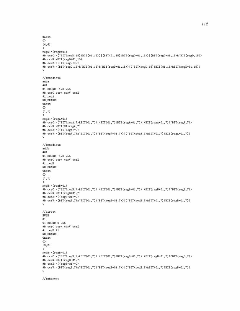
112
@next
{}
[4,4]
<
regD:=(regD+@1)
#b ccrC:=(~BIT(regD,15)&BIT(@1,15))|(BIT(@1,15)&BIT(regD+@1,15))|(BIT(regD+@1,15)&~BIT(regD,15))
#b ccrN:=BIT(regD+@1,15)
#b ccrZ:=((@1+regD)=0)
#b ccrV:=(BIT(regD,15)&~BIT(@1,15)&~BIT(regD+@1,15))|(~BIT(regD,15)&BIT(@1,15)&BIT(regD+@1,15))
>
//immediate
adda
#@1
@1 BOUND -128 255
#b ccrC ccrN ccrV ccrZ
#i regA
NO_BRANCH
@next
{}
[1,1]
<
regA:=(regA+@1)
#b ccrC:=(~BIT(regA,7)&BIT(@1,7))|(BIT(@1,7)&BIT(regA+@1,7))|(BIT(regA+@1,7)&~BIT(regA,7))
#b ccrN:=BIT(@1+regA,7)
#b ccrZ:=((@1+regA)=0)
#b ccrV:=(BIT(regA,7)&~BIT(@1,7)&~BIT(regA+@1,7))|(~BIT(regA,7)&BIT(@1,7)&BIT(regA+@1,7))
>
//immediate
addb
#@1
@1 BOUND -128 255
#b ccrC ccrN ccrV ccrZ
#i regB
NO_BRANCH
@next
{}
[1,1]
<
regB:=(regB+@1)
#b ccrC:=(~BIT(regB,7)&BIT(@1,7))|(BIT(@1,7)&BIT(regB+@1,7))|(BIT(regB+@1,7)&~BIT(regB,7))
#b ccrN:=BIT(regB+@1,7)
#b ccrZ:=((regB+@1)=0)
#b ccrV:=(BIT(regB,7)&~BIT(@1,7)&~BIT(regB+@1,7))|(~BIT(regB,7)&BIT(@1,7)&BIT(regB+@1,7))
>
//direct
SUBB
@1
@1 BOUND 0 255
#b ccrC ccrN ccrV ccrZ
#i regB @1
NO_BRANCH
@next
{}
[3,3]
<
regB:=(regB-@1)
#b ccrC:=(~BIT(regB,7)&BIT(@1,7))|(BIT(@1,7)&BIT(regB-@1,7))|(BIT(regB-@1,7)&~BIT(regB,7))
#b ccrN:=BIT(regB-@1,7)
#b ccrZ:=((regB-@1)=0)
#b ccrV:=(BIT(regB,7)&~BIT(@1,7)&~BIT(regB-@1,7))|(~BIT(regB,7)&BIT(@1,7)&BIT(regB-@1,7))
>
//inherent

113
SBA
#b ccrC ccrN ccrV ccrZ
#i regB regA
NO_BRANCH
@next
{}
[2,2]
<
regA:=(regA-regB)
#b ccrC:=(~BIT(regA,7)&BIT(regB,7))|(BIT(regB,7)&BIT(regA-regB,7))|(BIT(regA-regB,7)&~BIT(regA,7))
#b ccrN:=BIT(regA-regB,7)
#b ccrZ:=((regA-regB)=0)
#b ccrV:=(BIT(regA,7)&~BIT(regB,7)&~BIT(regA-regB,7))|(~BIT(regA,7)&BIT(regB,7)&BIT(regA-regB,7))
>
//immediate
andb
#@1
@1 BOUND -128 255
#b ccrC ccrN ccrV ccrZ
#i regB
NO_BRANCH
@next
{}
[1,1]
<
regB:=and(regB,@1)
#b ccrN:=(and(and(@1,regB),128)=128)
#b ccrZ:=(and(@1,regB)=0)
#b ccrV:=false
>
//direct
orab
@1
#b ccrC ccrN ccrV ccrZ
#i regB @1
NO_BRANCH
@next
{}
[1,1]
<
regB:=or(regB,@1)
#b ccrN:=(and(or(@1,regB),128)=128)
#b ccrZ:=(or(@1,regB)=0)
#b ccrV:=false
>
//immediate
cmpa
#@1
@1 BOUND -128 255
#b ccrC ccrN ccrV ccrZ
#i regA
NO_BRANCH
@next
{}
[1,1]
<
#b ccrC:=(~BIT(regA,7)&BIT(@1,7))|(BIT(@1,7)&BIT(regA-@1,7))|(BIT(regA-@1,7)&~BIT(regA,7))
#b ccrN:=BIT(regA-@1,7)
#b ccrZ:=((regA-@1)=0)
#b ccrV:=(BIT(regA,7)&~BIT(@1,7)&~BIT(regA-@1,7))|(~BIT(regA,7)&BIT(@1,7)&BIT(regA-@1,7))
>

114
//immediate
cmpb
#@1
@1 BOUND -128 255
#b ccrC ccrN ccrV ccrZ
#i regB
NO_BRANCH
@next
{}
[1,1]
<
#b ccrC:=(~BIT(regB,7)&BIT(@1,7))|(BIT(@1,7)&BIT(regB-@1,7))|(BIT(regB-@1,7)&~BIT(regB,7))
#b ccrN:=BIT(regB-@1,7)
#b ccrZ:=((regB-@1)=0)
#b ccrV:=(BIT(regB,7)&~BIT(@1,7)&~BIT(regB-@1,7))|(~BIT(regB,7)&BIT(@1,7)&BIT(regB-@1,7))
>
BRA
@1
BRANCH
@1
{}
[3,3]
<
>
BSR
@1
#b @1_1
NO_BRANCH
@next
{}
[3,3]
<
#b @1_1:=TRUE
>
{~@1_1}
[0,0]
<
>
BGE
@1
#b ccrN ccrV
BRANCH
@1
{((ccrN&~ccrV)|(~ccrN&ccrV))}
[3,3]
<
>
NO_BRANCH
@next
{((ccrN&ccrV)|(~ccrN&~ccrV))}
[1,1]
<
>
BLO
@1
#b ccrC
BRANCH
@1
{(ccrC)}
[3,3]
<
>

115
NO_BRANCH
@next
{(~ccrC)}
[1,1]
<
>
BLS
@1
#b ccrC ccrV
BRANCH
@1
{(ccrC|ccrZ)}
[3,3]
<
>
NO_BRANCH
@next
{(~ccrC&~ccrZ)}
[1,1]
<
>
BPL
@1
#b ccrN
BRANCH
@1
{~ccrN}
[3,3]
<
>
NO_BRANCH
@next
{ccrN}
[1,1]
<
>
BEQ
@1
#b ccrZ
BRANCH
@1
{ccrZ}
[3,3]
<
>
NO_BRANCH
@next
{~ccrZ}
[1,1]
<
>
//pragma "set_pred"
set_pred
@1
#b @1
NO_BRANCH
@next
{}
[0,0]
<
#b @1:=TRUE
>

116
//pragma "clear_pred"
clear_pred
@1
#b @1
NO_BRANCH
@next
{}
[0,0]
<
#b @1:=FALSE
>
//pragma "pred"
pred
@1
#b @1
NO_BRANCH
@next
{@1}
[0,0]
<
>
A.3 enviro2.s;@ include <example.inst>
init_rate temp -2
init_val temp 2200
e_start set_rate temp<=2200 temp 2 5 5
dr_rod set_rate temp>=9800 temp -2 5 5
link e_start
A.4 adc2.sinclude <example.inst>
init_val VRl 0
init_val VRh 10000
init_sig adc_start false
init_sig adc_ccf false
init_val AN2 undef
init_val AN3 undef
; initiate round robin reading from an0-an3
a_start set_sig adc_start&adc_mult&~adc_cc adc_start false 0 0
ins0 set_val ~adc_start ADR1 (temp-VRl)*255/(VRh-VRl) 32 32
ins1 set_val ~adc_start ADR2 (temp-VRl)*255/(VRh-VRl) 32 32
ins2 set_val ~adc_start ADR3 AN2 32 32
ins3 set_val ~adc_start ADR4 AN3 32 32
set_sig NO_TRANS adc_ccf true 0 0
iff adc_scan ins0 0 0 0 0
link a_start
ins0 pause adc_start 0 0
link a_start
ins1 pause adc_start 0 0
link a_start
ins2 pause adc_start 0 0
link a_start
ins3 pause adc_start 0 0
link a_start
; initiate round robin reading from an7-an7

117
a_start set_sig adc_start&adc_mult&adc_cc adc_start false 0 0
ins4 set_val ~adc_start ADR1 (temp-VRl)*255/(VRh-VRl) 32 32
ins5 set_val ~adc_start ADR2 (temp-VRl)*255/(VRh-VRl) 32 32
ins6 set_val ~adc_start ADR3 AN2 32 32
ins7 set_val ~adc_start ADR4 AN3 32 32
set_sig NO_TRANS adc_ccf true 0 0
iff adc_scan ins4 0 0 0 0
link a_start
ins4 pause adc_start 0 0
link a_start
ins5 pause adc_start 0 0
link a_start
ins6 pause adc_start 0 0
link a_start
ins7 pause adc_start 0 0
link a_start
A.5 react2.s;@ include <6811.inst>
main ldab #48
stab ADCTL
test ldab ADCTL
bpl test
loop ldab ADR1
ldaa ADR2
sba
adda #7
cmpa #14
bls loop
;@ fail_set
ldab #7
stab PORTB
term bra term

REFERENCES
[1] Aho, A. V., Sethi, R., and Ullman, J. D. Compilers: Principles, Techniquesand Tools. Addison-Wesley, 1988.
[2] Alur, R. Timed automata. In Proc. International Conference on Computer AidedVerification (CAV) (1999), N. Halbwachs and D. Peled, Eds., vol. 1633 of LectureNotes in Computer Science, Springer, pp. 8–22.
[3] Alur, R., Courcoubetis, C., Halbwachs, N., Henzinger, T. A., Ho, P. H.,Nicollin, X., Olivero, A., Sifakis, J., and Yovine, S. The algorithmicanalysis of hybrid systems. Theoretical Computer Science 138, 1 (1995), 3 – 34.Hybrid Systems.
[4] Alur, R., Courcoubetis, C., Henzinger, T. A., and Ho, P.-H. Hybridautomata: An algorithmic approach to the specification and verification of hybridsystems. In Hybrid Systems (1992), R. L. Grossman, A. Nerode, A. P. Ravn,and H. Rischel, Eds., vol. 736 of Lecture Notes in Computer Science, Springer,pp. 209–229.
[5] Alur, R., Dang, T., Esposito, J., Hur, Y., Ivancic, F., Kumar, V., Mishra,P., Pappas, G. J., and Sokolsky, O. Hierarchical modeling and analysis ofembedded systems. Proc. of the IEEE 91, 1 (Jan 2003), 11 – 28.
[6] Alur, R., and Dill, D. L. A theory of timed automata. Theoretical ComputerScience 126, 2 (1994), 183–235.
[7] Alur, R., Henzinger, T. A., and Ho, P.-H. Automatic symbolic verificationof embedded systems. IEEE Transactions on Software Engineering 22, 3 (1996),181–201.
[8] Annichini, A., Bouajjani, A., and Sighireanu, M. TReX: A tool for reacha-bility analysis of complex systems. In Proc. International Conference on ComputerAided Verification (CAV) (2001), G. Berry, H. Comon, and A. Finkel, Eds., vol. 2102of Lecture Notes in Computer Science, Springer, pp. 368–372.
[9] Balakrishnan, G., Reps, T., Kidd, N., Lal, A., Lim, J., Melski, D., Gruian,R., h. Chen, C., and Teitelbaum, T. Model checking x86 executables withcodesurfer/x86 and wpds. Tech. rep., In CAV, 2005.
[10] Balarin, F., and Sangiovanni-Vincentelli, A. L. An iterative approach tolanguage containment. In CAV ’93: Proceedings of the 5th International Conferenceon Computer Aided Verification (London, UK, 1993), Springer-Verlag, pp. 29–40.
[11] Balduzzi, F., Giua, A., and Menga, G. First-order hybrid petri nets: A modelfor optimization and control. IEEE Transactions on Robotics and Automation 16, 4(Aug. 2000), 382–399.

119
[12] Ball, T., and Rajamani, S. K. The slam project: debugging system softwarevia static analysis. In POPL ’02: Proceedings of the 29th ACM SIGPLAN-SIGACTsymposium on Principles of programming languages (New York, NY, USA, 2002),ACM, pp. 1–3.
[13] Belluomini, W., Myers, C. J., and Hofstee, H. P. Timed circuit verificationusing TEL structures. IEEE Transactions on Computer-Aided Design of IntegratedCircuits and Systems 20, 1 (Jan. 2001), 129–146.
[14] Bengtsson, J., Larsen, K. G., Larsson, F., Pettersson, P., and Yi, W.Uppaal — a Tool Suite for Automatic Verification of Real–Time Systems. In Proc.of Workshop on Verification and Control of Hybrid Systems III (Oct. 1995), no. 1066in Lecture Notes in Computer Science, Springer–Verlag, pp. 232–243.
[15] Berthelot, G. Checking properties of nets using transformations. In Lecture Notesin Computer Science, 222 (1986), pp. 19–40.
[16] Berthomieu, B., and Diaz, M. Modeling and verification of time dependentsystems using time petri nets. IEEE Transactions on Software Engineering 17, 3(1991), 259–273.
[17] Berthomieu, B., and Vernadat, F. Time petri nets analysis with TINA.pp. 123–124.
[18] Biere, A., Cimatti, A., Clarke, E. M., Strichman, O., and Zhu, Y.Bounded model checking, 2003.
[19] Bryant, R. E. Graph-based algorithms for boolean function manipulation. IEEETransactions on Computers 35, 8 (1986), 677–691.
[20] Burch, J. R., Clarke, E. M., McMillan, K. L., Dill, D. L., and Hwang,L. J. Symbolic model checking: 1020 states and beyond. In IEEE Symposium onLogic in Computer Science (June 1990), IEEE Computer Society Press, pp. 428–439.
[21] Clarke, E., Grumberg, O., Jha, S., Lu, Y., and Veith, H. Counterexample-guided abstraction refinement for symbolic model checking. J. ACM 50, 5 (2003),752–794.
[22] Clarke, E. M., and Emerson, E. A. Design and synthesis of synchronizationskeletons using branching-time temporal logic. In Logic of Programs, Workshop(London, UK, 1982), Springer-Verlag, pp. 52–71.
[23] Clarke, E. M., Grumberg, O., and Peled, D. A. Model Checking. The MITPress, 1999.
[24] Clarke, E. M., and Kurshan, R. P. Computer-aided verification. IEEESpectrum 33, 6 (June 1996), 61–67.
[25] Cousot, P., and Cousot, R. Abstract interpretation: a unified lattice modelfor static analysis of programs by construction or approximation of fixpoints. InConference Record of the Fourth Annual ACM SIGPLAN-SIGACT Symposium onPrinciples of Programming Languages (Los Angeles, California, 1977), ACM Press,New York, NY, pp. 238–252.

120
[26] David, R., and Alla, H. On hybrid Petri nets. Discrete Event Dynamic Systems:Theory and Applications 11, 1–2 (Jan. 2001), 9–40.
[27] Davis, M., Logemann, G., and Loveland, D. A machine program for theorem-proving. Commun. ACM 5, 7 (July 1962), 394–397.
[28] Davis, M., and Putnam, H. A computing procedure for quantification theory.Journal of the ACM (JACM) 7, 3 (July 1960), 201–215.
[29] Daws, C., and Yovine, S. Reducing the number of clock variables of timedautomata. In Proc. RTSS’96 (1996), IEEE Computer Society Press, pp. 73–81.
[30] Dill, D. L. Timing assumptions and verification of finite-state concurrent systems.In Proc. Automatic Verification Methods for Finite-State Systems (1989), J. Sifakis,Ed., vol. 407 of Lecture Notes in Computer Science, Springer, pp. 197–212.
[31] D’Silva, V., Kroening, D., and Weissenbacher, G. A survey of automatedtechniques for formal software verification. IEEE Transactions on Computer-AidedDesign of Integrated Circuits and Systems (TCAD) 27, 7 (July 2008), 1165–1178.
[32] Edelman, J. R. Machine code verification using the bogor framework. Master’sthesis, Brigham Young University, 2008.
[33] Eide, E., and Regehr, J. Volatiles are miscompiled, and what to do about it. InEMSOFT ’08: Proceedings of the 7th ACM international conference on Embeddedsoftware (New York, NY, USA, 2008), ACM, pp. 255–264.
[34] Fernandez, J.-C., Bozga, M., and Ghirvu, L. State space reduction based onlive variables analysis. Sci. Comp. Prog. 47, 2-3 (2003), 203–220.
[35] Frehse, G. PHAVer: Algorithmic verification of hybrid systems past hytech. InHybrid Systems: Computation and Control (HSCC) (2005), M. Morari and L. Thiele,Eds., vol. 3414 of Lecture Notes in Computer Science, Springer, pp. 258–273.
[36] Henzinger, T., Jhala, R., Majumdar, R., and Sutre, G. Software verificationwith blast. 2003, p. 624.
[37] Hickey, T., Ju, Q., and Van Emden, M. H. Interval arithmetic: From principlesto implementation. J. ACM 48, 5 (2001), 1038–1068.
[38] Holzmann, G. J. The model checker spin. IEEE Trans. Softw. Eng. 23, 5 (1997),279–295.
[39] Holzmann, G. J. Software model checking with spin. Advances in Computers 65(2005), 78–109.
[40] Holzmann, G. J. The power of ten: Rules for developing safety critical code. IEEEComputer 39, 6 (2006), 95–97.
[41] Hsiung, P.-A. Hardware-software coverification of concurrent embedded real-timesystems. Real-Time Systems, Euromicro Conference on 0 (1999), 0216.

121
[42] Iversen, T. K., Kristoffersen, K. J., Larsen, K. G., Laursen, M., Mad-sen, R. G., Mortensen, S. K., Pettersson, P., and Thomasen, C. B.Model-checking real-time control programs verifying lego mindstorms systems usinguppaal. In In Proc. of 12th Euromicro Conference on Real-Time Systems (2000),IEEE Computer Society Press, pp. 147–155.
[43] Jaffe, M., Leveson, N., Heimdahl, M., and Melhart, B. Software require-ments analysis for real-time process-control systems. IEEE Transactions on SoftwareEngineering 17, 3 (1991), 241–258.
[44] Johnsonbaugh, R., and Murata, T. Additional methods for reduction andexpansion of marked graphs. In IEEE TCAS, vol. CAS-28, no. 1 (1981), pp. 1009–1014.
[45] Kern, C., and Greenstreet, M. R. Formal verification in hardware design: Asurvey. ACM Transactions on Design Automation of Electronic Systems 4, 2 (Apr.1999), 123–193.
[46] Kinder, J., Katzenbeisser, S., Schallhart, C., Veith, H., and Mnchen,T. U. Detecting malicious code by model checking. In In Proc. 2nd Conference onDetection of Intrusions and Malware & Vulnerability Assessment (DIMVA05 (2005),pp. 174–187.
[47] Kropf, T. Introduction to Formal Hardware Verification. Springer, 1999.
[48] Kurshan, R. P. Computer-aided verification of coordinating processes: theautomata-theoretic approach. Princeton University Press, Princeton, NJ, USA, 1994.
[49] Little, S., Seegmiller, N., Walter, D., Myers, C., and Yoneda, T.Verification of analog/mixed-signal circuits using labeled hybrid Petri nets. InProc. International Conference on Computer Aided Design (ICCAD) (2006), IEEEComputer Society Press, pp. 275–282.
[50] Little, S., Walter, D., and Myers, C. Analog/mixed-signal circuit verifica-tion using models generated from simulation traces. In Automated Technology forVerification and Analysis (ATVA) (2007), K. S. Namjoshi, T. Yoneda, T. Higashino,and Y. Okamura, Eds., vol. 4762 of Lecture Notes in Computer Science, Springer,pp. 114–128.
[51] Little, S. R. Efficient Modeling and Verification of Analog/Mixed-Signal CircuitsUsing Labeled Hybrid Petri Nets. PhD thesis, University of Utah, May 2008.
[52] Majumdar, R., and Saha, I. Symbolic robustness analysis. Real-Time SystemsSymposium, IEEE International 0 (2009), 355–363.
[53] Maka, H., Frehse, G., and Krogh, B. H. Polyhedral domains and wideningfor verification of numerical programs. In NSV-II: Second International Workshopon Numerical Software Verification (2009).
[54] Mercer, E., and Jones, M. Model checking machine code with the gnu debugger.In In 12th International SPIN Workshop (2005), Springer, pp. 251–265.

122
[55] Merlin, P. M., and Farber, D. J. Recoverability of communication protocols.IEEE Transactions on Communications 24, 9 (Sept. 1976), 1036–1043.
[56] Murata, T. Petri nets: Properties, analysis, and applications. In Proceedings ofthe IEEE 77(4) (1989), pp. 541–580.
[57] Murata, T., and Koh, J. Y. Reduction and expansion of lived and safe markedgraphs. In IEEE TCAS, vol. CAS-27, no. 10 (1980), pp. 68–70.
[58] Myers, C. J., Belluomini, W., Killpack, K., Mercer, E., Peskin, E., andZheng, H. Timed circuits: A new paradigm for high-speed design. In Proc. of Asiaand South Pacific Design Automation Conference (ASPDAC) (Feb. 2001), ACMPress, pp. 335–340.
[59] Naur, P. Checking of operand types in algol compilers. BIT, 5 (1965), 151–163.
[60] Nieuwenhuis, R., Oliveras, A., and Tinelli, C. Solving SAT and SAT modulotheories: from an abstract davis-putnam-logemann-loveland procedure to DPLL(T).Journal of the ACM (JACM) 53, 6 (Nov. 2006), 937–977.
[61] Petri, C. A. Kommunikation mit Automaten. PhD thesis, Institut fur instru-mentelle Mathematik, Bonn, 1962.
[62] Petri, C. A. Communication with automata. Tech. Rep. RADC-TR-65-377, Vol.1, Suppl 1, Applied Data Research, Princeton, NJ, 1966.
[63] Pettersson, P., and Larsen., K. G. Uppaal2k. Bulletin of the EuropeanAssociation for Theoretical Computer Science 70 (Feb. 2000), 40–44.
[64] Prasad, M. R., Biere, A., and Gupta, A. A survey of recent advances in SAT-based formal verification. International Journal on Software Tools for TechnologyTransfer 7, 2 (Apr. 2005), 156–173.
[65] Queille, J.-P., and Sifakis, J. Specification and verification of concurrentsystems in cesar. In Proceedings of the 5th Colloquium on International Symposiumon Programming (London, UK, 1982), Springer-Verlag, pp. 337–351.
[66] Robby, M., Dwyer, B., and Hatcliff, J. Bogor: An extensible and highly-modular software model checking framework, 2003.
[67] Rokicki, T. Representing and Modeling Digital Circuits. PhD thesis, StanfordUniversity, Dec. 1993.
[68] Schlich, B. Model Checking of Software for Microcontrollers. Dissertation, RWTHAachen University, Aachen, Germany, June 2008.
[69] Schmidt, D. A. Data flow analysis is model checking of abstract interpretations.In POPL ’98: Proceedings of the 25th ACM SIGPLAN-SIGACT symposium onPrinciples of programming languages (New York, NY, USA, 1998), ACM, pp. 38–48.
[70] Staff, N. R. C. Embedded Everywhere: A Research Agenda for Networked Systemsof Embedded Computers. National Academy Press, Washington, DC, USA, 2001.

123
[71] Steffen, B. Data flow analysis as model checking. In TACS ’91: Proceedings ofthe International Conference on Theoretical Aspects of Computer Software (London,UK, 1991), Springer-Verlag, pp. 346–365.
[72] Suzuki, I., and Murata, T. Stepwise refinements for transitions and places. NewYork: Springer-Verlag, 1982.
[73] Suzuki, I., and Murata, T. A method for stepwise refinements and abstractionsof petri nets. In Journal Of Computer System Science, 27(1) (1983), pp. 51–76.
[74] Vogler, W., and Wollowski, R. Decomposition in asynchronous circuit design.In Concurrency and Hardware Design, Advances in Petri Nets (London, UK, 2002),Springer-Verlag, pp. 152–190.
[75] Walter, D., Little, S., Myers, C., Seegmiller, N., and Yoneda, T.Verification of analog/mixed-signal circuits using symbolic methods. IEEE Transac-tions on Computer-Aided Design of Integrated Circuits and Systems 27, 12 (2008),2223–2235.
[76] Walter, D. C. Verification of analog and mixed-signal circuits using symbolicmethods. PhD thesis, University of Utah, May 2007.
[77] Yoneda, T. VINAS-P: A tool for trace theoretic verification of timed asynchronouscircuits. In Proc. International Conference on Computer Aided Verification (CAV)(2000), E. A. Emerson and A. P. Sistla, Eds., vol. 1855 of Lecture Notes in ComputerScience, Springer, pp. 572–575.
[78] Yovine, S. Kronos: A verification tool for real-time systems. International Journalof Software Tools for Technology Transfer 1, 1–2 (Oct. 1997), 123–133.
[79] Zheng, H. Modular synthesis and verification of timed circuits using automaticabstraction. PhD thesis, University of Utah, May 2001.
Related Documents


![Formal Verification and Performance Analysis of … · Formal Verification and Performance Analysis of Embedded Systems ... [Alur & Dill’89] ... Jens Ellebæk Kristian S. Knudsen](https://static.cupdf.com/doc/110x72/5b25cffa7f8b9a794f8b48c5/formal-verification-and-performance-analysis-of-formal-verification-and-performance.jpg)