A new approach for dynamic modeling of an electrorheological damper using a lumped parameter method

A new approach for dynamic modeling of an electrorheological damper using a lumped

parameter method

This article has been downloaded from IOPscience. Please scroll down to see the full text article.

2009 Smart Mater. Struct. 18 115020

(http://iopscience.iop.org/0964-1726/18/11/115020)

Download details:

IP Address: 165.246.93.151

The article was downloaded on 16/09/2009 at 05:42

Please note that terms and conditions apply.

The Table of Contents and more related content is available

HOME | SEARCH | PACS & MSC | JOURNALS | ABOUT | CONTACT US

IOP PUBLISHING SMART MATERIALS AND STRUCTURES

Smart Mater. Struct. 18 (2009) 115020 (11pp) doi:10.1088/0964-1726/18/11/115020

A new approach for dynamic modeling ofan electrorheological damper using alumped parameter methodQuoc-Hung Nguyen and Seung-Bok Choi1

Smart Structures and Systems Laboratory, Department of Mechanical Engineering,Inha University, Incheon 402-751, Korea

E-mail: [email protected]

Received 2 January 2009, in final form 10 June 2009Published 15 September 2009Online at stacks.iop.org/SMS/18/115020

AbstractThis work proposes a new method for dynamic modeling of an electrorheological (ER) damperusing a lumped parameter method. After describing the configuration and operating principle ofthe ER damper, quasi-static modeling of the damper is conducted on the basis of the Binghammodel of ER fluid. Subsequently, the lumped parameter models of ER fluid flows in the damperare established and the integrated lumped model of the whole damper system is obtained bytaking into account the dynamic motions of the annular duct, upper chamber, lower chamberand connecting pipe. In order to demonstrate the effectiveness of the proposed dynamic model,a comparative work between the simulation and the experiment is undertaken. This isperformed under various piston motions with different excitation magnitudes and frequencies.In addition, the effect of ER fluid compressibility and initial pressure in the accumulator on thehysteresis of the ER damper is investigated.

(Some figures in this article are in colour only in the electronic version)

1. Introduction

The control of mechanical and structural vibration hassignificant applications in manufacturing, infrastructureengineering, and consumer products. In the machine toolindustry, mechanical vibration degrades both the fabricationrate and quality of the end products. In civil engineeringconstructs, structural vibration degrades human comfort andcauses damage to the structures. In automotive and aerospacefields, vibration reduces component life, and the associatedacoustics noise annoys passengers. Thus, various methodshave been developed and applied to vibration control in diverseengineering fields. Essentially, based on the amount of externalpower required for the system, vibration-control systems areclassified into three approaches: the passive, active and semi-active vibration-control method.

A passive vibration-control unit consists of a resilientmember (stiffness) and an energy dissipator (damper) toeither absorb vibratory energy or load the transmission

1 Author to whom any correspondence should be addressed. http://www.ssslab.com

path of the disturbing vibration [1]. This configurationhas significant limitations in structural applications wherebroadband disturbances of a highly uncertain nature areencountered. Furthermore, the passive vibration-controlsystems (especially vibration absorbers) are often hamperedby a phenomenon known as ‘de-tuning’. This occurs due todeterioration of the structural parameters and/or variations inthe excitation frequency. In order to compensate for theselimitations, active vibration-control systems are utilized. Withan additional active force introduced as a part of a suspensionunit, the vibration-control system is then controlled usingdifferent algorithms to make it more responsive to sourcesof disturbance [2–4]. Generally, the active system providesa high control performance in a wide frequency range, butit requires high power sources, complicated components suchas sensors, servo valves, and sophisticated control algorithms.The semi-active configuration addresses these limitations byeffectively integrating a tuning control scheme with tunablepassive devices. For this, active force generators are replacedby modulated variable compartments such as a variable ratedamper and stiffness. Therefore, the semi-active suspension

0964-1726/09/115020+11$30.00 © 2009 IOP Publishing Ltd Printed in the UK1

Smart Mater. Struct. 18 (2009) 115020 Q-H Nguyen and S-B Choi

can offer a desirable performance without requiring largepower sources and expensive hardware [5–7].

Recently, various semi-active dampers featuring magne-torheological (MR) or electrorheological (ER) fluid have beenproposed and successfully applied in the real field, especiallyin vehicle suspension systems [8–11]. It is well known thatMR/ER dampers exhibit nonlinear behavior with hysteresis.There have been many efforts devoted to model the nonlinearbehavior of ER/MR dampers. These models are classified asquasi-static and dynamic models. For the quasi-static models,several works have been reported in the literature using nonlin-ear Bingham or Herschel–Bulkley models [12–14]. Althoughthe quasi-static models are capable of describing the force–displacement behavior of the ER/MR damper reasonably well,they are not sufficient to describe the nonlinear force–velocitybehavior of the damper [15]. In order to remedy this limitation,several dynamic models considering the hysteresis behavior ofthe ER/MR damper have been proposed [16–19]. Essentially,these dynamic models are experiment-based models. The pa-rameters of the models are derived based on the experimentalresults of a real damper which results in a high cost of mod-eling. Moreover, the identified dynamic models can provide aconsiderably accurate solution only at a certain value of exci-tation frequency and amplitude treated in experiments.

Consequently, the main contribution of this study is todevelop a new dynamic model of an ER damper based ona lumped parameter method. The proposed dynamic modelcan well express the nonlinear behavior with hysteresis of theER damper without experimental results. After describing theconfiguration of the ER damper, quasi-static modeling of thedamper is carried out on the basis of the Bingham model ofER fluid. After that, the lumped parameter models of ERfluid flows in the damper are considered and the integratedlumped model of the whole damper is then obtained. Basedon the proposed lumped parameter model of the ER damper,the simulated results are obtained and compared with measuredones in order to evaluate the effectiveness of the proposedmodel. Finally, the effect of ER fluid compressibility and initialpressure in the accumulator on the hysteresis of the ER damperis investigated through simulated results.

2. Quasi-static modeling of an ER damper

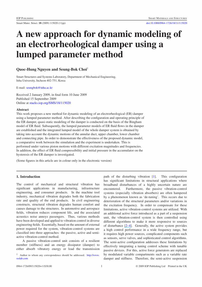
In this study, the cylindrical ER damper for passenger vehiclesuspensions proposed by Choi et al [11] is considered. Theschematic diagram of the damper is shown in figure 1. TheER damper is divided into upper and lower chambers by thepiston. These chambers are fully filled with the ER fluid.As the piston moves, the ER fluid flows from one chamberto the other through the annular duct between the inner andouter cylinder. The inner cylinder is connected to the positivevoltage produced by a high voltage supply unit, acting as thepositive (+) electrode. The outer cylinder is connected to theground, acting as the negative (−) electrode. On the otherhand, the gas chamber located outside of the lower chamberacts as an accumulator of the ER fluid induced by the motionof the piston. In the absence of electric fields, the ER damperproduces the damping force only caused by the fluid resistance.

V

Fd

xp

Voltage Source

Ld

d

ER Duct

Inner Electrode

ER Fluid

Gas ChamberDiaphragm

Outer Electrode

Figure 1. Schematic configuration of the ER damper.

However, if a certain level of the electric field is suppliedto the ER damper, the ER damper produces an additionaldamping force owing to the yield stress of the ER fluid. Thisdamping force of the ER damper can be continuously tunedby controlling the intensity of the electric field. By neglectingthe compressibility of the ER fluid, the frictional force andassuming quasi-static behavior of the damper, the dampingforce can be expressed as follows:

Fd = P2 Ap − P1(Ap − As) (1)

where Ap and As are the piston and the piston shaft cross-sectional areas, respectively. P1 and P2 are pressures in theupper and lower chambers of the damper, respectively. Therelations between P1, P2 and the pressure in the gas chamber,Pa, can be expressed as follows:

P2 = Pa + �Pa∼= Pa; P1 = Pa − �P (2)

where �Pa and �P are the pressure drops of the ER fluidflow from the lower chamber to the accumulator and the ERfluid flow through the annular duct between the outer and innercylinders, respectively. The pressure in the gas chamber can becalculated as follows:

Pa = P0

(V0

V0 − Asxp

)γ

(3)

where P0 and V0 are the initial pressure and volume of theaccumulator. γ is the coefficient of thermal expansion whichranges from 1.4 to 1.7 for adiabatic expansion. xp is the pistondisplacement. From equations (1) and (2), the damping forceof the ER damper can be calculated by

Fd = Pa As + �P(Ap − As). (4)

In order to determine the pressure drop �P , it is assumed thatthe flow through the annular duct is equivalent to the flow

2

Smart Mater. Struct. 18 (2009) 115020 Q-H Nguyen and S-B Choi

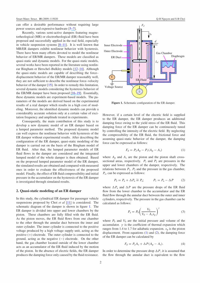
Figure 2. Equivalent flow of the ER fluid flow in the annular duct.(a) ER fluid flow in the annular duct, (b) equivalent parallel-plateduct.

through the duct between two parallel plates (parallel-plateduct) shown in figure 2. This is valid because the radius ofthe duct is much larger than its gap. By neglecting the minorloss, �P can be calculated as follows [12]:

�P = 6μLd

π t3d Rd

Qd + cLd

dτy (5)

where Qd is the flow rate of the ER flow given by Qd =(Ap − As)xp; τy is the yield stress of the ER fluid inducedby the applied electric field; μ is the post-yield viscosity ofthe ER fluid; Ld, Rd and d are the length, average radius andgap of the annular duct, respectively. c is the coefficient whichdepends on the flow velocity profile and has a value range froma minimum value of 2.07 to a maximum value of 3.07. Thecoefficient c can be approximately estimated as follows:

c = 2.07 + 12Qdμ

12Qdμ + 0.8π Rdd2τy. (6)

Plugging �P from equation (5) into equation (4) one obtains

Fd = Pa As + cvisxp + FMRsgn(xp) (7)

where,

cvis = 6μLd

π Rdd3(Ap − As)

2; FMR = (Ap − As)cLd

dτy.

The first term in equation (7) represents the elastic force fromthe gas compliance, the second term represents the dampingforce due to ER fluid viscosity and the third one is the force dueto the yield stress of the ER fluid which can be continuouslycontrolled by the electric field across the ER fluid duct. In thiswork, the commercial ER fluid (Rheobay, TP Al 3565) is used.The induced yield stress of the ER fluid can be approximatelyestimated by

τy = αEβ . (8)

Here, E is the applied electric field whose unit is kV mm−1. α

and β are intrinsic values of the ER fluid to be experimentallydetermined. At room temperature, the values of α and β areevaluated to be 591 and 1.42, respectively.

Figure 3. Lumped parameter model of Newtonian fluid flow in apipeline. (a) Lumped model, (b) analogous mechanical model.

3. Lumped parameter modeling of an ER damper

In section 2, the damping force of the ER damper was obtainedbased on the assumption of steady behavior of ER fluid flowthrough the duct and the incompressibility of the ER fluid. Thisassumption is valid for a damper working at low frequencyand small stroke. However, for a high frequency and largestroke damper, the assumption is no longer valid and theunsteady behavior of the ER fluid flow should be taken intoconsideration. In this section, the dynamic modeling of theER damper is performed considering unsteady behavior of ERfluid flows in the damper and compressibility of the ER fluidusing a lumped parameter model.

The lumped parameter model of a fluid system was firstlyproposed by Doebelin [20] for Newtonian fluid flow in acircular pipe and then well developed in other contexts [21, 22].In the lumped parameter model, the fluid system is dividedinto lumps with lumped masses and average parameters suchas velocity and pressure. The system elements are obtainedby applying conservation of mass and Newton’s law to thelumps of fluid. Figures 3(a) and (b) show the lumped modelof the Newtonian fluid flow in a circular pipe and its analogousmechanical model, respectively. In the model, ki , bi and mi arethe analogous stiffness, damping and mass of the i th lump ofthe fluid which can be calculated as follows [20, 21]:

ki = A2

Ci= AB

li; bi = A2 Rμi = 8πμli ;

mi = A2 Ii = ρ Ali

(9)

where Ci , Rμi and Ii are the capacitance, resistance andinductance of the i th lump of the fluid in the pipe, respectively.A is the cross-sectional area of the pipe, li is the length of thei th lump of the fluid in the pipe and ρ is the density of the fluid.

3

Smart Mater. Struct. 18 (2009) 115020 Q-H Nguyen and S-B Choi

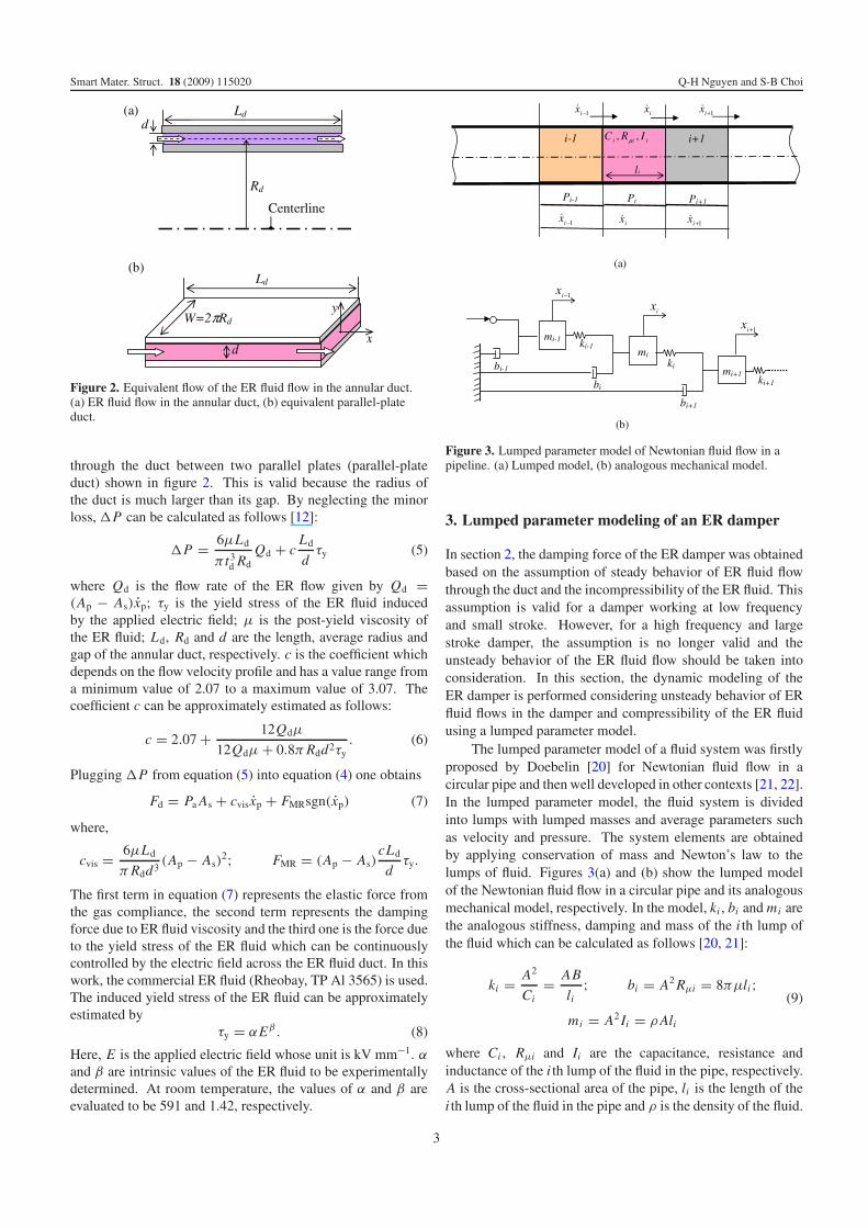
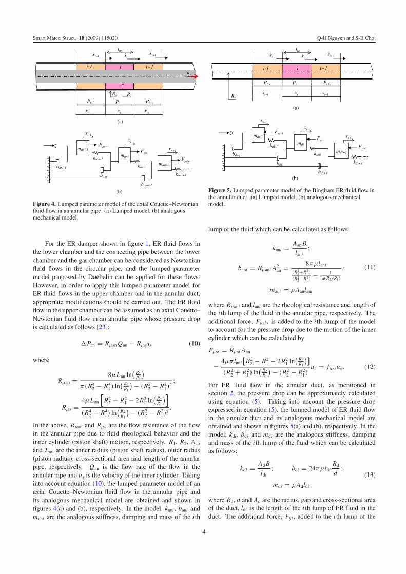
Figure 4. Lumped parameter model of the axial Couette–Newtonianfluid flow in an annular pipe. (a) Lumped model, (b) analogousmechanical model.

For the ER damper shown in figure 1, ER fluid flows inthe lower chamber and the connecting pipe between the lowerchamber and the gas chamber can be considered as Newtonianfluid flows in the circular pipe, and the lumped parametermodel proposed by Doebelin can be applied for these flows.However, in order to apply this lumped parameter model forER fluid flows in the upper chamber and in the annular duct,appropriate modifications should be carried out. The ER fluidflow in the upper chamber can be assumed as an axial Couette–Newtonian fluid flow in an annular pipe whose pressure dropis calculated as follows [23]:

�Pan = Rμan Qan − Rμsus (10)

where

Rμan = 8μLan ln(

R2R1

)π(R4

2 − R41) ln

(R2R1

) − (R22 − R2

1)2;

Rμs =4μLan

[R2

2 − R21 − 2R2

1 ln( R2

R1

)](R4

2 − R41) ln

( R2R1

) − (R22 − R2

1)2.

In the above, Rμan and Rμs are the flow resistance of the flowin the annular pipe due to fluid rheological behavior and theinner cylinder (piston shaft) motion, respectively. R1, R2, Aan

and Lan are the inner radius (piston shaft radius), outer radius(piston radius), cross-sectional area and length of the annularpipe, respectively. Qan is the flow rate of the flow in theannular pipe and us is the velocity of the inner cylinder. Takinginto account equation (10), the lumped parameter model of anaxial Couette–Newtonian fluid flow in the annular pipe andits analogous mechanical model are obtained and shown infigures 4(a) and (b), respectively. In the model, kani , bani andmani are the analogous stiffness, damping and mass of the i th

Figure 5. Lumped parameter model of the Bingham ER fluid flow inthe annular duct. (a) Lumped model, (b) analogous mechanicalmodel.

lump of the fluid which can be calculated as follows:

kani = Aan B

lani;

bani = Rμani A2an = 8πμlani

(R22+R2

1 )

(R22−R2

1 )− 1

ln(R2/R1)

;

mani = ρ Aanlani

(11)

where Rμani and lani are the rheological resistance and length ofthe i th lump of the fluid in the annular pipe, respectively. Theadditional force, Fμsi , is added to the i th lump of the modelto account for the pressure drop due to the motion of the innercylinder which can be calculated by

Fμsi = Rμsi Aan

= 4μπlani[R2

2 − R21 − 2R2

1 ln(

R2R1

)](R2

2 + R21) ln

(R2R1

) − (R22 − R2

1)us = fμsi us. (12)

For ER fluid flow in the annular duct, as mentioned insection 2, the pressure drop can be approximately calculatedusing equation (5). Taking into account the pressure dropexpressed in equation (5), the lumped model of ER fluid flowin the annular duct and its analogous mechanical model areobtained and shown in figures 5(a) and (b), respectively. In themodel, kdi , bdi and mdi are the analogous stiffness, dampingand mass of the i th lump of the fluid which can be calculatedas follows:

kdi = Ad B

ldi; bdi = 24πμldi

Rd

d;

mdi = ρ Adldi

(13)

where Rd, d and Ad are the radius, gap and cross-sectional areaof the duct, ldi is the length of the i th lump of ER fluid in theduct. The additional force, Fyi , added to the i th lump of the

4

Smart Mater. Struct. 18 (2009) 115020 Q-H Nguyen and S-B Choi

model in order to account for the pressure drop due to the yieldstress of the fluid which can be calculated by

Fyi = 2π Rddcildi

dτysgn(xp) (14)

where

ci = 2.07 + 12μQdi

12μQdi + 0.8π Rdd2τy

= 2.07 + 12μAdxdi

12μAdxdi + 0.8π Rdd2τy.

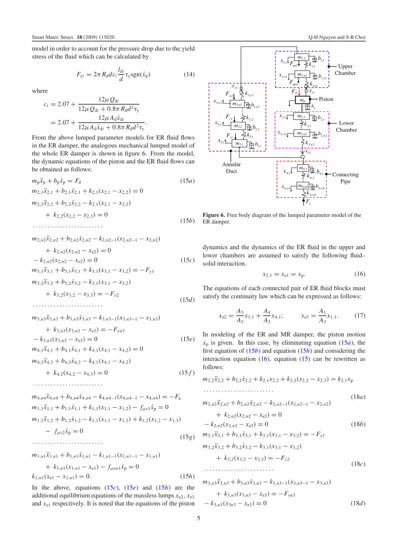
From the above lumped parameter models for ER fluid flowsin the ER damper, the analogous mechanical lumped model ofthe whole ER damper is shown in figure 6. From the model,the dynamic equations of the piston and the ER fluid flows canbe obtained as follows:

mpxp + bp xp = Fd (15a)

m2,1x2,1 + b2,1x2,1 + k2,1(x2,1 − x2,2) = 0

m2,2x2,2 + b2,2x2,2 − k2,1(x2,1 − x2,2)

+ k2,2(x2,2 − x2,3) = 0

· · · · · · · · · · · · · · · · · · · · · · · ·m2,n2x2,n2 + b2,n2x2,n2 − k2,n2−1(x2,n2−1 − x2,n2)

+ k2,n2(x2,n2 − xe2) = 0

(15b)

− k2,n2(x2,n2 − xe2) = 0 (15c)

m3,1x3,1 + b3,1x3,1 + k3,1(x3,1 − x3,2) = −Fy1

m3,2x3,2 + b3,2x3,2 − k3,1(x3,1 − x3,2)

+ k3,2(x3,2 − x3,3) = −Fy2

· · · · · · · · · · · · · · · · · · · · · · · ·m3,n3x3,n3 + b3,n3x3,n3 − k3,n3−1(x3,n3−1 − x3,n3)

+ k3,n3(x3,n3 − xe3) = −Fyn3

(15d)

− k3,n3(x3,n3 − xe3) = 0 (15e)

m4,1x4,1 + b4,1x4,1 + k4,1(x4,1 − x4,2) = 0

m4,2x4,2 + b4,2x4,2 − k4,1(x4,1 − x4,2)

+ k4,2(x4,2 − x4,3) = 0

· · · · · · · · · · · · · · · · · · · · · · · ·m4,n4x4,n4 + b4,n4x4,n4 − k4,n4−1(x4,n4−1 − x4,n4) = −Fa

(15 f )

m1,1x1,1 + b1,1x1,1 + k1,1(x1,1 − x1,2) − fμs1 xp = 0

m1,2x1,2 + b1,2x1,2 − k1,1(x1,1 − x1,2) + k1,2(x1,2 − x1,3)

− fμs2 xp = 0

· · · · · · · · · · · · · · · · · · · · · · · ·m1,n1x1,n1 + b1,n1x1,n1 − k1,n1−1(x1,n1−1 − x1,n1)

+ k1,n1(x1,n1 − xe1) − fμsn1 xp = 0

(15g)

k1,n1(xe1 − x1,n1) = 0. (15h)

In the above, equations (15c), (15e) and (15h) are theadditional equilibrium equations of the massless lumps xe2, xe3

and xe1 respectively. It is noted that the equations of the piston

Figure 6. Free body diagram of the lumped parameter model of theER damper.

dynamics and the dynamics of the ER fluid in the upper andlower chambers are assumed to satisfy the following fluid–solid interaction.

x2,1 = xe1 = xp. (16)

The equations of each connected pair of ER fluid blocks mustsatisfy the continuity law which can be expressed as follows:

xe2 = A3

A2x3,1 + A4

A2x4,1; xe3 = A1

A3x1,1. (17)

In modeling of the ER and MR damper, the piston motionxp is given. In this case, by eliminating equation (15a), thefirst equation of (15b) and equation (15h) and considering theinteraction equation (16), equation (15) can be rewritten asfollows:

m2,2x2,2 + b2,2x2,2 + k2,1x2,2 + k2,2(x2,2 − x2,3) = k2,1xp

· · · · · · · · · · · · · · · · · · · · · · · ·m2,n2x2,n2 + b2,n2x2,n2 − k2,n2−1(x2,n2−1 − x2,n2)

+ k2,n2(x2,n2 − xe2) = 0

(18a)

− k2,n2(x2,n2 − xe2) = 0 (18b)

m3,1x3,1 + b3,1x3,1 + k3,1(x3,1 − x3,2) = −Fy1

m3,2x3,2 + b3,2x3,2 − k3,1(x3,1 − x3,2)

+ k3,2(x3,2 − x3,3) = −Fy2

· · · · · · · · · · · · · · · · · · · · · · · ·m3,n3x3,n3 + b3,n3x3,n3 − k3,n3−1(x3,n3−1 − x3,n3)

+ k3,n3(x3,n3 − xe3) = −Fyn3

(18c)

− k3,n3(x3n3 − xe3) = 0 (18d)

5

Smart Mater. Struct. 18 (2009) 115020 Q-H Nguyen and S-B Choi

Dam

ping

For

ce [k

N]

Dam

ping

For

ce [k

N]

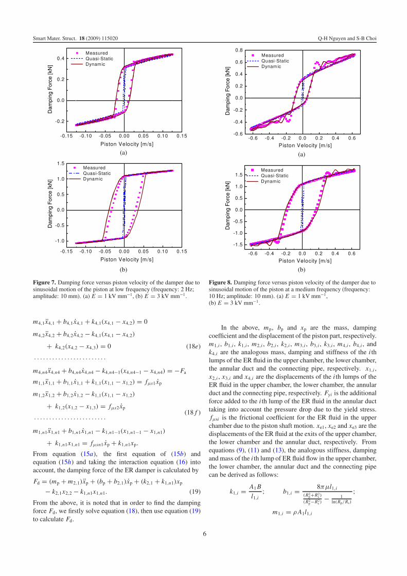
Figure 7. Damping force versus piston velocity of the damper due tosinusoidal motion of the piston at low frequency (frequency: 2 Hz;amplitude: 10 mm). (a) E = 1 kV mm−1, (b) E = 3 kV mm−1.

m4,1x4,1 + b4,1x4,1 + k4,1(x4,1 − x4,2) = 0

m4,2x4,2 + b4,2x4,2 − k4,1(x4,1 − x4,2)

+ k4,2(x4,2 − x4,3) = 0

· · · · · · · · · · · · · · · · · · · · · · · ·m4,n4x4,n4 + b4,n4x4,n4 − k4,n4−1(x4,n4−1 − x4,n4) = −Fa

(18e)

m1,1x1,1 + b1,1x1,1 + k1,1(x1,1 − x1,2) = fμs1 xp

m1,2x1,2 + b1,2x1,2 − k1,1(x1,1 − x1,2)

+ k1,2(x1,2 − x1,3) = fμs2 xp

· · · · · · · · · · · · · · · · · · · · · · · ·m1,n1x1,n1 + b1,n1x1,n1 − k1,n1−1(x1,n1−1 − x1,n1)

+ k1,n1x1,n1 = fμsn1 xp + k1,n1xp.

(18 f )

From equation (15a), the first equation of (15b) andequation (15h) and taking the interaction equation (16) intoaccount, the damping force of the ER damper is calculated by

Fd = (mp + m2,1)xp + (bp + b2,1)xp + (k2,1 + k1,n1)xp

− k2,1x2,2 − k1,n1x1,n1. (19)

From the above, it is noted that in order to find the dampingforce Fd, we firstly solve equation (18), then use equation (19)to calculate Fd.

Dam

ping

For

ce [k

N]

Dam

ping

For

ce [k

N]

Figure 8. Damping force versus piston velocity of the damper due tosinusoidal motion of the piston at a medium frequency (frequency:10 Hz; amplitude: 10 mm). (a) E = 1 kV mm−1,(b) E = 3 kV mm−1.

In the above, mp, bp and xp are the mass, dampingcoefficient and the displacement of the piston part, respectively.m1,i , b1,i , k1,i , m2,i , b2,i , k2,i , m3,i , b3,i , k3,i , m4,i , b4,i , andk4,i are the analogous mass, damping and stiffness of the i thlumps of the ER fluid in the upper chamber, the lower chamber,the annular duct and the connecting pipe, respectively. x1,i ,x2,i , x3,i and x4,i are the displacements of the i th lumps of theER fluid in the upper chamber, the lower chamber, the annularduct and the connecting pipe, respectively. Fyi is the additionalforce added to the i th lump of the ER fluid in the annular ducttaking into account the pressure drop due to the yield stress.fμsi is the frictional coefficient for the ER fluid in the upperchamber due to the piston shaft motion. xe1, xe2 and xe3 are thedisplacements of the ER fluid at the exits of the upper chamber,the lower chamber and the annular duct, respectively. Fromequations (9), (11) and (13), the analogous stiffness, dampingand mass of the i th lump of ER fluid flow in the upper chamber,the lower chamber, the annular duct and the connecting pipecan be derived as follows:

k1,i = A1 B

l1,i; b1,i = 8πμl1,i

(R2p+R2

s )

(R2p−R2

s )− 1

ln(Rp/Rs)

;

m1,i = ρ A1l1,i

6

Smart Mater. Struct. 18 (2009) 115020 Q-H Nguyen and S-B Choi

Dam

ping

For

ce [k

N]

Dam

ping

For

ce [k

N]

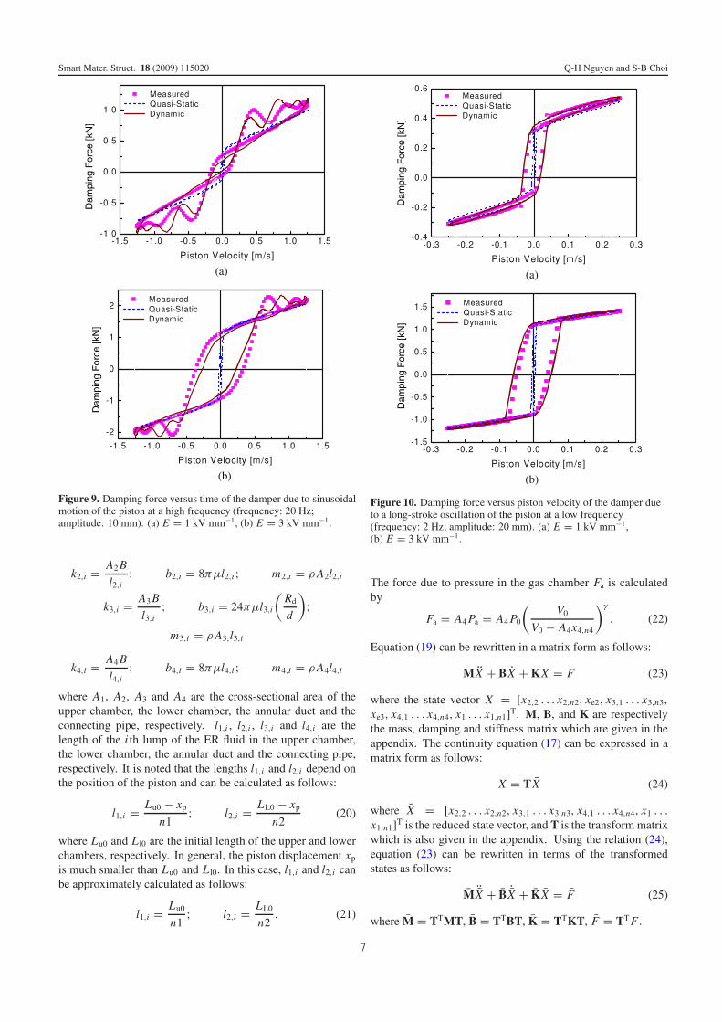
Figure 9. Damping force versus time of the damper due to sinusoidalmotion of the piston at a high frequency (frequency: 20 Hz;amplitude: 10 mm). (a) E = 1 kV mm−1, (b) E = 3 kV mm−1.

k2,i = A2 B

l2,i; b2,i = 8πμl2,i ; m2,i = ρ A2l2,i

k3,i = A3 B

l3,i; b3,i = 24πμl3,i

(Rd

d

);

m3,i = ρ A3,l3,i

k4,i = A4 B

l4,i; b4,i = 8πμl4,i ; m4,i = ρ A4l4,i

where A1, A2, A3 and A4 are the cross-sectional area of theupper chamber, the lower chamber, the annular duct and theconnecting pipe, respectively. l1,i , l2,i , l3,i and l4,i are thelength of the i th lump of the ER fluid in the upper chamber,the lower chamber, the annular duct and the connecting pipe,respectively. It is noted that the lengths l1,i and l2,i depend onthe position of the piston and can be calculated as follows:

l1,i = Lu0 − xp

n1; l2,i = LL0 − xp

n2(20)

where Lu0 and L l0 are the initial length of the upper and lowerchambers, respectively. In general, the piston displacement xp

is much smaller than Lu0 and L l0. In this case, l1,i and l2,i canbe approximately calculated as follows:

l1,i = Lu0

n1; l2,i = LL0

n2. (21)

Dam

ping

For

ce [k

N]

Dam

ping

For

ce [k

N]

Figure 10. Damping force versus piston velocity of the damper dueto a long-stroke oscillation of the piston at a low frequency(frequency: 2 Hz; amplitude: 20 mm). (a) E = 1 kV mm−1,(b) E = 3 kV mm−1.

The force due to pressure in the gas chamber Fa is calculatedby

Fa = A4 Pa = A4 P0

(V0

V0 − A4x4,n4

)γ

. (22)

Equation (19) can be rewritten in a matrix form as follows:

MX + BX + KX = F (23)

where the state vector X = [x2,2 . . . x2,n2, xe2, x3,1 . . . x3,n3,

xe3, x4,1 . . . x4,n4, x1 . . . x1,n1]T. M, B, and K are respectivelythe mass, damping and stiffness matrix which are given in theappendix. The continuity equation (17) can be expressed in amatrix form as follows:

X = TX (24)

where X = [x2,2 . . . x2,n2, x3,1 . . . x3,n3, x4,1 . . . x4,n4, x1 . . .

x1,n1]T is the reduced state vector, and T is the transform matrixwhich is also given in the appendix. Using the relation (24),equation (23) can be rewritten in terms of the transformedstates as follows:

M ¨X + B ˙X + KX = F (25)

where M = TTMT, B = TTBT, K = TTKT, F = TT F .

7

Smart Mater. Struct. 18 (2009) 115020 Q-H Nguyen and S-B Choi

Dam

ping

For

ce [k

N]

Dam

ping

For

ce [k

N]

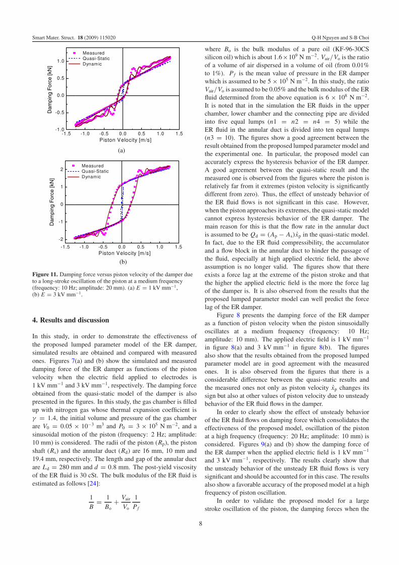
Figure 11. Damping force versus piston velocity of the damper dueto a long-stroke oscillation of the piston at a medium frequency(frequency: 10 Hz; amplitude: 20 mm). (a) E = 1 kV mm−1,(b) E = 3 kV mm−1.

4. Results and discussion

In this study, in order to demonstrate the effectiveness ofthe proposed lumped parameter model of the ER damper,simulated results are obtained and compared with measuredones. Figures 7(a) and (b) show the simulated and measureddamping force of the ER damper as functions of the pistonvelocity when the electric field applied to electrodes is1 kV mm−1 and 3 kV mm−1, respectively. The damping forceobtained from the quasi-static model of the damper is alsopresented in the figures. In this study, the gas chamber is filledup with nitrogen gas whose thermal expansion coefficient isγ = 1.4, the initial volume and pressure of the gas chamberare V0 = 0.05 × 10−3 m3 and P0 = 3 × 105 N m−2, and asinusoidal motion of the piston (frequency: 2 Hz; amplitude:10 mm) is considered. The radii of the piston (Rp), the pistonshaft (Rs) and the annular duct (Rd) are 16 mm, 10 mm and19.4 mm, respectively. The length and gap of the annular ductare Ld = 280 mm and d = 0.8 mm. The post-yield viscosityof the ER fluid is 30 cSt. The bulk modulus of the ER fluid isestimated as follows [24]:

1

B= 1

Bo+ Vair

Vo

1

Pf

where Bo is the bulk modulus of a pure oil (KF-96-30CSsilicon oil) which is about 1.6×109 N m−2. Vair/Vo is the ratioof a volume of air dispersed in a volume of oil (from 0.01%to 1%). Pf is the mean value of pressure in the ER damperwhich is assumed to be 5 × 105 N m−2. In this study, the ratioVair/Vo is assumed to be 0.05% and the bulk modulus of the ERfluid determined from the above equation is 6 × 108 N m−2.It is noted that in the simulation the ER fluids in the upperchamber, lower chamber and the connecting pipe are dividedinto five equal lumps (n1 = n2 = n4 = 5) while theER fluid in the annular duct is divided into ten equal lumps(n3 = 10). The figures show a good agreement between theresult obtained from the proposed lumped parameter model andthe experimental one. In particular, the proposed model canaccurately express the hysteresis behavior of the ER damper.A good agreement between the quasi-static result and themeasured one is observed from the figures where the piston isrelatively far from it extremes (piston velocity is significantlydifferent from zero). Thus, the effect of unsteady behavior ofthe ER fluid flows is not significant in this case. However,when the piston approaches its extremes, the quasi-static modelcannot express hysteresis behavior of the ER damper. Themain reason for this is that the flow rate in the annular ductis assumed to be Qd = (Ap − As)xp in the quasi-static model.In fact, due to the ER fluid compressibility, the accumulatorand a flow block in the annular duct to hinder the passage ofthe fluid, especially at high applied electric field, the aboveassumption is no longer valid. The figures show that thereexists a force lag at the extreme of the piston stroke and thatthe higher the applied electric field is the more the force lagof the damper is. It is also observed from the results that theproposed lumped parameter model can well predict the forcelag of the ER damper.

Figure 8 presents the damping force of the ER damperas a function of piston velocity when the piston sinusoidallyoscillates at a medium frequency (frequency: 10 Hz;amplitude: 10 mm). The applied electric field is 1 kV mm−1

in figure 8(a) and 3 kV mm−1 in figure 8(b). The figuresalso show that the results obtained from the proposed lumpedparameter model are in good agreement with the measuredones. It is also observed from the figures that there is aconsiderable difference between the quasi-static results andthe measured ones not only as piston velocity xp changes itssign but also at other values of piston velocity due to unsteadybehavior of the ER fluid flows in the damper.

In order to clearly show the effect of unsteady behaviorof the ER fluid flows on damping force which consolidates theeffectiveness of the proposed model, oscillation of the pistonat a high frequency (frequency: 20 Hz; amplitude: 10 mm) isconsidered. Figures 9(a) and (b) show the damping force ofthe ER damper when the applied electric field is 1 kV mm−1

and 3 kV mm−1, respectively. The results clearly show thatthe unsteady behavior of the unsteady ER fluid flows is verysignificant and should be accounted for in this case. The resultsalso show a favorable accuracy of the proposed model at a highfrequency of piston oscillation.

In order to validate the proposed model for a largestroke oscillation of the piston, the damping forces when the

8

Smart Mater. Struct. 18 (2009) 115020 Q-H Nguyen and S-B Choi

Dam

ping

For

ce [k

N]

Dam

ping

For

ce [k

N]

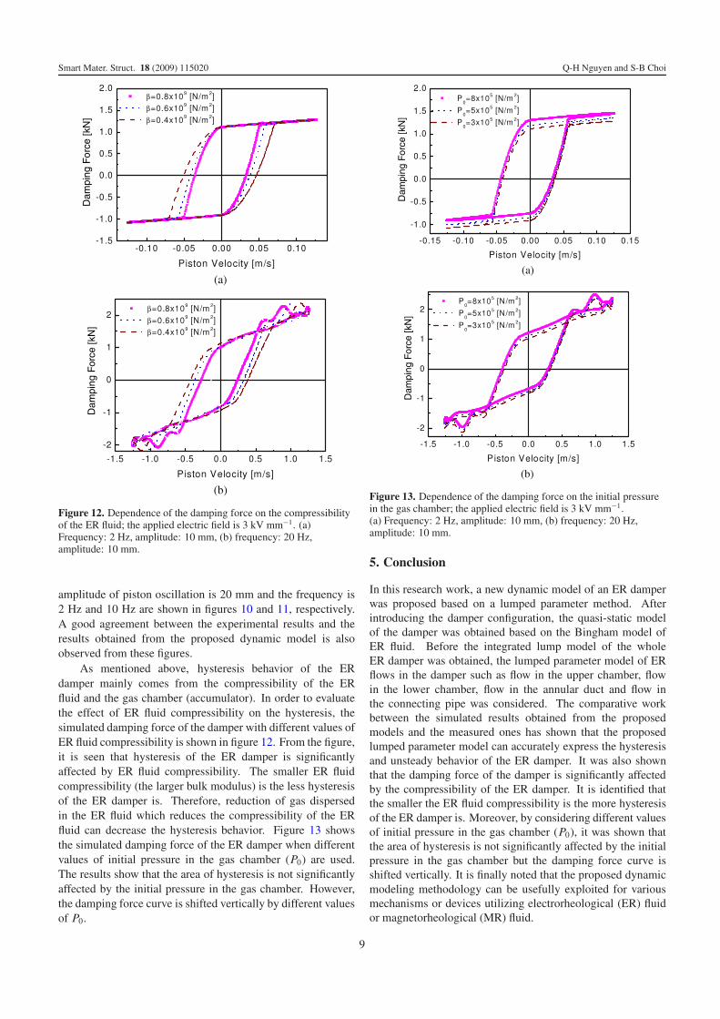
Figure 12. Dependence of the damping force on the compressibilityof the ER fluid; the applied electric field is 3 kV mm−1. (a)Frequency: 2 Hz, amplitude: 10 mm, (b) frequency: 20 Hz,amplitude: 10 mm.

amplitude of piston oscillation is 20 mm and the frequency is2 Hz and 10 Hz are shown in figures 10 and 11, respectively.A good agreement between the experimental results and theresults obtained from the proposed dynamic model is alsoobserved from these figures.

As mentioned above, hysteresis behavior of the ERdamper mainly comes from the compressibility of the ERfluid and the gas chamber (accumulator). In order to evaluatethe effect of ER fluid compressibility on the hysteresis, thesimulated damping force of the damper with different values ofER fluid compressibility is shown in figure 12. From the figure,it is seen that hysteresis of the ER damper is significantlyaffected by ER fluid compressibility. The smaller ER fluidcompressibility (the larger bulk modulus) is the less hysteresisof the ER damper is. Therefore, reduction of gas dispersedin the ER fluid which reduces the compressibility of the ERfluid can decrease the hysteresis behavior. Figure 13 showsthe simulated damping force of the ER damper when differentvalues of initial pressure in the gas chamber (P0) are used.The results show that the area of hysteresis is not significantlyaffected by the initial pressure in the gas chamber. However,the damping force curve is shifted vertically by different valuesof P0.

Dam

ping

For

ce [k

N]

Dam

ping

For

ce [k

N]

Figure 13. Dependence of the damping force on the initial pressurein the gas chamber; the applied electric field is 3 kV mm−1.(a) Frequency: 2 Hz, amplitude: 10 mm, (b) frequency: 20 Hz,amplitude: 10 mm.

5. Conclusion

In this research work, a new dynamic model of an ER damperwas proposed based on a lumped parameter method. Afterintroducing the damper configuration, the quasi-static modelof the damper was obtained based on the Bingham model ofER fluid. Before the integrated lump model of the wholeER damper was obtained, the lumped parameter model of ERflows in the damper such as flow in the upper chamber, flowin the lower chamber, flow in the annular duct and flow inthe connecting pipe was considered. The comparative workbetween the simulated results obtained from the proposedmodels and the measured ones has shown that the proposedlumped parameter model can accurately express the hysteresisand unsteady behavior of the ER damper. It was also shownthat the damping force of the damper is significantly affectedby the compressibility of the ER damper. It is identified thatthe smaller the ER fluid compressibility is the more hysteresisof the ER damper is. Moreover, by considering different valuesof initial pressure in the gas chamber (P0), it was shown thatthe area of hysteresis is not significantly affected by the initialpressure in the gas chamber but the damping force curve isshifted vertically. It is finally noted that the proposed dynamicmodeling methodology can be usefully exploited for variousmechanisms or devices utilizing electrorheological (ER) fluidor magnetorheological (MR) fluid.

9

Smart Mater. Struct. 18 (2009) 115020 Q-H Nguyen and S-B Choi

Acknowledgment

This work was supported by Korea Science and Engineer-ing Foundation (Acceleration Research Project No. R17-2007-028-01000-0). This financial support is gratefully acknowl-edged.

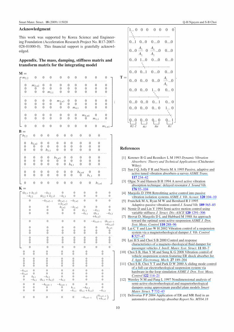
Appendix. The mass, damping, stiffness matrix andtransform matrix for the integrating model

M =⎡⎢⎢⎢⎢⎢⎢⎢⎢⎢⎢⎢⎢⎢⎢⎢⎣

m2,2 0 0 0 0 0 0 0 0 0· · · · · · · · · · · · · · · · · · · · · · · · · · · · · · · · · · · · · · · · · · · · · · · · · · · · · · · · ·

0 m2,n2 0 0 0 0 0 0 0 00 0 0 0 0 0 0 0 0 00 0 0 m3,1 0 0 0 0 0 0

· · · · · · · · · · · · · · · · · · · · · · · · · · · · · · · · · · · · · · · · · · · · · · · · · · · · · · · · ·0 0 0 0 m3,n3 0 0 0 0 00 0 0 0 0 0 0 0 0 00 0 0 0 0 0 m4,1 0 0 0

· · · · · · · · · · · · · · · · · · · · · · · · · · · · · · · · · · · · · · · · · · · · · · · · · · · · · · · · ·0 0 0 0 0 0 0 m4,n4 0 00 0 0 0 0 0 0 0 m1,1 0

· · · · · · · · · · · · · · · · · · · · · · · · · · · · · · · · · · · · · · · · · · · · · · · · · · · · · · · · ·0 0 0 0 0 0 0 0 0 m1,n1

⎤⎥⎥⎥⎥⎥⎥⎥⎥⎥⎥⎥⎥⎥⎥⎥⎦

;

B =⎡⎢⎢⎢⎢⎢⎢⎢⎢⎢⎢⎢⎢⎢⎢⎢⎣

b2,2 0 0 0 0 0 0 0 0 0· · · · · · · · · · · · · · · · · · · · · · · · · · · · · · · · · · · · · · · · · · · · · · · · · · · · · · · · ·

0 b2,n2 0 0 0 0 0 0 0 00 0 0 0 0 0 0 0 0 00 0 0 b3,1 0 0 0 0 0 0

· · · · · · · · · · · · · · · · · · · · · · · · · · · · · · · · · · · · · · · · · · · · · · · · · · · · · · · · ·0 0 0 0 b3,n3 0 0 0 0 00 0 0 0 0 0 0 0 0 00 0 0 0 0 0 b4,1 0 0 0

· · · · · · · · · · · · · · · · · · · · · · · · · · · · · · · · · · · · · · · · · · · · · · · · · · · · · · · · ·0 0 0 0 0 0 0 b4,n4 0 00 0 0 0 0 0 0 0 b1,1 0

· · · · · · · · · · · · · · · · · · · · · · · · · · · · · · · · · · · · · · · · · · · · · · · · · · · · · · · · ·0 0 0 0 0 0 0 0 0 b1,n1

⎤⎥⎥⎥⎥⎥⎥⎥⎥⎥⎥⎥⎥⎥⎥⎥⎦

K =⎡⎢⎢⎢⎢⎢⎢⎢⎢⎢⎢⎢⎢⎢⎢⎢⎢⎢⎢⎣

(k2,1 + k2,2) −k2,2 0 0 0 0 0−k2,2 (k2,2 + k2,3) −k2,3 0 0 0 0· · · · · · · · · · · · · · · · · · · · · · · · · · · · · · · · · · · · · · · · · · · · · · · · · · · · · · · · · · · · · · · · · · · · ·

0 −k2,n2−1 (k2,n2−1 −k2,n2 0 0 0+ k2,n2)

0 0 k2,n2 −k2,n2 0 0 00 0 0 0 k3,1 −k3,1 00 0 0 0 −k3,1 (k3,1 −k3,2

+k3,2)· · · · · · · · · · · · · · · · · · · · · · · · · · · · · · · · · · · · · · · · · · · · · · · · · · · · · · · · · · · · · · · · · · · · ·0 0 0 0 0 −k3,n3−1 (k3,n3−1

+k3,n3)0 0 0 0 0 0 k3,n30 0 0 0 0 0 00 0 0 0 0 0 0· · · · · · · · · · · · · · · · · · · · · · · · · · · · · · · · · · · · · · · · · · · · · · · · · · · · · · · · · · · · · · · · · · · · ·0 0 0 0 0 0 00 0 0 0 0 0 00 0 0 0 0 0 0· · · · · · · · · · · · · · · · · · · · · · · · · · · · · · · · · · · · · · · · · · · · · · · · · · · · · · · · · · · · · · · · · · · · ·0 0 0 0 0 0 0

0 0 0 0 0 0 00 0 0 0 0 0 0· · · · · · · · · · · · · · · · · · · · · · · · · · · · · · · · · · · · · · · · · · · · · · · · · · · · · · · · · · · · · · · · · · · · · · · ·0 0 0 0 0 0 00 0 0 0 0 0 00 0 0 0 0 0 00 0 0 0 0 0 0· · · · · · · · · · · · · · · · · · · · · · · · · · · · · · · · · · · · · · · · · · · · · · · · · · · · · · · · · · · · · · · · · · · · · · · ·−k3,n3 0 0 0 0 0 0

−k3,n3 0 0 0 0 0 00 k4,1 −k4,1 0 0 0 00 −k4,1 (k4,1 + k4,2) −k4,2 0 0 0· · · · · · · · · · · · · · · · · · · · · · · · · · · · · · · · · · · · · · · · · · · · · · · · · · · · · · · · · · · · · · · · · · · · · · · ·0 0 −k4,n4−1 −k4,n4−1 0 0 00 0 0 0 k1,1 −kk1,1 00 0 0 0 −k1,1 (k1,1 + k1,2) −k1,2· · · · · · · · · · · · · · · · · · · · · · · · · · · · · · · · · · · · · · · · · · · · · · · · · · · · · · · · · · · · · · · · · · · · · · · ·0 0 0 0 0 −k1,n1−1

( k1,n1−1+k1,n1

)

⎤⎥⎥⎥⎥⎥⎥⎥⎥⎥⎥⎥⎥⎥⎥⎥⎦

T = .

References

[1] Korenev B G and Reznikov L M 1993 Dynamic VibrationAbsorbers: Theory and Technical Applications (Chichester:Wiley)

[2] Sun J Q, Jolly F R and Norris M A 1995 Passive, adaptive andactive tuned vibration absorbers-a survey ASME Trans.117 234–42

[3] Olgac N and Hansen B H 1994 A novel active vibrationabsorption technique: delayed resonator J. Sound Vib.176 93–104

[4] Margolis D 1998 Retrofitting active control into passivevibration isolation systems ASME J. Vib. Acoust. 120 104–10

[5] Franchek M A, Ryan M W and Bernhard R J 1995Adaptive-passive vibration control J. Sound Vib. 189 565–85

[6] Nemir D and Lin Y 1994 Semi-active motion control usingvariable stiffness J. Struct. Div.-ASCE 120 1291–306

[7] Hrovat D, Margolis D L and Hubbard M 1988 An approachtoward the optimal semi-active suspension ASME J. Dyn.Syst. Meas. Control 110 288–96

[8] Lai C Y and Liao W H 2002 Vibration control of a suspensionsystem via a magnetorheological damper J. Vib. Control8 527–47

[9] Lee H S and Choi S B 2000 Control and responsecharacteristics of a magneto-rheological fluid damper forpassenger vehicles J. Intell. Mater. Syst. Struct. 11 80–7

[10] Choi S B, Han Y M and Sung K G 2008 Vibration control ofvehicle suspension system featuring ER shock absorber Int.J. Appl. Electromag. Mech. 27 189–204

[11] Choi S B, Choi Y T and Park D W 2000 A sliding mode controlof a full-car electrorheological suspension system viahardware in-the-loop simulation ASME J. Dyn. Syst. Meas.Control 122 114–21

[12] Wereley N M and Pang L 1997 Nondimensional analysis ofsemi-active electrorheological and magnetorheologicaldampers using approximate parallel plate models SmartMater. Struct. 7 732–43

[13] Delivorias P P 2004 Application of ER and MR fluid in anautomotive crash energy absorber Report No. MT04.18

10

Smart Mater. Struct. 18 (2009) 115020 Q-H Nguyen and S-B Choi

[14] Wang X J and Gordaninejad F 2007 Flow analysis andmodeling of field-controllable, electro- andmagneto-rheological fluid dampers J. Appl. Mech. ASME 7413–22

[15] Yang G 2001 Large-scale magnetorheological fluid damper forvibration mitigation: modeling, testing and control PhDDissertation University of Notre Dame Indiana

[16] Guo S Q, Yang S P and Pan C Z 2006 Dynamic modeling ofmagnetorheological damper behavior J. Intell. Mater. Syst.Struct. 17 3–14

[17] Spencer B F, Dyke S J, Sain M K and Carlson J D 1997Phenomenological model for a magnetorheological damperJ. Eng. Mech. ASCE 123 230–8

[18] Dominguez A, Sedaghati R and Stiharu J 2006 A new dynamichysteresis model for magnetorheological dampers SmartMater. Struct. 15 1179–89

[19] Choi S B and Lee S K 2001 A hysteresis model for thefield-dependent damping force of a magnetorheologicaldamper J. Sound Vib. 245 375–83

[20] Doebelin E 1972 System Dynamics Modeling and Response(Columbus, OH: Bell and Howell Company)

[21] William E H 2002 Piezohydraulic actuator design and modelingusing a lumped-parameter approach Master’s Thesis VirginiaPolytechnic Institute Blackburg, Virginia, USA

[22] Khalil M N 2000 Development and analysis of the lumpedparameter model of piezohydraulic actuator Master’s ThesisVirginia Polytechnic Institute Blackburg, Virginia, USA

[23] White F M 2003 Fluid Mechanics (New York: McGraw-Hill)University of Rhode Island

[24] Stringer J D 1976 Hydraulic System Analysis: An Introduction(New York: Wiley)

11