A mean field approximation in data assimilation for nonlinear dynamics

A mean field approximation in data assimilation for non-linear

dynamics

Eyink, G. L. et al.

• non-linear filtering/smoothing problems

• Connections with other methods

• Mean-field variational approach

• Closure techniques

• Toy example: a bistable double-well system

1

Non-linear estimation problem

dX(t) = f(X, t)dt + (2D)1/2(X, t)dW(t),

Y(t) = Z(X(t), t) + R1/2(t)η(t),

• X(t): state vectors at ti ≤ t ≤ tf

• f(X, t): a drift/dynamical vector

• W(t): a vector Wiener process

• D: a diffusion matrix;

• η(t): a white noise;

• Y(t): an observation process → data Y(t′) = {Y(t) : t ≤ t′}

• R(t): a covariance function;

• Z(·): a measurement function

2

−→ optimal estimation of the conditional probability

• P(x, t|Y(t)) with t < tf for filtering problem

• P(x, t|Y(tf )) with t < tf for smoothing problem

Discrete-Time Data:

yi = Y(ti) with ti ≤ t1 < t2 < ... < tM−1 < tM ≤ tf .

optimal filtering → P(x, t|Y(tf )) is the solver of the forward

Kolmogorov equation ( Kushner and Stratonovich )

∂tP(x, t) = L(t)P(x, t) with P(x, t = ti) = P0(x)

where

L(t) = −∑

k

∂[f(x, t)(·)]∂xk

+∑

ij

∂2[Dij(x, t)(·)]∂xi∂xj

.

3

At measurement times tm, P (x, t) satisfies the forward jump

condition

P (x, t+) =exp[y>

mR−1

mZ(x, tm) − 1

2Z>(x, tm)R−1

mZ(x, tm)]

W (y1, ..., ym)P (x, t−)

optimal smoothing → P(x, t|R(tf )) = A(x, t)P (x, t) where A(x, t)

is the solver of the backward Kolmogorov equation ( Pardoux )

∂tA(x, t) + L∗(t)A(x, t) = 0 with A(x, tf ) = 1)

At measurement times tm, A(x, t) satisfies the backward jump

condition

A(x, t−) = A(x, t+)exp[y>

mR−1

mZ(x, tm) − 1

2Z>(x, tm)R−1

mZ(x, tm)]

W (y1, ..., ym)

−→ infinite-dimensional filter and smoother!

4

In the linear case, where

f(x, t) = A(t)x, D(x, t) = D(t) and Z(x, t) = B(t)x

−→ the finite dimensional Kalman-Bucy optimal linear filter.

From estimation theory to control theory: a variation formulation

of the linear estimation problem:

ΓX [x] =1

4

∫ tf

ti

dt[dx

dt−A(t)x]>D−1(t)[

dx

dt−A(t)x]

︸ ︷︷ ︸

the Onsager-Machlup action

ΓY [x] =1

2

∫ tf

ti

dt[Y(t) − B(t)x]>R−1(t)[Y(t) − B(t)x]

The minimizer of the combined cost function

ΓX,Y [x,y] = ΓX [x] + ΓY [x]

coincides with the Kalman-Bucy filter and smoother.

5

Can the Onsager-Machlup action be generalised for nonlinear cases?

−→ a mean-field variational approach

Consider noise-free observations Z(t),

• Definition of ΓZ [z]

−→ the Cramer theory ( the theory of large deviations )

limN→∞

P(ZN (t) = z(t) : ti < t < tf

)∼ lim

N→∞exp (−N · ΓZ [z])

where

ZN (t) =1

N

N∑

n=1

Zn(t).

−→ the minimizer of ΓZ [z] is sub-optimal!

6

• Calculation of ΓZ [z]

−→ the action functional ( Balian and Veneroni )

Γ[A,P] =

∫ tf

ti

dt

∫

dxA(x, t)(∂t − L(t)P(x, t)

−→ΓZ [z] = st.pt.A,PΓ[A,P]

subject to∫

dxA(x, t)P(x, t) = 1

and ∫

dxA(x, t)Z(t)P(x, t) = z(t).

7

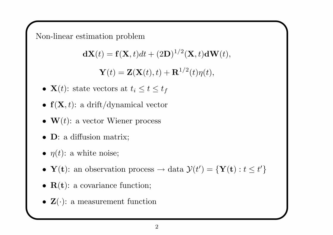
−→ the Lagrange multiplier h(t)

h(t) =M∑

k=1

λkδ(t − tk)

−→ the Euler-Lagrange equations are the forward- and

backward Kolmogorov equations with the jump conditions

P(x, tk+) =exp(λ>

k Z(x, tk))

W(tk−)P(x, tk−)

and

A(x, tk−) =exp(λ>

k Z(x, tk))

W(tk−)A(x, tk+)

−→ a cumulant generating function

FZ(λ1, ..., λM ) =M∑

k=1

log < eλ>

k Z(tk) >=M∑

k=1

logW(tk−)

8

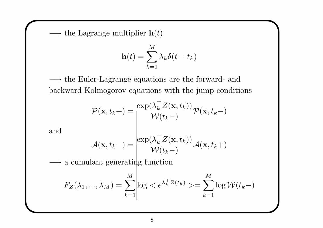
• multitime entropy HZ(z1, ..., zM )

−→ the Legendre transform of FZ

HZ(z1, ..., zM ) = maxλ1,...,λM

{M∑

k=1

z>k λk − FZ(λ1, ..., λM )

}

−→ the Contraction Principle ( Varadhan )

HZ(z1, ..., zM ) = minz:z(tk)=zk,k=1,...,MΓZ [z]

−→ Two useful relations in a descent algorithm

λm =∂HZ

∂xmand xm =

∂FZ

∂λm.

9

Closure Techniques: Basic Idea

• The Rayleigh-Ritz method which is based upon a variational

formulation of the moment-closure scheme;

• A set of moment functions, say Mi(x, t), i = 1, ..., R, and their

expectation functions µi(t) w.r.t. P(x, t);

• P(x, t) is parameterized by µ(t) = (µ1(t), ..., µR(t))>. Thus,

P(x, t; µ);

• Left-Linear Ansatz

A(x, t; α) = 1 +R∑

i=1

αi[Mi(x, t) − µi(t)]

︸ ︷︷ ︸

α>[M(x,t)−µ(t)]

10

• The resulting Euler-Lagrange equations

dµ

dt= V (µ, t)

︸ ︷︷ ︸

standard moment-closure

+ C>Z (µ, t) · h(t)

anddα

dt=

(∂VZ

∂µ

)>

α +

(∂ξ

∂µ

)>

h(t)

subject t0

µ(ti) = µ0 and α(tf ) = 0

where

V (µ, t) =< (∂t + L∗)M(t) >µ(t)

ξ(µ, t) =< Z(t) >µ

C>Z (µ, t) =< Z(t)M>(t) >µ(t) −ξ(µ, t)µ>

VZ(µ,h, t) =dµ

dt= V (µ, t) + C>

Z (µ, t) · h(t)

11

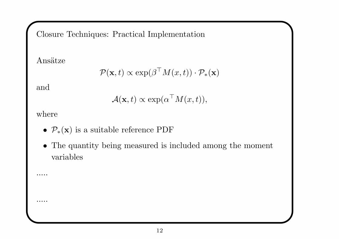
Closure Techniques: Practical Implementation

Ansatze

P(x, t) ∝ exp(β>M(x, t)) · P∗(x)

and

A(x, t) ∝ exp(α>M(x, t)),

where

• P∗(x) is a suitable reference PDF

• The quantity being measured is included among the moment

variables

.....

.....

12

.....

.....

The Euler-Lagrange equations

λ = W (λ, t) + 2S(λ, t)γ

and

γ +

(∂W

∂λ

)>

γ +∂

∂λ(γ>Sγ) = 0

with jump condition

γ+m = γ−

m + C(λ(tm), tm)R−1m [m(tm) − ym].

−→ a boundary-value problem

−→ Newton relaxation algorithm

13

Toy example : a stochastically forced double-well system

dx

dt= 4x(1 − x2) + κη(t) with κ = 0.5

−→ the steady-state probability distribution of the system

Ps(x) ∝ exp

(

−2U(x)

κ2

)

where U(x) = −2x2 + x4

14

moment-closure:

• the reference PDF

P∗(x) =1√

2πσ2

[

e−(x+1)2

2σ2 + e−(x−1)2

2σ2

]

· 1

2

where σ2 = κ16 ;

• first-order closure

P(x, t) ∝ eλ1x · P∗(x) and dµ1

dt = 4µ1 − 4µ3

• second-order closure

P(x, t) ∝ eλ1x+λ2x2 · P∗(x)

dµ1

dt = 4µ1 − 4µ3 and dµ2

dt = 8µ2 − 8µ4 + κ2

15

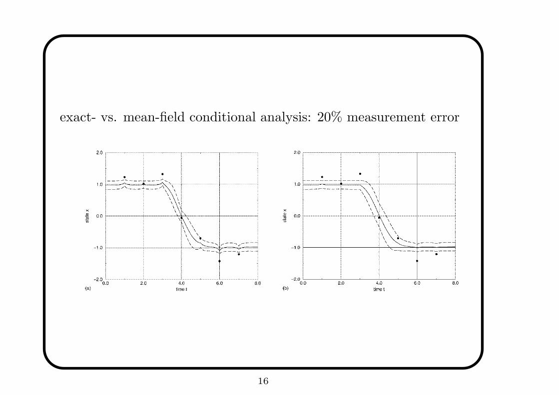
exact- vs. mean-field conditional analysis: 20% measurement error

16

exact- vs. mean-field conditional analysis: 40% measurement error

17

Mean-Field Variational Method with Moment-Closure

18

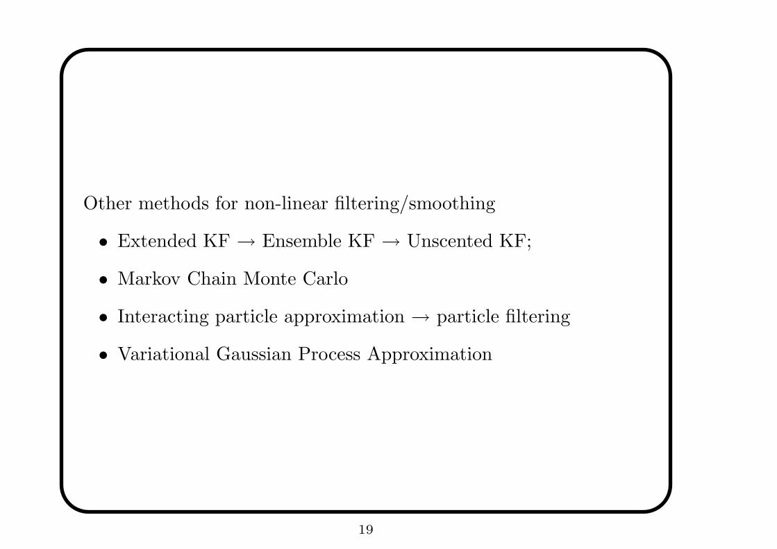
Other methods for non-linear filtering/smoothing

• Extended KF → Ensemble KF → Unscented KF;

• Markov Chain Monte Carlo

• Interacting particle approximation → particle filtering

• Variational Gaussian Process Approximation

19