A Matrix Formulation for the Moment Distribution Method Applied to ...

Hindawi Publishing CorporationAdvances in Civil EngineeringVolume 2011, Article ID 725395, 9 pagesdoi:10.1155/2011/725395

Research Article

A Matrix Formulation for the Moment Distribution MethodApplied to Continuous Beams

Arlindo Pires Lopes,1, 2 Adriana Alencar Santos,2 and Rogerio Coelho Lopes2

1 Department of Civil Engineering, Portland State University, Portland, OR 97201-3252, USA2 Coordenacao de Engenharia Mecanica, Escola Superior de Tecnologia, Universidade do Estado do Amazonas,Avenida Darcy Vargas 1200, 69065-020, Manaus, AM, Brazil

Correspondence should be addressed to Arlindo Pires Lopes, [email protected]

Received 8 January 2011; Accepted 14 February 2011

Academic Editor: Farid Taheri

Copyright © 2011 Arlindo Pires Lopes et al. This is an open access article distributed under the Creative Commons AttributionLicense, which permits unrestricted use, distribution, and reproduction in any medium, provided the original work is properlycited.

The Moment Distribution Method is a quite powerful hand method of structural analysis, in which the solution is obtainediteratively without even formulating the equations for the unknowns. It was formulated by Professor Cross in an era wherecomputer facilities were not available to solve frame problems that normally require the solution of simultaneous algebraicequations. Its relevance today, in the era of personal computers, is in its insight on how a structure reacts to applied loads byrotating its nodes and thus distributing the loads in the form of member-end moments. Such an insight is the foundation of themodern displacement method. This work has a main objective to present an exact solution for the Moment Distribution Methodthrough a matrix formulation using only one equation. The initial moments at the ends of the members and the distribution andcarry-over factors are calculated from the elementary procedures of structural analysis. Four continuous beams are investigated toillustrate the applicability and accuracy of the proposed formulation. The use of a matrix formulation yields excellent results whencompared with those in the literature or with a commercial structural program.

1. Introduction

It is observed in practice that the greater the complexityof a structure, the greater the number of unknowns andtherefore the greater the number of simultaneous equationsrequiring solution. Hand methods of analysis then becomeextremely tedious if not impracticable, so that alternatives aredesirable. One obvious alternative is to employ computer-based techniques, but another quite powerful hand methodis an iterative procedure known as the moment distributionmethod (MDM).

The MDM for the analysis of rigid-jointed structures wasintroduced by Professor Hardy Cross over seventy five yearsago. In the past, when structural engineers had to computethe forces and displacements in a statically indeterminatestructure, they inevitably turned to what was generallyknown as the Hardy Cross method. In this method, thefixed-end moments in the framing members are gradually

distributed to adjacent members in a number of steps, suchthat the system eventually reaches its natural equilibriumconfiguration.

The method is still taught in every undergraduate civilengineering course on the analysis and design of engineeringstructures, and although the Hardy Cross Method has beensuperseded by more powerful procedures such as the finiteelement method, the MDM made possible the efficient andsafe design of many reinforced concrete buildings during anentire generation.

The original paper written by Cross [1] explaining themethod was followed afterwards by a famous textbookwritten by Cross and Morgan [2]. In the former one, he wrotethe following: “The essential idea which the writer wishes topresent involves no mathematical relations except the sim-plest arithmetic.” The MDM depends on the solution of threeproblems for beam constants: the determination of fixed-endmoments, of the stiffness at each end of a beam, and of the

mailto:[email protected]

2 Advances in Civil Engineering

A B C D

Fixed

Fixed

Rotation

Fixed

Fixed

Rotation

Figure 1: Continuous beam subjected to static loads.

MDBA

MDBC

Figure 2: Free-body diagram of node B.

carry-over factor at each end for every member of the struc-ture under consideration, which will be explained afterwards.

Lightfoot [3] believes that the simpler possibilities of theMDM have now all been discovered and that its economicaluse for the analysis and design of complex structures mustnow be assessed in relation to available electronic computingprograms and facilities.

The purpose of this paper is to enhance and improve theMDM used in solving continuous beams. In this study, theoriginal MDM has been formulated in a closed form througha matrix formulation. Numerical results are presented todemonstrate the accuracy and efficiency of the proposedformulation.

2. The Moment Distribution Method

The MDM relies on a series of calculations that are repeateduntil every cycle comes closer to the final situation. In thisway, it is possible to avoid solving simultaneous algebraicequations. This method is a unique method of structuralanalysis, in which the solution is obtained iteratively withouteven formulating the equations for the unknowns. Thefollowing beam will be used to illustrate the method.

In the first stage of Figure 1, rotation is possible at bothB and C. The second stage is that rotation at B and C is pre-vented, and the load is applied obtaining the initial moments.Afterwards, in the third stage, allow B to rotate until moment

equilibrium is reached and then rotation at B will induce amoment at C. Finally, in the fourth stage of Figure 1, allow Cto rotate until moment equilibrium is reached. The rotationof C will induce a moment at B. This process is repeated untilmoment equilibrium is reached at all nodes.

Assume that the sum of the initial moments at the nodeB is equal to M0. Rotation will take place until momentequilibrium is attained, that is,

∑MB = 0 (Figure 2).

Therefore,

MDBA + MD

BC + M0 = 0, (1)

where MDBA and MD

BC are the moments as a result of therotation at B and are called the distribution moments.Remember that all the other rotations and sway are fixed.Using the equations from the slope-deflection method [4, 5],it is easy to demonstrate that

MDBA =

2EIABLAB

(2θB) = 4EIABLAB

θB,

MDBC =

2EIBCLBC

(2θB) = 4EIBCLBC

θB ,

(2)

where EI is the cross-section rigidity, L is the member length,and θB is the rotation at B.

Applying (2) into (1) and solving for θB, the rotation at Bcan be written as

θB = − M0

4EIAB/LAB + 4EIBC/LBC. (3)

Finally, the distribution moments are obtained, as fol-lows:

MDBA = −

(4EIAB/LAB)M0

4EIAB/LAB + 4EIBC/LBC

= − kBAM0

kBA + kBC= −kBAM0∑

kB,

MDBC = −

(4EIBC/LBC)M0

4EIAB/LAB + 4EIBC/LBC

= − kBCM0

kBA + kBC= −kBCM0∑

kB,

(4)

where kBA is the stiffness of the member BA at node B. Itis also the moment that would be induced if a unit rotationwas applied at B in the member BA and the rotation at A waszero. If B rotates, a bending moment will be induced at A andC. Assuming a rotation θB, the moment at A can be writtenas follows:

MDAB = −

(2EIAB/LAB)M0

4EIAB/LAB + 4EIBC/LBC. (5)

For this case, the distributed bending moment is halfthe value of the distributed bending moment at B. Thisis called the carry-over factor, CBA = 0, 5. It shouldbe mentioned that stiffness and carry-over factors mayvary with several parameters, depending on the shape ofthe structural member, the restraint conditions, and thestructural effects considered.

Advances in Civil Engineering 3

In summary, the MDM still remains an important toolfor analysis of structures in practice and can be programmedfor complicated problems without the use of modernstructural analysis software. At the first stage of the analysis,it is assumed that the rigid joints of the structural membersare initially fixed against rotations as in the displacementmethod. The reactive moments produced by external loadsare computed. These moments are unbalanced at the joints ofthe original nonrestrained structure. In order to equilibratethe joints the moments are distributed proportionally to thecorresponding member stiffness. These distributed momentsare associated with the so-called carry-over moments at theopposite ends of structural members. They are considered tobe new incremental unbalanced moments, and the procedurerepeats until the unbalanced moments become negligible.The final moments at the ends of all members are the sum ofall distributed moment increments. This procedure assumesthe joint rotations only.

According to Volokh [6], the MDM is nothing but Jacobiiterative scheme in disguise. It is shown that the method isthe incremental form of Jacobi iterative scheme applied tothe classical displacement formulation of the problem.

3. Sign Convention

The MDM convention that the final moments at a jointor a support are considered to be acting from the joint orsupport to the member is used. The convention adopted hereis easier for moments and just as easy for forces, so its use isrecommended. The positive direction for final moments istaken as clockwise.

The use of a rotational sense to determine the sign of finalmoments automatically arranges that the algebraic sum ofsuch moments equates to zero, at any joint in equilibrium.The clockwise direction also implies the use of the fourthquadrant for the definition of positive linear directions.Thus, forces, distances, and linear displacements are takenas positive when measured from left to right or verticallydownwards. This is in accordance with the positive directionsused in beam theory [7].

This sign convention is convenient when consideringjoint equilibrium in the slope-deflection and momentdistribution methods. For a horizontal beam subjected todownward loading, the MDM convention gives negative andpositive fixed-end moment at the left-hand and right-handsupports, respectively.

4. Matrix Formulation

This section reports some of the basic relations of theproposed formulation for the MDM based on a matrixnotation. Let the distribution and carry-over factors and theinitial moments be written as follows:

{M} = {M0} +[β]{M0} + [α]

[β]{M0} +

[β][α][β]{M0}

+ [α][β][α][β]{M0} +

[β][α][β][α][β]{M0} + · · · ,

(6)

where {M} is a vector which contains the final moments atthe ends of the members and dimension (m×1), {M0} is alsoa column vector which contains the fixed-ends moments ofthe members and dimension (m× 1), [β] is a square matrixwhich contains the distribution factors and dimension (m×m), [α] is a square matrix which contains the carry-overfactors and dimension (m×m), and, finally, m is the numberof the structural members multiplied by two.

Note that the first term of the series represented by (6)is the vector which contains the fixed-ends moments ofthe members. The second term is a product between thedistribution factors and the fixed-ends moments, obtaininga new set of moments when all nodes of the structureare released simultaneously. The third term of the series isthe product between the distribution factors and the set ofmoments obtained previously, and the series continues for ncycles. Equation (6) can be rewritten as

{M} = ([I] +[β]

+ [α][β]

+[β][α][β]

+ [α][β][α][β]

+[β][α][β][α][β]

+ · · · ){M0},(7)

where [I] is a simplest nontrivial diagonal matrix known asidentity matrix. After n cycles of the method and using someproperties of the identity matrix, the following equation isobtained:

{M} = {[I] +[β]}{

[I] + [α][β]

+([α][β])2 +

([α][β])3

+ · · · +([α][β])n−1

}{M0}

(8)

or

{M} = {[I] +[β]}{Sn}{M0}, (9)

where {Sn} = {[I] + [α][β] + ([α][β])2 + ([α][β])3 + · · · +([α][β])n−1}. Since a geometric progression series is a sumof terms in which two successive terms always have the sameratio, {Sn} is a geometric progression with a common ratioof r = {[α][β]}.

The sum of the first n terms of a geometric progression isgiven by

{Sn} = a1(1− rn)(1− r)

, (10)

where a1 is the first term and r is the ratio of the series.Substituting [I] as the first term and [α][β] as the ratio of

the series into (10) gives

{Sn} =[I]{

[I]− ([α][β])n}

{[I]− [α]

[β]} . (11)

Note that the terms in matrix [β] are less than the unity.Therefore, when n in the term ([α][β])n tends to the infinite,{Sn} can be written as

{Sn} = [I]{

[I]− [α][β]} or {Sn} =

{[I]− [α]

[β]}−1

.

(12)


1 3 5

2 4 6

Figure 3: Reference coordinates of the structure.

Substituting (12) into (9) gives

{M} = {[I] +[β]}{

[I]− [α][β]}−1{M0}, (13)

which represents the closed form of the MDM through amatrix formulation.

5. Reference Coordinates

The analysis of a continuous beam by the closed form ofthe MDM can be achieved, as previously demonstrated,by solving (13) which is expressed in a matrix form. Thedevelopment of the matrix elements of the latter equationmust be described with respect to the reference coordinates.It is necessary to identify the ends of the members as shownin Figure 3.

In the case of matrix [β] which represents the distribu-tion factors, it is observed that in the MDM the distributionfactor at the end of member corresponding to referencecoordinate 2 will multiply the bending moments associatedto reference coordinates 2 and 3. Thus, the distributionfactor has to be repeated two times in line 2 of the matrixand located in columns 2 and 3. The distribution factorcorresponding to reference coordinate 5 will multiply thebending moments associated to reference coordinates 4 and5. This distribution factor will be repeated two times in line5 of the matrix, and located in columns 4 and 5. In otherwords, the reference coordinate of each distribution factordefines the line of the matrix and its value is repeated as manytimes according to the number of the end members in a node.The location in the columns is defined by the reference coor-dinates of the end members, while the other values are zero.

In this way, the matrix [β] for the continuous beam inFigure 3 is given by

[β] =

⎡

⎢⎢⎢⎢⎢⎢⎢⎢⎢⎢⎢⎢⎣

−β1 0 0 0 0 0

0 −β2 −β2 0 0 0

0 −β3 −β3 0 0 0

0 0 0 −β4 −β4 0

0 0 0 −β 5 −β5 0

0 0 0 0 0 −β6

⎤

⎥⎥⎥⎥⎥⎥⎥⎥⎥⎥⎥⎥⎦

6×6

. (14)

In order to evaluate the matrix [α] in Figure 3, whichrepresents the carry-over factors, consider, for instance, thecase at the end of the member corresponding to referencecoordinate 2. The carry-over factor will multiply the bendingmoments associated to reference coordinate 2, but the resultwill be added to the bending moments associated to referencecoordinate 1. Therefore, this carry-over factor will be locatedin column 2 and line 1 in matrix [α]. Similarly, the carry-over

factor corresponding to reference coordinate 5 will multiplythe bending moments associated to reference coordinates5, but the result will be added to the bending momentsassociated to reference coordinate 6. This carry-over factorwill be located in column 5 and line 6 in matrix [α]. Tosummarize the procedure, in the case of the carry-overfactors, the member’s reference coordinate identifies thecolumn in which the correspondent value will be located andthe opposite reference coordinate identifies the line of thematrix, while the other values are zero.

Applying this procedure in the matrix of the carry-overfactors leads to

[α] =

⎡

⎢⎢⎢⎢⎢⎢⎢⎢⎢⎢⎢⎢⎣

0 α2 0 0 0 0

α1 0 0 0 0 0

0 0 0 α4 0 0

0 0 α3 0 0 0

0 0 0 0 0 α6

0 0 0 0 α5 0

⎤

⎥⎥⎥⎥⎥⎥⎥⎥⎥⎥⎥⎥⎦

6×6

. (15)

After all of the required matrices have been obtained,some of them with respect to the chosen reference coordi-nates, the closed form of the MDM can be done.

6. Numerical Examples

To compare the performance of the proposed formulationwith the traditional one previously reported in the literature,four numerical examples are presented.

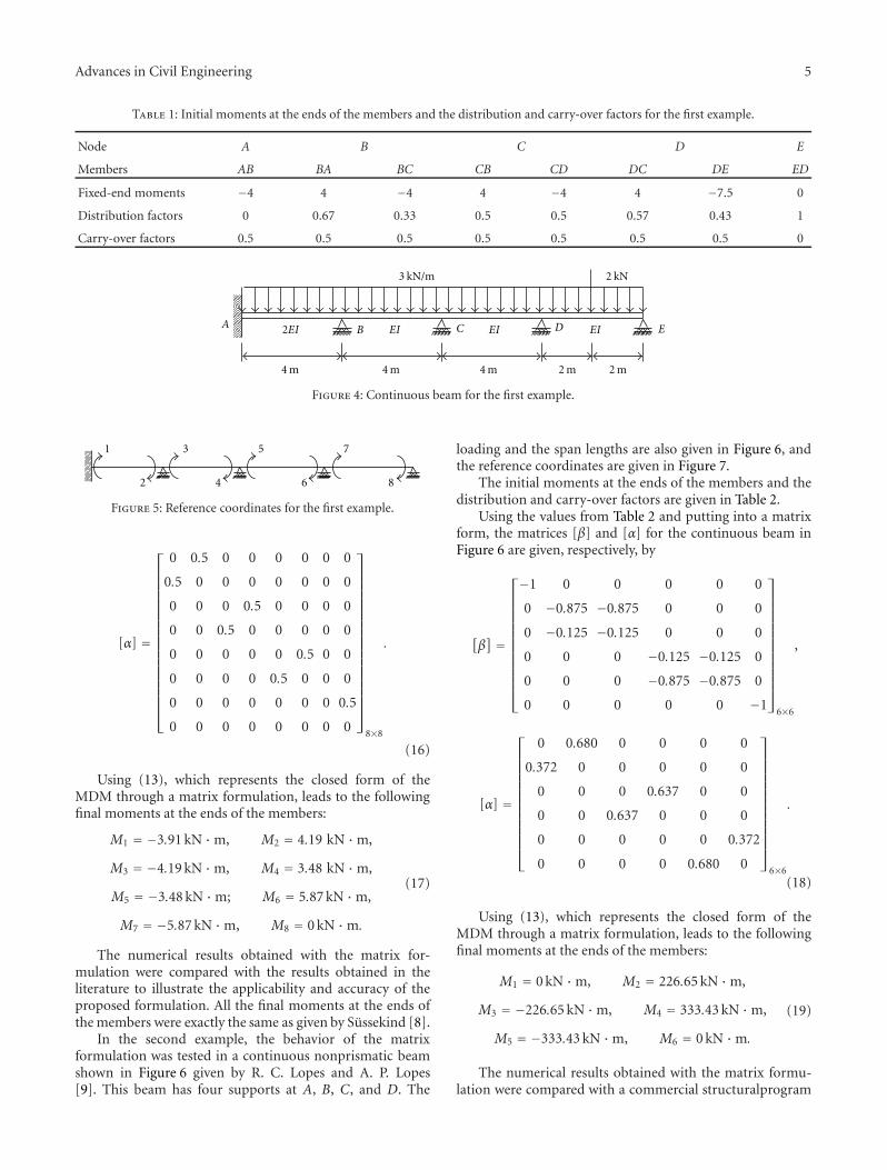
The first example is a continuous beam shown in Figure 4given by Sussekind [8]. This beam is selected as a benchmarkproblem in the present study. In this particular, examplecertain features should be noted. First, the support at A is afixed one and the support at E is an outside pinned support,so that the final moment at E must be zero. The loading andthe span lengths are given in Figure 4. As seen before, it isnecessary to identify the ends of the members, with respectto reference coordinates, as shown in Figure 5.

The fixed-end moments of the members and the dis-tribution and carry-over factors are calculated from theelementary procedures of structural analysis. These valuesare given in Table 1 as follows.

Using the values from Table 1 and putting into a matrixform, the matrices [β] and [α] for the continuous beam inFigure 4 are given, respectively, by

[β]=

⎡

⎢⎢⎢⎢⎢⎢⎢⎢⎢⎢⎢⎢⎢⎢⎢⎢⎢⎢⎣

0 0 0 0 0 0 0 0

0 −0.67 −0.67 0 0 0 0 0

0 −0.33 −0.33 0 0 0 0 0

0 0 0 −0.5 −0.5 0 0 0

0 0 0 −0.5 −0.5 0 0 0

0 0 0 0 0 −0.57 −0.57 0

0 0 0 0 0 −0.43 −0.43 0

0 0 0 0 0 0 0 −1

⎤

⎥⎥⎥⎥⎥⎥⎥⎥⎥⎥⎥⎥⎥⎥⎥⎥⎥⎥⎦

8×8

,


Table 1: Initial moments at the ends of the members and the distribution and carry-over factors for the first example.

Node A B C D E

Members AB BA BC CB CD DC DE ED

Fixed-end moments −4 4 −4 4 −4 4 −7.5 0

Distribution factors 0 0.67 0.33 0.5 0.5 0.57 0.43 1

Carry-over factors 0.5 0.5 0.5 0.5 0.5 0.5 0.5 0

2EIA B C D EEI EI EI

4 m 4 m 4 m 2 m 2 m

3 kN/m 2 kN

Figure 4: Continuous beam for the first example.

1

2

3

4

5

6

7

8

Figure 5: Reference coordinates for the first example.

[α] =

⎡

⎢⎢⎢⎢⎢⎢⎢⎢⎢⎢⎢⎢⎢⎢⎢⎢⎢⎢⎣

0 0.5 0 0 0 0 0 0

0.5 0 0 0 0 0 0 0

0 0 0 0.5 0 0 0 0

0 0 0.5 0 0 0 0 0

0 0 0 0 0 0.5 0 0

0 0 0 0 0.5 0 0 0

0 0 0 0 0 0 0 0.5

0 0 0 0 0 0 0 0

⎤

⎥⎥⎥⎥⎥⎥⎥⎥⎥⎥⎥⎥⎥⎥⎥⎥⎥⎥⎦

8×8

.

(16)

Using (13), which represents the closed form of theMDM through a matrix formulation, leads to the followingfinal moments at the ends of the members:

M1 = −3.91 kN ·m, M2 = 4.19 kN ·m,

M3 = −4.19 kN ·m, M4 = 3.48 kN ·m,

M5 = −3.48 kN ·m; M6 = 5.87 kN ·m,

M7 = −5.87 kN ·m, M8 = 0 kN ·m.

(17)

The numerical results obtained with the matrix for-mulation were compared with the results obtained in theliterature to illustrate the applicability and accuracy of theproposed formulation. All the final moments at the ends ofthe members were exactly the same as given by Sussekind [8].

In the second example, the behavior of the matrixformulation was tested in a continuous nonprismatic beamshown in Figure 6 given by R. C. Lopes and A. P. Lopes[9]. This beam has four supports at A, B, C, and D. The

loading and the span lengths are also given in Figure 6, andthe reference coordinates are given in Figure 7.

The initial moments at the ends of the members and thedistribution and carry-over factors are given in Table 2.


[β] =

⎡

⎢⎢⎢⎢⎢⎢⎢⎢⎢⎢⎢⎢⎣

−1 0 0 0 0 0

0 −0.875 −0.875 0 0 0

0 −0.125 −0.125 0 0 0

0 0 0 −0.125 −0.125 0

0 0 0 −0.875 −0.875 0

0 0 0 0 0 −1

⎤

⎥⎥⎥⎥⎥⎥⎥⎥⎥⎥⎥⎥⎦

6×6

,

[α] =

⎡

⎢⎢⎢⎢⎢⎢⎢⎢⎢⎢⎢⎢⎣

0 0.680 0 0 0 0

0.372 0 0 0 0 0

0 0 0 0.637 0 0

0 0 0.637 0 0 0

0 0 0 0 0 0.372

0 0 0 0 0.680 0

⎤

⎥⎥⎥⎥⎥⎥⎥⎥⎥⎥⎥⎥⎦

6×6

.

(18)


M1 = 0 kN ·m, M2 = 226.65 kN ·m,

M3 = −226.65 kN ·m, M4 = 333.43 kN ·m,

M5 = −333.43 kN ·m, M6 = 0 kN ·m.

(19)

The numerical results obtained with the matrix formu-lation were compared with a commercial structuralprogram


Table 2: Initial moments at the ends of the members and the distribution and carry-over factors for the second example.

Node A B C D

Members AB BA BC CB CD DC

Fixed-end moments −215.11 78.17 −218.40 358.60 −78.17 215.11

Distribution factors 1 0.875 0.125 0.125 0.875 1

Carry-over factors 0.372 0.680 0.637 0.637 0.680 0.372

80 kN 80 kN100 kN

150 cm80 cm 80 cm50 cm

20 cm 20 cm150 cm

AB C

D

7.5 m 7.5 m11.3 m 11.3 m15 m 10 m

Figure 6: Continuous beam for the second example.

1

2

3

4

5

6

Figure 7: Reference coordinates for the second example.

known as SAP2000 v. 14.1.0. The matrix formulation yieldsexcellent results.

In the third example, the proposed formulation wastested in a symmetric continuous beam shown in Figure 8given by Leet et al. [10]. This beam has five supports atA, B, C, D, and E. Supports A and B are fixed, and theflexural stiffness is assumed to be constant. The loading andthe span lengths are also given in Figure 8, and the referencecoordinates are given in Figure 9.

The fixed-end moments of the members and the dis-tribution and carry-over factors are calculated from theelementary procedures of structural analysis. These valuesare given in Table 3 as follows.


[β] =

⎡

⎢⎢⎢⎢⎢⎢⎢⎢⎢⎢⎢⎢⎢⎢⎢⎢⎢⎢⎣

0 0 0 0 0 0 0 0

0 −0.43 −0.43 0 0 0 0 0

0 −0.57 −0.57 0 0 0 0 0

0 0 0 −0.5 −0.5 0 0 0

0 0 0 −0.5 −0.5 0 0 0

0 0 0 0 0 −0.57 −0.57 0

0 0 0 0 0 −0.43 −0.43 0

0 0 0 0 0 0 0 0

⎤

⎥⎥⎥⎥⎥⎥⎥⎥⎥⎥⎥⎥⎥⎥⎥⎥⎥⎥⎦

8×8

,

[α] =

⎡

⎢⎢⎢⎢⎢⎢⎢⎢⎢⎢⎢⎢⎢⎢⎢⎢⎢⎢⎣

0 0.5 0 0 0 0 0 0

0.5 0 0 0 0 0 0 0

0 0 0 0.5 0 0 0 0

0 0 0.5 0 0 0 0 0

0 0 0 0 0 0.5 0 0

0 0 0 0 0.5 0 0 0

0 0 0 0 0 0 0 0.5

0 0 0 0 0 0 0.5 0

⎤

⎥⎥⎥⎥⎥⎥⎥⎥⎥⎥⎥⎥⎥⎥⎥⎥⎥⎥⎦

8×8

.

(20)


M1 = −234.28 kN ·m, M2 = 150.11 kN ·m,

M3 = −150.11 kN ·m, M4 = 38.38 kN ·m,

M5 = −38.38 kN ·m, M6 = 150.11 kN ·m,

M7 = −150.11 kN ·m, M8 = 234.28 kN ·m.

(21)

The numerical results obtained with the matrix for-mulation were compared with a commercial structuralprogram known as SAP2000 v. 14.1.0. The bending momentdiagram is plotted in Figure 10. The matrix formulationyields excellent results, and the minor differences less than1% are due to shear deformations included in the analysisvia SAP2000.

In the fourth example, the proposed formulation wastested in an asymmetric continuous beam shown in Figure 8


Table 3: Initial moments at the ends of the members and the distribution and carry-over factors for the third example.

Node A B C D E

Members AB BA BC CB CD DC DE ED

Fixed-end moments −206.225 206.225 −75.625 75.625 −75.625 75.625 −206.225 206.225

Distribution factors 0 0.43 0.57 0.5 0.5 0.57 0.43 0

Carry-over factors 0.5 0.5 0.5 0.5 0.5 0.5 0.5 0.5

Table 4: Initial moments at the ends of the members and the distribution and carry-over factors for the fourth example.

Node A B C D

Members AB BA BC CB CD DC

Fixed-end moments −63.875 63.875 −133.225 133.225 0 0

Distribution factors 0 0.5 0.5 0.33 0.67 0

Carry-over factors 0.5 0.5 0.5 0.5 0.5 0.5

3.65 m 3.65 m80 kN 80 kN

A B C D

7.3 m 7.3 m5.5 m 5.5 m

w = 30 kN/m

E

Figure 8: Continuous beam for the third example.

1

2

3 5

4 6

7

8

Figure 9: Reference coordinates for the third example.

−235.63 kN·m −235.63 kN·m−150.94 kN·m −150.94 kN·m

25.69 kN·m 25.69 kN·m154.74 kN·m 154.74 kN·m

Figure 10: Bending moment diagram for the third example.

3.65 m

A B C D

7.3 m 7.3 m 3.65 m

w = 30 kN/m

P = 70 kN

Figure 11: Continuous beam for the fourth example.


2

3

Figure 12: Section properties for the fourth example.

1

2

3

4

5

6

Figure 13: Reference coordinates for the fourth example.

−41.65 kN·m

−113.42 kN·m −105.42 kN·m

52.64 kN·m92.21 kN·m

51.08 kN·m

Figure 14: Bending moment diagram for the fourth example.

given by Leet et al. [10]. This beam has four supports at A, B,C, and D. Supports A and B are fixed and the cross-sectionof the beam is a C-Shape (C10× 25) given by the AISCsteel construction manual [11]. The loading and the spanlengths are also given in Figure 11, the section properties aregiven in Figure 12, and the reference coordinates are given inFigure 13.

The initial moments at the ends of the members and thedistribution and carry-over factors are given in Table 4.


[β] =

⎡

⎢⎢⎢⎢⎢⎢⎢⎢⎢⎢⎢⎢⎣

0 0 0 0 0 0

0 −0.5 −0.5 0 0 0

0 −0.5 −0.5 0 0 0

0 0 0 −0.33 −0.33 0

0 0 0 −0.67 −0.67 0

0 0 0 0 0 0

⎤

⎥⎥⎥⎥⎥⎥⎥⎥⎥⎥⎥⎥⎦

6×6

,

[α] =

⎡

⎢⎢⎢⎢⎢⎢⎢⎢⎢⎢⎢⎢⎣

0 0.5 0 0 0 0

0.5 0 0 0 0 0

0 0 0 0.5 0 0

0 0 0.5 0 0 0

0 0 0 0 0 0.5

0 0 0 0 0.5 0

⎤

⎥⎥⎥⎥⎥⎥⎥⎥⎥⎥⎥⎥⎦

6×6

.

(22)


M1 = −40.06 kN ·m, M2 = 111.51 kN ·m,

M3 = −111.51 kN ·m, M4 = 105.22 kN ·m,

M5 = −105.22 kN ·m, M6 = −52.61 kN ·m.

(23)

The numerical results obtained with the matrix for-mulation were compared with a commercial structuralprogram known as SAP2000 v. 14.1.0. The bending momentdiagram is plotted in Figure 13. The matrix formulation


yields excellent results, and the minor differences less than2% are due to shear deformations included in the analysisvia SAP2000.

7. Conclusions

A new formulation for the MDM based on a matrixformulation has been developed. The main advantage ofthe proposed scheme is the use of only one equation tosolve the problem without iteration. The results obtainedhere show that accurate values for the final moments atthe ends of the members have been achieved comparedto previous examples given in the literature or using acommercial structural program. It should be mentioned thatthe matrix formulation can be applied to framed structurestoo. Nowadays, it seems that the simpler possibilities of theMDM have all been discovered and that its economical usefor the analysis and design of complex structures must nowbe assessed in relation to available electronic computingprograms and facilities. From this point of view, the matrixformulation of the MDM emerges as an option to solvestructural problems. It is apparent, therefore, that withresearch developments here and abroad the MDM stillhas many exciting possibilities to add to its considerableachievements. The next step of this research is to extend theproposed formulation to three-dimension problems and alsothe analysis of structures considering shear deformations.

References

[1] H. Cross, “Analysis of continuous frames by distributing fixed-end moments,” Proceedings of the American Society of CivilEngineers, vol. 96, pp. 919–928, 1930.

[2] H. Cross and N. D. Morgan, Continuous Frames of ReinforcedConcrete, John Wiley & Sons, New York, NY, USA, 1932.

[3] E. Lightfoot, Moment Distribution: A Rapid Method of Analysisfor Rigid-Jointed Structures, Barnes & Noble, New York, NY,USA, 1961.

[4] H. I. Laursen, Structural Analysis, McGraw-Hill, New York,NY, USA, 2nd edition, 1978.

[5] A. Kassimali, Structural Analysis, International ThomsonPublishing, New York, NY, USA, 1995.

[6] K. Y. Volokh, “On foundations of the Hardy Cross method,”International Journal of Solids and Structures, vol. 39, no. 16,pp. 4197–4200, 2002.

[7] S. P. Timoshenko and J. N. Goodier, Theory of Elasticity,McGraw-Hill, New York, NY, USA, 1980.

[8] J. C. Sussekind, Curso de Analise Estrutural, vol. 3, Editora daUniversidade de Sao Paulo, Sao Paulo, Brasil, 1973.

[9] R. C. Lopes and A. P. Lopes, “Structural analysis: The momentdistribution method” (Portuguese), In press.

[10] K. M. Leet, C. M. Uang, and A. M. Gilbert, Fundamentalsof Structural Analysis, McGraw-Hill, New York, NY, USA, 4thedition, 2011.

[11] AISC, Steel Construction Manual, American Institute of SteelConstruction, 13th edition, 2008.

International Journal of

AerospaceEngineeringHindawi Publishing Corporationhttp://www.hindawi.com Volume 2010

RoboticsJournal of

Hindawi Publishing Corporationhttp://www.hindawi.com Volume 2014


Active and Passive Electronic Components

Control Scienceand Engineering

Journal of



RotatingMachinery


Hindawi Publishing Corporation http://www.hindawi.com

Journal ofEngineeringVolume 2014

Submit your manuscripts athttp://www.hindawi.com

VLSI Design



Shock and Vibration


Civil EngineeringAdvances in

Acoustics and VibrationAdvances in



Electrical and Computer Engineering

Journal of

Advances inOptoElectronics

Hindawi Publishing Corporation http://www.hindawi.com

Volume 2014

The Scientific World JournalHindawi Publishing Corporation http://www.hindawi.com Volume 2014

SensorsJournal of


Modelling & Simulation in EngineeringHindawi Publishing Corporation http://www.hindawi.com Volume 2014


Chemical EngineeringInternational Journal of Antennas and

Propagation




Navigation and Observation



DistributedSensor Networks


A Matrix Formulation for the Moment Distribution Method Applied to ...

Documents