A hybrid method for solving multi-objective global optimization problems

J Glob Optim (2007) 38:265–281DOI 10.1007/s10898-006-9105-1

O R I G I NA L PA P E R

A hybrid method for solving multi-objective globaloptimization problems

C. Gil · A. Márquez · R. Baños · M. G. Montoya ·J. Gómez

Received: 28 December 2005 / Accepted: 11 October 2006 / Published online: 22 November 2006© Springer Science+Business Media B.V. 2006

Abstract Real optimization problems often involve not one, but multiple objectives,usually in conflict. In single-objective optimization there exists a global optimum,while in the multi-objective case no optimal solution is clearly defined but rather aset of optimums, which constitute the so called Pareto-optimal front. Thus, the goalof multi-objective strategies is to generate a set of non-dominated solutions as anapproximation to this front. However, most problems of this kind cannot be solvedexactly because they have very large and highly complex search spaces. The objectiveof this work is to compare the performance of a new hybrid method here proposed,with several well-known multi-objective evolutionary algorithms (MOEA). The mainattraction of these methods is the integration of selection and diversity maintenance.Since it is very difficult to describe exactly what a good approximation is in terms of anumber of criteria, the performance is quantified with adequate metrics that evaluatethe proximity to the global Pareto-front. In addition, this work is also one of the fewempirical studies that solves three-objective optimization problems using the conceptof global Pareto-optimality.

C. Gil (B) ·A. Márquez · R. Baños ·M. G. MontoyaDpt. de Arquitectura de Computadores y Electrónica, Universidad de Almeria, Cañada de SanUrbano, 04120 Almería, Spaine-mail: [email protected]

J. GómezDpt. Lenguajes y Computación, Universidad de Almeria, Cañada de San Urbano, 04120 Almería,Spaine-mail: [email protected]

A. Márqueze-mail: [email protected]

R. Bañose-mail: [email protected]

M. G. Montoyae-mail: [email protected]

266 J Glob Optim (2007) 38:265–281

Keywords Multi-objective optimization ·Global pareto-optimal front ·Evolutionary algorithms

1 Introduction

The aim of global optimization (GO) is to find the best solution of decisionmodels, in presence of multiple local solutions [1]. In recent years, researchers havebegun to apply different GO techniques to problems that occur in the analysisand solution of multi-objective linear and non linear programming problems [2,3].However, when the problem has several objective functions, the notion of opti-mum changes. Classical optimization methods (including multi-criteria decision-mak-ing methods) suggest converting the multi-objective optimization problem (MOP)into a single-objective optimization problem by combining the objectives in a sin-gle mathematical function [4]. However, in last two decades most papers dealingwith MOPs used the concept of Pareto-dominance [5], where the goal is to findtrade-off solutions (widely known as Pareto-optimal solutions) rather thana single solution. In the absence of any further information, none of these Pa-reto-optimal solutions is considered to be better than the others. Generating thePareto-optimal set in complex problems is computationally expensive and ofteninfeasible, but using heuristic methods can allow to obtain a representative sampleof it.

Conceptually, evolutionary algorithms (EA) [5] base their operation on main-taining a set of solutions (individuals) which evolve in successive iterations (gen-erations) trying to optimize an objective function. In the multi-objective context,it is necessary to design strategies that obtain good solutions in all the objectives.The main advantage of the multi-objective EAs (MOEAs) [6,7] is their ability tofind multiple Pareto-optimal solutions in one single run. Over the past decade, anumber of MOEAs have been suggested [8–16]. The interest in the design and imple-mentation of hybrid meta-heuristics has increased remarkably in recent years [17].However, to date there has been little research effort dedicated to the hybridiza-tion of meta-heuristics for multi-objective optimization. Some studies [15,16] haveshown that combining ideas of different methods allows the quality of the solutionsto be improved. Although many MOEAs have adequately demonstrated their abil-ity to solve two-objective problems, there are few studies in problems with threeor more objectives. For instance, Deb et al. [18] compared the performance oftwo Pareto-based MOEAs in some three-objective optimization problems. This pa-per presents a new hybrid method, msPESA, whose performance is evaluated ver-sus other well-known MOEAs in several test functions of two and threeobjectives.

The remainder of the paper is organized as follows. Section 2 gives some gen-eral Multi-objective optimization concepts, and a brief overview of some well knownMOEAs found in the literature. Section 3 describes the new hybrid method here pro-posed. Section 4 details the test problems and performance metrics used to evaluatethe performance of the MOEAs described in Sects. 2 and 3. Experimental results areprovided and analyzed in Sect. 5. Finally, we outline the conclusions of this paper inSect. 6.

J Glob Optim (2007) 38:265–281 267

2 Multi-objective optimization: concepts and techniques

This section introduces some multi-objective concepts, and briefly describe some well-known methods we have implemented to compare their performance with the newmethod presented in Sect. 3.

Definition 1 Multi-Objective Optimization is the process of searching for one ormore decision variables that simultaneously satisfy all constraints, and optimize anobjective function vector that maps the decision variables to two or more objectives.

minimize/maximize(fk(s)),∀k ∈ [1, K]Each decision vector or solution s = {(s1, s2, .., sm)} represents accurate numerical

qualities for a MOP. The set of all decision vectors constitutes the decision space.The set of decision vectors that simultaneously satisfies all the constraints is calledfeasible set (F). The objective function vector (f ) maps the decision vectors fromthe decision space into a K-dimensional objective space Z ∈ �K, z = f (s), f (s) ={f1(s), f2(s), . . . , fK(s)}, z ∈ Z, s ∈ F.

Given a MOP with K ≥ 2 objectives, instead of giving a scalar value to each solu-tion, a partial order is defined according to Pareto-dominance relations, as we detailbelow.

Definition 2 Order relation between decision vectors Let s and s′ be two decisionvectors. The dominance relations in a minimization problem are:

s dominates s′ (s ≺ s′) iff fk(s) < fk(s′) ∧ fk′(s) �> fk′(s′) ,∀k′ �= k ∈ [1, K]

s, s′ are incomparable (s ∼ s′) iff fk(s) < fk(s′) ∧ fk′(s) > fk′(s′) , k′ �= k ∈ [1, K]

Definition 3 Pareto-optimal solution A solution s is called Pareto-optimal if there isno other s′ ∈ F, such that f (s′) < f (s). All the Pareto-optimal solutions define thePareto-optimal set.

Definition 4 Non-dominated solution A solution s ∈ F is non-dominated with respectto a set S′ ∈ F if and only if � ∃s′ ∈ S′, verifying that s′ ≺ s.

Definition 5 Non-dominated set Given a set of solutions S′, such that S′ ∈ F andZ′ = f (S′), the function ND(S′) returns the set of non-dominated solutions from S′:

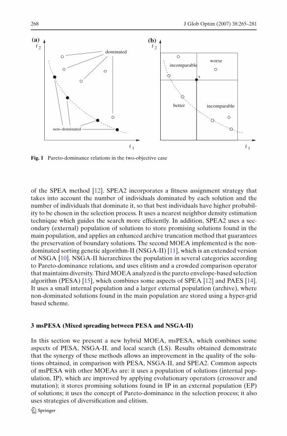
ND(S′) = {∀s′ ∈ S′ | s′ is non-dominated by any other s”, s′′ ∈ S′}Figure 1 graphically describes the Pareto-dominance concept for a minimization

problem with two objectives (f1 and f2). Figure 1a shows the location of several solu-tions. The filled circles represent non-dominated solutions, while the non-filled onessymbolize dominated solutions. Figure 1b shows the relative distribution of the solu-tions in reference to s. There exist solutions that are worse (in both objectives) thans, better (in both objectives) than s, and incomparable (better in one objective andworse in the other).

Over the past decade, a number of MOEAs have been proposed [8–16]. In thefollowing we offer a brief description of three methods implemented to be comparedwith the new MOEA presented in Sect. 3. The first method we have adapted is thestrength pareto evolutionary algorithm 2 (SPEA2) [12], which is an improved version

268 J Glob Optim (2007) 38:265–281

f 2

f 1

f 2

f 1

dominated

worse

incomparablebetter

incomparable

(b)

s

non−dominated

(a)

Fig. 1 Pareto-dominance relations in the two-objective case

of the SPEA method [12]. SPEA2 incorporates a fitness assignment strategy thattakes into account the number of individuals dominated by each solution and thenumber of individuals that dominate it, so that best individuals have higher probabil-ity to be chosen in the selection process. It uses a nearest neighbor density estimationtechnique which guides the search more efficiently. In addition, SPEA2 uses a sec-ondary (external) population of solutions to store promising solutions found in themain population, and applies an enhanced archive truncation method that guaranteesthe preservation of boundary solutions. The second MOEA implemented is the non-dominated sorting genetic algorithm-II (NSGA-II) [11], which is an extended versionof NSGA [10]. NSGA-II hierarchizes the population in several categories accordingto Pareto-dominance relations, and uses elitism and a crowded comparison operatorthat maintains diversity. Third MOEA analyzed is the pareto envelope-based selectionalgorithm (PESA) [15], which combines some aspects of SPEA [12] and PAES [14].It uses a small internal population and a larger external population (archive), wherenon-dominated solutions found in the main population are stored using a hyper-gridbased scheme.

3 msPESA (Mixed spreading between PESA and NSGA-II)

In this section we present a new hybrid MOEA, msPESA, which combines someaspects of PESA, NSGA-II, and local search (LS). Results obtained demonstratethat the synergy of these methods allows an improvement in the quality of the solu-tions obtained, in comparison with PESA, NSGA-II, and SPEA2. Common aspectsof msPESA with other MOEAs are: it uses a population of solutions (internal pop-ulation, IP), which are improved by applying evolutionary operators (crossover andmutation); it stores promising solutions found in IP in an external population (EP)of solutions; it uses the concept of Pareto-dominance in the selection process; it alsouses strategies of diversification and elitism.

J Glob Optim (2007) 38:265–281 269

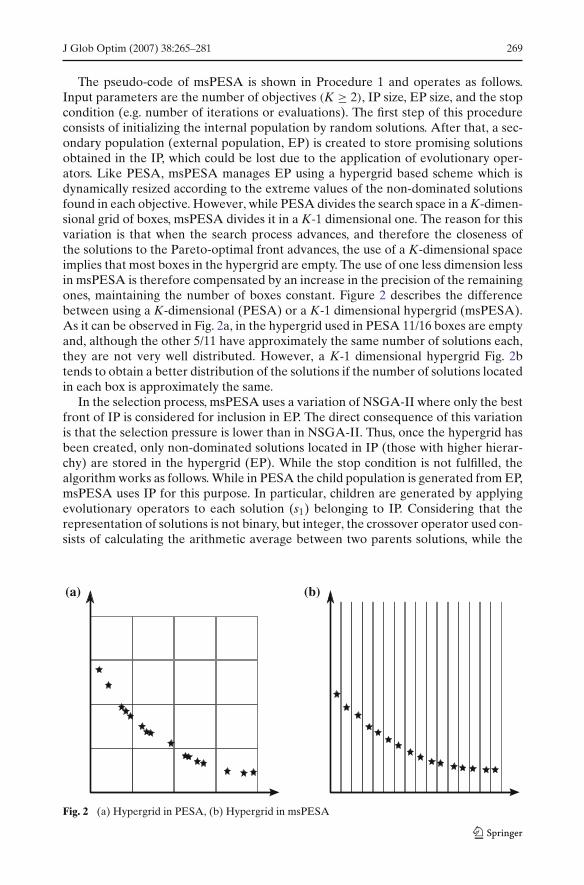
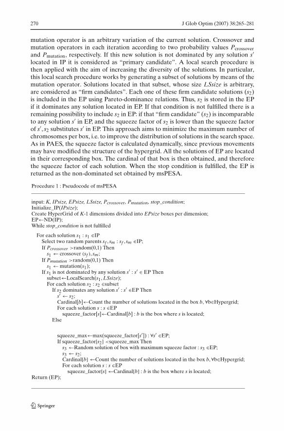
The pseudo-code of msPESA is shown in Procedure 1 and operates as follows.Input parameters are the number of objectives (K ≥ 2), IP size, EP size, and the stopcondition (e.g. number of iterations or evaluations). The first step of this procedureconsists of initializing the internal population by random solutions. After that, a sec-ondary population (external population, EP) is created to store promising solutionsobtained in the IP, which could be lost due to the application of evolutionary oper-ators. Like PESA, msPESA manages EP using a hypergrid based scheme which isdynamically resized according to the extreme values of the non-dominated solutionsfound in each objective. However, while PESA divides the search space in a K-dimen-sional grid of boxes, msPESA divides it in a K-1 dimensional one. The reason for thisvariation is that when the search process advances, and therefore the closeness ofthe solutions to the Pareto-optimal front advances, the use of a K-dimensional spaceimplies that most boxes in the hypergrid are empty. The use of one less dimension lessin msPESA is therefore compensated by an increase in the precision of the remainingones, maintaining the number of boxes constant. Figure 2 describes the differencebetween using a K-dimensional (PESA) or a K-1 dimensional hypergrid (msPESA).As it can be observed in Fig. 2a, in the hypergrid used in PESA 11/16 boxes are emptyand, although the other 5/11 have approximately the same number of solutions each,they are not very well distributed. However, a K-1 dimensional hypergrid Fig. 2btends to obtain a better distribution of the solutions if the number of solutions locatedin each box is approximately the same.

In the selection process, msPESA uses a variation of NSGA-II where only the bestfront of IP is considered for inclusion in EP. The direct consequence of this variationis that the selection pressure is lower than in NSGA-II. Thus, once the hypergrid hasbeen created, only non-dominated solutions located in IP (those with higher hierar-chy) are stored in the hypergrid (EP). While the stop condition is not fulfilled, thealgorithm works as follows. While in PESA the child population is generated from EP,msPESA uses IP for this purpose. In particular, children are generated by applyingevolutionary operators to each solution (s1) belonging to IP. Considering that therepresentation of solutions is not binary, but integer, the crossover operator used con-sists of calculating the arithmetic average between two parents solutions, while the

(a) (b)

Fig. 2 (a) Hypergrid in PESA, (b) Hypergrid in msPESA

270 J Glob Optim (2007) 38:265–281

mutation operator is an arbitrary variation of the current solution. Crosssover andmutation operators in each iteration according to two probability values Pcrossoverand Pmutation, respectively. If this new solution is not dominated by any solution s′located in IP it is considered as “primary candidate”. A local search procedure isthen applied with the aim of increasing the diversity of the solutions. In particular,this local search procedure works by generating a subset of solutions by means of themutation operator. Solutions located in that subset, whose size LSsize is arbitrary,are considered as “firm candidates”. Each one of these firm candidate solutions (s2)is included in the EP using Pareto-dominance relations. Thus, s2 is stored in the EPif it dominates any solution located in EP. If that condition is not fulfilled there is aremaining possibility to include s2 in EP: if that “firm candidate” (s2) is incomparableto any solution s′ in EP, and the squeeze factor of s2 is lower than the squeeze factorof s′, s2 substitutes s′ in EP. This approach aims to minimize the maximum number ofchromosomes per box, i.e. to improve the distribution of solutions in the search space.As in PAES, the squeeze factor is calculated dynamically, since previous movementsmay have modified the structure of the hypergrid. All the solutions of EP are locatedin their corresponding box. The cardinal of that box is then obtained, and thereforethe squeeze factor of each solution. When the stop condition is fulfilled, the EP isreturned as the non-dominated set obtained by msPESA.

Procedure 1 : Pseudocode of msPESA

input: K, IPsize, EPsize, LSsize, Pcrossover, Pmutation, stop_condition;Initialize_IP(IPsize);Create HyperGrid of K-1 dimensions divided into EPsize boxes per dimension;EP←ND(IP);While stop_condition is not fulfilled

For each solution s1 : s1 ∈IPSelect two random parents sf , sm : sf , sm ∈IP;If Pcrossover >random(0,1) Then

s1 ← crossover (sf ), sm;If Pmutation >random(0,1) Then

s1 ←mutation(s1);If s1 is not dominated by any solution s′ : s′ ∈ EP Then

subset←LocalSearch(s1, LSsize);For each solution s2 : s2 ∈subset

If s2 dominates any solution s′ : s′ ∈EP Thens′ ← s2;Cardinal[b]←Count the number of solutions located in the box b, ∀b∈Hypergrid;For each solution s : s ∈EP

squeeze_factor[s]←Cardinal[b] : b is the box where s is located;Else

squeeze_max←max(squeeze_factor[s′]) : ∀s′ ∈EP;If squeeze_factor[s2] <squeeze_max Then

s3 ←Random solution of box with maximum squeeze factor : s3 ∈EP;s3 ← s2;Cardinal[b] ←Count the number of solutions located in the box b,∀b∈Hypergrid;For each solution s : s ∈EP

squeeze_factor[s] ←Cardinal[b] : b is the box where s is located;Return (EP);

J Glob Optim (2007) 38:265–281 271

4 Test problem suite

With the aim of evaluating the performance of the MOEAs described in Sect. 3, wepropose to apply several test problems. In particular NSGA-II, SPEA2, PESA, andmsPESA have been evaluated on eight test problems (five two-objective problems,and three three-objective problems).

4.1 Two-objective test problems

Here we describe five bi-objective test problems [19] we have used in our comparison.Each is structured in the same manner and consists of three functions f1, g, h:

Minimize F(x) = (f1(x1), f2(x))

subject to : f2(x) = g(x2, . . . , xm) h(f1(x1), g(x2, . . . , xm))

where x = (x1, . . . , xm)

Function f1 is a function of x1 only, g is a function of the remaining m-1 variables,and the parameters of h are the function values of f1 and g. The test functions differ inthese three functions. Each of the functions is a two-objective minimization problemon m parameters.Test Problem ZDT1 (convex Pareto-optimal front)

f1(x1) = x1g(x2, . . . , xm) = 1+ 9

m−1

∑mi=2 xi

h(f1(x1), g(x2, . . . , xm)) = 1−√

f1g

where m = 30, xi ∈ [0, 1].Test Problem ZDT2 (non-convex Pareto-optimal front)

f1(x1) = x1g(x2, . . . , xm) = 1+ 9

(m−1)

∑mi=2 xi

h(f1(x1), g(x2, . . . , xm)) = 1− ( f1g

)2

where m = 30, xi∈[0,1].Test Problem ZDT3 (discontinuous Pareto-optimal fronts)

f1(x1) = x1g(x2, . . . , xm) = 1+ 9

(m−1)

∑mi=2 xi

h(f1(x1), g(x2, . . . , xm)) = 1−√

f1g − f1

g sin (10πf1)

where m = 30, xi∈[0,1].Test Problem ZDT4 (multi-modal problem)

f1(x1) = x1g(x2, . . . , xm) = 1+ 10(m− 1)+∑m

i=2(x2i − 10cos (4πxi))

h(f1(x1), g(x2, . . . , xm)) = 1−√

f1g

where m = 10, x1 ∈[0,1], x2, . . . , xm ∈[-5,5]Test Problem ZDT6 (non-uniformity problem)

f1(x1) = 1− exp−4x1 sin6(6πx1)

g(x2, . . . , xm) = 1+ 9(m−1)

.∑m

i=2 x.25i

h(f1(x1), g(x2, . . . , xm)) = 1− (f1/g)2

where m = 10, xi ∈[0,1]

272 J Glob Optim (2007) 38:265–281

4.2 Three-objective test problems

Most papers dealing with multi-objective optimization try to solve two-objective testproblems. However, the effect of increasing the number of objectives to optimizebecomes an interesting aspect to analyze. With this aim, we evaluate the MOEAsdescribed above in some three-objective optimization problems proposed by Debet al. [18].

Test Problem DTLZ1 This test function is K-objective problem with a linear Pareto-optimal front:

Minimize f1(x) = 12

x1x2....xK−1(1+ g(xK)),

Minimize f2(x) = 12

x1x2....(1− xK−1)(1+ g(xK)),

· ·· ·

Minimize fK−1(x) = 12

x1(1− x2)(1+ g(xK)),

Minimize fK(x) = 12(1− x1)(1+ g(xK))

subject to 0 ≤ xi ≤ 1, for i = 1, 2, .., n

The function g(xK) requires |xK| = w variables and must take any function withg ≥ 0, e.g. the following one:

g(xK) = 100[|xK| +

∑

xi(xi − 0.5)2 − cos(20π(xi − 0.5))

], ∀xi ∈ xK

The Pareto-optimal solution corresponds to xK = 0 and the objective function val-ues lie on the linear hyper-plane:

∑Kk=1 fk = 0.5. A value of w = 5 is suggested here.

In the above problem, the total number of variables is n = K + w− 1. The difficultyin this problem is to converge to the hyper-plane. The search space contains (11w− 1)local Pareto-optimal fronts.Test Problem DTLZ2 This test function is very suitable to evaluate the ability to scaleup its performance in a large number of objectives:

Minimize f1(x) = (1+ g(xK)) cos (x1π/2) cos(x2 π/2) ... cos (xK−2π/2) cos (xK−1 π/2),

Minimize f2(x) = (1+ g(xK)) cos (x1π/2) cos(x2 π/2) ... cos (xK−2π/2) sin (xK−1 π/2),

Minimize f3(x) = (1+ g(xK)) cos (x1π/2) cos(x2 π/2) ... sin (xK−2π/2),

· ·· ·

Minimize fK−1(x) = (1+ g(xK)) cos (x1π/2) sin(x2π/2),

Minimize fK(x) = (1+ g(xK)) sin (x1π/2)

subject to 0 ≤ xi ≤ 1, for i = 1, 2, .., n

where: g(xK) =∑

xi(xi − 0.5)2, ∀xi ∈ xK

Here, a value of w = |xK| = 10 is used. The total number of decision variablesis n = K + w − 1. The function g introduces (3w − 1) local Pareto-optimal fronts,

J Glob Optim (2007) 38:265–281 273

and one global Pareto-optimal front. All the local Pareto-optimal fronts are parallelto the global Pareto-optimal front. The global Pareto-optimal front corresponds toxK = (0.5, . . . , 0.5)T .Test Problem DTLZ7 The last test function we use in our comparison is DTLZ7,which is formed by several disconnected sets of Pareto-optimal regions:

Minimize f1(x1) = x1,

Minimize f2(x2) = x2,

· ·· ·

Minimize fK−1(xK−1) = xK−1,

Minimize fK(x) = (1+ g(xK))h(f1, f2, . . . , fK−1, g)

subject to 0 ≤ xi ≤ 1, for i = 1, 2, .., n

where : g(xK) = 1+ 9xK

∑

xixi,

h(f1, f2, . . . , fK−1, g) = K −K−1∑

i=1

fi

(1+ g)(1+ sin(3πfi))]), ∀xi ∈ xK

The test problem has 2K−1 disconnected Pareto-optimal regions in the search space.The functional g requires w = |xK|decision variables and the total number of variablesis n = K+w− 1. Authors suggest w = 20. The Pareto-optimal solutions correspondsto xK = 0. This test problem will evaluate the ability of the MOEAs to maintain thesolutions in different Pareto-optimal regions.

4.3 Performance measures

The elaboration of a merit ranking between several methods is not a trivial proce-dure. In general, an exact order of merit in MOEAs is almost impossible, although itis possible to extract some results from the behavior of each algorithm using accuratemetrics. Some authors [20,21] have analyzed a large variety of performance metricsfor MOPs. In these studies, metrics are classified in two main categories, according towhether they evaluate the closeness to the Pareto-optimal front, or the diversity inthe obtained front.

In the first category, almost all metrics suggested for bi-objective MOPs can beapplied to problems with more objectives. In this category we can find the errorratio metric, set coverage metric, generational distance metric, etc.. The second cate-gory, which includes the spacing metric, has the drawback that measurements of thespread in bi-objective MOPs cannot be directly applied to problems with three ormore objectives. This is because a set of non-dominated solutions with a good spacingmetric does not necessarily mean a good distribution of solutions in the entire Pareto-optimal front. Other alternatives, like the maximum spread metric, which measuresthe Euclidean distance between extreme solutions, do not reveal the true distributionof intermediate solutions. Other authors have proposed applying the hyper-volumemetric, in combination with the relative set coverage metric, in the 2, 3, and 4-objec-tive knapsack problem [12]. Our empirical study is focused to evaluate the proximity

274 J Glob Optim (2007) 38:265–281

of the solutions to the Pareto-optimal front, reason why we have adapted the metricsproposed in SPEA [12], as we describe now.

Definition 6 Set coverage metric (C) Let X, X ′ be two subsets of solutions. The func-tion C (see Formula (1)) maps the ordered pair (X, X ′) to the interval [0,1]. The valueC(X, X ′) = 1 means that all points in X’ are dominated by or incomparable to thepoints of X.

C(X, X ′)← |a′ ∈ X ′; ∃a ∈ X : a a′|

|X ′| (1)

Definition 7 Average size of the space covered (S) Given a set of solutions, X ={x1, x2, . . . , xn}, the function S(X) returns the average volume enclosed by the unionof the polytopes p1, p2, . . . pK, where each pi is formed by the intersections of thefollowing hyperplanes arising out of xi, along with the axes: for each axis in the objec-tive space, there is a perpendicular hyperplane passing through the point (f1(xi), . . . ,fK(xi)). In the bi-dimensional case, each pi represents a rectangle defined by thepoints (0,0) and (f1, f2). Figure 1b displays how this rectangle is calculated for solu-tion s. Thus, the smaller this average volume is, the better the approximation to the(unknown) Pareto-optimal front is supposed. In order to compare sets of differentsizes, the sum of space covered is normalized according to the number of solutions ofeach non-dominated set, as it is shown in Formula (2).

S(X)←∑|X|

i=1

(∏|K|k=1

fk(xi)max(fk(X))

)

|X| (2)

5 Experimental results

In the search for an impartial, accurate comparison that excludes the effects of chance,it is necessary to consider many aspects, and for this reason we have made our ownimplementation of each algorithm, and all of them have been integrated in the sameplatform.

Since EAs are highly configurable procedures [5], the first step is to assign val-ues to the parameters. Some values are fixed and equal for all the methods duringthe whole comparison. Although each algorithm could be undoubtedly improved byassigning particular values to the parameters, authors do not suggest this, leaving theusers freedom of choice. The genetic operators are the same for all the algorithms,as are the data structures, so the running conditions are equivalent, and the differ-ences between results appear as a consequence of the implementation of the differentalgorithms. Due to the recommendation in [15], the size of the IP in PESA shouldbe smaller than the EP. For this reason, all the methods use the following IP and EPsizes: {IPsize = 10; EP = 100}. On the other hand, all the algorithms are run for thesame number of evaluations of the fitness function. In particular, in the bi-objectiveproblems this number of evaluations is 10000, while in the three-objective problemsthis value has been increased to 25000, due to the higher complexity of these problems.Crossover and mutation probabilities are the same in all the executions. These proba-bilities, {Pcrossover = 0.9, Pmutation = 0.1}, are often used in the design of evolutionaryalgorithms. Finally, in msPESA the subset size is LSsize = 10.

J Glob Optim (2007) 38:265–281 275

0

0.5

1

1.5

2

2.5

3

0 0.2 0.4 0.6 0.8 1

ZDT1 on msPESA (5000 ev)ZDT1

msPESA1msPESA2msPESA3msPESA4

0

0.1

0.2

0.3

0.4

0.5

0.6

0.7

0.8

0.9

1

0 0.2 0.4 0.6 0.8 1

ZDT2 on msPESA (5000 ev)

ZDT2msPESA1msPESA2msPESA3msPESA4

-1

-0.5

0

0.5

1

1.5

2

2.5

3

3.5

4

0 0.1 0.2 0.3 0.4 0.5 0.6 0.7 0.8 0.9

ZDT3

ZDT3 on msPESA (5000 ev)

msPESA1msPESA2msPESA3msPESA4

0

0.2

0.4

0.6

0.8

1

1.2

1.4

1.6

1.8

0.2 0.3 0.4 0.5 0.6 0.7 0.8 0.9 1

ZDT6 on msPESA (5000 ev)

ZDT6msPESA1msPESA2msPESA3msPESA4

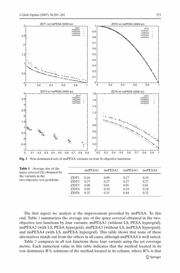
Fig. 3 Non-dominated sets of msPESA variants on four bi-objective functions

Table 1 Average size of thespace covered (S) obtained bythe variants in thetwo-objective test problems

msPESA1 msPESA2 msPESA3 msPESA4

ZDT1 0.16 0.09 0.17 0.10ZDT2 0.27 0.27 0.27 0.27ZDT3 0.06 0.01 0.01 0.01ZDT4 0.05 0.10 0.19 0.10ZDT6 0.32 0.31 0.44 0.32

The first aspect we analyze is the improvement provided by msPESA. To thisend, Table 1 summarizes the average size of the space covered obtained in the two-objective test functions by four variants: msPESA1 (without LS, PESA hypergrid),msPESA2 (with LS, PESA hypergrid), msPESA3 (without LS, msPESA hypergrid),and msPESA4 (with LS, msPESA hypergrid). This table shows that none of thesealternatives stands out from the others in all cases, although msPESA4 is well suited.

Table 2 compares in all test functions these four variants using the set coveragemetric. Each numerical value in this table indicates that the method located in itsrow dominates R% solutions of the method located in its column, where R% is that

276 J Glob Optim (2007) 38:265–281

0

0.5

1

1.5

2

2.5

3

3.5

4

0 0.2 0.4 0.6 0.8 1

ZDT1 (5000 ev)

0

0.1

0.2

0.3

0.4

0.5

0.6

0.7

0.8

0.9

1

0 0.2 0.4 0.6 0.8 1

ZDT2 (5000 ev)

-1

-0.5

0

0.5

1

1.5

2

2.5

3

3.5

0 0.1 0.2 0.3 0.4 0.5 0.6 0.7 0.8 0.9

ZDT3 (5000 ev)

ZDT3msPESANSGA-II

PESASPEA2

0

0.5

1

1.5

2

2.5

0.2 0.3 0.4 0.5 0.6 0.7 0.8 0.9 1

ZDT6 (5000 ev)

ZDT6msPESANSGA-II

PESASPEA2

ZDT6msPESANSGA-II

PESASPEA2

ZDT6msPESANSGA-II

PESASPEA2

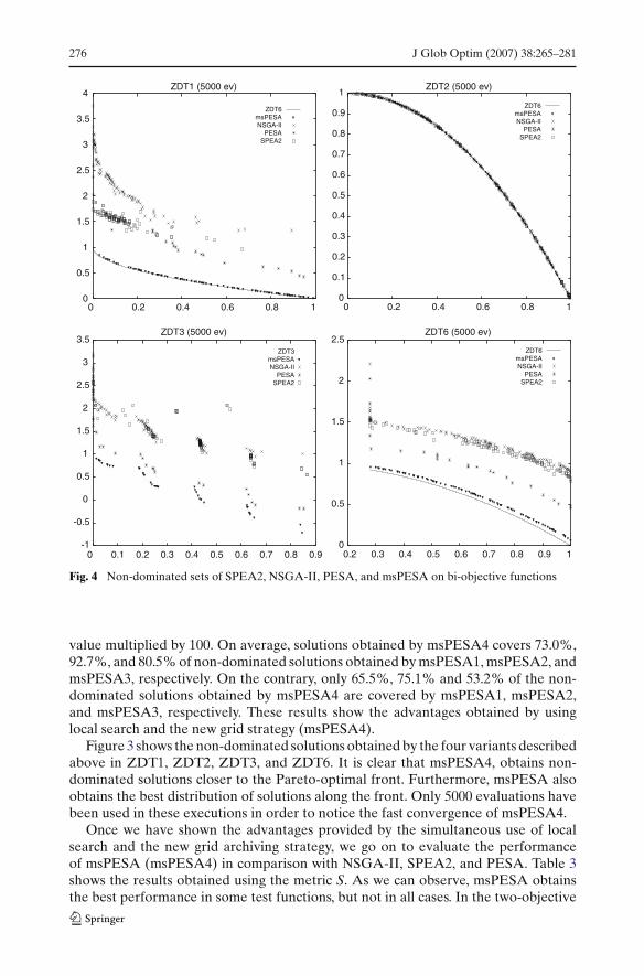
Fig. 4 Non-dominated sets of SPEA2, NSGA-II, PESA, and msPESA on bi-objective functions

value multiplied by 100. On average, solutions obtained by msPESA4 covers 73.0%,92.7%, and 80.5% of non-dominated solutions obtained by msPESA1, msPESA2, andmsPESA3, respectively. On the contrary, only 65.5%, 75.1% and 53.2% of the non-dominated solutions obtained by msPESA4 are covered by msPESA1, msPESA2,and msPESA3, respectively. These results show the advantages obtained by usinglocal search and the new grid strategy (msPESA4).

Figure 3 shows the non-dominated solutions obtained by the four variants describedabove in ZDT1, ZDT2, ZDT3, and ZDT6. It is clear that msPESA4, obtains non-dominated solutions closer to the Pareto-optimal front. Furthermore, msPESA alsoobtains the best distribution of solutions along the front. Only 5000 evaluations havebeen used in these executions in order to notice the fast convergence of msPESA4.

Once we have shown the advantages provided by the simultaneous use of localsearch and the new grid archiving strategy, we go on to evaluate the performanceof msPESA (msPESA4) in comparison with NSGA-II, SPEA2, and PESA. Table 3shows the results obtained using the metric S. As we can observe, msPESA obtainsthe best performance in some test functions, but not in all cases. In the two-objective

J Glob Optim (2007) 38:265–281 277

0 –1 –2 –3 –4 –5 –6 –7 –8 0 1 2 3 4 5 6 7 80

1

2

3

4

5

6

7

8

9

DTLZ1 (lateral)

Pareto frontmsPESANSGA-II

PESASPEA2

Pareto frontmsPESANSGA-II

PESASPEA2

01

23

45

67

8

01

23

45

67

8

0

1

2

3

4

5

6

7

8

9

DTLZ1 (frontal)Pareto front

msPESANSGA-II

PESASPEA2

0 0.2 0.4 0.6 0.8 1 1.2 1.4 1.6 1.80

0.2 0.4

0.6 0.8

1 1.2

1.4 1.6

0

0.2

0.4

0.6

0.8

1

1.2

DTLZ2 (lateral)

0 0.2

0.4 0.6

0.81

1.2 1.4

1.6 1.8

0 0.2

0.4 0.6

0.81

1.2 1.4

1.6

0

0.2

0.4

0.6

0.8

1

1.2

DTLZ2 (frontal)

Pareto FrontmsPESANSGA-II

PESASPEA2

0 0.1 0.2 0.3 0.4 0.5 0.6 0.7 0.8 0.9 10 0.1 0.2 0.3 0.4 0.5 0.6 0.7 0.8 0.91

2468

10 12 14 16 18 20 22

DTLZ7 (lateral)

DTLZ7msPESANSGA-II

PESASPEA2

0 0.1 0.2 0.3 0.4 0.5 0.6 0.7 0.8 0.91

0 0.1 0.2 0.3 0.4 0.5 0.6 0.7 0.8 0.91

2468

10 12 14 16 18 20 22

DTLZ7 (frontal)

DTLZ7msPESANSGA-II

PESASPEA2

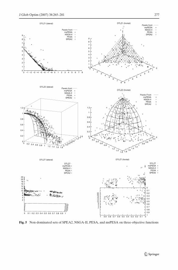
Fig. 5 Non-dominated sets of SPEA2, NSGA-II, PESA, and msPESA on three-objective functions

278 J Glob Optim (2007) 38:265–281

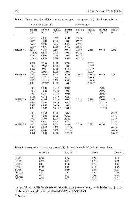
Table 2 Comparison of msPESA alternatives using set coverage metric (C) in all test problems

On each test problem On average

msPES msPES msPES msPES msPES msPES msPES msPESA1 A2 A3 A4 A1 A2 A3 A4

ZDT1 0.091 0.227 0.182 ZDT1ZDT2 1.000 1.000 1.000 ZDT2ZDT3 0.303 0.212 0.272 ZDT3ZDT4 0.571 1.000 0.762 ZDT4

msPESA1 ZDT6 0.185 0.147 0.037 ZDT6 0.635 0.616 0.655DTLZ1 0.980 0.770 1.000 DTLZ1DTLZ2 0.960 0.580 1.000 DTLZ2DTLZ7 0.989 0.989 0.989 DTLZ7

0.947 ZDT1 1.000 0.789 ZDT11.000 ZDT2 1.000 1.000 ZDT20.897 ZDT3 1.000 0.448 ZDT31.000 ZDT4 1.000 1.000 ZDT4

msPESA2 1.000 ZDT6 1.000 0.321 0.664 DTLZ6 0.825 0.7510.020 DTLZ1 0.250 0.470 DTLZ10.450 DTLZ2 0.350 0.980 DTLZ20.000 DTLZ7 1.000 1.000 DTLZ7

1.000 0.000 ZDT1 0.034 ZDT11.000 1.000 ZDT2 1.000 ZDT21.000 0.375 ZDT3 0.025 ZDT30.136 0.182 ZDT4 0.227 ZDT4

msPESA3 0.985 0.106 ZDT6 0.000 0.718 0.578 ZDT6 0.5320.680 1.000 DTLZ1 0.970 DTLZ10.940 0.960 DTLZ2 1.000 DTLZ20.000 1.000 DTLZ7 1.000 DTLZ7

1.000 0.963 1.000 ZDT1 ZDT11.000 1.000 1.000 ZDT2 ZDT21.000 1.000 1.000 ZDT3 ZDT31.000 0.871 1.000 ZDT4 ZDT4

msPESA4 1.000 1.000 1.000 ZDT6 0.730 0.927 0.805 ZDT60.340 0.940 0.250 DTLZ1 DTLZ10.490 0.640 0.190 DTLZ2 DTLZ20.091 1.000 1.000 DTLZ7 DTLZ7

Table 3 Average size of the space covered (S) obtained by the MOEAs in all test problems

msPESA NSGA-II PESA SPEA2

ZDT1 0.10 0.24 0.29 0.19ZDT2 0.27 0.23 0.28 0.23ZDT3 0.01 0.30 0.05 0.46ZDT4 0.10 0.05 0.13 0.02ZDT6 0.32 0.80 0.53 0.81DTLZ1 5.24 1.61 3.49 3.47DTLZ2 0.47 0.25 0.36 0.48DTLZ7 0.28 0.27 0.16 0.21

test problems msPESA clearly obtains the best performance, while in three-objectiveproblems it is slightly worse than SPEA2, and NSGA-II.

J Glob Optim (2007) 38:265–281 279

Table 4 Comparison of MOEAs using set coverage metric (C) in all test problems

On each test problem On average

msPESA NSGA-II PESA SPEA2 msPESA NSGA-II PESA SPEA2

ZDT1 1.000 1.000 1.000 ZDT1ZDT2 1.000 1.000 1.000 ZDT2ZDT3 1.000 1.000 1.000 ZDT3ZDT4 1.000 1.000 1.000 ZDT4

msPESA ZDT6 1.000 1.000 1.000 ZDT6 0.935 0.946 0.945DTLZ1 0.890 0.790 0.810 DTLZ1DTLZ2 0.820 0.870 0.940 DTLZ2DTLZ7 0.870 0.910 0.810 DTLZ7

0.300 ZDT1 0.000 0.000 ZDT11.000 ZDT2 1.000 1.000 ZDT20.180 ZDT3 0.010 0.200 ZDT30.810 ZDT4 0.580 0.510 ZDT4

NSGA-II 0.050 ZDT6 0.060 0.020 0.666 DTLZ6 0.578 0.5851.000 DTLZ1 0.990 1.000 DTLZ10.990 DTLZ2 0.990 1.000 DTLZ21.000 DTLZ7 0.990 0.950 DTLZ7

0.208 1.000 ZDT1 0.750 ZDT10.700 0.890 ZDT2 0.800 ZDT20.308 1.000 ZDT3 1.000 ZDT30.476 1.000 ZDT4 1.000 ZDT4

PESA 0.077 0.885 ZDT6 0.808 0.503 0.893 ZDT6 0.8720.680 1.000 DTLZ1 0.970 DTLZ10.750 0.610 DTLZ2 0.940 DTLZ20.830 0.760 DTLZ7 0.710 DTLZ7

0.090 1.000 0.360 ZDT1 ZDT11.000 1.000 1.000 ZDT2 ZDT20.100 0.560 0.000 ZDT3 ZDT30.890 0.600 0.520 ZDT4 ZDT4

SPEA2 0.010 0.960 0.300 ZDT6 0.546 0.815 0.595 ZDT60.770 0.900 0.990 DTLZ1 DTLZ10.540 0.520 0.610 DTLZ2 DTLZ20.970 0.980 0.980 DTLZ7 DTLZ7

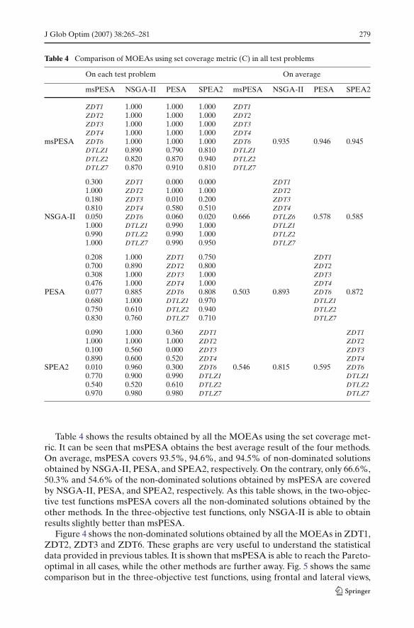
Table 4 shows the results obtained by all the MOEAs using the set coverage met-ric. It can be seen that msPESA obtains the best average result of the four methods.On average, msPESA covers 93.5%, 94.6%, and 94.5% of non-dominated solutionsobtained by NSGA-II, PESA, and SPEA2, respectively. On the contrary, only 66.6%,50.3% and 54.6% of the non-dominated solutions obtained by msPESA are coveredby NSGA-II, PESA, and SPEA2, respectively. As this table shows, in the two-objec-tive test functions msPESA covers all the non-dominated solutions obtained by theother methods. In the three-objective test functions, only NSGA-II is able to obtainresults slightly better than msPESA.

Figure 4 shows the non-dominated solutions obtained by all the MOEAs in ZDT1,ZDT2, ZDT3 and ZDT6. These graphs are very useful to understand the statisticaldata provided in previous tables. It is shown that msPESA is able to reach the Pareto-optimal in all cases, while the other methods are further away. Fig. 5 shows the samecomparison but in the three-objective test functions, using frontal and lateral views,

280 J Glob Optim (2007) 38:265–281

respectively. Lateral views provide better information on the proximity to the Pareto-optimal front, while frontal views are suitable to have an idea about the distributionof the solutions. For instance, in the lateral view of DTLZ2 it is clear that SPEA2 isfar from the Pareto-optimal front, while the frontal view shows that msPESA obtainsa good distribution.

6 Conclusions

In this paper, we have proposed a new hybrid multi-objective evolutionary algorithmbased on combining some aspects of NSGA-II, and PESA. Furthermore, this newapproach also includes a local search procedure in an attempt to improve the qual-ity of the solutions. The performance of this new multi-objective meta-heuristic hasbeen compared with three well-known MOEAs on a suite of five two-objective andthree three-objective test problems. Although establishing an order of merit betweendifferent algorithms is a difficult task, the use of accurate metrics can evaluate theirperformance. Metrics used in our experimental analysis, set coverage metric, and aver-age size of the space covered, evaluate the quality of the non-dominated solutions interms of closeness to the global Pareto-optimal fronts. First conclusion obtained fromthe results is that the use of the K-1 dimensional hypergrid scheme in combinationwith local search outperforms the quality of the solutions. On the other hand, resultsdemonstrate that msPESA is able to reach the Pareto-optimal fronts in the two-objec-tive test functions, and be close in the three-objective one. In comparison with theother methods, msPESA obtains the best results in the two-objective test functions,while in the three-objective problems is very close to SPEA2 and NSGA-II.

Acknowledgements This work was supported by the Spanish MCyT under contract TIN2005-00447.Authors appreciate the support of the "Structuring the European Research Area" program, RII3-CT-2003-506079, funded by the European Commission.

References

1. Horst, R., Pardalos, P.M. (eds.): Handbook of global optimization. Kluwer Academic Publishers,Dordrecht (1995)

2. Benson, H.P.: An outer approximation algorithm for generating all efficient extreme points inthe outcome set of a multiple-objective linear programming problem. J. Global Optim. 13,1–24 (1998)

3. Horst, R., Thoai, N.V.: Maximizing a concave function over the efficient or weakly-efficientset. Eur. J. Oper. Res. 117, 239–252 (1999)

4. Hajela, P., Y-Lin, C.: Genetic search strategies in multi-criterion optimal design. Struct.Optim. 4, 99–107 (1992)

5. Goldberg, D.E.: Genetic algorithms in search, optimization and machine learning. AddisonWesley, New York (1989)

6. Deb K.: Multi-objective optimization using evolutionary algorithms. John Wiley & Sons (2002)7. Coello, C. A., Van Veldhuizen, D.A., Lamont, G.B.: Evolutionary algorithms for solving multi-

objective problems. Kluwer Academic Publishers (2002)8. Fonseca, C. M., Flemming, P.J.: Genetic algorithms for multiobjective optimization: formula-

tion, discusion and generalization. Proceedings of the Fifth International Conference on GeneticAlgorithms, San Mateo, California, 416–423 (1993)

9. Horn, J., Nafpliotis N., Goldberg D.: A niched pareto genetic algorithm for multiobjective opti-mization. Proceedings of the First IEEE Conference on Evolutionary Computation, Piscataway,New Jersey, USA, 82–87 (1994)

J Glob Optim (2007) 38:265–281 281

10. Srinivas, N., Deb, K.: Multiobjective optimization using nondominated sorting in genetic algo-rithms. Evol. Comput. 2(3), 221–248 (1994)

11. Deb, K., Agrawal, S., Pratap, A., Meyarivan, T.: A fast elitist non-dominated sorting ge-netic algorithm for multiobjective optimization: nusa-ii. Springer Lecture Notes in Computer Sci-ence. 1917, 849–858 (2000)

12. Zitzler, E., Thiele, L.: Multiobjective evolutionary algorithms: a comparative case study and thestrength pareto approach. IEEE Trans. Evol. Comput. 3(4), 257–271 (1999)

13. Zitzler, E., Laumanns, M., Thiele, L.: SPEA2: improving the strength pareto evolutionary algo-rithm. Technical Report 103, Computer Engineering and Networks Laboratory (TIK), SwissFederal Institute of Technology (ETH) Zurich, Switzerland (2001)

14. Knowles, J.D., Corne D.W.: The pareto archived evolution strategy: a new baseline algorithm forpareto multiobjective optimisation. Proceedings of the Congress on Evolutionary Computation,Piscataway, NJ, 98–105 (1999)

15. Corne, D.W., Knowles, J.D., Oates, H.J.: The pareto-envelope based selection algorithm formultiobjective optimisation. Springer Lecture Notes in Computer Science. 1917, 869–878 (2000)

16. Baños, R., Gil, C., Paechter, B., Ortega, J.: A hybrid meta-heuristic for multi-objective optimiza-tion: MOSATS. J. Math. Model. Algorithm, DOI: 10.1007/s10852-006-9041-6: (2006)

17. Talbi, E.: A taxonomy of hybrid metaheuristics. J. Heuristics. 8(5), 541–564 (2002)18. Deb, K., Thiele, L., Laumanns, M., Zitzler, E. Scalable test problems for evolutionary multi-

objective optimization. Evolutionary computation based multi-criteria optimization: theoreticaladvances and applications. Springer-Verlag, USA 105–145: (2005)

19. Zitler, E., Deb, K., Thiele, L.: Comparison of multiobjective evolutionary algorithms: empiricalresults. Evolu. Comput. 8(2), 173–195 (2000)

20. Veldhuizen, D.V.: Multiobjective evolutionary algorithms: classifications, analyses, and new inno-vations. PhD thesis, Department of Electrical and Computer Engineering. Graduate School ofEngineering, Air Force Institute of Technology, Wright-Patterson AFB, Ohio (1999)

21. Deb, K., Thiele, L., Laumanns, M., Zitler, E.: Constrained test problems for multi-objective evo-lutionary optimization. Proceedings of First International Conference on Evolutionary Multi-Criterion Optimization, 284–298 (2001)