On Solving Fully Rough Multi-Objective Integer Linear ...

DJS 41 (2020) 1-11

Delta Journal of Science

Available online at https://djs.journals.ekb.eg/

Research Article MATHEMATICS

On Solving Fully Rough Multi-Objective Integer Linear Programming Problems

Authors: El-Saeed Ammar, Abdusalam Emsimir

Affiliations: Department of mathematics, Faculty of science. Tanta University.

KEY WORDS

ABSTRACT

Integer linear programming, weightings, ε- Constraint, Upper approximation, Lower approximation, Multi Objective, Crisp coefficients.

In this paper a suggested algorithm to solve fully rough multi-objective integer linear programming problem [FRMOILP] is described. In order to solve this problem and find rough value efficient solutions and decision rough integer variables by the slice-sum method with the branch and bound technique, we will use two methods, the first one is the method of weights and the second is ε- Constraint method. The basic idea of the computational phase of the algorithm is based on constructing two LP problems with interval coefficients, and then to four crisp LPs. In addition to determining the weights and the values of ε-constraint. Also, we reviewed some of the advantages and disadvantages for them. We used integer programming because many linear programming problems require that the decision variables are integers. Also, rough intervals (RIs) are very important to tackle the uncertainty and imprecise data in decision making problems. In addition, the proposed algorithm enables us to search for the efficient solution in the largest range of possible solutions range. Also, we obtain N suggested solutions and which enables the decision maker to choose the best decisions. Finally, two numerical examples are given to clarify the obtained results in the paper.

© Faculty of Science, Tanta University.

1. Introduction

Linear programming (LP) is one of the most popular models used in decision making and optimization problems. Many researches, studies and applications of LP models have

been reported in numerous books, monographs, articles and chapters in books, for instance see [3,5]. Taha. H. T, (1997) Integer programming (IP) problems are optimization problems that

2 El-Saeed Ammar

min or max the objective function taking into consideration the limits of constraints and integer variables. More widely application of integer programming can be used to appropriately describe the decision problems on the management and effective use of resources in engineering technology, business management and other numerous fields [15]. Rough set theory (RST) was initiated by Pawlak in (1982) as a method for ambiguity management

[10]. RST approach has fundamental importance in the fields of pattern recognition, data mining, artificial intelligence, machine learning and medical applications [8]. For a vague concept R, a lower approximation is contained of all objects which surely belong to the concept R and an upper approximation is contained of all objects which possibly belong to the concept R. In other words, the lower approximation of the concept is the union of all elementary concepts which are included in it, whereas the upper approximation is the union of all elementary concepts which have nonempty intersection with the concept [11]. Ammar and Khalifa in (2014) applied a new method named, separation method for solving Rough Interval Multi Objective Transportation Problems (RIMOTP), where transportation cost, supply and demand are rough intervals [1] Also, they discussed the separation method as an important tool for the decision makers when they are handling various types of logistic problems having rough interval parameters of transportation problems. Osman et al, in (2016) presented a solution approach for RIMOTP. The concept of solving conventional interval programming combined with fuzzy programming is used to build the solution approach for RIMOTP [9]. G. Mavrotas in (2009) Effective implementation of the ε-constraint method in Multi-Objective Mathematic programming problems see [20]. In this paper, the focus of our study is improvement a method to solve fully rough multi objective integer linear programming

(FRMOILP) problems. For determine rough value efficient solutions and rough decision integer optimal value. Also, we will obtain on solutions such as completely satisfactory solutions (surely solutions) and rather satisfactory solutions (possibly solutions) by lower approximation interval and upper approximations interval respectively. In our problem we assume that all parameters and decision variables in the both of constraints and the objective functions are rough intervals (RIs). We used integer programming because many linear programming (LP) problems require that the decision variables are integers. Also, rough intervals are very important to tackle the uncertainty and imprecise data in decision making problems. In addition, the proposed algorithm enables us to search for the optimal solution in the largest range of possible solutions range. The rest of the paper is organized as follows. In Section 2, some basic about the preliminaries of RIs are presented and problem formulation and solution concept. In section 3, the weighting problem and procedures for the solution FRMOILP problems were considered. In section 4 the ε-constraint method was described. In addition, we will use slice-sum method [12] with the branch and bound technique for solving FRMOILP problems. Numerical examples for demonstrating the solution procedure of the proposed method and the conclusion are given.

2. Problem Formulation and solution concept

2.1. Fully Rough Multi objective Integer Linear Programming Problems

Let 𝐴 , 𝐵 represent the two sets of rough intervals. A rough interval multi-objective linear programming (FRMOILP) problems, see [17] with "k" linear objective functions

𝑀𝑎𝑥 𝑓 (𝑥) = 𝐶 𝑥 , 𝑟 = 1,2, … 𝑘, as

3 On Solving Fully Rough Multi-Objective Integer Linear Programming Problems

𝑴𝒂𝒙 𝑓 (𝑥) =

( 𝑓 (𝑐 , 𝑥 ), 𝑓 (𝑐 , 𝑥 ), … , 𝑓 (𝑐 , 𝑥 ))

𝑆𝑢𝑏𝑗𝑒𝑐𝑡 𝑡𝑜

𝑥 ∈ 𝑋 = 𝑥 ∈ ℛ | 𝑔 (𝐴 , 𝑥 ) ≤ 𝐵 , 𝑥 ≥ 0 ⎭⎪⎬

⎪⎫

(1)

where

𝐴 = [ 𝑎 ] ∗ , 𝐵 = (𝑏 , 𝑏 , … , 𝑏 ) , 𝑥 =

(𝑥 , 𝑥 , … , 𝑥 ) and 𝐶 = (𝑐 , 𝑐 , … , 𝑐 ), 𝑟 =

1, … , 𝑠𝑒𝑡 𝑜𝑓 𝑘 , 𝑖 ∈ 𝐼 , 𝑗 ∈ 𝐽 , 𝐼 = 1, … , 𝑛 , 𝐽 =

1, … , 𝑚 are rough interval integer parameters 𝑥 denote a set of decision rough variables, 𝑓 denote rough objective function.

Definition 1 (Rough efficient solution) [1]: The rough vector 𝑥∗ (𝐴∗ , 𝐵∗ ) which satisfies the condition in problem (1), is called a rough efficient solution of problem (1), if and only if there does not exist another 𝑥 (𝐴 , 𝐵 ) ∈ 𝑋 such that

𝑓 (𝑐 , 𝑥 ) ≤ 𝑓∗ (𝑐∗ , 𝑥∗ )

For all r and 𝑓 (𝑥 ) ≠ 𝑓 (𝑥∗ ) for at least one r = 1, 2,…,K and 𝑖 ∈ 𝐼 , 𝑗 ∈ 𝐽 where from (1) we have:

𝐶∗ = [ 𝐶∗ , 𝐶∗ , 𝐶∗ , 𝐶∗ ]

𝑎∗ = [ 𝑎∗ , 𝑎∗ , 𝑎∗ , 𝑎∗ ]

𝑏∗ = [ 𝑏∗ , 𝑏∗ , 𝑏∗ , 𝑏∗ ]

𝑥∗ = [ 𝑥∗ , 𝑥∗ , 𝑥∗ , 𝑥∗ ]

r = 1, 2,…, k , I=1,2,...,n , J= 1,2,…,m

3. The weighting problem

The idea is to associate each objective function with a weighting coefficient and minimize the weight sum of the objectives. In this way multiple objective function are transformed into a single objective function. We suppose that the weighting coefficient w are real numbers such that w ≥ 0 for all r =1, 2,…,k . It is also usually supposed that the weight is normalized

that is ∑ w = 1.

To be more exact, the multi objective optimized problem is modified into the following problem to be called a weighting that problem (2) LP (w):

𝑴𝒂𝒙𝒊𝒎𝒊𝒛𝒆 𝑤 𝑓 (𝑐 , 𝑥 )

𝑆𝑢𝑏𝑗𝑒𝑐𝑡 𝑡𝑜

𝑥 ∈ 𝑋 = {𝑥 ∈ ℛ | 𝐴 𝑥 ≤ 𝐵 , 𝑥 ≥ 0 𝑎𝑛𝑑 𝑖𝑛𝑡𝑒𝑔𝑒𝑟𝑠 }

𝑊ℎ𝑒𝑟𝑒 𝑤 ∈ 𝑊 = 𝑤 ∈ ℛ , 𝑤 ≥ 0 𝑎𝑛𝑑 𝑤 = 1⎭⎪⎪⎬

⎪⎪⎫

(2)

The relationship between the optimal solution 𝑥∗ of the weighting problem (2) and the efficient solution of problem (1) can be characterized by the following theorems [16, 18].

Theorem 1 If 𝑥∗(w∗) ∈ X is optimal solution of the weighting problem (2) for some w∗ > 0, then 𝑥∗ is optimal solution of problem (1).

Theorem 2 If x∗ ∈ X is an optimal solution of problem (1) then there exists w∗ ∈ W such that

𝑥∗ solves LP (w∗) and if either one of the following two conditions holds: (i) w∗ > 0, 𝑓𝑜𝑟 𝑎𝑙𝑙 𝑟 = 1,2, … , 𝑘, 𝑜𝑟 (ii) 𝑥∗ is the unique optimal solution for a given (𝑤∗).

The weighting problem determines the complete set of optimal solution of problem (2) if the problem is convex.

3.1. Procedures for the solution FRMOILP

problems:

Step (1): The idea is to associate each objective function with a weighting coefficient and maximize the weight sum of the objectives:

𝑀𝑎𝑥 𝑤 (𝑐 𝑥 ) + 𝑤 (𝑐 𝑥 ) + ⋯ + 𝑤 (𝑐 𝑥 )

𝑆. 𝑡 ∑ 𝑎 𝑥 ≤ 𝑏 𝑗 ∈ 𝐽

𝑤ℎ𝑒𝑟𝑒 𝑥 ≥ 0 𝑟𝑜𝑢𝑔ℎ 𝑖𝑛𝑡𝑒𝑔𝑒𝑟𝑠 𝑗 𝐽 = {1, … , 𝑚}

𝑤 ≥ 0 𝑓𝑜𝑟 𝑟 = 1,2, … , 𝑘 𝑎𝑛𝑑 ∑ 𝑤 = 1

⎭⎪⎬

⎪⎫

(3)

and then will deal with a single objective function.

4 El-Saeed Ammar

Step (2): The general FRMOILP problem after the first step to become as a single problem (4).

([𝐼𝐿𝑃 ], [𝐼𝐿𝑃 ]) = 𝑀𝑎𝑥

𝑤 ([𝑐 , 𝑐 ]: [𝑐 , 𝑐 ])⨂([ 𝑥 , 𝑥 ]: [ 𝑥 , 𝑥 ])

𝑠. 𝑡

( 𝑎 , 𝑎 : [𝑎 , 𝑎 ])⨂( 𝑥 , 𝑥 : [ 𝑥 , 𝑥 ])

≤ ([𝑏 , 𝑏 ] ∶ [𝑏 , 𝑏 ])

𝑥 , 𝑥 , 𝑥 , 𝑥 ≥ 0 , 𝑤ℎ𝑒𝑟𝑒 𝑗 ∈ 𝐽

𝑎𝑛𝑑 𝑟𝑜𝑢𝑔ℎ 𝑖𝑛𝑡𝑒𝑔𝑒𝑟 𝑣𝑎𝑟𝑖𝑎𝑏𝑙𝑒𝑠 ⎭⎪⎪⎪⎪⎬

⎪⎪⎪⎪⎫

(4)

Where ([ 𝑐 , 𝑐 ] , [𝑐 , 𝑐 ]) ,

([ 𝑎 , 𝑎 ] , [𝑎 , 𝑎 ]) , ([𝑏 , 𝑏 ] , [𝑏 , 𝑏 ])

And 𝑥 , 𝑥 , 𝑥 , 𝑥 (𝐼 = 1, … , 𝑛; 𝐽 = 1, … , 𝑚)

are rough intervals coefficient and variables of the objective function and the constraints.

Step (3): Find the possibly optimal range or the upper approximation interval [UAI] as [ILP , ILP ] By solving integer interval linear programming as following:

𝐼𝐿𝑃 = 𝑀𝑎𝑥 𝑤 [𝑐 , 𝑐 ]⨂[𝑥 , 𝑥 ]

𝑆. 𝑡 𝑎 , 𝑎 ⨂ 𝑥 , 𝑥 ≤ [𝑏 , 𝑏 ]

𝑥 , 𝑥 ≥ 0 , 𝑤ℎ𝑒𝑟𝑒 𝑖 ∈ 𝐼 , 𝑗 ∈ 𝐽

and integer variables, (𝐼 = 1, … , 𝑛; 𝐽 = 1, … , 𝑚) .

⎭⎪⎪⎬

⎪⎪⎫

(5)

Step (4): Find the surly optimal range or the lower approximation interval [LAI] as [ILP , ILP ]by solving the following:

𝐼𝐿𝑃 = 𝑀𝑎𝑥 𝑤 𝑐 , 𝑐 ⨂ 𝑥 , 𝑥

𝑆. 𝑡 𝑎 , 𝑎 ⨂ 𝑥 , 𝑥 ≤ [𝑏 , 𝑏 ]

𝑥 , 𝑥 ≥ 0 , 𝑤ℎ𝑒𝑟𝑒 𝑖 ∈ 𝐼 , 𝑗 ∈ 𝐽

and integer variables (𝐼 = 1, … , 𝑛; 𝐽 = 1, … , 𝑚). ⎭⎪⎪⎬

⎪⎪⎫

(6)

Step (5): According to step (3), the possibly optimal range of problem (5) by solving two classical LPs as follows

𝐼𝐿𝑃 : = 𝑀𝑎𝑥 𝑤 𝑐 𝑥

𝑆. 𝑡 𝑎 𝑥 ≤ 𝑏

𝑥 ≥ 0 𝑎𝑛𝑑 𝑖𝑛𝑡𝑒𝑔𝑒𝑟𝑠 𝑖 ∈ 𝐼 , 𝑗 ∈ 𝐽

𝐽 = 1, … … , 𝑚 , 𝐼 = 1, … … , 𝑛 ⎭⎪⎪⎬

⎪⎪⎫

(7)

And




𝐽 = 1, … … , 𝑚 , 𝐼 = 1, … … , 𝑛 ⎭⎪⎪⎬

⎪⎪⎫

(8)

Step (6) The surly optimal range of problem (6) follows by solving the two classical LPs:




𝐽 = 1, … … , 𝑚 , 𝐼 = 1, … … , 𝑛

⎭⎪⎪⎬

⎪⎪⎫

(9)

And




𝐽 = 1, … … , 𝑚 , 𝐼 = 1, … … , 𝑛

⎭⎪⎪⎬

⎪⎪⎫

(10)

where the rough optimal values (𝑍∗ ) and

rough integer efficient solutions (𝑥∗ ) will be

as:

𝑍∗ = [𝑧∗ , 𝑧∗ ], 𝑧∗ , 𝑧∗

𝑥∗ = 𝑥∗ , 𝑥∗ , 𝑥∗ , 𝑥∗ (𝑗 = 1, … , 𝑛)

In addition, the possible optimal values range for problem (5) are [𝑧∗ , 𝑧∗ ] and the surely optimal values range for problem (6) are [𝑧∗ , 𝑧∗ ]. Also, the intervals 𝑥∗ , 𝑥∗ jJ

are the integer completely satisfactory solutions. Furthermore, the intervals 𝑥∗ , 𝑥∗ jJ are

integer rather satisfactory solutions.


Definition 2 Consider all of the corresponding FRMOILP problems and LP of problem (4).

(a) The interval[𝐼𝐿𝑃 , 𝐼𝐿𝑃 ]([𝐼𝐿𝑃 , 𝐼𝐿𝑃 ]) is called the surely (possibly) optimal range symbolized [𝐼𝐿𝑃 ] ([𝐼𝐿𝑃 ]) of problem (4), if the optimal range of each (ILPFRI) is a superset (subset) of [𝐼𝐿𝑃 , 𝐼𝐿𝑃 ]([𝐼𝐿𝑃 , 𝐼𝐿𝑃 ]).

(b) Let [𝐼𝐿𝑃 , 𝐼𝐿𝑃 ]([𝐼𝐿𝑃 , 𝐼𝐿𝑃 ]) be surely optimal (possibly) optimal range of the problem (4). Then the rough interval ([𝐼𝐿𝑃 , 𝐼𝐿𝑃 ], [𝐼𝐿𝑃 , 𝐼𝐿𝑃 ]) is called the rough optimal range of problem (4), also any point, optimal value belongs to [𝐼𝐿𝑃 , 𝐼𝐿𝑃 ], ([𝐼𝐿𝑃 , 𝐼𝐿𝑃 ]) is called a completely (rather) satisfactory solution of the problem (4).

(c) A solution 𝑥∗ is surely-feasible, iff it belongs to the lower approximation of the feasible set.

(d) A solution 𝑥∗ is possibly -feasible, iff it belongs to the upper approximation of the feasible set.

(e) A solution 𝑥∗ is surely-not feasible, iff it does not belong to the upper approximation of the feasible set [2,7].

Now, the establish of the relation between optimal solutions of the integer linear programming problem with fully rough intervals for problem (4) and four problems ILPUU, ILPLU, ILPLL and ILPUL the problems (7), (8), (9) and (10) respectively. The established relation is used in the proposed method, namely, slice-sum method.

Theorem 3 [14] If the set { 𝑥 , for all 𝑗 ∈ 𝐽} is an optimal

solution for the (𝐼𝐿𝑃 ) or (7) problem of the problem (4) with the maximum optimal value for (𝑍 ) , the set { 𝑥 , for all 𝑗 ∈ 𝐽} is an

optimal solution for the (𝐼𝐿𝑃 ) or (10) problem of the problem (4) with the maximum optimal value for (𝑍 ), the set {𝑥 , for all 𝑗 ∈

𝐽} is an optimal solution for the (𝐼𝐿𝑃 ) or (9)

problem of the problem (4) with the maximum optimal value for (𝑍 ), the set {𝑥 , for all 𝑗 ∈

𝐽} is an optimal solution for the (𝐼𝐿𝑃 ) or (8) problem of the problem (4) with the maximum optimal value for (𝑍 ), then the set of rough integer intervals { 𝑥 , 𝑥 , 𝑥 , 𝑥 , for all 𝑗 ∈ 𝐽} is an optimal solution for the problem (4) with maximum optimal values [𝑧 , 𝑧 ], 𝑧 , 𝑧 provided 𝑥 ≤ 𝑥 ≤ 𝑥 ≤ 𝑥 , for all 𝑗 ∈ 𝐽.

Proof: Since {𝑥 , for all 𝑗 ∈ 𝐽}, {𝑥 , for all 𝑗 ∈

𝐽} , {𝑥 , for all 𝑗 ∈ 𝐽} , {𝑥 , for all 𝑗 ∈ 𝐽} are optimal solutions for the problems 𝐼𝐿𝑃 , 𝐼𝐿𝑃 , 𝐼𝐿𝑃 and 𝐼𝐿𝑃 , respectively and 𝑥 ≤ 𝑥 ≤ 𝑥 ≤ 𝑥 , for all 𝑗 ∈ 𝐽, then we can conclude that the set of rough integer intervals { 𝑥 , 𝑥 , 𝑥 , 𝑥 , for all 𝑗 ∈ 𝐽} is a feasible solution to the problem (4).

Let { 𝑥∗ , 𝑥∗ , 𝑥∗ , 𝑥∗ , for all 𝑗 ∈

𝐽} be a feasible solution to the problem (4).

Therefore { 𝑥∗ , for all 𝑗 ∈ 𝐽}, {𝑥∗ , for all 𝑗 ∈

𝐽} , {𝑥∗ , for all 𝑗 ∈ 𝐽} , {𝑥∗ , for all 𝑗 ∈ 𝐽}

are feasible solutions to the problems 𝐼𝐿𝑃 , 𝐼𝐿𝑃 , 𝐼𝐿𝑃 𝑎𝑛𝑑 𝐼𝐿𝑃 , respectively.

Since {𝑥 , for all 𝑗 ∈ 𝐽}, {𝑥 , for all 𝑗 ∈ 𝐽} ,

{𝑥 , for all 𝑗 ∈ 𝐽}, {𝑥 , for all 𝑗 ∈ 𝐽} are

feasible solutions to the problems 𝐼𝐿𝑃 , 𝐼𝐿𝑃 , 𝐼𝐿𝑃 𝑎𝑛𝑑 𝐼𝐿𝑃 , respectively. We have:

𝑍 = 𝑐 𝑥∗ ≥ 𝑐 𝑥 ,

𝑍 = 𝑐 𝑥∗ ≥ 𝑐 𝑥 ,

𝑍 = 𝑐 𝑥∗ ≥ 𝑐 𝑥 ,

𝑎𝑛𝑑 𝑍 = 𝑐 𝑥∗ ≥ 𝑐 𝑥 .

6 El-Saeed Ammar

This implies that [𝑍 , 𝑍 ]: 𝑍 , 𝑍 =

( 𝑐 , 𝑐 : [𝑐 , 𝑐 ]) ⨂ ( 𝑥 , 𝑥 : [ 𝑥 , 𝑥 ])

And

𝑐 , 𝑐 : 𝑐 , 𝑐 ⊗

𝒎

𝒋 𝟏

𝑥∗ , 𝑥∗ : 𝑥∗ , 𝑥∗

≥ 𝑐 , 𝑐 : 𝑐 , 𝑐 ⊗

𝒎

𝒋 𝟏

𝑥 , 𝑥 : 𝑥 , 𝑥

Therefore, the set of rough integer intervals

{ 𝑥∗ , 𝑥∗ : 𝑥∗ , 𝑥∗ , for all 𝑗 ∈ 𝐽} is

optimal solution for the problem (4) with maximum

optimal values [𝑍 , 𝑍 ], 𝑍 , 𝑍 . Hence,

the theorem is proved [14].

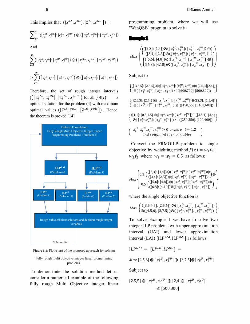
Figure (1): Flowchart of the proposed approach for solving

Fully rough multi objective integer linear programming problems.

To demonstrate the solution method let us consider a numerical example of the following fully rough Multi Objective integer linear

programming problem, where we will use ''WinQSB'' program to solve it.

Example 1

𝑀𝑎𝑥

⎝

⎜⎛

([2,3]: [1,4])⨂([ 𝑥 , 𝑥 ]: [ 𝑥 , 𝑥 ]) ⊕

([3,4]: [2,5])⨂([ 𝑥 , 𝑥 ]: [ 𝑥 , 𝑥 ]) ,

([5,6]: [4,8])⨂([ 𝑥 , 𝑥 ]: [ 𝑥 , 𝑥 ])⨁

([6,8]: [4,10])⨂([ 𝑥 , 𝑥 ]: [ 𝑥 , 𝑥 ]) ⎠

⎟⎞

Subject to

([ 3,3.5]: [2.5,5])⨂([ 𝑥 , 𝑥 ]: [𝑥 , 𝑥 ])⨁([2.5,3][2,4])

⨂( [ 𝑥 , 𝑥 ]: [ 𝑥 , 𝑥 ]) ≤ ([600,700], [500,800])

([2.5,3]: [2,4]) ⨂([ 𝑥 , 𝑥 ]: [ 𝑥 , 𝑥 ])⨁([3,3]: [1.5,4])

⨂( [ 𝑥 , 𝑥 ]: [ 𝑥 , 𝑥 ] ) ≤ ([450,550]: [400,600])

([1,1]: [0.5,1.5] ⨂([ 𝑥 , 𝑥 ]: [ 𝑥 , 𝑥 ])⨁([3.5,4]: [3,4)

⨂( [ 𝑥 , 𝑥 ]: [ 𝑥 , 𝑥 ] ) ≤ ([250,350], [100,400])

𝑥 , 𝑥 , 𝑥 , 𝑥 ≥ 0 , 𝑤ℎ𝑒𝑟𝑒 𝑖 = 1,2

𝑎𝑛𝑑 𝑟𝑜𝑢𝑔ℎ 𝑖𝑛𝑡𝑒𝑔𝑒𝑟 𝑣𝑎𝑟𝑖𝑎𝑏𝑙𝑒𝑠

Convert the FRMOILP problem to single objective by weighting method 𝑓(𝑥) = 𝑤 𝑓 +

𝑤 𝑓 where 𝑤 = 𝑤 = 0.5 as follows:

𝑀𝑎𝑥

⎩⎪⎨

⎪⎧0.5

([2,3]: [1,4])⨂([ 𝑥 , 𝑥 ]: [ 𝑥 , 𝑥 ])⨁

([3,4]: [2,5])⨂([ 𝑥 , 𝑥 ]: [ 𝑥 , 𝑥 ]) ⨁

0.5 ([5,6]: [4,8])⨂([ 𝑥 , 𝑥 ]: [ 𝑥 , 𝑥 ])⨁

([6,8]: [4,10])⨂([ 𝑥 , 𝑥 ]: [ 𝑥 , 𝑥 ]) ⎭⎪⎬

⎪⎫

where the single objective function is

𝑀𝑎𝑥 ([3.5,4.5], [2.5,6]) ⨂( [ 𝑥 , 𝑥 ], [ 𝑥 , 𝑥 ])

⨁([4.5,6], [3,7.5] )⨂( [ 𝑥 , 𝑥 ], [ 𝑥 , 𝑥 ])

To solve Example 1 we have to solve two integer ILP problems with upper approximation interval (UAI) and lower approximation interval (LAI) [ILP , ILP ] as follows:

I𝐿𝑃 = [𝐿𝑃 , 𝐿𝑃 ] =

𝑀𝑎𝑥 [2.5,6] ⨂ [ 𝑥 , 𝑥 ] ⨁ [3,7.5]⨂[ 𝑥 , 𝑥 ]

Subject to

[2.5,5] ⨂ [ 𝑥 , 𝑥 ] ⨁ [2,4]⨂ [ 𝑥 , 𝑥 ]

≤ [500,800]

Solution for

Problem Formulation Fully Rough Multi-Objective Integer Linear

Programming Problems (Problem 4)

LAIILP(Problem 6)

UAIILP(Problem 5)

LLILP(Problem 9)

LUILP(Problem8)

ULILP(Problem 10)

UUILP(Problem 7)

Rough value efficient solutions and decision rough integer variables


[2,4]⨂[ 𝑥 , 𝑥 ] ⨁ [1.5,4]⨂[ 𝑥 , 𝑥 ]

≤ [400,600]

[0.5,1.5]⨂[ 𝑥 , 𝑥 ]⨁[3,4]⨂[ 𝑥 , 𝑥 ]

≤ [100,400]

𝑥 , 𝑥 ≥ 0 , 𝑤ℎ𝑒𝑟𝑒 𝑗 = 1,2 ,

𝑖 = 1,2 𝑎𝑛𝑑 𝑖𝑛𝑡𝑒𝑔𝑒𝑟 𝑣𝑎𝑟𝑖𝑎𝑏𝑙𝑒𝑠

[𝐿𝑃 , 𝐿𝑃 ] = 𝐼𝐿𝑃 =

𝑀𝑎𝑥 [3.5,4.5]⨂[ 𝑥 , 𝑥 ]⨁ [4.5,6]⨂[ 𝑥 , 𝑥 ]

Subject to

[3,3.5]⨂ [ 𝑥 , 𝑥 ]⨁ [2.5,3] ⨂[ 𝑥 , 𝑥 ]

≤ [600,700]

[2.5,3] ⨂[ 𝑥 , 𝑥 ] ⨁ [3,3] ⨂[ 𝑥 , 𝑥 ]

≤ [450,550]

[1,1] ⨂[ 𝑥 , 𝑥 ] ⨁ [3.5,4] ⨂[ 𝑥 , 𝑥 ]

≤ [250,350]

𝑥 , 𝑥 ≥ 0 , where 𝑗 = 1, 2 ;

𝑖 = 1, 2 and integer variables

In the ILPFI Problem (ILP ) is transformed to LP problems ILP and ILP , and in the

ILPFI Problem (ILP ) is transformed to LP problems ILP and ILP as following:

𝐼𝐿𝑃 ∶= max 6𝑥 + 7.5𝑥

S.t 5𝑥 + 4𝑥 ≤ 800

4𝑥 + 4𝑥 ≤ 600

1.5𝑥 + 4𝑥 ≤ 400

𝑥 ≥ 0, 𝑗 = 1,2

𝑎𝑛𝑑 𝑟𝑜𝑢𝑔 𝑖𝑛𝑡𝑒𝑔𝑒𝑟 𝑣𝑎𝑟𝑖𝑎𝑏𝑙𝑠,

𝐼𝐿𝑃 ∶= max 4.5𝑥 + 6𝑥

S.t 3.5𝑥 + 3𝑥 ≤ 700

3𝑥 + 3𝑥 ≤ 550

1𝑥 + 4𝑥 ≤ 350

𝑥 ≤ 𝑥 , 𝑥 ≥ 0, 𝑗 = 1,2

𝑟𝑜𝑢𝑔ℎ 𝑖𝑛𝑡𝑒𝑔𝑒𝑟 𝑣𝑎𝑟𝑖𝑎𝑏𝑙𝑠. 𝐴𝑛𝑑

𝐼𝐿𝑃 ∶= max 3.5𝑥 + 4.5𝑥

S.t 3𝑥 + 2.5𝑥 ≤ 600

2.5𝑥 + 3𝑥 ≤ 450

𝑥 + 3.5𝑥 ≤ 250

𝑥 ≤ 𝑥 , 𝑥 ≥ 0, 𝑗 = 1,2


𝐼𝐿𝑃 ∶= max 2.5𝑥 + 3𝑥

S.t 2.5𝑥 + 2𝑥 +≤ 500

2𝑥 + 1.5𝑥 ≤ 400

0.5𝑥 + 3𝑥 ≤ 100

𝑥 ≤ 𝑥 , 𝑥 ≥ 0, 𝑗 = 1,2

𝑎𝑛𝑑 𝑟𝑜𝑢𝑔ℎ 𝑖𝑛𝑡𝑒𝑔𝑒𝑟 𝑣𝑎𝑟𝑖𝑎𝑏𝑙𝑠

We used ''WinQSB'' program to find efficient values and efficient integer solutions for the UAI and the LAI for example (1), also, we will use apply branch and bound algorithm for integer programming, as following results:

𝐼𝐿𝑃 = 1005 , 𝑤ℎ𝑒𝑟𝑒 𝑥 = 80 , 𝑥 = 70

𝐼𝐿𝑃 = 762 , 𝑤ℎ𝑒𝑟𝑒 𝑥 = 80 , 𝑥 = 67

𝐼𝐿𝑃 = 550 , 𝑤ℎ𝑒𝑟𝑒 𝑥 = 80 , 𝑥 = 48

𝐼𝐿𝑃 = 260 , 𝑤ℎ𝑒𝑟𝑒 𝑥 = 80 , 𝑥 = 20

here the rough efficient values range solutions for

𝑍∗ = ([ILP ], [ILP ]) = [550, 762] ([260,1005])

The integer rough optimal solutions are

𝑥∗ = ([80, 80], [80,80]), 𝑥∗ = ([48,67], [20,70]).

And the possibly optimal values range solutions for

ILP are [ILP , ILP ] = [260,1006 ] .

Moreover, the surely optimal values range solutions

for ILP are [ILP , ILP ] = [ 550,760 ].

In addition, the integer completely satisfactory

for [𝑥∗ , 𝑥∗ ] = [80,80], [𝑥∗ , 𝑥∗ ] = [48,67]

and the integer rather satisfactory solution for

[𝑥∗ , 𝑥∗ ] = [80,80], [𝑥∗ , 𝑥∗ ] = [20,70].

8 El-Saeed Ammar

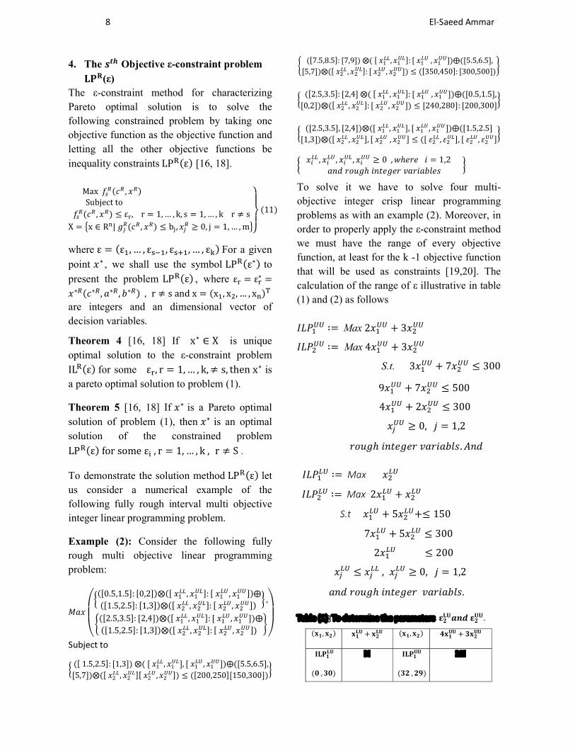
4. The 𝒔𝒕𝒉 Objective ε-constraint problem

𝐋𝐏𝐑(ε) The ε-constraint method for characterizing Pareto optimal solution is to solve the following constrained problem by taking one objective function as the objective function and letting all the other objective functions be inequality constraints LP (ε) [16, 18].

Max 𝑓 (𝑐 , 𝑥 ) Subject to

𝑓 (𝑐 , 𝑥 ) ≤ ε , r = 1, … , k, s = 1, … , k r ≠ s

X = x ∈ R | 𝑔 (𝑐 , 𝑥 ) ≤ b , 𝑥 ≥ 0, j = 1, … , m ⎭⎪⎬

⎪⎫

(11)

where ε = (ε , … , ε , ε , … , ε ) For a given

point 𝑥∗ , we shall use the symbol LP (ε∗) to present the problem LP (ε) , where ε = ε∗ =

𝑥∗ (𝑐∗ , 𝑎∗ , 𝑏∗ ) , r ≠ s and x = (x , x , … , x ) are integers and an dimensional vector of decision variables.

Theorem 4 [16, 18] If x∗ ∈ X is unique optimal solution to the ε-constraint problem IL (ε) for some ε , r = 1, … , k, ≠ s, then x∗ is a pareto optimal solution to problem (1).

Theorem 5 [16, 18] If 𝑥∗ is a Pareto optimal solution of problem (1), then 𝑥∗ is an optimal solution of the constrained problem

LP (ε) for some ε , r = 1, … , k , r ≠ S .

To demonstrate the solution method LP (ε) let us consider a numerical example of the following fully rough interval multi objective integer linear programming problem.

Example (2): Consider the following fully rough multi objective linear programming problem:

𝑀𝑎𝑥

⎝

⎜⎛

([0.5,1.5]: [0,2])⨂([ 𝑥 , 𝑥 ]: [ 𝑥 , 𝑥 ])⨁

([1.5,2.5]: [1,3])⨂([ 𝑥 , 𝑥 ]: [ 𝑥 , 𝑥 ]) ,

([2.5,3.5]: [2,4])⨂([ 𝑥 , 𝑥 ]: [ 𝑥 , 𝑥 ])⨁

([1.5,2.5]: [1,3])⨂([ 𝑥 , 𝑥 ]: [ 𝑥 , 𝑥 ]) ⎠

⎟⎞

Subject to

([ 1.5,2.5]: [1,3]) ⨂( [ 𝑥 , 𝑥 ], [ 𝑥 , 𝑥 ])⨁([5.5,6.5],

[5,7])⨂([ 𝑥 , 𝑥 ][ 𝑥 , 𝑥 ]) ≤ ([200,250][150,300])

([7.5,8.5]: [7,9]) ⨂( [ 𝑥 , 𝑥 ]: [ 𝑥 , 𝑥 ])⨁([5.5,6.5],

[5,7])⨂([ 𝑥 , 𝑥 ]: [ 𝑥 , 𝑥 ]) ≤ ([350,450]: [300,500])

([2.5,3.5]: [2,4] ⨂( [ 𝑥 , 𝑥 ]: [ 𝑥 , 𝑥 ])⨁([0.5,1.5],

[0,2])⨂([ 𝑥 , 𝑥 ]: [ 𝑥 , 𝑥 ]) ≤ [240,280]: [200,300]

([2.5,3.5], [2,4])⨂([ 𝑥 , 𝑥 ], [ 𝑥 , 𝑥 ])⨁([1.5,2.5]

[1,3])⨂([ 𝑥 , 𝑥 ], [ 𝑥 , 𝑥 ] ≤ ([ 𝜀 , 𝜀 ], [ 𝜀 , 𝜀 ]

𝑥 , 𝑥 , 𝑥 , 𝑥 ≥ 0 , 𝑤ℎ𝑒𝑟𝑒 𝑖 = 1,2


To solve it we have to solve four multi-objective integer crisp linear programming problems as with an example (2). Moreover, in order to properly apply the ε-constraint method we must have the range of every objective function, at least for the k -1 objective function that will be used as constraints [19,20]. The calculation of the range of ε illustrative in table (1) and (2) as follows 𝐼𝐿𝑃 ∶= Max 2𝑥 + 3𝑥

𝐼𝐿𝑃 ∶= Max 4𝑥 + 3𝑥

S.t. 3𝑥 + 7𝑥 ≤ 300

9𝑥 + 7𝑥 ≤ 500

4𝑥 + 2𝑥 ≤ 300

𝑥 ≥ 0, 𝑗 = 1,2


𝐼𝐿𝑃 ∶= Max 𝑥

𝐼𝐿𝑃 ∶= Max 2𝑥 + 𝑥

S.t 𝑥 + 5𝑥 +≤ 150

7𝑥 + 5𝑥 ≤ 300

2𝑥 ≤ 200

𝑥 ≤ 𝑥 , 𝑥 ≥ 0, 𝑗 = 1,2

𝑎𝑛𝑑 𝑟𝑜𝑢𝑔ℎ 𝑖𝑛𝑡𝑒𝑔𝑒𝑟 𝑣𝑎𝑟𝑖𝑎𝑏𝑙𝑠.

Table (1): To determine the parameters 𝛆𝟐𝐋𝐔𝒂𝒏𝒅 𝛆𝟐

𝐔𝐔.

(𝐱𝟏, 𝐱𝟐) 𝐱𝟏𝐋𝐔 + 𝐱𝟐

𝐋𝐔 (𝐱𝟏, 𝐱𝟐) 𝟒𝐱𝟏𝐔𝐔 + 𝟑𝐱𝟐

𝐔𝐔

𝐈𝐋𝐏𝟏𝐋𝐔

(𝟎 , 𝟑𝟎)

30 𝐈𝐋𝐏𝟏𝐔𝐔

(𝟑𝟐 , 𝟐𝟗)

215


𝐈𝐋𝐏𝟐𝐋𝐔

(𝟒𝟐, 𝟏)

85 𝐈𝐋𝐏𝟏𝐔𝐔

(𝟓𝟒 , 𝟐)

222

Max 85 Max 222

Min 30 Min 215

ε 𝟑𝟎 ≤ 𝛆𝟐𝐋𝐔

≤ 𝟖𝟓 ε 𝟐𝟏𝟓 ≤ 𝛆𝟐

𝐔𝐔

≤ 𝟐𝟐𝟐

𝐼𝐿𝑃 ∶= Max 1.5𝑥 + 2.5𝑥

𝐼𝐿𝑃 ∶= Max 3.5𝑥 + 2.5𝑥

S.t 2.5𝑥 + 6.5𝑥 ≤ 250

8.5𝑥 + 6.5𝑥 ≤ 450

3.5𝑥 + 1.5𝑥 ≤ 280

𝑥 ≤ 𝑥 , 𝑥 ≥ 0, 𝑗 = 1,2

𝑟𝑜𝑢𝑔ℎ 𝑖𝑛𝑡𝑒𝑔𝑒𝑟 𝑣𝑎𝑟𝑖𝑎𝑏𝑙𝑒𝑠. And

𝐼𝐿𝑃 ∶= Max 0.5𝑥 + 1.5𝑥

𝐼𝐿𝑃 ∶= Max 2.5𝑥 + 1.5𝑥

S.t 1.5𝑥 + 5.5𝑥 ≤ 200

7.5𝑥 + 5.5𝑥 ≤ 350

2.5𝑥 + 0.5𝑥 ≤ 240

𝑥 ≤ 𝑥 , 𝑥 ≥ 0, 𝑗 = 1,2


Table (2): To determine the parameters 𝛆𝟐𝐋𝐋𝒂𝒏𝒅 𝛆𝟐

𝐔𝐋.

(𝐱𝟏, 𝐱𝟐) 𝟐. 𝟓𝐱𝟏𝐋𝐋 + 𝟏. 𝟓𝐱𝟐

𝐋𝐋 (𝐱𝟏, 𝐱𝟐) 𝟑. 𝟓𝐱𝟏𝐔𝐋 + 𝟐. 𝟓𝐱𝟐

𝐔𝐋

ILP

(3 , 3)

102.5

ILP

(32 , 26)

177

ILP

(3, 3)

115.5 ILP

(52 , 1)

184.5

Max 115.5 Max 184.5

Min 102.5 Min 177

ε 𝟏𝟎𝟐. 𝟓 ≤ 𝛆𝟐𝐋𝐋

≤ 𝟏𝟏𝟓. 𝟓 ε 𝟏𝟕𝟕 ≤ 𝛆𝟐

𝐔𝐋

≤ 𝟏𝟖𝟒. 𝟓

𝑳𝒆𝒕 𝜀 = 85 , 𝜀 = 220

𝐼𝐿𝑃 ∶= 𝑀𝑎𝑥 2𝑥 + 3𝑥

𝒔. 𝒕 3𝑥 + 7𝑥 ≤ 300

9𝑥 + 7𝑥 ≤ 500

4𝑥 + 2𝑥 ≤ 300

4𝑥 + 3𝑥 ≤ 220

𝑥 ≥ 0, 𝑗 = 1,2

𝑟𝑜𝑢𝑔𝑒 𝑖𝑛𝑡𝑒𝑔𝑒𝑟 𝑣𝑎𝑟𝑖𝑎𝑏𝑙𝑒𝑠. And

𝐼𝐿𝑃 ∶= Max 𝑥

S.t 𝑥 + 5𝑥 +≤ 150

7𝑥 + 5𝑥 ≤ 300

2𝑥 + ≤ 200

2𝑥 + 𝑥 ≤ 85

𝑥 ≤ 𝑥 , 𝑥 ≥ 0, 𝑗 = 1,2

𝑟𝑜𝑢𝑔ℎ 𝑖𝑛𝑡𝑒𝑔𝑒𝑟 𝑣𝑎𝑟𝑖𝑎𝑏𝑙𝑒𝑠. 𝐴nd

𝑳𝒆𝒕 𝜀 = 102 , 𝜀 = 180

𝐼𝐿𝑃 ∶= 𝑀𝑎𝑥 1.5𝑥 + 2.5𝑥

𝑠. 𝑡. 2.5𝑥 + 6.5𝑥 ≤ 250

8.5𝑥 + 6.5𝑥 ≤ 450

3.5𝑥 + 1.5𝑥 ≤ 280

3.5𝑥 + 2.5𝑥 ≤ 180

𝑥 ≤ 𝑥 , 𝑥 ≥ 0, 𝑗 = 1,2

𝑟𝑜𝑢𝑔ℎ 𝑖𝑛𝑡𝑒𝑔𝑒𝑟 𝑣𝑎𝑟𝑖𝑎𝑏𝑙𝑒𝑠. And

𝐼𝐿𝑃 ∶= Max 0.5𝑥 + 1.5𝑥

𝑠. 𝑡 1.5𝑥 + 5.5𝑥 ≤ 200

7.5𝑥 + 5.5𝑥 ≤ 350

2.5𝑥 + 0.5𝑥 ≤ 240

2.5𝑥 + 1.5𝑥 ≤ 102

𝑥 ≤ 𝑥 , 𝑥 ≥ 0, 𝑗 = 1,2

𝑎𝑛𝑑 𝑟𝑜𝑢𝑔ℎ 𝑖𝑛𝑡𝑒𝑔𝑒𝑟 𝑣𝑎𝑟𝑖𝑎𝑏𝑙𝑒𝑠.

We used ''WinQSB'' program to find efficient value solutions and efficient integer solutions for the UAI and the LAI for example (2). Also, we used to apply branch and bound algorithm for integer programming, as following results:

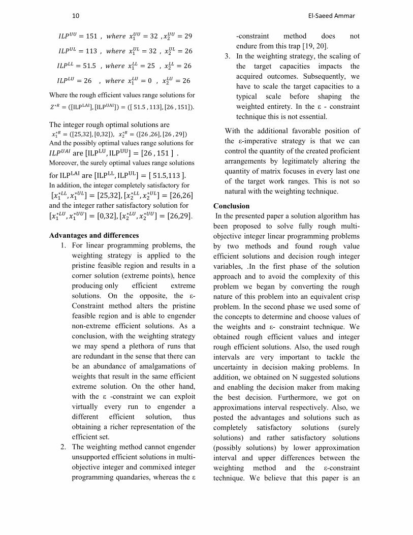
10 El-Saeed Ammar

𝐼𝐿𝑃 = 151 , 𝑤ℎ𝑒𝑟𝑒 𝑥 = 32 , 𝑥 = 29

𝐼𝐿𝑃 = 113 , 𝑤ℎ𝑒𝑟𝑒 𝑥 = 32 , 𝑥 = 26

𝐼𝐿𝑃 = 51.5 , 𝑤ℎ𝑒𝑟𝑒 𝑥 = 25 , 𝑥 = 26

𝐼𝐿𝑃 = 26 , 𝑤ℎ𝑒𝑟𝑒 𝑥 = 0 , 𝑥 = 26

Where the rough efficient values range solutions for

𝑍∗ = ([ILP ], [ILP ]) = ([ 51.5 , 113], [26 , 151]).

The integer rough optimal solutions are 𝑥∗ = ([25,32], [0,32]), 𝑥∗ = ([26 ,26], [26 , 29])

And the possibly optimal values range solutions for

𝐼𝐿𝑃 are [ILP , ILP ] = [26 , 151 ] . Moreover, the surely optimal values range solutions

for ILP are [ILP , ILP ] = [ 51.5,113 ]. In addition, the integer completely satisfactory for

[𝑥∗ , 𝑥∗ ] = [25,32], [𝑥∗ , 𝑥∗ ] = [26,26] and the integer rather satisfactory solution for [𝑥∗ , 𝑥∗ ] = [0,32], [𝑥∗ , 𝑥∗ ] = [26,29].

Advantages and differences 1. For linear programming problems, the

weighting strategy is applied to the pristine feasible region and results in a corner solution (extreme points), hence producing only efficient extreme solutions. On the opposite, the ε- Constraint method alters the pristine feasible region and is able to engender non-extreme efficient solutions. As a conclusion, with the weighting strategy we may spend a plethora of runs that are redundant in the sense that there can be an abundance of amalgamations of weights that result in the same efficient extreme solution. On the other hand, with the ε -constraint we can exploit virtually every run to engender a different efficient solution, thus obtaining a richer representation of the efficient set.

2. The weighting method cannot engender unsupported efficient solutions in multi-objective integer and commixed integer programming quandaries, whereas the ε

-constraint method does not endure from this trap [19, 20].

3. In the weighting strategy, the scaling of the target capacities impacts the acquired outcomes. Subsequently, we have to scale the target capacities to a typical scale before shaping the weighted entirety. In the ε - constraint technique this is not essential.

With the additional favorable position of the ε-imperative strategy is that we can control the quantity of the created proficient arrangements by legitimately altering the quantity of matrix focuses in every last one of the target work ranges. This is not so natural with the weighting technique.

Conclusion In the presented paper a solution algorithm has been proposed to solve fully rough multi-objective integer linear programming problems by two methods and found rough value efficient solutions and decision rough integer variables, .In the first phase of the solution approach and to avoid the complexity of this problem we began by converting the rough nature of this problem into an equivalent crisp problem. In the second phase we used some of the concepts to determine and choose values of the weights and ε- constraint technique. We obtained rough efficient values and integer rough efficient solutions. Also, the used rough intervals are very important to tackle the uncertainty in decision making problems. In addition, we obtained on N suggested solutions and enabling the decision maker from making the best decision. Furthermore, we got on approximations interval respectively. Also, we posted the advantages and solutions such as completely satisfactory solutions (surely solutions) and rather satisfactory solutions (possibly solutions) by lower approximation interval and upper differences between the weighting method and the ε-constraint technique. We believe that this paper is an


attempt to establish underlying results which hopefully help others to answer some of these questions. References

[1] Ammar. E. E and Khalifa. A. M, On Solving of Rough Interval Multi-Objective Transportation Problems, Journal of Advances in Physics, 7 (2014), 1233-1244.

[2] Atteya. T. E. M, Rough multiple objective programming, European Journal of the Operational Research, 248(1) (2016), 204-210.

[3] Bazaraa. M. S, Jarvis. J.J and Sherali. H. D, Linear programming and network flows, John Wiley and Sons, New York, (2010).

[4] Chinneck. J. W and Ramadan. K, Linear programming with interval coefficients, Journal of the Operational Research Society 51(2) (2000) 209–220.

[5] Dantzig. G and Wolfe. P,The Decomposition Algorithm for Linear Programming, Econometric, 9(4) (1961) 767–778.

[6] Dantzig. G. B and Thapa. N, Linear programming: Theory and extensions, Springer Verlag, Berlin, (2003).

[7] Hamazehee. A, Yaghoobi. M. A and Mashinchi. M, Linear Programming with Rough Interval Coefficients, Journal of Intelligent and Fuzzy Systems, 26 (2014), 1179-1189.

[8] Nasiri. J and Mashinchi. M, Rough Set and Data Analysis in Decision Tables, Journal of Uncertain Systems, 3(3) (2009) 232–240.

[9] Osman. M. S, El-Sherbiny.M .M, Khalifa. H. A and Farag. H. H, A Fuzzy Technique for Solving Rough Interval Multiobjective Transportation Problem, International Journal of Computer Applications, 147 (10) (2016) 49-57.

[10] Pawlak. Z, Rough Sets, International Journal of Computer and Information Sciences, 11 (1982), 341-356.

[11] Pawlak. Z and Skowron. A, Rudiment of rough sets, Information Sciences 177 (2007), 3–27.

[12] Pandian. P, Natarajan. G and Akilbasha. A, Fully Rough Integer Interval Transportation Problems, International Journal of Pharmacy & Technology, 8 (2) (2016) 13866-13876.

[13] Rebolledo. M, Rough intervals-enhancing intervals for qualitative modeling of technical systems, Artificial Intelligence, 170 (2006), 667–685.

[14] Shaocheng. T, Interval number and fuzzy number linear programming, Fuzzy Sets and Systems, 66(3) (1994), 301–306.

[15] Taha. H. T, Operation Research-An Introduction, 6th Edition, Mac Milan Publishing Co, New York (1997).

[16] Hwang, C.L., and Masued, A. S. M., Multiple Objective Decision-Making Methods and Applications, Springer Berline, (1979).

[17] Hongwei lu. Guohe H. and Li He., An inexact rough-interval fuzzy linear programming method for generating conjunactive, Water-allocation strategies to agricultural irrigation system, (35) (2011) 4330-4340.

[18] Sakawa M., Fuzzy sets and Interactive Multiobjective Optimization, NEW York (1993).

[19] G.R. Reeves, R.C. Reid, Minimum values over the efficient set in multiple objective decision making, European Journal of Operational Research, 36 (1988) 334–338.

[20] G. Mavrotas, Effective implementation of the e-constraint method in Multi-Objective, Mathematical programming problems, 213(2009) 455-465.

[21] Rani. D, Gulati. T. R and Garg. H, Multi-objective non-linear programming problem in intuitionistic fuzzy environment: Optimistic and pessimistic view point, Expert Systems with Applications 64(1) (2016), 228-238.

[22] Garg. H, Multi-objective optimization problem of system reliability under intuitionistic fuzzy set 11 environment using Cuckoo Search algorithm, Journal of Intelligent & Fuzzy Systems 29 (2015), 1653-1669.

[23] Saad. O.M, Biltage. M and Tamer. B, On the Solution of Fuzzy Multi-objective Integer Linear Fractional Programming Problem, International Journal of Contemporary Mathematical Sciences, 5(41) (2010), 2003-2018.

On Solving Fully Rough Multi-Objective Integer Linear ...

Documents