A generalized meta-analysis model for binary diagnostic test performance Ben A. Dwamena, MD The University of Michigan & VA Medical Centers, Ann Arbor FNASUG - November 13, 2008

Welcome message from author
This document is posted to help you gain knowledge. Please leave a comment to let me know what you think about it! Share it to your friends and learn new things together.
Transcript

A generalized meta-analysis model for binarydiagnostic test performance
Ben A. Dwamena, MD
The University of Michigan & VA Medical Centers, Ann Arbor
FNASUG - November 13, 2008

Diagnostic Test Evaluation
DIAGNOSTIC TESTAny measurement aiming to identify individuals who couldpotentially benefit from preventative or therapeutic interventionThis includes:
1 Elements of medical history
2 Physical examination
3 Imaging procedures
4 Laboratory investigations
5 Clinical prediction rules
Diagnostic Test Evaluation
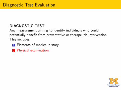
DIAGNOSTIC TESTAny measurement aiming to identify individuals who couldpotentially benefit from preventative or therapeutic interventionThis includes:
1 Elements of medical history
2 Physical examination
3 Imaging procedures
4 Laboratory investigations
5 Clinical prediction rules

Diagnostic Test Evaluation
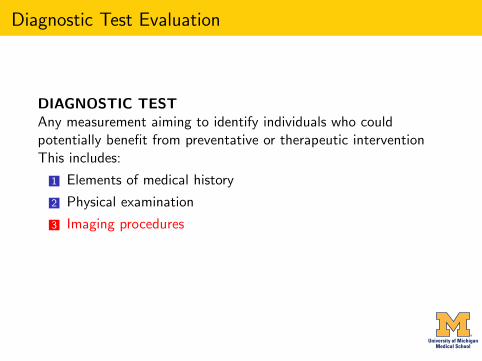
DIAGNOSTIC TESTAny measurement aiming to identify individuals who couldpotentially benefit from preventative or therapeutic interventionThis includes:
1 Elements of medical history
2 Physical examination
3 Imaging procedures
4 Laboratory investigations
5 Clinical prediction rules
Diagnostic Test Evaluation
DIAGNOSTIC TESTAny measurement aiming to identify individuals who couldpotentially benefit from preventative or therapeutic interventionThis includes:
1 Elements of medical history
2 Physical examination
3 Imaging procedures
4 Laboratory investigations
5 Clinical prediction rules

Diagnostic Test Evaluation
1 The performance of a diagnostic test assessed by comparisonof index and reference test results on a group of subjects
2 Ideally these should be patients suspected of the targetcondition that the test is designed to detect.
Binary test data often reported as 2×2 matrix
Reference TestPositive
Reference TestNegative
Test Positive True Positive False Positive
Test Negative False Negative True Negative
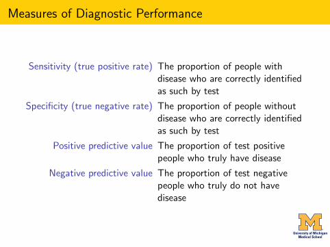
Measures of Diagnostic Performance
Sensitivity (true positive rate) The proportion of people withdisease who are correctly identifiedas such by test
Specificity (true negative rate) The proportion of people withoutdisease who are correctly identifiedas such by test
Positive predictive value The proportion of test positivepeople who truly have disease
Negative predictive value The proportion of test negativepeople who truly do not havedisease

Measures of Diagnostic Performance
Likelihood ratios (LR) The ratio of the probability of a positive (ornegative) test result in the patients withdisease to the probability of the same testresult in the patients without the disease
Diagnostic odds ratio The ratio of the odds of a positive testresult in patients with disease compared tothe odds of the same test result in patientswithout disease.
ROC Curve Plot of all pairs of (1-specificity, sensitivity)as positivity threshold varies

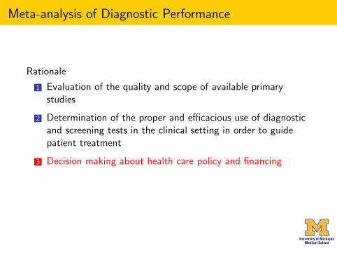
Meta-analysis of Diagnostic Performance
Rationale
1 Evaluation of the quality and scope of available primarystudies
2 Determination of the proper and efficacious use of diagnosticand screening tests in the clinical setting in order to guidepatient treatment
3 Decision making about health care policy and financing
4 Identification of areas for further research, development, andevaluation

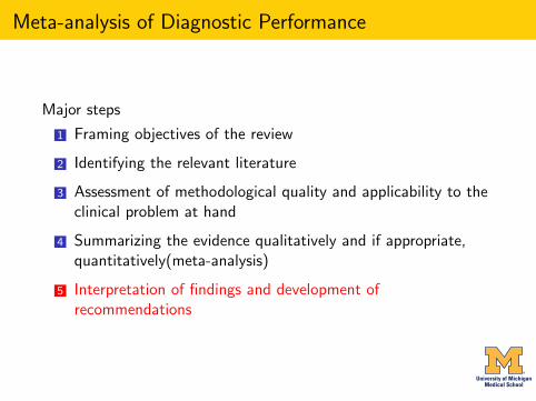
Meta-analysis of Diagnostic Performance
Major steps
1 Framing objectives of the review
2 Identifying the relevant literature
3 Assessment of methodological quality and applicability to theclinical problem at hand
4 Summarizing the evidence qualitatively and if appropriate,quantitatively(meta-analysis)
5 Interpretation of findings and development ofrecommendations

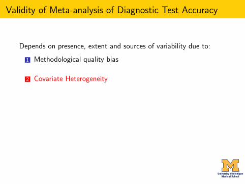
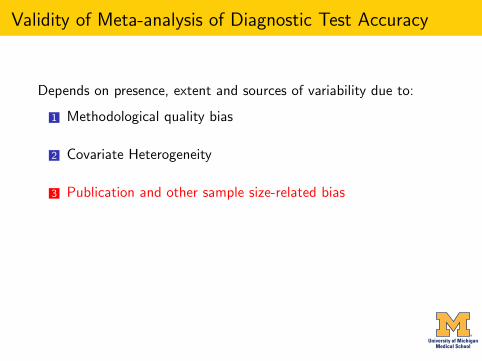
Validity of Meta-analysis of Diagnostic Test Accuracy
Depends on presence, extent and sources of variability due to:
1 Methodological quality bias
2 Covariate Heterogeneity
3 Publication and other sample size-related bias
4 Threshold Effects
5 Unobserved heterogeneity
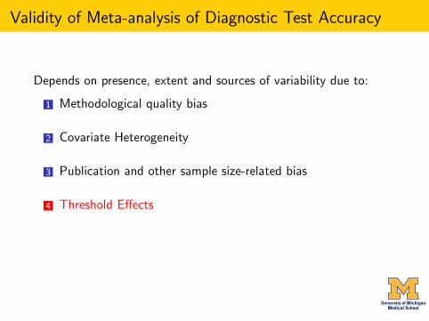
Validity of Meta-analysis of Diagnostic Test Accuracy
Depends on presence, extent and sources of variability due to:
1 Methodological quality bias
2 Covariate Heterogeneity
3 Publication and other sample size-related bias
4 Threshold Effects
5 Unobserved heterogeneity
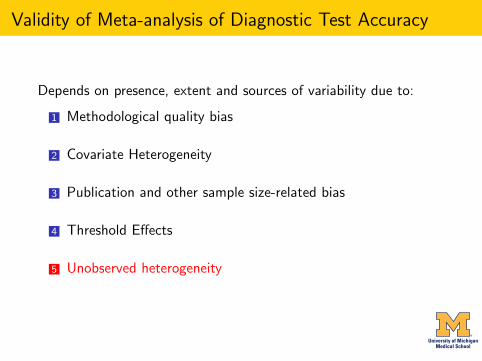
Validity of Meta-analysis of Diagnostic Test Accuracy
Depends on presence, extent and sources of variability due to:
1 Methodological quality bias
2 Covariate Heterogeneity
3 Publication and other sample size-related bias
4 Threshold Effects
5 Unobserved heterogeneity
Validity of Meta-analysis of Diagnostic Test Accuracy
Depends on presence, extent and sources of variability due to:
1 Methodological quality bias
2 Covariate Heterogeneity
3 Publication and other sample size-related bias
4 Threshold Effects
5 Unobserved heterogeneity
Validity of Meta-analysis of Diagnostic Test Accuracy
Depends on presence, extent and sources of variability due to:
1 Methodological quality bias
2 Covariate Heterogeneity
3 Publication and other sample size-related bias
4 Threshold Effects
5 Unobserved heterogeneity

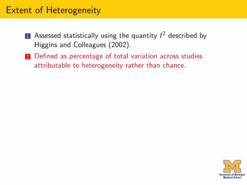
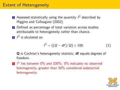
Extent of Heterogeneity
1 Assessed statistically using the quantity I 2 described byHiggins and Colleagues (2002).
2 Defined as percentage of total variation across studiesattributable to heterogeneity rather than chance.
3 I 2 is alculated as:
I 2 = ((Q − df )/Q)× 100. (1)
Q is Cochran’s heterogeneity statistic; df equals degrees offreedom.
4 I 2 lies between 0% and 100%: 0% indicates no observedheterogeneity, greater than 50% considered substantialheterogeneity.
5 Advantage of I 2 : does not inherently depend on the numberof the studies.

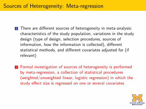
Sources of Heterogeneity: Meta-regression
1 There are different sources of heterogeneity in meta-analysis:characteristics of the study population, variations in the studydesign (type of design, selection procedures, sources ofinformation, how the information is collected), differentstatistical methods, and different covariates adjusted for (ifrelevant)
2 Formal investigation of sources of heterogeneity is performedby meta-regression, a collection of statistical procedures(weighted/unweighted linear, logistic regression) in which thestudy effect size is regressed on one or several covariates

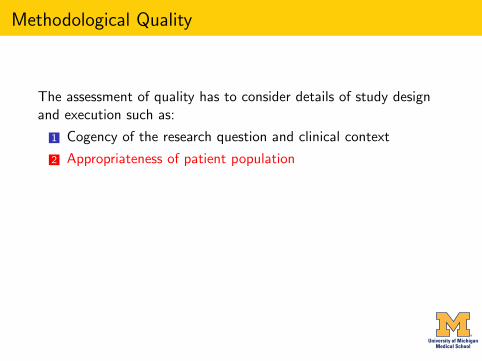
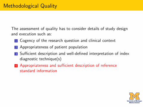
Methodological Quality
The assessment of quality has to consider details of study designand execution such as:
1 Cogency of the research question and clinical context
2 Appropriateness of patient population
3 Sufficient description and well-defined interpretation of indexdiagnostic technique(s)
4 Appropriateness and sufficient description of referencestandard information
5 Other factors that can affect the integrity of the study andthe generalizability of the results

Methodological Quality
Methods of quality assessment may focus on:
1 Absence or presence of key qualities in the study report(checklist approach)
2 Scores developed for this purpose (scale approach)
3 Levels-of-evidence methods by which a level or grade isassigned to studies fulfilling a predefined set of criteria
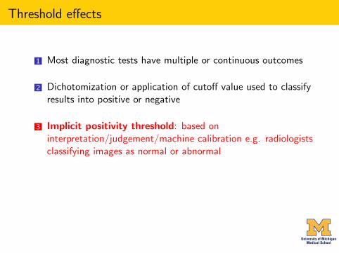
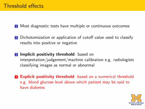
Threshold effects
1 Most diagnostic tests have multiple or continuous outcomes
2 Dichotomization or application of cutoff value used to classifyresults into positive or negative
3 Implicit positivity threshold: based oninterpretation/judgement/machine calibration e.g. radiologistsclassifying images as normal or abnormal
4 Explicit positivity threshold: based on a numerical thresholde.g. blood glucose level above which patient may be said tohave diabetes
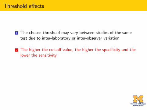
Threshold effects
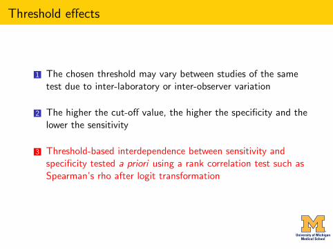
1 The chosen threshold may vary between studies of the sametest due to inter-laboratory or inter-observer variation
2 The higher the cut-off value, the higher the specificity and thelower the sensitivity
3 Threshold-based interdependence between sensitivity andspecificity tested a priori using a rank correlation test such asSpearman’s rho after logit transformation
Threshold effects
1 The chosen threshold may vary between studies of the sametest due to inter-laboratory or inter-observer variation
2 The higher the cut-off value, the higher the specificity and thelower the sensitivity
3 Threshold-based interdependence between sensitivity andspecificity tested a priori using a rank correlation test such asSpearman’s rho after logit transformation

Publication and Other Precision-related Biases
Publication bias Tendency for investigators, reviewers, and editorsto submit or accept manuscripts for publicationbased on the direction or strength of the studyfindings.
Funnel plot Exploratory tool for investigating publication bias,plotting a measure of effect size versus a measureof study precision
1 Funnel plot should appear symmetric if no bias is present
2 Assessment of such a plot is very subjective.
3 Non-parametric and linear regression methods used toformally test funnel plot asymmetry.

Examples of Tests For Funnel Plot Asymmetry
(Begg 1994) Rank correlation between standardized effect andits standard error
(Egger 1997) Linear regression of intervention effect against itsstandard error weighted by inverse of thevariance of intervention effect estimate
(Macaskill 2001) Linear regression of intervention effect on samplesize
(Harbord 2006) Modified vesion of (Egger 1997) based on”score” and ”score variance” of the log oddsratio
(Peters 2006) Linear regression of intervention effect on inverseof sample size
Problems with sample size and standard error
1 The asymptotic standard error is a biased estimate of the truestandard error, with larger bias for smaller cell sizes, as occurswith larger DORs and smaller studies
2 Diagnostic studies have unequal sample sizes in diseased andnon-diseased groups which reduces the precision of anestimate of test accuracy for a given sample size
3 The standard error of the logDOR depends on proportiontesting positive. However, individual studies often differ inpositivity threshold leading to variability in proportion testingpostive

Summary ROC Meta-analysis of Diagnostic Test Accuracy
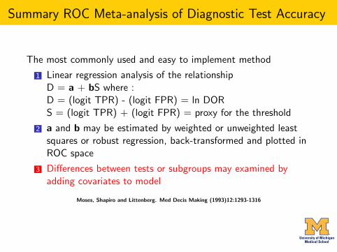
The most commonly used and easy to implement method
1 Linear regression analysis of the relationshipD = a + bS where :D = (logit TPR) - (logit FPR) = ln DORS = (logit TPR) + (logit FPR) = proxy for the threshold
2 a and b may be estimated by weighted or unweighted leastsquares or robust regression, back-transformed and plotted inROC space
3 Differences between tests or subgroups may examined byadding covariates to model
Moses, Shapiro and Littenberg. Med Decis Making (1993)12:1293-1316

Summary ROC Meta-analysis of Diagnostic Test Accuracy
The most commonly used and easy to implement method
1 Linear regression analysis of the relationshipD = a + bS where :D = (logit TPR) - (logit FPR) = ln DORS = (logit TPR) + (logit FPR) = proxy for the threshold
2 a and b may be estimated by weighted or unweighted leastsquares or robust regression, back-transformed and plotted inROC space
3 Differences between tests or subgroups may examined byadding covariates to model
Moses, Shapiro and Littenberg. Med Decis Making (1993)12:1293-1316

Summary ROC Meta-analysis of Diagnostic Test Accuracy
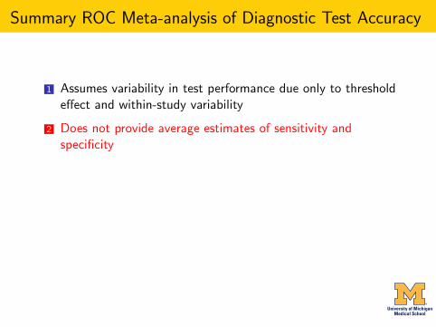
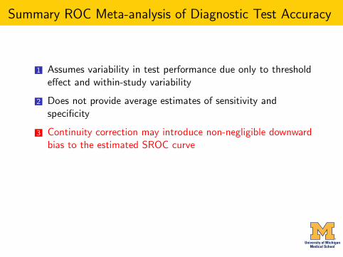
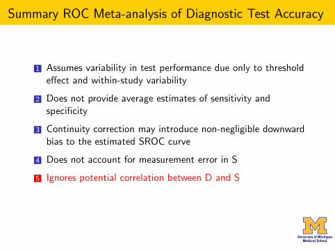
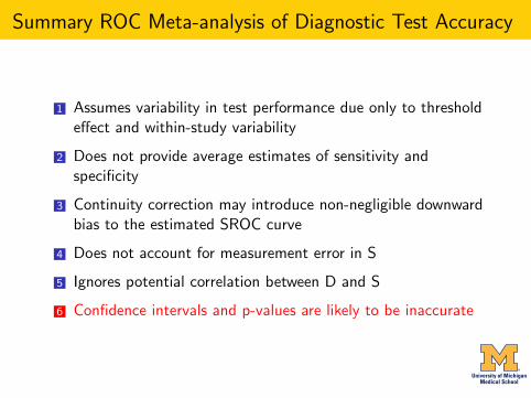
1 Assumes variability in test performance due only to thresholdeffect and within-study variability
2 Does not provide average estimates of sensitivity andspecificity
3 Continuity correction may introduce non-negligible downwardbias to the estimated SROC curve
4 Does not account for measurement error in S
5 Ignores potential correlation between D and S
6 Confidence intervals and p-values are likely to be inaccurate
Summary ROC Meta-analysis of Diagnostic Test Accuracy
1 Assumes variability in test performance due only to thresholdeffect and within-study variability
2 Does not provide average estimates of sensitivity andspecificity
3 Continuity correction may introduce non-negligible downwardbias to the estimated SROC curve
4 Does not account for measurement error in S
5 Ignores potential correlation between D and S
6 Confidence intervals and p-values are likely to be inaccurate
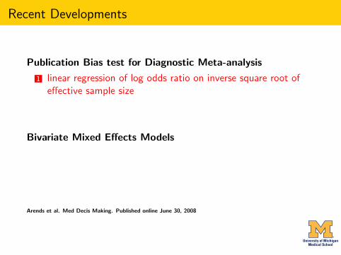
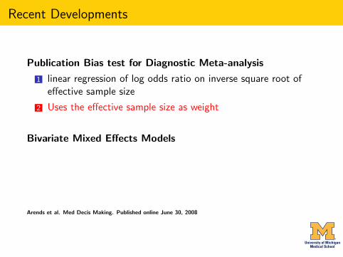
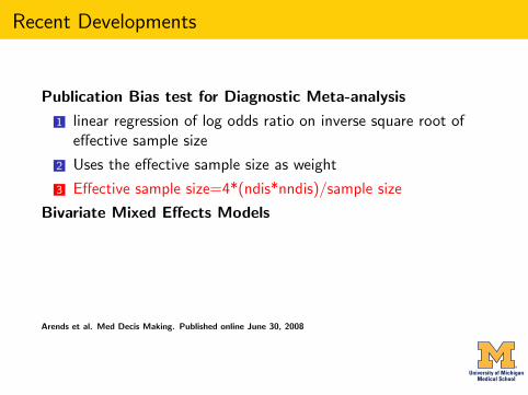
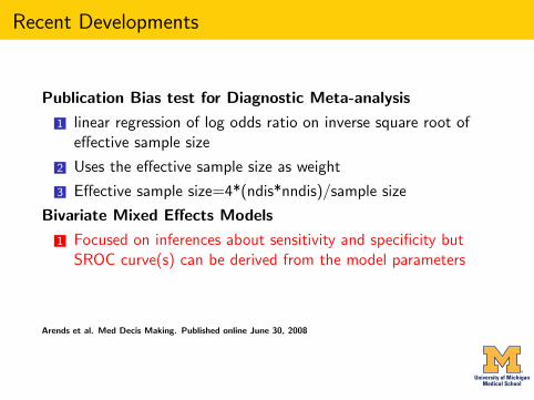
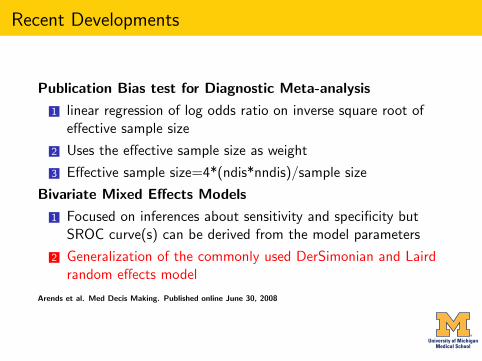
Recent Developments
Publication Bias test for Diagnostic Meta-analysis
1 linear regression of log odds ratio on inverse square root ofeffective sample size
2 Uses the effective sample size as weight
3 Effective sample size=4*(ndis*nndis)/sample size
Bivariate Mixed Effects Models
1 Focused on inferences about sensitivity and specificity butSROC curve(s) can be derived from the model parameters
2 Generalization of the commonly used DerSimonian and Lairdrandom effects model
Arends et al. Med Decis Making. Published online June 30, 2008

Publication Bias test for Diagnostic Meta-analysis
1
2
3
4
5
6
7
8
9
10
11
12
13
14
15
16
17
18
19
20
21
22
23
2425
26
27
28
29
3031
32
33
34
35
36
37
38
3940
41
42
43
.05
.1
.15
.2
.25
.3
1/ro
ot(E
SS
)
1 10 100 1000
Diagnostic Odds Ratio
Study
RegressionLine
Deeks’ Funnel Plot Asymmetry Testpvalue = 0.89

Bivariate Linear Mixed Model
Level 1: Within-study variability(logit (pAi )logit (pBi )
)∼ N
((µAi
µBi
),Ci
)
Ci =
(s2Ai 00 s2
Bi
)pAi and pBi Sensitivity and specificity of the ith study
µAi and µBi Logit-transforms of sensitivity and specificity of theith study
Ci Within-study variance matrix
s2Ai and s2
Bi variances of logit-transforms of sensitivity andspecificity
Reitsma JB et al. J. Clin Epidemiol (2005) 58:982-990

Bivariate Linear Mixed Model
Level 2: Between-study variability(µAi
µBi
)∼ N
((MA
MB
),ΣAB
)
ΣAB =
(σ2
A σAB
σAB σ2B
)µAi and µBi Logit-transforms of sensitivity and specificity of the
ith study
MA and MB Means of the normally distributed logit-transforms
ΣAB Between-study variances and covariance matrix
Reitsma JB et al. J. Clin Epidemiol (2005) 58:982-990
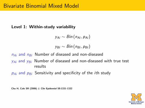
Bivariate Binomial Mixed Model
Level 1: Within-study variability
yAi ∼ Bin (nAi , pAi )
yBi ∼ Bin (nBi , pBi )
nAi and nBi Number of diseased and non-diseased
yAi and yBi Number of diseased and non-diseased with true testresults
pAi and pBi Sensitivity and specificity of the ith study
Chu H, Cole SR (2006) J. Clin Epidemiol 59:1331-1332

Bivariate Binomial Mixed Model
Level 2: Between-study variability(µAi
µBi
)∼ N
((MA
MB
),ΣAB
)
ΣAB =
(σ2
A σAB
σAB σ2B
)µAi and µBi Logit-transforms of sensitivity and specificity of the
ith study
MA and MB Means of the normally distributed logit-transforms
ΣAB Between-study variances and covariance matrix
Chu H, Cole SR (2006) J. Clin Epidemiol 59:1331-1332

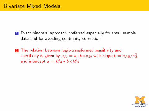
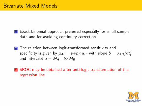
Bivariate Mixed Models
1 Exact binomial approach preferred especially for small sampledata and for avoiding continuity correction
2 The relation between logit-transformed sensitivity andspecificity is given by µAi = a+b×µBi with slope b = σAB/σ2
A
and intercept a = MA - b×MB
3 SROC may be obtained after anti-logit transformation of theregression line
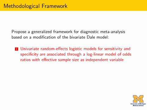
Methodological Framework
Propose a generalized framework for diagnostic meta-analysisbased on a modification of the bivariate Dale model:
1 Univariate random-effects logistic models for sensitivity andspecificity are associated through a log-linear model of oddsratios with effective sample size as independent variable
2 This unifies the estimation of summary test performance andassessment of the presence, extent, and sources of variability
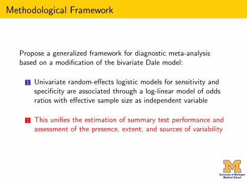
Methodological Framework
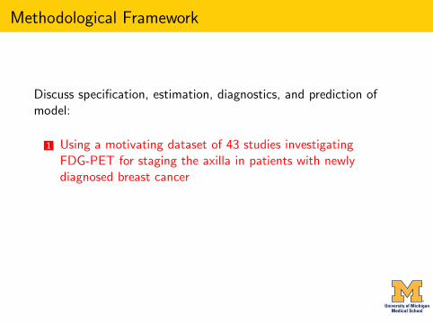
Discuss specification, estimation, diagnostics, and prediction ofmodel:
1 Using a motivating dataset of 43 studies investigatingFDG-PET for staging the axilla in patients with newlydiagnosed breast cancer
2 Taking advantage of the ability of gllamm to model a mixtureof discrete and continous outcomes

Methodological Framework
Discuss specification, estimation, diagnostics, and prediction ofmodel:
1 Using a motivating dataset of 43 studies investigatingFDG-PET for staging the axilla in patients with newlydiagnosed breast cancer
2 Taking advantage of the ability of gllamm to model a mixtureof discrete and continous outcomes
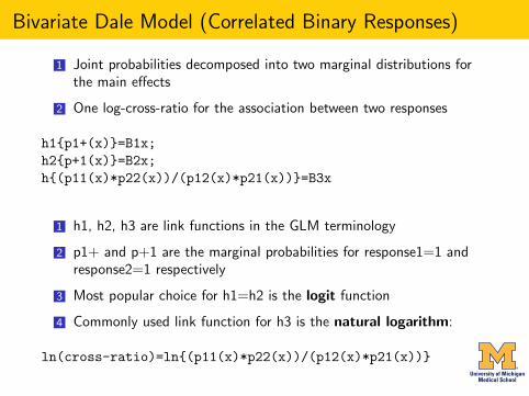
Bivariate Dale Model (Correlated Binary Responses)
1 Joint probabilities decomposed into two marginal distributions forthe main effects
2 One log-cross-ratio for the association between two responses
h1{p1+(x)}=B1x;h2{p+1(x)}=B2x;h{(p11(x)*p22(x))/(p12(x)*p21(x))}=B3x
1 h1, h2, h3 are link functions in the GLM terminology
2 p1+ and p+1 are the marginal probabilities for response1=1 andresponse2=1 respectively
3 Most popular choice for h1=h2 is the logit function
4 Commonly used link function for h3 is the natural logarithm:
ln(cross-ratio)=ln{(p11(x)*p22(x))/(p12(x)*p21(x))}

Modified Bivariate Dale Model
Within-study variability
yAi ∼ Bin (nAi , pAi )
yBi ∼ Bin (nBi , pBi )
nAi and nBi Number of diseased and non-diseased
yAi and yBi Number of diseased and non-diseased with true testresults
pAi and pBi Sensitivity and specificity of the ith study
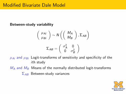
Modified Bivariate Dale Model
Between-study variability(µAi
µBi
)∼ N
((MA
MB
),ΣAB
)
ΣAB =
(σ2
A 00 σ2
B
)µAi and µBi Logit-transforms of sensitivity and specificity of the
ith study
MA and MB Means of the normally distributed logit-transforms
ΣAB Between-study variances

Modified Bivariate Dale Model
Association Model
Associates the univariate random-effects logistic models forsensitivity and specificity in the form a log-linear model:
logDORi = a+b×ESSi
intercept a = adjusted odds ratio
and slope b = bias coefficient
Example: PET for axillary staging of breast Cancer
1 PET or Positron Emission Tomography uses radiolabeledglucose analog to evaluate tumor metabolism
2 This radiological test may be used to stage and/or examinethe extent of breast cancer
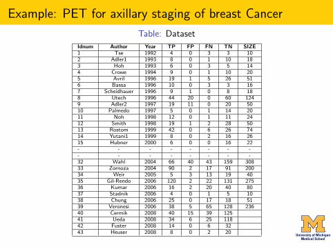
3 The accuracy of axillary PET has been studied by manyresearchers
4 We obtained, by searching PUBMED, 43 studies publishedbetween 1990 and 2008
Example: PET for axillary staging of breast Cancer
1 PET or Positron Emission Tomography uses radiolabeledglucose analog to evaluate tumor metabolism
2 This radiological test may be used to stage and/or examinethe extent of breast cancer
3 The accuracy of axillary PET has been studied by manyresearchers
4 We obtained, by searching PUBMED, 43 studies publishedbetween 1990 and 2008
Example: PET for axillary staging of breast Cancer
Table: Dataset
Idnum Author Year TP FP FN TN SIZE1 Tse 1992 4 0 3 3 102 Adler1 1993 8 0 1 10 183 Hoh 1993 6 0 3 5 144 Crowe 1994 9 0 1 10 205 Avril 1996 19 1 5 26 516 Bassa 1996 10 0 3 3 167 Scheidhauer 1996 9 1 0 8 188 Utech 1996 44 20 0 60 1249 Adler2 1997 19 11 0 20 5010 Palmedo 1997 5 0 1 14 2011 Noh 1998 12 0 1 11 2412 Smith 1998 19 1 2 28 5013 Rostom 1999 42 0 6 26 7414 Yutani1 1999 8 0 2 16 2615 Hubner 2000 6 0 0 16 22- - - - - - - -- - - - - - - -32 Wahl 2004 66 40 43 159 30833 Zornoza 2004 90 2 17 91 20034 Weir 2005 5 3 13 19 4035 Gil-Rendo 2006 120 2 22 131 27536 Kumar 2006 16 2 20 40 8037 Stadnik 2006 4 0 1 5 1038 Chung 2006 25 0 17 18 5139 Veronesi 2006 38 5 65 128 23640 Cermik 2008 40 15 39 12541 Ueda 2008 34 6 25 11842 Fuster 2008 14 0 6 3243 Heuser 2008 8 0 2 20
Recode Data for gllamm
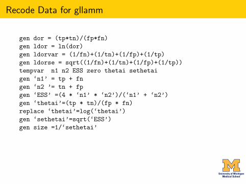
gen dor = (tp*tn)/(fp*fn)gen ldor = ln(dor)gen ldorvar = (1/fn)+(1/tn)+(1/fp)+(1/tp)gen ldorse = sqrt((1/fn)+(1/tn)+(1/fp)+(1/tp))tempvar n1 n2 ESS zero thetai sethetaigen ‘n1’ = tp + fngen ‘n2 ’= tn + fpgen ‘ESS’ =(4 * ‘n1’ * ‘n2’)/(‘n1’ + ‘n2’)gen ‘thetai’=(tp * tn)/(fp * fn)replace ‘thetai’=log(‘thetai’)gen ‘sethetai’=sqrt(‘ESS’)gen size =1/‘sethetai’
Recode Data for gllamm
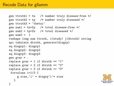
gen ttruth1 = tn /* number truly disease-free */gen ttruth2 = tp /* number truly diseased */gen ttruth3 = ‘thetai’gen num1 = tn+fp /* total disease-free */gen num2 = tp+fn /* total diseased */gen num3 = 1reshape long num ttruth, i(study) j(dtruth) stringqui tabulate dtruth, generate(disgrp)eq disgrp1: disgrp1eq disgrp2: disgrp2eq disgrp3: disgrp3gen gvar = .replace gvar = 1 if dtruth == "1"replace gvar = 2 if dtruth == "2"replace gvar = 3 if dtruth == "3"forvalues i=1/3 {
g size_‘i’ = disgrp‘i’* size}
}
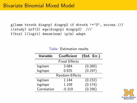
Bivariate Binomial Mixed Model
gllamm ttruth disgrp1 disgrp2 if dtruth !="3", nocons ///i(study) nrf(2) eqs(disgrp1 disgrp2) ///f(bin) l(logit) denom(num) ip(m) adapt
Table: Estimation results
Variable Coefficient (Std. Err.)
Fixed Effectslogitsen 3.084 (0.260)logitspe 0.925 (0.197)
Random-Effectslogitsen 1.144 (0.232)logitspe 1.109 (0.174)Correlation -0.319 (0.256)
Bivariate Binomial Mixed Model
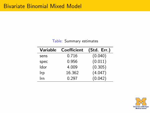
Table: Summary estimates
Variable Coefficient (Std. Err.)sens 0.716 (0.040)spec 0.956 (0.011)ldor 4.009 (0.305)lrp 16.362 (4.047)lrn 0.297 (0.042)
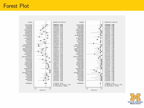
Forest Plot
SENSITIVITY (95% CI)
Q =286.37, df = 42.00, p = 0.00I2 = 85.33 [81.61 − 89.06]
0.72[0.63 − 0.79]
0.57 [0.18 − 0.90]0.89 [0.52 − 1.00]0.67 [0.30 − 0.93]0.90 [0.55 − 1.00]0.79 [0.58 − 0.93]0.77 [0.46 − 0.95]1.00 [0.66 − 1.00]1.00 [0.92 − 1.00]1.00 [0.82 − 1.00]0.83 [0.36 − 1.00]0.92 [0.64 − 1.00]0.90 [0.70 − 0.99]0.88 [0.75 − 0.95]0.80 [0.44 − 0.97]1.00 [0.54 − 1.00]0.74 [0.49 − 0.91]0.50 [0.25 − 0.75]0.94 [0.86 − 0.98]0.79 [0.62 − 0.91]0.50 [0.12 − 0.88]0.68 [0.43 − 0.87]0.43 [0.18 − 0.71]0.20 [0.01 − 0.72]0.47 [0.21 − 0.73]0.53 [0.27 − 0.79]0.80 [0.56 − 0.94]0.25 [0.11 − 0.43]0.21 [0.05 − 0.51]0.67 [0.09 − 0.99]0.60 [0.42 − 0.76]0.36 [0.18 − 0.57]0.61 [0.51 − 0.70]0.84 [0.76 − 0.90]0.28 [0.10 − 0.53]0.85 [0.77 − 0.90]0.44 [0.28 − 0.62]0.80 [0.28 − 0.99]0.60 [0.43 − 0.74]0.37 [0.28 − 0.47]0.51 [0.39 − 0.62]0.58 [0.44 − 0.70]0.70 [0.46 − 0.88]0.80 [0.44 − 0.97]0.80 [0.44 − 0.97]
StudyId
COMBINED
Tse/1992Adler1/1993
Hoh/1993Crowe/1994
Avril/1996Bassa/1996
Scheidhauer/1996Utech/1996
Adler2/1997Palmedo/1997
Noh/1998Smith/1998
Rostom/1999Yutani1/1999Hubner/2000
Ohta/2000Yutani2/2000
Greco/2001Schirrmeister/2001
Yang/2001Danforth/2002
Guller/2002Kelemen/2002
Nakamoto1/2002Nakamoto2/2002
Rieber/2002Van_Hoeven/2002
Barranger/2003Fehr/2004
Inoue/2004Lovrics/2004
Wahl/2004Zornoza/2004
Weir/2005Gil−Rendo/2006
Kumar/2006Stadnik/2006Chung/2006
Veronesi/2006Cermik/2008
Ueda/2008Fuster/2008
Heuser/2008
0.0 1.0SENSITIVITY
SPECIFICITY (95% CI)
Q =245.64, df = 42.00, p = 0.00I2 = 82.90 [78.37 − 87.44]
0.96[0.93 − 0.97]
1.00 [0.29 − 1.00]1.00 [0.69 − 1.00]1.00 [0.48 − 1.00]1.00 [0.69 − 1.00]0.96 [0.81 − 1.00]1.00 [0.29 − 1.00]0.89 [0.52 − 1.00]0.75 [0.64 − 0.84]0.65 [0.45 − 0.81]1.00 [0.77 − 1.00]1.00 [0.72 − 1.00]0.97 [0.82 − 1.00]1.00 [0.87 − 1.00]1.00 [0.79 − 1.00]1.00 [0.79 − 1.00]1.00 [0.75 − 1.00]1.00 [0.85 − 1.00]0.86 [0.78 − 0.93]0.92 [0.84 − 0.97]1.00 [0.74 − 1.00]0.67 [0.30 − 0.93]0.94 [0.71 − 1.00]1.00 [0.69 − 1.00]0.95 [0.76 − 1.00]0.86 [0.64 − 0.97]0.95 [0.75 − 1.00]0.97 [0.86 − 1.00]1.00 [0.81 − 1.00]0.62 [0.38 − 0.82]0.96 [0.85 − 0.99]0.97 [0.89 − 1.00]0.80 [0.74 − 0.85]0.98 [0.92 − 1.00]0.86 [0.65 − 0.97]0.98 [0.95 − 1.00]0.95 [0.84 − 0.99]1.00 [0.48 − 1.00]1.00 [0.81 − 1.00]0.96 [0.91 − 0.99]0.89 [0.83 − 0.94]0.95 [0.90 − 0.98]1.00 [0.89 − 1.00]1.00 [0.83 − 1.00]1.00 [0.83 − 1.00]
StudyId
COMBINED
Tse/1992Adler1/1993
Hoh/1993Crowe/1994
Avril/1996Bassa/1996
Scheidhauer/1996Utech/1996
Adler2/1997Palmedo/1997
Noh/1998Smith/1998
Rostom/1999Yutani1/1999Hubner/2000
Ohta/2000Yutani2/2000
Greco/2001Schirrmeister/2001
Yang/2001Danforth/2002
Guller/2002Kelemen/2002
Nakamoto1/2002Nakamoto2/2002
Rieber/2002Van_Hoeven/2002
Barranger/2003Fehr/2004
Inoue/2004Lovrics/2004
Wahl/2004Zornoza/2004
Weir/2005Gil−Rendo/2006
Kumar/2006Stadnik/2006Chung/2006
Veronesi/2006Cermik/2008
Ueda/2008Fuster/2008
Heuser/2008
0.3 1.0SPECIFICITY

SROC Curve
1
2
3
4
56
7 8 9
10
1112
13
14
15
16
17
18
19
20
21
22
23
24
25
26
27
28
29
30
31
32
33
34
35
36
37
38
39
40
41
42
43
0.0
0.5
1.0
Sen
sitiv
ity
0.00.51.0Specificity
Observed Data
Summary Operating PointSENS = 0.72 [0.63 − 0.79]SPEC = 0.96 [0.93 − 0.97]
SROC CurveAUC = 0.94 [0.92 − 0.96]
95% Confidence Contour
95% Prediction Contour
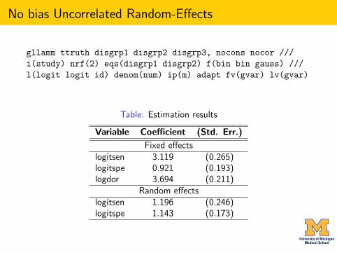
No bias Uncorrelated Random-Effects
gllamm ttruth disgrp1 disgrp2 disgrp3, nocons nocor ///i(study) nrf(2) eqs(disgrp1 disgrp2) f(bin bin gauss) ///l(logit logit id) denom(num) ip(m) adapt fv(gvar) lv(gvar)
Table: Estimation results
Variable Coefficient (Std. Err.)
Fixed effectslogitsen 3.119 (0.265)logitspe 0.921 (0.193)logdor 3.694 (0.211)
Random effectslogitsen 1.196 (0.246)logitspe 1.143 (0.173)

No bias Uncorrelated Random-Effects
Table: Summary estimates
Variable Coefficient (Std. Err.)sens 0.715 (0.039)spec 0.958 (0.011)ldor 3.694 (0.211)lrp 16.888 (4.384)lrn 0.297 (0.041)
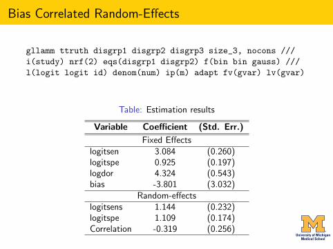
Bias Correlated Random-Effects
gllamm ttruth disgrp1 disgrp2 disgrp3 size_3, nocons ///i(study) nrf(2) eqs(disgrp1 disgrp2) f(bin bin gauss) ///l(logit logit id) denom(num) ip(m) adapt fv(gvar) lv(gvar)
Table: Estimation results
Variable Coefficient (Std. Err.)
Fixed Effectslogitsen 3.084 (0.260)logitspe 0.925 (0.197)logdor 4.324 (0.543)bias -3.801 (3.032)
Random-effectslogitsens 1.144 (0.232)logitspe 1.109 (0.174)Correlation -0.319 (0.256)
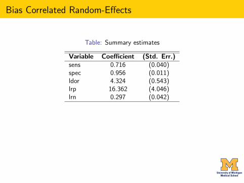
Bias Correlated Random-Effects
Table: Summary estimates
Variable Coefficient (Std. Err.)sens 0.716 (0.040)spec 0.956 (0.011)ldor 4.324 (0.543)lrp 16.362 (4.046)lrn 0.297 (0.042)

Bias Uncorrelated Random-Effects
gllamm ttruth disgrp1 disgrp2 disgrp3 size_3, nocons nocor ///i(study) nrf(2) eqs(disgrp1 disgrp2) f(bin bin gauss) ///l(logit logit id) denom(num) ip(m) adapt fv(gvar) lv(gvar)
Table: Estimation results
Variable Coefficient (Std. Err.)
Fixed effectslogitsen 3.119 (0.265)logitspe 0.921 (0.193)logdor 4.324 (0.543)bias -3.801 (3.032)
Random effectslogitsen 1.196 (0.246)logitspe 1.144 (0.173)
Bias Uncorrelated Random-Effects
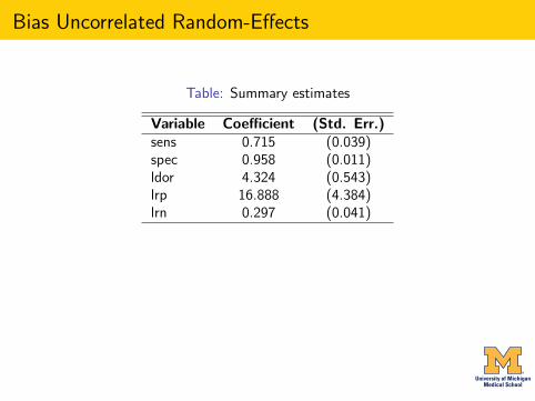
Table: Summary estimates
Variable Coefficient (Std. Err.)sens 0.715 (0.039)spec 0.958 (0.011)ldor 4.324 (0.543)lrp 16.888 (4.384)lrn 0.297 (0.041)

Comparative Results
Table: Fit and Complexity Measures
Model nparm Deviance BICNo Bias 7 548.42 582.44Bias Correlated Random-effects 8 548.42 587.30Bias Uncorrelated Random-effects 7 548.37 582.39
Table: Sensitivity and Specificity
Model Sens SpecNo Bias 0.716 (0.638 - 0.795) 0.956 (0.935 - 0.978)Bias Correlated RE 0.716 (0.638 - 0.795) 0.956 (0.935 - 0.978)Bias Uncorrelated RE 0.715 (0.638 - 0.792) 0.958 (0.937 - 0.979)

Prediction and Diagnostics
May use gllapred for empirical bayes predictions, residual analysis, influence analysis, normality testingetc
0.00
0.25
0.50
0.75
1.00
Dev
ianc
e R
esid
ual
0.00 0.25 0.50 0.75 1.00Normal Quantile
(a) Goodness−Of−Fit
0.00
0.25
0.50
0.75
1.00
Mah
alan
obis
D−
squa
red
0.00 0.25 0.50 0.75 1.00Chi−squared Quantile
(b) Bivariate Normality
8
9
29
0.00
0.50
1.00
1.50
2.00
Coo
k’s
Dis
tanc
e
0 10 20 30 40study
(c) Influence Analysis
7
222418
32 28
35
6
3036
2
13 2014
198
15121131
2925
26
161723
3
21
27
42
1
37
5
43
4941
38
4033
34
39
10
−3.0
−2.0
−1.0
0.0
1.0
2.0
3.0
Sta
ndar
dize
d_R
esid
ual2
−3.0 −2.0 −1.0 0.0 1.0 2.0 3.0Standardized_Residual1
(d) Outlier Detection
Model Diagnostic Plots

Conclusions
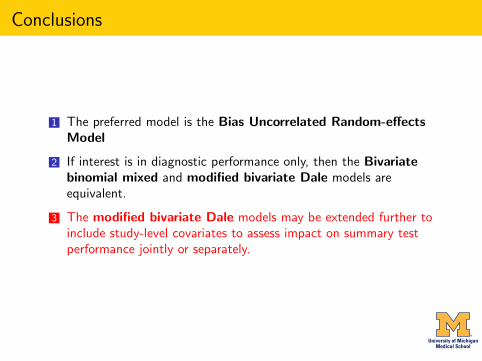
1 The preferred model is the Bias Uncorrelated Random-effectsModel
2 If interest is in diagnostic performance only, then the Bivariatebinomial mixed and modified bivariate Dale models areequivalent.
3 The modified bivariate Dale models may be extended further toinclude study-level covariates to assess impact on summary testperformance jointly or separately.

Conclusions
1 The preferred model is the Bias Uncorrelated Random-effectsModel
2 If interest is in diagnostic performance only, then the Bivariatebinomial mixed and modified bivariate Dale models areequivalent.
3 The modified bivariate Dale models may be extended further toinclude study-level covariates to assess impact on summary testperformance jointly or separately.
Related Documents


![Day 4 [03 Sept€¦ · Web view2012/03/04 · GENMOD – generalized linear models LOGISTIC – [grouped] binary regression PROBIT – [grouped] binary regression (INVERSECL) CATMOD](https://static.cupdf.com/doc/110x72/5f6460262813764a924bb395/day-4-03-web-view-20120304-genmod-a-generalized-linear-models-logistic-a.jpg)