A Didactic Procedure to Solve the Equation of Steady-Static ...

mathematics

Article

A Didactic Procedure to Solve the Equation ofSteady-Static Response in Suspended Cables

José Agüero-Rubio 1 , Javier López-Martínez 2 , Marta Gómez-Galán 2 andÁngel-Jesús Callejón-Ferre 2,*

1 Department of Electricity, IES Alhamilla of Almería, 04005 Almería, Spain; [email protected] Department of Engineering, University of Almería, Research Center CIAIMBITAL (CeiA3), Ctra. Sacramento,

s/n, La Cañada, 04120 Almería, Spain; [email protected] (J.L.-M.); [email protected] (M.G.-G.)* Correspondence: [email protected]

Received: 8 August 2020; Accepted: 27 August 2020; Published: 1 September 2020�����������������

Abstract: Students in the electrical branch of the short-cycle tertiary education program acquiredevelopmental and design skills for low voltage transmission power lines. Aerial power line designrequires mathematical tools not covered well enough in the curricula. Designing suspension cablesrequires the use of a Taylor series and integral calculation to obtain the parabola’s arc length. Moreover,it requires iterative procedures, such as the Newton–Raphson method, to solve the third-order equationof the steady-static response. The aim of this work is to solve the steady-static response equation forsuspended cables using simple calculation tools. For this purpose, the influence of the horizontalcomponent of the cable tension on its curvature was decoupled from the cable’s self-weight, whichwas responsible for the tension’s vertical component. To this end, we analyzed the laying andoperation of the suspended cables by defining three phases (i.e., stressing, lifting, and operation).The phenomena that occurred in each phase were analyzed, as was their manifestation in the cablemodel. Herein, we developed and validated the solution of the steady-static response equation insuspended cables using simple equations supported with intuitive graphics. The best results of theproposed calculation procedure were obtained in conditions of large temperature variations.

Keywords: power transmission lines; suspended cables; reduced-order models; problem-basedlearning; mathematical modeling; high-temperature and low-sag conductors (HTLS conductors)

1. Introduction

Programs like vocational education and training studies for electrical and automatic systems(Spanish Royal Decree (RD) 1127/2010 [1]) and short-cycle tertiary education (classified at aninternational standard classification of education (ISCED) level 5 [2]) are designed to provide participantswith professional knowledge, skills, and competencies. Academic tertiary education programs belowthe level of a bachelor’s program or equivalent are also classified as ISCED level 5.

The mathematical competencies with which students enter these studies do not include differentialor integral calculus. According to RD 1127/2010 [1], electrical and mechanical calculations are requiredfor low voltage power transmission lines. The mathematical model that describes the behavior of thecable is based on the catenary curve and, in most cases, the parabola is used as an approximation, as itis easier to apply [3]. The use of a Taylor series is required to approximate both the profile and lengthof the cable [4,5]. The arc length of the parabola is essential for solving the steady-static responseequation of the cable [6,7]. It is a polynomial equation that can be solved with a simple code [7]. Both aTaylor series and iterative resolution algorithms take the student away from real physical phenomena.According to Huilier [8], difficulties in mathematics are the main obstacle for young students to getinterested in science and technology disciplines. When studying the subject of suspended cables in the

Mathematics 2020, 8, 1468; doi:10.3390/math8091468 www.mdpi.com/journal/mathematics

Mathematics 2020, 8, 1468 2 of 19

final years of secondary education, students ask themselves questions such as: What length of cable isnecessary to join two points? Since students do not have integral calculation tools, they often cannotanswer this question and resort to formulas that need to be memorized.

According to Moreno-Clemente [9], computers are a valuable tool for calculating powertransmission lines. It is also important for students to analyze the physical implications of eachapproximation made in the mathematical model. It is important that students learn how to doscience [10]. When considering problem-solving activities applied to the cables, there is an initialpart that students can do on their own (i.e., puzzle activities [11]) and a final part in which they usecomputer applications as the only tool to obtain a quick solution to the static response equation.

In this paper, we propose a procedure that in only two steps provides an approximate solutionto the real solution. In this way, the student is encouraged to use mathematical models of reducedorder to solve the whole problem. The problem has become a puzzle situation [11] by having a fixed(approximate) solution. Proposing appropriate strategies for problem-solving is important to correctlyachieve conceptual and procedural competencies [12].

The student uses reduced-order models to compare the results obtained by the proposed procedureand those provided by computer applications when using higher-order models. The student is allowedto build his own knowledge and draw his own conclusions through the use of different mathematicalmodels for the same physical system. It is important to highlight student motivations for using accurateand simplified mathematical models [13,14], as well as graphic and intuitive tools [15].

Regarding the detailed models of suspended cables, Irvine [16] carried out a complete study of staticequations for state of the suspended cables. Changes in the static state of suspended cables are due totemperature variations [17,18], ice loads [19,20], moving mass [21–23], vibrations [24–27], or intentionalpower overloads that raise cable temperatures [28]. Although most of the works start from an initialstatic curved state [16–28], Yang [29] considered the initial state without mechanical tension (stress) andwith the cable in a horizontal position. Luongo and Zulli [30] described the first step in solving the staticresponse equation in cables under vertical loads.

In this work, we start from an initial state of the cable without curvature and support the cableon a horizontal surface. The aim is to decouple the influence that the horizontal component of thecable tension had on the cable curvature and the cable’s own weight, which is responsible for verticalcomponent tension. To achieve this, the laying and operation of the suspended cables were analyzedin detail by defining three phases. Phase I is stressing, during which the external horizontal forcewas applied to the cable. Phase II is lifting, during which the vertical external force was applied andthe cable acquired curvature, defining its profile. This phase was studied in detail and the energyrelationships were analyzed. Finally, phase III is operation, in which we proposed a procedure to solvethe steady-static response equation using simple equations. This last phase was traditionally studied.

The aim of this work was to provide a calculation procedure to solve the static response equationfor suspended cables using simple arithmetic operations and intuitive graphics that allow locating themain physical magnitudes.

This paper is organized as follows. Section 2 describes the mathematical models of staticequilibrium of suspended cables. Section 3 describes the three phases for the laying and operationof the suspended cables and the procedure to obtain an approximation of the equation of static statechange for the cable. At the end of Section 3, we show several examples solved by vocational educationand training students of the electricality branch (secondary school Alhamilla (Almería), Spain).

2. Materials and Methods

This section describes the mathematical models of the static equilibrium for suspended cables [16].The loads of the displaced state [16] were modified by introducing a load per unit length in thedisplaced state, m2, which was different from the load per unit length of the initial state, m1. Moreover,given the importance of suspended cables applied to low voltage overhead lines, the temperature

Mathematics 2020, 8, 1468 3 of 19

variation in both states, t2 and t1, respectively, was considered. Finally, we obtained the static statechange equation for cables suspended between two fixed supports A and B (see Figure 1).

Mathematics 2020, 8, x FOR PEER REVIEW 3 of 19

displaced state, m2, which was different from the load per unit length of the initial state, m1. Moreover, given the importance of suspended cables applied to low voltage overhead lines, the temperature variation in both states, t2 and t1, respectively, was considered. Finally, we obtained the static state change equation for cables suspended between two fixed supports A and B (see Figure 1).

2.1. Initial Static State: Subscript 1

The static equilibrium of the cable was previously obtained [16]. 𝑑𝑑𝑠 𝑇 𝑑𝑥𝑑𝑠 = 0, 𝑑𝑑𝑠 𝑇 𝑑𝑧𝑑𝑠 = 𝑚 𝑔 (1)

Herein, ds1 is the initial length of a differential element of the cable, T1 is the tension inside the cable and m1g is the self-weight of the cable per unit length in the initial static state and x-z are the Cartesian coordinates. We use the following restrictions: 𝑑𝑥𝑑𝑠 + 𝑑𝑧𝑑𝑠 = 1 → 𝑑𝑠𝑑𝑥 = 1 + 𝑑𝑧𝑑𝑥 . (2)

Figure 1. Cable profile for one static equilibrium state.

Further, we solve

𝑇 𝑑𝑥𝑑𝑠 = 𝐻 , 𝐻 𝑑 𝑧𝑑𝑥 = 𝑚 𝑔 1 + 𝑑𝑧𝑑𝑥 (3)

where H1 is the horizontal component of the applied external force. The cable profile is a catenary (hyperbolic cosine function) and can be approximated by a flat

parabola, as shown in Figure 1. For the small sag, the static equilibrium equation simplifies into [17] 𝑑𝑙 < 18 ⇒ 𝑑𝑧𝑑𝑥 << 1 → 𝐻 𝑑 𝑧𝑑 𝑥 = 𝑚 𝑔 (4)

where l is its span. The boundary conditions are 𝑧 − 𝑙2 = 𝑧 + 𝑙2 = 𝑑, 𝑧 0 = 0. (5)

The solution for the cable profile is then 𝑧 𝑥 = 𝑚 𝑔𝑥2𝐻 . (6)

The sag is 𝑑 = 𝑚 𝑔𝑙8𝐻 . (7)

Figure 1. Cable profile for one static equilibrium state.

2.1. Initial Static State: Subscript 1

The static equilibrium of the cable was previously obtained [16].

dds1

(T1

dxds1

)= 0,

dds1

(T1

dzds1

)= m1g (1)

Herein, ds1 is the initial length of a differential element of the cable, T1 is the tension inside thecable and m1g is the self-weight of the cable per unit length in the initial static state and x-z are theCartesian coordinates. We use the following restrictions:

(dxds1

)2

+

(dzds1

)2

= 1→ds1

dx=

√1 +

(dzdx

)2

. (2)

Further, we solve (T1

dxds1

)= H1,

(H1

d2zdx2

)= m1g

√1 +

(dzdx

)2

(3)

where H1 is the horizontal component of the applied external force.The cable profile is a catenary (hyperbolic cosine function) and can be approximated by a flat

parabola, as shown in Figure 1. For the small sag, the static equilibrium equation simplifies into [17]

dl<

18⇒

(dzdx

)2

<< 1→ H1d2zd2x

= m1g (4)

where l is its span.The boundary conditions are

z(−

l2

)= z

(+

l2

)= d, z(0) = 0. (5)

The solution for the cable profile is then

z(x) =m1gx2

2H1. (6)

The sag is

d =m1gl2

8H1. (7)

Figure 1 shows the cable suspended between two fixed points: A and B and Cartesian coordinates((−l/2, d) and (+l/2, d), respectively). The vertical external force on the support is V and H is the

Mathematics 2020, 8, 1468 4 of 19

horizontal external force, which coincides with the constant horizontal component of cable tension.One must have H > V (for d/l to be less than 1/8). The cable length, L, can be approximated by afirst-order Taylor:

L =

l∫0

√1 +

(dzdx

)2

dx, L = l

1 +m2

1g2l2

24H21

. (8)

This is mechanical, i.e., the length of the profile [16,17].

2.2. Stressed Static State: Subscript 2

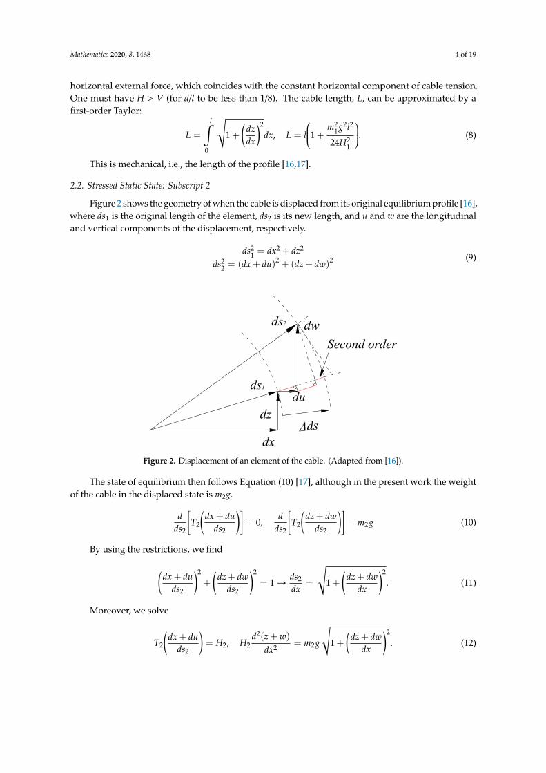
Figure 2 shows the geometry of when the cable is displaced from its original equilibrium profile [16],where ds1 is the original length of the element, ds2 is its new length, and u and w are the longitudinaland vertical components of the displacement, respectively.

ds21 = dx2 + dz2

ds22 = (dx + du)2 + (dz + dw)2 (9)

Mathematics 2020, 8, x FOR PEER REVIEW 4 of 19

Figure 1 shows the cable suspended between two fixed points: A and B and Cartesian coordinates ((−l/2, d) and (+l/2, d), respectively). The vertical external force on the support is V and H is the horizontal external force, which coincides with the constant horizontal component of cable tension. One must have H > V (for d/l to be less than 1/8). The cable length, L, can be approximated by a first-order Taylor:

𝐿 = 1 + 𝑑𝑧𝑑𝑥 𝑑𝑥, 𝐿 = 𝑙 1 + 𝑚 𝑔 𝑙24𝐻 . (8)

This is mechanical, i.e., the length of the profile [16,17].

2.2. Stressed Static State: Subscript 2

Figure 2 shows the geometry of when the cable is displaced from its original equilibrium profile [16], where ds1 is the original length of the element, ds2 is its new length, and u and w are the longitudinal and vertical components of the displacement, respectively.𝑑𝑠 = 𝑑𝑥 + 𝑑𝑧𝑑𝑠 = 𝑑𝑥 + 𝑑𝑢 + 𝑑𝑧 + 𝑑𝑤 (9)

Figure 2. Displacement of an element of the cable. (Adapted from [16]).

The state of equilibrium then follows Equation (10) [17], although in the present work the weight of the cable in the displaced state is m2g. 𝑑𝑑𝑠 𝑇 𝑑𝑥 + 𝑑𝑢𝑑𝑠 = 0, 𝑑𝑑𝑠 𝑇 𝑑𝑧 + 𝑑𝑤𝑑𝑠 = 𝑚 𝑔 (10)

By using the restrictions, we find𝑑𝑥 + 𝑑𝑢𝑑𝑠 + 𝑑𝑧 + 𝑑𝑤𝑑𝑠 = 1 → 𝑑𝑠𝑑𝑥 = 1 + 𝑑𝑧 + 𝑑𝑤𝑑𝑥 . (11)

Moreover, we solve

𝑇 𝑑𝑥 + 𝑑𝑢𝑑𝑠 = 𝐻 , 𝐻 𝑑 𝑧 + 𝑤𝑑𝑥 = 𝑚 𝑔 1 + 𝑑𝑧 + 𝑑𝑤𝑑𝑥 . (12)

Herein, T2 is the tension inside the cable in the displaced state. For small sag, the static equilibrium equation simplifies into [17]

Figure 2. Displacement of an element of the cable. (Adapted from [16]).

The state of equilibrium then follows Equation (10) [17], although in the present work the weightof the cable in the displaced state is m2g.

dds2

[T2

(dx + du

ds2

)]= 0,

dds2

[T2

(dz + dw

ds2

)]= m2g (10)

By using the restrictions, we find

(dx + du

ds2

)2

+

(dz + dw

ds2

)2

= 1→ds2

dx=

√1 +

(dz + dw

dx

)2

. (11)

Moreover, we solve

T2

(dx + du

ds2

)= H2, H2

d2(z + w)

dx2 = m2g

√1 +

(dz + dw

dx

)2

. (12)

Mathematics 2020, 8, 1468 5 of 19

Herein, T2 is the tension inside the cable in the displaced state. For small sag, the static equilibriumequation simplifies into [17]

dl<

18⇒

(dz + dw

dx

)2

<< 1→ H2d2(z + w)

dx2 = m2g. (13)

Using (13), (12) becomes

T2

(dx + du

ds2

)= H2, H2

d2(z + w)

dx2 = m2g. (14)

Equation (14) then becomes

T2(dx + du) = H2ds2 = H2(ds1 + ∆ds) (15)

where ∆ds is the module of the length variation between the length of the displaced state s2, and thelength of the initial state s1 (see Figure 2). Substituting (3) into (15),

T1dx = H1ds1 → (T2 − T1)dx + T2du = (H2 −H1)ds1 + H2∆ds. (16)

When the cable is curved and suspended between two fixed points [16] it is assumed that:∆ds << dx y du << dx. Then, the following value results for T′:

(T2 − T1) ≈ (H2 −H1)dsdx→ T′ ≈ h

dsdx

(17)

where T′ = (T2 − T1) and h = (H2 − H1), according to a prior notation [16].With respect to Equation (14), the second becomes

H2d2zdx2 + H2

d2wdx2 = m2g. (18)

By substituting (4) into (18):d2wdx2 =

m2gH2−

m1gH1

. (19)

Further, integrating in (19) results in

w(x) =(

m2gH2−

m1gH1

)x2

2. (20)

On the other hand, the variation of cable length exclusively attends to geometric considerations(see Figure 2) and corrects the second order of small quantities [16,25].

ds2 − ds1 = dxds1

du + dzds1

dw +(

12

dwds1

)dw

ds2−ds1ds1

= dxds1

duds1

+ dzds1

dwds1

+ 12

(dwds1

)2 (21)

When the cable is fixed between two supports, the change in cable length is due to changes in itsinternal tension, according to Hooke’s law [31] and variations in cable temperature [32].

T′

EA+ α∆t =

ds2 − ds1

ds1=

∆dsds1

(22)

Here, E, A, and T′ denote the Young modulus, the cross-section area, and the additional tensionexerted on the element, respectively. α is the thermal expansion coefficient and ∆t is the temperature

Mathematics 2020, 8, 1468 6 of 19

change of the cable. By putting Equation (21) into (22), the cable equation for an element ds1 isas follows:

T′

EA+ α∆t =

dxds1

duds1

+dzds1

dwds1

+12

(dwds1

)2

. (23)

Substituting (17) into (23) allows for the following:(h

EAds1

dx+ α∆t

)(ds1

dx

)2

=dudx

+dzdx

dwdx

+12

(dwdx

)2

. (24)

If the A and B supports are fixed, there is no horizontal movement between them. Therefore theintegral of the first summand in the right hand side of (24) is zero.

+ 12∫

−12

du = 0 (25)

The integral of the second summand on the right side in (24) is as follows:

+ 12∫

−12

dzdx

dwdx

dx =

+ 12∫

−12

m1gxH1

(m2gH2−

m1gH1

)xdx = 2

m1gxH1

(m2gH2−

m1gH1

)l3

24. (26)

The integral of the third summand of the right side in (24) is as follows:

+ 12∫

−12

12

(dwdx

)2

dx =

+ 12∫

−12

(m2gH2−

m1gH1

)2 x2

dx =

(m2gH2−

m1gH1

)2 l3

24. (27)

Assuming ds1 ≈ dx, integrating (24) and substituting (25)–(27) obtains the following:

(H2 −H1)

EAl + α(t2 − t1)l =

m22g2l3

24H22

−m2

1g2l3

24H21

. (28)

This is a third-order equation with H2 as the unknown. It is the equation of steady-static responsethat students need to solve. It can be solved using Cardano’s formulae, Ruffini’s rule or some otherprocedure for solving cubic equations.

3. Results

As a starting point, we sought to separate the influence that the horizontal external force H and thevertical external force V (due to the cable’s own weight, m) had on (28). To achieve this, we analyzedthe laying and operation of suspended cables by defining three phases.

Phase I is stressing, in which the external horizontal force, H, was applied to the cable. This phasewas exclusively influenced by H and the cable acquired its internal tension. Phase II is lifting, in whichthe external vertical force, V, was applied, keeping the force H constant. In this phase, the cableacquired its full curvature and its internal tension hardly changed. This phase was analyzed in detailsince it was in this phase when the cable defined its initial profile. The final state of this phase, where thecable was fully raised, corresponded to the initial conditions described in Section 2. Finally, Phase IIIwas operation, which sought to solve (28) using simple arithmetic equations supported by equationsand graphical representations obtained during the analysis of the two previous phases.

Mathematics 2020, 8, 1468 7 of 19

3.1. Phase I: Stressing—Horizontal Static State

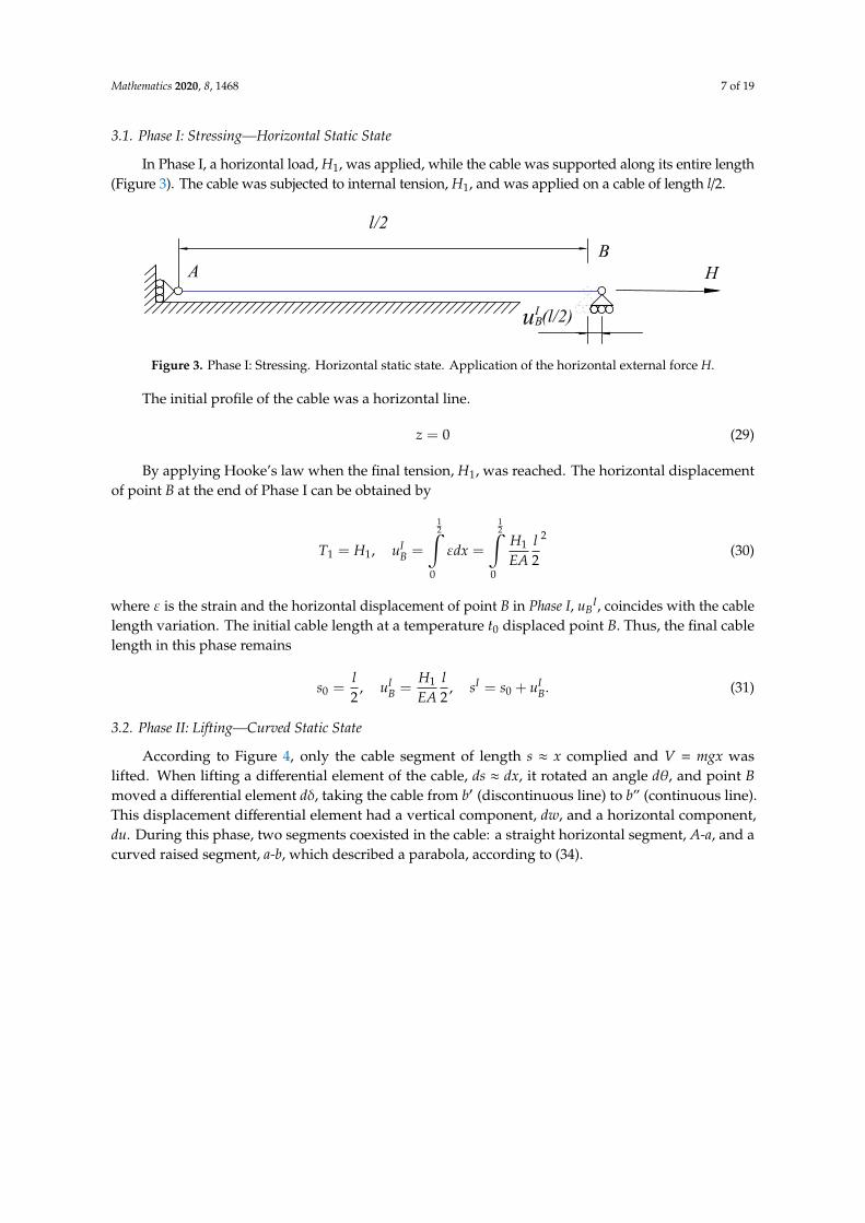
In Phase I, a horizontal load, H1, was applied, while the cable was supported along its entire length(Figure 3). The cable was subjected to internal tension, H1, and was applied on a cable of length l/2.

Mathematics 2020, 8, x FOR PEER REVIEW 7 of 19

Figure 3. Phase I: Stressing. Horizontal static state. Application of the horizontal external force H.

The initial profile of the cable was a horizontal line. 𝑧 = 0 (29)

By applying Hooke’s law when the final tension, H1, was reached. The horizontal displacement of point B at the end of Phase I can be obtained by

𝑇 = 𝐻 , 𝑢 = 𝜀𝑑𝑥 = 𝐻𝐸𝐴 𝑙2 (30)

where ε is the strain and the horizontal displacement of point B in Phase I, uBI, coincides with the cable length variation. The initial cable length at a temperature t0 displaced point B. Thus, the final cable length in this phase remains 𝑠 = 𝑙2 , 𝑢 = 𝐻𝐸𝐴 𝑙2 , 𝑠 = 𝑠 + 𝑢 . (31)

3.2. Phase II: Lifting—Curved Static State

According to Figure 4, only the cable segment of length s ≈ x complied and V = mgx was lifted. When lifting a differential element of the cable, ds ≈ dx, it rotated an angle dθ, and point B moved a differential element dδ, taking the cable from b′ (discontinuous line) to b″ (continuous line). This displacement differential element had a vertical component, dw, and a horizontal component, du. During this phase, two segments coexisted in the cable: a straight horizontal segment, A-a, and a curved raised segment, a-b, which described a parabola, according to (34).

Figure 4. Differential elements in Phase II (lifting). Right segment AB of the final parabola.

Figure 3. Phase I: Stressing. Horizontal static state. Application of the horizontal external force H.

The initial profile of the cable was a horizontal line.

z = 0 (29)

By applying Hooke’s law when the final tension, H1, was reached. The horizontal displacementof point B at the end of Phase I can be obtained by

T1 = H1, uIB =

12∫

0

εdx =

12∫

0

H1

EAl2

2(30)

where ε is the strain and the horizontal displacement of point B in Phase I, uBI, coincides with the cable

length variation. The initial cable length at a temperature t0 displaced point B. Thus, the final cablelength in this phase remains

s0 =l2

, uIB =

H1

EAl2

, sI = s0 + uIB. (31)

3.2. Phase II: Lifting—Curved Static State

According to Figure 4, only the cable segment of length s ≈ x complied and V = mgx waslifted. When lifting a differential element of the cable, ds ≈ dx, it rotated an angle dθ, and point Bmoved a differential element dδ, taking the cable from b′ (discontinuous line) to b” (continuous line).This displacement differential element had a vertical component, dw, and a horizontal component,du. During this phase, two segments coexisted in the cable: a straight horizontal segment, A-a, and acurved raised segment, a-b, which described a parabola, according to (34).

Mathematics 2020, 8, 1468 8 of 19

Mathematics 2020, 8, x FOR PEER REVIEW 7 of 19

Figure 3. Phase I: Stressing. Horizontal static state. Application of the horizontal external force H.

The initial profile of the cable was a horizontal line. 𝑧 = 0 (29)

By applying Hooke’s law when the final tension, H1, was reached. The horizontal displacement of point B at the end of Phase I can be obtained by

𝑇 = 𝐻 , 𝑢 = 𝜀𝑑𝑥 = 𝐻𝐸𝐴 𝑙2 (30)

where ε is the strain and the horizontal displacement of point B in Phase I, uBI, coincides with the cable length variation. The initial cable length at a temperature t0 displaced point B. Thus, the final cable length in this phase remains 𝑠 = 𝑙2 , 𝑢 = 𝐻𝐸𝐴 𝑙2 , 𝑠 = 𝑠 + 𝑢 . (31)

3.2. Phase II: Lifting—Curved Static State

According to Figure 4, only the cable segment of length s ≈ x complied and V = mgx was lifted. When lifting a differential element of the cable, ds ≈ dx, it rotated an angle dθ, and point B moved a differential element dδ, taking the cable from b′ (discontinuous line) to b″ (continuous line). This displacement differential element had a vertical component, dw, and a horizontal component, du. During this phase, two segments coexisted in the cable: a straight horizontal segment, A-a, and a curved raised segment, a-b, which described a parabola, according to (34).

Figure 4. Differential elements in Phase II (lifting). Right segment AB of the final parabola. Figure 4. Differential elements in Phase II (lifting). Right segment AB of the final parabola.

3.2.1. Segment 1: Horizontal Segment—Segment A-a

As shown in Figure 4, only part of the cable was lifted. The rest remained in the same conditionas in Phase I, as well as maintaining the same tension, T, since the external force H1 remained constant(T = H1).

3.2.2. Segment 2: Curved Segment—Segment a-B

Equations (32)–(34) were obtained by applying the static equilibrium equations, which are easy toapply for high-school students. In this work, the mathematical models developed in Section 2 wereapplied to the cable shown in Figure 4. The initial profile was a horizontal line, z = 0, and, in this phase,there was displacement in the z axis, dw > 0.

ds ≈ dx, z = 0, dw , 0 (32)

Replacing (32) in the vertical component of (14) results in

H1d2wdx2 = m1g, ρ1 =

H1

m1g→

d2wdx2 =

1ρ1

(33)

where ρ1 is a good approximation for the radius of curvature of the curve w. Integrating (33) results in

w(x) =m1gx2

2H1=

x2

2ρ1. (34)

The vertical displacement w, according to (34), is easily obtained by secondary school studentsapplying the static equations. Calculation difficulties came with horizontal displacement u. Next,the horizontal displacement was analyzed in detail to find a simple analytical expression.

The mathematical model for horizontal displacement applied polar coordinates to point b.Cartesian coordinates of point b in Phase II are as follows:(

x, w =x2

2ρ1

). (35)

Mathematics 2020, 8, 1468 9 of 19

Polar coordinates of point b, according to Figure 5, assume small values for the angleθ, and thereforealso for ϕ (Equation (13)).

(ϕ, r)→

tanϕ = wx , ϕ ≈ tanϕ = x

2ρ ≈θ2 → w = ϕx

r =√

x2 + z2 = x√

1 + tan2ϕ = xcosϕ

→(θ2

,x

cosϕ

)(36)

Mathematics 2020, 8, x FOR PEER REVIEW 9 of 19

Figure 5. Polar coordinates for the right segment of the parabola, a-b (Phase II). Radius aBI.

𝑠 + 𝑑𝑠 = 𝑥 + 𝑑𝑥 − 𝑢 − 𝑑𝑢, 𝑥 = 𝑟 cos 𝜑 → 𝑑𝑠 = 𝑑𝑟 cos 𝜑 − 𝑟 sin 𝜑𝑑𝜑 − 𝑑𝑢 (37)

When drawing a circle in the center of a, the total length of the cable raised s + ds (segment aBI). Figure 6 shows that between the polar coordinate r + dr (segment ab″) and radius s + ds, there was a difference sc + sc, representation the length applied in defining the cable curvature. Equation (38) was thus satisfied.

Figure 6. Polar coordinates for the right segment of the parabola a-b (Phase II). Radius ab″.

𝑠 + 𝑑𝑠 = 𝑟 + 𝑑𝑟 + 𝑠 + 𝑑𝑠 → 𝑑𝑠 = 𝑑𝑟 + 𝑑𝑠 (38)

Replacing (38) with (37) and approximating for small values of φ results in 𝑑𝑟 − 𝑥𝜑𝑑𝜑 − 𝑑𝑢 = 𝑑𝑟 + 𝑑𝑠 → 𝑑𝑢 + 𝑑𝑠 = −𝑥𝜑𝑑𝜑. (39)

If it is established as a hypothesis that half of the horizontal displacement of point b is used to follow the profile curvature according to (40), then 𝑑𝑠 = − 𝑑𝑢2 . (40)

Therefore, we have obtained an expression for u(x) and sc(x). If w is substituted according to (36), then (39) can be solved as

Figure 5. Polar coordinates for the right segment of the parabola, a-b (Phase II). Radius aBI.

In Figure 5, when the external force, V, was applied at point B (not represented in the figure forsimplicity) a differential dV = mgds increased and a cable element of length ds was raised, which metEquation (37) and was no longer horizontal. Point a was the vertex of the parabola a-b of Equation (34)and moved dx > 0 to the left. Point b was displaced to the left of du, having negative values, accordingto the coordinate axes of Figure 5.

s + ds = x + dx− u− du, x = r cosϕ→ ds = dr cosϕ− r sinϕdϕ− du (37)

When drawing a circle in the center of a, the total length of the cable raised s + ds (segment aBI).Figure 6 shows that between the polar coordinate r + dr (segment ab”) and radius s + ds, there was adifference sc + sc, representation the length applied in defining the cable curvature. Equation (38) wasthus satisfied.

s + ds = r + dr + sc + dsc → ds = dr + dsc (38)

Mathematics 2020, 8, 1468 10 of 19

Mathematics 2020, 8, x FOR PEER REVIEW 9 of 19

Figure 5. Polar coordinates for the right segment of the parabola, a-b (Phase II). Radius aBI.

𝑠 + 𝑑𝑠 = 𝑥 + 𝑑𝑥 − 𝑢 − 𝑑𝑢, 𝑥 = 𝑟 cos 𝜑 → 𝑑𝑠 = 𝑑𝑟 cos 𝜑 − 𝑟 sin 𝜑𝑑𝜑 − 𝑑𝑢 (37)

When drawing a circle in the center of a, the total length of the cable raised s + ds (segment aBI). Figure 6 shows that between the polar coordinate r + dr (segment ab″) and radius s + ds, there was a difference sc + sc, representation the length applied in defining the cable curvature. Equation (38) was thus satisfied.

Figure 6. Polar coordinates for the right segment of the parabola a-b (Phase II). Radius ab″.

𝑠 + 𝑑𝑠 = 𝑟 + 𝑑𝑟 + 𝑠 + 𝑑𝑠 → 𝑑𝑠 = 𝑑𝑟 + 𝑑𝑠 (38)

Replacing (38) with (37) and approximating for small values of φ results in 𝑑𝑟 − 𝑥𝜑𝑑𝜑 − 𝑑𝑢 = 𝑑𝑟 + 𝑑𝑠 → 𝑑𝑢 + 𝑑𝑠 = −𝑥𝜑𝑑𝜑. (39)

If it is established as a hypothesis that half of the horizontal displacement of point b is used to follow the profile curvature according to (40), then 𝑑𝑠 = − 𝑑𝑢2 . (40)

Therefore, we have obtained an expression for u(x) and sc(x). If w is substituted according to (36), then (39) can be solved as

Figure 6. Polar coordinates for the right segment of the parabola a-b (Phase II). Radius ab”.

Replacing (38) with (37) and approximating for small values of ϕ results in

dr− xϕdϕ− du = dr + dsc → du + dsc = −xϕdϕ. (39)

If it is established as a hypothesis that half of the horizontal displacement of point b is used tofollow the profile curvature according to (40), then

dsc = −du2

. (40)

Therefore, we have obtained an expression for u(x) and sc(x). If w is substituted according to (36),then (39) can be solved as

u(x) = −x∫

0wdθ

sc(x) =x∫

0wdϕ.

(41)

The integral of (41) for u(x) was proportional to the first moment of area for the triangle definedby angle θ, according to Figure 4. It is referred to as M and was the first-order static moment withrespect to the z-axis (coordinate origin in the point a).

u(x) = −x∫

0wdθ =

w = x2θ

dθ = dxρ

, u(x) = − 12ρ

x∫0

xθdx = − x3

6ρ2

u(x) = − 12ρM, M = 2

3 x 12 x x

ρ → u(x) = − x3

6ρ2

(42)

Equation (42) gives an expression for the horizontal displacement of point B, u. Therefore, accordingto the hypothesis of Equation (40), the cable length defines the curvature, sc. Both expressions can beobtained by making first-order static moments, which are mathematical tools that students in the finalyears of secondary education use.

Accepted mathematical models were used to validate the above hypothesis [16].The mathematical model for horizontal displacement, u, was used [16].We transitioned from an initial horizontal profile, z = 0, to a curved profile, w. The vertical

displacements w(x) corresponded to (34). The horizontal component in the straight (A-a) and curved(a-b) segments remained constant and equal to H1. Therefore h = 0, according to (17). If the temperatureremains constant at t0, it results in the following:

0 =

xB∫0

du +12

xB∫0

(mgxH

)2dx. (43)

Mathematics 2020, 8, 1468 11 of 19

Integrating the horizontal displacement for point B in Phase II results in the following:

uIIB =

m21g2x3

6H21

→ uIIB = −

x3

6ρ21

. (44)

The displacement of point b is w(x) in the z-axis, according to (34), and uB_II(x) in the x-axis,according to (44). The value of uB_II, according to (44) for a half-span of l/2, corresponds to the lengthincrease of the profile of a parabola with span l, according to (8).

Since (44) corresponds to (42), the hypothesis of Equation (40) is correct.Once the right-hand segment of the cable with a length of s0 = l/2 has been raised, the total

accumulated horizontal displacement of Phase II and the temperature variation from t0 to t1 remainsas follows:

uTB =

H1l2EA

+ α(t1 − t0)l2−

m21g2l3

48H21

, wTB =

m1gl2

8H1. (45)

3.2.3. Segment 2: Curved Segment—Energy Relations

Energy analysis helps students to understand the meaning of this phenomenon [33]. This sectiondescribes the energy relationships that appear in Phases I and II in order to clarify the concepts involved.

The work done by the load is stored in two forms: gravitational potential energy and elastic strainenergy of extensions [16]. The external force, V, is gradually applied at point b, which moves vertically,according to (34), as V increases. The work done for a span, l, is

WV = 2

d∫0

VBdwB = 2

l2∫

0

m21g2x2

Hdx =

43

Vd →

V = m1g l2

d =m1 gl2

8H1

(46)

While applying V, the external force H1 is fully applied. Therefore, it exerts work since point bmoves horizontally, according to (44), for a constant temperature, t0:

WH1 = 2

d∫0

H1duIIB = −2H1uII

B , uIIB = −

m21g2l3

48H21

→ WH1 = −23

Vd. (47)

Thus, the total work of the external forces is

WT = WV + WH = −23

Vd. (48)

The gravitational potential energy is given by

Vg = 2

l2∫

0

m1gwds. (49)

Including the constraints given in (32) and substituting (34) into (49), we find that

Vg = 2

l2∫

0

m21g2x2

2H1dx =

23

Vd. (50)

The potential strain energy is depicted as Ve = 0 and conservation of energy requires that

WT = Vg. (51)

Mathematics 2020, 8, 1468 12 of 19

3.3. Phase III: Operation—Equation of Static Response

The cable was tightened, lifted, and fixed at point B for operation (Figure 7).

Mathematics 2020, 8, x FOR PEER REVIEW 11 of 19

The work done by the load is stored in two forms: gravitational potential energy and elastic strain energy of extensions [16]. The external force, V, is gradually applied at point b, which moves vertically, according to (34), as V increases. The work done for a span, l, is

𝑊 = 2 𝑉 𝑑𝑤 = 2 𝑚 𝑔 𝑥𝐻 𝑑𝑥 = 43 𝑉𝑑 → ⎩⎨⎧𝑉 = 𝑚 𝑔 𝑙2𝑑 = 𝑚 𝑔𝑙8𝐻 (46)

While applying V, the external force H1 is fully applied. Therefore, it exerts work since point b moves horizontally, according to (44), for a constant temperature, t0:

𝑊 = 2 𝐻 𝑑𝑢 = −2𝐻 𝑢 , 𝑢 = − 𝑚 𝑔 𝑙48𝐻 → 𝑊 = − 23 𝑉𝑑. (47)

Thus, the total work of the external forces is 𝑊 = 𝑊 + 𝑊 = − 23 𝑉𝑑. (48)

The gravitational potential energy is given by

𝑉 = 2 𝑚 𝑔𝑤𝑑𝑠. (49)

Including the constraints given in (32) and substituting (34) into (49), we find that

𝑉 = 2 𝑚 𝑔 𝑥2𝐻 𝑑𝑥 = 23 𝑉𝑑. (50)

The potential strain energy is depicted as Ve = 0 and conservation of energy requires that 𝑊 = 𝑉 . (51)

3.3. Phase III: Operation—Equation of Static Response

The cable was tightened, lifted, and fixed at point B for operation (Figure 7).

Figure 7. Final static state. Fixed point B.

The cable was fixed at point B by changing the static conditions of the vertex of the parabola (point A) and this it moved in a vertical direction. This was not the case with horizontal displacement, where both points A and B were restricted in their horizontal displacement. Therefore, the horizontal displacements for the same cable under different conditions, 1 and 2, were the same.

Figure 7. Final static state. Fixed point B.

The cable was fixed at point B by changing the static conditions of the vertex of the parabola(point A) and this it moved in a vertical direction. This was not the case with horizontal displacement,where both points A and B were restricted in their horizontal displacement. Therefore, the horizontaldisplacements for the same cable under different conditions, 1 and 2, were the same.

uTB

∣∣∣2 = H2l

2EA + α(t2 − t0)l2 −

m22 g2l3

48H22

uTB

∣∣∣1 = H1l

2EA + α(t1 − t0)l2 −

m21 g2l3

48H21

(52)

Equation (52) can be obtained by following Phases I, II, and III (for a span of length l/2). It is,therefore, identical to (28) (for a span of length l), which demonstrates the classical cable theory [16,17].Therefore, we determined that the application of the three phases were valid.

Application of Polar Coordinates at Point B

Once in Phase III, the x-coordinate of point B remains constant at x = +l/2. Now,Equation (37) becomes

ds = −du. (53)

Equation (38), using (40), now reads as

dsc = dr =ds2

. (54)

Thus, (41) can be written as

dsc =l2ϕdϕ. (55)

3.4. Didactic Procedure for Solving the Equation of Steady-Static Response

The procedure obtained ∆sc, beginning with a known length variation caused by temperature orstress variations, ∆s, and using (55).

dsc =l2ϕdϕ, ∆sc = zB∆ϕ (56)

The order in which the variables are grouped in the second member of (55) is significant.When grouped as in (56), the product of the first two variables corresponds to the initial z-coordinateof point B, zB1 (see Figure 8).

Mathematics 2020, 8, 1468 13 of 19

Mathematics 2020, 8, x FOR PEER REVIEW 12 of 19

𝑢 = 𝐻 𝑙2𝐸𝐴 + 𝛼 𝑡 − 𝑡 𝑙2 − 𝑚 𝑔 𝑙48𝐻

𝑢 = 𝐻 𝑙2𝐸𝐴 + 𝛼 𝑡 − 𝑡 𝑙2 − 𝑚 𝑔 𝑙48𝐻

(52)

Equation (52) can be obtained by following Phases I, II, and III (for a span of length l/2). It is, therefore, identical to (28) (for a span of length l), which demonstrates the classical cable theory [16,17]. Therefore, we determined that the application of the three phases were valid.

3.3.1. Application of Polar Coordinates at Point B

Once in Phase III, the x-coordinate of point B remains constant at x = +l/2. Now, equation (37) becomes 𝑑𝑠 = −𝑑𝑢. (53)

Equation (38), using (40), now reads as 𝑑𝑠 = 𝑑𝑟 = 𝑑𝑠2 . (54)

Thus, (41) can be written as 𝑑𝑠 = 𝑙2 𝜑𝑑𝜑. (55)

3.4. Didactic Procedure for Solving the Equation of Steady-Static Response

The procedure obtained Δsc, beginning with a known length variation caused by temperature or stress variations, Δs, and using (55). 𝑑𝑠 = 𝑙2 𝜑𝑑𝜑, ∆𝑠 = 𝑧 ∆𝜑 (56)

The order in which the variables are grouped in the second member of (55) is significant. When grouped as in (56), the product of the first two variables corresponds to the initial z-coordinate of point B, zB1 (see Figure 8).

Figure 8. Graphical representation of Δsc according to Equation (56).

The calculation procedure starts from initial conditions (subscript 1) and obtains a variation of the angle of rotation, Δθ, to approximate H2 in two steps:

Figure 8. Graphical representation of ∆sc according to Equation (56).

The calculation procedure starts from initial conditions (subscript 1) and obtains a variation of theangle of rotation, ∆θ, to approximate H2 in two steps:

Step 1 uses (56) to determine the length variation caused by temperature changes from t1 to t2, ∆s.Then, the previous length is calculated for curvature length, ∆sc. Then, ∆ϕ and the value of H2

I can beobtained as an approximation of H2, according to (57).

x = l2 , ϕ1=

m1 gx2H1

, zB1 = xϕ1

Step 1:∆sc =

∆s2 , ∆s = xα(t2 − t1)

∆ϕI =∆sczB1

ϕI = ϕ1 + ∆ϕI → HI2 =

m2 gx2ϕI

(57)

Step 2 calculates the length variation when changing the cable tension from H1 to H2I, ∆s. Then,

the previous length is calculated for curvature length, ∆sc. Then, ∆ϕ and the value of H2II can be

obtained as an approximation of H2, according to (58).

x = l2 , ϕ1=

m1 gx2H1

, zB1 = xϕ1, ∆ϕI

Step 2:

∆sc =∆s2 , ∆s =

x(HI2−H1)SE

∆ϕII =∆sczB1

ϕII = ϕ1 + ∆ϕI + ∆ϕII → HII2 =

m2 gx2ϕII≈ H2

(58)

3.5. Application of the Procedure to Cables Used in Low-Voltage Aerial Lines

The above algorithm was applied to cables for low voltage aerial lines that were referred toin Royal Decree 842/2002, which approved low voltage electrotechnical regulations in Spain [34].To evaluate the results, the exact values were provided by MATLAB’s fsolve algorithm, which uses avariant of an algorithm previously described [35]. It was applied to solve (28).

Table 1 provides the mechanical characteristics of the cable with designation RZ 3x50 Al/54.6 Alm.

Table 1. Characteristics of cable RZ 3x50 Al/54.6 Alm.

Designation Characteristics

RZ 3x50 Al/54.5 AlmS = 54.6 mm2; m = 0.755 kg ·m−1;

E = 6000 kg ·mm−2; α = 23× 10−6 ◦C−1

Mathematics 2020, 8, 1468 14 of 19

The change of static state conditions described in Table 2 was carried out for the cable withdesignation RZ 3x50 Al/54.6 Alm, for a span of l = 50 m. The initial state of the conditions correspondedto the maximum tension reached by the cable and the final state corresponded to the maximum sag onthe cable. The conditions were obtained according to Spanish standards [34].

Table 2. Conditions for the cable RZ 3x50 Al/54.6 Alm.

Initial State Conditions: Tmax Final State Conditions: dmax

H1 = 345 kp; m1 = 1.99 kg ·m−1; t1 = 15◦

C H2; m2 = 0.755 kg ·m−1; t2 = 50◦

C

Table 3 shows the solution of each step and the relative error as a percentage of the solutionprovided by fsolve.

Table 3. Results for the cable RZ 3x50 Al/54.6 Alm.

Procedure Result

MATLAB: fsolve H2 = 128.33 kpStep I: H2 = 128.45 kp

Error % 0.099%Step II: H2 = 128.02 kpError % 0.063%

Table 4 provides the mechanical characteristics of the cable with designation RZ 3x95 Al/54.6 Alm.

Table 4. Characteristics of cable RZ 3x95 Al/54.6 Alm.

Designation Characteristics

RZ 3x95 Al/54.6 AlmS = 54.6 mm2; m = 1.26 kg ·m−1;

E = 6000 kg ·mm−2; α = 23× 10−6 ◦C−1

The change of static state conditions described in Table 5 was carried out for the cable withdesignation RZ 3x95 Al/54.6 Alm, for a span of l = 50 m. The initial state of the conditions correspondedto the maximum tension reached by the cable and the final state corresponded to the maximum sag onthe cable. The conditions were obtained according to Spanish standards [34].

Table 5. Conditions for the cable RZ 3x95 Al/54.6 Alm.

Initial state conditions: Tmax Final State Conditions: dmax

H1 = 345 kp; m1 = 2.58 kg ·m−1; t1 = 15◦

C H2; m2 = 1.26 kg ·m−1; t2 = 50◦

C

Table 6 shows the solution of each step and the relative error as a percentage of the solutionprovided by fsolve.

Table 6. Results for the cable RZ 3x95 Al/54.6 Alm.

Procedure Result

MATLAB: fsolve H2 = 165.017 kpStep I: H2 = 167.67 kp

Error % 1.00%Step II: H2 = 166.06 kpError % 0.987%

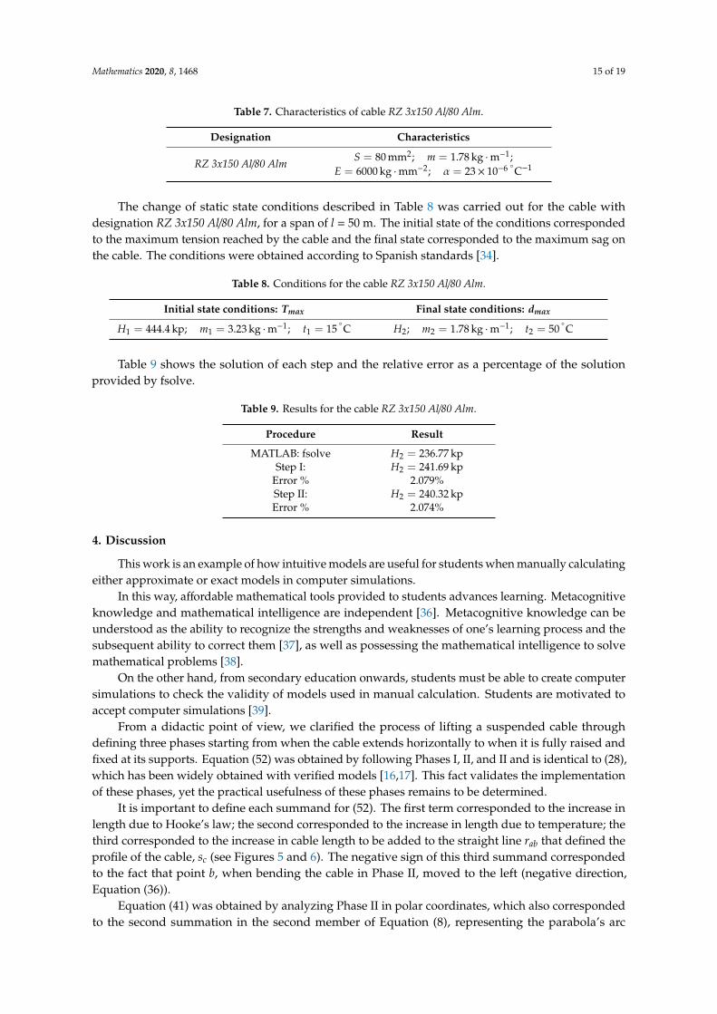
Table 7 provides the mechanical characteristics of the cable with designation RZ 3x150 Al/80 Alm.

Mathematics 2020, 8, 1468 15 of 19

Table 7. Characteristics of cable RZ 3x150 Al/80 Alm.

Designation Characteristics

RZ 3x150 Al/80 AlmS = 80 mm2; m = 1.78 kg ·m−1;

E = 6000 kg ·mm−2; α = 23× 10−6 ◦C−1

The change of static state conditions described in Table 8 was carried out for the cable withdesignation RZ 3x150 Al/80 Alm, for a span of l = 50 m. The initial state of the conditions correspondedto the maximum tension reached by the cable and the final state corresponded to the maximum sag onthe cable. The conditions were obtained according to Spanish standards [34].

Table 8. Conditions for the cable RZ 3x150 Al/80 Alm.

Initial state conditions: Tmax Final state conditions: dmax

H1 = 444.4 kp; m1 = 3.23 kg ·m−1; t1 = 15◦

C H2; m2 = 1.78 kg ·m−1; t2 = 50◦

C

Table 9 shows the solution of each step and the relative error as a percentage of the solutionprovided by fsolve.

Table 9. Results for the cable RZ 3x150 Al/80 Alm.

Procedure Result

MATLAB: fsolve H2 = 236.77 kpStep I: H2 = 241.69 kp

Error % 2.079%Step II: H2 = 240.32 kpError % 2.074%

4. Discussion

This work is an example of how intuitive models are useful for students when manually calculatingeither approximate or exact models in computer simulations.

In this way, affordable mathematical tools provided to students advances learning. Metacognitiveknowledge and mathematical intelligence are independent [36]. Metacognitive knowledge can beunderstood as the ability to recognize the strengths and weaknesses of one’s learning process and thesubsequent ability to correct them [37], as well as possessing the mathematical intelligence to solvemathematical problems [38].

On the other hand, from secondary education onwards, students must be able to create computersimulations to check the validity of models used in manual calculation. Students are motivated toaccept computer simulations [39].

From a didactic point of view, we clarified the process of lifting a suspended cable throughdefining three phases starting from when the cable extends horizontally to when it is fully raised andfixed at its supports. Equation (52) was obtained by following Phases I, II, and II and is identical to (28),which has been widely obtained with verified models [16,17]. This fact validates the implementationof these phases, yet the practical usefulness of these phases remains to be determined.

It is important to define each summand for (52). The first term corresponded to the increase inlength due to Hooke’s law; the second corresponded to the increase in length due to temperature; thethird corresponded to the increase in cable length to be added to the straight line rab that defined theprofile of the cable, sc (see Figures 5 and 6). The negative sign of this third summand correspondedto the fact that point b, when bending the cable in Phase II, moved to the left (negative direction,Equation (36)).

Equation (41) was obtained by analyzing Phase II in polar coordinates, which also correspondedto the second summation in the second member of Equation (8), representing the parabola’s arc

Mathematics 2020, 8, 1468 16 of 19

length. The latter is of great importance for the mathematical procedure in suspended cables and istraditionally obtained via integral calculation. This is a difficulty for students in secondary education,since they often have not yet studied integral calculus or it is not contemplated in their curricula.Equation (44) was obtained as the first-order static moment of the triangular area defined by angle θ

(see Figure 5 and Equation (42)). This fact is of notable didactic importance at the secondary educationlevel, since students have knowledge of mathematics applied to the calculation of static momentsand centers of gravity. Thus, (42) provides a calculation tool for students that allows them to advancetheir studies.

Energy helps students understand the meaning of this phenomenon [33]. For this reason, it hasbeen considered useful to obtain energy relations in Phases I and II, in order to clarify the conceptsinvolved in these phases. They are simple expressions that can be used to perform didactic problemswhile teaching, although obtaining them requires integral calculus. Applying energetic relationshipsallows one to clarify the physical processes that occurs during each phase. Thus, during Phase Iof stressing, only elastic potential energy is accumulated, while during Phase II of lifting, the cableaccumulates gravitational potential energy and elastic potential energy, the latter being negligible.

Equations (37)–(39) are of considerable importance when developing the calculation proceduredescribed in Section 3.4. The polar coordinate r is related to the cable length s and to the Cartesiancoordinate x, according to Figure 5 and Equation (38). In (39), (41) was replaced by (37) afterdifferentiation, wherein the approximation for small values of the angle θ was made. It is important topoint out that if, in (37), the approximation for small angles was made first, the information providedby the differential process would be lost. In that case, Equation (39), fundamental to the calculationprocedure, would be reduced to a trivial equality (0=0). This fact has great didactic value since itrecognizes the implications of the approaches made in the model. These details stimulate the interest ofmany students. Examples of systems with similar effects on students are the elastic pendulum [40] orthe three-body problem [41]. These are simple approaches that can present complex or simple dynamicbehaviors depending on their state.

In (39), the calculation process was stopped because two unknowns appeared, sc and u.A hypothesis is still needed, which is stated in (40). This is a conceptual advance for the didacticdevelopment of suspended cables. It states that only half of the horizontal displacement of pointb during Phase II is applied when varying the cable curvature and therefore the angle θ at point B(see Figure 6). Solutions for (39) and (40) results in (41). It provides an expression for both sc and uin Phase II. In the case of u, it is identical to the expression of Equation (44) from widely validatedmathematical models [16,17]. This validates the hypothesis of (40), which is half of the horizontaldisplacement u (in modulus) in Phases II and III. This is responsible for the curvature of the cable profile.

Considering the importance of (41), it is convenient to indicate that the expression obtainedcorresponds to first-order static moments of triangular figures (see (42)). This fact favors their study insecondary education and specifically for students not required to have skills in differential calculus.

For the calculation procedure of cable conditions changes in Phase III, Figure 8 is relevant.It graphically shows the result of (56), interpreted as the product of a radius by an angle. This graphictool has great didactic power since it allows the visualization of a calculation procedure, as well aslocates the main magnitudes involved in ∆s, ∆u, and ∆sc. Even the veracity of the hypothesis ofEquation (40) can be assessed. This affords students the possibility to understand mathematical modelsthrough formulas (i.e., Equation (56)) and graphs (i.e., Figure 8).

In Section 3, the calculation procedure was applied to the three most used cables in low-voltageaerial lines. The cables were laid in a span of l = 50 m, which is an average span for this type of line.A change in static conditions was applied from conditions, implying maximum internal tension in thecable (subscript 1) to conditions implying maximum sag in the cable (subscript 2). Step I correspondedto the variation in curvature due to temperature (i.e., Equation (57)), achieving good results in all threecases with results having errors below 2.1% with respect to the exact solution provided by MATLAB’s

Mathematics 2020, 8, 1468 17 of 19

fsolve. The calculation procedure described in Section 3.4 can be reduced to step I, especially whenconcerning temperature variation. The application of step II slightly improved the results.

Since these were standard problems in low-voltage aerial line design, they became puzzleproblems [10]. These were complete problems with statements, analytical resolution proceduressupported by graphics, and concrete/intuitive analytical solutions. However, this was an approximatesolution because the procedure did not lead to an exact solution, as it is not an algorithm. The procedureallows students to advance their studies by having mathematical tools that analyze cables in anycondition. These are tools that students are familiar and friendly with. The problems were posed tostudents in secondary education, specifically in vocational education and training in the electricalbranch. They accepted the calculation procedure positively because it allowed them to manuallymake a complete problem. They can thus obtain a computer solution to compare results. In addition,students can be encouraged to search independently for other methods of solving the equation ofsteady-static response in suspended cables, such as the Cardano’s formulae or the Ruffini’s rule.

In future works, the described calculation procedure should be applied to more complex calculationconditions, i.e., cables with several spans and different lengths [20], and spans with supports at differentlevels. The main point of interest is to apply the procedure to cables with large thermal uprating,which would increase their power transfer capacity [42–44]. The conductors (i.e., high-temperatureand low-sag conductors) can support temperatures up to 150 ◦C, against 80 ◦C of the conductors theyreplace [45]. In this case, there were large temperature variations and this was where the calculationprocedure described in this paper obtained the best results.

5. Conclusions

In this study, an approximate method to calculate low voltage aerial lines was successfullydeveloped. The method facilitated the acquisition of professional and mathematic competences forvocational education and training students in the electrical branch. Educational exercises were hereinproposed and students provided affordable calculations and analysis tools.

Three phases have been differentiated in the laying and operation of the suspended cables, owingto which a graphic procedure has been obtained in which each of the magnitudes involved in theprocess are identified. It is an approximate but useful tool for solving exercises manually, and for thestudent to have a simple model of resolution and understanding of the physical phenomena involved.

The equation of steady-static response in suspended cables to solve is a cubic equation, which canbe solved by well-known methods such as the Cardano’s formulae or the Ruffini’s rule, among others.This work provides a graphical solution of the equation of steady-static response and requires applyingthe physical laws used in suspended cables. Step I of the procedure considers the variation in cablelength with the change in temperature, and step II evaluates the variation in length with the changein tension. This procedure has great didactic value, since it allows the student to apply previouslyacquired concepts, which are necessary for the study of suspended cables.

As disadvantages or limitations of the proposed procedure, it provides only approximate results tothe exact solution and requires more time to resolve the exercise. In addition, it is a specific procedure,not applicable to other subjects of the course.

Author Contributions: Conceptualization, J.A.-R., Á.-J.C.-F., J.L.-M., and M.G.-G.; methodology, J.A.-R., Á.-J.C.-F.,J.L.-M., and M.G.-G.; software, J.A.-R., Á.-J.C.-F., J.L.-M., and M.G.-G.; validation, J.A.-R., Á.-J.C.-F., J.L.-M., andM.G.-G.; formal analysis, J.A.-R., Á.-J.C.-F., J.L.-M., and M.G.-G.; investigation, J.A.-R., Á.-J.C.-F., J.L.-M., andM.G.-G.; resources, J.A.-R., Á.-J.C.-F., J.L.-M., and M.G.-G.; data curation, J.A.-R., Á.-J.C.-F., J.L.-M., and M.G.-G.;writing—original draft preparation, J.A.-R., Á.-J.C.-F., J.L.-M., and M.G.-G.; writing—review and editing, J.A.-R.,Á.-J.C.-F., J.L.-M., and M.G.-G.; visualization, J.A.-R., Á.-J.C.-F., J.L.-M., and M.G.-G.; supervision, J.A.-R., Á.-J.C.-F.,J.L.-M., and M.G.-G.; and project administration, J.A.-R., Á.-J.C.-F., J.L.-M., and M.G.-G. All authors have read andagreed to the published version of the manuscript.

Funding: This research received no external funding.

Mathematics 2020, 8, 1468 18 of 19

Acknowledgments: José Agüero-Rubio wants to thank the Consejería de Educación de la Junta de Andalucía for theresearch stay during the 2011–12 academic year. Further, he would like to thank the vocational education andtraining students in the branch of electricity of the IES Alhamilla in Almeria (Spain) for their positive predispositionto realize the examples presented in this work.

Conflicts of Interest: The authors declare no conflict of interest.

References

1. Real Decreto 1127/2010 de 10 de Septiembre. [Royal Decree 1127/2010 of 10 of September]; The Title of SuperiorTechnician in Electrotechnical and Automated Systems Is Established and Their Minimum Teachings AreEstablished. Ed. Boletín Oficial del Estado de 8 de octubre de 2010 [Official State Gazette of October 8]. In BOE(Boletín Oficial del Estado); State Agency Official State Gazette: Madrid, Spain, 2010; Number 244; p. 85006.

2. UNESCO Institute for Statistics. International Standard Classification of Education: ISCED 2011; UIS: Montreal,QC, USA, 2012. [CrossRef]

3. Boyse, C.O.; Simpson, N.G. The problem of conductor sagging on overhead transmission lines. J. Inst. Electr.Eng. Part II Power Eng. 1944, 91, 219–238.

4. Landau, M. Incremental method for sag-tension calculations. Trans. Am. Inst. Electr. Eng. 1951, 70, 1564–1571.[CrossRef]

5. Lummis, J.; Fischer, J.R. Practical design of transmission line tensions. Electr. Eng. 1955, 74, 39. [CrossRef]6. Balangó, D.; Mémeth, B.; Göcsei, G. Predicting conductor sag of power lines in a new model of Dynamic Line

Rating. In Proceedings of the IEEE Electrical Insulation Conference (EIC), Seattle, WA, USA, 7–10 June 2015.7. Dong, X. Analytic method to calculate and characterize the sag and tension of overhead lines. IEEE Trans.

Power Deliv. 2016, 31, 20646–20671.8. Huilier, D.G.E. Forty Years’ Experience in Teaching Fluid Mechanics at Strasbourg University. Fluids 2019, 4, 199.

[CrossRef]9. Moreno-Clemente, J. Evolución del cálculo mecánico de conductores en líneas aéreas con la aplicación de la

informática. DYNA 2001, 76, 6–10.10. Leite, L.; Dourado, L. Laboratory activities, science education and problem-solving skills. Procedia Soc. Behav. Sci.

2013, 106, 1677–1686. [CrossRef]11. Garrett, R.M. Issues in science education: Problem-solving, creativity and originality. Int. J. Sci. Educ. 1987,

85, 113–119. [CrossRef]12. Roberts, R. Using different types of practical within a problem-solving model of science. Sch. Sci. Rev. 2004,

9125–9137.13. Dodge, R.E.; Fisher, B.E.; King, J.J.; Kuehl, P.G.; Matsuki, S.; Mitchell, W.E.; Dailey, J.F.; Boyajian, D.M.

Introducing the Structural Engineering Encounter laboratory: A physical approach to teaching statics,mechanics of materials and structural analysis. World Trans. Eng. Technol. Educ. 2011, 9, 86–91.

14. Teik-Cheng, L. Revisiting the elasticity solution for a simply supported beam under sinusoidal load. Int. J.Mech. Eng. Educ. 2018, 46, 41–49.

15. Raviv, D.; Barb, D. A Visual, Intuitive and Engaging Approach to Explaining the Center of Gravity Conceptin Statics. In Proceedings of the 2019 126th ASEE Annual Conference & Exposition, Tampa, FL, USA,15–19 June 2019.

16. Irvine, H.M. Statics of a Suspended Cable. In Cable Structures; The MIT Press: Cambridge, NJ, USA, 1981;pp. 43–44.

17. Treyssède, F. Free linear vibrations of cables under thermal stress. J. Sound Vib. 2009, 327, 1–8. [CrossRef]18. Yaobing, Z.; Chaohui, H.; Lincong, C.; Peng, J. Nonlinear vibration behaviors of suspended cables under

two-frequency excitation with temperature effects. J. Sound Vib. 2018, 416, 279–294.19. Majid, K.; Masoud, F.; László, E.K. Estimation of stresses in atmospheric ice during Aeolian vibration of

power transmission lines. J. Wind Eng. Ind. Aerodyn. 2010, 98, 592–599.20. Wu, C.; Yan, B.; Zhang, L.; Zhang, B.; Li, Q. A method to calculate jump height of iced transmission lines

after ice-shedding. Cold Reg. Sci. Technol. 2016, 125, 40–47. [CrossRef]21. Bertand, C.; Plut, C.; Ture Savadkoohi, A.; Lamarque, C.H. On the modal response of mobile cables.

Eng. Struct. 2020, 210, 110231. [CrossRef]

Mathematics 2020, 8, 1468 19 of 19

22. Wang, L.; Rega, G. Modelling and transient planar dynamics of suspended cables with moving mass. Int. J.Solids Struct. 2010, 47, 2733–2744. [CrossRef]

23. Gattulli, V.; Martinelli, L.; Perotti, F.; Vestroni, F. Nonlinear oscillations of cables under harmonic loadingusing analytical and finite element models. Comput. Methods Appl. Mech. Eng. 2004, 193, 68–85. [CrossRef]

24. Luongo, A.; Rega, G.; Vestroni, F. Monofrequent oscillations of a non-linear model of a suspended cable.J. Sound Vib. 1982, 82, 247–259. [CrossRef]

25. Rega, G.; Vestroni, F.; Benedettini, F. Parametric analysis of large amplitude free vibrations of a suspendedcable. Int. J. Solids Struct. 1984, 20, 95–105. [CrossRef]

26. Lianhua, W.; Jianjun, M.; Jian, P.; Lifeng, L. Large amplitude vibration and parametric instability ofinextensional beams on the elastic foundation. Int. J. Mech. Sci. 2013, 67, 1–9.

27. Rezaiee-Pajand, M.; Mokhtari, M.; Massodi, A.R. A novel cable element for nonlinear thermo-elastic analysis.Eng. Struct. 2018, 167, 431–444. [CrossRef]

28. Pereira da Silva, A.A.; de Barros Bezerra, J.M. A Model for Uprating Transmission Lines by Using HTLSConductors. IEEE Trans. Power Deliv. 2011, 26, 2180–2188.

29. Yang, Y.B.; Tsay, J.Y. Geometric nonlinear analysis of cable structures with a two node cable element bygeneralized displacement control method. Int. J. Struct. Stab. Dyn. 2007, 7, 571–588. [CrossRef]

30. Luongo, A.; Zulli, D. Statics of Shallow Inclined Elastic Cables under General Vertical Loads: A PerturbationApproach. Mathematics 2018, 6, 24. [CrossRef]

31. Rychlewski, J. On Hooke’s law. J. Appl. Math. Mech. 1984, 48, 303–314. [CrossRef]32. Lepidi, M.; Gattulli, V. Static and dynamic response of elastic suspended cables with thermal effects. Int. J.

Solids Struct. 2012, 49, 1103–1116. [CrossRef]33. Nordine, J.; Fortus, D.; Lehavi, Y.; Neumann, K.; Krajcik, J. Modelling energy transfers between systems to

support energy knowledge in use. Stud. Sci. Educ. 2018, 54, 177–206. [CrossRef]34. Royal Decree 842/2002 of 2 of August. Low Voltage Electro-Technical Regulations and Their Complementary Technical

Instructions; Ministerio de Ciencia y Tecnología: Madrid, Spain, 2002.35. Powell, M.J.D. A Fortran Subroutine for Solving Systems of Nonlinear Algebraic Equations. Numerical Methods for

Nonlinear Algebraic Equations; Atomic Energy Research Establishment: Harwell, UK, 1968.36. Chytry, V.; Rícan, J.; Eisenmann, P.; Medová, J. Metacognitive knowledge and mathematical intelligence-two

significant factors influencing school performance. Mathematics 2020, 8, 969. [CrossRef]37. Azevedo, R. Theoretical, conceptual, methodological, and instructional issues in research on metacognition.

Metacognition Learn. 2009, 4, 87–95. [CrossRef]38. Eisenmann, P.; Novotná, J.; Pˇribyl, J.; Bˇrehovský, J. The development of a culture of problem solving with

secondary students through heuristic strategies. Math. Ed. Res. J. 2015, 27, 535–562. [CrossRef]39. Rodríguez-Martín, M.; Rodríguez-Gonzálvez, P.; Sánchez-Patrocinio, A.; Ramón-Sánchez, J. Short CFD

Simulation Activities in the Context of Fluid-Mechanical Learning in a Multidisciplinary Student Body.Appl. Sci. 2019, 9, 4809. [CrossRef]

40. Cuerno, R.; Rañada, F.; Ruiz-Lorenzo, J.J. Deterministic chaos in the elastic pendulum: A simple laboratoryfor nonlinear dynamics. Am. J. Phys. 1992, 60, 73–79. [CrossRef]

41. Hayes, W. Computer simulations, exact trajectories, and the gravitational N-body problem. Am. J. Phys.2004, 72, 1251–1257. [CrossRef]

42. Daconti, J.R.; Lawry, D.C. Increasing power transfer capability of existing transmission lines. IEEE Xplore2003. [CrossRef]

43. Albizu, I.; Mazón, A.J.; Valverde, V.; Buigues, G. Aspects to take into account in the application of mechanicalcalculation to high-temperature low-sag conductors. IET Gener. Transm. Dis. 2010, 4, 631–640. [CrossRef]

44. Mazón, A.J.; Zamora, I.; Eguía, P.; Torres, E.; Miguélez, S.; Median, R.; Saenz, J.R. Gap-type conductors:Influence of high temperature in the compression clamp systems. In Proceedings of the 2003 IEEE BolognaPower Tech Conference, Bolgna, Italy, 23–26 June 2003.

45. Michiori, A.; Nguyen, H.-M.; Alessandrini, S.; Bremnes, J.B.; Dierer, S.; Ferrero, E.; Nygaard, B.-E.; Pinson, P.;Thomaidis, N. Forecasting for dynamic line rating. Renew. Sust. Energ. Rev. 2015, 52, 1713–1730. [CrossRef]

© 2020 by the authors. Licensee MDPI, Basel, Switzerland. This article is an open accessarticle distributed under the terms and conditions of the Creative Commons Attribution(CC BY) license (http://creativecommons.org/licenses/by/4.0/).