A Decomposition Algorithm for Uniform Traveling Salesman Problem

A Decomposition Algorithm for Uniform Traveling Salesman

Problem

Roman Bazylevych1, Bhanu Prasad2, Roman Kutelmakh3, Rémy Dupas4, Lubov Bazylevych5 1University of Information Technology and Management in Rzeszow, Poland

[email protected] 2Department of Computer and Information Sciences,

Florida A & M University, Tallahassee, Florida 32307, USA

[email protected] 3Lviv Polytechnic National University, Ukraine

[email protected] 4 Université de Bordeaux - IMS UMR 5218 CNRS, France

5Institute of Applied Problems of Mechanics and Mathematics, Academy of Science, Ukraine

Abstract. This paper presents a decomposition algorithm for solving the uniform

Travelling Salesman Problem (TSP). The algorithm assumes that the initial set of points is

divided into subsets and overlapping regions between these subsets. The algorithm starts by

considering a subset and find the solution in that subset. The solution in the next subset is

calculated by expanding the earlier solution for the current subset and this process

continues until all the subsets are considered. In this algorithm, a given problem with n

points is replaced by m problems, each having k (k << n) points. The algorithm is tested

with 10000-points and the results prove that it considerably reduces the computational time.

In addition, its quality is close to that of the best known heuristic algorithm.

Keywords: Traveling Salesman Problem, combinatorial optimization, decomposition.

1. Introduction

The algorithms related to vehicle routing problems have a wide range of practical applications

[1, 2] and some of them can be applied to the domains such as telecommunication systems,

VLSI design, laser cutting of plastic and metal, genome sequencing, etc. [3]. The demand for

faster algorithms that can provide better quality solutions is always increasing. In addition, the

problem size (i.e., number of points) is also increasing. As a result, there is a great need for

designing specialized algorithms that are faster and can produce high-quality solutions for large-

scale problems.

The Traveling Salesman Problem (TSP) is one of the fundamental problems in

combinatorial optimization [4]. In the uniform TSP, the points are distributed uniformly over the

space/area. There is a great need for the development of efficient decomposition algorithms for

TSP, which can work for large-scale instances, with a computation complexity of O(nlogn) or

better, where n is the total number of points in the given area. There are a few heuristic

algorithms that can guarantee high-quality solutions for this problem [4]. Lin-Kernighan

4th Indian International Conference on Artificial Intelligence (IICAI-09)

47

algorithm [5, 6] is one of the most efficient algorithms and its complexity is O(n2). The results

obtained by this algorithm are within 1-3% range of the optimal results [4]. Helsgaun [7]

developed a new version of Lin-Kernighan algorithm that can find the optimal solution for a

85900-point problem from the TSPLIB tests library [8, 9]. According to the DIMACS TSP

Challenge test results [4], it is the best heuristic algorithm [4, 10]. Its complexity is O(n2.2

). The

new Helsgaun’s Lin-Kernighan algorithm [11] includes some additional features such as k-opt

moves, tour merging [12], backbone-guided search [13, 14] and partitioning. Decomposition

approaches were also investigated by Rohe [15].

For the problems that need exact solutions, Concorde TSP Solver [3] was developed. It

combines branch-and-cut and linear programming techniques. Concorde TSP Solver can provide

optimal solutions for all the tests (from TSPLIB) that are having up to 85900 points. The

solution for the 85900-point problem took nearly 136 years of the processor time when a cluster

of Intel Xeon and AMD Opteron processors are used.

The rest of the paper is organized as follows: Section 2 describes the problem

formulation, Section 3 describes the proposed algorithm, Section 4 presents some experimental

results and finally, Section 5 provides some conclusions.

2. Problem Formulation

The TSP is formulated as a graph G = (�, E), where � (|�| = n) is the set of vertices (also called

nodes or points) and E is the set of edges. cij is the cost (i.e., weight) of the edge eij ∈ E and it is

given for all i, j ∈ �. The general form of TSP is to find a minimum cost closed cycle visiting

every vertex in � exactly once. The problem is symmetric if cij = cji ∀i, j ∈ �. The problem is

Euclidean if every element of � is provided with its coordinates (xi, yi) and the cost function is

the Euclidean distance between the points. Note that cij + cjk ≥ cik ∀i, j, k ∈ � in case the problem

is Euclidean.

This paper addresses the problem of finding a minimum cost closed cycle that includes

all vertices of a given symmetric Euclidean graph. If this cycle is denoted by S* then its length

L(S*) = Σij lij* → min Σij lij ∀ lij, where lij is the length of the edge between the vertices i and j

(i.e., Euclidean distance between i and j) in the given graph.

3. Proposed Solution

The proposed decomposition algorithm assumes that the given set � is already divided into m

subsets. The solution to the problem begins in a subset that is chosen arbitrarily. The solution in

the next subset is then calculated and both these solutions (i.e., solution in the initial subset and

the solution in the current subset) are combined (i.e., concatenated) as explained later. This

process continues until the solutions in all of the subsets are calculated and combined. The given

problem with n points is replaced by m problems with k points in each. Obviously k << n, and


48

this relatively small value k facilitates finding the solution to the problem easily. An efficient

basic algorithm is used to solve the TSP in every subset. In our proposed approach, we used Lin-

Kernighan-Helsgaun (LKH) algorithm [7] as the basic algorithm.

Figure 1. The initial set partitioning into subsets and overlapping areas.

Figure 2. TSP solution S11 for the subset �11 (some points of �11 are not shown in S11 to

make S11 look simple).

We also developed a simple method for splitting the overall vertex set (i.e., given area)

into subsets and overlapping regions between these subsets. The method is not formally

explained in this paper due to its simplicity but an example is provided in Fig. 1. The figure

represents the initial set � and its division into subsets. The square representing � (left hand side

portion of the figure) has 1000 x 1000 units and the width and height of each subset is 250 units

(right hand side portion of the figure). The overlapping areas between the subsets are marked

gray.

�11 �12 �13 �14

�21 �22 �23 �24

�31 �32 �33 �34

�41 �42 �43 �44


49

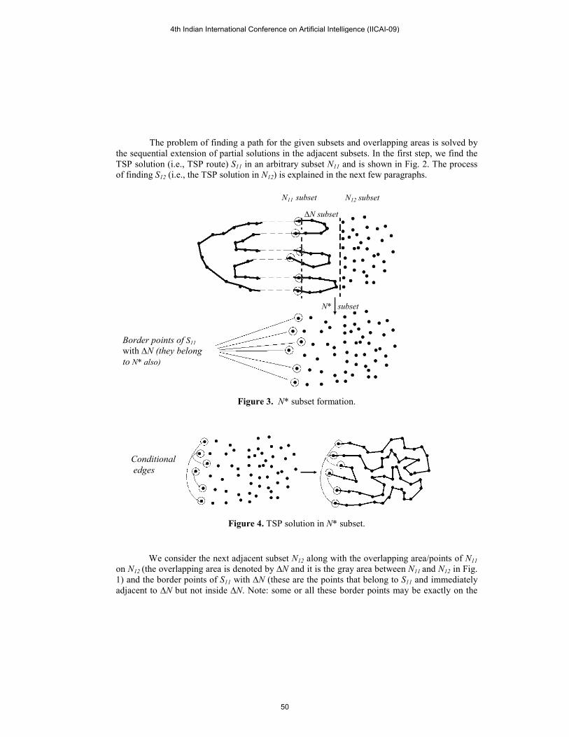
The problem of finding a path for the given subsets and overlapping areas is solved by

the sequential extension of partial solutions in the adjacent subsets. In the first step, we find the

TSP solution (i.e., TSP route) S11 in an arbitrary subset �11 and is shown in Fig. 2. The process

of finding S12 (i.e., the TSP solution in �12) is explained in the next few paragraphs.

Figure 3. �* subset formation.

Figure 4. TSP solution in �* subset.

We consider the next adjacent subset �12 along with the overlapping area/points of �11

on �12 (the overlapping area is denoted by "� and it is the gray area between �11 and �12 in Fig.

1) and the border points of S11 with "� (these are the points that belong to S11 and immediately

adjacent to "� but not inside "�. Note: some or all these border points may be exactly on the

�11 subset �12 subset

�* subset

∆� subset

Border points of S11

with "� (they belong

to �* also)

Conditional

edges


50

border line of S11 with "�). The resultant subset is named �*. Experimental results show that

the size of "� plays a significant role in the quality of the overall solution. Fig. 3 contains the

formation of �*. Note that "� is treated as a part of �11 while generating S11. In general, the "�

between any two neighboring subsets �i and �j will be treated as part of �i, while finding the

TSP solution for �i, if any only if the TSP solution for �j is not already found by that time. In

addition, if the TSP solution for �i is found before finding the TSP solution for �j then "� will

be treated as part of �i and also as the overlapping area of �i on �j for all other purposes late on.

The partial route segments (of S11) those connect the border points of S11 with "� and

do not lie within "� are replaced by conditional edges (note: a conditional edge is a temporarily

created edge and it will be replaced (in S11) by the actual partial route, once S12 is found). This is

done by partitioning the border points into groups with each group contains two points that are

connected by one such partial route segment; then connecting the points in each group by a

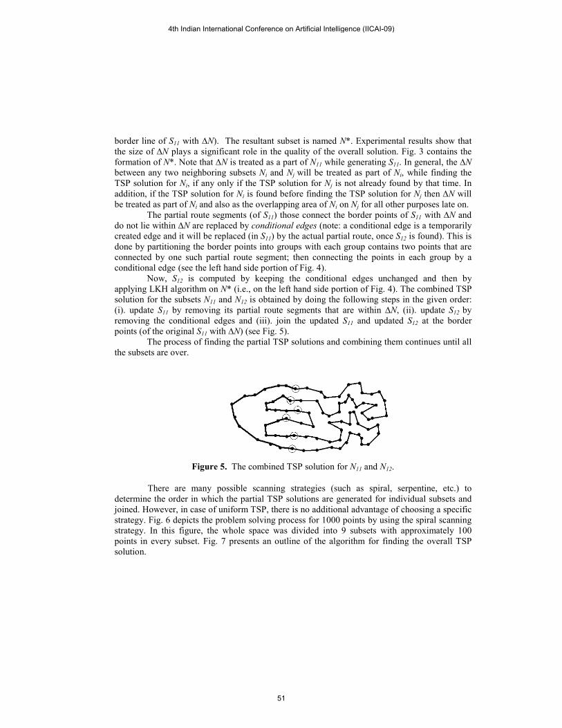
conditional edge (see the left hand side portion of Fig. 4). Now, S12 is computed by keeping the conditional edges unchanged and then by

applying LKH algorithm on �* (i.e., on the left hand side portion of Fig. 4). The combined TSP

solution for the subsets �11 and �12 is obtained by doing the following steps in the given order:

(i). update S11 by removing its partial route segments that are within "�, (ii). update S12 by

removing the conditional edges and (iii). join the updated S11 and updated S12 at the border

points (of the original S11 with "�) (see Fig. 5).

The process of finding the partial TSP solutions and combining them continues until all

the subsets are over.

Figure 5. The combined TSP solution for �11 and �12.

There are many possible scanning strategies (such as spiral, serpentine, etc.) to

determine the order in which the partial TSP solutions are generated for individual subsets and

joined. However, in case of uniform TSP, there is no additional advantage of choosing a specific

strategy. Fig. 6 depicts the problem solving process for 1000 points by using the spiral scanning

strategy. In this figure, the whole space was divided into 9 subsets with approximately 100

points in every subset. Fig. 7 presents an outline of the algorithm for finding the overall TSP

solution.


51

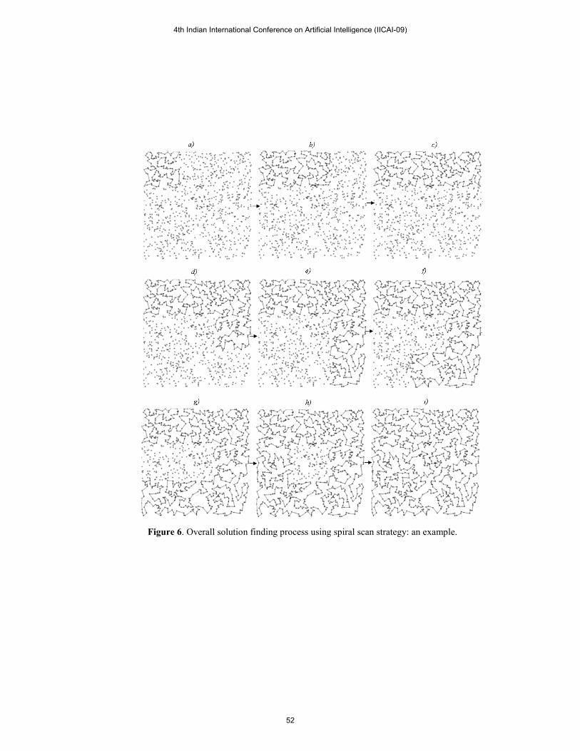
Figure 6. Overall solution finding process using spiral scan strategy: an example.


52

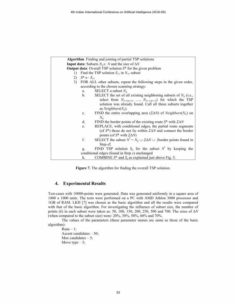
Algorithm Finding and joining of partial TSP solutions

Input data: Subsets �ij ∈ � and the size of "�

Output data: Overall TSP solution S* for the given problem

1) Find the TSP solution S11 in �11 subset

2) S* ← S11

3) FOR ALL other subsets, repeat the following steps in the given order,

according to the chosen scanning strategy:

a. SELECT a subset �ij

b. SELECT the set of all existing neighboring subsets of �ij (i.e.,

select from �(i-1)(j-1), …, �(i+1)(j+1)) for which the TSP

solution was already found. Call all these subsets together

as �eighbors(�ij).

c. FIND the entire overlapping area (Σ"�) of �eighbors(�ij) on

�ij

d. FIND the border points of the existing route S* with Σ"�

e. REPLACE, with conditional edges, the partial route segments

(of S*) those do not lie within Σ"� and connect the border

points (of S* with Σ"�)

f. SELECT the subset �*

= �ij ∪ Σ"� ∪ {border points found in

Step d}

g. FIND TSP solution Sij for the subset �*

by keeping the

conditional edges (found in Step e) unchanged

h. COMBINE S* and Sij as explained just above Fig. 5.

Figure 7. The algorithm for finding the overall TSP solution.

4. Experimental Results

Test-cases with 10000-points were generated. Data was generated uniformly in a square area of

1000 x 1000 units. The tests were performed on a PC with AMD Athlon 3000 processor and

1GB of RAM. LKH [7] was chosen as the basic algorithm and all the results were compared

with that of the basic algorithm. For investigating the influence of subset size, the number of

points (k) in each subset were taken as: 50, 100, 150, 200, 250, 500 and 700. The sizes of "�

(when compared to the subset size) were: 20%, 30%, 50%, 60% and 70%.

The values of the parameters (these parameter names are same as those of the basic

algorithm):

Runs – 1;

Ascent candidates – 50;

Max candidates – 5;

Move type – 5;


53

Restricted search – yes;

Subgradient optimization – yes;

Trials – [problem dimension]/2.

The parameter values used for the decomposition approach were same as those of the basic

algorithm.

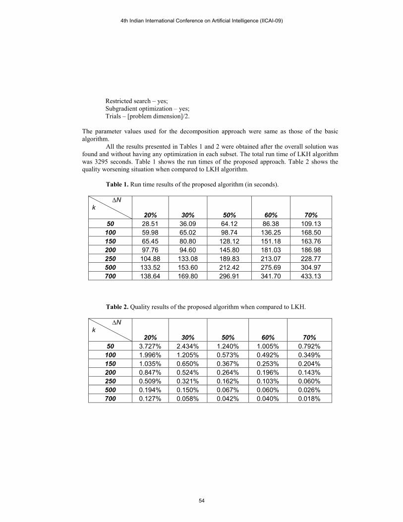
All the results presented in Tables 1 and 2 were obtained after the overall solution was

found and without having any optimization in each subset. The total run time of LKH algorithm

was 3295 seconds. Table 1 shows the run times of the proposed approach. Table 2 shows the

quality worsening situation when compared to LKH algorithm.

Table 1. Run time results of the proposed algorithm (in seconds).

∆N

k

20% 30% 50% 60% 70%

50 28.51 36.09 64.12 86.38 109.13

100 59.98 65.02 98.74 136.25 168.50

150 65.45 80.80 128.12 151.18 163.76

200 97.76 94.60 145.80 181.03 186.98

250 104.88 133.08 189.83 213.07 228.77

500 133.52 153.60 212.42 275.69 304.97

700 138.64 169.80 296.91 341.70 433.13

Table 2. Quality results of the proposed algorithm when compared to LKH.

∆N

k

20% 30% 50% 60% 70%

50 3.727% 2.434% 1.240% 1.005% 0.792%

100 1.996% 1.205% 0.573% 0.492% 0.349%

150 1.035% 0.650% 0.367% 0.253% 0.204%

200 0.847% 0.524% 0.264% 0.196% 0.143%

250 0.509% 0.321% 0.162% 0.103% 0.060%

500 0.194% 0.150% 0.067% 0.060% 0.026%

700 0.127% 0.058% 0.042% 0.040% 0.018%


54

5. Conclusions

According to the experimental results, the proposed decomposition approach provides

substantial reduction in the run time (433 seconds in the worst case vs. 3295 seconds for LKH)

but the quality of the solution provided by the proposed approach is worsened by more than

0.018%, which is very close to the LKH algorithm [7]. The parameters of the algorithm show

that both the subset and overlapping area sizes play an important role in the quality and run time

of the solution. To obtain a reasonable quality solution (e.g. a gap of 0.067%), it is enough to

divide the 10000-points problem into 20 approximately 500-points sub-problems and an

overlapping area of 50% of the subset size. In this case, we can solve the problem 15 times

faster.

Since the Tables 1 and 2 were obtained without any solution optimization, it is possible

to improve the quality of the overall solution by using some local search optimization

approaches such as route scanning and space scanning [16].

Our future work will be focused on solution optimization and testing large-scale

instances from DIMACS TSP Challenge that consists of up to 107

points. Also some new types

of subset creation and combination techniques will be investigated along with some parallel

implementation approaches.

References

1. G. Reinelt. The Traveling Salesman: Computational Solutions for TSP Applications.

Lecture Notes in Computer Science 840, Springer–Verlag, Berlin, 1994.

2. G. Reinelt. Fast Heuristics for Large Geometric Traveling Salesman Problems. ORSA

Journal on computing, 4, 1992, pp. 206-217.

3. Concorde TSP Solver: http://www.tsp.gatech.edu/concorde.html, accessed on July 1,

2009

4. D.S. Johnson and L.A. McGeoch. Experimental Analysis of Heuristics for the STSP. In

G. Gutin and A. P. Punnen (editors), The Traveling Salesman Problem and its

Variations. Kluwer Academic Publishers, Dordrecht, 2002, pp. 369-443.

5. S. Lin and B.W. Kernighan. An Effective Heuristic Algorithm for the Traveling

salesman Problem. Operations Research, 21, 1973, pp. 498-516.

6. S. Lin. Computer Solutions of the Travelling Salesman Problem. Bell System Technical

Journal 44, 1965, pp. 2245-2269.

7. K. Helsgaun. An Effective Implementation of the Lin–Kernighan Traveling Salesman

Heuristic, European Journal of Operational Research, Vol. 126, 2000, pp. 106-130.

8. G. Reinelt. TSPLIB – A Traveling Salesman Problem Library, ORSA Journal on

Computing 3, 1991, pp. 376-384.

9. D. L. Applegate, R. E. Bixby, V. Chvatal, W. Cook, D. G. Espinoza, M. Goycoolea and

K. Helsgaun. Certification of an Optimal TSP Tour through 85,900 Cities, Operations

Research Letters, 37, 2009, pp. 11-15.


55

10. 8th

DIMACS Implementation Challenge: The Traveling Salesman Problem:

http://www.research.att.com/~dsj/chtsp, accessed on July 1, 2009.

11. K. Helsgaun. An Effective Implementation of K-opt Moves for the Lin-Kernighan TSP

Heuristic, (Writings on Computer Science), 2006, Roskilde University, Roskilde,

Denmark.

12. W. Cook and P. Seymour. Tour Merging via Branch-Decomposition, INFORMS

Journal on Computing 15(3), 2003, pp. 233-248.

13. W. Zhang and M. Looks. A Novel Local Search Algorithm for the Traveling Salesman

Problem that Exploits Backbones, L.P. Kaelbing and A. Saffiotti (editors), Proceedings

of the 19th

International Joint Conference on Artificial Intelligence (IJCAI-05), 2005,

pp. 343-350.

14. D. Richter, B. Goldengorin, G. Jäger and P. Molitor. Improving the Efficiency of

Helsgaun’s Lin-Kernighan Heuristic for Symmetric TSP, J. Jassen and P. Pralat

(editors), 4th

Workshop on Combinatorial and Algorithmic Aspects of Networking

(CAAN), Lecture Notes in Computer Science 4852, 2007, pp. 99-111.

15. A. Rohe. Parallel Lower and Upper Bounds for Large TSPs, Journal of Applied

Mathematics and Mechanics, 77(2), 1997, pp. 429-432.

16. R. Bazylevych, B. Prasad, R. Kutelmakh and L. Bazylevych. Decomposition and

Scanning Optimization Algorithms for TSP, Proceedings of the 2008 International

Conference on Theoretical and Mathematical Foundations of Computer Science

(TMFCS-08), Orlando, Florida, USA, 2008, pp. 110-116.


56

A Decomposition Algorithm for Uniform Traveling Salesman Problem

Documents